arX

iv:c

ond-

mat

/050

7180

v1 [

cond

-mat

.dis

-nn]

7 J

ul 2

005

Random multi-index matching problems

O. C. Martin, M. Mezard and O. RivoireLaboratoire de Physique Theorique et Modeles Statistiques

Universite Paris-Sud, Bat. 100, 91405 Orsay Cedex, France

(Dated: July, 2005)

The multi-index matching problem (MIMP) generalizes the well known matching problem bygoing from pairs to d-uplets. We use the cavity method from statistical physics to analyze itsproperties when the costs of the d-uplets are random. At low temperatures we find for d ≥ 3 afrozen glassy phase with vanishing entropy. We also investigate some properties of small samplesby enumerating the lowest cost matchings to compare with our theoretical predictions.

PACS numbers: 75.10.Nr (Spin-glass and other random models), 75.40.Mg (Numerical simulation studies)Keywords: Combinatorial optimization, Cavity method.

I. INTRODUCTION

The statistical properties of random combinatorial optimization problems can be studied from a number of angles,with tools depending on the discipline. Recent years have however witnessed a convergence of interests and techniquesacross mathematics, computer science and statistical physics. An archetype example is the matching problem withrandom edge weights, defined as follows: suppose one has M different jobs and M people to perform them, one personper job, and let cij be the cost when job i is executed by person j; the 2-index matching problem consists in assigningjobs to people in such a way as to minimize the total cost. The statistical properties of the optimal matching when thecost cij are drawn independently from a common distribution were found two decades ago using the replica [1] and thecavity [2] methods. These two non-rigorous statistical physics approaches have recently been used to tackle a numberof computationally more difficult problems such as satisfiability or graph coloring, but the 2-index matching problemsets apart for belonging to one of the very few problems where such predictions have been rigorously confirmed [3].

In this work, we take the statistical physics approach and study the properties of a generalization of the 2-index tomulti-index matching problems (MIMPs) where the elementary costs are now associated with d-uplets, representingfor example persons, jobs and machines when d = 3. At variance with the 2-index matching, d-index matchingproblems with d ≥ 3 are NP-hard. We show here that their low lying configurations also have a different, glassy,structure whose description requires replica symmetry to be broken. Remarkably, the replica symmetry breakingscheme differs from the common picture that has emerged from the study of other optimization problems such asthe coloring [4] and satisfiability problems [5]. In particular, a naıve application of the 1-RSB cavity method at zerotemperature [6], which successfully solves these two problems, is here doomed to fail. The reason for this will betraced back to the presence of “hard constraints”. By unraveling this specificity, we put forward arguments whoserelevance goes beyond matching problems; they indicate when a similar scenario can be expected on other constrainedsystems. The particularly simple glassy structure that we find is also of interest from the interdisciplinary point ofview: in conjunction with the rigorous formalism available for the 2-index case, it places MIMPs in a choice place forworking out a most awaited mathematical understanding of replica symmetry breaking.

The present paper provides an extensive account of our results on the MIMPs, some of which have already beenmentioned in [7]. The paper is organized as follows. We first define precisely multi-index matching problems, andbriefly review the past approaches from physics, mathematics and computer science that were developed mainly toaddress the 2-index case. Then we start our statistical study by establishing the scaling of the minimal cost as afunction of the number of variables and by providing a lower bound from an annealed calculation. A large part of thepaper is then devoted to present our implementation of the cavity method to matching problems, including a detaileddiscussion of its relations with the rigorous formalism proposed by Aldous; we explain why and how replica symmetrymust be broken when d ≥ 3, in order to account for the presence of a frozen glassy phase. Finally, the last section isdedicated to a numerical analysis of small samples that provides support to the proposed scenario.

II. MULTI-INDEX MATCHINGS

A. Definitions

Two classes of MIMPs can be distinguished, d-partite matching problems and simple d-matching problems, whoseasymptotic properties will be shown to be related. We first start with the d-partite matching problem that corresponds

2

i

ijkc

k

j

M M

M

FIG. 1: Tripartite matching problem. Factor graph repre-sentation : the hyperedges, or factor nodes, are representedwith squares.

i

ijkc

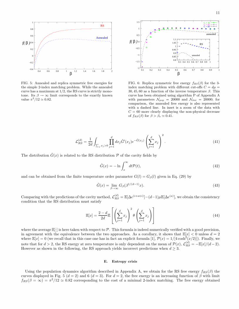
k

j

M

M

N

FIG. 2: Simple 3-index matching problem. The factorgraph representation is similar to the tripartite case.

to the version alluded to in the introduction. An instance consists of d sets, A1,. . . , Ad, of M nodes each, and a costca is associated with every d-uplet a = {i1, . . . , id} ∈ A1 × · · · × Ad. Graphically, it is represented by a factor graphas shown in Fig. 1 with hyperedges (factor nodes) joining exactly one node from each ensemble. A matching M is amaximal set of disjoint hyperedges, such that each node is associated to one and only one hyperedge of the matching;it can be described by introducing an occupation number na ∈ {0, 1} on each hyperedge a, with the correspondence

a ∈ M ⇔ na = 1. (1)

The condition for a set of hyperedges to be a matching can then be written

∀r = 1, . . . , d, ∀ir ∈ Ar,∑

a : ir∈a

na = 1. (2)

The d-partite matching problem consists in finding the matching with minimal total cost,

C(d)M = min

{na}

∑

a

cana (3)

with the {na} subject to the constraints (2). We consider here the random version of the problem, where the costs caare independent identically distributed random variables taken from a distribution ρ(c), and we are interested in thetypical value of an optimal matching in the M → ∞ limit. For definiteness, we take for ρ the uniform distribution in[0, 1], but the asymptotic properties of d-matchings depend only on the behavior of ρ close to c = 0, and are identicalfor all distributions ρ with ρ(c) ∼ 1 as c → 0, such as the exponential distribution, ρ(c) = e−c. The case ρ(c) ∼ cr,r > 0, can be treated along the same lines, but gives different quantitative results.

A variant of this setup is the simple d-matching problem, where a unique set of N nodes, with N being a multipleof d, is considered and a cost is associated to each d-uplet of nodes (see Fig. 2). The d-partite case can be seen as aparticular instance of a simple d-matching problem where the hyperedges joining more than one node of any Ai aregiven an infinite cost. Simple d-matchings problems are formulated as finding

L(d)N = min

{na}

∑

a

cana (4)

under the constraints

∀i = 1, . . . , N,∑

a : i∈a

na = 1. (5)

Before presenting our analysis of random matching problems by means of an adaptation of the cavity method forfinite connectivity statistical physics models, we briefly review past approaches to the subject, with an emphasis onopen questions that motivated the present study.

B. Physical approach

The 2-index matching problem was the first combinatorial optimization problem to be tackled with the replicamethod, an analytical method initially developed in the context of spin glasses [8]. In the paper [1], Mezard and

3

Parisi analyzed both the simple and bipartite matching problems for cost distributions ρ with ρ(c) ∼ cr as c → 0.Using replica theory within a replica symmetric Ansatz, they derived the minimal total cost; thus, for the bipartite

matching with r = 0, they predicted limM→∞ C(2)M = π2/6; moreover, they obtained the distribution of cost in the

optimal matching. Support in favor of their prediction has first come from numerical results and from an analyticalstudy of the stability of the replica symmetric solution [9, 10]. This last analysis further yields the leading correctionsof order 1/N for the value of the minimum matching.

Interestingly, the same results can be reobtained using a variant of the cavity method based on a representationof self-avoiding walks using m-component spins [2]. This alternative formulation, avoiding the bold prescriptions ofreplica theory, furthermore suggests that, if the cost of the hyperedges connected to a given node are ordered fromthe lowest to the highest, the probability for the k-th hyperedge to be included in the optimal matching is 2−k [11],as first conjectured from a numerical study [12].

C. Mathematical approach

Replica theory, while a powerful tool to obtain analytical formulae, is not a rigorously controlled method, and itspredictions have only the status of conjectures within the usual mathematical standards. For the 2-index matchingproblem with r = 0 however, the results mentioned above (value of the optimal matching, distribution of costs, andprobability of inclusion of k-th hyperedge) have all been confirmed by a rigorous derivation, due to Aldous [3]. Hiscontribution also includes the proof an asymptotic essential uniqueness property that mathematically expresses thefact that replica symmetry indeed holds for this problem. The weak convergence approach [13] on which the proofis built is closely related to the cavity method we will employ, and the relations between the two formalisms will bediscussed in Sec. IVD. Confirmation of the ζ(2) = π2/6 value for the bipartite assignment problem also comes fromthe recent proofs [14, 15] of a more general conjecture formulated by Parisi [16]; this conjecture states that, for thebipartite matching with exponential distribution of the costs, ρ(c) = e−c, the mean optimal matching for finite M is∑M

k=1 k−2.

These mathematical contributions are part of a more ambitious program aiming at developing rigorous proofs andpossibly a rigorous framework of the replica and cavity methods. Interestingly, Talagrand, one of the prominentadvocate of this program, devotes the last chapter of his book on the subject [17] to the 2-index matching problem,stressing that, in spite of the major advances mentioned, it stays a particularly challenging issue. Indeed, finitetemperature properties have so far resisted to mathematical investigations, even in the limit of high temperature,that has been successfully addressed in other spin-glass like models [17]. We shall comment on the peculiarities ofmatchings with respect to other constrained systems in Sec. V B. It is our hope that our work not only provides newchallenging conjectures, but also suggests some hints for solving unanswered preexisting mathematical questions.

D. Computer science approach

If analytical studies of random d-matchings by statistical physicists and mathematicians have been restricted up tonow to the d = 2 case, d-index matching problems with d > 2 have a longer history in the computer science community.d-partite extensions of the bipartite matching problem were introduced in 1968 under the name of multidimensional

assignment problems [18]; they are also referred in the literature as multi-index assignment problems, and, morespecifically, as multi-index axial assignment problems (to distinguish them from the so-called planar versions [19, 20]).MIMPs, as we call them (for multi-index matching problems), have a number of practical applications. The mostcommonly cited one is for data association in connection with multi-target tracking [21]. Besides a major interest forreal-time air traffic control, such approaches are for instance helpful for tracking elementary particles in high energyphysics experiments [22].

From the algorithmic complexity point of view, matching problems have also a pioneering role since the 3-indexmatching problem was among the first 21 problems to be proved NP-complete [23]. In contrast, polynomial algorithmsare known that solve 2-index matching problems [24]. Note that being based on a worst case analysis, NP-hardnessis however only a necessary condition for hard typical complexity, which is the issue which interests us here. Due totheir intrinsic algorithmic difficulty and to the broad range of their applications, generalized assignment problems arethe subject of numerous studies in the computer science community; we refer to the reviews [19, 20] for additionalinformation and references.

4

III. SCALING AND A LOWER BOUND

The first task in studying random optimization problems is to determine the scaling of the optimal cost with thenumber of variables [25]. Here, we address this issue for the two variants of MIMPs, the multi-partite and simplemulti-index matching problems. The scaling is inferred from an heuristic argument, and confirmed by an annealedcalculation (first moment method) yielding a lower bound. This leads us to a statistical physics formulation thatencompasses the two versions of MIMPs.

A. Scaling

The statistical physics approach of combinatorial optimization problems consists in defining the energy E(M) ofeach admissible solution, here a d-matching M, as its total cost, E(M) =

∑

a∈M ca, and in determining the minimaltotal cost, identified with the ground-state energy, by looking at the zero temperature properties of the system. Ford-matchings, the corresponding Hamiltonian

H[{na}] =∑

a

cana (6)

defines a lattice gas model, where the particles are occupying the hyperedges. The constraints (2) or (5) implementa hard-core interaction between the particles: two “neighboring” hyperedges are not allowed to be occupied simulta-neously. To have a sensible statistical physics model, the ground state has to be extensive, i.e., proportional to M

in the d-partite case, and to N in the simple case. We propose here a heuristic argument to determine how E[C(d)M ]

and E[L(d)N ] scale with M and N respectively, where E[·] represents the average over the different realizations of the

costs. The central (local) quantity that monitors the scaling behavior is the number of hyperedges to which a given

node belongs, noted W(d)Λ (Λ = M or N). Indeed, with the costs uniformly distributed in [0,1], the lowest costs

to which a node can be associated are of order 1/W(d)Λ and the optimal matching is expected to scale like Λ/W

(d)Λ .

Thus, for d-partite matchings, W(d)M = Md−1 and E[C

(d)M ] ∼ M2−d, while for simple d-matchings, W

(d)N =

(

N−1d−1

)

and

E[L(d)N ] ∼ (d− 1)!N2−d. We will therefore be interested in computing the (finite) quantities

C(d) = limM→∞

Md−2E[C

(d)M ],

L(d) = limN→∞

Nd−2

(d− 1)!E[L

(d)N ].

(7)

The factor (d − 1)! in the second definition is meant to reflect the different number of hyperedges to which a givennode can connect, in the d-partite and simple versions (this difference is absent when d = 2). With this conventionwe will find the equality C(d) = dL(d), where the remaining d factor merely comes from the fact that the total numberof nodes is N for simple d-matchings, but is dM for d-partite matchings.

B. Annealed approximation

When energies are extensive in the size N of the system, the equilibrium properties of a statistical physics model areentirely encoded in the partition function, ZN (β) =

∑

M e−βE(M), or, equivalently, in its logarithm, the free energyFN (β) ≡ − log[ZN(β)]/β. The free energy depends on the realization of the elementary costs, but it is expected to bea self-averaging quantity, i.e., such that the free-energy density f(β) = limN→∞ FN (β)/N exists and is independentof the sample. The self-averaging property is proved for d = 2 [26], and we assume here that it holds for d ≥ 3 aswell. The value of the optimal matching is given by the ground state energy, obtained as limβ→∞ f(β), where thefree energy is calculated by performing a quenched average of the partition function, E[lnZ], with E[·] referring to theaverage with respect to the realization of the elementary costs.

A much simpler calculation is the annealed average, ln E[Z]. Due to the concavity of the logarithm, it yields a lowerbound on the correct quenched free energy, fan(β) ≡ − ln E[Z]/(Nβ) ≤ −E[lnZ]/(Nβ) ≡ f(β). In fact, since theentropy s(β) = β2∂βf(β) is necessarily positive for a system with discrete degrees of freedom, the free energy f(β)must be an increasing function, and a tighter lower bound can be inferred for the ground-state energy [25],

limβ→∞

f(β) ≥ supβ>0

fan(β). (8)

5

These considerations are made under the hypothesis that the energies, or equivalently the temperature β, arecorrectly scaled with N , so that limβ→∞ f(β) is indeed finite. Reciprocally, requiring the annealed free energy to beextensive provides us with the appropriate scaling of β. For d-index matching problems, we have

E[Z] = E

∑

{na}

e−β∑

acana

= (#M)E[e−βca ]#{a∈M} (9)

where #M denotes the total number of possible matchings and #{a ∈ M} the number of hyperedges contained in agiven matching. For d-partite matchings, #M = (M !)d−1 and #{a ∈ M} = M . To enforce the correct scaling of the

free energy, we anticipate a rescaling in temperature of the form β = Mαβ, yielding

ln E[Z] = [d− 1 − α]M lnM − [ln β + d− 1]M + o(M). (10)

An extensive annealed free energy is therefore obtained by taking α = d− 1, in which case

f (d−part)an (β) =

ln β + d− 1

β. (11)

The scaling 1/(Mβ) ∼ M2−d we obtain corresponds to one introduced in Eq. (7). For simple d-index matchings,

#M = N !/[(N/d)!(d!)N/d] and #{a ∈ M} = N/d. Rescaling the temperature as β = Nd−1β, we get

ln E[Z] = −[ln β + d− 1 − ln(d− 1)!]N/d+ o(N). (12)

To make contact with the d-partite case however, we adopt a slightly different scaling, β = Nd−1β/(d− 1)!, so that

f (simple)an (β) =

ln β + d− 1

dβ=

1

df (d−part)an (β = β). (13)

This annealed calculation illustrates the correspondence between the d-partite and simple d-matchings stated in theprevious section. Apart for the trivial factor d, corresponding to the relation N = dM , the equality is obtained by

normalizing differently β and β, thereby accounting for the difference in the number of hyperedges a given node locally

sees [extra factor (d− 1)! in Eq. (7)]. The annealed free energy is a concave function with maximum for β∗d = e2−d so

that we get lower bounds C(d) ≥ ed−2 and L(d) ≥ ed−2/d.

C. Statistical physics reformulation

From now on, we will cease distinguishing between d-partite and simple d-matchings, and consider a unique sta-tistical physics model that describes both problems in a common framework. Our approach is indeed based on thecavity method [27] for which only the local properties at the level of each node are relevant, and we have seen thatby making the appropriate scalings of β, we can match the local properties of both models. The Hamiltonian weconsider is

H[{na}] =∑

a

ξana, (14)

with the ξa ≡ Md−1ca uniformly distributed in [0,Md−1] for the d-partite case, and ξa ≡ Nd−1ca/(d − 1)! in

[0, Nd−1/(d− 1)!] for the simple case. The (inverse) temperature, denoted by β to simplify, will correspond to β for

the d-partite case and β for the simple case. The only remaining difference kept is the factor d between the two freeenergies, accounting for the relation N = dM . Unless explicitly stated, the formulae to be given hold for the simpleversion ; to get the d-partite counterparts, one has consequently to multiply by d the intensive quantities.

IV. REPLICA SYMMETRIC SOLUTION

The approach we adopt to treat the d-matching problems is the cavity method recently developed to solve statisticalphysics models defined on finite connectivity graphs [27]. This section explains the formalism of the replica symmetricsolution for general d. While the correctness of the replica symmetric approach is a mathematical fact when d = 2,we show that it leads to some inconsistency when d = 3, requiring replica symmetry to be broken.

6

A. From complete to dilute graphs

The hypergraph on which an instance of the simple d-matching problem is defined is complete, in the sense thatevery possible hyperedge arises once and is given a random cost. However, the factor nodes with the smallestelementary costs are more likely to belong to the optimal matching; for instance the probability that the k-th mostcostly hyperedge originating from a given node will be included in the optimal 2-matching is 2−k [3]. This suggeststhat hyperedges with large costs can be ignored while retaining most of the structure relevant to the determinationof the optimal matching. Eliminating hyperedges results in a diluted hypergraph, where each node is connected toonly a restricted number of hyperedges. From this point of view, in spite of being defined on a complete graph,random matchings are effectively closer to statistical physics models defined on finite connectivity random graphs.In fact, such a feature already transpired from the initial replica treatment [1] of 2-index matchings where all themultioverlaps Qa1...ap

were required, and not only the two replica overlaps Qa1a2 , like in usual Curie-Weiss mean fieldmodels of disordered systems [8].

To exploit the underlying diluted structure, one possible method is to introduce a cut-off C, suppress all nodeswith rescaled cost ξa > C, solve the matching problem on the diluted hypergraph, and finally send C → ∞. Thehypergraph obtained by this procedure is Poissonian: if ξ1, ξ2, . . . are the costs ordered in increasing sequence of thehyperedges connected to a given node, the probability for the connectivity to be k is

pk = Prob[ξ1 < · · · < ξk < C < ξk+1 < · · · ] =

(

W(d)Λ

k

)

(

C

W(d)Λ

)k(

1 − C

W(d)Λ

)W(d)Λ −k

→ Ck

k!e−C , (15)

with W(d)Λ giving the number of hyperedges to which a node is connected, as in Sec. III B. Diluting the complete

graph has a major drawback however: the diluted hypergraph typically does not allow any matching at all, since forinstance there is always a finite probability e−C that a given node is isolated.

To circumvent this problem, we come back to the model on the complete graph and start by weakening theconstraints, allowing a node not to belong to a matching, at the expense of paying an extra cost. In more physicalterms, we view a matching as the close-packing limit of a lattice gas model whose particles are subject to hard-coreinteractions: particles can occupy the hyperedges but two hyperedges connected through a node can not both admita particle. We introduce a grand-canonical Hamiltonian

Hµ[{na}] =∑

a

ξana − dµ∑

a

na =∑

a

(ξa − dµ)na. (16)

where dµ is a chemical potential per hyperedge (µ per node). In the limit µ→ ∞, the maximum number of hyperedgesis occupied by a particle and we recover the matching problem. For finite µ however, the constraints reflecting thehard-core repulsion are

∀i,∑

a : i∈a

na ≤ 1, (17)

to be compared with the hard constraints of Eq. (5), recovered only in the µ → ∞ limit. Each value of µ definesan optimization problem whose minimum energy Eµ corresponds to a zero temperature limit β → ∞. The solutionof the matching problem thus appears as the result of a double limit, β → ∞ and µ → ∞. The point is that adiluted structure is now naturally associated with the system at finite µ. Indeed since Hµ is minimized by takingna = 0 whenever ξa > dµ, the ground state is unaffected if all hyperedges a with ξa > dµ are suppressed, yielding thePoissonian hypergraph considered above with C = dµ. This construction allows us to formulate the initial MIMP asthe limit µ → ∞ of optimization problems defined on Poissonian graphs with increasing mean connectivity dµ. Wewill give in Sec. IVD an alternative construction based on regular graphs.

B. Cavity method

The problem at finite µ defined on a Poissonian hypergraph can be studied by means of the cavity method asdeveloped for finite connectivity graphs [27]; one of the main advantages of this method over the replica method [1] orprevious versions of the cavity method [2] is that it allows for a practical investigation of replica symmetry breaking(RSB). Since we are interested in the ground-state properties, the cavity method directly at zero temperature seemsparticularly well suited [28]. However, it will turn out to be necessary to get the finite temperature equations as well,and we therefore work at finite β, postponing the discussion of the β → ∞ limit to the next section.

7

a

i

jb

aξ

FIG. 3: Local structure of a Poissonian hypergraph. Whenthe node i is removed, it leaves a rooted-tree with root a.

β = 0.5

β = 10

x

P(x)

β = 0.1

0

0.05

0.1

0.15

0.2

0.25

−15 −10 −5 0 5 10 15

FIG. 4: Distribution P(x) of cavity fields for 3-indexmatchings at different temperatures β in the replica sym-metric approximation. These distributions are obtainedby population dynamics, using algorithm P described inAppendix A, with parameters C = 60, Niter = 1 andNpop = 200000.

In strong analogy with Aldous’ framework (see Sec. IVD), the RS cavity method associates the diluted hypergraphwith an infinite tree or, stated differently, a tree with self-consistent boundary conditions. The starting point ishowever finite rooted trees, that is trees with a singularized node i called the root. Consider for instance the partof a tree represented in Fig. 3: given a hyperedge a and one of its connected nodes i (relation noted i ∈ a), we callZ(a→i) the partition function of the system defined on the rooted-tree with root a resulting from the removal of i. Toexpress it in terms of the partition functions Z(b→j) where j refers to the nodes, connected to a, but distinct from i

(noted j ∈ a− i), we decompose Z(a→i) as Z(a→i) = Z(a→i)0 + Z

(a→i)1 , where Z

(a→i)0 and Z

(a→i)1 are the conditional

partition functions where the root a is either constrained to be empty or occupied by a particle. As an intermediate

stage in the recursion, we also introduce Y(j→a)0 and Y

(j→a)1 , which are defined similarly to Z

(a→i)0 and Z

(a→i)1 , but

for rooted-trees whose root is the node j, in absence of the hyperedge a: the index 1 means that j is already matchedand the index 0 that it is not. With the notations of Fig. 3, we have the relation

Z(a→i)0 =

∏

j∈a−i

(

Y(j→a)0 + Y

(j→a)1

)

,

Z(a→i)1 = e−β(ξa−dµ)

∏

j∈a−i

Y(j→a)0 ,

Y(j→a)0 =

∏

b∈j−a

Z(b→j)0 ,

Y(j→a)1 =

∑

b∈j−a

Z(b→j)1

∏

c∈j−{a,b}

Z(c→j)0 .

(18)

These formulae have simple interpretations: for instance, the first line means that when a is empty, the neighboringnodes j ∈ a − i can be equally matched or not with upstream hyperedges, while the second line means that when ais occupied, it generates a cost ξa − dµ and requires the nodes j ∈ a − i to not be matched. From the conditionalpartition functions, we define the cavity fields

eβx(j→a) ≡ eβµ Y(j→a)0

Y(j→a)0 + Y

(j→a)1

,

eβu(a→i) ≡ eβ(ξa−µ)Z(a→i)1

Z(a→i)0

.

(19)

These definitions are made to insure a proper scaling when µ→ ∞ and recover quantities used in previous studies ford = 2. Note however that for finite β, it is more natural to introduce ψ(j→a) ≡ exp[β(x(j→a) − µ)] interpreted as theprobability that node j not matched in the absence of a (or equivalently that j is associated to a in a matching); thisalternative notation will turn out to be particularly convenient when discussing the freezing phenomenon, in Sec. VB.On a given rooted tree, it follows from Eq. (18) that the fields attached to the different oriented edges are related by

8

the following message-passing rules,

u(a→i) =∑

j∈a−i

x(j→a),

x(j→a) = − 1

βln

e−βµ +∑

b∈j−a

e−β(ξa−u(b→j))

.

(20)

The limit of infinite rooted trees is taken implicitly by considering the stationary distribution P(x) that is assumed toresult from the repeated iteration of the message passing relations. By definition P(x) is a distribution of cavity fieldsover the different oriented edges that satisfies the following self-consistent equation, called the RS cavity equation,

P(x(0)) = Ek,ξ

∫ k∏

a=1

d−1∏

ja=1

dx(ja)P(x(ja))δ(

x(0) − x(k,ξ)[{x(ja)}])

(21)

where the function x(k,ξ) is defined according to Eq. (20) as

x(k,ξ)[{x(ja)}] ≡ − 1

βln

(

e−βµ +

k∑

a=1

e−β(ξ−∑d−1

ja=1 x(ja))

)

, (22)

and the expectation Ek,ξ expresses the average over the disorder, which includes both an average over the connectivityk and over the rescaled costs ξ,

Ek,ξ[F(k)({ξa})] ≡

∞∑

k=0

(dµ)ke−dµ

k!

k∏

a=1

(

1

dµ

∫ dµ

0

dξa

)

F (k)(ξ1, . . . , ξk). (23)

The RS cavity equation (21) can be solved by a population dynamics algorithm, whose principle is presented inAppendix A; the resulting distribution P(x) for d = 3 and different β is shown in Fig. 4. P(x) contains all theinformation on the equilibrium properties and, in particular, allows one to compute the free-energy density. It can bederived from the Bethe approximation which produces on a given hypergraph the formula

f(β) =1

N

[

∑

i

∆F (i+a∈i)(β) −∑

a

(ℓa − 1)∆F (a)(β)

]

(24)

where ℓa is the degree of hyperedge a, which here is ℓa = d independently of a. The shifts ∆F (i+a∈i)(β) and ∆F (a)(β)correspond respectively to the free-energy shift induced by the addition of a node i together with its connectedhyperedges a ∈ i, and to the free-energy shift induced by the addition of hyperedge a. They are given by

e−β∆F (i+a∈i)(β) =Y

(i)0 + Y

(i)1

∏

a∈i

∏

j∈a−i

(

Y(j)0 + Y

(j)1

) = e−βµ +∑

a∈i

e−β(ξa−∑

j∈a−ix(j→a)),

e−β∆F (a)(β) =Z

(a)0 + Z

(a)1

∏

j∈a−i

(

Y(j)0 + Y

(j)1

) = 1 + e−β(ξa−∑

j∈ax(j→a)),

(25)

where we introduced the analogs of the partitions functions for rooted tree, but on the complete trees:

Z(a)0 =

∏

j∈a

(

Y(j→a)0 + Y

(j→a)1

)

,

Z(a)1 = e−β(ξa−dµ)

∏

j∈a

Y(j→a)0 ,

Y(j)0 =

∏

b∈j

Z(b→j)0 ,

Y(j)1 =

∑

b∈j

Z(b→j)1

∏

c∈j−b

Z(c→j)0 .

(26)

9

Physically, Z(a)1 /(Z

(a)0 +Z

(a)1 ) gives the probability for the hyperedge a to be included in the matching. By averaging

over the realizations of the disorder, since the mean number of hyperedges per nodes is µ, we get

fRS(β) = E[∆F (i+a∈i)(β)] − (d− 1)µE[∆F (a)(β)] (27)

with explicitly

E[∆F (i+a∈i)(β)] = − 1

βEk,ξ

∫ k∏

a=1

d−1∏

ja=1

dx(ja)P(x(ja)) ln

(

e−βµ +

k∑

a=1

e−β(ξa−∑d−1

ja=1 x(ja))

)

,

E[∆F (a)(β)] = − 1

βEξ

∫ d∏

j=1

dx(j)P(x(j)) ln(

1 + e−β(ξa−∑

dj=1 xj)

)

.

(28)

C. Integral relations

The µ → ∞ limit can be taken explicitly. The corresponding equations generalize the formulae established byMezard and Parisi in their first treatment of the 2-index matching problem [1]. For general d, they are

G(l) =1

β

∫ +∞

−∞

d−1∏

j=1

dyje−G(yj)Bd

l +

d−1∑

j=1

yj

,

Bd(x) ≡∞∑

p=1

(−1)p−1pd−2epx

(p!)d.

(29)

Given G(ℓ), the energy ǫ(β) and entropy s(β) are

ǫ(β) =1

βd

∫ +∞

−∞

dlG(l)e−G(l),

s(β) =

∫ +∞

−∞

dl[

e−el − e−G(l)]

− d− 2

d

∫ +∞

−∞

dlG(l)e−G(l),

(30)

and the free energy is obtained as f(β) = ǫ(β) − s(β)/β. The relation between the function G(l) and the orderparameter P(x) is, up to a change of variable, a Laplace transform,

e−G(l) =

∫ +∞

−∞

dxP(x)e−el−βx

. (31)

From the practical point of view of numerically solving the cavity equations, the finite µ cavity equations are howevereasier to handle than these compact formulae.

D. Zero temperature limit

In view of an extension of the mathematical approach from 2-index to d-index matchings with d > 2, it is interestingto discuss in some details the relations between our equations and those used by Aldous in his rigorous study of the2-index matching problem [3]. Aldous’ formalism is obtained from our RS cavity equations by taking the zerotemperature, β → ∞. When β → ∞, Eqs. (20) become

u(a→i) =∑

j∈a−i

x(j→a),

x(j→a) = minb∈j−a

(ξb − u(b→j)).(32)

Taking µ = ∞ and d = 2 leads to the recursive distributional equation [29],

x(a) = minb

(

ξb − x(b))

(33)

10

on which Aldous’ work is based [3]. A difference is however that its costs ξb derive from a Poisson point process(the uniform distribution does not make sense when µ = ∞). This Poisson process can nonetheless be related to ourformalism by implementing a variant of the cut-off procedure. Consider selecting at each step of the cavity recursionthe k parents of smallest costs, k being now fixed. Then the successive k costs are distributed according to a Poissonprocess with rate one. Nonetheless, while the cavity recursion is perfectly well defined, the corresponding system ona given hypergraph does not make sense: a hyperedge may belong to the the list of the hyperedges with the k-thsmallest costs for one of its node but not for an other one. This is why we introduced the version with a cut-off on thecosts, which constitutes for finite µ a perfectly sensible statistical physics model. From a purely formal point of viewthe version with cut-off on the number of connected clauses works as well, and provides an alternative formulationfor numerically solving the cavity equations (see Appendix A for the details and Fig. 9 for an illustration).

The cavity fields at zero temperature have an interpretation in terms of differences in ground-state energies. Thecavity field x(j→a) corresponds to the extra cost of a particle on node j with respect to no particle, in the absenceof hyperedge a, and the cavity bias u(a→i) to the cost of connecting the node i to the hyperedge a. Note that thesequantities are actually well defined only if µ is kept finite, otherwise a particle cannot be removed or added withoutdestroying the perfect matching, i.e., without leaving the space of admissible configurations. Similarly, the total fieldson the complete graph are

U (a) =∑

j∈a

x(j→a),

X(i) = minb∈i

(ξb − u(b→i)).(34)

From the interpretation given, it appears that the hyperedges which indeed participate to the optimal matchingare those which achieve the minima, i.e., the solution is given by

na = δa,a∗ , a∗ = argmina

(ξa − u(a→i)). (35)

Since this has to hold for all i ∈ a, the question arises whether this prescription effectively defines a matching, i.e.,whether arg mina(ξa − u(a→i)) = argmina(ξa − u(a→j)) for all i, j ∈ a. A positive answer is obtained by generalizingto d > 2 the inclusion criterion invoked by Aldous when d = 2, which states

a∗ = argmina

(ξa − u(a→i)) = 1 ⇐⇒ ξa ≤ u(a→i) + x(i→a). (36)

The independence on i is then a consequence of the dentity u(a→i)+x(i→a) = U (a). The proof of the inclusion criterionitself is straightforward with the present notations: if a∗ = arg mina(ξa − u(a→i)),

ξa∗ − u(a∗→i) = minb∈i

(ξb − u(b→i)) ≤ minb∈i−a∗

(ξb − u(b→i)) = x(i→a∗). (37)

Reciprocally, if a 6= arg minb(ξb − u(b→i)),

ξa − u(a→i) ≥ minb∈i

(ξb − u(b→i)) = minb∈i−a

(ξb − u(b→i)) = x(i→a). (38)

As an alternative to the Bethe formula, the value of the optimal matching can be obtained by inferring 〈ξa∗〉 fromthe distribution of the fields P(x). Thanks to the inclusion criterion, we have

L(d)RS =

1

d〈ξa∗〉 =

1

d

∫ ∞

0

dξ ξ Prob(U > ξ)

=1

d

∫ ∞

0

dξ

∫ d∏

j=1

dxjP(xj) ξ θ

d∑

j=1

xj − ξ

(39)

where the factor d corresponds to the number of nodes per hyperedge and θ represents the Heaviside function, θ(x) = 1if x > 0 and 0 otherwise. The RS cavity equations at zero temperature can also be written in terms of closed integralrelations that generalize known equalities for the d = 2 case,

G(x) =

∫

∑

jtj>−x

d−1∏

j=1

dtjG′(tj)e

−G(tj)

x+

d−1∑

j=1

tj

, (40)

11

Annealed

RS

β

βf( )

−0.4

−0.2

0

0.2

0.4

0.6

0.8

1

0.4 0.6 0.8 1 1.2 1.4 1.6 1.8 2

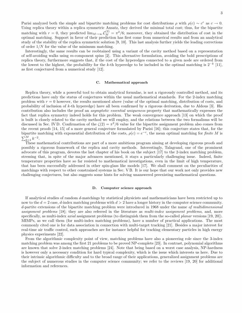
FIG. 5: Annealed and replica symmetric free energies forthe simple 2-index matching problem. While the annealedcurve has a maximum at 1/2, the RS curve is strictly mono-tone. Its β → ∞ limit corresponds to the exactly knownvalue π2/12 ≃ 0.82.

f( )β

β

annealed

RS

annealed

−2

−1.5

−1

−0.5

0

0.5

1

1.5

0.1 0.2 0.3 0.4 0.5 0.6 0.7 0.8 0.9 1

C = 30C = 45C = 60

0.8

0.85

0.9

0.95

1

1.05

1.1

0.3 0.4 0.5 0.6 0.7 0.8 0.9 1

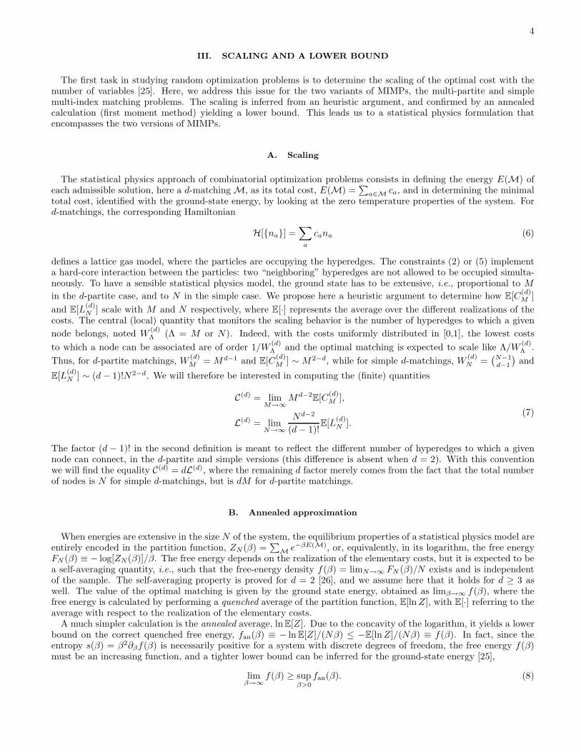
FIG. 6: Replica symmetric free energy fRS(β) for the 3-index matching problem with different cut-offs C = dµ =30, 45, 60 as a function of the inverse temperature β. Thiscurve has been obtained using algorithm P of Appendix Awith parameters Npop = 20000 and Niter = 20000; forcomparison, the annealed free energy is also representedwith a dashed line. In inset is a zoom of the data withC = 60 more clearly displaying the non-physical decreaseof fRS(β) for β > βs ≃ 0.41.

L(d)RS =

1

2d

∫

∑

jxj>0

d∏

j=1

dxjG′(xj)e

−G(xj)

d∑

j=1

xj

2

. (41)

The distribution G(x) is related to the RS distribution P of the cavity fields by

G(x) = − ln

∫ ∞

x

dtP(t), (42)

and can be obtained from the finite temperature order parameter G(l) = Gβ(l) given in Eq. (29) by

G(x) = limβ→∞

Gβ(β1/(d−1)x). (43)

Comparing with the predictions of the cavity method, L(d)RS = E[∆ǫ(i+a∈i)]−(d−1)µE[∆ǫ(a)], we obtain the consistency

condition that the RS distribution must satisfy

E[x] =2 − d

2dE

d∑

j=1

xj

2

θ

d∑

j=1

xj

(44)

where the average E[·] is here taken with respect to P . This formula is indeed numerically verified with a good precision,in agreement with the equivalence between the two approaches. As a corollary, it shows that E[x] < 0 unless d = 2where E[x] = 0 (we recall that in this case one has in fact an explicit formula [1], P(x) = 1/[4 cosh2(x/2)]). Finally, we

note that for d > 2, the RS energy at zero temperature is only dependent on the mean of P(x), L(d)RS = −E[x]/(d− 2).

However as shown in the following, the RS approach yields incorrect predictions when d ≥ 3.

E. Entropy crisis

Using the population dynamics algorithm described in Appendix A, we obtain for the RS free energy fRS(β) thecurves displayed in Fig. 5 (d = 2) and 6 (d = 3). For d = 2, the free energy is an increasing function of β with limitfRS(β = ∞) = π2/12 ≃ 0.82 corresponding to the cost of a minimal 2-index matching. The free energy obtained

12

sRS

β

d = 3

−0.008

0

0.004

0.008

0.012

0.395 0.4 0.405 0.41 0.415 0.42 0.425

−0.004

FIG. 7: RS entropy of the 3-index matching problem. Thedata is from population dynamics, using algorithm R pre-sented in Appendix A, with K = 50, Npop = 50000 andNiter = 5000. The line is a linear regression. The RSentropy is found to vanish at βc = 0.412 ± 0.001

(ln

)/r

µ r

r

−2.5

−2

−1.5

−1

−0.5

0

0.5

1

1.5

2

0 1 2 3 4 5 6

0.40.50.60.70.80.9

FIG. 8: Stability analysis of the RS solution for the 3-indexmatching problem at finite temperature. (ln µr)/r is plot-ted versus r for different temperatures β (from algorithmP given in Appendix A with C = 36, Npop = 20000 andNiter = 109). The RS solution is stable if the slope of(ln µr)/r is negative (see text), which is found to be thecase for β < βi ≃ 0.6.

for d = 3 is qualitatively different, as it displays a maximum at a finite temperature βs ≃ 0.41 (see Fig.7). Thisentropy crisis reflects an inconsistency of the RS approach [30]. If one assumes the RS approximation holds at hightemperature in some range of temperature (a non-trivial statement), a phase transition must occur at some βc ≤ βs.

F. Stability of the replica symmetric Ansatz

Replica symmetry fails to correctly describe the low temperature properties of many frustrated systems [8]. Anecessary requirement for its validity is that it be stable. Here we show that when d = 3 the RS solution is unstablebelow a strictly posisive temperature, that is for β > βi. Even if the breakdown of the RS hypothesis was alreadyinferred above from the negative value of the RS entropy, studying the stability is instructive since the relativepositions of βi and βs will establish the discontinuous nature of the phase transition. In [9], Mezard and Parisi usedthe replica method to prove that the RS Ansatz is stable when d = 2 [1]; their approach is however quite complicated(see [11] for a recent reexamination of their analysis), and to tackle the d = 3 case, we adopt a simpler approach basedon the cavity method [31]. Physically, it amounts to computing the non-linear susceptibility χ2 and checking that itdoes not diverge [32]. Picking a hyperedge labeled 0 at random, this susceptibility is written

χ2 =∑

a

〈n0na〉2c ≃∞∑

r=0

[C(d− 1)]rE[〈n0nr〉2c ] (45)

where E[·] denotes the thermal average and E[·] the spatial average over the disorder. Using the fluctuation-dissipationrelation, the averaged squared correlation function E[〈n0nr〉2c ] between two hyperedges separated by distance r canbe expressed in terms of the cavity fields as [32]

E[〈n0nr〉2c ] ∼ E

r∏

i=1

(

∂x(k,ξ)(xi1 , . . . , xi(d−1)k)

∂xi1

)2

(r → ∞), (46)

where the average E[·] is performed with respect to the distribution of the disorder (k, ξ) and to the distribution P(x)of the cavity fields, except for the xi1 with i > 1 which are fixed by x(i+1)1 = x(k,ξ)(xi1 , . . . , xi(d−1)k

). To determine

whether the series in Eq. (45) converges or not, we compute

lnµr = r ln[C(d− 1)] + ln E

r∏

i=1

(

∂x(k,ξ)(xi1 , . . . , xi(d−1)k)

∂xi1

)2

(47)

by using cavity fields from the population dynamics, and check whether limr→∞(lnµr)/r < 0 or not. The numericalresults are limited to small values of r, but as shown in Fig. 8 they are sufficient to conclude unambiguously that

13

an instability shows up for 3-index matchings at βi ≃ 0.6, thus confirming the incorrectness of the RS Ansatz fordescribing the β = ∞ limit (the same procedure with d = 2 consistently finds no instability). In addition, since theinstability takes place only after the entropy crisis, βi > βs, we conclude from this analysis that the phase transition,located at βc ≤ βs, must be discontinuous as a function of the order parameter.

V. REPLICA SYMMETRY BREAKING

The inconsistencies of the RS Ansatz indicate that replica symmetry must be broken in the low temperature phase.This feature is present in many other NP-hard combinatorial optimization problems and is commonly overcome byadopting a one-step replica symmetry breaking (1RSB), which, in most favorable cases, turns out to be exact.

A. General 1RSB Ansatz

As formulated by Aldous with the essential uniqueness property [3], replica symmetry in matching problems meansthat quasi-solutions, that is low energy configurations (LECs), all share most of their hyperedges. In contrast, replicasymmetry breaking (RSB) refers to a situation where LECs arise, which, while being close in cost to the optimalsolution, are far apart in the configurational space (the measure of distances is the overlap between two matchings,i.e., the fraction of common hyperedges, see Sec. VC). One-step replica symmetry breaking (1RSB) is a particularscheme of RSB where the structure of the set of LECs can be described with only two characteristic distances, d0 andd1 < d0. For it to be correct, two LECs taken at random (with the Gibbs probability measure when working at finiteβ) must be typically found either at distance d0 or d1. In the replica jargon, close by LECs (at the short distanced1) are said to belong to the same state (or cluster). At the level of 1RSB, it is assumed that the number NN (f) ofstates with a given free energy f grows exponentially with N and is characterized by a complexity Σ(f) defined byΣ(f) = limN→∞[lnNN (f)]/N .

The 1RSB cavity method derives this “entropy of states” by a Legendre transformation method mimicking thederivation of entropy from the free energy in canonical statistical mechanics [33]. The object generalizing the freeenergy is the replica potential φ(β,m); the parameter m is the Lagrange multiplier fixing the free energy of therelevant states, in the same way that the temperature β selects the energy of equilibrium configurations in thecanonical ensemble. The replica potential is defined as

e−Nβmφ(β,m) ≡∑

α

e−Nβmfα , (48)

where the sum is over the states α, and fα denotes the free energy of a system whose configurations are restricted toα. To obtain the relevant states for the equilibrium properties, replica theory prescribes to choose the m in [0, 1] thatmaximizes φ(β,m) [8], so that the equilibrium free energy is given by

f1RSB(β) = max0≤m≤1

φ(β,m). (49)

Calculating φ(β,m) requires introducing as order parameter a distribution Q[Q(j→a)] over the oriented edges (j → a)of distributions Q(j→a)(x) of the cavity fields, taken over the different states α [27]. The 1RSB cavity equations forthe order parameter read

Q[Q(0)] = Ek,ξ

∫ k∏

a=1

d−1∏

ja=1

DQ(ja)Q[Q(ja)]δ[

Q(0) − Q(k,ξ)[{Q(ja)}]]

,

Q(k,ξ)[{Q(ja)}](x(0)) =1

Z

∫ k∏

a=1

d−1∏

ja=1

dx(ja)Q(ja)(x(ja))δ(

x(0) − x(k,ξ)({x(ja)}))

e−βm∆F (k,ξ)n ({x(ja)}),

(50)

where x(k,ξ) is given by Eq. (22) and the reweighting term is

e−β∆F (k,ξ)n ({x(ja)}) = e−βµ +

k∑

a=1

e−β(ξa−∑d−1

ja=1 x(ja)). (51)

The latter corresponds to the shift of free energy due to the addition of the new node. Its presence insures that thedifferent states described by the Q(j→a)(x) have indeed all the same free energy, in spite of the fact that the addition

14

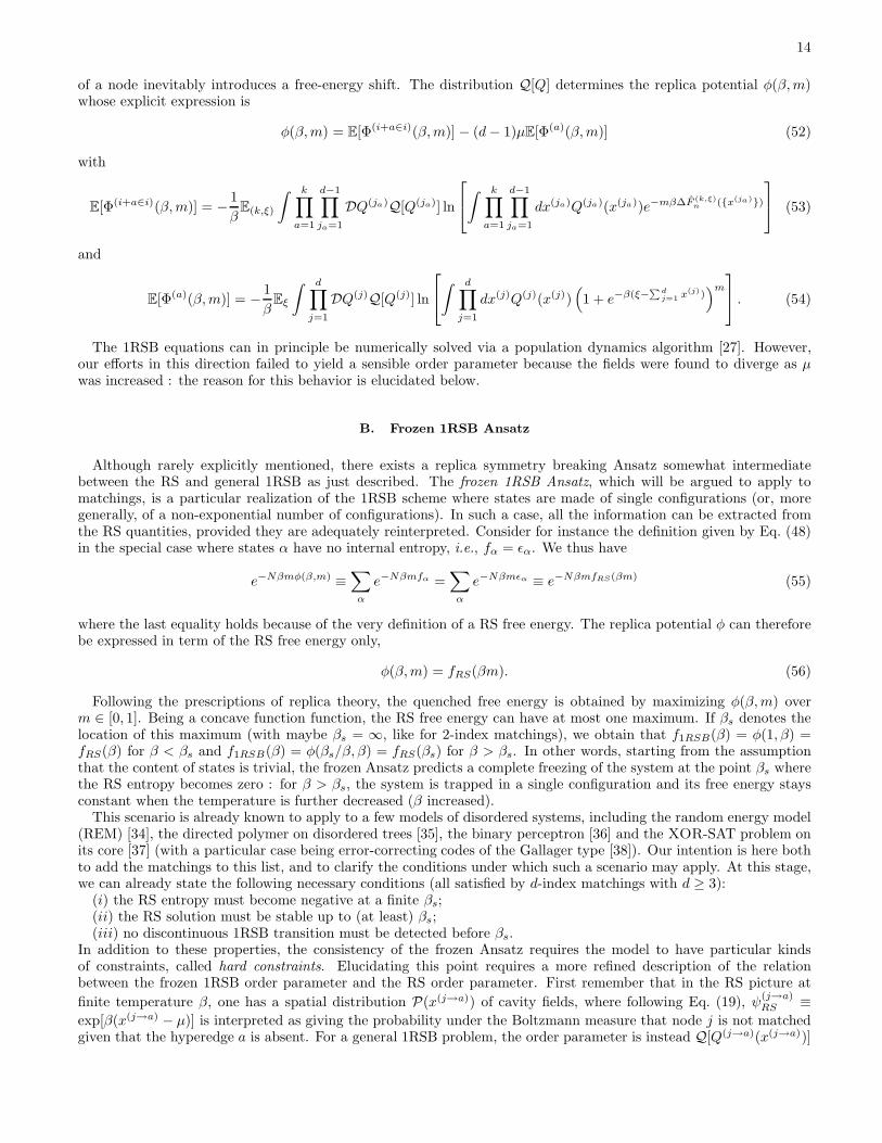
of a node inevitably introduces a free-energy shift. The distribution Q[Q] determines the replica potential φ(β,m)whose explicit expression is

φ(β,m) = E[Φ(i+a∈i)(β,m)] − (d− 1)µE[Φ(a)(β,m)] (52)

with

E[Φ(i+a∈i)(β,m)] = − 1

βE(k,ξ)

∫ k∏

a=1

d−1∏

ja=1

DQ(ja)Q[Q(ja)] ln

∫ k∏

a=1

d−1∏

ja=1

dx(ja)Q(ja)(x(ja))e−mβ∆F (k,ξ)n ({x(ja)})

(53)

and

E[Φ(a)(β,m)] = − 1

βEξ

∫ d∏

j=1

DQ(j)Q[Q(j)] ln

∫ d∏

j=1

dx(j)Q(j)(x(j))(

1 + e−β(ξ−∑

dj=1 x(j))

)m

. (54)

The 1RSB equations can in principle be numerically solved via a population dynamics algorithm [27]. However,our efforts in this direction failed to yield a sensible order parameter because the fields were found to diverge as µwas increased : the reason for this behavior is elucidated below.

B. Frozen 1RSB Ansatz

Although rarely explicitly mentioned, there exists a replica symmetry breaking Ansatz somewhat intermediatebetween the RS and general 1RSB as just described. The frozen 1RSB Ansatz, which will be argued to apply tomatchings, is a particular realization of the 1RSB scheme where states are made of single configurations (or, moregenerally, of a non-exponential number of configurations). In such a case, all the information can be extracted fromthe RS quantities, provided they are adequately reinterpreted. Consider for instance the definition given by Eq. (48)in the special case where states α have no internal entropy, i.e., fα = ǫα. We thus have

e−Nβmφ(β,m) ≡∑

α

e−Nβmfα =∑

α

e−Nβmǫα ≡ e−NβmfRS(βm) (55)

where the last equality holds because of the very definition of a RS free energy. The replica potential φ can thereforebe expressed in term of the RS free energy only,

φ(β,m) = fRS(βm). (56)

Following the prescriptions of replica theory, the quenched free energy is obtained by maximizing φ(β,m) overm ∈ [0, 1]. Being a concave function function, the RS free energy can have at most one maximum. If βs denotes thelocation of this maximum (with maybe βs = ∞, like for 2-index matchings), we obtain that f1RSB(β) = φ(1, β) =fRS(β) for β < βs and f1RSB(β) = φ(βs/β, β) = fRS(βs) for β > βs. In other words, starting from the assumptionthat the content of states is trivial, the frozen Ansatz predicts a complete freezing of the system at the point βs wherethe RS entropy becomes zero : for β > βs, the system is trapped in a single configuration and its free energy staysconstant when the temperature is further decreased (β increased).

This scenario is already known to apply to a few models of disordered systems, including the random energy model(REM) [34], the directed polymer on disordered trees [35], the binary perceptron [36] and the XOR-SAT problem onits core [37] (with a particular case being error-correcting codes of the Gallager type [38]). Our intention is here bothto add the matchings to this list, and to clarify the conditions under which such a scenario may apply. At this stage,we can already state the following necessary conditions (all satisfied by d-index matchings with d ≥ 3):

(i) the RS entropy must become negative at a finite βs;(ii) the RS solution must be stable up to (at least) βs;(iii) no discontinuous 1RSB transition must be detected before βs.

In addition to these properties, the consistency of the frozen Ansatz requires the model to have particular kindsof constraints, called hard constraints. Elucidating this point requires a more refined description of the relationbetween the frozen 1RSB order parameter and the RS order parameter. First remember that in the RS picture at

finite temperature β, one has a spatial distribution P(x(j→a)) of cavity fields, where following Eq. (19), ψ(j→a)RS ≡

exp[β(x(j→a) − µ)] is interpreted as giving the probability under the Boltzmann measure that node j is not matchedgiven that the hyperedge a is absent. For a general 1RSB problem, the order parameter is instead Q[Q(j→a)(x(j→a))]

15

where ψ(j→a) ≡ exp[β(x(j→a) −µ)] is again a thermal probability, but now restricted to a particular state taken fromthe distribution over statesQ(j→a). In this context, a RS system, characterized by a single state, hasQ(j→a)(ψ(j→a)) =

δ(ψ(j→a) − ψ(j→a)RS ). For a system in a frozen glassy phase instead, the thermal averages inside each state are trivial

since there is a single frozen configuration, ψ(j→a) = 0 or 1 meaning that a particle is present or absent with probabilityone. Therefore, the relation with the RS order parameter has the form

Q(j→a)(ψ(j→a)) = ψ(j→a)RS δ(ψ(j→a)) + (1 − ψ

(j→a)RS )δ(ψ(j→a) − 1). (57)

Plugging this expression into the general 1RSB cavity equation, it is found that such an Ansatz is consistent only ifthe system satisfies the condition that in the cavity recursion, the variable on a node is completely determined bythe values of the variables on the neighboring nodes. Such is the case with matchings when µ = ∞ where a particleis to be assigned to a hyperedge if and only if none of the neighboring edges are occupied. This is however not thecase in all constraint problems. Consider for instance the 3-coloring problem where each node is assigned one of threecolors with the constraint that its color must differ from its neighbors : in the case where all the neighbors have thesame color, the choice is left for the node between the two other colors. When a variable is fixed by the value of itsneighbors in the cavity recursion, we say that the system has hard constraints ; hard constraints can be shown [39] toindeed be present in the binary perceptron and in the XOR-SAT model on its core, models where the frozen Ansatzapplies too. Finally, we note that in the presence of hard constraints, the cavity fields ψ(j→a) take at the 1RSB levelvalues 0 and 1 only, which are associated with x(j→a) = µ and −∞. This explains the divergences observed whentrying to implement the 1RSB population algorithm at zero temperature with µ→ ∞.

C. Distances

As mentioned in Sec. VA, a 1RSB glassy system is generally described by two distances, d0 corresponding to thetypical distance between two states, and d1 corresponding to the typical distance between two configurations insidea common state. In the case of a frozen 1RSB glassy phase, one has however d1 = 0 and the structure of low-energyconfigurations (LECs) is characterized by only one distance, d0. If 〈na〉 denotes the mean occupancy of a particularhyperedge a, with the average 〈·〉 taken over the LECs, the probability for a to belong to two different LECs is givenby 〈na〉2. Averaging over the different hyperedges, it defines the overlap

q = E[〈na〉2], (58)

which is directly related to the typical distance between LECs through d0 = 1 − q. As argued before, for a systemin a frozen glassy phase the distribution of energies of the LECs is described by the thermal average at βc in the RSapproximation, so that

〈na〉 =Y

(a)1

Y(a)0 + Y

(a)1

=1

1 + e−βc(ξa−∑

i∈ax(i→a))

. (59)

Averaging over the disorder therefore yields

q = E[〈na〉2βc] = Eξa

∫ d∏

j=1

dx(j)P(x(j))(

1 + e−βc(ξa−∑

i∈a x(j)))−2

. (60)

The overlap q(β) is represented for all values of β in Fig. 10 when d = 3; given the value of βc obtained before, weget q = q(βc) = 0.321 ± 0.002.

VI. NUMERICAL ANALYSIS OF FINITE SIZE SYSTEMS

The theoretical analysis provided concerned the M → ∞ limit. How is that limit reached, and in particular isthe convergence exponentially fast in M or is it algebraic? To answer such questions, we consider in this section theproperties of d-partite matchings when M is finite; in the absence of other tools, we do this numerically. It should beclear that the most challenging questions concern the low temperature phase of our system; because of that, we willfocus on the optimum matching and low lying excitations. Even though such a numerical approach requires samplingthe disorder (random instances) and extracting for instance distributions with inevitable statistical uncertainties, itwill give evidence that our frozen 1RSB Ansatz is correct; it will also provide some statistical properties of finite sizesystems that are of interest on their own.

16

Annealed

f( )β

β 1.5

1.6

1.7

1.8

1.9

2

0.05 0.1 0.15 0.2 0.25

K = 30K = 40K = 50K = 60

C = 100C = 120C = 160C = 200

FIG. 9: RS free energies for d = 4 as obtained from the twoversions of the population dynamics algorithm described inAppendix A (here with Npop = 10000 and Niter = 1000).Note that the approximation based on Poissonian graphs(mean connectivities C = 100, 120, 160, 200) approachesthe solution from below, while the approximation basedon regular graphs (fixed connectivities K = 30, 40, 50, 60)approaches it from above. As expected, the two limitsC → ∞ and K → ∞ are found to match.

βc

qRS

β 0

0.2

0.4

0.6

0.8

1

0 1 2 3 4 5

FIG. 10: Overlap q(β) = E[〈na〉2] in the 3-index matching

as given by Eq. (60). In particular q(βc) = 0.321±0.002 de-scribes the typical overlap between two low-energy match-ings, that is the fraction of hyperedges generically share.

A. The branch and bound procedure

WhenM is very small, it is possible to enumerate all [M !]d−1

d-partite matchings of a given sample. Not surprisingly,this becomes unwieldy even when M reaches 10, forcing us to choose an alternate approach. Since it is the low energymatchings that are of greatest interest, we have developed a branch and bound algorithm that computes the p lowestenergy matchings, for any given p. Some technical aspects of the algorithm are presented in Appendix B, but theessential elements are as follows.

We represent a matching via a list of M hyperedges, one for each of the M sites of the first set (recall that thereare d sets, each of M sites). Such a representation includes also some non-legal matchings as some of the sites inthe second or higher sets could belong to more than one hyperedge; if a matching is not legal, it is discarded. Thisrepresentation can be mapped onto a rooted tree: each level of the tree is associated with one of the sites of the firstset, while a segment (branch) emerging from a node corresponds to a choice of hyperedge that contains the site ofthat node’s level. The root node is associated with the first site, the nodes of the next level are associated with thesecond site, etc... This tree is regular, each node having Md−1 outgoing segments as there are that many hyper-edgescontaining a given site of the first set. Furthermore, it has M + 1 levels: there is one level for each site of the firstset while the last level consists of leaves rather than of nodes; each leaf corresponds to a candidate matching specifiedby the list of hyperedges obtained when going from the tree’s root to that leaf. This list may correspond to a legalmatching or not, but each matching appears exactly once as a leaf. (In fact, there are MM(d−1) leaves while there

are only [M !]d−1

legal matchings.)The principle of the branch and bound algorithm is to find those leaves which satisfy the desired criterion (the

energy must be less or equal to that of the pth lowest energy matching) by exploiting a pruning procedure, therebyavoiding having to explore all leaves. To begin our pruned search, we produce p distinct legal matchings and putthem into a list L; the largest energy of the matchings in this list is an upper bound EUB on the pth energy level forour system. Then we start at the level of the tree’s root and consider all of its segments; for each choice of segment,the search problem corresponds to finding matchings on a smaller system with one less site in each of the d sets; thesearch can thus be implemented recursively. Suppose we have done k recursions; the sub-problem is associated tothe node on our tree that is obtained by following the choices of hyperedges in the recursive construction. This nodecorresponds to a partial matching in which the first k sites of the first set have each been assigned a hyperedge. Animportant property is that all hyperedges have positive energies; then we know that any matching that is compatiblewith the current partial matching has an energy greater than it, thereby providing a lower bound on all the leafenergies obtainable from the current node. If that lower bound is greater than EUB , then the subtree rooted on thecurrent node can be pruned (discarded from the search); otherwise, one iterates the recursion (that is one performsbranching on the different choices of the hyperedge to include at the present level) and k goes to k + 1. When thisprocess leads to a leaf that corresponds to a legal matching, we compute the energy E of this matching. If E < EUB ,

17

1.5

1.6

1.7

1.8

0 0.05 0.1 0.15 0.2

σ / M

1/2

1/M

2.2

2.4

2.6

2.8

3

0 0.05 0.1 0.15 0.2

Mea

n gr

ound

-sta

te e

nerg

y de

nsity

1/M

2.2

2.4

2.6

2.8

3

0 0.05 0.1 0.15 0.2

Mea

n gr

ound

-sta

te e

nerg

y de

nsity

1/M

FIG. 11: Mean ground-state energy density as a functionof 1/M at d = 3. The line is the quadratic fit using M ≥ 10data. Inset: the rescaled standard deviation of the ground-state energy, suggesting a central limit theorem behavior.

0

0.02

0.04

0.06

0.08

0.1

0.12

0 10 20 30 40 50 60 70 80

P(

E0

)

E0

M=6M=10M=14M=18M=22

FIG. 12: Distribution of the extensive ground-state energyfor increasing M values (from left to right) at d = 3.

we insert that matching into our list L and remove its worst element so that it always has p elements; we also updateEUB which by definition is the largest energy of the matchings in L; on the contrary, if E > EUB , we discard thematching (leaf). After a finite number of branchings and prunings, the algorithm has explored all choices for thesegments emerging from the tree’s root and one is done. The best p matchings are then in the list L.

The algorithm without pruning requires O(MM(d−1)) operations; with pruning and the different optimizationssketched in Appendix B, the number of operations grows roughly by a constant factor when M is increased by 1; inparticular, for the random instances studied here and d = 3, this factor is about 2.2.

B. Ground state energies

We generated a large number of random samples (disorder instances with the hyperedge costs taken to be inde-pendent uniformly distributed random variables in [0, 1]) and for each sample determined its ground state. We usedseveral random number generators to check that our results were robust. Because of the exponential growth of thecomputation time with M , in practice we were limited to relatively modest values of M . For the results presentedhere and involving only ground states, at d = 3 we used 10000 samples for M = 20 and M = 22, while for the smallervalues of M we used 20000 samples. We also performed runs at d = 4 but with lower statistics because the algorithmbecomes less efficient as d increases; in fact, we were limited to M ≤ 14 for that case and had only 5000 samples foreach M .

Let’s first focus on the behavior of ground-state energy. For each sample, we determine with our Branch & Bound

algorithm the ground-state energy density e0 ≡ E0/M ≡Md−2C(d)M [cf. Eq. (7)]; then we can analyse its mean in our

ensemble or consider other properties of its distribution.In Fig. 11 we show how the mean ground-state energy density E[e0] changes as one increases M . The behavior is

roughly linear in 1/M , but by eye one can definitely see some curvature. Because of this, linear fits do not give goodvalues of χ2 unless the M < 10 data are ignored; for instance, keeping only the M ≥ 10 data, the linear fit gives3.040(3) as the limiting value with χ2 = 3.6 for 9 degrees of freedom, while if we use all the data we obtain 3.021(3)with χ2 = 32 for 14 degrees of freedom. We have also tried corrections of the type ln(M)/M but this did not workwell. Thus we proceed by considering quadratic fits. In that case, the resulting M = ∞ intercept does not dependmuch on whether one uses all or just the highest values of M . In particular, for all the data, we get the limiting value3.046(5) with χ2 = 9.6 for 13 degrees of freedom, while using the M ≥ 10 data only one has 3.06(1) with χ2 = 2.3 for8 degrees of freedom. (In all these estimates, the error bars quoted are statistical only, as obtained from the statisticalfluctuations.) We have also considered power fits, namely E[e0] = a + b/M c. Fitting all the data gives the limitingvalue 3.08(1) with χ2 = 7.2 for 13 degrees of freedom while keeping only the M ≥ 10 data leads to 3.09(3) withχ2 = 2.3 for 8 degrees of freedom (in both cases, the exponent c is close to 0.88). Since these χ2 are similar to thoseof the quadratic fits, we see that the systematic errors are not negligible and are at least of the same order as thestatistical errors; because of these effects, the agreement with the theoretical value of 3.126 can be considered rathergood.

We studied similarly the case d = 4. The data again has positive curvature when plotted as a function of 1/M ,

18

but since we have less statistics and a much smaller range of M , much less precision can be obtained for the large Mlimit. For the linear fit (M ≥ 9) we get a limiting value of 6.75(3) with χ2 = 4.7 for 4 degrees of freedom. For thequadratic fit (M ≥ 9 again), we get 7.22(8) with χ2 = 0.37 for 3 degrees of freedom. Finally, for the power fit we get10.2(9) with χ2 = 1.0 for 5 degrees of freedom; the exponent is c = 0.3 which is small and leads to a large upturn forM > 100; clearly that regime is far beyond our reach and suggests that the power fit is probably inappropriate as nonrobust (note for instance that the uncertainty on the limiting value is far higher here than for the other fits). Thedifferent estimates show that uncertainties arising from systematic effects (M too small) are severe; instead of the1% precision we had at d = 3, we have a precision of at best 10% at d = 4 (compare to the theoretical prediction of7.703). The conclusion is that numerics do not teach us much for the case d = 4 and so hereafter we shall concentrateon the different properties arising when d = 3.

One of the expectations for the d-index matching problem is that the free energy is self-averaging. Although atpresent there is no proof of such a property, there is no reason to expect otherwise; here we are limited by the numericalapproach to ground states, but in that framework we can determine empirically the distribution of energies in theensemble of random instances. Fig. 12 displays the probability distribution of the (extensive) ground-state energy E0

for several values of M (d = 3). If as expected, the ground-state energy is self-averaging, the relative width of thesedistributions should go to zero. We have thus measured the first few moments of these distributions. In the inset ofFig. 11, we have plotted the standard deviation σ of the ground-state energy divided by

√M as a function of 1/M .

Self-averaging corresponds to having σ/M → 0; from the inset we see that σ/M1/2 goes to a constant at large M soself-averaging holds and the convergence of the distribution is compatible with a central limit theorem type behavior;such a scaling arises from sums of not too dependent random variables and leads to a Gaussian limiting shape. Toconfirm this, we have looked at higher moments: we find that indeed the skewness and kurtosis of the distributionsdecrease, in line with a central limit theorem type convergence.

Having a limiting Gaussian distribution for E0 is not a consequence of the frozen 1RSB pattern of replica symmetrybreaking since in the random energy model the distribution of E0 follows a Gumbel distribution; furthermore, inthat case the fluctuations in E0 are O(1) whereas in the matching problem they are O(

√M). To see why such large

fluctuations are “natural”, consider instead of E0 the quantity E0 obtained by adding the lengths ℓi of the shortesthyperedges containing each site i of the first set. This quantity arises in a greedy algorithm (but which does notnecessarily generate a legal matching) and clearly one has E0 ≤ E0. The central limit theorem applies to E0, so it

will have a standard deviation that grows as√M and its distribution will become Gaussian at large M . The actual

ground-state energy E0 is obtained by allowing hyperedge lengths that are slightly larger than the ℓi, but this shouldnot suppress the large fluctuations nor prevent the central limit theorem scaling.

C. Other ground state properties

As discussed at the beginning of this paper, one expects the hyperedge containing a given site in the ground statematching to be one of the shortest possible ones. To investigate this issue quantitatively, let us order all the hyperedgescontaining a given site, going from the shortest to the longest hyperedge. The “order” of a hyperedge is then 1 if itis the shortest, 2 if it is the next shortest, etc... The orders arising in the ground state should be dominated by thelowest ones, 1, 2, 3... Consider thus the frequencies with which these orders arise; in Fig.13 we show the behaviorof these frequencies for increasing M in the case d = 3. We see that there is a limiting histogram at large M , andthat indeed the lowest orders dominate. Furthermore, we see that for large k the probability of occupation of anedge tends to decrease exponentially with k (the data are displayed on a semi log plot). Note that in the standardmatching (d = 2) problem, the decrease goes as 1/2k exactly, while for our d = 3 case, the exponential decay is onlyasymptotic; furthermore, we have found no simple expression giving the decay rate of this exponential.

D. Excited states

Let us consider now states above the ground state. Define the excitation energy or “gap” as E1 − E0 where E0 isthe extensive ground-state energy and E1 that of the next lowest energy state. In Fig. 14 we show that this randomvariable has a limiting distribution so that E1−E0 = O(1) in the large M limit, just as happens in the random energymodel. Furthermore, the distribution is very well fit by an exponential (cf. the curve shown in the figure).

Following our theoretical conclusions obtained earlier, consider now the overlap between the ground state and thefirst excited state. In our frozen 1RSB picture, these matchings are expected to have a fixed (self-averaging) overlapwhen M grows. In Fig. 15 we show the probability distribution of such overlaps for increasing M . We see that thereis a local peak at large overlap that shifts toward q = 1 but which simultaneously decays. The bulk of the overlapshowever arise around q = 0.3 and when M increases we see that the corresponding peak both gets higher and more

19

0.0001

0.001

0.01

0.1

1

0 2 4 6 8 10 12

Fre

quen

cy

k

M=6M=10M=16M=20

FIG. 13: Histogram of the occupation probabilities in theground state of the hyperedges as a function of their orderk (d = 3). (Order is 1 for the lowest value among thosehyperedges containing a given site, 2 for the next lowestvalue etc...) At large k, these frequencies approach an ex-ponential law.

0

0.1

0.2

0.3

0.4

0.5

0.6

0 1 2 3 4 5 6

Pro

babi

lity

dens

ity

Energy Gap = E1 - E0

M=8M=10M=14M=18M=22

0.5 exp(-x/2)

FIG. 14: Probability density of the gap, E1 − E0, that isthe energy difference between the first excited state andthe ground state (extensive) energies in the case d = 3.The curve is a pure exponential to guide the eye.

0

0.5

1

1.5

2

2.5

0 0.1 0.2 0.3 0.4 0.5 0.6 0.7 0.8 0.9 1

Pro

babi

lity

dens

ity

(discrete) value of overlap

M=8M=10M=14M=18M=22

FIG. 15: Probability density of the overlap q between theground state and the first excited state for increasing M(d = 3).

excitation energy

2

Den

sity

of

stat

es

10

0 1 2 3 4 5 6 7

M=100.57 exp(0.405 x)

1

FIG. 16: Density of energy levels, measured from theground-state energy. At low energies (before finite sizeeffects dominate), this density grows exponentially asexp[βc(E − E0)] thereby giving the model’s critical tem-perature. Shown is the case d = 3 for M = 10.

narrow. Overall, the behavior is compatible with a convergence toward a Dirac peak near q = 0.32, to be comparedwith the theoretical prediction qc = 0.321.

E. Low energy entropy

Finally, consider the density of energy levels. In the case of the random energy model, this density becomes self-averaging when the excitation energy grows. We have thus computed the disorder averaged density of levels as afunction of the excitation energy, E−E0. That is a measure of the exponential of the microcanonical entropy; withinthe frozen 1RSB scenario, it gives the critical temperature via ρ(E − E0) ∼ exp[βc(E − E0)]. In Fig. 16 we displayour numerical estimate of ρ and see that it is very nearly a pure exponential. From the slope on the semi-log plot weextract βc ≈ 0.405; this value should be compared to the theoretical prediction of 0.412; the agreement is reasonablebut not perfect. To get better agreement, we believe it would be necessary to go to larger M and also to go furtherin the self-averaging regime, i.e., to consider larger E − E0 which numerically is an arduous task.

20

VII. CONCLUSION

We presented an analysis of multi-index matching problems (MIMPs) based on an adaptation of the cavity methodfor finite connectivity systems. For the well-known two-index matching problem, our approach provides an alternativederivation of results previously obtained using the replica and cavity methods. With respect to these older studies, thepresent one has the advantages of being closer to the mathematical framework developed by Aldous, and of allowingreplica symmetry breaking effects to be incorporated in a tractable manner. Exploiting this latter possibility, wepredict the value of the asymptotic minimal cost to be given for d-index matching problems by L(d) = ǫRS(βs) withǫRS obtained from Eq. (29) and (30) and βs satisfying sRS(βs) = 0. Formally, this d ≥ 3 conjecture differs from thecase d = 2 (where it is a theorem) in that βs = ∞ when d = 2, while βs < ∞ when d ≥ 3. The distinction between2-index and d-index matching problems with d ≥ 3 arises clearly from our analytical and numerical analysis: in thefirst case all low cost matchings share most of their hyperedges, while in the second case they differ from each otherby a finite fraction of their hyperedges. In mathematical terms, the essential uniqueness property does not hold whend ≥ 3 or in physical terms replica symmetry must be broken. Extending Aldous’ framework to rigorously accountfor this fact and providing a proof of our conjecture for d ≥ 3 seems to us a particularly interesting mathematicalchallenge.

From a physical perspective, the qualitative difference between 2-index and d-index matchings problems with d ≥ 3hinges on the presence at low temperature of a glassy phase. This is similar to the difference that has been foundbetween the 2-SAT and 2-coloring problems, which are polynomial, and the K-SAT and q-coloring problems withK ≥ 3 and q ≥ 3, which are NP-complete. For MIMPs, the nature of the glassy phase is however simpler, as it is madeof isolated configurations instead of separate clusters of many configurations. We termed this phase a “frozen 1RSBglassy phase” and attributed it to the nature of the constraints, called hard constraints. As a technical consequenceof this distinctive feature, a particular frozen 1RSB Ansatz has to be implemented. Such an Ansatz has repetitivelybeen used in the literature as a convenient (but rarely justified) substitute for the more complicated general 1RSBAnsatz; our discussion on the role of hard constraints provides a clarification of its conditions of validity which webelieve is of general interest for the investigation of glassy phases in other systems.

Acknowledgments

This work was supported in part by the European Community’s Human Potential Programme under contractsHPRN-CT-2002-00307 (DYGLAGEMEM) and HPRN-CT-2002-00319 (STIPCO) as well as by the Community’sEVERGROW Integrated Project.

APPENDIX A: POPULATION DYNAMICS ALGORITHM

Here we give a short description of the population dynamics algorithm we used to solve the RS cavity equations.We implemented two different versions, corresponding to the two different cut-off procedures mentioned in the text,associated either with Poissonian (algorithm P) or regular graphs (algorithm R). In addition to the inputs d and β,the algorithm has essentially 3 parameters: the mean degree of the nodes, C (algorithm P) or K (algorithm R), thesize of the population, Npop, and the number of iterations Niter. The common structure of the two algorithms is thefollowing:

• Initialize with random values a population of cavity fields x[i], i = 1, . . . ,Npop;

• Do Ntrans = 100 times: Update();

• Do Niter times: Update() and Measure().

The first loop allows the system to equilibrate toward the stationary distribution. The subroutine Update() dependson the cut-off procedure and can schematically described as follows:

Do Npop times:

• Draw k either at random with Poissonian distribution of mean C (algorithm P), or take k = K (algorithm R);

• Draw costs {ξa}a=1,...,k either independently with the uniform distribution in [0, C] (algorithm P), or accordingto a Poisson process with rate 1 (algorithm R);

21

• Draw at random k(d− 1) members of the population and use them together with the ξa to compute a new fieldx0 according to Eq. (22);

• Draw at random one member of the population and replace its cavity field value with x0.

The subroutine Measure() is implemented similarly and computes the free energy according to Eqs. (27)-(28).The final output for the free energy is obtained by averaging over the Niter iterations, while the fluctuations acrossiterations are used to check convergence. The algorithm must be run for increasing values of C or K to extrapolate theC → ∞ (algorithm P) orK → ∞ (algorithm R) limit, requiring one to consider larger and larger population sizes Npop

to obtain reliable results. Taking this limit is however facilitated by the numerical observation that the Poissonianapproximation (algorithm P) approaches the solution from below while the regular approximation (algorithm R)approaches it from above; this is illustrated in Fig. 9 with d = 4. We refer to the captions of the various figures fortypical choices of the parameters C, Npop and Niter. The numerical results we obtained for d = 2 are consistent withthe exact solution, βc = ∞ and fRS(βc) = π2/12, and are the following for d = 3, 4:

d = 3 : βc = 0.412 ± 0.001, fRS(βc) = 1.042± 0.0003,

d = 4 : βc = 0.135 ± 0.002, fRS(βc) = 1.925± 0.0006.(A1)

The free-energy densities are given here for simple matching problems and their counterpart for d-partite matchingsare obtained by multiplying the values by d.

We have also implemented the generalization of this algorithm to solve the 1RSB cavity equations (50) and used itto check that no discontinuous transition occurs prior to the entropy crisis (see [27] for algorithmic details).

APPENDIX B: ASPECTS OF THE BRANCH AND BOUND ALGORITHM

Our objective is to solve d-partite matching problems at sufficiently largeM so that an extrapolation to the M → ∞limit can be performed without too much uncertainty. For many problems (satisfiability, coloring, etc...), one prefersan easily implementable algorithm such as one in the class of “heuristic” algorithms; in such approaches one performsa fast search for the ground state but no guarantee is provided that the global optimum will be found. Examples ofthese algorithms are simulated annealing and variable depth local search. Heuristic algorithms typically attempt tomove towards regions of lower energy by searching in the neighborhood of a current configuration. However, sincethe search is local, such an approach is bound to break down for problems in which the frozen 1RSB scenario applies.This fact pushed us towards the development of an “exact” algorithm capable of delivering a certificate of optimalityof the proposed ground state. Amongst exact algorithms, enumeration can be discarded because it is much too slow;Branch & Bound gets around this problem through pruning of the enumeration/search. There are also other possiblemethods such as Branch & Cut, but these require an in depth understanding of polytopes and rely on separationprocedures which have not yet been developped for MIMP. Note that in all exact methods, the key to efficiency is tohave good bounds; fortunately MIMPs are relatively well adapted to such a strategy.

We already discussed in the main text our choice of representation of matchings and partial matchings. Given apartial matching of the first k sites of the first set, we have to solve a MIMP with M−k sites and so the algorithm canbe implemented recursively. Since at each node we need to consider all of its possible branchings (naively, there are(M − k)d−1 of these), it is useful to order these branchings according to the length of the corresponding hyperedges,going from short to long. Rather than recompute these orderings dynamically every time the partial matching changes,we do it once and for all at the initialization of the program. This allows for speed but it must be compensated bya rapid determination of whether a given hyperedge is allowed; for that we use a data structure which tells us foreach site of each set whether it is matched (belongs to one of the occupied hyperedges). This structure is updatedwhenever a partial matching is extended or reduced.

The pruning of the search must be as stringent as possible, and this depends on the quality of the bounds. Oursimplest bound B1 is just the current partial matching’s energy Ek: if that energy is higher than EUB (the upperbound EUB as defined in section VI A), then the whole sub-tree below the current node can be pruned. A betterbound is B2, obtained by adding to Ek the sum over each remaining unmatched site of the first set of the shortesthyperedge containing that site. This sum can be precomputed and tabulated. A still better bound is B3 obtained asB2 but where now one takes for each site the shortest hyperedge that is compatible with the current partial matching.This bound cannot be predefined once and for all and is slow to compute. Since we have found it to be useful forpruning, we have optimized its determination by noticing that it can be tabulated and modified incrementally: everytime the partial matching is extended (a hyperedge is added), we perform the search for the compatible hyperedgesof each unmatched site starting from the index (order) previously found to be compatible. When backtracking, one

22

has to remove a hyperedge and there we simply go back to the tables we had at that level: in effect, we maintainefficiency if we assign tables at each level and follow their updating one step at a time.

The rate of pruning is very different for the three bounds, and we found that a good strategy (for balancing pruningrate and computation time) was to apply the three bounds successively: if the first one does not prune, one goes onto the second one and so forth. To speed up the computation further, we found it useful to implement the recursivityof the program in a limited mode only: the data structures are set up once and for all at initialization time, thehyperedges are ordered once and for all too, and then the recursion is used mainly to go through the branchings andto maintain the tables. Efficiency is gained as no reorganization of the instance (hyperedge weights) is performed,and in particular no “smaller matching problem” is ever defined explicitly.

[1] M. Mezard and G. Parisi, J. Physique 46, L771 (1985).[2] M. Mezard and G. Parisi, Europhys. Lett. 2, 913 (1986).[3] D. J. Aldous, Rand. Struct. Algo. 18, 381 (2001).[4] R. Mulet, A. Pagnani, M. Weigt, and R. Zecchina, Phys. Rev. Lett. 89, 268701 (2002).[5] M. Mezard and R. Zecchina, Phys. Rev. E 66, 056126 (2002).[6] M. Mezard, G. Parisi, and R. Zecchina, Science 297, 812 (2002).[7] O. C. Martin, M. Mezard, and O. Rivoire, Phys. Rev. Lett. 93, 217205 (2004).[8] M. Mezard, G. Parisi, and M. A. Virasoro, Spin-Glass Theory and Beyond, vol. 9 of Lecture Notes in Physics (World

Scientific, Singapore, 1987).[9] M. Mezard and G. Parisi, J. Physique 48, 1451 (1987).

[10] G. Parisi and M. Ratieville, Eur. J. Phys. B 29, 4 (2002).[11] G. Parisi and M. Ratieville, Eur. J. Phys. B 22, 229 (2001).[12] J. Houdayer, J. H. Boutet de Monvel, and O. C. Martin, Eur. Phys. Jour. B 6, 383 (1998).[13] D. Aldous and M. Steele, in Encyclopedia of Mathematical Sciences, edited by H. Kesten (Springer, 2003), vol. 110, pp.

1–72.[14] S. Linusson and J. Wastlund (2003), arXiv:math.CO/0303214.[15] B. P. C. Nair and M. Sharma (2003), available at http://www.stanford.edu/∼balaji/rap.html.[16] G. Parisi (1998), cond-mat/9801176.[17] M. Talagrand, Spin glasses: A challenge for mathematicians (Springer, 2003).[18] W. P. Pierskalla, Operations Research 16, 422 (1968).[19] F. C. R. Spieksma, in Nonlinear Assignment Problems, Algorithms and Applications, edited by L. Pitsoulis and P. Pardalos

(Kluwer, Dordrecht, 2000), pp. 1–12.[20] R. E. Burkard, Discrete Applied Mathematics 123, 257 (2002).[21] A. B. Poore, Comput. Opt. Appl. 3, 27 (1994).[22] J. Pusztaszeri, P. E. Rensing, and T. M. Liebling, Journal of Global Optimization 16, 422 (1995).[23] R. Karp, in Complexity of Computer Computations, edited by R. Miller and J. Thatcher (Plenum Press, New-York, 1972),

pp. 85–103.[24] C. H. Papadimitriou and K. Steiglitz, Combinatorial Optimization: Algorithms and Complexity (Prentice Hall, Englewood

Cliffs, NJ, 1982).[25] J. Vannimenus and M. Mezard, J. Physique Lett. 45, L1145 (1984).[26] D. J. Aldous, Rand. Struct. Algo. 1, 383 (1990).[27] M. Mezard and G. Parisi, Eur. Phys. J. B 20, 217 (2001).[28] M. Mezard and G. Parisi, J. Stat. Phys. 111, 1 (2003).[29] D. J. Aldous and A. Bandyopadhyay (2004), arXiv:math.PR/0401388.[30] An additional evidence that the naıve generalization of the formulae used when d = 2 fails for d ≥ 3 is found when d = 4

(extending presumably to all d ≥ 4) where the RS prediction for L(d)RS

violates the annealed bound.[31] A. Montanari and F. Ricci-Tersenghi, Eur. Phys. J. B 33, 339 (2003).[32] O. Rivoire, G. Biroli, O. C. Martin, and M. Mezard, Eur. Phys. J. B 37, 55 (2004).[33] R. Monasson, Phys. Rev. Lett. 75, 2847 (1995).[34] B. Derrida, Phys. Rev. Lett 45, 79 (1980).[35] B. Derrida and H. Spohn, J. Stat. Phys. 51, 817 (1988).[36] W. Krauth and M. Mezard, Europhys. Lett. 8, 213 (1989).[37] M. Mezard, F. Ricci-Tersenghi, and R. Zecchina, J. Stat. Phys. 111, 505 (2003).[38] A. Montanari, Eur. Phys. J. B. 23, 121 (2001).[39] O. Rivoire, Ph.D. thesis, Universite Paris-Sud (2005).