arX

iv:0

903.

1846

v1 [

stat

.ME

] 1

0 M

ar 2

009

Expectations of Random Sets and Their Boundaries

Using Oriented Distance Functions

Larissa I. Stanberry∗ and Hanna K. Jankowski∗∗

∗School of Mathematics, University of Bristol.

∗∗Department of Mathematics and Statistics, York University.

March 10, 2009

Abstract

Shape estimation and object reconstruction are common problems in image analysis. Mathematically,

viewing objects in the image plane as random sets reduces the problem of shape estimation to inference

about sets. Currently existing definitions of the expected set rely on different criteria to construct the

expectation. This paper introduces new definitions of the expected set and the expected boundary,

based on oriented distance functions. The proposed expectations have a number of attractive properties,

including inclusion relations, convexity preservation and equivariance with respect to rigid motions. The

paper introduces a special class of separable oriented distance functions for parametric sets and gives

the definition and properties of separable random closed sets. Further, the definitions of the empirical

mean set and the empirical mean boundary are proposed and empirical evidence of the consistency of the

boundary estimator is presented. In addition, the paper gives loss functions for set inference in frequentist

framework and shows how some of the existing expectations arise naturally as optimal estimators. The

proposed definitions of the set and boundary expectations are illustrated on theoretical examples and

real data.

1 Introduction

Boundary reconstruction and shape estimation are frequently encountered problems in image analysis. For

example, it is often of interest to determine a characteristic shape of a cell, reconstruct tissue boundary in

medical images, or estimate a probable area in the earthquake disaster zone. Mathematically, the objects

of interest can be viewed as sets, whilst inherent stochasticity of the acquisition process turns them into

random entities. The problems of boundary reconstruction and shape estimation thus reduce to inference

about random sets.

Early results in the theory of random sets date back to Choquet (1953) with a thorough mathemat-

ical treatment appearing in Matheron (1975) and the most recent developments in the field presented in

(Molchanov, 2005). Because the family of closed sets is nonlinear, there is no natural way to define the

1

expected set. Currently, there exist a number of definitions of the expectation, though neither can be spoken

of as the best. As pointed out in Molchanov (2005), the definition of the expectation depends on set features

that are important to emphasize.

Many of the existing definitions are not based on a random set directly, but use an embedding into a

function space. For example, the Vorob’ev definition uses the representation of a set given by its characteristic

function to construct an expectation that is optimal with respect to Lebesgue measure (Vorob’ev, 1984).

The distance-average approach maps a set into the space of distance functions, so that the expected set is

optimal among all of the level sets of the expected distance function with respect to a predefined metric

(Baddeley and Molchanov, 1998).

Currently existing definitions of the expected set do not address the question of boundary estimation,

which is often of primary interest in practice. In this paper, we introduce a new definition of the expected

set and the expected boundary based on oriented distance functions (ODFs). As opposed to a conventional

distance function, an ODF takes into account the set and its complement, providing a more informative

representation of a set (Delfour and Zolesio, 2001). In comparison with currently existing definitions, the

new expectations have a number of attractive theoretical properties. In particular, they satisfy inclusion

relations, preserve convexity and remain equivariant with respect to rigid motions. We introduce a new

class of ODFs for parametric sets and show the connection between the expectation of a parametric random

closed set and the expected parameter. We also outline a general framework for set inference and show how

different expectations arise as natural estimators for different loss functions.

2 Random Closed Sets

2.1 Notation

For set A ⊂ Rd, denote by Ac, ∂A, cl A, int A, λ(A) its complement, boundary, closure, interior, and Lebesgue

measure, respectively. We write x = (x1, . . . , xd) for point x ∈ Rd and use |· | for the standard Euclidean

norm. Let F (resp. K) be the family of closed (resp. compact) subsets of Rd and let the tripple (Ω, A ,P)

denote the probability space.

2.2 Definitions and Examples

Definition 2.1. A random closed set is the mapping A : Ω 7→ F such that for every compact set K ∈ K,

ω : A(ω) ∩ K 6= ∅ ∈ A .

Here, we consider random closed sets taking values in Rd. Throughout this paper, we write “r.c.s.” for

a random closed set, though some texts prefer RACS. We write A for an r.c.s. A(ω) and reserve capital

roman letters for closed subsets of Rd.

Random closed sets give rise to several random variables and random functions, including the character-

istic function

χA(x) =

1, if x ∈ A,

0, if x /∈ A,(1)

2

the Lebesgue measure λ(A) =∫

Rdχ

A(x)dx, and the distance function from point x ∈ Rd to A,

dA(x) =

infy∈A ρ(x, y), A 6= ∅,

+∞, A = ∅,(2)

where ρ(x, y) is a metric on Rd. Some examples of ρ include the L2 Euclidean metric, the L∞ Chebyshev

metric, and the L1 Manhattan metric. Throughout this paper, we use the Euclidean distance function with

ρ(x, y) = |x − y| in (2).

2.3 Expectations of Random Closed Sets

Because the space F of all closed subsets of Rd is nonlinear, there is no natural way to define the expected

set. In this section, we briefly review some of the existing definitions and refer for more details to (Aumann,

1965; Artstein and Vitale, 1975; Vorob’ev, 1984; Baddeley and Molchanov, 1998; Molchanov, 2005).

Definition 2.2 (Selection expectation). A random element ξ is called the selection of A, if it belongs to

A with probability one. A selection ξ is integrable, if E |ξ| < ∞. The selection expectation, ES[A], is the

closure of the set of the expectations of all integrable selections of A,

ES[A] = cl E[ξ] : ξ is a selection and E |ξ| < ∞.

The selection expectation depends on the structure of the probability space (Molchanov, 2005, see Example

1.14, Section 2). In addition, if the probability space is nonatomic, ES[A] is necessarily convex, even for

nonconvex deterministic sets.

In the context of image analysis, the Vorob’ev expectation is perhaps the most intuitive construction

(Vorob’ev, 1984). Consider an r.c.s. A ⊂ D. For every point x ∈ D, we assign a probability mass depending

on whether or not x ∈ A. For example, assigning one to all points in A and zero to points in Ac converts the

observed set into a binary image. Averaging binary images over all realizations of A, we obtain a gray-scale

image, where the intensity at each pixel is the probability of the point being in A. The gray-scale image is

not a binary image, unless A is deterministic. The Vorob’ev definition then provides a criterion to construct

an expected set that is optimal with respect to Lebesgue measure.

More precisely, given the characteristic function χA

of an r.c.s. A, define the coverage function by

E[χA(x)] = P(x ∈ A). (3)

The excursions sets of the coverage function are given by

Au = x ∈ Rd : E[χ

A(x)] ≥ u, q ∈ [0, 1]. (4)

Definition 2.3 (Vorob’ev expectation). The expectation, EV[A], of a random closed set A is the excursion

set Aq, where q ∈ [0, 1] is such that

λ(Au) ≤ E[λ(A)] ≤ λ(Aq) for all u > q. (5)

3

Note that the optimality criterion (5) ensures that the Vorob’ev expectation ignores sets of measure zero.

The distance-average expectation is based on a representation of a set given by some function fA : D 7→ R

(Baddeley and Molchanov, 1998). We call fA a representative function of the set A. Examples of f include

the distance function, the ODF, the characteristic function and others. For an r.c.s. A with representative

function fA, let E[fA(x)] be the expected value of fA at x, assuming it exists.

Definition 2.4 (Distance-average expectation). For a compact window W , define a (pseudo-) metric

m(A,B) = mW(fA(·), fB(·)). The distance-average expectation, EDA[A], of an r.c.s. A is the level set

Au = x ∈ W : E[fA(x)] ≤ u, where u = arg infs∈R

m(E[fA], fAs) (6)

Examples of pseudometric m in (6) include Lq distances and their variates, Baddeley’s ∆q-distance, or

any custom definitions (Baddeley, 1992). Note that the pseudometric m is computed over the window W ,

which can be the entire domain D or its subset. For brevity, we omit the subscript W whenever possible.

The distance-average expectation strongly depends on the choice of the representative function f , window

W , (pseudo-) metric m and parameters of m (Baddeley and Molchanov, 1998). The Vorob’ev expectation

can be viewed as a special case of the distance-average definition with fA(x) = 1 − χA(x) and L1 distance

m (Baddeley and Molchanov, 1998, see Example 5.14).

The linearization approach gives a unified view of the existing expectations (Molchanov, 2005). In

particular, consider a mapping f : F 7→ Y, where Y is some Banach space. Let fA be the image of A in

Y and assume that E[|fA(x)|] < ∞. If there exists a unique F ∈ F such that fF (x) = E[fA(x)], then

declare E[A] = F . In general, the inverse image rarely exists, and we need to define the criterion so that the

resulting expectation is optimal in some sense. This is done as follows. Let d be a pseudometric in Y, then

the expectation of an r.c.s. A is given by

E[A] = arg minF∈F

d(E[ζ(A)], ζ(F )). (7)

Minimizing over the entire family F is often nontrivial. Therefore, we can consider optimizing d(·, ·) over

a subfamily H ⊂ F of candidate sets. Clearly, the resulting expectation depends on the choice of Banach

space Y, mapping f , metric d, subfamily H and any implicit parameters that enter into the calculation.

For bounded closed covex sets, the selection expectation is an example of a linearization approach, where

the embedding into a Banach space is realised by support functions of random sets on the unit sphere

and the expected set is given by the support function of the selection expectation. Another example is

the Vorob’ev definition, which is based on the mapping given by χA

and gives the expected set EV[A]

which is optimal with respect to Lebesgue measure; the family of candidate sets H consists of excursion

sets (4) of the coverage function. The distance-average expectation is based on the embedding into the

space of representative function and the resulting average is optimal among the level sets of the expected

representation with respect to metric m(·, ·) (Baddeley and Molchanov, 1998; Molchanov, 2005).

2.4 Oriented Distance Functions

In comparison to a distance function (2), an ODF takes into account both the set and its compliment, thus

reflecting the interior and exterior properties. In addition, the ODF provides a level-set description of the

4

boundary.

Definition 2.5. The ODF from point x to set A ⊂ Rd with ∂A 6= ∅ is defined by

bA(x) = dA(x) − dAc(x), for all x ∈ Rd. (8)

Using basic properties of the distance function, the expression (8) can be written as

bA(x) =

dA(x) = d∂A(x), x ∈ int Ac

0, x ∈ ∂A

−dAc(x) = −d∂A(x), x ∈ int A .

(9)

Below we summarize some properties of the ODFs and refer for proofs and details to Delfour and Zolesio

(2001).

Proposition 2.1. Let A and B be some subsets of cl D with ∂A, ∂B 6= ∅.

1. The ODF provides a level-set description of a set, i.e

cl A = x : bA(x) ≤ 0, ∂A = x : bA(x) = 0.

2. A ⊃ B implies bA ≤ bB.

3. bA ≤ bB in D iff cl B ⊂ cl A and cl Ac ⊂ cl Bc.

4. bA = bB in D iff cl A = cl B and ∂A = ∂B.

5. For a convex set A with ∂A 6= ∅, bA = bcl A is a convex function in Rd.

6. The function bA(x) is uniformly Lipschitz in Rd with constant one, i.e.

|bA(y) − bA(x)| ≤ |y − x| for any x, y ∈ Rd.

In addition, bA(x) is (Frechet) differentiable with |∇bA(x)| ≤ 1 a.e. in Rd. When it exists, the gradient

of the ODF coincides with the outward unit normal to the boundary.

Note that the ODF identifies the set up to its closure and boundary. In other words, ODF describes

equivalence classes of sets with identical closure and boundary.

Example 2.1. For a singleton A = θ, θ ∈ Rd, the ODF coincides with the distance function and

bA(x) = dA(x) = |x − θ| for all x ∈ Rd. Note that bA(x) > 0 for all x 6= θ and the isocontours of bA(x) are

spheres centered at θ; Figure 1, 1st plot.

Example 2.2. Consider a closed ball in Rd centered at the origin with radius θ, i.e. A = x ∈ R

d : |x| ≤ θ.

The distance function of A is dA(x) = |x| − θ, for x ∈ A, and zero, elsewhere. Hence, the ODF has a form

bA(x) = |x| − θ for all x ∈ Rd. The isocontours of bA(x) are spheres centered at the origin; Figure 1, 2nd

plot.

5

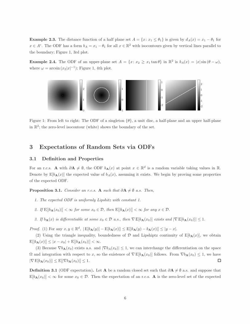
Example 2.3. The distance function of a half plane set A = x : x1 ≤ θ1 is given by dA(x) = x1 − θ1 for

x ∈ Ac. The ODF has a form bA = x1 − θ1 for all x ∈ R2 with isocontours given by vertical lines parallel to

the boundary; Figure 1, 3rd plot.

Example 2.4. The ODF of an upper-plane set A = x : x2 ≥ x1 tan θ in R2 is bA(x) = |x| sin (θ − ω),

where ω = arcsin (x2|x|−1); Figure 1, 4th plot.

1

2

0

-1

1

0

-2

-1

1

0

-2

-1

1

2

0

Figure 1: From left to right: The ODF of a singleton θ, a unit disc, a half-plane and an upper half-plane

in R2; the zero-level isocontour (white) shows the boundary of the set.

3 Expectations of Random Sets via ODFs

3.1 Definition and Properties

For an r.c.s. A with ∂A 6= ∅, the ODF bA(x) at point x ∈ Rd is a random variable taking values in R.

Denote by E[bA(x)] the expected value of bA(x), assuming it exists. We begin by proving some properties

of the expected ODF.

Proposition 3.1. Consider an r.c.s. A such that ∂A 6= ∅ a.s. Then,

1. The expected ODF is uniformly Lipshitz with constant 1.

2. If E[|bA(x0)|] < ∞ for some x0 ∈ D, then E[|bA(x)|] < ∞ for any x ∈ D.

3. If bA(x) is differentiable at some x0 ∈ D a.s., then ∇E[bA(x0)] exists and |∇E[bA(x0)]| ≤ 1.

Proof. (1) For any x, y ∈ Rd, |E[bA(y)] − E[bA(x)]| ≤ E[|bA(y) − bA(x)|] ≤ |y − x|.

(2) Using the triangle inequality, boundedness of D and Lipshiptz continuity of E[bA(x)], we obtain

E[|bA(x)|] ≤ |x − x0| + E[|bA(x0)|] < ∞.

(3) Because ∇bA(x0) exists a.s. and |∇bA(x0)| ≤ 1, we can interchange the differentiation on the space

Ω and integration with respect to x, so the existence of ∇E[bA(x0)] follows. From ∇bA(x0) ≤ 1, we have

|∇E[bA(x0)]| ≤ E[|∇bA(x0)|] ≤ 1.

Definition 3.1 (ODF expectation). Let A be a random closed set such that ∂A 6= ∅ a.s. and suppose that

E[bA(x0)] < ∞ for some x0 ∈ D. Then the expectation of an r.c.s. A is the zero-level set of the expected

6

ODF and expectation of the boundary of A is the zero-level isocontour of the expected ODF, i.e.

E[A] = x : E[bA(x)] ≤ 0, (10)

E[∂A] = x : E[bA(x)] = 0. (11)

We refer to E[A] as “the expected set” or “the ODF expectation” of A. Note, that the expected set defined

by (3.1) can be an empty set. Later we give examples of such random sets and discuss the appropriateness

of the outcome.

Theorem 3.1 (Inclusion properties). Consider r.c.s. A,B ⊂ cl D with ∂A, ∂B 6= ∅ and assume that

E[bA(x)] and E[bB(x)] exist for some x ∈ cl D. That is, suppose E[A] and E[B] are well-defined. Then,

1. The expectation E[A] is a closed set.

2. If A = A a.s., for some deterministic A ∈ F , then E[A] = A and E[∂A] = ∂A.

3. Suppose that an r.c.s. A satisfies ∂A = B a.s. for some deterministic set B, then E[∂A] ⊃ B.

4. For an r.c.s. A, ∂ E[A] ⊂ E[∂A].

5. If E[bA(x)] ≥ E[bB(x)] a.s., then E[A] ⊂ E[B].

6. If A ⊂ B a.s., then E[A] ⊂ E[B].

Proof. (1) The closedness of E[A] follows from the continuity of E[bA].

(2) is straightforward.

(3) It suffices to note that for all points x ∈ B, bB(x) = bA(x) = 0, so that E[bA(x)] = 0 and B ⊂ E[∂A].

(4) For any x ∈ ∂ E[A], E[bA(x)] = 0 and hence x ∈ E[∂A]. Example 3.2 shows that the reverse relation

does not hold.

(5) For any x ∈ E[A], 0 ≥ E[bA(x)] ≥ E[bB(x)]. Thus x ∈ E[B] and E[A] ⊂ E[B].

(6) The proof follows immediately from the previous statement and Property 3 of the ODFs, which

implies that for A ⊂ B, bA(x) ≥ bB(x) in D and hence, E[bA(x)] ≥ E[bB(x)] a.s..

Corollary 3.1. If an r.c.s. A ⊃ U a.s. for some deterministic set U ⊂ cl D, then E[A] ⊃ cl U. Similarly,

if an r.c.s. A ⊂ W a.s. for some deterministic set W ⊂ cl D, then E[A] ⊂ cl W .

Proof. Follows from statements (2) and (6) of Theorem 3.1.

Although the inclusion properties of Theorem 3.1 and Corollary 3.1 seem natural, they do not necessarily

hold for other definitions, including the selection expectation (Molchanov, 2005) and the distance-average

definition. The latter does not satisfy a weaker version of inclusion in the sense that the resulting expectation

is not necessarily contained in the convex hull of the union of all possible realizations of a random set

(Baddeley and Molchanov, 1998).

Example 3.1. (random singleton) Let ξ be a random variable and consider an r.c.s. A = ξ. Then, for

any x ∈ D, E[bA(x)] = E[|x − ξ| > 0] and hence E[A] = ∅.

7

The last result does not agree with suggestions in Molchanov (2005), where E[ξ] = E[ξ] is listed as one

of the desirable properties of the expected set. Indeed, the selection expectation satisfies the suggested prop-

erty and so does the distance-average definition, for certain choices of m, f and W (Baddeley and Molchanov,

1998, see Example 5.4). However, the ODF definition of the expected set was primarily motivated by prob-

lems in image analysis, where random singletons are often regarded as noise. Example 3.1 highlights the

natural denoising property of the ODF expectation in a sense that any speckles, unless observed a.s., are not

present in the average reconstruction. We argue that if random singletons are the sets of primary interests,

they should be viewed as random vectors rather than random sets, in which case conventional definitions of

the expectation and dispersion are applicable.

More generally, Example 3.1 can be extended to random sets with zero Lebesgue measure. In particular,

for a r.c.s. A with int A = ∅ and λ(A) = 0, we have bA(x) > 0 for all x ∈ Ac and bA(x) = 0 for all x ∈ ∂A.

Thus, unless x ∈ ∂A almost surely, E[bA(x)] > 0 and the expected set E[A] = x : x ∈ A almost surely.

In the rest of this section, we discuss equivariance properties of the ODF expectation. To begin with,

recall that the translation of a set A ⊂ Rd by a ∈ R

d is the set a + A = a + x : x ∈ A. Similarly, the

homothecy of A by a scalar α is given by αA = αx : x ∈ A. The homothecy is a dilation for α ≥ 1,

a contraction for α ∈ [0, 1), and a reflection for α = −1. For negative α, the homothecy is a dilation or

a contraction of the reflection for |α| < −1 and |α| ∈ (0, 1), respectively. Rigid motion transformations

g : Rd 7→ R

d are given by g(x) = Γx + a, where Γ ∈ O(n) is an orthogonal matrix and a ∈ Rd. In R

d, these

transformations are isometries, i.e. |x − y| = |g(x) − g(y)|, and form the Euclidean group E(d) with respect

to the composition.

Theorem 3.2 (Equivariance properties). The expected set and the expected boundary are equivariant with

respect to:

1. Homothecy, i.e. for a fixed scalar α 6= 0,

E[αA] = α E[A] and E[∂αA] = α E[∂A]. (12)

2. The group of rigid motions, i.e. for any g ∈ E(d),

E[gA] = gE[A] and E[g ∂A] = gE[∂A]. (13)

Proof. (1) We begin by establishing the relation between the ODFs of a set and its homothecy. In particular,

dαA(x) = infy∈αA |y − x| = infy∈A |αy − x| = |α|dA(x/α). Similarly, d(αA)c(x) = |α|dAc(x/α), so that

bαA(x) = |α|bA(x/α).

For any y ∈ E[αA], E[bαA(y)] ≤ 0. Writing y = αx for some x, we obtain 0 ≥ E[bαA(y)] = E[bαA(αx)] =

|α|E[bA(x)]. Thus, E[bA(x)] ≤ 0 and y = αx with x ∈ E[A]. Hence, y ∈ α E[A] and E[αA] ⊆ α E[A].

For any y ∈ α E[A], y = αx for some x ∈ E[A]. Then E[bαA(y)] = E[|α|bA(y/α)] = |α|E[bA(x)] ≤ 0.

Thus, y ∈ E[αA] and E[αA] ⊇ α E[A].

The equivariance property for the boundary is proved similarly and we omit the details.

(2) A transformation g(x) = Γx + a, for some orthogonal matrix Γ ∈ O(d) and a ∈ Rd, is a bijection

and g−1(x) = Γ−1(x − b) = ΓT(x − b). For sets gA = g(x) : x ∈ A and (gA)c = g(x) : x ∈ Ac, we

8

obtain dgA(x) = infy∈gA |y − x| = infy∈A |Γy + b − x| = infy∈A |y − ΓT(x − b)| = dA(g−1(x)). Similarly,

d(gA)c(x) = dAc(g−1(x)) and bgA = bA(g−1(x)).

Recall that gE[A] = g(x) : x ∈ E[A] and E[gA] = x : E[bgA(x)] ≤ 0. Hence, for any y ∈ gE[A],

there exists x ∈ E[A] such that y = g(x). From here, E[bgA(y)] = E[bA(g−1(Γx + b))] = E[bA(x)] ≤ 0.

Hence, y ∈ E[gA] and E[gA] ⊇ g E[A].

On the other hand, any y ∈ E[gA] can be written as y = Γx + b, where x = g−1(y). It then follows that

0 ≥ E[bgA(y)] = E[bA(g−1(g(x)))] = E[bA(x)]. Thus, any y ∈ E[gA] has a form y = Γx + b, where x ∈ E[A].

Hence, E[gA] ⊆ gE[A] and E[gA] = gE[A].

Corollary 3.2. Note that any translation in Rd can be described as an isometry with an identity matrix Γ.

Thus, it immediately follows that the expected set and the expected boundary are translation-equivariant, i.e.

for some fixed a ∈ Rd,

E[a + A] = a + E[A] and E[∂(a + A)] = a + E[∂A]. (14)

Theorem 3.3 (Convexity preservation). Suppose that an r.c.s. A is convex a.s.. Then the expectation E[A]

of A is also convex.

Proof. The a.s. convexity of A implies that cl A is convex and bA = bcl A is a convex function a.s.

(Delfour and Zolesio, 2001, Theorem 7.1). Hence, for all α ∈ [0, 1], bA(αx+(1−α)y) ≤ αbA(x)+(1−α)bA(y)

a.s.. Taking expectations, we obtain that E[bA] is convex, and so is E[A].

We refer to Theorems 3.2 and 3.3 as the shape-preservation properties of the ODF expectation. These

qualities are particularly desirable in shape and image analysis. In contrast, given a nonatomic probability

space, the selection expectation of an r.c.s. is convex and coincides with the expectation of its convex hull.

Notably, the convexification of ES[A] holds even for nonconvex deterministic sets (Molchanov, 2005). The

distance-average expectation preserves the convexity, but only if the set, its representative function and the

window are convex (Baddeley and Molchanov, 1998).

Example 3.2 (Set and its boundary). Consider an r.c.s. A such that A = 0, 1 or A = [0, 1] in R with

probabilty p and 1 − p, respectively. Note that the boundary ∂A = 0, 1 a.s. in R, so essentially, we are

observing either the set or its boundary. The expected ODF is given by

E[bA(x)] =

−x, x ≤ 0

(2p − 1)x, 0 < x ≤ 0.5

(2p − 1)(1 − x), 0.5 < x ≤ 1

x − 1, x > 1.

For p = 0.5, E[A] = E[∂A] = [0, 1]. For p < 0.5, E[A] = [0, 1] and E[∂A] = 0, 1. For p > 0.5, E[A] =

E[∂A] = 0, 1. Note that for p = 0.5, ∂A = 0, 1 a.s. However, E[∂A] 6= 0, 1, but rather ∂A ⊂ E[∂A],

as in Proposition 3.1(3).

For p = 0.5, the distance-average expectation is EDA[A] = [−1/12, 1/6]∪ [5/6, 13/12], for m uniform, and

EDA[A] = 0, 1, for m = ∆pW

with sufficiently large W (Baddeley and Molchanov, 1998).

9

More generally, consider an r.c.s. A such that, for some deterministic B ∈ F , A = B with probability p

and A = ∂B, otherwise. From

b∂B(x) =

bB(x), x ∈ Bc,

0, x ∈ ∂B,

−bB(x), x ∈ int B,

it follows that

E[bA(x)] =

bB(x), x ∈ Bc,

0, x ∈ ∂B,

(1 − 2p)bB(x), x ∈ int B.

Hence,

for p = 0.5, E[A] = E[∂A] = B,

for p < 0.5, E[A] = B, E[∂A] = ∂B,

for p > 0.5, E[A] = E[∂A] = ∂B.

Example 3.3 (Ball with random radius). Consider a random closed ball A in Rd with a fixed center x0

and a random radius Θ. Recall that the ODF of A is given by bA(x) = |x− x0| −Θ for all x ∈ Rd. Hence,

E[bA(x; Θ)] = |x − x0| − E[Θ] and the expected set is a closed ball centered at x0 with radius E[Θ]. The

expected boundary E[∂A] is a sphere centered at x0 with radius E[Θ].

Example 3.4 (Flashing discs). Let Θ be a Bernoulli random variable with parameter p. Consider an r.c.s.

A ⊂ R2 given by a disc of radius r centered at the origin, with probability p, and centered at a point a ∈ R

2,

otherwise. The ODF of A is given by bA(x) = |x|I(Θ = 1) + |x − a|I(Θ = 0) − r, where I(·) is an indicator

function. Taking the expectation with respect to Θ, we obtain E[bA(x)] = p|x| + (1 − p)|x − a| − r. The

isocontours of the expected ODF are Cartesian ovals with foci 0, a.

Figure 2 shows the expected ODF with the expected boundary superimposed in white, for p = 0.8 and

three different values of a. The observed discs A are shown in gray. When the realizations of A do not

intersect, the expected boundary is nearly a circle contained in the leftmost disc (Figure 2, left). As the

distance between the centers decreases, the expected set expands. In general, as p → 1, the expected ODF

approaches that of a disc centered at the origin with radius r. Alternatively, as p → 1/2, the isocontours

approach an elliptical shape.

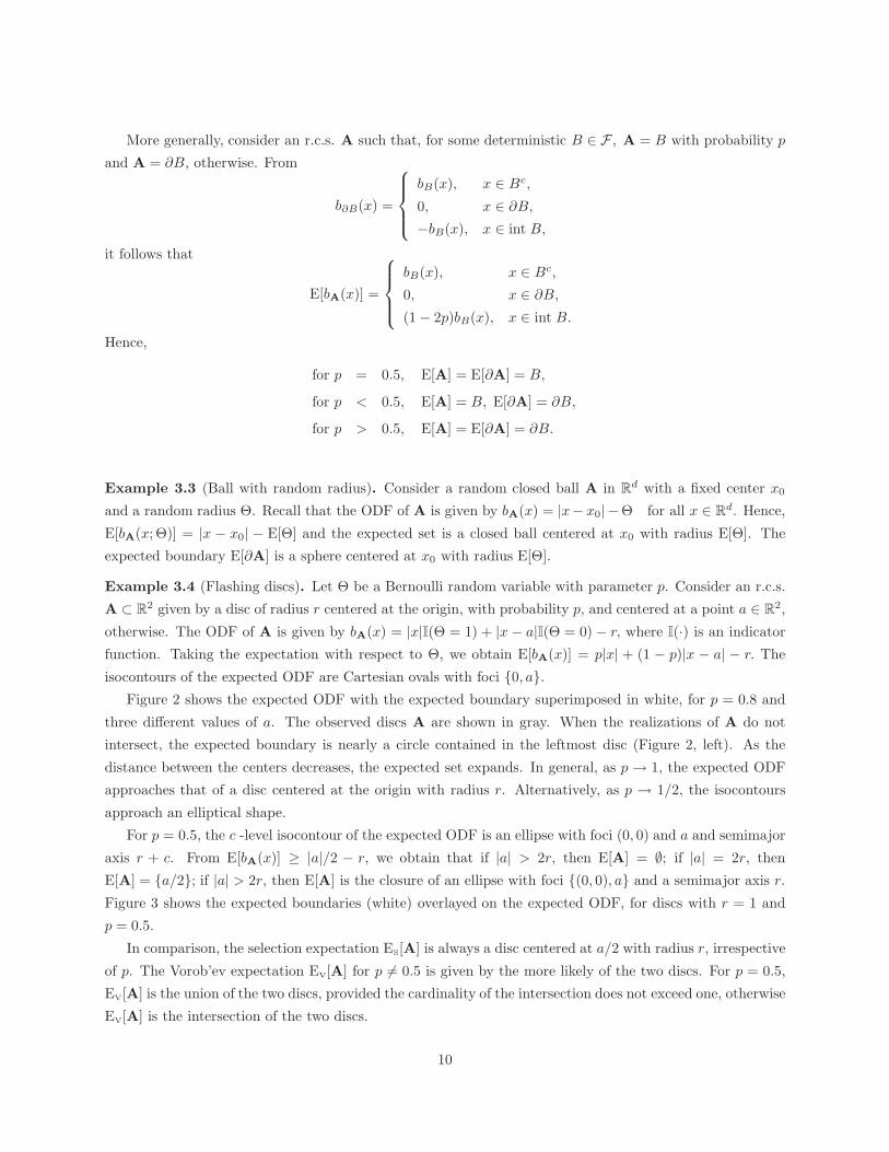
For p = 0.5, the c -level isocontour of the expected ODF is an ellipse with foci (0, 0) and a and semimajor

axis r + c. From E[bA(x)] ≥ |a|/2 − r, we obtain that if |a| > 2r, then E[A] = ∅; if |a| = 2r, then

E[A] = a/2; if |a| > 2r, then E[A] is the closure of an ellipse with foci (0, 0), a and a semimajor axis r.

Figure 3 shows the expected boundaries (white) overlayed on the expected ODF, for discs with r = 1 and

p = 0.5.

In comparison, the selection expectation ES[A] is always a disc centered at a/2 with radius r, irrespective

of p. The Vorob’ev expectation EV[A] for p 6= 0.5 is given by the more likely of the two discs. For p = 0.5,

EV[A] is the union of the two discs, provided the cardinality of the intersection does not exceed one, otherwise

EV[A] is the intersection of the two discs.

10

0 0.5 1 1.5 2 2.5 3

!

!

!"#$ " "#$ % %#$ & &#$ '

!

!

!"#$ " "#$ % %#$ & &#$ '

Figure 2: The expected boundaries (white) for A with p = 0.8, r = 1 and |a| = 3, 2, 1.5 (from left to right),

superimposed on the gray-scale image of the expected ODF. Realizations of ∂A are shown in white.

!

!

"#$ "#% & &#' &#( &#$ &#% ' '#' '#( '#$

0 0.5 1 1.5 2 2.5

0 0.5 1 1.5 2 2.5

Figure 3: The expected boundaries (white) for random discs with p = 0.5, r = 1 and |a| = 3, 2, 1.5 (from

left to right), superimposed on the gray-scale image of the expected ODF. Realized boundaries are shown in

gray.

11

Example 3.5 (Random half-plane). Let Θ be a random variable and consider a random half-plane in R2

given by A = x : x1 ≤ Θ with ∂A = x : x1 = Θ. The ODF of A is bA(x) = x1 − Θ and the expectation

has a form E[bA(x; Θ)] = x1 − E[Θ]. From here, the expected set is a half-plane intersecting the horizontal

axis at point E[Θ] and E[∂A] = x : x1 = E[Θ]. In this example, ES[A] = EV[A] = E[A].

Example 3.6 (Random upper half-plane). Consider a random upper half-plane in R2 given by A =

x : x2 ≥ x1 tan Θ with ∂A = x : x2 = x1 tan Θ. The ODF of A is bA(x) = |x| sin (Θ − ω), where ω =

arcsin (x2|x|−1). For Θ ∼ U[a, b] the expected ODF is E[bA(Θ)(x)] = 2(b−a)−1 sin ((b − a)/2)|x| sin ((a + b)/2 − ω).

From here, the expected set is a homothecy with coefficient α = (b − a)−1(2 sin (b − a)/2))−1 of an upper

half-plane with boundary angle (a + b)/2. Hence, E[A] is an upper half-plane with boundary given by the

line that passes through the origin and makes angle (a + b)/2 with the positive horizontal axis. Again, we

have ES[A] = EV[A] = E[A].

4 Separable Oriented Distance Functions

Consider a parametric closed set, whose geometry depends on the parameter θ ∈ Rp. We call θ the generating

parameter and write A(θ) for a closed set generated by θ. For example, a disc with a center γ and a radius

ρ has generating parameters (γ, ρ). We now extend the notion of parametric sets to random closed sets.

Specifically, let Θ be a p-dimensional (p ≥ 1) random variable defined on the probability space (Ω, A ,P)

with E |Θ| < ∞. Consider a random closed set given by a mapping from Ω to F , so that the geometry of

the set depends on the realized value of Θ. Similarly, we call Θ the generating parameter of a r.c.s. A(Θ).

For example, a disc with a random center C and a random radius R has generating parameters Θ = (C, R),

whilst a disc with a fixed center and a random radius R has a generating parameter Θ = R. The ODF bA(x)

of A(Θ) is a function of random variable Θ and so, is a random quantity. We again assume that bA(x) is

integrable for some x0 ∈ D and hence is well-defined.

Definition 4.1 (Separable ODF). The ODF of set A = A(θ) with parameter θ is separable, if it has a form

bA(x; θ) = hT (x)g(θ), where h(x) = (h1(x), . . . , hK(x))T and g(θ) = (g1(Θ), . . . , gK(θ))T for some functions

hi(x), gi(θ), i = 1, . . . , K.

Definition 4.2 (Separable r.c.s). An r.c.s. A is separable, if there exists a random variable Θ such that

bA(x; Θ) is separable a.s.. That is bA(x; Θ) = hT (x)g(Θ) a.s., with h(x) = (h1(x), . . . , hK(x))T and

g(θ) = (g1(θ), . . . , gK(θ))T for some functions hi(x), gi(θ), i = 1, . . . , K.

The following theorem establishes the connection between the expectation of a set and its generating

parameter.

Theorem 4.1. Let Θ be a generating parameter of a separable r.c.s. A(Θ) and assume that E[|gi(Θ)|] < ∞

for every i = 1, . . . , K. Then,

1. If g(θ) is convex in every argument, then E[A(Θ)] ⊂ A(E[Θ]).

2. If g(θ) is an affine function of θ in every component gi(θ) a.s., then E[A(Θ)] = A(E[Θ]).

12

Proof. (1) It follows from Jensen’s inequality that E[bA(x; Θ)] = hT (x) E[g(Θ)] ≥ h(x)T g(E[Θ]). The right-

hand side of the equation is the ODF of a set with parameter E[Θ]. For any x ∈ E[A(Θ)], we have

hT (x)g(E[Θ]) ≤ E[bA(x; Θ)] ≤ 0 and x ∈ cl A(E[Θ]) = A(E[Θ]). Thus, E[A(Θ)] ⊂ A(E[Θ]).

(2) From Jensen’s inequality, E[bA(x; Θ)] = hT (x)g(E[Θ]) iff the function gi(θ) is affine in θ for every

i = 1, . . . , K. The expression on the right-hand site is the ODF of a set with parameter E[Θ], hence the

statement (2) of the theorem follows.

Note that although the linearity of g(θ) is a necessary and sufficient condition for the form of E[bA(x; Θ)],

it is only a sufficient condition for the separability of E[A(Θ)]. This is because the expected set depends on

E[bA(x; Θ)] up to a constant, so that for fixed c > 0, E[bA(x; Θ)] and c E[bA(x; Θ)] define the same expected

set.

Example 4.1. In Example 3.3, the ODF of a closed ball with random radius bA(x) = |x| − Θ is separable

with h(x) = (|x|,−1)T and g(θ) = (1, θ)T , and the expected set is a closed ball with radius E[Θ].

In Example 3.4, the ODF of flashing discs is not separable, and the geometry of the expected set differs

from that of the observed sets. However, note that both the random set and its expectation can be described

as Cartesian ovals.

In Example 3.5, the ODF of a half-plane is separable with h(x) = (x1,−1)T and g(θ) = (1, θ)T . Hence,

the expected set is a half-plane with parameter E[Θ].

In Example 3.6, the ODF of an upper half-plane can be written as bA(x) = x1 sin Θ− x2 cosΘ, and so is

separable with h(x) = (x1,−x2)T and g(θ) = (sin θ, cos θ)T . The expected set is an upper half-plane whose

boundary makes angle E[Θ] with the positive horizontal axis. This example illustrates the second statement

of Theorem 4.1, in that E[A(Θ)] = A(EΘ), even for nonlinear g.

Remark 4.1. Note that if g is invertible in every component, we can reparametrize the expected ODF

as E[bA(x; Θ)] = hT (x)g(η), where ηi = g−1i (E gi(Θ)), i = 1, . . . , K. Hence, the expected set and the

expected boundary have the same geometric form in terms of parameters ηi. The relation between ηi

and the moments of Θ is established on a case-by-case basis. In particular, for the ODFs of the form

bA(x) = h(x) + g(Θ) for some function h(x) : Rd 7→ R and an invertible function g(θ) : R

p 7→ R, we obtain

that E[bA(x; Θ)] = h(x) + E[g(Θ)] = h(x) + g(g−1(E[g(Θ)])) and E[A(Θ)] = A(g−1 E[g(Θ)]).

Remark 4.2. In digital processing, data are stored as an array of pixels and so the ODF of an object in

the image is discretised. This discretization implies that for realizations of an r.c.s. A at times t = 1, 2, . . .,

the ODFs of At can be viewed as a random sample of arrays in the time domain. For a separable ODF, the

space-time covariance matrix has a form

cov(bAt(x), bAτ

(y)) = hT (x) cov(g(Θt), g(Θτ ))h(y),

for lattice vertices x, y and time points t, τ . This expression shows that the covariance of a separable

ODF is a product of a deterministic spatial component and the covariance of the stochastic time compo-

nent. In particular, for an ODF of the form bA(x) = h(x) + g(Θ), the space-time covariance is given by

cov(bAt(x), bAτ

(y)) = cov(g(Θt), g(Θτ )), and hence the dependence between the sets can be inferred from

their generating parameters.

13

5 Further Developments and Applications

5.1 The Sample Mean Set

Let A1, . . . ,Am be the observed realizations of an r.c.s. A. For every i, we assume that Ai ⊂ cl D and

∂Ai 6= ∅ and denote by bi(x) the ODF of Ai at point x. Let bm(x) = m−1∑m

i=1 bi(x) be the sample mean

ODF at point x.

Proposition 5.1. The sample mean ODF bm(x) is uniformly Lipshitz with constant one.

Proof. The proof follows immediately from the Lipshitz continuity of bi(x).

Definition 5.1 (Sample mean set). The sample mean set Am and the sample mean boundary ∂Am are

given by the zero-level set and by the zero-level isocontour of the empirical ODF, respectively, i.e.

Am = x : bm(x) ≤ 0, ∂Am = x : bm(x) = 0. (15)

The sample mean set defined in (15) is a random closed set, since Am ∩ K 6= ∅ = infx∈K bm(x) ≤ 0 is

measurable.

100

101

102

103

0.85

0.9

0.95

1

1.05

1.1

1.15

1.2

Sample size, m

100

101

102

103

−1.5

−1

−0.5

0

0.5

1

1.5x 10

−3

Sample size, m

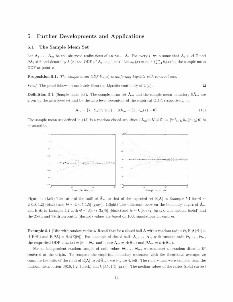
Figure 4: (Left) The ratio of the radii of Am to that of the expected set E[A] in Example 5.1 for Θ ∼

U[0.8, 1.2] (black) and Θ ∼ U[0.5, 1.5] (gray). (Right) The difference between the boundary angles of Am

and E[A] in Example 5.2 with Θ ∼ U[π/8, 3π/8] (black) and Θ ∼ U[0, π/2] (gray). The median (solid) and

the 25-th and 75-th percentile (dashed) values are based on 1000 simulations for each m.

Example 5.1 (Disc with random radius). Recall that for a closed ball A with a random radius Θ, E[A(Θ)] =

A(E[Θ]) and E[∂A] = ∂A(E[Θ]). For a sample of closed balls A1, . . . ,Am with random radii Θ1, . . . , Θm,

the emprirical ODF is bm(x) = |x| − Θm and hence Am = A(Θm) and ∂Am = ∂A(Θm).

For an independent random sample of radii values Θ1, . . . , Θm, we construct m random discs in R2

centered at the origin. To compare the empirical boundary estimator with the theoretical average, we

compute the ratio of the radii of E[A] to A(Θm); see Figure 4, left. The radii values were sampled from the

uniform distribution U[0.8, 1.2] (black) and U[0.5, 1.5] (gray). The median values of the ratios (solid curves)

14

and the 25-th and 75-th percentiles (dashed curves) are based on 1000 samples for each sample size m. The

figure shows that the accuracy of the empirical estimate is higher for bigger sample sizes and for smaller

variance values of the generating parameter.

Example 5.2 (Random upper half-plane). Consider an r.c.s. in Example 3.6 given by A(Θ) = x ∈

R2 : x2 ≥ x1 tan Θ, where Θ is the angle between the boundary of the plane and the positive horizontal

axis. Recall that for Θ ∼ U[a, b], E[A(Θ)] = A(E[Θ]) and E[∂A] = ∂A(E[Θ]).

For an independent random sample of the angle values Θ1, . . . , Θm, we construct m upper half-planes.

The empirical mean boundary is estimated by the zero-level isocontour of the empirical mean ODF. Figure 4

(right) shows the difference between the boundary angles for the empirical mean set and that of the expected

set for Θ ∼ U[π/8, 3π/8] (black) and Θ ∼ U[0, π/2] (gray). The median values of the ratios (solid curves)

and the 25-th and 75-th percentiles (dashed curves) are based on 1000 replicates for each value of m. As in

the previous case, the boundary estimate is more accurate for bigger sample sizes and for smaller variance

values of Θ.

The empirical mean set and the empirical boundary provide a recipe for practical construction of the set

and boundary estimators. Examples 5.1 and 5.2 suggest the consistency of the boundary estimator, based

on the empirical ODF. Note that both the expected set E[A] and the empirical mean set Am are described

as level sets of the continuous function bA and hence, under certain conditions, the consistency of Am as

an estimator of E[A] can be inferred from (Molchanov, 1998, Theorem 2). The result of (Molchanov, 1998),

however, does not apply to the boundary estimator ∂Am. In our upcoming paper, we study the consistency

of the boundary estimator in greater detail Jankowski and Stanberry (in preparation).

5.2 Loss Functions

Assume that the observed data A ∈ F follows a distribution FA with mean parameter A = E[A], A ∈ F . We

call A the parameter set. Here, data A represent random closed sets with nonempty boundary. In practice,

it is more common to acquire images rather than observe sets per se, so the observed A can be seen as a

result of the first-step analysis. The goal is to estimate the parameter set A given the observed data A.

If set A is parametric with parameter θ, we can construct an estimator of A using conventional loss

functions for θ. For example, if A is a collection of deformed balls, the distribution F can be parametrized

by the center and radius of a ball. Depending on the problem, we might be interested in testing the hypothesis

about either the location or the size of the ball, or both. Then the optimal estimator θ is determined using

standard loss functions, e.g. the indicator loss ℓ(θ, a) = I(a = θ), the absolute error loss ℓ(θ, a) = |a − θ| or

the squared error loss ℓ(θ, a) = (a − θ)2. However, often, the sets of interest cannot be parametrized and

at best can be described as “blobs”, in which case conventional loss functions are not applicable. Here, we

relay loss functions for Bayesian inference about sets introduced in Stanberry and Besag (in preparation) in

the frequentist framework.

To begin with, we consider a loss function based on representation of a set A given by its characteristic

15

function χA(x) = 1A(x). The space of characteristic functions is complete with metric

d(A, B) = ||χA − χB||Lq =

(∫

D

|χA(x) − χB(x)|qλ( dx)

)1/q

. (16)

Here and later, the integration domain D is either the entire image or its subset. Let χ be an estimator of

χA. Given the metric d, we define an L1 loss function as

ℓ1(χA, χ) = ||χA − χ||L1 =

∫

D

|χA(x) − χ|λ( dx). (17)

Because the estimator χ is the characteristic function that minimizes the expected loss, the estimator A of

A is immediately available. Strictly speaking, d(A, B) distinguishes between sets up to a set of Lebesgue

measure zero, so we assume that the parameter set has no punctures and hence A is uniquely determined.

Note that the equation (17) is the measure of the symmetric difference, since

ℓ1(χA, χ) = λ(A∆A) = λ((A \ A) ∪ (A \ A)) (18)

and, hence, ℓ1(χA, χ) is akin to the absolute error loss in conventional settings. The set that minimizes

E[λ(A∆A)] is the Vorob’ev median, i.e. is the median level set of the coverage function (3); (see Molchanov,

2005, p. 178). The Vorob’ev median is a set-analog of the ordinary median in the sense that, as the latter,

the former minimizes the absolute error loss.

Moreover, the Vorob’ev median is optimal with respect to a much broader class of Lq loss functions,

ℓq(χA, χ) = ||χA − χ||Lq , 1 ≤ q < ∞. (19)

This is because χA takes values in 0, 1 and the induced Lq topologies (19) are all equivalent for 1 ≤ q < ∞;

(see Delfour and Zolesio, 2001, Theorem 2.2).

Instead of optimizing the expected Lq loss over the set of characteristic functions, consider minimizing

(19) over a larger set of functions with values in [0, 1]. For the squared L2 loss

ℓ2(χA, χ) = ||χA − χ||2L2, (20)

the pointwise estimator χ(x) ∈ [0, 1] is the coverage function (3). The estimator χ(x) is a global minimum in

L2 since E[||χA −E[χA]||2L2] ≤ E[||χA − χ||2L2

]. Note that χ is essentially a gray-scale image with intensities

reflecting the probability of a pixel being in A.

The coverage function, however, is not necessarily a characteristic function, unless A is deterministic

a.s.. Consider a set-valued estimator given by an excursion set of χ(x) so that determining the optimal

estimator A now reduces to choosing an appropriate threshold u for the excursion set (4). The Vorob’ev

criterion (5) gives an estimator A, which is optimal with respect to Lebesgue measure in the sense that

E[λ(A∆A)] ≤ E[λ(A∆A)] for all measurable sets with measure E[λ(A)] (see Molchanov, 2005, Theorem 2.3,

pg. 177). From (18) and the equivalence of the Lq-topologies on the space of characteristic functions, it

follows that the Vorob’ev expectation minimizes the expected loss (19) for any q ∈ [1,∞) over all of the sets

with Lebesgue measure E[λ(A)].

16

In general, given the representative functions fA and fB of sets A and B, the discrepancy between A and

B can be taken in terms of some (pseudo-) metric

m(A, B) = mW(fA, fB), (21)

defined on a compact window W ⊆ D. Further, we suppress the subscript W whenever possible. Given the

metric m(A, B) = ||fA − fB||L2, the global estimator based on the squared L2 loss

ℓ2(fA, f) = ||fA − f ||2L2(22)

is the average function E[fA]. Hence, the distance-average expectation (6) is an optimal estimator of A with

respect to (22), among all of the level sets of E[fA].

Note that although the distance-average expectation arises naturally for the L2 loss, it was originally

defined for a generic (pseudo-) metric m(·, ·) (Baddeley and Molchanov, 1998). Thus, in principle, we can

construct an estimator as the level set of the expected representation for arbitrary choice of m. For that,

we must specify the representative function f , select an appropriate (pseudo-)metric m, and choose the loss

function ℓ(fA, f) based on m. The threshold u in (6) then determines the optimal estimator with respect to

ℓ(fA, f) among all of the level sets of E[fA(x)].

We now consider a representation of a set given by its ODF. Recall that the space of ODFs of sets with

non-empty boundary is complete with metric d(A, B) = ||bB − bA||Lq. For the loss function

ℓ2(bA, b) = ||bA − b ||2L2=

∫

D

|bA(x) − b(x)|2λ( dx), (23)

let b be the estimator of bA that minimizes the expectation of (23). Because the ODF gives a unique (up to

the boundary) representation of a set, the estimator A is given by the zero-level set of b. However, optimizing

E[ℓ2(bA, b)] over the set of ODFs is nontrivial, so instead we consider unrestricted minimization over the set

of functions defined on D. In this case, the pointwise estimator is the expected ODF, which is also a global

minimum. Because the estimator E[bA(x)] is not necessarily an ODF itself, it does not uniquely determine

the set. Hence, we take the set-valued estimator A of A to be the zero-level set of E[bA(x)], so that A is the

expected set as defined in (3.1). The estimator of the boundary ∂A is given by the zero-level isocontour of

E[bA(x)].

5.3 Image Averaging

In this section, we consider the example of image averaging originally discussed in Baddeley and Molchanov

(1998). In image averaging, which relates to Bayesian image classification and reconstruction, the goal is is

to determine an average object or a typical shape from the collection of images of the same scene or objects

of the same type.

To begin with, we quickly outline the image sampling procedure and refer for more details to Baddeley and Molchanov

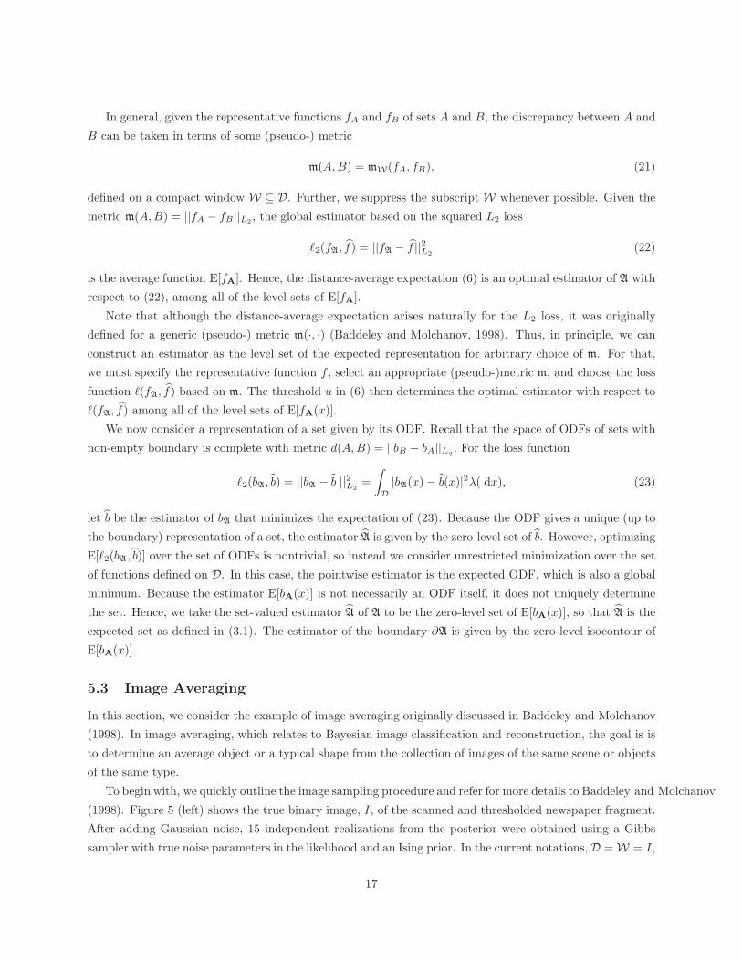
(1998). Figure 5 (left) shows the true binary image, I, of the scanned and thresholded newspaper fragment.

After adding Gaussian noise, 15 independent realizations from the posterior were obtained using a Gibbs

sampler with true noise parameters in the likelihood and an Ising prior. In the current notations, D = W = I,

17

A is the true newspaper text and A1, . . . ,A15 are the 15 independent reconstruction of A. The data for this

example was downloaded from Baddeley (2009).

Figure 5: The true binary image of the newspaper fragment.

Figure 5 shows the ODF estimator AODF (left) and the distance-average estimator ADA (right) with

fA(·) = bA(·) and m(·, ·) = L2(·, ·); see also Figure 6 in Baddeley and Molchanov (1998). The estimator

AODF appears less noisy and more accurate as compared to ADA, where the letters look overinflated.

Figure 6: The ODF estimator AODF (left) and the distance-average estimator ADA (right).

To compare the results of the reconstruction, it is instructive to look at the residual images for AODF

and ADA in Figure 7, left and right, respectively. Note that black (resp. gray) pixels in the figure correspond

to the set A \ A (resp. A \ A). The residual image for ADA shows a clear spatial pattern, indicating that

ADA tends to overestimate the set. In turn, the residuals of AODF show little spatial clustering. In addition,

AODF ⊂ ADA, that is the distance-average estimator is inclusive of the ODF one, with discrepancies observed

along the boundary and in the background.

To compare the quality of the estimators, it is common to use the fraction of misclassified pixels. Here, the

error is 4.12% for AODF and 10.68% for ADA. However, a small misclassification error does not necessarily

imply similar looking images (Baddeley, 1992), therefore, we compare the two estimators by computing an

18

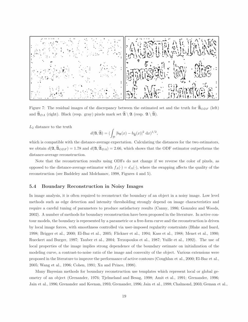
Figure 7: The residual images of the discrepancy between the estimated set and the truth for AODF (left)

and ADA (right). Black (resp. gray) pixels mark set A \ A (resp. A \ A).

L2 distance to the truth

d(A, A) = (

∫

D

|bA(x) − bbA(x)|2 dx)1/2,

which is compatible with the distance-average expectation. Calculating the distances for the two estimators,

we obtain d(A, AODF ) = 1.78 and d(A, ADA) = 2.66, which shows that the ODF estimator outperforms the

distance-average reconstruction.

Note that the reconstruction results using ODFs do not change if we reverse the color of pixels, as

opposed to the distance-average estimator with fA(·) = dA(·), where the swapping affects the quality of the

reconstruction (see Baddeley and Molchanov, 1998, Figures 4 and 5).

5.4 Boundary Reconstruction in Noisy Images

In image analysis, it is often required to reconstruct the boundary of an object in a noisy image. Low level

methods such as edge detection and intensity thresholding strongly depend on image characteristics and

require a careful tuning of parameters to produce satisfactory results (Canny, 1986; Gonzalez and Woods,

2002). A number of methods for boundary reconstruction have been proposed in the literature. In active con-

tour models, the boundary is represented by a parametric or a free-form curve and the reconstruction is driven

by local image forces, with smoothness controlled via user-imposed regularity constraints (Blake and Isard,

1998; Brigger et al., 2000; El-Baz et al., 2005; Flickner et al., 1994; Kass et al., 1988; Menet et al., 1990;

Rueckert and Burger, 1997; Tauber et al., 2004; Terzopoulos et al., 1987; Yuille et al., 1992). The use of

local properties of the image implies strong dependence of the boundary estimate on initialization of the

modeling curve, a contrast-to-noise ratio of the image and convexity of the object. Various extensions were

proposed in the literature to improve the performance of active contours (Coughlan et al., 2000; El-Baz et al.,

2005; Wang et al., 1996; Cohen, 1991; Xu and Prince, 1998).

Many Bayesian methods for boundary reconstruction use templates which represent local or global ge-

ometry of an object (Grenander, 1976; Tjelmeland and Besag, 1998; Amit et al., 1991; Grenander, 1996;

Jain et al., 1996; Grenander and Keenan, 1993; Grenander, 1996; Jain et al., 1998; Chalmond, 2003; Geman et al.,

19

1990). The stochastic method in Qian et al. (1996) models the boundary by closed polygons. The method

was then extended to allow for the dynamic estimation of the number of polygon vertices, thus balancing

the complexity and the flexibility of the model (Pievatolo and Green, 1998). However, the reconstruction is

given by a gray-scale image, where intensities reflect the posterior mean state of pixels, so that constructing

a boundary estimator requires additional post-processing.

In Stanberry and Besag (in preparation), the authors proposed a new method to reconstruct a smooth

connected boundary of an object in a noisy image using B-spline curves. The method is Bayesian and uses a

Markov chain Monte Carlo algorithm to obtain curve samples from the posterior. Using the squared L2-loss

based on ODFs, the posterior estimator is given by the posterior expected boundary as defined in (10).

The simulation study showed that the ODF estimator is more accurate as compared to the distance-average

reconstruction and Vorob’ev sets.

5.5 Implementation

In addition to its appealing theoretical properties, the ODF expectation can be efficiently computed, using

algorithms for the distance function (Breu et al., 1995; Freidman et al., 1977; Rosenfeld and Pfaltz, 1966).

The ODF is computed by combining the distance function for the original image and that of the inverted

image, i.e. the black and white colors are interchanged. The examples and results reported in this paper

were coded in MATLAB (R2008A, The MathWorks), where the distance function to a set is computed using

the bwdist command.

In comparison to the distance-average and Vorob’ev expectations, the ODF average is more efficient,

because it requires no optimization since the threshold level is fixed at zero. This difference is particularly

prominent in Bayesian reconstruction, where the estimator is based on thousands of samples from the

posterior. In addition, the storage requirements for the ODF reconstruction in Bayesian framework are

miniscule, as we only need to update the average after every sweep.

6 Discussion

In this paper, we present new definitions of the expected set and the expected boundary, using the ODF

representation of a set. In conventional settings, where the parameter of interest is a scalar or a vector, it is

straightforward to construct an estimator of the mean from the observed data. However, statistical inference

about sets is nontrivial. When dealing with sets, one has to determine the features that are important to

emphasize and develop inference methods based on them. These features may include the location, the size,

or the orientation of a set. If a set has an analytic representation, the most natural approach to set inference

is via inference about its parameters. This, however, is not applicable for sets with arbitrary geometry.

A number of existing definitions of the expected set are based on the linearization idea outlined in

Molchanov (2005), where inference is made on the space of functions representing a set. The resulting

estimator necessarily depends on the type of linearization and the choice of the representative function. In

this paper, we use an approach similar in spirit to the linearisation idea and define the expectation based

on the ODF representation of a set. However, we forgo the optimality criterion and simply choose zero as

20

a threshold. Whilst the choice might appear simplistic, it gives an expectation with attractive theoretical

traits, including equivariance, convexity-preservation and inclusion properties.

The definition is particularly appealing for problems in image analysis. In particular, its denoising prop-

erty implies that random specks will be averaged out unless observed with probability one. In comparison,

the distance-average expectation is not empty by construction, and therefore identifies false positives in any

noisy image. Furthermore, the distance-average reconstruction strongly depends on the choice of pseudo-

metric, representative function, restriction window and any parameters of the above. In turn, the selection

expectation depends on the structure of the probability space, whilst the Lebesgue measure criterion of the

Vorob’ev expectation is not well suited for image analysis, although, the optimality of the Vorob’ev median

is rather attractive.

In our upcoming paper, we study the asymptotic properties of the ODF estimators for the boundary and

describe a method for constructing confidence sets (Jankowski and Stanberry, in preparation).

References

Y. Amit, U. Grenander, and M. Piccioni. Structural image restoration through deformable templates. Journal

of the American Statistical Association, 86(414):376–387, 1991.

Z. Artstein and R.A. Vitale. A strong law of large numbers for random compact sets. Annals of Probability,

3(5):879–882, 1975.

R.J. Aumann. Integrals of set-valued functions. Journal of Mathematical Analysis and Applications, 12:

1–12, 1965.

A. J. Baddeley. Errors in binary images and an Lp version of the Hausdorff metric. Nieuw Archief voor

Wiskunde, 10:157–183, 1992. URL citeseer.ist.psu.edu/baddeley92errors.html.

A. J. Baddeley, 2009. URL http://school.maths.uwa.edu.au/homepages/adrian/.

A. J. Baddeley and I. Molchanov. Averaging of random sets based on their distance functions. Journal of

Mathematical Imaging and Vision, 8(1):79–92, 1998.

A. Blake and M. Isard. Active Contours: The Application of Techniques from Graphics, Vision, Control

Theory and Statistics to Visual Tracking of Shapes in Motion. Springer-Verlag New York, Inc., Secaucus,

NJ, USA, 1998.

H. Breu, J. Gil, D. Kirkpatrick, and M. Werman. Linear time euclidean distance transform algorithms. IEEE

Transactions on Pattern Analysis and Machine Intelligence, 17(5):529–533, May 1995. ISSN 0162-8828.

P. Brigger, J. Hoeg, and M. Unser. B-spline snakes: a flexible tool for parametric contour detection. IEEE

Transactions on Image Processing, 9(9):1484–1496, 2000.

J. Canny. A computational approach to edge detection. IEEE Trans. Pattern Anal. Mach. Intell., 8(6):

679–698, 1986. ISSN 0162-8828.

21

B. Chalmond. Modeling and Inverse Problems in Imaging Analysis, volume 155 of Applied Mathematical

Sciences. Springer-Verlag, New York, 2003.

G. Choquet. Theory of capacities. Ann. Inst. Fourier, 5:131–295, 1953.

L.D. Cohen. On active contour models and balloons. Computer Vision, Graphics, and Image Processing.

Image Understanding, 53:211–218, 1991.

J. Coughlan, A.L. Yuille, C. English, and D. Snow. Efficient deformable template detection and localization

without user initialization. Computer Vision and Image Understanding, 78(3):303–319, 2000.

M.C. Delfour and J.-P. Zolesio. Shapes and Geometries, volume 4 of Advances in Design and Control. Society

for Industrial and Applied Mathematics (SIAM), Philadelphia, PA, 2001.

A. El-Baz, S.E. Yuksel, H. Shi, A.A. Farag, M. Abou El-Ghar, T. Eldiasty, and M.A. Ghoneim. 2D and 3D

shape based segmentation using deformable models. In MICCAI (2), pages 821–829, 2005.

M. Flickner, H. Sawhney, D. Pryor, and J. Lotspiech. Intelligent interactive image outlining using spline

snakes. Conference Record of the 28th Asilomar Conference on Signals, Systems and Computers., 1:

731–735 vol.1, 1994.

J. H. Freidman, J. L. Bentley, and R. A. Finkel. An algorithm for finding best matches in logarithmic

expected time. ACM Trans. Math. Softw., 3(3):209–226, 1977. ISSN 0098-3500.

D. Geman, S. Geman, C. Graffigne, and P. Dong. Boundary detection by constrained optimization. IEEE

Trans. Pattern Anal. Mach. Intell., 12(7):609–628, 1990. ISSN 0162-8828.

R. C. Gonzalez and R. E. Woods. Digital Image Processing (2nd Edition). Prentice Hall, January 2002.

ISBN 0201180758.

U. Grenander. Pattern Synthesis. Springer-Verlag, New York, 1976. Lectures in Pattern Theory, Vol. 1,

Applied Mathematical Sciences, Vol. 18.

U. Grenander. Elements of Pattern Theory. Johns Hopkins Studies in the Mathematical Sciences. Johns

Hopkins University Press, Baltimore, MD, 1996.

U. Grenander and D.M. Keenan. On the shape of plane images. SIAM Journla of Applied Mathematics, 53

(4):1072–1094, 1993.

A.K. Jain, Y. Zhong, and S. Lakshmanan. Object matching using deformable templates. IEEE Transactions

on Pattern Analysis and Machine Intelligence, 18(3):267–278, 1996.

A.K. Jain, Y. Zhong, and M.-P. Dubuisson-Jolly. Deformable template models: a review. Signal Processing,

71(2):109–129, 1998.

H.K. Jankowski and L.I. Stanberry. On boundary estimation. in preparation.

22

M. Kass, A. P. Witkin, and D. Terzopoulos. Snakes: Active contour models. International Journal of

Computer Vision, 1(4):321–331, 1988.

G. Matheron. Random Sets and Integral Geometry. J. Wiley & Sons, New York-London-Sydney, 1975.

S. Menet, P. Saint Marc, and G. Medioni. B-snakes: Implementation and application to stereo. In Image

Understanding Workshop, volume 90, pages 720–726, 1990.

I. Molchanov. A limit theorem for solutions of inequalities. Scandinavian Journal of Statistics, 25:235–242,

1998.

I. Molchanov. Theory of Random Sets. Probability and its Applications (New York). Springer-Verlag London

Ltd., London, 2005.

A. Pievatolo and P.J. Green. Boundary detection through dynamic polygons. Journal of the Royal Statistical

Society, Series B, Statistical Methodology, 60(3):609–626, 1998.

W. Qian, D.M. Titterington, and J.N. Chapman. An image analysis problem in electron microscopy. Journal

of American Statistical Association, 91(435):944–952, 1996.

A. Rosenfeld and J.L. Pfaltz. Sequential operations in digital picture processing. J. ACM, 13(4):471–494,

1966. ISSN 0004-5411.

D. Rueckert and P. Burger. Geometrically deformable templates for shape-based segmentation and tracking

in cardiac MR images. In EMMCVPR ’97: Proceedings of the First International Workshop on Energy

Minimization Methods in Computer Vision and Pattern Recognition, pages 83–98, London, UK, 1997.

Springer-Verlag.

L.I. Stanberry and J. Besag. Boundary reconstruction in binary images using splines. in preparation.

C. Tauber, H. Batatia, G. Morin, and A. Ayache. Robust B-spline snakes for ultrasound image segmentation.

Computers in Cardiology, pages 325–328, 2004.

D. Terzopoulos, A.P. Witkin, and M. Kass. Snakes: Active contour models. In IEEE International Conference

on Computer Vision, pages 259–268, 1987.

H. Tjelmeland and J. Besag. Markov random fields with higher-order interactions. Scandinavian Journal of

Statistics. Theory and Applications, 25(3):415–433, 1998.

O.Yu. Vorob’ev. Srednemernoe Modelirovanie. Nauka, Moscow, USSR, 1984.

M. Wang, J. Evans, L. Hassebrook, and C. Knapp. A multistage, optimal active contour model. IEEE

Transactions on Image Processing, 5(11):1586–1591, 1996.

C. Xu and J.L. Prince. Snakes, shapes, and gradient vector flow. IEEE Transactions on Image Processing,

7(3):359–369, 1998.

A.L. Yuille, P.W. Hallinan, and D.S. Cohen. Feature extraction from faces using deformable templates. Int.

J. Comput. Vision, 8(2):99–111, 1992.

23