Node Sampling using Random Centrifugal Walks

Andrés Sevilla1, Alberto Mozo2, and Antonio Fernández Anta3

1 Dpto Informática Aplicada, U. Politécnica de Madrid, Madrid, Spainasevilla@eui.upm.es

2 Dpto Arquitectura y Tecnología de Computadores, U. Politécnica de Madrid, Madrid, Spainamozo@eui.upm.es

3 Institute IMDEA Networks, Madrid, Spainantonio.fernandez@imdea.org

Abstract. Sampling a network with a given probability distribution has been identified as a usefuloperation. In this paper we propose distributed algorithms for sampling networks, so that nodes areselected by a special node, called the source, with a given probability distribution. All these algorithmsare based on a new class of random walks, that we call Random Centrifugal Walks (RCW). A RCW isa random walk that starts at the source and always moves away from it.Firstly, an algorithm to sample any connected network using RCW is proposed. The algorithm assumesthat each node has a weight, so that the sampling process must select a node with a probabilityproportional to its weight. This algorithm requires a preprocessing phase before the sampling of nodes.In particular, a minimum diameter spanning tree (MDST) is created in the network, and then nodes’weights are efficiently aggregated using the tree. The good news are that the preprocessing is done onlyonce, regardless of the number of sources and the number of samples taken from the network. Afterthat, every sample is done with a RCW whose length is bounded by the network diameter.Secondly, RCW algorithms that do not require preprocessing are proposed for grids and networks withregular concentric connectivity, for the case when the probability of selecting a node is a function of itsdistance to the source.The key features of the RCW algorithms (unlike previous Markovian approaches) are that (1) they donot need to warm-up (stabilize), (2) the sampling always finishes in a number of hops bounded by thenetwork diameter, and (3) it selects a node with the exact probability distribution.

1 Introduction

Sampling a network with a given distribution has been identified as a useful operation in many contexts. Forinstance, sampling nodes with uniform probability is the building block of epidemic information spreading[13,12]. Similarly, sampling with a probability that depends on the distance to a given node [3,17] is usefulto construct small world network topologies [14,7,2]. Other applications that can benefit from distance-based node sampling are landmark-less network positioning systems like NetICE9 [16], which does samplingof nodes with special properties to assign synthetic coordinates to nodes. In a different context, currentlythere is an increasing interest in obtaining a representative (unbiased) sample from the users of onlinesocial networks [9]. In this paper we propose a distributed algorithm for sampling networks with a desiredprobability distribution.

Related Work One technique to implement distributed sampling is to use gossiping between the networknodes. Jelasity et al. [12] present a general framework to implement a uniform sampling service using gossip-based epidemic algorithms. Bertier et al. [2] implement uniform sampling and DHT services using gossiping.As a side result, they sample nodes with a distribution that is close to Kleinberg’s harmonic distribution(one instance of a distance-dependent distribution). Another gossip-based sampling service that gets close toKleinberg’s harmonic distribution has been proposed by Bonnet et al. [3]. However, when using gossip-baseddistributed sampling as a service, it has been shown by Busnel et al. [5] that only partial independence(ε-independence) between views (the subsets of nodes held at each node) can be guaranteed without re-executing the gossip algorithm. Gurevich and Keidar [11] give an algorithm that achieves ε-independence inO(ns log n) rounds (where n is the network size and s is the view size).

arX

iv:1

107.

1089

v3 [

cs.D

C]

27

Sep

2012

Another popular distributed technique to sample a network is the use of random walks [18]. Most random-walk based sampling algorithms do uniform sampling [1,9], usually having to deal with the irregularities ofthe network. Sampling with arbitrary probability distributions can be achieved with random walks by re-weighting the hop probabilities to correct the sampling bias caused by the non-uniform stationary distributionof the random walks. Lee et al. [15] propose two new algorithms based on Metropolis-Hastings (MH) randomwalks for sampling with any probability distribution. These algorithms provide an unbiased graph samplingwith a small overhead, and a smaller asymptotic variance of the resulting unbiased estimators than genericMH random walks.

Sevilla et al. [17] have shown how sampling with an arbitrary probability distribution can be done withoutcommunication if a uniform sampling service is available. In that work, as in all the previous approaches, thedesired probability distribution is reached when the stationary distribution of a Markov process is reached.The number of iterations (or hops of a random walk) required to reach this situation (the warm-up time)depends on the parameters of the network and the desired distribution, but it is not negligible. For instance,Zhong and Sheng [18] found by simulation that, to achieve no more than 1% error, in a torus of 4096nodes at least 200 hops of a random walk are required for the uniform distribution, and 500 hops arerequired for a distribution proportional to the inverse of the distance. Similarly, Gjoka et al. [10] showthat a MHRW sampler needs about 6K samples (or 1000-3000 iterations) to obtain the convergence to theuniform probability distribution. In the light of these results, Markovian approaches seem to be inefficientto implement a sampling service, specially if multiple samples are desired.

Contributions In this paper we present efficient distributed algorithms to implement a sampling service.The basic technique used for sampling is a new class of random walks that we call Random Centrifugal Walks(RCW). A RCW starts at a special node, called the source, and always moves away from it.

All the algorithms proposed here are instances of a generic algorithm that uses the RCW as basic element.This generic RCW-based algorithm works essentially as follows. A RCW always starts at the source node.When the RCW reaches a node x (the first node reached by a RCW is always the source s), the RCWstops at that node with a stay probability. If the RCW stops at node x, then x is the node selected by thesampling. If the RCW does not stop at x, it jumps to a neighbor of x. To do so, the RCW chooses onlyamong neighbors that are farther from the source than the node x. (The probability of jumping to each ofthese neighbors is not necessarily the same.) In the rest of the paper we will call all the instances of thisgeneric algorithm as RCW algorithms.

Firstly, we propose a RCW algorithm that samples any connected network with any probability distribu-tion (given as weights assigned to the nodes). Before starting the sampling, a preprocessing phase is required.This preprocessing involves building a minimum distance spanning tree (MDST) in the network4, and usingthis tree for efficiently aggregating the node’s weights. As a result of the weight aggregation, each node hasto maintain one numerical value per link, which will be used by the RCW later. Once the preprocessingis completed, any node in the network can be the source of a sampling process, and multiple independentsamplings with the exact desired distribution can be efficiently performed. Since the RCW used for samplingfollow the MDST, they take at most D hops (where D is the network diameter).

Secondly, when the probability distribution is distance-based and nodes are at integral distances (mea-sured in hops) from the source, RCW algorithms without preprocessing (and only a small amount of statedata at the nodes) are proposed. In a distance-based probability distribution all the nodes at the same dis-tance from the source node are selected with the same probability. (Observe that the uniform and Kleinberg’sharmonic distributions are special cases of distance-based probability distributions.) In these networks, eachnode at distance k > 0 from the source has neighbors (at least) at distance k − 1. We can picture nodesat distance k from the source as positioned on a ring at distance k from the source. The center of all therings is the source, and the radius of each ring is one unit larger than the previous one. Using this graphicalimage, we refer the networks of this family as concentric rings networks. 5

4 Using, for instance, the algorithm proposed by Bui et al. [4] whose time complexity is O(n).5 Observe that every connected network can be seen as a concentric rings network. For instance, by finding thebreadth-first search (BFS) tree rooted at the source, and using the number of hops in this tree to the source asdistance.

2

The first distance-oriented RCW algorithm we propose samples with a distance-based distribution in anetwork with grid topology. In this network, the source node is at position (0, 0) and the lattice (Manhattan)distance is used. This grid contains all the nodes that are at a distance no more than the radius R fromthe source (the grid has hence a diamond shape6). The algorithm we derive assigns a stay probability toeach node, that only depends on its distance from the source. However, the hop probabilities depend on theposition (i, j) of the node and the position of the neighbors to which the RCW can jump to. We formallyprove that the desired distance-based sampling probability distribution is achieved. Moreover, since everyhop of the RCW in the grid moves one unit of distance away from the source, the sampling is completedafter at most R hops.

We have proposed a second distance-oriented RCW algorithm that samples with distance-based distri-butions in concentric rings networks with uniform connectivity. These are networks in which all the nodes ineach ring k have the same number of neighbors in ring k − 1 and the same number in ring k + 1. Like thegrid algorithm, this variant is also proved to finish with the desired distribution in at most R hops, where Ris the number of rings.

Unfortunately, in general, concentric rings networks have no uniform connectivity. This case is faced bycreating, on top of the concentric rings network, an overlay network that has uniform connectivity. In theresulting network, the algorithm for uniform connectivity can be used. We propose a distributed algorithmthat, if it completes successfully, builds the desired overlay network. We have found via simulations that thisalgorithm succeeds in building the overlay network in a large number of cases.

In summary, RCW can be used to implement an efficient sampling service because, unlike previousMarkovian (e.g., classical random walks and epidemic) approaches, (1) it always finishes in a number ofhops bounded by the network diameter, (2) selects a node with the exact probability distribution, and (3)does not need warm-up (stabilization) to converge to the desired distribution. Additionally, in the case thatpreprocessing is needed, this only has to be executed once, independently on the number of sources and thenumber of samples taken from the network.

The rest of the paper is structured as follows. In Section 2 we introduce concepts and notation that willbe used in the rest of the paper. In Section 3 we present the RCW algorithm for a connected network. InSections 4 and 5 we describe the RCW algorithm on grids and concentric rings networks with uniform con-nectivity. In Section 6 we present the simulation based study of the algorithm for concentric rings topologieswithout uniform connectivity. Finally, we conclude the paper in Section 7.

2 Definitions and Model

Connected Networks In this paper we only consider connected networks. This family includes most ofthe potentially interesting networks we can find. In every network, we use N to denote the set of nodes andn = |N | the size of that set. When convenient, we assume that there is a special node in the network, called thesource and denoted by s. We assume that each node x ∈ N has an associated weight w(x) > 0. Furthermore,each node knows its own weight. The weights are used to obtain the desired probability distribution p, sothat the probability of selecting a node x is proportional to w(x). Let us denote η =

∑j∈N w(j). Then,

the probability of selecting x ∈ N is p(x) = w(x)/η. (In the simplest case, weights are probabilities, i.e.,w(x) = p(x),∀x and η = 1.)

RCW in Connected Networks As mentioned, in order to use RCW to sample connected networks, somepreprocessing is done. This involves constructing a spanning tree in the network and performing a weightaggregation process. After the preprocessing, RCW is used for sampling. A RCW starts from the source.When the RCW reaches a node x ∈ N , it selects x as the sampled vertex with probability q(x), which wecall the stay probability. If x is not selected, a neighbor y of x in the tree is chosen, using for that a collectionof hop probabilities h(x, y). The values of q(x) and h(x, y) are computed in the preprocessing and stored atx. The probability of reaching a node x ∈ N in a RCW is called the visit probability, denoted v(x).6 A RCW algorithm for a square grid is easy to derive from the one presented.

3

Concentric Rings Networks We also consider a subfamily of the connected networks, which we callconcentric rings networks. These are networks in which the nodes of N are at integral distances from s. Inthese networks, no node is at a distance from s larger than a radius R. For each k ∈ [0, R], we use Rk 6= ∅to denote the set of nodes at distance k from s, and nk = |Rk|. (Observe that R0 = {s} and n0 = 1.) Thesenetworks can be seen as a collection of concentric rings at distances 1 to R from the source, which is thecommon center of all rings. For that reason, we call the set Rk the ring at distance k. For each x ∈ Rk andk ∈ [1, R], γk(x) > 0 is the number of neighbors of node x at distance k− 1 from s (which is only 1 if k = 1),and δk(x) is the number of neighbors of node x at distance k + 1 from s (which is 0 if k = R).

The concentric rings networks considered must satisfy the additional property that the probability distri-bution is distance based. This means that, for all k ∈ [0, R], every node x ∈ Rk has the same probability pk tobe selected. We assume that each node x ∈ Rk knows its own pk. These properties allow, in the subfamiliesdefined below, to avoid the preprocessing required for connected networks.

Grids A first subfamily of concentric rings networks considered is the grid with lattice distances. In thisnetwork, the source is at position (0, 0) of the grid, and it contains all the nodes (i, j) so that i, j ∈ [−R,R]and |i|+ |j| ≤ R. For each k ∈ [0, R], the set of nodes in ring k is Rk = {(i, j) : |i|+ |j| = k}. The neighborsof a node (i, j) are the nodes (i− 1, j), (i+ 1, j), (i, j − 1), and (i, j + 1) (that belong to the grid).

Uniform Connectivity The second subfamily considered is formed by the concentric rings networks withuniform connectivity. These networks satisfy that

∀k ∈ [1, R],∀x, y ∈ Rk, δk(x) = δk(y) ∧ γk(x) = γk(y). (1)

In other words, all nodes of ring k have the same number of neighbors δk in ring k+1 and the same numberof neighbors γk in ring k − 1.

RCW in Concentric Rings Networks The behavior of a generic RCW was already described. In the algorithmthat we will present in this paper for concentric rings networks we guarantee that, for each k, all the nodesin Rk have the same visit probability vk and the same stay probability qk. A RCW starts from the source.When it reaches a node x ∈ Rk, it selects x as the sampled vertex with stay probability qk. If x is notselected, a neighbor y ∈ Rk+1 of x is chosen.

The desired distance-based probability distribution is given by the values pk, k ∈ [0, R], where it musthold that

∑Rk=0 nk × pk = 1. The problem to be solved is to define the stay and hop probabilities so that

the probability of a node x ∈ Rk is pk.

Observation 1 If for all k ∈ [0, R] the visit vk and stay qk probabilities are the same for all the nodes inRk, the RCW samples with the desired probability iff pk = vk · qk.

3 Sampling in a Connected Network

In this section, we present a RCW algorithm that can be used to sample any connected network. As men-tioned, in addition to connectivity, it is required that each node knows its own weight. A node will be selectedwith probability proportional to its weight.

Preprocessing for the RCW Algorithm The RCW algorithm for connected networks requires somepreprocessing which will be described now. This preprocessing has to be done only once for the wholenetwork, independently of which nodes act as sources and how many samples are taken.

Building a spanning tree. Initially, the algorithm builds a spanning tree of the network. A feature of thealgorithm is that, if several nodes want to act as sources for RCW, they can all share the same spanningtree. Hence only one tree for the whole network has to be built. The algorithm used for the tree constructionis not important for the correctness of the RCW algorithm, but the diameter of the tree will be an upperbound on the length of the RCW (and hence possibly the sampling latency). There are several well knowndistributed algorithms (see, e.g., [6] and the references therein) that can be used to build the spanning tree.

4

1 task Weight_Aggregation(i)2 if i is a leaf then3 send WEIGHT(w(i)) to neighbor x4 receive WEIGHT(p) from neighbor x5 Ti(x) ← p6 else7 repeat8 receive WEIGHT(p) from x ∈ neighbors(i)9 Ti(x) ← p10 foreach y ∈ neighbors(i) \ {x} do11 if received WEIGHT(·) from neighbors(i) \ {y} then12 send WEIGHT(w(i) +

∑z∈neighbors(i)\{y} Ti(z)) to y

13 end foreach14 until received WEIGHT(·) from every x ∈ neighbors(i)

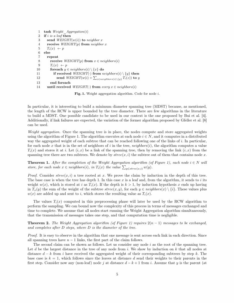
Fig. 1. Weight aggregation algorithm. Code for node i.

In particular, it is interesting to build a minimum diameter spanning tree (MDST) because, as mentioned,the length of the RCW is upper bounded by the tree diameter. There are few algorithms in the literatureto build a MDST. One possible candidate to be used in our context is the one proposed by Bui et al. [4].Additionally, if link failures are expected, the variation of the former algorithm proposed by Gfeller et al. [8]can be used.

Weight aggregation. Once the spanning tree is in place, the nodes compute and store aggregated weightsusing the algorithm of Figure 1. The algorithm executes at each node i ∈ N , and it computes in a distributedway the aggregated weight of each subtree that can be reached following one of the links of i. In particular,for each node x that is in the set of neighbors of i in the tree, neighbors(i), the algorithm computes a valueTi(x) and stores it at i. Let (i, x) be a link of the spanning tree, then by removing the link (i, x) from thespanning tree there are two subtrees. We denote by stree(x, i) the subtree out of them that contains node x.

Theorem 1. After the completion of the Weight Aggregation algorithm (of Figure 1), each node i ∈ N willstore, for each node x ∈ neighbors(i), in Ti(x) the value

∑y∈stree(x,i) w(y).

Proof. Consider stree(x, i) a tree rooted at x. We prove the claim by induction in the depth of this tree.The base case is when the tree has depth 1. In this case x is a leaf and, from the algorithm, it sends to i itsweight w(x), which is stored at i as Ti(x). If the depth is k > 1, by induction hypothesis x ends up havingin Tx(y) the sum of the weight of the subtree stree(x, y), for each y ∈ neighbors(x) \ {i}. These values plusw(x) are added up and sent to i, which stores the resulting value as Ti(x).

The values Ti(x) computed in this preprocessing phase will later be used by the RCW algorithm toperform the sampling. We can bound now the complexity of this process in terms of messages exchanged andtime to complete. We assume that all nodes start running the Weight Aggregation algorithm simultaneously,that the transmission of messages takes one step, and that computation time is negligible.

Theorem 2. The Weight Aggregation algorithm (of Figure 1) requires 2(n − 1) messages to be exchanged,and completes after D steps, where D is the diameter of the tree.

Proof. It is easy to observe in the algorithm that one message is sent across each link in each direction. Sinceall spanning trees have n− 1 links, the first part of the claim follows.

The second claim can be shown as follows. Let us consider any node i as the root of the spanning tree.Let d be the largest distance in the tree of any node from i. We show by induction on k that all nodes atdistance d − k from i have received the aggregated weight of their corresponding subtrees by step k. Thebase case is k = 1, which follows since the leaves at distance d send their weights to their parents in thefirst step. Consider now any (non-leaf) node j at distance d− k + 1 from i. Assume that y is the parent (at

5

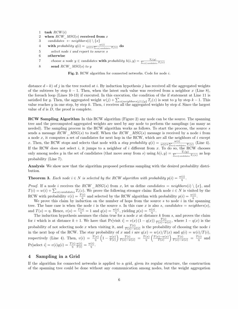
1 task RCW (i)2 when RCW_MSG(s) received from x3 candidates ← neighbors(i) \ {x}4 with probability q(i) = w(i)

w(i)+∑

z∈candidates Ti(z)do

5 select node i and report to source s6 otherwise7 choose a node y ∈ candidates with probability h(i, y) = Ti(y)∑

z∈candidates Ti(z)

8 send RCW_MSG(s) to y

Fig. 2. RCW algorithm for connected networks. Code for node i.

distance d−k) of j in the tree rooted at i. By induction hypothesis j has received all the aggregated weightsof the subtrees by step k − 1. Then, when the latest such value was received from a neighbor x (Line 8),the foreach loop (Lines 10-13) if executed. In this execution, the condition of the if statement at Line 11 issatisfied for y. Then, the aggregated weight w(j) +

∑z∈neighbors(j)\{y} Tj(z) is sent to y by step k − 1. This

value reaches y in one step, by step k. Then, i receives all the aggregated weights by step d. Since the largestvalue of d is D, the proof is complete.

RCW Sampling Algorithm In this RCW algorithm (Figure 2) any node can be the source. The spanningtree and the precomputed aggregated weights are used by any node to perform the samplings (as many asneeded). The sampling process in the RCW algorithm works as follows. To start the process, the source ssends a message RCW_MSG(s) to itself. When the RCW_MSG(s) message is received by a node i froma node x, it computes a set of candidates for next hop in the RCW, which are all the neighbors of i exceptx. Then, the RCW stops and selects that node with a stay probability q(i) = w(i)

w(i)+∑

z∈candidates Ti(z)(Line 4).

If the RCW does not select i, it jumps to a neighbor of i different from x. To do so, the RCW choosesonly among nodes y in the set of candidates (that move away from s) using h(i, y) = Ti(y)∑

z∈candidates Ti(z)as hop

probability (Line 7).

Analysis We show now that the algorithm proposed performs sampling with the desired probability distri-bution.

Theorem 3. Each node i ∈ N is selected by the RCW algorithm with probability p(i) = w(i)η .

Proof. If a node i receives the RCW_MSG(s) from x, let us define candidates = neighbors(i) \ {x}, andT (i) = w(i) +

∑z∈candidates Ti(z). We prove the following stronger claim: Each node i ∈ N is visited by the

RCW with probability v(i) = T (i)η and selected by the RCW algorithm with probability p(i) = w(i)

η .We prove this claim by induction on the number of hops from the source s to node i in the spanning

tree. The base case is when the node i is the source s. In this case x is also s, candidates = neighbors(s),and T (s) = η. Hence, v(s) = T (s)

η = 1 and q(s) = w(s)η , yielding p(s) = w(s)

η .The induction hypothesis assumes the claim true for a node x at distance k from s, and proves the claim

for i which is at distance k + 1. We have that Pr[visit i] = v(x) (1− q(x)) T (i)T (x)−w(x) , where 1 − q(x) is the

probability of not selecting node x when visiting it, and T (i)T (x)−w(x) is the probability of choosing the node i

in the next hop of the RCW. The stay probability of x and i are q(x) = w(x)/T (x) and q(i) = w(i)/T (i),respectively (Line 4). Then, v(i) = T (x)

η

(1− w(x)

T (x)

)T (i)

T (x)−w(x) = T (x)η

(T (x)−w(x)

T (x)

)T (i)

T (x)−w(x) = T (i)η and

Pr[select i] = v(i)q(i) = T (i)η

w(i)T (i) = w(i)

η .

4 Sampling in a GridIf the algorithm for connected networks is applied to a grid, given its regular structure, the constructionof the spanning tree could be done without any communication among nodes, but the weight aggregation

6

process has to be done as before. However, we show in this section that all preprocessing and the state datastored in each node can be avoided if the probability distribution is based on the distance. RCW samplingprocess was described in Section 2, and we only redefine stay and hop probabilities. From Observation 1, thekey for correctness is to assign stay and hop probabilities that guarantee visit and stay probabilities that arehomogenous for all the nodes at the same distance from the source.Stay probability For k ∈ [0, R], the stay probability of every node (i, j) ∈ Rk is defined as

qk =nk · pk∑Rj=k nj · pj

=nk · pk

1−∑k−1j=0 nj · pj

. (2)

As required by Observation 1, all nodes in Rk have the same qk. Note that q0 = p0 and qR = 1, as onemay expect. Since the value of pk is known at (i, j) ∈ Rk, nk can be readily computed7, and the value of∑k−1j=0 nj · pj can be piggybacked in the RCW, the value of qk can be computed and used at (i, j) without

requiring precomputation nor state data.

Hop probability In the grid, the hops of a RCW increase the distance from the source by one unit.We want to guarantee that the visiting probability is the same for each node at the same distance, to useObservation 1. To do so, we need to observe that nodes (i, j) over the axes (i.e., with i = 0 or j = 0) haveto be treated as a special case, because they can only be reached via a single path, while the others nodescan be reached via several paths. To simplify the presentation, and since the grid is symmetric, we give thehop probabilities for one quadrant only (the one in which nodes have both coordinates non-negative). Thehop probabilities in the other three quadrants are similar. The first hop of each RCW chooses one of thefour links of the source node with the same probability 1/4. We have three cases when calculating the hopprobabilities from a node (i, j) at distance k, 0 < k < R, to node (i′, j′).

– Case A: The edge from (i, j) to (i′, j′) is in one axis (i.e., i = i′ = 0 or j = j′ = 0). The hop probabilityof this link is set to hk((i, j), (i′, j′)) = i+j

i+j+1 = kk+1 .

– Case B: The edge from (i, j) to (i′, j′) is not in the axes, i′ = i+ 1, and j′ = j. The hop probability ofthis link is set to hk((i, j), (i+ 1, j)) = 2i+1

2(i+j+1) =2i+1

2(k+1) .– Case C: The edge from (i, j) to (i′, j′) is not in the axes, i′ = i, and j′ = j + 1. The hop probability of

this link is set to hk((i, j), (i, j + 1)) = 2j+12(i+j+1) =

2j+12(k+1) .

It is easy to check that the hop probabilities of a node add up to one.

Analysis In the following we prove that the RCW that uses the above stay and hop probabilities selectsnodes with the desired sample probability.

Lemma 1. All nodes at the same distance k ≥ 0 to the source have the same visit probability vk.

Proof. The proof uses induction. The base case is k = 0, and obviously vk = 1. When k = 1, the probabilityof visiting each of the four nodes at distance 1 from the source s is vi = 1−q0

4 , where 1− q0 is the probabilityof not staying at source node. Assuming that all nodes at distance k > 0 have the same visit probability vk,we prove the case of distance k + 1. Recall that the stay probability is the same qk for all nodes at distancek.

The probability to visit a node x = (i′, j′) at distance k + 1 depends on whether x is on an axis or not.If it is in one axis it can only be reached from its only neighbor (i, j) at distance k. This happens withprobability (case A) Pr[visit x] = vk(1− qk) i+j

i+j+1 = vk(1− qk) kk+1 . If x is not on an axis, it can be reached

from two nodes, (i′− 1, j′) and (i′, j′− 1), at distance k (Cases B and C). Hence, the probability of reachingx is then Pr[visit x] = vk(1 − qk) 2(i

′−1)+12(i′+j′) + vk(1 − qk) 2(j

′−1)+12(i′+j′) = vk(1 − qk) k

k+1 . Hence, in both cases thevisit probability of a node x at distance k + 1 is vk+1 = vk(1 − qk) k

k+1 . This proves the induction and theclaim.7 n0 = 1, while nk = 4k for k ∈ [1, R].

7

1 task RCW (x, k, δk, γk, pk)2 when RCW_MSG(s, vk−1, pk−1, nk−1, δk−1) received:3 nk ← nk−1

δk−1

γk; vk ← nk−1

vk−1−pk−1

nk; qk ← pk

vk

4 with probability qk do select node x and report to s5 otherwise6 choose a neighbor y in ring k + 1 with uniform probability7 send RCW_MSG(s, vk, pk, nk, δk) to y

Fig. 3. RCW algorithm for concentric rings with uniform connectivity (code for node x ∈ Rk, k > 0).

Theorem 4. Every node at distance k ∈ [0, R] from the source is selected with probability pk.

Proof. If a node is visited at distance k, it is because no node was selected at distance less than k, since aRCW always moves away from the source. Hence, Pr[∃x ∈ Rk visited] = 1−

∑k−1j=0 njpj . Since all the nk nodes

in Rk have the same probability to be visited (from the previous lemma), we have that vk =1−

∑k−1j=0 njpj

nk.

Now, since all the nk nodes in Rk have the same stay probability is qk, the probability of selecting a particular

node x at distance k from the source is Pr[select x] = vkqk =1−

∑k−1j=0 njpj

nk

nkpk∑Rj=k njpj

= pk, where it has been

used that (1−∑k−1j=0 njpj) =

∑Rj=k njpj .

5 Sampling in a Concentric Rings Network with Uniform Connectivity

In this section we derive a RCW algorithm to sample a concentric rings network with uniform connectivity,where all preprocessing is avoided, and only a small (and constant) amount of data is stored in each node.Recall that uniform connectivity means that all nodes of ring k have the same number of neighbors δk inring k + 1 and the same number of neighbors γk in ring k − 1.

Distributed algorithm The general behavior of the RCW algorithm for these networks was described inSection 2. In order to guarantee that the algorithm is fully distributed, and to reduce the amount of dataa node must know a priori, a node at distance k that sends the RCW to a node in ring k + 1 piggybackssome information. More in detail, when a node in ring k receives the RCW from a node of ring k− 1, it alsoreceives the probability vk−1 of the previous step, and the values pk−1, nk−1, and δk−1. Then, it calculatesthe values of nk, vk, and qk. After that, the RCW algorithm uses the stay probability qk to decide whetherto select the node or not. If it decides not to select it, it chooses a neighbor in ring k + 1 with uniformprobability. Then, it sends to this node the probability vk and the values pk, nk, and δk, piggybacked in theRCW.

The RCW algorithm works as follows. The source s selects itself with probability q0 = p0. If it does notdo so, it chooses one node in ring 1 with uniform probability, and sends it the RCW message with valuesv0 = 1, n0 = 1, p0, and δ0. Figure 3 shows the code of the RCW algorithm for nodes in rings Rk for k > 0.Each node in ring k must only know initially the values δk, γk and pk. Observe that nk (number of nodesin ring k) can be locally calculated as nk = nk−1δk−1/γk. The correctness of this computation follows fromthe uniform connectivity assumption (Eq. 1).

Analysis The uniform connectivity property can be used to prove by induction that all nodes in the samering k have the same probability vk to be reached. The stay probability qk is defined as qk = pk/vk. Then,from Observation 1, the probability of selecting a node x of ring k is pk = vkqk. What is left to prove is thatthe value vk computed in Figure 3 is in fact the visit probability of a node in ring k.

Lemma 2. The values vk computed in Figure 3 are the correct visit probabilities.

Proof. Let us use induction. For k = 1 the visit probability of a node x in ring R1 is 1−q0n1

= 1−p0n1

. On theother hand, when a message RCW_MSG reaches x, it carries v0 = 1, n0 = 1, p0, and δ0 (Line 2). Then,

8

s

/2

k+1

k 1

k

x

Fig. 4. Node deployment and connectivity used in the simulations.

v1 is computed as v1 = n0v0−p0n1

= 1−p0n1

(Line 3). For a general k > 1, assume the value vk−1 is the correctvisit probability of a node in ring k − 1. The visit probability of a node in ring k is vk−1nk−1(1− qk−1)/nk,which replacing qk−1 = pk−1/vk−1 yields the expression used in Figure 3 to compute vk (Line 3).

The above lemma, together with the previous reasoning, proves the following.

Theorem 5. Every node at distance k of the source is selected with probability pk.

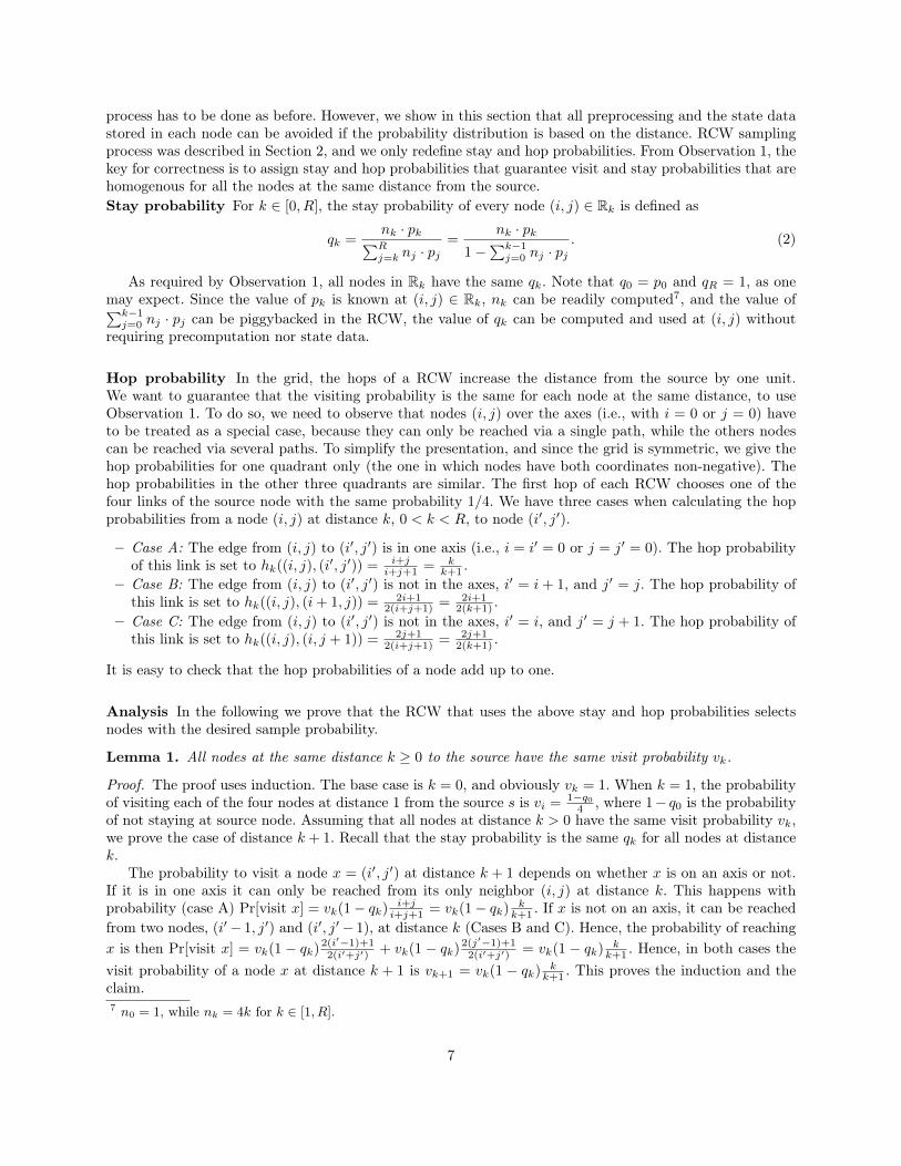
6 Concentric Rings Networks without Uniform Connectivity

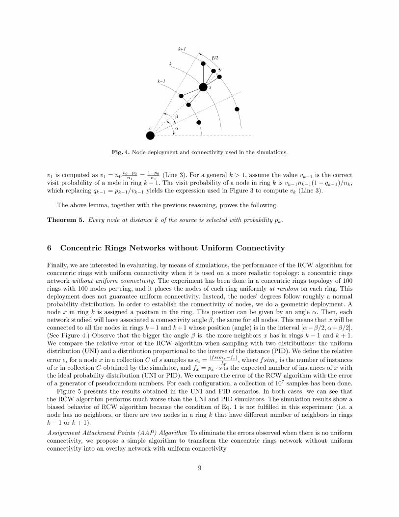
Finally, we are interested in evaluating, by means of simulations, the performance of the RCW algorithm forconcentric rings with uniform connectivity when it is used on a more realistic topology: a concentric ringsnetwork without uniform connectivity. The experiment has been done in a concentric rings topology of 100rings with 100 nodes per ring, and it places the nodes of each ring uniformly at random on each ring. Thisdeployment does not guarantee uniform connectivity. Instead, the nodes’ degrees follow roughly a normalprobability distribution. In order to establish the connectivity of nodes, we do a geometric deployment. Anode x in ring k is assigned a position in the ring. This position can be given by an angle α. Then, eachnetwork studied will have associated a connectivity angle β, the same for all nodes. This means that x will beconnected to all the nodes in rings k−1 and k+1 whose position (angle) is in the interval [α−β/2, α+β/2].(See Figure 4.) Observe that the bigger the angle β is, the more neighbors x has in rings k − 1 and k + 1.We compare the relative error of the RCW algorithm when sampling with two distributions: the uniformdistribution (UNI) and a distribution proportional to the inverse of the distance (PID). We define the relativeerror ei for a node x in a collection C of s samples as ei =

|fsimx−fx|fx

, where fsimx is the number of instancesof x in collection C obtained by the simulator, and fx = px · s is the expected number of instances of x withthe ideal probability distribution (UNI or PID). We compare the error of the RCW algorithm with the errorof a generator of pseudorandom numbers. For each configuration, a collection of 107 samples has been done.

Figure 5 presents the results obtained in the UNI and PID scenarios. In both cases, we can see thatthe RCW algorithm performs much worse than the UNI and PID simulators. The simulation results show abiased behavior of RCW algorithm because the condition of Eq. 1 is not fulfilled in this experiment (i.e. anode has no neighbors, or there are two nodes in a ring k that have different number of neighbors in ringsk − 1 or k + 1).

Assignment Attachment Points (AAP) Algorithm To eliminate the errors observed when there is no uniformconnectivity, we propose a simple algorithm to transform the concentric rings network without uniformconnectivity into an overlay network with uniform connectivity.

9

0.01

0.1

1

10

45 60 75 90 180 360

aver

age

rela

tive

erro

r

angles

UNI RCW maxPID RCW max

UNI simulator maxPID simulator max

UNI RCW avgPID RCW avg

UNI simulator avgPID simulator avg

Fig. 5. UNI and PID scenarios without uniform connectivity.

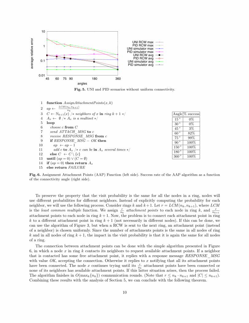
1 function AssignAttachmentPoints(x, k)

2 ap ← LCM (nk,nk+1)

nk

3 C ← Nk+1(x) /∗ neighbors of x in ring k + 1 ∗/4 Ax ← ∅ /∗ Ax is a multiset ∗/5 loop6 choose c from C7 send ATTACH_MSG to c8 receive RESPONSE_MSG from c9 if RESPONSE_MSG = OK then

10 ap ← ap− 111 add c to Ax /∗ c can be in Ax several times ∗/12 else C ← C \ {c}13 until (ap = 0) ∨ (C = ∅)14 if (ap = 0) then return Ax15 else return FAILURE

Angle % success15 ◦ 0%30 ◦ 0%45 ◦ 3%60 ◦ 82%75 ◦ 99%90 ◦ 100%150 ◦ 100%180 ◦ 100%360 ◦ 100%

Fig. 6. Assignment Attachment Points (AAP) Function (left side). Success rate of the AAP algorithm as a functionof the connectivity angle (right side).

To preserve the property that the visit probability is the same for all the nodes in a ring, nodes willuse different probabilities for different neighbors. Instead of explicitly computing the probability for eachneighbor, we will use the following process. Consider rings k and k+1. Let r = LCM (nk, nk+1), where LCMis the least common multiple function. We assign r

nkattachment points to each node in ring k, and r

nk+1

attachment points to each node in ring k+1. Now, the problem is to connect each attachment point in ringk to a different attachment point in ring k + 1 (not necessarily in different nodes). If this can be done, wecan use the algorithm of Figure 3, but when a RCW is sent to the next ring, an attachment point (insteadof a neighbor) is chosen uniformly. Since the number of attachments points is the same in all nodes of ringk and in all nodes of ring k + 1, the impact in the visit probability is that it is again the same for all nodesof a ring.

The connection between attachment points can be done with the simple algorithm presented in Figure6, in which a node x in ring k contacts its neighbors to request available attachment points. If a neighborthat is contacted has some free attachment point, it replies with a response message RESPONSE_MSGwith value OK, accepting the connection. Otherwise it replies to x notifying that all its attachment pointshave been connected. The node x continues trying until its r

nkattachment points have been connected or

none of its neighbors has available attachment points. If this latter situation arises, then the process failed.The algorithm finishes in O(maxk{nk}) communication rounds. (Note that r ≤ nk · nk+1 and |C| ≤ nk+1).Combining these results with the analysis of Section 5, we can conclude with the following theorem.

10

0 0.1 0.2 0.3 0.4 0.5 0.6 0.7 0.8

75 90 150 180 360

aver

age

rela

tive

erro

r

angles

UNI RCW maxPID RCW max

UNI simulator maxPID simulator max

UNI RCW avgPID RCW avg

UNI simulator avgPID simulator avg

Fig. 7. UNI and PID scenarios without uniform connectivity, using the AAP algorithm.

Theorem 6. Using attachment points instead of links and the distributed RCW-based algorithm of Figure3, it is possible to sample a concentric rings network without uniform connectivity with any desired distance-based probability distribution pk, provided that the algorithm of Figure 6 completes (is successful) in all thenodes.

Figure 7 shows the results when using the AAP algorithm. As we can see, the differences have disappeared.The conclusion is that, when nodes are placed uniformly at random and AAP is used to attach neighbors toeach node, RCW performs as good as perfect UNI or PID simulators.

In general, the algorithm of Figure 6 may not be succesful. It is shown in the table of Figure 6 (rightside) the success rate of the algorithm for different connectivity angles. It can be observed that the successrate is large as long as the connectivity angles are not very small (at least 60◦). (For an angle of 60◦ theexpected number of neighbors in the next ring for each node is less than 17.) For small angles, like 15◦ and30◦, the AAP algorithm is never successful. For these cases, the algorithm for connected network presentedin Section 3 can be used.

7 Conclusions

In this paper we propose distributed algorithms for node sampling in networks. All the proposed algorithmsare based on a new class of random walks called centrifugal random walks. These algorithms guarantee thatthe sampling end after a number of hops upper bounded by the diameter of the network, and it sampleswith the exact probability distribution. As future works we want to explore sampling in dynamic networksusing random centrifugal walks. Additionally, we will investigate a more general algorithm that would alsoconcern distributions that do not only depend on the distance from the source.

References

1. Asad Awan, R. A. Ferreira, Suresh Jagannathan, and Ananth Grama. Distributed uniform sampling in unstruc-tured peer-to-peer networks. In HICSS. IEEE CS, 2006.

2. M. Bertier, F. Bonnet, A.M. Kermarrec, V. Leroy, S. Peri, and M Raynal. D2HT: The best of both worlds,integrating RPS and DHT. In EDCC. IEEE CS, 2010.

3. F. Bonnet, A.-M. Kermarrec, and M. Raynal. Small-world networks: From theoretical bounds to practical systems.Proc. OPODIS, LNCS. Springer, 2007.

4. M. Bui, F. Butelle, and C. Lavault. A distributed algorithm for constructing a minimum diameter spanning tree.J. Parallel Distrib. Comput., May 2004.

5. Y. Busnel, R. Beraldi, and R. Baldoni. On the uniformity of peer sampling based on view shuffling. Journal ofParallel and Distributed Computing, 2011.

11

6. Michael Elkin. A faster distributed protocol for constructing a minimum spanning tree. In Proceedings of thefifteenth annual ACM-SIAM symposium on Discrete algorithms, SODA ’04, Philadelphia, PA, USA, 2004. Societyfor Industrial and Applied Mathematics.

7. P. Fraigniaud and G. Giakkoupis. On the searchability of small-world networks with arbitrary underlyingstructure. In L. J. Schulman, editor, STOC. ACM, 2010.

8. B. Gfeller, N. Santoro, and P. Widmayer. A distributed algorithm for finding all best swap edges of a minimum-diameter spanning tree. IEEE Trans. Dependable Secur. Comput., January 2011.

9. Minas Gjoka, Maciej Kurant, Carter T. Butts, and Athina Markopoulou. Walking in facebook: A case study ofunbiased sampling of osns. In INFOCOM, pages 2498–2506. IEEE, 2010.

10. M. Gjoka, M. Kurant, Carter T. Butts, and A. Markopoulou. Practical recommendations on crawling onlinesocial networks. Selected Areas in Communications, IEEE Journal on, october 2011.

11. M. Gurevich and I. Keidar. Correctness of gossip-based membership under message loss. SIAM J. Comput.,39(8), December 2010.

12. M. Jelasity, S. Voulgaris, R. Guerraoui, A.-M. Kermarrec, and M. van Steen. Gossip-based peer sampling. ACMTrans. Comput. Syst., 25(3), 2007.

13. D. Kempe, Jon M. Kleinberg, and Alan J. Demers. Spatial gossip and resource location protocols. J. ACM,51(6):943–967, 2004.

14. J. M. Kleinberg. Navigation in a small world. Nature, 406(6798), August 2000.15. Chul-Ho Lee, Xin Xu, and Do Young Eun. Beyond random walk and metropolis-hastings samplers: why you

should not backtrack for unbiased graph sampling. SIGMETRICS ’2012. ACM.16. D. Milić and and T. Braun. Netice9: A stable landmark-less network positioning system. In Local Computer

Networks, 2010 IEEE 35th Conference on, oct. 2010.17. A. Sevilla, A. Mozo, M. Lorenzo, J.L. López-Presa, P Manzano, and A. Fernández Anta. Biased selection for

building small-world networks. OPODIS 2010.18. Ming Zhong and Kai Shen. Random walk based node sampling in self-organizing networks. SIGOPS Oper. Syst.

Rev., 40:49–55, July 2006.

12