Random Sampling for Continuous Streamswith Arbitrary Updates

Yufei Tao, Xiang Lian, Dimitris Papadias, and Marios Hadjieleftheriou

Abstract—The existing random sampling methods have at least one of the following disadvantages: they 1) are applicable only to

certain update patterns, 2) entail large space overhead, or 3) incur prohibitive maintenance cost. These drawbacks prevent their

effective application in stream environments (where a relation is updated by a large volume of insertions and deletions that may arrive

in any order), despite the considerable success of random sampling in conventional databases. Motivated by this, we develop several

fully dynamic algorithms for obtaining random samples from individual relations, and from the join result of two tables. Our solutions

can handle any update pattern with small space and computational overhead. We also present an in-depth analysis that provides

valuable insight into the characteristics of alternative sampling strategies and leads to precision guarantees. Extensive experiments

validate our theoretical findings and demonstrate the efficiency of our techniques in practice.

Index Terms—Sampling, selectivity estimation.

Ç

1 INTRODUCTION

A general stream relation receives a large number ofupdates per time unit, which include tuple insertions

and deletions that may arrive in any order. Specifically,each I-command has the form fI; id; SAg, where the first fieldis a tag indicating “insertion,” the second denotes the id ofthe tuple being inserted, and SA corresponds to the set ofthe remaining attributes of the tuple. Similarly, aD-command fD; idg removes the tuple with a specified id.The content of a relation includes all the tuples that wereinserted, but have not been removed; the cardinality of therelation is the number of such tuples.

We consider that all tuples currently in a relation have

distinct ids. Specifically, the id in each I-command should

not be identical to the id of any existing tuple in the relation.

However, provided that the previous tuple with an id has

been deleted, a tuple with the same id can be inserted. In

other words, multiple tuples with the same id may be

inserted throughout the history, but at any moment, there

can be only one tuple with this id.We address two fundamental problems of approximate

processing. Given a single relation T , the first one aims at

providing accurate answers to queries of the form:

Q1 : SELECT COUNTð�Þ FROM T WHERE �any:

Q1 is a counting query with arbitrary conditions �any in the

WHERE clause. We assume no a priori knowledge about �any,

which excludes potential solutions [16], [17] that rely onspecial counting “sketches” (including histograms, wave-lets, etc.) for certain attributes (or their combinations).Specifically, although these methods can produce accurateresults on the preprocessed columns, they are not useful forgeneral ad hoc queries involving other predicates. Random-sampling techniques, on the other hand, constitute a naturalmethodology for this problem because, by keeping allattributes of the sampled tuples, it is possible to supportany predicate �any with good accuracy guarantees.

The second problem tackled in this paper is to accuratelypredict the join size of two stream relations Ta and Tb:

Q2 : SELECT COUNTð�Þ FROM Ta; Tb

WHERE �all and �any:

�all includes a set of registered conditions common in allQ2 queries, which differ in their own formulation of �any (anarbitrary predicate). As an example, assume that Ta hasattributes ðid; AaÞ, Tb has ðid; AbÞ, and �all is Ta:id ¼ Tb:id.Then, every possible Q2 query contains this equi-joincondition, but can also include a predicate �any onindividual columns of a single table (e.g., Ta:Aa > 10), orboth tables (e.g., Ta:Aa þ Tb:Ab > 100). Equivalently, the setof records counted in a Q2 query is a subset of the results ofjoining Ta and Tb using only the condition Ta:id ¼ Tb:id. Ourgoal is to process Q1 and Q2 accurately using at mostM random samples, where M is (by far) lower than the sizeof the database.

Query types Q1 and Q2 are important to a large numberof applications. For example, consider a relation withschema PRðstock-id; priceÞ, where each tuple records thecurrent price of a stock. Whenever a stock’s price changes, aD-command streams in, removing the obsolete tuple of thestock; then, an I-command immediately follows, inserting anew tuple carrying the updated price. Obviously, unlike thesliding-window stream model [5], the order that the tuplesin PR are inserted is most likely not equivalent to the order

96 IEEE TRANSACTIONS ON KNOWLEDGE AND DATA ENGINEERING, VOL. 19, NO. 1, JANUARY 2007

. Y. Tao is with the Department of Computer Science and Engineering,Chinese University of Hong Kong, Sha Tin, New Territories, Hong Kong.E-mail: taoyf@cse.cuhk.edu.hk.

. X. Lian and D. Papadias are with the Department of Computer Science andEngineering, Hong Kong University of Science and Technology, ClearWater Bay, Hong Kong. E-mail: {xlian, dimitris}@cse.ust.hk.

. M. Hadjieleftheriou is with AT&T Labs, 180 Park Avenue, Building 103,Florham Park, NJ 07932. E-mail: marioh@research.att.com.

Manuscript received 14 May 2005; revised 12 Jan. 2006; accepted 3 Aug.2006; published online 20 Nov. 2006.For information on obtaining reprints of this article, please send e-mail to:tkde@computer.org, and reference IEEECS Log Number TKDE-0184-0505.

1041-4347/07/$20.00 � 2007 IEEE Published by the IEEE Computer Society

that they are deleted. A Q1 query in this context mayretrieve the number of stocks whose prices qualify a certainpredicate.

To motivate Q2 queries, assume that we have anotherstream relation TOðstock-id; turnoverÞ, which captures thecurrent turnovers of the stocks. As with PR, TO is updatedwith continuously arriving I and D-commands, generatedby the buying/selling of any stock. Note that the streamscorresponding to PR and TO are typically separate,because they are usually generated by different agents. Inthis case, to study the statistic relationship between pricesand turnovers, a user needs to join PR and TO togetherwith an equality condition on stock-id, and then apply otherpredicates on price and turnover. Such operations form aQ2 query, where �all is the equality condition and �anycorresponds to the other predicates.

We are interested in solutions that incur small computa-tional overhead for processing each incoming command, asopposed to methods (e.g., the counting sample reviewed inthe next section) that have low amortized cost but poorworst-case performance for individual updates. For datastreams with a high record arrival rate, spending consider-able time on any tuple necessarily delays a large number ofsubsequent records, which need to be stored in a systembuffer. When the size of this buffer is exceeded, some tuplesmust be discarded (i.e., load shedding [25]), in which caseobtaining a truly random sample set is impossible. Forinstance, in the stock-trading application mentioned earlier,shedding an update command causes the price of a stock tobe inaccurate. Furthermore, shedding a D-command mayeven lead to duplicate tuples for the same stock.

As elaborated in Section 2, the existing samplingalgorithms have at least one of the following disadvantages:1) they rely on certain assumptions on data updates (e.g.,only insertions are allowed, or tuples must be deletedaccording to the insertion order), 2) they require consider-able space (e.g., the underlying relations must be fullymaterialized for resampling), or 3) they incur prohibitivemaintenance overhead (e.g., they must periodically scan theentire sample set). These problems prevent their effectivedeployment on data stream applications, despite thesuccess of random sampling in conventional databases.

In this paper, we develop sampling algorithms that arefully dynamic (supporting any sequence of insertions anddeletions), efficient (processing each update with very lowspace and computational overhead), and accurate (produ-cing approximate answers for Q1 and Q2 queries with smallerrors). Specifically, for single relations, our methodssignificantly improve the well-known reservoir sampling

and counting sample approaches in the presence of intensiveupdates. For join results, we propose the first samplingalgorithm that enables effective approximate processing onstreams containing arbitrary update requests (the previoussolutions [24] discuss only the special case of slidingwindows). In addition, we present an in-depth analysisthat provides valuable insight into the characteristics ofalternative solutions. Extensive experiments validate ourtheoretical findings and confirm the efficiency of theproposed techniques in practice.

The rest of the paper is organized as follows: Section 2reviews previous work that is directly related to ours.Sections 3 and 4 present algorithms for sampling singlerelations, and analyze their effectiveness on Q1 queries.Section 5 focuses on sampling join results for approximateQ2 processing. Section 6 contains the experimental results,and Section 7 concludes the paper with directions forfuture work.

2 RELATED WORK

Section 2.1 first reviews approaches for sampling a singlerelation in the presence of updates, and clarifies theirproblems. Then, Section 2.2 discusses algorithms forsampling the join result of multiple tables.

2.1 Sampling a Single Relation

Sampling from a static table with n tuples is straightfor-ward. Specifically, a sequence number can be assigned toeach record (i.e., the first tuple has number 1, the second 2,and so on). To obtain s samples, we only need to randomlygenerate s distinct values in the range ½1; n�, and select thetuples with these sequence numbers. It is more difficult,however, to maintain the randomness of the sample setwhen new records are inserted into the table, or existingones are removed. A naive solution would resample therelation as described above whenever its content changes.Obviously, this method is impractical since a resamplingprocess may require accessing a large number of disk pages.Reservoir sampling and counting sample aim at solving theseproblems.

2.1.1 Reservoir Sampling

The first reservoir algorithms [26], [22] in the databasecontext maintain an array RS with maximum size s (thetarget sample size), which is initially empty. The firsts tuples are directly added into RS, after which the arraybecomes full. For each subsequent insertion, a randominteger x is generated in the range ½1; n�, where n is thenumber of insertions handled so far (n continuously growswith time). If x is larger than s, the incoming tuple isignored; otherwise, ðx � sÞ, it is recorded at the xth positionof RS, replacing the sample that was originally there. It canbe shown [26] that, at any time, the tuples in RS constitute arandom sample set of the current content of the data set T .Jermaine et al. [21] present an alternative reservoir techniqueto manage sample sets whose sizes exceed the capacity ofthe available memory. Similar to [26], [22], this approachsupports only insertions.

Gibbons et al. [14] propose an extension, referred to asdelete-at-will in the sequel, for producing a random sampleset in the presence of deletions. Let s be the current size ofthe sample set RS and n the cardinality of T . If the tuple tbeing deleted does not belong to RS, the sample set remainsunchanged. If t is found in RS, it is removed, after whichthe size of RS becomes s� 1. In either case (whether tappears in RS or not), the cardinality of the relation Tchanges to n� 1 to reflect the removal of t. The handling ofinsertions is similar to the reservoir technique. Assume, forinstance, that after a sample is deleted (i.e., the sample sizeis s� 1 and the data cardinality is n� 1) a new record

TAO ET AL.: RANDOM SAMPLING FOR CONTINUOUS STREAMS WITH ARBITRARY UPDATES 97

arrives. A random integer x is generated in the range ½1; n�1� and if x is larger than s� 1, the incoming tuple is ignored;otherwise, ðx � s� 1Þ, it is recorded at the xth position ofRS, replacing the sample that was originally there. Gibbonset al. [14] prove that the resulting RS is still random withrespect to the remaining tuples in T .

The problem with delete-at-will is that the sample setgradually shrinks with time, and eventually ceases to beuseful (e.g., it can no longer provide accurate selectivityestimation). Therefore, T must be scanned so that asufficient number of samples are retrieved again. Thisrequires retaining all the tuples that have been inserted butnot yet deleted, which is impossible in stream environ-ments. In Section 3, we propose R�, an improved reservoiralgorithm that supports deletions without decreasing thesample size.

2.1.2 Counting Sample

Counting sample (CS) [13] can produce a random sample setfor any sequence of insertions and deletions withoutresampling the base relation, even in the existence ofduplicate tuples (consequently, it is trivially applicable toconventional tables where each record is different). Speci-fically, CS maintains a list RS (with maximum size s) ofelements in the form1 ft; cg, where c is a counter thatsummarizes the number of identical records t in the sampleset. Furthermore, a variable � , initially set to 1, is used tocontrol the probability that a record is sampled.

To handle an incoming tuple t, CS first probes the existingsample set to see if t has been included before. If yes, thecounter c in the corresponding pair ft; cg is increased by one,and the insertion terminates. Otherwise, (t is not in RS), CStosses a coin c1 with probability 1=� head, and discards t if c1

tails. Alternatively (c1 heads), the algorithm includes a newentry ft; 1g inRS. IfRS does not overflow (i.e., it contains nomore than s elements), the insertion is completed. In case ofan overflow, a rejecting pass is performed to expunge someexisting samples from RS.

Specifically, at the beginning of the rejecting pass, anumber � 0 larger than the current � (that governs thesampling probability, as mentioned earlier) is chosen. Then,for each element ft; cg in RS, a coin c2 is flipped withprobability �=� 0 head. If c2 tails, the rejecting algorithmmoves on to the next element in RS. Otherwise (c2 heads), itdecreases the counter c by 1, and then repeatedly throws acoin c3 with probability 1=� 0 head, until c3 turns on tail. Oneach head occurrence of c3, the counter c is further reducedby 1, until the element ft; cg is eliminated when c equals 0.At the end of a rejecting pass (after processing all elements),the value of � is updated to � 0. If the overflow of RS persists(i.e., no counter became 0 in the previous pass), anotherpass is executed. This process is repeated until the overflowis remedied.

Deleting a tuple t is much easier. The deletion is ignored ift is not in RS. Otherwise, the counter c in the correspondingpair ft; cg is decreased, and the pair is removed from RS if creaches 0. Note that, unlike delete-at-will, the removal of ft; cg

does not reduce the size of RS, that is, a future sample maystill be stored at the original position of the removed entry. Itis worth mentioning that the set of tuples in RS is not arandom sample set of the current relation T . However, it canbe converted into one by scanning the entire RS (see [13] fordetails).

A disadvantage of CS (that restricts the applicability ofthis method in practice) is that the entire RS must bescanned (sometimes repeatedly) for expunging existingsample(s) in case of overflows. When the size of RS is large,scanning RS may delay processing a large number ofsubsequently arriving records, some of which may need tobe discarded from the system after the input buffer becomesfull. In this case, it is simply impossible to obtain a trulyrandom sample set. Furthermore, the selection of � 0 in therejecting pass is ad hoc. Gibbons et al. [13] suggest that � 0

should be 10 percent higher than the current � , without,however, providing justification on this choice. In Section 4,we present CS�, an enhanced version of CS that avoidsthese problems.

Motivated by the shortcomings of reservoir and countingsample, Babcock et al. [5] propose alternative algorithms2 forproducing random samples in the specific context of“sliding window streams,” where tuples are deletedaccording to the order of their arrival. Since these algo-rithms are inapplicable to arbitrary sequences of insertions/deletions, we do not discuss them further.

Finally, there exist numerous papers ([4], [7], [18], [20] tomention just some recent ones) on applications of samplingto various estimation tasks (e.g., selectivity estimation,clustering, etc.). The solutions in those papers do notcompute random samples, and cannot be used to solve Q1and Q2 queries formulated in Section 1. Recently, somesketch-based algorithms [9], [10], [11] have been developedto obtain a “probabilistic” random sample set, i.e., thesamples may be random with a high probability, but thereis no guarantee. We aim at deriving truly random samplesin all cases.

2.2 Sampling the Join Results

Let T1 and T2 be two relations, and � be a joinpredicate. Naive stream join (NSJ) is a straightforwardmethod that maintains random sample sets RSðT1Þ andRSðT2Þ on T1 and T2, respectively (e.g., by using thetechniques of the previous section). Then, given a Q2query q, it finds the number nq of tuple pairs ðt1; t2Þ 2RSðT1Þ �RSðT2Þ that satisfy q, and estimates the queryresult as ðnq � jT1j � jT2jÞ = ðjRSðT1Þj � jRSðT2ÞjÞ. This esti-mation, however, is usually not accurate, because thejoin between the sample sets of T1 and T2 typicallyleads to a very small subset of the actual join result.This phenomenon is caused by the fact [8] that theprojection of the join result onto the columns of T1 ðT2Þis not a random sample set of T1 ðT2Þ.

98 IEEE TRANSACTIONS ON KNOWLEDGE AND DATA ENGINEERING, VOL. 19, NO. 1, JANUARY 2007

1. CS adopts a slightly more complex element representation to minimizethe space consumption. Since the basic idea is the same, we ignore thisdifference here for simplicity.

2. It is worth mentioning that the sliding-window algorithms in [5] havelower update cost than the proposed approaches. Specifically, thosealgorithms require Oð1Þ cost for each incoming tuple, while our approachesincur OðlogMÞ time, where M is the memory size. This comparison,however, is not fair because the algorithms in [5] utilize the specialproperties of a sliding-window stream to reduce the update cost, and arenot applicable in our problem settings.

To illustrate this, we use an example similar to that in

[8]. Consider that T1 and T2 have a single attribute A

with the following tuples: T1 ¼ f1; 1; . . . ; 1; 2g, and

T2 ¼ f2; 2; . . . ; 2; 1g. Most probably, a random sample

RSðT1Þ (or RSðT2Þ) on T1 (or T2) will include only

records with A ¼ 1 (or 2). Therefore, the size of T1 ffl� T2

(where � is T1:A ¼ T2:A) is estimated as 0, even though

the join actually produces a large number of records.To solve this problem, Chaudhuri et al. [8] suggest

sampling the join result in a two-step manner. The first step

joins each tuple t 2 T1 with the data in T2, and records t:w

(the weight of t) as the number of records in T2 that qualify �

with t. Then, in the second step, each record t 2 T1 is re-

examined. This time, a coin is thrown with head probability

proportional to t:w. If the coin tails, t is ignored and the

execution proceeds with the next tuple in T1. Otherwise (the

coin heads), a subset of the records in t ffl� T2 (all the join

results produced by t) is randomly extracted and included

into RS� (the sample set over the join results). The expected

size of this subset is also proportional to t:w (see [8] for

details).The above method is static because subsequent inser-

tions and deletions on T1 or T2 necessarily affect the weights

of individual tuples and, hence, change the probabilities

that they should appear in RS�. Srivastava and Widom [24]

develop a similar sampling strategy that can handle

updates. Their work, however, is restricted to sliding

windows and assumes a priori knowledge about data

distributions (records follow either the “age-based” or

“frequency-based” model). In Section 5.2, we develop

alternative methods without such constraints. Acharya

et al. [2] propose the “join synopsis” for obtaining random

samples in the special case of foreign-key joins, but their

methods are inapplicable to arbitrary join conditions. Other

relevant work [3], [9], [19] focuses on estimating the join

sizes without computing samples.

3 DYNAMIC RESERVOIR SAMPLING

In this section, we present the R� algorithm, an extension ofreservoir sampling that supports an arbitrary sequence ofinsertions and deletions. Section 3.1 discusses the algorith-mic details of R� and Section 3.2 analyzes its characteristics.

3.1 Algorithm

R� maintains an array RS with size M, whose value isdetermined by the amount of available memory. At anytime, only a subset of valid records in RS belongs to thecurrent sample set. Each element RS½i� ð1 � i �MÞ isassociated with a tag RS½i�:valid that equals TRUE if RS½i�is valid, and FALSE, otherwise. Initially, every RS½i�:validequals FALSE, indicating an empty sample set. Insertionsare handled in a way similar to the conventional reservoirmethod. Specifically, for each I-command (let t be therecord being inserted), we generate a random integer x inthe range ½1; nI �, where nI is the total number of insertionsprocessed so far. If x �M, we place t at the xth positionRS½x� of RS, and set RS½x�:valid to TRUE. Otherwise,ðx > MÞ, no further action is taken and t is ignored.

To handle a D-command fD; idg, on the other hand,we first check if the tuple with the requested id belongsto the sample set, namely, whether there exists a numberx ð1 � x �MÞ such that the id of RS½x� equals id, andRS½x�:valid ¼ TRUE. If x is found, deletion is completedby simply modifying RS½x�:valid to FALSE, withoutaffecting the other elements in RS. Fig. 1 presents thepseudocode of R�.

We emphasize several differences between R� and thereservoir algorithm coupled with delete-at-will (reviewed inSection 2.1). First, although both algorithms generate arandom number for each incoming I-command, the upperbound of the random number generated by R� equals nI(Line 2 of R�-insert in Fig. 1), as opposed to jT j in reservoir.

Second, whenever a sample is deleted, reservoir wastes anelement in array RS, that is, the element can no longer beused to hold a sample. Accordingly, the maximum possiblesample-set size also decreases, thus wasting an increasinglylarge part of the memory. R�, on the other hand, does not

TAO ET AL.: RANDOM SAMPLING FOR CONTINUOUS STREAMS WITH ARBITRARY UPDATES 99

Fig. 1. Adapted reservoir sampling.

reduce the size of RS, i.e., in the future, the sample set sizecan still be as large as permitted by the available memory.

Third, after deleting a sample, the positions of theremaining samples in RS are not important for reservoir

(e.g., the algorithm is still correct, even if two samplesswitch their positions). For R�, however, the remainingsamples must be fixed to their original positions. The reasonfor this will be clear in the correctness proof of R� in thenext section.

In order to efficiently retrieve records with particular ids(during deletion), we create an appropriate index IðRSÞ(e.g., a main-memory B-tree [15]) on the sample ids. IðRSÞis updated whenever the content of RS changes. Note that,since IðRSÞ contains only the ids of the tuples, its size is 1=d

of the space occupied by the relation, where d is the numberof attributes of a tuple.

Given a Q1 query q, we count the number nq of valid

records in RS that satisfy q, and report nq � jT j=s as theapproximate answer, where jT j is the current cardinality ofT , and s is the number of valid samples. Obviously, both jT jand s can be maintained with trivial overhead—they aresimply increased (decreased) whenever a tuple is insertedinto (deleted from) T and RS, respectively.

3.2 Analysis

We first show that R� indeed produces a random sampleset. Let Useq be the sequence of all the update requestssorted according to their arrival order, and Ii be theith I-command; similarly, Dj is the jth D-command.Lemma 1 provides a crucial observation:

Lemma 1. Let Dj and Ii be a pair of consecutive commands in

sequence Useq such that Dj arrives before Ii (i.e.,

Useq ¼ f. . .DjIi . . .g). Denote U 0seq as the sequence obtained

from Useq by simply swapping the order of Ii and Dj (i.e.,

U 0seq ¼ f. . . IiDj . . .g). Then, executing R� on Useq and U 0seqleads to the same RS.

Proof. Since Dj arrives before Ii in the original sequenceUseq, the two updates refer to different records. LetRSbfr ðRS0bfrÞ be the content of RS when all thecommands before Dj ðIiÞ in sequence Useq ðU 0seqÞ havebeen processed. Obviously, RSbfr ¼ RS0bfr since they arethe content of RS after processing the same sequence ofupdates. Similarly, let RSaft ðRS0aftÞ be the content of RSafter processing Ii ðDjÞ in Useq ðU 0seqÞ. We will show thatRSaft is also identical to RS0aft, which establishes thecorrectness of the lemma, because the remaining parts ofUseq and U 0seq are exactly the same.

To prove RSaft ¼ RS0aft, notice that handling aD-command does not generate any random number.Therefore, the value x produced at Line 2 of R�-insert(Fig. 1) for Ii is the same in both Useq and U 0seq (this iswhy, after deleting a sample, the remaining samplesmust be kept to their original positions in the array). Thisindicates that the tuple inserted by Ii will appear in bothRSaft and RS0aft simultaneously, or will not appear in anyof them. Furthermore, if the tuple requested by Dj existsin RSbfr ðRS0bfrÞ, it will disappear in RSaft ðRS0aftÞ, whichestablishes the correctness of the lemma. tu

Based on the above lemma, we prove the randomness ofthe sample set obtained by R�:

Theorem 1. Let T be the relation being sampled by R�. Then, thevalid records in RS always constitute a random sample set forthe current content of T .

Proof. Assume that the original update sequence Useq has nIinsertions and nD deletions. Let us continuously swappairs of consecutive D and I-commands, if theD-command is before the I-command. Eventually, weobtain a sequence U 0seq ¼ fI1 . . . InID1 . . .DnDg, whereevery I-command is positioned before all the D-com-mands. Let RSI be the content of RS after performing allthe I-commands using the R� algorithm, which in thiscase is the same as the conventional reservoir. Hence, RSIis a random sample set over all tuples that have beeninserted. The subsequent execution of R� on theremaining D-commands is reduced to the delete-at-willapproach reviewed in Section 2.1, and therefore, the finalRS is still a random sample set of U 0seq. By Lemma 1, RSthus computed is identical to that obtained by runningR� on the original sequence Useq, completing the proof.tu

Note that the above theorem is correct even if the sameobject is repeatedly inserted and removed from thedatabase. In this case, special care should be taken tounderstand semantics of the insertions/deletions in U 0seq inthe above proof. For example, assume that an object isinserted and removed twice by operation sequenceIa;Db; Ic;Dd, for some integers a < b < c < d. These fourupdates have order Ia; Ic;Db;Dd in U 0seq. Hence, when Db isprocessed (according to U 0seq), there are two copies of theobject in the database (inserted by Ia and Ic, respectively).Then, Db removes the copy created by Ia, and similarly, Dd

removes the one created by Ic.As a second step, we quantify the number s of valid

elements in RS (i.e., the sample size). In particular, our goalis to show that, unlike the delete-at-will approach, the samplesize of R� does not decrease with time, but stabilizes at acertain value depending on the total numbers of insertionsand deletions already seen.

Lemma 2. Let s be the number of valid records in RS producedby R�. Then, the probability Pfs ¼ vg that s equals aparticular value v (1 � v �M, where M is the maximum sizeof RS) is given by:

pfs ¼ vg ¼ nDM � v

� �nI � nD

v

� ��nIM

� �; ð1Þ

where nI ðnDÞ is the total number of insertions (deletions)processed, assuming nI M (i.e., at least M I-commandshave been received).

Proof. In the same way as described in the proof for

Theorem 1, we convert the original update sequence Useq

into U 0seq ¼ fI1 . . . InID1 . . .DnDg (the result of R� on Useq

is equivalent to that on U 0seq). Let RSI be the content of

RS after processing all the I-commands. Since RSI is a

simple random sample set (with M samples) of the

relation T 0 containing the nI inserted records, the

100 IEEE TRANSACTIONS ON KNOWLEDGE AND DATA ENGINEERING, VOL. 19, NO. 1, JANUARY 2007

number of possible RSI equalsnIM

� �. Furthermore, an

RSI leads to a final RS with v valid elements after

handling the D-commands in Useq if and only if two

conditions are satisfied. First, M � v (out of M) tuples of

RSI are chosen from the set TD of records deleted by the

nD D-commands. Second, the other v tuples of RSI are

selected from T 0 � TD (involving nI � nD records). The

number of RSI qualifying the above conditions is�nDM�v

���nI�nDv

�. Therefore, the probability Pfs ¼ vg

can be computed as�nDM�v

���nI�nDv

�.�nIM

�. tu

As a corollary, the expected sample size EðsÞ of R�

equals:

EðsÞ ¼XMv¼0

ðv � Pfs ¼ vgÞ ¼XMv¼1

ðv � Pfs ¼ vgÞ; ð2Þ

where Pfs ¼ vg is represented in (1). Solving this formularesults in the following lemma:

Lemma 3. The expected sample size EðsÞ equals:

EðsÞ ¼M � ðnI � nDÞ=nI; ð3Þ

where nI and nD are as defined in Lemma 2.

Proof. We prove the lemma by induction. First, for M ¼ 1,

(2) becomes 1 � Pfs ¼ 1g, which, by Lemma 2, is�nD1�1

���nI�nD1

�.�nI1

�¼ ðnI � nDÞ=nI . Hence, the lemma

is correct in this case. Next, assuming that the lemma

holds for M equal to any integer k, we show that it also

holds for M ¼ kþ 1.Let us write u ¼ v� 1. Hence, (2) can be rewritten as

(setting M to kþ 1):

Xku¼0

ðuþ 1Þ � nDk� u

� �nI � nDuþ 1

� ��nIkþ 1

� �:

Since�nI�nDuþ1

�¼�nI�nDþ1uþ1

���nI�nDu

�and

�nIkþ1

�¼ kþ 1ð Þ

.hnI � kð Þ

�nIk

�i;

the above equation can be transformed to:

kþ 1

nI � kXku¼0

ðuþ 1Þ �nD

k� u

� �nI � nD þ 1

uþ 1

� ��nI

k

� �

� kþ 1

nI � kXku¼0

ðuþ 1Þ �nD

k� u

� �nI � nD

u

� ��nI

k

� �:

ð4Þ

It holds that nI�nDþ1uþ1

� �¼ nI�nDþ1

uþ1nI�nDu

� �. Furthermore, by

the inductive assumption (Lemma 3 holds for M ¼ k),

we havePk

u¼0 u �nDk�u� �

nI�nDu

� �= nI

k

� �¼ k � nI�nDnI

. Combin-

ing these facts, we simplify (4) as:

kþ 1

nI � k� ðnI � nDÞ �

Xku¼0

nD

k� u

� ��

nI � nDu

� ��nI

k

� �

� kþ 1

nI � k� k � nI � nD

nI

� �:

Observe thatPk

u¼0nDk�u� �

nI�nDu

� �¼ nI

k

� �. Hence, the above

equation becomes:

kþ 1

nI � k� ðnI � nDÞ �

kþ 1

nI � k� k � nI � nD

nI

� �

¼ ðkþ 1Þ � nI � nDnI

:

Thus, we complete the proof. tuThe above equation has a clear intuition: The percen-

tage of the valid tuples in RS corresponds to thepercentage of the records currently in T among all thoseever inserted. Indeed, the probability Pfs ¼ vg given in(1) peaks at v ¼M � ðnI � nDÞ=nI , and quickly diminishesas v drifts away from this value. This, in turn, indicates asmall variance for s, thus validating the usefulness of (3).As a corollary of Lemma 3, the actual sample size of R� isexpected to remain constant with time provided that theratio nI=nD between the numbers of insertions anddeletions is fixed.

We are now ready to quantify the per-tuple processingcost of R�.

Theorem 2. For each I-command, R� performs a deletion fromIðRSÞ with probability EðsÞ=nI , and an insertion into IðRSÞwith probability M=nI , where EðsÞ is the expected sample sizegiven in (2) or (3), M the memory capacity, and nI the totalnumber of insertions. For a D-command, R� always executes asearch in IðRSÞ, and then a deletion from IðRSÞ withprobability EðsÞ=ðnI � nDÞ.Theorem 2 shows that, for each I-command, R� performs

Oð1Þ work with a high probability; when it needs to dosomething, it performs a single insertion to IðRSÞ. On theother hand, for a D-command, R� always performs a searchand, with a small probability, also a deletion on IðRSÞ.Since IðRSÞ is a main-memory B-tree, the worst-case per-tuple cost of R� is OðlogjRSjÞ ¼ OðlogMÞ.

4 DISTINCT COUNTING SAMPLE

In this section, we develop an alternative samplingapproach CS�, which is motivated by the counting samplereviewed in Section 2.1, but improves its update perfor-mance considerably. The next section first elaborates thesampling procedures of CS�, and Section 4.2 analyzes itsbehavior.

4.1 Algorithm

As with R�, CS� maintains an array RS (containing at mostM elements), and associates each record RS½i� ð1 � i �MÞwith a tag RS½i�.valid to indicate its validity in the currentsample set. In addition, it uses a stack, denoted as vacant, toorganize the positions of invalid elements. If RS containss valid tuples, then vacant contains M � s numbers. Let x bethe value of vacant½i� ð1 � i �M � sÞ; it follows thatRS½x�.valid must be FALSE. Adopting the idea of theoriginal CS method, CS� deploys a variable � to controlthe probability of sampling an incoming tuple. Beforereceiving any record, RS½i�:valid ¼ FALSE, vacant½i� is setto i (for all 1 � i �M), and � is initialized to 1.

Consider that an I-command arrives at the system,inserting tuple t. CS� throws a coin with probability 1=�head (i.e., 1=� is the sampling rate), and discards t if the cointails. Otherwise, it checks whether vacant is empty (equiva-lently, if all the elements in RS are valid). If not, the positionx ¼ vacant½M � s� (i.e., the top of the stack) is obtained, and

TAO ET AL.: RANDOM SAMPLING FOR CONTINUOUS STREAMS WITH ARBITRARY UPDATES 101

t is stored at RS½x�, which completes the insertion. Now,consider the scenario where vacant is empty (i.e., t is notignored, but RS already contains M valid samples). In thiscase, a memory overflow occurs, and CS� generates a randomnumber x in the range ½1;M þ 1�. If x ¼M þ 1, t isexpunged, leaving the content of RS intact; otherwise,ðx �MÞ, t is placed at the xth element of RS, replacing theoriginal sample RS½x�. Finally, regardless of the value of x, �is increased to � � ðM þ 1Þ=M (i.e., the next incoming recordis sampled with lower probability).

Processing a D-command (deleting tuple t) is relativelyeasy. Specifically, we first check whether t exists in RS. Ifthe answer is positive (let RS½x� ¼ t), t is removed from RS

by 1) marking RS½x�:valid ¼ FALSE, and 2) stackingposition x into vacant. Similar to R�, to efficiently retrievet by its id, we maintain an index IðRSÞ on the ids in RS,which is updated with RS.

Fig. 2 summarizes the above procedures. Note that, foreach I (D-) command, updating vacant can be done inOð1Þ time. The query processing algorithm for CS� is exactlythe same as that for R�. Specifically, we count the number nqof valid elements in RS satisfying q, and scale up nq by afactor of jT j=s. Finally, recall that the stack vacant is notneeded in R� because the position RS½x�, where anincoming sample should be stored, is randomly generatedeven though some records in RS are invalid (i.e., theinclusion of t does not necessarily result in a larger samplesize). CS�, on the other hand, always uses vacant positionsto accommodate new samples (thus increasing the samplesize), which requires dedicated structures for recordingvacancies.3

4.2 Analysis

In the sequel, we analyze the performance of CS�, andcompare it with the R� algorithm. Similar to R�, CS�

guarantees the randomness of the samples:

Theorem 3. Let T be the stream relation being sampled by CS�.The probability for any tuple in T to be a valid record in RS

always equals the current sampling rate 1=� . As a result, theset of valid elements in RS is a random sample set of T .

Proof. We prove the statement by induction. Before thememory overflows for the first time (i.e., � ¼ 1), everytuple in T appears in RS, in which case the theorem istrivially true. As the inductive step, we assume that thetheorem holds after the kth ðk 0Þ overflow, and weshow that it is still correct after the next overflow. Let t bethe arriving record that causes the ðkþ 1Þst overflow,and t0 be any other tuple in T . Then, t ðt0Þ appears in RSafter the overflow if 1) the coin heads at line 2 ofCS�-insert in Fig. 2 (t0 was already in RS before tarrived), and 2) it is not discarded (lines 9-12 ofCS�-insert) during the overflow resolution. The prob-ability for both events to occur equals ð1=�Þ �M=ðM þ 1Þ,which is the adjusted sampling rate after the insertion,thus completing the proof. tuAt any time, every tuple that has been inserted but not

deleted has a probability 1=� to be a valid sample in CS�.Therefore:

Lemma 4. The expected sample size of CS� is ðnI � nDÞ=� , where� is the current sampling rate, and nI ðnDÞ is the total numberof insertions (deletions) that have been processed so far.

A natural question is “which is more accurate: R� or CS�?”Since both methods return random samples, their accuracydepends solely on the cardinality of their sample sets.Furthermore, notice that the sampling rate of R� at any timeis essentially M=nI which, when multiplied with thecurrent database cardinality nI � nD, gives the expectedsample set size as in (3). Therefore, in order to compare thesample set sizes of R� and CS�, it suffices to relate M=nI tothe sampling rate 1=� of CS�. The comparison result,however, is not definite, i.e., it is possible for eithertechnique to have a larger sample set, depending on theupdate pattern of the underlying stream. We illustrate thiswith two concrete examples.

Consider a database whose cardinality jT j remains fixedwith time, and assume jT j > M. The update sequenceconsists of jT j initial insertions, after which every subse-quent insertion is preceded by a deletion. In this case, theR� sampling rate M=nI continuously decreases with timedue to the growth of the denominator. On the other hand,the sampling rate of CS� remains fixed as soon as the firstjT j insertions have been completed, because there is nooverflow of array RS after that (recall that CS� decreases itssampling rate by a factor of M=ðM þ 1Þ only when anoverflow occurs). Therefore, eventually, CS� will have alarger sample size than R�.

Assume, on the other hand, that the update sequencecontains a large volume nI of insertions, followed by acertain number nD of deletions. Then, the sampling rates ofboth techniques stabilize after all the insertions areprocessed. At this moment, CS� has incurred nI �Moverflows (in array RS), leading to a final sampling rateM=ðM þ 1Þ½ �nI�M , which can be considerably smaller than

102 IEEE TRANSACTIONS ON KNOWLEDGE AND DATA ENGINEERING, VOL. 19, NO. 1, JANUARY 2007

3. It is worth mentioning that, the stack vacant could be avoided byreorganizing the positions of valid tuples in RS whenever a samplebecomes invalid. We do not follow this approach as it leads to considerablemaintenance overhead of IðRSÞ.

Fig. 2. Adapted counting sample algorithm.

the R� sampling rate M=nI (note that the rate of CS� decaysexponentially with nI). Therefore, after handling all thedeletions, R� will end up with a more sizable sample set.

We summarize the update performance of CS� with thefollowing theorem.

Theorem 4. For each I-command, CS� performs a deletion and aninsertion on IðRSÞ with probability 1=� , where 1=� is thecurrent sampling rate. For each D-command, a deletion isrequired with probability 1=� .

Similarly to R�, by implementing IðRSÞ as a main-memory B-tree, the per-command processing cost of CS� isbounded by OðlogMÞ.

5 SAMPLING METHODS ON STREAM JOINS

Based on the techniques developed in the previous sections,we proceed to discuss Q2 queries, which return aggregateinformation about the join of two relations. Section 5.1presents an algorithm that solves the problem by maintain-ing random samples on the join results. Then, Section 5.2proposes an alternative approach with considerably lessspace consumption and computation overhead.

5.1 Rigorous Join Sampling

Recall that all Q2 formulations (on stream relations Ta andTb) possess a common set �all of predicates. We denote Tffl asthe results of Ta ffl�all Tb. Any concrete Q2 instance can beregarded as a Q1 query with its own condition �any on asingle relation Tffl. This observation establishes a naturalreduction from problem Q2 to Q1: Given a random sampleset RSðTfflÞ on Tffl, we can answer any Q2 query in the sameway as Q1.

If Ta and Tb are fully preserved in the system, RSðTfflÞcan be maintained using a method (such as R� or CS�) thatdynamically computes random samples of a relation.Consider, for example, an arriving I-command that insertstuple ta into Ta. This arrival adds a set of tuples to Tfflcorresponding to the results of ta ffl�all Tb (involving ta andthe data in Tb). These tuples are passed to the insertionmodule of the deployed sampling method for updatingRSðTfflÞ. A D-command that removes a tuple ta from Ta canbe processed in the reverse manner. Specifically, thedeletion eliminates from Tffl all tuples ta ffl�all Tb, whichare fed to the deletion module of the sampling method.

To answer a Q2 query q, we count the number nq ofsamples in RSðTfflÞ that qualify the condition �any of q. Thequery result equals nq � jTfflj=jRSðT fflÞj, where jTfflj andjRSðTfflÞj are the sizes of Tffl and RSðTfflÞ, respectively. Wecall this approach the rigorous join sampling (RJS). Unfortu-nately, RJS cannot be implemented in stream environmentsbecause it requires 1) keeping the entire Ta and Tb inmemory and 2) examining a complete relation for eachupdate.

Therefore, in the sequel, we focus on approximatesolutions that do not have theoretical guarantees, but1) are scalable to the available amount M of memory,2) have low update overhead, and 3) yet are able to provideaccurate answers to Q2 queries.

5.2 Approximate Join Sampling

Approximate join sampling (AJS) aims at “simulating” thebehavior of RJS. For example, whereas RJS maintains Ta and

Tb completely, AJS preserves only two sets RSðTaÞ, RSðTbÞof random samples on the two tables (using the R� or CS�

algorithm). Furthermore, as opposed to RJS that outputs asample set RSðTfflÞ, AJS approximates RSðTfflÞ with a setaRSðTfflÞ, whose elements are partial pairs of the form fta;�gor f�; tbg, where “�” means NULL, and ta, tb are tuples inRSðTaÞ, RSðTbÞ, respectively. Assume, for instance, that the

RSðTfflÞ of RJS currently contains four joined pairs fa1; b1g,fa1; b2g, fa2; b2g, and fa3; b3g. Then, AJS would produce anaRSðTfflÞ with elements fa1;�g, fa1;�g, fa2;�g, andf�; b3g. The first pair, for example, corresponds to a joinpair (according to �all) involving a1, without indicating thetuple from Tb that produces the result. An alternativeinterpretation of fa1;�g is that: any record (e.g., b1; b2) in Tbqualifying �all with a1 can appear in the “�” field with an equal

probability. We first explain how to use such incomplete

information to answer Q2 queries.

5.2.1 Query Algorithm

As discussed earlier, given a Q2 query (with predicate �any),RJS obtains the number nq of samples in RSðTfflÞ thatqualify �any, and then returns nq � jTfflj=jRSðTfflÞj, wherejRSðTfflÞj and jTfflj are the cardinalities of RSðTfflÞ and Tffl,respectively. A similar approach is taken by AJS. Specifi-cally, for every partial pair (e.g., fta;�g) in aRSðTfflÞ, AJSincreases nq by 1 with the probability that the pair satisfies

�any. The final result equals nq � w=jaRSðTfflÞj, wherejaRSðTfflÞj is the size of aRSðTfflÞ, and w is an estimate forjTfflj (its computation will be clarified later).

Assuming tb to be any tuple in Tb, the probability thatfta;�g satisfies �any equals the conditional probability

Pf�anyjta; �allg that fta; tbg satisfies �any, given that fta; tbgpasses �all (the “given” condition is needed for fta;�g toappear in aRSðTfflÞ). We consider that �any and �all areindependent, so that Pf�anyjta; �allg is identical to the

probability Pf�anyjtag that fta; tbg satisfies �any. Pf�anyjtagequals the percentage of samples in RSðTbÞ qualifying �anywith ta and, hence, can be easily obtained upon the arrivalof ta. Fig. 3 formally presents the query algorithm based onthe above discussion.

5.2.2 Insertion

We explain how to update aRSðTfflÞ assuming that thesystem has received an I-command inserting tuple ta into Ta(the case of inserting into Tb is symmetric). Recall that in this

case, RJS computes ta ffl�all Tb (the results of joining ta withall tuples in Tb). AJS, on the other hand, simply creates a setof fta;�g pairs to represent the join results. The number ofsuch pairs corresponds to the estimated size of ta ffl�all Tb.This estimation reduces to a Q1 query: “How many tuplesin Tb qualify �all with ta?” Thus, using the random sampleset RSðTbÞ, the cardinality of ta ffl�all Tb can be predicted asna jTbj=jRSðTbÞj, where na is the number of samples inRSðTbÞ satisfying this Q1 query.

Next, RJS will pass the records in ta ffl�all Tb to theinsertion module of a sampling method for updatingRSðTfflÞ. Accordingly, AJS passes all the fta;�g pairs tothe same module for modifying aRSðTfflÞ, i.e., some offta;�g are sampled into aRSðTfflÞ, while the rest are

TAO ET AL.: RANDOM SAMPLING FOR CONTINUOUS STREAMS WITH ARBITRARY UPDATES 103

discarded. Processing the I-command is completed after the

sampling.Each fta;�g added to aRSðTfflÞ corresponds to a complete

pair fta; tbg incorporated intoRSðTfflÞ by RJS. Every record tbin Tb, which qualifies �all with ta, has the same probability to

appear in the field “�” of this sampled fta;�g. We refer to

the probability as “the appearance probability of fta;�g.”Specifically, let nsam be the number of fta;�g taken into

aRSðTfflÞ (during the processing of the I-command); the

appearance probability equals nsam = ½najTbj=jRSðTbÞj�,where the term surrounded by the block parentheses

describes the expected number of Tb tuples satisfying �allwith ta (recall that na is the number of tuples in RSðTbÞsatisfying �all with ta, when ta arrives). We associate this

probability with every sampled fta;�g (its use will be

discussed later).

5.2.3 Deletion

AJS handles deletions also by “following” the correspond-

ing actions of RJS. Given a D-command that deletes a record

ta from Ta, RJS will remove from RSðTfflÞ all the elements

involving ta. Motivated by this, AJS eliminates the partial

pairs in aRSðTfflÞ that may include ta. Such pairs may have

the form fta;�g or f�; tbg. Since the first case is trivial, we

focus on the second one.Let f�; tbg be a member of aRSðTfflÞ. Resorting to the

analogy with RJS, the corresponding “complete” pair in

RSðTfflÞ would include ta only if all the following

conditions hold:

1. Tuples ta and tb satisfy �all.2. Record ta must have arrived before tb.3. When tb was inserted, ta was sampled among all the

tuples in Ta that qualify �all with tb.

Hence, AJS decides to retain f�; tbg if ta and tb violate �all.Otherwise, it removes f�; tbgwith probability Psecond � Pthird,where PsecondðPthirdÞ is the probability that the second (third)criterion is satisfied. Next, we explain heuristics forobtaining Psecond and Pthird, respectively.

Assume that we know the number tb:naft of records in Tathat arrived after tb, and qualify �all with tb. Then, Psecond canbe approximated as ðNb � tb:naftÞ=Nb, where Nb is thenumber of tuples currently in Ta satisfying �all with tb. Inparticular, Nb can be obtained by a Q1 query on the randomsample set RSðTbÞ, with the query predicate derived from�all and tb. Value tb:naft, on the other hand, can bemonitored precisely in a simple way. We only have to setit to 0 when f�; tbg is first included in aRSðTfflÞ. Then, every

time a record from stream Ta is received, we increase tb:naftby 1 if the new record qualifies �all with tb.

It remains to clarify the computation of Pthird. In fact, it isexactly the “appearance probability of f�; tbg,” computedwhen tuple tb was inserted. As mentioned earlier, thisappearance probability is associated with f�; tbg and, thus,does not need to be recalculated. We summarize theinsertion/deletion procedures in Fig. 4, which also includesthe modification of the estimated size w of Tffl (required forquery processing), during updates.

6 EXPERIMENTS

We empirically evaluate the effectiveness and efficiency ofthe proposed methods, using a Pentium IV CPU at 3GHz.The experimental results are presented in two parts,focusing on Q1 queries in Section 6.1 and Q2 in Section 6.2.

6.1 Performance of Q1 Processing

The experiments of this section involve stream relations thathave two columns ðid; AÞ. Specifically, the tuples of astream T are generated according to two parameters distand �. The first parameter dist determines the distributionof A-values in the domain [0, 10,000]. Unless specificallystated, we use synthetic data, where dist can be Gau or Zipf(we also include real data towards the end of thesubsection). Gau denotes a Gaussian function with mean5,000 and variance 2,000, while Zipf corresponds to a Zipfdistribution skewed towards 0 with coefficient 0.8. Thesecond parameter �, is an integer that controls the ratio ofinsertions/deletions in the generated stream. Specifically,each update is an I-command with probability �=ð�þ 1Þ, ora D-command with probability 1=ð�þ 1Þ, i.e., the chance ofreceiving an I-command is � times higher than aD-command. An I-command inserts a tuple into T with aunique id, whose A-value is determined by dist. AD-command randomly removes a record from the currentT . For both Gau or Zipf, the entire stream contains fourmillion I-commands, while the number of D-commands isapproximately � times lower than that of I-commands.

A Q1 query selects tuples whose A-values fall in aninterval with length qlen (i.e., its �any is a range condition).The query interval is uniformly distributed in theuniverse [0, 10,000]. A workload consists of 1,000 queriesobtained with the same qlen. The relative error of anapproximate answer est is defined as jact� estj=act,where act is the actual number of records satisfying�any. We use two metrics to evaluate accuracy: 1) rel" isthe average (relative) error of all queries in the workload,and 2) max"80 (called 80%-max error), is the 200th largesterror, that is, the error of the remaining 800 queries(80 percent of the workload) is bounded by max"80.While rel" indicates the expected accuracy of a technique,

104 IEEE TRANSACTIONS ON KNOWLEDGE AND DATA ENGINEERING, VOL. 19, NO. 1, JANUARY 2007

Fig. 3. AJS query algorithm.

max"80 reveals its robustness—small max"80 means that it

is able to capture the results of most queries.

6.1.1 Performance versus Time

The first set of experiments evaluates the randomness of the

samples obtained by R� and CS�. For this purpose, we

assume memory size M ¼ 10; 000 (i.e., the sample set can

accommodate up to 10k tuples) and streams with � ¼ 4.

After every 400k I-commands (10 percent of the insertions

in the stream), we randomly select two sets SR and SCS of

tuples from the current T , using the reservoir and delete-at-

will algorithms, respectively. The cardinality of SR ðSCSÞ is

TAO ET AL.: RANDOM SAMPLING FOR CONTINUOUS STREAMS WITH ARBITRARY UPDATES 105

Fig. 4. AJS update algorithms.

Fig. 5. Query error verification. (a) rel" versus time (Gau). (b) rel" versus time (Zipf). (c) max"80 versus time (Gau). (d) max"80 versus time (Zipf).

equivalent to the sample size of R� ðCS�Þ at this time. The

rationale is that, if the samples obtained by R� ðCS�Þ are

random, they should lead to roughly the same error as

SR ðSCSÞ.Fig. 5a (or 5b) shows the rel" as a function of the number

of I-commands handled for stream Gau (or Zipf) using

workloads with qlen ¼ 600. Figs. 5c and 5d illustrate similar

results with respect to max"80. In all cases, the accuracy of

R� ðCS�Þ is statistically similar to that of SR ðSCSÞ. Specifi-

cally, the maximum deviation between the rel" ðmax"80Þ of

R� and SR is around 0.3 percent (2 percent), while thecorresponding value for CS� and SCS is 0.4 percent(1 percent). Hence, R� and CS� indeed produce randomsample sets at the presence of insertions and deletions.

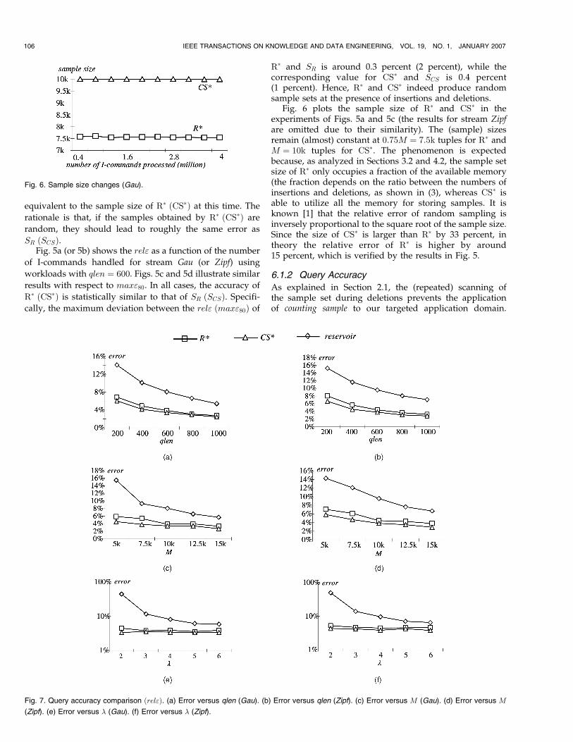
Fig. 6 plots the sample size of R� and CS� in theexperiments of Figs. 5a and 5c (the results for stream Zipfare omitted due to their similarity). The (sample) sizesremain (almost) constant at 0:75M ¼ 7:5k tuples for R� andM ¼ 10k tuples for CS�. The phenomenon is expectedbecause, as analyzed in Sections 3.2 and 4.2, the sample setsize of R� only occupies a fraction of the available memory(the fraction depends on the ratio between the numbers ofinsertions and deletions, as shown in (3), whereas CS� isable to utilize all the memory for storing samples. It isknown [1] that the relative error of random sampling isinversely proportional to the square root of the sample size.Since the size of CS� is larger than R� by 33 percent, intheory the relative error of R� is higher by around15 percent, which is verified by the results in Fig. 5.

6.1.2 Query Accuracy

As explained in Section 2.1, the (repeated) scanning ofthe sample set during deletions prevents the applicationof counting sample to our targeted application domain.

106 IEEE TRANSACTIONS ON KNOWLEDGE AND DATA ENGINEERING, VOL. 19, NO. 1, JANUARY 2007

Fig. 6. Sample size changes (Gau).

Fig. 7. Query accuracy comparison ðrel"Þ. (a) Error versus qlen (Gau). (b) Error versus qlen (Zipf). (c) Error versus M (Gau). (d) Error versus M

(Zipf). (e) Error versus � (Gau). (f) Error versus � (Zipf).

Therefore, we use reservoir with delete-at-will as a bench-mark since it is the only existing sampling method thatincurs small per-record update overhead and can supportarbitrary insertions/deletions. The following experimentscompare the accuracy of R�, CS� and reservoir at the endof streams (recall that the precision of R�=CS� remainsrelatively stable with time).

Figs. 7a and 7b illustrate the rel" of all algorithms as afunction of qlen assuming M ¼ 10k and � ¼ 4. Clearly, theerror of R�=CS� is significantly lower than that of reservoir.The better precision for higher qlen is expected as samplingis, in general, more accurate for queries with large outputsizes. To study the behavior of alternative techniques underdifferent memory constraints, Figs. 7c and 7d, measure theirprecision as a function of M, setting qlen and � to 600 and 4,respectively. Since a larger memory accommodates moresamples, the effectiveness of all algorithms increases withM.

Figs. 7e and 7f evaluate rel" for different �, after fixingqlen and M to their median values 600 and 10k, respectively.For � ¼ 2, R� and CS� outperform reservoir by more than anorder of magnitude (note the logarithmic scale). Theperformance gap decreases with �, because a small numberof deletions leads to sample sets with similar cardinalitiesfor all algorithms. Fig. 8 repeats the experiments of Fig. 7 formax"80. In all cases, the results of max"80 are similar to rel"confirming the robustness of our algorithms.

In order to further verify the generality of our approaches,we also use the real data sets Stock and Tickwise [27]. Theformer contains the values of 197 North American stocksduring the period from 1993 through 1996, and the latterconsists of the exchange rates from Swiss francs to US dollarsrecorded from 7 August 1990 to 18 April 1991. The seriesStock (Tickwise) has 512k (279k) values in total. Next, we fixM and � to their median values 10k and 4, respectively, andmeasure the accuracy of all solutions at the end of the Stockand Tickwise streams. Figs. 9a and 9b compare the rel" ofdifferent algorithms as a function of qlen for the twodistributions, respectively, whereas Figs. 9c and 9d demon-strate results of max"80. Clearly, R� and CS� again outper-form reservoir considerably in all cases, and their behavior issimilar to Figs. 7a, 7b, 8a, and 8b.

6.1.3 Update Overhead

Finally, we examine the maintenance overhead of R� andCS�, which, as explained in Sections 3.2 and 4.2, isdominated by the cost for maintaining IðRSÞ (i.e., the indexon the sample set). In order to provide results independentof index implementation, we measure the total number oftimes that IðRSÞ is modified throughout the history (in allcases, the per-tuple cost is so small that it is not evenmeasurable). For instance, R�-I-ins and R�-I-del denote the

TAO ET AL.: RANDOM SAMPLING FOR CONTINUOUS STREAMS WITH ARBITRARY UPDATES 107

Fig. 8. Query accuracy comparison ðmax"80Þ. (a) Error versus qlen (Gau). (b) Error versus qlen (Zipf). (c) Error versus M (Gau). (d) Error versus M

(Zipf). (e) Error versus � (Gau). (f) Error versus � (Zipf).

number of index insertions and deletions incurred by R� forprocessing I-commands. R�-D-del corresponds to thenumber of index deletions for handling D-commands.Fig. 10 illustrates these numbers for R� and CS� as afunction of the memory size for Zipf (the overhead is thesame for all distributions). In accordance with Theorems 2and 4, both methods require higher update costs to producelarger sample sets. R� incurs about 20 percent fewermodifications than CS� for each type of IðRSÞ updatesdue to its smaller sample size.

6.2 Performance of Q2 Processing

Having established the effectiveness of R�=CS� forQ1 queries, we proceed to evaluate the efficiency of AJSfor Q2 processing. The participating streams T1 and T2

contain columns ðid; A;BÞ and ðid; A;CÞ, respectively. Thedomains of attributes A, B, and C are [0, 10,000]. Thetuples of each relation are generated in a way similar tothe previous section. Specifically, the A-values of T1 ðT2Þ

follow the Zipf distribution with skew coefficients 0.8, andthe B ðCÞ values are decided according to a Gaussianfunction with mean 5,000 and variance 2,000. Theprobability of receiving an I-command is � ¼ 4 timeshigher than that of a D-command. Furthermore, streamsT1 and T2 are equally fast, i.e., the next tuple belongs toeither relation with equal likelihood.

We consider two scenarios that differ in the way theA-values in T1 and T2 are skewed. Specifically, in thefirst case skew-skew, the A-values in both T1 and T2 areskewed towards 0 in the domain of [0, 10,000]. In thesecond case antiskew, data of T1 are still skewed toward0, while those of T2 are towards 10,000—the dense areasof T1 and T2 are opposite.

Each query involves two conditions. The first one �all,common to all (1,000) queries in the same workload, has theform jT1:A� T2:Aj � lenall, where lenall is a workloadparameter. The second condition �any includes two rangepredicates on T1:B and T2:C; extracting the tuples of T1 andT2 falling in these intervals, respectively. Specifically, eachrange has length lenany (another parameter), and isuniformly distributed in the universe [0, 10,000]. Queriesin a workload have different �any. Similar to Section 6.1, wequantify the precision of alternative methods by their rel"and max"80 for processing a workload. The size of theavailable memory is fixed to 10k samples.

6.2.1 Tuning AJS

Recall that AJS consumes a percentage � of the memory forkeeping two sample sets on T1 and T2, respectively. Thenext experiment identifies the value of � that achieves the

108 IEEE TRANSACTIONS ON KNOWLEDGE AND DATA ENGINEERING, VOL. 19, NO. 1, JANUARY 2007

Fig. 9. Query accuracy comparison (real data). (a) rel" versus qlen (Stock). (b) rel" versus qlen (Tickwise). (c) max"80 versus qlen (Stock).

(d) max"80 versus qlen (Tickwise).

Fig. 10. Update cost comparison (Zipf).

best results. Toward this, we measure the error of AJS inanswering a workload with lenall ¼ 10 and lenany ¼ 600,after all updates of streams T1 and T2 have been processed.Figs. 11a and 11b demonstrates the rel" and max"80 for theskew-skew (antiskew) distribution, as a function of �,including both R� and CS� as the underlying samplingalgorithms (recall that AJS can be integrated with anysampling technique on individual relations).

The accuracy of AJS initially improves as � increases andthen deteriorates, i.e., the quality of approximation iscompromised when too much or little memory is assignedto the random samples on individual relations. A very small� prevents correct estimation of the result size of T1 ffl�all T2

(i.e., variable w in Figs. 4 and 5), leading to biased results.On the other hand, an excessive � leaves limited space forthe approximate sample set aRSðTfflÞ on the join results. Inthe sequel, we set � to 40 percent, which constitutes a goodtrade-off. Furthermore, we use CS� as the representativesingle-relation algorithm of AJS.

6.2.2 Query Accuracy.

Due to the absence of previous methods for sampling joinresults under tight memory footprint, we compare AJS withthe NJS method (see Section 2.2), which maintains random

sample sets (using CS�) on the base relations and producesapproximate answers by joining the two sets. Figs. 12a and12b compare the error of AJS and NJS as a function of lenall,setting lenany to 600. Clearly, for both skew-skew and antiskew,AJS outperforms NJS significantly in terms of accuracy androbustness. To study the influence of lenany, we set lenall toits median value 10, and repeat the above experiments byvarying lenany from 200 to 1,000. As shown in Figs. 12c and12d, AJS again outperforms NJS considerably.

7 CONCLUSIONS

This paper presents the first random sampling algorithms,R� and CS�, for efficiently computing aggregate data overstreams of arbitrary updates. Going one step further, wepropose AJS, a method for sampling join results. We prove,both theoretically and empirically, that our techniquesprovide accurate answers with small space and computa-tional overhead. While our current focus is on sample setsthat fit in the main memory, we plan to investigatesituations where part of the sample set is migrated to thedisk [21]. Further, it has been observed [6] that theperformance of sampling (for approximate aggregateprocessing) can be improved if query statistics are available

TAO ET AL.: RANDOM SAMPLING FOR CONTINUOUS STREAMS WITH ARBITRARY UPDATES 109

Fig. 11. AJS memory allocation tuning. (a) Error versus � (skew-skew). (b) Error versus � (antiskew).

Fig. 12. Query accuracy comparison. (a) Error versus qlenall (skew-skew). (b) Error versus qlenall (antiskew). (c) Error versus qlenany (skew-skew).

(d) Error versus qlenany (antiskew).

in advance. The design of such “workload-aware” methods

in stream environments constitutes an interesting topic.

Finally, we would like to explore the applicability of

random sampling for tracking the positions of continuously

moving objects [23].

ACKNOWLEDGMENTS

Yufei Tao was supported CERG Grant 1202/06, andDimitris Papadias by CERG Grant 6184/05 from the

Research Grant Council of Hong Kong.

REFERENCES

[1] S. Acharya, P.B. Gibbons, and V. Poosala, “Congressional Samplesfor Approximate Answering of Group-By Queries,” Proc. ACMSIGMOD Conf., 2000.

[2] S. Acharya, P.B. Gibbons, V. Poosala, and S. Ramaswamy, “JoinSynopses for Approximate Query Answering,” Proc. ACMSIGMOD Conf., 1999.

[3] N. Alon, P.B. Gibbons, Y. Matias, and M. Szegedy, “Tracking Joinand Self-Join Sizes in Limited Storage,” Proc. 18th ACM SIGACT-SIGMOD-SIGART Symp. Principles of Database Systems, 1999.

[4] B. Babcock, S. Chaudhuri, and G. Das, “Dynamic Sample Selectionfor Approximate Query Processing,” Proc. ACM SIGMOD Conf.,2003.

[5] B. Babcock, M. Datar, and R. Motwani, “Sampling from a MovingWindow over Streaming Data,” Proc. Ann. ACM-SIAM Symp.Discrete Algorithms, 2002.

[6] S. Chaudhuri, G. Das, and V. Narasayya, “A Robust, Optimiza-tion-Based Approach for Approximate Answering of AggregateQueries,” Proc. ACM SIGMOD Conf., 2001.

[7] S. Chaudhuri, G. Das, and U. Srivastava, “Effective Use of Block-Level Sampling in Statistics Estimation,” Proc. ACM SIGMODConf., 2004.

[8] S. Chaudhuri, R. Motwani, and V. Narasayya, “On RandomSampling over Joins,” Proc. ACM SIGMOD Conf., 1999.

[9] G. Cormode, S. Muthukrishnan, and I. Rozenbaum, “Summariz-ing and Mining Inverse Distributions on Data Streams viaDynamic Inverse Sampling,” Proc. 31st Int’l Conf. Very Large DataBases, 2005.

[10] G. Frahling, P. Indyk, and C. Sohler, “Sampling in Dynamic DataStreams and Applications,” Proc. Ann. Symp. ComputationalGeometry, 2005.

[11] S. Ganguly, M. Garofalakis, and R. Rastogi, “Processing SetExpressions over Continuous Update Streams,” Proc. ACMSIGMOD Conf., 2003.

[12] S. Ganguly, P.B. Gibbons, Y. Matias, and A. Silberschatz, “BifocalSampling for Skew-Resistant Join Size Estimation,” Proc. ACMSIGMOD Conf., 1996.

[13] P.B. Gibbons and Y. Matias, “New Sampling-Based SummaryStatistics for Improving Approximate Query Answers,” Proc.ACM SIGMOD Conf., 1998.

[14] P.B. Gibbons, Y. Matias, and V. Poosala, “Fast IncrementalMaintenance of Approximate Histograms,” ACM Trans. DatabaseSystems, vol. 27, no. 3, pp. 261-298, 2002.

[15] G. Graefe and P.-A. Larson, “B-Tree Indexes and CPU Caches,”Proc. Int’l Conf. Data Eng., 2001.

[16] S. Guha, C. Kim, and K. Shim, “Xwave: Approximate ExtendedWavelets for Streaming Data,” Proc. 30th Int’l Conf. Very Large DataBases, 2004.

[17] S. Guha, K. Shim, and J. Woo, “Rehist: Relative Error HistogramConstruction Algorithms,” Proc. 30th Int’l Conf. Very Large DataBases, 2004.

[18] P.J. Haas and C. Konig, “A Bi-Level Bernoulli Scheme forDatabase Sampling,” Proc. ACM SIGMOD Conf., 2004.

[19] P.J. Haas, J.F. Naughton, and A.N. Swami, “On the Relative Costof Sampling for Join Selectivity Estimation,” Proc. 13th ACMSIGACT-SIGMOD-SIGART Symp. Principles of Database Systems,1994.

[20] C. Jermaine, “Robust Estimation with Sampling and ApproximatePre-Aggregation,” Proc. 29th Int’l Conf. Very Large Data Bases, 2003.

[21] C. Jermaine, A. Pol, and S. Arumugam, “Online Maintenance ofVery Large Random Samples,” Proc. ACM SIGMOD Conf., 2004.

[22] K.-H. Li, “Reservoir-Sampling Algorithms of Time Complexityoðnð1þ logðn=nÞÞÞ,” ACM Trans. Math. Software, vol. 20, no. 4,pp. 481-493, 1994.

[23] M.F. Mokbel, X. Xiong, and W.G. Aref, “Sina: Scalable IncrementalProcessing of Continuous Queries in Spatio-Temporal Databases,”Proc. ACM SIGMOD Conf., 2004.

[24] U. Srivastava and J. Widom, “Memory-Limited Execution ofWindowed Stream Joins,” Proc. 30th Int’l Conf. Very Large DataBases, 2004.

[25] N. Tatbul, U. Cetintemel, S.B. Zdonik, M. Cherniack, and M.Stonebraker, “Load Shedding in a Data Stream Manager,” Proc.29th Int’l Conf. Very Large Data Bases, 2003.

[26] J.S. Vitter, “Random Sampling with a Reservoir,” ACM Trans.Math. Software, vol. 11, no. 1, pp. 37-57, 1985.

[27] E. Keogh, The UCR Time Series Data Mining Archive, Univ. ofCalifornia—Computer Science & Eng. Dept., http://www.cs.ucr.edu/~eamonn/TSDMA/index.html, 2006.

Yufei Tao received the PhD degree in computerscience from the Hong Kong University ofScience and Technology in 2002. After that, hespent a year as a visiting scientist at theCarnegie Mellon University. From 2003 to2006, he was an assistant professor at the CityUniversity of Hong Kong. Currently, he is anassistant professor in the Department of Com-puter Science and Engineering, the ChineseUniversity of Hong Kong. Professor Tao is

interested in research of spatial, temporal databases, data privacy,and security. He is the winner of the Hong Kong Young Scientist Award2002. He has published extensively in SIGMOD, VLDB, ICDE, the ACMTransaction on Database Systems, and the IEEE Transactions onKnowledge and Data Engineering.

Xiang Lian received the BS degree from theDepartment of Computer Science and Technol-ogy, Nanjing University, in 2003. He is currentlya PhD candidate in the Department of ComputerScience and Engineering, Hong Kong Universityof Science and Technology, Hong Kong. Hisresearch interests include spatio-temporal data-bases and stream time series.

Dimitris Papadias is a professor in the Com-puter Science and Engineering Department,Hong Kong University of Science and Technol-ogy (HKUST). Before joining HKUST in 1997, heworked and studied at the German NationalResearch Center for Information Technology(GMD), the National Center for GeographicInformation and Analysis (NCGIA, Maine), theUniversity of California at San Diego, theTechnical University of Vienna, the National

Technical University of Athens, Queen’s University (Canada), and theUniversity of Patras (Greece). He has published extensively and beeninvolved in the program committees of all major database conferences,including SIGMOD, VLDB, and ICDE. He is an associate editor of theVLDB Journal, the IEEE Transactions on Knowledge and DataEngineering, and on the editorial advisory board of Information Systems.

Marios Hadjieleftheriou received the diplomain electrical and computer engineering in 1998from the National Technical University ofAthens, Greece, and the PhD degree in compu-ter science from the University of California,Riverside, in 2004. He has worked as a researchassociate at Boston University. Currently, he isworking for AT&T Labs—Research. His re-search interests are in the areas of spatio-temporal data management, data mining, data

stream management, time-series databases, and database indexing.

110 IEEE TRANSACTIONS ON KNOWLEDGE AND DATA ENGINEERING, VOL. 19, NO. 1, JANUARY 2007