Journal of Non-Newtonian Fluid Mechanics, 39 (1991) 189-206

Elsevier Science Publishers B.V., Amsterdam

189

Simulation of highly elastic fluid flows without additional numerical diffusivity

Fernando G. Basombrio, Gustav0 C. Buscaglia and Enzo A. Dari

Divisibn Mecbnica Computational, DIA, Centro At6mico Bariloche, CNEA,

8400 S. C. de Bariloche, RN (Argentina)

(Received April 5, 1990; in revised form October 20, 1990)

Abstract

A transient decoupled method to treat viscoelastic flows is presented, using Lagrange-Gale&in techniques for velocities and the Lesaint-Raviart method for extra-stresses.

An important point of our scheme is the linear interpolation employed for all fields: this allows for high Weissenberg numbers to be reached with no need for streamline upwinding (SU).

Numerical results for the 4 : 1 plane contraction are presented, including comparisons with other methods and an analysis of the effect of mesh refinement and SU addition.

Keywork decoupled approach; finite element method; Lesaint-Raviart method; viscoelastic fluids

1. Introduction

In recent years, important progress has been made in the numerical simulation of viscoelastic fluid flows for increasing elasticities. It has been shown that apparent limits in the Weissenberg (We) or Deborah (De) numbers were mainly due to singularities (turning points, bifurcations, etc.) [l-4] in the system of discrete equations, .’ and could be overcome by improving the numerical methods. Nevertheless, the High Weissenberg Number Problem remains an open question in computational fluid dy- namics (see the review papers in refs. 5 and 6).

0377-0257/91/$03.50 0 1991 - Elsevier Science Publishers B.V.

190

One important step towards extending the range of solvable flows-up to De = 6 (we refer in all cases to the popular 4 : 1 contraction problem)-was given by Marchal and Crochet [7,8] by eliminating spurious wiggles already present in the Newtonian limit for many mixed formulations. They required the gradient of discrete velocities to belong to the space of discrete stresses, either exactly [7] or approximately [8], thus allowing their scheme to reduce to the classical UVP (velocity-pressure) formulation when We = 0.

Further improvement came from avoiding spurious oscillations: those arising when conventional Gale&in finite elements are used for hyperbolic equations such as the constitutive law of viscoelastic stresses. In the context of coupled approaches, Marchal and Crochet [8,9] introduced non-consistent streamline upwinding (SU) and carried out the first successful simulation of highly elastic fluids (with no apparent limit in De).

Decoupled techniques are more flexible in what concerns integration of the constitutive equation, and many variants have been published [1,2,6,10 and 11, etc.]. Nevertheless, only Fortin and Fortin [12] could increase De without apparent limit, again after adding SU to their original method.

To our knowledge, for the 4 : 1 contraction problem no simulation has so far been reported for De > 7 without non-consistent streamline dissipation. The effect of this extra term is, however, not fully understood, as it surely modifies convergence rates and distorts the underlying set of equations.

In this paper, we present a transient decoupled approach capable of handling highly elastic flows without resource to additional SU diffusivity. The finite element method, based upon the Lesaint-Raviart technique, was first used by Fortin and Fortin [12]. Our improvement comes (not surpris- ingly) from eluding second-order elements, which exhibit oscillatory internal modes. We thus confirm the clever conjecture of ref. 6 about the conveni- ence of low-degree interpolation. In our work we use a continuous piecewise linear approximation for velocities and pressures (Courant triangles). In order to satisfy the Ladyshenskaza-Babuska-Brezzi (LBB) condition, each pressure element contains four velocity elements. (this interpolation is sometimes called 4 X Pi/Pi [13]). Viscoelastic stresses are approximated by piecewise linear and discontinuous triangles, in correspondence with the velocity mesh. This discretisation has good properties of mass conservation, and reduces to the classical UVP formulation in the Newtonian limit (the gradient of the discrete velocities belongs to the space of discrete stresses). In this way, our choice of element satisfies the desirable criterion introduced by Marchal and Crochet [7].

In Section 2 of the paper we establish the basic equations for the problem. The numerical method is described in Section 3. Our main results are presented in Section 4, together with comparisons with previous works. In Section 5 we perform an empirical analysis of the effect of mesh refinement

191

and SU diffusivity. Section 6 is devoted to the discussion of results, and Section 7 to the conclusions.

2. Basic equations

From the constitutive equations

T=T,+7 (extra-stress decomposition), (24

7+h70=2pLld (viscoelastic part), (24

TN = 2pL,d (Newtonian part), (2.3)

for the Cauchy stress tensor splitting into a spherical part and extra-stress

u= -pl+ T, (2.4

the momentum and mass conservation equations, one gets the final system

pg - div 7 - pL2v *v’+ vp = pf’, (2.5)

7 + x70 = 2/.Qd, (2.6)

div u’= 0 (2.7)

for the unknown fields of velocity (3, pressure ( p) and viscoelastic extra- stress (r), with the following notation. D/Dt: material time derivative, 70=a7/af+~.v7+7.r-r.7-e(d.7+

7. d), 8 E [ - 1, 11: objective stress rate, p: specific mass, 4: body forces, V: the ‘nabla’ operator, d (resp. r): symmetric (resp. antisymmetric) part of the velocity gradient, A: characteristic time and pr, p2: polymer and solvent viscosities.

These equations corresponds to a Johnson-Segalman fluid with ad- ditional viscosity (fluid of Jeffreys type). For later use, we also introduce the tensor

T =T+% A A . (2.8)

associated with the well-posedness of the problem when p2 = 0 (Maxwell model) [14].

3. Discrete formulation

We begin the discretisation procedure of eqns. (2.5)-(2.7) by decoupling velocity and pressure from extra-stress unknowns, that means Algorithm: For each time step,

192

Step 1: Solve the mass (2.7) and momentum (2.5) balance equations for

V +M and P”+’ keeping 7n fixed. Step 2: Solve the viscoelastic constitutive equation (2.6) for rn+i keeping

V ++I fixed. Step 3: Check for convergence (if searching a steady-state solution) and

go back to Step 1 if necessary. This algorithm has already been successfully used by Fortin and Fortin

[12]. Step 1 amounts to the solution of a transient Navier-Stokes problem, which we compute by means of the direct Lagrange-Gale&in (characteris- tics) method [15] with non-exact integration at the mid-sides of each (triangular) element.

Preconditioned conjugate gradients [16] are then used to solve the result- ing system of equations.

Step 2 requires the solution of a linear hyperbolic system, and the Lesaint-Raviart method is used to handle it at element level. Convergence was checked by evaluating the relative variation of solutions in the maxi- mum norm. Although none of these techniques is innovative, let us briefly outline the discrete equations of Step 2.

After (implicit) temporal discretisation (of time step At), equation (2.6) can be written in compact form as

Xu’. VT”+’ + L?+i = F, (3-l)

where L denotes the linear operator

LT n+i=

and

x F = 2pld + p”. (3.3) Introducing now the finite element space

w,= {wEL,(Q), wI,EPk(K),tfK~%} (3 -4)

of piecewise polynomials in a triangulation Yh of the domain Q, with no continuity requirements at interelement boundaries, the Lesaint-Raviart method [17] for the viscoelastic constitutive equation reads

Au’- VTh”f’ + Lr;+i) : X dx+J;K_~(~~+1-_7,.f1): Xiu’.~dT

nxn

= nF: x dx, Vx E (W,) ’ , J (3.5)

193

Fig. 1. Example showing the need for a relaxation scheme. T IK2 must be known to find

TIKI, and viceversa.

where UC__ stands for the inflow boundary of element K, and subscript ‘e’ (resp. ‘i ‘) represents the external (resp. internal) evaluation of the function

?lXtl

at aK_.(JV,) ’ is the space of symmetric tensor fields with components in

w,. It should be kept in mind that a certain amount of upwinding is

automatically introduced by the previous formulation. This can be seen in eqn. (3.5), since the boundary integral is only performed over the ‘upwind

part X_ of the element boundary. An important result of this work is that this intrinsic upwinding suffices for high De simulation when linear interpo- lation is used for stresses. Error bounds of order hk+1/2 are shown in ref. 18.

Equation (3.5) can be solved at element level, provided r=‘+’ is known whenever needed. This requires a flow-dependent ordering of the mesh elements, starting at X4_ (inflow boundary). Nevertheless, except for uni- form velocity fields, such an optimal ordering fails to exist in the general case, as can be readily seen in the example of Fig. 1. We successfully avoided this obstacle by successive relaxation together with the following strategy (repeated at each time step), which we give in detail:

(i) compute the upstream neighbours for all elements; (ii) order first all elements that need no iterative solution, starting at XI_ (that is, until situations analogous to that that of Fig. 2 arise, and no element exists whose upstream neighbours have already been numbered). These conform to a connected (if XI_ is connected) set of elements that we will call ‘indepen- dent sub-mesh’; (iii) starting at the boundary of the independent sub-mesh, let the ordering front go ahead including that element that receives flow from not-already-numbered neighbours through less than a half side. Such an element generally exists for triangles if the flow is approximately incom- pressible (if this is not the case, it is always possible to arbitrarily choose an element adjacent to the ordering front and continue); (iv) once all elements have been numbered, sweep the independent sub-mesh solving (3.5); (v)

194

x2 -

20,o

IfI

u =(O,par abolic

- 16,O ti = ( 0, parabolic)

t= 0

Fig. 2. Sketch of the domain and boundary conditions for the 4: 1 sudden contraction problem. The finite element mesh used through the calculations is also included.

finally, with initial guess rl, sweep the remaining elements in the prescribed order, as many times as required for convergence. This relaxation procedure based upon flow-oriented ordering required in most time steps only two iterations to converge within a tolerance (in the maximum norm) of 10P5.

It is also possible to introduce in (3.5) a non-consistent SU by adding an anisotropic diffusivity proportional to local mesh size h, in the flow direc- tion. This was implemented to allow for comparison with the pure Lesaint- Raviart method, and amounts to the addition, in the left-hand side of eqn. (3.5) of the term [18]

(3.6)

195

4. Numerical results

These concern the well-known benchmark of the planar four-to-one contraction (see layout with dimensions and boundary conditions in Fig. 2), for the upper-convected case (8 = l), with solvent viscosity pL2 = 0.11 and viscosity ratio

P2 ~ = 0.11. Pl + P2

(4.1) The Deborah number is defined as

De=X+,,

where p, is the shear-rate at the downstream distant wall. (4.4

The finite element mesh is also shown in Fig. 2 (post processing was made with program PITUCO [19]); it consists of 1868 velocity-stress elements, with a total of 19139 unknowns. Care was taken to avoid abrupt mesh size changes, which could probably generate spurious oscillations in the stress field [12].

We used the transient method of Section 3 to obtain steady-state solu- tions. In fact, we began with the Newtonian case and slowly stepped the Deborah number towards higher elasticities (the typical step was 1). The initial conditions for De = 1 were a Navier-Stokes velocity field with p = pi + p2 and extra-stresses according to eqn. (2.6) with h = 0. For the increments, we followed two alternatives: (i) to use the latest results as initial condition, or, (ii) to perform a linear extrapolation of all fields from the latest two De, and use this rough guess as initial state for a new (with higher X) calculation. The latter approach turned out to be economically preferable, as convergence was attained faster.

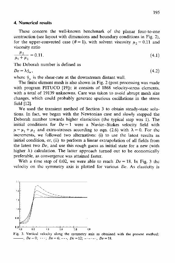
With a time step of 0.02, we were able to reach De = 18. In Fig. 3 the velocity on the symmetry axis is plotted for various De. As elasticity is

8.201 ! ! 1 ~ ’ ’ j ~ j -4.8 B.t3 46 8.8 12.0 5.8

Fig. 3. Vertical velocity along the symmetry axis as obtained with the present method: -, De = 0; . . . ; De=6; ---, De=12; ---.-., De=18.

196

Fig. 4. A comparison of Couette correction prediction for various methods: -, FVELR; - - -, FVE4 [ll]; . . . . Debbaut, Marchal and Crochet [9]. v corresponds to FVELR after SU

addition.

increased, the streamlines move left in the vicinity of the contraction, thus reducing the shear rate at the wall. A macroscopic effect of this phenomenon is the Couette correction, given by

C=aP-aPfd 27, ' (4.3)

0.201 ’ ’ s ! ! ! ’ ! ’ -4.0 -2.0 0.0 2.8 4.8 6.0

Fig. 5. (a) 722 viscoelastic stress along the line x1 = 1 at De = 6 -, FVELR; . . . , FVE4 [ll]; (b) velocity along the symmetry axis -, FVELR; . . . , FVE4 [ll].

197

where Ap stands for the calculated pressure difference, Apfd for that obtained assuming fully developed flow in both channels which conform to the contraction problem, and T_, represents the fully developed wall shear stress in the downstream section. In Fig. 4 we show C values obtained by the present method (program FVELR). For comparison, we also include results from Debbaut, Marchal and Crochet [9], and from a simultaneous calculation by a method of characteristics developed by Basombrio [ll] (program FVE4). For high elasticities our results are probably inaccurate due to an inadequate exit channel length, as discussed in ref. 9. The matching of all predictions is nevertheless satisfactory.

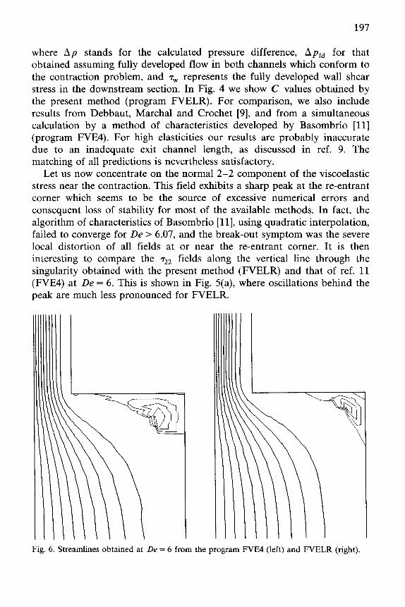
Let us now concentrate on the normal 2-2 component of the viscoelastic stress near the contraction. This field exhibits a sharp peak at the re-entrant corner which seems to be the source of excessive numerical errors and consequent loss of stability for most of the available methods. In fact, the algorithm of characteristics of Basombrio [ll], using quadratic interpolation, failed to converge for De > 6.07, and the break-out symptom was the severe local distortion of all fields at or near the re-entrant corner. It is then interesting to compare the 722 fields along the vertical line through the singularity obtained with the present method (FVELR) and that of ref. 11 (FVE4) at De = 6. This is shown in Fig. 5(a), where oscillations behind the peak are much less pronounced for FVELR.

Fig. 6. Streamlines obtained at De = 6 from the program FVE4 (left) and FVELR (right).

198

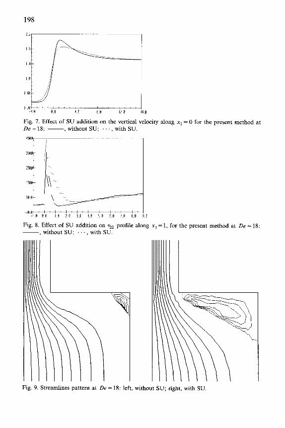
Fig. 7. Effect of SU addition on the vertical velocity along x1 = 0 for the present method at De = 18: -, without SU; . . . , with SU.

-5e.d ! I ! I I ! ! ( ! -LB 84 LB 2.6 3.6 4.8 5.6 6.6 7.B 8 0 9.8

Fig. 8. Effect of SU addition on T 22 profile along x1 =l, for the present method at De =18: -, without SU; . . . , with SU.

Fig. 9. Streamlines pattern at De =18: left, without SU; right, with SU.

199

Other comparisons with results obtained with the program FVEM [ll] are shown in Figs. 5(b) and 6.

Although our results of Fig. S(a) are not as smooth as we would have desired, we found no convergence limit in the Deborah number (see discus- sion in Section 5). After reaching De = 18, it became obvious that a new (longer) geometry was required to continue. We prefered to leave this for future work and turn to another crucial aspect of viscoelastic flow simula- tion; the influence of adding SU dissipation to the discrete formulation, eqn. (3.5). The vertical velocity along xi = 0 and the 722 stress along x2 = 1, with and without SU, are presented in Figs. 7 and 8 for De = 18. We also observed an enlargement of the corner vortex after SU addition (see stream- lines in Fig. 9), together with a significant rise in the total pressure loss (see Fig. 4). This is discussed in the following sections.

All the described results were run on a VAX11/780 computer.

5. The effect of mesh refinement

In the previous section, we have shown that our method leads to satisfac- tory results even at high elasticities and in the presence of geometric singularities. However, some features of the numerical solutions seem to be mesh sensitive (oscillations in Figs. 5(a) and 8), or dependent on purely numerical devices (vortex of Fig. 9). We must then turn our attention to the effect of mesh refinement, both with and without SU addition, so as to ascertain that the results of Section 4 are not just numerical artifacts.

Let us begin by introducing four more meshes, labelled Yz to Y& while the triangulation of Fig. 2 will be hereafter refered to as Yi. See a description of the meshes in Table 1, and note in Fig. 10 the region surrounding the re-entrant comer. Y3 to Y5 are uniform triangulations,

TABLE 1

Triangulations for convergence analysis

Mesh Mesh size ’ x2 Min x2 Max Elements Degrees of (pressure/ve- freedom locity-stress)

5 non-uniform - 16.0 20.0 467/1868 % non-uniform - 16.0 20.0 659/2636 6 0.1 -4.0 8.0 480/1920 =? 0.077 - 4.0 8.0 780/3120 7 0.066 -4.0 8.0 1080/4320

’ Mean length of velocity-stress elements in the x2 direction.

19139 26925 19673 31888 44088

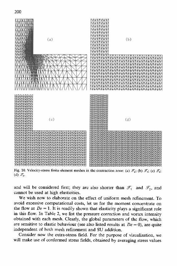
Fig. 10. Velocity-stress finite element meshes in the contraction zone: (a) Y2;; (b) T3;; (c) 4’;

(4 %.

and will be considered first; they are also shorter than Y1 and Yz, and cannot be used at high elasticities.

We wish now to elaborate on the effect of uniform mesh refinement. To avoid excessive computational costs, let us for the moment concentrate on the flow at De = 1. It is readily shown that elasticity plays a significant role in this flow. In Table 2, we list the pressure correction and vortex intensity obtained with each mesh. Clearly, the global parameters of the flow, which are sensitive to elastic behaviour (see also listed results at De = 0), are quite independent of both mesh refinement and SU addition.

Consider now the extra-stress field. For the purpose of visualisation, we will make use of conformed stress fields, obtained by averaging stress values

201

Fig. 11. Hevations of q2 at De = 1 for different meshes: (a) T3; (b) Y4; (c) T5.

Fig. 11 (continued).

TABLE 2

Comparative results of pressure correction and vortex intensity

Mesh Pressure correction Vortex intensity

De=0 De=1 De=0 De=1

~~ 0.533 q 0.530 q 0.522

without su

0.288 0.287 0.268

with su

0.288 0.296 0.268

0.246E-3 0.287B3 0.278E-3

without su

0.201E-3 0.226E-3 0.234E-3

with su

0.214E-3 0.246E-3 0.244E-3

TABLE 3

Comparative results of ~~~(0, 0) and T~~(O,O)

Mesh r11(010)

De=0 De=1

without su

with su

?2(0> 0)

De=0 De=1

without su

with su

9? - 0.665 - 0.704 - 0.691 0.672 1.462 1.398 % - 0.658 - 0.681 - 0.673 0.6613 1.416 1.379 % - 0.679 - 0.698 - 0.690 0.682 1.432 1.395

203

Fig. 12. Q viscoelastic stress along the line x1 =1 at De = 1, as obtained with mesh T5 -, without SU; . . . , with SU.

at each velocity node. We studied the behaviour of numerical solutions at the point (x1, x2) = (0, 0). Results are listed in Table 3 and are similar for the three meshes. We also show, in Figs. 11(a), (b), and (c), spatial views of the elevations of Tag (conformed) as obtained on the triangulations 9& Yd and Y5 (identical scale for all meshes). Except locally at the singularity, the agreement is remarkably good. The same is observed when studying the effect of SU at De = 1. To illustrate this, Fig. 12 plots the 722 field, along x1 = 1, both with and without SU for mesh F5. The effect of the extra term eqn. (3.6), when added to our non-conforming formulation, is a tendency of the solution to become constant in the streamline direction inside each element.

To further assess the robustness of our scheme, we will compare results obtained at high elasticities on the non-uniform meshes Yr and Yz. Our calculations show that steady solutions, in reasonable agreement with those of Section 4, can be obtained with Yz up to De = 10, where we stopped for

Fig. 13. rz2 along x1 = 1 at De = 6, as obtained with mesh .Tz -, without SU; . . . , with su.

204

lack of interest. Also, at De = 1, Yz generates results which deviate only slightly from those of Tables 2 and 3.

But, although our method remains stable up to De = 10 even for the highly unstructured mesh Y1, some oscillations appear in the stress field, and are expected to thwart convergence of the algorithm at some higher De. Amazingly enough, a cure for this wiggly behaviour was found in the SU diffusivity. See Fig. 13 for an example of this observations at De = 6 (compare with Fig. 5(a)). The striking fact concerning SU is that, while on Yz it brings obvious improvement at De = 6, its effects on Yi, are as disastrous at De = 6 as they are at De = 18 (see previous section). We must add for completeness that the SU term, when used in flows of low elasticity, causes unimportant changes in the numerical solutions (on all our tests), and that the phenomenon of vortex enlargement does not happen in Yz.

6. Discussion

Some topics in the previous results deserve additional comment. To assess the numerical accuracy of the method, a condition number may be defined as

q=2 s2+5 -l, i i Sl s2

(6-l)

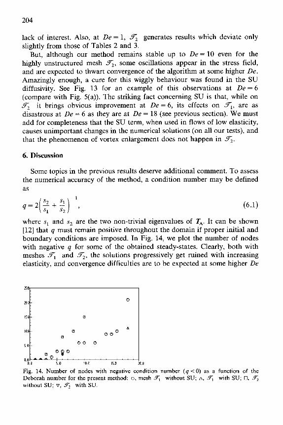
where si and s2 are the two non-trivial eigenvalues of TA. It can be shown [12] that q must remain positive throughout the domain if proper initial and boundary conditions are imposed. In Fig. 14, we plot the number of nodes with negative q for some of the obtained steady-states. Clearly, both with meshes Yi and Y2, the solutions progressively get ruined with increasing elasticity, and convergence difficulties are to be expected at some higher De

&- 0

150- I3

oo”

A

100- [3 0

w- 00 0

q OgO

d---Q! ! ! 88 5.0 180 15.0 0.0

Fig. 14. Number of nodes with negative condition number (q < 0) as a function of the Deborah number for the present method: o, mesh Yl without SU; A, Fl with SU; 0, T2 without SU; V, Fz with SU.

205

[12] (i.e., limit points probably exist, although not reached). Nodes with 4 < 0 appear in the neighbourhood of the singularity (when analysing Fig. 14 remember that & is much denser than Y1 in this region). Also note that, although SU improved the results of one mesh and spoiled those of the other, it lowered the number of nodes with negative q on both meshes.

We must now collect the facts concerning the effects of mesh refinement and SU diffusivity: (i) our method is empirically seen to converge in mesh (with and without SU), at least a moderate elasticities and regularly spaced meshes; (ii) it provides a way to achieve steady solutions for highly elastic fluids with no serious restrictions on mesh geometry; (iii) at low elasticities, the SU term just forces the stress to reduce its derivative along streamlines inside each element; (iv) the stabilising effect of SU is seen at high De. It must nevertheless be used with care for it can give erroneous results (much worse than the pure Lesaint-Raviart method) if the mesh is inappropriate (what is a priori not known).

Concerning the choice of interpolants, Fig. 5(a) shows one of the ad- vantages of linear elements. The quadratic interpolation of FVE4 [ll] allows for spurious oscillations inside each element, that eventually cause the break out of the algorithm. This effect was also observed by Fortin and Fortin [12], and our results confirm their assumption that linear elements could be an improvement.

While tuning parameters (particularly the time step) for the results of Section 4, we did observe some instabilities together with loss of conver- gence of the algorithm. One of the advantages of our transient approach is that such phenomena can be traced back and partially understood. Our experiences revealed that instabilities arise in regions with strong coupling of unknowns, where an unstable distortion of the velocity field develops during the iterative process. By unstable we mean that such a distortion modifies the stresses towards its own amplification and collapse. This happens locally near singularities, while most of the flow seems to be converging. It is not obvious how to control and/or take advantage of this feature to extend convergence limits.

7. Conclusions

A modified version of the method of Fortin and Fortin [12] has been introduced with linear triangular elements for all fields. In general lines, both the algorithm and the treatment of the constitutive equation remain the same, but the new interpolants bring significant improvement and inertia is included by means of the Gale&in method. Indeed, we computed flows up to De = 18 with the pure Lesaint-Raviart method for stresses, while previ- ous schemes need streamline dissipation to go beyond De = 7.

206

Once more, experience confirms that convergence limits for the High Weissenberg Number Problem can be extended by an appropriate treatment of the hyperbolic character of the constitutive equation. In particular, any effort to avoid spurious oscillations (using for example Total Variation Decreasing approaches [20]) produces better behaviour of the algorithms.

Acknowledgements

F.G. Basombrio wishes to express his gratitude to Professor Roland Glowinski for his kind invitation to visit the Department of Mathematics of the University of Houston and for the fruitful discussions on numerical simulation of viscoelastic fluid flows.

References

1 M. Fortin and D. Esselaoui, Int. J. Numer. Meth. Fluids, 7 (1987) 1035. 2 M. El Hadj and P.A. Tanguy, A finite element procedure coupled with the method of

characteristics for simulation of the viscoelastic fluid flows; University of Laval, Quebec (submitted for publication 1989).

3 F. Dupret, J.M. Marchal and M.J. Crochet, J. Non-Newtonian Fluid Mech., 18 (1985) 173.

4 F. Dupret and J.M. Marchal, J. Non-Newtonian Fluid Mech., 20 (1986) 143. 5 R. Keunings, Simulation of Viscoelastic Fluid Flows, in C.L. Tucker III (Ed.), Fundamen-

tals of Computer Modelling for Polymer Processing, Verlag, 1987. 6 M.J. Crochet, Rubber Chemistry and Technology 62 (1989) 426. 7 J.M. Marchal and M.J. Crochet, J. Non-Newtonian Fluid Mech., 20 (1986) 187. 8 J.M. Marchal and M.J. Crochet, J. Non-Newtonian Fluid Mech., 26 (1987) 77. 9 B. Debbaut, J.M. Marchal and M.J. Crochet, J. Non-Newtonian Fluid Mech. 29 (1988)

119. 10 X.-L. Luo and R.I. Tanner, J. Non-Newtonian Fluid Mech., 31 (1989) 143. 11 F.G. Basombrio, Flows of viscoelastic fluids treated by the method of characteristics, J.

Non-Newtonian Fluid Mechanics (submitted for publication, 1990). 12 M. Fortin and A. Fortin, J. Non-Newtonian Fluid Mech., 32 (1989) 295. 13 F. Thomasset, Implementation of Finite Element Methods for Navier-Stokes Equations,

Springer-Verlag, New York-Heidelberg-Berlin, 1981. 14 F. Dupret and J.M. Marchal, J. Met. ThCor. Appl., 5 (1986) 403. 15 K.W. Morton, A. Priestley and E. Suli, Math. Model. Numer. Anal., 22 (1988) 625. 16 J. Cahouet and J.P. Chabard, Int. J. Numer. Meth. Fluids 8 (1988) 869. 17 P. Lesaint and P.A. Raviart, On a finite element method for solving the neutron transport

equation, in C. de Boor (Ed.), Mathematical Aspects of Finite Element Methods in Partial Differential Equations, Academic Press, New York, 1974 pp. 89.

18 C. Johnson, U. Navert and J. Pitklranta, Comp. Meth. Appl. Mech. Eng., 45 (1984) 285. 19 M.J. VCnere, Proc. MECOM’88, IX Latinoamerican and Iberic Congress on Computa-

tional Methods for Engineering, November 1988, Cordoba, Argentina, 1988. 20 A. Harten, J. Comput. Phys., 49 (1983) 357.