AC 2012-2942: THE EFFECT OF SURFACE AREA AND THERMAL DIF-FUSIVITY IN TRANSIENT COOLING

Dr. Awlad Hossain, Eastern Washington University

Awlad Hossain is an Assistant Professor in the Department of Engineering and Design at Eastern Wash-ington University, Cheney. His research interests involve the computational and experimental analysis oflightweight space structures and composite materials. Hossain received M.S. and Ph.D. degrees in ma-terials engineering and science from South Dakota School of Mines and Technology, Rapid City, SouthDakota.

Dr. Hani Serhal Saad, Eastern Washington UniversityProf. Martin W. Weiser, Eastern Washington University

Martin Weiser is an Assistant Professor in the Engineering and Design Department at Eastern WashingtonUniversity. He earned his B.S. in ceramic engineering from the Ohio State University and his M.S.and Ph.D. in materials science and mineral engineering from the University of California, Berkeley. Hethen joined the Mechanical Engineering Department at the University of New Mexico, where he taughtmaterials science, thermodynamics, manufacturing engineering, and technical communication. Weiserthen joined Johnson Matthey Electronics/Honeywell Electronic Materials, where he held positions intechnical service, product management, Six Sigma, and research and development. He is inventor on adozen patents and patent applications and has published more than 30 papers and book chapters on topicsincluding ceramic processing, Pb-free solder development, experimental design, and biomechanics.

c©American Society for Engineering Education, 2012

Page 25.1295.1

1

The Effect of Surface Area and Thermal Diffusivity in Transient Cooling

Abstract

We have recently developed a new one-quarter heat transfer course as part of our Mechanical

Engineering curriculum. This course includes a significant laboratory component to reinforce the

material taught in the lecture. The students normally do not have too much trouble with steady

state heat transfer. However, transient heat transfer often causes confusion due to a combination

of more difficult mathematics and the use of material parameters that are less intuitive.

Therefore, we use a combination of analytical, numerical, and experimental studies to improve

the students’ understanding of this topic. This paper documents development of this integrated

heat transfer project and our plans to assess how it influences the students’ understanding of

transient heat transfer.

The two projects discussed here vary the surface area and thermal diffusivity of samples to show

that these parameters are important in transient cooling. In the first project, the temperature

distribution of different objects (or shapes) having the same volume but different surface area are

analyzed and measured. The use of finite element analysis is necessary for some of the shapes

since analytical solutions do not exist. Comparison of the analytical, numerical, and experimental

results improves the student’s confidence in the techniques and teaches them to test their models

using simplified geometry before fully trusting any one technique. Transient heat transfer

depends upon the thermal diffusivity of the material that is often a difficult concept for students.

During the second project, the analysis and measurements are repeated for the same shapes but

prepared from materials with different thermal diffusivities such as metals (graphite, aluminum,

and copper) and non-metals (maple, lignum vitae, and basswood). This paper will explain the

details of this teaching methodology and discuss our plans to evaluate the educational outcomes

obtained in our heat transfer curriculum.

Introduction

This paper documents a heat transfer project that incorporates analytical, numerical (finite

element), and experimental analyses to enhance students’ understanding of convection through

transient cooling. The project is designed to demonstrate the fundamental heat transfer concepts

once they have been covered in the lecture. It is evident from our previous courses that

conducting experiments and solving analytical equations for devices that students can handle

increase their understanding. We use three different methods to solve the transient cooling

problem for two reasons, (1) some students relate better to each of the methods and (2) by the

time it has been done three times, most students will finally understand what is being done. The

first project, reported earlier, dealt with a one-dimensional (1D) steady state heat transfer

conduction and convection problem, which is solved analytically, numerically and finally

experimentally.[1]

This project is followed by current project that deals with transient heat

transfer convection problems, which are solved experimentally, analytically and numerically. All

these projects are conducted in a one-quarter long undergraduate heat transfer course (ME 444).

The purpose of these projects is to strengthen the students’ understanding of conduction and

convection heat transfer through computational methods and corresponding experimental testing

beyond the regular class lectures.

Page 25.1295.2

2

This course will meet for four 50 minute long lectures and one lab section of 100 minutes that is

taught by the same faculty member as the lecture. The total enrollment is capped at 36 with a

maximum of 18 in each laboratory section. Furthermore, the laboratory sections are split into 3

groups that work on different experiments during the laboratory session (referred to as the 3 ring

circus by some students in other classes). Although this presents logistical and noise issues, the

use of staggered starting times permits the small groups that are much more conducive to

learning. The topics that we plan to cover in this class are listed below.

Convection, conduction and radiation

One-dimensional steady state problems, radial and planar cases

Two-dimensional steady state problems, analytical and numerical methods

Fins and extended surfaces

Transient response including lumped heat capacity model and the Halser and Fourier

Charts approach

Free convection over tubes, spheres and plates

Heat exchangers, their types and applications

Radiation and the black body

Similar project works were previously completed by other educators. Halloran and Doughty2,3

combined numerical analysis with experimental testing to strengthen the students’ understanding

of heat transfer dealing with convection. Educators also used numerical tools besides

experiments to strengthen students’ concept on academic interests. Besser4 used spreadsheets to

solve two-dimensional (2D) heat transfer problems. Goldstein5 also used computational methods

to teach several topics in heat transfer courses besides the standard in-class lectures. All of the

above mentioned efforts were provided to strengthen the students’ understanding in several

topics in a heat transfer course.

At our institution, we usually conduct several laboratory experiments along with the regular

lectures to enhance the students’ understanding. Courses where we take this approach include

Engineering Materials, Fluid Mechanics, Robotics, HVAC, Thermodynamics, and now Heat

Transfer. We have found that this approach is definitely beneficial for our students to get real

hands-on experience. However, some experiments might be difficult to perform and time

consuming, particularly in Heat Transfer. Additional experimental work to conduct parametric

analysis is simply challenging. Therefore, computational (or numerical) analysis will be

incorporated besides the regular laboratory experimental work to lessen the burden of

experiments, and subsequently strengthen students’ understanding.

At our institution, a laboratory exercise dealing with the transient response of a wooden sphere is

part of the Thermodynamics course for both the Mechanical Engineering (ME) and the

Mechanical Engineering Technology (MET) students. The students’ feedback for this particular

lab is very positive. Especially from the MET students who are not required to take a separate

heat transfer course.

This paper is organized as follows. Following the introduction, the experimental procedures to

determine the temperature distribution of a sphere, cylinder and cube are presented. Then, the

analytical solutions are discussed. Next, the transient temperature response of the sphere,

Page 25.1295.3

3

cylinder and cube are determined by using the commercially available finite element analysis

(FEA) code ANSYS. Numerical results are compared with corresponding experimental and

analytical solutions. Detailed discussions are presented to justify the mismatch found in different

methods. Finally, a student survey is provided that we will use to gauge the effectiveness of

students’ learning of the intended course materials.

Experimental Procedure

The students will collect cooling curves for several different samples for comparison with the

analytical and finite element results. The samples and cooling conditions included conditions that

were easy to model analytically (a vertical cylinder that is insulated at both ends) to those that

are more difficult (a cube in free convection). The samples were machined to size and 0.081”

thermocouple holes were drilled to the center and in some cases half way to the center of the

sample. 24 gauge glass braid insulated thermocouples were inserted into the holes with a

thermally conductive, but electrically isolative thermal compound to measure the temperature

which was recorded manually. The sample materials, geometries, and cooling conditions are

listed in Table 1. The simple experimental setup is used to show the students that good data can

be collected using the tools that are at hand rather than having to procure specialized equipment.

An example of the experimental setup is shown in Figure 1.

Table 1: Sample Summary

Material Geometry Size Cooling Condition

Maple Cylinder 2.406” diam, 4.063” long Vertical, insulated ends

Graphite Cylinder 1.563” diam, 5.625” long Vertical, insulated ends

Maple Sphere 3.0” diam Free & forced convection

Maple Cube 2.45” Free & forced convection

Maple Square Prism 1.65” sq., 5.17” long Forced convection

Page 25.1295.4

4

Figure 1: Example of the experimental setup.

The initial experiments were performed using a sphere, cube, and square prism of approximately

equal volume but different surface areas in forced convection. All of these samples were

prepared with maple, and the surface to volume ratio is shown in Table 2.

Table 2: Surface to Volume Ratio of Different Maple Blocks

Geometry Size Volume (V) Surface Area (A) A/V

Sphere 3.0” diameter 14.14 in3 28.27 in

2 2.00 in

-1

Cube 2.45” 14.71 in3 36.02 in

2 2.45 in

-1

Square Prism 1.65” sq., 5.17” long 14.08 in3 39.57 in

2 2.81 in

-1

The Thermodynamics students measured the temperature at the center of each sample as

described above as the parts cooled on a wire rack in front of a small fan. The results of this

experiment are shown in Figure 2 with the full set of curves on the left and the portion that best

fit the exponential cooling model on the right. It is the same data from the same experiment,

except that on the right the first 8 minutes of the data was eliminated. This was the period when

the heat was diffusing into the part before it reached steady state cooling where the temperature

distribution could be modeled as if were a lumped sum. The exponential time constant for each

shape is also listed in the figure. The square prism with the highest surface to volume ratio

cooled the fastest, but the cube cooled slower than the sphere, particularly at longer times. In

addition, the center temperature of the sphere increased for the first two minutes after it was

removed from the oven. This is explained by the sphere temperature not being uniform when the

experiment was started, but that was confusing to the students since the objective was to show

that the cooling rate depends upon the surface to volume ratio. In addition, these results could not

be modeled very well using either analytical or finite element methods.

Page 25.1295.5

5

Figure 2: Cooling curves for the initial experiments using maple blocks in forced convection.

To better tie the experiment to the modeling we decided to cool a maple cylinder in free

convection with the top and bottom surfaces insulated in a manner similar to that employed by

Doughty and O’Halloran[2]

. One of our Senior Project students did this development work to

both give them R&D experience and to gain student input on the proposed experiment. Cooling

of the maple cylinder could be modeled fairly well via the finite element method, but not via the

analytical method as will be described later. We quickly added a thermocouple hole to an

existing graphite cylinder and had the student conduct the cooling experiment using this sample.

These results are shown in Figure 3 and provide a very clear demonstration of the effect of the

thermal diffusivity on the cooling behavior. The student terminated cooling of the graphite

cylinder after 25 minutes since plotting of the data clearly showed that graphite cylinder was

cooling as expected from an analytical approach. In addition, cooling of the graphite cylinder

could be modeled quite accurately using both the analytical and finite element approaches.

Future experiments will use materials with intermediate thermal diffusivities to show the

transition from one behavior to the other. The thermophysical properties of the maple and

graphite used in this study along with those of several other candidate materials are presented in

Table 3. We selected maple for the initial experiments due to its ease of machining and thermal

properties, which result in it being safer to handle while hot and immune to variations in the data

collection. However, it appears that we will need to use materials of higher thermal diffusivity to

obtain reasonable cooling times in free convection even though they are a bit more difficult to

machine and handle safely.

Page 25.1295.6

6

Figure 3: Cooling of the maple and graphite cylinders with insulated ends.

Table 3: Typical Thermophysical Properties of the Sample Materials

Material Density

(g/cm3)

Thermal

Conductivity

(W/m-K)

Heat

Capacity

(J/g-K)

Thermal

Diffusivity

(m2/s)

Maple 0.6 0.14 1.3 1.8x10-7

Stainless Steel 304 8.0 16.2 0.5 4.05x10-6

Zinc 7.14 116 0.39 4.17x10-5

Tin 7.365 67 0.21 4.33x10-5

Aluminum 6061-T6 2.7 167 0.896 6.9x10-5

Graphite 1.76 120 0.71 9.6x10-5

Copper 8.93 400 0.385 1.16x10-4

In standard heat transfer analysis, volumetric heat capacity represents the product of density ( )

and specific heat capacity (cp). In same context, thermal diffusivity (α) represents the ratio of the

thermal conductivity (k) and volumetric heat capacity as expressed by following equation:

pC

k

* (1) P

age 25.1295.7

7

In a sense, thermal diffusivity measures the rate at which heat moves or transfers through

solids. In a substance with high thermal diffusivity, heat moves rapidly because the substance

conducts heat quickly relative to its volumetric heat capacity. Due to high thermal diffusivity,

the graphite cylinder cools much faster compared to maple cylinder as shown in experimental

response in Figure 3.

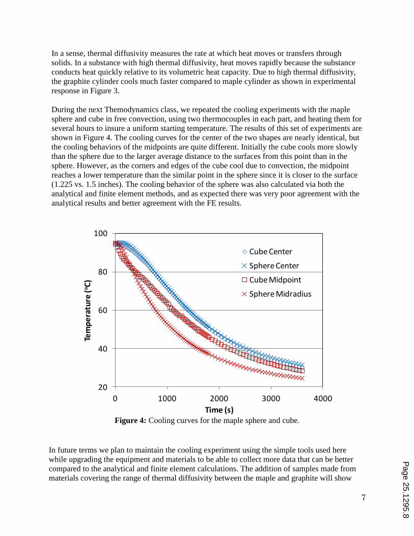
During the next Themodynamics class, we repeated the cooling experiments with the maple

sphere and cube in free convection, using two thermocouples in each part, and heating them for

several hours to insure a uniform starting temperature. The results of this set of experiments are

shown in Figure 4. The cooling curves for the center of the two shapes are nearly identical, but

the cooling behaviors of the midpoints are quite different. Initially the cube cools more slowly

than the sphere due to the larger average distance to the surfaces from this point than in the

sphere. However, as the corners and edges of the cube cool due to convection, the midpoint

reaches a lower temperature than the similar point in the sphere since it is closer to the surface

(1.225 vs. 1.5 inches). The cooling behavior of the sphere was also calculated via both the

analytical and finite element methods, and as expected there was very poor agreement with the

analytical results and better agreement with the FE results.

20

40

60

80

100

0 1000 2000 3000 4000

Tem

pe

ratu

re (o C

)

Time (s)

Cube Center

Sphere Center

Cube Midpoint

Sphere Midradius

Figure 4: Cooling curves for the maple sphere and cube.

In future terms we plan to maintain the cooling experiment using the simple tools used here

while upgrading the equipment and materials to be able to collect more data that can be better

compared to the analytical and finite element calculations. The addition of samples made from

materials covering the range of thermal diffusivity between the maple and graphite will show

Page 25.1295.8

8

how this changes the Biot number and therefore the ability to use analytic methods. The second

change will be to automate collection of the data so that the temperature can be measured at

multiple points on the part. A Senior Projects student is building a set of general-purpose data

acquisition modules that use a low cost DATAQ A/D unit to bring the data into the computer as

their Senior Project. Two of the boxes will be set up for type K thermocouples, but unlike full

commercial systems, the students will have to calibrate the system before use. We are taking this

approach to build the calibration skills for use with any type of sensor they will use in the future.

Transient Cooling – Analytical Solution

The lumped heat capacity method is used to analyze the transient heat response of a long

cylinder. This method assumes no temperature gradient throughout the whole body, i.e., it will

be assumed that all the points in the body have the same temperature at any time. It is, in a sense,

the equivalent of lumping the position of all points in a body to that of its center of mass. This

assumption can be later checked to see if it is valid.

The cylinder is assumed to be at an initial temperature Ti and is then placed in still air at a

temperature T∞. The coefficient of convection and surface area of the body are referred to as h

and A, respectively. If the body is at a temperature T, then, the heat transfer Q due to convection

is given by

Q = dU/dt = hA(T-Tinf) (2)

where U is the total energy stored in the system. The temperature T obviously varies with time.

The quantity Q can also be expressed in terms of the heat capacity C of the material. Indeed, by

definition C is

dt

dTm

QC (3)

where t, m and C are the time, mass, and heat capacity of the material, respectively. The previous

equation can also be expressed as

dt

dTmCQ (4)

By substituting the value of the mass m in terms of the density and the volume V, the previous

result becomes

(5)

Page 25.1295.9

9

This differential equation has the following solution

TeTTtTt

cV

hA

i )()( (6)

This result can also be expressed as

tcV

hA

ii

eTT

TtTt

)(

))(()( (7)

The lumped heat capacity method is valid when the Biot number (Bi), defined as the quantity

where k is the material thermal conductivity, is less than 0.1, or

Bi = < 0.1, (8)

For the graphite cylinder the diameter and height are 1.563 inch and 5.623 inch, respectively.

The initial temperature is 97oC, and the ambient temperature is 20

oC. The free convection

experimental conditions and materials properties are h = 13 W/m2•K, k = 120 W/m•K, =1760

kg/m3 and C = 710 J/kg-K, which yields the solution

77 (9)

or

(10)

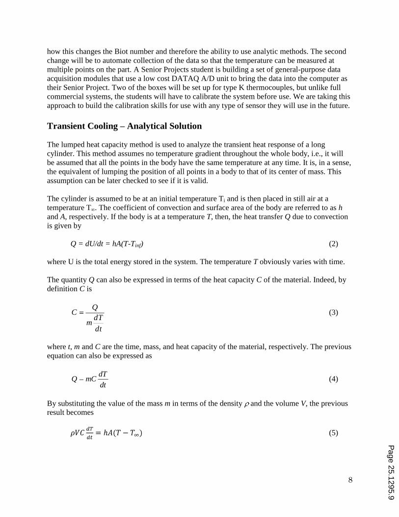
Figure 5 shows a plot of the response as a function of time. The Biot number is 0.0011, well

below the 0.1 value, and as a result, the lumped heat capacity model seems valid.

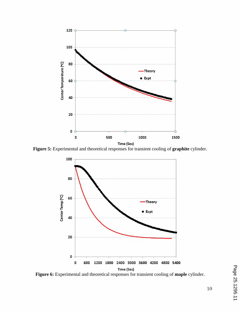
The theoretical calculation to determine the transient response of a maple cylinder with diameter

2.406 in and height 4.063 in was also performed. Due to low thermal conductivity of maple (k =

0.14 W/m-K), the Biot number becomes 1.39, which is much higher than 0.1. Therefore, the

lump capacitance method to determine the transient response of maple cylinder deviates

significantly from the experimental response as shown in Figure 6. The lumped capacitance

model predicts that the center temperature will fall quickly once the surface temperature is

changed while it takes several minutes for the center of the part to “see” the change of the

surface temperature. Comparison of the graphite and maple cylinders is a dramatic

demonstration of the importance of thermal diffusivity and Biot number.

Page 25.1295.10

10

Figure 5: Experimental and theoretical responses for transient cooling of graphite cylinder.

Figure 6: Experimental and theoretical responses for transient cooling of maple cylinder.

Page 25.1295.11

11

Numerical Analysis

The learning process of numerical analysis starts with solving for the temperature distribution of

a 1D rectangular aluminum fin as described in a previous paper[1]

. The objectives of this simple

analysis were two fold:

(1) To demonstrate the basic mathematics of Finite Element Analysis (FEA) procedure using

Matrix Algebra.

(2) To compare the numerical results, obtained by Matrix Algebra and ANSYS, with

analytical and experimental solutions. Comparing numerical results with corresponding

analytical and experimental solutions is important to achieve proper confidence.

The detailed methodology we plan to use to teach our students numerical methods in a heat

transfer course is described by Hossain, Weiser, and Saad[1]

and therefore not repeated herein. In

Mechanical Engineering curriculum, we offer Finite Element Analysis (FEA) in Winter quarter

and Heat Transfer in Spring. Therefore, students get a chance to learn FEA before taking Heat

Transfer course. The FEA class covers the following topics:

Explain the concept of basic numerical methods

Explain the mathematical foundations of the finite element method using matrix algebra

Be familiar with different types of elements and understand their advantages and limitations

Analyze structural problems using ANSYS dealing with axial members

Understand the concept of using one, two and three dimensional elements and their

applications

Perform the static stress analysis, fatigue analysis, and dynamic analysis of a component

made of a linear elastic material using ANSYS

Understand the concept of nonlinearity and how to use finite element program to perform

nonlinear analysis

Perform heat transfer (steady state and transient) problems using ANSYS

To understand the concept of Graphical User Interface (GUI) and Batch files to solve

engineering problems using ANSYS

Solving structural and thermal problems using ANSYS WOKRBENCH

Perform a project using ANSYS, and prepare and present a technical report summarizing the

modeling approach and results

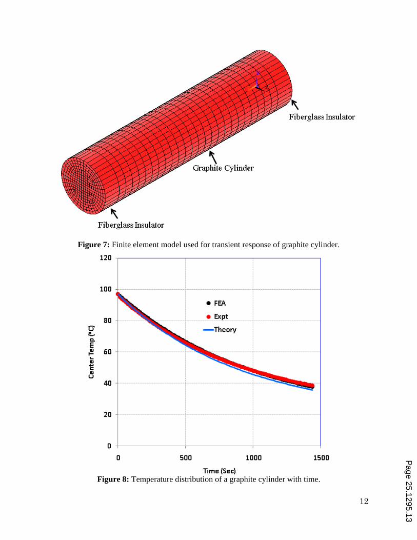
Our students are familiar with FEA code ANSYS6, which was used to analyze the transient

response of a graphite cylinder. The ANSYS analysis is straight-forward. First, the element types

are defined with all required information. In this case, students use 3D thermal solid element

(SOLID 70), defined by eight nodes with a single degree of freedom, temperature. The element

is applicable to a 3-D, steady-state or transient thermal analysis. Second, material properties

associated with thermal conductivity, density and specific heat are defined. Then the

representative FEA model is created according to the dimensions mentioned before, and shown

in Figure 7. Boundary conditions are assigned representing the uniform initial and ambient

temperature. Finally, the FEA model was solved and nodal temperatures are obtained with time.

The ANSYS output for transient response for the graphite cylinder was found to match very

closely with corresponding analytical and experimental solutions, as shown in Figure 8.

Page 25.1295.12

12

Figure 7: Finite element model used for transient response of graphite cylinder.

Figure 8: Temperature distribution of a graphite cylinder with time.

Page 25.1295.13

13

The physical significance of Biot number, which is mentioned before, can be easily explained

to our students by imagining the heat flow from a small hot metal cylinder suddenly immersed

in a pool, to the surrounding fluid. In this case, the heat flow experiences two resistances. First,

the heat flow depends on the solid metal, which is influenced by its size and composition.

Second, it depends at the surface of the cylinder. If the thermal resistance of the fluid/solid

interface exceeds that thermal resistance offered by the interior of the metal, the Biot number

will be less than one. For systems where it is much less than one, typically less that 0.1, the

interior of the cylinder may be presumed always to have the same temperature. The

temperature gradients are negligible inside the body and the transient heat transfer from the

body can be explained using the lamped-capacitance model. As the Biot number of graphite

cylinder is 0.0011, which is less than 0.1, the temperature profile at center and surface was

found to be almost the same as shown in Figure 9. However for maple wood, the thermal

conductivity is much smaller (0.14 W/m-K) and the Biot number is larger than 0.1.

Subsequently, the temperature distribution along the centerline and surface are significantly

different, as shown in Figure 10.

Figure 9: Temperature distribution of a graphite cylinder with time.

Page 25.1295.14

14

Figure 10: Temperature distribution of a maple cylinder with time.

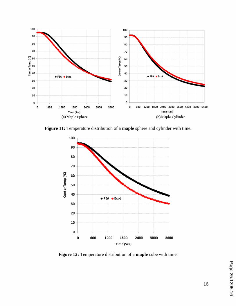
Additional numerical analyses were conducted to investigate the transient response of a maple

sphere and cube. The numerical results for the maple sphere and cylinder were found to match

very well with corresponding experiments as shown in Figure 11. However, the FEA result for

transient response of the maple cube differs noticeably when compared with corresponding

experiment, as shown in Figure 12. The additional surfaces of the cube and difficulty in dealing

with the convection coefficient of a part with different surfaces might be the reasons for the

deviation found between the FEA and experimental results. All of these issues seem instructive

to teach to our students.

Page 25.1295.15

15

Figure 11: Temperature distribution of a maple sphere and cylinder with time.

Figure 12: Temperature distribution of a maple cube with time.

Page 25.1295.16

16

Student Survey

Upon completion of the analytical, numerical and experimental measurements of transient

temperature response of different geometrical blocks, a student survey will be conducted. This

survey evaluates the effectiveness of this teaching methodology to enhance the students’

understanding on several concepts of heat transfer including thermal diffusivity. Several

questions will be asked, as listed below, and students’ response will be studied to improve the

teaching methodology.

Question # 1:

Did use of the different methodologies (analytical, numerical, and experimental) to measure the

transient temperature response help increase your understanding of heat transfer?

Question # 2:

Which method (analytical, numerical, experimental) do you feel was most valuable to increase

your understanding of heat transfer? Why?

Question # 3:

Which method (analytical, numerical, experimental) do you feel was least valuable to increase

your understanding of heat transfer? Why?

Question # 4:

What suggestions do you have to improve this exercise to increase student understanding of

conductive/convective heat transfer?

Question # 5:

If you are given a real heat sink (several blocks like the one used in this exercise) which method

would you use to evaluate the performance? Why?

One reviewer suggested that we compare the effect of the proposed teaching methodology on the

students’ learning by splitting the students into two groups – one that conducted the experiments

and FEA modeling and another that did not. We agree that this would be the best way to

determine if there was a measurable benefit of our approach. However, based upon our

experience in other classes and the nature of our students (many whom are first generation

college students) we are confident that removing the hands-on components would be very

detrimental. Therefore, we are attempting to implement what we see as the best practice the first

time we teach the class and then improve it based upon student feedback.

Conclusions

Students will be introduced to three different ways to evaluate transient heat transfer from

geometrical blocks with different shapes and materials to the environment. The progression from

the analytical solution to the numeric solution and finally experimental measurement of the

temperature profile will build confidence in their ability to use the different tools. The transient

response of temperature profile of graphite cylinder matched very well between the

experimental, analytical and FEA methods, which shows the students that such problems can be

Page 25.1295.17

17

solved in multiple ways. In addition, it builds confidence in the use of numeric methods for more

complex geometries that cannot be solved analytically. The variability of the analytical results

and the close, but inexact match to the corresponding FEA and experimental models

demonstrates that the models are just that – models of real world behavior that are only as good

as the assumptions used in building them. The survey outcomes collected from students

including their feedback will be studied further to improve this exercise to increase the students’

understanding of heat transfer.

Page 25.1295.18

18

Bibliography

1. A. Hossain, M. Weiser and H. Saad, “Integration of Numerical and Experimental Studies

in a Heat Transfer Course to Enhance the Students’ Understanding,” 2011 ASEE Annual

Conference and Exposition, American Society of Engineering Education.

2. T.A. Doughty, and O’Halloran, S.P., “A Cross Curricular Numerical and Experimental

Study in Heat Transfer,” 2010 ASEE Annual Conference and Exposition, American

Society of Engineering Education.

3. O’Halloran, S.P. and T.A. Doughty, “Integration of Numerical Analysis and

Experimental Testing Involving Heat Transfer for a Small Heated Cylinder During

Cooling,” 2009 ASEE Annual Conference and Exposition, American Society of

Engineering Education.

4. Besser, R.S., “Spreadsheet Solutions to Two-Dimensional Heat Transfer Problems,”

Chemical Engineering Education, Vol. 36, No. 2, 2002, pp. 160-165.

5. Goldstein, A.S., “A Computational Model for Teaching Free Convection,” Chemical

Engineering Education, Vol. 38, No. 4, 2004, pp. 272-278.

6. ANSYS Documentation, version 11

Page 25.1295.19