The University of Manchester Research

Transient thermal boundary value-problems in the half-space with mixed convective boundary conditionsDOI:10.1007/s10665-019-09986-6

Document VersionAccepted author manuscript

Link to publication record in Manchester Research Explorer

Citation for published version (APA):Gorbushin, N., Nguyen, V-H., Parnell, W., Assier, R., & Naili, S. (2019). Transient thermal boundary value-problems in the half-space with mixed convective boundary conditions. Journal of Engineering Mathematics.https://doi.org/10.1007/s10665-019-09986-6

Published in:Journal of Engineering Mathematics

Citing this paperPlease note that where the full-text provided on Manchester Research Explorer is the Author Accepted Manuscriptor Proof version this may differ from the final Published version. If citing, it is advised that you check and use thepublisher's definitive version.

General rightsCopyright and moral rights for the publications made accessible in the Research Explorer are retained by theauthors and/or other copyright owners and it is a condition of accessing publications that users recognise andabide by the legal requirements associated with these rights.

Takedown policyIf you believe that this document breaches copyright please refer to the University of Manchester’s TakedownProcedures [http://man.ac.uk/04Y6Bo] or contact uml.scholarlycommunications@manchester.ac.uk providingrelevant details, so we can investigate your claim.

Download date:31. Jan. 2022

Journal of Engineering Mathematics manuscript No.(will be inserted by the editor)

Transient thermal boundary value-problems in thehalf-space with mixed convective boundary conditions

Nikolai Gorbushin · Vu-Hieu Nguyen ·William J. Parnell · Raphael C. Assier ·Salah Naili

Received: date / Accepted: date

Abstract Numerous problems in thermal engineering give rise to problems withabrupt changes in boundary conditions particularly as regards structural and con-struction applications. There is a continual need for improved analytical and nu-merical techniques for the study and analysis of such canonical problems. Thepresent work considers transient heat propagation in a two-dimensional half-spacewith mixed boundary conditions of the Dirichlet and the Robin (convective) type.The exact temperature field is obtained in double integral form by applying theWiener-Hopf technique and this integral is then efficiently evaluated numericallywith the help of numerical algorithms developed for the present problem and byexploiting the properties of the integrand. The results are then compared with nu-merical solutions using finite element methods and excellent agreement is shown.Some potential application areas of the theory are also discussed, specifically inthe regime where edge effects can influence thermal convection processes.

Keywords Heat convection · Transient heat problem · Mixed boundaryconditions and Wiener-Hopf technique

1 Introduction

Transient heat transfer problems arise frequently in complex engineering appli-cations and in general physical phenomena. For instance, the dynamic character

Nikolai Gorbushin · Vu-Hieu Nguyen · Salah NailiLaboratoire Modelisation et Simulation Multi Echelle, Universite Paris-Est, Creteil, 94000,FranceE-mail: nikolai.gorbushin@u-pec.frE-mail: vu-hieu.nguyen@u-pec.frE-mail: naili@u-pec.fr

William J. Parnell · Raphael C. AssierSchool of Mathematics, University of Manchester, Manchester, M13 9PL, UKE-mail: william.j.parnell@manchester.ac.ukE-mail: raphael.assier@manchester.ac.uk

2 Nikolai Gorbushin et al.

of a temperature field enables defect sizing analysis through transient thermog-raphy [1, 2] with the help of infrared cameras. This technique is based on thescattering of the temperature field, initiated by a short-duration pulse of a heatflux to a free surface of a specimen, by virtue of the presence of various defects in asolid. Another example refers to the cooling of a hot solid by means of a fluid. Thetemperature difference may cause vaporisation of the liquid. Further cooling of thesolid results in a steady-state process with an established boundary between partsof the solid covered by liquid and vapour, forming the so-called “quench front”.This problem is known as the “quench front propagation problem” [3, 4] and itplays an important role in the nuclear, metallurgical, chemical and cryogenic in-dustries [5, 6]. One more interesting application concerns the hot-film technique,which is based on the dynamic heat exchange between a viscous fluid in a chan-nel and a hot-film attached to its wall. It is possible to establish the dependencebetween the heat flux across the film and the local shear rate, which is importantfor the analysis of fluid behaviour [7] and can be determined through the knowl-edge of the heat flux. The movement of the fluid introduces some complications inthe mathematical treatment of the problem although it is possible to determineanalytical results by adopting some simplifications [8, 9]. Ignoring the temporal de-pendence of temperature allows one to obtain exact solutions [10, 11], however theproblem reduces to one with mixed boundary conditions for which the derivationof final solutions is not straightforward and requires special treatment. Therefore,the development of mathematical models for transient heat propagation makes itpossible to address a number of practical issues.

The difficulties in obtaining purely analytical results involve the presence of thedynamic terms in the heat equation and, what is more important, the mixed typeof boundary conditions. The Wiener-Hopf technique [12] appears to be a powerfultool in handling the latter difficulty. This method allows one to obtain the solutionof the problem in terms of the Fourier and Laplace transforms, which can beinverted either analytically (for some special cases) or numerically. The applicationof this technique is preferred to specific numerical modelling of the problem, e.g.by means of the finite element method (FEM), as it avoids problems associatedwith the changes in boundary conditions, and it also reduces computation timesfor the analysis of physical problems.

The aim of this work is to obtain the solution of a transient heat problemwith the anisotropic thermal conductivity in the half-space with mixed bound-ary conditions of the Dirichlet and the Robin (convective) type by means of theWiener-Hopf technique. This problem is of essential significance for numerous en-gineering applications and in this manuscript we demonstrate it on two practicalexamples. The mathematical challenge in obtaining the solution is related to theWiener-Hopf method requiring the function factorisation which, to the best of ourknowledge, is not available in an analytical form in the literature. Furthermore,the consideration of dynamic effects introduce additional difficulties for obtain-ing the factorisation. For these reasons, we perform the factorisation by using arobust algorithm developed for the considered transient problem and which canbe adapted for more complicated problems as well. In such a case, the suitablereduction of singularities of the function can be achieved for better performance ofthe subsequent computations and improved accuracy of the results in comparisonwith the purely numerical methods. Moreover, we focus on the solution behaviourclose to the location of the change in boundary condition where the computational

Transient thermal boundary value-problems 3

x

Ω

y

@Ω+

@Ω−

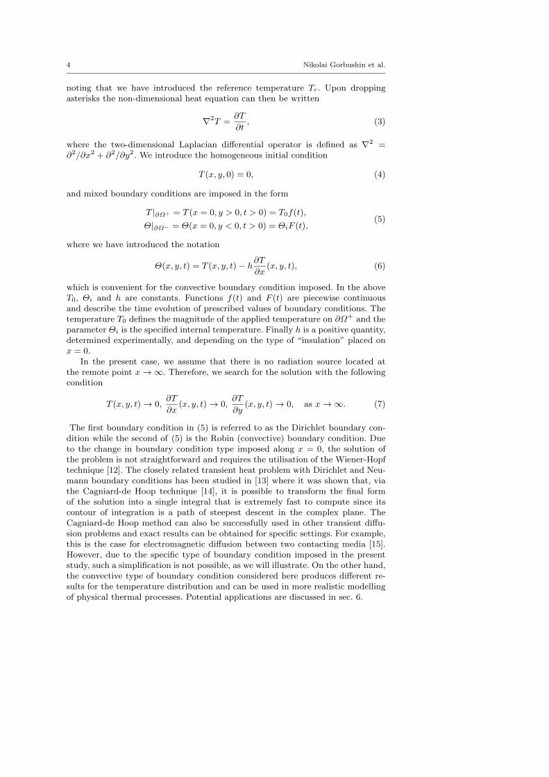
Fig. 1 Domain Ω of the problem under consideration with marked boundaries ∂Ω+ and ∂Ω−,where the Dirichlet and Robin conditions are stated, respectively.

difficulties usually appear. We estimate the asymptotic behaviour of functions inthis region which shows that the associated accuracy of results is complicated toachieve with FEM unless significant mesh refinement is accomplished.

The paper is organised as follows. The formulation of the mathematical prob-lem and associated notation are introduced in section 2. Section 3 presents thereduction of the problem to one that is suitable for treatment by the Wiener-Hopfmethod and solutions are derived together with their asymptotic form close tothe change in boundary condition. The numerical procedures that have been em-ployed in the present study are described in section 4, followed by the presentationof results for some particular cases in section 5. We discuss particular applicationareas in section 6. Conclusions are drawn and future work discussed in section 7.The efficiency of the proposed numerical algorithm for the function factorisation isshown in Appendix A. For reference the weak formulation for the FEM is providedin Appendix B.

2 Governing equations and integral transforms

With reference to Fig. 1 we are interested in a transient heat problem in twospatial dimensions. The physical domain of interest occupies the half space Ω =(x, y) : 0 ≤ x <∞,−∞ < y <∞. The governing equation for the temperaturefield T (x, y, t) in a medium with transversely isotropic thermal conductivity isgiven by

κ

ρcV

(∂2T

∂x2+ `

∂2T

∂y2

)=∂T

∂t, 0 < x <∞, −∞ < y <∞, t > 0, (1)

where κ and κ` are the thermal conductivities in the x and y directions, respec-tively, where ` > 0 is a non-dimensional constant, cV is the specific heat at constantvolume, ρ is the mass density of the medium and t is time. Thanks to the spe-cific type of the material anisotropy (a transverse anisotropy), one may performa simple non-dimensionalisation, which also scales out the anisotropy coefficient `by introducing the following non-dimensional variables:

x∗ = x, y∗ =y√`, t∗ = ρcV

t

κ, T ∗ =

T − TrTr

, (2)

4 Nikolai Gorbushin et al.

noting that we have introduced the reference temperature Tr. Upon droppingasterisks the non-dimensional heat equation can then be written

∇2T =∂T

∂t, (3)

where the two-dimensional Laplacian differential operator is defined as ∇2 =∂2/∂x2 + ∂2/∂y2. We introduce the homogeneous initial condition

T (x, y, 0) = 0, (4)

and mixed boundary conditions are imposed in the form

T |∂Ω+ = T (x = 0, y > 0, t > 0) = T0f(t),

Θ|∂Ω− = Θ(x = 0, y < 0, t > 0) = ΘiF (t),(5)

where we have introduced the notation

Θ(x, y, t) = T (x, y, t)− h∂T∂x

(x, y, t), (6)

which is convenient for the convective boundary condition imposed. In the aboveT0, Θi and h are constants. Functions f(t) and F (t) are piecewise continuousand describe the time evolution of prescribed values of boundary conditions. Thetemperature T0 defines the magnitude of the applied temperature on ∂Ω+ and theparameter Θi is the specified internal temperature. Finally h is a positive quantity,determined experimentally, and depending on the type of “insulation” placed onx = 0.

In the present case, we assume that there is no radiation source located atthe remote point x→∞. Therefore, we search for the solution with the followingcondition

T (x, y, t)→ 0,∂T

∂x(x, y, t)→ 0,

∂T

∂y(x, y, t)→ 0, as x→∞. (7)

The first boundary condition in (5) is referred to as the Dirichlet boundary con-dition while the second of (5) is the Robin (convective) boundary condition. Dueto the change in boundary condition type imposed along x = 0, the solution ofthe problem is not straightforward and requires the utilisation of the Wiener-Hopftechnique [12]. The closely related transient heat problem with Dirichlet and Neu-mann boundary conditions has been studied in [13] where it was shown that, viathe Cagniard-de Hoop technique [14], it is possible to transform the final formof the solution into a single integral that is extremely fast to compute since itscontour of integration is a path of steepest descent in the complex plane. TheCagniard-de Hoop method can also be successfully used in other transient diffu-sion problems and exact results can be obtained for specific settings. For example,this is the case for electromagnetic diffusion between two contacting media [15].However, due to the specific type of boundary condition imposed in the presentstudy, such a simplification is not possible, as we will illustrate. On the other hand,the convective type of boundary condition considered here produces different re-sults for the temperature distribution and can be used in more realistic modellingof physical thermal processes. Potential applications are discussed in sec. 6.

Transient thermal boundary value-problems 5

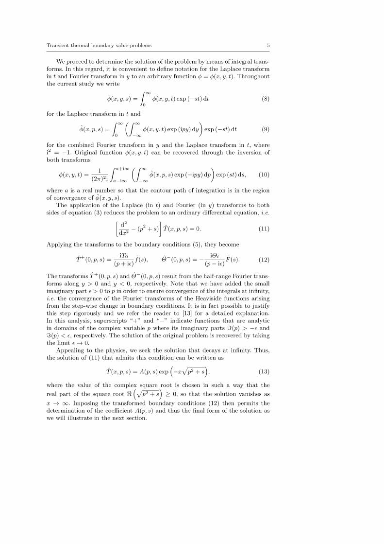
We proceed to determine the solution of the problem by means of integral trans-forms. In this regard, it is convenient to define notation for the Laplace transformin t and Fourier transform in y to an arbitrary function φ = φ(x, y, t). Throughoutthe current study we write

φ(x, y, s) =

∫ ∞0

φ(x, y, t) exp (−st) dt (8)

for the Laplace transform in t and

φ(x, p, s) =

∫ ∞0

(∫ ∞−∞

φ(x, y, t) exp (ipy) dy

)exp (−st) dt (9)

for the combined Fourier transform in y and the Laplace transform in t, wherei2 = −1. Original function φ(x, y, t) can be recovered through the inversion ofboth transforms

φ(x, y, t) =1

(2π)2i

∫ a+i∞

a−i∞

(∫ ∞−∞

φ(x, p, s) exp (−ipy) dp

)exp (st) ds, (10)

where a is a real number so that the contour path of integration is in the regionof convergence of φ(x, y, s).

The application of the Laplace (in t) and Fourier (in y) transforms to bothsides of equation (3) reduces the problem to an ordinary differential equation, i.e.[

d2

dx2− (p2 + s)

]T (x, p, s) = 0. (11)

Applying the transforms to the boundary conditions (5), they become

T+(0, p, s) =iT0

(p+ iε)f(s), Θ−(0, p, s) = − iΘi

(p− iε)F (s). (12)

The transforms T+(0, p, s) and Θ−(0, p, s) result from the half-range Fourier trans-forms along y > 0 and y < 0, respectively. Note that we have added the smallimaginary part ε > 0 to p in order to ensure convergence of the integrals at infinity,i.e. the convergence of the Fourier transforms of the Heaviside functions arisingfrom the step-wise change in boundary conditions. It is in fact possible to justifythis step rigorously and we refer the reader to [13] for a detailed explanation.In this analysis, superscripts “+” and “−” indicate functions that are analyticin domains of the complex variable p where its imaginary parts =(p) > −ε and=(p) < ε, respectively. The solution of the original problem is recovered by takingthe limit ε→ 0.

Appealing to the physics, we seek the solution that decays at infinity. Thus,the solution of (11) that admits this condition can be written as

T (x, p, s) = A(p, s) exp(−x√p2 + s

), (13)

where the value of the complex square root is chosen in such a way that the

real part of the square root <(√

p2 + s)≥ 0, so that the solution vanishes as

x → ∞. Imposing the transformed boundary conditions (12) then permits thedetermination of the coefficient A(p, s) and thus the final form of the solution aswe will illustrate in the next section.

6 Nikolai Gorbushin et al.

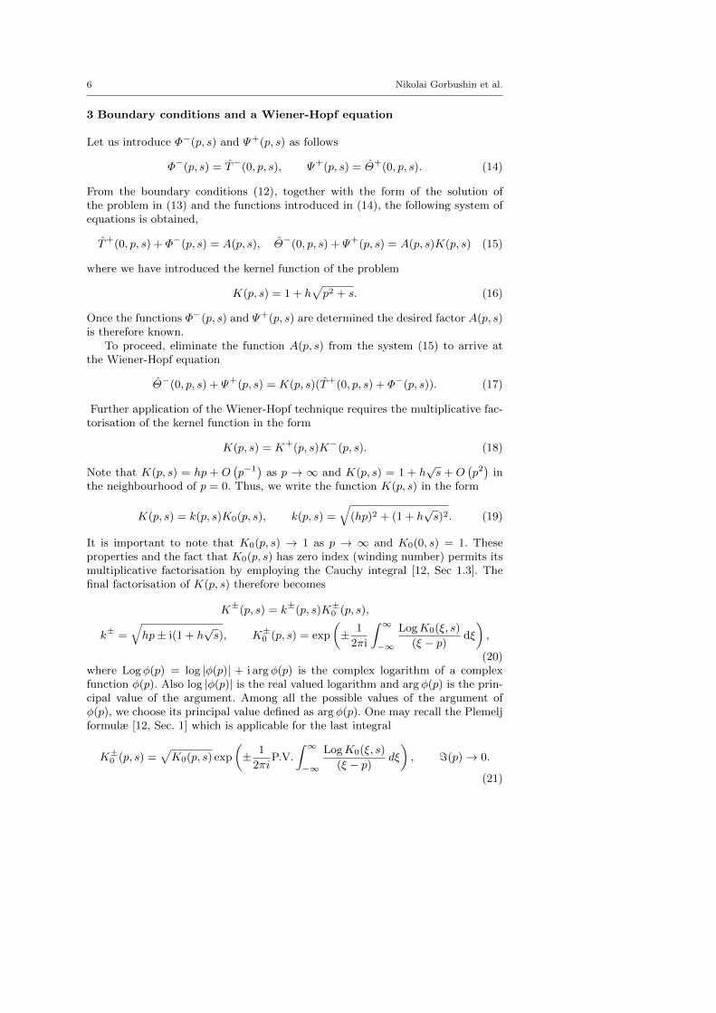
3 Boundary conditions and a Wiener-Hopf equation

Let us introduce Φ−(p, s) and Ψ+(p, s) as follows

Φ−(p, s) = T−(0, p, s), Ψ+(p, s) = Θ+(0, p, s). (14)

From the boundary conditions (12), together with the form of the solution ofthe problem in (13) and the functions introduced in (14), the following system ofequations is obtained,

T+(0, p, s) + Φ−(p, s) = A(p, s), Θ−(0, p, s) + Ψ+(p, s) = A(p, s)K(p, s) (15)

where we have introduced the kernel function of the problem

K(p, s) = 1 + h√p2 + s. (16)

Once the functions Φ−(p, s) and Ψ+(p, s) are determined the desired factor A(p, s)is therefore known.

To proceed, eliminate the function A(p, s) from the system (15) to arrive atthe Wiener-Hopf equation

Θ−(0, p, s) + Ψ+(p, s) = K(p, s)(T+(0, p, s) + Φ−(p, s)). (17)

Further application of the Wiener-Hopf technique requires the multiplicative fac-torisation of the kernel function in the form

K(p, s) = K+(p, s)K−(p, s). (18)

Note that K(p, s) = hp + O(p−1

)as p → ∞ and K(p, s) = 1 + h

√s + O

(p2)

inthe neighbourhood of p = 0. Thus, we write the function K(p, s) in the form

K(p, s) = k(p, s)K0(p, s), k(p, s) =

√(hp)2 + (1 + h

√s)2. (19)

It is important to note that K0(p, s) → 1 as p → ∞ and K0(0, s) = 1. Theseproperties and the fact that K0(p, s) has zero index (winding number) permits itsmultiplicative factorisation by employing the Cauchy integral [12, Sec 1.3]. Thefinal factorisation of K(p, s) therefore becomes

K±(p, s) = k±(p, s)K±0 (p, s),

k± =

√hp± i(1 + h

√s), K±0 (p, s) = exp

(± 1

2πi

∫ ∞−∞

LogK0(ξ, s)

(ξ − p) dξ

),

(20)where Logφ(p) = log |φ(p)| + i arg φ(p) is the complex logarithm of a complexfunction φ(p). Also log |φ(p)| is the real valued logarithm and arg φ(p) is the prin-cipal value of the argument. Among all the possible values of the argument ofφ(p), we choose its principal value defined as arg φ(p). One may recall the Plemeljformulæ [12, Sec. 1] which is applicable for the last integral

K±0 (p, s) =√K0(p, s) exp

(± 1

2πiP.V.

∫ ∞−∞

LogK0(ξ, s)

(ξ − p) dξ

), =(p)→ 0.

(21)

Transient thermal boundary value-problems 7

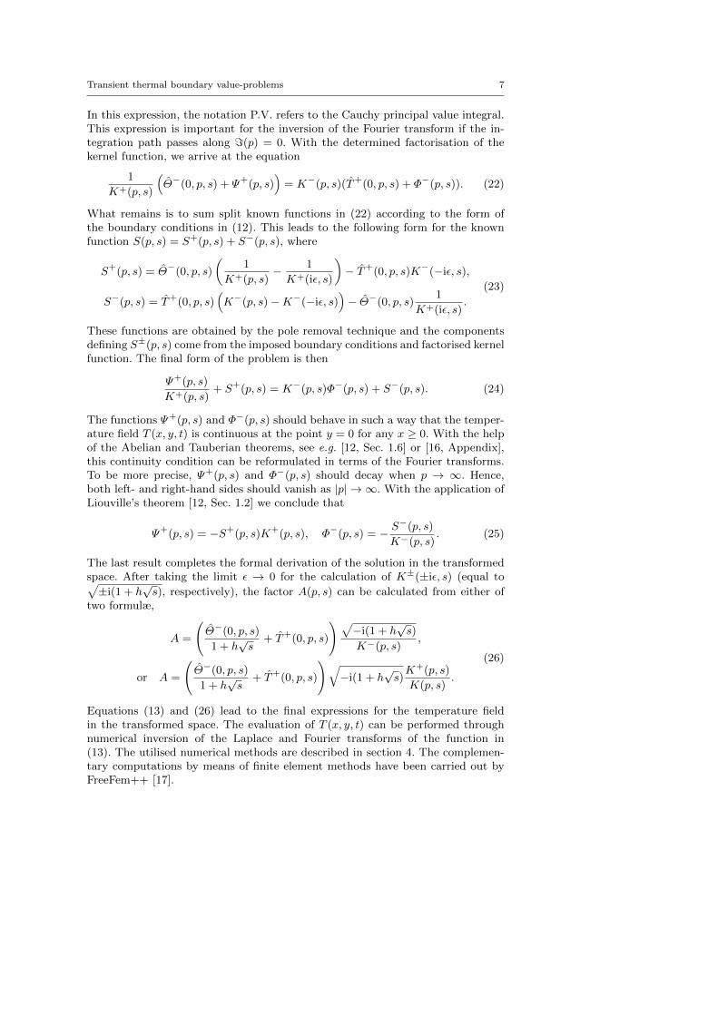
In this expression, the notation P.V. refers to the Cauchy principal value integral.This expression is important for the inversion of the Fourier transform if the in-tegration path passes along =(p) = 0. With the determined factorisation of thekernel function, we arrive at the equation

1

K+(p, s)

(Θ−(0, p, s) + Ψ+(p, s)

)= K−(p, s)(T+(0, p, s) + Φ−(p, s)). (22)

What remains is to sum split known functions in (22) according to the form ofthe boundary conditions in (12). This leads to the following form for the knownfunction S(p, s) = S+(p, s) + S−(p, s), where

S+(p, s) = Θ−(0, p, s)

(1

K+(p, s)− 1

K+(iε, s)

)− T+(0, p, s)K−(−iε, s),

S−(p, s) = T+(0, p, s)(K−(p, s)−K−(−iε, s)

)− Θ−(0, p, s)

1

K+(iε, s).

(23)

These functions are obtained by the pole removal technique and the componentsdefining S±(p, s) come from the imposed boundary conditions and factorised kernelfunction. The final form of the problem is then

Ψ+(p, s)

K+(p, s)+ S+(p, s) = K−(p, s)Φ−(p, s) + S−(p, s). (24)

The functions Ψ+(p, s) and Φ−(p, s) should behave in such a way that the temper-ature field T (x, y, t) is continuous at the point y = 0 for any x ≥ 0. With the helpof the Abelian and Tauberian theorems, see e.g. [12, Sec. 1.6] or [16, Appendix],this continuity condition can be reformulated in terms of the Fourier transforms.To be more precise, Ψ+(p, s) and Φ−(p, s) should decay when p → ∞. Hence,both left- and right-hand sides should vanish as |p| → ∞. With the application ofLiouville’s theorem [12, Sec. 1.2] we conclude that

Ψ+(p, s) = −S+(p, s)K+(p, s), Φ−(p, s) = − S−(p, s)

K−(p, s). (25)

The last result completes the formal derivation of the solution in the transformedspace. After taking the limit ε → 0 for the calculation of K±(±iε, s) (equal to√±i(1 + h

√s), respectively), the factor A(p, s) can be calculated from either of

two formulæ,

A =

(Θ−(0, p, s)

1 + h√s

+ T+(0, p, s)

) √−i(1 + h

√s)

K−(p, s),

or A =

(Θ−(0, p, s)

1 + h√s

+ T+(0, p, s)

)√−i(1 + h

√s)K+(p, s)

K(p, s).

(26)

Equations (13) and (26) lead to the final expressions for the temperature fieldin the transformed space. The evaluation of T (x, y, t) can be performed throughnumerical inversion of the Laplace and Fourier transforms of the function in(13). The utilised numerical methods are described in section 4. The complemen-tary computations by means of finite element methods have been carried out byFreeFem++ [17].

8 Nikolai Gorbushin et al.

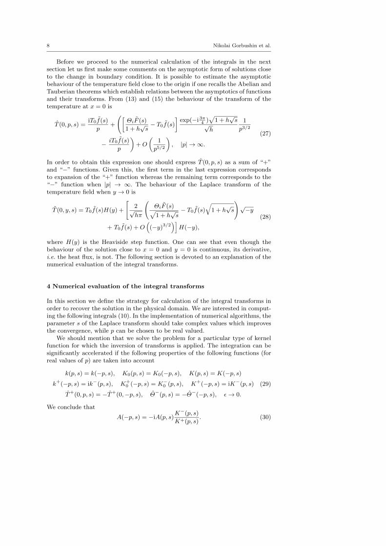
Before we proceed to the numerical calculation of the integrals in the nextsection let us first make some comments on the asymptotic form of solutions closeto the change in boundary condition. It is possible to estimate the asymptoticbehaviour of the temperature field close to the origin if one recalls the Abelian andTauberian theorems which establish relations between the asymptotics of functionsand their transforms. From (13) and (15) the behaviour of the transform of thetemperature at x = 0 is

T (0, p, s) =iT0f(s)

p+

([ΘiF (s)

1 + h√s− T0f(s)

]exp(−i3π4 )

√1 + h

√s

√h

1

p3/2

− iT0f(s)

p

)+O

(1

p5/2

), |p| → ∞.

(27)

In order to obtain this expression one should express T (0, p, s) as a sum of “+”and “−” functions. Given this, the first term in the last expression correspondsto expansion of the “+” function whereas the remaining term corresponds to the“−” function when |p| → ∞. The behaviour of the Laplace transform of thetemperature field when y → 0 is

T (0, y, s) = T0f(s)H(y) +

[2√hπ

(ΘiF (s)√1 + h

√s− T0f(s)

√1 + h

√s

)√−y

+ T0f(s) +O(

(−y)3/2)]H(−y),

(28)

where H(y) is the Heaviside step function. One can see that even though thebehaviour of the solution close to x = 0 and y = 0 is continuous, its derivative,i.e. the heat flux, is not. The following section is devoted to an explanation of thenumerical evaluation of the integral transforms.

4 Numerical evaluation of the integral transforms

In this section we define the strategy for calculation of the integral transforms inorder to recover the solution in the physical domain. We are interested in comput-ing the following integrals (10). In the implementation of numerical algorithms, theparameter s of the Laplace transform should take complex values which improvesthe convergence, while p can be chosen to be real valued.

We should mention that we solve the problem for a particular type of kernelfunction for which the inversion of transforms is applied. The integration can besignificantly accelerated if the following properties of the following functions (forreal values of p) are taken into account

k(p, s) = k(−p, s), K0(p, s) = K0(−p, s), K(p, s) = K(−p, s)

k+(−p, s) = ik−(p, s), K+0 (−p, s) = K−0 (p, s), K+(−p, s) = iK−(p, s)

T+(0, p, s) = −T+(0,−p, s), Θ−(p, s) = −Θ−(−p, s), ε→ 0.

(29)

We conclude that

A(−p, s) = −iA(p, s)K−(p, s)

K+(p, s). (30)

Transient thermal boundary value-problems 9

Given these properties it is possible to decrease the number of function evaluationsat points p, i.e. it is enough to evaluate functions for positive p only and then utilisethese properties to construct values for negative p. In addition, one may notice thatthere is a singularity at p = 0 of the function A(p, s) which causes problems in thecalculation of the integral transform since the function values become unboundedin the close neighbourhood of this point. To overcome this, (13) can be written as

T (p, s) =

[A(p, s) exp

(−x√p2 + s

)−

(Θ−(0, p, s)

1 + h√s

+ T+(0, p, s)

)

× exp(−(|p|+

√s)x)]

+

(Θ−(0, p, s)

1 + h√s

+ T+(0, p, s)

)exp

(−(|p|+

√s)x).

(31)

where we subtract and add the same term, the second and the third in the lastexpression, to the original expression. In this case, the inverse integral of the lastterm can be calculated analytically whereas the function composed of the firsttwo terms does not possess singularity at p = 0 any more. We include the factorexp(−|p|x) which preserves the fast decay of the function when x > 0 and, atthe same time, it does not affect the subtracted singularity at p = 0. Hence, theexpression in the first square parenthesis does not have any singularities along thereal axis of p while the second expression can be calculated analytically and addedto the final result. For that purpose, we employ convolutions, noting the followingintegrals

1

2π

∫ ∞−∞

exp (−|p|x− ipy) dp =x

π

1

(x2 + y2),

H(y) ∗(x

π

1

(x2 + y2)

)=

1

πatan

(yx

)+

1

2,

H(−y) ∗(x

π

1

(x2 + y2)

)=

1

2− 1

πatan

(yx

),

(32)

where symbol “∗” stands for the convolution of the functions in y and atan(x)is the inverse tangent function. The inverse Fourier transform of the term on thesecond line of (31) can thus be evaluated analytically and it takes the form

1

(2π)2i

∫ a+i∞

a−i∞

∫ ∞−∞

(Θ−(0, p, s)

1 + h√s

+ T+(0, p, s)

)exp

(−(|p|+

√s)x− ipy + st

)dpds

=1

2πi

∫ a+i∞

a−i∞

(ΘiF (s)

1 + h√s

[1

2− 1

πatan

(yx

)]H(−y)

+T0f(s)

[1

πatan

(yx

)+

1

2

]H(y)

)exp

(−√sx+ st

)ds.

(33)It therefore remains to perform the following inverse Laplace transform in

(33), which can be done through convolution formulae numerically or analytically,depending on the form of the functions F (t) and f(t) that appear on the righthand side of the boundary conditions (5).

What remains is the evaluation of the term in the first line of (31). Inversion ofLaplace transform depends on the form of the functions F (s) and f(s). Below, wedescribe numerical schemes that have been used for calculations of final results.

10 Nikolai Gorbushin et al.

1. Inversion of the Fourier transformFor inversion of the Fourier transform the Fast Fourier Transform (FFT) canbe used. This procedure is implemented in many codes and can be appliedstraightforwardly. In the present study, MATLAB software has been used topresent all the numerical results.

2. Inversion of the Laplace transformThe Laplace transform was evaluated through the convolution quadraturemethod (CQM) which was implemented in MATLAB; the method is describedin [18]. In summary, this method evaluates the convolution of two arbitraryfunctions φ(t) and ψ(t)

Q(t) =

∫ t

0

φ(t− τ)ψ(τ) dτ. (34)

Firstly, the time step ∆t is chosen and the value of the integral at the pointn∆t is computed as

Q(n∆t) =n∑

m=0

ωn−m(∆t)ψ(m∆t), n = 0, 1, ..., N. (35)

Coefficients ωn are computed through the values of the Laplace transform φ(s)of the function φ(t)

ωn(∆t) =R−N

N

N−1∑k=0

φ

(γ(R exp

(ik 2πN

))∆t

)exp

(−ink

2π

N

),

γ(z) =3

2− 2z +

1

2z2.

(36)

Due to the presence of the exponential factor in the definition of ωn, the FFTcan be applied, thus rendering computational efficiency in time. If the valuesφ(s) are calculated with an error bounded by ε, then the choice R−N =

√ε

yields an error in ωn of O(√ε). Additionally, this formula allows the calculation

of φ(s) regardless of the value of t. This is advantageous if the computation ofthe function itself is time consuming.

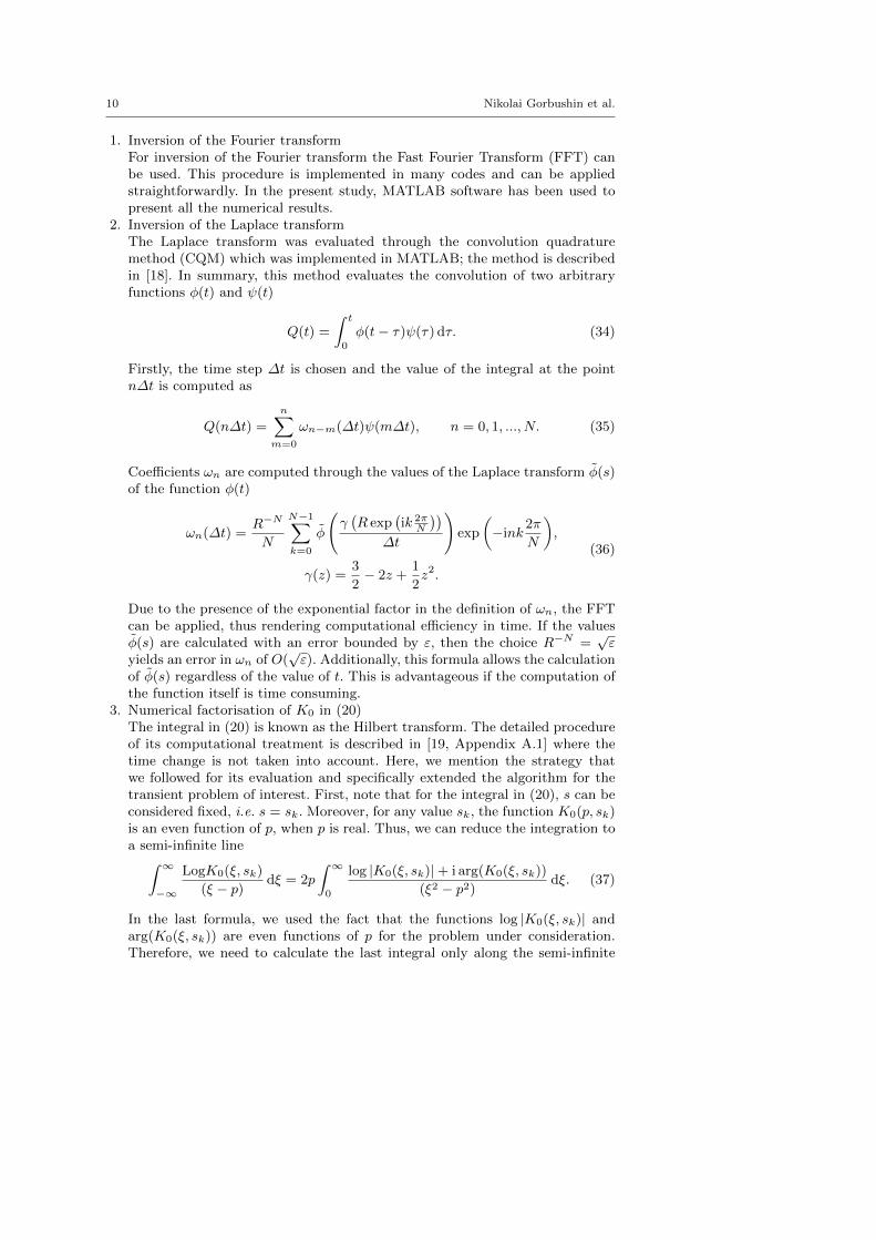
3. Numerical factorisation of K0 in (20)The integral in (20) is known as the Hilbert transform. The detailed procedureof its computational treatment is described in [19, Appendix A.1] where thetime change is not taken into account. Here, we mention the strategy thatwe followed for its evaluation and specifically extended the algorithm for thetransient problem of interest. First, note that for the integral in (20), s can beconsidered fixed, i.e. s = sk. Moreover, for any value sk, the function K0(p, sk)is an even function of p, when p is real. Thus, we can reduce the integration toa semi-infinite line∫ ∞

−∞

LogK0(ξ, sk)

(ξ − p) dξ = 2p

∫ ∞0

log |K0(ξ, sk)|+ i arg(K0(ξ, sk))

(ξ2 − p2)dξ. (37)

In the last formula, we used the fact that the functions log |K0(ξ, sk)| andarg(K0(ξ, sk)) are even functions of p for the problem under consideration.Therefore, we need to calculate the last integral only along the semi-infinite

Transient thermal boundary value-problems 11

-1 -0.8 -0.6 -0.4 -0.2 0 0.2 0.4 0.6 0.8 1

y

0

0.1

0.2

0.3

0.4

0.5

0.6

0.7

0.8

0.9

1

T Analytical solution

FEM

x = 0.05, t = 0.1

x = 0.5, t = 0.1

a)

0 0.1 0.2 0.3 0.4 0.5 0.6 0.7 0.8 0.9 1

t

0

0.1

0.2

0.3

0.4

0.5

0.6

0.7

0.8

0.9

1

T

Analytical solution

FEM

x = 0.05, y = 0.1

x = 0.05, y = −0.1

b)

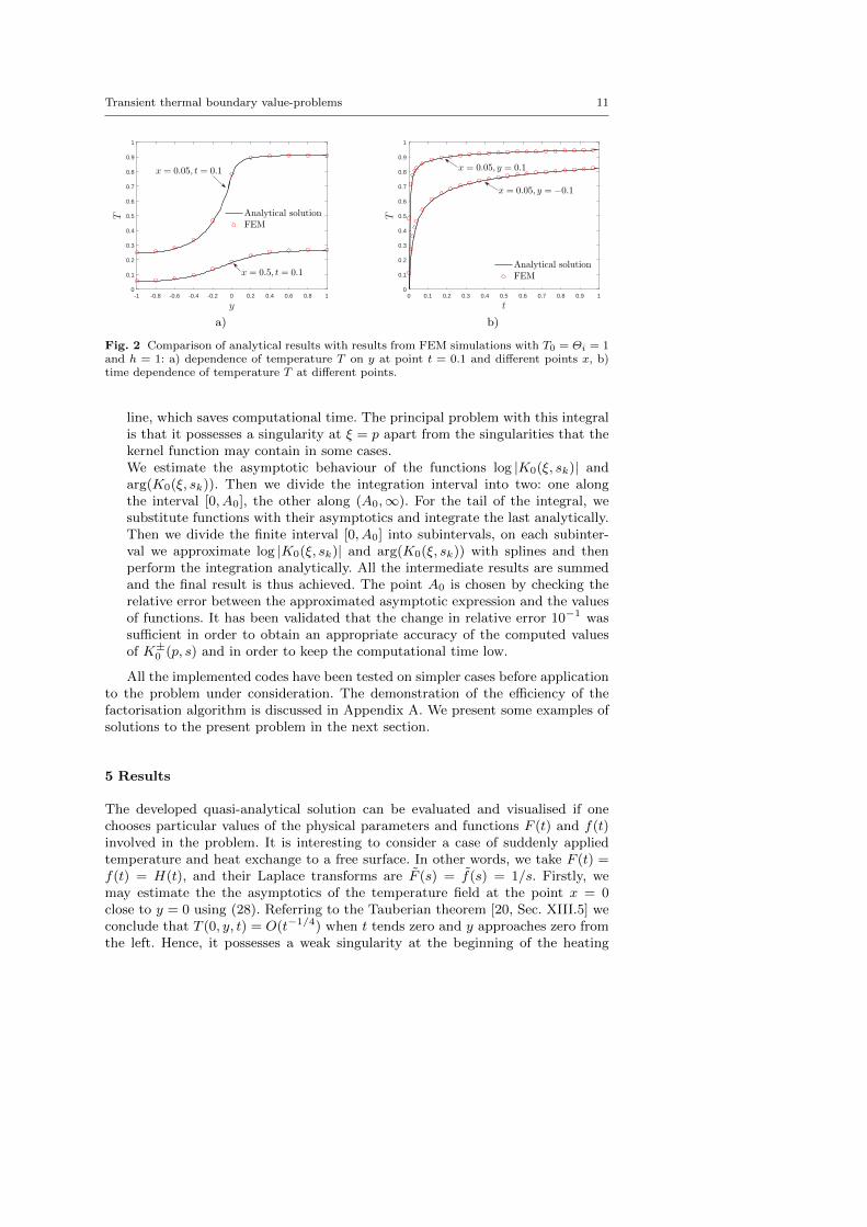
Fig. 2 Comparison of analytical results with results from FEM simulations with T0 = Θi = 1and h = 1: a) dependence of temperature T on y at point t = 0.1 and different points x, b)time dependence of temperature T at different points.

line, which saves computational time. The principal problem with this integralis that it possesses a singularity at ξ = p apart from the singularities that thekernel function may contain in some cases.We estimate the asymptotic behaviour of the functions log |K0(ξ, sk)| andarg(K0(ξ, sk)). Then we divide the integration interval into two: one alongthe interval [0, A0], the other along (A0,∞). For the tail of the integral, wesubstitute functions with their asymptotics and integrate the last analytically.Then we divide the finite interval [0, A0] into subintervals, on each subinter-val we approximate log |K0(ξ, sk)| and arg(K0(ξ, sk)) with splines and thenperform the integration analytically. All the intermediate results are summedand the final result is thus achieved. The point A0 is chosen by checking therelative error between the approximated asymptotic expression and the valuesof functions. It has been validated that the change in relative error 10−1 wassufficient in order to obtain an appropriate accuracy of the computed valuesof K±0 (p, s) and in order to keep the computational time low.

All the implemented codes have been tested on simpler cases before applicationto the problem under consideration. The demonstration of the efficiency of thefactorisation algorithm is discussed in Appendix A. We present some examples ofsolutions to the present problem in the next section.

5 Results

The developed quasi-analytical solution can be evaluated and visualised if onechooses particular values of the physical parameters and functions F (t) and f(t)involved in the problem. It is interesting to consider a case of suddenly appliedtemperature and heat exchange to a free surface. In other words, we take F (t) =f(t) = H(t), and their Laplace transforms are F (s) = f(s) = 1/s. Firstly, wemay estimate the the asymptotics of the temperature field at the point x = 0close to y = 0 using (28). Referring to the Tauberian theorem [20, Sec. XIII.5] weconclude that T (0, y, t) = O(t−1/4) when t tends zero and y approaches zero fromthe left. Hence, it possesses a weak singularity at the beginning of the heating

12 Nikolai Gorbushin et al.

a) b)

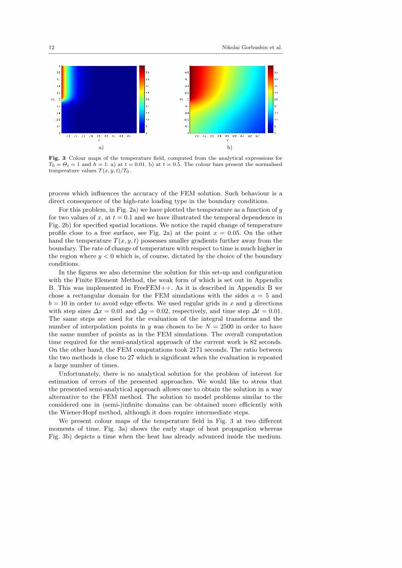
Fig. 3 Colour maps of the temperature field, computed from the analytical expressions forT0 = Θi = 1 and h = 1: a) at t = 0.01, b) at t = 0.5. The colour bars present the normalisedtemperature values T (x, y, t)/T0.

process which influences the accuracy of the FEM solution. Such behaviour is adirect consequence of the high-rate loading type in the boundary conditions.

For this problem, in Fig. 2a) we have plotted the temperature as a function of yfor two values of x, at t = 0.1 and we have illustrated the temporal dependence inFig. 2b) for specified spatial locations. We notice the rapid change of temperatureprofile close to a free surface, see Fig. 2a) at the point x = 0.05. On the otherhand the temperature T (x, y, t) possesses smaller gradients further away from theboundary. The rate of change of temperature with respect to time is much higher inthe region where y < 0 which is, of course, dictated by the choice of the boundaryconditions.

In the figures we also determine the solution for this set-up and configurationwith the Finite Element Method, the weak form of which is set out in AppendixB. This was implemented in FreeFEM++. As it is described in Appendix B wechose a rectangular domain for the FEM simulations with the sides a = 5 andb = 10 in order to avoid edge effects. We used regular grids in x and y directionswith step sizes ∆x = 0.01 and ∆y = 0.02, respectively, and time step ∆t = 0.01.The same steps are used for the evaluation of the integral transforms and thenumber of interpolation points in y was chosen to be N = 2500 in order to havethe same number of points as in the FEM simulations. The overall computationtime required for the semi-analytical approach of the current work is 82 seconds.On the other hand, the FEM computations took 2171 seconds. The ratio betweenthe two methods is close to 27 which is significant when the evaluation is repeateda large number of times.

Unfortunately, there is no analytical solution for the problem of interest forestimation of errors of the presented approaches. We would like to stress thatthe presented semi-analytical approach allows one to obtain the solution in a wayalternative to the FEM method. The solution to model problems similar to theconsidered one in (semi-)infinite domains can be obtained more efficiently withthe Wiener-Hopf method, although it does require intermediate steps.

We present colour maps of the temperature field in Fig. 3 at two differentmoments of time. Fig. 3a) shows the early stage of heat propagation whereasFig. 3b) depicts a time when the heat has already advanced inside the medium.

Transient thermal boundary value-problems 13

Electrode

x

a)

disk drop band

ring array

y

z

b)

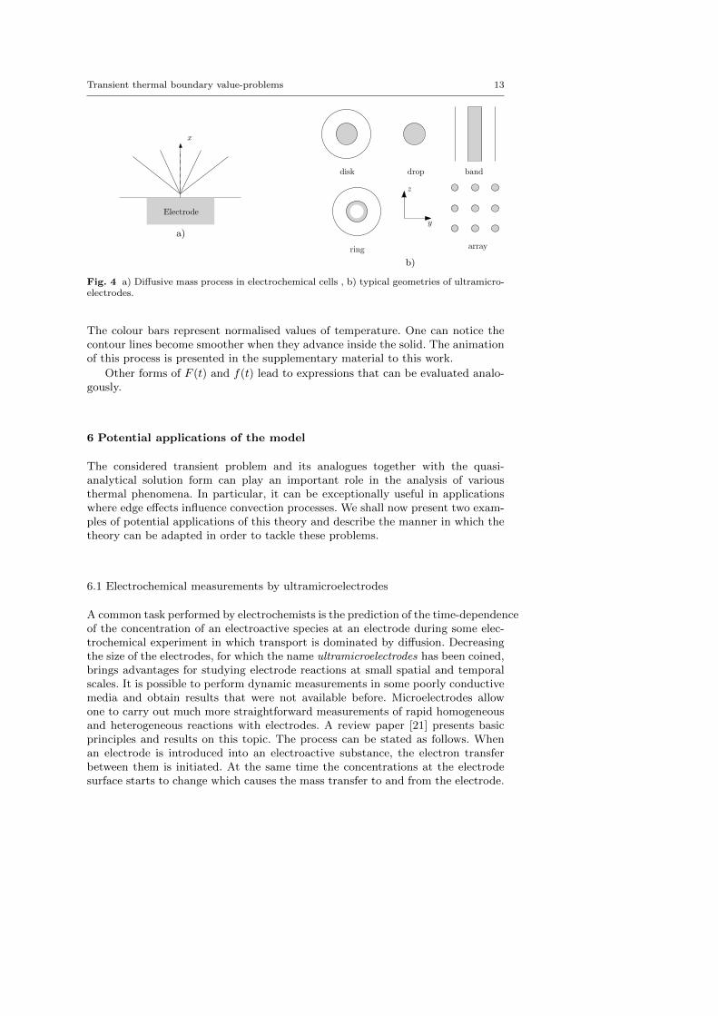
Fig. 4 a) Diffusive mass process in electrochemical cells , b) typical geometries of ultramicro-electrodes.

The colour bars represent normalised values of temperature. One can notice thecontour lines become smoother when they advance inside the solid. The animationof this process is presented in the supplementary material to this work.

Other forms of F (t) and f(t) lead to expressions that can be evaluated analo-gously.

6 Potential applications of the model

The considered transient problem and its analogues together with the quasi-analytical solution form can play an important role in the analysis of variousthermal phenomena. In particular, it can be exceptionally useful in applicationswhere edge effects influence convection processes. We shall now present two exam-ples of potential applications of this theory and describe the manner in which thetheory can be adapted in order to tackle these problems.

6.1 Electrochemical measurements by ultramicroelectrodes

A common task performed by electrochemists is the prediction of the time-dependenceof the concentration of an electroactive species at an electrode during some elec-trochemical experiment in which transport is dominated by diffusion. Decreasingthe size of the electrodes, for which the name ultramicroelectrodes has been coined,brings advantages for studying electrode reactions at small spatial and temporalscales. It is possible to perform dynamic measurements in some poorly conductivemedia and obtain results that were not available before. Microelectrodes allowone to carry out much more straightforward measurements of rapid homogeneousand heterogeneous reactions with electrodes. A review paper [21] presents basicprinciples and results on this topic. The process can be stated as follows. Whenan electrode is introduced into an electroactive substance, the electron transferbetween them is initiated. At the same time the concentrations at the electrodesurface starts to change which causes the mass transfer to and from the electrode.

14 Nikolai Gorbushin et al.

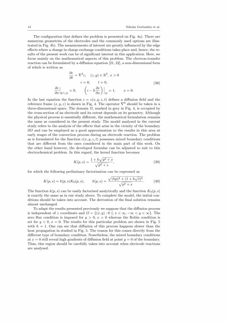
The configuration that defines the problem is presented on Fig. 4a). There arenumerous geometries of the electrodes and the commonly used options are illus-trated in Fig. 4b). The measurements of interest are greatly influenced by the edgeeffects where a change in charge exchange conditions takes place and, hence, the re-sults of the present work can be of significant interest in this application. Here, wefocus mainly on the mathematical aspects of this problem. The electron-transferreaction can be formulated by a diffusion equation [21, 22], a non-dimensional formof which is written as

∂c

∂t= ∇2c, (z, y) ∈ R2, x > 0

c = 0, t = 0,

∂c

∂x

∣∣∣R2\Ω

= 0,

(c− h ∂c

∂x

) ∣∣∣Ω

= 1, x = 0.

(38)

In the last equation the function c = c(x, y, z, t) defines a diffusion field and thereference frame (x, y, z) is shown in Fig. 4. The operator ∇2 should be taken in athree-dimensional space. The domain Ω, marked in grey in Fig. 4, is occupied bythe cross-section of an electrode and its extent depends on its geometry. Althoughthe physical process is essentially different, the mathematical formulation remainsthe same as considered in the present study. The model analysed in the currentstudy refers to the analysis of the effects that arise in the vicinity of the boundary∂Ω and can be employed as a good approximation to the results in this area atearly stages of the convection process during an electrode reaction. The problemas is formulated for the function c(x, y, z, t) possesses mixed boundary conditionsthat are different from the ones considered in the main part of this work. Onthe other hand however, the developed formulae can be adjusted to suit to thiselectrochemical problem. In this regard, the kernel function becomes

K(p, s) =1 + h

√p2 + s√

p2 + s, (39)

for which the following preliminary factorisation can be expressed as

K(p, s) = k(p, s)K0(p, s), k(p, s) =

√(hp)2 + (1 + h

√s)2√

p2 + s. (40)

The function k(p, s) can be easily factorised analytically and the function K0(p, s)is exactly the same as in our study above. To complete the model, the initial con-ditions should be taken into account. The derivation of the final solution remainsalmost unchanged.

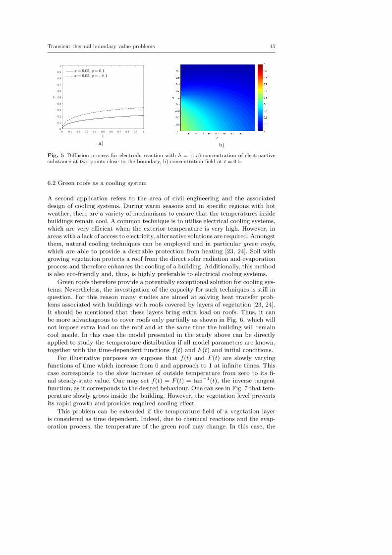
To adapt the results presented previously we suppose that the diffusion processis independent of z coordinate and Ω = (x, y) : 0 ≤ x <∞,−∞ < y <∞. Thezero flux condition is imposed for y > 0, x = 0 whereas the Robin condition isset for y < 0, x = 0. The results for this particular problem are shown in Fig. 5with h = 1. One can see that diffusion of this process happens slower than theheat propagation in studied in Fig. 5. The reason for this comes directly from thedifferent type of boundary condition. Nonetheless, the mixed boundary conditionsat x = 0 still reveal high gradients of diffusion field at point y = 0 of the boundary.Thus, this region should be carefully taken into account when electrode reactionsare analysed.

Transient thermal boundary value-problems 15

0 0.1 0.2 0.3 0.4 0.5 0.6 0.7 0.8 0.9 1

t

0

0.1

0.2

0.3

0.4

0.5

0.6

0.7

0.8

0.9

1

c

x = 0.05, y = 0.1

x = 0.05, y = −0.1

a) b)

Fig. 5 Diffusion process for electrode reaction with h = 1: a) concentration of electroactivesubstance at two points close to the boundary, b) concentration field at t = 0.5.

6.2 Green roofs as a cooling system

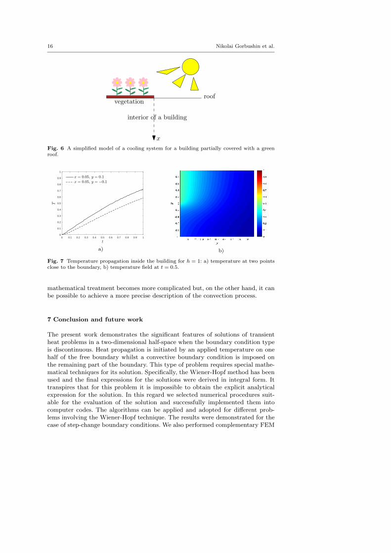
A second application refers to the area of civil engineering and the associateddesign of cooling systems. During warm seasons and in specific regions with hotweather, there are a variety of mechanisms to ensure that the temperatures insidebuildings remain cool. A common technique is to utilise electrical cooling systems,which are very efficient when the exterior temperature is very high. However, inareas with a lack of access to electricity, alternative solutions are required. Amongstthem, natural cooling techniques can be employed and in particular green roofs,which are able to provide a desirable protection from heating [23, 24]. Soil withgrowing vegetation protects a roof from the direct solar radiation and evaporationprocess and therefore enhances the cooling of a building. Additionally, this methodis also eco-friendly and, thus, is highly preferable to electrical cooling systems.

Green roofs therefore provide a potentially exceptional solution for cooling sys-tems. Nevertheless, the investigation of the capacity for such techniques is still inquestion. For this reason many studies are aimed at solving heat transfer prob-lems associated with buildings with roofs covered by layers of vegetation [23, 24].It should be mentioned that these layers bring extra load on roofs. Thus, it canbe more advantageous to cover roofs only partially as shown in Fig. 6, which willnot impose extra load on the roof and at the same time the building will remaincool inside. In this case the model presented in the study above can be directlyapplied to study the temperature distribution if all model parameters are known,together with the time-dependent functions f(t) and F (t) and initial conditions.

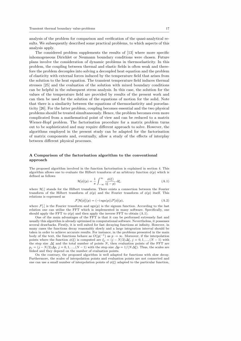
For illustrative purposes we suppose that f(t) and F (t) are slowly varyingfunctions of time which increase from 0 and approach to 1 at infinite times. Thiscase corresponds to the slow increase of outside temperature from zero to its fi-nal steady-state value. One may set f(t) = F (t) = tan−1(t), the inverse tangentfunction, as it corresponds to the desired behaviour. One can see in Fig. 7 that tem-perature slowly grows inside the building. However, the vegetation level preventsits rapid growth and provides required cooling effect.

This problem can be extended if the temperature field of a vegetation layeris considered as time dependent. Indeed, due to chemical reactions and the evap-oration process, the temperature of the green roof may change. In this case, the

16 Nikolai Gorbushin et al.

x

roof

interior of a building

vegetation

Fig. 6 A simplified model of a cooling system for a building partially covered with a greenroof.

0 0.1 0.2 0.3 0.4 0.5 0.6 0.7 0.8 0.9 1

t

0

0.1

0.2

0.3

0.4

0.5

0.6

0.7

0.8

0.9

1

T

x = 0.05, y = 0.1

x = 0.05, y = −0.1

a) b)

Fig. 7 Temperature propagation inside the building for h = 1: a) temperature at two pointsclose to the boundary, b) temperature field at t = 0.5.

mathematical treatment becomes more complicated but, on the other hand, it canbe possible to achieve a more precise description of the convection process.

7 Conclusion and future work

The present work demonstrates the significant features of solutions of transientheat problems in a two-dimensional half-space when the boundary condition typeis discontinuous. Heat propagation is initiated by an applied temperature on onehalf of the free boundary whilst a convective boundary condition is imposed onthe remaining part of the boundary. This type of problem requires special mathe-matical techniques for its solution. Specifically, the Wiener-Hopf method has beenused and the final expressions for the solutions were derived in integral form. Ittranspires that for this problem it is impossible to obtain the explicit analyticalexpression for the solution. In this regard we selected numerical procedures suit-able for the evaluation of the solution and successfully implemented them intocomputer codes. The algorithms can be applied and adopted for different prob-lems involving the Wiener-Hopf technique. The results were demonstrated for thecase of step-change boundary conditions. We also performed complementary FEM

Transient thermal boundary value-problems 17

analysis of the problem for comparison and verification of the quasi-analytical re-sults. We subsequently described some practical problems, to which aspects of thisanalysis apply.

The considered problem supplements the results of [13] where more specificinhomogeneous Dirichlet or Neumann boundary conditions were chosen. Futureplans involve the consideration of dynamic problems in thermoelasticity. In thisproblem, the coupling between thermal and elastic fields is often weak and there-fore the problem decouples into solving a decoupled heat equation and the problemof elasticity with external forces induced by the temperature field that arises fromthe solution to the heat equation. The transient temperature field induces thermalstresses [25] and the evaluation of the solution with mixed boundary conditionscan be helpful in the subsequent stress analysis. In this case, the solution for thevalues of the temperature field are provided by results of the present work andcan then be used for the solution of the equations of motion for the solid. Notethat there is a similarity between the equations of thermoelasticity and poroelas-ticity [26]. For the latter problem, coupling becomes essential and the two physicalproblems should be treated simultaneously. Hence, the problem becomes even morecomplicated from a mathematical point of view and can be reduced to a matrixWiener-Hopf problem. The factorisation procedure for a matrix problem turnsout to be sophisticated and may require different approach to solve. However, thealgorithms employed in the present study can be adapted for the factorisationof matrix components and, eventually, allow a study of the effects of interplaybetween different physical processes.

A Comparison of the factorisation algorithm to the conventionalapproach

The proposed algorithm involved in the function factorisation is explained in section 4. Thisalgorithm allows one to evaluate the Hilbert transform of an arbitrary function φ(p) which isdefined as follows

H[φ](p) =1

π

∫ ∞−∞

φ(ξ)

(ξ − p)dξ, (A.1)

where H[.] stands for the Hilbert transform. There exists a connection between the Fouriertransform of the Hilbert transform of φ(p) and the Fourier transform of φ(p) itself. Thisrelations is expressed as

F [H[φ]](p) = (−i sgn(p))F [φ](p), (A.2)

where F [.] is the Fourier transform and sgn(p) is the signum function. According to the lastrelation one can utilise the FFT which is implemented in many software. Specifically, oneshould apply the FFT to φ(p) and then apply the inverse FFT to obtain (A.1).

One of the main advantages of the FFT is that it can be performed extremely fast andusually this algorithm is already optimised in computational software. Nevertheless, it possessesseveral drawbacks. Firstly, it is well suited for fast decaying functions at infinity. However, inmany cases the functions decay reasonably slowly and a large integration interval should betaken in order to achieve accurate results. For instance, in the problems presented in the mainbody of the text, the functions behave as O(|p|−1) as p → ∞. Moreover, if the interpolationpoints where the function φ(ξ) is computed are ξj = (j − N/2)∆ξ, j = 0, 1, ..., (N − 1) withthe step size ∆ξ and the total number of points N , then evaluation points of the FFT arepj = (j −N/2)∆p, j = 0, 1, ..., (N − 1) with the step size ∆p = 1/(N∆ξ). Thus, the scales arelinked and they depend on the number of evaluation points.

On the contrary, the proposed algorithm is well adapted for functions with slow decay.Furthermore, the scales of interpolation points and evaluation points are not connected andone can use a small number of interpolation points of φ(ξ) adapted to the particular function,

18 Nikolai Gorbushin et al.

0 2 4 6 8 10 12 14 16 18 20

p

10-7

10-6

10-5

10-4

10-3

10-2

RelativeError

FFT-based algorithm

This work

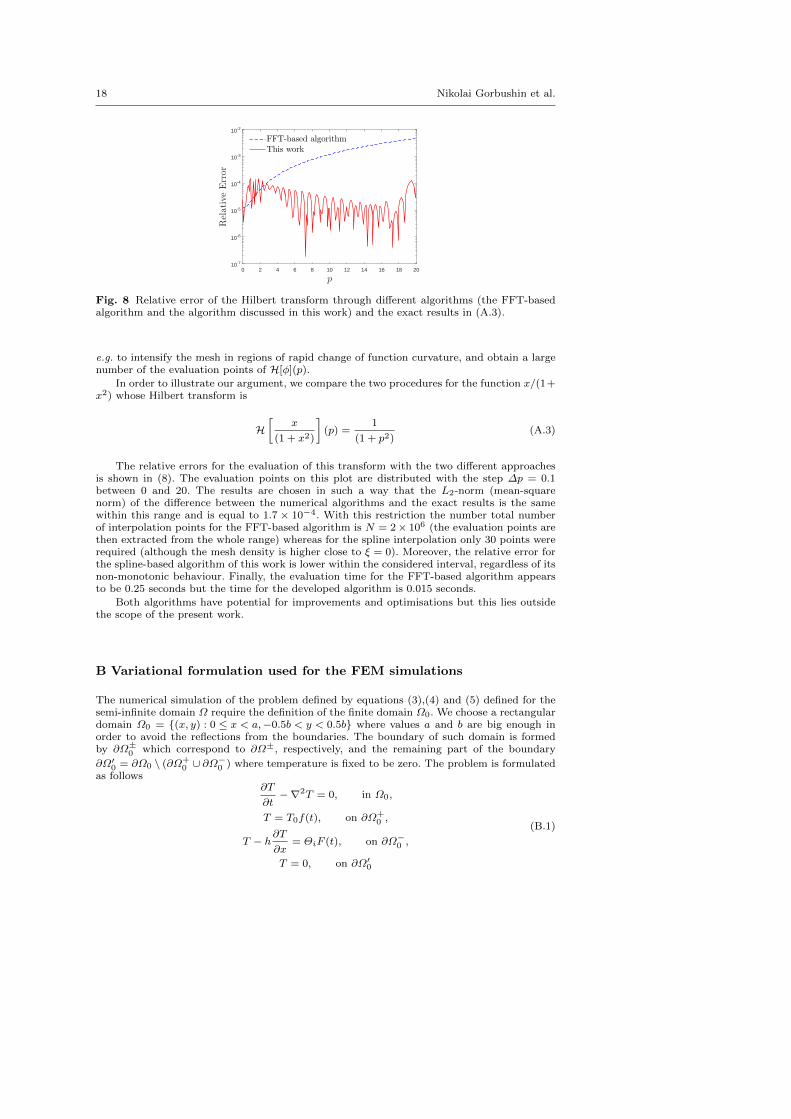
Fig. 8 Relative error of the Hilbert transform through different algorithms (the FFT-basedalgorithm and the algorithm discussed in this work) and the exact results in (A.3).

e.g. to intensify the mesh in regions of rapid change of function curvature, and obtain a largenumber of the evaluation points of H[φ](p).

In order to illustrate our argument, we compare the two procedures for the function x/(1+x2) whose Hilbert transform is

H[

x

(1 + x2)

](p) =

1

(1 + p2)(A.3)

The relative errors for the evaluation of this transform with the two different approachesis shown in (8). The evaluation points on this plot are distributed with the step ∆p = 0.1between 0 and 20. The results are chosen in such a way that the L2-norm (mean-squarenorm) of the difference between the numerical algorithms and the exact results is the samewithin this range and is equal to 1.7 × 10−4. With this restriction the number total numberof interpolation points for the FFT-based algorithm is N = 2× 106 (the evaluation points arethen extracted from the whole range) whereas for the spline interpolation only 30 points wererequired (although the mesh density is higher close to ξ = 0). Moreover, the relative error forthe spline-based algorithm of this work is lower within the considered interval, regardless of itsnon-monotonic behaviour. Finally, the evaluation time for the FFT-based algorithm appearsto be 0.25 seconds but the time for the developed algorithm is 0.015 seconds.

Both algorithms have potential for improvements and optimisations but this lies outsidethe scope of the present work.

B Variational formulation used for the FEM simulations

The numerical simulation of the problem defined by equations (3),(4) and (5) defined for thesemi-infinite domain Ω require the definition of the finite domain Ω0. We choose a rectangulardomain Ω0 = (x, y) : 0 ≤ x < a,−0.5b < y < 0.5b where values a and b are big enough inorder to avoid the reflections from the boundaries. The boundary of such domain is formedby ∂Ω±0 which correspond to ∂Ω±, respectively, and the remaining part of the boundary

∂Ω′0 = ∂Ω0 \ (∂Ω+0 ∪ ∂Ω

−0 ) where temperature is fixed to be zero. The problem is formulated

as follows∂T

∂t−∇2T = 0, in Ω0,

T = T0f(t), on ∂Ω+0 ,

T − h∂T

∂x= ΘiF (t), on ∂Ω−0 ,

T = 0, on ∂Ω′0

(B.1)

Transient thermal boundary value-problems 19

Let δT be a trial function of T , the weak formulation of this problem becomes∫Ω0

δT∂T

∂tdV +

∫Ω0

∇ (δT ) · ∇T dV +

∫∂Ω−

0

T −ΘiF (t)

hdS = 0,

T = T0f(t), on ∂Ω+0 , and T = 0, on ∂Ω′0,

(B.2)

where differential elements of surface and volume are denoted by dS and dV respectively, testfunction δT and function T belongs to the spaces S1 and S2 respectively

S1 =f(x, y) ∈ H1(Ω0) : f(x, y) = 0, (x, y) ∈ ∂Ω+

0 ∪ ∂Ω′0

, S2 =

f(x, y) ∈ H1(Ω0)

.

The space H1(Ω0) designates the Sobolev spaces of scalar functions, having square-integrable1st generalized derivatives. For the simulations, we chose a = 5 and b = 10 while the simulationtime range was t = [0, 1]. The border lines were discretised with the element sizes ∆x = 0.05and ∆y = 0.05 in x and y directions, respectively. The time step is ∆t = 0.005 and piecewisecontinuous elements were taken.

Acknowledgements This work has benefited from a French government grant managed byANR within the frame of the national program of Investments for the Future ANR-11- LABX-022-01 (LabEx MMCD project). W.J.P. is grateful to the EPSRC for his fellowship awardEP/L018039/1.

References

1. Almond D, Lau S (1994) Defect sizing by transient thermography. I. An analytical treat-ment. Journal of Physics D: Applied Physics 27(5):1063

2. Maldague X, Marinetti S (1996) Pulse phase infrared thermography. Journal of AppliedPhysics 79(5):2694–2698

3. Caflisch R, Keller J (1981) Quench front propagation. Nuclear Engineering and Design65(1):97–102

4. Levine H (1982) On a mixed boundary value problem of diffusion type. Applied ScientificResearch 39(4):261–276

5. Sahu S, Das P, Bhattacharyya S (2015) Analytical and semi-analytical models of conduc-tion controlled rewetting: a state of the art review. Thermal Science 19(5):1479–1496

6. Satapathy A (2009) Wiener-hopf solution of rewetting of an infinite cylinder with internalheat generation. Heat and Mass Transfer 45(5):651–658

7. Leveque A (1928) Les Lois de la transmission de chaleur par convection. Dunod8. Liu T, Campbell B, Sullivan J (1994) Surface temperature of a hot film on a wall in shear

flow. International Journal of Heat and Mass Transfer 37(17):2809–28149. Wang D, Tarbell J (1993) An approximate solution for the dynamic response of wall

transfer probes. International Journal of Heat and Mass Transfer 36(18):4341–434910. Springer S (1974) The solution of heat-transfer problems by the Wiener-Hopf technique

II. Trailing edge of a hot film. Proc R Soc Lond A 337(1610):395–41211. Springer S, Pedley T (1973) The solution of heat transfer problems by the Wiener-Hopf

technique. I. Leading edge of a hot film. Proc R Soc Lond A 333(1594):347–36212. Noble B (1988) Methods based on the Wiener-Hopf technique for the solution of partial

differential equations. Chelsea Pub Co13. Parnell W, Nguyen VH, Assier R, Naili S, Abrahams I (2016) Transient thermal mixed

boundary value problems in the half-space. Journal on Applied Mathematics (SIAM)76(3):845–866

14. de Hoop A (1959) The surface line source problem. Appl Sci Res B 8(349-356):115. de Hoop A, Oristaglio M (1988) Application of the modified Cagniard technique to tran-

sient electromagnetic diffusion problems. Geophysical Journal 94(3):387–39716. Piccolroaz A, Mishuris G, Movchan A (2009) Symmetric and skew-symmetric weight func-

tions in 2D perturbation models for semi-infinite interfacial cracks. Journal of the Mechan-ics and Physics of Solids 57(9):1657–1682

20 Nikolai Gorbushin et al.

17. Hecht F (2012) New development in FreeFem++. Journal of Numerical Mathematics20(3-4):251–266

18. Schanz M, Antes H (1997) Application of ’operational quadrature methods’ in time domainboundary element methods. Meccanica 32(3):179–186

19. Gorbushin N (2017) Analysis of admissible steady-state fracture processes in discrete lat-tice structures. PhD thesis, Aberystwyth University

20. Feller W (1971) An Introduction to Probability Theory, vol II. New York: John Wiley &Sons

21. Heinze J (1993) Ultramicroelectrodes in electrochemistry. Angewandte Chemie Interna-tional Edition 32(9):1268–1288

22. Rajendran L, Sangaranarayanan M (1999) Diffusion at ultramicro disk electrodes:Chronoamperometric current for steady-state Ec’ reaction using scattering analogue tech-niques. The Journal of Physical Chemistry B 103(9):1518–1524

23. Del Barrio E (1998) Analysis of the green roofs cooling potential in buildings. Energy andbuildings 27(2):179–193

24. Kumar R, Kaushik S (2005) Performance evaluation of green roof and shading for thermalprotection of buildings. Building and Environment 40(11):1505–1511

25. Nowacki W (2013) Thermoelasticity. Elsevier26. Zimmerman R (2000) Coupling in poroelasticity and thermoelasticity. International Jour-

nal of Rock Mechanics and Mining Sciences 37(1-2):79–87