Electromagnetic Transient - Transient Stability Hybrid Simulation

for Electric Power Systems with Converter Interfaced Generation

by

Denise Athaide

A Thesis Presented in Partial Fulfillmentof the Requirements for the Degree

Master of Science

Approved November 2018 by theGraduate Supervisory Committee:

Jiangchao Qin, ChairRaja Ayyanar

Meng Wu

ARIZONA STATE UNIVERSITY

December 2018

ABSTRACT

With the increasing penetration of converter interfaced renewable generation into

power systems, the structure and behavior of the power system is changing, catalyzing

alterations and enhancements in modeling and simulation methods.

This work puts forth a Hybrid Electromagnetic Transient-Transient Stability sim-

ulation method implemented using MATLAB and Simulink, to study power electronic

based power systems. Hybrid Simulation enables detailed, accurate modeling, along

with fast, efficient simulation, on account of the Electromagnetic Transient (EMT)

and Transient Stability (TS) simulations respectively. A critical component of hy-

brid simulation is the interaction between the EMT and TS simulators, established

through a well-defined interface technique, which has been explored in detail. This re-

search focuses on the boundary conditions and interaction between the two simulation

models for optimum accuracy and computational efficiency.

A case study has been carried out employing the proposed hybrid simulation

method. The test case used is the IEEE 9-bus system, modified to integrate it with

a solar PV plant. The validation of the hybrid model with the benchmark full EMT

model, along with the analysis of the accuracy and efficiency, has been performed.

The steady-state and transient analysis results demonstrate that the performance of

the hybrid simulation method is competent. The hybrid simulation technique suitably

captures accuracy of EMT simulation and efficiency of TS simulation, therefore ade-

quately representing the behavior of power systems with high penetration of converter

interfaced generation.

i

ACKNOWLEDGMENTS

I would like to thank my research advisor, Dr. Jiangchao Qin, for giving me

direction and advice throughout my master’s thesis. His knowledge, insight and

guidance have been very valuable to me. My sincere thanks also to the members of

my committee, Dr. Raja Ayyanar and Dr. Meng Wu, for lending me their support

and expertise in reviewing my work. I also appreciate the technical advice given to

me by my colleague Yuntao Zou.

I am also very grateful to my parents, for their unwavering support and for al-

ways believing in me. I would like to express my gratitude to my sister, the rest of

my family, friends and colleagues at ASU, for their motivation, moral support and

continuous encouragement throughout my studies.

Lastly, the student support system and vast opportunities provided by Arizona

State University, have helped me grow as an engineer and as an individual, during

my studies here, for which I am exceedingly grateful.

ii

TABLE OF CONTENTS

Page

LIST OF TABLES . . . . . . . . . . . . . . . . . . . . . . . . . . . . . . . . . . . . . . . . . . . . . . . . . . . . . . . . . vi

LIST OF FIGURES . . . . . . . . . . . . . . . . . . . . . . . . . . . . . . . . . . . . . . . . . . . . . . . . . . . . . . . . vii

CHAPTER

1 INTRODUCTION . . . . . . . . . . . . . . . . . . . . . . . . . . . . . . . . . . . . . . . . . . . . . . . . . . . 1

1.1 Background . . . . . . . . . . . . . . . . . . . . . . . . . . . . . . . . . . . . . . . . . . . . . . . . . . . . 1

1.2 Thesis Objectives . . . . . . . . . . . . . . . . . . . . . . . . . . . . . . . . . . . . . . . . . . . . . . . 2

1.3 Thesis Outline . . . . . . . . . . . . . . . . . . . . . . . . . . . . . . . . . . . . . . . . . . . . . . . . . . 3

2 HYBRID SIMULATION . . . . . . . . . . . . . . . . . . . . . . . . . . . . . . . . . . . . . . . . . . . . . 4

2.1 Simulation Techniques . . . . . . . . . . . . . . . . . . . . . . . . . . . . . . . . . . . . . . . . . . 4

2.1.1 Electromagnetic Transient (EMT) Simulation . . . . . . . . . . . . . . 4

2.1.2 Transient Stability (TS) Simulation . . . . . . . . . . . . . . . . . . . . . . . 5

2.2 Need for Hybrid Simulation . . . . . . . . . . . . . . . . . . . . . . . . . . . . . . . . . . . . . 6

2.3 Introduction to Hybrid Simulation . . . . . . . . . . . . . . . . . . . . . . . . . . . . . . . 7

2.4 History and Current Status of Hybrid Simulation . . . . . . . . . . . . . . . . . 8

3 DEVELOPMENT OF THE PROPOSED HYBRID SIMULATION METHOD

IN MATLAB . . . . . . . . . . . . . . . . . . . . . . . . . . . . . . . . . . . . . . . . . . . . . . . . . . . . . . . . 11

3.1 Advantages of using MATLAB/Simulink for Hybrid Simulation . . . . 11

3.2 Requirements of Hybrid Simulation . . . . . . . . . . . . . . . . . . . . . . . . . . . . . . 12

3.3 Hybrid Simulation Scheme . . . . . . . . . . . . . . . . . . . . . . . . . . . . . . . . . . . . . . 13

4 TRANSIENT STABILITY (TS) MODELING AND SIMULATION . . . . . 16

4.1 Description of the System . . . . . . . . . . . . . . . . . . . . . . . . . . . . . . . . . . . . . . . 16

4.2 Modeling and Simulation of the IEEE 9-Bus System. . . . . . . . . . . . . . . 17

5 ELECTROMAGNETIC TRANSIENT (EMT) MODELING AND SIM-

ULATION . . . . . . . . . . . . . . . . . . . . . . . . . . . . . . . . . . . . . . . . . . . . . . . . . . . . . . . . . . 19

iii

CHAPTER Page

5.1 Description of the System . . . . . . . . . . . . . . . . . . . . . . . . . . . . . . . . . . . . . . . 19

5.2 Modeling of the Solar PV Array . . . . . . . . . . . . . . . . . . . . . . . . . . . . . . . . . 20

5.3 Modeling of the Inverter with Control . . . . . . . . . . . . . . . . . . . . . . . . . . . . 22

5.4 Modeling of the Filter and Network Interconnection . . . . . . . . . . . . . . . 23

6 INTERFACE BETWEEN TS AND EMT SIMULATIONS . . . . . . . . . . . . . 25

6.1 Network Partition and Selection of Interface Bus . . . . . . . . . . . . . . . . . . 25

6.2 Equivalent Models and Selection of Exchanged Data . . . . . . . . . . . . . . 26

6.3 Data Extraction . . . . . . . . . . . . . . . . . . . . . . . . . . . . . . . . . . . . . . . . . . . . . . . . 28

6.4 Interaction Protocol. . . . . . . . . . . . . . . . . . . . . . . . . . . . . . . . . . . . . . . . . . . . . 29

6.5 Communication . . . . . . . . . . . . . . . . . . . . . . . . . . . . . . . . . . . . . . . . . . . . . . . . . 30

6.6 Plotting . . . . . . . . . . . . . . . . . . . . . . . . . . . . . . . . . . . . . . . . . . . . . . . . . . . . . . . . 31

7 TESTING AND VALIDATION . . . . . . . . . . . . . . . . . . . . . . . . . . . . . . . . . . . . . . . 33

7.1 Steady-State Analysis . . . . . . . . . . . . . . . . . . . . . . . . . . . . . . . . . . . . . . . . . . . 34

7.2 Transient Analysis . . . . . . . . . . . . . . . . . . . . . . . . . . . . . . . . . . . . . . . . . . . . . . 36

7.2.1 Single-Phase Line-to-Ground Fault . . . . . . . . . . . . . . . . . . . . . . . . 36

7.2.2 Interface Time Step Analysis . . . . . . . . . . . . . . . . . . . . . . . . . . . . . 40

7.2.3 Variation in Solar Irradiance . . . . . . . . . . . . . . . . . . . . . . . . . . . . . . 43

8 CONCLUSIONS AND FUTURE WORK . . . . . . . . . . . . . . . . . . . . . . . . . . . . . 49

8.1 Conclusions . . . . . . . . . . . . . . . . . . . . . . . . . . . . . . . . . . . . . . . . . . . . . . . . . . . . 49

8.2 Future Work . . . . . . . . . . . . . . . . . . . . . . . . . . . . . . . . . . . . . . . . . . . . . . . . . . . 50

REFERENCES . . . . . . . . . . . . . . . . . . . . . . . . . . . . . . . . . . . . . . . . . . . . . . . . . . . . . . . . . . . . 51

APPENDIX

A WSCC IEEE 9-Bus System Data . . . . . . . . . . . . . . . . . . . . . . . . . . . . . . . . . . . . . 55

B Solar PV Panel Datasheet Specification . . . . . . . . . . . . . . . . . . . . . . . . . . . . . . . 58

iv

CHAPTER Page

C MATLAB Code for EMT-TS Interface . . . . . . . . . . . . . . . . . . . . . . . . . . . . . . . . 60

v

LIST OF TABLES

Table Page

2.1 Comparison between EMT and TS Simulation Methods. . . . . . . . . . . . . . . 6

4.1 Summary of Load Flow Results . . . . . . . . . . . . . . . . . . . . . . . . . . . . . . . . . . . . . 18

7.1 Simulation Parameters . . . . . . . . . . . . . . . . . . . . . . . . . . . . . . . . . . . . . . . . . . . . . 33

7.2 Error Evaluation between the Hybrid Simulation EMT Subsystem and

TS Subsystem RMS Currents and Voltages at Bus 3 during Steady State 36

A.1 Synchronous Generator Data . . . . . . . . . . . . . . . . . . . . . . . . . . . . . . . . . . . . . . . 56

A.2 Load Data. . . . . . . . . . . . . . . . . . . . . . . . . . . . . . . . . . . . . . . . . . . . . . . . . . . . . . . . . 57

A.3 Line Data . . . . . . . . . . . . . . . . . . . . . . . . . . . . . . . . . . . . . . . . . . . . . . . . . . . . . . . . . 57

A.4 Transformer Data . . . . . . . . . . . . . . . . . . . . . . . . . . . . . . . . . . . . . . . . . . . . . . . . . . 57

B.1 Electrical Specifications of Jakson Solar PV Module at STC . . . . . . . . . . 59

vi

LIST OF FIGURES

Figure Page

3.1 EMT-TS Hybrid Simulation Scheme in MATLAB/Simulink . . . . . . . . . . . 15

4.1 Single-Line Diagram of the WSCC IEEE 9-Bus System . . . . . . . . . . . . . . . 16

4.2 Transient Stability Simulation Block Diagram in Simulink . . . . . . . . . . . . 18

5.1 Circuit Diagram of Solar PV Inverter System . . . . . . . . . . . . . . . . . . . . . . . . 19

5.2 Electromagnetic Transient Simulation High-Level Block Diagram in

Simulink . . . . . . . . . . . . . . . . . . . . . . . . . . . . . . . . . . . . . . . . . . . . . . . . . . . . . . . . . . 20

5.3 EMT Solar PV Array Implementation in Simulink . . . . . . . . . . . . . . . . . . . . 20

5.4 EMT Inverter Implementation in Simulink . . . . . . . . . . . . . . . . . . . . . . . . . . . 22

5.5 EMT Current Controller Implementation in Simulink . . . . . . . . . . . . . . . . . 22

5.6 EMT Filter and Network Interconnection Implementation in Simulink . 24

6.1 EMT-TS Hybrid Simulation Interface in MATLAB/Simulink . . . . . . . . . . 25

6.2 Data Extraction . . . . . . . . . . . . . . . . . . . . . . . . . . . . . . . . . . . . . . . . . . . . . . . . . . . 28

6.3 Serial Interaction Protocol . . . . . . . . . . . . . . . . . . . . . . . . . . . . . . . . . . . . . . . . . . 29

6.4 Communication . . . . . . . . . . . . . . . . . . . . . . . . . . . . . . . . . . . . . . . . . . . . . . . . . . . . 31

6.5 Procedure for Plotting . . . . . . . . . . . . . . . . . . . . . . . . . . . . . . . . . . . . . . . . . . . . . 32

7.1 Instantaneous Voltage at Bus 3 (Interface Bus) during Steady State . . . 34

7.2 Instantaneous Current through Bus 3 (Interface Bus) during Steady

State . . . . . . . . . . . . . . . . . . . . . . . . . . . . . . . . . . . . . . . . . . . . . . . . . . . . . . . . . . . . . . 35

7.3 Comparison of Simulation Speed . . . . . . . . . . . . . . . . . . . . . . . . . . . . . . . . . . . . 36

7.4 Instantaneous Voltage at Bus 3 (Interface Bus) during a SLG Fault at

Bus 4 . . . . . . . . . . . . . . . . . . . . . . . . . . . . . . . . . . . . . . . . . . . . . . . . . . . . . . . . . . . . . 37

7.5 Instantaneous Current through Bus 3 (Interface Bus) during a SLG

Fault at Bus 4 . . . . . . . . . . . . . . . . . . . . . . . . . . . . . . . . . . . . . . . . . . . . . . . . . . . . . 38

7.6 Power at Bus 3 (Interface Bus) during an SLG Fault at Bus 4 . . . . . . . . . 39

vii

CHAPTER Page

7.7 Effect of Interface Time Step Variation on Simulation Time . . . . . . . . . . . 40

7.8 Instantaneous Voltage at Bus 3 (Interface Bus) during a SLG Fault at

Bus 4 for a Range of Interface Time Steps . . . . . . . . . . . . . . . . . . . . . . . . . . . 41

7.9 Instantaneous Current through Bus 3 (Interface Bus) during a SLG

Fault at Bus 4 for a Range of Interface Time Steps . . . . . . . . . . . . . . . . . . . 41

7.10 Phasor Voltage at Bus 3 (Interface Bus) during a SLG Fault at Bus 4

for a Range of Interface Time Steps . . . . . . . . . . . . . . . . . . . . . . . . . . . . . . . . . 42

7.11 Phasor Current through Bus 3 (Interface Bus) during a SLG Fault at

Bus 4 for a Range of Interface Time Steps . . . . . . . . . . . . . . . . . . . . . . . . . . . 42

7.12 Instantaneous Voltage at Bus 3 (Interface Bus) during a Decrease in

Solar Irradiance . . . . . . . . . . . . . . . . . . . . . . . . . . . . . . . . . . . . . . . . . . . . . . . . . . . . 44

7.13 Instantaneous Current through Bus 3 (Interface Bus) during a Decrease

in Solar Irradiance . . . . . . . . . . . . . . . . . . . . . . . . . . . . . . . . . . . . . . . . . . . . . . . . . 45

7.14 Phasor Voltage and Current at Bus 3 (Interface Bus) during a Decrease

in Solar Irradiance . . . . . . . . . . . . . . . . . . . . . . . . . . . . . . . . . . . . . . . . . . . . . . . . . 46

7.15 Phasor Voltage and Current at Bus 7 during a Decrease in Solar Irra-

diance. . . . . . . . . . . . . . . . . . . . . . . . . . . . . . . . . . . . . . . . . . . . . . . . . . . . . . . . . . . . . 47

7.16 Power at Bus 3 (Interface Bus) during a Decrease in Solar Irradiance . . 48

B.1 I-V Curve Variation with Irradiance . . . . . . . . . . . . . . . . . . . . . . . . . . . . . . . . . 59

viii

Chapter 1

INTRODUCTION

1.1 Background

The use of fossil fuels, along with their increasing rate of depletion, is causing

alarming levels of degradation to the environment. On the other hand, renewable

energy is a completely clean and freely available resource.

However, they do pose a number of challenges. References [1], [2], [3], [4] and

[5] elaborate on some of these challenges arising in power systems due to renewable

energy integration. Renewable energy sources most often do not generate electricity

in the same form that it can be utilized, transmitted or distributed. Power electronic

converters are required for DC/AC conversion, step-up or step-down of voltages and

power conditioning. As more and more distributed generation is being integrated

with the grid, and more loads are being driven by electronic drives, the structure and

behavior of power systems is changing, with a high fraction of the generation as well

as loads being interfaced through power converters.

Such power electronic equipment is best modeled using electromagnetic transient

(EMT) simulation, to represent the converters in full detail, including the precise, fast

switching operations and non-linear nature. However, these programs also require

large computation times. On the other hand, transient stability analysis programs

are suitable for modeling the electromechanical transients and hence are extensively

used for assessing the rotor angle stability of power networks with a much smaller

computation time, but not adequate to represent the dynamic response under many

conditions [6, 7].

1

A simulation method, called Hybrid Simulation, is explored in this thesis. This

technique tries to capture the advantages of both EMT and TS simulations, in order

to represent the behavior of a system, with a large number of distributed generators

(DGs), both accurately and efficiently.

MATLAB, being flexible, user-friendly, commonly used and easily accessible, would

be an ideal platform on which to perform hybrid simulation. With this goal, a hybrid

simulation process has been developed using MATLAB and Simulink. This hybrid

simulation method has been tested and validated using the IEEE 9-bus system.

1.2 Thesis Objectives

The contributions of this research are outlined below:

• Development of an effective hybrid simulation method to study networks with

penetration of converter interfaced generation and loads

• Implementation of hybrid simulation in MATLAB/Simulink

• Proposal of an improved interface algorithm or method between the two simu-

lations (EMT and TS) for Hybrid Simulation in MATLAB environment

• Development of a MATLAB-based communication framework for the interac-

tion between the EMT and TS models

• Validation of the effectiveness of the proposed simulation technique

• Analysis and comparison of the boundary conditions (solvers, time steps, inter-

action protocol and exchanged variables) used and their impact on simulation

performance, in terms of accuracy and speed or efficiency

• Creation of a flexible, user-friendly and easily accessible hybrid simulation

scheme

2

1.3 Thesis Outline

This thesis is organized as follows:

• Chapter 1 discusses the motivation behind this research, including the impacts

and challenges of converter interfaced generation, along with the background

and previous work. The main contributions of this thesis are outlined as well.

• Chapter 2 gives a broad overview of the simulation techniques widely in use. It

addresses the need for hybrid simulation and introduces the hybrid simulation

technique.

• Chapter 3 summarizes the proposed hybrid simulation method developed in

MATLAB-Simulink and highlights its salient features.

• Chapter 4 describes the transient stability modeling and simulation techniques

in MATLAB-Simulink for the particular network under study.

• Chapter 5 explains the EMT solar PV inverter system model developed and its

simulation in MATLAB-Simulink.

• Chapter 6 presents the interfacing algorithm between the EMT and Phasor

simulations and its implementation in detail.

• Chapter 7 provides a comprehensive validation of the proposed hybrid simula-

tion method for the system under consideration, for a range of conditions. In

addition, an analysis of the simulation performance is carries out, for a variation

in the interface time step.

• Chapter 8 summarizes the research work and contributions of this thesis, while

giving direction to future work.

3

Chapter 2

HYBRID SIMULATION

2.1 Simulation Techniques

In power system studies, depending on the type of study to be conducted, a

suitable simulation tool must be selected [7].

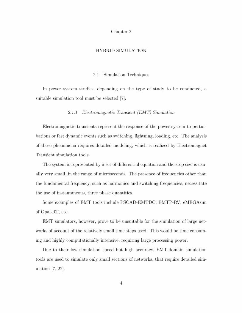
2.1.1 Electromagnetic Transient (EMT) Simulation

Electromagnetic transients represent the response of the power system to pertur-

bations or fast dynamic events such as switching, lightning, loading, etc. The analysis

of these phenomena requires detailed modeling, which is realized by Electromagnet

Transient simulation tools.

The system is represented by a set of differential equation and the step size is usu-

ally very small, in the range of microseconds. The presence of frequencies other than

the fundamental frequency, such as harmonics and switching frequencies, necessitate

the use of instantaneous, three phase quantities.

Some examples of EMT tools include PSCAD-EMTDC, EMTP-RV, eMEGAsim

of Opal-RT, etc.

EMT simulators, however, prove to be unsuitable for the simulation of large net-

works of account of the relatively small time steps used. This would be time consum-

ing and highly computationally intensive, requiring large processing power.

Due to their low simulation speed but high accuracy, EMT-domain simulation

tools are used to simulate only small sections of networks, that require detailed sim-

ulation [7, 22].

4

2.1.2 Transient Stability (TS) Simulation

Electromechanical Transient simulation and transient stability studies focus on

analyzing the ability of the power system to remain in synchronism and maintain

voltage and frequency, following a small or large disturbance and analyze the dynamic

behavior of the system. As transient stability simulation captures slow dynamics,

these studies are carried out during the planning, operation, control and analysis of

power systems.

In transient stability analysis, the power system under consideration is represented

nonlinear algebraic equations. In power networks, this usually involves solving a large

number of equations. It can be assumed that the fundamental power frequency of

50Hz or 60Hz is maintained throughout the system under most conditions. Phasors

of the electrical quantities are therefore sufficient to model these system. Transient

stability simulators generally use comparatively large integration timesteps, in the

range of milliseconds, to run efficiently.

Some examples of TS tools include OpenDSS, PSS/e, PSLF, PowerWorld, ePHA-

SORsim of Opal-RT, ETAP, etc. On account of their speed, Phasor-domain simu-

lation tools are used to simulate large-scale networks. On the other hand, the large

timesteps used in TS programs prevent them from representing non-linear elements

such as power electronic converters, FACTS devices and HVDC equipment, insulation

coordination as well as fast dynamics in detail in the power system [7, 22].

5

The key points of comparison between the two simulation techniques has been

summarized below, in Table 2.1.

Table 2.1: Comparison between EMT and TS Simulation Methods

2.2 Need for Hybrid Simulation

Today, as a large number of renewable energy distributed generators (DGs) are

being integrated into distribution system, it is important to represent their impacts

on the network. The presently used transient stability simulation technique is not suf-

ficient to portray the complex behavior and dynamics of these systems [7]. Their true

6

dynamics are best represented accurately by electromagnetic transient simulation.

This would however reduce the simulation efficiency drastically for a large system.

For instance, TS simulation is suitable for the analysis of phenomena such as

voltage fluctuation, flicker, voltage regulation, etc., occurring due to DG penetration

in power systems. However, to study DG impacts on power quality such as harmonic

distortion, resonance and voltage sag, EMT studies with high accuracy and small time

steps, representing high frequency dynamics, are required. Moreover, EMT simulation

is also important for analyzing the operation and control of power electronic converters

[7]. Since the impacts of renewable energy penetration impacts vary over a wide range

of time scales, depending on the whether slow or fast dynamics are to be studied, TS

simulation or EMT simulation must be chosen accordingly.

EMT simulation offers the required accuracy, while, TS simulation is computa-

tionally efficient. Therefore, a combined hybrid simulation that could incorporate the

advantages of both types of tools is the need of the hour.

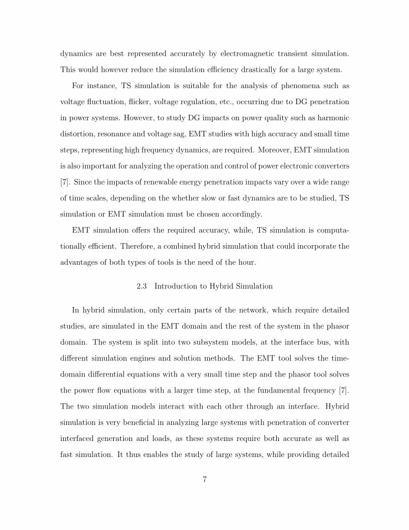
2.3 Introduction to Hybrid Simulation

In hybrid simulation, only certain parts of the network, which require detailed

studies, are simulated in the EMT domain and the rest of the system in the phasor

domain. The system is split into two subsystem models, at the interface bus, with

different simulation engines and solution methods. The EMT tool solves the time-

domain differential equations with a very small time step and the phasor tool solves

the power flow equations with a larger time step, at the fundamental frequency [7].

The two simulation models interact with each other through an interface. Hybrid

simulation is very beneficial in analyzing large systems with penetration of converter

interfaced generation and loads, as these systems require both accurate as well as

fast simulation. It thus enables the study of large systems, while providing detailed

7

dynamic information about them, which is impossible to achieve with either EMT or

TS simulation tools alone.

Hybrid simulation however poses a number of challenges, which are explored in

detail in this work.

2.4 History and Current Status of Hybrid Simulation

A number of progressive hybrid simulation techniques have been proposed in lit-

erature up to date.

The concept of Hybrid Simulation was first introduced in references [8], [9] and

[10], for the purpose of High Voltage Direct Current (HVDC) converter studies in

1981.

References [11], [12] and [13] focus on progressively incorporating EMT models

of nonlinear elements such as flexible AC transmission (FACTS) and HVDC systems

into traditional TS simulation programs. They integrate a static VAR compensator

(SVC), modeled at the device level, concentrating on interaction protocol and other

interface requirements to be taken into consideration.

Reference [22] classifies and addresses the main requirements and challenges faced

in interfacing EMT and TS simulators for hybrid simulation. It also proposes an

integrated EMT-TS simulation using frequency adaptive modeling and simulation,

including frequency shifting and companion models.

Reference [19] puts forward a relaxation approach applied to time interpolation

and phasor extraction. It also summarizes the main equivalent models or boundary

conditions used in hybrid simulation literature.

In reference [6], an open-source hybrid simulation tool, OpenHybridSim, is de-

veloped. It uses InterPSS for TS simulation and can be integrated with various

EMT simulators, with a socket communication based interface. Reference [14] em-

8

ploys this tool for fault-induced delayed voltage recovery (FIDVR) studies, using

PSCAD/EMTDC and InterPSS. A combined interaction protocol with automatic

switching as well as multi-port three-phase Thvenin equivalent was also introduced

in the tool.

References [7] and [16] introduce an open-source hybrid simulation tool, using

the OpenDSS TS simulator and a Matlab-scripted EMT simulator interfaced with a

component object model (COM) server. It is designed to perform solar PV impact

studies in distribution systems. Reference [17] demonstrates the tools ability to per-

form islanding detection studies in such distribution networks. Reference [15] extends

this tool to use Python-scripted EMT simulation instead of Matlab scripts.

Reference [20] proposes a distributed hybrid simulation method, with a combined

interaction protocol and a two-level Schur complement interfacing technique. In ref-

erence [21], a dynamic phasor-based interface model (DPIM) has been developed, to

study the interactions between HVDC systems and the AC grid.

In reference [23], an EMT modular multilevel converter (MMC) based HVDC sys-

tem in in PSCAD/EMTDC is combined with the AC grid programmed in C language

as a user-defined model in PSCAD.

An implicitly-coupled solution method is presented in reference [24], where the

EMT and TS equations are combined and solved simultaneously.

Reference [25] focuses on the application of hybrid simulation to VSC-HVDC

systems and techniques to improve accuracy.

The above mentioned hybrid simulation implementations use EMT and TS off-line

software.

OPAL-RT’s real-time simulation tools primarily include ePHASORsim, HYPER-

SIM, eMEGAsim and eFPGAsim, suitable for simulation time-steps ranging from

milliseconds to nanoseconds and large to small model sizes respectively [27]. The RT-

9

LAB suits simulation environment has the potential to run two types of simulations,

namely The TS simulator ePHASORsim and the EMT simulator eMEGAsim, in one

working model, thus enabling hybrid simulation [26, 28]. Reference [30] explains this

capability and the interfacing method in detail. Reference [29] explores parallelization

techniques for real-time simulation and the suitability of hybrid simulation, using the

OPAL-RT real time digital simulator, for islanding detection.

10

Chapter 3

DEVELOPMENT OF THE PROPOSED HYBRID SIMULATION METHOD IN

MATLAB

3.1 Advantages of using MATLAB/Simulink for Hybrid Simulation

As seen in Chapter 2, hybrid simulation methods and tools have been developed

which combines two different software to run the EMT and TS simulations separately.

However, there is are complexities, inconsistencies and inaccuracies involved when

interfacing two different simulation platforms. There lacks a hybrid simulation tool

or methodology that can run the entire simulation on a single simulation platform.

Matlab/Simulink has the capacity to run EMT as well as phasor domain simula-

tions. It serves as a suitable platform to integrate both simulations to build a hybrid

simulation. Hybrid simulation has not yet been implemented in Matlab alone. There

are potentially added capabilities arising since a single simulation software is being

employed.

This work puts forth a Hybrid EMT-TS simulation method in MATLAB, to study

power electronic based power systems. The entire simulation is run on a single simula-

tion platform, MATLAB. The purpose of selecting Matlab over individual softwares

optimized for TS and EMT simulation is to deliver a more general simulation en-

vironment, to test the hybrid simulation algorithm and procedure, particularly the

interface between the TS and EMT simulations. It also ensures improved and less

complex interfacing, communication and compatibility between the EMT and TS

simulation models.

11

3.2 Requirements of Hybrid Simulation

In hybrid simulation, only certain parts of the network, which require detailed

studies, are simulated in the EMT domain and the rest of the system is simulated in

the phasor domain. The system is split into two subsystem models, at the interface

bus and the two simulation models interact with each other through an interface.

In order to carry out hybrid simulation of a given system, the basic components

listed below should be in place:

1. A simulation model of the power network in the Phasor or TS domain

2. A simulation model of the portion of the system requiring detailed analysis in

the EMT domain

3. An interface between the two simulation models, which considers the following:

(a) Network Partitioning

(b) Selection of the Interface Bus

(c) Equivalents Models of the Detailed and External Systems

(d) Selection of the Exchanged Data Variables

(e) Data Extraction

(f) Interaction Protocol

(g) Communication

[6, 15, 19, 22]

12

3.3 Hybrid Simulation Scheme

The flow chart for running the proposed hybrid simulation method is shown in

Fig. 3.1. The following steps have been followed:

1. Select the power network to be studied

2. Split the power system under study into the TS-modeled external network and

EMT-modeled detailed system for the hybrid simulation

3. Set the interface conditions such as the boundary bus, interaction protocol, data

exchange time step, simulation duration, etc.

4. Initialize the TS and EMT simulation models

5. Measure the Thevenin equivalent impedance of the network, as seen from the

interface bus, in the TS model

6. Solve the power flow in the TS simulation model

7. Run the TS simulation for ∆Tts seconds

8. Convert the phasor quantities to instantaneous waveforms by Time Interpola-

tion

9. Transfer the required instantaneous quantities to the EMT model and update

the TS equivalent model in the EMT simulation model

10. Run the EMT simulation for ∆Tts seconds with a time step of ∆Temt seconds

11. Measure the real and reactive power at the interface bus in the EMT model

12. Convert the instantaneous waveforms to phasor quantities by Phasor Extraction

13

13. Transfer the required phasors to the TS model and update the EMT equivalent

model in the TS simulation model

14. Repeat steps 6 to 14 until the simulation end time is reached

15. Stop the Hybrid Simulation

16. Plot the desired results

14

Figure 3.1: EMT-TS Hybrid Simulation Scheme in MATLAB/Simulink

15

Chapter 4

TRANSIENT STABILITY (TS) MODELING AND SIMULATION

Figure 4.1: Single-Line Diagram of the WSCC IEEE 9-Bus System

4.1 Description of the System

The network being considered in this work is the WSCC IEEE 9-bus test system,

also known as P.M Anderson 9-bus [40]. It represents a simple approximation of the

Western System Coordinating Council (WSCC) to an equivalent system with nine

16

buses and three generators. This test system includes three two-winding transformers,

six transmission lines and three loads. The base voltage levels are 13.8 kV, 16.5 kV,

18 kV, and 230 kV. The single-line diagram of the WSCC 9-bus case is shown in

Fig. 4.1. The key information of this test case has been elaborated in more detail in

Appendix A [36, 37, 38].

In this study, the WSCC 9-bus system has been modified to replace the syn-

chronous generator at bus 3 by a solar photovoltaic plant with a capacity to generate

maximum 85 MW of power.

It must be noted that the real merits of hybrid simulation are striking in much

larger systems. However, in order to develop the hybrid simulation framework in

MATLAB and enable feasible validation, a 9-bus system has been employed in this

work.

4.2 Modeling and Simulation of the IEEE 9-Bus System

Simulink has been used to run the power flow solution and dynamic simulation of

the network in the Phasor domain [35, 39]. The implementation of this modified 9-bus

system in the TS domain in Simulink is depicted in Fig. 4.2. The Powergui block

offers the ability to set the solution method to ’Phasor’. There are nine Load Flow

Bus blocks in the model, defining the bus locations, parameters to solve the load flow

and base voltages at their respective buses. The Load Flow tool of Powergui is used

to compute the voltage, real power and reactive power flows at each bus using the

Newton-Raphson method, initialize the network and start the simulation in steady-

state. In this case, positive-sequence load flow is applied to the three-phase system

[32].

Every block that can be potentially used in Load Flow studies has a Load Flow

tab, where the Load Flow parameters are specified. The loads are modeled using the

17

Figure 4.2: Transient Stability Simulation Block Diagram in Simulink

Constant PQ Three Phase Parallel RLC load blocks, where real and reactive powers

are specified. The solar PV plant at bus 3 is represented by the EMT equivalent model

in the TS simulation model, the PQ type Three-Phase Source block, as explained in

detail in Chapter 6. The generators at buses 1 and 2 are implemented using Three-

Phase Source blocks. The Three-Phase Transformer and Three-Phase PI Section Line

blocks are used to model the transformers and transmission lines respectively. The

load flow results are tabulated in Table 4.1. The ODE4 (Runga-Kutta) solver and a

step size of 10 ms has been used in the TS simulation.

Table 4.1: Summary of Load Flow Results

18

Chapter 5

ELECTROMAGNETIC TRANSIENT (EMT) MODELING AND SIMULATION

Figure 5.1: Circuit Diagram of Solar PV Inverter System

5.1 Description of the System

The grid-tied 85 MW Solar Photovoltaic (PV) Plant at Bus 3 of the 9-bus network

is modeled in Simulink for the EMT simulation. Fig. 5.1 depicts the three-phase

circuit diagram of this system, including all the components that have been modeled.

It consists of a PV array, a three-phase pulse width modulated (PWM) voltage source

inverter, a current controller, an AC inductive filter and the Thevenin equivalent

model of the TS simulation represented in the EMT simulation model.

19

Figure 5.2: Electromagnetic Transient Simulation High-Level Block Diagram inSimulink

The high-level block diagram of the detailed switching EMT simulation model in

Simulink is shown in Fig. 5.2. The ODE 4 solver and a step size of 5 µs has been

used. The solution method in the Powergui block has been set to ’Continuous’ and

uses ideal switches.

5.2 Modeling of the Solar PV Array

Figure 5.3: EMT Solar PV Array Implementation in Simulink

20

The Solar PV array is modeled using the five-parameter model, as seen in Fig. 5.3.

The basic practical PV cell is modeled as a current source supplying a current equal

to the photon current from the P-N junction (Iph) under irradiance, in anti-parallel

with a forward diode. The current of the diode (Id) is dependent on the dark current

flowing through it, temperature, diode ideality factor, Boltzman constant and charge

of an electron in Coulombs. A series resistor (Rs) represents the surface resistance,

cell body resistance between the electrodes and the PV cell and metal conductor

resistance. A shunt resistor (Rsh) represents the leakage currents and irregularities

[7, 33, 34].

The open-circuit voltage, short-circuit current, maximum power point voltage

and maximum power point current of the cell are extracted from the datasheet. The

output current and voltage from the PV cell follow a typical V-I characteristic. The

V-I characteristic of a particular PV cell along with the datasheet parameters are used

to determine the parameters for that cell’s model at the Standard Test Conditions

(STC) of 1000W/m2 irradiance, 25◦C cell temperature and 1.5 air mass. The model

parameters are affected if the conditions deviate from the STC conditions and in turn

the cell output [7, 33, 34].

In order to obtain the desired voltage and current from the solar plant, cells are

connected in series to form a module, modules in series to form strings and strings in

parallel to form an array. The model shunt and series resistances, voltage and current

are modified accordingly [33].

A 300kW Jakson solar PV module ”JP300W24V” has been selected for this case

study. Appendix B elaborates on the specifications of the module, as obtained from

the datasheet. 152 panels in series and 1776 series strings in parallel together meet

the required power, voltage and current.

21

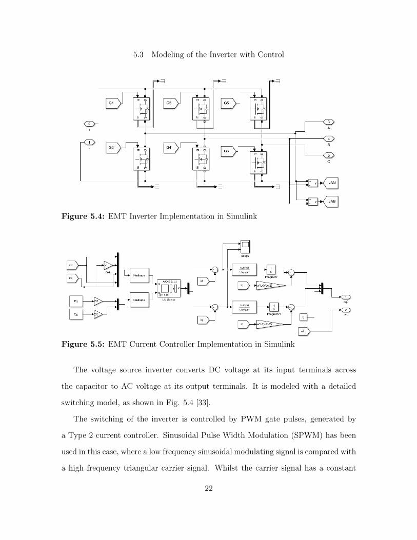
5.3 Modeling of the Inverter with Control

Figure 5.4: EMT Inverter Implementation in Simulink

Figure 5.5: EMT Current Controller Implementation in Simulink

The voltage source inverter converts DC voltage at its input terminals across

the capacitor to AC voltage at its output terminals. It is modeled with a detailed

switching model, as shown in Fig. 5.4 [33].

The switching of the inverter is controlled by PWM gate pulses, generated by

a Type 2 current controller. Sinusoidal Pulse Width Modulation (SPWM) has been

used in this case, where a low frequency sinusoidal modulating signal is compared with

a high frequency triangular carrier signal. Whilst the carrier signal has a constant

22

magnitude and frequency, the magnitude and phase angle of the modulating signal is

varied by the controller in order to achieve the desired output from the inverter. A

20 kHz carrier frequency or switching frequency is used here.

In this case, the output AC current is to be controlled. In order to simplify the

control scheme, the dq frame of reference is used. This transformation is beneficial

as the system is changed from three dimensional to two dimensional and decoupled

control of the d-axis and q-axis quantities is possible. The natural abc quantities

sensed at the output of the inverter are transformed into synchronously rotating

dq quantities and fed into the controller. The Proportional-Integral (PI) or Type

2 controller controls the dq components of the inverter current injected into the

network. The reference currents are derived from the desired output voltage, real

power and reactive power. id and iq indirectly controls real power and reactive power

respectively. This system is designed to supply a real power of 85 MW and a reactive

power of 3 MVArs. The implemented controller is depicted in Fig. 5.5.

Large solar power plants, such as the one modeled at bus 3, typically utilize a

number of MW-scale inverters. There could be individual string inverters assigned to

separate strings of solar panels or one central inverter assigned to the entire array of

panels.

5.4 Modeling of the Filter and Network Interconnection

An inductive (L) filter is designed to filter out the high switching frequency com-

ponent in the AC current and limit the total harmonic distortion (THD) in the AC

current to 5%. The solar PV inverter system is interfaced with the network through

the L filter.

The Thevenin equivalent circuit represents the TS model in the EMT domain. It

consists of a Thevenin AC voltage source in series with a Thevenin impedance for

23

Figure 5.6: EMT Filter and Network Interconnection Implementation in Simulink

each of the three phases.

The filter and network equivalent, as implemented in Simulink, are shown in Fig.

5.6.

24

Chapter 6

INTERFACE BETWEEN TS AND EMT SIMULATIONS

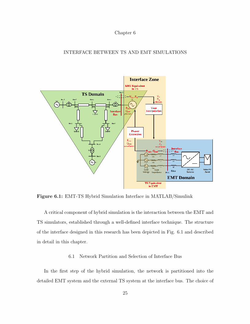
Figure 6.1: EMT-TS Hybrid Simulation Interface in MATLAB/Simulink

A critical component of hybrid simulation is the interaction between the EMT and

TS simulators, established through a well-defined interface technique. The structure

of the interface designed in this research has been depicted in Fig. 6.1 and described

in detail in this chapter.

6.1 Network Partition and Selection of Interface Bus

In the first step of the hybrid simulation, the network is partitioned into the

detailed EMT system and the external TS system at the interface bus. The choice of

25

the interface bus is important in obtaining the boundary conditions.

This selection is based on the understanding of which part of the system requires

a detailed study [7, 22]. Expanding the detailed system increases the accuracy, but

also increases the complexity and decreases the efficiency.

Usually, in grid-connected renewable energy systems, the distributed generation

system is the portion requiring EMT simulation, therefore the point of common cou-

pling (PCC), where the distributed generator connects to the grid, is chosen as the

interface bus.

In the 9-bus system under study, bus 3 is selected as the interface bus, as it

separates the PV system, which has been modeled in detail, from the rest of the

system.

6.2 Equivalent Models and Selection of Exchanged Data

Since the EMT and TS simulation models are solved independently, each must

contain an equivalent representation of the other in its own model. The equivalent

model of the EMT system in the TS simulation model should appropriately repre-

sent the behavior of the EMT simulation and must be updated dynamically at each

interface time step during the hybrid simulation and vice versa.

The phasor system is represented in the EMT simulation model as a Thevenin

voltage source in series with a Thevenin impedance. The required values of the

external system must be transformed into three-phase time-varying quantities for the

detailed system model. [6, 7, 15, 19, 21, 24]

The equivalent Bus 3 voltage magnitude and phase angle is obtained from the

phasor simulation results. These values are fed into three AC Voltage Source blocks

in Simulink, one representing each of the three phases. They generate sinusoidal

voltages at the specified frequency (fundamental frequency in this case), magnitude

26

and phase obtained from the phasor model [32].

The equivalent grid impedance is measured at Bus 3 in the phasor simulation

model. It is measured during the initialization and does not usually change during

the simulation, unless there are changes in the network configuration, such as faults.

The Impedance Measurement block in Simulink measures the impedance between

two nodes of the network, as seen from Bus 3, as a function of frequency. Using the

Impedance Measurement tool of the Powergui block, the impedance measurement

at the fundamental frequency is stored in the Workspace and retrieved by the EMT

simulation. This block has two input measurement terminals and consists of a current

source between them and a voltage source across the current source terminals. The

transfer function of the state-space model, from the current input to voltage output

is the measured impedance of the network. The positive-sequence impedance is 0.5

times the impedance measured between two phases in a three-phase circuit [32].

Apart from a fundamental Thevenin equivalent circuit, a simple voltage source,

a Norton equivalent or a Frequency-Dependent Norton Equivalent (FDNE) may also

be used to represent the equivalent of the external system in the EMT simulation

[19, 22, 31].

In this case, the EMT system is represented in the phasor simulation model as

a Three-Phase Voltage Source, specifically a PQ type generator injecting a real and

reactive power [7, 15, 25].

A PQ generator has controlled real or active power (in Watts) and reactive power

(In VArs) generation. The specified real and reactive power generation is obtained

from the results of the EMT simulation. The time-varying quantities from the EMT

simulation results undergo phasor extraction in order for them to be converted into

a fundamental frequency, phasor form usable in the TS simulation [32].

The network equivalent of the detailed system in the TS simulation is also often

27

a current source, a voltage source, an impedance, a time varying Norton equivalent

or a Thevenin equivalent [19, 21, 22, 24, 25].

6.3 Data Extraction

Figure 6.2: Data Extraction

The phasor equivalent model in the EMT simulation model requires the instanta-

neous voltage at the interface bus whereas the EMT equivalent model in the phasor

simulation requires the phasors of the injected real and reactive powers. Therefore,

before the selected data is exchanged between the simulation models, it must be

transformed into the appropriate form, as depicted in Fig. 6.2.

In order to convert the instantaneous three-phase waveforms of the quantities from

the EMT simulation into phasor quantities at the fundamental frequency, Phasor Ex-

traction technique such as RMS Approximation, Digital Filtering, Fourier Transform,

Curve Fitting and Projection on Synchronously Rotating Axes can be implemented

[22, 19, 25].

In this work, at every TS time step, the RMS values of the real and reactive

powers for that given time period are calculated using the dq currents and voltages,

extracted and sent to the TS simulation. The high-frequency component is also

28

eliminated before phasor extraction for better accuracy. In order to implement Fourier

Transform or Curve Fitting, on the other hand, the TS time step should be of the

length of the fundamental time period window or more, which imposes a restriction

on the minimum interface time step.

To obtain instantaneous waveforms for the EMT simulation from phasor values

of the TS simulation parameters, Time Interpolation is implemented [19, 15].

Here, time interpolation using an AC voltage source controlled by peak amplitude,

phase and frequency has been used in Simulink, to perform the phasor-to-waveform

conversion. The magnitude and phase angle for each phase is updated at every

interaction time step.

.

6.4 Interaction Protocol

Figure 6.3: Serial Interaction Protocol

The interaction protocol of the hybrid simulation determines the order of data

exchange at the EMT-TS interface [7]. The protocols for data transfer between the

EMT and TS models may be either serial, parallel or a combination of both. The serial

29

protocol ensures better accuracy, whereas the parallel protocol improves efficiency [6].

The process followed in this work, when a serial protocol is used, is illustrated

in Fig. 6.3. The four main interaction protocol steps are also stated in more detail

below:

1. At t0, transform the active and reactive power instantaneous waveforms, from

the previous interface step EMT simulation result, to phasors. Transfer these

phasors from the EMT domain to the TS simulation model.

2. Solve the power flow and execute the TS simulation with a time step of ∆Tts

until t1 is reached.

3. Transform the current and voltage phasors to instantaneous waveforms. Trans-

fer these quantities from the TS domain to the EMT simulation model.

4. Execute the EMT simulation from t0 to t1 with a timestep of ∆Temt.

This process is repeated until the total simulation time T is reached.

Therefore, at any give time instant during the simulation, only one model is

running whilst the other one is idle.

6.5 Communication

Interaction and data transfer between the two simulation models is facilitated

by the MATLAB Workspace. The EMT and TS simulations are each modeled in

the EMT and phasor domains, respectively, in separate Simulink files. The interface

algorithm is implemented in an m-file, using Matlab code. Fig. 6.4 depicts the

communication framework between the EMT and TS simulation models through the

Matlab interface.

30

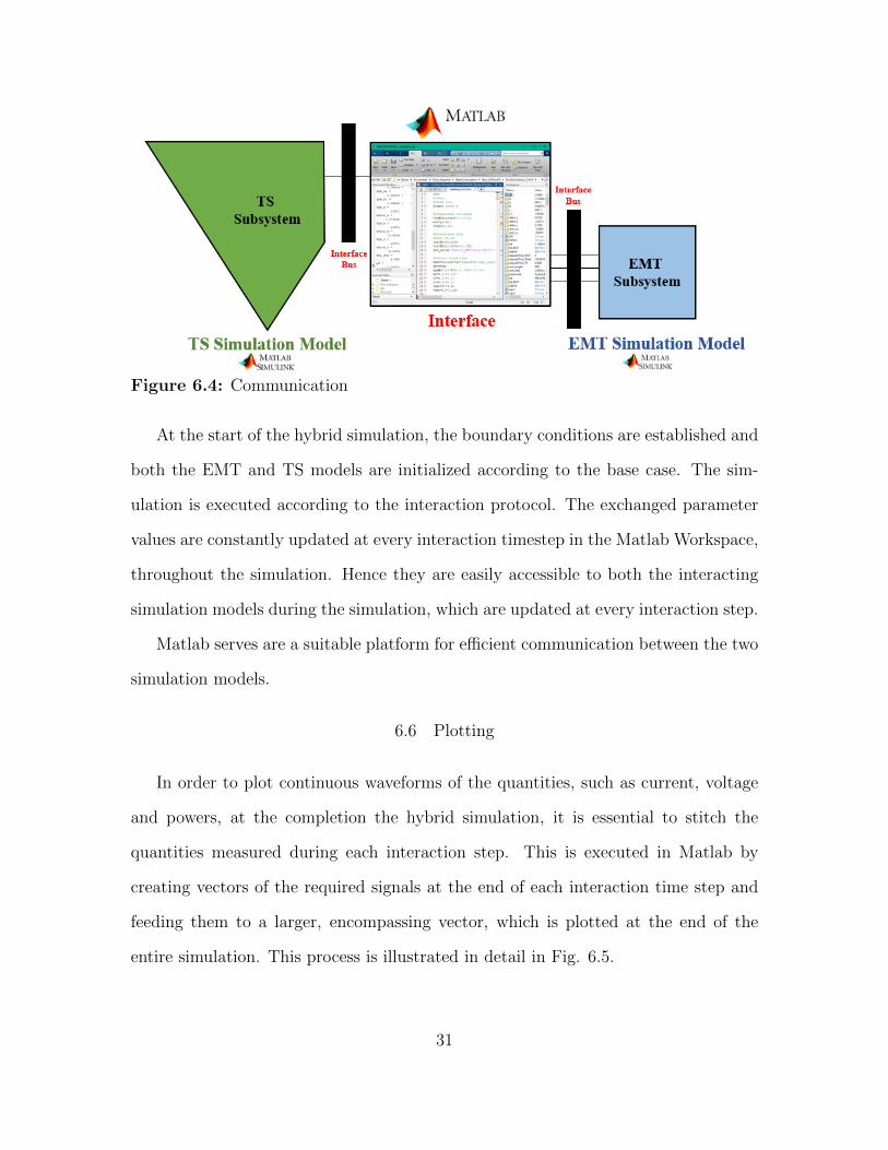
Figure 6.4: Communication

At the start of the hybrid simulation, the boundary conditions are established and

both the EMT and TS models are initialized according to the base case. The sim-

ulation is executed according to the interaction protocol. The exchanged parameter

values are constantly updated at every interaction timestep in the Matlab Workspace,

throughout the simulation. Hence they are easily accessible to both the interacting

simulation models during the simulation, which are updated at every interaction step.

Matlab serves are a suitable platform for efficient communication between the two

simulation models.

6.6 Plotting

In order to plot continuous waveforms of the quantities, such as current, voltage

and powers, at the completion the hybrid simulation, it is essential to stitch the

quantities measured during each interaction step. This is executed in Matlab by

creating vectors of the required signals at the end of each interaction time step and

feeding them to a larger, encompassing vector, which is plotted at the end of the

entire simulation. This process is illustrated in detail in Fig. 6.5.

31

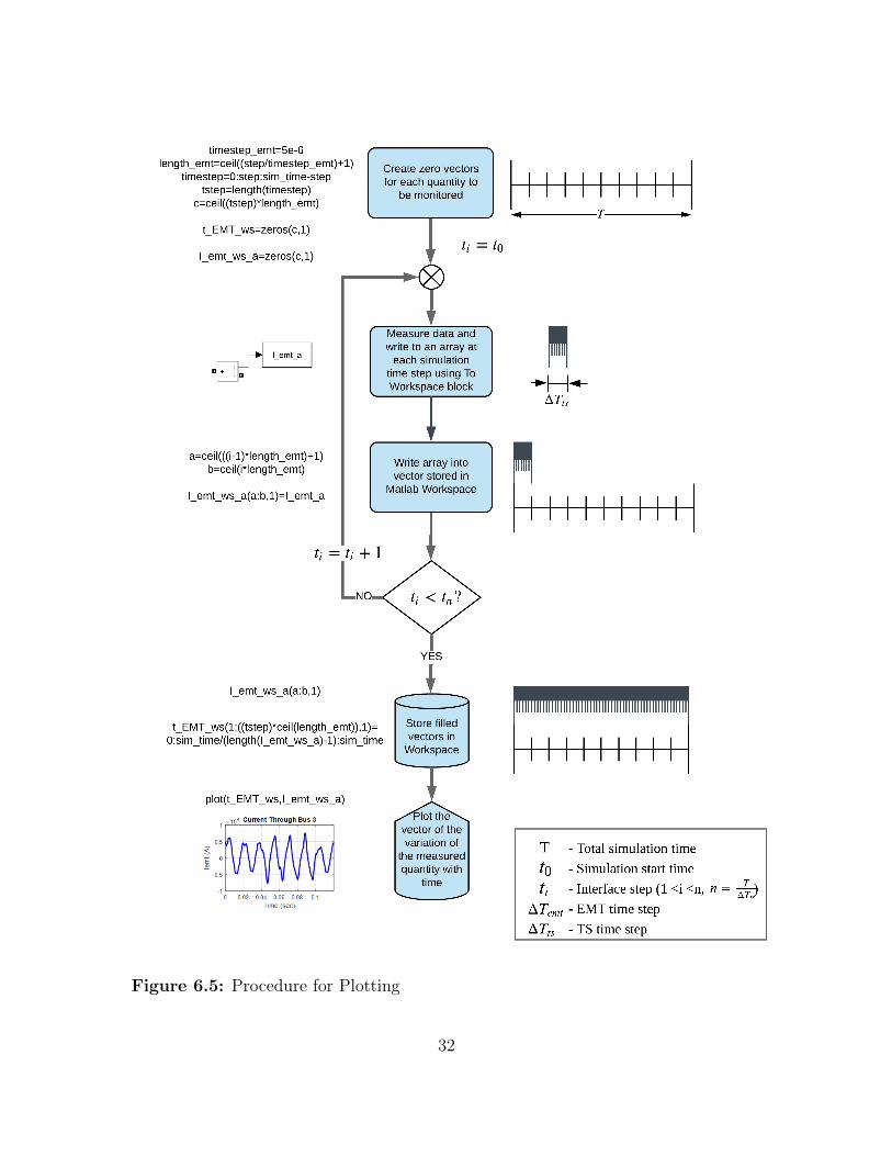
Figure 6.5: Procedure for Plotting

32

Chapter 7

TESTING AND VALIDATION

In this section, the hybrid simulation method described in the previous chapters

is tested and validated. The system under consideration is the WSCC IEEE 9 bus

network, modified to replace the synchronous generator at bus 3 by a solar PV plant.

It has been described in detail in chapters 4 and 5.

Steady-state analysis and transient analysis case studies have been performed,

and the results have been documented in this chapter. The transients considered

here include a Single Phase Line-to-Ground Fault and Variation in Solar PV Power

Output, which represent transients in the TS and EMT domains respectively.

Table 7.1 indicates the general hybrid simulation parameters for these case studies.

Voltage, current, real power and reactive power at the interface bus, which is the Bus

3, which is the point of common coupling (PCC), and Bus 7, have been observed in

all cases. The results have been compared with the benchmark full EMT simulation

model of the network under consideration, including the solar PV inverter system,

implemented in Simulink.

Table 7.1: Simulation Parameters

33

7.1 Steady-State Analysis

Figure 7.1: Instantaneous Voltage at Bus 3 (Interface Bus) during Steady State

Fig. 7.1 and Fig. 7.2 show the instantaneous voltages and currents at the PCC

during steady state. The errors in the magnitude and phase of these quantities

are negligible. Table 7.2 compares the RMS values of the boundary currents and

voltages during steady-state. It can be seen that the maximum error between the PCC

quantities in the EMT and TS subsystems is only around 0.53%. Closely matching

34

Figure 7.2: Instantaneous Current through Bus 3 (Interface Bus) during SteadyState

boundary currents, voltages, real power and reactive power, signify that the model is

running fairly accurately.

Fig. 7.3 indicates the runtime of each, the full EMT and the hybrid simulation

models, for a simulation of 0.3 seconds. It is evident that the hybrid simulation

method drastically reduces the simulation time, by almost 82%, yet maintaining a

suitable level of accuracy.

35

Figure 7.3: Comparison of Simulation Speed

Table 7.2: Error Evaluation between the Hybrid Simulation EMT Subsystem andTS Subsystem RMS Currents and Voltages at Bus 3 during Steady State

7.2 Transient Analysis

7.2.1 Single-Phase Line-to-Ground Fault

This case represents a transient in the Phasor domain. At the instant of 0.1 s, a

single phase line-to-ground (SLG) fault between phase A and ground is applied at bus

4. It is implemented by the Three-Phase Fault block in the TS model in Simulink.

The fault resistance Ron is 0.001 and ground resistance Rg is 0.1 . It is cleared

after 0.1 s (6 cycles), with the original configuration of the network restored. The

Thevenin Impedance is altered, from 0.45078 + 0.36572i Ohm before and after the

fault to 0.25576 + 0.35426i Ohm during the fault.

36

Figure 7.4: Instantaneous Voltage at Bus 3 (Interface Bus) during a SLG Fault atBus 4

Fig. 7.4 and Fig. 7.5 show the instantaneous voltages and currents at the PCC

during the SLG fault. There is a good match between the hybrid simulation and full

EMT simulation results before and after the fault and a negligible error in phase shift

and magnitude during the fault. It is important to note that such results are not

possible to acquire using only a phasor-domain tool.

Fig. 7.6 depicts the real power and reactive power at the PCC. During the SLG

37

Figure 7.5: Instantaneous Current through Bus 3 (Interface Bus) during a SLGFault at Bus 4

fault, the full EMT simulation PCC power results have an oscillation at double the

fundamental frequency, which is not seen in the hybrid simulation results.

The minor errors observed during the transient can be attributed to loss of some

information at the EMT-TS interface. For instance, all the harmonics injected by

the inverter in the EMT simulation are not represented in the TS simulation, as the

latter only considers the fundamental frequency components of voltage and current.

38

Figure 7.6: Power at Bus 3 (Interface Bus) during an SLG Fault at Bus 4

Also, inadequacies in data extraction, equivalent models and data exchanged can

contribute towards errors or deviation from the true results as obtained from the full

EMT simulation.

39

7.2.2 Interface Time Step Analysis

The interface time step has been varied from 10 ms to 50 ms, for the SLG fault

transient case. In Fig. 7.7, it can be seen that the total time taken by the hybrid

simulation to run decreases as the time step increases. However, the accuracy of the

results is affected. This can be noticed in Fig. 7.8 and Fig. 7.9, which depict the

instantaneous phase A voltage and current at the PCC during the SLG fault case,

for a range of interface time steps. Fig. 7.10 and Fig. 7.11 show the phasors of these

voltages and currents at the PCC.

Figure 7.7: Effect of Interface Time Step Variation on Simulation Time

These inaccuracies observed particularly during the transient, can be attributed to

interaction timing inconsistencies. As the TS simulation time step is the same as the

40

Figure 7.8: Instantaneous Voltage at Bus 3 (Interface Bus) during a SLG Fault atBus 4 for a Range of Interface Time Steps

Figure 7.9: Instantaneous Current through Bus 3 (Interface Bus) during a SLGFault at Bus 4 for a Range of Interface Time Steps

interface time step, a transient occurring in the external system at any instant within

the interface time step is reflected only at the end of that interval in the TS model,

unless it occurs on instances that are multiples of the interface time step. Also, in

41

Figure 7.10: Phasor Voltage at Bus 3 (Interface Bus) during a SLG Fault at Bus 4for a Range of Interface Time Steps

Figure 7.11: Phasor Current through Bus 3 (Interface Bus) during a SLG Fault atBus 4 for a Range of Interface Time Steps

the serial protocol, a transient occurring in the external system at any instant within

the interface time step is reflected at the beginning of the EMT simulation for that

interval, through the Thevenin equivalent of the TS subsystem in the EMT subsystem.

42

Therefore, a smaller time step would deliver more accurate results, whereas a larger

time step might pick up the transient at a slightly different instant than the exact

instant of occurrence.

7.2.3 Variation in Solar Irradiance

This case represents a transient in the EMT domain. The solar irradiance drops

from 1000 W/m2 to 800 W/m2 at 0.1 s. This causes a decrease in current and hence

in real power output from the solar PV plant, from 85 MW to 68 MW at 0.1 s, as

seen in Fig. 7.16.

Fig. 7.12 and Fig. 7.13 show the instantaneous voltages and currents at the

PCC during the fluctuation in solar irradiance, where as Fig. 7.14 and 7.15 depict

the phasors of the voltages and currents at the PCC (bus 3) and bus 7 respectively.

There is a good agreement between the results from the hybrid simulation and those

from the benchmark full EMT simulation.

43

Figure 7.12: Instantaneous Voltage at Bus 3 (Interface Bus) during a Decrease inSolar Irradiance

44

Figure 7.13: Instantaneous Current through Bus 3 (Interface Bus) during a Decreasein Solar Irradiance

45

Figure 7.14: Phasor Voltage and Current at Bus 3 (Interface Bus) during a Decreasein Solar Irradiance

46

Figure 7.15: Phasor Voltage and Current at Bus 7 during a Decrease in SolarIrradiance

47

Figure 7.16: Power at Bus 3 (Interface Bus) during a Decrease in Solar Irradiance

48

Chapter 8

CONCLUSIONS AND FUTURE WORK

8.1 Conclusions

In this work, an electromagnetic transient and transient stability hybrid simulation

method has been developed in MATLAB. This approach combines EMT simulation

accuracy and TS simulation speed. It enables the study of power networks with

penetration of power electronic converter interfaced generation and loads.

The process for implementation of Hybrid Simulation in MATLAB has been estab-

lished and a suitable interface algorithm has been developed. This hybrid simulation

scheme has been tested on the WSCC IEEE 9-bus system. The system behavior

during steady state and under faults and solar irradiance variation has been studied.

There is a close match between the measured quantities, such as current, voltage,

real and reactive powers, obtained from the hybrid simulation and the benchmark

complete EMT simulation, under steady state as well as during a range of transients.

In comparison with a phasor-domain tool, this hybrid simulation method enables the

assessment of accurate, instantaneous quantities, regularly only obtained through an

EMT-domain tool. In addition, the simulation speed and efficiency increased sub-

stantially from the full EMT simulation. This indicates that the method meets the

desired requirements and provides advantages over complete TS or complete EMT

simulations, by combining the benefits and overcoming the drawbacks of the two

kinds of simulation methods.

A significant contribution is made, in terms of simulation performance and user

experience. The primary advancements concerning simulation performance include

49

the development of a unique and simple interface algorithm, an analysis of the interac-

tion parameters and communication, and an improvement in accuracy and efficiency.

The most salient features of this method that enhance the user experience include

the flexibility, accessibility, user-friendliness, and ease of access, on account of the

implementation in MATLAB.

8.2 Future Work

The computational advantages of this simulation method will be even more promi-

nent in the simulation of larger systems with high penetration of converter interfaced

generation and loads. A case study with a larger system should be performed in

future.

A more detailed error analysis, would be beneficial, in order to work on reduction

in errors between the EMT and TS variables and loss of information at the interface.

To further improve the accuracy of the hybrid simulation method, an analysis of

the impact of the selection of boundary conditions, consideration of non-fundamental

frequencies in the TS simulation, and incorporation of dynamic generator models, are

some important steps that need to be taken.

To enhance the functionality of the hybrid simulation method, a graphical user

interface should also be developed.

50

REFERENCES

[1] D. Ramasubramanian, Z. Yu, R. Ayyanar, V. Vittal and J. Undrill, ”ConverterModel for Representing Converter Interfaced Generation in Large Scale GridSimulations,” in IEEE Transactions on Power Systems, vol. 32, no. 1, pp. 765-773, Jan. 2017.

[2] D. Ramasubramanian, V. Vittal and J. M. Undrill, ”Transient stability analysisof an all converter interfaced generation WECC system,” 2016 Power SystemsComputation Conference (PSCC), Genoa, 2016, pp. 1-7.

[3] Paving the Way, IEEE Power & Energy Magazine, November/December 2017

[4] D. Boroyevich, R. Burgos, L. Arnedo and F. Wang, ”Synthesis and Integrationof Future Electronic Power Distribution Systems,” 2007 Power Conversion Con-ference - Nagoya, Nagoya, 2007, pp. K-1-K-8.

[5] B. Da, A. Nadar, A. R. Boynueri, A. Karaka and Y. Ate, ”A fault analysismethod for microgrids consisting of inverter interfaced distributed generators,”12th IET International Conference on Developments in Power System Protection(DPSP 2014), Copenhagen, 2014, pp. 1-5.

[6] Q. Huang and V. Vittal, ”OpenHybridSim: An open source tool for EMT andphasor domain hybrid simulation,” 2016 IEEE Power and Energy Society GeneralMeeting (PESGM), Boston, MA, 2016, pp. 1-5.

[7] A. Hariri and M. O. Faruque, ”A Hybrid Simulation Tool for the Study of PVIntegration Impacts on Distribution Networks,” in IEEE Transactions on Sus-tainable Energy, vol. 8, no. 2, pp. 648-657, April 2017.

[8] M. D. Heffernan, K. S. Turner, J. Arrillaga and C. P. Arnold, ”Computation ofA.C.-D.C. System Disturbances - Part I. Interactive Coordination of Generatorand Convertor Transient Models,” in IEEE Transactions on Power Apparatusand Systems, vol. PAS-100, no. 11, pp. 4341-4348, Nov. 1981.

[9] K. S. Turner, M. D. Heffernan, C. P. Arnold and J. Arrillaga, ”Computation ofA.C.-D.C. System Disturbances. PT. II - Derivation of Power Frequency Vari-ables from Convertor Transient Response,” in IEEE Transactions on Power Ap-paratus and Systems, vol. PAS-100, no. 11, pp. 4349-4355, Nov. 1981.

[10] K. S. Turner, M. D. Heffernan, C. P. Arnold and J. Arrillaga, ”Computationof A.C.-D.C. System Disturbances. PT. III-Transient Stability Assessment,” inIEEE Transactions on Power Apparatus and Systems, vol. PAS-100, no. 11, pp.4356-4363, Nov. 1981.

[11] Hongtian Su, K. K. W. Chan and L. A. Snider, ”Interfacing an electromagneticSVC model into the transient stability simulation,” Proceedings. InternationalConference on Power System Technology, Kunming, China, 2002, pp. 1568-1572vol.3.

51

[12] H. Su, L. A. Snider, K. W. Chan, and B. Zhou, A new approach for integration oftwo distinct types of numerical simulator, in Proc. 2003 Power Syst. Transients,Int. Conf., pp. 16.

[13] H. T. Su, K. W. Chan and L. A. Snider, ”Parallel interaction protocol for electro-magnetic and electromechanical hybrid simulation,” in IEE Proceedings - Gen-eration, Transmission and Distribution, vol. 152, no. 3, pp. 406-414, 6 May 2005.

[14] Q. Huang and V. Vittal, ”Application of Electromagnetic Transient-TransientStability Hybrid Simulation to FIDVR Study,” in IEEE Transactions on PowerSystems, vol. 31, no. 4, pp. 2634-2646, July 2016.

[15] A. Hariri, A. Newaz and M. O. Faruque, ”Open-source python-OpenDSS inter-face for hybrid simulation of PV impact studies,” in IET Generation, Transmis-sion & Distribution, vol. 11, no. 12, pp. 3125-3133, 24 8 2017.

[16] A. Hariri, A. Newaz, andM. O. Faruque, A Matlab-openDSS hybrid simulationsoftware for the analysis of PV impacts on distribution networks, in Proc. 59thInt. Soc. Autom. Power Ind. Division Symp., 2016, pp. 112.

[17] A. Hariri and M. O. Faruque, ”Performing islanding detection in distributionnetworks with interconnected photovoltaic systems using a hybrid simulationtool,” 2016 IEEE Power and Energy Society General Meeting (PESGM), Boston,MA, 2016, pp. 1-5.

[18] A. Hariri and M. O. Faruque, ”Impacts of distributed generation on power qual-ity,” 2014 North American Power Symposium (NAPS), Pullman, WA, 2014, pp.1-6.

[19] F. Plumier, P. Aristidou, C. Geuzaine and T. Van Cutsem, ”Co-Simulation ofElectromagnetic Transients and Phasor Models: A Relaxation Approach,” inIEEE Transactions on Power Delivery, vol. 31, no. 5, pp. 2360-2369, Oct. 2016.

[20] D. Shu, X. Xie, Q. Jiang, Q. Huang and C. Zhang, ”A Novel Interfacing Tech-nique for Distributed Hybrid Simulations Combining EMT and Transient Stabil-ity Models,” in IEEE Transactions on Power Delivery, vol. 33, no. 1, pp. 130-140,Feb. 2018.

[21] D. Shu, X. Xie, V. Dinavahi, C. Zhang, X. Ye and Q. Jiang, ”Dynamic PhasorBased Interface Model for EMT and Transient Stability Hybrid Simulations,” inIEEE Transactions on Power Systems, vol. 33, no. 4, pp. 3930-3939, July 2018.

[22] V. Jalili-Marandi, V. Dinavahi, K. Strunz, J. A. Martinez and A. Ramirez, ”In-terfacing Techniques for Transient Stability and Electromagnetic Transient Pro-grams IEEE Task Force on Interfacing Techniques for Simulation Tools,” in IEEETransactions on Power Delivery, vol. 24, no. 4, pp. 2385-2395, Oct. 2009.

[23] X. Meng and L. Wang, ”Interfacing an EMT-type modular multilevel converterHVDC model in transient stability simulation,” in IET Generation, Transmission& Distribution, vol. 11, no. 12, pp. 3002-3008, 24 8 2017.

52

[24] S. Abhyankar and A. J. Flueck, ”An implicitly-coupled solution approach forcombined electromechanical and electromagnetic transients simulation,” 2012IEEE Power and Energy Society General Meeting, San Diego, CA, 2012, pp.1-8.

[25] A. A. van der Meer, M. Gibescu, M. A. M. M. van der Meijden, W. L. Klingand J. A. Ferreira, ”Advanced Hybrid Transient Stability and EMT Simulationfor VSC-HVDC Systems,” in IEEE Transactions on Power Delivery, vol. 30, no.3, pp. 1057-1066, June 2015.

[26] S. Abourida, J. Blanger and V. Jalili-Marandi, Real-Time Power System Sim-ulation: EMT vs. Phasor, White Paper [Online]. Available: https://www.opal-rt.com/wp-content/themes/enfold-opal/pdf/L00161 0121.pdf

[27] OPAL-RT. Accessed October 2018. [Online]. Available: https://www.opal-rt.com/

[28] OPAL-RTs Solution for Hybrid EMT-TS Simulation. Accessed October2018. [Online]. Available: http://sites.ieee.org/pes-itst/files/2017/06/2017-Panel-4.pdf

[29] N. Panigrahy, Gopalakrishnan K. S., Ilamparithi T. and M. V. Kashinath, ”Real-time phasor-EMT hybrid simulation for modern power distribution grids,” 2016IEEE International Conference on Power Electronics, Drives and Energy Systems(PEDES), Trivandrum, 2016, pp. 1-6.

[30] V. Jalili-Marandi, F. J. Ayres, C. Dufour and J. Blanger, ”Real-time Electro-magnetic and Transient Stability Simulations for Active Distribution Networks,”in IPST, 2013.

[31] Y. Zhang, A. M. Gole, W. Wu, B. Zhang and H. Sun, ”Development and Analysisof Applicability of a Hybrid Transient Simulation Platform Combining TSA andEMT Elements,” in IEEE Transactions on Power Systems, vol. 28, no. 1, pp.357-366, Feb. 2013.

[32] MathWorks Documentation. Accessed October 2018. [Online]. Available:https://www.mathworks.com/help/

[33] R. Ayyanar, Renewable Electric Energy Systems, EEE 598, Lecture Notes, Fall2012.

[34] Xue, Jinhui, Zhongdong Yin, Bingbing Wu, and Jun Peng. ”Design of PV ArrayModel Based On EMTDC/PSCAD.” Power and Energy Engineering Conference,2009. APPEEC 2009. Asia-Pacific, 2009, 1-5.

[35] T. MathWorks, ”Introducing the Phasor Simula-tion Method”, 14 07 2015. [Online]. Available:http://www.mathworks.com/help/physmod/sps/powersys/ug/introducing-the-phasor-simulation-method.html. [Accessed 10 17 2018].

53

[36] Manitoba HVDC Research Center, ”IEEE Test Systems”, 2015. [ONLINE] Avail-able at: http://forum.hvdc.ca/1598644/IEEE-Test-Systems.

[37] OPAL-RT Technologies, ”IEEE 9 Bus Sys-tem Example”, Oct 2017. [ONLINE] Available at:http://www.kios.ucy.ac.cy/testsystems/images/Documents/Data/IEEE9 modeldocumentation R0.pdf

[38] KIOS Centre for Intelligent Systems & Networks, ”IEEE 9-bus modified test system”, 2013. [ONLINE] Available at:http://www.kios.ucy.ac.cy/testsystems/index.php/dynamic-ieee-test-systems/ieee-9-bus-modified-test-system.

[39] Jaikumar Pettikkattil, ”IEEE 9 Bus,” Mathworks Simulink File Ex-change Center, Mar. 2014, [Accessed 10 17 2018]. [Online]. Available:http://www.mathworks.com/matlabcentral/fileexchange/45936-ieee-9-bus

[40] Francisco M. Gonzalez-Longatt, ”Test Case P.M. Anderson Power Sys-tem,” Power Systems Test Cases, [Accessed 10 17 2018]. [Online].Available:http://fglongatt.org/OLD/Test Case Anderson.html

54

APPENDIX A

WSCC IEEE 9-BUS SYSTEM DATA

55

Table A.1: Synchronous Generator Data

56

Table A.2: Load Data

Table A.3: Line Data

Table A.4: Transformer Data

57

APPENDIX B

SOLAR PV PANEL DATASHEET SPECIFICATION

58

Table B.1: Electrical Specifications of Jakson Solar PV Module at STC

Figure B.1: I-V Curve Variation with Irradiance

59

APPENDIX C

MATLAB CODE FOR EMT-TS INTERFACE

60

1 %Written by Denise Athaide2

3 clc;4 clear;5 close all;6 format short g7

8 %Solar PV Array Parameter Extraction and Initialization ...(JP300W24V module)

9 Nseries=177610 Nparallel=15211 Temp=298;12 k=1.38*10ˆ−23;13 q=1.6*10ˆ−19;14 Ns=72*Nseries;15 didv sc=−2.488*10ˆ−3;16 didv oc=−2.05;17 Voc=44.8*Nseries;18 Vmp=36.6*Nseries;19 Isc=8.6*Nparallel;20 Imp=8.2*Nparallel;21 Irr=1000/1000;22 Vsource=Vmp23

24 Iph=Isc*Irr;25 Rsh=−Nseries*(didv sc)ˆ−126 C1=1*10ˆ−12;27

28 syms IO DIF Rs29 eqn1 = IO == (Isc−(Voc/Rsh))/(exp((q*Voc)/(Ns*DIF*k*Temp))−1);30 eqn2 = Imp == Isc − ...

IO*exp(q*((Vmp+(Imp*Rs))/(Ns*DIF*k*Temp)))−((Vmp+(Imp*Rs))/Rsh);31 eqn3 = Rs == −((didv oc)ˆ−1)− ...

(1/(((q*IO)/(Ns*DIF*k*Temp))*(exp((q*Voc)/(Ns*DIF*k*Temp)))));32 sol = solve([eqn1, eqn2, eqn3], [IO, DIF, Rs]);33 IOSol = sol.IO;34 DIFSol = sol.DIF;35 RsSol = sol.Rs;36 IO=vpa(IOSol,4);37 DIF=vpa(DIFSol,4);38

39 Rs=vpa(abs(RsSol),4)40 I0=double(IO)41 a=double(DIF)42

43 %Independent variables44 Vdc=Vsource45 w=2*pi*60;46 j=sqrt(−1);47

48 %Initial conditions49 Ppm=Vsource*Isc*Irr1;50 Ppv=Ppm;51 Qpm=3*(10ˆ6)52 Iemt=4776.4;53 Vemt=11871.25;

61

54 ph shift=0;55

56 %Filter parameters57 Rf=0.1;58 Lf=0.0052;59

60 %Controller parameters61 wc=2*pi*2000;62 PM=60;63 s=j*wc;64

65 %Simulation parameters66 sim time=0.3;67 step=0.02;68 timestep=0:step:sim time−step;69

70 %SLG fault parameters71 tf=0;72 tf 1=0;73 Rg=0.1;74 t0=0.1;75 t1=0.2;76

77 %Irrandiance step78 tp=1;%0.179 Irr1=1000/100080 Irr2=800/1000%800/100081 set param('hybrid EMT/Solar PV/Irr','Value','Irr1')82

83 %Creation and initialization of vectors for TS quantities84 tstep=length(timestep);85 ts step=0.0286 ts length=ceil((step/ts step)+1);87 f=ceil((tstep)*ts length);88

89 Its a=zeros(f,1);90 Its b=zeros(f,1);91 Its c=zeros(f,1);92 Vts a=zeros(f,1);93 Vts b=zeros(f,1);94 Vts c=zeros(f,1);95 Pts=zeros(f,1);96 Qts=zeros(f,1);97 Tts=zeros(f,1);98 Its7 a=zeros(f,1);99 Its7 b=zeros(f,1);

100 Its7 c=zeros(f,1);101 Vts7 a=zeros(f,1);102 Vts7 b=zeros(f,1);103 Vts7 c=zeros(f,1);104 Its a(1) = 4776.4;105 Vts a(1) = 11871.25;106 Pts(1) = 85*(10ˆ6);107 Qts(1) = 3*(10ˆ6);108

109 I emt a(2001)=0;110 I emt b(2001)=0;

62

111 I emt c(2001)=0;112 V1 pm mag a(ts length)=16500;113 V2 pm mag a(ts length)=18000;114 P1 pm(ts length)= 71*10ˆ6;115 P2 pm(ts length)= 163*10ˆ6;116

117 %Creation and initialization of vectors for EMT quantities118 emt step=5e−6;119 emt length=ceil((step/emt step)+1);120 c=ceil((tstep)*emt length);121

122 t EMT ws=zeros(c,1);123 I emt ws a=zeros(c,1);124 I emt ws b=zeros(c,1);125 I emt ws c=zeros(c,1);126 V emt ws a=zeros(c,1);127 V emt ws b=zeros(c,1);128 V emt ws c=zeros(c,1);129 P emt ws=zeros(c,1);130 Q emt ws=zeros(c,1);131 P emt avg=zeros(c,1);132 Q emt avg=zeros(c,1);133 Ed EMT=zeros(c,1);134 Eq EMT=zeros(c,1);135 Id EMT=zeros(c,1);136 Iq EMT=zeros(c,1);137

138 %Simulation timer initialization139 elapsedTime TS=0;140 elapsedTime EMT=0;141

142

143 %Start hybrid simulation144 for i=1:tstep145 time=timestep(i);146 time147

148 %Transient 1: Single Phase L−G Fault at Bus 4149 if (time≥t0) && (time≤(t1−step))150 set param('hybrid TS/tf','Value','1')151 tf 1=1;152 else153 set param('hybrid TS/tf','Value','0')154 tf 1=0;155 end156

157 %Transient 2: Solar Irrandiance Variation158 if (time≥tp)159 set param('hybrid EMT/Solar PV/Irr','Value','Irr2')160 Ppv=Vsource*Isc*Irr2161 else162 set param('hybrid EMT/Solar PV/Irr','Value','Irr1')163 Ppv=Vsource*Isc*Irr1164 end165

166 %Calculation of TS equivalent Thevenin impedance in EMT167 Zdata B3 = power zmeter('hybrid TS',linspace(59,61,3));

63

168 Zpm=(Zdata B3.Z(2))169 Rgrid=real(Zpm);170 Lgrid=imag(Zpm)/377;171 Rpm=Rf+Rgrid;172 Lpm=Lf+Lgrid;173 L=Lpm;174

175 tic176

177 %Load TS simulation model178 tsmodel = 'hybrid TS';179 load system(tsmodel)180 %Solve pflow, apply to model181 LF1 = power loadflow('−v2',tsmodel,'solve');182 LF1;183 %Run TS model for interface timestep184 sim(tsmodel)185

186 %Get V, ∆, I, P & Q data from TS simulation (saved in WS)187 Vpm a=V pm mag a(ts length)188 ∆ a=V pm ang a(ts length)189 phi a=V pm ang a(ts length)−(I pm ang a(ts length));190

191 Vpm b=V pm mag b(ts length)192 ∆ b=V pm ang b(ts length)193 phi b=V pm ang b(ts length)−(I pm ang b(ts length));194

195 Vpm c=V pm mag c(ts length)196 ∆ c=V pm ang c(ts length)197 phi c=V pm ang c(ts length)−(I pm ang c(ts length));198

199 Phi deg=phi a*180/pi %in degrees200 pf=cos(phi a)201

202 %For plotting203 g=ceil(((i−1)*ts length)+1)204 h=ceil(i*ts length);205

206 Its a(g:h,1)=I pm mag a;207 Its b(g:h,1)=I pm mag b;208 Its c(g:h,1)=I pm mag c;209

210 Vts a(g:h,1)=V pm mag a;211 Vts b(g:h,1)=V pm mag b;212 Vts c(g:h,1)=V pm mag c;213

214 Pts(g:h,1)=P pm;215 Qts(g:h,1)=Q pm;216

217 Its7 a(g:h,1)=I7 pm mag a;218 Its7 b(g:h,1)=I7 pm mag b;219 Its7 c(g:h,1)=I7 pm mag c;220

221 Vts7 a(g:h,1)=V7 pm mag a;222 Vts7 b(g:h,1)=V7 pm mag b;223 Vts7 c(g:h,1)=V7 pm mag c;224

64

225 toc226 elapsedTime TS = elapsedTime TS + toc227

228

229 tic230

231 %Controller design232

233 Gp=(Vdc/2)*(1/((s*Lpm)+Rpm));234 Phi sys=(angle(Gp))*(180/pi);235 Phi boost=PM−90−Phi sys;236 k=tan((pi/4)+((pi/180)*(Phi boost/2)));237 wz=wc/k;238 wp=k*wc;239 Gc pre=(1/s)*((1+(s/wz))/(1+(s/wp)));%??240 G OL pre=Gp*Gc pre;241 Kc=1/abs(G OL pre);242

243 Pg=85*10ˆ6244 Qg=3*10ˆ6;245 set param('hybrid EMT/Controller/Constant Ppm','Value','Pg')246 set param('hybrid EMT/Controller/Constant Qpm','Value','Qg')247

248 %Update parameters in EMT model249

250 Vgrid mag a=Vpm a;251 Vgrid ∆ a=ph shift+(∆ a*(180/pi));252 Vgrid mag b=Vpm b;253 Vgrid ∆ b=ph shift+(∆ b*(180/pi));254 Vgrid mag c=Vpm c;255 Vgrid ∆ c=ph shift+(∆ c*(180/pi));256

257 set param('hybrid EMT','SimulationCommand','update');258

259 %Load EMT simulation model260 emtmodel = 'hybrid EMT';261 load system(emtmodel)262 %Run EMT sim for interface timestep263 sim(emtmodel)264

265 %For plotting266 a=ceil(((i−1)*emt length)+1);267 b=ceil(i*emt length);268 I emt ws a(a:b,1)=I emt a;269 I emt ws b(a:b,1)=I emt b;270 I emt ws c(a:b,1)=I emt c;271 V emt ws a(a:b,1)=V emt a;272 V emt ws b(a:b,1)=V emt b;273 V emt ws c(a:b,1)=V emt c;274 P emt ws(a:b,1)=P emt;275 Q emt ws(a:b,1)=Q emt;276 Ed EMT(a:b,1)=edemt;277 Eq EMT(a:b,1)=eqemt;278 Id EMT(a:b,1)=idemt;279 Iq EMT(a:b,1)=iqemt;280

281 %Optional Phasor Extraction of V, I, theta from instantaneous EMT ...

65

waveforms using FFT in the Powergui282 %(May be used only if the interface time step is greater than one ...

fundamental cycle)283

284 %get I285 %FFTDATAI = power fftscope(Scope Iemt);286 %%power fftscope(FFTDATAI);287 %Iemt=FFTDATAI.magFundamental288

289 %get V290 %FFTDATAV = power fftscope(Scope Vemt);291 %%power fftscope(FFTDATAV);292 %Vemt=FFTDATAV.magFundamental293

294 %Calculation of P & Q from I, V and cos theta using the equations295 %thetaemt=(angle(Vpm)*angle(Ig))*(180/pi)296 %Pemt cal=(3/2)*Iemt*Vemt*cos(thetaemt)297 %Qemt cal=(3/2)*Iemt*Vemt*sin(thetaemt)298

299 %Measurement of P & Q from EMT model300 %get P301 %FFTDATAP = power fftscope(Scope Pemt);302 %Pemt=FFTDATAP.DCcomponent303 %get Q304 %FFTDATAQ = power fftscope(Scope Qemt);305 %Qemt=FFTDATAQ.DCcomponent306

307 %Ipv{i} = Iemt;308 %Vpv{i} = Vemt;309 %Ppv{i} = Pemt;310 %Qpv{i} = Qemt;311

312 Pemt=P emt(emt length)313 Qemt=Q emt(emt length)314

315 %Update Parameters (P & Q) in TS model316 Ppm=Pemt317 Qpm=Qemt318

319 ph shift=(((rem(step,0.016667))/0.016667)*360)*i;320

321 xInitial emt=xFinal emt;322 save myModel init xInitial emt323

324 set param('hybrid TS','SimulationCommand','update');325

326 toc327 elapsedTime EMT=elapsedTime EMT+toc328

329 end330

331 %Total hybrid simulation time332 elapsedTime Total=elapsedTime TS+elapsedTime EMT333

334 %Filled time vectors for plotting335 Tts(1:((tstep)*ceil(ts length)),1) = ...

0:sim time/(length(Its a)−1):sim time;

66

336 t EMT ws(1:((tstep)*ceil(emt length)),1) = ...0:sim time/(length(I emt ws a)−1):sim time;

67