Upslope flows in atmosphere and water tank, part II: Fluid-dynamical smoothness as a possible cause...
14
188 The Open Atmospheric Science Journal, 2010, 4, 188-201 1874-2823/10 2010 Bentham Open Open Access Upslope Flows in Atmosphere and Water Tank, Part II: Fluid-Dynamical Smoothness as a Possible Cause for Velocity Similarity Violation C. Reuten * , S. E. Allen, and D. G. Steyn Atmospheric Science Program, Department of Earth and Ocean Sciences, The University of British Columbia, Vancouver, Canada Abstract: Water-tank models of meso-scale atmospheric processes often show good qualitative agreement of bulk quantities and flow characteristics and good quantitative agreement of turbulence quantities with field observations. However, it was demonstrated in the first part of this two-part communication that the similarity of velocities of thermally driven upslope flows in atmosphere and water tank is violated. It is shown in this part that the velocities of thermally driven upslope flows in the atmosphere and in a water-tank model have statistically different dependences on proposed governing parameters. Of four substantially different hypotheses of upslope velocities, three agree with field observations because of large uncertainties and sparse data, but all hypotheses disagree with tank observations. One hypothesis that includes the influence of the total slope height agrees with field and tank observations when assuming fluid-dynamically rough atmospheric flows and fluid-dynamically smooth tank flows. The non-dimensional upslope flow velocities corresponding to rough and smooth flows depend differently on the governing parameters. Therefore, non-dimensional upslope flow velocities are different for atmosphere and water tank. Furthermore, as this hypothesis includes a dependence of the upslope flow velocity on the total height of the slope it implies that upslope flow systems are non-local phenomena. Because fluid-dynamical roughness is technically difficult to achieve in water-tank models, velocity similarity violations can also be expected in water-tank models of other thermally driven meso-scale flows and our technique of explicitly including roughness length dependence may have wider applications. Keywords: Bayesian analysis, physical scale model, scaling, similarity, upslope flows, water tank. 1. INTRODUCTION Water-tank models have been used for several decades to study atmospheric phenomena. Some of the earlier experiments focused primarily on turbulence in the convective boundary layer (CBL) in salt- or heat-stratified water over a heated flat horizontal plate [1-6] and the role of turbulence in dispersion of pollutants [7-20]. Many of these studies investigated the CBL under externally imposed advection. Examples of thermally driven flows that have been studied with water-tank models are sea breezes [21], urban heat islands [22, 23] and their interactions [24], and upslope flows [25-27], which are the focus here. Simply speaking, upslope flows arise over heated sloping terrain in a stratified background fluid; fluid near the slope surface will be warmer than fluid at the same elevation further from the slope. Buoyancy and pressure-gradient forces together cause an upslope flow approximately parallel to the slope. This paper is the second part of a two-part communication. From here on we will refer to part I and part II for simplicity. Previous tank studies of upslope flows showed similarity between atmosphere and water tank for turbulence parameters [28], flow characteristics [25, 29], and the order *Address correspondence to this author at the RWDI AIR Inc., Suite 1000, 736 8 th Ave. SW, Calgary, AB T2P 1H4, Canada; Tel: 1-403-232-6771; Fax.: 1-403-232-6762; Email: [email protected] of magnitude of bulk quantities like CBL height and upslope flow velocity [26, 27]. In part I, it was shown that quantitative similarity can be achieved for CBL depth within approximately the uncertainty of field and tank observations (20%) but that upslope flow velocities are significantly different. Here in part II, the cause for the similarity violation of upslope flow velocity will be studied. A summary of the scaling and a description of the field and tank experiments are provided in section 2. In section 3, four alternative upslope flow velocity hypotheses are developed. In section 4 these are compared with field and tank observations using Bayesian analysis. A detailed discussion of the results is presented in section 5, and conclusions are drawn in section 6. The derivation of the equations used for the Bayesian analysis is provided in the appendix. Quantities in the atmosphere will be denoted with subscript ‘a’ to distinguish them from those in the water tank with subscript ‘w’; no subscripts will be used if the quantity or equation applies to both atmosphere and water tank. 2. METHODS a. Field Observations Details of the field site and instrumentation at Minnekhada Park in the Lower Fraser Valley, British Columbia, Canada, are presented in [30]. The slope is fairly homogeneous over a width of roughly 3 km; the slope angle is approximately constant at 19° and ridge height is 760 m.
Transcript of Upslope flows in atmosphere and water tank, part II: Fluid-dynamical smoothness as a possible cause...
188 The Open Atmospheric Science Journal, 2010, 4, 188-201
1874-2823/10 2010 Bentham Open
Open Access
Upslope Flows in Atmosphere and Water Tank, Part II: Fluid-Dynamical Smoothness as a Possible Cause for Velocity Similarity Violation
C. Reuten*, S. E. Allen, and D. G. Steyn
Atmospheric Science Program, Department of Earth and Ocean Sciences, The University of British Columbia,
Vancouver, Canada
Abstract: Water-tank models of meso-scale atmospheric processes often show good qualitative agreement of bulk
quantities and flow characteristics and good quantitative agreement of turbulence quantities with field observations.
However, it was demonstrated in the first part of this two-part communication that the similarity of velocities of thermally
driven upslope flows in atmosphere and water tank is violated.
It is shown in this part that the velocities of thermally driven upslope flows in the atmosphere and in a water-tank model
have statistically different dependences on proposed governing parameters. Of four substantially different hypotheses of
upslope velocities, three agree with field observations because of large uncertainties and sparse data, but all hypotheses
disagree with tank observations. One hypothesis that includes the influence of the total slope height agrees with field and
tank observations when assuming fluid-dynamically rough atmospheric flows and fluid-dynamically smooth tank flows.
The non-dimensional upslope flow velocities corresponding to rough and smooth flows depend differently on the
governing parameters. Therefore, non-dimensional upslope flow velocities are different for atmosphere and water tank.
Furthermore, as this hypothesis includes a dependence of the upslope flow velocity on the total height of the slope it
implies that upslope flow systems are non-local phenomena.
Because fluid-dynamical roughness is technically difficult to achieve in water-tank models, velocity similarity violations
can also be expected in water-tank models of other thermally driven meso-scale flows and our technique of explicitly
including roughness length dependence may have wider applications.
Keywords: Bayesian analysis, physical scale model, scaling, similarity, upslope flows, water tank.
1. INTRODUCTION
Water-tank models have been used for several decades to study atmospheric phenomena. Some of the earlier experiments focused primarily on turbulence in the convective boundary layer (CBL) in salt- or heat-stratified water over a heated flat horizontal plate [1-6] and the role of turbulence in dispersion of pollutants [7-20]. Many of these studies investigated the CBL under externally imposed advection. Examples of thermally driven flows that have been studied with water-tank models are sea breezes [21], urban heat islands [22, 23] and their interactions [24], and upslope flows [25-27], which are the focus here. Simply speaking, upslope flows arise over heated sloping terrain in a stratified background fluid; fluid near the slope surface will be warmer than fluid at the same elevation further from the slope. Buoyancy and pressure-gradient forces together cause an upslope flow approximately parallel to the slope. This paper is the second part of a two-part communication. From here on we will refer to part I and part II for simplicity.
Previous tank studies of upslope flows showed similarity between atmosphere and water tank for turbulence parameters [28], flow characteristics [25, 29], and the order
*Address correspondence to this author at the RWDI AIR Inc., Suite 1000,
736 8th Ave. SW, Calgary, AB T2P 1H4, Canada; Tel: 1-403-232-6771;
Fax.: 1-403-232-6762; Email: [email protected]
of magnitude of bulk quantities like CBL height and upslope flow velocity [26, 27]. In part I, it was shown that quantitative similarity can be achieved for CBL depth within approximately the uncertainty of field and tank observations (20%) but that upslope flow velocities are significantly different. Here in part II, the cause for the similarity violation of upslope flow velocity will be studied. A summary of the scaling and a description of the field and tank experiments are provided in section 2. In section 3, four alternative upslope flow velocity hypotheses are developed. In section 4 these are compared with field and tank observations using Bayesian analysis. A detailed discussion of the results is presented in section 5, and conclusions are drawn in section 6. The derivation of the equations used for the Bayesian analysis is provided in the appendix. Quantities in the atmosphere will be denoted with subscript ‘a’ to distinguish them from those in the water tank with subscript ‘w’; no subscripts will be used if the quantity or equation applies to both atmosphere and water tank.
2. METHODS
a. Field Observations
Details of the field site and instrumentation at Minnekhada Park in the Lower Fraser Valley, British Columbia, Canada, are presented in [30]. The slope is fairly homogeneous over a width of roughly 3 km; the slope angle is approximately constant at 19° and ridge height is 760 m.
Upslope Flows in Atmosphere and Water Tank, Part II The Open Atmospheric Science Journal, 2010, Volume 4 189
Figure 2 in [30] suggests that a plateau better represents the terrain on the other side of the ridge than a slope. The plain adjacent to the slope is approximately flat. Observations used in this paper were taken under mostly cloudless skies in the morning hours of 25-26 July 2001, before the onset of sea-breeze and up-valley flows. Vertical profiles of moisture and temperature were measured with a tethersonde 3.5 km from the bottom of the slope. Early morning profiles showed roughly constant lapse rates up to about 1000 m, except very near the surface. Range-height indicator (RHI) scans with a lidar provided information on the backscatter boundary layer (BBL) depth over plain and slope, which reached values of about 800 m. Over the plain close to the slope a Doppler sodar was employed to measure vertical profiles of wind velocity averaged over approximately 20 minutes. ‘Upslope flow velocities’ were determined from each vertical profile as the maximum value of the horizontal component of the slope wind, typically 3-6 m s
-1.
b. Water Tank
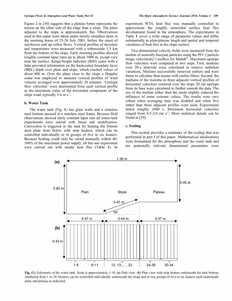
The water tank (Fig. 1) has glass walls and a stainless steel bottom encased in a stainless steel frame. Because field observations showed fairly constant lapse rate all water-tank experiments were started with linear salt stratification. Convection is triggered in the tank by heating the bottom steel plate from below with strip heaters, which can be controlled individually or in groups of five to six heaters. Because heating could only be varied manually within 40-100% of the maximum power supply, all but one experiment were carried out with steady heat flux (Table 1). In
experiment WT4, heat flux was manually controlled to approximate the roughly sinusoidal surface heat flux development found in the atmosphere. The experiments in Table 1 cover a wide range of parameter values and differ substantially in plain/plateau length and spatial and temporal variations of heat flux at the slope surface.
Two-dimensional velocity fields were measured from the motion of neutrally buoyant particles using the PIV (‘particle image velocimetry’) toolbox for Matlab
®. Maximum upslope
flow velocities were computed in two steps. First, medians over 20-s intervals were calculated to remove turbulent variations. Medians successfully removed outliers and were faster to calculate than means with outlier filters. Second, the medians of the maxima in three adjacent vertical profiles of horizontal velocities centered over the slope 20 cm upslope from its base were calculated to further smooth the data. The use of the median rather than the mean slightly reduced the influence of some extreme values. The results were very robust when averaging time was doubled and when five rather than three adjacent profiles were used. Experiments lasted roughly 1000 s. Maximum horizontal velocities ranged from 0.5-2.0 cm s
-1. More technical details can be
found in [29].
c. Scaling
This section provides a summary of the scaling that was
performed in part I of this paper. Mathematical idealizations
were formulated for the atmosphere and the water tank and
ten potentially relevant dimensional parameters were
Fig. (1). Schematic of the water tank. Scale is approximately 1:10. (a) Side view. (b) Plan view with strip heaters underneath the tank bottom
numbered from 1 to 34. Heaters can be controlled individually underneath the slope and in two groups of five to six heaters each underneath
plain and plateau as indicated.

190 The Open Atmospheric Science Journal, 2010, Volume 4 Reuten et al.
identified for the atmosphere and an additional two for the
water tank: Ridge height H, sensible surface heat flux QH,
buoyancy frequency N, horizontal length of slope L, total
supplied energy density E, buoyancy parameter g (g is the
gravitational acceleration and the coefficient of thermal
expansion), kinematic viscosity , thermal diffusivity ,
length of the plain Lb, length of the plateau Lt, and roughness
height Zr; in addition for the water tank its width Ww and the
water depth over the plain Dw. We speculated in part I that
the difference in Reynolds number, at the roughness height,
may play an important role for the upslope flow velocity
violation. In fluid-dynamically rough flow, the roughness
elements lead to momentum roughness lengths much greater
than thermal roughness lengths [31]. If the Reynolds
number, at the scale of the roughness, is too small, molecular
properties dominate and the appropriate momentum length
and thermal length will be more similar. Thus, in part II, we
change from using Zr as a parameter, to introducing two
separate parameters, the momentum zm and thermal zT
roughness lengths. The Buckingham Pi Theorem [32]
implies that the three involved fundamental units (K, m, s)
require three independent key parameters, which were
chosen to be H, QH, and N, to non-dimensionalize the
remaining parameters and form nine atmospheric and eleven
water-tank Pi Groups (Table 2).
Convective boundary layer depth h is non-
dimensionalized by dividing by H, h* = h/H, and maximum
upslope flow velocity U is non-dimensionalized by dividing
by HN, U* = U/(HN). In the first part it was proposed that
h* and U* only depend on the aspect ratio 1 = L H , non-
dimensional (ND) energy density 2 = EN QH , and ND
buoyancy parameter 3 = g QH H 2N 3( ) . Analyses of
atmospheric and tank observations showed similarity of CBL
depth and a similarity violation of upslope flow velocity. The
value of the aspect ratio 1 is the same for the idealized
mathematical models of field site (‘atmospheric
idealization’) and water-tank (‘water-tank idealization’) and
can therefore not be responsible for the similarity violation.
In this paper it will be investigated if the exponents m1 and
m2 in the assumed monomial relationship U* = c 2m1
3m2
are the same for atmospheric and tank observations. If they
are the same then, because U* differs, the coefficient c
would have to be different and therefore depend not only on
the aspect ratio 1 but also on other Pi groups, which are
different for atmosphere and water tank. Before the
functional dependence of U* on 2 and 3 is further
investigated, alternative hypotheses of upslope flow
velocities are developed from the literature.
3. UPSLOPE FLOW VELOCITY HYPOTHESES
Four hypotheses of upslope flow velocities in atmosphere
and water tank are proposed. Three are modifications of
hypotheses extracted from the literature and for easy
reference are named after the first author of the publications.
To facilitate a comparison of the hypotheses, the notation is
adapted to be the same across all hypotheses. The goal is to
express the model predictions for ND upslope flow velocity
in the form U* = c 2m1
3m2 . Further assumptions are
necessary to bring the equations into this form. Most
hypotheses include CBL depth h as a known external
parameter. We treat h as an externally forced quantity and
express it in terms of total supplied energy E . The
assumption of an encroachment model [33] in part I led to
similarity of CBL in atmosphere and water tank within
expected uncertainties of 20%. The more realistic
entrainment model [34] would only lead to improvements if
further research could establish the dependence of the
entrainment coefficient on the Pi groups 2 and 3 . Heidt
Table 1. Overview of Water-Tank Experiments Used for Upslope Flow Velocities Analyses
QH,w Details (10-3
K m s-1
) Name Nw (s
-1) QH ,w (10
-3 K m s
-1) 3,w Lb,w (m) Lt,w (m)
Plain Slope Plateau
WT1 0.567 1.85 0.00117 0.470 0.470 1.85 1.85 1.85
WT2 0.379 1.85 0.00406 0.470 0.470 1.85 1.85 1.85
SP 0.379 1.85 0.00406 0.225 0.470 1.85 1.85 1.85
TR1 0.379 2.68 0.00588 0.470 0 1.48 1.67-3.70 -
TR2 0.342 3.15 0.00903 0.470 0 1.48/2.04 2.59-3.70 -
WT3 0.374 2.96 0.00649 0.470 0.470 1.85 2.96 1.85
WT4 0.423 1.48-3.52 0.00219-0.00521 0.470 0.470 1.48-3.52 1.48-3.52 1.48-3.52
Experiments are named according to their geometry as: WT (‘Whole Tank’), SP (‘Short Plain’, additional end wall over the plain Lb,w = 0.225 m from the slope), and TR
(‘Triangular Ridge’, additional end wall at the ridge top, Lt ,w = 0 ); numbers distinguish experiments with equal geometry. 3,w is computed forQH ,w , the surface heat flux spatially
averaged over the slope only. The last three columns show details of the heat flux supplied to the tank. In TR1 the heat flux at the slope surface increased with height along the slope
in twelve equal increments from 1.67 to 3.70 10 3 K m s-1 . In TR2, the slope surface heat flux increased from 2.39 to 3.70 10 3 K m s-1 , and the surface heat flux in left and right
half of the plain was 1.48 and 2.04 10 3 K m s-1 , respectively. In WT4, heat flux was stepped up manually to roughly follow sinusoidal time development.
Upslope Flows in Atmosphere and Water Tank, Part II The Open Atmospheric Science Journal, 2010, Volume 4 191
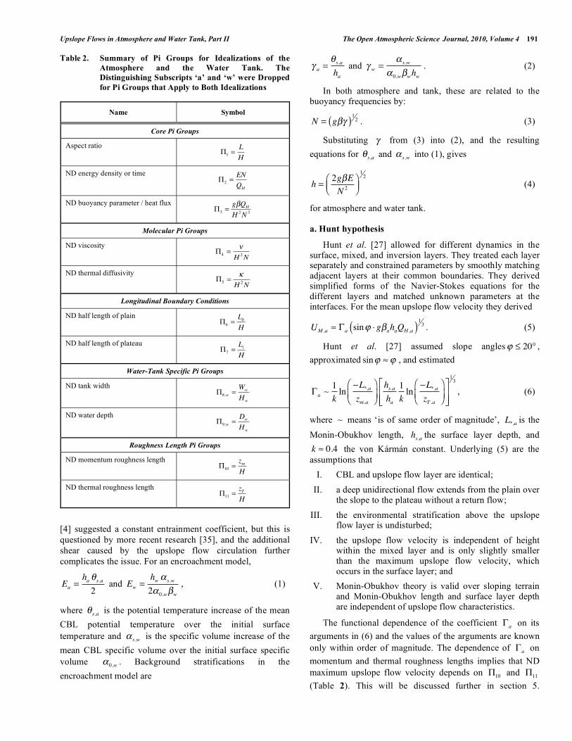
Table 2. Summary of Pi Groups for Idealizations of the
Atmosphere and the Water Tank. The
Distinguishing Subscripts ‘a’ and ‘w’ were Dropped
for Pi Groups that Apply to Both Idealizations
Name Symbol
Core Pi Groups
Aspect ratio 1 =
L
H
ND energy density or time 2 =
EN
QH
ND buoyancy parameter / heat flux 3 =
g QH
H 2N 3
Molecular Pi Groups
ND viscosity 4 = H 2N
ND thermal diffusivity 5 = H 2N
Longitudinal Boundary Conditions
ND half length of plain 6 =
LbH
ND half length of plateau 7 =
LtH
Water-Tank Specific Pi Groups
ND tank width 8,w =
Ww
Hw
ND water depth 9,w =
Dw
Hw
Roughness Length Pi Groups
ND momentum roughness length 10 =
zmH
ND thermal roughness length 11 =
zTH
[4] suggested a constant entrainment coefficient, but this is
questioned by more recent research [35], and the additional
shear caused by the upslope flow circulation further
complicates the issue. For an encroachment model,
Ea =ha s,a
2 and Ew =
hw s,w
2 0,w w
, (1)
where s,a is the potential temperature increase of the mean
CBL potential temperature over the initial surface
temperature and s,w is the specific volume increase of the
mean CBL specific volume over the initial surface specific
volume 0,w . Background stratifications in the
encroachment model are
a =s,a
ha and w =
s,w
0,w whw. (2)
In both atmosphere and tank, these are related to the buoyancy frequencies by:
N = g( )12 . (3)
Substituting from (3) into (2), and the resulting
equations for s,a and s,w into (1), gives
h =2g E
N 2
12
(4)
for atmosphere and water tank.
a. Hunt hypothesis
Hunt et al. [27] allowed for different dynamics in the surface, mixed, and inversion layers. They treated each layer separately and constrained parameters by smoothly matching adjacent layers at their common boundaries. They derived simplified forms of the Navier-Stokes equations for the different layers and matched unknown parameters at the interfaces. For the mean upslope flow velocity they derived
UM ,a a sin g ahaQH ,a( )13 . (5)
Hunt et al. [27] assumed slope angles 20° ,
approximated sin , and estimated
a
1
kln
L*,azm,a
hs,aha
1
kln
L*,azT ,a
13
, (6)
where means ‘is of same order of magnitude’, L*,a is the
Monin-Obukhov length, hs,a the surface layer depth, and
k 0.4 the von Kármán constant. Underlying (5) are the
assumptions that
I. CBL and upslope flow layer are identical;
II. a deep unidirectional flow extends from the plain over the slope to the plateau without a return flow;
III. the environmental stratification above the upslope flow layer is undisturbed;
IV. the upslope flow velocity is independent of height within the mixed layer and is only slightly smaller than the maximum upslope flow velocity, which occurs in the surface layer; and
V. Monin-Obukhov theory is valid over sloping terrain and Monin-Obukhov length and surface layer depth are independent of upslope flow characteristics.
The functional dependence of the coefficient a on its
arguments in (6) and the values of the arguments are known
only within order of magnitude. The dependence of a on
momentum and thermal roughness lengths implies that ND
maximum upslope flow velocity depends on 10 and 11
(Table 2). This will be discussed further in section 5.
192 The Open Atmospheric Science Journal, 2010, Volume 4 Reuten et al.
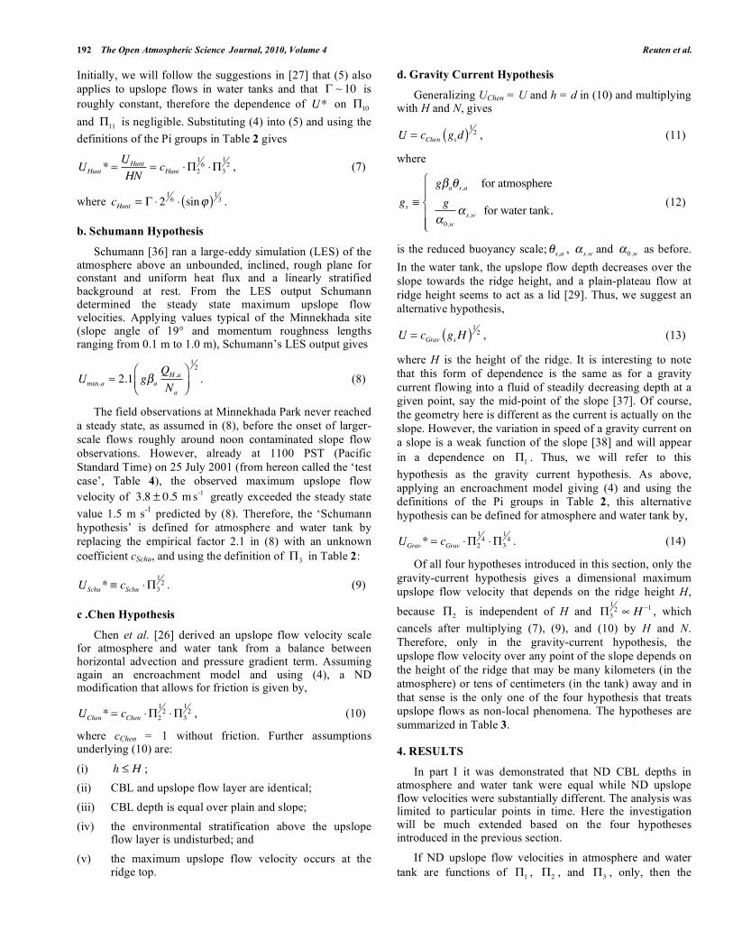
Initially, we will follow the suggestions in [27] that (5) also
applies to upslope flows in water tanks and that 10 is
roughly constant, therefore the dependence of U* on 10
and 11 is negligible. Substituting (4) into (5) and using the
definitions of the Pi groups in Table 2 gives
UHunt* =UHunt
HN= cHunt 2
16
3
12 , (7)
where cHunt = 216 sin( )
13 .
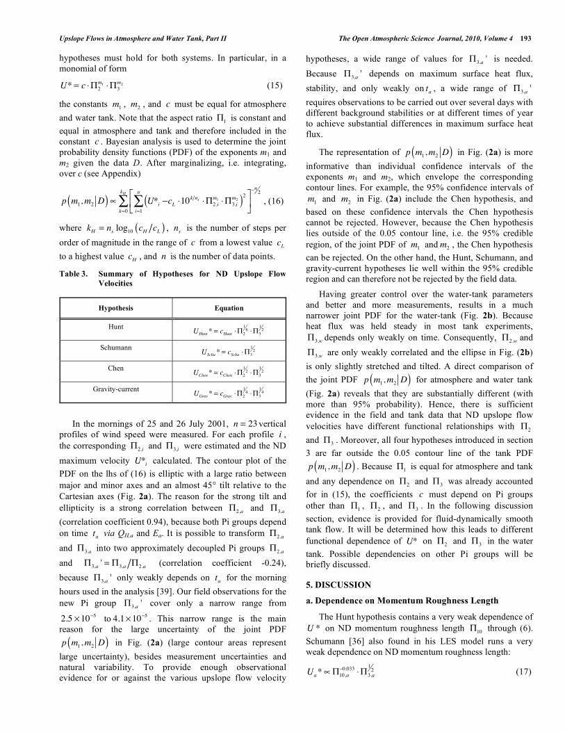
b. Schumann Hypothesis
Schumann [36] ran a large-eddy simulation (LES) of the atmosphere above an unbounded, inclined, rough plane for constant and uniform heat flux and a linearly stratified background at rest. From the LES output Schumann determined the steady state maximum upslope flow velocities. Applying values typical of the Minnekhada site (slope angle of 19° and momentum roughness lengths ranging from 0.1 m to 1.0 m), Schumann’s LES output gives
Umax,a 2.1 g a
QH ,a
Na
12
. (8)
The field observations at Minnekhada Park never reached
a steady state, as assumed in (8), before the onset of larger-
scale flows roughly around noon contaminated slope flow
observations. However, already at 1100 PST (Pacific
Standard Time) on 25 July 2001 (from hereon called the ‘test
case’, Table 4), the observed maximum upslope flow
velocity of 3.8 ± 0.5 m s-1 greatly exceeded the steady state
value 1.5 m s-1
predicted by (8). Therefore, the ‘Schumann
hypothesis’ is defined for atmosphere and water tank by
replacing the empirical factor 2.1 in (8) with an unknown
coefficient cSchu, and using the definition of 3 in Table 2:
USchu* cSchu 3
12 . (9)
c .Chen Hypothesis
Chen et al. [26] derived an upslope flow velocity scale for atmosphere and water tank from a balance between horizontal advection and pressure gradient term. Assuming again an encroachment model and using (4), a ND modification that allows for friction is given by,
UChen* = cChen 2
12
3
12 , (10)
where cChen = 1 without friction. Further assumptions underlying (10) are:
(i) h H ;
(ii) CBL and upslope flow layer are identical;
(iii) CBL depth is equal over plain and slope;
(iv) the environmental stratification above the upslope flow layer is undisturbed; and
(v) the maximum upslope flow velocity occurs at the ridge top.
d. Gravity Current Hypothesis
Generalizing UChen = U and h = d in (10) and multiplying with H and N, gives
U = cChen gsd( )12 , (11)
where
gs
g a s,a for atmosphere
g
0,ws,w for water tank,
(12)
is the reduced buoyancy scale; s,a , s,w and 0,w as before.
In the water tank, the upslope flow depth decreases over the
slope towards the ridge height, and a plain-plateau flow at
ridge height seems to act as a lid [29]. Thus, we suggest an
alternative hypothesis,
U = cGrav gsH( )12 , (13)
where H is the height of the ridge. It is interesting to note
that this form of dependence is the same as for a gravity
current flowing into a fluid of steadily decreasing depth at a
given point, say the mid-point of the slope [37]. Of course,
the geometry here is different as the current is actually on the
slope. However, the variation in speed of a gravity current on
a slope is a weak function of the slope [38] and will appear
in a dependence on 1 . Thus, we will refer to this
hypothesis as the gravity current hypothesis. As above,
applying an encroachment model giving (4) and using the
definitions of the Pi groups in Table 2, this alternative
hypothesis can be defined for atmosphere and water tank by,
UGrav* = cGrav 2
14
3
14 . (14)
Of all four hypotheses introduced in this section, only the
gravity-current hypothesis gives a dimensional maximum
upslope flow velocity that depends on the ridge height H,
because 2 is independent of H and 3
12 H 1 , which
cancels after multiplying (7), (9), and (10) by H and N.
Therefore, only in the gravity-current hypothesis, the
upslope flow velocity over any point of the slope depends on
the height of the ridge that may be many kilometers (in the
atmosphere) or tens of centimeters (in the tank) away and in
that sense is the only one of the four hypothesis that treats
upslope flows as non-local phenomena. The hypotheses are
summarized in Table 3.
4. RESULTS
In part I it was demonstrated that ND CBL depths in atmosphere and water tank were equal while ND upslope flow velocities were substantially different. The analysis was limited to particular points in time. Here the investigation will be much extended based on the four hypotheses introduced in the previous section.
If ND upslope flow velocities in atmosphere and water
tank are functions of 1 , 2 , and 3 , only, then the
Upslope Flows in Atmosphere and Water Tank, Part II The Open Atmospheric Science Journal, 2010, Volume 4 193
hypotheses must hold for both systems. In particular, in a
monomial of form
U* = c 2m1
3m2 (15)
the constants m1 , m2 , and c must be equal for atmosphere
and water tank. Note that the aspect ratio 1 is constant and
equal in atmosphere and tank and therefore included in the
constant c . Bayesian analysis is used to determine the joint
probability density functions (PDF) of the exponents m1 and
m2 given the data D. After marginalizing, i.e. integrating,
over c (see Appendix)
p m1,m2 D( ) U*i cL 10k ns
2,im1
3,im2( )
2
i=1
nn2
k=0
kH
, (16)
where kH = ns log10 cH cL( ) , ns is the number of steps per
order of magnitude in the range of c from a lowest value cL
to a highest value cH , and n is the number of data points.
Table 3. Summary of Hypotheses for ND Upslope Flow
Velocities
Hypothesis Equation
Hunt UHunt * = cHunt 2
16
3
12
Schumann USchu* = cSchu 3
12
Chen UChen* = cChen 2
12
3
12
Gravity-current UGrav* = cGrav 2
14
3
14
In the mornings of 25 and 26 July 2001, n = 23vertical
profiles of wind speed were measured. For each profile i ,
the corresponding 2,i and 3,i were estimated and the ND
maximum velocity U*i calculated. The contour plot of the
PDF on the lhs of (16) is elliptic with a large ratio between
major and minor axes and an almost 45° tilt relative to the
Cartesian axes (Fig. 2a). The reason for the strong tilt and
ellipticity is a strong correlation between 2,a and 3,a
(correlation coefficient 0.94), because both Pi groups depend
on time ta via QH,a and Ea. It is possible to transform 2,a
and 3,a into two approximately decoupled Pi groups 2,a
and 3,a ' = 3,a 2,a (correlation coefficient -0.24),
because 3,a ' only weakly depends on ta for the morning
hours used in the analysis [39]. Our field observations for the
new Pi group 3,a ' cover only a narrow range from
2.5 10 5 to 4.1 10 5
. This narrow range is the main
reason for the large uncertainty of the joint PDF
p m1,m2 D( ) in Fig. (2a) (large contour areas represent
large uncertainty), besides measurement uncertainties and
natural variability. To provide enough observational
evidence for or against the various upslope flow velocity
hypotheses, a wide range of values for 3,a ' is needed.
Because 3,a ' depends on maximum surface heat flux,
stability, and only weakly on ta , a wide range of 3,a '
requires observations to be carried out over several days with
different background stabilities or at different times of year
to achieve substantial differences in maximum surface heat
flux.
The representation of p m1,m2 D( ) in Fig. (2a) is more
informative than individual confidence intervals of the
exponents m1 and m2, which envelope the corresponding
contour lines. For example, the 95% confidence intervals of
m1 and m2 in Fig. (2a) include the Chen hypothesis, and
based on these confidence intervals the Chen hypothesis
cannot be rejected. However, because the Chen hypothesis
lies outside of the 0.05 contour line, i.e. the 95% credible
region, of the joint PDF of m1 andm2 , the Chen hypothesis
can be rejected. On the other hand, the Hunt, Schumann, and
gravity-current hypotheses lie well within the 95% credible
region and can therefore not be rejected by the field data.
Having greater control over the water-tank parameters
and better and more measurements, results in a much
narrower joint PDF for the water-tank (Fig. 2b). Because
heat flux was held steady in most tank experiments,
3,w depends only weakly on time. Consequently, 2,w and
3,w are only weakly correlated and the ellipse in Fig. (2b)
is only slightly stretched and tilted. A direct comparison of
the joint PDF p m1,m2 D( ) for atmosphere and water tank
(Fig. 2a) reveals that they are substantially different (with
more than 95% probability). Hence, there is sufficient
evidence in the field and tank data that ND upslope flow
velocities have different functional relationships with 2
and 3 . Moreover, all four hypotheses introduced in section
3 are far outside the 0.05 contour line of the tank PDF
p m1,m2 D( ) . Because 1 is equal for atmosphere and tank
and any dependence on 2 and 3 was already accounted
for in (15), the coefficients c must depend on Pi groups
other than 1 , 2 , and 3 . In the following discussion
section, evidence is provided for fluid-dynamically smooth
tank flow. It will be determined how this leads to different
functional dependence of U* on 2 and 3 in the water
tank. Possible dependencies on other Pi groups will be
briefly discussed.
5. DISCUSSION
a. Dependence on Momentum Roughness Length
The Hunt hypothesis contains a very weak dependence of
U * on ND momentum roughness length 10 through (6).
Schumann [36] also found in his LES model runs a very
weak dependence on ND momentum roughness length:
Ua* 10,a0.033
3,a
12 (17)

194 The Open Atmospheric Science Journal, 2010, Volume 4 Reuten et al.
for a slope angle of 10°. Schumann’s one-dimensional slope
with the assumption of a steady state may not be a good
representation of the field and water-tank observations used
here, but it is worth pursuing the idea of a functional
dependence of U * on 10 further. Assume a dependence on
10 was contained in the coefficients c in the four
hypotheses introduced in section 3. Separating this
dependence from the coefficient generalizes (15):
U* = c1 10A
2m1
3m2 , (18)
where a minus sign was added to the exponent of 10
because it can be expected that U* is inversely related to
10 so that the unknown parameter A > 0 .
For the atmosphere, all but the Chen hypothesis give
functional dependences of U * on 2 and 3 that agree
with field observations. Hence, the field observations
support an approximately constant momentum roughness
length in the atmosphere, as would be expected from land-
use characteristics at the field site. For the water-tank
observations, however, a hypothesis of form (18) requires
that ND momentum roughness length 10,w is a function of
at least one of the two Pi groups 2,w and 3,w . A
hypothesis for such dependence will be presented next.
a. Similarity Violation as a Result of Fluid-Dynamic Feedback
In wind tunnel experiments, aerodynamical roughness is an important, yet often violated, scaling requirement [40]. In general, a flow is fluid-dynamically smooth if the viscous sublayer of depth
w
5 w
u*,w (19)
(chapter XX in [41]) is deeper than surface roughness
protuberances. In the atmosphere over land surfaces, this is
practically never the case [31]. However, an order-of-
magnitude estimation shows that in our tank experiments the
flow was fluid-dynamically smooth: The ratio between
velocity and friction velocity is of order 10, i.e.
Uw u*,w 10 [41, 42]; with the tank values for Uw and w
in Table 4 this gives w 0.01m , which is approximately
two orders of magnitude larger than the roughness elements
on the well-sanded and painted tank bottom.
Because of fluid-dynamical smoothness, momentum roughness length in the water tank is not a function of distribution and size of roughness elements but of viscosity and friction velocity (Chapter 7 in [42]):
zm,w0.11 w
u*,w. (20)
An increase of upslope flow velocity leads to increased friction velocity, which in turn leads to decreased roughness length in (20). This permits further increase of upslope flow velocity. A possible approach to quantifying this positive fluid-dynamical feedback will be presented next.
b. Quantification of Fluid-Dynamic Feedback
The goal is to express Uw* as a monomial of the two Pi
groups 2,w and 3,w by substituting (20) into the definition
of 10,w in Table 4, which is substituted into (18) to give
Fig. (2). Joint PDF p m1,m2 D( ) of the exponents m1 and m2 in an empirical relationship U* = c 2m1
3m2 between ND upslope flow velocity
U* and the two Pi groups 2 and 3 . For the large ellipses in (a) and (b), contour lines are shown for 0.05 (outer line) and from 0.1 to 0.9
in steps of 0.1. (a) Large ellipse is for the field data on the mornings of 25 and 26 July 2001; small ellipse (only the 0.05 and 0.5 contour
lines are shown) is for the data from seven water-tank experiments (Table 1); labeled squares are the positions of the upslope flow velocity
hypotheses discussed in section 3; error bars indicate 95% confidence intervals from a nonlinear regression. (b) Zoomed into the dashed region in (a) around the PDF for the tank data.

Upslope Flows in Atmosphere and Water Tank, Part II The Open Atmospheric Science Journal, 2010, Volume 4 195
Uw* c10.11 w
u*,wHw
A
2m1
3m2 (21)
To express the friction velocity u*,w in terms of known
quantities, we use convective transport theory [43],
u* = C*Dw*U( )12 , (22)
where the momentum transport coefficient C*D depends on
the surface characteristics, U is the maximum in the vertical
profile of upslope flow velocity, and
w* = g hQH( )13 (23)
is the convective velocity scale.
Table 4. Data for Test Case
Name Symbol (Units) Atmosphere Water Tank
Ridge height H (m) 760 0.149
Instantaneous heat flux
QH (K m s-1) 0.21± 0.05 1.9 ± 0.2( ) 10 3
Energy density E (K m) 1600 ± 400 0.56 ± 0.05
Buoyancy frequency N (s-1) 0.015 ± 0.001 0.38 ± 0.02
Buoyancy parameter g (m s-2 K-1) 0.036 0.0026
Kinematic viscosity (m2 s-1) 1.52 10 5 8.9 10 7
Prandtl number at 25°C
Pr 0.72 6.1
CBL depth h (m) 720 ±120 0.14 ± 0.02
Upslope flow velocity
U (m s-1) 3.8 ± 0.5 0.005 ± 0.001
Atmospheric data are for the field site at Minnekhada Park at 1100 PDT 25 July 2001;
water-tank experiment was designed such that, i.e. 2,w = 2,a and 3,w = 3,a .
Uncertainties roughly represent 95% confidence intervals.
Equation (22) was extensively validated for atmospheric convection over land and ocean surfaces [43-45]. The derivation of (22) in [43] applies equally to free convection in air or water. It assumes that surface- and micro-layer processes can be ignored, therefore it can also be applied to fluid-dynamically smooth flow. To ignore these processes, they must be fast enough to maintain higher temperatures in surface- and micro-layer than in the mixed layer. This was the case in all tank experiments, because convection and upslope flows continued for at least another minute after heat flux was shut down. Stull [43] showed that (22) also holds under non-calm conditions as long as the mixed-layer Richardson number
RwB
U
2
, (24)
is greater than 3 (‘quasi-free convection’). Here, the
buoyancy velocity scale wB is defined by
wB2
g a skin,a ha for atmosphere
g
0,wskin,w hw for water tank,
(25)
where skin,a and skin,w are the differences of potential
temperature at the land surface and specific volume at the
tank bottom to the corresponding quantities in the mixed
layer. All other quantities were introduced before, and
typical values used here are given in Table 4. Because we do
not have measurements of the skin temperatures, we estimate
lower limits. At the field site we measured differences
between 2-m and mixed-layer temperatures of approximately
2 K. Because skin temperatures can be expected to be
substantially larger, we use skin,a = 3K as a lower limit,
which was also the lowest value observed in Oklahoma
under much weaker surface heat fluxes [43]. Substituting
this value into (25) gives wB,a > 9 m s-1
, and the mixed-layer
Richardson number becomes R ,a > 5 , meeting the
requirement for quasi-free convection. In the water tank,
rising thermals hitting the CT probes lead to rapid increases
in specific volume, which are used here as a conservatively
low estimate of the difference between skin and mixed-layer
temperatures: skin,w = 0.5 10 6 m3 kg-1 (Fig. 7 in [29]).
This value gives wB,w > 0.02 m s-1 and R ,w > 16 , indicative
of quasi-free convection.
The convective boundary-layer depth h is substituted
from the encroachment model (4) to give the convective
velocity scale (23). Then the convective velocity scale (23) is
substituted into (22) to give the friction velocity, which is
substituted into (21) to give
Uw* c10.11 w
C*D,w g w
2g E
N 2
12
QH ,w
13
Uw
12
Hw
A
2,wm1
3,wm2 . (26)
On the rhs of the last equation, the viscosity w appears,
so that ND upslope flow velocity depends on ND
viscosity 4,w . Moreover, the appearance of upslope flow
velocity Uw with the positive exponent A 2 on the rhs
quantifies the positive feedback mechanism described
qualitatively in the previous subsection. Expanding the rhs
with monomials of Hw and Nw , applying the definitions of
2,w , 3,w , and 4,w in Table 2, and solving for Uw* yields
Uw* c1
2
2 A 0.112A
2 A 2A
6 2 A( ) C*D,w
A
2 A4,w
2A
2 A2,w
A+12m16 2 A( )
3,w
A+4m22 2 A( ) . (27)
The first three factors are constant. The fourth and fifth
factors are not constant, but the tight contour lines in Fig. (2)
suggest that they did not vary much. This will be further

196 The Open Atmospheric Science Journal, 2010, Volume 4 Reuten et al.
discussed below. The pairs of exponents
A +12m1
6 2 A( ),A + 4m2
2 2 A( ) are a parametric representation of a
path in the m1 m2 plane. Each point on the path
corresponds to a particular value of the exponent A of ND
momentum roughness length 10,w in (18). Most probable
values of A are those within the PDF contours near the
mode of p m1,m2 D( ) . There are four different paths, one
for each hypothesis introduced in section 3 and its fixed pair
m1,m2( ) of exponents (Fig. 3a). Only the path for the
gravity-current hypothesis is within the 5% contour of the
PDF and runs close to the mode (Fig. 3b). There is a range
of probable values for A . Representative values of simple
rationals for A are shown in Fig. (3b). We chose for the
following discussion A = 3 4 fairly close to the mode,
because it seems more likely that this value could be derived
from first principles than 4/5 or 5/6. The gravity-current
hypothesis therefore agrees well with water-tank
observations if the ND momentum roughness length with an
exponent of A = 3 4 is included in (27):
Uw* 15.15 c185 C*D,w
35
4,w
65
2,w
12
3,w
710 = c2,w 2,w
12
3,w
710 . (28)
Substituting A = 3 4 into (18) gives the corresponding
equation for the atmosphere:
Ua* = c1 10,a
34
2,a
14
3,a
14 = c2,a 2,a
14
3,a
14 . (29)
Here c2,a depends on surface characteristics and slope
angle, but is constant with respect to the quantities changed
in our experiments listed in Table 1: Nw , QH ,w , and Ew . In
the water tank, c2,w depends rather strongly on Nw :
c2,w Nw
65 . However, because Uw* Nw
25 Ew
12 QH ,w
15 and
the range of buoyancy frequency Nw and instantaneous heat
flux QH ,w in our tank experiments is rather small (Table 1),
the posterior distribution of Uw* in Figs. (2, 3) is dominated
by Ew , which ranges from 0 to its maximum value. More
experiments over a much wider range of buoyancy
frequencies Nw will be required in the future to test the
dependence of ND upslope flow velocity on Nw and
therefore test the applicability of convective transport theory
to upslope flows in water tanks.
c. Plausibility Test and Future Research Needs
From the data of the test case in Table 4, Ua* = 0.33 and
Uw* = 0.088 . It seems counterintuitive at first that a fluid-
dynamically smooth flow is slower than a rough flow.
Estimating roughly zm,a 0.3 m at the field site, the
momentum roughness length in the tank that is required from
similarity with the atmosphere, 10,w = 10,a , is
zm,w = zm,aHw Ha 0.06 mm . In other words, if the flow in
the tank was fluid-dynamically rough with a roughness
length of 0.06 mm then similarity of ND upslope flow
velocity could be expected. However, the smooth flow in the
tank has the characteristics of a rough flow over a surface
with much larger momentum roughness length: Field
observations for the test case (Table 4) substituted into (29)
Fig. (3). Parameter paths of the exponent A in upslope flow velocity hypotheses of formUw* = c1 10,wA
2,wm1
3,wm2 , superimposed on the joint
PDF of m1 and m2 for the tank observations, only. The pairs A +12m1
6 2 A( ),A + 4m2
2 2 A( ) are shown for four upslope flow velocity hypotheses as
labeled in (a). Contour plots of the PDF are shown as in Fig (2). (b) is zoomed into the dotted rectangular region of (a). Representative
values of A are shown in (b) as labeled squares.

Upslope Flows in Atmosphere and Water Tank, Part II The Open Atmospheric Science Journal, 2010, Volume 4 197
give c1 1.1 10 3. A corresponding rough flow in the
water tank should follow the equivalent equation to (29),
U
w* = c
1 10,w
34
2,w
14
3,w
14 , (30)
with the same value for c1 as in the atmosphere. Substituting
this value and the tank observations of the test case (Table 4)
into (30) gives zm,w 0.3 mm . In other words, with respect
to momentum roughness length, the smooth flow in the
water tank represents a rough atmospheric flow over a
surface with a roughness length about five times greater than
the one estimated for the field site. Therefore, from (29), the
ND upslope flow velocity in the atmosphere should be 534
times the tank value, in good agreement with the data above.
The dependence of the gravity-current hypothesis on
roughness length as detailed here can only be tentative and
guide in a search for underlying first principles. Future
research will have to address several questions and
challenges: Is convective transport theory applicable to
smooth flows? Can the unknown coefficients c1 and C*D,w
in (28) be derived from first principles? Moreover, it is
desirable to refine the upslope flow velocity hypotheses by
replacing the encroachment model with the entrainment
model. Finally, with more tank data the probability density
function of m3 in an upslope flow hypothesis of form
Uw = cw 4,wm3
2,wm1
3,wm2 (31)
can be determined and compared with m3 = 6 5 in (28).
Such future research would make it possible to
quantitatively scale between water tank and atmosphere,
albeit not simply by applying (15) with the constants m1 ,
m2 , and c being equal for atmosphere and water tank.
Currently, even if fluid-dynamical smoothness could be
overcome in water-tank experiments, the constants m1 , m2 ,
and c in (15) remain poorly constrained. Particularly, more
accurate field data for nearly idealized environmental
settings are needed. This paper suggests that previously
observed quantitative agreement was within the uncertainties
associated with field and tank measurements and with
environmental settings that were either badly known or
difficult to model in the water tank. However, previous
research mentioned in the introduction has demonstrated the
value of water-tank experiments to qualitatively model
atmospheric flows over sloping terrain. For example, Reuten
et al. (2007) demonstrated similar development of pollutant
layers in water tank and field observations.
d. The Role of Other Pi Groups
The previous subsections of the discussion provide a
tentative explanation for the different functional
dependences of ND upslope flow velocities in tank and
atmosphere on the governing parameters. The explanation
focused on the importance of momentum roughness length
10 in the atmosphere and led to the inclusion of ND
viscosity 4 in the water tank. A brief discussion of the
potential role of other ND governing parameters is provided
next.
Thermal Roughness Length and Diffusivity
A hint at another important difference between tank and
atmosphere comes from [27], who included the thermal
roughness length zT, (5) and (6). The ratio between
momentum and thermal roughness length strongly depends
on the Prandtl number (which is very different for air and
water, Table 4) and surface properties. For the field site,
zm,a zT ,a [31], and for smooth tank flow
zm,w zT ,w by
many orders of magnitude (table 4.1 in [46]). Hence, heat
transport is very inefficient in both systems. Further research
into the coefficient a for the atmosphere in [27], (6), and
w for the water tank is required to assess the impact of a
similarity violation of ND thermal roughness length
11 = zT H on upslope flow velocity in the Hunt
hypothesis. It was shown above that the characteristics of
fluid-dynamically smooth flow introduce a dependence on
ND viscosity 4,w in (28). Future research will have to
investigate if a dependence of ND upslope flow velocity on
ND thermal roughness length 11 introduces a dependence
on ND thermal diffusivity 5,w in the water tank.
Reynolds Number
As the flow is dependent on the viscosity, it is Reynolds-
number (Re) dependent. A more direct and usual route
would be to investigate the effect of Reynolds number
directly, rather than consider roughness lengths. However, as
was pointed out in part I, this approach is inconclusive. The
critical Reynolds number, above which the flow would be
dominated by turbulence, is strongly dependent on the
choice of length and velocity scales and the particular system
and flow geometry. Using the definition in [26], the tank
experiments used in this part give
Re = LU = 2.2 8.7( ) 103 . According to [26], this
would suggest similarity with the atmosphere based on a
critical pipe flow Reynolds number. However, the geometry
in the water tank is not that of a pipe flow and may therefore
have a different critical value. An example of a different
geometry (a plume stack) is given by Contini et al. (2009)
where they find that a value of 2196 in a wind tunnel is
insufficient to achieve similarity with the full-scale
atmosphere. In contrast [39] defined the Reynolds number
based on upslope-flow profiles observed in the tank
assuming the geometry of an open channel flow: Only for
the fastest flows observed in our experiments, values in the
range 1350-1800 of intermittently turbulent flow are
reached. The approach taken in this study via the momentum
roughness lengths provides deeper insight into the flow
characteristics in the tank.
Plain and Plateau Lengths
Non-dimensional plain and plateau lengths, 6,w and
7,w , cannot be significant for the similarity violation. The
water-tank experiments (Table 1) had substantially different

198 The Open Atmospheric Science Journal, 2010, Volume 4 Reuten et al.
6,w and 7,w but p m1,m2 D( ) is very narrow.
Furthermore, p m1,m2 D( ) for all seven experiments is
narrower than for any subset of six experiments (not shown).
In other words, each tank experiment contributes to
improved predictions of m1 and m2 even if inclusion of the
data increases the range of 6,w and 7,w .
Tank Width
Observations early into the tank experiments show no
influence of friction at the lateral side walls of the tank on
upslope flow velocities near the slope centre. At later times,
which we did not use for the analyses here, more complex
3D flow structures developed which can be attributed to
temperature gradients and possibly friction at the lateral side
walls (figure 8 in [29]). The opposite effect, lateral side walls
suppressing horizontally mass-compensating flows and
forcing return flows against gravity above the upslope flow,
seems plausible. However, despite a lack of lateral
confinement at the field site [30] observed flows in
downslope direction above the upslope flows, which
compensated most of the upslope mass flux. Therefore, ND
upslope flow velocities should not substantially depend on
ND tank width 8,w .
Water Depth and Gravity Waves
Non-dimensional water depth over the plain, 9,w , is
unlikely an important factor for upslope flow velocities,
because in all experiments the water surface was far above
the top of the CBL. In agreement with [25], we observed
elevated layers of alternating flows above the plain-plateau
flow. These were shallow, their velocities decreased
substantially with height, and they never seemed to affect
water near the top surface.
An indirect effect of the confinement of the tank by 6,w
to 9,w could be that energy dissipation by gravity waves in
the atmosphere is greater than in the water tank, but that
contradicts observations of greater upslope flow velocities in
the atmosphere (part I). In can be concluded that it is
unlikely that ND upslope flow velocities depend
substantially on 6,w to 9,w and that such a dependence
could explain the similarity violation.
CONCLUSIONS
Four hypotheses for ND maximum upslope flow
velocities were introduced based on [27, 36, 26], and a
gravity-current flow into a fluid of decreasing depth. The
hypotheses were all of form U* = c 2m1
3m2 with
unknown coefficient c. 2 =EN
QH
and 3 =g QH
H 2N 3 were
initially assumed the only governing ND parameters. The
Bayesian joint PDF of the exponents m1 and m2 differed
between atmosphere and water tank with greater than 95%
probability. The Hunt, Schumann, and gravity-current
hypotheses agreed well with the PDF for the field data, but
none of them agreed with the PDF for the tank data. It was
concluded that ND upslope flow velocity requires additional
dependence on other Pi groups. Observational evidence rules
out Pi groups related to the size and geometry of the tank
( 6,w to 9,w ). Estimations of surface roughness and
viscous sublayer depth suggest that the upslope flow in the
water tank is fluid-dynamically smooth, and therefore
momentum roughness length zm,w depends on friction
velocity. This results in a stronger dependence of Uw* on
2,w and 3,w in the tank than in the atmosphere, because
an increase of 2,w or 3,w leads to a decrease of zm,w and
therefore stronger increase of Uw* than for fluid-
dynamically rough flow. It was demonstrated that only for
the gravity-current hypothesis the inclusion of ND
momentum roughness length in Uw* can lead to good
agreement with the tank data. This success of the gravity-
current hypothesis suggests that upslope flows must be
treated as non-local phenomena, because only in the gravity-
current hypothesis are upslope flow velocities dependent on
ridge height.
More research should be carried out to test the
applicability of convective transport theory to smooth flows,
to replace the encroachment model of CBL growth by the
more realistic entrainment model, and to test the predicted
value -6/5 of the exponent of ND viscosity 4,w in (28).
The work presented here implies that water-tank models of other thermally driven meso-scale circulations like up-valley flows, sea breezes, and urban heat islands may suffer the same velocity similarity violation as upslope systems. It is difficult in a laboratory setting to ensure both fluid-dynamically rough flow and a match between roughness elements in the atmosphere and tank. However, as shown here, it is possible to explicitly include the dependence on the momentum roughness length and use the tank data to distinguish between flow dependence models for the atmosphere.
ACKNOWLEDGEMENTS
We wish to thank Greg Lawrence for providing laboratory space for the water tank and sharing computer resources and instrumentation. The water tank was built in the workshop of the Department of Civil Engineering at UBC; the work by Bill Leung, Scott Jackson, and Harald Schrempp is gratefully acknowledged. We thank Ian Chan for his help on tank re-design, MatPIV, and several experiments. Funding support was provided by grants from NSERC and CFCAS to Douw Steyn and Susan Allen.
APPENDIX
Bayesian Parameter Estimation
This appendix briefly derives the equations used in this communication. Background information and details of the following derivations can be found in [47-50].
Starting point is Bayes’ Theorem
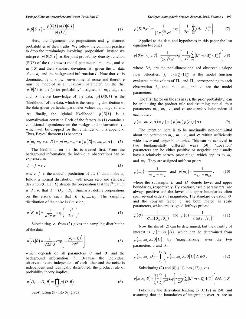
Upslope Flows in Atmosphere and Water Tank, Part II The Open Atmospheric Science Journal, 2010, Volume 4 199
p D, I( ) =p I( ) p D , I( )
p D I( ). (1)
Here, the arguments are propositions and p denotes
probabilities of their truths. We follow the common practice
to drop the terminology involving ‘proposition’; instead we
interpret p D, I( ) as the joint probability density function
(PDF) of the (unknown) model parameters m1 , m2 , and c
in (15) and their standard deviation , given the n data
d1, ..., dn and the background information I . Note that is
dominated by unknown environmental noise and therefore
must be modeled as an unknown parameter. On the rhs,
p I( ) is the ‘prior probability’ assigned to m1 , m2 , c ,
and before knowledge of the data; p D , I( ) is the
‘likelihood’ of the data, which is the sampling distribution of
the data given particular parameter values m1 , m2 , c , and
; finally, the ‘global likelihood’ p D I( ) is a
normalization constant. Each of the factors in (1) contains a
conditional dependence on the background information I ,
which will be dropped for the remainder of this appendix.
Thus, Bayes’ theorem (1) becomes
p m1,m2 , c, D( ) p m1,m2 , c,( ) p D m1,m2 , c,( ) . (2)
The likelihood on the rhs is treated first. From the background information, the individual observations can be expressed as
di = fi + ei , (3)
where fi is the model’s prediction of the ith
datum; the ei
follow a normal distribution with mean zero and standard
deviation . Let Di denote the proposition that the ith
datum
is di , so that D = D1, ..., Dn . Similarly, define propositions
on the errors, such that E = E1, ..., En . The sampling
distribution of the noise is Gaussian,
p Ei( ) =1
2exp
ei2
2 2 . (4)
Substituting ei from (3) gives the sampling distribution
of the data
p Di( ) =1
2exp
di fi( )2
2 2 , (5)
which depends on all parameters and and the
background information I . Because the individual
observations are independent of each other and the noise is
independent and identically distributed, the product rule of
probability theory implies,
p D1, ...,Dn( ) = p Di( )i=1
n
. (6)
Substituting (5) into (6) gives
p D ,( ) =1
2( )n2 n
exp1
2 2 di fi( )2
i=1
n
. (7)
Applied to the data and hypotheses in this paper the last equation becomes
p D m1,m2 , c,( ) =1
2( )n2 n
exp1
2 2 U*i c 2,im1
3,im2( )
2
i=1
n
, (8)
where U*i are the non-dimensionalized observed upslope
flow velocities, fi = c 2,im1
3,im2 is the model function
evaluated at the values of 2 and 3 corresponding to each
observation i , and m1 , m2 , and c are the model
parameters.
The first factor on the rhs in (2), the prior probability, can
be split using the product rule and assuming that all four
parameters m1 , m2 , c , and are a priori independent of
each other,
p m1,m2 , c,( ) = p m1( ) p m2( ) p c( ) p ( ) . (9)
The intention here is to be maximally non-committal
about the parameters m1 , m2 , c , and within sufficiently
wide lower and upper boundaries. This can be achieved in
two fundamentally different ways [50]. ‘Location’
parameters can be either positive or negative and usually
have a relatively narrow prior range, which applies to m1
and m2 . They are assigned uniform priors
p m1( ) =1
m1,H m1,L
and p m2( ) =1
m2,H m2,L
, (10)
where the subscripts L and H denote lower and upper
boundaries, respectively. By contrast, ‘scale parameters’ are
always positive and the lower and upper boundaries often
span several orders of magnitude. The standard deviation
and the constant factor c are both treated as scale
parameters, which are assigned Jeffreys priors:
p ( ) =1
ln H L( ) and p c( ) =
1
c ln cH cL( ). (11)
Now the rhs of (2) can be determined, but the quantity of
interest is p m1,m2 D( ) , which can be determined from
p m1,m2 , c, D( ) by ‘marginalizing’ over the two
parameters c and :
p m1,m2 D( ) = p m1,m2 , c, D( )dc dcL
cH
L
H
. (12)
Substituting (2) and (8)-(11) into (12) gives
p m1,m2 D( )1
ccL
cH 1n+1 exp
1
2 2 U*i c 2,im1
3,im2( )
2
i=1
n
L
H
d dc .(13)
Following the derivation leading to (C.17) in [50] and
assuming that the boundaries of integration over are so

200 The Open Atmospheric Science Journal, 2010, Volume 4 Reuten et al.
wide that practically L 0 and H , the inner
integral of (13) simplifies so that,
p m1,m2 D( ) dc1
ccL
cH
U*i c 2,im1
3,im2( )
2
i=1
nn2
, (14)
where the gamma function that results from the integration is absorbed in the proportionality.
The integral in (14) is replaced by a sum in which both
ck and the step length ck increase exponentially with
index k . Let ns denote the number of steps per order of
magnitude, then
ck = cL 10k ns (15)
ck = ck+1 ck = cL 10k+1( ) ns cL 10
k ns = cL 10k ns 101 ns 1( ) , (16)
so that
ckck
=cL 10
k ns 101 ns 1( )cL 10
k ns= 101 ns 1 = const . (17)
The final expression for the joint probability distribution therefore becomes
p m1,m2 D( ) U*i cL 10k ns
2,im1
3,im2( )
2
i=1
nn2
k=0
kH
, (18)
with kH = ns log10 cH cL( ) . In this form, the joint probability
distribution can be computed easily with very good
resolution on a standard stand-alone computer.
REFERENCES
[1] Deardorff JW, Willis GE, Lilly DK. Laboratory investigation of non-steady penetrative convection. J Fluid Mech 1969; 35: 7-31.
[2] Willis GE, Deardorff JW. Laboratory model of the unstable planetary boundary layer. J Atmos Sci 1974; 31: 1297-307.
[3] Willis GE, Deardorff JW. Laboratory simulation of the convective planetary boundary layer. Atmos Technol 1975; 7: 80-6.
[4] Heidt FD. The growth of the mixed layer in a stratified fluid due to penetrative convection. Bound-Layer Meteor 1977; 12: 439-61.
[5] Deardorff JW, Willis GE, Stockton BH. Laboratory studies of the entrainment zone of a convectively mixed layer. J Fluid Mech
1980; 100: 41-64. [6] Deardorff JW, Willis GE. Further results from a laboratory model
of the convective planetary boundary layer. Bound-Layer Meteor 1985; 32: 205-36.
[7] Deardorff JW, Willis GE. Computer and laboratory modeling of the vertical diffusion of nonbuoyant particles in the mixed layer.
Adv Geophys 1974; 18B: 187-200. [8] Deardorff JW, Willis GE. Ground-level concentrations due to
fumigation into an entraining mixed layer. Atmos Environ 1982; 16: 1159-70.
[9] Willis GE, Deardorff JW. On the use of Taylor's translation hypothesis for diffusion in the mixed layer. Q J R Meteor Soc
1976; 102: 817-22. [10] Willis GE, Deardorff JW. Laboratory study of dispersion from an
elevated source within a modelled convective planetary boundary layer. Atmos Environ 1978; 12: 1305-11.
[11] Willis GE, Deardorff JW. Laboratory study of dispersion from a source in the middle of the convectively mixed layer. Atmos
Environ 1981; 15: 109-17. [12] Willis GE, Deardorff JW. On plume rise within a convective
boundary layer. Atmos Environ 1983; 17: 2435-47.
[13] Deardorff JW. Laboratory experiments on diffusion: The use of
convective mixed-layer scaling. J Clim Appl Meteor 1985; 24(11): 1143-51.
[14] Ohba R, Kakishima S, Ito S. Water tank experiment of gas diffusion from a stack in stably and unstably stratified layers under
calm conditions. Atmos Environ 1991; 25: 2063-76. [15] Hibberd MF, Sawford BL, Design criteria for water tank models of
dispersion in the planetary convective boundary layer. Bound-Layer Meteor 1994; 67: 97-118.
[16] Hibberd MF, Sawford BL. A saline laboratory model of the planetary convective boundary layer. Bound-Layer Meteor 1994;
67: 229-50. [17] Luhar AK, Hibberd MF, Hurley PJ. Comparison of closure
schemes used to specify the velocity PDF in Lagrangian stochastic dispersion models for convective conditions. Atmos Environ 1996;
30: 1407-18. [18] Park OH, Seo SJ, Lee SH. Laboratory simulation of vertical plume
dispersion within a convective boundary layer. Bound-Layer Meteor 2001; 99: 159-69.
[19] Snyder WH, Lawson RE Jr, Shipman MS, Lu J. Fluid modelling of atmospheric dispersion in the convective boundary layer. Bound-
Layer Meteor 2002; 102: 335-66. [20] van Dop H, van As D, van Herwijnen A, Hibberd MF, Jonker H.
Length scales of scalar diffusion in the convective boundary layer: laboratory observations. Bound-Layer Meteor 2005; 116: 1-35.
[21] Mitsumoto S, Ueda H, Ozoe H. A laboratory experiment on the dynamics of the land and sea breeze. J Atmos Sci 1983; 40: 1228-
40. [22] Lu J, Arya SP, Snyder WH, Lawson RE Jr. A laboratory study of
the urban heat island in a calm and stably stratified environment. Part I: Temperature field. J Appl Meteor 1997; 36: 1377-91.
[23] Lu J, Arya SP, Snyder WH, Lawson RE Jr. A laboratory study of the urban heat island in a calm and stably stratified environment.
Part II: Velocity field. J Appl Meteor 1997; 36: 1392-402. [24] Cenedese A, Monti P. Interaction between an inland urban heat
island and a sea-breeze flow: A laboratory study. J Appl Meteor 2003; 42: 1569-83.
[25] Mitsumoto S. A laboratory experiment on the slope wind. J Meteor Soc Japan 1989; 67: 565-74.
[26] Chen RR, Berman NS, Boyer DL, Fernando HJS. Physical model of diurnal heating in the vicinity of a two-dimensional ridge. J
Atmos Sci 1996; 53: 62-85. [27] Hunt JCR, Fernando HJS, Princevac M. Unsteady thermally driven
flows on gentle slopes. J Atmos Sci 2003; 60: 2169-82. [28] Deardorff JW, Willis GE. Turbulence within a baroclinic
laboratory mixed layer above a sloping surface. J Atmos Sci 1987; 44: 772-78.
[29] Reuten C, Steyn DG, Allen SE. Water-Tank studies of atmospheric boundary layer structure and air-pollution transport in upslope flow
systems. J Geophys Res 2007; 112: D11114. [30] Reuten C, Steyn DG, Strawbridge KB, Bovis P. Observations of
the relation between upslope flows and the convective boundary layer in steep terrain. Bound-Layer Meteor 2005; 116: 37-61.
[31] Garratt JR. The atmospheric boundary layer. 1st paperback ed. Cambridge Univ Press: Cambridge, UK 1994.
[32] Buckingham E. On physically similar systems; illustrations of the use of dimensional equations. Phys Rev Lett 1914; Second Series,
IV: 345-376. [33] Lilly DK. Models of cloud-topped mixed layers under a strong
inversion. Q J R Meteor Soc 1968; 94: 292-309. [34] Carson DJ. The development of a dry inversion-capped
convectively unstable boundary layer. Q J R Meteor Soc 1973; 99: 450-67.
[35] Plate, EJ. Convective boundary layer: a historical introduction. In: Buoyant Convection in Geophysical Flows. Plate EJ, et al., Eds.
Kluwer Acad Pub 1998: 1-22. [36] Schumann U. Large-eddy simulation of the upslope boundary
layer. Q J R Meteor Soc 1990; 116: 637-70. [37] Simpson JE. Gravity currents in the environment and the
laboratory. 2nd ed, Cambridge Univ Press: Cambridge, UK 1997. [38] Britter RE, Linden PF. The motion of the front of a gravity current
traveling down an incline. J Fluid Mech 1980; 99: 531-43. [39] Reuten C. “Scaling and kinematics of daytime slope flow systems,”
The University of British Columbia, Vancouver, Canada, 2006.
Upslope Flows in Atmosphere and Water Tank, Part II The Open Atmospheric Science Journal, 2010, Volume 4 201
[40] Obasaju ED, Robins AG. Simulation of pollution dispersion using
small scale physical models – An assessment of scaling options. Bound-Layer Meteor 1998; 52: 239-54.
[41] Schlichting H. Boundary-layer theory. 7th ed, McGraw-Hill: Hamburg, Germany 1979.
[42] Hinze JO. Turbulence: An introduction to its mechanism and theory. 2nd ed, McGraw-Hill: New York, USA 1975.
[43] Stull R. A convective transport theory for surface fluxes. J Atmos Sci 1994; 51: 3-22.
[44] Santoso E, Stull R. Convective transport theory: Further evaluation, and evidence of counter-difference surface heat fluxes. Boundary
Layer Research Team Tech. Rep. BLRT-98-3, 1998. (Available from [email protected])
[45] Greischar L, Stull R. Convective transport theory for surface fluxes
tested over the western pacific warm pool. J Atmos Sci 1999; 56: 2201-11.
[46] Brutsaert W. Evaporation into the atmosphere. Kluwer: Dordrecht, The Netherlands 1982.
[47] Sivia DS. Data analysis. A Bayesian tutorial. Oxford University Press: Oxford, UK 1996.
[48] Jaynes ET. Probability theory. The logic of science. Cambridge Univ Press, Cambridge, USA 2003.
[49] Gelman A, Carlin JB, Stern HS, Rubin DB. Bayesian data analysis. 2nd ed, Chapman & Hall/CRC: Boca Raton, USA 2004.
[50] Gregory P. Bayesian logical data analysis for the physical sciences. Cambridge Univ Press, Cambridge, UK 2005.
Received: May 25, 2010 Revised: June 22, 2010 Accepted: July 12, 2010
© Reuten et al.; Licensee Bentham Open
This is an open access article licensed under the terms of the Creative Commons Attribution Non-Commercial License (http: //creativecommons.org/licenses/by-nc/3.0/) which permits unrestricted, non-commercial use, distribution and reproduction in any medium, provided the work is properly cited.