Differential Diffusion in Turbulent Reacting Flows

Differential Diffusion in Turbulent Reacting Flows

VEBJØRN NILSEN* and GEORGE KOSALYDepartment of Mechanical Engineering, University of Washington, Seattle, WA 98195

Results obtained from direct numerical simulations are presented to examine effects due to differentialdiffusion on reacting scalars in isotropic, decaying turbulence. In the simulations fuel and oxidant react via aone-step, isothermal reaction (activation energy is set to zero). The results demonstrate that effects due todifferential diffusion decrease with increasing Reynolds numbers and increase with increasing Damkohlernumber values. A principal issue investigated in this paper is whether a conditional moment closure-flameletapproach can be applied to accurately account for differential diffusion effects. The results show that theneglect of the conditional fluctuations in the modeling amplifies the influence of differential diffusion and leadsto incorrect dependence on the Reynolds number. The paper investigates the different terms representing theconditional fluctuations in the model equations. Also investigated is the influence of differential diffusion on thevalidity of the boundary conditions set in conserved scalar space. © 1999 by The Combustion Institute

INTRODUCTION

It is often assumed in the modeling of gaseousdiffusion flames that the molecular diffusivitiesof the participating species are equal, that is, theSchmidt numbers are equal. It is, furthermore,common to assume that the Lewis number isunity, i.e., the diffusivity of heat is equal to thekinematic viscosity. The purpose of these as-sumptions is to define a single conserved scalar,the mixture fraction, which uniquely determinesthe species mass fractions and the enthalpy ifthe Damkohler numbers are sufficiently large[1]. However, in many combustion problems ofpractical interest, the molecular transport coef-ficients differ from each other quite significantly(“differential diffusion”). An important exam-ple is the preferential diffusion of H2 and H inhydrogen/oxygen combustion.

It is often argued, however, that the effects ofdifferential diffusion on quantities of interestcan be neglected provided the Reynolds num-ber (Re) is sufficiently large. (With increasingvalues of Re, the Peclet numbers of the speciesand the enthalpy increase as well.) Large valuesof Re mean that the small and large scales ofturbulence are well separated. If one assumesthat the main quantities of interest, such as theaverage temperature and concentrations, aremostly associated with the large turbulentscales, it is plausible to assume that they will not

be influenced by differential diffusion, which isa small scale phenomenon. However, in flowswith substantial heat release the resulting tem-perature increase can significantly reduce Reand effects due to differential diffusion can beexpected, even on quantities associated with thelarge turbulent scales [2].

Drake et al. [3, 4] reported measurements oftemperature and species concentrations in a jetflame of H2 in air, which showed significanteffects of differential diffusion at low Reynoldsnumbers. The effects due to differential diffu-sion were found to disappear for larger values ofRe [4]. Meier et al. [5] observed differentialdiffusion effects in turbulent H2/N2/air flamesclose to the jet nozzle. Similar findings were alsoreported by Masri et al. [6] and Vranos et al. [7].In their chemical reacting jet experiments Smithet al. [8] found that differential diffusion effectswere present at all Reynolds numbers consid-ered (1000 # Re # 30,000). Menon et al. [9]performed Linear Eddy Modeling of a Sandia-hydrogen jet flame to show that the computedradical concentrations are sensitive to the ef-fects of differential diffusion.

To better understand the fundamental phys-ics governing differential diffusion in turbulentflows Yeung and Pope [10], Yeung and co-workers [11, 12], Yeung [13], and Kronenburgand Bilger [14] as well as Nilsen and Kosaly [15]investigated conserved scalars with non-equaldiffusion coefficients via direct numerical simu-lations (DNS). A DNS investigation of the

*Corresponding author. E-mail: [email protected]

COMBUSTION AND FLAME 117:493–513 (1999)© 1999 by The Combustion Institute 0010-2180/99/$–see front matterPublished by Elsevier Science Inc. PII S0010-2180(98)00113-8

problem in case of non-reacting and reactingscalars can be found in [16].

This paper reports on a DNS investigation ofdifferentially diffusing reacting scalars in isotro-pic, decaying turbulence. The following sectionpresents the equations that were solved in thesimulations, describes the numerical experi-ment, and discusses issues related to numericalresolution. General results pertaining to theeffects of differential diffusion are discussed inthe first part of the subsequent section. In thesecond part, the conditional moment closure-flamelet modeling of differential diffusion isreviewed and examined. The third part dis-cusses the influence of the conditional fluctua-tions and the boundary conditions on the mod-eling of differential diffusion effects. Theconclusions of the work are summarized in thefinal section.

NUMERICAL EXPERIMENT

The evolution of the simulated velocity fields isgoverned by the incompressible Navier-Stokesequations, i.e.,

¹ z u 5 0, r 5 constant, (1a)

ut

1 u z ¹u 2 n¹2u 5 2¹p. (1b)

For the reacting scalars a one-step, second-order, irreversible, isothermal reaction with thestoichiometric equation F 1 r z O ™™3

A (r 11) z P was considered. Here r is the mass ofoxidant that disappears with a unit mass of fueland A is the reaction rate constant (sec21). Thesystem is sufficiently dilute to assume that thescalars obey Fickian diffusion. In the absence ofdifferential diffusion the governing equationsfor the mass fractions of fuel (YF) and oxidant(YO) are given by

YF

t1 u z ¹YF 2 n¹2YF 5 2vF, (2a)

YO

t1 u z ¹YO 2 n¹2YO 5 2vO, (2b)

where vF 5 AYFYO and vO 5 rAYFYO. In Eqs.2a, b the molecular diffusion coefficients of fueland oxidant are identical and equal to the

kinematic viscosity ($F 5 $O 5 n). Defining theSchmidt number as Sci [ n/$i, ScF 5 ScO 5 1.In the case where the fuel and oxidant diffuse atdifferent rates, the species evolve according to

YF

t1 u z ¹YF 2 $F¹2YF 5 2vF, (3a)

YO

t1 u z ¹YO 2 n¹2YO 5 2vO, (3b)

where vF 5 AYFYO and vO 5 rAYFYO, i.e., theactivation energy has been equated to zero. InEqs. 3a, b $F Þ n. We refer to this effect as“differential diffusion.” Note that the “tilde” isused to denote the differentially diffusing fuel andoxidant pair. In this study, the molecular diffusioncoefficient of the fuel ($F) is larger than that ofthe oxidant ($F . $O 5 n, ScF , ScO 5 1).

Note that in gaseous combustion most of therelevant Schmidt or Lewis numbers are notexactly unity but are close to this value. Thephrase “differential diffusion” refers to phe-nomena caused by the few species whoseSchmidt numbers are significantly below unity(e.g., ScH2

. 0.2, ScH . 0.13). In the DNS wecompare the case when both reactants haveunity Schmidt numbers (Eqs. 2a, b) to the casewhen the fuel (corresponding to H2) diffusesfaster (Eqs. 3a, b).

The transport equation for a conserved scalar(Z), with unity Schmidt number is given as

Zt

1 u z ¹Z 2 n¹2Z 5 0. (4)

Equations 1–4 have been integrated in timenumerically.

In all the simulations performed, r 5 1. Sincethe stoichiometric value of Z is defined as Zst 5YO

` /(rYF 1 YO`) and in our DNS YF

` 5 YO` 5 1,

r 5 1 is equivalent to Zst 5 0.5. Here YF` and YO

`

are the fresh values of the fuel and oxidant massfractions, respectively.

The equations listed above were solved with apseudo-spectral parallel code [written in Con-nection Machine Fortran (CMF)] tailor madefor computations on the CM-5 at the NationalCenter for Supercomputing Applications in Il-linois (NCSA). Periodic boundary conditionswere employed on all sides of the computationalcube and a second order Adams-Bashforth

494 V. NILSEN AND G. KOSALY

scheme was used to advance the fields in time.Computational domains of 643, 1283, and 2563

grid points were used in this investigation.

Velocity Fields

The simulated velocity fields were designed tomimic the incompressible decaying isotropicturbulence associated with laboratory grid tur-bulence experiments [17, 18]. To examine howeffects caused by differential diffusion are influ-enced by the Reynolds number, four differentspatially homogeneous velocity fields createdfrom a predefined kinetic energy spectrum [19]were employed. These velocity fields were thenintegrated in time until the velocity-derivativeskewness had peaked and the Kolmogorov, Tay-lor, and integral length scales were all increasingwith time. These conditions are characteristic offully developed turbulence. The time origin,t(u9/,)o 5 0, is here defined to be the time atwhich the velocity fields become fully devel-oped. Table 1 lists quantities characteristic ofthe four velocity fields at t(u9/,)o 5 0.

Here kmax is the radius of the spherical filteremployed in the dealiasing procedure of thenumerical simulations, hK is the Kolmogorovlength scale, u9 is the root mean square of thevelocity fluctuations, , is the integral length scaleof the velocity field, Rel denotes the TaylorReynolds number, Re, is the Reynolds numberbased on the integral length scale, and N3 is thesize of the employed computational domain. Theinitial velocity fields were designed to have ap-proximately identical large scales. Their Reynoldsnumbers differ due to different values of thekinematic viscosity. In most of the simulations thevelocity fields were advanced in time for two initiallarge eddy turnover time, t(u9/,)o 5 2. In a fewcases, to be described shortly, the simulationswere extended to t(u9/,)o 5 3.

Scalar Fields

The initial scalar fields were created using asimple extension of the method utilized byEswaran and Pope [20]. This method producesspatially homogeneous, non-premixed fields ofthe conserved scalar consisting of “islands” withZ 5 1 in an “ocean” where Z 5 0. Theresulting scalar gradients are infinite and cannotbe resolved numerically. To smooth out thescalar gradients it is therefore necessary to allowa small amount of premixing. The initial scalardistribution is loosely analogous to the oneproduced using the “chimney” arrangement em-ployed by Sirivat and Warhaft [21]. The initialintegral length scale of the scalar blobs wasapproximately equal to the integral length scaleof the velocity field at the time when the scalarswere introduced into the flow. Approximatelyhalf of the computational domain consisted ofthese blobs; thus the initial average value of theconserved scalar was close to 0.5.

In the numerical experiments the speciesmass fractions were initially related to the con-served scalar as YF( x, 0) 5 YF( x, 0) 5 Z( x, 0)and YO( x, 0) 5 YO( x, 0) 5 1 2 Z( x, 0). Thisinitialization was applied to mimic the non-premixed, two-feed situation characteristic ofdiffusion flames. (The YF

` 5 YO` 5 1 choice does

not restrict generality.) With this initialization itis evident from Eqs. 2, 3 that any subsequentdifference between the fuel mass fractions (YF,YF) and oxidant mass fractions (YO, YO) is dueto differential diffusion alone.

The basic set of simulations represents thesolutions of Eqs. 1–4 in the four velocity fields(R1–R4) with the choice of $F 5 2n. Thechemistry rates considered correspond to theinitial Damkohler number values, Dao [ A(,/u9)o 5 0.5, 2, 8. These simulations covered thetime region 0 # t(u9/,)o # 2 and were appliedto study general effects of differential diffusion(see first part of following section) and thevalidity of the CMC-FL approximation (seesecond part of following section).

A substantial portion of this paper is devotedto the investigation of issues related to theconditional fluctuations of the mass fractionsand reaction rates (for the definition of theconditional fluctuations, see below). It has beendetermined that the amplitude of the condi-

TABLE 1.

Summary of Specified Quantities for the Initial VelocityFields

Vel. field kmax z hK u9/, ,/hK Rel Rel N3

R1 1.76 1.02 15 19 33 643

R2 1.93 1.02 27 32 78 1283

R3 2.37 1.02 44 49 158 2563

R4 1.53 1.02 69 87 326 2563

495DIFFUSION IN TURBULENT REACTING FLOWS

tional fluctuations of the mass fractions and reac-tion rates increases with increasing values of $F/nand Dao. To ensure accuracy with regard to theconditional fluctuations we have therefore con-ducted further simulations in the R1, R2, and R4velocity fields with $F 5 4n and Dao 5 A(,/u9)o 58 (a further reason of increasing $F is related toresolution issues, see below). This second set ofsimulations was applied to study both the statis-tical quantities related to the conditional fluc-tuations (see third part of next section) and theinfluence of differential diffusion on the bound-ary conditions set at Z 5 0, 1 (see below). Thetime region covered in this second set of DNSwas 0 # t(u9/,)o # 3. Note that the untimelyretirement of the CM-5 at NCSA, for which theparallel code was tailor made, allowed only forone 2563 simulation with $F 5 4n and Dao 5A(,/u9)o 5 8. To cover the largest possible Rerange, the R4 velocity field was selected insteadof the R3 velocity field.

The scalar fields were introduced into theflow at t(u9/,)o 5 0. As explained earlier thisimplies that the scalars were injected into fullydeveloped DNS turbulence.

Resolution

To ensure numerical accuracy it is important toreduce errors due to poor spatial and temporalresolution. Quantities associated with thesmaller turbulent scales require better resolu-tion than quantities related to the larger scales.Statistics involving derivatives of a conservedscalar with Sc [ n/$ 5 1 were found by Mellet al. [22] to be adequately resolved providedkmax z hK $ 1.5. This criterion is more stringentthan kmax z hK $ 1, which ensures sufficientresolution of the variance and average dissipa-tion rate of a scalar with Sc 5 0.7 [20] (asmentioned above, kmax is the radius of thespherical filter employed in the dealiasing pro-cedure of the numerical simulations and hK isthe Kolmogorov length scale). The same re-quirement is sufficient to resolve the velocityfield. In decaying turbulence, the turbulentlength scales increase with time, therefore, theresolution of the velocity field improves. Oncethe length scales of the conserved scalar startincreasing in time, resolution of the conservedscalar fields will improve as well. Using kmax z hK

$ 1.5 as the criterion for adequate resolution,the simulated velocity and conserved scalarfields are well resolved (see Table 1).

However, the spatial resolution required forthe reactive scalars can be larger than thatrequired for the velocity and conserved scalarfields. Earlier work by Mell et al. [22] demon-strated that their Sc 5 1, reacting results wereadequately resolved for the ^Z& 5 Zst 5 0.5,Dao 5 8 case when kmax z hK 5 2.0. Based onthis observation one can argue that the reactivescalar fields for the DNS with the R2 and R3velocity fields are sufficiently resolved. BecauseMell et al. [22] did not investigate whether theirresults would have been resolved for kmax z hK ,2.0 it is not clear what is the minimum value ofkmax z hK that ensures adequate resolution ofour fastest reacting scalars (Dao 5 8). Since theR4 velocity field is associated with the smallestinitial value of kmax z hK (see Table 1) we believethat, if the simulation with this velocity fieldyields acceptable resolution then all of thesimulations are adequately resolved. This issuewas investigated by performing two simulationsinvolving the R4 velocity field with identicalinitial conditions but with different values ofkmax(kmax 5 100, 120) (note that changing thevalue of kmax is equivalent to changing thespatial resolution). The results demonstratedthat all the quantities investigated here are wellresolved except for eF (defined below) in the$F/n 5 2 case. It was determined that to ensuresufficient resolution of eF, $F/n 5 4 is required.

When solving the CMC-FL model equations(Eqs. 10a, b in second part of following section)steep gradients in conserved scalar space wereobserved. This was especially evident in thecalculations with $F/n 5 4 (see, e.g., Fig. 20a).To resolve the steep gradients it was necessaryto cluster grid points. To this end the stretchingtransformation of Roberts [23] was employed.

RESULTS AND DISCUSSION

General Results

Figure 1a shows the ratio of the average fuelmass fractions with and without differentialdiffusion (^YF&/^YF&) for the four different ve-locity fields (Dao [ A(,/u9)o 5 8, $F/n 5 2).


The ratio of the corresponding reaction rates(^vF&/^vF&) can be seen in Fig. 1b. The tildedenotes the presence of differential diffusion.The absence of the tilde signifies that the mo-lecular diffusion coefficients of fuel and oxidantare equal. The abbreviation EML is the acro-nym for the equal mixing line. This is the line onwhich the results would fall if there were noeffects due to differential diffusion [8]. Notethat since YF diffuses faster than YF, the fueland oxidant pair (YF, YO) mixes faster than thepair with equal molecular diffusion coefficients(YF, YO). Due to faster molecular mixing YFand YO react sooner than YF and YO. Thismeans that YF is being consumed faster than YF;thus ^YF&/^YF& # 1 as demonstrated in Fig. 1a(note that in these simulations ^YF&/^YF& 5^YO&/^YO&). The most important facts to benoted from Fig. 1a, b are that i) the influence of

differential diffusion decreases with increasingvalues of Re and ii) the effect is larger in thereaction rate than in the mass fractions.

The average mass fractions conditioned on agiven value of the conserved scalar Z are de-noted as Qi(h, t) [ ^YiuZ 5 h&t; i 5 F, O. Asdescribed in the previous section, the moleculardiffusion coefficient of Z is equal to the kine-matic viscosity. Figure 2a, b shows the condi-tionally averaged fuel mass fractions with andwithout differential diffusion for the R1 and R4velocity fields (Dao 5 8, t(u9/,)o 5 2, $F/n 54). The conditionally averaged oxidant massfractions with and without differential diffusionare depicted in Fig. 3a, b. Figure 3a, b refer tothe respective velocity fields, R1 and R4 (Dao 58, t(u9/,)o 5 2, $F 5 4n). Figures 2 and 3demonstrate that the influence of differentialdiffusion on the conditional averages becomesweaker with increasing Re. Figure 2a, b alsoshows that QF , QF for Z , Zst and QF . QFfor Z . Zst (Zst 5 0.5). This effect is due to the

Fig. 1. a: ^YF&/^YF& vs t(u9/,)o for the R1, R2, R3, and R4velocity fields (Dao [ A(,/u9)o 5 8, $F/n 5 2). The tildeindicates the presence of differential diffusion. The absenceof the tilde signifies that the coefficients of moleculardiffusion are identical. b: ^vF&/^vF& vs t(u9/,)o for the R1,R2, R3, and R4 velocity fields (Dao [ A(,/u9)o 5 8, $F/n5 2). The tilde indicates the presence of differential diffu-sion. The absence of the tilde signifies that the coefficientsof molecular diffusion are identical.

Fig. 2. a: ^YFuZ 5 h&t 5 QF(h, t) and ^YFuZ 5 h&t 5QF(h, t) vs h for the R1 velocity field (Dao 5 8, $F/n 5 4,t(u9/,)o 5 2). b: ^YFuZ 5 h&t 5 QF(h, t) and ^YFuZ 5 h&t

5 QF(h, t) vs h for the R4 velocity field (Dao 5 8, $F/n 54, t(u9/,)o 5 2).


enhanced penetration of the fuel into the fuellean region ($F . n).

The finding that the influence of differentialdiffusion decreases with increasing Reynoldsnumbers is not surprising. Differential diffusionis related to the dissipative (small) turbulentscales. With increasing Re values the large andsmall turbulent scales are increasingly sepa-rated. It is quite plausible, therefore, to believethat with increasing scale separation the ensem-ble averages become less sensitive to the smallscale dynamics. This result is in accordance withthe findings of Drake et al. [4], Smith et al. [8],Kronenburg and Bilger [14], as well as Nilsenand Kosaly [15].

Figure 4a, b again shows the respective ratiosof the average mass fractions and reaction rateswith and without differential diffusion but nowfor different chemistry rates (velocity field: R2,$F/n 5 2). With increasing chemistry rates theprocess of mixing and reaction becomes gradually

more mixing limited. Since differential diffusionaffects the process through its influence on mix-ing, it is understandable that effects due to differ-ential diffusion become stronger with increasingchemistry rates. As pointed out by one of thereviewers another reason to suppose that differ-ential diffusion effects increase with Da is thatthe fuel and oxidant gradients become steeper,and therefore diffusive effects are enhanced.

Conditional Moment Closure (CMC) andFlamelet (FL) Modeling

Model formulation and performanceevaluation

Bilger [24] has derived the exact equationssatisfied by the average mass fractions condi-tioned on a given value of the conserved scalarZ. The conditionally averaged mass fractionshave been denoted above as Qi(h, t) [ ^YiuZ 5h&t; i 5 F, O. The equations for the incompress-ible and spatially homogeneous case with one-step, second-order isothermal reaction are

Fig. 3. a: ^YOuZ 5 h&t 5 QO(h, t) and ^YOuZ 5 h&t 5QO(h, t) vs h for the R1 velocity field (Dao 5 8, $F/n 5 4,t(u9/,)o 5 2). b: ^YOuZ 5 h&t 5 QO(h, t) and ^YOuZ 5 h&t

5 QO(h, t) vs h for the R4 velocity field (Dao 5 8, $F/n 54, t(u9/,)o 5 2).

Fig. 4. a: ^YF&/^YF& vs t(u9/,)o for initial Damkohler num-bers Dao 5 0.5, 2, and 8. The velocity field is R2 and $F/n5 2. b: ^vF&/^vF& vs t(u9/,)o for initial Damkohler numbersDao 5 0.5, 2, and 8. The velocity field is R2 and $F/n 5 2.


QF

t2

$F

2n^xuh&t

2QF

h2 2~$F 2 n!

n^Quh&t

QF

h5 2A@QFQO 1 ^yFyOuh&t# 1 eF~h, t!,

(5a)

QO

t2

12

^xuh&t2QO

h2

5 2rA@QFQO 1 ^yFyOuh&t# 1 eO~h, t!. (5b)

Here ^xuh&t [ 2n^¹Z z ¹ZuZ 5 h&t and ^Quh&t

[ n^¹2ZuZ 5 h&t, the conditional averages ofthe dissipation and diffusion rate of Z. Thefluctuations around the conditional averages(the conditional fluctuations) are defined as

yi~ x, t! ; Yi~ x, t! 2 Qi@Z~ x, t!, t#. (6)

The last terms on the right-hand side (RHS) ofEqs. 5a, b are related to the conditional fluctu-ations as [24]

eF~h, t! 5 2KF yF

t1 u z ¹yF 2 $F¹2yFGUZ 5 hL

t,

(7a)

eO~h, t! 5 2KF yO

t1 u z ¹yO 2 n¹2yOGUZ 5 hL

t.

(7b)The conditional averages of the mass fractionsare assumed to satisfy the usual initial andboundary conditions:

QF~h, t 5 0! 5 h, QO~h, t 5 0! 5 1 2 h,(8a)

QF~0, t! 5 0, QF~1, t! 5 1, QO~0, t!

5 1, and QO~1, t! 5 0. (8b)

The model equation of the CMC [24] can beobtained by neglecting the terms related to theconditional fluctuations in Eqs. 5a, b:

eF~h, t! 5 eO~h, t! 5 A^yFyOuh&t 5 0. (9)

The CMC model equations, therefore, read

QF

t2

$F

2n^xuh&t

2QF

h2 2~$F 2 n!

n^Quh&t

QF

h5 2AQFQO (10a)

QO

t2

12

^xuh&t2QO

h2 5 2rAQFQO. (10b)

Equations (10a, b) are to be solved using theinitial and boundary conditions given in Eqs. 8a,b with ^xuh& and ^Quh& either modeled or takenfrom the DNS.

Model equations similar to Eqs. 10a, b havebeen proposed recently by Pitsch and Peters[25] who used flamelet arguments in the devel-opment. Equations 8a, b and 10a, b will bereferred to as the Conditional Moment Closure-Flamelet (CMC-FL) model equations of differ-ential diffusion. The only difference betweenEqs. 10a, b and their flamelet version is that inthe latter, the respective h-dependence of ^xuh&and ^Quh& is taken to be identical with themixture fraction dependence of the scalar dissi-pation and diffusion rate in one-dimensionallaminar counterflow [25] (see Eq. A.8 in theAppendix). Since the conserved scalar field isavailable in the DNS, we did not need thisadditional assumption. In solving Eqs. 10a, b,^xuh& and ^Quh& were taken from the numericalcomputations. For details of the method (and itscomparison to a possible counterflow-basedprocedure) the reader is referred to the Appen-dix.

Before discussing the results pertaining to thevalidity of the CMC-FL equations it should beemphasized that Bilger [26] did argue that Eqs.10a, b are invalid. The results to be presentedshortly will, indeed, demonstrate that theCMC-FL model equations do not properly ac-count for effects due to differential diffusion aspredicted by Bilger [26].

Figure 5a, b shows the mass fraction andreaction rate ratios predicted by CMC-FL forincreasing reaction rates ($F/n 5 2, R2). Com-parison with Figs. 4a, b demonstrates that,although the CMC-FL model overestimates theinfluence of differential diffusion, it predicts thesame trend as the simulated results.

Figure 6a, b compares the simulated values ofthe average fuel mass fraction and reaction rateto the CMC-FL predictions ($F/n 5 2, Dao 5 8,R2). Also shown in the figures are the simulatedresults obtained without accounting for differ-ential diffusion ($F/n 5 1, Dao 5 8, R2). Figure7a, b exhibits the same quantities as Fig. 6a, bbut $F/n 5 4 (Dao 5 8, R2). It is plausible to


expect that an appropriate model of differentialdiffusion leads to predictions that are better thanneglecting the differential diffusion effect all to-gether. The figures indicate that the CMC-FLpredictions do not meet this expectation. Thisobservation also holds for the conditional aver-ages of the fuel and oxidant (not shown).

Next we discuss the Re dependence of theCMC-FL predictions. Figure 8a, b is to becompared to Fig. 1a, b. Figure 8a shows theratio of the average fuel mass fractions with andwithout differential diffusion as computed fromEqs. 10a, b using Eqs. 8a, b. The average fuelmass fraction ratios computed from CMC-FL

are less sensitive to the change of Re than theirsimulated counterparts. The CMC-FL reactionrate ratios shown in Fig. 8b indicate increasinginfluence of differential diffusion with increas-ing values of Re when t(u9/,)o . 0.5. This isinconsistent with the true behavior depicted inFig. 1b.

To explain the observation that CMC-FLdoes not predict correctly the Re dependence ofthe simulated results, the curves of ^xuh& and^Quh& for the four velocity fields considered inthis work are shown in Figs. 9a, b [t(u9/,)o 5 2].With increasing values of Re the simulatedvalues of ^Quh& nearly overlap, while ^xuh& de-pends on Re. It is expedient at this point todefine a new “time” variable as

tZ ; 2 lnF s~t!s~0!G . (11)

Fig. 5. a: The ratio of ^YF&/^YF& vs t(u9/,)o as predicted byCMC-FL for Damkohler numbers Dao 5 0.5, 2, and 8. Thevelocity field is R2 and $F/n 5 2. b: The ratio of ^vF&/^vF&vs t(u9/,)o as predicted by CMC-FL for Damkohler num-bers Dao 5 0.5, 2, and 8. The velocity field is R2 and $F/n5 2.

Fig. 6. a: The average fuel mass fraction versus t(u9/,)o

from DNS (dashed curve) and as predicted by CMC-FL( ) for the R2 velocity field (Dao 5 8, $F/n 5 2). Thedotted curve refers to the DNS results for the $F 5 n case.b: The average fuel consumption rate vs t(u9/,)o from DNS(dashed curve) and as predicted by CMC-FL ( ) forthe R2 velocity field (Dao 5 8, $F/n 5 2). The dotted curverefers to the DNS results for the $F 5 n case.


Here s(t)/s(0) is the normalized standard de-viation of the conserved scalar. The behavior oftZ vs t(u9/,)o for the four simulated velocityfields is shown in Fig. 10.

Figure 11a, b demonstrates that both ^xuh&and ^Quh& overlap for the R2, R3, and R4velocity fields if shown, not at a given time, butfor a given value of tZ. The results of the DNScomputations show that with increasing valuesof Re the conditional average of the scalardissipation and diffusion rate start to depend onRe only through the parameter tZ. That in Fig.11a the R1 curve does not collapse with the restcan be attributed to the low Reynolds numberassociated with this velocity field. The puremolecular mixing (u 5 0, Re 5 0) curvedeviates markedly from the turbulent results.This is consistent with the idea that the collapseis characteristic of turbulence.

Although Fig. 11a, b refers only to a limitedrange of parameters, it is suggested that thetendency shown in the figures is quite general.In spatially homogeneous mixing in isotropichigh Reynolds number turbulence ^xuh& and^Quh& depend on Re through tZ. Note that thisstatement is in essence equivalent to the obser-vation of Eswaran and Pope [20] that the prob-ability density function of Z can be parameter-ized by tZ (see, e.g., their Fig. 21).

That ^xuh& and ^Quh& depend on Re throughtZ is not unexpected. This property is inherentin two widely used closure models: the AmplitudeMapping Closure ([27], for details see Appendixof this paper) and the LMSE approximation(“linear mean square estimation” closure, [28]).

Next, we use the hypothesis that ^xuh& and^Quh& depend on Re through tZ to explain thenon-physical behavior of the CMC-FL resultsdemonstrated in Fig. 8a, b. To this end the

Fig. 7. a. The average fuel mass fraction vs t(u9/,)o fromDNS (dashed curve) and as predicted by CMC-FL ( )for the R2 velocity field (Dao 5 8, $F/n 5 4). The dottedcurve refers to the DNS results for the $F 5 n case. b: Theaverage fuel consumption rate versus t(u9/,)o from DNS(dashed curve) and as predicted by CMC-FL ( ) forthe R2 velocity field (Dao 5 8, $F/n 5 4). The dotted curverefers to the DNS results for the $F 5 n case.

Fig. 8. a: ^YF&/^YF& vs t(u9/,)o as computed from CMC-FLfor the R1 ( ), R2 ( ), R3 (OLO), and R4( ) velocity fields (Dao 5 8, $F/n 5 2). b: ^vF&/^vF& vs.t(u9/,)o as computed from CMC-FL for the R1 ( ),R2 ( ), R3 (OLO), and R4 ( ) velocity fields(Dao 5 8, $F/n 5 2).


Reynolds number dependence of ^xuh& and^Quh& is discussed. It is known that the timeevolution of the standard deviation of Z be-comes approximately independent of Re as Re

becomes large [29]. Owing to Eq. 11 it followsthen, that in high Re turbulence the tZ versust(u9/,)o curve becomes approximately indepen-dent of Re as well. The finding that ^xuh& and^Quh& depend on Re through tZ leads to theconclusion that they both become approxi-mately independent of Re in high Reynoldsnumber turbulence. The Re dependence seen inFig. 9a merely indicates then that even ourhighest Reynolds number is not yet high enoughto make the time evolution of the standarddeviation of Z independent of Re.

The non-physical behavior of the CMC-FLpredictions can be explained by noticing that inEq. 10a, b turbulence is represented by ^xuh&and ^Quh&, neither of which is very sensitive tothe small scales. Since differential diffusion is asmall scale effect, it is not surprising that theCMC-FL model does not represent properly itsRe dependence. The Re dependence seen inFig. 8a, b does not reflect the true dependenceof differential diffusion on the Reynolds num-

Fig. 9. a: The conditional scalar dissipation rate ^xuh&t vs hat t(u9/,)o 5 2.0 for the R1 ( ), R2 ( ), R3(OLO), and R4 ( ) velocity fields. b: The conditionalscalar diffusion rate ^Quh&t vs h at t(u9/,)o 5 2.0 for the R1( ), R2 ( ), R3 (OLO), and R4 ( ) velocityfields.

Fig. 10. Plot of tZ vs t(u9/,)o for the R1 ( ), R2( ), R3 (OLO), and R4 ( ) velocity fields (seeEq. 11 for the definition of tZ).

Fig. 11. a: ^xuh&t vs h at tZ 5 0.42 for the R1 ( ), R2( ), R3 (OLO), and R4 ( ) velocity fields. Alsoincluded is the u 5 0, Re 5 0 case (22ƒ22). b: ^Quh&t vs hat tZ 5 0.42 for the R1 ( ), R2 ( ), R3 (OLO),and R4 ( ) velocity fields. Also included is the u 5 0,Re 5 0 case (22ƒ22).


ber but is rather due to the residual Re depen-dence of ^xuh& at the moderate Re values at-tained in the DNS.

Summary of the discussion of the Re depen-dence of the CMC-FL predictions: Figs. 1, 2,and 3 demonstrate that increasing separationbetween the small and large turbulent scalesgradually alleviates the influence of the actualvalues of the molecular transport coefficients onthe ensemble averages. CMC-FL overestimatesdifferential diffusion effects since it contains no“vehicle” to account for this alleviation. Indeed,inspection of Eq. 10a, b shows that in theCMC-FL model, differential diffusion scaleswith $F/n, as in laminar flow. The model pre-dicts finite differential diffusion effects even inthe Re 3 ` limit. As mentioned earlier, theobservation that Eq. 10a, b is not appropriatefor the modeling of differential diffusion waspredicted on theoretical grounds by Bilger [26].

Investigation of the boundary conditions

Next the CMC-FL boundary conditions given inEq. 8b are discussed. In the absence of differ-ential diffusion the boundary conditions can berationalized through the known relationship be-tween the conserved scalar and the mass frac-tions [1]:

Z 5rYF 2 YO 1 YO

`

rYF` 1 Y0

` 5rYF 2 YO 1 1

r 1 1. (12)

(Recall that in the simulations the fresh valuesof the fuel and oxidant were unity, YF

` 5 YO` 5

1). Since Z, YF, and YO can only take on valuesbetween zero and unity, it is clear from Eq. 12that YF 5 0, YO 5 1 if Z 5 0 and YF 5 1, YO5 0 if Z 5 1, in accordance with Eq. 8b. In thepresence of differential diffusion there is norelationship between Z and the mass fractionsYF and YO; therefore Eq. 8b cannot be verified.

Let us start the investigation of this issue byevaluating from the simulations QF, QO at h 50, 1 in the initial time interval when Z 5 0, 1are still present in the computational domain.The respective values h 5 0, 1 have beenassigned to the computational grid points if 0 #Z # DZ, 1 2 DZ # Z # 1. Here DZ 5 1.0 31026.

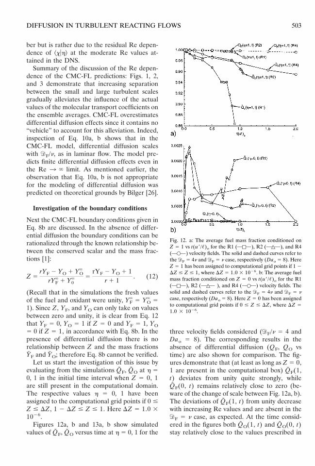
Figures 12a, b and 13a, b show simulatedvalues of QF, QO versus time at h 5 0, 1 for the

three velocity fields considered ($F/n 5 4 andDao 5 8). The corresponding results in theabsence of differential diffusion (QF, QO vstime) are also shown for comparison. The fig-ures demonstrate that (at least as long as Z 5 0,1 are present in the computational box) QF(1,t) deviates from unity quite strongly, whileQF(0, t) remains relatively close to zero (be-ware of the change of scale between Fig. 12a, b).The deviations of QF(1, t) from unity decreasewith increasing Re values and are absent in the$F 5 n case, as expected. At the time consid-ered in the figures both QO(1, t) and QO(0, t)stay relatively close to the values prescribed in

Fig. 12. a: The average fuel mass fraction conditioned onZ 5 1 vs t(u9/,)o for the R1 ( ), R2 ( ), and R4( ) velocity fields. The solid and dashed curves refer tothe $F 5 4n and $F 5 n case, respectively (Dao 5 8). HereZ 5 1 has been assigned to computational grid points if 1 2DZ # Z # 1, where DZ 5 1.0 3 1026. b: The average fuelmass fraction conditioned on Z 5 0 vs t(u9/,)o for the R1( ), R2 ( ), and R4 ( ) velocity fields. Thesolid and dashed curves refer to the $F 5 4n and $F 5 ncase, respectively (Dao 5 8). Here Z 5 0 has been assignedto computational grid points if 0 # Z # DZ, where DZ 51.0 3 1026.


Eq. 8b. Figures 12, 13 demonstrate that theoxidant is always closer to the Eq. 8b values thanthe fuel.

The deviation from zero and unity at the endpoints is a direct consequence of differentialdiffusion. Consider, e.g., QF(1, t) and QF(1, t).In the absence of differential diffusion, Z 5 1means that the fluid parcel in question has notparticipated in molecular mixing yet. Since Zand YF diffuse at the same rate (and reactioncannot precede molecular mixing) from Z 5 1,YF 5 1 follows. If the fuel diffuses faster than Z,it may have participated in molecular mixing(even reaction) while the value of Z is still unityin the fuel parcel considered. The expectation is

that this effect is stronger for the fuel than forthe oxidant and this indeed can be seen in thefigures. QF(0, t) is closer to zero than QF(1, t)is to unity because YF 5 0 values are constantlybeing produced by the chemical reaction. Thatthe end point effects decrease with increasingRe is in accordance with the idea that theinfluence of differential diffusion on the ensem-ble averages of interest disappears in highReynolds number turbulence. Figures 12a, band 13a, b are relevant to the investigation ofthe boundary conditions only in the initial timeperiod, when Z 5 0, 1 are still in the compu-tational domain.

In this Section the CMC-FL modeling ofdifferential diffusion has been discussed. Theconclusion is, firstly, that the conditional fluctu-

Fig. 14. a: The conditional probability density function ofthe fuel mass fraction at t(u9/,)o 5 2 for the R4 velocityfield (Dao 5 8). The circles ( ) and squares ( )refer to the $F 5 4n and $F 5 n case, respectively. b: Theconditional probability density function of the oxidant massfraction at t(u9/,)o 5 2 for the R4 velocity field (Dao 5 8).The circles ( ) and squares ( ) refer to the $F 54n and $F 5 n case, respectively.

Fig. 13. a: The average oxidant mass fraction conditionedon Z 5 1 vs t(u9/,)o for the R1 ( ), R2 ( ), andR4 ( ) velocity fields. The solid and dashed curvesrefer to the $F 5 4n and $F 5 n case, respectively (Dao 58). Here Z 5 1 has been assigned to computational gridpoints if 1 2 DZ # Z # 1, where DZ 5 1.0 3 1026. b: Theaverage oxidant mass fraction conditioned on Z 5 0 vst(u9/,)o for the R1 ( ), R2 ( ), and R4 ( )velocity fields. The solid and dashed curves refer to the $F

5 4n and $F 5 n case, respectively (Dao 5 8). Here Z 5 0has been assigned to computational grid points if 0 # Z #

DZ, where DZ 5 1.0 3 1026.


ations play an important part in the modeling.This conclusion corroborates the early theoret-ical predictions of Bilger [30] and Klimenko[31]. The role of the conditional fluctuations inthe modeling of differential diffusion has beenrecognized recently by Kronenburg and Bilger[14] as well as Nilsen and Kosaly [15] in con-nection with non-reacting simulations.

The investigations show secondly, that theboundary conditions set in Eq. 8b are not fullysatisfied in the presence of differential diffu-sion. This issue will be revisited in the followingpart.

The Conditional Fluctuations: FurtherInvestigation of the Influence of the BoundaryConditions

The importance of the modeling of the termsassociated with conditional fluctuations is a

characteristic consequence of differential diffu-sion. In earlier simulation work our group con-sidered flows without differential diffusion ($F

5 n) and found the terms related to the condi-tional fluctuations negligible in Eq. 5a, b [22]. Ithas been argued in this reference that thenegligibility of the “conditional” terms is due tothe smallness of the conditional fluctuations.

Figure 14a, b shows the probability densityfunction (pdf) of the mass fractions conditionedon Z 5 0.5 for the R4 velocity field [Dao 5 8,$F/n 5 4, t(u9/,)o 5 2]. Also shown are the$F/n 5 1 results for comparison. The figuredemonstrates the increase of the conditionalfluctuations due to differential diffusion.

Next the magnitude and behavior of thedifferent terms in Eq. 5a, b are investigated. Tothis end the equations are rewritten in moredetail as

1 2 3 4 5 6QF

t2

$F

2n^xuh&t

2QF

h2 2~$F 2 n!

n^Quh&t

QF

h1 AQFQO 1 A^yFyOuh&t 2 eF~h, t! 5 0, (13a)

a bc d e

QO

t2

12

^xuh&t2QO

h2 1 AQFQO 1 A^yFyOuh&t 2 eO~h, t! 5 0. (13b)

Here r 5 1 has been substituted in accordancewith the case considered in the simulations.

It will be discussed shortly that the conditionalfluctuations are sensitive to the small turbulentscales, it is easier to resolve them when the Pecletnumber is small. In addition, accurate evaluationof the terms appearing in the definition of eF andeO (see Eq. 7a, b) is easier when the conditionalfluctuations are large. To ensure adequate resolu-tion of the results pertaining to the R4 velocityfield and an accurate evaluation of eF and eO, thefigures to be presented in the rest of this sectionrefer to DNS with $F/n 5 4 instead of $F/n 5 2(as mentioned previously only R1, R2, and R4results are available for $F/n 5 4).

To compare cases which at different Reyn-olds numbers refer to similar states of mixing,results for a given value of tZ (instead of a givenvalue of t(u9/,)o) are shown (the tZ vs t(u9/,)o

curves are shown in Fig. 10). Figures 15a, b and

16a, b show the different terms in Eq. 13a, b fordifferent Reynolds number cases (R2, R4) at tZ

5 0.42. The figures illustrate that A^yFyOuh&(term 5 in Fig. 15a, b, term d in Fig. 16a, b) issmall compared to the other terms and cantherefore be neglected. It could also be arguedthat QF/t (term 1 in Fig. 15a, b) and QO/t(term a in Fig. 16a, b) is small enough to beneglected. However, the results at earlier times(not shown) demonstrate that the neglection ofQF/t and QO/t is not justified.

Figure 15a, b shows that eF (term 6) is notnegligible compared to the other terms. Itsmagnitude increases with Re. Inspection of Fig.16a, b suggests however to neglect eO (term e).The modeling assumptions

eO~h, t! 5 0, A^yFyOuh&t 5 0 (14)

suggested by the numerical results, lead then tothe equations


QF

t2

$F

2n^xuh&t

2QF

h2 2~$F 2 n!

n^Quh&t

QF

h

5 2AQFQO 1 eF~h, t!, (15a)

QO

t2

12

^xuh&t2QO

h2 5 2AQFQO. (15b)

To investigate the eF(h, t) term in Eq. 15a, wewrite Eq. 15a, b for the $F 5 n case as

QF

t2

12

^xuh&t2QF

h2 5 2AQFQO (16a)

QO

t2

12

^xuh&t2QO

h2 5 2AQFQO. (16b)

Equations 16a, b and 8a, b have been inves-tigated in a scalar mixing layer experiment byBilger [24] and in DNS turbulence by Mell et al.

[22]. The equations led to excellent predictionof the laboratory data and simulated results ($F5 n). The results in [24,22] demonstrate that eF5 0 is a valid closure approximation if $F . n.Figures 1–3 show furthermore that with increas-ing Reynolds number values the effects due to$F/n Þ 1 decrease. This suggests the hypothesisthat in high Re turbulence QF(h, t) > QF(h, t),QO(h, t) > QO(h, t). Comparing Eq. 15a withEq. 16a, it follows then that for large Re values

eF~h, t! > eF`~h, t!, (17a)

where

eF`~h, t! ; 2

~$F 2 n!

n

z H12

^xuh&t2QF

h2 1 ^Quh&tQF

h J . (17b)

Fig. 15. a: Plot of terms in the equation for QF(h, t) vs h attZ 5 0.42 for the R2 velocity field (Dao 5 8, $F/n 5 4).Term 1 5 QF/t ( ), term 2 5 2($F/2n)^xuh&t

2QF/h2 ( ), term 3 5 2[($F 2 n)/n]^Quh&tQF/h (22ƒ22),term 4 5 AQFQO (OLO), term 5 5 A^yFyOuh&t (22�22)and term 6 5 2eF(h, t) ( ). b: Plot of terms in theequation for QF(h, t) vs h at tZ 5 0.42 for the R4 velocityfield (Dao 5 8, $F/n 5 4). Definition of the terms andsymbols as in Fig. 15a.

Fig. 16. a: Plot of terms in the equation for QO(h, t) vs h attZ 5 0.42 for the R2 velocity field (Dao 5 8, $F/n 5 4).Term a 5 QO/t ( ), term b 5 2(1/2)^xuh&t

2QO/h2

( ), term c 5 AQFQO (OLO), term d 5 A^yFyOuh&t

(22�22) and term e 5 2eO(h, t) ( ). b: Plot of termsin the equation for QO(h, t) vs h at tZ 5 0.42 for the R4velocity field (Dao 5 8, $F/n 5 4). Definition of the termsand symbols as in Fig. 16a.


Equation 17a represents a plausible hypothesis.To investigate it through the simulated results it isexpedient to study its validity for a given value oftZ, rather than for a given value of t(u9/,)o.Figures 17a, b, indeed, show that the eF

` vs hcurves depend somewhat on the Reynolds num-ber when shown for a given value of t(u9/,)o, butoverlap when shown at the same value of tZ (tZ 50.42). The observation refers to the R2 and R4curves. That the R1 curve does not quite collapsewith R2 and R4 can again be attributed to thelow Reynolds number. The curve correspondingto pure molecular mixing (u 5 0, Re 5 0)differs markedly from the rest of the curves.

Figure 18 compares eF to eF` at tZ 5 0.42 for

the R1, R2, and R4 velocity fields and for theRe 5 0 case. (The eF

` curve shown in the figurehas been evaluated using results from the R4velocity field.) The figure demonstrates that i) eF isdependent on Re even when shown at a givenvalue of tZ and ii) with increasing Re values eFgets closer to eF

` in accordance with Eq. 17a.

It has been discussed several times in this paperhow the Reynolds number dependence of certainquantities disappears when they are compared atthe same value of tZ rather than at the same time.Such Reynolds number dependences have beencharacterized as “residual” since they disappear inhigh Re turbulence (see Figs. 9–11, Fig. 17a, b,and the corresponding discussions). Figure 18demonstrates that the Re dependence of eF is notresidual but essential. It is this Reynolds numberdependence that governs the behavior of differen-tial diffusion with increasing values of Re.

Next, the discussion of the Eq. 8b boundaryconditions is resumed. It was shown above thatdue to differential diffusion the boundary con-dition QF(h 5 1, t) 5 1 is not strictly valid forthe low to moderate Reynolds numbers consid-ered here. The issue to be investigated is,whether the suspect boundary condition leadsto inaccurate predictions of the ensemble aver-ages of interest.

Figures 19, 20 compare the results of DNScomputations to predictions obtained from Eqs.5a, b and 8b. The unclosed terms [^xuh&t, ^Quh&t,A^yFyOuh&t, eF(h, t) and eO(h, t)] have beentaken from the simulations (we refer to thisprocedure as CMCA). As long as Z 5 0, 1 arepresent in the computational domain the un-closed terms satisfy the conditions:

A^yFyOuh 5 0&t 5 A^yFyOuh 5 1&t 5 0, (18a)

eF~h 5 0, t! 5 eF~h 5 1, t! 5 0, (18b)

eO~h 5 0, t! 5 eO~h 5 1, t! 5 0. (18c)

Fig. 17. a: eF`(h, t), defined in Eq. 17b, vs h at t(u9/,o) 5 2.0

for the R1 ( ), R2 ( ), and R4 ( ) velocityfields (Dao 5 8, $F/n 5 4). b: eF

`(h, t), defined in Eq. 17b,vs h at tZ 5 0.42 for the R1 ( ), R2 ( ), and R4( ) velocity fields (Dao 5 8, $F/n 5 4). Also includedis the u 5 0, Re 5 0 case (22ƒ22).

Fig. 18. Plot of eF(h, t) vs h for the R1 ( ), R2( ), and R4 ( ) velocity field at tZ 5 0.42 (Dao 58, $F/n 5 4). Also included is the pure mixing case u 5 0,Re 5 0 (22ƒ22). The Re3 ` limit of eF(eF

`), denoted by thedashed curve, was taken from the R4 velocity field.


Equation 18a–c has been enforced in the com-putations by linear extrapolation even after Z 50, 1 disappeared from the computational do-main.

Figures 19, 20 refer to the R1 velocity field.Because the influence of differential diffusion isstrongest here, QF(h 5 1, t) deviates signifi-cantly from unity (see Fig. 12a). Also includedin the figures are the $F/n 5 1 results andCMC-FL predictions. Any deviation betweenCMCA and the DNS results is due to theapplication of the invalid boundary condition,QF(h 5 1, t) 5 1. It can be concluded from

Figs. 19, 20 that (at least in the time andparameter range covered by the simulations)QF(h 5 1, t) , 1 does not corrupt thepredictive capabilities of CMCA in any majorway (a small effect can be observed in ^vF&, seeFig. 19b). It is concluded that the major sourceof disagreement between CMC-FL and theDNS results is the neglection of the conditionalfluctuations terms in the modeling.

Next the modeling assumptions eO(h, t) 5 0and A^yFyOuh&t 5 0 (see Eq. 14) are investi-gated. In the figures to follow, CMCB refers tothe predictions using Eq. 15a, b with Eq. 14 andwith ^xuh&t, ^Quh&t, eF(h, t) taken from the DNS.If Eq. 14 represents valid modeling, the resultsobtained using CMCB and CMCA (defined inthe previous paragraph) will closely resemble

Fig. 19. a: The average mass fraction of fuel vs t(u9/,)o forthe R1 velocity field (Dao 5 8, $F/n 5 4). The 2 zz 2 curve(^YF&CMCA) refers to the solution of Eqs. 5a, b with theunclosed terms taken from the DNS. Also included is theCMC-FL predictions (dashed curve) and DNS values of^YF& (circles) as well as ^YF& ($F/n 5 1) represented by thedotted curve. b: The average consumption rate of fuel vst(u9/,)o for the R1 velocity field (Dao 5 8, $F/n 5 4).The 2 zz 2 curve (^vF&CMCA) refers to the solution of Eqs.5a, b with the unclosed terms taken from the DNS. Alsoincluded is the CMC-FL predictions (dashed curve) andDNS values of ^vF& (circles) as well as ^vF& ($F/n 5 1)represented by the dotted curve.

Fig. 20. a: The average conditional fuel mass fraction vs hfrom DNS ( ), as predicted by CMC-FL (2 2 2) andCMCA (2 zz 2) at t(u9/,)o 5 3 for the R1 velocity field(Dao 5 8, $F/n 5 4). The $F 5 n case ( ) is alsoincluded. For the definition of CMCA see Fig. 19a. b: Theaverage conditional oxidant mass fraction vs h from DNS (

), as predicted by CMC-FL (2 2 2) and CMCA (2zz 2) at t(u9/,)o 5 3 for the R1 velocity field (Dao 5 8, $F/n5 4). The $F 5 n case ( ) is also included. For thedefinition of CMCA see Fig. 19b.


each other. In Fig. 21a, b the predicted (CMCA,CMCB) average mass fraction and consumptionrate of the fuel are shown for the R2 velocityfield (Dao 5 8, $F/n 5 4). Although smalldifferences between the predictions fromCMCA and CMCB are observed in the figures,it appears that the modeling assumptions eO(h,t) 5 0 and A^yFyOuh&t 5 0 are acceptable. Amore severe test of the validity is to compare thepredicted curves of QF and QO as obtained fromCMCA and CMCB. Figure 22a, b shows thiscomparison (the figures refer to the same sim-ulation as Figs. 21a, b, t(u9/,)o 5 3). Againgood overall agreement between CMCA andCMCB is observed. Note that the neglection ofeO(h, t) and A^yFyOuh&t (CMCB) results in a

slight overestimation of effects due to differen-tial diffusion. This is most clearly seen in thepredictions of QO (Fig. 22b). The results ob-tained with the R1 and R4 velocity fields (notshown) displayed the same qualitative behavior asthat discussed in connection with Figs. 21, 22. Tosummarize, the DNS results suggest that the mod-eling assumptions stated in Eq. 14 are valid. Itfollows then that to properly account for differen-tial diffusion the eF term is to be modeled.

Equation 17a, b and Fig. 18 suggest to modeleF as a time dependent factor times eF

`. It is alsoplausible to assume that this factor goes to unitywith increasing values of Re that is

eF~h, t! > S1 2b~t!ReaDeF

`~h, t!. (19)

Fig. 21. a: The average mass fraction of fuel vs t(u9/,)o

from DNS (circles), as predicted by CMCA (2 zz 2) andCMC-FL (2 2 2) for the R2 velocity field (Dao 5 8, $F/n5 4). ^YF&CMCB (2 z 2) refers to the solution of Eq. 15a, bwith eF taken from the DNS. Also included is the $F/n 5 1case (. . .). b: The average consumption rate of fuel vst(u9/,)o from DNS (circles), as predicted by CMCA (2 zz 2)and CMC-FL (2 2 2) for the R2 velocity field (Dao 5 8,$F/n 5 4). ^vF&CMCB (2 z 2) refers to the solution of Eq.15a, b with eF taken from the DNS. Also included is the$F/n 5 1 case (. . .).

Fig. 22. a: The average conditional fuel mass fraction vs hfrom DNS ( ), as predicted by CMC-FL (2 2 2),CMCA (2 zz 2), and CMCB (2 z 2) at t(u9/,)o 5 3 for theR2 velocity field (Dao 5 8, $F/n 5 4). The $F 5 n case( ) is also included. b: The average conditional oxidantmass fraction vs h from DNS ( ), as predicted byCMC-FL (2 2 2), CMCA (2 zz 2), and CMCB (2 z 2) att(u9/,)o 5 3 for the R2 velocity field (Dao 5 8, $F/n 5 4).The $F 5 n case ( ) is also included.


Here a . 0 and b(t) . 0, the Re dependenceis concentrated in the denominator of the sec-ond term within the parenthesis, this means,b(t) does not depend on the Reynolds number.

It should be emphasized here that althoughEq. (19) is plausible, we have no evidence tocorroborate it. The Reynolds number rangeattained in the DNS was not sufficiently broadto study whether eF and eF

` are indeed approx-imately related by Eq. (19) or a similar relation-ship. Further DNS studies are needed to inves-tigate this issue. This is an important problemdue to the universality of the small scales. Oncethe value of a has been established from DNS itcan be applied in “real world” problems.

CONCLUSIONS

Two reacting species (fuel and oxidant) havebeen investigated via direct numerical simula-tions (DNS) in isotropic, decaying turbulence.In the simulations fuel and oxidant reactedwithout heat release, in a one-step reaction(activation energy was equated to zero). Initiallythe two species were approximately segregated.The molecular diffusion coefficient of the fuelwas larger than that of the oxidant, whosediffusion coefficient was equal to the kinematicviscosity (“differential diffusion”). The con-served scalar computed in parallel with thereacting species had the same molecular diffu-sion coefficient as the oxidant. The conclusionsof the investigations can be summarized asfollows:

(1) The influence of differential diffusion onensemble averages of the mass fractionsand the reaction rates were observed todiminish with increasing Reynolds num-bers. This finding is in line with earlierresults obtained in non-reacting cases [4, 8,14, 15]. With increasing Damkohler num-bers, however, differential diffusion effectsbecame more pronounced.

(2) The equations satisfied by the average fueland oxidant mass fractions conditioned onvalues of the conserved scalar are attractivestarting points of modeling efforts. In theabsence of differential diffusion the termsassociated with the conditional fluctuationscan be neglected [24]. The conditional fluc-

tuations, however, play an important role inthe modeling of differential diffusion. Theneglection of the conditional fluctuationsleads to an overestimation of the influenceof differential diffusion and results in erro-neous Re dependence of the average massfractions and reaction rates.

(3) Among the different terms that account forthe conditional fluctuations in the equationsof the conditionally averaged mass frac-tions, the investigations identified the one(eF defined above) that has a major influ-ence on the predictions. It is the Re depen-dence of eF that governs the decrease of theinfluence of differential diffusion with in-creasing values of Re. The Re-dependence(and large Re behavior) of eF was studied.A model was suggested to compute eF butwas not corroborated due to the limitedrange of Reynolds number values availablein the DNS.

(4) The boundary conditions in the conservedscalar space are generally given as the re-spective fresh values of the fuel and oxidantat values of zero and unity of the conservedscalar. In the presence of differential diffu-sion this condition cannot be proven math-ematically. The DNS results were applied tostudy the breakdown of the above boundaryconditions due to differential diffusion. Theresults show substantial violation of theboundary conditions, especially at low Revalues. However, the use of the erroneousboundary conditions did not lead to signif-icant error in the predicted average massfractions and reaction rates.

Partial support by NSF (CTS-9415280) andAFOSR (F49620-97-1-0092) is acknowledged.The National Center for Supercomputing Appli-cations in Illinois provided supercomputer hoursfor the numerical simulations. The authors areindebted to J. J. Riley for numerous discussionsthroughout the research work.

APPENDIX: SMOOTHING PROCEDUREOF ^Xzh&t AND ^Qzh&t

In our past work ($F 5 $O 5 n) we solved theCMC equations (Eqs. 16a, b) for QF(h, t) [


^YFuZ 5 h&t and QO(h, t) [ ^YOuZ 5 h&t with^xuZ 5 h&t(x [ 2n¹Z z ¹Z) taken directlyfrom the DNS without any smoothing of fluctu-ations due to statistical noise [22]. An extensionof this procedure to the $F . n case wouldinvolve the use of ^xuh& and ^Quh& (Q [ n¹2Z)obtained directly from the DNS computations.However, when solving CMC-FL (Eq. 10a, b), itwas observed that employing the above proce-dure, with regard to ^xuh& and ^Quh&, led to ^YF&t

Þ ^YO&t for the 643 and 1283 simulations. Thisprediction is clearly unphysical in the r 5 1,^YF&o 5 ^YO&o case. Indeed, ^YF&t 5 ^YO&t

follows mathematically from Eq. 10a, b. De-tailed study of the issue showed that CMC-FL issensitive to noise caused by poor statistics in^xuh&t and ^Quh&t. To remove the noise asmoothing procedure is needed.

In the physical problem considered here thepdf of Z is symmetric about ^Z&. For this casethe Amplitude Mapping Closure (AMC) hasbeen shown to produce good predictions of^xuh&t, ^Quh&t and PZ(h, t) [27, 32, 33]. SinceAMC also yields a smooth representation of theconditional scalar dissipation and diffusion rate,as well as the pdf of Z, the AMC was used toremove fluctuations due to poor statistics in theDNS values of ^xuh&t and ^Quh&t. For consistencythis procedure was also used when solving theCMC-FL model equations pertaining to simu-lations with good statistics (2563 grid points). Itseems that the sensitivity to the statistics of ^xuh&and ^Quh& is peculiar to the CMC-FL model.The same problem was not observed when usingthe CMCA and CMCB (defined above). Thesmoothing via AMC procedure was, however,applied in all cases for consistency.

To explain the procedure, the following shapefunctions are defined:

F~h! 5 exp $22@erf21 ~2h 2 1!#2% (A.1)

and

H~h! 5 erf21 ~2h 2 1!

z exp $2@erf21 ~2h 2 1!#2%. (A2)

If ^Z& 5 0.5 and PZ(h, 0) 5 [d(h) 1 d(h 2 1)]/2the AMC predicts that

^xuh&t 5 ^xu0.5&tF~h!, (A.3)

^Quh&t 52Îp

sin @2ps2~t!#^xu0.5&tH~h! (A.4)

and

PZ~h, t! 5 &~t! exp $@1 2 &2~t!#

z @erf21 ~2h 2 1!#2}. (A5)

Here

^xu0.5&t 5 H1 1 sin @2ps2~t!#1 2 sin @2ps2~t!#J

1/ 2

^x&t, (A.6)

&~t! 5 HF1 11

~tan @2ps2~t!#!2G1/ 2

2 1J1/ 2

,

(A.7)

s2(t) is the variance of the conserved scalar Z.Equations A.1–A.7 were taken from Frankel etal. [33].

Note that in the spatially homogeneous case

Fig. A.1. a: The conditional scalar dissipation rate ^xuh& vs hfrom the DNS (circles) and as predicted by AMC (solidcurve) at t(u9/,)o 5 0.5 for the R1 velocity field. b: Theconditional scalar dissipation rate ^xuh& vs h from the DNS(circles) and as predicted by AMC (solid curve) at t(u9/,)o

5 3 for the R1 velocity field.


ds2(t)/dt 5 2^x&t. The variance (s2) was takenfrom the DNS. With s2(t) known Eqs. A.3–A.5can be evaluated and applied to solve Eqs. 5a, b,10a, b, and 15a, b. This procedure has beenfollowed earlier and led to good predictions ofDNS results [32, 33]. We include here a briefinvestigation of the issue for the sake of com-pleteness.

Figures A.1a, b show ^xuh& from the DNSdirectly and as predicted by AMC for the R1velocity field at t(u9/,)o 5 0.5 and t(u9/,)o 53.0, respectively. Figures A.2a, b display ^Quh&from AMC and DNS for the same velocity fieldand times as in Figs. A.1a, b. AMC is seen toyield good overall agreement with the DNSresults and reduce noise due to poor statistics.Similar results have been observed for the R2,R3, and R4 velocity fields (not shown).

Next the predictions of PZ(h, t) from AMC iscompared to the pdf taken directly from the

DNS. Figures A.3a, b refer to the R1 velocityfield at t(u9/,)o 5 0.5. Although AMC overes-timates the peaks at Z 5 0, 1 it providesexcellent agreement with the DNS results “inthe middle,” even at this early time. Figure A.3cdepicts the pdf of Z at t(u9/,)o 5 3.0 for the R1velocity field as determined from the DNS and

Fig. A.2. a: The conditional scalar diffusion rate ^Quh& vs hfrom the DNS (circles) and as predicted by AMC (solidcurve) at t(u9/,)o 5 0.5 for the R1 velocity field. b: Theconditional scalar diffusion rate ^Quh& vs h from the DNS(circles) and as predicted by AMC (solid curve) at t(u9/,)o

5 3 for the R1 velocity field.

Fig. A.3. a: Plot of PZ(h, t) vs h from the DNS (circles) andas computed via AMC (solid curve) at t(u9/,)o 5 0.5. Thevelocity field is R1. b: PZ(h, t) vs h from the DNS (circles)and as evaluated via AMC (solid curve) at t(u9/,)o 5 0.5 forthe R1 velocity field. Note the change in the vertical scale[see Fig. A.3(a)]. c: Plot of PZ(h, t) vs h from the DNS(circles) and as computed via AMC (solid curve) at t(u9/,)o

5 3. The velocity field is R1.


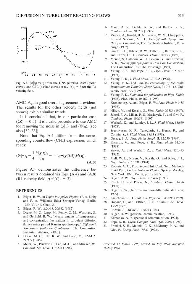
AMC. Again good overall agreement is evident.The results for the other velocity fields (notshown) exhibit similar trends.

It is concluded that, in our particular case(^Z& 5 0.5), it is a valid procedure to use AMCfor removing the noise in ^xuh&t and ^Quh&t (seealso [32, 33]).

Note that Eq. A.4 differs from the corre-sponding counterflow (CFL) expression, whichreads:

^Quh&t 514

^xuh&t

h5 2 Îp^xu0.5&tH~h!.

(A.8)

Figure A.4 demonstrates the difference be-tween results obtained via Eqs. (A.4) and (A.8)(R1 velocity field, t(u9/,)o 5 3).

REFERENCES

1. Bilger, R. W., in Topics in Applied Physics, (P. A. Libbyand F. A. Williams Eds.) Springer-Verlag, Berlin,1980, Vol. 44, Chap. 3.

2. Bilger, R. W., AIAA J. 20:962 (1982).3. Drake, M. C., Lapp, M., Penny, C. M., Warshaw, S.,

and Gerhold, B. W., “Measurements of temperatureand concentration fluctuations in turbulent diffusionflames using pulsed Raman spectroscopy,” EighteenthSymposium (Intl.) on Combustion, The CombustionInstitute, Pittsburgh (1981).

4. Drake, M. C., Pitz, R. W., and Lapp, M., AIAA J.,24:905 (1986).

5. Meier, W., Prucker, S., Cao, M.-H., and Stricker, W.,Combust. Sci. Tech., 118:293 (1996).

6. Masri, A. R., Dibble, R. W., and Barlow, R. S.,Combust. Flame, 91:285 (1992).

7. Vranos, A., Knight, B. A., Proscia, W. M., Chiappetta,L., and Smooke, M. D., Twenty-fourth Symposium(Intl.) on Combustion, The Combustion Institute, Pitts-burgh (1992).

8. Smith, L. L., Dibble, R. W., Talbot, L., Barlow, R. S.,and Carter, C. D., Combust. Flame 100:153 (1995).

9. Menon, S., Calhoon, W. H., Goldin, G., and Kerstein,A. R., Twenty-fifth Symposium (Intl.) on Combustion,The Combustion Institute, Pittsburgh (1994).

10. Yeung, P. K., and Pope, S. B., Phys. Fluids A 5:2467(1993).

11. Yeung, P. K., J. Fluid Mech. 321:235 (1996).12. Yeung, P. K., and Luo, B., Proceedings of the Tenth

Symposium on Turbulent Shear Flows, 31-7-31-12, Uni-versity Park, PA (1995).

13. Yeung, P. K., Submitted for publication in Phys. Fluids(1998). Phys. Fluids 10:2621 (1998).

14. Kronenburg, A., and Bilger, R. W., Phys. Fluids 9:1435(1997).

15. Nilsen, V., and Kosaly, G., Phys. Fluids 9:3386 (1997).16. Jaberi, F. A., Miller, R. S., Mashayek, F., and Givi, P.,

Combust. Flame 109:561 (1997).17. Warhaft, Z., and Lumley, J. L., J. Fluid Mech. 88:659

(1978).18. Sreenivasan, K. R., Tavoularis, S., Henry, R., and

Corrsin, S., J. Fluid Mech. 88:63 (1978).19. Orszag, S. A., Phys. Fluids Suppl. II, 12:250 (1969).20. Eswaran, V., and Pope, S. B., Phys. Fluids 31:506

(1988)21. Sirivat, A., and Warhaft, Z., J. Fluid Mech. 120:475

(1982).22. Mell, W. E., Nilsen, V., Kosaly, G., and Riley, J. J.,

Phys. Fluids A 6:1331 (1994).23. Roberts, G. O., Proc. Second Int. Conf. Num. Methods

Fluid Dyn., Lecture Notes in Physics, Springer-Verlag,New York, 1971, Vol. 8, pp. 171–177.

24. Bilger, R. W., Phys. Fluids A 5:436 (1993).25. Pitsch, H., and Peters, N., Combust. Flame 114:26

(1998).26. Bilger, R. W., (Informal notes on differential diffusion,

1995).27. Kraichnan, R. H., Bull. Am. Phys. Soc. 34:2298 (1989).28. Dopazo, C., and O’Brien, E. E., Combust. Sci. Tech.

13:99 (1976).29. Corrsin, S., AIChE J. 10:870 (1964).30. Bilger, R. W. (personal communication, 1993).31. Klimenko, A. Y. (personal communication, 1994).32. Pope, S. B., Theor. Comput. Fluid Dyn. 2:255 (1991).33. Frankel, S. H., Madnia, C. K., McMurtry, P. A., and

Givi, P., Energy Fuels, 7:827 (1993).

Received 12 March 1998; revised 16 July 1998; accepted16 July 1998

Fig. A.4. ^Quh& vs h from the DNS (circles), AMC (solidcurve), and CFL (dashed curve) at t(u9/,)o 5 3 for the R1velocity field.


Differential Diffusion in Turbulent Reacting Flows

Documents

Transcript of Differential Diffusion in Turbulent Reacting Flows