Numerical methods for unsteady compressible multi-component reacting flows on fixed and moving grids

Journal of Computational Physics 202 (2005) 710–736

www.elsevier.com/locate/jcp

Numerical methods for unsteady compressiblemulti-component reacting flows on fixed and moving grids

V. Moureau a,*, G. Lartigue b, Y. Sommerer b, C. Angelberger a,O. Colin a, T. Poinsot c

a Energy Application Techniques Department, IFP, 1 Avenue du Bois Preau, 92500 Rueil-Malmaison, Franceb CERFACS, 42 Avenue G. Coriolis, 31057 Toulouse Cedex, France

c IMFT, Avenue C. Soula, 31400 Toulouse, France

Received 12 August 2003; received in revised form 13 July 2004; accepted 2 August 2004

Available online 16 September 2004

Abstract

Deriving high precision schemes to compute turbulent flows on fixed or moving complex grids is becoming a central

issue in the direct numerical simulation (DNS) and large eddy simulation (LES) community. The step between classical

DNS/LES codes on fixed structured grids and future methods on moving unstructured grids is a significant evolution in

terms of numerical methods. For reacting flows, this evolution must also include more precise descriptions of multispe-

cies flows and boundary conditions. This paper describes the development of a method for unsteady multispecies react-

ing flows on moving grids. The target field of application of this method is DNS and LES but this paper focuses on the

method development and elementary test cases. The theoretical basis for the numerical method, the boundary condi-

tions and the moving grid extension are first discussed. Various tests of the method are then provided on fixed and mov-

ing grids for simple reacting and non-reacting flows to demonstrate the precision and power of the method in simple

reference laminar cases.

� 2004 Elsevier Inc. All rights reserved.

Keywords: LES; DNS; ALE; Realistic thermochemistry; High-order methods; Boundary conditions

1. Introduction

The fast development of large eddy simulation (LES) techniques for reacting flows [1,2] is also driving

research efforts for specific numerical techniques: this is especially true for gas turbines [3–6] or piston en-

0021-9991/$ - see front matter � 2004 Elsevier Inc. All rights reserved.

doi:10.1016/j.jcp.2004.08.003

* Corresponding author. Tel.: +33 1 47 52 52 31.

E-mail address: [email protected] (V. Moureau).

mailto:[email protected]

V. Moureau et al. / Journal of Computational Physics 202 (2005) 710–736 711

gines for which LES require non-dissipative schemes able to handle compressible multi-species flows on

fixed or moving grids. These schemes must also provide high-order accuracy even though ensuring such

a property on arbitrary grids is more difficult than it is on Cartesian grids classically used for DNS for

example. Such schemes can not be straightforward extensions of usual Reynolds averaged Navier–Stokes

(RANS) solvers in which the levels of numerical viscosity are too high. Maintaining low numerical dissipa-tion in LES computations requires specific efforts in terms of algorithm [7] but also of boundary conditions

formulations [1]:

� There is still some controversy about the type of scheme which can be accepted for LES: while upwind

schemes [8–11] are sometimes used, most groups try to use spatially centered schemes [12–14] because

these schemes are not dissipative. This property is usually considered as necessary to avoid damping

small turbulent scales (which are essential in reacting flows) even if these schemes are also more sensitive

to oscillations. For �academic� LES in simple geometries, structured meshes can be used and high-orderschemes are easily designed. For complex geometries, however, unstructured methods are mandatory

and on such grids, constructing high-order schemes becomes much more difficult. Existing LES solvers

for unstructured meshes are limited to second-order [7] or third-order [15] methods. The situation is

more complex when such solvers must be used on moving meshes: simple extensions of existing

solvers for moving meshes may lead to a loss of the convergence order and an increase of numerical

dissipation.

� For compressible reacting flows, specifying boundary conditions becomes critical for LES. The low dis-

sipation of the algorithm required for precision introduces new difficulties: first, errors introduced byapproximate boundaries are not damped any more by the scheme (as they were in RANS) so that bound-

ary conditions must generate as few numerical perturbations as possible; second, acoustic waves created

by the flow also propagate through the computational domain without damping and must be evacuated

through non-reflecting boundaries. Moreover, LES also require to inject turbulence (and sometimes con-

trolled acoustic waves [16]) through inlet boundaries. Methods to reach all these objectives are mostly

based on characteristic techniques developed for aerodynamics [1,17–19]. These techniques work for

pure gases with constant molecular weights, heat capacities and sound speed. When the gas is a mixture

of species, they must be extended to account for variable molecular weights and heat capacities as pro-posed by Baum et al. [20] for perfect gases or O�Kongo and Bellan [21] for real gases.

� Finally, even the choice of the equations required to describe reacting flows is open to discussion. For a

long time, DNS or LES have been restricted to zero heat release flames [22–25] in which fresh and burnt

gases had the same temperature: even though this assumption is clearly not satisfied in real flames, such

simulations have brought new qualitative information on the physics of turbulent flames. Over the years,

multiple other simplifications have appeared in the DNS/LES community: two-dimensional flow [26,27],

infinitely fast chemistry, one-step chemistry [27–32], reduced chemistry [33]. Despite the efforts of the

DNS/LES community, the precision of the submodels used for DNS or LES is not yet up to whatcan be done for laminar flames for which precise diffusion models (including the inversion of the diffu-

sion matrix) and complex chemistry can be taken into account: in most existing DNS or LES, the heat

capacity Cp of all species is equal and constant while diffusion is usually modeled with Fick�s law. Theseassumptions lead to erroneous flame temperatures (due to the constant Cp approximation) and flame

speeds (due to simplification of transport models) which have no real importance in academic problems

for turbulent combustion. However, in the last years, the quest for DNS/LES tools has changed: quan-

titative computations are now required and this leads to difficult choices because it is not possible yet to

incorporate all the necessary physics into existing codes. Certain DNS codes now incorporate full chem-istry for simple fuels [34–36]: most LES, however, are limited to simpler descriptions. The present study

describes a compromise in terms of complexity, precision and cost which has been validated in multiple

cases and compared to other codes: the multispecies characteristics of the flow (variable molecular

712 V. Moureau et al. / Journal of Computational Physics 202 (2005) 710–736

weights and heat capacities) are fully accounted for, gases are supposed to be perfect, molecular diffusion

terms are computed using simplified forms, reduced chemistry schemes can be easily incorporated while

preserving the computational parallel efficiency which must remain one of the key features of such codes.

The objectives of this paper are to present the development of a compressible high-order solver for LESof reacting flows on fixed and moving grids. Though the main objective is LES, direct numerical simula-

tions (DNSs) of reacting flows can also be achieved with the same tool. The main features of this solver

are summarized below:

� Multi-component compressible reacting gas.

� Unstructured hybrid meshes.

� Explicit time integration.

� Second and third-order spatial accuracy for convective terms on fixed and moving grids.� Characteristic boundary conditions.

Section 2 first presents the thermochemistry model and the transport equations. The treatment of the

boundary conditions in a multi-species gas is presented in Section 3: using different primitive variables

leads to a major simplification of the initial formulation of [20]. The integration of the conservation equa-

tions on fixed and moving grids is presented in Section 4 for both finite volume and finite element formu-

lations. From this integration, a second-order Lax–Wendroff like scheme is derived in Section 5 and a

third-order Taylor–Galerkin scheme is developed in Section 6. Test cases are then described in Section8: one-dimensional laminar premixed flame on a fixed grid (Section 8.2), uniform flow on a moving grid

(Section 8.3), uniformly accelerated piston (Section 8.4) and measurements of convergence order for scalar

and vorticity convection (Section 8.5). Finally, conclusions and perspectives of applications are given in

Section 9.

2. Thermochemistry model and transport equations

The variables required for the description of a compressible reacting flow are:

U ¼ mx;my ;mz;E; qk

� �t; ð1Þ

where ~m ¼ ðmx;my ;mzÞt is the momentum vector, E is the total non-chemical energy density and qk (for

k = 1 to N) are the partial densities of the N species present in the mixture. The density q is not transported

by the solver since it is the sum of the partial densities. The total non-chemical energy is the sum of kineticenergy ec and thermal energy es:

E ¼ q ec þ es½ � ¼ q1

2ðu2 þ v2 þ w2Þ þ

XNk¼1

Y kesk

" #; ð2Þ

where Yk is the mass fraction of species k. The thermal energy esk of species k is defined by:

eskðT Þ ¼Z T

0

CvkðHÞ dH: ð3Þ

To simplify the computation of the energy from temperature (an operation which must be performed at

each time step and for each mesh point), the internal energy of each species is tabulated from data bases [37]every 100 K, in a range going from 0 to 5000 K. On each 100 K range, the heat capacity of any species is

constant. The energy at a given temperature is then obtained by linear interpolation. This interpolation also

provides a fast method to recover temperature from energy data.


The equation of state relating temperature T, pressure P and density q is:

P ¼ qrT : ð4Þ
The gas constant of the mixture r is defined from each species gas constant rk by:
r ¼XNk¼1

Y krk ¼XNk¼1

Y kR

W k¼ R

Wwith

1

W¼XNk¼1

Y k

W k; ð5Þ

where R ¼ 8:3143 J=K=mol is the universal gas constant, Wk is the molar mass of species k and W is the

molar mass of the mixture.

The quantities Cp, Cv, r and c change locally but the usual relations between them still hold:

Cp � Cv ¼ rrCv

¼ c� 1 ¼ b; ð6Þ

where c = Cp/Cv is the isentropic coefficient of the mixture.

The equations to solve are the compressible and reacting Navier–Stokes equations, written here in flux-

divergence form:

oUot

þr �F ¼ _W ; ð7Þ

where r �F is the divergence of the fluxes and _W is the source terms vector. Each component of the fluxes

can be decomposed into three terms: inviscid, viscous and LES contributions.

Fx;y;z ¼ FIx;y;z þFV

x;y;z þFLESx;y;z: ð8Þ

The system of conservative equation (7) can handle both DNS and LES. In the second case the vector Uis the vector of filtered variables. For simplicity, only DNS cases will be discussed here ðFLES

x;y;z ¼ 0Þ, as LESintroduces no particular difficulty from the point of view of numerical methods compared to DNS.

The inviscid flux FI is defined by:

FIx ¼

quuþ P

quv

quw

quE þ Pu

qku

0BBBBBB@

1CCCCCCA; FI

y ¼

qvu

qvvþ P

qvw

qvE þ Pv

qkv

0BBBBBB@

1CCCCCCA

and FIz ¼

qwu

qwv

qwwþ P

qwE þ Pw

qkw

0BBBBBB@

1CCCCCCA: ð9Þ

The viscous fluxes are modeled by:

FVi ¼

�six�siy�siz

�ðusix þ vsiy þ wsizÞ þ qiJk;i

0BBBBBB@

1CCCCCCA

ð10Þ

for i = x, y or z. Here, q is the heat flux and Jk the diffusive flux of the species k. The stress tensor s is

defined by: � �
sij ¼ � 2
3loukoxk

dij þ louioxj

þ oujoxi

; ð11Þ

where the molecular viscosity l is a function of the temperature (through a Sutherland or a power law).

This coefficient is defined for the mixture only: there is no influence of the composition on the viscosity.


The diffusive flux of species k is defined by:

Jk;i ¼ qY kV k;i; ð12Þ

where Vk,i is the ith component of the diffusion velocity of the species k. To ensure mass conservation each

component of the flux must verify:

XNk¼1

Y kV k;i ¼ 0: ð13Þ

The diffusion velocity Vk,i is modeled by the Hirschfelder and Curtis approximation [38]:

X kV k;i ¼ �DkoX k

oxi; ð14Þ

where Xk and Dk are, respectively, the molar fraction and the diffusion coefficient of the species k. This coef-

ficient is computed from the viscosity l as

Dk ¼l

qSck; ð15Þ

The Schmidt number Sck is a constant depending on the species. A major issue [1] is that this formulation

does not satisfy (13), i.e. the global mass conservation, if the Schmidt numbers Sck are not equal for all

species. In this case, a correction velocity V Ci must be added to the diffusion velocity Vk,i in (12) to satisfy

the continuity equation:

Jk;i ¼ qY k V k;i þ V Ci

� �: ð16Þ

This correction velocity is defined by:

V Ci ¼

XNj¼1

DjW j

WoX j

oxi: ð17Þ

The effects of the simplification of the diffusion matrix using the Hirschfelder model and a correction

velocity are discussed in [39] or [40]. These effects are very small in most flames using air as oxidizer.

The final expression for the species diffusive flux is thus:

Jk;i ¼ �qDkW k

WoX k

oxiþ qY k

XNj¼1

DjW j

WoXk

oxi

!; ð18Þ

which is compatible with total mass conservation.

Finally, the heat flux q is defined by:

qi ¼ �koToxi

þXNk¼1

Jk;ihsk: ð19Þ

The first term is the heat flux due to the classical heat conduction process (Fourier law) while the secondterm is the heat flux due to the diffusion of species having different enthalpies. The heat conduction coef-

ficient k is computed from the viscosity l as:

k ¼ lCp

Pr; ð20Þ

where the Prandtl number Pr is assumed to be constant: this property is very well satisfied in most air

flames.


The source terms vector _W is defined by:

_W ¼ 0; 0; 0; _xT; _xkð Þt; ð21Þ
where _xk is the net mass production of the species k due to combustion and _xT is the associated heat release
given by:

_xT ¼XNk¼1

Dh0f ;k _xk: ð22Þ

The standard formation enthalpy Dh0f ;k of the species k is also obtained from data bases [37].

The modeling of chemistry is done using classical Arrhenius laws [1,41].

3. Characteristic boundary conditions for multi-component mixtures

Specifying boundary conditions is a critical part in compressible DNS and LES codes [17,19,42]. Char-

acteristic methods are commonly used for compressible aerodynamics codes but require extensions for

reacting flows where the gas is a mixture of species for which quantities such as Cp, Cv or r change locally.

The method described here is a new formulation of the NSCBC procedure proposed by Poinsot and Lele

[43] for mono-component gas and extended by Baum et al. [20] to multi-component mixtures, i.e. a mixtureof perfect gases. If the state equation of each gas can not be approximated by a perfect gas law, this for-

mulation can be modified as done for real gases in [21] but the present study does not extend to this case.

Note also that, even though the present solver can handle moving grids, the present boundary condition

treatment is valid only for fixed boundaries. Imposing boundary conditions on a moving boundary is

not necessary in most practical applications (except for the walls of piston engines which can be handled

in a simpler way and do not require characteristic treatments).

More generally, the method described here is sufficient for engine computations but would have to be

complemented by the use of �sponge� domains and higher-order wave expansions on the boundaries to han-dle for example aeroacoustic problems [44–46] which require a higher accuracy on boundaries.

3.1. Extension of the NSCBC method

The NSCBC method proposed in [20] can be ill-posed: there are 5 + N variables but one more equation

(the relationP

Yk = 1 or equivalently q =P

qk). To avoid this problem, the solution is then either to keep

the conservation equation for q and to suppress one species equation or to keep all species equations but to

suppress the equation for q. Here, the choice has been made to keep all species and to leave q. The system ofequations that is obtained is now perfectly ‘‘symmetric’’ as far as species are concerned.

The second major difference compared to [20] is the choice of primitive variables. The primitive variable

associated to energy is not temperature but pressure. For the species, the partial densities qk are taken as

primitive variables instead of mass fractions Yk. This simplifies drastically the formulation.

3.2. Recasting equations from conservative to primitive variables

The Navier–Stokes equation (7) have previously been written in terms of flux of conservative variables.This form is very well suited for the discretization in the finite volume context. However, for deriving

boundary conditions, it is easier to rewrite the equations in the quasi-linear primitive form. Moreover,

the velocity components are written in a generic direct orthonormal basis ð~n;~t1;~t2Þ, in which~u ¼ ðun; ut1; ut2Þt. The~n direction corresponds to the outgoing normal vector on boundaries. Characteristic

analysis [17,18] leads to a new form of the conservation equations:


oVot

þ d ¼ T ; ð23Þ

where V = (un,ut1, ut2,P,q1,. . .,qN)t is the primitive variable vector. The d term (also called normal term) rep-

resents the contributions of the derivatives along ~n:

dun

dut1

dut2

dP

dqk

0BBBBBB@

1CCCCCCA

¼

un ouno~n þ 1

qoPo~n

unout1o~n

unout2o~n

un oPo~n þ qc2 oun

o~n

unoqko~n þ qk

ouno~n

0BBBBBBB@

1CCCCCCCA; ð24Þ

where oao~n ¼ oa

o~x nx þ oao~y ny þ oa

o~z nz.This can be written in matrix notation:

d ¼ E~n �oVo~n

; ð25Þ

where E~n is the Jacobian matrix of the system:

E~n ¼

un 0 0 1q 0 . . . 0

0 un 0 0 0 . . . 0

0 0 un 0 0 . . . 0

qc2 0 0 un 0 . . . 0

q1 0 0 0 un . . . 0

..

. ... ..

. ... ..

. . .. ..

.

qN 0 0 0 0 . . . un

0BBBBBBBBBBBBBBB@

1CCCCCCCCCCCCCCCA

: ð26Þ

The T term represents all the other contributions (tangential, diffusion, reaction).

3.3. The characteristic variables

The matrix E~n can be diagonalized and this decomposition allows to write convection equations for the

waves amplitudes:

oAot

þ koAo~n

¼ T A; ð27Þ

where A is the wave amplitude, k is the wave convection velocity and TA is the sum of all non-hyperbolic

terms associated to the wave.

The amplitudes of the 4 + N waves can be written as

oAþ

oA�

oAt1

oAt2

oAk

0BBBBBB@

1CCCCCCA

¼

oun þ 1qc oP

oun � 1qc oP

out1out2

� Y kc2 oP þ oqk

0BBBBBB@

1CCCCCCA

ð28Þ


and the associated convection velocities are:

kþk�kt1kt2kk

0BBBBBB@

1CCCCCCA

¼

un þ c

un � c

ununun

0BBBBBB@

1CCCCCCA: ð29Þ

Keeping the notation L ¼ koAo~n of [43] for the waves amplitude variations, the normal term d of (24) is:

dun

dut1

dut2

dP

dqk

0BBBBBB@

1CCCCCCA

¼

12ðLþ �L�Þ

Lt1

Lt2qc2ðLþ þL�Þ

qk2c ðLþ þL�Þ þLk

0BBBBBB@

1CCCCCCA: ð30Þ

The acoustic wavesLþ andL� are convected, respectively, at the velocity un+c and un�c. All other waves

are convected with the flow at the velocity un. The waves Lt1 and Lt2 are known as shear waves. The

remaining waves Lk (for k = 1 to N) are species waves. No wave can easily be identified with the classical

entropy wave because density is not directly solved for. However, all species waves Lk have the same con-vection velocity un and any linear combination of these waves is still a wave convected at the velocity un.

For example

LS ¼XNk¼1

Lk ¼ un � 1

c2oPo~n

þ oqo~n

� �ð31Þ

is proportional to the entropy wave given by Poinsot and Lele [43].

3.4. The LODI relations

The central idea of characteristic methods for boundary conditions is to identify the outgoing and

incoming waves crossing a boundary. The outgoing waves carry information from the interior of the do-

main and must be kept as computed by the numerical scheme. However, the incoming waves carry infor-

mation coming from the outside (i.e. controlled by the boundary condition). They cannot be computed

from interior points data. The principle of the present method is to infer the amplitude of the incoming

waves from the amplitude of the outgoing waves and from some appropriate LODI (local one-dimensional

inviscid) relations [43]. These LODI relations are obtained by writing (23) near the boundary as if the flowwas locally inviscid and one-dimensional. Of course, at this point, the physical behaviour of the boundary

must be taken into account to choose which LODI relation should be used. Some examples of LODI rela-

tions are given below:

oPot

þ qc2ðLþ þL�Þ ¼ 0; ð32Þ

ounot

þ 1

2ðLþ �L�Þ ¼ 0; ð33Þ

out1ot

þLt1 ¼ 0; ð34Þ


out2ot

þLt2 ¼ 0; ð35Þ

oqk

otþ qk

2cðLþ þL�Þ þLk ¼ 0; ð36Þ

oqot

þ q2c

ðLþ þL�Þ þLS ¼ 0; ð37Þ

oY k

otþ 1

qðLk � Y kLSÞ ¼ 0; ð38Þ

orot

þ 1

qðrLS þ

XrkLkÞ ¼ 0; ð39Þ

oTot

þ bT2c

ðLþ þL�Þ �Tqr

XrkLk ¼ 0: ð40Þ

Additional LODI equations can be written for enthalpy, entropy, momentum or for normal gradients.

3.5. Example of practical implementation

From the LODI relations, it is straightforward to write various characteristic boundary conditions using

the technique described in [43]. Only a single example is given here: a subsonic inlet with time-varying veloc-

ity, temperature and composition. For a subsonic inlet, only the backward travelling acoustic wave L� is

leaving the computational domain while the 3 + N other waves are entering it. Since L� leaves the domain

it can be evaluated using (28) and one-sided derivatives. To determine the 3 + N incoming waves

Lþ; Lt1 and Lt2, the nature of the boundary suggests to use the LODI relations (33)–(35).

Lþ ¼ L� � 2outnot

; ð41Þ

Lt1 ¼ � outt1ot

; ð42Þ

Lt2 ¼ � outt2ot

: ð43Þ

The �t� superscript is here to remind that the values in the temporal derivatives are the ‘‘target’’ values to

impose on the boundary (for example, a turbulent or an acoustic signal). To find the N remaining Lk

waves, (40) is used to have:
XNk¼1
rkLk ¼qrT

oT t

otþ bT

cL� � outn

ot

� �� : ð44Þ

Introducing this value in (39) gives for the entropy wave:

LS ¼ � qToT t

ot� q

XNk¼1

rkroY t

k

otþ qb

coutnot

�L�

� �ð45Þ

and finally, using (38), the species waves are:

Lk ¼ Y kLS � qoY t

k

ot: ð46Þ


The 3 + N waves Lþ; Lt1; Lt2 and Lk are now specified. These values and the scheme-computed va-

lue of L� can then be put back in the normal terms vector d and the variables on the boundary can be

updated for the next time-step using (23). An additional difficulty associated to the use of characteristic

boundary conditions is the possible drift of mean values. This drift can be controlled in the present ap-

proach by adding corrective terms in (41)–(43) and (46). This corrective treatment follows the methods pro-posed in [1,42,43].

4. Integration of the conservation equations on dynamic meshes

Solving the Navier–Stokes equations on a deforming domain X(t) is usually achieved using a body-

force method [47] or an arbitrary Lagrangian–Eulerian (ALE) method [48]. The body-force method con-

sists of imposing a given speed on an arbitrary surface which does not necessarily coincide with themesh. Complex deforming geometries can be simulated on fixed Cartesian grids with this method but

an important drawback is that imposing characteristic boundary conditions as described in the previous

section is very difficult. An appealing alternative is the ALE method in which each mesh node i has a

given displacement speed _X iðtÞ and the boundaries of the computational domain oX(t) coincide with

mesh vertices. In conjunction with the ALE approach, the characteristic method developed in Section

3 can be used for inlets and outlets, which are fixed in most simulations of real applications (gas tur-

bines, piston engines). The moving parts (blades, pistons) are generally rigid walls and can therefore be

considered as being perfectly reflective. This kind of acoustic boundary condition can be easily achievedby imposing directly the velocity. For this reason, no specific acoustic boundary condition for moving

walls was developed.

This section presents the formalism used to integrate the Navier–Stokes equations on moving grids for

finite volume (FV) and finite element (FE) methods. The originality of the following approach is the gen-

eralization of existing fixed-grid schemes to moving grids. In the case of fluid–structure interactions or free-

surface flows, the grid velocities and the mesh deformations may reach high values and specific numerical

schemes must be designed. For example, Masud et al. [49] and Tezduyar et al. [50] have described finite-

element schemes adapted for such flows. Concerning gas turbines and piston engines, the position andthe velocity of the boundaries are always known and the grid velocities and the mesh deformations are

much lower. In this case, fixed-grid numerical schemes are useable provided that they have been modified

to handle moving meshes. This can be done by introducing a time dependency of the volumes and of the

test functions. If this generalization is rigorously done, the resulting schemes should have the same numer-

ical properties than their fixed-grid equivalents.

Considering the Navier–Stokes equations written in the partial derivative form:

oUot

þr � ðFI þFVÞ ¼ _W ð47Þ

the source terms _W do not involve spatial gradients and their implementation in an explicit code is straight-

forward. These terms are therefore left out of the remainder of the derivation. Due to the different nature of

the inviscid fluxes FI and viscous fluxes FV, two different types of numerical schemes must be applied on

each. The diffusion fluxes FV do not raise specific difficulties and are treated here with a standard second-order centered scheme. The critical term for LES and DNS is the inviscid flux FI and the numerical

schemes presented here only apply to this inviscid part. From now on, the inviscid fluxes FI are simply

writtenF. The conservative variables U and the fluxesF are considered to be functions of the grid position

and time: U(X,t) and FðX ; tÞ. To simplify the derivation of the schemes, the grid velocity _X iðtÞ is supposedconstant during a computational time step Dt. Since the time steps are small compared to the simulation

time, it does not limit the generality of the method.


4.1. Finite volume schemes

The spatial integration for FV schemes is developed for arbitrarily node-centered control volumes Vi.

The integration of (47) with Leibniz transport theorem gives:
Z tnþ1
tn

d

dt

ZV iðtÞ

U dV dt þZ tnþ1

tn

ZV iðtÞ

r � ðF� _XUÞ dV dt ¼ 0: ð48Þ

Referring to the second term of the left-hand side of (48) as DtVnþ1

2i Ri and using the FV approximation

for the first term gives:

V nþ1i Unþ1

i � V ni U

ni ¼ �DtV

nþ12

i Ri: ð49Þ
Eq. (49) is a generic form for ALE one-step FV schemes where the expression of the residual Ri deter-
mines the scheme type. The use of the volume Vnþ1

2i is justified in Section 5.

4.2. Finite element schemes

After choosing suitable scalar test functions /i for 1 6 i 6 Np, where Np is the number of mesh points,

and applying the Galerkin method, (47) becomes:
Z tnþ1
tn

ZXðtÞ

/ioUot

U dV dt þZ tnþ1

tn

ZXðtÞ

/ir �F dV dt ¼ 0: ð50Þ

The scalar test functions depend only on the node position. Thus they satisfy a conservation relation:

D/i

Dt/i ¼ 0 where

D

Dt¼ oU

otþ _X � r: ð51Þ

Eq. (51) and Leibniz transport theorem leads to:
Z tnþ1
tn

d

dt

ZXðtÞ

/iU dV dt þZ tnþ1

tn

ZXðtÞ

/ir � ðF� _XUÞ dV dt ¼ 0: ð52Þ

Then U is decomposed on the scalar test functions base as follows:

UðX Þ ¼XNp

k¼1

/kðX ÞUk: ð53Þ

Defining the mass matrix:

Mik ¼ZX/i/k dV ð54Þ

and the FE residual S:

DtS ¼Z tnþ1

tn

ZXðtÞ

/ir � ðF� _XUÞ dV dt ð55Þ

the generic form for ALE one-step FE schemes is:

XNp

k¼1

Mnþ1ik Unþ1

k �XNp

k¼1

MnikU

nk ¼ �DtS: ð56Þ

The exact formulation of S determines the scheme type.


5. Formulation of the FV Lax–Wendroff scheme on dynamic meshes

The Lax–Wendroff scheme is the simplest second-order centered finite volume scheme. On fixed grids, it

is obtained by performing a time centered second-order Taylor development of U and replacing the tem-

poral derivatives with spatial derivatives. For dynamic meshes, the Taylor developments must be done afterthe spatial integration in order to take into account the mesh movement.

5.1. Derivation

The residual Ri of (49) is written as

DtVnþ1

2i Ri ¼

Z tnþ1

tnQiðtÞ dt; ð57Þ

where

QiðtÞ ¼ZV iðtÞ

r � ðF� _XUÞ dV : ð58Þ

As the scheme is centered, Qi(t) is developed at the second order in time around tnþ12:

QiðtÞ ¼ Qnþ1

2i þ ðt � tnþ

12Þ dQi

dtþO½ðt � tnþ

12Þ2�: ð59Þ

Consequently, the residual is expressed as follows:

DtVnþ1

2i Ri ¼ DtQiðtnþ

12Þ þO½Dt3� � Dt

ZVnþ1

2i

r � ðFnþ12 � _XUnþ1

2Þ dV : ð60Þ

For the scheme to remain explicit, fluxes and conservative variables of Eq. (60) must be expanded in time

as:

Unþ12 ¼ Un þ Dt

2

oUot

��tnþ Dt

2ð _X � ~rÞUn; ð61Þ

Fnþ12 ¼ Fn þ Dt

2

oF

ot

��tnþ Dt

2ð _X � ~rÞFn: ð62Þ

Introducing the flux Jacobian A and using (47), the final formulation of the residual is obtained:

Ri ¼1

Vnþ1

2i

ZVnþ1

2i

r � ðFn � _XUnÞ dV � Dt

2Vnþ1

2i

ZVnþ1

2i

r � ½An � I _X �

� r � ðFn � _XUnÞ þ Unðr � _X Þ� �

dV : ð63Þ

Eq. (63) corresponds to the time integrated formulation of the FV Lax–Wendroff schemes. To obtain thediscrete formulation, the spatial integrations have to be replaced by suitable FV approximations.

5.2. Interpretation

The ALE formulation of the Lax–Wendroff scheme (63) differs from the classical scheme on two main

points. The first concerns the integration volumes which are taken at the middle of the time step. Recalling

that Lax–Wendroff is a centered scheme justifies the use of these volumes. The second point is the emer-

gence of correcting terms of two types:


� � _XUn for the fluxes and �I _X for the Jacobian,

� volumes in V nþ1i Unþ1

i � V ni U

ni in (49) and Unðr � _X Þ in the second order operator of (63).

The first terms take into account the movement of the nodes. The second terms come from the mesh

dilatation. The term r � _X appears indeed in the geometrical relation:

V nþ1i � V n

i ¼ DtZVnþ1

2i

ðr � _X Þ dV : ð64Þ

The correcting terms (�I _X and Unðr � _X Þ) in the second-order operator of (63) are non-intuitive terms

required to maintain the accuracy of the method.

6. Formulation of the TTGC scheme on dynamic meshes

TTGC is a two-step Taylor–Galerkin FE scheme developed by Colin and Rudgyard [15] that provides athird-order spatial and temporal accuracy. It has been specifically written for LES applications by minimiz-

ing the numerical dissipation of the small scales. On fixed grids this scheme is written under partial deriv-

ative form:

~Un ¼ Un þ aDt

oUot

þ bDt2o2Uot2

; ð65Þ

Unþ1 ¼ Un þ Dto ~Uot

þ cDt2o2Uot2

: ð66Þ

On fixed grids, the Galerkin method is applied to these equations and suitable approximations are made

to obtain the discrete spatial operators. However, for dynamic meshes the Galerkin method cannot be di-rectly applied to (65) and (66). Consequently, the derivation starts from (49) where the Galerkin method

has already been applied and the mesh movement has been taken into account. The discretization is done

as if the two steps were two time steps of duration aDt (0 < a < 0.5) and Dt, respectively. Then the same

methodology as the Lax–Wendroff scheme is used. The Taylor developments are done in the time integral

introducing the Jacobian and paying attention to the development coefficients. Finally, the scheme takes the

time integrated form:

~Mnþa ~U �MnUn ¼ �Dt aLnþa

2ðUnÞ þ DtbLLnþa2ðUnÞ

� �; ð67Þ

Mnþ1Unþ1 �MnUn ¼ �Dt Lnþ12ð ~UnÞ þ DtcLLnþ1

2ðUnÞh i

; ð68Þ

where

Lnþa2ðUnÞ ¼

ZXnþa

2

/ir � ðFn � _XUnÞ dV ; ð69Þ

LLnþa2ðUnÞ ¼

ZXnþa

2

/ir � ½An � I _X � r � ðFn � _XUnÞ þ Unðr � _X Þ� �

dV : ð70Þ

When writing _X ¼ 0 in (69) and (70), the fixed grid method is recovered. Compared to the Lax–Wendroffscheme on moving grids the same correcting terms appear except V nþ1

i Unþ1i � V n

i Uni which becomes Mn + 1

Un + 1�Mn Un.


7. Geometric conservation properties of the schemes

The integration of the Navier–Stokes equations on fixed meshes requires special care to ensure the exact

conservation of quantities as mass or momentum. On dynamic grids, extra geometric properties must also

be satisfied to conserve the surfaces and the volumes during the computation. Farhat [51] has shown thatsatisfying this set of properties called the geometric conservation law (GCL) is a necessary condition for

first-order time accuracy. Schemes which do not verify this law, generate non-physical perturbations.

As the numerical scheme, the GCL can be written under many forms: partial derivative form (or con-

tinuous), time integrated form, time and space integrated form (or discrete form). Each form of the

GCL (CGCL, TIGCL and DGCL) is associated to a different level of discretization. The most important

form is the discrete one (DGCL) which is involved in the numerical solver. Moreover these forms are dif-

ferent depending on the formalism (FV or FE).

This section demonstrates that the numerical schemes developed on dynamic meshes in the previous sec-tions satisfy the different forms of the GCL.

7.1. FV forms of the GCL

For every mobile volume in the computational domain the FV continuous GCL (CGCL) is written as

d

dt

ZV ðtÞ

dV ¼ZoV ðtÞ

_X � ~dS ¼ZV ðtÞ

r � _X dV : ð71Þ

After time-integration, (71) becomes:

V nþ1 � V n ¼Z tnþ1

tn

ZoV ðtÞ

_X � ~dS dt: ð72Þ

Following the main hypothesis that _X is constant during a time step, the surface vectors ~dS vary linearly

in time. Consequently, (72) is equivalent to the time integrated GCL (TIGCL):

V nþ1 � V n ¼ DtZoV nþ1

2

_X � ~dS ¼ DtZV nþ1

2

r � _X dV : ð73Þ

Replacing the spatial integrals of (73) by exact discrete summations leads to the discrete form of the

GCL (DGCL).Showing that the Lax–Wendroff scheme developed in Section 5 satisfies the GCL is done by considering

a uniform flow U(X,t) = U0. In this case (48) leads directly to the CGCL and (49) and (63) lead to the

TIGCL. The verification of the DGCL is subordinated to the discretization of the spatial operators of

the scheme.

7.2. FE forms of the GCL

For FE schemes the CGCL takes the form:

d

dt

ZXðtÞ

/i dV ¼ZXðtÞ

/ir � _X dV : ð74Þ

During a time step the test functions and the grid velocity only depend on the mesh position implying:

D

Dt/ir � _X� �

¼ 0: ð75Þ


This relation is used to replace the right-hand term of (74) and obtain the FE TIGCL:
ZXnþ1
/i dV �ZXn/i dV ¼ Dt

ZXnþ1

2

/ir � _X dV : ð76Þ

The same methodology as for the Lax–Wendroff scheme is used. When the flow is uniform:

Ui ¼ x0 ¼ ððquÞ0; ðqvÞ0; ðqwÞ0; ðqEÞ0; ðqY kÞ0Þt

for each node i: ð77Þ
Eq. (50) leads to the FE form of the CGCL. For the TIGCL, the mass matrix multiplied by U gives:
MUð Þk ¼ x0

XNp

i¼1

ZX/i/k dX

!k

¼ x0

ZX/k dX

� �k

: ð78Þ

Therefore, Eqs. (78) and (67) to (70) lead to (76). It means that the TTGC scheme on dynamic meshes

satisfies the TIGCL. The verification of the DGCL depends on the discretization of the spatial operators in

Eq. (69) and (70).

8. Validation test cases

8.1. Note on the solver used for the validation test cases

All the previous developments have been implemented in an existing solver: the AVBPVBP code (jointly devel-

oped by IFP and CERFACS). Results presented below have all been obtained with this solver.

8.2. One-dimensional flame

The aim of this test is to check the accuracy of both the thermochemistry model and the boundary con-

ditions on a fixed grid. A one-dimensional methane/air flame with 6 species and 2 reactions is simulated (see[52] for more details about this scheme):

CH4 þ3

2O2 ! COþ 2H2O ð79Þ

COþ 1

2O2 �CO2 ð80Þ

The inlet and the outlet are non-reflecting. The main parameters of this computation are given in Table

1. After a transient time following the initialization where acoustic waves are evacuated by the boundary

conditions, the computation converges and the steady solution is plotted in Figs. 1 and 2. A solution ob-

tained with the PREMIXREMIX tool from the CHEMKINHEMKINpackage is also given as a reference. The PREMIXREMIX solver is

the reference code for the simulation of one-dimensional laminar flames with complex transport and chem-

istry. Figs. 1 and 2 show that the temperature and species mass fractions profiles predicted by AVBPVBP and

PREMIXREMIX are very close. The maximum flame temperatures are nearly the same for AVBPVBP (2260 K) andPREMIXREMIX (2252 K).

The flame speeds predicted by AVBPVBP (38.06 cm/s) and PREMIXREMIX (36.66 cm/s also match very well, confirm-

ing that the level of precision used for thermodynamic and chemical data is sufficient. The small differences

between the two codes may be explained by the numerical method, the thermodynamic databases and the

computation of the diffusion coefficients that are treated differently in the two codes. Finally, the time evo-

lutions of inlet and outlet pressure are presented in Fig. 3 to show the non-reflecting character of the bound-

ary conditions: a first wave due to the initialization reaches both outlet and inlet at t = 2 ms, it leaves the

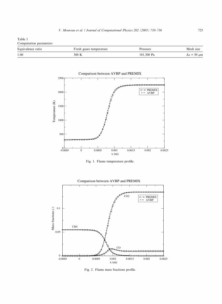
Table 1

Computation parameters

Equivalence ratio Fresh gases temperature Pressure Mesh size

1.00 300 K 101,300 Pa Dx = 50 lm

-0.0005 0 0.0005 0.001 0.0015 0.002 0.0025x (m)

0

500

1000

1500

2000

2500

Tem

pera

ture

(K

)

PREMIXAVBP

Comparison between AVBP and PREMIX

Fig. 1. Flame temperature profile.

-0.0005 0 0.0005 0.001 0.0015 0.002 0.0025x (m)

0

0.05

0.1

Mas

s fr

actio

ns (

-)

PREMIXAVBP

Comparison between AVBP and PREMIX

CH4

CO2

CO

Fig. 2. Flame mass fractions profile.



domain through the boundaries and no reflection takes place. After 5 ms, the acoustic activity at both ends

of the domain is zero and both pressures are constant.

8.3. Uniform flow

Simulating this case allows to check if a numerical scheme really satisfies the discrete form of the GCL. It

consists of a closed box with a uniform mixture initially at rest. The boundaries of the box are fixed but the

mesh points are moving. The initial meshes used in this case are an unstructured triangular grid (TRI) and a

regular quadrangular grid (QUAD). The deformation law of the mesh is a periodic radial contraction-

expansion distortion illustrated in Fig. 4. The simulation time corresponds to hundred periods sD of the

deformation law. For schemes that satisfy the discrete GCL the flow should remain uniformly at rest.

An estimation of the numerical error is thus defined by:

error ¼ K1sD

RsD

12j _X j2

D Edt

; ð81Þ

which is the ratio of the mean kinetic energy K of the flow and a mean grid kinetic energy averaged in time.

Fig. 5 shows this error for different schemes and meshes: if it remains equal to zero the DGCL criterion is

satisfied. The tests performed confirm the theoretical analysis from the previous section: the DGCL is sat-isfied for all combinations, except for TTGC on irregular bilinear elements. However even in this case, the

error is small, leading only to negligible perturbations.

8.4. Uniformly Accelerated Piston

A uniformly accelerated piston (UAP) induces an acoustic wave (see Fig. 6) for which analytical solu-

tions have been given by Landau and Lifchitz [53]. The simulation time is limited by the reflection of

the wave on the opposite wall to the piston and by the piston speed which must remain small compared

0 0.005 0.01 0.015 0.02 0.025 0.03

time (s)

101320

101325

101330

101335

Pres

sure

(Pa

)

inletoutlet

AVBP inlet and outlet pressure profiles

Fig. 3. Time evolution of inlet and outlet pressure for flame computation.

Fig. 4. Mesh deformations.

98 99 100t/τ

D

0e+00

1e-04

2e-04

3e-04

erro

r

LW-TRILW-QUADTTGC-TRITTGC-QUAD

Fig. 5. Kinetic energy error.


to the speed of sound in order to avoid creating a shock. The Lax–Wendroff and TTGC schemes are tested

on two meshes composed of regular triangles (TRI) or regular quadrangles (QUAD), respectively. The ele-

ments remain regular with time as the meshes are uniformly distorted. For each scheme, five velocity pro-

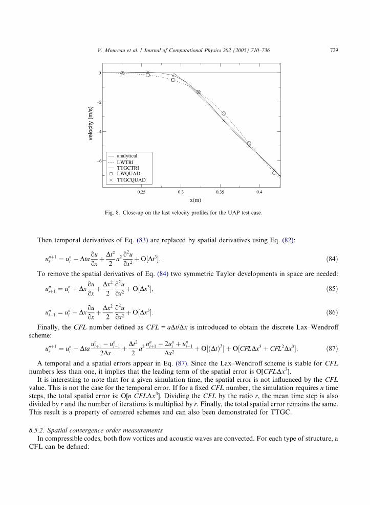
files at different times are compared to the analytical solution. Results are presented in Fig. 7. A close-up onthe last profiles is presented in Fig. 8. Note that the piston is initially located at x = 1 m and is moving to-

wards x = 0 m. As expected the schemes give results very close to the analytical solutions, thus validating

the ALE formulations. Fig. 8 shows that the Lax–Wendroff scheme behaves more like a low-pass filter than

TTGC, underlining the higher precision of the latter.

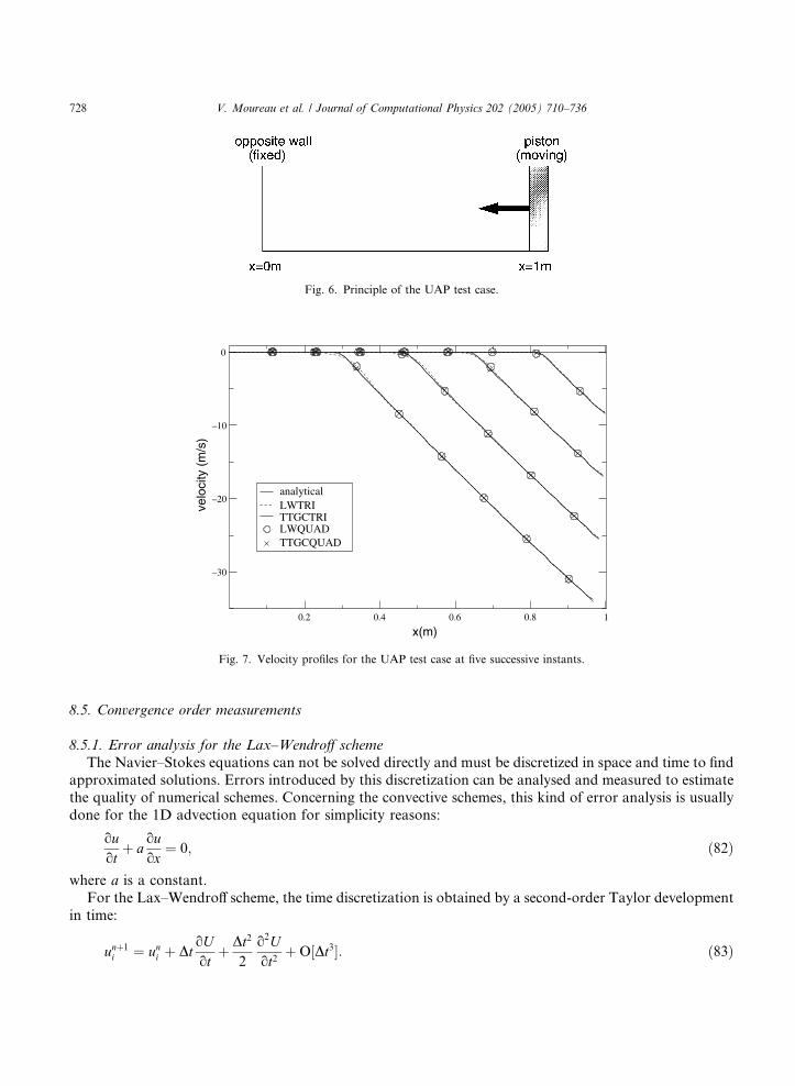
Fig. 6. Principle of the UAP test case.

0.2 0.4 0.6 0.8 1

x(m)

–30

–20

–10

0

velo

city

(m

/s)

analyticalLWTRITTGCTRILWQUADTTGCQUAD

Fig. 7. Velocity profiles for the UAP test case at five successive instants.


8.5. Convergence order measurements

8.5.1. Error analysis for the Lax–Wendroff scheme

The Navier–Stokes equations can not be solved directly and must be discretized in space and time to find

approximated solutions. Errors introduced by this discretization can be analysed and measured to estimate

the quality of numerical schemes. Concerning the convective schemes, this kind of error analysis is usually

done for the 1D advection equation for simplicity reasons:

ouot

þ aouox

¼ 0; ð82Þ

where a is a constant.

For the Lax–Wendroff scheme, the time discretization is obtained by a second-order Taylor development

in time:

unþ1i ¼ uni þ Dt

oUot

þ Dt2

2

o2Uot2

þO½Dt3�: ð83Þ

0.25 0.3 0.35 0.4

x(m)

–6

–4

–2

0

velo

city

(m

/s)

analyticalLWTRITTGCTRILWQUADTTGCQUAD

Fig. 8. Close-up on the last velocity profiles for the UAP test case.


Then temporal derivatives of Eq. (83) are replaced by spatial derivatives using Eq. (82):

unþ1i ¼ uni � Dta

ouox

þ Dt2

2a2

o2uox2

þO½Dt3�: ð84Þ

To remove the spatial derivatives of Eq. (84) two symmetric Taylor developments in space are needed:

uniþ1 ¼ uni þ Dxouox

þ Dx2

2

o2uox2

þO½Dx3�; ð85Þ

uni�1 ¼ uni � Dxouox

þ Dx2

2

o2uox2

þO½Dx3�: ð86Þ

Finally, the CFL number defined as CFL = aDt/Dx is introduced to obtain the discrete Lax–Wendroff

scheme:

unþ1i ¼ uni � Dta

uniþ1 � uni�1

2Dxþ Dt2

2a2

uniþ1 � 2uni þ uni�1

Dx2þO½ðDtÞ3� þO½CFLDx3 þ CFL2Dx3�: ð87Þ

A temporal and a spatial errors appear in Eq. (87). Since the Lax–Wendroff scheme is stable for CFL

numbers less than one, it implies that the leading term of the spatial error is O[CFLDx3].It is interesting to note that for a given simulation time, the spatial error is not influenced by the CFL

value. This is not the case for the temporal error. If for a fixed CFL number, the simulation requires n timesteps, the total spatial error is: O[n CFLDx3]. Dividing the CFL by the ratio r, the mean time step is also

divided by r and the number of iterations is multiplied by r. Finally, the total spatial error remains the same.

This result is a property of centered schemes and can also been demonstrated for TTGC.

8.5.2. Spatial convergence order measurements

In compressible codes, both flow vortices and acoustic waves are convected. For each type of structure, a

CFL can be defined:


CFLconv ¼Dt umax

Dxand CFLacou ¼

Dt jumax þ cjDx

ð88Þ

and

CFLconv ¼M

1þMCFLacou; ð89Þ

where M is the Mach number. The stability condition of the numerical scheme is of the form:

maxðCFLacou;CFLconvÞ < CFLmax: ð90Þ
For subsonic flows (M < 0.3), M/(1 + M) is small and CFLconv is far smaller than CFLacou. The non-
acoustic structures of the flow are thus well time-resolved and the numerical errors are mainly caused by

the spatial resolution.The purpose of the following test cases is to characterize the convective properties of the ALE schemes

for the non-acoustic structures. CFLacou is fixed at 0.7 and the influence of the spatial resolution on the

convergence order is studied. Some additional tests about the influence of the CFL number are also pre-

sented to underline the fact that spatial errors prevail on temporal errors. The spatial error measurements

are performed for two analytical solutions of the Euler equations. The first case is linear and consists in

the convection of a Gaussian profile of a species k on periodic meshes. The flow velocity is uniform in

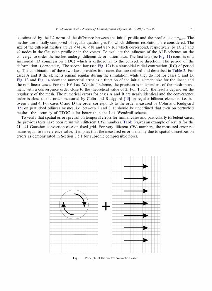
order to obtain the same profile as the initial one after a convective time sconv. The principle of this linearcase is illustrated in Fig. 9. The second test case is non-linear. It consists of a vortex convected by auniform flow on a periodic mesh. After a convective time sconv, supposing that there are no interactions

between the various vortices on the infinite domain, the vortex profile should be the same as the initial

one. This test is illustrated in Fig. 10. For these two cases the numerical error introduced by the schemes

+

Fig. 9. Principle of the scalar convection case.


is estimated by the L2 norm of the difference between the initial profile and the profile at t = sconv. Themeshes are initially composed of regular quadrangles for which different resolutions are considered. The

size of the different meshes are 21 · 41, 41 · 81 and 81 · 161 which correspond, respectively, to 13, 25 and

49 nodes in the Gaussian profile or in the vortex. To evaluate the influence of the ALE schemes on the

convergence order the meshes undergo different deformation laws. The first law (see Fig. 11) consists of asinusoidal 1D compression (1DC) which is orthogonal to the convective direction. The period of the

deformation is denoted su. The second law (see Fig. 12) is a sinusoidal radial contraction (RC) of period

sc. The combination of these two laws provides four cases that are defined and described in Table 2. For

cases A and B the elements remain regular during the simulation, while they do not for cases C and D.

Fig. 13 and Fig. 14 show the numerical error as a function of the initial element size for the linear and

the non-linear cases. For the FV Lax–Wendroff scheme, the precision is independent of the mesh move-

ment with a convergence order close to the theoretical value of 2. For TTGC, the results depend on the

regularity of the mesh. The numerical errors for cases A and B are nearly identical and the convergenceorder is close to the order measured by Colin and Rudgyard [15] on regular bilinear elements, i.e. be-

tween 3 and 4. For cases C and D the order corresponds to the order measured by Colin and Rudgyard

[15] on perturbed bilinear meshes, i.e. between 2 and 3. It should be underlined that even on perturbed

meshes, the accuracy of TTGC is far better than the Lax–Wendroff scheme.

To verify that spatial errors prevail on temporal errors for similar cases and particularly turbulent cases,

the previous tests have been rerun with different CFL numbers. Table 3 gives an example of results for the

21 · 41 Gaussian convection case on fixed grid. For very different CFL numbers, the measured error re-

mains equal to its reference value. It implies that the measured error is mainly due to spatial discretizationerrors as demonstrated in Section 8.5.1 for subsonic compressible flows.

+

Fig. 10. Principle of the vortex convection case.

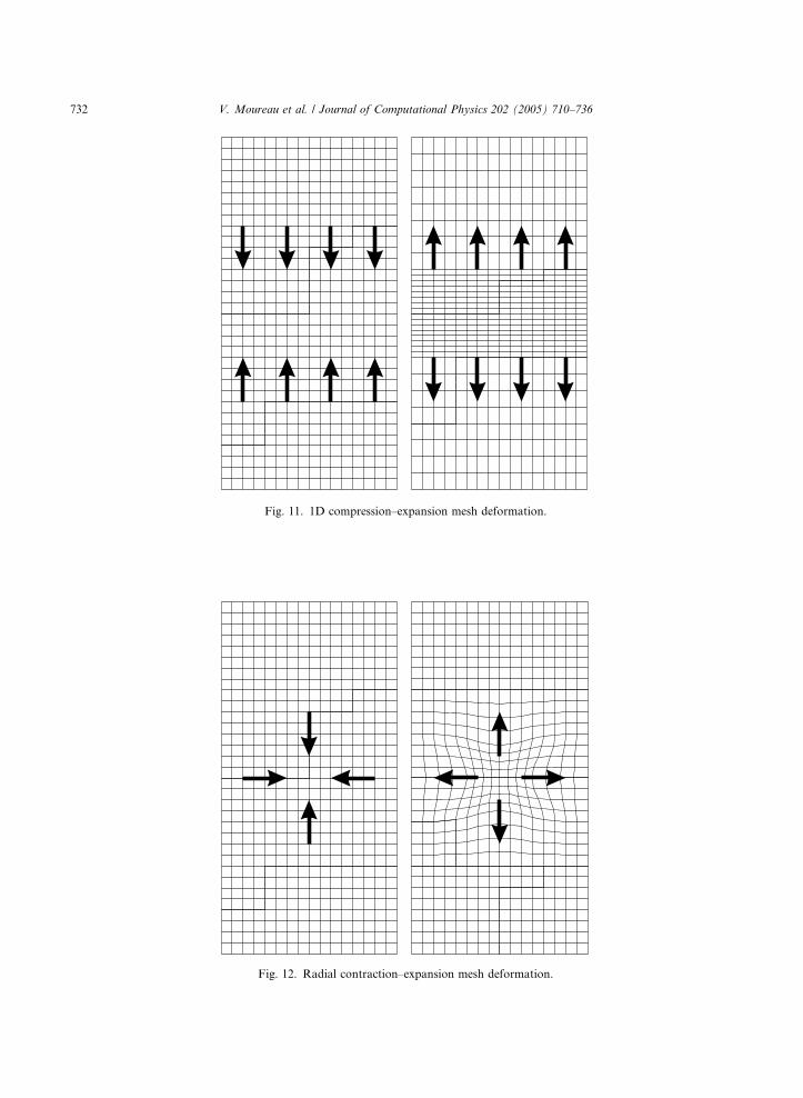
Fig. 11. 1D compression–expansion mesh deformation.

Fig. 12. Radial contraction–expansion mesh deformation.


0.050.01

∆x

0.0001

0.001

0.01

0.1

L2 e

rror

ABCD

LW

TTGC

dx2

dx3

dx4

Fig. 13. Error for the scalar convection case versus mesh size.

∆x 0.050.01

0.001

0.01

0.1

1

L2 e

rror

ABCD

LW

TTGC

dx2

dx3

dx4

Fig. 14. Error for the vortex convection case versus mesh size.

Table 2

Mesh movement cases

Case Type Parameters j _X jmax

A Fixed

B 1DC susconv

¼ 0:2 26.2 m/s

C 1DC + RC susconv

¼ scsconv

¼ 0:2 26.2 m/s

C 1DC + RC susconv

¼ 0:2; scsconv

¼ 0:125 27.8 m/s

1DC: mono-dimensional compression; RC: radial compression.


Table 3

Error for the 21 · 41 Gaussian convection case versus CFL value

CFL L2 error

0.7 0.1535

0.1 0.1541

0.01 0.1543


9. Conclusions

A methodology for unsteady multispecies reacting flows on fixed and moving grids has been presented

and tested in simple laminar flows (applications to DNS and LES of fully turbulent cases may be found in

[16,52] or [54]). The importance of boundary conditions was stressed and a new simple formulation to

implement characteristic boundary conditions in compressible DNS/LES codes was described. This formu-

lation has been tested and results for laminar flames are presented. It was also shown that high-order (sec-

ond and third order) schemes can be constructed on hybrid moving grids but that their derivation required

some care to preserve accuracy. These schemes have been tested on various cases such as uniform flow onmoving grids, uniformly accelerated pistons, scalar convection and vortex propagation on deforming grids,

to confirm the validity of the various methods and measure the exact order or precision of these techniques.

The mesh deformations used in these cases are representative of the distortions that can be found in many

practical configurations such as piston engines. But when the grid becomes too distorted during a simula-

tion, the ALE method can be used in conjunction with interpolation techniques to change mesh and keep

numerical dissipation low.

References

[1] T. Poinsot, D. Veynante, in: R.T. Edwards (Ed.), Theoretical and Numerical Combustion, 2001.

[2] N. Peters, Turbulent combustion, Cambridge University Press, Cambridge, 2000.

[3] C. Angelberger, D. Veynante, F. Egolfopoulos, Large Eddy Simulations of chemical and acoustic forcing of a premixed dump

combustor, Flow Turbul. Combust. 65 (2) (2000) 205–222.

[4] H. Pitsch, H. Steiner, Large Eddy Simulation of a turbulent piloted methane/air diffusion flame (Sandia flame D), Phys. Fluids 12

(2000) 2541–2554.

[5] H. Pitsch, L.D. de la Geneste, Large Eddy Simulation of premixed turbulent combustion using a level-set approach, in: Proc. of

the Comb. Institute, vol. 29, 2002, pp. 2001–2008.

[6] D. Caraeni, C. Bergstrom, L. Fuchs, Modeling of liquid fuel injection evaporation and mixing in a gas turbine burner using Large

Eddy Simulations, Flow Turbul. Combust. 65 (2000) 223–244.

[7] K. Mahesh, G. Constantinescu, P. Moin, A numerical method for Large-Eddy Simulation in complex geometries, J. Comput.

Phys. 197 (2004) 215–240.

[8] M.M. Rai, P. Moin, Direct simulations of turbulent flow using finite-difference schemes, J. Comput. Phys. 96 (1991) 15–53.

[9] S.I. Moller, E. Lundgren, C. Fureby, Large Eddy Simulations of unsteady combustion, in: 26th Symp. (Int.) on Comb., The

Combustion Institute, Pittsburgh, 1996, pp. 241–248.

[10] W.W. Kim, S. Menon, An unsteady incompressible navier stokes solver for LES of turbulent flows, Int. J. Numer. Meth. Fluids

31 (1999) 983–1017.

[11] N. Branley, W.P. Jones, Large Eddy Simulation of a turbulent non-premixed flame, Combust. Flame 127 (2001) 1914–1934.

[12] C.D. Pierce, P. Moin, Progress-variable approach for Large Eddy Simulation of non-premixed turbulent combustion, J. Fluid

Mech. 504 (2004) 73–97.

[13] P.E. DesJardin, S.H. Frankel, Large Eddy Simulation of a nonpremixed reacting jet: application and assessment of subgrid-scale

combustion models, Phys. Fluids 10 (1998) 2298–2314.

[14] J. Schluter, T. Schonfeld, LES of jets in cross flow and its application to gas turbine burners, Flow Turbul. Combust. 65 (2000)

177–203.


[15] O. Colin, M. Rudgyard, Development of high-order Taylor–Galerkin schemes for unsteady calculations, J. Comput. Phys. 162 (2)

(2000) 338–371.

[16] A. Kaufmann, F. Nicoud, T. Poinsot, Flow forcing techniques for numerical simulation of combustion instabilities, Combust.

Flame 131 (4) (2002) 371–385.

[17] K.W. Thompson, Time dependent boudary conditions for hyperbolic systems, J. Comput. Phys. 68 (1987) 1–24.

[18] C. Hirsch, Numerical Computation of Internal and External Flows, Wiley, New York, 1988.

[19] M. Giles, Non-reflecting boundary conditions for Euler equation calculations, AIAA J. 28 (1990) 2050–2058.

[20] M. Baum, T. Poinsot, D. Thevenin, Accurate boundary conditions for multicomponent reactive flows, J. Comput. Phys. 116

(1994) 247–261.

[21] N. Okong�o, J. Bellan, Consistent boundary conditions for multicompoment real gas mixtures based on characteristic waves, J.

Comput. Phys. 176 (2002) 330–344.

[22] W.T. Ashurst, N. Peters, M.D. Smooke, Numerical simulation of turbulent flame structure with non-unity Lewis number,

Combust. Sci. Technol. 53 (1987) 339–375.

[23] R.J. Cattolica, P.K. Barr, N.N. Mansour, Propagation of a premixed flame in a divided-chamber combustor, Combust. Flame 77

(1989) 101–121.

[24] P.K. Yeung, S.S. Girimaji, S.B. Pope, Straining and scalar dissipation on material surfaces in turbulence: implications for

flamelets, Combust. Flame 79 (1990) 340–365.

[25] C.J. Rutland, A. Trouve, Direct simulations of premixed turbulent flames with nonunity Lewis number, Combust. Flame 94

(1993) 41–57.

[26] D. Haworth, T. Poinsot, Numerical simulations of Lewis number effects in turbulent premixed flames, J. Fluid Mech. 244 (1992)

405–436.

[27] C.J. Rutland, J. Ferziger, Simulation of flame–vortex interactions, Combust. Flame 84 (1991) 343–360.

[28] C. Westbrook, F. Dryer, Simplified reaction mechanism for the oxidation of hydrocarbon fuels in flames, Combust. Sci. Technol.

27 (1981) 31–43.

[29] W.P. Jones, R.P. Lindstedt, Global reaction schemes for hydrocarbon combustion, Combust. Flame 73 (1988) 222–233.

[30] S. Zhang, C. Rutland, Premixed flame effects on turbulence and pressure related terms, Combust. Flame 102 (1995) 447–461.

[31] D. Veynante, T. Poinsot, Effects of pressure gradients on turbulent premixed flames, J. Fluid Mech. 353 (1997) 83–114.

[32] D. Veynante, A. Trouve, K.N.C. Bray, T. Mantel, Gradient and counter-gradient scalar transport in turbulent premixed flames,

J. Fluid Mech. 332 (1997) 263–293.

[33] B. Bedat, F. Egolfopoulos, T. Poinsot, Direct numerical simulation of heat release and nox formation in turbulent non premixed

flames, Combust. Flame 119 (1) (1999) 69–83.

[34] M. Baum, D. Haworth, T. Poinsot, N. Darabiha, Direct numerical simulation H2/O2/N2 flames with complex chemistry in two-

dimensional turbulent flows, J. Fluid Mech. 281 (1994) 1–32.

[35] G. Patnaik, K. Kailasanath, A computational study of local quenching in flame vortex interactions with radiative losses, in: 27th

Symp. (Int.) on Combust., The Combustion Institute, Pittsburgh, 1998, pp. 711–717.

[36] M.Y.N. Tanahashi, M.T.M. Fujimura, Fine scale structure of H2-air turbulent premixed flames, in: S. Banerjee, J. Eaton (Eds.),

1st International Symposium on Turbulence and Shear Flow, 1999, pp. 59–64.

[37] D.R. Stull, H. Prophet, JANAF Thermochemical Tables, second ed., Report No. NSRDS-NBS 37, US National Bureau of

Standards, 1971.

[38] J.O. Hirschfelder, C.F. Curtiss, R.B. Byrd, Molecular Theory of Gases and Liquids, Wiley, New York, 1969.

[39] A. Ern, V. Giovangigli, Multicomponent Transport Algorithms, Springer, Heidelberg, 1994.

[40] V. Giovangigli, Multicomponent Flow Modeling, Birkhauser, Boston, 1999.

[41] F.A. Williams, Combustion Theory, Benjamin Cummings, Menlo Park, CA, 1985.

[42] J.C. Strikwerda, Initial boundary value problem for incompletely parabolic systems, Commun. Pure Appl. Math. 30 (1977)

797.

[43] T. Poinsot, S. Lele, Boundary conditions for direct simulations of compressible viscous flows, J. Comput. Phys. 101 (1) (1992)

104–129.

[44] T. Colonius, S. Lele, P. Moin, Boundary conditions for direct computation of aerodynamic sound generation, AIAA J. 31 (9)

(1993) 1574–1582.

[45] T. Colonius, Numerically nonreflecting boundary and interface conditions for compressible flow and aeroacoustic computations,

AIAA J. 35 (7) (1997) 1126–1133.

[46] K. Rowley, T. Colonius, Discretely nonreflecting boundary conditions for linear hyperbolic systems, J. Comput. Phys. 157 (2)

(2000) 500–538.

[47] R. Verzicco, J. Mohd-Yusof, P. Orlandi, D. Haworth, Large-Eddy Simulation in complex geometric configurations using

boundary body forces, AIAA J. 38 (2000) 427–433.

[48] C. Hirt, A. Amsden, J. Cook, An Arbitrary Lagrangian–Eulerian computing method for all flow speeds, J. Comput. Phys. 14

(1974) 227–253.


[49] A. Masud, T. Hughes, A space–time Galerkin/least-squares finite element formulation of the Navier–Stokes equations for moving

domain problems, Comput. Meth. Appl. Mech. Eng. 146 (1997) 91–126.

[50] T. Tezduyar, M. Behr, J. Liou, A new strategy for finite element computations involving moving boundaries and interfaces – the

deforming-spatial-domain/space–time procedure: I. the concept and the preliminary tests, Comput. Meth. Appl. Mech. Eng. 94

(1992) 339–351.

[51] C. Farhat, P. Geuzaine, C. Grandmont, The discrete geometric conservation law and the nonlinear stability of the ale schemes for

the solution of flow problems on moving grids, J. Comput. Phys. 174 (2) (2001) 669–694.

[52] L. Selle, G. Lartigue, T. Poinsot, R. Koch, K.-U. Schildmacher, W. Krebs, B. Prade, P. Kaufmann, D. Veynante, Compressible

Large-Eddy Simulation of turbulent combustion in complex geometry on unstructured meshes, Combust. Flame 137 (4) (2004)

489–505.

[53] L. Landau, E. Lifchitz, Physique Theorique – Tome 6: Mecanique des Fluides, Librairie du Globe, Editions MIR, 1984.

[54] C. Priere, L. Gicquel, A. Kaufmann, W. Krebs, T. Poinsot, LES of mixing enhancement: LES predictions of mixing enhancement

for jets in cross-flows, J. Turbul. 5 (1) (2004) 005.

Numerical methods for unsteady compressible multi-component reacting flows on fixed and moving grids

Documents

Transcript of Numerical methods for unsteady compressible multi-component reacting flows on fixed and moving grids