An Implicit Multigrid Method for the Simulation of Chemically Reacting Flows

JOURNAL OF COMPUTATIONAL PHYSICS146,322–345 (1998)ARTICLE NO. CP986061

An Implicit Multigrid Method for the Simulationof Chemically Reacting Flows

P. Gerlinger, P. Stoll, and D. Br¨uggemann

Universitat Stuttgart, Pfaffenwaldring 31, 70550 Stuttgart, Germany

Received December 31, 1997; revised July 20, 1998

The application of multigrid methods is complicated if the set of governing equa-tions contains strongly nonlinear source terms. This is the case for finite-rate chem-istry as well as for turbulence conservation equations. In most cases strong nonlinear-ities within the chemical production rates prevent convergence of standard multigridmethods. This paper investigates different approaches to treating chemical and turbu-lent production terms on coarse grids in order to enable convergence. Independent ofcombustion, supersonic flows require special care during restriction and prolongationif strong shock waves occur. A full coarsening four-level nested multigrid methodis used for all conservation equations including those of turbulence and speciestransport. Strong convergence accelerations are achieved by a local source term-dependent damping of the restricted residual error. Several test cases with and with-out combustion demonstrate the efficiency and accuracy of the proposed multigridalgorithm. c© 1998 Academic Press

Key Words:multigrid; combustion; supersonic flows; finite-rate chemistry.

1. INTRODUCTION

The simulation of chemically reacting flows using finite-rate chemistry still requirestremendous computer time, making convergence accelerations extremely necessary. Fornonreactive flows multigrid techniques belong to the most efficient methods to reach asteady state solution. They have first been employed to elliptic subsonic flows, where ex-cellent results may be achieved [1–3]. Jamesonet al. [4, 5] developed an implicit multigridmethod for transonic flows. Modifications also allow the calculation of supersonic andhypersonic problems [6–15]. Due to their hyperbolic character, such cases require charac-teristic restriction and prolongation operators [11] or a damping of the transferred residualerrors at shock waves [12–15]. Even if the achieved convergence accelerations for super-sonic flows are smaller than those for subsonic cases, a strong reduction in computer timeis demonstrated by all authors cited above.

322

0021-9991/98 $25.00Copyright c© 1998 by Academic PressAll rights of reproduction in any form reserved.

MULTIGRID APPROACH FOR COMBUSTION SIMULATION 323

Very little work has been done on application of multigrid methods if the set of governingequations includes strongly nonlinear source terms. Difficulties often arise due to widelydisparate time and length scales which in the case of finite-rate chemistry may differ manyorders in magnitude. The resulting numerical stiffness is usually treated with implicit orat least point-implicit numerical methods for time integration. Therefore the multigridtechnique has to be adapted for implicit schemes also. Convergence acceleration of multigridmethods is based on the fact that low frequencies of the error are damped more efficientlyon coarser grid levels. This is in contrast to the local behavior of turbulent or chemicalproduction terms. If the source vector contains strongly nonlinear parts, coarse grid valuesstrongly differ from corresponding fine grid values and therefore may no longer representthe problem on the finest grid. A second difficulty is that even small coarse grid correctionsinterpolated back to the finest grid may lead to strong changes within the source vectorwhich can prevent convergence. Therefore special techniques are necessary to treat thenonlinear source terms as well as the corresponding source Jacobians on coarse grids. Theproblems arising from turbulent source terms are less severe than those due to chemistry, asthe coupling between turbulence and fluid variables is quite weak. Even if low-Reynolds-number turbulence models are employed, multigrid methods may achieve considerablespeedups. Liu and Zheng [16] use a point-implicit method, freezing turbulent productionterms on coarse grids. In Refs. [14, 15], a coarse grid treatment for the turbulent sourcevector is presented that speeds up convergence to a steady state drastically even in casesof massively separated flows, shock wave/boundary layer interactions, and extreme cellaspect ratios.

Up to now, only a few papers have been published on the use of multigrid techniquesfor combustion calculations. Most of these papers achieved no or only small convergenceaccelerations. Slomskiet al. [17] and Radespielet al. [18] calculated reacting or disso-ciating air with small reaction schemes using standard multigrid procedures. Liaoet al.[19–21] employed the multigrid technique for the momentum equations only without prov-ing convergence accelerations. Considerable speedups are obtained by Shefferet al.[22] fordetonation waves using a two-level multigrid method. Most notably, Edwards [23] employedmultigrid techniques for hypersonic chemically reacting flows and hydrogen combustion[24]. A global damping of the transferred residual error is used in Ref. [24] to enableconvergence. This paper investigates several approaches on coarse grids to approximatechemical source terms and source Jacobians. The solution favored by the authors is a localdamping of the restricted residual error in regions of high chemical activity. To our knowl-edge this is the first paper where a four-level multigrid method is successfully employedfor diffusion-dominated flames and low-Reynolds-number turbulence closure.

2. GOVERNING EQUATIONS

The investigation of high-speed turbulent combustion requires the solution of the ex-panded Navier–Stokes equations which are given in two-dimensional form by

∂Q∂t+ ∂(F− Fν)

∂x+ ∂(G−Gν)

∂y= S, (1)

where the conservative variable vector is

Q = [ρ, ρu, ρv, ρE, ρq, ρω, ρYi ]T , i = 1, 2, . . . , Ns − 1. (2)

324 GERLINGER, STOLL, AND BRUGGEMANN

F andG are inviscid,Fν andGν are viscous fluxes inx- and y-directions, respectively.The source vectorS results from turbulence and chemistry. The variables in Eq. (2) arethe densityρ, the velocity componentsu andv, the total specific energyE, the turbulencevariablesq=√k (k is the turbulent kinetic energy) andω = ε/k (ε is the dissipation rateof k), and the species mass fractionsYi . Ns is the number of different species. The simula-tion of hydrogen combustion involves a 9-species (N2,O2,H2,H2O,OH,O,H,NO2, andH2O2), 20-step reaction scheme developed by Jachimowski [25] excluding the nitrogenreactions. Fourth-order polynomials of temperature are employed for molecular viscosity,thermal conductivity, and diffusivity calculation of pure species. Mixture values of molec-ular viscosity and thermal conductivity are determined using Wilke’s law [26], and diffu-sivity of one species in relation to the remaining gas is calculated according to Mason andSaxena [27]. Diffusion velocities and the associated heat flux terms are modeled usingFick’s law. Turbulent contributions to thermal conductivity and diffusivity are obtained us-ing constant turbulent Prandtl and Schmidt numbers. For turbulence closure a two-equationlow-Reynolds-numberq-ω model is employed [28–30].

A critical point for the multigrid method is the source vector appearing in Eq. (1) whichis given by

S= [0, 0, 0, 0, Sq, Sω, Si ]T , i = 1, 2, . . . , Ns − 1. (3)

The turbulent source termsSq andSω are calculated by [28]

Sq = Cq1

(CµDq

Sω2− 2

3

D

ω− 1

)ρωq (4)

Sω =[Cω1

(Cµ

Sω2− Cω3

D

ω

)− Cω2

]ρω2 (5)

and are also representative for other two equation turbulence closures.D is the divergenceof the velocity field;S is the strain invariant; andCq1,Cµ,Cω2, andCω3 are modelingconstants [29]. Two types of terms cause problems in multigrid methods: Terms formed bysquares of velocity derivatives as the strain invariant,

S =[2∂u

∂x− 2

3

(∂u

∂x+ ∂v∂y

)]∂u

∂x+(∂u

∂y+ ∂v∂x

)2

+[2∂v

∂y− 2

3

(∂u

∂x+ ∂v∂y

)]∂v

∂y, (6)

and exponential damping functions which depend on a turbulent Reynolds numberRq,

Dq= 1− exp(−0.022Rq), Cω1 = 0.5Dq + 0.055. (7)

Damping functions are necessary in many low-Reynolds-number turbulence models foran accurate simulation of the logarithmic near wall behavior. Like chemistry, turbulentproduction and dissipation are local phenomena. Nevertheless, there is a strong differencebetween turbulent and chemical source terms. While chemical production terms only dependon local values of the variable vector, turbulent production terms also depend on flow variablederivatives which in discretized form require values from neighboring cells. Therefore,the resulting value of these terms (e.g.,S) is strongly grid size (grid level) dependent.Like chemical source terms, turbulent damping functions (e.g.,Dq) cause problems in the


multigrid method due to their local nonlinear behavior. The turbulent Reynolds numberdepends linearly on the distance of a cell center to the nearest wall. Especially close to solidwalls, differences in wall distances at different grid levels cause strong changes within theseexponential damping functions. For cases with flow separation a coarse grid recalculationof these terms may prevent convergence [14].

3. NUMERICAL METHOD

The unsteady form of governing equations is integrated in time using an implicit finite-volume LU algorithm [4, 31]. Jameson and Yoon [32] have demonstrated the ability ofthis driving scheme to rapidly damp out high-frequency error modes. This is a basic andnecessary feature for an algorithm to be used as a smoother for multigrid methods. In additionto the inviscid Jacobians, simplified viscous Jacobians are included in the implicit part basedon the thin-layer Navier–Stokes equations. In Eq. (8) this is shown for theη-direction only.The discretized implicit LU scheme is given by [31][

I + 1t(A+i, j − A−i, j + B+i, j − B−i, j + 2T i, j − H i, j

)−1t(A+i−1, j + B+i, j−1+ T i, j−1

)−1t

(A−i+1, j + B−i, j+1+ T i, j+1

)]1Qi, j = 1tRi, j . (8)

To ensure diagonal dominance the upwind differenced inviscid Jacobians on the cell inter-facesA andB are split in+ and−matrices containing only positive or negative eigenvalues[4, 31]. T are centrally differenced Jacobians of the viscous fluxes, andH= ∂S/∂Q is thesource Jacobian due to chemistry and turbulence. The turbulence equations are solved ina loosely coupled form with the fluid motion. FinallyR is the discretized residual. If thediagonal, lower, and upper Jacobians of Eq. (8) are combined to formD, L, andU , thisequation can be expressed by

(D + L +U )1Qn+1 = −1tR. (9)

Approximately factored, Eq. (9) is solved in two steps [31]:

Lower sweep:

(D + L)1Q = −1tR. (10)

Upper sweep:

(D +U )1Qn+1 = D1Q. (11)

The solution is updated byQn+1=Qn +1Qn+1. The source and viscous Jacobians add tothe diagonalD, forming a matrix which has to be inverted directly at every grid point. Anapproximation for the chemistry source Jacobian has been proposed by Eberhardt and Imlay[33], resulting in a diagonal matrix only. However, the computational, more expensive useof a full chemical source Jacobian is preferred in the present paper. Local time stepping isused to enhance convergence to a steady state.

As the right-hand side (RHS) is discretized with central differences, a second- and fourth-order matrix dissipation is added to reduce oscillations near shock waves and to enableconvergence to machine accuracy [34, 35].


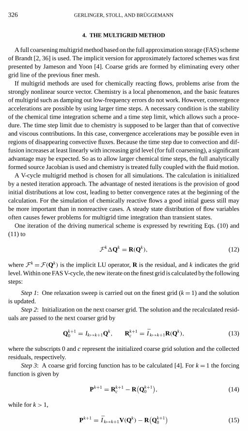
4. THE MULTIGRID METHOD

A full coarsening multigrid method based on the full approximation storage (FAS) schemeof Brandt [2, 36] is used. The implicit version for approximately factored schemes was firstpresented by Jameson and Yoon [4]. Coarse grids are formed by eliminating every othergrid line of the previous finer mesh.

If multigrid methods are used for chemically reacting flows, problems arise from thestrongly nonlinear source vector. Chemistry is a local phenomenon, and the basic featuresof multigrid such as damping out low-frequency errors do not work. However, convergenceaccelerations are possible by using larger time steps. A necessary condition is the stabilityof the chemical time integration scheme and a time step limit, which allows such a proce-dure. The time step limit due to chemistry is supposed to be larger than that of convectiveand viscous contributions. In this case, convergence accelerations may be possible even inregions of disappearing convective fluxes. Because the time step due to convection and dif-fusion increases at least linearly with increasing grid level (for full coarsening), a significantadvantage may be expected. So as to allow larger chemical time steps, the full analyticallyformed source Jacobian is used and chemistry is treated fully coupled with the fluid motion.

A V-cycle multigrid method is chosen for all simulations. The calculation is initializedby a nested iteration approach. The advantage of nested iterations is the provision of goodinitial distributions at low cost, leading to better convergence rates at the beginning of thecalculation. For the simulation of chemically reactive flows a good initial guess still maybe more important than in nonreactive cases. A steady state distribution of flow variablesoften causes fewer problems for multigrid time integration than transient states.

One iteration of the driving numerical scheme is expressed by rewriting Eqs. (10) and(11) to

Fk1Qk = R(Qk), (12)

whereFk=F(Qk) is the implicit LU operator,R is the residual, andk indicates the gridlevel. Within one FAS V-cycle, the new iterate on the finest grid is calculated by the followingsteps:

Step 1: One relaxation sweep is carried out on the finest grid (k= 1) and the solutionis updated.

Step 2: Initialization on the next coarser grid. The solution and the recalculated resid-uals are passed to the next coarser grid by

Qk+10 = Ik 7→k+1Qk, Rk+1

c = I k 7→k+1R(Qk), (13)

where the subscripts 0 andc represent the initialized coarse grid solution and the collectedresiduals, respectively.

Step 3: A coarse grid forcing function has to be calculated [4]. Fork= 1 the forcingfunction is given by

Pk+1 = Rk+1c − R

(Qk+1

0

), (14)

while for k> 1,

Pk+1 = I k 7→k+1V(Qk)− R(Qk+1

0

)(15)


is used. The residual error at levelk+1 is the sum of the forcing function and the calculatedresidual

Vk+1 = R(Qk+1)+ Pk+1, (16)

and the coarse grid solution is calculated similar to the procedure on the finest grid by

Fk+11Qk+1 = Vk+1. (17)

One iteration is performed at every grid level.Step 4: If the coarsest grid is reached, the obtained coarse grid corrections are inter-

polated on the fine level and added to the old solution by

Qknew= Qk + pk+17→k

(Qk+1

new −Q0k+1

). (18)

No additional relaxation sweeps are performed on coarse grids after each prolongation step.

4.1. Restriction and Prolongation

The simulation of supersonic and hypersonic flows requires modifications during re-striction and prolongation in comparison to standard (sub- or transonic) multigrid algo-rithms. This is due to the hyperbolic character of the governing equations. A pressure-baseddamping [12–15] of the restricted defect error is used in the present paper to avoid anunphysical upwind influence at shock waves which otherwise would prevent convergence.This method is numerically stable and computationally cheap, and allows one to treat evencomplicated flow structures. Koren and Hemker [12] have shown for inviscid hypersonicflows that a local damping of the restricted defect error improves robustness of the non-linear multigrid method. Leclercq and Stoufflet [11] employed characteristic restriction andprolongation operators to solve the Euler equations. Especially for multicomponent flows,this mathematically correct treatment is computationally expensive, requiring matrix vectormultiplications.

The following transfer operators are used for the applied full coarsening cell-centeredfinite-volume method.

• Ik 7→k+1 for restriction of the flow variables [4],

Ik 7→k+1Qk = 1

Äk+1

4∑l=1

Äkl Qk

l , (19)

whereÄk is the corresponding cell area at grid levelk. Four fine grid volumes are alwayscollected forming one coarse grid volume.• I k 7→k+1 for restriction of residuals and residual errors [13, 14],

I k 7→k+1Rk =4∑

l=1

Rkl max

(0, 1− κk

l

), I k 7→k+1Vk =

4∑l=1

Vkl max

(0, 1− κk

l

). (20)

Instead of four fine grid residuals simply being added, the transfer is damped by parameterκk

l . This treatment is only necessary near shock waves which are located by the same sensor


as employed for adding artificial viscosity. Especially for multigrid applications we foundit advantageous to use a blend between a standard pressure-based sensor [37] and a sensorwith TVD properties [34],

νξi, j =

|pi+1, j − 2pi, j + pi−1, j |(1− χ)(|pi+1, j − pi, j | + |pi, j − pi−1, j |)+ χ(pi+1, j + 2pi, j + pi−1, j )

, (21)

which is given here for theξ -direction. Values between 0.5 and 0.8 are used forχ in all ofthe following simulations. The damping parameterκk is formed by the maximum of someneighboring values ofν,

κk = Ck max(νξi, j , ν

ξi−1, j , ν

ξi+1, j , ν

ηi, j , ν

ηi, j−1, ν

ηi, j+1

), (22)

and constantsCk are used to adapt the damping factors to the decreasing smoothness of thepressure distribution on successively coarser grids.• pk+17→k is a prolongation operator used to transfer corrections from coarse to fine

grids. While in subsonic or smooth supersonic regions of the flowfield a second-ordercentral prolongation operator is used (bilinear interpolation), a simple first-order upwindprolongation is employed near shock waves [38]. Again, the pressure-based sensor ofEq. (22) works as a switch between both kinds of prolongation operators.

In addition to the described damping of the transferred residual error, for implicit numeri-cal schemes it is advantageous to reduce the coarse grid time step near shock waves. Insteadof the standard time step1ts which is formed by convective and diffusive contributions,the following time step is employed:

1tk = 1tks max[ε, (1− κk)n] for k> 1. (23)

The exponentn is necessary to adjust the coarse grid time step damping to different shockstrengths, andε is a limitation that usually is chosen to be 0.01.

4.2. Treatment of Source Terms

The greatest problem for multigrid solutions of turbulent reactive flows is the connectionbetween fine grid source terms and their representation on coarse grids. In contrast tofinite-rate chemistry, the coupling between turbulent source terms and fluid flow variablesis quite weak, making the use of multigrid methods for the turbulence equations muchmore favorable. A simple freezing of nonlinear parts already enables convergence even incomplicated cases with strong turbulence production and up to five grid levels [14, 15, 38].For theq-ω model used, the strain invariantS and the damping functionDq are calculatedon the finest grid only and passed to coarser grids by

Sk+1 = Ik 7→k+1Sk, Dk+1q = Ik 7→k+1Dk

q, (24)

where they are kept constant. Because only these nonlinear contributions to the source termare kept constant, turbulent source term and source Jacobian are still able to react and tofollow changes within the turbulent variables. This method is numerically very stable andworks well even for massively separated flows.


The sensitivity of the chemical source terms

Si = Mi

Nr∑r=1

[(ν ′′i,r − ν ′i,r )

(k fr

Nk∏l=1

cν ′l ,rl − kbr

Nk∏l=1

cν ′′l ,rl

)], i = 1, 2, . . . , Ns − 1 (25)

to changes within the flow variables makes the treatment of finite-rate chemistry with multi-level multigrid much more difficult. The coupling is given by the species concentrationsci

and the exponential dependence of forwardk f and backward reaction ratekb on temperature.An Arrhenius form is adopted for forward reaction rates while equilibrium constants areused to obtain backward reaction rates.

A linear transfer operatorIk 7→k+1 is used to restrict the flow variables to the next coarsergrid in a conservative manner. Thus recalculation of strongly nonlinear source terms maycause strong differences within these terms at both grid levels (if gradients exist within theflow variables on the finer grid). If these differences become too strong, the relation betweenthe grid levels gets lost, causing divergence of the multigrid algorithm. In the first three outof four investigated approaches, coarse grid source terms and Jacobians are approximatedusing additional information from the finest grid. This is done to separate coarse grid localproduction terms and Jacobians (which are fully or partially determined from the finestgrid) from coarse grid variables.

• Approach 1: The chemical source terms and Jacobians are calculated on the finestgrid only and are kept constant on coarser grids. While the coarse grid source terms areobtained by simply adding four fine grid values, the corresponding Jacobians are cell areaweighted usingIk 7→k+1.• Approach 2: The chemical source terms are treated in the same way as in approach 1.

However, the transfer of chemical source Jacobian entries from fine to coarse grids isweighted using parameters that evaluate the chemical importance of the correspondingvolume. The entries of the source JacobianH are given byHi, j with i, j = 1, 2, . . . , Ns+5.All entries within the first six rowsi = 1, . . . ,6 of the source Jacobian are zero due tothe absence of source terms (neglecting contributions from turbulence which are treatedseparately). While the columnsj = 1, . . . ,6 for i = 7, . . . , Ns + 5 are determined usingtransfer operatorIk 7→k+1 the submatrixi, j = 7, . . . , Ns + 5 is formed in a special way.First, the changes in gas composition

1Q = [0, 0, 0, 0, 0, 0,1Q1,1Q2, . . . , 1QNs−1

]T(26)

due to pure chemistry are calculated for every volume using local chemical productionterms. Such a treatment additionally requires one to solve a set ofNs− 1 equations forevery volume. The same time step1tk is used for the four fine grid volumes, formingone coarse grid volume. The fine grid changes1Qi thereby achieved are now used forweighting the coarse grid Jacobians. The purpose of this procedure is to achieve coarsegrid changes due to pure chemistry which approximate the cell area weighted changes ofthe four corresponding fine grid volumes. If geometric weighting factors for correspondingfine and coarse grid volumes are denoted by

vl = Äkl

Äk+1, l = 1, . . . ,4, (27)


coarse grid Jacobian entries are calculated by the expression

Hk+1i+6, j+6Ä

k+1 =∑4

l=1

(Hk

i+6, j+6Äk∣∣1Qk+1

j

∣∣)l∑4

l=1

(∣∣1Qk+1j

∣∣v)l+ ε , i, j = 1, 2, . . . , Ns − 1. (28)

Absolute values of changes in species concentrations are used andε is a small value to avoida zero denominator. Every column of the coarse grid sub-Jacobiani, j = 7, . . . , Ns + 5 isformed by weighting four corresponding fine grid columns with the same value. If fourfine grid changes have the same sign, and if coarse and fine grid time steps are chosenidentically, this Jacobian achieves a change on coarse grid which is identical to the four cellarea weighted fine grid changes.• Approach 3: The rates of forward and backward reaction are calculated on the

finest grid only, transferred to coarser grids, and kept constant. Additionally, a transfer oftemperature derivatives for the reaction rates is necessary to calculate coarse grid Jacobians.This approach was chosen because the most nonlinear dependence of the source term isdue to temperature within the Arrhenius form. This approach still allows the coarse gridchemical production terms to vary due to changes in species densities.• Approach 4: A new sensor is calculated to locate regions with high chemical intensity

γ =(

1

Ns − 1

Ns−1∑i=1

|Si ||Si |max+ ε

)α(29)

to reduce the transferred residual error. Instead of the transfer operators defined by Eq. (20)now

I k 7→k+1Rk =4∑

l=1

Rkl max

[0,min

(1− κk

l , 1− Bkγ kl

)]I k 7→k+1Vk =

4∑l=1

Vkl max

[0,min

(1− κk

l , 1− Bkγ kl

)] (30)

is used. Such a local damping was preferred to the global one presented in Ref. [24].Combustion is often limited to small regions, thus allowing the full multigrid scheme towork outside combustion zones.|Si |max is the maximum absolute production rate of speciesi within the flowfield,Bk is a grid level-dependent constant, andε again is a small numberto avoid division by zero. It is found to be advantageous that all individual production ratescontribute to this sensor which is limited to 0≤ γ ≤ 1. An important condition for the sensorto work is its smooth distribution. An exponentα of 0.25 worked satisfactory for all testcases described later. A further possibility to improve convergence of the multigrid schemeis to perform the above described damping for the species residual errors only. This resultsin a decoupling in time between continuity and species conservation equations. However,steady state solutions are unaffected by such a treatment.

4.2.1. Assessment of different approaches.All methods which keep parts or the to-tal chemical source vector or source Jacobian constant suffer from the extremely strongcoupling between chemistry and fluid motion. Changes within species concentrations ortemperature not being reflected within the parts kept constant are the major drawbacks ofapproaches 1 to 3. These methods worked for all investigated test cases employing up to


three grid levels and a time step reduction on the third grid. A fourth grid level alwaysaggravated the results. Therefore, we prefer the simple local damping of approach 4. Adisadvantage of this method is the strong case dependence of the choice of parametersBk

andα to limit the degree of damping. The reductions in CPU time achieved by using afourth grid level are small but there still is an improvement.

While strong reductions in CPU time are obtained for attached flames, results for detachedflames are still unsatisfactory. If the point of ignition is determined by chemical kinetics,differences between the grid levels destroy convergence. With approach 3 we hoped tolocalize ignition on coarse grids with reaction rates determined from the finest grid. However,no satisfactory results could be achieved with this method for detached flames.

5. RESULTS AND DISCUSSION

Numerical tests are performed to evaluate efficiency and robustness of the presentedmultigrid method for turbulent supersonic flows. All computations are initialized by fixingthe inflow properties in the interior of the domain. The first set simulates nonreactive flowsto demonstrate the ability of the multigrid technique to treat shock waves as well as sourceterms due to turbulent production. Next, three simulations are presented which includesource terms due to both turbulence and chemistry. These test cases cover premixed anddiffusion-dominated hydrogen combustion. All converged solutions of single and multi-grid calculations are identical. The employed 20-step reaction mechanism [25] results ina numerical stiff system of governing equations. The maximum cell species Damk¨ohlernumbersDai = (l refSi )/(ρ

√u2+ v2) are 18.9, 1.1, and 24.1 for the first, second, and third

test case. The reference lengthl ref was chosen to be 1 cm. The maximum ratio of maximumto minimum species Damk¨ohler numbers within any volume is up to 109. For comparisonthe last two test cases also show convergence rates of nonreactive calculations.

5.1. Ramped Ducts with and without Separation

Three planar ramped duct test cases without combustion are calculated and compared withexperimental data of Settleset al.[39, 40]. In accordance with the experiment the angles ofthe compression corners are 8◦, 16◦, and 20◦. The inflow Mach number is 2.85, and inflowstatic temperature and pressure are 100 K and 0.229 bar, respectively. All simulations start6.2 cm upstream of the ramp (x= 0 is located at the corner) using calculated, fully developedturbulent inflow profiles matching the experimentally measured boundary layer thicknessof δ= 2.1 cm. The computational grid contains 152× 80 volumes and is strongly refinedat the wall and in the separation zone near the corner. All values of the normalized distanceto the wall,y+, are smaller than 0.6 at stationary condition. Such a level of refinement isrequired by most low-Reynolds-number turbulence models for an accurate resolution ofthe viscous sublayer. The resulting cell aspect ratios on the surface are as high as 4500.While the flow over the 8◦ ramp is still attached, a very small separation zone occurs forthe 16◦ ramp, and the flow is separated over a region of about 18 mm for the 20◦ ramp.With increasing separation zone, turbulent production and dissipation terms increasinglydominate the turbulence conservation equations. Figure 1 shows a comparison betweenexperimental and calculated normalized wall static pressure profiles. With the exception ofthe 20◦ ramp, where the increase in pressure in front of the separation zone is located toofar downstream, the results compare quite well. Skin friction distributions are illustrated in


FIG. 1. Normalized surface static pressure distributions for ramped duct test cases.

Fig. 2. The results indicate that the predicted increase in skin friction after separation is toosteep in comparison to the experiment. The good overall agreement between experiment andsimulation makes theq-ω model interesting due to its favorable properties in conjunctionwith multigrid methods.

Convergence behavior of the calculations is displayed in Figs. 3 and 4. Plotted are theaveraged absolute residuals of the continuity andq (turbulence) conservation equationsversus the number of multigrid cycles. A four-level V-cycle multigrid method with twocoarse grid iterations is employed, commencing on the finest grid. It may be seen that fluidand turbulence residuals converge at nearly the same rate. This is valid for all investigatedtest cases and is an advantage if all equations are treated with the multigrid technique.According to Eq. (20) the transferred residual errors are damped in the vicinity of shockwaves. While the damping factorsκk are zero in the smooth parts of the flowfield, theymay approach one near shock waves. For the 20◦ ramp the maximum valueκk at stationarycondition out of all volumes is 0.27, 0.63, and 0.89 for the transfer from first to second,second to third, and third to fourth grid level, respectively. An unfavorable property of theLU-SGS scheme may also be observed from Fig. 3. With the occurrence of a large separatedregion for the 20◦ ramp and subsequently a large pocket of subsonic flow, the convergencerate of the algorithm degrades. This is due to an increased amount of upwind influence[41]. If the multigrid method is employed, convergence histories also differ due to flowseparation. However, machine accuracy is obtained after the same number of multigridcycles. Convergence histories of the density residuals in terms of work units are plottedin Fig. 5. One work unit is defined as the computational time necessary for one fine griditeration. Because all computations are performed on vector computers (Cray C94 and NEC-SX4) using a fully vectorized code, reductions achieved in CPU time are smaller than thetheoretically possible values. This is due to shorter vector lengths on coarse grids reducingthe performance of the code. However, the convergence improvement relative to the singlegrid iteration is at least threefold.


FIG. 2. Surface skin friction distributions for ramped duct test cases(cf = 2τW/(ρ∞u2∞)).

5.2. Oblique Detonation Wave

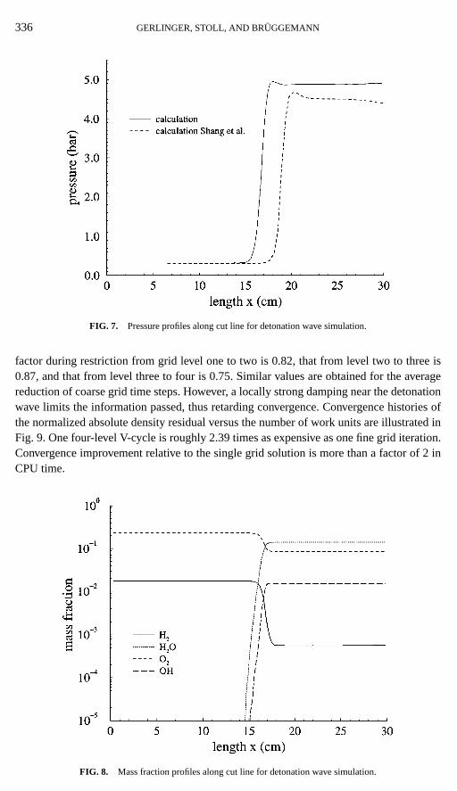
The first test case including finite-rate chemistry is a supersonic Mach 5 flow over a wedgewith 26.5◦ half angle (see Fig. 6). The inflow conditions are a static pressure and temperatureof 0.324 bar and 450 K, respectively. Hydrogen and air are premixed at an equivalence ratioof 0.6. Due to these inflow conditions a stationary stable detonation wave is obtained. AnEuler solution for the same problem may be found in Ref. [42]. A 1-block grid containing120× 80 volumes is used for this calculation. The minimum normal spacing for the grid atsolid walls is 1.7×10−6 m, fine enough to ensurey+ values smaller than 0.7 even at the tipof the wedge. The refinement near the solid wall results in cell aspect ratios of up to 2100.For detonation waves there is a direct coupling between the increase in pressure due to theshock wave and the increase in pressure due to heat release from combustion. Downstreamof the detonation wave, combustion is nearly completed. According to our experience thedetonation wave angle strongly depends on the finite-rate chemistry model used and isdetermined by the amount and speed of heat release due to combustion. Figure 7 shows


FIG. 3. Convergence histories of the density residuals for nonreactive ramped duct test cases versus thenumber of multigrid cycles.

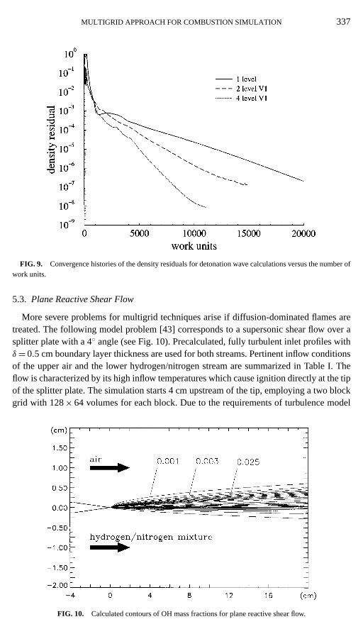
pressure profiles along the cut liney= 6.6 cm forx≤ 10 cm andy= 0.334x+3.26 cm forx> 10 cm. The differences between the present calculation and those of Ref. [42] mainlyresult from different reaction schemes and subsequent different detonation wave angles. Byuse of a simpler 8-step reaction scheme instead of the 20-step reaction scheme the sameangle and shock location was obtained as in Ref. [42], where a 9-step reaction scheme isemployed. Mass fraction profiles of H2,H2O,O2 and OH are plotted in Fig. 8.

FIG. 4. Convergence histories of theq residuals for nonreactive ramped duct test cases versus the number ofmultigrid cycles.


FIG. 5. Convergence histories of the density residuals for nonreactive ramped duct test cases versus thenumber of work units.

From a numerical point of view an attached detonation wave is less critical for the useof multigrid methods than diffusion-dominated flows. In such cases combustion only takesplace in a spatially very limited zone coupled with strong gradients in static pressure. Thissimplifies the calculation of sensors to locate main reaction zones. The chemically slowcombustion downstream of the detonation wave did not cause any problem for the multigridmethod. All four proposed approaches worked well for this test case using a nested four-levelV-cycle multigrid algorithm. Moreover, the described standard residual error damping andtime step reduction at shock waves (see Eqs. (20) and (23)) already enable convergence. Thisdemonstrates the possibility to achieve convergence of a multigrid method by blending offthe transferred residual error in critical regions. On the other hand every reduction of coarsegrid information degrades the achievable acceleration rates, making optimum dampingparameters desirable. If the damping factors 1− κk (see Eq. (20)) are multiplied withthe cell volume, added, and normalized with the total flowfield area, the average damping

FIG. 6. Geometry and inflow conditions for detonation wave simulation.


FIG. 7. Pressure profiles along cut line for detonation wave simulation.

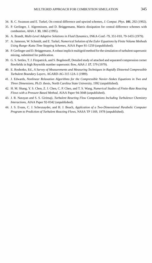
factor during restriction from grid level one to two is 0.82, that from level two to three is0.87, and that from level three to four is 0.75. Similar values are obtained for the averagereduction of coarse grid time steps. However, a locally strong damping near the detonationwave limits the information passed, thus retarding convergence. Convergence histories ofthe normalized absolute density residual versus the number of work units are illustrated inFig. 9. One four-level V-cycle is roughly 2.39 times as expensive as one fine grid iteration.Convergence improvement relative to the single grid solution is more than a factor of 2 inCPU time.

FIG. 8. Mass fraction profiles along cut line for detonation wave simulation.


FIG. 9. Convergence histories of the density residuals for detonation wave calculations versus the number ofwork units.

5.3. Plane Reactive Shear Flow

More severe problems for multigrid techniques arise if diffusion-dominated flames aretreated. The following model problem [43] corresponds to a supersonic shear flow over asplitter plate with a 4◦ angle (see Fig. 10). Precalculated, fully turbulent inlet profiles withδ= 0.5 cm boundary layer thickness are used for both streams. Pertinent inflow conditionsof the upper air and the lower hydrogen/nitrogen stream are summarized in Table I. Theflow is characterized by its high inflow temperatures which cause ignition directly at the tipof the splitter plate. The simulation starts 4 cm upstream of the tip, employing a two blockgrid with 128× 64 volumes for each block. Due to the requirements of turbulence model

FIG. 10. Calculated contours of OH mass fractions for plane reactive shear flow.


TABLE I

Inflow Conditions for the Upper Air and Lower

Hydrogen/Nitrogen Stream

Upper air stream Lower H2/N2 stream

p (bar) 1 1u (m/s) 1800 2697T (K) 2000 2000YH2 0 0.1YN2 0.7664 0.9YO2 0.2336 0

and flow characteristic the grid is highly clustered near solid walls, at the tip of the splitterplate, and in the combustion zone, resulting in cell aspect ratios of up to 2200. Ally+ valuesof near wall cell centers are smaller than 0.2. Figure 10 shows calculated OH mass fractioncontours indicating the main combustion zone.

Figures 11 and 12 illustrate convergence histories of the density residuals versus the num-ber of multigrid cycles and work units, respectively. One four-level V-cycle is roughly 2.34times as expensive as one fine grid iteration. All calculations up to the second grid level areperformed without modifications due to chemistry. As already mentioned, approaches 1 to3 suffer from the parts kept constant in source term and source Jacobian. The use of a thirdgrid level already destroyed or aggravated convergence. However, a further improvementin comparison to the two-level multigrid is achieved by a global time step reduction on thethird grid level. No improvement was obtained employing a fourth grid level. For this testcase approaches 1 to 3 achieved quite similar results. The disadvantage of the first threeapproaches is a strong sensitivity to flow conditions, such as grid spacing and resolution of

FIG. 11. Convergence histories of the density residuals for planar nonreactive and reactive shear flows versusthe number of multigrid cycles.


the combustion zone. Even if the best results for this test case could be achieved by approach3 and three grid levels, approach 4 is recommended because of its higher stability. As forthe first three approaches, a four-level multigrid did not improve the convergence usingapproach 4 but at least achieved about the same acceleration as the three level multigridmethod. The greatest problem is the optimum choice of damping parameters because theseinput values define the degree of convergence acceleration. Nevertheless, improvement interms of CPU time in comparison to the single grid iteration is slightly better than threefold.

5.4. Axisymmetric Shear Flow

The final test case considered corresponds to an experiment of Evanset al.[44]. Figure 13illustrates the axisymmetric hydrogen injection into a preheated vitiated air stream. A three-block grid is chosen to resolve the lip thickness at the end of the injector. The grid contains136× 72, 112× 48, and 136× 48 volumes to simulate the upper half of the symmetric prob-lem. The calculation starts atx=−0.33 cm, thus simulating the inner and outer boundarylayers at the tube surfaces (see Fig. 15). Precalculated, fully turbulent boundary layer pro-files are specified as inflow conditions. The computational grid is highly clustered near solidwalls as well as in the recirculation zone at the end of the tube. The minimum radial spacingis 1× 10−6 m, fine enough to ensurey+ values smaller than 0.8 for the converged solution.The highest cell aspect ratio is about 500. The inflow conditions of the pure hydrogen andthe vitiated air are summarized in Table II. Figures 14 and 15 show calculated temperatureand pressure contours to illustrate some overall features of the flowfield. Expansion fansare formed at the outer and inner rims at the end of the tube, followed by shock waves(see Fig. 15). A strongly refined grid arrangement is necessary to resolve these featureswhich may be important for ignition. Species profiles have been measured at four differentstreamwise locations. One of these profiles is plotted in Fig. 16.

FIG. 12. Convergence histories of the density residuals for planar reactive shear flows versus the number ofwork units.


TABLE II

Inflow Conditions for Axisymmetric Combustion

Experiment of Evanset al. [44]

Hydrogen jet Vitiated air stream

p (bar) 1 1u (m/s) 2432 1510T (K) 251 1495Ma 2 1.9YH2 1 0YH2O 0 0.281YN2 0 0.478YO2 0 0.241

The best convergence histories are obtained by damping the transferred residuals of themultigrid method in regions of intense chemistry (approach 4). This method is only ap-plied for restriction at grid levels higher than two. For the same test case Edwards [24]obtained best results for a seven-species calculation with two grid levels and for a nine-species calculation with three grid levels. The proposed application of local damping ofthe restricted residual error still achieves improved convergence rates by the applicationof a four-level V-cycle multigrid algorithm. Additionally, we found it feasible to reducethe damping factorγ (see Eq. (29)) as the solution approaches the stationary condition.When the residual has dropped more than one order in magnitude,γ is reduced in a log-arithmic way until, after a drop of five orders in magnitude,γ is set to zero. At this pointthe full four-level multigrid is working. Note, however, that there is still a reduction intransferred residual error and time step (n= 1 in Eq. (23)) in the vicinity of shock waves.The benefits of the multigrid algorithm are demonstrated in Figs. 17 and 18. Given are theconvergence histories for density andq residuals versus the number of multigrid cycles andwork units, respectively. It appears that one multigrid cycle requires 2.26 times the time of

FIG. 13. Geometry (cm) for the Evanset al. [44] axisymmetric combustion experiment.


FIG. 14. Calculated temperature contours (K) for the Evanset al. [44] experiment.

one fine grid iteration. As in the previous cases this factor is grid size dependent and muchhigher than the theoretically possible value due to short vector lengths on coarse grids.Thus, still better convergence rates may be expected if scalar computers are employed. Thefour-level nested multigrid algorithm converges about three times faster than the one-gridsolution.

6. CONCLUSIONS

An implicit multigrid method has been successfully applied to supersonic reactive flowsusing a low-Reynolds-numberq-ω turbulence model as well as 20-step finite-rate chem-istry. All conservation equations are treated with the multigrid technique. This algorithmis robust in handling very small grid spacings and high aspect ratio grids, necessary for

FIG. 15. Calculated pressure contours (bar) near the injector for the Evanset al. [44] experiment.


FIG. 16. Profiles of H2,O2,H2O, and N2 molar fractions atx/D= 21.7 for the Evanset al. [44] experiment(diameterD= 0.9525 cm).

high-Reynolds-number flows. Modifications to standard multigrid methods are used toavoid unphysical upwind influences near shock waves. Turbulent source terms are treatedby freezing strongly nonlinear parts on coarse grids. Several approaches are investigatedto treat the chemical source terms in order to extend multigrid methods to reacting flows.A simple local damping of the restricted residual error together with a time step reduction

FIG. 17. Convergence histories of the density andq residuals for the Evanset al. [44] experiment versus thenumber of multigrid cycles.


FIG. 18. Convergence histories of the density andq residuals for the Evanset al. [44] experiment versus thenumber of work units.

in regions of high chemical intensity achieved best results for all investigated hydrogenflames. While the treatment of turbulent source terms is very robust from a numerical pointof view, the chemistry still remains quite sensitive to the choice of local damping parame-ters. In addition, there are severe problems in simulating detached flames. The calculationof several test cases has demonstrated the ability of the proposed nested multigrid methodto speed up convergence to a steady state by a factor of three in CPU time for attachedflames and low-Reynolds-number turbulence closure.

ACKNOWLEDGMENTS

We thank the Deutsche Forschungsgemeinschaft (DFG) for the financial support of this work within theSFB 259 at the University of Stuttgart. Parts of this work were performed during the first author’s stay at NorthCarolina State University. This author thanks Professor H. A. Hassan for the possibility to work with him and hisgroup.

REFERENCES

1. W. Hackbusch,Computational Mathematics (4)(Springer-Verlag, Berlin/Heidelberg/New York, 1985).

2. A. Brandt, Multi-level adaptive solutions to boundary-value problems,Math. Comp.31, 333 (1977).

3. S. W. McCormick, Ed.,Frontiers in Applied Mathematics Series(SIAM, Philadelphia, 1987).

4. A. Jameson and S. Yoon, Lower–upper implicit schemes with multiple grids for the Euler equations,AIAA J.25, 929 (1987).

5. L. Martinelli, A. Jameson, and F. Grasso,A Multigrid Method for the Navier–Stokes Equations, AIAA Paper86-0208 (unpublished).

6. R. C. Swanson, E. Turkel, and J. A. White,An Effective Multigrid Method for High-Speed Flows, NASAICASE Report 91-56, 1991 (unpublished).

7. E. Turkel, R. C. Swanson, V. N. Vatsa, and J. A. White,Multigrid for Hypersonic Viscous Two- and Three-Dimensional Flow, NASA ICASE Report 91-57, 1991 (unpublished).


8. V. N. Vatsa, E. Turkel, and J. S. Abolhassani, Extension of multigrid methodology to supersonic/hypersonic3-D viscous flows,Int. J. Numer. Methods Fluids17, 825 (1993).

9. P. W. Hemker and B. Koren,Defect Correction and Nonlinear Multigrid for the Euler Equations, Lect. Series1988-05 (von Karman Institute for Fluid Dynamics, 1988).

10. J. R. Edwards, Upwind relaxation multigrid method for computing three-dimensional, viscous internal flows,J. Prop. Power12, 146 (1996).

11. M. P. Leclercq and B. Stoufflet, Characteristic multigrid method application to solve the Euler equations withunstructured and unnested grids,J. Comput. Phys104, 329 (1993).

12. B. Koren and P. W. Hemker, Damped, direction-dependent multigrid for hypersonic flow computations,Appl.Numer. Math.7, 309 (1990).

13. R. Radespiel and R. C. Swanson, Progress with multigrid schemes for hypersonic flow problems,J. Comput.Phys.116, 103 (1995).

14. P. Gerlinger and D. Brüggemann, Multigrid convergence acceleration for turbulent supersonic flows,Int. J.Numer. Methods Fluids24, 1019 (1997).

15. P. Gerlinger and D. Brüggemann, An implicit multigrid scheme for the compressible Navier–Stokes equationswith low-Reynolds-number turbulence closure,ASME J. Fluids Eng.120, 257 (1998).

16. F. Liu and X. Zheng, A strongly coupled time-marching method for solving the Navier–Stokes and k-ω

turbulence model equations with multigrid,J. Comput. Phys128, 289 (1996).

17. J. F. Slomski, J. D. Anderson, and J. J. Gorski,Effectiveness of Multigrid in Accelerating Convergence ofMultidimensional Flows in Chemical Nonequilibrium, AIAA Paper 90-1575 (unpublished).

18. R. Radespiel, J. M. A. Longo, S. Brück, and D. Schwamborn,Efficient Numerical Simulation of Complex 3DFlows with Large Contrast, AGARD-CP-578 33-1 (1996).

19. C. Liao, Z. Liu, X. Zheng, and C. Liu,NOx Prediction in 3-D Turbulent Diffusion Flames by Using ImplicitMultigrid Methods, AIAA Paper 95-3166 (unpublished).

20. C. Liao, Z. Liu, and C. Liu,Implicit Multigrid Method for Modeling 3-D Turbulent Diffusion Flames withDetailed Chemistry, AIAA Paper 95-0801 (unpublished).

21. X. Zheng, C. Liao, Z. Liu, and C. Liu, Mass-fluxed-based implicit multigrid method for modeling multi-dimensional combustion,J. Prop. Power13, 97 (1997).

22. S. G. Sheffer, A. Jameson, and L. Martinelli,A Multigrid Method for High Speed Reactive Flows, AIAAPaper 97-2106 (unpublished).

23. J. R. Edwards, An implicit multigrid algorithm for computing hypersonic, chemically reacting viscous flows,J. Comput. Phys.123, 84 (1996).

24. J. R. Edwards,Advanced Implicit Algorithms for Finite Rate Hydrogen–Air Combustion Calculations, AIAAPaper 96-3129 (unpublished).

25. C. J. Jachimowski,An Analytical Study of the Hydrogen–Air Reaction Mechanism with Application to ScramjetCombustion, NASA TP 2791, 1988 (unpublished).

26. C. R. Wilke, A viscosity equation for gas mixtures,J. Chem. Phys.18, 517 (1950).

27. R. B. Bird, W. E. Steward, and E. N. Lightfood,Transport Phenomena(Wiley, New York, 1960).

28. T. J. Coakley,Turbulence Modeling Methods for the Compressible Navier–Stokes Equations, AIAA Paper83-1693 (unpublished).

29. T. J. Coakley and P. G. Huang,Turbulence Modeling for High Speed Flows, AIAA Paper 92-0436(unpublished).

30. P. Gerlinger, J. Algermissen, and D. Brüggemann, Numerical simulation of mixing for turbulent slot injection,AIAA J.34, 73 (1996).

31. J. S. Shuen, Upwind differencing and LU factorization for chemical non-equilibrium Navier–Stokes equations.J. Comput. Phys.99, 233 (1992).

32. A. Jameson and S. Yoon, Multigrid solution of the Euler equations using implicit schemes,AIAA J.24, 1737(1986).

33. S. Eberhardt and S. Imlay,A Diagonal Implicit Scheme for Computing Flows with Finite-Rate Chemistry,AIAA Paper 90-1577 (unpublished).


34. R. C. Swanson and E. Turkel, On central difference and upwind schemes,J. Comput. Phys.101, 292 (1992).

35. P. Gerlinger, J. Algermissen, and D. Br¨uggemann, Matrix dissipation for central difference schemes withcombustion,AIAA J.33, 1865 (1995).

36. A. Brandt,Multi-Level Adaptive Solutions in Fluid Dynamics, INKA-Conf.-79, 351-010, 79-1455 (1979).

37. A. Jameson, W. Schmidt, and E. Turkel,Numerical Solution of the Euler Equations by Finite Volume MethodsUsing Runge–Kutta Time Stepping Schemes, AIAA Paper 81-1259 (unpublished).

38. P. Gerlinger and D. Br¨uggemann, A robust implicit multigrid method for the simulation of turbulent supersonicmixing, submitted for publication.

39. G. S. Settles, T. J. Fitzpatrick, and S. Bogdonoff, Detailed study of attached and separated compression cornerflowfields in high Reynolds number supersonic flow,AIAA J.17, 579 (1979).

40. E. Roshotko, Ed.,A Survey of Measurements and Measuring Techniques in Rapidly Distorted CompressibleTurbulent Boundary Layers, AGARD-AG-315 12A-1 (1989).

41. J. Edwards,Nonlinear Relaxation Algorithms for the Compressible Navier–Stokes Equations in Two andThree Dimensions, Ph.D. thesis, North Carolina State University, 1992 (unpublished).

42. H. M. Shang, Y. S. Chen, Z. J. Chen, C. P. Chen, and T. S. Wang,Numerical Studies of Finite-Rate ReactingFlows with a Pressure Based Method, AIAA Paper 94-3048 (unpublished).

43. J. R. Narayan and S. S. Girimaji,Turbulent Reacting Flow Computations Including Turbulence ChemistryInteractions, AIAA Paper 92-0342 (unpublished).

44. J. S. Evans, C. J. Schexnayder, and H. J. Beach,Application of a Two-Dimensional Parabolic ComputerProgram to Prediction of Turbulent Reacting Flows, NASA TP 1169, 1978 (unpublished).

An Implicit Multigrid Method for the Simulation of Chemically Reacting Flows

Documents

Transcript of An Implicit Multigrid Method for the Simulation of Chemically Reacting Flows