Numerical Investigation into CO2 Emission, CO2 Depletion, and Thermal Decomposition in a Reacting...

Hindawi Publishing CorporationMathematical Problems in EngineeringVolume 2011, Article ID 208426, 19 pagesdoi:10.1155/2011/208426

Research ArticleNumerical Investigation into CO2 Emission, O2Depletion, and Thermal Decomposition in aReacting Slab

O. D. Makinde,1 T. Chinyoka,2 and R. S. Lebelo1

1 Institute for Advance Research in Mathematical Modeling and Computations, Cape Peninsula Universityof Technology, P.O. Box 1906, Bellville 7535, South Africa

2 Center for Research in Computational and AppliedMechanics, University of Cape Town, Rondebosch 7701,South Africa

Correspondence should be addressed to T. Chinyoka, [email protected]

Received 29 January 2011; Revised 15 June 2011; Accepted 25 July 2011

Academic Editor: Ben T. Nohara

Copyright q 2011 O. D. Makinde et al. This is an open access article distributed under the CreativeCommons Attribution License, which permits unrestricted use, distribution, and reproduction inany medium, provided the original work is properly cited.

The emission of carbon dioxide (CO2) is closely associated with oxygen (O2) depletion, andthermal decomposition in a reacting stockpile of combustible materials like fossil fuels (e.g.,coal, oil, and natural gas). Moreover, it is understood that proper assessment of the emissionlevels provides a crucial reference point for other assessment tools like climate change indicatorsand mitigation strategies. In this paper, a nonlinear mathematical model for estimating theCO2 emission, O2 depletion, and thermal stability of a reacting slab is presented and tacklednumerically using a semi-implicit finite-difference scheme. It is assumed that the slab surfaceis subjected to a symmetrical convective heat and mass exchange with the ambient. Bothnumerical and graphical results are presented and discussed quantitatively with respect to variousparameters embedded in the problem.

1. Introduction

Studies relating to transient heating of combustible materials due to exothermic oxidationchemical reactions are extremely important and have awide range of applications in industry,engineering, and environmental science [1]. For instance, fossil fuels (coal, oil, and naturalgas) account for 85% of world’s primary energy supply, 70% of worlds electricity and heatgeneration and over 94% of energy for transportation [2]. The production and use of thesecombustible materials contribute up to 80% of CO2 emission. Given expected increases inglobal population, economic growth, and energy demand, a continuous rise in emissionsis expected unless fundamental technology changes occur in global energy systems which

2 Mathematical Problems in Engineering

−k ∂T∂y

(a, t) = h1[T(a, t) − Ta]

Convective heat transfer

−D∂C

∂y(a, t) = h2[C(a, t) − Ca]

O2 exchange with ambient

−γ ∂P∂y

(a, t) = h3[P(a, t) − Pa]

Slab

Oxidation reaction

Combustiblematerial

CO2 exchange with ambient

−a 0 ay

Figure 1: Geometry of the problem.

0 0.1 0.2 0.3 0.4 0.5 0.6 0.7 0.8 0.9 10

0.2

0.4

0.6

0.8

1

θ

y

t = 0t = 2t = 4

t = 8

t = 20

t = 100

Figure 2: Transient and steady-state temperature profiles.

are currently dominated by fossil fuels. The CO2 pollution is the principal human causeof global warming and climate change [3]. Meanwhile, for proper assessment of the CO2

emission and O2 depletion levels together with their impact on both the environment andlife on Earth, knowledge of the mathematical models of these complex chemical systemsis essential. These provide crucial reference points for other assessment tools like thermalstability of the materials, climate change indicators, and mitigation strategies. It may alsohelp in developingmedium to long-term action plans for climate change research and reliabledesign of the systems [4].

An extensive review of detailed chemical kinetic models for the heating-up ofcombustible materials is given by Simmie [5]. His review considered post-1994 workand focuses on the modeling of hydrocarbon fuel oxidation in the gas phase by detailedchemical kinetics and those experiments which validate them.Moreover, thermal combustionanalysis has received much attention in the literature [6–8]. Several studies have beendirected towards obtaining critical conditions for thermal ignition to occur in the form ofa critical value for the Frank-Kamenetskii parameter [9]. Usually, chemical processes includemany, up to a several hundred, intermediate elementary reactions [10]. For example, in

Mathematical Problems in Engineering 3

0.2

0.25

0.3

0.35

0.4

0.45

0.5

Φ

t = 0

t = 2

t = 3

t = 6

t = 40

t = 100

0 0.1 0.2 0.3 0.4 0.5 0.6 0.7 0.8 0.9 1

y

Figure 3: Transient and steady state oxygen profiles.

0 0.1 0.2 0.3 0.4 0.5 0.6 0.7 0.8 0.9 1

y

0

0.4

0.8

1.2

1.6

2

Ψ

t = 0t = 2

t = 3

t = 6

t = 40

t = 100

Figure 4: Transient and steady state carbon dioxide profiles.

combustion science, it is very common to use complex multistep reaction mechanisms topredict the oxidation of hydrocarbons [11]. However, the use of one-step decompositionkinetics clearly simplifies the complicated chemistry involved in the problem but is bothpractical and necessary without additional information about the individual decompositionreaction steps [12, 13]. Meanwhile, analytical solutions of the partial differential equationsgoverning transient heating of the combustible material undergoing oxidation reactions areusually impossible or extremely difficult to obtain. The exothermic nature of such reactionsleads to complex nonlinear transient interaction of heat conduction, mass diffusion, andchemical reactions, resulting in steep concentration and temperature gradients [14]. In suchcircumstances, a better understanding of the system behavior can only be accomplished byconducting numerical simulations to capture the frontal behavior of the processes.

The basic objective of this study is to provide a numerical estimate for the thermalstability together with the rate of CO2 emission and O2 depletion in transient heating of aslab of combustible material in the presence of convective heat and mass exchange with theambient at the slab surface. The mathematical formulation of the problem is established insection two. In section three, the semi-implicit finite difference technique is implementedto tackle the problem. Both numerical and graphical results are presented and discussedquantitatively with respect to various parameters embedded in the system in Section 4.


0.4

0.5

0.6

0.7

0.8

0.9

1

θ

n = 1

n = 2

n = 3

n = 4

n = 5

0 0.1 0.2 0.3 0.4 0.5 0.6 0.7 0.8 0.9 1

y

Figure 5: Effects of n on temperature.

0 0.1 0.2 0.3 0.4 0.5 0.6 0.7 0.8 0.9 1

y

0.1

0.2

0.3

0.4

0.5

0.6

0.7

0.8

Φ

n = 1

n = 2

n = 3

n = 4

n = 5

Figure 6: Effects of n on O2.

2. Mathematical Model

We consider a stockpile of combustible material in a rectangular slab. It is assumed thatthe slab is undergoing an nth-order oxidation chemical reaction, and its surface is subjectedto a symmetrical convective heat and mass exchange with the ambient (see Figure 1). Thecomplicated chemistry involved in this problem can be simplified by assuming a one-stepfinite-rate irreversible reaction between the combustible material (hydrocarbon) and theoxygen of the air; that is,

CiHj +(i +

j

4

)O2 −→ iCO2 +

j

2H2O +Heat. (2.1)

Following [1, 5, 6, 12, 14], the nonlinear partial differential equations describing temperature,oxygen, and carbon dioxide concentration in the combustible material can be written as


n = 1

n = 2

n = 3

n = 4

n = 5

0 0.1 0.2 0.3 0.4 0.5 0.6 0.7 0.8 0.9 1

y

1.31.41.51.61.71.81.92

Ψ

Figure 7: Effects of n on CO2.

0 0.1 0.2 0.3 0.4 0.5 0.6 0.7 0.8 0.9 1

y

0.650.70.750.80.850.90.95

1

θ

m = −2m = 0

m = 0.5

Figure 8: Effects ofm on temperature.

ρcp∂T

∂t= k

∂2T

∂y2+QA

(KT

νl

)m

Cn exp

(− E

RT

),

∂C

∂t= D

∂2C

∂y2−A

(KT

νl

)m

Cn exp

(− E

RT

),

∂P

∂t= γ

∂2P

∂y2+A

(KT

νl

)m

Cn exp

(− E

RT

),

(2.2)

with initial and boundary conditions as follows:

T(y, 0

)= T0, C

(y, 0

)=

1

2Ca, P

(y, 0

)= 0,

∂T

∂y

(0, t

)=

∂C

∂y

(0, t

)=

∂P

∂y

(0, t

)= 0,

−k∂T∂y

(a, t

)= h1

[T(a, t

)− Ta

],


0.2

0.25

0.3

0.35

0.4

0.45

0.5

Φ

0 0.1 0.2 0.3 0.4 0.5 0.6 0.7 0.8 0.9 1

y

m = −2m = 0

m = 0.5

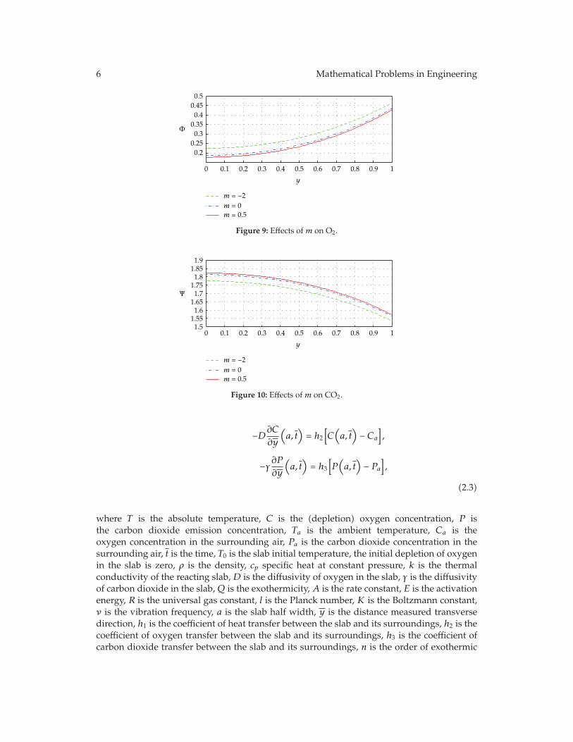
Figure 9: Effects of m on O2.

1.51.551.61.651.71.751.81.851.9

Ψ

0 0.1 0.2 0.3 0.4 0.5 0.6 0.7 0.8 0.9 1

y

m = −2m = 0

m = 0.5

Figure 10: Effects of m on CO2.

−D∂C

∂y

(a, t

)= h2

[C(a, t

)− Ca

],

−γ ∂P∂y

(a, t

)= h3

[P(a, t

)− Pa

],

(2.3)

where T is the absolute temperature, C is the (depletion) oxygen concentration, P isthe carbon dioxide emission concentration, Ta is the ambient temperature, Ca is theoxygen concentration in the surrounding air, Pa is the carbon dioxide concentration in thesurrounding air, t is the time, T0 is the slab initial temperature, the initial depletion of oxygenin the slab is zero, ρ is the density, cp specific heat at constant pressure, k is the thermalconductivity of the reacting slab,D is the diffusivity of oxygen in the slab, γ is the diffusivityof carbon dioxide in the slab, Q is the exothermicity, A is the rate constant, E is the activationenergy, R is the universal gas constant, l is the Planck number, K is the Boltzmann constant,ν is the vibration frequency, a is the slab half width, y is the distance measured transversedirection, h1 is the coefficient of heat transfer between the slab and its surroundings, h2 is thecoefficient of oxygen transfer between the slab and its surroundings, h3 is the coefficient ofcarbon dioxide transfer between the slab and its surroundings, n is the order of exothermic


0 0.1 0.2 0.3 0.4 0.5 0.6 0.7 0.8 0.9 1

y

0.1

0.3

0.5

0.7

0.9

θ

Bi1 = 1

Bi1 = 3

Bi1 = 5Bi1 = 10

Figure 11: Effects of Bi1 on temperature.

0.20.250.30.350.40.450.50.55

Φ

0 0.1 0.2 0.3 0.4 0.5 0.6 0.7 0.8 0.9 1

y

Bi1 = 1

Bi1 = 3

Bi1 = 5Bi1 = 10

Figure 12: Effects of Bi1 on O2.

chemical reaction, and m is the numerical exponent such that m ∈ {−2, 0, 0.5}. The threevalues taken by the parameter m represent the numerical exponent for sensitized, Arrheniusand Bimolecular kinetics, respectively, (see [1, 6]). We introduce the following dimensionlessvariables into (2.2)-(2.3):

θ =E(T − T0)

RT20

, θa =E(Ta − T0)

RT20

, Φ =C

Ca, Ψ =

P

Pa,

Bi1 =ah1

k, Bi2 =

ah2

D, Bi3 =

ah2

γ, β1 =

ρcpRT20

QECa,

β2 =ρcpRT

20

QEPa, λ =

(KT0νl

)mQAEa2Cna

kRT20

exp

(− E

RT

),

y =y

a, t =

kt

ρcpa2, ε =

RT0E

, α =Dρcp

k, σ =

γρcp

k,

(2.4)


0 0.1 0.2 0.3 0.4 0.5 0.6 0.7 0.8 0.9 1

y

Bi1 = 1

Bi1 = 3

Bi1 = 5Bi1 = 10

1.51.551.61.651.71.751.81.85

Ψ

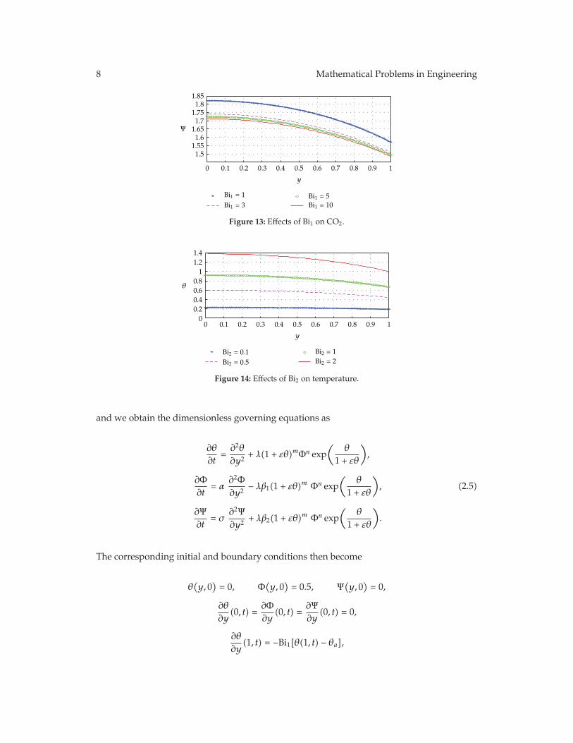
Figure 13: Effects of Bi1 on CO2.

0

0.2

0.4

0.6

0.8

1

1.2

1.4

θ

Bi2 = 0.1

Bi2 = 0.5

Bi2 = 1

Bi2 = 2

0 0.1 0.2 0.3 0.4 0.5 0.6 0.7 0.8 0.9 1

y

Figure 14: Effects of Bi2 on temperature.

and we obtain the dimensionless governing equations as

∂θ

∂t=

∂2θ

∂y2+ λ(1 + εθ)mΦn exp

(θ

1 + εθ

),

∂Φ∂t

= α∂2Φ∂y2

− λβ1(1 + εθ)m Φn exp

(θ

1 + εθ

),

∂Ψ∂t

= σ∂2Ψ∂y2

+ λβ2(1 + εθ)m Φn exp

(θ

1 + εθ

).

(2.5)

The corresponding initial and boundary conditions then become

θ(y, 0

)= 0, Φ

(y, 0

)= 0.5, Ψ

(y, 0

)= 0,

∂θ

∂y(0, t) =

∂Φ∂y

(0, t) =∂Ψ∂y

(0, t) = 0,

∂θ

∂y(1, t) = −Bi1[θ(1, t) − θa],


Bi2 = 0.1

Bi2 = 0.5

Bi2 = 1

Bi2 = 2

0 0.1 0.2 0.3 0.4 0.5 0.6 0.7 0.8 0.9 1

y

0.050.10.150.20.250.30.350.40.450.5

Φ

Figure 15: Effects of Bi2 on O2.

Bi2 = 0.1

Bi2 = 0.5

Bi2 = 1

Bi2 = 2

0 0.1 0.2 0.3 0.4 0.5 0.6 0.7 0.8 0.9 1

y

1

1.5

2

2.5

Ψ


∂Φ∂y

(1, t) = −Bi2[Φ(1, t) − 1],

∂Ψ∂y

(1, t) = −Bi3[Ψ(1, t) − 1],

(2.6)

where λ, ε, β1, β2, α, σ, Bi1, Bi2, and Bi3 represent the Frank-Kamenetskii parameter,activation energy parameter, oxygen consumption rate parameter, carbon dioxide emissionrate parameter, oxygen diffusivity parameter, carbon dioxide diffusivity parameter, thethermal Biot number, oxygen Biot number, and carbon dioxide Biot number, respectively.A body of material releasing heat to its surroundings may achieve a safe steady state wherethe temperature of the body reaches some moderate value and stabilizes. However, whenthe rate of heat generation in the material exceeds the rate of heat loss to the surroundings,then ignition can occur. In the following sections, (2.5)-(2) are solved numerically using asemi-implicit finite difference scheme.


0.1

0.5

1

2

0 0.1 0.2 0.3 0.4 0.5 0.6 0.7 0.8 0.9 1

y

1

2

3

4

5

6

7

Ψ

Bi3 =Bi3 =

Bi3 =Bi3 =


0.20.30.40.50.60.70.80.91

θ

λ = 0.1

λ = 0.5

λ = 1

λ = 1.3

0 0.1 0.2 0.3 0.4 0.5 0.6 0.7 0.8 0.9 1

y

Figure 18: Effects of λ on temperature.

λ = 0.1

λ = 0.5

λ = 1

λ = 1.3

0 0.1 0.2 0.3 0.4 0.5 0.6 0.7 0.8 0.9 1

y

0.10.20.30.40.50.60.70.80.9

Φ

Figure 19: Effects of λ on O2.

3. Numerical Solution

Our numerical algorithm is based on the semi-implicit finite difference scheme [15–18]. Theimplicit terms are taken at the intermediate time level (N + ξ)where 0 ≤ ξ ≤ 1. The algorithmemployed in [18] uses ξ = 1/2, we will, however, follow the formulation in [15–17] and takeξ = 1 in this paper so that we can use larger time steps. In fact being nearly fully implicit,our numerical algorithm presented in this paper is conjectured to work for any value of thetime step! The discretization of the governing equations is based on a linear Cartesian meshand uniform grid on which finite differences are taken. We approximate both the second andfirst spatial derivatives with second-order central differences. The equations corresponding to


λ = 0.1

λ = 0.5

λ = 1

λ = 1.3

0 0.1 0.2 0.3 0.4 0.5 0.6 0.7 0.8 0.9 1

y

1.11.21.31.41.51.61.71.81.9

Ψ

Figure 20: Effects of λ on CO2.

0 0.1 0.2 0.3 0.4 0.5 0.6 0.7 0.8 0.9 1

y

0.40.60.81

1.21.41.61.82

θ

β1 = 0.5

β1 = 0.8

β1 = 1.2

β1 = 1.5

Figure 21: Effects of β1 on temperature.

the first and last grid points are modified to incorporate the boundary conditions. The semi-implicit schemes for the temperature, O2 concentration, and CO2 concentration, respectively,read

θ(N+1) − θ(N)

∆t=

∂2

∂y2θ(N+ξ) + λ

[(1 + εθ)mΦn exp

(θ

1 + εθ

)](N)

,

Φ(N+1) −Φ(N)

∆t= α

∂2

∂y2Φ(N+ξ) − λβ1

[(1 + εθ)mΦn exp

(θ

1 + εθ

)](N)

,

Ψ(N+1) −Ψ(N)

∆t= σ

∂2

∂y2Ψ(N+ξ) + λβ2

[(1 + εθ)mΦn exp

(θ

1 + εθ

)](N)

.

(3.1)


0 0.1 0.2 0.3 0.4 0.5 0.6 0.7 0.8 0.9 1

y

β1 = 0.5

β1 = 0.8

β1 = 1.2

β1 = 1.5

0.10.150.20.250.30.350.40.450.5

Φ

Figure 22: Effects of β1 on O2.

0 0.1 0.2 0.3 0.4 0.5 0.6 0.7 0.8 0.9 1

y

β1 = 0.5

β1 = 0.8

β1 = 1.2

β1 = 1.5

1.4

1.6

1.8

2

2.2

2.4

2.6

2.8

Ψ

Figure 23: Effects of β1 on CO2.

The equations for θ(N+1), Φ(N+1), and Ψ(N+1), thus, become

−rξθ(N+1)j−1 + (1 + 2rξ)θ(N+1)

j − rξθ(N+1)j+1 = −r(1 − ξ)θ(N)

j−1 + (1 − 2r(1 − ξ))θ(N)j

− r(1 − ξ)θ(N)j+1

+ λ∆t

[(1 + εθj

)mΦnj exp

(θj

1 + εθj

)](N)

,

−rξαΦ(N+1)j−1 + (1 + 2rξα)Φ(N+1)

j − rξαΦ(N+1)j+1 = −r(1 − ξ)αΦ(N)

j−1 + (1 − 2r(1 − ξ)α)Φ(N)j

− r(1 − ξ)αΦ(N)j+1

− λ∆tβ1

[(1 + εθj

)mΦnj exp

(θj

1 + εθj

)](N)

,


0 0.1 0.2 0.3 0.4 0.5 0.6 0.7 0.8 0.9 1

y

1.4

1.6

1.8

2

2.2

2.4

2.6

Ψ

β2 = 0.5

β2 = 0.8β2 = 1.2β2 = 1.5

Figure 24: Effects of β2 on CO2.

0 0.1 0.2 0.3 0.4 0.5 0.6 0.7 0.8 0.9 1

y

0.65

0.7

0.75

0.8

0.85

0.9

0.95

1

θ

ε = 0

ε = 0.1ε = 0.2

ε = 0.3

Figure 25: Effects of ε on temperature.

−rξσΨ(N+1)j−1 + (1 + 2rξσ)Ψ(N+1)

j − rξσΨ(N+1)j+1 = −r(1 − ξ)σΨ(N)

j−1 + (1 − 2r(1 − ξ)σ)Ψ(N)j

− r(1 − ξ)σΨ(N)j+1

+ λ∆tβ2

[(1 + εθj

)mΦnj exp

(θj

1 + εθj

)](N)

,

(3.2)

where r = ∆t/∆y2. The solution procedures reduce to inversion of tridiagonal matrices. Theschemes (3.2) were checked for consistency. For ξ = 1, these are first-order accurate in timebut second order in space. The schemes in [18] have ξ = 1/2 which improves the accuracy intime to second order. We use ξ = 1 here so that we are free to choose larger time steps andstill converge to the steady solutions. As already conjectured, our algorithm works for anyvalue of the time step! The code was checked for both spatial and temporal convergence. Inparticular, solutions calculated from, say ∆t = 1, using 200 time steps are exactly the same asthose after 40 time steps with ∆t = 5 or those after 20,000 time steps with ∆t = 0.01. Similarlysolutions using∆y = 0.02 converge to the same results as those say for∆t = 0.025 or∆t = 0.05,and so forth. Our code, thus, runs extremely fast, and; hence, we can easily obtain and, thus,present all our results at steady state using nearly insignificant computational times.


0 0.1 0.2 0.3 0.4 0.5 0.6 0.7 0.8 0.9 1

y

0.2

0.25

0.3

0.35

0.4

0.45

0.5

Φ

ε = 0

ε = 0.1ε = 0.2ε = 0.3

Figure 26: Effects of ε on O2.

0 0.1 0.2 0.3 0.4 0.5 0.6 0.7 0.8 0.9 1

y

ε = 0

ε = 0.1ε = 0.2ε = 0.3

1.55

1.6

1.65

1.7

1.75

1.8

1.85

1.9

Ψ

Figure 27: Effects of ε on CO2.

4. Results and Discussion

Unless otherwise stated, we employ the parameter values:

m = 0.5, n = 1, θa = 0.1, α = 1, σ = 1,

β1 = 1, β2 = 1, Bi1 = 1, Bi2 = 1, Bi3 = 1,

ε = 0.1, ∆y = 0.01, ∆t = 1, t = 200.

(4.1)

These will be the default values in this work, and; hence, in any graph where any of theseparameters is not explicitly mentioned, it will be understood that such parameters take onthe default values.

4.1. Transient and Steady Flow Profiles

We display the transient solutions in Figures 2, 3, and 4. At the given parameter values,Figure 2 shows a transient increase in temperature until a steady-state is reached. A similarscenario obtains in Figure 4 in which a transient increase of carbon dioxide emission isobserved until a steady state is reached. An opposite situation is noticed in Figure 3 wherea decrease in oxygen concentration is observed with increasing time until a steady-state


0 0.1 0.2 0.3 0.4 0.5 0.6 0.7 0.8 0.9 1

y

00.20.40.60.81

1.21.41.61.8

θ

α = 0.1

α = 0.5

α = 1

α = 2

Figure 28: Effects of α on temperature.

0 0.1 0.2 0.3 0.4 0.5 0.6 0.7 0.8 0.9 1

y

α = 0.1

α = 0.5

α = 1

α = 2

00.050.10.150.20.250.30.350.40.45

Φ

Figure 29: Effects of α on O2.

concentration is attained. These results are consistent with intuition regarding exothermicoxidation reactions.

4.1.1. Parameter Dependance of Solutions in Steady State

It is understood from Figures 2–4 that, at the default parameter values, solutions have reachedsteady state at, say, times t ≥ 40. All the solutions at t = 200 given below will, thus, beunderstood to be steady solutions. The dependence of solutions on parameter n is illustratedin Figures 5, 6, and 7. As n increases, the results show a decrease in both the temperature andthe CO2 emission. The reduced oxidation reactions mean lower oxygen consumption, hence,lead to a corresponding increase in O2 concentration.

The dependence of solutions on parameter m is illustrated in Figures 8, 9, and 10. Asm increases, the results show an increase in both the temperature and the CO2 emission. Theincreased oxygen consumption from higher oxidation reactions correspondingly decreasesO2 concentration.

The dependence of solutions on parameter Bi1 is illustrated in Figures 11, 12, and13. As Bi1 increases, the results show a decrease in both the temperature and the CO2

emission. The reduced oxidation reactions mean lower oxygen consumption, hence, lead to acorresponding increase in O2 concentration.

The dependence of solutions on parameter Bi2 is illustrated in Figures 14, 15,and 16. An increase in Bi2 directly corresponds to an increase in O2 concentration. This


0 0.1 0.2 0.3 0.4 0.5 0.6 0.7 0.8 0.9 1

y

α = 0.1

α = 0.5

α = 1

α = 2

11.21.41.61.82

2.22.42.62.8

Ψ

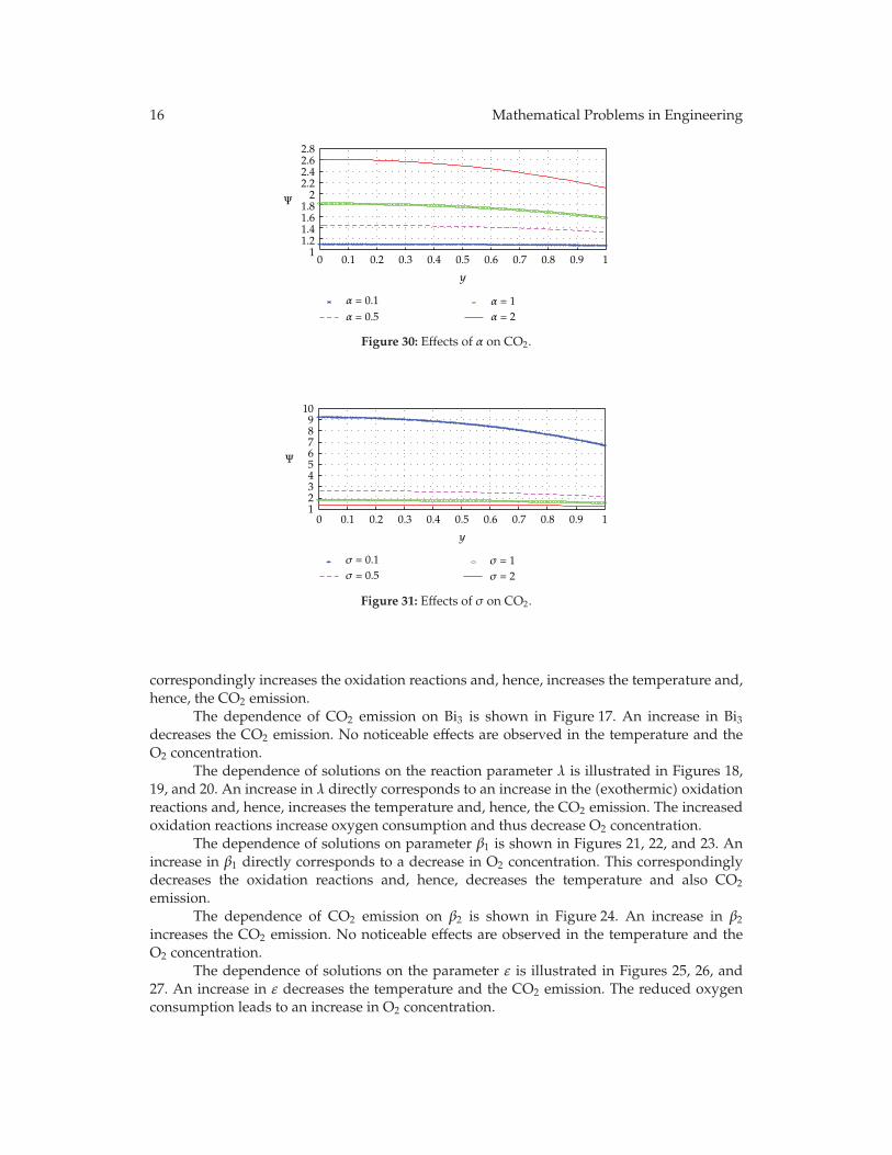
Figure 30: Effects of α on CO2.

0 0.1 0.2 0.3 0.4 0.5 0.6 0.7 0.8 0.9 1

y

12345678910

Ψ

σ = 0.1

σ = 0.5

σ = 1

σ = 2

Figure 31: Effects of σ on CO2.

correspondingly increases the oxidation reactions and, hence, increases the temperature and,hence, the CO2 emission.

The dependence of CO2 emission on Bi3 is shown in Figure 17. An increase in Bi3decreases the CO2 emission. No noticeable effects are observed in the temperature and theO2 concentration.

The dependence of solutions on the reaction parameter λ is illustrated in Figures 18,19, and 20. An increase in λ directly corresponds to an increase in the (exothermic) oxidationreactions and, hence, increases the temperature and, hence, the CO2 emission. The increasedoxidation reactions increase oxygen consumption and thus decrease O2 concentration.

The dependence of solutions on parameter β1 is shown in Figures 21, 22, and 23. Anincrease in β1 directly corresponds to a decrease in O2 concentration. This correspondinglydecreases the oxidation reactions and, hence, decreases the temperature and also CO2

emission.The dependence of CO2 emission on β2 is shown in Figure 24. An increase in β2

increases the CO2 emission. No noticeable effects are observed in the temperature and theO2 concentration.

The dependence of solutions on the parameter ε is illustrated in Figures 25, 26, and27. An increase in ε decreases the temperature and the CO2 emission. The reduced oxygenconsumption leads to an increase in O2 concentration.


0 0.5 1 1.5 2 2.5 3 3.5 4 4.5−0.1

00.10.20.30.40.50.60.7

θy(1,t)

λ

n = 1

n = 2

n = 3

n = 4

n = 5

Figure 32: Effects of variation of n on the thermal criticality or blowup in the system.

−0.10

0.10.20.30.40.50.60.7

θy(1,t)

0 0.2 0.4 0.6 0.8 1 1.2 1.4 1.6 1.8

λ

m = −2m = 0

m = 0.5

Figure 33: Effects of variation of m on the thermal criticality or blowup in the system.

The dependence of solutions on the parameter α is shown in Figures 28, 29, and 30. Anincrease in α directly corresponds to an increase in O2 concentration. This correspondinglyincreases the oxidation reactions and hence increases the temperature and also CO2 emission.

The dependence of CO2 emission on σ is shown in Figure 31. An increase in σdecreases the CO2 emission. No noticeable effects are observed in the temperature and O2

concentration.

4.2. Thermal Stability and Blowup

In Figures 32, 33, 34, and 35, we plot θy(1, t) against λ for varying values of n, m, Bi1, andBi2, respectively. The solutions are given up to the values of λ at which the onset of blowupin temperature is observed. We notice that parameters that increase the temperature (θ)correspondingly increase θy(1, t). The results also show that early onset of blowup (and,hence, thermal instability) can be delayed by using higher values of n, lower values of m,higher values of Bi1, lower values of Bi2, and so forth.


0 0.5 1 1.5 2 2.5

0.8

λ

Bi1 = 1

Bi1 = 3

Bi1 = 5

Bi1 = 10

−0.10

0.10.20.30.40.50.60.7

θy(1,t)

Figure 34: Effects of Bi1 variation on the thermal criticality or blowup in the system.

0 0.2 0.4 0.6 0.8 1 1.2 1.4 1.6 1.8

λ

θy(1,t)

−0.20

0.2

0.4

0.6

0.8

1

1.2

Bi2 = 0.1

Bi2 = 0.5

Bi2 = 1

Bi2 = 2

Figure 35: Effects of Bi2 variation on the thermal criticality or blowup in the system.

5. Conclusion

We develop an unconditionally stable (works for any time step size) and convergent semi-implicit finite-difference scheme and utilize it to computationally investigate the transientdynamics of CO2 emission, O2 depletion, and thermal decomposition in a reacting slab. Thesolutions show that those processes that increase the oxidation reactions lead to enhancedoxygen depletion as well as increased carbon dioxide emission. The results also show thatenhanced thermal stability and reduced carbon dioxide emission are best achieved by cuttingdown on those processes that would otherwise increase the oxidation reactions.

References

[1] J. Bebernes and D. Eberly, Mathematical Problems from Combustion Theory, vol. 83 of Applied Math-ematical Sciences, Springer, New York, NY, USA, 1989.

[2] J. C. Quick and D. C. Glick, “Carbon dioxide from coal combustion: variation with rank of US coal,”Fuel, vol. 79, no. 7, pp. 803–812, 2000.

[3] R. Betz andM. Sato, “Emissions trading: lessons learnt from the 1st phase of the EU ETS and prospectsfor the 2nd phase,” Climate Policy, vol. 6, no. 4, pp. 351–359, 2006.

[4] R. Quadrelli and S. Peterson, “The energy-climate challenge: recent trends in GHG emissions fromfuel combustion,” Energy Policy, vol. 35, no. 11, pp. 5938–5952, 2007.

[5] J. M. Simmie, “Detailed chemical kinetic models for the combustion of hydrocarbon fuels,” Progressin Energy and Combustion Science, vol. 29, no. 6, pp. 599–634, 2003.


[6] O. D. Makinde, “Exothermic explosions in a slab: a case study of series summation technique,”International Communications in Heat and Mass Transfer, vol. 31, no. 8, pp. 1227–1231, 2004.

[7] E. Balakrishnan, A. Swift, and G. C.Wake, “Critical values for some non-class A geometries in thermalignition theory,”Mathematical and Computer Modelling, vol. 24, no. 8, pp. 1–10, 1996.

[8] S. Tanaka, F. Ayala, and J. C. Keck, “A reduced chemical kinetic model for HCCI combustion ofprimary reference fuels in a rapid compression machine,” Combustion and Flame, vol. 133, no. 4, pp.467–481, 2003.

[9] D. A. Frank-Kamenetskii, Diffusion and Heat Transfer in Chemical Kinetics, Plenum Press, New York,NY, USA, 1969.

[10] F. S. Dainton, Chain Reaction: An Introduction, Wiley, New York, NY, USA, 1960.[11] R. vas Bhat, J. Kuipers, and G. Versteeg, “Mass transfer with complex chemical reaction in gasliquid

system: two-steps reversible reactions with unit stoichiometric and kinetic orders,” ChemicalEngineering Journal, vol. 76, pp. 127–152, 2000.

[12] J. Warnatz, U. Maas, and R. Dibble, Combustion: Physical and Chemical Fundamentals, Modeling andSimulation, Experiments, Pollutant Formation, Springer and Co. K, Berlin, Hiedelberg GmbH, Germany,2001.

[13] F. A. Williams, Combustion Theory, Benjamin & Cuminy Publishing, Menlo Park, Calif, USA, 2nd edi-tion, 1985.

[14] M. A. Sadiq and J. H. Merkin, “Combustion in a porous material with reactant consumption: the roleof the ambient temperature,”Mathematical and Computer Modelling, vol. 20, no. 1, pp. 27–46, 1994.

[15] O. D. Makinde and T. Chinyoka, “Transient analysis of pollutant dispersion in a cylindrical pipe witha nonlinear waste discharge concentration,” Computers & Mathematics with Applications, vol. 60, no. 3,pp. 642–652, 2010.

[16] O. D. Makinde and T. Chinyoka, “MHD transient flows and heat transfer of dusty fluid in a chan-nel with variable physical properties and Navier slip condition,” Computers & Mathematics withApplications, vol. 60, no. 3, pp. 660–669, 2010.

[17] T. Chinyoka, “Poiseuille flow of reactive Phan-Thien-Tanner liquids in 1D channel flow,” Journal ofHeat Transfer, vol. 132, no. 11, pp. 111701–7111708, 2010.

[18] T. Chinyoka, “Computational dynamics of a thermally decomposable viscoelastic lubricant undershear,” Journal of Fluids Engineering, vol. 130, no. 12, pp. 1212011–1212017, 2008.

Numerical Investigation into CO2 Emission, CO2 Depletion, and Thermal Decomposition in a Reacting...

Documents

Transcript of Numerical Investigation into CO2 Emission, CO2 Depletion, and Thermal Decomposition in a Reacting...