Revisiting Near-Inertial Wind Work: Slab Models, Relative Stress, and MixedLayer Deepening

MATTHEW H. ALFORD

Scripps Institution of Oceanography, University of California, San Diego, La Jolla, California

(Manuscript received 15 May 2020, in final form 11 August 2020)

ABSTRACT: The wind generation of near-inertial waves is revisited through use of the Pollard–Rhines–Thompson

theory, the Price–Weller–Pinkel (PWP) mixed layer model, and KPP simulations of resonant forcing by Crawford and

Large. An Argo mixed layer climatology and 0.68 MERRA-2 reanalysis winds are used to compute global totals and

explore hypotheses. First, slab models overestimate wind work by factors of 2–4 when the mixed layer is shallow relative to

the scaling H* [ u*/(Nf)1/2, but are accurate for deeper mixed layers, giving overestimation of global totals by a factor of

1.23 6 0.03 compared to PWP. Using wind stress relative to the ocean currents further reduces the wind work by an

additional 13 6 0.3%, for a global total wind work of 0.26 TW. Second, the potential energy increase DPE due to wind-

driven mixed layer deepening is examined and compared to DPE computed from Argo and ERA-Interim heat flux cli-

matology. Argo-derived DPE closely matches cooling, confirming that cooling sets the seasonal cycle of mixed layer depth

and providing a new constraint on observational estimates of convective buoyancy flux at the mixed layer base. Locally and

in fall, wind-driven deepening is comparable in importance to cooling. Globally, wind-driven DPE is about 11% of wind

work, implying that.50%of wind work goes to turbulence and thus not into propagating inertial motions. The fraction into

this ‘‘modified wind work’’ is imperfectly estimated in two ways, but we conclude that more research is needed into mixed

layer and transition-layer physics. The power available for propagating near-inertial waves is therefore still uncertain, but

appears lower than previously thought.

KEYWORDS: Internal waves; Oceanic mixed layer

1. IntroductionNear-inertial internal waves (NIW) are known to dominate

internal wave kinetic energy and shear spectra at all depths in

the ocean (Alford andWhitmont 2007; Silverthorne and Toole

2009). Because NIW energy (Alford and Whitmont 2007) and

parameterized mixing (Whalen et al. 2018) both show strong

seasonal cycles, a reasonable hypothesis is that wind-generated

near-inertial waves contribute significantly to ocean mixing. In

attempts to quantify the energy input of NIW, a number of

authors (D’Asaro 1985; Alford 2001, 2003b; Watanabe and

Hibiya 2002; Jiang et al. 2005; Rimac et al. 2013) have used the

slab model of Pollard and Millard (1970, hereafter PM70) to

estimate the work done by the wind on mixed layer inertial

motions, in analogy to previous estimates of the work done by

the wind on the mean circulation (Wunsch 1998). Global totals

range from 0.3 to 1.3 TW, with the spread due to various

methods and the temporal and lateral resolution of the wind

products (Jiang et al. 2005). These totals are comparable to

the ;1 TW of power converted from the barotropic tides to

baroclinic tides, but the spread hampers quantitative certainty

regarding the relative importance of near-inertial waves and

internal tides in mixing the ocean. Because the climate change

response of wind-forced NIW and internal tides should be

quite different, resolution of this issue is important.

In addition to the spread in the slab model estimates, more

fundamental issues exist. First, a number of seminal papers on

mixed layer deepening in the late 1960s and 1970s (Kraus and

Turner 1967; PM70; Pollard et al. 1973, hereafter PRT73; Niiler

1975) documented the role that inertial oscillations have in

deepening the mixed layer. Specifically, they generate shear at

the base of the mixed layer that entrains fluid from the interior.

The power to the turbulence supporting this increase in po-

tential energy is a ‘‘tax’’ that must be paid out of the wind work

from the near-inertial motions in the mixed layer that will

eventually propagate into the interior. How large is this loss?

Second, Plueddemann and Farrar (2006, hereafter PF06)

showed that these mixing processes, which occur on time scales

faster than the Rayleigh damping in the slab model, causes slab

model estimates to be biased high by a factor up to 4 because

inertial kinetic energy (IKE) grows much too quickly and the

work is overestimated. At several buoys, they found that the

Price–Weller–Pinkel (PWP) model (Price et al. 1986) repro-

duced observed estimates of the wind work much better. How

large is this overestimation globally?

Finally, it has been shown that relative versus absolute

stress makes a difference in wind-driven mean equatorial

currents (Kelly et al. 2001). For wind work estimates, Liu

et al. (2019), Zhai (2017), and Rath et al. (2013) found that

estimates computed with stresses relative to the Earth rather

than the inertial currents causes overestimates from 28% to

60%. We examine this here too, obtaining a more modest

13% 6 1% overestimate.

In this paper we revisit the mixed layer deepening literature

in order to address these issues and obtain a global estimate of

the near-inertial wind work that imperfectly addresses the

shortcomings of the slab model and includes the losses due to

turbulence. After presenting estimates of the wind work using

the PWP model that are improved over adiabatic slab model

estimates, we find that these must be further reduced by aCorresponding author: Matthew H. Alford, malford@ucsd.edu

NOVEMBER 2020 AL FORD 3141

DOI: 10.1175/JPO-D-20-0105.1

� 2020 American Meteorological Society. For information regarding reuse of this content and general copyright information, consult the AMS CopyrightPolicy (www.ametsoc.org/PUBSReuseLicenses).

Brought to you by OLD DOMINION UNIVERSITY | Unauthenticated | Downloaded 10/13/21 04:20 PM UTC

poorly constrained further factor between 2 and 3 to account

for the energy lost to turbulence. To contextualize these esti-

mates of wind-driven potential energy increase, we compare

them to the total observed potential energy (PE) increase

computed from Argo and the surface cooling-induced buoy-

ancy flux from the ERA-Interim reanalysis. In doing so, a

powerful new constraint on the ratio of buoyancy flux between

the surface and the mixed layer base (e.g., Ball 1960; Anis and

Moum 1994) is obtained.

2. Methods

a. ApproachVarious authors (Zilitinkevich 1972; PRT73; Niiler 1975;

Davis et al. 1981; Large et al. 1994; Crawford and Large 1996,

hereafter CL96; Skyllingstad et al. 2000; Grant and Belcher

2011) have presented energy budgets for the mixed layer.

Owing to the complexity of the turbulent processes there and

the long timeline over which the research has occurred, rec-

onciliation of the different frameworks can be difficult. A

central dichotomy between approaches is whether or not to

treat the mixed layer as a ‘‘slab’’ in which momentum is as-

sumed to be distributed infinitely quickly down themixed layer

depth H. Observations show that shear exists in the mixed

layer and that momentum penetrates beneath it into the so-

called ‘‘transition layer’’ (e.g., Davis et al. 1981; Johnston and

Rudnick 2009; Dohan and Davis 2011). The PWP model Price

et al. (1986) is one of the simplest nonslab models, employing a

bulk and a gradient Richardson number closure following

PRT73. Comparisons with bothmore sophisticated 1Dmodels,

including large-eddy simulations (LES; Skyllingstad et al. 2000;

Grant and Belcher 2011) and K-profile parameterizations

(KPP; CL96), as well as observations (PF06) have demon-

strated the skill of PWP in modeling deepening mixed layers.

Recognizing the PWP’smodel’s neglect of a variety ofmixed

layer processes of known importance including lateral re-

stratification by submesoscale motions (Hosegood et al. 2008;

Fox-Kemper et al. 2008), Langmuir turbulence and surface

wave breaking (e.g., McWilliams et al. 1997; Li et al. 2019), we

leverage the numerous above-listed demonstrations of its ac-

curacy for wind-driven mixed layer deepening in order to ex-

tend PF06’s examination of PWP at a few locations to the

globe. Additionally, the potential energy increase of the mixed

layer during the generation process of inertial motions is ex-

plicitly calculated.

b. Theory

The momentum equations for a slab-like mixed layer un-

dergoing stress at its upper and lower boundaries (due to wind

stress and turbulent processes at the mixed layer base, re-

spectively) are

dZI

dt1 ifZ

I5 2

1

if

d

dt

(Tw2T

R)

H, (1)

whereH is the mixed layer depth, ZI [ uI 1 iyI is the complex

inertial current, Tw 5 r21o tw, and TR 5 r21

o tR. The terms twand tR are the complex wind stress and turbulent stress, re-

spectively, where ro is the density of seawater. The bulk and

gradient Richardson number closures employed by PRT73 will

be introduced below. With a Rayleigh drag r, the turbulent

stress becomes TR 5 rHZI and (1) reduces to the damped slab

model of PM70.

An energy equation is obtained by multiplying (1) by roHZI*

(D’Asaro 1985, PF06) and integrating in time, obtaining

IKE5

ðt

P1

ðt

PM1

ðt

PH, (2)

where IKE [ 1/2roHjZj2 is the mixed layer inertial kinetic

energy and P [ Re{[ZI/(v*H)](dT*/dt)]} is the familiar wind

work derived byD’Asaro (1985). Since PF06 concluded that an

additional term PH 5 (ro/2)jZIj2(dH/dt) associated with con-

version from KE per unit mass to KE per unit area is small

(1%–2% of the other terms), we follow them in neglecting it.1

The shear production term PM (equivalent to PR in PF06)

represents energy lost to turbulent motions, or equivalently the

production of turbulent kinetic energy. As with any turbulence

in a stratified fluid, some of this energy goes into mixing (in this

context, raising the potential energy by deepening the mixed

layer) and some goes into kinetic energy dissipation. A central

point of this paper is that the energy available for propagating

near-inertial motions increases through (dIKE/dt), which is

diminished relative to P by the amount of energy that was lost

to turbulence.

Absent lateral terms, PM 5 «1 Jb, where « is the dissipation

rate and Jb is the buoyancy flux (e.g., Tennekes and Lumley

1972). The buoyancy flux is traditionally related to the pro-

duction via the flux Richardson number,

Rf[ J

b/P

M. (3)

Equivalently, a mixing efficiency G [ Jb/« can be defined. For

stratified turbulence in the ocean interior, Osborn (1980) ar-

gued that that Rf 5 G/(G 1 1) # 1/6, giving G # 0.2.

Since we follow CL96 in defining PM and « as the integrals

from the surface to a reference depth D well below the mixed

layer, the buoyancy flux equals the rate of increase of potential

energy, Jb 5 (dPE/dt), where

PE5

ð0D

r(z)gz dz . (4)

Thus,

PM5R21

f

d

dtPE. (5)

The increase in PE relative to the energy put into inertial

motions was a central focus of the PRT73 theory and the KPP

1We will follow CL96’s notation of referring to P and PM in

terms of their time integral over a specified period (here one

month), such that IKE, P, PM, and DPE are directly comparable

and all have units of joules per square meter (Jm22). At times in

the sections below, they will also be presented as rates in watts per

square meter (Wm22), comparable to past estimates of wind work,

by dividing by the time interval.

3142 JOURNAL OF PHYS ICAL OCEANOGRAPHY VOLUME 50

Brought to you by OLD DOMINION UNIVERSITY | Unauthenticated | Downloaded 10/13/21 04:20 PM UTC

simulations of CL96. For initial deepening of a mixed layer

from zero, PRT73 found that potential energy was one-third

of IKE. Simulating observationally motivated winds in the

northeast Pacific, CL96 found that the partitioning was strongly

dependent on how resonant the wind forcing was. Specifically,

for resonant conditions, IKE was about half of P, with the rest

lost to turbulent motions PM. Of this, Jb associated with mixed

layer deepening was about 12%, implying a flux Richardson

number of about 25%. The fraction decreased for winds that

were more off-resonance.

In the following, we will use the imperfect but useful tool of

the PWP model. First, we will examine the energetics of the

slab and PWP models during resonant and realistic forcing for

a variety of mixed layer depths, and then will investigate the

implications by extending the calculations to the globe.

c. Price–Weller–Pinkel (PWP) mixed layer model

We use the Price et al. (1986) mixed layer model as im-

plemented by PF06, which contains the same physics as in

PRT73. Specifically, the momentum equations are solved

with specified initial conditions and prescribed surface fluxes,

subject to a closure using both a bulk and a gradient

Richardson number. When these thresholds are exceeded,

momentum and buoyancy are redistributed until stability is

restored. The model can be run with this closure on or off;

with it off, the solution is identical to the damped slab model

of PM70. That is, TR is the turbulent stress due to the tur-

bulent closure in PWP; when mixing is turned off we repro-

duce the Rayleigh damping of the PM70 slab model intended

to model the propagation of near-inertial waves over a time

scale of days.

Our approach is to run the model with mixing on and off at

each location. The wind work estimates computed with mixing

on and off are then referred to asPPWP andPslab, respectively.

The model is run at 0.5-m vertical resolution and forced with

wind stress from the Modern-Era Retrospective Analysis for

Research and Applications Version 2 (MERRA-2) product

(Gelaro et al. 2017), which are gridded hourly at about 0.68resolution from the year 2019. Hourly output avoids compli-

cations with underresolved inertial response for coarse sampling

(D’Asaro 1985; Alford 2003b). Detailed information about the

MERRA project can be found at http://gmao.gsfc.nasa.gov/

research/merra/. Because our focus here is wind forcing and it

dominates buoyancy forcing on time scales of days (CL96), we

set surface heat and freshwater fluxes to zero for these calcu-

lations, but will return to this issue in section 4e by comparing

our wind-forced DPE estimates to total observed DPE from

Argo and cooling-induced surface buoyancy fluxes from the

ERA-Interim reanalysis. Additional comparisons are done in

section 4c by modifying the model to allow forcing with stress

computed from current-relative rather than absolute winds.

One-month simulations were conducted at each location

and for each month of the year 2019. Initial stratification pro-

files were computed at each time and place, beginning with the

World Ocean Atlas 2001 (Conkright et al. 2002). Mixed layer

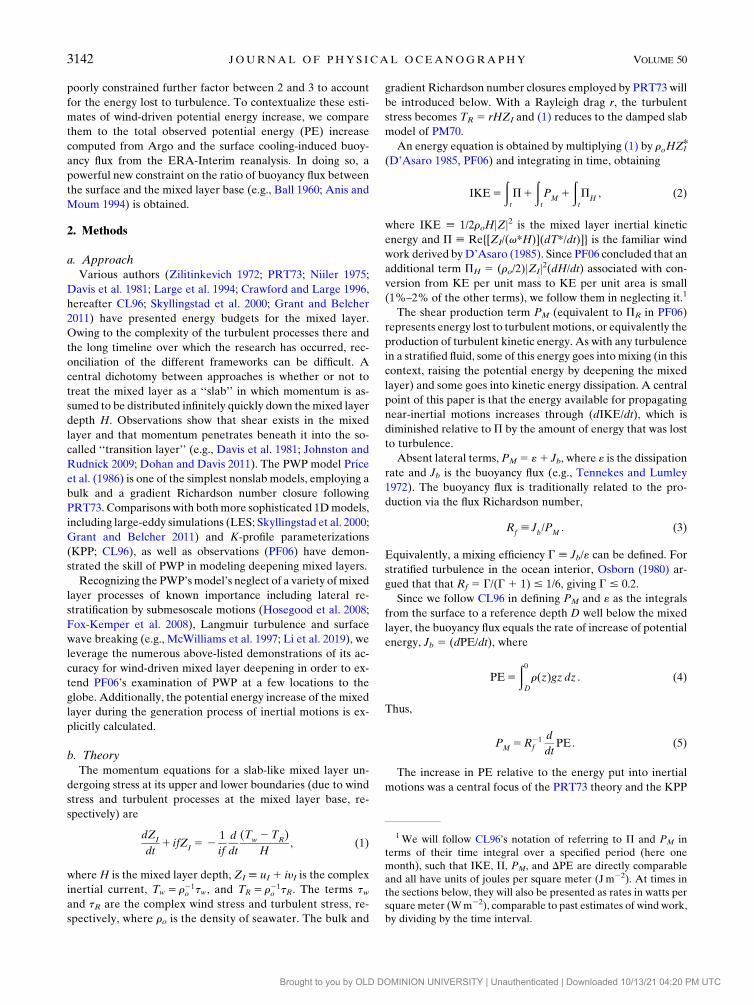
depth H (Fig. 1) is from the 18 3 18 monthly climatology

computed from Argo profiles published by Holte et al. (2017).

At each location, the climatological temperature and salinity

FIG. 1. Maps of mixed layer depthH from (a),(c) theHolte et al. (2017)Argo climatology and (b),(d) the scalingH*[ u*/(Nf )1/2, for (top)

March and (bottom) October; N is the value of the stratification immediately below the mixed layer.

NOVEMBER 2020 AL FORD 3143

Brought to you by OLD DOMINION UNIVERSITY | Unauthenticated | Downloaded 10/13/21 04:20 PM UTC

values were made uniform down to a depth H, and the calcu-

lation was run with winds for that month. Following PF06, a

Rayleigh damping was implemented, though our value of r 51/3.7 days is slightly greater than the value used by PF06. We

did not find significant sensitivity of our results to the value

of r used.

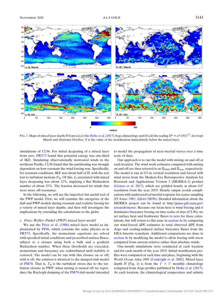
3. Slab model and PWP estimates as functions of mixedlayer depthSample calculations forced with resonant inertially rotating

winds (tx 1 ity 5 e2ift, where f is the inertial frequency) for

one-half period are presented (Fig. 2) for shallow and deep

mixed layers. The results reproduce familiar behavior. At left,

an initially shallow mixed layer rapidly deepens (Fig. 2b) in

response to the input of momentum by the wind stress on

2 July. Because the slab calculation has no mixing and cannot

reproduce this deepening, kinetic energy rapidly increases

(Fig. 2c, blue) much more than for the PWP case, so that the

wind work P (Fig. 2d) is much greater for the slab model as

shown by PF06. The energy input by the wind (Fig. 2e), com-

puted as the time integral of each flux term) is overestimated in

the slab model, with a significant portion of the wind work in

the PWP model put into potential energy (black).

The deepening extends to about 50m in this case, following

the PRT73 prediction:

H*5u*ffiffiffiffiffiffiNf

p , (6)

where u*[ffiffiffiffiffiffiffiffiffiffiffit/rair

pis the friction velocity of the imposed

stress andN is the stratification immediately below the mixed

layer. For a constant wind,H* is the maximum depth to which

the deepening occurs after half an inertial period, when the

ocean currents oppose the wind and therefore arrest the wind

work. For steady winds, large-eddy simulations (Ushijima and

Yoshikawa 2020) show that the deepening continues after

half a period, and for purely inertial winds, deepening would

continue indefinitely. However, the parameter is a useful in-

dicator of a long-known observation (e.g., Turner and Kraus

1967) that deepening greatly slows in the fall (i.e., deep mixed

layers are hard to deepen further). We can indeed see that for

a mixed layer deeper than H* (Fig. 2, right), deepening is

much smaller. Since a much smaller fraction of energy goes

to deepening the mixed layer, the slab model once again

becomes a good approximation.

TheH* scaling is demonstrated by rerunning the resonantly

forced simulations keeping forcing the same for each run

(givingH*5 40m) but for a range of mixed layer depths from

5 to 80m (Fig. 3). At left, PWP and slab wind work are plotted

versusH, withH* indicated (vertical dashed line). At right, the

ratio is plotted versus H/H*. The slab model estimate of P

FIG. 2. Example PWP and slab model calculations with idealized winds for (left) shallow H and (right) deep H. (a),(f) Wind stress.

(b),(g) Temperature contours (thin; 0.58 spacing) and mixed layer depth (thick) for the PWP calculation. (c),(h) Meridional velocity from

the PWP and slab calculation. (d),(i) Wind work. (e),(j) Time-integrated wind work (blue, red) and potential energy increase (black; 103is plotted). In (h)–(j), the blue line is obscured by the red one as the quantities are nearly identical.

3144 JOURNAL OF PHYS ICAL OCEANOGRAPHY VOLUME 50

Brought to you by OLD DOMINION UNIVERSITY | Unauthenticated | Downloaded 10/13/21 04:20 PM UTC

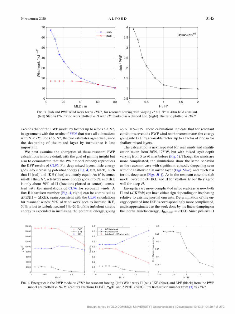
exceeds that of the PWP model by factors up to 4 for H , H*,

in agreement with the results of PF06 that were all at locations

with H , H*. For H . H*, the two estimates agree well, since

the deepening of the mixed layer by turbulence is less

important.

We next examine the energetics of these resonant PWP

calculations in more detail, with the goal of gaining insight but

also to demonstrate that the PWP model broadly reproduces

the KPP results of CL96. For deep mixed layers, little energy

goes into increasing potential energy (Fig. 4, left, black), such

that P (red) and IKE (blue) are nearly equal. As H becomes

smaller thanH*, relatively more energy goes into PE and IKE

is only about 50% of P (fractions plotted at center), consis-

tent with the simulations of CL96 for resonant winds. A

flux Richardson number (Fig. 4, right) can be computed as

DPE/(P 2 DIKE), again consistent with the CL96 calculations

for resonant winds: 50% of wind work goes to increase IKE,

50% is lost to turbulence, and 3%–20%of the turbulent kinetic

energy is expended in increasing the potential energy, giving

Rf ’ 0.05–0.35. These calculations indicate that for resonant

conditions, even the PWP wind work overestimates the energy

going into IKE by a variable factor, up to a factor of 2 or so for

shallow mixed layers.

The calculation is next repeated for real winds and stratifi-

cation taken from 308N, 1758W, but with mixed layer depth

varying from 5 to 80m as before (Fig. 5). Though the winds are

more complicated, the simulations show the same behavior

as the resonant case with significant episodic deepening seen

with the shallow initial mixed layer (Figs. 5a–e), and much less

for the deep case (Figs. 5f–j). As in the resonant case, the slab

model overpredicts IKE and P for shallow H but they agree

well for deep H.

Energetics aremore complicated in the real case as now both

P and (dIKE/dt) can have either sign depending on its phasing

relative to existing inertial currents. Determination of the en-

ergy deposited into IKE is correspondingly more complicated,

and is approximated as the work done by the linear damping on

the inertial kinetic energy,PRayleigh5 2rIKE. Since positive P

FIG. 3. Slab and PWP wind work for vs H/H*, for resonant forcing with varying H but H* 5 40m held constant.

(left) Slab vs PWP wind work plotted vs H with H* marked as a dashed line. (right) The ratio plotted vs H/H*.

FIG. 4. Energetics in the PWPmodel vsH/H* for resonant forcing. (left) Wind workP (red), IKE (blue), and DPE (black) from the PWP

model are plotted vs H/H*. (center) Fractions IKE/P, PM/P, and DPE/P. (right) Flux Richardson number from (3) vs H/H*.

NOVEMBER 2020 AL FORD 3145

Brought to you by OLD DOMINION UNIVERSITY | Unauthenticated | Downloaded 10/13/21 04:20 PM UTC

can increase IKE but negative P cannot remove energy that

has already propagated away, IKERayleigh/P is an overesti-

mate for real forcing. Indeed, for the example shown the

behavior is similar to the resonant case with DPE/P de-

creasing and IKE/P increasing for deeper H (Fig. 6).

However, the implied mixing efficiency is too high to be

physically reasonable because IKE is overestimated. For

this reason, we use other methods below to estimate IKE for

the realistic winds.

4. Global calculations

a. Slab model resultsGlobal slab model calculations are very similar in spatial,

temporal patterns and overall total of 0.37 TW (Fig. 7a,

Table 1) as previous work, showing the familiar wintertime

enhancement in midlatitudes and in the western portion of

each basin where the storm tracks are. Since these patterns

have been presented elsewhere, we simply focus on the

FIG. 5. As in Fig. 2, but forMERRA-2winds fromSeptember 2019. Stratification and forcing are the same in each case, but initialH is 20m

at left and 60m at right.

FIG. 6. As in Fig. 4, but for MERRA-2 winds from September 2019. IKE is computed, unsuccessfully, as the energy removed by the

Rayleigh drag, giving unrealistically high values of Rf (see text).

3146 JOURNAL OF PHYS ICAL OCEANOGRAPHY VOLUME 50

Brought to you by OLD DOMINION UNIVERSITY | Unauthenticated | Downloaded 10/13/21 04:20 PM UTC

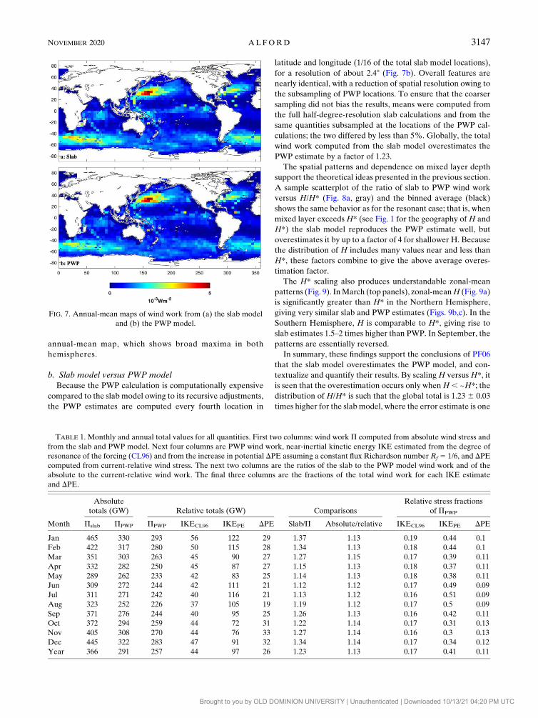
annual-mean map, which shows broad maxima in both

hemispheres.

b. Slab model versus PWP modelBecause the PWP calculation is computationally expensive

compared to the slab model owing to its recursive adjustments,

the PWP estimates are computed every fourth location in

latitude and longitude (1/16 of the total slab model locations),

for a resolution of about 2.48 (Fig. 7b). Overall features are

nearly identical, with a reduction of spatial resolution owing to

the subsampling of PWP locations. To ensure that the coarser

sampling did not bias the results, means were computed from

the full half-degree-resolution slab calculations and from the

same quantities subsampled at the locations of the PWP cal-

culations; the two differed by less than 5%. Globally, the total

wind work computed from the slab model overestimates the

PWP estimate by a factor of 1.23.

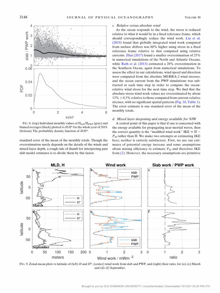
The spatial patterns and dependence on mixed layer depth

support the theoretical ideas presented in the previous section.

A sample scatterplot of the ratio of slab to PWP wind work

versus H/H* (Fig. 8a, gray) and the binned average (black)

shows the same behavior as for the resonant case; that is, when

mixed layer exceedsH* (see Fig. 1 for the geography ofH and

H*) the slab model reproduces the PWP estimate well, but

overestimates it by up to a factor of 4 for shallower H. Because

the distribution of H includes many values near and less than

H*, these factors combine to give the above average overes-

timation factor.

The H* scaling also produces understandable zonal-mean

patterns (Fig. 9). InMarch (top panels), zonal-meanH (Fig. 9a)

is significantly greater than H* in the Northern Hemisphere,

giving very similar slab and PWP estimates (Figs. 9b,c). In the

Southern Hemisphere, H is comparable to H*, giving rise to

slab estimates 1.5–2 times higher than PWP. In September, the

patterns are essentially reversed.

In summary, these findings support the conclusions of PF06

that the slab model overestimates the PWP model, and con-

textualize and quantify their results. By scalingH versusH*, it

is seen that the overestimation occurs only whenH, ~H*; the

distribution of H/H* is such that the global total is 1.23 6 0.03

times higher for the slab model, where the error estimate is one

FIG. 7. Annual-mean maps of wind work from (a) the slab model

and (b) the PWP model.

TABLE 1. Monthly and annual total values for all quantities. First two columns: wind work P computed from absolute wind stress and

from the slab and PWP model. Next four columns are PWP wind work, near-inertial kinetic energy IKE estimated from the degree of

resonance of the forcing (CL96) and from the increase in potential DPE assuming a constant flux Richardson number Rf 5 1/6, and DPEcomputed from current-relative wind stress. The next two columns are the ratios of the slab to the PWP model wind work and of the

absolute to the current-relative wind work. The final three columns are the fractions of the total wind work for each IKE estimate

and DPE.

Absolute

totals (GW) Relative totals (GW) Comparisons

Relative stress fractions

of PPWP

Month Pslab PPWP PPWP IKECL96 IKEPE DPE Slab/P Absolute/relative IKECL96 IKEPE DPE

Jan 465 330 293 56 122 29 1.37 1.13 0.19 0.44 0.1

Feb 422 317 280 50 115 28 1.34 1.13 0.18 0.44 0.1

Mar 351 303 263 45 90 27 1.27 1.15 0.17 0.39 0.11

Apr 332 282 250 45 87 27 1.15 1.13 0.18 0.37 0.11

May 289 262 233 42 83 25 1.14 1.13 0.18 0.38 0.11

Jun 309 272 244 42 111 21 1.12 1.12 0.17 0.49 0.09

Jul 311 271 242 40 116 21 1.13 1.12 0.16 0.51 0.09

Aug 323 252 226 37 105 19 1.19 1.12 0.17 0.5 0.09

Sep 371 276 244 40 95 25 1.26 1.13 0.16 0.42 0.11

Oct 372 294 259 44 72 31 1.22 1.14 0.17 0.31 0.13

Nov 405 308 270 44 76 33 1.27 1.14 0.16 0.3 0.13

Dec 445 322 283 47 91 32 1.34 1.14 0.17 0.34 0.12

Year 366 291 257 44 97 26 1.23 1.13 0.17 0.41 0.11

NOVEMBER 2020 AL FORD 3147

Brought to you by OLD DOMINION UNIVERSITY | Unauthenticated | Downloaded 10/13/21 04:20 PM UTC

standard error of the mean of the monthly totals. Though the

overestimation surely depends on the details of the winds and

mixed layer depth, a rough rule of thumb for interpreting past

slab model estimates is to divide them by this factor.

c. Relative versus absolute windAs the ocean responds to the wind, the stress is reduced

relative to what it would be in a fixed reference frame, which

should correspondingly reduce the wind work. Liu et al.

(2019) found that globally integrated wind work computed

from surface drifters was 60% higher using stress in a fixed

reference frame relative to that computed using relative

currents. Zhai (2017) found a smaller overestimation of 25%

in numerical simulations of the North and Atlantic Oceans,

while Rath et al. (2013) estimated a 28% overestimation in

the Southern Ocean, again from numerical simulations. To

assess the effect in our calculations, wind speed and direction

were computed from the absolute MERRA-2 wind stresses,

and the ocean current from the PWP simulations was sub-

tracted at each time step in order to compute the ocean-

relative wind stress for the next time step. We find that the

absolute-stress wind work values are overestimated by about

13%6 0.3% relative to those computed from current-relative

stresses, with no significant spatial patterns (Fig. 10, Table 1).

The error estimate is one standard error of the mean of the

monthly totals.

d. Mixed layer deepening and energy available for NIWA central point of this paper is that if one is concerned with

the energy available for propagating near-inertial waves, then

the correct quantity is the ‘‘modified wind work’’ IKE [ P 2PM rather than P. We make two attempts at estimating IKE

here; neither is entirely satisfactory. First, we use our esti-

mates of potential energy increase and some assumptions

about mixing efficiency to estimate PM and therefore IKE

from (2). However, the necessary assumptions are primitive

FIG. 8. (top) Individual monthly values ofPslab/PPWP (gray) and

binned averages (black) plotted vsH/H* for thewhole year of 2019.

(bottom) The probability density function of H/H*.

FIG. 9. Zonal-mean plots vs latitude of (left)H andH*, (center) wind work from slab and PWP, and (right) their ratio, for (a)–(c) March

and (d)–(f) September.

3148 JOURNAL OF PHYS ICAL OCEANOGRAPHY VOLUME 50

Brought to you by OLD DOMINION UNIVERSITY | Unauthenticated | Downloaded 10/13/21 04:20 PM UTC

and unsatisfying, so we obtain a second estimate using the

KPP results from CL96.

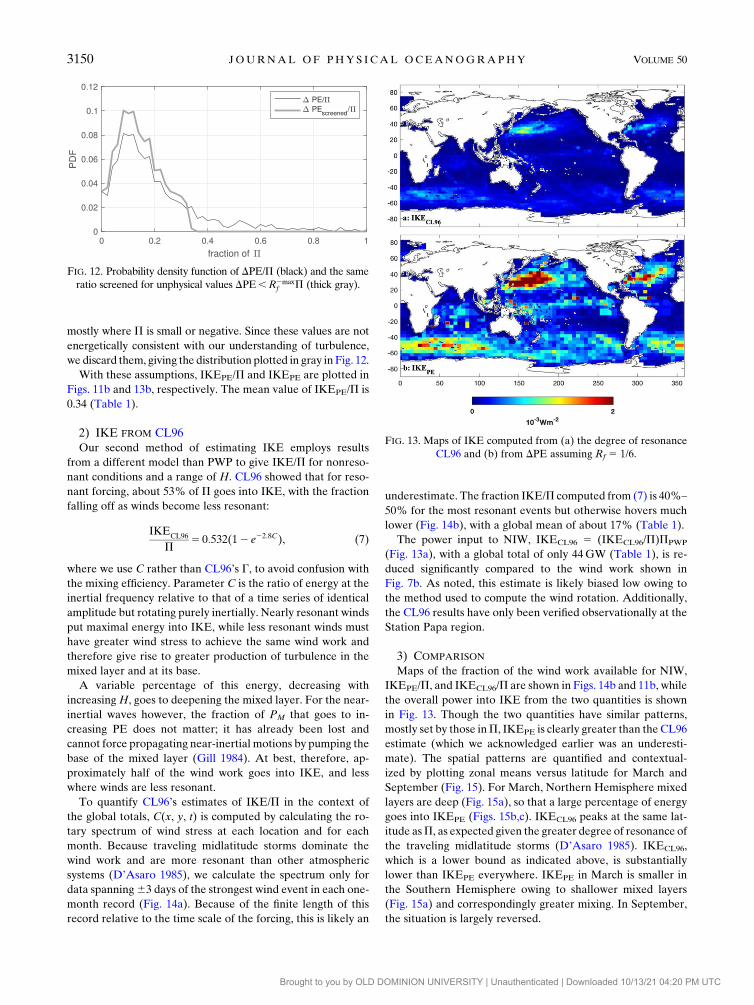
1) IKE FROM DPEOur first estimate of IKE estimates PM from DPE computed

from the PWP simulations. DPE is straightforward to calculate

from the density profiles at the beginning and end of each

monthly simulation, using a reference depth of D 5 350m to

ensure integration below the deepest mixed layers. The time-

mean map of DPE/P (Fig. 11a) shows that the regions of

strongest forcing tend to put the smallest fraction of energy into

deepening the mixed layer, consistent with CL96. Integrated

globally, the fraction is consistent throughout the year, with an

annual mean of 11% (Table 1).

The turbulence production can then be crudely estimated as

PM 5R21f DPE, where Rf is taken as 1/6 following Osborn

(1980). Though Rf is a parameter of the flow rather than a

constant, substantial observational evidence supports a mean

value near 1/6 in the ocean interior, including agreement

with dye and microstructure estimates of turbulent diffusion

(Ledwell et al. 1993) and comparison of thermal and kinetic

energy dissipation rates (Moum 1996; Monismith et al. 2018).

For deepening mixed layers, CL96 and Skyllingstad et al.

(2000) found values spanning this number, but with consider-

able spread depending on H (as shown in Fig. 2), stratification

at the mixed layer base, and the degree of resonance of the

forcing (motivating the next section). Intuitively, deep mixed

layers might have less efficient mixing owing to the large

fraction of ‘‘unmixed’’ water with buoyancy flux only occurring

in the transition layer, as suggested by Fig. 2.

Glossing over these variations in Rf, whose parameter

dependencies need to be explored more fully, we here

simply estimate turbulence production for each location

and month from (5), taking a constant value of Rf 5 1/6.

Then IKEPE 5P2R21f DPE.

The interpretation of PM determined in this way from the

monthly estimates is somewhat complicated because DPE can

only increase in time as the PWP model cannot ‘‘unmix’’ the

fluid. The integrated wind work, however, can increase and

decrease depending on the phasing of the wind (e.g., Fig. 5).

The ratio of DPE/P is usually 5%–20% (CL96 and Fig. 12,

black), but values R21f DPE.P occur about 18% of the time,

FIG. 10. Comparison of fluxes from wind stress computed from the PWP model using Earth-relative winds

(‘‘absolute,’’ thin black) and those relative to the inertial currents (‘‘relative,’’ thick gray), for April. (a) Absolute

and relative wind work. (b) Their ratio.

FIG. 11. Annual-mean maps of (a) the ratio of potential energy

increase to wind work, DPE/P, and (b) the associated ratio of near-

inertial kinetic energy increase to the wind work, IKEPE/P.

NOVEMBER 2020 AL FORD 3149

Brought to you by OLD DOMINION UNIVERSITY | Unauthenticated | Downloaded 10/13/21 04:20 PM UTC

mostly where P is small or negative. Since these values are not

energetically consistent with our understanding of turbulence,

we discard them, giving the distribution plotted in gray in Fig. 12.

With these assumptions, IKEPE/P and IKEPE are plotted in

Figs. 11b and 13b, respectively. The mean value of IKEPE/P is

0.34 (Table 1).

2) IKE FROM CL96Our second method of estimating IKE employs results

from a different model than PWP to give IKE/P for nonreso-

nant conditions and a range of H. CL96 showed that for reso-

nant forcing, about 53% of P goes into IKE, with the fraction

falling off as winds become less resonant:

IKECL96

P5 0:532(12 e22:8C), (7)

where we use C rather than CL96’s G, to avoid confusion with

the mixing efficiency. Parameter C is the ratio of energy at the

inertial frequency relative to that of a time series of identical

amplitude but rotating purely inertially. Nearly resonant winds

put maximal energy into IKE, while less resonant winds must

have greater wind stress to achieve the same wind work and

therefore give rise to greater production of turbulence in the

mixed layer and at its base.

A variable percentage of this energy, decreasing with

increasingH, goes to deepening the mixed layer. For the near-

inertial waves however, the fraction of PM that goes to in-

creasing PE does not matter; it has already been lost and

cannot force propagating near-inertial motions by pumping the

base of the mixed layer (Gill 1984). At best, therefore, ap-

proximately half of the wind work goes into IKE, and less

where winds are less resonant.

To quantify CL96’s estimates of IKE/P in the context of

the global totals, C(x, y, t) is computed by calculating the ro-

tary spectrum of wind stress at each location and for each

month. Because traveling midlatitude storms dominate the

wind work and are more resonant than other atmospheric

systems (D’Asaro 1985), we calculate the spectrum only for

data spanning63 days of the strongest wind event in each one-

month record (Fig. 14a). Because of the finite length of this

record relative to the time scale of the forcing, this is likely an

underestimate. The fraction IKE/P computed from (7) is 40%–

50% for the most resonant events but otherwise hovers much

lower (Fig. 14b), with a global mean of about 17% (Table 1).

The power input to NIW, IKECL96 5 (IKECL96/P)PPWP

(Fig. 13a), with a global total of only 44GW (Table 1), is re-

duced significantly compared to the wind work shown in

Fig. 7b. As noted, this estimate is likely biased low owing to

the method used to compute the wind rotation. Additionally,

the CL96 results have only been verified observationally at the

Station Papa region.

3) COMPARISON

Maps of the fraction of the wind work available for NIW,

IKEPE/P, and IKECL96/P are shown in Figs. 14b and 11b, while

the overall power into IKE from the two quantities is shown

in Fig. 13. Though the two quantities have similar patterns,

mostly set by those inP, IKEPE is clearly greater than the CL96

estimate (which we acknowledged earlier was an underesti-

mate). The spatial patterns are quantified and contextual-

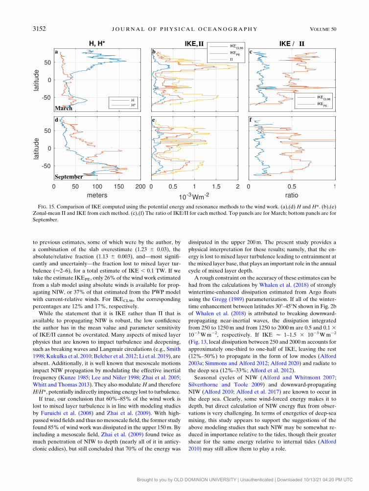
ized by plotting zonal means versus latitude for March and

September (Fig. 15). For March, Northern Hemisphere mixed

layers are deep (Fig. 15a), so that a large percentage of energy

goes into IKEPE (Figs. 15b,c). IKECL96 peaks at the same lat-

itude asP, as expected given the greater degree of resonance of

the traveling midlatitude storms (D’Asaro 1985). IKECL96,

which is a lower bound as indicated above, is substantially

lower than IKEPE everywhere. IKEPE in March is smaller in

the Southern Hemisphere owing to shallower mixed layers

(Fig. 15a) and correspondingly greater mixing. In September,

the situation is largely reversed.

FIG. 12. Probability density function of DPE/P (black) and the same

ratio screened for unphysical values DPE,R2maxf P (thick gray).

FIG. 13. Maps of IKE computed from (a) the degree of resonance

CL96 and (b) from DPE assuming Rf 5 1/6.

3150 JOURNAL OF PHYS ICAL OCEANOGRAPHY VOLUME 50

Brought to you by OLD DOMINION UNIVERSITY | Unauthenticated | Downloaded 10/13/21 04:20 PM UTC

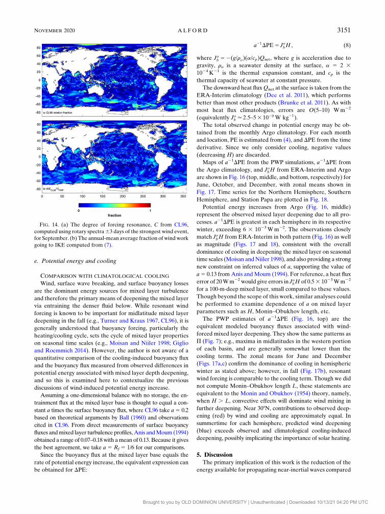
e. Potential energy and cooling

COMPARISON WITH CLIMATOLOGICAL COOLING

Wind, surface wave breaking, and surface buoyancy losses

are the dominant energy sources for mixed layer turbulence

and therefore the primary means of deepening the mixed layer

via entraining the denser fluid below. While resonant wind

forcing is known to be important for midlatitude mixed layer

deepening in the fall (e.g., Turner and Kraus 1967, CL96), it is

generally understood that buoyancy forcing, particularly the

heating/cooling cycle, sets the cycle of mixed layer properties

on seasonal time scales (e.g., Moisan and Niiler 1998; Giglio

and Roemmich 2014). However, the author is not aware of a

quantitative comparison of the cooling-induced buoyancy flux

and the buoyancy flux measured from observed differences in

potential energy associated with mixed layer depth deepening,

and so this is examined here to contextualize the previous

discussions of wind-induced potential energy increase.

Assuming a one-dimensional balance with no storage, the en-

trainment flux at the mixed layer base is thought to equal a con-

stant a times the surface buoyancy flux, where CL96 take a5 0.2

based on theoretical arguments by Ball (1960) and observations

cited in CL96. From direct measurements of surface buoyancy

fluxes andmixed layer turbulence profiles,Anis andMoum(1994)

obtained a range of 0.07–0.18with amean of 0.13. Because it gives

the best agreement, we take a 5 Rf 5 1/6 for our comparisons.

Since the buoyancy flux at the mixed layer base equals the

rate of potential energy increase, the equivalent expression can

be obtained for DPE:

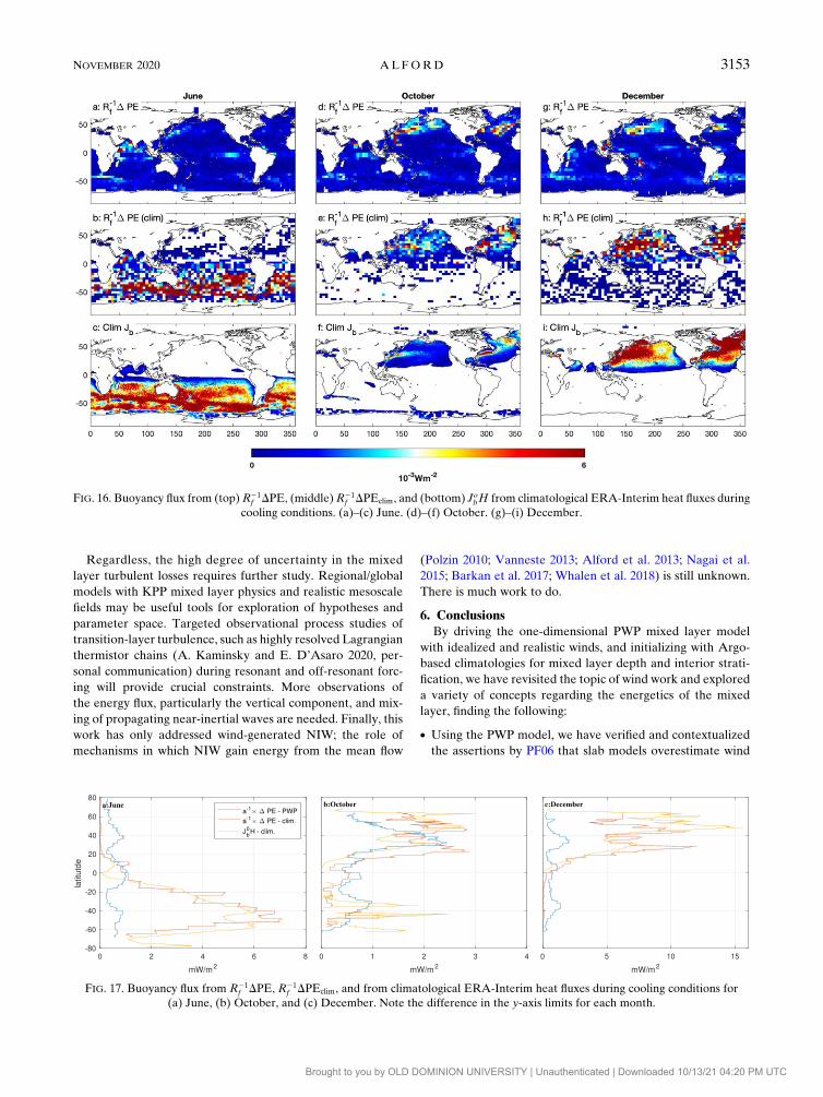
a21DPE5 JobH , (8)

where Job 52(g/ro)(a/cp)Qnet, where g is acceleration due to

gravity, ro is a seawater density at the surface, a 5 2 31024 K21 is the thermal expansion constant, and cp is the

thermal capacity of seawater at constant pressure.

The downward heat fluxQnet at the surface is taken from the

ERA-Interim climatology (Dee et al. 2011), which performs

better than most other products (Brunke et al. 2011). As with

most heat flux climatologies, errors are O(5–10) Wm22

(equivalently Job ’ 2:5–53 1029 W kg21).

The total observed change in potential energy may be ob-

tained from the monthly Argo climatology. For each month

and location, PE is estimated from (4), and DPE from the time

derivative. Since we only consider cooling, negative values

(decreasing H) are discarded.

Maps of a21DPE from the PWP simulations, a21DPE from

the Argo climatology, and JobH from ERA-Interim and Argo

are shown in Fig. 16 (top, middle, and bottom, respectively) for

June, October, and December, with zonal means shown in

Fig. 17. Time series for the Northern Hemisphere, Southern

Hemisphere, and Station Papa are plotted in Fig. 18.

Potential energy increases from Argo (Fig. 16, middle)

represent the observed mixed layer deepening due to all pro-

cesses. a21DPE is greatest in each hemisphere in its respective

winter, exceeding 6 3 1023Wm22. The observations closely

match JobH from ERA-Interim in both pattern (Fig. 16) as well

as magnitude (Figs. 17 and 18), consistent with the overall

dominance of cooling in deepening the mixed layer on seasonal

time scales (Moisan andNiiler 1998), and also providing a strong

new constraint on inferred values of a, supporting the value of

a5 0.13 fromAnis andMoum (1994). For reference, a heat flux

error of 20Wm22 would give errors in JobH of 0.53 1023Wm22

for a 100-m-deep mixed layer, small compared to these values.

Though beyond the scope of this work, similar analyses could

be performed to examine dependence of a on mixed layer

parameters such as H, Monin–Obukhov length, etc.

The PWP estimates of a21DPE (Fig. 16, top) are the

equivalent modeled buoyancy fluxes associated with wind-

forced mixed layer deepening. They show the same patterns as

P (Fig. 7); e.g., maxima in midlatitudes in the western portion

of each basin, and are generally somewhat lower than the

cooling terms. The zonal means for June and December

(Figs. 17a,c) confirm the dominance of cooling in hemispheric

winter as stated above; however, in fall (Fig. 17b), resonant

wind forcing is comparable to the cooling term. Though we did

not compute Monin–Obukhov length L, these statements are

equivalent to the Monin and Obukhov (1954) theory, namely,

when H . L, convective effects will dominate wind mixing in

further deepening. Near 308N, contributions to observed deep-

ening (red) by wind and cooling are approximately equal. In

summertime for each hemisphere, predicted wind deepening

(blue) exceeds observed and climatological cooling-induced

deepening, possibly implicating the importance of solar heating.

5. DiscussionThe primary implication of this work is the reduction of the

energy available for propagating near-inertial waves compared

FIG. 14. (a) The degree of forcing resonance, C from CL96,

computed using rotary spectra63 days of the strongest wind event,

for September. (b) The annual-mean average fraction of wind work

going to IKE computed from (7).

NOVEMBER 2020 AL FORD 3151

Brought to you by OLD DOMINION UNIVERSITY | Unauthenticated | Downloaded 10/13/21 04:20 PM UTC

to previous estimates, some of which were by the author, by

a combination of the slab overestimate (1.23 6 0.03), the

absolute/relative fraction (1.13 6 0.003), and—most signifi-

cantly and uncertainly—the fraction lost to mixed layer tur-

bulence (’2–6), for a total estimate of IKE , 0.1 TW. If we

take the estimate IKEPE, only 26% of the wind work estimated

from a slab model using absolute winds is available for prop-

agating NIW, or 37% of that estimated from the PWP model

with current-relative winds. For IKECL96, the corresponding

percentages are 12% and 17%, respectively.

While the statement that it is IKE rather than P that is

available to propagating NIW is robust, the low confidence

the author has in the mean value and parameter sensitivity

of IKE/P cannot be overstated. Many aspects of mixed layer

physics that are known to impact turbulence and deepening,

such as breaking waves and Langmuir circulations (e.g., Smith

1998; Kukulka et al. 2010; Belcher et al. 2012; Li et al. 2019), are

absent. Additionally, it is well known that mesoscale motions

impact NIW propagation by modulating the effective inertial

frequency (Kunze 1985; Lee and Niiler 1998; Zhai et al. 2005;

Whitt and Thomas 2013). They also modulateH and therefore

H/H*, potentially indirectly impacting energy lost to turbulence.

If true, our conclusion that 60%–85% of the wind work is

lost to mixed layer turbulence is in line with modeling studies

by Furuichi et al. (2008) and Zhai et al. (2009). With high-

passedwind fields and thus nomesoscale field, the former study

found 85% of wind work was dissipated in the upper 150m. By

including a mesoscale field, Zhai et al. (2009) found twice as

much penetration of NIW to depth (nearly all of it in anticy-

clonic eddies), but still concluded that 70% of the energy was

dissipated in the upper 200m. The present study provides a

physical interpretation for these results; namely, that the en-

ergy is lost to mixed layer turbulence leading to entrainment at

the mixed layer base, that plays an important role in the annual

cycle of mixed layer depth.

A rough constraint on the accuracy of these estimates can be

had from the calculations by Whalen et al. (2018) of strongly

wintertime-enhanced dissipation estimated from Argo floats

using the Gregg (1989) parameterization. If all of the winter-

time enhancement between latitudes 308–458N shown in Fig. 2b

of Whalen et al. (2018) is attributed to breaking downward-

propagating near-inertial waves, the dissipation integrated

from 250 to 1250m and from 1250 to 2000m are 0.5 and 0.1 31023Wm22, respectively. If IKE ’ 1–1.5 3 1023Wm22

(Fig. 13, local dissipation between 250 and 2000m accounts for

approximately one-third to one-half of IKE, leaving the rest

(12%–50%) to propagate in the form of low modes (Alford

2003a; Simmons and Alford 2012; Alford 2020) and radiate to

the deep sea (12%–33%; Alford et al. 2012).

Seasonal cycles of NIW (Alford and Whitmont 2007;

Silverthorne and Toole 2009) and downward-propagating

NIW (Alford 2010; Alford et al. 2017) are known to occur in

the deep sea. Clearly, some wind-forced energy makes it to

depth, but direct calculation of NIW energy flux from obser-

vations is very challenging. In terms of energetics of deep-sea

mixing, this study appears to support the suggestions of the

above modeling studies that such NIW may be somewhat re-

duced in importance relative to the tides, though their greater

shear for the same energy relative to internal tides (Alford

2010) may still allow them to play a role.

FIG. 15. Comparison of IKE computed using the potential energy and resonance methods to the wind work. (a),(d) H and H*. (b),(e)

Zonal-meanP and IKE from each method. (c),(f) The ratio of IKE/P for each method. Top panels are for March; bottom panels are for

September.

3152 JOURNAL OF PHYS ICAL OCEANOGRAPHY VOLUME 50

Brought to you by OLD DOMINION UNIVERSITY | Unauthenticated | Downloaded 10/13/21 04:20 PM UTC

Regardless, the high degree of uncertainty in the mixed

layer turbulent losses requires further study. Regional/global

models with KPP mixed layer physics and realistic mesoscale

fields may be useful tools for exploration of hypotheses and

parameter space. Targeted observational process studies of

transition-layer turbulence, such as highly resolved Lagrangian

thermistor chains (A. Kaminsky and E. D’Asaro 2020, per-

sonal communication) during resonant and off-resonant forc-

ing will provide crucial constraints. More observations of

the energy flux, particularly the vertical component, and mix-

ing of propagating near-inertial waves are needed. Finally, this

work has only addressed wind-generated NIW; the role of

mechanisms in which NIW gain energy from the mean flow

(Polzin 2010; Vanneste 2013; Alford et al. 2013; Nagai et al.

2015; Barkan et al. 2017; Whalen et al. 2018) is still unknown.

There is much work to do.

6. ConclusionsBy driving the one-dimensional PWP mixed layer model

with idealized and realistic winds, and initializing with Argo-

based climatologies for mixed layer depth and interior strati-

fication, we have revisited the topic of wind work and explored

a variety of concepts regarding the energetics of the mixed

layer, finding the following:

d Using the PWP model, we have verified and contextualized

the assertions by PF06 that slab models overestimate wind

FIG. 17. Buoyancy flux from R21f DPE, R21

f DPEclim, and from climatological ERA-Interim heat fluxes during cooling conditions for

(a) June, (b) October, and (c) December. Note the difference in the y-axis limits for each month.

FIG. 16. Buoyancy flux from (top) R21f DPE, (middle)R21

f DPEclim, and (bottom) JobH from climatological ERA-Interim heat fluxes during

cooling conditions. (a)–(c) June. (d)–(f) October. (g)–(i) December.

NOVEMBER 2020 AL FORD 3153

Brought to you by OLD DOMINION UNIVERSITY | Unauthenticated | Downloaded 10/13/21 04:20 PM UTC

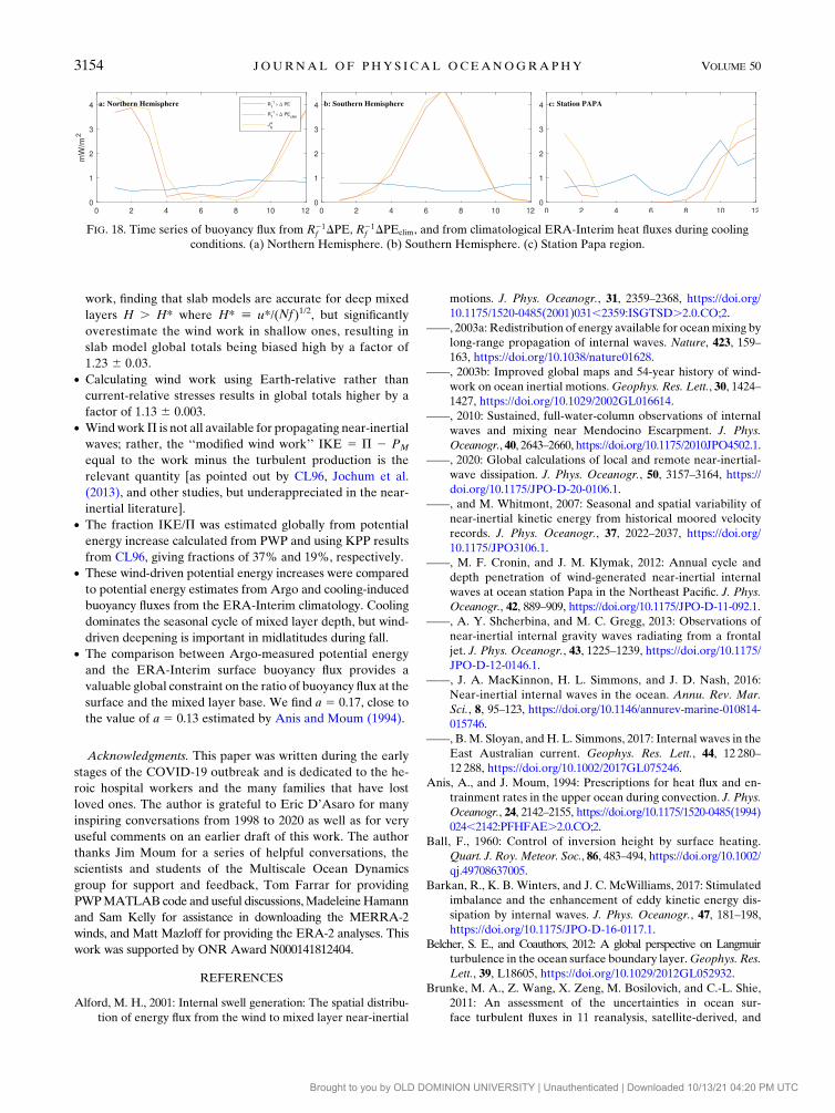
work, finding that slab models are accurate for deep mixed

layers H . H* where H* [ u*/(Nf)1/2, but significantly

overestimate the wind work in shallow ones, resulting in

slab model global totals being biased high by a factor of

1.23 6 0.03.d Calculating wind work using Earth-relative rather than

current-relative stresses results in global totals higher by a

factor of 1.13 6 0.003.d WindworkP is not all available for propagating near-inertial

waves; rather, the ‘‘modified wind work’’ IKE 5 P 2 PM

equal to the work minus the turbulent production is the

relevant quantity [as pointed out by CL96, Jochum et al.

(2013), and other studies, but underappreciated in the near-

inertial literature].d The fraction IKE/P was estimated globally from potential

energy increase calculated from PWP and using KPP results

from CL96, giving fractions of 37% and 19%, respectively.d These wind-driven potential energy increases were compared

to potential energy estimates from Argo and cooling-induced

buoyancy fluxes from the ERA-Interim climatology. Cooling

dominates the seasonal cycle of mixed layer depth, but wind-

driven deepening is important in midlatitudes during fall.d The comparison between Argo-measured potential energy

and the ERA-Interim surface buoyancy flux provides a

valuable global constraint on the ratio of buoyancy flux at the

surface and the mixed layer base. We find a 5 0.17, close to

the value of a 5 0.13 estimated by Anis and Moum (1994).

Acknowledgments. This paper was written during the early

stages of the COVID-19 outbreak and is dedicated to the he-

roic hospital workers and the many families that have lost

loved ones. The author is grateful to Eric D’Asaro for many

inspiring conversations from 1998 to 2020 as well as for very

useful comments on an earlier draft of this work. The author

thanks Jim Moum for a series of helpful conversations, the

scientists and students of the Multiscale Ocean Dynamics

group for support and feedback, Tom Farrar for providing

PWPMATLAB code and useful discussions,MadeleineHamann

and Sam Kelly for assistance in downloading the MERRA-2

winds, and Matt Mazloff for providing the ERA-2 analyses. This

work was supported by ONR Award N000141812404.

REFERENCES

Alford, M. H., 2001: Internal swell generation: The spatial distribu-

tion of energy flux from the wind to mixed layer near-inertial

motions. J. Phys. Oceanogr., 31, 2359–2368, https://doi.org/

10.1175/1520-0485(2001)031,2359:ISGTSD.2.0.CO;2.

——, 2003a: Redistribution of energy available for oceanmixing by

long-range propagation of internal waves. Nature, 423, 159–

163, https://doi.org/10.1038/nature01628.

——, 2003b: Improved global maps and 54-year history of wind-

work on ocean inertial motions.Geophys. Res. Lett., 30, 1424–1427, https://doi.org/10.1029/2002GL016614.

——, 2010: Sustained, full-water-column observations of internal

waves and mixing near Mendocino Escarpment. J. Phys.

Oceanogr., 40, 2643–2660, https://doi.org/10.1175/2010JPO4502.1.

——, 2020: Global calculations of local and remote near-inertial-

wave dissipation. J. Phys. Oceanogr., 50, 3157–3164, https://

doi.org/10.1175/JPO-D-20-0106.1.

——, and M. Whitmont, 2007: Seasonal and spatial variability of

near-inertial kinetic energy from historical moored velocity

records. J. Phys. Oceanogr., 37, 2022–2037, https://doi.org/

10.1175/JPO3106.1.

——, M. F. Cronin, and J. M. Klymak, 2012: Annual cycle and

depth penetration of wind-generated near-inertial internal

waves at ocean station Papa in the Northeast Pacific. J. Phys.

Oceanogr., 42, 889–909, https://doi.org/10.1175/JPO-D-11-092.1.

——, A. Y. Shcherbina, and M. C. Gregg, 2013: Observations of

near-inertial internal gravity waves radiating from a frontal

jet. J. Phys. Oceanogr., 43, 1225–1239, https://doi.org/10.1175/

JPO-D-12-0146.1.

——, J. A. MacKinnon, H. L. Simmons, and J. D. Nash, 2016:

Near-inertial internal waves in the ocean. Annu. Rev. Mar.

Sci., 8, 95–123, https://doi.org/10.1146/annurev-marine-010814-

015746.

——, B.M. Sloyan, and H. L. Simmons, 2017: Internal waves in the

East Australian current. Geophys. Res. Lett., 44, 12 280–

12 288, https://doi.org/10.1002/2017GL075246.

Anis, A., and J. Moum, 1994: Prescriptions for heat flux and en-

trainment rates in the upper ocean during convection. J. Phys.

Oceanogr., 24, 2142–2155, https://doi.org/10.1175/1520-0485(1994)

024,2142:PFHFAE.2.0.CO;2.

Ball, F., 1960: Control of inversion height by surface heating.

Quart. J. Roy. Meteor. Soc., 86, 483–494, https://doi.org/10.1002/

qj.49708637005.

Barkan, R., K. B. Winters, and J. C. McWilliams, 2017: Stimulated

imbalance and the enhancement of eddy kinetic energy dis-

sipation by internal waves. J. Phys. Oceanogr., 47, 181–198,

https://doi.org/10.1175/JPO-D-16-0117.1.

Belcher, S. E., and Coauthors, 2012: A global perspective on Langmuir

turbulence in the ocean surface boundary layer.Geophys. Res.

Lett., 39, L18605, https://doi.org/10.1029/2012GL052932.

Brunke, M. A., Z. Wang, X. Zeng, M. Bosilovich, and C.-L. Shie,

2011: An assessment of the uncertainties in ocean sur-

face turbulent fluxes in 11 reanalysis, satellite-derived, and

FIG. 18. Time series of buoyancy flux from R21f DPE, R21

f DPEclim, and from climatological ERA-Interim heat fluxes during cooling

conditions. (a) Northern Hemisphere. (b) Southern Hemisphere. (c) Station Papa region.

3154 JOURNAL OF PHYS ICAL OCEANOGRAPHY VOLUME 50

Brought to you by OLD DOMINION UNIVERSITY | Unauthenticated | Downloaded 10/13/21 04:20 PM UTC

combined global datasets. J. Climate, 24, 5469–5493, https://

doi.org/10.1175/2011JCLI4223.1.

Conkright, M. E., R. A. Locarnini, H. E. Garcia, T. D. O’Brien,

T. P. Boyer, C. Stephens, and J. I. Antonov, 2002: World

Ocean Atlas 2001: Objective Analyses,Data Statistics, and

Figures.CD-ROMDocumentation,NODCInternalRep. 17,17pp.,

ftp://ftp.nodc.noaa.gov/pub/data.nodc/woa/PUBLICATIONS/

readme.pdf.

Crawford, G., and W. Large, 1996: A numerical investigation of

resonant inertial response of the ocean to wind forcing.

J. Phys. Oceanogr., 26, 873–891, https://doi.org/10.1175/1520-

0485(1996)026,0873:ANIORI.2.0.CO;2.

D’Asaro, E., 1985: The energy flux from the wind to near-inertial

motions in the mixed layer. J. Phys. Oceanogr., 15, 1043–1059,

https://doi.org/10.1175/1520-0485(1985)015,1043:TEFFTW.2.0.CO;2.

Davis, R., R. A. De Szoeke, D. Halpern, and P. Niiler, 1981:

Variability in the upper ocean during MILE. Part I: The heat

and momentum balances. Deep-Sea Res., 28A, 1427–1451,

https://doi.org/10.1016/0198-0149(81)90091-1.

Dee, D. P., and Coauthors, 2011: The ERA-Interim reanalysis:

Configuration and performance of the data assimilation sys-

tem.Quart. J. Roy. Meteor. Soc., 137, 553–597, https://doi.org/

10.1002/qj.828.

Dohan, K., and R. E. Davis, 2011: Mixing in the transition layer

during two storm events. J. Phys. Oceanogr., 41, 42–66, https://

doi.org/10.1175/2010JPO4253.1.

Fox-Kemper, B., R. Ferrari, andR.Hallberg, 2008: Parameterization

of mixed layer eddies. Part I: Theory and diagnosis. J. Phys.

Oceanogr., 38, 1145–1165, https://doi.org/10.1175/2007JPO3792.1.

Furuichi, N., T. Hibiya, and Y. Niwa, 2008: Model predicted dis-

tribution of wind-induced internal wave energy in the world’s

oceans. J. Geophys. Res., 113, C09034, https://doi.org/10.1029/

2008JC004768.

Gelaro, R., and Coauthors, 2017: The Modern-Era Retrospective

Analysis for Research and Applications, version 2 (MERRA-2).

J. Climate, 30, 5419–5454, https://doi.org/10.1175/JCLI-D-16-

0758.1.

Giglio, D., and D. Roemmich, 2014: Climatological monthly heat

and freshwater flux estimates on a global scale from Argo.

J. Geophys. Res. Oceans, 119, 6884–6899, https://doi.org/

10.1002/2014JC010083.

Gill, A. E., 1984: On the behavior of internal waves in the wake of a

storm. J. Phys. Oceanogr., 14, 1129–1151, https://doi.org/10.1175/

1520-0485(1984)014,1129:OTBOIW.2.0.CO;2.

Grant, A. L., and S. E. Belcher, 2011: Wind-driven mixing below

the oceanic mixed layer. J. Phys. Oceanogr., 41, 1556–1575,

https://doi.org/10.1175/JPO-D-10-05020.1.

Gregg, M., 1989: Scaling turbulent dissipation in the thermo-

cline. J. Geophys. Res., 94, 9686–9698, https://doi.org/10.1029/

JC094iC07p09686.

Holte, J., L. D. Talley, J. Gilson, andD. Roemmich, 2017: AnArgo

mixed layer climatology and database.Geophys. Res. Lett., 44,

5618–5626, https://doi.org/10.1002/2017GL073426.

Hosegood, P. J., M. C.Gregg, andM.H.Alford, 2008: Restratification

of the surface mixed layer with submesoscale lateral density

gradients: Diagnosing the importance of the horizontal di-

mension. J. Phys. Oceanogr., 38, 2438–2460, https://doi.org/

10.1175/2008JPO3843.1.

Jiang, J., Y. Lu, and W. Perrie, 2005: Estimating the energy flux

from the wind to ocean inertial motions: The sensitivity to

surface wind fields. Geophys. Res. Lett., 32, L15610, https://

doi.org/10.1029/2005GL023289.

Jochum, M., B. P. Briegleb, G. Danabasoglu, W. G. Large,

S. R. Jayne, M. H. Alford, and F. O. Bryan, 2013: On

the impact of oceanic near-inertial waves on climate.

J. Climate, 26, 2833–2844, https://doi.org/10.1175/JCLI-D-

12-00181.1.

Johnston, T. M. S., and D. L. Rudnick, 2009: Observations of the

transition layer. J. Phys. Oceanogr., 39, 780–797, https://

doi.org/10.1175/2008JPO3824.1.

Kelly, K. A., S. Dickinson, M. J. McPhaden, and G. C. Johnson,

2001: Ocean currents evident in satellite wind data.

Geophys. Res. Lett., 28, 2469–2472, https://doi.org/10.1029/

2000GL012610.

Kraus, E. B., and J. S. Turner, 1967: A one-dimensional model of

the seasonal thermocline II. The general theory and its

consequences. Tellus, 19, 98–106, https://doi.org/10.3402/

tellusa.v19i1.9753.

Kukulka, T., A. J. Plueddemann, J. H. Trowbridge, and P. P.

Sullivan, 2010: Rapid mixed layer deepening by the combi-

nation of Langmuir and shear instabilities: A case study.

J. Phys. Oceanogr., 40, 2381–2400, https://doi.org/10.1175/

2010JPO4403.1.

Kunze, E., 1985: Near-inertial wave propagation in geostrophic

shear. J. Phys. Oceanogr., 15, 544–565, https://doi.org/10.1175/

1520-0485(1985)015,0544:NIWPIG.2.0.CO;2.

Large, W. G., J. C. McWilliams, and S. C. Doney, 1994: Oceanic

vertical mixing: A review and a model with a nonlocal

boundary layer parameterization.Rev. Geophys., 32, 363–403,

https://doi.org/10.1029/94RG01872.

Ledwell, J. R., A. Watson, and C. Law, 1993: Evidence for slow

mixing across the pycnocline from an open-ocean tracer-

release experiment. Nature, 364, 701–703, https://doi.org/

10.1038/364701a0.

Lee, D., and P. Niiler, 1998: The inertial chimney: The near-inertial

energy drainage from the ocean surface to the deep layer.

J. Geophys. Res., 103, 7579–7591, https://doi.org/10.1029/

97JC03200.

Li, Q., and Coauthors, 2019: Comparing ocean surface boundary

vertical mixing schemes including Langmuir turbulence.

J. Adv. Model. Earth Syst., 11, 3545–3592, https://doi.org/

10.1029/2019MS001810.

Liu, Y., Z. Jing, and L. Wu, 2019: Wind power on oceanic near-

inertial oscillations in the global ocean estimated from surface

drifters. Geophys. Res. Lett., 46, 2647–2653, https://doi.org/

10.1029/2018GL081712.

McWilliams, J. C., P. P. Sullivan, andC.-H.Moeng, 1997: Langmuir

turbulence in the ocean. J. Fluid Mech., 334, 1–30, https://

doi.org/10.1017/S0022112096004375.

Moisan, J. R., and P. P. Niiler, 1998: The seasonal heat budget of

the North Pacific: Net heat flux and heat storage rates (1950–

1990). J. Phys. Oceanogr., 28, 401–421, https://doi.org/10.1175/

1520-0485(1998)028,0401:TSHBOT.2.0.CO;2.

Monin, A. S., and A. M. Obukhov, 1954: Basic laws of turbulent

mixing in the atmosphere near the ground. Tr. Geofiz. Inst.,

Akad. Nauk SSSR, 24, 163–187.Monismith, S. G., J. R. Koseff, and B. L. White, 2018: Mixing ef-

ficiency in the presence of stratification: When is it constant?

Geophys. Res. Lett., 45, 5627–5634, https://doi.org/10.1029/

2018GL077229.

Moum, J. N., 1996: Efficiency of mixing in the main thermocline.

J. Geophys. Res., 101, 12 057–12 069, https://doi.org/10.1029/

96JC00508.

Nagai, T.,A. Tandon, E.Kunze, andA.Mahadevan, 2015: Spontaneous

generation of near-inertial waves from the Kuroshio front.

NOVEMBER 2020 AL FORD 3155

Brought to you by OLD DOMINION UNIVERSITY | Unauthenticated | Downloaded 10/13/21 04:20 PM UTC

J. Phys. Oceanogr., 45, 2381–2406, https://doi.org/10.1175/JPO-

D-14-0086.1.

Niiler, P. P., 1975: Deepening of the wind-mixed layer. J. Mar. Res.,

33, 405–421.Osborn, T. R., 1980: Estimates of the local rate of vertical diffu-

sion from dissipation measurements. J. Phys. Oceanogr., 10,

83–89, https://doi.org/10.1175/1520-0485(1980)010,0083:

EOTLRO.2.0.CO;2.

Plueddemann, A., and J. Farrar, 2006: Observations and models

of the energy flux from the wind to mixed-layer inertial

currents. Deep-Sea Res. II, 53, 5–30, https://doi.org/10.1016/

j.dsr2.2005.10.017.

Pollard, R. T., and R. C. Millard Jr., 1970: Comparison between

observed and simulated wind-generated inertial oscillations.

Deep-Sea Res., 17, 813–816, https://doi.org/10.1016/0011-7471(70)90043-4.

——, P. B. Rhines, and R. O. Thompson, 1973: The deepening of

thewind-mixed layer.Geophys. FluidDyn., 4, 381–404, https://

doi.org/10.1080/03091927208236105.

Polzin, K. L., 2010: Mesoscale eddy–internal wave coupling. Part

II: Energetics and results from PolyMode. J. Phys. Oceanogr.,

40, 789–801, https://doi.org/10.1175/2009JPO4039.1.

Price, J. F., R. A. Weller, and R. Pinkel, 1986: Diurnal cycling:

Observations and models of the upper ocean response to di-

urnal heating, cooling, and wind mixing. J. Geophys. Res., 91,

8411–8427, https://doi.org/10.1029/JC091iC07p08411.

Rath, W., R. Greatbatch, and X. Zhai, 2013: Reduction of near-

inertial energy through the dependence of wind stress on the

ocean-surface velocity. J. Geophys. Res. Oceans, 118, 2761–

2773, https://doi.org/10.1002/jgrc.20198.

Rimac, A., J.-S. von Storch, C. Eden, and H. Haak, 2013: The in-

fluence of high-resolution wind stress field on the power input

to near-inertial motions in the ocean. Geophys. Res. Lett., 40,

4882–4886, https://doi.org/10.1002/grl.50929.

Silverthorne, K. E., and J. M. Toole, 2009: Seasonal kinetic energy

variability of near-inertial motions. J. Phys. Oceanogr., 39,

1035–1049, https://doi.org/10.1175/2008JPO3920.1.

Simmons, H. L., andM. H. Alford, 2012: Simulating the long range

swell of internal waves generated by ocean storms.Oceanography,

25, 30–41, https://doi.org/10.5670/oceanog.2012.39.

Skyllingstad, E. D., W. Smyth, and G. Crawford, 2000: Resonant

wind-driven mixing in the ocean boundary layer. J. Phys.

Oceanogr., 30, 1866–1890, https://doi.org/10.1175/1520-0485(2000)

030,1866:RWDMIT.2.0.CO;2.

Smith, J., 1998: Evolution of Langmuir circulation during a storm.

J. Geophys. Res. Oceans, 103, 12 649–12 668, https://doi.org/

10.1029/97JC03611.

Tennekes,H., and J. L. Lumley, 1972:AFirst Course in Turbulence.

MIT Press, 300 pp.

Turner, J., and E. Kraus, 1967: A one-dimensional model of the sea-

sonal thermocline I. A laboratory experiment and its interpreta-

tion. Tellus, 19, 88–97, https://doi.org/10.3402/tellusa.v19i1.9752.Ushijima, Y., and Y. Yoshikawa, 2020: Mixed layer deepening due

to wind-induced shear-driven turbulence and scaling of the

deepening rate in the stratified ocean. Ocean Dyn., 70, 505–

512, https://doi.org/10.1007/S10236-020-01344-w.

Vanneste, J., 2013: Balance and spontaneous wave generation in

geophysical flows.Ann. Rev. Fluid Mech., 45, 147–172, https://

doi.org/10.1146/annurev-fluid-011212-140730.

Watanabe, M., and T. Hibiya, 2002: Global estimates of the wind-

induced energy flux to inertial motions in the surface mixed

layer. Geophys. Res. Lett., 29, 1239, https://doi.org/10.1029/

2001GL014422.

Whalen, C. B., J. A. MacKinnon, and L. D. Talley, 2018: Large-

scale impacts of the mesoscale environment on mixing from

wind-driven internal waves. Nat. Geosci., 11, 842–847, https://

doi.org/10.1038/s41561-018-0213-6.

Whitt, D. B., and L. N. Thomas, 2013: Near-inertial waves in

strongly baroclinic currents. J. Phys. Oceanogr., 43, 706–725,

https://doi.org/10.1175/JPO-D-12-0132.1.

Wunsch, C., 1998: The work done by the wind on the oceanic

general circulation. J. Phys. Oceanogr., 28, 2332–2340, https://

doi.org/10.1175/1520-0485(1998)028,2332:TWDBTW.2.0.CO;2.

Zhai, X., 2017: Dependence of energy flux from the wind to surface

inertial currents on the scale of atmospheric motions. J. Phys.

Oceanogr., 47, 2711–2719, https://doi.org/10.1175/JPO-D-17-

0073.1.

——, R. J. Greatbatch, and J. Zhao, 2005: Enhanced vertical

propagation of storm-induced near-inertial energy in an ed-

dying ocean channel. Geophys. Res. Lett., 32, L18602, https://

doi.org/10.1029/2005GL023643.

——, ——, C. Eden, and T. Hibiya, 2009: On the loss of wind-

induced near-inertial energy to turbulent mixing in the upper

ocean. J. Phys. Oceanogr., 39, 3040–3045, https://doi.org/

10.1175/2009JPO4259.1.

Zilitinkevich, S., 1972: On the determination of the height of the

Ekman boundary layer. Bound.-Layer Meteor., 3, 141–145,

https://doi.org/10.1007/BF02033914.

3156 JOURNAL OF PHYS ICAL OCEANOGRAPHY VOLUME 50

Brought to you by OLD DOMINION UNIVERSITY | Unauthenticated | Downloaded 10/13/21 04:20 PM UTC