applied sciences

Article

Reinforced Concrete Slab Optimization withSimulated Annealing

Flavio Stochino 1,* and Fernando Lopez Gayarre 2

1 Department of Civil Environmental Engineering and Architecture, University of Cagliari,09123 Cagliari, Italy

2 Polytechnic School of Engineering, University of Oviedo, Campus de Viesques, 33203 Gijón, Spain* Correspondence: fstochino@unica.it; Tel.: +39-070-675-5115

Received: 11 July 2019; Accepted: 1 August 2019; Published: 3 August 2019�����������������

Featured Application: An optimization method, based on Simulated Annealing, is developed forthe design of reinforced concrete slab.

Abstract: Flat slabs have several advantages such as a reduced and simpler formwork, versatility,and easier space partitioning, thus making them an economical and efficient structural system.When producing structural components in series, every detail can lead to significant cost differences.In these cases, structural optimization is of paramount relevance. This paper reports on the structuraloptimization of reinforced concrete slabs, presenting the case of a rectangular slab with two clampedadjacent edges and two simply supported edges. Using the yield lines method and the principle ofvirtual work, a cost function can be formulated and optimized using simulated annealing (SA). Thus,the optimal distribution of reinforcing bars and slab thickness can be found considering the flexuralultimate limit state and market materials costs. The optimum result was defined by the orthotropiccoefficient k = 8, anisotropic coefficient g = 1.4, and slab thickness H = 11.8 cm. A sensitivity analysisof the solution was developed considering different material costs.

Keywords: reinforced concrete; concrete slab; structural optimization; simulated annealing

1. Introduction

The earliest studies on structural optimization can be dated back to 1500–1600 when, first Leonardoda Vinci, and later Galileo, carried out experimental tests on scale models specifically designed toenhance certain characteristics [1]. Maxwell’s early work in 1869 [2] is commonly considered as theforefather of classic structural optimization, while the first computer-based optimization study wascarried out by Schmit in 1960 [3]. Following the improvement of computational power, there was agreat development in numerical methods applied to structural optimization.

In the 1980s, important heuristic algorithms were developed, thus establishing the benchmark forstructural optimization in the following years. A representative example is simulated annealing [4],which uses numerical techniques to simulate the processes of evolution and selection. The specificlanguage of the procedure is borrowed from the Darwinian evolutionary system: a possible solution toa problem is called an “individual”, while a set of solutions is called a “population”.

In the following years, several evolutionary algorithms were developed, which can be groupedinto four main categories:

• Evolution Strategies (ES) [5];• Evolutionary Programming (EP) [6];• Genetic Algorithms (GAs) [7]; and

Appl. Sci. 2019, 9, 3161; doi:10.3390/app9153161 www.mdpi.com/journal/applsci

Appl. Sci. 2019, 9, 3161 2 of 14

• Genetic Programming (GP) [8].

Over the years, these four categories have been merged and updated, giving rise to many hybridoptimization algorithms that share an evolutionary origin. Harmony search was conceptualized byusing the musical process of searching for a perfect state of harmony [9]. Evolutionary structuraloptimization (ESO) algorithms are based on the idea that the optimal structure can be reached bygradually removing ineffectively used materials from the design domain (see [10]). In [11], geneticalgorithms (GAs) were integrated with ESO to obtain genetic evolutionary structural optimization(GESO), which uses GA for global optimum searches, based on the ESO approach. The constrainedevolution method searches for the optimum design as a single-objective optimization problem, thereforeenforcing various constraints. Interesting applications can be found in [12] for pre-stressed concretebeams and in [13] for force-limiting floor anchorage systems. Another example is the particle swarmoptimization algorithm, which was developed in the last years of the 1990s. A note-worthy applicationof this algorithm to structural optimization can be found in [14], while in [15], it was used for theidentification of Van der Pol–Duffing non-linear oscillators.

Structural optimization problems can be described with different approaches. Often, the objectiveof the analysis is to obtain a construction with the minimum cost, or minimum mass. The well-knownpaper by Sarma and Adeli [16] highlighted that the construction of concrete structures involved at leastthree different materials: concrete, steel, and the formwork. Thus, depending on the scope, the designof these structures can be based on cost rather than weight minimization. This aspect is particularlyrelevant in structural retrofitting. Examples dealing with reinforced concrete structures under seismicloads are reported in [17,18], while masonry structure cases are reviewed in [19–21].

The research aimed at reducing vibrations and improving the dynamic structural behavior ofreinforced concrete structures based on optimization algorithms deserves special attention. In [22],the slab track optimization problem was discussed with a review of the available solutions. A geneticalgorithm was employed for the multi-objective optimization of structural passive control systemsin [23], while the optimization of a concrete cable stayed bridge under seismic action was discussedin [24]. The optimization of a tuned slab dumper for a metro system was presented in [25].The optimization of vibration control is of particular relevance in the case of tall buildings (see [26] fora comprehensive analysis), but also in the case of concrete slabs [27,28]).

Structural systems with reinforced concrete slabs are a common structural solution. Their structuralbehavior is complex and is currently being studied. Fatigue [29], punching shear [30–32] resistance,aging [33], and cracking properties [34,35] have been discussed in the current literature.

Flat slabs have several advantages such as a reduced and simple formwork as well as versatilityand easy space partitioning, thus making them an economical and efficient structural system.

Slab optimization has been thoroughly discussed in the literature. The case of flat slabs withan arbitrary configuration is presented in [36], where materials and construction costs were takeninto account. The yield lines method is usually adopted to assess the slab collapse load with lowcomputational cost. The discontinuity layout optimization (DLO) procedure [37] can be used tosystematically automate the method to be applied to a wide range of practical slab problems. A hybridgenetic algorithm was proposed for slab optimization in [38]. A very interesting example of designoptimization of simply supported slabs using finite elements was described in [39].

An emerging trend in this kind of problem is the analysis of the whole life-cycle of the structure,and consequently the optimization of the total costs of the building from construction to demolition.Various papers have been published on this specific topic in recent years. In particular, it is worthhighlighting the results of the work dealing with flat slabs as presented in [40] as well as the sensitivityanalysis of the life-cycle assessment in [41], which proves how transport and material waste aresignificant parameters. CO2 emissions were the focus of [42,43], which dealt with slab life-cycleoptimization. More recently, in [44], deep learning neural networks were used to optimize slab design.Finally, in [45,46], criteria to optimize structural and energy retrofitting in order to optimize greenhousegas emissions and economic cost were discussed.

Appl. Sci. 2019, 9, 3161 3 of 14

Simulated annealing (SA) applications to slab optimization are not common in the literature.In this work, the cost optimization of rectangular anisotropic RC slabs was developed in an innovativeway using limit analysis, based on yield lines theory and the SA algorithm.

The main target of this research was to demonstrate the effectiveness of this new optimizationmethod for a flat slab with a given set of boundary conditions.

The rest of this paper is organized as follows. Section 2 presents the structural model basedon limit analysis and yield lines theory and the equations that will be the target of the optimization.The main characteristics of the SA algorithm are presented in Section 3. The results of the specific casestudy are shown in Section 4, which also reports a comparison with finite element analysis. Finally,conclusive remarks are made in Section 5.

2. Structural Model

2.1. Problem Definition

In general, structural optimization problems can always be expressed using an objective functionF(x1, x2, . . . , xn) and constraints gn(x1, x2, . . . , xn), which depend on the characteristic parameters ofthe problem.

F(x1, x2, . . . , xn) =∑r

i=1 pi mi(x1, x2, . . . , xn)

g1(x1, x2, . . . , xn) ≤ 0g2(x1, x2, . . . , xn) ≤ 0

. . .gn(x1, x2, . . . , xn) ≤ 0

, (1)

where the objective function F(x1, x2, . . . , xn) is expressed as the sum of the products between theunit prices pi and the corresponding quantities mi(x1, x2, . . . , xn) of the construction components.The constraint system represents the conditions necessary to satisfy the limit states expressed throughthe problem variables.

2.2. Yield Line Method

The yield line method makes it possible to model the structural behavior of a structure in theultimate limit state (ULS). To better explain the physics of the problem, it is useful to describe thelimit behavior of reinforced concrete (RC) slabs: under increasing load, the structure has linear elasticbehavior, followed by non-linear plastic behavior characterized by tensile reinforcement yielding andplasticization of the cross section. In this condition, a redistribution of internal stresses is expected andreinforcement yielding is spread over a wide set of points until a collapse mechanism is reached. Suchbehavior can be modeled with some simplifications:

• The materials present a plastic constitutive law.• Plastic deformations are located only along hinge lines.• Hinge lines are always straight lines.

The yield line method can be divided into two distinct steps:

(1) Taking into account the geometrical, constraint and load characteristics of the slab, one or morefamilies of possible failure mechanisms are determined. Each family is defined by a certainnumber of geometric parameters that can express the ultimate load as a scalar function of thesame parameters p = p(x1, x2, . . . , xn).

(2) Enforcing the kinematic limit analysis theorem, the failure mechanism corresponding to thesmallest limit load is identified for each mechanism family. The smallest value among the loadsof each family will be the collapse load of the slab.

Appl. Sci. 2019, 9, 3161 4 of 14

The core of the method is the expression of the collapse load as a function of the mechanismparameters p = p(x1, x2, . . . , xn). Typically, this expression is non-linear and its minimization is acomplex operation.

2.3. Internal Work

Consider a rectangular plate, whose dimensions are Lx and Ly, with both top and bottomreinforcements arranged in the direction of the axes of the reference system x, y. Ax

+ representsthe area, per unit length, of the reinforcement located in the bottom part of the section parallel tothe x-axis, while Ax

− denotes the area, per unit length, of the top reinforcements in the x-direction.Similarly, in the y direction, Ay

+ and Ay+ represent the area, per unit length, of the bottom and top

reinforcements, respectively.It is necessary to introduce the following coefficients of k, characterizing the orthotropy, and g,

the anisotropy of the slab:

k =A+

y

A+x

=A−yA−x

, (2)

g =A−xA+

x=

A−yA+

y, (3)

The ultimate limit bending moment of the cross section can be expressed as a function of itsgeometrical and mechanical characteristics. In a conservative approach, the role of the compressivereinforcements is neglected, thus, considering the bottom reinforcements along the x-axis area, A+

x ,is characterized by a tensile strength, fyd, it is possible to define the ultimate bending moment M+

x :

M+x = A+

x × z× fyd (4)

where z represents the distance between the tensile force and the compressive force.Considering that RC slabs have relatively low levels of reinforcement compared to beams and the

values of z are almost constant, the ultimate bending moments can be considered proportional to thereinforcement areas. This approximation makes it possible to express the other bending moments as afunction of the M+

x as defined in Equation (4):

M+y = k×M+

x (5)

M−x = g×M+x (6)

M−y = k× g×M+x (7)

where k is the orthotropic coefficient and g denotes the anisotropic coefficient. Given the k-th yield linecharacterized by length ∆l parallel to the x-axis, the internal work Di can be expressed by Equation (8).

Dk = Mn × ∆l× |θ| (8)

where Mn is the ultimate bending moment per unit length corresponding to the yield line whileθ is the relative rotation between the rigid parts separated by the given yield line. Considering ageneric yield line, characterized by an inclination angle ϕ with respect to the x-axis, the ultimatebending moments corresponding to the top M−p and to the bottom M+

p reinforcements can be expressedfollowing Johansen’s criterion [47] (see Figure 1a).

M+p = M+

x ×(sin2 ϕ+ k cos2 ϕ

)(9)

M−p = M+x × g×

(sin2 ϕ+ k cos2 ϕ

)(10)

Appl. Sci. 2019, 9, 3161 5 of 14

Appl. Sci. 2019, 9, x FOR PEER REVIEW 5 of 14

(a) (b)

Figure 1. Collapse mechanism characteristics: Yield line (a), fan (b).

2.3.1. Yield Line Internal Work

By applying Equations (9) and (10), it is possible to have a more general expression of the internal work corresponding to a generic yield line, whose inclination with respect to the x-axis is 𝜑: 𝑤 = (sin 𝜑 + 𝑘 cos 𝜑) × 𝑙 × |𝜃| (12) 𝑤 = 𝑔 × (sin 𝜑 + 𝑘 cos 𝜑) × 𝑙 × |𝜃| (13)

where the characteristic length of the slab 𝐿 , 𝑙 = Δ𝑙/𝐿 , and 𝑤 = ∙ are given. Thus, the internal

work of the whole set of n yield lines is:

𝑊 = 𝑤 + 𝑤 (14)

2.3.2. Fan Internal Work

In orthotropic RC slabs, the internal work dissipated in the j-th fan can be expressed with Equation (15) (see Figure 1b). 𝐷 = 𝑀 × (𝑔 − 1) × 1 − 𝑘2 × cos 𝛼 − 𝛽 sin 𝛹 + (1 + 𝑔) × 1 − 𝑘2 × 𝛹 𝛿 (15)

where 𝛿 is the virtual displacement of the fan vertex; 𝛹 is the angle at the fan center, while 𝛼 and 𝛽 are the angles between the two outer fan rays and the x axis. Given 𝑤 = ∙ , the internal

work dissipated in the whole fan set is:

𝑊 = 𝑤 (16)

2.4. External Work

The external load work can be obtained by integrating the product between the specific force per surface unit and the corresponding displacements over the whole slab surface A: 𝑊 = 𝑝(𝑥, 𝑦) × 𝑣(𝑥, 𝑦) × 𝑑𝐴 (17)

Mx+

My+

Mp+y

x

φ

k-th Yield Line

y

xα

βii

i-th fan

Ψi

Figure 1. Collapse mechanism characteristics: Yield line (a), fan (b).

In this case, the principle of virtual work is defined by Equation (11).

Wi + Wϕ = We (11)

where Wi is the internal work corresponding to the yield lines; Wϕ is the fan internal work; and We isthe external work.

2.3.1. Yield Line Internal Work

By applying Equations (9) and (10), it is possible to have a more general expression of the internalwork corresponding to a generic yield line, whose inclination with respect to the x-axis is ϕ:

w+k =

(sin2 ϕ+ k cos2 ϕ

)× l× |θ| (12)

w−k = g×(sin2 ϕ+ k cos2 ϕ

)× l× |θ| (13)

where the characteristic length of the slab Lx, l = ∆l/Lx, and wk =Di

Lx·M+x

are given. Thus, the internalwork of the whole set of n yield lines is:

Wi =n∑

k=1

w+i + w−i (14)

2.3.2. Fan Internal Work

In orthotropic RC slabs, the internal work dissipated in the j-th fan can be expressed withEquation (15) (see Figure 1b).

D+ϕ j = M+

x ×

[(g− 1) ×

1− k2× cos

(α j − β j

)sin

(Ψ j

)+ (1 + g) ×

1− k2×Ψ j

]δvj (15)

where δvj is the virtual displacement of the fan vertex; Ψ j is the angle at the fan center, while α j and β j

are the angles between the two outer fan rays and the x axis. Given wϕ j =DΨ j

L·M+x

, the internal workdissipated in the whole fan set is:

Wϕ =m∑

k=1

∣∣∣wϕ j∣∣∣ (16)

Appl. Sci. 2019, 9, 3161 6 of 14

2.4. External Work

The external load work can be obtained by integrating the product between the specific force persurface unit and the corresponding displacements over the whole slab surface A:

WE =

∫A

p̃(x, y) × v(x, y) × dA (17)

where p̃(x, y) = P(x, y)L2x/

(6×M+

x

)is the non-dimensional surface load and v(x, y) = V(x, y)/Lx is

the non-dimensional displacements for each slab point.In the case of constant surface load p̃, the external load work becomes:

WE = p̃×V0 (18)

where

V0 =

∫A

v(x, y) × dA

2.5. Reinforcement Arrangement Optimization

Now, by applying Equations (10), (14), (16)–(18), it is possible to obtain the ultimate slab load as afunction of the selected collapse mechanism:

p̃ =Wi + Wϕ

V0(19)

Actually, the problem can be formulated in order to find the minimum of the ratio between thenon-dimensional reinforcements volume va = Vs/(A+

x Lx) and the non-dimensional slab collapse loadp̃ (see Equation (19)). In this way, it is possible to find the optimal reinforcement arrangement. Indeed,the optimization of Equation (20) can be performed considering different reinforcement distributionsthat are represented by different values of k and g.

ρ =va

p̃LyLc

(20)

Equation (20) is typically a very complex non-linear expression. It makes it possible to express theultimate load of the slab as a function of the geometric parameters of the considered collapse mechanism.

Applying the kinematic theorem of the limit analysis gives the definition of the slab collapse load:it is the load corresponding to the combination of parameters that minimizes the value of Equation(20). This optimization was developed using the simulated annealing algorithm described in thenext paragraph.

2.6. Slab Cost Optimization

In order to optimize the total cost of the slab, it is necessary to take into account the differentprices of concrete pc and steel ps. For the sake of simplicity, the cost of formworks, casting operationsetc. will be included in these prices. Equation (21) presents the cost equation given the volume ofconcrete Vc and steel Vs.

T = pcVc + psVs (21)

In the following, a slab cross section with unitary width will be considered. The materials’constitutive laws are presented in Figure 2, showing the concrete stress-block model on the left and thesteel ideal elasto-plastic model on the right. In the same figure, yn denotes the neutral axis depth, fcd isthe concrete design compressive strength, and fyd is the steel design tensile strength.

Appl. Sci. 2019, 9, 3161 7 of 14Appl. Sci. 2019, 9, x FOR PEER REVIEW 7 of 14

Figure 2. Material constitutive laws: (a) concrete, (b) steel.

Now, by applying the equilibrium conditions of the slab cross section, it is possible to express the total cost as a function of the prices of materials and of the bottom reinforcements area 𝐴 . Indeed, the slab thickness, H, can be obtained by considering a certain concrete cover c, bar diameter 𝜙, and applying equilibrium equations given the material mechanical characteristics and the reinforcements: 𝐻 = 𝑀𝐴 𝑓 + 𝐴 × 𝑓1 × 0.8 × 𝑓 + 𝑐 + 𝜙2 (22)

Thus, the total cost can be obtained by applying the definition of H in Equation (22) into Equation (21). The latter equation is a function of 𝐴 given the value of k and g, obtained by the optimization of Equation (20). 𝑇 = 𝑝 𝑀𝐴 𝑓 + 𝐴 × 𝑓1 × 0.8 × 𝑓 + 𝑐 + 𝜙2 𝐿 × 𝐿 + 𝑝 𝑉 (23)

In order to have sufficient ductility for the collapse mechanism development, the ratio between the neutral axis, yn, and the effective depth, d, should be limited [48]: 𝑦𝑑 0.25 (24)

Equation (23) has been minimized by means of the simulated annealing (SA) algorithm. Thus, the optimization procedure can be synthetized as follows:

1. Input of geometrical characteristics and boundary conditions. 2. Expression of the collapse mechanism and definition of collapse load (Equation (20)) as a

function of the mechanism parameters: 𝒑(𝒙𝟏, 𝒙𝟐, . . , 𝒙𝒏). 3. Optimization of 𝒑(𝒙𝟏, 𝒙𝟐, . . , 𝒙𝒏) varying anystropic and orthotropy coefficients (g, k) in order to

find the reinforcement distribution that minimizes Equation (20) by means of the SA algorithm. 4. Optimization of slab thickness (Equation (23)) given the reinforcement distribution by means of

the SA algorithm.

σs σc (<0)

fcd

(a)

εcu εc4 εc (<0)

fyd

εs Es

(b) εsy

0.8yn

Figure 2. Material constitutive laws: (a) concrete, (b) steel.

Now, by applying the equilibrium conditions of the slab cross section, it is possible to expressthe total cost as a function of the prices of materials and of the bottom reinforcements areaA+

x . Indeed, the slab thickness, H, can be obtained by considering a certain concrete cover c,bar diameter φ, and applying equilibrium equations given the material mechanical characteristics andthe reinforcements:

H =

M+x

A+x fyd

+A+

x × fyd

1× 0.8× fcd+ c +

φ

2

(22)

Thus, the total cost can be obtained by applying the definition of H in Equation (22) intoEquation (21). The latter equation is a function of A+

x given the value of k and g, obtained by theoptimization of Equation (20).

T = pc

M+x

A+x fyd

+A+

x × fyd

1× 0.8× fcd+ c +

φ

2

Lx × Ly + psVs (23)

In order to have sufficient ductility for the collapse mechanism development, the ratio betweenthe neutral axis, yn, and the effective depth, d, should be limited [48]:

yn

d< 0.25 (24)

Equation (23) has been minimized by means of the simulated annealing (SA) algorithm.Thus, the optimization procedure can be synthetized as follows:

1. Input of geometrical characteristics and boundary conditions.2. Expression of the collapse mechanism and definition of collapse load (Equation (20)) as a function

of the mechanism parameters: p(x1, x2, . . . , xn).3. Optimization of p(x1, x2, . . . , xn) varying anystropic and orthotropy coefficients (g, k) in order to

find the reinforcement distribution that minimizes Equation (20) by means of the SA algorithm.4. Optimization of slab thickness (Equation (23)) given the reinforcement distribution by means of

the SA algorithm.

3. Simulated Annealing

The simulated annealing algorithm is often defined as a general technique for solving combinatorialoptimization problems. It is a heuristic algorithm that finds the solution through a stochastic anditerative procedure. In its original form, the SA was proposed by Kirkpatrik, Gelatt, and Vecchi [4].The word “annealing” denotes a physical process where a solid is progressively heated until fusion

Appl. Sci. 2019, 9, 3161 8 of 14

and then cooled down slowly. If a sufficiently high temperature has been reached and the coolingprocess has been slow, the molecules are arranged in the minimum potential energy configuration.

In this work, a MATLAB™ version of the SA algorithm was adopted, see [49].The input values of the algorithm parameters are:

• c0 = 1 initial value of the control parameter;• cmin = 10−8 final value of the control parameter; and• kB = 1 Boltzmann constant.

The maximum number of iterations allowed before decreasing the control parameter is fixed at150. The decrement procedure of the control parameter is expressed by Equation (25):

ck+1 =C

1150min

C0ck (25)

4. Results

4.1. Test Case

Consider the rectangular slab shown in Figure 3 with two simply supported edges and twoclamped edges subjected to a uniform surface load. The collapse mechanism that produces the lowestcollapse load is depicted in Figure 3 and is characterized by three fans and five geometrical parametersx1, x2, x3, x4, and x5. For the sake of clarity, these parameters are non-dimensional because all lengthsrefer to the largest slab size, Lx.

Appl. Sci. 2019, 9, x FOR PEER REVIEW 8 of 14

3. Simulated Annealing

The simulated annealing algorithm is often defined as a general technique for solving combinatorial optimization problems. It is a heuristic algorithm that finds the solution through a stochastic and iterative procedure. In its original form, the SA was proposed by Kirkpatrik, Gelatt, and Vecchi [4]. The word “annealing” denotes a physical process where a solid is progressively heated until fusion and then cooled down slowly. If a sufficiently high temperature has been reached and the cooling process has been slow, the molecules are arranged in the minimum potential energy configuration.

In this work, a MATLAB™ version of the SA algorithm was adopted, see [49]. The input values of the algorithm parameters are:

• c0 = 1 initial value of the control parameter; • cmin = 10−8 final value of the control parameter; and • kB = 1 Boltzmann constant.

The maximum number of iterations allowed before decreasing the control parameter is fixed at 150. The decrement procedure of the control parameter is expressed by Equation (25):

𝑐 = 𝐶𝐶 𝑐 (25)

4. Results

4.1. Test Case

Consider the rectangular slab shown in Figure 3 with two simply supported edges and two clamped edges subjected to a uniform surface load. The collapse mechanism that produces the lowest collapse load is depicted in Figure 3 and is characterized by three fans and five geometrical parameters 𝑥 , 𝑥 , 𝑥 , 𝑥 , and 𝑥 . For the sake of clarity, these parameters are non-dimensional because all lengths refer to the largest slab size, Lx.

Figure 3. Slab geometry and mechanism parameters.

The reinforcement distribution is presented in Figure 4. The bottom reinforcements were uniformly distributed over the slab surface while the top ones were compliant with the collapse mechanism shown in Figure 4.

The material characteristics and prices are shown in Table 1.

Figure 3. Slab geometry and mechanism parameters.

The reinforcement distribution is presented in Figure 4. The bottom reinforcements were uniformlydistributed over the slab surface while the top ones were compliant with the collapse mechanismshown in Figure 4.

The material characteristics and prices are shown in Table 1.

Appl. Sci. 2019, 9, 3161 9 of 14

Appl. Sci. 2019, 9, x FOR PEER REVIEW 9 of 14

Table 1. Materials characteristics and specific prices.

fcd (MPa) εc4 ‰ εcu ‰ fyd (MPa) εsy ‰ ps €/m3 pc €/m3 14 0.7 3.5 391 2.2 10822 200

Figure 4. Reinforcement distributions: top reinforcements (left) and bottom reinforcements (right).

4.2. Reinforcement Arrangement Optimization

The non-dimensional parameter, 𝜌, defined in Equation (20) was minimized for various combinations of k (from 0 to 10) and g (from 1 to 2) using the SA algorithm.

The adopted constraints enforce the geometrical limits that characterize the mechanism: 0 𝑥 𝐿 /𝐿 (25a) 0 𝑥 1 − (𝐿 /𝐿 − 𝑥_1) (25b) 0 𝑥 𝐿 /𝐿 (25c) 0 𝑥 𝐿 /𝐿 (25d)

The 𝜌 values are presented in Figure 5 where a red dot indicates the minimum value: 𝜌 = 0.294 corresponding to k = 8 and g = 1.4. The collapse mechanism parameter values for this case are shown in Table 2. It is important to highlight that this result was obtained for a non-dimensional problem. In order to find the optimal slab thickness, it is necessary to introduce material characteristics, load conditions, and material prices.

Figure 5. Values of 𝜌 = as a function of 𝑘 = and 𝑔 = . The red dot indicates the optimal

solution of 𝜌 = 0.294.

Y

X

1

Ly/Lx

X3

X3Ax

-

-Ay

0.5(Ly-X1)Ax

-Ay

--Ax

Ay-

0.5(Ly-X1)

0.4X1

0.5Ay-

Ax-

-Ay

0.4X2

0.5Ax-

Ay-

-Ax

Ay+

+Ax

Ly/Lx

1

Figure 4. Reinforcement distributions: top reinforcements (left) and bottom reinforcements (right).

Table 1. Materials characteristics and specific prices.

fcd (MPa) εc4 %� εcu %� fyd (MPa) εsy %� ps €/m3 pc €/m3

14 0.7 3.5 391 2.2 10,822 200

4.2. Reinforcement Arrangement Optimization

The non-dimensional parameter, ρ, defined in Equation (20) was minimized for variouscombinations of k (from 0 to 10) and g (from 1 to 2) using the SA algorithm.

The adopted constraints enforce the geometrical limits that characterize the mechanism:

0 < x1 < Ly/Lx (25a)

0 < x2 < 1− (Ly/Lx − x_1) (25b)

0 < x4 < Ly/Lx (25c)

0 < x5 < Ly/Lx (25d)

The ρ values are presented in Figure 5 where a red dot indicates the minimum value: ρ = 0.294corresponding to k = 8 and g = 1.4. The collapse mechanism parameter values for this case areshown in Table 2. It is important to highlight that this result was obtained for a non-dimensionalproblem. In order to find the optimal slab thickness, it is necessary to introduce material characteristics,load conditions, and material prices.

Appl. Sci. 2019, 9, x FOR PEER REVIEW 9 of 14

Table 1. Materials characteristics and specific prices.

fcd (MPa) εc4 ‰ εcu ‰ fyd (MPa) εsy ‰ ps €/m3 pc €/m3 14 0.7 3.5 391 2.2 10822 200

Figure 4. Reinforcement distributions: top reinforcements (left) and bottom reinforcements (right).

4.2. Reinforcement Arrangement Optimization

The non-dimensional parameter, 𝜌, defined in Equation (20) was minimized for various combinations of k (from 0 to 10) and g (from 1 to 2) using the SA algorithm.

The adopted constraints enforce the geometrical limits that characterize the mechanism: 0 𝑥 𝐿 /𝐿 (25a) 0 𝑥 1 − (𝐿 /𝐿 − 𝑥_1) (25b) 0 𝑥 𝐿 /𝐿 (25c) 0 𝑥 𝐿 /𝐿 (25d)

The 𝜌 values are presented in Figure 5 where a red dot indicates the minimum value: 𝜌 = 0.294 corresponding to k = 8 and g = 1.4. The collapse mechanism parameter values for this case are shown in Table 2. It is important to highlight that this result was obtained for a non-dimensional problem. In order to find the optimal slab thickness, it is necessary to introduce material characteristics, load conditions, and material prices.

Figure 5. Values of 𝜌 = as a function of 𝑘 = and 𝑔 = . The red dot indicates the optimal

solution of 𝜌 = 0.294.

Y

X

1

Ly/Lx

X3

X3Ax

-

-Ay

0.5(Ly-X1)Ax

-Ay

--Ax

Ay-

0.5(Ly-X1)

0.4X1

0.5Ay-

Ax-

-Ay

0.4X2

0.5Ax-

Ay-

-Ax

Ay+

+Ax

Ly/Lx

1

Figure 5. Values of ρ = va

p̃LyLc

as a function of k =A+

y

A+x

and g =A−xA+

x. The red dot indicates the optimal

solution of ρ = 0.294.

Appl. Sci. 2019, 9, 3161 10 of 14

Table 2. Collapse mechanism parameters.

Parameters Value

x1 0.28667x2 0.14872x3 0.27574x4 0.21739x5 0.36519

4.3. Slab Thickness Optimization

The optimal reinforcement arrangement obtained in Section 4.2 (k = 8 and g = 1.4) was thestarting point for the slab thickness optimization. Indeed, these values of orthotropic and anisotropiccoefficients represent a constraint in this section.

The slab thickness that minimizes the slab material cost and satisfies the ultimate limit state can befound considering Lx = 7 m and Ly = 4.9 m. The service load applied to the slab surface was 3 kN/m2.The material characteristics and prices are shown in Table 1, where the concrete and reinforcementsteel prices came from the current Italian construction market.

The optimization of Equation (21) gives A+x = 38 mm2/m and H = 11.8 cm. The authors studied

the stability of the solution for different material prices and found no significant differences.

4.4. Finite Element Method Comparison

In order to test the accuracy of the obtained results, the authors developed a nonlinear finiteelement in ANSYS™. Concrete was modeled with 900 SOLID65 brick elements while reinforcementswere represented by 830 LINK180 elements.

The reinforcement distribution, slab thickness, material characteristics, and models were equal tothose adopted for the test case.

A nonlinear static analysis was obtained and the results are presented in Figure 6, which showsthe FE load–displacement curve. The results are non-dimensionalized with respect to the SA algorithmload. It can be seen how the ratio between the SA ultimate load and the FE element load was similar toone, and how the collapse of the slab corresponded to a mid-span displacement of about 0.06 m.

Appl. Sci. 2019, 9, x FOR PEER REVIEW 10 of 14

Table 2. Collapse mechanism parameters.

Parameters Value x1 0.28667 x2 0.14872 x3 0.27574 x4 0.21739 x5 0.36519

4.3. Slab Thickness Optimization

The optimal reinforcement arrangement obtained in Section 5.2 (k = 8 and g = 1.4) was the starting point for the slab thickness optimization. Indeed, these values of orthotropic and anisotropic coefficients represent a constraint in this section.

The slab thickness that minimizes the slab material cost and satisfies the ultimate limit state can be found considering Lx = 7 m and Ly = 4.9 m. The service load applied to the slab surface was 3 kN/m2. The material characteristics and prices are shown in Table 1, where the concrete and reinforcement steel prices came from the current Italian construction market.

The optimization of Equation (21) gives 𝐴 = 38 mm2/m and H = 11.8 cm. The authors studied the stability of the solution for different material prices and found no significant differences.

4.4. Finite Element Method Comparison

In order to test the accuracy of the obtained results, the authors developed a nonlinear finite element in ANSYS™. Concrete was modeled with 900 SOLID65 brick elements while reinforcements were represented by 830 LINK180 elements.

The reinforcement distribution, slab thickness, material characteristics, and models were equal to those adopted for the test case.

A nonlinear static analysis was obtained and the results are presented in Figure 6, which shows the FE load–displacement curve. The results are non-dimensionalized with respect to the SA algorithm load. It can be seen how the ratio between the SA ultimate load and the FE element load was similar to one, and how the collapse of the slab corresponded to a mid-span displacement of about 0.06 m.

Figure 6. Load–displacement curve obtained with the finite element model. The y-axis represents the ratio between the Finite Element and the Simulated Annealing ultimate load.

Good agreement between the FE and SA results was found considering the crack pattern distribution reported in Figure 7. Indeed, by comparing Figure 7 with Figure 3, it can be seen how the assumed yield lines distribution was very similar to the crack pattern obtained with finite elements in the collapse condition.

0 0.01 0.02 0.03 0.04 0.05 0.06 0.07Midspan displacement (m)

0

0.2

0.4

0.6

0.8

1

FE lo

ad/S

A L

oad

Figure 6. Load–displacement curve obtained with the finite element model. The y-axis represents theratio between the Finite Element and the Simulated Annealing ultimate load.

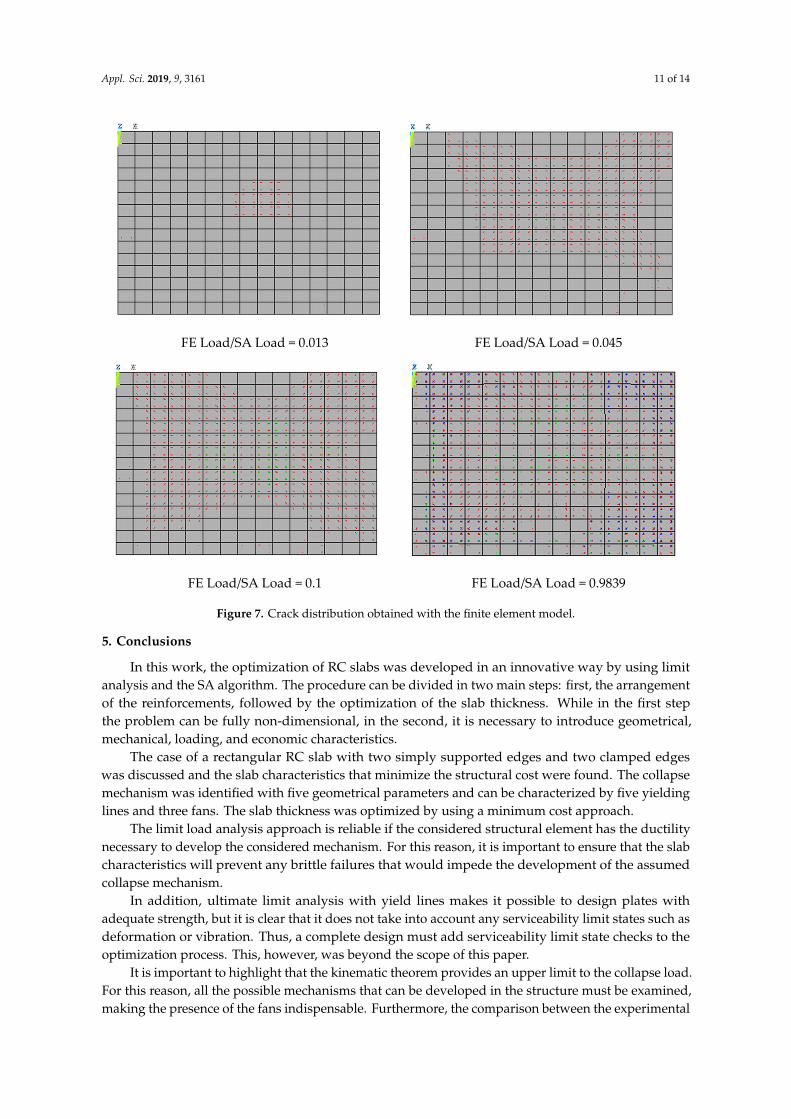
Good agreement between the FE and SA results was found considering the crack patterndistribution reported in Figure 7. Indeed, by comparing Figure 7 with Figure 3, it can be seen how theassumed yield lines distribution was very similar to the crack pattern obtained with finite elements inthe collapse condition.

Appl. Sci. 2019, 9, 3161 11 of 14Appl. Sci. 2019, 9, x FOR PEER REVIEW 11 of 14

FE Load/SA Load = 0.013

FE Load/SA Load = 0.045

FE Load/SA Load = 0.1

FE Load/SA Load = 0.9839

Figure 7. Crack distribution obtained with the finite element model.

5. Conclusions

In this work, the optimization of RC slabs was developed in an innovative way by using limit analysis and the SA algorithm. The procedure can be divided in two main steps: first, the arrangement of the reinforcements, followed by the optimization of the slab thickness. While in the first step the problem can be fully non-dimensional, in the second, it is necessary to introduce geometrical, mechanical, loading, and economic characteristics.

The case of a rectangular RC slab with two simply supported edges and two clamped edges was discussed and the slab characteristics that minimize the structural cost were found. The collapse mechanism was identified with five geometrical parameters and can be characterized by five yielding lines and three fans. The slab thickness was optimized by using a minimum cost approach.

The limit load analysis approach is reliable if the considered structural element has the ductility necessary to develop the considered mechanism. For this reason, it is important to ensure that the slab characteristics will prevent any brittle failures that would impede the development of the assumed collapse mechanism.

In addition, ultimate limit analysis with yield lines makes it possible to design plates with adequate strength, but it is clear that it does not take into account any serviceability limit states such as deformation or vibration. Thus, a complete design must add serviceability limit state checks to the optimization process. This, however, was beyond the scope of this paper.

It is important to highlight that the kinematic theorem provides an upper limit to the collapse load. For this reason, all the possible mechanisms that can be developed in the structure must be examined, making the presence of the fans indispensable. Furthermore, the comparison between the experimental tests and the theoretical results of the limit analysis with the yield lines method

Figure 7. Crack distribution obtained with the finite element model.

5. Conclusions

In this work, the optimization of RC slabs was developed in an innovative way by using limitanalysis and the SA algorithm. The procedure can be divided in two main steps: first, the arrangementof the reinforcements, followed by the optimization of the slab thickness. While in the first stepthe problem can be fully non-dimensional, in the second, it is necessary to introduce geometrical,mechanical, loading, and economic characteristics.

The case of a rectangular RC slab with two simply supported edges and two clamped edgeswas discussed and the slab characteristics that minimize the structural cost were found. The collapsemechanism was identified with five geometrical parameters and can be characterized by five yieldinglines and three fans. The slab thickness was optimized by using a minimum cost approach.

The limit load analysis approach is reliable if the considered structural element has the ductilitynecessary to develop the considered mechanism. For this reason, it is important to ensure that the slabcharacteristics will prevent any brittle failures that would impede the development of the assumedcollapse mechanism.

In addition, ultimate limit analysis with yield lines makes it possible to design plates withadequate strength, but it is clear that it does not take into account any serviceability limit states such asdeformation or vibration. Thus, a complete design must add serviceability limit state checks to theoptimization process. This, however, was beyond the scope of this paper.

It is important to highlight that the kinematic theorem provides an upper limit to the collapse load.For this reason, all the possible mechanisms that can be developed in the structure must be examined,making the presence of the fans indispensable. Furthermore, the comparison between the experimental

Appl. Sci. 2019, 9, 3161 12 of 14

tests and the theoretical results of the limit analysis with the yield lines method confirmed that theapproach is safe and well-founded [50,51], and that the comparison between finite elements and limitanalysis showed very good agreement.

This method can be easily applied to very different structural systems with different loadingand boundary conditions. The main difficulties arise in the definition of the collapse mechanism thatproduces the lowest collapse load.

The simulated annealing algorithm proved to be efficient and reliable in this context. A comparisonwith other heuristic optimization algorithms is projected in future developments of this research.

In conclusion, this method represents an effective procedure for the early design of concrete slabs.

Author Contributions: F.S. conceived the illustrated strategy, the theoretical formulation, and also contributedto the numerical analysis; F.L.G. analyzed the numerical results and contributed to the theoretical formulation.Both authors wrote the paper.

Funding: Financial support received from the Autonomous Region of Sardinia under grant PO-FSE 2014–2020,CCI: 2014-IT05SFOP021 through the project “Retrofitting, rehabilitation and requalification of the historicalcultural architectural heritage (R3-PAS)” is acknowledged by Flavio Stochino. Both authors would also like tothank the support of project BIA2016-78460-C3-2-R that was sponsored by the Spanish Ministry of Economyand Competitiveness.

Conflicts of Interest: The authors declare no conflicts of interest.

References

1. Grierson, D.E. Practical optimization of structural steel frameworks. In Advances Design Optimization;Adeli, H., Ed.; Chapman & Hall: London, UK, 1994; pp. 451–491.

2. Maxwell, C. Scientific Papers; Dover Publications: New York, NY, USA, 1952; Volume 2.3. Schmit, L.A. Structural Design by Systematic Synthesis. In Proceedings 2nd Conference on Electronic Computation;

ASCE: New York, NY, USA, 1960; pp. 105–132.4. Kirkpatrick, S.; Gelatt, C.D.; Vecchi, M.P. Optimization by simulated annealing. Science 1983, 220, 671–680.

[CrossRef] [PubMed]5. Hansen, N.; Arnold, D.V.; Auger, A. Evolution strategies. In Springer Handbook of Computational Intelligence;

Springer: Berlin/Heidelberg, Germany, 2015; pp. 871–898.6. Kicinger, R.; Arciszewski, T.; De Jong, K. Evolutionary computation and structural design: A survey of the

state-of-the-art. Comp. Struct. 2005, 83, 1943–1978. [CrossRef]7. Chisari, C.; Bedon, C. Multi-objective optimization of FRP jackets for improving the seismic response of

reinforced concrete frames. Am. J. Eng. App. Sci. 2016, 9, 669–679. [CrossRef]8. Tran, B.; Xue, B.; Zhang, M. Genetic programming for feature construction and selection in classification on

high-dimensional data. Memet. Comput. 2016, 8, 3–15. [CrossRef]9. Lee, K.S.; Geem, Z.W. A new structural optimization method based on the harmony search algorithm.

Comp. Struct. 2004, 82, 781–798. [CrossRef]10. Huang, X.; Xie, Y.M. Convergent and mesh-independent solutions for the bi-directional evolutionary

structural optimization method. Finite Elem. Anal. Des. 2007, 43, 1039–1049. [CrossRef]11. Liu, X.; Yi, W.J.; Li, Q.S.; Shen, P.S. Genetic evolutionary structural optimization. J. Constr. Steel Res. 2008, 64,

305–311. [CrossRef]12. Quaranta, G.; Fiore, A.; Marano, G.C. Optimum design of prestressed concrete beams using constrained

differential evolution algorithm. Struct. Multidiscip. Optim. 2014, 49, 441–453. [CrossRef]13. Scodeggio, A.; Quaranta, G.; Marano, G.C.; Monti, G.; Fleischman, R.B. Optimization of force-limiting seismic

devices connecting structural subsystems. Comput. Struct. 2016, 162, 16–27. [CrossRef]14. Chatterjee, S.; Sarkar, S.; Hore, S.; Dey, N.; Ashour, A.S.; Balas, V.E. Particle swarm optimization trained

neural network for structural failure prediction of multistoried RC buildings. Neural Comput. App. 2017, 28,2005–2016. [CrossRef]

15. Quaranta, G.; Monti, G.; Marano, G.C. Parameters identification of Van der Pol–Duffing oscillators viaparticle swarm optimization and differential evolution. Mech. Syst. Signal Process. 2010, 24, 2076–2095.[CrossRef]

16. Sarma, K.C.; Adeli, H. Cost optimization of concrete structures. J. Struct. Eng. 1998, 124, 570–578. [CrossRef]

Appl. Sci. 2019, 9, 3161 13 of 14

17. Sassu, M.; Puppio, M.L.; Mannari, E. Seismic reinforcement of a RC school structure with strength irregularitiesthroughout external bracing walls. Buildings 2017, 7, 58. [CrossRef]

18. Puppio, M.; Pellegrino, M.; Giresini, L.; Sassu, M. Effect of material variability and mechanical eccentricityon the seismic vulnerability assessment of reinforced concrete buildings. Buildings 2017, 7, 66. [CrossRef]

19. Giresini, L.; Solarino, F.; Paganelli, O.; Oliveira, D.V.; Froli, M. One-sided rocking analysis of cornermechanisms in masonry structures: Influence of geometry, energy dissipation, boundary conditions.Soil Dyn. Earthq. Eng. 2019, 123, 357–370. [CrossRef]

20. Bruggi, M.; Milani, G.; Taliercio, A. Design of the optimal fiber-reinforcement for masonry structures viatopology optimization. Int. J. Solids Struct. 2013, 50, 2087–2106. [CrossRef]

21. Kouris, L.A.S.; Triantafillou, T.C. State-of-the-art on strengthening of masonry structures with textilereinforced mortar (TRM). Constr. Build. Mater. 2018, 188, 1221–1233. [CrossRef]

22. Gautier, P.E. Slab track: Review of existing systems and optimization potentials including very high speed.Constr. Build. Mater. 2015, 92, 9–15. [CrossRef]

23. Hejazi, F.; Toloue, I.; Jaafar, M.S.; Noorzaei, J. Optimization of earthquake energy dissipation system bygenetic algorithm. Comput. Aided Civ. Infrastruct. Eng. 2013, 28, 796–810. [CrossRef]

24. Martins, A.M.; Simões, L.M.; Negrão, J.H. Optimization of concrete cable-stayed bridges under seismicaction. Comp. Struct. 2019, 222, 36–47. [CrossRef]

25. Xu, G.H. Dynamic Parameter Optimization and Experimental Study of Tuned Slab Damper on Metro Systems.Shock Vib. 2019, 2019, 1–14. [CrossRef]

26. Huang, M. Integrated Structural Optimization and Vibration Control for Improving Dynamic Performance ofTall Buildings. In High-Rise Buildings under Multi-Hazard Environment; Springer: Singapore, 2017; pp. 133–156.

27. Engle, T.; Mahmoud, H.; Chulahwat, A. Hybrid tuned mass damper and isolation floor slab system optimizedfor vibration control. J. Earthq. Eng. 2015, 19, 1197–1221. [CrossRef]

28. Setareh, M.; Ritchey, J.K.; Baxter, A.J.; Murray, T.M. Pendulum tuned mass dampers for floor vibrationcontrol. J. Perform. Constr. Fac. 2006, 20, 64–73. [CrossRef]

29. Lantsoght, E.O.L.; Koekkoek, R.; van der Veen, C.; Sliedrecht, H. Fatigue Assessment of Prestressed ConcreteSlab-Between-Girder Bridges. Appl. Sci. 2019, 9, 2312. [CrossRef]

30. Bielak, J.; Adam, V.; Hegger, J.; Classen, M. Shear Capacity of Textile-Reinforced Concrete Slabs withoutShear Reinforcement. Appl. Sci. 2019, 9, 1382. [CrossRef]

31. Mashrei, M.A.; Mahdi, A.M. An Adaptive Neuro-Fuzzy Inference Model to Predict Punching Shear Strengthof Flat Concrete Slabs. Appl. Sci. 2019, 9, 809. [CrossRef]

32. Francesconi, L.; Pani, L.; Stochino, F. Punching shear strength of reinforced recycled concrete slabs.Constr. Build. Mater. 2016, 127, 248–263. [CrossRef]

33. Fang, J.; Ishida, T.; Yamazaki, T. Quantitative Evaluation of Risk Factors Affecting the Deterioration of RCDeck Slab Components in East Japan and Tokyo Regions Using Survival Analysis. Appl. Sci. 2018, 8, 1470.[CrossRef]

34. Ishida, T.; Pen, K.; Tanaka, Y.; Kashimura, K.; Iwaki, I. Numerical Simulation of Early Age Cracking ofReinforced Concrete Bridge Decks with a Full-3D Multiscale and Multi-Chemo-Physical Integrated Analysis.Appl. Sci. 2018, 8, 394. [CrossRef]

35. Stochino, F.; Pani, L.; Francesconi, L.; Mistretta, F. Cracking of Reinforced Recycled Concrete Slabs. Int. J.Struct. Glass Adv. Mater. Res. 2017, 1, 3–9. [CrossRef]

36. Aldwaik, M.; Adeli, H. Cost optimization of reinforced concrete flat slabs of arbitrary configuration inirregular highrise building structures. Struct. Multidiscip. Optim. 2016, 54, 151–164. [CrossRef]

37. He, L.; Gilbert, M.; Shepherd, M. Automatic yield-line analysis of practical slab configurations via discontinuitylayout optimization. J. Struct. Eng. 2017, 143, 04017036. [CrossRef]

38. Sahab, M.G.; Ashour, A.F.; Toropov, V.V. A hybrid genetic algorithm for reinforced concrete flat slab buildings.Comput. Struct. 2005, 83, 551–559. [CrossRef]

39. Hossain, K.M.A.; Olufemi, O.O. Design optimization of simply supported concrete slabs by finite elementmodelling. Struct. Multidiscip. Optim. 2005, 30, 76–88. [CrossRef]

40. Fraile-Garcia, E.; Ferreiro-Cabello, J.; Martinez-Camara, E.; Jimenez-Macias, E. Optimization based onlife cycle analysis for reinforced concrete structures with one-way slabs. Eng. Struct. 2016, 109, 126–138.[CrossRef]

Appl. Sci. 2019, 9, 3161 14 of 14

41. Ferreiro-Cabello, J.; Fraile-Garcia, E.; Martinez-Camara, E.; Perez-de-la-Parte, M. Sensitivity analysis of LifeCycle Assessment to select reinforced concrete structures with one-way slabs. Eng. Struct. 2017, 132, 586–596.[CrossRef]

42. Ferreiro-Cabello, J.; Fraile-Garcia, E.; de Pison Ascacibar, E.M.; de Pison Ascacibar, F.J.M. Minimizinggreenhouse gas emissions and costs for structures with flat slabs. J. Clean. Prod. 2016, 137, 922–930.[CrossRef]

43. Paya-Zaforteza, I.; Yepes, V.; Hospitaler, A.; Gonzalez-Vidosa, F. CO2-optimization of reinforced concreteframes by simulated annealing. Eng. Struct. 2009, 31, 1501–1508. [CrossRef]

44. Ferreiro-Cabello, J.; Fraile-Garcia, E.; de Pison Ascacibar, E.M.; Martinez-de-Pison, F.J. Metamodel-baseddesign optimization of structural one-way slabs based on deep learning neural networks to reduceenvironmental impact. Eng. Struct. 2018, 155, 91–101. [CrossRef]

45. Mistretta, F.; Stochino, F.; Sassu, M. Structural and thermal retrofitting of masonry walls: An integratedcost-analysis approach for the Italian context. Build. Environ. 2019, 155, 127–136. [CrossRef]

46. Sassu, M.; Stochino, F.; Mistretta, F. Assessment method for combined structural and energy retrofitting inmasonry buildings. Buildings 2017, 7, 71. [CrossRef]

47. Johansen, K.W. Yield-Line Formulae for Slabs; Cement and Concrete Association: London, UK, 1972; p. 106.48. European Committee for Standardization. EN-1992-1-1, Eurocode 2–Design of Concrete Structures; Part 1-1:

General Rules and Rules for Buildings; European Committee for Standardization: Brussels, Belgium, 2008.49. Oldenhuis, R.P. Trajectory Optimization for a Mission to the Solar Bow Shock and Minor Planets. Master’s

Thesis, University of Delft, Delft, The Netherlands, 2010.50. Bailey, C.G. Membrane action of unrestrained lightly reinforced concrete slabs at large displacements.

Eng. Struct. 2001, 23, 470–483. [CrossRef]51. Foster, S.J.; Bailey, C.G.; Burgess, I.W.; Plank, R.J. Experimental behaviour of concrete floor slabs at large

displacements. Eng. Struct. 2004, 26, 1231–1247. [CrossRef]

© 2019 by the authors. Licensee MDPI, Basel, Switzerland. This article is an open accessarticle distributed under the terms and conditions of the Creative Commons Attribution(CC BY) license (http://creativecommons.org/licenses/by/4.0/).