Modeling traveler choice behavior using the concepts of relative utility and relative interest

Transportation Research Part B 38 (2004) 215–234www.elsevier.com/locate/trb

Modeling traveler choice behavior using the conceptsof relative utility and relative interest

Junyi Zhang a,*, Harry Timmermans b, Aloys Borgers b, Donggen Wang c

a Transport Studies Group, Graduate School for International Development and Cooperation, Hiroshima University,

Kagamiyama 1-5-1, Higashi, Hiroshima 739-8529, Japanb Urban Planning Group, Faculty of Architecture, Building and Planning, Eindhoven University of Technology,

P.O. Box 513, 5600 MB Eindhoven, The Netherlandsc Department of Geography, Hong Kong Baptist University, Kowloon Tong, Hong Kong, People’s Republic of China

Received 2 May 2001; received in revised form 18 November 2002; accepted 17 January 2003

Abstract

Individual choice behavior usually involves a complex decision-making process, and is often context-

dependent reflecting the influence of choice environment and the fact that the individual has limited in-

formation processing ability and varying levels of interest in alternatives. However, the existing models intransportation have not represented these behavioral mechanisms satisfactorily, although to avoid the

Independence of Irrelevant Alternatives (IIA) property of the widely used multinomial logit (MNL) model,

a variety of non-IIA models have been suggested in the literature. This paper will propose another random

utility choice model by introducing the concepts of relative utility and relative interest. A revised MNL

model and a revised Nested-MNL model will be developed. Both of these models do not have the IIA

property. The performance of these new models will be assessed using conjoint-based activity diary data

about the choice of destination and stop pattern.

� 2003 Elsevier Ltd. All rights reserved.

Keywords: Relative utility; Relative interest; Context dependence; IIA property; r-MNL model; r-NL model

1. Introduction

During the last two decades, choice models have proven to be very powerful tools for policyanalysis and evaluation in transportation research. The multinomial logit (MNL) model,

* Corresponding author. Tel./fax: +81-824-24-6919.

E-mail address: [email protected] (J. Zhang).

0191-2615/$ - see front matter � 2003 Elsevier Ltd. All rights reserved.

doi:10.1016/S0191-2615(03)00009-2

mail to: [email protected]

216 J. Zhang et al. / Transportation Research Part B 38 (2004) 215–234

characterized by the Independence of Irrelevant Alternatives (IIA) property, has become the mostwidely used choice model in transportation. Convincing examples have been put forward howeverto show that the IIA property is counterintuitive in many real choice situations. Thus, the de-velopment of non-IIA choice models has become a major methodological challenge in the study ofindividual choice behavior since the late 1970s in many disciplines. In transportation, the interestin developing the non-IIA models seems to have faded slightly as a result of the emerging field ofactivity-based models of travel demand, but recently a renewed interest is visible (e.g., see Wenand Koppelman, 2000).On the other hand, individual choice behavior usually involves a complex decision-making

process. Individuals utilize different heuristics that will keep the information processing demandswithin the bounds of their limited capacity (Payne, 1976). A wealth of literature in behavioraldecision theory and psychology has shown that task complexity and choice environment affectindividual choice behavior (Rushton, 1969; Swait and Adamowicz, 2001a). However, most of theexisting models in transportation typically do not account for the effect of this kind of contextdependence.This paper therefore suggests an alternative random utility choice model based on the concepts

of relative utility and relative interest. The concept of relative utility assumes that utility ismeaningful only relative to some reference point(s). It acknowledges the fact that the individualchoice behavior is context-dependent. The concept of relative interest stems from multiple-issuegroup decision-making theory (Coleman, 1973; Gupta, 1989), which argues that actors involvedin negotiations are usually more interested in one issue than in another.The remainder of this paper is organized as follows. First, to position the suggested choice

model, Section 2 briefly reviews existing choice models with context dependence and other non-IIA choice models. Following that, Section 3 discusses the relative utility theorem, which providesthe theoretic and behavioral basis for the new models. Section 4 then develops equivalents to thewidely used MNL and NL models based on the concepts of relative utility and relative interest.These models were estimated in the context of the choice of destination and stop pattern. Section5 describes the conjoint-based activity diary data for the model estimation as well as the esti-mation results. Finally, Section 6 concludes this study and discusses some future research.

2. Review of existing choice models

Traditional random utility maximization theory assumes that individuals choose the alternativewith the highest utility, independent of context and learning etc. This is also true for most of theexisting models in transportation. However, there is a wealth of literature in psychology andbehavioral decision sciences, showing counter-evidence. Simonson and Tversky (1992) arguedthat context effects are both common and robust, representing the rule rather than the exceptionin choice behavior. Non-IIA models are required to capture such effects. Timmermans andGolledge (1990) classified the existing non-IIA choice models into three categories. The first groupof non-IIA models avoids the IIA property by relaxing the assumption of identically and inde-pendently distributed error terms. The second group circumvents the IIA property by extendingthe utility specification to account explicitly for similarity between alternatives. The third groupassumes a hierarchical decision-making process.

J. Zhang et al. / Transportation Research Part B 38 (2004) 215–234 217

2.1. Choice models with context dependence

2.1.1. The definition of context dependence

Choice behavior is highly adaptive and context-dependent from a psychological viewpoint(McFadden, 2001). There exists however no unified and widely acknowledged definition aboutcontext dependence in the sense that it is described inconsistently in different disciplines. Tverskyand Simonson (1993) classified the context into background context and local context, where theformer refers to previous choice results and the latter to the choice set. Oppewal and Timmermans(1991) grouped the context into choice set composition and background, where the latter refers tocircumstantial factors, such as tax levels in housing choice and trip purposes in mode choice.Kahneman et al. (1991) and Tversky and Kahneman (1991) argued that choice behavior is de-pendent on status quo or reference point(s) and empirically confirmed that change of referencepoint might lead to preference reversal.The above-mentioned discussion suggests that the context refers to the pre-conditions of the

decision-making. As an initial attempt to unify the definition of the context dependence, here were-classify these pre-conditions into three categories: (1) alternative-specific context, (2) circum-

stantial context and (3) individual-specific context. The alternative-specific context includes thenumber of alternatives and their attributes, the correlated structure of attributes and the avail-ability of alternatives. The background context defined by Oppewal and Timmermans belongs tothe circumstantial context. This context can also include the status quo of choice over a popu-lation. The individual-specific context refers to the individuals� choice history, household orworkplace attributes, and the cognitive status quo of the reference group such as the car own-ership of their neighbors and acquaintances.

2.1.2. Choice complexity and individual information-processing ability

Choice behavior is a complex decision making process and highly adaptive to the demands ofthe task. Therefore, no single heuristic does well across all tasks and context conditions (Payneet al., 1988). When the complexity (defined by the number of alternatives, number of attributes,correlation between attributes etc.) in choice tasks increases, decision makers usually use simple,local and myopic choice strategies (Olshavsky, 1979; Payne et al., 1988, 1993; De Palma et al.,1994). This observation has given rise to information-processing theories of choice, which aredominant in the behavioral sciences. It is also pointed out that decision makers will choose thestrategy to delay choice, seek new alternatives, or even revert to status quo option when the choiceenvironment is made complex (Dhar, 1997a,b).

2.1.3. Relevant choice models with context dependence

Swait and Adamowicz (2001a) proposed a latent class model of decision strategy switching torepresent the influence of task complexity on consumer choice. Swait and Adamowicz (2001b)developed a theoretical model that simultaneously considers task complexity, the amount of effortapplied by the consumer, ability to choose, and choice. By using the data from conjoint-basedexperiment, Oppewal and Timmermans (1991) applied mother logit model (McFadden et al.,1977) to estimate context effects in the choice of housing, shopping center and transportationmodes. Anderson et al. (1992) developed a similar model to represent attribute-cross effects andavailability-cross effects in a study of mode choice.


Gaudry and Dagenais (1979) proposed a dogit model to avoid the IIA property by introducingnon-negative alternative-specific parameters to represent substitution/similarity effects. Borgersand Timmermans (1988) developed a context-sensitive model of spatial choice behavior to capturesubstitution/similarity effects as well as spatial structure effects.

2.2. Non-IIA choice models

2.2.1. Non-IIA models with more general variance–covariance matrixModels belonging to this category differ in terms of their assumptions about the type of dis-

tribution of the error terms and the assumptions on the variance–covariance structure of errorterms. The relevant models include McFadden�s (1978) generalized extreme value (GEV) model,Hausman and Wise�s (1978) conditional probit model, multinomial probit model (Daganzo,1979), heteroscedastic extreme value model (Bhat, 1995), and mixed logit/probit model (Brown-stone et al., 2000).

2.2.2. Non-IIA models with a hierarchical decision structure

The best-known model with a hierarchical decision structure is the NL model (Ben-Akiva andLerman, 1987), which is a special case of McFadden�s GEV model. Other types of such modelshave also been derived from the GEV model, including PCL model, CNL model, OGEV model,PD model and GNL model (Wen and Koppelman, 2000). Recently, nested PCL model was de-veloped by Fujiwara et al. (2000). Especially, the GNL model can include the above-mentionedmodels and the MNL model as special cases and closely approximates the NL model. A com-pletely different approach is Tversky�s (1972) elimination by aspects model. This model is one ofnon-compensatory models, however, cannot be easily operationalized and calibrated for thepurpose of real-world prediction.Most of the models described in this section assume that choice behavior is compensatory.

These models allow a low score on some attribute to be at least partially compensated by highscores of one or more remaining attributes. In contrast, non-compensatory models assume thatindividuals screen choice alternatives on an attribute-by-attribute basis when arriving at a choiceor decision. Since this paper only treats compensatory models, the non-compensatory models arenot further reviewed here.

3. Relative utility and relative interest

3.1. The concept of relative utility

The concept of relative utility has its roots in the research about income (Stadt et al., 1985).Duesenberry�s (1949) relative income hypothesis is probably the best-known example of a theorythat rests on the concept of relative utility. Kapteyn (1977) developed a theory of preferenceformation, which assumed that utility was completely relative. Before continuing the discussion, itis necessary to define the concept of relative utility. We argue that an individual evaluates analternative by comparing it to other alternatives, or perhaps to the alternatives the individualchose in the past, or to alternatives chosen by other individuals. More specifically, the following


three types of relative utilities can be defined, dependent on whether it focuses on an alternative(j), an individual (i), or time (t).

3.1.1. Type AThis type of relative utility Uij;t is defined with respect to alternatives, as a function of the utility

uij;t of alternative j and the utility uij0;tfj0 6¼ jg of all other alternatives in the choice set.
Uij;t ¼ f fuij;tjðuij0;t : 8j0 6¼ jÞg ð1Þ
3.1.2. Type B

This type of relative utility focuses on both alternatives and time. The relative utility Uij;t isdefined as a function of uij;t and uij0;t0 , where t0 refers to the previous point of time.

Uij;t ¼ f fuij;tjðuij0;t0 : t0 < t and 8j0Þg ð2Þ

3.1.3. Type C

This type of relative utility Uij;t is defined as a function of uij;t and ui0j0;t, with respect to bothindividuals and alternatives, where i0 refers to a social reference group for individual i.

Uij;t ¼ f fuij;tjðui0j0;t : i0 2 social reference groupÞg ð3Þre, we only deal with the first type of relative utility and develop the model structure at the
He
individual level in a given point of time. Henceforth, we do not use subscript i; t for the sake ofsimplifying the equations. We propose the following operational relative utility, defined by addingall the differences of standard utilities between alternative j in question and all other alternativej0ðj0jj0 6¼ jÞ.X

Uj ¼j0 6¼j

ðuj � uj0 Þ ð4Þ

nsidering that the relative utility Uj is defined as the difference of standard utilities and the
Cofact that the smaller the difference between the attributes of two alternatives, the similar the twoalternatives, Uj can be also used to represent the alternative similarity. Furthermore, it can beinterpreted that Uj regards the standard utilities of all other alternatives except for the alternativej of interest as the reference points, which is suggested by Tversky and Simonson (1993).Therefore, we can adopt this concept of relative utility as an alternative means of representingcontext dependence in choice models.
3.2. The concept of relative interest

Conventional choice models assume that individuals recognize different alternatives in thechoice set equally. This assumption can be easily violated in real situations since individuals areusually more interested in one alternative than in another. To describe collective actions (i.e.group decision-making), Coleman (1973) provided a definition of the interest to represent groupdecision-making. Coleman first defined an index rij, called relative utility difference, as follows:

rij ¼ ðuij1 � uij2ÞXj

juij1

,� uij2 j ð5Þ


where uij1 represents the utility of actor i taking action on event j and uij2 does the utility of noaction.Coleman suggests the absolute value jrijj to be the actor�s interest in the event. The interest of an

actor in an event refers to the importance of the outcome (action or no action) for him/her. Thescaling

Pj jrijj ¼ 1 implies that jrijj is actor i�s relative interest in event j.

Gupta (1989) modified Coleman�s (1973) definition of relative interest by removing the absolutefunction expression from the original formula as follows:

rij ¼ ðu1ij � u0ijÞXj

ðu1ij

,� u0ijÞ ð6Þ

where u1ij is the utility from the most preferred outcome for the event j, u0ij is the utility from the

least preferred outcome for event j, 06 rij 6 1 andP

j jrijj ¼ 1.Coleman and Gupta applied their definitions to represent the relative influence of each actor

involved in the group decision making, however, their definitions are difficult to be directly ap-plied in the utility-based choice model. Therefore, we propose adopting another modeling strat-egy, as described later. Let rj define the relative interest of individual i in alternative j. We proposeusing the following relative utility considering the relative interest as a new choice rule instead ofstandard utility uj.

Uj ¼ rjXj0 6¼j

ðuj � uj0 Þ ð7Þ

To simplify the interpretation of the concept of relative interest, it is assumed here that rj P 0. Thegreater the relative interest, the more important the individual regards the choice of the alternativein question, vice versa. Henceforth, we simply call Uj in Eq. (7) the relative utility. Then, we cansummarize the foregoing specification as the principle of relative utility maximization.

The principle of relative utility maximization: An individual is assumed to choose an alternativewith the highest relative utility considering his/her relative interests in alternatives from his/herchoice set, where the relative utility reflects the context-dependence and the relative interestrepresents the relative importance of different alternatives.By assuming all the relative interest parameters to be equal, the relative utility maximization

comes to the maximization of standard utility (Relative utility theorem). The reader can find theproof about this theorem in Appendix A. This implies that the choice models based on relativeutility can include those based on the standard utility as special cases.

Relative utility theorem: Maximization of relative utility is equal to the maximization ofstandard utility if individuals regard all the alternatives in the choice set equally.

3.3. Redefining the utility function

Assume that the relative utility Uj consists of a deterministic term Vj and an error term ej asfollows, where mj describes the influence of alternative j and mj0 represents the influence of otheralternatives.

Uj ¼ rjXj0 6¼j

ðuj � uj0 Þ ¼ Vj þ ej ¼ rjXj0 6¼j

ðmj � mj0 Þ þ ej ð8Þ


Eq. (8) assumes that analysts know the relative utility is a linear combination of deterministicterm and error term, but do not know exactly about the standard utility since the utility is arelative concept and meaningful only in the presence of some reference point(s). Then, the choiceprobability can be expressed as follows:

Pj ¼ ProbfUj > Uj0 ; 8j0 6¼ jg ¼ ProbfVj þ ej > Vj0 þ ej0 ; 8j0 6¼ jg ð9Þ

Different assumptions on the error terms lead to different choice models. This definition ofrelative utility provides an alternative way of representing substitution/similarity effects and hastwo important features. First, it introduces the influence of other alternatives on the utility of thealternative under consideration based on the utility comparisons as opposed to adding the utilityof other alternatives. Second, it does not impose any extra restriction on the error terms comparedwith most of the existing non-IIA models. In this sense, this relative utility can be directly in-corporated into almost all of the existing choice models, to represent substitution/similarity ef-fects.

4. A new family of choice models based on the concepts of relative utility and relative interest

Although all of the three classes of non-IIA choice models, reviewed in Section 2, do not havethe IIA property, each class of models has its own shortcomings and unresolved problems.Concerning the first class of non-IIA choice models, there is no way to know exactly what kind ofspecification will really reflect the real structure and/or distribution of error terms. One can onlyverify an assumed specification based on empirical analysis. Most importantly however, this classof models has no immediate behavioral interpretation. While the second class of models canrepresent the context dependence in a straightforward manner, their theoretical underpinningslargely remain unexplored. The theoretical weakness of the third class of models concerns the lackof any clear behavioral guidelines on how to segment the choice set. Moreover, when the nestingstructure is heterogeneous across a population, the modeling process becomes more complicated.The introduction of the concepts of relative utility and relative interest can be expected to

provide an alternative approach of relaxing the above-mentioned issues.

4.1. Revising the MNL model

4.1.1. Derivation of relative utility based choice model

If it is further assumed that the error terms in Eq. (8) follow an independent and identicalWeibull distribution across all alternatives and individuals, a revised MNL model can be obtainedbelow.

Pj ¼ ProbfVj þ ej >MaxðVj0 þ ej0 Þ;8j0 6¼ jg ¼ expfrjVjgPk expfrkVkg

¼exp rj

Pj0 6¼jðmj � mj0 Þ

n oP

k exp rkP

k0 6¼kðmk � mk0 Þn o ð10Þ


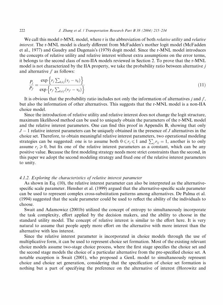
We call this model r-MNL model, where r is the abbreviation of both relative utility and relativeinterest. The r-MNL model is clearly different from McFadden�s mother logit model (McFaddenet al., 1977) and Gaudry and Dagenais�s (1979) dogit model. Since the r-MNL model introducesthe concepts of relative utility and relative interest without extra assumptions on the error terms,it belongs to the second class of non-IIA models reviewed in Section 2. To prove that the r-MNLmodel is not characterized by the IIA property, we take the probability ratio between alternative jand alternative j0 as follows:

PjPj0

¼exp rj

Pk 6¼jðmj � mkÞ

n oexp rj0

Pk 6¼j0 ðmj0 � mkÞ

n o ð11Þ

It is obvious that the probability ratio includes not only the information of alternatives j and j0,but also the information of other alternatives. This suggests that the r-MNL model is a non-IIAchoice model.Since the introduction of relative utility and relative interest does not change the logit structure,

maximum likelihood method can be used to uniquely obtain the parameters of the r-MNL modeland the relative interest parameters. One can find this proof in Appendix B, showing that onlyJ � 1 relative interest parameters can be uniquely obtained in the presence of J alternatives in thechoice set. Therefore, to obtain meaningful relative interest parameters, two operational modelingstrategies can be suggested: one is to assume both 06 rj 6 1 and

Pj rij ¼ 1, another is to only

assume rj P 0, but fix one of the relative interest parameters as a constant, which can be anypositive value. Because the first modeling strategy needs more strict constraints than the second, inthis paper we adopt the second modeling strategy and fixed one of the relative interest parametersto unity.

4.1.2. Exploring the characteristics of relative interest parameterAs shown in Eq. (10), the relative interest parameter can also be interpreted as the alternative-

specific scale parameter. Hensher et al. (1999) argued that the alternative-specific scale parametercan be used to represent complex cross-substitution patterns among alternatives. De Palma et al.(1994) suggested that the scale parameter could be used to reflect the ability of the individuals tochoose.Swait and Adamowicz (2001b) utilized the concept of entropy to simultaneously incorporate

the task complexity, effort applied by the decision makers, and the ability to choose in thestandard utility model. The concept of relative interest is similar to the effort here. It is verynatural to assume that people apply more effort on the alternative with more interest than thealternative with less interest.Since the relative interest parameter is incorporated in choice models through the use of

multiplicative form, it can be used to represent choice set formation. Most of the existing relevantchoice models assume two-stage choice process, where the first stage specifies the choice set andthe second stage models the choice of a particular alternative from the pre-specified choice set. Anotable exception is Swait (2001), who proposed a GenL model to simultaneously representchoice and choice set generation, considering that the specification of choice set formation isnothing but a part of specifying the preference on the alternative of interest (Horowitz and


Louviere, 1995). The relative interest parameter is also similar to the independent availability forchoosing alternatives, which was defined by Swait and Ben-Akiva (1987). In line with this researchdirection, the r-MNL model can be used to implement choice set formation endogenously, byappropriately defining the relative interest parameter.As discussed above, the relative interest parameter has great potential and its characteristics

should be examined empirically in various choice circumstances. In this paper, however, we donot further elaborate the discussion, but directly estimate it as one parameter. We leave the furthertheoretical discussion and empirical examination of the relative interest parameter as a futureresearch issue.

4.2. Revising the NL model

Since the r-MNL model is a non-IIA choice model, it can be expected to explain some choiceissues described in the NL model. However, in case that a hierarchical decision-making process isdeemed preferable, the relative utility can be easily used to represent the interdependence betweenalternatives in the same nest. The NL model can be written as follows:

Pdm ¼ Pdjm Pm ¼ eðvdþvdmÞPd 0 e

ðvd0þvd0mÞelðvmþv0mÞPm0 e

lðvm0þv0m0 Þ

ð12Þ

v0m ¼ lnXd 0eðvd0þvd0mÞ

!and 0 < l6 1 ð13Þ

where vd , vm and vdm are the non-stochastic terms of utility function specific to alternative d inchoice set Dm, alternative m in choice set M and the combination of these two choice facets, re-spectively.Introducing the relative utility defined in Eq. (8) into Eqs. (12) and (13), one can obtain the

following revised NL model, which is called r-NL model in this paper.

Pdjs ¼exp cd

Pd 0 6¼dððmd þ mdsÞ � ðmd 0 þ md 0sÞÞ

� P

d 0 exp cd 0P

d 00 6¼d 0 ððmd 0 þ md 0sÞ � ðmd 00 þ md 00 sÞÞ� n o ð14aÞ

Ps ¼exp lcs

Ps0 6¼sððms þ m0sÞ � ðms0 þ m0s0 ÞÞ

� P

s0 exp lcs0P

s00 6¼s0 ððms0 þ m0s0 Þ � ðms00 þ m0s00ÞÞ

� n o ð14bÞ

m0s ¼ lnXd

exp cdXd 0 6¼d

ððmd

0@

0@ þ mdsÞ � ðmd 0 þ md 0sÞÞ

1A1A and 0 < l6 1 ð14cÞ

Since the r-NL model incorporates the similarity effects explicitly and also assumes a hierarchicaldecision-making process, it belongs to both the second and the third class of non-IIA modelsreviewed in Section 2. The r-NL model can be estimated using the maximum likelihood method.


5. Empirical analysis

5.1. Data

To examine the effectiveness of the r-MNL and r-NL models, a conjoint-based activity data set(Wang et al., 2000), collected in the Netherlands in 1997 for analyzing the choice of destinationand stop pattern, was used. In the experiment, the respondents had to decide where, when, in whatsequence and according to what types of home-based tours the activities would be conducted. Theattributes assumed to influence the choices of destination and stop pattern are listed in Tables 1and 2. Two alternatives are respectively prepared for the choice of destination and the choice of

Table 1

Attributes and their levels: choice of destination

Attributes Levels

Accessibility of destination

T_HM-WK: Travel time between home and work place 1. 0–15 (min)

T_HM-SH: Travel time between home and shopping center 2. 16–29 (min)

T_HM-SP: Travel time between home and sport center 3. 30-more (min)

T_WK-SH: Travel time between work place and shopping center

T_WK-SP: Travel time between work place and sport center

T_SH-SP: Travel time between shopping center and sport center

Attractiveness of destination

OPEN_SH: Opening hours of shopping center 1. 9:00–18:00

2. 8:00–18:00

3. 9:00–21:00

SIZE_SH: Size of shopping center 1. Small

2. Medium

3. Large

PARK_SH: Parking convenience of shopping center 1. Ample parking available

PARK_SP: Parking convenience of sport center 2. Ample parking available except for rush

hours when it is difficult to find parking

spaces

3. Parking spaces often occupied

OPEN_SP: Opening hours of sport center 1. 8:00–23:00

2. 7:00–19:00

3. 7:00–21:00

Table 2

Attributes and their levels: choice of stop pattern

Attributes Levels

N_TOUR: Number of home-based tours 1. 1 tours

2. 2 tours

3. 4 tours

Timing_SH: Timing of shopping activity 1. Before morning work

Timing_SP: Timing of sport activity 2. Between morning and afternoon work

3. After afternoon work

Table 3

Illustration of orthogonal coding scheme

Levels of the attribute Vector 1 Vector 2

Level 1 )1 1

Level 2 0 )2Level 3 1 1


stop pattern, i.e. A, B for destinations and, C, D for stop patterns. A single orthogonal fraction ofthe 32�14 factorial design consisting of 81 profiles was constructed. To reduce the respondents�burden, the 81 profiles were grouped into nine balanced blocks. Each respondent received onlyone block of nine profiles and was asked to choose one alternative from five predefined alter-natives, i.e., (1) A–C, (2) A–D, (3) B–C, (4) B–D, and (5) base alternative referring to that therespondents prefer none of the possible combinations.Questionnaires were distributed by surface mail to 1400 households located across the Neth-

erlands. As a result, 335 usable questionnaires were obtained for this study. Since categoricalattributes are adopted in the experiment, their levels (three levels for each attribute) need to becoded before model estimation. There are three types of coding schemes that are normally used:dummy coding, effect coding and orthogonal coding (Kerlinger and Pedhazur, 1973). The last isadopted here as shown in Table 3, where vector 1, called linear effect, is used to capture thecontrast between levels 1 and 3, and vector 2, called quadratic effect, is used to capture thecontrast between the average of levels 1 and 3, and level 2.The following logarithm likelihood function was used to estimate the choice models in this

paper.

Lm ¼Xi

Xj

Xk

dij;k lnðPmij;kÞ ð15Þ

where dij;k is the dummy variable at the profile k, which is equal to 1 when traveler i choosesalternative j, otherwise 0; Pm

ij;k is the choice probability at the profile k expressed in the model m(m¼MNL, r-MNL, NL and r-NL models).The estimation results for the MNL and r-MNL models are shown in Table 4, those for the NL

and r-NL models are shown in Table 5. For the sake of comparison, the MNL and NL modelswere estimated by assuming that all relative interest parameters are equal to unity in the r-MNLand r-NL models.

5.2. Comparison of MNL model and r-MNL model

5.2.1. Goodness-of-fit indicesAs indicated by McFadden�s Rho-squared and adjusted Rho-squared, both the MNL and

r-MNL models provide statistically high goodness-of-fit indices. In order to judge if these twomodels are significantly different, the v2 statistic is calculated based on the values of finallogarithm likelihood in Table 4.

v2 ¼ �2fLLðb_

MNLÞ � LLðb̂br-MNLÞg ¼ 27:02 > v2ð4; 0:01Þ ¼ 13:28 ð16Þ

Table 4

Estimation results for MNL and r-MNL models

Parameters MNL model� r-MNL model Ratio of

parameters

(r-MNL/

MNL)

Estimate

parameter

t-Statistic Estimate

parameter

t-Statistic

Constant term )7.199E)02 )8.109 )7.248E)02 )8.449 1.007

T_HM-WK: Linear effect )7.990E)02 )11.343 )6.824E)02 )8.081 0.854

T_HM-WK: Quadratic effect )1.797E)03 )0.449 )5.100E)04 )0.152 0.284

T_HM-SH: Linear effect )7.373E)02 )10.45 )6.260E)02 )7.650 0.849

T_HM-SH: Quadratic effect 1.998E)02 4.930 1.718E)02 4.621 0.860

T_HM-SP: Linear effect )4.868E)02 )6.889 )4.458E)02 )6.325 0.916

T_HM-SP: Quadratic effect )1.880E)03 )0.472 )2.430E)03 )0.716 1.293

T_WK-SH: Linear effect )4.539E)02 )6.355 )3.674E)02 )5.237 0.809

T_WK-SH: Quadratic effect )3.701E)03 )0.949 )3.740E)03 )1.141 1.010

T_WK-SP: Linear effect )3.841E)02 )5.548 )3.388E)02 )5.048 0.882

T_WK-SP: Quadratic effect 4.174E)03 1.041 4.700E)03 1.358 1.126

T_SH-SP: Linear effect )3.509E)02 )4.889 )3.025E)02 )4.687 0.862

T_SH-SP: Quadratic effect )7.883E)03 )1.913 )7.240E)03 )2.078 0.918

OPEN_SH: Linear effect 1.153E)02 1.672 1.003E)02 1.700 0.870

OPEN_SH: Quadratic effect 1.641E)04 0.042 )1.260E)03 )0.382 )7.678SIZE_SH: Linear effect 2.327E)02 3.363 2.348E)02 3.680 1.009

SIZE_SH: Quadratic effect )3.343E)03 )0.848 )3.610E)03 )1.084 1.080

PARK_SH: Linear effect )1.253E)02 )1.840 )1.040E)02 )1.797 0.830

PARK_SH: Quadratic effect 6.956E)03 1.747 5.430E)03 1.627 0.781

OPEN_SP: Linear effect 9.272E)04 0.134 2.500E)04 0.044 0.270

OPEN_SP: Quadratic effect 6.679E)03 1.659 5.870E)03 1.723 0.879

PARK_SP: Linear effect )1.177E)02 )1.705 )8.160E)03 )1.367 0.693

PARK_SP: Quadratic effect 1.912E)03 0.486 )2.200E)04 )0.068 )0.115N_TOUR: Linear effect )7.707E)02 )10.42 )6.703E)02 )7.390 0.870

N_TOUR: Quadratic effect )2.637E)02 )6.603 )2.218E)02 )5.405 0.841

Timing_SH: Linear effect 5.175E)02 7.271 4.310E)02 5.894 0.833

Timing_SH: Quadratic effect 1.233E)02 2.970 9.310E)03 2.532 0.755

Timing_SP: Linear effect 1.062E)01 15.25 8.841E)02 8.070 0.833

Timing_SP: Quadratic effect 5.344E)02 12.29 4.467E)02 7.338 0.836

Relative interest parameter of A–C alternative�� 1.41061 2.235a

Relative interest parameter of A–D alternative�� 1.19441 1.207a

Relative interest parameter of B–C alternative�� 0.89781 0.696a

Relative interest parameter of B–D alternative�� 1.39552 2.243a

Initial logarithm likelihood: LLð0Þ )4849.20 )4849.20Final logarithm likelihood: LLðb̂bMNLÞ andLLðb̂br-MNLÞ

)4293.36 )4279.85

Likelihood ratio test 1111.68 1138.70

McFadden�s Rho-squared 0.11463 0.11741

Adjusted McFadden�s Rho-squared 0.11249 0.11499*MNL model was estimated by assuming all of relative interest parameters equal to 1 in r-MNL model.** The relative interest parameter for the base alternative is predefined as unity.a t-Statistic for the relative interest parameter is calculated with respect to 1.


Table 5

Estimation results for NL and r-NL models

Parameters NL model� r-NL model Ratio of

parameters

(r-NL/NL)

Estimate

parameter

t-Statistic Estimate

parameter

t-Statistic

Constant term )8.158E)02 )0.987 )3.820E)02 )0.404 0.468

T_HM-WK: Linear effect )2.506E)01 )11.65 )2.883E)01 )5.567 1.151

T_HM-WK: Quadratic effect 5.179E)03 0.447 6.514E)03 0.487 1.258

T_HM-SH: Linear effect )2.219E)01 )10.46 )2.517E)01 )5.752 1.134

T_HM-SH: Quadratic effect 6.950E)02 5.966 7.831E)02 4.681 1.127

T_HM-SP: Linear effect )1.613E)01 )7.485 )1.842E)01 )4.690 1.142

T_HM-SP: Quadratic effect )1.176E)02 )0.996 )1.406E)02 )1.029 1.196

T_WK-SH: Linear effect )1.290E)01 )6.117 )1.486E)01 )4.442 1.152

T_WK-SH: Quadratic effect )1.796E)02 )1.564 )2.157E)02 )1.544 1.201

T_WK-SP: Linear effect )1.171E)01 )5.767 )1.377E)01 )4.334 1.176

T_WK-SP: Quadratic effect 2.264E)03 0.190 1.316E)03 0.097 0.581

T_SH-SP: Linear effect )1.160E)01 )5.631 )1.318E)01 )4.338 1.136

T_SH-SP: Quadratic effect )1.704E)02 )1.424 )1.808E)02 )1.301 1.061

OPEN_SH: Linear effect 2.963E)02 1.526 3.323E)02 1.466 1.121

OPEN_SH: Quadratic effect )1.188E)03 )0.103 )2.734E)03 )0.205 2.301

SIZE_SH: Linear effect 5.495E)02 2.747 6.349E)02 2.577 1.155

SIZE_SH: Quadratic effect )2.939E)03 )0.257 )4.112E)03 )0.312 1.399

PARK_SH: Linear effect )2.982E)02 )1.507 )3.507E)02 )1.482 1.176

PARK_SH: Quadratic effect 2.876E)02 2.518 3.398E)02 2.431 1.182

OPEN_SP: Linear effect 1.863E)02 0.911 2.520E)02 1.030 1.353

OPEN_SP: Quadratic effect 2.666E)02 2.309 2.994E)02 2.176 1.123

PARK_SP: Linear effect )4.074E)02 )2.061 )4.510E)02 )1.883 1.107

PARK_SP: Quadratic effect 2.865E)03 0.255 2.959E)03 0.230 1.033

N_TOUR: Linear effect )1.327E)01 )10.91 )1.764E)01 )7.939 1.330

N_TOUR: Quadratic effect )4.605E)02 )6.930 )6.404E)02 )5.674 1.391

Timing_SH: Linear effect 8.626E)02 7.404 1.154E)01 6.076 1.338

Timing_SH: Quadratic effect 1.801E)02 2.621 2.710E)02 2.704 1.505

Timing_SP: Linear effect 1.773E)01 15.36 2.453E)01 8.390 1.384

Timing_SP: Quadratic effect 8.849E)02 12.31 1.236E)01 7.853 1.396

Parameter of inclusive value 2.516E)01 2.465 2.384E)01 2.052

Relative interest parameter of B destination�� 0.74871 0.968a

Relative interest parameter of C stop pattern�� 0.61573 4.019a

Relative interest parameter of D stop pattern�� 0.73158 2.605a

Initial logarithm likelihood: LLð0Þ )4880.10 )4880.10Final logarithm likelihood: LLðb̂bNLÞ andLLðb̂br-NLÞ

)4272.96 )4267.82

Likelihood ratio test 1214.28 1224.56

McFadden�s Rho-squared 0.12441 0.12546

Adjusted McFadden�s Rho-squared 0.12223 0.12306*NL model was estimated by assuming all of relative interest parameters equal to 1 in r-NL model.** The relative interest parameter for A destination is predefined as unity.*** The relative interest parameter for the alternative of base stop pattern: neither C nor D.a t-Statistic for the relative interest parameter is calculated with respect to 1.



Since the value 27.02 of this v2 statistic is larger than the critical value 13.28 (freedom is 4, thenumber of estimated relative interest parameters) at the 99% level of significance, the r-MNLmodel is superior to the MNL model in explaining the simultaneous choices of destination andstop pattern.

5.2.2. Relative interest parameters

In the r-MNL model, the relative interest parameter for the base alternative is predefined asunity before the model estimation. The t-test results, on whether the estimated relative interestparameters are different from 1 or not, can be found in Table 4. The alternatives A–C and B–Dare statistically different from 1 at the 95% level of significance. Since the values of relative interestparameters distribute over a large range (the maximal value is 1.57 times larger than the minimalone), at least, we can conclude that not all the values of relative interest parameters are equal.With respect to why the relative interest parameters for the alternatives A–C and B–D are

larger than the others, we can give two possible reasons: one is because the respondents might bemore familiar with or have more experiences about these two alternatives, another is because therespondents might harbor greater expectations about the two alternatives (i.e. activity patterns).For some respondents, both reasons might apply. We leave the further discussion as one of thefuture research issues because confirming these reasons needs some new modelling approaches.

5.2.3. Other parametersConcerning the choice of stop pattern, all of the parameters about linear-effect and quadratic-

effects are statistically significant in both models. This implies that the utility changes for theseattributes are not linear. In the case of destination choice, all of the parameters of travel time arereasonably negative and statistically significant regarding their linear effects. As for the attrac-tiveness indicators, only the linear-effect parameter for the size of shopping center is significant.To make clear how different the parameters of explanatory variables in the r-MNL and MNL

models are, we show the ratio between the parameters of explanatory variables of the two modelsin the last column of Table 4. It is obvious that 22 out of total 29 parameters in the r-MNL modelare smaller than the ones in the MNL model. This is caused by the introduction of relative utilityand relative interest.

5.3. Comparison of NL model and r-NL model

To describe the nested choices of destination and stop pattern, two model structures can beassumed: (1) the choice of destination nested under the choice of stop pattern, (2) the choice ofstop pattern nested under the choice of destination. The estimation results of the NL modelsuggest that only the first case is reasonable because the estimated parameter of the inclusive valueis between 0 and 1. The estimated parameters of the r-NL suggest that both structures are rea-sonable. Since the r-NL model for the first case has a higher goodness-of-fit index, the corre-sponding estimation results are shown in Table 5.

5.3.1. Goodness-of-fit indicesSimilar to the MNL and r-MNL models, the NL and r-NL models also have high goodness-

of-fit indices, but the latter two models perform better than the former two models based on the


Rho-squared. The v2 statistic for testing if the NL and r-NL models are statistically different ornot is 10.28, which is larger than the critical value 7.81 with freedom 3 (the number of relativeinterest parameters) at the 95% level of significance. This suggests that the r-NL model is superiorto the NL model in this study.

v2 ¼ �2fLLðb_

NLÞ � LLðb̂br-NLÞg ¼ 10:28 > v2ð3; 0:05Þ ¼ 7:81 ð17Þ

One can see that the degree of accuracy improvement by the r-NL model is lower than that ofthe r-MNL. This is because the NL structure itself has partly incorporated the alternative simi-larity, which is one type of context dependence. The fact that the NL has a higher final logarithmlikelihood value than the r-MNL model might suggest that in the adopted activity data, the in-troduction of nested model structure can represent the alternative similarity better than the in-troduction of relative utility and relative interest. However, this does not deny the effectiveness ofintroducing relative utility and relative interest because of the larger values of the v2 statistics inEqs. (16) and (17).

5.3.2. Relative interest parametersIn estimating the r-NL model, one of relative interest parameters in each choice nest has to be

fixed. In this paper, the relative interest parameter for the choice of destination A and the one forthe choice of base stop pattern are predefined as unity, respectively. It is shown that the relativeinterest parameters for stop patterns C and D are significantly different from 1, however, that fordestination B is not. This means that individuals regard stop patterns C and D unequally, but viewthe two destinations A and B equally. The reasons why the values of relative interest parametersfor stop patterns C and D are all smaller than 1, are not quite clear. This might be caused by theobserved and unobserved heterogeneity (Sugie et al., 1999; Zhang et al., 2001) in the sample,remaining as a future research issue.

5.3.3. Other parametersConcerning the choice of stop pattern, the interpretations of the MNL and the r-MNL models

also hold here. However, several insignificant quadratic-effect parameters in the MNL andr-MNL models become significant in the NL and r-NL models, such as travel time between workplace and shopping center, parking convenience for the shopping center, and opening hours forsports center. All attractiveness indicators are statistically significant. These are all caused by theconsideration of the nested model structure. It seems that the introduction of relative utility andrelative interest does not contribute substantially to this point. Next, based on the ratio betweenthe parameters of explanatory variables in the last column of Table 5, 27 out of total 29 para-meters in the r-NL model are larger than the ones in the NL model.

6. Conclusions and future research

The MNL and NL models have dominated in transportation for about 20 years. To avoid theIIA property of the MNL model and interdependence among alternatives in the same nest in


the NL model, developing non-IIA choice models is still a major methodological challenge in thestudy of choice behavior. On the other hand, it has not been satisfactorily examined how to tacklethe complex choice decision-making process from the perspective of context dependence.This paper argues and illustrates that these problems can be largely avoided by introducing the

concepts of relative utility and relative interest. More specifically, this paper proposed introducingthe principle of relative utility maximization, as a new choice decision rule instead of standardutility maximization.The proposed r-MNL and r-NL models are theoretically superior to the MNL and NL

models because the r-MNL model does not have the IIA property, and the r-NL model canrepresent the interdependency among alternatives in the same choice nest. In addition to thebehavioral rationality, the r-MNL and r-NL models are much easier to estimate than most ofthe existing non-IIA models. Finally, the internal validity of the r-MNL and r-NL models wasconfirmed by using a conjoint-based activity data about the choice of destination and stoppattern.One can see that the proposed models do not display a dramatic improvement comparing with

the existing ones based on the values of final log-likelihood in Tables 4 and 5. This should beexamined from both theoretical and empirical perspectives. According to our definition of contextdependence, the context can be classified into the alternative-specific context, circumstantialcontext and individual-specific context. Since not all these context factors are available in ourapplication data, at this time point, it cannot be examined empirically if our SP data is likely todecontextualize the utilities.As for the future research issues, it is important to further investigate the roles of relative

utility and relative interest parameters in explaining other choice aspects. For example, thedifference-type relative utility shown in Eq. (8) can provide an alternate way of solving theoverlap issue in transportation assignment models. The concept of relative interest might beuseful to represent travelers� information acquisition behavior, considering that travelers havedifferent experiences for different routes/modes and different information sources have differentlevels of information accuracy, presentation methods and access fees. The introduction of thesecond type of relative utility in Eq. (2) can provide an alternate way to represent the temporaldynamics of choice behavior. Likewise, the concept of relative utility in Eq. (3) might be aninteresting approach for modeling car ownership. Finally, our approach shows an additionalmethodology to represent the task complexity. Incorporating the mechanism suggested by Swaitand Adamowicz (2001b) into our models, and representing the choice set formation by utilizingthe relative interest parameter can be expected to provide fruitful insights about people�s choicebehavior.

Appendix A. A proof of relative utility theorem

Assume that the relative interest parameters in Eq. (7) are all equal to unity without the loss ofgenerality. The maximization of standard utility uj means that fuj P uk 8k 6¼ jg. Similarly,the maximization of relative utility Uj means that fUj PUk 8k 6¼ jg. Define Uj ¼

Pj0 6¼jðuj � uj0 Þ

and Uk ¼P

k0 6¼kðuk � uk0 Þ, then, fUj PUk; 8k 6¼ jg is equivalent toP

j0 6¼jðuj � uj0 ÞPPk0 6¼kðuk � uk0 Þ;8k 6¼ j.


Transform the expression of relative utility as follows:
Xj0 6¼j
ðuj � uj0 ÞPXk0 6¼k

ðuk � uk0 Þ; 8k 6¼ j )Xj0 6¼j

ðujÞ �Xj0 6¼j

ðuj0 ÞPXk0 6¼k

ðukÞ �Xk0 6¼k

ðuk0 Þ

) ðJ � 1Þuj �Xj0 6¼j

ðuj0 ÞðJ � 1Þuk �Xk0 6¼k

ðuk0 Þ

) Juj �Xj

ðujÞP Juk �Xk

ðukÞ ) Juj P Juk ) uj P uk

As a result, fuj P uk 8k 6¼ jg is derived. This implies nothing but the maximization of standardutility. Therefore, the Relative Utility Theorem, shown in Section 3, is proved.

Appendix B. A proof of the uniqueness of relative interest parameters based on maximum likelihoodmethod––in the case of r-MNL model

Rewrite Eq. (8) as follows:

Uj ¼ rjXj0 6¼j

ðuj � uj0 Þ ¼ rj ~VVj þ ej ¼ rjXj0 6¼j

ðmj � mj0 Þ þ ej ðB:1Þ

Therefore, the log-likelihood function for the choice probability (Eq. (10)) can be easily defined.

L ¼ logYi

Yj

ðPijÞdij( )

¼Xi

Xj

dij logðPijÞ

¼Xi

Xj

dij rj ~VVij

(� log

Xk

expfrk ~VVikg)

ðB:2Þ

It is easy to confirm that the first partial derivative with respect to the relative interest para-meter rj satisfy the following condition, irrespective of the values of relative interest parameters.

oLorj

¼Xi

dij~VVij

(� ~VVij expfrj ~VVijg

Xk

expfrj ~VVijg, )

¼ 0 ðB:3Þ

On the other hand, the second partial derivative for the Eq. (B.2) can be calculated as follows:

o2Lorjork

¼ �Xi

~VVij ~VVikPijPik ðB:4Þ

The sufficient condition to guarantee the uniqueness of the solutions of relative interest pa-rameters is that the matrix including the Eq. (B.4) as elements should be negatively semi-definite.To prove this, define a N � K matrix A with the following element.

ank ¼ ðPijPikÞ1=2 ~VVik ðB:5Þ

Since all the elements for the matrix A are real, it is clear that A0A is positively semi-definite. Itis obvious that the matrix including Eq. (B.4) as elements is nothing but A0A. Therefore, it isnegatively semi-definite. However, in order to prove if all the relative interest parameters can be


uniquely estimated, it is necessary to make clear the relationship between the relative interestparameters and the parameters of explanatory variables. For the sake of explanation, we intro-duce the relative interest parameter into the traditional MNL model.

pij ¼ expðrjvijÞXj0expðrj0vij0 Þ

,ðB:6Þ

vij ¼Xk

bkxij;k ðB:7Þ

where xij;k, bk are explanatory variable and its parameter.Transform Eq. (B.6) by using Eq. (B.7).

pij ¼ 1

24 þ

Xj0exp

Xk

ðrj0

� rjÞbkxij;k

!35�1

ðB:8Þ

One can see that the relative interest parameter can only be estimated in the form of rj0 � rj.This means that the uniqueness of J � 1 relative interest parameters, not J relative interest pa-rameters, can be guaranteed. This is also true for the Eq. (10).

References

Anderson, D., Borgers, A.W.J., Ettema, D., Timmermans, H.J.P., 1992. Estimating availability effects in travel choice

modeling: a stated choice approach. Transportation Research Record 1357, 51–65.

Ben-Akiva, M., Lerman, S.R., 1987. Discrete Choice Analysis: Theory and Application to Travel Demand. The MIT

Press, Cambridge.

Bhat, C.R., 1995. A heteroscedastic extreme value model of intercity travel mode choice. Transportation Research 29B

(6), 471–483.

Borgers, A.W.J., Timmermans, H.J.P., 1988. A context-sensitive model of spatial choice behavior. In: Golledge, R.G.,

Timmermans, H.J.P. (Eds.), Behavioural Modelling in Geography and Planning. Croom Helm, London, 159–178.

Brownstone, D., Bunch, D.S., Train, K., 2000. Joint mixed logit models of stated and revealed preferences for

alternative-fuel vehicles. Transportation Research 34B, 315–338.

Coleman, J.S., 1973. The Mathematics of Collective Action. Aldine Publishing Company, Chicago, Chapter 3.

Daganzo, C., 1979. Multinomial Probit: The Theory and its Applications to Demand Forecasting. Academic Press,

New York.

De Palma, A., Meyer, G.M., Papageorgiou, Y.Y., 1994. Rational choice under an imperfect ability to choose. American

Economic Review 84, 419–440.

Dhar, R., 1997a. Consumer preference for a no-choice option. Journal of Consumer Research 24, 215–231.

Dhar, R., 1997b. Context and task effects on choice deferral. Marketing Letters 8, 119–130.

Duesenberry, J.S., 1949. Income, Saving and The Theory of Consumer Behavior. Harvard University Press,

Cambridge.

Fujiwara, A., Sugie, Y., Moriyama, M., 2000. Nested paired combinatorial logit model to analyze recreational touring

behaviour. Paper presented at the 9th International Association for Travel Behaviour Research Conference,

Shereton Mirage Gold Coast, Queensland, Australia, July 2–7.

Gaudry, M.J.I., Dagenais, M.G., 1979. The dogit model. Transportation Research 13B, 105–111.

Gupta, S., 1989. Modeling integrative, multiple issue bargaining. Management Science 35 (7), 788–806.

Hausman, J., Wise, D., 1978. A conditional probit model for qualitative choice: discrete decisions recognizing

interdependence and heterogeneous preferences. Econometrica 46, 403–426.


Hensher, D.A., Louviere, J.J., Swait, J., 1999. Combining sources of preference data. Journal of Econometrics 89, 197–

221.

Horowitz, J.L., Louviere, J.J., 1995. What is the role of consideration sets in choice modeling? International Journal of

Research in Marketing 12, 39–54.

Kahneman, D., Knetsch, J.L., Thaler, R., 1991. The endowment effect, loss aversion, and the status quo bias. Journal of

Economic Perspectives 5, 193–201.

Kapteyn, A., 1977. A theory of preference formation. Unpublished Ph.D. Thesis, Leiden University, The Netherlands.

Kerlinger, F.N., Pedhazur, E.J., 1973. Multiple Regression in Behavioral Research. Holt, Reinhart and Winston, New

York.

McFadden, D., 1978. Modeling the choice of residential location. In: Karlquist, A. et al. (Eds.), Spatial Interaction

Theory and Residential Location. North Holland, Amsterdam, pp. 75–96.

McFadden, D., 2001. Disaggregate behavioral travel demand�s RUM side: A 30-year retrospective. Invited paper

presented at the 9th International Association for Travel Behaviour Research Conference, Shereton Mirage Gold

Coast, Queensland, Australia, July 2–7.

McFadden, D., Train, K., Tye, W.B., 1977. An application of diagnostics tests for the independence

from irrelevant alternatives property of the multinomial logit model. Transportation Research Record 637, 39–

46.

Olshavsky, R.W., 1979. Task complexity and contingent processing in decision making: a replication and extension.

Organizational Behavior and Human Performance 24, 300–316.

Oppewal, H., Timmermans, H.J.P., 1991. Context effects and decompositional choice modeling. Papers in Regional

Science 70 (2), 113–131.

Payne, J., 1976. Task complexity and contingent processing in decision making: an information search and protocol

analysis. Organizational Behavior and Human Performance 16, 366–387.

Payne, J., Bettman, J., Johnson, E., 1988. Adaptive strategy in decision making. Journal of Experimental Psychology:

Learning, Memory and Cognition 14, 534–552.

Payne, J., Bettman, J., Johnson, E., 1993. The Adaptive Decision Maker. Cambridge University Press, New York.

Rushton, G., 1969. Analysis of spatial behavior by revealed space preference. Annals of the Association of American

Geographers 59, 391–400.

Simonson, I., Tversky, A., 1992. Choice in context: tradeoff contrast and extremeness aversion. Journal of Marketing

Research 29, 231–295.

Sugie, Y., Zhang, J., Fujiwara, A., 1999. Dynamic discrete choice models considering unobserved heterogeneity with

mass point approach. Journal of the Eastern Asia Society for Transportation Studies 3 (5), 245–260.

Swait, J., 2001. Choice set generation within the generalized extreme value family of discrete choice models.

Transportation Research 35B, 643–666.

Swait, J., Adamowicz, W., 2001a. The influence of task complexity on consumer choice: a latent class model of decision

strategy switching. Journal of Consumer Research 28 (1), 135–148.

Swait, J., Adamowicz, W., 2001b. Choice environment, market complexity, and consumer behavior: a theoretical and

empirical approach for incorporating decision complexity into models of consumer choice. Organizational Behavior

and Human Decision Processes 86 (2), 141–167.

Swait, J., Ben-Akiva, M., 1987. Incorporating random constraints in discrete models of choice set generation.

Transportation Research 21B (2), 91–102.

Timmermans, H.J.P., Golledge, R.G., 1990. Applications of behavioural research on spatial problems II: preference

and choice. Progress in Human Geography 14 (3), 311–354.

Tversky, A., 1972. Elimination by aspects: a theory of choice. Psychological Review 79, 281–299.

Tversky, A., Kahneman, D., 1991. Loss aversion in riskless choice: a reference-dependent model. Quarterly Journal of

Economics 107, 1039–1061.

Tversky, A., Simonson, I., 1993. Context-dependent preferences. Management Science 39 (10), 1179–1189.

van de Stadt, H., Kapteyn, A., van de Geer, S., 1985. The relativity of utility: evidence from panel data. The Review of

Economics and Statistics LXVII (2), 179–187.

Wang, D., Borgers, A.W.J., Oppewal, H., Timmermans, H.J.P., 2000. A stated choice approach to developing multi-

faceted models of activity behavior. Transportation Research 34A, 625–643.


Wen, C.H., Koppelman, F.S., 2000. The generalized nested logit model. Papers at the 79th Annual Meeting of

Transportation Research Board, Washington DC, January 9–13.

Zhang, J., Sugie, Y., Fujiwara, A., 2001. A mode choice model separating taste variation and stated preference

reporting bias. Journal of the Eastern Asia Society for Transportation Studies 4 (3), 23–38.

Modeling traveler choice behavior using the concepts of relative utility and relative interest

Documents

Transcript of Modeling traveler choice behavior using the concepts of relative utility and relative interest