A 1D model for the description of mixing-controlled reacting diesel sprays
16
Combustion and Flame 156 (2009) 234–249 Contents lists available at ScienceDirect Combustion and Flame www.elsevier.com/locate/combustflame A 1D model for the description of mixing-controlled reacting diesel sprays J.M. Desantes, J.V. Pastor, J.M. García-Oliver ∗ , J.M. Pastor CMT – Motores Térmicos, Universidad Politécnica de Valencia, Camino de Vera s/n, 46022, Valencia, Spain article info abstract Article history: Received 21 February 2008 Received in revised form 17 September 2008 Accepted 14 October 2008 Available online 5 November 2008 Keywords: Diesel sprays Mixing-controlled combustion Flame penetration The paper reports an investigation on the transient evolution of diesel flames in terms of fuel– air mixing, spray penetration and combustion rate. A one-dimensional (1D) spray model, which was previously validated for inert diesel sprays, is extended to reacting conditions. The main assumptions of the model are the mixing-controlled hypothesis and the validity of self-similarity for conservative properties. Validation is achieved by comparing model predictions with both CFD gas jet simulations and experimental diesel spray measurements. The 1D model provides valuable insight into the evolution of the flow within the spray (momentum and mass fluxes, tip penetration, etc.) when shifting from inert to reacting conditions. Results show that the transient diesel flame evolution is mainly governed by two combustion-induced effects, namely the reduction in local density and the increase in flame radial width. © 2008 The Combustion Institute. Published by Elsevier Inc. All rights reserved. 1. Introduction The evolution of diesel engines in the last decades has been driven by the stringent pollution legislation. To fulfil the regu- lated limits, a detailed study of the fuel–air mixing and combustion processes has been necessary, which has been achieved by a com- bination of experimental investigation and numerical models. The experimental description of diesel combustion has been gained by means of pressure measurement, and the subsequent calculation of heat release rate, as well as by means of optical tech- niques. The former method is the most traditional way of studying diesel combustion, especially when no optical accesses to the com- bustion chamber are available. In the latter case, three groups of techniques can be found, depending on the origin of the radiation recorded: • Information can be obtained from flame spontaneous radiation (chemiluminescence or soot incandescence) to define the parts of the flame where chemical activity (OH radicals, soot, etc.) is present [1–3], or even to estimate average temperature and soot quantity as in the two-colour method [4,5]. Even in the last case, the lack of spatial resolution, as well as the compli- cated origins of the recorded radiation are the main drawbacks for the interpretation of the flame local structure based on ex- perimental results. • On the other hand, one can measure global geometrical pa- rameters, such as the transient spray tip penetration and spreading angle, by using visualisation techniques with exter- * Corresponding author. E-mail address: [email protected] (J.M. García-Oliver). nal light sources (Schlieren or shadowgraphy). Even though this approach has been largely used for inert sprays, the ap- plication to diesel flames is not so common [6,7]. This kind of measurements can be quite interesting because they can de- liver information about the non-radiating parts of the flame, i.e. the non-sooting part of the flame outside of the reaction surface, where combustion products are present. • Finally, if local variables, mainly related to species concentra- tion or temperature, are to be measured, laser-based optical techniques such as laser-induced fluorescence (LIF) or laser- induced incandescence (LII) are often employed [8,9]. This type of information is probably the most interesting one, due to the high spatial resolution, and the immediate link to lo- cal heat release and in-cylinder pollutant formation processes. The availability of this highly refined experimental informa- tion has made it possible to build a conceptual description of the governing physics behind diesel flame evolution [10–13]. The main drawback in this case lies in the amount of effort and resources needed for the technique, as well as uncertain- ties related to the measurement of absolute quantities, which is not always feasible. On the other hand, CFD calculations deliver spatially and tem- porally resolved information according to some combustion mod- els. Different approaches have been developed for turbulent com- bustion modelling, which range from the eddy dissipation concept to flamelet models [14–16]. A one-to-one validation against exper- imental results is very often not possible for all these parameters, and qualitative comparisons are mainly performed [17]. Additionally, some simplified models can make reasonable pre- dictions of some of the interesting processes for combustion anal- ysis. Such models usually contain the necessary physics to solve 0010-2180/$ – see front matter © 2008 The Combustion Institute. Published by Elsevier Inc. All rights reserved. doi:10.1016/j.combustflame.2008.10.008
-
Upload
independent -
Category
Documents
-
view
0 -
download
0
Transcript of A 1D model for the description of mixing-controlled reacting diesel sprays
Combustion and Flame 156 (2009) 234–249
Contents lists available at ScienceDirect
Combustion and Flame
www.elsevier.com/locate/combustflame
A 1D model for the description of mixing-controlled reacting diesel sprays
J.M. Desantes, J.V. Pastor, J.M. García-Oliver ∗, J.M. Pastor
CMT – Motores Térmicos, Universidad Politécnica de Valencia, Camino de Vera s/n, 46022, Valencia, Spain
a r t i c l e i n f o a b s t r a c t
Article history:Received 21 February 2008Received in revised form 17 September2008Accepted 14 October 2008Available online 5 November 2008
Keywords:Diesel spraysMixing-controlled combustionFlame penetration
The paper reports an investigation on the transient evolution of diesel flames in terms of fuel–air mixing, spray penetration and combustion rate. A one-dimensional (1D) spray model, which waspreviously validated for inert diesel sprays, is extended to reacting conditions. The main assumptionsof the model are the mixing-controlled hypothesis and the validity of self-similarity for conservativeproperties. Validation is achieved by comparing model predictions with both CFD gas jet simulations andexperimental diesel spray measurements. The 1D model provides valuable insight into the evolution ofthe flow within the spray (momentum and mass fluxes, tip penetration, etc.) when shifting from inertto reacting conditions. Results show that the transient diesel flame evolution is mainly governed by twocombustion-induced effects, namely the reduction in local density and the increase in flame radial width.
© 2008 The Combustion Institute. Published by Elsevier Inc. All rights reserved.
1. Introduction
The evolution of diesel engines in the last decades has beendriven by the stringent pollution legislation. To fulfil the regu-lated limits, a detailed study of the fuel–air mixing and combustionprocesses has been necessary, which has been achieved by a com-bination of experimental investigation and numerical models.
The experimental description of diesel combustion has beengained by means of pressure measurement, and the subsequentcalculation of heat release rate, as well as by means of optical tech-niques. The former method is the most traditional way of studyingdiesel combustion, especially when no optical accesses to the com-bustion chamber are available. In the latter case, three groups oftechniques can be found, depending on the origin of the radiationrecorded:
• Information can be obtained from flame spontaneous radiation(chemiluminescence or soot incandescence) to define the partsof the flame where chemical activity (OH radicals, soot, etc.) ispresent [1–3], or even to estimate average temperature andsoot quantity as in the two-colour method [4,5]. Even in thelast case, the lack of spatial resolution, as well as the compli-cated origins of the recorded radiation are the main drawbacksfor the interpretation of the flame local structure based on ex-perimental results.
• On the other hand, one can measure global geometrical pa-rameters, such as the transient spray tip penetration andspreading angle, by using visualisation techniques with exter-
* Corresponding author.E-mail address: [email protected] (J.M. García-Oliver).
0010-2180/$ – see front matter © 2008 The Combustion Institute. Published by Elsevierdoi:10.1016/j.combustflame.2008.10.008
nal light sources (Schlieren or shadowgraphy). Even thoughthis approach has been largely used for inert sprays, the ap-plication to diesel flames is not so common [6,7]. This kind ofmeasurements can be quite interesting because they can de-liver information about the non-radiating parts of the flame,i.e. the non-sooting part of the flame outside of the reactionsurface, where combustion products are present.
• Finally, if local variables, mainly related to species concentra-tion or temperature, are to be measured, laser-based opticaltechniques such as laser-induced fluorescence (LIF) or laser-induced incandescence (LII) are often employed [8,9]. Thistype of information is probably the most interesting one, dueto the high spatial resolution, and the immediate link to lo-cal heat release and in-cylinder pollutant formation processes.The availability of this highly refined experimental informa-tion has made it possible to build a conceptual description ofthe governing physics behind diesel flame evolution [10–13].The main drawback in this case lies in the amount of effortand resources needed for the technique, as well as uncertain-ties related to the measurement of absolute quantities, whichis not always feasible.
On the other hand, CFD calculations deliver spatially and tem-porally resolved information according to some combustion mod-els. Different approaches have been developed for turbulent com-bustion modelling, which range from the eddy dissipation conceptto flamelet models [14–16]. A one-to-one validation against exper-imental results is very often not possible for all these parameters,and qualitative comparisons are mainly performed [17].
Additionally, some simplified models can make reasonable pre-dictions of some of the interesting processes for combustion anal-ysis. Such models usually contain the necessary physics to solve
Inc. All rights reserved.
J.M. Desantes et al. / Combustion and Flame 156 (2009) 234–249 235
Nomenclature
0D, 1D, 2D Zero-, one- or two-dimensionalA, B, C Constants for the solution of conservation equations
within a cellCFD Computational fluid dynamicsASOE After start of injector energisingd Diameterf Fuel mass fraction (inert sprays) or mixture fraction
(reacting sprays)F Density-averaged radial integral of self-similar profile;
also focal lengthG Generic parameter for the application of the radial in-
tegral F to a generic conserved property (axial velocityor mixture fraction)
h EnthalpyI Cross-sectional integrated axial momentum fluxIL Intact lengthk Constant in the Gaussian profileLOL Lift-off lengthM Cross-sectional integrated mass fluxm Spray-integrated massP PressurePr Turbulent Prandtl numberr Radial coordinate perpendicular to the main spray di-
rections Spray tip penetrationSc Turbulent Schmidt numberT Temperaturet Timeu Axial velocity
V Volumex Axial coordinate in the main spray directionY Mass fraction
Greek symbols
ρ Densityτcomb Autoignition delay time for the spray modelθ Spray cone angleς Constant for the definition of spray cone angleξ Ratio of radial to axial coordinate
Subscripts
0 Relative to conditions at the nozzle exit (velocity, di-ameter, virtual origin)
a,∞ Relative to ambient conditions far away from the noz-zle
avg Averageair Air conditions at the start of injectionb Relative to the burning processcl Spray axis (centreline)eq Equivalent (for equivalent diameter)evap Relative to conditions at the maximum liquid lengthf Relative to fuel massf ,0 Relative to pure fuel conditionsinert Relative to inert spraysinj Relative to the injection processreac Relative to reacting spraysu Relative to the conservation equation of axial momen-
tum
the problem, but in a way that enables a straightforward identi-fication of the link between the problem boundary condition (airdensity, injection velocity, etc.) and the results. For example, manyapproaches have been developed for the prediction of heat releaseby means of zero- or one-dimensional (1D) calculations [18–21].
A central assumption for most of these simplified combus-tion models is the hypothesis of a mixing-controlled combus-tion, i.e. combustion occurs at the same rate as fuel–air mix, andthus characteristic chemical times are usually shorter than mixingtimes [22]. Furthermore, there is strong evidence that the control-by-mixing hypothesis also governs the spray evaporation process.The fact that, under current engine conditions, atomisation is veryefficient results in very small droplets that reach a dynamic equi-librium from almost the nozzle outlet. As a consequence, the evap-oration process is controlled by the rate at which air is entrainedinto the spray, which heats the droplet surroundings, rather thanby the local diffusion from the liquid droplets to the surroundings.This has made it possible to develop phenomenological models forthe prediction of inert spray evolution [23–26], both in terms ofspray tip penetration or vaporisation length. However, not so manyapplications for reacting sprays can be found. Most of them do notaccount for local variations in density with heat release, or theyjust introduce corrections to air entrainment [27] based on at-mospheric gas jet measurements such as those reported in [28].Even in multizone phenomenological models [29,30], which aresomewhat intermediate between 0D/1D approaches and CFD, heatrelease effects on spray development are not always properly con-sidered.
All in all, the relationship between the spray dynamic be-haviour, flame structure and burning is not totally clarified. Someconceptual descriptions can be found in [11], but quantitative linksare still missing. This paper reports an investigation that aims at
understanding the existing relationship between local fuel–air mix-ing process, spray dynamic evolution, transient penetration andsubsequent heat release occurring within the spray flame. For thatpurpose, a one-dimensional spray model is presented with a gen-eral formulation that enables the prediction of diesel sprays underworking engine conditions, both for inert and reacting cases. Fur-thermore, due to the mixing-controlled hypothesis upon which themodel is based, it can also be used for the description of gas jets.The model enables the estimation of the spray tip penetration, aswell as the distribution of properties within the spray (composi-tion, temperature, density, etc.).
The work is presented in a series of two papers. In the firstone [25], the description of inert spray transient evolution wasmade based on the application of the model to non-reacting con-ditions. In the present paper, the inert model will be extendednaturally to account for combustion reactions. No detailed chem-istry is considered, but the approach is sufficient to predict themajor variables within the spray, in terms of global mixing andspray tip penetration.
The paper is structured as follows: after the introduction, thedata sources used for validation are presented. Later on, the modelextension to reacting conditions is explained. Following the samemethodology as in the first part of this work, the validation of theconcepts will be done in two steps. First, results from CFD cal-culations for gas jets will be used as a controlled experiment tocompare with predictions. Due to the mixing-controlled hypothe-sis behind the model, both gas jets and liquid sprays can be treatedin a similar way. In a subsequent section, a comparison of themodel with experimental results from diesel sprays will providethe definite validation for the developed concepts. Finally, someconclusions on the work are presented.
236 J.M. Desantes et al. / Combustion and Flame 156 (2009) 234–249
2. Data sources
The analysis developed in this paper has been validated againstboth numerical CFD calculations and experimental data. The for-mer ones have been used as a source of gas jet information. Onthe other hand, experimental results in a spray test rig have beenused to validate diesel spray concepts.
2.1. CFD gas jet calculations
The CFD methodology has been aimed at simulating the tur-bulent steady gas jet to validate the concepts that can be laterapplied to the more complex but also more real case of a dieselspray. CFD atomisation models, based on a Lagrangian approachto track the liquid phase, are certainly dependent on some non-physical parameters such as grid size. Gas jet simulations do nothave such disadvantages, and the information they can provide ismore reliable.
Calculation results will be used for validating the mixing-controlled 1D model under controlled conditions. In some sense,the 1D model tries to reproduce CFD results by making use ofsome ad-hoc simplifications that can be justified according togas jet theory. There is no claim that these CFD gas jet resultsare as accurate as experimental measurements, as the comparisonagainst experimental data is out of the scope of the present work.However, the underlying basic concepts, e.g. the self-similar radialprofiles, governing equations, etc. will be validated to extrapolatethem to diesel sprays. This strategy has been used very often inthe literature [31,32].
2.1.1. MethodologyCFD calculations have been performed with the commercial
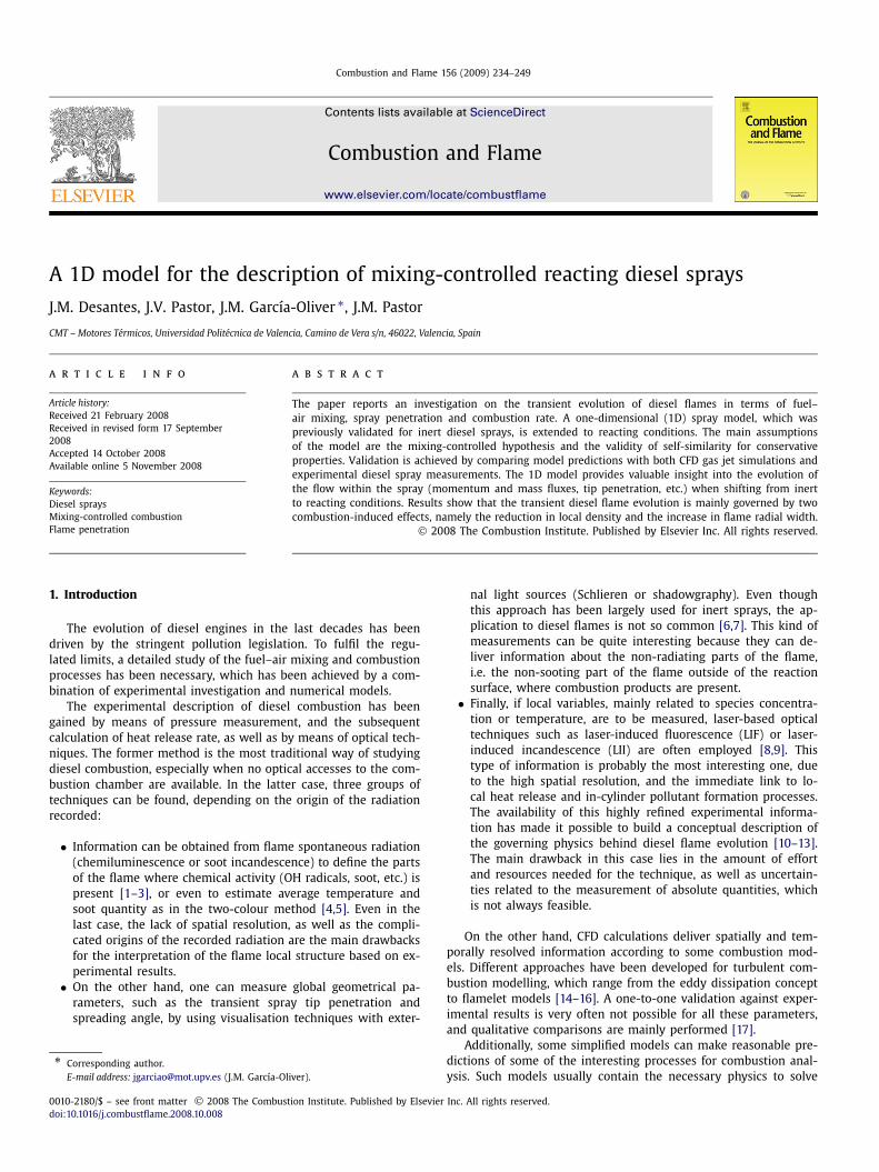
code FLUENT. The basic problem is a steady gas jet injected into anopen domain, whose geometrical definition is shown schematicallyin Fig. 1 (top). The steady approach simplifies the results analy-sis by eliminating time as an additional variable, but conclusionsare still useful to analyse transient jet flows, where a large steadyzone exists in the part closest to the nozzle [33,34]. No lateralair velocity is assumed, which results in an axisymmetric prob-lem. Therefore, a 2D domain corresponding to the jet symmetryplane has been used.
The 2D domain size has been parametrised in terms of the
problem equivalent diameter deq = d0
√ρ f ,0ρa,∞ , which is a scale of
the gas jet flow under inert conditions [35]. d0 stands for thenozzle geometrical diameter, whereas ρ stands for density, wheresub-indexes ( f ,0) and (a,∞) correspond to pure fuel and air con-ditions, respectively. This nomenclature will be kept throughoutthe paper. By using this standardised domain, grid size is scaled tothe spatial variability of the computed problem, and thus compar-ison of gas jet problems with very different boundary conditionscan be made with high confidence. For steady gas jet problems,the standardised domain has been 120deq × 55deq, which has beendiscretised into 350 × 52 cells.
An example of the grid resolution is shown in Fig. 1 (middle),together with a zoom on the nozzle exit (bottom). A structuredgrid has been used, with more refinement in zones close to thenozzle and to the axis, where the highest spatial gradients can befound.
The following models have been used:
• Turbulence: The standard k–ε model has been selected withthe constants that are usually accepted in most of the prob-lems where this model is applied [36]. Turbulent Schmidt andPrandtl number have been set equal to the unity, which pro-duces similar solutions for the conservation equations of axialvelocity, fuel mass and enthalpy (Section 3).
Fig. 1. Top: Basic CFD domain for gas jet studies: 1 – injection orifice; 2 – jet axis;3 and 4 – flow inlet and outlet; 5 – wall. Middle and bottom: Example of grid res-olution. Symbols correspond to cell node coordinates. The middle plot correspondsto the whole domain, whereas the lower one is a zoom on the nozzle exit. For thisgrid, deq = 1.04 mm.
• Combustion: The source term in conservation equations forspecies has been calculated according to an eddy dissipationapproach, which is similar to the generalisation of the Spald-ing eddy breakup model by Magnussen and Hjertager [37]. Thisassumes that combustion is controlled by the turbulent mixingof reactants, depending only on the species mass fraction andthe turbulence generation and dissipation terms. A single-stepirreversible combustion reaction has been assumed.
• Equation of state: The ideal gas equation of state has beenused to calculate local density. In this equation, local temper-ature and composition are considered, but a constant pressurehas been assumed to decouple the pressure from the othervariables and speed up the solution convergence. This meansthat results should be valid for incompressible gas jets. Calcu-lations have shown that local pressure changes occur in thenozzle vicinity, where maximum velocities are achieved. Thiszone is less than 10d0, which means that the hypothesis isvalid in most of the calculated domain.
A segregated solver has been used, with a first order upwinddiscretisation scheme in the equations of momentum, turbulent ki-
J.M. Desantes et al. / Combustion and Flame 156 (2009) 234–249 237
Table 1Definition of gas jet CFD simulation. Calculations have been performed under bothinert and reacting conditions.
Fuel C16H34
Air N2, O2
YO2,∞ 0.23
P (MPa) 8.1T f ,o (K) 300Ta,∞ (K) 900ρ f ,o/ρa,∞ 23.5
uo (m/s) 150do (μm) 200deq (μm) 970
netic energy and dissipation, species and energy, and the SIMPLEmethod for the pressure–velocity coupling.
2.1.2. Simulated casesGas jet results presented in Section 4 correspond to the condi-
tions defined in Table 1. The idea is to use a high molecular weightfuel (hexadecane) to have a high density ratio (ρ f ,0/ρa,∞) similarto diesel engine sprays. Fuel and air temperatures have been cho-sen close to engine conditions. On the other hand, nozzle diameteris close to heavy duty engine characteristics, and injection veloc-ity is kept low so that the incompressible flow hypothesis is stillvalid.
2.2. Experimental spray measurements
In this paper, extensive use is made of experimental informa-tion obtained at a hot spray test rig. For that purpose, differentvisualisation techniques have been applied, which are briefly de-scribed below, together with the experimental conditions that havebeen investigated.
2.2.1. Test rig descriptionExperiments were conducted in a hot spray test rig described
in [38]. This facility is based on a modified loop-scavenged singlecylinder 2-stroke direct injection diesel engine (Jenbach JW 50),with a displacement of 3 litres (bore 150 mm, effective stroke108 mm) and low rated rotational speed (500 rpm). The experi-mental setup makes it possible to study the injection–combustionprocess under thermodynamic conditions (pressure, temperatureand density) which are similar to those existing close to top deadcentre (TDC) in current direct injection diesel engines.
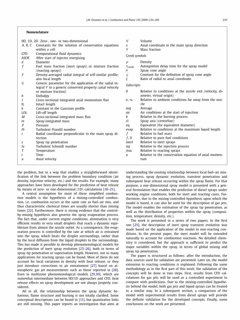
Due to the absence of inlet or exhaust valves, optical accessto the combustion chamber can be easily achieved through thecylinder head, which encloses a cylindrical combustion chamber(diameter 45 mm, height 91 mm) (Fig. 2). The resulting effectivecompression ratio is 9.3. This chamber has an upper access wherethe fuel injector is mounted, and four lateral orthogonal accesses.One of them is used to install a pressure transducer, whereas theother three accesses are equipped with elliptical quartz windows,81 mm high, 33 mm wide and 20 mm thick.
The hot spray test rig can be operated under inert or reactingambient conditions. For the latter configuration, the rig is oper-ated as a conventional engine, i.e. ambient air is aspirated throughthe intake system. In the inert atmosphere configuration, nitro-gen is supplied to the rig instead of air, so that fuel combustionis avoided. A roots compressor is used as an intake superchargingsystem to increase intake air pressure. Intake air temperature iscontrolled by means of two conditioning units and a small settlingchamber.
The fuel injection system is based on an electronically con-trolled Bosch Common Rail, capable of injection pressures upto 1350 bar using a solenoid activated injector. The injector is
Fig. 2. Schematic of the 2-stroke engine cylinder head [38].
equipped with single-hole mini-sac axial nozzles. The injectioncontrol system makes it possible to modify any parameter of theinjection events such as timing, duration and pressure. A standarddiesel fuel has been used for the study.
The engine is operated under a skip fire mode, i.e. one injec-tion event occurs every 20 engine cycles. This strategy has beenused due to limitations in the maximum acquisition frequencyof the digital cameras and to minimise window fouling. Further-more, an injection per cycle would create a temperature transientin the engine walls during the first cycles of the test, as the enginechanges from non-combusting to fully combusting cycles. The skipfire mode has a lower heat release due to the lower amount ofcombusting cycles, and thus prevents this transient heating pro-cess from occurring. As only one image is recorded at each ofthese injection cycles, samples of 10 images are recorded for everytime step to obtain a representative description of the injection–combustion process.
2.2.2. Measurement techniquesSeveral diagnostics have been employed in the experiments.
The simplest one is the measurement of in-cylinder pressure,which has been used to detect the time period in which heatrelease from the spray is occurring. Additionally, the spray evo-lution has been tracked by means of shadowgraphy and radiationimaging techniques, which have made it possible to record spraymacroscopic parameters as well as flame radiation information.Digital images have been analysed by means of purpose-developedprocessing software, which delivers the spray/flame geometricalparameters. Shadowgraphy has been used to measure maximumspray penetration during the autoignition delay phase, visible radi-ation has been employed to measure maximum flame penetrationafter the diffusion flame onset and OH radiation has been em-ployed to measure the diffusion flame lift-off length (LOL).
Shadowgraphy imaging The spatial evolution of the spray in thecombustion chamber has been recorded by means of transmissionshadowgraphy imaging [39]. This technique is sensitive to the sec-ond spatial derivative of density within the combustion chamber,which makes it useful to detect spray boundaries and thus evaluatemacroscopic spray scales, whether vaporising or non-vaporising,inert or reactive.
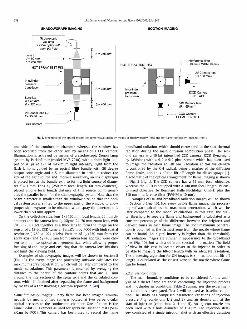
A schematic of the optical arrangement for shadowgraph imag-ing is shown in Fig. 3 (left). The spray has been illuminated from
238 J.M. Desantes et al. / Combustion and Flame 156 (2009) 234–249
Fig. 3. Schematic of the optical system for spray visualisation by means of shadowgraphy (left) and for flame luminosity imaging (right).
one side of the combustion chamber, whereas the shadow hasbeen recorded from the other side by means of a CCD camera.Illumination is achieved by means of a stroboscopic Xenon lampsystem by PerkinElmer (model MVS 7010), with a short light out-put of 20 μs at 1/3 of maximum light intensity. Light from theflash lamp is guided by an optical fibre bundle with 80 degreeoutput cone angle and a 5 mm diameter. In order to reduce thesize of the light source and improve sensitivity, an iris diaphragmis placed just at the bundle exit, to form a light source of diame-ter d = 1 mm. Lens L1 (250 mm focal length, 60 mm diameter),placed at one focal length distance of this source point, gener-ates the parallel beam for the shadowgraphy system. Note that thebeam diameter is smaller than the window size, so that the opti-cal system axis is shifted to the upper part of the window to allowproper shadowgrams to be obtained when spray tip penetration islower than 50 mm approx.
On the collecting side, lens L2 (450 mm focal length, 60 mm di-ameter) and the camera lens L3 (Sigma 24–70 mm zoom lens, withf # 3.5–5.6), act together as a thick lens to form the image on thesensor of a 12-bit CCD camera (SensiCam by PCO) with high spatialresolution (1280 × 1024 pixels). Position of L2 (330 mm from thespray axis), and L3 (400 mm from camera lens approx.) were cho-sen to minimise optical arrangement size, while allowing properfocusing of the image and ensuring that the camera lens iris doesnot limit the viewing field.
Examples of shadowgraphy images will be shown in Section 5(Fig. 10). For every image, the processing software calculates themaximum spray penetration, which will be later compared to themodel calculations. This parameter is obtained by averaging thedistance to the nozzle of the contour points that are ±1 mmaround the intersection of the spray axis and the calculated con-tour, which is obtained after separating the flame and backgroundby means of a thresholding algorithm reported in [40].
Flame luminosity imaging Spray flame has been imaged simulta-neously by means of two cameras located at two perpendicularoptical accesses to the combustion chamber. One of them is thesame 12-bit CCD camera as used for spray visualisation tests (Sen-siCam by PCO). This camera has been used to record the flame
broadband radiation, which should correspond to the soot thermalradiation during the main diffusion combustion phase. The sec-ond camera is a 16-bit intensified CCD camera (ICCD Dynamightby LaVision) with a 512 × 512 pixel sensor, which has been usedto image the radiation at 310 nm. Radiation at this wavelengthis controlled by the OH radical, being a marker of the diffusionflame limits, and thus of the lift-off length for diesel sprays [1].A schematic of the optical arrangement for flame imaging is shownin Fig. 3 (right). The CCD camera has a 55 mm focal objective,whereas the ICCD is equipped with a 100 mm focal length UV cus-tomised objective (by Bernhard Halle Nachfolger GmbH) plus the310 nm interference filter (FWHM = 10 nm).
Examples of OH and broadband radiation images will be shownin Section 5 (Fig. 10). For every visible flame image, the process-ing software calculates the maximum penetration, which will belater compared to the model calculations. In this case, the digi-tal threshold to separate flame and background is calculated as aconstant percentage of the difference between the brightest anddarkest zones in each flame image. The soot maximum penetra-tion is obtained as the farthest zone from the nozzle where flamecan be found (i.e. digital intensity is higher than the threshold).OH radiation images are similar in appearance to the broadbandones (Fig. 10), but with a different spectral information. The fieldof view in this case is located closer to the injector, in order tobe able to measure the lift-off length with an adequate resolution.The processing algorithm for OH images is similar, too, but lift-offlength is calculated as the closest zone to the nozzle where flamecan be found.
2.2.3. Test conditionsThe main boundary conditions to be considered for the anal-
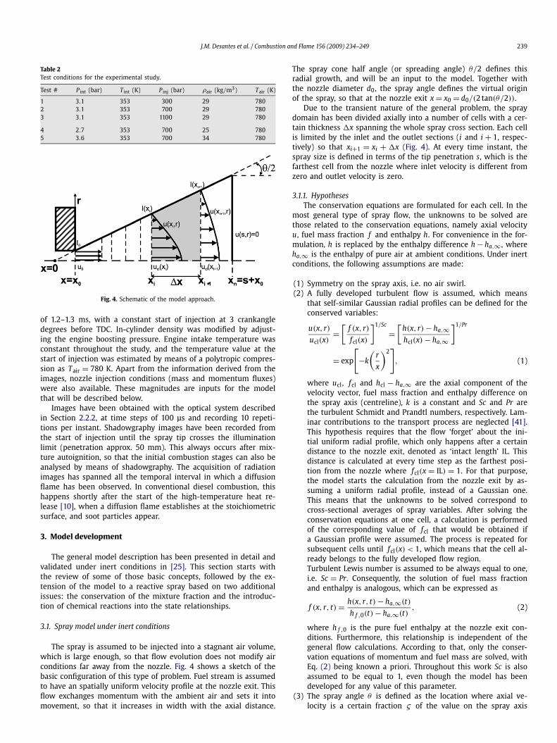
ysis of a diesel flame are those controlling the injection processand in-cylinder air conditions. Table 2 summarises the experimen-tal conditions investigated. Test 2 will be used as baseline condi-tion. The study has comprised parametric variations of injectionpressure P inj (conditions 1, 2 and 3), and air density ρair at thestart of injection (conditions 2, 4 and 5). An injector nozzle hasbeen used with a hole diameter of 119 μm. The injection strat-egy consisted of a single injection shot with an effective duration
J.M. Desantes et al. / Combustion and Flame 156 (2009) 234–249 239
Table 2Test conditions for the experimental study.
Test # P int (bar) T int (K) P inj (bar) ρair (kg/m3) Tair (K)
1 3.1 353 300 29 7802 3.1 353 700 29 7803 3.1 353 1100 29 780
4 2.7 353 700 25 7805 3.6 353 700 34 780
Fig. 4. Schematic of the model approach.
of 1.2–1.3 ms, with a constant start of injection at 3 crankangledegrees before TDC. In-cylinder density was modified by adjust-ing the engine boosting pressure. Engine intake temperature wasconstant throughout the study, and the temperature value at thestart of injection was estimated by means of a polytropic compres-sion as Tair = 780 K. Apart from the information derived from theimages, nozzle injection conditions (mass and momentum fluxes)were also available. These magnitudes are inputs for the modelthat will be described below.
Images have been obtained with the optical system describedin Section 2.2.2, at time steps of 100 μs and recording 10 repeti-tions per instant. Shadowgraphy images have been recorded fromthe start of injection until the spray tip crosses the illuminationlimit (penetration approx. 50 mm). This always occurs after mix-ture autoignition, so that the initial combustion stages can also beanalysed by means of shadowgraphy. The acquisition of radiationimages has spanned all the temporal interval in which a diffusionflame has been observed. In conventional diesel combustion, thishappens shortly after the start of the high-temperature heat re-lease [10], when a diffusion flame establishes at the stoichiometricsurface, and soot particles appear.
3. Model development
The general model description has been presented in detail andvalidated under inert conditions in [25]. This section starts withthe review of some of those basic concepts, followed by the ex-tension of the model to a reactive spray based on two additionalissues: the conservation of the mixture fraction and the introduc-tion of chemical reactions into the state relationships.
3.1. Spray model under inert conditions
The spray is assumed to be injected into a stagnant air volume,which is large enough, so that flow evolution does not modify airconditions far away from the nozzle. Fig. 4 shows a sketch of thebasic configuration of this type of problem. Fuel stream is assumedto have an spatially uniform velocity profile at the nozzle exit. Thisflow exchanges momentum with the ambient air and sets it intomovement, so that it increases in width with the axial distance.
The spray cone half angle (or spreading angle) θ/2 defines thisradial growth, and will be an input to the model. Together withthe nozzle diameter d0, the spray angle defines the virtual originof the spray, so that at the nozzle exit x = x0 = d0/(2 tan(θ/2)).
Due to the transient nature of the general problem, the spraydomain has been divided axially into a number of cells with a cer-tain thickness �x spanning the whole spray cross section. Each cellis limited by the inlet and the outlet sections (i and i + 1, respec-tively) so that xi+1 = xi + �x (Fig. 4). At every time instant, thespray size is defined in terms of the tip penetration s, which is thefarthest cell from the nozzle where inlet velocity is different fromzero and outlet velocity is zero.
3.1.1. HypothesesThe conservation equations are formulated for each cell. In the
most general type of spray flow, the unknowns to be solved arethose related to the conservation equations, namely axial velocityu, fuel mass fraction f and enthalpy h. For convenience in the for-mulation, h is replaced by the enthalpy difference h − ha,∞ , whereha,∞ is the enthalpy of pure air at ambient conditions. Under inertconditions, the following assumptions are made:
(1) Symmetry on the spray axis, i.e. no air swirl.(2) A fully developed turbulent flow is assumed, which means
that self-similar Gaussian radial profiles can be defined for theconserved variables:
u(x, r)
ucl(x)=
[f (x, r)
fcl(x)
]1/Sc
=[
h(x, r) − ha,∞hcl(x) − ha,∞
]1/Pr
= exp
[−k
(r
x
)2], (1)
where ucl, fcl and hcl − ha,∞ are the axial component of thevelocity vector, fuel mass fraction and enthalpy difference onthe spray axis (centreline), k is a constant and Sc and Pr arethe turbulent Schmidt and Prandtl numbers, respectively. Lam-inar contributions to the transport process are neglected [41].This hypothesis requires that the flow ‘forget’ about the ini-tial uniform radial profile, which only happens after a certaindistance to the nozzle exit, denoted as ‘intact length’ IL. Thisdistance is calculated at every time step as the farthest posi-tion from the nozzle where fcl(x = IL) = 1. For that purpose,the model starts the calculation from the nozzle exit by as-suming a uniform radial profile, instead of a Gaussian one.This means that the unknowns to be solved correspond tocross-sectional averages of spray variables. After solving theconservation equations at one cell, a calculation is performedof the corresponding value of fcl that would be obtained ifa Gaussian profile were assumed. The process is repeated forsubsequent cells until fcl(x) < 1, which means that the cell al-ready belongs to the fully developed flow region.Turbulent Lewis number is assumed to be always equal to one,i.e. Sc = Pr. Consequently, the solution of fuel mass fractionand enthalpy is analogous, which can be expressed as
f (x, r, t) = h(x, r, t) − ha,∞(t)
h f ,0(t) − ha,∞(t), (2)
where h f ,0 is the pure fuel enthalpy at the nozzle exit con-ditions. Furthermore, this relationship is independent of thegeneral flow calculations. According to that, only the conser-vation equations of momentum and fuel mass are solved, withEq. (2) being known a priori. Throughout this work Sc is alsoassumed to be equal to 1, even though the model has beendeveloped for any value of this parameter.
(3) The spray angle θ is defined as the location where axial ve-locity is a certain fraction ς of the value on the spray axis
240 J.M. Desantes et al. / Combustion and Flame 156 (2009) 234–249
ucl, in other words, where the self-similar axial velocity pro-file equals ς , as it is usually done for boundary layer flows.In this case, ς = 0.01 has been used as a reference. Accordingthis hypothesis, and by equating the right-hand side term inEq. (1) to ς , one can derive a relationship between the spraycone angle and the constant k in the self-similar profiles:
k = Ln(1/ς)
tan2(θ/2). (3)
(4) Locally homogeneous flow is assumed [41], i.e. there exists alocal equilibrium both in thermal and velocity conditions. Thisallows for a consideration of the spray as a gas jet.
(5) Pressure is assumed to be constant all over the spray, and thuscompressibility effects are neglected.
(6) Local density is calculated under an assumption of ideal mix-ing:
ρ(x, r) = 1∑n
Yn(x,r)ρn(x,r)
, (4)
where Yn is the mass fraction of the mixture component n,and ρn is the density for the pure component n at the mix-ture local temperature T (x, r) and pressure P . It must be notedthat density and temperature do not necessarily exhibit a ra-dial Gaussian profile, even though enthalpy, velocity, and fuelmass fraction do.
3.1.2. Conservation equations and boundary conditionsUnder the previous assumptions, the conservation equations of
axial momentum and fuel mass are formulated for each cell, andlead to the following expressions:
I(xi, t) − I(xi+1, t) = d
dt
[∫ρ(x, r, t)u(x, r, t)dV
],
M f (xi, t) − M f (xi+1, t) = d
dt
[∫ρ(x, r, t) f (x, r, t)dV
]. (5)
The terms on the left-hand side of the equations correspond to theconserved property fluxes across the cell inlet (xi) and outlet (xi+1)surfaces. Thus, I and M f stand for the axial momentum (related tou) and fuel mass (related to f ) fluxes, respectively. The right-handside terms represent the temporal variation of the integral overthe whole cell, which quantifies the process of accumulation orde-accumulation of momentum and fuel within a cell.
Some boundary conditions are necessary inputs for each cal-culation, and will be obtained experimentally for each particularinjection system and experimental environment:
• Momentum I0 and fuel mass M0 fluxes at the nozzle exit(i = 0). Both of them can be constant or a function of the time.
• The spray cone angle θ/2. This parameter will be assumed tobe constant with time.
• Finally, the relationship between local density and the otherunknowns has to be made explicit to solve the conservationequations. Formally, this is expressed as a function of the typeρ = ρ( f ) (e.g. Eq. (4)), which falls into the category of the so-called state relationships. The function is known a priori, andit depends on some additional boundary conditions, namelythe composition and thermodynamic conditions of the purefuel (conditions at the nozzle exit, subscripted as f ,0) andpure air (conditions subscripted as a,∞), which may be con-stant (e.g. for a steady problem) or variable along time (e.g.for an internal combustion engine). According to the way thestate relationships are calculated, the type of spray flow to becalculated will vary (non-vaporising or vaporising, inert or re-acting).
3.1.3. Solution procedureThe solution procedure starts by re-writing the previous con-
servation equations in terms of the on-axis variables ucl and fcl.Throughout the text, sub-indexes (i, i + 1) correspond to the spa-tial discretised coordinates (xi+1 = xi +�x), whereas super-indexes( j, j + 1) refer to the time variable (t j+1 = t j + �t). For every cell,conditions at the inlet face are assumed to be known, and thusthe only unknowns are the on-axis cell outlet variables u j+1
cl,i+1 and
f j+1cl,i+1. Appendix A shows how the discretised differential equa-
tions can be converted into the following set of algebraic equa-tions:
Au(u j+1
cl,i+1
)2 + Buu j+1cl,i+1 + Cu = 0,
A f(u j+1
cl,i+1 f j+1cl,i+1
) + B f f j+1cl,i+1 + C f = 0, (6)
where A, B and C (with the corresponding sub-indexes) are func-tions depending on the known terms of Eqs. (5). At every timestep, the calculation process starts from the first cell closest to thenozzle orifice. The solving process is repeated downstream untilthe outlet velocity ucl,i+1 is zero. In this way, the spray tip pene-tration is directly derived from the calculations as the farthest cellreached at a time step.
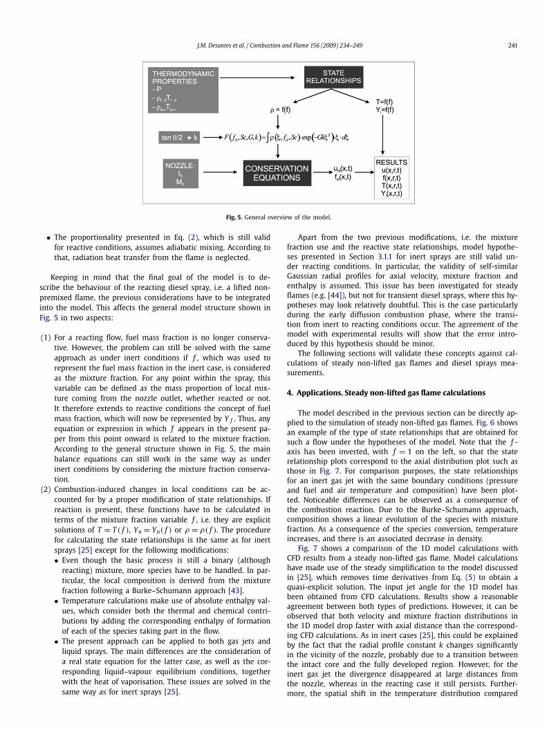
Fig. 5 summarises the model structure. The main componentsare shown explicitly, namely the solver of the conservation equa-tions, the nozzle outlet boundary conditions, the spray cone angleand the calculation of state relationships. The latter two affect di-rectly the calculation of radial integrals, which are used to writethe conservation equations in terms of the on-axis variables. Fur-thermore, after solving the conservation equations, the value ofany variable at any spray position can be obtained by means ofthe on-axis unknowns ucl and fcl, together with the self-similarprofiles and the state relationships.
3.2. Extension of the spray model to reacting conditions
Combustion has several implications on the flow description bythe model:
• Compared to the inert case, a reactive flow will result inspecies recombination and energy release. Higher local tem-peratures and, consequently, lower densities are achieved,which will interact with the conservation equations to yielda different distribution of velocities. In the present approach,chemical reaction times are assumed to be much shorterthan turbulent mixing times. Furthermore, a frozen chemistryassumption is made, and thus scalar dissipation effects areneglected. As a result, chemical equilibrium conditions are at-tained within the spray. A single-step irreversible reaction isassumed:
CmHn +(
m + n
4
)O2 → mCO2 + n
2H2O. (7)
This represents a major simplification compared to the realflame. Local species concentration and temperature will not beproperly calculated in fuel-rich regions, but results will showthat it is sufficient to describe the macroscopic spray charac-teristics.
• Buoyancy effects are not an issue for diesel flames. Estimationsof the density-weighted Froude number according to the defi-nition in [42] for conventional diesel engine conditions (P inj =100 MPa, ρ f ,0 = 830 kg/m3, d0 = 150 μm, ρa,∞ = 29 kg/m3),indicate that this parameter is in the order of magnitude of9 × 105. This implies that conservation equations can still beformulated in the momentum-dominated regime in the sameway as for a non-reacting spray.
J.M. Desantes et al. / Combustion and Flame 156 (2009) 234–249 241
Fig. 5. General overview of the model.
• The proportionality presented in Eq. (2), which is still validfor reactive conditions, assumes adiabatic mixing. According tothat, radiation heat transfer from the flame is neglected.
Keeping in mind that the final goal of the model is to de-scribe the behaviour of the reacting diesel spray, i.e. a lifted non-premixed flame, the previous considerations have to be integratedinto the model. This affects the general model structure shown inFig. 5 in two aspects:
(1) For a reacting flow, fuel mass fraction is no longer conserva-tive. However, the problem can still be solved with the sameapproach as under inert conditions if f , which was used torepresent the fuel mass fraction in the inert case, is consideredas the mixture fraction. For any point within the spray, thisvariable can be defined as the mass proportion of local mix-ture coming from the nozzle outlet, whether reacted or not.It therefore extends to reactive conditions the concept of fuelmass fraction, which will now be represented by Y f . Thus, anyequation or expression in which f appears in the present pa-per from this point onward is related to the mixture fraction.According to the general structure shown in Fig. 5, the mainbalance equations can still work in the same way as underinert conditions by considering the mixture fraction conserva-tion.
(2) Combustion-induced changes in local conditions can be ac-counted for by a proper modification of state relationships. Ifreaction is present, these functions have to be calculated interms of the mixture fraction variable f , i.e. they are explicitsolutions of T = T ( f ), Yn = Yn( f ) or ρ = ρ( f ). The procedurefor calculating the state relationships is the same as for inertsprays [25] except for the following modifications:• Even though the basic process is still a binary (although
reacting) mixture, more species have to be handled. In par-ticular, the local composition is derived from the mixturefraction following a Burke–Schumann approach [43].
• Temperature calculations make use of absolute enthalpy val-ues, which consider both the thermal and chemical contri-butions by adding the corresponding enthalpy of formationof each of the species taking part in the flow.
• The present approach can be applied to both gas jets andliquid sprays. The main differences are the consideration ofa real state equation for the latter case, as well as the cor-responding liquid–vapour equilibrium conditions, togetherwith the heat of vaporisation. These issues are solved in thesame way as for inert sprays [25].
Apart from the two previous modifications, i.e. the mixturefraction use and the reactive state relationships, model hypothe-ses presented in Section 3.1.1 for inert sprays are still valid un-der reacting conditions. In particular, the validity of self-similarGaussian radial profiles for axial velocity, mixture fraction andenthalpy is assumed. This issue has been investigated for steadyflames (e.g. [44]), but not for transient diesel sprays, where this hy-potheses may look relatively doubtful. This is the case particularlyduring the early diffusion combustion phase, where the transi-tion from inert to reacting conditions occur. The agreement of themodel with experimental results will show that the error intro-duced by this hypothesis should be minor.
The following sections will validate these concepts against cal-culations of steady non-lifted gas flames and diesel sprays mea-surements.
4. Applications. Steady non-lifted gas flame calculations
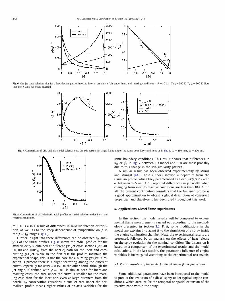
The model described in the previous section can be directly ap-plied to the simulation of steady non-lifted gas flames. Fig. 6 showsan example of the type of state relationships that are obtained forsuch a flow under the hypotheses of the model. Note that the f -axis has been inverted, with f = 1 on the left, so that the staterelationship plots correspond to the axial distribution plot such asthose in Fig. 7. For comparison purposes, the state relationshipsfor an inert gas jet with the same boundary conditions (pressureand fuel and air temperature and composition) have been plot-ted. Noticeable differences can be observed as a consequence ofthe combustion reaction. Due to the Burke–Schumann approach,composition shows a linear evolution of the species with mixturefraction. As a consequence of the species conversion, temperatureincreases, and there is an associated decrease in density.
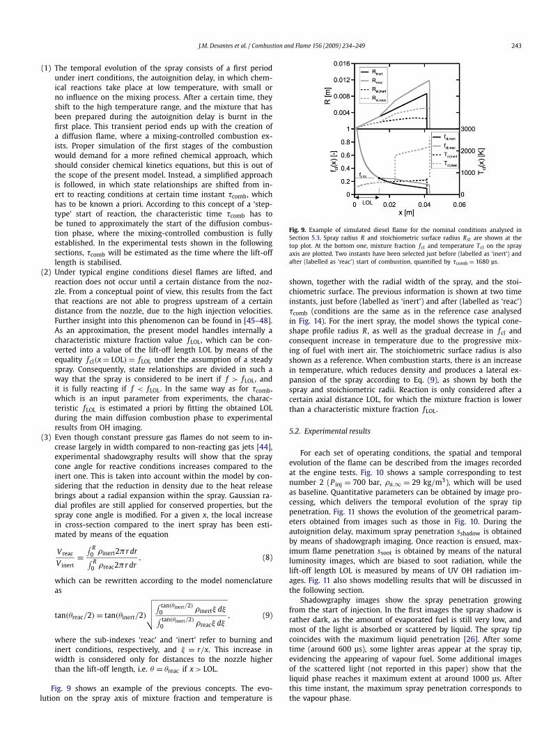
Fig. 7 shows a comparison of the 1D model calculations withCFD results from a steady non-lifted gas flame. Model calculationshave made use of the steady simplification to the model discussedin [25], which removes time derivatives from Eq. (5) to obtain aquasi-explicit solution. The input jet angle for the 1D model hasbeen obtained from CFD calculations. Results show a reasonableagreement between both types of predictions. However, it can beobserved that both velocity and mixture fraction distributions inthe 1D model drop faster with axial distance than the correspond-ing CFD calculations. As in inert cases [25], this could be explainedby the fact that the radial profile constant k changes significantlyin the vicinity of the nozzle, probably due to a transition betweenthe intact core and the fully developed region. However, for theinert gas jet the divergence disappeared at large distances fromthe nozzle, whereas in the reacting case it still persists. Further-more, the spatial shift in the temperature distribution compared
242 J.M. Desantes et al. / Combustion and Flame 156 (2009) 234–249
Fig. 6. Gas jet state relationships for a hexadecane gas jet injected into an ambient of air under inert and reacting conditions – P = 80 bar, T f ,0 = 300 K, Ta,∞ = 900 K. Notethat the f -axis has been inverted.
Fig. 7. Comparison of CFD and 1D model calculations. On-axis results for a gas flame under the same boundary conditions as in Fig. 6. u0 = 150 m/s, d0 = 200 μm.
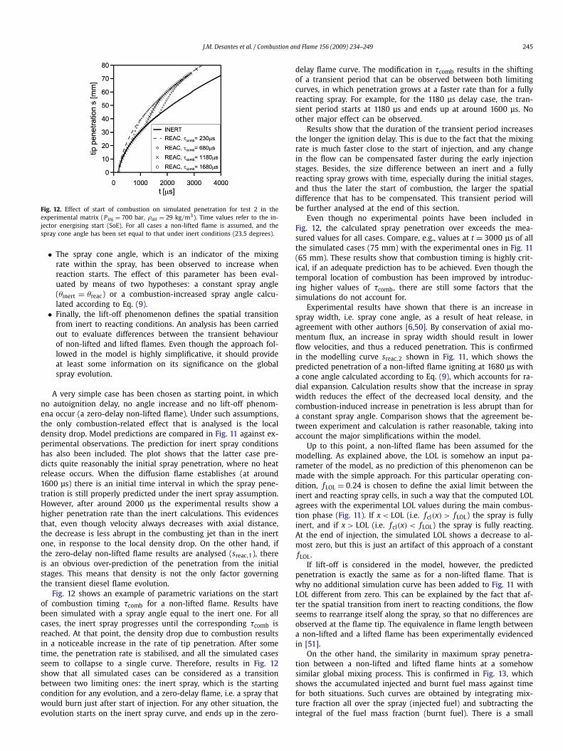
Fig. 8. Comparison of CFD-derived radial profiles for axial velocity under inert andreacting conditions.
to CFD is also a result of differences in mixture fraction distribu-tion, as well as to the steep dependence of temperature on f inthe f < fst range (Fig. 6).
Further insight into these differences can be obtained by anal-ysis of the radial profiles. Fig. 8 shows the radial profiles for theaxial velocity u obtained at different gas jet cross sections (20, 40,60, 80 and 100deq from the nozzle) both for the inert and com-busting gas jet. While in the first case the profiles maintain theexponential shape, this is not the case for a burning gas jet. If re-action is present there is a slight scattering among the differentcurves, especially for (r/x) < 0.15. On the other hand, although thejet angle, if defined with ς = 0.01, is similar both for inert andreacting cases, the area under the curve is smaller for the react-ing case than for the inert one, even at large distances from thenozzle. By conservation equations, a smaller area under the nor-malised profile means higher values of on-axis variables for the
same boundary conditions. This result shows that differences inucl or fcl in Fig. 7 between 1D model and CFD are most probablydue to this change in the self-similarity pattern.
A similar result has been observed experimentally by Muñizand Mungal [44]. These authors showed a departure from theGaussian profile, which they parametrised as a exp(−k(r/x)α) withα between 1.65 and 1.75. Reported differences in jet width whenchanging from inert to reactive conditions are less than 10%. All inall, the present contribution considers that the Gaussian profile isa good approximation to obtain a global description of conservedproperties, and therefore it has been used throughout this work.
5. Applications. Diesel flame experiments
In this section, the model results will be compared to experi-mental flame measurements carried out according to the method-ology presented in Section 2.2. First, some modifications in themodel are explained to adapt it to the simulation of a spray insidethe engine combustion chamber. Next, the experimental results arepresented, followed by an analysis on the effects of heat releaseon the spray evolution for the nominal condition. The discussion isbased on a comparison of the experimental results and the modelcalculations. In the last section, the parametric influence of enginevariables is investigated according to the experimental test matrix.
5.1. Particularisation of the model for diesel engine flame predictions
Some additional parameters have been introduced to the modelto predict the evolution of a diesel spray under typical engine con-ditions, which account for the temporal or spatial extension of thereactive zone within the spray:
J.M. Desantes et al. / Combustion and Flame 156 (2009) 234–249 243
(1) The temporal evolution of the spray consists of a first periodunder inert conditions, the autoignition delay, in which chem-ical reactions take place at low temperature, with small orno influence on the mixing process. After a certain time, theyshift to the high temperature range, and the mixture that hasbeen prepared during the autoignition delay is burnt in thefirst place. This transient period ends up with the creation ofa diffusion flame, where a mixing-controlled combustion ex-ists. Proper simulation of the first stages of the combustionwould demand for a more refined chemical approach, whichshould consider chemical kinetics equations, but this is out ofthe scope of the present model. Instead, a simplified approachis followed, in which state relationships are shifted from in-ert to reacting conditions at certain time instant τcomb, whichhas to be known a priori. According to this concept of a ‘step-type’ start of reaction, the characteristic time τcomb has tobe tuned to approximately the start of the diffusion combus-tion phase, where the mixing-controlled combustion is fullyestablished. In the experimental tests shown in the followingsections, τcomb will be estimated as the time where the lift-offlength is stabilised.
(2) Under typical engine conditions diesel flames are lifted, andreaction does not occur until a certain distance from the noz-zle. From a conceptual point of view, this results from the factthat reactions are not able to progress upstream of a certaindistance from the nozzle, due to the high injection velocities.Further insight into this phenomenon can be found in [45–48].As an approximation, the present model handles internally acharacteristic mixture fraction value fLOL, which can be con-verted into a value of the lift-off length LOL by means of theequality fcl(x = LOL) = fLOL under the assumption of a steadyspray. Consequently, state relationships are divided in such away that the spray is considered to be inert if f > fLOL, andit is fully reacting if f < fLOL. In the same way as for τcomb,which is an input parameter from experiments, the charac-teristic fLOL is estimated a priori by fitting the obtained LOLduring the main diffusion combustion phase to experimentalresults from OH imaging.
(3) Even though constant pressure gas flames do not seem to in-crease largely in width compared to non-reacting gas jets [44],experimental shadowgraphy results will show that the spraycone angle for reactive conditions increases compared to theinert one. This is taken into account within the model by con-sidering that the reduction in density due to the heat releasebrings about a radial expansion within the spray. Gaussian ra-dial profiles are still applied for conserved properties, but thespray cone angle is modified. For a given x, the local increasein cross-section compared to the inert spray has been esti-mated by means of the equation
V reac
V inert=
∫ R0 ρinert2πr dr∫ R0 ρreac2πr dr
, (8)
which can be rewritten according to the model nomenclatureas
tan(θreac/2) = tan(θinert/2)
√√√√∫ tan(θinert/2)
0 ρinertξ dξ∫ tan(θinert/2)
0 ρreacξ dξ, (9)
where the sub-indexes ‘reac’ and ‘inert’ refer to burning andinert conditions, respectively, and ξ = r/x. This increase inwidth is considered only for distances to the nozzle higherthan the lift-off length, i.e. θ = θreac if x > LOL.
Fig. 9 shows an example of the previous concepts. The evo-lution on the spray axis of mixture fraction and temperature is
Fig. 9. Example of simulated diesel flame for the nominal conditions analysed inSection 5.3. Spray radius R and stoichiometric surface radius Rst are shown at thetop plot. At the bottom one, mixture fraction fcl and temperature Tcl on the sprayaxis are plotted. Two instants have been selected just before (labelled as ‘inert’) andafter (labelled as ‘reac’) start of combustion, quantified by τcomb = 1680 μs.
shown, together with the radial width of the spray, and the stoi-chiometric surface. The previous information is shown at two timeinstants, just before (labelled as ‘inert’) and after (labelled as ‘reac’)τcomb (conditions are the same as in the reference case analysedin Fig. 14). For the inert spray, the model shows the typical cone-shape profile radius R , as well as the gradual decrease in fcl andconsequent increase in temperature due to the progressive mix-ing of fuel with inert air. The stoichiometric surface radius is alsoshown as a reference. When combustion starts, there is an increasein temperature, which reduces density and produces a lateral ex-pansion of the spray according to Eq. (9), as shown by both thespray and stoichiometric radii. Reaction is only considered after acertain axial distance LOL, for which the mixture fraction is lowerthan a characteristic mixture fraction fLOL.
5.2. Experimental results
For each set of operating conditions, the spatial and temporalevolution of the flame can be described from the images recordedat the engine tests. Fig. 10 shows a sample corresponding to testnumber 2 (P inj = 700 bar, ρa,∞ = 29 kg/m3), which will be usedas baseline. Quantitative parameters can be obtained by image pro-cessing, which delivers the temporal evolution of the spray tippenetration. Fig. 11 shows the evolution of the geometrical param-eters obtained from images such as those in Fig. 10. During theautoignition delay, maximum spray penetration sshadow is obtainedby means of shadowgraph imaging. Once reaction is ensued, max-imum flame penetration ssoot is obtained by means of the naturalluminosity images, which are biased to soot radiation, while thelift-off length LOL is measured by means of UV OH radiation im-ages. Fig. 11 also shows modelling results that will be discussed inthe following section.
Shadowgraphy images show the spray penetration growingfrom the start of injection. In the first images the spray shadow israther dark, as the amount of evaporated fuel is still very low, andmost of the light is absorbed or scattered by liquid. The spray tipcoincides with the maximum liquid penetration [26]. After sometime (around 600 μs), some lighter areas appear at the spray tip,evidencing the appearing of vapour fuel. Some additional imagesof the scattered light (not reported in this paper) show that theliquid phase reaches it maximum extent at around 1000 μs. Afterthis time instant, the maximum spray penetration corresponds tothe vapour phase.

244 J.M. Desantes et al. / Combustion and Flame 156 (2009) 234–249
Fig. 10. Instantaneous images of shadowgraphy (top), broadband radiation (middle)and OH radiation (bottom) for test 2 in the experimental matrix (P inj = 700 bar,ρair = 29 kg/m3). Broadband and OH radiation images are simultaneous, shadowg-raphy images were obtained in a separate test. Captions at the bottom of each imagecorrespond to time values after the injector energising start (ASoE). Injector locationis indicated on the radiation images by a small cross.
Fig. 11. Experimental and modelling results for test 2 in the experimental ma-trix (P inj = 700 bar, ρair = 29 kg/m3). Time values refer to the injector energis-ing start (SoE). Start of injection at 180 μs. Top plot: Experimental in-cylinderpressure under motoring and injection conditions. Bottom plot: Results from im-age processing (symbols), compared with model predictions (lines). Every pointrepresents the ensemble average of ten images. Error bars correspond to ± onestandard deviation. sinert = penetration under inert conditions with θinert = 23.5 de-grees. sreac,1 = penetration under reactive conditions, τdelay = 0 μs and θreac = θinert .sreac,2 = penetration under reactive conditions, τdelay = 1680 μs and θreac accordingto Eq. (9). As commented in the text, consideration of lift-off does not modify thepredicted spray penetration for reacting cases.
Evidence of chemical activity may be detected around 1110 μs,mainly in the form of a spray broadening at the tip, due to expan-sion of the burning spray. The image at 1310 μs shows a morenoticeable increase in spray width, which diverges clearly fromthe cone-type shadow which could be observed in the previousimages. Flame radiation images show that a sooting flame is es-tablished at 1530 μs (camera settings are optimised for the maindiffusion flame, and thus early stages cannot be visualised prop-erly). Pressure trace also starts to separate from that obtainedunder motored conditions by the time soot appears. This sootingregion is the dominating factor in the subsequent combustion de-velopment, and it can be guessed in shadowgraphy images as ablurred lighter grey zone inside the detected contour. The increasein width mainly occurs downstream of lift-off length.
Due to limitations in lens size in shadowgraphy images, themaximum penetration measurements for time instants later than2000 μs can only be obtained from the sooting flame measure-ments. In the overlap zone, results show that the maximum ex-tent of the sooting flame coincides with that of the shadowgraphyspray. It is expected that the penetration calculated from the soot-ing flame still marks the evolution of the flame until the timeinstant in which the flame stabilises, just in the same way as ithappens to the liquid phase in the early injection stages [25]. Forthe investigated operating conditions, no stabilisation can be ob-served in the maximum soot extent during the injection period,i.e. the maximum soot penetration grows steadily during the restof the injection process.
On the other hand, the temporal evolution of flame lift-off canbe obtained from OH chemiluminescence images, which showsthat this parameter is almost constant from the onset of the dif-fusion flame until the end of the injection process, when there isan increase in the measured values. Furthermore, the whole flamestructure corresponds to the typical lifted diffusion flame describedin [10] without any large alteration until the end of injection.
5.3. Effect of heat release on transient spray evolution
This section intends to shed some light on the effects of heatrelease on the flame geometry and temporal evolution. For thatpurpose, 1D model results shown in Fig. 11 will be compared tothe experimental results. Inputs for the model are experimentalnozzle momentum and mass flow rates, in-cylinder air thermo-dynamic conditions, which were estimated by means of a poly-tropic compression process, inert spray cone angle, which was ob-tained from measurements under non-reacting conditions reportedin [49], and experimental values of autoignition delay and lift-offlength. The analysis will be performed for the nominal conditionsdescribed in the previous section, i.e. injection pressure 700 barand air density 29 kg/m3.
The discussion will deal with the following effects of combus-tion on the spray evolution:
• The immediate effect induced by combustion is a modificationin local conditions (temperature, composition and density),which is accounted for by means of adequate state relation-ships, together with the mixture fraction concept. Particularly,the combustion-induced density drop affects the density termin the conservation equations (Eq. (10)) and leads to majormodifications within the velocity and mixture fraction fields.
• Combustion reaction starts at a certain time instant, depend-ing on which the amount of ready-to-burn mixture is different,and the initial combustion stages will develop consequently.Combustion start is defined in the model by the start of com-bustion timing τcomb, which has been varied to evaluate differ-ences in spray behaviour due to the temporal transition frominert to reacting conditions.
J.M. Desantes et al. / Combustion and Flame 156 (2009) 234–249 245
Fig. 12. Effect of start of combustion on simulated penetration for test 2 in theexperimental matrix (P inj = 700 bar, ρair = 29 kg/m3). Time values refer to the in-jector energising start (SoE). For all cases a non-lifted flame is assumed, and thespray cone angle has been set equal to that under inert conditions (23.5 degrees).
• The spray cone angle, which is an indicator of the mixingrate within the spray, has been observed to increase whenreaction starts. The effect of this parameter has been eval-uated by means of two hypotheses: a constant spray angle(θinert = θreac) or a combustion-increased spray angle calcu-lated according to Eq. (9).
• Finally, the lift-off phenomenon defines the spatial transitionfrom inert to reacting conditions. An analysis has been carriedout to evaluate differences between the transient behaviourof non-lifted and lifted flames. Even though the approach fol-lowed in the model is highly simplificative, it should provideat least some information on its significance on the globalspray evolution.
A very simple case has been chosen as starting point, in whichno autoignition delay, no angle increase and no lift-off phenom-ena occur (a zero-delay non-lifted flame). Under such assumptions,the only combustion-related effect that is analysed is the localdensity drop. Model predictions are compared in Fig. 11 against ex-perimental observations. The prediction for inert spray conditionshas also been included. The plot shows that the latter case pre-dicts quite reasonably the initial spray penetration, where no heatrelease occurs. When the diffusion flame establishes (at around1600 μs) there is an initial time interval in which the spray pene-tration is still properly predicted under the inert spray assumption.However, after around 2000 μs the experimental results show ahigher penetration rate than the inert calculations. This evidencesthat, even though velocity always decreases with axial distance,the decrease is less abrupt in the combusting jet than in the inertone, in response to the local density drop. On the other hand, ifthe zero-delay non-lifted flame results are analysed (sreac,1), thereis an obvious over-prediction of the penetration from the initialstages. This means that density is not the only factor governingthe transient diesel flame evolution.
Fig. 12 shows an example of parametric variations on the startof combustion timing τcomb for a non-lifted flame. Results havebeen simulated with a spray angle equal to the inert one. For allcases, the inert spray progresses until the corresponding τcomb isreached. At that point, the density drop due to combustion resultsin a noticeable increase in the rate of tip penetration. After sometime, the penetration rate is stabilised, and all the simulated casesseem to collapse to a single curve. Therefore, results in Fig. 12show that all simulated cases can be considered as a transitionbetween two limiting ones: the inert spray, which is the startingcondition for any evolution, and a zero-delay flame, i.e. a spray thatwould burn just after start of injection. For any other situation, theevolution starts on the inert spray curve, and ends up in the zero-
delay flame curve. The modification in τcomb results in the shiftingof a transient period that can be observed between both limitingcurves, in which penetration grows at a faster rate than for a fullyreacting spray. For example, for the 1180 μs delay case, the tran-sient period starts at 1180 μs and ends up at around 1600 μs. Noother major effect can be observed.
Results show that the duration of the transient period increasesthe longer the ignition delay. This is due to the fact that the mixingrate is much faster close to the start of injection, and any changein the flow can be compensated faster during the early injectionstages. Besides, the size difference between an inert and a fullyreacting spray grows with time, especially during the initial stages,and thus the later the start of combustion, the larger the spatialdifference that has to be compensated. This transient period willbe further analysed at the end of this section.
Even though no experimental points have been included inFig. 12, the calculated spray penetration over exceeds the mea-sured values for all cases. Compare, e.g., values at t = 3000 μs of allthe simulated cases (75 mm) with the experimental ones in Fig. 11(65 mm). These results show that combustion timing is highly crit-ical, if an adequate prediction has to be achieved. Even though thetemporal location of combustion has been improved by introduc-ing higher values of τcomb, there are still some factors that thesimulations do not account for.
Experimental results have shown that there is an increase inspray width, i.e. spray cone angle, as a result of heat release, inagreement with other authors [6,50]. By conservation of axial mo-mentum flux, an increase in spray width should result in lowerflow velocities, and thus a reduced penetration. This is confirmedin the modelling curve sreac,2 shown in Fig. 11, which shows thepredicted penetration of a non-lifted flame igniting at 1680 μs witha cone angle calculated according to Eq. (9), which accounts for ra-dial expansion. Calculation results show that the increase in spraywidth reduces the effect of the decreased local density, and thecombustion-induced increase in penetration is less abrupt than fora constant spray angle. Comparison shows that the agreement be-tween experiment and calculation is rather reasonable, taking intoaccount the major simplifications within the model.
Up to this point, a non-lifted flame has been assumed for themodelling. As explained above, the LOL is somehow an input pa-rameter of the model, as no prediction of this phenomenon can bemade with the simple approach. For this particular operating con-dition, fLOL = 0.24 is chosen to define the axial limit between theinert and reacting spray cells, in such a way that the computed LOLagrees with the experimental LOL values during the main combus-tion phase (Fig. 11). If x < LOL (i.e. fcl(x) > fLOL) the spray is fullyinert, and if x > LOL (i.e. fcl(x) < fLOL) the spray is fully reacting.At the end of injection, the simulated LOL shows a decrease to al-most zero, but this is just an artifact of this approach of a constantfLOL.
If lift-off is considered in the model, however, the predictedpenetration is exactly the same as for a non-lifted flame. That iswhy no additional simulation curve has been added to Fig. 11 withLOL different from zero. This can be explained by the fact that af-ter the spatial transition from inert to reacting conditions, the flowseems to rearrange itself along the spray, so that no differences areobserved at the flame tip. The equivalence in flame length betweena non-lifted and a lifted flame has been experimentally evidencedin [51].
On the other hand, the similarity in maximum spray penetra-tion between a non-lifted and lifted flame hints at a somehowsimilar global mixing process. This is confirmed in Fig. 13, whichshows the accumulated injected and burnt fuel mass against timefor both situations. Such curves are obtained by integrating mix-ture fraction all over the spray (injected fuel) and subtracting theintegral of the fuel mass fraction (burnt fuel). There is a small
246 J.M. Desantes et al. / Combustion and Flame 156 (2009) 234–249
Fig. 13. Comparison of the temporal evolution of experimental pressure increase(�P ), injected mass (m f ,inj) and predictions of accumulated burnt fuel mass (m f ,b)for test 2 in the experimental matrix (P inj = 700 bar, ρair = 29 kg/m3). Calculationscorrespond to the lifted and non-lifted cases presented in Fig. 11.
difference if LOL is considered or not due to the amount of fuel al-located between the lift-off length and the nozzle orifice, which isburnt for the non-lifted flame. However, the spray behaves globallyvery similar in both cases. Even if one looks at the total amount ofair entrained within the spray (not shown) there is a total overlapbetween both cases. Differences disappear after the end of injec-tion when LOL goes to zero for the lifted flame case.
Further evidence of the validity of the present approach can beobtained in Fig. 13 by comparison of the predicted accumulatedburnt fuel mass m f ,b with the pressure increase �P . The latterparameter is defined as the difference between in-cylinder pres-sure in the combustion and in the motored cycles. Due to the lowrotational speed, and to the fact that injection–combustion occurswithin ±10 CAD around TDC, volume variation is very small, andthis difference can be used as an estimation of the accumulatedheat release. Plot axes have been chosen in such a way that thedistance between zero and maximum values is the same in bothcases (m f ,b and �P ), showing the proportionality between the cal-culated and experimental heat release. One cannot claim that thereis a one-to-one correspondence, but agreement is quite reasonable,and confirms the validity of the mixing-controlled model for dieselcombustion studies.
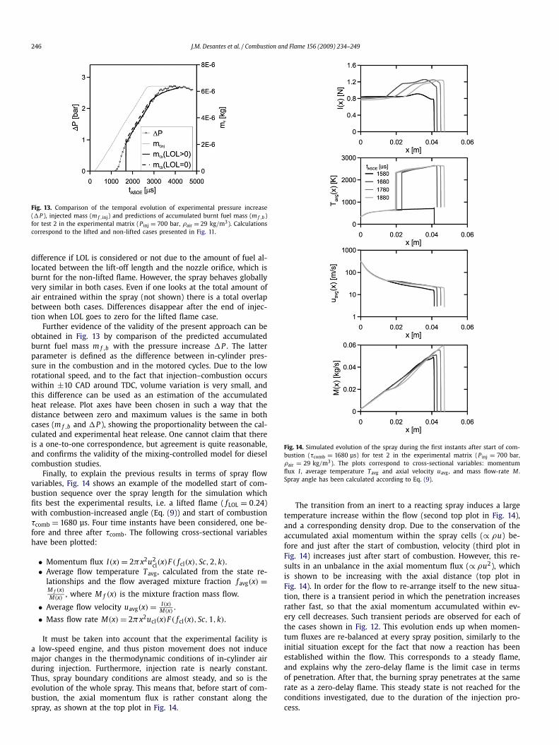
Finally, to explain the previous results in terms of spray flowvariables, Fig. 14 shows an example of the modelled start of com-bustion sequence over the spray length for the simulation whichfits best the experimental results, i.e. a lifted flame ( fLOL = 0.24)with combustion-increased angle (Eq. (9)) and start of combustionτcomb = 1680 μs. Four time instants have been considered, one be-fore and three after τcomb. The following cross-sectional variableshave been plotted:
• Momentum flux I(x) = 2πx2u2cl(x)F ( fcl(x), Sc,2,k).
• Average flow temperature Tavg, calculated from the state re-lationships and the flow averaged mixture fraction favg(x) =M f (x)M(x) , where M f (x) is the mixture fraction mass flow.
• Average flow velocity uavg(x) = I(x)M(x) .
• Mass flow rate M(x) = 2πx2ucl(x)F ( fcl(x), Sc,1,k).
It must be taken into account that the experimental facility isa low-speed engine, and thus piston movement does not inducemajor changes in the thermodynamic conditions of in-cylinder airduring injection. Furthermore, injection rate is nearly constant.Thus, spray boundary conditions are almost steady, and so is theevolution of the whole spray. This means that, before start of com-bustion, the axial momentum flux is rather constant along thespray, as shown at the top plot in Fig. 14.
Fig. 14. Simulated evolution of the spray during the first instants after start of com-bustion (τcomb = 1680 μs) for test 2 in the experimental matrix (P inj = 700 bar,ρair = 29 kg/m3). The plots correspond to cross-sectional variables: momentumflux I , average temperature Tavg and axial velocity uavg, and mass flow-rate M .Spray angle has been calculated according to Eq. (9).
The transition from an inert to a reacting spray induces a largetemperature increase within the flow (second top plot in Fig. 14),and a corresponding density drop. Due to the conservation of theaccumulated axial momentum within the spray cells (∝ ρu) be-fore and just after the start of combustion, velocity (third plot inFig. 14) increases just after start of combustion. However, this re-sults in an unbalance in the axial momentum flux (∝ ρu2), whichis shown to be increasing with the axial distance (top plot inFig. 14). In order for the flow to re-arrange itself to the new situa-tion, there is a transient period in which the penetration increasesrather fast, so that the axial momentum accumulated within ev-ery cell decreases. Such transient periods are observed for each ofthe cases shown in Fig. 12. This evolution ends up when momen-tum fluxes are re-balanced at every spray position, similarly to theinitial situation except for the fact that now a reaction has beenestablished within the flow. This corresponds to a steady flame,and explains why the zero-delay flame is the limit case in termsof penetration. After that, the burning spray penetrates at the samerate as a zero-delay flame. This steady state is not reached for theconditions investigated, due to the duration of the injection pro-cess.
J.M. Desantes et al. / Combustion and Flame 156 (2009) 234–249 247
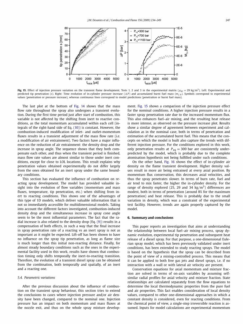
Fig. 15. Effect of injection pressure variation on the transient flame development. Tests 1, 2 and 3 in the experimental matrix (ρair = 29 kg/m3). Left: Experimental andpredicted tip penetration (s). Right: Time evolution of in-cylinder pressure increase (�P ) and accumulated burnt fuel mass (m f ,b). Symbols correspond to experimentalvalues (penetration or pressure increase), whereas continuous lines correspond to model predictions (penetration or burnt fuel mass).
The last plot at the bottom of Fig. 14 shows that the massflow rate throughout the spray also undergoes a transient evolu-tion. During the first time period just after start of combustion, thisvariable is not affected by the shifting from inert to reactive con-ditions, as the total momentum accumulated within each cell (in-tegrals of the right-hand side of Eq. (10)) is constant. However, thecombustion-induced modification of inlet- and outlet-momentumfluxes results in a transient adjustment of the mass flow rate (i.e.a modification of air entrainment). Two factors have a major influ-ence on the reduction of air entrainment: the density drop and theincrease in spray angle. The sequence shows that they both com-pensate each other, and thus when the transient period is finished,mass flow rate values are almost similar to those under inert con-ditions, except for close to LOL locations. This result explains whypenetration values obtained experimentally do not differ largelyfrom the ones obtained for an inert spray under the same bound-ary conditions.
This section has evaluated the influence of combustion on re-acting spray development. The model has provided valuable in-sight into the evolution of flow variables (momentum and massfluxes, temperature, tip penetration, etc.) when shifting from in-ert to reacting conditions. This shows one of the advantages ofthis type of 1D models, which deliver valuable information that isnot so immediately accessible for multidimensional models. Takinginto account the different factors investigated, combustion-induceddensity drop and the simultaneous increase in spray cone angleseem to be the most influential parameters. The fact that the ra-dial increase is also related to the density drop (Eq. (9)) results in acompensation of both effects, in such a way that the final increasein spray penetration rate of a reacting vs an inert spray is not asimportant as it might be expected. Lift-off has been shown to haveno influence on the spray tip penetration, as long as flame sizeis much longer than this initial non-reacting distance. Finally, foralmost steady boundary conditions such as the ones in the experi-mental facility used in this work, results have shown that combus-tion timing only shifts temporally the inert-to-reacting transition.Therefore, the evolution of a transient diesel spray can be obtainedfrom the combination, both temporally and spatially, of an inertand a reacting one.
5.4. Parametric variations
After the previous discussion about the influence of combus-tion on the transient spray behaviour, this section tries to extendthe conclusions to cases where injection pressure and/or air den-sity have been changed, compared to the nominal one. Injectionpressure has an impact on both momentum and mass fluxes atthe nozzle exit, and thus on the whole spray mixture develop-
ment. Fig. 15 shows a comparison of the injection pressure effectfor the nominal conditions. A higher injection pressure results in afaster spray penetration rate due to the increased momentum flux.This also enhances fuel–air mixing, and the resulting heat releaseis more intense, as observed on the pressure increase plot. Resultsshow a similar degree of agreement between experiment and cal-culation as in the nominal case, both in terms of penetration andestimation of the accumulated burnt fuel. This means that the con-cepts on which the model is built also capture the trends with dif-ferent injection pressure. For the conditions explored in this work,only penetration results at P inj = 300 bar are consistently under-predicted by the model, which is probably due to the completeatomisation hypothesis not being fulfilled under such conditions.
On the other hand, Fig. 16 shows the effect of in-cylinder airdensity on the flame transient development. Higher density val-ues result in more air being entrained at every axial position. Bymomentum flux conservation, this decreases axial velocities, andthus the spray penetrates slower. In terms of burn rate, fuel andair tend to mix faster, the higher the in-cylinder density. For therange of density explored (25, 29 and 34 kg/m3) differences aremodest, both in terms of penetration (around 8% for the maximumpenetration) and heat release. This is probably due to the smallvariation in density, which was a constraint of the experimentaltest facility. However, trends are again properly captured by themodel.
6. Summary and conclusions
This paper reports an investigation that aims at understandingthe relationship between local fuel–air mixing process, spray dy-namic evolution, experimental tip penetration and subsequent heatrelease of a diesel spray. For that purpose, a one-dimensional Eule-rian spray model, which has been previously validated under inertconditions, has been extended to study reacting sprays. The modelis based on the hypothesis that the spray can be described fromthe point of view of a mixing-controlled process. This means thatit can be applied to both free gas jets and diesel sprays, i.e. if nointeraction with a wall or with lateral air velocity are present.
Conservation equations for axial momentum and mixture frac-tion are solved in terms of on-axis variables by assuming self-similar radial profiles for axial velocity and mixture fraction. Staterelationships are calculated separately from the flow equations todetermine the local thermodynamic properties from the pure fueland air properties. This fact enables consideration of local densityvalues, compared to other one-dimensional approaches in which aconstant density is considered, even for reacting conditions. Fromthe chemical point of view, a single-step irreversible reaction is as-sumed. Inputs for model calculations are experimental momentum
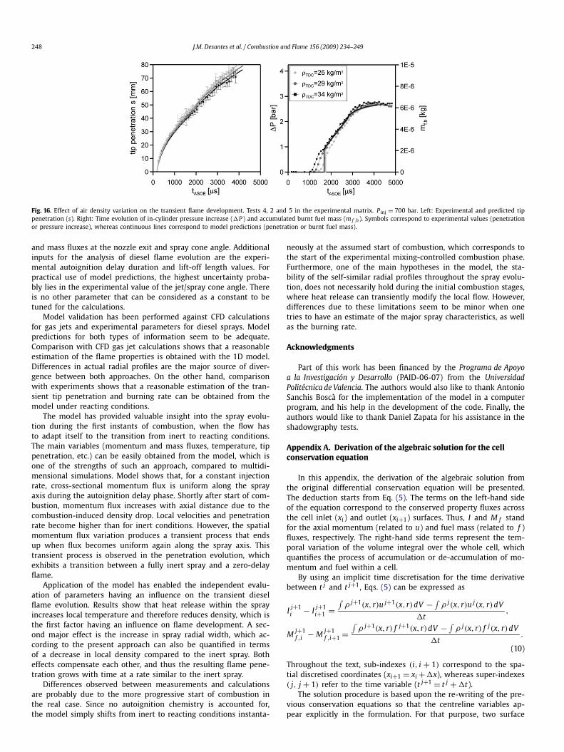
248 J.M. Desantes et al. / Combustion and Flame 156 (2009) 234–249
Fig. 16. Effect of air density variation on the transient flame development. Tests 4, 2 and 5 in the experimental matrix. P inj = 700 bar. Left: Experimental and predicted tippenetration (s). Right: Time evolution of in-cylinder pressure increase (�P ) and accumulated burnt fuel mass (m f ,b). Symbols correspond to experimental values (penetrationor pressure increase), whereas continuous lines correspond to model predictions (penetration or burnt fuel mass).
and mass fluxes at the nozzle exit and spray cone angle. Additionalinputs for the analysis of diesel flame evolution are the experi-mental autoignition delay duration and lift-off length values. Forpractical use of model predictions, the highest uncertainty proba-bly lies in the experimental value of the jet/spray cone angle. Thereis no other parameter that can be considered as a constant to betuned for the calculations.
Model validation has been performed against CFD calculationsfor gas jets and experimental parameters for diesel sprays. Modelpredictions for both types of information seem to be adequate.Comparison with CFD gas jet calculations shows that a reasonableestimation of the flame properties is obtained with the 1D model.Differences in actual radial profiles are the major source of diver-gence between both approaches. On the other hand, comparisonwith experiments shows that a reasonable estimation of the tran-sient tip penetration and burning rate can be obtained from themodel under reacting conditions.
The model has provided valuable insight into the spray evolu-tion during the first instants of combustion, when the flow hasto adapt itself to the transition from inert to reacting conditions.The main variables (momentum and mass fluxes, temperature, tippenetration, etc.) can be easily obtained from the model, which isone of the strengths of such an approach, compared to multidi-mensional simulations. Model shows that, for a constant injectionrate, cross-sectional momentum flux is uniform along the sprayaxis during the autoignition delay phase. Shortly after start of com-bustion, momentum flux increases with axial distance due to thecombustion-induced density drop. Local velocities and penetrationrate become higher than for inert conditions. However, the spatialmomentum flux variation produces a transient process that endsup when flux becomes uniform again along the spray axis. Thistransient process is observed in the penetration evolution, whichexhibits a transition between a fully inert spray and a zero-delayflame.
Application of the model has enabled the independent evalu-ation of parameters having an influence on the transient dieselflame evolution. Results show that heat release within the sprayincreases local temperature and therefore reduces density, which isthe first factor having an influence on flame development. A sec-ond major effect is the increase in spray radial width, which ac-cording to the present approach can also be quantified in termsof a decrease in local density compared to the inert spray. Botheffects compensate each other, and thus the resulting flame pene-tration grows with time at a rate similar to the inert spray.
Differences observed between measurements and calculationsare probably due to the more progressive start of combustion inthe real case. Since no autoignition chemistry is accounted for,the model simply shifts from inert to reacting conditions instanta-
neously at the assumed start of combustion, which corresponds tothe start of the experimental mixing-controlled combustion phase.Furthermore, one of the main hypotheses in the model, the sta-bility of the self-similar radial profiles throughout the spray evolu-tion, does not necessarily hold during the initial combustion stages,where heat release can transiently modify the local flow. However,differences due to these limitations seem to be minor when onetries to have an estimate of the major spray characteristics, as wellas the burning rate.
Acknowledgments
Part of this work has been financed by the Programa de Apoyoa la Investigación y Desarrollo (PAID-06-07) from the UniversidadPolitécnica de Valencia. The authors would also like to thank AntonioSanchis Boscà for the implementation of the model in a computerprogram, and his help in the development of the code. Finally, theauthors would like to thank Daniel Zapata for his assistance in theshadowgraphy tests.
Appendix A. Derivation of the algebraic solution for the cellconservation equation
In this appendix, the derivation of the algebraic solution fromthe original differential conservation equation will be presented.The deduction starts from Eq. (5). The terms on the left-hand sideof the equation correspond to the conserved property fluxes acrossthe cell inlet (xi) and outlet (xi+1) surfaces. Thus, I and M f standfor the axial momentum (related to u) and fuel mass (related to f )fluxes, respectively. The right-hand side terms represent the tem-poral variation of the volume integral over the whole cell, whichquantifies the process of accumulation or de-accumulation of mo-mentum and fuel within a cell.
By using an implicit time discretisation for the time derivativebetween t j and t j+1, Eqs. (5) can be expressed as
I j+1i − I j+1
i+1 =∫
ρ j+1(x, r)u j+1(x, r)dV − ∫ρ j(x, r)u j(x, r)dV
�t,
M j+1f ,i − M j+1
f ,i+1 =∫
ρ j+1(x, r) f j+1(x, r)dV − ∫ρ j(x, r) f j(x, r)dV
�t.
(10)
Throughout the text, sub-indexes (i, i + 1) correspond to the spa-tial discretised coordinates (xi+1 = xi +�x), whereas super-indexes( j, j + 1) refer to the time variable (t j+1 = t j + �t).
The solution procedure is based upon the re-writing of the pre-vious conservation equations so that the centreline variables ap-pear explicitly in the formulation. For that purpose, two surface
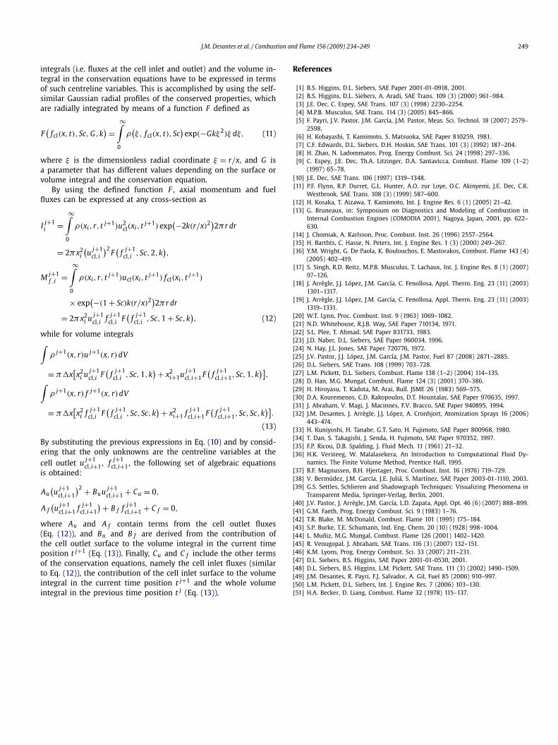
J.M. Desantes et al. / Combustion and Flame 156 (2009) 234–249 249
integrals (i.e. fluxes at the cell inlet and outlet) and the volume in-tegral in the conservation equations have to be expressed in termsof such centreline variables. This is accomplished by using the self-similar Gaussian radial profiles of the conserved properties, whichare radially integrated by means of a function F defined as
F(
fcl(x, t), Sc, G,k) =
∞∫0
ρ(ξ, fcl(x, t), Sc
)exp(−Gkξ2)ξ dξ, (11)
where ξ is the dimensionless radial coordinate ξ = r/x, and G isa parameter that has different values depending on the surface orvolume integral and the conservation equation.
By using the defined function F , axial momentum and fuelfluxes can be expressed at any cross-section as
I j+1i =
∞∫0
ρ(xi, r, t j+1)u2cl(xi, t j+1)exp
(−2k(r/x)2)2πr dr
= 2πx2i
(u j+1
cl,i
)2F(
f j+1cl,i , Sc,2,k
),
M j+1f ,i =
∞∫0
ρ(xi, r, t j+1)ucl(xi, t j+1) fcl(xi, t j+1)
× exp(−(1 + Sc)k(r/x)2)2πr dr
= 2πx2i u j+1
cl,i f j+1cl,i F
(f j+1cl,i , Sc,1 + Sc,k
), (12)
while for volume integrals∫ρ j+1(x, r)u j+1(x, r)dV
= π�x[x2
i u j+1cl,i F
(f j+1cl,i , Sc,1,k
) + x2i+1u j+1
cl,i+1 F(
f j+1cl,i+1, Sc,1,k
)],∫
ρ j+1(x, r) f j+1(x, r)dV
= π�x[x2
i f j+1cl,i F
(f j+1cl,i , Sc, Sc,k
) + x2i+1 f j+1
cl,i+1 F(
f j+1cl,i+1, Sc, Sc,k
)].
(13)
By substituting the previous expressions in Eq. (10) and by consid-ering that the only unknowns are the centreline variables at thecell outlet u j+1
cl,i+1, f j+1cl,i+1, the following set of algebraic equations
is obtained:
Au(u j+1
cl,i+1
)2 + Buu j+1cl,i+1 + Cu = 0,
A f(u j+1
cl,i+1 f j+1cl,i+1
) + B f f j+1cl,i+1 + C f = 0,
where Au and A f contain terms from the cell outlet fluxes(Eq. (12)), and Bu and B f are derived from the contribution ofthe cell outlet surface to the volume integral in the current timeposition t j+1 (Eq. (13)). Finally, Cu and C f include the other termsof the conservation equations, namely the cell inlet fluxes (similarto Eq. (12)), the contribution of the cell inlet surface to the volumeintegral in the current time position t j+1 and the whole volumeintegral in the previous time position t j (Eq. (13)).
References
[1] B.S. Higgins, D.L. Siebers, SAE Paper 2001-01-0918, 2001.[2] B.S. Higgins, D.L. Siebers, A. Aradi, SAE Trans. 109 (3) (2000) 961–984.[3] J.E. Dec, C. Espey, SAE Trans. 107 (3) (1998) 2230–2254.[4] M.P.B. Musculus, SAE Trans. 114 (3) (2005) 845–866.[5] F. Payri, J.V. Pastor, J.M. García, J.M. Pastor, Meas. Sci. Technol. 18 (2007) 2579–
2598.[6] H. Kobayashi, T. Kamimoto, S. Matsuoka, SAE Paper 810259, 1981.[7] C.F. Edwards, D.L. Siebers, D.H. Hoskin, SAE Trans. 101 (3) (1992) 187–204.[8] H. Zhao, N. Ladommatos, Prog. Energy Combust. Sci. 24 (1998) 297–336.[9] C. Espey, J.E. Dec, Th.A. Litzinger, D.A. Santavicca, Combust. Flame 109 (1–2)
(1997) 65–78.[10] J.E. Dec, SAE Trans. 106 (1997) 1319–1348.[11] P.F. Flynn, R.P. Durret, G.L. Hunter, A.O. zur Loye, O.C. Akinyemi, J.E. Dec, C.K.
Westbrook, SAE Trans. 108 (3) (1999) 587–600.[12] H. Kosaka, T. Aizawa, T. Kamimoto, Int. J. Engine Res. 6 (1) (2005) 21–42.[13] G. Bruneaux, in: Symposium on Diagnostics and Modeling of Combustion in
Internal Combustion Engines (COMODIA 2001), Nagoya, Japan, 2001, pp. 622–630.
[14] J. Chomiak, A. Karlsson, Proc. Combust. Inst. 26 (1996) 2557–2564.[15] H. Barthts, C. Hasse, N. Peters, Int. J. Engine Res. 1 (3) (2000) 249–267.[16] Y.M. Wright, G. De Paola, K. Boulouchos, E. Mastorakos, Combust. Flame 143 (4)
(2005) 402–419.[17] S. Singh, R.D. Reitz, M.P.B. Musculus, T. Lachaux, Int. J. Engine Res. 8 (1) (2007)
97–126.[18] J. Arrègle, J.J. López, J.M. García, C. Fenollosa, Appl. Therm. Eng. 23 (11) (2003)
1301–1317.[19] J. Arrègle, J.J. López, J.M. García, C. Fenollosa, Appl. Therm. Eng. 23 (11) (2003)
1319–1331.[20] W.T. Lynn, Proc. Combust. Inst. 9 (1963) 1069–1082.[21] N.D. Whitehouse, R.J.B. Way, SAE Paper 710134, 1971.[22] S.L. Plee, T. Ahmad, SAE Paper 831733, 1983.[23] J.D. Naber, D.L. Siebers, SAE Paper 960034, 1996.[24] N. Hay, J.L. Jones, SAE Paper 720776, 1972.[25] J.V. Pastor, J.J. López, J.M. García, J.M. Pastor, Fuel 87 (2008) 2871–2885.[26] D.L. Siebers, SAE Trans. 108 (1999) 703–728.[27] L.M. Pickett, D.L. Siebers, Combust. Flame 138 (1–2) (2004) 114–135.[28] D. Han, M.G. Mungal, Combust. Flame 124 (3) (2001) 370–386.[29] H. Hiroyasu, T. Kadota, M. Arai, Bull. JSME 26 (1983) 569–575.[30] D.A. Kouremenos, C.D. Rakopoulos, D.T. Hountalas, SAE Paper 970635, 1997.[31] J. Abraham, V. Magi, J. Macinnes, F.V. Bracco, SAE Paper 940895, 1994.[32] J.M. Desantes, J. Arrègle, J.J. López, A. Cronhjort, Atomization Sprays 16 (2006)
443–474.[33] H. Kuniyoshi, H. Tanabe, G.T. Sato, H. Fujimoto, SAE Paper 800968, 1980.[34] T. Dan, S. Takagishi, J. Senda, H. Fujimoto, SAE Paper 970352, 1997.[35] F.P. Ricou, D.B. Spalding, J. Fluid Mech. 11 (1961) 21–32.[36] H.K. Versteeg, W. Malalasekera, An Introduction to Computational Fluid Dy-
namics. The Finite Volume Method, Prentice Hall, 1995.[37] B.F. Magnussen, B.H. Hjertager, Proc. Combust. Inst. 16 (1976) 719–729.[38] V. Bermúdez, J.M. García, J.E. Juliá, S. Martínez, SAE Paper 2003-01-1110, 2003.[39] G.S. Settles, Schlieren and Shadowgraph Techniques: Visualizing Phenomena in
Transparent Media, Springer-Verlag, Berlin, 2001.[40] J.V. Pastor, J. Arrègle, J.M. García, L.D. Zapata, Appl. Opt. 46 (6) (2007) 888–899.[41] G.M. Faeth, Prog. Energy Combust. Sci. 9 (1983) 1–76.[42] T.R. Blake, M. McDonald, Combust. Flame 101 (1995) 175–184.[43] S.P. Burke, T.E. Schumann, Ind. Eng. Chem. 20 (10) (1928) 998–1004.[44] L. Muñiz, M.G. Mungal, Combust. Flame 126 (2001) 1402–1420.[45] R. Venugopal, J. Abraham, SAE Trans. 116 (3) (2007) 132–151.[46] K.M. Lyons, Prog. Energy Combust. Sci. 33 (2007) 211–231.[47] D.L. Siebers, B.S. Higgins, SAE Paper 2001-01-0530, 2001.[48] D.L. Siebers, B.S. Higgins, L.M. Pickett, SAE Trans. 111 (3) (2002) 1490–1509.[49] J.M. Desantes, R. Payri, F.J. Salvador, A. Gil, Fuel 85 (2006) 910–997.[50] L.M. Pickett, D.L. Siebers, Int. J. Engine Res. 7 (2006) 103–130.[51] H.A. Becker, D. Liang, Combust. Flame 32 (1978) 115–137.

![Effect of nutrient sprays on granulation and fruit quality of [] Dancy tangerine'mandarin](https://static.fdokumen.com/doc/165x107/63286a59f406ae55d2051207/effect-of-nutrient-sprays-on-granulation-and-fruit-quality-of-dancy-tangerinemandarin.jpg)