A 1D model for the description of mixing-controlled inert diesel sprays

Fuel 87 (2008) 2871–2885

Contents lists available at ScienceDirect

Fuel

journal homepage: www.fuelfirst .com

A 1D model for the description of mixing-controlled inert diesel sprays

José V. Pastor, J. Javier López, José M. García *, José M. PastorCMT – Motores Térmicos, Universidad Politécnica de Valencia, Camino de Vera s/n, 46022 Valencia, Spain

a r t i c l e i n f o

Article history:Received 1 February 2008Received in revised form 22 April 2008Accepted 23 April 2008Available online 21 May 2008

Keywords:Diesel spraysMixingEvaporation

0016-2361/$ - see front matter � 2008 Elsevier Ltd. Adoi:10.1016/j.fuel.2008.04.017

* Corresponding author. Tel.: +34 96 387 76 50; faxE-mail address: [email protected] (J.M. García).

a b s t r a c t

The paper reports an investigation focusing on the transient evolution of diesel sprays. In order to under-stand the relationship between fuel–air mixing and spray penetration, a one-dimensional spray model isdeveloped, which is capable of predicting the spray behaviour under transient conditions. The mainassumptions of the model are the mixing-controlled hypothesis and the validity of self-similarity for con-servative properties. Validation of such concepts is achieved by comparing model predictions with bothCFD gas jet simulations and experimental diesel spray measurements. Results show that a reasonableestimation of the spray evolution can be obtained for both non-vaporising and vaporising conditions.

� 2008 Elsevier Ltd. All rights reserved.

1. Introduction

The evolution of diesel engines in the last decades has been dri-ven by the stringent pollution legislation. In order to fulfill the reg-ulated limits, a detailed study of fuel–air mixing and combustionprocesses has been necessary. Such a research task has made itpossible to optimise engine performance as well as to lower pollu-tant emissions.

Understanding of diesel sprays is essential in this optimizationprocess. Due to the engine working principle, fuel and air meet in-side the combustion chamber thanks to the spray momentum,which controls both fuel stream penetration inside the combustionchamber and the simultaneous mixing with air. Furthermore, suchprocesses have a direct impact on the characteristics of the flamethat forms after the onset of combustion reactions, both in termsof local temperatures and pollutant formation. Thus, momentumflux, spray tip penetration, mixture composition and temperatureare closely linked.

The previous relationship is implicit to the conservation equa-tions that are at the base of CFD models. However, the fact thatsuch equations are solved at small cells hinders the identificationof the link between macroscopic spray results and the boundaryconditions of the problem (air density, injection velocity, . . .). Thislimitation can be overcome with the use of one-dimensional (1D)spray models, which usually contain the necessary physics to solvethe problem, but in a way that enables a straightforward identifi-cation of the influence of boundary parameters on the results.

One-dimensional models have been successfully used in thepast for the prediction of spray tip penetration [1]. They have been

ll rights reserved.

: +34 96 387 76 59.

usually developed in the form of a more or less general correlationfor this parameter [2]. In some cases, such models have also con-sidered some kind of mixture distribution within the spray. How-ever, they have been used mainly for inert conditions. Transientflame behaviour has not been so thoroughly investigated, and cor-responding 1D models have made use of corrections of air entrain-ment from gas jet experiments to account for heat release effects[3,4].

This paper reports an investigation that aims at understandingthe existing relationship between the local fuel–air mixing process,the spray dynamic evolution and the transient tip penetration. Forthat purpose, a one-dimensional spray model is presented with ageneral formulation that enables the prediction of any type ofspray flow, under both inert and reacting conditions. Furthermore,due to the mixing-controlled hypothesis upon which the model isbased, it can be used for the description of both a gas jet and also adiesel spray working under real engine conditions. By makingsome assumptions derived from the theory of turbulent gas jets,the model enables the estimation of the distribution of propertieswithin the spray (composition, temperature, density, . . .), as well asthe tip penetration.

The work is presented as a series of two papers. This is the firstone, which is devoted to the analysis of the spray under inert con-ditions. Even though this problem is largely analysed in the litera-ture, the approach presented here is original in the formulation ofthe conservation equations, which solves the on-axis variables byusing cross-sectional integrals. A transient formulation makes itpossible to use the model for both constant and also variable injec-tion rate shapes. The model is an improvement of a previous ver-sion reported in [5], which discretised the injected fuel mass inparcels that were tracked along the spray axis in a one-dimen-sional fashion. However, this approach could only be used under

mailto:[email protected]

http://www.sciencedirect.com/science/journal/00162361

http://www.fuelfirst.com

Nomenclature

1D, 2D One-dimensional, two-dimensionalA, B, C constants for the solution of conservation equations

within a cellCFD computational fluid dynamicscp heat capacity at constant pressured diameterf fuel mass fractionF density-averaged radial integral of self-similar profileG generic parameter for the application of the radial inte-

gralF to a generic conserved property qH cross-sectional integrated enthalpy fluxh enthalpyI cross-sectional integrated axial momentum fluxIL intact lengthk constant in the Gaussian profileLL maximum liquid lengthM cross-sectional integrated mass fluxP PressurePr turbulent Prandtl numberQ cross-sectional integrated flux for a generic conserved

property qq generic conserved propertyr radial coordinate perpendicular to the main spray direc-

tions spray tip penetrationSc Turbulent Schmidt number

T temperaturet timeu axial velocityV volumex axial coordinate in the main spray directionY mass fraction

Greek symbolsq densitysmix;st characteristic mixing time at stoichiometric conditionsh spray cone angle1 constant for the definition of spray cone anglen ratio of radial to axial coordinate

Subscripts0 relative to conditions at the nozzle exita,1 relative to ambient conditions far away from the nozzlecl spray axis (Centerline)eq equivalentevap relative to conditions at the maximum liquid lengthf relative to fuel massf,l relative to liquid fuelf,v relative to vapor fuelf,0 relative to pure fuel conditionsinj relative to injectionu relative to the conservation equation of axial momen-

tum

2872 J.V. Pastor et al. / Fuel 87 (2008) 2871–2885

inert conditions, and the consideration of transient injection ratewas based on corrections on the constant injection rate case, whichwere derived from CFD gas jet simulations. The present paper setsup the main equations of the model in a more general way by usingan Eulerian approach. This enables a very easy description of thetransient spray evolution from the model solutions, without anyfurther correction. Furthermore, the present formulation will en-able, in a second paper, the extension of the spray analysis to react-ing conditions, and thus the prediction of the flame transientevolution.

The paper is structured as follows: after the introduction, someconcepts will be reviewed that make up the conceptual basis uponwhich the model has been built. In a subsequent section, the datasources used for validation are presented. Later on, the generalmodel description is given and, in the subsequent section, valida-tions for the approach are presented, both for non-vaporising andvaporising sprays. Finally, some conclusions on the work arepresented.

2. Background

Keeping in mind the goal of the present work, namely thedescription of the inert diesel spray by means of mixing-controlledconcepts, this section reviews the experimental support for this ap-proach, as well as the possibilities that modelling offers when try-ing to understand the transient spray behaviour.

Spray evolution is an intrinsically complicated problem, due tothe high velocity, and consequently small temporal and spatialscales, together with the two phases appearing in the fuel. How-ever, experimental results have confirmed the hypothesis thatspray evolution is controlled by fuel–air mixing rates. Current en-gine technologies (high boost and injection pressure, and smallnozzle hole diameter) result in a complete atomisation regime in-

side the spray very near the nozzle exit [6]. Even under non-vaporising conditions, in which the problem is undoubtedly atwo-phase flow, the spray can be analysed from a point of viewof the gas jet theory, as droplets reach almost immediately a dy-namic equilibrium with the surrounding gas phase [7–12]. There-fore, droplet sizes under realistic engine conditions are so smallthat atomisation is no longer a limitation in the subsequent phys-ical processes (evaporation and mixing) leading to combustion.

On the other hand, experimental results for vaporising sprays bydifferent authors have shown that the maximum liquid length iscontrolled by in-cylinder air density and temperature, nozzle orificediameter and fuel type [13–18]. Injection pressure has little, if any,influence on this parameter. The latter result is one of the most evi-dent confirmations of the hypothesis that the vaporisation process islimited by fuel–air mixing rate. Due to the complete atomisation re-gime, droplets reach a dynamic equilibrium with the air very close tothe nozzle, and local transfer rates of momentum, mass and energybetween liquid droplets and surrounding air are fast in comparisonto the rate of development of the flow field as a whole [13,19]. Thismeans that fuel droplets evaporate as long as there is enough air forthem to heat up and vaporise. Consequently, non-reacting vaporis-ing diesel sprays fit adequately in the ‘locally-homogeneous flow’description [19], which makes it possible to treat an a priori compli-cated two-phase problem from the point of view of single-phaseflows. In summary, experimental information shows that dieselsprays under both non-vaporising and vaporising conditions canbe properly described with a mixing-controlled approach, and thusthey can be analysed in the same way as gas jets.

In parallel with the experimental research, modelling has triedto quantify the previous physical processes, and to evaluate thevalidity of the theoretical approaches. Improvements in computercapabilities and code refinement has increased CFD reliability asa tool for diesel combustion analysis, as well as to explore theinfluence of engine modifications. Extensive comparison with

r

1

3

4

5

J.V. Pastor et al. / Fuel 87 (2008) 2871–2885 2873

measurements has enabled experimental validation of combustionmodels [20]. However, CFD has still limitations regarding the mod-elling of the atomisation process, which results in an inherentdependency of results on grid resolution [21,22]. This does not usu-ally occur if a single phase gas jet is calculated. Fortunately, theexisting analogy between gas jets and diesel sprays makes it possi-ble to compare results for both types of flow [23]. In some cases,this has enabled the calculation of the vaporisation process of adiesel spray based on the assumption of a mixing-controlled pro-cess, such as in [24].

Apart from CFD codes, phenomenological spray models are alsoemployed for basic studies. They simplify to different degrees thephysics present in the problem, leading to zero- or one-dimen-sional approaches, so that in some cases analytical solutions canbe derived. In this way, fast computations can be performed, andthere is an explicit link between the spray boundary conditionsand the corresponding solutions. A good example can be found in[1] for the maximum spray penetration for steady injection andambient conditions, later extended to the maximum liquid length[25]. Similar correlations are quite often found in the literature[26–28], but they are usually limited to single-spray cases, whereboundary conditions are quasi-steady, i.e., constant injection rate.

Fully transient spray models demand for a more elaborated ap-proach. In this sense, one can find multi-zone phenomenologicalmodels, which simplify conservation equations. In a first group ofsuch models, following the work in [29], the spray is discretisedin small parcels in both axial and radial directions. Compositionand temperature of each of these parcels are tracked along thecombustion chamber. This approach has been used by differentauthors [30,31], even though an assumption of quasi-steady evolu-tion is made for the spray penetration. A second type of multi-zonemodel follows the development of equivalence ratio zones sur-rounding a central liquid core [32].

Finally, some approaches simplify the problem to a single spa-tial dimension, but consider boundary conditions that may varywith time. A recent example can be found in [33], which is mainlyfocused on predicting spray tip penetration. Wan and Peters [8]also derive a model where variables are averaged over the wholespray cross-section. This model is capable of predicting the sprayevolution under both non-vaporising and vaporising condition. Itdelivers not only the spray tip penetration, but also the evolutionof the main properties along the spray. Furthermore, the modelhas been coupled to a CFD code in order to eliminate the griddependency of the 3D computations [34]. This approach solvesthe 3D conservation equations of the gas phase, and the sourceterms for evaporation are obtained from the one-dimensionalmodel which solves both the liquid and vapor phases. This is prob-ably the best example of how a one-dimensional model can givevaluable information on the spray evolution. The present contribu-tion will present a one-dimensional model that follows a similarapproach in order to describe a fully transient diesel spray, butincorporating the mixing-control hypothesis.

X2

Fig. 1. Basic CFD domain for gas jet studies: (1) injection orifice, (2) jet axis, (3) and(4) flow inlet and outlet, (5) wall. Boundary conditions are defined in Table 1.

Table 1Definition of gas jet CFD boundary conditions

Surface Boundary type Defining variables

(1) Injection orifice Velocity inlet u0; Tf ;0;qf ;0

(2) Jet axis Symmetry axis –(3) Flow inlet/outlet Constant pressure boundary P; Ta;1; qa;1(4) Wall Rigid wall, non-slip –

Nomenclature corresponds to the schematic in Fig. 1.

3. Data sources

The analysis developed in this paper has been validated againstboth numerical CFD calculations and experimental data. The for-mer ones have been used as a source of gas jet information. Onthe other hand, experimental results in a spray test rig have beenused to validate diesel spray concepts.

3.1. CFD gas jet calculations

The CFD methodology has been aimed at simulating the turbu-lent gas jet, in order to validate the concepts that can be later

applied to the more complex but also more real case of a dieselspray. In the latter case, CFD atomisation models are certainlydependent on some non-physical parameters such as grid size.Gas jet simulations do not have such disadvantages, and the infor-mation they can provide is more reliable.

Calculation results will be used for validating the 1D model un-der fully controllable conditions. To a given extent, the 1D modeldeveloped in Section 4 tries to reproduce CFD results by makinguse of some ad-hoc simplifications that can be justified accordingto gas jet theory. There is no claim that these CFD gas jet resultsare as accurate as experimental measurements, as the comparisonagainst experimental data is out of the scope of the present work.However, the underlying basic concepts, e.g. the self-similar radialprofiles, governing equations, etc. will be validated in order toextrapolate them to diesel sprays [23,35].

3.1.1. MethodologyCFD calculations have been performed with the commercial

code FLUENT. The basic problem is a steady gas jet injected intoan open domain, the geometrical definition is shown schematicallyin Fig. 1 and boundary conditions are summarised in Table 1. Thesteady approach simplifies the analysis by eliminating time as anadditional variable, but conclusions are still useful to analyse tran-sient jet flows, where a large steady zone exists in the part closestto the nozzle [36,37]. Some transient calculations have also beenperformed. No lateral air velocity is assumed, which results in anaxisymmetric problem. Therefore, a 2D domain has been used cor-responding to the jet symmetry plane.

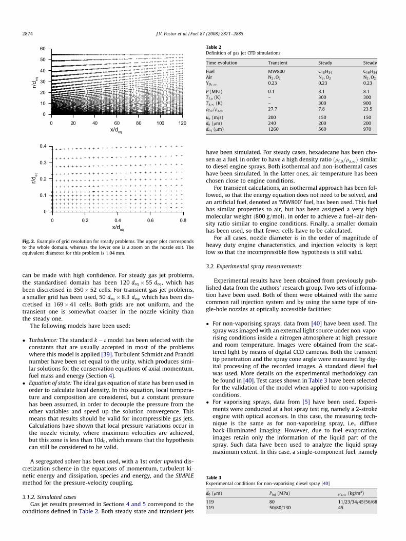
An example of the grid resolution is shown in Fig. 2, togetherwith a zoom on the nozzle exit. An structured grid has been used,with more refinement in zones close to the nozzle and to the axis,where the highest spatial gradients can be found.

The 2D domain size has been parameterised in terms of the

problem equivalent diameter deq ¼ d0

ffiffiffiffiffiffiffiqf ;0qa;1

q, which is a scale of

the gas jet flow under inert conditions [38]. d0 stands for the noz-zle geometrical diameter, whereas, q stands for density, wheresub-indexes (f,0) and (a,1) correspond to pure fuel and air condi-tions, respectively. This nomenclature will be kept throughout thepaper. By using this standardised domain, grid size is scaled tothe spatial variability of the computed problem, and thus compar-ison of gas jet problems with very different boundary conditions

0 20 40 60 80 100 120

0

10

20

30

40

50

60

0 0.2 0.4 0.6 0.8x/deq

x/deq

0

0.1

0.2

0.3

0.4

r/deq

r/deq

Fig. 2. Example of grid resolution for steady problems. The upper plot correspondsto the whole domain, whereas, the lower one is a zoom on the nozzle exit. Theequivalent diameter for this problem is 1:04 mm.

Table 2Definition of gas jet CFD simulations

Time evolution Transient Steady Steady

Fuel MW800 C16H34 C16H34

Air N2;O2 N2;O2 N2;O2

YO2 ;1 0.23 0.23 0.23

P (MPa) 0:1 8:1 8:1Tf ;o (K) – 300 300Ta;1 (K) – 300 900qf ;o=qa;1 27:7 7:8 23:5

uo (m/s) 200 150 150do (lm) 240 200 200deq (lm) 1260 560 970

Table 3Experimental conditions for non-vaporising diesel spray [40]

d0 (lm) Pinj (MPa) qa;1 (kg/m3)

119 80 11/23/34/45/56/68119 50/80/130 45


can be made with high confidence. For steady gas jet problems,the standardised domain has been 120 deq � 55 deq, which hasbeen discretised in 350� 52 cells. For transient gas jet problems,a smaller grid has been used, 50 deq � 8:3 deq, which has been dis-cretised in 169� 41 cells. Both grids are not uniform, and thetransient one is somewhat coarser in the nozzle vicinity thanthe steady one.

The following models have been used:

� Turbulence: The standard k� e model has been selected with theconstants that are usually accepted in most of the problemswhere this model is applied [39]. Turbulent Schmidt and Prandtlnumber have been set equal to the unity, which produces simi-lar solutions for the conservation equations of axial momentum,fuel mass and energy (Section 4).

� Equation of state: The ideal gas equation of state has been used inorder to calculate local density. In this equation, local tempera-ture and composition are considered, but a constant pressurehas been assumed, in order to decouple the pressure from theother variables and speed up the solution convergence. Thismeans that results should be valid for incompressible gas jets.Calculations have shown that local pressure variations occur inthe nozzle vicinity, where maximum velocities are achieved,but this zone is less than 10d0, which means that the hypothesiscan still be considered to be valid.

A segregated solver has been used, with a 1st order upwind dis-cretization scheme in the equations of momentum, turbulent ki-netic energy and dissipation, species and energy, and the SIMPLEmethod for the pressure-velocity coupling.

3.1.2. Simulated casesGas jet results presented in Sections 4 and 5 correspond to the

conditions defined in Table 2. Both steady state and transient jets

have been simulated. For steady cases, hexadecane has been cho-sen as a fuel, in order to have a high density ratio ðqf ;0=qa;1Þ similarto diesel engine sprays. Both isothermal and non-isothermal caseshave been simulated. In the latter ones, air temperature has beenchosen close to engine conditions.

For transient calculations, an isothermal approach has been fol-lowed, so that the energy equation does not need to be solved, andan artificial fuel, denoted as ‘MW800’ fuel, has been used. This fuelhas similar properties to air, but has been assigned a very highmolecular weight ð800 g=molÞ, in order to achieve a fuel–air den-sity ratio similar to engine conditions. Finally, a smaller domainhas been used, so that fewer cells have to be calculated.

For all cases, nozzle diameter is in the order of magnitude ofheavy duty engine characteristics, and injection velocity is keptlow so that the incompressible flow hypothesis is still valid.

3.2. Experimental spray measurements

Experimental results have been obtained from previously pub-lished data from the authors’ research group. Two sets of informa-tion have been used. Both of them were obtained with the samecommon rail injection system and by using the same type of sin-gle-hole nozzles at optically accessible facilities:

� For non-vaporising sprays, data from [40] have been used. Thespray was imaged with an external light source under non-vapo-rising conditions inside a nitrogen atmosphere at high pressureand room temperature. Images were obtained from the scat-tered light by means of digital CCD cameras. Both the transienttip penetration and the spray cone angle were measured by dig-ital processing of the recorded images. A standard diesel fuelwas used. More details on the experimental methodology canbe found in [40]. Test cases shown in Table 3 have been selectedfor the validation of the model when applied to non-vaporisingconditions.

� For vaporising sprays, data from [5] have been used. Experi-ments were conducted at a hot spray test rig, namely a 2-strokeengine with optical accesses. In this case, the measuring tech-nique is the same as for non-vaporising spray, i.e., diffuseback-illuminated imaging. However, due to fuel evaporation,images retain only the information of the liquid part of thespray. Such data have been used to analyze the liquid spraymaximum extent. In this case, a single-component fuel, namely

Table 4Experimental conditions for vaporising diesel spray [5]

d0 (lm) Pinj (MPa) qa;1 (kg/m3)

165 70 22.7/26.4/30.4165 30/70/110 26.4


hexadecane, has been used. More details on the experimentalmethodology can be found in [5]. Test cases in Table 4 have beenselected for the validation of the model when applied to vaporis-ing conditions.

Apart from the information derived from the images, nozzleinjection conditions (mass and momentum fluxes) were also avail-able. These magnitudes are inputs for the model that will be de-scribed below.

4. Model development

The model description has been divided into different subsec-tions. First, the model approach and general hypotheses are pre-sented. In a subsequent section, the conservation equations andboundary conditions are analysed, followed by the solution proce-dure. Later on, particularisations of the model for the two maintypes of inert spray flows, namely the non-vaporising and thevaporising ones, are analysed. Finally, a general overview of themodel is presented. Appendix A complements the model descrip-tion by including a simplified steady approach directly derivedfrom the transient one, which is directly linked to the classicalanalysis of steady gas jets.

4.1. Approach

Fuel sprays are injected through a nozzle hole into the combus-tion chamber of a diesel engine, where they mix with air. Swirl orany other type of engine-induced air movement are not the consid-ered in this work. The ambient volume is large enough, so that thespray evolution does not modify air conditions far away from thenozzle. Fig. 3 shows a sketch of the basic configuration of this typeof problem. Fuel stream is assumed to have an spatially uniformvelocity profile at the nozzle exit. This flow exchanges momentumwith the ambient air and sets it into movement, so that it increasesin width with the axial distance. The spray cone half angle (orspreading angle) h defines this radial growth, and will be an inputto the model. Together with the nozzle diameter d0, the spray angledefines the virtual origin of the spray, so that at the nozzle exitx ¼ x0 ¼ d0=2= tanðh=2Þ.

Due to the transient nature of the general problem, the spraydomain has been divided axially into a number of cells with a cer-tain thickness Mx spanning the whole spray cross-section. Each cell

Fig. 3. Schematic of the model approach.

is limited by the inlet and the outlet sections (i and iþ 1, respec-tively) so that xiþ1 ¼ xi þ Mx (Fig. 3). At every time instant, thespray size is defined in terms of the tip penetration s, which isthe farthest cell from the nozzle where inlet velocity is differentfrom zero and outlet velocity is zero.

4.2. General hypotheses of the model

The conservation equations are formulated for each cell. In themost general type of spray flow, the unknowns to be solved arethose related to the conservation equations, namely axial velocityu, fuel mass fraction f and enthalpy h. For convenience in the for-mulation, h is replaced by the enthalpy difference h� ha;1. The fol-lowing hypotheses are assumed for any time instant t:

(1) Symmetry on the spray axis, i.e., no air swirl.(2) A fully-developed turbulent flow is assumed, which means

that self-similar radial profiles can be defined for the con-served variables, i.e., the ratio of any conserved variabledivided by the centerline value does not depend on the axialcoordinate. This is probably one of the major assumptions inthe model, which is usually accepted for steady gas jet orspray flows. Under transient injection conditions, some kindof similarity can also be assumed, as shown in [41].A Gauss-ian radial distribution function has been used, which is validfor steady inert atmospheric gas jets [42], as well as fordeveloped diesel fuel sprays at typical engine conditions[43]. The formulation could also admit other types of nor-malising functions, e.g. those in [44] or [45]. This leads tothe following equation:

� � � �
uðx; rÞuclðxÞ
¼ f ðx; rÞfclðxÞ

1=Sc

¼ hðx; rÞ � ha;1

hclðxÞ � ha;1

1=Pr

¼ exp �krx

� �2� �

; ð1Þ

where ucl, fcl and hcl � ha;1 are the axial component of thevelocity vector, fuel mass fraction and enthalpy differenceon the spray axis (centerline), k is a constant and Sc and Prare the turbulent Schmidt and Prandtl numbers, respectively.The latter two parameters are set to 1, unless otherwise sta-ted. Laminar contributions to the transport processes are ne-glected [19].This hypothesis requires that the flow ‘forget’about the initial uniform radial profile, which only happensafter a certain distance to the nozzle exit, denoted as ‘intactlength’ IL. This distance is calculated at every time step asthe farthest position from the nozzle where fclðx ¼ ILÞ ¼ 1.For that purpose, the model starts the calculation from thenozzle exit by assuming a uniform radial profile, instead of aGaussian one. This means that the unknowns to be solved cor-respond to cross-sectional averages of spray variables. Aftersolving the conservation equations at one cell, a calculationis performed of the corresponding value of fcl that would beobtained if a Gaussian profile were assumed. The process isrepeated for subsequent cells until fclðxÞ < 1, which meansthat the cell already belongs to the fully-developed flowregion.

(3) The spray angle is defined as the location where the self-similar axial velocity profile equals 1 ¼ 0:01. According tothat, there is a relationship between the spray cone angleand the constant k in the self-similar Gaussian profiles:

k ¼ lnð1=1Þtan2ðh=2Þ

: ð2Þ

(4) Locally-homogeneous flow is assumed [19], i.e., there existsa local equilibrium both in thermal and velocity conditions.


This allows for a consideration of the spray as a gas jet. Thebackground section has shown that this hypothesis is quitereasonable for current diesel sprays.

(5) Pressure is assumed to be constant all over the spray, andthus compressibility effects are neglected.

(6) Local density is calculated under an assumption of idealmixing:

Ijþ1i �

Mjþ1f ;i �

Hjþ1i �

qðx; rÞ ¼ 1Pi

Yiðx;rÞqiðx;rÞ

; ð3Þ

where Yi is the mass fraction of the mixture component i, andqi is the density for the pure component i at the mixture localtemperature Tðx; rÞ and pressure P. For fuel species f ¼ Y f .

4.3. Conservation equations and boundary conditions

For each cell, the differential conservation equations of axialmomentum, fuel mass and energy are formulated as follows:

Iðxi; tÞ � Iðxiþ1; tÞ ¼ddt

Zqðx; r; tÞ � uðx; r; tÞ � dV

� �;

Mf ðxi; tÞ �Mf ðxiþ1; tÞ ¼ddt

Zqðx; r; tÞ � f ðx; r; tÞ � dV

� �;

Hðxi; tÞ � Hðxiþ1; tÞ ¼ddt

Zqðx; r; tÞ � ðhðx; r; tÞ � ha;1Þ � dV

� �;

ð4Þ

The terms on the left hand-side of the equation correspond to theconserved property fluxes across the cell inlet (xi) and outlet (xiþ1)surfaces. Thus, I, Mf and H stand for the axial momentum (relatedto u), fuel mass (related to f) and enthalpy (related to h� ha;1)fluxes, respectively. The right hand-side terms represent the tempo-ral variation of the volume integral to the whole cell, which quan-tifies the process of accumulation or de-accumulation ofmomentum, fuel or energy within a cell. Throughout the text,sub-indexes ði; iþ 1Þ correspond to the spatial discretised coordi-nates (xiþ1 ¼ xi þ Mx), whereas, super-indexes ðj; jþ 1Þ refer to thetime variable (tjþ1 ¼ tj þ Mt). An implicit time discretization is used,so that temporal balances between tj and tjþ1 are expressed as:

Ijþ1iþ1 ¼

Rqðx; r; tjþ1Þuðx; r; tjþ1ÞdV �

Rqðx; r; tjÞuðx; r; tjÞdV

Dt;

Mjþ1f ;iþ1 ¼

Rqðx; r; tjþ1Þf ðx; r; tjþ1ÞdV �

Rqðx; r; tjÞf ðx; r; tjÞdV

Dt;

Hjþ1iþ1 ¼

Rqðx; r; tjþ1Þ hðx; r; tjþ1Þ � ha;1

� �dV �

Rqðx; r; tjÞ hðx; r; tjÞ � ha;1

� �dV

Dt:

ð5Þ

Some boundary conditions are necessary inputs for each calcula-tions, and will be obtained experimentally for each particular injec-tion system and experimental environment:

� Momentum I0, fuel mass M0 and enthalpy H0 fluxes at the nozzleexit (i ¼ 0). All of them can be considered as constant or a func-tion of the time. The first two can be obtained experimentally fora particular nozzle.

� The spray cone angle h=2. This parameter will be assumed to beconstant with time. Due to the difficulties for obtaining experi-mental values, it can be regarded to some extent as the only fit-ting parameter in the model.

� Finally, in order to be able to solve the conservation equations,the relationship between local density and the other unknownshas to be made explicit. Formally, this is expressed as a functionof the type q ¼ qðf Þ, which falls into the category of the so-calledstate relationships. The function is known a priory, and it

depends on some additional boundary conditions, namely thecomposition and thermodynamic conditions of pure fuel (condi-tions at the nozzle exit, subscripted as f ;0) and pure air (condi-tions subscripted as a,1), which may be constant (e.g. for asteady problem) or variable along time (e.g. for an internal com-bustion engine). According to the way the state relationships arecalculated, the type of flow will be an inert or reacting gas jet orliquid spray. In the former case, there is also a differencebetween non-vaporising or vaporising conditions.

4.4. Solution procedure

In order to obtain a solution, the system of conservation Eqs. (5)is re-written, so that a formulation is obtained where the on-axisvariables ucl, fcl or hcl on the cell inlet and outlet will be the param-eters to be solved for every time instant and axial position. Valuesat any other position can be derived by using the corresponding ra-dial profile (Eq. (1)). Therefore, the three unknowns can be ex-pressed as a function of the variables on the spray axis and thenon-dimensional coordinate ðr=xÞ, e.g. uðx; r; tÞ ¼ uðuclðx; tÞ; nÞ,where n ¼ r=x.

In order to reformulate the equations, both the inlet/outlet fluxintegrals and the volume integrals for each cell have to be ex-pressed in such a way that they only depend on the correspondinginlet and outlet cross-sections. Thus, for any conserved variable q(corresponding to u, f or h) the flux Q (corresponding to I, Mf orH) can be expressed at any cross-section as:

Qjþ1i ¼

Z 1

0qðxi; r; tjþ1Þ � uclðxi; tjþ1Þ � qclðxi; tjþ1Þ � exp �Gkn2� �

� 2pr dr; ð6Þ

where G is a parameter that has different values according to theconserved variable q. If q ¼ u then G ¼ 2, if q ¼ f then G ¼ ð1þ ScÞand if q ¼ h� ha;1 then G ¼ ð1þ PrÞ. This equation can be furtherexpressed as follows:

Qjþ1i ¼ 2px2

i � ujþ1cl;i � q

jþ1cl;i � F f jþ1

cl;i ; Sc;G; k� �

; ð7Þ

where the cross-sectional integral has been included in the functionF:

F fclðx; tÞ; Sc;G; kð Þ ¼Z 1

0q n; fclðx; tÞ; Scð Þ � exp �Gkn2� �

� n � dn ð8Þ

Thus, conserved property fluxes depend on a spray characteristicarea (2px2), the convective flow on the spray axis (ucl � qcl) and athird integral term F. This function is used extensively throughoutthe model formulation, as it contains the influence of density andspray angle on the conservation equations. For example, the equa-tion can be integrated analytically for a constant-density flow:

Fðq ¼ constÞ ¼ q2Gk

¼ q tan2ðh=2Þ2G lnð1=1Þ : ð9Þ

Therefore, F can be interpreted as a weighted-average density overthe spray cross-section. For a more general problem, where theSchmidt number, the spray cone angle (i.e., k) and the parameter

Pure air, q(1-f) [kg/s]

a,ω

Pure fuel, qf [kg/s]

f,o

q(x,r)= f(x,r)q + (1-f(x,r))qa,ωf,o

1 [kg/s]

r

x

Fig. 4. Adiabatic mixing concept.


G are known, F is only a function of the density law (i.e., q ¼ qðf Þ)and the on-axis fuel mass fraction fcl. Thus, it can be calculated inde-pendently of the conservation equations.

By using the same type of formulation, the volume integrals canbe referred to the surface integrals at the cell inlet (xi) and outlet(xiþ1) cross-sections, and later on to the corresponding on-axisvariables and radial integrals:

Zqðx; r; tjþ1Þ � qðx; r; tjþ1Þ � dV

¼ pDx � xi � qjþ1cl;i � F f jþ1

cl;i ; Sc;G; k� �

þ xiþ1 � qjþ1cl;iþ1F f jþ1

cl;iþ1; Sc;G; k� �h i

;

ð10Þ

where G ¼ 1 if q ¼ u, G ¼ Sc if q ¼ f and G ¼ Pr if q ¼ h� ha;1.At every time instant tjþ1, the equations for the whole set of

cells are solved in a ‘downstream’ fashion. For example, the firstcell to be solved is that closest to the nozzle hole (from i ¼ 0 toi ¼ 1), where the inlet section corresponds to the injection bound-ary condition, which is already known. For that cell, the only un-knowns are the outlet variables ujþ1

cl;1, f jþ1cl;1 and hjþ1

cl;1 which are atthe same time the inlet conditions to the next cell downstream(from i ¼ 1 to i ¼ 2). This process can be applied iteratively tothe consecutive cells. Therefore, for a generic cell (from i toiþ 1), the only unknowns will be ujþ1

cl;iþ1, f jþ1cl;iþ1 and hjþ1

cl;iþ1.After the previous comments, by substituting the previous der-

ivations (Eqs. (6) and (10)) in Eq. (5) the following set of algebraicequations can be obtained for each cell:

Au � ujþ1cl;iþ1

� �2þ Bu � ujþ1

cl;iþ1 þ Cu ¼ 0;

Af � ujþ1cl;iþ1 � f

jþ1cl;iþ1

� �þ Bf � f jþ1

cl;iþ1 þ Cf ¼ 0;

Ah � ujþ1cl;iþ1 � h

jþ1cl;iþ1

� �þ Bh � hjþ1

cl;iþ1 þ Ch ¼ 0

ð11Þ

where A, B and C (with the corresponding sub-indexes) are func-tions depending on the known terms of Eqs. (5). At every time step,the calculation process starts from the first cell closest to the nozzleorifice. The solving process is repeated downstream until the outletvelocity ucl;iþ1 is practically zero. This process delivers in a directway the spray tip penetration, which is the furthest cell reachedat a time step. Appendix A shows a simplified solution to the modelequations that assumes steady conditions.

4.5. State relationships

The calculation of local mixture thermodynamics is a major partin the prediction of spray development, especially as local densityappears explicitly in the conservation equations. This section pre-sents the state relationships for the two basic types of inert flowthat are addressed by the 1D model.

4.5.1. Non-vaporising spraysThe first case to be studied is probably the simplest one, which

would correspond to fuel being injected into an environment at thesame temperature. As a consequence, energy exchanges are notrelevant to the problem, and the enthalpy conservation equationdoes not need to be solved. The only relevant variable in the staterelationship is local density, as temperature is constant. If idealmixing is assumed, neither fuel nor air change in partial density,and the local density (Eq. (3)) can be simplified to the isothermalmixture of two species:

qðx; rÞ ¼ 1f ðx;rÞqf ;0þ 1�f ðx;rÞ

qa;1

ð12Þ

where qf ;0 and qa;1 correspond to the pure fuel and pure air densi-ties. This case includes the constant-density spray, which would be

obtained if qf;0 ¼ qa;1. Under the assumption of a mixing-controlledspray, the solution is identical both for a gas jet and a non-vaporis-ing spray.

4.5.2. Vaporising spraysThe next step in the applicability of the 1D model is the intro-

duction of thermal exchanges. In a diesel spray, this results fromthe entrainment of hot air, which heats liquid fuel up and producesthe subsequent vaporisation process. In order to solve conservationequations, the following considerations are made:

� If the general problem is considered, three equations (conserva-tion of axial momentum, fuel and energy) and three unknownsfor each cell (ucl, fcl and hcl) have to be solved. However, the tur-bulent Lewis number can be assumed to be equal to one, i.e.,Sc ¼ Pr. This is a quite generalised hypothesis for turbulentnon premixed flames. Consequently, the solutions for fuel massfraction and enthalpy in Eq. (5) are analogous (Af ¼ Ah, Bf ¼ Bh

and Cf ¼ Ch), which can be expressed as:

f ðx; r; tÞ ¼ hðx; r; tÞ � ha;1

hf ;0 � ha;1; ð13Þ

where hf ;0 is the pure fuel enthalpy at the nozzle exit conditions,and ha;1 is the enthalpy of pure air at ambient conditions.Although the temporal dependency of both enthalpy valueshas been eliminated for brevity, such boundary conditions mayvary with time. However, this relationship is independent ofthe general flow calculations. Therefore, only the conservationequations of momentum and fuel mass are solved, with Eq.(13) being known a priori.

� In order to solve the conservation equations, the radial integralfunction F defined in Eq. (8) has to be calculated as a functionof fcl. This function couples energy (i.e., Eq. (13)), momentumand fuel equations by means of the local density q. At constantpressure, and according to Eq. (3), density depends on the localcomposition and temperature, which will have to be calculatedby feeding additional information into the problem. This is thestarting point of the state relationships. These functions definethe local thermodynamic equilibrium for any local property qin terms of fuel mass fraction f, i.e., they are explicit solutionsof T ¼ Tðf Þ, Yi ¼ Yiðf Þ or q ¼ qðf Þ. For that purpose, local condi-tions are calculated under the assumption of an adiabatic mixingprocess of two streams of pure fuel and air, respectively, in a cer-tain proportion given by f (Fig. 4). The following procedure hasbeen developed:(1) Local mixture enthalpy h is calculated by means of Eq.

(13). This expression shows that the local value for h isthe result of the addition of the pure fuel enthalpy hf ;0

and the pure air one ha;1 in a proportion given by f.(2) By applying the inert adiabatic mixing hypotheses of two

streams, local composition can be easily obtained as:

f þ Ya ¼ 1: ð14Þ

1 0.8 0.6 0.4 0.2 0f [-]

0

200

400

600

800

ρ [kg

/m3 ]

200

400

600

800

1000

T[K]

1 0.8 0.6 0.4 0.20f [-]

0

0.2

0.4

0.6

0.8

1

T YN2

YO2

Fig. 5. Gas jet state relationships for a hexadecane gas jet injected into an ambient of air – P ¼ 8:1 MPa – T f;0 ¼ 300 K – Ta;1 ¼ 900 K. Note that the f-axis has been inverted.

Figambee


(3) If h (Eq. (13)) and local composition are known for thewhole range of fuel mass fraction (0–1), a local tempera-ture T can be obtained from the following equation:

. 6. Liqubient ofn invert

hðT; f Þ ¼X

i

Y i � hiðTÞ ð15Þ

which assumes an ideal mixture, i.e., hi is the enthalpy ofthe pure component ‘i’ at the local mixture temperature T.

(4) After calculating the local temperature, the density ofeach mixture component can be calculated by assumingan ideal-gas equation of state (gas jet) or a real-gas onewith a compressibility factor (diesel spray). Finally, byusing Eq. (3), the local mixture density can be calculatedfor the whole range of fuel mass fraction q ¼ qðf Þ.

� In order to close the problem, the enthalpy of the different spe-cies as a function of temperature and/or pressure have to beknown. Appendix B summarises the equations used for enthalpycalculations of both gas species and liquid/vapor fuel.

Fig. 5 shows an example of state relationships for a gas jet ofhexadecane injected into air as calculated from the 1D model.The main variables are the mixture temperature, density and com-position, the latter in terms of the species mass fraction. Values forf ¼ 1 and f ¼ 0 correspond to the pure fuel (f ;0) and air (a,1)properties, respectively. For intermediate f, the state relationshipsreach values between the extreme ones, due to the adiabatic mix-

0

200

400

600

800

ρ [kg

/m3 ]

200

400

600

800

1000

T[K]

1 0.8 0.6 0.4 0.2 0f [-]

0

0.2

0.4

0.6

0.8

1

T

YN2

Yf,v/f

fevap

ρNON-VAP

ρ

id spray state relationships for a hexadecane spray injected into anair – P ¼ 8:0 MPa – T f ;0 ¼ 400 K – Ta;1 ¼ 900 K. Note that the f-axis hased.

ing hypotheses. Note that the f-axis has been inverted, so that staterelationship plots correspond to axial distribution plots (e.g. Fig. 7),with f ¼ 1 on the left.

Fig. 6 shows an example of the kind of state relationships thatmay be obtained for a hexadecane liquid spray injected into anambient of air. Compared to the gas jet curves in Fig. 5 two zoneswith quite different slopes can be easily distinguished. They bothmeet at a characteristic fuel mass fraction, which has been definedas fevap, which is fuel mass fraction where the last droplets disap-pear, i.e., no liquid fuel is present but vapor is still at saturationconditions. From a point of view of mixing-controlled evaporation,this is precisely the fuel mass fraction (or fuel–air ratio) that wouldbe present at the maximum liquid length, the liquid spray beingcontained by an iso-line of fevap. The change in the slope of the tem-perature curve can be explained by the vaporisation process. If li-quid is present, the energy increase by air entrainment is spenton fuel evaporation, and thus the latent heat incorporates the en-thalpy from air. Once vaporisation is over, no energy is spent onthe phase change. As a consequence, the enthalpy from air is di-rectly used for rising the temperature, and the slope of the temper-ature curve increases.

The zone with f > fevap would correspond to the liquid spraycore, close to the nozzle and up to the maximum liquid length,where both liquid and vapor are present. In this zone, moving to-ward lower f values means that more air has been entrained, whichtransfers enthalpy into the mixture, increasing local temperatureup to a certain limit, defined by fevap. At this point, complete evap-oration has been achieved, and liquid phase is no longer present.The Y f ;v=f curve shows that most of the evaporation takes place be-

0 0.02 0.04 0.06 0.08x[m]

0

40

80

120

160

u cl[m

/s]

200

400

600

800

1000

T cl[K

]

C16H34-AirTf,0= 400 K, Ta,ω= 900 K

VaporizingNon-vaporizing

Tclucl

LL

Fig. 7. 1D model calculations for a steady hexadecane spray injected into an am-bient of air under both non-vaporising and vaporising conditions. In both cases, thesame spray cone angle has been assumed - P ¼ 8:0 MPa – T f;0 ¼ 400 K -Ta;1 ¼ 900 K, u0 = 150 m/s, d0 = 0.0002 m.

Fig. 8. General overview of the model.


tween f ¼ 0:6 and fevap, even though the proportion of entrained airis always proportional to ð1� f Þ. This is due to the fact that in therange 0:6 < f < 1 evaporation rates are not very high, due to thelow quantity of entrained air. For f < fevap evaporation is complete,and no liquid is present.

On the other hand, mixture density, which is a basic variable forconservation equations, does not show a very marked inflection inthe limit between both zones. A density curve corresponding to acase with the same pure fuel and air densities but for non-vaporis-ing conditions has been included. The comparison makes it possibleto state a first effect of the vaporisation, i.e., the increase in the localdensity compared to the non-vaporising case. According to themomentum flux equations, this should increase the radial integralterms and reduce local velocities, compared to the isothermal (ornon-vaporising) spray. This is confirmed in Fig. 7, where the on-axisvelocity distributions for both a non-vaporising and a vaporisingspray are shown. Boundary conditions are the same as in Fig. 6.The maximum reduction in axial velocity due to local density effectsis around 15%. The latter plot also shows the maximum liquid length(LL), which is defined by the position on the axis where fcl ¼ fevap. Atthis location an inflection point can be observed in the temperaturecurve, in the same way as for the state relationships.

In summary, the non-isothermal gas jet or vaporising spray canbe handled very similarly to the isothermal case by introducingstate relationships which consider that fuel and air may be at dif-ferent temperatures. This leads to the general description of themodel structure in Fig. 8. The model solves the conservation equa-tions (either in a transient or steady formulation) for axial momen-tum and fuel mass in terms of the on-axis variables ucl and fcl. Forthat purpose, the radial integral F has to be calculated in advance.This function depends on fcl, the Schmidt number, the jet/spray an-gle (k), the self-similar function of the radial profiles and the localdensity. The latter variable is a part of the state relationships,which calculate the local equilibrium from the boundary condi-tions of the problem, i.e., the composition and thermal state of purefuel and air. Additional boundary conditions are the nozzle exitmomentum and fuel mass fluxes. After solving conservation equa-tions and obtaining ucl and fcl, the values of these variables at anyjet/spray position can be calculated by means of the self-similarprofiles. Furthermore, if f is known at a certain position, the corre-sponding values of the thermodynamic properties at that positioncan be calculated from the state relationships.

5. Model validation

As already commented, the present approach can be applied forthe study of both isothermal and non-isothermal flows. Therefore,

model validation has been divided into four subsections: the firsttwo correspond to isothermal flows, i.e., isothermal gas jets andnon-vaporising sprays, whereas, the second two subsections corre-spond to non-isothermal flows, i.e., non-isothermal gas jets andvaporising sprays. Thus, a two-step validation of the model is per-formed. First, model results are compared to CFD calculations forgas jets, which reproduce the detailed spatial distribution of vari-ables that are not easy to measure experimentally. In a second step,experimental measurements of characteristic lengths for dieselsprays are used, in order to check if the approach is also adequatewhen liquid fuel is injected.

5.1. Isothermal gas jet calculations

1D Model calculations have been compared with correspondingCFD simulations of a gas jet in which fuel and air are at the sametemperature. A first set of calculations has been performed understeady-state conditions, in order to eliminate the transient termsin the conservative equations. Fig. 9 shows a comparison of the cal-culated axial distribution of ucl and fcl. In both cases, the typicaldrop with axial distance in both axial velocity and fuel mass frac-tion can be observed, as a result of the increase air entrainmentalong the spray evolution.

There is a good agreement between both types of calculations atdistances farther than 40deq from the nozzle, in the fully developedflow zone, where they overlap each other. The biggest differencesappear in the zone closest to the injector. Furthermore, the plotalso shows the values of the k constant obtained by fitting a Gauss-ian function to the CFD fuel mass fraction radial profiles at differ-ent cross-sections in the spray. For the 1D model calculationsh=2 ¼ 16:4�, which according to Eq. (2) corresponds to the stabi-lised value of k ¼ 53:0 from CFD. Results show that k is not trulyconstant for CFD calculations. In the initial zone, the values in-crease rather fast, due to the transition from a uniform radial pro-file at the nozzle exit to a Gaussian one. In this transition zone thevalues of the constant are higher than the stabilised ones, whichwould indicate narrower radial profiles (Eq. (2)) and, if fluxes areconserved, higher on-axis variables compared to the 1D model,which assumes a uniform k. Thus, CFD calculations show a transi-tion between the end of the initial zone up to the fully developedflow, where the self-similar profiles are not totally established.

In a second step, calculations of transient gas jets have beenperformed. Three cases have been considered, which have beenparameterised in terms of the injection velocity. This variable hasbeen considered constant (u0 ¼ 200 m=s), linearly increasing orlinearly decreasing with time. The latter two cases ended orstarted with an injection velocity of u0 ¼ 200 m=s, respectively.

0 20 40 60 80 100x/deq [-]

0

40

80

120

160

200

u cl[m

/s]

C16H34 - AirNon-vaporizing

ModelCFD

0 20 40 60 80 100x/deq [-]

0

0.2

0.4

0.6

0.8

1

f cl[-]

0

15

30

45

60

75

k CFD

[-]C16H34 - AirNon-vaporizing

CFDModelk - CFDk - 1D Model

Fig. 9. Comparison of CFD (second case in Table 2) and 1D model calculations. On-axis results (ucl and fcl) and gaussian fit constant for an isothermal steady gas jet.

0 0.02 0.04 0.06x [m]

0

50

100

150

200

250

u cl[m

/s]

ConstantIncreasingDecreasingSteady

0 0.02 0.04 0.06x [m]

0

0.2

0.4

0.6

0.8

1

f cl[-]


Fig. 10. Comparison of CFD (symbols) and 1D model (lines) calculations. On-axis results for isothermal gas jets with constant, linearly increasing or decreasing injectionvelocity. t ¼ 0:002 ms.

0 0.0005 0.001 0.0015 0.002t [s]

0

0.02

0.04

0.06

s [m

]

0

100

200

u 0[m

/s]


Fig. 11. Comparison of CFD (symbols) and 1D model (lines) calculations. Tip pen-etration (lower plot) for isothermal gas jets with constant, linearly increasing ordecreasing injection velocity (upper plot). Discontinuous line corresponds to thepenetration evolution estimated from the steady solution (Appendix A).


The injection rate duration has been 2 ms for all cases, whichmeans that the variable injection rate cases delivered half the masscompared to the constant one.

Fig. 10 shows the spatial distribution of the on-axis propertiesat the end of the injection (t ¼ 0:002 s). For the constant injectionrate, the axial evolution of both ucl and fcl is practically the sameas for a steady-state calculation, which have also been includedas a reference. There is an obvious difference between the steadyand transient cases due to the presence of a finite spray tip pene-tration in the latter case. Due to the fact that purely convectiveconservation equations are used, where radial diffusion is only ac-counted for by the self-similar radial profiles, no transient head canbe obtained with the 1D model. Thus, there is a steep drop in bothucl and fcl at the jet tip, which marks the maximum penetration.

For increasing or decreasing injection rates, results on the sprayaxis reflect the accumulation or de-accumulation of axial momen-tum and fuel within the spray cells. For the increasing rate case cal-culated with the 1D model, there is a quite noticeable peak of thefuel mass fraction at the spray tip. The authors think that this isagain due to the hypotheses of the model, which simplifies the dif-fusive nature of the transient spray tip, and results in fuel beingaccumulated at the spray tip when the injection rate increases withtime.

Given the simplifications in the 1D model, the agreement withCFD is reasonable for the three cases, both in terms of axial velocityand fuel mass fraction on the spray axis. It must be noted that thesame kind of divergence occurs close to the nozzle origin for thethree cases. This is due to the transition zone in the radial profiles,which has already been explained for the steady calculations.

Fig. 11 shows the injection velocity and spray tip penetrationfor the three cases. The constant injection case, which may be usedas a reference, shows the typical spray penetration with the squareroot of time. The case with decreasing injection velocity startsquite close to the reference one, but after 0:0005 s, the smallermomentum flux supplied to the spray results in a slower spray


tip penetration. On the other hand, the case with an increasinginjection velocity starts with a very slow penetration, and endsup with almost the same penetration velocity as the referenceone, being the temporal evolution of the tip penetration ratherlinear.

Comparison between CFD and the 1D model show that the lat-ter one always exhibits a slower penetration rate. The time lag inthe 1D model tip penetration compared to the CFD case can be ex-plained by the higher velocity in the initial part of the spray in thelatter case, as observed in Fig. 10. This is the result of the develop-ment of the self-similar profiles. Besides, at the spray tip, where themomentum and mass exchange is highly transient, axial diffusionis playing a role, and it cannot be stated that self-similarity stillholds, i.e., Gaussian profiles are no longer representative for the lo-cal flow. Such effects may also lead to a lower calculated penetra-tion for the 1D model.

Fig. 11 shows that the evolution of spray tip penetration canalso be predicted from the steady case, which coincides with thetransient jet with a constant injection rate. This penetration hasbeen calculated by assuming that the spray tip velocity is exactlythe flow averaged axial velocity defined by Eq. (20) (see AppendixA). This demonstrates that steady calculations, which are muchfaster than transient ones, can be used for simulating the transientspray penetration of the spray for cases at which all boundary con-ditions are constant with time.

5.2. Non-vaporising diesel spray experiments

This section presents some experimental results that validatethe concepts for a non-vaporising diesel spray in terms of the spraytip penetration. Even though this parameter is not probably thebest estimator of the mixing process within the spray, it is widelyused for validation of the performance of models, probably due tothe fact that it can be measured at a reasonable cost.

The experimental results have been previously published by theauthors group in [40], where a simplified correlation was derivedfor the whole set of tests based on a constant-density approachfor non-vaporising sprays. The spray was imaged under non-vapo-rising conditions in a nitrogen atmosphere at high pressure androom temperature, which made it possible to derive both the tran-sient tip penetration and the spray cone angle. The latter parame-ter is an input to the model, together with the experimental nozzlemomentum and fuel mass flow rates, which were measured sepa-rately as shown in [40]. The study comprised the parametric vari-ation of nitrogen density, injection pressure and nozzle diameter.

Fig. 12 shows a sample of the comparison of the experimentaland predicted tip penetration. Nominal ambient density and injec-

0

0.02

0.04

0.06

0.08

s[m

]

0 0.0005 0.001 0.0015t [s]

Pinj = 80MPaρa,∞[kg/m3]

112334455668

Fig. 12. Comparison between non-vaporising experimental spray tip penetration mPinj ¼ 80 MPa; qa;1 ¼ 45 kg=m3. The plot on the left shows a parametric variation of air dpressure. The time axis is referred to the start of injection.

tion pressure are Pinj ¼ 80 MPa and qa;1 ¼ 45 kg=m3, respectively.The plot shows results from a parametric variation of ambient den-sity at a constant injection pressure (left) and a variation of injec-tion pressure at constant ambient density (right). Due to the factthat experimental injection rates are rather constant during mostof the injection period, the steady 1D model approach has beenused.

Experimental penetration decreases with increasing density,due to the increase in air entrainment into the spray. This reducesflow velocities, and hence spray penetration. This effect can be ob-served directly in Eq. (19) (Appendix A), where an increasing den-sity results in higher F terms, which reduces on-axis variables and,consequently, penetration velocity is lower. On the other hand,increasing injection pressure also increases nozzle flow, both interms of fuel mass and momentum. Again, Eq. (19) shows that thisincreases local velocity, and spray tip penetration rate is higher, asobserved in the experimental results. However, the fuel mass frac-tion distribution does not change, as M2

0=I0 is constant with injec-tion pressure (Eq. (19)). In summary, a higher injection pressureincreases both fuel mass flow and also entrainment, therefore thespray tip penetration is higher, but fuel mass distribution doesnot change.

Comparison between experiments and measurements in Fig. 12shows that the agreement is reasonable at medium–high densityand injection pressure, where model predictions are within �5%

of the measured value, and more doubtful for the low densityand injection pressure cases. Under those conditions atomisationis probably poorer, and the full atomisation regime, upon whichthe model is based, is not probably so acceptable. The divergenceis especially noticeable during the initial injection stages, whereslip between liquid droplets and surrounding air is more probable.After the early stages, the maximum error in the prediction for thelow density case is within �10% of the measured value. Experi-mental results at the lowest density show a linear trend which isdefinitely different from the modelled curves. Calculations havebeen made with the 1D model steady approach. If the transientmass and momentum flow rates are used as input, the predictedpenetration during the early stages lags behind the experimentalone, even for the high density and injection pressure conditions.However, the slopes of both simulated and measured penetrationvalues are much the same along most of the time interval, and thusthe predicted penetration rate is very similar to the experimentalone.

Further insight about the transient fuel–air mixing process canbe obtained from the 1D model as presented in Fig. 13. The plotshows the effect of both density and injection pressure on theparameter dmf ;st=dt, which is an estimation of the mixing rate

0

0.02

0.04

0.06

0.08

s[m

]

0 0.0005 0.001 0.0015t [s]

Pinj [MPa]1308050

ρa,∞=45kg/m3

easurements (symbols) and 1D model simulations (lines). Nominal conditions:ensity, whereas, the one on the right corresponds to a parametric study of injection

0 0.002 0.004 0.006t [s]

0

0.002

0.004

0.006

0.008

dmf,s

t/dt[

kg/s

]Pinj ρa,∞

Pinj ρa,∞

[MPa] [kg/m3]80 -- 3480 -- 4580 -- 6850 -- 45130 -- 45

0 0.5 1 1.5

t/τmix,st [-]

0

0.2

0.4

0.6

0.8

1

1.2

dmf,s

t/dt/

M0

[-]

[MPa] [kg/m3]80 -- 3480 -- 4580 -- 6850 -- 45130 -- 45

Fig. 13. Effect of air density and injection pressure on fuel–air mixing rate (left), as evaluated for stoichiometric conditions. On the right-hand-side plot, the same results areshown on normalised coordinates.


based on the temporal derivative of the fuel mass that is mixed at afuel mass fraction below a characteristic value. In this case,fst ¼ 0:06, which is a reference value for the stoichiometric fuelmass fraction for most fuels in ambient air. In other words, theamount of fuel outside the stoichiometric surface is integrated,and the temporal derivative is defined as dmf ;st=dt. For all condi-tions, the trend is the same. There is a progressive increase ofdmf ;st=dt with time. If injection process is steady, and duration islong enough, the parameter reaches a maximum value which is ex-actly the injection rate. This means that the stoichiometric surfacehas reached a steady state, i.e., mass flow through the nozzle is thesame as through this surface.

When in-cylinder density is increased, air entrainment in-creases for the same mass of injected fuel, and the mixing rate in-creases. Therefore, steady conditions are reached faster (Fig. 13,left). On the other hand, increasing injection pressure increasesmomentum flux. Thus, more fuel is injected but also more air is en-trained. The plot shows that steady conditions are reached faster,the higher the injection pressure (Fig. 13, left).

A scaling of the previous mixing curves can be obtained if thetime axis is divided by smix;st, the time instant at which steady mix-ing is achieved, and the mixing rate is divided by the injectionmass flow rate. Fig. 13, right, shows that all curves collapse to a sin-gle one if plotted in normalised coordinates. As a conclusion, themixing process scales with the injection rate (or momentum flux)and the characteristic mixing time smix;st. A theoretical estimationcan be derived for smix;st by calculating the time after which thespray tip has reached a distance xst to the nozzle where fclðxstÞ ¼ fst:

0 20 40 60 80 100x/deq [-]

0

40

80

120

160

u cl[m

/s]

200

400

600

800

1000

T cl[K

]

C16H34 - AirTf,0= 300 K, Ta,∞= 900 K

ModelCFD

Tclucl

Fig. 14. Comparison of CFD (third case in Table 2) and 1D model calculations. On-axis resambient of air – P ¼ 8:1 MPa – T f;0 ¼ 300 K – Ta;1 ¼ 900 K.

smix;st ¼Z xst

0

dx�uðxÞ ; ð16Þ

which, for a constant-density steady spray and by combining Eqs.(22)–(24) and (Appendix A) can be shown to reduce to the followingequation:

smix;st ¼ffiffiffiffiffiffiffiffiffiffiffiffiffiffiffiffilnð1=1Þ

2

rð1þ ScÞ2

4deq

u0 tanðh=2Þ1f 2st: ð17Þ

This equation shows that increasing both air density (i.e., reducingdeq) and injection pressure (i.e., increasing u0) enhances mixing byreducing characteristic mixing times, as observed in Fig. 13.

5.3. Non-isothermal gas jet calculations

In this section, CFD calculations for a gas jet injected into anatmosphere of air at different temperature are compared to the1D model calculations. Steady-state calculations are shown, in or-der to assess the influence of temperature differences within theflow.

Fig. 14 shows the comparison of the 1D model approach withCFD calculations. The boundary conditions are the same as forthe state relationships in Fig. 5. In this case h=2 ¼ 16:29� for the1D model, which according to Eq. (2) corresponds to the stabilisedvalue of k ¼ 53:95, and coincides with that from CFD calculations(Fig. 14). The agreement of the on-axis conserved variables ucl

and fcl is similar to the isothermal case (Fig. 10), with an overlapbetween both calculations in the fully-developed flow, and a

0 20 40 60 80 100x/deq [-]

0

0.2

0.4

0.6

0.8

1

f cl[-]

0

15

30

45

60

75

k CFD

[-]

C16H34 - AirTf,0= 300 K, Ta,∞= 900 K

ModelCFDk - CFDk - 1D Model

ults (ucl , fcl and Tcl) and gaussian fit constant for a hexadecane gas jet injected into an

0 0.0005 0.001 0.0015 0.002 0.0025t [s]

0

0.02

0.04

0.06

0.08

s [m

]

Pinj [bar]3007001100

LL

S

0 0.0005 0.001 0.0015 0.002 0.0025t [s]

0

0.02

0.04

0.06

0.08

s [m

]

[kg/m3]22.726.430.4

LL

S

ρa,∞

Fig. 15. Comparison between experimental maximum liquid length measurements (symbols) and 1D model simulations (lines). Nominal conditions:Pinj ¼ 70 MPa; qa;1 ¼ 26:4 kg=m3. The plot on the left shows a parametric variation of air density, whereas, the one on the right corresponds to a parametric study ofinjection pressure. The time axis is referred to the start of injection.


transient region close to the nozzle where some divergences arise.The same considerations on the validity of the self-similar Gauss-ian profiles apply as in the isothermal case. Furthermore, in the re-gion closer to the nozzle exit, the plot shows some divergences ofthe calculated temperature of the 1D model compared to CFD. Thisis just a result of the divergence in fcl. CFD calculations follow ex-actly the same state relationships as the 1D code, but any shift inthe spatial distribution of fcl will result in the shift of temperature,density or any other variable from state relationships.

5.4. Vaporising diesel sprays

This section will show a comparison of the 1D model calcula-tions with diesel spray characterization measurements, whichwere obtained by means of backlight diffuse illumination. Thistechnique delivers the information related to the liquid part ofthe spray. Accordingly, the basis for the comparison will be themaximum liquid length, i.e., the farthest axial position where li-quid can be found. Experimental measurements for the validationof the model have been taken from [5]. The spray was imaged un-der vaporising conditions in a nitrogen atmosphere at high pres-sure and temperature. The study comprised the parametricvariation of nitrogen density and injection pressure. Followingthe same methodology as for the non-vaporising experiments,the experimental nozzle momentum and fuel mass flow rates weremeasured separately. The spray cone angle was assumed to be thesame as under non-vaporising conditions.

A comparison between the model predictions and the experi-mental maximum liquid length is presented in Fig. 15, where bothmeasured and predicted liquid spray penetration are shown.Increasing in-cylinder density increases entrainment, but it also in-creases vaporisation pressure. The first effect should enhancevaporisation, as more mass of hot air is mixed with fuel at the samedistance from the nozzle hole. However, increasing vaporisationpressure increases the temperature at which vaporisation occurs,and thus more air is needed to reach this temperature, which inturn increases fevap. If both effects are accounted for, the first isthe dominant one, and thus experimental liquid length is reducedwith increasing density. On the other hand increasing injectionpressure does not modify fuel mass fraction distribution, norfevap, and thus liquid length remains essentially constant. This isthe case for the lower and medium injection pressure values. Theobserved variation for the higher injection pressure is probablydue to some effect that cannot be explained based on the mix-ing-controlled approach, as discussed in [5].

For all considered conditions, the accuracy in the estimation ofthe maximum liquid length is within �5% of measured values.

Apart from the observed lag at the beginning of the injection pro-cess, the model captures quite well the experimental variation inmaximum liquid length with density and injection pressure.

In summary, the model offers a detailed description of the vapo-rising spray transient evolution by calculating not only the charac-teristic transient penetration, but also the spatial distribution ofimportant flow variables (local velocity, fuel/air mass fraction ortemperature). The agreement with the experimental maximum li-quid length confirms that the mixture field is adequately predicted.

6. Summary and conclusions

This paper reports an investigation that aims at understanding therelationship between the local fuel–air mixing process, the spray dy-namic evolution and the experimental tip penetration. For that pur-pose, a one dimensional Eulerian spray model has been presented,which is based on the hypothesis that the spray can be described fromthe point of view of a mixing-controlled process, i.e., droplet diffusionprocesses are much faster than turbulent flow development. A lo-cally-homogeneous flow assumption is made, which means that themodel can be applied to both gas jets and diesel sprays. In this paper,the basis of the model have been described in detail, and applicationsto inert jet and spray flows have been presented.

Conservation equations for axial momentum and fuel mass aresolved in terms of on-axis variables by assuming self-similar radialprofiles for axial velocity and fuel mass fraction. Turbulent Lewisnumber has been assumed to be equal to unity, and thus state rela-tionships are calculated separately from the flow equations, in or-der to determine the local thermodynamic properties from thepure fuel and air properties, which are inputs to the model. Thisfact enables consideration of local density values, compared toother type of one-dimensional approaches in which a constant-density is considered.

Apart from pure fuel and air thermodynamic conditions, otherinputs for model calculations are experimental momentum andmass fluxes at the nozzle exit and spray cone angle. For practicaluse of model predictions, the highest uncertainty probably lies inthe value of the jet/spray cone angle to be used. In the present con-tribution, this parameter has been obtained from CFD, when com-paring with gas jet CFD calculations, and from experimentalmeasurements, when comparing with diesel spray results. How-ever, it must be noted that an accurate measurement of cone angleis very difficult to obtain, even during the steady state regime, someasurement uncertainties can also affect predictions.

Model validation has been performed against CFD calculationsfor gas jets and experimental measurements for diesel sprays.

;


Comparison with CFD gas jet calculations shows that the momen-tum and fuel mass accumulation and de-accumulation processeswith variable injection rates are adequately captured by the model.On the other hand, comparison with experiments shows that mod-el estimations of the transient tip penetration are within �5% ofexperimental measurements for high density non-vaporisingsprays. Maximum liquid length penetration is within �5% ofexperimental measurements. However, for low air density condi-tions (less than 20 kg=m3), accuracy is significantly reduced, asthe mixing-controlled hypothesis does not necessarily hold.

Model predictions are limited by the validity of the assumedhypotheses. The spray model makes use of 1D simplifications thatare only reasonable for free sprays. No wall impingement effectscan be considered, and corrections should be included if spray–swirl interaction has to be accounted for. Another main assump-tion, namely flow self-similarity, is quite usual for gas jets,although it has not been validated for transient diesel sprays. Final-ly, the validity of state relationships is limited to situations wherethe spray evolution is mixing-controlled. Conditions may exist un-der which such a hypothesis cannot be fulfilled, such as very lowinjection pressures and/or air density, or high viscosity and/orlow volatility fuels. All in all, the model can be used as a tool forparametric investigation of the influence of operating parameterson spray development.

Acknowledgement

The authors would like to thank Antonio Sanchis Bosca for theimplementation of the model in a computer program, and his helpin the development of the code.

Appendix A. Steady spray formulation

The model can be particularised for the case of a steady spray,i.e., a spray flow in which boundary conditions are steady, and asufficiently large amount of time has elapsed from the start ofinjection so that the spatial distribution of the spray propertiesdoes not depend on time. This means that any temporal derivativewithin the spray domain is zero, and the solution is valid for anytime instant t. Consequently, the flux of any conserved variable isconstant and equal to that at the nozzle exit. In this case, the solu-tion procedure is highly simplified, as conservation equations canbe formulated as:

I0 ¼ IðxÞ ¼ 2px2 � u2clðxÞ � FðfclðxÞ; Sc;2; kÞ;

Mf ;0 ¼ Mf ðxÞ ¼ 2px2 � uclðxÞ � fclðxÞ � FðfclðxÞ; Sc;1þ Sc; kÞ;H0 ¼ HðxÞ ¼ 2px2 � uclðxÞ � ðhclðxÞ � ha;1Þ � FðfclðxÞ; Sc;1þ Pr; kÞ;

ð18Þ

and there is an almost explicit solution, which is obviously indepen-dent of time:

uclðxÞ ¼ffiffiffiffiffiffiffiffiffiffiffiffiffiffiffiffiffiffiffiffiffiffiffiffiffiffiffiffiffiffiffiffiffiffiffiffiffiffiffiffi1

2pI0

F fclðxÞ; Sc;2; kð Þ

s� 1

x;

fclðxÞ ¼

ffiffiffiffiffiffiffiffiffiffiffiffiffiffiffiffiffiffiffiffiffiffiffiffiffiffiffiffiffiffiffiffiffiffiffiffiffiffiffiffiffiffiffiffiffiffiffiffiffiffiffiffiffiffiffiffiffiffiffiffiffi1

2pF fclðxÞ; Sc;2; kð Þ

F2 fclðxÞ; Sc;1þ Sc; kð ÞM2

0

I0

s� 1

x;

hclðxÞ � ha;1 ¼

ffiffiffiffiffiffiffiffiffiffiffiffiffiffiffiffiffiffiffiffiffiffiffiffiffiffiffiffiffiffiffiffiffiffiffiffiffiffiffiffiffiffiffiffiffiffiffiffiffiffiffiffiffiffiffiffiffiffiffiffiffi1

2pF fclðxÞ; Sc;2; kð Þ

F2 fclðxÞ; Sc;1þ Pr; k;ð ÞH2

0

I0

s� 1

x:

ð19Þ

Furthermore, results in Section 5 show that this steady approachcan also be used to obtain the evolution of a transient spray underconstant boundary conditions, if Sc ¼ 1. For that purpose, it is as-sumed that the spray tip penetrates with an axial velocity that cor-

responds to the steady cross-sectional average velocity calculatedaccording to the following definition:

�uðxÞ ¼ I0

MðxÞ ¼ uclðxÞF fclðxÞ; Sc;2; kð ÞF fclðxÞ; Sc;1; kð Þ ; ð20Þ

where MðxÞ is the total mass flow rate through the spray cross-sec-tion, which accounts for air entrained from the surroundings:

MðxÞ ¼Z 1

0qðx; rÞ � uðx; rÞ � 2pr dr

¼

ffiffiffiffiffiffiffiffiffiffiffiffiffiffiffiffiffiffiffiffiffiffiffiffiffiffiffiffiffiffiffiffiffiffiffiffiffiffiffiffiffiffiffiffiffi2pI0

F2 fclðxÞ; Sc;1; kð ÞF fclðxÞ; Sc;2; kð Þ

s� x: ð21Þ

In Eq. (19), the three equations are coupled by the variable fclðxÞ. Ananalytical solution with power series has been derived in [46] for anisothermal spray case. If a constant-density flow is further assumed,the enthalpy does not need to be solved, and the solution to conser-vation equations simplify to:

uclðxÞ ¼ffiffiffiffiffiffiffiffiffiffiffiffiffiffiffiffiffiffiffiffiffiffiffiffiffiffiffiffiffiffiffiffiffiffiffiffiffiffiffiffiffiffiffiffiffi2 lnð1=1Þ

pI0

q tan2ðh=2Þ

s� 1

x¼

ffiffiffiffiffiffiffiffiffiffiffiffiffiffiffiffilnð1=1Þ

2

r� dequ0

tanðh=2Þ �1x;

fclðxÞ ¼

ffiffiffiffiffiffiffiffiffiffiffiffiffiffiffiffiffiffiffiffiffiffiffiffiffiffiffiffiffiffiffiffiffiffiffiffiffiffiffiffiffiffiffiffiffiffiffiffiffiffilnð1=1Þ

2pð1þ ScÞ2

q tan2ðh=2ÞM2

0

I0

s� 1

x¼

ffiffiffiffiffiffiffiffiffiffiffiffiffiffiffiffilnð1=1Þ

2

r� 1þ Sc

2� deq

tanðh=2Þ �1x

ð22Þ

where deq ¼ 2M0ffiffiffiffiffiffiffipqI0

p ¼ d0

ffiffiffiffiffiffiffiqf ;0qa;1

qand u0 ¼ I0=M0 are the effective nozzle

diameter and injection velocity, respectively. Finally, the corre-sponding mass flow rate and cross-sectional average velocity for aconstant-density spray are:

MðxÞ ¼ffiffiffiffiffiffiffiffiffiffiffiffiffiffiffiffi

2plnð1=1Þ

s�ffiffiffiffiffiffiffiI0q

p� tanðh=2Þ � x; ð23Þ

�uðxÞ ¼ uclðxÞ2

; ð24Þ

Appendix B. Calculation of species enthalpy

For each of the gaseous species ‘i’ (i.e., entrained air) enthalpy iscalculated as:

hiðTÞ ¼Z T

Tref

cp;i dT; ð25Þ

where Tref is a reference temperature, and cp;i is the heat capacity atconstant pressure for species ‘i’. If a gas jet is calculated, the previ-ous equation applies also for the fuel. However, for the case of Die-sel sprays, fuel has to be handled differently because it can bepresent both as liquid and as vapor. In this case, liquid hf ;l and vaporfuel hf;v enthalpies are calculated as:

hf ;lðTÞ ¼Z T

Tref

cp;fl dT; ð26Þ

hf ;vðTÞ ¼Z T

Tref

cp;fl dT þ Y f ;v

f� DhvðTÞ; ð27Þ

where DhvðTÞ is the latent heat of vaporisation at temperature T,and Yf ;v

f represents the mass proportion of vaporised fuel, which isnot known a priori. If fuel is not totally vaporised (Y f;v

f < 1), anassumption is made that a local equilibrium of liquid and vapor fuelexists. This means that the local mixture temperature T is linked toa saturation pressure for the fuel and, by consideration of Raoultsand Daltons laws, to a partial fuel vapor pressure. This providesan additional equation for the problem to be solved.


On the other hand, if fuel is totally vaporised, enthalpy is calcu-lated as:

hf ðTÞ ¼ hf ;vðTÞ ¼Z Tevap

Tref

cp;fl dT þ DhvðTevapÞ þZ T

Tevap

cp;fv dT; ð28Þ

where Tevap is the temperature corresponding to fevap, i.e., the tem-perature of the last vaporised droplets.

References

[1] Naber JD, Siebers DL. Effects of gas density and vaporization on penetrationand dispersion of diesel spray. SAE paper 960034; 1996.

[2] Hay N, Jones JL. Comparison of the various correlations for spray penetration.SAE paper 720776; 1972.

[3] Han D, Mungal MG. Direct measurement of entrainment in reacting/nonreacting turbulent jets. Combust Flame 2001;124:370–86.

[4] Pickett LM, Siebers DL. Soot in diesel fuel jets: effects of ambient temperature,ambient density, and injection pressure. Combust Flame 2004;138:114–35.

[5] Desantes JM, López JJ, García JM, Pastor JM. Evaporative diesel spraymodelling. Atomization Spray 2007;17:193–231.

[6] Smallwood GJ, Gülder ÖL. Views on the structure of transient diesel sprays.Atomization Spray 2000;10:355–86.

[7] Hiroyasu H. Experimental and theoretical studies on the structure of fuel sprayin diesel engines. Keynote Lecture. In: Proceedings of ICLASS-91, paper B;1991.

[8] Wan Y, Peters N. Scaling of spray penetration with evaporation. AtomizationSpray 1999;9:111–32.

[9] Iyer VA, Abraham J, Magi V. Exploring injected droplet size effects on steadyliquid penetration in a diesel spray with a two-fluid model. Int J Heat MassTransf 2002;45:519–31.

[10] Way RJB. Investigation of interaction between swirl and jets in direct injectiondiesel engines using a water model. SAE paper 770412; 1977.

[11] Rife J, Heywood JB. Photographic and performance studies of dieselcombustion with a rapid compression machine. SAE paper 740948; 1974.

[12] Arcoumanis C, Whitelaw JH, Stiener JC. Gaseous simulation of diesel-typesprays in a motored engine. SAE paper 890793; 1989.

[13] Siebers DL. Liquid-phase fuel penetration in diesel sprays. Trans SAE1998;107:1205–27.

[14] Espey ChCH, Dec JE. The effect of TDC temperature and density on the liquid-phase fuel penetration in a DI diesel engine. Trans SAE 1995;104:1400–14.

[15] Bruneaux G. Liquid and vapour spray structure in high-pressure common raildiesel injection. Atomization Spray 2001;11:533–56.

[16] Verhoeven D, Vanhemelryck JL, Baritaud T. Macroscopic and ignitioncharacteristics of high-pressure sprays of single-component fuels. SAE paper981069; 1998.

[17] Higgins BS Mueller CJ, Siebers DL. Measurements of fuel effects on liquid-phase penetration in DI sprays. SAE paper 1999-01-0519; 1999.

[18] Desantes JM, Pastor JV, Payri R, Pastor JM. Experimental characterization ofinternal nozzle flow and diesel spray behavior Part II. Evaporative conditions.Atomization Spray 2005;15:517–43.

[19] Faeth GM. Evaporation and combustion of sprays. Prog Energ Combust Sci1983;9:1–76.

[20] Singh S, Reitz RD, Musculus MPB, Lachaux T. Validation of engine combustionmodels against detailed in-cylinder optical diagnostics data for a heavy-dutycompression–ignition engine. Int J Engine Res 2007;8:97–126.

[21] Iyer VA, Abraham J. Penetration and dispersion of transient gas jets and sprays.Combust Sci Technol 1997;130:315–34.

[22] Post S, Abraham J. A computational study of the processes that affect thesteady liquid penetration in full-cone diesel sprays. Combust Sci Technol2001;165:1–40.

[23] Abraham J, Magi V, Macinnes J, Bracco FV. Spray versus spray injection: whichmixes faster? SAE paper 940895; 1994.

[24] Versaevel PH, Motte P, Wieser K. A new 3D model for vaporizing diesel spraysbased on mixing-limited vaporization. SAE paper 2000-01-0949; 2000.

[25] Siebers DL. Scaling liquid-phase fuel penetration in diesel sprays based onmixing – limited vaporization. Trans SAE 1999;108:703–28.

[26] Hiroyasu H, Arai M. Structure of diesel sprays in diesel engines. Trans SAE1990;99:1050–61.

[27] Dent JC. A basis for the comparison of various experimental methods forstudying spray penetration. Trans SAE 1971;80:1881–4.

[28] Sazhin SS, Feng G, Heikal MR. A model for spray penetration. Fuel2001;80:2171–80.

[29] Hiroyasu H, Kadota T, Arai M. Development and use of a spray combustionmodeling to predict diesel engine efficiency and pollutant emission. Bull JSME1983;26:569–75.

[30] Kouremenos DA, Rakopoulos CD, Hountalas DT. Multi-zone combustionmodelling for the prediction of pollutants emissions and performance of DIdiesel engines. SAE paper 970635; 1997.

[31] Stiesch G, Merker GP. A phenomenological model for accurate and timeefficient prediction of heat release and exhaust emissions in direct-injectiondiesel engines. SAE paper 1999-01-1535; 1999.

[32] Chiu WS, Shahed SM, Lyn WT. A transient spray mixing model for dieselcombustion. SAE paper 790128; 1979.

[33] Abani N, Reitz RD. A model to predict spray-tip penetration for time-varyinginjection profiles. In: ILASS Americas, 20 annual conference on liquidatomization and spray systems; 2007.

[34] Wan YP, Peters N. Application of the cross-sectional average method tocalculations of the dense spray region in a diesel engine. SAE paper 972866;1997.

[35] Desantes JM, Arregle J, Lopez JJ, Cronhjort A. Scaling laws for free turbulent gasjets and diesel-like sprays. Atomization Spray 2006;16:443–74.

[36] Kuniyoshi H, Tanabe H, Sato GT, Fujimoto H. An investigation on thecharacteristics of diesel fuel spray. SAE paper 800968; 1980.

[37] Dan T, Takagishi S, Senda J, Fujimoto H. Effects of ambient gas properties forcharacteristics of non-reacting diesel fuel spray. SAE paper 970352; 1997.

[38] Ricou FP, Spalding DB. Measurements of entrainment by axisymmetricalturbulent jets. J Fluid Mech 1961;11:21–32.

[39] Versteeg HK, Malalasekera W. An introduction to computational fluiddynamics. The finite volume method. Prentice Hall; 1995.

[40] Desantes JM, Payri R, Salvador FJ, Gil A. Development and validation of atheoretical model for diesel spray penetration. Fuel 2006;85:910–97.

[41] Boree J, Atassi N, Charnay G, Taubert L. Measurements and image analysis ofthe turbulent field in an axisymmetric jet subject to a sudden velocitydecrease. Exp Thermal Fluid Sci 1997;14:45–51.

[42] Muñiz L, Mungal MG. Effects of heat release and buoyancy on flow structureand entrainment in turbulent nonpremixed flames. Combust Flame2001;126:1402–20.

[43] Kim T, Ghandhi JB. Characterization of evaporating diesel sprays usingexciplex laser-induced fluorescence measurements. Atomization Spray2003;13:535–9.

[44] Abramovich RGN. The theory of turbulent jets. MIT Press; 1963. p. 586–600.[45] Hinze JO. Turbulence. New York: McGraw-Hill Publishing; 1975.[46] Desantes JM, Payri R, García JM, Salvador FJ. A contribution to the

understanding of isothermal diesel spray dynamics. Fuel 2007;7–8:1093–101.

A 1D model for the description of mixing-controlled inert diesel sprays

Documents

Transcript of A 1D model for the description of mixing-controlled inert diesel sprays