Splitting Algorithms for Fast Relay Selection: Generalizations, Analysis, and a Unified View

arX

iv:0

911.

4357

v1 [

cs.N

I] 2

3 N

ov 2

009

Splitting Algorithms for Fast Relay Selection:

Generalizations, Analysis, and a Unified View

Virag Shah,Student Member, IEEE, Neelesh B. Mehta,Senior Member, IEEE,

Raymond Yim,Member, IEEE

Abstract

Relay selection for cooperative communications promises significant performance improvements,

and is, therefore, attracting considerable attention. While several criteria have been proposed for selecting

one or more relays, distributed mechanisms that perform theselection have received relatively less

attention. In this paper, we develop a novel, yet simple, asymptotic analysis of a splitting-based multiple

access selection algorithm to find the single best relay. Theanalysis leads to simpler and alternate

expressions for the average number of slots required to find the best user. By introducing a new

‘contention load’ parameter, the analysis shows that the parameter settings used in the existing literature

can be improved upon. New and simple bounds are also derived.Furthermore, we propose a new

algorithm that addresses the general problem of selecting the bestQ ≥ 1 relays, and analyze and

optimize it. Even for a large number of relays, the algorithmselects the best two relays within 4.406

slots and the best three within 6.491 slots, on average. We also propose a new and simple scheme for

the practically relevant case of discrete metrics. Altogether, our results develop a unifying perspective

about the general problem of distributed selection in cooperative systems and several other multi-node

systems.

Index Terms

Relays, cooperative communications, selection, multipleaccess, splitting.

V. Shah and N. B. Mehta are with the Electrical CommunicationEngineering Dept. at the Indian Institute of Science (IISc),

Bangalore, India. R. Yim is with the Mitsubishi Electric Research Labs (MERL), Cambridge, MA, USA.

Emails:{[email protected], [email protected], [email protected]}.

A portion of this work has appeared in the IEEE InternationalConference on Communications (ICC) 2009.

November 23, 2009 DRAFT

http://arxiv.org/abs/0911.4357v1

1

Splitting Algorithms for Fast Relay Selection:

Generalizations, Analysis, and a Unified View

I. INTRODUCTION

Selection mechanisms arise in many wireless communicationschemes that use most suitable

candidates from among a set of many candidates. A pertinent example is a cooperative commu-

nication system that exploits spatial diversity by selecting the best relay(s) to forward a message

from a source to a destination. Selection makes cooperationpractical because it mitigates the tight

synchronization that is required among many geographically distributed cooperating relays [1]–

[11]. Another example is a cellular system that schedules ina proportional fair manner to the

best mobile station based on the average data rate and the current state of the channel between

the base station and the mobiles [12]. QoS requirements can also be incorporated in the selection

metric, as is done, for example, in a wireless local area network (WLAN). In sensor networks,

node selection is known to improve network lifetime.

Several relay selection criteria have been proposed and analyzed in the literature. For example,

[1] showed that for a decode-and-forward cooperation scheme, best relay selection achieves full

diversity. In [3], criteria for selecting multiple relays were proposed to minimize data transmission

time. In [10] relay subset selection was considered for ratemaximization. In [6], best two relay

selection was used to improve the diversity-multiplexing tradeoff of an amplify and forward

protocol. In [7], multiple relay selection was optimized for cooperative beamforming. Multiple

relay selection for wireless network coding was consideredin [13].

The design of the mechanism that physically selects – as per the selection or suitability criteria

– the best relay or, in general, theQ best relays is, therefore, an important problem. Depending

on the transmission scheme, the suitability metric can be a function of both the source-relay

and relay-destination channel gains or just the relay-destination or source-relay channel gains.

It is desirable that the mechanism be distributed since, typically, the knowledge of the metric

is initially available only locally at the relay. For example, a centralized polling mechanism for

selection is undesirable as the time to select increases linearly with the number of available

relays. To this end, a decentralized back-off timer-based scheme for single best relay selection


2

were proposed in [1]. In it, each node transmits a short message when its timer expires. Making

the timer value inversely proportional to the metric ensures that the first node that the sink hears

from is the best node. A distributed single relay selection algorithm was also proposed in [14]

to minimize the bit error rate. In [15], the source uses handshake messages from relays to track

the rate that each candidate relay can support.

An alternate approach considers a time-slotted multiple access contention based algorithm in

which each active node locally decides whether or not to transmit in a certain time slot. Recently,

variations based on splitting algorithms, which were extensively researched two decades ago for

multiple access control [16, Chp. 4], have been proposed forsingle relay selection [17], [18]. In

each step of the splitting-based selection algorithm proposed in [17], only those nodes whose

metrics lie between two thresholds transmit. The nodes update the thresholds (independently) in

each slot based on the outcome of the previous slot fed back bythe sink.1 It was shown in [17]

for continuous metrics that the best node can be found, on average, within at most 2.507 slots

even for an infinite number of nodes. This result was obtainedby deriving an upper bound on

the average number of slots when the number of relays tends toinfinity. However, the analysis

was quite involved and the upper bound was in the form of an infinite series.

While distributed selection mechanisms have proposed for single relay selection, several ques-

tions remain open. For example, developing a comprehensiveanalysis of the splitting mechanism

is an important problem. A natural question that such an analysis will answer is how to optimally

choose the thresholds to improve the speed of selection. In [17], the thresholds are initially set

greedily so to maximize the probability of success. As we show, this is not optimal. Furthermore,

efficient mechanisms are yet to be developed for multiple relay selection. The only option known

currently is to run the single relay selection algorithm multiple times, which, as we show in

this paper, is inefficient. Finally, the mechanisms above assume that the selection metric is

continuous, and exploit the fact that, with probability 1, no two relays have the same metric. The

mechanism catastrophically breaks down when the metrics are discrete, which can often occur

in practice. This occurs, for example, when the estimation inaccuracy renders higher resolution

representations unnecessary, or when quantized metrics for feedback or QoS are considered [11],

1We use the generic term ‘sink’ to refer to the source or accesspoint or base station, as the case may be, that needs to select

the best node/relay.


3

[19].

This paper thoroughly examines splitting-based selectionalgorithms for both continuous and

discrete metrics, and makes the following significant contributions:

• Analysis of single relay selection:The paper develops a novel and considerably simpler

exactasymptotic analysis for a general version of the splitting algorithm. It achieves this

by developing a different Poisson process interpretation of the metric distribution, which

has not been used before to the best of our knowledge. Furthermore, it also derives a new

convex and simple upper bound for the average number of slotsrequired to select the best

relay.

• Optimization of single relay selection:The paper analytically determines the optimal perfor-

mance of the splitting algorithm. It also rigorously shows that the greedy parameter choice

of [17] is sub-optimal, but is still very good.

• An alternate Markovian analysis:The Poisson process interpretation also leads to an alter-

nate and novel Markovian analysis, which among other thingsyields a new exact asymptotic

expression for the average number of slots. As we shall see, while the two new expressions

derived in this paper are equivalent, they exhibit different behaviors when truncated.

• New mechanism for multiple relay selection, including its analysis and optimization:The

paper proposes a novel scalable, fast, and decentralized algorithm for the general problem

of selecting not just the single best but the bestQ ≥ 1 relays. To the best of our knowledge,

this is the fastest family ofQ relay selection algorithms proposed to date. We develop an

asymptotic analysis of the generalQ relay selection algorithm, and determine its optimal

parameters. We show that asQ increases, the greedy parameter choice becomes more

suboptimal. In effect, asQ increases, the optimal splitting algorithm prefers that more

nodes collide since it is faster to resolve a collision than avoid one.

• Unifying perspective:The paper shows that the optimized best relay selection algorithm,

the proposed multiple relay selection mechanism, and Gallager’s First Come First Serve

(FCFS) multiple access control algorithm [16] are intimately related.

• New scalable algorithm for discrete metrics:Finally, the paper proposes a novel, scalable,

and an intuitive distributed scheme calledProportional Expansion, which enables the single

and multiple relay selection algorithms to be applied to thepractical case of discrete metrics.


4

The rest of the paper is organized as follows. The analysis and results for single best node

selection is developed in Sec. II. The new algorithm forQ ≥ 1 node selection is proposed,

analyzed, and simulated in Sec. III. We conclude in Sec. IV. Several mathematical proofs are

relegated to the Appendix.

II. SINGLE RELAY SELECTION

A. System Setup

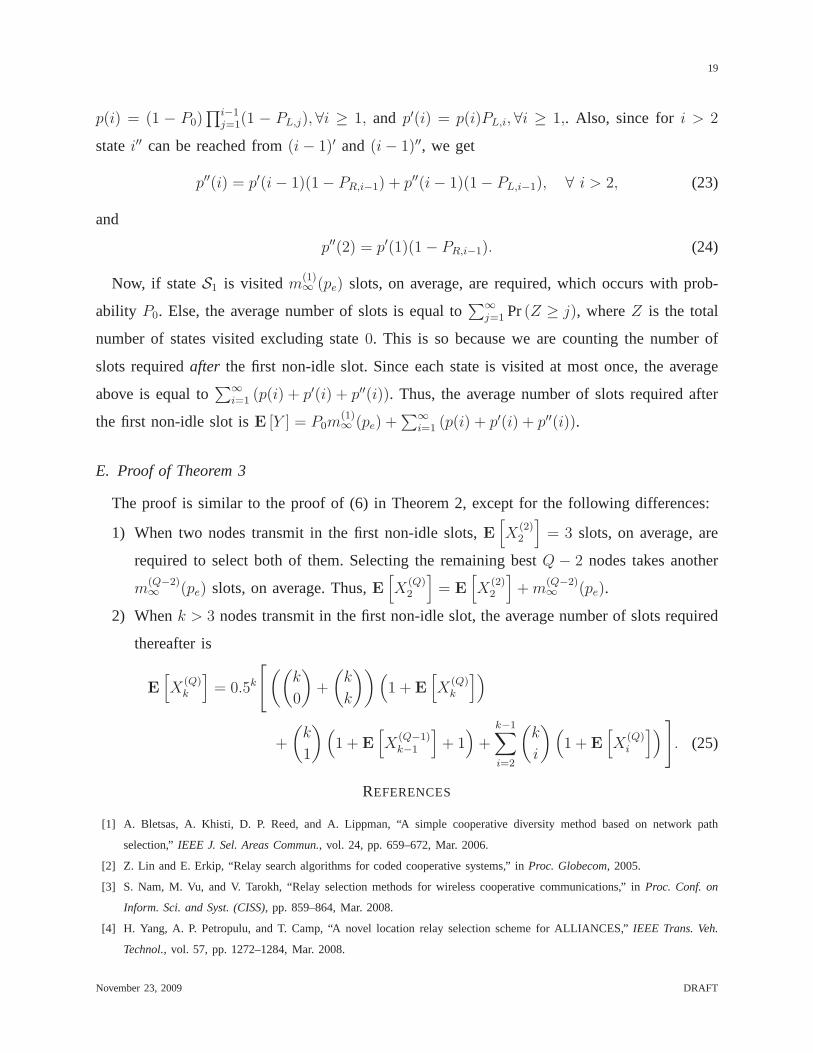
Consider a time-slotted system withn active nodes and a sink, as shown in Fig. 1. Each nodei

has a suitability metricui, which is known only to that specific node. In this section, the goal is to

select the node with the highest metric. The metrics are continuous and i.i.d. with complementary

CDF (CCDF) denoted byFc(u) = Pr(ui > u). Therefore, theFc(.) is monotonically decreasing

and invertible. (The discrete metric case, where this is notso, is tackled in Sec. III-F.)

B. Splitting Algorithm: Brief Review and Notation

We now formally define the splitting algorithm for single relay selection. To keep the treatment

concise, we first define the state variables maintained by thealgorithm and their initialization.

Thereafter, we describe how the algorithm controls the transmissions of the nodes, how the sink

generates feedback based on these transmissions, and how the state variables get autonomously

updated based on the feedback.

Definitions:The generalized best relay selection algorithm is specifiedusing three variables

HL(k), HH(k) andHmin(k); the notation being consistent with that in [17].HL(k) andHH(k)

are the lower and upper metric thresholds such that a nodei transmits at time slotk only if its

metric ui satisfiesHL(k) < ui < HH(k). Hmin(k) tracks the largest value of the metric known

up to slotk above which the best metric surely lies.

Initialization: In the first slot (k = 1), the parameters are initialized as follows:HL(1) =

F−1c (pe/n), HH(1) = ∞, andHmin(1) = 0. Here,pe is a system parameter, and shall henceforth

be referred to as theContention load parameter.

Transmission rule:At the beginning of each slot, each node locally decides to transmit. As

mentioned, it transmits if and only if its metric lies between HL(k) andHH(k).

Feedback generation:At the end of each slot, the sink broadcasts to all nodes a two-bit

feedback: (i)0 if the slot was idle (when no node transmitted), (ii)1 if the outcome was a


5

success (when exactly one node transmitted), or (iii)e if the outcome was a collision (when

multiple nodes transmitted).2

Response to feedback:We first define the split function3 to facilitate description: Let split(a, b) =

F−1c

(

Fc(a)+Fc(b)2

)

. Then, depending on the feedback, the following possibilities occur:

1) If the feedback (of thekth slot) is an idle (0) and no collisions has occurred so far, then

setHH(k + 1) = HL(k), HL(k + 1) = F−1c (k+1

npe), andHmin(k + 1) = 0.

2) If the feedback is a collision (e), then setHL(k + 1) = split(HL(k), HH(k)), HH(k+1) =

HH(k), andHmin(k + 1) = HL(k)

3) If the feedback is an idle (0) and a collision has occurred in the past, then setHH(k+1) =

HL(k), HL(k + 1) = split(Hmin(k), HL(k)), andHmin(k + 1) = Hmin(k).

Termination:The algorithm terminates when the outcome is a success (1).

We shall call the durations before and after the first non-idle slot as theidle and collision

phases, respectively. Thus, the contention load parameter, pe, is the average number of users

that transmit in a slot in the idle phase. The Qin-Berry algorithm [17] usespe = 1, which is the

value that maximizes the probability of a success outcome inan idle phase slot.

C. Main Analytical Results

The floor and ceil operations are denoted by⌊.⌋ and ⌈.⌉, respectively.E [Z] will denote the

expected value of a random variableZ.

We now develop a new analysis of the average time taken,mn(pe), by the splitting algorithm

to select the single best relay. The following lemma gives anexact expression formn(pe).

Lemma 1: Let Xk be the number of slots required to resolve a collision amongk nodes.

Let q =⌈

npe

⌉

− 1 denote the idle phase duration in slots. The average number of slots,mn(pe),

required to find the best node is given by,

mn(pe) =

q∑

i=1

n∑

k=1

(

n

k

)

(pe

n

)k(

1 −ipe

n

)n−k

(E [Xk] + i) +(

1 −qpe

n

)n

(E [Xn] + q + 1), (1)

2The sink can distinguish between these outcomes using, for example, the strength of the total received power [20].

3The split function makes sure that on an average half of the nodes involved in the last collision transmit in the next slot.

Splitting can be made faster as was done in [21]. However, doing so requires each node to numerically calculate thresholds in

each slot that are solutions of degreen−1 equations. Also, the improvement due to this scheme turns out to be less than0.5%.


6

whereE [Xk] follows the recursionE [Xk] =0.5k(

Pk−1l=2 (k

l)E[Xl])+1

1−0.5k−1 , for all k ≥ 2, andE [X1] = 0.

Proof: The proof is given in Appendix A.

The above expression is complex and does not directly revealthe scalable nature of the

algorithm. The theorem below provides two equivalent and new expressions for the asymptotic

case (n → ∞).

Theorem 1: The average number of slots required to find the best node asn → ∞ is given

by following two different yet equivalent expressions.

1) Recursive expression:

m∞(pe) =1

epe − 1

∞∑

k=1

E [Xk] pke

k!+

1

1 − e−pe. (2)

2) Non-recursive expression:

m∞(pe) =1

1 − e−pe+

∞∑

i=1

p(i), (3)

wherep(i) = (1 − P0)∏i−1

j=1(1− Pj), P0 = pee−pe

1−e−pe, Pi = 2−ipee−2−ipe (1−e−2−ipe)

1−(1+2−(i−1)pe)e−2−(i−1)pe, ∀ i ≥ 1.

Proof: We show the proof for the recursive expression in (2) below asit leads to a powerful

new Poisson point process interpretation that will be useful throughout this paper. For example,

it will lead to the derivation of the non-recursive expression in (3), whose proof is relegated to

Appendix B. The physical meaning ofp(i) andPj will become clear after the proof.

Let nodei have metricui with CCDF Fc(u). Let yi = nFc(ui). Then,yi are i.i.d. and are

uniformly distributed in[0, n]. Note that selecting the node with the highestui is equivalent to

selecting the node with the lowestyi because the CCDF is a monotonically decreasing function.

Sorting{yi}ni=1 in ascending order, we gety[1] ≤ y[2] ≤ y[3] · · · ≤ y[n], where[i] is the index of

the relay with theith largest metric.

Given yi, we can define a point process [22]M(t) asM(t) = max{

k ≥ 1 : y[k] ≤ t}

. Thus,

M(t) is the number of points that have occurred up to timet. Since {yi}ni=1 are i.i.d. and

uniformly distributed,M(t) is binomially distributed. Asn → ∞, it can be shown thatM(t)

forms a Poisson process with rate 1 [22]. Now, the probability that the first non-idle slot is the

ith slot andk ≥ 1 nodes are involved is equal to the probability thaty[1], . . . , y[k] lie between

(i− 1)pe and ipe, andy[j] > ipe, for k + 1 ≤ j ≤ n. It also implies that no points lie between0


7

and (i − 1)pe. Therefore,

Pr(

x[1] > (i − 1)pe

n, (i − 1)

pe

n< x[k] < i

pe

n, x[k+1] > i

pe

n

)

= Pr(M((i − 1)pe) = 0, M(ipe) = k) ,

= Pr(M((i − 1)pe) = 0) Pr(M(ipe) = k |M((i − 1)pe) = 0) ,

a=

n→∞

e−(i−1)pe e−pepk

e

k!= e−ipe

pke

k!. (4)

Here, (a) follows from the memoryless property of the Poisson process [22]. Recall thatE [Xk]

is the expected number of slots required to resolve a collision amongk nodes. Thus, if the

first non-idle slot is theith slot and k ≥ 1 nodes are involved, thenE [Xk] + i slots are

required to find the best node. Also, asn → ∞, qpe/n → 1. Hence, we getm∞(pe) =∑

∞

i=1

∑

∞

k=1 e−ipe pke

k!(E [Xk] + i). The desired result follows with the help of combinatorial iden-

tities [23].

The main theorem readily gives rises to the following upper bound expression that does not

involve an infinite series.

Corollary 1: For any realk0 ≥ e/2,

m∞(pe) ≤pe

k0 loge(2)+ log2

(

2k0

e

)

+1

1 − e−pe. (5)

Proof: The proof is given in Appendix C.

Alternatively, since both the expressions derived in Theorem 1 involve only positive terms

in the series summation, considering only the first few termsof the infinite series in (2) and

(3) results in tight lower bounds near the optimal contention parameter value. These simplified

expressions allow system designers to quickly compute the necessary parameters for system

optimization. As we shall see, their behavior turns out to bequite different and sheds light on

the differences between the two equivalent expressions derived in Theorem 1.

D. Results for Single Relay Selection

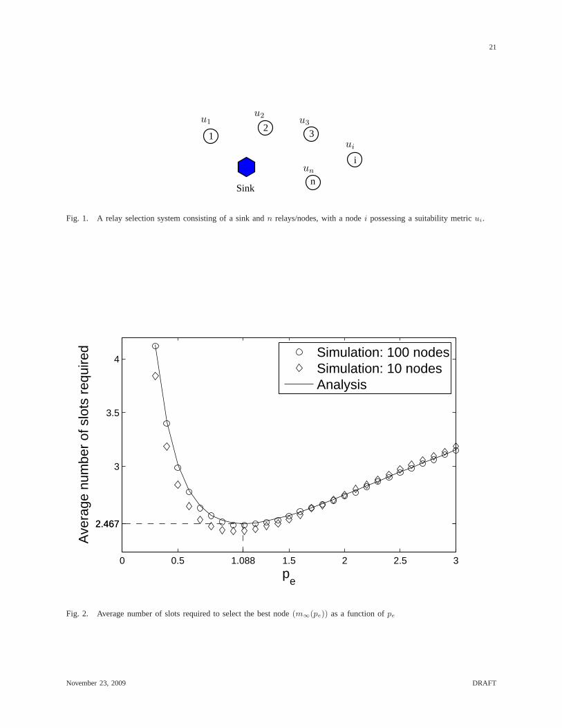
Figure 2 plots the average number of slots required to selectthe best node as a function of

pe for the two expressions and verifies them using Monte Carlo simulations. It can be seen

that the asymptotic expression is accurate even when the number of relays is small (e.g., 10).

Furthermore, the optimal value ofm∞(pe) is 2.467, and occurs atpe = 1.088. As expected,

the optimalpe does not exceed 2. This is because having more than two nodes on average to


8

transmit and collide in a slot is suboptimal. We also observethat m∞(pe) at pe = 1 is quite

close to the optimal value.

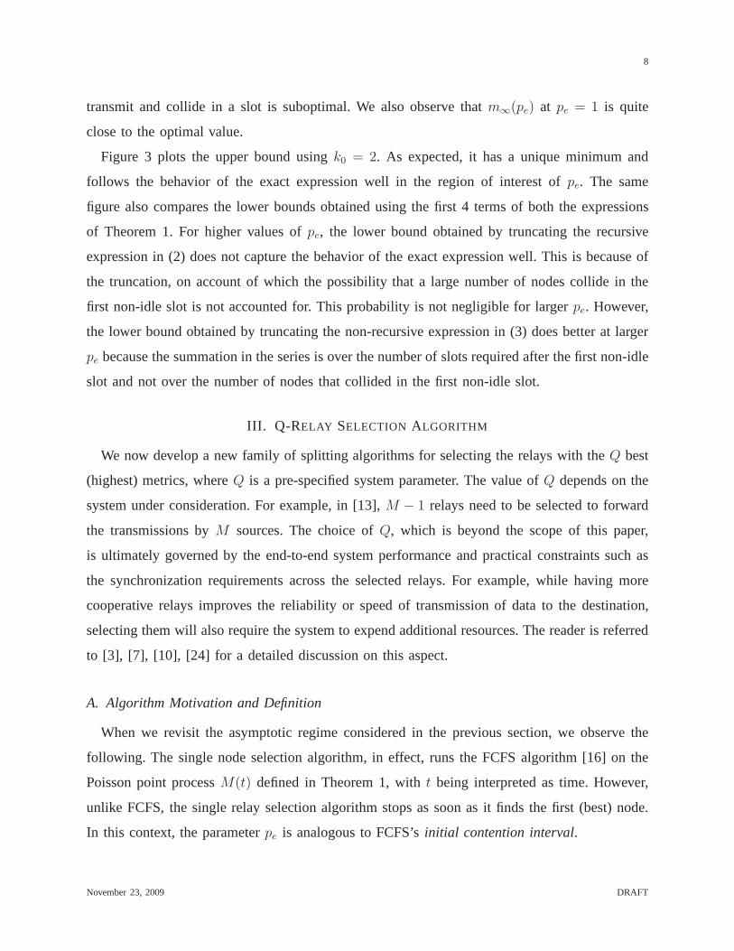
Figure 3 plots the upper bound usingk0 = 2. As expected, it has a unique minimum and

follows the behavior of the exact expression well in the region of interest ofpe. The same

figure also compares the lower bounds obtained using the first4 terms of both the expressions

of Theorem 1. For higher values ofpe, the lower bound obtained by truncating the recursive

expression in (2) does not capture the behavior of the exact expression well. This is because of

the truncation, on account of which the possibility that a large number of nodes collide in the

first non-idle slot is not accounted for. This probability isnot negligible for largerpe. However,

the lower bound obtained by truncating the non-recursive expression in (3) does better at larger

pe because the summation in the series is over the number of slots required after the first non-idle

slot and not over the number of nodes that collided in the firstnon-idle slot.

III. Q-RELAY SELECTION ALGORITHM

We now develop a new family of splitting algorithms for selecting the relays with theQ best

(highest) metrics, whereQ is a pre-specified system parameter. The value ofQ depends on the

system under consideration. For example, in [13],M − 1 relays need to be selected to forward

the transmissions byM sources. The choice ofQ, which is beyond the scope of this paper,

is ultimately governed by the end-to-end system performance and practical constraints such as

the synchronization requirements across the selected relays. For example, while having more

cooperative relays improves the reliability or speed of transmission of data to the destination,

selecting them will also require the system to expend additional resources. The reader is referred

to [3], [7], [10], [24] for a detailed discussion on this aspect.

A. Algorithm Motivation and Definition

When we revisit the asymptotic regime considered in the previous section, we observe the

following. The single node selection algorithm, in effect,runs the FCFS algorithm [16] on the

Poisson point processM(t) defined in Theorem 1, witht being interpreted as time. However,

unlike FCFS, the single relay selection algorithm stops as soon as it finds the first (best) node.

In this context, the parameterpe is analogous to FCFS’sinitial contention interval.


9

Based on the above insight, we now formally state the new multi-relay selection algorithm

given anyQ. We then explain the logic behind it and fully analyze it. Forthis, we adopt the

notation used for FCFS in [16], as it turns out to be more convenient.

As in Sec. II, letyi = nFc(ui). The algorithm specifies four state variablesS(k), T (k), α(k),

andσ(k) for each slotk. S(k) is the number of nodes selected before slotk. (T (k), T (k)+α(k))

represents thethreshold intervalfor slot k, i .e., all the nodes withyi ∈ (T (k), T (k) + α(k))

transmit in slotk. (Equivalently,HH(k) = F−1c (T (k)/n) andHL(k) = F−1

c ((T (k) + α(k)) /n).

σ(k) ∈ {L, R} indicates whether thekth slot interval is the left half or the right half of the

previously split interval. During initial slots, when no collision is to be resolved,σ(k) = R by

convention. Thus, fork = 1, we haveS(1) = 0, T (1) = 0, α(1) = pe, andσ(1) = R.

In the (k + 1)th slot (k ≥ 1):

1) If feedback is a collision (e), thenT (k+1) = T (k), α(k + 1) = α(k)/2, andσ(k+1) = L.

2) If feedback is a success (1) andσ(k) = L, thenT (k + 1) = T (k) + α(k), α(k+1) = α(k),

andσ(k + 1) = R.

3) If feedback is an idle (0) andσ(k) = L, thenT (k + 1) = T (k) + α(k), α(k+1) = α(k)/2,

andσ(k + 1) = L.

4) If feedback is an idle (0) or a success (1), andσ(k) = R, thenT (k + 1) = T (k) + α(k),

α(k + 1) = pe, andσ(k + 1) = R.

5) IncrementS(k + 1) by 1 if feedback is a success (1). Terminate ifS(k + 1) reachesQ.

B. Brief Explanation

The logic behind the algorithm is as follows: (i) When a collision occurs, the threshold interval

for the next slot is the left (L) half of that of the present slot. (ii) When a collision occurs, the

threshold interval must have at least 2 nodes. Thus, when a success follows a collision, the

threshold interval for the next slot is the right (higher) half (R) of the previous slot, since it

is known to have at least one node. (iii) When an idle follows acollision, it implies that all

the nodes involved in collision lie in the right half of the previous split interval. Thus, it is

further split it into two equal halves, and the threshold interval for the next slot is the left half

of this split. (iv) When there is no collision to be resolved,the algorithm moves to the adjacent


10

threshold interval (which we call as collision resolution interval) of sizepe.4 As mentioned above,

the algorithm terminates after theQ successes.

Comments:The proposed algorithm is equivalent to the algorithm of Sec. II when Q = 1.

It is similar to FCFS, except that it stops after theQth success. There is one subtle difference,

however, between the algorithm and FCFS. In FCFS, the contention resolution interval can be

smaller thanpe if the difference between the current time and the time of thelast resolved

interval is small. However, this does not happen in our algorithm (step 4) because all the nodes

know their individual metrics a priori. Notice that the algorithm is greedy in that it does not

account for possible interactions between metrics of the relays. However, such a greedy approach

has often been used given its inherent distributability [13].5

C. Algorithm Analysis: Best Two Nodes Selection

First, we analyze the algorithm for selecting the best two nodes using the Poisson point

approach that came out of Sec. II. This will lead to an analysis for the generalQ > 2 node

selection case. TheQ = 2 analysis is shown separately as it turns out to be richer.

Let m(Q)∞ (pe) represent the average number of slots required to select thebest Q nodes.

Thus, the symbolm∞(pe), which was used in the previous section on single relay selection,

is equivalent tom(1)∞ (pe). The following theorem gives two different but equivalent and exact

expressions form(2)∞ (pe).

Theorem 2: Let E

[

X(Q)k

]

denote the average number of slots required to select the best Q

nodes afterk nodes collide. Asn → ∞, m(2)∞ (pe) is given by

m(2)∞

(pe) =1

epe − 1

∞∑

k=1

E

[

X(2)k

]

pke

k!+

1

1 − e−pe, (6)

where

E

[

X(2)k

]

=(

2k − 2)

−1

(

( k−1∑

i=2

(

k

i

)

E

[

X(2)i

]

+ k(

1 + E

[

X(1)k−1

])

)

+ 2k

)

, ∀ k ≥ 3, (7)

4We can relax the restriction that each collision resolutioninterval is of lengthpe. However, it can be shown that doing this

leads to a negligible improvement.

5A more general version of the algorithm would allow for the metrics to be modified on the basis of the relays that have

already been selected. Developing such an algorithm is an interesting avenue for future work, and would find several applications,

such as in the time-sharing proportional fair solution of [25].


11

E

[

X(2)2

]

= 3, andE

[

X(2)1

]

= m(1)∞ (pe).

Alternately,m(2)∞ (pe) also equals

m(2)∞

(pe) =1

1 − e−pe+ P0m

(1)∞

(pe) +

∞∑

i=1

(p(i) + p′(i) + p′′(i + 1)) , (8)

wherep(i) = (1−P0)∏i−1

j=1(1−PL,j), ∀ i ≥ 1, p′(i) = p(i)PL,i, ∀ i ≥ 1, p′′(2) = p′(1)(1−PR,1),

and p′′(i) = p′(i − 1)(1 − PR,i−1) + p′′(i − 1)(1 − PL,i−1), ∀ i > 2. Here,P0 = pee−pe

1−e−pe, PL,i =

2−ipee−2−ipe (1−e−2−ipe)

1−(1+2−(i−1)pe)e−2−(i−1)pe, ∀i ≥ 1, PR,i = 2−ipee−2−ipe

1−e−2−ipe, ∀i ≥ 1.

Proof: The proof is given in Appendix D. It also gives a physical meaning for p(i), p′(i),

p′′(i), PL,i, andPR,i.

D. Algorithm Analysis: BestQ > 2 Nodes Selection

We now derive a general expression form(Q)∞ (pe) for any Q > 2 This generalizes the first

result of Theorem 2.

Theorem 3: As n → ∞, the average number of slots required to select the bestQ > 2 nodes

is

m(Q)∞

(pe) =1

epe − 1

∞∑

k=1

E

[

X(Q)k

]

pke

k!+

1

1 − e−pe, (9)

where

E

[

X(Q)k

]

=(

2k − 2)

−1

(

( k−1∑

i=2

(

k

i

)

E

[

X(Q)i

]

+ k(

1 + E

[

X(Q−1)k−1

])

)

+ 2k

)

, ∀ k ≥ 3, (10)

E

[

X(Q)2

]

= m(Q−2)∞ (pe) + 3, ∀ Q > 2, E

[

X(2)2

]

= 3, andE

[

X(Q)1

]

=m(Q−1)∞ (pe).

Proof: The proof is given in Appendix E.

A non-recursive expression form(Q)∞ (pe) for Q > 2 along the lines of (3) of Theorem 1 and (6)

of Theorem 2 can be derived. However, the Markov chains become more involved.

E. Results forQ Best Relay Selection

Figure 4 plotsm(2)∞ (pe) as a function ofpe using Theorem 2 and verifies it using Monte

Carlo simulations. It can be seen that the asymptotic expressions are accurate even for a small

number of nodes, e.g.,n = 20. The lowest average number of slots required to select two users

is 4.406, which occurs atpe = 1.221. This is 10.7% faster than running the single relay selection

algorithm twice, which requires2 × 2.467 = 4.934 slots. The increase in the optimalpe from


12

1.088 slots for Q = 1 to 1.221 slots for Q = 2 occurs because now it is faster to resolve a

collision than to avoid it. Specifically, the time taken to select two nodes given that they are

involved in a collision isE[

X(2)2

]

= 3.0 slots. Where as, the number of slots required to select

two nodes, given that the previous slot was idle, is4.4 slots.

Table I provides the optimum values ofpe and the average number of slots as a function of

the number of relays that need to be selected. We can see that selecting the best three nodes

takes6.491 slots, on average, and is achieved whenpe = 1.214.6 As Q → ∞, the optimum

value ofpe increases to1.266, which is also the optimum value maximizing the throughput of

FCFS [16].7 Also, it can be shown that Q

m(Q)∞ (1.266)

, which represents the average number of users

selected per slot by the algorithm forpe = 1.266, increases to0.487 asQ → ∞.

F. Tackling Discrete Metrics Using Proportional Expansion

The thresholding algorithms in Sec. II-A and Sec. III-A exploit the critical fact that with

probability one no two metrics are equal. However, as mentioned in the Introduction, when the

metric has a discrete probability distribution, the algorithms break down because the probability

that the metrics of the best two nodes are exactly equal is non-zero. We now provide a simple

and novel distributed solution calledProportional Expansionto tackle this practical problem.

Proportional Expansion: Let the metricui be a realization of anω-valued discrete random

variable that, without loss of generality, takes values1, 2, . . . , ω with probability ρ1, ρ2, . . . , ρω,

respectively. Each node independently maps its metricui into a new metricνi as follows:When

ui = j, νi is a realization of a uniformly distributed random variablein(

∑j−1ℓ=0 ρℓ,

∑j

ℓ=1 ρℓ

)

,

whereρ0 , 0. In other words, each node chooses a new random metricνi that is uniformly

distributed over a bin of lengthproportional to the probability mass of its original metricui.

The overall distribution of the new metric across all users is then uniformly distributed in

(0, 1). Proportional Expansion satisfies two key properties:

6The marginal decrease in the optimal value ofpe from 1.221 to 1.214 whenQ increases from2 to 3 can be explained

as follows. The time taken to select three nodes after a collision among two nodes isEh

X(3)2

i

= 5.48 slots. However, the

number of slots required to select three nodes after an idle slot, is 6.49 slots, which is just17.8% more than5.48. Therefore,

the optimumpe decreases since the selection times after an idle and a collision are not as unequal as forQ = 2.

7The maximum arrival rate of 0.487 is supported when initial collision interval is capped at 2.6. This implies that there are

on average0.487× 2.6 = 1.266 nodes transmitting. The contention parameterpe is set using normalized metric CCDF with an

‘arrival rate’ equal to 1.


13

• It preserves the sorting order of the metrics: ifui > uj, thenνi > νj . Hence, selecting the

bestQ nodes with the highestνis is equivalent to selectingQ nodes with the highestuis.

• The probability thatνi = νj, for i 6= j, is 0 sinceνi is a continuous random variable.

Therefore, the selection algorithm of Sec. III for anyQ ≥ 1 can then be run onνi. The

following Proposition formally quantifies the performanceof Proportional Expansion. It implies

that proportional expansion is scalable,i.e., it takes at most 2.47 slots for best relay selection,

4.406 slots for selecting the best 2 relays, and so on, for any number of relays,n.

Proposition 1: The average number of slots required to select the bestQ relays by Proportional

Expansion for the discrete metrics case is the same as that ofthe bestQ relay threshold based

selection algorithm of Sec. III-A that operates on continuous metrics.

Proof: The proof is omitted since it directly follows from the abovediscussion.

IV. CONCLUSIONS

We developed a new asymptotic analysis for the single relay splitting based selection algorithm,

which was based on a new Poisson point process interpretation of the dynamics of the algorithm.

This led to a characterization of the optimal parameters of the algorithm, and enabled a rigorous

benchmarking of the greedy parameter setting used in the literature. We also proposed a new

splitting based algorithm for selecting the bestQ relays, which are useful for several cooperative

protocols proposed in the literature. The new algorithm wasmore efficient than running the single

relay selection algorithm multiple times. Furthermore, wegeneralized the analytical techniques

to handle multiple relay selection, and derived the exact expressions for the average number of

slots for multiple relay selection. Interestingly, the asymptotic expressions were accurate even

for a small number of relays. With the help of proportional expansion, we showed, for the first

time, that splitting algorithms can be adapted to work for discrete metrics as well without any

loss in performance or scalability whatsoever.

The analysis shows that the greedy policy of maximizing the success probability in the next

slot is suboptimal. While it works well for single relay selection, it becomes more and more

suboptimal as the number of relays to be selected increases.The analysis also shows that the

general single relay selection algorithm, the proposed multiple relay selection algorithm, and

the FCFS multiple access control algorithm are intimately related. For example, the optimal

value of the contention load parameter increases as the number of relays to be selected increases


14

and finally approaches the optimal setting for FCFS. This is despite the fact that selection

and multiple access control algorithms serve very different purposes, and, therefore, evaluated

differently. While multiple access control algorithms attempt to serve all nodes and are evaluated,

for example, by the maximum traffic they can handle with a finite delay, selection algorithms

are evaluated by how fast they can select the best nodes. We hope that this insight will help

develop better selection algorithms. An important property about splitting algorithms is that

besides being distributed, they are both extremely fast andscalable. This suggests that selection

based protocols will deliver improvements in the overall end-to-end system-level performance

even when the time overhead incurred by the selection algorithm is accounted for. The system-

level benefits can be further improved if the multiple relay selection algorithm proposed in this

paper can be modified to allow the metrics to be updated duringthe selection process.

APPENDIX

A. Proof of Lemma 1

It can be easily seen that the idle phase consists of at the most q =⌈

npe

⌉

− 1 slots since at

this stage the lower threshold equals the smallest value0. Given that the first non-idle slot is

the ith slot andk nodes are involved, the average number of slots required to find the best node

is E [Xk] + i. (The recursive expression forE [Xk] is given in [17, (6)].) The probability that

the first non-idle slot is theith slot andk nodes transmit in it equals(

n

k

) (

pe

n

)k (

1 − ipe

n

)n−k, for

i ≤ q. This constitutes the first term of the right side of (1). The probability that the(q+1)th slot

is the first non-idle slot is(1− qpe

n)n since all nodes’ metrics must lie in interval((q + 1)pe, 1].

In the event that this happens, alln nodes will transmit and collide, which will takeE [Xn] slots

to resolve. Hence, the second term on the right side of (1) follows.

B. Proof of Non-Recursive Expression of Theorem 1

Let the random variableI denote the number of slots required until (and including) the first

non-idle slot andY denote the number of slots required after that.

Consider the state transition diagram of Figure 6, in which the state represents the number

of slots that have elapsed since the first non-idle slot. The node goes to stateS whenever

success occurs, and the algorithm terminates. Otherwise, in case of an idle or collision, the

node increments its state by 1. By definition, state0 is the first non-idle slot itself; thus, an idle


15

outcome cannot occur in it. The following lemma is crucial inanalyzing this transition diagram.

Lemma 2: The state transition diagram of Fig. 6 is a Markov chain.

Proof: To prove this, it is sufficient to prove that the transition probability from any state

i to S is dependent only oni. (Having done so, we shall denote this probability byPi.)

We refer to the interval inM(t) allocated to statei as its threshold interval. Here,P0 is the

probability that in a threshold interval of sizepe only one node transmits given that at least one

node transmits in that slot. LetN(x) = M(t + x)−M(t). Then, from the memoryless property

of the Poisson process, Pr(N(x) = i) is independent oft and is equal toxie−x

i!. Thus,

P0 = Pr(

N(pe) = 1∣

∣

∣N(pe) > 1

)

=pee

−pe

1 − e−pe. (11)

P1 is the probability that the second non-idle slot is a successgiven that the first non-idle slot (of

threshold interval sizepe) is a collision. Due to splitting, the second slot will have athreshold

interval size that is half that of the first one. Therefore,P1 is the probability that conditioned on

N(pe) having at least 2 nodes (i.e., a collision),N(pe/2) has exactly one. Thus,

P1 = Pr(

N(pe

2

)

= 1∣

∣

∣N(pe) ≥ 2

)

=Pr(

N(

pe

2

)

= 1, N(pe) ≥ 2)

Pr(N(pe) ≥ 2). (12)

Therefore,

P1 =Pr(

N(

pe

2

)

= 1, N(pe) − N(

pe

2

)

≥ 1)

Pr(N(pe) > 1)=

pe

2e−

pe2 (1 − e−

pe2 )

1 − (1 + pe)e−pe. (13)

For P2, the following two trajectories can occur: State 2 was reached by a collision in state 1

or by an idle in state 1. In case of a collision, the threshold interval of the second non-idle slot

(of sizepe/2) gets split into two halves. Even in the case of an idle the interval would be split

into two halves and nodes from the left half would contend. Thus,P2 is equal to the probability

that conditioned on an interval of sizepe/2 having at least two nodes, half the interval (of size

pe/4), has exactly one node. Thus,

P2 = Pr(

N(pe

4

)

= 1∣

∣

∣N(pe

2

)

≥ 2)

=Pr(

N(

pe

4

)

= 1, N(

pe

2

)

≥ 2)

Pr(N(pe) ≥ 2)=

pe

4e−

pe4 (1 − e−

pe4 )

1 − (1 + pe

2)e−

pe2

.

In similar way, we can show thatPi, ∀ i ≥ 1, is equal to the probability that conditioned on

an interval of size2−(i−1)pe having at least two nodes, one half of the interval (of size2−ipe)

has exactly one node. Thus,

Pi = Pr(

N(pe

2i

)

= 1∣

∣

∣N( pe

2i−1

)

> 1)

=2−ipee

−2−ipe(1 − e−2−ipe)

1 − (1 + 2−(i−1)pe)e−2−(i−1)pe. (14)


16

Now, m∞(pe) = E [I]+E [Y ]. From the Poisson process interpretation of Theorem 1, we can

show that Pr(I = i) = e−(i−1)pe(1−e−pe). Therefore,E [I] =∑

∞

i=1 ie−(i−1)pe(1−e−pe) = 11−e−pe

.

The average number of slots required after the first non-idleslot to select the best node,E [Y ],

is calculated as follows. First,E [Y ] =∑

∞

i=1 i Pr(Y = i), can be shown to be identically equal

to∑

∞

i=1 Pr(Y ≥ i). Second, since each state in the Markov chain is visited at most once, it

follows thatE [Y ] =∑

∞

i=1 p(i), wherep(i) is the probability that theith state is visited. From

the state transition diagram, it is easy to see thatp(i) = (1 − P0)∏i−1

j=1(1 − Pj) . Hence, the

desired expression form∞(pe) follows.

C. Proof of Corollary 1

From [17], we haveE [Xk] ≤ log2(k) + 1, k ≥ 2, andE [X1] = 0. Sincelog2(x) is concave

with respect tox, a tangent to it at any point(k0, log2(k0)) is an upper bound. Therefore,

log2(k) ≤k − k0

k0 loge(2)+ log2(k0). (15)

Consequently,E [Xk] ≤k

k0 loge(2)+ log2(2k0/e), k ≥ 2. Substituting this in (2), we get

m∞(pe) ≤ log2

(

2k0

e

)∑

∞

k=2pk

e

k!

epe − 1+

1

k0(epe − 1) loge(2)

∞∑

k=2

kpk

e

k!+

1

1 − e−pe. (16)

For k0 ≥ e/2, log2(2k0/e) ≥ 0. Also,∑

∞

k=2pk

e

k!= epe − 1 − pe < epe − 1 since pe > 0.

Therefore, fork0 ≥ e/2, the first term in the right hand side of (16) is less thanlog2

(

2k0

e

)

.

Substituting this inequality in (16) and simplifying leadsto the desired result in (5).

D. Proof of Theorem 2

Proof of (6): Given that the first non-idle slot is theith slot andk ≥ 1 nodes are involved, the

average number of slots required to select the best2 nodes isE[

X(2)k

]

+ i. The probability that

the first non-idle slot is theith slot andk ≥ 1 nodes are involved ise−ipepke/k!. Hence, we get

m(2)∞

(pe) =

∞∑

i=1

∞∑

k=1

e−ipepk

e

k!

(

E

[

X(2)k

]

+ i)

, (17)

simplifying which yields (9).

If only one node transmits in the first non-idle slot, then a success occurs and the node gets

selected. Selecting one more node will takem(1)∞ (pe) slots, on average. (This follows from the


17

memoryless property of the Poisson process [22].) Thus,E

[

X(1)1

]

= m(1)∞ (pe). Also, if exactly

two nodes transmit in the first non-idle slot, only one node transmits in the slot just after the

first success. Thus,E[

X(2)2

]

= E

[

X(2)1

]

+ 1 = 3 slots. Whenk > 3 nodes transmit in the

first non-idle slot, the following three cases are possible for the next slot: (i)Collision amongi

nodes: E

[

X(2)i

]

more slots would then be required, on average. (ii)Idle: E

[

X(2)k

]

more slots

are required, on average. (iii)Success: The next slot would then surely involve a collision among

k − 1 nodes.E[

X(1)k−1

]

slots, on average, would be requiredafter that. The probability thati

nodes transmit in the next slot is(

k

i

)

/2k. Thus,

E

[

X(2)k

]

=1

2k

(

((

k

0

)

+

(

k

k

))

(

1 + E

[

X(2)k

])

+

(

k

1

)

(

1 + E

[

X(1)k−1

]

+ 1)

+k−1∑

i=2

(

k

i

)

(

1 + E

[

X(2)i

])

)

. (18)

Simplifying this further using combinatorial identities [23] results in (7).

Proof of (8):This proof also involves constructing a state transition diagram that will be proved

to be a Markov chain. Consider the state transition diagram of Figure 7. It is more involved

than that in Figure 6 because we need to also track how many successes have occurred. Statei

corresponds to theith split before the first success (which takesi slots), statei′ corresponds to the

first success occurring at theith slot, and statei′′ corresponds to the first success having already

occurred by theith slot. The state transition diagram can be explained in detail as follows.

State0 corresponds to the first non-idle slot. If the first non-idle slot is a success, the node

moves from state0 to stateS1. Now, the algorithm starts a new collision resolution to find

the second colliding node. This takes timem(1)∞ (pe), which is given by Theorem 1. If the first

non-idle slot is a collision, its threshold interval is split and the node transitions from state0

to state1. Each subsequent idle or collision results in one additional split and the node moves

from statei to i + 1. In case of a success, the node moves from from statei to statei′ as no

additional split occurs. A success in statei′ results in a transition to stateS, at which time the

algorithm terminates. In case of a collision in statei′, the node moves to state(i + 1)′′, as one

more split occurs. In case of a success in statei′′, the node moves to stateS, and the algorithm

terminates. Otherwise, an idle or collision results in a transition from statei′′ to (i + 1)′′. Note

that in each state (i, i′, or i′′) the size of threshold interval is2−ipe.

The following Lemma shall prove to be crucial in analyzing this transition diagram.


18

Lemma 3: The state transition diagram of Fig. 7 is a Markov chain.

Proof: For this, it is sufficient to prove that transition probabilities for each state depend

only on thei and not on the path taken to reach that state.

Let P0 be the probability of success in state0 (the first non-idle slot). It is equal to the

probability that in a slot of sizepe only one node transmits given that at least one node transmits

in that slot. LetN(x) = M(t+x)−M(t). Then, by memoryless property of the Poisson process,

Pr(N(x) = i) is independent oft and is equal toxie−x

i!. Thus,

P0 = Pr(

N(pe) = 1∣

∣

∣N(pe) > 1

)

=pee

−pe

1 − e−pe. (19)

Let PL,i be the probability of success in statei, which is equal to the probability that given an

interval of size2−ipe having more than one nodes, left half of it has exactly one node. Thus,

PL,i = Pr(

N(pe

2i

)

= 1∣

∣

∣N( pe

2i−1

)

> 1)

=2−ipee

−2−ipe(1 − e−2−ipe)

1 − (1 + 2−(i−1)pe)e−2−(i−1)pe. (20)

Let PR,i be the probability of success in statei′. Statei′ can be entered only after success in

statei. Thus, threshold interval of statei, which is right half of the split during statei− 1, has

at leastone node. ThusPR,i is equal to the probability that exactly one node transmits in the

slot with interval size2−ipe, given that at least one node lies in that interval, which equals

PR,i = Pr(

N(pe

2i

)

= 1∣

∣

∣N(pe

2i

)

> 1)

=2−ipee

−2−ipe

1 − e−2−ipe. (21)

The probability of success in statei′′ is again equal to the probability that given that an interval

of size2−ipe has more than one node, its left half has exactly one node. This probability equals

PL,i. Thus, from (20) and (21), the transition probabilitiesPL,i andPR,i only depend oni, which

proves that Fig. 7 is a Markov chain.

Let the random variableI denote the number of slots required until (and including) the first

non-idle slot andY denote the number of slots required after that. Then,m(2)∞ (pe) = E [I]+E [Y ].

Again, using Poisson point process interpretation, Pr(I = i) = e−(i−1)pe(1−e−pe), which implies,

E [I] =

∞∑

i=1

ie−(i−1)pe(1 − e−pe) =1

1 − e−pe. (22)

E [Y ] can be calculated from Lemma 3 as follows. Letp(i), p′(i), andp′′(i) be the probability

that statesi, i′, and i′′ are visited, respectively. From the state transition diagram, since statei

can be reached only from statei − 1 and statei′ can be reached only from statei, we get


19

p(i) = (1 − P0)∏i−1

j=1(1 − PL,j), ∀i ≥ 1, and p′(i) = p(i)PL,i, ∀i ≥ 1,. Also, since fori > 2

statei′′ can be reached from(i − 1)′ and (i − 1)′′, we get

p′′(i) = p′(i − 1)(1 − PR,i−1) + p′′(i − 1)(1 − PL,i−1), ∀ i > 2, (23)

and

p′′(2) = p′(1)(1 − PR,i−1). (24)

Now, if stateS1 is visitedm(1)∞ (pe) slots, on average, are required, which occurs with prob-

ability P0. Else, the average number of slots is equal to∑

∞

j=1 Pr(Z ≥ j), whereZ is the total

number of states visited excluding state0. This is so because we are counting the number of

slots requiredafter the first non-idle slot. Since each state is visited at most once, the average

above is equal to∑

∞

i=1 (p(i) + p′(i) + p′′(i)). Thus, the average number of slots required after

the first non-idle slot isE [Y ] = P0m(1)∞ (pe) +

∑

∞

i=1 (p(i) + p′(i) + p′′(i)).

E. Proof of Theorem 3

The proof is similar to the proof of (6) in Theorem 2, except for the following differences:

1) When two nodes transmit in the first non-idle slots,E

[

X(2)2

]

= 3 slots, on average, are

required to select both of them. Selecting the remaining best Q − 2 nodes takes another

m(Q−2)∞ (pe) slots, on average. Thus,E

[

X(Q)2

]

= E

[

X(2)2

]

+ m(Q−2)∞ (pe).

2) Whenk > 3 nodes transmit in the first non-idle slot, the average numberof slots required

thereafter is

E

[

X(Q)k

]

= 0.5k

[

((

k

0

)

+

(

k

k

))

(

1 + E

[

X(Q)k

])

+

(

k

1

)

(

1 + E

[

X(Q−1)k−1

]

+ 1)

+k−1∑

i=2

(

k

i

)

(

1 + E

[

X(Q)i

])

]

. (25)

REFERENCES

[1] A. Bletsas, A. Khisti, D. P. Reed, and A. Lippman, “A simple cooperative diversity method based on network path

selection,”IEEE J. Sel. Areas Commun., vol. 24, pp. 659–672, Mar. 2006.

[2] Z. Lin and E. Erkip, “Relay search algorithms for coded cooperative systems,” inProc. Globecom, 2005.

[3] S. Nam, M. Vu, and V. Tarokh, “Relay selection methods forwireless cooperative communications,” inProc. Conf. on

Inform. Sci. and Syst. (CISS), pp. 859–864, Mar. 2008.

[4] H. Yang, A. P. Petropulu, and T. Camp, “A novel location relay selection scheme for ALLIANCES,”IEEE Trans. Veh.

Technol., vol. 57, pp. 1272–1284, Mar. 2008.


20

[5] J. Luo, R. S. Blum, L. J. Cimini, L. J. Greenstein, and A. M.Haimovich, “Link-failure probabilities for practical cooperative

relay networks,” inProc. VTC (Spring), pp. 1489–1493, 2005.

[6] S. Yang and J.-C. Belfiore, “A novel two-relay three-slotamplify-and-forward cooperative scheme,” inProc. Conf. on

Inform. Sci. and Syst. (CISS), pp. 1329–1334, 2005.

[7] R. Madan, N. B. Mehta, A. F. Molisch, and J. Zhang, “Energy-efficient cooperative relaying over fading channels with

simple relay selection,”IEEE Trans. Wireless Commun., vol. 7, pp. 3013–3025, Aug. 2008.

[8] E. Beres and R. Adve, “Selection cooperation in mutli-source cooperative networks,”IEEE Trans. Wireless Commun.,

vol. 7, pp. 118–127, Jan. 2008.

[9] D. S. Michalopoulos and G. K. Karagiannidis, “PHY-layerfairness in amplify and forward cooperative diversity systems,”

IEEE Trans. Wireless Commun., vol. 7, pp. 1073–1083, Mar. 2008.

[10] C. K. Lo, J. R. W. Heath, and S. Vishwanath, “Relay subsetselection in wireless networks using partial decode-and-forward

transmission,”IEEE Trans. Veh. Technol., vol. 58, pp. 692–704, Feb. 2009.

[11] C. K. Lo, J. R. W. Heath, and S. Vishwanath, “The impact ofchannel feedback on opportunistic relay selection for

hybrid-ARQ in wireless networks,”IEEE Trans. Veh. Technol., vol. 58, pp. 1255–1268, Mar. 2009.

[12] D. Tse and P. Vishwanath,Fundamentals of Wireless Communications. Cambridge University Press, 2005.

[13] Z. Ding, K. K. Leung, D. L. Goeckel, and D. Towsley, “On the study of network coding with diversity,”IEEE Trans.

Wireless Commun., vol. 8, pp. 1247–1259, Mar. 2009.

[14] I. Krikidis and J.-C. Belfiore, “Three scheduling schemes for amplify-and-forward relay environments,”IEEE Commun.

Lett., vol. 5, pp. 414–416, May 2007.

[15] P. Liu, Z. Tao, Z. Lin, E. Erkip, and S. Panwar, “Cooperative wireless communications: a cross-layer approach,”IEEE

Trans. Wireless Commun., vol. 13, pp. 84–92, Aug. 2006.

[16] D. P. Bertsekas and R. G. Gallager,Data Networks. Prentice Hall, 2 ed., 1992.

[17] X. Qin and R. Berry, “Opportunistic splitting algorithms for wireless networks,” inProc. INFOCOM, pp. 1662–1672, Mar.

2004.

[18] R. Yim, N. B. Mehta, and A. F. Molisch, “Fast multiple access selection through variable power transmission,”IEEE

Trans. Wireless Commun., vol. 8, pp. 1962–1973, Apr. 2009.

[19] K. Choumas, T. Korakis, and L. Tassiulas, “New prioritization schemes for QoS provisioning in 802.11 wireless networks,”

in Proc. 16th IEEE Workshop on Local and Metropolitan Area Networks, pp. 25–30, Sept. 2008.

[20] R. Yim, N. B. Mehta, and A. F. Molisch, “Best node selection through distributed fast variable power multiple access,” in

Proc. ICC, pp. 5028–5032, 2008.

[21] A. Cohen, M. Kam, and R. Conn, “Partitioning a sample using binary-type questions with ternary feedback,”IEEE Trans.

Sys., Man, And Cybernetics, vol. 25, pp. 1405–1408, Oct. 1995.

[22] R. W. Wolff, Stochastic Modeling and the Theory of Queues. Prentice Hall, 1989.

[23] L. S. Gradshteyn and L. M. Ryzhik,Tables of Integrals, Series and Products. Academic Press, 2000.

[24] V. Shah, N. B. Mehta, and R. Yim, “Relay selection and data transmission throughput tradeoff in cooperative systems,”

in Proc. Globecom (to appear), Nov. 2009.

[25] T. J. Oechtering and H. Boche, “Bidirectional regenerative half–duplex relaying using relay selection,”IEEE Trans. Wireless

Commun., vol. 7, pp. 1879–1888, May 2008.


21

12

Sink

3

i

nun

u1u2 u3

ui

Fig. 1. A relay selection system consisting of a sink andn relays/nodes, with a nodei possessing a suitability metricui.

0 0.5 1.088 1.5 2 2.5 3

2.4672.467

3

3.5

4

pe

Ave

rage

num

ber

of s

lots

req

uire

d Simulation: 100 nodesSimulation: 10 nodesAnalysis

Fig. 2. Average number of slots required to select the best node (m∞(pe)) as a function ofpe


22

0 1 2 3 42

2.5

3

3.5

4

4.5

5

pe

Ave

rage

num

ber

of s

lots

req

uire

d

Exact expressionUpper boundLower bound: Recursive expressionLower bound: Non−recursive expression

Fig. 3. Upper and lower bounds for the average number of slotsrequired to select the best node.

0.5 1 1.221 1.5 2 2.5 34.3

4.406

4.5

4.6

4.7

4.8

4.9

5

5.1

5.2

pe

Ave

rage

num

ber

of s

lots

req

uire

d

AnalysisSimulation: 100 nodesSimulation: 20 nodes

Fig. 4. Average number of slots required to select the best two nodes(m(2)∞ (pe)) as a functionpe.


23

TABLE I

OPTIMUM pe AND THE AVERAGE NUMBER OF SLOTS REQUIRED TO SELECT THE BESTQ RELAYS

Q Optimumpe Optimumm(Q)∞ (pe) (slots) Improvement

1 1.088 2.467 -

2 1.221 4.406 10.7%

3 1.214 6.491 12.3%

4 1.231 8.537 13.5%

5 1.236 10.592 14.1%

6 1.241 12.645 14.6%

0.7

1

10.2

ui = 1

ρ1 = 0.2 ρ3 = 0.3ρ2 = 0.5

νi

ui = 2 ui = 3pdf of ν

Fig. 5. Illustration of Proportional Expansion for discrete metrics. An example shown is for the case where the metric takes

3 values1, 2, and3 with probabilities 0.2, 0.5, and 0.3, respectively.

0 21

P1

S

1−P0

P0 P2

1−P1

Fig. 6. State transition diagram for the number of slots required to select the best node after the first non-idle slot.


24

After First Success

1

3’’

1’

0

. . . .

. . . .

. . . . 432

2’ 3’

2’’ 4’’

The First Success

Before First SuccessP0

PL,1 PL,2 PL,3

PL,2

PL,3

PR,1 PR,2 PR,3

PL,4

S

S1

Fig. 7. State transition diagram for the number of slots required to select the best two nodes after the first non-idle slot.


Splitting Algorithms for Fast Relay Selection: Generalizations, Analysis, and a Unified View

Documents

Transcript of Splitting Algorithms for Fast Relay Selection: Generalizations, Analysis, and a Unified View