arX

iv:c

s/05

1000

2v2

[cs.

IT]

5 Ju

l 200

61

Optimal Relay Functionality for SNR Maximization

in Memoryless Relay Networks

Krishna Srikanth Gomadam, Syed Ali Jafar

Electrical Engineering and Computer Science

University of California, Irvine, CA 92697-2625

Email: kgomadam@uci.edu, syed@ece.uci.edu

Abstract

We explore the SNR-optimal relay functionality in amemorylessrelay network, i.e. a network where, during each

channel use, the signal transmitted by a relay depends only on the last received symbol at that relay. We develop

a generalized notion of SNR for the class of memoryless relayfunctions. The solution to the generalized SNR

optimization problem leads to the novel concept of minimum mean square uncorrelated error estimation(MMSUEE).

For the elemental case of a single relay, we show that MMSUEE is the SNR-optimal memoryless relay function

regardless of the source and relay transmit power, and the modulation scheme. This scheme, that we call estimate and

forward (EF), is also shown to be SNR-optimal with PSK modulation in a parallel relay network. We demonstrate

that EF performs better than the best of amplify and forward (AF) and demodulate and forward (DF), in both parallel

and serial relay networks. We also determine that AF is near-optimal at low transmit power in a parallel network,

while DF is near-optimal at high transmit power in a serial network. For hybrid networks that contain both serial

and parallel elements, and when robust performance is desired, the advantage of EF over the best of AF and DF is

found to be significant. Error probabilities are provided tosubstantiate the performance gain obtained through SNR

optimality. We also show that, forGaussianinputs, AF, DF and EF become identical.

Index Terms

Estimate and forward, memoryless relay networks, relay function, MMSUE, parallel relay networks, serial relay

networks, hybrid relay networks

2

I. INTRODUCTION

The traditional wireless communication problem is to design effective coding and decoding techniques to enable

reliable communication at data rates approaching the capacity of a channel. The channel is defined by a set of

givenassumptions regarding the physical signal propagation environment between the transmitter and the receiver.

However, recent focus on cooperative communications presents a remarkable change of paradigm where in addition

to the physical environment,the network is the channel[1]. In other words, with cooperative communications

the effective channel between the original source and the final destination of a message depends not only on the

given physical signal propagation conditions but also the signal processing at the cooperating nodes. The change

of paradigm is quite significant. With cooperative communications, not only is there a need to optimally design

the encoder and decoder at the source and destination, but also todesign the channelitself by optimally choosing

the functionality of the intermediate relay nodes. The choice of relay function is especially important as it directly

affects the potential capacity benefits of cooperation which have been shown to be quite significant [2]–[6].

A number of relay strategies have been studied in literature. These strategies include amplify-and-forward [7]

[8], where the relay sends a scaled version of its received signal to the destination, demodulate-and-forward [8]

in which the relay demodulates individual symbols and retransmits, decode-and-forward [9] in which the relay

decodes the entire message, re-encodes it and re-transmitsit to the destination, and compress-and-forward [10] [4]

where the relay sends a quantized version of its received signal. In [11], gains are determined for AF relays to

minimize the MMSE of the source signal at the destination. Itis shown that significant savings in power is achieved

if there is no power constraint on the relays. Similarly in [12] gains for AF relays in a multiuser parallel network

are determined that realizes a joint minimization of the MMSE of all the source signals at the destination.

From a practical standpoint, the benefits of cooperation areoffset by the cost of cooperation in terms of the

required processing complexity and transmit power at the relay nodes. The complexity of the signal processing

at the relay could range from highly sophisticated decode-and-forward or compress-and-forward techniques [13]

that require joint processing of a long sequence of receivedsymbols to memoryless schemes such as amplify-and-

forward or demodulate-and-forward that process only one symbol at a time. Clearly, the most desirable schemes are

those that approach the limits of cooperative capacity withminimal processing complexity at the relays. Memoryless

relay functions are highly relevant for this objective. In addition to their simplicity, memoryless relays are quite

powerful in their capacity benefits. For example, the memoryless scheme of amplify-and-forward is known to be the

3

capacity-optimal relay scheme for many interesting cases [1], [14]–[17]. The effect of finite block-length processing

at the relay on the capacity of serial networks is analyzed in[18], [19]. In [20], the memoryless MMSE estimate

and forward scheme has been shown to be capacity optimal for asingle relay system. For a single relay and with

BPSK modulation, the BER-optimal memoryless scheme is found by Faycal and Medard [21]. The BER-optimal

relay function turns out to be a Lambert W function normalized by the signal and noise power.

In this paper we explore the SNR-optimal signal processing function for memoryless networks with possibly

multiple relays. While SNR optimality does not always guarantee capacity or BER optimality, it is a practically

useful performance metric. SNR-optimization is especially interesting for its greater tractability that allows analytical

results where capacity and BER optimizations may be intractable, e.g. with multiple relays.

A. Notations

Throughout the paper,E [.] denotes the standard expectation operator,∗ represents the conjugation operation.|.|

andRe(.) denotes the absolute and real part of the argument respectively.

II. SHAPING THE RELAY CHANNEL : AMPLIFICATION , DEMODULATION AND ESTIMATION

In this section, we discuss the relay functions of common memoryless forwarding strategies and provide new

perspectives that lead us to a novel and superior memorylessforwarding technique.

A. Soft and Hard Information: Amplify and Demodulate

Within the class of memoryless relay strategies, amplification and demodulation are the most basic forwarding

techniques [8]. An AF relay simply forwards the received signalr after scaling it down to satisfy its power constraint.

The relay function for AF can be written as

fAF (r) =

√PR

P + 1r. (1)

Evidently with AF, the relay tries to provide soft information to the destination. A disadvantage with this technique

is that significant power is expended at the relay when|r| is high. In DF schemes, demodulation of the received

symbol at the relay is followed by modulation with its own power constraintPR. For BPSK modulation, the relay

function for DF can be expressed as

fDF (r) =√

PRsign(r), (2)

4

where sign(r) outputs the sign ofr. Due to demodulation, the relay transmitted signal carriesno information about

the degree of uncertainty in the relay’s choice of the optimal demodulated symbol. Demodulation at the relays

can lead to severe performance degradation in some scenarios. For example, in a parallel relay network, reliability

information can be utilized to achieve better performance over DF.

From the relay functions of AF and DF, one can argue that an optimal relay function should provide soft

information when there is an uncertainty in the received symbol, and at the same time should not expend a lot of

power when the cost of power out-weighs the value of soft information.

B. Estimate and Forward: A Novel Memoryless Forwarding Strategy

The forwarding schemes can also be related to the fundamental signal processing operations:detectionand

estimation. In DF, the relay demodulates the received symbol employingMAP detection rule, which is the optimal

detection technique. So a DF function can be viewed as a MAP detector followed by a modulator. In a similar

vein, AF can be viewed as a linear MMSE1 estimation scheme followed by normalization to satisfy therelay power

constraint.

fAF (r) = β′

Xlinear(r)

where the linear estimateXlinear(r) obtained at the relay is given by

Xlinear(r) =P

P + 1r,

and

β′

=

√PR(P + 1)

P 2.

Viewing AF as linear MMSE leads naturally to the forwarding scheme of EF where the unconstrained MMSE

estimate is forwarded. The unconstrained MMSE estimator which minimizes the distortion is given by

X(r) = E(x|r).

1Because of the normalization associated with the relay power constraint all linear estimates are equivalent

5

−5 −4 −3 −2 −1 0 1 2 3 4 5−4

−3

−2

−1

0

1

2

3

4

Relay Input r

Rel

ay O

utpu

t f(r

)

AmplifyEstimateDemodulate

AF: Power Inefficient

DF: No Soft Information

EF: Soft Information

EF: Power Efficient

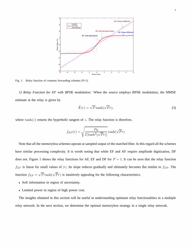
Fig. 1. Relay function of common forwarding schemes (P=1)

1) Relay Function for EF with BPSK modulation:When the source employs BPSK modulation, the MMSE

estimate at the relay is given by

X(r) =√

P tanh(√

Pr), (3)

wheretanh(z) returns the hyperbolic tangent ofz. The relay function is therefore,

fEF (r) =

√PR

E [tanh2(√

Pr)]tanh(

√Pr)

Note that all the memoryless schemes operate at sampled output of the matched filter. In this regard all the schemes

have similar processing complexity. It is worth noting thatwhile EF and AF require amplitude digitization, DF

does not. Figure 1 shows the relay functions for AF, EF and DF for P = 1. It can be seen that the relay function

fEF is linear for small values of|r|. Its slope reduces gradually and ultimately becomes flat similar to fDF . The

function fEF =√

P tanh(√

Pr) is intuitively appealing for the following characteristics.

• Soft information in region of uncertainty.

• Limited power in region of high power cost.

The insights obtained in this section will be useful in understanding optimum relay functionalities in a multiple

relay network. In the next section, we determine the optimalmemoryless strategy in a single relay network.

6

III. S INGLE RELAY CHANNEL

A. Problem Statement

Consider an elemental relay channel model as shown in the figure below, in which a single relay R assists the

communication between the source S and the destination D. Both S-R and R-D links are assumed to be non-fading.

S R Dx f(x + n1) y = f(x + n1) + n2

Elementary Relay Channel

There is no direct link between the source and the destination, which may be due to the half duplex constraint

of the nodes, where in the first slot D serves a different set ofnodes. The transmit power at the source and the

relay isP andPR respectively. At both the relay and the destination, the received symbol is corrupted by additive

white Gaussian noise of unit power. Relay R observesr, a noisy version of the transmitted symbolx. Based on

the observationr, the relay transmits a symbolf(r) which is received at the destination along with its noisen2.

r = x + n1

y = f(r) + n2 (4)

The relay functionf satisfies the average power constraint,i.e. Er

[f(r)|2

]= PR. Without loss of generality,

channel gains for the source-relay and the relay-destination link can be incorporated into the model by modifying

P and PR appropriately. We seek to determine the memoryless relay function f(.) that maximizes SNR at the

destination.

B. What is the definition of SNR?

Given an observationy, that contains a desired signalx as well as some distortion (noise), SNR is traditionally

defined as the power of the signalPx divided by the power in the noise componentPn. For observations of the

form y = x + n where the observed powerPy = Px + Pn (i.e. signal and noise are uncorrelated) it is easy to

separately identify the contribution of the signal power and the noise power to the observed power. However, what

is the definition of SNR if the observationy is not already explicitly presented in the standard formy = x+n with

7

uncorrelated signal and noise components? In general, the observationy may have an arbitrary and possibly non-

linear dependence on the desired signalx. For example, consider the signal at the destination:y = f(x + n1) + n2

with an arbitrary functionf() describing the memoryless relay functionality. In order todefine SNR one needs

to separately identify the power contributions of the signal and noise components to the observed signaly. If we

can identifyPy = Px + Pn then the definition of SNR readily follows asPx

Pn. In other words, the definition of

SNR follows from a representation of the observationy in the form y = x + n, with uncorrelatedsignal and

noise components. To this end, we view the signaly as a scaled version of the sum of the signalx and an error

componenteu uncorrelated withx.

y = f(x + n) =E [x∗y]

E [|x|2] (x + eu). (5)

Notice that any signaly can be expressed as above regardless of whethery is a linear or non-linear function of

x + n. Rearranging (5),

eu =E [|x|2]E [x∗y]

y − x. (6)

It is easy to verify thateu is uncorrelated tox.

E [x∗eu] = E[x∗(E [|x|2]E [x∗y]

y − x

)](7)

=E [|x|2]E [x∗y]

E [x∗y] − E [x∗x] = 0 (8)

To calculate the SNR of the received signaly, we need to identify the error term in the received signaly, that

is uncorrelated to the signalx. The scaling factorE[x∗y]E[|x|2] in (5) is common to both the signal and error terms.

Therefore, the generalized SNR is defined as follows:

GSNR=E [|x|2]E [|eu|2]

=E [|x|2]

E [|αy − x|2] , (9)

whereα = E[|x|2]E[x∗y] . The advantage of the generalized definition lies is its applicability to both linear and nonlinear

relay functions. Note that the conventional definition of SNR for point to point links is a special case of the

generalized SNR. For example, consider a received signaly = hx + n. The conventional SNR is|h|2P . To obtain

the generalized SNR, we need to expressy as a sum of the signalx and uncorrelated erroreu in the following

8

form.

y =E [x∗y]

E [|x|2] (x + eu),

where E[x∗y]E[|x|2] = h, in this case. Thereforeeu = n

h. The generalized SNR from (9) is,

GSNR=P1

|h|2= |h|2P,

which is also the conventional definition of SNR.

The GSNR concept can be viewed as a decomposition of an observation into a component along the desired

signal space and its orthogonal signal (uncorrelated noise) space. The orthogonal projections are evident in the

second moment constraintPy = Px + Pn (Pythagoras Theorem). GSNR is therefore as natural and meaningful a

metric as the orthogonal projections themselves. While GSNR optimization does not guarantee capacity or BER

optimality it is interesting to note that all three metrics(BER, capacity, GSNR) lead to very similar optimal relay

functions for BPSK. The BER optimal Lambert-W function is very similar to the GSNR optimal tan-hyperbolic

function(EF). Moreover, in a separate work we have shown that, numerically, the GSNR optimal EF function is

also capacity optimal for BPSK [20]. To summarize, GSNR optimality is related to capacity and BER optimality

and offers a tractable performance optimization metric.

C. Optimal Relay Function

We first derive the optimal estimation method that maximizesGSNR. Based on this result, we determine the

optimal relay function.

Theorem 1:Given an observationr that contains both the signalx and noisen, the MMSUE (SNR maximizing

estimate) ofx is

X(r) =E [|x|2]

E [x∗E(x|r)]E [x|r],

regardless of the input and the noise distributions.

Proof: Without loss of generality, any estimatorX(r) can be expressed as

X(r) = x + eu,

9

whereeu is uncorrelated withx. It is clear from (9) that minimizing the mean square uncorrelated estimation error

(MMSUEE),E [|eu|2] amounts to maximizing SNR. The optimization problem is therefore to minimizeE [|eu|2] with

respect toX(r) subject to the constraint thateu is uncorrelated withx. The constraint is equivalent toE [xe∗u] = 0

asE [x] = 0 for all signal constellations. Employing Lagrange multipliers2, we write the constrained minimization

as the minimization of

E = E [|eu|2] − λE [x∗eu] − λ∗E [xe∗u]

= E [|X(r) − x|2] − λE [x∗(X(r) − x)] − λ∗E [x(X∗(r) − x∗)]

= E [|X(r)|2] + (−λ + 1)E [x∗X(r)] + (−λ∗ + 1)E [xX∗(r)] − P (−λ − λ∗ − 1)

= Er

[|X(r)|2 − (λ − 1)X(r)E [x∗|r] − (λ∗ − 1)X∗(r)E [x|r]

]+ P (λ + λ∗ + 1)

= Er

[|X(r) − (λ − 1)E [x|r]|2 − |(λ − 1)E [x|r]|2

]+ P (2Re(λ) + 1)

From the above equation, it is clear thatE is minimized when

X(r) = (λ − 1)E [x|r],

and the minimum mean squared uncorrelated estimation erroris

E∗ = P (2Re(λ) + 1) − |λ − 1|2|Er

[|E [x|r]|2

](10)

From the constraint that

E [x∗eu] = 0 ⇒ E [x∗X(r)] = P,

we have

λ − 1 =P

E [x∗E(x|r)] .

ThereforeX(r) = PE[x∗E(x|r)]E [x|r] is the SNR maximizing estimate. It should be noted that the above result is

completely general and is valid for all input and noise distributions.

This result implies that any scaled version of MMSE estimator is GSNR optimal. Thus regardless of the power

constraint at the relay, EF maximizes GSNR at the output of the relay.

2As the constraintE [xe∗u] is a complex quantity, the Lagrange multipliers areλ andλ∗ corresponding toE [xe∗u] andE [x∗eu] respectively.

10

Theorem 2:In a single relay network, maximizing GSNR at the output of the relay amounts to maximizing

GSNR at the destination.

Proof: Consider any estimateX(r) = x + eu, with E[|eu|2

]= E, the uncorrelated estimation error power.

Let f(r) = αX(r) (11)

whereα2 = PR

P+Esatisfies the relay power constraint. The received symbol atthe destination is

y = αX(r) + n = α(x + eu) + n

The GSNR at the destination is given by

GSNRD =α2P

α2E + 1=

P

E + P+EPR

. (12)

Clearly minimizingE amounts to maximizing GSNR at the destination.

As scaling does not alter the GSNR of the estimate, forwarding MMSUE and MMSE results in the same relay

function. The fundamental relationship between these estimation methods is discussed in Appendix A. From the

results of theorem 1 and theorem 2, we have the following theorem for the optimal relay function.

Theorem 3:For a network with a single relay that has a power constraintPR, the relay function that maximizes

GSNR at the destination is

f(r) =

√PR

Er[|E(x|r)|2]E [x|r],

regardless of the input and noise distributions.

Thus the new memoryless forwarding strategy, estimate and forward is GSNR optimal in a single relay network.

In the next section, we compare the performance

IV. COMPARATIVE ANALYSIS

From the mean square uncorrelated estimation error at the relay, the SNR at the destination for any forwarding

scheme can be obtained directly from (12). Therefore calculation of uncorrelated error power of DF and AF allows a

direct comparison of these schemes with the SNR optimal EF. To determine the estimate whose error is uncorrelated

to the signalx from the actual relay function, we only need to obtain the scaling factor that allows the relay function

to be expressed as in (5). The relay function for DF depends onthe modulation scheme as discussed earlier. In this

11

section, we compare the schemes for BPSK modulation and illustrate the concept of generalized SNR.

A. Demodulate and Forward

We express the relay function of a demodulating relay as

fDF (x + n) =√

PRsign(x + n) =

√PR

P(x + d)

whered is the Euclidean distance between the input symbolx and the demodulated symbol. The distribution ofd

conditioned onx is given by

d =

0 1 − ǫ

−2x ǫ

(13)

whereǫ = Q(√

P)

, the probability of symbol error. As seen from the error distribution, the demodulation error

d is correlated withx. The correlation between the input and the error is given by

E(xd) = −2Pǫ. (14)

The uncorrelated error can be calculated from (5) accordingto which

eu =P

E(xfDF (x + n))fDF (x + n) − x =

P

P − 2Pǫ(x + d) (15)

From (14), the power of the uncorrelated error in (15) can be calculated and is given by

MSUEEDF =4Pǫ(1 − ǫ)

(1 − 2ǫ)2(16)

To characterize the mean squared uncorrelated error at the output of the DF relay, we first considerǫ, the probability

of decision error at the relay.

ǫ = Q(√

P)

=1√2π

∫ ∞√

P

exp(−x2

2)dx =

1

2− 1√

2π

∫ √P

0exp(−x2

2)dx

For small values ofP ,

ǫ =1

2−√

P

2π

12

−10 −5 0 5 10 15 200

0.2

0.4

0.6

0.8

1

1.2

1.4

1.6

10 log P (in dB)

Unc

orre

late

d E

rror

Pow

er "E

"

EstimateDemodulateAmplify

Fig. 2. Uncorrelated error power vs transmit power with BPSKmodulation

Therefore at low source transmit power, the mean squared uncorrelated error can be expressed as a function ofP .

MSUEEDF (P ) =

4P

(12 −

√P2π

)(12 +

√P2π

)

(1 −

(1 −

√2Pπ

))2 = 2π

[1

4− P

2π

](17)

As P → 0, the uncorrelated error power shoots up toπ2 . It should be noted that the noise variance at the relay is

1. This suggests that DF is not preferable at lowP .

B. Amplify and Forward

As the relay function of an AF relay is a scaled version of the received signalr, it is simple to determine the

mean squared uncorrelated error. From (5), we have

eu =P

E [x∗fAF (x + n)]fAF (x + n) − x = n

The uncorrelated error power is therefore the same as the noise variance, MSUEEAF = 1, interestingly independent

of the source transmit power.

Fig. 2 plots the uncorrelated estimation error as a functionof transmit power for all the three schemes. Several

interesting observations can be made. It can be seen that AF is close to optimum (EF) at lowP while DF is near

optimal at highP . In the intermediate range, both AF and DF are far from optimal. It is well known that AF

suffers from noise amplification at low SNR [22], which is in contrast to the results here. When we view the relay

operation as an estimation, it is only natural that the estimation error is high at lowP , which results in noise

13

amplification. In fact AF is very close to optimum among all memoryless function at lowP . Rather it is DF that

suffers the most from noise/error3 amplification. However AF is inefficient at highP as MSUEEAF = 1 does not

decrease withP , while uncorrelated error in DF and EF vanishes at highP . The mean squared uncorrelated error

power of the schemes for extreme values ofP is listed in Table I.

MMSUERelay Function P → 0 P → ∞

Amplify 1 1

Demodulate π2 0

Estimate 1 0

TABLE I

UNCORRELATED ERROR POWER AT OUTPUT OF RELAY FORBPSKMODULATION .

C. Higher Order Constellations

We know from theorem 3 that EF is GSNR optimal for all modulation schemes. For fixed input powerP ,

increasing the number of constellation pointsM will result in an increased mean squared uncorrelated powerfor

EF. This is rather intuitive from the fact that increasing the number of constellation points for fixed power increases

the estimation error. Fig. 3 shows the relay functions for 4-PAM constellation set. Interestingly, the relay functions

of the schemes become more and more similar with increase in constellation points.

For Gaussian inputs, the unconstrained MMSE estimate and the linear MMSE estimate are equivalent.

E [x|r] =P

P + 1r

Thus AF and EF strategies are the same for a Gaussian source. In this context, it can also be shown that DF and

AF are equivalent for Gaussian inputs. The notion of demodulation of symbols from a Gaussian source is explained

through the following. A Gaussian distribution is quantized into a number of states with the probability of theith

state given by,

Pr(xi) =1√2πP

∫ i∆x

(i−1)∆x

exp

(−x2

2P

)dx.

Suppose the source transmits symbolsxi according to the probability distribution above, then the MAP detection

3the term ‘error’ is more appropriate as noise process is usually independent of the input

14

−10 −8 −6 −4 −2 0 2 4 6 8 10−10

−8

−6

−4

−2

0

2

4

6

8

10

Received Symbol "r"

Tran

smitt

ed S

ymbo

l "f(r

)"

AmplifyDemodulateEstimate

Fig. 3. Relay Functions for 4-PAM modulation

rule at the relay is given by

X(r) = argmaxxi

Pr(x|r)

In the limit ∆x → 0, x andr become jointly Gaussian. It is well known that the conditional meanE(x|r) maximizes

the joint probability. ThereforeE(x|r) which is also the MMSE estimate is the output of the ML detector. Thus

for Gaussian inputs AF, EF and DF are identical.

V. PARALLEL RELAY NETWORK

A Gaussian parallel relay channel [14] is shown in Fig. 4. It consists of a single source destination pair withL

relays that assist in the communication. All the links are assumed to be non-fading with unequal channel gains and

+

+

+

+Source

Relay 1

Relay 2

Relay L

Destinationr2

r1

rL

f(r2)

f(r1)

f(rL)

n1

nL

n2n

Fig. 4. Gaussian Parallel Relay Channel

information is transferred in two time slots. The relays observe{ri}Li=1, the noisy version of the transmitted signal

x.

ri = gix + ni (18)

15

wheregi is the gain of the link between the source and theith relay. ni denotes an additive Gaussian noise with

σ2=1. Since the relays are assumed to be memoryless, each relayRi transmits a signal that is a function of its

observationri. We assume that the relay function in a parallel relay network is the same for all the relays, although

the channel gains of the relays may be different. Strictly speaking, an optimal power allocation based on the channel

gains is necessary. However, it is beyond the scope of the paper. For ease of notation, we denote the transmit power

at the source asP and the relay transmit power as{Pi}Li=1. Without loss of generality, the channel gain for the

relay destination links can be introduced through the relaytransmit power. The destination receives the sum of all

the relay observations along with its own noise.

y =

L∑

i=1

f(ri) + n

By viewing relay operation as an estimation we have,

f(ri) = f(gix + ni) = αi(x + ei)

whereei is the uncorrelated estimation error at theith relay, αi =√

Pi

P+Eiand Ei = E [|ei|2], the mean square

uncorrelated error power associated with the relay function. The received signal at the destination can be expressed

as

y =L∑

i=1

αi(x + ei) + n (19)

For any forwarding scheme, the SNR at the destination is given by

GSNR=(∑L

i=1 αi)2P

∑Li=1 α2

i Ei +∑L

i=1

∑Lj=1,j 6=i αiαjCij + 1

, (20)

whereCij = E(e∗i ej) is the correlation between errorsei andej at relaysi and j, i 6= j. For the zero correlation

case (Cij = 0, ∀ij), it is clear from (20) that the SNR is maximized when the uncorrelated estimation error at

the relays (Ei) are minimized. This can also be inferred from the generalized definition of SNR in (5). Error in

the received symbol at the destination in (19) is a linear combination of errors at the output of relays and the

destination noise. When the errors are uncorrelated, minimizing the error at the output of each of the relays clearly

amounts to maximizing SNR at the destination.

For AF, the correlationC is always zero as the error terms represent independent AWGNnoise. For both DF

16

and EF, the correlation depends on the modulation scheme andis not always zero. Although eachEi is minimized

by EF, due to the possibility of error correlation, maximum SNR is not always guaranteed. However for most

constellation sets, the error correlation can be shown to beeither very close or exactly equal to zero. Theorem 5

in Appendix B characterizes the rotational property of estimate and forward for MPSK constellation sets and will

be useful to prove zero correlation property of EF. It provesthat, due to the symmetry in the constellation, MMSE

estimate of a signal rotated by an angle that belongs to a constellation point is the same as the rotated version of

the MMSE estimate of the signal.

X(rejθm) = ejθmX(r) whereθm = 2πmM

,m = 0, 1, ...M − 1, the signal phases of MPSK.

Theorem 4:Error at the relays that estimate and forward are uncorrelated with each other if MPSK modulation

is employed at the source.

Proof: In Appendix C. ThusE [e1e∗2] = 0 for all MPSK constellation set inputs. This directly suggests that SNR

achieved at the destination is always the highest with estimate and forward.

A. Effect of Error Correlation on EF

The correlation between errors at the output of EF relays, ingeneral, is not zero for all constellations. However

it is negligible for many constellation sets like M-QAM and it does not result in any tangible SNR loss. In

fact, the correlation can be expected to decrease for large QAM constellations where the ‘edge effects’ become

insignificant. However due to the combination ofL(L − 1) terms for the correlation expression in (20), we can

expect the performance of the system to degrade for very large values ofL. In a symmetrical relay network where

the channel gain of all the links are equal, the SNR for any relay function, as a function of correlation between

errors is obtained from (20) as

GSNR=L2P

LE + L(L − 1)C + 1 + EP

, (21)

Suppose the source employs a modulation scheme that resultsin nonzero correlation between errors with EF in

a parallel network with unit channel gains, GSNRAF > GSNREF only if

C >1 − E

L(L − 1)

(L +

1

P

)(22)

As the scaling associated with the correlation isL(L − 1), its effect is prominent for largeL. For a given error

17

−10 −5 0 5 10 15 20 25−1

0

1

2

3

4

5

6

7

8x 10

−3

Single Hop SNR

Err

or C

orre

latio

n

Correlation

Fig. 5. Error Correlation in Estimate and Forward for 16 QAM

correlationC, GSNRAF > GSNREF if

L '1 − E

C+ 1 (23)

The above relation along with Fig. 5 suggests that, even if the correlation with EF is nonzero, the number of relays

has to be very large for AF to outperform EF at high SNR, with modulation schemes like M-QAM.

B. Error Correlation in DF

Similar to EF, the error correlation in DF depends on the modulation scheme at the source. For BPSK modulation,

the error term in uncorrelated estimate of DF from (15) is

ei =di + 2ǫix

1 − 2ǫi, (24)

whereǫi depends on the transmit power and the source-relay channel.From the distribution ofdi in (13), we can

calculate the correlation between errorsei andej at relayi andj.

C = E(eiej) =E [didj ] + 2ǫiE [xdi] + 2ǫjE [xdj ] + 4ǫiǫjE [|x|2]

(1 − 2ǫi)(1 − 2ǫj)

=4ǫiǫjP − 8ǫiǫjP + 4ǫiǫjP

(1 − 2ǫi)(1 − 2ǫj)= 0 (25)

For BPSK modulation and with unit channel gain for all the links, the effective SNR at the destination is

GSNRDF =PL2(1 − 2ǫ)2

4PLǫ(1 − ǫ) + 1(26)

For large M-QAM constellation ignoring edge effects, the demodulation error can be assumed to be independent

18

of the transmitted symbol, with the distribution given by

d =

0 1 − ǫ

dminǫ

4

−dminǫ

4

jdminǫ

4

−jdminǫ

4

(27)

where, from [23] we have

dmin =

√6P

M − 1

ǫ ≤ 4

(1 − 1√

M

)Q

(√3P

M − 1

)

(28)

Here we assume that decisions error occur only among the nearest neighbors. Although this is an optimistic

assumption, it closely predicts the performance of the system at medium and high SNR where the assumption is

justified. The effective SNR at the destination is,

GSNRDF ≈ PL2

Ld2minǫ + 1

. (29)

C. Asymptotic GSNR Comparison

While EF is superior to AF and DF at all SNR regardless of the number of relays, it will be interesting to

characterize the asymptotic gain of EF as a function of L and P. For ease of analysis, we restrict the channel gains

to be equal. From the SNR expressions of EF and AF, we have the ratio,

GSNREF

GSNRAF=

LP + P + 1

LPE(P ) + P + E(P ),

whereE(P ) is the mean squared uncorrelated error power of EF that is a function of P . Note that the above

expression does not include the correlation term. Therefore, it is valid only when there is zero correlation between

the error terms. For any input distributionpX(x), i.e. for all modulation schemes,

E(P ) ≤ 1, ∀P.

19

1) FixedP : With large number of relays ,

L → ∞,GSNREF (P )

GSNRAF (P )=

MSUEEAF

MSUEEEF=

1

E(P )

GSNREF (P )

GSNRDF (P )=

MSUEEDF

MSUEEEF=

4Pǫ(1 − ǫ)

(1 − 2ǫ)2E(P )

Notice that MSUEE of the schemes determine the gain. We know from Section. IV thatE(P ) decreases withP

and ultimately becomes zero asP → .∞. This implies that in a large relay network, maximum gain over AF is

obtained for high source transmit powerP . Similarly maximum gain over DF is obtained at lowP . This is due to

the fact that DF is inefficient at lowP as indicated by its mean squared uncorrelated error power.

2) Fixed L: For a fixed number of relays, the GSNR gain of EF over AF at highP is approximatelyL + 1.

Similarly the GSNR gain of EF over DF at low P is very high as indicated in the following expressions.

P → ∞,GSNREF (L)

GSNRAF (L)= L + 1

GSNREF (L)

GSNRDF (L)= 1 (30)

P → 0,GSNREF (L)

GSNRAF (L)= 1

GSNREF (L)

GSNRDF (L)=

π

2(31)

Above expressions clearly demonstrate the inefficiency of DF and AF at low and high SNR respectively.

D. Numerical Results

Fig. 6 provides the GSNR performance of the schemes in a parallel relay network with equal channel gains. The

corresponding error probabilities are provided in Fig. 7. The error probabilities closely follow the trend exhibited

in GSNR. It can be seen that EF achieves substantial error probability gains over AF and DF for all values ofP .

As seen in GSNR plot, AF is superior to DF at lowP while DF performs better than AF at highP . This is also

indicated by (30) and (31). For our system model, the AF relaying scheme is equivalent to the one proposed in

[12]. It will be interesting to compare the performance of the schemes with optimal power allocation similar to

[12].

VI. SERIAL RELAY NETWORK

A serial relay network with Gaussian noise at all receivers in shown in Fig. 8. All the relays are memoryless

and employ a relay function to transmit a symbol based on its received symbol. It should be noted that the relay

functions, in general, need not be the same for all the relaysunlike in a parallel network. This is due to the fact that

20

−15 −10 −5 0 5 10 15 20−30

−20

−10

0

10

20

30

Transmit Power in dB

Effe

ctiv

e S

NR

at d

est

ina

tion

in d

B

EstimateAmplifyDemodulate

Fig. 6. Comparison of SNR at the destination as a function oftransmit powerP = PR for a parallel network (L = 2)

−6 −4 −2 0 2 4 6 8 10 1210

−4

10−3

10−2

10−1

100

10 log P (in dB)

BE

R

EstimateAmplifyDemodulate

Fig. 7. BER of schemes in a parallel network (L = 2) for BPSKmodulation

+ +Relay 1 Relay L +Source Destination

n1

r1

nL

rL fL(rL)

n

f1(r1)

Fig. 8. Serial Network Model

the noise distribution gets altered at every hop depending on the relay function of the preceding relay for multiple

relay networks. We assume unit channel gains for the links and equal transmit power at all the nodes for simplicity

of exposition.

A. Amplify and Forward

With AF relays in series, the received symbol at the destination can be expressed as

yL+1 = βLx +

L∑

i=1

βini + n. (32)

GSNRAF =β2LP

1 +∑L

i=1 β2i(33)

B. Demodulate and Forward

As in Section V-B, we express the received signal at the destination as

yL+1 = x +

L∑

i=1

di + n (34)

21

From (13) and (27), the effective SNR at the destination withBPSK modulation and for a large QAM modulation

is obtained.

GSNRBPSK

DF =P (1 − 2ǫ)2

4PLǫ(1 − ǫ) + 1GSNR

QAM

DF ≈ P

Ld2minǫ + 1

C. Estimate and Forward

With estimate and forward at all the relays, the corresponding relay functions varies with each relay as the noise

distribution gets altered at each link due to nonlinear operations performed at the preceding relay. The relay function

for the ith is given by

fi(ri) = αiE [x|ri = fi−1(ri−1) + ni]

Proposition 1: In a serial relay network, the last relay should perform estimate and forward for maximizing SNR

at the destination,regardless of the relay function in the preceding relays.

Proof: Regardless of the relay functions at the preceding relays, the received signal at the last relay can be

expressed in the same form as (5). From theorem 1, which is valid for all input and noise distributions, it is

straightforward that EF at the last relay maximizes the SNR at the destination.

D. Performance Comparison

Fig. 9 compares the destination SNR of the schemes for two serial relays. Here the relay functions for DF and AF

remain the same for both the relays. For EF,f1(r1) = α1 tanh(√

Pr1) andf2(r2) = α2E [x|r2 = α1 tanh(√

Pr1)+

n2]. As expected, EF is the best performing scheme and DF closelyfollows it.

It can be easily noticed that in a serial network, the effective SNR decreases with each stage. AF, being power

inefficient at high SNR, suffers the most due to multi-hop communication.

GSNRAF =P

1 +∑L

k=11

β2k

<P

L + 1(35)

For large M-QAM modulation, effective SNR at the destination with DF scheme can be approximated as

GSNRDF =P

Ld2minǫ + 1

(36)

Clearly whend2minǫ < 1 (at high SNR regime),

GSNRDF ≥ P

L + 1, (37)

22

−10 −5 0 5 10 15−30

−25

−20

−15

−10

−5

0

5

10

15

Transmit Power in dB

Effe

ctiv

e S

NR

at d

est

ina

tion

in d

B

EstimateAmplifyDemodulate

Fig. 9. Comparison of SNR at the destination as a function oftransmit powerP = PR for a serial network (L = 2)

−2 0 2 4 6 8 10 12 14 1610

−3

10−2

10−1

100

10 log P (in dB)

BE

R

EstimateDemodulateAmplify

Fig. 10. BER of schemes in a parallel network (L = 2) forBPSK modulation

indicates that DF is superior to AF at high SNR. We can also observe the case where GSNRAF > GSNRDF at

low SNR (whend2minǫ > 1). Note that the variance of the error components associatedwith DF (d2

minǫ) decreases

exponentially withP , while those in AF( 1β2k for the kth relay) decreases linearly withP . These observations can

be clearly seen in Fig. 9, where AF performs slightly better than DF at very low SNR. Gradually with increase in

P , DF outperforms AF and the performance gap widens with further increase inP .

E. Hybrid Relay Networks

From the previous sections, we determine that EF is well suited to both parallel and serial relay network regardless

of P , and substantial performance gain can be obtained over AF and DF in many scenarios. We also observe that

DF is close to optimal in a serial relay network at high SNR where as AF is near-optimal in parallel relay networks

at low SNR. In these regimes, the performance gain of EF is limited. Thus, it is interesting to determine the

performance gain of EF in general memoryless relay networks. Consider a network consisting of both parallel and

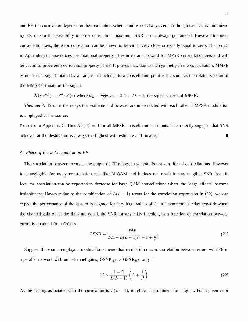
serial subnetworks as shown in Fig. 11. Due to the presence ofparallel and serial elements together in the network,

we find a significant performance degradation in both AF and DFat all P . Precisely, this is a scenario where EF

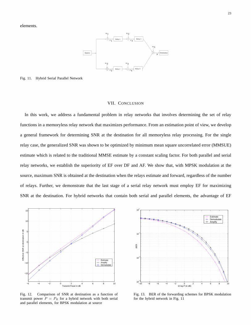
obtains a large gain over the best of DF and AF. Fig. 12 compares the performance of schemes for the hybrid

network in Fig. 11. It can be noticed that EF performs significantly better than the best of DF and AF. Fig. 13

displays the error probability of the schemes for the hybridnetwork. It can be seen that substantial gain is obtained

over the best of DF and AF. The performance gain will increasefor a large network with both parallel and serial

23

elements.

+ DestinationSource

+

+ Relay 1

+

+

Relay 2

Relay 3

Relay 4

n5

n1 n3

n4n2

r3r1

r2 r4

y

Fig. 11. Hybrid Serial Parallel Network

VII. C ONCLUSION

In this work, we address a fundamental problem in relay networks that involves determining the set of relay

functions in a memoryless relay network that maximizes performance. From an estimation point of view, we develop

a general framework for determining SNR at the destination for all memoryless relay processing. For the single

relay case, the generalized SNR was shown to be optimized by minimum mean square uncorrelated error (MMSUE)

estimate which is related to the traditional MMSE estimate by a constant scaling factor. For both parallel and serial

relay networks, we establish the superiority of EF over DF and AF. We show that, with MPSK modulation at the

source, maximum SNR is obtained at the destination when the relays estimate and forward, regardless of the number

of relays. Further, we demonstrate that the last stage of a serial relay network must employ EF for maximizing

SNR at the destination. For hybrid networks that contain both serial and parallel elements, the advantage of EF

−6 −4 −2 0 2 4 6 8 10

−15

−10

−5

0

5

10

15

Transmit Power in dB

Eff

ect

ive

SN

R a

t d

est

ina

tion

in d

B

EstimateAmplifyDemodulate

Fig. 12. Comparison of SNR at destination as a function oftransmit powerP = PR for a hybrid network with both serialand parallel elements, for BPSK modulation at source

−10 −8 −6 −4 −2 0 2 4 6 8 1010

−3

10−2

10−1

100

10 log P (in dB)

BE

R

Estimate DemodulateAmplify

Fig. 13. BER of the forwarding schemes for BPSK modulationfor the hybrid network in Fig. 11

24

over the best of AF and DF is found to be significant.

APPENDIX

A. Relation between MMSUEE and MMSEE

Although the relay functions arising out of MMSUE and MMSE estimates are identical, they are fundamentally

distinct as the objectives optimized by them are different.MMSUE is the minimum achievable uncorrelated error

power while MMSE is the minimum achievable distortion. By proving that the correlation of the MMSE errore

and the inputx, we obtain the relationship between MMSE and MMSUE.

Proposition 2: Correlation between the MMSE errore and the inputx is always non positive.

(Proof: We express the MMSE estimate as

X(r) = x + e = x +µ

Px + eu,

whereµ = E [x∗e] andeu is uncorrelated tox,

eu = e − µ

Px (38)

Consider another estimate which is a scaled version of the MMSE estimate such that

Xnew(r) =X(r)

1 + µP

= x +eu

1 + µP

.

As MMSE estimation is optimal distortion minimizing method, we have the relation

E [|e|2] ≤ 1(1 + µ

P

)2 E [|eu|2] (39)

≤ 1(1 + µ

P

)2

(E [|e|2] − µ2

P

)(40)

<1

(1 + µ

P

)2 E [|e|2] (41)

which impliesµ ≤ 0.

For Gaussian inputs, a unique relationship between MMSE estimate and the correlation exists, which isµ =

E(Xe) = −MMSEE = −PP+1 . A direct consequence of the negative correlation of the error with the signalx leads

25

to the following inequality.

SNR≤ PMMSEE

.

Proposition 3: The minimum mean squared uncorrelated estimation error cannot be less than MMSEE. The

precise relationship between MMSUEE and MMSEE is

MMSUEE =MMSEE− µ2

P

(1 + µP

)2

Proof: We have MMSUEE≥ MMSE, by observingeu to be the distortion arising out of another estimation

method that cannot achieve a mean squared estimation error less than MMSEE. The exact relationship between the

mean square error of these methods can be obtained from (38).

B. Rotational Property of EF

Theorem 5:For all MPSK constellation inputs, the MMSE estimate has theproperty

X(rejθm) = ejθmX(r),

whereθm = 2πmM

,m = 0, 1, ...M − 1, the signal phases of MPSK.

Proof:

E [x|r = rejθm] =

√P

M

M−1∑

k=0

ejθiPr[x =√

Peθk |rejθm] (42)

=

√P

M

M−1∑

k=0

ejθkPr[x =√

Peθie−jθm|r] (43)

=

√P

Mejθm

M−1∑

k=0

ejθ(k−m)Pr[x =√

Peθ(k−m) |r] (44)

= ejθmE [x|r]

26

C. Proof for Zero Error Correlation of EF

Expressing error as the difference of the estimate and the actual symbol, we have

C = E [e1e∗2] = E [(X(r1) − x)(X∗(r2) − x∗)] (45)

=

[P 2

E [x∗E(x|r1 = g1x + n1)]E [x∗E∗(x|r2 = g2x + n1)]E [E [x|r1]E [x∗|r2]]

]− P

E [E [x|r1]E [x∗|r2]] =1

M

M−1∑

i=0

En1E [x|r = g1xi + n1]En2

E [x∗|r2 = g2xi + n2]

=1

M

M−1∑

i=0

EnE [x|r = g1xi + n]E∗nE [x|r = g2xi + n] (46)

= EnE [x|r = g1x0 + n]E∗nE [x|r = g2x0 + n], (47)

where (47) is obtained by applying theorem 5 in (46).

E [x∗E(x|r = ri) =1

M

M−1∑

i=0

xiEn [E [x|r = xi + n]]

=√

P1

M

M−1∑

i=0

En [E [x|r = x0 + n]] (48)

=√

PEn [E [x|r = g1x0 + n]] , (49)

where (48) is reduced to (49) using theorem 5. Substituting (47) and (49) in (45), we have

C = E [e1e∗2] =

P 2EnE [x|r = g1x0 + n]E∗nE [x|r = g2x0 + n]

PEn [E [x|r = g1x0 + n]] E∗n [E [x|r = g2x0 + n]]

− P

= 0 (50)

REFERENCES

[1] A.F. Dana, R. Gowaikar, B. Hassibi, M. Effros and M. Medard, “Should we break a wireless network into subnetworks?,” in Allerton

Conference on Communication, Control and Computing., 2003.

[2] A. Sendonaris, E. Erkip, and B. Aazhang, “User cooperation diversity, Part I: System description,”IEEE Transaction On Communica-

tions, vol. 51, no. 11, pp. 1927–1938, 2003.

[3] A. Sendonaris, E. Erkip, and B. Aazhang, “User cooperation diversity, Part II: Implementation aspects and performance analysis,”IEEE

Transaction On Communications, vol. 51, no. 11, pp. 1939–1948, 2003.

27

[4] G. Kramer, M. Gastpar and P. Gupta, “Cooperative Strategies and Capacity Theorems for Relay Channels,”IEEE Transactions on

Information Theory, submitted for publication.

[5] A. Høst-Madsen,, “On the capacity of wireless relaying,” in Proc. IEEE Vehic. Techn. Conf., VTC 2002 Fall, (Vancouver, BC), Sep

2002.

[6] M. A. Khojastepour, A. Sabharwal, and B. Aazhang, “On thecapacity of ‘cheap’ relay networks,” inProc. 37th Annual Conf. on

Information Sciences and Systems (CISS), (Baltimore, MD), Mar 2003.

[7] J. N. Laneman and G. W. Wornell, “Exploiting DistributedSpatial Diversity in Wireless Networks ,” inin Proc. Allerton Conf. Commun.,

Contr., Computing, Illinois, Oct 2000.

[8] D. Chen and J. N. Laneman, “Modulation and demodulation for cooperative diversity in wireless systems,”To appear in IEEE Trans.

Wireless Commun., 2005.

[9] J. N. Laneman, D. N. C. Tse, and G. W. Wornell, “Cooperative diversity in wireless networks: Efficient protocols and outage behavior,”

IEEE Trans. Inform. Theory, vol. 50, no. 12, pp. 3062–3080, 2004.

[10] T. M. Cover and A. El Gamaal, “Capacity Theorems for the relay channel,”IEEE Transactions on Information Theory, vol. 25, no. 5,

pp. 572–584, Sep 1979.

[11] N. Khajehnouri and A. H. Sayed, “A distributed MMSE relay strategy for wireless sensor networks,” inProc. IEEE Workshop on

Signal Processing Advances in Wireless Communications, NY, Jun 2005.

[12] S. Berger and A. Wittneben, “ Cooperative Distributed Multiuser MMSE Relaying in Wireless Ad Hoc Networks,” inAsilomar

Conference on Signals, Systems, and Computers, Pacific Grove, CA, 0ct 2005.

[13] L. Lai, K. Liu, and H. El Gamal, “ The Three Node Wireless Network: Achievable Rates and Cooperation Strategies ,”IEEE Transactions

on Information Theory, to appear.

[14] M. Gastpar and M. Vetterli, “On the Capacity of Large Gaussian Relay Networks ,”IEEE Transactions on Information Theory, vol. 51,

no.3, pp. 765–779, March 2005.

[15] M. Gastpar and M. Vetterli, “On the capacity of wirelessnetworks: the relay case,” inProc. 2002 INFOCOM.

[16] S. Zahedi, M. Mohseni, A. El Gamal, “On the capacity of AWGN relay channels with linear relaying functions,” inProc. 2004 IEEE

Int. Symp. Info. Theory.

[17] A. El Gamaal and N. Hassanpour, “Relay without delay,” in Proc. International Symposium on Information Theory, Adelaide, Australia,

Sep 2005.

[18] D. Tuninetti, U. Niesen, C. Fragouli, “On capacity of line networks,” inProc. 2006 Workshop on Information Theory and its Applications,

UC San Diego, Feb. 2006.

[19] U.Niesen and C.Fragouli and D.Tuninetti, “On cascade of Channels with Finite Complexity Intermediate Processing,” in Allerton

Conference 2005, Urbana-Champaign, Illinois USA, September 2005.

[20] K. Gomadam and S. A. Jafar, “On the Capacity of Memoryless Relay Networks,” inProc. IEEE ICC 2006, Istanbul, Jun 2006.

[21] I. Abou-Faycal, M. Medard, “Optimal Uncoded Regeneration for Binary Antipodal Signaling,” inProc. IEEE ICC, 2004.

[22] I. Maric and R. Yates, “Forwarding Strategies for Gaussian Parallel-Relay Networks,” inProc. Conf. on Information Sciences and

Systems (CISS), (Baltimore, MD), 2004.

[23] J. G. Proakis,Digital Communications. New York: McGraw-Hill, 4th ed., 2001.