Boundary behavior of p-harmonic functions in the Heisenberg group

arX

iv:1

005.

2602

v1 [

mat

h.A

P] 1

4 M

ay 2

010

BOUNDARY BEHAVIOR p-HARMONIC FUNCTIONS IN THE

HEISENBERG GROUP

NICOLA GAROFALO AND NGUYEN CONG PHUC

1. Introduction

The study of the boundary behavior of nonnegative solutions of elliptic and parabolic pde’sis a central subject with a long and rich history, see e.g. [Ke]. Over the past few years theattention of several groups of workers in the field has increasingly focused on boundary valueproblems for a class of second order partial differential equations which arise from problemsin geometry, several complex variables and also, and pre-eminently, in the applied sciences(e.g., robotics, neuroscience, financial mathematics). The relevant pde’s, known as subellipticequations, display many challenging new aspects and typically, they fail to be elliptic at everypoint.

Some interesting progress in the analysis of the boundary behavior of solutions to theseequations has come with the works [NS], [Ci], [Da], [CG], [LU], [CGN2], [MM1], [MM2], [CGN3].The prototypical situation is that of a graded nilpotent Lie group G with a fixed sub-LaplacianL =

∑mi=1X

2i associated to an orthonormal basis of the bracket generating layer of the Lie

algebra. Given an open set Ω ⊂ G, a distribution u is called harmonic if Lu = 0 in D′(Ω). ByHormander’s hypoellipticity theorem [H] one has that every harmonic function is in fact C∞(Ω).Similarly to its classical counterpart a central problem is that of understanding the boundarybehavior of nonnegative solutions of Lu = 0 in a given bounded open set Ω ⊂ G.

This question poses remarkable new challenges with respect to the classical elliptic theory.On one hand, the vector fields X1, ...,Xm satisfy nontrivial commutation relations and thecommutators are, effectively, derivatives of higher order. This is reflected in the fact that thenatural geometry attached to L is not the Riemannian geometry of the ambient manifold G,but a much more complicated nonisotropic one in which different directions in the tangent spaceweight in a different way, according to their order of commutation. A remarkable new aspectis then the interplay between the sub-Riemannian geometry associated with L and the natureof the boundary of the domain Ω. In this connection, those points of ∂Ω at which the vectorfields X1, ...,Xm become tangent to ∂Ω play a special role. At such points, which are known ascharacteristic points, a hoist of new phenomena can occur and a solution of Lu = 0 can displaybehaviors quite different from classical harmonic functions.

The subtle role of characteristic points first became apparent in the pioneering works ofFichera [F1], [F2] (who first introduced the notion of characteristic set), Kohn-Nirenberg [KN1]and Bony [Bo]. In his work [Je1] on the Dirichlet problem in the Heisenberg group, D. Jerisonfirst constructed an example of a smooth (in fact, real analytic) domain for which the Dirichletproblem admits a Green function which, in the neighborhood of a characteristic point, is atmost Holder continuous up to the boundary, see also [Je2]. This is in sharp contrast with theclassical elliptic theory, in which smooth data on smooth domains produce solutions which aresmooth up to the boundary.

Date: May 17, 2010.First author supported in part by NSF Grant DMS-0701001.Second author supported in part by NSF Grant DMS-0901083.

1

http://arxiv.org/abs/1005.2602v1

2 NICOLA GAROFALO AND NGUYEN CONG PHUC

In the papers [CGN2], [CGN3] a complete solution of the Dirichlet problem was obtainedfor the class of the so-called ADP domains, i.e., domains which are admissible for the Dirichletproblem. Such domains are defined by imposing that they be NTA (non-tangentially accessible)with respect to the sub-Riemannian distance associated with the vector fields X1, ...,Xm, andthat furthermore they satisfy a uniform outer tangent ball condition reminiscent of that intro-duced by Poincare in the classical setting [P]. This second assumption was imposed to rule outD. Jerison’s negative phenomenon mentioned above. For an extensive discussion of the variousramifications of these hypothesis we refer the reader to the paper [CGN3]. The reader is alsoreferred to Section 5 for the definitions of NTA, and ADP domains.

In this paper we initiate the study of the boundary behavior of nonnegative p-harmonicfunctions, i.e., weak solutions to the nonlinear equation

(1.1) Lpudef=

m∑

i=1

Xi(|Xu|p−2Xiu) = 0, 1 < p <∞.

Equation (1.1) arises as the Euler-Lagrange equation of the p-energy in the Folland-Stein Sobolevembedding in [Fo] and, similarly to its classical counterpart, the Euclidean p-Laplacian, it playsan important role in the analysis of sub-Riemannian spaces. In (1.1) we have indicated with

|Xu| = (∑m

i=1(Xiu)2)1/2 the length of the sub-gradient of u.

The relevant geometric setting of the present paper is the Heisenberg group Hn, which is the

simplest and perhaps most important example of a graded nilpotent Lie group of step two. Fora detailed description of such group we refer the reader to Section 2. There is a reason for whichwe confine our analysis to H

n, rather then considering an arbitrary nilpotent Lie group, or evenmore general settings, as it is done for instance in [CGN3]. Such reason will become apparent tothe reader in the main body of the paper, and is related to the considerable difficulties connectedwith: 1) the nonlinear nature of (1.1); 2) the present lacking of those tools which, in the classicalsetting, play an essential role in the analysis of the p-Laplacian.

We will be primarily interested in the range 1 Q is also of interest in view of possible applications to the horizontal ∞-Laplacian

L∞u =

m∑

i,j=1

u,ijXiuXju,

where u,ij =12(XiXju+XjXiu). However, in such range the proofs are completely analogous,

perhaps a bit easier due to the non singular nature of the corresponding fundamental solution(incidentally, in view of the Morrey type theorem in [GN], for the domains in this paper functions

in the horizontal Sobolev space W 1,pH are automatically Holder continuous up to the boundary).

Our main objective is understanding, in the model situation of Hn, the boundary behavior ofthose nonnegative weak solutions of (1.1) which continuously vanish on a portion of the boundaryof a relevant domain Ω. In this perspective, our main contributions can be summarized as follows:

1) Theorem 1.1, in which we obtain an estimate from above which says that any such solu-tion should vanish at most linearly like the sub-Riemannian distance from the boundary:

(1.2)u(g)

u(Ar(g0))≤ C−1d(g, ∂Ω)

r,

where Ar(g0) ∈ Ω is a non-tangential point relative to g0 ∈ ∂Ω.2) Theorem 1.2, in which we establish an estimate from below which states that the order

of vanishing is exactly linear, i.e:

(1.3)u(g)

u(Ar(g0))≥ C

d(g, ∂Ω)

r.

BOUNDARY BEHAVIOR FOR p-HARMONIC FUNCTIONS, ETC. 3

Combining these two results we obtain

(1.4) Cd(g, ∂Ω)

r≤ u(g)

u(Ar(g0))≤ C−1d(g, ∂Ω)

r.

Finally, since the constant C > 0 is independent of the particular p-harmonic function u, we con-clude in Theorem 1.3 that for any two nonnegative p-harmonic functions u, v, which continuouslyvanish on a portion of the boundary, one has

(1.5) Cu(Ar(g0)

v(Ar(g0))≤ u(g)

v(g)≤ C−1 u(Ar(g0)

v(Ar(g0)).

Thus, all nonnegative p-harmonic functions which vanish on a portion of the boundary, must doso at the same rate.

This description clearly provides an oversimplified picture, since we have not specified underwhich assumptions, and where, each of the relevant estimates (1.2), (1.3) is valid. In this respect,it is worth observing that, in the Euclidean setting and for p = 2, although the comparisontheorem (1.5) does hold for large classes of domains with rough boundaries (for instance, inLipschitz or even NTA domains, see [CFMS], [JK]), the linear decay estimate (1.4) breaks downif the domain fails to satisfy a uniform bound on its curvatures.

For instance, if 0 < θ0 < π/2 and we consider in R2 the convex circular sector Ω = (r, θ) |

0 < r < 1, |θ| < θ0, where θ indicates the angle formed by the directional vector of the point(x, y) with the positive direction of the y-axis, the function u(r, θ) = rλ cos(λθ) is a nonnegativeharmonic function in Ω vanishing on that portion of ∂Ω corresponding to |θ| = θ0 provided that

λ =π

2θ0.

From our choice, we have λ > 1 and therefore this example shows that for domains without aninterior tangent ball the estimate from below (1.3) cannot possibly hold in general. Using thesame type of domain and function, but this time with π/2 < θ0 < π (a non-convex cone) we seethat if the tangent outer ball condition fails, then there exist harmonic functions which vanish atthe boundary at best with a Holder rate < 1. Therefore, the estimate from above (1.2) cannotpossibly hold in general.

In the classical setting of Rn, when the domain satisfies a uniform tangent ball condition,i.e., it possesses at every boundary point a ball tangent from the inside, and one tangent fromthe outside, with a uniform control on the radii of such balls, the linear decay estimate (1.4)does hold, even for solutions to uniformly elliptic or parabolic equations, and its proof can befound in [G]. Recently, this result has been extended to the classical p-Laplacian in R

n in thepaper [AKSZ]. Now, it is well-known that the uniform tangent ball condition characterizes C1,1

domains, and from the above examples it is clear that this degree of smoothness is essentiallyoptimal if one looks for a linear decay such as that in (1.4). This introduces us to the centraltheme of the present paper.

In the study of the sub-Riemannian Dirichlet problem the (Euclidean) smoothness of theground domain has no bearing on the boundary behavior of the relevant harmonic functions.This is due to the presence of characteristic points on the boundary. To illustrate this point,consider the real-analytic domain ΩM = (z, t) ∈ H

n | t > −M |z|2, which possesses an isolatedcharacteristic point e = (0, 0). Then, in [Je1], part II, it was proved that there exists M > 0such that ΩM supports a nonnegative harmonic function (a solution of the real part of theKohn-Spencer sub-Laplacian in H

n) which vanishes on the boundary, and which goes to zeronear e = (0, 0) ∈ ∂ΩM at most like d((z, t), ∂ΩM )λ, for some 0 < λ < 1. Therefore, for thisΩM an estimate such as (1.2) fails (the reader should also notice that this example shows thefailure of Schauder type estimates at characteristic points). We note here that, from the point ofview of the sub-Riemannian geometry of Hn (the dilations of Hn are the non-isotropic dilations(z, t) → (λz, λ2t)), near its characteristic point e the paraboloid ΩM looks like the (Euclidean)

non-convex cone discussed above and, in fact, such domain fails to satisfy the intrinsic tangentouter ball condition at e.

But the situation is even worse than this! The domain Ω = (z, t) ∈ Hn | |z|4+16(t−1)2 < 1

is a smooth domain (in fact, real analytic) which satisfies the uniform interior (and exterior) ballcondition at every point of its boundary (for this see [CG]). In such domain for every 1 < p <∞the function u(z, t) = t is a positive p-harmonic function which vanishes at the (characteristic)boundary point e = (0, 0) ∈ ∂Ω. But for the sub-Riemannian distance d of Hn we have for any0 < t < 1

d((0, t), e)) ∼=√t,

and therefore u((0, t)) ∼= d((0, t), ∂Ω)2. Thus, the linear estimate from below (1.3) fails for thisexample.

It should be clear from this discussion that: 1) If one hopes for an estimate from above suchas (1.2) a condition such as an intrinsic uniform outer ball must be imposed. The interestingaspect of this geometric assumption is that it does not distinguish between characteristic ornon-characteristic points. In the sense that, once it is assumed, the twisted geometry of thesub-Riemannian balls at characteristic points automatically rules out negative examples such asthe above domain ΩM . 2) The situation for the estimate from below (1.3) is quite more difficult.As we have seen, it cannot hold on the characteristic set, but it is not clear for which domainsit does hold. There is also a third important aspect which pertains both estimates (1.2), (1.3).One needs to have enough regions of non-tangential approach to the boundary, and for this oneneeds to assume that the relevant domain be NTA (non-tangentially accessible) with respect tothe sub-Riemannian metric.

We are now in the position of presenting the precise statement of (1.2).

Theorem 1.1. Let Ω ⊂ Hn be an ADP domain and let g0 ∈ ∂Ω, 0 < r < R0/6 where R0 >

0 depends only on the ADP character of Ω. If u is a nonnegative p-harmonic function inΩ∩B(g0, 6r) which vanishes continuously on ∂Ω∩B(g0, 6r), then there exists C = C(n,Ω, p) > 0such that for every g ∈ Ω ∩B(g0, r) one has

(1.6)u(g)

u(Ar(g0))≤ C

d(g, ∂Ω)

r.

As we have mentioned above, ADP domains are defined by imposing that they be NTAwith respect to the sub-Riemannian distance associated with the vector fields X1, ...,Xm, andthat furthermore they satisfy a uniform outer tangent ball condition, see Definition 5.1. It isworth emphasizing here that in H

n the class of such domains is very rich. For instance, every(Euclidean) convex and C1,1 domain is ADP. This follows from the fact that (Euclidean) C1,1

domains are NTA, see [MM2] and Theorem 5.4 below, and that (Euclidean) convex domainspossess a uniform gauge ball tangent from the outside, see [LU]. Concerning (1.6) we note that,by the Harnack inequality in [CDG1], we know that u > 0 in Ω, and thus it makes sense todivide by u(Ar(g0)).

We now turn our attention to the estimate from below (1.3). The implementation of theideas in [G] in the sub-Riemannian setting involves a delicate analysis whose central objectiveis proving the existence of appropriate uniform families of intrinsic balls which are tangent fromthe inside to the relevant domain, and whose centers are located along paths which possess acrucial segment, or quasi-segment property with respect to the sub-Riemannian distance. Itis remarkable that away from the characteristic set, at every scale, (Euclidean) C1,1 domainspossess such uniform families of balls. Proving this fact involves a substantial amount of work,and it constitutes the entire content of Sections 7 and 8. As a consequence of such work weshow that every (Euclidean) C1,1 domain Ω ⊂ H

n satisfies the uniform ball condition awayfrom its characteristic set, in the sense of Definition 5.2 below. As we have mentioned, on the

characteristic set this delicate geometric property fails even if ∂Ω is real analytic, but, on theother hand, we have seen that the estimate (1.3) fails as well.

Theorem 1.2. Let u be a nonnegative p-harmonic function in a bounded (Euclidean) C1,1

domain Ω ⊂ Hn. Then, there exists M > 1 depending only on Ω such that for every g0 ∈ ∂Ω\ΣΩ

and every 0 < r < d(g0,ΣΩ)M , one has for some constant C = C(n,Ω, p) > 0

(1.7)u(g)

u(Ar(g0))≥ C

d(g, ∂Ω)

r

for every g ∈ Ω ∩B(g0, r).

In the above statement we have indicated by ΣΩ the characteristic set of ∂Ω. This is acompact subset of ∂Ω. We emphasize that, as far as we are aware of, Theorem 1.2 is new evenin the linear case p = 2. Finally, by combining Theorems 1.1 and 1.2 we obtain the followingresult.

Theorem 1.3 (Boundary comparison principle). Let Ω ⊂ Hn be a bounded (Euclidean) C1,1

domain. Given g0 ∈ ∂Ω \ΣΩ, for 0 < r < d(g0,ΣΩ)M , where M > 1 depends only on Ω, let u, v be

two nonnegative p-harmonic functions in Ω∩B(g0, 6r) vanishing continuously on ∂Ω∩B(g0, 6r).There exists C = C(n,Ω, p) > 0 such that for every g ∈ Ω ∩B(g0, r) one has

(1.8) Cu(Ar(g0)

v(Ar(g0))≤ u(g)

v(g)≤ C−1 u(Ar(g0)

v(Ar(g0)).

It is worth mentioning here that, because of the nature of our approach, we obtain (1.8) onlyaway from the characteristic set. On the other hand, in [CG] it was proved that, in the linearcase p = 2, a result like Theorem 1.3 does hold in every NTA domain and for general sub-Laplacians associated with smooth vector fields satisfying Hormander’s finite rank condition.We also mention the recent paper [LN] in which the authors have established a result suchas (1.8) for the classical p-Laplacian in a Lipschitz domain in R

n. Whether in the nonlinearsetting of the present paper Theorem 1.3 can be extended on the characteristic set remains atthe moment a very challenging direction of investigation, which we defer to a future study.

In connection with Theorem 1.1 we also have the following result which provides a sharpestimate at the boundary for the Green function associated with the nonlinear operator in (1.1).In the linear case p = 2, such estimate was first obtained for the Heisenberg group H

n in [LU],and it was generalized to groups of Heisenberg type in [CGN2], and to general operators ofHormander type in [CGN3]. We recall that, in such general setting, it was proved in [CDG2]that the fundamental solution Γp of quasilinear equations modeled on (1.1) satisfies the followingasymptotic estimate near its singularity

C

(

d(g, g′)p

|B(g, d(g, g′))|

)1

p−1

≤ Γp(g, g′) ≤ C−1

(

d(g, g′)p

|B(g, d(g, g′))|

)1

p−1

.

If now Ω is a bounded open set, then from this estimate and the weak maximum principle oneimmediately derives that the p-Green function GΩ,p for Ω must satisfy the same control fromabove, i.e.,

GΩ,p(g, g′) ≤ C−1

(

d(g, g′)p

|B(g, d(g, g′))|

)1

p−1

,

for all points g, g′ ∈ Ω with g 6= g′. However, for a domain Ω ⊂ Hn which satisfies the uniform

outer ball condition, we obtain the following sharp result.

Theorem 1.4. Let Ω ⊂ Hn be a bounded domain satisfying the uniform outer ball condition.

Given 1 < p ≤ Q, let GΩ,p denote the Green function associated with (1.1) and Ω.

(i) If 1 0 such that

GΩ,p(g′, g) ≤ C

(

d(g, g′)

|B(g, d(g, g′))|

)1/(p−1)

d(g′, ∂Ω), g, g′ ∈ Ω, g′ 6= g.

(ii) If 1 < p < Q and p and Ω are such that the GΩ,p(g′, g) = GΩ,p(g, g

′), then one has

GΩ,p(g, g′) ≤ C

(

d(g, g′)

|B(g, d(g, g′))|

)1/(p−1) d(g, ∂Ω)d(g′, ∂Ω)

d(g, g′), g, g′ ∈ Ω, g 6= g′.

(iii) If p = Q, then

GΩ,p(g′, g) ≤ C log

(

diam(Ω)

d(g, g′)

)

d(g′, ∂Ω)

d(g, g′), g, g′ ∈ Ω, g′ 6= g,

(iv) When p = Q and GΩ,p(g′, g) = GΩ,p(g, g

′) one has

GΩ,p(g′, g) ≤ C log

(

diam(Ω)

d(g, g′)

)

d(g, ∂Ω)d(g′ , ∂Ω)

d(g, g′)2, g, g′ ∈ Ω, g′ 6= g.

Remark 1.5. Concerning parts (ii) and (iv) we mention that to the best of our knowledge thequestion of symmetry (or non-symmetry) of the Green function is largely unsettled even in theclassical case of Rn and of the standard p-Laplace equation. Using conformal invariance, Janfalk[Ja] has shown that the Green function for the unit ball and the n-Laplacian is symmetric whenn > 2. He also proved that for the same domain given any x 6= 0 there exists a px > n suchthat GΩ,p(x, 0) 6= GΩ,p(0, x) for all p > px. We are not aware of results in either direction when1 < p < n.

In the linear case p = 2 treated in [CGN2], [CGN3] the sharp estimate (i) in Theorem 1.4 wasused, in combination with several basic harmonic analysis results obtained in [CG], and with acrucial Ahlfors’ type estimate for the horizontal perimeter, to prove that for a ADP domain thesubelliptic Poisson kernel satisfies a reverse Holder inequality. As a consequence of this fact, itwas shown that harmonic measure, the horizontal perimeter measure, and the standard surfacemeasure are mutually absolutely continuous. Furthermore, the Dirichlet problem was solved forboundary data in Lp with respect to the surface measure. We plan to address some of thesequestions in the nonlinear setting of this paper in a future study.

2. Preliminaries

The simplest and most important example of a non-Abelian Carnot group of step r = 2 is the(2n+1)-dimensional Heisenberg groupH

n. We recall that a Carnot group of step r is a connected,simply connected Lie group G whose Lie algebra g admits a stratification g = V1⊕· · ·⊕Vr whichis r-nilpotent, i.e., [V1, Vj ] = Vj+1, j = 1, ..., r − 1, [Vj , Vr] = 0, j = 1, ..., r. A trivial exampleof (an Abelian) Carnot group is G = R

n, whose Lie algebra admits the trivial stratificationg = V1 = R

n. The prototype par excellence of a non-Abelian Carnot group is the Heisenberggroup H

n.To describe such group it will be convenient to identify the generic point x + iy ∈ C

n withz = (x, y) ∈ R

2n. With such identification Cn × R is identified with R

2n+1, and henceforth wedenote with g = (x, y, t), g′ = (x′, y′, t′), etc., generic points in R

2n+1. For a given z = (x, y) ∈R2n, we will denote z⊥ = (y,−x). Notice that z⊥ = Jz, where J is the simplectic matrix in R

2n

(2.1) J =

(

0 I−I 0

)

.

The Heisenberg group Hn is the Lie group whose underlying manifold (in real coordinates) is

R2n+1 with non-Abelian group multiplication

g g′ = (x, y, t) (x′, y′, t′)(2.2)

=

(

x+ x′, y + y′, t+ t′ +1

2(< x, y′ > − < x′, y >)

)

=

(

z + z′, t+ t′ +1

2< z, (z′)⊥ >

)

.

We will indicate with e = (0, 0, 0) ∈ Hn the group identity with respect to (2.2). Notice that

for a given g = (x, y, t) one has g−1 = (−x,−y,−t). We let Lg(g′) = gg′ denote the operator of

left-translation on Hn, and indicate with (Lg)∗ its differential. The Heisenberg algebra admits

the decomposition hn = V1 ⊕ V2, where V1 = R2n × 0t, and V2 = 0R2n × Rt. Identifying hn

with the space of left-invariant vector fields on Hn, one easily recognizes that a basis for hn is

given by the 2n+ 1 vector fields

(2.3)

(Lg)∗

(

∂∂xi

)

def= Xi(g) =

∂∂xi

− yi2

∂∂t , i = 1, . . . , n,

(Lg)∗

(

∂∂yi

)

def= Xn+i(g) =

∂∂yi

+ xi

2∂∂t , i = 1, . . . , n,

(Lg)∗(

∂∂t

) def= T (g) = ∂

∂t ,

and that the only non-trivial commutation relation is

(2.4) [Xi,Xn+j ] = Tδij , i, j = 1, . . . , n.

The relation (2.4) shows that [V1, V1] = V2. Since, as we have said, [V1, V2] = 0, theHeisenberg group is a Carnot group of step r = 2.

The subspace V1 is called the horizontal layer, whereas V2 is called the vertical layer of theHeisenberg algebra. It is clear that V2 constitutes the center of hn with respect to (2.2). Elementsof Vj, j = 1, 2, are assigned the formal degree j. The associated non-isotropic dilations of Hn

are given by

(2.5) δλ(g) = (λx, λy, λ2t).

The homogeneous dimension of Hn with respect to (2.5) is the number Q = 2n + 2. In theanalysis of Hn such number plays much the same role as that of the Euclidean dimension of Rn.This is justified by the fact that, given that Lebesgue measure dg is a left- and right-invariantHaar measure on H

n, one easily checks that

(d δλ)(g) = λQdg.

We denote by dcc(g, g′) the CC (or Carnot-Caratheodory) distance on H

n associated withthe system X = X1, . . . ,X2n. It is well-known that in the Heisenberg group there is anotherdistance equivalent to dcc(g, g

′). Consider in fact the Koranyi-Folland nonisotropic gauge on Hn

N(g) = (|z|4 + 16t2)1/4.

Then it was proved in [Cy] that

d(g, g′) = N(g−1g′)

defines a metric on Hn, the so called gauge distance. The following formula, which follows from

(2.2) will be often useful in the rest of this paper

(2.6) d(g, g′) =

|z′ − z|4 + 16

(

t′ − t+1

2< z′, z⊥ >

)21/4

.

For later use we will need the following lemma.

Lemma 2.1. Let S ∈ U(n) be a unitary matrix. If for g = (z, t) we denote Sg = (Sz, t) theaction of U(n) on H

n, then

(2.7) d(Sg, Sg′) = d(g, g′), g, g′ ∈ Hn.

Proof. Note that if S ∈ O(2n) is an orthogonal matrix such that

(2.8) SJ = JS,

where J is the symplectic matrix in (2.1), then we have

Sz⊥ = (Sz)⊥,

and thus from (2.6) we conclude that (2.7) holds. Therefore, the transformations which leavethe gauge distance in H

n invariant are those arising from matrices S ∈ O(2n) which satisfy(2.8). Now, notice that for (2.8) to hold one must have

S =

(

A −BB A

)

.

The group of these matrices is the symplectic group Spn(R), and it is well-known that

O(2n) ∩ Spn(R) = U(n),

the unitary group, see for instance [Be], p. 24.

One easily verifies that there exists C = C(n) > 0 such that

(2.9) C d(g, g′) ≤ dcc(g, g′) ≤ C−1 d(g, g′), g, g′ ∈ H

n.

Both dcc and d are left-invariant

(2.10) dcc(Lg(g′), Lg(g

′′)) = dcc(g′, g′′) , d(Lg(g

′), Lg(g′′)) = d(g′, g′′) ,

and homogeneous of degree one

dcc(δλ(g′), δλ(g

′′)) = λ dcc(g′, g′′) , d(δλ(g

′), δλ(g′′)) = λ d(g′, g′′) .

In view of (2.9) we can use either one of the two distances in all metric questions. Since,unlike dcc, the gauge distance is smooth, in this paper we will exclusively work with the latter.If |E| indicates the Lebesgue measure of a set E ⊂ H

n, then denoting with

B(g,R) = g′ ∈ Hn | d(g′, g) < R,

the gauge ball centered at g with radius R, one easily recognizes that there exist αn > 0 suchthat for every g ∈ H

n, R > 0,|B(g,R)| = αnR

Q.

3. p-Harmonic functions

Let Ω ⊂ Hn be an open set. For 1 ≤ p ≤ ∞ we indicate with W 1,p

H (Ω) the Folland-SteinSobolev space of the functions f ∈ Lp(Ω) whose distributional horizontal derivatives Xif ∈Lp(Ω) for i = 1, ...,m, where m = 2n, and the vector fields X1, ...,X2n are defined by (2.3). The

spaces W 1,pH,loc(Ω) and

oW

1,p

H (Ω) are defined similarly to the classical ones. Given 1 dg = 0,

for every φ ∈oW

1,p

H (Ω) such that supp(φ) ⊂⊂ Ω. From the results in [CDG1] it is known thatp-harmonic functions can be redefined on a set of measure zero so that they become α-Holdercontinuous for some α = α(n, p) ∈ (0, 1). Furthermore, nonnegative p-harmonic functions satisfy

the uniform Harnack inequality, see [CDG1]. For the following results we refer the reader to[Da].

Theorem 3.1 (Existence and uniqueness in the Dirichlet problem). Let Ω ⊂ Hn. Given any

φ ∈W 1,pH (Ω), there exists a unique p-harmonic function u = HΩ,p

φ ∈W 1,pH (Ω) such that u− φ ∈

oW

1,p

H (Ω).

We also have the following.

Theorem 3.2 (Comparison principle). Let u ∈ W 1,pH,loc(Ω) be a p-superharmonic function and

v ∈ W 1,pH,loc(Ω) be a p-subharmonic function in Ω. If minu − v, 0 ∈

oW

1,p

H (Ω), then u ≥ v a.e.in Ω.

Given a bounded open set Ω ⊂ Hn a point g0 ∈ ∂Ω is called regular for the Dirichlet problem

if for every φ ∈W 1,pH (Ω) ∩C(Ω), one has

limg→g0

HΩ,pφ (g) = φ(g0) .

If every g0 ∈ ∂Ω is regular, then we say that Ω is regular for the Dirichlet problem. A basicWiener type estimate was proved in [Da]. From such result it follows that a sufficient geometriccondition for Ω to be regular is that its exterior have uniform positive density. This means thatthere exist C > 0 and R0 > 0 such that for every g0 ∈ ∂Ω, and 0 < r < R0 one has

(3.1) |Ωc ∩B(g0, r)| ≥ CrQ.

In fact, from the main result in [Da] one can infer that (3.1) actually implies the Holdercontinuity up to the boundary (with respect to the distances d or dcc in (2.9)) of the solution tothe Dirichlet problem. For instance, any non-tangentially accessible (NTA) domain with respectto either one of the distances d or dcc possesses a uniform exterior non-tangential point attachedto every boundary point (for the notion of NTA domain see Definition 5.3 below). This impliesthat any such domain satisfies (3.1), and therefore it is regular for the Dirichlet problem and thesolution to such problem is in fact Holder continuous up to the boundary. For a detailed studyof the Dirichlet problem in NTA domains in the linear case p = 2 we refer the reader to [CG].For the purpose of this paper the reader should keep in mind that in H

n every bounded domainwhose boundary is Euclidean C1,1 is NTA, and therefore satisfies (3.1). This interesting resultwas proved (in fact, for every Carnot group of step r = 2), in [MM2], see Theorem 5.4 below.

4. Singular solutions

Let 1 < p < ∞. A distribution Γp(·, g) is called a fundamental solution of (1.1) with singu-

larity at g ∈ Hn if: (i) Γp(·, g) ∈W 1,p

H,loc(Hn \ g); (ii) |XΓp(·, g)|p−1 ∈ L1

loc(Hn); and (iii)

∫

Hn

|XΓp(·, g)|p−2 < XΓp(·, g),Xφ > dg′ = φ(g),

for every φ ∈ C∞0 (Hn). We will need the following special case of a basic result from [CDG2]

(for the case p = Q see also [HH]).

Theorem 4.1. For every 1 < p <∞ the function

(4.1) Γp(g, g′) = Γp(g

′, g) =

p−1Q−pσ

− 1

p−1

p d(g, g′)p−Q

p−1 , p 6= Q,

− σ− 1

p−1

p log d(g, g′), p = Q,

with g′ 6= g, is a fundamental solution of (1.1) with singularity at g ∈ Hn.

In (4.1) we have let σp = Qωp, where

ωp =

∫

B(e,1)|Xd(·, e)|pdg.

Definition 4.2. Given a bounded domain Ω ⊂ Hn we say that a distribution GΩ,p(·, g) ≥ 0 is

a Green function with singularity at g ∈ Ω for (1.1) if: (i) GΩ,p(·, g) ∈ W 1,pH,loc(Ω \ g); (ii)

|XGΩ,p(·, g)|p−1 ∈ L1(Ω); (iii) φ GΩ,p(·, g) ∈oW

1,p

H (Ω), for any φ ∈ C∞0 (Hn) such that φ ≡ 0 in

a neighborhood of g; and (iv)∫

Ω|XGΩ,p(·, g)|p−2 < XGΩ,p(·, g),Xφ > dg′ = φ(g),

for every φ ∈ C∞0 (Ω).

In [DG] it was proved, among other things, that given any regular bounded open set Ω ⊂ Hn,

there exists a Green function GΩ,p(·, g) with singularity at g ∈ Ω. It was also shown in [DG]that a Green function satisfies an asymptotic estimate near the singularity similar to that inTheorem 4.1. From such estimate and the comparison principle (Theorem 3.2) we conclude thatthere exists a constant C(n,Ω, p) > 0 such that for every g′ ∈ Ω, g′ 6= g,

(4.2) GΩ,p(g′, g) ≤

C d(g, g′)(p−Q)/(p−1), 1 < p < Q,

−C log d(g, g′), p = Q.

5. NTA and ADP domains

We now introduce the relevant classes of domains for the results in this paper. We beginwith recalling a geometric condition introduced in [LU], [CGN1], [CGN2], [CGN3], which isreminiscent of the classical outer sphere condition of Poincare [P]. We recall that the notationB(g, r) indicates the non-isotropic gauge ball with respect to the distance (2.6).

Definition 5.1. We say that a bounded domain Ω ⊂ Hn satisfies the uniform outer (interior)

ball condition if there exists R0 > 0 such that for every g0 ∈ ∂Ω and every 0 < r < R0, thereexists B(g1, r) ⊂ H

n \Ω (B(g1, r) ⊂ Ω) for which g0 ∈ ∂B(g1, r). If Ω satisfies both the uniformouter and interior ball conditions, then we say that Ω satisfies the uniform ball condition.

We emphasize that, as we have mentioned in Section 1, in Hn there exist real analytic domains,

such as for instance Ω = (z, t) ∈ Hn | t > −M |z|2, for any fixed M > 0, which fail to satisfy

the outer tangent ball condition. In this particular case, the domain Ω does not possess an outertangent ball at the characteristic point e = (0, 0). In fact, in view of the parabolic dilationsλ→ (λz, λ2t) of Hn, from the geometric viewpoint of Hn the domain Ω looks like a non-convexcone.

For some of the results in this paper the uniform outer ball condition, or the uniform ballcondition will not be needed on the whole of the boundary of a given domain, but just awayfrom its characteristic set.

Definition 5.2. We say that a bounded domain Ω ⊂ Hn satisfies the uniform outer (interior)

ball condition away from its characteristic set ΣΩ if there exists ǫ > 0 such that for everyg0 ∈ ∂Ω \ ΣΩ and every 0 < r < ǫ d(g0,ΣΩ), there exists B(g1, r) ⊂ H

n \ Ω (B(g1, r) ⊂ Ω) forwhich g0 ∈ ∂B(g1, r). If Ω satisfies both the uniform outer and interior ball conditions awayfrom ΣΩ, then we say that Ω satisfies the uniform ball condition away from its characteristicset.

Next, we recall the class of NTA (non-tangentially accessible) domains. In the Euclideansetting such class was introduced in [JK]. We emphasize that the definition of NTA domainis purely metrical, i.e. it can be formulated in an arbitrary metric space. In the framework of

metrics associated with a system of smooth vector fields satisfying the finite rank condition, adetailed study of such domains was developed in [CG], and we refer the reader to that sourcefor all relevant results. One should also consult the paper [AS] for further generalizations. Here,we will focus on the special yet basic setting of Hn with its gauge metric. First, given a boundeddomain Ω ⊂ H

n, a ball B(g, r) is called M -nontangential in Ω ifr

M< d(B(g, r), ∂Ω) < Mr.

Given two points g, g′ ∈ Ω, a sequence ofM -nontangential balls in Ω, B1, . . . , Bk, will be called aHarnack chain of length k joining g to g′ if g ∈ B1, g

′ ∈ Bk, and Bi∩Bi+1 6= φ for i = 1, . . . , k−1.It should be noted that consecutive balls have comparable radii.

Definition 5.3. We say that a bounded domain Ω ⊂ Hn is a nontangentially accessible domain

(NTA domain, hereafter) if there exist M , R0 > 0 for which:

(i) (Interior corkscrew condition) For any g0 ∈ ∂Ω and 0 < r ≤ R0 there exists Ar(g0) ∈Ω such that r

M < d(Ar(g0), g0) ≤ r and d(Ar(g0), ∂Ω) > rM . (This implies that

B(Ar(g0),r

2M ) is 3M -nontangential.)

(ii) (Exterior corkscrew condition) Ωc satisfies property (i).

(iii) (Harnack chain condition) For any ǫ > 0 and g, g′ ∈ Ω such that d(g, ∂Ω) > ǫ, d(g′, ∂Ω) >ǫ, and d(g, g′) < Cǫ, there exists a Harnack chain joining g to g′ whose length dependson C but not on ǫ.

In [CG] it was proved that in every Carnot group of step r = 2 the gauge balls are NTAdomains. Subsequently, in [MM2] the authors proved the following interesting result.

Theorem 5.4. In every Carnot group of step two, and hence in particular in Hn, every (Eu-

clidean) C1,1 domain is NTA. Furthermore, such regularity is sharp as there exist C1,α domains,0 < α < 1, which are not NTA.

The class of ADP (admissible for the Dirichlet problem) domains was introduced in [CGN1],[CGN2], [CGN3], in connection with the study of the Dirichlet problem in the linear case p = 2.We now recall the relevant definition.

Definition 5.5. We say that a bounded domain is ADP if it is NTA and it satisfies the uniformouter ball condition.

In the Euclidean setting every C1,1 or convex domain is an example of an ADP domain.Thanks to Theorem 5.4 we have the following result.

Proposition 5.6. In the Heisenberg group Hn every (Euclidean) C1,1 domain which also satisfies

the uniform outer ball condition is ADP.

For instance, every (Euclidean) convex and C1,1 domain is ADP. This follows from the fact,proved in [LU], that Euclidean convexity implies the uniform outer ball condition. The sameproperty holds, more in general, in every Carnot group of step two, see [CGN2].

6. Proof of Theorems 1.1 and 1.4

In this section we provide the proof of Theorems 1.1 and 1.4. We begin by establishing aresult which shows that a nonnegative p-harmonic function which vanishes near a boundarypoint at which there exists a gauge ball tangent from the outside, must vanish at most at a ratewhich is linear with respect to the distance. In the linear case p = 2 predecessors of this resultwere obtained in [LU], [CGN2], [CGN3]. Hereafter, given an open set Ω ⊂ H

n we will use thenotation

∆(g0, R) = ∂Ω ∩B(g0, R)

for a surface ball centered at g0 ∈ ∂Ω with radius R > 0.

Proof of Theorem 1.1. We will consider only the case 1 < p < Q as the case p = Q can beproceeded similarly. Let 0 < r < R0/6, where R0 is the smallest among the R0’s appeared inDefinitions 5.1 and 5.3. By the uniform Harnack inequality in [CDG1] we know that u > 0 inΩ ∩B(g0, 6r). Again by the uniform Harnack inequality we conclude that

u(A5r(g0)) ≤ C u(Ar(g0)) ,

for some C > 0 depending only on n and p. By the Carleson estimate in [AS] which is validfor uniform domains, and hence for NTA domains, in Carnot groups, we obtain for a constantC = C(n,Ω, p) > 0 such that

(6.1) u(g) ≤ Cu(A5r(g0)) ≤ Cu(Ar(g0)) for every g ∈ Ω ∩B(g0, 5r).

Fix now a point g ∈ Ω∩B(g0, r) and let g ∈ ∂Ω be such that d(g, g) = d(g, ∂Ω). Without loss ofgenerality we can assume that d(g, ∂Ω) ≤ r

2 , otherwise the conclusion follows immediately from(6.1). By the assumptions on Ω there exists an outer ball B(g1,

r2) tangent to ∂Ω at g. Since

d(g, ∂Ω) ≤ r2 , by the triangle inequality

d(g1, g0) ≤ d(g1, g) + d(g, g0) ≤r

2+ d(g, g) + d(g, g0) ≤ 2r.

This implies that

(6.2) Ω ∩B(g0, r) ⊂ Ω ∩B(g1, 3r) ⊂ Ω ∩B(g0, 5r).

By this inclusion and (6.1) we infer that

u(g′)

u(Ar(g0))≤ C, for every g′ ∈ Ω ∩B(g1, 3r).

On the other hand, if we consider the function

f(g′) =r(p−Q)/(p−1) − d(g′, g1)

(p−Q)/(p−1)

r(p−Q)/(p−1) − (3r)(p−Q)/(p−1)=d(g, g1)

(p−Q)/(p−1) − d(g′, g1)(p−Q)/(p−1)

r(p−Q)/(p−1) − (3r)(p−Q)/(p−1),

then by Theorem 4.1 f is p-harmonic in Hn \ g1, f ≥ 0 in Ω, and f ≡ 1 on ∂B(g1, 3r) ∩ Ω.

Since by assumption u vanishes continuously on ∂Ω ∩ B(g1, 3r), by (6.1) and the comparisonprinciple (Theorem 3.2) we conclude that

(6.3)u(g′)

u(Ar(g0))≤ Cf(g′), for every g′ ∈ Ω ∩B(g1, 3r).

From (6.3) and (6.2) we find in particular

u(g)

u(Ar(g0))≤ Cf(g), for every g ∈ Ω ∩B(g0, r).

To complete the proof it will thus suffice to show that

f(g) ≤ Cd(g, g)

r.

Applying the mean value theorem to the function h(s) = s(p−Q)/(p−1), we find

f(g) ≤ C(Q, p)|d(g, g1)− d(g, g1)|

r≤ C(Q, p)

d(g, g)

r.

This yields the desired conclusion.

Next we prove a result which will be needed in the proof of Theorem 1.4.

Proposition 6.1. Let Ω ⊂ Hn be a bounded domain, and let 1 0,

depending only on n and p, such that if φ ∈W 1,pH (Ω)∩C(Ω), φ ≡ 0 on ∆(g0, 2r), then for every

g ∈ Ω one has

|HΩ,pφ (g)| ≤ C

d(g, g0)

rmax∂Ω

|φ|.

Proof. We can assume that max∂Ω

|φ| > 0, otherwise there is nothing to prove. Since if u is

a weak solution of (1.1), then for λ > 0 one has Lp(λu) = λp−1Lpu = 0, and so also λu isa weak solution, by considering ψ = φ/max

∂Ω|φ|, we can also assume that max

∂Ω|φ| = 1. By

the comparison principle (Theorem 3.2) we obtain |HΩ,pφ | ≤ 1 in Ω. We only discuss the case

1 Q can be treated in a completely analogous fashion.Consider the function

f(g) =r(p−Q)/(p−1) − d(g, g1)

(p−Q)/(p−1)

r(p−Q)/(p−1) − (2r)(p−Q)/(p−1), g ∈ Ω.

Clearly, f ≥ 0 in Ω, f(g0) = 0, f ≡ 1 on Ω∩∂B(g1, 2r), whereas f ≥ 1 in Ω∩B(g1, 2r)c. Thanks

to Theorem 4.1, f is p-harmonic in Ω. By Theorem 3.2 we obtain |HΩ,pφ | ≤ f in Ω. To finish

the proof it thus suffices to show that

f(g) ≤ Cd(g, g0)

r, g ∈ Ω.

Since g0 ∈ ∂B(g1, r) we have for every g ∈ Ω

f(g) =d(g0, g1)

(p−Q)/(p−1) − d(g, g1)(p−Q)/(p−1)

r(p−Q)/(p−1) − (2r)(p−Q)/(p−1).

From this observation, the sought for conclusion follows from a standard application of the meanvalue theorem to the function h(t) = t(p−Q)/(p−1) once we keep into account that d(g, g1) ≥ rfor g ∈ Ω.

We can now present the proof of Theorem 1.4.

Proof of Theorem 1.4. Once again, we only discuss the case 1 < p < Q, leaving the details of thecase p = Q to the interested reader. Let Ω ⊂ H

n be a bounded domain satisfying the uniformouter ball condition, and fix g, g′ ∈ Ω. Let GΩ,p(·, g) be its Green function with singularity atg. We begin by proving (i). If either

d(g′, ∂Ω) ≥ d(g, g′)

4, or d(g′, ∂Ω) ≥ R0,

then from (4.2) we obtain for some constant C∗(n,Ω, p) > 0

GΩ,p(g′, g) ≤ C∗d(g′, ∂Ω)d(g, g′)(1−Q)/(p−1),

and we are done. We thus assume

d(g′, ∂Ω) <d(g, g′)

4, and d(g′, ∂Ω) < R0,

and set

r = min

(

d(g, g′)

8,R0

2

)

.

Notice that d(g′, ∂Ω) < 2r. Let g0 ∈ ∂Ω be such that d(g′, ∂Ω) = d(g′, g0). By the assumptionthat we have made on Ω there exists a ball B(g1, r) ⊂ Ωc such that g0 ∈ ∂B(g1, r). We consider

the bounded open set Ωr = Ω ∩B(g1, 4r) and pick a function φ ∈ W 1,pH (Ωr) ∩ C(Ωr), such that

0 ≤ φ ≤ 1, φ = 1 on ∂B(g1, 4r) ∩ Ω and φ = 0 on ∂Ω ∩B(g1, 2r). Let HΩr,pφ be the solution to

the Dirichlet problem for (1.1) with boundary datum φ. Since Ωr has a outer tangent ball atg0, by Proposition 6.1 we obtain for every g′′ ∈ Ωr

|HΩr ,pφ (g′′)| ≤ C

d(g′′, g0)

r.

We now notice that the point g′ belongs to Ωr. One has in fact

d(g′, g1) ≤ d(g′, g0) + d(g0, g1) = d(g′, ∂Ω) + r < 2r + r = 3r.

We thus have

(6.4) |HΩr ,pφ (g′)| ≤ C

d(g′, g0)

r= C

d(g′, ∂Ω)

r.

From the triangle inequality and d(g′, g1) < 3r we find

d(g, g1) ≥ d(g, g′)− 3r ≥ d(g, g′)− 3

8d(g, g′) =

5

8d(g, g′) ≥ 5r,

or equivalentlyg ∈ H

n \B(g1, 5r).

For g∗ ∈ Ωr we now define

w(g∗) = C−1

(

d(g, g′)

8

)(Q−p)/(p−1)

GΩ,p(g∗, g),

where C > 0 is the constant in (4.2). Since g 6∈ Ωr, from Theorem 4.1 we see that w is p-harmonicin Ωr. Moreover, when g∗ ∈ ∂B(g1, 4r) we have

d(g∗, g) ≥ d(g, g1)− d(g∗, g1) ≥ 5r − 4r ≥ d(g, g′)

8.

We thus obtain in view of (4.2) for any g∗ ∈ ∂Ωr ∩Ω

w(g∗) ≤ C−1

(

d(g, g′)

8

)(Q−p)/(p−1)

Cd(g∗, g)(p−Q)/(p−1) ≤ 1.

On the other hand w = 0 on Ωr ∩ ∂Ω. If instead we look at HΩr ,pφ , then we have HΩr,p

φ = 1

on ∂Ωr ∩ Ω, whereas HΩr ,pφ ≥ 0 on Ωr ∩ ∂Ω. By Theorem 3.2 we conclude that w ≤ HΩr ,p

φ in

Ωr. In particular, we must have w(g′) ≤ HΩr,pφ (g′). Combining this with (6.4) we finally obtain

C−1

(

d(g, g′)

8

)(Q−p)/(p−1)

GΩ,p(g′, g) ≤ C

d(g′, ∂Ω)

r.

To reach the desired conclusion it now suffices to observe that

d(g, g′)

r≤ max

(

8,2diam(Ω)

R0

)

= C(Ω).

This proves part (i) of the theorem. Next, we prove part (ii). Suppose that GΩ,p is symmetric,i.e., GΩ,p(g

′, g) = GΩ,p(g, g′). But then from part (i) we obtain for every g, g′ ∈ Ω

(6.5) GΩ,p(g′, g) = GΩ,p(g, g

′) ≤ Cd(g, ∂Ω)

d(g, g′)(Q−1)/(p−1).

We now argue exactly as in the proof of part (i) except that we define

w(g∗) = C−1d(g, ∂Ω)−1d(g, g′)(Q−1)/(p−1)GΩ,p(g∗, g), g∗ ∈ Ωr.

Using (6.5) instead of (4.2) we reach the desired conclusion.The proofs of (iii) and (iv) are left to the reader.

7. Non-characteristic segments

The remainder of this paper is devoted to proving Theorems 1.2 and 1.3. Before we can doso, however, we need to develop some preliminary delicate analysis aimed at constructing, awayfrom the characteristic set of any C1,1 domain Ω ⊂ H

n, a suitable family of paths connectinga given non-characteristic point g ∈ ∂Ω to a point g(λ) ∈ Ω which is the center of an interiortangent gauge ball at g. Among the important features of these paths are: 1) The fact thatfor every λ the point g realizes the distance of g(λ) to ∂Ω; 2) A quasi-segment property withrespect to the gauge distance holds along the path itself. These paths will play a crucial role inthe proof of Theorems 1.2, 1.3.

In what follows, we will use the notation z = (x, y), z0 = (x0, y0) for points of R2n. Given a

vector ω = (a, b) ∈ R2n \ 0, we will indicate with

Hω = (z, t) ∈ Hn |< z, ω >=< a, x > + < b, y >> 0,

the vertical half-space whose boundary will be denoted by

Πω = (z, t) ∈ Hn |< z, ω >= 0.

Without restriction we will assume throughout this section that

|ω|2 = |a|2 + |b|2 = 1.

We observe explicitly that the vertical hyperplane Πω has empty characteristic set.

Lemma 7.1. Consider the vertical half-space Hω. Given a point g = (z0, t0) ∈ Hω, one has

d(g,Πω) = d(g, g) =< z0, ω >,

where g = (z, t), with

(7.1) z = z0− < z0, ω > ω, t = t0 +1

2< z0, ω >< z⊥0 , ω > .

Furthermore, one has

(7.2) B(g,< z0, ω >) ⊂ Hω, and g ∈ ∂B(g,< z0, ω >) ∩Πω.

Finally, the straight half-line in R2n+1 originating at g and parallel to the vector g − g

(7.3) g(λ) =

(

z0 + (λ− 1) < z0, ω > ω, t0 −λ− 1

2< z0, ω >< z⊥0 , ω >

)

, λ ≥ 0,

possesses the property of being a segment with respect to the gauge distance. By this we meanthat for every λ ≥ 1 we have

(7.4) d(g(λ), g) = d(g(λ), g) + d(g, g).

Proof. Given a point g = (z0, t0) ∈ Hω consider the fourth power of the gauge distance of g froma generic point (z, t) ∈ Πω. Denoting by f(z, t) such function, we obtain from (2.6)

f(z, t) = d((z0, t0), (z, t))4 = |z − z0|4 + 16

(

t− t0 +1

2< z⊥0 , z >

)2

.

Since we want to minimize f subject to the constraint that (z, t) ∈ Πω, by the method ofLagrange multipliers we see that the critical points of f , subject to the constraint < z, ω >= 0,are the solutions of

(7.5)

4|z − z0|2(z − z0) = λω,

t− t0 +12 < z⊥0 , z >= 0.

Taking the inner product of the first equation in (7.5) with ω, we easily recognize that it mustbe

λ = −4|z − z0|2 < z0, ω > .

The value λ = 0 must be discarded, as in view of (7.5) it gives z = z0, t = t0, and therefore wewould conclude that f has its minimum value (= 0) at such point. Now, for λ 6= 0 we obtainz 6= z0 from (7.5), and therefore we conclude that the point g = (z, t) ∈ Πω, at which f attainsits maximum value, has coordinates

z = z0− < z0, ω > ω, t = t0 +1

2< z0, ω >< z⊥0 , ω >,

which proves (7.1). With this information in hands, a simple computation shows that

d(g, g) = d(g,Πω) =< z0, ω > .

From the latter equation and from (7.1) it follows immediately that

g ∈ ∂B(g,< z0, ω >) ∩Πω,

thus proving the second part of (7.2). For the first part of (7.2), we need to show that

B(g,< z0, ω >) ⊂ Hω.

To see this inclusion it suffices to observe that: 1) Every gauge ball is convex (in the Euclideansense); 2) The manifold ∂B(g,< z0, ω >) is tangent to the vertical plane Πω at g. Now 1) followsfrom the fact that any gauge ball centered at the origin is obviously (Euclidean) convex, andthe left-translations generated by (2.2), being affine maps, preserve convex sets. To prove 2) itsuffices to show that the Euclidean unit normal to ∂B(g,< z0, ω >) at g is parallel to ω ∈ R

2n+1.Now with

F (z, t) = d((z0, t0), (z, t))4− < z0, ω >

4,

a computation using (7.1) shows that such a Euclidean normal is given by

∇F (g) = −4 < z0, ω >3 ω,

and so we are done.Finally, we want to show that g(λ) defined in (7.3) possesses the segment property (7.4) with

respect to the gauge distance. This is equivalent to showing that for any λ ≥ 1 one has

(7.6) d(g(λ), g)− d(g(λ), g) = d(g, g).

Using (2.6) we have for any λ ≥ 1,

d(g(λ), g) = (λ− 1) < z0, ω >= (λ− 1)d(g, g).

By a similar computation we find

d(g(λ), g) = λ < z0, ω >= λd(g, g).

The desired conclusion (7.6) thus follows.

Remark 7.2. We stress that given g0 ∈ Hω, the point g0 in (7.1) which realizes the gaugedistance of g0 to the boundary Πω belongs to the horizontal plane through g0. We recall that thehorizontal plane through a point g0 = (z0, t0) ∈ H

n is given by

(z, t) ∈ Hn | t = t0 −

1

2< z⊥0 , z >

,

see for instance [DGN]. We also notice that from the proof of Lemma 7.1 it follows that

d(g,Πω) = de(g,Πω),

where we have indicated with de(g,Πω) the Euclidean distance in R2n+1 from g to the vertical

hyperplane Πω.

00.5

11.5

2x

-2

-1

0

1

2

y

-2

-1

0

1

2

t

00.5

11.5

x

-2

-1

0

1y

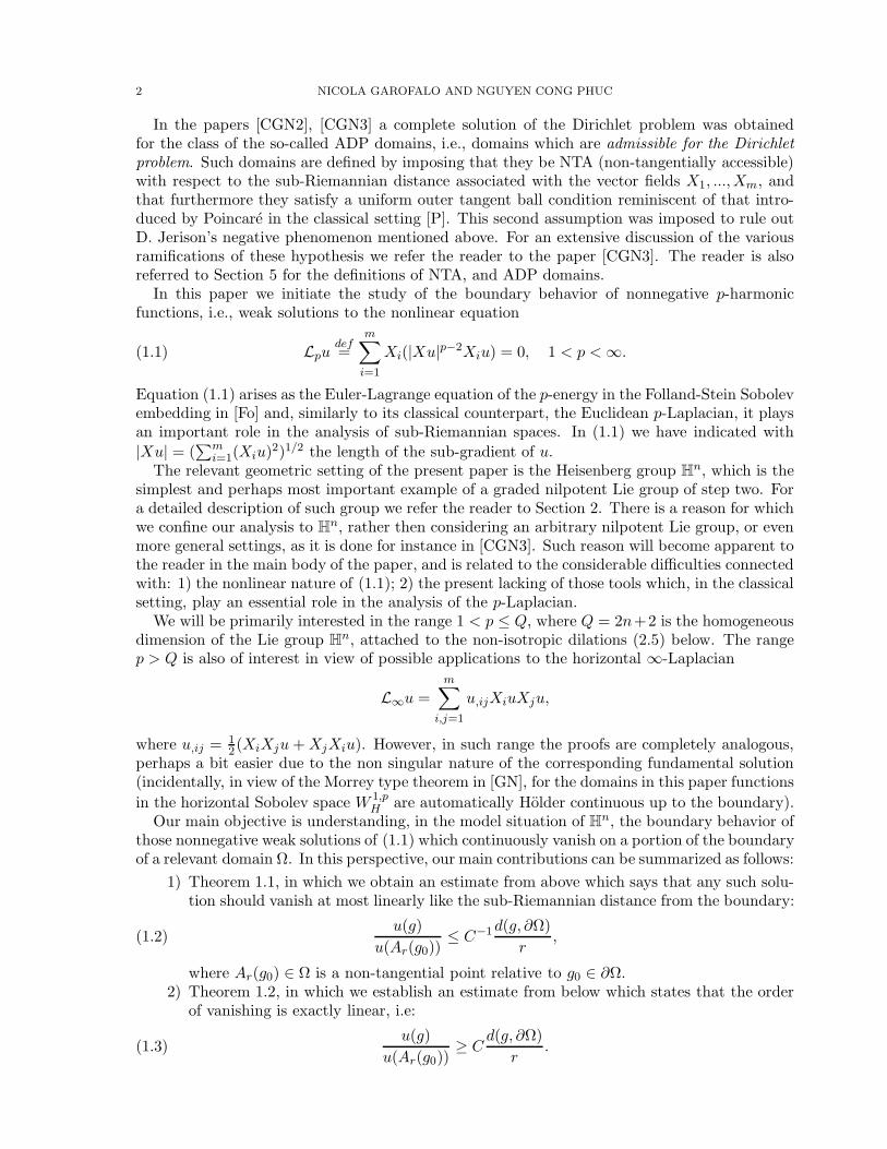
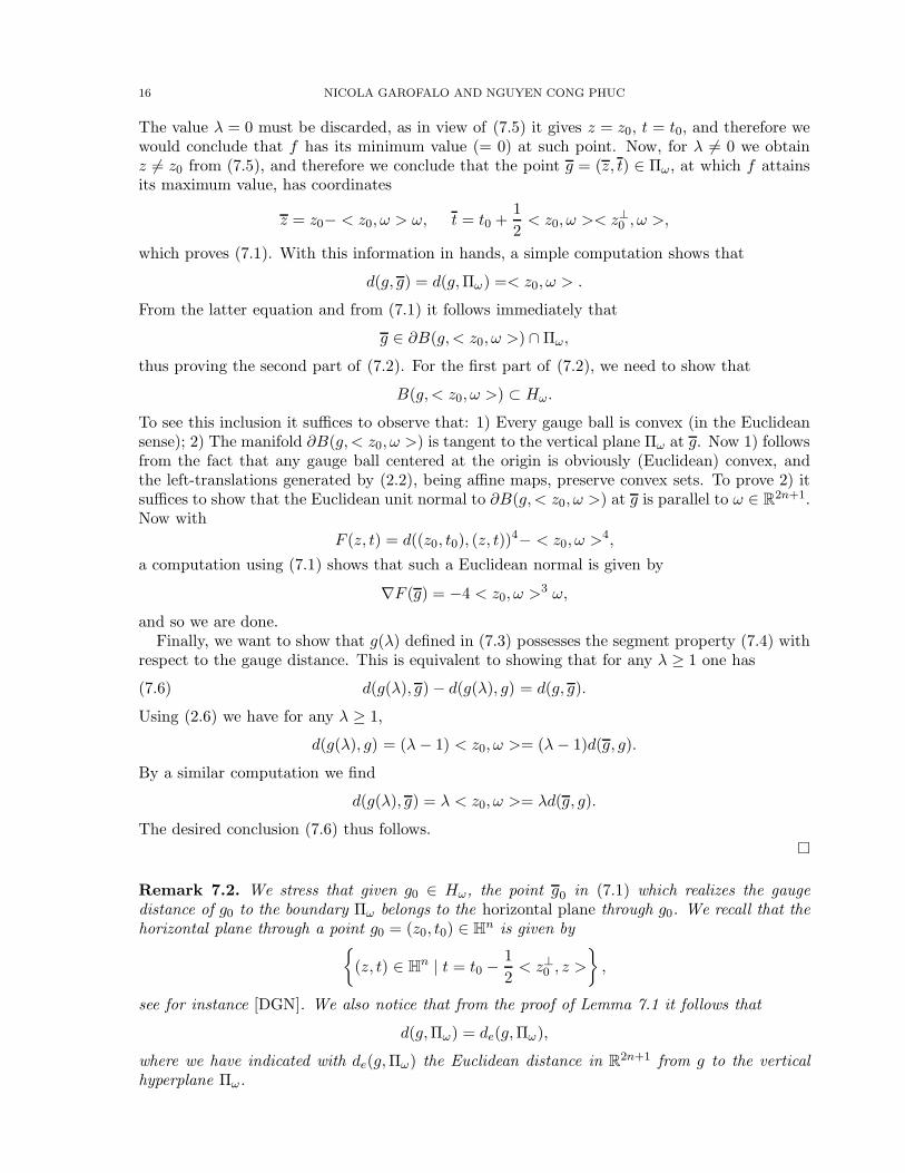
Figure 1. The tangent ball at a point of the vertical plane x = 0 in H1.

Theorem 7.3. Let Ω ⊂ Hn be a (Euclidean) C1,1 domain. Suppose that at a given point

g ∈ ∂Ω the tangent hyperplane to ∂Ω is the vertical hyperplane Πω, and that < ν(g), ω >= 1,where ν(g) is the unit inward normal to ∂Ω at g. This means, in particular, that g = (z, t), with< z, ω >= 0. Consider the straight half-line segment whose points are given by

g(λ) =

(

z + λω, t− λ

2< z⊥, ω >

)

, λ > 0.

Then for every λ > 0 the gauge ball B(g(λ), λ) is tangent to Πω at g, and there exists λ0 > 0depending only on the C1,1 character of Ω such that for every 0 < λ < λ0 one has

(7.7) B(g(λ), λ) ⊂ Ω.

Proof. Using (7.1) it is not difficult to verify that for any given λ > 0 we have

d(g(λ),Πω) = d(g(λ), g) = λ.

As we have seen in the proof of Lemma 7.1, this shows that the gauge ball B(g(λ), λ) is fullycontained in the vertical half-space Hω, and tangent to Πω at g. To prove (7.7) we argueas follows. We let S ∈ U(n) be a unitary matrix such that Sω = e1 = (1, 0, ..., 0). Suchtransformation sends the vertical hyperplane Πω = Π(g) into the vertical hyperplane

Π1 = (x, y, t) ∈ Hn | x1 = 0.

Furthermore, thanks to Lemma 2.1 such transformation preserves the gauge distance, see (2.7),and therefore it is not restrictive to assume from the start that the hyperplane Π(g) coincideswith Π1. And that the point g at which the domain Ω and the hyperplane Π1 touch is a non-characteristic point for ∂Ω.

Having done this, the boundary of the gauge ball B(g(λ), λ) is now described by the equation(

(x1 − λ)2 + |x′ − x′|2 + |y − y|2)2

(7.8)

+ 16

(

t− t− λ

2(y1 − y1) +

1

2

(

< x, y > − < x′, y′ >)

)2

= λ4 ,

where we have let (x, y) = (x1, x′, y1, y

′) and (x, y) = (x1, x′, y1, y

′) ∈ R×Rn−1 × R× R

n−1.

Since we are assuming that ∂Ω is tangent to the vertical plane x1 = 0 at g, we can locallydescribe the boundary of Ω as a graph in the variables (x′, y, t). This means that we can findr0 > 0 sufficiently small, and a C1,1 function

φ :

(x′, y, t) ∈ Rn−1 × R

n × R | |x′ − x′|2 + |y − y|2 + (t− t)2 < r20

→ R,

such that φ(x′, y, t) = 0, ∇φ(x′, y, t) = 0, and for which the set

∂Ω ∩

(x, y, t) ∈ Hn | |x′ − x′|2 + |y − y|2 + (t− t)2 < r20, |x1| < r20

is given by

(x, y, t) ∈ Hn | x1 = φ(x′, y, t), |x′ − x′|2 + |y − y|2 + (t− t)2 < r20, |x1| < r20

,

whereas, since < ν(g), e1 >= 1 > 0, the set

Ω ∩

(x, y, t) ∈ Hn | |x′ − x′|2 + |y − y|2 + (t− t)2 < r20, |x1| < r20

is given by

(x, y, t) ∈ Hn | x1 > φ(x′, y, t), |x′ − x′|2 + |y − y|2 + (t− t)2 < r20, |x1| < r20

.

By the C1,1 assumption on Ω we can find A > 0 such that

(7.9) |φ(x′, y, t)| ≤ A(

|x′ − x′|2 + |y − y|2 + (t− t)2)

,

whenever|x′ − x′|2 + |y − y|2 + (t− t)2 < r20.

To prove (7.7) it will thus suffice to show that the gauge ball B(g(λ), λ) is entirely containedin the paraboloid with respect to the variables (x′, y, t) in the right-hand side of (7.9).

To simplify the situation we left-translate Ω and Π1 by the point g0 = (0,−x′,−y,−t) ∈ Π1.Such a left-translation leaves Π1 unchanged, but has the effect that now the boundary of thegauge ball (7.8) becomes

(7.10)

(

(x1 − λ)2 + |x′|2 + |y|2)2

+ 16

(

t− λ

2y1

)2

= λ4,

whereas the paraboloid in the right-hand side of (7.9) is now given by

(7.11) x1 = A(|x′|2 + |y|2 + t2), |x′|2 + |y|2 + t2 < r20.

The advantage is that we can now easily solve with respect to the variable x1 the equation oforder four (7.10) obtaining

(7.12) x1 = λ −

√

√

√

√

√

λ4 − 16

(

t− λ

2y

)2

− (|x′|2 + |y|2),

Notice that the variable x1 in (7.10) ranges from 0 to 2λ, and that the allowable region ofpoints (x′, y, t) is obtained by projecting onto the (x′, y, t)-hyperplane the intersection of (7.10)with the plane x1 = λ, which gives

(7.13)(

|x′|2 + |y|2)2

+ 16

(

t− λ

2y1

)2

< λ4.

To further simplify the situation we consider the global diffeomorphism of R2n+1 onto itselfgiven by

ξ = x, η = y, τ = t− λ

2y1.

Such diffeomorphism transforms (7.12) and (7.11) respectively into

ξ1 = λ −√

√

λ4 − 16τ2 − (|ξ′|2 + |η|2),

and

ξ1 = A

(

|ξ′|2 + |η|2 +(

τ +λ

2η1

)2)

, |ξ′|2 + |η|2 +(

τ +λ

2η1

)2

< r20,

and the region (7.13) into

(7.14)(

|ξ′|2 + |η|2)2

+ 16τ2 < λ4.

Notice that (7.14) imposes that λ4− 16τ2 >(

|ξ′|2 + |η|2)2 ≥ 0. After these reductions we are

left with proving that if λ is sufficiently small then

(7.15) λ−√

√

λ4 − 16τ2 − (|ξ′|2 + |η|2) > A

(

|ξ′|2 + |η|2 +(

τ +λ

2η1

)2)

,

provided that (7.14) holds. We find

λ−√

√

λ4 − 16τ2 − (|ξ′|2 + |η|2) =λ2 −

√λ4 − 16τ2 + (|ξ′|2 + |η|2)

λ+√√

λ4 − 16τ2 − (|ξ′|2 + |η|2)

≥ λ2 −√λ4 − 16τ2 + (|ξ′|2 + |η|2)

2λ.

Thus for (7.15) to hold it is enough to find λ0 > 0 so that for 0 < λ < λ0,

λ2 −√

λ4 − 16τ2 + (|ξ′|2 + |η|2) > 2Aλ

(

|ξ′|2 + |η|2 +(

τ +λ

2η1

)2)

,

provided that (7.14) holds. Note that if 0 < λ < 2, then

λ2 −√

λ4 − 16τ2 + |ξ′|2 + |η|2 =16τ2

λ2 +√λ4 − 16τ2

+ |ξ′|2 + |η|2

≥ 8τ2

λ2+ |ξ′|2 + |η|2 ≥ 2τ2 + |ξ′|2 + |η|2.

On the other hand, we easily have

2Aλ

(

|ξ′|2 + |η|2 +(

τ +λ

2η1

)2)

≤ 6Aλ(|ξ′|2 + |η|2 + τ2).

It thus suffices to show that

2τ2 + |ξ′|2 + |η|2 > 6Aλ(|ξ′|2 + |η|2 + τ2) .

It is now easy to verify that this latter inequality is valid provided that 0 < λ < 1/6A. Weconclude that (7.15) holds for 0 < λ < λ0 = min2, 1/6A.

8. Characteristic quasi-segments

In this section we study the distance from a characteristic hyperplane away from the charac-teristic set.

Lemma 8.1. Consider the half-space H0 = (z, t) ∈ Hn | t > 0 whose boundary is the charac-

teristic hyperplane Π0 = (z, 0) ∈ Hn | z ∈ R

2n. For any point (z0, t0) ∈ H0, with z0 6= 0, itsgauge distance to Π0 is realized by the point g0 = (z0 +λz

⊥0 , 0) ∈ H0 and is given by the formula

(8.1) d((z0, t0),Π0) =

(

λ4|z0|4 + 16

(

t0 −λ

2|z0|2

)2)1/4

,

where λ = λ(z0, t0) is the real root of the cubic equation λ3 + 2λ = 4t0|z0|2

. Equivalently,

λ = G(

2t0|z0|2

)

> 0 with G being given by the equation (8.11) below. Moreover, one has

(8.2) d((z0, t0),Π0) =2t0|z0|

(1 + o(1)), as t0 → 0+,

where o(1) indicates a function which goes to zero as t0/|z0| → 0. Keeping in mind thatde((z0, t0),H0) = t0, this gives in particular

d((z0, t0),H0) =2de((z0, t0),H0)

|z0|(1 + o(1)), as t0 → 0+.

Proof. Let (z0, t0) ∈ H0 be such that z0 = (x0, y0) 6= 0, and consider the function

f(z) = d((z0, t0), (z, 0))4 .

From (2.6) we find (recall that z⊥0 = (y0,−x0))

(8.3) f(z) = |z − z0|4 + 16

(

t0 −1

2< z, z⊥0 >

)2

.

The possible critical points of f are solutions to the equation

∇f(z) = 4|z − z0|2(z − z0)− 16

(

t0 −1

2< z, z⊥0 >

)

z⊥0 = 0.

Notice that z = z0 cannot possibly be a critical point of f since ∇f(z0) = −16t0z⊥0 6= 0. This

forces

t0 −1

2< z, z⊥0 > 6= 0,

at a critical point z for otherwise we would have to have z = z0. Also notice that z ∈ R2n is a

critical point of f iff we have for z

(8.4) |z − z0|2(z − z0) = 4

(

t0 −1

2< z, z⊥0 >

)

z⊥0 .

This means that z must satisfy the equation

(8.5) z = z0 + λ z⊥0 ,

for the real number λ given by

(8.6) λ =4(t0 − 1

2 < z, z⊥0 >)

|z − z0|2.

From what we have observed above, it must be that |λ| > 0. At a critical point we have from(8.5)

< z, z⊥0 >=< z0 + λz⊥0 , z⊥0 >= λ|z0|2, |z − z0|2 = λ2|z0|2.

Substituting these equations and (8.5) in (8.4), we find

λ3|z0|2z⊥0 = 4

(

t0 −λ

2|z0|2

)

z⊥0 .

Taking the inner product of both sides with z⊥0 we obtain

(8.7) |z0|2λ3 = 4

(

t0 −λ

2|z0|2

)

.

From (8.7) we conclude that λ must satisfy the cubic equation

(8.8) λ3 + 2λ =4t0|z0|2

.


If we consider the strictly increasing function on [0,∞)

(8.9) Ψ(λ) =λ3

2+ λ,

then (8.8) can be written

(8.10) Ψ(λ) = b, with b =2t0|z0|2

.

Let now G = Ψ−1 : [0,∞) → R be the inverse function of Ψ, using the Cardano-Tartagliaformula, see [Ca], we find for b ≥ 0

(8.11) G(b) =

(

(

8

27+ b2

)1/2

+ b

)1/3

−(

(

8

27+ b2

)1/2

− b

)1/3

.

It is clear from (8.11) that G(0) = 0. We conclude that one real root of (8.8) is given by

λ = λ(z0, t0) = G

(

2t0|z0|2

)

(8.12)

=

(

(

8

27+

4t20|z0|4

)1/2

+2t0|z0|2

)1/3

−(

(

8

27+

4t20|z0|4

)1/2

− 2t0|z0|2

)1/3

> 0.

Notice that as t0 → 0+ one has λ(z0, t0) → 0 for every z0 6= 0 fixed. We also notice that sinceΨ′(0) = 1 and Ψ′′(0) = 0, the inverse function theorem gives

(8.13) G′(0) =1

Ψ′(0)= 1, G′′(0) = −Ψ′′(0)

Ψ′(0)3= 0.

We observe that (8.10) gives

(8.14) t0 =|z0|22

Ψ(λ).

Since t0 > 0, the other two roots of (8.8) are necessarily complex conjugates, and therefore theyare to be discarded since λ ∈ R, see (8.6). Equation (8.5) thus produces one single critical pointz0 with λ given by (8.12). From (8.3) we thus conclude that for z0 6= 0

(8.15) d((z0, t0),Π0) = f(z0)1/4 =

(

λ4|z0|4 + 16

(

t0 −λ

2|z0|2

)2)1/4

,

which gives (8.1). If we keep (8.7) in mind, we can re-write this formula as follows

d((z0, t0),Π0) = |z0|λ(1 + λ2)1/4.

Therefore,

(8.16) λ = ψ−1

(

d((z0, t0),Π0)

|z0|

)

, where ψ(s)def= s(1 + s2)1/4.

We note that ψ : [0,∞) → R is strictly increasing and that, since ψ′(0) = 1, ψ′′(0) = 0, we have

(ψ−1)′(0) = 1, (ψ−1)′′(0) = 0.

Therefore

(8.17) ψ−1(s) = s(1 +O(s2)), as s→ 0+.

This shows that

(8.18) λ(z0, t0) =d((z0, t0),Π0)

|z0|(1 + o(1)), as t0 → 0+,

with o(1) → 0 as t0/|z0| → 0. On the other hand, (8.12) and (8.13) imply that

(8.19) λ(z0, t0) =2t0|z0|2

(1 + o(1)).

From (8.18), (8.19) we thus conclude

d((z0, t0),Π0) =2t0|z0|

(1 + o(1)), as t0 → 0+,

which proves (8.2) and completes the proof of the lemma.

Remark 8.2. Before proceeding further we observe explicitly that, contrarily to what happensin the case of a vertical plane, in the present situation the point g0 which realizes the gaugedistance of g0 to Π0 does not belong to the horizontal plane through g0. To see this let us recallthat, given a point g0 = (z0, t0), then the equation of such plane is given by

(8.20) t = t0 −1

2< z⊥0 , z > .

Using g0 = (z0 + λz⊥0 , 0) (by Lemma 8.1) in (8.20) we find that the condition g0 belongs to thehorizontal plane through g0 is equivalent to saying that

t0 −λ

2|z0|2 = 0.

But this is impossible by (8.7) and by the fact that λ = G(

2t0|z0|2

)

> 0.

The next result shows that the ball centered at g0 ∈ H0 and with radius d(g0, g0) is tangentto Π0 at g0.

Lemma 8.3. Let g0 = (z0, t0) ∈ Hn with z0 6= 0 and t0 > 0, then the gauge ball B(g0, d(g0, g0))

is tangent to Π0 at g0, and

(8.21) B(g0, d(g0, g0)) ⊂ H0, and g0 ∈ Π0,

where g0 is as in Lemma 8.1.

Proof. To prove this we set R0 = d(g0, g0) and consider the function

F (z, t) = d((z0, t0), (z, t))4 −R4

0 = |z − z0|4 + 16

(

t− t0 +1

2< z⊥0 , z >

)2

− R40

by formula (2.6). We have

∇F (z, t) = 4

(

|z − z0|2(z − z0) + 4

(

t− t0 +< z⊥0 , z >

2

)

z⊥0 , 8

(

t− t0 +< z⊥0 , z >

2

))

.

Now with g0 = (z0, 0) = (z0 + λz⊥0 , 0), we find that

∇F (g0) = 4

(

λ3|z0|2z⊥0 − 4

(

t0 −λ

2|z0|2

)

z⊥0 ,−8

(

t0 −λ

2|z0|2

))

.

Using (8.7) we conclude that

∇F (g0) = −32

(

0,

(

t0 −λ

2|z0|2

))

= −32|z0|22

(

2t0|z0|2

−G

(

2t0|z0|2

))

(0, 1) .

Thus the gauge ball B(g0, R0) is tangent to Π0 at g0. Since B(g0, R0) is convex, we see thatit must obey the inclusion in (8.21).


-4

-2

0

2

x

-2

0

2

4

y

0

1

2

3

4

t

-4

-2

0

2

x

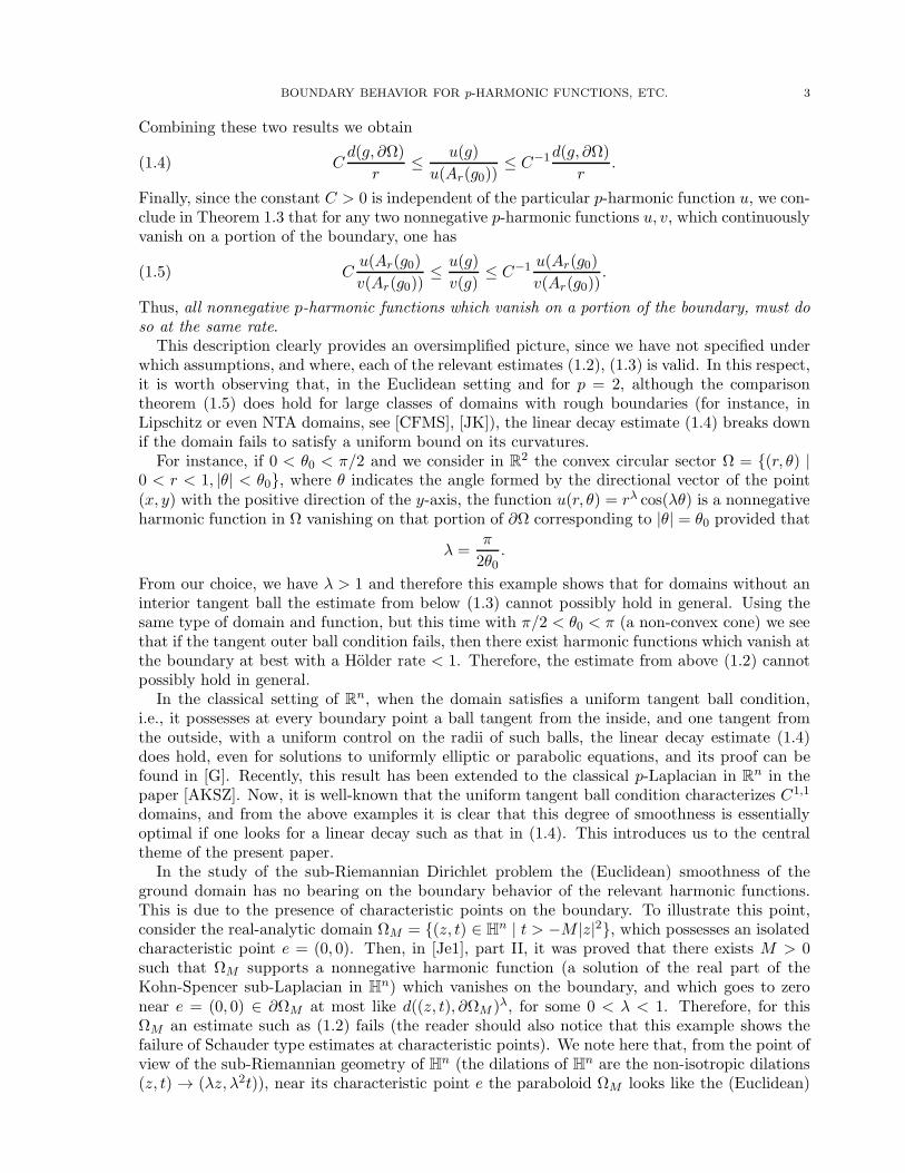
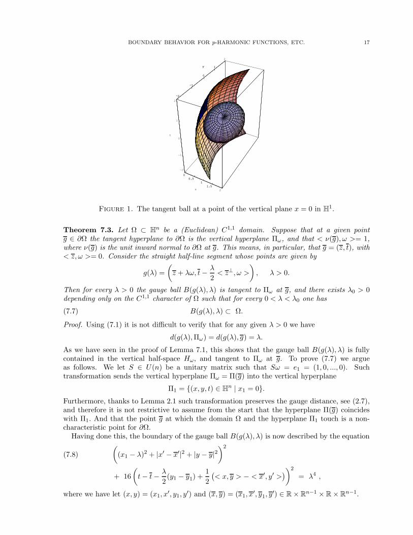
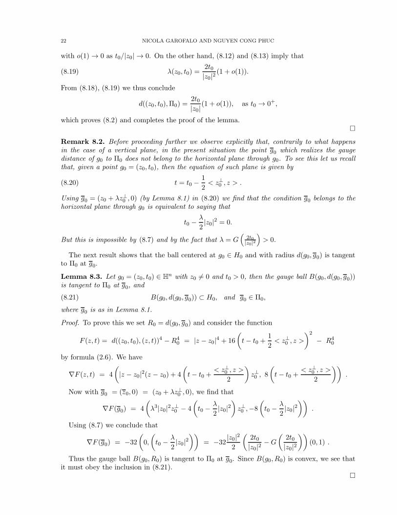
Figure 2. The tangent ball at a non-characteristic point of the horizontal planet = 0.

Suppose now we are given a point g = (z, 0) ∈ Π0. For any given λ ∈ R we want to find allsolutions z of the equation

(8.22) z + λz⊥ = z.

The matrix of this system is

Aλ =

(

1 λ−λ 1

)

whose determinant is 1 + λ2 > 0, and thus Aλ is invertible, and one has

A−1λ =

(

11+λ2 − λ

1+λ2

λ1+λ2

11+λ2

)

.

From this we easily find that (8.22) admits a unique solution given by

(8.23) z(λ) =1

1 + λ2z − λ

1 + λ2z⊥.

When λ > 0 then equation (8.14) allows to find the t-coordinate of the point g(λ) = (z(λ), t(λ)) ∈H0 having the property that

d(g(λ), g) = d(g(λ),Π0).

Such t-coordinate is given by the equation

t(λ) =|z(λ)|2

2Ψ(λ) =

Ψ(λ)

2(1 + λ2)|z|2,

where Ψ(λ) is as defined in (8.9).Summarizing, given g = (z, 0) ∈ Π0 and λ > 0 the corresponding point g(λ) that admits g as

the point that realizes its gauge distance to Π0 is given by

(8.24) g(λ) = (z(λ), t(λ)) =

(

1

1 + λ2z − λ

1 + λ2z⊥,

Ψ(λ)

2(1 + λ2)|z|2)

.

Theorem 8.4. Let Ω ⊂ Hn be a (Euclidean) C1,1 domain. Suppose that the characteristic

hyperplane Π0 is tangent to ∂Ω at a non-characteristic point g = (z, 0) ∈ ∂Ω where z 6= 0 insuch a way that < ν(g), e2n+1 >= 1, where ν(g) denotes the unit inward normal to ∂Ω at gand e2n+1 = (0, 0, . . . , 0, 1) ∈ R

2n+1. Then there exists a λ0 > 0 depending on |z| and the C1,1

character of Ω, such that for every 0 < λ < λ0, one has

B(g(λ), R(λ)) ⊂ Ω, ∂Ω ∩B(g(λ), R(λ)) = g,where g(λ)0<λ<λ0

is given by (8.24) and R(λ) = d(g(λ), g).

Proof. To prove this lemma we locally describe the boundary of Ω as a graph over the hyperplaneH0. This means that we can find r0 > 0 sufficiently small, and a C1,1 function

φ :

z ∈ R2n | |z − z| < r0

→ R,

such that φ(z) = 0, Dφ(z) = 0, and for which

∂Ω ∩

(z, t) ∈ Hn | |z − z| < r0, |t| < r20

is given by

(z, t) ∈ Hn | t = φ(z), |z − z| < r0, |t| < r20

,

whereas, by the assumption < ν(g), e2n+1 >= 1 > 0, the set

Ω ∩

(z, t) ∈ Hn | |z − z| < r0, |t| < r20

is given by

(z, t) ∈ Hn | t > φ(z), |z − z| < r0, |t| < r20

.

Notice from (2.3) that X(φ − t)(z, 0) = Dφ(z) + z⊥/2 = z⊥/2 6= 0, thanks to the assumptionz 6= 0. Notice also that in view of the assumption that φ ∈ C1,1 the graph of φ is containedbetween two paraboloids, i.e., there exists a constant A > 0 such that

(8.25) −A|z − z|2 ≤ φ(z) ≤ A|z − z|2, for every |z − z| < r0.

Next, consider the ball B(g(λ), R(λ)) centered at g(λ) and with radius R(λ) = d(g(λ), g). Wenote that

R(λ) =ψ(λ)√1 + λ2

|z| = λ

(1 + λ2)1/4|z|.

As it was proved before such ball is tangent to H0 at g. Its boundary is described by theequation

(8.26) |z − z(λ)|4 + 16

(

t− t(λ) +1

2< z(λ)⊥, z >

)2

= R(λ)4,

or equivalently∣

∣

∣

∣

t− t(λ) +1

2< z(λ)⊥, z >

∣

∣

∣

∣

=1

4

√

R(λ)4 − |z − z(λ)|4.

Since at g we have

t− t(λ) +1

2< z(λ)⊥, z >= −t(λ) + 1

2< z(λ)⊥, z >= − λ3

4(1 + λ2)|z|2 < 0,

a local description of ∂B(g(λ), R(λ)) near g is given by

t = Φλ(z) = t(λ)− 1

2< z(λ)⊥, z > −1

4

√

R(λ)4 − |z − z(λ)|4.

Such representation is valid for all points (z, t) which are below the horizontal planeHg(λ) passingthrough g(λ). Since the equation of such plane is given by

t = t(λ)− 1

2< z(λ)⊥, z >,

it is clear from (8.26) that the projection onto H0 of the intersection of B(g(λ), R(λ)) with Hg(λ)

is given by the 2n-dimensional Euclidean ball Be(z(λ), R(λ)) = z ∈ R2n | |z − z(λ)| < R(λ).

In view of (8.25) it will thus suffice to show that

(8.27) Φλ(z) > A|z − z|2 , for every |z − z(λ)| < R(λ) .

Now, for every z such that |z − z(λ)| < R(λ) there exist 0 ≤ s ≤ 1 and ω such that |ω| = 1for which z = z(λ) + sR(λ)ω. We thus have

|z − z|2 = |z(λ)− z|2 + s2R(λ)2 + 2sR(λ) < z(λ)− z, ω > .

From (8.24) we obtain

(8.28) z(λ)− z = − λ

1 + λ2(z⊥ + λz),

and therefore

(8.29) |z(λ) − z|2 =λ2

1 + λ2|z|2 .

Substituting (8.28), (8.29) in the above equation we find

|z − z|2 = λ2

1 + λ2|z|2 + s2

λ2

(1 + λ2)1/2|z|2(8.30)

− 2sλ2

(1 + λ2)(1 + λ2)1/4|z|2 < z⊥

|z| + λz

|z| , ω > .

Next, we recall that

t(λ) =Ψ(λ)

2(1 + λ2)|z|2 = λ(1 + λ2

2 )

2(1 + λ2)|z|2.

Keeping in mind (8.24) we find

< z(λ)⊥, z >= sR(λ) < z(λ)⊥, ω >=sR(λ)|z|1 + λ2

<z⊥

|z| + λz

|z| , ω > .

From the latter two equations and from (8.30) we conclude that proving (8.27) is equivalent toproving that for every A > 0 there exists λ(A) > 0 such that for every 0 < λ < λ(A), and forevery 0 ≤ s ≤ 1 and |ω| = 1,

λ(1 + λ2

2 )|z|22(1 + λ2)

− sλ|z|22(1 + λ2)(1 + λ2)1/4

<z⊥

|z| + λz

|z| , ω > −λ2|z|2(1− s4)1/2

4(1 + λ2)1/2(8.31)

> A

λ2|z|21 + λ2

+s2λ2|z|2

(1 + λ2)1/2− 2sλ2|z|2

(1 + λ2)(1 + λ2)1/4<z⊥

|z| + λz

|z| , ω >

.

Establishing (8.31) is in turn equivalent to proving

2 + λ2 − 2s(1− 4Aλ)

(1 + λ2)1/4<z⊥

|z| + λz

|z| , ω > −λ(1 + λ2)1/2(1 − s4)1/2(8.32)

> 4Aλ[

1 + s2(1 + λ2)1/2]

.

At this point we let λ(A) = 14A , then it is clear that 1 − 4Aλ > 0 for every 0 < λ < λ(A).

Since∣

∣

∣

z⊥

|z| + λ z|z|

∣

∣

∣= (1 + λ2)1/2, by Cauchy-Schwarz inequality it is clear that, provided that

0 < λ < λ(A), for (8.32) to hold it suffices to have

2 + λ2 − 2s(1− 4Aλ)(1 + λ2)1/4 − λ(1 + λ2)1/2(1− s4)1/2 > 4Aλ[

1 + s2(1 + λ2)1/2]

.

or equivalently,

2 + λ2 − 2s(1 + λ2)1/4 − λ(1 + λ2)1/2(1− s4)1/2(8.33)

> 4Aλ[

1 + s2(1 + λ2)1/2 − 2s(1 + λ2)1/4]

.

Since the quantity in the square brackets in right-hand side of (8.33) is positive (it is a square),considering the fact that 4Aλ < 1, for (8.33) to hold it suffices that the inequality

2 + λ2 − 2s(1 + λ2)1/4 − λ(1 + λ2)1/2(1− s4)1/2 ≥ 1 + s2(1 + λ2)1/2 − 2s(1 + λ2)1/4,

does hold for every 0 < λ < λ(A) and every 0 ≤ s ≤ 1. This inequality, however, is equivalentto the inequality

λ(1− s4)1/2 + s2 ≤ (1 + λ2)1/2.

The validity of this latter inequality now follows by applying Cauchy-Schwarz inequality to thevectors a = (λ, 1), b = ((1− s4)1/2, s2), and noting that |a| = (1 + λ2)1/2, |b| = 1.

In the next lemma we establish the quasi-segment property with respect to the gauge distancealong the path g(λ).

Lemma 8.5. Let g0 = (z0, t0) ∈ H0 with z0 6= 0, and g(λ)λ≥0 = (z(λ), t(λ))λ≥0 be as in

(8.24) with g = g0 = (z0 + λ0z⊥0 , 0) and λ0 = G

(

2t0|z0|2

)

. Then there exists λ > 0 such that if

λ0 < λ1 < λ then

d(g(λ1), g0)− d(g(λ1), g0) ≥1

2d(g0, g0).

Proof. From Lemma 8.1 we see that g is the point that realizes the distance of g0 = (z0, t0) toΠ0. Moreover, by the hypothesis we have

(8.34) λ0 = G

(

2t0|z0|2

)

, or equivalently t0 =|z0|22

Ψ(λ0).

Replacing z with z0 + λ0 z⊥0 in (8.23) we find for the corresponding g(λ) = (z(λ), t(λ))

(8.35)

z(λ) = α(λ)z0 + β(λ)z⊥0 ,

t(λ) = γ(λ)|z0|2,where

(8.36)

α(λ) = 1+λ0λ1+λ2 , β(λ) = λ0−λ

1+λ2 ,

γ(λ) = 12

1+λ20

1+λ2 Ψ(λ) .

Notice that

α(λ0) = 1 , β(λ0) = 0 , γ(λ0) =1

2Ψ(λ0) ,

and so (8.35) and (8.34) give

(8.37) g(λ0) = (z(λ0), t(λ0)) = (z0, t0) = g0 .

Also notice that when λ→ 0+, we have (recall that Ψ(λ) → 0 as λ→ 0+)

α(λ) → 1 , β(λ) → λ0 , γ(λ) → 0 , as λ→ 0+ .

We thus have

(8.38) g(0) = g0 = (z0 + λ0z⊥0 , 0) .

Furthermore,

|z(λ)| =√

α(λ)2 + β(λ)2 |z0| ,

and that when 0 < λ0 < λ, one has

α(λ)2 + β(λ)2 =1 + λ20λ

2 + λ20 + λ2

(1 + λ2)2< 1 .

We set henceforth

ρ = d(g0, g0) = d(g0,Π0) = d((z0, t0),Π0) .

Notice that from (8.15) we obtain

(8.39) ρ =

(

λ40|z0|4 + 16

(

t0 −λ02|z0|2

)2)1/4

.

On the other hand, using (8.7) we find

16

(

t0 −λ02|z0|2

)2

= |z0|4λ60 ,

and so (8.39) gives

(8.40) ρ = |z0| λ0(1 + λ20)1/4 .

If we introduce the strictly increasing function

ψ(s) = s(1 + s2)1/4 , s ≥ 0

as in (8.16), then it is clear from (8.40) that

(8.41) λ0 = ψ−1

(

ρ

|z0|

)

.

At this point we fix a real number λ1 > λ0 and call g1 = g(λ1). Clearly, by the way we haveconstructed the path λ → g(λ), the point g1 = g(λ1) which realizes the distance of g1 to Π0

coincides with g0. We have in fact

α(λ) − λβ(λ) = 1

λα(λ) + β(λ) = λ0 ,

and this gives

z(λ) + λz(λ)⊥ = z0 + λ0z⊥0 , for every λ ≥ 0 .

We now set

g(λ) = g(λ1 − λ) , 0 ≤ λ ≤ λ1 ,

and define a function φλ1: [0, λ1] → [0,∞) by letting

φλ1(λ) = d(g(λ), g1) = N(g−1

1 g(λ)) .

Notice that if λ0 = λ1 − λ0, then we have

φλ1(λ0) = d(g(λ0), g1) = d(g0, g1) ,

where in the last equality we have used (8.37). On the other hand, from (8.38) we have

φλ1(λ1) = d(g(λ1), g1) = d(g0, g1) .

From the mean value theorem we thus obtain for some λ0 < λ∗ < λ1

d(g1, g0)− d(g1, g0) = φλ1(λ1)− φλ1

(λ0) = (λ1 − λ0)φ′λ1(λ∗)

= λ0φ′λ1(λ∗) = ψ−1

(

ρ

|z0|

)

φ′λ1(λ∗) ,

where in the last equality we have used (8.41). Our goal is to show that there exists λ > 0sufficiently small, and C > 0, such that for all 0 < λ0 < λ1 < λ we have

(8.42) ψ−1

(

ρ

|z0|

)

φ′(λ∗) ≥ 1

2ρ .

Since from (8.17) we have

ψ−1

(

ρ

|z0|

)

=ρ

|z0|(1 + o(1)) , as

ρ

|z0|→ 0+ ,

we see from (8.40) that there exists r > 0 such that

(8.43) ψ−1

(

ρ

|z0|

)

≥ 1

2

ρ

|z0|, provided that λ0 < r .

To establish (8.42) it will thus be enough to show that there exists λ > 0 such that

(8.44) φ′λ1(λ∗) ≥ |z0| > 0 , for every λ1 − λ0 < λ∗ < λ1 ≤ λ .

Since from φλ1(λ) = N(g−1

1 g(λ1 − λ)), and

φ′λ1(λ∗) = − d

dλN(g−1

1 g(λ))∣

∣

λ=λ1−λ∗ ,

it is clear that it will suffice to show that there exist λ > 0 such that, if we set Φλ1(λ) =

N(g−11 g(λ)),

Φ′λ1(λ) ≤ − |z0| , for every 0 ≤ λ ≤ λ0 < λ1 ≤ λ .

Now we have from (8.35)

g−11 g(λ) = (−z1,−t1)(α(λ)z0 + β(λ)z⊥0 , γ(λ)|z0|2)(8.45)

=(

(α(λ)− α(λ1))z0 + ((β(λ) − β(λ1))z⊥0 , (γ(λ) − γ(λ1))|z0|2

+1

2< α(λ)z0 + β(λ)z⊥0 , z

⊥1 >

)

=(

(α(λ)− α(λ1))z0 + ((β(λ) − β(λ1))z⊥0 ,(

γ(λ)− γ(λ1))

+1

2

(

β(λ)α(λ1)− α(λ)β(λ1)))

|z0|2)

Using (8.45) we find

Φλ1(λ) = φ(λ1 − λ) =

(

(α(λ)− α(λ1))2 + (β(λ)− β(λ1))

2

)2

+ 16

(

γ(λ)− γ(λ1) +1

2

(

β(λ)α(λ1)− α(λ)β(λ1)))

)21/4

|z0| ,


and thus

Φ′λ1(λ) = |z0|

(

(α(λ) − α(λ1))2 + (β(λ)− β(λ1))

2

)2

(8.46)

+ 16

(

γ(λ)− γ(λ1) +1

2

(

β(λ)α(λ1)− α(λ)β(λ1)))

)2−3/4

× 4

(

(α(λ) − α(λ1))2 + (β(λ) − β(λ1))

2

)

×(

(α(λ) − α(λ1))α′(λ) + (β(λ) − β(λ1))β

′(λ)

)

+ 8

(

γ(λ)− γ(λ1) +1

2

(

β(λ)α(λ1)− α(λ)β(λ1)))

)

×(

γ′(λ) +1

2(β′(λ)α(λ1)− α′(λ)β(λ1))

)

.

Recalling that α(0) = 1, β(0) = λ0, γ(0) = 0, α′(0) = λ0, β′(0) = −1, and γ′(0) = 1/2, we

obtain from (8.46), after some crucial cancellations

Φ′λ1(0) = |z0|

(

(1− α(λ1))2 + (λ0 + |β(λ1)|)2

)2

(8.47)

+ 16

(

− γ(λ1) +1

2

(

λ0α(λ1) + |β(λ1)|))

)2−3/4

× 4

−(

(1− α(λ1))2 + (λ0 + |β(λ1)|)2

)(

λ0α(λ1)) + |β(λ1)|))

+ 4

(

− γ(λ1) +1

2

(

λ0α(λ1) + |β(λ1)|))

)(

1− α(λ1) + λ0|β(λ1)|)

At this point we observe the following formulas which follow from (8.36) after some elementarycomputations

(1− α(λ1))2 + (λ0 + |β(λ1)|)2 = λ21

1 + λ20λ21 + λ20 + λ21

(1 + λ21)2

.

λ0 α(λ1) + |β(λ1)| = λ11 + λ201 + λ21

,

γ(λ1) =λ12

(

1 +λ212

)

1 + λ201 + λ21

,

− γ(λ1) +1

2(λ0 α(λ1) + |β(λ1)|) = − λ31

4

1 + λ201 + λ21

,

1− α(λ1) + λ0|β(λ1)| =λ21 − λ201 + λ21

.

Substituting these equations in (8.47) we finally obtain

Φ′λ1(0) = −4 |z0| (1 + λ20)

1 + λ20λ21 + λ20 + λ21 + (1 + λ21)(λ

21 − λ20)

[(1 + λ20λ21 + λ20 + λ21)

2 + λ21(1 + λ20)2(1 + λ21)

2]3/4

= −4 |z0|(1 + λ20)(1 + λ21)

2

[(1 + λ20λ21 + λ20 + λ21)

2 + λ21(1 + λ20)2(1 + λ21)

2]3/4.

Keeping in mind that 0 < λ0 < λ1, we see that if λ1 → 0+, then

(1 + λ20)(1 + λ21)2

[(1 + λ20λ21 + λ20 + λ21)

2 + λ21(1 + λ20)2(1 + λ21)

2]3/4→ 1 .

It is thus clear that there exists λ > 0 such that

(8.48) Φ′λ1(0) ≤ − 1

2|z0| , provided that 0 ≤ λ1 < λ .

By continuity, (8.43) and (8.48), if we choose λ > 0 sufficiently small, we achieve (8.44), thuscompleting the proof.

9. Proof of Theorems 1.2 and 1.3

With the preliminary work developed in Sections 7 and 8, we are finally able to establishTheorems 1.2 and 1.3.

Proof of Theorem 1.2. We only discuss the case p < Q, leaving it to the reader to provide theappropriate modifications for the case p = Q. By the uniform Harnack inequality in [CDG1] we

know that u > 0 in Ω. Let g0 ∈ ∂Ω which is not a characteristic point of ∂Ω. For 0 < r < d(g0,ΣΩ)M ,

where M is sufficiently large, let g ∈ Ω ∩ B(g0, r) and denote by g ∈ ∂Ω a point such thatd(g, ∂Ω) = d(g, g). We observe right away that

(9.1) d(g, g) < r.

One has in fact d(g, g) = d(g, ∂Ω) ≤ d(g, g0) < r. Moreover, g ∈ B(g0, 2r) since d(g, g0) ≤d(g, g) + d(g, g0) < 2r. If M has been fixed large enough, this gives in particular that g 6∈ ΣΩ.We now let Π(g) be the hyperplane tangent to ∂Ω at g. There are two possibilities: either Π(g)has a characteristic point, or it does not.Case 1) If Π(g) has no characteristic point then it must have the form

Π(g) = (x, y, t) ∈ Hn |< a, x > + < b, y > +d = 0,

where a, b ∈ Rn and d ∈ R. By a left-translation we may assume without loss of generality that

Π(g) takes the form

Πω = (x, y, t) ∈ Hn |< a, x > + < b, y >= 0,

where ω = (a, b) ∈ R2n. We emphasize that, thanks to (2.10), left-translations do not change the

gauge distance d, so that we can assume from the start that Π(g) is in the form Πω. Furthermore,without loss of generality we can assume that |ω|2 = |a|2 + |b|2 = 1. And that the point g atwhich the domain Ω and the hyperplane Πω touch is a non-characteristic point for ∂Ω.Case 2) If instead Π(g) has a characteristic point, then it is of the type

Π(g) = (x, y, t) ∈ Hn |< a, x > + < b, y > +c t+ d = 0,

where c 6= 0. Notice that its characteristic point is

g0 =

(

−2b

c,2a

c,−d

c

)

∈ Π(g).

If in this case we left-translate Π(g) by the point g−10 , it is easy to recognize that the hyperplane

Π(g) is mapped into Π0 = (x, y, t) ∈ Hn | t > 0. Invoking Theorem 7.3 and Lemma 7.1 in Case

1), and Theorem 8.4 and Lemma 8.5 in Case 2), we can construct a quasi-segment g(λ)0<λ<λ

such that for every 0 < λ < λ,

B(g(λ), R(λ)) ⊂ Ω, ∂Ω ∩B(g(λ), R(λ)) = g,where R(λ) = d(g(λ), g).

Figure 3. Tangent balls and a quasi-segment at a non-characteristic point ofthe horizontal plane t = 0.

Moreover, by (9.1) we may also assume that there exist 0 < λ0 < λ1 < λ such that g = g(λ0)and R(λ1) = 2r. Thus with g1 = g(λ1) we have B(g1, 2r) ⊂ Ω, g ∈ ∂B(g1, 2r) and

(9.2) d(g1, g)− d(g1, g) ≥1

2d(g, g),

by the segment or quasi-segment property.Since by Theorem 5.4 any (Euclidean) C1,1 domain in H

n is NTA, every boundary point ofΩ has attached to it a non-tangential corkscrew, see Definition 5.3. Now, it is clear that g1 is anon-tangential corkscrew associated with g. Furthermore, for any 0 < ǫ < 1, g′ ∈ B(g1, ǫ r) andany g′′ ∈ ∂Ω one has

2r ≤ d(g′′, g1) ≤ d(g′′, g′) + d(g′, g1) ≤ d(g′′, g′) + ǫ r,

and alsod(g′, ∂Ω) ≤ d(g′, g) ≤ d(g′, g1) + d(g1, g) = d(g′, g1) + 2r ≤ (2 + ǫ)r.

These inequalities imply that

(2− ǫ)r ≤ d(B(g1, ǫ r), ∂Ω) ≤ (2 + ǫ)r.

By the Harnack inequality in [CDG1] we obtain for some Cǫ > 0

(9.3)u(g′)

u(g1)≥ Cǫ > 0, for every g′ ∈ B(g1, ǫ r).

Since g1 is a corkscrew for g, and Ar(g0) is a corkscrew for g0, and d(g, g0) < 2r, we see thatthere exists a Harnack chain of N balls (with N independent of r) connecting g1 to Ar(g0). Arepeated application of the Harnack inequality thus gives

u(g1) ≤ CNu(Ar(g0)).

From this estimate and (9.3) we obtain

(9.4)u(g′)

u(Ar(g0))≥ Cǫ > 0, for every g′ ∈ B(g1, ǫ r).

We now consider the function

f(g′) =d(g′, g1)

(p−Q)/(p−1) − (2r)(p−Q)/(p−1)

(ǫ r)(p−Q)/(p−1) − (2r)(p−Q)/(p−1)=

d(g′, g1)(p−Q)/(p−1) − d(g, g1)

(p−Q)/(p−1)

(ǫ r)(p−Q)/(p−1) − (2r)(p−Q)/(p−1)

on the ring B(g1, 2r) \ B(g1, ǫ r), and we clearly have f ≡ 1 on ∂B(g1, ǫ r) and f ≡ 0 on∂B(g1, 2r). By (9.4) and the comparison principle (Theorem 3.2) we conclude that

(9.5)u(g′)

u(Ar(g0))≥ C f(g′) , for every g′ ∈ B(g1, 2r) \B(g1, ǫ r) .

Now, thanks to (9.2), g ∈ B(g1, 2r) \B(g1, ǫ r) and hence we obtain from (9.5)

u(g)

u(Ar(g0))≥ C f(g) .

It thus suffices to prove that

f(g) ≥ Cd(g, g)

r.

Applying the mean value theorem to the function h(s) = s(p−Q)/(p−1) with ǫ r ≤ s ≤ 2r, andusing the fact that 0 < ǫ < 1 we find

f(g) ≥ C(Q, p)d(g1, g)− d(g1, g)

r.

At this point we apply the quasi-segment property (9.2) to get the desired estimate. Thiscompletes the proof of the theorem.

Proof of Theorem 1.3. Combine Theorem 1.1 with Theorem 1.2.

References

[AS] H. Aikawa & N. Shanmugalingam, Carleson-type estimates for p-harmonic functions and the conformal

Martin boundary of John domains in metric measure spaces, Michigan Math. J. 53 (2005), 165–188.[AKSZ] H. Aikawa, T. Kilpelainen, N. Shanmugalingam & X. Zhong, Boundary Harnack principle for p-harmonic

functions in smooth Euclidean domains, Potential Anal. 26 (2007), no. 3, 281-301.[Be] R. Berndt, An introduction to symplectic geometry, Grad. Studies in Math., Vol. 26, AMS, 2001.[Bo] J. M. Bony, Principe du maximum, inegalite de Harnack et unicite du probleme de Cauchy pour les operateurs

elliptique degeneres, Ann. Inst. Fourier, Grenoble, 19 (1969), 277–304.[CFMS] L. Caffarelli, E. Fabes, S. Mortola & S. Salsa, Boundary behavior of nonnegative solutions of elliptic

operators in divergence form, Indiana Univ. Math. J. 30 (1981), 621–640.[CDG1] L. Capogna, D. Danielli & N. Garofalo, An embedding theorem and the Harnack inequality for nonlinear

subelliptic equations, Comm. Partial Differential Equations 18 (1993), 1765–1794.[CDG2] , Capacitary estimates and the local behavior of solutions of nonlinear subelliptic equations, Amer.

J. Math. 118 (1996), 1153–1196.[CG] L. Capogna & N. Garofalo, Boundary behavior of nonegative solutions of subelliptic equations in NTA

domains for Carnot-Caratheodory metrics, J. Fourier Anal. Appl. 4 (1998), 403–432.[CGN1] L. Capogna, N. Garofalo & D. M. Nhieu, A version of a theorem of Dahlberg for the subelliptic Dirichlet

problem, Math. Res. Letters 5 (1998), 541–549.[CGN2] , Properties of harmonic measures in the Dirichlet problem for nilpotent Lie groups of Heisenberg

type, Amer. J. Math. 124 (2002), 273–306.[CGN3] , Mutual absolute continuity of harmonic and surface measures for Hormander type operators,

Perspectives in partial differential equations, harmonic analysis and applications, 49–100, Proc. Sympos.Pure Math., 79, Amer. Math. Soc., Providence, RI, 2008.

[Ca] G. Cardano, Artis Magnae, 1545.[Ci] G. Citti, Wiener estimates at boundary points for Hormander’s operators, Boll. U.M.I. 2-B (1988), 667–681.


[Cy] J. Cygan, Subadditivity of homogeneous norms on certain nilpotent Lie groups, Proc. Amer. Math. Soc.83 (1981), 69–70.

[Da] D. Danielli, Regularity at the boundary for solutions of nonlinear subelliptic equations, Indiana Univ. Math.J. 44 (1995), 269–286.

[DG] D. Danielli & N. Garofalo, Green functions in nonlinear potential theory in Carnot groups and the geometry

of their level sets, preprint, 2004.[DGN] D. Danielli, N. Garofalo, Nicola & D. M. Nhieu, Notions of convexity in Carnot groups, Comm. Anal.

Geom. 11 (2003), 263–341.[F1] G. Fichera, Sulle equazioni alle derivate parziali del secondo ordine ellittico-paraboliche, (Italian) Univ. e

Politec. Torino. Rend. Sem. Mat. 15 (1955–56), 27–47.[F2] , On a unified theory of boundary value problems for elliptic-parabolic equations of second order. 1960

Boundary problems in differential equations pp. 97–120, Univ. of Wisconsin Press, Madison.[Fo] G. Folland, Subelliptic estimates and function spaces on nilpotent Lie groups, Ark. Math. 13 (1975), 161–207.[G] N. Garofalo, Second order parabolic equations in nonvariational form: Boundary Harnack principle and

comparison theorems for nonegative solutions, Ann. Mat. Pura Appl. (4) 138 (1984), 267–296.[GN] N. Garofalo & D. M. Nhieu, Lipschitz continuity, global smooth approximations and extension theorems for

Sobolev functions in Carnot-Caratheodory spaces, J. d’Analyse Math. 74 (1998), 67–97.[HH] J. Heinonen & I. Holopainen, Quasiregular maps on Carnot groups, J. Geom. Anal. 7 (1997), 109–148.[H] H. Hormander, Hypoelliptic second-order differential equations, Acta Math. 119 (1967), 147–171.[Ja] U. Janfalk, Behaviour in the limit, as p → ∞, of minimizers of functionals involving p-Dirichlet integrals,

SIAM J. Math. Anal. 27 (1996), 341–360.[Je1] D. Jerison, The Dirichlet problem for the Kohn Laplacian on the Heisenberg group, Parts I and II, J. Funct.

Analysis 43 (1981), 97–142.[Je2] , Boundary regularity in the Dirichlet problem for b on CR manifolds, Comm. Pure Appl. Math.

36 (1983), 143–181.[JK] D. Jerison & C. E. Kenig, Boundary behavior of harmonic functions in non-tangentially accessible domains,

Adv. Math. 46 1982, 80–147.[Ke] C. E. Kenig, Harmonic analysis techniques for second order elliptic boundary value problems, Amer. Math.

Soc., CBMS 83, 1994.[KN1] J. J. Kohn & L. Nirenberg, Non-coercive boundary value problems, Comm. Pure and Appl. Math. 18 (1965),

443–492.[LU] E. Lanconelli & F. Uguzzoni, On the Poisson kernel for the Kohn Laplacian, Rend. Mat. Appl. (7) 17 (1997),

659–677 (1998).[LN] J. Lewis & K. Nystrom, Boundary behavior for p-harmonic functions in Lipschitz and starlike Lipschitz ring

domains, Annales Scientifiques de LEcole Normale Superieure, Volume 40, Issue 5, September-October 2007,p.765-813.

[MM1] R. Monti & D. Morbidelli, Non-tangentially accessible domains for vector fields, Indiana Univ. Math. J.54 (2005), 473–498.

[MM2] , Regular domains in homogeneous groups, Trans. Amer. Math. Soc. 357 (2005), 2975–3011.[NS] P. Negrini & V. Scornazzani, Wiener criterion for a class of degenerate elliptic operators, J. Differential

Equations 66 (1987), 151–164.[P] H. Poincare, Sur les equations aux derivees partielles de la physique mathematique, Amer. J. of Math.

12 (1890), 211–294.

Department of Mathematics, Purdue University, West Lafayette, IN 47907

E-mail address, Nicola Garofalo: [email protected]

Department of Mathematics, Louisiana State University, Baton Rouge, LA 70803-4918

E-mail address, Nguyen Cong Phuc: [email protected]

Boundary behavior of p-harmonic functions in the Heisenberg group

Documents

Transcript of Boundary behavior of p-harmonic functions in the Heisenberg group