Harmonic modelling of transmission systems containing ...
288
HARMONIC MODELLING OF TRANSMISSION SYSTEMS CONTAINING SYNCHRONOUS MACHINES AND STATIC CONVERTORS A thesis presented for the degree of Doctor of Philosophy in Electrical Engineering in the University of Canterbury by J. F, Eggleston, B.E. (Hans) J 1985
-
Upload
khangminh22 -
Category
Documents
-
view
4 -
download
0
Transcript of Harmonic modelling of transmission systems containing ...
HARMONIC MODELLING OF TRANSMISSION SYSTEMS CONTAINING
SYNCHRONOUS MACHINES AND STATIC CONVERTORS
A thesis
presented for the degree of
Doctor of Philosophy in Electrical Engineering
in the
University of Canterbury
by
J. F, Eggleston, B.E. (Hans) J
1985

LIBRARY
~ ! , r
i
CONTENTS
Page
List of Figures List of Tables
vii xi i i
xv
xxi
xxi i i
List of Principal Symbols Abstract Acknowledgements
CHAPTER 1
CHAPTER 2
CHAPTER 3
INTRODUCTION
AN OVERVIEW OF POWER SYSTEM HARMONICS AND THEIR MODELLING
2.1 Steady State Modelling of Electrical Transmission Systems
2.2 Harmonics in the Power System
1
5
5
6
2.3 Power System Modelling of Harmonics 8 2.3.1 Early Models 8 2.3.2 Harmonic Penetration 8 2.3.3 Dynamic Simulation of Convertor 11
Interaction 2.3.4 Limitations of Conventional Models 12
2.4 Harmonic Modelling of Convertors 13 2.5 Iterative Algorithm for Modelling Harmonic 15
Interaction 2.6 Introduction to Modelling in the Harmonic 16
Space
HARMONIC MODELLING OF CONVERTOR OPERATION 3.1 Introduction 3.2 An Outline of the Iterative Algorithm
19
19
21
3.3 Solving the Operation of the Convertor 24 3.3.1 Calculating the Commutation Current 25 3.3.2 Sampling the A.C. Current Inj ions 28 3.3.3 Sampling the D.C. Voltage Waveform 34 3.4.4 Conversion from the Time Domain to the 36
Frequency Domain 3.4 Solving the A.C. System 37 3.5 Solving the D.C. System 40 3.6 Implementing Control
3.6.1 Calculating the Zero Crossings 3.6.2 Calculating the Delay Angles
3.7 Conclusions
41
41
41
42

CHAPTER 4
i i
Page
HARMONIC INTERACTION BETWEEN A.C., D.C. AND
CONVERTOR SYSTEMS 43
4.1 Introduction 43 4.1.1 The Effect of Interactions on the 43
Harmonic Currents Produced 4.1.2 Harmonic Instability 44 4.1.3 Can the Iterative Algorithm be Used to 46
Examine Harmonic Instabilities? 4.2 Six-Pulse Convertor at Tiwai : Six Busbar 47
A.C. System Representation 4.2.1 Instability with Improved Representation 50
of the A.C. System
4.2.2 Further Investigation of the Instability 52 4.2.2.1 Reduced current 53 4.2.2.2 Diagonalizing the A.C. system 56 4.2.2.3 Strengthening the A.C. system 56 4.2.2.4 Further linking of the insta- 57
bility to the third harmonic 4.2.2.5 Improved initial conditions 58 4.2.2.6 The use of an acceleration 60
factor 4.2.3 The Effect of Harmonic Voltage During 62
Commutation 4.2.3.1 A stable case 62
4.2.3.2 An unstable case 62 4.2.3.3 Further investigation of third 74
harmonic dur'ing commutation
4.2.4 Conclusions 80
4.3 Single Generator and Line A.C. System Supplying 81 a 6-pulse Convertor at Tiwai 4.3.1 Initial Conditions 82 4.3.2 The Harmonic Impedances
4.3.2.1 The system without the lters 83
4.3.2.2 The effect of filters 83
4.3.3 Initial Results of Iterative Algorithm 86
4.3.4 Modifications to Avoid Premature 88 Convergence of the Iterative Algorithm
4.3.4.1 Closer tolerance 88
4.3.4.2 Introducing a disturbance 89
4.3.5 The Effect of Control Disturbance 91
4.3.6 Harmonic Voltage Distortion of the 93 Simplified Test System with Increased Fi Her Capacity

CHAPTER 5
4.3.7 The Inclusion of the Non-infinite D.C. System
4.3.8 Conclusions
4.4 Verification of the Iterative Algorithm
4.4.1 Introduction
Page
96
97
98
98 4.4.2 TCS Comparison Without Filters 99
4.4.3 TCS Comparison with A.C. Filters and 102 a Non-infinite D.C. System
4.4.4 Unstable Case 103
4.4.5 Conclusions
4.5 Future Work with the Iterative Algorithm 104
104 4.5.1 Multiple Sources 104
4.5.2 Inclusion of the Harmonic Effects in 105 the Three Phase Power Flow
4.5.3 Harmonic Instability 106
HARMONIC MODELLING OF SINGLE PHASE FEEDER AND
CONVERTOR SYSTEMS
107
5.1 Harmonic Modelling of the New Zealand Railway 107 Feeder System
5.1.1 Component Models
5.1.1.1 Feeder wires
108
108
5.1.1.2 Locomotive, including power 110 factor correction
5.1.1.3 The substation and locomotive 110 transformer model
5.1.1.4 The line terminations 110
5.1.1.5 The three phase transmission 110
5.1.1.6 The harmonic filters III
5.1.2 Forming the Admittance Matrix for the III Feeder System
5.1.3 The Response of the Feeder System to 114 Harmonics
5.1.4 Evaluating the Currents in the 116 Individual System Components
5.1.5 Results of a Test Section of Line 117
5.1.6 Conclusions of the Single Phase Harmonic Penetration 121
5.2 Modelling Single Phase Systems 121
5.2.1 Calculating the Commutation Current 122
5.2.2 Calculating the D.C. Voltage 123
CHAPTER 6
CHAPTER 7
iv
Page
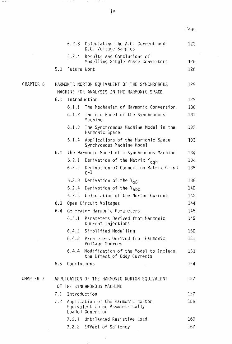
5.2.3 Calculating the A.C. Current and 123 D.C. Vol Samples
5.2.4 Results and Conclusions of Modelling Single Phase Convertors 126
5.3 Future Work 126
HARMONIC NORTON EQUIVALENT OF THE SYNCHRONOUS 129 MACHINE FOR ANALYSIS IN THE HARMONIC SPACE
6.1 Introduction 129 6.1.1 The Mechanism of Harmonic Conversion 130 6.1.2 The d-q l'1odel of the Synchronous 131
Machine 6.1.3 The Synchronous Machine Model in the 132
Harmonic Space 6.1.4 Applications of the Harmonic Space 133
Synchronous Machine Model 6.2 The Harmonic Model of a Synchronous Machine 134
6.2.1 Derivation of the Matrix Ydqh 134 6.2.2 Derivation of Connection Matrix C and 135
C-l
6.2.3 Derivation of the YaS 138 6.2.4 Derivation of the Yabc 140 6.2.5 Calculation of the Norton Current 142
6.3 Open C i rcui t Voltages 144 6.4 Generator Harmonic Parameters 145
6.4.1 Parameters Derived from Harmonic 145 Current Injections
6.4.2 Simplified Modelling 150 6.4.3 Parameters Derived from Harmonic 151
Voltage Sources 6.4.4 Modification of the Model to Include 153
the Effect of Eddy Currents 6.5 Conclusions
APPLICATION OF THE HARMONIC NORTON EQUIVALENT OF THE SYNCHRONOUS MACHINE
7.1 Introduction 7.2 Application of the Harmonic Norton
Equivalent to an Asymmetrically Loaded Generator 7.2.1 Unbalanced Resistive Load
7.2.2 Effect of Saliency
154
157
157 158
160
162
CHAPTER 8
REFERENCES
v
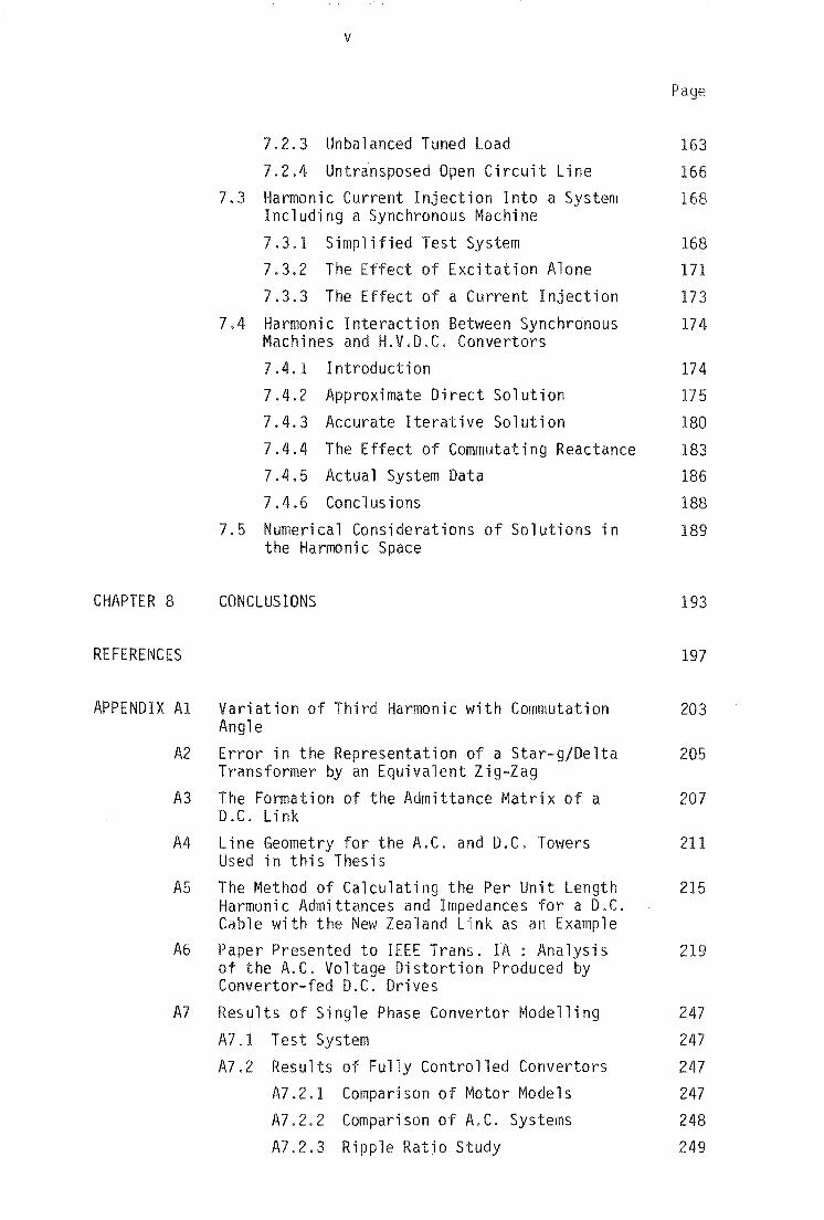
7.2.3 Unbalanced Tuned Load 7.2.4 Untransposed Open Circuit Line
p
163
166
7.3 Harmonic Current Injection Into a System 168 Including a Synchronous Machine
7.3.1 Simplified Test System 168 7.3.2 The of Excitation Alone 171 7.3.3 The Effect of a Current Injection 173
7.4 Harmonic Interaction Between Synchronous 174 Machines and H.V.D.C. Convertors 7.4.1 Introduction 7.4.2 Approximate Direct Solution
174 175
7.4.3 Accurate Iterative Solution 180 7.4.4 The Effect of Commutating Reactance 183 7.4.5 Actual System Data 186 7.4.6 Conclusions 188
7.5 Numerical Considerations of Solutions in 189 the Harmonic Space
CONCLUSIONS 193
197
APPENDIX Al Variation of Third Harmonic with Commutation 203 Angle
A2 Error in the Representation of a Star-gjDelta 205 Transformer by an Equivalent Zig a9
A3 The Formation of the Admittance Matrix of a 207 D.C. Link
A4 Line Geometry for the A.C. and D.C. Towers 211 Used in this Thesis
A5 The Method of Calculating the Per Unit Length 215 Harmonic Admittances and Impedances for a D.C. Cable with the New Zealand Link as an Example
A6 Paper Presented to IEEE Trans. IA : Analysis 219
A7
of the A.C. Voltage Distortion Produced by Convertor-fed D.C. Drives Results of Single Phase Convertor Modelling A7.1 st System A7.2 ults of Fully Controlled Convertors
A7.2.1 Comparison of Motor Models A7.2.2 Comparison of A.C. Systems A7.2.3 Ripple Ratio Study
247 247 247 247 248 249

A8
A9
A7.3
A7.4
Results
A7.3.1
A7.3.2
A7.3.3
vi
Page
A7.2.3.1 Theoretical study 250
A7.2.3.2 Test system for the 250 study of D.C. current ripple
A7.2.3.3 Results of the study 251 of D.C. current ripple
of Half Controlled Convertors
Classical Harmonic Behaviour of a Half-controlled Convertor Comparison of Models
The Effect of Ripple Ratio with Half-controlled Rectification
251
251
255
255
Conclusions
The Harmonic Spectrum of V f
260
261
263 Test Data for Benmore Pole
FIGURE
3.1
3.2
vii
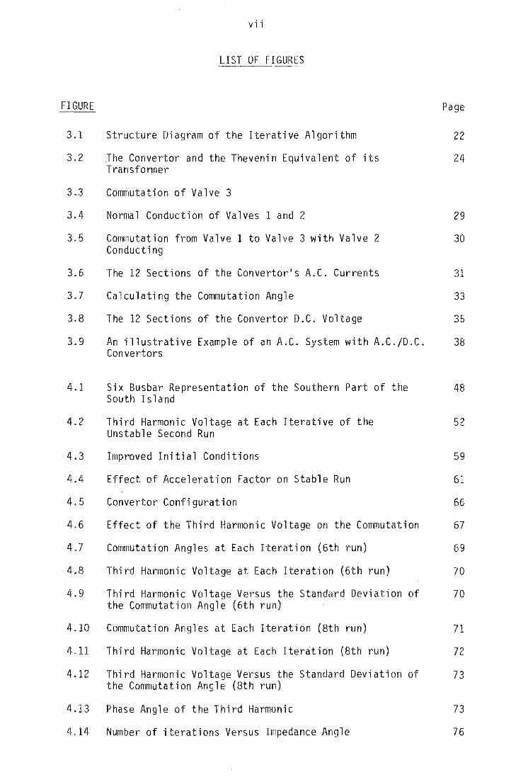
LI ST OF FI GURES
Structure Diagram of the I rative Algorithm
The Convertor and the Thevenin Equivalent of its Transformer
3.3 Commutation of Valve 3
Page
22
24
3.4 Normal Conduction of Valves 1 and 2 29
3.5 CO~lutation from Valve 1 to Valve 3 with Valve 2 30 Conducting
3.6 The 12 Sections of the Convertor's A.C. Currents 31
3.7 Calculating the Commutation Angle 33
3.8 The 12 Sections of the Convertor D.C. Voltage 35
3.9 An illustrative Example of an A.C. System with A.C./D.C. 38 Convertors
4.1 Six Busbar Representation of the Southern Part of the 48 South Island
4.2 Third Harmonic Voltage at Each Iterative of the 52 Unstable Second Run
4.3 Improved Initial Conditions 59
4.4 Effect of Acceleration Factor on Stable Run 61
4.5 Convertor Configuration 66
4.6 Effect of the Third Harmonic Voltage on the Commutation 67
4.7 Commutation Angles at Each Iteration (6th run) 69
4.8 Third Harmonic Voltage at Each Iteration (6th run) 70
4.9 Third Harmonic Voltage Versus the Standard Deviation of 70 the Commutation Angle (6th run)
4.10 Commutation Angles at Each Iteration (8th run) 71
4.11 Third Harmonic Voltage at Each Iteration (8th run) 72
4.12 Third Harmonic Voltage Versus the Standard Deviation of 73 the Commutation Angle (8th run)
4.13 Phase Angle of the Third Harmonic 73
4.14 Number of iterations Versus Impedance Angle 76

viii
FIGURE Page
4.15 Third Harmonic Voltage Versus Impedance Angle 76
4.16 Total Admittance Loci Including Filters for Variable 77 Impedance Angle
4.17 Convertor Supplied by a Single Generator/Transformer 81 and Line A.C. System
4.18 Three Phase Impedance Loci 84
4.19 The Effect of Filters on the Positive Sequence 85 Impedance Loci
4.20 The Effect of the Fourth, Fifth and Sixth Delay Angle 90 Errors on the A.C. Current Injections
4.21 The Magnitude of the Second and Fourth Harmonic Currents 90 Against Delay Angle Error
4.22 Third Harmonic Voltage in the Three Phases of the 93 Convertor Terminal with Equidistant Control and Perfectly Flat D.C. Current: Without Iterations
4.23 Third Harmonic Voltage in the Three Phases of the 94 Convertor Terminal with Equidistant Control and Perfectly Flat D.C. Current : With Iterations
4.24 Third Harmonic Voltage in the Three Phases of the 95 Convertor Terminal with Constant Delay Control and D.C. Current
4.25 Third Harmonic Voltage in the Three Phases of the 96 Convertor Terminal with Increased Filter Rating
4.26 Effect of D.C. Current Ripple on the Third Harmonic 97 at the Convertor Terminal
4.27 Test System Without Filters 99
4.28 Test System With Filters 102
~
5.1 Cross Section of the Feeder System Towers 108
5.2 The Auto Transformer Position 109
5.3 A Single Locomotive Left on the Substation 111
5.4 Circuit Diagram for a Single Locomotive 112
5.5 Transmission System Currents for a 1.0 p.u. Injection 118 (No Filters)
5.6 Transmission System Currents for the Locomotive's 118 Injection (No Filters)

ix
FI GURE Page
5.7 Transmission System Currents for the Locomotive's 119 Injections with the Proposed Harmonic Filters
5.8 Comparing the Transmission System Currents for the 120 Various Filter Configurations
5.9 Comparing the Pantograph Voltage Distortions for the 120 Various Filter Configurations
5.10 Single Phase Convertor Bridge 121
5.11 Fully Controlled A.C. Current and D.C. Voltage Waveforms 124
5.12 Half Controlled A.C. Current and D.C. Voltage Waveforms 125
6.1(a) Schematic Diagram of Exciter System
(b) Norton Equivalent of the Synchronous Generator
6.2
6.3
6.4
6.5
6.6
6.7
6.8
6.9
6.10
6.11
7.1
7.2
7.3
7.4
7.5
Harmonic Interaction Between Synchronous Machine and the System
Magnitude of the Hydrogenerator Harmonic Impedance
Phase of the Hydrogenerator Harmonic Impedances
Open Circuit Voltage Ratios for the Hydrogenerator
Magnitude of the Harmonic Impedances of the Round Rotor Generator
Phase Angle of the Harmonic Impedance of the Round Rotor Generator
Comparison of the Hydro Generator Impedances
Current Ratios for the Hydrogenerator
Effect of Eddy Current Representation on the Magnitude of zt~
Effect of E dd~ Current Representation on the Phase of Z-h and Z+
h +h
Test System
Variation of Positive Sequence Third Harmonic Voltage with Coupling and Loading
Simplified Equivalent Circuit of the Machine
Effect of Saliency on Generator Harmonic Voltages
Tuned Delta Load
133
133
140
147
148
149
150
150
152
153
155
155
158
161
162
163
164

x
GURE Page
7.6 Harmonic Voltage Distortion Versus fOl f02 with 165 Centre Frequency fo = 150 Hz
7.7 Variation of Third Harmonic Voltage with Transmission 167 Line Length
7.8 Modified Test System 169
7.9 Variation of Third Harmonic Voltage, V2 included 172
7.10 Comparison of Conventional and Harmonic Space Penetration 174
7.11 Single Generator-Transformer-Generator Unit 176
7.12 Negative Sequence Fifth and Positive Sequence 178 Seventh Versus Delay Angle
7.13 Graphical Deviation of Negative Fifth and Positive 179 Seventh Voltage Magnitudes
7.14 Generator Representation 181
7.15 Simplified Equivalent of a Single Generator Convertor 181 Unit
7.16 Voltage Distortion Versus Delay Angle 182
7.17 Commutation Angle Versus Delay Angle for the Various 183 Commutation Reactances
7.18 Negative Sequence Fifth Harmonic Voltage Versus Delay 184 Angle
7.20 Schematic Diagram of a Benmore Pole 186
Al.1 The Current Waveform 203
Al.2 The Percentage Third Harmonic Current Versus the 204 Difference Between the Commutation Angles
A2.1(a) Star-g/Delta Connection
(b) Equivalent Zi ag Connection
A3.1 The New Zealand D.C. Link Sections
A3.2 The Zero and Positive Sequences of a D.C. Line
A4.1 Inland Overhead Line Tower (D.C.)
A4.2 The Single Circuit Tower
A4.3 The Double Circuit Tower
A5.1 Simplified Representation of the Cross Section
205
205
207
207
211
212
213
215

xi
Figure Page
A7.1 Harmonic Currents [10 mH System, Fully Controlled] 248
A7.2 Harmonic Voltages [Various Systems, Fully Controlled] 249
A7.3 Theoretical A.C. Current Waveform 250
A7.4 Fundamental Current Behaviour with Ripple 252 [Fully Controlled]
A7.5 Harmonic Current Behaviour with Ripple [Alpha;O.l 253
A7.6 Harmonic Current Behaviour with Ripple [Alpha=O.l] 254
A7.7 Simplified Half-controlled A.C. Current Waveform 251
A7.8 Harmonic Currents [10 mH system, Half-controlled] 256
A7.9 Fundamental Current Behaviour with Ripple 257 [Half-Controlled]
A7.10 Harmonic Current Behaviour with Ripple [Alpha=O.l]
A7.11 Harmonic Current Behaviour with Ripple [Alpha=1.0]
258
259


TABLE
3.1
3.2
4.1
4.2
4.3
4.4
4.5
4.6
4.7
4.8
4.9
4.10
4.11
4.12
4.13
4.14
4.15
4.16
4.17
4.18
4.19
5.1
5.2
5.3
xi i i
LIST OF TABLES
The Three Phase Currents in Each Phase and Section
The d.c. Voltage in Each Section
Harmonic Impedance Data for the Tiwai Busbar
Harmonic Filter Data
A Series Convergence
B Series Convergence
Third Harmonic Voltage and Current at Each D.C. Current Leve 1
Comparison of the Stable Runs
Comparison of the Three Variations of the Unstable Runs that Converged
A Set of Third Harmonic A.C. Admittances and Impedances with Angles from -90 to +90 degrees
Total A.C. Admittance With Filters
Total A.C. Admittance Without Filters
Level of Third Harmonic Voltage (%) at Each Iteration
The Effect of Harmonic Filters on System Impedance
D.C. Power and Iterations for Various D.C. Resistances
Level of Third and Fourth Harmonic Voltage (%) for Each Stable D.C. Power
D.C. Power and Number of Iterations for an Introduced Controller Disturbance
Comparison of Phase IAI Harmonic Currents
Comparison of Phase IAI Harmonic Voltages
Harmonic Current Comparison for the Case With Filters
Harmonic Voltage Comparison for the Case With Filters
Conductor Data
Busbar Numbering Convention
The Set of Maximum Expected Injections
Page
32
36
49
50
53
54
54
63
65
75
77
78
79
86
87
88
92
101
101
103
103
109
112
115

TABLE
5.4
5.5
6.1
7.1
A.C. Current and D.C. Voltage Waveforms for a Fully Controlled Covertor
A.C. Current and D.C. Voltage Waveforms for a Half Controlled Convertor
Data for the Two Test Machines
Comparison of Models for 6-Pulse Operation
Page
124
125
144
188

SYMBOL
Ah
B I 811
h' h
C nm d 1,2,3
Eln Gh+2 -(h-2) -h G+h
h
H-(h-2) Hh+2 +h '-h
i ,[I]
xv
1ST OF PRINC P LS
hth harmonic diagonal block of Y b a c
hth harmonic off-diagonal block of Y b a c integration constant
feeder system line lengths
commutating voltage
; rative zero crossing error
open circuit voltage ratios
harmonic order
short circuit current ratios
current vector in the harmonic space
commutation current
convertor d.c. current
vector of convertors d.c. currents
hth harmonic component of direct axis current
IdNorton' IqNorton Norton current in d and q quantities
Ii gh
Ih
[I inj ]
Ilt
10
I pfi
Iqh
I rec I rt
feeder system filter currents
fi lter current
current injection to take into account harmonic convers; on
Iqh at ith iteration
hth harmonic component of injected current
current injection
left termination fi lter current
synchronous machine Norton current
ith locomotive power factor current
hth harmonic component of quadrature axis current
current in feed line, towards terminations
right termination filter current

SYMBOL
Isend
I sys
I ti
Its
I 1,2,3
1+ V +
NCONV
NHARM
NSAMPL
Nt
NTERM
p
R
xvi
current in feeder line, towards substation
system harmonic current
. th 1 t' t 1 ocomo lve curren
substation transformer current
currents in phases 1. 2 and 3
positive sequence component of harmonic space current or voltage
positive sequence current or voltage of order h
negative sequence current or voltage of order h
no. trains left of substation
direct axis inductance
field winding inductance and resistance
quadrature axis inductance
direct axis damper inductance and resistance
quadrature axis damper inductance and resistance
locomotive convertor commutating inductance
inductance in phases 1,2 and 3
mutual inductance between direct axis and field winding
mutual inductance between direct axis and direct axis damper winding
mutual inductance between field and direct axis damper wi ndi ngs
mutual inductance between quadrature axis and quadrature axis damper winding
number of convertors
maximum harmonic to be considered
number of sample points
number of trai ns
number of terminal busbars
the valve commutating in
stator resitance d,q quantities

R 1,2,3
SCALE
T
T
TCS
U
v. [V]
V a,b,c
Vd
V d' I d
Vdh
Vdh
Vdq Idq
V f' If
[V hJ
Vhm
[V. . J , nJ
V ,I q q
Vqh
Vrec V , I s s
V send V sys Vt
V t' It
Vx
V 1,2,3
xv i i
resistance in phases 1,2 and 3
harmonic voltage scale factor
matrix to extract positive sequence fundamental
connection matrix from phase to a.(3o components
Transient Convertor Simulation
identify matrix
voltage vector in the harmonic space
voltage on phases a, band c
convertor d.c. voltage
direct axis voltage and current
hth harmonic component of d.c. voltage
hth harmonic of direct axis voltage
dq components of stator harmonic voltages and currents
field winding voltage and current
vector of the 3 phase voltages at harmonic h
is the peak magnitude of the hth harmonic of the outgoing phase
is the peak magnitude of the hth harmonic of the incoming phase
voltage at point of injection
quadrature axis voltage and current
hth harmonic at quadrature axis voltage
voltage at the terminations end of the feeder line
direct axis damper voltage and current
voltage at the substation and of feeder line
system voltage
term; na 1 voltage
quadrature axis damper voltage and current
secondary voltage on a commutating phase
voltage on phases 1,2 and 3
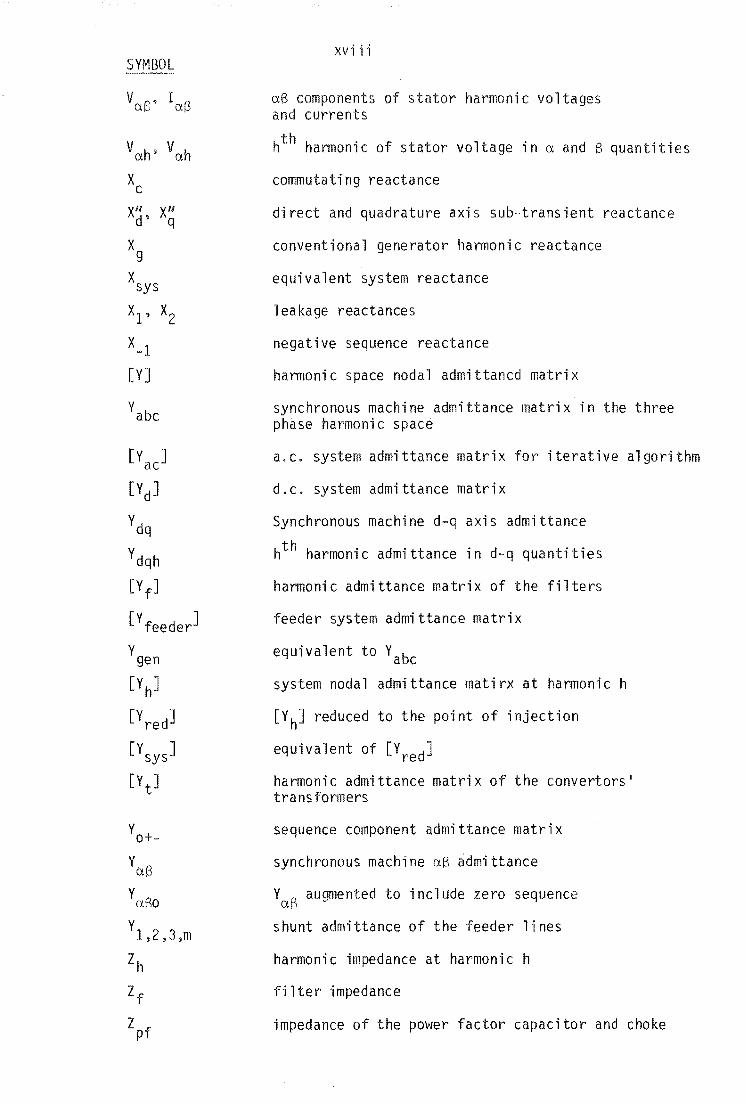
SYMBOL
V I as' ap
Vah' Vah
X c XII XII d' q
Xg
XSYS
Xl' X2
X_I
[YJ
Y abc
[Vac]
[V dJ
Vdq
Ydqh
[V f]
[V feeder]
V gen [V h]
[Y red]
[\ysJ
[Yt
]
V 1,2,3,m
xviii
as components of stator harmonic voltages and currents
hth harmonic of stator voltage in a and S quantities
commutating reactance
direct and quadrature axis sub-transient reactance
conventional generator harmonic reactance
equivalent system reactance
leakage reactances
negative sequence reactance
harmoni c space nodal admi ttancd matri x
synchronous machine admittance matrix in the three phase harmonic space
a.c. system admittance matrix for iterative algorithm
d.c. system admittance matrix
Synchronous machine d-q axis admittance
hth harmonic admittance in d~q quantities
harmonic admittance matrix of the filters
feeder system admittance matrix
equivalent to Vabc
system nodal admittance matirx at harmonic h
[V h] reduced to the point of injection
equivalent of [VredJ
harmonic admittance matrix of the convertors I
transformers
sequence component admittance matrix
synchronous machine as admittance
VaS augmented to include zero sequence
shunt admittance of the feeder lines
harmonic impedance at harmonic h
filter impedance
impedance of the power factor capacitor and choke

SYMBOL
f
Zts th -h
Z+h' Z_h Z+h+2 Z-(h-2) -h +h
Z 1,2,3,m ze
n
E
e p
w
xix
transmission system impedance
harmonic impedance of the system
locomotive's transformer impedance
termination filter impedance
sUbstation transformer impedance
open circuit harmonic impedance
open circuit conversion impedance
series impedance of the feeder lines
zero crossing of the commutating voltage at iteration n
delay angle
permittivity of insulation
firing instant of valve p
permeability of insulation
commutation angle
pth commutation angle
excitation constant
standard deviation of the commutation angles
phase of the hth harmonic component of the d.c. voltage
rotor flux at harmonic h
is the phase of the hth harmonic of the outgoing phase
is the phase of the hth harmon; c of the i ncomi ng phase
fundamental angular frequency

xx
xxi
ABSTRACT
This thesis describes the modelling of the major sources
of harmonic distortion in electrical transmission systems, especially
those of relevance to the New Zealand power system.
The harmonics generated by the operation of a.c./d.c. convertors
are modelled using an interactive algorithm. The algorithm ;s applied
to a number of test systems and verified using a transient convertor
simulation program.
A harmonic admittance matrix model of a single phase traction
system is derived and used to assess the effect of propossed harmonic
filters. In this case the three phase iterative algorithm had to
be modified to be able to model the locomotive's single phase
convertors.
Synchronous machines are modelled using a harmonic Norton
equivalent~ derived from the d-q axes differential equations. The
case of this model yields harmonic impedances consistent with
existing models and demonstrates the well known, but greatly ignored,
phenomenon of harmonic conversion. The modelling of harmonic
conversion is shown to significantly modify the harmonic flows under
certain system conditions.

xxi i

xxiii
ACKNOWLEDGEMENTS
I would like to thank my supervisor, Professor J. Arrillaga,
for his advice, assistance, friendship and patience during the
course of my study.
The financial support of the New Zealand Energy Research
and Development Committee was most appreciated.
Special thanks are due to J. Baird, Professor H. Dommel
and particularly Professor A. Semlyem for their guidance and technical
assistance. Also, the encouragement and help of the staff and
postgraduate students, especially T.J. Densem. N.R. Watson and
C.D. Callaghan, is gratefully acknowledged.
Thank you to Mary Kinnaird for her excellent typing.
Particular thanks for my family and friends' patience and
interest.

xxiv

CHAPTER 1
I NTRODUCT ION
In recent years there has been a trend tovJards the use of power
electronic devices in electric power transmission systems. In New
Zealand this trend has been strong in the past with an aluminium
smelter at Tiwai and one of the world's first h.v.d.c. links. In the
future this trend is expected to continue with possible expansions to
the existing h.v.d.c. link, the possibility of a second link and the
electrification of part of the North Island main truck line. Also
many altel~native energy sources (micro-hydro, solar, wind and \,'Jave
power) are electrically orientated and rely on power electronics for
their control.
Thus much of the apparatus used for the generation, transmission
and utilisation of electrical energy in the future will result in
considerable waveform distortion due to the non-linear nature of power
electronic devices. This is a form of electrical enviromental
pollution which, like any other form of pollution, affects all the system
users and is expensive to eliminate. In New Zealand the problems
associ a ted with harmoni cs are becomi ng 1 arger. As a result, New
Zealand was one of the first countries in the world to introduce
Harmonic Standards (New Zealand Electricity 1983).
The aim of this thesis, therefore, is to examine the major
sources of harmonic distortion in transmission systems and develop
techniques to predict their impact.
In Chapter 2 harmonic distortion is introduced as a steady state
phenomenon. The existing techniques for modelling power systems
in the steady state, and in particular at harmonics frequencies are
examined and their shortcomings discussed.

2
r 3 develops an i ive algorithm for the modelling
of conve r operation and its associated harmonic current injections.
The algorithm is based on previous work by Harker (1980) and
Yacamini and Oliveira (1980a and 1980b). with improvements as
required.
In Chap r 4 various t are used to establish the
usefulness of the iterative algorithm described in chapter 3.
Firstly. a six busbar a.c. system supplying a 6-pulse convertor ;s
considered~ followed by a more simple system consisting of a sin e
generator and sformer feeding a transmission line which supplies
a 6-pulse convertor. Finally, the results of the iterative algorithm
are verified by comparing them with those produced by a transient
convertor simulation program.
The case of a single phase traction system is examined in
chapter 5. This is of particular interest in New Zealand as rt
of the North Island main trunk line is to be electrified. The
chapter is divided into two parts. The rst part describes the
modelling of the feeder system and analyses the performance of harmonic
filters. The second part describes how the iterative algorithm of
chapters 3 and 4 is modified to analyse the operation of the single
phase convertors used in modern locomotives.
presented in appendix A7.
The results are
A less important, and hitherto ignored, source of harmonic
distortion is the harmonic conversion in nt in synchronous
machines. and in icular. hydro ge t\ harmonic model
including this veloped in chapter 6, is used to examine
harmon; c character; i cs of the synchr'onous mach; ne. The r'esul
are compared to the eXisting synchronous machine harmonic models to
O.ssess the re 1 ative importance of harmon; c convers; on.
Chapter 7 examines the effect of synchronous machine harmonic
conversion in simple te systems to assess its significance. These
3
systems include unbalanced loads. such as transmission lines. and
h.v.d.c. converter installations. Further applications of the
proposed machine model are discussed and possible problems examined.
Finally in chapter 8 the main conclusions and contributions
of the work in this thesis are discussed.

4

5
ER 2
AN OVERVIEW OF POWER SYSTEM HARMONICS AND THEIR MODELLING
2.1
In the steady state an ideal three phase transmission system
would have uniform magnitude, perfectly balanced and purely sinusoidal
voltages at each system busbar. However, these three ideals are not
met in an actual system.
Because of voltage drop across system components due to the
flow of real and reactive power in a system, the voltage magnitudes
throughout an actual transmission system are not uniform. Various
methods can be used to control the problem including series and shunt
reactors and capacitors on long transmission lines, variable
excitation of synchronous genrators and synchronous compensators and
more recently, static Var controllers. The single phase power flow
algorithm was developed to help system designers and operators
maintain the system voltage magnitudes within specified limits.
Also in an actual transmission system the voltages are not
perfectly balanced. There are several sources of unbalance (Roper
and Leedham 1974), including untransposed lines, three phase transformers,
unequal phase sharing by single phase distributed loads and large
single phase loads such as arc furnaces and traction systems (Winthrop
1 ) . Because the of unbalance on and some
critical loads can be important, the establis single phase power
ow algorithm was extended to model three phase systems.
Because h.v.d.c. links and other large convertors are at
present in many transmission systems,and can dom; some lHe the
South Island of New Zealand a detailed representation of convertors
was integrated into both single phase and three phase power flows.
6
Convertors need to be considered specifically~ rather than as fixed
loads~ because their reactive power requirements depend both on the
terminal busbar voltage and the control strategy. as well as the d.c.
power. Significant interaction exists between the unbalanced
operation of the a.c. and d.c. systems. To investigate the nature
of the interaction requires a three phase a.c./d.c. power flow.
A detailed description of both single phase and three phase
power flows. with and without the specific representation of convertors,
is given by Arrillaga et al (1983a).
The third ideal not met in an actual transmission system is
that of purely sinusoidal voltages. It is well known that any non
linear devices will generate harmonic voltages and currents. Common
examples of such devices are power transformers and d.c. power
conversion equipment.
2.2 HARMONICS IN THE POWER SYSTEM
In recent years power system harmonics have attracted
significant attention. A conference specifically about power system
harmonics was held in UMIST (1981) to examine the problem. Several
other conferences have also made contributions in the area of
harmonics (lEE Conf. Nos. 22. 107, 110, 197, 205, 210, 234 and IEEE
(1984a). The IEEE have produced an overview (IEEE 1983) and a
bibliography (IEEE 1984b). Much of the existing literature has been
collated in Arrillaga et al (1985a) in a recent book.
The problems caused by power system harmonics are well documented
(Kimbark 1971 and Arrillaga et a1 1985a). In the New Zealand high
voltage transmission system the most significant problems are inter
ference with post office communications and ripple control equipment
(Harker 1980). At the distribution level the significant problems
are dielectric breakdown of power factor correction capacitors and

7
the masking of ripple control si (Ross 1972).
The tional sources of harmonics in transmission systems
are transformers and synchronous machines. The non linearity of the
iron core of power transformers resul in magnetizing currents
containing odd harmonic orders. However, because the magnetizing
current is relatively small. transformer related harmonics are
generally insignificant. Similarly, the emf of a synchronous machine
stator caused by a non-sinusoidal distribution of rotor flux is
insignificant with good machine design. In more recent years, h.v.d.c.
convertors for d.c. power transmission or metal smelting have become
more common. This trend is expected to continue, or even accelerate,
in the -immediate future.
It is expected that, with the increased use of semiconductor
controllers for drives, light dimmers, etc., and the large scale use
of fluorescent lighting, many of the future harmonic problems will be
found in distribution systems. This;s expected to get worse if
electric vehicles gain popularity, as they would be charged night
when the system is least damped~ due to light night loading, Also the
increased use of power factor correction capacitors may cause local
resonances which exaggerate local harmonic problems.
Other sources of harmonic problems are electrified railway
traction systems. This;s of particular interest in the North Island
of New Zealand where a large section of the main trunk line is ing
electrified. Apart from the normal problems when the harmonic currents
enter the transmission system at the substation~ the main area of
concern with such systems is the local interference between the single
phase reticulation wires to the locomotive and local communication
rcu;
8
2.3 POWER
To understand existing power system harmonic problems, and in
order to predict future difficulties with system expansion, it ;s
essential to be able to perform reliable simulations.
2.3.1 Early Models
Early insight with power system harmonics in New Zealand was
gained when the h.v.d.c. link was being commissioned (Robinson 1966a).
Another study was carried out by modelling the French end of the cross
channel link on a simulator (Laurent et al 1962). Both studies found
it difficult to match simulated results with those measured. A
considerable level of harmonic voltage unbalance was reported with the
measured results. The main problem with physical simulators is the
difficulty of modelling the strong frequency dependencies of the
various power system components by means of discrete RLC components.
Also a transmission system may have hundreds of busbars, each of which
may need to be considered. With the limitations of simulators and the
developments in modern digital computers, most of the present power
system harmonic studies are performed in software.
2.3.2 Harmonic Penetration
Harmonic penetration can be defined as the analysis of the
propagation of harmonic currents in an a.c. system from their source.
Generally all system components are assumed to be passive and linear,
and therefore, each frequency has to be separately.
Initial harmonic penetration studies used balanced models for
each system component (Ross and Smith 1948, Northcote-Green et al 1973
and Breuer et al 1982) to give a single phase positive sequence
uivalent system representation, The results of Breuer et al (1982)
show poor matching of measured and calculated results near system
9
resonances as well as significant unbalance. Also the of
coupling between the positive and zero sequences, reported by Whitehead
and Radley (1949), could not be detected with a balanced line model.
Because of the poor results obtained when modelling system resonances,
and the importance of modelling system unbalance, it was concluded
(Densem 1983) that a realistic analysis of harmonic levels requires
a three phase representation of the power system. As the harmonic
regulations normally refer to the phase to neutral voltages and line
currents, the phase frame of reference was preserved. The use
of sequence components provide no computational advantage in an
unbalanced system but can be useful for the interpretation of resul
The basis of a harmonic penetration algorithm is the system
nodal admittance matrix [Y h], calculated at each harmonic h. For a
three phase study each element is a 3 x 3 block, consisting of self
and mutual admittances between the three phases and ground. Details
of the formation of the [Y h] from the nodal admittances are given by
Arrillaga et a1 (1985a). and are based on the techniques used in power
flow analysis.
Individual nodal admittance matrix models for the various system
component at harmonic frequencies have been collated by Arrilla9a et a1
(1985a) .
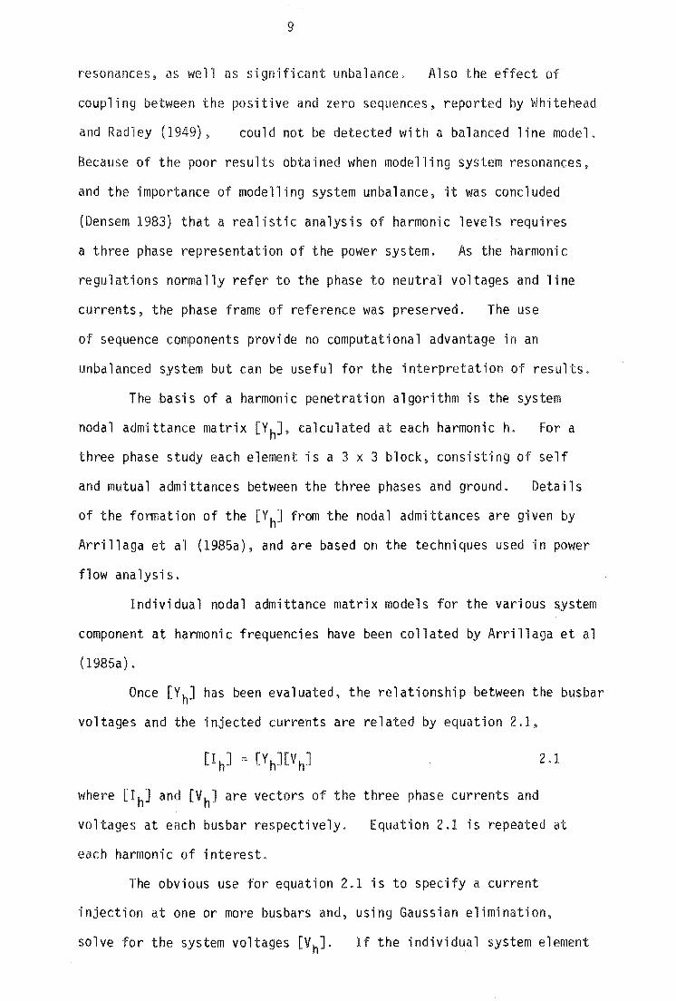
Once [Y h] has been evaluated, the relationship between the busbar
voltages and the injected currents are related by equation 2.1.
2.1
where [I h] and [V h] are vectors of the three phase currents and
voltages at each bus bar respectively.
each harmonic of interest.
Equation 2.1 is repeated at
The obvious use for equation 2.1 is to specify a current
injection at one or more bus bars and, using Gaussian elimination,
solve for the system voltages [VhJ. If the individual system element

10
admittances are preserved. the currents in each element can be
calculated. With the propagation of harmonic currents clearly defined,
potential harmonic overvoltages and potential communication inter-
ference problems can be identified.
Similarly. the same method can be used to determine the
propagati on of non-i nteger harmoni c currents such as r-j pp 1 e control
signals (Ross 1972 and Densem 1983). The results of such a study
determine whether or not the ripple signals will be strong enough
throughout the system to operate the ripple relays and to test for
spillover of the ripple signal into other supply authority systems,
via the transmission system.
The [YhJ matrix can be used to evaluate the admittance of an
a.C. system at harmonic frequencies, as seen from the point of
injection. If Ih is zero at all the busbars except one, the [Y h] can
be reduced by Gaussian elimination to a single 3 x 3 block (Densem
1983), such that
[ I .. J = [Y dJ[V .. J 1 nJ re 1 nJ
2.2
[YredJ can be inverted to derive the harmonic impedance loci (Densem
1983) which are often used to characterise the a.c. system at
harmonic frequencies. [Y dJ can also be used directly in the design re of harmonic filters (Arrillaga 1983). For two or more points of
injection [YredJ is of dimension 3n x 3n, where n is the number of
points of injection.
Transmission lines are the major source of unbalance in power
systems and are strongly frequency dependent. They therefore dominate
the propagation of harmonic currents in the power system and must be
modelled accurately. Details of the techniques used in the modelling
of transmission lines are given by Arrillaga et al (1985a).
Standing wave effects are observed in both power and
communication systems whenever the transmission distance is greater

11
than about 1/12th of a wavelength, for 1.2% accuracy (Arrillaga et a1
1985a). In power systems this corresponds to 500 km fundamental
frequency, but only 10 km at 50th harmonic. Standing wave effects are
accounted for by the use of an equ;valent-n model of each line at
each harmonic (Arrillaga et al 1985a).
With a three phase line three modes of propagation exist which
can be found by modal analysis (Densem 1983). Each mode propagates
in a different combination of conductors, including the earth, and will
in general have slightly different propagation velocities. The effect
of these slightly different velocities is most significant near
resonance, with each mode resonating at different frequencies (Densem
1983), causing system unbalance.
The frequency dependence of the series impedance is an
important aspect of transmission line modelling. Skin effect increases
the a.c. resistance of a conductor and decreases the internal
inductance. However, the effect on the internal inductance is usually
ignored (Kimbark 1950). Carson's earth return correction terms
increase both the series resistance and the inductance of a line. The
variation of the series impedance with frequency will alter the
resonant frequencies of the various propagation modes and the value of
system impedance at resonance (Demsem 1983).
2.3.3 Dynamic Simulation of Harmonic Interaction
Convertor operation, and hence the uncharacteristic current
injections produced, is modified by the presence of voltage distortion
on the convertor bus. This phenomenon is discussed more fully in
section 3.1.
Similarly. equation 2.2 shows that the injected harmonic
currents will modify the voltage distortion on the convertor busbar.
This interdependence of the voltage and current distortions is

12
discussed here as harmonic interaction.
It has been reported by several authors (Ainsworth 1967 and
Kauferle et al 1970) that convertor operation may be unstable, if the
background level of distortion is reinforced by the action of the
convertor control on the a.c. current injections. This problem.
often called harmonic instability, is discussed in detail in section
4.1.2.
One method of modelling the harmonic interaction of a
converter is to simulate the convertor in the time domain (Reeve and
Subba Rao 1974 and Kitchen 1981). After a period of simulation, about
six cycles (Reeve and Subba Rao 1974), successive cycles are expected
to be sufficiently similar to be regarded as the steady state
solution. The time required will depend on the accuracy of the initial
conditions and the degree of interaction.
In section 4.4 the use of the time domain algorithm TCS
(Heffernan 1980), developed for the study of convertor faults. is
discussed.
2.3.4 Limitations of Conventional Models
The present harmonic penetration techniques have several
shortcomings. Firstly, more detailed models of the sources of harmonic
current are needed to determine more accurately the size of the
injected a.c. current injections and hence the distortion in the
system.
CPU time.
Dynamic modelling can be used but requires large amounts of
Also the complex nature of the a.c. system response has to
be ignored or simplified to a balanced RLC network (Hingorani and
Burbery 1970) when represented in the time domain. As the system
impedances are a major factor contribut·in~ to harmonic interaction
any degradation of their representation reduces the effectiveness of a
dynamic simulation. Converter modelling is discussed in section 2.4

13
and the use of an alternative iterative algorithm to model convertor
interaction is discussed in ion 2.5 and chapter 3.
There is also a lack of agreement as to the most appropriate
representation of some system components (Densem 1983). This is
especially true of loads, transformers and synchronous machines.
Synchronous machines are discussed more fully in chapter 6, while
loads and transformers require future work.
Normally the system components are considered passive and
linear with each frequency treated separately. The converter is an
exception, being treated as a fixed injection. However, coupling
between frequencies can exist and will be discussed in section 2.6 and
in chapters 6 and 7.
2.4 HARMONIC MODELLING OF CONVERTORS
With increased understanding of non-ideal convertor operations
and its associated problems, convertor modelling techniques have
improved since those developed for ideal operation (Read 1945).
An important aspect of convertor modelling is the representation
of the commutation process. Normally the commutating impedance is
assumed ta be a linear inductance. However, this was extended to
include a series resistance (de Oliveira 1978). Some authors,
including Phadke and Harlow (1968) and Harker (1980),use only the
fundamental component of the terminal voltage to evaluate the
commutating current and voltage waveforms.
The most detail representation of the commutation process,
provided by de Oliveira (1978) and Yacamini and de Oliveira (1980a and
1980b), includes series resistance in the commutating impedance and
the effect of the full spectrum of commutating voltage harmonics.
Yacamini and de Oliveira (1980a) also provide for any transformer
connection with the use of g-zag connected transformers. However,

14
there are limitations in the use of zig-zag transformers and these
are discussed in section 3.3.1.
Earlier studies, including Ainsworth (1967), Reeve and
Krishnayya (1968), Phadke and Harlow (1968) and Yacamin; and de
Oliveria (1980a), did not include d.c. current ripple. This is
generally a reasonable assumption in the presence of a large smoothing
reactor. Later studies have used a series inductor and resistor to
represent the d.c. system (Reeve and Subba Rao 1971 and Yacomini and
Smith 1983). Discrete RLC components have also been used to represent
h.v.d.c. lines and cable combinations (Yacamini and de Olivera 1980b
and Yacamini and Smith 1983). An area for improvement is the inclusion
of standing wave and frequency dependency effects for the d.c. system
lines and cables. This is discussed in section 3.5.
The method of representing the a.c. system is also important.
Yacamini and de Oliveira (1980a and 1980b) generally use a series
resistor and inductor combinations, based on the short circuit ratio.
A similar representation (Rowles 1970) is generally used in dynamic
studies (Reeve and Subba Rao 1974). However, the consensus of opinion
(Kaufer1e et a1 1970, Reeve and Baron 1971 and Harker 1980) is that
individual impedances at each harmonic are required for an accurate
harmonic analysis of converter operation because the system impedance,
including the filters, is a major factor in harmonic stability
(Ainsworth 1967). As discussed in sections 2.3.2 and 3.4, the harmonic
penetration algorithm of Densem (1983) can be used to calculate the
admittance matrix [Y dJ at each harmonic. re Each [YredJ contains all
the information of frequency dependence and unbalance which can effect
the operation of the convertor.
Many studies of the operation of convertors include accurate
models of the convertor plant but simply specify arbitrary levels of

15
fundamental vol ge unbalance and control variables. As these
parameters di the convertors operation, the results of such
studies are not representative of the actual convertor. Harker (1980)
evaluated the fundamental terminal voltages, including unbalance. the
d.c. current, the transformer tap ratios and the delay angles of the
convertor for the actual system configuration present using an a.c./d.c.
fundamental power flow.
The unbalanced operation of convertors and details of the
iterative algorithm proposed in this thesis are discussed in chapter 3.
2.5 ITERATIVE ALGORITHM FOR MODELLING HARMONIC INTERACTION
The alternative to dynamic modelling is an iterative process
adopted by several authors (Reeve and Baron 1971, Yacamini and de
Oliveria 1980a and 1980b and Harker 1980). Normally the voltages at
the convertors is -initially assumed to be sinusoidal (Harker 1980)
and the resulting a.c. current injections calculated. Then at each
harmonic successively, the currents are injected into the a.c. system
and the terminal voltage updated. The controller strategy is
implemented by updating the firing instants from the distorted terminal
voltage waveform zero crossings at each iteration. The later studies
of Yacamini and de Oliveira (1980b) and Yacamini and Smith (1983)
include a d.c. system. At each iteration the d.c. side voltage
harmonics are calculated and the d.c. current ripple updated. The
main advantages of the iterative approach are a reduction in CPU
time and the ease of representing the complex harmonic behaviours of
the a.c. and d.c. systems. Because the a.c. and d.c. systems are
represented by admittance matrices at each harmonic, any frequency
dependence of mutual couplings between phases can be modelled.
However. the disadvantage of an iterative algorithm is that convergence
is not guaranteed and divergence may not necessarily mean the actual

16
convertor is unstable. This problem is discussed in section 4.1.3.
In chapter 3 the iterative algorithm has been further
developed with an enhanced representation of a.c. and d.c. systems.
The problem of harmonic instability is further examined in chapter 4.
2.6 INTRODUCTION TO MODELLING IN THE HARMONIC SPACE
Throughout harmonic penetration studies it has been assumed
that the a.c. system components are linear and passive. This has
meant that each harmonic can be treated separately. Because a.c./d.c.
convertors are not passive and linear they are not included in
harmonic penetration studies, hence the need for the iterative
algorithm.
However, synchronous machines and power transformers also
produce coupling between harmonics. In the case of synchronous
machines, the coupling is due to the salient nature of the rotor flux,
while the power transformer's coupling is due to the magnetic non
linearity of the iron core. Therefore, with existing harmonic
penetration algorithms. it is not possible to fully model all the
harmonic phenomena associated with either synchronous machines or
power transformers.
The problem of coupling between harmonics can be solved by
introducing the concept of the harmonic space. This is defined as a
set of 3nk phasors describing a quantity of voltage and currents, in
each phase of the n busbar system at each of the k harmonics being
considered. All the voltage phasors in each phase. busbar and
frequency are combined to form a single vector [VJ. and similarly. all
the currents combined to form [IJ.
The conventional harnlonic penetration relationships of the
harmonic currents and voltages. described at each harmonic by equation
2.1. can be combined to an equivalent representation in the harmonic
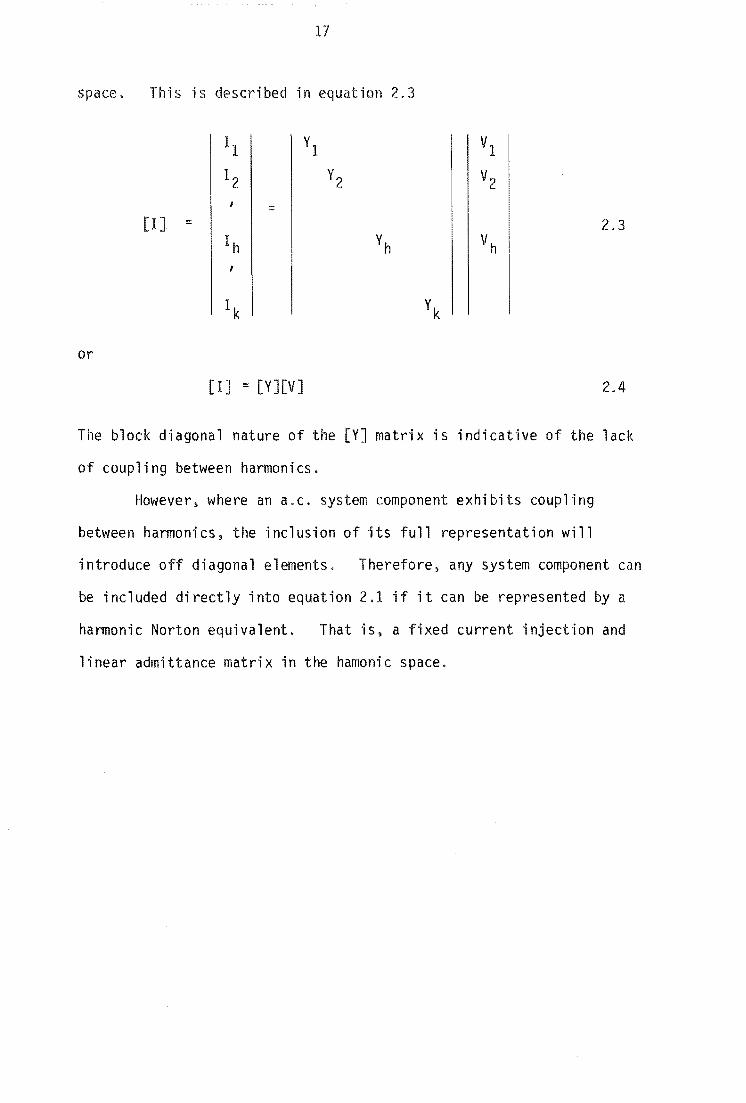
space. This is described in equation 2.3
11 YI VI
12 Y2 V2
= [1 ] == 2.3
Ih Yh Vh
or
[1] = [Y][V] 2.4
The block diagonal nature of the [Y] matrix ;s indicative of the lack
of coupling between harmonics.
However, where an a.c. system component exhibits coupling
between harmonics, the inclusion of its full representation will
introduce off diagonal elements. Therefore, any system component can
be included directly into equation 2.1 if it can be represented by a
harmonic Norton equivalent. That is, a fixed current injection and
linear admittance matrix in the hamonic space.

18

19
CHAPTER
HARMONIC MODELLING OF CONVERTOR OPERATION
3.1 INTRODUCTION
Under the ideal conditions of a flat d.c. current~ balanced
fundamental terminal busbar voltage and commutating impedances,
convertors produce only characteristic harmonics. In the a.c. system
the characteristic harmonic currents are the negative sequence pk-l
and positive sequence pk+l orders, where p is the pulse number of the
convertor and k is an integer. Similarly, the characteristic voltage
harmonics on the d.c. side of the convertor are of order pk. A summary
of the characteristic harmonics was given by Read (1945).
However, convertor operation is susceptible to non-ideal
system behaviour and will generate uncharacteristic a.c. and d.c.
currents. Because the uncharacteristic ha~lonics are generally not
filtered, the mechanisms for their generation need to be examined.
One of the major causes of non-ideal operation of convertors
is an unbalanced fundamental terminal voltage (Reeve and Krishnayya
1968 and Phadke and Harlow 1968). Unbalanced voltages give rise to
unequally spaced zero crossings. With a conventional constant delay
angle controller the conduction periods in each phase are unequal,
resulting in all the odd harmonics generated on the a.c. system and
all the even harmonics generated on the d.c. side. A smaller
modification to the current and voltage waveforms is due to the
unequal commutation angles resulting from the unbalanced commutations
voltages. Even with an equidistant controller giving firing pulses
every 60 de'grees (Ainsworth 1968), all the a.C. system odd harmonics
and the d.c. side even harmonics will be produced due to the resulting
unequal coolmutation angles. Appendix Al shows the relationship between

20
third harmonic current and unequal commutation angles for an
equidistant controller,
A similar effect to that of unbalanced terminal voltage ;s
produced by unequal commutating reactances in each phase of the
convertor transformer (Subbarao and Reeve 1976). The unbalanced
reactances produce unequal commutation angles which cause the odd
uncharacteristic a.c. harmonic currents and even uncharacteristic
d.c. harmonic voltages.
Any voltage distortion on the convertor terminal busbar can
cause the convertor to produce uncharacteristic harmonic currents
(Ainsworth 1967. Phadke and Harlow 1968 and Reeve et al 1969). As for
unbalanced terminal voltages. harmonic voltages shift the zero
crossings which cause a variety of harmonic currents, depending on the
nature of the distortion. When only a single disturbing harmonic
voltage is considered at any time. it was found (Reeve et al 1969)
that odd harmonic voltages produce odd harmonic currents only while
even harmonic voltages produce harmonic currents of all orders. For
both even and odd harmonic voltages which are balanced no triplen
harmonics are produced. The effect of convertor terminal voltage
distortion can be reduced by control system filters or an equidistant
controller (Ainsworth 1967). The advantages of an equidistant
controller over control system filters is discussed in section 4.1.2.
It has been shown by Dobinson (1975) that the presence of d.c.
current ripple can dramatically modify the magnitudes of the
characteristic harmonics. In the presence of convertor unbalance. and,
a finite smoothing inductor, uncharacteristic currents will flow in
the d,c. system resulting in modified uncharacteristic a.c. currents.
This has been observed by Giesner and Arrillaga (1972) and later by
Yacamini and Smith (1983) for the case of second harmonic ripple
producing third harmonic currents on the a.c. side.

21
The other source of uncharacteristic harmonics in the
literature are controller errors (Reeve and Krishnayya 1968 and Reeve
et a1 1969). These errors produce unequal conduction periods in each
phase, including half-wave asymmetry, and therefore all a.c. harmonic
currents and d.c. side harmonic voltages are generated in a random
fashion. This includes a d.c. current in the converter transformer
which can produce saturation of the core and additional harmonics
(Yacamini and de Oliveira 1978).
The iterative algorithm described in this chapter includes the
effects of unbalanced terminal voltage and commutating reactance, as
well as distortion on the a.c. terminal busbar voltage and d.c.
current. Control system errors were ignored, as they are either due to
a steady state disturbance already included in the algorithm or, only
a random error not sustained in the steady state.
3.2 AN OUTLINE OF THE ITERATIVE ALGORITHM
It is clear that the operation of a convertor, and hence its
associated a.c. current injections and d.c. voltage waveform, is
dependent on the voltage on its terminal and the d.c. current ~ipple.
At the same time however, the voltage distortion on the convertor's
terminal is due to the a.c. current injected into the combined
admittance of the a.c. system and the harmonic filters. Similarly. the
ripple on the d.c. current ;s related to the d,c. voHage by the
admittance of the d.c. system.
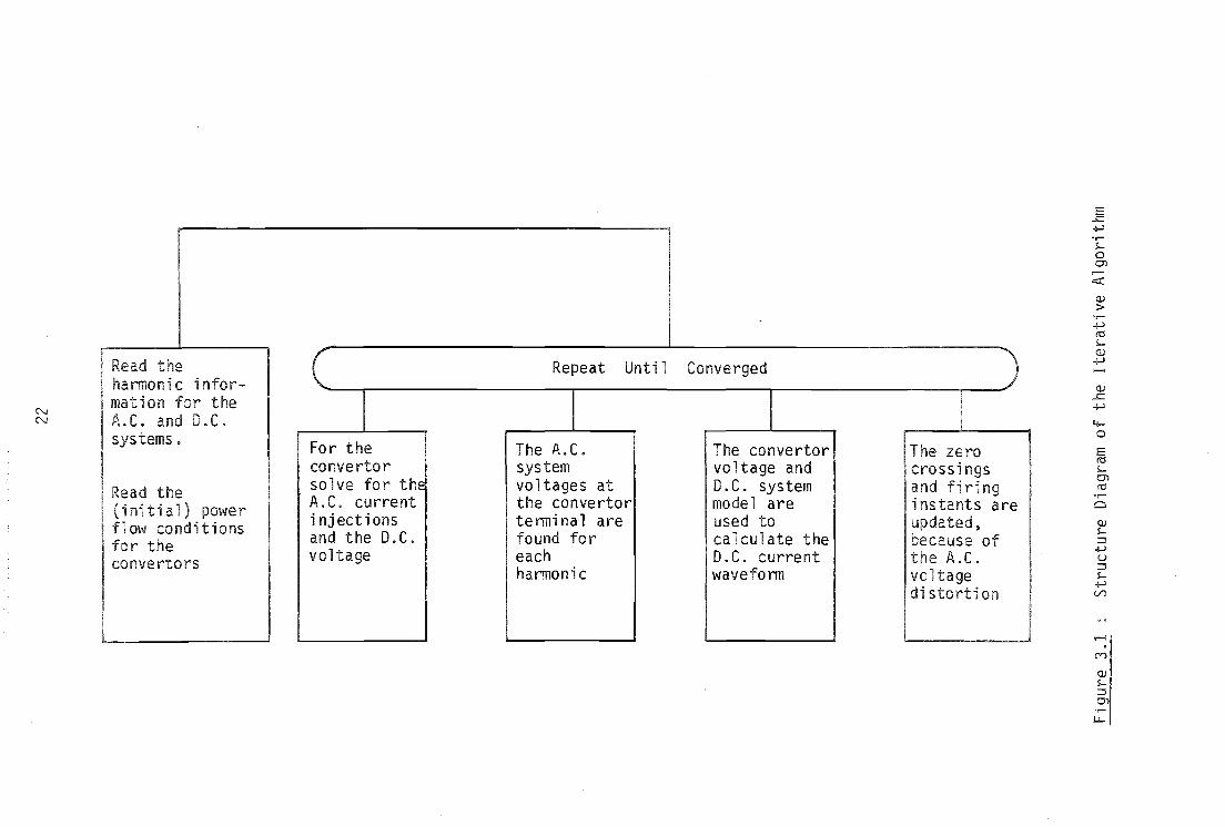
The proposed iterative algorithm, the structure of which is
given in figure 3.1, is needed to assess the harmonic interaction that
occurs between transmission systems and static convertors.
Firstly. the execution parameters. filter data and admittance
matrices for the a.c. and d.c. systems are entered. A preliminary
power flow must be carried out to provide an approximate estimate of
N N
Read the hannoni c i nfor-mation for the A.C. and D.C. systems.
Read the (initial) power flow conditions for the convertors
'--
Repeat Until
I For the The A.C. convertor system solve for the voltages at A.C. current the convertor i nj ect ions terminal are and the D.C. found for vo ltage each
hannonic
Converged
I I The convertor The zero voltage and crossings D.C. system and fi ri ng model are instants are used to updated, calculate the because of D.C. current the A.C. wavefonn voltage
distortion
E ..s:::. .j..J
",.... 5-o 0)
.---«
Q)
> ",.... +-' It:S 5-Q)
+-' ~
Q) ..s:::. .j..J
~ o E It:S 5-0)
It:S
Cl
Q) 5-::::J
.j..J
U ::::J 5-
.j..J (/)
.-i
M
Q)
5-::::J 0) .,.... ~

the fundamental frequency voltages and currents the converter a.c.
and d.c. terminals. In the presence of transmission line unbalance,
the a.c./d.c. power flow must be three phase (Harker and Arrillaga
1979). The a.c./d,c. power flow contains the necessary information to
derive the three-phase fundamental voltage and current waveforms at
the convertor terminal, used to calculate the first estimates of the
three hase harmonic current injections and the d.c. side voltage
waveform.
The iterative loop is divided into four blocks. Firstly the
convertor operation is solved for its a.c. current injections and d.c.
voltage waveform. This process is discussed in section 3.3. With the
a.c. current injections calculated, the a.c. system is solved for the
terminal voltage distortion. Similarly, the d.c. voltage waveform is
used to derive the d.c. system current ripple. The solution of the
a.c. and d.c. systems is examined in sections 3.4 and 3.5 respectively.
Finally. from the firing strategy and the voltage distortion, control is
implemented in the fourth block, as described in section 3.6.
The iterative loop is terminated by either convergence or
divergence being detected. The solution has converged when the voltage
and current distortions do not change significantly between successive
iterations. However, instead of checking each individual voltage and
current component, the iterative changes of the commutating voltage
zero crossings are used to test for convergence. If all the zero
crossings change by less than 0.0001 radians a flag is set and one
more iteration performed.
Divergence of the algorithm is indicated when the maximum
number of iterations is exceeded. multiple zero crossings are detected
or the controller specifies a negative delay angle. An excessive
number of iterations implies a marginally stable solution while either
multiple zero crossings or negative delay angles point to large
uncharacteristic voltage distortion.

24
3.3 SOLVING THE OPERATION OF THE CONVERTOR
Each convertor is solved for the a.c, harmonic current
injections and the d.c. voltage hannonics. To achieve this, the
convertor commutating voltages, the d,c. current waveform and
firing instants are needed at each iteration. The commutating
impedances. the transformer connection and tap ratios must also be
specified.
The commutating voltages and impedances are defined in terms
of a Thevenin equivalent for the secondary of the convertor
transformer, as described in figure 3.2
Figure 3.2 The Convertor and the Thevenin Equivalent of its Transformer
The commutating voltages are the transformer primary voltages,
including distortion, referred to the secondary with the transformer
connection and tap ratios taken into account. The commutating
impedances are the transformer's leakage inductance per phase with a
series resistance. If data is available the three commutating
impedances can be unbalanced.
The d,c. current waveform, Id,contains ripple and ;s at any
instant of time

25
3.1
where Ido is the d.c. current specified by the power flow and Idh and
¢dh are the rms magnitude and phase of the hth harmonic component of
ripple respectively. NHARM is the maximum harmonic order to be
considered. The convertor firing instants are calculated at each
previous iteration. The process of evaluating the firing instants is
described in section 3.6.
3.3.1 Calculating the Commutation Current
The commutation is the period of time taken to turn off an
outgoing valve when an incoming valve is fired. The incoming valve is
fired after it is forward biased and cannot turn on instantaneously
because the energy stored in the commutating reactance of the outgoing
phase needs to be transferred to the incoming phase. The situation of
valve 3 turning valve 1 off is described in figure 3.3.
Figure 3.3 Commutation of Valve 3
At the instant valve 3 is fired II = Id and 12 = O. However~
because V2 is more positive than VI' the commutation current 12 grows,
thus reducing the current II' When II reaches zero, 12 = Id, valve 1
turns off and valve 3 is fully conducting. A generalised equation to
describe any commutation, developed by Yacamini and de Oliveira (1980a),
and is

26
. NHARM Bh [( Hh + liT ) -+/T 1 , ( t):: I - ~.:.---::-_n~m e nm + n h 1 L h2 2 + 1/T2 hw = nm w nm
3.2
where P is the valve commutating in
8p
;s the firing instant of valve P
m is the outgoing phase
n is the incoming phase
3.3
3.4
Tnm = Lnm/Rnm 3.5 A A
Ah = Vhn cos(h8p + ¢hn) - Vhm cos(h8 p + ¢hm) 3.6 A A
Bh ~ Vhn sin(h8p + ¢hn) - Vhm sin(h8p + ¢hm) 3.7
Hh = h.Ah/B h 3.8
-1(1 ) -1 Hh) ¢h= tan Ihw Tnm -tan (hw 3.9
Vhn is the peak magnitude of the hth harmonic of the incoming
phase
is the peak magnitude of the hth harmonic of the outgoing
phase
¢hn is the phase of the hth harmonic of the incoming phase
¢hm is the phase of the hth harmonic of the outgoing phase
Cnm an integration constant such that in(O) = O.
Equation 3.2 can be simplified to

27
3.10
tiT + Y(l-e nm) + C nm
Bh (Hh -1
where IT nm) 3.11 xh ::: Lnm I/T2 h2w2 + nm
Bh H2 + I/T2 Sh :::
h nm 3.12 hwLnm h2 w2 + IT2
nm
Y ::: Rm1d/Rnm 3.13
Cnm is evaluated by setting t and in(O) equal to zero in equation
3.10. This yields
3.14
If equation 3.14 is substituted into 3.10
NHARM [ -tiT ] ( in(t) = h~1 Xh(e nm -1) + Sh(sin(hwt + ¢h) - sin¢h) +Y l-e-t/T nm)
3.15
To calculate VI' V2 and V3 for the convertor transformer
secondary, Yacamini and de Oliveira (1980a) used a zig-zag
representation of the convertor transformer connection. This has the
advantage of being able to represent any phase shift of the
transformer and is therefore useful for modelling convertors of large
pulse number. While the zi ag connection ;s perfectly accurate for
the star-g/star connection, it is not for the star-g/del connection
in the presence of zero sequence voltage at the convertor terminal.
Because of the unbalance of transformers and transmission lines, and
the fact that the star-g/delta connection is not a perfect short
circuit to zero sequence (Chen and Dillon 1974), a finite level of zero
sequence voltage can exist on the convertor's terminal busbar. This

28
zero nee voltage cannot exist on the secondary of a star-gjdelta
transformer but is referred to the secondary of an equivalent zig-zag.
This is demonstrated in Appendix A2 for a transformer with a DYll
connect ion.
The need for a zig-zag equivalent and its associated
inaccuracies can be overcome by calculating the secondary phase to
phase voltages directly from the primary voltages rather than solving
for VI' V2 and V3 explicitly. Thus, if Va' Vb and Vc are the primary
phase voltages, the secondary phase to phase voltages for a star-g/star
transformer are
V21 (t) = Vb(t) - Va(t)
V 32 ( t) = V c ( t ) - V b ( t )
V13(t) = Va(t) - Vc(t)
and for a star-g/delta (DY11) transformer
V21 (t) = l,l3Va (t)
/3v b(t)
13V c (t)
where the i3 is due to the P.U. system.
3.3.2 Sampling the A.C. Current Injections
3.16
3.17
3.18
3.19
3.20
3.21
To calculate the a.c. current injections in the frequency domain,
each of the three phases are sampled at NSAMPL equally spaced
points in the time domain over one cycle and a Fast Fourier Transform
performed. The method of sampling is preferable to the equation form
used by Yacamini and de Oliveira (1980a) because of its generality and
ease of adding new features (Harker 1980).
The three current waveforms can be divided into 12 sections.
For six of the sections normal conduction by one valve on each side of
the bridge occurs. This situation is described in figure 3.4 for
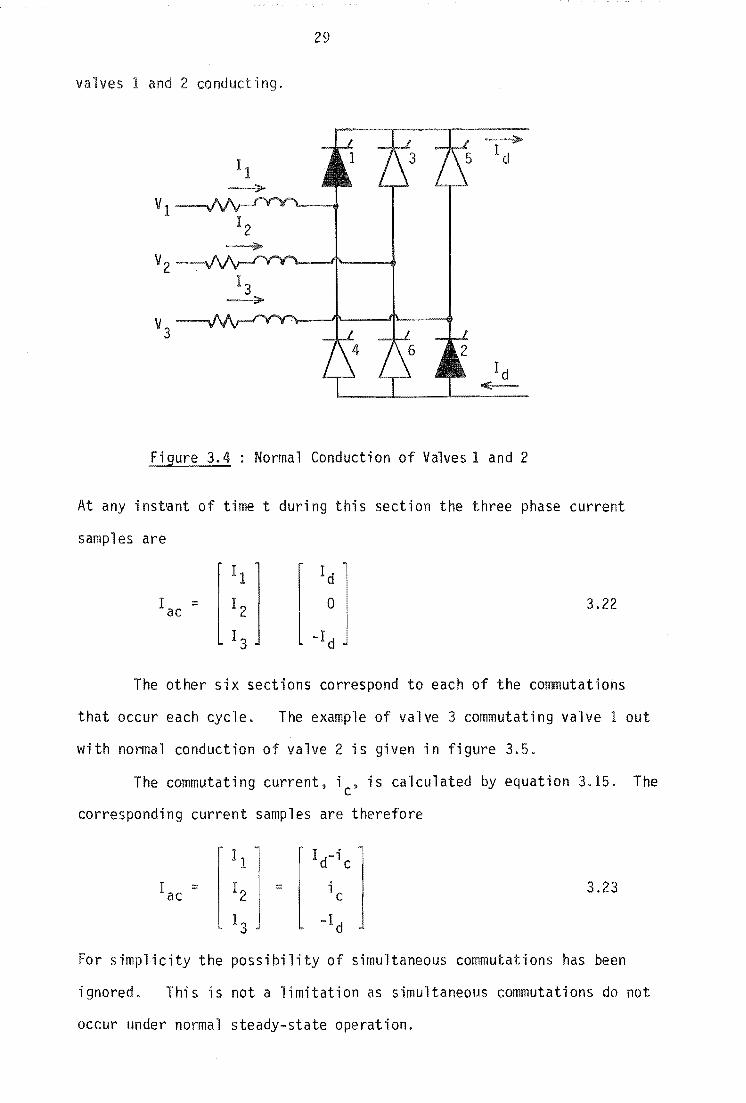
29
valves 1 and 2 conducting.
II ~
VI I2 ~
V2 I
V3
Figure 3.4: Normal Conduction of Valvesl and 2
At any instant of time t during this section the three phase current
samples are
3.22
The other six sections correspond to each of the commutations
that occur each cycle. The example of valve 3 commutating valve lout
with normal conduction of valve 2 is given in figure 3.5.
The commutating current, ; , is calculated by equation 3.15. The c corresponding current samples are therefore
3.23
For simplicity the possibility of simultaneous commutations has been
ignored. This is not a limitation as simultaneous commutations do not
occur under normal steady-state operation.

30
Vl
Figure 3.5 Commutation from Valve 1 to Valve 3 with Valve 2 Conducting
The first sample point, and the time reference, is taken
as the firing instant of valve 1. For each conduction and commutating
section, equivalent equations to 3.22 and 3.23 are derived to describe
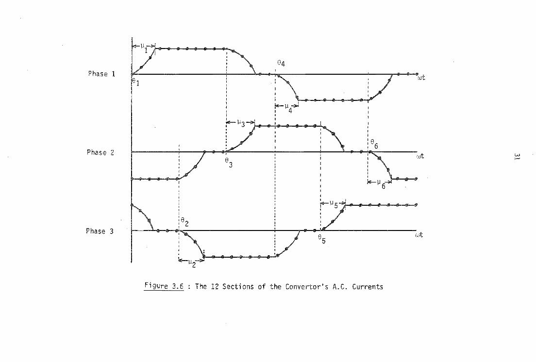
a complete cycle of each phase. Figure 3.6 shows the three phase
current waveform for a cycle. Similarly, table 3.1 defines the
current in each phase for each section.
At the beginning of the iteration each phase to phase
voltage pair Vnm(t) is calculated such that
3.24
where t is referenced to 81" For a star-g/star transformer equations
3.6 and 3.7 are used to calculate the Ah and Bh respectively where,
V. For a star-g/delta transformer c '
Vnm(t) - !3Vq(t) 3.25 A
- - Ij ~ Vqsin(hwt + ¢qh + h81)
- - }Ij I A~nm) sin(hwt) + B~nm) cos(hwt) 3.26 h
where n,m and q are defined by equations 3.19, 3.20 and 3.21, and
Pel 61
2
p 3
Fi
i ~]J~ I 4 , I I
The 12 Sections of Convertor's A.C. Currents
(JJt
w ......

e 3.1 : three phase currents in each phase and on
on P se 1 Phase 2 Phase 3 Limits, reference to 81
1 ic -I d I d - i c 0 < wt < ]11
2 Id -Id 0 ]11 < < 82 - 81
3 Id -I - i i * 82 - 81 < < 82 - 81 + d c c
4 Id 0 -Id 82 - 81 + ]12 < < 83 - 81
5 Id \ i -I d 83 - 81 < wt < 83 - 81 + ]13 c
6 0 Id -Id 83 - 81 + ]13 < wt < 81 - 81
7 i * Id -I d - ic 81 - 81 < < 81 - 81 + c
8 -I d Id 0 81 - 81 + ]11 < < 85 - 81
9 -1 d
I - i d c \ 85 - 81 < wt < 85 - 81 + ]15
-Id 0 Id 85 - 81 + ]15 < < 86 - 81
11 -I - i d c i * c Id 86 - 81 < < 86 - 81 +
0 -Id Id 86 - 81 + ]16 < < 2rr
* the commutation cu on the common neqative values_
A(nm) h
B(nm) h
Vq cos(¢qh + hS l )
Vq s;n(¢qh + hS l )
3.27
3.28
Because during the pth commutation the time t of the
commutation equation 3.15 is referenced to S the A(nm) and B(nm) p' h h
a re mod ifi ed to Ah and Bh such that
A
Ah = Vhn cos(hSp + ¢hm) Vhm cos(h8 p + ¢hm) 3.29
_ A(nm) - h cos(h8 p ~ h8 1) B(nm)
- h sin(hS p - hs 1) 3.30
and B - A(nm) h8 ) + B(nm) sin(hS - cos (h8 P - hs 1) 3.31 h - h P 1 h
Note that equations 3.30 and 3.31 also hold for star-g/delta
transformers, even though Vn and Vm are not explicitly formed.
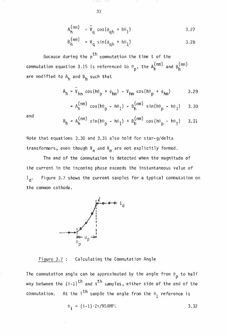
The end of the commutation is detected when the magnitude of
the current in the incoming phase exceeds the instantaneous value of
Id. Figure 3.7 shows the current samples for a typical commutation on
the common cathode.
Sp
I
I I I I
I I
flp -;;.I
Calculating the Commutation Angle
The commutation angle can be approximated by the angle from Sp to half
way between the (i l)th and ;th samples, either side of the end of the
commutation. At the ith sample the angle from the 81 reference is
S. 1
(i 1) '2'fT/NSAMPL 3.32
34
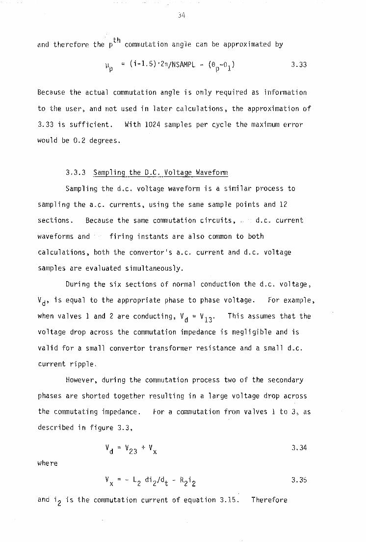
and therefore the pth commutation angle can be approximated by
3.33
Because the actual commutation angle is only required as information
to the user, and not used in later calculations~ the approximation of
3.33 is sufficient. With 1024 samples per cycle the maximum error
would be 0.2 degrees.
3.3.3 Sampling the D.C. Voltage Waveform
Sampling the d.c. voltage waveform is a similar process to
sampling the a.c. currents, using the same sample points and 12
sections. Because the same commutati on circui ts" d.c. current
waveforms and firing instants are also common to both
calculations, both the convertor's a.c. current and d.c. voltage
samples are evaluated simultaneously.
During the six sections of normal conduction the d.c. voltage.
Vd, is equal to the appropriate phase to phase voltage, For example.
when valves 1 and 2 are conducting, Vd V13, This assumes that the
voltage drop across the commutation impedance ;s neglig'ible and is
valid for a small convertor transformer resistance and a small d.c.
current ripple.
However. during the commutation process two of the secondary
phases are shorted together resulting in a large voltage drop across
the commutating impedance.
described in figure 3.3,
where
For a commutation from valves 1 to 3, as
3.34
Vx = - L2 di 2/d t - R2i2 3.35
and i2 is the commutation current of equation 3.15. Therefore

35
-t/Tnm V = W e + I Mh cos(hwt) + Nh s;n(hwt) + K
x h n
where Mh - - (hwL n Sh cos(¢h) + Rn Sh sin(¢h)) 3.37
1\ = (hwLn Sh sin(¢h) - Rn Sh cos(¢h)) 3.38
W = (Ln/Tnm - Rn)(X h - Y) 3.39
Kn = - R (Y + C ) n nm 3.40
The d.c. voltage waveform over one cycle is shown in figure
3.8, while the value of d.c. voltage is defined in table 3.2.
Phase voltages
Figure 3.8 The 12 Sections of the Convertor D.C. Voltage

Table 3.2 : The d.c. vol ;n each section
Section d.c. voltage Limits, reference to 81
1 V 12 + V x 0 < wt < 111
2 V12 111 < wt < 82 - 81 3 Vl3 - Vx 82 81 < wt < 82 - 81 + 112
4 V13 82 - 81 + 112 < wt < 83 - 81 5 V 23 + V x 83 - 81 < wt < 83 - 81 + 113
6 V23 83 - 81 + 113 < wt < 81 - 81
7 V 21 - V x 81 - 81 < wt < 81 - 81 + 114
8 V21 84 - 81 + 114 < wt < 85 - 81
9 V 31 + V x 85 - 81 < wt < 85 - 81 + 115
10 V31 85 - 81 + 115 < wt < 86
- 81
11 V 32 - V x 86
- 81
< wt < 86 - 81 + 116
12 V32 86 - 81 + 116 < wt < 27T
3.3.4 Conversion from the Time Domain to the Frequency Domain
With information of the d.c. current injections and d.c.
voltage for the convertor described for one cycle in the time domain,
an FFT ;s performed on each waveform to calculate their harmonic
components.
The output of the FFT is an exponential series with time
reference 81, However. during the rest of the iterative algorithm a
sinewave series is assumed. Also the a.c. currents are in the form of
an injection and need their sign reversed. Therefore the a.c. current
phasors become
and the d.c. voltage phasors
3.41
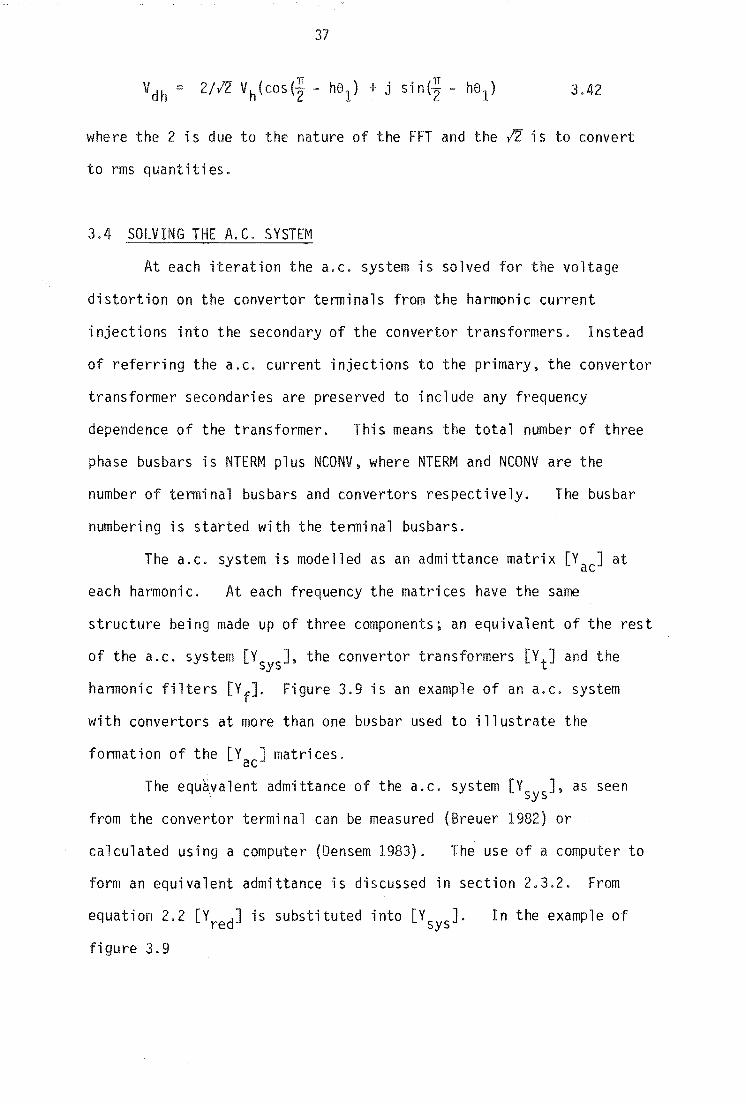
37
3.42
where the 2 is due to the nature of the FFT and the ~ ;s to convert
to rms quantities.
3.4 SOLVING THE A.C. SYSTEM
At each iteration the a.c. system is solved for the voltage
distortion on the convertor terminals from the harmonic current
injections into the secondary of the convertor transformers. Instead
of referring the a.c. current injections to the primary. the convertor
transformer secondaries are preserved to include any frequency
dependence of the transformer. This means the total number of three
phase busbars is NTERM plus NCONV, where NTERM and NCONV are the
number of terminal busbars and convertors respectively. The bus bar
numbering is started with the terminal busbars.
The a.c. system is modelled as an admittance matrix [Y ac ] at
each harmonic. At each frequency the matrices have the same
structure being made up of three components; an equivalent of the rest
of the a.c. system [Y Sys]' the convertor transformers [Y t ] and the
harmonic filters [Y f ]. Figure 3.9 is an example of an a.c. system
with convertors at more than one bus bar used to illustrate the
formation of the [Yac ] matrices.
The equayalent admittance of the a.c. system [\ysJ. as seen
from the convertor terminal can be measured (Breuer 1982) or
calculated using a computer (Densem 1983). The use of a computer to
form an equivalent admittance is discussed in section 2.3.2. From
equation 2.2 [Y red ] is substituted into [Y Sys ]'
figure 3.9
In the example of

38
A C F1
System --
T2 C2
N T3 C3
N F2
Figure 3.9 An Illustrative Example of an A.C. System with A.C./D.C. Convertors
y sys11 \ys12 0 0 0
~ NTERM Ysys21 \ys22 0 0 0
Y1
[\ysJ ;;:: 0 0 0 0 0 I 3.43 0 0 0 0 0 NCONV
0 0 0 0 0
where Ysys11 and Ysys22 are the self admittances of the terminal
busbars. Similarly, YSyS12 and YSys21 represent the mutual couplings
of the system between the busbars.
An individual transformer has an admittance matrix of the form
Y2
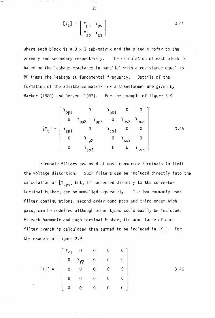
3,44
where each block is a 3 x 3 sub-matrix and the p and s refer to the
primary and secondary respectively. The calculation of each block is
based on the leakage reactance in parallel with a resistance equal to
80 times the leakage at fundamental frequency. Details of the
formation of the admittance matrix for a transformer are given by
Harker (1980) and Densem (1983). For the example of figure 3.9
\PI
o
o
o
Y sp2
\p3
Y psI o
\sl o
o
o 0
YpS2 YpS3 o 0
Yss2 0
o \s3
3.45
Harmonic filters are used at most convertor terminals to limit
the voltage distortion. Such filters can be included directly into the
calculation of [YSysJ but, if connected directly to the convertor
terminal busbar, can be modelled separately. The two commonly used
filter configurations, second order band pass and third order high
pass, can be modelled although other types could easily be included.
At each harmonic and each rminal busbar, the admittance of each
filter branch is calculated then summed to be included in [Yf ]. For
the example of figure 3.9
o
o
o
o
o
o
o
o
o
o
o
o
o
o
o
o
o
o
o
3.46

40
The total admittance matrix [Yac] is the sum of [VSysJ, [YtJ
and [V f ]. At each iteration, the harmonic equation
'" [V ] ac 3.47
is solved where Ic are the NCONV current injections at the convertor
and Vt and Vc are the NTERM and NCONV voltage components at the
convertor terminals and transformer secondaries, respectively.
3.5 SOLVING THE D.C. SYSTEM
In a similar way to the a.c. system, at each iteration the
d.c. system is solved for the ripple on the d.c. current from the d.c.
voltage generated on the convertors d.c. terminal. As for the a.c.
system, the most convenient representation of the d.c. system is an
admittance matrix. At each harmonic the vector of d.c. terminal
voltages ;s multiplied by the d.c. admittance matrix to give the
current ripple at that frequency. That is
[IdJ = [VdJ [VdJ 3.48
For the example of fi gure 3.9 the structure of [VdJ is
Idl VI 0 0 Vd1
Id2 a V2 V2 Vd2 3.49
Id3 a Y2 V2 Vd2
where Vl and V2 are the harmonic admittance of eac~ of the loads.
Note that VI and Y2 are single elements rather than 3 x 3 blocks in the
case of the a.c. system.
In chapter 4 the following representations of the d.c. system
have been used.

41
1. An infin; system with no ripple
2. RL series d.c, system.
3. D.C. motors using the series RL and Ewing (1968) models.
4. D.C. transmission systems including overhead lines and smoothing
inductors. The algorithm used to derive [YdJ in this case is
described in Appendix A3.
3.6 IMPLEMENTING
The presence of harmonic voltages on the convertor terminal
busbar will cause the actual zero crossings of the commutating
voltages to be shifted from those of the fundamental alone. With the
zero crossings modified, the control strategy is used at each
iteration to recalculate the firing instants and delay angles.
3.6.1 Calculating the Zero Crossings
The zero crossings are the instant in time when the
transformer secondary phase to phase voltages pass through zero and
the next valve can be fired.
Because of the difficulty in calculating the zero crossings
analytically, the regula falsi (Kreyzig 1979) iterative method is
used. With an initial estimate of the most recent values, the six
zero crossings are updated at each iteration.
If the zero crossing fail to converge in 100 iterations
multiple zero crossings are assumed, indicating a divergent solution
due to excessive distortion.
3.6.2 Calculating the Delay Angles
The delay angle refers to the angle between the actual zero
crossing and the instant of firing for a pa~ticular valve. Given the
set of zero crossings, the control strategy is implemented to

42
calcul the individual delay angles.
The two types of control strategies specified by the power
flow are constant delay angle and equidistant control. Constant delay
angle control maintains equal delay angles for each valve. An
equidistant controller produces valve firings every 60 degrees. This
is achieved within the algorithm by fixing the delay angle on valve
one and adjusting the other delay angles to maintain equal conduction
periods.
In many h.v.d.c. controllers filters are included in the
control loop. The effect of these can be included into the iterative
algorithm by calculating the delay angles such that the firing
instants are unaltered by the presence of voltage distortion. This
applies to either a constant delay angle or equidistant controller.
3.7 CONCLUSIONS
In this chapter an iterative algorithm has been developed
to calculate the harmonic iteraction that occurs at a.c./d.c. convertors.
While the algorithm accurately models the convertor's
operation and the a.c. and d.c. systems, the algorithm is susceptible
to numerical instability. This problem is analysed in chapter 4.
Furthermore, the iterative algorithm developed to model three phase
convertors, is modified in chapter 5 to analyse the operation of single
phase convertors.

43
CHAPTER 4
HARMONIC INTERACTION BETWEEN A.C. 5 D.C. AND CONVERTOR SYSTEMS
4.1 INTRODUCTION
When considering the interaction between a.c, and d.c. systems
in the steady state two main areas of investigation are evident. The
first~ and in general the most important area, is that of fundamental
voltage and power interactions which are solved by the use of an
integrated a.c./d.c. power flow (Harker and Arrillaga 1979). The other
area is that of harmonics.
4.1.1. The Effect of Interactions on the Harmonic Currents
Produced
The harmonic currents produced by the converter depend not
only on the fundamental voltage conditions at the convertor terminals
and the d.c. power being transmitted, both being calculated in the
power flow, but also on the presence of a.c. voltage distortion on the
terminal busbar and d.c. current distortion.
The iterative algorithm described in chapter 3 can be used to
analyse the harmonic interactions between the convertor, a.c. and d.c.
systems. A large 6-pulse convertor at Tiwai, in the system of the
South Island of New Zealand, ;s used in this chapter together with
various a.c. system and filter configurations as well as constant
delay angle and equidistant control. Also the effect of the d.c.
system was examined. The results are examined in sections 4.2 and 4.3.
At the distribution system level, three phase d.c. convertor
drives have been examined and discussed in Appendix A6 in the form of
a paper (Arrillaga al 1985b).

44
Single phase traction convertor d.c. drives have been examined
in a similar fashion to three phase d.c. drives.
in chapter 5.
4.1.2 Harmonic Instability
This is discussed
A problem associated with some h.v.d.c. schemes is harmonic
magnification and/or instability. A harmonic instability can be
characterised by excessive voltage distortion on the convertor
terminal busbar (Kauferle et al 1970), which can make the link
i noperabl e.
At the lEE conference No. 22. entitled High Voltage D.C.
Transmission, several examples of harmonic magnification and
instability were reported. A third harmonic instability at the
Cross-Channel link (Holmborn and Martenssen 1966) often developed
under some a.c. system configurations. This caused the link to be
inoperable. The problem was removed by the inclusion of a third
harmonic filter. Because of the Cross-Channel link experience, a
third harmonic filter was included at the design stage of the Sardinian
h.v.d.c. terminal to prevent a potential instability (Natale et al
1966 and Holmborn and Martenssen 1966).
Similarly, a problem was found during tests of the Kingsnorth
Scheme (Last et al 1966). Excessive second harmonic voltage distortion
under some system conditions was able to trigger the generator
protection circuits and cause errors in the over-voltage protection of
the fi lters.
At the Benmore terminal of the New Zealand d.c. link excessive
ninth harmonic voltage was reported (Robinson 1966b). This was solved
by the inclusion of a ninth harmonic filter.
A harmonic instability can, therefore. be defined as the
generation and/or magnification of non-characteristic frequencies by a

d.c. system containing, initially. no unbalance asymmetry
(Ainsworth 1981 and Arrillaga 1983).
At the convertor a positive feedback loop can exist such that
distortion of either the a.c. or d.c. systems reaches the control
system causing firing pulse irregularities which, in turn, can produce
harmonic magnification or instability. Note that this is a waveform
distortion rather than an ordinary low frequency instability
(Ainsworth 1967).
The relative size of the converter currents and the a.c.
system is an important factor contributing to a harmonic magnification
and/or instability. The short circuit ratio, which is the ratio of
the short circuit MVA at the terminal a.c. busbar to the total nominal
d.c. power of the covertor station (Arrillaga 1983), is used as a
practical criterion of convertor behaviour. However, since the
combination of a.c. system and harmonic filters will have a low
parallel resonance frequency, normally lower than fifth harmonic, the
short circuit ratio does not define the impedance or system strength
at these harmonic orders. The resulting resonance is normally the
determining factor in the development of harmonic instabilities
(Kauferle et al 1970). As a temporary measure, a harmonic instability
can be removed because the effective size of a convertor can be
reduced by decreasing the d.c. current (Ainsworth 1967).
The convertor controller is an important part of any harmonic
instability positive feedback loop. The control strategy determines
the firing pulses and therefore the extent the original disturbance is
reinforced. Control system filters can be added to a conventional
constant delay angle controller to attenuate the loop gain to
harmonics and hence reduce the probability of instability. However,
control system filters have several disadvantages (Ainsworth 1967). A
filter introduces a variable phase shift to the control signal which
46
depends on the system frequency. Similarly. filters cannot filter the
negative sequence fundamental which is i lf a cause of irregular
firing pulses. Repeated commutation ilures with inverters can also
occur as the valves respond to the actual system voltages, including
harmonics, and the controller to the fundamental voltages only.
An a1 rnative to the conventional constant delay angle
controller is the equidistant controller (Ainsworth 1968). A phase
locked oscillator produces six firing pulses per cycle with the
frequency adjusted to maintain the delay angle which gives the
specified d.c. current. The firing pulses are independent of the a.c.
system voltages and, therefore, immune to conventional harmonic
magnification and instabilities. However, the phase locked oscillator
can be susceptible to d.c. current ripple entering the controller and
modulating the firing pulses (Yacamini and de Oliveira 1980b).
4.1.3 Can the Iterative Algorithm be Used to Examine Harmonic
Instabilities?
The problem with using the iterative algorithm of chapter 3 to
analyse convertor harmonic interaction is the possibility of numerical
instability. It was claimed by Yacamin; and de Oliveira (1980a) that
their harmonic interaction program did not involve problems of
numerical stability, that is, in each case the program had been tried
it converged when the actual system was stable and a harmonic
instability of an actual system was characterised by divergence of the
iterative algorithm. However, no mathematical proof has been given to
substantiate that divergence of the algorithm is always due to a
harmonic instability of the corresponding system.
A more cautious claim was made of a simpler algorithm by Reeve
and Baron (1971). That is, that failure of their algorithm to converge
is considered to be either indicative of a system harmonic instability

47
or at least a vulnerability of the system to unstable. Examining
the harmonic voltages and currents at the final iteration would expose
the weaknesses of the system.
Harmonic instability with particular reference to the
iterative algorithm of chapter 3 will be examined in sections 4.2 and
4.3. A comparison of the iterative algorithm of chapter 3 and a
Transient Convertor Simulation algorithm (Heffernan 1980) is made in
section 4.4. Future work is discussed in section 4.5.
4.2 SIX PULSE CONVERTOR AT TIWAI SIX BUSBAR A.C. SYSTEM
REPRESENTATION
The iterative program was first used with the data in chapter
8 of Harker1s (1980) thesis of a six busbar representation of the
South Island of New Zealand1s 220 kV transmission system around the
Tiwai smelter. The system is illustrated in figure 4.1 and the
fundamental operating conditions were specified by a three phase power
flow.
The solution involved the first 25 odd harmonics. At these
frequencies the system is represented by the set of harmonic impedance
data given in table 4.1.
The a.c. system is assumed to be perfectly balanced and its
admittance matrix is
The harmonic filters were those used at Benmore end of the
New Zealand h.v.d.c. link. These consist of tuned branches connected
to the 220 kV convertor terminal for the fifth. seventh, ninth,
eleventh and thirteenth harmonics and a third order high pass filter.

Figure 4.1
48
Roxburgh
Six Busbar Representation of the Southern Part of the South Island
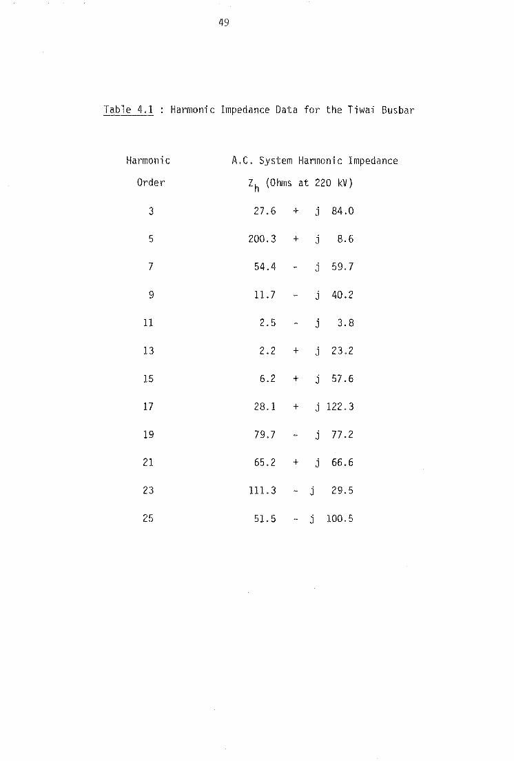
49
Table Harmonic Impedance Data for the Tiwai Busbar
Harmonic A.C. System Harmonic Impedance
Order Zh (Ohms at 220 kV)
3 27.6 + j 84.0
5 200.3 + j 8.6
7 54.4 j 59.7
9 11.7 j 40.2
11 2.5 j 3.8
13 2.2 + j 23.2
15 6.2 + j 57.6
17 28.1 + j 122.3
19 79.7 j 77 .2
21 65.2 + j 66.6
23 111. 3 j 29.5
25 51. 5 j 100.5
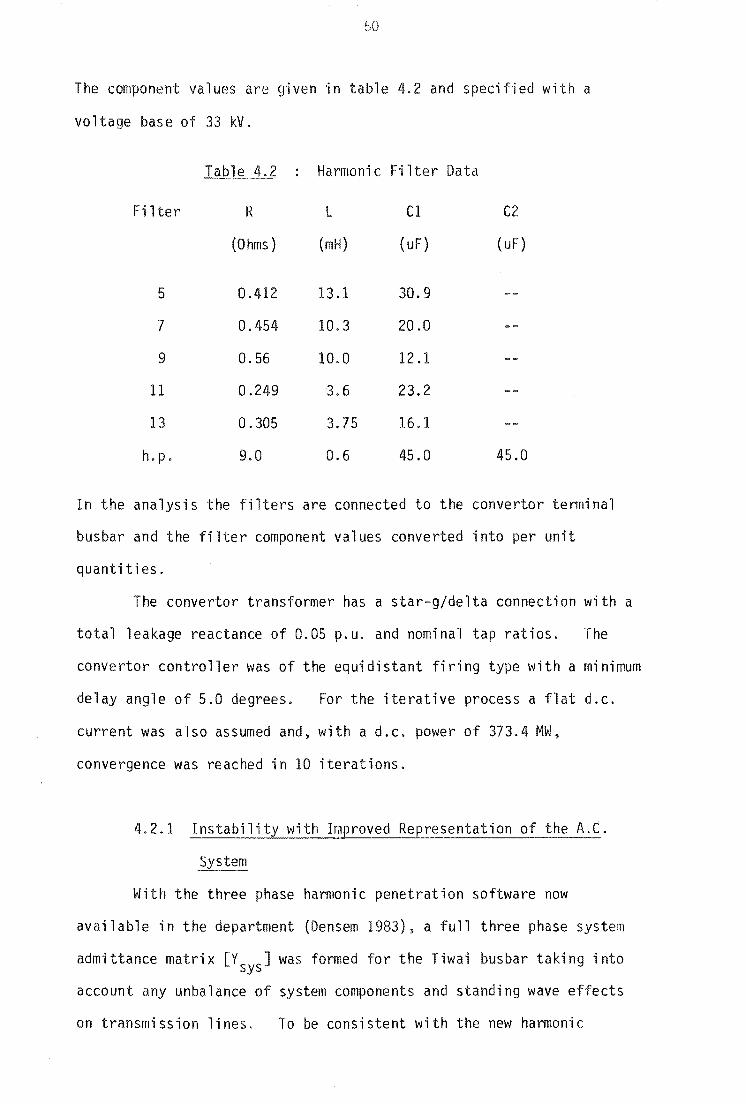
so
The component values are given in table 4.2 and specified with a
voltage base of 33 kV.
Table 4.2 Harmonic Fil ter Data
Fil R L C1 C2
(Ohms) (mH) (uF) (uF)
5 0.412 13.1 30.9
7 0.454 10.3 20.0
9 0.56 10.0 12.1
11 0.249 3.6 23.2
13 0.305 3.75 16.1
h.p. 9.0 0.6 45.0 45.0
In the analysis the filters are connected to the convertor terminal
busbar and the filter component values converted into per unit
quantities.
The convertor transformer has a star-gJdelta connection with a
total leakage reactance of 0.05 p.u. and nominal tap ratios. The
convertor controller was of the equidistant firing type with a minimum
delay angle of 5.0 degrees. For the iterative process a flat d.c.
current was also assumed and, with a d.c. power of 373.4 MW,
convergence was reached in 10 iterations.
4.2.1 Instabili Re resentation of the A.C.
With the three phase harmonic penetration software now
available in the department (Densem 1983), a full three phase system
admittance matrix [YSysJ was formed for the Tiwa; busbar taking into
account any unbalance of system components and standing wave effects
on transmission lines. To be consistent with the new harmonic

51
regulations in New land (New Zealand Electricity 1983), [YsysJ
was obtained for the first 50 harmonics, including both the odd and even
orders.
However, with the new a.c. system representation the Harmonic
Interaction program did not converge to a steady-state solution. The
problem was to decide if the instability was numerical, i.e., within
the computer, or due to a genuine instability (Yacamini and de
Oliveira 1980b). A 373.3 MW 6-pulse convertor at Tiwai is potentially
unstable as the actual smelter at Tiwai operates at 450 MW and uses a
48-pulse convertor configuration.
Under balanced conditions a convertor does not produce any
third harmonic current, but when the a.c. system is unbalanced third
harmonic current is produced (Phadke and Harlow 1968 and Reeve and
Krishnayya 1968). As a result the levels of third harmonic current
of the second run, and therefore the third harmonic voltage, were high
and a potential cause of the instability. The magnitude of the third
harmonic voltage for each phase at each iteration was plotted in
figure 4.2.
It can be seen that the level of third harmonic voltage was
high and unstable. The degree of instability is more clearly shown
when the third harmonic is compared to the 5th. The level of the
fifth harmonic is about 3% and does not vary more than 20% between
iterati ons .
To confirm that the instability with the improved a.c. system
representation is due to the third harmonic voltage, the ninth
harmonic filter was replaced by a third harmonic filter. The Q was
chosen to be 50, the same as the other filters. and a resistance value
equal to that used in the fifth harmonic filter (0.412 ohms at 33 kV).
With the new filter configuration the level of third harmonic voltage
was reduced and the solution converged on the fourth iteration.
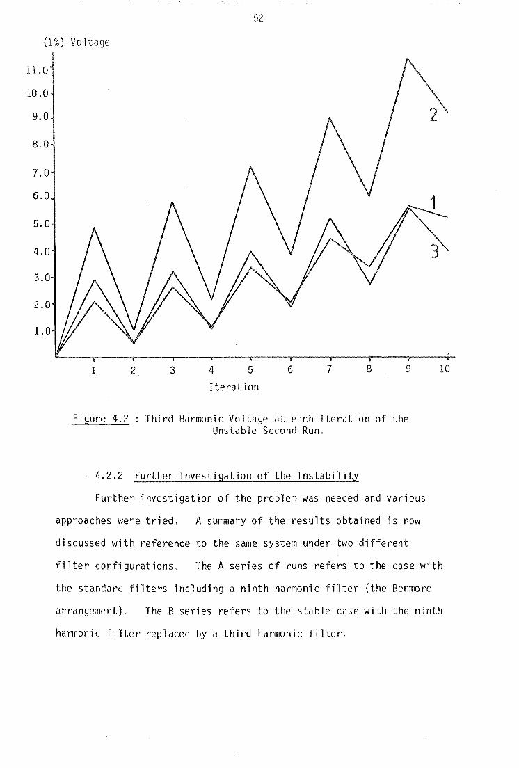
(1%) Voltage
11.0
10.0
g.O
8.0
7.0
6.0
5.0
4.0
3.0
2.0
1.0
1 2 3 4 5 6 7 8 9
Iteration
Figure 4.2 Third Harmonic Voltage at each Iteration of the Unstable Second Run.
4.2.2 Further Investigation of the Instability
Further investigation of the problem was needed and various
approaches were tried. A summary of the results obtained is now
discussed with reference to the same system under two different
10
filter configurations. The A series of runs refers to the case with
the standard filters including a ninth harmonic filter (the Benmore
arrangement). The B series refers to the stable case with the ninth
harmonic filter replaced by a third harmonic filter.

53
4.2.2.1 Reduced current
A harmoni c i nstabi 1 i ty can OCcUl~ when the size of the
convertor is large compared to the short-circuit MVA of the terminal
busbar. Therefore, the first approach used to determine the unstable
condition was to repeat the study under gradually increasing convertor
d.c. current. Convergence was obtained for values of current of 1.0,
2.0, 3.0 and 4.0 p.u. compared to the unstable 5.29 p.u. nominal case.
The larger the current the more iterations were required to obtain a
solution. Table 4.3 below shows the d.c. current, the d.c. power, the
short-circuit ratio and the number of iterations for each of the 5
levels of d.c. current.
Table 4.3 A Series Convergence
Run Id Power Short circuit ratio No. iterations
(p.u.) (MW)
Al 1.0 70.6 28.3 5
A2 2.0 141.2 14.2 8
A3 3.0 211.8 9.1 12
A4 4.0 282.3 7.1 37
A5 5.29 373.4 5.4
Looking at the number of iterations to convergence it can be
seen that as the current increases the solution becomes less stable.
A set of corresponding runs were performed with the third harmonic
filter. Table 4.4 shows that convergence was reached in less
iterations in each case.

54
Table 4. B Series Convergence
Run Id Pm ... er Short circuit ratio No. iterations
(p. u. ) (MW)
B1 1.0 70.6 28.3 4
B2 2.0 141.2 14.2 4
B3 3.0 211.8 9.1 4
B4 4.0 282.3 7.1 5
B5 5.29 373.4 5.4 4
The increased rate of convergence is obviously due to the
reduced level of third harmonic voltage distortion, although the
actual injections of third harmonic current were slightly higher.
Table 4.5 shows the magnitude of third harmonic voltage and current
for each of the runs Al - A5 and B1 - B5. The values of the table
the average of three phases.
Table Third Harmonic Voltage and Current at Each D.C. Current Level
Runs Al - A5 Runs Bl - B5
Id vo ltage current voltage current
(p. u.) (p.u.) (p.u.) (p.u.) (p.u.)
1.0 .002552 .00517 .000201 .00535
2.0 .005568 .01094 .000522 .01398
3.0 .007669 .01503 .000880 .02304
4.0 .009309 .01806 .001214 .03151
5.29 .001584 .Oll032
From figure 4.2. the third harmonic voltage for the unstable
A5 run was the cause of the instability. When the third harmonic
voltage was reduced by the inclusion of a third harmonic filter the
level of third harmonic voltages was reduced and stability restored.
are

55
In an actual system the stability is dependent on the relative size of
the convertor and the strength of the a.c. system. When the load was
reduced to about 75%, run A4 compared to run A5, the instability
disappeared.
The level of third harmonic voltage is,therefore, critical. The
worse the distortion the less equally spaced the zero-crossings become
causing distortion in the a.c. current injections.
For each iteration the convertor is modelled as a current
generator at harmonic frequencies. Therefore, the current injection
into the secondary of the convertor transformers, I h, causes a current
to flow into the a.c. system, Isys and the harmonic filters, Ifil . The
ratio Isys/lh is dependent on the relative size and phase of [Ysys ] and
[Yf ]· Under normal conditions the ratio is less than 1 but at
resonance can be greater than 1. In the run B5 the ratio is small.
The result of this is that the B series of runs can produce a smaller
level of third harmonic voltage distortion even though they produce
larger levels of third harmonic current, i.e .• there is only a small
harmonic current injection into the a.c. system.
Because of the relatively large change in d.c. current between
runs A4 and AS. another run (A4.5) was performed with the d.c. current
set at 4.5 p.u. After initial settling down the solution started to
converge. but after 100 iterations the execution was stopped as the
solution had reached a limit cycle. Therefore, this run did not add any
further information to the investigation.
There was also an attempt to make a B series to diverge.
This was done by increasing the d.c. current from the nominal value of
5.29 p.u. to 10.0 and 14.0 p.u. Both these runs were stable and gave
acceptable levels of harmonics. The level of 14.0 p.u. could not be
exceeded as this gave commutation angles of 55.9, 54.3 and 56.1
degrees, with the sampling routine used in the harmonic interaction
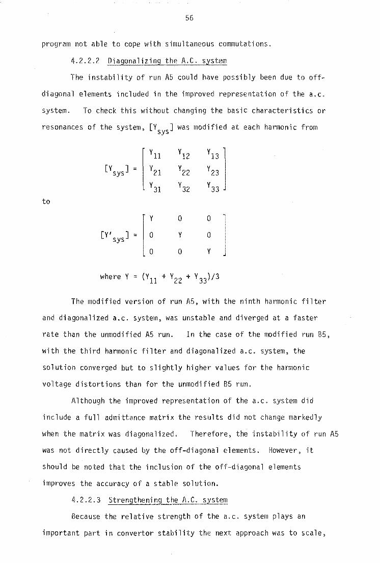
program not able to cope with simultaneous commutations.
4.2.2.2
The instability of run A5 could have possibly been due to off
diagonal elements included in the improved representation of the a.c.
system. To check this without changing the basic characteristics or
resonances of the system, [YSysJ was modified at each harmonic from
VII V12 VI3
[VSysJ = Y2I Y22 V23 V3I Y32 V33
to
V a a
[V/SYSJ = a V a a a V
where V = (VII + V22 + V33)/3
The modified version of run A5, with the ninth harmonic filter
and diagonalized a.c. system, was unstable and diverged a faster
rate than the unmodified AS run. In the case of the modified run 85,
with the third harmonic filter and diagonalized a.c. system, the
solution converged but to slightly higher values for the harmonic
voltage distortions than for the unmodified 85 run.
Although the improved representation of the a.c. system did
include a full admittance matrix the results did not change markedly
when the matrix was diagonalized. Therefore, the instability of run AS
was not directly caused by the off-diagonal elements. However, it
should be noted that the inclusion of the off-diagonal elements
improves the accuracy of a stable solution.
4.2.2.3 Strengthening the A.C. system
Because the relative strength of the a.c. system plays an
important part in convertor stability the next approach was to scale,

or strengthen, the a.c. syste, i ,e.,
[VlsYSJ == [V J. scale factor sys
Strengthening the a.c. system had a similar effect to
decreasing the current and only a small increase in system strength
was requried for stability. The results could be summarised as
fo llows:
1. As the scale factor decreases the number of iterations required
increases.
2. As the scale factor decreases the delay angles (and zero-crossings)
move further from their power-flow values.
3. As the scale factor decreases the level of non-characteristic
harmonic currents increase.
4. The voltage distortion is approximately inversely proportional to
the scale factor.
These observations are consistent with a genuine instability caused
by excessive third harmonic voltage. It;s also important to realise
that, as the scale factor changes, the resonance is modified and the
susceptibility to harmonic instability affected.
4.2.2.4 Further linking of the instability to the third
hannoni c
The relationship between the instability and third harmonic
voltage distortion was further emphasised by two additional runs.
The first run was with the maximum harmonic order present
being the third. This left the fundamental, the second harmonic which
was essentially zero, and the problem third harmonic. That is, all
the higher order harmonic voltages had a value zero and the
corresponding hannonic current injections were not calculated. Even
though only the third harmonic was present, the solution was still
unstable.

58
The second run included all harmonic orders except the
third, which was set to zero at each iteration in the routine which
solves for the a.c. harmonic vol ges. This run proved to be stable.
Therefore the instability is definitely due to the third
harmonic voltage being either genuinely or at least numerically
unstable.
4.2.2.5 Improved initial conditions
Numerical instabilities are often avoided by a better set of
initial conditions, and, therefore, the next strategy to try and achieve
convergence aimed at improving the initial conditions.
One way of achieving this ;s by initially eliminating the
third harmonic, or in general any other troublesome harmonic, from the
problem. After reaching an intermediate point of convergence the
harmonic is introduced gradually. With the use of a scale factor
which starts at zero and is incremented at each intermediate solution,
the program is reconverged until the scale factor equals one. This is
demonstrated in figure 4.3.
The algorithm was tested on the stable 85 case and was found
to be reliable in that it gave the same solution independently of the
rate at which the scale factor was increased.
However, when the algorithm of figure 4.3 was applied to the
unstable case convergence was still unobtainable. Different
strategies for increasing the scale factor were tried. Some results
and conclusions are given below:
1. When the increment was 0.2 a solution was reached at scale factors
of 0, 0.2, 0.4 and 0.6.
of O.S.
However no solution was reached with a value
2. When more than one strategy was used to reach the same scale
factor, essentially the same solution was reached at that value of
scale factor.

59
3. Starting from the converged state with a scale factor of 0.0 was of
no advantage over starting directly from a value of scale factor of
0.6. This was because the third harmonic was the harmonic which
caused the problems and therefore ignoring it (scale factor of 0.0) gave
no useful interaction and hence did not help convergence.
4. Increasing the scale factor slowly only gave a solution marginally
closer to that of the scale factor of 1.0 as compared to cases of more
rapid increases.
I ( DO UNTIL CONVERGED with SCALE=1.0
Read systems and initial conditions Converge Harmonic I ncrease SCALE SCALE=O Interaction
Figure 4.3 Improved Initial Conditions
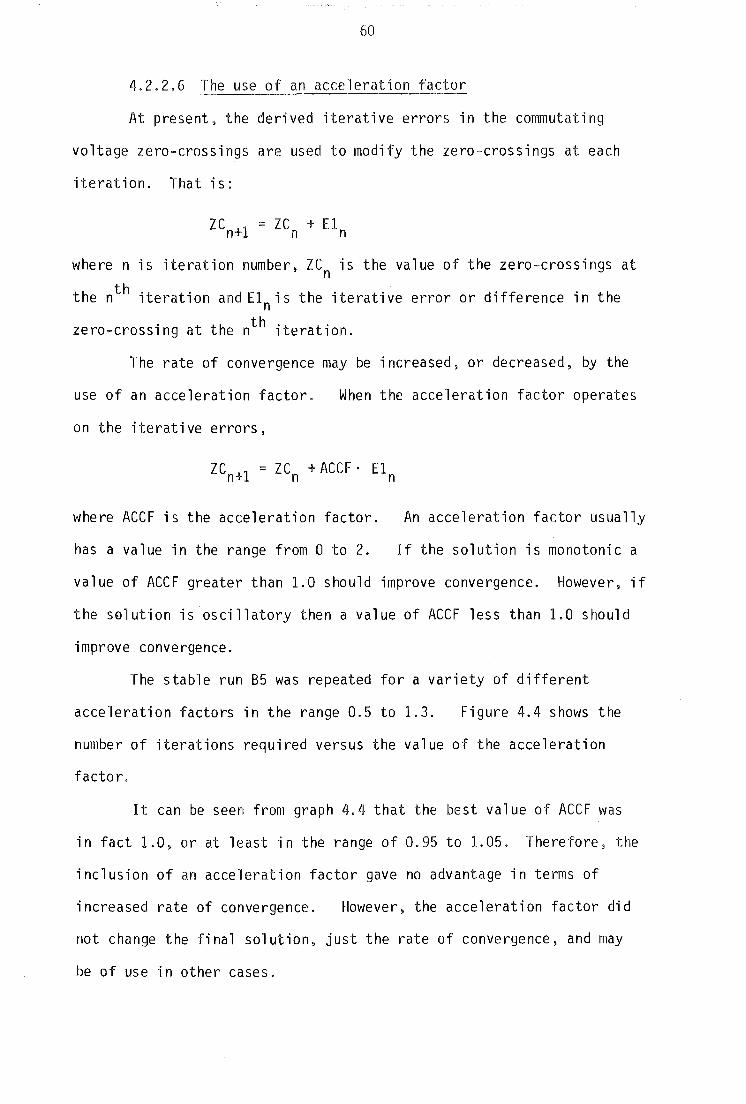
60
4.2.2.6 The use of an acceleration factor
At present, the derived iterative errors in the commutating
voltage zero-crossings are used to modify the zero-crossings at each
iteration. That is:
where n is iteration number, ZCn is the value of the zero-crossings at
the nth iteration and El n is the iterative error or difference in the
zero-crossing at the nth iteration.
The rate of convergence may be increased, or decreased, by the
use of an acceleration factor. When the acceleration factor operates
on the iterative errors,
where ACCF is the acceleration factor. An acceleration factor usually
has a value in the range from 0 to 2. If the solution is monotonic a
value of ACCF greater than 1.0 should improve convergence. However, if
the s~lution is oscillatory then a value of ACCF less than 1.0 should
improve convergence.
The stable run B5 was repeated for a variety of different
acceleration factors in the range 0.5 to 1.3. Figure 4.4 shows the
number of iterations required versus the value of the acceleration
factor.
It can be seen from graph 4.4 that the best value of ACCF was
in fact 1.0, or at least in the range of 0.95 to 1.05. Therefore. the
inclusion of an acceleration factor gave no advantage in terms of
increased rate of convergence. However, the acceleration factor did
not change the final solution, just the rate of convergence, and may
be of use in other cases.

Number of iterations
9
8
7
6
5
4
3
2
1
61
0.2 0.4 0.6 0.8 1.0 1.2
Acceleration Factor
Figure 4.4 : Effect of Acceleration Factor on Stable Run
For the unstable case of run A5 two acceleration factors of
0.2 and 0.1 were initially tried. In both cases a large amount of
third harmonic voltage was generated and divergence occurred. It is
improbable that an acceleration factor of 0.1 is too large but to test
this a value of 0.01 was tried. The solution was still divergent and
levels of third harmonic voltage distortion soon went well outside the
New Zealand harmonic regulations (New Zealand Electricity 1983).
Therefore the use of acceleration factors on both the stable run9
to try and improve the rate of convergence, and on the unstable
run, to try and improve reliability, both proved to be of no value.
4.2.3 The Effect of Harmonic Voltage During Commutation
4.2.3.1 e
In the previous work of Harker (1980) only the fundamental
terminal voltage and a purely inductive commutating impedance were
used to calculate the current samples during commutation. However, all
the runs so far have been sampled using an equation based on the
equation of Yacamini and de Oliveira (1980a). This includes the
voltage harmonic distortion on the terminal busbar and a series
resistance in the commutating impedance.
The effect of including all the voltage information during the
commutation was first tested on the stable 85 run. The first run was
carried out with full harmonic information, as normal. During the
second run, at each iteration only the fundamental voltages were used
during the sampling routine. That is, only the sampling was affected.
A third run was performed which took the solution of the second run as
initial conditions. then continued with all subsequent iterations
including full harmonic voltage during the sampling. A summary of
results is given in table 4.6.
Because the harmonic voltages did not directly affect the
commutation the solution of the second run took three iterations. The
third run, which took two extra iterations. produced essentially the
same solution as the first run as it is the same physical problem
solved via a different path.
4.2.3.2 An unstable case
The effect of including, or not including. the harmonic
voltage information when calculating the commutation current for the
unstable case was very interesting. A total of 8 runs were performed
to investigate different aspects of the phenomenon.
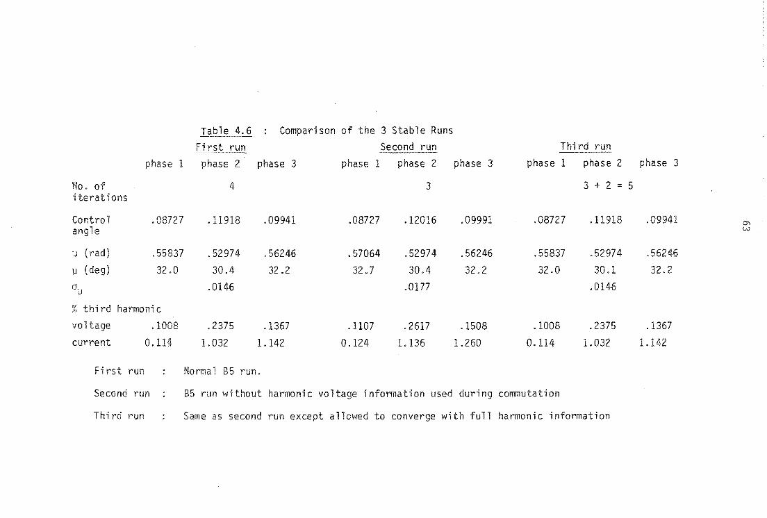
Table 4.6 Compari son of 3 Stable Kuns Second run I mrd
p 1 phase 2 3 phase 1 phase 2 phase 3 phase 1 phase 2 phase 3
4 3 3 + 2 = 5 ions
Contro 1 .08727 .11918 .09941 .08727 .12016 .09991 .08727 .11 .v.;J.;I""'f.1.
e
]J (rad) 837 .52974 .56246 .57064 .52974 .56246 .55837 .52
]J (deg) 32.0 30.4 32.2 32.7 30.4 32.2 .0 30.1 .2
a]J .0146 .0177 .0146
% tnlra narmonlC
tage .2375 .1367 .1107 .2617 .1508 .1008 .2375
0.1 1.032 1.142 0.124 1.136 1.260 0.114 1.032 1.1
First run Normal 85 run.
Second run 85 run without harmonic voltage information used durinq commutation
Thi rd run Same as second run exce allowed to converge with full harmonic information

64
1. Only the fundamental voltages were used to calculate the
commutation currents, with 512 samples per cycle.
only 5 iterations.
Convergence took
2. The second run took the solution of the first run and then added
the full harmonic voltage information in an unsuccessful attempt to
reconverge the unstable A5 run.
3. The full harmonic voltage information excluding the third harmonic,
the third harmonic being manually set to zero at each iteration, was
used to calculate the commutation samples.
iterations.
Convergence took 5
4. Because it was thought that 512 sample points may not be enough,
the third run was repeated with 2048 sample points. Again it took 5
iterations to converge.
5. Also the original unstable A5 run was repeated with 2048 sample
points and diverged.
6. In an attempt to isolate the instability the fifth run was repeated
with only the fundamental, second and third harmonic voltages being
used for the entire program run. Again convergence failed.
7. For the sake of completeness the first run was repeated with 2048
sample points instead of the previous 512.
but the results not analysed.
Convergence was obtained
8. To test whether the off-diagonal elements of the a.c. system
admittance matrix played an important part in the instability of the
sixth run it was repeated with the diagonalized form of the a.c.
system. Convergence failed.
The first, third, fourth and seventh runs converged. Table 4.7
shows the final solution for the first, third and fourth runs. There
were also four unstable runs, the second, fifth. sixth and eighth.

e 4.7 : Comparison of the Three Variations of the Unstable Run that Converged
First run Third run Fourth run
p 1 phase 2 phase 3 phase 1 phase 2 p 3 phase 1 2 3
No. of -iterations 5 3 + 2 ::: 5 3 + 3 5 -sample poi 512 512 2018
Control .08574 .09632 .08727 .08560 .09624 .08727 .08562 .09597 e
(rad) .54201 .57473 .57064 .52974 .57473 .57831 .54354 ,57933
lJ (deg) 33.4 31.1 32.9 32.7 30.4 32.9 33.1 31.1 33.2 0'\ tn
.0177 .0203 .0166 IJ
% thi rd harmoni c
voltage 1.5 3.602 2.097 1. 9 3.600 2.074 1.505 3.525 2. current 0.136 1.168 1.303 0.139 1.152 1.288 0.142 1.110 1. 9
rst run y fundamental voltage during commutation
T rd run c voltage excluded ng commutation
run ~ame as tnlrd run except 2048 sample points

66
By removing the harmonic voltage information from the
commutation a solution was reached in 5 iterations. However, when the
solution of the first run was used as initial conditions for a normal
full harmonic run a stable solution was not reached. These two runs
show the potential importance of including the full harmonic voltage
information during the commutation process.
The third run shows that the primary cause of the instability
is the effect of the third harnlonic voltage during commutation. With
all the harmonic voltages with the exception of the third present a
solution was obtained. Table 4.7 shows that including the other
harmonics does not have a significant great effect on the level of
distortion. In the fourth run the number of samples was increased to
2048 points but the difference between the third and fourth runs were
small, with only minor discrepancies in the commutation angle. This
was because with more sample points the fourth run could measure the
commutation angles more accurately.
Because the commutation circuit is mainly inductive, the lower
order harmonic voltages have the greatest effect on the commutation
current. Therefore, the third harmonic, if it is not filtered) is
very important, especially if the system has a resonance near the
third harmonic,
Figure 4.5 shows the configuration used for our example
VI Lc
II
12
V3 13 V2
Figure 4.5 Convertor Configuration

67
Figure 4.6 shows the effect of the third harmonic voltage on
the commutations when equidistant firings are assumed with zero delay
angle.
Fundamental Terminal Voltage
Positive Sequence
third Harmonic Voltage
Phase 1 Current
Phase 2 Current
Phase 3 Current
Figure 4.6
1 2 3
Effect of the Third Harmonic Voltage on the Commutation
From figures 4.5 and 4.6, commutations 1 and 4 are driven by
voltage V3" Similarly,commutations 2 and 5 are driven by V2 while
commutations 3 and 6 are driven by VI' Also. the current II is

68
cted by ~1 and ~3' while 12 is affected by ~2 and ~3 and I3 is
cted by ~l and ~3' In our case the even hprmonics were negligible
maki ng it safe to assume that ~l =~4 ~ ~2 = ~5 and ~6'
The third harmonic voltage shown is that of the open circuit
secondary voltage and the current is the line current in phases 1, 2
and 3. A positive sequence third harmonic with the phase relationship
as shown would accelerate the first and third commutations and retard
the second commutation, as demonstrated. In phase 1 both the
commutations are accelerated causing very little effect on the third
harmonic current. However, in phases 2 and 3 one commutation is
accelerated and the other retarded having an effect on the magnitude
of the third harmonic.
The effect of a component of negative sequence third harmonic
voltage is similar to that of the positive sequence. The first
commutation is retarded and the second and third commutations are
accelerated.
To simplify the problem a sixth run was performed with just
the third harmonic volta used. Again it was unstable. However,
when the sixth run was repeated with only a fundamental voltage used
during the commutation (the seventh run) the solution was stable.
Again this clearly shows that the presence of third harmonic during
the commutation process is the primary cause of the instability. This
was further emphasised by the last run which was a repeat of the sixth
run except with the diagonalized form of the a.c. system. The
diagonalized form of the a.c. system did not change the nature of the
instability.
For the sixth run the commutation angles and the level of
third harmonic voltage distortion are plotted for each iteration in
figures 4.7 and 4.8 respectively.

69
Commutation Angles (Radians)
0.6
0.5
0.4
0.3
0.2
0.1
1 2 3 4 5 6 7 8 9 10 11
Iteration Number
Fi .7 : Commutation Angles at Each Iteration (6 tn run)
Similarly a plot of the magnitude of the third harmonic voltage
distortion against the standard deviation of the commutation
angles is included in figure 4.9
On comparing these graphs several trends can be seen.
1. Odd iterations of the solution have a peak in the standard
deviation of the commutation angles. This corresponds to a peak
in the level of third harmonic voltage.

(%) Vol
12.0
11.0
10.0
9.0
8.0
7.0
6.0
5.0
4.0
3.0
2.0
1.0
70
1 2 3 4 5 6 7
Iterarion Number
2
8 9 10 11
3
1
Figure 4.8: Third Harmonic Voltage at Each Iteration (6th run)
(%) Voltage
11.0
10.0
9.0
B.O
7.0
6.0
5.0
4.0
3.0
2.0
1.0
Figure 4.9
0.01 0.02 0.03 0.04
2
3
1
0.05 Standard Variation of the Commutation Angles
Third Harmonic Voltage Versus the Standard Deviation of the Commutation Angles
(6th run)

71
2~ k in third harmonic voltage magnitude, occurring on an odd
i ration, producing an extension in ~2 decreasing the standard
deviation for the next iteration (an even iteration).
3. Because the standard deviation is smaller during the even
iterations the level of third harmonic is a minimum.
4. A minimum in third harmonic voltage magnitude, occurring on even
iterations, produces a shortening of ~2 increasing the standard
deviation for the next iteration (an odd iteration).
Figure 4.9 shows that there is a distinct correlation between
unsymmetrical commutation angles and the level of third harmonic
distortion.
Commutation Angles (Radians)
0.6
0.5
0.4
0.3
0.2
0.1
Figure 4.10
2 3 4 5 Iteration Number
Commutation Angles at Each Iteration (8th run)

72
Similarly. run eight was included to reduce the complexity of
the full three phase representation of the a.c. system present in the
fifth and sixth runs. The commutation angles and the level of third
harmonic voltage distortion are plotted for each iteration in figures
4.10 and 4.11 respectively.
(%) Voltage 2
10.0
9.0
8.0
7.0
6.0
5.0
4.0
3.0
2.0
1.0
1 2 3 4 5
Iteration Number
Third Harmonic Voltage at Each Iteration (bth
run)
Also, a plot of the magnitude of the third harmonic voltage distortion
against the standard deviation of the commutation angles is included
in figure 4.12.
These graphs show the same trends as figures 4.7 and 4.8 for
the 6th run. That is, a maximum in standard deviation leading to
a maximum in the third harmonic distortion. This in turn leads
to a reduction in standard deviation of the commutation angles.

73 Vo ltage (%)
10.0
9.0
8.0
7.0
6.0
5.0
4.0
3.0
2.0
1.0
0.01 0.02 0.03 0.04
Standard Qeviati9n of commutatlon ang es
Figure 4.12 : Third Harmonic Voltage Versus the Standard Deviation of the Commutation Angles (8 th run)
To help understand the oscillatory nature of the solution,
a graph of the phase angle of the third harmonic voltage at each
iteration is illustrated in figure 4.13.
1
Figure 4·13
2 3 Iteration
number
4 5
Phase Angle of the Third Harmonic

74
To express the phase in terms of the third harmonic, firstly the
phase angles of the third harmonic voltages were multiplied by 3 and
then put into the range -180 to +180 degrees. In each case the phase
angles of the third harmonic voltages alternated by 180 degrees between
consecutive iterations. This means that the effect of the third
harmonic is opposite at each consecutive iteration. This would
produce the oscillatory nature of the graphs in figures 4.10 and 4.11
for the eighth run and explain the oscillatory nature of the sixth
run with the full three phase a.c. system representation.
4.2.3.3 Further investigation of third harmonic during
commutation
Further investigation of the effect of third harmonic voltage
during the commutation process should be concentrated on the eighth
run. This represents the most simple situation as only the third
harmonic voltage is present and the a.c. system representation is
purely diagonal. The approach used was to change the phase angle of
the a.c. system third harmonic admittance and give a different phase
relationship between the current injected into the a.c. system and the
resulting voltage produced on the terminal busbar.
This was done by keeping the admittance constant and the angle
varied from -90 to +90 degrees. As a comparison the process was
repeated for the same case but without filters in order to avoid
possible parallel resonances. Therefore, any variation of stability
will be due to the change of system angle at third harmonic and not
due to resonance effects.
At the third harmonic Ysys = 0.0026 - jO.0063 siemens.
therefore Z = l/Y sys sys = 55.97 + j135.63 ohms
= 146.72 angle 67.57 ohms.

75
The actual system angle is approximately 67.5 degrees.
Therefore a useful range of sy~tem impedance angles would be -90 to
+90 degrees with steps of 22.5 degrees. The a.c. system admittance,
and impedance, from table 4.8 were used in the eight run of the
previous section with and without filters.
Table 4.8 A Set of Third Harmonic A.C. Admittances and Impedances with Angles from -90 to +90 degrees
Angle of Zsys Zsys(rl) \ys (s)
-90.0 - j146. 72 + j.0068
-67.5 56.15 - j135.55 .0026 + j.0063
-15.0 103.75 - j 103.75 .0048 + j.0048
-22.5 135.55 - j 56.15 .0063 + j.0026
0.0 146.72 .0068
22.5 135.55 + j 56.15 .0063 - j.0026
45.0 103.75 + jl03.75 .0048 - j.0048
67.5 56.15 + j135.55 .0026 - j.0063
90.0 + jI46.72 - 'j .0068
The results are summarized in figure 4.14 which shows the
number of iterations for each of the 18 runs.
With filters the problem of resonance may occur. That is at
a particular system angle the total system admittance can become
purely conductive, when the susceptance of the filters cancels the
susceptance of the a.c. system.
The system admittance = 0.0068 I mpedance angle siemens @ 220 kV
:::: 3.2987 I-Impedance angle p.u. @ PBASE 100MVA
The filter admittance 0.0154 + jl.7906 p.u.
With these parameters. a resonance occurs at 32.87 degrees.

76 Number of ite ions
24
22
20
18
16
14
4
2
, I I
00, I
\ I , \
\ \ I \ \ \
\ With filters
Without fi lters
90° 45° a 45° 90° Phase of System Impedance at Third Harmonic
Figure 4.14 : Number of Iterations Versus Impedance Angle
While figure 4.15 is a plot of the percentage third harmonic
distortion in each of the runs.
.... ~ .........
Without fi lters
....... With fi lters
Voltage (%)
3.0
2.5
2.0
,
, . · ,
! , . , , , , , I , , , ,
........ ...... 1 .. 5 ",,~~I I
~"_~~. _.a ~ __ ..... m .. '" "
La
·:1·············· .. ·.· ..
0.5
· . · . · ' · ' , ; :. , . . '
" .... ~. " I
· 2
· . .:.: .. '
., ! •
-90 0 45° a 45° gUo Phase of System Impedance at T~ird HRrmonic
----'''--_.c...-..:..-'- : Third Harmonic Voltage Versus Impedance Angle

77
The total a.c. system admittances (filters plus a.c. system)
for the nine cases investigated are given in table 4.9 and figure 4.16
shows the admittance locus indicating the total, system and filter,
admittances.
B
----~------~-----G
Figure 4.16 Total Admittance Loci Including Fi lters for Variable Impedance Angle
Tabl Total A.C. Admittance with Filters
Impedance Total admittance (angle) Conductance Susceptance Angle
-90.0 5.0893 89.8 0.0154 5.0983
-67.5 5.0041 75.2 1.2778 4.8382
-45.0 4.7448 60.3 2.3479 4.1231
-22.5 4.3246 43.8 3.0630 3.0530
0.0 3.7669 28.4 3.3141 1. 7906
22.5 3.1082 9.8 3.0630 0.5282
45.0 2.4097 13.0 2.3479 -0.5419
67.5 1.7924 -44.5 1.2778 -1.2570
90.0 1.5082 -89.3 0.0154 -1. 5081
If table 4.9 is compared with the results of figures 4.14 and 4.15, some
interesting facts emerge.

78
The case with an impedance angle of 67,5°was stopped after 5
iterations, because the third harmonic distortion was large enough to
force the delay angle to attempt to go negative. Similarly, the case
with an impedance angle of 45,0 0 was stopped at the 202 nd
iteration with a negative delay angle.
For the cases with negative values of th<ird harmonic system
angle the number of iterations required was reasonably constant, as
was the level of third harmonic voltage.
However for values of system angle 45.00 and 67.So no solution
could be reached, Also for a small change in system angle near the
instability, a large change in third harmonic voltage occurred.
Table 4,10 shows the total a.c. system admittance for the
nine impedance angles in the absence of filters.
Table 4.10 : Total A.C. Admittance Without Filters
Impedance Total admittance (angle) Conductance Susceptance Angle
-90,0 3.2912 90.0 0.0000 3.2912
-67.5 3.2987 67.6 1.2584 3.0492
-45.0 3.2855 45.0 2.3232 2.3232
-22.5 3.2987 22.4 3.0492 1.2584
0.0 3.2912 0.0 3.2912 0.0000
22.5 3.2987 -22.4 3.0492 1.2584
45.0 2.4097 -45.0 2.3232 -2.3232
67.5 3.2987 .6 1.2582 -3.0492
90.0 3.2912 -90.0 0.0000 3.2912
In this case the effect of varying the system angle can be
investigated more accurately and any changes in percentage distortion
or the number of iterations can be better assessed.
For capacitive systems figure 4.14 shows that convergence was
rapidly achieved. As the a,c. system goes inductive the convergence

79
slows down the number of iterations reaching a peak at an impedance
angle of 45 degrees. With a purely inductive system the rate of
convergence was fast.
In contrast the curves for % third harmonic voltage distortion
follow the opposite trend. The impedance angle of 45.0° gave a
minimum value whereas it required the most iterations.
Table 4.11 shows the actual levels of third harmonic
distortion for -67.5°,0.00and 67.5°degrees at each iteration. For
the first iteration the values are essentially the same because the
currents are identical and the magnitude of the system impedance
constant. But after subsequent iterations three different
solutions were produced. The greater the difference between the final
solution and the first, in terms of the zero-crossings, the more
iterations required.
Table 4.11 : Level of Third Harmonic Voltage (%) at Each Iteration
No fi He rs and constant magnitude of a.c. system impedance.
ImEedance Angle = -67.5 Impedance Angl e = 0.0 Impedance Angle = 67.5
1 0.952 2.214 1.263 0.954 2.219 1.266 0.952 2.214 1.263
2 l.077 2.420 1.345 0.352 0.782 0.434 0.336 0.827 0.495
3 1.058 2.368 1.311 0.735 1. 698 0.961 0.716 1.673 0.959
4 1.052 2.357 1.306 0.492 1.116 0.626 0.486 1.167 0.683
5 1.053 2.358 1.306 0.647 1.487 0.841 0.625 1.472 0.848
6 0.550 1.252 0.705 O. 5~"1 1.288 0.750
7 0.612 1.402 0.792 . 0.592 1.400 0.809
8 0.572 1.306 0.736 0.561 1.333 0.774
9 0.597 1.366 0.771 0.580 1. 373 0.795
10 0.569 1. 349 0.783
11 0.575 1.363 0.790
12 0.571 1.355 0.786
13 0.574 1.360 0.788

4.2.4 Co ons
The nature of the instability was examined using a variety of
methods. These included reducing the load and strengthening the a.c.
system. Both these gave results consistent with a genuine instability
caused by excessive third harmonic voltage distortion due to the
relative size of the convertor. Similarly, when the a.c. system was
diagonalized in section 4.2.2.2 the stability did not change which is
consistent with an actual instability.
Two numerical analysis approaches were also tried. Neither
improving the initial conditions nor introducing an acceleration
factor made any real improve~ent to the solution. This is consistent
with the presence of a genuine instability rather than purely a
numerical problem.
An attempt was made to isolate the problem. It was clear that
the instability was due to the third harmonic and in particular the
presence of third harmonic voltage distortion during the commutation
process. The problem was still further simplified by the removal of
all the other harmonics except the third, but still the instability
remained.
Another interesting aspect is the effect of varying the system
impedance angle at third harmonic on the stability and the level of
distortion. For simplicity this was done with only the third harmonic
present. This investigation clearly shows that both the stability of
the solution and the level of distortion depend on the system angle as
well as the magnitude of the system impedance. That is, the angle
between the current injections and the voltage distortion play an
important part in the harmonic interaction. The impedance angle at
harmonics is not indicated by the S.C.R. concept, making the SCR a
poor indication of system strength.

81
The stable B series of runs also provided useful information.
As in the case of the operation of a stable convertor small
disturbances should not affect its steady state operation. Similarly.
the stability and final solution of the B series are not affected by
the path chosen. That is, whether a scale factor for the harmonic
voltages (section 4.2.2.5), an acceleration factor for the zero
crossings {section 4.2.2.6} or a scale factor for the harmonic
voltages only during the commutation process (section 4.2.3.1) is used
or simply the unmodified algorithm is used, the final solution is
unaltered.
At this stage it should be emphasised that instability of the
iterative algorithm cannot necessarily be attributed to a genuine
instability.
4.3 SINGLE GENERATOR AND LINE A.C. SYSTEM SUPPLYING A 6-PULSE
CONVERTOR AT TIWAI
To try and isolate the root of the problem, the a.c. system
was simplified to a single generator and transformer and two
parallel double circuit lines to transfer the power to the convertor.
Figure 4.17 shows the simplified a.c./d.c. system.
Convertor Supplied by a Single Generator/Transformer and Line A.C. System
While the system ;s not a realistic representation of the actual South
Island transmission system (Densem 1983), it does include line
82
unbalance and series and parallel resonances typical of a.c. systems
which are important in the operation of convertor loads.
The generator is a single equivalent generator representing
the seven machines at Manapouri power station giving the total
generation of 690 MW. The equivalent generator has a positive
sequence reactance of 0.04 p.u., a zero sequence reactance of 0.02
p.u. and a negative sequence reactance of 0.004 p.u. at a power base
of 100 MVA. For simplicity the machine's sequence resistances were
neglected. The generator transformer has 0.0164 p.u. leakage
reactance, 0.006 p.u. resistance and a star-g/delta connection.
The transmission system consists of two 166.6 Km double circuit lines
as described in Appendix A4. An earth resistivity of 100 ohm-metres
was used when modelling the earth return.
The star-g/delta connected convertor transformer has a leakage
reactance of 0.05 p.u. The convertor was operated with either a
constant delay angle or equidistant firing control with the delay
angle on valve one specified as 5.0 degrees. The d.c. system consists
of a resistance, specified to vary the d.c. power. and an infin;
smoothing inductor to give a flat d.c. current.
The harmonic filters are the same as those used in section 4.2
except that no uncharacteristic third or ninth harmonic filters have
been included. This gives a fundamental filter susceptance of 0.043
siemens, or 0.46933 p.u .• and provides 46.9 MVars of reactive
compensation.
4.3.1 Initial Conditions
As for the previous case, the initial conditions have been
calculated using the three phase a.c./d.c. power flow. The power flow
requires six control specifications to define the convertor's operation
(Harker 1980). The delay angle on valve one and the three tap ratios

83
are fixed, with the other two specifications being supplied by the
control strategy. Finally, with the voltage at the generator's phase
lal terminal fixed at 1.045 p.u. and the d.c. system resistance
specified, the power flow can be run to produce the required initial
conditions.
4.3.2 The Harmonic Impedances
4.3.2.1 The system without the filters
The impedance looking back into the Tiwai busbar. not
including the harmonic filters, is made up of the three system
components, i.e., the line, the transformer and the generator, with the
line being the most dominant.
Using the three phase harmonic penetration software of Densem
(1983). a full three phase system admittance matrix [YSysJ, and the
corresponding equivalent impedance information, was formed for the
Tiwai busbar.
The large level of harmonic impedance unbalance can be seen
in figure 4.18 which shows the three phase impedance up to the sixth
harmonic. Because the impedances are calculated assuming a positive
sequence current injection, a negative resistance is observed in phase
lalnear the sixth harmonic.
4.3.2.2 The effect of filters
As the a.c. system impedance is inductive below the fifth
harmonic and the filters capacitive, a parallel resonance may occur
which would affect any harmonic interaction.
Because a convertor can only produce positive and negative
sequence injections, and because the a.c. system and filter impedances
to the positive and negative sequences are equal. the effect of the
filters was analysed in the positive sequence only.

X(n)
1500
1000
500
300 290
-500
1000
84
R(n)
Three Phase Impedance Loci
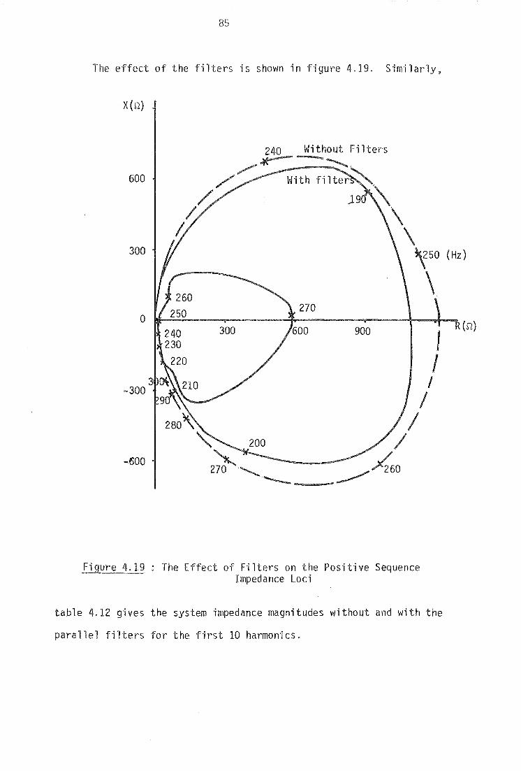
85
The effect of the filters is shown in figure 4.19. Similarly,
X(n)
Without Fil ters -600 With fi lter'~
)9 <~
\ \
300 50
\ 270
0 300 900
J
I I
/ /
-f)00
Figure 4.19 The Effect of Filters on the Positive Sequence Impedance Loci
table 4.12 gives the system impedance magnitudes without and with the
parallel filters for the first 10 harmonics.
(Hz)
R (n)
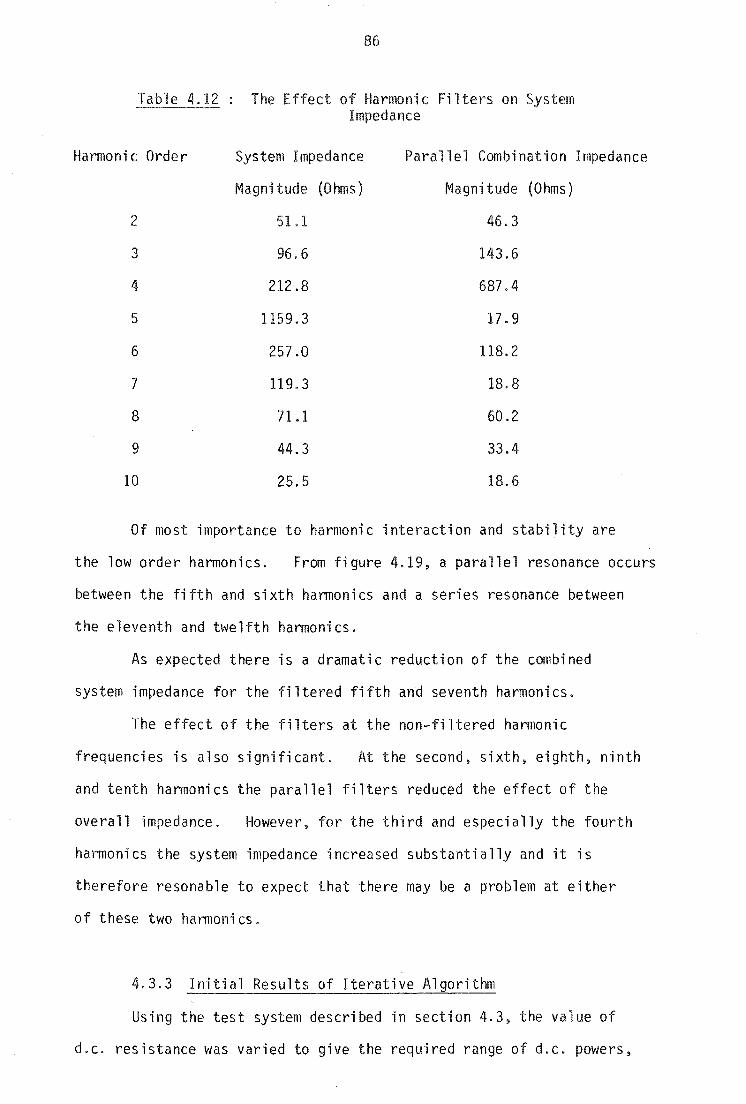
86
Table .12 The E of Harmonic Filters on System Impedance
Harmonic Order System Impedance Parallel Combination Impedance
Magnitude (Ohms) Magnitude (Ohms)
2 51.1 46.3
3 96.6 143.6
4 212.8 687.4
5 1159.3 17.9
6 257.0 118.2
7 119.3 18.8
8 71.1 60.2
9 44.3 33.4
10 25.5 18.6
Of most importance to harmonic interaction and stability are
the low order harmonics. From figure 4.19, a parallel resonance occurs
between the fifth and sixth harmonics and a series resonance between
the eleventh and twelfth harmonics.
As expected there is a dramatic reduction of the combined
system impedance for the fi ltered fifth and seventh harmoni cs.
The effect of the filters at the non-filtered harmonic
frequencies is also significant. At the second, sixth. eighth. ninth
and tenth harmonics the parallel filters reduced the effect of the
overall impedance. However, for the third and especially the fourth
hal~onics the system impedance increased substantially and it is
therefore resonable to expect that there may be a problem at either
of these two hal1llOni cs.
4.3.3 Initial Results of Iterative Algorithm
Using the test system described in section 4.3, the value of
d.c. resistance was varied to give the required range of d.c. powers,

in MW. The number of iterations for cases of constant delay angle
and equidistant firing control, without control filters, are given in
table 4.13.
Table 4.13 D.C. Power and Number of Iterations for Various D.C. Rei ances
D.C. Resistance Constant Delay Angle Equidistant
Kilo ohms D.C. Power No. Iterations D.C. Power No. Iterations
0.004650
0.004000
0.003500
0.003000
0.002800
0.002750
0.002740
0.002735
0.002730
0.002725
0.002700
0.002600
0.002325
238.86
267.95
295.18
327.88
342.74
346.65
347.46
347.86
348.25
348.65
350.65
358.85
382.97
5
5
6
7
9
8
8
9
x
x
x
x
x
238.68
267 .72
294.93
327.59
342.46
346.35
347.14
347.53
347.93
348.33
350.32
358.48
382.59
4
5
5
6
6
6
6
6
6
6
6
6
7
An instability numerical or real) is evident with constant
delay angle control when a d.c. power of 347.86 is exceeded. When the
a.c. system admittance was diagonalized to its positive sequence value
the instability shifted an insignificant amount to 348.25. The
instability is consistent with the definition in section 4.2.1 as it
appears to be independent of the unbalanced nature of the a.c. system.
The level of uncharacteristic third and fourth harmonic
voltages for the stable runs with the constant delay angle control are
given in table 4.

88
Table 4.14 Level of Third and Fourth Harmonic Voltage (%) for Each Stable D.C. Power
D.C. Power
MW
238.86
267.95
295.18
327.88
342.74
346.65
347.46
347.86
Thi rd Harmon; c
abc
0.0432 0.0864 0.1290
0.0491 0.1078 0.1560
0.0507 0.1329 0.1822
0.0413 0.1602 0.1998
0.0415 0.1676 0.2068
0.0414 0.1658 0.2049
0.0409 0.1679 0.2065
0.0409 0.1723 0.2106
Fourth Harmonic
abc
0.0001 0.0002 0.0002
0.0001 0.0001 0.0002
0.0008 0.0004 0.0008
0.0013 0.0011 0.0015
0.0102 0.0090 0.0125
0.0030 0.0023 0.0042
0.0026 0.0028 0.0036
0.0116 0.0093 0.0133
The level of third harmonic voltage is approximately linear
with d.c. power. However, the level of fourth harmonic voltage, which
is initially insignificant, increases in an erratic manner. This
cannot be explained in terms of a simple harmonic magnification. The
erratic nature of the fourth harmonic of the stable runs is due to an
unstable fourth harmonic component which grows too slowly between
successive iterations to be detected. This results in the premature
convergence of the iterative algorithm.
4.3.4 Modifications to Avoid Premature Conve nce of the
Iterative Algorithm
The problem of premature convergence of the iterative algorithm
can be rectified by either specifying a smaller convergence tolerance
or introducing a disturbance to excite any potential instability.
4.3.4.1 Closer tolerance
There are two main disadvantages in simply reducing the
convergence tolerance. Firstly~ with the closer tolerance, stable
runs would take an excessive number of iterations. Secondly, even
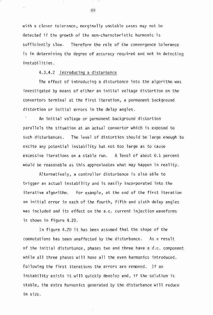
89
with a closer tolerance, marginally unstable cases may not be
detected if the growth of the non-characteristic harmonic is
sufficiently slow. Therefore the role of the convergence tolerance
is in determining the degree of accuracy required and not in detecting
instabilities.
4.3.4.2 Introducing a disturbance
The effect of introducing a disturbance into the algorithm was
investigated by means of either an initial voltage distortion on the
convertors terminal at the first iteration, a permanent background
distortion or initial errors in the delay angles.
An initial voltage or permanent background distortion
parallels the situation at an actual convertor which is exposed to
such disturbances. The level of distortion should be large enough .to
excite any potential instability but not too large as to cause
excessive iterations on a stable run. A level of about 0.1 percent
would be reasonable as this approximates what may happen in reality.
Alternatively, a controller disturbance is also able to
trigger an actual instability and is easily incorporated into the
iterative algorithm. For example, at the end of the first iteration
an initial error in each of the fourth, fifth and sixth delay angles
was included and its effect on the a.c. current injection waveforms
is shown in figure 4.20.
In figure 4.20 it has been assumed that the shape of the
commutations has been unaffected by the disturbance. As a result
of the initial disturbance, phases two and three have a d.c. component
while all three phases will have all the even harmonics introduced.
Following the first iterations the errors are removed. If an
instability exists it will quickly develop and) if the solution ;s
stable, the extra harmonics generated by the disturbance will reduce
in size,
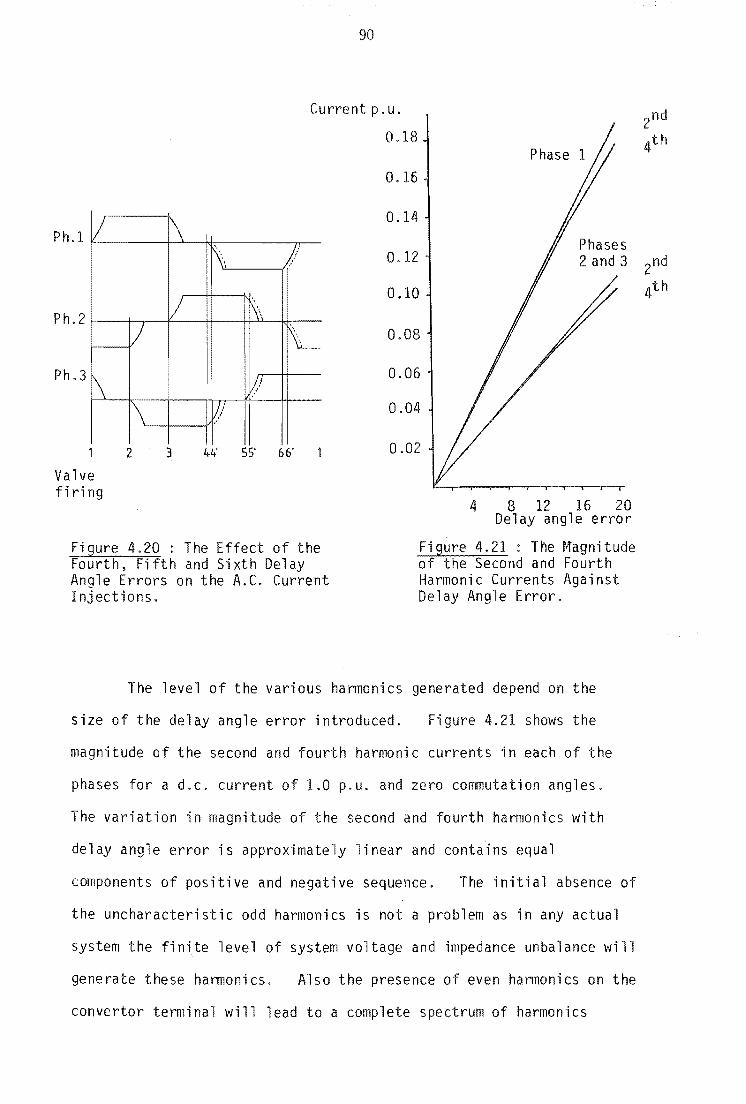
90
Current p. u.
0.18
Ph.1 V
Ph.2 1
Ph.3 \
Valve firing
\
/ I)
1\ 2 3
1\ /I
i I\. L
w j./ "
44' 55' 66'
Figure 4.20 : The Effect of the Fourth. Fifth and Sixth Delay Angle Errors on the A.C. Current I nj ect ions.
0.16
0.14
0.12
0.10
0.08
0.06
0.04
0.02
4 8 12 16 20 Delay angle error
Figure 4.21 : The Magnitude of the Second and Fourth Harmonic Currents Against Delay Angle Error.
The level of the various harmonics generated depend on the
size of the delay angle error introduced. Figure 4.21 shows the
magnitude of the second and fourth harmonic currents in each of the
phases for a d.c. current of 1.0 p.u. and zero commutation angles.
The variation in magnitude of the second and fourth harmonics with
delay angle error is approximately linear and contains equal
components of positive and negative sequence. The initial absence of
the uncharacteristic odd harmonics is not a problem as in any actual
system the finite level of system voltage and impedance unbalance will
generate these harmonics. Also the presence of even harmonics on the
convertor terminal will lead to a complete spectrum of harmonics
2nd
4th

91
(Reeve et al 1969) which will become evident at the end of the second
iteration. Finally, minor reductions in the magnitudes of the
characteristic harmonics may occur but this will have no effect on
the stability.
An alternative approach of introducing the errors to the delay
angles of the evenly numbered valves would, if adopted, generate no
uncharacteristic odd harmonics, as for the previous case, and only
produce uncharacteristic even harmonics on one sequence. That is,
positive sequence for orders of 6k + 4 and nagative sequence for
orders 6k + 2. where k is an integer. Because harmonic instabilities
can exist either because of a positive or a negative sequence
uncharacteristic harmonic voltage (Ainsworth 1967). this type of
disturbance was not used.
4.3.5 The Effect of Control Disturbance
When a control disturbance is introduced at the end of the
first iteration of the iterative algorithm. several program runs
previously thought to be stable diverged. Table 4.15 shows the d.c.
power and the number of iterations for the case of a constant delay
angle controller for a disturbance of 0.1 radians to the fourth,
fifth and sixth delay angles.
Instead of the previous maximum d.c. power before divergence
(347.86 MW). the inclusion of controller disturbance has reduced
the d.c. power limit to 151.83 MW.
The stable 85.59 MW d.c. power case was examined with a
varying sized initial disturbance. With an initial error of
0.0025 radians the algorithm converged to a stable solution in seven
iterations. This was increased to thirteen iterations with an
initial disturbance of 0.1 radians. Similarly, the 225.53 MW d.c.
power case, previously thought to be stable, was examined more fully.

92
Table 4.15 D.C. Power and Number of Iterations for An Introduced Controller Disturbance
D.C. Resistance D.C. Power No. I terat ions
Ki 10 ohms
0.02000 65.15 8
0.01500 85.59 10
0.01200 105.33 12
0.01100 114.12 15
0.01050 119.02 17
0.01000 124.40 19
0.00800 151. 83 221
0.00775 156.11 232 diverged
0.00750 160.71 81 diverged
0.00700 170.55 49 diverged
0.00600 194.34 19 diverged
0.00500 225.53 11 diverged
When the disturbance was equal to or less than 0.000126 radians the
solution converged in five iterations. For slightly larger
disturbances divergence of the solution was found, being detected by
the presence multiple zero crossings of the commutating voltages.
in 23 iterations and in only seven iterations for a disturbance of 0.1
radians.
Ideally, for a stable case. a small if not zero disturbance
is desirable for rapid convergence. However. for an unstable case
a large disturbance is required to detect an instability quickly.
Therefore as it is not known before the iterative algorithm is run
whether convergence or divergence will occur, a compromise is needed.
About 3.0 degrees or about 0.05 radians would be a good size of
disturbance as this would be a typical value for controller errors
(Reeve and Krishnayya 1968). Also, from the results in this section,

a disturbance of this size would be large enough to trigger a
potential instability.
4.3.6 Harmonic Voltage Distortion of the Simplified Test
System with Increased Filter Capacity
The reactive power rating of the filters was increased from
previous value of 46.9 MVar to 66 MVar. This was achieved in the
algorithm by increasing the voltage base on the filters from 33 kV to
39 kV. This had the effect of reducing the a.c. system impedance at
fourth harmonic and increasing the system impedance at third harmonic.
Also the equidistant controller was modified to produce firing
instants which are independent of the terminal voltage distortion,
instead of the previous strategy described in chapter 3 of fixing the
delay angle of valve one and adjusting the other delay angle to
maintain equidistant firing pulses.
Figures 4.22 to 4.26 show the level of third harmonic voltage
on the convertor terminal, as a function of the d.c. power, for
various combinations of control strategy and system conditions.
The need for an iterative algorithm is clearly demonstrated by
comparing figures 4.22 and 4.23. V /V1 (%)
.6
.5
.4
.3
.2
. 1
100 200 300 400 D.C. Power (MW)
Figure 4.22 : Third Harmonic Voltage in the Three Phases of the Convertor Terminal with Equidistant Control and Perfectly Flat
D.C. Current: Without Iterations

1.3
1.2
1.1
1.0
.9
.8
.7
.6
.5
.4
.3
.2
.1
94
100 200 300 400 D. C. Power (MW)
Figure 4.23 Third Harmonic Voltage in the Three Phases of the Convertor Terminal with Equidistant Control and
Perfectly Flat D.C. Current: With Iterations
In both cases an equidistant controller is specified, the d.c. current
is assumed to be perfectly flat and the d.c. power varied. Figure 4.22
illustrates the voltage distortion without iterations, that is the
a.c. current is due to the fundamental component of the terminal
voltage only. while figure 4.23 shows the voltage distortion at the
end of the iterative process. The iterative solution greatly changes
the level of the uncharacteristic third harmonic.

The effect
4.23 (equidistant
V 3/V 1 (%)
1.2
1.1
1.0
0.9
0.8
0.7
0.6
0.5
0.4
0.3
0.2
0.1
95
of the type of controller is illustrated in figures
control) and 4.24 (constant delay angle control).
100 200 300 D.C. Power (MW)
Figure 4.24 Third Harmonic Voltage in the Three Phases of the Convertor Terminal with Constant Delay Control and
Perfectly Flat D.C. Current
As expected (Ainsworth 1967) the levels of third harmonic distortion
for the same d.c. power are seen to be much larger in the case of
phase angle control.
If the size of the filters is further increased the
characteristic harmonics are reduced due to the lower filter
impedance. However, such an increase results in larger capacitance
at lower order harmonics, in particular the third. The results of
figure 4.25 are for the case when the filters have been increased
from 66 MVar to 83 MVar which produces an a.c. system impedance closer

to resonance the third harmonic. V3/V 1 (%)
6.0 .
5.0
4.0
3.0
2.0
1.0
100
96
200 300 400 D.C. Power (MW)
Figure 4.25 Third Harmonic Voltage in the Three Phases of the Converter Terminal with Increased Filter Rating
When these last results are compared to those in figure 4.23 the
greatly increased distortion clearly shows the need to accurately
model the filters and the a.c. system, especially near resonance.
4.3.7 The Inclusion of the Non-infinite D.C.
The test system of figure 4.17 was modified to include a more
realistic d.c. system consisting of a 600 km d.c. transmission line
with 0.8 H smoothing inductors at each end and in each pole with 0.32
ohms resistance per inductor. The results for a case with 66 MVar
rated filters are shown in figure 4.26.
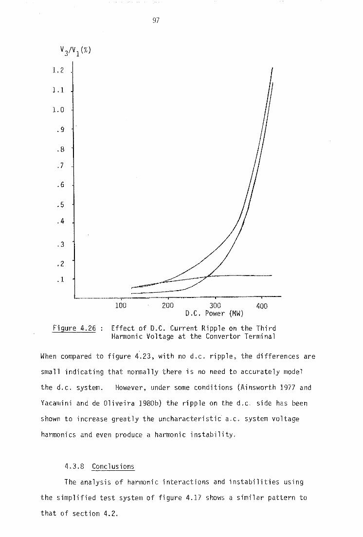
1.2
1.1
1.0
.9
.8
.7
.6
.5
.4
.3
.2
.1
Figure 4.26
97
100 200 300 400 D.C. Power (MW)
Effect of D.C. Current Ripple on the Third Harmonic Voltage at the Convertor Terminal
When compared to figure 4.23, with no d.c. ripple, the differences are
small indicating that normally there ;s no need to accurately model
the d.c. system. However, under some conditions (Ainsworth 1977 and
Yacamini and de Oliveira 198Gb) the ripple on the d.c. side has been
shown to increase greatly the uncharacteristic a.c. system voltage
harmon; cs and even produce a harmon; c ins tab-j 1 ity.
4.3.8 Conclusions
The analysis of harmonic interactions and instabilities using
the simplified t system of figure 4.17 shows a similar pattern to
that of section 4.2.

As in section 4.2.2.2, diagonaliz;ng the a.c. system produced
no significant change in the stability of the solution. Also the
filter system combination appears to be the primary cause of the
instability as this causes a resonance which weakens the system to
harmonics by increasing the magnitude of the system impedance seen by
the convertor.
Premature convergence of the iterative algorithm has been
exposed as a possible problem. However, this can be overcome by the
inclusion of a controller disturbance as described in section 4.3.4.2.
The results of section 4.3.5 show that this is a successful technique
of exciting potentially unstable harmonics. Also when a controller
disturbance is applied to a stable case the solution did not diverge
indicating that the final answer is independent of the path of the
solution, as in conclusions of section 4.2.
4.4 VERIFICATION OF THE ITERATIVE ALGORITHM
4.4.1 Introduction
The use of an iterative algorithm introduces the possibility
of false solutions and numerical instability. Therefore, the
accuracy and reliability of such an algorithm needs to be established,
especially when a divergent solution is detected.
In order to test the iterative algorithm it is neccessary to
compare the results with those obtained from a credible alternative
method. In our department two possible alternatives exist. These are
a physical simulator (Graham 1984) and a Transient Convertor Simulator
(TCS) computer program (Heffernan 1980). The TCS program was used
because the convertor transformers of the physical simulator are
inherently non-linear. This effect ;s not yet included into the
iterative algorithm but is an area of research in the department.

99
If the same problem is solved using both the iterative
algorithm and TeS (without the application of a fault), the two sets
of results can be compared. In the cases of the TeS results, the
computer run must be long enough for the intial transients to
decrease to a negligible level. The harmonic content of the waveforms
is then evaluated using an
A divergent run of the iterative algorithm could be compared
to the dynamic solution of TeS. As Tes mimics the operation of the
convertor in the time domain, any harmonic instability will develop in
the same way as in an actual convertor, and will be free of the
potential numerical instability problems of the iterative algorithm.
4.4.2 TCS Comparison Without A.e. Filters
A simple system that can be used to compare the iterative
algorithm with TeS ;s a single-bridge convertor connected to a purely
inductive system with no filters on the a.c. side and to a large
smoothing inductor on the d.c. side (i.e., a perfectly flat d.c.
current). This is described in figure 4.27.
p.u.
E
Figure 4.27: Test System Without Filters
Traditionally the commutating voltage is defined as the
sinusoidal voltage Ec which drives the commutation current (Arrillaga
1983), with the commutating reactance being the sum of Xl and X2, The
delay angle is measured from the zero crossings of the E phase to c

100
phase voltages and is set to 20° for the test example.
Analytically (Arrillaga 1983)
::: cOSa - cos(a+~)
with V ::: 13 p.u., X 0.2 p.u., Id 1.0 p.u. and a ::: 20°, the c c
commutation angle is 19.07°
The a.c. system current injections and the Vt voltage
distortion for the system of figure 4.27 were solved using the three
following methods.
1. In the t"ime domain us"ing the TeS algorithm.
2. Using the iterative algorithm with Ec as the commutating voltage
and a commutating reactance of 0.2 p.u.
3. Using the iterative algorithm, but with Vt as the commutating
voltage, an a.c. system of 0.1 p.u. inductance and a commutating
reactance of 0.1 p.u.
For the third method the initial value of the voltage Vt is
specified as the fundamental voltage at that busbar. This can be
found either using Tes or a simple power flow.
Using the Tes algorithm gives the current injections and
terminal voltage Vt waveforms with reference to a 1LO° cosine voltage
on phase 'a' of E. However, the harmonic interaction algorithm uses c
a 1LO° sinewave as reference. Also the a.c. currents are treated as
injections in the harmonic interaction algorithm~ Therefore, to
compare the results the TeS reference needs to be advanced by 1/4 of
a cycle and the FFT performed. This gives a set of phasors with an
exponential or cosine ser1~s. To convert this to a sine series 90°
is added to the phase of each phasor, at each harmonic.
The convertor currents in phase 'a'. calculated by the three
methods, are given in table 4.16 for the first five characteristic

101
harmon; cs. Non-characteristic harmonics are not generated because
E is balanced. c
Table 4.16 : Comparison of Phase 'a' Harmonic Currents
Harmonic Method 1 Method 2 Method 3
Order Mag. Phase Mag. Phase Mag. Phase
1 0.7666 149.3 0.7762 149.5 0.7658 149.6
5 0.1384 -152.9 0.1392 -152.6 0.1374 -152.3
7 0.0874 145.8 0.0887 146.1 0.0876 146.4
11 0.0381 -159.3 0.0386 -158.3 0.0383 -157.8
13 0.0246 137.9 0.0244 137.7 0.0243 138.2
Similarly. the phase 'a' harmonic voltages at Vt are compared
in table 4.17. Because the case of the iterative algorithm with an
infinite a.c. system source does not explicitly solve for Vt the
results are not given.
Table 4.17 Comparison of Phase 'a' Harmonic Vo ltages
Harmonic Method 1 Method 3
Order Mag. Phase Mag. Phase
1 0.96319 -4.1 0.96300 -4.1
5 0.06907 -63.2 0.06949 -62.3
7 0.06099 -124.1 0.06191 -123.6
11 0.04213 -69.0 0.04218 -67.9
13 0.03218 -132.5 0.03134 -131.9
The results of tables 4.16 and 4.17 for the phase 'a' harmonic
currents and voltages show a close agreement. The magnitude of the
harmonic currents also agree with those expected (Arrillaga 1983).
The comparison in this section verifies the formulation of
both the iterative algorithm and TCS software.

102
4.4.3 TCS Comparison With A.C. Filters and a Non-Infinite
D.C. System
Because a harmonic instability generally occurs when the a.c.
system is near to resonance at a low order harmonic and the short
circuit ratio is small, the a.c. system was chosen to have a parallel
resonance between the filters and the a.c. system near the third
harmonic. For simplicity, the a.c. system was a series inductor
resistor combination and the filters the fifth, seventh, eleventh and
thirteenth harmonic tuned branches of table 4.2. The a.c. system
inductance was tuned to resonate near the third harmonic (140 Hz)
with the equivalent capacitance of the filters (calculated at the
third harmonic). For the iterative algorithm the d.c. current
was made perfectly smooth. This was not possible for the TCS
algorithm so the smoothing inductor was made sufficiently large to
give an insignificant d.c. current ripple. The convertor transformer
was specified as a star-g/star connection with a 0.05 p.u. leakage
reactance per phase.
figure 4.28.
The system configuration is described in
Figure 4.28 : Test System With Filters
The convertor was operated with an equidistant firing control
strategy, a nominal delay angle of 5° and a d.c. current level of
1.0417 p.u. The a.c. system phase 'a' current and terminal voltage
distortions are compared in tables 4.18 and 4.19 respectively.
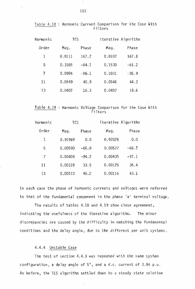
103
Table 4.18 Harmonic Current Comparison for the Case With Fi lters
Harmonic TCS Iterative Algorithm
Order l'1ag. Phase Mag. Phase
1 0.8111 167.2 0.8102 167.8
5 0.1585 -64.1 0.1530 -61. 2
7 0.0984 -86.1 0.1031 -85.9
11 0.0549 40.9 0.0546 44.2
13 0.0402 16.3 0.0407 18.6
Table 4.19 Harmonic Voltage Comparison for the Case With Fi lters
Harmonic TCS I terat i ve Algorithm
Order Mag. Phase Mag. Phase
1 0.91969 0.0 0.92026 0.0
5 0.00590 -66.8 0.00577 -66.7
7 0.00408 -94.2 0.00435 -97.1
11 0.00128 33.5 0.00125 35.4
13 0.00123 46.2 0.00116 43.1
In each case the phase of harmonic currents and voltages were referred
to that of the fundamental component in the phase la l terminal voltage.
The results of tables 4.18 and 4.19 show close agreement,
indicating the usefulness of the iterative algorithm. The minQr
discrepancies are caused by the difficulty in matching the fundamental
conditions and the delay angle. due to the different per unit systems.
4.4.4 Unstable Case
The test of section 4.4.3 was repeated with the same system
configuration, a delay angle of 5°, and a d.c. current of 3.94 p.u.
As before, the TCS algorithm settled down to a steady state solution

104
but the iterative algorithm did not converge.
4.4.5 Conclusions
The test comparisons made between the iterative harmonic
interaction and TCS algorithms illustrate both the positive and
negative aspects of the iteration algorithm.
The iterative algorithm has been shown to be accurate as it
produces results which are in close agreement with those produced by
the TCS algorithm. Also, the case of a purely inductive system
without filters, which can be solved analytically, shows the accuracy
of both the iterative and TCS algorithms.
During the course of the comparisons it was observed that the
iterative algorithm required less complex data preparation and
generally less CPU time to reach a solution.
However, the iterative algorithm may diverge even when stable
operation exists in the time domain. In this case the convertor1s
steady state operation needs to be solved using the TCS algorithm.
4.5 FUTURE WORK WITH THE ITERATIVE ALGORITHM
4.5.1 Multiple Sources
In many transmission systems there are several sources of
harmonics. For instance, in the South Island of New Zealand system
there is an h.v.d.c. link and an aluminium smelter, both of which are
relatively large. The operation of each source depends on the
distortion from the other sources and therefore the sources should not
be treated separately.
The iterative algorithm of chapter 3 can be used to model
multiple sources. The a.c. current injections and the d.c. voltage
waveforms of each convertor are solved for at the beginning of each
iterat ion. With each of the convertors operation updated, the a.c.

105
voltage distortion and d.c. current ripple on each convertor are
evaluated together. However~ while this is simple~ it may not be
the most computationally efficient method.
Most of the computational effort is needed to solve the
operation of the convertor and relatively little needed to solve the
a.c. and d.c. systems. Therefore, each convertor could be solved
individually with the complete a.c. and d.c. systems updated before
the next convertor is solved. As in the Gauss-Seidel method for
solving simultaneous sparse linear equations (Kreyz;g 1979), this
would provide the convertor with the most accurate information
possible when it is solved and would probably accelerate the
solution.
In the case where one or more convertors is a twelve pulse
configuration, both bridges should be solved before the a.c. and d.c.
systems to prevent the unnecessary generation of harmonics that would
otherwise cancel due to the connection of the converter transformers.
To assess the effect of a second source on an existing
convertor, a test system containing two convertors should be derived.
With one convertor turned off. the iterative algorithm could be run
and the system solved. Then the power of the second convertor could be
gradually increased and the operation of the first convertor examined
for any change.
4.5.2 I lusion of the Harmonic Effects in the Three Phase
Power Flow
The three phase power flow algorithm assumes that the voltage
distortion on the convertor terminal is zero. As the results of this
chapter show, the terminal busbar voltage is not purely sinusoidal and
this may result in the fundamental current injections being altered.
This may affect the solution of the power flow which may require
further interactions to reach the improved solution.

106
This would not be a major effect in case of adequate
filtering, but may have an effect in the case of negative sequence
terminal voltage which causes uncharacteristic odd harmonic orders
which are generally unfiltered. As the magnitude of the fundamental
convertor currents is reasonably independent of the delay angles,
and hence commutation angles (Harker 1980). the major effect of
voltage distortion is expected to be on the current angles and hence
the system real power flows.
4.5.3 Harmonic Instability
Further work may be warranted to assess when the iterative
algorithm diverges and TeS is needed. Similarly, further comparisons
between the iterative algorithm and TCS should be performed to check
an unbalanced case. However, because a detailed harmonic system
admittance matrix ;s used for both the a.c. and d.c. systems in the
iterative algorithm. a comparison with TCS for a real system with an
unbalanced impedance loci will require an equally detailed time domain
equivalents for these systems. This is an area of current work in
the department (Watson et al 1985).
107
CHAPTER
HARMONIC MODELLING OF SINGLE PHASE FEEDER AND CONVERTOR SYSTEMS
Of particular interest in New Zealand is the fact that part of
the main trunk line in the North Island is being electrified. A 25/50
kV single phase feeder system is to be used to supply power to the
locomotive's d.c. drives via single phase a.c./d.c. convertors. The
use of convertors will result in harmonic currents entering the feeder
system. The harmonic modelling of the operation of the traction system
can be divided into the modelling of the a.c. feeder system and the
harmonic interaction of the locomotive's single phase convertors with
their associated a.c. and d.c. systems. These are discussed in
sections 5.1 and 5.2 respectively.
It should be noted that in this chapter single phase refers to
an actual single phase system, rather than balanced three phase which
is often termed single phase.
5.1 HARMONIC MODELLING OF THE NEW ZEALAND RAILWAY FEEDER SYSTEM
To help assess the effect of a.c. current distortion from the
locomotives on local communication circuits and the three phase
transmission system supplying the railway substations, a single phase
harmonic penetration study was performed. Harmonic models of the
feeder and contact wires, the rails, the lines terminations, the
locomotive and substations' transformers and the three phases
transmission system were collated. At each frequency of interest the
models were formed into an admittance matrix.
Proposed filters at the substation and line terminations were
assessed by calculating the ha~lonic voltages and the current flows
throughout the feeder system. This involved the use of the harmonic

108
admittance matrix and fixed current injections into the secondary
(convertor side) of the locomotive's transformer.
5.1.1 Component Models
5.1.1.1 Feeder wires
The cross section of the proposed towers is in figure 5.1.
3 2
1
8. 8 7.39 m m
III
, /' '\.
.54 .:.!
IE-l.42-11 ~2.05~
4
,
I
3.85 6. m m
... 51 , m
87
1 Contact 2 Catenary 3 A.T. Feeder 4 Protection
: Cross Section of the Feeder System Towers
In the absence of specific data the following assumptions were made.
1. Data for the protection wire is identical to that used for the
protection wire in the New Zealand d.c. link.
2. The rails consisted of solid circular conductors of 100 mm diameter.
3. The catenary wire and contact wire are assumed to identical.
4. All conductors are flat between towers and, therefore. of constant
cross section.
This gives the conductor data of table 5.1.
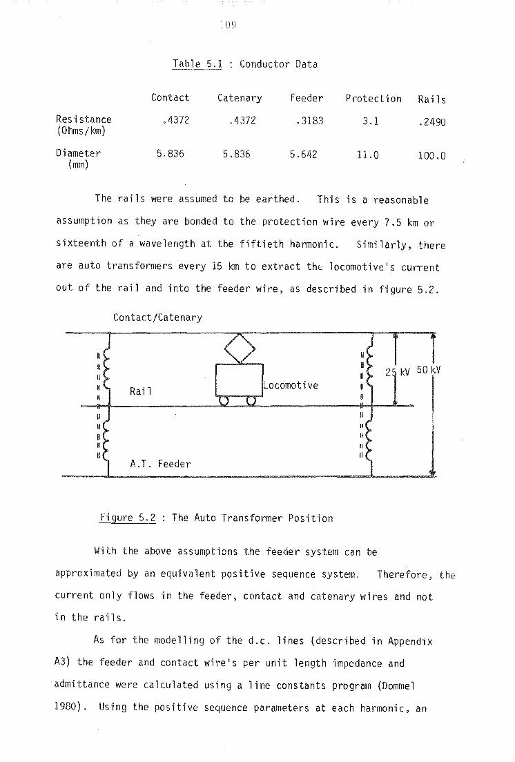
10
Table 5.1 Conductor Data
Contact Catenary Feeder Protection Rails
Resistance .4372 .4372 .3183 3.1 .2490 (Ohms/km)
Diameter 5.836 5.836 5.642 11.0 100.0 (mm)
The rails were assumed to be earthed. This is a reasonable
assumption as they are bonded to the protection wire every 7.5 km or
sixteenth of a wavelength at the fiftieth harmonic. Similarly~ there
are auto transformers every 15 km to extract the locomotive's current
out of the rail and into the feeder wire, as described "in figure 5.2.
Contact/Catenary
1/ II II 2 kV 50 kV
Rail Locomotive II II II
II II
II II
II II
II II
II II A.T. Feeder
Figure 5.2 : The Auto Transformer Position
With the above assumptions the feeder system can be
approximated by an equivalent positive sequence system. Therefore, the
current only flows in the feeder, contact and catenary wires and not
in the rails.
As for the modelling of the d.c. lines (described in Appendix
A3) the feeder and contact wire's per unit length impedance and
admittance were calculated using a line constants program (Dommel
1980). Using the positive sequence parameters at each harmonic. an

110
equivalent-n model can be derived for each section which takes into
account the transmission line effects.
5.1.1.2 Locomotive, including power factor correction
The proposed locomotives have four convertors with power
factor correction on each of the convertor transformer's secondary
windings. For the analysis the four convertor secondary windings were
reduced to a single equivalent transformer. As the leakage of each
transformer is 0.0985 p.u. on a 1043 KVA base, the equivalent
reactance of the single group becomes 0.0236 p.u. on a 1 MVA base.
Similarly, the four sets of 2.1 mH series inductors and the
1.5 mF capacitors, at a 0.570 kV voltage base, are combined to single
equivalent reactances of 0.5076 p.u. and 1.6 p.u. at fundamental
frequency, respectively.
5.1.1.3 The substation and locomotive transformer model
The harmonic model chosen for the transformer was a parallel
combination of the leakage reactance and a resistance 80 times the
leakage at fundamental (Harker 1980 and Densem 1983). The leakage
reactance of the locomotive transformer is 0.0236 p.u., as in section
5.1.1.2, and that of the substation transformer 0.013 p.u.
5.1.1.4 The line terminations
The line terminations consist of a series connection of a 600
ohms resistor and a 6366 ohms (at 50 Hz) capacitor. These are
connected between the feeder wire and the protection wire and,
similarly, between the contact wire and the protection wire. They are
included to terminate the feeder system in its characteristic impedance.
5.1.1.5 The three hase transmission
An equivalent impedance looking into the three phase transmission
system from the substation ;s required. Owing to the lack of data it was
assumed that the transmission system is sufficiently strong to be
regarded as a short circuit to harmonics. The transmission system

111
impedance would generally be of little significance as the substation
transformer impedance is in series with it.
5.1.1.6 The harmon c filters
The harmonic filters proposed for the substation were single
tuned shunt branches for the third and fifth harmonics. They have a
Q of 50 and supply a total of 5.0 MVAr reactive power compensation~
with the third and fifth harmonic filter were specified to give 3.0 MVAr
and 2.0 MVAr compensation respectively.
5.1.2 Forming the Admittance Matrix for the Feeder System
With all of the individual system component models defined at
harmonic frequencies~ an overall admittance matrix can be formed for
the feeder system at each harmoni c. The exarnp 1 e of a s -i ngl e 1 ocomoti ve
on the left of the substation is given in figure 5.3.
220 kV
Sub station
Locomotive
--'-''''---''--'--''-: A Single Locomotive Left of the Substation
To describe the feeder system 2Nt + 4 bus bars are required,
where Nt is the number of locomotives. ble 5.2 shows the numbering
convention of the busbars chosen.
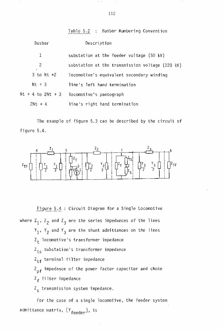
Nt
Busbar
1
2
3 to Nt
Nt + 3
+ 4 to 2Nt
2Nt + 4
+2
+ 3
112
Tab"le 5.2 Busbar Numbering Convention
Descr"iption
substation at the feeder voltage (50 kV)
substation at the transmission voltage (220 kV)
locomotive's equivalent secondary winding
line's left hand termination
locomotive's pantograph
line's right hand termination
The example of figure 5.3 can be described by the circuit of
figure 5.4.
where
Figure 5.4 : Circuit Diagram for a Single Locomotive
ZI' Z2 and Z3 are the series impedances of the 1 i nes
YI , Y2 and Y3 are the shunt admittances on the 1 i nes
Zt locomotive's transformer impedance
Zts substation's transformer impedance
Ztf terminal filter impedance
Zpf impedance of the power factor capacitor and choke
Zf filter impedance
Zs transmission system impedance.
For the case of a single locomotive, the feeder system
admittance matrix, [Y f d ]. is ee er
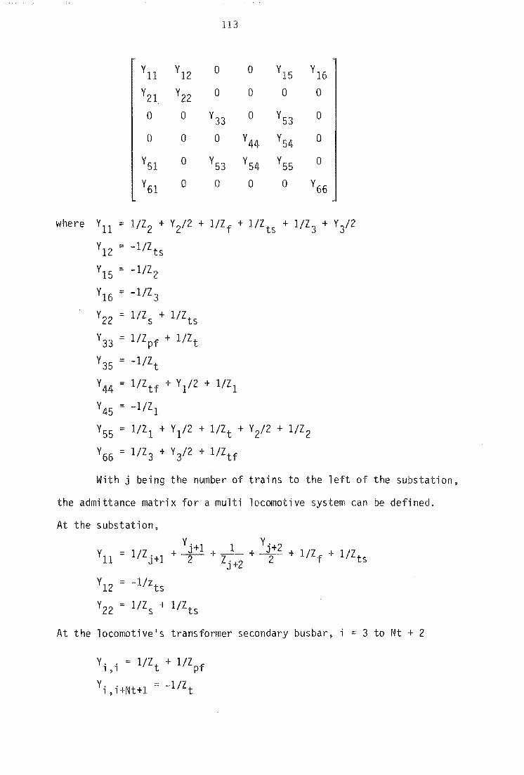
113
Yll
YI2 0 0 Y15 Yl6 Y2l Y22 0 0 0 0
0 0 Y33 0 Y53 0
0 0 0 Y44 Y54 0
Y 0 Y53 Y YS5 0
Y6l a 0 0 0 Y66
where Yll == l/Z2 + Y2/2 + l/Zf + l/Zts + I/Z 3 + Y3/2
Y12 == -l/Zts
Y 15 ::: -l/Z2
Y16 ::: -1/Z3
Y22 = l/Zs + l/Zts
Y33 = l/Zpf + I/Zt
Y35 = -I/Zt
Y44 = I/Ztf + Yl/2 + I/ZI
Y45 :::: -11Z1
Y55 = I/ZI + Yl /2 + I/Zt + Y2/2 + I/Z2
Y66 == I/Z3 + Y3/2 + I/Ztf
With j being the number of trains to the left of the substation,
the admittance matrix for a multi locomotive system can be defined.
At the substation,
YI2 ::: l/Zts
Y22 :::: I/Zs + I/Zts
I Y j+2 + -2- + l/Zf + I/Zts
+2
At the locomotive's transformer secondary busbar, i ::: 3 to Nt + 2
Y. . :::: I/Zt + liZ f 1 ,1 P
Yi,i+Nt+l = -I/Zt

114
At the 1 termination, i "" Nt + 3
At the right termination, i "" 2Nt + 4
Y •• 1 ,1
Y liZ + 2+Nt + =--,1_
tf 2 t
At the contact wire, i = Nt + 4 to 2Nt + 3
right to substation Yi,i :: l/Z k+1 + Yk+1/2 + 1/Zt + Yk+2/2
+ l/Zk+2
where k is the number of the train, i.e., k 1 to Nt. The mutual
admittances along the line are
YNt+2+m,Nt+3+m m = 1, j (if j > 0)
Y1•Nt +2+m - - l/Zm m :: j + 1
VI 'Nt+2+m - - l/Zm m = j + 2
YNt+1+m,Nt+2+m - liZ m m :: j + 2, Nt + 2 (if j < Nt)
5.1.3 The Response of the Feeder System to Harmonics
With a harmonic admittance matrix calculated at each harmonic.
the response of the feeder system to harmonic injections at the
locomotive can be assessed. In the absence of more realistic data, the
case of one locomotive was examined with the harmonic currents
injected at the locomotive's transformer secondary busbar. such that,
0 VI
0 V2 I [Y feeder] V3 5.1
0 V4 0 Vs 0 V6

115
Equation 5.1 is solved for the voltages throughout the feeder system
by Gaussian elimination.
The two values of I in equation 5.1 of interest are a fixed
1.0 p.u. injection for each harmonic and the set of maximum expected
injections supplied by the manufacturer. and given in table 5.3
Ta e 5.3 The Set of Maximum Expected Injections
Harmonic Order Value (amps) Percentage of Fundamental
1 142.281
3 32.998 23.19
5 19.251 13.53
7 12.769 8.97
9 8.030 5.64
11 5.425 3.81
13 4.309 3.03
15 3.088 2.17
17 2.354 1.65
19 2.602 1.83
21 2.538 1. 78
23 2.293 1.61
25 2.445 1.72
27 2.442 1.72
29 2.096 1.47
31 1.905 1.34
33 1.891 1. 33
35 1.630 1.15
37 1.386 0.97
39 1.426 1.00
41 1.383 0.97
43 1.246 0.88
1. 318 0.93
47 1.374 0.97
49 1.281 0.90
Of most interest are the voltages at the locomotive1s pantograph
and the currents into the harmonic filters and transmission system.

116
5.1.4 Evaluating the Currents in the Individual System
Components
As the equivalent harmonic model represents the individual
feeder system components, once the harmonic voltages are known the
currents in each of the individual system components can be found.
Current in the harmonic fi lters If = Y f Vl II II II termi nat i on left fi lter Ilt :.= Ytf VNt +3 II II II termination ri ght fi 1 ter Irt = \f V2Nt+4 II II II substation transformer Its =Y (V 1-V 2) ts II II II locomotive transformer I ti =Yt (V 2+i -V 3+Nt+1) i=l.Nt II II II locomotive p. f. circuit If' = Y pf V 2+i .Nt
P 1
For the calculation of the line currents, sending was defined
as towards to the substation (i .e., sending into the system) and
receiving as towards the line terminations.
Isend :.= V (Yi /2 + liZ.) - V (liZ;) send 1 rec
I rec ::: V (Y;l2 + liZ.) Vsend (lIz i) rec 1
where i refers to the section number on the line. The Vsend and Vrec which correspond to a particular i depends on the number of locomotives
left on the substation j.
Case i Vsend V rec
j=O I V3+Nt VI
2 V4+Nt VI
; ,Nt+l V 2+Nt+i V 1 +Nt+i
Nt+2 V2Nt+4 V2Nt+3

117
j=Nt 1 V 3+Nt V4+Nt i=2,Nt V 2+Nt+i V 3+Nt+i (j> 1)
Nt+1 V2Nt+3 VI
Nt+2 V 2Nt+4 VI
O<j<Nt 1 V3+Nt V4+Nt i =2 ,j V 2+Nt+i V 3+Nt+i
j+I V 3+Nt+i VI
j+l V 4+Nt+i VI
i:::j+3,Nt+1 V 2+Nt+i V1+Nt+i Nt+2 V 2Nt+4 VI
5.1. 5 Results of a Test Section of Line
The test system chosen consists of a single locomotive on a
110 km section of line with the substation 70 km from the left line
termi nat i on.
Figure 5.5 shows the transmission system harmonic currents for
a 1.0 p.u. current injection into the secondary of the locomotive's
transformer at various positions to the left of the substation.
Simil ar results to these were found for a locoilloti ve to the ri ght of
the substation. Similarly, figure 5.6 shows the transmission system
currents for the locomotive current injections as listed in table 5.3
Figures 5.5 and 5.6 show that the harmonic currents entering
the transmission system increase when the separation between the
locomotive and the substation is larger.
To try and reduce the excessive current distortion expected
in the transmission system, the third and fifth harmonic filters
described in section 5.1.1.6 were proposed. Figure 5.7 shows the
transmission system currents with the locomotive1s injections and
the proposed harmonic filters.

Current 4.0
3.0
2.0
1.0
118
p.u. LocomoUve at 70 km
50 km 30 km
10 km
5 10 15 20 25 30 35 40 Harmon; cOrder
Transmission System Currents for a 1.0 p.u. Injection (no filters).
CUrrent 40.0 (amps)
30.0
20.0
10.0
5
Locomotive at 70 km 50 km 30 km
10 km
45
Figure 5.6 Transmission System Currents for the Locomotive's Injections (no filters).
50

Current Amps 20.0
10.0
119
Locomotive at
70 km 50 km 30 ~ 10 km
5 10 15 Harmonic Order
20 25
Figure 5.7 Transmission System Currents for the Locomotive's Injections with the Proposed Harmonic Filters
A comparison of figures 5.6 and 5.7 illustrates the effect of the
filters.
Because relatively large levels of seventh. ninth and eleventh
harmonics still exist with the proposed filters. the effect of
including a seventh harmonic filter was examined. To keep the total
filtres rating of 5 MVar reactive power compensation. the third.
fifth and seventh harmonic filters were rated at 2.333, 1.667 and
1.0 MVar respectively.
For the case of a locomotive 50 ~ to the left of the
substation, figure 5.8 shows:
(1) the currents injected by the locomotive,
(2) the currents entering the transmission system for the case without
filters,
(3) the currents entering the transmission system in the presence of
third and fifth harmonic filters,
(4) the currents entering the transmission system for the case of
third, fifth and seventh harmonic filters.
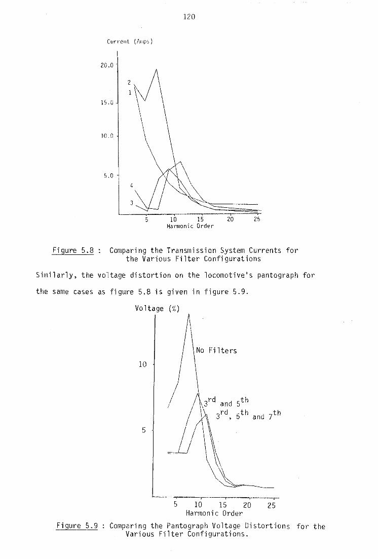
Fi gure 5.8
Current (
20.0
15.0
10.0
5.0
2
1
4
3
120
5 10 15 20 25 Harmonic Order
Comparing the Transmission System Currents for the Various Filter Configurations
Similarly, the voltage distortion on the locomotive's pantograph for
the same cases as figure 5.8 is given in figure 5.9.
Vo ltage (%)
10
3rd and 5th
3rd , 5th and 7th
5
5 10 15 20 25 Harmonic Order
Figure 5.9 Comparing the Pantograph Voltage Distortions for the Various Filter Configurations.

121
5.1.6 Conclusions of the Single Phase Harmonic Penetration
As the final design of the line terminations, the positioning
of the power factor correction components and harmonic filters is not
known, any more detailed analysis is not warranted at this stage.
However, only minor changes to the existing algorithm would be needed
to include any likely system changes.
5.2 MODELLING SINGLE PHASE SYSTEMS
The basic problem of modelling the harmonic interaction
between single phase convertors and their associated a.c. and d.c.
systems is similar to that of three phase convertors. The main
differences are in the sampling routine and the need to model half
controlled convertors which are common in single phase applications.
Also the associated a.c. system is single phase.
Figure 5.10 consists of a single phase convertor bridge with
its commutating voltage Vt and inductance Lt'
Figure 5.10 Single Phase Convertor Bridge

122
5.2.1 Calculating the Commutation Current
The commutat i on ci rcui t of fi gure 5.10 is as sumed to be pure ly
inductive. Therefore, during a commutation
or
With
where
Vt = Ltdlt/dt
It 0 l/LtJ\t dt + C 0
NHARM A
Vt(t) = I Vh sin(¢h + h8 + hwt) h=l P
Vh is the magnitude of the hth harmonic of Vt th ¢h is the phase of the h harmonic of Vt
th 8 is the firing instant of the p valve p
t is referred to 8 . P
Therefore
To simplify A
Vh cos(¢h + h8 p + hwt) = Vj cos(¢h + h8p)cos(hwt)
A
- Vh sin(¢h + h8 p)sin(hwt)
5.2
5.3
5.4
5.5
= Aph cos(hwt)- Bph sin(hwt)
5.6
A
where Aph = Vh cos(¢h + h8 p) 5.7
A
Bph = Vh sin(¢h + h8 p) 5.8
This makes equation 5.5 become
1 \' 1 C - -- L -h (A h cos(hwt) + Bph sin(hwt)) wL h p 5.9

123
The integration constant C can be found by setting t to zero, i.e.,
where It(O) is the current at the beginning of the commutation.
5.2.2 Calculating the D.C. Voltage
With va lves 1 and 2 conducting V d = V t" Similarly, when valves
3 and 4 are conducting Vd = - Vt . Otherwise Vd = O. At any instant
= I A1h sin(hwt) + B1h cos(hwt) h
5.11
5.12
where t is referenced to 81 and A1h and B1h are calculated using
equations 5.7 and 5.8.
5.2.3 Calculating the A.C. Current and D.C. Voltage Samples
For fully controlled convertors the valves are fired in pairs,
being delayed by an angle alpha after the zero crossing. This is
described in figure 5.11.
During the commutation process the d.c. voltage drops to zero
and the a.c. current injection, It' reverses direction. Two
commutations per cycle occur in a fully controlled convertor. Table
5.4 shows a complete cycle of the a.c. current injections and d.c.
voltage waveforms for a fully controlled convertor.

I ac
I I I I
I I a fll12
I I I I
1
I • I I
Figure 5.11 Fully Controlled A.C. Current and D.C. Voltage Waveforms
Table 5.4 A.C. Current and D.C. Voltage Waveforms for a Fully Controlled Convertor
Section lac Vdc Limits, reference to 01
1 I c 0 0 < wt < fl12
2 Id Vt fl12 < wt < 83 - 81
3 I 0 83 - 81 < wt < 83 - 81 + tl34 c 4 -Id -V t 83 - 81 + fl34 < wt < 2n
Half control is achieved by setting the delay angles for
valves 1 and 3 equal to zero, effectively making them into diodes.
Valves 2 and 4 are fired in the usual way after the specified delay
angle. Thus, if valve 1 and 2 are conducting, valve 3 will commutate
on when it becomes forward biased, causing valve 1 to turn off. This

gives rise to four commutations per cycle, as described in figure
5.12.
, I
I , ,
Vd 81
18 ,8 3 I 8
I 2 I 4 I I
I ac I I I
I I I I I I I I lJ2 \J3 \J4
Figure 5.12 Half Controlled A.C. Current and D.C. Voltage Waveforms
Table 5.5 shows a complete cycle of the a.c. current injections
and d.c. voltage waveforms for a half controlled convertor.
Table 5.5 : A.C. Current and D.C. Voltage Waveforms for a Half Controlled Convertor
Section lac Vdc Limits. reference to 8 1
1 I c 0 0 < wt < \J1 2 0 0 1-11 < wt < DC
3 I C
0 DC < wt < DC + \J 2
4 Id Vt DC + 1-12 < wt < 83 - 81
5 I 0 83 - 8 c 1 < wt < 83 - 8 1 + \J3
6 0 0 8 -3 81 + \J 3 < wt < 83 - 81 + DC
7 I 0 83
- 81 + DC < wt < 83 81 + DC + 1-14 c 8 -Id -V t 83 - 81 + DC + \J 4 < wt < 2n

126
However, if the delay angle is sufficiently small with half
control, the first and second, and similarly, the third and fourth,
commutations merge to give the same waveforms as a fully controlled
convertor operating on a zero delay angle. If the delay angle is
close to 180 0 then no commutation is complete and the d.c. voltage is
zero for a complete cycle. This situation is ignored as this is not
a practical operating state.
5.2.4 Results and Conclusions of Modelling Single Phase
Convertors
The iterative algorithm of chapter 3 was modified and used by
a final year project student, C.D. Callaghan. A summary of his
results and conclusions are given in Appendix A7.
5.3 FUTURE WORK
The development of a detailed positive sequence admittance
matrix representation of the feeder system has been discussed in
section 5.1. Similarly, section 5.2 has given a detailed
description of the operation of the locomotive's convertors.
For the analysis of the interaction between single phase
convertors and their associated a.c. and d.c. systems, the a.c. system
has been modelled either as a pure inductance or with data obtained
from a three phase industrial busbar. This was for simplicity and
because of a lack of data for a traction feeder system. However the
a.c. system representation can be improved considerably by evaluating
the impedance looking into the feeder system at the pantograph using a
similar admittance matrix to that formed ln section 5.1.
Because the locomotive transformer is already included into
the a,c. system of the single phase iterative algorithm, this should

127
removed from the feeder system admittance matrix before calculating
its impedance. Similarly, if power factor correction is included on
the secondary of the locomotive transformer, this should also
included in the a.c. system admittance matrix within the iterative
algorithm. This leaves the locomotive pantographs, the left and
right line terminations and the two substation busbars.
The inclusion of the power factor correction components on the
secondary of the locomotive transformer may also affect the
calculation of the commutation currents in the iterative algorithm.
However~ because the power factor series inductor/capacitor
combination is tuned at about 90 Hz. their effect on the commutation
process can be ignored.
Because not all the necessary convertor data and controller
information was available, the operation of the proposed locomotives
and feeder system could not be modelled. However, if more data is
made available for both the locomotive and the feeder system, work
in this area could continue.

1

129
CHAPTER 6
HARMONIC NORTON EQUIVALENT OF THE SYNCHRONOUS MACHINE
FOR ANALYSIS IN THE HARMON C SPACE
6.1 INTRODUCTION
The harmonic behaviour of the synchronous machine has not been
given serious consideration in harmonic analysis (Densem et al 1984),
even though it is well known that it converts negative sequence
currents into third harmonic voltage (Clarke 1950), and, in general,
acts as a harmonic convertor. This is probably because of the
complexity of the problem and the fact that the conversion means
coupling between harmonics that are otherwise considered separately.
Therefore, synchronous machines are often represented by a single
impedance, based on the subtransient reactances or the negative sequence
reactance (Densem 1983).
Therefore, to a greater or lesser extent every synchronous
machine acts as a harmonic source, as a harmonic impedance and a
harmonic convertor.
The behaviour of the synchronous machine as a harmonic generator
is well understood (Arrillaga et al 1985a) and the generated harmonic
emf's are normally reduced to insignificant levels by appropriate
machine design. In present harmonic flow analysis, or harmonic
penetration studies, the synchronous machines are represented by
inductor/resistor combinations derived empirically, i.e., the
frequency conversion process is ignored. However, as part of any
practical power system the synchronous machine is always subjected to
some imbalance as well as imperfect external voltage and current
waveforms that will excite the mechani Sill of harmoni c convers i all.
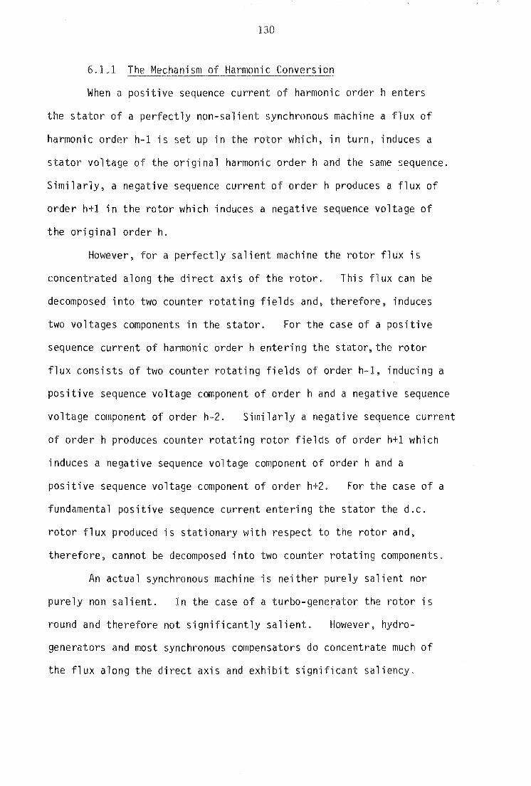
130
6.1.1 T of Harmonic Conversion
When a positive sequence current of harmonic order h enters
the stator of a perfectly non-salient synchronous machine a flux of
harmonic order h-1 is set up in the rotor which~ in turn, induces a
stator voltage of the original harmonic order h and the same sequence.
Similarly. a negative sequence current of order h produces a flux of
order h+l in the rotor which induces a negative sequence voltage of
the original order h.
However, for a perfectly salient machine the rotor flux is
concentrated along the direct axis of the rotor. This flux can be
decomposed into two counter rotating fields and, therefore, induces
two voltages components in the stator. For the case of a positive
sequence current of harmonic order h entering the stator, the rotor
flux consists of two counter rotating fields of order h-l, inducing a
positive sequence voltage component of order h and a negative sequence
voltage component of order h-2. Similarly a negative sequence current
of order h produces counter rotating rotor fields of order h+l which
induces a negative sequence voltage component of order h and a
positive sequence voltage component of order h+2. For the case of a
fundamental positive sequence current entering the stator the d.c.
rotor flux produced is stationary with respect to the rotor and,
therefore, cannot be decomposed into two counter rotating components.
An actual synchronous machine is neither purely salient nor
purely non salient. In the case of a turbo-generator the rotor is
round and therefore not significantly salient. However, hydro
generators and most synchronous compensators do concentrate much of
the flux along the direct axis and exhibit significant saliency.

1
6.1.2 The d-q Model of the Synchronous Machine
Data for synchronous machines is normally available in terms
of the d-q axis and implicit in this information is the effect of the
second harmonic terms of the inductances (Adkins and Harley 1975 and
Anderson and Fouad 1977). Information on fourth order terms~ absent
from the d-q model, is not generally available and is ignored from this
analysis.
Inherent in the d-q differential equations are the following
assumptions (O'Kelly and Simmons 1968).
1. Magnetic saturation is neglected with the self and mutual
inductances of all the machine windings being independent of the
magnitude of the winding currents.
2. Air-gap m.m.f.s and fluxes are represented by the fundamental
components of their spatial distributions.
3. Slotting effects are ignored. Distributed windings comprise finely
spread conductors of negligible diameter.
4. Magnetic materials are free of eddy currents and hysterisis losses.
Assumption 1 is accurate for a machine which is not over excited.
In the case of an over excited machine the incremental values of the
machine's self and mutual inductances should be used at harmonic
frequencies. Assumptions 2 and 3 hold for,a large machine of good
deSign. Throughout this analysis it will be assumed that assumption
4 holds for hydro-generators with the effects of eddy currents in
round rotor machines treated in section 6.4.4,
The formation of the harmonic admittance of the synchronous
machine is given in section 6.2. The effect of the excitation is
included as a harmonic Norton current source, and, therefore, the
field w"inding voltage is assumed to be zero during the formulation
of the admittance matrix.
132
6.1.3 The Synchronous Machine Model in the Harmonic Space
The d-q model can be used to derive the time variation of the
steady state current and voltage waveforms of the synchronous machine
(Heffernan 1980) and their harmonic content can be obtained with the
help of the FFT. However, difficulties in providing sufficient
accuracy for the initial conditions. coupled with the very large time
constants involved, mean extremely long computer runs are required
to reach a particular steady state condition. Thus the derivation
of voltage and current harmonics in the time domain is a very
inefficient process and there is considerable incentive in developing
alternative algorithms in the harmonic space.
Because of the significance of the sequences in the harmonic
conversion process, the harmonic equivalent of the synchronous machine
needs to be a full three phase representation, rather than simply a
single phase. Also, because the coupling between the harmonics, the
harmonic equivalent of the synchronous machine needs to be defined in
the harmonic space. As discussed in section 2.6, each current and
voltage in the harmonic space is described by a vector containing
each phase, busbar and harmonic.
The synchronous machine, with the effect of the excitation
removed. can modelled by an admittance matrix [Y abc ] such that
i :: Y v abc
where i. Yabc and v are expressed in the harmonic space.
and even harmonics are considered.
6.1
Both odd
Equation 6.1 can be modified to include the excitation in the
form of a Norton current source, 10
,
6.1(a)
This is described in figure

133
v s
Figure 6.1(a) : Schematic diagram of exciter system
I o
y g
I
Figure 6.1(b) : Norton Equivalent of the Syn
chronous generator
with the current defined in the reverse direction. Thi s gi ves
the nodal equation
i = 10 - Yabc v 6.2
The excitation of a synchronous machine can usually be assumed to be
a purely flat d.c. voltage in the steady state. That is, any
harmonic currents in the machine1s windings have no effect on the
field winding excitation voltage. The effect of ripple on the field
voltage is examined in section 6.3.
6.1.4 Applications of the Harmonic Space Synchronous
Machine Model
In this chapter the synchronous machine model derived in
section 6.2 is analysed in isolation to the rest of the transmission
system. Section 6.3 discusses the open circuit voltage distortion
in the stator due to ripple in the field winding voltage. Similarly
the characteristics of the synchronous machine model, as seen from the
stator without any excitation, are discussed in section 6.4.
Chapter 7 discusses the use of the Norton harmonic equivalent
model to analyse harmonic aspects of systems containing synchronous
machines.

134
6.2 THE HARMONIC MODEL OF A SYNCHRONOUS MACHINE
6.2.1 Derivation of the Matrix Ydqh
The synchronous machine admittance model is derived from the
d,q-axis differential equations. Generally accepted conventions
and notations are used (O'Kelly and Simmons 1968). With two
damper windings in the rotor, sand t, the equations are:
vd = Rid + p(Ldid + Mdfi f + Mdsis) - w(Lqi q + Mqti t )
Vq = Ri q + P{Lqi q + Mqti t ) + w{Ldi d + Mdfi f + Mdsis) 6.3'
Vf = Rfi f + p(Lfi f + Mdfi d + Mfsis) = a
v = Rsis + p(Lsis + Mdsid + Mfsi f ) = a 6.3" s
vt = Rti t + p(Lti t + Mqti q) a
In equations6.3, Vf has been set to zero for the calculation
of the synchronous machine admittance matrix because the field voltage
will be considered in the Norton current source.
All variables are phasors of harmonic h:
where
W = W + j WII 6.4" h h h
denotes any phasor. With
p jhw 6.5
equations 6.3 becomes algebraic equations in Vdh , Vqh , I dh , Iqh , I fh ,
Ish and I th . The last three can be eliminated from 6.3', using 6.3",
so that
6.6
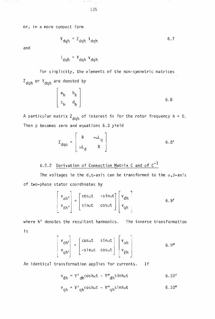
135
or, ina more compact form
6.7
and
For simplicity, the elements of the non-symmetric matrices
Zdqh or Ydqh are denoted by
[:: :: 1 6.8
A particular matrix Zdqh of interest is for the rotor frequency h = O.
Then p becomes zero and equations 6.3 yield
of
Z dqo [ R -wLq 1
wL R d
6.2.2 Derivation of Connection Matrix C and of C- 1
The voltages in the d,q-axis can be transformed to the
two-phase stator coordinates by
r v hi = [coswt -s i nwt] Vdh 1 l V:h• sinwt coswt Vqh
6.8'
a,S-axis
6.9'
where h' denotes the resultant harmonics. The inverse transformation
is
[ coswt s i nwt 1 [\X.h 1
= -sinwt coswt VSh
· 6.911
An identical transformation applies for currents. If
6.10'
Vqh V' qhcoshwt - VUqhsinhwt 6.1011

and
in the
where
and
and
1 6
titute 6.10 into 6.9' we obta"in expressions for vah and v Sh
form 6,4, with h' =: h ± 1:
V ah ::; V,h
exh-l cos (h-l)wt _ V" h ah-1 sin( l)wt
6.11' t V~h+l cos(h+1)wt V'I
ah+1 sin(h+1)wt
V Sh - V' h - Sh-1 cos (h-l)wt _ V" h
Sh-1 sin (h-l) wt
V,h V" h 6.11" cos(h+1)wt sin(h+1)wt + Sh+1 Sh+1
V,h - 1(V' + V" ) ah 1 - 2 dh qh V" h ;;;; l(VII - V' ) ah-1 2 dh qh
V,h l(V' - V" ) ah+ 1 2 dh qh Vlih l(V" + V' ) ah+l 2 dh qh
6.12'
V,h :::l(_VII +V' ) V" h ;;;; l(V' + V" ) Sh-l 2 dh qh h-l 2 dh qh 6.12"
Vll h Sh+1 =l(V" +V' )
2 dh qh V" h Sh+l l(_V' + V" ) 2 dh qh
These can be combined into phasors, as in 6.4" yielding:
V~h_1 ::: ~(Vdh - jV dh )
V~h+l ~(Vdh + jVqh )
V~h_1 ;;:; iUV dh + Vqh )
V~h+l ;;:; ~(-jVdh + Vqh )
6.13'
6.13"
In equations 6.11, 6.12 and 6.13 the superscript h indicates
the related d,q-axis harmonic for a component of order h±1 of a stator
(a,S-axis) harmonic. When two such components of the same order
(related to a lower and a higher order rotor harmonic) combine, the
superscript is dropped; see the vector 6.16'.
Equations 6,13 should be written for all h. However, if
h=O or h-1=0 then Vo ;;;; Va' If h=O then we obtain directly from 6.9'

1
converted into phasor relations.
Val:: VdO + jV qQ
VSl :: jV dO + VqO
6.14'
6.14"
By assembling equations 6.13 and taking 6.14 into account.
we obtain
An identical transformation applies for currents:
In 6.15
and
c
with
1 2
2M
N
N
M N
M
N
M N
M
M N*:: [1 j 1 -j 1
6.15'
6.15"
6.16'
where the asterisk denotes the conjugate and n the highest harmonic
investigated.
The matrix C is singular because it contains two redundant
variables. one at d.c. and the other at the maximum harmonic considered.

At doc.
at h=n
Also at d.co
similarly at h=n
vn I(V an-l :::: '2 dn
138
·v ) J qn
jV a
Vn- 1 1(·v V) 'V n- 1 8n = 2 -J dn-l + qn-1 = -J an
This singularity of C could of course be removed by keeping only a
reduced number of variables. It is preferable, however, to preserve
the symmetry and simplicity of the full matrix C of 6.17. An
inverse relationship to 6.15 can then be derived starting with equation
6.9 and performing calculations as in equations 6.10 to 6.14.
This gives
v ::: C*v dq as i dq C*i
a8
6.2.3 Derivation of Matrix Y S ~--~~~--~--~a
Equations 6.7 u are assembled for all h, into the relation
where Ydq is block diagonal with blocks of the form 6.8.
where
Equations 6.18 / , 6.19 and 6.15u can be combined to give
Y = CY C* as dq
6.18'
6.19
6.20
6.21

Y :;; as
where
139
The non-syrrrnetri c matr; x Y has the form
AO B" 1
Al B" , 2
8' 1 A2
8' 2
Ah
B' h
AO ::::: NYdq1 N/2
Al ::::: (2MY dqOM + NY dq2 N}/4
Ah ::::: {MYdqh_IM + NY dqh+1N}/4
B'1 :: MYdq1 N/2
B' h :: MY dqhN/ 4
BII ::::: NY M/4 h dqh
A = MY d 1M/4 n qn-
8" h
8" n-l
A n-l
B~_I A n
(for h=2 p •• ,n-l)
{for h=2, ... ,n-l}
(for h=1, ... ,n-1)
These expressions can be calculated from:
where
MYdqiM::: ({ai+d i ) - j(b;-ci))M
NYdqiN:= ((a;+d;) + j(b;-c;))N
MYdq;N '" ((a;-d i ) + j(b;+c;})P
NY d q i M '" (( a i - d i) - j ( b i +c i )) Q
[1 1 [1 jj p '" • Q = -j -1 j -1
6.22
6.23
6.24
6.25
From equations 6.23 it can be seen that the self admittance
Ah for the harmonic of order h depends only on the rotor frequencies
of order h±l. and the mutuals B'h and B'\ between harmonics h+1 and h-l
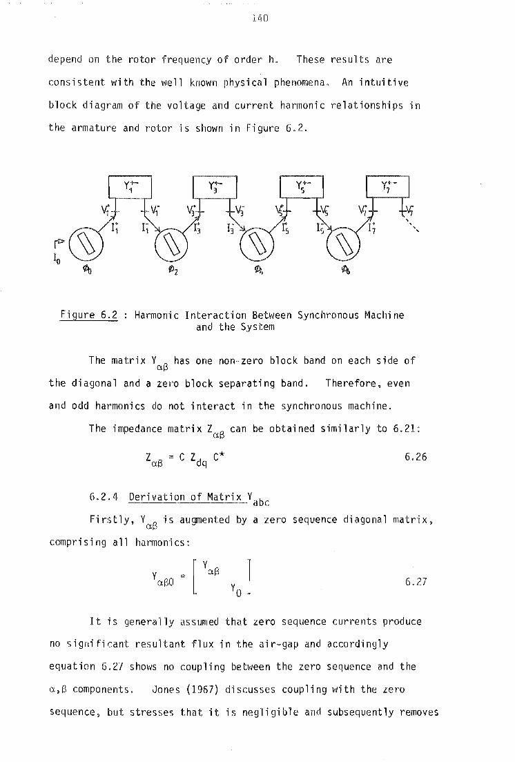
140
depend on the rotor frequency of order h. These results are
consistent with the well known physical phenomena. An intuitive
block diagram of the voltage and current harmonic relationships in
the armature and rotor is shown in Figure 6.2.
Figure 6.2 Harmonic Interaction Between Synchronous Machine and the System
The matrix VaS has one non-zero block band on each side of
the diagonal and a zero block separating band. Therefore, even
and odd harmonics do not interact in the synchronous machine.
The impedance matrix laS can be obtained similarly to 6.21:
l = C l C* as dq 6.26
6.2.4 Derivation of Matrix Vabc
Firstly, VaS is augmented by a zero sequence diagonal matrix,
comprising all harmonics:
6.27
It is generally assumed that zero sequence currents produce
no significant resultant flux in the air-gap and accordingly
equation 6.27 shows no coupling between the zero sequence and the
a,S components. Jones (1967) discusses coupling with the zero
sequence. but stresses that it is negligible and subsequently removes

141
the coupling from the analysis. Coupling between the zero
sequence and the a and S components is inherently zero in the d-q
synchonous machine equations 6.3.
For any harmonic
vaSOh :::
T hV abch 6.28
i aSOh ::: T hi abch
where
1 1 1 - "2 - "2
Th 0 13 6.29'
1 1 1 3 } 3
The ; nverse of T h is
2 a 1
T -1:; 1 1 1 6.29" h -3 13
1 1 1 -} -
13
Equations 6.27,6.28 and 6.29 can be completed and combined
to yield
An admittance matrix
:; Y aSOv asa
-1 ::: T iasa
6.30
6.31'
;s evaluated and of the same fom as 6.1, with the subscripts abc
having omitted from v and i. That is
142
i ::: Y b v 6.31" a c
on of the Norton rrent
In figure 6,1(a) V • the system voltage, is applied to the sys exciter via a star/star transformer. From Vsys and the exciter bridge
delay angle the harmonic content of the field voltage Vf can be
calculated, including the d.c. component Vfo ' The Norton current,
10
, is calculated in d-q quantities from the machine parameters and
field voltage, then transformed into phase quantities and applied
to the generator, as in figure 6.1(b).
The current injection 10 of the Norton equivalent of figure
6.1(b) consists of a specified fundamental frequency current,
derived from the d,c. excitation to maintain a particular terminal
voltage, and an unwanted harmonic contribution caused by the ripple
content of the excitation voltage waveform.
The relative importance of the excitation voltage harmonics can be
assessed with the generator isolated from the system, i.e., with switch
S open in figure 6,1(a). Moreover, the presence of any practical
harmonic distortion in the system voltage will have negligible effect
on the rectified voltage waveform. VSys is therefore assumed
perfectly sinusoidal but provision is made to show the effect of
voltage imbalance.
Appencix AS gives the equations required for the calculation
of Vf from Vsys and the specified delay angle.
A transfer function from field voltage harmonics to the dq axis
Norton currents can be derived from the equations 6.3, presented
in a simplified form in equation 6.32,
6.32
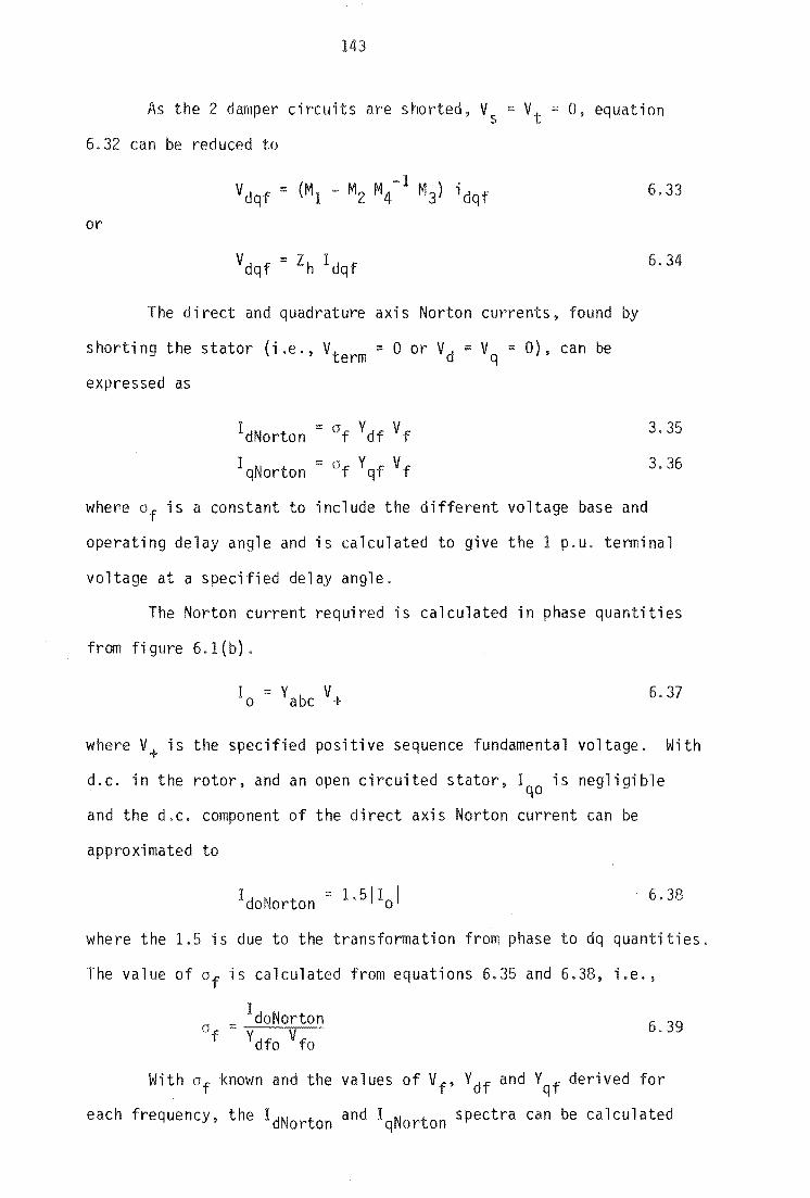
143
As the 2 damper circuits are shorted, Vs
6.32 can be reduced to
v = O~ equation t
or
The direct and quadrature axis Norton currents, found by
shorting the stator {i .e., Vt = 0 or Vd = V :: O}, can be erm q expressed as
IdNorton Of Ydf Vf
I :: a Y V qNorton f qf f
6.33
6.34
3.35
3.36
wher.e Of is a constant to include the different voltage base and
operating delay angle and is calculated to give the 1 p.u. terminal
voltage at a specified delay angle.
The Norton current required is calculated in phase quantities
from figure 6.1{b}.
6.37
where V+ is the specified positive sequence fundamental voltage. With
d.c. in the rotor, and an open circuited stator, Iqo is negligible
and the d.c. component of the direct axis Norton current can be
approximated to
6.38
where the 1.5 is due to the transformation from phase to dq quantities.
The value of Of is calculated from equations 6.
a :: IdoNorton f Y dfo V fo
and 6.38, i. e. ,
6.39
With Of known and the values of Vf , Ydf and Yqf derived for
each frequency, the IdN t and I N t spectra can be calculated or on q or on
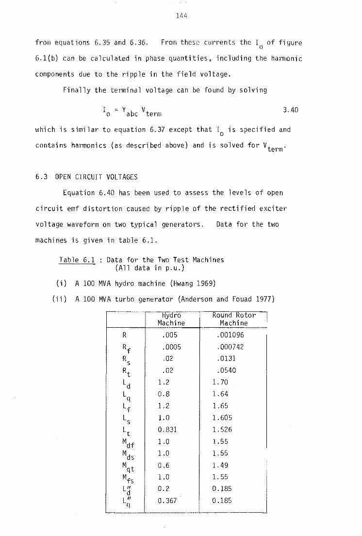
1
from equations 6.35 and 6.36. From these currents the I of figure o 6.1(b) can calculated in phase quantities, including the harmonic
components due to the ripple in the field voltage.
Finally the terminal voltage can be found by solving
I = Y V o abc term 3.40
which ;s similar to equation 6.37 except that I is specified and o
contains harmonics (as described above) and is solved for Vterm .
6.3 OPEN CIRCUIT VOLTAGES
Equation 6.40 has been used to assess the levels of open
circuit emf distortion caused by ripple of the rectified exciter
voltage waveform on two typical generators. Data for the two
machines is given in table 6.1.
Table 6.1 Data for the Two Test Machines (All data in p.u.)
(i) A 100 MVA hydro machine (Hwang 1969)
(ii) A 100 MVA turbo generator (Anderson and Fouad 1977)
Hydro Round Rotor Machine Machine
R .005 .001096 Rf .0005 .000742
Rs .02 .0131
Rt .02 .0540
Ld 1.2 1. 70 L 0.8 1.64 q Lf 1.2 1.65
Ls 1.0 1.605
Lt 0.831 1.526
Mdf 1.0 1. 55
Mds 1.0 1. 55
Mqt 0.6 1.49 Mfs 1.0 1.55 LII d 0.2 0.185
L" q 0.367 0.185
145
With a balanced system voltage and a firing angle of 85° the
round rotor machine produced .023% and .031% harmonic emf's for the
-5th and +7th harmonics respectively. For the same conditions the
hydro generator only produced .002% levels of +5th and +7th harmonic
emf's.
The addition of 4% imbalance (negative sequence) to the system
voltage resulted in the appearance of some second harmonic on the
field voltage, which then produced third harmonic positive sequence
in the stator. The magnitude of the third harmonic with a delay
angle of 75° was .148% for the round rotor machine and .028% for
the hydro machine.
Thus the effect of excitation voltage ripple is small.
Relatively large values of field resistance Rf or damper resistances
Rs ' Rt will increase the harmonic levels. However, such effect is
not significant with large synchronous generators and the Norton
equivalent current injection can in most cases be assumed to consist
of purely fundamental frequency.
6.4 Ie PARAMETERS
The response of the synchronous generator to the presence of
individual current and voltage harmonics in the stator can be better
understood with reference to a series of harmonic transfer
relationships described in this section.
6,4.1 Harmonic Current I
With reference to the general matrix equations 6.22 and 6.3J1'
, the injection of 1 per unit current of harmonic order h into the
machine stator causes harmonic voltages of the same sequence and
order, i.e .• Vh, and also of orders Vh_2 or Vh+2 depending on whether
the current injection is of positive or negative sequence respectively.
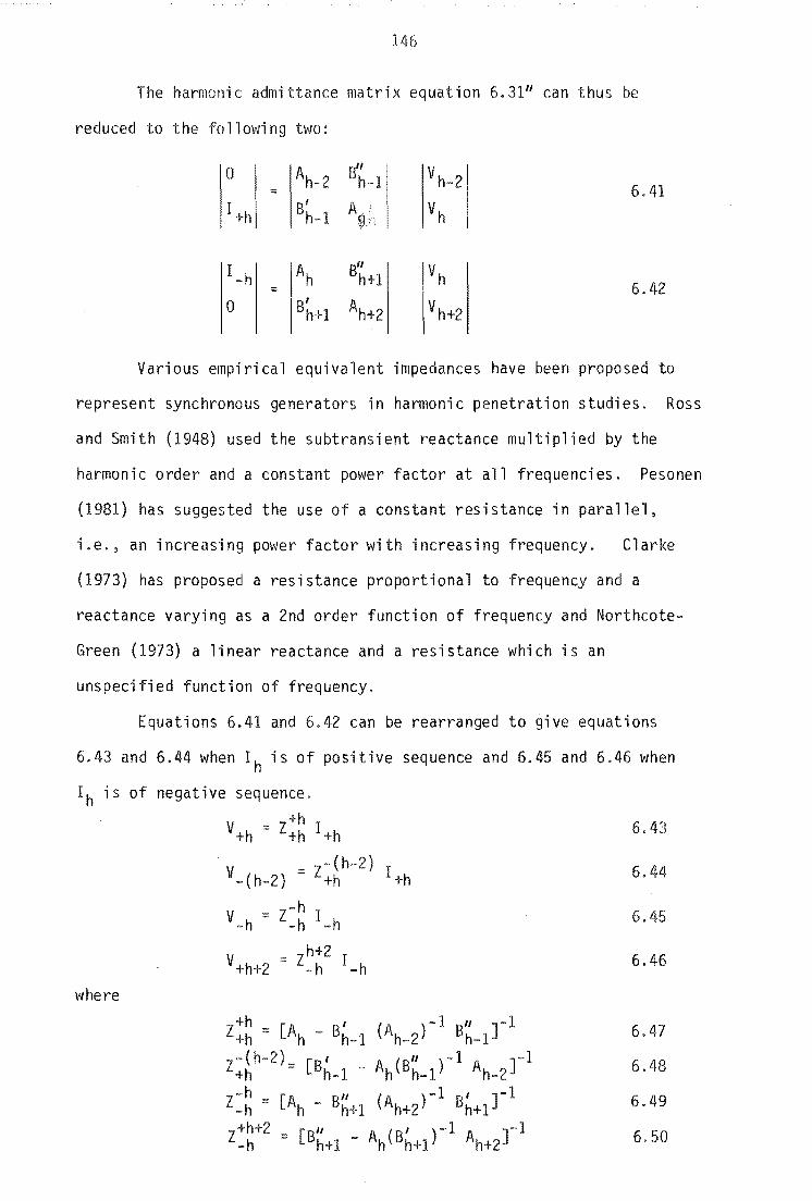
146
The harmonic admittance matrix equation 6.3111 can thus be
reduced to the fo 110wi ng two:
0 Ah_2 Bit
V h-2 h-l 6.41 =
I +h Bh_l Vh
I_h IAh 811 Vh h+l 6.42 = 0 I Bh+1 Ah+2 Vh+2
Various empirical equivalent impedances have been proposed to
represent synchronous generators in harmonic penetration studies. Ross
and Smith (1948) used the subtransient reactance multiplied by the
harmonic order and a constant power factor at all frequencies. Pesonen
(1981) has suggested the use of a constant resistance in parallel.
i.e. ~ an increasing power factor with increasing frequency. Clarke
(1973) has proposed a resistance proportional to frequency and a
reactance varying as a 2nd order function of frequency and Northcote
Green (1973) a linear reactance and a resistance which is an
unspecified function of frequency.
Equations 6.41 and 6.42 can be rearranged to give equations
6.43 and 6.44 when Ih is of positive sequence and 6.45 and 6.46 when
I his of negative sequence.
V+h +h
Z+h I+h
V -(h-2) Z (h-2)
+h I +h
V+h+2
where
+h [ '( )-1 It J 1 Z+h Ah - Bh- 1 Ah_2 Bh_l Z (h-2) [8' - A (B" )-1 A ]
+h h-l h h-l h-2 -h [ II ( )-1, J-l Z_h Ah Bh+1 Ah+2 Bh+1 +h+2 [II (' )-1 ] 1 Z h = Bh+1 - Ah Bh+1 Ah+2
6.43
6.44
6.45
6.46
6.47
6.48
6.49
6.50

147
The subscripts of the impedances refer to the harmonic order
of the current injection, the superscript to the harmonic order of the
voltage produced and the sign of subscripts and superscripts refer
to the sequence (i . e. , + for positive sequence) . +h
Z+h and h
-h are defined as the open circuit harmonic impedances
while Z (h-2) -h and zh+2
-h are defi ned as the open circuit conversion
impedances.
The variation in the magnitude of these impedances with frequency
is illustrated in figure 6.3 for the hydro set described in table 6.1
15 (i)
10
........
;:l . p", '-'
(\) u ~ CI,\ ~ It) p", e .....
5
0 S
Figure 6.3
15 25 Harmonic Order
3S 4S
Magnitude of the hydrogenerator harmon; c 'j mpedances
(i) z:~ and z=~ (ii) Z+(h+2)
h (iii) Z (h-2)
+h
Figure 6.3 shows that the magnitude of the (self) harmonic
inductance is very close to that of the established models (Adkins
and Harley 1975), i.e.,
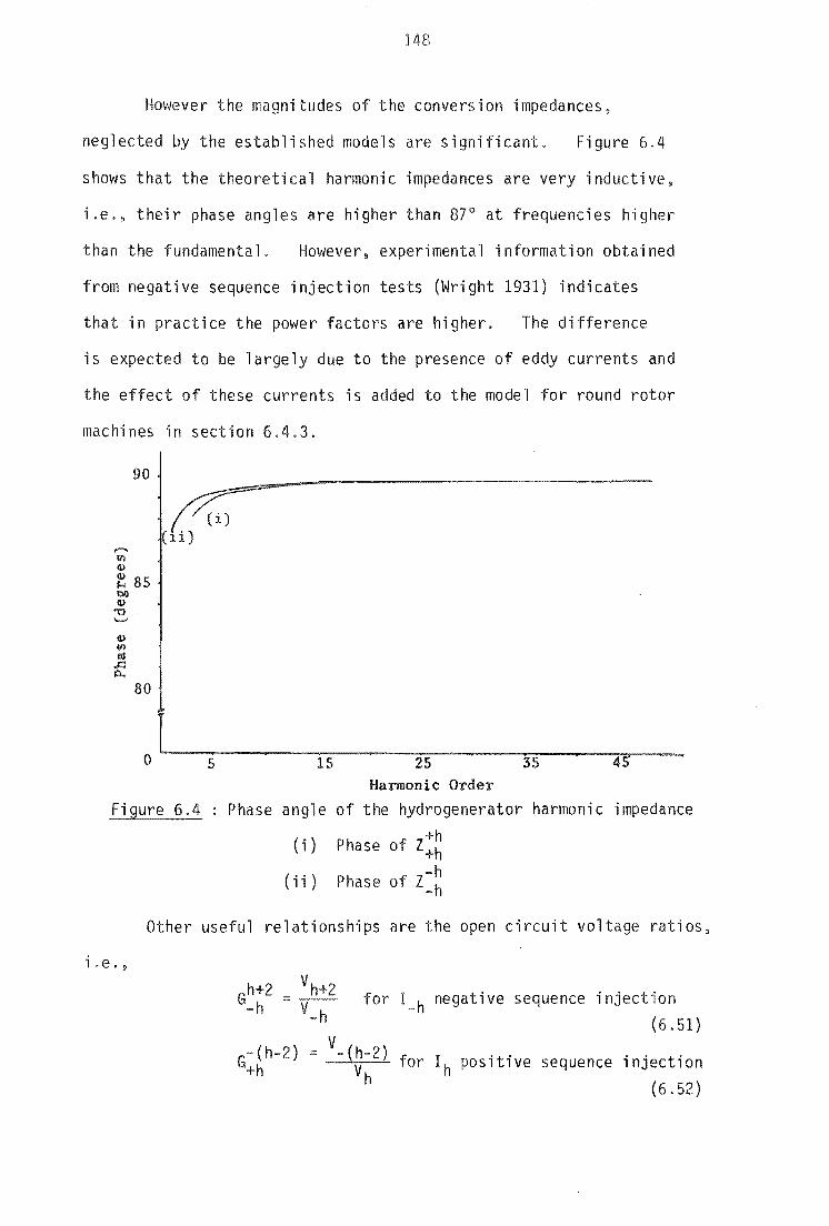
148
However the magnitudes of the conversion impedances,
neglected by the established models are significant. Figure 6.4
shows that the theoretical harmonic impedances are very inductive,
i,e" their phase angles are higher than 87° at frequencies higher
than the fundamental. However, experimental information obtained
from negative sequence injection tests (Wright 1931) indicates
that in practice the power factors are higher. The difference
is expected to be largely due to the presence of eddy currents and
the effect of these currents is added to the model for round rotor
machines in section 6.4.3.
Figure 6.4 Phase angle
(i)
(i i)
Harmonic Order
of the hydrogenerator +h
Phase of Z+h -h Phase of Z_h
harmonic impedance
Other useful relationships are the open circuit voltage ratios,
Le .•
Gh+2 = Vh+2 -h h
for I_h negative sequence injection (6.51)
-(h-2) G+h
v (h-2) V
h for Ih positive sequence injection
(6.52)
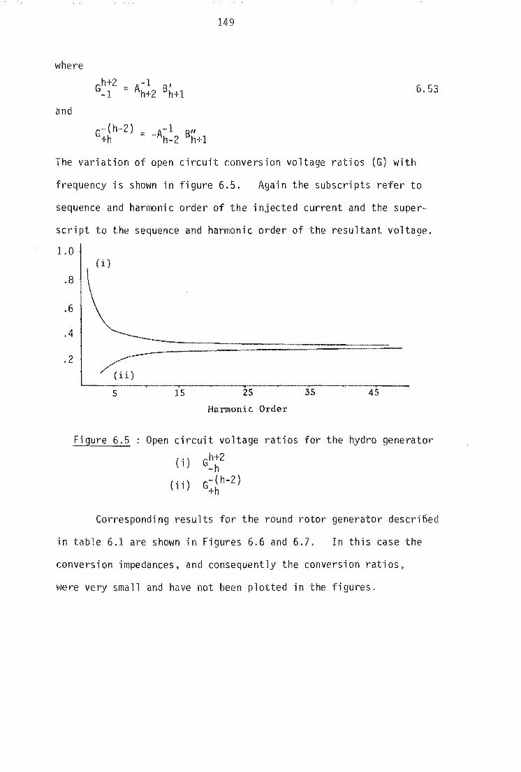
149
where
6.53
and
G-{h-2) = _A- 1 B" +h h-2 h+1
The variation of open circuit conversion voltage ratios (G) with
frequency is shown in figure 6.5. Again the subscripts refer to
sequence and harmonic order of the injected current and the super-
script to the sequence and harmonic order of the resultant voltage.
1.0
.8
.6
.4
.2
(i)
5 15 2S 35 4S
Harmonic Order
Open circuit voltage ratios for the hydro generator
(i) Gh~2
(ii) G~~h-2)
Corresponding results for the round rotor generator described
in table 6.1 are shown in Figures 6.6 and 6.7. In this case the
conversion impedances, and consequently the conversion ratios~
were very small and have not been plotted in the figures.

,,-..
::l
0.. ------(J,J u s:::: n:l
'"0 (J,J 0.. E I-l
10.0
8.0
6.0
4.0
2.0
15
150
25 Harmonic Order
35 45
Figure 6.6 Magnitude of the harmonic impedances of the round
( +h -h) rotor generator Z+h and Z_h
90
88
86
(i) 84
82
80
0 5 15 25 35 45 Harmonic Order
Figure 6.7 Pha;;e angle of the harmonic impedance of the round
rotor nerator (i) Phase +h
of Z+h
( ; i ) Phase -h of Z_h
6.4.2 Simplified Modelling
As the phase of the open circuit conversion impedances is close
to -90 0 and that of the Gh~2 and Gh(h-2) is about 180 0 the resistances
can be neglected if desired and the following approximate harmonic
conversion relationships result:

151
Zh+2 -h
j h+2 (Lit 'q L~p
Z(h-2) = . h-2 (Lit Lit) J ~ -+h 2 q d
Gh+2 h+2( L~ Lit
+ L~) -h h L" q
G-(h-2) = - ¥( L" - LII
9 d) +h LII + L" q d
The approximations of equations 6.55 to 6.58 agree well with the
results of figures 6.3 to 6.7.
6.4.3 Parameters derived from harmonic voltage sources
6.55
6.56
6.57
6.58
If instead of the current injection of the machine stator is
connected to a 1 per unit harmonic voltage source of either positive
or negative sequence the harmonic matrix equations, i.e., 6.22 and 6.31"
reduce to:
=
or
Ih = Ah Vh Ih_2 = B" Vh (when h-l
I h+2 Bh+1 Vh (when
a BII
h+l
Ah+2
Ih is
Ih is
of
of
6.59
6.60
positive sequence) 6.61
negative sequence) 6.62
An alternative harmonic impedance can then be derived from 6.60
such that
Figure 6.8 shows a comparison between Zh and the previously
calculated Z~ for the hydro machine. The difference is about 8% and
therefore of significance. For the round rotor machine, however, the
difference is negligible.

1
::l
0.. B
(]) 6 u
r::: rt:!
'"0 (]) 4 0.. E
I-<
2
0 5 15
152
25 Harmonic Order
3S
Figure 6.8 Comparison of hydro generator impedances
4S
(i)
(ii)
(i) Derived from current injection (Z:~ and Z-~)
(ii) Derived from voltage application (Zh)
Several authors (Kimbark 1956 and Adkins and Harley 1975)
have used the following expression for the negative sequence
reactance when the generator has a negative sequence voltage applied
to it. 2 XII XII
::: d q XII + XII d q
At harmonic frequencies the corresponding expression would be:
2 XII X" d q
j h X" + X" d q
6.63
6.64
Equation (6.64) gives approximately ~qual results to those calculated
and plotted in figure 6.8.
Similarly to the voltage ratios defined earlier the following
short circuit relationships can be defined from equations 6.60, 6.61
and 6.62.
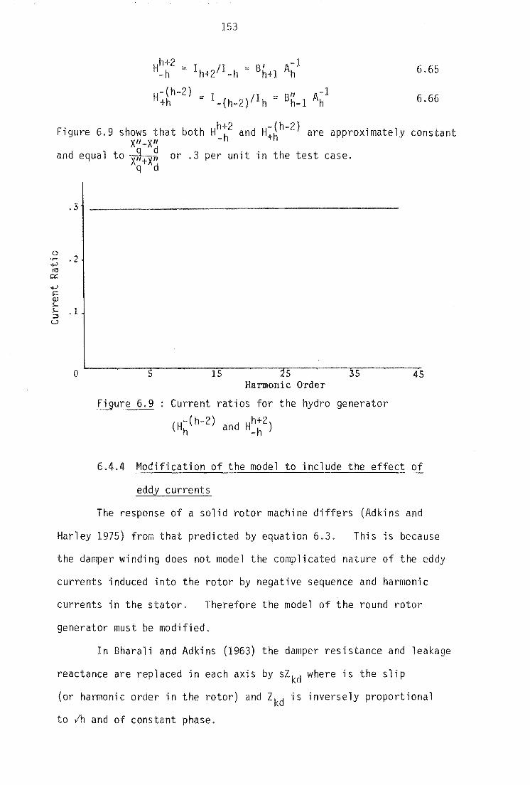
153
h+2 I A-l H_h = Ih+2 /I _h = Bh+1 h 6.65
H~~h-2) = I_(h_2)/I h = Bh_1 Ah1 6.66
h+2 -(h-2) Figure 6.9 shows that both H_h and H+h are approximately constant X"_XII
and equal to X~+X~ or.3 per unit in the test case. q d
.3
o .2
o 5 15 5 Harmonic Order
3S
Figure 6.9 Current ratios for the hydro generator
(Hh(h-2) and H~~2)
4S
6.4.4 Modification of the model to include the effect of
eddy currents
The response of a solid rotor machine differs (Adkins and
Harley 1975) from that predicted by equation 6.3. This is because
the damper winding does not model the complicated nature of the eddy
currents induced into the rotor by negative sequence and harmonic
currents in the stator. Therefore the model of the round rotor
generator must be modified.
In Bharali and Adkins (1963) the damper resistance and leakage
reactance are replaced in each axis by kd where is the slip
(or harmonic order in the rotor) and Zkd is inversely proportional
to Ih and of constant phase.

154
Thus the elements of the impedance matrix of equation (6.3") are
modified by
6.67
This assumes that the frequencies are sufficiently high to make the
resistance dominated by skin effect.
The effect of the improved model on the magnitude and phase
of z=~ and Z:~ is quite significant. Figure 6.10 shows that the
magnitudes of z:~ (equal to the magnitude of Z=~) with the improved
model and those of the basic model differ by about 15%. Figure 6.11.
when compared to figure 6.7 also shows a decrease in the phases of
+h -h h Z+h and Z_h' Both these effects are consistent wit the decrease
in damper leakage reactance and increased damper resistance resulting
from equations 6.67 and 6.68.
6.5 CONCLUSIONS
Existing harmonic equivalents are derived from experimental
tests and the results vary considerably. Moreover, they tend to
use the same expressions for the derivation of the harmonic
impedances of hydro and solid rotor machines.
A general Norton equivalent circuit has been developed that
represents the steady state behaviour of synchronous generators in the
harmonic space. The open circuit harmonic impedances of the Norton
equivalent are in reasonable agreement with the empirical harmonic
impedances in current use, except for the resistive dampings which
are lower in the theoretical model. Such differences have been
reduced in the case of solid rotor mach'ines by the addition of
eddy current representation in the form of frequency dependent damper
leakage and resistances.
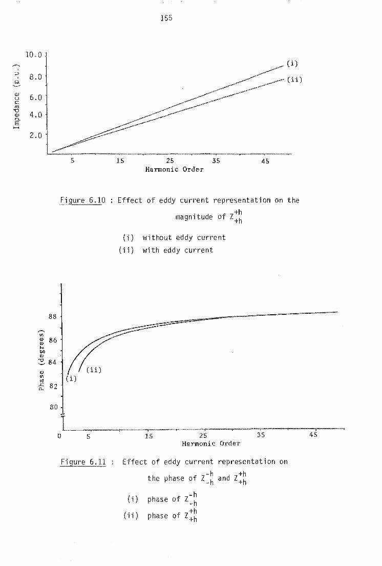
10,0
:;::l 8.0 CL
OJ 6.0 u t:: ro
"'0 4.0 OJ
CL E .....
2.0
5
88
80
o 5
Figure 6.11
15
155
2S Harmonic Order
35
Ci)
(ii )
45
Effect of eddy current representation on the
magnitude of Z:~
(i) without eddy current
(ii) with eddy current
15 2S Harmonic Order
Effect of eddy current representation
the -h and Z+h phase of Z_h +h
(i) phase -h of Z_h
(i i) phase +h of Z+h
on

156
The main contribution of the generalized model is the inclusion
of the already observed but practically ignored effect of frequency
conversion, which ;s considerable in the case of hydrogenerators.
The model has also shown the existence of different harmonic impedances
in the cases of voltage and current harmonic injections.
The effect of static excitation on the Norton current injection
distortion has been shown to be negligible in most practical cases.
As a result of harmonic coupling the use of independent
frequency harmonic flows is unrealistic. Instead, the harmonic Norton
equivalent derived in this chapter should provide the means for a
realistic direct solution in the harmonic space.
in chapter 7.
This is discussed
157
CHAPTER 7
APPLICATION OF THE HARMONIC NORTON EQUIVALENT OF
THE SYNCHRONOUS MACHINE
7.1 INTRODUCTION
In section 6.4 the harmonic Norton equivalent of the salient
poled synchronous machine, examined in isolation to any other system
components, has been shown to have significant levels of coupling
between frequencies. To examine the proposed synchronous machine
equivalent in conjunction with other system components, and hence to
show fully its potential impact on the solution of transmission system
harmonic distortion, several system configurations are examined in this
chapter.
As it is known that negative sequence stator currents of
fundamental frequency lead to third harmonic voltage distortion, the
synchronous machine model was tested with unbalanced loads.
described in section 7.2.
This is
In the presence of a current harmonic injection the harmonic
current propagates into the system an,d a proporti on of it wi 11 enter
the stator of the machine. Due to harmonic conversion, other harmonic
currents and voltages are then produced which in turn propagate through
out the system. This case is considered in section 7.3.
The largest sources of harmonic distortion in transmission
systems are generally h.v.d.c. convertor stations. As many convertor
stations include either generators or synchronous compensators, the
effect of a synchronous machine model which includes harmonic
conversion needs to be assessed. This is discussed in section 7.4.
The coupling between freaquencies, ignored in conventional
harmonic flows, is discussed in section 7.5.

158
7.2 APPLICATION OF THE HARMONIC NORTON EQUIVALENT TO AN ASYMMETRICALLY
LOADED GENERATOR
It has been shown by Clarke (1950) that under unbalanced fault
conditions significant harmonic currents and voltages are produced due
to harmonic conversion. In the steady state a generator is rarely
unbalanced to such an extent, but under conditions of large unbalance
or resonance, significant levels of distortion may arise. The presence
of significant levels of third harmonic in the Souht Island of New
Zealand (Hyland 1981) could be due in part to negative sequence
currents entering the machine's stators.
The synchronous generator of table 6.1(1) is used as a test
system with various unbalanced loads. The system, illustrated in
Figure 7.1 consists of a single cirucit line of flat configuration
corresponding to the Islington to Kikiwa 220 kV transmission line
"in the New Zealand system (Densem et al 1984). The transformer
is star-g/star connected, and its rating is 100 MVA, 14 kV/220 kV,
with a leakage reactance of 0.112 p.u.
untransposed till'! ~+---~~~~---------bpm
I
c
: Test System
The Norton current, 10 1 is a positive sequence fundamental
current injection which maintains a constant (1 p.u.) positive
sequence component of fundamental voltage at the generator terminals.
Taking into account the sign convention indicated in gure 7.1 the
generator current is
i = - Y ge n v + I 0 7.1
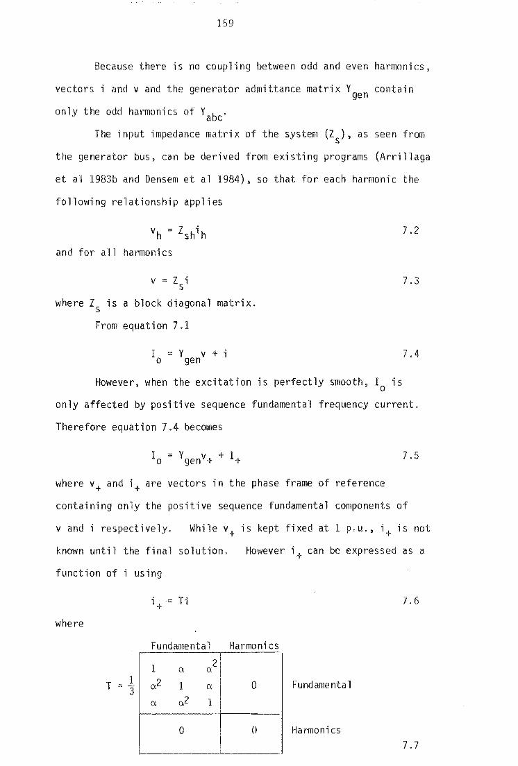
159
Because there is no coupling between odd and even harmonics,
vectors ; and v and the generator admi
only the odd harmonics of Y b ' a c
matrix Ygen contain
The input impedance matrix of the system (Zs)' as seen from
the generator bus, can be derived from existing programs (Arrillaga
et al 1983b and Densem et al 1984)~ so that for each harmonic the
following relationship applies
Vh = Zshih
and for all harmonics
v = Z i s
where Zs is a block diagonal matrix.
From equation 7.1
10 = Y v + i gen
7,2
7.3
7.4
However, when the excitation is perfectly smooth, 10 is
only affected by positive sequence fundamental frequency current,
Therefore equation 7.4 becomes
7.5
where v+ and i+ are vectors in the phase frame of reference
containing only the positive sequence fundamental components of
v and i respectively. While v+ is kept fixed at 1 p.u., i+ is not
known until
function of
where
T
the final solution.
using
i+ Ti
Fundamental
1 3
1 0,2
a
a 0,2
1 ex 0,2 1
0
However i+ can be expres s as a
7.6
Harmoni cs
0 Fundamenta 1
0 Harmoni cs 7.7
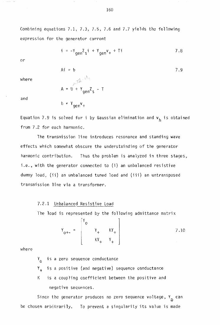
160
Combining equations 7.1, 7.3, 7.5, 7.6 and 7.7 yields the following
expression for the generator current
or
where
and
i = -Y Z i + Y v + Ti gen s gen +
Ai = b
A = U + Y Z T gen s
b = Y v gen +
7.8
7.9
Equation 7.9 is solved for i by Gaussian elimination and vh is obtained
from 7.2 for each harmoni c.
The transmission line introduces resonance and standing wave
effects which somewhat obscure the understainding of the generator
harmonic contribution. Thus the problem is analyzed in three stages,
i.e., with the generator connected to (i) an unbalanced resistive
dummy load, (ii) an unbalanced tuned load and (iii) an untransposed
transmission line via a transformer.
where
7.2.1 Unbala istive Load ~~~~~~~~~~~
The load is represented by the following admittance matrix
Yo
Y 0+-
Yo is a zero
KY+ Y+
uence conductance
Y+ is a positive (and negative) sequence conductance
K is a coupling coefficient between the positive and
negative sequences.
7.10
Since the generator produces no zero sequence voltage, Y~ can
be chosen arbitrarily. To prevent a singularity its value is made

161
equal to Y+, Thus the three phase admittance matrix becomes
1 + 2K K K - "3 - "3
Y y+ K 1 K 2K
::::: - "3 "3 abc 3 7,11
K 2K 1 K 3 - "3
The matrix, although not physically realizable, can be used
to examine the effect of generator loading and degrees of unbalance.
Figure 7.2 shows the effect of coupling and loading on the level
of 3rd harmonic voltage distortion. The results indicate that for
loads within the nominal rating (i.e. 1 p.u.) the 3rd harmonic voltage
Voltage (%)
1 p.u. 10.0 power
9.0
8.0
7.0
6.0 0.5 p.u. power
5.0
4.0 0.25p.u. power
2.0
1.0
0.1 0.2 Coupling Coefficient
Figure 7.2 Variation of Positive Sequence Third Harmonic Voltage with Coupling and Loading

1
is almo directly proportional to the load admittance, and hence to
current or power. Also, the 3rd harmonic voltage is seen to be
directly proportional to the level of coupling. The 5th harmonic
voltage, not shown in the figure, varies approximately in proportion
to K2.
7.2.2 Effect of Saliency
It is apparent from chapter 6 that saliency is the main deter-
mining factor in the process of harmonic conversion. To exami ne the
effect of saliency, the simplified equivalent circuits in figure 7.3 are
used for the machine's direct and quadrature axes respectively.
circuits include only one winding in each axis of the rotor (i.e.
These
Mds = Mfs = 0). Further simplification is achieved by setting the direct
axis magnetizing inductance Mdf to 1 p.u. and making Ld = Lf • Lq = Lt
and Rf = Rt and assuming equal leakage in both axes (i .e .• Ld - Mdf
= Lq - Mqt ). nally saliency. defined as the ratio of quadrature to
direct axis rotor fluxes. can be expressed by
M t S = 1 - ~
Mdf 7.12
Thus from specified leakage, saliency and resistances Rand Rf , the
machine parameters of equation 7.1 can be calculated. While this
model is not representative of an actual machine, it does prove a useful
indication of the effect of saliency.
Figure 7.3 Simplified Equivalent Circuit of the Machine
(a) Direct axis, (b) Quadrature axis

163
The effect of saliency has been tested on a purely resistive
load of 484~ (1 p,u.) with a coupling coefficient of 10%. Cases of .
perfect saliency (Mqt a) and zero saliency (Mqt = 1) produced no
noticeable effect with perfect coupling (i .e. zero leakages),
However, the addition of some leakage (0.2 p.u.) showed considerable
difference in the resulting levels of harmonic voltage distortion,
as shown in figure 7.4.
Voltage (%)
9.0
8.0
7.0
6.0
5.0
4.0
3.0
2.0
1.0
25 50 Saliency (%)
75
-1
100
Fi 7.4 Effect of Saliency on nerator Harmonic Voltages
7.2.3 Unbalanced Tuned Load
This case introduces the effect of resonance by replacing the
resistive load with the delta connected circuit of figure 7.5. The
resonance frequencies approximating those of the open circuited line

164
of the te system. The original machine data of table 6.1(a) was
used.
B
(
(
Figure 7.5 Tuned Delta Load
The sequence components admittance matrix of the delta circuit
is
0 0 0
y :::: 0 (3+0)Yl aY1 7.13 0+-
0 2 -oa Y1 3 + 0
where
a ::: lL120°
Y2 (1+o)Y p valid at a particular frequency
and, using the previous definition of coupling coefficient,
I KI 7.14
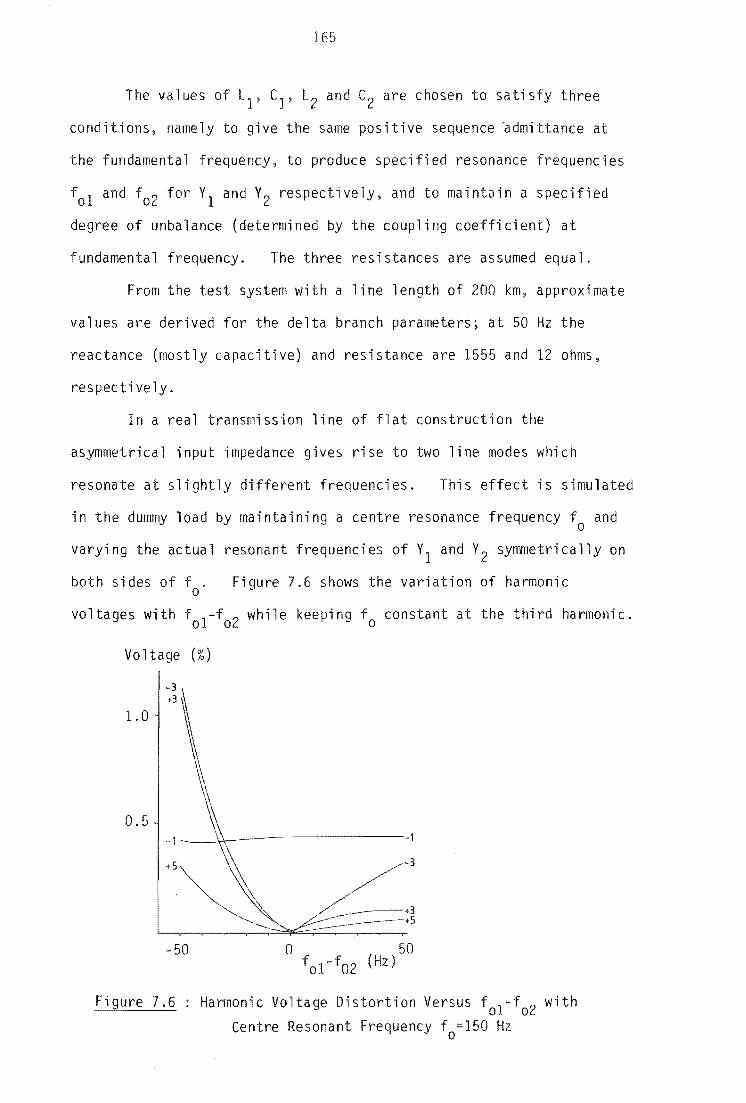
1
The values of LI , CI , L2 and C2 are chosen to satisfy three
conditions, namely to give the same positive sequence ~dmittance at
the fundamental frequency, to produce specified resonance frequencies
fol and f02 for VI and V2 respectively, and to maintain a specified
degree of unbalance (determined by the coupling coefficient) at
fundamental frequency. The three resistances are assumed equal.
From the test system with a line length of 200 km, approximate
values are derived for the delta branch parameters; at 50 Hz the
reactance (mostly capacitive) and resistance are 1555 and 12 ohms,
respectively.
In a real transmission line of flat construction the
asymmetrical input impedance gives rise to two line modes which
resonate at slightly different frequencies. This effect is simulated
in the dummy load by maintaining a centre resonance frequency f and o
varying the actual resonant frequencies of VI and V2 symmetrically on
both sides of f . o
Figure 7.6 shows the variation of harmonic
voltages with fol-f02 while keeping fo constant at the third harmonic.
Vo ltage (%)
1.0 -3 \ .3
0.5
50
Fi ure 7.6
------1
-3
Harmonic Voltage Distortion Versus f ol -f02 with
Centre Resonant Frequency fo=150 Hz

By maintaining a constant unbalance, the amount of negative
sequence voltage and current at fundamental frequency is approximately
constant with varying fo1 -fo2 '
With fo1>fo2 YI is capacitive and Y2 inductive and vice versa
with fo2 >fo1 ' This results in a strong unbalance at 3rd harmonic,
leading to increasing negative sequence 3rd harmonic voltage and current
This is followed by corresponding increases of 5th
harmonic voltage and current. The ratio of 5th harmonic positive
sequence to 3rd harmonic negative sequence is approximately constant.
7.2.4 Untransposed Open Circuit Line
In the test system of figure 7.1 the length of the untransposed
line was varied from 50 to 800 km.
gures 7.7{a} and {b} show the positive and negative sequence
third harmonic voltages at the machine terminals. While the machine
cannot generate harmonics directly, these appear as a result of the
unbalance proproduced by the untransposed line and are therefore very
dependent on the length of line.
In the range of line lengths between 165 to 200 km each harmonic
voltage shows a double peak. These peaks correspond to the different
resonant lengths of the a and 8 propagation modes present in a line of
flat construction. The peaks occur at different lengths for the
different harmonics {e.g. at 170 and 195 km for positive sequence
third and at 1 and 190 km for negative sequence third}, This effect
is due to the impedances and degree of unbalance varying greatly near
the resonances of the two modes.
The harmonic voltage levels in this range of distances are too
large to be ignored, i.e., 6!% of positive sequence third and 4% of
negative sequence third harmonics respectively. This clearly
demonstrates the need for detailed generator representation as proposed

167
oj n chapte~' 6. The levels of distortion are also substantially
higher than the levels calculated in the dummy loads, as a consequence
of the standing wave effect of the line.
,-...
Q) 01 ttl +' v-a :>
,,-.. ~
Q) 01 ttl +' r-
5.0
4.0
3.0
2.0
LO
7.0
6.0
5.0
4.0
3.0
2.0
1.0
(a)
100 500 6 0 700 8 0 Line length (km)
(b)
100 200 300 400 500 600 700 800 Line length (km)
Figure 7.7 Variation of third harmonic voltage with transmission line length
(a) Negative sequence (b) Positive sequence
A generalized steady state model of the synchronous machine
has been developed which can take into account any assymmetry or
distortion present in the armature voltages. The level of inter
harmonic coupling has proved to be partly load related (size
and degree of unbalance) and partly generator related (saliency).

168
Such harmonic coupling cannot be detected with present harmonic
models, where the generator is short-circuited behind the subtransient
reactance.
t results~ with the machine connected to a dummy (asymmetrical)
load and to an untransposed transmission line, have been obtained to
corroborate the theory. They indicate that the harmonics generated
by the machine may often exceed the levels prescribed by harmonic
legislation and they need to be assessed accurately. The effect of
two different resonant modes have been demonstrated, leading to a
strong unbalance and thus high voltage distortion. The main harmonic
contributions from the generator are positive and negative sequence third
harmonic currents, which therefore cannot be eliminated by generator
or transformer connections.
7.3 HARMONIC CURRENT INJECTION INTO A SYSTEM INCLUDING A SYNCHRONOUS
MACHINE
Normally in any real power system the sources of harmonics are
geographically separated from the synchronous machines in the system
by one or more transmission lines. A typical example of this is in
the South Island of New Zealand with the large smelter at Tiwai being
supplied predominantly by the large hydro station at Manapouri (Densem
1983).
7.3.1 Simplified Test System
To simplify the system to a more manageable size, the same
test system used in section 7.2 was chosen, i.e., figure 7.1, with the
point of injection chosen to be the open circuited end of the
transmission line, as described in figure 7.8. As the only busbars
of interest are 1, to maintain the fundamental voltage at the synchronous

169
generators terminal, and 2, the point of injection, the system was
reduced by eliminating bus bar 3.
Figure 7.8 : Modified Test System
The system can then be described by the 2 x 2 matrix equations
7.14 and 7.15.
II = Y11 VI + Y12 V2
12 = Y21 VI + Y22 V2
Combining equations 7.1,7.5, 7.6 and 7.7, of section 7.2, gives
7.14
7.15
7.16
In this case Ygen contains both even and odd harmonics, necessary if
the current injection 12 is an even harmonic. Therefore, combining
equations 7.14 and 7.16 gives
=Y (V+-V 1) gen 7.17
or
Finally, combining equations 7.15 and 7.18 into matrix form gives
r V r [Y + (U - T) Yll (U-T) Y 12] [V 1 1 ge~2 + gen 7.19
Y21 Y 22 V 2
or [IJ =[y][VJ 7.20

The matrix (U-T)
2 3
1 - - a2
3
1 a 3
l
170
has the follow; ng form
1 1 - - a 3 3
2 1 0 3 - - a 3
1 3" a2
o
2 3"
U N-3,N-3
7.21
where N is three times the number of harmonics. Because T is zero at
harmonics, only the fundamental values of YII and Y12 are changed
in equation (7.19).
For consistency with existing software and with the definition of
the harmonic space in section 2.6, I (and V) were rearranged to be of the
form
11 1 fundamental 12 J
I 11 7.22
} 2nd harmon; c 12
II
Similarly, Y in equations 7.19 and 7.20 needs to be rearranged to

171
Al + (U-T)Yll (U-T)Y 12 0 0 BU
2 0
Y21 Y22 0 0 0 0
0 0 A2 + 2 Vl1 Yf2
0 0 V~1 2
Y22
3 3 B I 2 0 0 0 A3 + Y11 Y12
0 0 0 0 3 Y~2
I Y21
where the superscripts of yil' Vi2' Y~1 and Y~2 refer to the ;th
harmonic.
7.23
Equation 7.20 can be solved for VI and V2 by Gaussian
elimination. Equation 7.19 shows that the voltages VI and V2 are made
up of 2 components. One due to the harmonic current injection, I2,
which is considered in conventional harmonic penetraction studies, the
second component being due to the asymmetrically loaded generator as
analysed in section 7.2. Because equaiton 7.19 is linear, these two
effects can be examined separately and combined using superposition.
7.3.2 The Effect of Excitation Alone
This is essentially the same problem described in section 7.2.4
with the exception that the solution includes the voltage at the
unterminated end of the transmission line, V2.
For the range of line lengths 50 to 800 km the negative and
positive sequence third harmonic voltage components are given in
figures 7.9(a) and (b) respectively.
For both the negative and positive sequences the generator
terminal voltage (VI) is identical to that previously calculated in
section 7.2.4, i.e., figure 7.7. It can also be seen that the open
circuit voltages are significantly larger than the generator terminal
voltages.
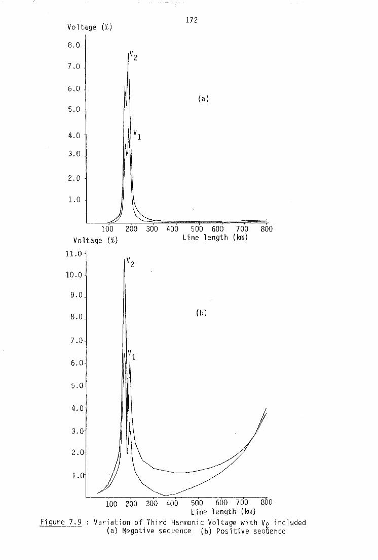
172 Va 1 (% )
8.0 V2
7,0
6.0 (a)
5,0
4,0 VI
3,0
2.0
1.0

173
7.3.3 The Effect of a Current Injection
If the synchronous generator excitation is removed, by setting
v+ to zero in equation 7.19, the effect of an injected current into
bus bar 2 can be assessed. Because the test system of figure 7.1
was shown in section 7.2 to be close to third harmonic resonance
for the range of line lengths 155 to 195 km, this range of line lengths
was chosen. It is expected that when a 1.0 p.u. positive sequence
fifth harmonic current is injected into busbar 2, significant levels
of both negative and positive sequence third harmonic voltage will be
produced due to the coupling between frequencies exhibited by the
synchronous generator. As for section 7.2, the generator data is
that of the hydro generator of table 6.1(1).
As discussed in sections 2.3.2 and 2.6, conventional harmonic
penetration algorithms treat each frequency separately and would,
therefore, not be able to predict voltage distortion at any other
frequency except the injected fifth harmonic. The positive sequence
fifth harmonic voltage predicted by a conventional harmonic penetration
algorithm (Densem 1983) is given as a function of line length in curve (1)
of figure 7.10. Note that while negative sequence fifth harmonic
voltage will also be produced, it is not included in figure 7.10.
However when equation 7.19 is solved with 1.0 p.u. positive
sequence fifth harmonic injection into bus bar 2, significant levels
of positive fifth, negative third. positive third and negative sequence
fundamental harmonic voltage are produced. These are plotted as
curves (2) to (5) in figure 7.10 respectively. As was the case
previously in sections 7.2 and 7.3.2, the peaks in the negative and
positive sequence third harmonic components do not occur at the same
line length, being due to the different propagation modes of the system.

Voltage (p. u. )
1 ) +5 th Conventi Dna 1
2) +5 th Proposed 4.0 3) _3 rd " 4) +3rd
" 5) _1 st
"
3.0
174
Generator II
" " "
Model
3
4
2
1
---------------------5 155 160 165 170 175 180 185 190 195
Line length (km)
Figure 7.10 Comparison of Conventional and Harmonic Space Penetration Studies
The relatively large levels of negative and positive sequence
third harmonic magnitudes, 3.78 and 2.38 times the positive fifth (
harmonic voltage of 190 km respectively, show the importance of
modelling the harmonic process of synchronous machine.
7.4 HARMONIC INTERACTION BETWEEN SYNCHRONOUS MACHINES AND H.V.D.C.
CONVERTORS
7.4.1 Introduction
When assessing power system harmonics distortion, synchronous
machines are currently modelled by their negative sequence reactance.
As already shown, the synchronous machine acts as a frequency convertor
and, if this property is not adequately represented, the harmonic
175
assessment will be in error.
Synchronous machines, either as generators or synchronous
compensators, have found their place in many h.v.d.c. convertor
schemes. Although the harmonic filters are generally located between
the synchronous machines and the convertor, some harmonic currents
enter the machines in the presence of imperfect filtering and
uncharacteristic harmonics. Moreover, in some schemes the machines
are placed between the convertor and the harmonic filters and they
will attract a substantial proportion of the convertor harmonic current.
With single generator-convertor units (Arrillaga 1983) all the convertor
currents enter the machines. In all these cases the harmonic current
entering the machines provides the source of harmonic conversion.
As many h.v.d,c. links are associated with remote hydro-
generation and synchronous compensators, both of which are generally
salient in nature, the use of a synchronous machine model which includes
harmonic conversion is important when assessing the waveform distortion
associated with h.v.d.c. convertors.
Harmonic conversion results from the off-diagonal B' and BN
terms of Y in equation 7.1. Therefore, a harmonic voltage Vh may gen
produce harmonic currents Ih_2' Ih and I h+2 depending on the sequence
S·imilarly. a harmon; c current may produce components of
voltage Vh_2> Vh and Vh+2. In thi s sect i on the harmoni c space
representation of the synchronous machine ;s used to provide a more accurate
assessment of the harmonic interaction that takes place between h.v.d.c.
convertors and local synchronous machines such as hydro-generators and
synchronous compensators.
7.4.2 Approximate Direct Solution
The significance of the harmonic conversion of synchronous
machines, when associated with h.v.d.c. convertors, is first examined

176
by modelling the convertor as a fixed injection of characteristic
current harmonics. The simplest system for the phenomena under
consideration is illustrated in figure 7.11 which consists of a single
generator-transformer-convertor unit.
Figure 7.11 : Single Generator-Transformer-Generator Unit
Under idealized a.c. and d.c. conditions (Arrilliga 1983) the
a.c. current is a perfectly rectangular waveform which contains only
the characteristics (6Q+1) positive and (6Q-1) negative sequence
harmonic orders, where Q is an integer.
I n the time domai n phase 'a1current has the form
1 \ 1 i (t) "'------'" [cos(wt+o:) + cos(5wt+50: +n) +-7 cos(7wt + 70:) a n
1 + cos(llwt + 110: + n) ... J 7.24
where 0: ;s the delay angle. The magnitude of the hth harmonic rms
component is
7.25
For conventional harmonic studies the generator impedance is
jh(Xd + Xq)/2 (Clarke 1950 and Ross and Smith 1948). When these
impedances are multiplied by the corresponding frequency component of the
phase current, equation 7.25~ the resultant voltage distortion is

177
(XII + X")/2 TI d q 7.26
For the hydro-generator described in table 6.1(1), but adjusted to
a 500 MVA rati~g rather than the previous 100 MYA. equation 7.26
gives a value of Yh 0.0442.
However, when the effect of harmonic conversion is included
these currents cannot be treated separately for salient machines
because the characteristic negative sequence (6Q-l) and positive
sequence (6Q+l) harmonic current pairs produced by the convertor
correspond to the same rotor harmonic Q. Each positive sequence
(6Q+1) voltage is therefore made up of two components due to the
corresponding positive sequence (6Q+l) and the negative sequence
(6Q-l) respectively. Similarly, each negative sequence (6Q-l) voltage
is made up of two components. This is demonstrated in equations 7.27
and 7.28 for the positive and negative sequence voltage respectively.
V 6Q+l = y6Q+ 1
6Q+l + y6Q +1 -(6Q-l) 7.27
V Y (6Q-l) - (6Q-l) -(6Q-l) - (6Q-1) + Y (6Q+1) 7.28
where
V6Q +1 6Q+1
= Z6Q+1 6Q+l 16Q+1 7.29
y-(6Q-l) -(6Q-l)
::: Z-(6Q-l) -(6Q-l) I -(6Q-l) 7.30
y6Q+1 6Q+l I :;:;
Z (6Q+ 1) -(6Q-l) -(6Q-l) 7.31
-(6Q-l) Z (6Q-l) 16Q+1 y 6Q+l 6Q+1 7.32
where the Z are defined in section 6.4. Note the subscripts and
superscripts indicate the harmonic order and sequence of the current
injections and voltage distortions respectively.
It is clear that the relative phase between I_{6Q_l) and
I(6Q+l) is important. As shown by equation 7.24. in the case of an

178
a.c./d.c. convertor the relative phase of these two current components
vary with the delay angle. This effect was examined by injecting
rectangular pulses of current into the test generator and varying
the delay angle. Figure 7.12 shows the effect of varying the delay
angle on the negative sequence fifth and positive sequence seventh
harmonic voltage distortions. The dotted line indicates the value
of Vh derived from equation 7.26.
Voltage (%) +7
6. -5
5.0
4.0
3.0
2.0
1.0
30 60 90 120 Delay Angle (Degrees)
150 180
Figure 7.12 Negative Sequence Fifth and Positive Sequence Seventh Versus Delay Angle
From equation 7.24 it can be seen that for a delay angle of
zero degrees the relative phase of the fifth and seventh harmonic currents 6Q+l -(6Q-1) . is 180°. From section 6.4 the phase of Z6Q+l and Z_(6Q_l 1S
6Q+l (6Q-l) . . approximately 90° while the phase of Z_(6Q_l) and Z6Q+l 1S approxlmately
-90 0, Therefore~ with zero delay angle the two components of voltage
in equations 7.27 and 7,28 add in phase. However, as the delay angle
increases the relative phase of the harmonics changes as the higher
order harmonics are shifted by a larger amount.

179
With reference to equation 7.24, the phase difference between
the 6Q+ 1 and 6Q-l harmoni c currents is (7T - 2a) and, therefore, the
sum of the resulting voltage components vary with a. Figure 7.13(a)
demonstrates this effect for the negative sequence fifth harmonic and
gure 7.13(b) for the positive sequence seventh harmonic voltage.
approximate values for the machines ' impedances. derived from
section 6.4, are as follows
Z7 = j ~(Xd + X") :-: j 0.3969 p.u. 7 q
-5 ::: j i(XII + XII) =j 0.2835 Z_5 2 d q p.u.
Z~5 ::: -j ~(X~ - Xd) = -j 0.1169 p.u.
Z;5= -j i(X~ - Xd) = -j 0.0835 p.u.
and the corresponding voltage magnitudes are
7 -5 V7 ::: V_ 5 = 0.0442 p.u.
7 V_5 = 0.0182 p.u.
V7 = 0.0093 p.u.
(a)
Figure 7.13 Graphical Derivation of the a) Negative Fifth and b) Positive Seventh Voltage Magnitudes
7.33
7.34
7.35
7.36
(b)

180
The magnitudes of the negative sequence fi h and positive
seventh harmonic voltages, derived graphically in figures 7.13{a) and
(b), agree with the values calculated from the full admittance matrix
and plotted in figure 7.12.
7.4.3 Solution
Modelling the static convertor as a fixed source of current
harmonics is unrealistic because convertor currents depend on the
terminal voltage waveform. As described in chapter 3, the harmonic
interaction between the convertor and the a.c. system requires an
iterative algorithm with the convertor analysis in the time domain and
the harmonic power flows in the frequency domain.
The a.C. system representation in chapter 3 does not represent
harmonic coupling and, consequently, harmonic flows are carried out
independently for each harmonic and their effect is finally superimposed
to update the voltage distortion at the convertor terminals in order to
derive the new harmonic current injections. However, with the
inclusion of harmonic conversion into the generator model the individual
harmonics are no longer independent and their effect must be considered
together.
For a three-phase study involving many harmonics the system
admittance matrix is extremely large. An efficient way of solving
this problem is to replace the off diagonal terms of the generator
admittance matrix by an equivalent current injection.
6. and 6.31",
From equation
7.37
This current can be divided into two components. as illustrated in
figure 7.14, one due to the diagonal Ah term and the second due to the
off diagonal Bh_1 and Bh+1 terms. That is

1
7.38
where
7.39
v v
Figure 7.14 : Generator Representation a) Conventional Admittance b) Modified to Include Conversion
A simplified equivalent of a rectifier connected to a generator
via the convertor transformer is illustrated in figure 7.15. Current
injection II represents the effect of the off diagonal terms while 12
is the convertor current injection. VI is the generator~ and convertor,
terminal voltage.
Figure 7.15 Simplified Equivalent of a Single Generator Convertor Unit
As described in chapter 3,12 is calculated in the time domain
from the terminal voltage each iteration and then converted to the
frequency domain using an FFT. For each hannoni c "j n turn IIi s
calculated using equation 7.39 and) with 12, the a.c. system is solved
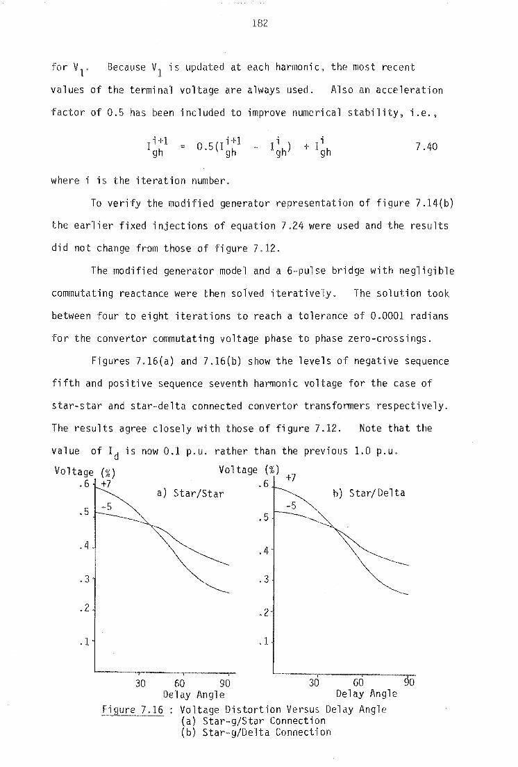
1
Because VI is updated at each harmonic, the most recent
values of the terminal voltage are always used. Also an acceleration
factor of 0.5 has been included to improve numerical stability, i.e.,
7.40
where i is the iteration number.
To verify the modified generator representation of figure 7.14(b)
the earlier fixed injections of equation 7.24 were used and the results
did not change from those of figure 7.12.
The modified generator model and a 6-pulse bridge with negligible
commutating reactance were then solved i ratively. The solution took
between four to eight iterations to reach a tolerance of 0.0001 radians
for the convertor commutating voltage phase to phase zero-crossings.
Figures 7.16(a) and 7.16(b) show the levels of negative sequence
fifth and positive sequence seventh harmonic voltage for the case of
star-star and star-delta connected convertor transformers respectively.
The results agree closely with those of figure 7.12. Note that the
value of Id
Vo ltage (%) .6 +7
.5
.4
.3
.2
.1
is now 0.1 p.u. rather than the previous 1.0 p.u.
Voltage (%) +7 .6
a) Star/Star b) Star/Delta
.5
.4
.3
.2
.1
30 60 90 30 60 90 Delay Angle Delay Angle
Voltage Distortion Versus Delay Angle (a) Star-g/Star Connection (b) Star-g/Delta Connection.
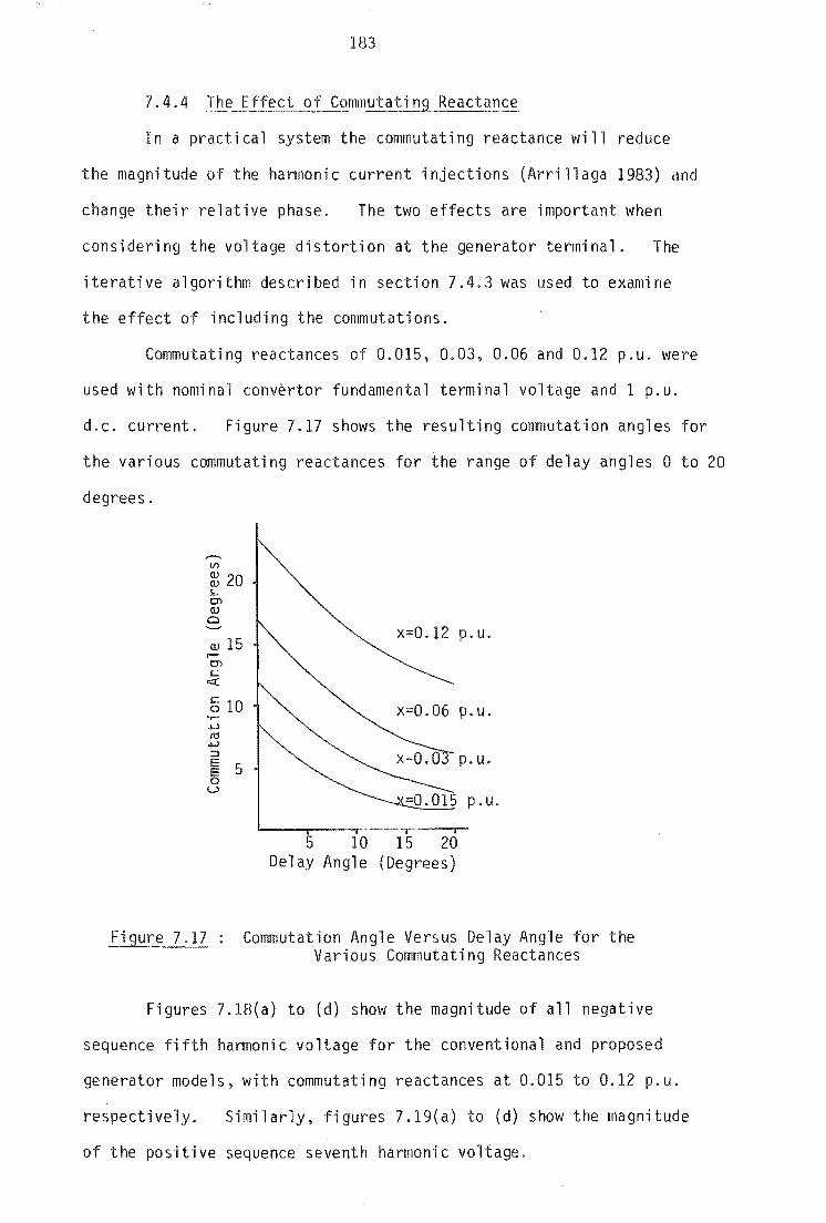
183
7.4.4 The Eff~ct of Commutating Reactance
In a practical system the commutating reactance will reduce
the magnitude of the harmonic current injections (Arrillaga 1983) and
change their relative phase. The two effects are important when
considering the voltage distortion at the generator terminal. The
iterative algorithm described in section 7.4.3 was used to examine
the effect of including the commutations.
Commutating reactances of 0.015, 0.03, 0.06 and 0.12 p.u. were
used with nominal convertor fundamental terminal voltage and 1 p.u.
d.c. current. Figure 7.17 shows the resulting commutation angles for
the various commutating reactances for the range of delay angles a to 20
degrees.
x=0.12 p.u.
x=0.06 p.u.
p.u.
p.u.
5 10 15 20 Delay Angle (Degrees)
Commutation Angle Versus Delay Angle for the Various Commutating Reactances
Figures 7.18(a) to (d) show the magnitude of all negative
sequence fifth harmonic voltage for the conventional and proposed
generator models. with commutating reactances at 0.015 to 0.12 p.u.
respectively. Similarly, figures 7.19(a) to (d) show the magnitUde
of the positive sequence seventh harmonic voltage.

1
Vo ltage (%) Vo ltage (%) 6
(a) 6 (b)
5 11)
5 11)
1 ) 1)
4 4
X ::: 0.015 p. u. Xc ::: 0.03 p.u. 3 c
3
2 2
1 1
5 10 15 20 5 10 15 20 Voltage (%) Delay Angle
Vol (%) Delay Angle
6 6 (c) (d)
5 11) 5 11)
1) 1) 4 4
Xc = 0.06 p.u. 3
Xc ::: 0.12 p.u. 3
2 2
1 1
5 10 15 20 5 10 15 20 Delay Angle Delay Angle
Figure 7.18 Negative Sequence Fifth Harmonic Vol Versus Delay Angle
a) Xc = 0.015 p.u.
b) Xc = 0.03 p. u.
c) X ::: 0.06 p.u. c d) Xc - 0.12 p.u.
In both figures 7.18 and 7.19 (1) refers to the conventional generator
model results and (11) to the results of the proposed model.

1
Voltage (%)
6 11)
5 1)
4 (a)
3 Xc 0,015 p.u.
2
1
5 10 15 20 Voltage (%) Delay Angle 6
11)
5
1) 4
(c) 3
X = 0.06 p. u. c
2
1
5 10 15 20 Delay Angle
Voltage (% )
6
5
4
3 Xc
2
1
Voltage (%) 6
5
4
3 Xc
2
1
5
11)
1)
(b)
'" 0.03 p.u.
10 15 20 Delay Angle
== 0,12 p.u.
10 15 20 Delay Angle
11)
1)
Figure 7.19 Positive Sequence Seventh Harmonic Voltage Versus Delay Angle (Including Commutations)
a) Xc = 0.015 p.u.
b) X = 0.03 p.u. c c) Xc = 0,06 p.u. d) X = 0.12 p.u,
c
As the delay angle is increased with the conventional generator
model, and the commutation angle reduced, the level of harmonic distortion

increases. This effect is most pronounced with the larger commutating
reactances. Reduced distortion at zero delay angle has been given as
one of the advantages of diode generator units (Arrillaga 1983),
However, the results of figures 7.18 and 7.19 show that when the
generator is represented by the proposed synchronous machine model of
chapter 6, the voltage distortion is significantly greater than expected
due to coupling between the harmonics and that, similarly to figure 7.12,
the voltage distortion can even decrease at large delay angles.
7.4.5 Actual System Data
The proposed synchronous machine has been used to calculate the
voltage distortion caused by one pole of the Benmore terminal of the
New Zealand H.V.D.C. link. The relevant components attached to the
terminal are shown in figure 7.20.
a.c. system
105 kv r---""'I
16 kV
Figure 7.20 : Schematic Diagram of a Benmore Pole
To simplify the problem the filters, connected to the tertiary
of the system transformer, are assumed to provide a perfect short
circuit t6 harmonics and the d.c. current made perfectly smooth. The
three winding transformer, the perfect filters and the a.c. system are
187
reduced to a single equivalent reactor Xsys the 16 kV bus.
Moreover, when the conventional nerator is used a reactance
Xg = l(X" + XII) is added in parallel for the claculation of X 2 d q sys Relevant data for the test system is given in Appendix A9.
Two system configurations, i.e., an open and short circuit at the
220 kV bus, are considered with both the conventional and new
synchronous machine models.
With the conventional generator model the overall system
reactance, including the generator, at the convertor terminal is
for the open circuit case, and
for the short circuit case.
With proposed synchronous machine model the generator is
represented separately and the reactance of the system is
for the open circuit case, and
7.41
7.43
Table 7.1 shows the comparison between the conventional and
proposed machine models for pulse operation with a delay angle of

188
Table 7.1 Comparison of Models for Pul se Operation (a=5°)
Open Circuit Short Ci rcuit
Conventional Proposed % Di ff. Conventional Proposed % Di
h voltage (%) 2.007 2.0595 2.6 1.960 2.009 2.5
+7 th voltage (%) 1.894 2.0402 7.7 1.855 1.986 7.1
11 th voltage (%) 1.586 1.630 2.8 1.545 1. 597 3.4
3th voltage (%) 1.400 1.488 6.3 1.368 1.452 6.1
As expected from figure 7.12, the largest percentage difference occurs at
the seventh harmonic. Also for the open circuit case a larger proportion
of the convertor harmonics enter the stator and, therefore, produces a
larger difference between the models.
7.4.6 Conclusions
It has been shown that in the presence of harmonic currents the
effect of harmonic conversion inherent in salient pole synchronous
machines is significant and should not be ignored when modelling
synchronous machines at convertor stations. When the convertor terminal
offers several paths to the harmonic currents, the proportion entering
the synchronous machines reduce and the resulting harmonic conversion
will be less significant.
The case of a single generator~convertor unit has shown
considerable differences in the voltage distortion calculated with the
conventional and detailed synchronous machine models. It has also been
shown that the use of diode rectification does not necessarily result
in lower voltage distortion because the delay angle affects the relative
phase of the current harmonics, and hence the harmonic conversion process.
In general it is di cult to predict the level of harmonic
distortion resulting from the interactions between the generator and

189
convertor. The extent to whi ch the generator can affect the leve 1 of
voltage distortion depends on the harmonic current paths at the
convertor terminal, i.e. the proportion of the harmonic currents
entering the machine. Therefore, each particular terminal config-
uration and operating condition needs to be modelled separately to
determine the resulting distortion. Because the harmonic conversion
process can made a significant difference to the distortion, the
proposed synchronous machine model should be used when modelling
hydro-generators or salient pole synchronous compensators.
7.5 Numerical Considerations of Solutions in the Harmonic Space
As discussed in section 2.6, the solution of a transmission
system in the harmonic space requires a matrix [YJ of dimension
3nk x 3nk, where n is the number of busbars and k is the number of
harmonics to be considered.
For the simple systems in section 7.2, only the synchronous
machine's terminal busbar exists and the odd harmonics up to the 49th
considered. This means that the dimension of [YJ is 75 x 75 which is
not too large to be explicitly formed. Similarly, for the system
in section 7.3, two busbars were considered for 15 harmonics. Thus
the dimension of [YJ is 90 x 90 and it was explicitly formed. However,
for any real system containing several hundred busbars to be solved for
the first 50 harmonics, to be consistent with the harmonic regulations
(New Zealand Electricity 1983), the dimension of [YJ becomes too
large to be represented explicitly.
Sparsity storage techniques are already used in power system
computer modelling (Arrillaga et al 1983a). This is because in large
power systems each busbar is generally connected to only a few other
busbars.

190
Transmission systems described in the harmonic space would
be more sparse than single frequency studies as nearly all system
components produce no coupling between frequencies.
Synchronous machines only produce coupling between a particular
harmonic and the components two harmonic orders either side, as
described in equation 7.37.
Power transformers also produce harmonic conversion due to
the magnetic non-linearity of their iron core. For a single valued
magnetizing characteristic, odd harmonic voltages couple to all other
odd orders of current and, similarly, even harmonic voltages couple
to all other even orders. For a double valued magnetizing character-
istic, i.e., including hysteresis, odd harmonic voltages will produce
all harmonic orders of currents but even orders will produce all
other orders. While the admittance matrix of each magnetizing
branch of a transformer is not sparse, the overall admittance matrix
[YJ is still very sparse, making sparsity storage techniques efficient.
The alternative to forming the matrix [YJ using sparsity
storage techniques is to include the effect of harmonic conversion as
an equivalent current injection, and solving each frequency separately
using existing harmonic penetration techniques. However, since the
exact voltage distortion at each frequency and therefore the current
injection due to harmonic conversion are not known, this alternative
requires the use of an iterative process which repetitively updates
each harmonic (using the most up-to-date data available). This is
essentially what occurred in section 7.4 when the harmonic conversion
of a synchronous machine was included into the convertor interaction
algorithm.
Forming the entire system admittance matrix in the harmonics
space using sparsity storage techniques is immune to numerical
instability, as the solution if found using row reduction techniques

191
as in the present harmonic netration algorithms. Because the
representation of harmonic conversion as an equivalent current
injection requires an iterative process, it may be susceptible to
numerical instability and not give reliable operation. This would
be more probable in the case of a resonate system and a strong
harmonic source.
However the effect of harmonic conversion was included as a
current injection in section 7.4 because the operation of a convertor
already required an iterative algortihm. In that case as the system
contained no potential resonances, the numerical stability of the
convertor interaction algorithm did not deteriorate.
From sections 7.2 and 7.3.2, where no external harmonic current
injections exist, the sole excitation for the harmonic distortion
is the positive sequence fundamental Norton current injection, 10
, with
the primary cause being the fundamental negative sequence current
entering the machine stator. Therefore any assessment of the harmonic
distortion of a system should include the effect of the fundamental
frequency power flows.
Three phase fundamental power flows must be used to solve for
the fundamental voltages at the terminals of each system component
which either generates or converts harmonics. This includes
synchronous machines, a.c./d.c. convertors and transformer. With
the fundamental conditions fixed, the harmonic voltages throughout
the system can be solved using equaiton 2.4. Alternatively, the
harmonic flows could be integrated into the fundamental power flow
a"lgorithm and solved together. This takes into account the effect
that "large harmonic distortion may have on the fundamental power flow.
When the system contains one or more convertors the solution
becomes more complex as the solution of the harmonic interaction
requires an iterative algorithm at each convertor. I f the

192
fundamental conditions are fixed by an initial power flow, the
solution of the convertors is the same as in chapter 3. but with the
harmonic conversion of the synchronous machines and power transformers
included as either current injections or an interharmonic mutual
admittance, as seen from the convertor terminals.
However, the most general solution would be found by integrating
the harmonic interactions of the convertors, synchronous machines and
power transformers into a multi harmonic power flow. A similar
algorithm (Xia and Heydt 1982) may be proposed, but only includes a
single phase system representation of the system. This means that
only characteristic harmonic orders can be considered. Moreover,
the synchronous machine and transformer models do not represent
harmonic conversion.
193
R 8
IONS
As a complement to the propagation of harmonic currents in a
transmission system, defined by Densem (1983), the aim of this thesis
has been to model the major harmonic sources, especially those of
relevance to the New Zealand system.
By far the largest harmonic source in a transmission system is
the h.v.d.c. convertor. An iterative algorithm which evaluates the
harmonic interaction at a.c./d.c. convertors has been developed which
incorporates the best features of existing models and includes
improvements as required. The iterative algorithm has been tested with
several system configurations including a large 6-pulse convertor
connected to a transmission system and a d.c. drive connected to an
industrial busbar. In each case the results are consistent with the
operation of a real convertor, although the algorithm appeared to be
susceptible to numerical instability.
To verify the results produced by the iterative algorithm, and
to investigate further the problem of divergence. a simple test system
was devised and the iterative algorithm results were compared with
those produced by a Transient Convertor Simulation program. The
results of the two algorithms were in good agreement for cases where
the iterative algorithm converged. However, with very large current
ratings the iterative algorithm diverged whereas the TCS program
produced stable solutions in the t"ime domain. Despite this
limitation the iterative algorithm is preferable as it requires
less complex data preparation, uses less cpu time and is able to
accurately model the frequency dependencies of the a.c. and d.c. systems.

1
However, the TeS algorithm must be used in cases of divergence
of the iterative algorithm. A genuine case of harmonic instab-ility
would show up by divergence of both algorithms.
Of special interest at the moment in New Zealand is the
harmonic distortion associated with single phase traction systems.
Consequently, an admittance matrix model has been devised to evaluate
the harmonic flows throughout the feeder system as well as the
effectiveness of prospect harmonic filters.
Similarly to the three phase case, to solve for the current
inj ions at the locomotive's convertor requires an iterative
technique. Thus the three phase iterative algorithm has been adapted
to model half and fully controlled single phase convertors. The
results show the importance of detailed convertor and d.c. drive
models, as compared to fixed injections.
Salient poled synchronous machines have also been shown to be
a source of harmonics by converting power from one frequency to
another, with the strongest coupling between the negative sequence
fundamental and the positive sequence third harmonic. A harmonic
Norton equivalent of the synchronous machine based on the d-q axes
differential equations has been derived. Harmonic and conversion
impedances have been defined and evaluated for typical machines.
The harmonic impedances have been shown to match those of
conventional models. However, conventional machine models do not
include the effect of harmonic conversion, which has been shown to be
Significant for salient poled machines. Also, the effect of eddy
currents, which is important for round rotor machines, has been added
to the model.
The conditions under which the modelling of harmonic
conversion is important have been determined. The saliency of the
subtransient reactances plays an important part. ,Strong coupling

1 5
between frequencies is found where the machine is connected to an
extremely unbalanced load, such as an open circuited transmission
line, or a more balanced but larger load. A current injection
at a particular frequency into a system containing a synchronous
machine can produce larger voltage distortion at another (coupled)
frequency if the system is near resonance at a sound frequency.
Similarly, the effect of harmonic conversion in the synchronous
machines at a convertor terminal modifies the harmonic current flows
and voltage distortion.
Because synchronous machines (and power transformers) produce
coupling between frequencies, conventional harmonic penetration
techniques are not sufficient as each harmonic is solved separately.
Therefore. the harmonic space has been defined to allow for this
interharmonic coupling and some techniques discussed for the solution
of larger systems.
In general the distortion produced by a harmonic source such
as a convertor or synchronous machine depends greatly on the
fundamental voltages in the system. At present a three phase power
flow is used to evaluate the fundamental voltage at the terminals of
the harmonic sources and the resulting distortion calculated using the
techniques described in this thesis. However, because the presence
of distortion modifies the operation of the harmonic sources, the
fundamental currents, and hence the bus bar voltages, are dependent on
the harmonic interaction in the system. Therefore, a more accurate
steady state algorithm should integrate the effects of the harmonic
interaction of the harmonic sources into the three phase power flow
solution.

196

RE NCES
Adkins, B. and Harley, R.G. (1975). "The General Theory of Alternating Current IYJachi nes", Chapman and Ha 11, London.
Anderson, P.M. and Fouad, A.A. (1977). "Power System Control and Stability", The Iowa State University Press, Ames, Iowa, USA.
Ainsworth, J.D. (1967). "Harmonic Instability Between Controlled Static Convertors and A.C. Networks", Proc. I , Vol. 114, No. 7, pp 949-957.
Ainsworth, J.D. (1968). "The Phase Locked Oscillator - a New Control System for Controlled Static Convertors", IEEE Trans., PAS-87, pp 859-864.
Ainsworth, J.D. (1977). "Core Saturation Instability in the Kingsworth H.V.D.C. Link", paper to CIGRE Study Committee 14.
Ainsworth, J.D. (1981). IIHarmonic Instabilities!!, paper presented at an international conference on Harmonics in Power Systems, UMIST, Manchester.
Arrillaga, J. (1983). "High Voltage Direct Current Transmission", Peter Peregrinus Ltd., London.
Arrillaga, J., Arnold, C.P. and Harker, B.J. (1983a). IIComputer Modelling of Electrical Power Systems!!, John Wiley and Sons.
Arrillaga, J., Densem, T.J. and Harker, B.J. (1983b). "Z ero Sequence Harmonic Current Generation in Transmission Lines Connected to Large Convertor Plant", IEEE Trans., PAS 102, No.7, pp 2357-2363.
Arrillaga, J., Bradley, D.A. and Bodger, P.S. (1985a). "Power System Harmonics '\ John Wiley and Sons, London.
Arrillaga, J., Eggleston, J.F. and Watson, N.R. (1985b). "Analysis of the AC Voltage Distortion Produced by Convertor Feed DC Drives ll
IEEE Trans., IA-21 No.6.
Baker, W.P. (1981). liThe Measurement of the System Impedance at Harmonic Frequencies", paper presented at an international conference on Harmonics in Power Systems, UMIST, Manchester.
Bharali P. and Adkins, B. (1963). "Operational Impedances of Turbogenerators with Solid Rotors", lEE Proc., Vol. 110, No. 12, pp 2185-2199.
Bowles, J.P. (1970). IIA.C. System and Transformer Representation for H.V.D.C. Transmission Studies", IEEE Trans., PAS-89, No.7, pp 1603-1609.
Breuer, G.D., Chow, J.A., Gentile, T.J., Lindh, C.B., Numrich, F.H., Lasseter, R.H., Addis, G. and Vithayathil, J.J. (1982). IIHVDC-AC Harmonic Interaction, Parts I and II", I E Trans., PAS 101, No.3 pp 701-718.
198
Chen, M.S. and Dillon, W.E. (1974). "Power System Modelling", IEEE Proc., Vol. 62, No.7, pp 901-915.
Clarke, E. (1950). "Circuit Analysis of AC Power Systems", Vol. 2, John Wiley, New York.
Clarke, C.D. (1973). Discussion on Northcote-Green et al (1973), High Voltage DC and/or AC Power Transmission, lEE No. 107, pp 100.
Densem, T .J. (1983). "Three Phase Power System Harmoni c Penetration", Ph.D. Thesis, University of Canterbury. New Zealand.
Densem, T.J., Bodger, P,S. and Arrillaga, J. (1984). IIThree Phase Transmission System Modelling for Harmonic Penetration Studies", IEEE Trans., Vol. PAS 103, No.2, pp 310-317.
de Oliveira, J.C. (1978). IIMultiple Convertor Harmonic Calculations with Non-Ideal Conditions", Ph.D. Thesis, UMIST, Manchester, Engl and.
Dobinson, L.G. (1975). "Closer Accord on Harmonics", Electronics and Power, Vol. 21, pp 567-572.
Dornmel. H.W. (1980), "Line Constants Program Manual II , part of the EMPT pac ka ge .
Ewing, J.S. (1968). "Lumped Circuit Impedance Representation for D.C. Machines ll , IEEE Trans., PAS-87. No.4, pp 1106-1110.
Giesner, D.B. and Arrillaga, J. (1972) IIBehaviour of H.V.D.C. Links Under Unbalanced A.C. Fault Conditions", Proc. lEE, Vol. 119, No.2. pp 209,215.
Graham, J. (1984). "Microprocessor Based Control and Protection for HVDC Convertors ll
, Ph.D. Thesis, University of Canterbury. New Zealand.
Harker, B.J. and Arrillaga, J. (1979). 113-Phase A.C./D.C. Load Flow", Proc. lEE, Vol. 126, No. 12. pp 1275-1281.
): Harker, B.J. (1980). "Steady State Analysis of Integrated A.C. and D.C. Systems II , Ph.D. Thesis, University of Canterbury, New Zealand.
Heffernan, M.D. (1980) "Ana1ysis of A.C./D.C. System Disturbances ll,
Ph.D. Thesis, University of Canterbury, New Zealand.
Hingorani, N.G. and Burbury, M.P. (1970). "Simulation of A.C. System Impedance in H.V.D.C. System Studies", Trans. I E, PAS-89, No.7, pp 820-828.
Holmborn. H. and Martensson, H. (1966). tlExperience with A.C. Harmonics from H.V.D.C. Installations ll
• lEE Conf. Publ. 22. pp 445-449.
Hwang, H.H. (1969), "Unbalanced Operations of Three-Pha·se Machines vJith Damper Circuits", IEEE Trans., Vol. PAS-88, No. 11. pp 1585 1593.
199
Hyl and ~ P. R. (1981). II Report on Harmon; cs Tes Conducted on July 8, 1981", New Zealand Electricity.
IEEE (1983). "Power System Harmonics: An Overview", IEEE Working Group on Power System Harmonics lEE Trans., Vol. PAS 102, No.8, pp 2455-2460.
IEEE (1984a), "DC Power Transmi ss ion", I nternat i ona 1 Conference on DC Power Transmission, June 4-8, Montreal, Quebec, Canada.
IEEE (1984b) "Bibliography of Power System Harmonics", Parts I and II, Trans, IEEE, PAS-I03, No.9, pp 2460-2479.
Jones, C.V. (1967). "The Unified Theory of Electrical Machines", Butterworks, London.
Kauferle, J., Mey, R. and Rogowsky, Y. (1970). "HVDC Stations Connected to Weak AC Systems", IEEE Trans., PAS-89, No.7, pp 1610-1617.
Kimbark, E.W. (1950). "Electrical Transmission of Power and Signals lt,
John Wiley, New York.
Kimbark, E. W. (1956). IIPower System Stabil ity : Synchronous Machi nes" • Dover Publications, New York.
Kimbark, E. W. (1971). ItO; rect Current Transmi ss; on, Vol. 1", WileyInterscience, New York.
Kitchen, R.H. (1981). "New Method for Digital-Computer Evaluation of Convertor Harmonics in Power Systems Using State-Variable Analysis",Proc. lEE, Vol. 128, Pi. C., No.4, pp 196-207.
Kreyszig, E. (1979). ItAdvanced Engineering Mathematics ll, 4th edition,
N.Y., Wiley.
Last, F.H., Jarrett, G.S.H .• Huddart, K.W., Brewer, G.L. and Watson, W.G. (1966). "Isolated Generator-DC Link Feasibility Trail sit , I Conf. Publ. 22, pp 58-65.
Laurent, P.G., Gary, C. and Clade, J. (1962). "D.C. Interconnection Between France and Great Britain by Submarine Cables", CIGRE, Vol. III, Paper No. 1.
Natale, M., Lane, F.J. and Calverley, T. (1966). "The SardinianItalian Mainland H.V.D.C. Interconnection", lEE Conf. Publ. 22, pp 42-45.
New aland Electricity (1983). "Limitation of Harmonic Levels", Issue 2.
Northcote-Green, J.E.D., Baron, J.A. and Vilks, P. (1973). "The Computation of Impedance Frequency Loci and Harmonic Current Penetration for AC Systems Adjacent to HVDC Conversion Equipment", Conference on High Voltage DC and/or AC Power Transmission, I , No. 107, pp 97-102.
OIKelly. D. and Simmons, S. (1968). "Introduction to Generalized Machi ne Theoryll, McGraw-Hi 11, London.
200
onen, M.A. (I981). "Harmonics, Characteristic Parameters, t>1ethods of Study, Estimates of Existing Values in the Newwork", ELECTRA, Vol. 77, pp 35-54.
Phadke, A.G. and Harlow, J.H. (1968). "Generation of Abnormal Harmonics in Hi gh Vo ltage ACDC Power Systems" IEEE Trans., PAS-87, No.3, pp 873-882.
Read, J.C. (1945). liThe Calculation of Rectifier and Inverter Performance Characteristics", JEEE 92, Pi. II, pp 495-509.
Reeve, J. and Krishnayya, P.C.S. (1968). "Unusual Current Harmonic Arising from High-Voltage DC Transmission", IE Trans., PAS-87, No.3, pp 883-893.
Reeve, J., Baron, J.A. and Krishnayya, p.e.s. (1969). lIA General Approach to Harmonic Current Generation by HVDC Concertors". IEEE Trans., PAS-88, No.7, pp 989-995.
Reeve, J. and Baron, J.A. (1971). "Harmonic Interaction Between HVDC Convertors and AC Power Systems", IEEE Trans., PAS-90, No.6, pp 2785-2791.
Reeve, J. and Subba Rao, T. (1974). IIDynamic Analysis of Harmonic Interaction Between A.C. and D.C. System~", IEEE Trans., Vol. PAS-93, No.2, pp 640-646. ..
Robinson, G.H. (1966a). "Harmonic Phenomena Associated with the Benmore-Haywards HVDC Scheme", New Zealand Eng; neeri ng, 21 (1) pp 16-29.
Robinson, G.H. (1966b). "Experience with Harmonics: New Zealand HVDC Scheme", lEE Cont. Publ. 22) pp 442-444.
Roper. R.D. and Leedham, P.J. (1974). "A Review of the Causes and Effects of Distribution System Three Phase Unbalance", Conference on Sources and Effects of Power System Disturbances, lEE Conf. No. lID, London, pp 83-92.
Ross, 1.W. and Smith, R.M.A. (1948). "Centralized Ripple Control on High Voltage Networks", lEE Proc., Vol. 95, Part II. pp 470-479.
Ross. N.W. (1972). "Modelling a Ripple Control System", The New Zealand Electrical Journal~ pp 116-123.
Stevenson, W.O. (1975). "Elemen of Power System Analysis", 3rd Edition, McGraw-Hill International Student Edition.
Subbarao,1. and Reeve, J. (1976). "Harmonics Caused by Imbalanced Transformer Impedances and Imperfect Twelve-Pulse Operation in HVDC Conversion", IEEE Trans., PAS-95, No.5. pp 1732-1737.
UMIST (1981). "Harmonic in Power Systems", An International Conference on Harmonics in Power Systems, UMIST, Manchester.
Watson, N.R. (1 ). "Harm'tnic Distortion Caused by Convertor Fed DC Drives", Final year project, University of Canterbury. New Zealand.

201
Watson, N.R., Arrillaga, J. and Joosten, A.P.B. (1985). "AC System Equivalent for the Dynamic Simulation of HVDC Convertors", Fourth International Conference on AC and DC Power Transmission, lEE Conf. No.2, pp 394-399.
Whitehead, S. and Radley, W.G. (1949). "Generation and Flow of Harmonics in Transmission Systems", Proc. lEE, Vol 96, pp 22-48.
Wintrop, D.A. (1983). "Planning for a Railway Traction Load on the New Zealand Power System", IPENZ Conference, paper No. 62.
Wri ght. S. H. (1931). "Determinat ion of Synchronous Machi ne Constants by Tests; Reactances, Resistances and Time Constants ll
,
AlEE Trans., Vol. 50, pp 1331 51.
Xia, D. and Heydt, G.T. (1982). IIHarmonic Power Flow Studies, Parts I and II", IEEE Trans., Vol. PAS-lOl, No.6, pp 12571270.
Yacamini, R. and de Oliveira, J.e. (1978). "Harmonics Produced by Direct Current in Converter Transformers ll
, Proc. lEE, Vol. 125. No.9, pp 873-878.
Yacamini, R. and de Oliveira, J.e. (1980a). "Harmonics in Multiple Converter Systems; A Generalized Approach ll
, Proc. lEE. Vol. 127. Pt. B., No.2, pp 96-106.
Yacamini, R. and de Oliveira, J.C. (1980b). "Instability in H.V.D.e. Schemes at Low-Order Harmonics", Proc. lEE, Vol. 127, Pt. C., No.3., pp 179-188.
Yacamini, R. and Smith W.C. (1983). "Third Harmonic Current from Unbalanced ACjDC Convertors", Proc. lee, Vol. l30, Pt. C., No.3, pp 122 126.

202

203
APPENDIX Al
VARIATION OF THIRD HARMONIC WITH COMMUTATION ANGLE
There is a well established link between non-equal commutation
angles and the production of non-characteristic harmonics, especially
the third.
effect.
A brief investigation was carried out to quantify the
For simplicity, the shape of each commutation is assumed to be
linear, with the resulting current waveform as given in figure Al.l.
Current
1.0
60
Figure AI.I: The Current Waveform
average of the commutation angles
difference of the commutation angles = ~2 - ~l
where ~I and ~2 are the commutation angles.
For values of the average commutation angles of 10, 20, 30, 40
and 50 degrees, the difference between the two commutation angles was
varied from -20 to 20 degrees. The resulting waveforms were sampled
with 2048 samples per cycle and the FFT taken. The ratio of the
magnitude of the third harmonic current component to the fundamental
component was calculated and expressed as a percentage.
For a given average commutation angle, figure Al.2 shows that
the percentage of third harmonic current is approximately linear with
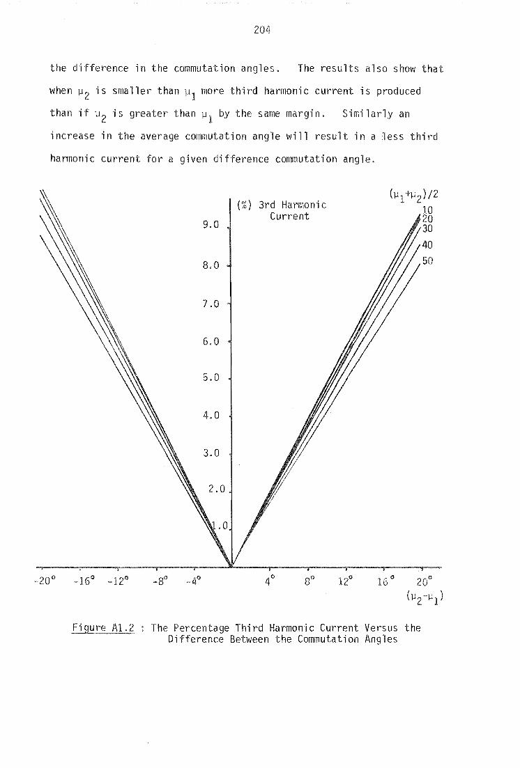
204
the difference in the commutation angles. The results also show that
when ~2 is smaller than ~l more third harmonic current is produced
than if ~2 is greater than ~l by the same margin. Similarly an
increase in the average commutation angle will result in a less third
harmonic current for a given difference commutation angle.
9.0
8.0
7.0
6.0
5.0
O~) 3rd Harmon; c Current
(~l +~2) /2
10 20 30
40 50
16 0 20°
(~2-Wl)
The Percentage Third Harmonic Current Versus the Difference Between the Commutation Angles

205
APPENDIX 2
ERROR IN THE REPRESENTATION OF A STAR-g/DELTA TRANSFORMER
BY AN EQUIVALENT ZIG-ZAG
Figure A2.1(a) shows the connection of a DYll star-g/delta
connected transformer while figure A2.1(b) shows its zig-zag equivalent.
B B
A
II C C
a----7\.
.~al ratlo -\/j
I C b'
c ----__ ~ d
Figure A2.1 (a) : Figure A2.1(b) :
Star-g/Delta Connection Equivalent Zig-zag Connection
The secondary phase to phase voltages for the star-g/delta and
the equivalent zig-zag are
Actual star-g/delta
V :::13"" V ac B
Equivalent zig-zag
::: 1 /13 ( (V B V C ) - (V A - V C) )
::: /j VB + 1//3 (V A + V B + V C)
Vc/bl Vel Vb l
1 /13 (V A - VB) - (V C V A) )
== 13 V A + 1//3 (V A + V B + V C )
Vb/al Vb/ - Val
:;;: It] {(VC - VA) - (VB - Vc))
=13 Vc + 1/13(VA + VB + Vc)

206
only if, V + Vb + V = O. a c A star-g/delta connected transformer acts
like a short circuit to zero sequence currents and voltages. However,
this short circuit has a finite impedance due to the leakage reactance
of the transformer (Chen and Dillon 1974). Therefore, zero sequence
currents in the a.c. system may cause some zero sequence voltage on
the primary of the star-g/delta transformer. This means that, because
Va + Vb + Vc will not be zero in practice, the equivalent zig-zag
connection is not a valid representation of a star-g/delta transformer.

207
APPE
THE FORMATION OF THE ADMITTANCE MATRIX OF A D.C. LINK
A d.c. link will in general be able to be divided into several
sections which may include overhead lines and cables as well as
smoothing inductors, surge capacitors and d.c. filters. These sections
are numbered starting at the end of the link of most interest. For
example the New Zealand d.c. link can be divided into six sections as
described in figure A3.1.
Figure A3.1 : The New Zealand D.C. Link Sections
Section 1 Benmore Inductors
Section 2 South Island Inland Section
Section 3 South Island Coastal Section
Section 4 Cook's Strait Submarine Cable
Section 5 North Island Coastal Section
Section 6 Haywards ' Inductors
Because d.c. lines are balanced~ of flat construction, the
propagation modes are identical to the zero and positive sequences.
shown in figure A3.2. I
I zero
2
Figure A3.2 The Zero and Positive Sequences of a D.C Line
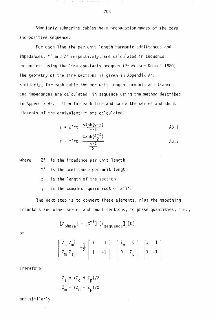
208
Similarly submarine cables have propagation modes of the zero
and positive sequence.
For each line the per unit length harmonic admittances and
impedances, Y' and Z' respectively, are calculated in sequence
components using the line constants program (Professor Dommel 1980),
The geometry of the line sections is given in Appendix A4.
Similarly, for each cable the per unit length harmonic admittances
and impedances are calculated in sequence using the method described
in Appendix A5. Then for each line and cable the series and shunt
elements of the equivalent- n are calculated,
where
Z I' *9.- sinh(yo9.-) '(.9.-
Y y/*9.-tanh (Y;9.-)
= r!
2
Zl is the impedance per unit length
Y' is the admittance per unit length
9.- is the length of the section
'( is the complex square root of I/Y/.
A3.1
A3.2
The next step is to convert these elements, plus the smoothing
inductors and other series and shunt sections, to phase quantities, i.e.,
or
Therefore
and similarly
Is = (Zo + Zp)/2
Zm '" (Zo - Zp)/2
1
-1
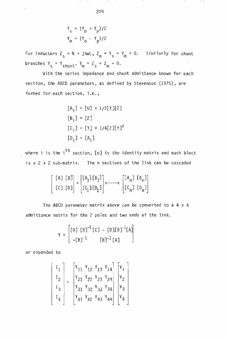
209
Y '" (Y + Y )/2 sop
Ym (Yo - Yp)/2
For inductors Zs R + jhwL, Zm ::: Y s ::: Ym :;;; O. Similarly for shunt
branches Ys Yshunt' Ym :;;; Zs ::: Zm = O.
With the series impedance and shunt admittance known for each
section, the ABCD parameters, as defined by Stevenson (1975), are
formed for each section, i.e.,
[A.J = [UJ + 1/2[Y][ZJ 1
[B.J ::: [Z] 1
[CiJ [Y] + 1/4[ZJ[YJ2
:;;; [A.J 1
where i ;s the ith section, [uJ is the identity matrix and each block
is a 2 x 2 sub-matrix. The n sections of the link can be cascaded
The ABCD parameter matrix above can be converted to a 4 x 4
admittance matrix for the 2 poles and two ends of the link.
Y ::: [[DJ [Brl
[CJ - [DJ[Brl[AJl
-[Br l [B]-l [A] J
or expanded to
II YII YI2 YI3 YI4 VI
12 Y21 Y22 Y23 Y24 V2 :::
13 Y31 Y32 Y33 Y34 V3
14 Y4I Y42 Y43 Y44 V4
210
In practice the far end of the link can be regarded as a short to
harmonics and, if the far end of the link is also earthed then V3 V4 = o. This assumption reduces the admittance matrix to
[:~ [::: :::1 [::1
Finally, if only the positive sequence admittance is to be
considered
Ypos = (Y 11 Y12 )/2
= (Y 22 Y21 )/2
This corresponds to a voltage 2V1 across the terminals of the link
causing a current of II and -II to flow in the positive and negative
poles respectively.
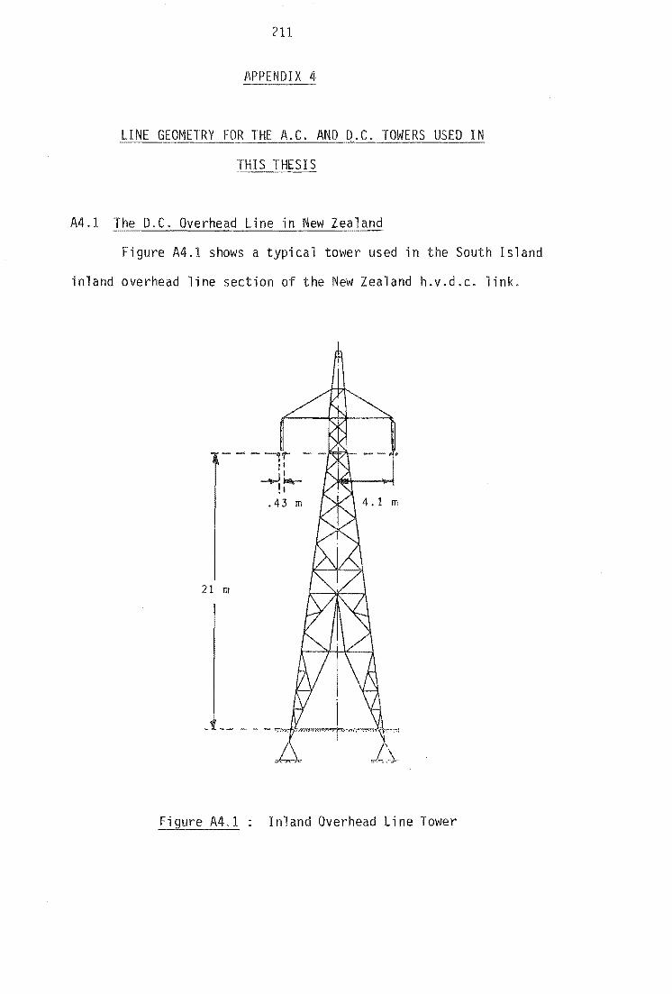
211
APPENDI
LINE GEOMETRY FOR THE A.C. AND D.C, TOWERS USED IN
THIS THESIS
A4.1 The D,C. Overhead Line in New Zealand
Figure A4.1 shows a typical tower used in the South Island
inland overhead line section of the New Zealand h.v.d.c. link.
21 m
Figure A4.1 Inland Overhead Line Tower

Resistance
Diameter
Skin ratio T/D
Bundle Spacing
212
Main conductors
.0351 Ohms/Km
38,4 mm
0.3849
431. 8 mm
Earth Wire
3.1 Ohms/Km
11.5 mm
0.5
Towers in the coastal sections are identical to those in figure
A4.1 except the spacing between conductors is increased from 8.2 m to
12.8 m.
A4.2 The A.C, Overhead Lines
The a.c. line used in chapters 4 and 7 are the single and
double circuit used by Densem (1983) with the length varied to
suit as necessary. The tower of the single circuit line, shown in
figure A4.2, is one from the Islington to Kikiwa line.
E Lf)
("I
Conductor type Zebra (54/3.18 + 7/3.18)
Figure A4.2 : The Single Circuit Tower
Similarly, the double circuit tower, shown in figure A4,3, is one from
the Makarewa to Manapouri line,

Figure A4.3
213
2 conductors per bundle
Bundle spacing .45m Conductor
30/3.71+7/3.71
The Double Circuit Tower
Full details of the line and conductor geometry can be
obtained from Densem (1983).
is 100 ohm-metres.
In every case the earth resistivity

214

215
APPENDI 5
THE METHOD OF CALCULATING THE PER UNIT LENGTH HARMONIC
ADMITTANCES AND
ZEALAND LINK AS AN EXAMPLE
In New Zealand there are three d,c. cables across Cook's
Strait and only two are used at anyone time, Because the cables are
well separated the mutual effects between the cables can be ignored.
This means that
and
Zm Ym := zero
= Z = Z o p
Y = Y = Y sop
The actual cross section of the cable is very complex, but it
can be simplified to the cross section of figure AS.I.
Fi A5.1 Simplified Representation of the Cross Section
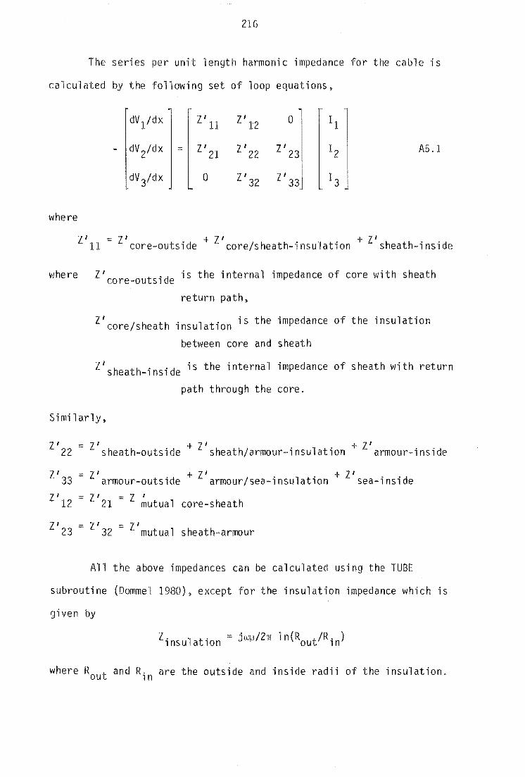
216
The seri es per unit length harmonic impedance for the cable ;s
calculated by the following set of loop equations,
dVl/dx Z/11 Z/12
Z' :J 11
dV 2/dx = Z '21 Z/22 12 A5.l
dV 3/dx 0 Z I 32 Z I I
33J 13
where
Z/ ll Z/core-outside + Z/core/sheath-insulation + Z/sheath-inside
where ZI is the internal impedance of core with sheath core-outside return path.
ZI I h th' 1 t' is the impedance of the insulation core s ea lnsu a 10n between core and sheath
Zl is the internal impedance of sheath with return sheath-inside path through the core.
Similarly,
Z 122 = Z I h h . d + Z I h t hi . 1 t' + Z I .• d seat -outSl e s ea armour-lnsu a 10n armour-lnSl e
Z/33 = ZI + Z' I . 1 t' + ZI ., d armour-outside armour sea-lnsu a lon sea-lnSl e
Z/12
= Z I = Z I
21 mutual core-sheath
Z/23 = Z' 32 ::: Z I mutua 1 sheath-armour
All the above impedances can be calculated using the TUBE
subroutine (Dommel 1980). except for the insulation impedance which is
given by
Z . 1 . :::: J' w11/2n 1 n (R IR.) lnsu atlon·~ out ln
where Rout and Rin are the outside and inside radii of the insulation.
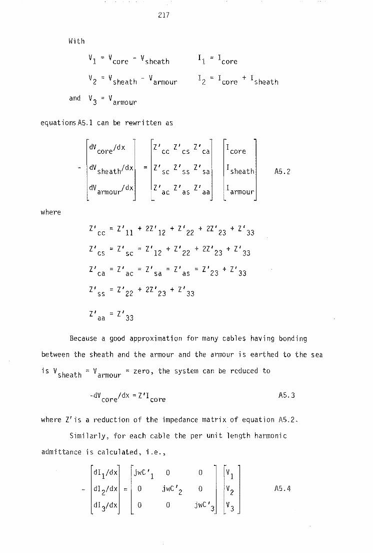
With
VI '"
V2 ;;;;
and V3 ;;;;
V core -
Vsheath
Varmour
217
Vsheath
- Varmour
I I '" I core
equationsA5.1 can be rewri tten as
dV jdx core ZI Zl Z'
cc cs ca Icore
dV s he at h j d x ;;;; Z I S C Z ISS Z I sa Isheath
dV /dx armour Z' Z' Z' ac as aa Iarmour
where
Z' ;;;; Z I 11 + 2Z ' 12 + Z' 22 + 2Z ' 23 + Z' 33 cc
ZI cs ;;;; Z' == Z' 12 + Z/
22 + 2Z /
23 + Z/
33 sc
Z' = Z' = ZI sa = Z' ::: Z' 23 + ZI33 ca ac as
Z' ss = Z I
22 + 2Z ' 23 + Z/
33
ZI aa
= Z I 33
A5.2
Because a good approximation for many cables having bonding
between the sheath and the armour and the armour is earthed to the sea
is Vsheath ::: Varmour ;;;; zero, the system can be reduced to
-dV jdx = Z II core core A5.3
where Z'is a reduction of the impedance matrix of equation A5.2.
Similarly, for each cable the per unit length harmonic
admittance is calculated, i.e .•
dI/dxl jwC ' 1 0 0 VI
- dI 2/dx ::::: 0 jwC I 2 0 V2 A5.4
dI 3/dx 0 0 jwC ' 3 V3

where C i = 2 TIEoEr/ln(Rout/Rin)' Therefore, when converted to core,
sheath and armour quantities,
dlcore/dX
dlsheath/dx
dlarmour/dx o
-V' 1
V I + V I 1 2
-V' 2
o
-V' 2
V' + V' 2 3
V core
Vsheath AS.5
V armour
where V I. = jwC .. 1 1 If, as before, Vsheath = Varmour zero, equation
A5.5 reduces to
-dI Idx = V I V core 1 core A5.6
Therefore, for frequency of interest, the cable, the per unit
length harmonic impedance, Z/, and admittance, V', are calculated with
both the zero and positive sequence values being equal to the Z/of
equation A5.3 and the V'I of equation A5.6 respectively.
Table AS.l contains the geometry of the New Zealand submarine
cable.
Table AS.1 The Data for the New Zealand Cable System
Conductor Diameter Outside Diameter Resistance
core 13.462 mm 33.477 mm .0331 Ohms/Km
sheath 63.242 mm 71.044 mm .2865 Ohms/Km
armour 88.189 mm 98.958 mm .1148 Ohms/Km
sea 110.896 mm .21 Ohm-metres
A relative permittivity of 3.5 and a relative permeability of 1.0 for
the insulation are also assumed.

Abstract
219
APPENDIX A6 IA 11-01 8404171
ANALYSIS OF THE A.C. VOLTAGE DISTORTION PRODUCED
BY CONVERTOR-FED D.C. DRIVES
J. Arril1aga (Sen. Mem.), J.F. Eggleston and N.R. Watson
An iterative algorithm is presented for the analysis of the
harmonic interaction between convertor-fed d.c. drives and a relatively
weak a.c. distribution system. The individual effect of each of the
main parameters influencing the level of voltage distortion ;s
assessed, with reference to a typical large d.c. drive. Special
attention is given to the analysis of the current waveform during
commutations, without the restrictions normally used in such analysis,
i.e. constant d.c. current and undistorted a.c. supply voltages.
The authors are with the Department of Electrical & Electronic
Engineering, University of Canterbury, Christchurch, New Zealand.
22CJ
INTRODUCTION
In the analysis of the harmonic currents produced by thyristor
controlled d.c. drives any distortion present on ,the supply voltage or
created by the d.c. drive, is generally ignored. While this practice
is perfectly reasonable for small and medium size drives. it is likely
to yield unacceptable information in cases where either the d.c. drive
is large and/or the supply system weak.
Moreover. as the numbers and ratings of power electronic devices
increase there is a need for stricter harmonic regulations.
In the absence of accurate analytical models it is difficult to
predict the levels of prospective distortion and to determine with
certainty the liability of an alleged offender.
There is information in the 1 iterature on the harmonic behaviour
of a.c. system impedances, d.c. motors. convertors and convertor trans-
formers. However each publication tends to emphasixe only one aspect of
the problem. e.g. the effect of the d.c. drive(2), the static convertor(3)
or the a.c. system(4). However these references do not consider the
harmonic interaction between the drive, convertor and supply system. The
solution of such problem requires a comprehensive computer model with
flexibility to investigate the sensitivity of each particular scheme to
variations in the representation of its individual components. Such a
model, 'described in this paper. is essential in the prediction of harmonic
current and voltage levels in the system. It also provides the basis
for the optimization of filter design when required.
STRUCTURE OF THE PROGRAM
In the context of this paper harmonic interaction is the process
by which any distortion present in the a.c. system voltage waveform can
influence the harmonic currents generated by the convertor-fed d.c. drive
and vice versa. A brief outline of the program structure deve10ped to

221
invest; such harmonic interaction is illustrated in Figure 1.
The harmonic admittances for the a.c. and d.c. systems as well as
the initial load flow conditions. are read-in prior to entering the
iterative loop.
A load flow study is necessary to provide information of active
power, reactive power and phase voltages at the convertor terminals as
well as convertor firing delay angles for the particular operating
condition. If a load flow program is unavailable the iterative program
can start from information of the nominal voltage and operating conditions.
At each iteration the system can be considered to be constructed
of three regions, each of which is solved in succession (Figure 2). For
the first iteration it is assumed that the d.c. current is constant and
the a.c. system voltages are sinusoidal. The sequence for each iteration
is as fo 11 ows :
Region 1: Using the a.c. system voltages and d.c. current waveform
(from the previous iteration), the harmonic current injections and d.c.
voltage waveform are found.
Region 2: From the harmonic currents injected into the a.c. system
and its harmonic impedances. the a.c. system voltages are calculated.
Region 3: The d.c. voltage waveform (found when solving region 1)
and d.c. system admittance at harmonic frequencies. are used to calculate
the d.c. current waveform.
The terminating condition for the iterative loop is when the changes
in voltage zero crossings between two successive iterations is smaller
than a specified value. When this condition is met, one further iteration
is performed.
A.C. System Representation
The degree to which the a.c. power system must be represented depends

222
on the purpose of the investigation. In general, the more simplifying
assumptions made without invalidating the study the better. An obvious
and simple representation often used is the short circuit impedance of
the a.c. system at the busbar.
However. the variation of power system impedance with frequency is
far from linear and can even change from inductive to capacitive in a
spiral-like fashion when plotted in the impedance plane. At the
utilization end of the scale, however. the impedance tends to be resistive-
inductive as illustrated by the snap-shot information shown in Figure 3
which relates to an 11 kV supply to a mixed load system consisting of
domestic. commercial and industrial customers(5).
Moreover, the harmonic impedances of the three phases are not exactly
balanced. Transmission line geometry is such that some mutual impedance
imbalance exists between phases. Also the imperfect distribution of single
phase loadings contributes to the imbalance. Even when the system is
reasonably balanced at fundamental frequency. the impedance imbalance
may be considerable at harmonic frequencies. Due to the asymmetry
inherent in all power systems, even if the harmonic currents injected into
the a.c. system are balanced the harmonic voltages in the power system can
be significantly unbalanced. So a realistic quantitative analysis of
harmonic levels necessitates a detailed three phase model, which is
capable of representing the coupling between circuits as well as the
impedance imbalance between phases. A harmonic penetration model
developed by one of the authors(6) provides such detail.
In harmonic penetration studies, the a.c. system components, other
than those generating the harmonic injections, can be a~sumed to be
linear and thus the voltage distorting effect of each harmonic can be
considered separately.
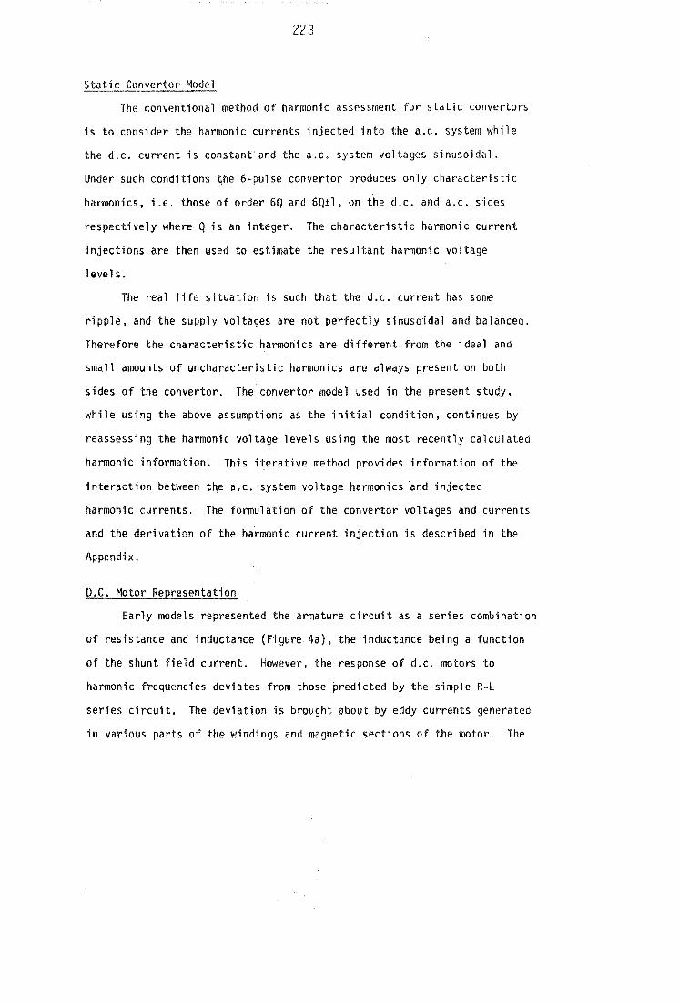
223
The conventional method of harmonic assessment for static convertors
is to consider the harmonic currents injected into the a.c. system while
the d.c. current is constant'and the a.c. system voltages sinusoidal.
Under such conditions ~he 6-pulse convertor produces only characteristic
harmonics, i.e. those of order 6Q and 6Q11. on the d.c. and a.c. sides
respectively where Q is an integer. The characteristic harmonic current
injections are then used to estimate the resultant harmonic voltage
levels.
The real life situation is such that the d.c. current has some
ripple, and the supply voltages are not perfectly sinusoidal and balanced.
Therefore the characteristic harmonics are different from the ideal and
small amounts of uncharacteristic harmonics are always present on both
sides of the convertor. The convertor model used in the present study,
while using the above assumptions as the initial condition, continues by
reassessing the harmonic voltage levels using the most recently calculated
harmonic information. This iterative method provides information of the
interaction between the a.c. system voltage harmonics and injected
harmonic currents. The formulation of the convertor voltages and currents
and the derivation of the harmonic current injection is described in the
Appendix.
D.C. Motor Representation
Early models represented the armature circuit as a series combination
of resistance and inductance (Figure 4a), the inductance being a function
of the shunt field current. HoweVer, the response of d.c. motors to
harmonic frequencies deviates from those predicted by the simple R-L
series circuit. The deviation is brought about by eddy currents generated
in various parts of the windings and magnetic sections of the motor. The
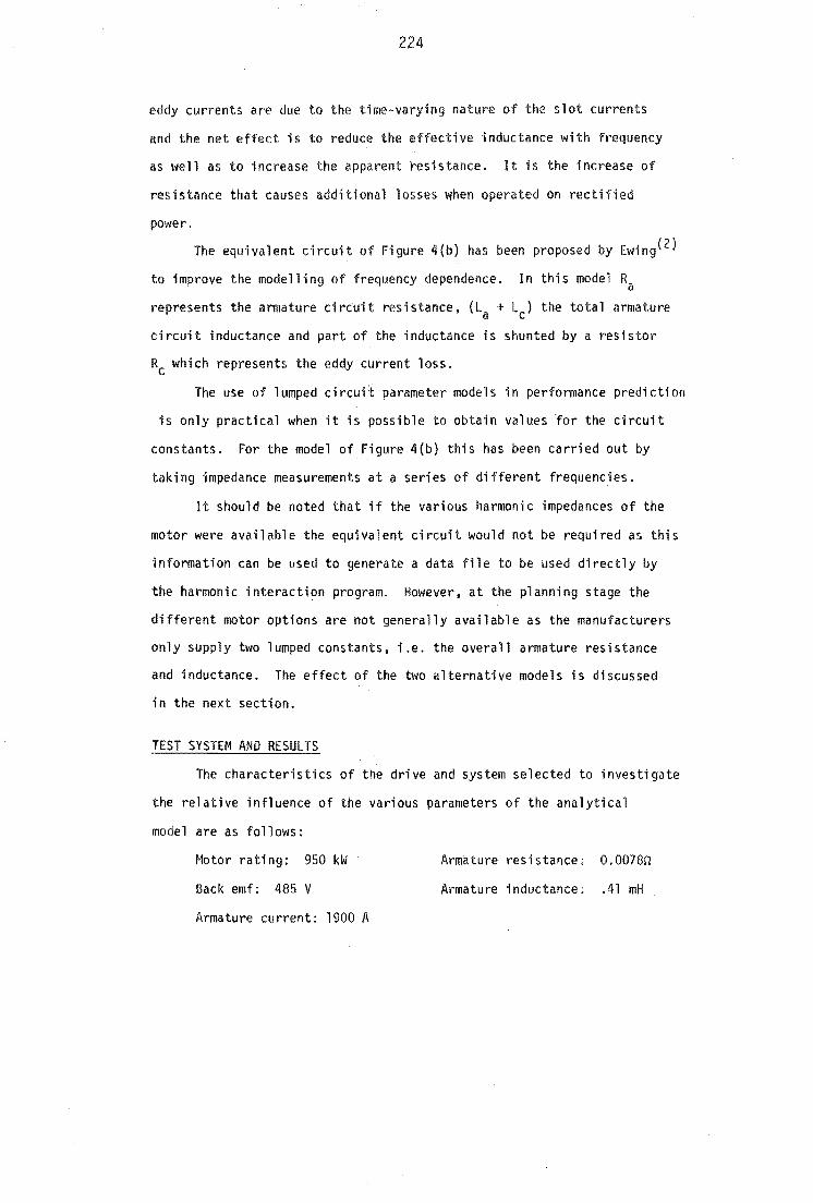
224
eddy currents are due to the time-varying nature of the slot currents
and the net effect is to reduce the effective inductance with frequency
as well as to increase the apparent resistance. It is the increase of
resistance that causes additional losses when operated on rectified
power.
The equivalent circuit of Figure 4(b) has been proposed by Ewing(2)
to improve the modelling of frequency dependence. In this model R a
represents the armature circuit resistance, (La + Lc) the total armature
circuit inductance and part of the inductance is shunted by a resistor
Rc which represents the eddy current loss.
The use of lumped circuit parameter models in performance prediction
is only practical when it is possible to obtain values for the circuit
constants. For the model of Figure 4{b) this has been carried out by
taking impedance measurements at a series of different frequencies.
It should be noted that if the various harmonic impedances of the
motor were available the equivalent circuit would not be required as this
information can be used to generate a data file to be used directly by
the harmonic interaction program. However, at the planning stage the
different motor options are not generally available as the manufacturers
only supply two lumped constants, i.e. the overall armature resistance
and inductance. The effect of the two alternative models is discussed
in the next section.
TEST SYSTEM AND RESULTS
The characteristics of the drive and system selected to investigate
the relative influence of the various parameters of the analytical
model are as follows:
Motor rating: 950 kW
Back emf: 485 V
Armature current: 1900 A
Armature resistance: 0.0078n
Armature inductance: .41 mH

225
The d.c. motor is connected to the 101'/ voltage side of a 33 kV/4l5 V star~
delta distribution transformer through a six-pulse SCR-controlled bridge
rectifier.
The results presented in this section relate to a balanced a.c.
system at the nominal voltage. However. the modelling of transformer
and a.c. system impedances was varied in different studies.
Effect of Motor Representation
In order to assess the 'effect of the improved Ewing model. the
armature inductance is divided in two parts, i.e. La =0.272 mH and Lc 0.138
mH, while a resistance (Rc" O.1495n)is connected in parallel with Lc '
The levels of 5th and 7th voltage harmonic distortion of the Ewing
and series R-L models are plotted in Figure 5 versus a.c. system impedance.
Although the difference is small for reasonably strong supply systems it
can be substantial for weak ,systems. For instance the total harmonic
distortion calculated by the conventional model exceeds the limit
recommended by Engineering Recommendation G5/3(7) with a system induc
tance of 43.5 mH whereas that of the Ewing model is still within the
1 i mit.
The difference between the two models is more marked at large
firing angles, i.e. when the d.c. side harmonic content increases. For
example during motor start, under nominal d.c. current, the firing delay
required is 860 and the results of the two models with a system inductance
of 43.5 mH are plotted in Figure 6. Under these conditions the Ewing
model produces 7.5% extra 5th harmonic voltage but reduces the level
of the 7th harmonic by 22%.
Effect of Commutating Reactance
The harmonics produced by a thyristor-controlled d.c. drive are
largely affected by the leakage reactance of the convertor transformer
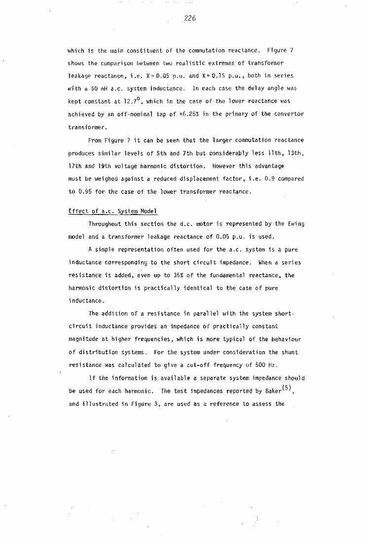
226
which is the ma'in constituent of the cOllll1utation reactance. Figure 7
shows the comparison between two realistic extremes of transformer
leakage reactance, i.e. X=O.05p.u. and X=0.15 p.u., both in series
with a 50 mH a.c. system induciance. In each case the delay angle was
kept constant at 12.70, which in the case of the lower reactance was
achieved by an off-nominal tap of +6.25% in .the primary of the convertor
transformer.
From Figure 7 it can be seen that the larger COllll1utation reactance
produces similar levels of 5th and 7th but considerably less 11th, 13th,
17th and 19th voltage harmonic distortion. However this advantage
must be weighed against a reduced displacement factor, i.e. 0.9 compared
to 0.95 for the case of the lower transformer reactance.
Effect of a.c. System Model
Throughout this section the d.c. motor is represented by the Ewing
model and a transformer leakage reactance of 0.05 p.u. is used.
A simple representation often used for the a.c. system is a pure
inductance corresponding to the short circuit impedance. When a series
resistance is added, even up to 35% of the fundamental reactance, the
harmonic distortion is practically identical to the case of pure
inductance.
The addition of a resistance in parallel with the system short
circuit inductance provides an impedance of practically constant
magnitude at higher frequencies, which is more typical of the behaviour
of distribution systems. For the system under consideration the shunt
resistance was calculated to give a cut-off frequency of 500 Hz.
If the information is available a separate system impedance should
be used for each harmonic. The test impedances reported by Baker(5),
and illustrated in Figure 3, are used as a reference to assess the
7
accuracy of the other models. To compensate for the different primary
voltage. the a.c. system impedances had to be scaled from 11 to 33 kV.
Figure 8 indicates that considerable differences exist between
the harmonic voltages obtained using the test impedances and those
derived from the simpler parallel resistor/inductor or a pure inductance
equivalents.
The comparison between studies using the pure inductance and the
test impedances (Figure 8(a)) shows very little agreement. In particular
the 5th harmonic level voltages of the test impedances is about double
that of the pure inductance model. while those of the higher harmonics
are only a half.
At frequencies above 500 Hz the magnitude of the test distribution
a.c. system impedance appears 'to be reasonably constant(5) and thus the
parallel inductance/resistance combination (Figure 8(b)) proves to be a
reasonable approximation at higher frequencies. However the presence
of a resonance near the 5th harmonic causes more voltage distortion than
the short circuit impedance would have predicted.
As a rough approximation the distribution systems impedance in
Figure 3 can be considered constant from about 250 Hz. Consequently the
a.c. system was also modelled as a pure resistance, i.e. a constant
impedance magnitude versus frequency. The results, compared to the case
of the test impedances (Figure 8(c)). show very good agreement. Although
there is some difficulty in choosing the value of the resistance. the
magnitude of the system impedance of a typical distribution system appears
to level off at about 500 HZ,(S) therefore the reactance of the short-
circuit inductance at 500 Hz would thus prove to be a reasonable value.
CONCLUSIONS
The paper has described the structure of an iterative algorithm
capable of assessing accurately the harmonic voltages produced by convertor-

228
controlled d.c. drives gt the point of common coupling with other loads.
This algorithm provides a pr,actical alternative to commonly used
pessimistic models. which may suit the supply authority involved. but
often results in an unnecessary expense to the industry.
The application of the algorithm in a practical situation has shown
the importance of modelling the frequency dependence of the d.c. drive
and the a.c. system wherever'possible. The a.c. system can rarely be
modelled with any degree of confidence and therefore a realistic worst
case will often be a reasonable compromise; however. the use of the
short-circuit impedance will in general produce unacceptable error.
The results have also highlighted the advantage of· high transformer
impedance in reducing the voltage distortion at the point of common coup11ng;
this, however, worsens the power factor and may lead to excessive internal
distortion when the same transformer feeds other plant components.
ACKNOWLEDGEMENTS
The authors wish to acknowledge the advice received from Dr. P.S.
Badger. Or. B.J. Harker and Dr. T.J. Densem. They are also grateful to
the New Zealand Energy Research and Development Corporation for the
financial help towards this project and to Mr. W.P. Baker (Electricity
Council Research Centre. Capenhurst) for the use of some of his
experimental results.

c j
In terms of the phase to neutral vol of the incoming and outgoing
phases the following general expression has been derived(3) for the
commutation current:
where B.
X "..::.L . L J nm
n is the incoming phase and m is the outgoing phase.
Lnm/Rnm
Vjn COS(j9n + ¢ljn)'
V. sin(j9 + ¢l. ) In n In Hj '" jwA/Bj
Vjm COS(j9n ~ ·jm'
Vjm sin(j9n + $jm)
1 1 H. tan- (l/jwT ) - tan- (~) nm JW
V. and., are the magnitude and phase of the jth harmonic of the phase In In
to neutral voltage of the incoming phase. ~
Vjm and $jm are as above for the outgoing phase.
Cnm is an integration constant such that 1n
(0) = 0
However for a more general transformer model, capable of representing
the star-delta connection in the presence of zero sequence voltage, the
above equation needs to be rewritten in terms of the phase to phase
vol tages. i.e.
v '" nm
50 I A
J. sin jwt + Bjcosjwt
j" 1
using ilS time reference 61 (the first firing angle).
For a star/star transformer
Aj Vjn cos(j6 , + ~jn) Vjm cos(j61 + $jm)
BJ. V
jn sin(j6, + <p. ) - V. cosUSl + Ql. ) In Jm Jm
For a star-g/delta transformer (OYll), and a commutation from valve 1 to
valve 3;
Aj " -/~ Vl COs(j8 , + $jl)
Bj V, sin(j6, + $j1)
with equivalent equations for the other phase to phase pairs.
For the nth valve commutation the new A~ and B~ are calculated . J J
from the original Aj and Bj '(with 81 as their reference). i.e.
Aj = Vjn cas(j6n + ~jn) - Vjm COS(j6n + $jm)
" Vjn COS((j9n j61) + (j61 + $.jm)) - Vjm COS((j9n - j8, )
+ (jS, + ¢>. )) Jm • Aj cos (j9~ - j9, ) - Bj sin(j8n ~ j61)
similarly 8j = Aj sin(j9n ~ j91) + BjCOS(j8n - j9 , )
A.C. Current Injections
The general expression for the d.c. current waveform is:
50 Id = Ida + .r IdJ· sin(jwt + ~dJ')
J=l
where Ido is the average d.t. current level and the Idj coefficients
are obtained from the previous iteration of the d.c. model, i.e.
where Yj are the harmonic admittances of thed.c. drive.

231
When only two valves conduct, say 1 and 2. the instantaneous phase
current injections at'e derived from the exprl;!ssion:
With reference to Figure 9 during the commutation from valve 1 to 3 the
current injections are:
11 Id-i n '" 12 i n
13 -Id
where in is the commutation current.
In order to calculate the current injections in the frequency domain
the current waveforms are divided into 12 sections (Table Al). six of
them with one conducting valve on ea~h side of the bridge and the other
six with one side of the bridge undergoing a commutation. Each of the
three phases is sampled and a Fast Fourier Transform performed, to
derive the harmonic content of the current injections.
Convertor d.c. Voltage
As with the current injections information of the commutating voltage,
commutating impedance, the d.c. current waveform and the firing instants
is needed. Because these are the same in both studies, and the same 12
sections are used, the current injections. and the d.c. voltage can be
sampled simultaneously.
The situation of one valve on each side of the bridge conducting is
described in the previous section. With valves 1 and 2 conducting:
Vd " V' - V' 1 3
Yacamini and de Oliveira(3) used the approximation that Vi ::: V1 and V) "V3 and hence Vd V1 -V3, i.e. the voltage drop across the commutating

232 impedance is ignored.
However. during the commutation process the voltage drop across the
commutating impedance is significant as the secondary of the transformer
has two phases with a temporary short ci rcuit. Fi gure 9, in the prev; ous
section. describes this situation. Valve 2 is conducting and there is a
commutation from valves 1 to 3.
V '" VI - VI d 2 3
and VI '" VI 1 2
assume V3::: V3
where V",
50 and i 2 ::: L [X. e-t/Tnm .;. S. sin(jwt .;. 6.)]
j=l J J J
.;. Y[l - e-t/Tnm] .;. C nm
the commutation current, with n=2 and m=1.
50 Therefore Vl( '" W e-t/Tnm.;. I [M. cos(jwt) .;. N. sin(jwt)] .;. K .
j=l J J n
where Mj :: -(jwLn5jcosoj .;. Rn5j Sino j )
NJ. '" jwL 5.sino. - R 5.C056.
n J J n J J
L 50 W '" (Tn - Rn) '.I Xj - Y}
nm J"'l
Kn -Rn (Y .;. Cnm )
The equations applying to each of the 12 sections of the waveform
are listed in Table A2.

233
'I'ABLE AI. The 12 Sections of the 1 ine current wave forms .
Section Equation line 1 line 2 line 3 Limit referenced to 61
0-1 -Id
0 ~ 6 ~ fJ 1
1-2 ld -Id
0 fJ 1 ~ 6 ~ 62-6
1
2-3 -I -1 -61 ~ 6 ~ 62-6 1+\12 d e
3-4 0 62
-B1
+fJ2 ~
B ~ B3-8
1
4-5 i B -B ~ B < B3-B1
+\13 c 3 1
5-6 0 Id -Id
8 -8 +fJ ( 3 1 3
B ::: 6 -B 4 1
6-7 Id -Id
B4-8
1 ~ B ~ B4-61+\14
7-8 Id 0 84-81+\14 ~ 6 ~ 8s-B1
8-9 I -i i .~ 8 ~ 85-8 1+\15 ,d c e
9-10 0 Id 85-81~ \1 5 ' 8 ~ 8 -8 6 1
10-11 i Id 86
-61
~ 8 ~ 86-61+\16 c
11-12 0 -Id Id '6 -6 +\1 ~ 616 8 ~ 21T
where 1 is the commutating current in the incoming valve. e
TABLE A2. The 12 Sections of the d.c. voltage waveform.
Section Equation Limits
6 references to 61
0- 1 Vd '" VI - V2 + V O~ 6~ \11 x
1- 2 Vd '" VI - V 2 III ~ 8 :f 62 61
2- 3 Vd VI - V3 - V B2-81 $ 8 ~ 82-61 + fJ 2 x
3- 4 Vd VI - V3 62-81+\11~ 6 ~ - 6 1
4- 5 Vd V2 - V + V 6 -6 ,8 < 6 -6 + \1
3 3 x 3 1 '3 1
5- 6 Vd V2 - V3 63-61+\13' 8 .( 64-8 1
6- 7 Vd V - VI - V B4-Bl~ B :f B4-61 + \14 :2 x
7- 8 Vd - VI B -8 +11 ",6 ~ 6 -6 4 1 4 5 1
8- 9 Vd V3 VI + V e -6 ~ 6 ( + \15 x 5 1
9-10 Vd V3 VI e -B +11 :f B Iii 515
10-11 Vd V) - V - V 66
-61
11;6 :$ 66-6
1 + 116 2 x
11-12 Vd c V3 V2 B6-B1 +116 ( e ~ 211

234
(1) Goldberg, G. 'The effect of voltage and current humonics on
electrical equipment'. Der Electroniker, Vol. 14 No.7, July 1975,
pp. ELl-7.
(2) Ewing, J.S. 'Lumped circuit impedance representation for DC machines',
Trans. IEEE, PAS-87, No.4, 1968. pp. 1106-1110.
(3) Yacamini. R. and de Oliveira, J.C. 'Harmonics in multiple convertor
systems: a generalised approach'. Proc. lEE, Vol. 127, Pt. B, No.2,
1980, pp. 96-106.
(4) Oensem. LJ •• Bodger, P.S. and Arr1l1aga, J. 'Three phase transmission
system modelling for harmonic penetration studies', IEEE Power
Eng1 neeri ng Soci • Summer Meeti ng 1983. Los Angeles. paper 835M444 -7 .
(5) Baker, W.P. 'Measured impedances of power systems", International
Conference on harmonics in Power Systems, University of Manchester
Institute of Science and Technology,1981, pp. 141-158.
(6) Arril1aga, J., Oensem. T.J. and Harker"B.J. 'Zero sequence harmonic
current generation in transmission lines connected to large convertor
plant', Trans. IEEE. PAS-107, No.7. 1983, pp. 2357-2363.
(7) Engineering Recommendation G5/3 (1976), ~Limits for harmonics in
the United Kingdom Supply System'. Electricity Council.
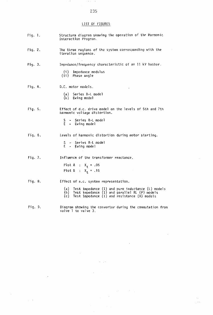
Fi g. 1.
Fi g. 2.
Fi g. 3.
Fig. 4.
Fig. 5.
Fig. 6.
Fi g. 7.
Fi g. B.
Fig. 9.
235
Structure diagram showing the operation of the Harmonic Interaction Program.
The three regions of the system corresponding with the iteration sequence.
Impedance/frequency characteristic of an 11 kV busbar.
(i) Impedance modulus (ii) Phase angle
D.C. motor models.
(a) Series R-L model (b) Ewing model
Effect of d.c. drive model on the levels of 5th and 7th harmonic vol distortion.
S - Series R-L model E - Ewing model
Levels of harmonic distortion during motor starting.
S - Series R-L model E - Ewing model
Influence of the transformer reactance.
Plot A Plot B
Effect of a.c. system representation.
(a) Test impedance (I) and pure inductance (L) models (b) Test impedance (I) and parallel RL (p) models (c) Test impedance (1) and resistance (R) models
Diagram showing the convertor during the commutation from valve 1 to valve 3.

\.0 M N
Read the ( REPEAT UNTIL CONVERGEO I.. ""{,,, il.'l£or-
. ution: -for the I I I A.Co and D.C. systems.
For each The A~C. The D.C. Read the convertor, system vol- I1IlOtor lIOOdel (initial) load flow COI.'Idi tions
solve for tages are is used to
for the the A.C. found for calculate
convertors current in- each the D.C. jections haI'lllOnic current into the waveform A.C. system and the D.C. voltage
Fig. 1. Struct.ure diagram showing the operation of the HaI'IIIOnic Interaction Program.
J ..
The. zero c:ros~~n~ and instants are updated, because of the A.C. voltage distortion

Region 2
A lrar:tlonic· Curtent Injl!ctions
Region 1
Fig. 2. The three regions of the system corresponding with the iteration sequence.
Region 3
1'\.,' w '-I
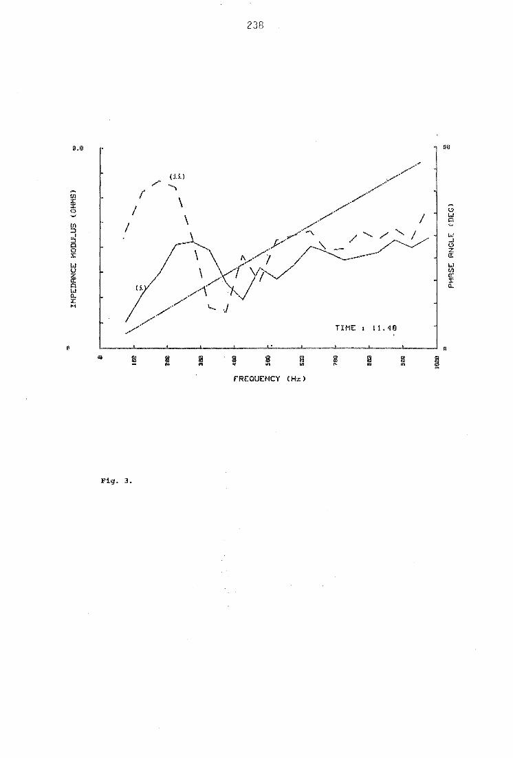
In :J ..J a o :t:
W U :z 0: Q W a. :t: ....
/
Fig_ 3_
/ /
(ii)
/" \
238
\
TINE I 11,48
fREQUENCY (Hz)
I
110
u.s ..J l:J Z a: u.s In II: J: a.
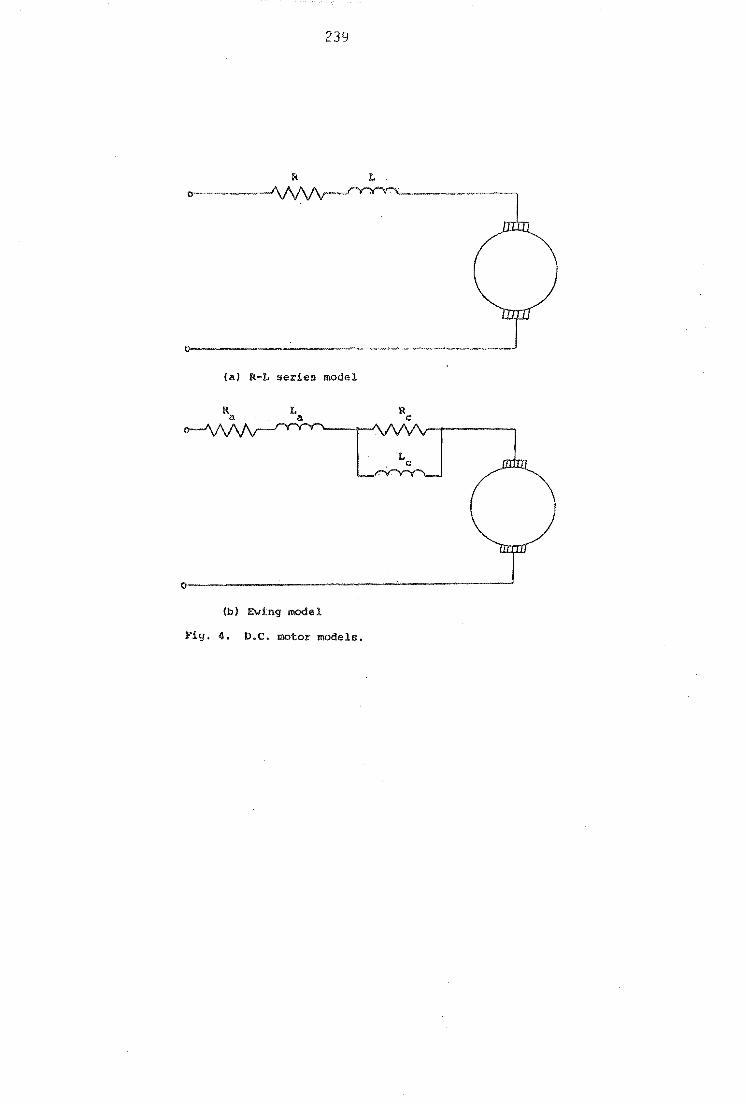
239
(a) R-L series moael
(b) Ewing lIIOdel
Fig. 4. D.C. motor models.
L
R e
L c

v IV (\) n
2.0
1.5
1.0
o.
o 10 20
240
30 40 A.C. System Inductance
E
S
s
E
50 (rnH)
Fig. 5. Effect of d.c. drive model on the levels of 5th and 7th harmonic voltage distortion.

0 :=l
H
CJ « 2
« r
>
vn/V1
(%)
25
E
S R
1.0 \ /\ A S
1 3 7 1 1 13
ORO OF FiQ. 6. I£vels of harmonic distortion durino startinq.
15 17
RMONI
A S
1 9 1
s ,...., E
2 5

i"'l
1 4:
H N q N
I \ II \ I \ I ,,8\ I \ / A B
1 3 7 9 1 1 13 15 17 19 21 25
OR OF ARMONIC Fig. 7. Influence of the 1:rdnsformer reactance on the harmonic voltag<' distortion.

243
Lf) (\j
...J (l) (\j
r-I
(\j
~
rn ---
r-I
["-. U
H
r-I
Z
0 Lf) r-I
cr «
(T) r-I
LL 0
r-I
r-I cr W
0
c C
.~
rn cr
4-'"
0 '-' c <:; u; v " ~;,
["-. G
\...
E
G
~,
if. :--. u.
Lfl
4-G
(T) 4
-j.....:.
"" til
..... r-I
-'-:> "-
ill (D
~
(\j lS)
t7 C
:>
• "'-
On
.lIN V~
V
I /\

w o =:J
H
z CJ « L
w l')
« I~ o >
V IV (!!oj
1.0
~B I
1 I ~6 l I
j .., I
l j
• j 1 3 5 7 1 1 13 15 17
OR R OF HARMONIC Fig. 8 II,; Test impedance and paralh,l RJ, mude]s.
1 1 23


246
3 5 Vl V' 1 V2 V' 2
Vd
V3 V' 3
,q
Fig. 9. Diagram showing the convertor during the commutation from valve 1 to valve J.

247
APPENDIX A7
RESULTS OF SINGLE PHASE CONVERTOR MODELLING
A7.1 TEST SYSTEM
The test system was that previously used for three phase d.c.
motor drives (Arrillaga et al 1985b) and included as Appendix A6.
The a.c. systems used in the study are a 10, 25 and 50 mH
inductive system and an industrial busbar locus (Baker 1981), each at
33 kV. In each case the fundamental terminal busbar voltage was
specified as 1.0 p.u.
A7.2 RESULTS OF ED CONVERTORS
A7.2.1 Comparison of Motor Models
The R/L series and Ewing (1968) model injections were compared
with a square pulse (classical solution) using a 10 mH system. a delay
angle of 0.1 radians and a 1.0 p.u. d.c. current. Figure A7.1 shows
the a.c. harmonic injections, as a fraction of the fundamental,
for each case.
The Ewing model produced significantly smaller harmonic
currents than the R/L series model. particularly at the higher order
harmonics, while both the d.c. models give dramatically lower harmonic
currents than those predicted using a square pulse. For the Ewing
model. the inclusion of ripple on the d.c. current and a finite length
of commutation results in 0.129 p.u. third harmonic current as
compared to 0.333 p.u. expected using a rectangular a.c. current
injection,
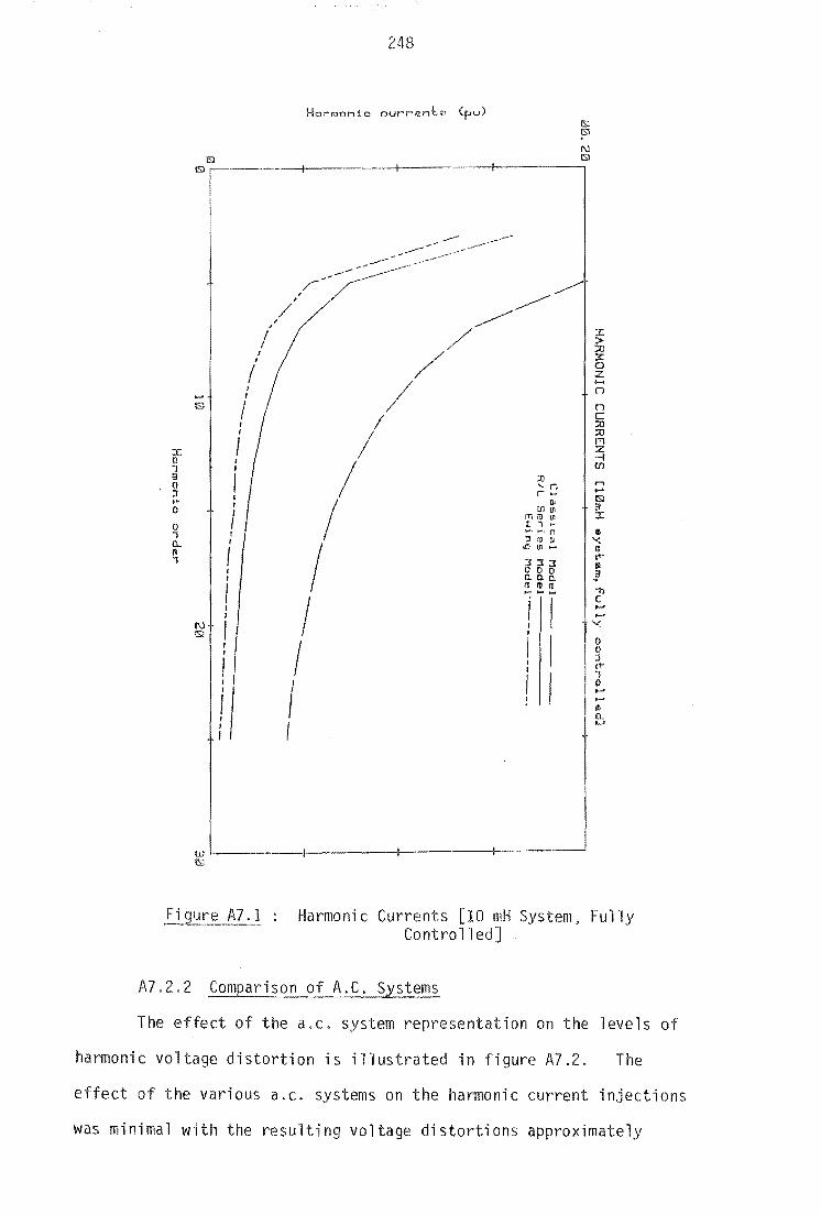
:c 0 .., 3 0 :J ... 0
0 , 0... /I ,
248
Hormonio our rent a (pu)
~~~---.-----+--------+---------r--------,
~~ / :c
> :;u
/ ~ 0 z
/ .....
I n .... I IS) I n
/ c
I :;u I AJ
I 111 Z -I
/ (f)
)) ..... '(i r~
.... I ISl ,
/ ill 3 (f)\Jl
I rn 11) !II :c ~ "1 ~
I )01. 1-<. n 0
I , 11) £II "<
f I .0 !II .... til
ct-:I:t:t 1\1 I 000
~ , 0.0.0.
I III III 11) "f) ............
j I c .....
I\l IS)
I I
I 0 0 I :J
/1
ct-
I ,
/ 0 ..... >-' /I 0...
I LJ
wL-----·---+--------~--------;-------~ ~
Harmonic Currents [10 mH System, Fully Contro 11 ed]
A7.2.2 Comparison of A.C. Systems
The effect of the a.c. system representation on the levels of
harmonic voltage distortion is illustrated in figure A7.2. The
effect of the various a.c. systems on the harmonic current injections
was minimal with the resulting voltage distortions approximately

249
proportional to the harmonic impedance of the system.
1~ \ I I I .... , ..... , II o I I I
l , }
, ..j>' I .c f I I o I I I I) i I : I
I I I I i >..i I I
~{ I : I I
I j re I I
I II I I I :
I , 1 I
I I
: I I : I ' I I
/1 !
E: S S B I r L ! I I
i Q)Q)Ql
I III
+'+'+' i) III I Ol!l}lllO
I! t l..
51 !;;!Bt!t4 I I I)
/ r
'LI ~~~2 I 0 ... Il , I I 1:
C;! Olt"\O~ J
I 0 Ir\ ('h- I V i
E l..
raJ 0 ffil I I
/ I ::t: el' .~ I I
~l J..l I +'
j t~ III I I ::l
/ I "1:1
I I=i H U, I I
.... I
/ I
~I I I I I I I 1 0:::,
) ..:: ! I // ::t:! // i
f I ,
/ I , I j/ J t ~/ ,-
I ~~ ,,/" / I ~..-
----..-~ .,./ / I
I I I I
L I I I
-- -_ ... -+--..... --f----~. _---+_~ __ ._.J
Figure A7.2 : Harmonic Voltages [Various Systems, Fully Controlled]
A7.2.3
A simple theoretical study, which gives an indication as to
the effect of d.c. current ripple on the a.c. system current
injections, has been performed for three phase convertors (Dobinson
1975). In the absence of an equivalent study for single phase
convertors, the following theoretical study was performed.

250
A7.2.3.1 Theoretical study
Assuming that the dominant ripple component is the second
harmonic. the current waveform of figure A7.3 results.
Id
Figure A7.3 : Theoretical A.C. Current Waveform
, I .- --I I I
Since the waveform is odd and contains half wave symmetry
the Fourier series consists only of the odd B sin terms, such that n
Bn ::: 2/TIf(Id - 12 cos(2x))sin{nx)dx 0
4Id 12 ::::
7T{ n1_4) niT A7.1
where
R 21/Id A7.2
It can be seen that the fundamental component incre§ses with
increased ripple while the odd harmonics decrease.
A7.2.3.2 Test system for the study of D.C. current ripple
A series of runs were performed to investigate the effect of
d.c. current ripple on the a.c. system current injections. The test
system consisted of a resistor in series with a variable inductor, in

1
the range 0.4 mH to 2.0 mH, for the d.c. system, a 10 mH lumped
inductance for the a.c. system~ a 1.0 p.u. d.c. current and delay
angles fo 0.1 and 1.0 radians. For simplicity the ripple ratio was
defined as the ratio of the peak to peak second harmonic to the d.c.
component.
A7.2.3.3 Results for the study of D.C. current ripple
The fundamental current injection as a function of the ripple
ratio are given in figure A7.4 for the two delay angles in A7.2.3.2.
Similarly, figures A7.5 and A7.6 show the third, fifth, seventh and
ninth harmonic current injections, as a fraction of the fundamental,
for the two delay angles respectively. The trends of these figures
are similar to those predicted in the theoretical analysis of section
A7.2.3.1, although this analysis does not take into account the
commutation angles, which also affect the a.c. current injections.
A7.3 RESULTS FOR HALF-CONTROLLED CONVERTORS
A7.3.1 Classical Harmonic Behaviour of a Half-controlled
Convertor
Assuming a perfectly flat d.c. current and zero commutation
angles, the a.c. current waveform ;s that of figure A7.7.
Figure A7.7 Simplified Hal controlled A.C. Current Waveform

252
lSI !Sl w
_ lS
I lS
I lS
I .-
----
----
----
.-+
----
----
---I
----
----
---
...... -
---!----~-'l
j
\ \ \ \
\
, \ \ \
\ \ \ \
\ \ \ \ \ \ \ \ \ \ \ \ \ \ \ \ \ \
\,
\ \ \ \ \ \ \ \ \ \ \ \ \ \ \ \
l;iU
:r
~:r
~
a, II
Ii -
C'
I I i I Ii !z -l >
r n ,C
!~
im t~ I
!l < .... o c ,
; :t
t~ i Ii!
I ......
. . ~
I~ H
12.-
' .... \~
IL
J
I I I ._
-+--
____
__ . _
__ J
Fund
amen
tal
Cur
rent
Beh
avio
ur w
ith R
ippl
e (F
ully
Con
trol
led)

r----I !
!:O!
• i
.-II
'01 l
!
"t!
H
J I
1+-1 ~
I .....
i
lSi'
B \J
...c Il.. ...... \J '-'
I ...c: *'
i I
-; ! /
~l I
1 I /
Jl! /
!z! I
i~ <, :rl I !
2
~------+-------+------~-------r------~
I , I J
! I I I
/ I \' !
I I
I ,
[ I J I
I I !
I
I II j II
U
U
U
U
°M'~
..........
c: c: c c
o 0
0 0
e E
E
E
L
L L
L I1l
III III
<Ii :r:r:r:r
I I , I I I
I I I
I , I
I
I , I
I , I
I , , I I I
I I I
I I I
I I I
I I , I
( , I , I , I , / I , I I I J I
/ I I
I
I 1
I , I
I I
I
I I
I
/ J
J I I
J I /
1 I I I I
1 I t I U~~~
,
~~~t J'
I --+
-------+---
-------+------\-------
~ . .....
Figure A7.5
Harm
onic C
urrent B
ehaviour with R
ipple [A
lpha=O
.l]
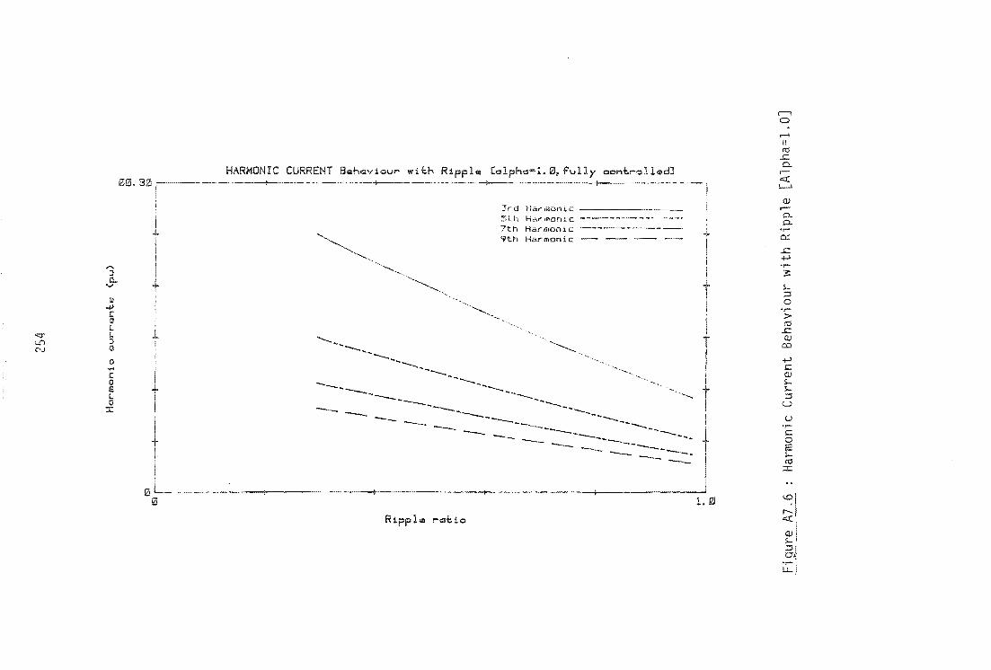
....
i I I . j I f , j I I I
254
Harm
on
ia o
urren
ts
(pu
)
/ I
/ I
I
I I
! I
I
I I
! I
I
I /
! I
I
/ I
/ I Ii!
I I
I /
/ ,
I
! /
/ ! /
!
l /'
/ I
I I
!! !
1
/ /
f,
/ f I
I I.
! /
, I
/
/
I / ,
/ /
/ / l I
..jJ
'-l
Lq "~
rtrtrtl
:r :
r :r
c.
J: :
r :r
::1:
Il>
Il>
u' n,
, , ,
"\
3 3
!;
::;
00
0
0 ::l
:;)
:J
:;)
"".
.....' .. ' ..
... n
n n
n
I 1 :
I : I 1 : , I
II I
I I
I
I II I ; i
~ L
..-.
---+
----
.---
-+--
-_+
--__
___ -
+-__
__ ._
4-. _
__
... _
-'
Fi
A7.
6 H
arm
onic
C
urre
nt B
ehav
iour
wit
h R
ippl
e [A
lpha
=l,O
]

255
By shi ing the origin to make the waveform odd produces
cos{na) - cos{n{TI - ~))J 2 2 A7.3
where n=1~3,5 ...
A7.3.2 Comparison of Motor Models
The a.c. harmonic current injections, as a fraction of the
fundamental, for the two motor models were compared with the
classically predicted currents of equation A7.3 in figure A7.8, for
a delay angle of 0.609 radians.
The injections of the two motor models show large deviations
from the classical injections of section A7.3.1. Of particular note
are the levels of third and fifth harmonics which differ by factors
of 2.5 and 12 respectively. This clearly shows that a simple fixed
current injection is not an adequate representation of the harmonic
current injections of a single phase half-controlled convertor when
connected to a d.c. drive.
A7.3.3 The Effect of Ripple Ratio with Half-controlled
Rectification
A similar ripple ratio study to that used in ion A7.2.3
was performed for the hal controlled case. As well as the 0.1
radians delay, a case of 0.302 radians was also investigated.
The fundamental current injections versus the ripple ratio,
for delay angles of both 0.1 and 0.302 radians, are given in
figure A7.9. Similarly, figures A7.10 and A7.11 show the third,
fifth, seventh and ninth harmonic current injections, as fractions
of the fundamental, for the two delay angles.
In contrast to the fully controlled case, the same d.c.
conditions cover a much higher range of ripple. The tendency for

if , !J o :J .... o o , Il..
III 1
256
Harm
on
ia o
urren
l.
Cpu
)
I I W
L .. __
_ -+-_
. __
-+_
. __
--+
_
tSl
3::
13
0
00
0
.0.0
. III
In
i1J
....
........
i I I j I I
I I
! !
A7.
8 H
arm
onic
Cur
rent
s [1
0 mH
sy
stem
, H
alf-
Con
trol
led]
-~--"----'----'':;''

257
r-----l---------+------+
------I I . .....
i I I I N
o \""4 f/'J
, \
, \ \ \ \ \ \
\ \
\, \ \ , \
, \
\ , \ \ \
\
\ , , \ , \ \ \ \ \
ts:l . ....
() ... ..j.l 0 l , .... 0.. 0.. ... 0::
Figure A
7.9 Fundam
ental C
urrent B
ehaviour with R
ipple (H
alf-Controlled)
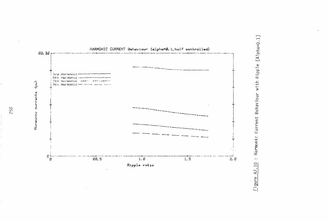
258
Harm
on
ia o
urren
te
(pu
) IS
> ~
W
ts;l
t£
;J ts
l ,,-
"---
-"+-------"""~--I------
.<J
'-J
In I
~'
1"'
+,.
. ...
. ,
:r::
r:t
rl
IJ:J:I
w ~
, W
lU
"'I
,
"'I
"'I
" " "
" o
C' 0
0 ::l
:;l
;:)
:l
1-
< ...
...
1>-' ..
....
n n
n n
I I .
1 I
11
:
:r:
~t I I
>
II :
::u
X
! I
0 :z
U1,
.... I I
: in
,
I I
In
I~
I l~
X
l I
I~
... I
I -T
'1
J
I I
I 0
'1J
I
H
......
~t I
!III I
I
i ,
I I
I Il
&
-i
I
!Il
... I
I I
0
I I
I J
' .....
. I
I}
, ,
I I
I I~
I
i I
I
1:-'
I
I I
I I
·T
I
II
I I
i 1
....
~t I
I
ti I
I I I
, I
I I
I I
t
l~ I
I
I I
I
I /
I I
I Ie
:;
I I , ! I
__ +
_
_ J
I
fJ L
~---+---~----+----+--
Gl
Figu
re A
7.IO
H
arm
onic
C
urre
nt B
ehav
iour
with
Rip
ple
[Alp
ha=
O.l]

I I I ......
1 "'0
1
!i
!t Iii
~l iTll
~ j ""I
> ,
{I I
.r.l III
I
il ~I
it oc <
::r:
1 ! I I
Fi gure A
7. 11
1 \ I I
I
I I
! I u
u u
u ''''''
01"1:''''' '>"1
c: C
c
c o
0 0
0 e e e e I..
I.. I..
I.. III
III III
<1l ::r.:r::r.:r -O
,C£
.I: L~""'of..I
~') 10
I' CI'
259 I I I I I I I I I I I I I I I I I \ I I \
i Itn
t g I
Harm
onic C
urrent Behaviour w
ith R
"ipple [A
lp .OJ
260
harmonics to reduce with increasing ripple ;s not so apparent in this
case. Because of difficulties in formulating a simple theory, there
are no predicted results, as in section A7.2.3.1.
interpretation of the results more difficult.
A7.4 CONCLUSIONS
This makes the
The main result of this study is that classical methods of
fixed current injections based on a flat d.c. current waveform are
inadequate. This is especially true of the hal controlled case.
The choice of d.c. motor representation is not so important, and in the
absence of accurate information the R/L series model is adequate.
The a.c. system representation has little effect on the
harmonic current injections, but should be accurate in order to assess
the harmonic voltage distortions.
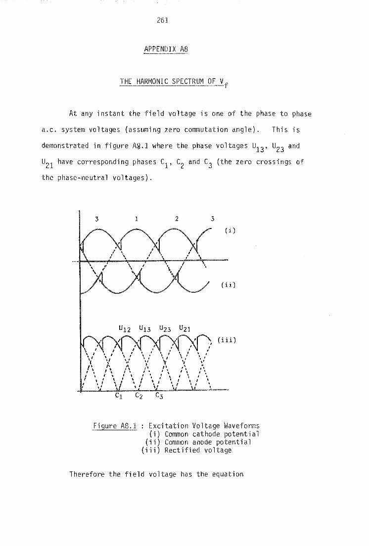
261
APPENDIX AB
THE HARMONIC SPECTRUM OF Vf
At any instant the field vol ge is one of the phase to phase
a.c. system voltages (assuming zero commutation angle). Thi sis
demonstrated in figure A9.1 where the phase voltages U13 , U23 and
U21 have corresponding phases C1, C2 and C3 (the zero crossings of
the phase-neutral voltages),
3 1
. , .. , , , .. I ' ,
.. '{ 'f 1\ " I'
2
'" ,. " I, ,. '\ I , , I ' I , I
" '. I " I , , \ I •
, , " ' " • " I '.
I • \ , •
3
(i)
(i i)
(i il)
Figure AB.1 : Excitati on Vo ltage Waveforrns (i) Common cathode potential
(ii) Common anode potential (iii) Rectified vol ge
Therefore the field voltage has the equation

262
v f( t) = /2 U21 sin (wt C3 + TI) for C1 + a < wt < C2 + a
/2 U 13 s; n ( wt - C1) C2 + a < wt < C3 + a
/2 U23 si n(wt C2) C3 + a < wt < C1 + a + TI
AB.1
where the waveform ;s repeated for the second half of the cycle. leading
to only even harmonics h.
Vf(t) can also be expressed in terms of a Fourier series
00
AB.2
where
/2 [ ) ( ( ) ah ::: TI(1+h){U21 cos((l+h) (C 1+a)-C3+TI - cos l+h (C 2+a) - C3+TI)]
+ U13[coS((1+h)(C2+a) C1) - cos((1+h)(C3+a) - C1)J
+ U23[cos((1+h) (C3+a) - C2) - cos((l+h) (C1+a+n) - C2)]}
12 + TI(l-h) {U21 [cos((1-h)(C1+a) - C3+TI) cos((1-h)(C2+a) - C3+TI)J
+ U13[cos((1-h)(C2+a) - C1) - cos((1-h)(C3+a) C1)J
+ U23[coS((1-h)(C3+a) - C2) - cos((l-h) (C1+a+TI) - C2)}
AB.3
bh ::: TI~Lh) {U21 [sin((l-h)(C2+a) - C3+TI) - sin((l-h)(C1+a) - C3+TI)]
+ U13[sin((1-h)(C3+a) - C1) - sin((1-h)(C2+a) - C1)J
+ U23[sin((1-h)(C1+a+TI) - C2) - sin((1-h)(C3+a) - C2)J}
12 - TI 0-h ) { U 21 [s i n ((1 h) (C 2 +a ) - C 3 +TI ) sin ( (1- h) (C 1 +cx) - C 3 +11) ]
+ U13[sin((1-h)(C3+a) C1) sin((1-h)(C2+a) C1)J
+ U23[sin((1-h) (C1+a+TI) - C2) - sin((l-h)(C3+a) - C2)J}
AB.4
For each harmonic frequency ah and bh are combined to an equivalent
Y'ms harmonic phasoY',
v =..J:.(a -jb) f /'l h h
AB.5
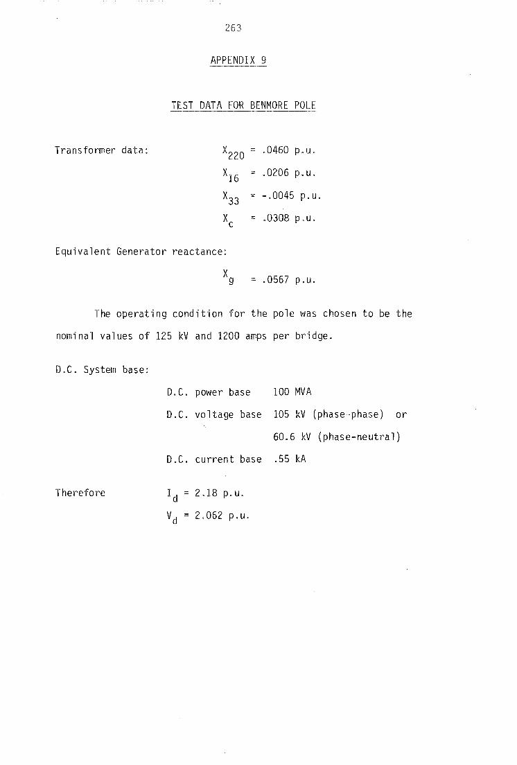
263
APPENDIX 9
TEST DATA FOR BENMORE POLE
Transformer data: X220 :: .0460 p. u.
X16 ::: .0206 p.u.
X33 = -.0045 p.u.
Xc ::: .0308 p.u.
Equivalent Generator reactance:
Xg ::: .0567 p.u.
The operating condition for the pole was chosen to be the
nominal values of 125 kV and 1200 amps per bridge.
D.C. System base:
Therefore
D.C. power base 100 MVA
D.C. voltage base 105 kV (phase-phase) or
60.6 kV (phase-neutral)
D.C. current base .55 kA
Id = 2.18 p.u.
Vd ::: 2.062 p.u.