Time-Harmonic Electromagnetic Fields with E ∥ B ...

Progress In Electromagnetics Research M, Vol. 104, 171–183, 2021

Time-Harmonic Electromagnetic Fields with E ∥ B Representedby Superposing Two Counter-Propagating Beltrami Fields

Ryo Mochizuki1, *, Naoki Shinohara1, and Atsushi Sanada2

Abstract—In this paper, we present a general solution for time-harmonic electromagnetic fields with itselectric and magnetic fields parallel to each other (E ∥ B fields) in source-free vacuum and demonstratethat every time-harmonic E ∥ B field is composed of the superposition of two counter-propagatingBeltrami fields. We show that every E ∥ B field can be categorized into one of two cases dependingon the time dependence of the function that describes the proportionality between the electric andmagnetic fields. After presenting the mathematical definition of a Beltrami field in electromagnetismand its handedness, we perform a detailed analysis of time-harmonic E ∥ B fields for each case. Forthe first case, we find the general solution for the E ∥ B fields using the angular-spectrum methodand prove that every first-case E ∥ B field can be generated by superposing two oppositely travelingBeltrami fields with the same handedness. For the second case, we deduce the general solution for theE ∥ B fields by employing complex analysis and demonstrate that every time-harmonic E ∥ B field iscomposed of two counter-propagating planar Beltrami fields with opposite handedness.

1. INTRODUCTION

For almost a century, Beltrami fields have attracted considerable research attention. A Beltrami fieldV is a vector field that satisfies the equation

∇×V = κV, (1)

where κ is a scalar function, possibly of both time and position. This equation implies that a Beltramifield is parallel to its curl everywhere. Moreover, the equation can be regarded as an eigenvalue equationinvolving the curl operator ∇×. In this interpretation, V and κ correspond to the eigenvector andeigenvalue, respectively.

The Beltrami-field concept originated in the study of fluid dynamics [1]. For the Navier-Stokesequation, we can find solutions such that the flow velocity is parallel to the vorticity. Because thevorticity is equal to the curl of the flow velocity, these solutions are Beltrami fields. One such Beltramifield that applies to the Arnold-Beltrami-Childress (ABC) flow exhibits chaotic trajectories and hasbeen employed in analyzing turbulence [2].

Beltrami fields have also been studied in electromagnetism. The first study dealing withelectromagnetic fields that have the property expressed by Eq. (1) dates back to Silberstein [3], and theconcept of such a field has since been incorporated in several branches of electromagnetism. In plasmaphysics, for instance, Beltrami fields have been employed in the investigation of force-free magneticfield [4]. In such a field, the current behaves as if there were no Lorentz forces in the system becausethe magnetic field is a Beltrami field, i.e., in a force-free field, the magnetic field is parallel to thecurrent density, which is equivalent to the curl of the magnetic field. In electromagnetism withoutcharged particles, the Beltrami-field concept has also been exploited for analyzing electromagnetic fields

Received 16 July 2021, Accepted 1 September 2021, Scheduled 7 September 2021* Corresponding author: Ryo Mochizuki (ryo [email protected]).1 Research Institute for Sustainable Humanosphere, Kyoto University, Japan. 2 Graduate School of Engineering Science, OsakaUniversity, Japan.

172 Mochizuki, Shinohara, and Sanada

in chiral and bi-isotropic media, i.e., in complex materials where the electric and magnetic fields arecoupled [5–7].

In this study, we focus on the relation between Beltrami fields and electromagnetic fields in which theelectric and magnetic fields are parallel to each other, which we refer to as E ∥ B fields. Some importantstudies involving E ∥ B fields include the work of Chu and Ohkawa, who first demonstrated thepossibility of E ∥ B fields by obtaining a solution of Maxwell’s equations for transverse electromagneticfields with E ∥ B [8]. However, this claim has since been confronted by a series of controversies [9–12].Subsequently, some researchers have attempted to find general solutions for electromagnetic fields withE ∥ B that are subject to no specific assumption, but such solutions are yet to be derived. In the struggleto find a general solution, some solutions for E ∥ B fields have been obtained under specific assumptions.For instance, Zaghloul and Buckmaster [13] and Shimoda et al. [14] independently presented a generalsolution for transverse electromagnetic fields with E ∥ B. Subsequently, Uehara et al. found somenontransverse E ∥ B fields [15]. Recently, Nishiyama derived the general solution for a spherical E ∥ Bfield, which is a special type of nontransverse E ∥ B field [16]. In addition to the purely theoretical worksabove, the studies on practical applications using E ∥ B fields were presented. Evtuhov and Siegmandescribed the method for achieving the energy uniformity in a laser cavity by using a “twisted-mode”standing wave, a special type of planar E ∥ B fields [17]. Subsequently, some laser techniques exploitingtwisted-mode waves were proposed [18–21]. Raab et al. developed the magneto-optic trap using theelectromagnetic field expressed as the superposition of three twisted-mode waves, which had the E ∥ Bproperty [22].

This study deals with the analytical and mathematical aspects of E ∥ B fields. In the earliertheoretical works already mentioned, E ∥ B fields have been analyzed under various assumptionsregarding the geometric properties of the electric and magnetic fields; i.e., in those papers, theelectromagnetic fields were assumed to be planar or to be tangent to concentric spheres. In contrast tothese earlier works, we focus here on E ∥ B fields that have a harmonic time dependence of the forme−iωt, which has not been considered in the earlier works. In physics and engineering, the analysis oftime-harmonic waves is important from both theoretical and practical points of view.

In this paper, our goal is to find the general solution for time-harmonic E ∥ B fields in a source-free vacuum region and to demonstrate that every time-harmonic E ∥ B field can be generated by thesuperposition of two Beltrami fields traveling in opposite directions.

The difference between this study and the earlier works is as follows. Uehara et al. presented ageneric form of an E ∥ B field using both a scalar and a vector field, denoted by f and v, respectively.They classified E ∥ B fields with arbitrary time dependence into three groups, corresponding to thethree types of the vector field v, which they refer to as “Case I”, “Case II”, and “Case III”. In contrast,this paper classifies time-harmonic E ∥ B fields into two groups depending on the time dependence ofthe scalar function f ; thus, we need to investigate fewer cases. For the first case (which correspondsto Case II of Uehara et al.), we derive the general solutions for v and E ∥ B field with the amplitudepossibly unbounded at infinity, which were not obtained explicitly by Uehara et al. For the secondcase, which has not been considered directly in any of the abovementioned works, we uniquely performthe analytical derivation of the functional form of f from the condition defining this case and obtainthe corresponding v and E ∥ B field. Furthermore, unlike the earlier studies on E ∥ B fields, we alsopresent a discussion that may help in experimentally generating E ∥ B fields; we demonstrate that, aswith any other standing wave, every time-harmonic E ∥ B field is composed of the superposition of twooppositely propagating waves.

This paper is organized as follows. In Section 2, we show that every time-harmonic E ∥ B fieldcan be classified into one of two groups depending on the properties of f . In addition, we deduce thepartial-differential equations satisfied by f and v. In Section 3, after introducing the handedness ofthe Beltrami fields, we derive a general mathematical expression for the first-case E ∥ B fields usingthe angular-spectrum method. Moreover, we demonstrate that a first-case E ∥ B field is necessarilycomposed of the superposition of two counter-propagating Beltrami fields with the same handedness.In Section 4, we obtain a general solution for E ∥ B fields belonging to the second group. Moreover, weshow that the second-case E ∥ B fields always consist of the superposition of two counter-traveling planarBeltrami fields with opposite handedness. Finally, in Section 5, we present our general conclusions asto the findings of this paper and note some open problems.

Progress In Electromagnetics Research M, Vol. 104, 2021 173

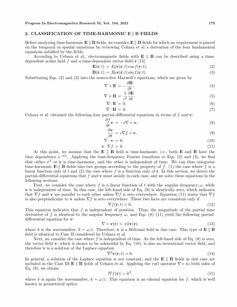
2. CLASSIFICATION OF TIME-HARMONIC E ∥ B FIELDS

Before analyzing time-harmonic E ∥ B fields, we consider E ∥ B fields for which no requirement is placedon the temporal or spatial variations by reviewing Uehara et al.’s derivation of the four fundamentalequations satisfied by the fields.

According to Uehara et al., electromagnetic fields with E ∥ B can be described using a time-dependent scalar field f and a time-dependent vector field v [15]:

E(r; t) = E0v(r; t) cos f(r; t), (2)

B(r; t) = B0v(r; t) sin f(r; t). (3)

Substituting Eqs. (2) and (3) into the source-free Maxwell’s equations, which are given by

∇×E = −∂B∂t, (4)

∇×B =1

c2∂E

∂t, (5)

∇ ·E = 0, (6)

∇ ·B = 0, (7)

Uehara et al. obtained the following four partial-differential equations in terms of f and v:∂f

∂tv = −c∇× v, (8)

∂v

∂t= c∇f × v, (9)

∇ · v = 0, (10)

v · ∇f = 0. (11)

At this point, we assume that the E ∥ B field is time-harmonic, i.e., both E and B have thetime dependence e−iωt. Applying the time-frequency Fourier transform to Eqs. (2) and (3), we findthat either eif or v is time-harmonic, and the other is independent of time. We can thus categorizetime-harmonic E ∥ B fields into two groups according to the property of f : (1) the case where f is alinear function only of t and (2) the case where f is a function only of r. In this section, we derive thepartial-differential equations that f and v must satisfy in each case, and we solve these equations in thefollowing sections.

First, we consider the case where f is a linear function of t with the angular frequency ω, whilev is independent of time. In this case, the left-hand side of Eq. (9) is identically zero, which indicatesthat ∇f and v are parallel to each other unless ∇f is zero everywhere. Equation (11) states that ∇fis also perpendicular to v unless ∇f is zero everywhere. These two facts are consistent only if

∇f(r; t) = 0. (12)

This equation indicates that f is independent of position. Thus, the magnitude of the partial timederivative of f is identical to the angular frequency ω, and Eqs. (8)–(11) yield the following partial-differential equation for v:

∇× v(r) = ±kv(r), (13)

where k is the wavenumber, k = ω/c. Therefore, v is a Beltrami field in this case. This type of E ∥ Bfield is identical to Case II considered by Uehara et al.

Next, we consider the case where f is independent of time. As the left-hand side of Eq. (8) is zero,the vector field v, which is shown to be solenoidal by Eq. (10), is also an irrotational vector field, andtherefore v is a solution of the Laplace equation

∇2v(r; t) = 0. (14)

In general, a solution of the Laplace equation is not constant, and the E ∥ B fields in this case areincluded in the Case III E ∥ B fields of Uehara et al. Applying the curl operator ∇× to both sides ofEq. (9), we obtain

|∇f(r)| = k2, (15)

where k is again the wavenumber, k = ω/c. This equation is an eikonal equation for f , which is wellknown in geometrical optics.


3. E ∥ B FIELD WITH LINEARLY TIME-DEPENDENT f

3.1. Electromagnetic Beltrami Field

Before performing the analysis of the Case II E ∥ B fields, we introduce two important concepts forthe analysis of the E ∥ B fields: the electromagnetic Beltrami field and its handedness. We considertime-harmonic electromagnetic fields whose the electric and magnetic fields satisfy

∇×E = ±kE, (16)

∇×B = ±kB, (17)

where the double signs in the two equations correspond to each other. These equations can be regardedas the eigenequations of the curl operator ∇× with the eigenvalues ±k. Hereinafter, we refer toelectromagnetic fields that satisfy these eigenequations as Beltrami fields. One of the simplest Beltramifields is a circularly polarized wave. A left-handed circularly polarized wave satisfies the eigenvalueEqs. (16) and (17) with the eigenvalue +k, whereas a right-handed circularly polarized wave satisfies theequations with the eigenvalue −k. We can expand the concept of handedness associated with circularlypolarized waves to a general Beltrami field; we define a left-handed Beltrami field as a Beltrami fieldwith the eigenvalue +k and a right-handed Beltrami field as a Beltrami field with the eigenvalue −k.

From Eqs. (2), (3), and (13), we find that a Case II E ∥ B field is a Beltrami field. The eigenvalueequation for v, namely Eq. (13), determines the handedness of the Case II E ∥ B field; if the eigenvalueof Eq. (13) is positive, the Case II E ∥ B field is a left-handed Beltrami field, while if the eigenvalue isnegative, it is a right-handed Beltrami field.

3.2. General Solution for an E ∥ B Field

In this subsection, we derive the general solution for a Case II E ∥ B field using the angular-spectrummethod [23]. This method helps in understanding the physical implications of Case II E ∥ B andBeltrami fields.

Applying the curl operator to both sides of Eq. (8) yields the following Helmholtz equation for v:

∇2v(r) + k2v(r) = 0. (18)

The general expression for the vector field v(r) has the form

v(r) =

∫dp

∫dq[v1(p,q) + iv2(p,q)]e

ik(p+iq)·r, (19)

where v1 and v2 are purely real vector-valued functions of the two purely real vector variablesp = (px, py, pz) and q = (qx, qy, qz), and the two vectors, p and q, satisfy

|p2 − |q|2 = 1, (20)

p · q = 0. (21)

From the divergence-free condition, Eq. (10), and the eigenvalue equation Eq. (13), we find the followingconstraints on the spectra v1 and v2. Substituting Eq. (19) into the divergence-free condition, Eq. (10),gives ∫

dp

∫dqk[−(p · v2 + q · v1) + i(p · v1 − q · v2)][v1(p,q) + iv2(p,q)]e

ik(p+iq)·r = 0. (22)

This equation imposes the requirement that the integrand be identically zero; i.e.,

p · v2 + q · v1 = 0, (23)

p · v1 − q · v2 = 0. (24)

Similarly, substituting Eq. (19) into the eigenvalue Eq. (13) gives∫dp

∫dqk[−(q× v1 + p× v2 ± v1) + i(p× v1 − q× v2 ∓ v2)]e

ik(p+iq)·r = 0, (25)


which yields the requirement that the integrand be identically zero; that is,

q× v1 + p× v2 ± v1 = 0, (26)

p× v1 − q× v2 ∓ v2 = 0. (27)

Equations (23), (24), (26), and (27) define the geometrical relations among v1, v2, p, and q. Becausethe scalar product of v1 and the left-hand side of Eq. (26) is identical to that of v2 and left-side ofEq. (27), we find the relation

|v1| = |v2|. (28)

As the scalar product of v2 and the left-hand side of Eq. (26) is identical to the product of v1 andleft-side of Eq. (27), we find the orthogonality condition

v1 · v2 = 0. (29)

By choosing an appropriate local Cartesian coordinate with the orthonormal basis {e1, e2, e3}, the twovectors v1 and v2 can thus be represented in the form

v1 = v0e1, (30)

v2 = v0e2, (31)

where the coefficient v0 is real. The vector variables p and q can be represented in the form

p = p1e1 + p2e2 + p3e3, (32)

q = q1e1 + q2e2 + q3e3. (33)

Substituting Eqs. (32) and (33) into the requirements given by Eqs. (26) and (27), we obtain

p1 = q2, (34)

p2 = −q1, (35)

p3 = ±1, (36)

q3 = 0. (37)

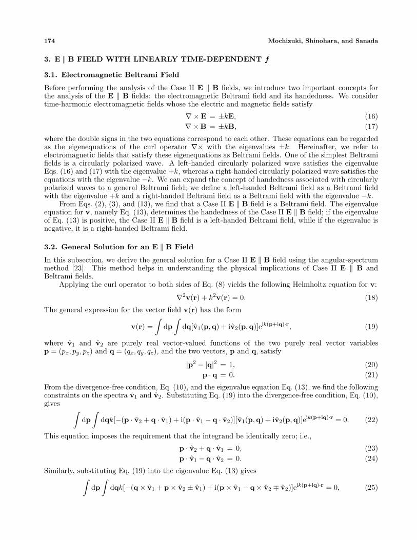
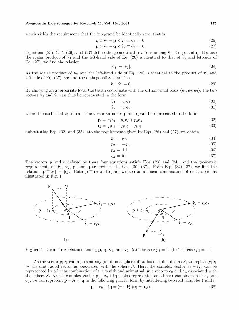
The vectors p and q defined by these four equations satisfy Eqs. (23) and (24), and the geometricrequirements on v1, v2, p, and q are reduced to Eqs. (30)–(37). From Eqs. (34)–(37), we find therelation |p∓ e3| = |q|. Both p ∓ e3 and q are written as a linear combination of e1 and e2, asillustrated in Fig. 1.

p e3

p − e3

q

v1 = v0e1

v2 = v0e2

p + e3

q

(a) (b)p −e3

v2 = v0e2

v1 = v0e1

Figure 1. Geometric relations among p, q, v1, and v2. (a) The case p3 = 1. (b) The case p3 = −1.

As the vector p3e3 can represent any point on a sphere of radius one, denoted as S, we replace p3e3by the unit radial vector ek associated with the sphere S. Here, the complex vector v1 + iv2 can berepresented by a linear combination of the zenith and azimuthal unit vectors eθ and eϕ associated withthe sphere S. As the complex vector p− ek + iq is also represented as a linear combination of eθ andeϕ, we can represent p−ek +iq in the following general form by introducing two real variables ξ and η:

p− ek + iq = (η + iξ)(eθ ± ieϕ), (38)


where the double sign corresponds to that of Eq. (13). As ek, eθ, and eϕ are functions only of θ and ϕ,we recognize that the vector variables p and q are represented by just the four variables θ, ϕ, ξ, and η.Using a complex function of θ, ϕ, ξ, and η, denoted as u(θ, ϕ, ξ, η), v1 + iv2 can thus be expressed inthe form

v1 + iv2 = u(θ, ϕ, ξ, η)(eθ ± ieϕ), (39)

where the double sign also corresponds to the handedness of the Beltrami field in Eq. (13). Summarizingthe results obtained so far, we find that v(r) can be represented in the integral form

v(r) =

π∫0

dθ

π∫−π

dϕ (eθ ± ieϕ)

∞∫−∞

∞∫−∞

u(θ, ϕ, ξ, η)eik(η+iξ)(eθ±ieϕ)·rdξdη

eikek·r. (40)

Here, we define the angular spectrum v(θ, ϕ, r) as

v(θ, ϕ, r) =

∞∫−∞

∞∫−∞

u(θ, ϕ, ξ, η)eik(η+iξ)(eθ±ieϕ)·rdξdη. (41)

As v(r) is a purely real vector, for every r, any two angular spectra at opposite points on the sphere Smust satisfy the symmetry condition

v(θ, ϕ, r) = v(π − θ, π + ϕ, r). (42)

Substituting Eq. (41) into this symmetry relation, we have

∞∫−∞

∞∫−∞

(u(θ, ϕ, ξ, η)eikη(eθ±ieϕ)·r − u(π − θ, π + ϕ, ξ, η)e−ikη(eθ±ieϕ)·r)dη

e−kξ(eθ±ieϕ)·rdξ = 0. (43)

For this equation to hold regardless of position r, the η-dependence of u(θ, ϕ, ξ, η) must be the Diracdelta function δ(η), which suggests that u is actually a function of only θ, ϕ, and ξ. Therefore, therequirement that v(r) be a purely real vector is reduced to the equation

u(θ, ϕ, ξ) = u(π − θ, π + ϕ, ξ). (44)

As a result, the angular spectrum v(θ, ϕ, r) can be written in the form

v(θ, ϕ, r) =

∞∫−∞

dξu(θ, ϕ, ξ)e−kξ(eθ±ieϕ)·r, (45)

where u(θ, ϕ, ξ) is a symmetric function satisfying Eq. (44). By employing the surface integral ofv(θ, ϕ, r) on the sphere S, we obtain the general solution for v(r) as

v(r) =

π∫0

dθ

π∫−π

dϕ(eθ ± ieϕ)v(θ, ϕ, r)eikek·r

=

π2∫

0

dθ

π∫−π

dϕρ[cos(kek · r+ ψ)eθ ∓ sin(kek · r+ ψ)eϕ], (46)

where ρ and ψ are respectively the magnitude and argument of the angular spectrum v(θ, ϕ, r), i.e.,

ρ = |v(θ, ϕ, r)|, (47)

ψ = Arg(v(θ, ϕ, r)). (48)


Conversely, we can readily confirm that every vector field that satisfies Eqs. (44)–(48) is necessarily asolution for v(r). As a result, we obtain the general solution for a Case II E ∥ B field in the form

E(r; t) = E0 cosωt

π2∫

0

dθ

π∫−π

dϕρ [cos(kek · r+ ψ)eθ ∓ sin(kek · r+ ψ)eϕ] , (49)

B(r; t) = ∓B0 sinωt

π2∫

0

dθ

π∫−π

dϕρ [cos(kek · r+ ψ)eθ ∓ sin(kek · r+ ψ)eϕ] . (50)

Looking now at Eq. (46), we see that the superposition principle is valid for these solutions; thesuperposition of multiple Case II E ∥ B fields yields a Case II E ∥ B field as long as all the originalE ∥ B fields have the same handedness.

Next, we investigate the functional form of the angular spectrum v(θ, ϕ, r) given by Eq. (45). If theangular spectrum exists for any r, due to the nature of the integral transform, the angular spectrumv(θ, ϕ, r) is an entire function of the complex variable (eθ± ieϕ) ·r, where eθ± ieϕ is a complex constantvector for fixed (θ, ϕ). Conversely, if the angular spectrum is reduced to an entire function of (eθ±ieϕ)·rfor every fixed (θ, ϕ), the integral of Eq. (46) yields a solution for v(r). This is easily confirmed as follows.Suppose that for a given (θ, ϕ), an entire function of (eθ ± ieϕ) · r is written as Φθϕ((eθ ± ieϕ) · r). Then,the curl of the vector field given by Eq. (46) is computed as

∇× v(r)

= ∇×

π∫0

dθ

π∫−π

dϕ(eθ ± ieϕ)Φθϕ((eθ ± ieϕ) · r)eikek·r

=

π∫0

dθ

π∫−π

dϕ[(eθ ± ieϕ)× (eθ ± ieϕ)Φ

′θϕ((eθ ± ieϕ) · r) + ikek × (eθ ± ieϕ)Φθϕ((eθ ± ieϕ) · r)

]eikek·r

= ±kv(r). (51)

We now present a specific example of a Beltrami field v(r). Let u be given by

u(θ, ϕ, ξ) = δ′(ξ), (52)

where δ′(ξ) denotes the first derivative of the Dirac delta function. From Eq. (45), we have the angularspectrum

v(θ, ϕ, r) = −k(eθ ± ieϕ) · r, (53)

which satisfies the symmetry relation of Eq. (42). The Beltrami field v(r) is represented in the integralform

v(r) =

π∫0

dθ

π∫−π

dϕ(eθ ± ieϕ)[−k(eθ ± ieϕ) · r]eikek·r. (54)

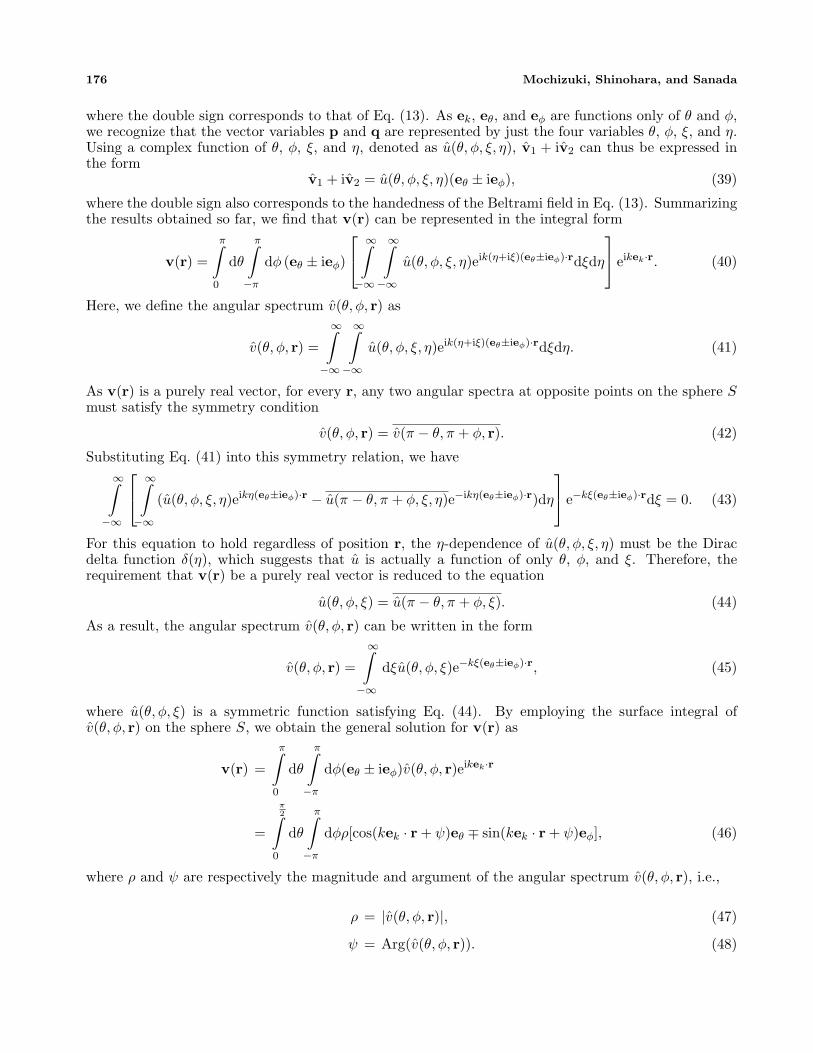
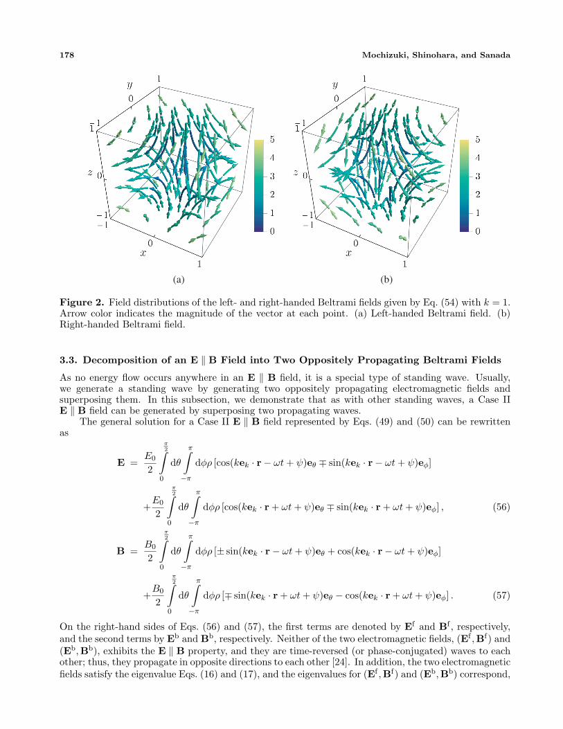
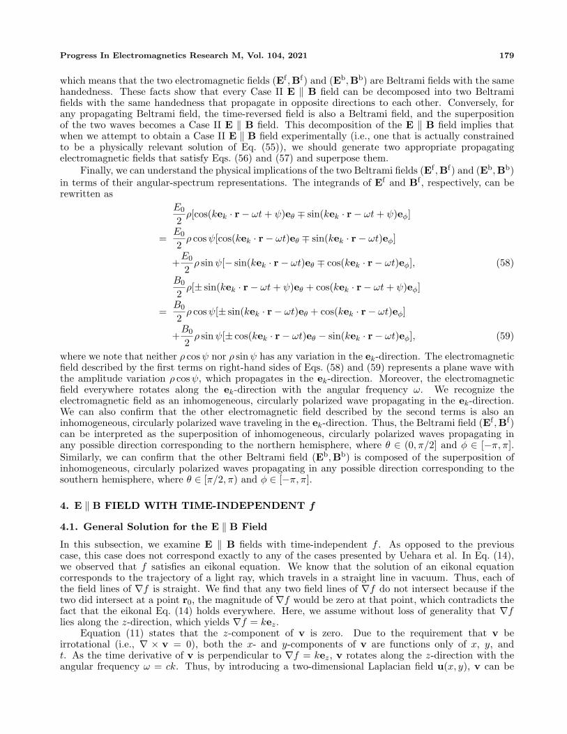
As the integral on the right-hand side of Eq. (54) cannot be evaluated analytically, we calculatenumerically the field distributions of the left- and right-handed Beltrami fields, and the numericalresults are shown in Fig. 2.

Finally, we note the physically relevant solutions. If the angular spectrum v(θ, ϕ, r) depends onposition r, the vector field v(r) given by Eq. (46) diverges to infinity as |r| → ∞, and the correspondingelectromagnetic field also diverges at infinity. Thus, the resulting electromagnetic field is not physicallyacceptable. Physically realizable electromagnetic fields can be obtained only if the ξ dependence ofu(θ, ϕ, ξ) is a delta function δ(ξ), and the angular spectrum v is provided as a function of only θ and ϕ.Therefore, the physically relevant solution for v(r) can be represented in the form

v(r) =

π2∫

0

dθ

π∫−π

dϕ|v(θ, ϕ)|[cos(kek · r+Arg(v(θ, ϕ)))eθ ∓ sin(kek · r+Arg(v(θ, ϕ)))eϕ]. (55)


(a) (b)

Figure 2. Field distributions of the left- and right-handed Beltrami fields given by Eq. (54) with k = 1.Arrow color indicates the magnitude of the vector at each point. (a) Left-handed Beltrami field. (b)Right-handed Beltrami field.

3.3. Decomposition of an E ∥ B Field into Two Oppositely Propagating Beltrami Fields

As no energy flow occurs anywhere in an E ∥ B field, it is a special type of standing wave. Usually,we generate a standing wave by generating two oppositely propagating electromagnetic fields andsuperposing them. In this subsection, we demonstrate that as with other standing waves, a Case IIE ∥ B field can be generated by superposing two propagating waves.

The general solution for a Case II E ∥ B field represented by Eqs. (49) and (50) can be rewrittenas

E =E0

2

π2∫

0

dθ

π∫−π

dϕρ [cos(kek · r− ωt+ ψ)eθ ∓ sin(kek · r− ωt+ ψ)eϕ]

+E0

2

π2∫

0

dθ

π∫−π

dϕρ [cos(kek · r+ ωt+ ψ)eθ ∓ sin(kek · r+ ωt+ ψ)eϕ] , (56)

B =B0

2

π2∫

0

dθ

π∫−π

dϕρ [± sin(kek · r− ωt+ ψ)eθ + cos(kek · r− ωt+ ψ)eϕ]

+B0

2

π2∫

0

dθ

π∫−π

dϕρ [∓ sin(kek · r+ ωt+ ψ)eθ − cos(kek · r+ ωt+ ψ)eϕ] . (57)

On the right-hand sides of Eqs. (56) and (57), the first terms are denoted by Ef and Bf , respectively,and the second terms by Eb and Bb, respectively. Neither of the two electromagnetic fields, (Ef ,Bf) and(Eb,Bb), exhibits the E ∥ B property, and they are time-reversed (or phase-conjugated) waves to eachother; thus, they propagate in opposite directions to each other [24]. In addition, the two electromagneticfields satisfy the eigenvalue Eqs. (16) and (17), and the eigenvalues for (Ef ,Bf) and (Eb,Bb) correspond,


which means that the two electromagnetic fields (Ef ,Bf) and (Eb,Bb) are Beltrami fields with the samehandedness. These facts show that every Case II E ∥ B field can be decomposed into two Beltramifields with the same handedness that propagate in opposite directions to each other. Conversely, forany propagating Beltrami field, the time-reversed field is also a Beltrami field, and the superpositionof the two waves becomes a Case II E ∥ B field. This decomposition of the E ∥ B field implies thatwhen we attempt to obtain a Case II E ∥ B field experimentally (i.e., one that is actually constrainedto be a physically relevant solution of Eq. (55)), we should generate two appropriate propagatingelectromagnetic fields that satisfy Eqs. (56) and (57) and superpose them.

Finally, we can understand the physical implications of the two Beltrami fields (Ef ,Bf) and (Eb,Bb)in terms of their angular-spectrum representations. The integrands of Ef and Bf , respectively, can berewritten as

E0

2ρ[cos(kek · r− ωt+ ψ)eθ ∓ sin(kek · r− ωt+ ψ)eϕ]

=E0

2ρ cosψ[cos(kek · r− ωt)eθ ∓ sin(kek · r− ωt)eϕ]

+E0

2ρ sinψ[− sin(kek · r− ωt)eθ ∓ cos(kek · r− ωt)eϕ], (58)

B0

2ρ[± sin(kek · r− ωt+ ψ)eθ + cos(kek · r− ωt+ ψ)eϕ]

=B0

2ρ cosψ[± sin(kek · r− ωt)eθ + cos(kek · r− ωt)eϕ]

+B0

2ρ sinψ[± cos(kek · r− ωt)eθ − sin(kek · r− ωt)eϕ], (59)

where we note that neither ρ cosψ nor ρ sinψ has any variation in the ek-direction. The electromagneticfield described by the first terms on right-hand sides of Eqs. (58) and (59) represents a plane wave withthe amplitude variation ρ cosψ, which propagates in the ek-direction. Moreover, the electromagneticfield everywhere rotates along the ek-direction with the angular frequency ω. We recognize theelectromagnetic field as an inhomogeneous, circularly polarized wave propagating in the ek-direction.We can also confirm that the other electromagnetic field described by the second terms is also aninhomogeneous, circularly polarized wave traveling in the ek-direction. Thus, the Beltrami field (Ef ,Bf)can be interpreted as the superposition of inhomogeneous, circularly polarized waves propagating inany possible direction corresponding to the northern hemisphere, where θ ∈ (0, π/2] and ϕ ∈ [−π, π].Similarly, we can confirm that the other Beltrami field (Eb,Bb) is composed of the superposition ofinhomogeneous, circularly polarized waves propagating in any possible direction corresponding to thesouthern hemisphere, where θ ∈ [π/2, π) and ϕ ∈ [−π, π].

4. E ∥ B FIELD WITH TIME-INDEPENDENT f

4.1. General Solution for the E ∥ B Field

In this subsection, we examine E ∥ B fields with time-independent f . As opposed to the previouscase, this case does not correspond exactly to any of the cases presented by Uehara et al. In Eq. (14),we observed that f satisfies an eikonal equation. We know that the solution of an eikonal equationcorresponds to the trajectory of a light ray, which travels in a straight line in vacuum. Thus, each ofthe field lines of ∇f is straight. We find that any two field lines of ∇f do not intersect because if thetwo did intersect at a point r0, the magnitude of ∇f would be zero at that point, which contradicts thefact that the eikonal Eq. (14) holds everywhere. Here, we assume without loss of generality that ∇flies along the z-direction, which yields ∇f = kez.

Equation (11) states that the z-component of v is zero. Due to the requirement that v beirrotational (i.e., ∇ × v = 0), both the x- and y-components of v are functions only of x, y, andt. As the time derivative of v is perpendicular to ∇f = kez, v rotates along the z-direction with theangular frequency ω = ck. Thus, by introducing a two-dimensional Laplacian field u(x, y), v can be


represented in the form

v(x, y; t) = u(x, y) cosωt+ (ez × u(x, y)) sinωt, (60)

which implies that the E ∥ B field considered in the present section is a special case of the planarCase III field analyzed by Nishiyama [16]. We can find such a two-dimensional Laplacian field u(x, y)by employing the technique described by Nishiyama. Here, we consider a complex function g(x + iy)whose real and imaginary parts are equivalent to the x- and y-components of u(x, y), respectively; i.e.,g(x+ iy) = ux + iuy. The requirement that u be irrotational yields

∂uy∂x

− ∂ux∂y

= 0, (61)

∂ux∂x

+∂uy∂y

= 0. (62)

These equations correspond to the Cauchy-Riemann equations for the complex function g(x + iy).Therefore, g(x+iy) is an entire function, and the x- and y-components of the Laplacian field u correspondrespectively to the real and imaginary parts of an arbitrary entire function. Thus, the general solutionfor an E ∥ B field with ∂f/∂t = 0 can be represented in the form

E(r; t) = E0ρ[cos(ωt+ ψ)ex + sin(ωt+ ψ)ey] cos kz, (63)

B(r; t) = B0ρ[cos(ωt+ ψ)ex + sin(ωt+ ψ)ey] sin kz, (64)

where ρ and ψ are the magnitude and argument of an entire function of x + iy, respectively. Wenow note that the superposition principle is applicable to these solutions due to the nature of entirefunctions; the superposition of multiple E ∥ B fields with time-independent f produces an E ∥ B fieldwith time-independent f , provided that ∇f of each original E ∥ B field points in the same direction.

A specific example of v(r; t) is now considered. Suppose that the entire complex function is definedby

g(x+ iy) = e−(x+iy)2 . (65)

The corresponding v(r; t) is calculated from Eq. (60) as

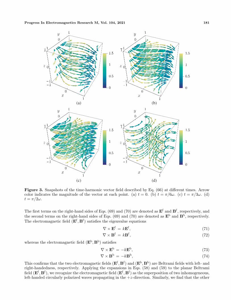
v(r; t) = e−x2+y2 [cos (2xy − ωt)ex − sin (2xy − ωt)ey]. (66)

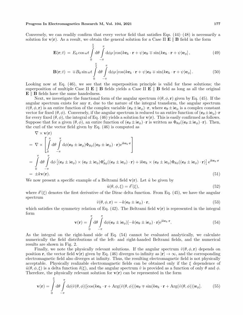
A series of snapshots of the field distribution of v(r; t) is shown in Fig. 3.As with the previous E ∥ B field case, we note the physically reasonable solutions. As an

electromagnetic field in a physical system is required to be a bounded function, both ux and uy must bebounded functions. Applying Liouville’s theorem to g(x+iy), we find that g(x+iy) must be a constantfunction. Therefore, a physically relevant E ∥ B field with ∂f/∂t = 0 is constrained to have the form

E(z; t) = E0(cosωtex + sinωtey) cos kz, (67)

B(z; t) = B0(cosωtex + sinωtey) sin kz, (68)

where E0 and B0 are constants. This physically acceptable result corresponds to the solution for theCase I E ∥ B field presented by Uehara et al.

4.2. Decomposition of E ∥ B Field into Two Counter-Propagating Planar Beltrami Fields

The general solution for the E ∥ B field given by Eqs. (63) and (64) can be rewritten as

E(r; t) =E0

2ρ[cos(kz − ωt− ψ)ex − sin(kz − ωt− ψ)ey]

+E0

2ρ[cos(−kz − ωt− ψ)ex − sin(−kz − ωt− ψ)ey], (69)

B(r; t) =B0

2ρ[sin(kz − ωt− ψ)ex + cos(kz − ωt− ψ)ey]

+B0

2ρ[− sin(−kz − ωt− ψ)ex − cos(−kz − ωt− ψ)ey]. (70)


(a) (b)

(c) (d)

Figure 3. Snapshots of the time-harmonic vector field described by Eq. (66) at different times. Arrowcolor indicates the magnitude of the vector at each point. (a) t = 0. (b) t = π/6ω. (c) t = π/3ω. (d)t = π/2ω.

The first terms on the right-hand sides of Eqs. (69) and (70) are denoted as Ef and Bf , respectively, andthe second terms on the right-hand sides of Eqs. (69) and (70) are denoted as Eb and Bb, respectively.The electromagnetic field (Ef ,Bf) satisfies the eigenvalue equations

∇×Ef = kEf , (71)

∇×Bf = kBf , (72)

whereas the electromagnetic field (Eb,Bb) satisfies

∇×Eb = −kEb, (73)

∇×Bb = −kBb, (74)

This confirms that the two electromagnetic fields (Ef ,Bf) and (Eb,Bb) are Beltrami fields with left- andright-handedness, respectively. Applying the expansions in Eqs. (58) and (59) to the planar Beltramifield (Ef ,Bf), we recognize the electromagnetic field (Ef ,Bf) as the superposition of two inhomogeneous,left-handed circularly polarized waves propagating in the +z-direction. Similarly, we find that the other


Beltrami field (Eb,Bb) consists of two right-handed circularly polarized waves with inhomogeneousamplitudes, traveling in the −z-direction. We can summarize these results concerning the decompositionof an E ∥ B field with time-independent as follows: Every E ∥ B field with ∂f/∂t = 0 can be decomposedinto counter-propagating left- and right-handed planar Beltrami fields, each of which is composed ofthe superposition of two inhomogeneous, circularly polarized waves.

5. CONCLUSIONS

In this study, we derived general solutions of the time-harmonic Maxwell’s equations such that theelectric and magnetic fields are parallel to each other. We also demonstrated that every time-harmonicE ∥ B field is composed of the superposition of two oppositely propagating Beltrami fields.

We started with the classification of time-harmonic E ∥ B fields. After reviewing Uehara et al.’sexpressions for E ∥ B fields, i.e., E = E0v cos f and B = B0v sin f , we classified time-harmonic E ∥ Bfields into one of two types, corresponding to the cases where f is a linear function of time (first case) orf is independent of time (second case). Before analyzing the first-case E ∥ B field, which is a particulartype of Beltrami fields, we defined the handedness of a Beltrami field by expanding the concept of thehandedness of circularly polarized waves. Subsequently, we obtained the general solution for the first-case E ∥ B field in integral form and thereby demonstrated that every first-case E ∥ B field is composedof two oppositely propagating Beltrami fields with the same handedness. Next, we derived the generalsolution for the second-case E ∥ B field and proved that every second-case E ∥ B field always consistsof two counter-propagating, planar Beltrami fields with opposite handedness.

The findings of this work can guide further studies on two pending issues, namely (a) findinggeneral solutions for time-harmonic E ∥ B fields close to charge or current distributions and (b) derivinggeneral solutions for E ∥ B fields with an arbitrary time dependence. In addition to the results of thepresent work, further mathematical approaches are necessary for analyzing these issues. Solving the firstproblem requires the development of a Green’s function method that can be used to find the fundamentalsolution of the nonhomogeneous Helmholtz equation that describes time-harmonic electromagnetic fieldsin the vicinity of charged particles and current sources. Solving the second problem requires exploitingtime-frequency Fourier-transform techniques. Using the Fourier transform of E ∥ B fields having anarbitrary time dependence, the problem can be reduced to the calculus of vector fields with a single-frequency time dependence, which we studied herein.

ACKNOWLEDGMENT

This work was supported by JSPS KAKENHI Grant Number JP20J14118.

REFERENCES

1. Drazin, P. G. and N. Riley, Steady Flows Bounded by Plane Boundaries, Ser. London MathematicalSociety Lecture Note Series, 11–44, Cambridge University Press, 2006.

2. Dombre, T., U. Frisch, J. M. Greene, M. Henon, A. Mehr, and A. M. Soward, “Chaotic streamlinesin the ABC flows,” Journal of Fluid Mechanics, Vol. 167, 353–391, 1986.

3. Silberstein, L., “Elektromagnetische grundgleichungen in bivektorieller behandlung,” Annalen derPhysik, Vol. 327, No. 3, 579–586, 1907, [Online], available: https://onlinelibrary.wiley.com/doi/abs/10.1002/andp.19073270313.

4. Woltjer, L., “A theorem on force-free magnetic fields,” Proc. Natl. Acad. Sci. U.S.A., Vol. 44, No. 6,489–491, 1958, [Online], available: https://www.pnas.org/content/44/6/489.

5. Lakhtakia, A., Beltrami Fields in Chiral Media, World Scientific, 1994, [Online], available:https://www.worldscientific.com/doi/abs/10.1142/2031.

6. Weiglhofer, W. S. and A. Lakhtakia, “Time-dependent Beltrami fields in free space: Dyadic greenfunctions and radiation potentials,” Phys. Rev. E, Vol. 49, 5722–5725, Jun. 1994, [Online], available:https://link.aps.org/doi/10.1103/PhysRevE.49.5722.


7. Lakhtakia, A., “Time-dependent Beltrami fields in material continua: The Beltrami-Maxwellpostulates,” International Journal of Infrared and Millimeter Waves, Vol. 15, No. 2, 369–394,Feb. 1994, [Online], available: https://doi.org/10.1007/BF02096247.

8. Chu, C. and T. Ohkawa, “Transverse electromagnetic waves with E∥B,” Phys. Rev. Lett., Vol. 48,837–838, Mar. 1982, [Online], available: https://link.aps.org/doi/10.1103/PhysRevLett.48.837.

9. Lee, K. K., “Comments on “transverse electromagnetic waves with E∥B”,” Phys. Rev. Lett., Vol. 50,138–138, Jan. 1983, [Online], available: https://link.aps.org/doi/10.1103/PhysRevLett.50.138.

10. Chu, C., “Chu responds,” Phys. Rev. Lett., Vol. 50, 139–139, Jan. 1983, [Online], available:https://link.aps.org/doi/10.1103/PhysRevLett.50.139.

11. Zaghloul, H., K. Volk, and H. A. Buckmaster, “Comment on “transverse electromagneticwaves with E∥B”,” Phys. Rev. Lett., Vol. 58, 423–423, Jan. 1987, [Online], available:https://link.aps.org/doi/10.1103/PhysRevLett.58.423.

12. Chu, C. and T. Ohkawa, “Chu and ohkawa respond,” Phys. Rev. Lett., Vol. 58, 424–424, Jan. 1987,[Online], available: https://link.aps.org/doi/10.1103/PhysRevLett.58.424.

13. Zaghloul, H. and H. A. Buckmaster, “Transverse electromagnetic standing waves withE∥B,” American Journal of Physics, Vol. 56, No. 9, 801–806, 1988, [Online], available:https://doi.org/10.1119/1.15489.

14. Shimoda, K., T. Kawai, and K. Uehara, “Electromagnetic plane waves with parallel electric andmagnetic fields E∥H in free space,” American Journal of Physics, Vol. 58, No. 4, 394–396, 1990,[Online], available: https://doi.org/10.1119/1.16482.

15. Uehara, K., T. Kawai, and K. Shimoda, “Non-transverse electromagnetic waves with parallelelectric and magnetic fields,” Journal of the Physical Society of Japan, Vol. 58, No. 10, 3570–3575,1989, [Online], available: https://doi.org/10.1143/JPSJ.58.3570.

16. Nishiyama, T., “General plane or spherical electromagnetic waves with electric and magneticfields parallel to each other,” Wave Motion, Vol. 54, 58–65, 2015, [Online], available:http://www.sciencedirect.com/science/article/pii/S016521251400167X.

17. Evtuhov, V. and A. E. Siegman, “A “twisted-mode” technique for obtaining axially uniform energydensity in a laser cavity,” Appl. Opt., Vol. 4, No. 1, 142–143, 1965.

18. Draegert, D., “Efficient single-longitudinal-mode Nd:YAG laser,” IEEE J. Quantum Electron.,Vol. 8, No. 2, 235–239, Feb. 1972.

19. De Jong, D. J. and D. Andreou, “An Nd: YAG laser whose active medium experiences no holeburning effects,” Opt. Commun., Vol. 22, No. 2, 138–142, 1977.

20. Polynkin, P., A. Polynkin, M. Mansuripur, J. Moloney, and N. Peyghambarian, “Singlefrequency laser oscillator with watts-level output power at 1.5µm by use of a twisted-mode technique,” Opt. Lett., Vol. 30, No. 20, 2745–2747, Oct. 2005, [Online], available:http://ol.osa.org/abstract.cfm?URI=ol-30-20-2745.

21. Zhang, Y., C. Gao, M. Gao, Z. Lin, and R. Wang, “A diode pumped tunable single-frequencytm:YAG laser using twisted-mode technique,” Laser Physics Letters, Vol. 7, No. 1, 17–20, Jan. 2010,[Online], available: https://doi.org/10.1002/lapl.200910098.

22. Raab, E. L., M. Prentiss, A. Cable, S. Chu, and D. E. Pritchard, “Trapping of neutral sodiumatoms with radiation pressure,” Phys. Rev. Lett., Vol. 59, 2631–2634, Dec. 1987, [Online], available:https://link.aps.org/doi/10.1103/PhysRevLett.59.2631.

23. Clemmow, P. C., Plane Wave Representation, 11–38, Wiley-IEEE Press, 1997.

24. Zel’dovich, B. Y., N. F. Pilipetsky, and V. V. Shkunov, Introduction to Optical Phase Conjugation,1–24, Springer Berlin Heidelberg, 1985, [Online], available: https://doi.org/10.1007/978-3-540-38959-0 1.

Time-Harmonic Electromagnetic Fields with E ∥ B ...

Documents

Transcript of Time-Harmonic Electromagnetic Fields with E ∥ B ...