
fields - OSTI.GOV
136
On the dynamics of excited atoms in time dependent electromagnetic fields Morten Fgrre Department of Physics and Technology University of Bergen June 2004 Thesis submitted in partial fulfillment of the requirements for dcgree Doctor Scicntiarum
-
Upload
khangminh22 -
Category
Documents
-
view
3 -
download
0
Transcript of fields - OSTI.GOV

On the dynamics of excited atoms in time dependent electromagnetic
fields
Morten Fgrre
Department of Physics and Technology University of Bergen
June 2004
Thesis submitted in partial fulfillment of the requirements for dcgree Doctor Scicntiarum

On the dynamics of excited atoms in time dependent electromagnetic
fields
Morten Farre
Department, of Physics and Technology University of Bergen
June 2004
Thesis submitted in partial fulfillment of the requirements for degree Doctor Scientiarum

Abstract
This thesis is composed of seven scientific publications written in the period 2001-2004. The focus has been set on Rydberg atoms of hydrogen and lithium in relatively weak electromagnetic fields. Such atoms have been studied extensively during many years, both experimentally and theoretically. They are relatively easy to handle in the labora- tory. Their willingness t.0 react to conventional field sources and their long lifetimes, are two reasons for t,his. Much new insight into fundamental quantum mechanics has been extracted from such studies.
By exciting a non-hydrogenic ground state atom or molecule into a highly excited stat,e, many properties of atomic hydrogen are adopted. In many cases the dynamics of such systems can be accurately described by the hydrogenic theory, or alternatively by some slightly modified version like quantum defect t,heory. In such theories the Rydberg electron(s) of the non-hydrogenic Rydberg system is treated like it is confined in a modified Coulomb potential, which arises from the non-hydrogenic core, defined by the non-excited elect,rons and the nucleus. The more heavily bound core electrons are less influenced from external perturbations than the excited electrons, giving rise to the so-called frozen-core approximation, where the total effect of the core electrons is put into a modified Coulomb potential.
A major part of this thesis has been allocated to the study of core effects in highly excited states of lithium. In collaboration with the experimental group of Erik Horsdal- Pedersen at. Aarhus University, we have considered several hydrogenic and non-hydrogenic aspects of such states; when exposed to weak slowly varying electromagnetic fields. The dynamics was restricted to one principal shell (intrashell). Two general features were ob- served, either the hydrogenic theory applied or alt,ernatively, in case of massive deviation, the dynamics was accurately $scribed by quantum defect theory, clearly demonst,rating the usefulness of such theories. The deviations were local in the sense that they appeared at a certain range of field parameters and for specific states.
The intershell dynamics of lithium where different manifolds meet and interact was studied in a separate theoretical work. This kind of dynamics is especially important due to its prevalence in the selective field ionization (SFI) technique. We considered it from two different theoretical models, including a close coupling integration of the Schrodinger equation and an analytical multichannel Landau-Zener-Stueckelberg model. Results from such st,udies are decisive in order to uncover experimental opportunities and limitations.
The ability for extensive simplification of t,he theoretical treatment of intrashell dy- namics of pure hydrogenic systems opens for many potential analytical models. Such dynamics is effectively described by two independent two-level systems, which is a dra- matic simplification of the problem. This also put some constraints on the range of
i

variety of the dynamics. The ability of quantum control in transitions are restricted, since the number of free variables becomes very limited. These are some of the aspects we have looked into. \.lie have also considered highly non-linear processes like multipho- ton intrashell resonances in linearly and circularly polarized fields. with emphasis on the dependence of broadening and resonance shift on the field strength. Analytical formulas for resonance positions and widths were obtained. based on an analytical two-level model.
In the last period of time we have looked in some detail into the dynamics of lower lying hydrogenic states in intense ultrashort laser pulses. with emphasis on the ionization process. Different features like atomic stabilization. and its dependence on the orientation of the field with respect to the symmetry axis of the atomic states. were considered.
11

Preface
I would first of all thank all students, friends and colleagues I have met over t,he years a t the university. Then I thank my supervisor Jan Petter Hansen for eminent collaboration during t'hese three years of my Ph.D. period. His go-ahead spirit and encouragement have been invaluable, and his will to co-operate was initiated already at t,he time I was an undergraduate student. I also want to thank my co-supervisor Erik Horsdal-Pedersen at the University of Aarhus for a long and fruitful co-operation. In this connection I should mention Knud Taulbjerg who passed away in 2001. In many ways this thesis is in his spirit. Bot,h Erik and Knud have been to great support, all since I came to Aarhus the first, t.ime in 1999 as an undergraduate student. ,&o thanks to Ladislav Kocbach for always being helpful and friendly.
I want to acknowledge the staff a t Laboratoire de Chimie Physique-Matikre et Ray- onnement, Universit6 Pierre et, Marie Curie (Paris) and at the Foundation for Research and Technology-Hellas (Cret,e) for all their hospit,ality and help during may stays there.
I thank the Norwegian Research Council for the fellowship, NOTUR program for pro- viding access to supercomputers, the Nordplus, Norfa and Marie-Curie funds for several study t,ravels, and the Department of Physics and Technology, Universit,y of Bergen, for cscellent. working conditions.
Finally, a special thank for all care and understanding from my family and in particular my wife Stephanie, who has given me two lovely daughters, Emie and Mari, during t,he last two years.
-Thank you.
... 111


List of papers
Paperl: hl. Fsrre, D. Fregenal, J. C. Day. T. Ehrenreich, J. P. Hansen, B. Henningsen. E. Horsdal- Pedersen. L. Nvvang. 0. E. Povlsen, K. Taulbjerg and I. Vogelius, Dynamzcs of a szngle Rydberg shell an tame dependent externalfields. J. Phys. B: At. Mol. Opt. Phys. 35. 401 (2002)
Paper2: L. Yyvang, D. Fregenal, hl. Fsrre and E. Horsdal-Pedersen, Intrashell dynamics of Ryd- berg atoms: Core effects, Submitted to J. Phys. B: At. Mol. Opt. Phys.
Paper3: hl. Fgrre, H. hf. Nilsen and J. P. Hansen. Dynamzcs of a H ( n ) atom an tame-dependent electmc and magnetzc fields. Phys. Rev. A 65. 053409 (2002)
Paper4: h1. Fmrre and J. P. Hansen, Selective-field-ionization dynamics of a lithium rn = 2 Ryd- berg state: Landau-Zener model versus quantal approach, Phys. Rev. A 67: 053402 (2003)
Paper5: D. Fregenal. E. Horsdal-Pedersen, L. B. hladsen, hl. Fmrre, J. P. Hansen and i’. N. Os- trovsky. Multaphoton zntrashell resonances an Rydberg atoms: Bloch-Saegert shzfts and wzdths. Phvs. Rev. A 69. 031401(R) (2004)
Paper6: hlorten Fsrre, Landau-Zener-Stueckelberg theory for multiphoton intrashell transitions i n Rydberg atoms: Bloch-Siegert shifts and widths; to appear in Phys. Rev. A
Paper7: T. Birkeland, h.1. F@rre, J. P. Hansen and S. Se l s t~ , Ionization and stabilization dynamics of H ( 2 p ) in ultrashort strong laser pulses, Submitted to J. Phys. B: At. Mol. Opt. Phvs.


Contents
1 Introduction 1
2 Theory and models 5 2.1 The hydrogen atom in external fields . . . . . . . . . . . . . . . . . . . . . 5 2.2 Basis expansion . . . . . . . . . . . . . . . . . . . . . . . . . . . . . . . . . 7 2.3 The split-operator spectral method in spherical coordinates . . . . . . . . . 8 2.4 The Landau-Zener-Stueckelberg model for the two-level atom . . . . . . . . 9
3 The hydrogen atom in weak low-frequency fields 13
4 The hydrogen atom in intense high-frequency laser fields 17 4.1 Stabilization dynamics in intense laser fields . . . . . . . . . . . . . . . . . 18 4.2 Wavepacket calculations . . . . . . . . . . . . . . . . . . . . . . . . . . . . 20
5 Introduction to the papers 25
6 Summary and outlook 29
References 31
vii

... V l l l
Chapter 1
Introduction
In many respects the foundation of modern atomic physics and quantum mechanics start,ed with Max Planck, and his discovery of the famous formula for blackbody ra- diation in October, 1900. In order to fit. to available experimental data Planck was obliged to int,roduce the concept of quantization of energy. In 1905 Einstein post,ulated the existence of light quanta [l]. The driving force for the creation of quantum mechanics was the need to understand the structure of atoms. The Bohr model of 1913 [a] was a first attempt on the way t,oward a complete quantum theory of atoms and molecules. Bohr introduced the concept of stationary stat,es in atomic systems, an idea completely incompatible with traditional physics. Further progress by Bohr, Sommerfelt, de Broglie, Heisenberg, Schrodinger, Born and others ultimately led to the fundamental equation of modern atomic physics; i.e. the Schrodinger equation [3; 41. When Dirac published the relativistic version of the equation in 1928 [5], the foundation of basic quantum me- chanics as we know it today was completed. And with the discovery of the last nuclear constituent, the neutron, in 1932, the scene of modern atomic physics was set.
Although there have been many new contributions to the theory also in the time after, e.g. the creation of the relativistic theory of quantum electrodynamics (QED) by J. Schwinger and R. P. Feynman, the major concept for the quantum mechanical description of nature has remained unchanged since that time. Instead much effort have been spent to gain insight into the new t,heory. It has proved to have numerous from beforehand unknown experimental and theoretical predictions, and has also led to a significant change in our understanding of reality. Many implications of the theory have been and still are a subject, to deep controversies. An outstanding example was the famous EPR paradox, published by Einstein, Podolsky and Rosen in 1935 [6]. They sustained the traditional picture of reality, a hypothesis one had to leave after the experimental verification of the Bell inequalities in 1982 [7, 81.
Based on element,ary ideas from quantum mechanics the development of new exper- imental methods as well as several technological inventions characterize the second half part of the twentieth century. Two of the most important inventions in this period are the maser and the laser, which were first demonstrated by Townes et a1 in 1954 [9] and Maiman in 1960 [lo], respectively. The laser has proved to become very important both in the scientific world and in our daily life. It is today one of the principal tools of modern atomic physics and has revolutionized the concept of spectroscopy. With it' many new ar- eas of research have opened, e.g. quantum optics, quantum control, quantum information

and low temperature physics. The development of laser cooling techniques and ion traps ultimately leading to Bose-Einstein condensation in atoms, are some of the great achieve- ments in the last part of the 20,th century. The evolution of more and more int.ense laser pulses with field intensities comparable to internal atomic elect,ric fields or even higher, and with frequencies varying from the infrared to the ultraviolet, spectrum, has led to the observation of highly nonlinear phenomena such as above threshold ionization and high-order harmonic generation [ 111.
Parallel to the technological and experimental revolution much effort, has been put into the development of refined theories and models for the description of the interaction between the electromagnetic field and matt,er. Simple analytical models are desired, but most often not obtainable. Great advance in the development of numerical algorithms parallel to an enormous increase in obtainable computer capacity, opens undoubtedly many new opportunit,ies for the scientist. But. again, the value of simple models are decisive for a full understanding of the quantum world of atoms and molecules.
The development of ultrashort strong laser pulses has a potential to further revo- lutionize the ability of scientists to st,udy atoms and molecules. Theoretical studies of ionization processes of atomic systems in such intense laser fields have been object' of intensive research the last t,wo decades [ll]. Advanced Floquet models as well as many other simplified models are developed and go hand in hand with exact numerical calcu- lations, based on either direct solut.ions of the time-dependent Schrodinger equation on a grid or alternatively by large-scale basis expansions. From such studies a rather counter- intuitive effect involving an overall decrease of t,he ionization probability wit.h increasing intensity of the laser field; has been predicted t o occur under special circumstances. I t has been shown t,hat. under tho condition that. the frequency of the laser field becomes high compared t,o the binding energy of the ground state in the field, then the lifetime of the ionizing stat,e may reach a minimum as a function of increasing intensity. After the minimum the lifetimc is sccn to incrcase and the at,oms become st,abilized. The effect has been demonstrakd experimentally for circular Rydberg states, but is at t,he moment not yet realizable for ground st,atc' hydrogen. For a topical review on the progress within the field, atomic stabilization in intcnsc laser fields, see Gavrila (2002) [Ill.
I t is not a coincidcncc that multiphoton ionization of hydrogenic syst,ems first was realized from Rydbcrg statcs in microwave fields [la]. The early access to reliable mi- crowave sources and thc fact that cscited st,ates are much more heavily influenced by microwave fields than t h c morv strongly bound ground state, are some reasons for this. Anot,her very important aspcct is thc long lifetimes of highly excited Rydberg states. On an atomic scale thcy may livo alniost forever, a fact experimentalists have taken great advantage of.
The extension of Rydberg atoms or molecules can become rather extreme on the at,omic scale, with radii sclcral t lionsand times larger than the stretching of the ground states. The development of rcfincd cspcrimental tools, such as the invention of the dye laser in 1965 [13]; had great impact on the ability to excite high number of atoms into R.ydberg states. By engineering high angular momentum states, such as the circular state [14] or the more general coherent elliptic state (CES) [15], both with well defined classical properties, the quantum mechanical bchavior of atoms and molecules are squeezed into the classical limit. It is generally accepted that quantum theory and classical theory should agree as the difference between quantized energy levels becomes very small, e.g.
2
for mesoscopic Rydberg syst,ems. This is the famous correspondence principle proposed by Bohr [lS]: I n the limit of large orbits and large energies, quantum calculations must agree with classical calculations.
The possibility for quantum controlled transitions between Rydberg stat,es opened for a new era of research wit,hin quantum electrodynamics. In the early 1980s cavity QED effects were observed with Rydberg atoms in cavities. Outstanding examples are the one-atom maser [l'i] and the entanglement of atoms and photons [18].
The possibility for direct comparison of experiment and theory at, the very same level of accuracy is always desirable. The Selective Field Ionization (SFI) technique [12] has played a major role in the experimental detection of Rydberg states. In principle an unknown mixture of quantum states in an arbitrary Rydberg wavepacket could be dissolved by SFI. It, was recently important in connection with the observation of cold anti-hydrogen [19]. The ability to control a system at, the quantum level, as well as maintaining the experimental accuracy at the same level of precision as pure quantum calculat,ions, are decisive for future applications of complex quantum systems in high- precision technology.
This t,hesis offers a brief introduction to the theory, and to the numerical and analytical models which have been developed and used in the enclosed papers. We have focused on the dynamics of highly excited Rydberg states of either hydrogen or lithium in electric and magnetic fields. In addition we have analyzed the ionization dynamics of the hydrogenic 1s state in int,ense laser fields. Chapt,er 2 gives a short introduction to the quantum theory of the hydrogenic one-electron atom interacting with the classical electromagnetic field, and to the applied numerical methods for solving the time-dependent Schrodinger equation. In section 2.4 the Landau-Zener-Stueckelberg model for the two-level atom is presented. This is followed by theory for the spin 1/2 description of the dynamics within one single n-shell of hydrogen (chapter 3). In chapter 4 different aspects of the ionization dynamics of atomic hydrogen in laser fields is discussed, including multiphoton ionization and stabilization. A short introduction t,o the scientific papers which contain the principal results is present,ed in chapter 5 , followed by summary and outlook in chapter 6.
Atomic units (e = me = F, = 1) have been used, unless otherwise explicitly stated. Here e is the elementary charge, me is the electron mass, and h is the unit of angular momentum.
3


Chapter 2
Theory and models
2.1 The hydrogen atom in external fields The simplest system in atomic physics consists of one single electron in a central potential. Atomic hydrogen belongs to this group. In 1913 Niels Bohr [2] derived approximative formulas for the energy spectrum of hydrogen from simple ideas of quantization. IVhen Erwin Schrodinger laid the foundation of wave-mechanics in 1926 both the eigenenergies and the stationary states of atomic hydrogen could be derived. The relatively simple theory of the hydrogen atom is an attractive starting point in order to get insight into more complex systems. In r-space the hydrogenic Schrodinger equation takes the form.
a at
z--Q(r, t ) = H q ( r ; t )
with the Hamiltonian,
and with p = -iV. In hydrogen the relativistic effects are minor and can most often be ignored.
For a proper analysis of the interaction between the electromagnetic field and matter, the radiation field itself must be considered to consist of quantized particles, i.e. photons. Effectively the Hamiltonian of the fully system can be separated into three parts,
where Hatom and Hfzeld are the Hamiltonians of the isolated atom and radiation field, re- spectively. and Hutom-fzeld represents the interaction between the atom and the field. The aim of quantum electrodynamics (QED) [20] is to solve the time-dependent Schrodinger equation (or the Dirac equation) with the Hamiltonian (Eq. 2.3). This problem very fast becomes an extremely difficult task to handle as the number of accessible atom-photon states increases. The number can become so high that it is simply impossible to solve the enormous set of differential equations.
In the interaction between a single quantum system and a classical environment there will be an exchange of energy. If the exchanged energy is small compared to the total energy of the environment, then the dynamics can be described by the sema-classacal
5
Schrodinger equation [all. It is possible to construct specific wavepackets of photon states in the radiation field that share classical properties in the high photon number limit [22]. These are the so-called coherent states which can approximate the action of a laser. Hence. the electromagnetic field may ultimately be described by the classical equations of Maxwell. The semi-classical Hamiltonian for atomic hydrogen interacting with the classical electric (F) and magnetic (B) fields is given by.
1 2
HL = Ho + F(r, t ) . r + -B(r, t ) . L (2.4)
with Ho = p2/2- l / r the Hamiltonian of the unperturbed hydrogenic atom, and L = r x p the angular momentum operator. The analysis is considerably simplified if the fields are spatial independent. Let us assume the electric field has the form of a continuous traveling wave in the positive x-direction with polarization direction along the z-axis. i.e. F(z. t ) = FO sin(& - kz)e,. Then the dipole approximation. F(z; t ) N F(t), applies as long as the criterion lkzJ < kr << 1 is fulfilled. For the case of a laser the dipole approximation is expected to be valid as long as,
c 137 r < < - - -
w w
\There c is the speed of light and w the angular frequency of the laser light. This is equivalent to say that the field is approximately constant over the spatial extension of the interacting states. Here we will assume the dipole approximation to be valid if not ot herwise explicitly stated.
For hydrogen the eigenstates are known analytically and the propagation in time is trivial in the absence of external fields. Once time-dependent fields (electric and/or magnetic) are present the possibility for transitions between states opens. Sometimes analytical models are sufficient to describe the resulting dynamics. but one is frequentlv forced to solve the time-dependent Schrodinger equation numerically. There are many different methods for propagating the equation in time given some initial conditions. The difficulty is often to approximate accurately the action of the different operators on the wavefunction.
\\-hen the wavefunction is expanded in a global basis set of analytical functions, then the effect of differential operators acting on the wavefunction is trivial. The remaining task is to solve the system of coupled differential equations. Alternatively. in the B-spline tech- nique [23] the wavefunction is expanded in non-orthogonal polynomials (splines) which are defined locally. i.e. the differential operations are again well-defined.
Common for grid methods is that the wavefunction is defined a t a finite set of grid points in space. By using local approximations the action of operators is obtained. There are many different techniques to approximate the effect of a differential operator. Exam- ples of such methods are the finite difference method [24]. the discrete variable represen- tation (DYR) [25] and the spectral method [26, 271. The split-operator method [28] and the Crank-Nicholson method [24] are two different schemes for propagating the wavefunc- tion in time. These methods are in particular efficient for cases where the corresponding global basis expansion on eigenstates of the bare atom requires a very large basis set. Their disadvantage is that the eigenstates may not be precisely described.
6
2.2 Basis expansion
In order to solve the time-dependent, Schrodinger equation with the Hamiltonian (Eq. 2.4) the problem can be reformulated in any complete basis set which span the space of possible solutions. The eigenstates of the bare atom [29] or alternatively Sturmian functions [30] are possible choices of basis sets. All couplings between states are calculated in advance and put int,o a coupling matrix. The advantage of the method is t,hat the the eigenstates are directly obtained from diagonalization of the coupling matrix. The natural choice of basis set depends on t,he internal degree of symmetry hidden in the specific problem. For the hydrogen abom in a magnetic field the set, of hydrogenic eigenstates is convenient; whereas for the case of an electric field a basis set consisting of parabolic states is oft,en preferred due to the axial symmetry of the problem. For mixed dynamics with bot,h magnetic and electric fields present we will take as a start,ing point the hydrogenic stationary states. One advantage with this set is that all coupling elements are easily derived from analytical formulas.
Since in this thesis we are primarily interested in the dynamics of highly excited states of atomic lithium, we add an extra potential term into the Hamiltonian to take account for thc presence of the inner-electrons, which together with the nucleus define the core. We assume t.hat the much more tightJy bound core-electrons are unaffected by the external fields. This gives rise to the so-called frozen-core approximation, where the total effect of t,he core-elecbrons is put into a slightly modified Coulomb potential. The Hamiltonian then becomes,
H = H L + V J r ) (2.6)
where the core pokntial I,:(.) is the difference between the Li pot,ential and the pure Coulomb potential, - l / ~ . Also in lithium the spin-orbits effects are small and can fre- quently be ignored [12; 311. Assuming that the dynamics is restricted to quasi-bound states only; a suitable basis set is the infinite set of discrete hydrogenic eigenstates { Idrn,)} .
At any time, the state vector can be obtained from the expansion in the orthonormal spherical state vectors;
Then the evolution is described by the set of linearly coupled equations for t,he expansion coefficients:
The matrix elements Hlm,ltmt(t) can be evaluated in closed form and the equations in- tegrated numerically. The coupling matrix is sparse with all non-zero matrix e1ement.s known analyt,ically [la; 32, 33: 341. A numerical algorithm t,o solve t,he set of coupled equations was developed in relation with the numerical results for lithium presented in paper 1; 2 and 4.
7

2.3 The split-operator spectral method in spherical coordinates
The split-operator method is based on the fact that, the Hamiltonian can be written as a sum of terms which are diagonal in different. basis sets. Assume H = T + V; where T and V are the kinetic and pot,ential energy operators, respectively. Then the propagat,ion At in time for the operator can be approximat,ed by any split version of the operator; e.g.
(2.9) e - i H A t - e-il’At/2 e -iTAte-iVAt/2
where the error of this particular choice of splitting is of the order At3. The advantage with such a splitting is that the operations T and 1’ become diagonal in Fourier and configuration spaces; respectively.
It is most often advantageous t o choose numerical methods that effectively exploits the internal degrees of symmetry of the specific system. For spherical symmet,ric pot,entials like the Coulomb potent.ia1 the system of spherical coordinates are the natural choice of reference frame. The split-operat,or spectral method in spherical coordinates [27; 351 is an efficient, way of propagating the time-dependent Schrodinger equat,ion on a grid of dis- cretized spherical coordinates (Ti; 0,; @ k ) . The Schrodinger equation with the Hamilbonian (Eq. 2.4) in spherical polar coordinates becomes
with Q, = r q ? the reduced wavefunction; and
(2.10)
(2.11)
The scaled wavefunction @ is expanded in spherical harmonics a t a finite number of grid points (rt , 4. @ t ) ,
L,,, @ ( r z . o j . b k . t ) = f l m ( r t . t ) & n ( @ j , $ k ) (2.12)
lrn
where the summation is truncated a t 1 = L,,,. The approximative solution after one time step At (from the time t to the time t + At) becomes
(2.13)
where the error is of order At2 for time-dependent potentials. Eq. 2.13 can be further approximated by the split-operator expression [27],
(2.14) t + A ~ ) zli e-zAt.4/2 -zAtB/2 -zAtU’(r.t) -tAtB/2 -aAtA/2~, e e e e ( , t )
L= 1 with A = -+& and B = By successive transformations between the Fourier and configuration space each term
in the split operator become diagonal in their respective spaces, i.e. the operations on the wavefunction effectively reduce to simple multiplications by constant factors. The
- ;.
8

propagation from the time t to the time t + At is explicitly performed in the following sysbematic way:
Step 1: The radial function f im(r, , t ) is derived for all ri;
f im(r i ; t ) = w f j k J % ( 0 j ; 4k)@(rz> 0 3 , $ k > t ) (2.15) j k
where the weights u',k ensure that standard orthogonality properties of the spherical harmonics are fulfilled.
Step 2: firn(ri; t ) is rewritten as a Fourier series,
(2.16)
where Ro is the radial extension of the grid.
onto each Fourier coefficient, Step 3: The first operation reduces to multiplication by a constant factor
91 k rn ~ p A t n 2 k 2 / 4 R ; Qlnl k (2.17)
Step 4: The inverse Fourier transform (Eq. 2.16) is employed to obtain the new set
Step 5: The effect of the second operation reduces to another multiplication of radial functions flrn(rz. t ) .
by a constant factor.
e-zAtB/2 f1m(rz.t) -$ e -zAt[ l ( l+l) /47,2 - lI27J flm(r2, t ) (2.18)
Step 6: The total wavefunction @(rz , 0,; 4 k , t ) is reconstructed as in Eq. 2.12, and the effect of the external potential is evaluated. i.e.
@(TL, 0,. @ k , t ) -+ e- zAtLl'(7, e, &. ')@(Tz, 01, @'k> t ) (2.19)
Step 7: The wavefunction is re-expanded and the steps 5 , 2; 3 and l are repeated in
In paper 7 the ionization dynamics of hydrogenic atoms in strong laser fields was the appropriate order to complete the cycle.
studied by means of this split-operator propagation scheme.
2.4 The Landau-Zener-Stueckelberg model for the two-level atom
In 1932 Landau, Zener and Stueckelberg [36. 37, 381 published. independent of each other. analytical solutions to the time-dependent Schrodinger equation a c = H e , for the two-state Hamiltonian with real diagonal energies H1l = -H22 = at/2 and complex coupling H12 = H& = d. In Fig. 2.1 the constants a and d. which we will assume to be positive and real. have a plain graphical interpretation. The two-level system is easily solved numerically. but sometimes it is desirable to derive explicitly the dependence of the transition probability on the parameters in the system.
9

' I
-1 ' -5 0
Time (arb. units)
Figurc 2.1: Schematic drawing of the LZS energies for the two-level crossing in the diabatic (full curves) and adiabatic (dashed curves) basis, respectively. The LZS parameters a and d are indicated.
This model is sometimes termed the linear model corresponding to the t-dependence of the diagonal energies, and for this Hamiltonian the coupled equations can be solved csactlp to yield the transition probabilit.ies beheen the states. The LZS Hamiltonian has proved to be applicable to a large class of problems and is in many cases the only existing rcalizable model; due to its simplicity. Since the diagonal energies cross exactly at t = 0 it is often referred to as t'he LZS model in the diabat,ic basis. The amplitudes c1.2 are termed thc diabatic coefficients. For many applications it can be useful to rewrite the model in the lclss known adiabatic basis. The eigenvalue equation, H(t )A( t ) = E(t )A( t ) , defines t.he cigcnvalues/energies E1.2(t) and the adiabatic basis states {A1.2(t)}, respectively. When transforming to the new basis the Schrodinger equation implies a coupling, +iAla242/dt, bctmen the adiabatic sbates. The Hamiltonian Had in this basis becomes,
(2.20)
For a single LZS crossing one is free to choose the sign (+ or -) on the non-adiabatic couplings. However, the =k sign is important when many LZS crossings follow successively. i.e. in the so-called multichannel Landau-Zener-Stueckelberg (MLZS) model. The new diagonal energies do not cross, but show so-called avoided crossings. The correspondence between the diabatic and adiabatic basis sets are illustrated in Fig. 2.1. The adiabatic transition probabilitv p for a transition from an initial adiabatic state [l 01 a t t = -m to the final adiabatic state [O 11 a t t = cc is given by the formula. [37]
p = (2.21)
If a multilevel system exists in which couplings are between pairs of states, and each
10

2 3 -
! ' -1 S '
0 5 10 15 20 Time (arb. units)
Figure 2.2: An example of an energy spectrum representing the eigenenergies of two adiabatic states (full curve), and the corresponding Landau-Zener-Stueckelberg approximation (dashed curves). The arrow indicates that the spectrum may include further crossings. There are avoided crossings at 1,2 and 3 etc.
pseudo-crossing is isolated (separated) from the others. then the system can be represented as a series of coupled two-level systems. [39, 401.
For the sake of simplicity we will only consider the case with two states here. An example of such a hILZS system (including only two states) is shown in Fig. 2.2. The adiabatic eigenenergy spectrum contains many identical avoided crossings between the two adiabatic states at the points 1, 2, 3 etc. To each crossing one can identify a two- state LZS transition probability p , (z = I , 2.3 , ...). Here we simply assume p1 = p2 = p3 = .... = p . The probability for a state-tsstate transition after many cycles does not only include the transition probability associated with each LZS crossing. In addition the phase accumulation on the states between the crossings plays a crucial role in order to take proper account for interference effects. Let a, and ut (z = 1.2) be the amplitudes on the adiabatic state A, before and after a crossing point is passed, respectively. Then the coherent hlLZS model gives [41],
where R' is the change of the state's phase between the crossings at 1 and 2. 2 and 3, etc. in Fig. 2 .2 . The sign-shift can be directly associated with the sign-shift in Eq. (2.20). It is straightforward to expand Eq. (2.22) to take into account crossings between more than two states. In the LZS model the phase R' contains two parts. i.e. R' = R + as. with R the ordinary dynamical (adiabatic) phase accumulation between each LZS crossing.
Q = s, IEl.dt)Idt (2.23)
where T is the time separation between the crossings. and E1,2(t) are the eigenenergies. Furthermore the Stokes phase [41]. is a measure of the relative phase accumulation
11

induced by the coupling,
(2.24)
In most physical applications of the hILZS model the Stokes phase has either been ne- glected completely or it has been treated as a fitting parameter.
For the special situation with only two levels (Fig. 2.2) the probability Pad to remain in the initial adiabatic state [al a2] = [l 01 after K cycles (avoided crossings) is given by.
(2.25)
By the notation (S*)K we mean a multiplication of totally K S+ or S- matrices. where the order (eg . S+S-S+S- .... S+S+S-S- .... S+S+S+S +.... etc.) depends on the specific physical problem. The result (Eq. 2.25) is exact if p and 0’ are preciselv determined.
The Landau-Zener-Stueckelberg model was employed in paper 1. 4-6.
12
Chapter 3
The hydrogen atom in weak low-frequency fields
Under the condition that the electric and magnetic fields are sufficientlv weak and the time variation of the fields slow, an electron initially excited into an arbitrary Rydberg n-shell has no way to escape. since ionization/excitation requires a prohibitively large number of photons. iVe then assume that radiative decay like spontaneous emission can be ignored. Although it remains captured within the n-manifold, there might possibly be much dynamics within the shell. i.e. intrashell dynamics. The criteria to keep the dynamics intrashell can be formulated as follows: The maximal Stark and Zeeman en- ergy splittings must be much smaller than the field-free energv separation between the manifold in question and the closest neighbor n-shell, i.e. 3n2F << l / n 3 and n B << l/n3. Moreover. any intrinsic frequency LJ of the fields must be much lower than the character- istic frequency between the neighboring manifolds. i.e LJ << l/n3.
\$'henever the dynamics is restricted to a single hydrogenic n-shell the Pauli's operator replacement [42. 43, 44, 451.
(3.1) 3
r = -nA 2
applies. Here A is the quantum mechanical counterpart to the classical Runge-Lenz vector,
( 3 4 r '1 1 1 A = - d q [5(P x L - L x P) - -
We define two general spins (pseudospins) by,
(3.3) 1
J+ = -(L + A ) 2
(3.4) 1 2
J- = -(L - A)
With the energy replacement, Ho = -1/2n2, the Hamiltonian for the intrashell dynamics becomes,
with
H = w + . J+ + w - . J- ( 3 . 5 )
(3.6) 1 3 2 2
W+ = -B + -nE
13
(3.7) 1 3
W - = -B - -nE 2 2
The constant energy term -1/2n2 has been omitted due to a redefinition of the zero energy level. J + obey ordinary commutation relations for angular moment.um operators [42; 44, 451. They play the role of two independent spins, J:lj*m+) = j ( j + l)lj+m+) with j = (n - 1)/2, rotating in t,he effective 'magnetic fields' w&, respectively. The eigenenergies of t,he Hamilt,onian becomes,
E = m+lw+/ + m-lw-/ (3.8)
m+ = -(n - 1)/2> -(n - 1)/2 + 1, ....., (n - 1)/2 - 1, (n - 1)/2. The eigenstates are uniquely defined by the quant,um numbers n; m, and m-. In the strong magnetic field limit (Zeeman limit) the quantum numbers are related t,o the magnetic quantum number m by m = m+ + m-, and in the strong electric field limit (Stark limit) to the Stark quant,um numbers k and m by k = m+ + m- and m = m+ - m-; respectively.
I t was pointed out, by Kazansky and Ost,rovsky (1996) [46] t,hat, the solution of the Schrodinger equation with the Hamiltonian (3.5) could be obtained from two independent spin 1/2 systems. This is a tremendous reduction of the init.ia1 problem. The idea is simple and based on the so-called hlajorana reduction of a general spin system [47, 481. hlajorana showed that there is a one-t,o-one correspondence between the solut,ion of the spin j system in the field and 2j identical spin 1/2 systems rotating in the very same field. Formally the spin operators J + become sums of spin l / 2 operators S+,
2 j
J* = c s * 1
(3.9)
Separation of the Schrodinger equation into two sets of independent two-state systems is then straightforward. Assumc the Schrodinger equation is expanded in the basis set { (n . m+. m - ) } of cigcnstates. Assume further that the state (n. m:. m l ) is populated at some initial timc to. Then thc probability P(t ) for a transition from the initial state to some final state (71. m+. ? ? I - ) after the time t becomes [49],
with,
(3.10)
(3.11)
The index "Y' has been omitted to keep the notation short. Here jT,,,,& = max(0, m+ - m i } and jlnas = min{m* + y. - m;}, and c(t) = [c l ( t ) cp(t)] is the corresponding
14

solution of the spin l / 2 system,
(3.12)
with initial condition [l 01 and wh = [ U ~ ) . L @ ) . L J ~ ) ] . Note that the =t sign always refers to the rn* quantum numbers. and that the total solution within the n manifold includes the solutions of two independent spin l / 2 systems. The two-level systems can easily be solved numerically. In some cases approximative or exact analytical solutions are obtainable. One such analytical model was discussed in section 2.4.
The rather complex expression for the transition probability simplifies considerably if e.g. the population is in the uppermost eigenenergy state initially [46].
n - 1 n - 1
n-1
(3.13)
with p + ( t ) = Ic$(t)l' and p - ( t ) = ic;(t) I2, the diabatic transition probabilities of the corresponding spin 1/2 systems. Eq. 3.13 could, alternatively, be derived from purely combinatorial considerations.
The fact that the intrashell dynamics of hydrogenic systems in weak electromagnetic fields effectively reduces into two independent spin 1/2 problems was exploited in paper 1-3. 5 and 6.
n-1 (1 - p + ) + n + p + 7 " + m + ( l n- 1 - p-)T-nL-p_2+"-
15

Figure 3.1: Equisurface plot of the electron density of a linear and circular Rydberg s ta te for n = 20. The color indicate the phase of t he wavefunction a t the surface. T h e circular s ta te is the doughnut which has a radius of 1000 a.u.
16

Chapter 4
The hydrogen atom in intense high-frequency laser fields
The interaction of atoms and molecules with intense laser pulses of the same order of magnitude as internal atomic electric fields leads to highly non-linear phenomena such as multiphoton ionization and high-order harmonic generation. The atoms are "shocked to the core" by such fields, leading to verv complex dynamical processes. In the strong field limit perturbation theories frequently fail. and one is obliged to use non-perturbative methods. Simplified models are most often not sufficient for a complete understanding of the process. In some limits analytical relations can be obtained from e.g. Floquet theory and Born approximations. One significant complication in the strong field limit is that one needs to take proper account for the contznuum. which often can be ignored in weak fields. like e.g. for the intrashell dynamics of Rydberg states.
Here we simply assume the laser field is linearly polarized.
where Fo is the field amplitude, Q, the polarization direction, and f ( t ) ; the carrier, defines the specific shape of the laser pulse. The less import,ant, magnetic field component of the laser field has been ignored. The phase $ is adjusted to assure t,hat the pulse satisfies the condition of a real physical pulse; i.e. Jplse F(t ' )dt ' = 0, with Tpulve the duration of the pulse. Recall that the semi-classical Schrodinger equation of atomic hydrogen interacting with the classical time-dependent electric field reads
d 1 1 i--9L = [:1p2 - ; + F(t) .I-] - 9 ~ at
The subscript "L" on the mavefunction indicates that the equation is represented in the so-called length gauge. By unitary transformations the Schrodinger equation can be trans- formed from one representation to another. For the specific case of a local phase-factor transformation in configuration space it is called a gauge transformatzon. Common for them all is that the phvsics remains unchanged, i.e. the predicted values of all observ- ables are the same. The choice of the most suitable gauge depends of the specific physical problem. The length gauge corresponds to a reference frame at rest with respect to the nucleus. Then the canonical momentum p essentially represents the velocity of a free elec- tron. The veloczty gauge is another commonly used gauge. In this gauge the Schrodinger
17

equation becomes a 1 1 at r
Z--9" = [T(p + A(t))* - -1 Qv (4.3)
where A ( t ) = - Jt F(t ')dt '
0 (4.4)
is the electromagnetic vector potential. The two gauges are related by the transformation Q L = exp [--zr. A(t)]Qv. The term containing A' can be removed by a simple phase- factor transformation. Also here the reference frame is the same. but now the momentum is equal the momentum in length gauge subtracted the momentum of the free electron. A third "gauge-like" reference frame is the so-called Kramers-Henneberger frame (oscillating frame). This is the frame of reference of a free classical electron oscillating in the field. i.e. r + r + a. so that [50. 51, 52, 531
where a represents the quiver motion of the free electron.
t a(t) = / 0 A(t')dt' (4.6)
It is obtained from the velocity gauge by unitary transformation Q K = exp [-2p . a(t)]Ql . but it is not a gauge transformation. Nevertheless. it is often called the acceleratzon gauge.
From the modeling point of view, various physical processes are expressed in different gauges. The split-operator propagation method presented in section 2.3 is based on an expansion in spherical harmonics. i.e. the computation time strongly depends on the maximum angular momentum populated through the dynamics. The scheme allows for direct implementation in both the length and acceleration gauge. Since we intend to study the ionization dynamics of hydrogenic atoms in intense laser fields. the electron becomes strongly polarized by the field. This implies that very high angular momentum states are populated during the duration of the pulse in the length gauge. and a verv large basis set is required to obtain converged results. On the other hand, in the acceleration gauge the frame of reference follows the motion of the electron, resulting in a considerable reduction of the maximum angular momentum populated through the pulse. Hence the required cpu time is appreciable reduced.
4.1 Stabilization dynamics in intense laser fields A new concept called atomzc stabzlzxatzon was established about a decade ago 154, 551. It was pointed out that multiphoton ionization of atoms in laser fields could be suppressed under special conditions. The occurrence of stabilization is characterized by a decrease of the ionization probabilitv with increasing intensity of the laser field. or alternatively the ionization probability saturates a t a value less than one. The phenomenon is rather counter-intuitive from the perspective of perturbation theory. Extensive theoretical re- search during the last 10 years has revealed many aspects of this peculiar phenomenon [I l l .
18

The occurrence of stabilization in the high frequency limit was first understood within the framework of high-frequency Floquet theorv in the Kramers-Henneberger frame.
lye summarize briefly the method of approach. The starting point is the Schrodinger equation in Eq. 4.5 with the laser pulse from Eq. 4.1. For the sake of simplicity we assume f ( t ) = 1, i.e. the pulse has the form of a square pulse. Then the Hamiltonian becomes perfectly periodic and Floquet theory applies [56, 57. 58, 591. From Floquet’s theorem a complete set of complex time-dependent eigenfunctions (quasi-stationary states) of the Hamiltonian can be constructed as follows,
n=O
where E(q) is the complex “quasi-energy” of these states. The potential in the Kramers- Henneberger frame is rewritten as a Fourier series,
m
T”,(ao, r) = - 12 pZ‘Ldt\J(r + a(t))c~t (4.9) T o with a0 = Eo/w2 and T = 2 n / w . Insertion of these equations into the Schrodinger equation leads to an infinite set of time-independent coupled differential equations for the components &) (r) and the complex eigenvalues E(7);
(4.10)
Note that only terms with n > 0 contribute to multiphoton ionization. From high- frequency Floquet theory it can be shown that only the term with n = 0 survives in the high-frequency limit w -+ cc [ll. 561. i.e. the set of Floquet equations reduces to a single one;
-p2 + rl , - E(”‘) ($p = 0 ( 4 (4.11)
with r/b(ao. r) the time-average of the potential over one period of the field. The quasi- stationarv states of the Hamiltonian (Eq. 4.5); then becomes
q ( 7 ) K (r, t ) 2: e-zE(”)t 4 0 (7) ( r ) (4.12)
In this limit the atom is stable against multiphoton ionization, i.e. for w + cc the electron does not feel the rapid oscillations of the nucleus. but only its average value over a period. The decrease/stabilization of the ionization probability/rate (increase of lifetime) for the ionizing state is usually referred to as adiabatic or dvnamic stabilization. The differences between the two is rather diffuse. One usually call it adiabatic stabilization when an overall decrease of the ionization rate is observed at some point as the field is increased. FVhen stabilization occurs at the end of a laser pulse it is called dynamic stabilization. The stabilization will then depend on the specific shape of the pulse of which the name “dynamic” enters. A sufficient criterion for stabilization is [ll. 561.
w >> llt6(ao)l (4.13)
19
where lWo(ao)I is the binding energy of the ground state in the field. For linear polariza- tion along the z-axis the rn-quantum number is conserved in all transitions, i.e. lltb(ao)I becomes the binding energy of the lowest. state with quantum number rn. This has some pract,ical consequences. The direct observation of stabilization for the 1s &ate of hydrogen is not yet technically feasible due to t,he high frequencv/intensit,y required for stabiliza- tion t,o occur, whereas it has been observed for circular Rydberg st’ates [60, 61, 621. The binding energy of the states depends on the field amplihde of the laser light. It is well known that the binding energy of the ground st’ate decreases monotonically toward zero as a the intensity increases ill, 561. This implies that stabilization is enhanced as the laser becomes more intense.
4.2 Wavepacket calculations In the following we give some examples of ionization charact,eristics in the Kramers- Henneberger frame. H(1s) is ionized by a linearly polarized laser field with frequency LU’ = 2 and variable intensity. The pulse carrier is assumed to have a simple square shape, and the durat,ion of the pulse is 5 laser periods. The approach is analogous to one presented in paper 7. The int,ention is to visualize different aspects of the ionizat,ion dynamics, i.e. multiphoton ionization and stabilization. Calculat,ions both with the potential I’(r + a(t)) and its t,ime-averaged potential Vo(a0, r) are performed, with focus on the relative role of the \IO potent.ia1 on the dynamics as compared to the higher order terms T’, (n > 0) in the Fourier series. The Schrodinger equation is propagated in time by means of the split-operat.or scheme described in section 2.3.
The ionization probabilities are derived by project’ion on the field-free continuum eigenfunctions of hydrogen,
,,L(r) = REI(T)J5m(Q; 4) (4.14)
where E and R E ~ ( T ) are thcx rwrgy and radial function of the continuum states; respec- tively. The radial frcc particlc Coulomb waves KS[(T) T & ( T ) are found by iterative solutions of the eigcnvaluc cyuwtion.
(4.15)
wit,h boundary conditions I iL l (0 ) = I < E / ( T ~ ~ ~ ) = 0, where T,,, is the maximum extension of the grid.
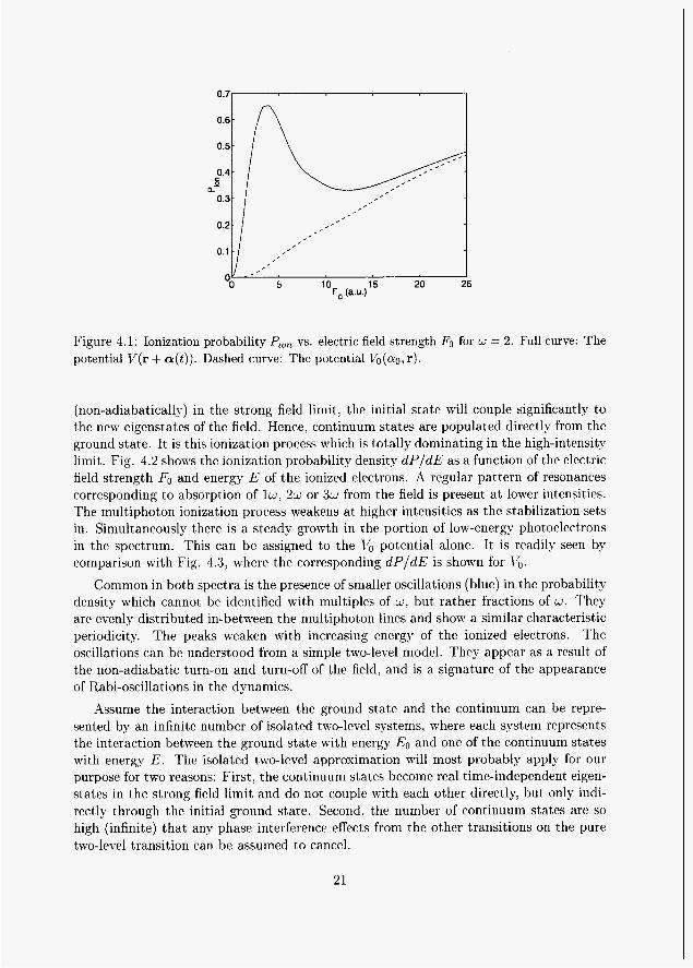
In Fig. 4.1 the ionization probability Pi,, as a function of the amplitude of t,he laser field is shown for u = 2 . .-\lso the ionization resulting from the time-averaged potential alone is shown for comparison. Stabilization occurs when Eo N 3.5, but only temporarily. For Eo > 12.5 t h r ionization probability starts to increase again. At this point the multiphoton ionization process is st,rongly suppressed and the 1’0 potential is the predominant factor in the ionizat.ion process. From the Vo potential the stationary states and their energies can be derived. Since t,he potential deviates significantly from the Coulomb potent,ial when thc ficld is strong; the 1s state does not belong to this group of states. And since the non-Coulombic potential is effectively turned on instantaneously
20
I 5 15 20 25
'OF, (a.u.1
Figure 4.1: Ionization probability Pi,, vs. electric field strength FO for w = 2. Full curve: The potential V(r + a(t)). Dashed curve: The potential V O ( ( Y ~ , r).
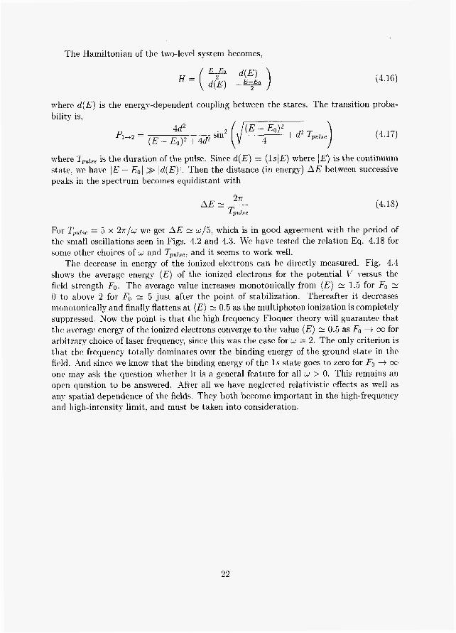
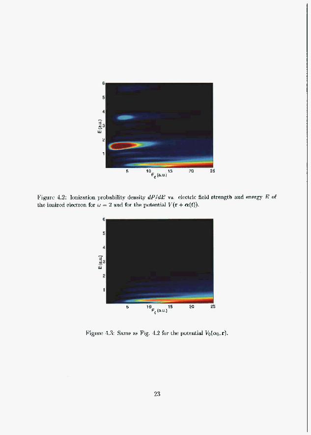
(non-adiabatically) in the strong field limit, the initial state will couple significantly t.o the new eigenstates of the field. Hence; continuum states are populated directly from the ground state. It is this ionization process which is totally dominating in the high-intensity limit. Fig. 4.2 shows the ionization probability density dP/dE as a function of the electric field st.rength Fo and energy E of the ionized electrons. A regular pattern of resonances corresponding to absorption of lw, ~ L J or 3w from the field is present a t lower intensities. The multiphoton ionization process weakens at higher intensities as the stabilization sets in. Simultaneously there is a steady growth in the port,ion of low-energy photoelectrons in the spectrum. This can be assigned to the \lo potential alone. It is readily seen by comparison with Fig. 4.3, where the corresponding dP/dE is shown for 16.
Common in both spectra is the presence of smaller oscillat,ions (blue) in the probability density which cannot. be identified with multiples of w: but rather fractions of w . They are evenly distributed in-between the multiphoton lines and show a similar characteristic periodicity. The peaks weaken with increasing energy of the ionized electrons. The oscillations can be understood from a simple two-level model. They appear as a result of the non-adiabatic turn-on and turn-off of the field, and is a signature of the appearance of Rabi-oscillations in the dynamics.
Assume the interaction between the ground state and the continuum can be repre- sented by an infinite number of isolat,ed two-level systems, where each system represents the interaction between the ground stat,e with energy EO and one of t,he continuum states with energy E. The isolated two-level approximation will most probably apply for our purpose for two reasons: First, the continuum states become real t,ime-independent. eigen- states in the strong field limit and do not couple with each other directly, but only indi- rectly through the initial ground state. Second, the number of continuum stat,es are so high (infinite) that, any phase int,erference effects from the other transitions on the pure t,wo-level transition can be assumed to cancel.
21
The Hamiltonian of the two-level system becomes,
(4.16)
where d ( E ) is the energy-dependent coupling between the states. The transition proba- bility is,
p1+2 = ( E - Eo)2 4d2 + 4d2 sin2 (/y + d2 Tpulse ) (4.17)
where Tpuise is the duration of the pulse. Since d(E) = (1sjE) where \ E ) is the continuum state. we have IE - E0l >> Id(E)/. Then the distance (in energy) A E between successive peaks in the spectrum becomes equidistant with
(4.18)
For Tpulse = 5 x 27rlw we get, A E N w / 5 , which is in good agreement with the period of thc small oscillations seen in Figs. 4.2 and 4.3. We have test,ed the relation Eq. 4.18 for some other choices of LU’ and Tpulse, and it seems to work well.
Thc decrease in energy of the ionized electrons can be directly measured. Fig. 4.4 shows t,he average energy (E) of the ionized electrons for the potential 1’’ versus the ficld st,rength Fo. The average value increases monotonically from (E) N 1.5 for FO N
0 to above 2 for Fo N 5 just after the point of stabilization. Thereafter it, decreases nionot.onically and finally flattens at ( E ) N 0.5 as the multiphoton ionization is completely supprcssed. Now the point, is that the high frequency Floquet theory will guarantee that thc average energy of the ionized electrons converge to the value ( E ) N 0.5 as FO + cc for arbitrary choice of laser frequency, since this was the case for w = 2 . The only criterion is that the frequency totally dominates over the binding energy of the ground state in the ficld. And since we know that the binding energy of the 1s stat,e goes to zero for FO + cc onc may ask the question whet,her it is a general feature for all w > 0. This remains an open question to be answered. Aft,er all we have neglected relativistic effects as well as any spatial dependence of the fields. They both become important in the high-frequency and high-intensity limit, and must be taken int.0 consideration.
22
4
Lu
1
IU 25 Fo (a.u.1
Figure 4.2: Ionization probability dcntlity dP/dE vs. electric field strength and energy E of the ionietd electron for w = 2 and for the potential V(r $. cr(t)).
10 1 25 Fc (a.u.1
5
Figure 4.3: Same as Fig. 4.2 for the puteiltial Vo(cY0,r).
23

1 -.
0 5 10 15 20 F, (a.v.)
Figtire 4.4: The average energy { E ) uf the ionixed electrrons vs. electric field Ytrength for w 2.
24
Chapter 5
Introduction to the papers
The main part of this thesis is allocated to studies of the dynamics of highly excited Rydberg states in time dependent electric and magnetic fields. A close coupling integra- tion scheme to solve the time-dependent Schrodinger equation in a spherical hydrogenic basis has been developed. After some modifications the algorit,hm has proved to be ap- plicable to alkali Rydberg systems with one single electron in an excited st,ate. The field-free eigenstates are perturbed by the non-hydrogenic core, and these corrections ap- pear as characteristic quantum defect,s in the theory. For highly excited Rydberg st,ates the values of the quantum defects become real constants, which can be obtained from spectroscopy. They exclusively effect low angular momentum states since only then the Rydberg electron has a non-zero probability distribution within the core region. The first t,wo papers (paper 1 and 2) contain a detailed analysis of the role of quantum defects in the int,eraction bet.ween Rydberg states of lithium and weak t,ime-dependent electric and magnetic fields. The field paramct,ers were chosen such that only states within the mani- fold were populated at all timcs. Differences and similarities with the hydrogenic theory were pointed out. \Ve derived cxact analytical formulas for the transition probabilit,ies for the hydrogenic counterpart. \\'henever a deviation from hydrogenic theory was met it. could be explained as a corc c+kct. In collaboration with the experimental group of Erik Horsdal-Pedersen at the Uniwrsity of Aarhus, Denmark, we published both theoretical and experiment.al results in two joint papers. A good agreement between theory and experiment was achicwd.
In paper 3 the dynamics of H hydrogenic system in time-dependent electric and mag- netic fields was studicd. Our starting point was a recently published paper by Kazansky and Ostrovsky (1996) [46]. Tlwy derived simple formulas for the description of the in- trashell dynamics of atomic hydrogen in weak electromagnetic fields. The description is attractive due t,o its simplicit!. and reduces in many cases completely to analytical for- mulas for the transition probalditics. In our paper we re-derived the same results from an alternative algebraic approach. and generalized it to be valid for arbitrary initial con- ditions. The paper also includw a n analysis of state control by the external fields as well as simple analytical solutions to proposed schemes for driving the Rydberg atom into a high angular momentum state.
In paper 4 t,hc Selcctivc Field Ionization (SFI) dynamics of Li(n = 25) Rydberg states with magnetic quantum number Iml = 2 are studied from two different models, one analytical and one numerical model. The principle of SFI is simply to expose a from
25

beforehand unknown mixture of Rydberg states to a time-dependent increasing electric field. The point is t.hat different quantum states will ionize at different field strengths. The ionized elecbrons are accelerated by the field and hit an ion-counter. Depending on the specific time electrons from different. Rydberg stat,es hit t.he det,ector, a SFI spect,rum reflecting the ionization yield of the different states are plotted as a function of field strength (time). Each state has its own SFI signature in the spectrum. In an ideal experiment exact knowledge of the populations distribution on the different states are obtainable from such an analysis. The numerical model we have used is a generalization of the close coupling integration scheme first, developed in relation with paper 1. Now the program is modified in order t o take into account the couplings between states from different n-manifolds. The analytical model is based on the multichannel Landau-Zener- Stueckelberg model, which have been frequently used in the t,heoretical description of e.g. atomic collisions. The Iml = 2 states define a border zone between fully adiabatic (lmi < 2 ) and fully diabatic (Iml > 2 ) ionization dynamics. The conclusion of this research has been t.hat these states indeed have a mixed dynamics, which suggests that analysis of experimental SFI spectra should be performed with care and most likely in parallel with theoretical studies. Knowledge of adiabaticity/diabaticity of Iml = 2 stat,es proved to be decisive for the interpret,ation of t,he experimental data in paper 2, which contains further discussion about the influence of a magnetic field on the SFI dynamics.
Paper 5 and 6 are basically concerned with the same topic, i.e. multiphoton int.rashel1 resonances in Rydberg atoms; with emphasis on Bloch-Siegert shifts and widths of the resonances. The resonance positions and widths are seen to shift and broaden with increasing intensity of the oscillating field. This shift is often called t.he Bloch-Siegert. shift and is related to counter-rotating terms in the Hamiltonian. In the commonly used rotating-wave-approximation (RWA) such terms are oft,en neglected in order to simplify the theoretical treatment. Paper 5 is a joint. paper including a brief report on the experimental and theoretical attainments on the topic. In paper 6 an analytical Landau- Zener-Stueckelberg theory for the theoretical description of such processes is developed. The basis for the experiments were initially prepared circular Rydberg states of Li(n = 25) quantized along an initially static electric or magnetic field. Then the atoms were exposed to a circularly polarized electric field arranged such that the initial static field lies in the same plane as the rotating field. The frequency was of the same order of magnitude as the typical splitting of the levels within the manifold; i.e. in the radio frequency domain. Is was demonstrated that, the hydrogenic theory describes the dynamics quite well. This is after all not' too surprising as the circular Rydberg states of lithium are basically identical with their hydrogenic counterparts. In the theoretical description we also looked into the important case with a linearly polarized field, in order to compare our analytical model with already known analytical models.
At the end of this Ph.D. period we became engaged with the ongoing research on ionization of atoms and molecules in intense laser fields. We have taken advantage of re- cently developed algorithms to obtain exact solutions of t.he Schrodinger equation in three dimensions on the grid [35]. It is based on the split-step operator method by Hermann and Fleck [27] and is especially well suited for spherical problems. We plan to study the ionization and stabilizat'ion of excited Rydberg states of hydrogen in linear polarized laser fields, with emphasis on directional dependencies of the emitted photoelectrons, as well as the dependence of the ionization yield on the alignment of the laser field with respect
26

to the arrangement of the initial atomic state. \Ye also plan to look into more complex composite systems like the H g molecule. For the time being we have only studied ori- entation effects in the 2p(m = 0) state of hydrogen. i.e. not really a Rydberg state. ‘4 review of the recently obtained results for this state are presented in paper 7.
27

28
Chapter 6
Summary and outlook
During this Ph.D. period we have mosbly been working with relatively slow intrashell processes in highly excited Rydberg states of hydrogen and lithium, with emphasis on t,he differences and similarities between the two systems. By "slow processes" we mean that, the frequencies of the external fields are kept, much smaller than the int,ernal orbital frequency of the n-shell. Several numerical and analytical models have been developed for this purpose. Much of the theoretical effort had its source in parallel experimental activities a t the University of Aarhus. The mutual and close collaboration was adwn- tageous for both parts, and resulted in new insight into mesoscopic atoms. It. was a challenge, both experimentally and theoretically, to attain a uniform understanding of experimental and theoretical data at the very same level. The underlying frozen-core approximation and quantum defect, theory have proved to apply for the highly excited stat,es of atomic lithium int,eracting with slowly varying electromagnetic fields. Whether similar approximations also are valid for corresponding processes in composite systems like Rydberg molecules or systems with more than one active electron, remains an open question. Another open question is whether the spin-reduction scheme for hydrogenic systems has counterpart,s in other relat,ed systems; like e.g. quant.um dots.
We have also studied geometric effects on the ionizat,ion yield and stabilization of lower-lying states of hydrogen in intense laser fields. In the high-frequency (fast process) limit the ionization of the 2 p ( m = 0) state is seen to depend critically on the angle between the H(2p) symmetry axis and the polarization direction of the electric field. The angular dependence was most prominent within a certain range of field intensities. 4 possible explanation of the geometric effect in the context of atomic stabilization was proposed. An overall and systematic decrease of the energy of the photo-ionized electrons was predicted to occur from t,he point where stabilization processes set in.
In this thesis we have studied fast, and slow processes separately. A combination of slow and fast processes in mesoscopic atoms and molecules is an extremely difficult task to handle theoretically, especially when they interfere with each other. The efficient theoretical means are oft,en different in the two regimes. The study of such systems is only one of the potential future directions of this research.
29

30

References
31

[l] 4 . Einstein, Ann. Phys. 17, 132 (1905).
[2] N. Bohr, Philosophical Magazine 26, 1 (1913).
[3] E. Schrodinger, Naturwissenshaften 4, 664 (1926).
141 E. Schrodinger, Naturwissenshaften 14; 137 (1926).
[5] P. A. M. Dirac, Proc. Roy. Soc. A117, 610 (1928).
[6] '4. Einstein, B. Podolsky and N. Rosen, Phys. Rev. 47, 777 (1935).
[7] J. S. Bell, Rev. Mod. Phys. 38; 447 (1966).
[8] '4. Aspect, J. Dalibard and G. Roger, Phys. Rev. Let,t. 49; 1804 (1982).
[9] J. P. Gordon, H. J. Zeiger and C. H. Townes, Phys. Rev. 95; L282 (1954).
[lo] T. H. Maiman, Nature 187, 493 (1960)
[ll] M. Gavrila, J. Phys. B 35, R147 (2002).
[ la] T. F. Gallagher; Rydberg Atoms, Cambridge Universitr Press (1994).
[13] P. P. Sorokin and J. R. Lankard, IBhl J. Res. Develop. 10, 162 (1966).
[14] R. G. Hulet and D. Kleppner, Phys. Rev. Lett. 51. 1430 (1983).
[15] J. C. Day. T. Ehrenreich. S. B. Hansen. E. Horsdal-Pedersen. K. S. Mogensen and Knud Taulbjerg. Phys. Rev. Lett. 72. 1612 (1994).
[16] P. 4. Tiplcr and R. A. Llewellyn. Modern Physzcs, LV. H. Freeman and Com- pany. Ncw York (2002).
[17] D. hlcschcdc. H. LValther and G. hluller. Phys. Rev. Lett. 54. 551 (1985).
[18] 3 . M. Raimond. A I . Brunc and S. Harochc, Rev. Mod. Phys. 73, 565 (2001).
[19] G. Gabriclsc. N. S. Bowden; P. Oxley. A. Speck, C. H. St,orry, J. N. Tan, M. \Vessels: D. Grzonka. LV. Oelert, G. Schepers, T. Sefzick, J. Walz; H. Pittner, T. W. Hiinsch and E. A. Hessels, Phys. Rev. Lett. 89; 213401 (2002).
[20] F. niandl and G. Sliaw. Quantum Field Theory, Wiley & Sons (2001)
[all J. S. Briggs and J . 11. ILost; Eur. Phys. J . D 10; 311 (2000).
[22] R. Loudon. The Qunnfum Theory of Light, Clarendon Press, Oxford (1973).
[23] E. Cormier and P. La~~il~ropoulos, J. Phys. B 30, 77 (1997).
[24] FV. H. Press. S. A. Teukolskv. \I7. T. Vetterling and B. P. Fannery. Numeracal Reczpes zn C. Cambridgc University Press (1992).
[25] D. Baye and P. H. Heenan, J. Phys. '4 19, 2041 (1986).
32

[26] hl. D. Feit, J . '4. Fleck Jr. and A. Steiger, J. Comput. Phys. 47, 412 (1982).
[27] hf. R. Hermann and J. A. Fleck Jr., Phys. Rev. A 38, 6000 (1988).
[28] T. R. Taha and M. J. Ablowitz, J . Comp. Phys. 55, 203 (1984).
[29] J . Zhang and P. Lambropoulos, J . Nonlinear Opt. Phys. Mater. 4; 633 (1995).
[30] P. Antoine, B. Piraux and A. hfaquet; Phys. Rev. A 51, R1750 (1995)
[31] hl. L. Zimmerman, hf. G. Littman, M. M. Kash and D. Kleppner Phys. Rev. A 20, 2251 (1979).
[32] I. V. Komarov, T. P. Grozdanov and R. K. Janev, J . Phys. B 13, 573 (1980).
[33] H. A. Bethe and E. E. Salpeter, Quantum Mechanics of One- and Two- Electron Atoms, Springer Verlag (1957).
[34] D. M. Brink and G. R. Satchler, Angular Momentum, Edited by B. Bleaney et al; Oxford University Press (1968).
[35] J. P. Hansen, T. Sorevik and L. B. Madsen, Phys. Rev. A 68, 031401(R) (2003).
[36] L. Landau, Phys. Z. Soviet Union 2, 46 (1932).
[37] C. Zener, Proc. R. SOC. A 137, 696 (1932).
[38] E. C. G. Stueckelberg, Helvetica Physica Acta 5, 369 (1932).
[39] D. A. Harmin and P. N. Price, Phys. Rev. A 49, 1933 (1994).
[40] D. 4 . Harmin, Phys. Rev. A 56, 232 (1997).
[41] E. E. Nikitin and S. Y. Umanskii, Theory of Slow Atomic Collisions, Springer Verlag, (1984).
[42] W. Pauli, Z. Phys. 36, 339 (1926).
[43] h l . J. Engelfield, Group Theory and the Coulomb Problem, Wiley, New York (1972).
[44] Y. N. Demkov, B. S. hlonozon and V. N. Ostrovsky, Zh. Eksp. Teor. Fiz. 57, 1431 (1970) [Sov. Phys. JETP 30; 775 (1969)l.
[45] Y. N. Demkov, c'. N. Ostrovsky and E. ,4. Solov'ev, Zh. Eksp. Teor. Fiz. 66, 125 (1974) [Sov. Phys. JETP 39, 57 (1974)].
[46] A. K. Kazansky and Lr. N. Ostrovsky, J. Phys. B 29; 855 (1996).
[47] E. Majorana, Nuovo Cimento 9, 43 (1932).
33
[48] L. D. Landau and E. M. Lifschits, Quantum Mechanics, Pergamon Press (1976).
[49] hl. Fmrre, H. hl. Nilsen and J. P. Hansen. Phys. Rev. A 65. 053409 (2002).
[50] Tl r . Pauli and hl. Fierz. Nuovo Cimento 15, 167 (1938).
[5l] H. A. Kramers. Collected Sczentzfic Papers. Amsterdam: North-Holland. p. 866 (1956).
[52] W. C. Henneberger, Phys. Rev. Lett. 21; 838 (1968).
[53] F. H. Faisal, J. Phys. B 6, L89 (1973).
[54] h1. Pont and M. Gavrila. Phys. Rev. Lett. 65, 2362 (1990).
[55] Q. Su. J . H. Eberly and J. Javanainen, Phys. Rev. Lett. 64, 862 (1990).
[56] hl. Gavrila. Atoms zn Intense Laser Fzelds edited by M. Gavrila. Academic Press. San Diego p. 435 (1992).
[57] S. I. Chu, Adv. Chem. Phys. 73, 739 (1989).
[58] S. I. Chu, -4dv. At. Mol. Phys. 21, 197 (1985).
[59] R. M. Potvliege and R. Shakeshaft, Atoms in Intense Laser Fields edited by M. Gavrila, Academic Press, San Diego p. 373 (1992).
[60] M. P. van Boer, J. H. Hoogenraad, R. B. Vrijen; R. C. Constantinescu, L. D. Noordam and H. G. Muller: Phys. Rev. Lett. 71, 3263 (1993).
[61] M. P. van Boer; J. H. Hoogenraad, R. B. Vrijen, R. C. Constantinescu; L. D. Yoordam and H. G. Muller, Phvs. Rev. A 50, 4085 (1994).
[62] N. J. van Druten, R. C. Constant,inescu, J. M. Schins, H. Xieuwenhuize and H. G. Muller, Phys. Rev. A 55; 622 (1997).
34

Papers
Paper 1
Dynamics of a single Rydberg shell in time dependent external fields
hl. Forre. L). Fregenal, J. C. Day, T Ehrenreich. J P. Hansen, I3 Hrnningsun. E. HorsdaI Ptxkruen, L. Xrvang. 0. E. fovben , K. 'I'aulhlerg and I. I'ogelius
J., I'hy?. B. At. Mol. Opt. Phys. 35. 401 (2002) - 'I '- \Y - ' . - '
, . . - - - I ' r-- .. :- &'L-F -1 . . I -
. , .

b%STlTU7E OF PHYSICS ~ U s H n V c JOURNAL OF PHYSICS B: ATOMIC, MOLECULAR AND OPTICAL PHYSICS ~~
J. Phys. B: At. Mol. Opt. phys. 35 (ZMn) 401-419 PII: S0953-4075(02)29634-0
Dynamics of a single Rydberg shell in time dependent external fields*
M FOrrel, D Fregena12, J C Day3, T Ehrenreich4, J-P Hansen', B Henningsen', E Horsdal-Pedersenz, L Nyvang2, 0 E Povlsen2, K Taulbjerg and I Vogelius2
' Institute of physics, University of Bergen, N5007 Bergen, Noway * Institute of physics and Astronomy, Aarhus University, DK-8000 Aarhus C, Denmark
Division of Natural Sciences, Transylvania University, Lexington, KY 40508, USA J R Macdonald Laboratory, Department of physics, Kansas State University, Manhattan,
KS 66506, USA
Received 8 October 2001, in final form 22 November 2001 Published 9 January 2002 Online at s~~ks.iop.~~~i3PhysS/35/40 I
Abstract Probabilities for adiabatic or near-adiabatic state transformation within a highly excited shell of Li(n = 25) were-studied experimentally and theoretically for a time dependent electric field, E ( t ) , and a constant magnetic field, E . The fields were sufficiently weak and the time dependence slow enough such that only states belonging to the chosen shell were involved. The studies show that the dynamics are governed by the approximate hydrogenic character of the system in most cases, but for some specific time dependences it is influenced strongly by core interactions as expressed through the quantum defects, 6,. The s-state is effectively decoupled from the rest of the n = 25 manifold due to a very large quantum defect. However the quantum defects of the p, d and f states are shown to play a decisive role in the dynamics. The core interactions lead to avoided crossings, non-adiabatic state transformations, and possibly even phase-interference effects. When a resonance condition pertaining to the hydrogenic character of the system is fulfilled, a linear Star+k state is trans- formed completely into a circular Stark state oriented along Ef.
1. introduction
The possibility of creating and manipulating Rydberg atoms [l , 21 in well defined states by external fields has provided a new precision tool for fundamental studies of quantum mechanics. For example, entanglement between circular Rydberg atoms and single-photon states of a cavity have been reported [3], and many studies of the detailed dynamics of Rydberg atoms in response to time dependent fields have been published: Kazansky and Ostrovsky discussed
* This paper is dedicated to the memory of K Tanlbjerg.
0953-4075/02/020401+19$30.00 0 2002 IOP publishing Ltd Printed in the UK 401
402 M F@m et al
intra-shell transitions in hydrogenic systems induced by homogeneous, macroscopic fields varying relatively slowly [4], and by ions in distant collisions [5]. Bellomo et a1 [6] discussed the same transitions but with special emphasis on the classical aspects of the problem. Galvez et d [ 7 ] studied in detail, theoretically and experimentally, transitions induced by black-body radiation between Stark states of nearest-neighbouring shells. Goodgame and Softley [SI considered the motion in inhomogeneous electric fields of atoms excited to Rydbexg states of large electric dipole moments. They concluded that the Rydberg atoms keep their electric dipole moments, responding adiabatically to the apparent time dependence of the fields, and that a cold beam of such Rydberg atoms can be effectively deflected or focused by the fields. The extent to which quantum defects may influence the conclusions of the above studies was at most touched upon briefly. Yet, a non-hydrogenic core destroys the important dynamical symmetry of a purely hydrogenic system, and it significantly modifies the adiabatic Stark- Zeeman structure of a shell by perturbing some energy levels and causing many avoided crossings among these levels as the external fields are varied [9]. Despite the symmetry breakdown, the Hilbert space is still limited to the well defined n2 states which make such systems a unique playground for numerical time dependent quantum models.
The intra-shell dynamics of a non-hydrogenic system (Li(n = 25)) with known quantum defects was recently studied experimentally [IO]. -The electric field, E @ ) , was switched linearly in-time without rotation from one direction, E', to the-diametrically opposite direction, E' = -E', in the presence of a constant magnetic field, B. The Stark state of maximum polarization and energy within the n-manifold was populated initially. The onset of transitions to neighbouring states in slightly non-adiabatic transformations was described accurately by hydrogenic theory, but strongly non-adiabatic transformations which lead to the population of Stark states located near the centre of the manifold were clearly not described satisfactorily. A comprehensive numerical treatment of the system including quantum defects brought theory into much better agreement with experiment and showed that core interactions cannot be neglected in strongly non-adiabatic transformations [ 111.
Like the experiment described previously the present one deals with intra-shell transitions, butJor a soyewh:t different field configuration an! time dependence. The electric field varies as E(r ) = Ef-(Ef-Ei) exp(-1?), where& andEfaretheinitialandfinalfields,respectively, and 1 is a time constant. The field is homogeneous and it varies smoothly in a)solute magnitude as before but now the direction of the field is also a smooth function of time. F ( t ) always rotates by more than 90", and initially and finally the Stark frequency &(?) = qnE(t) is much larger than the constant Larmor frequency & = ig. The magnetic field d is in the plane of & and &,+and it is perpendicular to_&. F o b es were determined as a function of the direction of Ef for selected values of IEf 1, I B I and the time constant 1. The varying Stark frequency thus resonates with the constant *or frequency at a certain time during the switching for specific choices of the parameters of E(t ) . Hydrogenic theory predicts strong deviation from adiabatic transformation near such a resonance. The prediction is c o n h e d by the experiments but the experimental probabilities for adiabatic state transformation also show unexpected structures far from the resonance region. A thorough theoretical analysis of these structures has brought out new interesting details of the intra-shell dynamics of non-hydrogenic systems. Atomic units (b = rn = e = 1) are used throughout except where units are given explicitly.
2. Experimental arrangement and procedures
The experimental arrangement is shown in figure 1. Some parts of it were used earlier in collision experiments with coherent elliptic Rydberg states [12,13]. The set-up and the experimental procedures are described in some detail in the next paragraphs.

Dynamics of a single Rydberg shell in time dependent external fields 403
EM
Figure 1. Experimental arrangement. A vertical beam of Li atoms is produced by an oven. Three pulsed laser beams excite the Li atoms to Rydberg states in the presence of a horizontal elecmc field inside the Stark cage. The elecmc field is subsequently vaned to study the dynamics of the Rydberg states in time dependent external fields. The Rydbq atoms are selectively field ionized between the plates, P, and counted by the secondary-elechun multiplier, SEM. A quadrupole magnet (not shown) forms a homogeneous magnetic field perpendicular to the Li beam.
2.1. Thermal Li beam and lasers
An oven loaded with metallic Li and heated to about 400 "C produces a vapour of Li atoms, which stream out through a long vertical channel that collimates the atoms to form a thermal beam with a mean velocity of ~ 1 . 5 mm ps-l and a spread of about the same magnitude. Three tunable lasers pump the Li atoms from the ground state to the desired Rydberg state of principal quantum numher n according to the scheme 2s -+ 2p + 3d -+ n. This requires wavelengths near 670,610, and 831 nm, respectively, when n = 25. The laser system consists of three dye lasers pumped by the 532 nm light from a frequency-doubled, pulsed Nd:YAG laser running at a repetition rate of 14 Hz. Each period of 1/14 s starts at time t = 0 when the pump laser is fired, and the three dye lasers are then on for about 5 ns. The beams from the dye lasers are collinear in the interaction region and linearly polarized in the horizontal plane. The bandwidth of the 831 nm laser is limited to 3.3 GHz or 0.11 cm-I by a beam expander and a Fabry-Perot etalon.
2.2. Stark cage and electromagnet
The first step of the experimental technique is the selective laser excitation at t = 0 of a specific Stark state of the selected shell. This is done in the presence of a relatively strong electric field that partially lifts the degeneracy of the shell. The field is parallel to the laser polarization. Shortly after the excitation the field is varied in a precisely controlled way. The experiment determines probabilities of populating other states than the initial one as a result of the variation. Since the field is essential to the experiments, its formation is discussed in detail.
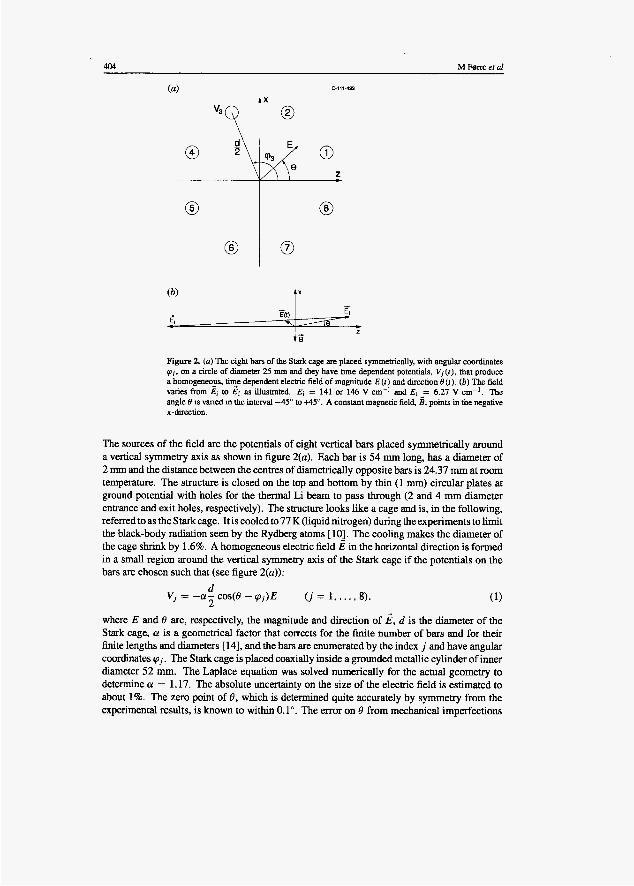
404 M FBm et al
Figure 2. (a) The eight bars of the Stark cage are placed symmetrically, with angular coordinates q j , on a circle of diameter 25 mm and they have time dependent potentials, V, ( t ) , that produce a homogeneous, time dependent elechic field of magnitude E ( f ) and duection O ( t ) . (b ) The field varies from 6 to & as illustrated. E, = 141 or 146 V cm-' and Er = 6.27 V cm-'. The angle 0 is vaned in the interval -45" to 1.45". A constant magnetic field, i, points in the negative x-direction.
The sources of the field are the potentials of eight vertical bars placed symmetrically around a vertical symmetry axis as shown in figure 2(a). Each bar is 54 mm long, has a diameter of 2 mm and the distance between the centres of diametrically opposite bars is 24.37 mm at room temperature. The structure is closed on the top and bottom by thin (1 mm) circular plates at ground potential with holes for the thermal Li beam to pass through (2 and 4 mm diameter entrance and exit holes, respectively). The structure looks like a cage and is, in the following, referred to as the Stark cage. It is cooled to 77 K (liquid nitrogen) during the experiments to limit the black-body radiation seen by the Rydberg atoms [ 104. The cooling makes the diameter of the cage shrink by 1.6%. A homogeneous electric field E in the horizontal direction is formed in a small region around the vertical symmetry axis of the Stark cage if the potentials on the bars are chosen such that (see figure 2(a)):
d 2
vj = --a- cos(e - Q,)E ( j = 1 , . . . ,8). (1)
where E and 8 are, respectively, the magnitude and direction of s, d is the diameter of the Stark cage, (Y is a geometrical factor that corrects for the finite number of bars and for their finite lengths and diameters [ 141, and the bars are enumerated by the index j and have angular coordinates Q, . The Stark cage is placed coaxially inside a grounded metallic cylinder of inner diameter 52 mm. The Laplace equation was solved numerically for the actual geometry to determine (Y = 1.17. The absolute uncertainty on the size of the electric field is estimated to about 1%. The zero point of 8, which is determined quite accurately by symmetry from the experimental results, is known to within 0.1". The error on 8 from mechanical imperfections
Dynamics of a single Rydberg shell in time dependent external fields 405
oftheStarkcagecouldbeabout 1% (0.1 mmdisplacementsofthebarsonaradiusof 12.5mm). The electric field is homogeneous at all times if each of the eight potentials of the bars
vary from initial to final values that satisfy equation (1) and the relative time dependences of the potentials are identical, i s .
(2)
where the common function r ( t ) varies from 0 to 1 within a certain period, and Vj and Vj' are the initial and the final potentials, respectively, of the j th bar. The electric field is then given
vi@) = vi + (vi - vj)r(r),
by i ( t ) = Ei + (if - i i ) r ( t ) , (3)
where i i and if are the initial and final fields, and it is related geometricaliy ty zi and & as illustrated in figure 2(b). The absolute value of the total rotation angle, L(Ei, Ef), was larger than 135" and smaller than 180". The initial field always points in the negative z-direction and its value is chosen to give a large Stark splitting without inter-n mixing for n = 25. It lies within the interval 140-148 V cm-I. The final field has a constant magnitude of 6.27 V cm-l throughout the experiment, and its direction, specified by the angle 0 to $e z-axis, is the independent parameter routinely used for varying the time dependence of E. The function r (t) is defined by:
The starting time, to, was fixed at 1 ps, but two values of the rate constant A. were used, Aslow = 0.621 ps-l or A.fast = 1.24 ps-'. The electric field thus settles at its final value within a few ps after the excitation while the Li atoms are still well within the Stark cage. The exponential time constants were extracted with a precision of better than 2% from measured time dependences of the potentials on the bars.
An electromagnet forms a horizontal magnetic field 2 inside the Stark cage. The field can be considered as locally homogeneous at the position on the symmetry axis of the cage where the transitions take piace, but the field varies slightly along the axis by about 0.035 gauss mm-I. Three field values, B = ( B x , 0,O) with B, = -13.36, -23.59, or -33.37 gauss, were used in the present experiments (figure 2(b)). They were measured with an absolute error of less than 1.5% by a calibrated Hall probe. The precise direction of the field is not critical. It is sufficient that Bz is a small fraction of B,.
The spQtting of a shell_by external fields is described by Stark and Larmor frequencies (3s = ;nE and 3~ = i B , respectively). The magnitude of the Stark frequency, os, for n = 25 equals the magnitude of the Larmor frequency, o ~ . when p = E/B = 2.92 x lo-' (V cm-')/gauss. The electric field thus dominates initially ( ( E i / B ) / p 2 150) and finally ( ( E f / B ) / p 2 6), but the magnetic field may dominate in between when 0 is small.
In the present field configuration the dynamics of a single hydrogenic shell are approximately described by three parameters. One of these is the constant Larmor frequency, o~~ = i B x . The two others are the x-component, os,(&), and the time-derivative of the z-component of the Stark frequency, ~ ~ ~ ( t , ) taken at th? time f = t, when the Stark-Zeeman splittingoftheshellisminimal[4]. ThishappenswhenE(t)isparallel toB (orthex-axis). The three parameters combine into two dimensionless parameters K = and y = d~Jo;,, which measure, respectively, the minimum splitting (given by Ao = I1 - 1 ~ 1 1 0 ~ ) and the speed at which the point of minimum splitting is passed. The probability for non-adiabatic transformation can be expressed in terms of two elementary two-state probabilities p+ and p - [4] which, for the present fields, are given quite accurately by the Landau-Zener formula,

406 M E ~ r r e et a1
p i z = exp(- 5 w). The probability p,"" is always vanishingly small, but p? is close to unity in a region near I K 1 = 1. Non-adiabatic transformation of the wavefunction is thus expected in two intervals of widths E,/- around K = +l.
For given values of Ei, Ef, 0, and A one finds Ex(&) = Ef sin(0)/(l+ Ef/Ei cos(@)) and dE,/dtl,c = AEf cos(@), which leads to
3 n ~ ~ ( ~ cm-') sin(0) B,(gauss)(l + E f / E i cos@))
K = 0.457
and 6nEf(V cm-') [Bx '
y = 2.60 x 10⁻²A(ps-') cos(@)
(5)
The independent variable of the experiment, 8, is never very large so the parameter y is approximately constant in a given run with fixed A and Ef. However, during the experiment y was varied by more than a factor of 10 by different choices of X and B,. Based on the absolute uncertainties quoted earlier, the parameters K and y are determined experimentally to withm 2.5 and 3.0%, respectively.
2.3. Selective j e l d ionization
The Rydberg atoms are detected by the method of selective field ionization (SFI), which is discussed in [15]. The capacitor plates and the detector for the SFI are shown in figure 1. The electric field produced between the plates is parallel to the external magnetic field, which extends all the way from the Stark cage to the SFI region. As the Rydberg atoms drift out of the Stark cage and into the SFI-region they experience a slowly varying electric field. In the Stark cage it is 6.27 V cm-' y d it points in the direction given by 0, and in the SFI region it is 10 V cm-I and parallel to B . The top plate of the Stark cage, which is at ground potential, shields the electric fields somewhat, but the combined Stark-Zeeman splitting of the Rydberg energy levels and the rate-of-change of the moving electric field as seen by the Rydberg atoms are such as to make the transformation of the states adiabatic.
One of the capacitor plates in the SFT region is fixed at - 10 V. The other plate is connected to a positive high-voltage ramp, which is started from 0 V at 45.5 ps when the majority of the Rydberg atoms are between the plates. The electric field is thus 10 V cm-' for t 6 45.5 ps, and it rises for about 8 ps at a constant rate of 421 (V cm-') ps-', finally returning to 10 V cm-' at 53.5 ps.
In one series of measurements, the lasers populate the Stark state, In,nl,nz,m) = 125,24,0,0), where nl, nz, and m are parabolic quantum numbers [15]. It is the uppermost component of the Stark spectrum for the shell. It has maximum polarization along the direction of the initial electric field in the Stark cage, and is called a linear state. In another series, the lasers populate the Stark states, In, n1, nz, m } = 125,23,0, H]. They correspond to the second component from above in the Stark spectrum. The transformation properties of the two initial states are similar but interesting differences relating to the quantum defects of Li were observed. These effects are discussed later in the paper in connection with the detailed theoretical analysis of the dynamics.
In order to clarify the experimental analysis and detection of the final states we discuss in some detail the transformation of the linear state, 125,24,0,0]. If the instantaneous Stark-Zeeman splitting of the shell is large at all times as compared to the rateof-change of the electric field in the Stark cage, (1 - I K ~ ) ~ / Y >> 1, the linear state is transformed adiabatically. The wavefunction therefore returns to its initial linear shape, but it is rotated
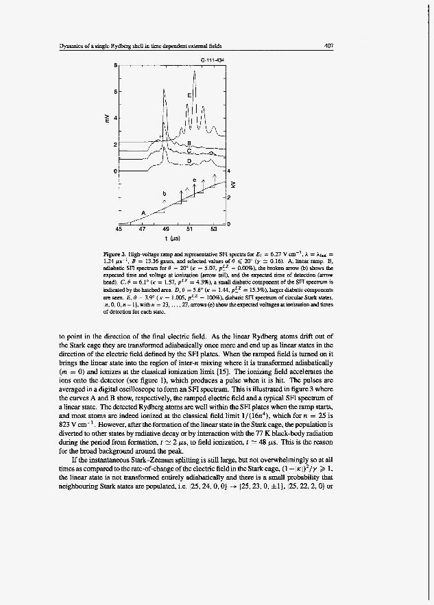
Dynamics of a single Rydberg shell in time dependent external fields 407
C-I11434 8
6
z 4
2
0 4
2 2
0 45 47 49 51 53
Figure 3. High-voltage ramp and representative SFI spectra for Er = 6.27 V cn-', I = Ifut = 1.24 ps-', B = 13.36 gauss, and selected values of 0 6 20" ( y 2 0.16). A, hear ramp. B, adiabatic SFI spectrum for 0 = 20' (Y = 5.07, p!' = 0.00%). the broken anuw (b) shows the expected time and voltage at ionization (arrow tail), and the expected time of detection (arrow head). C, 0 = 6.1" (K = 1.57, p!' = 4.3%), a small diabatic component of the SFI spectrum is indicatedby the hatched area. D, 0 = 5.6" (K = 1.44, p!' = 15.3%), largerdiabatic components are seen. E , 9 = 3.9" ( Y = 1.005, p!? = 100%), diabatic SFI spectrum of circular Stark states, In, 0.0, n - l) , with n = 23, , . . ,27, arrows (e) show the expected voltages at ionization and times of detection for each state.
to point in the direction of the final electric field. As the linear Rydberg atoms drift out of the Stark cage they are transformed adiabatically once more and end up as linear states in the direction of the electric field defined by the SFI plates. When the ramped field is turned on it brings the linear state into the region of inter-n mixing where it is transformed adiabatically (m = 0) and ionizes at the classical ionization limit [15]. The ionizing field accelerates the ions onto the detector (see figure l), which produces a pulse when it is hit. The pulses are averaged in a digital oscilloscope to form an SFI spectrum. This is illustrated in figure 3 where the curves A and B show, respectively, the ramped electric field and a typical SFI spectrum of a linear state. The detected Rydberg atoms are well within the SFI plates when the ramp starts, and most atoms are indeed ionized at the classical field limit 1/(16n4), which for n = 25 is 823 V cm-' . However, after the formation of the linear state in the Stark cage, the population is diverted to other states by radiative decay or by interaction with the 77 K black-body radiation during the period from formation, t = 2 ps, to field ionization, t 48 pus. This is the reason for the broad background around the peak.
If the instantaneous Stark-Zeeman splitting is still large, but not overwhelmingly so at all timesascomparedtotherate-of-changeoftheelectricfieldintheStarkcage, (1 - I K \ ) ' / ~ 2 1, the linear state is not transformed entirely adiabatically and there is a small probability that neighbouring Stark states are populated, i.e. 125,24,0,0} -+ 125,23,0, fl}, 125,22,2,0} or
408 M F m e e t a l
)25,22,0, f2). The SFI technique does not distinguish between the states with rn = 0 or f 1 since they all field ionize at the classical limit, but the two states with 1rn/ = 2 behave mostly diabatically in the region of inter-n mixing and do not ionize at the classical limit, but far above it by tunnelling [15,16]. They are therefore clearly distinguished from the rn = 0 or f l states by the SFI technique. This is illustrated by spectrum C in figure 3 where the states 125,22,0, f 2 ) form an easily identifiable intensity.
If the Stark-Zeeman splitting of the shell and the instantaneous values of the rate-of- change of the electric field in the Stark cage are comparable for a period of time during the switching, (1 - / K 1)2/y E 1, the transformation of the linear state deviates strongly from being adiabatic. The probability for remaining in the linear state is small, and a wide spectrum of other Stark states is populated. This is illustrated by spectrum D in figure 3, which shows a diminished adiabatic peak and a broad distribution of diabatic field ionization with clear peaks within the interval 51.C53.5 ps.
If, finally, the Stark-kman splitting becomes negligible as compared to the rate-of- change of the electric field, (1 - / K 1)'/y << 1, the linear Stark state 125,24,0,0) is trans- formed into the circular Stark state j25,0,0,24) with a probability of unity. This is illustrated by spectrum E in figure 3, which shows the characteristics of the formation in the Stark cage of a single circular state. Radiative decay and black-body radiation redistributes population from the initial circular state to circular states of neighbouring shells during the period from formation to field ionization. The expected positions of the five circular states In, 0, 0, n - 1) with n ranging from 23-27 are indicated by arrows [ 161. The populated circular Stark states are peculiar in-the sense that th$r magnetic dipole moments (angular momenta) are adiabatically locked to E rather than to B. If one attempts tz transform them into coherent elliptic states by lowering E in the presence of an orthogonal B field, instabilities are predicted to arise within a specific interval of eccentricities [ 171. This behaviour differs strongly from the one found for circularzeemanstates In, I , rn) = In, n - 1, +(n - I ) ) , whichare stableundertransformation in orthogonal fields.
2.4. Initial state selection
The ground state of the Li atom has only one fine-structure component, Ilsj) = 10, f . f ) , but eachoftheintermediatestatesusedintheexcitationtotheRydbergshellhavetwo, 11, $, ;+or 4) and 12, f , 4 or $). The lasers are all linearly polarized parallel to the initial Stark field Ei, but they do not resolve the fine-structure components. The dipole selection rules Arnl = 0 and Am, = 0 for linear polarization restrict the excitation to states with rnl = 0 and Jrn, 1 = 1/2. However, the spin-orbit coupling can flip the spin and thus increase lrnl I by one unit, so all Rydberg states with lrnrl = 0 or 1 are accessible. The external fields and imperfections of the laser polarization make it possible even to excite states with Irnr I = 2. The external fields are strong enough to lift the spin-rbit coupling in the Rydberg states. The dynamics of these states are therefore independent of the spin, and one can drop the index I on rn as done already in the preceding paragraphs. Due to the spin-rbit coupling in the intermediate states, the selective excitation of individual Stark states with /mi = 0 or 1 is possible only when the energy separations of the relevant states are larger than the linewidth of the 831 nm laser. Figure 4(a) shows total SFI areas, Amt, as a function of the initial Stark field for constant laser wavelength. The uppermost state of the Stark manifold, 125,24,0,0), located near 142 V cm-', is only partially resolved from the neighbouring states 125,23,0, f l ) , located near 145 V cm-', but the resolution is nevertheless sufficient to ensure selective population of the rn = 0 state at Ei = 141 V cm-' and of the Irn I = 1 states at 146 V cm-'. The intensity near 150 V cm-' is due to /25,22,0, f 2 ) .

Dynamics of a single Rydberg shell in time dependent external fields 409
s c '. - '*-. ./.-e-.-._. _ - p;ml=l '*.. . _-
138 140 142 1 4 4 146 148 150 152 0
E, Wcm)
Figure 4. SR area Am, and adiabatic parameter Po versus the initial electric field, E,, for Y = 3.81 andy =0.157(Er =6.27Vcm-',A=AraSt = 1.24wsK1,B= 13.36gauss,andO = 14.9").(a) Full points are the experimental values of Atot(E,) and full-drawn curves labelled rn = 0 and Iml = 1 are Gaussian functions fiaed to the data (separation 3.4 GHz and FWHM 3.3 GHz). (b) Pa(E,) wlth P:=O = 1 and PAm'=' rz 0.6.
2.5. Data analysis
It is clear from figure 3 that the shapes of the SFI spectra vary dramatically near K = 1. We have chosen to quantify this variation by just one characteristic parameter. It is the relative adiabatic content Po = Ada/Amt, where Aaaa and Aw are the integrated adiabatic and total SFI signals, respectively. This parameter is the probability that the system develops such that Iml is finally 0 or 1. It is essentially the probability that the dynamics are adiabatic and the system remains in the chosen initial state, which is 125,24,0,0} or 125,23,0, &I) , but one should keep in mind that a few non-adiabatic transitions like 125,24,0,0} c, /25,23,0, +1} are included in Pa as well.
The extraction of P,"=O for the initial state 125,24,0,0} is illustrated in figure 5. The sum of a purely adiabatic spectrum (adia) measured at a large value of K and a smooth background function in the form of a two-order polynomial was fitted to the total spectrum (tot) in the range 48.15-49.65 ps . The fitted spectrum (which represents the adiabatic content of the total SFI spectrum) and the total SFI spectrum were integrated to give A d a and Ami, respectively. The value of P,"=O, defined by P,"=O = A ~ d i , / A t o t proved not to depend on the choice of the fitting range within reasonable limits.
Measured values of P,"=O are shown in figure 6 as a function of 8. The data are symmetric with respect to (3 = 0" as expected. Similar data were taken in all cases to ensure the correct symmetry. The dips seen in figure 6 are located at 8 = 3~3.9" which corresponds to K = 1. The FWHM of A8 z 4" corresponds to AK N 1. Both values are in good agreement with the qualitative predictions for a hydrogenic system given in section 2.2.
The parameter P,"=O is a measure of the total probability Pm=o that the Rydberg atom remains in the initial state, /25,24,0,0}, or jumps into another state with Iml < 1. The
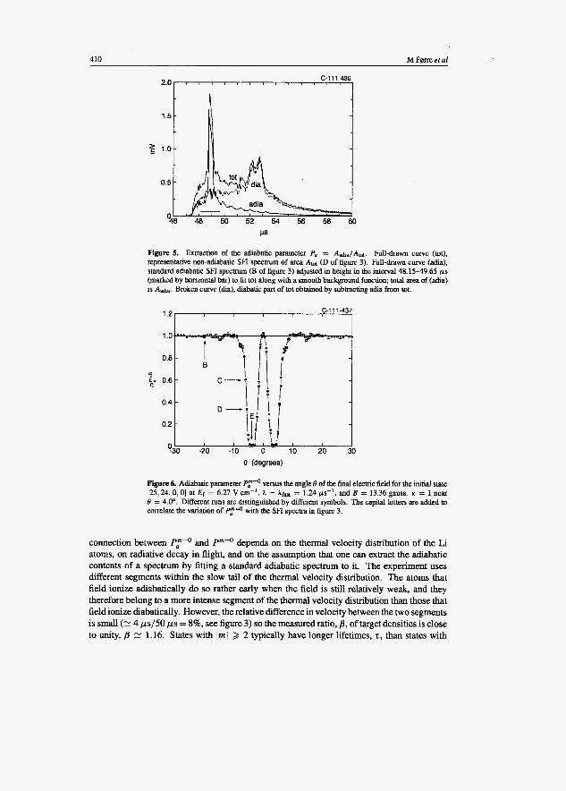
410 M Forre et a1
C-1 1 1-436
"i- 0.5
$6 48 50 52 54 56 58 60
Fipre 5. Extraction of the adiabatic parameter Pa = Aa&JAmt. Full-drawn curve (tot), lepresentative non-adiabatic SFI spechum of area Atm (D of figure 3). Full-drawn curve (adia), standard dabatic SFI spectrum (Ei of figure 3) adjusted in height in the interval 48.1549.65 @s (marked by horizontal bar) to fit tot along with a smooth background function; total area of (adia) is Aaha. Broken curve (dia), diabatic part of tot obtained by subtracting adia from tot.
1 .o
0.8
0.6 U
0.4
0.2
030 -20 -10 0 10 20 30 e (degrees)
Figure 6. Adiabatic parameter P."=O versus the angle 0 of the final electric field for the initial state /25,24,0,0] at Er = 6.27 V cm-', A = .*fast = 1.24 @s-', and B = 13.36 gauss. K = 1 near 0 = 4.0". Different runs are distinguished by different symbols. The capital letters are added to correlate the variation of P."=O with the SFI spectra in figure 3.
connection between P,"=O and Pm=o depends on the thermal velocity distribution of the Li atoms, on radiative decay in flight, and on the assumption that one can extract the adiabatic contents of a spectrum by fitting a standard adiabatic spectrum to it. The experiment uses different segments within the slow tail of the thermal velocity distribution. The atoms that field ionize adiabatically do so rather early when the field is still relatively weak, and they therefore belong to a more intense segment of the thermal velocity distribution than those that field ionize diabatically. However, the relative difference in velocity between the two segments is small (E 4 ~ s / 5 0 ws = 8%, see figure 3) so the measured ratio, p, of target densities is close to unity, p E 1.16. States with Irn/ 2 2 typically have longer lifetimes, t, than states with

Dvnamics of a sinxle Rvdbere shell in time deoendent extemal fields 41 1
/ m < 1. States that field ionize in the diabatic channel therefore have larger probabilities for surviving the transit through the apparatus than the ones that field ionize in the adiabatic channel (t N 22 ps for the linear state 125,24,0,0], 71 ps for 125,22,0, &2], and 918 ps for the circular state 125,0,0,24)). Correction for these velocity and lifetime perturbations was done as follows. Let N,,(K) and N ~ ( K ) be the number of atoms found immediately after the switching with Im I < I and Iml 2 2, respectively, and let fa and fd be the corresponding fractions surviving until field ionization. As they depend on the actual population of the quantum states belonging to each of the two groups, they depend on K . Then:
The total SFI area, normalized at K-value K, where the switching is purely adiabatic, is given by:
(8)
where we have used Nn(~.) = N=(K) + N d ( K ) (the population is just distributed differently at K~ and K ) and the approximation f. ( K ) N f 0 ( ~ = ) (the lifetimes of states with /m/ 6 1 that field ionize adiabatically do not differ much). With this approximation the probability Pm=o is given by
BN&)fa(K) f Nd(K)fd(K) BN&)f&) f Nd(K)fd(K) -
B ( N o ( K ) + N d ( K ) ) f a ( K ) ' A t o t ( ~ ) =
BN. (K.) fa (K.)
Figure 7(a) shows P;='(K), AIot(~), and P""(K) for the initial state 125,24,0, O}. Even though AIot(~) deviates strongly from 1 near K = 1 the difference between Pm=' and P,"=O can safely be neglected. This is true for all the measured probabilities. Note that the peak in A m I ( ~ ) is significantly narrower than the dip in P,"'O(K) or P"='(K). This is qualitatively understandable, because 125,24,0,0} and the neighbouring states, which are populated when P,"'O(K) is only a little less than 1, have similar lifetimes and therefore Atot = 1. The area AIot deviates significantly from 1 only when states of much longer lifetimes, like /25,0,0, are populated when P,"'O(K) << 1.
Figure 4(b) illustrates the dependence of the transformation on the initial state by showing Pa as a function of the Stark field Ei. The values of the parameters K and y are such that one should expect purely adiabatic behaviour for a hydrogenic system. The transformation of 125,24,0,0] is indeed adiabatic or it populates at most states of Iml 6 1 (P,"=O = l), but 125,23,0, k l ] isclearlytransformednon-adiabatically (Pj"'=' = 0.6) showingthatthesystem is not totally hydrogenic.
Figure 7(b) shows P ; m " l ( ~ ) and corresponding values of AIot for the initial states 125,23,0, +l) . It is clear that the difference between Pl"l=l and P~""' can be neglected. The two probability functions P""(K) and P1"l=l(~) are obviously different. While they both show dips at K = 1 in perfect agreement with hydrogenic theory, Pl"l=l (K) has dips also near K = 2.10,3.85 and 4.45, which are not seen in P"'O(K) and which are not explained by hydrogenic theory.
3. Theory
The Hamiltonian of a pseudo-one-electron atom interacting with the present electric and magnetic fields may be written,
H = Ho + EL(t)z + E,(t)x + $&L,,
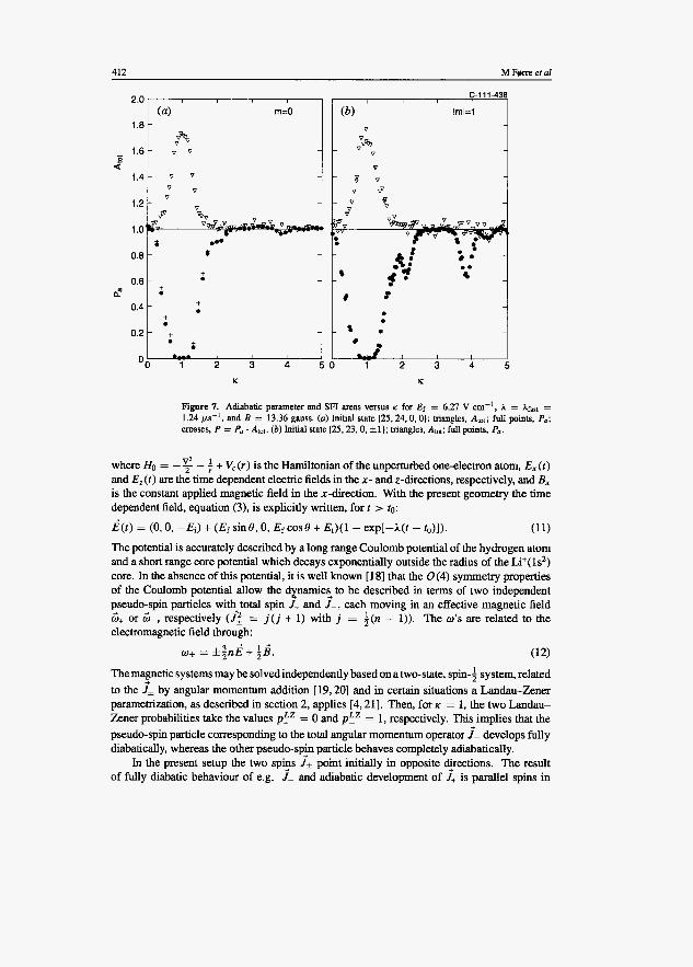
M Fern et al 412
a"
O 0 1 2 3 4
K
C-111-4
I m k l
V
v v v
I:-!, , , * e
0 1 2 3 4
K
Figure 7. Adiabatic parameter and SFl areas versus K for Ef = 6.27 V cm-', A = Afasl = 1.24 LLS-' , and B = 13.36 gauss. (a) Initial state 125,24,0,0]; triangles, Amt; full points, Pa; crosses, P = Pa . Atot. (6) Initial state 125,23,0, *I]; mangles, Alol; full points, Pa.
where HO = - $ - + V, (r) is the Hamiltonian of the unperturbed one-electron atom, E, (t) and E, ( t ) are the time dependent electric fields in the x- and z-directions, respectively, and B, is the constant applied magnetic field in the x-direction. With the present geometry the time dependent field, equation (3), is explicitly written, for t > to:
(11) Z ( t ) = ( O , O , -Ei) + (Ef sinB,O, EfcosO + &)(I - exp[-l(t -to)]).
The potential is accurately described by a long range Coulomb potential of the hydrogen atom and a short range core potential which decays exponentially outside the radius of the Li+(ls2) core. In the absence of this potential, it is well known [18] that the O(4) symmetry properties of the Coulomb potential allow the dynamics_ to be described in terms of two independent pseudo-spin particles with- total spin J+ and J - , each moving in an effective magnetic field 6+ or 6-, respectively (J: = j ( j + 1) with j = i ( n - 1)). The 0 ' s are related to the electromagnetic field through:
w* = + ;i. (12)
Themagnetic systems maybe solvedindependently based on a two-state, spin-; system, related to the j+ by angular momentum addition [ 19,201 and in certain situations a Landau-Zener parametrization, as described in section 2, applies [4,21]. Then, for K = 1, the two Landau- Zener probabilities take the values p t z = 0 and p!' = 1, respectively. This implies that the pseudo-spin particle corresponding to the total angular momentum operator j- develops fully diabatically, whereas the other pseudo-spjn particle behaves completely adiabatically.
In the present setup the two sp$s J* point initially in opposite d@tions. The result of fully diabatic behaviour of e.g. J- and adiabatic development of J+ is parallel spins in

Dynamics of a single Rydberg shell in time dependent external fields 413
the final state. The total wavefunction, which is just the product of these two independent pseudo-parficle wavefunctions, will then necessarily be in a high angular momentum state. This state is identified with quantum numbers Inlrn) = 125, 24, 24), i.e. a circular state, where m refers to a quantization axis parallel to the electric field. Indeed, as seen in figure 3 and in calculations, this process takes place even in the presence of core electrons.
Generally, the core potential breaks the 0 (4) symmetry and a spinor representation is only approximately correct. Specifically, the core potential introduces non-negligible quantum defects, 81, of the low angular momentum states, which modify the field free energy levels according to:
1 E",[ = --
2(n - & ) 2 '
The quantum defects are almost independent of the principal quantumnumber n, which implies that the symmetry breakdown is 'global': as long as the presence of inner electrons manifests itself in non-negligible quantum defects, they cannot be ignored with reference to increasingly larger radii of the atomic states with increasing n. In the present systems the relevant quantum defects are 8, = 0.3995,8, = 0.0472,8, = 0.0021, af = 0.0003.
The wavefunction is therefore expanded in terms of hydrogen-like quantum-defect wavefunctions of the n = 25 manifold,
where n' = n - 81 is the effective quantum number. The radial function outside the core is accurately described by the Bates-Damsgaard type [22]. Inserting this expansion into the time dependent Schrodinger equation, (H - i$)Q(r, t ) = 0, leads to a first-order coupled matrix system of equations for the expansion coefficients, c&(t):
d dt
i--c' = M(t)c',
The coupling matrix, M, becomes sparse due to the Al = 0, f l , Am = 0, f l selection rules of the x - , z and L,-operators. Thus, the time integration is rather simple with present computer power. A significant speed up is further obtained when noting that the quantum defect of the 25s state is so large that this state falls completely outside the energy range of the relevant dynamics. Since the state is never populated, but requires much smaller time steps due to the fast induced oscillation of the quantum defect, it is left out of the expansion, leaving 624 coupled states. In contrast, the p-, d- and f-quantum defects are of the correct order to perturb the eigenenergy levels of the core-free hydrogen atom significantly. The perturbation of the f levels of hydrogen, Sf, which only covers 0.08% of the strength of the s quantum defect, is of the same order of magnitude as a typical splitting of the Stark-Zeeman levels for the fields discussed here [l l] . The effects of the quantum defect wavefunctions on the non-diagonal terms are found to be negligible, and replaced by analytical values for hydrogen.
The quantum defects however do have a significant effect on the dynamics through the diagonal elements of the coupling matrix, given by equation (13). Even quite small quantum defects change the dynamical features completely. To illustrate this point we compare in figure 8 the energy levels of hydrogen and lithium near the 'turning point', i.e. the time region of minimal splitting when the z-component of the electric field changes sign. In the discussion to follow relating to figure 8 the states are labelled according to the Stark states with which they correlate adiabatically. We observe two distinctly different features of the uppermost energy curves: for Li the two uppermost pairs exhibit avoided crossings, a single distinct crossing between the states 125,24,0, m = 0) and /25,23,0, m = 1) and two diffuse crossings around

414 M Fern et al
Time @) Time (p)
Figure 8. Time dependent uppermost adiabatic energies of a H(n = 25) (a) and a Li(n = 25) (b) atom following a diagonalization of the Hamiltonian with B = 13.36 gauss, K = 3.88 and A = 0.71 /LS-'. ' h e solid curves show the states that correlate with the Stark states In, n i , n z , r n ) = 125,23.0, l), 125,22,0,2). The armws in (b ) indicate the location where the coupling between these states can be approximated by the dynamics pertaining to two states going through two isolated avoided crossings. ( c ) shows the probability of the system to remain in the initial Li(n = 25,nl = 23,nz = 0 , m = 1) (solid curve) and to transfer to the Li(n = 25, nl = 22, nz = 0, rn = 2) state (dasbed curve).
t = 2.30 and 2.35 ps between the states 125,23,0, rn = -1) and /25,22,0, m = 2). In hydrogen no such crossings occur and, correspondingly, the dynamics through this region become very different. This is shown in the lower panel of figure 8 where the probabilities of remaining in an initial 125,23,0, rn = -1) state and ofpopulating the state 125,22,0, rn. = 2) are shown. Around the two crossing regions the two states interact strongly leaving less than 20% in the initial state. A corresponding calculation for hydrogen shows zero interaction between the two states, leaving 100% in the initial state.
The effect of the avoided crossing between the two uppermost Li states are shown in figure 9, where the calculated probability for remaining in the initial 125,24,0, m = 0) state and for populating the /25,23,0, rn = 1) state are shown as a function of K . For K > 3 the only relevant dynamics are governed by these two states which interact around a single isolated crossing. The passage of the crossing is determined by experimentally controllable parameters, an ideal situation for precision testing of the Landau-Zener approximation. Again, for hydrogen this strong interaction does not take place for K > 3. The two-state-interplay may in future experiments be studied by the SFI technique if it is possible to form high-voltage pulses fast enough to force the rn = 1 states to field ionize diabatically.

Dynamics of a single Rydberg shell in time dependent external fields 415
K
Figure 9. Probability for remaining in the initial Li(n = 25, n, = 24, n2 = 0, m = 0) state (solid curve) as a function of K for B = 13.36 gauss, A = 0.71 ~ s - l . The dotted curve shows the probability for msfer to the Li(n = 25, nl = 23, nz = 0. rn = 1) state. The dashed curve is the sum of these two probabilities.
4. Results and discussion
In this section a series of calculations will be compared with experiments but before doing so we make two comments. First, the transformation of the Rydberg states as they drift from the Stark cage to the SFI region is expected to be adiabatic (section 2.3) so it is sufficient to select from the calculations all states with corresponding to Im I = 0 , l immediately after the rotation of the electric field (os >> o~ so m is approximately a 'good' quantum number). These are the states that eventually field ionize in the adiabatic channel, and the probabilities of populating those states correspond to the experimental adiabatic probabilities Pm=' and
If the adiabaticity assumption is incorrect one would expect to see a fmt indication in the region around K = 1 since in this region most states of the n-manifold are populated: a large (unknown) number of diabatic crossings between these states before the SFI region would expectedly lead to large deviations from a theoretical spectrum. Second, while the non- degenerate Stark state 125,24,0, m = 0) could be excited selectively, it is natural to assume that the two degenerate Stark states 125,23,0, m = k l } were populated equally (figure 4). Only 50% of the Rydberg atoms are thus initially in the state 125,23,0, m = -1) that shows avoided crossings with 125,22,0, m = 2) and the rest are in the state 125,23,0, m = 1) that couples to 125,24,0, m = 0) (figure 8). Therefore, even though the probability for the transition 125,23,0, m = - 1) --f 125,22,0, m = 2) approaches unity (figure 8), at most 50% of the total population of 125,23,0, rn = kl) is transferred to states with /mi 2 2 that field ionize diabatically. This explains why the dips in figure 7 at K > 1.8 never go below 50%.
for the selected values of B, and 1 are shown in figures 10-13. The overall agreement between experiment and theory is amazingly good. Almost every structure seen experimentally is reproduced in the calculations, and the trend towards sharper structures for increasing magnetic field strength or time constant for the variation of the electric field is also followed closely. Some deviation is seen, however, in the exact positions of the structures. Since the largest deviation (-.3.5%, figure ll(b)) is within the error on K , it is most likely due to calibration errors. There is also some deviation in the strengths of the dips near K = 4. The experimental dips are not as deep as expected. In the interpretation of the experimental data it was assumed that states with Iml = 0 , l field
Experimental and theoretical probabilities Pm=O and
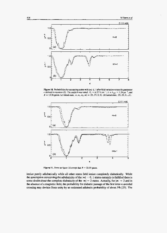
M Fern ef al 416
c 4
K
Figurelo. Probabilitiesforoccupyingastatewith lrnl < 1 afterfieldvariationversustheparameter ~ d e i i ~ d i n q u a t i o n ( 5 ) . TbeangleOwasvaried. Ef = 6 . 2 7 V ~ n - ' , A = A f , ~ = 1.24&s-',and B = 13.36 gauss. (a) Initial state, In, nl, nz. rnl = 125,24,0,0). (b ) Initial state, 125,23,0, i l l .
c-111.440 L I
L i
K
Figure 11. Same as figure 10 except that B = 23.59 gauss
ionize purely adiabatically while all other states field ionize completely diabatically. While the assumption concerning the adiabaticity of the Im I = 0 , l states certainly is fulfilled there is some doubt about the complete diabaticity of the /m I = 2 states. Actually, for Im I = 2 and in the absence of a magnetic field, the probability for diabatic passage of the first inter-n avoided crossing may deviate from unity by an estimated adiabatic probability of about 5% [23]. The

Dynamics of a single Rydberg shell in time dependent external fields 417
c- 1 1 1.441
c
X
Figure 12. Same as figure 10 except that B = 33.37 gauss.
e m=O. slow
t
c
K
Figure 13. Same as figure 12 except that A = Adow = 0.621 11s-l.
small magnetic fields present in the experiments could increase the interaction at the avoided crossing a little and lead to an even larger adiabatic probability. A smal l fraction of Rydberg atoms with Im I = 2 thus behave in field ionization as if they had m = 0 or f 1. It is therefore likely that the observed deviation is due to a small adiabatic SFI channel for m = 2 states. The observed trend towards larger deviations for larger magnetic fields is explained qualitatively by the same hypothesis.

418 M F m et a1
The dips at the higher K-values (K 2: 4) appear as a result of the re-organization of the energy levels due to the decoupling of the s state by the s quantum defect. The exact magnitude of 8, plays a minor role. It places the dips near K = 3 for a range of values around its nominal value 8, = 0.399. For the p-, d- and f-quantum defects, which cover only 12,0.5 and 0.08% of S,, respectively, the situation is different. Their successive inclusion causes the dips to move systematically towards higher K-values. Even the tiny f-quantum defect causes a significant shift of a few percent.
It is interesting to note that the transition between the uppermost m = 0 state and the neighbouring m = + I state is due to one single avoided crossing, whereas the transition between the m = -1 and m = +2 states is due to two time-separated avoided crossings, each obeying pure two-state dynamics (see figures 8 and 9). The difference between the two situations, one showing a single dip and the other a regular pattern of several dips, is a result of phase correlations between the two avoided crossings governing the latter case. The general features of such two-state dynamics will be explored in a future work.
In contradiction to the dips near K = 4, the lower-lying dips around K = 2 are a result of multi-state dynamics. Here not only two but at least six states from the top of the n-manifold contribute. Many more states, forming a dstribution centred near the middle of the manifold, are populated when K approaches 1 from above or below, but in a narrow region around K = 1 the distribution collapses into a single state. For rn = 0 this is the circular Stark state 125,0,0,24}.
Small and irregular oscillations of high frequency are predicted by theory near K = 1. The oscillations were resolved in the experiments in a few cases (K = 1.22 in figure 13(u) and K = 1.47 in figure 1 l(b)) and in others the oscillations were merely reflected in the form of irregular kinks in the experimental curves (K = 0.85 in figures 12(a) and (b) and K = 1.27 in figure 13(b)).
5. Summary and conclusion
In the present paper we described a detailed experimental and theoretical investigation of the Li(n = 25) state dynamics in a specified time dependent electric and magnetic field configuration. Excellent agreement between experimental and theoretical results was achieved. The agreement allowed for the interpretation of the dynamics in terms of time dependent passages through avoided crossings. In particular, complete diabatic passage of avoided crossings at K = 1 leads to the selective population of a circular Stark state.
Quantum defects of the p, d and f states have been shown to play a decisive role in the dynamics. The departure from the pure Coulomb potential results in effectively isolated avoided crossings between two or a few energy curves. The traversal of the crossing region can be very precisely controlled through experimental parameters. By a correspondingly careful selection of initial states as well as possible enhancements in the SFI technique, few state time developments may be studied at a precision which may be difficult to obtain in atomic collision or quantum optics experiments. For example, a series of coherently controlled transitions from an initial to a circular state may provide new and exciting dynamics as well as applications.
Acknowledgments
This research was supported by NFR, SNF and through a European community Marie Curie fellowship.

Dynamics of a single Rydberg shell in time dependent external fields 419
References
[l] Hulet R G and Kleppner D 1983 Phys. Rev, Lett. 51 1430 [2] Liang J, G r o s s M, Goy P and Hamche S 1986 Phys. Rev. A 33 R4437 [3] Osnaghi S, Bertet P, Auffeves A, Maioli P, Brune M, Raimond J M and Haroche S 2001 Phys. Rev, Len. 87
[4] Kazansky A K and Ostmvsky V N 1996 J. Phys. E: At. Mol. Opt. Phys. 29 L855 [5] Kazansky A K and Ostmvsky V N 1996 Phys. Rev. Len. 77 3094 [6] Bellomo P, Stroud C R, Fml ly D and Uzer T 1998 Phys. Rev. A 58 3896
Bellomo P and Stroud C R 1999 Phys. Rev. A 59 2139 [7] Galvez E J, Lewis J R, Chaudhuri B, Rasweiler J J, Latvakoski H, De Zela F, Massoni E and Castillo H 1995
Galvez E J, MacGregor C W, Chaudhuri B, Gupta S , Massoni E and De Zela F 1997 Phys. Rev. A 55 3002 [SI Goodgame A L and Softley T P 1999 J. Phys. E: At. Mol. Opt. Phys. 32 4839 [9] Braun P A 1985 J. Phys. E: At. Mol. Phys. 18 4187
Penent F, Delande D and Gay J C 1988 Phys. Rev. A 37 4707
037902.1
Phys. Rev. A 51 4010
[lo] S0rensen P, Day J C, DePaola B D, Ehrenreich T, Horsda-Pedersen E and Kristensen L 1999 J. Phys. E: At.
[l l] Mijatovic M, Solov'ev E A and Taulhjerg K 2001 J. Phys. E: At. Mol. Opt. Phys. 34 1897 1121 Kristensen L, BovC T, DePaola B D, Ehrenreich T, Horsda-Pedersen E and Povlsen 0 E 2000 J. Phys. E: At.
[13] Bove T, DePaola B D, Ehrenreich T, Horsdal-Pedersen E, Kristensen L, MacAdam K B and Povlsen 0 E 2001
[14] Horn J L, Homan D M, Hwang C S , Fugua W L Ill and MacAdam K B 1998 Rev. Sci. Instnun 69 4086 [15] Gallagher T F 1994 Rydbcrg Atoms (Cambridge: Cambridge University Press) [16] D a m b q R J and Kolosov V V 1979 J. Phys. E: At. Mol. Phys. 12 2637 [17] Flothmaun E, Mann J and Welge K H 1994 J. Phys. E: At. Mol. Opt. Phys. 27 2821 (181 Engelfield M J 1972 Group Theory and the Coulomb Problem (New York Wiley) [19] M a j o m E 1932 Nuovo Cimento 9 43 [ZO] Landau L D and Lifschits EM 1976 Quantwn Mechonics (Oxford Pergamon) [21] Vitanov N V and Suominen K A 1997 Phys. Rev. A 56 R4377 [22] Bates D R and Damsgaard A 1949 Phil. Trans. R. SOC. 22 101 [23] Harmin D A and Rice P N 1994 Phys. Rev. A 49 1933
Mol. Opt. Phys. 32 1207
Mol. Opt. Phys. 33 1103
J. Phys. E: At. Mol. Opt. Phys. 34 579

Paper 2
Entrashell dynamics of Rydberg atoms: Core effects
L. Syvang; D. Fkgcnal. M. Forre and E. Borsdal-Pcdersen
Suhmittcd t o J. Phys. 3: At. Mol. Opt. Fhys.

Intrashell dynamics of Rydberg atoms: Core effects
L Nyvangt, D Fregenalt, M Forre$ and E Horsdal-Pedersent +Institute of Physics and Astronomy, Aarhus University, DK-8000 Aarhus C, Denmark $Department of Physics and Technology, University of Bergen, N-5007 Bergen, Norway
Abstract. The intrashell dynamics of Rydberg states of Li in time-dependent fields was studied with special emphasis on the influence of the Li(ls2)+ core. We present experimental approximate probabilities for adiabatic transformation of the Rydberg states and compare with theoretical predictions with and without core effects included. The core can perturb the dynamics significantly. Circumstances under which this is likely to be the case are discussed.
Submitted to: J. Phys. B: At . Mol. Phys.
PACS numbers: 32.80.Rm,32.60.+i

Core effects in intrashell dynamics 2
1. Introduction
The intrashell dynamics of highly excited Rydberg states of atoms under the influence of time-dependent fields has been a subject of increasing interest after it was realised that the problem in many cases can be simplified considerably. The ext,remely complex problem involving a large Hilbert space of degenerate states can be reduced to just two independent, two-state problems provided the fields are weak and the dynamic symmetry of the field-free Coulomb potential is intact, as for Rydberg states of hydrogen [l]. The fields are weak when inter-shell mixing by the electric field and diamagnetic effects of the magnetic field can be ignored. The dynamic symmetry is broken when the potential deviates from the Coulomb form 1 / r ; where r is the distance between the positively charged atomic core and the electron. Due to the long range of the Coulomb force, electrons in highly excit,ed states move over large spatial regions on the atomic scale and are only seldom, if ever; found near the nucleus; where the potential may deviat,e from the pure Coulomb form. Deviation is found in the presence of inner electrons, which screen the Coulomb potential of the bare nucleus. Highly excited electrons of high angular momentum are effectively kept away from the inner electrons of the core region by a strong centrifugal barrier. These electrons experience an almost pure Coulomb potential and their motion deviates only insignificantly from hydrogenic motion in most respects. For these reasons it is expected that. the reduction of the intrashell dynamics t,o two simple two-state problems, which is exact, for hydrogen, applies also for other atoms provided the angular momentum is sufficiently high. Exactly what. "sufficient.ly high" means in t.his cont,ext, is an important question, which is not easily answered.
In an attempt to elucidate the question a series of experimental and theoretical studies were conduct,ed on Rydberg states of Li with principal quantum number n = 25 [a, 3; 4; 5; 6, 71. They concentrate on slowly varying superpositions of electric and magnetic fields for which the electronic motion typically adjusts itself adiabatically to the changing external field. Deviation from adiabaticity occurs near avoided crossings of the field-dependent, Stark-Zeeman levels of the n-shell; and is expressed in terms of adiabatic probabilities, Pad. The st.udies took advantage of the unique properties of t,he coherent elliptic states (CES) and their immediate neighbours in the n-manifold. Of particular interest is the continuous range of angular momentum expectation values obtainable experimentally, a range that extends from zero to the largest possible value for the shell [8, 91.
The previous studies include the switching without rotation of an electric field, l?, from one direction; +E; to the opposite one, -E , a t constant rate, d E / d t , in the presence of a static magnetic field, 2 [2, 3, 41. Strong deviation from adiabat,ic response was seen experimentally when the switching time T was short and the magnetic field had only a small component perpendicular to the electric field, Bp [ 3 ] . Transition from the initial state took place while the electric field was close to zero and the initial state almost circular. The boundary between the adiabatic regime at large Bp and 'T and a non-adiabatic regime at smaller Bp and T was found to be described accurately by the
Core effects in intrashell dynamics . 3
two-state theory, as one would expect due to the large angular momentum of the initial state involved. However, the population of states close to the middle of the manifold for strongly non-adiabatic switching was reproduced only qualitat,ively [3]. A numerical calculation which took into account effects of the Li+ core improved t,he agreement with experiment considerably and showed that, the dynamic response of states of low angular momentum, as found near the middle of the manifold, is strongly core-dependent, [4].
In another study the electric field switching implied a rotation as well as a change in absolute strength [6]. The end-point of the field vector, l?(t), followed a straight line from initial, l?, to final, l?f, values. The rotation of l? was by more than 150"; and the switching again took place in the presence of a static magnetic field, g, which in these measurements was perpendicular t,o l?i. In agreement with hydrogenic theory, strong deviation from adiabatic behaviour was observed when the field paramebers were such that, 3nE N 6 or 3nE N -6 a t some critical time during the switching when close avoided crossings are met, (Stark frequency close to Larmor frequency). For other ficld parameters, the transformation deviated only little from being adiabatic in the case of init,ial CES. The two stat,es nearest to the CES in the Li energy spectrum were also studied. One of these behaves quite differently from the CES. At. specific field parameters it shows strong resonance-like deviation from adiabaticity, modulated by intcrfrwnce fringes. These structures were reproduced in numerical simulations and attributed to couplings arising from core effects [6].
In yet another previous study it was shown that circular Rydberg states in a homogeneous magnet,ic field show resonance behaviour when perturbed by a harmonic electric field [5]. The resonances may shift and broaden when the strength of the harmonic field is increased [7]. This is in full agreement with hydrogenic theory [lo, 111 which also reveals a close similarity between this phenomenon and nuclear magnetic rcsonancc. The agreement, with hydrogenic theory was expect,ed since circular Rydberg statm were involved.
Whenever a deviat,ion from hydrogenic theory was met in the previous studies, it could be explained as a core effect. The present theoretical and experimental effort was done to provide more information on the limits of applicability of hydrogenic theory by choosing field configurat,ions that result in more massive deviat,ion than seen previously in field-switching studies [a; 3; 4; 61. Simply increasing the strength of the magnetic field and changing its direction towards .!?i suits this purpose, but it, also complicates thc analysis since the two independent spin systems of the hydrogenic theory become different. Two sets of avoided crossings among the Stark-Zeeman levels, one belonging to each spin system, are now passed a t two different times during the switching. This complication can be avoided; however, by switching t,he electric field through 90" only, (Ef I EZ). One set, of avoided crossings is then never met so transitions near the other can be studied without dist,urbance.
Improved knowledge of Rydberg intrashell t,ransitions driven by ext,ernal homogeneous fields is valuable in other areas of physics. We mentioned already the close similarity between magnetic resonance phenomena and resonant intrashell t'ransitions.

Core effects an intrashell dynamics 4
Resonance shifts and broadenings can be studied relatively easily for a wide variet,y of field configurations in t.he case of intrashell resonances, a task which is much more difficult for magnetic resonances. Intrashell resonances are also important for microwave ionisation of Rydberg atoms [la, 13; 141. The simplicity of the intrashell part of this complex process is brought out' clearly by hydrogenic theory [15, 161 but complications can certainly arise for non-hydrogenic syst,ems. Distant collisions between charged particles and Rydberg atoms occur in various plasmas and contribute to their properties. Such collisions can be studied experimentally, but only with difficulty [17]. Intrashell transitions have huge total collision cross sections dominated by contributions from large impact parameters. The time-dependent field of the ion is therefore approximately homogeneous over the volume of the Rydberg atom, so knowledge from studies like the present becomes applicable to this type of collision process too [18, 191. Since explicit time-dependence of the fields can be associated with semi-classical motion and impact, parameter selected collisions, the connection is a t the level of differential cross sections.
Atomic units ( f i = e = me = 1) are used throughout in formal expressions. Experimental electric and magnetic fields are given in units of V/cm and G, respectively. The St,ark frequency for 1 V/cm and n = 25 is 27r.47.98 hlHz and t,he Larmor frequency for 1 G is 27r . 1.400 MHz.
2. Experimental arrangement and procedures
The experimental setup is described extensively elsewhere [6], so only the features important to this experiment will be discussed here (figure 1). Briefly, a Li atomic beam is produced in an oven heat,ed to about 400°C. The beam is collimated by a long vertical channel before entering into the interaction region, called the Stark cell. A set of three pulsed, tunable dye lasers excite the Li atoms to a Rydberg state with principal quantum number n = 25 according to the sequence 2s ---+ 2p --+ 3d --+ n, which corresponds to wavelengths of 670, 610 and 831 nm, respectively. The three lasers are pumped for about 5 ns by the 532 nm light. from a Nd:YAG laser pulsed with a frequency of 14 Hz. A beam expander and Fabry-Perot etalon limit the bandwidth of the third laser (831nm) to 3.3 GHz or 0.11 cm-'. The excitation takes place in the presence of a strong electric field (1: 145 V/cm) parallel to the polarisation direction of the laser light. The field is created by applying appropriate voltages to a set of 8 vertical bars distributed symmetrically around t,he beam axis. It partially removes the degeneracy of the shell allowing the selective excitation of the initial state [6].
In this experiment the dynamics of cert,ain initial states is studied when these are influenced by a constant magnetic field B' produced by an elect,romagnet and a time- dependent electric field, which varies according to the expression
Z( t ) = ,i$ + (Ef - Si) . r ( t ) , (1)
where Zi and Ef: as before, are the initial and final fields, and the switching function
Core effects in intrashell dynamics
r ( t ) can be expressed as
t < to 1 - exp(-X(t - to)) t 2 t o ;
r ( t ) =
5
with t = 0 at, the laser excitation, to = 1 ps, and X = 1.24 pus-'. The swit,ching thus takes place within a few microseconds during which the at,oms move a dist,ance of a few mm. Following the switching the at,oms fly in t,he combined fields (l?f and 2) and after about 30 ps they exit the Stark cell and drift in between a set of two parallel plates wit,h a constant applied field of typically 10 Y/cm. About 40 ps after the excit,ation, a rising electric field with a constant slew rate of 421 (Y/cm)/ps is applied for about 8 ps. The rising field can be started a t various times to test for a possible influence on the results from the thermal velocity component thus selected. The field ionises the atoms at field-values that depend on the quantum numbers. The ions formed are accelerated onto an electron multiplier and t,he pulses from this detector are averaged over typically 100 laser shots and stored in a digital oscilloscope. The resulting spectrum is a so-called select.ive field ionisation (SFI) spectrum by which it. is possible to extract, information on the state distribution of the Rydberg atoms [ZO].
The strength of the initial field allowed the selective excitation of each of the two uppermost Stark levels of the manifold. These have the parabolic quant,um numbers In, n1; 122: m} = 125,24,0; 0) and 125,23,0, +l} [20]. The rn, = f l states are not resolved experimentally so we assume that the state initially excited by the laser is a superposition of the form (l25,23,0,1}+ 125,23,0; -l})/fi; but the coherence is lost in the averaging over many laser shots (bypically 100). After excitation the electric field swept through 90" while its strength was reduced to a final value beheen -6 V/cm and 6 Y/cm (equation (1) and figure lb) . The swit,ching was done in the presence of a magnetic field of 123 G or 133 G and angles 9 = 0"; 7" or 13" wit,h respect, to the z-axis (figure 1 b). The angles and fields were chosen t,o give x-projections of 0; 15 and 30 G; which are close to the values used in [6].
If the dynamics is adiabatic throughout the experiment until SFI; i.e. without transitions; the Stark quantum numbers of the wavefunction are unchanged; but they now refer to the direction of the final field. This happens when the Stark-Zeeman splitting is large in comparison with the rat,e of change of the wavefunction at all times; including the period near the avoided crossings.
When the atoms leave the Stark cell and ent,er the SFI region the transformation is slow and adiabatic. The ramp field carries the atoms into the region of inter- n mixing where the evolution is different for different states. Atoms in stat,es with lml = 0 or 1 behave adiabatically in this region and ionise a t the classical limit; being indistinguishable with our experimental resolution. On the contrary, the dynamics is totally diabatic when Iml > 2. Such states ionise a t a field value far above the classical limit [ZO]. States with Iml = 2 do not belong to any one of these two limiting cases. This is discussed further in Section 4.4. While adiabatic evolution during SFI implies ionisation a t the classical limit and a sharp peak in t,he SFI spectra, diabatic evolution

Core eflects i n intrashell dynamics
@pically leads to a broad distribution of intensity above the sharp adiabatic peak. To have a measure of the adiabatic probabilit.y, Pad; we took the ratio between
the area of t,he adiabatic peak and the total SFI spectrum. Despite the dependence of this apparent, probability on the atomic velocit,y distribution and the radiative decay in flight,, several checks have proved that it is representative of the real adiabatic probability [6]. In detailed comparisons with theory it, should be remembered, however, that the experiment, does not necessarily detect the smallest deviations from adiabaticit,y. Pad is not, identical with the brue adiabat,ic probabilit,y but represents the total probability of populating a final state that correlates wit.h a Stark state of Iml = 0: 1 or possibly 2. When the initial state; which correlates with Stark states of Iml = 0 or 1; is strongly coupled to the rest of the manifold the population quickly spreads to states that correlate with 2 2 which are distinguishable. Pad is thus a good proxy for the true adiabatic probability when the coupling is not too weak or limited to an immediate neighbour of thc initial state. An example of failure in detecting a transition to a single neighbouring state can be found in [6] where theoretical predictions of the population of an lml = 1 states from an initial m = 0 were concealed.
The experimental results have systematic errors. Absolute field values are known only to within 2: 2%; there are inhomogeneities of the same order of magnitude, and thc rclative direct.ion of electric and magnetic fields is uncertain by = 1". There is also a systematic error from the analysis of the SFI spectra. This error is responsible for thc deviat.ion of Pud from 0 a t the large hvdrogenic dip seen in each set of experimental data. The point-to-point, fluctuations of P a d ( E f ) expose statistical errors. Structures of period 2 0.1 \.'/cm are real and reproducible.
.6
3. Theory
3.1. Hydrogenzc theory
Thc intrashell dynamics of a Rydberg hvdrogenic atom in time dependent electric and magnetic fields may be reduced to two independent problems for pseudoparticles with spin-l/2 [1]. This reduction uses the symmetry properties of the Coulomb potential [all and describes the dynamics in terms of two independent pseudospins of the same constant length, (n - 1)/2, precessing around two pseudomagnetic fields defined as a lincar combination of the electric and magnetic fields
(3) - . + 3, = GL + & and 3- = W L - ws.
where GL = i6 is the Larmor frequency and GS = spectrum of energies is
the Stark frequency. The
where i+ and i- are quantum numbers between &(n - 1)/2. Transitions take place predominantly when w+ or ~ i l - goes through a minimum.

Core eflects in intrashell dynamics 7
The problem can be reduced further. For each of the two pseudoparticles of spin (n - 1)/2 one can formally introduce a system of (n - 1) independent pseudoparticles of spin 1/2. The dynamics is then simplified to (n - 1) independent and identical spin- 1/2 problems for each of the fields uh. For transient field variations, the two spin-l/2 problems that need to be solved result in spin-flip probabilitiesph associated with uh. If the uppermost state in the manifold is considered, the probability that the atoms remain in the same state when the fields become stationary is Pad = (1 - p+)"-'(l - p-)"- ' . In the present case only one spin system is active. p+ = 0. Then Pad simplifies to P a d = (1 - p-)"-'.
3.2. Numerical simulations
The non-relativistic Hamiltonian of a pseudo-one-electron Rydberg atom in homoge- neous time-dependent electric- and magnetic fields is given by
where ?is the electron coordinate. [the angular momentum. and Ifc(r) the core potential defined as the difference between the Li potential and the coulomb potential. - l /r . Spin-orbit effects have been neglected since they are small for lithium [20. 221. and the diamagnetic term is left out because the fields are assumed to be weak. If the electron is localised in a single Rydberg manifold n, with degeneracy n2. a suitable basis is the set of n2 orthonormal spherical states Inlm). Restricting the Hilbert space to this basis is justified on timescales much shorter than the natural lifetime, and for field strengths such that neighbouring Stark n-manifolds do not overlap ( E << n-j and B << n-').
At any time. the state vector can be expanded in the orthonormal spherical state vectors:
IS) = C 4 m ( t ) I n W .
i k l r n ( t ) = Hlm.llm! (t)CVrn! ( t ) . (7)
lrn
Then the evolution is described by the linear coupled equations
I'm'
The matrix elements Hlrn.l,mt(t) can be evaluated in closed form and the equations integrated numerically. The coupling matrix is sparse with all non-zero matrix elements known analytically [20, 23. 24. 251:
( I 7 m - 1)(1 m)(n2 - 1 2 )
4(4P - 1) (nlmlE,zlnl- l m i 1) = T
(nlmlE,zlnl- l m )
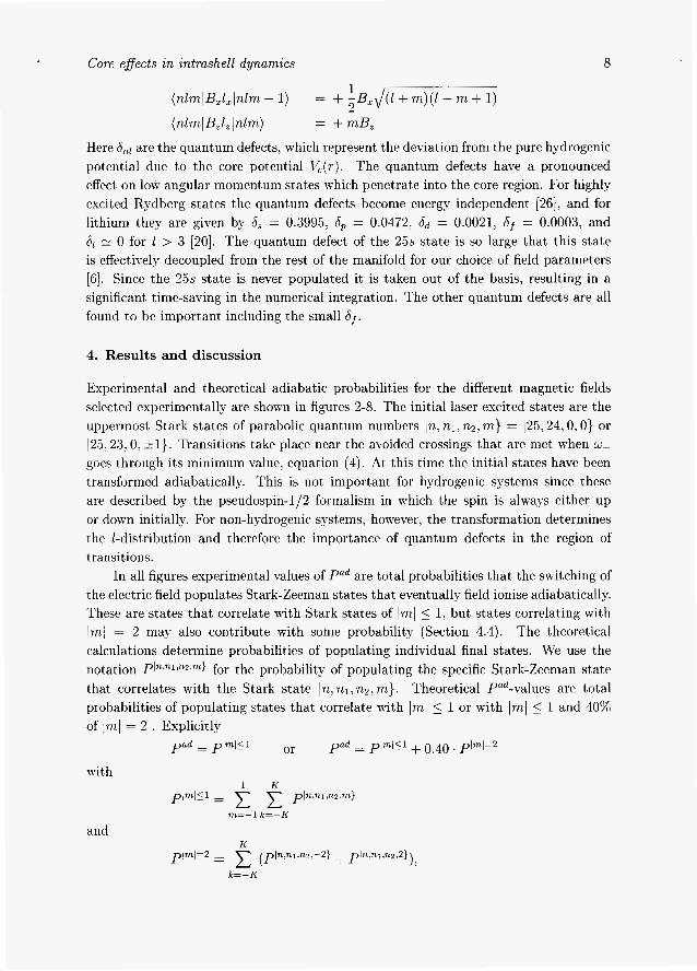
Core effects in intrashell dynamics 8
(nlmlB,I, I nlm) = +mB,
Here 6 , ~ are the quantum defects. which represent the deviation from the pure hydrogenic potential due to the core potential T.lc(r). The quantum defects have a pronounced effect on low angular momentum states which penetrate into the core region. For highlv excited Rydberg states the quantum defects become energy independent [as]. and for lithium they are given by 6, = 0.3995. 6, = 0.0472. 6 d = 0.0021, 6, = 0.0003. and 61 N 0 for I > 3 [20]. The quantum defect of the 25s state is so large that this state is effectively decoupled from the rest of the manifold for our choice of field parameters [6]. Since the 25s state is never populated it is taken out of the basis, resulting in a significant time-saving in the numerical integration. The other quantum defects are all found t o be important including the small 6 ~ .
4. Results and discussion
Experimental and theoretical adiabatic probabilities for the different magnetic fields selected experimentally are shown in figures 2-8. The initial laser excited states are the uppermost' Stark states of parabolic quant,um numbers In, n1, 122, m} = 125,240, 0} or 125; 23,O: +l}. Transitions take place near the avoided crossings that are met when LL
goes through it,s minimum value, equation (4). At, this time the initial st,ates have been transformed adiabatically. This is not important for hydrogenic systems since these are described by the pseudospin-1/2 formalism in which the spin is always either up or down initially. For non-hydrogenic systems, however, the transformation determines the I-distribution and therefore the importance of quantum defects in the region of transitions.
In all figures experimental values of Pad are total probabilities that the switching of the electric field populat'es Stark-Zeeman states that' eventually field ionise adiabatically. These are states that correlate with Stark states of Iml 5 1, but states correlat'ing with Iml = 2 may also contribut,e with some probability (Section 4.4). The theoretical calculations determine probabilities of populating individual final states. We use the notation Pln.n1.n2.7n} for the probability of populating the specific Stark-Zeeman state that correlates with the Stark state 112; ~~1,712; m}. Theoretical Pad-values are total probabilities of populating states that correlate with lml 5 1 or with Iml 5 1 and 40% of In61 = 2 . Explicitly
p a d = p l m l i l or p a d = pimi51 + 0.40. p lml=2
with 1 K
plmI51 = pIn.n1.n2.m1
m = - I k=-K
and K
1, p/nLl=2 = (pln,nl.n2;-2) + pInm.n2 .2 )
k=-K
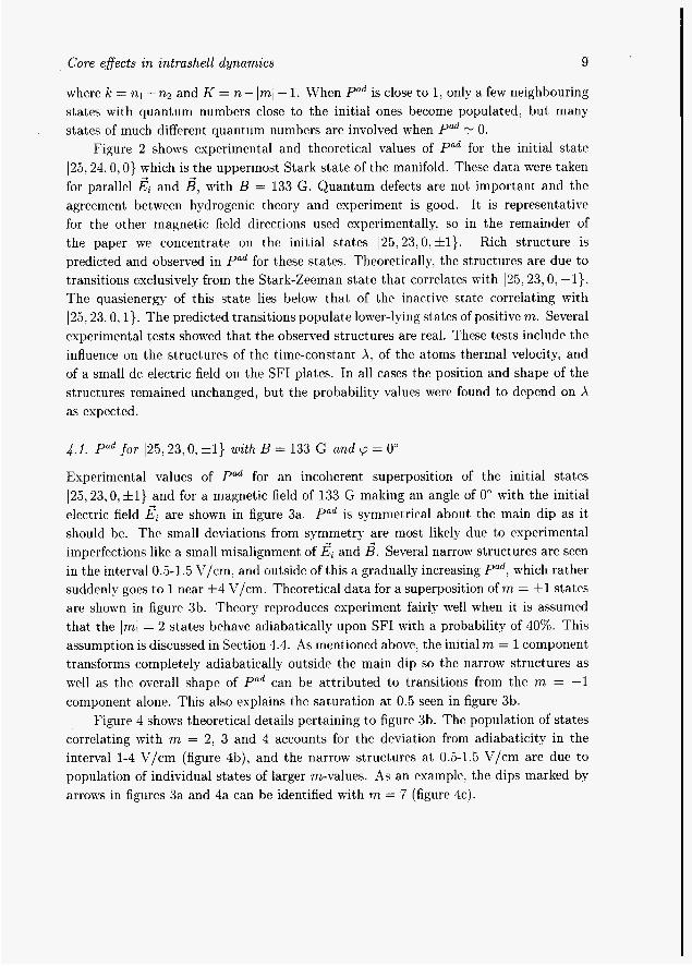
Core effects an intrashell dynamics g
where k = n1- n2 and K = n- Irn,l- 1. When Pad is close to 1, only a few neighbouring states with quantum numbers close to the initial ones become populated, but many states of much different, quantum numbers are involved when Pad 1: 0.
Figure 2 shows experimental and theoretical values of Pad for the initial state 125,24, O,O} which is the uppermost Stark state of the manifold. These data were taken for parallel I?i and B', with B = 133 G. Quantum defects are not important and the agreement between hydrogenic theory and experiment is good. It is representative for the other magnetic field directions used experimentally, so in the remainder of the paper we concentrate on the initial stat,es 125,23,0,+1}. Rich structure is predicted and observed in Pad for these states. Theoretically, the structures are due to transitions exclusively from the Stark-Zeeman state that correlates with 125,23, 0, -1}. The quasienergy of this state lies below that of the inactive state correlating with 125,23,0, 1). The predicted transitions populat,e lower-lying states of positive m. Several experimental tests showed that the observed structures are real. These t.ests include the influence on the structures of the time-constant X; of the atoms thermal velocity, and of a small d r electric field on t,he SFI plates. In all cases the position and shape of the structures remained unchanged, but the probability values were found to depend on X as expected.
4.1. Pod .for 125,23,0, *l} with B = 133 G and p = 0"
Experimental values of Pad for an incoherent superposition of the initial stat,es 125,23,0, +l} and for a magnetic field of 133 G making an angle of 0" wit,h the initial electric field 3; are shown in figure 3a. Pad is symmetrical about the main dip as it should be. The small deviations from symmetry are most likely due to experimental imperfections like a small misalignment of I?i and 2. Several narrow structures are seen in the interval 0.5-1.5 V/cm, and outside of t,his a gradually increasing Pad, which rather suddenly goes to 1 near +4 V/cm. Theoretical data for a superposition of m = f l states are shown in figure 3b. Theory reproduces experiment fairly well when it is assumed that t,he Iml = 2 states behave adiabatically upon SFI with a probability of 40%. This assumption is discussed in Section 4.4. As mentioned above, the initial m = 1 component t.ransforms completely adiabatically outside the main dip so the narrow st,ructures as well as the overall shape of Pad can be attributed to transitions from the m = -1 component alone. This also explains the saturation a t 0.5 seen in figure 3b.
Figure 4 shows theoretical details pertaining to figure 3b. The population of stat,es correlating with m = 2, 3 and 4 accounts for the deviation from adiabaticit,y in the interval 1-4 V/cm (figure 4b), and the narrow structures a t 0.5-1.5 V/cm are due to populat,ion of individual states of larger m-values. As an example, the dips marked by arrows in figures 3a and 4a can be identified with m = 7 (figure 4c).
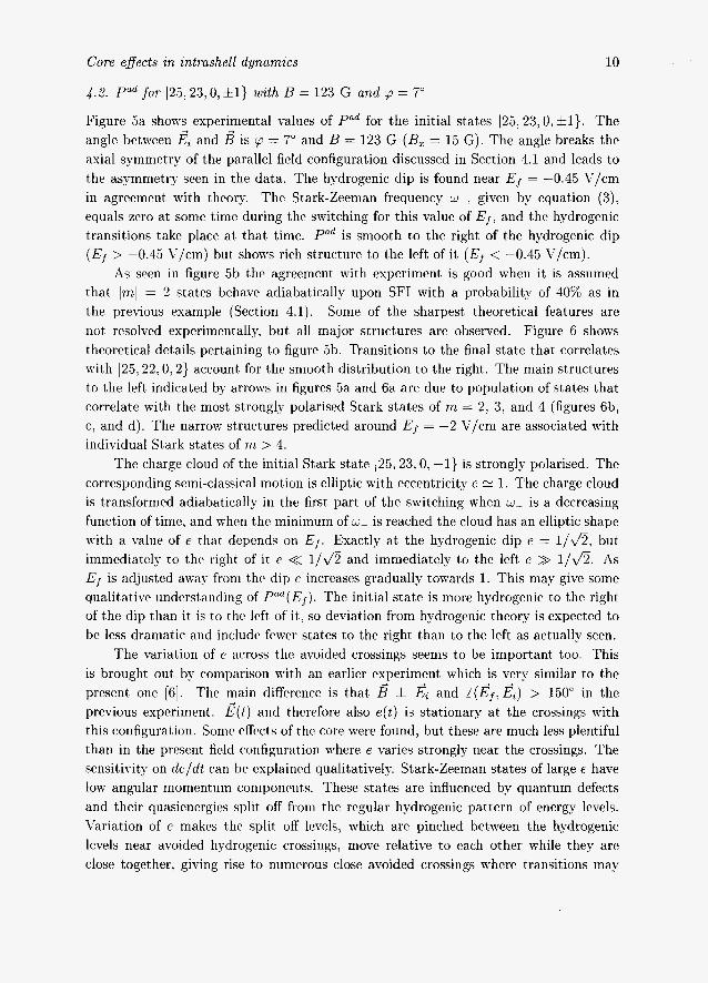
Core effects in intrashell dynamics
4.2. Pad for /25,23,0, +1} with B = 123 G and 9 = 7"
10
Figure 5a shows experimental values of Pad for the initial states 125,23,0; +l}. The angle between l?i and L? is p = 7" and B = 123 G (B, = 15 G). The angle breaks the axial symmetry of the parallel field configuration discussed in Section 4.1 and leads to the asymmetry seen in the data. The hydrogenic dip is found near EJ = -0.45 \.'/cm in agreement with theory. The Stark-Zeeman frequency w- , given by equation (3), equals zero at some time during the switching for this value of E f ; and the hydrogenic transitions take place at that time. Pad is smoot,h to the right of the hydrogenic dip ( E j > -0.45 V/cm) but shows rich structure t,o the left of it (E j < -0.45 V/cm).
As seen in figure 5b the agreement, with experiment is good when it, is assumed that Iml = 2 stat,es behave adiabatically upon SFI with a probability of 40'% as in the previous example (Section 4.1). Some of the sharpest theoretical features are not resolved experimentally. but, all major structures are observed. Figure 6 shows theorebical details perbaining t.0 figure 5b. Transitions to the final state that correlates with /25,22, 0,2} account, for t,he smooth distribution to the right. The main st.ructures to the left, indicated by arrows in figures 5a and 6a are due to population of states that, correlate with the most strongly polarised Stark states of m = 2, 3, and 4 (figures 6b, c; and d). The narrow structures predicted around EJ = -2 V/cm are associat,ed with individual Stark states of nz > 4.
The charge cloud of the initial Stark state /25,23,0, -1} is strongly polarised. The corresponding semi-classical motion is elliptic with eccentricity e N 1. The charge cloud is transformed adiabatically in the first part of the switching when w_ is a decreasing funct,ion of time, and when t,hc minimum of LU'- is reached the cloud has an ellipt,ic shape 1vit.h a value of e that depends on Ej . Exact.ly at the hydrogenic dip e = 1/&, but immediat.ely to the right of it e << l/& and immediately to the left e >> I/&. 4 s Ej is adjusted away from thci dip e increases gradually towards 1. This may give some qualitative understanding of Pu"(Ef ) . The initial state is more hydrogenic t,o the right of the dip than it is to thc lcft of it; so deviation from hydrogenic theory is expected to be less dramat.ic and includc fmer states to the right than to the left as actually seen.
The variation of e across thc avoided crossings seems t,o be important too. This is brought out by comparison with an earlier experiment which is very similar to the present one [6]. The main diffwrnce is that L? i l?i and L(l?f,gt) > 150" in the previous experiment. g( t ) and thcrefore also e ( t ) is stationary at the crossings with this configuration. Somc cffccts of the core were found, but these are much less plentiful than in the present field configuration where e varies strongly near the crossings. The sensitivity on de/dt can bc cxplainc~d qualit,at,ively. Stark-Zeeman states of large e have low angular moment,um componrnts. These states are influenced by quantum defects and their quasienergies split off from the regular hydrogenic pattern of energy levels. Variation of e makes the split off levels; which are pinched between the hydrogenic levels near avoided hydrogenic crossings, move relative to each other while they are close together, giving rise to numerous close avoided crossings where transitions may
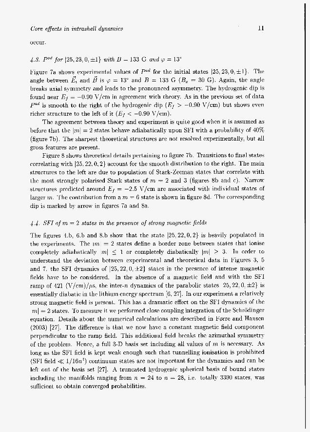
Core effects in intrashell dynamics 11
occur.
4.3. Pad for 125,23,0;+1} with B = 133 G and y = 13"
Figure 7a shows experimental values of Pad for the initial states 1 2 5 , 2 3 , 0 , f l ) . The angle between l& and B' is p = 13" and B = 133 G (B, = 30 G). Again; the angle breaks axial symmetry and leads to the pronounced asymmetry. The hydrogenic dip is found near Ef = -0.90 V/cm in agreement with theory. '4s in the previous set of data Pad is smooth to the right of the hydrogenic dip ( E f > -0.90 V/cm) but shows even richer structure to the left of it (Ef < -0.90 \'/cm).
The agreement, between theory and experiment is quite good when it is assumed as before that the Iml = 2 states behave adiabatically upon SFI with a probability of 40% (figure 7b). The sharpest theoretical structures are not resolved experimentally, but all gross features are present.
Figure 8 shows theoretical details pertaining to figure 7b. Transitions to final states correlating with 125,22, 0, 2} account for the smooth distribution to the right. The main structures to the left are due to population of Stark-Zeeman states that correlate with the most strongly polarised Stark states of m = 2 and 3 (figures 8b and c). Narrow structures predicted around Ef = -2.5 V/cm are associated with individual states of larger m. The contribution from a m = 6 state is shown in figure 8d. The corresponding dip is marked by arrow in figures 7a and 8a.
4.4. SFI of m = 2 states an the presence of strong magnetic ,fields
The figures 4.b, 6.b and 8.b show that the state 125,22; 0 , 2 } is heavily populated in the experiments. The lml = 2 states define a border zone bet,ween states that ionise completely adiabatically Iml 5 1 or completely diabatically lml 2 3. In order to understand the deviation between experimental and theoretical data in Figures 3, 5 and 7 , the SFI dynamics of 125,22,0,+2} states in the presence of intense magnetic fields have to be considered. In the absence of a magnetic field and with t,he SFI ramp of 421 (V/cm)/ps, the inter-n dynamics of the parabolic states 125,22,0, +2} is essentially diabatic in the lithium energy spectrum [6; 271. In our experiment a relatively strong magnetic field is present. This has a dramatic effect on the SFI dynamics of the Iml = 2 states. To measure it we performed close coupling integration of t,he SchrGdinger equation. Details about the numerical calculations are described in FOrre and Hansen (2003) [27]. The difference is t,hat we now have a constant magnetic field component perpendicular to the ramp field. This additional field breaks the azimuthal symmetry of the problem. Hence, a full 3-D basis set including all values of m is necessary. As long as the SFI field is kept weak enough such that tunnelling ionisation is prohibited (SFI field << 1/16n4) continuum stat,es are not important for the dynamics and can be left out, of the basis set [27]. A truncated hydrogenic spherical basis of bound states including the manifolds ranging from n = 24 to n = 28, i.e. totally 3390 states, was sufficient to obtain converged probabilities.

Core e.ffects an intrashell dynamics 12
In figure 9 the population on the initial 125.22.0, Z } state as a function of the SFI field is plotted for selected values of the magnetic field. The magnetic field is seen to become less and less important with increasing electric field. and for a field > 600 V/cm the role of the magnetic field is negligible. Note that even for B=O G the dvnamics is not completely diabatic, as already pointed out by Fgrre and Hansen (2003) [27]. The curves are extrapolated up to the classical ionisation limit (N 850 i’/cm) Figure 9 shows that more than 80 % of the initial state has been transfered to other channels a t this limit for the case of the strongest magnetic field (133 G). It is reasonable to assume that the loss of probability on the initial state equally distributes on states that ionisc either adiabatically or diabaticallv [27]. N’ithin this assumption we find that the 125.22,O. &2} states have a probability of about 40 % to ionise adiabatically and to contribute to the adiabatic peak in the SFI spectrum.
5. Summary and conclusion
Intrashell dynamics within a highly excit,ed Rydberg shell of Li driven by homogeneous t,imc-dependent electric and magnetic fields has been studied theoretically and experimentally for situat.ions in which the non-hydrogenic Li+ core plays a significant role. When the Rydberg atom is initially excit,ed to a coherent, elliptic state; the dynamics is found to be mainly adiabatic wit,h deviations described accurately by hydrogenic t.heory. Core effects can be very important, however, even for the nearest neighbours in the Stark-Zeeman spectrum. Yon-adiabatic dynamics is always found near avoided crossings among the Stark-Zeeman levels, and core effects are most important when the eccentricity of the elliptic-shaped charge clouds of the nearly coherent elliptic states is high and strongly field-dependent, near the avoided crossings. The overall agreement between experiment, and theory suggests that the frozen core approximation in equat,ion ( 5 ) and the use of quantum defects indeed is valid for highly excited Rydberg systems.
Acknowledgments
We wish to acknowledge support from the Nordic Academy for Advanced Study (NorFa). COYICET (D.F.), and the Norwegian Research Council.
References
[l] Kazansky A K and Ostrovsky V N 1996 J. Phys. B: At . Mol. Phys. 29 L855. [2] Kristensen L, Horsdal-Pedersen E and Sorensen P 1998 J. Phys. B: At. Mol. Phys. 31, 1049. [3] Smensen P, Day J C, DePaola B D, Ehrenreich T, Horsdal-Pedersen E and Kristensen L 1999 J.
[4] hlijatovic ILl, Solov’ev A E and Taulbjerg K 2001 J. Phys. B: At . Mol. Phys. 34, 1897. [5] Fregenal D, Ehrenreich T, Henningsen B, Horsdal-Pedersen E, Nyvang L and Ostrovsky V N 2001
Phys. B: At. Mol. Phys. 32, 1207.
Phys. Rev. Lett. 87, 223001.
Core effects in intrashell dynamics 13
[6] Fmrre M, Fregenal D, Day J C, Ehrenreich T, Hansen J P, Henningsen B, Horsdal-Pedersen E, Nyvang L, Povlsen 0 E, Taulbjerg K and Vogelius I2002 J. Phys. B: At . Mol. Phys. 35 401.
[7] Fregenal D, Horsdal-Pedersen E, Madsen L B, Fmrre M, Hansen J P and Ostrovsky V N 2004 Phys. Rev. A 69, 031401(R).
[8] Day J C, Ehrenreich T, Hansen S B, Horsdal-Pedersen E, Mogensen K S and Taulbjerg K 1994 Phys. Rev. Lett. 72 1612.
[9] Mogensen K S, Day J C, Ehrenreich T , Horsdal-Pedersen E and Taulbjerg K 1995 Phys. Rev. A 51, 4038.
[lo] Forre M 2004 preprint. [ll] Ostrovsky V N and Horsdal-Pedersen E 2004 preprint. [12] Koch P hf, Galvez E J and Zelazny S .4 1999 Physica D 131 90. [13] Galvez E J, Koch P M, D. Richards and Zelazny S -4 2000 Phys. Rev. A 61 060101. [14] Cheng CH and Gallagher T F 2000 Phys. Rev. A 61 063411. [15] Ostrovsky V N and Horsdal-Pedersen E 2003 Phys. Rev. A 67 033408. [16] Ostrovsky V N and Horsdal-Pedersen E 2003 Eur. Phys. J. D 23 15. [17] Nagesha K and MacAdam K B 2003 Phys. Rev. Lett. 91 113202. [18] Demkov Y N, Ostrovsky V N and Solov’ev E A 1974 Zh. Eksp. Teor. Fiz. 66 125 [1974 Sov. Phys.
[19] Kazansky .4 K and Ostrovsky V N 1996 Phys. Rev. Lett. 77 3094. [20] Gallagher T F 1994 Rydberg Atoms (Cambridge University Press). [21] Engelfield M J 1972 Group Theory and the Coulomb Problem (New York: Wiley). [22] Zimmerman ILI L, Littman M G, Kash R;I R/I and Kleppner D 1979 Phys. Rev. A 20 2251. [23] Komarov I V, Grozdanov T P and Janev R K 1980 J. Phys. B 13 573. [24] Bethe H A and Salpeter E E 1957 Quantum Mechanics of One- and Two-Electron Atoms (Springer
[25] Brink D hf and Satchler G R 1968 Angular Momentum (Oxford University Press). [26] Seaton M J 1958 Man. Not. R . Astron. Soc. 118 504. [27] Fmrre bl and Hansen J P 2003 Phys. Rev. A 67 053402.
JETP 39 571.
Verlag, Berlin).
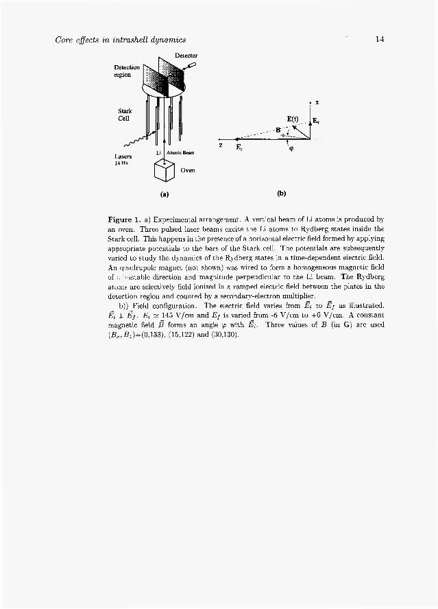
Core egects an intrashell dynamics
~ Detector
14
Figure 1. a) Experimental arrangement. A vertical beam of Li atoms is produced by an oven. Three pulsed laser beams excite the Li atoms to Rydberg states inside the Stark cell. This happens in the presence of a horizontal electric field formed by applying appropriate potentials to the bars of the Stark cell. The potentials are subsequently varied to study the dynamics of the Rydberg states in a time-dependent electric field. An quadrupole magnet (not shown) was wired to form a homogeneous magnetic field of I " (stable direction and magnitude perpendicular to the Li beam. The Rydberg atoms are selectively field ionised in a ramped electric field between the plates in the detection region and counted by a secondary-electron multipli_er.
b)) Field configuration. The electric field varies from E, to i?f as illustrated. g2 I Ef. E, N 145 V/cm and E f is varied from -6 V/cm to +6 V/cm. A constant magnetic field 6 forms an angle 9 with I&. Three values of B [in G) are used (B,,BZ)=(0,133), (15,122) and (30,130).
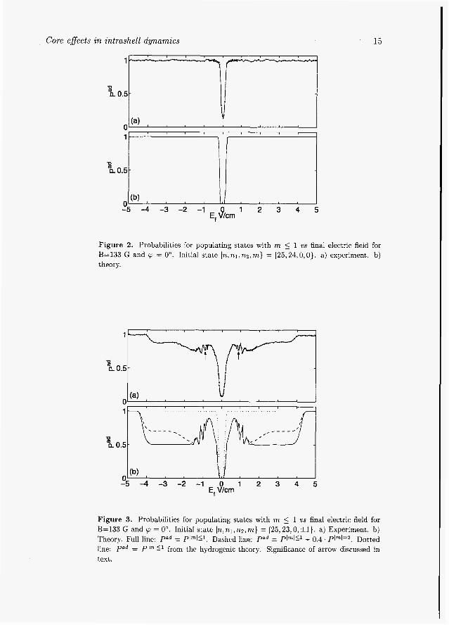
Core effects in intrashell dynamics
"
1
u "a 0.5
I
-
(b)
Figure 2. Probabilities for populating states with rn 5 1 us final electric field for B=133 G and 9 = 0". Initial state 1n,n,,nz,rn} = 125,24,0,0}. a) experiment. b) theory.
P
"a 0.5
-1 0 1 E, Vlcm
-4 -3 -2 2 3 4 5
Figure 3. Probabilities for populating states with m 5 1 us final electric field for B=133 G and 9 = 0". Initial state In, nl , n2, m} = (25,23,0, +I}. a) Experiment. b) Theory. Full line: Pad = PlmI~l, Dashed line: Pad = PIrnlL1 + 0.4. PIrn[=?. Dotted line: Pad = Plmlsl from the hydrogenic theory. Significance of arrow discussed in text.
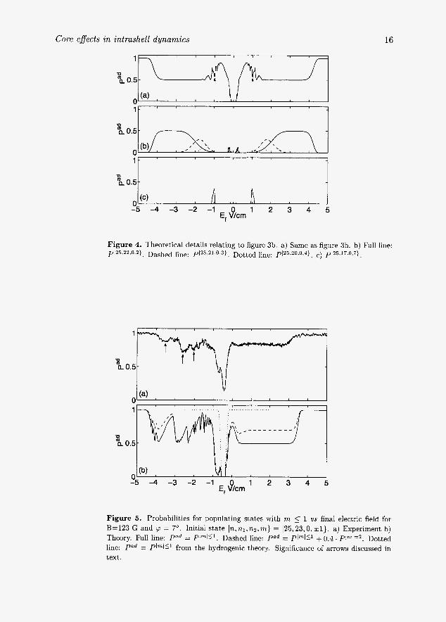
Core effects in intrashell dynamics
(c) ,
16
a 0.5 '1
1
* - - - - - - - - - U
*a 0.5
-05 -4 -3 -2 -1 0 1 2 3 4 5 E, Vlcm
Figure 5. Probabilities for populating states with m 5 1 us final electric field for B=123 G and p = 7". Initial state ln,nlrn2,m} = 125,23 ,0 , f l ) . a) Experiment b) Theory. Full line: Pad = T)lrn1s1. Dashed line: Pad = Plmlsl + 0.4 . Plml=2. Dotted line: Pad = Plnls' from the hydrogenic theory. Significance of arrows discussed in text.
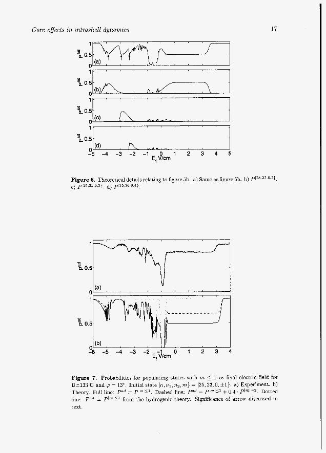
Care effects in intrashell dynamics
1‘-
“a 0.5 - v
, 0
17
11 1
Figure 6. Theoretical details relating to figure 5b. a) Same as figure 5b. b) Plz5.22.0.2}. c) p125.21.0.3) d) p125,20.0.4}
1
v “a 0.5 -
0 1
0
“a 0.5
-0s -5 -4 -3 -2 -1 0 1 2 3 4 E, Vlcrn
Figure 7. Probabilities for populating states with m 5 1 us final electric field for B=133 G and p = 1 3 O . Initial state In, nl, n2, m } = 125,23,0, fl}. a) Experiment. b) Theory. Full line: Pad = PIml5l. Dashed line: Pad = PlmI_<l + 0.4. Plml=2. Dotted line: Pad = Plm151 from the hydrogenic theory. Significance of arrow discussed in text.
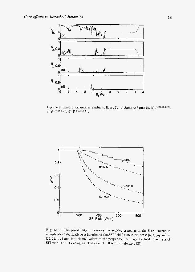
Core effects in intrashell dynamics
I , , , ’
U “a 0.5-
U “a 0.5-
0 n
(d)
18
Figure 8. Theoretical details relating to figure 7b. a) Same as figure 7b. b) P125,22 O.’).
c) p l 2 5 21 033). d) p l 2 5 18,O 6 ) .
J 200 400 600 800
SFI Field (V/cm)
Figure 9. The probability to traverse the avoided-crossings in the Stark spectrum completely diabatically as a function of the SFI field for an initial state In, nl , 712, m } = 125,22,0,2} and for selected values of the perpendicular magnetic field. Slew rate of SFI field is 421 (V/cm)/ps. The case B = 0 is from reference [27].

Paper 3
Dynamics of a H ( n ) atom in time-dependent electric and rnagnctir fields
hI. Fprrc; H. hI. Sihen and J. P. Hansen
Phyr,. Rev. .I 65. 053401) (2OW)

PHYSICAL REVIEW A, VOLUME 65,053409
Dynamics of a H(n) atom in time-dependent electric and magnetic fields
M. Fdrre Institute of Physics, University of Bergen, Alllgaten 55, N-5007 Bergen, Norway
and Foundation for Research and Technology-Hellas, IESL, P.0. Box 1527, Herdlion 71117, Crete
H. M. Nilsen and J. P. Hansen InstirUte of Physics, University of Bergen, Alllgaten 55, N-5007 Bergen, Norway
(Received 12 December 2001; published 2 May 2002)
The symmetry properties of the Coulomb potential allow for a dynamical spin-1/2 description of any fixed n level of a hydrogenlike atom in a time-dependent sufficiently weak electric andfor magnetic field. An explicit expression for the time dependence of the l,m amplitudes peaaining to a general n level is derived. The derivation follows on purely algebraic operations. Based on the derivation, we give analytical n-independent solutions to established and proposed schemes for driving the atom into a high angular-momentum state.
DOI: 10.1103/PhysRevA.65.053409
I. INTRODUCTION
The theoretical description of atoms and molecules inter- acting with various electromagnetic sources often requires an infinite Hilbert space due to a continuum of accessible elec- tronic states. A rather complex mathematical description is then necessary, with possibly slow convergence. In general, numerical schemes, therefore, often require large basis or small grid sizes in order to achieve a solution of the Schro- dinger equation. The underlying physical mechanisms may then be veiled, either because one simple process does not exist, or because the calculations are so complex that one fails to spot this process. In contrast, when only two or a few states are important, like for slow near-resonant atomic col- lisions or atoms in weak resonant laser fields, the dynamics becomes very simple and is well understood, for example, as Stiickelberg or Rabi oscillations.
Very few Hamiltonians offer an analytical solution for multidimensional Hilbert spaces. Some well-known such systems are certain versions of the multichannel Landau- Zener model [l] or slow, distant collisions between ions and Rydberg atoms [2], and certain two-photon transitions in quantum optics [3]. The study of such quantum systems are particularly important in two respects: First, they may give insight into new dynamical features that may have potential application, e.g., in quantum computing [4]. Second, they may be used as benchmark systems for testing and verifying numerical algorithms. The most important analytic multistate problem is perhaps the dynamics of a spin-1 particle in a magnetic field, with H E S . ~ . It was showed as early as 1932 by Majorana [5] that this problem can be reduced to a spin- 112 problem with each spin-1/2 “particle” evolving in the very same field. The original spin-J system can at any time be restored by angular-momentum addition. This property is closely related to the existence of analytic solutions of cer- tain specific problems of atomic dynamics in magnetic fields, see, e.g., [6].
Recently it has been pointed out that hydrogenic Rydberg atoms interacting with time-dependent electric and/or mag- netic fields in many cases also belong to this class of analytic spin problems [7]: When the fields are weak such that the
PACS number(s): 32.80.Rm, 34.60.+2, 42.50.Ct
65 053409-1
dynamics is well described within one principal n shell the symmetry properties of the Coulomb potential open for a spin description. By using the “Majorana reduction” the dy- namics of the n level can be analyzed analytically. Interesting resonance phenomena, based on the solutions of a single spin-flip probability, were predicted and tested experimen- tally [8]. This is a truly remarkable feature, since the comple- mentary “real-space” process is described in a n2-dimensional Hilbert space where all states can take part in the dynamics in a completely nonperhubed way.
The time dependence of the spin amplitudes may be ex- pressed in terms of rotation matrices [9,10]. In an alternative algebraic approach Vitanov and Suominen [ 113 expressed the final-state amplitudes of an atom in a magnetic field in terms of a single transition probability, for a situation when the atom is initially in the rn = If: I state. Triggered by their solu- tion we generalize the algebiaic approach such that it applies to any initial state and for any combination of electric and magnetic fields. The paper is organized as follows: In the following section the general theory is reviewed with empha- sis on the derivation of the general connection formula. In Sec. III we apply the results to an analytical study of various time-dependent fields, which can produce a circular long- living state of a general n level of the hydrogen atom. Atomic units are used throughout except where units are given explicitly.
11. THEORY
For weak-field strengths the Hamiltonian of a hydrogenic one-electron atom interacting with a time-dependent electric and magnetic field can be written as
1 , A = A , + i ( t ) . F+ ?B(‘) .i,
where A,= -V2/2-Z/r is the Hamiltonian of the unper- turbed hydrogenic atom with nuclear charge Z. The con- straints on the field strengths are such that different n mani- folds do not mix, which imply that the electric-field strength is smaller than the Inglis-Teller limit 1/3n’, and the
02002 The American Physical Society
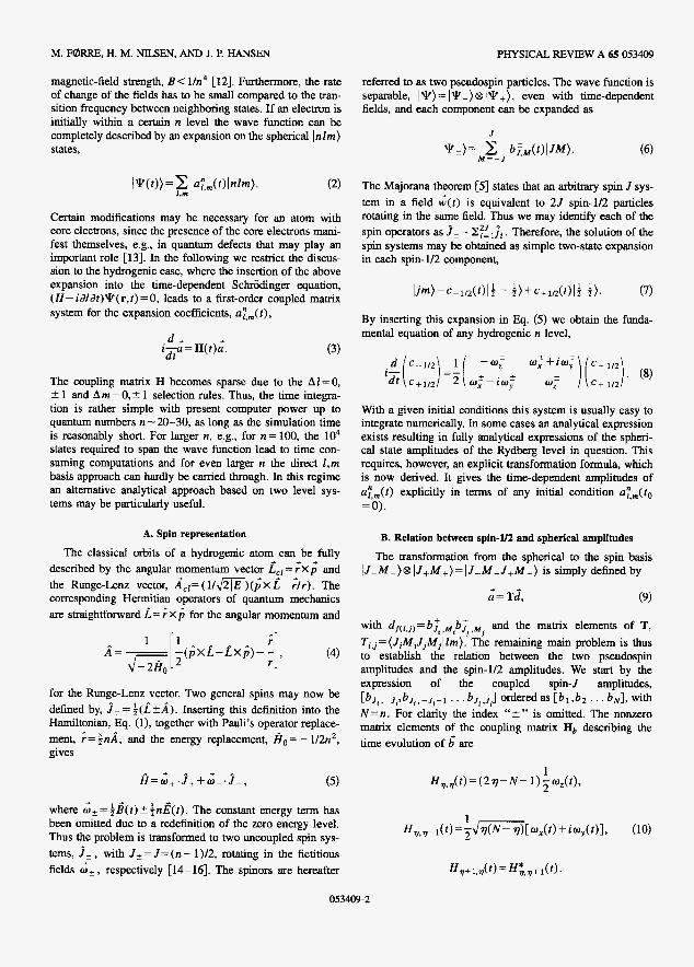
M. FBRRE, H. M. NILSEN, AND J. P. HANSEN PHYSICAL REVIEW A 65 053409
magnetic-field strength, B < l/n4 [12]. Furthermore, the rate of change of the fields has to be small compared to the tran- sition frequency between neighboring states. If an electron is initially within a certain n level the wave function can be completely described by an expansion on the spherical InZm) states,
Certain modifications may be necessary for an atom with core electrons, since the presence of the core electrons rnan- fest themselves, e g , in quantum defects that may play an important role [13]. In the following we restrict the discus- sion to the hydrogenic case, where the insertion of the above expansion into the time-dependent Schrodinger equation, (H- i d / d t ) q ( r , ? ) =0, leads to a first-order coupled matrix system for the expansion coefficients, c&(t),
d , i - u = H(t)a. dt (3)
The coupling matrix H becomes sparse due to the AI = 0, ? 1 and Am = 0, -t 1 selection rules. Thus, the time integra- tion is rather simple with present computer power up to quantum numbers n - 20-30, as long as the simulation time is reasonably short. For larger n, e.g., for n= 100, the lo4 states required to span the wave function lead to time con- suming computations and for even larger n the direct Z,m basis approach can hardly be carried through. In this regime an alternative analytical approach based on two level sys- tems may be particularly useful.
A. Spin representation
The classical orbits of a hydrogenic atom can be fully described by the angular momentum vector LCl=;Xp and the Runge-Lenz vector, A , , = ( l / ~ ) ( p X i - ; l r ) . The corresponding Hermitian operators of quantum mechanics are straightforward f, = X i for the angular momentum and
(4)
for the Runge-Lenz vector. Two general spins may now be defined by, .?, = $ ( f , ? A ) . Inserting this definition into the Hamiltonian, Eq. (l), together with Pauli's operator replace- ment, ;= id, and the energy replacement, A,= - 1/2n2, gives
(5 )
where i ,=$l?(t)-tin,t?(f). The constant energy term has been omitted due to a redefinition of the zero energy level. Thus the problem is transformed to two uncoupled spin sys- tems, J , , with J,=J=(n-1)/2, rotating in the fictitious fields ;,, respectively [14-161. The spinors are hereafter
referred to as two pseudospin particles. The wave function is separable, IT)= IT-)@ IT+), even with time-dependent fields, and each component can be expanded as
J
The Majorana theorem [5] states that an arbitrary spin J sys- tem in a field w ( r ) is equivalent to 2 5 spin-1/2 particles rotating in the same field. Thus we may identify each of the spin operators as .?, = lji. Therefore, the solution of the spin systems may be obtained as simple two-state expansion in each spin- 1/2 component,
(7)
By inserting this expansion in Eq. (5) we obtain the funda- mental equation of any hydrogenic n level,
With a given initial conditions this system is usually easy to integrate numerically. In some cases an analytical expression exists resulting in fully analytical expressions of the spheri- cal state amplitudes of the Rydberg level in question. This requires, however, an explicit transformation formula, which is now derived. It gives the time-dependent amplitudes of ay,,(t) explicitly in terms of any initial condition ay,,(t, =O).
B. Relation between spin-VZ and spherical amplitudes
The transformation from the spherical to the spin basis I J - M - ) @ I J+M+)= IJ_M-J+M+) is simply defined by
+ + a = T d , (9)
with df,i,j,=b$,,FJ,,M, and the matrix elements of T, Ti,j=(JiMi5jMjlZm). The remaining main problem is thus to establish the relation between the two pseudospin amplitudes and the spin-112 amplitudes. We start by the expression of the coupled spin4 amplitudes, [bJ,,-.,,,b3z,-3i+l . . . bJl,,i] orderedas [b l ,bZ. . . bN1, with N=n. For clarity the index "+" is omitted. The nonzero matrix elements of the coupling matrix Hb describing the time evolution of 6 are
053409-2

DYNAMICS OF A H(n) ATOM IN TIME-DEPENDENT I PHYSICAL REVIEW A 65 053409
We label with q , q=1,2 ,..., N , instead of M labels, - J S M G J , such that M may be found from the relation M= -J+ q- 1 . The time dependence of the amplitudes can, therefore, be written as
i b , = ( 1 - N ) c b l + m V b 2 , j=min{q- 1 8 - k }
s4= V* (7- 1 - j ) fFz&#-k- j j =max( 0.7- k} q-2 - j k - q + j + l
X u 2 a1
i b , = J ( q - l ) ( N - q + 1 ) V * b , - 1 + ( 2 q - N - 1 ) ~ b ,
( 1 1 )
j=min{q- 1H- k )
with E ( t ) = t W z ( t ) and V ( f ) = f [ w x ( t ) + i ~ y ( t ) ] . Let &)
= [ a l ( t ) a z ( t ) l and j ( r ) = [ P l ( t ) Pz ( r ) ] be two solutions of Eq. (8) with initial conditions [0 11 and [ l o ] , respec- tively. It is immediately seen that this is the two linearly independent solutions for N = 2. As an ansafz we assume that the solution to Eq. ( 1 1 ) is
and
N , T - ( ~ ; ~ ) [ k - l ) f j , k - . q - 1 - j '
i = m i d n- 1,N- kl
(12) From Eq. (12), after some algebraic manipulations on the sums, we find that the Si satisfy
where k refers to the initial state with d(fo)
appropriate normalization factor. The vectors 6, i, and 8 satisfy the binomial relation,
= [ b , , . . . ,bk , . . . , b ~ ] = [ o , . . . , I , . . . ,0], and n:,~ iS an
b:-l k
1,k S2+ S4= ( N - q+ 1 )V* -,
lnserting Eq. (12) in Eq. (11) we obtain
j=min{ q- l a - k } b:+l k
1.k s,+s,= qv-.
With the requirement,
we have shown that the b:,k ( 1 < q < N ) given by Eq. (12) fulfill Eq. (11 ) as long as the condition, Eq. (20), holds. The two special cases q= 1 and q=N can now be verified fol- lowing exactly the same procedure. ~ o t e that a:,= 1 from the initial condition.
As an example we let pk+q be the probability for a tran- sition between the pseudospin states k and q, Pk+q = I b:,,I2. Hence the total probability for transition to a given state labeled with q+ , q- becomes P n+ = ~ b ~ + , k + ~ 2 ~ b ~ ~ , k ~ ~ 2 , where k, and k - refer to the initial states of J + , respectively. If the initial state is chosen as the uppermost Stark state, the two uncoupled spin Ji systems combine to a particularly simple analytical formula,
Here we have defined
Si= 4 2 7 - N - 1 ) j = m i n [ q - l , N - k )
i=min{n- 1,N- k1
053409-3
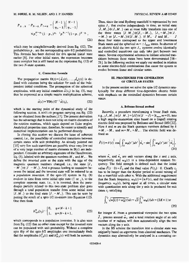
M. FBRRE, H. M. NJLSEN, AND J. P. HANSEN PHYSICAL REVIEW A 65 053409
(21)
which may be straightforwardly derived from Eq. (12). The probabilities p are the corresponding spin-ll2 probabilities. This formula has been derived for this special initial state earlier [8]. For other initial states, the expression becomes more complex but is still based on the expression Q. (12) of the two N-state systems.
C. Connection formula
The propagation matrix D ( t ) = [ d , ( t ) , . . . .d,(r)] is de- fined with columns being the solution for each of the inde- pendent initial conditions. The propagation of the spherical amplitudes, with any initial condition ; ( to ) in Eq. (3), may thus be expressed as a simple matrix multiplication scheme,
a ( t ) =TD(?)T~'~( to) , (22)
which is the starting point of the dynamical study of the following section. A MATLAB program carrying out Eq. (22) can be obtained from the authors [17]. The present derivation has the advantage that it does not relay on matrix elements of the rotation matrices, which again depend on Euler angles. Analytical properties may, therefore, be easier to identify and numerical implementation can be performed directly.
In closing this section we discuss the issue of coherent control, i.e., the possibility of controlled transitions between certain states with unit probability. As already pointed out [ 101 very few such transitions are possible since very few out of a very large number of matrix elements in D( t ) are inde- pendent. Consider an arbitrary eigenstate of the Hamiltonian, Eq. (5), labeled with the quantum numbers M + and M - . We define the inverted state as the state with the sign of the magnetic quantum numbers changed, i.e., the state IJ+ - M + ) @ l J - - M - ) . And a process leading to transition be- tween the initial and the inverted state will be referred to as a population inversion. If the spin-1R system in Eq. (8) evolves in time from some initial spin state ( t or J), to the complete opposite state, i.e., it is inverted, then the pseu- dospin particle related to this two-state problem also goes through a total population transfer from some initial state I J + M , ) to the final state l J + - M + ) . This can be seen by putting the result of a spin-112 inversion into Equation (12). One then finds
0, q f N - k + l
1, q = N - k + l , (23)
which corresponds to a population inversion. It is also seen from Eq. (12) that no other state except for the inverted state can be populated with unit probability. Without a complete spin flip of the spin-1R amplitudes one immediately finds that the amplitudes bTk(t) and b i , , ( t ) will both be nonzero.
Thus, since the total Rydberg manifold is represented by two spins J , that evolve independently in time, an initial state I J + M + ) @ l . - M _ ) can at most fully transform into one of the three states I J + M + ) ~ ~ J - - - M - ) , l J + - M + ) @ l J - -M-) or I J + - M + ) @ l J - M - ) . If M+=J and M-=-J these four states correspond lo the upper and lowermost Stark states and the spherical m = t l,,, states. In absence of an electric field the two spin J , systems evolve identically and controlled transitions can only take part between two states. Several experimental schemes to initiate selected tran- sitions between these states have been demonstrated [18- 211. In the following section we apply our method in relation to some electric-field combinations that cause the system to evolve between linear and circular states.
III. PROCEDURES FOR GENERATION OF CIRCULAR STATES
In the present section we solve the spin- 112 dynamics ana- lytically for three different time-dependent electric fields with emphasis on the controlled dynamics between certain states.
A. Bellomo-Stroud method
Recently, a procedure transforming a linear Stark state, e.g., I J + M + ) @ I J _ M - ) = IJJ)@ lJ - J ) = I k,,, m=O), into a high angular-momentum state based on a (rapid) rotating electric field was proposed by Bellomo and Stroud (BS) [22]. Here k and m are the Stark quantum numbers defined by k = M + - M - and m = M + + M - . The electric field was de- fined as
where and i, are unit vectors along the x and z axis, respectively, and q(?) is a time-dependent rotation fre- quency. The field strength is defined such that the initial value F( f = 0) = F,, and the final value F ( t f ) = 0. Clearly tf has to be longer than the Kepler period to avoid mixing of the n manifold with other n. With the additional requirement that the Stark frequency, os(?) = q n F ( t ) , and the rotational frequency, w,(t) , being equal at all times, a circular state with quantization axis along the y axis is produced for exit times ?, satisfying
(25)
for integer K. From a geometrical viewpoint the two spins ie precess around G, and a total rotation angle of an odd number of T radians will then automatically align the two vectors along the y axis.
In the BS scheme the transition into a circular state was originally based on arguments from classical mechanics. The dynamics may alternatively be analyzed in a corotating co-
053409-4

DYNAMICS OF A H(n) ATOM IN TIME-DEPENDENT PHYSICAL, REVIEW A 65 053409
ordinate frame based on the spin-1/2 systems. This intro- duces a fictitious magnetic field parallel with the y axis, B,(t)=2wR(t). The Schrijdinger equation in the rotating frame is obtained through the transfonnation
$L e - i Q R ( w y $ , (26)
with nR( t )= j&)R( t ' )d t ' . The spin-1/2 representation leads to the coupled two-state systems,
The analytical solution is
We note that the first column of M + and the second column of M- are eigenvectors of i,=i&,, both with positive ei- genvalues, where a, is the Pauli spin matrix. At exit times satisfying f i a R ( t ) = ( 2 K + l ) ~ we, therefore, obtain a cir- cular state along the y axis. At intermediate times all other states may be populated. As an illustration we choose a lin- early decreasing field strength, F( t) = eo( 1 - t/?,). In Fig. 1 the probabilities for population of the Stark states lkm) and the probability of total angular-momentum 1, summed over the magnetic quantum numbers, are shown for n=40. The initial Stark state is seen to decay similar to an excited state decaying into a continuum. Very little structure among the population of the other Stark states are seen as ?-+tf. The population of total angular-momentum is correspondingly without structure initially, until the linal high angular- momentum state is populated with unit probability at the exit time. An interesting observation, also shown by other au- thors, is that each angular-momentum have a rather localized time region when it is populated. Initially the small angular momenta are populated, while at the end of the interaction time higher and higher angular momenta reaches a peak at well-defined times before they decay again and linally "de- liver" all the probability to the states with 1 = n - l .
B. Oscillating clcctric field
Instead of requiring the electric field to vanish slowly we now consider the dynamics of an atom in an oscillating elec- tric field, F( t) = Focos(wt)iz, with constant field strength, Fo. We deline os= qnFo. The underlying spin-112 system is again easily solved,
ussin( wr)
(30)
with,
Time (a.u.) x IO6
0.8-
0.5 1 1.5 2 2.5 x io7 Time (a.u.)
FIG. 1. Upper: the Stark distribution as a function of time for n =40 based on the BS scheme with eo= 3 X lo-'. Lower: the cor- responding 1 distribution as a function of time.
"0
It is now seen that spin inversion is obtained periodically: If the initial state is taken as an arbitrary Stark state quantized along the z axis, the two state systems are seen to go through an inversion at times satisfying wssin(wt)/2w= T / ~ + K T , where K is an integer. The time relation implies w+ 12K + 1 I TU. For K = 0 the first population inversion occurs after a time ti",=(l/o)sin-'(?ro/ws). An arbitrary initial state Ikm) thus evolves into I - k - m ) . when w s < r o complete population inversion cannot occur with the present electric field. Furthermore an investigation of the general solution, Eq. (30), in terms of eigenstates of the angular-momentum operators, shows that for exit times satisfying ossin(wr)/2w = ? ~ / 4 + KT, an initial state Ikm), would correspond to the states I t m t k); . Now the time relation implies w s a I2K Z f l ~ o . Thus for ws<vw/2 total population transfer be- tween any states cannot happen.
053409-5
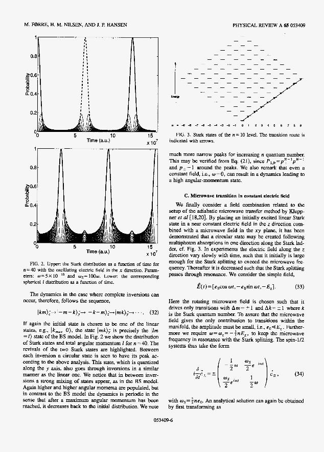
M. F@RRE, H. M. NILSEN, AND J. P. HANSEN PHYSICAL REVIEW A 65 053409
- Time (a.u.).- .-
x io'
x io' Time (a.u.)
FIG. 2. Upper: the Stark distribution as a function of tirne for n=40 with the oscillating electric field in the x direction. Param- eters: 0 = 5 X lo-'' and os= 1000. Lower: the corresponding spherical 1 distribution as a function of time.
The dynamics in the case where complete inversions can occur, therefore, follows the sequence,
Ikm);+ 1 - m - k ) ; - + - k - m ) ; + / m k ) ; A . . ' . (32)
If again the initial state is chosen to be one of the linear states, e.g., Ik,,, 0), the state Imk); is precisely the IZm = I ) state of the BS model. In Fig. 2 we show the distribution of Stark states and total angular momentum 2 for n = 40. The revivals of the two Stark states are highlighted. Between each inversion a circular state is seen to have its peak ac- cording to the above analysis. This state, which is quantized along the y axis, also goes through inversions in a similar manner as the linear one. We notice that in between inver- sions a strong mixing of states appear, as in the BS model. Again higher and higher angular momenta are populated, but in contrast to the BS model the dynamics is periodic in the sense that after a maximum angular momentum has been reached, it decreases back to the initial distribution. We note
much more narrow peaks for increasing n quantum number. This may be verified from Eq. (21), since P,,,=p:-'p?-' and p - 1 around the peaks. We also remark that even a constant field, Le., w=O, can result in a dynamics leading to a high angular-momentum state.
C. Microwave transition in constant electric field
We finally consider a field combination related to the setup of the adiabatic microwave transfer method by Klepp- ner et a2 [18,20]. By placing an initially excited linear Stark state in a near constant electric field in the z direction com- bined with a microwave field in the x y plane, it has been demonstrated that a circular state may be created following multiphoton absorptions in one direction along the Stark lad- der, cf. Fig. 3. In experiments the electric field along the z direction vary slowly with time, such that it initially is large enough for the Stark splitting to exceed the microwave fre- quency. Thereafter it is decreased such that the Stark splitting passes through resonance. We consider the simple field,
+ E(t)=[eocos ut, - eosin wt, -E,]. (33)
Here the rotating microwave field is chosen such that it drives only transitions with A m = 5 1 and Ak= t 1 where k is the Stark quantum number. To assure that the microwave field gives the only contribution to transitions within the manifold, the amplitude must be small, i.e., e o < E , . Further- more we require w = wz= - qnE,, to keep the microwave frequency in resonance with the Stark splitting. The spin-1/2 systems thus take the form
(34)
with os= ;ne,. An analytical solution can again be obtained by first transforming as
053409-6

DYNAMICS OF A H(n) ATOM IN TIME-DEPENDENT . . . PHYSICAL, REVIEW A 65 053409
We then obtain two simple spin-112 systems,
(35)
O S 0 -- i-dL= a , ( -~ :) d _ = M - d - . (36) at
Let the coupling matrices be indexed with M + and k , respectively, and let i be the identity matrix. The analytical solutions are
1 d+( t )= IC..( pt)
u2+ -
(37)
In the limit I wsi 1 0 1 the state vector d, has mainly a phase development with time as compared to d- . In terms of spin particles, the one referring to 6 , remains in its initial state, while the other goes through a full population inversion at time t = d / o S . This is equivalent to complete transfer from a general initial state Ikm) to the state Imk). Thus, if the initial state is a linear Stark state IkminO), the circular Stark state IOm,,,) is reached. In Fig. 4 the eigenstates Ikm) as a func- tion of time are shown for the n = 25 level. With increasing time, higher and higher magnetic quantum numbers are populated, and finally all the probability is in the m = I,,, state. The population of the Stark levels is seen to be rather similar to the dynamics of Fig. 2, except that the adiabaticity of the present scheme requires a much longer transition time.
IV. CONCLUSION
In the present paper we have constructed an algebraic method that describe the time development of a single atom
0.8 I
Time (a.u.) x lo8
FIG. 4. The population of the Ikm) eigenstates, as a function of time for n = 25, with a rotating microwave field in the x y plane and a constant electric field in the z direction. The initial and final states are highlighted. Parameters: eo= 1 X 10- and E,= 1 X 10.'.
in an arbitrary, but sufficient weak, electromagnetic field. The advantage of the present method vs the group theoretical approach is an explicit formula without any reference to ro- tation matrices and their arguments. The method is, there- fore, very simple to implement numerically and can, in prin- ciple, be applied to any fixed n. Based on th~s method the possibilities and limitations for controlled transitions have been discussed.
The dynamics of a H ( n ) atom in three different time- dependent electric fields have been discussed based on the analytic properties of the spin-112 system. In particular, we have solved the recent proposed scheme of Bellomo and Stroud [22] analytically. Furthermore, we have shown that the dynamics of this scheme is closely related to a linearly polarized oscillating field with constant amplitude and frt- quency. We have also compared these strongly nonadiabatic methods with analytic solutions for a field configuration re- lated to the adiabatic microwave method. The present results are a generalization of previous theoretical results and illu- minate the dynamics of established experimental techniques. Since the mathematical apparatus is independent of n and the details of the electric or magnetic field variations, it offers easy access to understand the single shell dynamics of atoms in electromagnetic fields. Apart from the dynamics of Ryd- berg atoms this may be useful in various types of magnetic interactions, for example for atoms in magnetic traps.
ACKNOWLEDGMENTS
We would like to thank P. Lambropoulos and E. Horsdal- Pedersen for useful discussions. This research was supported by NFR and Notur.
053409-7
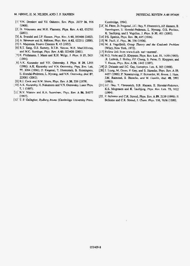
M. FBRRE, H. M. NILSEN, AND J. P. HANSEN
[l] Y.N. Demkov and V.I. Osherov, Sov. Phys. JETP 26, 916
[2] D. Vrinceanu and M.R. Flannery, Phys. Rev. A 63, 032701
[3] A. Svandal and J.P. Hansen, Phys. Rev. A 65, 033406 (2002). 141 A. Sbrensen and K. Mblmer, Phys. Rev. A 62, 022311 (2000). [5 ] E. Majorana, Nuovo Cimento 9, 43 (1932). [6] R.T. Sang, G.S. Summy, B.T.H. Varcoe, W.R. MacGillivray,
and M.C. Standage, Phys. Rev. A 63, 023408 (2001). [7] E. Flothmann, J. Mann and K.H. Welge, J. Phys. B 27, 2821
(1994). [8] A.K. Kazansky and V.N. Ostrovsky, J. Phys. B 29, L855
(1996); A.K. Kazansky and V.N. Ostrovsky, Phys. Rev. Lett. 77, 3094 (1996); D. Fregenal, T. Ehrenreich, B. Henningsen, E. Horsda-Pedersen, L. Nyvang, and V.N. Ostrovsky, ibid. 87, 223001 (2002).
(1968).
(200 I).
[9] R.J. Cook and B.W. Shore, Phys. Rev. A 20, 539 (1979). [lo] A.K. Kazansky, H. Nakamura and V.N. Ostrovsky, Laser Phys.
[ll] N.V. Vitanov and K.A. Suominen, Phys. Rev. A 56, R4377
1121 T. F. Gallagher, Rydberg A t o m (Cambridge University Press,
7, 1 (1997).
(1997).
PHYSICAL REVIEW A 65 053409
Cambridge, 1994). [13] M. Fbrre, D. Fregenal, J.C. Day, T. Ehrenreich, J.P. Hansen, B.
Henningsen, E. Horsdal-Pedersen, L. Nyvang, O.E. Povlsen, K. Taulbjerg, and I. Vogelius, J. Phys. B 35, 401 (2002).
[14] P.S. Epstein, Phys. Rev. 28, 695 (1926). [15] W. Pauli, Z. Phys. 36, 336 (1926). [16] M. J. Engelfield, Group Theory and the Coulomb Problem
1171 Follow link from www.fi.uib. no/-moxtenf . [18] R.G. Hulet and D. Kleppner, Phys. Rev. Lett. 51, 1430 (1983);
.R. Lutwak, J. Holley, P.P. Chang, S. Paine, D. Kleppner, and T. Ducas, Phys. Rev. A 56, 1443 (1997).
(Wiley, New York, 1972).
[19] D. Delande and J.C. Gay, Europhys. Lett. 5, 303 (1988). [20] J. Liang, M. Gross, P. Goy, and S. Haroche, Phys. Rev. A 33,
4437 (1986); P. Nussenzveig, F. Bemardot, M. Brune, J. Hare, J.M. Raimond, S. Haroche, and W. Gawlik, ibid. 48, 3991 (1993).
[21] J.C. Day, T. Ehrenreich, S.B. Hansen, E. Horsdal-Pedersen, K.S. Mogensen and K. Taulbjerg, Phys. Rev. Lett. 72, 1612 (1994).
[22] P. Bellomo and C.R. Stroud, Phys. Rev. A 59, 2139 (1999); P. Bellomo and C.R. Stroud, J. Chem. Phys. 110, 7658 (1999).
053409-8

I - .* . . .
Paper 4
Selective-field-ionization dynamics of a lithium ?n = 2 Rydberg state: Landau- Zener model versus quantal approach
hl. Forre and J. P. Hansen
Phy. Rev. A 67. 053402 (2003)
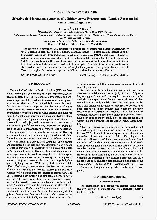
PHYSICAL REVIEW A 67, 053402 (2003)
Selective-field-ionization dynamics of a lithium m = 2 Rydberg state: Landau-Zener model versus quantal approach
M. FQrre’32 and J. P. Hansen3 ’Department of Physics, University of Bergen, All&$. 55. N-5007, Norway
‘Laboratoire de Chimie Physique-Matikre et Rayonnement, Universitk Pierre et Mane Curie, 11, rue Pierre et Mane Curie, 75231 Paris Cedex OS, France
3Deparhnent of Physics, Po. 7800, University of Bergen, Norway (Received 10 February 2003; published 28 May 2003)
The selective-field-ionization (SFI) dynamics of a Rydberg state of lithium with magnetic quantum number m = 2 is studied in detail based on two different theoretical models: (1) a close coupling integration of the Schrijdinger equation and (2) the multichannel (incoherent) Landau-Zener (MLZ) model. The m = 2 states are particularly interesting, since they define a border zone between fully adiabatic ( m = 0 , l ) and fully diabatic (m>2) ionization dynamics. Both sets of calculations are performed up to, and above, the classical ionization limit. It is found that the MLZ model is excellent in the description of the fully diabatic dynamics while certain discrepancies between the time dependent quantal amplitudes appear when the dynamics become involved. Thus, in th is region, the analysis of experimental SFI spectra should be performed with care.
DO1 10.1103/PhysRevA.67.053402
I. INTRODUCTION
The method of selective-field ionization (SFI) has been studied thoroughly both theoretically and experimentally for several decades [1,2]. SFI methods are now mature and well known experimental procedures to measure detailed quantal state-to-state dynamics. The method is in particular useful for characterization of the population distribution of highly excited states in atoms and molecules. Intrashell dynamics of hydrogenlike Rydberg atoms in weak electric and magnetic fields [3,4], collisions between slow ions and Rydberg atoms 1.51, manipulation of quantum entanglement of atoms and photons in a cavity [6], and, more recently, observation of cold antihydrogen [7] are examples where the SFI technique has been used to characterize the Rydberg level population.
The principle of SFI is simply to expose the Rydberg atoms to a time-dependent increasing (ramped) electric field. Depending on the specific state, atoms in different quantum states will ionize at different field strengths. The electrons are accelerated by the field and hit a detector, which produce a signal. In this way a SFI spectrum as a function of the field (time) is plotted. In alkali Rydberg atoms, which are used in most experiments, the level crossings between low angular momentum states show avoided crossings in the region of inter-n mixing in contrast to the exact crossings in hydro- genic Rydberg atoms. With a typical ramping field (400- 1000 V/cm/ps) one usually considers I rn I = 0,l states of lithium to traverse the avoided crossings adiabatically, whereas lrnlP2 states pass the crossings diabatically. The SFI technique does usually not distinguish between m = 0 and rn = ? 1 states since they for all practical purposes Lraverse the avoided crossings adiabatically with the field ramps specified above, and field ionize at the classical ion- ization limit E-( 16n4)-’ a.u. This is sometimes referred to as adiabatic field ionization. But the technique clearly distin- guishes these states from rn>2 states, which traverse the crossings plainly diabatically and field ionize at the hydro-
PACS number(s): 32.80.Rm, 33.80.Rv, 33.60.-q
1050-2947/2003/67(5)/053402(7)/$20.00 67 053402-1
genic ionization limit (the nonclassical ionization limit), at much higher fields.
Recently, it has been pointed out that I m 1 = 2 states may also have an adiabatic component [4,8]. A “mixed” dynam- ics, as suggested here., will then require particular care in the analysis of the spectra and from a theoretical point of view the validity of simple models should be investigated in de- tail. Most theoretical attempts to study the SFI process have been carried out in the extreme case where the evolution becomes purely diabatic or adiabatic after a few avoided crossings. However, a few more thorough theoretical works have been done on the system [2,8,9], but they are all treated within the multichannel LandauZener ( M U ) approxima- tion.
The main purpose of this paper is to carry out a first detailed study of the dynamics of various m = 2 states of the Li (n = 25) Stark manifold when exposed to a realistic time- dependent increasing electric field. The degree of adiabaticitykliabaticity of these states is studied in detail and the results of the MLZ model are confronted with ab initio time-dependent quantal calculations. The behavior of such a complex quantum system and its route from a localized bound state towards breakup is interesting in its own right. However, in the present study the main motivation is to in- vestigate the dynamics of the transition zone between fully diabatic and fully adiabatic field ionization in relation to the interpretation of experiments [4]. Atomic units ( f i=e=rn, = 1) are used throughout except where units are given ex- plicitly.
II. THEORETICAL MODELS
A. Numerical model
The Hamiltonian of a pseudo-one-electron alkali-metal Rydberg atom in a homogeneous time-dependent electric field is given by
H = H o + V,( r ) + F,( t ) z ,
02003 The American Physical Society
M. FORRE AND J. P. HANSEN
where Ho= - V2/2- llr and V c ( r ) are the unperturbed hy- drogenic Hamiltonian and the perturbation due to the core, respectively. Spin-orbit effects may safely be ignored for the lighter Rydberg atoms, Le., for H, Li, and Na [1,10].
The core potential is set up by the induced correction to the Coulomb potential resulting from the interaction between the excited electron and the inner shell electrons. The pertur- bation is assumed to be significant for low angular momen- tum states only, since high angular momentum states are pro- hibited from penetration into the core region. In the core region the effect on the Rydberg electron is a more strongly attractive force, which mainly accounts for a positive phase shift of the hydrogenic radial functions [Il l . For highly ex- cited states of the field free Hamiltonian the radial functions outside the core are accurately described by the Bates- Damgaard-type quantum defect radial wave functions [12]. These functions are basically hydrogenic wave functions with the nodes phase shifted inward. The field free energy levels are modified according to
PHYSICAL REVIEW A 67, 053402 (2003)
part of the matrix element is straightforward calculated by using the Wigner-Eckart theorem for spherical harmonics [17], with the well-known result,
where a,,, are the so-called quantum defects, which break the degeneracy of the energy levels. For high n values the quan- tum defects become almost energy independent [1,13], and for the Rydberg states of lithium the nonvanishing quantum defects take the values [l] 6,=0.3995, Sp=0.0472, 6, =0.0021, and S,=0.0003.
Because of spherical symmetry of the core potential the wave function may be expanded in hydrogenlike wave func- tions in the region outside the core [4,10,14]. In the present work it is more suitable to choose an expansion in ordinary hydrogenic wave functions,
q ( r , t ) = X c n t m ( t ) ~ n L r ) y ~ r n ( e,+), (3) nlm
to take advantage of known procedures for analytic calcula- tion of matrix elements [15]. The wave function expansion is inserted into the Schrodinger equation i ( d / d t ) V ( r , t ) = H Q ( r , t ) , leading to a first-order coupled matrix system of equations for the expansion coefficients, cnlm(t) ,
d , dr i - c = M( t);. (4)
Within the first-order perturbation theory the core induces couplings [1,16],
between the hydrogen nlm spherical states with the same I and m quantum numbers. This approximation is excellent for the highly excited states of interest in the present work.
The nonvanishing matrix elements of the z operator fol- low within the dipole approximation the selection rules A I = 2 1, Am=O. Since z= r cos 6= \1(4?r/3)rYIo, the angular
( h l c o s 812- 1m)=
The radial part of the dipole matrix elements, (nllrln'l - l ) , is either found by direct numerical integration or is given in terms of the hypergeometric function F ( a , b , c , d ) [ 181,
(- 1yI- l J" + 1 )!(nr + I - 1 )! (nllrln'Z- 1 ) = -
4 0 - 1 ) ! (n-z-l)!(n'-Z)!
-n+Z+l,-n'+Z,2Z,--
-[ -n+l-1,-nr+I,21,
The formula is valid for n # n ' . Within one principal shell the expression is in particular simple,
Since the core potential exclusively couples states of equal m quantum numbers due to the spherical symmetry of the po- tential, and since the z operator obeys the Am = 0 selection rule, it is sufficient to expand the Schrodinger equation on a basis set consisting only of m states identical to the initial m values.
B. Analytical multichannel Landau-Zener model
The dynamics will be compared with an incoherent MLZ model[19].LetP(r)=[Pl(t),P2(t), . . . ,P, , ( t ) , . . . ] bethe probability distributions on the eigenstates at each time t. As a bookkeeping device the probability corresponding to each state is chosen to be ordered with increasing energy in P , i.e., the state with lowest energy always comes first in the vector. We use the hydrogenic parabolic states {Innln2m)} as a basis set and calculate the couplings by formula [l],
- 4 n3n'3
X- $- (n ' lm /n ' n ;n;m).
(9)
053402-2

The crossing times I , (Le., lhe times where the diabatic en- ergy cum‘us cross) for each Landmdzner crossing, and thc infnrmation abnui which twurll S ~ C H that CMRS al cach I, mc fiwnd Fnim the expression for the eigenciiwgiea within sectmdader pe~turht ion theory in the electric held [ I XI.
X I I7n’- >!/I 1 - 1 1 1 ) ’ - 9t/i2+ 191.
(10)
where y is the slcw rate ( s lopj of the cleutric ticld. Let Pi (P , ) and P,! (1’;) be the population probability of the adia- t u t k si& i (j) {=Fore and after the crossing v i n t is passed. rcspcc~ivcly. The Landau-Zcncr mode1 thcn gives
where P, , in the two-qtate Landau-Zener prrhibiliv for 3 diahatic pa5age (nonadiabatic hnsition) thniugh he cnrss- ing points. The two-stille prdmbility is g k n by [20],
112)
w l w t u is the absoiute difference in slope of the two diabatic eigeiimergy cuwes at thc ciussiiig [calculalcd horn the de- rivarivc of Eq. (IO)], and d i.c tlic criupling fi-om Eq. (9). Wilhin the first-urder pcrturhation theory in the lield knih t i
and d arc C O ~ S ~ J F I I . i.e.. an alinusr ideal situation for applica- tion uf the Landau-Zener mudel.
C. Iunization probability
Since our haw wf only iiicludcs h u n d sta~cs, rhc flunieri- caI soluiion of the Sctidinger quation does not auiornati- caIly give any information about the held htrength needed tu ionize the states. To obtain an estimate of the ionization prrhability we use h e serniempiricnl frwnula for the ioniza- tion rate of hydrogen derived by Damburp iind Kol0r;ov [21].
where R { - 2 W)?F and fi- is the clectric field. The Stark enegy U’ is cnlcuhted hy a p t u r h t i o t i c x p s i o n up tu toiidh order in the field 1221. Thcy chim that rhiq forinuls is mrrcct within a precision of a few pcrccnt for tht. threshold field Tor ionimtiun of LIK diffewnt states. This accuracy is more than sufficient for the present analysis. We have tested tbc formula on the data in Fig. 4 of Rohicheirux. Wesdmp, and Noordaiti [Z]. and i t wccessfully reproduced the p)silirm of all tk pcakks it1 [he SFI spctrum calculated in Lha! work.
Assiuning a onc way exponential h a y into the con- tinuum the survival pmixhility ukes t k form
PHYSICAI. REVIEW h67. 053402 (2003)
Tht electric field is rarnpd tinearly rmni a11 iiiilial Lield
F(i )==F, ,+ yi . ( i 5 )
whcre f-o I F chosen arbitrady hut wcak enough LO avoid intershell mixing. i.c, F4j< I/3n5. For the present field ramps the spin-orbit cffcctn at x r o field m ignorable [I], hence F , , can likely be put to m o . Four ditfcrciit values of the ramp, y= I (#),42LIO(K1, and I0,IW Vlcmlps. have h e n tried. These values cormpond to relatively slow to ultrafast witching with respect to experimental applicahlc rangcs. For field strengths less than 1IH)C) V k m and with lhc: rnirlnl population distrihutirm within the n = 25 manihld, the en- ergy spxtrum of thc system iippears to be sufhcicntly con- verged for a basis XI including the Inanifdds From ti = 21 10 n=40. I t may seem suangc and even wrong IO solve this huge and complex system numericnliy by using B h i s set cinly including hmnd hydrogenic slaw.: since the eigenstates that decxaw i r i energy with increasing held. in [act, are con- tinuum stares immediately aftsr the ticld i . ~ turned on. What saves us is that. despite being continuum htatcs. thcy h h a v e ;IS bound states all the way up l o the dassical imsiatioii limit. Le.. in the cncrgy region [23],
(Id)
Thus. une shuuld be aware that the calculation< may tk, lcqs accurate in the region close tu the classical ionization l imit . For burllicr details on the discushion nf the applicability uf using a uunuated ha& bet see Ref. [lo].
Figurt 1 shows thc qumrurn dynamics of the parakilic states l i ~ n , t r ~ t ~ ~ ) = 125 23 0 1 ) ;md I n r r l n p n ) = ~ Z 5 21 0 3 ) for a 421 V/c i i~ /ps licid mmp. It is clearly seen h i t the ni = 3 state follows a curnplekly diahatic de\cIopmcnt, wherras the timc development o f the m = 1 stale i s plainly adiahtic. In the latter cxw the population spreads out to a hand nl atale<. The rormatiiin of a nmow band caii be UII-
derstood from the Landau-Zener model as P,, rapidly l‘alls to mu in thc regiori o w t d c the adiabatic state in the center 01’ the band. All stares in the bmnd will imix near Ihe c h - sical ionization limit, whew&< the state 175 21 0 ?} irmizrs ar the hydrogenic ioniration limit at w r y strong fields.
Now turning to the V I = ? case wc display in Fig. 2 the time development of the initial 15 220 2 ) sfah: linr thc same parameters ;I\ in Fig. I . Here, a inixed evolution, which is neither diahalic tior adiabatic, is ohscrved. The hrst crossing< wilh the *tates hetonging 10 tbc principal sheli above however. traversed curnpletely diabaticdlly. Af, ncw rcd cutes kom ahow are reached d increases, whereas ti decreases, i.u.. P,, dccwws 2nd thc dynamics become more and more adiabatic. At C F O S S ~ ~ ~ S with ihe .\late 12h8 152). the adia- batic leakagc heconic< visible (as srcen) in the figure As Ihu n = 27 levels cnter the dynamics, giving (he l int triple CTT)L<-

M. 1.RKRI’ ANT> I. P. HANSEN I’HYSICAI. REVILW A67.053402 (Zoos)
Electric Field (Vlcrn)
ings. thew is a sigiiiticant sharing of prnbbiliiirs helwt-en thc adiabatic and diabalic directinns for each new crwing Ishuwn in red). The tinic the various paths wach their iun- imtion iimit vuies and as a result an e x p i m e n ~ u l SFI spw- trtlm may contain a broad distribution.
We LICE the notation oi’ Refs. (1,181 and detine the smtcs dien: the elccucm i s most IikcIy h a t e d on Ihe sidc of the :itom away hlin the saddle point as blue SKIE~, and Ihc stater wirli the rlectrnn localed adjacent tl) the .;a&llc. point as rcd slaies. 31uc and red slates arc characterized hy Ihc cigunm- ergy CUTVCS in the Stork yxectrum going upward and down- ward. iwpcstivcly. Rougldy speahuig cine cxpccrc Lhe reed states fn ionize near the clawicnl i o n i h n n limit. whercas thu blue states ionize a i much higher field. BIIL in gcncral, this suMiuisiun into two groups is not miskiory. as &IC
dccay mtz function, F.q. (13). i E n continunus function rm { I ? .
f
0.95
0.9 .* 10.85 e n
0.8
0.75
0.7
0 200 4m 600 Elecalc Fleld (Wm)
klG. 3. A plot of Phlne P,, , and Pdrahrrrlc for the parabolic state 125 220 2 ) in a 121 V l c d p s field ramp.
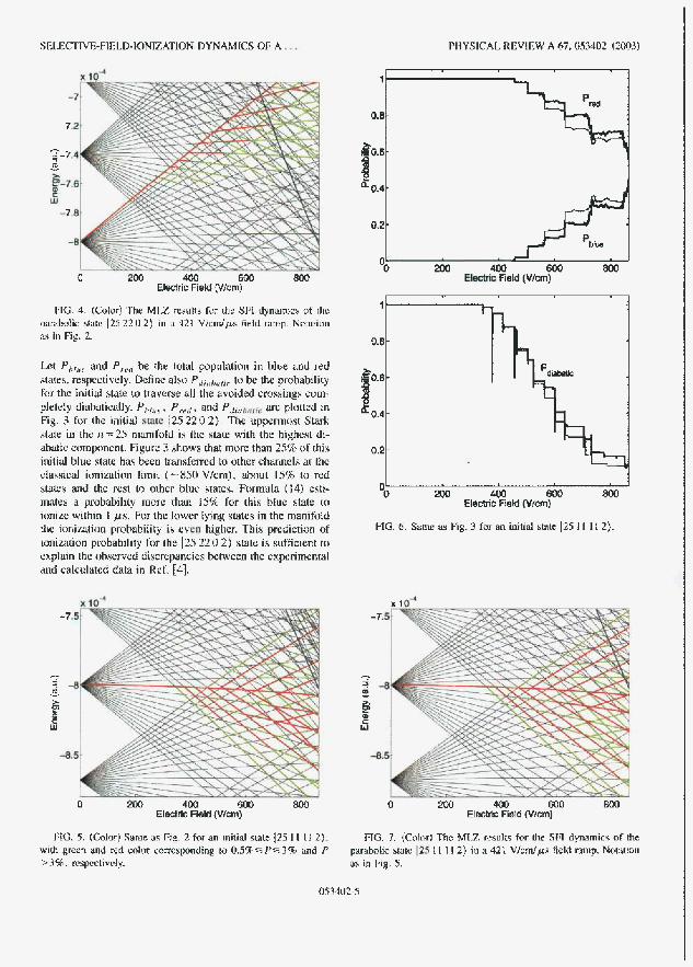
SEL.ECTIVE-FlEI.D-IONIZATION DYNAMICS Ofi A . . .
0.8
g0.6
1 0.4
0.2
PHYSICAL. REVIEW A 67,0.13302 (330.3)
-
-
*
-
ht Phlarr and Prrd be the total population in blue and red stales. rcspcctivcly. Define a h ? Pdlt,,,,2,,,. to be the probability for the inilia1 m t e to traverse all Khe avoided crossings cum- pletely dIab;l~ically. Phl ,6e , P r P d , and PSIuBAIis are plotted in Fig. 3 for the initial s t a ~ I25 220 2 ) The uppxniost Stark state in the 11-25 nianifold is the shte with the highcsi di- a h t i c componeni. Figure 3 ahows that more itian 25% of this initial blue state has been transferred to other channels ai B c classical innizatiiiii h i t { 2.- 850 Vlcm). a h u i I5%, 10 red < t a k s and the rest tn other blur: states. Frwinuln (14) csti- mates a probability more thm 15% For ihis bIuc state to iriniLc within I ps. For the lower lying states in the nianifuld the ionimion probability is even higher. This przdictiun of ioni~xiori probability for the 12.5 22 0 2) !&le i < sufficient to explain the ohserved discrepancies trehvcen h e experirnriital aiid calculated data in Kef. [4].
1
9.8
t": IL 0.4
0.2
11 10" -76
- ; - a - $ w
4.6
0 2w 400 MK) Electnc Weld (Wcm)
-
-
3 200 400 600 800 Electric Field (Wan)

h L m A N D J . p . H A N s w
p - n P i . ‘ I
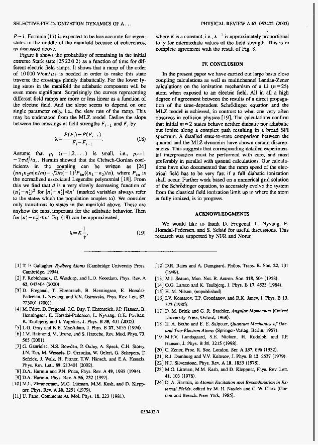
SELECTIVEFIELD-IONIZATION DYNAMICS OF A . . .
P - 1. Formula (17) is expected to be less accurate for eigen- states in the middle of the manifold because of coherences, as discussed above.
Figure 8 shows the probability of remaining in the initial extreme Stark state 125 22 0 2 ) as a function of time for dif- ferent electric field ramps. It shows that a ramp of the order of 10000 V/cm/ps is needed in order to make this state traverse the crossings plainly diabatically. For the lower ly- ing states in the manifold the adiabatic component will be even more significant. Surprisingly the curves representing different field ramps are more or less linear as a function of the electric field. And the slope seems to depend on one single parameter only, i.e., the slew rate of the ramp. This may be understood from the MLZ model. Define the slope between the crossings at field strengths F i - and Fi by
Assume that pi ( i = 1,2, . . . ) is small, i.e., p i = l - 2 ~ r d : / a , . Harmin showed that the Clebsch-Gordan coef- ficients in the coupling can be written as [24] (nnln2mlnZm)= @( - l)'P,,((nl-n2)/n), where P,, is the normalized associated Legendre polynomial [18]. From this we find that d is a very slowly decreasing function of (n;-n;)' for In;-n;l<n' (marked variables always refer to the states which the population couples to). We consider only transitions to states in the manifold above. These are anyhow the most important for the adiabatic behavior. Then for In;-nal<n' Q. (18) can be approximated,
1 X-K-,
Y
PHYSICAL REVIEW A 67,053402 (2003)
where K is a constant, i.e., X - ' is approximately proportional to y for intermediate values of the field strength. This is in complete agreement with the result of Fig. 8.
IV. CONCLUSION
In the present paper we have carried out large basis close coupling calculations as well as multichannel Landau-Zener calculations on the ionization mechanism of a Li (n = 25) atom when exposed to an electric field. All in all a high degree of agreement between the results of a direct propaga- tion of the time-dependent Schrodinger equation and the MLZ model is achieved, in contrast to what one very often observes in collision physics [ 191. The calculations confirm that initial rn = 2 states behave neither diabatic nor adiabatic but ionize along a complex path resulting in a broad SFI spectrum. A detailed state-to-state comparison between the quantal and the M U dynamics have shown certain discrep- ancies. This suggests that corresponding detailed experimen- tal interpretation must be performed with care, and most preferably in parallel with quantal calculations. Our calcula- tions have also documented that the ramp speed of the elec- trical field has to be very fast if a full diabatic ionization shall occur. Further work based on a numerical grid solution of the Schriidinger equation, to accurately evolve the system from the classical field ionization limit up to where the atom is fully ionized, is in progress.
ACKNOWLEDGMENTS
We would like to thank D. Fregenal, L. Nyvang, E. Horsdal-Pedersen, and S. Selstd for useful discussions. This research was supported by NFR and Nom.
[l] T. F. Gallagher, Rydberg A t o m (Cambridge University Press, Cambridge, 1994).
[2] F. Robicheaux, C. Wesdorp, and L.D. Noordam, Phys. Rev. A 62, 043404 (2000).
[3] D. Fregenal, T. Ehrenreich, B. Henningsen, E. Horsdal- Pedersen, L. Nyvang, and V.N. Ostrovsky, Phys. Rev. Lett. 87, 223001 (2001).
[4] M. FBrre, D. Fregenal, J.C. Day, T. Ehrenreich, J.P. Hansen, B. Henningsen, E. Horsdal-Pedersen, L. Nyvang, O.E. Povlsen, K. Taulbjerg, and I. Vogelius, J. Phys. B 35,401 (2002).
[5] L.G. Gray and K.B. MacAdam, J. Phys. B 27, 3055 (1994). [6] J.M. Raimond, M. Brune, and S. Haroche, Rev. Mod. Phys. 73,
565 (2001). [7] G. Gabrielse, N.S. Bowden, P. Oxley, A. Speck, C.H. Stony,
J.N. Tan, M. Wessels, D. Grzonka, W. Oelert, G. Schepers, T. Sefzick, J. Walz, H. Pitmer, T.W. Hinsch, and E.A. Hessels, Phys. Rev. Lett. 89, 213401 (2002).
[8] D.A. Harmin and P.N. Price, Phys. Rev. A 49, 1933 (1994). [9] D.A. Harmin, Pbys. Rev. A 56, 232 (1997). [lo] M.L. Zimmerman, M.G. L iman , M.M. Kash, and D. Klepp-
[ll] U. Fano, Comments At. Mol. Phys. 10, 223 (1981). ner, Phys. Rev. A 20, 2251 (1979).
1121 D.R. Bates and A. Damgaard, Philos. Trans. R. Soc. 22, 101
[13] M.J. Seaton, Mon. Not. R. Astron. SOC. 118, 504 (1958). [I41 O.G. Larsen and K. Taulbjerg, J. Phys. B 17,4523 (1984). [15] H. M. Nilsen, (unpublished). [16] I.V. Komarov, T.P. Grozdanov, and R.K. Janev, J. Pbys. B 13,
573 (1980). [17] D. M. Brink and G. R. Satchler, Angular Momentum (Oxford
University Press, Oxford, 1968). [18] H. A. Bethe and E. E. Salpeter, Qwultum Mechanics of One-
and Two-Electron A t o m (Springer-Verlag, Berlin, 1957). [19] M.F.V. Lundsgaard, S.E. Nielsen, H. Rudolph, and J.P.
Hansen, J. Phys. B 31, 3215 (1998). [20] C. Zener, Roc. R. Soc. London, Ser. A 137, 696 (1932). [21] R.J. Damburg and V.V. Kolosov, J. Phys. B 12, 2637 (1979). [22] H.J. Silverstone, Phys. Rev. A 18, 1853 (1978). [23] M.G. L i m a n , M.M. Kash, and D. Kleppner, Phys. Rev. Lett.
41, 103 (1978). [24] D. A. Hannin, in Atomic Excitafion and Recombination in Ex-
ternal Fields, edited by M. H. Nayfeh and C. W. Clark (Gor- don and Breach, New York, 1985).
(1 949).
053402-7
Paper 5
Multiphoton intrashell resonances in Rydberg atoms: Bloch-Siegert shifts and widths
D. Fregcnal, E. Horsdal-l’edersen. L. B. Madsen. hl. Forrc. J. 1’. Hanxti * , t r d 1’. N. .I . . . Ostrpvglry
;J :*. . ,, I ‘i .i 14 -* >-a! - . ir-. I L~~ sd* .I 4 I k l - b t - 4 , PhyT. Rev A’69, 031101(R) (2004)

PHYSICAL REVIEW A 69, 031401(K) (2004)
Multiphoton intrashell resonances in Rydberg atoms: Bloch-Siegert shifts and widths
D. Fregenal, E. Horsdal-Pedersen, and L. B. Madsen Department of Physics and Astronomy, Aarhus University, 8000 Aarhus C, Denmark
M. Feirre and J. P. Hansen Department of Physics, University of Bergen, 5007 Bergen, Norway
V. N. Ostrovsky Fock institute of Physics, University of St. Petersburg, 198904 St. Petersburg, Russia
(Received 1 December 2003; published 15 March 2004)
We measure for the first time, to our knowledge, N-photon intrashell resonances, widths, and Bloch-Siegert shifts up to N=23. Rydberg atoms of Li (n=25) in a rotating electric field and a static, in-plane electric or magnetic field are used. The measurements, in conjunction with theoretical estimates, precisely determine the Characteristics of the resonances (shifts and widths) and their dependence on the strength of the rotating field.
DOI: 10.1 103/€'hysRevA.69.031401
Nonperturbative and high-order nonlinear processes con- stantly challenge our understanding of the fundamental photon-atom interaction [I]. Bound-bound transitions where many photons are needed to bridge the energy gap between the states is one example. In the theoretical description, the photon-atom Hamiltonian can be split into right- and left- hand circularly polarized components. One of these shows resonance behavior while the other gives rise to ac Stark shifts of upper and lower energy levels and a shift of the resonance position known as the Bloch-Siegert (BS) shift [2].
The BS shift is of essential importance in a broad variety of different branches of physics. For a long time it has been a subject of concern in nuclear magnetic resonance [3,4] which besides numerous biological and medical applications is the only realization of a (small) quantum processor [5]. Furthermore, BS shifts may play a crucial role in electron paramagnetic resonance spectroscopy [6], light emission by laser-driven atoms [7-91, including Raman lines [IO], and polychromatic fields [Ill. BS shifts were observed in elec- tromagnetically induced transparency [12], included into theory of lasers [13], micromasers [14], as well as quantum optics [15-171. More recently the importance of BS shifts was pointed out in the theory of multiphoton far-infrared interband transitions in condensed matter [18] and in theory of continuously driven dissipative solid-state qubits [I91 within quantum information.
Measurements of BS shifts for the absorption of one or three photons were performed some time ago [20], but higher photon numbers N were not seen. Similar landmarks were achieved in a completely different physical realization within classical electrodynamics when interaction of two modes with orthogonal polarizations was considered in an optical ring resonator [21]. For intershell transitions in Ryd- berg atoms (gigahertz domain of driving frequency a) reso- nances with N up to 28 were observed but the shifts were not detected [22,23]. The effect is proportional to W2, hence it may become large for inrrushell transitions in the megahertz domain. Multiphoton intrashell resonances were previously observed only indirectly in microwave ionization spectra
PACS number(s): 32.60.+i, 32.80.h
which showed resonant multiphoton enhancement when the dc Stark splitting of the shell is close to an integer number of field quanta NO (NC5) [24], but BS shifts were not exposed. While microwave ionization is a complicated process which is difficult to understand in full detail [25], the intrashell resonance dynamics responsible for the observed resonances may be treated analytically with very few limita- tions [26].
In this work, we demonstrate that intrashell transitions in carefully prepared Rydberg atoms offer a unique possibility for studying multiphoton processes of high order in a con- trollable way. The unambiguous identification of high-N shifted and broadened resonances poses a special challenge which is met by carefully tracing the evolution of resonances with increasing field strength and with the help of nonpertur- bative calculations. A special field configuration with ac components both along and perpendicular to the dc field was employed to enhance the resonance effect.
For the pure Coulomb problem, the stationary states are described by two independent pseudospins of constant mag- nitude f(n- 1) quantized in two independent directions. Each of the two pseudospins can be decomposed into n - 1 inde- pendent pseudospin-; components. The intrashell dynamics of hydrogenic Rydberg states in time-dependent external electromagnetic fields may thus be reduced to the dynamics of two of these independent spin-; particles in two indepen- dent magnetic fields [27]. This description is very attractive due to its simplicity and accuracy. It was used recently in analysis of state control by external fields [28], experimental data on microwave ionization resonances [26], adiabatic or near-adiabatic state transformations [29-321, and intrashell single-photon resonances for circularly polarized fields [33]. It is used here to derive analytical expressions for positions and widths of intrashell multiphoton resonances. The general problem of laser excitation of atoms or molecules can in principle be treated by perturbation theory, but it becomes intractable even for relatively small photon orders. By con- trast, our analytical results do not have this restriction, and the present comparison with experimental data provides fur-
1050-2947/2004/69(3)/031401(4)/$22.50 69 031401-1 632004 The American Physical Society

FRESENAL et al.
#
PHYSICAL REVIEW A 69, 031401(R) (2004)
FIG. 1. Hydrogenic energy levels in electric (left) and magnetic (right) fields, respectively, where m is the magnetic-field quantum number. Spectral positions of initial circular Stark (CS) and Zeeman (CZ) states are marked. Multiphoton quanta NCk connect neighbor- ing states.
ther strong evidence for the validity of the pseudospin for- malism.
The experimental arrangement was described in Ref. [29]. In short, a Stark state of maximum polarization [a parabolic state with quantumnumbers /nl,n2,m}=/24,0,0} or a coher- ent elliptic state (CES) of eccentricity e= 1 [32]] was formed by laser excitation in a strong electric field (145 V/cm), then transformed by the adiabatic crossed-field method (ACFM) into a nearly circular CES (e = 0) stabilized by a static field [32], and finally exposed to a homogeneous, rotating electric field of frequency n and amplitude Fn for a time T. The rotation vector of the field, fi, was perpendicular to the static field which in turn was perpendicular to the orbital plane of the circular state. The static electric and magnetic fields ($ and E , respectively) produced a constant Stark-Zeeman split- ting of the shell described by frequencies a,= I&L+;~I, with I&= i n $ and GL= $B’ [27]. The Stark frequency of the rotat- ing field is wn=%nFfi. The parameters n/27r, on/27r, and w J 2 ~ were varied within the intervals 12-30MHz, 0-200 MHz, and 30-370 MHz, respectively. These fre- quencies are much smaller than the orbital frequency of the n=25 shell (421 GHz). The transformation was completed in <10 ps and the exposure to the rotating field lasted for T = 2 ps with switching times of a few field cycles [29]. A ramped electric field of slew rate 420 (V/cm)/ps triggered about 50 ps after laser excitation was used to analyze the final distribution of Rydberg states by selective field ioniza- tion (SFI) [22], and to determine the probability that the Rydberg atom remained in the original state, i.e., responded adiabatically to the rotating field.
In one version of the ACFM, Fi= 145 Vlcm was switched off in the presence of a weak magnetic field to produce a CES of e=O oriented relative to B’ with spherical quantum numbers ln,C,m),=125,24,24),. We call this a circularzee- man (CZ) state. It is nondegenerate and at the top of the n manifold (Fig. 1). In another version [29,30] the electric field rotated while it approached a constant final value Fr perpen- dicular to B’. This was arranged such that 3n$(t)=B’ at an intermediate time t = t , when sharp avoided crossings of quasienergy curves were encountered and purely diabatic transitions brought the CES into a new type of CES. As $ subsequently rotated and increased towards gr this new CES
f
f
FIG. 2 Mulhphoton resonances vs frequency Ck/2rr for (almost) cmular Stark states. F=6 V/cm (300 MHz), B=15 G (21.4 MHz), F I B , o+= 0- = 300 MHz, and e=0.07. Curves for different on are displaced vemcally for clanty. Photon numbers N are given next to each curve and unshlfted resonance positions are mmcated. The resonances N=21-23 are split (see text).
developed into a circular Stark (CS) state quantized along the direction of Ff, Le., ln,e,rn)F=125,24,24)F. The eigenen- ergy of the CS state is highly degenerate and located in the middle of the n manifold (Fig. 1).
The nearest-neighboring states of the initial CZ or CS state could not be distinguished by the SFI so only apparent adiabatic probabilities P:La were obtained. In the pseudospin description, transition to an adjacent state corresponds to a flip of one of the constituent spins. Therefore, not only one but at least two spin flips were required for having a detect- able change of the SFI spectra.
We first measured the dependence of Pi$, on n for vari- ous splittings w(w+=w-) and strengths wa to have an over- view of the resonances, and then in detail to determine BS shifts and resonance widths of selected resonances. The over- view is shown in Fig. 2 for initial CS states. Similar results were seen for initial CZ states, so the resonance structures do not depend on location within the manifold or degree of degeneracy. Some resonances were split (N=21,22, and 23). This happened when B’ and $ were not exactly perpendicular. One component corresponds to w+ and the other to 0-. The splitting could always be eliminated by adjusting the direc- tion of F or E . It was left in one case to expose the phenom- enon. The resonance frequency a,, is clearly shifted relative to n = w / N and it depends on wn. The correct assignment of the high photon numbers was made difficult by this shift and required careful measurements of n,,(wn) for many N.
For the theoretical description, an explicitly time- dependent multicycle LandauZener model ( M E ) [34] as well as an adiabatic time-independent Floquet theory (AD) [35,36] have been developed. The spin-flip probability p(n) is generally oscillatory with a Lorentzian envelope function approaching one at resonance unless q=on/w is very small. For the BS shift (N> 1) of the resonances both theories give
*
+ f
03 140 1-2
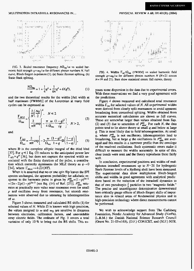
MULTIPHOTON INTRASHELL RESONANCES IN., .
FIG. 3. Scaled resonance frequency N f l , / o vs scaled har- monic field strength q= onlo for dlfferent photon numbers N. Full curve, Bloch-Siegen expression (1). (a) StahC Zeeman splimng. (b) Statlc Stark splittmg.
NaES 1 1 -- -1+-qZ+-q4+0(q6), w 4 64
and the two theoretical results for the widths [full width at half maximum (FWHM)] of the Lorentzian at many field cycles can be expressed as
and
where D is the complete elliptic integral of the third kind [37]. For qe 1 Eq. (3) reduces to the anticipated power law rADafl [36], but does not capture the spectral width as- sociated with the finite duration of the pulse, a contribu- tion which correctly dominates the MLZ theory as q+O [34], where TMLz+4fi/(NT).
When it is assumed that no or one spin flip leaves the SFI spectra unchanged, the apparent probability for adiabatic re- sponse to the harmonic pulse is given by P&=(l -p)%-* + ( 2 n - 2 ) ~ ( l - p ) & - ~ [see Eq. (14) of Ref. [27]]. P s a satu- rates at practically zero value near resonance even for small p and oscillates away from resonance, but smooth reso- nances were observed due to smearing by inhomogeneities of 0.
Figure 3 shows measured and calculated BS shifts (1) for selected values of N. While is known with high precision, the values assigned to w and on are sensitive to distances between electrodes, calibration factors, and unavoidable stray electric fields. The ordinate of Fig. 3 covers a total variation of only 10 % to bring out the BS shifts. This ex-
PHYSICAL REVIEW A 69, 031401(R) (2004)
, -. .
, ,
FIG. 4. Widths rmt/flms (FWHM) vs scaled harmonic field strength q = o n / w for different photon numbers N (N=21 covers N= 19 and 21). Bars show staustical errors; full curves, theory.
poses some dispersion in the data due to experimental errors. With these reservations we find a very good agreement with the predictions.
Figure 4 shows measured and calculated total resonance widths rtot for selected values of N. All experimental widths were derived from clearly split resonances to avoid apparent broadening from unresolved splitting. Widths obtained from accurate numerical calculations are shown as full curves. These are somewhat larger than values obtained from Eqs. (2) and (3) due to saturation of P s i , . For each N, the data points tend to lie above theory at small q and below at large q. This is most likely due to field inhomogeneities. At small q, where P& is not oscillatory, inhomogeneities lead to broadening, but at large q the oscillations in P s a are aver- aged and this results in a narrower profile than the envelope of the resolved oscillations. Such systematic errors make it difficult to measure the widths accurately. In spite of this, clear trends were seen and the theory reproduces these fairly well.
In conclusion, experimental positions and widths of mul- tiphoton intrashell resonances up to N=21 for hydrogenic Stark-Zeeman levels of a Rydberg shell have been measured. The experimental data show multiphoton Bloch-Siegert shifts and widths in good agreement with analytical @c- tions based on the reduction of the intrashell dynamics to that of two pseudospin-; particles in two “magnetic fields.” The precise and unambiguous determination demonstrated here critically gauge effects of Bloch-Siegert shifts of impor- tance also in related areas of fundamental physics and in high-precision technology where direct measurements cannot be performed.
We wish to acknowledge support from The Carlsberg Foundation, Nordic Academy for Advanced Study (NorFa), (L.B.M.) the Danish National Science Research Council (Grant No. 21-03-c163), (D.F.) CONICET, and (M.F.) NFR.
031401-3

FREGENAL et al. PHYSICAL REVIEW A 69, 031401(R) (2004)
[l] P. Lambropoulos, P. Maragakis, and J. Zhang, Phys. Rep. 305,
[2] E Bloch and A. Siegert, Phys. Rev. 57, 522 (1940). [3] S . A. Vierkotter, J. Magn. Reson., Ser. A 118, 84 (1996); M.
Steffen, L. M. K. Vandersypen, and I. L. Chuang, ibid. 146, 369 (2000).
[4] S . Zhang and D. G. Gorenstein, Chem. Phys. Lett. 362, 278 (2002); , J. Magn. Reson. 132, 81 (1998).
[5] N. A. Gershenfeld and I. L. Chuang, Science 275, 350 (1997); D. G. Cory, A. F. Fahmy, and T. E Havel, Proc. Natl. Acad. Sci. USA. 94, 1634 (1997).
[6] I. Gromov and A. Schweiger, J. Magn. Reson. 146, 110
[7] 2. Ficek and B. C. Sanders, J. F'hys. B 27, 809 (1994). [8] J. P. D. Martin, Phys. Rev. A 57, 2002 (1998). [9] C. Wei, A. S . M. Windsor, and N. B. Manson, J. Phys. B 30,
[lo] A. DiPiazza, E. Fiordilino, and M. H. Mittleman, Phys. Rev. A
[ll] A. D. Greentree, C. Wei, and N. B. Manson, Phys. Rev. A 59,
[I21 C. Wei and N. B. Manson, Phys. Rev. A 60, 2540 (1999). [13] R. Vyas and S . Singh, Phys. Rev. A 33, 375 (1986). [14] E De Zela, E. Solano, and A. Cago, Opt. Commun. 142, 106
[15] P. Zhou, S . Swain, G.-X. Li, and J.-S. Peng, Opt. Commun.
[16] M. D. Crisp, Pbys. Rev. A 43, 2430 (1991). [17] S . S. Hassan, H. A. Bat&, and R. K. Bullough, J. Opt. B:
Quantum Semiclassical Opt. 2, R35 (2000); S. S . Hassan and 0. Frege, ibid. 4, S218 (2002).
[18] A. Dargys, J. Phys.: Condens. Matter 12, L65 (2000); Phys. Status Solidi B 219,401 (2000).
[19] M. C. Goorden and F. K. Wilhelm, Phys. Rev. B 68, 012508 (2003).
[20] E. Arimondo and G. Moruzzi, J. Phys. B 6, 2382 (1973). [21] M. W. Beijersbergen, R. J. C. Spreeuw, L. Allen, and J. P.
203 (1998).
(2000).
4877 (1997).
64, 013414 (2001).
4083 (1999).
(1 997).
134, 455 (1997).
Woerdman, Phys. Rev. A 45, 1810 (1992).
Cambridge, 1994).
Rev. Lett. 57, 2512 (1986).
Phys. Rev. A 61,060101 (2000).
[22] T. Gallagher, Rydberg Atoms (Cambridge University Press,
[23] L. A. Bloomfield, R. C. Stoneman, and T. E Gallagher, Phys.
[24] E. J. Galvez, P. M. Koch, D. Richards, and S . A. Zelazny,
[25] E. Oks and T. Uzer, J. Phys. B 33, 1985 (2ooo). [26] V. N. Ostrovsky and E. Horsdal-Pedersen, Eur. Phys. J. D 23,
15 (2003); Phys. Rev. A 67, 033408 (2003). [27] A. K. Kazansky and V. N. Ostrovsky, J. Phys. B 29, L855
(1996). [28] M. F@m, H. M. Nilsen, and J. P. Hansen, Phys. Rev. A 65,
053409 (2002); A. K. Kazansky, H. Nakamura, and V. N. Os- trovsky, Laser Phys. 7, 713 (1997).
[29] M. F@m, D. Fregenal, J. C. Day, T. Ehrenreich, J.-P. Hansen, B. Henningsen, E. Horsdal-Pedersen, L. Nyvang, 0. E. Pov- Isen, K. Taulbjerg, and I. Vogelius, J. Phys. B 35, 401 (2002).
[30] L. Kristensen, E. Horsdal-Pedersen, and P. S@rensen, J. Phys. B 31, 1049 (1998).
[31] P. S@rensen, J. C. Day, B. D. DePaola, T. Ehrenreich, E. Horsdal-Pedersen, and L. Kristensen, J. Phys. B 32, 1207 (1999).
[32] J. C. Day, T. Ehrenreich, S . B. Hansen, E. Horsdal-Pedersen, K. S . Mogensen, and K. Taulbjerg, Phys. Rev. Lett. 72, 1612 (1994); K. S . Mogensen, J. C. Day, T. Ehrenreich, E. H. Ped- ersen, and K. Taulbjerg, Phys. Rev. A 51, 4038 (1995).
1331 D. Fregenal, T. Ehrenreich, B. Henningsen, E. Horsdal- Pedersen, L. Nyvang, and V. N. Ostrovsky, Phys. Rev. Lett. 87, 223001 (2001).
[34] M. F@m (unpublished). [35] J. H. Shirley, Phys. Rev. 138, B979 (1965). [36] V. N. Ostrovsky and E. Horsdal-Pedersen (unpublished); V. P.
Krainov and V. P. Yakovlev, 2%. Eksp. Teor. Fiz. 78, 2204 (1980); [Sov. Phys. JETP 51, 1104 (1980)l.
[37] I. S . Gradsteyn and I. M. Ryzhik, Table of Integrals, Series and Products (Academic Press, New York, 1980).
031401-4

Paper 6
Landau-Zener- Stueckelberg theory for multiphoton intrashell transitions in Rydberg atoms: Bloch-Siegert shifts and width:# \-?ha--, XIorfen Forre
To apprar in Plys. Rey. -4
Landau-Zener-Studelberg theory for multiphoton intrashell transitions in Rydberg atoms: Bloch-Siegert shifts and widths.
Morten F r n ' 'Department of Physics and Technology, University of Bergen, N-5007 Bergen, Noway
We derive closed analytic expressions for intrashell transitions in Rydberg atoms exposed to linearly-polarized or circularly-polarized periodic elecmmagnetic fields. The resonance energies and transition probabilities are calculated using multichannel Landau-Zener-Stueckelberg theory. The theory provides formulas for the reso- nance widths and positions for arbitrary field strength and frequency. The formulas are in excellent agreement with numerical solution of the evolution equations.
PACS numbers: 32.80.Rm, 33.80.Rv, 33.60.-q
I. INTRODUCTION
The understanding of the interaction of a quantum system with strong periodic fields is the foundation of spectroscopy. In the field of atomic physics, the complex dynamics of a mul- tilevel strongly-coupled atom has been and remains a major challenge for experiment and theory. It is of practical im- portance in both understanding the structure and measuring the excitation modes of the system as well as controlling or engineering the quantum states. The understanding and con- trol of the dynamics of quantum states in a discrete Hilbert space is of great importance in quantum information technol- ogy and processing. The development of laser pulses with in- tensities comparable with internal atomic electric fields, and frequencies in the infrared and ultraviolet spectrum, has led to the observation of highly nonlinear phenomena such as mul- tiphoton ionization and high-order harmonic generation [l]. In the simplest model of nonlinear interaction, the processes can be modeled by an idealized two-level atom [2-4]. This model assumes that the laser-atom coupling is weak enough that only near-resonant transitions will occur, and that selec- tion rules allow us to confine the population transfer between two-levels. Then the master equation of the system can be solved in closed analytic form. This provides a physical quali- tative understanding of the dynamics and predicts effects such as Rabi oscillations and resonance fluorescence with quan- titative precision. The essence of this simplification is the rotating-wave approximation in which the internal and exter- nal fields are supposed to be nearly in phase. Counter-rotating terms in the Hamiltonian are neglected to a first approxima- tion. The neglect of these non-resonant (virtual) transitions breaks down as the coupling strength increases. Remaining within the framework of the two-state approximation, the cor- rections that arise from the counter-rotating terms are the fa- miliar Bloch-Siegert (BS) shifts [5]. These virtual state cor- rections are extremely important in precision spectroscopy in- cluding photon-atom interactions [&lo], NMR spectroscopy [l l-151, EPR spectroscopy [16], far-infraredinterband transi- tions in condensed matter [17, 181 and in continuously driven dissipative solid-state qubits [19].
Metastable Rydberg atoms offer a unique opportunity for accurate studies of pure but strongly-driven quantum systems. The atoms have long lifetimes and very precisely determined energy spectra, and thus have important practical applications
in cavity quantum electrodynamics [20] and precise magnetic field measurements [21]. The detailed dynamics of the states within a single manifold, states with a common principal quantum number n, have been studied for single-photon pro- cesses, both theoretically and experimentally [21-261. When intense microwave fields are applied then multiphoton transi- tions between Rydberg shells can be observed directly [27- 291.
In recent high precision experiments, the Bloch-Siegert shifts and widths of multiphoton resonances in the radio fre- quency domain were measured [30]. The measurements were of intrashell (same n) transitions of a Rydberg manifold of atomic Lithium. Resonances with photon numbers N up to N = 23 were detected and characterized. Our paper presents closed analytic expressions for the resonance positions and widths corresponding to these measurements. The theoretical model is based on the coherent multichannel Landau-Zener- Stueckelberg model [3 1-33]. It is explicitly time-dependent and general in the sense that it can describe multiphoton ab- sorption dynamics for linear and circular polarization of the oscillating field and arbitrary alignment of an external static electric field. An important advantage of the model is that, as long as intershell mixing can be neglected, the results are valid for strong fields where perturbative methods break down. Our results are in excellent agreement with the observations re- ported [30].
11. MULTIPHOTON RESONANCES: NUMERICAL SIMULATIONS
The non-relativistic Hamiltonian of a hydrogenic one- electron atom interacting with a time-dependent electric field can be written as,
1 1 2 r
H = --V2 - - + F(t) . I-,
where F is the electric field perturbation, and the dipole ap- proximation is made. Atomic units (ti = e = m , = 1). Suppose that the electron is localized to a single Rydberg manifold n, with degeneracy n2 , and let us take F(t) = [F, coswt, 0, Fo + Ft sinwt]. Thus F, = 0 corresponds to linear polarization and F, = fF, to circular polariza- tion. For perturbations in the presence of a static electric field,
the most suitable basis is the set of n2 orthonormal parabolic states {In, k ,m)} where k = nl - 712 = -n + Iml+ 1, -n+ Iml+2,. . . , n - Iml- 2, n - (m( - 1 is the parabolic quantum number,andm = -n + 1, -n+2, . . . ,n - 2 , n - 1 thepro- jection of the orbital angular momentum along the static field direction. Restricting the Hilbert space to this basis is justified on timescales much shorter than the natural lifetime, and for field strengths such that neighboring Stark n-manifolds do not overlap, that is F n 2 < nV3 2341. Moreover only frequencies of the external field w much lower than the characteristic fre- quency between neighboring manifolds are considered, that is w < n-3 . In the experiments of interest, carried out by Fre- genal er a2 [30], the parameters were such that n = 25 Fo = 6 V/cm and 0 < (27r-'w < 300 MHz, and these conditions were satisfied for all the values of interest.
For a weak field Po, the energy shifts of the field-free degenerate manifold are given by the linear Stark effect; AEnkm = inFok. In Fig. 1 a schematic drawing of the energy levels and the direct transitions between the levels, for n = 25, are shown. In experimental studies, the state in the n-manifold with largest dipole moment and highestllowest en- ergy, which is also non-degenerate, can be populated by res- onant narrowband excitation from the 1s ground state. In the case of interest this corresponds to In, k , m) = 125,24,0). The initial conditions, prior to the application of the oscilla- tory field, are that this state is fully occupied and the other states are empty. The system can then evolve under the oscil- lating external field.
An exact one-to-one connection between the dynamics of a single Rydberg manifold perturbed by electromagnetic fields and two independent spin 112 systems was established some years ago [35, 361 and later generalized to arbitrary initial states 126, 371. The theory has been compared with experi- ment [2l, 301 and is now considered to be valid for a large class of problems. Let c ~ , ? , ~ ( t ) be the time-dependent state amplitudes on each Stark state In, k , m). From this theory the probability to remain in the initial Stark state 125,24,0) with time is given by the simple formula [21],
where p ( t) is the corresponding transition probability between eigenstates of the coupled two-state system,
with H11 = -HZZ = (3/4)n(Fo + F,sinwt) and Hlz = H z ~ = (3/4)nF, cosut. Prior to the detailed discussion of the physical and analytic aspects of our model, let us consider some results of the numerical integration of these equations. The tree-like pair-wise coupling of states is shown in Fig 1. In general, for low-frequency excitations w < (3 /2)nFo the transitions will be non-resonant and require multiphoton ex- citation through a sequence of virtual states. This leads to Bloch-Siegert shifts of the energy spectrum characteristic of non-resonant transitions. Suppose that the initial conditions are cz4 .o ( t = 0) = 1 and ~ k . ? ~ ( t = 0) = 0 for all other states. We consider the transfer of population from this state due to
a short pulse, 10 cycles, of linear or circularly polarized ra- diowaves in the MHz region. Results for the probability of remaining in the initial state (adiabatic probability) with re- spect to variation in the frequency of excitation are shown in Fig. 2. The upper figure indicates the frequency dependence of the probability for linear polarization, while the lower fig- ure considers the example of circular polarization. A regular pattern of resonances corresponding to absorption of a dis- crete number of photons appears: A ' h = E n k C t n , - E n k m , with N = 1 , 2 , 3 , . . .. Referring to Fig. 2, for the param- eters chosen, the low-frequency (higher-order N ) transitions are not saturated, while the population is completely depleted for the N = 4 and N = 3 transitions after 10 cycles. Accord- ing to symmetry selection rules [38], the linearly polarized field (Fz = 0) only couples an odd number of photons, while the circularly polarized field allows both even and odd pho- ton resonances. Furthermore the position of the resonances is shifted according to the polarization and coupling strength. For example, the N = 5 resonance is at a higher frequency for linear polarization. Our paper is concerned with a detailed description of these energy shifts. The strength (area of the central maximum) of the resonances decreases rapidly with increasing N. The number of sideband oscillations is propor- tional to the pulse duration. The relevant experimental param- eter is the FWHM of the resonance envelope rather than the central peak, as indicated in Fig. 3.
III. LANDAU-ZENER-STUECKELBERG MODEL
Recall that the solution to the general problem of intrashell dynamics is exactly described by the evolution of the state amplitudes in the coupled two-level system Eq. (3) [26]. For the Landau-Zener-Stueckelberg [31, 39, 401 model H11 = -Hzz = at/2 while H12 = H& = d. This model is sometimes termed the linear model corresponding to the t- dependence of the diagonal energies, and for this Hamilto- nian the coupled equations can be solved exactly to yield the transition probabilities between the states. The Landau-Zener- Stueckelberg Hamiltonian has proved to be applicable to a large class of problems and is in many cases the only exist- ing realizable model, due to its simplicity. The amplitudes c1.2 are termed the diabatic coefficients because of the cross- ing H11 = H22 at t = 0. We define the unitary (rotation) U , such that: a( t ) = U(t )c ( t ) , so that,
ih = [ U H U ~ - i c t ~ ] a , (4)
with the adiabatic Hamiltonian: H a = UHUt - iLrtc'. Choosing U to diagonalize H gives: H,4 = EY(t) =
d m and Hi2 = E;(t) = -EY(t). Furthermore a non-adiabatic coupling H & = H,4* = -iad/(a2t2 + 4d2) appears on the off-diagonal elements. The adiabatic transition probabilityp = l a z ( + c ~ ) 1 ~ fromtheinitial stateat(-cG) = 6il is given by the formula, [31]
3
If a multilevel system exists in which couplings are between pairs of states, and each pseudocrossing is isolated (separated) from the others, then the system can be represented as a series of coupled twelevel systems. [32,41,42]. However in apply- ing the two-level formula, one must take proper account of the phase of the coefficient in order to account for interference ef- fects. The S-matrix connects the adiabatic amplitudes before (7) and after (T') the avoided crossing, that is a ' = Sa, and it is given by [33],
where R' = R + Qs, with R the dynamical phase, T'
= s, IE,a,2(t)/ dt, (7)
and QS the Stokes phase,
Qs (a, d ) = + (In f - 1) - arg r (1 + i f ) . (8)
N. RYDBERG RESONANCES
A. Circular polarization
An in-plane circularly polarized field (Fz = F,) was re- cently used by Fregenal e? al [30] to drive multiphoton in- trashell transitions in the radio frequency domain, for highly excited Rydberg atoms. Consider the Hamiltonian in Eq. (3), for F3 = F,, rewritten in the adiabatic basis,
) 1 + a2 + 2 a sin ut + l ~ ~ ~ $ ~ ~ ~ ~ , t H" = ( 5' _ _ i a+ , ( a+s ind t ) _ _ l+a2+2a sin ; cy3 + 2 a sin ut ' (9)
where a F,/Fo and E E 3nFo/2. The adiabatic terms (di- agonal elements) now oscillate so that the closest approach of the terms occurs whenever: sinut = -1, that is at the fol- lowing times t , = 3 ~ / ( 2 w ) + 2iiq/w ( q = 0,1 ,2 , ...). This is the region where non-adiabatic coupling will be most ef- fective. The adiabatic energy spectrum in Fig. 4 represents a multilevel system with many identical avoided crossings ap- pearing periodically in time. Consider the Taylor expansion of the Hamiltonian near t zz t,. Comparing with the linear Landau-Zener-Stueckelberg ( U S ) model in the adiabatic rep- resentation, the following correspondenceis clear: a = EW ,/E and d t( 1 - a) /2 . The LZS approximation is accurate for a > 0.2 and w << E. Since the transition points t , are sep- arated by a field period, the isolated two-statc model can be used to calculate the depletion of the initial state for each cy- cle. The final transition matrix after li periods of the field can then be written as a product of totally li S-matrices, so that after K cycles (transitions) the probability, Pad(w, K), of remaining in the initial adiabatic state becomes,
with,
The phase R' = R + is defined by Eqs. (7) and (8). The phase (or action) R' generates additional oscillations within the central envelope (see Figs. 2 and 3). In the context of atomic collisions these are usually referred to as Stueckelberg oscillations.
The envelope function W ( w ) has a Lorentz lineshape,
1 W(w) = 1 -
1 + sin2 R' '
with the line center at R' = NB, for integer N. Therefore, the resonance frequency is defined by the transcendental equa- tion:
Here E(7r/2, k ) is the complete elliptic integral of the second kind [43]. The equation can be solved by iteration to give the simple result,
(131
1 1 wres = N T -?s(wo) ( 4 64
1 + -a2 + -a4 + U(a6)
. , We have here assumed that 9 s is a slowly-varying function of w near the resonance wo, where wo is found from Eq. (13) by putting @s = 0. Note that the Stokes phase can be neglected for large A'.
The energy shifts due to the Stokes phase correction can be investigated further. The scaled energy shifts ASS E Nw,,/E - 1 versus scaled harmonic field strength a = F5 / FO are shown in Fig. 5 for N = 10. Results for the analytic model with Qs = 0 and Qs # 0 are presented. Since QS > 0, the shifts increase when it is included. The exact result com- ing from numerical solution of the Schrodinger equation are in close agreement with the analytical estimates.
( l l) , the expression for the full-width half- maximum of the resonance corresponding to an N-photon res- onance is,
From Eq.
= "7 N" l+p' Therefore:
with p = p(wES) . Since t/uEks N N the width is almost in- dependent of the static field Fo. The widths for N = 1 ,2 have been derived by first making the phase transformation, (cl, e,) + (e13"1Fr/(43.) c0s .d t c ; , e--231LF./(4.d) c o s i , t e;), to re- move the oscillatiqg terms from the diagonal of the coupling matrix in Eq. (3). Keeping only terms involving one- and two- photon resonances, the widths are accurately obtained from
4
perturbation theory [2,44]. The FWHM (r F ) of a Rydberg resonance is closely related to the two-state width by Eq.2,
In Fig. 6 we have compared analytical and exact (numeri- cal) widths rbr/wEs for values of N from N = 1 - 20. A very high degree of agreement is achieved, illustrating that the an- alytic formulas, Eqs. (14) and (15), are extremely accurate in the range of physical interest 0 5 a < 1. In the limit a + 0, TN + 0 and the lines are sharp for long pulses. However for a pulse of finite duration AT, and for p <( 1 the probability that the initial state survives is given by;
P&J,K) = 1 - p ( l - cos2KR)/(1 - cos2R) + O(p2) ,
for @s = 0. Since limaio p~(wEs, IC) = 1 - h’2p, then the FWHM becomes,
4 d 2 lim I?N = - a i 0 N AT
B. Linear polarization
The case with a linearly polarized field ( F , = 0) has been widely studied due to its prevalence in optics [2,3, 10,451. In the adiabatic basis;
with a F,/Fo and E 3nFo/2 as before. Coupling occurs periodically at times t , = n / ( 2 w ) + r q / w (q = 0,1,2, ...). Accordingly, we have sinwt 21 f l W 2 ( t - t c ) 2 / 2 and coswt N w ( t - t c ) , near each avoided crossing. Once again the Hamiltonian corresponds to the linear model in the adiabatic representation with the parameters a = t w a and d = t/2. This in turn gives the transition probability p , the Stokes phase as, and the conditions for resonance. The LZS approximation is accurate for a >> 1/ fi and w (< t.
In the weak-coupling limit (a < 2) the probability of tran- sition at resonance becomes [21, p(w,,) = 4r2/{[(N - 1) /2] !}4 [3nFz / ( lGwEs)] 2 N .
In the strong-coupling region, the probability, Pd(w, K), of remaining in the initial state after K rotations of the field has the form,
polarized field than for the circularly polarized field. From Eq. (19) the envelope function which encloses the resonances becomes,
1 W ( w ) = 1 -
1 + y cos2 R’
The resonance condition is 0’ = N i ~ / 2 , where N is odd, is . ,
w,, = 2E m E ( E “-) (21 N7r - 2@s(wo) 2 ’ d i T - G
To second order in a the resonance frequency is similar for the two different polarizations (linear and circular). On the other hand the fourth-order correction differs in magnitude and sign, from +1/64cy4 for circularpolarization to -3/G4a4 forlinear polarization. To check the validity of the resonance formula we have compared it with earlier derivations by Shirley [2], Ahmad and Bullough [46] and Duvall, Vale0 and Oberman [3]. In those derivations the correction @ s was not considered. In the limit A‘ >> 1 when @s can be neglected, then our results are in complete agreement. For small values of a the LZS approximation for the Stokes phase is less accurate, and Eq. (21) should be used with caution. In this limit one can set 0s = 0 since lima+o @S = 0.
Results for the scaled Bloch-Siegert shift ASS versus scaled harmonic field strength a = FT/Fo is shown in Fig. 7 for K = 7. The shift becomes significant for strong coupling. However, even for high values of N ( N = 7), the importance of the Stokes phase is clearly visible. Only when this correc- tion is taken into account do we obtain complete agreement between theory and exact numerical calculations. The success for strong coupling reflects the fact that the LZS model is more realistic in this limit. Note that the shift increases linearly with thecouplingparameterinthisrange: - 2a/(7r -2a~ /N) for a >> 1.
Returning to the FWHM of a the N-photon resonance, we have that,
(22)
so that,
Note that the choice of approximation defmed by the value of N corresponds to a - 2. Thus the expression in Eq. (23)
with, appropriate to N 5 5 and N 2 5 is equivalent to a < 2 and cy > 2, respectively (see Fig. 8). The upper expression (N 5
A* = (1-p) cos2R’+pfi[Q(l-p) sin2 R ‘ + ( ~ - P ) ~ sin2 2R’]1/25) is based on Shirley’sresult [2], which deviates significantly from OUT result for N >> 5. On the other hand for N >> 5 we
Note that there are two avoided crossings for each period of obtain complete agreement with Duvall, Vale0 and Oberman the field, Le. totally 2 K crossings. Hence for finite times [3]. Numerical simulations show that Eqs. (22) and (23) are AT there are twice as many LZS crossings for the linearly indeed accurate for all N .
5
Note that the proportionality factor in Q. (22) is twice that for circular polarization [Es. (14)]. This is simply a conse- quence of the fact that there are twice as many avoided cross- ings per cycle. Note also that Q. (1 1) gives resonances for all integer N in contrast to the odd A' criteria for a linearly po- larized field, in agreement with conservation laws for angular momentum [38].
In Fig. 8 the scaled widths rN/u,, versus scaled harmonic field strength Q = F, / Fo are shown and compared with exact numerical widths for selected values of AT. For N = 5 both formulas valid for N 5 5 and N 2 5 are shown for compar- ison. Together the two analytical expressions cover all values of N.
Again for a pulse of finite duration AT the width ap- proaches the value 4 f i / ( A r A T ) for (Y -i 0. This is identical with the result for circular polarization [Eq. (17)]. It follows from the expansion,
f ' a ( ~ , K ) = l - p ( l - c o s 4 K R ) / ( 1 + ~ 0 ~ 2 R ) + C 3 ( p ~ )
under the conditions that s x 0.
V. CONCLUSION
In conclusion, simple analytical formulas for widths and positions of multiphoton intrashell resonances in hydrogenic atoms are derived and compared with numerical calculations. A very good agreement is achieved. The theoretical results are also in close agreement with recent related experiments [30]. The formulas are valid for arbitrary photon orders, and cover the entire scale of field intensities, ranging from the weak per- turbative limit to strong fields. This consistency opens the opportunity for applications in applied multiphoton high pre- cision technology. The theoretical results may serve as a tool kit for probing limitations and possibilities in photonics and in discrete-variable quantum systems with obvious applications in quantum information.
Acknowledgement: The author would like to thank V. Boisbourdain, A. Dubois, A. Maquet, S. Selsto, R. TaYeb and the NORFA network members for useful discussions. This research was sponsored by the Norwegian Research Council and NORFA.
[l] M. Gavrila, in Atoms in Intense Laser Fields, edited by M. Gavrila, Advances in Atomic, Molecular, and Optical Physics Suppl. 1 (Academic Press, San Diego, 1992).
[2] J. H. Shirley, Phys. Rev. 138,979 (1965). [3] R. E. Duvall, E. J. Valeo and C. R. Oberman, Phys. Rev. A 37,
[4] V. P. Krainov and V. P. Yakovlev, Zh. Eksp. Teor. Fiz. 78,2204
[SI F. Bloch and A. Siegert, Phys. Rev. 57,522 (1940). [6] Z. Ficek and B. C. Sanders, J. Phys. B 27,809 (1994). [7] J. P. D. Martin, Phys. Rev. A 57,2002 (1998). [8] C. Wei, A. S. M. Windsor and N. B. Manson, J. Phys. B 30,
[9] A. D. Greentree, C. Wei and N. B. Manson, Phys. Rev. A 59,
[lo] A. D. Piazza, E. Fiordilino and M. H. Mittleman, Phys. Rev. A
[ 111 M. H. Levitt, Spin Dynamics: Basics of Nuclear Magnetic Res-
[12] S . A. Vierkotter, J. Magn. Res. 118,84 (1996). [13] M. Steffen, L. M. K. Vandersypen and I. L. Chuang, J. Magn.
[14] S. Zhang and D. G. Gorenstein, Chem. Phys. Lett. 362, 278
[15] S. Zhang and D. G. Gorenstein, J. Magn. Res. 132,81 (1998). [16] I. Gromov and A. Schweiger, J. Magn. Res. 146,110 (2000). [17] A. Dargys, J. Phys.: Cond Matter 12, L65 (2000). [18] A. Dargys, Phys. Stat. Sol. 219,401 (zo00). [19] M. C. Goorden and F. K. Wilhehn, Phys. Rev. B 68, 012508
(2003). [20] J. M. Raimond, M. Bmne and S. Haroche, Rev. Mod. Phys. 73,
565 (2001). [21] D. Fregenal, T. Ehrenreich, B. Henningsen, E. Horsdal-
Pedersen, L. Nyvang and V. N. Ostrovsky, Phys. Rev. Lett. 87, 223001 (2001).
[22] R. G. Hulet and D. Kleppner, Phys. Rev. Lett. 51, 1430 (1983); R. Lutwak, J. Holley, P. P. Chang, S. Paine and D. Kleppner,
4685 (1988).
(1980) [Sov. Phys. JETP51, 1104 (1980)l.
4877 (1997).
4083 (1999).
64,013414 (2001).
o m c e (John Wiley & Sons, 2001).
Res. 146,369 (2000).
(2002).
Phys. Rev. A56, 1443 (1997). [23] J. Liang, M. Gross, P. Goy and S. Haroche, Phys. Rev. A 33,
4437 (1986); P. Nussenzveig, F. Bemardot, M. Bmne, J. M. Raimond, S. Haroche and W. Gawlik, Phys. Rev. A 48, 3991 (1993)
[24] P. Bellomo and C. R. Stroud, Phys. Rev. A 59, 2139 (1999); J. of Chemical Phys. 110,7658 (1999).
[25] V. N. Ostrovsky and E. Horsdal-Pedersen, Phys. Rev. A 67, 033408 (2003).
[26] M. Fflrre, H. M. Nilsen and J. P. Hansen, Phys. Rev. A 65, 053409 (2002).
[27] T. F. Gallagher, Rydberg Atoms (Oxford University Press, 1994).
[28] L. A. Bloomfield, R. C. Stoneman and T. F. Gallagher, Phys. Rev. Lett. 57,2512 (1986).
[29] E. J. Galvez, P. M. Koch, D. Richards and S. A. Zelazny, Phys. Rev. A 61,060101 (2000).
[30] D. Fregenal, E. Horsdal-Pedersen, L. B. Madsen, M. Forre, J. P. Hansen and V. N. Ostrovsky, accepted for publication in Phys. Rev. A.
[31] C. Zener, Pmc. R. SOC. A 137,696 (1932). [32] D. A. Harmin and P. N. Price, Phys. Rev. A 49,1933 (1994); D.
A. Harmin, Phys. Rev. A 56,232 (1997). [33] E. E. Nikitin and S. Y. Umanskii, Theory of Slow Atomic Colli-
sions (Springer, 1984). [34] Y. N. Demkov, V. N. Ostrovsky and E. A. Solov'ev, Zh. Eksp.
Teor. Fiz. 66,125 (1974) [Sov. Phys. JETF'39.57 (197411. [35] A. K. Kazansky and V. N. Ostrovsky, J. Phys. B 29, L855
(1996). [36] N. V. Vitanov and K. A. Suominen, Phys. Rev. A 56, R4377
(1997). [37] A. K. Kazansky H. Nakamura and V. N. Ostrovsky, Laser Phys.
7,713 (1997). [38] H. M. Nilsen, L. B. Madsen and J. P. Hansen, J. Phys. B 35,403
(2002). [39] L. Landau, Phys. Z. Soviet Union 2,46 (1932). [40] E. C. G. Stueckelberg, Helvetica Physica Acta 5,369 (1932).

6
[41] E Robicheaux, C. Wesdorp and L. D. Noordam, Pbys. Rev. A
[42] M. F@ne and J. P. Hansen, Phys. Rev. A 67,053402 (2003). [43] I. S . Gradshteyn and I. M. Ryzbik, Table of Integrals, Series,
and Products (Academic Press, Inc., USA, 1994). [44] N. Rosen and C. Zener, Pbys. Rev. 40,502 (1932). [45] L. Allen and J. H. Eberly, Optical Resonance and Two-Level
Atoms (Dover Publications, Inc., New York, 1987). [46] E Ahmad and R. K. Bullough, J. Phys. B 7,275 (1974).
62,043404 (2000).
FIG. 1: The energy spectnun of the Stark-split n = 25 manifold due to a static field Fo. The energy levels are equidistant and defined with respect to the center of the band by = 3/2nF&. The non-degenerate initial state k = n - 1. m = 0 is indicated with bold line in the energy spectrum and the dominant N-photon transitions for circular and linear polarizations are denoted by arrows.
Frequency (MHz)
FIG. 2: The probability of the atom remaining in the initial state In. k . m) = 125,24.0) following a 10 cycle pulse of radiofrequency radiation in the presence of a static field FO = G V/m. The frequency dependence of the probability is shown for both linear and circular polarizations. Upper figure: results for linear polarization with F, = 3.5 V/cm. Lower figure: results for circular polarization with F, = F, = 1.5 V/cm. The resonances are labeled by the photon number K corresponding to the energy gap: A E = :\:h.
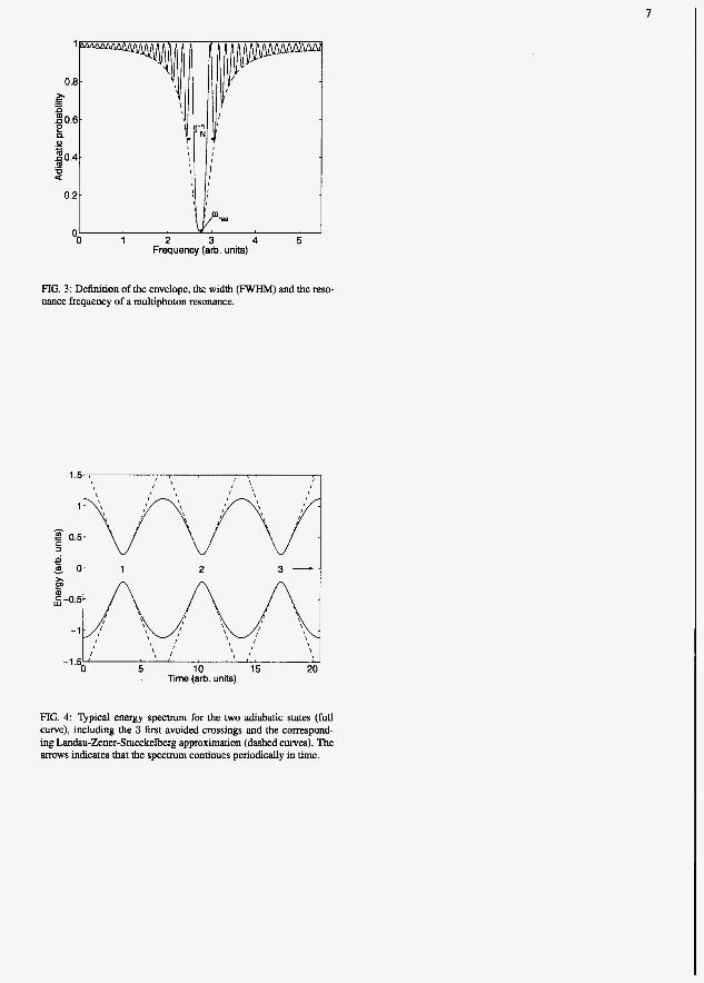
0.2 -
1 2 3 4 5 Frequency (arb. units)
OO
FIG. 3: Definition of the envelope, the width (FWHM) and the reso- nance frequency of a multiphoton resonance.
-1
\ ' \ ' 5 10 15 20
-1.5 0
Time (arb. units)
FIG. 4 Typical energy spectrum for the two adiabatic states (full curve), including the 3 first avoided crossings and the comspond- ing Landau-Zener-Stueckelberg approximation (dashed curves). The arrows indicates that the spectrum continues periodically in time.

8
FIG. 5 : Variation of scaled Bloch-Siegert shifts ASS N d J , / e - 1 with respect to field strength cy = FZ/Fo for a circularly polarized field (Fz = F,) and for X = 10. Analytic results [(Eq. (13)] with as = 0 (full curve) and as # 0 (dashed curve), respectively. Numerical (exact) results from the direct integration of the coupled equations are indicated by (*).
FIG. 6: Widths r.v/dm (FWHM) (for infinitely long pulse dum- tion) vs. scaled hannonic field strength cy = S / F O for different photon numbers N , and for a circularly polarized field (FL = Fs). Full curve shows the analytical result [(Eq. (14)l and (*) the exact numerical results.

9
4.5, I
FIG. 7: Same as Fig. 5 for a linearly polarized oscillating field (F2 = 0) and for N = 7. Analytical shifts [(Eq. (21)l with @S = 0 (full curve) and Os # 0 (dashed curve), respectively. Exact numerical shifts shown by (*).
FIG. 8: Same as Fig. 6 for a linearly polarized oscillating field (Fz = 0). Full curve shows the analytical widths [Eq. (23)] and (*) the exact numerical widths. For N = 5 both the formulas valid for A' 4 5 (full curve) and N 2 5 (dashed curve), respectively, are shown for comparison.

Paper 7
Ionization and stabilization dynamics of H ( 2 p ) in ultrashort strong laser pulses
T. Bwkeland, h.1 Forre, J. P. Hanwn a n d S. Selsta
" I . :.I -F v - ~ a ~ ~ - ' i
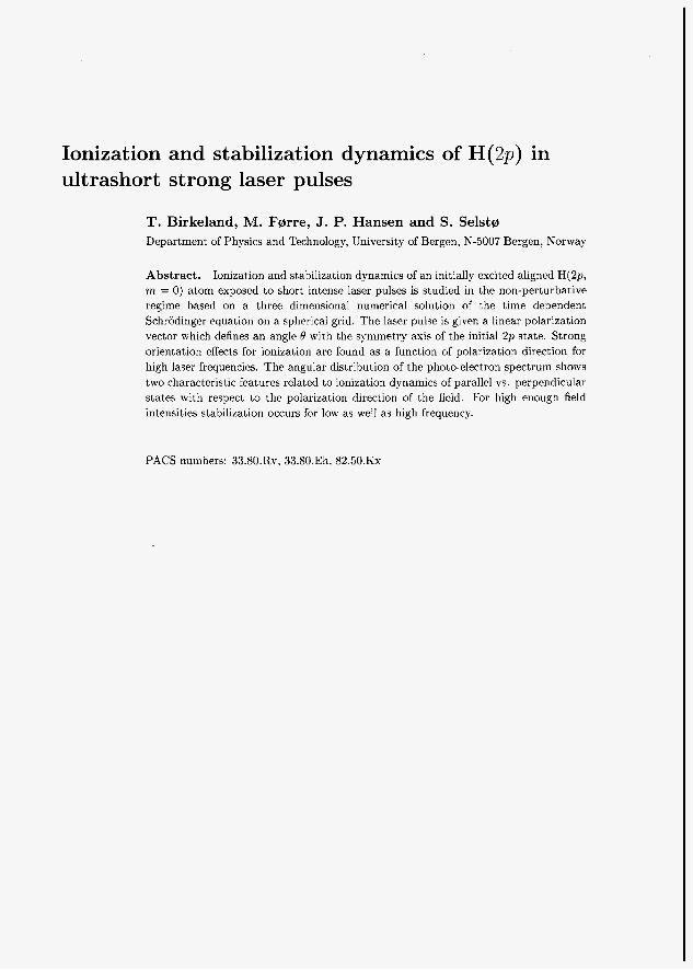
Ionization and stabilization dynamics of H( 2 p ) in ultrashort strong laser pulses
T. Birkeland, M. Farre, J. P. Hansen and S. Selsta Department of Physics and Technology, University of Bergen, N-5007 Bergen, Norway
Abstract. Ionization and stabilization dynamics of an initially excited aligned H(2p, m = 0) atom exposed to short intense laser pulses is studied in the non-perturbative regime based on a three dimensional numerical solution of the time dependent Schrodinger equation on a spherical grid. The laser pulse is given a linear polarization vector which defines an angle fl with the symmetry axis of the initial 2p state. Strong orientation effects for ionization are found as a function of polarization direction for high laser frequencies. The angular distribution of the photo-electron spectrum shows two characteristic features related to ionization dynamics of parallel vs. perpendicular states with respect to the polarization direction of the field. For high enough field intensities stabilization occurs for low as well as high frequency.
PACS numbers: 33.80.Rv, 33.80.Eh, 82.50.K~

Ionization and stabilization dynamics of H(2p) in ultrashort strong laser pulses
1. Introduction
In recent years the experimental tools t,o study dynamical processes of atom and molecule int,eractions with elect,romagnetic fields have improved dramatically. For example, attosecond laser pulses with phase control are now realized [l] and open for imaging of ultrafast, dynamics such as time dependent auger processes [2] or nuclear dynamics [3]. Other examples involve preparation of aligned molecules [4] and momentum recoil analysis of fragmenting products [5, 61 utilizing real studies of reaction dynamics to a degree which only few years ago were at the "gedanken" level.
In order t.o interpret and to understand the basic underlying quantum mechanics the need for optimal algorithms to solve the time dependent Schrodinger equation in parallel with the experimental progress is strengthened. When linear polarized laser light interacts with spherically symmetric ground state atoms the symmetry reduction to two effect'ive degrees of freedom has resulted in a variety of methods [7] which has been applied to a range of phenomena such as above threshold ionization (ATI) [8], dynamic stabilization (DS) [9] and high harmonic generation [lo]. A few groups, however; have reported relat,ed studies with broken cylindrical symmetry, e.g. at,omic stabilization in intense circular polarized light [ll. 121 molecular dynamics [13] and interaction wit,h cxcited hydrogen [14].
-hi logous to such studies of light-matter interactions with circular polarized light; intc>ract,ions between initially aligned atoms or molecules in general need a full three dimensional analysis as well [15]. An example is here the ability of a diatomic molecule to ionize as a function of the angle between the (linear) laser polarization vector and t hc molecular internuclear axis. It, was recently experimentally demonstrated a strong alignment dependence on the ionization probability of diatomic molecules exposed to femtosecond laser pulses [16]. On the theoretical side molecular alignment effects and the interplay between nuclear and electronic dynamics has only been studied within pcrturbation schemes [17, 181 or low-dimensional models [19, 201.
Concerning alignment and increasingly int,ense laser fields, it is well known that, the ionization probability of ground state atoms at some point may start to decrease, or altcrnat,ively saturate at' a level below one [9]. The geometrical aspects of t,his process for aligned atoms have only been briefly documented previously [14].
In the present paper we investigate the convergence properties of a three dimensional spectral split' st'ep met,hod. The method is shown to behave very efficiently in the Kramers-Henneberger frame for strong pulsed laser fields. It is based on an original two-dimensional formulation by Hermann and Fleck [21] which was recently cxt,ended to three dimensions [22]. The present method is then applied to geometrical aspects of the above mentioned light. matter interact,ions. We consider an initially excited hydrogen atom in the 2 p state with vanishing angular momentum around the quantization axis. The atom is then exposed to a 5-cycle laser pulse with frequency either in the XUV region or in the UV region. The linear polarization vector defines in both cases an angle 0 with the quantization axis. Ionization probabilities, alignment

Ionization and stabilization dynamics of H(2p) in ultrashort strong laser pulses 3
effects and the underlying dynamics are then investigated. The paper is organized as follows: In the following section the numerical method is described. In section 3 the method is applied to study geometrical effects and stabilization of hydrogen atoms in short pulsed laser fields. Atomic units, me = TI = e = 1, are used unless otherwise stated.
2. Three dimensional spectral method
A hydrogen atom interacting with the classical electromagnetic field is conveniently described by the semi-classical Hamiltonian.
(1) 1 1 2 r H = -[p + A(r; t)]* - -;
where A(r, t ) is the electromagnetic vector potential. In the present formulation we assume the dipole approximation to be valid. i.e. the wavelength of the radiation is much larger than the extent of the atom. Then A(r.t) A(t). and when introducing spherical coordinates the effective Hamiltonian can be expressed in the so called weloczty gauge.
H ( r ; t ) = -
with;
(3) 1 r
V,(r, R, t ) = -- + A(t) . V
Here R = (0,d) denotes the spherical angles. This Hamiltonian governs the time evolution of the reduced wavefunction @(r7 t ) = r 3 ( r , t ) . The squared term of the vector potential of equation 2 contributes in the dipole approximation to the wavefunction only as a global phase-factor. This factor is routinely removed by the transformat'ion Qu(r, t ) + $,(r; t)e-'/*J; A Z ( t ' ) d t ' . The velocity gauge is a frequently used starting point for perturbation theories [23] as well as non-perturbative treat,ments [24].
An alt,ernative formulation which is explicitly based on the physical electric and/or magnetic fields is obtained by the transformation
Qdr; t ) = &lQo(r, t ) (4) with; UU+[ = e-ir.A(t). Since t,he electric field is related to the vector potent,ial by; E(r,t) = -&A(r,t), we obtain the length gauge Hamiltonian H = HO + \$ ( r ,R; t ) where the potential is given by,
1 r
T / (r , R, t ) = -- + E(r; t ) . r ( 5 )
Alternatively, the laser pulse may be described from the accelerated frame [25] following the motion of a free electron in the field. The frame transformation is defined by, OL+a = e-zp 'a( t ) which gives the Kramers-Henneberger (KH) frame Hamiltonian, H = Ho + I/a(r, R, t ) , with
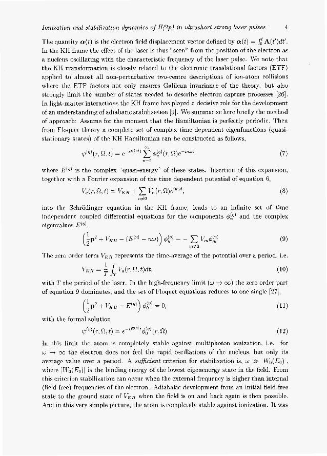
Ionzzatzon and stabalzzataon dynamics of H(2p) an ultrashort strong laser pulses 4
The quantitv a(t) is the electron field displacement vector defined by a(t) = Ji A(t')dt'. In the KH frame the effect of the laser is thus "seen" from the position of the electron as a nucleus oscillating with the characteristic frequency of the laser pulse. \!-e note that the KH transformation is closely related to the electronic translational factors (ETF) applied to almost all non-perturbative two-centre descriptions of ion-atom collisions where the ETF factors not only ensures Galilean invariance of the theory, but also strongly limit the number of states needed to describe electron capture processes [as]. In light-matter interactions the KH frame has plaved a decisive role for the development of an understanding of adiabatic stabilization [9]. it'e summarize here briefly the method of approach: Assume for the moment that the Hamiltonian is perfectly periodic. Then from Floquet theory a complete set of complex time dependent eigenfunctions (quasi- stationary states) of the KH Hamiltonian can be constructed as follows.
00
@7) (., R. t ) = e-zE("t &) ( r , R)e-z'Ldt n=O
where E(q) is the complex "quasi-energy" of these states. Insertion of this expansion. together with a Fourier expansion of the time dependent potential of equation 6.
into the SchrGdinger equation in the KH frame. leads to an infinite set of time independent coupled differential equations for the components and the complex eigenvalues ~ ( 7 ) .
( i P 2 + vK€f - nu)) = -
The zero order term \/I(H represents the time-average of the potential over a period. i.e.
with T the period of the laser. In the high-frequency limit (w -+ 00) the zero order part of equation 9 dominates, and the set of Floquet equations reduces to one single [27] ,
with the formal solution
d)(q)(r , R, t ) = e-iE("t@p)(r, R) (12)
In this limit the atom is completely stable against multiphoton ionization, i.e. for w -+ oc the electron does not feel the rapid oscillations of the nucleus, but only its average value over a period. A suficient criterion for stabilization is, w >> IW'O(Eo)l, where /T$'O(Eo)l is the binding energy of t'he lowest eigenenergy state in the field. From this criterion stabilization can occur when the external frequency is higher than internal (field free) frequencies of the electron. Adiabatic development from an initial field-free state to the ground stat,e of I7KH when the field is on and back again is then possible. And in this very simple picture, the atom is completely stable against ionization. It was
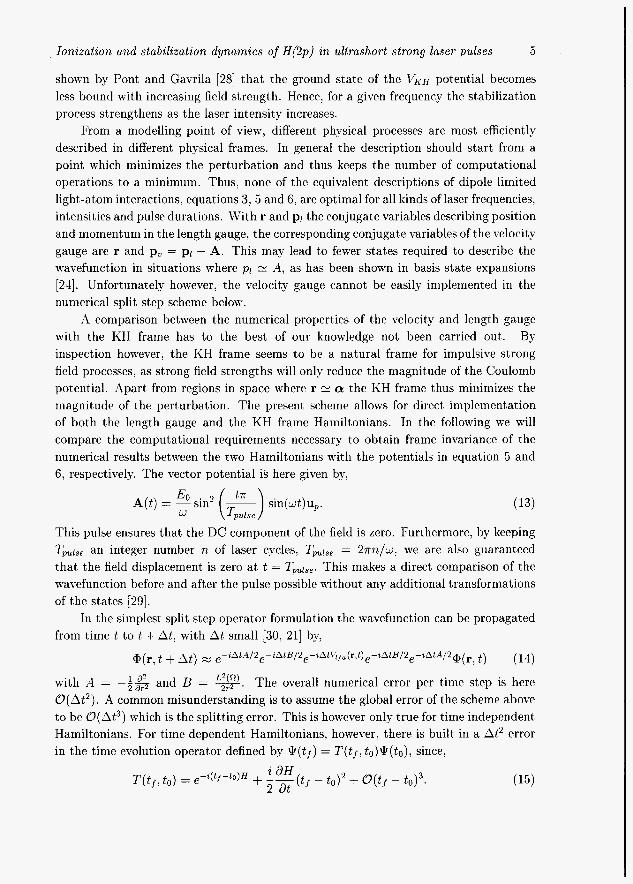
Ionization and stabilization dynamics of H(2p) an ultrashort strong laser pulses 5
shown by Pont and Gavrila [28] that t,he ground state of the V K H potential becomes less bound with increasing field strength. Hence, for a given frequency the stabilization process strengt,hens as the laser intensity increases.
From a modelling point of view, different physical processes are most efficiently described in different physical frames. In general the description should start, from a point which minimizes the perturbation and thus keeps the number of computational operations to a minimum. Thus, none of the equivalent descriptions of dipole limited light-atom interactions, equations 3, 5 and 6, are optimal for all kinds of laser frequencies, intensities and pulse durations. With r and p1 the conjugate variables describing position and momentum in the length gauge, the corresponding conjugate variables of the velocity gauge are r and pz: = pl - A. This may lead to fewer states required to describe the wavefunction in situations where pl N A; as has been shown in basis state expansions [24]. Unfortunately however, the velocity gauge cannot, be easily implemented in the numerical split st.ep scheme below.
A comparison between the numerical properties of the velocity and length gauge with the KH frame has to the best, of our knowledge not been carried out. By inspection however, the KH frame seems to be a natural frame for impulsive strong field processes; as st,rong field strengths will only reduce the magnitude of the Coulomb potential. Apart from regions in space where r N a the KH frame thus minimizes the magnitude of the perturbation. The present scheme allows for direct implementation of both bhe length gauge and the KH frame Hamiltonians. In t,he following we will compare the computational requirements necessary t,o obtain frame invariance of the numerical results between the two Hamiltonians with the potentials in equation 5 and 6; respectively. The vector potential is here given by,
A ( t ) = 3 sin2 (e) sin(wt) up. Lu’
This pulse ensures that the DC component of the field is zero. Furthermore, by keeping Tpuise an integer number n of laser cycles, Tpulse = 27rn/w, we are also guaranteed that the field displacement is zero a t t = Tpulse. This makes a direct comparison of the wavefunct,ion before and after the pulse possible without any additional transformations of the states [29].
In the simplest split step operator formulation the wavefunction can be propagated from time t to t + At , with At small [30; 211 by,
( r ; t ) (14 a(r, t + At ) e- iAtA/2 e ~ ~ ~ t B / ? , - i a t l i / , ( r : t ) ~ - i a t B / 2 e -iAtA/2@
with il = -i% 2 ar and B = -. The overall numerical error per t,ime step is here O(At2) . A common misunderstanding is to assume the global error of the scheme above to be (3(At3) which is the splitting error. This is however only true for time independent Hamiltonians. For time dependent Hamilt,onians, however, there is built in a At2 error in the time evolution operator defined by 9 ( t f ) = T ( t f , to)@(to), since,
+ O ( t f -

Ionization and stabilization dynamics of H(2p) in ultrashort strong laser pulses 6
The second order term is normally small for most laser processes. For short pulses towards attosecond duration. however. it is clear that this term is important and becomes the leading source of error.
Following Hansen et a1 [22]. the trick is now to expand the wavefunction in orthonormal polynomials which is partly diagonal in A and in B. By expanding in spherical harmonics.
1=0 m=-i
we obtain,
.flrn(ri; t ) = wjkl;*, ( f l j k ) ( T i , fljk, t ) (17) jk
with abscissas and weights (fljk; wjk) recently published in tabular form [31]. The sum is truncated at 1 = L,,,: where L,,, is chosen sufficiently large to assure convergence of t,he numerical scheme. The radial space is also truncated at r,,, which is set large enough to cover the spatial extension of the wavefunction at all times during the pulse. With the present expansion the operator B simply reduces to a phase multiplication of each angular function by exp[iAtI(l + 1)/4r?]. The operator A is correspondingly calculat.ed by expanding each radial basis function in it.s Fourier components which reduce> to another set, of multiplications accompanied by two fast Fourier transformations. Following the action of t,hese operators the wavefunction is calculated a t each grid point and t,he exponential potential operator e-ZAt '~/a( '~~'~~~') can act by straightforward multiplication.
The present. method is ideal for "near spherical" problems which restrict,s t,he number of necessary radial basis functions and keeps L,,, to a minimum. It has also some built in numerical advanccs such as providing an efficient parallel code [32], and it. can be applied in thc 1engt.h gaugc as well as the KH frame without extra programming.
The post-processing work needed to produce physical quantities following a numerical algorithm should also be considered. In the present scheme this work is minimized since t.he projcction onto field free eigenstates is part,icularly simple. For ionizat,ion for example. t hc hydrogenic free particle wavefunctions can be expanded in the spherical harmonics.
l = O 111=-l
Here k = a is the n.avenumIwr of the wavefunction; flk is the spherical angles of the outgoing wave and Rl(k: r ) is a rcd radial wavefunction. Furthermore, oi is the Coulomb phase required t.o satisfy the boundary condition as r -+ oc: and CT~ = arg r (I + 1 + i ) . For an infinitely large r-space. k is a continuous variable, while here the discrete k- spectrum is directly ohained from maximum box size of the simulation, rmu,. The radial free part.icle Coulomb n'avcs h ; ( k , r ) , is found by iterative solution of
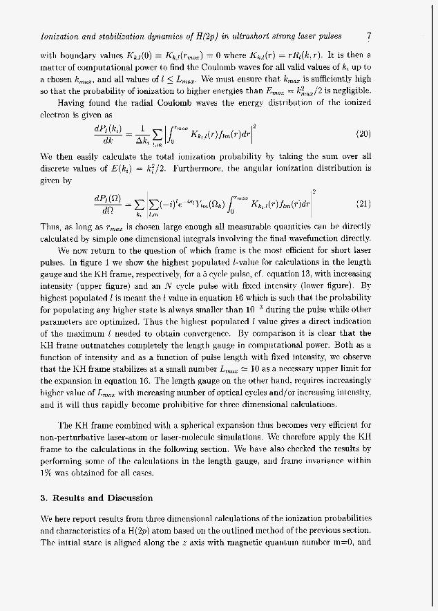
Ionazataon and stabalizataon dynamacs of H(2p) an ultrashort strong laser pulses 7
with boundary values Kk.L(O) = K ~ , J ( T ~ , , ) = 0 where Kk.l(r) = rRl(k, T ) . It is then a matter of computational power to find the Coulomb waves for all valid values of k , up to a chosen k,,,, and all values of 1 5 L,,,. \$'e must ensure that k,,, is sufficiently high so that the probability of ionization to higher energies than E,,, = kk,,/2 is negligible.
Having found the radial Coulomb waves the energy distribution of the ionized electron is given as
We then easily calculate the total ionization probability by taking the sum over all discrete values of E(k,) = k:/2. Furthermore, the angular ionization distribution is given by
Thus; as long as r,,, is chosen large enough all measurable quantities can be direct,ly calculated by simple one dimensional integrals involving the final wavefunction directly.
We now return to the quest,ion of which frame is the most efficient for short laser pulses. In figure 1 we show the highest populated I-value for calculations in the length gauge and the KH frame; respectively, for a 5 cycle pulse; cf. equation 13, with increasing inbensity (upper figure) and an N cycle pulse with fixed intensity (lower figure). By highest, populated 1 is meant the 1 value in equation 16 which is such t,hat. the probability for populating any higher state is always smaller than during the pulse while other parameters are optimized. Thus the highest. populated 1 value gives a direct indication of the maximum 1 needed to obtain convergence. By comparison it is clear that the KH frame outmatches complet,ely the length gauge in computational power. Both as a function of intensity and as a function of pulse length with fixed int,ensit,y, we observe that, the KH frame stabilizes at a small number L,,, N 10 as a necessary upper limit for the expansion in equation 16. The length gauge on the other hand, requires increasingly higher value of L,,, with increasing number of optical cycles and/or increasing intensity, and it will thus rapidly become prohibitive for three dimensional calculations.
The KH frame combined with a spherical expansion thus becomes very efficient for non-perturbative laser-atom or laser-molecule simulations. \lie therefore applv the KH frame to the calculations in the following section. We have also checked the results bv performing some of the calculations in the length gauge, and frame invariance within 1% was obtained for all cases.
3. Results and Discussion
\Ye here report results from three dimensional calculations of the ionization probabilities and characteristics of a H(2p) atom based on the outlined method of the previous section. The initial state is aligned along the z axis with magnetic quantum number m=O. and
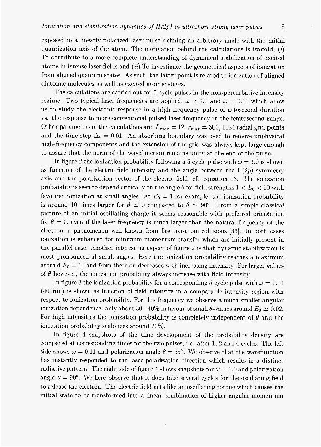
Ionization and stabilization dynamics of H(2p) in ultrashort strong laser pulses 8
exposed to a linearly polarized laser pulse defining an arbitrary angle with the initial quantization axis of the atom. The motivat.ion behind the calculations is twofold; ( i ) To contribute to a more complete understanding of dynamical stabilization of excit,ed atoms in intense laser fields and ( i i ) To invest,igate the geometrical aspects of ionization from aligned quantum states. 4 s such, the latter point is related to ionization of aligned diatomic molecules as well as excited atomic st,at,es.
The calculations are carried out. for 5 cycle pulses in the non-perturbative intensity regime. Two typical laser frequencies are applied, w = 1.0 and w = 0.11 which allow us to study the elect,ronic response in a high frequency pulse of attosecond duration vs. the response to more conventional pulsed laser frequency in the femtosecond range. Other parameters of the calculations are: L,,, = 12; T,,,, = 300, 1024 radial grid points and the time step At = 0.01. An absorbing boundary was used t.0 remove unphysical high-frequency components and the extension of the grid was always kept large enough to assure that the norm of the wavefunction remains unity at, the end of the pulse.
In figure 2 the ionization probability following a 5 cycle pulse with lu' = 1.0 is shown as funct,ion of the electric field intensit.y and the angle between t'he H(2p) symmetry axis and the polarizat'ion vector of the electric field, cf. equation 13. The ionization probability is seen to depend critically on the angle 8 for field strengths 1 < EO < 10 with favoured ionization at small angles. At Eo = 1 for example, t,he ionization probability is around 10 times larger for 8 2: 0 compared to 8 Y 90". From a simple classical picture of an initial oscillat,ing charge it seems reasonable with preferred orientation for 0 = 0; even if the laser frequency is much larger than the natural frequency of the electron, a phenomenon well known from fast ion-atom collisions [33]. In both cases ionization is enhanced for minimum momentum t,ransfer which are initially present in the parallel case. Another interesting aspect of figure 2 is that dynamic stabilization is most pronounced a t small angles. Here the ionization probability reaches a maximum around Eo = 10 and from there on decreases wit,h increasing intensity. For larger values of 8 however; the ionization probability always increase wit,h field intensity.
In figure 3 t,he ionization probabilit'y for a corresponding 5 cycle pulse with lu' = 0.11 (400nm) is shown as function of field int,ensity in a comparable intensity region with rcspect t,o ionization probability. For this frequency we observe a much smaller angular ionization dependence, only about 30-40% in favour of small 8-values around EO N 0.02. For high intensities the ionization probability is completely independent of 8 and the ionization probability stabilizes around 70%.
In figure 4 snapshots of the time development of the Probability densit,y are compared at corresponding times for the t.wo pulses, i.e. after 1, 2 and 4 cycles. The left side shows w = 0.11 and polarization angle 8 = 55". We observe that the wavefunction has instantly responded to the laser polarization direction which results in a distinct radiative pat,tern. The right side of figure 4 shows snapshots for LLI = 1.0 and polarization angle 8 = 90". We here observe t,hat, it does take several cycles for the oscillating field to release the electron. The electric field acts like an oscillating torque which causes the initial state to be transformed into a linear combination of higher angular momentum
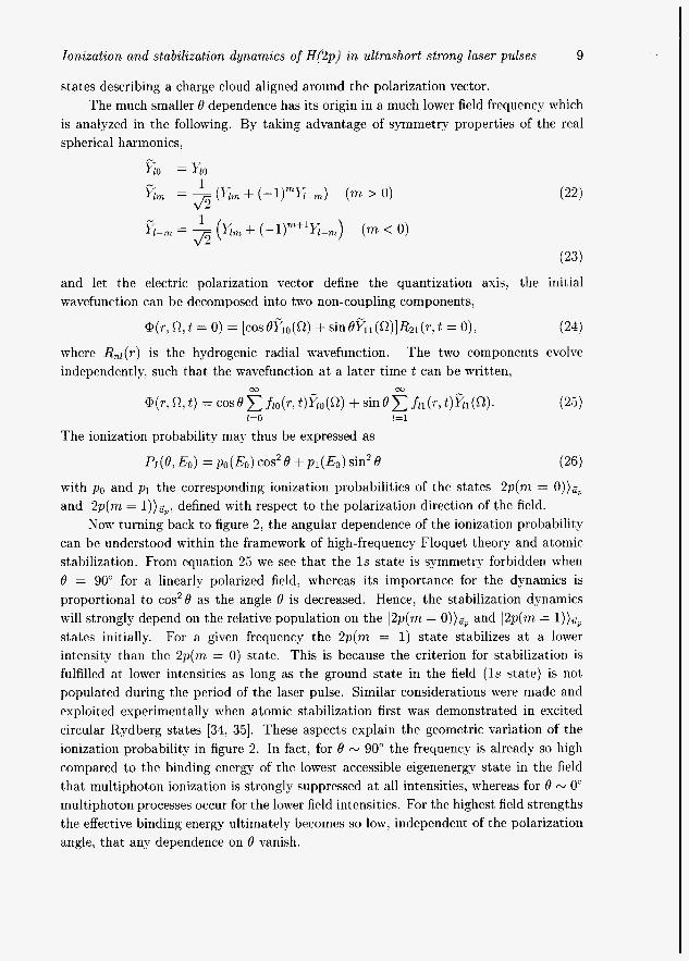
Ionization and stabilization dynamics of H(2p) in ultrashort strong laser pulses 9
states describing a charge cloud aligned around the polarization vector. The much smaller 8 dependence has its origin in a much lower field frequency which
is analyzed in the following. By taking advantage of symmetry properties of the real spherical harmonics,
1 Rm = - (15, + ( - l ) m L J (rn > 0) fi
and let the electric polarization vector define the quantization axis, the initial wavefunction can be decomposed into two non-coupling components,
a ( r , ~ , t = 0) = [ c o s ~ ~ l o ( ~ ) + S ~ ~ ~ Y ~ ~ ( R ) I R ~ ~ ( T , ~ = o) , (24)
where Rnl(r) is the hydrogenic radial wavefunction. independently, such that the wavefunction at a later time t can be written,
The two components evolve
l=O 1=1
The ionization probability may thus be expressed as
pI(8, E O ) = PO(&) cos28 + pl(&) sin2 0 (26)
with po and p1 the corresponding ionization probabilities of the states 12p(m = 0 ) ) ~ ~ and 12p(m = 1 ) ) ~ ~ ; defined with respect to the polarization direction of the field.
Now t,urning back to figure 2, the angular dependence of the ionization probability can be understood within the framework of high-frequency Floquet theory and atomic stabilizat.ion. From equation 25 we see t.hat the Is state is symmetry forbidden when 8 = 90" for a linearly polarized field, whereas its importance for the dynamics is proportional to cos28 as the angle 8 is decreased. Hence, the stabilization dynamics will strongly depend on t,he relative population on the 12p(m = 0 ) ) ~ ~ and 12p(rn = 1))g states initially. For a given frequency the 2 p ( m = 1) state stabilizes a t a lower int,ensity than the 2 p ( m = 0) state. This is because the criterion for stabilization is fulfilled at lower intensities as long as the ground state in the field (Is state) is not. populated during the period of the laser pulse. Similar considerations were made and exploited experimentally when atomic stabilization first was demonstrated in excited circular Rydberg states [34, 351. These aspects explain the geometric variation of the ionization probability in figure 2. In fact, for 8 - 90" the frequency is already so high compared to t,he binding energy of the lowest accessible eigenenergy state in the field that multiphoton ionization is strongly suppressed a t all intensities, whereas for 8 - 0" multiphoton processes occur for the lower field intensities. For the highest field strengths the effective binding energy ultimately becomes so low, independent of the polarization angle, that any dependence on 8 vanish.
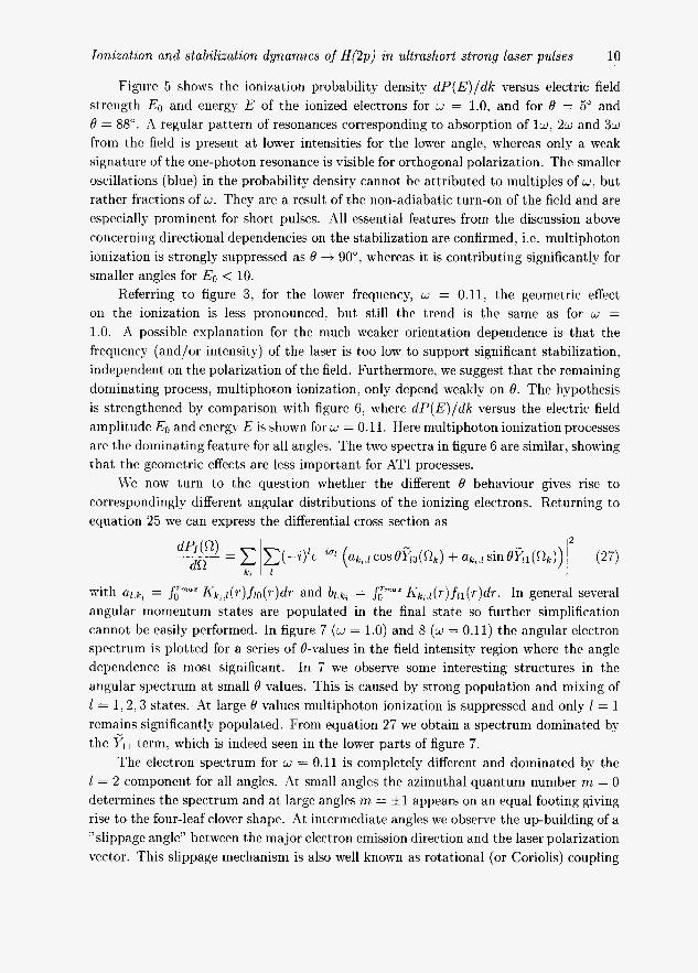
Ionization and stabilization dynamics of H(2p) in ultrashort strong laser pulses 10
Figure 5 shows the ionization probability density dP(E) /dk versus electric field strength EO and energy- E of the ionized electrons for w = 1.0, and for 0 = 5" and 0 = 88". A regular pattern of resonances corresponding to absorption of l w ; 2w and 3w from t,he field is present at, lower intensities for the lower angle; whereas only a weak signature of the one-photon resonance is visible for orthogonal polarization. The smaller oscillations (blue) in the probability density cannot be attributed to multiples of w , but rather fractions of w . They are a result of the non-adiabatic turn-on of the field and are especially prominent, for short pulses. All essential features from the discussion above concerning directional dependencies on the stabilization are confirmed, i.e. multiphoton ionization is strongly suppressed as 0 -+ 90"; whereas it. is contributing significantly for smaller angles for Eo < 10.
Referring to figure 3 , for the lower frequency, w = 0.11, the geometric effect on the ionization is less pronounced; but still the trend is the same as for w = 1.0. A possible explanation for the much weaker orientation dependence is that the frequency (and/or intensity) of the laser is too low to support significant stabilization, independent, on the polarization of the field. Furthermore, we suggest that the remaining dominating process; multiphoton ionization, only depend weakly on 0. The hypothesis is strengt,hened by comparison wit.h figure 6, where dP(E) /dk versus the electric field amplit,ude EO and energy E is shown for w = 0.11. Here multiphoton ionization processes are the dominating feature for all angles. The two spectra in figure 6 are similar, showing t,hat the geomet,ric effects are less important, for AT1 processes.
We now turn to the question whether the different 0 behaviour gives rise to correspondingly different angular distributions of t,he ionizing electrons. Returning to equation 25 we can express the differential cross section as
with a1 k, = Jlmaz Kk,.l(r) fio(r)dr and bl,k, = Jim"" Kkt.l(r)j l l(r)dr. In general several angular momentum states are populated in the final state so further simplification cannot be easily performed. In figure 7 (u = 1.0) and 8 (J = 0.11) the angular electron spectrum is plotted for a series of 0-values in the field intensity region where the angle dependence is most significant. In 7 we observe some interesting structures in the angular spectrum at small 0 values. This is caused by strong population and mixing of 1 = 1 . 2 , 3 states. At large 0 values multiphoton ionization is suppressed and only 1 = 1 remains significantly populated. From equation 27 we obtain a spectrum dominated bv the
The electron spectrum for w = 0.11 is completely different and dominated by the 1 = 2 component for all angles. At small angles the azimuthal quantum number m = 0 determines the spectrum and a t large angles m = &1 appears on an equal footing giving rise to the four-leaf clover shape. ,4t intermediate angles we observe the up-building of a "slippage angle" between the major electron emission direction and the laser polarization vector. This slippage mechanism is also well known as rotational (or Coriolis) coupling
term. which is indeed seen in the lower parts of figure 7.

Ionization and stabilization dynamics of H(2p) in ultrashort strong laser pulses
from ion-atom collisions [36].
11
4. Concluding remarks
In this work we have studied the convergence properties of a split step operator method for solution of the time dependent Schrodinger equation in three dimensions. The method is based on spherical coordinates and fast Fourier and spherical harmonics transformations. IVe have shown by explicit calculations in the length gauge and in the Kramers-Henneberger frame that the latter completely outperforms the length gauge calculations concerning convergence when atoms are exposed to strong few cycle laser pulses.
The ionization dynamics of an initially aligned H(2p) atom exposed to angle- specified linear polarized 5 cycle laser pulses with central frequencies in the XU\.‘ (w = 1.0) and UI’ (.: = 0.11) regimes has been analvzed in detail. Strong orientation effects in total ionization probability as well as differential probabilities in ejection angles and energy have been found in the XUY regime. For UY light the effect is much more modest. The results have been interpreted based on symmetry resolved basis functions. Dynamic stabilization is found to be most pronounced at high frequencies and for polarization vectors parallel to the initial 2p state. These findings are relevant for ongoing studies of ionization by aligned molecules [23] as well as the general understanding of atomic response to strong light sources of attosecond range duration.
Ionization and stabilization dynamics of H(2p) in ultrashort strong laser pulses 12
[l] BaltuSka A et al. 2003 it Nature 421 611 [2] Drescher M et al. 2001 it Nature 419 803 [3] Milosevic N, Corkum P B and Brabec T 2004 Phys. Rev. Lett. 92 013002 [4] Peronne E, Poulsen M D, Bisgaard C Z, Stapelfeldt H and Seideman T 2003 Phys. Rev. Lett. 91
[5] SVeber Th. et al. 2001 Phys. Rev. Lett. 86 224 [GI Moshammer R et al. 2000 Phys. Rev. Lett. 84 447 [7] Lambropoulos P, Maragakis P and Zhang J 1998 Physics Reports 305 1 [8] Eberly J H, Javanainen J and Rzazewski K 1991 Physics Reports 204 331 [9] Gavrila hl 2002 J . Phys. B: At. Mol. Opt. Phys. 35 R147
043003
[lo] Schafer K J , Gaarde M B, Heinrich A, Biegert J and Keller U 2004 Phys. Rev. Lett. 92 023003 [ll] Boca hl, Muller H G and Gavrila M 2004 J. Phys. B: At. Mol. Opt. Phys. 37 147 [12] Bauer D and Ceccherini F 2002 Phys. Rev. A 66 053411 [13] Dundas D 2002 Phys. Rev. A 65 023408 [14] Gajda M, Piraux B and Rzazewsky K 1994 Phys. Rev. A 50 2528 [15] Andersen N, Gallagher J TV and Hertel I V 1998 Physics Reports 165 1 [ l G ] Litvinyuk I V et al. 2003 Phys. Rev. Lett. 90 233003 [17] Zhao Z S, Tong X h l and Lin C D 2003 Phys. Rev. A 67 043404 [18] Kjeldsen T K, Bisgaard C Z, hladsen L B and Stapelfeldt H 2003 Phys. Rev. A 68 063407 [19] Rotenberg B, Taieb R, Veniard V and Maquet .4 2002 J . Phys. B: At. Mol. Opt. Phys. 35 L397 [20] Feuerstein B and Thumm U 2003 Phys. Rev. A 67 063408 [21] Hermann M R and Fleck J A 1988 Phys. Rev. A 38 6000 [22] Hansen J P, Ssrevik T and hladsen L B 2003 Phys. Rev. A 68 031401(R) [23] Kjeldsen T K and Madsen L B 2004 J. Phys. B: At. Mol. Opt. Phys. 37 2033 [24] Cormier E and Lambropoulos P 1996 J. Phys. B: At. Mol. Opt. Phys. 29 1667 [25] Pauli SV and Fierz hl 1938 Nuovo Cimento 15 167
Kramers H A 1956 Collected Scientific Papers (Bmsterdam: North-Holland) 866 Henneberger SV C 1968 Phys. Rev. Lett. 21 838
[as] Fritsch SV and Lin CD 1991 Physics Reports 202 1 [27] Gavrila h1 1992 Atoms in Intense Laser Fields edited by M. Gavrila (Academic Press, San Diego)
[28] Pont M and Gavrila hl 1990 Phys. Rev. Lett. 65 2362 [29] Madsen L B 2002 Phys. Rev. A 65 053417 [30] Feit M D, Fleck J A and Steiger A 1982 J. Comput. Phys. 47 412 [31] Sloan I H and LVommersley R S 2003 Adv. Computational Math
[32] Hansen J P, hlatthey T and Sorevik T 2003 A parallel split operator method for the time dependent
[33] Aumayr F, Gieler 11, Schweinzer J, Winther H and Hansen J P 1992 Phys. Rev. Lett. 68 3277 [34] de Boer l\il P, Hoogenraad J H. \.rijen R B, Constantinescu R C, Noordam L D and Muller H G
1993 Phys. Rev. Lett. 71 32G3 de Boer kl P, Hoogenraad J H. \iijen R B, Constantinescu R C, Noordam L D and hluller H G 1994 Phys. Rev. A 50 4085
[35] van Druten N J, Constantinescu R C. Schins J M, Nieuwenhuize H and hluller H G 1997 Phys. Rev. A 55 622
[36] Kocbach L and Hansen J P 1990 Physica Scripta 42 317
435
http:/ /wi~~w.rnaths.uiis~~~.edu.au/ rsw/Sphere/
Schr6dinger equation 10th Euro PVM/hlPI
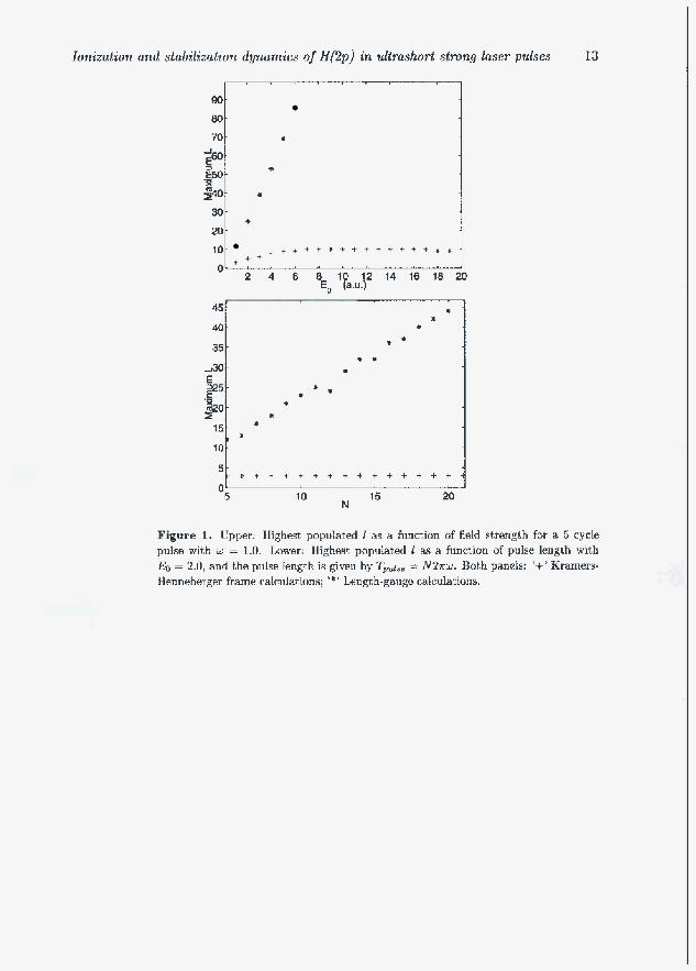
Ionizution and stabilization dynamics of H(2p) in trltmshorf strong laser p u b e ~
90.
80- 70
i - a
90.
80- 70
13
i - a
Figure 1. Upper: Highest populated I as a function of field gt,rerigtk for a 5 cycle puke with w = 1.0. Lower: Highest populated 1 a~ a function of pulse length with & = 2.0, and the pulse length is given by Tpdse = N 2 7 r ~ . h t , h panels: '+' f i rmer+ Henneberger frame calculations; 'I' Lmgth-gmgc ralculations.
E50 f
4
30-
20 - *
I O - + + + + t + + + + + + + + t + + -
+ t '
E50 f
4
30-
20 - *
I O - + + + + t + + + + + + + + t + + -
+ t '
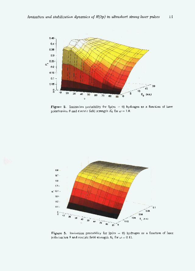
Ionization and stabilizcltion hjnamics of H(2pJ in ultrashort strong laser pukes
--
E
1 4
Figure 2. polariaatmion 0 and elacl.ric field strength Ea for w = 1.0.
Ioi~izal~ior~ probability for 2p(m =- 0) hyd-drogm a3 a function of laser
0.8
0.7 -
0.6
0.5 -
. "
Figure 3. polarixat,ion 0 and clectric field strmgt-kr & fur w = 0.11.
Ioriization probability fur 2 p ( m = 0) hydrogen as a fmct.ion of laser
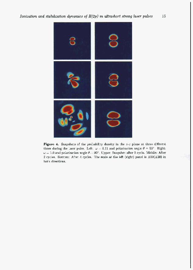
Ionization and stabilization dynamics of H(2p) in uItmshort strong laser pubyes
C l 15
Figure 4. Snapshots of the probability density in the x-z plane at t.hrwl differe~~t times during the laser pulse. Left: 2 = 0.11 and polarization angle 0 = 56* Right: w = 1.0 and poIarization angle 0 : 90". Upper: Snapshot after 1 cycle. Middle: .4fter 2 cycles. Bottom: After 4 cycles. The scale at, the left (right) panel is *50(&30) in bot,h directions.
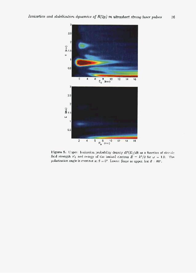
16
- 1 3 1.
Lu
Figure 5. Upper: Ionization probability density dP(E)/& as a function of cIcct,rir: field mength Eo and prlergy of the ioniml electrou E = k2/2 fnr u = 1.0. The polariaat.ion angle is constmt at B = 5" Lowcr: Same as upper, but, 8 - 88".
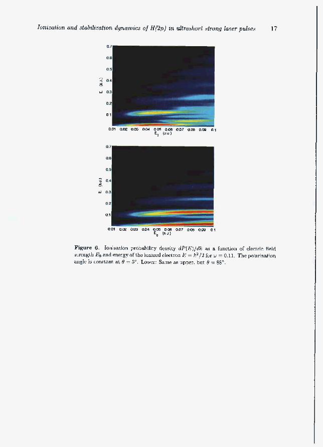
Ionizubion and stahdimtion dynamics of H(2p) in ultrashort strong laser pulses
u a -1 I
001 0.02 0.
0.1
0.01 0.W 0.a 0.04 0.m O(ls 0.07 OOB 0.W 0.1 Eo @J.)
17
Figure 6. Ionization probability density dP(E)/dk as a funcbion of electric field strength E, and encrgpof the ionized electron E = k2/2 for 1~ = 0.11, The polarization angle is constant at 0 = 5". Lower: Same as upper. but 0 = 88".
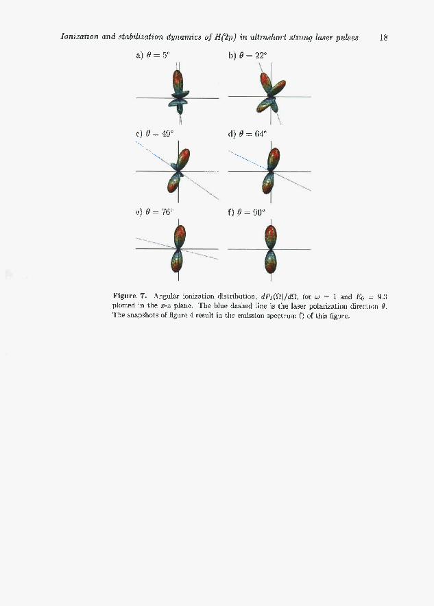
Ionazatzon and ,stabdiztsfion dynamics of H(2p) in ultmshort strong laser p d q e s
a) 0 = 5" b) 8 = 22"
18
c) 8 = 49" d) fi = 61"
e) 19 = 76" f) 8 = 90"
Figure 7. Angular ionization dishrikution, d f ' ~ ( d l ) / & , for LJ = 1 and EJo = 9.3 plotted in t81ie 2-z plaric. The blue dashed h e : i s the laser polarizat,ion dirpction 8. The snapshots of IigurP 4 result in the emission spectrum f) of this figure.

Ionization and stabilization dynamics of H(2p) in ultrashort stwtag h e r pulses
a ) 8 = 5 " b) 8 = 2 V
19
c) 0 = 55" d) 0 = 64"
e ) # = 7 6 " I
f) 8 = 90" I
Figure 8. Angular ionization distribution, dI',[n)/d>, for w = 0.1 1 arid Ea - 0.U4 plot.lt?d in t.hc 1-2 plane. The blue dashed line i s the laser polarization direction 0. The snapshot,s of figure 4 result in the emission spectrum c) of this figure.


![3} tj- 7] - OSTI.GOV](https://static.fdokumen.com/doc/165x107/631c4c86b8a98572c10cd705/3-tj-7-ostigov.jpg)