Fields Institute Communications
401
-
Upload
khangminh22 -
Category
Documents
-
view
0 -
download
0
Transcript of Fields Institute Communications


Fields Institute Communications
VOLUME 68
The Fields Institute for Research in Mathematical Sciences
Fields Institute Editorial Board:
Carl R. Riehm, Managing Editor
Edward Bierstone, Director of the Institute
Matheus Grasselli, Deputy Director of the Institute
James G. Arthur, University of Toronto
Kenneth R. Davidson, University of Waterloo
Lisa Jeffrey, University of Toronto
Barbara Lee Keyfitz, Ohio State University
Thomas S. Salisbury, York University
Noriko Yui, Queen’s University
The Fields Institute is a centre for research in the mathematical sciences, located inToronto, Canada. The Institutes mission is to advance global mathematical activityin the areas of research, education and innovation. The Fields Institute is supportedby the Ontario Ministry of Training, Colleges and Universities, the Natural Sciencesand Engineering Research Council of Canada, and seven Principal SponsoringUniversities in Ontario (Carleton, McMaster, Ottawa, Toronto, Waterloo, Westernand York), as well as by a growing list of Affiliate Universities in Canada, the U.S.and Europe, and several commercial and industrial partners.
For further volumes:http://www.springer.com/series/10503


Monika Ludwig • Vitali D. MilmanVladimir Pestov • Nicole Tomczak-JaegermannEditors
Asymptotic GeometricAnalysis
Proceedings of the Fall 2010 Fields InstituteThematic Program
123The Fields Institute for Researchin the Mathematical Sciences

EditorsMonika LudwigInstitut fur Diskrete Mathematik
und GeometrieTU WienWien, Austria
Vladimir PestovDepartment of Mathematics and StatisticsUniversity of OttawaOttawa, ON, Canada
Vitali D. MilmanDepartment of MathematicsUniversity of Tel AvivTel Aviv, Israel
Nicole Tomczak-JaegermannDepartment of Mathematical
and Statistical SciencesUniversity of AlbertaEdmonton, AB, Canada
ISSN 1069-5265 ISSN 2194-1564 (electronic)ISBN 978-1-4614-6405-1 ISBN 978-1-4614-6406-8 (eBook)DOI 10.1007/978-1-4614-6406-8Springer New York Heidelberg Dordrecht London
Library of Congress Control Number: 2012956543
Mathematics Subject Classification (2010): 46Bxx, 60Exx, 60Bxx, 26Dxx, 51Fxx, 47Bxx, 47Hxx,52Axx, 54H20, 05Dxx, 22F50, 37Bxx, 43A07
© Springer Science+Business Media New York 2013This work is subject to copyright. All rights are reserved by the Publisher, whether the whole or part ofthe material is concerned, specifically the rights of translation, reprinting, reuse of illustrations, recitation,broadcasting, reproduction on microfilms or in any other physical way, and transmission or informationstorage and retrieval, electronic adaptation, computer software, or by similar or dissimilar methodologynow known or hereafter developed. Exempted from this legal reservation are brief excerpts in connectionwith reviews or scholarly analysis or material supplied specifically for the purpose of being enteredand executed on a computer system, for exclusive use by the purchaser of the work. Duplication ofthis publication or parts thereof is permitted only under the provisions of the Copyright Law of thePublisher’s location, in its current version, and permission for use must always be obtained from Springer.Permissions for use may be obtained through RightsLink at the Copyright Clearance Center. Violationsare liable to prosecution under the respective Copyright Law.The use of general descriptive names, registered names, trademarks, service marks, etc. in this publicationdoes not imply, even in the absence of a specific statement, that such names are exempt from the relevantprotective laws and regulations and therefore free for general use.While the advice and information in this book are believed to be true and accurate at the date ofpublication, neither the authors nor the editors nor the publisher can accept any legal responsibility forany errors or omissions that may be made. The publisher makes no warranty, express or implied, withrespect to the material contained herein.
Cover illustration: Drawing of J.C. Fields by Keith Yeomans
Printed on acid-free paper
Springer is part of Springer Science+Business Media (www.springer.com)

Preface
Asymptotic geometric analysis is concerned with geometric and linear propertiesof finite-dimensional objects, normed spaces, and convex bodies, especially withasymptotics of their various quantitative parameters as the dimension tends toinfinity. Deep geometric, probabilistic, and combinatorial methods developed hereare used outside the field in many areas, related to the subject of the program.
The main tools of the theory belong to the concentration phenomenon and largedeviation inequalities. Concentration of measure is, in fact, an isomorphic formof isoperimetric problems, which was first developed inside asymptotic geometricanalysis and then became pertinent to many branches of mathematics as an efficienttool and useful concept. Some new techniques of the theory are connected with mea-sure transportation methods and with related PDEs. The concentration phenomenonis well known to be closely linked with combinatorics (Ramsey theory), and suchlinks have been recently better understood in the setting of infinite-dimensionaltransformation groups, by means of the so-called fixed point on compacta property:on the one hand, every classical Ramsey-type result is equivalent to the fixed pointon compacta property of the group of automorphisms of a suitable structure and onthe other hand, the fixed point on compacta property is often established by usingconcentration of measure in subgroups.
The last few years also witnessed the development of small ball probabilityestimates and their applications, especially for quantitative results on randommatrices. A deep understanding of classical convexity and its analytic methodsis necessary to advance new types of “isomorphic” results. It is now difficult todraw a borderline between asymptotic and classical convexity theories; and resultsof each are used in the other and also have numerous applications. Among therecent important ones are results of a geometric-probabilistic flavor on the volumedistribution in convex bodies and central limit theorems for convex bodies andothers, with close links with geometric inequalities and optimal transport.
More recently, similar results have been established for a larger category of log-concave distributions on Euclidean space, replacing uniform distributions on convexbodies. This is a remarkable extension of the whole theory which could be called“Geometrization of Probability” because it extends to the class of (log-concave)
v

vi Preface
probability measures many typical geometric notions and results. For example, thenotion of polarity, the Blaschke–Santalo inequality and its inverse (by Bourgain–Milman), the Brunn–Minkowski inequality, the Urysohn inequality, and manyothers are formulated and proved now on this larger category.
The achievements of asymptotic geometric analysis demonstrate new and unex-pected phenomena characteristic for high dimensions. These phenomena appear ina number of domains of mathematics and adjacent domains of science dealing withfunctions of a large number of variables. Besides the main subject of our program,asymptotic theory of normed spaces and convex bodies, it includes the branch ofdiscrete mathematics known as asymptotic combinatorics, including problems ofcomplexity and graph theory; a considerable part of probability dealing with largenumbers of correlated random components, including large deviation and the theoryof random matrices; and many others. The theory of computational complexitystudies the inherent computational difficulty of various computational problems,mostly originated in combinatorial optimization. Complexity theory is, actually,a purely asymptotic field, as is the notion of complexity classes; the most basicnotion here is formulated and perceived as an asymptotic notion, where the growingparameter is the size of the computational problem under investigation. The famous“P versus NP” problem asks in fact to compare two asymptotic complexity classes.In recent years several important breakthroughs in complexity theory were obtainedby applying tools from asymptotic geometric analysis such as the concentration ofmeasure phenomenon, spectral theory, and discrete harmonic analysis.
The thematic program on asymptotic geometric analysis took place at the FieldsInstitute for Research in Mathematical Sciences in July–December 2010. The maindirections of research covered by the program included:
• Asymptotic theory of convexity and normed spaces• Concentration of measure and isoperimetric inequalities with an optimal trans-
portation approach• Applications of the concept of concentration• Connections with transformation groups and Ramsey theory• Geometrization of probability• Random matrices• Connection with asymptotic combinatorics and complexity theory
Avi Wigderson (Institute for Advanced Study) delivered the DistinguishedLecture Series “Randomness, pseudorandomness and derandomization” and ShiriArtstein-Avidan (Tel-Aviv University) delivered the Coxeter Lecture Series “Ab-stract duality, the Legendre transform and a new duality transform,” “Orderisomorphisms and the fundamental theorem of affine geometry,” and “Multiplicativetransforms and characterization of the Fourier transform.”
Three workshops were held during the program:
1. Asymptotic Geometric Analysis and Convexity (September 13–17, 2010),organized by Monika Ludwig, Vitali Milman, and Nicole Tomczak-Jaegermann, preceded by a concentration period on convexity (September 8–10,

Preface vii
2010) and followed by a concentration period on asymptotic geometric analysis(September 20–22, 2010)
2. Concentration Phenomenon, Transformation Groups and Ramsey Theory(October 12–16, 2010), organized by Eli Glasner, Vladimir Pestov, and StevoTodorcevic
3. Geometric Probability and Optimal Transportation (November 1–5, 2010),organized by Bo’az Klartag and Robert McCann, preceded by a concentrationperiod on partial differential equations and geometric analysis (October 25–29)and followed by a concentration period on nonlinear dynamics and applications(November 8–10)
To give an idea of program’s scale, there were 426 participants, including 85graduate students and 17 postdocs and 49 long-term participants (those who camefore one month or more). The total number of participant days in the program wasan impressive 5162.
The program organizers and editors of this volume are grateful to the FieldsInstitute for an excellent working environment and generous financial support. Theyalso thank the US National Science Foundation for its support.
This volume contains a selection of papers by the participants of the thematicprogram, which reflects some of the main directions of the scientific activities.
Wien, Austria Monika LudwigTel Aviv, Israel Vitali D. MilmanOttawa, Canada Vladimir PestovEdmonton, Canada Nicole Tomczak-Jaegermann


Contents
The Variance Conjecture on Some Polytopes . . . . . . . . . . . . . . . . . . . . . . . . . . . . . . . . . 1David Alonso–Gutierrez and Jesus Bastero
More Universal Minimal Flows of Groups of Automorphismsof Uncountable Structures . . . . . . . . . . . . . . . . . . . . . . . . . . . . . . . . . . . . . . . . . . . . . . . . . . . . . . 21Dana Bartosova
On the Lyapounov Exponents of Schrodinger OperatorsAssociated with the Standard Map . . . . . . . . . . . . . . . . . . . . . . . . . . . . . . . . . . . . . . . . . . . . . 39J. Bourgain
Overgroups of the Automorphism Group of the Rado Graph . . . . . . . . . . . . . . 45Peter Cameron, Claude Laflamme, Maurice Pouzet, Sam Tarzi,and Robert Woodrow
On a Stability Property of the Generalized Spherical Radon Transform . . 55Dmitry Faifman
Banach Representations and Affine Compactificationsof Dynamical Systems. . . . . . . . . . . . . . . . . . . . . . . . . . . . . . . . . . . . . . . . . . . . . . . . . . . . . . . . . . . . 75Eli Glasner and Michael Megrelishvili
Flag Measures for Convex Bodies . . . . . . . . . . . . . . . . . . . . . . . . . . . . . . . . . . . . . . . . . . . . . . 145Daniel Hug, Ines Turk, and Wolfgang Weil
Operator Functional Equations in Analysis . . . . . . . . . . . . . . . . . . . . . . . . . . . . . . . . . . . 189Hermann Konig and Vitali Milman
A Remark on the Extremal Non-Central Sections of the Unit Cube . . . . . . . 211James Moody, Corey Stone, David Zach, and Artem Zvavitch
Universal Flows of Closed Subgroups of S1 and RelativeExtreme Amenability . . . . . . . . . . . . . . . . . . . . . . . . . . . . . . . . . . . . . . . . . . . . . . . . . . . . . . . . . . . . 229L. Nguyen Van The
ix
x Contents
Oscillation of Urysohn Type Spaces . . . . . . . . . . . . . . . . . . . . . . . . . . . . . . . . . . . . . . . . . . . . 247N.W. Sauer
Euclidean Sections of Convex Bodies . . . . . . . . . . . . . . . . . . . . . . . . . . . . . . . . . . . . . . . . . . 271Gideon Schechtman
Duality on Convex Sets in Generalized Regions . . . . . . . . . . . . . . . . . . . . . . . . . . . . . . 289Alexander Segal and Boaz A. Slomka
On Polygons and Injective Mappings of the Plane . . . . . . . . . . . . . . . . . . . . . . . . . . . 299Boaz A. Slomka
Abstract Approach to Ramsey Theory and Ramsey Theoremsfor Finite Trees . . . . . . . . . . . . . . . . . . . . . . . . . . . . . . . . . . . . . . . . . . . . . . . . . . . . . . . . . . . . . . . . . . . 313Sławomir Solecki
Some Affine Invariants Revisited . . . . . . . . . . . . . . . . . . . . . . . . . . . . . . . . . . . . . . . . . . . . . . . 341Alina Stancu
On the Geometry of Log-Concave Probability Measureswith Bounded Log-Sobolev Constant . . . . . . . . . . . . . . . . . . . . . . . . . . . . . . . . . . . . . . . . . . 359P. Stavrakakis and P. Valettas
f -Divergence for Convex Bodies . . . . . . . . . . . . . . . . . . . . . . . . . . . . . . . . . . . . . . . . . . . . . . 381Elisabeth M. Werner

The Variance Conjecture on Some Polytopes
David Alonso–Gutierrez and Jesus Bastero
Abstract We show that any random vector uniformly distributed on any hyperplaneprojection of Bn
1 or Bn1 verifies the variance conjecture
Var jX j2 � C sup�2Sn�1
EhX; �i2EjX j2:
Furthermore, a random vector uniformly distributed on a hyperplane projection ofBn1 verifies a negative square correlation property and consequently any of its linearimages verifies the variance conjecture.
Key words Variance conjecture • Polytopes
Mathematical Subject Classifications (2010): 46B06, 52B12
1 Introduction and Notation
Let X be a random vector in Rn with a log-concave density, i.e. X is distributed
on Rn according to a probability measure, �X , whose density with respect to the
Lebesgue measure is exp.�V / for some convex function V W Rn ! .�1;1�.
For instance, vectors uniformly distributed on convex bodies and Gaussian randomvectors are log-concave.
D. Alonso–Gutierrez (�)Departamento de Matematicas, Universidad de Murcia, Campus Espinardo,30100 Murcia, Spaine-mail: [email protected]
J. BasteroIUMA, Departamento de Matematicas Universidad de Zaragoza, 50009 Zaragoza, Spaine-mail: [email protected]
M. Ludwig et al. (eds.), Asymptotic Geometric Analysis, Fields InstituteCommunications 68, DOI 10.1007/978-1-4614-6406-8 1,© Springer Science+Business Media New York 2013
1

2 D. Alonso–Gutierrez and J. Bastero
A random vector X is said to be isotropic if:
1. The barycenter is at the origin, i.e., EX D 0, and2. The covariance matrix MX is the identity In, i.e. EhX; eiihX; ej i D ıi;j ,1 � i; j � n,
where feigniD1 denotes the canonical basis in Rn and ıi;j denotes the Kronecker
delta. It is well known that every centered random vector with full dimensionalsupport has a unique, up to orthogonal transformations, linear image which isisotropic.
Given a log-concave random vector X , we will denote by �2X the highesteigenvalue of the covariance matrixMX and by �X its “thin shell width”, i.e.
�2X D kMXk`n2!`n2D sup
�2Sn�1
EhX; �i2;
�X DrE
ˇjX j � .EjX j2/ 12
ˇ2:
(Sn�1 represents the Euclidean unit sphere in Rn).
In asymptotic geometric analysis, the variance conjecture states the following:
Conjecture 1. There exists an absolute constant C such that for every isotropic log-concave vector X , if we denote by jX j its Euclidean norm,
Var jX j2 � CEjX j2 D Cn:
This conjecture was considered by Bobkov and Koldobsky in the context of theCentral Limit Problem for isotropic convex bodies (see [7]). It was conjecturedbefore by Antilla, Ball and Perissinaki, (see [1]) that for an isotropic log-concavevector X , jX j is highly concentrated in a “thin shell” more than the trivial boundVarjX j � EjX j2 suggested. Actually, it is known that the variance conjecture isequivalent to the thin shell width conjecture:
Conjecture 2. There exists an absolute constant C such that for every isotropic log-concave vector X
�X DqEˇjX j � p
nˇ2 � C:
It is also known (see [3, 10]) that these two equivalent conjectures are strongerthan the hyperplane conjecture, which states that every convex body of volume 1has a hyperplane section of volume greater than some absolute constant.
The variance conjecture is a particular case of a stronger conjecture, due toKannan, Lovasz and Simonovits (see [15]) concerning the spectral gap of log-concave probabilities. This conjecture can be stated in the following way due tothe work of Cheeger, Maz’ya and Ledoux:
Conjecture 3. There exists an absolute constant C such that for any locallyLipschitz function, g W R
n ! R, and any centered log-concave random vectorX in R
n

The Variance Conjecture on Some Polytopes 3
Var g.X/ � C�2XEjrg.X/j2:Note that Conjecture 1 is the particular case of Conjecture 3, when we consider
only isotropic vectors and g.X/ D jX j2. Our purpose in this paper is to study theparticular case of Conjecture 3 in which g.X/ D jX j2 but X is not necessarilyisotropic. Thus, we will study the following general variance conjecture:
Conjecture 4. There exists an absolute constant C such that for every centered log-concave vector X
Var jX j2 � C�2XEjX j2:
In the same way that Conjecture 1 is equivalent to Conjecture 2, Conjecture 4can be shown (see Sect. 2) to be equivalent to the following general thin shell widthconjecture:
Conjecture 5. There exists an absolute constant C such that for every centered log-concave vector X
�X � C�X
Notice that since Conjecture 4 and Conjecture 5 are not invariant under linearmaps, these two conjectures cannot easily be reduced to Conjecture 1 and Conjec-ture 2. We will study how these conjectures behave under linear transformations andwe will also prove that random vectors uniformly distributed on a certain family ofpolytopes verify Conjecture 4 but, before stating our results, let us recall the resultsknown, up to now, concerning the aforementioned conjectures.
Besides the Gaussian vectors only a few examples are known to satisfy Conjec-ture 3. For instance, the vectors uniformly distributed on `np-balls, 1 � p � 1,the simplex and some revolution convex bodies [5, 14, 20, 25]. In [18], Klartagproved Conjecture 3 with an extra logn factor for vectors uniformly distributedon unconditional convex bodies and recently Barthe and Cordero extended thisresult for log-concave vectors with many symmetries (see [4]). Kannan, Lovasz andSimonovits proved Conjecture 3 with the factor .EjX j/2 instead of �2X (see [15]),improved by Bobkov to .VarjX j2/1=2 ' �X EjX j (see [6]).
In [18], Klartag proved Conjecture 1 for random vectors uniformly distributedon isotropic unconditional convex bodies. The best known (dimension dependent)bound for general log-concave isotropic random vectors in Conjecture 2 was provedby Guedon and Milman with a factor n1=3 instead of C , improving down to n1=4
when X is 2 (see, [12]). This results give better estimates than previous ones byKlartag (see [17]) and Fleury (see [11]). Given the relation between Conjecture 1and Conjecture 2 we have that Conjecture 1 is known to be true with an extrafactor n2=3.
Very recently Eldan, [9] obtained a breakthrough showing that Conjecture 2implies Conjecture 3 with an extra logarithmic factor. By using the result ofGuedon–Milman, Conjecture 3 is obtained with an extra factor n2=3.logn/2.
Since the variance conjecture is not linearly invariant, in Sect. 2 we will studyits behavior under linear transformations i.e., given a centered log-concave randomvector X , we will study the variance conjecture of the random vector TX , T 2

4 D. Alonso–Gutierrez and J. Bastero
GL.n/. We will prove that ifX is an isotropic random vector verifying Conjecture 1,then the non-isotropic T ıU.X/ verifies the variance Conjecture 4 for a typicalU 2O.n/. We will also show the equivalence between Conjecture 4 and Conjecture 5.As a consequence of Guedon and Milman’s result we obtain that every centered log-concave random vector verifies the variance conjecture with constant Cn
23 rather
than the Cn23 .logn/2 obtained from the best general known result in Conjecture 3.
The main results in this paper will be included in Sect. 3, where we will showthat random vectors uniformly distributed on hyperplane projections of Bn
1 or Bn1(the unit balls of `n1 and `n1 respectively) verify Conjecture 4. Furthermore, in thecase of the hyperplane projections of Bn1 we will see that they verify a negativesquare correlation property with respect to any orthonormal basis, which will allowus to deduce that also a random vector uniformly distributed on any linear image ofany hyperplane projection of Bn1 will verify Conjecture 4.
In order to compute some quantities on the hyperplane projections ofBn1 andBn1
we will use Cauchy’s formula which, in the case of polytopes can be stated like this:Let K0 be a polytope with facets fFi W i 2 I g andK D PHK0 be the projection
of K0 onto a hyperplane. If X is a random vector uniformly distributed on K , forany integrable function f W K ! R we have
Ef .X/ DXi2I
Vol.PH .Fi //
Vol.K/Ef .PHY
i /;
where Y i is a random vector uniformly distributed on the facet Fi and Vol denotesthe volume or Lebesgue measure.
Let us now introduce some notation. Given a convex bodyK , we will denote byQK its homothetic image of volume 1 (Vol. QK/ D 1). QK D K
Vol1n .K/
. We recall that a
convex body K � Rn is isotropic if it has volume Vol.K/ D 1, the barycenter of
K is at the origin and its inertia matrix is a multiple of the identity. Equivalently,there exists a constant LK > 0 called isotropy constant of K such that L2K DRK
hx; �i2 dx;8� 2 Sn�1. In this case if X denotes a random vector uniformlydistributed onK , �X D LK . Thus,K is isotropic if the random vectorX , distributedon L�1
K K with density LnK�L�1K K is isotropic.
When we write a � b, for a; b > 0, it means that the quotient of a and bis bounded from above and from bellow by absolute constants. O.n/ will alwaysdenote the orthogonal group on R
n.
2 General Results
In this section we are going to consider the variance conjecture for linear [16],transformations of a fixed centered log-concave random vector in R
n. Our first resultshows that if such random vector is not far from being isotropic and verifies thevariance conjecture, then the average perturbation (in the sense we will state in theproposition) will also verify the variance conjecture.

The Variance Conjecture on Some Polytopes 5
Proposition 1. Let X be a centered isotropic, log-concave random vector in Rn
verifying the variance conjecture with constant C1. Let T 2 GL.n/ be any lineartransformation. If U is a random map uniformly distributed in O.n/ then
EUVar jT ı U.X/j2 � CC1kT k2opkT k2HS D CC1�2T ıu.X/EjT ı u.X/j2
for any u 2 O.n/, where C is an absolute constant.
Proof. The non singular linear map T can be expressed by T D VU1 whereV;U1 2 O.n/ and D Œ�1; : : : ; �n� (�i > 0) a diagonal map.
Given feigniD1 the canonical basis in Rn, we will identify every U 2 O.n/ with
the orthonormal basis fi gniD1 such thatU1Ui D ei for all i . Thus, by uniqueness ofthe Haar measure invariant under the action ofO.n/ we have that, for any integrablefunction F
EUF.U /
D EUF.1; : : : ; n/
DZSn�1
ZSn�1\?
1
: : :
ZSn�1\?
1 \���\?
n�1
F .1; : : : ; n/d�.n/ : : : d�.1/;
where d�.i / is the Haar probability measure on Sn�1\?1 \� � �\?
i�1. Then, since
jT ı U.X/j2 D jU1UX j2 DnXiD1
hU1UX; eii2 DnXiD1
�2i hX; ii2
EUVar jT ı U.X/j2 DnXiD1
�4iEU .EhX; ii4 � .EhX; ii2/2/
CXi¤j
�2i �2jEU .EhX; ii2hX; j i2 � EhX; ii2EhX; j i2/:
Since for every i
EU .EhX; ii4 � .EhX; ii2/2/ � EUEhX; ii4 D EjX j4ZSn�1
he1; 1i4d�.1/
D 3
n.nC 2/EjX j4;
and for every i ¤ j , denoting by Y an independent copy of X ,
EU .EhX; ii2hX; j i2 � EhX; ii2EhX; j i2/
D EjX j4ZSn�1
�X
jX j ; 1�2 Z
Sn�1\?
1
�X
jX j ; 2�2d�.2/d�.1/
�EjX j2jY j2ZSn�1
�X
jX j ; 1�2 Z
Sn�1\?
1
�Y
jY j ; 2�2d�.2/d�.1/

6 D. Alonso–Gutierrez and J. Bastero
D EjX j4n � 1
�1
n�ZSn�1
he1; 1i4d�.1/�
�EjX j2jY j2n � 1
1
n�ZSn�1
�X
jX j ; 1�2 �
Y
jY j ; 1�2d�.1/
!
D EjX j4n � 1
�1
n� 3
n.nC 2/
�
�EjX j2jY j2n � 1
1
n� 1
n.nC 2/� 2
n.nC 2/
�X
jX j ;Y
jY j�2!
we have that
EUVar jT ı U.X/j2 � 3
n.nC 2/EjX j4
nXiD1
�4i
C EjX j4 � .EjX j2/2
n.nC 2/� 2EjX j2jY j2.n � 1/n.nC 2/
1 �
�X
jX j ;Y
jY j�2!!X
i¤j�2i �
2j
� 3
n.nC 2/EjX j4
nXiD1
�4i C Var jX j2n.nC 2/
Xi¤j
�2i �2j :
Now, since for every � 2 Sn�1, EhX; �i2 D 1 and X satisfies the varianceconjecture with constant C1, we have
EjX j4 D Var jX j2 C .EjX j2/2 � C1nC n2 � CC1n2:
and
EUVar jT ı U.X/j2 � CC1
nXiD1
�4i C C1
n
Xi¤j
�2i �2j
Hence, given any u 2 O.n/, let f�igniD1 be the orthonormal basis defined by �i DU1 ı u.e1/, for all i . Then we have
�2T ıu.X/ D sup�2Sn�1
EhT ı u.X/; �i2 D sup�2Sn�1
EhU1uX; �i2
D sup�2Sn�1
E
nXiD1
�i hX; �iihei ; �i!2
D sup�2Sn�1
nXiD1
�2i hei ; �i2 D max1�i�n �
2i D kT k2op

The Variance Conjecture on Some Polytopes 7
and
EjT ı u.X/j2 DnXiD1
�2iEhX; �ii2 DnXiD1
�2i D kT k2HS
Thus
EUVar jT ı U.X/j2 � CC1kT k2opkT k2HS C C1
nkT k2op
Xi¤j
�2j
� CC1kT k2opkT k2HS C C1kT k2opkT k2HSD CC1kT k2opkT k2HS D CC1�
2T ıu.X/EjT ı u.X/j2
utRemark 1. The same proof as before can be applied when X is not necessarilyisotropic. In this case
EUVar jT ı U.X/j2 � CC1B4�2T ıu.X/EjT ı u.X/j2
for any u 2 O.n/, where B is the spectral condition number of its covariancematrix i.e.
B2 D max�2Sn�1 EhX; �i2min�2Sn�1 EhX; �i2 :
As a consequence of Markov’s inequality we obtain the following
Corollary 1. Let X be an isotropic, log-concave random vector in Rn verifying
the variance conjecture with constant C1. There exists an absolute constant C suchthat the measure of the set of orthogonal operators U for which the random vectorT ı U.X/ verifies the variance conjecture with constant CC1 is greater than 1
2.
In [12] it was shown that every log-concave isotropic random vector verifies thethin-shell width conjecture with constant C1 D Cn
13 . Also, an estimate for �X was
given when X is not isotropic.The following proposition is well known for the experts. However we include it
here for the sake of completeness. As a consequence and, by using the result in [12],we will obtain that every centered log-concave vector, isotropic or not, verifies thevariance conjecture with constant Cn
23 rather than Cn
23 .logn/2.
Proposition 2. Let X be an isotropic log-concave random vector, T a linear mapand �TX the thin-shell width of the random vector TX i.e.
�2TX D E
ˇjTX j � .EjTX j2/ 12
ˇ2:

8 D. Alonso–Gutierrez and J. Bastero
Then
�2TX � Var jTX j2EjTX j2 � C1�
2TX C C2
kT k2opkT k2HS
�2TX :
Proof. The first inequality is clear, since
�2TX D E
ˇjTX j � .EjTX j2/ 12
ˇ2
� E
ˇˇjTX j � .EjTX j2/ 12
ˇˇ2ˇˇjTX j C .EjTX j2/ 12
ˇˇ2
EjTX j2D Var jTX j2
EjTX j2 :
Let us now show the second inequality. Let B > 0 to be chosen later.
Var jTX j2 D EˇjTX j2 � EjTX j2ˇ2 �� jTX j�B.EjTX j2/ 12
�
CEˇjTX j2 � EjTX j2ˇ2 �� jTX j>B.EjTX j2/ 12
� :
The first term equals
E
ˇjTX j C .EjTX j2/ 12
ˇ2 ˇjTX j � .EjTX j2/ 12ˇ2�� jTX j�B.EjTX j2/ 12
�
� .1C B/2�2TXEjTX j2:
If B � 1p2, the second term verifies
EˇjTX j2 � EjTX j2ˇ2 �� jTX j>B.EjTX j2/ 12
� � EjTX j4�� jTX j>B.EjTX j2/ 12�
By Paouris’ strong estimate for log-concave isotropic probabilities (see [23]) thereexists an absolute constant c such that
PfjTX j > ct.EjTX j2/ 12 g � e�t kTkHS
kTkop 8t � 1:
ChoosingB D maxnc; 1p
2
owe have that the second term is bounded from above by
EjTX j4�fjTX j>B.EjTX j2/ 12 g
D B4.EjTX j2/2PfjTX j > B.EjTX j2/ 12 gCB4.EjTX j2/2
Z 1
1
4t3PfjTX j > Bt.EjTX j2/ 12 gdt

The Variance Conjecture on Some Polytopes 9
� B4kT k4opkT k4HSkT k4op
e� kTkHS
kTkop C B4kT k4HSZ 1
1
4t3e�t kTkHS
kTkop dt
� C2kT k4op:
Hence, we achieve
Var jTX j2EjTX j2 � �2TX .1CB/2 C C2
kT k4opkT k2HS
� C1�2TX C C2
kT k4opkT k2HS
D C1�2TX C C2
kT k2opkT k2HS
�2TX :
utAs a consequence of this proposition we obtain that Conjecture 4 and Conjecture 5are equivalent. Combining it with the estimate of �TX given in [12] we obtain thefollowing
Corollary 2. There exists an absolute constant C such that for every log-concaveisotropic random vector X and any linear map T 2 GL.n/ we have
�TX � C1�TX H) Var jTX j2 � C1EjTX j2
and
Var jTX j2 � C2EjTX j2 H) �TX � C C2�TX :
Moreover, both inequalities are true with C2 D Cn2=3.
Proof. The two implications are a direct consequence of the previous propositionand the fact that kT kop � kT kHS . It was proved in [12] that
�TX � CkT k 13opkT k 2
3
HS :
Thus, by the previous proposition
Var jTX j2EjTX j2 � C1�
2TX C C2
kT k2opkT k2HS
�2TX
� C�2TX
0@kT k 4
3
HS
kT k 43op
C kT k2opkT k2HS
1A
� C�2TXkT k 4
3
HS
kT k 43op
� Cn23 �2TX ;
since kT kop � kT kHS � pnkT kop. ut

10 D. Alonso–Gutierrez and J. Bastero
The square negative correlation property appeared in [1] in the context of thecentral limit problem for convex bodies.
Definition 1. Let X be a centered log-concave random vector in Rn and figniD1
an orthonormal basis of Rn. We say that X satisfies the square negative correlationproperty with respect to fi gniD1 if for every i ¤ j
EhX; ii2hX; j i2 � EhX; ii2EhX; j i2:
In [1], the authors showed that a random vector uniformly distributed on Bnp
satisfies the square negative correlation property with respect to the canonical basisof Rn. The same property was proved for random vectors uniformly distributed ongeneralized Orlicz balls in [26], where it was also shown that this property doesnot hold in general, even in the class of random vectors uniformly distributed on1-symmetric convex bodies.
It is easy to see that if a random centered log-concave vector X satisfies thesquare negative correlation property with respect to some orthonormal basis, then italso satisfies the Conjecture 4. Furthermore, the following proposition shows that,in such case, also some class of linear perturbations of X verify the Conjecture 4.
Proposition 3. LetX be a centered log-concave random vector in Rn satisfying the
square negative correlation property with respect to any orthonormal basis, then theConjecture 4 holds for any linear image T 2 GL.n/.Proof. Let T D VU , with U; V 2 O.n/ and D Œ�1; : : : ; �n� (�i > 0) adiagonal map. Let fi gi the orthonormal basis defined by Ui D ei for all i . By thesquare negative correlation property
Var jTX j2 DnXiD1
�4i .EhX; i i4 � .EhX; i i2/2/
CXi¤j
�2i �2j .EhX; ii2hX; j i2 � EhX; i i2EhX; j i2/
�nXiD1
�4i .EhX; i i4 � .EhX; i i2/2/
By Borell’s lemma (see, for instance, [8], Lemma 3.1 or [22], Appendix III)
EhX; ii4 � C.EhX; ii2/2:
Thus
Var jTX j2 � C
nXiD1
�4i .EhX; ii2/2 � C�2TX
nXiD1
�2iEhX; ii2
D C�2TXEjTX j2:

The Variance Conjecture on Some Polytopes 11
utRemark 2. Notice that if X satisfies the square negative correlation property withrespect to one orthonormal basis fi gniD1 and U is the orthogonal map such thatU.i/ D ei , the same proof gives that UX verifies Conjecture 4 for any linearimage D Œ�1; : : : ; �n� (�i > 0).
Even though verifying the variance conjecture is not equivalent to satisfy a squarenegative correlation property, the following lemma shows that it is equivalent tosatisfy a “weak averaged square negative correlation” property with respect to oneand every orthonormal basis.
Lemma 1. Let X be a centered log concave random vector in Rn. The following
are equivalent
(i) X verifies the variance conjecture with constant C1
Var jX j2 � C1�2XEjX j2:
(ii) X satisfies the following “weak averaged square negative correlation” prop-erty with respect to some orthonormal basis figniD1 with constant C2
Xi¤j.EhX; ii2hX; j i2 � EhX; ii2EhX; j i2/ � C2�
2XEjX j2:
(iii) X satisfies the following “weak averaged square negative correlation” prop-erty with respect to every orthonormal basis figniD1 with constant C3
Xi¤j.EhX; i i2hX; j i2 � EhX; ii2EhX; j i2/ � C3�
2XEjX j2;
whereC2 � C1 � C2 C C C3 � C1 � C3 C C
with C an absolute constant.
Proof. For any orthonormal basis fi gniD1 we have
Var jX j2 DnXiD1.EhX; ii4 � .EhX; ii2/2/
CXi¤j.EhX; ii2hX; j i2 � EhX; ii2EhX; j i2/:
Denoting by A./ the second term we have, using Borell’s lemma, that
A./ � Var jX j2 � C�2XEjX j2 C A./;
sincenXiD1
EhX; i i4 � C supi
EhX; ii2nXiD1
EhX; ii2 D C�2XEjX j2: ut

12 D. Alonso–Gutierrez and J. Bastero
3 Hyperplane Projections of the Cross-Polytopeand the Cube
In this section we are going to give some new examples of random vectors verifyingthe variance conjecture. We will consider the family of random vectors uniformlydistributed on a hyperplane projection of some symmetric isotropic convex bodyK0.These random vectors will not necessarily be isotropic. However, as we will see inthe next proposition, they will be almost isotropic. i.e. the spectral condition numberB of their covariance matrix verifies 1 � B � C for some absolute constant C .
Proposition 4. Let K0 � Rn be a symmetric isotropic convex body, and let
H D �? be any hyperplane. Let K D PH.K0/ and X a random vector uniformlydistributed on K . Then, for any � 2 SH D fx 2 H I jxj D 1g
EhX; �i2 � 1
Vol.K/1C 2n�1
ZK
hx; �i2dx � L2K0:
Consequently �X � LK0 and B.X/ � 1.
Proof. The two first expressions are equivalent, since Vol.K/1
n�1 � 1. Indeed,using Hensley’s result [13] and the best general known upper bound for the isotropyconstant of an n-dimensional convex body [16], we have
Vol.K/1
n�1 � Vol.K0 \H/ 1n�1 �
�c
LK0
� 1n�1
��c
n14
� 1n�1
� c:
On the other hand, since (see [24] for a proof)
1
nVol.K/Vol.K0 \H?/ � Vol.K0/ D 1
we have
Vol.K/1
n�1 ��
n
2r.K0/
� 1n�1
��
n
2LK0
� 1n�1
� .cn/1
n�1 � c;
where we have used that r.K0/ D supfr W rBn2 � K0g � cLK0 , see [15].
Let us prove the last estimate. Let S.K0/ be the Steiner symmetrization of K0
with respect to the hyperplane H and let S1 be its isotropic position. It is known(see [2] or [21]) that for any isotropic n-dimensional convex body L and any linearsubspace E of codimension k
Vol.L\ E/1k � LC
LL;

The Variance Conjecture on Some Polytopes 13
where C is a convex body in E?. In particular, we have that
Vol.S1 \H/ � 1
LS.K0/
and
Vol.S1 \H \ �?/ � 1
L2S.K0/:
Since K0 is symmetric, S1 \ H is symmetric and thus centered. Then, byHensley’s result [13]
L2S.K0/ � Vol.S1 \H/2
Vol.S1 \H \ �?/2� 1
Vol.S1 \H/
ZS1\H
hx; �i2dx
� 1
Vol.S1 \H/1C 2n�1
ZS1\H
hx; �i2dx;
because Vol.S1 \H/ � 1LS.K0/
and so Vol.S1 \H/ 1n�1 � c.
But now, BS1 \H D Vol.S1 \H/� 1n�1 .S1 \H/ D ES.K0/\H D QK, because,
even though S.K0/ is not isotropic, S1 is obtained from S.K0/ multiplying it bysome � in H and by 1
�1
n�1
in H?. Thus,
L2S.K0/ �ZeS1\H
hx; �i2dx DZ
QKhx; �i2dx D 1
Vol.K/1C 2n�1
ZK
hx; �i2dx
and since LS.K0/ � LK0 we obtain the result. utThe first examples we consider are the random vectors uniformly distributed on
hyperplane projections of the cube. We will see that these random vectors satisfythe negative square correlation property with respect to any orthonormal basis.Consequently, by Proposition 3, any linear image of these random vectors will verifythe variance conjecture with an absolute constant.
Theorem 1. Let � 2 Sn�1 and let K D PHBn1 be the projection of Bn1 on the
hyperplaneH D �?. If X is a random vector uniformly distributed on K then, forany two orthonormal vectors 1; 2 2 H , we have
EhX; 1i2hX; 2i2 � EhX; 1i2EhX; 2i2:
Consequently, X satisfies the negative square correlation property with respect toany orthonormal basis in H .
Proof. Let Fi denote the facet Fi D fy 2 Bn1Iyji j D sgn ig , i 2 f˙1; : : : ;˙ng.From Cauchy’s formula, it is clear that for any function f

14 D. Alonso–Gutierrez and J. Bastero
Ef .X/ D˙nXiD˙1
j�ji jj2k�k1E.f .PHY
i //
where Y i is a random vector uniformly distributed on the facet Fi .Remark that
Vol.PH .Fi // D jh�; eji jij Vol.Fi / D 2n�1j�ji jj
for i D ˙1; : : : ;˙n and Vol.K/ D 2n�1k�k1.For any unit vector 2 H , we have by isotropicity of the facets of Bn1,
EhX; i2 D˙nXiD˙1
j�ji jj2k�k1EhY i ; i2 D
˙nXiD˙1
j�ji jj2k�k1E
nXjD1
2j Yij
2
D 1
2
nXjD1
2j
˙nXiD˙1
j�ji jjk�k1EY
ij
2 DnX
jD12j
0@ j�j j
k�k1 C 1
3
Xi 6Dj
j�i jk�k1
1A
DnX
jD12j
�2j�j j3k�k1 C 1
3
�D 1
3C 2
3
nXjD1
2jj�j jk�k1 :
Consequently,
EhX; 1i2EhX; 2i2
D 1
9C 2
9
nXiD1
j�i jk�k1 .1.i/
2 C 2.i/2/C 4
9
nXi1;i2D1
j�i1 jj�i2 jk�k21
1.i1/22.i2/
2
� 1
9C 2
9
nXiD1
j�i jk�k1 .1.i/
2 C 2.i/2/:
On the other hand, by symmetry,
EhX; 1i2hX; 2i2
D˙nXiD˙1
j�ji jj2k�k1EhY i ; 1i2hY i ; 2i2
D˙nXiD˙1
j�ji jj2k�k1
1
Vol.Bn�11 /
ZBn�1
1
.hy; Peji j1i C sgn.i/1.i//2
.hy; Peji j2i C sgn.i/2.i//2dy

The Variance Conjecture on Some Polytopes 15
DnXiD1
j�i jk�k1
1
Vol.Bn�11 /
ZBn�1
1
�hy; Pe?
i1i2hy; Pe?
i2i2 C 2.i/
2hy; Pe?
i1i2
C1.i/2hy; Pe?
i2i2 C 1.i/
22.i/2
C41.i/2.i/hy; Pe?
i1ihy; Pe?
i2idy
DnXiD1
j�i jk�k1
�1
31.i/
2jPe?
i2j2 C 1
32.i/
2jPe?
i1j2 C 1.i/
22.i/2
C41.i/2.i/ 1
Vol.Bn�11 /
ZBn�1
1
hy; Pe?
i1ihy; Pe?
i2idy
C 1
Vol.Bn�11 /
ZBn�1
1
hy; Pe?
i1i2hy; Pe?
i2i2dy
�
DnXiD1
j�i jk�k1
�1
31.i/
2 C 1
32.i/
2 C 1
31.i/
22.i/2C
C41.i/2.i/ 1
Vol.Bn�11 /
ZBn�1
1
hy; Pe?
i1ihy; Pe?
i2idy
C 1
Vol.Bn�11 /
ZBn�1
1
hy; Pe?
i1i2hy; Pe?
i2i2dy
�
Since
1
Vol.Bn�11 /
ZBn�1
1
hy; Pe?
i1ihy; Pe?
i2idy
D 1
Vol.Bn�11 /
ZBn�1
1
0@ Xl1;l2¤i
yl1yl21.l1/2.l2/
1Ady
D 1
Vol.Bn�11 /
ZBn�1
1
0@Xl¤i
y2l 1.l/2.l/
1Ady
D 1
3
Xl¤i
1.l/2.l/
D 1
3.h1; 2i � 1.i/2.i//
D �131.i/2.i/
the previous sum equals
nXiD1
j�i jk�k1
�1
31.i/
2 C 1
32.i/
2 � 1.i/22.i/2
C 1
Vol.Bn�11 /
ZBn�1
1
hy; Pe?
i1i2hy; Pe?
i2i2dy
�:

16 D. Alonso–Gutierrez and J. Bastero
Now,
1
Vol.Bn�11 /
ZBn�1
1
hy; Pe?
i1i2hy; Pe?
i2i2dy
D 1
Vol.Bn�11 /
ZBn�1
1
0@ Xl1;l2;l3;l4
yl1yl2yl3yl41.l1/1.l2/2.l3/2.l4/
1A dy
DXl¤i
1.l/22.l/
2 1
Vol.Bn�11 /
ZBn�1
1
y4l dy
CX
l1¤l2.¤i /
1
Vol.Bn�11 /
ZBn�1
1
y2l1y2l2dy.1.l1/
22.l2/2
C1.l1/1.l2/2.l1/2.l2//
D 1
5
Xl¤i
1.l/22.l/
2 C 1
9
Xl1¤l2.¤i /
.1.l1/22.l2/
2
C1.l1/1.l2/2.l1/2.l2//
D 1
5
Xl¤i
1.l/22.l/
2 C 1
9
24Xl¤i
1.l/
2.1 � 2.l/2 � 2.i/2/
C1.l/2.l/.h1; 2i � 1.l/2.l/� 1.i/2.i///
#
D 1
5
Xl¤i
1.l/22.l/
2 C 1
9
0@1 � 1.i/2 �
Xl¤i
1.l/22.l/
2 � 2.i/2
C1.i/22.i/2 �Xl¤i
1.l/22.l/
2 C 1.i/22.i/
2
1A
D 1
9� 1
91.i/
2 � 1
92.i/
2 C 2
91.i/
22.i/2 � 1
45
Xl¤i
1.l/22.l/
2:
Consequently
EhX; 1i2hX; 2i2 D 1
9C
nXiD1
j�i jk�k1
2 C 2
92.i/
2 � 7
91.i/
22.i/2
� 1
45
Xl¤i
1.i/22.l/
2
1A
� 1
9C 2
9
nXiD1
j�i jk�k1 .1.i/
2 C 2.i/2/
which concludes the proof. ut

The Variance Conjecture on Some Polytopes 17
By Proposition 3 we obtain the following
Corollary 3. There exists an absolute constant C such that for every hyperplaneH and any linear map T , if X is a random vector uniformly distributed on PHBn1,then TX verifies the variance conjecture with constant C , i.e.
Var jTX j2 � C�2TXEjTX j2
The next examples we consider are random vectors uniformly distributed onprojections of Bn
1 . Even though in this case we are not able to prove that thesevectors satisfy a square negative correlation property, we are still able to show thatthey verify the variance conjecture with some absolute constant.
Theorem 2. There exists an absolute constant C such that for every hyperplaneH , if X is a random vector uniformly distributed on PHBn
1 , X verifies the varianceconjecture with constant C , i.e.
Var jX j2 � C�2XEjX j2:
Proof. First of all, notice that by Proposition 4 we have that for every � 2 Sn�1\H
EhVol.Bn1 /
� 1n X; �i2 � L2Bn1
� 1
and so
�2X � 1
n2and EjX j2 � 1
n:
Thus, we have to prove that Var jX j2 � C
n3.
By Cauchy formula, denoting by � the unit vector orthogonal to H , Y a randomvector uniformly distributed on �n�1 D fy 2 R
n W yi � 0;Pn
iD1 yi D 1g, " arandom vector, independent of Y , in f�1; 1gn distributed according to
P." D "0/ D jh"0; �ijP"2f�1;1gn jh"; �ij D Voln�1.�n�1/jh"0; �ij
2pnVoln�1.PH .Bn
1 //
and"x D ."1x1; : : : ; "nxn/
we have that
Var jX j2 D EjX j4 � .EjX j2/2 D EjPH."Y /j4 � .EjPH."Y /j2/2D E.j"Y j2 � h"Y; �i2/2 � .E.j"Y j2 � h"Y; �i2//2D E.jY j2 � hY; "�i2/2 � .E.jY j2 � hY; "�i2//2� EjY j4 C Eh"Y; �i4 � .EjY j2 � Eh"Y; �i2/2:

18 D. Alonso–Gutierrez and J. Bastero
Since for every a; b 2 N with aC b D 4 we have
EY a1 Yb2 D aŠbŠ
.nC 3/.nC 2/.nC 1/n
we have
EjY j4 D nEY 41 C n.n � 1/EY 21 Y 22
D 4Š
.nC 3/.nC 2/.nC 1/C 4.n� 1/
.nC 3/.nC 2/.nC 1/
D 4
n2CO
�1
n3
�:
Denoting by a random vector uniformly distributed on f�1; 1gn we have, byKhintchine inequality,
Eh"Y; �i4 D Voln�1.�n�1/2pnVoln�1.PH .Bn
1 //EY
X"2f�1;1gn
jh"; �ijh"Y; �i4
D 2nVoln�1.�n�1/2pnVoln�1.PH .Bn
1 //EYE jh ; �ijh Y; �i4
� CEY
E h ; �i2� 12 E h Y; �i8� 12
� CEY
nXiD1
Y 2i �2i
!2
D C
0@EY 41
nXiD1
�4i C EY 21 Y22
Xi¤j
�2i �2j
1A
D C
.nC 3/.nC 2/.nC 1/n
0@24
nXiD1
�4i C 4
nXi;jD1
�2i �2j
1A
� C
n4
sincePn
iD1 �4i � PniD1 �2i D 1.
On the other hand, since
EY 21 D 2
.nC 1/nand EY1Y2 D 1
.nC 1/n
we have
EjY j2 D nEY 21 D 2
nC 1

The Variance Conjecture on Some Polytopes 19
and
Eh"Y; �i2 D E
0@ nXiD1
Y 2i �2i C
Xi¤j
"i"j YiYj �i�j
1A
D EY 21 CXi¤j
�i �jE""i "jEY Y1Y2
D 2
.nC 1/nC 1
.nC 1/n.E"h"; �i2 � 1/
D 1
.nC 1/n.1C E"h"; �i2/ � 1
n2;
since, by Khintchine inequality,
E"h"; �i2 D Voln�1.�n�1/2pnVoln�1.PH .Bn
1 //
X"2f�1;1gn
jh"; �ij3
� CE jh"; �ij3 � C
Thus
.EjY j2 � Eh"Y; �i2/2 D 4
n2CO
�1
n3
�
and so
Var jX j2 � C
n3:
ut
Acknowledgements The first named author is partially supported by Spanish grants MTM2010-16679 and “Programa de Ayudas a Grupos de Excelencia de la Region de Murcia”, FundacionSeneca, 04540/GERM/06. The second author is partially supported by Spanish grant MTM2010-16679. Part of this work was done while the first named author was a postdoctoral fellow at theDepartment of Mathematical and Statistical Sciences at University of Alberta. He would like tothank the department for providing such good environment and working conditions.
The authors also want to thank the referee for providing several comments which improved thepresentation of the paper a lot.
References
1. M. Anttila, K. Ball, I. Perissinaki, The central limit problem for convex bodies. Trans. Amer.Math. Soc. 355(12), 4723–4735 (2003)
2. K. Ball, Logarithmic concave functions and sections of convex bodies in Rn. Stud. Math. 88,
69–84 (1988)3. K.Ball, V.H. Nguyen, Entropy jumps for random vectors with log-concave density and spectral
gap, arXiv:1206.5098v34. F. Barthe, D. Cordero, Invariances in variance estimates, arXiv:1106.5985v1

20 D. Alonso–Gutierrez and J. Bastero
5. F. Barthe, P. Wolff, Remarks on non-interacting conservative spin systems: The case of gammadistributions. Stoch. Proc. Appl. 119, 2711–2723 (2009)
6. S. Bobkov, in On Isoperimetric Constants for Log-Concave Probability Distributions. Geo-metric Aspects of Functional Analysis, Lecture Notes in Mathematics, vol. 1910 (Springer,Berlin, 2007), pp. 81–88
7. S. Bobkov, A. Koldobsky, in On the Central Limit Property of Convex Bodies. GeometricAspects of Functional Analysis, Lecture Notes in Mathematics, vol. 1807 (Springer, Berlin,2003), pp. 44–52
8. C. Borell, Convex measures on locally convex spaces. Ark. Math. 12, 239–252 (1974)9. R. Eldan, Thin shell implies spectral gap up to polylog via a stochastic localization scheme
(2012), arXiv:1203.0893v3 [math.MG]10. R. Eldan, B. Klartag, Approximately gaussian marginals and the hyperplane conjecture.
Contemp. Math. 545, 55–68 (2011)11. B. Fleury, Between Paouris concentration inequality and variance conjecture. Ann. Inst. H.
Poincare Probab. Statist. 46(2), 299–312 (2010)12. O. Guedon, E. Milman, Interpolating thin-shell and sharp large-deviation estimates for
isotropic log-concave measures. Geom. Funct. Anal. 21, 1043–1068 (2011)13. D. Hensley, Slicing convex bodies, bounds of slice area in terms of the body’s covariance. Proc.
Amer. Math. Soc. 79, 619–625 (1980)14. N. Huet, Spectral gap for some invariant log-concave probability measures, Mathematika 57,
1, 51–62 (2011)15. R. Kannan, L. Lovasz, M. Simonovits, Isoperimetric problems for convex bodies and a
localization lemma. Discrete Comput. Geom. 13(3–4), 541–559 (1995)16. B.Klartag, On convex perturbations with a bounded isotropic constant. Geom. Funct. Anal.
16, 1274–1290 (2006)17. B.Klartag, Power law estimates for the central limit theorem for convex sets. J. Funct. Anal.
245, 284–310 (2007)18. B. Klartag, A Berry-Esseen type inequality for convex bodies with an unconditional basis.
Probab. Theory Rel. Field. 145(1–2), 1–33 (2009)19. B. Klartag, Poincare inequalities and moment maps, arXiv:1104.2791v3. To appear in Ann.
Fac. Sci. Toulouse Math20. R. Latala, J.O. Wojtaszczyk, On the infimum convolution inequality. Stud. Math. 189(2), 147–
187 (2008)21. V.D. Milman, A. Pajor, in Isotropic Position and Inertia Ellipsoids and Zonoids of the Unit
Ball of a Normed n-Dimensional Space. Geometric Aspects of Functional Analysis Seminar87–89, Lecture Notes in Mathematics, vol. 1376 (Springer, 1989), pp. 64–104
22. V.D. Milman, G. Schechtman, in Asymptotic Theory of Finite Dimensional Normed Spaces.Lecture Notes in Math, vol. 1200 (Springer, Berlin, 1986)
23. G. Paouris, Concentration of mass on convex bodies. Geom. and Funct. Anal. 16, 1021–1049(2006)
24. C.A. Rogers, G.C. Shephard, Convex bodies associated with a given convex body. J. LondonMath. Soc. 33, 270–281 (1958)
25. S. Sodin, An isoperimetric inequality on the `p balls. Ann. Inst. H. Poincare Probab. Statist.44(2), 362–373 (2008)
26. J.O. Wojtaszczyk, in The Square Negative Correlation Property for Generalized Orlicz Balls.Geometric Aspects of Functional Analysis Israel Seminar, Lecture Notes in Mathematics, vol.1910 (Springer, 2007), pp. 305–313

More Universal Minimal Flows of Groupsof Automorphisms of Uncountable Structures
Dana Bartosova
Abstract In this paper, we compute universal minimal flows of groupsof automorphisms of uncountable !-homogeneous graphs, Kn-free graphs,hypergraphs, partially ordered sets, and their extensions with an !-homogeneousordering. We present an easy construction of such structures, expanding the jungleof extremely amenable groups.
Key words Ramsey theory • Universal minimal flow • Jonsson structures
Mathematical Subject Classifications (2010): 37B05, 03E02, 05D10, 22F50,54H20
1 Introduction
In [12], Pestov first established a connection between extreme amenability ofgroups of automorphisms of structures and structural Ramsey theory. He showedthat the group of automorphisms of an !-homogeneous linearly ordered set isextremely amenable, which started a list of examples of “natural” extremelyamenable groups in contrast to pathological groups of Herer and Christensen [4].His result was extended to a full theory connecting groups of automorphisms ofcountable structures, structural Ramsey theory and model theory in [8]. However,Pestov’s original example does not distinguish between countable and uncountablecardinality and we show that this is indeed a general phenomenon.
D. Bartosova (�)Department of Mathematics, University of Toronto, Toronto, Ontario, Canada M5S 2E4
Charles University in Prague, Ke Karlovu 3, 121 16 Prague, Czech Republice-mail: [email protected]
M. Ludwig et al. (eds.), Asymptotic Geometric Analysis, Fields InstituteCommunications 68, DOI 10.1007/978-1-4614-6406-8 2,© Springer Science+Business Media New York 2013
21

22 D. Bartosova
In [1], we used the ultrafilter flow to compute universal minimal flows ofautomorphism groups of !-homogeneous uncountable structures such that the classof finite substructures satisfies the Ramsey property and admits an appropriateextension to a class of linearly ordered structures (e.g. Boolean algebras, vectorspaces over a finite field, linearly ordered sets etc.). Here, we apply this resultfor linearly ordered structures to generalize techniques of Kechris, Pestov andTodorcevic in [8] to compute universal minimal flows of more automorphism groupsof uncountable structures (e.g. (linearly ordered) graphs, hypergraphs, posets etc.).
In the first section, we remind the reader of the basic notions from topologicaldynamics and groups of automorphisms of structures. We recall a theorem charac-terizing extremely amenable groups of automorphisms and give new examples.
As in [8], we consider the action of G on the compact space LO.A/ of all linearorderings onA: For a linear ordering< in LO.A/;we denote byG < the topologicalclosure of the orbit G <D fg <W g 2 Gg of < under the action of G in the spaceLO.A/: If there exists a linear ordering< in LO.A/making .A;</ !-homogeneous,then as in Theorem 7.4 of [8] minimality of the space G < corresponds to theordering property for the class of finite substructure of .A;</ that has been isolatedin [8]. In accordance with Theorem 7.5 in [8], universality of G < is then impliedby the class of finite substructures of .A;</ satisfying the Ramsey property.
In the next two sections, we show that there are many structures in everyuncountable cardinality for which we can compute the universal minimal flow oftheir groups of automorphisms.
In the second section, we recall Josson’s construction of universal homogeneousstructures of cardinalities � whenever �<� D �: We show that results of [8] canbe extended from Fraısse structures to Jonsson structures without any obstaclesand compute universal minimal flows of groups of automorphisms of universalhomogeneous graphs, Kn-free graphs, hypergraphs, A-free hypergraphs and posetsof the relevant cardinality.
In the last section, we fill in the gap given by the restriction in Jonsson’sconstruction on cardinality. Given a graph (Kn-free graph, hypergraph, A-freehypergraph, poset) of an arbitrary cardinality, we find a superstructure of the sametype and the same cardinality that is !-homogeneous with an !-homogeneous linearordering to which we apply results from the first section to compute the universalminimal flows of their automorphism groups.
2 General Theory
Let G be a topological group with identity element e and X a compact Hausdorffspace. We say thatX is a G-flow via an action �; if � W G�X ! X is a continuousmap satisfying �.e; x/ D x for every x 2 X and �.gh; x/ D �.g; �.h; x// forevery g; h 2 G and x 2 X: Usually, � is understood and we simply say that Xis a G-flow and write gx in place of �.g; x/: A G-flow X is called minimal ifthere is no closed subspace of X invariant under the action of G: Equivalently,X is

Universal Minimal Flows of Groups of Automorphisms 23
minimal if for every x 2 X the orbit Gx D fgx W g 2 Gg is dense in X: Amongall minimal G-flows, there is a maximal one—the universal minimal flow M.G/:
It means that every other minimal G-flow is a factor of M.G/: In the study ofuniversal minimal flows, a construction of the greatest ambit turns out to be useful.An ambit is a G-flow X with a distinguished point x0 2 X whose orbit Gx0 Dfgx0 W g 2 Gg is dense in X: As for minimal flows, there is a maximal ambit—the greatest ambit .S.G/; e/: It means that every other ambit .X; x0/ is a factorof S.G/ via a quotient mapping sending e to x0: The study of S.G/ shows thatevery homomorphisms of M.G/ into itself is an isomorphism, which in turn givesthat the universal minimal flow is unique up to an isomorphism. For introduction totopological dynamics see [2].
In what follows, we will be interested in automorphism groups of structures ina countable signature and their dense subgroups. If A is a structure, we denote itsgroup of automorphisms by Aut.A/: We consider A as a discrete space and equipAut.A/ with the topology of pointwise convergence turning it into a topologicalgroup. If G is a subgroup of Aut.A/; then the topology on G is generated bypointwise stabilizers of finite substructures of A; where the pointwise stabilizer GFof a substructure F of A is the following clopen subgroup:
GF D fg 2 G W g.a/ D a 8 a 2 F g:
For a cardinal �; denote by S� the group of all bijections on � with the topology ofpointwise convergence. If A is a structure of cardinality �; then Aut.A/ is naturallyisomorphic to a closed subgroup of S� (see e.g. [5]).
We say that A is !-homogeneous, if every partial isomorphism between twofinitely generated substructures of A can be extended to an automorphism of A:
We will identify universal minimal flows of groups of automorphisms of certainstructures with spaces of linear orderings. Let us denote by LO.�/ the space of alllinear orderings on � with the topology inherited from the Tychonoff product 2���:LO.�/ is then a compact space and S� naturally acts on LO.�/ as follows:
� 2 S�;< 2 LO.�/; ˛; ˇ < � ! .˛.� </ˇ $ ��1˛ < ��1ˇ/:
Whenever we talk about an action of a groupG � Aut.A/;whereA is a structureof cardinality �; on the space of linear orderings, we always refer to the above actionwith Aut.A/ identified with a closed subgroup of S�:
It follows from [1] that whenever A is a structure and G is a dense subgroupof Aut.A/; then the universal minimal flow of G is the universal minimal flow ofAut.A/ under the restricted action.
We write B � A to denote that B is a substructure of A and Age.A/ to denotethe class of finitely generated substructures of A up to an isomorphism. We alsouse Age.A/ to denote the class of all finitely generated substructures of A withoutambiguity.
In computations of universal minimal flows of groups of automorphisms, theRamsey property for finite structures turns out to play a crucial role.

24 D. Bartosova
Definition 1 (Ramsey property). A class K of finite structures satisfies the Ram-sey property if for everyA � B 2 K and k � 2 a natural number there exists C 2 Ksuch that
C ! .B/Ak :
It means for every colouring of copies of A in C by k colours, there is a copy B 0 ofB in C; such that all copies of A in B 0 have the same colour.
Example 1. The following classes of finite structures satisfy the Ramseyproperty:
• Finite graphs equipped with arbitrary linear orderings,• Finite Kn-free graphs with arbitrary linear orderings for some n 2 !;• Finite hypergraphs of a given signature with arbitrary linear orderings,• Finite A-free hypergraphs of a given signature with arbitrary linear orderings,• Finite posets with linear orderings extending the partial order.
For graph and hypergraph classes see [9] and [11], for posets see [14].
By a graph we mean an unordered graph. A Kn-free graph is a graph that doesnot contain the complete graph on n-vertices as an induced subgraph. A hypergraphH is a structure in a finite signature L D fRi W i < kg of relational symbols,where each Ri is closed under permutations, i.e. if Ri has arity l and � is apermutation on f0; 1; : : : ; l � 1g; then .h0; h1; : : : ; hl�1/ 2 RHi � Hl implies thatall h0; h2; : : : ; hl�1 are distinct and .h�.0/; h�.1/; : : : ; h�.l�1// 2 RHi : In other words,we can think of RHi as a collection of subsets of H of size l: A hypergraph H iscalled irreducible if it contains at least two elements and whenever x ¤ y in Hthen there exists i < k and S 2 RHi such that fx; yg � S: Let A be a class ofirreducible hypergraphs in signature L: A hypergraph is A-free if no element of Acan be embedded into it. By a poset, we mean a partially ordered set.
We are ready to recall a characterization of extremely amenable subgroups of S�;that is to say subgroups whose universal minimal flow is trivial.
Definition 2 (Extreme amenability). A topological group G is called extremelyamenable if the universal minimal flow of G is a single point.
The following theorem was proved in [8] to characterize extremely amenablegroups of automorphisms of countable structures. It was verified in [1] that it holdsfor uncountable structures as well.
Theorem 1. Let G be a subgroup of S�: The following are equivalent:
(a) G is extremely amenable.(b) For every finite F � � .i/ GF D G.F /, where G.F / D fg 2 G W gF D F g
and .i i/ for every colouring c W G=GF ! f1; 2; : : : ; kg and for every finiteB � F; there is g 2 G and i 2 f1; 2; : : : ; ng such that c.hGF / D i wheneverhŒF � � gŒB�:
(c) .i 0/ G preserves an ordering and .i i/ as above.

Universal Minimal Flows of Groups of Automorphisms 25
Remark 1. Let A be an !-homogeneous structure such that G is dense in itsautomorphism group. If finitely generated substructures of A are finite, (ii) of(b) simply says that Age.A/ satisfies the Ramsey property. Whence the followingcorollary.
Corollary 1. Let A be an !-homogeneous linearly ordered structure with finitelygenerated substructures being finite and letG be a dense subgroup of Aut.A/: ThenG is extremely amenable if and only if Age.A/ satisfies the Ramsey property.
Since the classes of finite structures in Example 1 are all relational and satisfythe Ramsey property, we get new examples of extremely amenable groups ofuncountable structures (the result for countable structures was proved in [8]).
Corollary 2. Let A be an uncountable graph (Kn-free graph, hypergraph, A-free hypergraph, poset) and let < be a linear ordering such that .A;</ is!-homogeneous (and if A is a poset, < extends the partial order). Let G be a densesubgroup of Aut.A;</: If Age.A;</ is the class of all finite linearly ordered graphs(Kn-free graphs, hypergraphs, A-free hypergraphs, posets with the linear orderingextending the partial order), then G is extremely amenable.
We will compute universal minimal flows of groups of automorphisms of !-homogeneous structures that are not linearly ordered, but admit a suitable linearlyordered !-homogeneous extension. In [8], it was shown that “suitable” can beexpressed in terms of the ordering property.
Definition 3 (Ordering property). Let L � f>g be a signature and let K< be aclass of L-structures where < is interpreted as a linear ordering. Let L0 D L n f<gand K D K<jL0: We say that K< has the ordering property if for every A 2 Kthere exists B 2 K such that for every linear ordering � on A and for every linearordering �0 on B; if .A;�/ 2 K< and .B;�0/ 2 K< then .A;�/ is a substructureof .B;�0/:
All classes of structures in Example 1 satisfying the Ramsey property also satisfythe ordering property. For graph and hypergraph classes see [10] and for posetssee [14].
The following three theorems are Theorems 7.1, 7.4 and 7.5 from [8]. Theirproofs in [8] are given for countable structures, but with slight modifications theywork for uncountable structures as well, since the topology on an automorphismgroup of arbitrary size is given by finitely generated substructures.
Theorem 2. Let A be an !-homogeneous structure, � a linear ordering on A andlet G be a dense subgroup of Aut.A/: Then < 2 G � if and only if for every B 2Age.A/; .B;< jB/ 2 Age.A;�/:Proof. Let < 2 G �: It means that for every B 2 Age.A/ there exists g 2 Gsuch that g � jB D< jB: Thus g W g�1.B/ ! B is an isomorphism between.g�1.B/;� jg�1.B// and .B;< jB/; which shows that .B;< jB/ 2 Age.A;�/:
Conversely, suppose that < 2 LO.A/ and .B;< jB/ 2 Age.A;�/ for everyB 2 Age.A/: This means that for every B 2 Age.A/ there is an embedding i W

26 D. Bartosova
.B;< jB/! .A;�/: If C D i.B/; then i�1 is an isomorphism between .C;� jC/and .B;< jB/ and in particular i�1 is an isomorphism between C and B: By !-homogeneity of A; i�1 can be extended to a g 2 G: Then < jB D g � jB and thus< 2 G �: utTheorem 3. Let A be an !-homogeneous structure and let � be a linear orderingon A such that .A;�/ is !-homogeneous as well. Let G be a dense subgroup ofAut.A/: Then the following are equivalent:
(a) Age.A;�/ satisfies the ordering property,(b) G � is a minimal G-flow.
Proof. .a/) .b/ Let <2 G �: We would like to show that also � 2 G <: By theprevious theorem, this is equivalent to showing that Age.A;�/ � Age.A;</:
To that end, let .B;� jB/ 2 Age.A;�/ and find D 2 Age.A/ given by theordering property for B: Let D0 be an isomorphic copy of D in A and let i W .B;�jB/ ! .D0;< jD0/ be an embedding ensured by the ordering property. Then i isan isomorphism between .B;� jB/ and .i.B/;< ji.B// 2 Age.A;</; showing.B;� jB/ 2 Age.A;</:.b/) .a/ Given B 2 Age.A/ we need to find D 2 Age.A/ such that whenever
.B;�0/ 2 Age.A;�/ and .D;</ 2 Age.A;�/; there is an embedding of .B;�0/into .D;</: Fix .B;�0/ 2 Age.A;�/: For every C 2 Age.A/ consider the set
XC D f<2 G � W .B;�0 jB/ Š .C;< jC/g:
Then G � D SC2Age.A/ XC : Since each XC is open, there are C1; C2; : : : ; Cn 2
Age.A/ such that G � D SniD1 XCi by compactness of G �: Let D�0 be the
substructure of A generated bySniD1 Ci : We show that whenever .D�0 ; </ 2
Age.A;�/; then .B;�0/ � .D�0 ; </: It means we need to find <02 G � extending< : By minimality ofG �; we know that there exists an embedding i W .D�0 ; </!.A;�/: By !-homogeneity of A; there is g 2 G extending i to all of A: Then weget that g�1 � jD�0 D <; so g�1 �2 G � is the sought for extension of < :
Now we repeat the procedure for every linear ordering �0 on B with.B;�0/ 2 Age.A;�/ and set D to be the substructure of A generated by
[
.B;�0/2Age.A;�/D�0 :
ThenD is a witness of the ordering property for B and we are done. utTheorem 4. Let A be an !-homogeneous structures and let � be a linear orderingon A such that .A;�/ is also !-homogeneous. Suppose that finitely generatedsubstructures of A are finite. Let H D Aut.A/ and H� D Aut.A;�/:(a) Suppose that Age.A;�/ satisfies the Ramsey property. Then .H �;�/ is the
universal ambit among those H -ambits whose base point is fixed by the actionof H�:

Universal Minimal Flows of Groups of Automorphisms 27
(b) Suppose that Age.A;�/ satisfies both the Ramsey and the ordering properties.Then H � is the universal minimal H -flow.
Proof. .a/ Let .X; x0/ be an H -flow such that H�x0 D fx0g: Let ˚ be the closureof the following set in the compact Hausdorff space H � �X:
f.h �; hx0/ W h 2 H g � H � �X:
We will show that ˚ is a graph of a function � W H � ! X: Having proved this,it is easy to verify that � works: Since ˚ is closed, � is continuous. Also, � isan H -homomorphism: If .<; x/ 2 ˚; then there is a net fhi W i 2 I g such thatfhi �W i 2 I g converges to < and fhix0 W hi 2 I g converges to x: Let h 2 H:Then .hhi �; hhix0/ 2 ˚ for every i 2 I; and f.hhi ; hhix0/ W i 2 I g converges to.h <; hx/ 2 ˚: It follows that �.h </ D hx D h�.�/: Finally, since Hx0 is densein X; � is surjective.
First, let us show that for every< inH � there is an x 2 X such that .<; x/ 2 ˚:Indeed, let fhi W i 2 I g be a net such that fhi �g converges to < : Then fhix0g is anet in X; so by compactness ofX there is a subnet hji x0 converging to some x 2 X:Then .hji �; hji x0/ converges to .<; x/ 2 ˚:
Second, we prove that if .<; x1/; .<; x2/ 2 ˚; then x1 D x2: Let fhi W i 2 I gand fgj W j 2 J g be nets such that .hi �; hix0/ is a net converging to .<; x1/ and.gj �; gj x0/ is a net converging to .<; x2/ and suppose that x1 ¤ x2:
As X is a compact Hausdorff space, it is regular, so there are open neigh-bourhoods U1; U2 of x1; x2 respectively and V a neighbourhood of the diagonal� D f.x; x/ W x 2 Xg such that V \ .U1 � U2/ D ;: Without loss of generalitywe may assume that hix0 2 U1 for every i 2 I and gj x0 2 U2 for every j 2 J:For every y 2 X; there is a neighbourhood Uy of y such that Uy � Uy � V: Againby regularity, there are open Vy for y 2 X such that Vy � Uy: By compactness, wecan find y1; y2; : : : ; yn 2 X such that X DSn
iD1 Vyi :Let Homeo.X/ denote the group of homeomorphism ofX with the compact open
topology. Since the action of H on X is continuous, the map � W H ! Homeo.X/defined by �.h/.x/ D hx; is continuous. Since Vyi � Uyi for every i; the set
O Dn\
iD1ff 2 Homeo.X/ W f .Vyi / � Uyi g
is an open neighbourhoood of the identity in Homeo.X/: Let OH D ��1.O/: ThenOH is an open neighbourhood of the identity element in H and whenever h 2 OH;then hVyi � Uyi for i D 1; 2; : : : ; n; so .y; hy/ 2 V for every y 2 X: Since thetopology on H is determined by finite substructures of A; there exists B 2 Age.A/such that GB � OH: Since f.hi �; hix0/ W i 2 I g converges to .<; x1/ and f.gj �;gj x0/ W j 2 J g converges to .<; x2/; there are i0 2 I and j0 2 J such thathi0x0 2 U1; gj0x0 2 U2 and

28 D. Bartosova
hi0 � jB D gj0 � jB D< jB:
That is to say, for every b1; b2 2 B;
h�1i0.b1/ � h�1
i0.b2/$ g�1
j0.b1/ � g�1
j0.b2/:
If we denote h�1i0B D C and g�1
j0B D D; then .C;� jC/ and .D;� jD/ are
isomorphic via � W h�1i0.b/ 7! g�1
j0.b/ for b 2 B: Since .A;�/ is !-homogeneous,
there exists r 2 H� extending � to all .A;�/: It means that rh�1i0.b/ D g�1
j0.b/
for every b 2 B; in other words rh�1i0jB D g�1
j0jB: By the choice of B; gj0rh
�1i02
OH: So .hi0x0; gj0rh�1i0.hi0x0// 2 V: But r 2 H�; so rx0 D x0 and therefore
.hi0x0; gj0x0/ 2 V: But also .hi0x0; gj0x0/ 2 U1 � U2, which is a contradiction..b/ Since H� is extremely amenable, every H -flow has a fixed point under
the restricted action by H�: In particular, every minimal flow has a fixed point.Every point of a minimal flow has a dense orbit, so H � is universal among allminimalH -flows by part .a/. Since Age.A;�/ satisfies the ordering property,H �is a minimal H -flow by the previous theorem. Altogether we get that H � is theuniversal minimal flow of H: utCorollary 3. Let .A;�/ and H be as above and let G be a dense subgroup of H:Then the universal minimal flow of G is G �:
3 Jonsson Structures
In [3], Fraısse showed a correspondence between countable homogeneous structuresand countable classes of finitely generated structures satisfying certain properties.
In [6] and [7], Jonsson generalized Fraısse’s construction [3] to uncountablestructures of cardinality �, whenever �<� D �: In the first article, [6], Jonsson waslooking for conditions on a class K of relational structures that would give riseto a universal structure for K. In the second article, [6], he used the amalgamationproperty by Fraısse to answer in positive a question of R. Baer whether the universalstructure would be unique if an additional condition was imposed on the classK: Below, we recall Jonsson’s conditions (the third and the fourth are the jointembedding property and the amalgamation property introduced by Fraısse, thefirst and the fourth are variations of the original conditions from [6] ensuringhomogeneity in [7]. The last condition is a weakening of Fraısse’s condition thatthe class is hereditary).
I0. For each ordinal there is A 2 K of cardinality greater or equal to @ :II. If A 2 K and A is isomorphic to a structure B then B 2 K:
III. For every A;B 2 K there exist C 2 K and embeddings f W A ! C andg W B ! C:
Universal Minimal Flows of Groups of Automorphisms 29
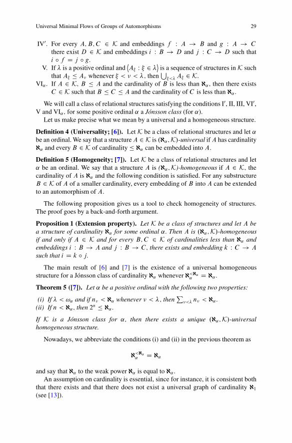
IV0. For every A;B;C 2 K and embeddings f W A ! B and g W A ! C
there exist D 2 K and embeddings i W B ! D and j W C ! D such thati ı f D j ı g:
V. If is a positive ordinal and˝A W 2
˛is a sequence of structures in K such
that A � A� whenever < � < ; thenS< A 2 K:
VI˛. If A 2 K; B � A and the cardinality of B is less than @˛; then there existsC 2 K such that B � C � A and the cardinality of C is less than @˛:
We will call a class of relational structures satisfying the conditions I0, II, III, VI0,V and VI˛; for some positive ordinal ˛ a Jonsson class (for ˛).
Let us make precise what we mean by a universal and a homogeneous structure.
Definition 4 (Universality; [6]). Let K be a class of relational structures and let ˛be an ordinal. We say that a structureA 2 K is .@˛;K/-universal ifA has cardinality@˛ and every B 2 K of cardinality � @˛ can be embedded into A:
Definition 5 (Homogeneity; [7]). Let K be a class of relational structures and let˛ be an ordinal. We say that a structure A is (@˛;K)-homogeneous if A 2 K; thecardinality of A is @˛ and the following condition is satisfied. For any substructureB 2 K of A of a smaller cardinality, every embedding of B into A can be extendedto an automorphism of A:
The following proposition gives us a tool to check homogeneity of structures.The proof goes by a back-and-forth argument.
Proposition 1 (Extension property). Let K be a class of structures and let A bea structure of cardinality @˛ for some ordinal ˛: Then A is .@˛;K/-homogeneousif and only if A 2 K and for every B;C 2 K of cardinalities less than @˛ andembeddings i W B ! A and j W B ! C; there exists and embedding k W C ! A
such that i D k ı j:The main result of [6] and [7] is the existence of a universal homogeneous
structure for a Jonsson class of cardinality @˛ whenever @<@˛˛ D @˛:
Theorem 5 ([7]). Let ˛ be a positive ordinal with the following two properties:
(i) If < !˛ and if n� < @˛ whenever � < ; thenP
�< n� < @˛:(ii) If n < @˛; then 2n � @˛:If K is a Jonsson class for ˛; then there exists a unique .@˛;K/-universalhomogeneous structure.
Nowadays, we abbreviate the conditions (i) and (ii) in the previous theorem as
@<@˛˛ D @˛
and say that @˛ to the weak power @˛ is equal to @˛:An assumption on cardinality is essential, since for instance, it is consistent both
that there exists and that there does not exist a universal graph of cardinality @1(see [13]).

30 D. Bartosova
Corollary 4 ([7]). If the General Continuum Hypothesis holds and K is a Jonssonclass for every positive ordinal ˛, then there is an .@˛;K/-universal homogeneousstructure for every positive ˛:
In the previous section, we presented a method which shows how to computeuniversal minimal flows of groups of automorphisms of structures provided thatthe structures admit a certain linearly ordered extension. To obtain correspondingresults for Jonsson classes, we require that the structures of those classes permit anextension to a Jonsson class of linearly ordered structures satisfying a mild conditionof reasonability as in the case of Fraısse classes in [8].
Definition 6 (Reasonable class). Let L � f>g be a language. Let K< be a classof L-structures with < interpreted as a linear ordering. Let L0 D L n f<g and K DK<jL0: We say that K< is reasonable, if whenever A;B 2 K; A is a substructureof B and � is a linear ordering on A with .A;�/ 2 K<; then there exists a linearordering�0 on B such that .B;�0/ 2 K< and .A;�/ is a substructures of .B;�0/:
The following proposition is Proposition 5.2 from [8] adjusted to Jonsson classes.It verifies that if we remove the linear order from the universal homogeneousstructure for a reasonable Jonsson class, we obtain the universal homogeneousstructure for the corresponding class of structures without linear orderings.
Proposition 2. Suppose that ˛ is a positive ordinal such that @<@˛˛ D @˛: Let
K< be a Jonsson class for ˛ in a language L � f<g with < interpreted as alinear ordering. Suppose that K< is closed under substructures. Let .A;</ be the.@˛;K</-universal homogeneous structure. Set L0 D L n f<g and K D K<jL0:Then the following are equivalent:
(a) K< is reasonable,(b) K is a Jonsson class and A D .A;</jL0 is an .@˛;K/-universal homogeneous
structure
Proof. .)/ Obviously, K satisfies conditions I’, II, V and VI˛: To verify thejoint embedding property III, let B;C 2 K: Find �;�0 linear orderings onB;C respectively such that .B;�/; .C;�0/ 2 K<: Since K< satisfies III, there isD< 2 K< such that .B;�/; .C;�0/ � D<: ThenD D D<jL0 is a witness of a jointembedding of B and C in K:
It remains to show the amalgamation property IV’: Fix B;C;D 2 K and embed-dings i W B ! C and j W B ! D: Let � be an ordering on B such that .B;�/ 2K<: Since K< is reasonable, we can find linear orders �0;�00 on C;D respectivelysuch that .C;�0/; .D;�00/ 2 K< and i W .B;�/! .C;�0/; j W .B;�/! .D;�00/are still embeddings. Amalgamation property for K< provides us with E< 2 K<
and embeddings k W .C;�0/ ! E<; l W .D;�00/ ! E< such that k ı i D l ı j:Let E D E<jL0 and embeddings k W C ! E; l W D ! E are witnesses ofamalgamation of C and D over B in K:
Finally, we check that A is .@˛;K/-universal and homogeneous. Let B 2 K ofcardinality � @˛ and let � be a linear ordering on B such that .B;�/ 2 K<: Since

Universal Minimal Flows of Groups of Automorphisms 31
.A;</ is .@˛;K</-universal, there is an embedding i W .B;�/ ! .A;</ which isalso an embedding from B to A: It means that A is .@˛;K/-universal.
To show that A is .@˛;K/-homogeneous, it is enough to check the extensionproperty in Proposition 1. For that, let B � C be structures in K with cardinality< @˛ and let i W B ! A and j W B ! C be embeddings. Denote by�D i�1.< ji.B//: Then .B;�/ 2 K<: Since K< is reasonable, there exists �0on C with .C;�0/ 2 K< such that j W .B;�/ ! .C;�0/ is also an embedding.Since .A;</ is .@˛;K</-homogeneous, it satisfies the extension property, i.e. thereis an embedding k W .C;�0/! .A;</ such that i D k ı j and we are done..(/ Fix B;C 2 K and an embedding i W B ! C: Let � be a linear ordering on
B such that .B;�/ 2 K<: Then there is an embedding j W .B;�/! .A;</; whichis of course also an embedding fromB toA. SinceA is homogeneous, it satisfies theextension property in Proposition 1, so there is an embedding k W C ! A extendingj: Let �0D j�1.< jj.C //: Then .C;�0/ 2 K< and i W .B;�/ ! .C;�0/ is anembedding. ut
We are ready to apply Theorem 1 and Theorem 4 to Jonsson structures. Weremind the reader that the structures need not be countable.
Theorem 6. Let L � f<g be a relational signature and let ˛ be a positive ordinalsuch that @<@˛
˛ D @˛: Let K< be a reasonable Jonsson class in the signatureL with< interpreted as a linear order and let K< be closed under substructures. Denoteby .A;</ the (@˛;K<)-universal homogeneous structure.
(a) If Age.A;</ satisfies the Ramsey property and G< is a dense subgroup ofAut.A;</; then G< is extremely amenable.
(b) If Age.A;</ satisfies both the Ramsey property and the ordering property, thenthe universal minimal flow of any dense subgroup G of Aut.A/ is G <:
Let us turn to concrete examples of Jonsson classes to which we can apply theabove theorem.
Proposition 3. Let K be one of the following classes:
• Graphs or graphs with arbitrary linear orderings,• Kn-free graphs or Kn-free graphs with arbitrary linear orderings,• Hypergraphs or hypergraphs with arbitrary linear orderings,• A-free hypergraphs or A-free hypergraphs with arbitrary linear orderings,
where A is a class of finite irreducible hypergraphs,• Posets or posets with linear orderings extending the partial order.
Then K is a Jonsson class for every positive ordinal ˛ and it is closed undersubstructures.
Proof. It is easy to see that in all cases, K satisfies conditions I0, II, V and that itis closed under substructures which is a strengthening of VI˛ for every ˛: We showthat they also satisfy III and IV0:
To satisfy the joint embedding property III for structures A;B 2 K; we take Cto be the disjoint union of A and B and the embeddings to be the identity. If A;Balso possess a linear order, then let elements of A precede elements of B in C:

32 D. Bartosova
The amalgamation property IV’ is proved similarly as in the case of finitestructures: Let A;B;C 2 K and let i W A ! B; j W A ! C be embeddings.Let the underlying set of D be a quotient of the disjoint union of B and C via anequivalence relation ; where b c if and only if b 2 B; c 2 C and there is ana 2 A such that i.a/ D b; j.a/ D c: Let k W B ! D and l W C ! D be the identityinjections. Then obviously, k ı i D l ı j: Now we equip D with a structure of thecorrect type to make sure that k and l are embeddings:
• If K is a class of hypergraphs in a signature L and Ri 2 L has arity n; then
.d1; d2; : : : ; dn/ 2 RDi � Dn
if and only if either
.k�1.d1/; k�1.d2/; : : : ; k�1.dn// 2 RBi � Bn
or.l�1.d1/; l�1.d2/; : : : ; l�1.dn// 2 RCi � Cn:
It means that RDi D RBi [ RCi when we identify B;C with their correspondingimages k.B/; l.C /: Notice that D will be a graph (Kn-free graph, A-freehypergraph) if A;B;C are.
• If K is the class of posets with � the symbol for the partial order, then �D is thetransitive closure of .k � k/.�B/[ .l � l/.�C /:If K is a class of linearly ordered structures with < the symbol for the linear
order, then <D on D is an arbitrary linear ordering extending the transitive closureof .k � k/.<B/ [ .l � l/.<C /: In the next section, we will need to be more carefulwhen amalgamating linear orders: we will set elements of B to precede elements ofC whenever we can. Formally, for b 2 B denote by .�; b/ D fa 2 A W k.a/ <B bgand for c 2 C denote by .�; c/ D fa 2 A W l.a/ <C cg: Let <D be the extension ofboth k �k.<B/ and l � l.<C / such that whenever b 2 B; c 2 C then k.b/ <D l.c/if and only if .�; b/ .�; c/: It is easy to see that <D extends�D if K is the classof posets with a linear ordering extending the partial order. So in all cases, K is aJonsson class for every ˛: ut
We know that if K is one of the ordered classes in the proposition above, thenfinite structures in K satisfy the ordering property and the Ramsey property. Also,the ordered classes are obviously reasonable. Therefore, Theorem 6 applies to K.
Corollary 5. Let � be a cardinal satisfying �<� D � and let .A;</ be the universalhomogeneous ordered graph (Kn-free graph, hypergraph, A-free hypergraph,poset) of cardinality �: Let G< be a dense subgroup of Aut.A;</ and let G bea dense subgroup of Aut.A/: Then G< is extremely amenable and the universalminimal flow of G is G <:

Universal Minimal Flows of Groups of Automorphisms 33
4 Constructing !-Homogeneous Structuresin Every Cardinality
In this section, we overcome the restriction on the size of structures given byJonsson’s construction for the price of losing universality and only keeping !-homogeneity. This is however sufficient to compute universal minimal flows ofgroups of automorphisms of such structures. Hence we obtain many more examplesof explicitly computed universal minimal flows.
We present a construction of !-homogeneous (linearly ordered) graphs,Kn-freegraphs, hypergraphs, A-free hypergraphs (where A is a class of finite irreduciblehypergraphs) and posets of arbitrary uncountable cardinality:
Let A be a graph (Kn-free graph, hypergraph, A-free hypergraph, poset) ofcardinality � and let< be an arbitrary linear ordering on A (respectively an orderingextending the partial order if A is a poset). We will construct an !-homogeneousstructure .A�;<�/ of cardinality � in which .A;</ is embedded and such that A�itself is !-homogeneous.
By induction, we construct a chain of superstructures h.A;</ W < �i of.A;</ such that .A;</ � .A�;<�/ whenever < � < � and .A�;<�/ DS<�.A;</: In step ; we deal with a pair of isomorphic finite substructures
.F;</ and .G;</ of .A;</ and an isomorphism � W F ! G and weconstruct .AC1; <C1/ with an automorphism C1 W AC1 ! AC1 extending� that is order-preserving if � is. Moreover, we make sure that if < and.F; </ D .F;</ and .G;</ D .G;</ and � D �; then � :
To ensure that A� and .A�;<�/ are both !-homogeneous, we need to considerevery triple ..F;</; .G;</; � W F ! G/ cofinality of �-many times forevery < �. In order to do so, we fix a book-keeping function—a bijection f W� ! � � �—which we only need to satisfy that whenever f ./ D .�; /; then� � : We will describe f in detail later.
If is limit, then .A;</ D S�<.A�;<�/: If D �C 1; then we construct
.A;</ from .A�;<�/ as follows.Let .F�;<�/; .G�;<�/ be the pair of finite substructures of .A�;<�/ and �� W
F� ! G� the automorphism given by f in step � (as described later). Denoteby .B;<B/ the union of all .A;</ such that � � and .F; </ D .F�;<�/;
.G;</ D .G�;<�/ and � D �� and let B be the union of the corresponding ’s. We need to set jB D B: For every a 2 A� n B we add two new pointsa1 and a�1 to be the image and the preimage of a under respectively. In the nextstep, we need to add for every a 2 A� n B another two points a2; a�2 to be theimage of a1 and the preimage of a�1 under respectively. We continue in the samemanner !-many times until we have taken care that every point has its image andpreimage. Formally, let Az
� be a copy of A� for z 2 Z and denote by az the elementof Az
� corresponding to an a in A�: We identify A0� with A�:We examine two cases depending on whether the triple ..F�;<�/; .G�;<�/;
��/ appears for the first time throughout the construction (i.e. B D ;) or not.However, in both cases the construction follows a similar pattern.

34 D. Bartosova
Case 1: B D ;: Let F z� and Gz
� denote the corresponding copies of F� and G� inAz� respectively. The underlying set of A will be a quotient of the disjoint union of
Az� for z 2 Z by an equivalence relation gluing Gz
� with F zC1� via �� W
az11 2 F z1
� ; az22 2 Gz2
� ! .az11 az2
2 $ .��.a1/ D a2 ^ z1 D z2 C 1//:
If az 2 Az� and a … F� then we write az to mean its -class Œaz�� D fazg: If
a 2 F�; then we write az to mean its -class Œaz�� D faz; ��.a/z�1g:
Let us define W A ! A to be the mapping az 7! azC1 whenever a … F�and z 2 Z and az 7! ��.a/
z whenever a 2 F�:If �� is order preserving, let us transfer the linear order<� onA� toAz
� for everyz 2 Z W
az <z� b
z if and only if �z .a
z/ <� �z .b
z/
We define the structure on A inductively using amalgamation as describedin the previous section. If �� is order preserving, then we use amalgamation forlinearly ordered structures letting elements of Az1
� precede elements of Az2� for
z1 < z2 whenever we can as described in the previous section. Otherwise, we useamalgamation for unordered structures and in the end obtain < as an arbitrarylinear extension of <� (and extending the partial order on A if A is a poset).
Let n 2 ! and let An� denote the subset of A consisting of points in Az
� forz 2 f�nC 1;�nC 2; : : : ; ng; i.e.,
An� D
n[
zD�nC1Az�
!�
:
Similarly let AnC denote the quotient
AnC D
n[
zD�nAz�=
of the disjoint union of Az� for z 2 f�n;�nC 1; : : : ; ng by . We have that A0 D
A�: Suppose that the structure on AnC has been defined. Then the structure on
A.nC1/� is given by amalgamatingAnC
with AnC1� along
F nC1� ! AnC
; anC1 7! .��.a//n and F nC1
� ! AnC1� ; anC1 7! anC1:
When the structure on An� has been defined, then the structure on AnC
is given byamalgamation of An�
and A�n� along
F�nC1� ! An�
; a�nC1 7! a�nC1 and F�nC1
� ! A�n� ; a
�nC1 7! .��.a//�n:

Universal Minimal Flows of Groups of Automorphisms 35
If �� is order preserving, then AnC (respectively A�n
� ) plays the role of Band AnC1
� (respectively An� ) the role of C in the amalgamation of linear orders
described in the previous section.We can see that AnC
� AnC1� � AnC1C
for every n 2 !; so we candefine the structure on A as the union of the chain
˝AnC W n 2 !
˛(equivalently˝
An� W n 2 !
˛):
A D[
n2!AnC D
[
n2!An� :
Case 2: B ¤ ;: The underlying set of A will then be a quotient of the disjointunion of Az
� for z 2 Z by an equivalence relation gluing corresponding copies ofB in Az
� via B W
az11 2 Az1
� ; az22 2 Az2
� ! .az11 az2
2 ! a1; a2 2 B ^ �z1B .a1/ D �z2
B .a2//;
We identify 0B with B:If az 2 Az
� and a … B then we write az to mean its -class Œaz�� D fazg: Ifa 2 B; then we write a to mean its -class Œa�� D faz W z 2 Zg:
Let us define W A ! A to be the mapping az 7! azC1 whenever a … B andz 2 Z and a 7! B.a/ whenever a 2 B:
As in Case 1, we can obtain the structure on A inductively by amalgamationalong B in !-many steps. However, we can obtain A via amalgamation of Az
�; z 2Z along B ! Az
�; b 7! z.b/ in one step:
• If A is a hypergraph in a signature L and Ri 2 L has arity n; then
.az11 ; a
z22 ; : : : ; a
znn / 2 RAi
if and only if
.z1 D z2 D : : : D zn/ ^ . �z1 .a
z11 /;
�z1 .a
z12 /; : : : ;
�z1 .az1
n // 2 RA�i :
Notice that A will be a graph (Kn-free graph, A-free hypergraph) if A� is.• If A is a poset with a partial order �, then � is the transitive closure of the
relation obtained as in the case of hypergraphs.
It remains to extend the linear order <� to a linear order < on A: If �� is notorder preserving, let< be an arbitrary linear ordering extending<� (and extendingthe partial order � on A in case that A is a poset). If �� is order preserving, wewill extend <� to < to make sure that is order preserving.
We can also describe < explicitly, without an inductive construction. We againlet elements in Az1
� precede elements in Az2� whenever z1 < z2 and we are free to do
so: Let az 2 Az� and denote by
.�; az/ D fb 2 B W b <� �z .a/g:

36 D. Bartosova
Let az11 2 Az
� and az22 2 Az2
� for some z1; z2 2 Z and az11 ¤ az2
2 :
• If z1 D z2; then az11 < a
z22 if and only if �z1
.az11 / <�
�z1 .a
z22 /:
• If z1 ¤ z2; then az11 < a
z22 if and only if .�; az1
1 / ¨ .�; az22 / or .�; az1
1 / D.�; az2
2 / and z1 < z2:
Obviously, < is antireflexive and antisymmetric. Let us check transitivity: Leta
z11 ; a
z22 ; a
z33 2 A and az1
1 < az22 and az2
2 < az33 : We have five possible cases:
1. z1 D z2 D z3: Then �z1 .a
z11 / <�
�z1 .a
z12 / <�
�z1 .a
z13 / so �z2
.az11 / <�
�z1 .a
z13 / by transitivity of <�.
2. z1 D z2 ¤ z3: Then �z1 .a
z11 / <�
�z1 .a
z12 /; so .�; az1
1 / .�; az12 /; and either
.�; az12 / ¨ .�; az3
3 / or .�; az12 / D .�; az3
3 / and z2 < z3:3. z1 ¤ z2 D z3: Then .�; az1
1 / ¨ .�; az22 / or .�; az1
1 / D .�; az22 / with z1 < z2 and
�z2 .a
z22 / <�
�z2 .a
z23 /; so .�; az2
2 / .�; az23 /:
4. z1 D z3 ¤ z2: Then .�; az11 / .�; az2
2 / .�; az13 / and at least one inclusion
is proper, since otherwise z1 < z2 < z1: So we get .�; az11 / ¨ .�; az1
3 /; whichimplies �z1
.az11 / <�
�z1 .a
z13 /.
5. z1 ¤ z2 ¤ z3; z1 ¤ z3: Then we have the following four cases:
(i) .�; az11 / ¨ .�; az2
2 / ¨ .�; az33 /:
(ii) .�; az11 / ¨ .�; az2
2 / D .�; az33 / and z2 < z3:
(iii) .�; az11 / D .�; az2
2 / ¨ .�; az33 / and z1 < z2
(iv) .�; az11 / D .�; az2
2 / D .�; az33 / and z1 < z2 < z3:
In all cases we get that az11 < a
z33 ; hence < is transitive.
If A is a poset with � the symbol for the partial order and � is the extension of� to A described above, let us verify that < extends �W If az
1; az2 2 Az
� for somez 2 Z; then az
1 < az2 if and only if az
1 � az2 by definition. If az1
1 2 Az1� ; a
z22 2 Az2
�
for some z1 ¤ z2 and az11 � az2
2 ; then there is a 2 B such that �z1 .a
z11 / <� a
and a <� �z2 .a
z22 /: It means that a 2 .�; az1
1 / while a … .�; az22 /; showing that
az11 < a
z22 :
Let us go back to the definition of the book-keeping function f : When .A�;<�/
has been constructed, let f..F �;<
�/; .G
�;<
�/; �
�/ W < �g be an enumeration
of all triples such that .F �;<
�/ and .G
�;<�/ are finite substructures of .A�;<�/
and �� is an isomorphism between F � and G
� (this is possible since �<! D �
for every infinite �). If f .�/ D .�; /; then the triple we consider in step �
is ..F � ; <
�/; .G
� ; <
�/; �
� /: The inequality � � � ensures that F
� and G� are
finite substructures of already defined A� � A�: The inclusion A� � A� for� < � < � provides that for every � < �; every triple ..F;<�/; .G�/; �/ oftwo finite substructures of .A�;<�/ and an isomorphism between F and G will beconsidered unboundedly many times throughout our construction.
The outcome of the construction can be formulated as the following theorem.
Theorem 7. Let A be a graph (Kn-free graph, hypergraph, A-free hypergraph,poset) of an infinite cardinality � and let < be an arbitrary linear ordering on A(respectively an ordering extending the partial order if A is a poset). Then there

Universal Minimal Flows of Groups of Automorphisms 37
exists a linearly ordered graph (Kn-free graph, hypergraph, A-free hypergraph,poset) .A0; <0/ of cardinality � in which .A;</ is embedded and such that both A0and .A0; <0/ are !-homogeneous (and if A is a poset, <0 extends the partial orderon A0).
If we start with A a graph (Kn-free graph, hypergraph, A-free hypergraph, poset)and a linear order < on A such that Age..A;<// is the class of all finite linearlyordered graphs (Kn-free graphs, hypergraphs, A-free hypergraphs) or posets withthe linear order extending the partial order, the construction provides us with astructure for which we are able to compute the universal minimal flow of its groupof automorphisms. This can easily be arranged for instance by requiring that .A;</contains a copy of the countable !-homogeneous ordered graph (Kn-free graph,hypergraph, A-free hypergraph, poset).
Theorem 8. Let A be an !-homogeneous graph (Kn-free graph, hypergraph, A-free hypergraph, poset) and let < be a linear ordering on A (extending the partialorder if A is a poset) such that .A;</ is !-homogeneous as well.
Suppose that Age.A;</ is the class of all finite linearly ordered graphs (Kn-freegraphs, hypergraphs, A-free hypergraphs) or posets with linear orderings extendingthe partial order.
If G is a dense subgroup of Aut.A/; then the universal minimal flow of G is thespace of all linear orderings on A (respectively the space of all linear orderingsextending the partial order if A is a poset).
Acknowledgements This project was partially supported by the grant GAUK 66509. I wishto thank Stevo Todorcevic for proposing the project of computing universal minimal flows ofgroups of automorphisms of uncountable structures, for introducing me to Jonsson structures andsuggesting the present construction of !-homogeneous structures. I am also grateful to LionelNguyen Van The and the anonymous referee for careful reading and valuable suggestions.
References
1. D. Bartosova, Universal minimal flows of groups of automorphisms of uncountable structures.In Canadian Mathematical Bulletin, Published electronically on July 27 (2012). http://dx.doi.org:10.4153/CMB-2012-023-4
2. J. de Vries, Elements of topological dynamics. In Mathematics and its Applications, vol. 257(Kluwer, Dordrecht, 1993)
3. R. Fraısse, Sur l’extension aux relations de quelques proprietes des ordres. Ann. Sci. EcoleNorm. Sup. 71(3), 363–388 (1954)
4. W. Herer, J.P.R. Christensen, On the existence of pathological submeasures and the construc-tion of exotic topological groups. Math. Ann. 213 203–210 (1975)
5. W. Hodges, A Shorter Model Theory (Cambridge University Press, Cambridge, 1997)6. B. Jonsson, Universal relational systems. Math. Scand. 4, 193–208 (1956)7. B. Jonsson, Homogeneous universal relational systems. Math. Scand. 8, 137–142 (1960)8. A.S. Kechris, V.G. Pestov, S. Todorcevic. Fraısse limits, Ramsey theory, and topological
dynamics of automorphism groups. Geom. Funct. Anal. 15(1), 106–189 (2005)
38 D. Bartosova
9. J. Nesetril, V. Rodl, Partitions of finite relational and set systems. J. Combinatorial Theory Ser.A 22(3), 289–312 (1977)
10. J. Nesetril, V. Rodl, On a probabilistic graph-theoretical method. Proc. Amer. Math. Soc. 72(2),417–421 (1978)
11. J. Nesetril, V. Rodl, Ramsey classes of set systems. J. Combin. Theory Ser. A 34(2), 183–201(1983)
12. V.G. Pestov, On free actions, minimal flows, and a problem by Ellis. Trans. Amer. Math. Soc.350(10), 4149–4165 (1998)
13. S. Shelah, On universal graphs without instances of CH. Ann. Pure Appl. Logic 26(1), 75–87(1984)
14. M. Sokic, Ramsey property of posets and related structures. Ph.D. Thesis, 2010

On the Lyapounov Exponents of SchrodingerOperators Associated with the Standard Map
J. Bourgain
Abstract It is shown that Schrodinger operators defined from the standard maphave positive (mean) Lyapounov exponents for almost all energies.
Key words Standard map • Lyapounov exponents
Mathematical classification subject (2010): 37D25, 37D50
1 Definitions
Let V be a bounded potential on ZC. Define
!.V / D fW D .Wn/n2ZI there is a sequence nj ! 1 such that
d.Snj V; W / ! 0g (1)
whered.V; V 0/ D
X2�njVn � V 0
nj and .SkV /.n/ D V.n C k/:
Let A � R; mes .A/ > 0. Denote
R.A/ D fbounded potentials W D .Wn/n2Zthat are reflectionless on Ag (2)
and RC .A/ D fW 2 R.A/I supn jWnj � C g W .Let H D W C � and let G.z/ be the Green’s function of H .
J. Bourgain (�)Institute for Advanced Study, Princeton, NJ 08540, USAe-mail: [email protected]
M. Ludwig et al. (eds.), Asymptotic Geometric Analysis, Fields InstituteCommunications 68, DOI 10.1007/978-1-4614-6406-8 3,© Springer Science+Business Media New York 2013
39

40 J. Bourgain
Recall that W is reflectionless on A if
ReG.t/.n/ D 0 for a.e. t 2 A and every n 2 Z:
2 Remling Theorems
We rely on following results from Remling’s paper [7]
!.V / � R X
ac
.V /
!([7] Theorem 1.4) (3)
RC .A/ is compact ([7] Proposition 4.1, (d)) (4)
The restriction maps R.A/ ! R˙.A/ are injective (˙ refers to �Z˙), and for
any constant C , the map
RC .A/ ! RCC.A/ is uniformly continuous (5)
(ŒR�Proposition 4.1 .c/; .e/).
W 2 R.A/ ) A �X
ac
.E˙/: (6)
To put things in perspective, one should point out the close relation betweenRemling’s results and Kotani’s theory [2–5] as well as the paper of Last and Simon[6], where the notion of ‘right limits’ is introduced.
3 Lyapounov Exponents
Let T be a measure preserving homeomorphism of a compact metric space ˝
endowed with a probability measure � that charges any non-empty open subset(we do not assume T ergodic).
Let ' 2 C.˝/.Consider the half-line SO
Hx D '.T nx/ın C � (7)
and denote
MN .E; x/ D1Y
N
�E � '.T nx/ �1
1 0
�

On the Lyapounov Exponents of Schrodinger Operators Associated: : : 41
LN .E/ D 1
N
Zlog kMN .E; x/k�.dx/:
Let A � R; mes .A/ > 0 and assume
limN
LN .E/ D 0 on A: (8)
Then
A �X
a:c.Vx/ for � a:e: x: (9)
Proof. Let
� DZ
ˇ ˛.dˇ/
be the ergodic decomposition of �.By Fubini, for E 2 A
LN .E/ DZ n 1
N
Zlog kMN .E; x/kˇ.dx/
o˛.dˇ/
and Z n lim
N
� 1
N
Zlog kMN .E; x/kˇ.dx/
�o˛.dˇ/:
Since ˇ is ergodic, it follows that for ˛ - a.e. ˇ
1
Nlog kMN .E; x/k ! 0 for ˇ - a.e. x 2 ˝ (10)
Again by Fubini, (10) holds for a.e. E 2 A and ˇ - a.e. x 2 ˝
By Kotani theory, this implies that
A �X
ac.Hx/ for ˇ � a:e: x 2 ˝: (11)
Since (11) is valid for ˛ - a.e. ˇ, (9) follows.
4 Use of Recurrence
Let T be as in �3.Let Vx D �
'.T nx/�
n2ZC.
Then
Vx 2 �ZC
�!.Vx/
�for � - a.e. x 2 ˝: (12)
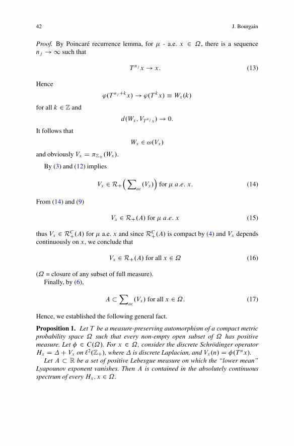
42 J. Bourgain
Proof. By Poincare recurrence lemma, for � - a.e. x 2 ˝ , there is a sequencenj ! 1 such that
T nj x ! x: (13)
Hence
'.T nj Ckx/ ! '.T kx/ � Wx.k/
for all k 2 Z and
d.Wx; VTnj x/ ! 0:
It follows that
Wx 2 !.Vx/
and obviously Vx D �ZC.Wx/.
By (3) and (12) implies
Vx 2 RC�X
ac.Vx/
�for � a:e: x: (14)
From (14) and (9)
Vx 2 RC.A/ for � a:e: x (15)
thus Vx 2 RCC.A/ for � a.e. x and since RCC.A/ is compact by (4) and Vx dependscontinuously on x, we conclude that
Vx 2 RC.A/ for all x 2 ˝ (16)
(˝ = closure of any subset of full measure).Finally, by (6),
A �X
ac.Vx/ for all x 2 ˝: (17)
Hence, we established the following general fact.
Proposition 1. Let T be a measure-preserving automorphism of a compact metricprobability space ˝ such that every non-empty open subset of ˝ has positivemeasure. Let � 2 C.˝/. For x 2 ˝ , consider the discrete Schrodinger operatorHx D � C Vx on `2.ZC/, where � is discrete Laplacian, and Vx.n/ D �.T nx/.
Let A � R be a set of positive Lebesgue measure on which the “lower mean”Lyapounov exponent vanishes. Then A is contained in the absolutely continuousspectrum of every Hx; x 2 ˝ .

On the Lyapounov Exponents of Schrodinger Operators Associated: : : 43
5 Application to Standard Map
Let T D T� be the standard map on the torus T2 D ˝ with sufficiently large �.
Thus
T�.x; y/ D .�y C 2x C � sin 2�x; x/: (18)
Let ' 2 C1.T2/ be a fixed not-constant function.If the corresponding SO has vanishing Lyapounov exponents for E 2 A, (17)
implies
A �X
ac.f'.T nx/gn2ZC
(19)
for all x 2 ˝ .By Duarte’s work (Theorem A in [1]), there is an invariant hyperbolic set
D � � ˝ such that T j is conjugate to a Bernoulli shift. In particular forx 2 ; (19) D �. Furthermore, Duarte’s result asserts that each point in T
2 iswithin a 4�� 1
3 -neighborhood of , so that ' will not be constant on for � largeenough. Hence (19) restricted to is non-deterministic and has no a.c. spectrum,by Kotani’s theory (cf. [K1, K2, K3, K4]), implying that A is of zero-measure(contradiction).
Hence we proved
Proposition 2. For � > �0, the SO (7) associated to the standard map T� haspositive (mean) Lyapounov exponents for a.e. E 2 R.
For comparison, let us recall the major open problem of positivity of theKolmogorov-Sinai metric entropy of the standard map and which is known to beequivalent to the positivity of the Lyapounov exponent at energy E D 0 (for the testfunction �.x; y/ D cos.2�x/).
Acknowledgements The author is grateful to A. Avila, S. Sodin and T. Spencer for somediscussions on this topic, and the referee for comments on the presentation.
References
1. P. Duarte, Plenty of elliptic islands for the standard family of area preserving maps. Ann. Inst.H. Poincare Anal. Non lineaire 11(4), 359–409 (1994)
2. S. Kotani, Ljapunov indices determine absolutely continuous spectra of stationary random one-dimensional Schrodinger operators, in Stochastic analysis (Katata/Kyoto, 1982). North-HollandMath. Library, vol. 32 (North-Holland, Amsterdam, 1984), pp. 225–247
3. S. Kotani, One-dimensional random Schrodinger operators and Herglotz functions, in Proba-bilistic Methods in Mathematical Physic (Katata/Kyoto 1985) (Academic Press, Boston, 1987),pp. 219–250
44 J. Bourgain
4. S. Kotani, Jacobi matrices with random potentials taking finitely many values. Ref. Math. Phys.1, 129–133 (1989)
5. S. Kotani, Generalized Floquet theory for stationary Schrodinger operators in one dimension.Chaos Sol. Fract. 8, 1817–1854 (1997)
6. Y. Last, B. Simon, Eigenfunctions, transfer matrices and absolutely continuous spectrum of one-dimensional Schrodinger operators. Inventiones Math. 135(2), 329–367 (1999)
7. C. Remling, The absolutely continuous spectrum of Jacobi matrices. Annals of Math 174(2),125–171 (2011)

Overgroups of the Automorphism Groupof the Rado Graph
Peter Cameron, Claude Laflamme, Maurice Pouzet, Sam Tarzi,and Robert Woodrow
Abstract We are interested in overgroups of the automorphism group of the Radograph. One class of such overgroups is completely understood; this is the class ofreducts. In this article we tie recent work on various other natural overgroups, inparticular establishing group connections between them and the reducts.
Key words Rado graph • Automorphism group • Overgroup • Homogeneousstructures
Mathematical Subject Classifications (2010): 05C25, 05C80, 05C55, 05C63,20F28
P. CameronSchool of Mathematical Sciences, Queen Mary, University of London,Mile End Road, London E1 4NS, UKe-mail: [email protected]
C. Laflamme (�) • R. WoodrowDepartment of Mathematics and Statistics, University of Calgary, 2500 UniversityDr. NW, Calgary, Alberta, Canada T2N 1N4e-mail: [email protected]; [email protected]
M. PouzetICJ, Mathematiques, 43 Bd. 11 Novembre 1918, 69622 Villeurbanne cedex, Francee-mail: [email protected]
S. TarziSchool of Mathematical Sciences, Queen Mary, University of London,Mile End Road, London E1 4NS, UKe-mail: [email protected]
M. Ludwig et al. (eds.), Asymptotic Geometric Analysis, Fields InstituteCommunications 68, DOI 10.1007/978-1-4614-6406-8 4,© Springer Science+Business Media New York 2013
45

46 P. Cameron et al.
1 Introduction
The Rado Graph R is the countable universal homogeneous graph: it is the unique(up to isomorphism) countable graph with the defining property that for every finitedisjoint subsets of vertices A and B there is a vertex adjacent to all vertices in A andnot adjacent to any of the vertices in B .
We are interested in overgroups of its automorphism group Aut.R/ in Sym.R/,the symmetric group on the vertex set of R. One class of overgroups of Aut.R/
is completely understood; this is the class of reducts, or automorphism groups ofrelational structures definable from R without parameters. Equivalently, this is theclass of subgroups of Sym.R/ containing Aut.R/ which are closed with respectto the product topology. According to a theorem of Thomas [5], there are just fivereducts of Aut.R/:
• Aut.R/
• D.R/, the group of dualities (automorphisms and anti-automorphisms) of R• S.R/, the group of switching automorphisms of R (see below)• B.R/ D D.R/:S.R/ (the big group)• Sym.R/, the full symmetric group
Given a set X of vertices in a graph G, we denote by �X .G/ the switchingoperation of changing all adjacencies between X and its complement in G, leavingthose within or outside X unchanged, thus yielding a new graph. Now a switchingautomorphism of G is an isomorphism which maps G to �X .G/ for some X , andS.G/ is the group of switching automorphisms. Thus the interesting question isoften for which subset X is �X .G/ isomorphic G, and for this reason will sometimesabuse terminology and may call �X .G/ a switching automorphism.
Thomas also showed (see [6], and also the work of Bodirsky and Pinsker [1]) thatthe group S.R/ can also be understood as the automorphism group of the 3-regularhypergraph whose edges are those 3-element subsets containing an odd numberof edges. Similarly, D.R/ is the automorphism group of the 4-regular hypergraphwhose edges are those 4-element subsets containing an odd number of edges, andB.R/ is the automorphism group of the 5-regular hypergraph whose edges are those5-element subsets containing an odd number of edges.
One can see that G is any subgroup of Sym.R/, then G:FSym.R/ (the groupgenerated by the union of G and FSym.R/, the group of all finitary permutations onR) is a subgroup of Sym.R/ containing G and highly transitive. The reducts D.R/
and S.R/ however are 2-transitive but not 3-transitive, while B.R/ is 3-transitivebut not 4-transitive. On the other hand we have the following.
Lemma 1. Any overgroup of Aut.R/ which is not contained in B.R/ is highlytransitive.
Proof. Let G with Aut.R/ � G 6� B.R/, and let G be the closure of G in Sym.R/.Since G 6� B.R/, we have G D Sym.R/ by Thomas’ theorem. Since G and G
have the same orbits of n-uples, G is highly transitive. ut

Overgroups of the Automorphism Group of the Rado Graph 47
Now for a bit of notation. With the understanding that R is the only graph underconsideration here, we write v � w when v and w are adjacent (in R), R.v/ for theset of vertices adjacent to v (the neighbourhood of v), and will use Rc.v/ for RnR.v/
(note that v 2 Rc.v/). We say that a permutation g changes the adjacency of v andw if .v � w/ , .vg 6� wg/. We say that g changes finitely many adjacencies at v ifthere are only finitely many points w for which g changes the adjacency of v and w.
Given two groups G1; G2 contained in a group H , we write G1:G2 for thesubgroup of H generated by their union.
In Sect. 2, we present various other natural overgroups and tie recent work and inparticular establish group connections between them and the reducts.
2 Other Overgroups of Aut.R/
Cameron and Tarzi in [2] have studied the following overgroups of R.
(a) Aut1.R/, the group of permutations which change only a finite number ofadjacencies.
(b) Aut2.R/, the group of permutations which change only a finite number ofadjacencies at each vertex.
(c) Aut3.R/, the group of permutations which change only a finite number ofadjacencies at all but finitely many vertices.
(d) Aut.FR/, where FR is the neighbourhood filter of R, the filter generated bythe neighbourhoods of vertices of R.
One shows that all these sets of permutations really are groups, as claimed. ForAuti .G/, this is because if C.g/ denotes the set of pairs fv; wg whose adjacency ischanged by g, then one verifies that C.g�1/ D C.g/g�1
and C.gh/ � C.g/ [C.h/g�1
.The main facts known about these groups are:
Proposition 1 ([2]).
(a) Aut.R/ < Aut1.R/ < Aut2.R/ < Aut3.R/.(b) Aut2.R/ � Aut.FR/, but Aut3.R/ and Aut.FR/ are incomparable.(c) FSym.R/ < Aut3.R/ \ Aut.FR/, but FSym.R/ \ Aut2.R/ D 1.(d) S.R/ 6� Aut.FR/, and Aut.FR/ \ D.R/ D Aut.FR/ \ S.R/ D Aut.R/.
Proof. (a) is clear.(b) For the first part, let g 2 Aut2.R/. It suffices to show that, for any vertex v,
we have R.v/g 2 F.R/. Now by assumption, R.v/g differs only finitely fromR.vg/; let R.v/g n R.vg/ D fw1; : : : ; wng. If we choose w such that wi 62 R.w/
for each i , then we have
R.vg/ \ R.w/ � R.v/g;
and we are done.

48 P. Cameron et al.
For the second part, choose a vertex v, and consider the graph R0 obtainedby changing all adjacencies at v. Then R0 Š R. Choose an isomorphism g fromR to R0; since R0 is vertex-transitive, we can assume that g fixes v. So g mapsR.v/ to R1.v/ D Rc.v/ n fvg. Clearly g 2 Aut3.R/, since it changes only oneadjacency at any point different from v. But if g 2 Aut.FR/, then we wouldhave R1.v/ 2 FR, a contradiction since R.v/ \ R1.v/ D ;.
In the reverse direction, let R00 be the graph obtained by changing alladjacencies between non-neighbours of v. Again R00 Š R, and we can pickan isomorphism g from R to R00 which fixes v. Now g changes infinitely manyadjacencies at all non-neighbours of v (and none at v or its neighbours), sog 62 Aut3.R/. Also, if w is a non-neighbour of v, then R.v/ \ R.w/g DR.v/ \ R.wg/, so g 2 Aut.FR/.
(c) Note that any non-identity finitary permutation belongs to Aut3.R/ n Aut2.R/.For if g moves v, then g changes infinitely many adjacencies at v (namely, allv and w, where w is adjacent to v but not vg and is not in the support of g). Onthe other hand, if g fixes v, then g changes the adjacency of v and w only if g
moves w, and there are only finitely many such w.Finally, if g 2 FSym.R/, then R.v/g differs only finitely from R.v/, for any
vertex v 2 V ; so g 2 Aut.FR/.Thus the left inclusion is proper: Aut2.R/ is contained in the right-hand side
but intersects FSym.R/ in f1g.(d) The graph R0 in the proof of (b) is obtained from R by switching with respect
to the set fvg; so the permutation g belongs to the group S.R/ of switchingautomorphisms. Thus S.R/ 6� Aut.FR/.
Now any anti-automorphism g of R maps R.v/ to a set disjoint from R.vg/;so no anti-automorphism can belong to Aut.FR/. Suppose that g 2 Aut.FR/ isan isomorphism from R to �X .R/. We may suppose that �X is not the identity,that is, X ¤ ; and Y D V n X ¤ ;. Choose x and y so that xg 2 X
and yg 2 Y . Then R.x/g 4 Y D R.xg/ and R.y/g 4 X D R.yg/. HenceR.xg/ \ R.x/g � X and R.yg/ \ R.yg/ � Y . Hence
R.xg/ \ R.x/g \ R.yg/ \ R.y/g D ;;
a contradiction. utOn the other hand, results of Laflamme, Pouzet and Sauer in [4] concern the
hypergraph H on the vertex set of R whose edges are those sets of vertices whichinduce a copy of R. Note that a cofinite subset of an edge is an edge. There are threeinteresting groups here:
(a) Aut.H/.(b) FAut.H/, the set of permutations g with the property that there is a finite subset
S of R such that for every edge E , both .E n S/g and .E n S/g�1 are edges.(c) Aut�.H/, the set of permutations g with the property that, for every edge E ,
there is a finite subset S of E such that .E n S/g and .E n S/g�1 are edges.

Overgroups of the Automorphism Group of the Rado Graph 49
Clearly Aut.H/ � FAut.H/ � Aut�.H/, and a little thought shows that all threeare indeed groups. Moreover one will note that for Aut�.H/ and FAut.H/ to begroups, both conditions on g and g�1 in their definitions are necessary. To see this,choose an infinite clique C � R, and also partition R into two homogeneous edgesE1 and E2: for every finite disjoint subsets of vertices A and B of R there is a vertexin E2 adjacent to all vertices in A and not adjacent to any of the vertices in B . Thenit is shown in [4] that there exists g 2 Sym.R/ such that Cg D A, and Eg is anedge for any edge E . But clearly .A n S/g�1 is not an edge for any (finite) S .
As a further remark let H� be the hypergraph on the vertex set of R whose edgesare subset of the form E [ F where E induces a copy of R and F is a finite subsetof R. Equivalently these are the subsets of R of the form E�F where E inducesa copy of R and F is a finite subset of R (this follows from the fact that for everycopy E and finite set F , E n F is a copy). Then observe that Aut.H�/ D Aut�.H/.
We now provide some relationships between these LPS groups and the CTgroups.
Proposition 2. (a) Aut.H/ < FAut.H/.(b) Aut2.R/ � Aut.H/ and Aut3.R/ � FAut.H/.(c) FSym.R/ � FAut.H/ but FSym.R/ \ Aut.H/ D 1.
Proof. (a) This follows from part (c).(b) If we alter a finite number of adjacencies at any point of R, the result is still
isomorphic to R. So induced copies of R are preserved by Aut2.R/. Similarly,given an element of Aut3.R/, if we throw away the vertices where infinitelymany adjacencies are changed, we are in the situation of Aut2.R/.
(c) The first part follows from Proposition 1 part (c) and part (b) above. For thesecond part, choose a vertex v and let E be the set of neighbours of v in R (thisset is an edge of H). Now, for any finitary permutation, there is a conjugate of itwhose support contains v and is contained in fvg[E . Then Eg D E [fvgnfwgfor some w. But the induced subgraph on this set is not isomorphic to R, sincev is joined to all other vertices. ut
We shall see later that FAut.H/ < Aut�.H/, but we present a bit moreinformation before doing so. In particular we now show that an arbitrary switchingis almost a switching isomorphism.
Lemma 2. Let X � R arbitrary and � D �X be the operation of switching R withrespect to X . Then there is a finite set S such that �.Rn S/ is an edge of H, namelyisomorphic to the Rado graph.
Proof. For E � R and disjoint U; V � E , denote by WE.U; V / the collection ofall witnesses for .U; V / in E . Note that if E is an edge, then WE.U; V / is an edgefor any such sets U and V . Now for C � R, denote for convenience by CX the setC \ X , and by C c
X the set C n X .Thus if �.R/ is not already an edge of H, then the Rado graph criteria regarding
switching yields finite disjoint U; V � R such that both:

50 P. Cameron et al.
• WR.U cX [ VX; UX [ V c
X / � X
• WR.UX [ V cX; U c
X [ VX / \ X D ;Define S D U [ V and E D R n S , we show that �.E/ is an edge of H.
For this let NU ; NV � E . But now we have:
WR. NUX [ NV cX [ U c
X [ VX ; NU cX [ NVX [ UX [ V c
X/
D WE. NUX [ NV cX ; NU c
X [ NVX / \ WR.U cX [ VX ; UX [ V c
X/
� X
In virtue of the Rado graph, the above first set contains infinitely many witnesses,and thus WE. NUX [ NV c
X; NU cX [ NVX / is non empty. Hence �.E/ contains a witness for
. NU ; NV /, and we conclude that �.E/ is an edge. utThe last item above shows that any graph obtained from R by switching has a
cofinite subset inducing a copy of R. This can be formulated as follows: Let G bea graph on the same vertex set as R and having the same parity of the number ofedges in any 3-set as R. Then G has a cofinite subset inducing R.
The next result is about the relation between the LPS-groups and the reducts.
Proposition 3. (a) D.R/ < Aut.H/.(b) S.R/ 6� Aut.H/.(c) S.R/ � Aut�.H/.
Proof. (a) Clearly D.R/ � Aut.H/ since R is self-complementary. We get a strictinequality since Aut.H/ is highly transitive (since Aut2.R/ � Aut.H/) whileD.R/ is not.
(b) We show that R can be switched into a graph isomorphic to R in such a waythat some induced copy E of R has an isolated vertex after switching. Then theisomorphism is a switching-automorphism but not an automorphism of H.
Let p, q be two vertices of R. The graph we work with will be R1 D R n fpg,which is of course isomorphic to R. Let A; B; C; D be the sets of vertices joined top and q, p but not q, q but not p, and neither p nor q, respectively. Let � be theoperation of switching R1 with respect to C , and let E D fqg [ B [ C . It is clearthat, after the switching � , the vertex q is isolated in E . So we have to prove twothings:
Claim. E induces a copy of R.
Proof. Take U , V to be finite disjoint subsets of E . We may assume without loss ofgenerality that q 2 U [ V .
Case 1: q 2 U . Choose a witness z for .U; V [ fpg/ in R. Then z 6� p and z � q,so z 2 C ; thus z is a witness for .U; V / in E .Case 2: q 2 V . Now choose a witness for .U [ fpg; V / in R; the argument issimilar. ut

Overgroups of the Automorphism Group of the Rado Graph 51
Claim. �.R1/ is isomorphic to R.
Proof. Choose U; V finite disjoint subsets of R n fpg. Again, without loss, q 2U [ V . Set U1 D U \ C , U2 D U n U1, and V1 D V \ C , V2 D V n V1.
Case 1: q 2 U , so q 2 U2. Take z to be a witness for .U2 [ V1 [ fpg; U1 [ V2/ inR. Then z � p; q, so z 2 A. The switching � changes its adjacencies to U1 and V1,so in �.R1/ it is a witness for .U1 [ U2; V1 [ V2/.Case 2: q 2 V , so q 2 V2. Now take z to be a witness for .U1 [ V2; U2 [ V1 [ fpg/in R. Then z � q, z 6� p, so z 2 C , and � changes its adjacencies to U2 and V2,making it a witness for .U1 [ U2; V1 [ V2/. ut(c) Let X � R, � be the operation of switching R with respect to X , and g W R !
�.R/ an isomorphism. In order to show that g 2 Aut.H�/ we need to show thatif E is an edge of H there is some finite S such that .E n S/g and .E n S/g�1
are edges of H.
However the graph Eg (in R) is obtained from switching the graph induced by�.R/ on Eg. Since the latter is a copy of R, Lemma 2 yields a finite S0 � R suchthat Eg n S0 is an edge of H. If S1 D S0g
�1, then .E n S1/g is an edge of H.Finally notice that g�1 is an isomorphism from R to �Xg�1 .R/, the above
argument shows that there is a finite S2 such that .E n S2/g�1 is an edge of H.
Since cofinite subsets of edges are edges S WD S1 [ S2 has the required property. utCorollary 1. B.R/ < Aut�.H/
Proof. That B.R/ � Aut�.H/ follows from parts (a) and (c) of Proposition 3.We get a strict inequality since Aut�.H/ is highly transitive (since Aut2.R/ �
Aut�.H/) while D.R/ is not. utProposition 4. S.R/ 6� FAut.H/.
In view of S.R/ � Aut�.H/ (by Proposition 3), this yields the followingimmediate Corollary.
Corollary 2. FAut.H/ < Aut�.H/.
Clearly we have the following immediate observation:
Note 1.Aut.H/:FSym.R/ � FAut.H/
Hence, the Corollary yields yet that Aut.H/:FSym.R/ < Aut�.H/.
Proof (of Proposition 4). The argument can be thought of as an infinite version ofthe one given in part (b) of Proposition 3.
We shall recursively define subsets of R:
• A D han W n 2 Ni• B D hbn W n 2 Ni• C D hcn W n 2 Ni

52 P. Cameron et al.
and set D so that:
1. 8n8k � n an 6� bk and cn � bk .2. 8n En WD fak W k � ng [ fbng [ fck W k � ng is an edge.3. If � is the operation of switching R with respect to C , then �.R/ is isomorphic
to R.4. D D R n .A [ B [ C / is infinite.
a0 a1 a2
b0 b1 b2
c0 c1 c2
The construction is as follows. First list all pairs .U; V / of disjoint finite subsetsof R so that each one reoccurs infinitely often. Start with A D B D C D D D ;and at stage n, assume we have constructed An D fak W k � ng, Bn D fbk W k � ng,and Cn D fck W k � ng satisfying condition (1) above, together with a finite setD disjoint from An, Bn and Cn. Then given .U; V /, proceed following one of thefollowing cases:
(a) Suppose U [V � An[Bn[Cn and contains at most one bi (i.e. .U; V / is a typecandidate for the eventual Ei ). Then, choosing from R n .An [ Bn [ Cn [ D/,add anC1 or cnC1 as a witness for .U; V / depending as to whether bi is in V orU (add anC1 if there is no such bi at all). Then choose two more elements fromRnD to complete the addition of elements anC1, bnC1, and cnC1 as required bycondition (1). Also throw a new point in D just to ensure it will become infinite.
(b) Else add the elements of U [ V n An [ Bn [ Cn to D, and select an element ofR n .An [ Bn [ Cn [ D/ as witness to .U n Cn [ V \ Cn; V n Cn [ U \ Cn/.
The construction in part (b) will ensure that �.R/ is isomorphic to R. Indeed letU and V be disjoint finite subsets of R, and without loss of generality U \ D ¤ ;.Thus when the pair .U; V / is handled at some stage n, part (b) will add a witness d
in D to .U n Cn [ V \ Cn; V n Cn [ U \ Cn/. But then d is a witness to .U; V / in�.R/.
Let g be the isomorphism from �.R/ to R.Finally the construction in part (a) clearly ensures condition (2). However note
that in �.R/, bn is isolated in En, and therefore �.En/ is not an edge.

Overgroups of the Automorphism Group of the Rado Graph 53
Finally for any finite set S � R, choose n so that S \ En D ;. Then .En n S/g
is not an edge. Thus g 2 S.R/ n FAut.H/. utWe now go back to Aut.FR/. One can readily verify that the automorphism g
produced in the reverse direction of Proposition 1 is in fact not in Aut.H/, thusAut.FR/ 6� Aut.H/. However we have the following.
Proposition 5. Aut.FR/ 6� Aut�.H/.
Proof. Fix a vertex v 2 R. Now partition Rc.v/ D E [ D, where E is an edge,D is an infinite independent set. This is easily feasible since Rc.v/ is an edge. Nowdefine g 2 Sym.R/ such that:
(a) g � R.v/ is the identity.(b) g � E is a bijection to D.(c) g � D is a bijection to Rc.v/.
Now for any vertex w, R.w/g � R.v/ \ R.w/ so g 2 Aut.FR/. However, for anyfinite set S of E , then .E n S/g is again an independent set, and thus certainly notan edge.
Hence g 62 Aut�.H/ and the proof is complete. ut
3 Conclusion
The following diagram summarizes the subgroup relationship between the variousgroups under discussion.
Aut(R)
D(R) S(R)
B(R)
Aut∗(H)
Sym(R)
Aut(H)
FAut(H)
Aut1(R)
Aut2(R)
Aut3(R)
(1)
F Sym(R)
Aut(FR)
We do not know if the inclusion is strict in Observation 1.

54 P. Cameron et al.
Acknowledgements Claude Laflamme’s work was supported by NSERC of Canada Grant# 690404.
References
1. M. Bodirsky, M. Pinsker, Minimal functions on the random graph. Preprint (2010).arXiv:1003.4030
2. P.J. Cameron, S. Tarzi, Filters, Topologies and Groups from the Random Graph. Manuscript(2007)
3. R. Diestel, Graph theory, in Graduate Texts in Mathematics, vol. 173 (Springer, Heidelberg,2005)
4. C. Laflamme, M. Pouzet, N. Sauer, The hypergraph of copies of the rado graph, in preparation5. S.R. Thomas, Reducts of the random graph. J. Symbolic Logic 56, 176–181 (1991)6. S.R. Thomas, Reducts of Random Hypergraphs. Ann. Pure Appl. Logic 80, 165–183 (1996)

On a Stability Property of the GeneralizedSpherical Radon Transform
Dmitry Faifman
Abstract In this note, we study the operator norm of the generalized sphericalRadon transform, defined by a smooth measure on the underlying incidence variety.In particular, we prove that for small perturbations of the measure, the sphericalRadon transform remains an isomorphism between the corresponding Sobolevspaces.
Key words Radon transform • Sobolev spaces • Pseudodifferential operators •Integral geometry
Mathematical Subject Classifications (2010): 44A12, 53C65
1 Introduction and Background
Throughout the note, we fix a Euclidean space V D RdC1, and consider the
Euclidean spheres X D Sd � V , and Y D Sd � V �. For p 2 Y , Cp � X willdenote the copy of Sd�1 � X given by Cp D fq 2 X W hq; pi D 0g. Let �d�1.q/denote the SO.d/-invariant probability measure on Cp. The set Cq � Y and themeasure �d�1.p/ on it are defined similarly. Then the spherical Radon transform isdefined as follows:
R W C1.X/ ! C1.Y /
Rf .p/ DZCp
f .q/d�d�1.q/:
D. Faifman (�)School of Mathematical Sciences, Tel-Aviv University, Tel Aviv 69978, Israele-mail: [email protected]
M. Ludwig et al. (eds.), Asymptotic Geometric Analysis, Fields InstituteCommunications 68, DOI 10.1007/978-1-4614-6406-8 5,© Springer Science+Business Media New York 2013
55

56 D. Faifman
Let � be the unique SO.d C 1/-invariant probability measure on the incidencevariety Z D f.q; p/ 2 X � Y W hq; pi D 0g. Assume one is given a smooth, notnecessarily positive measure d� on Z, given by �.q; p/� where � 2 C1.Z/,and which satisfies �.˙q;˙p/ D �.q; p/ (call such � symmetric). IntroduceR� W C1.X/ ! C1.Y / by
.R�f /.p/ DZCp
f .q/�.q; p/d�d�1.q/:
Introduce also the dual Radon transform RT� W C1.Y / ! C1.X/ which is
formally adjoint to R� and given by
.RT�g/.q/ D
ZCq
g.p/�.q; p/d�d�1.p/:
Let L2s .PX/ and L2s.PY / denote the Sobolev space of even functions on X and Y ,respectively. It is well known (see [2]) that the spherical Radon transform extendsto an isomorphism of Sobolev spaces:
R W L2s.PX/ ! L2sC d�1
2
.PY /
for every s 2 R. For general � as above, R� is a Fourier integral operator of orderd�12
(see [3, 5]), and so extends to a bounded map R� W L2s .PX/ ! L2sC d�1
2
.PY /.
We look for conditions on � so that this is again an isomorphism.It follows from Guillemin’s theorem on general Radon transforms associated to
double fibrations [1], that RT�R� W C1.PX/ ! C1.PX/ is an elliptic pseudo-
differential operator of order d � 1 for all smooth, positive, symmetric measures� on Z (for completeness, this is verified in the Appendix). The dependence of theprincipal symbol of RT
�R� on �was investigated in [5]. In this note, we analyze thedependence on � of the operator norm of RT
�R� W L2s .PX/ ! L2sC.d�1/.PX/. Wethen give a sufficient condition on a perturbation � of �0 so that R� W C1.PX/ !C1.PY / remains an isomorphism. Namely, we prove the following
Theorem. The set ofC1 measures� onZ for which R� W C1.PX/ ! C1.PY /is an isomorphism, is open in the C2dC1.Z/ topology.
2 Bounding the Norm of RT� R�
We start by recalling an equivalent description of the Radon transform. Consider thedouble fibration

On a Stability Property of the Generalized Spherical Radon Transform 57
Z
�
���������� �
�����
����
�
X Y
Let �X D ��� and �Y D ��� be the rotation-invariant probability measures on Xand Y , respectively. Then for f 2 C1.X/, .Rf /�Y D ��.�.��f //. For smoothsymmetric measures d�, d� on Z, given by �.q; p/� and �.q; p/� we can defineR� W C1.X/ ! C1.Y /, RT
� W C1.Y / ! C1.X/ respectively by
.R�f /�Y D ��.��.��f //
and.RT
� g/�X D ��.��.��g//:
It follows from [1] that both R� and RT� are Fourier integral operators of order d�1
2.
Thus we restrict to even functions and consider R� W L2s.PX/ ! L2sC d�1
2
.PY / and
RT� W L2
sC d�12
.PY / ! L2sC.d�1/.PX/.As before, q will denote a point in X and p a point in Y . We will often write
q 2 p instead of hq; pi D 0 ” q 2 Cp ” p 2 Cq . In the following, thefunctions f; g are even. We also assume d � 2.
Proposition 1. The Schwartz kernel of RT� R� W L2s.PX/ ! L2sC.d�1/.PX/ is
K.q0; q/ D cd
sin dist.q0; q/˛.q; q0/
that is,
RT� R�f .q
0/ DZX
f .q/K.q0; q/d�X.q/:
Here cd is a constant, and ˛.q; q0/ is the average over all p 2 Y s.t. q; q0 2 p of�.q; p/�.q0; p/. More precisely,
˛.q; q0/ DZSO.d�1/
�.q;Mp0/�.q0;Mp0/dM
where SO.d � 1/ D fg 2 SO.d C 1/ W gq D q; gq0 D q0g, Cp0 is any fixed copyof Sd through q; q0, and dM is the Haar probability measure on SO.d � 1/.Proof. Fix some q0 2 X , and p0 2 Y s.t. q0 2 p0. Let SO.d/ � SO.d C 1/ be thestabilizer of q0 2 X . For g 2 C1.Y / we may write
RT� g.q
0/ DZp3q0
g.p/�.q0; p/d�d�1.p/ DZSO.d/
g.Mp0/�.q0;Mp0/dM

58 D. Faifman
where dM is the Haar probability measure on SO.d/. Then taking
g.p/ D R�f .p/ DZ
Qq2pf . Qq/�. Qq; p/d�d�1. Qq/
we get
RT� R�f .q
0/ DZSO.d/
� ZQq2Mp0
f . Qq/�. Qq;Mp0/d�d�1. Qq/��.q0;Mp0/dM
DZSO.d/
� ZQq2p0
f .M Qq/�.M Qq;Mp0/d�d�1. Qq/��.q0;Mp0/dM
DZ
Qq2p0d�d�1. Qq/
ZSO.d/
f .M Qq/�.M Qq;Mp0/�.q0;Mp0/dM:
Denote � D dist. Qq; q0/, and Sd�1� D fq W dist.q0; q/ D �g. Let d��d�1.q/ denote
the rotationally invariant probability measure on Sd�1� . The inner integral may be
written as ZSd�1�
f .q/˛.q; q0/d��d�1.q/:
Here ˛.q; q0/ D RSO.d�1/ �.q;Mp0/�.q
0;Mp0/dM with SO.d � 1/ D Stab.q/\Stab.q0/ is just the average of �.q; p/�.q0; p/ over all .d�1/-dimensional spheresCp containing both q and q0. Then
RT� R�f .q
0/ DZ
Qq2p0d�d�1. Qq/
ZSd�1�
f .q/˛.q; q0/d��d�1.q/
and since the inner integral only depends on � D dist. Qq; q0/, this may be rewrittenas
cd
Z �=2
0
d� sind�2 �ZSd�1�
f .q/˛.q; q0/d��d�1.q/:
Finally, d�d D cd sind�1 �d�d��d�1, and so
RT� R�f .q
0/ D cd
ZX
1
sin �f .q/˛.q; q0/d�d .q/:
We conclude that the Schwartz kernel is
K.q0; q/ D cd
sin dist.q0; q/˛.q; q0/:
utWe proceed to estimate the norm of RT
� R�. Our main tool will be the followingproposition proved in Sect. C

On a Stability Property of the Generalized Spherical Radon Transform 59
Proposition. Consider a pseudodifferential operator P of orderm
P W L2sCm.Rn/ ! L2s .Rn/
between Sobolev spaces with x�compactly supported symbol p.x; �/ in K � Rn
s.t.jD˛
xp.x; �/j � C˛0.1C j�j/˛:There exists a constant C.n; s/ such that
kP kL2sCm.Rn/!L2s .R
n/ � C.n; s/ supj˛j�nCbjsjcC1
C˛0jKj:
Proposition 2. The norm of RT� R� W L2�.d�1/.PX/ ! L20.PX/ is bounded from
above by
kRT� R�k � C
2dC1XjCkD0
kDj�k1kDk�k1
for some constant C dependent on the double fibration.
Proof. First introduce coordinate charts. Choose a partition of unity i .q0/ corre-sponding to a covering of X by charts Ui , and a function � W Œ0;1/ ! RC withsupport in Œ0; 1 s.t. �.r/ D 1 for r � 1
2. Write
K.q0; q/ DXi
Ki.q0; q/C Li.q
0; q/
Ki .q0; q/ D i .q
0/�.sin dist.q0; q//K.q0; q/
andLi.q
0; q/ D i .q0/.1� �.sin dist.q0; q///K.q0; q/:
Let RT� R� D P
i TKi C TLi be the corresponding decomposition for the operators.First we will bound the norm of the diagonal terms, i.e., the operators defined
by Ki . Fix i , and choose some point q0 2 Ui . Introduce polar coordinates .r; /around q0 so that 2 Sd�1
1 .q0/ and r D sin � for r � 12, � D dist.q; q0/. Note that
˛.q0; .r; // D ˛.q0; .r;� //. By Proposition 5, the corresponding symbol is
p1.q0; �/ D i .q
0/Z 1
0
ZSd�1
˛.q0; r /r
e�ih�; i�.r/rd�1drd :
For a given q0, introduce spherical coordinates D .�; �1; : : : ; �d�2/ 0 � � � � ,on Sd�1
1 .q0/ in such a way that cos� D 1; Take �0 D .1; 0; : : : ; 0/. Then
p1.q0; T �0/ D Cd
Z 1
0
�.r/rd�2drZ �
0
m.q0; r; �/e�iT r cos� cosd�2 �d�

60 D. Faifman
where m.q0; r; �/ D i .q0/R �0: : :R �0
R 2�0d�1 : : : d�d�2˛.q0; r; �; �1; : : : ; �d�2/.
We then have m.q0; r; �=2 C �/ D m.q0; r; �=2 � �/. Take t D cos� andM.q0; r; t/ D m.q0; r; arccos t/. ThenM.q0; r; t/ D M.q0; r;�t/ and
p1.q0; T �0/ D Cd
Z 1
0
�.r/rd�2drZ 1
�1M.q0; r; t/e�iT rt .1 � t2/
d�32 dt:
Since M is even, we may write
p1.q0; T �0/ D 2
Z 1
0
�.r/rd�2drZ 1
0
M.q0; r; t/ cos.T rt/.1 � t2/ d�32 dt
and so for all multi-indices ˛
D˛q0
p1.q0; T �0/ D 2
Z 1
0
�.r/rd�2drZ 1
0
D˛q0
M.q0; r; t/ cos.T rt/.1 � t2/ d�32 dt:
Define as in Appendix A
I.d; �;m/ DZ 1
0
�.r/rd�2drZ 1
0
M.q0; r; t/ cos.T rt/.1 � t2/d�32 dt
then we can write
D˛q0
p1.q0; T �0/ D 2I.d; �;D˛
q0
m.q0; r; �//
and conclude by Proposition 3 that
jp1.q0; T �0/j � C
T d�1X
a C b � d
a � d=2; b � d � 1
sup
ˇˇˇ@aCb
@ra@�bm
ˇˇˇ
� C
T d�1X
jCk�dkDj�k1kDk�k1
and similarly for all multi-indices ˛
jD˛q0
p1.q0; T �0/j � C
T d�1X
jCk�j˛jCdkDj�k1kDk�k1:
It is also immediate that
jp1.q0; T �0/j � Cd
Z 1
0
�.r/rd�2drZ �
0
jm.q0; r; �/jd� � Ck�k1k�k1

On a Stability Property of the Generalized Spherical Radon Transform 61
and similarly
jD˛q0
p1.q0; T �0/j � C
XjCk�j˛j
kDj�k1kDk�k1:
So we can write
jD˛q0
p1.q0; �/j � C
.1C j�j/d�1X
jCk�j˛jCdkDj�k1kDk�k1
for some universal constant C D C.d/. Then choosing s D 0 and j˛j D d C 1 inProposition 4 we get that
kTKi kL2�.d�1/.PX/!L20.PX/
� C
2dC1XjCkD0
kDj�k1kDk�k1:
Now we bound the norm of the off-diagonal term, namely the sum of operatorscorresponding to Li . They constitute a smoothing operator TL.�; �/; its Schwartzkernel k.q0; q/ D .1 � �.dist.q0; q///K.q0; q/ is a smooth function in botharguments. Denoting by rj W C1.X/ ! .T �X/˝j the j -th derivative obtainedfrom the Levi-Civita connection,
����ZX
d�X.q/f .q/k.q0; q/
����2
L2d�1.PX/
DZX
ˇˇrd�1
q0
ZX
d�X.q/f .q/k.q0; q/
ˇˇ2d�X.q0/
DZX
ˇˇZX
d�X.q/f .q/rd�1q0
k.q0; q/ˇˇ2d�X.q0/
�ZX
d�X.q0/�Z
X
jf .q/2jd�X.q/ZX
jrd�1q0
k.q0; q/j2d�X.q/�
D kf k2L2.X/
ZX
jrd�1q0
k.q0; q/j2d�X.q/
and
supq0
sZX
jrd�1q0
k.q0; q/j2d�X.q/ � CX
jCk�d�1kDj�k1kDk�k1:
SokTL.�; �/kL20.PX/!L2d�1.PX/
� CX
jCk�d�1kDj�k1kDk�k1:

62 D. Faifman
It is easy to see that the adjoint operator TL.�; �/� W L2.d�1/.PX/� ! L20.PX/�
equals TL.�; �/ after the isomorphic identification L2s.PX/� ' L2�s.PX/ for
s D 0; d � 1. Since the bound above is symmetric in �; � we conclude
kTL.�; �/kL2�.d�1/.PX/!L20.PX/
� CX
jCk�d�1kDj�k1kDk�k1:
Finally
kRT� R�k � k
Xi
TKik C kTLk � C
2dC1XjCkD0
kDj�k1kDk�k1:
ut
Theorem 1. Assume d � 2, and let �0 2 C1.Z/ be such that R�0 W C1.PX/ !C1.PY / is an isomorphism. Then there exists �0 > 0 (depending on the doublefibration), such that if k� � �0kC2dC1.Z/ < �0 then R� W C1.PX/ ! C1.PY / isan isomorphism (for all s).
Proof. Since RT�0
R�0 W L2�.d�1/.PX/ ! L20.PX/ (and likewise for Y ) is elliptic,
it is an isomorphism. Let us verify that both of the maps RT�R� W L2�.d�1/.PX/ !
L20.PX/ and R�RT� W L2�.d�1/.PY / ! L20.PY / remain an isomorphism for small
perturbations � of �0 in the C2dC1.Z/ norm:
kRT�R� � RT
�0R�0k D k.RT
�0C RT
���0/.R�0 C R���0/� RT�0
R�0k� kRT
�0R���0k C kRT
���0R�0k C kRT���0R���0k
so by Corollary 2, there is an �0 > 0 s.t. all norms are indeed small whenk� � �0kC2dC1.Z/ < �0. The operator R�RT
� is treated identically, and we takethe minimal of the two �0.
Since both RT�R� and R�RT
� are elliptic operators, the dimension of the kerneland cokernel are independent of s. It follows that RT
�R� W L2s.PX/ ! L2sCd�1.PX/and R�RT
� W L2s.PY / ! L2sCd�1.PY / are isomorphisms for all s. In particular,Ker.R� W L2s .PX/ ! L2
sC d�12
.PY // D 0 and Coker.R� W L2s .PX/ !L2sC d�1
2
.PY // D 0, implying by the open mapping theorem that R� W L2s.PX/ !L2sC d�1
2
.PY / is an isomorphism for all s. The result follows. utRemark 1. It is unlikely that the result is sharp. For instance, in the case of d D 1
one only needs k��1kC0 to be small to conclude that R� is an isomorphism, whilethe statement (although non-applicable for d D 1) would suggest bounding theC3-norm.

On a Stability Property of the Generalized Spherical Radon Transform 63
Appendix
A Some Integral Estimates
Fix some real T > 0. For an integer d � 2, a smooth function � W Œ0;1/ ! R
compactly supported in Œ0; 1/, and smooth functions m.r; �/; n.r; �/ W Œ0;1/ �Œ0; �R we define the integrals
I.d; �;m/ DZ 1
0
�.r/rd�2drZ 1
0
M.r; t/ cos.T rt/.1 � t2/ d�32 dt
and
J.d; �;m/ DZ 1
0
�.r/rd�2drZ 1
0
N.r; t/ sin.T rt/.1 � t2/d�32 dt
whereM.r; t/ D m.r; �/ andN.r; t/ D n.r; �/ for t D cos�. We assumem is evenw.r.t. �
2, namelym.r; �
2C�/ D m.r; �
2��/ ” M.r; t/ D M.r;�t/; while n is
odd, i.e. n.r; �2
C �/ D �n.r; �2
� �/ ” N.r; t/ D �N.r;�t/.Proposition 3. There exists a constant C D C.d; �/ such that for d � 2 and alleven functionsm
jI.d; �;m/j � C
T d�1X
aC b � d
a � d=2; b � d � 1
sup
ˇˇˇ@aCb
@ra@�bm
ˇˇˇ
and for odd functions n
jJ.d; �; n/j � C
T d�1X
aC b � d
a � d=2; b � d � 1
sup
ˇˇˇ@aCb
@ra@�bn
ˇˇˇ:
Proof. Induction on d . Start by verifying the bounds for d D 2. To bound
I.2; �;m/ DZ 1
0
.1 � t2/� 12
Z 1
0
�.r/M.r; t/ cos.T rt/dr
we first integrate the inner integral by parts:
Z 1
0
M.r; t/�.r/ cos.T rt/dr D � 1
T t
Z 1
0
sin.T rt/.M.r; t/�0.r/C@M
@r.r; t/�.r//dr

64 D. Faifman
Let us bound separately
Z 1
0
dt
tp1 � t2
Z 1
0
sin.T rt/M.r; t/�0.r/dr
and
Z 1
0
dt
tp1 � t2
Z 1
0
sin.T rt/@M
@r.r; t/�.r/dr:
NowˇˇˇZ 1
12
sin.T rt/M.r; t/dt
tp1 � t2
ˇˇˇ � C sup jmj
and since @M@t
D � @m@�
1p1�t 2 ,
Z 12
0
sin.T rt/M.r; t/dt
tp1 � t2
D Si.T rt/M.r; t/p1 � t2
ˇˇˇ12
0
CZ 1
2
0
Si.T rt/
@m
@�.r; t/
1p1 � t2
2CM.r; t/
t
.1 � t2/3=2!dt:
Now since Si is bounded, it follows that
ˇˇˇZ 1
2
0
sin.T rt/M.r; t/dt
tp1 � t2
ˇˇˇ � C
�sup jmj C sup
ˇˇ@m@�
ˇˇ�
ThusˇˇˇZ 1
0
dt
tp1 � t2
Z 1
0
sin.T rt/M.r; t/�0.r/dr
ˇˇˇ
� C
�sup jmj C sup
ˇˇ@m@�
ˇˇ� Z 1
0
dr j�0.r/j � C
�sup jmj C sup
ˇˇ@m@�
ˇˇ�:
Similarly,
ˇˇˇZ 1
0
dt
tp1 � t2
Z 1
0
sin.T rt/@M
@r.r; t/�.r/dr
ˇˇˇ � C
�sup
ˇˇ@m@r
ˇˇC sup
ˇˇ @2m@r@�
ˇˇ�:

On a Stability Property of the Generalized Spherical Radon Transform 65
Tracing back,
jI.2; �;m/j � C
T
�sup jmj C sup
ˇˇ@m@r
ˇˇC sup
ˇˇ@m@�
ˇˇC sup
ˇˇ @2m@r@�
ˇˇ�:
Next we bound jJ.2; �; n/j
J.2; �; n/ DZ 1
0
.1 � t2/�1=2dtZ 1
0
N.r; t/�.r/ sin.T rt/dr:
Integrate the inner integral by parts:
Z 1
0
N.r; t/�.r/ sin.T rt/dr D � 1
T t
Z 1
0
.1 � cos.T rt//.N.r; t/�0.r/
C@N
@r.r; t/�.r//dr:
Let us bound separately
Z 1
0
dt
tp1 � t2
Z 1
0
.1 � cos.T rt//N.r; t/�0.r/dr
and Z 1
0
dt
tp1 � t2
Z 1
0
.1 � cos.T rt//@N
@r.r; t/�.r/dr:
Now ˇˇˇZ 1
12
.1 � cos.T rt//N.r; t/dt
tp1 � t2
ˇˇˇ � C sup jnj
and since @N@t
D � @n@�
1p1�t 2 and N.r; 0/ D 0 we get that j @
@tN.r; t/j � C sup j @n
@�j
for 0 � t � 12
so jN.r; t/j � C sup j @n@�
jt and
ˇˇˇZ 1
2
0
.1 � cos.T rt//N.r; t/dt
tp1 � t2
ˇˇˇ � C sup
ˇˇ @n@�
ˇˇ Z 1
0
dtp1 � t2
D C sup
ˇˇ@n@�
ˇˇ :
ThusˇˇˇZ 1
0
dt
tp1 � t2
Z 1
0
.1 � cos.T rt//N.r; t/�0.r/dr
ˇˇˇ
� C
�sup jnj C sup
ˇˇ @n@�
ˇˇ� Z 1
0
dr j�0.r/j � C
�sup jnj C sup
ˇˇ @n@�
ˇˇ�:

66 D. Faifman
Similarly,
ˇˇˇZ 1
0
dt
tp1 � t2
Z 1
0
.1�cos.T rt//@N
@r.r; t/�.r/dr
ˇˇˇ � C
�sup
ˇˇ@n@r
ˇˇC sup
ˇˇ @2n@r@�
ˇˇ�
and putting all together,
jJ.2; �; n/j � C
T
�sup jnj C sup
ˇˇ@n@r
ˇˇC sup
ˇˇ@n@�
ˇˇC sup
ˇˇ @2n@r@�
ˇˇ�
as required.Next consider the case d D 3. We bound I , J simultaneously. Apply integration
by parts to the inner integrals:
I.3; �;m/ DZ 1
0
�.r/rdr
Z 1
0
M.r; t/ cos.T rt/dt
D 1
T
Z 1
0
r�.r/dr
Z 1
0
@m
@�.r; t/
1p1 � t2
sin.T rt/
rdt
C 1
T
Z 1
0
r�.r/M.r; 1/sin.T r/
rdr
and similarly
J.3; �; n/ D � 1
T
Z 1
0
r�.r/dr
Z 1
0
@n
@�.r; t/
1p1 � t2
cos.T rt/
rdt
� 1
T
Z 1
0
r�.r/
�N.r; 1/
cos.T r/
r� N.r; 0/
r
�dr:
These first summands are
1
T
Z 1
0
�.r/dr
Z 1
0
@m
@�.r; t/
1p1 � t2 sin.T rt/dt D 1
TJ
�2; �;
@m
@�
�
and
� 1
T
Z 1
0
�.r/dr
Z 1
0
@n
@�.r; t/
1p1 � t2 cos.T rt/dt D � 1
TI
�2; �;
@n
@�
�
the second summand for I
1
T
Z 1
0
r�.r/M.r; 1/sin.T r/
rdr
D 1
T
Z 1
0
�.r/M.r; 1/ sin.T r/dr

On a Stability Property of the Generalized Spherical Radon Transform 67
D � 1
T�.r/M.r; 1/
cos.T r/
T
ˇˇˇ1
0
C 1
T 2
Z 1
0
.�0.r/M.r; 1/
C�.r/ @@rM.r; 1// cos.T r/dr
is bounded byC
T 2
�sup jmj C sup
ˇˇ@m@r
ˇˇ�:
Similarly since N.r; 0/ D 0, also the second summand for J
ˇˇˇ1
T
Z 1
0
r�.r/N.r; 1/cos.T r/
rdr
ˇˇˇ � C
T 2
�sup jnj C sup
ˇˇ@n@r
ˇˇ�
thus we showed that
jI.3; �;m/j � C.3; �/
TJ.2; �;
@m
@�/C C.3; �/
T 2
�sup jmj C sup
ˇˇ@m@r
ˇˇ�
and
jJ.3; �; n/j � C.3; �/
TI.2; �;
@n
@�/C C.3; �/
T 2
�sup jnj C sup
ˇˇ@n@r
ˇˇ�
and plugging the already proved estimates for d D 2 concludes the case d D 3.Finally, for d > 3 we will apply induction. Again consider both integrals
simultaneously. Start by integrating by parts the inner integral: the boundary term iszero (for J since n is odd), so
Z 1
0
M.r; t/ cos.T rt/.1 � t2/ d�32 dt
D 1
T r
Z 1
0
sin.T rt/
�@m
@�.1 � t2/ d�4
2 C .d � 3/M.r; t/t.1 � t2/ d�52
�dt
Z 1
0
N.r; t/ sin.T rt/.1 � t2/d�32 dt
D � 1
T r
Z 1
0
cos.T rt/
�@n
@�.1� t2/
d�42 C .d � 3/N.r; t/t.1� t2/
d�52
�dt:

68 D. Faifman
Thus
I.d; �;m/ DZ 1
0
�.r/rd�2drZ 1
0
M.r; t/ cos.T rt/.1 � t2/d�32 dt
D 1
T
Z 1
0
�.r/rd�3drZ 1
0
sin.T rt/@m
@�.1� t2/
d�42 dt
CCd
T
Z 1
0
�.r/rd�3Z 1
0
M.r; t/t.1 � t2/d�52 sin.T rt/dt
and
J.d; �; n/ DZ 1
0
�.r/rd�2drZ 1
0
N.r; t/ sin.T rt/.1 � t2/d�32 dt
D � 1
T
Z 1
0
�.r/rd�3drZ 1
0
cos.T rt/@n
@�.1 � t2/
d�42 dt
�CdT
Z 1
0
�.r/rd�3Z 1
0
N.r; t/t.1 � t2/ d�52 cos.T rt/dt:
The first terms are 1TJ.d � 1; �; @m
@�/ and � 1
TI.d � 1; �; @n
@�/, respectively.
In the second term, first change the order of integration:
Cd
T
Z 1
0
�.r/rd�3Z 1
0
M.r; t/t.1 � t2/d�52 sin.T rt/dt
D Cd
T
Z 1
0
t.1 � t2/ d�52 dt
Z 1
0
M.r; t/ sin.T rt/rd�3�.r/dr:
Now apply integration by parts to the inner integral. Since d � 3 > 0 and �.1/ D 0,again there is no boundary term:
Z 1
0
M.r; t/ sin.T rt/rd�3�.r/dr
DZ 1
0
drcos.T rt/
T t.rd�3�.r/
@M
@r.r; t/C .rd�3�0.r/
C.d � 3/rd�4�.r//M.r; t//
Thus
Cd
T
Z 1
0
�.r/rd�3Z 1
0
M.r; t/t.1 � t2/d�52 sin.T rt/dt
D Cd
T 2
Z 1
0
.1 � t2/d�52 dt
Z 1
0
dr cos.T rt/rd�3�.r/@M
@r.r; t/

On a Stability Property of the Generalized Spherical Radon Transform 69
CCd
T 2
Z 1
0
.1 � t2/d�52 dt
Z 1
0
dr cos.T rt/.rd�3�0.r/
C.d � 3/rd�4�.r//M.r; t/
D Cd
T 2I
�d � 2; r�.r/; @m
@r
�C Cd
T 2I.d � 2; �.r/C r�0.r/;m/
and the corresponding term for J :
�CdT
Z 1
0
�.r/rd�3Z 1
0
N.r; t/t.1 � t2/d�52 cos.T rt/dt
D �CdT
Z 1
0
t.1 � t2/ d�52 dt
Z 1
0
N.r; t/ cos.T rt/rd�3�.r/dr
D �CdT
Z 1
0
t.1 � t2/ d�52 dt
Z 1
0
drsin.T rt/
T t
��rd�3�.r/
@N
@r.r; t/C .rd�3�0.r/C .d � 3/rd�4�.r//N.r; t/
�
D �CdT 2J.d � 2; r�.r/;
@n
@r/C Cd
T 2J.d � 2; �.r/C r�0.r/; n/
and we conclude by induction. ut
B Guillemin’s Condition
For q 2 X , we denote by Nq 2 X the unique point proportional to q and distinctfrom it. We will consider the projective space PX D RP
d , PY D RPd and the
projectivized incidence variety PZ D f.q; p/ 2 PX � PY W hq; pi D 0g.Consider the projectivized double fibration
PZ
�
���������� �
�����
����
�
PX PY
Then any two fibers Fp.PX/ intersect transversally (since before projectivization,the only non-transversal intersection was between fibers over antipodal points).Denote NW � T �.PX � PY /, NE � T �.X � Y / the conormal bundles ofW;E respectively. Since dimE D 2d � 1 and dim.X � Y / D 2d , the fibersof NE , NW are one-dimensional. Recall that T.q;p/E D f.�; / 2 TqX � TpY W

70 D. Faifman
hq; i C h�; pi D 0g. Therefore, NE over .q; p/ 2 E has its fiber spannedby .p; q/ 2 T �
q X � T �p Y . One thus has NEn0 � .T �Xn0/ � .T �Y n0/, and
� W NEn0 ! T �Y n0 given by ..q; p/; t.p; q// 7! .p; tq/ is an immersion, whichis two-to-one since �..q; p/; t.p; q// D �.. Nq; p/; .�t/.p; Nq//. The correspondingmap � W NW n0 ! T �
PY n0 is already an injective immersion. Thus Guillemin’scondition is satisfied, and we conclude
Corollary 1. For any smooth positive measure � 2 M1.PZ/, RT�R� W C1
.PX/ ! C1.PX/ is an elliptic pseudodifferential operator.
C Pseudo-Differential Operators
For a survey of the subject, see for instance [4].We will study the norm of a pseudodifferential linear operator P W C1.Rn/ !C1.Rn/ which is given by its symbol p.x; �/
Pf .x/ DZd�eihx;�ip.x; �/ Of .�/
where p 2 Symm.K/, i.e.,
1. p 2 C1.Rn � Rn/
2. p has compact x�supportK � Rn
3. jDˇ
� D˛xp.x; �/j � C˛ˇ.1C j�j/m�jˇj
It is well known that for all s 2 R, P extends to a bounded operator betweenSobolev spaces
P W L2sCm.Rn/ ! L2s .Rn/
We will trace the proof of this fact to understand the dependence on p of the operatornorm kP k.
Proposition 4. There exists a constant C.n; s/ such that
kP kL2sCm!L2s� C.n; s/ sup
j˛j�nCbjsjcC1C˛0jKj
Proof. All the integrals in the following are over Rn. Start by integrating by parts:
ˇˇZdxD˛
xp.x; �/eihx;�i
ˇˇ D
ˇˇ�˛ˇˇˇˇZdxp.x; �/eihx;�i
ˇˇ:

On a Stability Property of the Generalized Spherical Radon Transform 71
SoˇˇZdxp.x; �/eihx;�i
ˇˇ � min.j�j�j˛jC˛0.1C j�j/mjKj; C00.1C j�j/mjKj/
� 2j˛j.C00 C C˛0/jKj.1C j�j/m.1C j�j/�j˛j
D C˛jKj.1C j�j/m.1C j�j/�j˛j
where C˛ D 2j˛j.C00 C C˛0/. We want to bound
P u.x/ DZd�eihx;�ip.x; �/Ou.�/:
Take v 2 L2�s.Rn/, then
.P u; v/ DZd� Ov.�/ OP u.�/ D
Zd� Ov.�/
ZdxP u.x/e�ihx;�i
DZ Z
d�dx Ov.�/e�ihx;�iZd� Ou.�/p.x; �/eihx;�i
DZ Z
d�d� Ou.�/Ov.�/Zdxp.x; �/eihx;���i
so denoting
˚.�; �/ D .1C j�j/�m�s.1C j�j/sˇˇZ dxp.x; �/eihx;���i
ˇˇ
we have
j.P u; v/j �Z Z
d�d� Ou.�/Ov.�/˚.�; �/.1C j�j/mCs.1C j�j/�s
�� Z
d�jOu.�/j2.1C j�/j/2.mCs/Zd�˚.�; �/
�1=2
�� Z Z
d�jOv.�/j2.1C j�j/�2sZd�˚.�; �/
�1=2:
Now
˚.�; �/ � C˛jKj.1C j�j/�m�s.1C j�j/s.1C j�j/m.1C j� � �j/�j˛j
� C˛jKj.1C j� � �j/jsj�j˛j:

72 D. Faifman
Therefore, Zd�˚.�; �/ � A.n; jsj � j˛j/C˛jKj
where
A.n; l/ DZd�.1C j�j/l
similarly Zd�˚.�; �/ � C.n; jsj � j˛j/C˛jKj
implyingj.P u; v/j � A.n; jsj � j˛j/C˛jKjkukmCskvk�s
) kP kL2sCm
!L2s� A.n; jsj � j˛j/C˛jKj
and this holds for all ˛ s.t. A.n; jsj � j˛j/ D Rd�.1 C j�j/jsj�j˛j < 1, i.e.
jsj � j˛j < �n ” j˛j > nC jsj. We thus choose ˛ s.t. j˛j D bjsjc C nC 1, andrecall that C˛ D 2j˛j.C00 C C˛0/ to obtain the stated estimate. utWe will also need the relation between the Schwartz kernel and the symbol.
Proposition 5. Suppose the Schwartz kernel of P is given by K.x; y/, namely
hPf .x/; g.x/i DZdxdyK.x; y/f .y/g.x/:
Then the symbol p.x; �/ of P is given by
p.x; �/ DZe�ihy;�iK.x; x � y/dy:
Proof. Write for smooth compactly supported f; g
hPf .x/; g.x/i DZdxd�eihx;�ip.x; �/ Of .�/g.x/
DZdxdyd�eihx�y;�ip.x; �/f .y/g.x/:
That is,K.x; y/ D Rd�eihx�y;�ip.x; �/, and hPf; gi D R
f .y/g.x/K.x; y/dydx.Denoting by Lh.x/ D R
d�h.�/eihx;�i the inverse Fourier transform, we can alsowrite K.x; y/ D Lp.x; �/.x � y/ ” K.x; x � y/ D Lp.x; �/.y/, so
p.x; �/ DZe�ihy;�iK.x; x � y/dy
as claimed. ut

On a Stability Property of the Generalized Spherical Radon Transform 73
Acknowledgements I would like to thank Semyon Alesker for numerous illuminating discus-sions, Victor Palamodov for his help with Fourier integral operators, and Alon Nishry for a usefulsuggestion. Finally, I want to thank Vitali Milman for his encouragement and interest in this work.
References
1. V. Guillemin, On some results of Gelfand in integral geometry, in Pseudodifferential Operatorsand Applications. Proceedings of Symposia in Pure Mathematics, vol. 43 (American Mathemat-ical Society, Provindence, 1985), pp. 149–155
2. S. Helgason, The Radon Transform, 2nd edn. (Birkhuser, Boston, 1999)3. L. Hormander, Fourier integral operators. I. Acta Math. 127(1–2), 79–183 (1971)4. H.B. Lawson Jr., M.L. Michelsohn, Spin Geometry. Princeton Mathematical Series, vol. 38
(Princeton University Press, Princeton, 1989)5. E.T. Quinto, The dependence of the generalized Radon transform on defining measures. Trans.
Am. Math. Soc. 257, 331–346 (1980)

Banach Representations and AffineCompactifications of Dynamical Systems
Eli Glasner and Michael Megrelishvili
Abstract To every Banach space V we associate a compact right topological affinesemigroup E.V /. We show that a separable Banach space V is Asplund if and only ifE.V / is metrizable, and it is Rosenthal (i.e., it does not contain an isomorphic copyof l1) if and only if E.V / is a Rosenthal compactum. We study representations ofcompact right topological semigroups in E.V /. In particular, representations of tameand HNS-semigroups arise naturally as enveloping semigroups of tame and HNS(hereditarily nonsensitive) dynamical systems, respectively. As an application weobtain a generalization of a theorem of R. Ellis. A main theme of our investigationis the relationship between the enveloping semigroup of a dynamical system X andthe enveloping semigroup of its various affine compactifications Q.X/. When thetwo coincide we say that the affine compactification Q.X/ is E-compatible. Thisis a refinement of the notion of injectivity. We show that distal non-equicontinuoussystems do not admit any E-compatible compactification. We present several newexamples of non-injective dynamical systems and examine the relationship betweeninjectivity and E-compatibility.
Key words Affine compactification • Affine flow • Asplund space • Envelopingsemigroup • Nonsensitivity • Right topological semigroup • Semigroup compact-ification • Tame system • Weakly almost periodic
Mathematical Subject Classifications (2010): 37Bxx, 54H20, 54H15, 46xx
E. GlasnerDepartment of Mathematics, Tel-Aviv University, Ramat Aviv, Tel Aviv, Israele-mail: [email protected]
M. Megrelishvili (�)Department of Mathematics, Bar-Ilan University, 52900 Ramat-Gan, Israele-mail: [email protected]
M. Ludwig et al. (eds.), Asymptotic Geometric Analysis, Fields InstituteCommunications 68, DOI 10.1007/978-1-4614-6406-8 6,© Springer Science+Business Media New York 2013
75

76 E. Glasner and M. Megrelishvili
1 Introduction
In this work we pursue our ongoing investigation of representations of dynamicalsystems on Banach spaces (see [24, 25, 27, 29, 31, 47, 48, 50]).
Recall that a representation of a dynamical system .G;X/ on a Banach spaceV is given by a pair .h; ˛/, where h W G ! Iso .V / is a co-homomorphism (i.e.,h.g1g2/ D h.g2/h.g1/ for all g1; g2 2 G) of the group G into the group Iso .V / oflinear isometries of V , and ˛ W X ! V � is a weak� continuous bounded G-mapwith respect to the dual action of h.G/ on V �. For semigroup actions .S;X/ weconsider the co-homomorphisms h W S ! �.V /, where �.V / is the semigroup ofall contractive operators. For every representation .h; ˛/, taking Q D cow�
.˛.X//,we get natural affine S -compactifications ˛ W X ! Q. This way of obtaining affinecompactifications establishes a direct link to our earlier works which were mainlyconcerned with representations on reflexive, Asplund, and Rosenthal Banach spaces.
In Sect. 3 we discuss semigroup compactifications which arise from certainlinear representations, the so-called operator compactifications. These were studiedby Witz [74] and Junghenn [39]. In the weakly almost periodic (WAP) case thisapproach retrieves the classical work of de Leeuw and Glicksberg [15].
To every Banach space V we associate a compact right topological affinesemigroup E.V /. This is actually the enveloping semigroup of the natural dynamicalsystem .�.V /op; B�/, where B� � V � is the weak� compact unit ball and�.V /op
is the adjoint semigroup of �.V /. We show that a separable Banach space V isAsplund if and only if E.V / is metrizable, and it is Rosenthal (i.e., it does notcontain an isomorphic copy of l1) if and only if E.V / is a Rosenthal compactum,Theorems 6 and 10, respectively. We note that the first assertion, about Asplundspaces, can in essence be already found in [29].
Among the representations of compact right topological semigroups in E.V / weare especially interested in tame and HNS-semigroups. These arise naturally in thestudy of tame and HNS (= hereditarily nonsensitive) dynamical systems.
Tame dynamical metric systems appeared first in the work of Kohler [41] underthe name of regular systems. In [24] we formulated a dynamical version of theBourgain-Fremlin-Talagrand (in short: BFT) dichotomy (Fact 14 below). Accordingto this an enveloping semigroup is either tame: has cardinality � 2@0 and consists ofBaire class 1 maps, or it is topologically wild and contains a copy of ˇN, the Cech-Stone compactification of a discrete countable set. This dichotomy combined witha characterization of Rosenthal Banach spaces, Theorem 8, leads to a dichotomytheorem for Banach spaces (Theorem 10).
The enveloping semigroup characterization of (metric) tame systems in [29] ledus in [27] to a general, more flexible definition of tame systems. A (not necessarilymetrizable) compact dynamical systemX is tame if every member of its envelopingsemigroup is a fragmented (Baire 1, for metrizable X ) self-map on X .
In the papers [24, 27, 48] we have shown that a metric system is HNS (tame,WAP) if and only if it admits a faithful representation on an Asplund (respectively,Rosenthal, reflexive) Banach space. The algebra of all Asplund (tame) functions on

Banach Representations and Affine Compactifications of Dynamical Systems 77
a semigroup S is defined as the collection of all functions on S which come fromHNS (respectively, tame) S -compactifications S ! X . These algebras are denotedby Asp.S/ and Tame.S/, respectively. Tame and HNS dynamical systems wereinvestigated in several recent publications. See for example the papers by Huang[34] and Kerr-Li [40].
In Sect. 8 we strengthen some of our earlier results regarding representations onBanach spaces. We show in Theorem 15 that the Polish groupG D HCŒ0; 1�, whichadmits only trivial Asplund representations, is however Rosenthal representable.
One of the main topics treated in this work is a refinement of the notion of“injectivity.” The latter was introduced by Kohler [41] (who, in turn, was motivatedby a problem of Pym [60]) and examined systematically in [21, 22]. A compactdynamical G-system X is called injective if the canonical (restriction) homomor-phism r W E.P.X// ! E.X/—where E.X/ denotes the enveloping semigroupof the system .G;X/ and P.X/ is the compact space of probability measures onX—is an injection, hence an isomorphism. The refinement we investigate in thepresent work is the following one (Sect. 5). Instead of considering just the spaceP.X/ we consider any embedding .G;X/ ,! .G;Q/ into an affine G-system.G;Q/ with Q D cow�
.X/ and we say that this embedding is E-compatible ifthe homomorphism r W E.Q/ ! E.X/ is injective (hence an isomorphism).
Distal affine dynamical systems have quite rigid properties. See for example thework of Namioka [54]. It was shown in [19] that a minimally generated metric distalaffine G-flow is equicontinuous. Using a version of this result we show that for aminimal distal dynamical system E-compatibility in any faithful affine compacti-fication implies equicontinuity. Thus such embedding is never E-compatible whenthe system is distal but not equicontinuous (Proposition 9). In particular this way weobtain in Theorem 3 a concrete example of a semigroup compactification which isnot an operator compactification. More precisely, for the algebra D.Z/ of all distalfunctions on Z, the corresponding semigroup compactification ˛ W Z ! Z
D.Z/ isnot an operator compactification.
Non-injectivity is not restricted to distal systems. We construct examples ofToeplitz systems which are not injective, Theorem 4. We do not have such examplesfor a weakly mixing system. We also describe an example of a Z
2-system whichadmits an E-compatible embedding yet is not injective (Example 1). We do nothave such an example for Z-systems.
The notion of a left introverted (we say shortly: introverted) linear subspaceof C.S/ was introduced by M.M. Day in 1957. It is an important tool in thestudy of semigroups of means and affine semigroup compactifications. It alsoplays a major role in the theory of Banach semigroup algebras and their secondduals, see for example [7, 13, 61]. A weaker property of subalgebras of C.S/ isbeing m-introverted. It turns out that a subalgebra of RUC.G/ is m-introvertediff the corresponding dynamical system is point-universal iff it is isomorphic (asa dynamical system) to its own enveloping semigroup. It is well known that thealgebras RUC.G/ and WAP.G/ are introverted. In general there is a large roombetween the algebras RUC.G/ and WAP.G/ for topological groups G. Indeed, by[51] ([1] for monotheticG), RUC.G/ D WAP.G/ iff G is precompact.

78 E. Glasner and M. Megrelishvili
We provide new nontrivial examples of introverted spaces. We show thatTame.S/ is always introverted. Moreover, all of its m-introverted S -subalgebras(like Asp.S/ and WAP.S/) are introverted. As a particular case (Theorem 19) itfollows that every m-introverted separable S -subalgebra of C.S/ is introverted.Note also that, by [26], the algebra Asp.G/ (which contains the algebra WAP.G/)is (left) amenable for every topological group G. This is in contrast to the fact thatthe larger algebra Tame.G/ is, in general, non-amenable.
We show that a semigroup compactification � W S ! P is an operatorcompactification iff the corresponding algebra of this compactification A� is intro-generated. The latter means that A� contains an introverted subspace F � A� suchthat the minimal closed subalgebra of C.S/ containing F is A� . (This phenomenonreflects the existence of an E-compatible system which is not injective.) The spaceD.Z/ of all distal functions on Z is not intro-generated (Theorem 3). The Z
2-flowfrom Example 1 mentioned above provides an intro-generated subspace of l1.Z2/which is not introverted.
In Sect. 9 we first show, in Theorem 16, that affine compactifications comingfrom representations on Rosenthal spaces are E-compatible. The core of theproof is Haydon’s characterization of Rosenthal spaces in terms of the w�-Krein-Milman property. Using results of Sect. 8 about representations of tame systems onRosenthal spaces we show in Theorem 17 that every tame S -space X is injective.This result was proved by Kohler [41] for metrizable systems. In [21] there is asimple proof of this which uses the fact that for a tame metrizable system X itsenveloping semigroup is a Frechet space.
Next we prove a representation theorem (Theorem 20) according to which theenveloping semigroup of a tame (respectively, HNS) system admits an admissibleembedding into E.V /, where V runs over the class of Rosenthal (respectively,Asplund) Banach spaces. These results extend the following well-known theorem:the class of reflexively representable compact right topological semigroups coin-cides with the class of compact semitopological semigroups (proved in [47, 67]).As an applications of Theorem 20, using Theorem 2, we obtain a generalizedEllis theorem: a tame compact right topological group is a topological group(Theorem 21).
Finally, a representation theorem for S -affine compactifications (Theorem 22)shows that for tame (HNS, WAP) compact metrizable S -systems, their S -affinecompactifications can be affinely S -represented on Rosenthal (Asplund, reflexive)separable Banach spaces.
2 Preliminaries
Topological spaces are always assumed to be Hausdorff and completely regular.The closure of a subset A � X is denoted by A or cl.A/. Banach spaces and locallyconvex vector spaces are over the fieldR of real numbers. For a subsetA of a Banachspace we denote by sp.A/ and spnorm.A/ the linear span and the norm-closed linear

Banach Representations and Affine Compactifications of Dynamical Systems 79
span of K , respectively. We denote by co.A/ and co.A/ the convex hull and theclosed convex hull of a set A, respectively. If A � V � is a subset of the dual spaceV � of V we mostly mean the weak� topology on A and co.A/ or cow�
.A/ willdenote the w�-closure of co.A/ in V �. For a topological space X we denote byC.X/ the Banach algebra of real valued continuous and bounded functions equippedwith the supremum norm. For a subset A � C.X/ we denote by hAi the smallestunital (i.e., containing the constants) closed subalgebra of C.X/ containing A.
2.1 Semigroups and Actions
Let S be a semigroup which is also a topological space. By �a W S ! S; x 7! ax
and �a W S ! S; x 7! xa we denote the left and right a-transitions. The subset�.S/ WD fa 2 S W �a is continuousg is called the topological center of S .
Definition 1. A semigroup S as above is said to be:
1. A right topological semigroup if every �a is continuous2. Semitopological if the multiplication S � S ! S is separately continuous3. [53] Admissible if S is right topological and�.S/ is dense in S
Let A be a subsemigroup of a right topological semigroup S . If A � �.S/
then the closure cl.A/ is a right topological semigroup. In general, cl.A/ is notnecessarily a subsemigroup of S (even if S is compact right topological and Ais a left ideal). Also �.S/ may be empty for general compact right topologicalsemigroup S . See [7, p. 29].
Definition 2. Let S be a semitopological semigroup with a neutral element e. Let� W S � X ! X be a left action of S on a topological space X . This means thatex D x and s1.s2x/ D .s1s2/x for all s1; s2 2 S and x 2 X , where as usual, wewrite sx instead of �.s; x/ D �s.x/ D �x.s/. Let S �X ! X and S � Y ! Y betwo actions. A map f W X ! Y between S -spaces is an S -map if f .sx/ D sf .x/
for every .s; x/ 2 S �X .We say that X is a dynamical S -system (or an S -space or an S -flow) if the action
� is separately continuous (that is, if all orbit maps �x W S ! X and all translations�s W X ! X are continuous). We sometimes write it as a pair .S;X/.
A right system .X; S/ can be defined analogously. If Sop is the oppositesemigroup of S with the same topology then .X; S/ can be treated as a left system.Sop; X/ (and vice versa).
Fact 1 ([43]). Let G be a Cech-complete (e.g., locally compact or completelymetrizable) semitopological group. Then every separately continuous action of Gon a compact space X is continuous.
Notation: All semigroups S are assumed to be monoids, i.e., semigroups with aneutral element which will be denoted by e. Also actions are monoidal (meaning

80 E. Glasner and M. Megrelishvili
ex D x;8x 2 X ) and separately continuous. We reserve the symbol G for thecase when S is a group. All right topological semigroups below are assumed to beadmissible.
Given x 2 X , its orbit is the set Sx D fsx W s 2 Sg and the closure of this set,cl .Sx/, is the orbit closure of x. A point x with cl .Sx/ D X is called a transitivepoint, and the set of transitive points is denoted by Xtr. We say that the system ispoint-transitive when Xtr ¤ ;. The system is called minimal if Xtr D X .
2.2 Representations of Dynamical Systems
A representation of a semigroup S on a normed space V is a co-homomorphismh W S ! �.V /, where �.V / WD fT 2 L.V / W jjT jj � 1g and h.e/ D idV . HereL.V / is the space of continuous linear operators V ! V and idV is the identityoperator. This is equivalent to the requirement that h W S ! �.V /op be a monoidhomomorphism, where �.V /op is the opposite semigroup of �.V /. If S D G, isa group then h.G/ � Iso .V /, where Iso .V / is the group of all linear isometriesfrom V onto V . The adjoint operator adj W L.V / ! L.V �/ induces an injectiveco-homomorphism adj W �.V / ! �.V �/; adj.s/ D s�. We will identify adj.L.V //and the opposite semigroupL.V /op, as well as adj.�.V // � L.V �/ and its oppositesemigroup�.V /op. Mostly we use the same symbol s instead of s�. Since �.V /op
acts from the right on V and from the left on V � we sometimes write vs for h.s/.v/and s for h.s/�. /.
A pair of vectors .v; / 2 V � V � defines a function (called a matrix coefficientof h)
m.v; / W S ! R; s 7! .vs/ D hvs; i D hv; s i:The weak operator topology on �.V / (similarly, on �.V /op) is the weak
topology generated by all matrix coefficients. So h W S ! �.V /op is weaklycontinuous iff m.v; / 2 C.S/ for every .v; / 2 V � V �. The strong operatortopology on�.V / (and on�.V /op) is the pointwise topology with respect to its left(respectively, right) action on the Banach space V .
Lemma 1. Let h W S ! �.V / be a weakly continuous co-homomorphism.Then forevery v 2 V the following map
Tv W V � ! C.S/; Tv. / D m.v; /
is a well-defined linear bounded weak�-pointwise continuous S -map between leftS -actions.
Definition 3 (See [24, 48]). Let X be a dynamical S -system.
1. A representation of .S;X/ on a normed space V is a pair
.h; ˛/ W S �X � �.V / � V �;

Banach Representations and Affine Compactifications of Dynamical Systems 81
where h W S ! �.V / is a co-homomorphism of semigroups and ˛ W X ! V � isa weak� continuous bounded S -mapping with respect to the dual action
S � V � ! V �; .s'/.v/ WD '.h.s/.v//:
We say that the representation is weakly (strongly) continuous if h is weakly(strongly) continuous. A representation .h; ˛/ is said to be faithful if ˛ is atopological embedding.
2. If K is a subclass of the class of Banach spaces, we say that a dynamical system.S;X/ is weakly (respectively, strongly) K-representable if there exists a weakly(respectively, strongly) continuous faithful representation of .S;X/ on a Banachspace V 2 K.
3. A subdirect product, i.e., an S -subspace of a direct product, of weakly (strongly)K-representable S -spaces is said to be weakly (strongly) K-approximable.
We consider in particular the following classes of Banach spaces: Reflexive,Asplund, and Rosenthal spaces. A reflexively (Asplund) representable compactdynamical system is a dynamical version of the purely topological notion of anEberlein (respectively, a Radon-Nikodym) compactum, in the sense of Amir andLindenstrauss (respectively, in the sense of Namioka).
2.3 Background on Banach Spaces and Fragmentability
Definition 4. Let .X; / be a topological space and .Y; / a uniform space.
1. [37]X is .; /-fragmented by a (typically, not continuous) function f W X ! Y
if for every nonempty subset A of X and every " 2 there exists an open subsetO of X such that O \ A is nonempty and the set f .O \ A/ is "-small in Y . Wealso say in that case that the function f is fragmented. Notation: f 2 F.X; Y /,whenever the uniformity is understood. If Y D R, then we write simply F.X/.
2. [24] We say that a family of functions F D ff W .X; / ! .Y; /g is fragmentedif condition (1) holds simultaneously for all f 2 F . That is, f .O\A/ is "-smallfor every f 2 F .
3. [28] We say that F is an eventually fragmented family if every infinite subfamilyC � F contains an infinite fragmented subfamilyK � C .
In point 1 of Definition 4 when Y D X; f D idX , and is a metric uniformstructure, we get the usual definition of fragmentability (more precisely, .; /-fragmentability) in the sense of Jayne and Rogers [38]. Implicitly it already appearsin a paper of Namioka and Phelps [56].
Remark 1 ([24, 27]).
1. It is enough to check the condition of Definition 4 only for closed subsetsA � X
and for " 2 from a subbase � of (that is, the finite intersections of theelements of � form a base of the uniform structure ).
2. When X and Y are Polish spaces, f W X ! Y is fragmented iff f is a Baireclass 1 function.

82 E. Glasner and M. Megrelishvili
3. When X is compact and .Y; �/ metrizable uniform space then f W X ! Y
is fragmented iff f has a point of continuity property (i.e., for every closednonempty A � X the restriction fjA W A ! Y has a continuity point).
4. When Y is compact with its unique compatible uniformity then p W X ! Y isfragmented if and only if f ı p W X ! R has a point of continuity property forevery f 2 C.Y /.
Lemma 2.
1. Suppose F is a compact space, X is Cech-complete, Y is a uniform space,and we are given a separately continuous map w W F � X ! Y . Then thenaturally associated family QF WD f Qf W X ! Y gf 2F is fragmented, whereQf .x/ D w.f; x/.
2. Suppose F is a compact metrizable space, X is hereditarily Baire, and M isseparable and metrizable. Assume we are given a map w W F � X ! M suchthat every Qx W F ! M;f 7! w.f; x/ is continuous and y W X ! M iscontinuous at every Qy 2 Y for some dense subset Y of F . Then the family QF isfragmented.
Proof.
(1) There exists a collection of uniform maps f'i W Y ! Migi2I into metrizableuniform spacesMi which generates the uniformity on Y . Now for every closedsubset A � X apply Namioka’s joint continuity theorem to the separatelycontinuous map 'i ı w W F � A ! Mi and take into account Remark 1 ofpoint 1.
(2) Since every Qx W F ! M is continuous, the natural map j W X !C.F;M/; j.x/ D Qx is well defined. Every closed nonempty subset A � X isBaire. By [29, Proposition 2.4], j jA W A ! C.F;M/ has a point of continuity,where C.F;M/ carries the sup-metric. Hence, QFA D f Qf �AW A ! M gf 2Fis equicontinuous at some point a 2 A. This implies that the family QF isfragmented. ut
For other properties of fragmented maps and fragmented families refer to[24, 27, 48].
Recall that a Banach space V is an Asplund space if the dual of every separableBanach subspace is separable. In the following result the equivalence (1) , (2) is awell-known criterion [55], and (3) is a reformulation of (2) in terms of fragmentedfamilies. When V is a Banach space we denote by B , or BV , the closed unit ball ofV . B� D BV � and B�� WD BV �� will denote the weak� compact unit balls in thedual V � and second dual V �� of V , respectively.
Fact 2 ([55, 56]). Let V be a Banach space. The following conditions areequivalent:
1. V is an Asplund space.2. Every bounded subset A of the dual V � is (weak�,norm)-fragmented.3. B is a fragmented family of real valued maps on the compactum B�.

Banach Representations and Affine Compactifications of Dynamical Systems 83
Assertion (3) is a reformulation of (2). Reflexive spaces and spaces of the typec0.� / are Asplund. For more details cf. [17, 55].
We say that a Banach space V is Rosenthal if it does not contain an isomorphiccopy of l1. Clearly, every Asplund space is Rosenthal.
Definition 5 ([27]). Let X be a topological space. We say that a subset F � C.X/
is a Rosenthal family (forX ) if F is norm bounded and the pointwise closure cl p.F /
of F in RX consists of fragmented maps, that is, cl p.F / � F.X/:
Let fn W X ! R be a uniformly bounded sequence of functions on a set X .Following Rosenthal we say that this sequence is an l1-sequence onX if there existsa real constant a > 0 such that for all n 2 N and all choices of real scalars c1; : : : ; cnwe have
a �nX
iD1jci j � jj
nX
iD1cifi jj:
This is the same as requiring that the closed linear span in l1.X/ of the sequencefn be linearly homeomorphic to the Banach space l1. In fact, in this case the map
l1 ! l1.X/; .cn/ !X
n2Ncnfn
is a linear homeomorphic embedding.The equivalence of (1) and (2) in the following fact is well known. See for
example, [68].
Fact 3 ([27,68]). Let X be a compact space and F � C.X/ a bounded subset. Thefollowing conditions are equivalent:
1. F does not contain a subsequence equivalent to the unit basis of l1.2. F is a Rosenthal family for X .3. F is an eventually fragmented family.
We need some known characterizations of Rosenthal spaces.
Fact 4. Let V be a Banach space. The following conditions are equivalent:
1. V is a Rosenthal Banach space.2. (Rosenthal [62]) Every bounded sequence in V has a weak-Cauchy subsequence.3. (Saab and Saab [65]) Each x�� 2 V �� is a fragmented map when restricted to
the weak� compact ball B�. Equivalently, if B�� � F.B�/.4. (Haydon [33, Theorem 3.3]) For every weak� compact subset Y � V � the
weak� and norm closures of the convex hull co.Y / in V � coincide: cow�
.Y / Dconorm.Y /.
5. B is a Rosenthal family for the weak� compact unit ball B�.
Condition (3) is a reformulation (in terms of fragmented maps) of a criterionfrom [65] which was originally stated in terms of the point of continuity property.(5) can be derived from (3).
84 E. Glasner and M. Megrelishvili
Fact 5 (Banach-Grothendieck theorem [4, Corollary 2.6]). If V is a Banachspace then for every continuous linear functional u W V � ! R on the dual spaceV � the following are equivalent:
1. u is w�-continuous.2. The restriction ujB� is w�-continuous.3. u is the evaluation at some point of V . That is, u 2 i.V /, where i W V ,! V �� is
the canonical embedding.
Let fVigi2I be a family of Banach spaces. The l2-sum of this family, denotedby V WD .˙i2I Vi /l2 , is defined as the space of all functions .xi /i2I on I such thatxi 2 Vi and
jjxjj WD X
i2Ijjxi jj2
! 12
< 1:
Lemma 3.
1. V � D .˙i2I Vi /�l2 D .˙i2I V �i /l2 and the pairing V � V � ! R is defined byhv; f i D P
i2I fi .vi /.2. If every Vi is reflexive (Asplund, Rosenthal) then V is reflexive (respectively:
Asplund, Rosenthal).3. For every semitopological semigroup S the classes of reflexively (Asplund,
Rosenthal) representable compact S -spaces are closed under countable prod-ucts.
Proof.
(1) This is well known (see, for example, [56]).(2) The reflexive case follows easily from (1). For the Asplund case see [56]
(or [17] for a simpler proof). Now suppose that each Vi is Rosenthal andl1 � V D .˙i2I Vi /l2 . Since l1 is separable one may easily reduce the questionto the case of countably many Rosenthal spaces Vi . So we can suppose thatV WD .˙n2NVn/l2 . In view of Fact 4 it suffices to show that every elementu D .un/2V �� is a fragmented map on the weak� compact unit ball BV � . Thatis, we need to check that u 2 F.BV �/. The set F.X/ \ l1.X/ is a Banachsubspace of l1.X/ for every topological space X . So the proof can be reducedto the case of coordinate functionals un0 . Also, hun0; .fn/n2Ni D fn0.un0/. Nowuse the fact that un0 is a fragmented map on BV �
n0because Vn0 is Rosenthal
(Fact 4).(3) Similar to [50, Lemma 3.3] (or [48, Lemma 4.9]) using (2) and the l2-sum
of representations .hn; ˛n/ of .S;Xn/ on Vn where jj˛n.x/jj � 2�n for everyx 2 Xn and n 2 N. ut

Banach Representations and Affine Compactifications of Dynamical Systems 85
2.4 S -Compactifications and Functions
A compactification of X is a pair .�; Y / where Y is a compact (Hausdorff, by ourassumptions) space and � is a continuous map with a dense range.
The Gelfand–Kolmogoroff theory [18] establishes an order-preserving bijectivecorrespondence (up to equivalence of compactifications) between Banach unitalsubalgebras A � C.X/ and compactifications � W X ! Y of X . Every Banachunital S -subalgebra A induces the canonical A-compactification ˛A W X ! XA,where XA is the spectrum (or the Gelfand space—the collection of continuousmultiplicative functionals on A). The map ˛A W X ! XA � A� is definedby the Gelfand transform, the evaluation at x functional, ˛A.x/.f / WD f .x/.Conversely, every compactification � W X ! Y is equivalent to the canonical A�-compactification ˛A� W X ! XA� , where the algebra A� is defined as the imagej�.C.Y // of the embedding j� W C.Y / ,! C.X/; 7! ı �:Definition 6. Let X be an S -system. An S -compactification of X is a contin-uous S -map ˛ W X ! Y , with a dense range, into a compact S -system Y .An S -compactification is said to be jointly continuous (respectively, separatelycontinuous) if the action S � Y ! Y is jointly continuous (respectively, separatelycontinuous).
By Sd we denote the discrete copy of S .
Remark 2. If �1 W X ! Y1 and �2 W X ! Y2 are two compactifications, then�2 dominates �1, that is, �1 D q ı �2 for some (uniquely defined) continuous mapq W Y2 ! Y1 iff A�1 � A�2 . If in addition, X , Y1, and Y2 are Sd -systems (i.e.,all the s-translations on X , Y1, and Y2 are continuous) and if �1 and �2 are S -maps, then q is also an S -map. Furthermore, if the action on Y1 is (separately)continuous then the action on Y2 is (respectively, separately) continuous. If �1 and�2 are homomorphisms of semigroups then q is also a homomorphism. See [72,Appendix D].
2.5 From Representations to Compactifications
Representations of dynamical systems .S;X/ lead to S -compactifications ofX . LetV be a normed space and let
.h; ˛/ W .S;X/ � .�.V /op; V �/
be a representation of .S;X/, where ˛ is a weak� continuous map. Consider theinduced compactification˛ W X ! Y WD ˛.X/, the weak� closure of ˛.X/. Clearly,the induced natural action S � Y ! Y is well defined and every left translation iscontinuous. So, Y is an Sd -system.

86 E. Glasner and M. Megrelishvili
Remark 3.
1. The induced action S�Y ! Y is separately continuous iff the matrix coefficientm.v; y/ W S ! R is continuous 8 v 2 V; y 2 Y .
2. If h is strongly (weakly) continuous then the induced dual action of S onthe weak� compact unit ball B� and on Y is jointly (respectively, separately)continuous.
To every S -spaceX we associate the regular representation on the Banach spaceV WD C.X/ defined by the pair .h; ˛/ where h W S ! �.V /; s 7! Ls (withLsf .x/ D f .sx/) is the natural co-homomorphism and ˛ W X ! V �; x 7! ıxis the evaluation map ıx.f / D f .x/. Denote by (WRUC.X/) RUC.X/ the set ofall (weakly) right uniformly continuous functions. That is functions f 2 C.X/
such that the orbit map Qf W S ! C.X/; s 7! f s D Ls.f / is (weakly)norm continuous. Then RUC.X/ and WRUC.X/ are norm-closed S -invariantunital linear subspaces of C.X/ and the restriction of the regular representationis continuous on RUC.X/ and weakly continuous on WRUC.X/. Furthermore,RUC.X/ is a Banach subalgebra of C.X/. If S � X ! X is continuous and Xis compact then C.X/ D RUC.X/. In particular, for the left action of S on itselfX WD S we write simply RUC.S/ and WRUC.S/. IfX WD G is a topological groupwith the left action on itself then RUC.G/ is the usual algebra of right uniformlycontinuous functions on G. Note that W RUC.S/ plays a major role in the theoryof semigroups being the largest left introverted linear subspace of C.S/ (Rao’stheorem; see for example, [6]).
We say that a function f 2 C.X/ on an S -space X comes from an S -compactification � W X ! Y (recall that we require only that the actions on X; Yare separately continuous) if there exists Qf 2 C.Y / such that f D Qf ı�. Denote byRMC.X/ the set (in fact a unital Banach algebra) of all functions onX which comefrom S -compactifications. The algebra RUC.X/ is the set of all functions whichcome from jointly continuous S -compactifications.
Remark 4. Let X be an S -system.
1. For every S -invariant normed subspace V of WRUC.X/ we have the reg-ular weakly continuous V -representation .h; ˛/ of .S;X/ on V defined by˛.x/.f / D f .x/; f 2 V , and the corresponding S -compactification ˛ W X !Y WD ˛.X/. The action of S on Y is continuous iff V � RUC.X/.
2. Let .h; ˛/ be a representation of the S -system X on a Banach space V . Theinclusion ˛.X/ � V � induces a restriction operator
r W V ! C.X/; r.v/.x/ D hv; ˛.x/i:
Then r is a linear S -operator (between right actions) with jjr jj � 1. If h is weakly(strongly) continuous then r.V / � WRUC.X/ (respectively, r.V / � RUC.X/).
3. For every topological space X the classical order-preserving Gelfand–Kolmogoroff correspondence between compactifications of X and unitalsubalgebras has a natural S -space generalization. More precisely, if X is an
Banach Representations and Affine Compactifications of Dynamical Systems 87
S -space, then S -invariant unital Banach subalgebrasF of RUC.X/ (respectively,RMC.X/) control the S -compactifications X ! Y with (respectively,separately) continuous actions S � Y ! Y .
The correspondence described in point 3 of Remark 4 for Banach subalgebrasF of RUC.X/ is well known for topological group actions, [71]. One can easilyextend it to the case of topological semigroup actions [4, 49]. Compare this also tothe description of jointly continuous affine S -compactifications (Sect. 4) in terms ofS -invariant closed linear unital subspaces of RUC.X/.
Regarding a description of separately continuous S -compactifications via subal-gebras of RMC.X/ and for more details about Remarks 3 and 4 see, for example,[48, 49] and, also, Remark 11 below.
A word of caution about our notation of WRUC.S/;RUC.S/;RMC.S/. Notethat in [6] the corresponding notation is WLUC.S/, LUC.S/, LMC.S/ (andsometimes WLC.S/, LC.S/, [7]).
Remark 5. Let P be a class of compact separately continuous S -dynamical sys-tems. The subclass of S -systems with continuous actions will be denoted by Pc .Assume that P is closed under products, closed subsystems, and S -isomorphisms.In such cases (following [72, Chap. IV]) we say that P is suppable. Let X be anot necessarily compact S -space and let P.X/ be the collection of functions on Xcoming from systems having property P . Then, as in the case of jointly continuousactions (see [24, Proposition 2.9]), there exists a universal S -compactificationX ! XP ofX such that .S;X/ 2 P . Moreover, j.C.XP// D P.X/. In particular,P.X/ is a uniformly closed, S -invariant subalgebra of C.X/. Analogously, onedefines Pc.X/. Again it is a uniformly closed, S -invariant subalgebra of C.X/,which is in fact a subalgebra of RUC.X/. For the corresponding S -compactificationX ! XPc the action of S on XPc is continuous.
In particular, for the left action of S on itself we get the definitions of P.S/and Pc.S/. As in [24, Proposition 2.9] one may show that P.S/ and Pc.S/ arem-introverted Banach subalgebras of C.S/ and they define the P-universal and Pc-universal semigroup compactifications S ! SP and S ! SPc .
In the present paper we are especially interested in the following classes ofcompact S -systems:
(a) Tame systems (Definition 18).(b) Hereditarily NonSensitive, HNS in short (Definition 17).(c) Weakly almost periodic, WAP in short (Sect. 7.2).
See Sects. 7.2–7.4 and also [24, 25, 27].For the corresponding algebras, defined by Remark 5, we use the following
notation: Tame.X/, Asp.X/, WAP.X/. Note that the Tame (respectively, HNS,WAP) systems are exactly the compact systems which admit sufficiently manyrepresentations on Rosenthal (respectively, Asplund, reflexive) Banach spaces(Sect. 8).

88 E. Glasner and M. Megrelishvili
Lemma 4.
1. For every S -space X we have Pc.X/ � RUC.X/ � WRUC.X/ � RMC.X/and Pc.X/ � P.X/ \ RUC.X/. If P is preserved by factors then Pc.X/ DP.X/\ RUC.X/.
2. If X is a compact S -system with continuous action then Pc.X/ D P.X/,RUC.X/ D WRUC.X/ D RMC.X/ D C.X/.
3. If S D G is a Cech-complete semitopological group then for every G-space Xwe have Pc.X/ D P.X/, RUC.X/ D WRUC.X/ D RMC.X/; in particular,RUC.G/ D WRUC.G/ D RMC.G/.
4. WAPc.G/ D WAP.G/ remains true for every semitopological group G.5. [7, p. 173] If S is a k-space as a topological space then WRUC.X/ D RMC.X/.
Proof.
(1) Is straightforward. In order to check the less obvious part Pc.X/ � P.X/ \RUC.X/ we use a fundamental property of cyclic compactifications (see point1 of Remark 11).
(2) Easily follows from (1). (3) follows from Fact 1, and (4) from Fact 11. (5) is ageneralized version of [7, Theorem 5.6] and easily follows from Grothendieck’sLemma [7, Corollary A6]. ut
Definition 7. Let X be a compact space with a separately continuous action � WS �X ! X . We say that X is WRUC-compatible (or that X is WRUC) if C.X/ DWRUC.X/. An equivalent condition is that the induced action �P W S � P.X/ !P.X/ be separately continuous (Lemma 13).
Remark 6. We mention three useful sufficient conditions for being WRUC-compatible (compare [48, Definition 7.6] where this concept appears under thename w-admissible): (a) the action S�X ! X is continuous; (b) S , as a topologicalspace, is a k-space (e.g., metrizable); (c) .S;X/ is WAP. Below in Proposition 14we show that Tame.X/ � WRUC.X/ for every S -space X . In particular, it followsthat every compact tame (hence, every WAP) S -system is WRUC-compatible.
2.6 Semigroup Compactifications
Definition 8. Let S be a semitopological semigroup.
1. [7, p. 105] A right topological semigroup compactification of S is a pair .�; T /such that T is a compact right topological semigroup, and � is a continuoussemigroup homomorphism from S into T , where �.S/ is dense in T and the lefttranslation �s W T ! T; x 7! �.s/x is continuous for every s 2 S , that is,�.S/ � �.T /.
It follows that the associated action
�� W S � T ! T; .s; x/ 7! �.s/x D �s.x/
is separately continuous.

Banach Representations and Affine Compactifications of Dynamical Systems 89
2. [64, p. 101] A dynamical right topological semigroup compactification of S isa right topological semigroup compactification .�; T / in the sense of (1) suchthat, in addition, � is a jointly continuous S -compactification, i.e., the action�� W S � T ! T is jointly continuous.
If S is a monoid (as we require in the present paper) with the neutral element ethen it is easy to show that necessarily T is a monoid with the neutral element �.e/.For a discrete semigroup S , (1) and (2) are equivalent. Directly from Lawson’stheorem mentioned above (Fact 1) we have:
Fact 6. Let G be a Cech-complete (e.g., locally compact or completely metrizable)semitopological group. Then � W G ! T is a right topological semigroupcompactification of G if and only if � is a dynamical right topological semigroupcompactification of G.
For every semitopological semigroup S there exists a maximal right topological(dynamical) semigroup compactification. The corresponding algebra is RMC.S/(respectively, RUC.S/). If in the definition of a semigroup compactification .�; T /we remove the condition �.S/ � �.T / then maximal compactifications (in thissetting) need not exist (see [6, Example V.1.11] which is due to J. Baker).
Let A be a closed unital subalgebra of C.X/ for some topological space X .We let �A W X ! XA be the associated compactification map (where, as before,XA is the maximal ideal space of A). For instance, the greatest ambit (see, forexample, [70, 72]) of a topological group G is the compact G-space GRUC WDGRUC.G/. It defines the universal dynamical semigroup compactification of G. ForA D WAP.G/ we get the universal semitopological compactification G ! GWAP
of G, which is the universal WAP compactification of G (see [15]). Note that by[51] the projection q W GRUC ! GWAP is a homeomorphism iff G is precompact.
Remark 7.
1. Recall that RUC.G/ generates the topology of G for every topological group G.It follows that the corresponding canonical representation (Teleman’s represen-tation)
.h; ˛RUC/ W .G;G/ � .�.V /op; B�/
on V WD RUC.G/ is faithful and h induces a topological group embedding of Ginto Iso .V /. See [58] for details.
2. There exists a nontrivial Polish group G whose universal semitopologicalcompactification GWAP is trivial. This is shown in [46] for the Polish groupG WD HCŒ0; 1� of orientation preserving homeomorphisms of the unit interval.Equivalently: every (weakly) continuous representation G ! Iso .V / of G on areflexive Banach space V is trivial.
3. A stronger result is shown in [25]: every continuous representationG ! Iso .V /of G on an Asplund space V is trivial and every Asplund function on G isconstant (note that Aspc.G/ D Asp.G/ for Polish G by Lemma 4 of point 3).

90 E. Glasner and M. Megrelishvili
Every nontrivial right topological semigroup compactification of the Polishtopological group G WD HCŒ0; 1� is not metrizable [29]. In contrast we showin Theorem 15 that G is Rosenthal representable.
2.7 Enveloping Semigroups
Let X be a compact S -system with a separately continuous action. Consider thenatural map j W S ! C.X;X/; s 7! �s . As usual denote by E.X/ D clp.j.S// �XX the enveloping (Ellis) semigroup of .S;X/. The associated homomorphismj W S ! E.X/ is a right topological semigroup compactification (say, Elliscompactification) of S , j.e/ D idX and the associated action �j W S � E.X/ !E.X/ is separately continuous. Furthermore, if the S -action on X is continuousthen �j is continuous, i.e., S ! E.X/ is a dynamical semigroup compactification.
Lemma 5.
1. Let X be a compact semitopological S -space and L a subset of C.X/ such thatL separates points of X . Then the Ellis compactification j W S ! E.X/ isequivalent to the compactification of S which corresponds to the subalgebraAL WD hm.L;X/i, the smallest norm-closed S -invariant unital subalgebra ofC.S/ which contains the family
fm.f; x/ W S ! R; s 7! f .sx/gf 2L; x2X:
2. Let q W X1 ! X2 be a continuous onto S -map between compact S -spaces. Thereexists a (unique) continuous onto semigroup homomorphism Q W E.X1/ !E.X2/ with jX1 ıQ D jX2 .
3. Let Y be a closed S -subspace of a compact S -system X . The map rX W E.X/ !E.Y /; p 7! pjY is the unique continuous onto semigroup homomorphism suchthat rX ı jX D jY .
4. Let ˛ W S ! P be a right topological compactification of a semigroup S .Then the enveloping semigroup E.S;P / of the semitopological system .S; P /
is naturally isomorphic to P .5. IfX is metrizable thenE.X/ is separable. Moreover, j.S/ � E.X/ is separable.
Proof.
(1) The proof is straightforward using the Stone-Weierstrass theorem.(2) By Remark 2 it suffices to show that the compactification jX1 W S ! E.X1/
dominates the compactification jX2 W S ! E.X2/. Equivalently we have toverify the inclusion of the corresponding algebras. Let q.x/ D y; f0 2 C.X2/
and f D f0 ı q. Observe that m.f0; y/ D m.f; x/ and use (1).(3) Is similar to (2).

Banach Representations and Affine Compactifications of Dynamical Systems 91
(4) Since E.S;P / ! P; a 7! a.e/ is a natural homomorphism, jP W S !E.S;P / dominates the compactification S ! P . So it is enough to show that,conversely, ˛ W S ! P dominates jP W S ! E.S;P /. By (1) the family offunctions
fm.f; x/ W S ! Rgf 2C.P /; x2Pgenerates the Ellis compactification jP W S ! E.S;P /. Now observe that eachm.f; x/ W S ! R can be extended naturally to the function P ! R; p 7!f .px/ which is continuous.
(5) SinceX is a metrizable compactum,C.X;X/ is separable and metrizable in thecompact open topology. Then j.S/ � C.X;X/ is separable (and metrizable)in the same topology. Hence, the dense subset j.S/ � E.X/ is separable in thepointwise topology. This implies that E.X/ is separable. ut
Remark 8. Every enveloping semigroup E.S;X/ is an example of a compact righttopological admissible semigroup. Conversely, every compact right topologicaladmissible semigroup P is an enveloping semigroup (of .�.P /; P /, as it followsfrom point 4 of Lemma 5).
3 Operator Compactifications
Operator compactifications provide an important tool for constructing and studyingsemigroup compactifications via representations of semigroups on Banach spaces(or, more generally, on locally convex vector spaces). In classical works by Eberlein,de Leeuw, and Glicksberg, it was shown that WAP Banach representations ofa semigroup S induce semitopological compactifications of S . In general thesituation is more complicated and we have to deal with right topological semigroupcompactifications of a semigroup S . We refer to the papers of Witz [74] andJunghenn [39]. We note also that in his book [16] R. Ellis builds his entire theory ofabstract topological dynamics using the language of operator representations.
First we reproduce the construction of Witz with some minor changes.Let h W S ! L.V / be a weakly continuous, equicontinuous representation(co-homomorphism) of a semitopological semigroup S into the space L.V / ofcontinuous linear operators on a locally convex vector space V . “Equicontinuous”here means that the subset h.S/ � L.V / is an equicontinuous family of linearoperators. Then the weak� operator closure h.S/op of the adjoint semigrouph.S/op � L.V /op D adj.L.V // in L.V �/ is a right topological semigroupcompactification of S . We obtain the compactification
S ! P WD h.S/op � L.V �/
which, following Junghenn, we call an operator compactification of S (inducedby the representation h). The weak� operator topology on L.V �/ is the weakesttopology generated by the system

92 E. Glasner and M. Megrelishvili
em.v; / W L.V �/ ! R; p 7! hv; p i D hvp; i
of maps, where v 2 V; 2 V �, vp D p�.v/ 2 V ��, and p� W V �� ! V �� is theadjoint of p.
In fact, the semigroup P can be treated also as the weak� operator closure ofh.S/ in L.V; V ��/. The latter version is found mainly in [39, 74].
The coefficient algebra Ah (respectively, coefficient space Mh) of the represen-tation h W S ! �.V / is the smallest norm-closed, unital subalgebra (respectively,subspace) of C.S/ containing all the matrix coefficients of h
m.V; V �/ D fm.v; / W S ! R; s 7! hvh.s/; ij v 2 V; 2 V �g:
That is, according to our notation
Ah D hm.V; V �/i and Mh D spnorm.m.V; V �/[ f1g/:
Lemma 6. Let S ! P WD h.S/op � L.V �/ be the operator compactificationinduced by a weakly continuous equicontinuous representation h W S ! L.V / ona locally convex space V . The algebra of this compactification is just the coefficientalgebra Ah.
Proof. For every .v; / 2 V � V � the function m.v; / W S ! R is a restrictionof the continuous map em.v; /jP W P ! R; p 7! hv; p i D .vp/. Such mapsseparate points of P . Now use the Stone-Weierstrass theorem. ut
3.1 The Enveloping Semigroup of a Banach Space
Let V be a Banach space and �.V / the semigroup of all non-expanding operatorsfrom V to itself. As in Sect. 2.2 consider the natural left action of �.V /op on theweak� compact unit ball B�. This action is separately continuous when �.V /op
carries the weak operator topology.
Definition 9. Given a Banach space V we denote by E.V / the enveloping semi-group of the dynamical system .�.V /op; B�/. We say that E.V / is the envelopingsemigroup of V .
Always, E.V / is a compact right topological admissible affine semigroup. Thecorresponding Ellis compactification j W �.V /op ! E.V / is a topologicalembedding. Alternatively, E.V / can be defined as the weak� operator closure ofthe adjoint monoid �.V /op in L.V �/ (point 2 of Lemma 7). So it is the operatorcompactification of the semigroup�.V /.
If V is separable then E.V / is separable by Lemma 5 of point 5 because B� ismetrizable. E.V / is metrizable iff V is separable Asplund, Theorem 6.

Banach Representations and Affine Compactifications of Dynamical Systems 93
Every weakly continuous representation h W S ! �.V / of a semitopologicalsemigroup on a Banach space V (by non-expanding operators) gives rise to a righttopological semigroup compactification
h W S ! h.S/op � E.V /;
where h.S/op is the closure in E.V /. We sometimes call it the standard operatorcompactification of S (generated by the representation h).
Definition 10. Let ˛ W P ! K be a continuous (not necessarily onto) homomor-phism between compact right topological admissible semigroups. Suppose that S isa dense subsemigroup of �.P /. We say that:
1. ˛ is S -admissible if ˛.S/ � �.K/.2. ˛ is admissible if it is S -admissible with respect to some dense subsemigroupS � �.P /.
3. P is representable on a Banach space V if there exists an admissible embedding˛ of P into E.V /. If V is Rosenthal (Asplund, reflexive) then we say that P isRosenthal (Asplund, reflexively) representable.
Every standard operator compactification generated by a representation h of S onV induces an admissible embedding of h.S/op into E.V / because, h.S/ � �.V /op
(and �.V /op D �.E.V //, Lemma 8 of point 5). In the next lemma, as before,given a subset A � C.S/, we let hAi denote the closed unital subalgebra of C.S/generated by A.
Lemma 7.
1. Every standard operator compactification h W S ! h.S/op � E.V / is equivalentto the Ellis compactification j W S ! E D E.S;B�/. The algebra of thesecompactifications is the coefficient algebra Ah D hm.V; V �/i.
2. �.V /op is isomorphic to E.V / and the algebra of the compactification j W�.V /op ,! E.V / is the coefficient algebraAh for h W �.V / ,! �.V /op D E.V /.
3. The natural inclusion ˛ W E.S;B�/ ,! E.V / is j.S/-admissible.
Proof. (1) Both of these compactifications have the same algebra Ah. IndeedLemma 6 implies this for the compactification h W S ! h.S/op � E.V /. Forj W S ! E.S;B�/ use point 1 of Lemma 5.
Note that (2) is a particular case of (1) for S D �.V /.(3) is trivial because j.S/ is dense in �.E.S;B�// and ˛.j.S// D h.S/ �
�.V /op. utProposition 1. Every semigroup compactification is a factor of an operator semi-group compactification.
Proof. Let .�; P / be a semigroup compactification of S . Take a faithful Banachrepresentation of the S -flow P on V . For example, one can take the regularrepresentation of P on V WD C.P /. Now the enveloping semigroup E.S;P /

94 E. Glasner and M. Megrelishvili
is a factor of E.S;B�/ which is an operator semigroup compactification of S(Lemma 7) and E.S;P / is naturally isomorphic to P (point 4 of Lemma 5). ut
In Example 3 we show that there exists a right topological semigroup compact-ifications of the group Z, which is not an operator compactifications. It followsthat compact right topological operator semigroups are not closed under factors.Indeed the compactification Z ! ˇZ D Z
RUC is an operator compactification (byRemarks 14 of point 1 below) and it is the universal Z-ambit.
Not every admissible compact right topological (semi)group admits a repre-sentation on a Banach space (see Theorem 3). On the other hand we will laterinvestigate the question when a “good” semigroup compactification can be realizedas a standard operator compactification on “good” Banach spaces (see Sect. 9).
In the sequel whenever V is understood we use the following simple notationsE WD E.V /; � WD �.V /; �op WD �.V /op. By SV we denote the unit sphere of V .
Lemma 8. For every Banach space V , every v 2 SV and 2 SV � we have
1. �v D B
2. vE D B��3. clw�.�op / D B�4. E D B�5. �.E/ D �op
Proof.
(1) Take f 2 SV � such that f .v/ D 1. For every z 2 B define the rank 1 operator
A.f; z/ W V ! V; x 7! f .x/z:
Then A.f; z/.v/ D z and A.f; z/ 2 � since jjA.f; z/jj D jjf jj � jjzjj Djjzjj � 1.
(2) By (1), v�op D �v D B which is pointwise dense in B�� by Goldstinetheorem. So, vE D B�� because E ! .V ��;w�/; p 7! vp is continuous,and E D �op.
(3) We can suppose that V is infinite-dimensional (use (1) for the finite-dimensionalcase). Then the unit sphere SV � is norm (hence, weak�) dense in B�. So it isenough to prove that the weak� closure of �op contains SV � . Let 2 SV � .We have to show that for every " > 0 and v1; v2; : : : ; vn 2 V there exists s 2 �such that jjs� .vi / � .vi /jj < " for every i D 1; 2; : : : ; n, where s� 2 �op
is the adjoint of the operator s. Since 2 V � and jj jj D 1 one may choosez 2 BV such that
j .vi /. .z/ � 1/j < "for every i D 1; 2; : : : ; n. Define s WD A. ; z/. Then
j.s� /.vi /� .vi /j D j .svi / � .vi /j D j . .vi /z/� .vi /jD j .vi /. .z/ � 1/j < "
for every i .

Banach Representations and Affine Compactifications of Dynamical Systems 95
(4) Follows from (3) because E is the weak� operator closure of �op.(5) Trivially, �.E/ � �op. Conversely, let � 2 �.E/: Then � 2 L.V �/ with
jj� jj � 1. Consider the adjoint operator �� W V �� ! V ��. We have to showthat ��.v/ 2 V � V ��, for every v 2 �, where we treat V as a Banachsubspace of V ��. By Fact 5 it is enough to show that ��.v/jB� W B� ! R
is w�-continuous. By our assumption, � 2 �.E/: That is, the left translationl� W E ! E is continuous. Choose a point z 2 SV � and consider the orbit mapQz W E ! B�; p 7! pz. Then, Qz ı l� D � jB� ı Qz. By (4) we have Ez D B�; hence,Qz W E ! B� is onto. Since E is compact, it follows that the map � jB� W B� !B� is continuous. This implies that ��.v/jB� W B� ! R is w�-continuous (forany v 2 V ), as desired. ut
4 Affine Compactifications of Dynamical Systemsand Introversion
4.1 Affine Compactifications in Terms of State Spaces
Let S be a semitopological semigroup. An S -system Q is an affine S -system if Qis a convex subset of a locally convex vector space and each �s W Q ! Q is affine.If in addition S D Q acts on itself by left translations and if right translationsare also affine maps then S is said to be an affine semigroup. For every compactaffine S -system Q each element of its enveloping semigroup is a (not necessarily,continuous) affine self-map ofQ.
Definition 11.
1. [7, p. 123] An affine semigroup compactification of a semitopological semigroupS is a pair . ;Q/, where Q is a compact right topological affine semigroup and W S ! Q is a continuous homomorphism such that co. .S// is dense in Qand .S/ � �.Q/.
2. By an affine S -compactification of an S -space X we mean a pair .˛;Q/, where˛ W X ! Q is a continuous S -map and Q is a convex compact affine S -flowsuch that ˛.X/ affinely generatesQ, that is, co.˛.X// D Q (see [19]).
3. In particular, for a trivial action (or for the trivial semigroup S ) we retrieve in (2)the notion of an affine compactification of a topological space X .
An affine S -compactification ˛ W X ! Q induces the S -compactification ˛ WX ! Y WD ˛.X/ � Q of X . Of course we have Y D ˛.X/ D ˛.X/ when X iscompact. Definition 11 of point 2 is a natural extension of Definition 11 of point 1.
Remark 9.
1. For any Banach space V , � is an affine semitopological semigroup, .�op; B�/is an affine system and the inclusion �op ,! E is an affine semigroupcompactification.

96 E. Glasner and M. Megrelishvili
2. Not every semigroup compactification (in contrast to affine semigroupcompactifications) comes as an operator compactification. See Theorem 3 (andProposition 5) below.
3. For every continuous compact S -system X , the weak� compact unit ball B� �C.X/� and its closed subset P.X/ of all probability measures, are continuousaffine S -systems (point 2 of Proposition 2).
4. Every Banach representation .h; ˛/ of an S -flowX naturally induces an S -affinecompactification X ! Q WD co ˛.X/ (Sect. 5). Conversely, every affinecompactification of an S -space X comes from a Banach representation ofthe S -space X on the Banach space V � C.S/ which is just the affinecompactification space (see Lemmas 12 and 13).
As in the case of compactifications of flows one defines notions of preorder,factors, and isomorphisms of affine compactifications. More explicitly, we say thatfor two affine compactifications, ˛1 W X ! Q1 dominates ˛2 W X ! Q2 if thereexists a continuous affine map (a morphism) q W Q1 ! Q2 such that q ı ˛1 D ˛2.Notation: ˛1 ˛2. If one may choose q to be a homeomorphism then we say that qis an isomorphism of affine compactifications. Notation: ˛2 Š ˛1. It is easy to seethat ˛2 Š ˛1 iff ˛2 ˛1 and ˛1 ˛2.
Lemma 9. If q W Q1 ! Q2 is a morphism between two Sd -affine compactifications˛1 W X ! Q1 and ˛2 W X ! Q1 then q is an S -map.
Proof. Since the s-translations in Q1 and Q2 are affine it easily follows that theinclusion maps co.˛1.X// ,! Q1, co.˛2.X// ,! Q2 are Sd -compactificationsand also the restriction map q W co.˛1.X// ! co.˛2.X// is an onto S -map. Theinduced map co.˛1.X// ! Q2 defines an Sd -compactification. Now Remark 2yields that q W Q1 ! Q2 is an S -map. ut
Recall that for a normed unital subspace F of C.X/ the state space of F is thew�-compact subset
M.F / WD f 2 F � W kk D .1/ D 1gof all means on F . If in addition F � C.X/ is a subalgebra, we denote byMM.F /the compact set of all multiplicative means on F . For a compact space X and forF D C.X/ the state space M.C.X// is the space of all probability measures on Xwhich we denote as usual by P.X/.
Lemma 10 ([6, 7, 59]). For every topological space X we have:
1. State space M.F / is convex and weak� compact in the dual F � of F .2. The map ı W X ! M.F/; ı.x/.f / D f .x/; is affine and weak�-continuous,
and its image ı.X/ affinely generatesM.F / (i.e., cow�
.ı.X// D M.F /).3. Every 2 F � is a finite linear combination of members of M.F /.4. If F � C.X/ is a subalgebra then ı.X/ is dense in MM.F /.
Thus ı W X ! M.F / is an affine compactification of X . We call it the canonicalF -affine compactification of X . The induced compactification ı W X ! ı.X/ D Y

Banach Representations and Affine Compactifications of Dynamical Systems 97
is said to be the canonical F -compactification of X . By Stone-Weierstrass theoremit follows that C.Y / is naturally isometrically isomorphic to Aı WD hF i, the closedunital subalgebra of C.X/ generated by F .
For every compact convex subsetQ of a locally convex vector space V we denoteby A.Q/ the Banach unital subspace of C.Q/ consisting of the affine continuousfunctions onQ. Of course f jQ W Q ! R is affine and continuous for every f 2 V �.So by the Hahn-Banach theorem A.Q/ always separates points of Q. It is wellknown (see [3, Corollary 4.8]) that the subspace
A0.Q/ WD ff jQ C c W f 2 V �; c 2 Rgis uniformly dense in A.Q/. If V is a Banach space then by Fact 5 every w�-continuous functional on V � is the evaluation at some point v 2 V . This impliesthe following useful lemma.
Lemma 11. For every Banach space V and a weak� compact convex set Q � V �the subspace
A0.Q/ WD fQvjQ C c W v 2 V; c 2 Rg D rQ.V /C R � 1
is uniformly dense in A.Q/, where Qv.'/ D hv; 'i and rQ W V ! C.Q/ is therestriction operator.
Next we classify the affine compactifications of a topological spaceX in terms ofunital closed subspaces of C.X/, in the spirit of the Gelfand–Kolmogoroff theorem(compare Remark 4 of point 3). At least for compact spacesX and point-separatingsubspacesF � C.X/ versions of Lemma 12 below can be found in several classicalsources. See for example [59, Chap. 6], [12, Chap. 6, Sect. 29], [2, Theorem II.2.1],[66, Chap. 6, Sect. 23], and [3, Chap. 1, Sect. 4]. For affine bi-compactifications oftransformation semigroups it remains true in a suitable setting, [36, Remark 3.2].
Lemma 12. Let X be a topological space. The assignment � W F 7! ıF ,where ıF W X ! M.F // is the canonical F -affine compactification, defines anorder-preserving bijective correspondence between the collection of unital Banachsubspaces F of C.X/ and the collection of affine compactifications of X (up toequivalence). In the converse direction, to every affine compactification ˛ W X ! Q
corresponds the unital Banach subspace F WD A.Q/jX � C.X/ (called the affinecompactification space). Then the canonical affine compactification ıF W X !M.F / is affinely equivalent to ˛ W X ! Q.
Proof. For a Banach unital subspace F of C.X/ define � .F / D .ıF ;M.F // as thecanonical F -affine compactification ıF W X ! M.F/.
Surjectivity of � :Every affine compactification ˛ W X ! Q, up to equivalence, is a canonicalF -affine compactification. In order to show this consider the set A.Q/ of allcontinuous affine functions on Q, viewed as a (Banach unital) subspace of C.Q/.Let A.Q/jX be the set of all functions onX which are ˛-extendable to a continuous

98 E. Glasner and M. Megrelishvili
affine function on Q. Thus A.Q/jX WD ˛].A.Q// � C.X/, where ˛] W C.Q/ !C.X/; f 7! f ı˛ is the natural linear operator induced by ˛ W X ! Q. Every suchoperator has norm 1. Moreover, since ˛.X/ affinely generatesQ and the functions inA.Q/ are affine, it follows that ˛] W A.Q/ ! C.X/ is a linear isometric embedding.Denote by F the Banach unital subspace ˛].A.Q// D A.Q/jX of C.X/. We aregoing to show that the affine compactifications ıF W X ! M.F / and ˛ W X ! Q
are isomorphic. Define the evaluation map
e W Q ! M.F / � F �; e.q/.f / D Qf .q/;where Qf WD ˛�1] .f / 2 A.Q/ is the uniquely defined extension of f 2 F WDA.Q/jX . Since ˛�1] W F ! A.Q/ is a linear isometry we easily obtain that e.q/ 2F �. Clearly, jje.q/jj D e.q/.1/ D 1 for every q 2 Q. Hence, indeed e.q/ 2 M.F /and the map e W Q ! M.F / is well defined. Since Qf W Q ! R is an affinemap for every f 2 F , it easily follows that e W Q ! M.F / is an affine map. Forevery x 2 X we have e.˛.x//.q/ D Qf .˛.x// D f .x/. So, ıF D e ı ˛. It is alsoclear that e is w�-continuous. Since ıF .X/ affinely generates M.F / (Lemma 10),it follows that e.Q/ D M.F /. Always, A.Q/ separates points of Q. This impliesthat e W Q ! M.F/ is injective, hence a homeomorphism.
The injectivity and order-preserving properties of � :
These properties follow from the next claim.
Claim. If ˛1 W X ! Q1 and ˛2 W X ! Q2 are two affine compactifications then ˛2dominates ˛1 if and only if F2 � F1, where F1 and F2 are the corresponding affinecompactification spaces.
Suppose F2 � F1 and let j W F1 ,! F2 be the inclusion map. Then the restrictedadjoint map j � W M.F2/ ! M.F1/ is a weak� continuous affine map and thefollowing diagram commutes:
X
ı1 �����
����
��
ı2�� M.F2/
j�
��M.F1/
:
Moreover j � is onto (use for example Lemma 10 of point 2). The second directionis trivial. utCorollary 1. For every compact space X the Banach space C.X/ determines theuniversal (greatest) affine compactification ˛b W X ! P.X/ D M.C.X//. Forany other affine compactification X ! Q we have a uniquely determined naturalaffine continuous onto map, called the barycenter map, b W P.X/ ! Q, such that˛b D b ı ı.
Next we deal with affine compactifications of S -systems.

Banach Representations and Affine Compactifications of Dynamical Systems 99
Lemma 13. Assume that X is endowed with a semigroup action S � X ! X
with continuous translations, i.e., X is an Sd -space. Let ˛ W X ! Q be anaffine compactification of the Sd -space X . Denote by F the corresponding affinecompactification space.
1. S �Q ! Q is naturally topologically S -isomorphic to the action S �M.F / !M.F /.
2. S �Q ! Q is separately continuous iff F � WRUC.X/.3. S �Q ! Q is continuous iff F � RUC.X/.
Proof.
(1) All the translations �s W X ! X are continuous and F D A.Q/jX is an S -invariant subset ofC.X/. So it is clear that the natural dual action S�F � ! F �is well defined and that every translation �s W F � ! F � is weak� continuous.Now observe that S �M.F / ! M.F / is a restriction of the action S �F � !F �. Since X ! Q and X ! M.F / are Sd -affine compactifications and theevaluation map e W Q ! M.F / from the proof of Lemma 12 is an isomorphismof affine compactifications, we obtain by Lemma 9 that e W Q ! M.F / is anS -map.
(2) Use Lemma 10 and the restriction operator r W F ! C.X/ (Remark 4).(3) Use Remark 4. utProposition 2.
1. If X is an S -space then the same assignment � , as in Lemma 12, establishes anorder-preserving bijection between the collection of S -invariant unital Banachsubspaces F of WRUC.X/ and (equivalence classes of) S -affine compactifica-tions of the S -system X . Furthermore, the subspaces of RUC.X/ correspondexactly to the S -affine compactifications X ! Q with continuous actionsS �Q ! Q.
2. Let X be a compact S -system and ˛b W X ! P.X/ D M.C.X// be theuniversal affine compactification of the space X .
(a) For every Sd -affine compactification ˛ W X ! Q the barycenter map b WP.X/ ! Q is an S -map.
(b) S � P.X/ ! P.X/ is separately continuous iff C.X/ D WRUC.X/ (iff Xis WRUC).
(c) S �X ! X is continuous iff S �P.X/ ! P.X/ is continuous iff C.X/ DRUC.X/.
Proof.
(1) Use Lemma 13.(2) (a) Apply Lemma 9 and Corollary 1. For (b) and (c) use Lemma 13. utRemark 10.
1. As we already mentioned every S -affine compactification ˛ W X ! Q
induces the S -compactification ˛0 W X ! Y WD ˛.X/ of X . Always

100 E. Glasner and M. Megrelishvili
the affine compactification space F WD A.Q/jX � C.X/ generates theinduced compactification algebra A of ˛0. That is, hF i D A. Indeed, affinecontinuous functions on Q separate the points. Hence, by Stone-Weierstrasstheorem, A.Q/jY generates C.Y /. It follows that ˛�0 .A.Q/jY / D F generates˛�0 .C.Y // D A, where ˛�0 W C.Y / ! C.X/ is the induced map.
2. For every weakly continuous representation h W S ! �.V / on a Banachspace V we have the associated affine semigroup compactification h W S !Q WD co.h.S/op/ � E . Observe that since co.h.S/op/ � �op D �.E/,the closure Q WD co.h.S/op/ in E is a semigroup. In this case we say thatS ! Q is a standard affine semigroup compactification. Every affine semigroupcompactification can be obtained in this way (see point 2 of Proposition 3).
3. More generally, every operator compactification (Sect. 3) h W S ! P WDh.S/op � L.V �/ of S on a locally convex vector space V induces an affinesemigroup compactification ˛h W S ! Q WD co.h.S/op � L.V �/. The affinecompactification space A.Q/jS coincides with the coefficient spaceMh. Indeed,Mh � A.Q/jS because every matrix coefficientm.v; / W S ! R is a restrictionof the map em.v; / W Q ! R which is continuous and affine. On the other handthe collection fem.v; /gv2V; 2V � separates the points of Q. It follows that theBanach unital subspaces Mh and A.Q/jS of C.S/ induce the isomorphic affinecompactifications of S . By Lemma 12 we obtain that Mh D A.Q/jS .
4.2 Cyclic Affine S -Compactifications
Let X be a (not necessarily compact) S -system. For every f 2 WRUC.X/denote by Af WD hfS [ f1gi � C.X/ the smallest S -invariant unital Banachsubalgebra which contains f . The corresponding Gelfand compactification is an S -compactification ˛f W X ! jAf j � A�f . We call it the cyclic compactification ofX (induced by f ). Now consider Vf WD spnorm.fS [ f1g/—the smallest closedlinear unital S -subspace of WRUC.X/ generated by f . By Proposition 2 we havethe affine S -compactification ıf W X ! M.Vf / � V �f (where, ıf .x/.'/ D '.x/
for every ' 2 Vf ) which we call the cyclic affine S -compactification ofX . A naturalidea is to reconstruct ˛f from ıf restricting the codomain of ıf . In the followingtechnical lemma we also give a useful realization (up to isomorphisms) of these twocompactifications in C.S/ with the pointwise convergence topology. Note that wehave also a left action of S on C.S/ defined by S � C.S/ ! C.S/; .sf /.t/ D.ts/ D Rsf .
Lemma 14.
1. The following map
Tf W V �f ! C.S/; Tf . / D m.f; /:
is a well-defined linear bounded weak�-pointwise continuousS -map between leftS -actions.

Banach Representations and Affine Compactifications of Dynamical Systems 101
2. The restriction Tf W M.Vf / ! Qf is an isomorphism of the affine S -compactifications ıf W X ! M.Vf / and �f W X ! Qf , where �f WD Tf ı ıfand Qf WD Tf .M.Vf // � C.S/.
3. Consider
Xf WD �f .X/p D clp.fm.f; ıf .x/gx2X/ � Qf :
The restriction of the codomain leads to the S -compactification �f W X ! Xfwhich is isomorphic to the cyclic compactification ˛f W X ! jAf j.
Proof.
(1) m.f; / 2 C.S/ 8 2 V �f because f 2 WRUC.X/. Other conditions arealso easy.
(2) Tf W M.Vf / ! Qf is a morphism of the affine S -compactifications ıf W X !M.Vf / and �f W X ! Qf , where �f WD Tf ı ıf . So, ıf �f . In orderto establish that �f ıf it is enough to show that our original function f WX ! R belongs to the affine compactification space of �f . This follows fromthe observation that the evaluation at e functional,be W C.S/ ! R, restricted toco.Xf / � C.S/, is an affine function such that f Dbe ı �f .
(3) By Remark 10 the algebra of the cyclic compactification �f W X ! Xf is justhVf i, but this is exactly Af , the algebra of the compactification ˛f W X !jAf j. ut
Remark 11.
1. Note that f D Fe ı �f , where Fe WDbejXf . So f comes from the S -system Xf .Moreover, if f comes from an S -system Y and an S -compactification � W X !Y , then there exists a continuous onto S -map ˛ W Y ! Xf such that �f D ˛ ı�.The action of S on Xf is continuous iff f 2 RUC.X/ (see Remark 4).
2. Moreover, Sbe D fbsgs2S separates points of Qf (wherebs is the evaluation at sfunctional) and .Xf /Fe D Xf .
3. The action of S on Xf is separately continuous iff f 2 RMC.X/ (use againRemark 4). By definition, Qf D cop.Xf / in C.S/. At the same time theextended action of S on Qf need not be separately continuous for f 2RMC.X/. This is a reflection of the fact that in general RMC.X/ is strictlylarger than WRUC.X/ (see [7, p. 219]). However by Lemma 4 we know thatWRUC.X/ D RMC.X/ in many natural cases. Also, Tame.X/ � WRUC.X/for every S -system X by Proposition 14.
Lemma 15. Let V be a Banach S -invariant unital subspace of WRUC.X/ andf 2 V . Then
1. Xf WD �f .X/p D clp.m.f; ıf .X///.
2. Qf D m.f;M.Vf // D m.f;M.V // D cop.Xf /.3. In the particular case of X WD S , with the left action of S on itself, we haveXf D Sf
p.

102 E. Glasner and M. Megrelishvili
Proof. Straightforward, using Lemma 14. utSome other useful properties of cyclic compactifications can be found in
[7, 24, 25].
4.3 Introversion and Semigroups of Means
In this section we assume that F is a normed unital subspace of C.S/, where S , asbefore, is a semitopological monoid. Suppose also thatF is left translation invariant,that is, the function .Lsf /.x/ D f .sx/ belongs to F for every .f; s/ 2 F �S . Thenthe dual action S�M.F / ! M.F / is well defined and each s-translation, being therestriction of the adjoint operator L�s , is continuous on M.F /.
We recall the fundamental definition of introverted subspaces which was intro-duced by M.M. Day. We follow [6, 7].
Definition 12 (M.M. Day).
1. F is left introverted if m.F; F �/ � F (equivalently (point 3 of Lemma 10),m.F;M.F // � F ).
2. When F is an algebra then F is said to be left m-introverted if m.F;MM.F //� F .Causion: We usually say simply that F is introverted (rather than left intro-verted).
Fact 7 (Evolution product (in the sense of J.S. Pym) [7], [8, Chap. 2.2]).
1. If F is an introverted closed subspace of C.S/ then F � is a Banach algebraunder the dual space norm and multiplication .; '/ 7! ˇ ', where
.ˇ '/.f / WD .m.f; '// .f 2 F /:
Furthermore, with respect to the weak� topology, F � is a right topologicalaffine semigroup, .M.F /;ˇ/ is a compact right topological affine subsemigroup,co.ı.S// � �.M.F //, and ı W S ! M.F / is an affine semigroupcompactification.
2. If F is an m-introverted closed subalgebra of C.S/ then .MM.F /;ˇ/ is acompact right topological subsemigroup of .M.F /;ˇ/. Furthermore, ı W S !MM.F / is a right topological semigroup compactification. See also Sect. 4.4below for another view of m-introverted algebras as the algebras correspondingto enveloping semigroups.
The following result shows that the m-introverted algebras and introvertedsubspaces of C.S/ correspond to the semigroup compactifications and affinesemigroup compactifications of S , respectively (compare Proposition 2).
Fact 8. Let S be a semitopological semigroup.

Banach Representations and Affine Compactifications of Dynamical Systems 103
1. [7, p. 108] If . ;K/ is a semigroup compactification of S then �C.K/is an m-introverted closed subalgebra of C.S/. Conversely, if F is an m-introverted closed subalgebra of C.S/ then there exists a unique semigroupcompactification . ;K/ of S such that �C.K/ D F , namely the canonicalsemigroup compactification ı W S ! MM.F /.
2. [7, p. 123] If . ;K/ is an affine semigroup compactification ofS then �A.K/ isan introverted closed subspace of WRUC.S/. Conversely, if F is an introvertedclosed subspace of WRUC.S/ then there exists a unique affine semigroupcompactification . ;K/ of S such that �A.K/ D F . Namely the canonicalaffine semigroup compactification ı W S ! M.F /.
Propositions 3 of point 1 and 5 of point 1 cover Fact 8 of point 2.
Remark 12 ([8, p. 123 and p. 172]). WRUC.S/ is the largest introverted subspaceof C.S/.
The next proposition demonstrates the universality of the standard operator affinesemigroup compactifications.
Proposition 3.
1. For every introverted closed unital subspace F of C.S/ there exists a naturalco.ı.S//-admissible affine embedding M.F / ,! E.F / of right topologicalcompact affine semigroups.
2. Every affine semigroup compactification ˛ W S ! Q is equivalent to a standardoperator affine semigroup compactification ˛0 W S ! Q0 � E.V / for someBanach space V .
Proof.
(1) The following natural map
i W M.F / ,! E.F /; i.m/.'/ D mˇ ' 8' 2 F �
is the desired embedding, where m ˇ ' is the evolution product (point 1 ofFact 7). The continuity is easy to verify, and the injectivity follows from thefact that if e is the neutral element of S then ı.e/ is the neutral element ofM.F /.
(2) Is a conclusion from (1) and point 2 of Fact 8. ut
4.4 Point-Universality of Systems
For a point-transitive compact separately continuous S -system .X; x0/ consider thenatural S -compactification map jx0 W S ! X; s 7! sx0 and the correspondingBanach algebra embedding j �x0 W C.X/ ,! C.S/. Denote A.X; x0/ D j �x0.C.X//.The enveloping semigroup .E.X/; e/ is always a point-transitive (separately con-tinuous) S -space. Hence, A.E.X/; e/ is well defined and E.X/ ! X;p 7! px0 isthe natural surjective S -map. Clearly A.X; x0/ � A.E.X/; e/.

104 E. Glasner and M. Megrelishvili
Recall that a point-transitive S -flow .X; x0/ is said to be point-universal [24,25]if it has the property that for every x 2 X there is a homomorphism �x W .X; x0/ !.cl .Sx/; x/. This is the case iff S ! X; g 7! gx0 is a right topological semigroupcompactification of S ; iff .X; x0/ is isomorphic to its own enveloping semigroup,.X; x0/ Š .E.X/; e/; iff the algebra A.X; x0/ is m-introverted.
5 Operator Enveloping Semigroups
5.1 The Notion of E-Compatibility
In a review article [60, p. 212] J. Pym asks the general question: “how affine flowsmight be obtained?” and then singles out the canonical construction where, witha given compact S -flow X one associates the induced affine flow on P.X/, thecompact convex space of probability measures on X , and where X is naturallyembedded into P.X/ by identifying the points of X with the corresponding diracmeasures. Then P.X/ is at least Sd -space with respect to the induced affine actionS � P.X/ ! P.X/. Recall that by Proposition 2, P.X/ is an S -space (i.e., theaction is separately continuous) iff X is WRUC.
In turn, P.X/ can be viewed (via Riesz’ representation theorem) as a part of theweak� compact unit ball B� in the dual space C.X/�. So we have the embeddingsof Sd -systems:
B� � P.X/ � X:
These embeddings induce the continuous onto homomorphisms of the envelopingsemigroups
E.B�/ ! E.P.X// ! E.X/:
The first homomorphismE.B�/ ! E.P.X// is always an isomorphism (point 3 ofLemma 10). Pym asks when the second homomorphism W E.P.X// ! E.X/ isan isomorphism. The first systematic study of this question is to be found in a paperof Kohler [41]. Since is an isomorphism iff it is injective, following [21], we saythat an S -systemX (with continuous action) is injective when is an isomorphism.See Definition 15 for a more general version.
For cascades (dynamical Z-systems) the first non-injective example was con-structed by Glasner [21], answering a question of Kohler [41]. Earlier Immervoll[35] gave an example of a non-injective system .S;X/ where S is a some specialsemigroup S .
Now we turn to a more general question. In the construction above instead ofthe Banach space C.X/ and the natural embeddings X � P.X/ � B� one mayconsider representations on general Banach spaces V .
Question 1. When is the enveloping semigroup of an affine compactification of acompact system X , arising from a representation on a Banach space V , isomorphicto the enveloping semigroup of the system itself?

Banach Representations and Affine Compactifications of Dynamical Systems 105
More precisely, let
.h; ˛/ W .S;X/ � .�.V /op; V �/
be a weakly continuous representation of a (not necessarily compact) S -system X
on a Banach space V . It induces an S -compactificationX ! Y , where Y WD ˛.X/
and an S -affine compactificationX ! Q, whereQ WD co ˛.X/. Since h is weaklycontinuous it follows that the action of S on the weak� compact unit ball B� (hencealso on Y and Q) is separately continuous.
By our definitions, ˛.X/ and hence Y and Q are norm bounded. So for somer > 0 we have the embeddings of S -systems:
rB� � Q � Y D ˛.X/:
By Lemma 5, we get the induced continuous surjective homomorphisms of theenveloping semigroups (of course, the S -spaces B� and rB� are isomorphic):
W E.B�/ ! E.Q/; ˚ W E.Q/ ! E.Y /:
Lemma 16.
1. m.V; spnorm.A// � spnorm.m.V;A// for every subset A � V �.2. The algebra of the compactification S ! E.Y / is A.E.Y /; e/ D hm.V; Y /i.3. The algebra of the compactification S ! E.Q/ is A.E.Q/; e/ D hm.V;Q/i.4. The algebra of the compactification S ! E.B�/ is A.E.B�/; e/ D
hm.V; V �/i D Ah; where Ah is the coefficient algebra.
Proof. (1) is straightforward. For other assertions use (1) and point 1 of Lemma 5taking into account the definitions of Sect. 4.4. utDefinition 13. Let X be an S -flow.
1. We say that an S -affine compactification (Definition 11) ˛ W X ! Q isE-compatible if the map ˚ W E.Q/ ! E.Y / is an isomorphism (equivalently,is injective), where Y WD ˛.X/. By Lemma 16 it is equivalent to saying that ifA.E.Q/; e/ � A.E.Y /; e/ or if m.V;Q/ � hm.V; Y /i.
2. We say that a weakly continuous Banach representation .h; ˛/ W .S;X/ �.�.V /op; V �/ of an S -flow X on a Banach space V is:
(a) E-compatible if the map˚ W E.Q/ ! E.Y / is an isomorphism whereQ WDco ˛.X/, that is, if the induced affine compactification of the representation.h; ˛/ is E-compatible.
(b) Strongly E-compatible if the map ˚ ı � W E.B�/ ! E.Y / is an isomor-phism. It is equivalent to saying that m.V; V �/ � hm.V; Y /i (equivalently,m.V; V �/ � A.E.Y /; e/).
We say that K � V � is a w�-generating subset of V � if sp.cow�
.K// is normdense in V �. A representation .h; ˛/ of a system .S;X/ on V is w�-generating(or simply generating) if ˛.X/ is a w�-generating subset of V �. Later on (in the

106 E. Glasner and M. Megrelishvili
proof of Theorem 11) we will have the occasion to use the versatile construction ofDavis-Figiel-Johnson-Pelczynski [14]. The second item of the next lemma refers tothis construction.
Lemma 17.
1. For every space X and a closed unital linear subspace V � C.X/ the regularV -representation ˛ W X ! V � is generating.
2. Let E be a Banach space and let k kn; n 2 N be a sequence of norms onE whereeach of the norms is equivalent to the given norm of E . For v 2 E; let
N.v/ WD 1X
nD1kvk2n
!1=2and V WD fv 2 E ˇ
N.v/ < 1g:
Denote by j W V ,! E the inclusion map. Then .V;N / is a Banach space,j W V ! E is a continuous linear injection such that j � W E� ! V � is normdense. If E D C.X/ and ˛ D j � ı ı W X ! V � is the induced map then ˛.X/is a w�-generating subset of V �.
Proof.
(1) Indeed by Lemma 10 every 2 V � is a finite linear combination of membersof M.V / D cow�
.˛.X//. Hence, sp.cow�
.˛.X// D V �.(2) For the proof that j � W E� ! V � is norm dense see Fabian [17, Lemma
1.2.2]. Since ı.X/ affinely generatesM.C.X/�/ andM.C.X/�/ linearly spansC.X/� (Lemma 10) it follows that sp.cow�
.˛.X/// is norm dense in V �, where˛.X/ D j �.ı.X//. So, ˛.X/ is w�-generating in V �. ut
Lemma 18.
1. Suppose cow�
.Y / D conorm.Y / holds for a weakly continuous representation
.h; ˛/ on a Banach space V , where Y WD ˛.X/w�
. Then the representation isE-compatible.
2. For w�-generating representations, E-compatibility implies strong E-compatibility.
3. For every regular representation of an S -space X on a closed unitalS -invariant linear subspace V � WRUC.X/, E-compatibility implies strongE-compatibility.
4. (Monotonicity) Let ˛1 and ˛2 be two faithful S -affine compactifications of acompact S -space X such that ˛1 ˛2; then E-compatibility of ˛1 impliesE-compatibility of ˛2.
Proof.
(1) By Lemma 16 we have spnorm.m.V; Y // � A.E.Y /; e/. By our assumption onQ WD cow�
.Y / D conorm.Y / and using Lemma 16 we get
m.V;Q/ D m.V; cow�
.Y //
D m.V; conorm.Y // � spnorm.m.V; Y // � A.E.Y /; e/:

Banach Representations and Affine Compactifications of Dynamical Systems 107
Since hm.V;Q/i D A.E.Q/; e/ (point 2 of Lemma 16), we obtainA.E.Q/; e/ � A.E.Y /; e/.
(2) Y is a w�-generating subset in V �. Therefore by assertions (1) and (3) ofLemma 16 we get that W E.B�/ ! E.Q/ is an isomorphism. So ˚ ı � WE.B�/ ! E.Y / is an isomorphism iff ˚ W E.Q/ ! E.Y / is an isomorphism.
(3) Use (2) and Lemma 17.(4) Since the affine compactifications are faithful and X is compact, we may
identify E.˛1.X// and E.˛2.X// with E.X/. Since ˛1 ˛2 we have the in-duced homomorphismE.Q1/ ! E.Q2/. The injectivity of the homomorphismE.Q1/ ! E.X/ implies the injectivity of E.Q2/ ! E.X/. ut
Note that (4) need not remain true if we drop the faithfulness of the affinecompactifications.
Lemma 19. Let X be an S -space and .h; ˛/ W .S;X/ � .�.V /op; V �/ a weaklycontinuous representation of .S;X/ on a Banach space V . Let j W S ! E.Y / be theEllis compactification for the S -system Y WD ˛.X/. The following are equivalent:
1. The representation .h; ˛/ is strongly E-compatible.2. There exists a j.S/-admissible embedding h0 W E.Y / ,! E.V / such thath0 ı j D h.
3. The semigroup compactifications j W S ! E.Y / and h W S ! h.S/, whereh.S/ is the closure in E.V /, are naturally isomorphic.
4. m.V; V �/ � hm.V; Y /i (equivalently,m.V; V �/ � A.E.Y /; e/).Proof. By Lemma 7,E.S;B�/ is naturally embedded into E.V / and the semigroupcompactifications S ! E.S;B�/ and S ! h.S/ are isomorphic. So (1), (2), and(3) are equivalent.
(1) , (4): Use Lemma 16. utProposition 4. The following are equivalent:
1. An affine S -compactification ˛ W X ! Q of an S -space X is E-compatible.2. The induced representation of .S;X/ on the Banach space V WD A.Q/jX �
WRUC.X/, the affine compactification space of ˛, is E-compatible (equivalently,strongly E-compatible).
3. m.V; V �/ � hm.V; Y /i, (equivalently,m.V;M.V // � hm.V; Y /i), where Y WD˛.X/.
4. For every f 2 V we have
co.Xf /p � hm.V; Y /i:
Proof.
(1) , (2): By Definition 13 and the description of affine compactifications(Lemma 12) taking into account Lemma 18 of point 3.
(2) , (3): Use Lemma 19 (taking into account that by Lemma 10 every 2 V � isa finite linear combination of members of M.V /).

108 E. Glasner and M. Megrelishvili
(3) , (4): Clearly,m.V;M.V // D Sf 2V m.f;M.V //:Recall that, by Lemma 15,
for each f 2 V we have co.Xf /p D m.f;M.V //: ut
5.2 Affine Semigroup Compactifications
The second assertion of the next result shows that every affine semigroup compact-ification is E-compatible.
Proposition 5. Let � W S ! Q be an affine semigroup compactification and letP D �.S/. Then
1. [7, p. 123] The space V D A.Q/jS is introverted.2. The affine compactification � W S ! Q is E-compatible, that is, the restriction
map E.Q/ ! E.P / D P is an isomorphism.
Proof.
(1) We have to show thatm.V;M.V // � V . As in the proof of Lemma 12 considerthe Banach space V D A.Q/jS of the affine compactification S ! Q. Forevery f 2 V and 2 M.V / D Q the corresponding matrix coefficientm.f;/ is again in V because m.f;/ is a restriction to S of the affinecontinuous map Q ! R; q 7! Qf .q ˇ /, where Qf 2 A.Q/ with f D Qf jSand q ˇ is the evolution product (see Fact 7) in the semigroupM.V / D Q.
(2) By (1) we have m.V; V �/ � V . Observe that V D A.Q/jS � A.P; e/.Since A.P; e/ � A.E.P /; e/, we get m.V; V �/ � A.E.P /; e/ D hm.V;P /i(Lemma 16). So, V is E-compatible by Proposition 4. ut
Definition 14. We say that a subalgebra A � C.S/ is intro-generated if there existsan introverted subspace V � A such that hV i D A.
Below, in Theorem 3, we show that the m-introverted algebra of all distalfunctions D.Z/ is not intro-generated. In Example 1 we present an m-introvertedintro-generated subalgebra A of l1.Z2/ which is not introverted.
Proposition 6. Let � W S ! P be a right topological semigroup compactificationand let A D A.P; e/ be the corresponding m-introverted subalgebra of C.S/. Thefollowing are equivalent:
1. The compactification � W S ! P is equivalent to a standard operatorcompactification on a Banach space.
2. The compactification � W S ! P is equivalent to an operator compactificationon a locally convex vector space.
3. There exists an affine (equivalently, standard affine) semigroup compactification W S ! Q such that the compactification W S ! .S/ is equivalent to� W S ! P .

Banach Representations and Affine Compactifications of Dynamical Systems 109
4. The algebra A of the compactification � W S ! P is intro-generated.5. There exists a Banach unital S -subspace V � WRUC.S/ such that hV i D A
and for every f 2 V we have
co.Sf /p � A:
Proof.
(1) ) (2): Trivial.(2) ) (3): By our assumption � W S ! P is equivalent to an operator
compactification. Therefore there exists a weakly continuous equicontinuousrepresentation h W S ! L.V / of a semitopological semigroup S on a locallyconvex vector space V such that � can be identified with h W S ! P where P isthe weak� operator closure h.S/op of the adjoint semigroup h.S/op � L.V /op
in L.V �/. Consider the compact subsemigroup Q WD co �.S/ D co.P / ofL.V �/ (in weak� operator topology). Then the map W S ! Q; .s/ D �.s/
is an affine compactification of S . Indeed, .S/ � �.Q/ because �.S/ �L.V /op. Observe that induces � because .S/ D P and .s/ D �.s/ forevery s 2 S . (By Proposition 3 we can assume that W S ! Q is a standardaffine semigroup compactification.)
(3) ) (4): By Proposition 5 the space V WD A.Q/jS of the affine compactification is introverted. Always, the affine compactification subspace V generates theinduced compactification algebra A (Remark 10). That is, hV i D A. Hence Ais intro-generated.
(4) ) (5): If V is an introverted subspace of A then m.f;M.V // � V forevery f 2 V . Also, V � WRUC.S/ by Remark 12. So Lemma 15 impliesm.f;M.V // D co.Sf /
p. Hence, co.Sf /
p � V � hV i D A.(5) ) (1): Consider the regular representation .h; ˛/ of the S -space X WD S
on the closed unital S -invariant linear subspace V � WRUC.S/. By theStone-Weierstrass theorem it follows that the algebra of the correspondingS -compactification ˛ W S ! Y WD ˛.X/ is hV i. By our assumptionhV i D A. So we obtain that ˛ W S ! Y can be identified with the originalS -compactification � W S ! P . Recall that co.Xf /
p D co.Sf /p
(Lemma 15)and A.E.P /; e/ D A.P; e/ D A (Lemma 5). Applying the equivalence (4) ,(1) of Proposition 4 we get that the regular V -representation .h; ˛/ of .S; S/is E-compatible, in fact, strongly E-compatible by Lemma 18. We obtain thatE.S;B�/ ! E.S;P / is an isomorphism. Now observe thatE.S;B�/ � E.V /(Lemma 7) and E.S;P / D P (Lemma 5). ut
5.3 Injectivity of Compact Dynamical Systems
Every continuous action is WRUC (point 2 of Lemma 4). So the following naturallyextends the definition from [21], mentioned in Sect. 5.1.

110 E. Glasner and M. Megrelishvili
Definition 15. We say that a compact WRUC S -system X is injective if one(hence all) of the following equivalent conditions are satisfied:
1. The greatest affine S -compactificationX ! P.X/ is E-compatible.2. The regular representation of .S;X/ on the Banach space C.X/ is (strongly)
E-compatible.3. m.C.X/; C.X/�/ � hm.C.X/;X/i (equivalently, m.C.X/; C.X/�/ �
A.E.X/; e/).4. Every faithful affine S -compactificationX ,! Q is E-compatible.
Proof. Here we prove that these conditions are equivalent. First of all since X isWRUC the action S � P.X/ ! P.X/ is separately continuous by Proposition 2.Regarding (2) note that by Lemma 18 every regular E-compatible representation isstrongly E-compatible.
(1) , (2) and (4) ) (1): Are trivial.(2) , (3): Use Lemma 19.(2) ) (4): Since X ,! P.X/ is the greatest S -affine compactification of X we
can apply the monotonicity of E-compatibility (Lemma 18). ut
Proposition 7. Let X be an injective S -system. Then the enveloping semigroupcompactification S ! E.X/ is equivalent to a (standard) operator compactifi-cation and hence all of the equivalent conditions of Proposition 6 are satisfied.
Proof. Since X is injective the regular representation of .S;X/ on C.X/ is weaklycontinuous and E-compatible. Now apply Lemma 19. utTheorem 1. Let V � C.S/ be an m-introverted Banach S -subalgebra and ˛ WS ! P be the corresponding right topological semigroup compactification. Thenthe S -system P is injective if and only if V is introverted.
Proof. By Definition 15 the S -flow P is injective iff m.C.P /; C.P // �A.E.S; P /; e/. By Lemma 5, E.S;P / is naturally isomorphic to the semigroup P .Hence, A.E.P /; e/ D A.P:e/ D j �.C.P // D V . Observe also that the canonicalrepresentations of .S; P / on C.P / and on V are naturally isomorphic. In particular,m.C.P /; C.P /�/ D m.V; V �/. Summing up we get: the S -flow P is injective iffm.V; V �/ � V iff V is introverted. utLemma 20. Let X be a compact point-transitive S -system. If the envelopingsemigroup E.X/, as an S -flow, is injective then X is also injective.
Proof. Let z 2 X be a transitive point and let q W E.X/ ! X; q.p/ D pz bethe corresponding onto continuous S -map. It induces the surjective homomorphismqE W E.BC.E.X//�/ ! E.BC.X/�/. By the injectivity of .S;E.X// the S -compactifications S ! E.E.X// and S ! E.BC.E.X//�/ are equivalent. Onthe other hand, S ! E.E.X// is equivalent to S ! E.X/. It follows thatS ! E.X/ dominates S ! E.BC.X/�/. Conversely, S ! E.BC.X/�/ clearlydominates S ! E.X/. Therefore these compactifications are equivalent. ut

Banach Representations and Affine Compactifications of Dynamical Systems 111
5.4 Some Examples of Injective Dynamical Systems
Let G be a topological group. As in Remark 5 a property P of continuousG-dynamical compact systems is said to be suppable if it is preserved by the opera-tions of taking products and subsystems. To every suppable property P correspondsa universal point-transitiveG-system .G;GP / (see e.g. [24, Proposition 2.9]).
Remark 13.
1. Suppose P is a suppable property of dynamical systems such that whenever.G;X/ has P then so does .G; P.X//. It then follows immediately that thecorresponding P-universal point-transitive system Y D GP is injective. Indeed,then the G-systems P.Y / and E.P.Y // have P . By the universality of Y it iseasy to see that Y and E.P.Y // are naturally isomorphic. On the other hand, Yand E.Y / are naturally isomorphic (point 4 of Lemma 5). Hence, also E.P.Y //and E.Y / are isomorphic. This way we see that, for example, the universalpoint-transitive (a) equicontinuous, (b) WAP, (c) HNS, and (d) tame dynamicalsystems, are all injective.
2. Another application of this principle is obtained by regarding the class of Z-flowshaving zero topological entropy. It is easy to check that this property is suppableand the fact that it is preserved under the functor X 7! P.X/ follows from atheorem of Glasner and Weiss [30].
3. Let ˝ D f0; 1gZ be the f0; 1g-Bernoulli system on Z. It is well known thatthe enveloping semigroup of .Z;˝/ is ˇZ, the Cech-Stone compactification ofZ (see [20, Exercise 1.25]). Since ˇZ is the universal enveloping semigroup,it follows that E.X/ D E.˝/ D ˇZ for every point-transitive system .Z; X/
which admits .Z;˝/ as a factor (e.g., every mixing Z-subshift of finite typewill have ˇZ as its enveloping semigroup since it has a Cartesian power whichadmits ˝ as a factor [11]). Moreover we necessarily have in that case that alsoE.P.X// D ˇZ. Thus every such X is injective (see [8, 41]).
4. Every tame S -system is injective (Theorem 17). This result for metrizablesystems was obtained by Kohler [41]. In [21] there is a simple proof which usesthe fact that the enveloping semigroup E.X/ of a tame metric system X is aFrechet space.
5. Every transitive continuous G-system X is a factor of the injective G-systemGRUC (see (1)). Thus injectivity is not preserved by factors. The same assertionholds for subsystems (Remark 15).
Remark 14.
1. Theorem 1 shows that injectivity can serve as a key property in providingintroverted subalgebras of C.S/. In particular, the algebras in point 1 ofRemark 13 are introverted.
It is well known (see [6, Chap. III, Lemma 8.8]) that every S -invariant unitalclosed subspace of WAP.S/ is introverted. In particular, Hilb.S/ and AP.S/are introverted. It is also well known that RUC.S/ is an introverted algebra

112 E. Glasner and M. Megrelishvili
(see [7, p. 163]). Hence, the corresponding semigroup compactifications, thegreatest ambit S ! SRUC, the Bohr compactification S ! SAP, and theuniversal semitopological semigroup compactification S ! SWAP, respectively,are operator compactifications (Proposition 6) and can be extended to affinesemigroup compactifications.
2. In Theorem 19, we show that in fact every m-introverted Banach S -subspace ofTame.S/ (hence also of Asp.S/ and WAP.S/) is introverted.
3. The Roelcke algebra UC.G/ D LUC.G/ \ RUC.G/ is not even m-introvertedin general, [25] for Polish topological groupsG.
5.5 The Iteration Process
Starting with an arbitrary topological group G and a compact dynamical system.G;X/ (with continuous action) we define inductively a sequence of new systemsby iterating the operation of passing to the space of probability measures. Explicitlywe let P .1/.X/ D P.X/ and for n 1 we let P .nC1/.X/ D P.P .n/.X//.Each P .n/.X/ is an affine dynamical system and thus the barycenter map b WP .nC1/.X/ ! P .n/.X/ is a well-defined continuous affine homomorphism.Moreover, identifying a measure 2 P .n/.X/ with the dirac measure ı 2P .nC1/.X/ we can consider b W P .nC1/.X/ ! P .n/.X/ as a retract. Next observethat the induced map b� W P .nC1/.X/ ! P .n/.X/ coincides with the map b WP .nC1/.X/ ! P .n/.X/. For convenience we write Zn D P .n/.X/ and we now letZ D P .1/.X/ D lim Zn, the inverse limit. We denote by �n W Z ! Zn the natural
projection.
Proposition 8. There is a natural bijection ˛ W P.Z/ ! Z. In particular .G;Z/is injective.
Proof. Given 2 P.Z/ we consider, for each n, its image znC1 D .�n/�./ Dn 2 P.Zn/ D P .nC1/.X/. Then,
znC2 D nC1 D .�nC1/�./
D .b ı �n/�./ D b�..�nC1/�.//
D b�.znC1/ D b.znC1/:
Therefore, the sequence .zn/ defines a unique point z D ˛./ in Z. Clearly ˛ WP.Z/ ! Z is a continuous G-map and it is easy to check that it is one-to-one.Finally for z 2 Z we have the sequence of measures znC1 D �nC1.z/ 2 ZnC1 DP .nC1/.X/ D P.Zn/. Because, as maps from P .nC1/.X/ to P .n/.X/, the maps band b� coincide, this choice of measures on the variousZn is consistent and definesa measure ˇ.z/ 2 P.Z/. One can check now that ˇ ı˛ is the identity map on P.Z/and our proof is complete. ut
Banach Representations and Affine Compactifications of Dynamical Systems 113
Remark 15. We note that in the above construction the compact affine space Zis metrizable when X is metrizable. Moreover, via the maps z 7! ız we havea natural embedding of X into the space Z. This iterated construction can servenow as a source of examples. Beginning with an arbitrary compact metric systemX with a property, say, R—which is preserved under inverse limits and such thatY 2 R ) P.Y / 2 R—we obtain in .Z; T /, with Z D P .1/.X/, a metrizableinjective system which contains X as a subsystem and has property R. Someproperties R as above are, e.g., “weak-mixing” ([5]), “zero topological entropy”([30]) and “uniform rigidity” (with respect to a given sequence) ([23]).
6 Examples of Non-Injective Systems
6.1 Minimal Distal Non-Equicontinuos Systemsare Not Injective
In this section G denotes a semitopological group. Let Q be an affine compactG-system and let extQ denote the set of extreme points ofQ. The systemQ is saidto be minimally generated [19] if the G-subsystem ext Q is minimal. We recall thefollowing theorem.
Fact 9 ([20, Theorem 1.1]). Let Q be a minimally generated metric distal affinecompactG-system. ThenQ is equicontinuous.
Lemma 21. Let Q be a compact convex affine G-flow and let X be a compactminimal G-subflow. The following are equivalent:
1. X D ext Q2. co.X/ D Q
Proof.
(1) ) (2): By Krein-Milman theorem (see, for example, [72, p. 659]), Q Dco.ext Q/. Hence, we get Q D co.ext Q/ D coX .
(2) ) (1): By Krein-Milman theorem extQ ¤ ;. Choose z 2 ext Q. The orbitGzis dense inX by minimality ofX . By Milman theorem [72, p. 659], extQ � X .Since G is a group of affine transformations, gz 2 ext Q for every g 2 G. Soext Q is dense in X . ut
Remark 16. Theorem 9 remains true for non-metrizable Q. Indeed, by [57] thegeneral case can be reduced to the metrizable case using Ellis’ construction.
At least for every separable G a more direct argument is as follows. Wetreat Q as an affine compactification of the minimal system X WD ext Q [(1)) (2) of Lemma 21] and observe that one may G-approximate the (faithful)

114 E. Glasner and M. Megrelishvili
affine compactification X ,! Q by metric (not necessarily faithful) affinecompactifications X ! Qi . More precisely, let V � C.X/ be the Banach unitalG-invariant space of the affine compactification X ,! Q. Since G is separablethere are sufficiently many separable Banach unital G-invariant subspaces Vi toseparate points of Q. The corresponding affine distal G-factors ri W Q ! Qi Dco.Xi/; Xi WD ri .X/ are again minimally generated ((2) ) (1) of Lemma 21).Since each Qi is metrizable, it is equicontinuous by Theorem 9, and the same isthen true for Q.
Proposition 9. Let X be a compact distal minimal G-flow. The following areequivalent:
1. The G-flow X admits an E-compatible faithful affine compactification˛ W X ,! Q.
2. The G-flow X admits an E-compatible faithful representation of .S;X/ on aBanach space.
3. X is an equicontinuousG-flow.4. X is an injective G-flow.
Proof.
(1) , (2): Follows directly from Proposition 4 and Definition 13.(1) ) (3): The distality of theG-flowX means, by Ellis result, that the enveloping
semigroup E.X/ is a group. Since by (1), E.Q/ ! E.X/ is an isomorphismwe obtain thatE.Q/ is also a group; henceQ is a distalG-flow. By Theorem 9,taking into account Lemma 21 and Remark 16 we conclude that Q, hence also,X are equicontinuous flows.
(3) ) (4): This follows, for example, from Theorem 17 below.(4) ) (1): Apply Definition 15. utTheorem 2. Let P be a compact right topological group and let � W G ! P bea right topological semigroup compactification of a group G. The following areequivalent:
1. The compactification � W G ! P is equivalent to an operator compactification.2. There exists a �.G/-admissible embedding of P into E.V / for some Banach
space V .3. P is a topological group.
Proof.
(3) ) (1): Every compact topological group is embedded into the unitary groupU.H/ � �.H/ for some Hilbert space H and in this case �.H/ D E.H�/.
(1) ) (3): By Proposition 6,G ! P can be embedded into an affine compactifica-tion G ! Q, so that co.P / D Q. The G-flow P is minimal (being distal andpoint-transitive) and by Lemma 21 Q is minimally generated. Now by Fact 9and Remark 16 we get that Q is equicontinuous. This implies that .G; P / isequicontinuous and hence E.G;P / D P is a topological group.
(1) , (2): Use Proposition 6 and Lemma 7. ut

Banach Representations and Affine Compactifications of Dynamical Systems 115
Let D.Z/ be the algebra of all distal functions on Z and Z ! ZD.Z/ the
corresponding semigroup compactification (see [7, p. 178]). The right topologicalgroup Z
D.Z/ is not a topological group so by Proposition 9 and Theorem 2 we get:
Theorem 3.
1. The semigroup compactification Z ! ZD.Z/ is not an operator compactification.
2. The algebra of all distal functions D.Z/ is not intro-generated.3. .Z;ZD.Z// is a minimal distal cascade which does not admit faithful
E-compatible affine compactifications.4. The compact right topological group Z
D.Z/ does not admit faithful admissiblerepresentations on Banach spaces.
The fact that D.Z/ is not introverted (weaker than Theorem 3) was shown in[7, p. 179].
6.2 A Toeplitz Non-Injective System
We give here an example of a non-injective metric minimal Z-system which is atransitive almost one-to-one extension of an adding machine. The latter property isactually a characterization of being a Toepliz dynamical system. For more details onToepliz systems we refer to [73].
Theorem 4. There is a Toeplitz non-injective system.
Proof. Let y0 2 f0; 1gZ be the “Heaviside” sequence defined by the rule
y0.n/ D(0 for n < 0
1 for n 0;
and let Y D NOS.y0/ be its orbit closure in f0; 1gZ under the shift transformation:S!.n/ D !.n C 1/; ! 2 f0; 1gZ; n 2 Z. Thus Y D fSny0 W n 2 Zg [ f0; 1g isisomorphic to the two-point compactification Z [ f˙1g of the integers.
Let .X; S/ be the (necessarily minimal and non-regular) Toeplitz system corre-sponding to the subshift Y and a suitable sequence of periods .pi /i2N as describedby Williams in Section 4 of [73]. Here, as usual, we write .X; S/ for the Z-action.Z; X/ generated by S .
By [73, Theorem 4.5] the system .X; S/ admits exactly two S -invariant ergodicprobability measures (corresponding to the dirac measures ı0 and ı1 on Y ), whichwe will denote by 0 and 1, respectively.
We will show the existence of a probability measure � on X for which, in theweak� topology on the compact space P.X/ of probability measures on X and theaction induced by S , we have
limn!�1S
n� D 0 and limn!C1S
n� D 1: (1)

116 E. Glasner and M. Megrelishvili
The dynamical system .X; S/ has a structure of an almost one-to-one extensionof an adding machine, say,
� W X ! G D lim Z=piZ:
It follows that the proximal relation Prox.X/ on X coincides with the �-relation:
R� D f.x; x0/ W �.x/ D �.x0/g:In particular this implies that Prox.X/ is an equivalence relation. Now this lattercondition is equivalent to the fact that E.X/, the enveloping semigroup of .X; S/,has a unique minimal ideal. Since E.E.X// D E.X/ we conclude that in anydynamical system .X 0; T / whose enveloping semigroup is isomorphic to E.X/ theproximal relation Prox.X 0/ is again an equivalence relation.
However Eq. (1) clearly shows that in the dynamical system .P.X/; S/ theproximal relation is no longer an equivalence relation. It therefore follows that thenatural restriction map r W E.P.X// ! E.X/ is not an isomorphism; i.e., .X; S/is not injective.
It thus remains to construct a measure � as above. For that purpose let us recall thefollowing objects constructed by Williams. Using the notations of [73] we let C Dfx 2 X W 0 62 Aper.x/g, and let D � X be the set of x 2 X with Aper.x/ a two-sided infinite sequence. We have C D ��1.�.C // so that the subset Aper.x/ � Z
is well defined on G, with Aper.x/ D Aper.�.x// for every x 2 X . By definitionthe fact thatX is a non-regular Toeplitz system means that we have 0 < m.�.C // Dd < 1, with m denoting the Haar measure on G. The (Borel) dynamical system.G � Y; T / is given by the Borel map T W G � Y ! G � Y defined as T .g; y/ D.g C 1; S�.g/y/, where � W G ! f0; 1g is the function 1�.C/. Williams shows that .G � Y / D X , that S ı D ı T , and that the restriction of to the subset�.D/ � Y is a Borel isomorphism from �.D/ � Y into X . In our case we have
�.D/ � Y D .�.D/ � f0g/[ [
n2Z�.D/ � fSny0g

Banach Representations and Affine Compactifications of Dynamical Systems 117
Note that by the ergodic theorem we have
limn!˙1
1
n�n.g/ D m.�.C //; m-a.e.: (2)
Next let us consider the integralsRf dSn� for a fixed continuous real valued
function f on X . We have
Z
X
f .x/ dSn�.x/ DZ
X
f .Snx/ d�.x/ DZ
G�Yf ı Sn ı .g; y/ d.m � ıy0/
DZ
G�Yf ı .T n.g; y// d.m � ıy0/
DZ
G
f ı ..g C n1; S�n.g/y0// dm.g/
DX
j2Z
Z
fgW�n.g/Dj gf ı ..g C n1; Sj y0// dm.g/:
If we now further assume that the function f depends only on coordinates i withji j � N for a fixed N then, taking into account the way the map is defined on�.D/ � Y as well as Eq. (2), we see that indeed
limn!�1
Zf dSn� D
Zf d0 and lim
n!C1
Zf dSn� D
Zf d1:
Since the collection of functions f depending on finitely many coordinates isuniformly dense in C.X/ this proves Eq. (1) and our proof is complete. ut
In view of the last two sections one would like to know how minimal weaklymixing systems behave with respect to injectivity.
Problem 1. Construct examples of minimal weakly mixing Z-flows which areinjective (not injective).
6.3 A Non-Injective Z2-Dynamical System Which Admits
an E -Compatible Faithful Affine Compactification
Let X D f0; 1gZ and let � denote the shift transformation on X . Define two Z2-
actions on X by
˚mnx D �mx and �mnx D �nx:
Since E.X; �/ is canonically isomorphic to ˇZ we clearly have E.X;˚/ ŠE.X;�/ Š ˇZ. In particular it follows that the two Z
2-systems .X;˚/ and .X;�/

118 E. Glasner and M. Megrelishvili
are injective. Next consider the product Z2-system .X �X;�/, where the action isdiagonal; i.e.,
�mn.x; y/ D .˚mnx; �mny/ D .�mx; �ny/:
The proof of the next claim is straightforward.
Claim. E.X � X;�/ Š E.X;˚/ � E.X;�/ Š ˇZ � ˇZ. Moreover, identifyingan element p of E.X �X;�/ with a pair p D .p˚ ; p� /, we have p D .p˚ ; p� / D.p˚ ; id/ ı .id; p� / and if �mini ! p then, .˚mi0; id/ D .˚mi0; �mi 0/ D �mi0 !.p˚ ; id/ and .id; �0ni / D .˚0ni ; �0ni / D �0ni ! .id; p� /.
Proposition 10. The product dynamical system .Z2; X � X/ (of two different Z2-flows) is not injective.
Proof. Suppose to the contrary that it is injective, i.e., that we have E.P.X �X/;�/ Š E.X � X;�/ Š E.X;˚/ � E.X;�/. Let be the Bernoulli measure.1=2.ı0 C ı1//
Z on X , an element of P.X/. We let �, an element of P.X � X/,be the corresponding graph measure on X � X defined as the push-forward of via the diagonal map x 7! .x; x/. Let A D f�mm W m 2 Zg and letp 2 A � E.P.X �X/;�/ be any element which is not in A so that p D lim�mimiwith mi % 1 a net in Z . We let p˚ denote its projection in E.P.X/;˚/ and p�its projection in E.P.X/; �/.
Claim.
1. p� D �
2. .p˚ ; id/� D � 3. .id; p� /� D � Proof. The first equality holds trivially as � is A-invariant. The second and thirdequalities follow from the fact that .X;; �/ is mixing as a measure dynamicalsystem. ut
We complete the proof of the proposition by pointing out the following absurd:
� D p� D .p˚ ; id/ ı .id; p� /� D .p˚ ; id/ � D � :
utExample 1.
1. The semigroup Z2-compactification defined naturally by the embedding
� W Z2 ! Y D ˇZ � ˇZis not injective but admits an E-compatible faithful affine compactification.
2. There exists an intro-generated m-introverted Banach subalgebra of l1.Z2/which is not introverted.
Proof. Let V be the Banach subspace of l1.Z2/ consisting of functions of theform f .x1; x2/ D f1.x1/ C f2.x2/ with f1; f2 2 l1.Z/. It is easy to see that

Banach Representations and Affine Compactifications of Dynamical Systems 119
V is an introverted Z2-subspace of C.Y /. Furthermore, by the Stone-Weierstrass
theorem, the closed algebra hV i generated by V is the algebra A � l1.Z2/which corresponds to the compactification � W Z
2 ! Y D ˇZ � ˇZ. Inparticular, by Propositions 4 and 6, .Z2; Y / admits an E-compatible faithful affinecompactification. However, the Z
2-flow Y is not injective. Indeed, Y is just theenveloping semigroup E.Z2; X � X/ of the Z
2-flow X � X from Proposition 10.Therefore, by Lemma 20 the injectivity of Y will imply (observe that Y is transitive)that X �X is injective contradicting Proposition 10. Finally, Theorem 1 shows thatA is not introverted. ut
The non-metrizability of Y in Example 1 and of ZD.Z/ in Theorem 3 is
unavoidable by Theorem 18.
Problem 2. Are there examples as above with Z as the acting group, rather than Z2?
7 Tame and HNS Systems and Related Classes of RightTopological Semigroups
7.1 Some Classes of Right Topological Semigroups
To the basic classes of right topological semigroups listed in Definition 1 above, weadd the following two which have naturally arisen in the study of tame and HNSdynamical systems.
Definition 16 ([24, 27]). A compact admissible right topological semigroup P issaid to be:
1. [27] tame if the left translation �a W P ! P is a fragmented map for everya 2 P .
2. HNS-semigroup (F -semigroup in [24]) if f�a W P ! P ga2P is a fragmentedfamily of maps.
These classes are closed under factors. We have the inclusions:
fcompact semitopological semigroupsg � fHNS-semigroupsg� fTame semigroupsg:
Lemma 22.
1. Every compact semitopological semigroup P is a HNS-semigroup.2. Every HNS-semigroup is tame.3. If P is a metrizable compact right topological admissible semigroup then P is a
HNS-semigroup.

120 E. Glasner and M. Megrelishvili
Proof.
(1) Apply Lemma 2 to P � P ! P .(2) Is trivial.(3) Apply Lemma 2 to P � P ! P . ut
If P is Frechet, as a topological space, thenP is a tame semigroup by Corollary 2below.
7.2 Compact Semitopological Semigroups and WAP Systems
As usual, a continuous function on a (not necessarily compact) S -space X is said tobe WAP if the weakly closure of the orbit fS is weakly compact in C.X/. Notation:f 2 WAP.X/. It is equivalent that f D Qf ı ˛ comes from an S -compactification˛ W X ! Y such that Qf 2 WAP.Y /. In fact, one may choose the cyclic S -compactification Y D Xf . A compact dynamical S -system X is said to be WAP ifC.X/ D WAP.X/. The latter happens iff every element p 2 E.X/ is a continuousself-map of X (Ellis and Nerurkar).
Proposition 11. Let V be a Banach space. The following are equivalent:
1. V is reflexive.2. The compact semigroup E is semitopological.3. E D �op.4. � is compact with respect to the weak operator topology.5. .�op; B�/ is a WAP system.
Proof. Use Lemma 8 and the standard characterizations of reflexive Banachspaces. utFact 10. ([49, Section 4]). Let S be a semitopological semigroup.
1. A compact (continuous) S -space X is WAP if and only if .S;X/ is weakly(respectively, strongly) reflexively approximable.
2. A compact (continuous) metric S -spaceX is WAP if and only if .S;X/ is weakly(respectively, strongly) reflexively representable.
We next recall a version of Lawson’s theorem [42] and its soft geometrical proofusing representations of dynamical systems on reflexive spaces.
Fact 11 (Ellis-Lawson’s Joint Continuity Theorem). Let G be a subgroup of acompact semitopological monoid S . Suppose that S � X ! X is a separatelycontinuous action with compact X . Then the action G � X ! X is jointlycontinuous and G is a topological group.
Proof. A sketch of the proof from [48]: It is easy to see by Grothendieck’s Lemmathat C.X/ D WAP.X/. Hence .S;X/ is a WAP system. By Theorem 10 theproof can be reduced to the particular case where .S;X/ D .�.V /op; BV �/ for

Banach Representations and Affine Compactifications of Dynamical Systems 121
some reflexive Banach space V with G WD Iso .V /, where �.V /op is endowedwith the weak operator topology. By [47] the weak and strong operator topologiescoincide on Iso .V / for reflexive V . In particular, G is a topological group and itacts continuously on BV � . ut
As a corollary one gets the classical result of Ellis. See also a generalization inTheorem 21.
Fact 12 (Ellis Theorem). Every compact semitopological group is a topologicalgroup.
Another consequence of Theorem 10 (taking into account Proposition 11) is
Fact 13 ([47, 67]). Every compact semitopological semigroup S is embedded into�.V / D E.V �/ for some reflexive V .
Thus, compact semitopological semigroups S can be characterized as closedsubsemigroups of E.V / for reflexive Banach spaces V . We will show below,in Theorem 20, that analogous statements (for admissible embeddings) hold forHNS and tame semigroups, where the corresponding classes of Banach spaces areAsplund and Rosenthal spaces, respectively.
7.3 HNS-Semigroups and Dynamical Systems
The following definition (for continuous group actions) originated in [24]. One mayextend it to separately continuous semigroup actions.
Definition 17. We say that a compact S -system X is hereditarily non-sensitive(HNS, in short) if one of the following equivalent conditions are satisfied:
1. For every closed nonempty subset A � X and for every entourage " from theunique compatible uniformity onX there exists an open subsetO ofX such thatA \O is nonempty and s.A \O/ is "-small for every s 2 S .
2. The family of translations eS WD fQs W X ! Xgs2S is a fragmented family ofmaps.
3. E.S;X/ is a fragmented family of maps from X into itself.
The equivalence of (1) and (2) is evident from the definitions. Clearly,(3) implies (2). As to the implication (2) ) (3), observe that the pointwise closureof a fragmented family is again a fragmented family, [27, Lemma 2.8].
Note that if S D G is a group then in Definition 17 one may consider only closedsubsets A which are G-invariant (see the proof of [24, Lemma 9.4]).
Lemma 23.
1. For every S the class of HNS compact S -systems is closed under subsystems,arbitrary products, and factors.
2. For every HNS compact S -system X the corresponding enveloping semigroupE.X/ is HNS both as an S -system and as a semigroup.

122 E. Glasner and M. Megrelishvili
3. Let P be a HNS-semigroup. Assume that j W S ! P be a continuoushomomorphism from a semitopological semigroup S into P such that j.S/ ��.P /. Then the S -system P is HNS.
4. fHNS-semigroupsg=fenveloping semigroups of HNS systemsg.
Proof.
(1) As in [27] using the stability properties of fragmented families.(2) .S;E/ is a HNS system because HNS is preserved by subdirect products. So,
by Definition 17, f�a W E ! Ega2j.S/ is a fragmented family of maps. Then itspointwise closure f�a W E ! Ega2E is also a fragmented family.
(3) Since j.S/ � �.P / the closure j.S/ is a subsemigroup of P . We can assumethat j.S/ D P . By Lemma 5, the enveloping semigroup E.S;P / � PP canbe naturally identified with P so that every a 2 E.S;P / is identified with thecorresponding left translation �a W P ! P . Since P is a HNS-semigroup theset of all left translations f�a W P ! P ga2E is a fragmented family. Hence,.S; P / is a HNS system (Definition 17).
(4) Combine (2) and (3) taking into account Lemma 5. utTheorem 5. Let V be a Banach space. The following are equivalent:
1. V is an Asplund Banach space.2. .�op; B�/ is a HNS system.3. E is a HNS-semigroup.
Proof.
(1) ) (2): Use Definition 17 and the following well-known characterization ofAsplund spaces: V is Asplund iff B� is .w�; norm/-fragmented (Fact 2).
(2) ) (1): By Fact 2 we have to show thatB is a fragmented family forB�. Choosea vector v 2 SV . Since �op is a fragmented family of self-maps on B� and asv W B� ! R is uniformly continuous we get that the system v�op D �v ofmaps from B� to R is also fragmented. Now recall that �v D B by Lemma 8.
(2) ) (3): Follows from Lemma 23 and the fact that E is the enveloping semigroupE.�op; B�/.
(3) ) (2): �.E/ D �op (Lemma 8) and E is a HNS-semigroup. So, .S; E/ isHNS by Lemma 23 with S D �op. Take 2 B� with jj jj D 1. The mapq W E ! B�; p 7! p defines a continuous homomorphism of �op-systems.By Lemma 8, we have E D B�. So q is onto. Now observe that the HNSproperty is preserved by factors of S -systems (Lemma 23). ut
Our next theorem is based on ideas from [29].
Theorem 6. Let V be a Banach space. The following are equivalent:
1. V is a separable Asplund space.2. E is homeomorphic to the Hilbert cube Œ�1; 1�N (for infinite-dimensional V ).3. E is metrizable.

Banach Representations and Affine Compactifications of Dynamical Systems 123
Proof.
(1) ) (2): Since E is a compact affine subset in the Frechet space RN we can use
Keller’s Theorem [9, p. 100].(2) ) (3): Is trivial.(3) ) (1): E is a HNS-semigroup by Lemma 22. Now Theorem 5 implies that V
is Asplund. It is also separable; indeed, by Lemma 8, B� is a continuous imageof E , so thatB� is also w�-metrizable, which in turn yields the separability of V .
utNow in Theorem 7 we obtain a short proof of one of the main results of [29]
(stated there for continuous group actions).
Theorem 7. Let X be a compact S -system. Consider the following assertions:
(a) E.X/ is metrizable.(b) .S;X/ is HNS.
Then:
1. (a) ) (b).2. If X , in addition, is metrizable then (a) , (b).
Proof.
(1) By Definition 17 we have to show that E.X/ is a fragmented family of mapsfrom X into itself. The unique compatible uniformity on the compactum X isthe weakest uniformity on X generated by C.X/. Using Remark 1 one mayreduce the proof to the verification of the following claim: Ef WD ff ıp W p 2E.X/g is a fragmented family for every f 2 C.X/. In order to prove this claimapply Lemma 2 to the induced mapping E.X/ � X ! R; .p; x/ 7! f .px/
(using our assumption that E.X/ is metrizable).(2) If X is a metrizable HNS S -system then by Theorem 11 below, .S;X/ is
representable on a separable Asplund space V . We can assume that X is S -embedded into B�. The enveloping semigroup E.S;B�/ is embedded into E(Lemma 7). The latter is metrizable by virtue of Theorem 6. Hence E.S;X/ isalso metrizable, being a continuous image of E.S;B�/. ut
Proposition 12. Let S be a semitopological semigroup and ˛ W S ! P be a righttopological semigroup compactification.
1. If P is metrizable then P is a HNS-semigroup and the system .S; P / is HNS.2. Let V � C.S/ be an m-introverted closed subalgebra of C.S/. If V is separable
then necessarily V � Asp.S/.
Proof.
(1) By Lemma 22, P is a HNS-semigroup. By Lemma 23, the system .S; P /
is HNS.

124 E. Glasner and M. Megrelishvili
(2) By Fact 8, the algebra V induces a semigroup compactification S ! P . SinceV is separable, P is metrizable. So by (1), .S; P / is HNS. Therefore, V �Asp.S/. ut
7.4 Tame Semigroups and Tame Systems
Definition 18. A compact separately continuous S -system X is said to be tame ifthe translation �a W X ! X; x 7! ax is a fragmented map for every elementa 2 E.X/ of the enveloping semigroup.
This definition is formulated in [27] for continuous group actions.According to Remark 5 we define, for every S -space X , the S -subalgebras
Tame.X/ and Tamec.X/ of C.X/. Recall that in several natural cases we havePc.X/ D P.X/ (see Lemma 4).
Lemma 24. Every WAP system is HNS and every HNS is tame. Therefore, for everysemitopological semigroup S and every S -space X (in particular, for X WD S ) wehave
WAP.X/ � Asp.X/ � Tame.X/ WAPc.X/ � Aspc.X/ � Tamec.X/:
Proof. We can suppose that X is compact. If .S;X/ is WAP then E.X/ �X ! X
is separately continuous. By Lemma 2 we obtain that E is a fragmented family ofmaps from X to X . In particular, its subfamily fQs W X ! Xgs2S of all translationsis fragmented. Hence, .S;X/ is HNS.
Directly from the definitions we conclude that every HNS is tame. utAnother proof of Lemma 24 comes also from Banach representations theory for
dynamical systems because every reflexive space is Asplund and every Asplund isRosenthal.
By [28], a compact metrizable S -systemX is tame iff S is eventually fragmentedon X , that is, for every infinite (countable) subset C � G there exists an infinitesubset K � C such that K is a fragmented family of maps X ! X .
Lemma 25.
1. For every S the class of tame S -systems is closed under closed subsystems,arbitrary products, and factors.
2. For every tame compact S -system X the corresponding enveloping semigroupE.X/ is tame both as an S -system and as a semigroup.
3. Let P be a tame right topological compact semigroup and let � W S ! P bea continuous homomorphism from a semitopological semigroup S into P suchthat �.S/ � �.P /. Then the S -system P is tame.
4. fTame semigroupsg=fenveloping semigroups of tame systemsg.

Banach Representations and Affine Compactifications of Dynamical Systems 125
Proof.
(1) As in [27] using the stability properties of fragmented maps.(2) .S;E/ is a tame system because by (1) tameness is preserved by subdirect
products. Its enveloping semigroup can be identified with E itself (Lemma 5),so that �p W E ! E is fragmented for every p 2 E .
(3) �.S/ � �.P /, so �.S/ is a semigroup. We can assume that �.S/ D P .By Lemma 5, the enveloping semigroup E.S;P / � PP can be naturallyidentified with P in such a way that every a 2 E.S;P / is identified with thecorresponding left translation �a W P ! P for some a 2 P . Since P is a tamesemigroup every left translation �a W P ! P is fragmented. Hence, .S; P / is atame system.
(4) Combine (2) and (3) taking into account Lemma 5 of point 4. utProposition 13. Let X be a compact S -space and f 2 C.X/. The followingconditions are equivalent:
1. f 2 Tame.X/.2. cl p.fS/ � F.X/ (i.e., the orbit fS is a Rosenthal family for X ).
Proof. See [27, Proposition 5.6]. ut
Theorem 8. Let V be a Banach space. The following are equivalent:
1. V is a Rosenthal Banach space.2. .�op; B�/ is a tame system.3. p W B� ! B� is a fragmented map for each p 2 E .4. E is a tame semigroup.
Proof.
(2) , (3): Follows from the definition of tame flows because E D E.�op; B�/.(2) ) (4): Since E D E.�op; B�/, Lemma 25 applies.(4) ) (2): By our assumption, E is a tame semigroup. Then by Lemma 25 the
system .�op; E/ is tame. Its factor (Lemma 8) .�op; B�/ is tame, too.(2) ) (1): By a characterization of Rosenthal spaces [27, Proposition 4.12] (see
also Fact 4) it suffices to show that B�� � F.B�/. Since .�op; B�/ is tame,p W B� ! B� is fragmented for every p 2 E.�op; B�/ D E . Pick an arbitraryv 2 BV with kvk D 1. Then vE is exactly B�� by Lemma 8. So every 2 B��is a composition v ı p, where p is a fragmented map. Since v W B� ! R isweak� continuous we conclude that W B� ! B� is fragmented.
(1) ) (3): We have to show that E � F.B�; B�/ for every Rosenthal space V . Letp 2 E . Then p 2 �.V �/. That is, p is a linear map p W V � ! V � with norm� 1. Then, for every vector f 2 V , the composition f ı p W V � ! R is alinear bounded functional on V �. That is, f ı p 2 V �� belongs to the seconddual. Again, by the above mentioned characterization of Rosenthal spaces, thecorresponding restriction f ı pjB� W B� ! R is a fragmented function forevery f 2 V . Since V separates points of B� we can apply [27, Lemma 2.3.3].It follows that p W B� ! B� is fragmented for every p 2 E . ut

126 E. Glasner and M. Megrelishvili
7.5 A Dynamical BFT Dichotomy
Recall that a topological space K is a Rosenthal compactum [32] if it is home-omorphic to a pointwise compact subset of the space B1.X/ of functions of thefirst Baire class on a Polish space X . All metric compact spaces are Rosenthal. Anexample of a separable non-metrizable Rosenthal compactum is the Helly compactof all nondecreasing self-maps of Œ0; 1� in the pointwise topology. Recall that atopological space K is Frechet (or, Frechet-Urysohn) if for every A � K and everyx 2 cl.A/ there exists a sequence of elements of A which converges to x. EveryRosenthal compact space K is Frechet by a result of Bourgain-Fremlin-Talagrand[10, Theorem 3F], generalizing a result of Rosenthal.
Theorem 9. If the enveloping semigroup E.X/ is a Frechet (e.g., Rosenthal)space, as a topological space, then .S;X/ is a tame system (and E.X/ is a tamesemigroup).
Proof. Let p 2 E.X/. We have to show that p W X ! X is fragmented. Byproperties of fragmented maps [27, Lemma 2.3.3] it is enough to show that f ı p WX ! R is fragmented for every f 2 C.X/. By the Frechet property of E.X/ wemay choose a sequence sn in S such that the sequence j.sn/ converges to p in E(X).Hence the sequence of continuous functions f ısn D f ıj.sn/ converges pointwiseto f ı p in R
X . Apply point 2 of Lemma 2 to the evaluation map F � X ! R,where F WD ff ı pg [ ff ı j.sn/gn2N � R
X carries the pointwise topology. Weconclude that F is a fragmented family. In particular, f ı p is a fragmented map.(E.X/ is a tame semigroup by Lemma 25 of point 2.) utCorollary 2. Let P be a compact right topological admissible semigroup. If Pis Frechet (e.g., when it is Rosenthal), as a topological space, then P is a tamesemigroup.
Proof. Applying Theorem 9 to the system .S; P /, with S WD �.P / we obtain thatE.S;P / D P is a tame semigroup. ut
The following result was proved in [24, Theorem 3.2] using the Bourgain-Fremlin-Talagrand (BFT) dichotomy in the setting of continuous group actions. Thesame arguments work also for separately continuous semigroup actions. For the sakeof completeness we include a simplified proof.
Fact 14 (A dynamical BFT dichotomy). Let X be a compact metric dynamicalS -system and let E D E.X/ be its enveloping semigroup. We have the followingalternative. Either
1. E is a separable Rosenthal compact, hence card E � 2@0; or2. The compact space E contains a homeomorphic copy of ˇN, hence cardE D 22
@0 .
The first possibility holds iff X is a tame S -system.

Banach Representations and Affine Compactifications of Dynamical Systems 127
Proof. For every f 2 C.X/ define Ef WD ff ı p W p 2 Eg. Then Ef is apointwise compact subset of R
X , being a continuous image of E under the mapqf W E ! Ef ; p 7! f ı p. Since X is metrizable by Lemma 5 there exists asequence fsmg1mD1 in S such that fj.sm/g1mD1 is dense in E.X/. In particular, thesequence of real valued functions ff ı smg1mD1 is pointwise dense in Ef .
Choose a sequence ffngn2N in C.X/ which separates the points of X . For everypair s; t of distinct elements of E there exist a point x0 2 X and a function fn0 suchthat fn0.sx0/ ¤ fn0.tx0/. It follows that the continuous diagonal map
˚ W E !Y
n2NEfn; p 7! .f1 ı p; f2 ı p; : : : /
separates the points of E and hence is a topological embedding. Now if for eachn the space Efn is a Rosenthal compactum then so is E Š ˚.E/ � Q1
nD1 Efn ,because the class of Rosenthal compacta is closed under countable products andclosed subspaces. On the other hand if at least one Efn D clp.ffn ı smg1mD1/ is notRosenthal then by a version of the BFT dichotomy (Todorcevic [69, Sect. 13]) itcontains a homeomorphic copy of ˇN and it is easy to see that so does its preimageE . In fact if ˇN Š Z � Efn then any closed subset Y of E which projects onto Zand is minimal with respect to these properties is also homeomorphic to ˇN.
Now we show the last assertion. If X is tame then every p 2 E.X/ is afragmented self-map of X . Hence every f ı p 2 Ef is fragmented. By Remark 1this is equivalent to saying that every f ıp is Baire 1. SoEf � B1.X/ is a Rosenthalcompactum. Therefore, E Š ˚.E/ � Q
n2NEfn is also Rosenthal. Conversely, ifE is a Rosenthal compactum then .S;X/ is tame by Theorem 9. utTheorem 10 (BFT dichotomy for Banach spaces). Let V be a separable Banachspace and let E D E.V / be its (separable) enveloping semigroup. We have thefollowing alternative. Either
1. E is a Rosenthal compactum, hence card E � 2@0; or2. The compact space E contains a homeomorphic copy of ˇN, hence card
E D 22@0 .
The first possibility holds iff V is a Rosenthal Banach space.
Proof. Recall that E D E.�op; B�/. By Theorem 8, V is Rosenthal iff .�op; B�/is tame. Since V is separable, B� is metrizable. So we can apply Fact 14. ut
7.6 Amenable Affine Compactifications
Let G be a topological group and X a G-space. Let us say that an affineS -compactification ˛ W X ! Y is amenable if Y has a G-fixed point. Wesay that a closed unital linear subspace A � WRUC.X/ is (left) amenable if

128 E. Glasner and M. Megrelishvili
the corresponding affine G-compactification is amenable. By Ryll-Nardzewski’sclassical theorem WAP.G/ is amenable. Let f 2 RUC.G/ and let �f W X ! Qf
be the corresponding cyclic affineG-compactification (Sect. 4.2). In our recent work[26] we show that Aspc.G/ is amenable and that for every f 2 Aspc.G/ thereexists a G-fixed point (a G-average of f ) in Qf . The first result together withProposition 12 yields the following:
Corollary 3. Let G be a topological group and A a (left) m-introverted closedsubalgebra of RUC.G/. If A is separable then A is amenable.
A topological group G is said to be amenable if RUC.G/ is amenable. By aclassical result of von Neumann, the free discrete group F2 on two symbols is notamenable. So, RUC.F2/ D l1.F2/ is not amenable. By [26], Tame.F2/ is notamenable. It would be interesting to study for which non-amenable groups G thealgebra Tamec.G/ is amenable and for which f 2 Tamec.G/ there exists a G-fixedpoint of Qf .
Example 2.
1. Results of [28] show that 'D.n/ D sgn cos.2�n˛/ is a tame function on Z
which is not Asplund.2. As a simple illustration of Proposition 12 note that the two-point semigroup
compactifications of Z and R are obviously metrizable. So the characteristicfunction �N W Z ! R and arctg W R ! R are both Asplund. Grothendieck’sdouble limit criterion shows that these functions are not WAP.
8 Representations of Semigroup Actions on Banach Spaces
As was shown in several of our earlier works some properties of dynamical systemsare clearly reflected in analogous properties of their enveloping semigroups on theone hand and in their representations on Banach spaces on the other. Our resultsfrom [24, 27, 29] are formulated for group actions. However the main results inthese papers remain true for semigroup actions.
For continuous group actions the results (1) and (2) of the following theoremwere proved, respectively, in [24, 27] (compare also with Theorem 10). We willshow next how the proofs of (1) and (2) can be modified to suit the more generalcase of semigroup actions, obtaining, in fact, also some new results.
Theorem 11. Let S be a semitopological semigroup and X a compact S -systemwith a separately continuous action.
1. .S;X/ is a tame (continuous) system if and only if .S;X/ is weakly (respectively,strongly) Rosenthal-approximable.
2. .S;X/ is a HNS (continuous) system if and only if .S;X/ is weakly (respectively,strongly) Asplund-approximable.

Banach Representations and Affine Compactifications of Dynamical Systems 129
If X is metrizable then in (1) and (2) “approximable” can be replaced by“representable.” Moreover, the corresponding Banach space can be assumed to beseparable.
Proof. The proof for continuous actions is the same as in [27]. So below we showonly how the proof can be adopted for separately continuous actions and weaklycontinuous representations.
The “only if” part: For (1) use the fact that .�op; B�/ is a tame system (Theorem 8)for every Rosenthal V and for (2), the fact that .�op; B�/ is HNS (Theorem 5) forAsplund V .
The “if” part: (1) For every f 2 C.X/ D Tame.X/ the orbit fS is a Rosenthalfamily forX (Proposition 13). Applying Theorem 12 below we conclude that everyf 2 C.X/ D Tame.X/ on a compact G-space X comes from a Rosenthalrepresentation. Since continuous functions separate points of X , this implies thatRosenthal representations of .S;X/ separate points ofX . So, for (1), it is enough toprove the following result.
Theorem 12. Let X be a compact S -space and let F � C.X/ be a Rosenthalfamily for X such that F is S -invariant; that is, fS � F 8f 2 F . Then thereexist a Rosenthal Banach space V , an injective mapping � W F ! BV , and arepresentation
h W S ! �.V /; ˛ W X ! V �
of .S;X/ on V such that h is weakly continuous, ˛ is a weak� continuous map, and
f .x/ D h�.f /; ˛.x/i 8 f 2 F 8 x 2 X:Thus the following diagram commutes:
F �X�
��˛
��
�� R
idR :
��V � V � �� R
(3)
If X is metrizable then in addition we can suppose that V is separable.If the action S � X ! X is continuous we may assume that h is strongly
continuous.
Proof.
Step 1: The construction of V .
For brevity of notation let A WD C.X/ denote the Banach space C.X/, B willdenote its unit ball, and B� will denote the weak� compact unit ball of the dualspace A� D C.X/�. Let W be the symmetrized convex hull of F ; that is, W WDco .F [ �F /: Consider the sequence of sets

130 E. Glasner and M. Megrelishvili
Mn WD 2nW C 2�nB: (4)
Then W is convex and symmetric. We apply the construction of Davis-Figiel-Johnson-Pelczynski [14] as follows. Let k kn be the Minkowski functional of theset Mn, that is,
kvkn D inf f� > 0 ˇ v 2 �Mng:Then k kn is a norm on A equivalent to the given norm of A. For v 2 A; set
N.v/ WD 1X
nD1kvk2n
!1=2and let V WD fv 2 A ˇ
N.v/ < 1g:
Denote by j W V ,! A the inclusion map. Then .V;N / is a Banach space, j W V !A is a continuous linear injection, and
W � j.BV / D BV �\
n2NMn D
\
n2N.2nW C 2�nB/: (5)
Step 2: The construction of the representation .h; ˛/ of .S;X/ on V .
The given action S �X ! X induces a natural linear norm preserving continuousright action C.X/ � S ! C.X/ on the Banach space A D C.X/. It follows bythe construction that W and B are S -invariant subsets in A. This implies that Vis an S -invariant subset of A and the restricted natural linear action V � S ! V;
.v; g/ 7! vg satisfies N.vs/ � N.v/. Therefore, the co-homomorphism h W S !�.V /; h.s/.v/ WD vs is well defined.
Let j � W A� ! V � be the adjoint map of j W V ! A. Define ˛ W X !V � as follows. For every x 2 X � C.X/� set ˛.x/ D j �.x/. Then .h; ˛/ is arepresentation of .S;X/ on the Banach space V .
By the constructionF � W � BV . Define � W F ,! BV as the natural inclusion.Then
f .x/ D h�.f /; ˛.x/i 8 f 2 F 8 x 2 X: (6)
Step 3: Weak continuity of h W S ! �.V /.
By our construction j � W C.X/� ! V �, being the adjoint of the bounded linearoperator j W V ! C.X/, is a norm and weak� continuous linear operator. ByLemma 17 we obtain that j �.C.X/�/ is norm dense in V �. Since V is Rosenthal,Haydon’s theorem (Fact 4) gives Q WD clw�.co.Y // D clnorm.co.Y //, whereY WD j �.X/. Now observe that j �.P.X// D Q. Since S � X ! X is separatelycontinuous, every orbit map Qx W S ! X is continuous, and each orbit mapj �.x/ W S ! j �.X/ is weak� continuous. Then also j �.z/ W S ! V � is weak�

Banach Representations and Affine Compactifications of Dynamical Systems 131
continuous for each z 2 clnorm.co.j�.X/// D Q. Since sp.Q/ is norm dense in V �
(and jjh.s/jj � 1 for each s 2 S ) it easily follows that Qj �.z/ W S ! V � is weak�continuous for every z 2 V �. This is equivalent to the weak continuity of h.
If the action S � X ! X is continuous we may assume that h is stronglycontinuous. Indeed, by the definition of the normN , we can show that the action ofS on V is norm continuous (use the fact that, for each n 2 N, the norm normjj�jjnon A is equivalent to the given norm on A).
Step 4: V is a Rosenthal space.
By results of [27, Sect. 4], W is a Rosenthal family for B� (and X ). Furthermore,a deeper analysis shows (we refer to [27, Theorem 6.3] for details) that BV is aRosenthal family for BV � . Thus V is Rosenthal by Fact 4.
If the compact space X is metrizable then C.X/ is separable and it is also easyto see that .V;N / is separable.
This proves Theorem 12 and hence also Theorem 11. utNow for point (2) of Theorem 11. (2) For the “Asplund case” one can modify the
proof of (1). The main idea is that the corresponding results of [48, Sect. 7] and [24,Sect. 9] can be adopted here, thus obtaining a modification of Theorem 12 whichreplaces a Rosenthal space by an Asplund space and a “Rosenthal family F ” for Xby an “Asplund set.” The latter means that for every countable subset A � F thepseudometric �A on X defined by
�A.x; y/ WD supf 2A
jf .x/ � f .y/j; x; y 2 X
is separable. By [17, Lemma 1.5.3] this is equivalent to saying that .C.X/�; �A/ isseparable. Now co.F [ �F / is an Asplund set for B� by [17, Lemma 1.4.3]. Therest is similar to the proof of [48, Theorem 7.7]. Checking the weak continuity of hone can apply a similar idea (using again Haydon’s theorem as in (1)).
Finally note that if X is metrizable then in (1) and (2) “approximable” can bereplaced by “representable” using an l2-sum of a sequence of separable Banachspaces (see Lemma 3). utRemark 17. The fundamental DFJP-factorization construction from [14] has an“isometric modification.” According to [44] one may assume in Theorem 12 that thebounded operator j W V ! A has the property jjj jj � 1. More precisely, we canreplace in Eq. 4 the sequence of setsMn WD 2nW C2�nB byKn WD a
n2 W Ca� n
2 B ,where 2 < a < 3 is the unique solution of the equation
P1nD1 an
.anC1/2 D 1.For details see [44]. Taking into account this modification (which is completelycompatible with our S -space setting) for a set F � C.X/ with supfjf .x/j W x 2X; f 2 F g � 1 we can assume that �.F / � B and ˛.X/ � B�. Hence thefollowing sharper diagram commutes:

132 E. Glasner and M. Megrelishvili
F �X�
��˛
��
�� Œ�1; 1�id :
��B � B� �� Œ�1; 1�
(7)
Note also that this modified version from [44] of the DFJP-construction repairs inparticular the proof of [48, Theorem 4.5]. The latter was first corrected in the arxivversion of [48, Theorem 4.5] using, however, diagrams like Eq. (3), where �.F / and˛.X/ are bounded.
Theorem 13.
1. Let X be a compact S -space. The following conditions are equivalent:
(a) f 2 Tame.X/ (respectively, f 2 Tamec.X/).(b) There exist a weakly (respectively, strongly) continuous representation .h; ˛/
of .S;X/ on a Rosenthal Banach space V and a vector v 2 V such thatf .x/ D hv; ˛.x/i 8 x 2 X:
2. Let S be a semitopological semigroup and f 2 C.S/. The following conditionsare equivalent:
(a) f 2 Tame.S/ (respectively, f 2 Tamec.S/).(b) f is a matrix coefficient of a weakly (respectively, strongly) continuous co-
representation of S on a Rosenthal space. That is, there exist a Rosenthalspace V , a weakly (respectively, strongly) continuous co-homomorphism h WS ! �.V /, and vectors v 2 V and 2 V � such that f .s/ D .vs/ forevery s 2 S .
3. Similar [to (1) and (2)] results are valid for:
(a) Asplund functions and Asplund Banach spaces;(b) WAP functions and reflexive Banach spaces.
Proof.
(1) (b) ) (a): .�.V /op; B�/ is a tame system for every Rosenthal space V
by Theorem 8. The action is separately (jointly) continuous for the weak(respectively, strong) operator topology on �.V /op.
(a) ) (b): Let f 2 Tame.X/. This means by Proposition 13 that the orbitfS is a Rosenthal family for X . Now we can apply Theorem 12 to the familyF WD fS (getting Xf as ˛.X/).
(2) (a) ) (b): f 2 Tame.S/ (respectively, f 2 Tamec.S/) means that there exista tame S -compactification � W S ! X of the S -space S such that S � X !X is separately continuous (respectively, jointly continuous) and a continuousfunction f0 W X ! R such that f D f0 ı �. Apply Theorem 12 to f0 gettingthe desired V and vectors v WD �.f / and WD ˛.�.e//. Now

Banach Representations and Affine Compactifications of Dynamical Systems 133
f .s/ D hv; ˛.�.s//i D m.v; /.s/ 8 s 2 S:
(b) ) (a): Since h W S ! �.V / is weakly (strongly) continuous the naturalaction of S on the compact space X WD clw�.S / is separately (respectively,jointly) continuous. Apply Theorem 8 to establish that .S;X/ is tame. Finallyobserve that f .s/ D hv; s i comes from the S -compactification S ! X;
s 7! s .(3) (a) is similar to (1) using the Asplund version of Theorem 12. For (b) note
that the case of f 2 WAP.S/ was proved in [48, Theorem 5.1]. The case off 2 WAPc.S/ is similar using [48, Theorem 4.6]. ut
If in Theorem 13, S WD G is a semitopological group then for any monoidco-homomorphism h W G ! �.V / we have h.G/ � Iso .V /. Recall also thatWAP.G/ D WAPc.G/ (point 4 of Lemma 4).
Proposition 14. Let S �X ! X be a separately continuous action. Then:
1. Tame.X/ � WRUC.X/. In particular, Tame.S/ � WRUC.S/.2. If X is a compact tame (e.g., HNS or WAP) system then .S;X/ is WRUC.
Proof.
(1) Let f 2 Tame.X/. Then there exist a compact tame S -system Y , anS -compactification � W X ! Y , and Qf 2 C.Y / such that f D Qf ı �. ByTheorem 12, Qf comes from a weakly continuous representation .h; ˛/ of .S; Y /on a Rosenthal space V . That is, Qf .y/ D h�. Qf /; ˛.y/i 8 y 2 Y: Consider therestriction operator (Remark 4), r W V ! C.X/; r.v/.x/ D hv; ˛.x/i. Thenfor the vector r.�. Qf // D f the orbit map S ! C.X/; s 7! f s is weaklycontinuous.
(2) Since X is tame we have Tame.X/ D C.X/. On the other hand, by (1), wehave Tame.X/ � WRUC.X/ � C.X/. Hence, WRUC.X/ D C.X/. ut
Remark 18. Proposition 14 allows us to strengthen some results of [48]. Namely, in7.7, 7.11, and 7.12 of [48] one may drop the assumption of WRUC-compatibility of.S;X/. Theorem 13 unifies and strengthens some earlier results from [27, 48].
8.1 Representations of Topological Groups
Theorem 14. Let G be a topological group such that Tamec.G/ (respectively,Aspc.G/, WAP.G/) separates points and closed subsets. Then there exists aRosenthal (respectively, Asplund, reflexive) Banach space V and a topologicalgroup embedding h W G ,! Iso .V / with respect to the strong topology.
Proof. We consider only the case of Tame.G/. Other cases are similar. The case ofWAP.G/ is known [48, 50].

134 E. Glasner and M. Megrelishvili
For every topological groupG the involution inv W g 7! g�1 defines a topologicalisomorphism between G and its opposite group Gop. So it is equivalent to showthat there exists a topological group embedding h W G ! Iso .V /op. Let ffigi2Ibe a collection of tame functions which come from jointly continuous tame G-compactifications of G and separates points and closed subsets. By Theorem 13for every i 2 I there exist a Rosenthal space Vi , a strongly continuous co-homomorphism hi W G ! Iso .Vi /, and vectors vi 2 Vi and i 2 V �i such thatfi .g/ D i .vig/ for every g 2 G. Consider the l2-type sum V WD .˙i2I Vi /l2which is Rosenthal by virtue of Lemma 3. We have the natural homomorphismh W G ! Iso .V /op defined by h.v/ D .hi .vi //i2I for every v D .vi /i2I 2 V . It iseasy to show that h is a strongly continuous homomorphism. Since ffigi2I separatespoints and closed subsets, the family of matrix coefficients fm.vi ; i /gi2I generatesthe topology of G. It follows that h W G ! Iso .V /op is a topological embedding. ut
Recall (see Remark 7) that for the group G WD HCŒ0; 1� every Asplund (hencealso every WAP) function is constant and every continuous representation G !Iso .V / on an Asplund (hence also reflexive) space V must be trivial. In contrastone may show that G is Rosenthal representable.
Theorem 15. The group G WD HCŒ0; 1� is Rosenthal representable.
Proof. Consider the natural action of G on the closed interval X WD Œ0; 1� andthe corresponding enveloping semigroup E D E.G;X/. Every element of G is a(strictly) increasing self-homeomorphism of Œ0; 1�. Hence every element p 2 E
is a nondecreasing function. It follows that E is naturally homeomorphic to asubspace of the Helly compact space (of all nondecreasing self-maps of Œ0; 1� inthe pointwise topology). Hence E is a Rosenthal compactum. So by the dynamicalBFT dichotomy, Fact 14, the G-system X is tame. By Theorem 11 we have afaithful representation .h; ˛/ of .G;X/ on a separable Rosenthal space V . Thereforewe obtain a G-embedding ˛ W X ,! .V �;w�/. Then the strongly continuoushomomorphism h W G ! Iso .V /op is injective. Since h.G/ � ˛.X/ ! ˛.X/
is continuous (and we may identify X with ˛.X/) it follows, by the minimalityproperties of the compact open topology, that h is an embedding. Thus h ı inv WG ! Iso.V/ is the required topological group embedding. utRemark 19.
1. Recall that by [45] continuous group representations on Asplund spaces havethe adjoint continuity property. In contrast this is not true for Rosenthal spaces.Indeed, assuming the contrary we would have, from Theorem 15, that thedual action of the group HCŒ0; 1� on V � is continuous, but this is impossibleby the following fact [25, Theorem 10.3] (proved also by Uspenskij (privatecommunication)): every adjoint continuous (co)representation of HCŒ0; 1� on aBanach space is trivial.
2. There exists a semigroup compactification � W G D HCŒ0; 1� ! P into a tamesemigroup P such that � is an embedding. Indeed, the associated envelopingsemigroup compactification j W G ! E of the tame system .G; Œ0; 1�/ is tame.

Banach Representations and Affine Compactifications of Dynamical Systems 135
Observe that j is a topological embedding because the compact open topologyon j.G/ � Homeo .Œ0; 1�/ coincides with the pointwise topology.
Question 2. Is it true that every Polish topological group G is Rosenthalrepresentable? Equivalently, is this true for the universal Polish groups G DHomeo .Œ0; 1�N/ or G D I so.U/ (the isometry group of the Urysohn space U)?By Theorem 14 a strongly related question is the question whether the algebraTame.G/ separates points and closed subsets.
9 Banach Representations of Right Topological Semigroupsand Affine Systems
9.1 Tame Representations
Theorem 16.
1. Every weakly continuous representation .h; ˛/ of an S -space X on a RosenthalBanach space is E-compatible.
2. If the representation in (1) is w�-generating then the representation is stronglyE-compatible.
Proof.
(1) Applying Haydon’s theorem (Fact 4) we get by Lemma 18 that the representa-tion .h; ˛/ is E-compatible.
(2) Use (1) taking into account Lemma 18. utTheorem 17 ([21,41] for metrizable systems). Every tame compact S -spaceX isinjective. Hence, every affine S -compactification of a tame system is E-compatible.
Proof. In view of Definition 15 we have to show that m.f; / 2 A.E.X/; e/for every f 2 C.X/; 2 C.X/�. By Theorem 12, f comes from a Rosenthalrepresentation. There exist a weakly continuous representation .h; ˛/ of .S;X/ ona Rosenthal Banach space V and a vector v0 2 V such that
f .x/ D hv0; ˛.x/i 8 x 2 X:Consider the restriction linear S -operator (point 2 of Remark 4)
r W V ! C.X/; r.v/.x/ D hv; ˛.x/i:Let r� W C.X/� ! V � be the adjoint operator. Since m.f; / D m.r.v0/; // Dm.v0; r�. //; it is enough to show that m.v0; r�. // 2 A.E.X/; e/.
Analyzing the proof of Theorem 12 we may assume in addition, in view ofLemma 17 of point 2, that the representation .h; ˛/ is generating. By Theorem 16the representation .h; ˛/ is strongly E-compatible. So by Lemma 19 we have

136 E. Glasner and M. Megrelishvili
m.v0; r�. // 2 A.E.˛.X//; e/. Since ˛ W X ! ˛.X/ is a surjective S -mapwe have the natural surjective homomorphism E.X/ ! E.˛.X//. Hence,A.E.˛.X//; e/ � A.E.X/; e/. Thus,m.v0; r�. // 2 A.E.X/; e/, as required. utTheorem 18. Let � W S ! P be a right topological semigroup compactification. IfP is a tame semigroup (e.g., HNS-semigroup, semitopological, or metrizable) thenthe S -system P is injective and the algebra of the compactification � is introverted(in particular, � is an operator compactification).
Proof. By Lemma 25, P is a tame S -system. Theorem 17 guarantees that it isinjective. Hence, by Theorem 1 the algebra of the compactification � is introverted(Proposition 6 implies that � is an operator compactification). utTheorem 19. Let V � C.S/ be an m-introverted Banach subalgebra. If V �Tame.S/ (e.g., if V is separable) then V is introverted. In particular, Tame.S/,Asp.S/, and WAP.S/ are introverted (and the same is true for Tamec.S/, Aspc.S/,and WAPc.S/).
Proof. Consider the corresponding semigroup compactification � W S ! P . SinceV � Tame.S/ the system .S; P / is tame. Then its enveloping semigroup E.S;P /is a tame semigroup (Lemma 25) and E.S;P / can be naturally identified with P(Lemma 5). Now combine Theorems 18 and 1. By Remark 5 the subalgebras aboveare m-introverted (if V is separable then V � Asp.S/ by Proposition 12, hence,V � Tame.S/). ut
9.2 Banach Representation of Enveloping Semigroups
By Theorem 8 the semigroup E.V / is tame for every Rosenthal space V . We nowshow that, in the converse direction, every tame (respectively, HNS) semigroupP , or equivalently, every enveloping semigroup of a tame (respectively, HNS)system, admits a faithful representation on a Rosenthal (respectively, Asplund)Banach space V . Fact 13 (for semitopological semigroups and reflexive spaces) is aparticular case of the following result.
Theorem 20 (Enveloping semigroup representation theorem).
1. Let P be a tame semigroup. Then there exist a Rosenthal Banach space V and a�.P /-admissible embedding of P into E.V /.
2. If P is a HNS-semigroup then there is a �.P /-admissible embedding of P intoE.V / where V is an Asplund Banach space.
3. If P is a semitopological semigroup then there is an embedding of P into�.V / D E.V �/ where V is a reflexive Banach space.
Proof. Let S D �.P / be the topological center of P . Since P is admissible, Sis a dense submonoid of P . Denote by j W S ! P the corresponding inclusion.

Banach Representations and Affine Compactifications of Dynamical Systems 137
Now P , as an S -system, is tame (Lemma 25). By Theorem 11 there exists a familyof flow representations f.hi ; ˛i /gi2I
hi W S ! �.Vi /op; ˛i W P ! BV �
i
of .S; P / on Rosenthal Banach spaces Vi , where each hi is a weakly continuoushomomorphism and f˛i gi2I separates points of P . As in the proof of Theorem 17we may assume (by Lemma 17) that these representations are generating. Then, byTheorem 16, they are strongly E-compatible.
Consider the l2-type sum V WD .˙i2I Vi /l2 . Then we have the natural l2-sumof representations h W S ! �.V /op defined by h.v/ D .hi .vi //i2I for everyv D .vi /i2I 2 V . Since V � D .˙i2I Vi /�l2 D .˙i2I V �i /l2 (point 1 of Lemma 3)and each hi is weakly continuous it is easy to show that h is a weakly continuoushomomorphism. We have the corresponding standard operator compactificationjK W S ! K D h.S/ � E.V /. Since h.S/ � �op.V / D �.E.V //, theembedding K � E.V / is S -admissible (Definition 10). By Lemma 3 we knowthat V is Rosenthal. So in order to complete the proof for “Rosenthal case” (othercases are similar) we have to check the following claim.
Claim. The semigroup compactifications j W S ! P and jK W S ! K areequivalent.
Proof of the claim. Let Aj and AK be the corresponding subalgebras of C.S/. Wewill show that each of them equals to
A WD*[
i2Im.Vi ; V
�i /
+:
Each Yi WD ˛i .P / is an S -factor of P . Consider its enveloping semigroupE.S; Yi/ and the compactification ji W S ! E.S; Yi/. Since the family ofS -maps f˛i W P ! Yi gi2I separates points of P the induced system ofhomomorphisms r˛i W E.S;P / ! E.S; Yi/ separates points of P D E.S;P /. So,h[i2IA.E.Yi /; e/i D Aj . The representations .hi ; ˛i / are strongly E-compatible.By Lemma 19 we get m.Vi ; V �i / � A.E.Yi/; e/. By Lemma 16, A.E.Yi /; e/ Dhm.Vi ; Yi /i. So, hm.Vi; V �i /i D A.E.Yi/; e/ 8i 2 I: This implies thath[i2Im.Vi ; V �i /i D h[i2IA.E.Yi /; e/i. Therefore, A D Aj .
Now we show that AK D A. First observe that the set L WD [i2I Vi separatespoints of V � D .˙i2I V �i /l2 (and hence of BV � ). By Lemma 7 the standardoperator compactification jK W S ! K is equivalent to the Ellis compactificationS ! E D E.S;BV �/. Apply Lemma 5 to the S -system X D BV � and L.Then AK D hm.L;BV �/i D hm.L; V �/i. For every v 2 Vi � L; 2V �; s 2 S we have .h.s/.v// D i .hi .s/.v//. So, m.v; / D m.v; i /. Therefore,m.[i2IVi ; V �/ D [i2Im.Vi ; V �/ D [i2Im.Vi ; V �i /. It follows that AK Dhm.L; V �/i D h[i2Im.Vi ; V �i /i D A, as desired. So the claim is proved.

138 E. Glasner and M. Megrelishvili
If P is a HNS-semigroup (or a semitopological semigroup) then one may modifyour proof accordingly to ensure that V is an Asplund (or a reflexive) Banach spaceusing Theorem 11 (respectively, 10) and Lemma 3. utTheorem 21 (A generalized Ellis’ theorem). Every tame compact right topologi-cal group P is a topological group.
Proof. By Theorem 20 there exists a �.P /-admissible embedding of P into E.V /for some Rosenthal Banach space V . Since P is a group it is easy to see that itstopological center G WD �.P / is a subgroup of P . Now apply Theorem 2 to thecompactification � W G ,! P (defined by the natural inclusion) and conclude thatP is a topological group. ut
Since every compact semitopological semigroup is tame, Ellis’ classical theorem(Fact 12) now follows as a special case of Theorem 21. (Note that we are not usingEllis’ theorem as an intermediate step in the proof of Theorem 21.)
Combining Corollary 2 and Theorem 21 we also have:
Corollary 4. Let P be a compact admissible right topological group. Assume thatP , as a topological space, is Frechet. Then P is a topological group.
In particular this holds in each of the following cases:
1. (Moors and Namioka [52]) P is first countable.2. (Namioka [53], Ruppert [63]) P is metrizable.
Corollary 5 (Glasner [21] for metrizable X ). A distal minimal (not necessarily,metric) compactG-system is tame if and only if it is equicontinuous.
Proof. We give the proof for the (nontrivial) “only if” part. When X is distal, E isa group by a well-known theorem of Ellis. Also E WD E.X/ is a tame semigroupby Lemma 25. By Theorem 21 we get that E is a topological group. Finally, X isequicontinuous because X can be identified with the compact coset E-space E=H ,whereH D St.x0/ is the stabilizer of some point x0 2 X . utCorollary 6. D.G/ \ Tame.G/ D AP.G/ for every topological group G.
Proof. Let f 2 D.G/ \ Tame.G/. Then the cyclic G-space Xf has the followingproperties: (a) distal, (b) minimal, and (c) tame. Indeed, for every distal functionon a topological group the cyclic system .G;Xf / is minimal (see [7, p.196]). NowCorollary 5 concludes that Xf is equicontinuous. Hence, f 2 AP.G/. This provesD.G/\ Tame.G/ � AP.G/. The reverse inclusion is trivial. utRemark 20 (Non-tame functions).
1. Corollary 6 implies that .D.G/ n AP.G// � .RUC.G/ n Tame.G//. Hence anydistal function on G which is not almost periodic is not tame. As a concreteexample forG D Z, take f .n/ D cos.2�n2˛/ with ˛ any irrational real number.
2. Any function f 2 l1.Z/ such that the system Xf either has positive entropy, oris minimal and weakly mixing, is non-tame.

Banach Representations and Affine Compactifications of Dynamical Systems 139
9.3 Haydon’s Functions
Recall (Sect. 4.2) that for every f 2 WRUC.X/ on an S -system X we have thecyclic affine S -compactification �f W X ! Qf , where Qf is the pointwiseclosure of co.Xf / inC.S/ andXf WD clp.fm.f; ıf .x/gx2X/ is the cyclic S -systemgenerated by f .
Definition 19. We say that f 2 WRUC.X/ has the Haydon’s property (oris a Haydon function) if the pointwise and norm closures of co.Xf / in C.S/
(equivalently, in l1.S/) coincide, that is, if
conorm.Xf / D cop.Xf /:
Proposition 15. Every tame function f 2 Tame.X/ has Haydon’s property.
Proof. By Theorem 13 there exist a weakly continuous representation .h; ˛/ of.S;X/ on a Rosenthal Banach space V and a vector v 2 V such that f .x/ Dhv; ˛.x/i 8 x 2 X:
Consider the linear bounded S -operator (between left S -actions)
T W V � ! C.S/; 7! m.v; /:
By Lemma 15, Xf WD clp.m.f; ıf .X///. By the choice of v 2 V we havem.f; ıf .X// D m.v; ˛.X//. So, T .˛.X// D ıf .X/. Then T .Y / D Xf , where
Y WD ˛.X/w�
. Since T is weak�-pointwise continuous, the compactness argumentimplies that T .cow�
.Y // D cop .Xf /: By Haydon’s theorem (point 4 of Fact 4),we have conorm.Y / D cow�
.Y /: By the linearity and norm continuity of T we getT .conorm.Y // � conorm.T .Y //. Clearly, conorm.T .Y // � cop.T .Y //. Summing up(and taking into account that T .Y / D Xf ) we obtain conorm.Xf / D cop.Xf /: utExample 3. Let ! 2 ˝ D f0; 1gZ be a transitive point under the shift � W ˝ ! ˝ .We consider ! as an element of l1.Z/. Then by assumption the cyclic flow X! D˝ , and it can be easily checked that conorm.X!/ D cop.X!/. Thus ! is a Haydonfunction which is clearly not tame. Thus the converse of Proposition 15 is not true.However we do have the following proposition.
Proposition 16. For a Haydon function f W X ! R, the cyclic affine compactifi-cation
˛ W X ! Qf D conorm.Xf / D cop.Xf /
is E-compatible.
Proof. By Lemma 14, Qf is a subset of C.S/. Therefore, the evaluation mapw W S � Qf ! R, where w.s; / D .s/, is separately continuous. Sincef 2 WRUC.X/, ˛ W X ! Qf is an affine S -compactification. In particular, theaction S �Qf ! Qf is separately continuous. So, the function
mw.t; y/ W S ! R; s 7! Qt.sy/ D y.ts/

140 E. Glasner and M. Megrelishvili
is continuous for every y 2 Qf and t 2 S . Clearly, S separates points of Qf .By Lemma 5 of point 1, hmw.S;Qf /i and hmw.S;Xf /i are the algebras of theEllis compactifications jQ W S ! E.Qf / and jXf W S ! E.Xf /, respectively.Since all s-translations on Qf are affine maps we have mw.t;
PniD1 ciqi / DPn
iD1 cimw.t; qi / for everyPn
iD1 ci D 1, ci > 0. Also,
jmw.t; y/.s/ �mw.t; y0/.s/j � jjy � y0jj1:
Since Qf D conorm.Xf /, it follows that
mw.S;Qf / � spnorm.mw.S;Xf // � hmw.S;Xf /i:
Hence, the Ellis compactifications jQfand jXf are equivalent. ut
Example 4. The distal function f .n/ D cos.2�n2˛/ in l1.Z/ is not a Haydonfunction. This follows from Propositions 16 and 9.
9.4 Banach Representations of Affine S -Systems
As we have already mentioned in Remark 9, all the affine S -compactifications˛ W X ! Q of X come, up to equivalence, from representations of dynamicalS -systems X on Banach spaces. In particular, it follows that Q is affinelyS -isomorphic to an affine S -subsystem of the weak�-compact unit ball B� ofV � for some Banach space V . This suggests the following question.
Question 3. Which metric affine S -compactificationsX ! Q can be obtained viarepresentations of .S;X/ on good Banach spaces V , (say, Rosenthal, Asplund, orreflexive) where Q is a weak� compact affine S -subset of V � (as in Sect. 5.1).
First note that there is no obstruction in the purely topological case (i.e., for trivialactions). Indeed, by Keller’s theorem [9, p. 98] any metric compact convex affine setQ in a locally convex linear space is affinely homeomorphic to a compact convexsubset K in the Hilbert space l2.
Theorem 22 (A representation theorem for S -affine compactifications). Let Xbe a tame (HNS, WAP) compact metric S -system. Then every S -affine compacti-fication � W X ! Q comes from a weakly continuous representation of .S;X/on a separable Rosenthal (respectively: Asplund, reflexive) Banach space V , whereQ � V � is a weak� compact affine subset. If S � X ! X is continuous we canassume that h is strongly continuous. If S D G is a group then h.G/ � Iso .V /op ��.V /op.
Proof. Let .�;Q/ be an S -affine compactification of a tame system X . As usuallet A.Q/jX � C.X/ be the corresponding affine compactification space. A.Q/jXis a closed linear unital subspace of C.X/. Moreover, it is separable because X

Banach Representations and Affine Compactifications of Dynamical Systems 141
is compact metrizable. Choose a countable subset ffngn2N � A.Q/jX such thatjjfnjj � 1
2n�1 and sp.ffngn2N/ is norm dense in A.Q/jX . We can suppose thatf1 D 1.
Since .S;X/ is tame, every fn 2 Tame.X/ D C.X/. So fnS is a Rosenthalfamily for X (Proposition 13) for any n 2 N. Hence, fnS is an eventuallyfragmented family of maps X ! R by Fact 3. Then F WD [n2N.fnS/ is againan eventually fragmented family, as can be shown by diagonal arguments, and thecondition jjfnjj � 1
2n�1 . Hence, F is a Rosenthal family for X by Fact 3.Since F is also S -invariant we can apply Theorem 12. We obtain a Rosenthal
space V , an injective continuous operator j W V ! C.X/, and a weakly continuousrepresentation .h; ˛/ of .S;X/ on the Rosenthal Banach space V .
As we have noticed in the proof of Theorem 12, one of the properties of thisconstruction is that F � V . Hence, sp.F / � V . Consider the associated S -affinecompactification �0 W X ! Q0 � V �. Here Q0 D cow�
.˛.X//. We claim that.�0;Q0/ is equivalent to .�;Q/. It suffices to show that A.Q0/jX D A.Q/jX .
Consider the restriction operators:
rX W V ! A.Q/jX � C.X/; rX.v/.x/ WD hv; ˛.x/i:rQ0 W V ! A.Q0/ � C.Q0/; rQ.v/.y/ WD hv; yi:
r0 W C.Q0/ ! C.X/; r0.v/.x/ WD hv; ˛.x/i D hv; �0.x/i:
By the choice of F , clearly, rX.sp.F // and hence also rX.V / are norm dense in theBanach space A.Q/jX . Now it suffices to show that rX.V / is dense also in A.Q0/jX .First, by Lemma 11, rQ0.V / C R � 1 is dense in A.Q0/. Since 1 D rQ0.f1/ 2rQ0.V0/ and rQ0.V / is a linear subspace we conclude that rQ0.V /CR �1 D rQ0.V /.Therefore, rQ0.V / is norm dense in the Banach space A.Q0/. Then r0.rQ0.V // isdense in r0.A.Q0// D A.Q0/jX . Finally, it is easy to check that r0.rQ0.V // DrX.V /. So we can conclude that indeed rX.V / is dense also in A.Q0/jX , as desired.This proves the Tame case.
For the Asplund (respectively, reflexive) case we use the corresponding versionof Theorem 12 as explained in the proof of Theorem 11 (respectively, [48, Theorem4.5]). ut
Theorem 22 can be extended to general (not necessarily metrizable) S -systemsX under the assumption that the space A.Q/jX of the affine compactification � WX ! Q is S -separable. The latter condition means that there exists a countablesubset C � A.Q/jX such that sp.CS/ is dense in A.Q/jX . In this general case thecorresponding Rosenthal space V is not necessarily separable.
Since the space Vf of any cyclic affine S -compactification �f W S ! Qf
is always S -separable we conclude that �f can be affinely S -represented on aRosenthal space for every f 2 Tame.S/.

142 E. Glasner and M. Megrelishvili
References
1. E. Akin, E. Glasner, Residual properties and almost equicontinuity. J. d’Anal. Math. 84,243–286 (2001)
2. E.M. Alfsen, Compact Convex Sets and Boundary Integrals (Springer, Berlin, 1971)3. L. Asimow, A.J. Ellis, Convexity Theory and Its Applications in Functional Analysis
(Academic, New York, 1980)4. R.N. Ball, J.N. Hagler, Real-valued functions on flows. Preprint (1996)5. W. Bauer, K. Sigmund, Topological dynamics of transformations induced on the space of
probability measures. Monatsh. fur math. 79, 81–92 (1975)6. J.F. Berglund, H.D. Junghenn, P. Milnes, Compact Right Topological Semigroups and Gen-
eralizations of Almost Periodicity. Lecture Notes in Mathematics, vol. 663 (Springer, Berlin,1978)
7. J.F. Berglund, H.D. Junghenn, P. Milnes, Analysis on Semigroups (Wiley, New York, 1989)8. K. Berg, D. Gove, K. Haddad, Enveloping semigroups and mappings onto the two-shift. Proc.
Am. Math. Soc. 126, 899–905 (1998)9. C. Bessaga, A. Pelczynski, Selected Topics in Infinite-Dimensional Topology (Monografie
Matematyczne, Warszawa, 1975)10. J. Bourgain, D.H. Fremlin, M. Talagrand, Pointwise compact sets in Baire-measurable
functions. Am. J. Math. 100(4), 845–886 (1977)11. M. Boyle, Lower entropy factors on topological dynamics. Ergod. Theor. Dyn. Syst. 4, 541–557
(1984)12. G. Choquet, Lectures on Analysis, vol. II (W. A. Benjamin, New York–Amsterdam, 1969)13. H.G. Dales, A.T. Lau, D. Strauss, Banach algebras on semigroups and on their compactifica-
tions, Memoir. Am. Math. Soc. 205, no. 966, pp. 165 (2010),14. W.J. Davis, T. Figiel, W.B. Johnson, A. Pelczynski, Factoring weakly compact operators.
J. Funct. Anal. 17, 311–327 (1974)15. K. de Leeuw, I. Glicksberg, Applications of almost periodic compactifications. Acta. Math.
105, 63–97 (1961)16. R. Ellis, Lectures on Topological Dynamics (W. A. Benjamin Inc., New York, 1969)17. M. Fabian, Gateaux Differentiability of Convex Functions and Topology: Weak Asplund
Spaces. Canadian Mathematical Society Series of Monographs and Advanced Texts (Wiley,New York, 1997)
18. I.M. Gelfand, A.N. Kolmogoroff, On the rings of continuous functions on topological spaces.Doklady Acad. Sci. USSR 22, 11–15 (1939)
19. E. Glasner, Distal and semisimple affine flows. Am. J. Math. 109, 115–132 (1987)20. E. Glasner, Ergodic Theory Via Joinings. Mathematical Surveys and Monographs, vol. 101
(AMS, Providence, 2003)21. E. Glasner, On tame dynamical systems. Colloq. Math. 105, 283–295 (2006)22. E. Glasner, The structure of tame minimal dynamical systems. Ergod. Theor. Dyn. Syst. 27,
1819–1837 (2007)23. E. Glasner, D. Maon, Rigidity in topological dynamics. Ergod. Theor. Dyn. Syst. 9, 309–320
(1989)24. E. Glasner, M. Megrelishvili, Linear representations of hereditarily non-sensitive dynamical
systems. Colloq. Math. 104(2), 223–283 (2006)25. E. Glasner, M. Megrelishvili, New algebras of functions on topological groups arising from
G-spaces. Fund. Math. 201, 1–51 (2008)26. E. Glasner, M. Megrelishvili, On fixed point theorems and nonsensitivity. Isr. J. Math. 190,
289–305 (2012)27. E. Glasner, M. Megrelishvili, Representations of dynamical systems on Banach spaces not
containing l1. Trans. Am. Math. Soc. 364, 6395–6424 (2012)28. E. Glasner, M. Megrelishvili, Eventual nonsensitivity and tame dynamical systems.
In preparation

Banach Representations and Affine Compactifications of Dynamical Systems 143
29. E. Glasner, M. Megrelishvili, V.V. Uspenskij, On metrizable enveloping semigroups. Isr.J. Math. 164, 317–332 (2008)
30. E. Glasner, B. Weiss, Quasifactors of zero-entropy systems. J. Am. Math. Soc. 8, 665–686(1995)
31. E. Glasner, B. Weiss, Hilbert Dynamical Systems. Ergodic Theory Dynam. Systems 32(2),629–642 (2012)
32. G. Godefroy, Compacts de Rosenthal. Pacific J. Math. 91, 293–306 (1980)33. R. Haydon, Some new characterizations of Banach spaces containing l1. Math. Proc. Camb.
Phil. Soc. 80, 269–276 (1976)34. W. Huang, Tame systems and scrambled pairs under an abelian group action. Ergod. Theor.
Dyn. Syst. 26, 1549–1567 (2006)35. S. Immervoll, A note on the enveloping semigroup of a flow. Proc. Roy. Irish Acad. 99,
185–188 (1999)36. A. Jalilian, M.A. Pourabdolah, Universal compactifications of transformation semigroups.
J. Sci. I.R. Iran 11(3), 239–244 (2000)37. J.E. Jayne, J. Orihuela, A.J. Pallares, G. Vera, � -fragmentability of multivalued maps and
selection theorems. J. Funct. Anal. 117(2), 243–273 (1993)38. J.E. Jayne, C.A. Rogers, Borel selectors for upper semicontinuous set-valued maps. Acta.
Math. 155, 41–79 (1985)39. H.D. Junghenn, Operator semigroup compactifications. Trans. Am. Math. Soc. 348, 1051–1073
(1996)40. D. Kerr, H. Li, Independence in topological and C�-dynamics. Math. Ann. 338, 869–926
(2007)41. A. Kohler, Enveloping semigrops for flows. Proc. Roy. Irish Acad. 95A, 179–191 (1995)42. J.D. Lawson, Joint continuity in semitopological semigroups. Illinois J. Math. 18, 275–285
(1974)43. J.D. Lawson, Additional notes on continuity in semitopological semigroups. Semigroup Forum
12, 265–280 (1976)44. A. Lima, O. Nygaard, E. Oja, Isometric factorization of weakly compact operators and the
approximation property. Isr. J. Math. 119, 325–348 (2000)45. M. Megrelishvili, Fragmentability and continuity of semigroup actions. Semigroup Forum 57,
101–126 (1998)46. M. Megrelishvili, Every semitopological semigroup compactification of the group HCŒ0; 1� is
trivial. Semigroup Forum 63(3), 357–370 (2001)47. M. Megrelishvili, Operator topologies and reflexive representability, in Nuclear groups and Lie
groups. Research and Exposition in Mathematical series, vol. 24 (Heldermann, Berlin, 2001),pp. 197–208
48. M. Megrelishvili, Fragmentability and representations of flows. Topology Proc. 27(2), 497–544(2003). See also: www.math.biu.ac.il/�megereli.
49. M. Megrelishvili, Compactifications of semigroups and semigroup actions. Topology Proc.31(2), 611–650 (2007)
50. M. Megrelishvili, Reflexively representable but not Hilbert representable compact flows andsemitopological semigroups. Colloq. Math. 110, 383–407 (2008)
51. M. Megrelishvili, V. Pestov, V. Uspenskij, A note on the precompactness of weakly almostperiodic groups, in Nuclear Groups and Lie Groups. Research and Exposition in MathematicSeries, vol. 24 (Heldermann, Lemgo, 2001), pp. 209–216
52. W.B. Moors, I. Namioka, Furstenberg’s structure theorem via CHART groups. Ergod. Theor.Dyn. Syst. Available on CJO 2012. doi:10.1017/ S0143385712000089
53. I. Namioka, Right topological groups, distal flows and a fixed point theorem. Math. Syst. Theor.6, 193–209 (1972)
54. I. Namioka, Affine flows and distal points. Math. Z. 184, 259–269 (1983)55. I. Namioka, Radon-Nikodym compact spaces and fragmentability. Mathematika 34, 258–281
(1987)

144 E. Glasner and M. Megrelishvili
56. I. Namioka, R.R. Phelps, Banach spaces which are Asplund spaces. Duke Math. J. 42, 735–750(1975)
57. D. Penazzi, An extension to the non-metric case of a theorem of Glasner. Rend. Sem. Mat.Univ. Pol. Torino 59, 37–41 (2001)
58. V. Pestov, Topological groups: where to from here? Topology Proc. 24, 421–502 (1999). http://arXiv.org/abs/math.GN/9910144
59. R.R. Phelps, Lectures on Choquet’s Theorem (D. Van Nostrand Company, Princeton, 1966)60. J.S. Pym, Compact semigroups with one sided continuity, in The Analytical and Topological
Theory of Semigroups, ed. by K.H. Hofmann, J.D. Lawson, J.S. Pym. (Walter de grueter, Berlin,1990), pp. 197–217
61. J.S. Pym, Affine semigroups and second duals. Semigroup Forum 47, 130–132 (1993)62. H.P. Rosenthal, A characterization of Banach spaces containing l1. Proc. Nat. Acad. Sci. USA
71, 2411–2413 (1974)63. W. Ruppert, Rechtstopologische Halbgruppen. J. Reine Angew. Math. 261, 123–133 (1973)64. W. Ruppert, Compact Semitopological Semigroups: An Intrinsic Theory. Lecture Notes in
Mathematics, vol. 1079 (Springer, New York, 1984)65. E. Saab, P. Saab, A dual geometric characterization of Bancah spaces not containing l1. Pacific
J. Math. 105(2), 413–425 (1983)66. Z. Semadeni, Banach Spaces of Continuous Functions, vol. 1 (PWN Polish Scientific
Publishers, Warsaw, 1971)67. A. Shtern, Compact semitopological semigroups and reflexive representability. Russian J.
Math. Physics 2, 131–132 (1994)68. M. Talagrand, Pettis integral and measure theory. Memoir. Am. Math. Soc. 51, no. 307, pp.
224 (1984)69. S. Todorcevic, Topics in Topology. Lecture Notes in Mathematics, vol. 1652 (Springer,
New York, 1997)70. V.V. Uspenskij, Compactifications of topological groups. Proceedings of the Ninth Prague
Topological Symposium (Prague, 19–25 August 2001), ed. by P. Simon, Topology Atlas(electronic publication), Toronto, April 2002, pp. 331–346. arXiv:math.GN/0204144
71. J. de Vries, Equivariant embeddings of G-spaces, in General Topology and its Relations toModern Analysis and Algebra IV, Part B, ed. J. Novak, Prague, 1977, pp. 485–493
72. J. de Vries, Elements of Topological Dynamics (Kluwer Academic Publishers, Dordrecht,1993)
73. S. Williams, Toeplitz minimal flows which are not uniquely ergodic. Z. Wahrsch. Verw. 67,95–107 (1984)
74. K. Witz, Applications of a compactification for bounded operator semigroups. Illinois J. Math.8, 685–696 (1964)

Flag Measures for Convex Bodies
Daniel Hug, Ines Turk, and Wolfgang Weil
Abstract Measures on flag manifolds have been recently used to describe localproperties of convex bodies and more general sets in R
d . Here, we provide asystematic account of flag measures for convex bodies, we collect various propertiesof flag measures and we prove some new results. In particular, we discuss mixed flagmeasures for several bodies and we present formulas for (mixed) flag measures ofgeneralized zonoids.
Key words Support measure • Mixed area measure • Flag support measure •Grassmannian • Integral geometry • Zonoids
Mathematical Subject Classifications (2010): 52A20, 52A22, 52A39, 53C65
1 Introduction (With Historical Remarks)
The classical Brunn–Minkowski theory of convex geometry is based on the notionof mixed volumes. Special cases of these multilinear expressions lead to thebasic functionals of compact convex sets (convex bodies), the intrinsic volumes(quermassintegrals, Minkowski functionals) Vj .K/, j D 0; : : : ; d , of a convexbody K in R
d . Already in the work leading to the celebrated Alexandrov–Fenchelinequalities, local variants of the intrinsic volumes, the area measures �j .K; �/,j D 0; : : : ; d � 1, and their mixed versions played an important role. The areameasures are finite Borel measures on the unit sphere Sd�1. In the full dimensionalcase, they describe the convex body K uniquely, up to translations. In the case of
D. Hug (�) • I. Turk • W. WeilDepartment of Mathematics, Institute of Stochastics, Karlsruhe Institute of Technology,D-76128 Karlsruhe, Germanye-mail: [email protected]; [email protected]; [email protected]
M. Ludwig et al. (eds.), Asymptotic Geometric Analysis, Fields InstituteCommunications 68, DOI 10.1007/978-1-4614-6406-8 7,© Springer Science+Business Media New York 2013
145

146 D. Hug et al.
polytopes and for j D d �1 this fact goes back even to Minkowski. As a counterpartmotivated by differential geometry, curvature measures ˚j .K; �/, j D 0; : : : ; d � 1,were introduced and studied by Federer in his seminal paper [6]. The curvaturemeasures also describe K uniquely, but sit on the boundary bd K of K . The twosequences of measures can be unified in the notion of support measures �j .K; �/,which are measures on R
d � Sd�1, concentrated on the generalized normal bundle
Nor K D f.x; u/ W x 2 bd K; u 2 Sd�1 an outer unit normal at xg:
We refer to Schneider [28] for an excellent survey on the Brunn–Minkowski theoryand for background information on most notions and results from convex geometrywhich we use here and in the sequel.
A fundamental relation between global and local functionals is the integralformula for the special mixed volume
V.KŒ1�; M Œd � 1�/ D 2
d
ZSd�1
h.K; u/ �d�1.M; du/ (1)
which holds true for arbitrary convex bodies K; M and involves the support functionh.K; �/ of K . This relation was generalized to mixed volumes
V.KŒm�; M Œd � m�/ D 2d�mmŠ
d Š
ZG.d;d�m/
Vm.KjE?/ �d�m.M; dE/; (2)
for m 2 f0; : : : ; d � 1g, provided M is centrally symmetric and smooth (differen-tiable of a sufficiently high order), whereas K may be arbitrary. Here, G.d; d � m/
is the Grassmannian of .d � m/-dimensional linear subspaces of Rd , Vm.KjE?/
is the m-dimensional volume of the orthogonal projection of K on the orthogonalcomplement E? 2 G.d; m/ of E 2 G.d; d � m/, and the measure �d�m.M; �/ isthe .d � m/th projection generating measure of M , normalized as in [10, p. 1315].If both bodies, K and M , are centrally symmetric and smooth (differentiable ofa sufficiently high order), then the mixed volume V.KŒm�; M Œd � m�/ can beexpressed in a symmetric way as
V.KŒm�; M Œd � m�/
D 2d
d Š
ZG.d;d�m/
ZG.d;m/
jhE; F ?ij �m.K; dF / �d�m.M; dE/; (3)
where jhE; F ?ij D jhE?; F ij denotes the absolute value of the determinant of theorthogonal projection of E on F ?.
It is known that (2) and (3) remain true without smoothness assumptions on M
(resp. K and M ), if distributions are used. See the introduction of [15], for remarkson the literature. However, the central symmetry of M (or K and M ) seems to

Flag Measures for Convex Bodies 147
be essential, as long as integrals over Grassmannians are considered. In fact, ageneralization of (3) to arbitrary bodies K; M was recently obtained in [15], whichuses measures on certain flag manifolds. This is strong evidence that flag measuresand other flag-type notions can play an important role in the further development ofmodern Brunn–Minkowski theory.
The first appearance of a flag-type result in convex geometry seems to be in apaper by Firey [8]. He showed that the area measure �d�1�j .K; A/ of a convexbody K evaluated at a Borel set A � Sd�1 can be interpreted as the natural measureof j -flats touching K in boundary points x with normal directions u 2 A. Schneider[24] provided a shorter proof of this result and in [25] he gave a correspondinginterpretation of the curvature measure ˚d�1�j .K; B/ of a convex body K ata Borel set B � R
d . It measures the set of j -flats touching K in boundarypoints x 2 B . For these integral-geometric interpretations of area and curvaturemeasures, a measure theoretic foundation was given in [32] by providing, foreach j 2 f0; : : : ; d � 1g, a finite Borel measure on the space of j -flats touchinga convex body K , the measure being obtained by a disintegration of the Haarmeasure on the affine Grassmannian A.d; j / of affine j -flats in R
d . The resultscan be reformulated in terms of flats which touch a convex body randomly and arealso strongly related to local formulas in integral geometry. The study of collisionprobabilities (touching probabilities) was continued by Firey and others in a varietyof similar situations, for example to a moving convex body M randomly touchinga fixed convex body K . Surveys on the subsequent development can be foundin [26, 33] and [30, Sect. 8.5]. The measure constructed in [32] can be seen asa measure Q .j /
d�j �1.K; �/ on pairs .x; L/, where x is a boundary point of K andL 2 G.d; j / such that the affine j -flat x C L touches K . In a diploma thesis,Kropp [17] introduced and studied corresponding measures Q� .j /
d�j �1.K; �/ on the flag
manifold of pairs .u; L/ 2 Sd�1 � G.d; j / such that u?L (that is, u is orthogonalto L). For bodies K , which are strictly convex and have unique support planes,the measures Q .j /
d�j �1.K; �/ and Q� .j /
d�j �1.K; �/ are image measures of each otherunder the Gauss map x 7! u.x/, where u.x/ denotes the (outer) unit normal inx 2 bd K , respectively its inverse. The curvature and area measures appear asprojection images,
˚d�j �1.K; �/ D Q .j /
d�j �1.K; � � G.d; j //;
�d�j �1.K; �/ D Q� .j /
d�j �1.K; � � G.d; j //;
for j D 0; : : : ; d � 1, and the intrinsic volumes equal the total measures,
Vd�j �1.K/ D Q .j /
d�j �1.K; Sd�1 � G.d; j // D Q� .j /
d�j �1.K; bd K � G.d; j //:
Kropp [17] also introduced flag-type support measures Q�.j /
d�j �1.K; �/ which areconcentrated on the manifold of triples .x; u; L/, where x 2 bd K , u is a unit normal

148 D. Hug et al.
of K at x, L 2 G.d; j / and u?L, and thus he unified the measures Q .j /
d�j �1.K; �/and Q� .j /
d�j �1.K; �/. The set of all such triples .x; u; L/ is denoted by Norj K and canbe used to parametrize j -flats touching K .
In the following, it will be convenient to use the different normalization�
.j /
d�j �1.K; �/ of the flag-type support measures and of the corresponding flag area
and flag curvature measures, then denoted by �.j /
d�1�j .K; �/ and ˚.j /
d�1�j .K; �/ (see(25) for the reason of this normalization). The two normalizations are related by
Q�.j /
d�j �1.K; �/ D c.d; j / � �.j /
d�j �1.K; �/ (4)
with
c.d; j / D ��
dC12
���
j C2
2
���
d�j C1
2
� D
d � 1
j
!��
d�j
2
���
j C1
2
�
��
d2
���
12
� ;
where the second equality follows from Legendre’s duplication formula. Note therelations c.d; 0/ D c.d; d � 1/ D 1 and c.d; j / D c.d; d � j � 1/.
The constructions in [17, 32] were based on projection formulas for curvatureand area measures, respectively. In his PhD thesis, Hinderer [12] studied the flagmeasures �
.j /
d�j �1.K; �/ more systematically, starting from a local Steiner-typeformula. As a main result, he showed that the projection function
L 7! Vj .P jL/;
for j D 1; : : : ; d � 2, a polytope P and L 2 G.d; j /, such that P and L are ingeneral relative position, can be expressed as an integral over flag measures (thecase j D d � 1 is a classical consequence of (1)). The results of [12] build the basisof the recent papers [11, 13].
Flag measures were also used by Ambartzumian [1, 2] in his sin2-representationof the width function of convex bodies in R
3. He introduced a flag measure,different from the one mentioned above, for polytopes and extended it to arbitrarybodies in R
3 by a compactness argument. However, as Hinderer [12] showed, thisextension is not continuous and thus lacks an important property which the measure�
.j /
d�j �1.K; �/ has.From a different point of view, flag-type measures for sets of positive reach were
constructed on the natural generalization Norj K of the normal bundle Nor K , asintegrals with respect to the corresponding Hausdorff measures. This developmentstarted with Zahle’s [35] integral representation of (signed) support measures, thencalled (Lipschitz–Killing) curvature measures, for sets with positive reach. Seizinga suggestion in [6], Zahle introduced absolute curvature measures, correspondingto �
.j /
d�1�j .K; � � G.d; j //, for sets with positive reach, as non-negative measures

Flag Measures for Convex Bodies 149
on Rd �Sd�1. These measures are introduced in [36], and further studied in [22], as
mean projection measures with the interpretation as the measure of j -flats locallycolliding with a set of positive reach in a given subset of Rd �Sd�1. This descriptionadmits a comparison of the total absolute curvature measures to correspondingquantities in the setting of smooth .d �1/-dimensional submanifolds that have beenconsidered before by Santalo [23] and Baddeley [4]. For convex sets, the absolutecurvature measures, as measures on R
d �Sd�1, coincide with the support measures,but they differ from these and from the total variation measures of support measuresfor sets with positive reach.
In [22, 36], absolute curvature measures are also described as integrals overNorj K , for a set K of positive reach, involving generalized (signed) curvaturefunctions on Nor K . At a given point .x; u; V / 2 Norj K , the definition involvessums of products of generalized curvatures of K at .x; u/, and these productsare weighted with a quantity that depends on the relative position of the linearsubspace V and the directions of curvature. In these papers, some basic propertiesof absolute curvature measures, corresponding to �
.j /
d�1�j .K; � � G.d; j // in the
present notation, are explored. In particular, for sets of the form B � Sd�1, witha Borel set B � R
d , a Crofton formula is established. A more general translativeand a kinematic Crofton formula, for certain unions of sets with positive reach, havebeen obtained by Rataj [20, 21].
In the present context, for each j 2 f0; : : : ; d � 1g, we investigate flag supportmeasures �
.j /r .K; �/, for all r D 0; : : : ; d � 1 � j , as measures on the product
space Rd � Sd�1 � G.d; j /. On a more technical level, a brief measure geometric
description of �.j /
d�1�j .K; �/ for convex bodies K is provided in [15]. An extension
of the measure geometric approach to all measures �.j /r .K; �/ and an analogous
investigation for convex functions is initiated in [5].In the following, we study flag measures for convex bodies systematically,
we compare the different approaches leading to flag measures and we collectvarious results which can be obtained in analogy to the well-known theory ofcurvature and area measures. We include proofs where it is convenient or whereresults are new, but refer to the literature when recent publications are available.We start with a section which collects the necessary notations and we recallsome classical results for support measures. Then we introduce flag measures ascoefficients in a local Steiner formula in Sect. 3. In Sect. 4 we describe an approachto flag measures via projection averages and Sect. 5 contains various properties andextensions of flag measures, including mixed flag measures. In Sect. 6, we presentformulas for (mixed) flag measures of generalized zonoids, a well-known class ofcentrally symmetric bodies, and in the final Sect. 7 we mention shortly some recentapplications of flag measures to projection functions, mixed volumes and translationinvariant valuations of convex bodies.

150 D. Hug et al.
2 Notations and Classical Results
We work in Euclidean space Rd , d � 2, with (standard) scalar product h�; �i
and Euclidean norm k � k. The closed unit ball in Rd is denoted by Bd , and the
unit sphere by Sd�1. We use �d for the d -dimensional Lebesgue measure andHj for the j -dimensional Hausdorff measure. Let G.d; k/ be the Grassmannianof k-dimensional linear subspaces of R
d , supplied with its invariant probabilitymeasure �k, and let A.d; k/ be the corresponding affine Grassmannian withinvariant measure k . The latter is normalized as in [30]. Both spaces, G.d; k/
and A.d; k/, carry the usual Fell–Matheron topology. For a topological space X ,we let B.X/ be the -algebra of Borel sets in X , and we denote by bd A, relbd A,int A and relint A the boundary, relative boundary, interior and relative interior of aset A. For non-empty, closed sets A; B � R
d , the projection point p.A; B/ is thepoint in A closest to B , provided this point exists and is unique. We write p.A; x/
if B D fxg. The standard set class to be used is the class K of convex bodies (non-empty, compact convex sets in R
d ). We endow K with the Hausdorff metric. Fora convex body K and a vector u ¤ o, the support function of K at u is h.K; u/,whereas the support set of K in direction u is denoted by F.K; u/ (independent ofthe length of u). For convex sets we frequently use the volume functional Vd insteadof �d . The constants �d D Vd .Bd / and !d D d�d will often appear in formulas.
Coming now to the more special notions, we start with the intrinsic volumesVj ; j D 0; : : : ; d � 1; which are conveniently defined through the Steiner formula
Vd ..K C �Bd / n K/ Dd�1Xj D0
�d�j �d�j Vj .K/; (5)
where K 2 K and � > 0.The support measures �j .K; �/, j D 0; : : : ; d � 1; of a convex body K 2 K
can be introduced by a local version of (5). In the following presentation, we followSchneider [28, Chap. 4]. Let
d.A; x/ D minfkx � yk W y 2 Agbe the distance of a point x 2 R
d to a closed set A � Rd and let p.K; �/ W Rd ! K ,
for K 2 K be the metric projection onto K , that is, p.K; x/ is the (in this case)unique projection point in K closest to x. For x … K , the direction from p.K; x/ tox is denoted by
u.K; x/ D x � p.K; x/
kx � p.K; x/k :
The vector u.K; x/ is an outer normal of K at p.K; x/. Therefore, .p.K; x/;
u.K; x// 2 Nor K is called a support element of K . For K 2 K, a Borel set� 2 B.Rd � Sd�1/ and � > 0, we define the local parallel set M�.K; �/ by
M�.K; �/ D fx 2 Rd W 0 < d.K; x/ � �; .p.K; x/; u.K; x// 2 �g:

Flag Measures for Convex Bodies 151
This is a Borel set and � 7! �.K; �/ D �d .M�.K; �// is a finite Borel measurewhich satisfies the following local Steiner formula.
Theorem 1 [28, Theorem 4.2.1]. For K 2 K, there are finite (positive) Borelmeasures �0.K; �/; : : : ; �d�1.K; �/ on R
d � Sd�1 such that, for all � 2 B.Rd �Sd�1/ and � > 0,
�.K; �/ Dd�1Xj D0
�d�j �d�j �j .K; �/: (6)
The measure �j .K; �/, j 2 f0; : : : ; d � 1g, is concentrated on Nor K .For j D 0; : : : ; d � 1, the mapping K 7! �j .K; �/ is weakly continuous and
K 7! �j .K; �/ is measurable, for each � 2 B.Rd � Sd�1/.
For a polytope P 2 K, we have a specific representation of the support measures,
�j .P; �/ D 1
!d�j
XF 2Fj .P /
ZF
Zn.P;F /
1f.y; u/ 2 �g Hd�1�j .du/ Hj .dy/; (7)
for j D 0; : : : ; d � 1 (see [28, (4.2.2)]). Here, Fj .P / is the set of j -faces of P andn.P; F / D n.P; x/ is the set of unit vectors in the normal cone of P at x, wherethe point x 2 relint F is arbitrary.
For a general convex body K 2 K, the coefficient measures �0.K; �/; : : : ;
�d�1.K; �/ in (6) are the support measures of K . If � � Nor K is measurable,then (6) turns into (5), hence the total measures equal the intrinsic volumes,
�j .K;Rd � Sd�1/ D Vj .K/;
for j D 0; : : : ; d � 1. The classical area measures �j .K; �/ appear now as imagemeasures of the support measures under projection onto the second component,
�j .K; �/ D �j .K;Rd � �/;
and the curvature measures ˚j .K; �/ are the image measures under projection ontothe first component,
˚j .K; �/ D �j .K; � � Sd�1/:
For polytopes, (7) implies corresponding representations for curvature and areameasures.
An important additional property of support measures concerns the behaviorunder rigid motions g 2 Gd . If g0 denotes the rotational part of g and if g� Df.gx; g0u/ W .x; u/ 2 �g, then
�j .gK; g�/ D �j .K; �/:
152 D. Hug et al.
In particular, the curvature measures are translation covariant, whereas the areameasures are translation invariant. Another important property of �j .K; �/ is itshomogeneity, which can be expressed by
�j .˛K; ˛�/ D ˛j �j .K; �/;
for ˛ > 0, where ˛� D f.˛x; u/ W .x; u/ 2 �g.For different normalizations of support measures, area measures and curvature
measures, see [28, 30]. We also mention that the support measures are locallydefined; for a given Borel set � � R
d � Sd�1 they only depend on an (arbitrarily)small neighborhood of the boundary points x with .x; u/ 2 � (see [28], for moredetails).
Since support measures arise from a local examination (expansion) of the sum setK C �Bd , one can expect that support measures can also be expanded, for generalcombinations �1K1 C � � � C �kKk , where K1; : : : ; Kk 2 K and �i � 0. In fact,under suitable additional assumptions, the measure �j .�1K1 C� � �C�kKk; �/ allowsa multilinear expansion. For the area measures this is classical, for the curvaturemeasures it was proved in [16] (see also [9,14], for special cases). Since the supportmeasure �j .K; �/ corresponds to the mixed curvature measure ˚j;d�j .K; Bd ; �/(cf. [16]), the following multilinear expansion of support measures is a consequenceof formula (5.16) in [16]. It holds for convex bodies K1; : : : ; Kk in general relativeposition. This condition requires that, for each direction u 2 Sd�1, the support setF.K1C� � �CKk; u/ D F.K1; u/C� � �CF.Kk; u/ satisfies dim F.K1C� � �CKk; u/ Ddim F.K1; u/ C � � � C dim F.Kk; u/. It is fulfilled, for example, if K1; : : : ; Kk
are strictly convex. Let K1; : : : ; Kk 2 K be in general relative position, and letˇ1; : : : ; ˇk � R
d be Borel sets with ˇi � Ki for i D 1; : : : ; k. In general,ˇ1 C � � � C ˇk � R
d need not be a Borel set. However, by [16, Lemma 3.2] itfollows that .ˇ1 C � � � C ˇk/ \ bd.K1 C � � � C Kk/ is a Borel set. Since for a convexbody K 2 K we have �j .K; �/ D �j .K; �\.bd K�Sd�1//, the left-hand side of (8)below is well defined. For later use we also mention that the orthogonal projectionof a Borel set ˇ � R
d to a subspace need not be a Borel set, but in case K 2 Kand ˇ � K the intersection .ˇjL/ \ bdL.KjL/ is a Borel set for �k-almost allL 2 G.d; k/, where bdL is the boundary with respect to L as the ambient space(see the proof of Theorem 6.2.1 in [30]).
In the following expressions, the notation KŒr� means that the correspondingentry K appears r times and .A/r , for a set A, is the r-fold product set.
Theorem 2. For k 2 N, let �1; : : : ; �k � 0, let K1; : : : ; Kk 2 K be convex bodiesin general relative position, let ˇ1; : : : ; ˇk � R
d be Borel sets with ˇi � Ki and let � Sd�1 be a Borel set.
(a) For j 2 f0; : : : ; d � 1g and i1; : : : ; ik 2 f0; : : : ; j g with i1 C � � � C ik D j ,there exist measures �i1;:::;ik .K1; : : : ; Kk; �/ on .Rd /k � Sd�1 concentrated onbd K1 � � � � � bd Kk � Sd�1 such that

Flag Measures for Convex Bodies 153
�j
kX
iD1
�i Ki ;� kX
iD1
�i ˇi
��
!
DjX
i1;:::;ikD0
j
i1; : : : ; ik
!�
i11 � � � �ik
k �i1;:::;ik .K1; : : : ; Kk; ˇ1 � � � � � ˇk � /:
(8)
The measure �i1;:::;ik .K1; : : : ; Kk; �/ depends in a weakly continuous way onK1; : : : ; Kk in general relative position, and it is symmetric, in the sense that
�i1;:::;ik .K1; : : : ; Kk; ˇ1 � � � � � ˇk � /
D �i�.1/;:::;i�.k/.K�.1/; : : : ; K�.k/; ˇ�.1/ � � � � � ˇ�.k/ � /;
for all permutations � of 1; : : : ; k. If i1 D 0, then
�i1;:::;ik .K1; : : : ; Kk; bd K1 � �/ D �i2;:::;ik .K2; : : : ; Kk; �/:
If i1 6D 0, then �i1;:::;ik .K1; : : : ; Kk; �/ is translation covariant and homogeneousof degree i1 in the first component, hence
�i1;i2;:::;ik .˛K1 C x; K2; : : : ; Kk; .˛ˇ1 C x/ � ˇ2 � � � � � ˇk � /
D ˛i1 �i1;:::;ik .K1; : : : ; Kk; ˇ1 � � � � � ˇk � /;
for ˛ > 0, x 2 Rd . Furthermore, �i1;i2;:::;ik .�; K2; : : : ; Kk; � � ˇ2 � � � � � ˇk � /
has a polynomial expansion.(b) Let j 2 f1; : : : ; d � 1g, i1; : : : ; ik 2 f1; : : : ; j g be such that i1 C � � � C ik D j .
If K1; : : : ; Kk 2 K are strictly convex bodies, we have
�i1;:::;ik .K1; : : : ; Kk; ˇ1 � � � � � ˇk � /
D �1;:::;1.K1Œi1�; : : : ; KkŒik�; .ˇ1/i1 � � � � � .ˇk/ik � /;
where the lower index 1 on the right-hand side appears j times.(c) For j 2 f0; : : : ; d � 1g, r 2 f0; : : : ; j g, a convex body K 2 K and Borel sets
ˇ � K , � Sd�1, we have
�r .K; ˇ � / D�
d
r
��
dj
� �d�j
�d�r
�r;j �r .K; Bd ; ˇ � Sd�1 � /:
In addition, for convex bodies K1; : : : ; Ks 2 K in general relative position andBorel sets � Sd�1, ˇ1; : : : ; ˇs � R
d with ˇi � Ki , we have

154 D. Hug et al.
�i1;:::;is .K1; : : : ; Ks; ˇ1 � � � � � ˇs � /
D�
dr
��
dj
� �d�j
�d�r
�i1;:::;is ;j �r .K1; : : : ; Ks; Bd ; ˇ1 � � � � � ˇs � Sd�1 � /;
where i1; : : : ; is 2 f0; : : : ; rg with i1 C � � � C is D r .
The strict convexity is needed, since the i1 copies of K1 etc. have to be in generalrelative position. The condition on the general relative position can be neglectedif the projections of the mixed measures onto the last (spherical) component areconsidered. The resulting expansion then reduces to the classical multilinearity ofthe mixed area measures.
Proof (of Theorem 2). (a) By [16, (5.16)] and since
�j .L; �/ D�
dj
�d�d�j
�j .L; �/
we obtain the polynomial expansion (8) with coefficient measures �i1;:::;ik
which are determined by this expansion. The asserted properties of these mixedmeasures then follow from [16, displayed formula on p. 328] and from theproperties stated in [16, Theorem 5.6 and Corollary 3.6].
(b) Let j 2 f1; : : : ; d � 1g and i1; : : : ; ik 2 f1; : : : ; j g with j D i1 C � � � C ik .Let K1; : : : ; Kk 2 K be strictly convex. We consider �11; : : : ; �1i1 ; : : : ; �k1; : : : ;
�kik � 0, ˇi � Ki for i D 1; : : : ; k, � Sd�1. Then, by (8), in the expansion of
�j
0@ kX
rD1
irXsr D1
�rsr Kr;
0@ kX
rD1
irXsr D1
�rsr ˇr
1A �
1A (9)
the coefficient of �11 � � � �kik is
j Š �1;:::;1.K1Œi1�; : : : ; KkŒik�; .ˇ1/i1 � � � � � .ˇk/ik � /:
Here, the index 1 in the measure �1;:::;1 appears j times. On the other hand,using that Kr is strictly convex and ˇr � Kr , we get
0@ kX
rD1
irXsr D1
�rsr ˇr
1A \ bd
0@ kX
rD1
irXsr D1
�rsr Kr
1A
D24 kX
rD1
0@ irX
sr D1
�rsr
1Aˇr
35 \ bd
24 kX
rD1
0@ irX
sr D1
�rsr
1AKr
35 :

Flag Measures for Convex Bodies 155
Hence, it follows that (9) is equal to
�j ..�11 C � � � C �1i1/K1 C � � � C .�k1 C � � � C �kik /Kk;
Œ.�11 C � � � C �1i1/ˇ1 C � � � C .�k1 C � � � C �kik /ˇk� � /:
Expanding this according to (8), we get
jXr1;:::;rkD0
j
r1; : : : ; rk
!.�11 C � � � C �1i1 /
r1 � � � .�k1 C � � � C �kik /rk
� �r1;:::;rk.K1; : : : ; Kk; ˇ1 � � � � � ˇk � /:
Then expanding each of the k expressions .: : :/rj , j D 1; : : : ; k, we arrive at apolynomial in �11; : : : ; �kik which is homogeneous of degree j . The monomial�11 � � � �1i1 � � � �k1 � � � �kik arises only in the expansion of r1 D i1; : : : ; rk D ikand occurs with multiplicity
�i1
1;:::;1
� � � � � ik1;:::;1
�. Hence the coefficient of this
monomial is
j
i1; : : : ; ik
! i1
1; : : : ; 1
!� � �
ik
1; : : : ; 1
!�i1;:::;ik .K1; : : : ; Kk; ˇ1 � � � � � ˇk � /
D j Š �i1;:::;ik .K1; : : : ; Kk; ˇ1 � � � � � ˇk � /:
A comparison of coefficients now shows that
�1;:::;1.K1Œi1�; : : : ; KkŒik�; .ˇ1/i1 � � � � � .ˇk/ik � /
D �i1;:::;ik .K1; : : : ; Kk; ˇ1 � � � � � ˇk � /:
(c) If K 2 K, we obtain from (a) that
�j .K C �Bd ; .ˇ C �Bd / � / DjX
rD0
�j �r
j
r
!�r;j �r .K; Bd ; ˇ � Sd�1 � /:
Let T�.x; u/ D .x C �u; u/ for .x; u/ 2 Rd � Sd�1. Since
�j .K C �Bd ; .ˇ C �Bd / � /
D �j .K C �Bd ; Œ.ˇ C �Bd / � � \ Nor.K C �Bd //
D �j .K C �Bd ; T�.ˇ � //
and using the polynomial expansion of the support measures ([28, Theo-rem 4.2.2] or [30, Theorem 14.2.4])

156 D. Hug et al.
�j .K C �Bd ; T�.ˇ � // DjX
rD0
�j �r
d � r
j � r
!�d�r
�d�j
�r.K; ˇ � /; (10)
a comparison of coefficients yields
�r .K; ˇ � / D�
dr
��
dj
� �d�j
�d�r
�r;j �r .K; Bd ; ˇ � Sd�1 � /:
Replacing K by a Minkowski combination ˛1K1C� � �C˛sKs , for K1; : : : ; Ks 2K in general relative position, expanding both sides and comparing coefficients,we get
�i1;:::;is .K1; : : : ; Ks; ˇ1 � � � � � ˇs � /
D�
dr
��
dj
� �d�j
�d�r
�i1;:::;is ;j �r .K1; : : : ; Ks; Bd ; ˇ1 � � � � � ˇs � Sd�1 � /;
where i1 C � � � C is D r . utRemark 1. In the following, we simply write �.K1; : : : ; Kj ; �/ for�1;:::;1.K1; : : : ; Kj ; �/. Here it is clear from the context that the lower index 1
appears j times.
We finish this section with a short description of the proof of Theorem 1, since thestructure of this proof also underlies the more general construction of flag measureswhich we discuss in the next section. Formula (6) is first proved for polytopes K ,by discussing the contributions to the measure �.K; �/ coming from the differentfaces of K . Here, an important aspect is to see that the summand which iscontributed by the faces of dimension j , is homogeneous of degree j . The formulafor polytopes then also implies the representation (7) of the support measures.Having proved this polynomial expansion for polytopes K , one considers �.K; �/,for � D 1; : : : ; d . This yields a system of linear equations for the coefficients�0.K; �/; : : : ; �d�1.K; �/ which is invertible (the corresponding determinant isa Vandermonde determinant), hence we obtain �j .K; �/ as a linear combinationof the values �.K; �/, � D 1; : : : ; d . Now K 7! �.K; �/, K 2 K, is weaklycontinuous (this is shown directly by an application of the Portmanteau theorem).Thus, the linear combination of the values �.K; �/, � D 1; : : : ; d , which wasobtained for polytopes, extends to arbitrary K 2 K by continuity and defines�j .K; �/ for K 2 K (in a weakly continuous way). Therefore, the local Steinerformula (6) also extends from polytopes to arbitrary K 2 K, by continuity. It is aconvenient strategy to establish properties of support measures of general convexbodies first for polytopes in a direct way, and then to deduce the correspondingproperty for arbitrary bodies by approximation with polytopes.

Flag Measures for Convex Bodies 157
3 Flag Measures as Coefficients of a Local Steiner Formula
In this section, we introduce flag measures as natural generalizations of supportmeasures by a similar procedure, namely a further variant of a local Steiner formula.The new aspect is that points in the neighborhood of a convex body K in R
d arereplaced by k-flats, k 2 f0; : : : ; d � 1g. We mainly follow Hinderer [12, Chap. 4]and mostly skip the proofs since a detailed exposition with proofs is available in therecent paper [13].
Let K be a convex body, � > 0 and k 2 f0; : : : ; d � 1g. For a flat E 2 A.d; k/,we let p.K; E/ and l.K; E/ D p.E; K/ be the points in K and E closest to eachother, provided this pair of closest points is unique. The distance between K and E
is then given by d.K; E/ D kp.K; E/ � l.K; E/k and the direction from K to E is
u.K; E/ D l.K; E/ � p.K; E/
d.K; E/
provided that d.K; E/ > 0 (see Fig. 1). Note that this direction is alwaysuniquely defined even if a pair of closest points is not unique. It follows from [28,Corollary 2.3.11] that, for k-almost all flats E 2 A.d; k/ with E \ K D ;, thedistance d.K; E/ is realized by a unique pair .x; y/ 2 K�E , and thus x D p.K; E/
and y D l.K; E/.Let A.d; k; K/ denote the Borel set of all flats E 2 A.d; k/ with E \ K D ;
and for which the pair of nearest points is unique. Then, the mappings d.�; �/, p.�; �/,l.�; �/ and u.�; �/ are continuous on f.K; E/ W K 2 K; E 2 A.d; k; K/g (see [12,Lemma 23]). We also define a continuous mapping E 7! L.E/ from A.d; k/ toG.d; k/, which maps each flat to the parallel linear subspace.
For K 2 K, � > 0 and � 2 B.Rd � Sd�1 � G.d; k//, we now consider the localparallel set
M .k/� .K; �/
D fE 2 A.d; k; K/ W 0 < d.K; E/ � �; .p.K; E/; u.K; E/; L.E// 2 �g:
K
El(K,E)
p(K,E)
d(K,E)u(K,E)
Fig. 1 Points realizing thedistance between K and E
158 D. Hug et al.
Then M.k/� .K; �/ is a Borel set in A.d; k/ and
.k/� .K; �/ D k.M .k/
� .K; �// (11)
defines a finite Borel measure on B.Rd � Sd�1 � G.d; k//.
Theorem 3. For K 2 K and k 2 f0; : : : ; d � 1g, there are finite (positive) Borelmeasures �
.k/0 .K; �/; : : : ; �
.k/
d�k�1.K; �/ on Rd � Sd�1 � G.d; k/ such that, for all
� > 0,
.k/� .K; �/ D
d�k�1XmD0
�d�k�m�d�k�m �.k/m .K; �/: (12)
The measure �.k/j .K; �/, j 2 f0; : : : ; d � k � 1g, is concentrated on
Nork K D f.x; u; L/ W .x; u/ 2 Nor K; L 2 G.d; k/; L?ug:
For j 2 f0; : : : ; d � k � 1g, the mapping K 7! �.k/j .K; �/ is weakly continuous.
Moreover, K 7! �.k/j .K; �/ is measurable, for each � 2 B.Rd � Sd�1 � G.d; k//.
The proof of the theorem is based on the following two lemmas.
Lemma 1. The mapping K 7! .k/� .K; �/ is weakly continuous.
This implies, in particular, that K 7! .k/� .K; �/ is measurable, for � 2 B.Rd �
Sd�1 � G.d; k//.
Lemma 2. For m 2 f0; : : : ; d � k � 1g and polytopes K � Rd , Theorem 3 holds
with
�.k/m .K; �/ D 1
!d�k�m
ZG.d;k/
XF 2Fm.K/
ZF jL?
ZL?\ n.K;F /
� 1f.p.F; L C x/; u; L/ 2 �g Hd�k�m�1.du/ Hm.dx/ �k.dL/:
Note that for a given F 2 Fm.K/, with m 2 f0; : : : ; d � k � 1g, and �k-almostall L 2 G.d; k/, F and L are in general relative position, that is, L.F / \ L D fog,where L.F / is the linear subspace parallel to F . This fact can be used to show thatall expressions involved in the preceding integral are well defined. In particular, for�k-almost all L 2 G.d; k/ we have dim.L? \ lin n.K; F // D d � k � m, wherelin denotes the linear hull of a set, and p.F; L C x/ is the unique intersection pointof F and L C x for a given point x 2 F jL?.
Using (12) with � D 1; : : : ; d � k, we obtain a system of linear equations for thevalues �
.k/0 .K; �/; : : : ; �
.k/
d�k�1.K; �/, where K is a polytope and � is a fixed Borelset. This system is invertible (again we have a Vandermonde determinant), hencethere is a representation

Flag Measures for Convex Bodies 159
�.k/m .K; �/ D
d�kXiD1
a.d; k; m; i/ .k/i .K; �/ (13)
with real numbers a.d; k; m; i/, which do not depend on � or K .For an arbitrary body K 2 K, we choose a sequence of polytopes Kr; r 2 N,
converging to K . Then (13) holds, for each polytope Kr . Due to Lemma 1, the right-hand side of (13) converges weakly to
Pd�kiD1 a.d; k; m; i/
.k/i .K; �/. Therefore,
also the left-hand side converges and defines the limit measure �.k/m .K; �/. The
measures thus obtained could be signed, but the explicit representation in Lemma 2shows that they are non-negative (first for polytopes but then for arbitrary bodiesby approximation). Lemma 1 also shows that the measures �
.k/m .K; �/ depend
continuously on K 2 K. Since (12) holds for the polytopes Kr , r 2 N, a continuityargument shows that it also holds for K , and the proof of Theorem 3 is complete.
The measures �.k/m .K; �/, m 2 f0; : : : ; d � k � 1g, are called flag measures of K .
More precisely, �.k/m .K; �/ is called flag support measure of type .k; m/.
For each k 2 f0; : : : ; d � 1g, we thus obtain a sequence �.k/0 .K; �/; : : : ;
�.k/
d�k�1.K; �/ of flag measures. In particular, for k D 0 we get back the classicalsupport measures. More generally, the support measures appear as image measuresof the flag measures under a projection map. This fact is expressed by Proposition 1below.
We also mention that the flag measures �.k/m .K; �/ induce flag area measures
�.k/m .K; �/ and flag curvature measures ˚
.k/m .K; �/ as image measures under the
projection map .x; u; L/ 7! .u; L/, respectively .x; u; L/ 7! .x; L/. The generalresults on flag measures, which will be discussed in the sequel, always includecorresponding assertions on flag area measures and flag curvature measures asspecial cases, even if we will not point this out explicitly in each case.
4 Flag Measures as Projection Averages
In Lemma 2 we have seen an explicit representation for the flag measure �.k/m .K; �/
of a polytope K as a sum over the m-dimensional faces of K . As an alternativeapproach, we could take this formula
�.k/m .K; �/ D 1
!d�k�m
ZG.d;k/
XF 2Fm.K/
ZF jL?
ZL?\ n.K;F /
� 1f.p.F; L C x/; u; L/ 2 �g Hd�k�m�1.du/ Hm.dx/ �k.dL/ (14)
as the definition of �.k/m .K; �/ and ask whether this measure has a (weakly)
continuous extension to arbitrary bodies K 2 K and whether this extension, if itexists, satisfies a local Steiner formula. In this section, we will provide answers tothese questions.

160 D. Hug et al.
In view of an extension to general bodies K 2 K, our first goal is to reformulatethe right-hand side of (14) appropriately. For this purpose, we replace p.F; L C x/
on the right-hand side of (14) by the value of a more generally defined functionwhich has suitable continuity properties (see Lemma 5). Let c.M / denote themidpoint of the circumsphere of a body M 2 K and define
g W Rd � G.d; k/ � K ! Rd ; .z; L; K/ 7! c
�.p.KjL?; z/ C L/ \ K
�:
Then, for F 2 Fm.K/, we have p.F; L C x/ D g.x; L; K/ for �k-almost allL 2 G.d; k/ such that L? \ relint n.K; F / ¤ ; and all x 2 F jL?, and therefore
�.k/m .K; �/ D 1
!d�k�m
ZG.d;k/
XF 2Fm.K/
ZF jL?
ZL?\n.K;F /
� 1f.g.x; L; K/; u; L/ 2 �g Hd�k�m�1.du/ Hm.dx/ �k.dL/: (15)
As we shall show now, the inner part of the integral can be expressed in terms of thesupport measure �L?
m .KjL?; �/ of KjL? in L?. Namely, from (7) we have
�L?
m .KjL?; �/ D 1
!d�k�m
XG2Fm.KjL?/
ZG
Zn
L?
.KjL?;G/
� 1f.x; u/ 2 �g Hd�k�m�1.du/ Hm.dx/; (16)
where nL?
.KjL?; G/ denotes the set of exterior unit normals of KjL? at G withrespect to L? as the ambient space. In order to see the connection between (15)and (16), the following lemmas are useful.
Lemma 3. Let K 2 K be a polytope, k 2 f0; : : : ; d � 1g, m 2 f0; : : : ; d � k � 1g,F 2 Fm.K/ and L 2 G.d; k/. If F and L are in general relative position andu 2 L? \ relint n.K; F /, then
F jL? 2 Fm.KjL?/
andu 2 relint nL?
.KjL?; F jL?/:
Proof. Let F; L and u be given as in the statement of the lemma. Since u 2relint n.K; F /, [28, (2.4.3)] implies that F D F.K; u/ D H.K; u/ \ K , whereH.K; u/ is the supporting hyperplane of K with exterior unit normal u. Sinceu 2 L?, H.K; u/\L? is a supporting hyperplane of KjL? with outer normal u andF jL? D .KjL?/ \ H.K; u/ \ L?. This implies that F jL? D FL?
.KjL?; u/ is aface of KjL?. Since L and F are in general relative position, we have L \ L.F / Dfog and therefore dim.F jL?/ D m, which shows that F jL? 2 Fm.KjL?/. Using[28, (2.4.3)] again, we see that u 2 relint nL?
.KjL?; F jL?/.

Flag Measures for Convex Bodies 161
For a convex polytope K 2 K and a subspace L 2 G.d; k/ we say that K andL are in general relative position if, for all faces F of K , F and L are in generalrelative position.
Lemma 4. Let K 2 K be a polytope, k 2 f0; : : : ; d � 1g, and let L 2 G.d; k/
be such that K and L are in general relative position. If G 2 Fm.KjL?/, m 2f0; : : : ; d � k � 1g, and if u 2 relint nL?
.KjL?; G/, then there is a unique faceF 2 Fm.K/ with F jL? D G and u 2 relint n.P; F /.
Proof. Let G; L; u be given as in the statement of the lemma. We use [28, (2.4.3)]again to get FL?
.KjL?; u/ D G. Moreover, F D F.K; u/ is a face of K withF jL? D G. Since K and L are in general relative position, we have dim.F / Ddim.G/ D m, hence F 2 Fm.K/ with G D F jL? and u 2 relint n.K; F / byanother application of [28, (2.4.3)]. The uniqueness assertion is clear.
Now we formulate the main result in this section. It describes the flag supportmeasures of a convex body as mixtures of support measures of projections ofthe given convex body. Intuitively, it can be interpreted as the measure of k-flatstouching a convex body in a given set of support elements and such that the linearsubspaces parallel to the k-flats also lie in a prescribed Borel set.
Theorem 4. Let K 2 K be a polytope and let the measure �.k/m .K; �/ be defined by
(15), for k 2 f0; : : : ; d � 1g and m 2 f0; : : : ; d � k � 1g. Then
�.k/m .K; �/ D
ZG.d;k/
Z1f.g.x; L; K/; u; L/ 2 �g �L?
m .KjL?; d.x; u// �k.dL/:
(17)If �
.k/m .K; �/ is defined for arbitrary K 2 K by (17), then the extended mapping
K 7! �.k/m .K; �/ is weakly continuous on K.
Proof. We start with a polytope K and a subspace L 2 G.d; k/ which are in generalrelative position. Since nL?
.KjL?; G/ and relint nL?.KjL?; G/ only differ by a
set of Hd�k�m�1-measure 0, the representation (16) turns into
�L?
m .KjL?; �/ D 1
!d�k�m
XG2Fm.KjL?/
ZG
Zrelint n
L?
.KjL?;G/
� 1f.x; u/ 2 �g Hd�k�m�1.du/ Hm.dx/:
Using Lemmas 3 and 4, we thus obtain
�L?
m .KjL?; �/ D 1
!d�k�m
XF 2Fm.K/
ZF jL?
ZL?\relint n.K;F /
� 1f.x; u/ 2 �g Hd�k�m�1.du/ Hm.dx/:

162 D. Hug et al.
The spherical set n.K; F / is the intersection of the unit sphere with a .d � m/-dimensional polyhedral cone (the normal cone N.K; F /) and the relative boundaryof N.K; F / is contained in a finite union of .d � m � 1/-dimensional subspaces.Excluding a set in G.d; k/ of �k-measure 0, we may assume that L? and each ofthese subspaces bounding N.K; F / are in general relative position. This implies
Hd�k�m�1.L? \ relbd n.K; F // D 0;
and hence
�L?
m .KjL?; �/ D 1
!d�k�m
XF 2Fm.K/
ZF jL?
ZL?\n.K;F /
� 1f.x; u/ 2 �g Hd�k�m�1.du/ Hm.dx/: (18)
Combining (18) with (15) yields (17).Now let K 2 K be arbitrary and let �
.k/m .K; �/ be defined by (17). We show that
K 7! �.k/m .K; �/ is weakly continuous.
Let USPk.K/ be the set of all subspaces L 2 G.d; k/ which have the unique sup-port property for K . This means that every k-flat parallel to L, which supports K ,meets K only in one point. If the subspace L is fixed, we write gL.x; K/ instead ofg.x; L; K/, in the following. We first discuss the continuity properties of gL.
Lemma 5. Let Ki 2 K and xi 2 Rd , i 2 N, be converging sequences, Ki ! K0,
xi ! x0 (as i ! 1). If L 2 USPk.K0/, then
limi!1 gL.xi ; Ki/ D gL.x0; K0/:
In particular, x 7! gL.x; K0/ is continuous and the convergence gL.�; Ki/ !gL.�; K0/, as i ! 1, is uniform on compact subsets of Rd .
Proof. The continuity of the metric projection ([28, Lemma 1.8.9]) and [30,Theorem 12.3.5] yield that p.Ki jL?; xi / C L ! p.K0jL?; x0/ C L, as i ! 1.
Case 1: p.K0jL?; x0/ C L and K0 cannot be separated by a hyperplane.Then the proof of Theorem 1.8.8 in [28] (with Theorem 1.8.7 replaced by
Theorem 12.2.2 in [30]) shows that .p.Ki jL?; xi / C L/ \Ki ! .p.K0jL?; x0/ CL/ \ K0, as i ! 1, in K. From the continuity of the map K 7! c.K/ (see [28,Lemma 4.1.1]) we thus get the assertion.
Case 2: p.K0jL?; x0/ C L and K0 can be separated by a hyperplane.Since L 2 USP.K0/, we get .p.K0jL?; x0/CL/\K0 D fz0g, for some z0 2 R
d .We show that
.p.Ki jL?; xi / C L/ \ Ki ! fz0g; (19)
which proves the assertion.
Flag Measures for Convex Bodies 163
For this, we choose points yi 2 .p.Ki jL?; xi /CL/\Ki , i 2 N, which convergeto some y0 2 K0 (as i ! 1 and possibly after selecting a subsequence). Since yi 2p.Ki jL?; xi /CL ! p.K0jL?; x0/CL, we also have y0 2 p.K0jL?; x0/CL andthus y0 2 .p.K0jL?; x0/ C L/ \ K0. This implies y0 D z0. Hence every sequenceyi 2 .p.Ki jL?; xi / C L/ \ Ki ¤ ;, i 2 N, has a subsequence which converges toz0. Thus yi converges to z0 and so (19) follows from [30, Theorem 12.2.2].
The remaining assertions are clear.
Now we continue the proof of Theorem 4. Let F be a (non-negative) continuousfunction on R
d � Sd�1 � G.d; k/. We have to show that
K 7!Z
G.d;k/
ZF.g.x; L; K/; u; L/ �L?
m .KjL?; d.x; u// �k.dL/
is continuous on K. For this purpose, we consider Ki ; K0 2 K, i 2 N, with Ki !K0, as i ! 1, and show that
limi!1
ZF.gL.x; Ki /; u; L/ �L?
m .Ki jL?; d.x; u//
DZ
F.gL.x; K0/; u; L/ �L?
m .K0jL?; d.x; u// (20)
for �k-almost all L 2 G.d; k/. The assertion then follows by the dominatedconvergence theorem.
From [28, Corollary 2.3.11] we get L 2 Ti2N0USPk.Ki / for �k-almost all linear
subspaces L 2 G.d; k/. For such an L, we have
ˇˇ Z F.gL.x; Ki /; u; L/ �L?
m .Ki jL?; d.x; u//
�Z
F.gL.x; K0/; u; L/ �L?
m .K0jL?; d.x; u//
ˇˇ
Dˇˇ Z F.gL.x; Ki /; u; L/ � F.gL.x; K0/; u; L/ �L?
m .Ki jL?; d.x; u//
CZ
F.gL.x; K0/; u; L/ �L?
m .Ki jL?; d.x; u//
�Z
F.gL.x; K0/; u; L/ �L?
m .K0jL?; d.x; u//
ˇˇ
�Z ˇˇF.gL.x; Ki /; u; L/ � F.gL.x; K0/; u; L/
ˇˇ�L?
m .Ki jL?; d.x; u//
Cˇˇ Z F.gL.x; K0/; u; L/ �L?
m .Ki jL?; d.x; u//
�Z
F.gL.x; K0/; u; L/ �L?
m .K0jL?; d.x; u//
ˇˇ: (21)

164 D. Hug et al.
Since Ki ! K0 and so Ki jL? ! K0jL?, the support of the measures�L?
m .Ki jL?; �/, i 2 N0, is contained in RBd � Sd�1 for some sufficiently largeR > 0. Therefore, Lemma 5 implies that, for � > 0, we find i0 D i0.�/ such that,for i � i0, ˇ
F.gL.x; Ki /; u; L/ � F.gL.x; K0/; u; L/ˇ � �
for all .x; u/ 2 RBd � Sd�1. Hence, the first summand in (21) can be made smallerthan c.d; k; R/ � �.
Since, by Lemma 5, the mapping .x; u/ 7! F.gL.x; K0/; u; L/ is continuousand bounded on RBd � Sd�1 and since �L?
m .Ki jL?; �/ ! �L?
m .K0jL?; �/, asi ! 1, in the weak topology, by [28, Theorem 4.2.1], we can also make the secondsummand in (21) smaller than �, for i � i1.�/.
This proves (20) and finishes the proof of Theorem 4.
We now show that the measures �.k/m .K; �/ defined by (17) satisfy a local Steiner
formula. Let .k/� .K; �/ D k.M
.k/� .K; �// be the measure of the outer parallel set
which we considered in (11), evaluated at some Borel set � � Rd �Sd�1 �G.d; k/.
By definition of k , we get
.k/� .K; �/ D
ZG.d;k/
Hd�k.T .L// �k.dL/ (22)
withT .L/ D fx 2 L? W L C x 2 M .k/
� .K; �/g:For �k-almost all L 2 G.d; k/ and for x 2 L?, the condition L C x 2 M
.k/� .K; �/
is equivalent to
0 < d.KjL?; x/ � �; .g.x; L; K/; u.KjL?; x/; L/ 2 �:
Hence, if �.L/ denotes the set of pairs .xjL?; u/ 2 L? � .L? \ Sd�1/ with.x; u; L/ 2 �, we have
.k/� .K; �/
DZ
G.d;k/
ZL?
1f0 < d.KjL?; x/ � �; .p.KjL?; x/; u.KjL?; x// 2 �.L/g
� Hd�k.dx/ �k.dL/
DZ
G.d;k/
Hd�k.M L?
� .KjL?; �.L/// �k.dL/; (23)
where M L?
� .KjL?; �.L// denotes an (ordinary) local outer parallel set of KjL? inL?. Applying the classical local Steiner formula (6) to KjL? in L?, we get
.k/� .K; �/ D
d�k�1XmD0
�d�k�m�d�k�m
ZG.d;k/
�L?
m .KjL?; �.L// �k.dL/: (24)

Flag Measures for Convex Bodies 165
For �k-almost all L 2 G.d; k/, for x 2 L? and u 2 L? \ Sd�1, we have.g.x; L; K/; u; L/ 2 � if and only if .x; u/ 2 �.L/. Therefore,
ZG.d;k/
�L?
m .KjL?; �.L// �k.dL/ D �.k/m .K; �/; (25)
which shows that (12) holds.Using [28, Theorem 4.5.10] (see also Note 2 for Sect. 6.2 in [30, p. 223]), we
obtain from (25) the following relationship.
Proposition 1. For K 2 K, k 2 f0; : : : ; d � 1g and m 2 f0; : : : ; d � k � 1g,the measure �m.K; �/ is the image of ˛.d; k; m/ � �
.k/m .K; �/ under the projection
.x; u; L/ 7! .x; u/, where
˛.d; k; m/ D ��
dC12
���
d�k�mC12
���
d�kC12
���
d�mC12
� :
Note that ˛.d; k; d � k � 1/ D c.d; k/ and thus we arrive at the normalization(4) from the introduction.
The arguments just given also lead to a possible introduction of the flag measures�
.k/m .K; �/. This is the approach chosen in Kropp [17]. Namely one starts with (22),
shows that this implies (23), uses the Steiner formula (6) to obtain formula (24) andthen defines the measure �
.k/m .K; �/ by (25).
5 Further Properties of Flag Measures
We now collect various additional properties of flag measures and study representa-tions and extensions.
Four major properties are homogeneity, motion covariance, local definedness andadditivity. Homogeneity means that �
.k/m .K; �/ is homogeneous of degree m, in the
sense that
�.k/m .˛K; ˛�/ D ˛m �.k/
m .K; �/;
for K 2 K, � 2 B.Rd � Sd�1 � G.d; k// and ˛ > 0, with
˛� D f.˛x; u; L/ W .x; u; L/ 2 �g:Furthermore, we say that �
.k/m .K; �/ is motion covariant, if
�.k/m .gK; g�/ D �.k/
m .K; �/
holds for K 2 K, each Borel set � 2 B.Rd � Sd�1 � G.d; k// and each rigidmotion g 2 Gd , where g� D f.gx; g0u; g0L/ W .x; u; L/ 2 �g and g0 is the

166 D. Hug et al.
rotational part of g. We call �.k/m .K; �/ locally defined, if
�.k/m .K; �/ D �.k/
m .M; �/
for all bodies K; M 2 K such that there is an open set A � Rd with K \ A =
M \ A and for all Borel sets �, for which the projection �1 onto the first componentlies in A. Finally, additivity means that the mapping K 7! �
.k/m .K; �/ is additive in
the sense that
�.k/m .K [ M; �/ C �.k/
m .K \ M; �/ D �.k/m .K; �/ C �.k/
m .M; �/
for all K; M 2 K for which K [ M 2 K.
Theorem 5. For k 2 f0; : : : ; d � 1g and m 2 f0; : : : ; d � k � 1g, the flag measure�
.k/m .K; �/ is homogeneous of degree m, it is motion covariant and locally defined
and, as a function of K , it is additive.
Proof. Concerning the homogeneity property, we notice that
�.k/m .˛K; ˛�/
DZ
G.d;k/
Z1f.g.x; L; ˛K/; u; L/ 2 ˛�g �L?
m .˛KjL?; d.x; u// �k.dL/
DZ
G.d;k/
Z1f.g.x; L; ˛K/; u; L/ 2 ˛�g �L?
m .˛.KjL?/; d.x; u// �k.dL/
DZ
G.d;k/
Z1f.g.˛x; L; ˛K/; u; L/ 2 ˛�g ˛m �L?
m .KjL?; d.x; u// �k.dL/
D ˛m
ZG.d;k/
Z1f.˛g.x; L; K/; u; L/ 2 ˛�g �L?
m .KjL?; d.x; u// �k.dL/
D ˛m �.k/m .K; �/:
Here, we used ˛KjL? D ˛.KjL?/, the homogeneity of �L?
m and g.˛x; L; ˛K/ D˛g.x; L; K/.
The motion covariance follows from the fact that
M.k/� .gK; g�/
D fE 2 A.d; k; gK/ W 0 < d.gK; E/ � �; .p.gK; E/; u.gK; E/; L.E// 2 g�gD fgE WE2A.d; k; K/; 0 < d.gK; gE/ � �; .p.gK; gE/; u.gK; gE/; L.gE// 2 g�gD fgE WE2A.d; k; K/; 0 < d.K; E/ � �; .gp.K; E/; g0u.K; E/; g0L.E// 2 g�gD gM
.k/� .K; �/:

Flag Measures for Convex Bodies 167
The motion invariance of k shows that .k/� .gK; g�/ D
.k/� .K; �/, and so the
motion covariance transfers to the coefficient measures in (12), by the proceduredescribed in detail in Sect. 3.
To show that �.k/m .K; �/ is locally defined, let K; M and A be such that K \ A D
M \ A, where A � Rd is open, and let � be a Borel set such that fx 2 R
d W.x; u; L/ 2 �g � A. By definition,
M .k/� .K; �/
D fE 2 A.d; k; K/ W 0 < d.K; E/ � �; .p.K; E/; u.K; E/; L.E// 2 �g:
Hence, for E 2 M.k/� .K; �/, we have p.K; E/ 2 A. Since A is open, the boundaries
of K and M coincide in a neighborhood of p.K; E/. Therefore, excluding possiblya set of E 2 A.d; k/ of k-measure zero, we have E 2 A.d; k; M / andp.K; E/ D p.M; E/. This implies u.K; E/ D u.M; E/ and thus E 2 M
.k/� .K; �/.
Interchanging the role of K and M , we conclude that M.k/� .K; �/ D M
.k/� .M; �/,
up to a set of E 2 A.d; k/ of k-measure zero. With the same argument as above,this implies �
.k/m .K; �/ D �
.k/m .M; �/.
Concerning the additivity, assume K; M; K [ M 2 K. It is sufficient, by thesame principle, to show that
1fE 2 M .k/� .K [ M; �/g C 1fE 2 M .k/
� .K \ M; �/gD 1fE 2 M .k/
� .K; �/g C 1fE 2 M .k/� .M; �/g (26)
holds for k-almost all E . In proving this, we follow [12, Lemma 28]. We assumeE 2 A.d; k; K/ \ A.d; k; M / and put y D p.K; E/; z D p.M; E/.
We first consider the case d.K [ M; E/ D d.K; E/, hence d.K [ M; E/ Dd.y; E/. If d.M; E/ < d.K; E/, then p.K [ M; E/ D y. If d.M; E/ D d.K; E/,then Œy; z� � K [ M . Since E 2 A.d; k; K/ \ A.d; k; M /, it follows that y D z.Then, we have again p.K [ M; E/ D y. Since K [ M is convex, Œy; z� is a subsetof K [ M , and so a point a 2 Œy; z� \ K \ M exists. The mapping
t 7! d.tz C .1 � t/y; E/
is convex on Œ0; 1� and has a minimum at t D 0. Therefore, d.y; E/ � d.a; E/ �d.z; E/. As z D p.M; E/, we have d.a; E/ � d.z; E/ and thus d.a; E/ D d.z; E/
(and a; z 2 M ). The uniqueness of the nearest point map now implies z D a 2K \ M . We get
d.K [ M; E/ D d.K; E/; d.K \ M; E/ D d.M; E/
andu.K [ M; E/ D u.K; E/; u.K \ M; E/ D u.M; E/:

168 D. Hug et al.
Therefore,
1fE 2 M .k/� .K [ M; �/g D 1fE 2 M .k/
� .K; �/g;1fE 2 M .k/
� .K \ M; �/g D 1fE 2 M .k/� .M; �/g;
which implies (26).In the other case, that is d.K[M; E/ D d.M; E/, we first get p.K[M; E/ D z,
and then we conclude in a similar way that
1fE 2 M .k/� .K [ M; �/g D 1fE 2 M .k/
� .M; �/g;1fE 2 M .k/
� .K \ M; �/g D 1fE 2 M .k/� .K; �/g;
which again implies (26).
Since the flag measures are the coefficients in a local Steiner formula, it isa natural question whether they themselves admit a polynomial expansion, if�
.k/m .K C�Bd ; �/ is considered. For the classical support measures, a corresponding
result is formula (10), which we used earlier, and the following proposition showsthat this carries over to flag measures.
Proposition 2. Let K 2 K, � > 0, k 2 f0; : : : ; d � 1g and m 2 f0; : : : ; d � k � 1g.Then we have
�.k/m .K C �Bd ; t��/ D
mXj D0
�j
d � k C j � m
j
!�d�kCj �m
�d�k�m
�.k/m�j .K; �/;
where t�.x; u; L/ D .x C �u; u; L/.
Proof. Using (10) and .K C �Bd /jL? D KjL? C �Bd jL?, we get
�.k/m .K C �Bd ; t��/
DZ
G.d;k/
Z1f.g.x; L; K C �Bd /; u; L/ 2 t��g
� �L?
m ..K C �Bd /jL?; d.x; u// �k.dL/
DZ
G.d;k/
Z1f.g.x � �u; L; K/ C �u; u; L/ 2 t��g
� �L?
m .KjL? C �Bd jL?; d.x; u// �k.dL/
DZ
G.d;k/
Z1f.g.x � �u; L; K/; u; L/ 2 �g
� �L?
m .KjL? C �Bd jL?; d.x; u// �k.dL/

Flag Measures for Convex Bodies 169
DmX
j D0
�j
d � k C j � m
j
!�d�kCj �m
�d�k�m
ZG.d;k/
Z
� 1f.g.z; L; K/; u; L/ 2 �g �L?
m�j .KjL?; d.z; u// �k.dL/
DmX
j D0
�j
d � k C j � m
j
!�d�kCj �m
�d�k�m
�.k/m�j .K; �/:
Proposition 2 is actually a special case of a multilinear expansion, which isin analogy to (8) and follows from this formula by using the projection averageapproach. For the latter, we need to know that the condition of general relativeposition is compatible with projections. Such a result is provided by the followinglemma.
Lemma 6. Let K1; K2 2 K be in general relative position in Rd . Let L 2 G.d; k/,
k 2 f0; : : : ; d � 1g, be such that there is no supporting k-flat of K1 C K2 parallelto L that contains a 1-dimensional convex subset of K1 C K2. Then K1jL? andK2jL? are in general relative position in L?.
Proof. For k 2 f0; d � 1g there is nothing to prove. Hence we assume that L is asin the assumptions of the lemma with 1 � k � d � 2.
Assume that K1jL? and K2jL? are not in general relative position in L?. Thenthere is a unit vector v 2 L? and there are parallel segments QSi � F.Ki jL?; v/,i D 1; 2. Hence there are segments Si � F.Ki ; v/ with QSi D Si jL?, i D 1; 2. SinceK1; K2 are in general relative position in R
d , the segments S1; S2 are not parallel,and therefore dim.S1 C S2/ D 2. But then S1 C S2 contains a segment S parallelto L and S C L � H.K1 C K2; v/ is a supporting k-flat of K1 C K2 parallel to L
which contains a 1-dimensional subset of K1 C K2. This is a contradiction to thechoice of L.
Theorem 6. Let l 2 N, K1; : : : ; Kl 2 K be convex bodies in general relativeposition, �1; : : : ; �l � 0 and ˇ1; : : : ; ˇl be Borel sets with ˇi � Ki . Let k 2f0; : : : ; d � 1g, and let � Sd�1 � G.d; k/ be a Borel set.
(a) For m 2 f0; : : : ; d � k � 1g and i1; : : : ; il 2 f0; : : : ; mg with i1 C � � � C il D m,there exist measures �
.k/i1;:::;il
.K1; : : : ; Kl ; �/ concentrated on bd K1�� � ��bd Kl �Sd�1 � G.d; k/ such that
�.k/m
lX
iD1
�i Ki ;� lX
iD1
�i ˇi
��
!
DmX
i1;:::;il D0
m
i1; : : : ; il
!�
i11 � � � �il
l �.k/i1;:::;il
.K1; : : : ; Kl ; ˇ1� � � � �ˇl � /:
(27)

170 D. Hug et al.
The measure �.k/i1;:::;il
.K1; : : : ; Kl ; �/ depends in a weakly continuous way onK1; : : : ; Kl in general relative position, and it is symmetric, in the sense that
�.k/i1;:::;il
.K1; : : : ; Kl ; ˇ1 � � � � � ˇl � /
D �.k/i�.1/;:::;i�.l/
.K�.1/; : : : ; K�.l/; ˇ�.1/ � � � � � ˇ�.l/ � /;
for all permutations � of 1; : : : ; l . If i1 D 0, then
�.k/i1;:::;il
.K1; : : : ; Kl ; bd K1 � �/ D �.k/i2;:::;il
.K2; : : : ; Kl ; �/:
If i1 6D 0, then �.k/i1;:::;il
.K1; : : : ; Kl ; �/ is translation covariant and homogeneousof degree i1 in the first component, hence
�.k/i1;i2;:::;il
.˛K1 C x; K2; : : : ; Kl ; .˛ˇ1 C x/ � ˇ2 � � � � � ˇl � /
D ˛i1 �.k/i1;:::;il
.K1; : : : ; Kl ; ˇ1 � � � � � ˇl � /;
for ˛ > 0, x 2 Rd . Moreover, �
.k/i1;i2;:::;il
.�; K2; : : : ; Kl ; � � ˇ2 � � � � � ˇl � / hasa polynomial expansion.
(b) Let m 2 f1; : : : ; d �1�kg and i1; : : : ; il 2 f1; : : : ; mg be such that i1C� � �Cil Dm. Then, for strictly convex bodies K1; : : : ; Kl , we have
�.k/i1;:::;il
.K1; : : : ; Kl ; ˇ1 � � � � � ˇl � /
D �.k/1;:::;1.K1Œi1�; : : : ; Kl Œil �; .ˇ1/i1 � � � � � .ˇl /
il � /;
where the lower index 1 on the right-hand side appears m times.(c) For m 2 f0; : : : ; d � 1 � kg, r 2 f0; : : : ; mg, K 2 K and Borel sets ˇ � K ,
� Sd�1 � G.d; k/, we have
�.k/r .K; ˇ � / D
�d�k
r
��
d�km
� �d�k�m
�d�k�r
�.k/r;m�r .K; Bd ; ˇ � Sd�1 � /:
In addition, for i1; : : : ; is 2 f0; : : : ; rg with i1 C � � � C is D r , convex bodiesK1; : : : ; Ks 2 K in general relative position and Borel sets ˇ1; : : : ; ˇs � R
d
with ˇi � Ki and � Sd�1 � G.d; k/, we have
�.k/i1;:::;is
.K1; : : : ; Ks; ˇ1 � � � � � ˇs � /
D�
d�kr
��
d�km
� �d�k�m
�d�k�r
�.k/i1;:::;is ;m�r .K1; : : : ; Ks; Bd ; ˇ1 � � � � � ˇs � Sd�1 � /:

Flag Measures for Convex Bodies 171
Proof. (a) We may assume D ! �A with Borel sets ! � Sd�1 and A � G.d; k/.In order to use (17) together with Theorem 2, we first need to show that
K1jL?; : : : ; Kl jL? are in general relative position, for �k-almost all L 2 G.d; k/.For this purpose, we combine Lemma 6 with a result due to Zalgaller (see the cases D 1 and r D k of the Theorem in Notes for Sect. 2.3 in [28, p. 93]) to obtainthat if K1 and K2 are in general relative position in R
d , then K1jL? and K2jL? arein general relative position in L? for �k-almost all L 2 G.d; k/. A straightforwardinduction argument yields the extension of this result to finitely many convex bodiesin general relative position.
By formulas (17) and (8), we now have
�.k/m
lX
iD1
�i Ki ;� lX
iD1
�i ˇi
��
!
DZ
G.d;k/
Z1n.g�x; L;
lXiD1
�i Ki
�; u; L/ 2
� lXiD1
�i ˇi
��
o
� �L?
m
� lXiD1
�i Ki
�jL?; d.x; u/
!�k.dL/
DZ
G.d;k/
Z1n.g�x; L;
lXiD1
�i Ki
�; u; L/ 2
� lXiD1
�i ˇi
��
o
� �L?
m
� lXiD1
�i .Ki jL?/; d.x; u/�
�k.dL/
DZ
G.d;k/
1fL2Ag�L?
m
lX
iD1
�i .Ki jL?/;� lX
iD1
�i .ˇi jL?/��.! \ L?/
!�k.dL/
DmX
i1;:::;il D0
m
i1; : : : ; il
!�
i11 � � � �il
l
ZG.d;k/
1fL 2 Ag
� �L?
i1;:::;il.K1jL?; : : : ; Kl jL?; .ˇ1jL?/ � � � � � .ˇl jL?/ � .! \ L?// �k.dL/
DmX
i1;:::;il D0
m
i1; : : : ; il
!�
i11 � � � �il
l �.k/i1;:::;il
.K1; : : : ; Kl ; ˇ1 � � � � � ˇl � /:
Here we denote the mixed support measure of the convex bodies K1jL?; : : : ; Kl jL?in L? by �L?
i1;:::;il.K1jL?; : : : ; Kl jL?; �/ and define the mixed flag measure
�.k/i1;:::;il
.K1; : : : ; Kl ; �/ by

172 D. Hug et al.
�.k/i1;:::;il
.K1; : : : ; Kl ; ˇ1 � � � � � ˇl � ! � A/
DZ
G.d;k/
1fL 2 Ag �L?
i1;:::;il.K1jL?; : : : ; Kl jL?; .ˇ1jL?/ � � � �
� � � � .ˇl jL?/ � .! \ L?// �k.dL/: (28)
The remaining assertions of (a) follow from (27), (28) and the correspondingproperties of mixed support measures in Theorem 2(a).
(b) and (c) follow from (28) and Theorem 2(b) and (c).
Remark 2. In the following, we simply write �.k/.K1; : : : ; Km; �/ for�
.k/1;:::;1.K1; : : : ; Km; �/, where m 2 f1; : : : ; d � 1 � kg and the index 1 in the
measure �.k/1;:::;1 appears m times.
We emphasize two special cases of the preceding theorem.
(1) Let m D d � 1 � k and r 2 f0; : : : ; d � 1 � kg in Theorem 6(c). Then, forK 2 K we have
�.k/r .K; ˇ � / D 2
�d�k
r
�.d � k/�d�k�r
�.k/
r;d�1�k�r .K; Bd ; ˇ � Sd�1 � /:
(2) Let m D d � 1 � k � 1 and r 2 f0; : : : ; d � 1 � kg. If K 2 K is strictly convex,Theorem 6(b) and (c) imply that
�.k/r .K; ˇ � /
D 2�
d�kr
�.d � k/�d�k�r
�.k/1;:::;1.KŒr�; Bd Œd�1�k � r�; .ˇ/r �.Sd�1/d�1�k�r � /:
The condition of general relative position is not necessary for the multilinearexpansion of the area measures. This carries over to the flag area measures. We listsome of the resulting formulas (using the obvious notation for the mixed measures),which are obtained from the preceding results by passing to image measures withrespect to the map .x; u; L/ 7! .u; L/ and using the weak continuity of these imagemeasures without the restriction to convex bodies in general relative position. Thuswe obtain
� .k/m .�1K1 C � � � C �l Kl ; �/
DmX
i1;:::;il D0
m
i1; : : : ; il
!�
i11 � � � �il
l � .k/.K1Œi1�; : : : ; Kl Œil �; �/
DlX
j1;:::;jmD1
�j1 � � � �jm� .k/.Kj1 ; : : : ; Kjm; �/;
� .k/m .K; �/ D 2
�d�k
m
�.d � k/�d�k�m
� .k/.KŒm�; Bd Œd � 1 � k � m�; �/ (29)

Flag Measures for Convex Bodies 173
and
� .k/m .K C �Bd ; �/ D
mXrD0
�r
m
r
!� .k/.KŒm � r�; Bd Œr�; �/
DmX
rD0
�r
m
r
!� .k/
m�r;r .K; Bd ; �/
DmX
rD0
�m�r
d � k � r
d � k � m
!�d�k�r
�d�k�m
� .k/r .K; �/:
The latter also follows directly from Proposition 2.Finally, in this section, we consider relations between the flag measures
�.k/m .K; �/, for fixed m but different k. In Theorem 7 we show that these measures
are connected by an integral relation. For k 2 f0; : : : ; d � 1g, r 2 fk; : : : ; d � 1g,
m 2 f0; : : : ; d � r � 1g and L 2 G.d; k/, we denote by �L?;.r�k/m .KjL?; �/ the
flag measure of type .r � k; m/ of the convex body KjL?, computed in L?. Thesame convention applies to gL?
. Note that the special case r D k of the followingtheorem boils down to relation (17).
Theorem 7. For K 2 K, k 2 f0; : : : ; d � 1g, r 2 fk; : : : ; d � 1g, m 2 f0; : : : ; d �r � 1g, we have
�.r/m .K; �/ D
ZG.d;k/
Z1f.g.x; L; K/; u; V C L/ 2 �g
� �L? ;.r�k/m .KjL?; d.x; u; V // �k.dL/:
Proof. In the following, if V 2 G.d; k/ is a subspace of Rd and l 2 f0; : : : ; kg, wewrite G.V; l/ for the set of W 2 G.d; l/ with W � V . However, if l 2 fk; : : : ; d g,then G.V; l/ is the set of all W 2 G.d; l/ with V � W . In any case, the Haarprobability measure on G.V; l/ is denoted by �V
l . Let f W Rd � Sd�1 � G.d; k/ !Œ0; 1/ be measurable. Then, applying (17) in L?, we get
ZG.d;k/
Zf .g.x; L; K/; u; V C L/ �L? ;.r�k/
m .KjL?; d.x; u; V // �k.dL/
DZ
G.d;k/
ZG.L?;r�k/
Zf�g�gL?
.z; W; KjL?/; L; K�
; w; W C L�
� �L?\W ?
m
�.KjL?/j.L? \ W ?/; d.z; w/
��L?
r�k.dW / �k.dL/

174 D. Hug et al.
DZ
G.d;k/
ZG.L?;r�k/
Zf .g.z; W C L; K/; w; W C L/
� �.W CL/?
m
�Kj.W C L/?; d.z; w/
��L?
r�k.dW / �k.dL/
DZ
G.d;k/
ZG.L;r/
Zf .g.z; U; K/; w; U / �U ?
m
�KjU ?; d.z; w/
��L
r .dU / �k.dL/;
where we put U D W C L. Now [30, Theorem 7.1.1] and another application of(17) yield that
ZG.d;k/
Zf .g.x; L; K/; u; V C L/ �L?;.r�k/
m .KjL?; d.x; u; V // �k.dL/
DZ
G.d;r/
Zf .g.z; U; K/; u; U / �U ?
m .KjU ?; d.z; u// �r.dU /
DZ
f .z; u; U / �.r/m .K; d.z; u; U //:
From the preceding result, extensions for mixed measures can be obtained by theprocedure described before.
6 Flag Measures for Generalized Zonoids
A generalized zonoid is a centrally symmetric convex body Z 2 K, the supportfunction of which is of the form
h.Z; �/ DZ
Sd�1
jh�; vij �.Z; dv/
(up to a linear function). Here, �.Z; �/ is an even finite signed Borel measure onSd�1, the generating measure of Z. For simplicity (and since flag area measuresare invariant under translations of the bodies), we assume that the center of Z is atthe origin o. Then, the mapping Z 7! �.Z; �/ is injective and the measure �.Z; �/is uniquely determined by Z. If �.Z; �/ � 0, then Z is a zonoid, and if �.Z; �/ ismoreover discrete (a finite combination of Dirac measures), Z is a zonotope (a finitesum of line segments).
For generalized zonoids, formulas are known which express mixed area measures(and thus also mixed volumes) in terms of the generating measures (see [31]).For the curvature measures, such representations are not available. In this section,we discuss corresponding results for flag area measures. We first give a generalresult for the (ordinary) mixed area measure. For vectors u1; : : : ; uk 6D 0, wedenote by E.u1; : : : ; uk/ their linear hull, if this space is k-dimensional, and weput E.u1; : : : ; uk/ D E0, for a fixed subspace E0 2 G.d; k/, otherwise. Let

Flag Measures for Convex Bodies 175
Dk.u1; : : : ; uk/ denote the k-dimensional volume of the parallelepiped spanned byu1; : : : ; uk. If Dk.u1; : : : ; uk/ > 0, this is also the absolute value of the determinantof u1; : : : ; uk (calculated in E.u1; : : : ; uk/). For a subspace M 2 G.d; m/ andk C m � d , we define DkCm.u1; : : : ; uk; M / by DkCm.u1; : : : ; uk; v1; : : : ; vm/,where v1; : : : ; vm is an orthonormal basis in M . This notion does not depend onthe choice of the basis.
In order to simplify the comparison with the literature, we remark that thenormalization of the mixed surface area measures S.K1; : : : ; Kd�1; �/ and areameasures Sj .K; �/, as used in [28], is related to the present normalization by
2�.K1; : : : ; Kd�1; �/ D S.K1; : : : ; Kd�1; �/and
�j .K; �/ D�
dj
�d�d�j
Sj .K; �/:
Since Sj .K/ D S.KŒj �; Bd Œd � 1 � j �; �/, we get (cf. (29))
�j .K; �/ D2�
dj
�d�d�j
�.KŒj �; Bd Œd � 1 � j �; �/:
Theorem 8. For k 2 f1; : : : ; d � 2g, let Z1; : : : ; Zk be generalized zonoidswith generating measures �.Z1; �/; : : : ; �.Zk; �/ and let KkC1; : : : ; Kd�1 2 K bearbitrary bodies. Then, for a Borel set ! � Sd�1, we have
�.Z1; : : : ; Zk; KkC1; : : : ; Kd�1; !/
D 2k
kŠ�
d�1k
�Z
Sd�1
� � �Z
Sd�1
Dk.u1; : : : ; uk/
� � E?
.KkC1jE?; : : : ; Kd�1jE?; ! \ E?/ �.Z1; du1/ : : : �.Zk; duk/
with E D E.u1; : : : ; uk/.
If in the statement of the theorem, the dimension of the subspace E issmaller than k, then � E?
.� � � / is not properly defined. In this case, however,Dk.u1; : : : ; uk/ D 0 and therefore it is consistent to define the integrand as zero.Similar conventions will be adopted in the following.
Proof. The proof follows the lines in [27, Proposition 3.7].We define a measure by
.!/ D 2k
kŠ�
d�1k
�Z
Sd�1
� � �Z
Sd�1
Dk.u1; : : : ; uk/
� � E?
.KkC1jE?; : : : ; Kd�1jE?; ! \ E?/ �.Z1; du1/ : : : �.Zk; duk/;
where ! � Sd�1 is a Borel set.

176 D. Hug et al.
For M 2 K, we use [28, Theorem 5.1.6] and [29, formula (31)] and get
ZSd�1
h.M; v/ .dv/
D 2k
kŠ�
d�1k
�Z
Sd�1
� � �Z
Sd�1
ZSd�1\E?
Dk.u1; : : : ; uk/ h.M; v/
� � E?
.KkC1jE?; : : : ; Kd�1jE?; dv/ �.Z1; du1/ : : : �.Zk; duk/
D 2k.d � k/
2kŠ�
d�1k
�Z
Sd�1
� � �Z
Sd�1
Dk.u1; : : : ; uk/
� V E?
.KkC1jE?; : : : ; Kd�1jE?; M jE?/ �.Z1; du1/ : : : �.Zk; duk/
D 2k.d � k/
2kŠ�
d�1k
� kŠ�
dk
�2k
V .KkC1; : : : ; Kd�1; M; Z1; : : : ; Zk/
D d
2V.M; KkC1; : : : ; Kd�1; Z1; : : : ; Zk/
DZ
Sd�1
h.M; v/ �.Z1; : : : ; Zk; KkC1; : : : ; Kd�1; dv/:
Since M was arbitrary and differences of support functions are densein the Banach space of continuous functions on Sd�1, we deduce D�.Z1; : : : ; Zk; KkC1; : : : ; Kd�1; �/.
For k D d�1, there would be no bodies KkC1; : : : ; Kd�1 in the above theorem. Ifwe interpret � E?
.KkC1jE?; : : : ; Kd�1jE?; �/, in this case, as 12H0 .E? \ Sd�1/
( denotes the restriction of a measure), then the proof goes through and yields
�.Z1; : : : ; Zd�1; !/ D 2d�1
.d � 1/Š
ZSd�1
� � �Z
Sd�1
Dd�1.u1; : : : ; ud�1/
� 1
2H0.! \ E?/ �.Z1; du1/ : : : �.Zd�1; dud�1/ (30)
with E D E.u1; : : : ; ud�1/. We can modify this formula slightly by introducinga (measurable) mapping T W .Sd�1/d�1 ! Sd�1. For linearly independentu1; : : : ; ud�1, we put T .u1; : : : ; ud�1/ D u, where u 2 E.u1; : : : ; ud�1/? is suchthat u1; : : : ; ud�1; u are positively oriented (with respect to a fixed reference basis).For linearly dependent u1; : : : ; ud�1, we put T .u1; : : : ; ud�1/ D u0 for a fixed vectoru0 2 Sd�1. Let T� denote the image measure (on Sd�1) of a (signed) measure� on .Sd�1/d�1 under T . If L 2 G.d; k/, we use an upper index T L to denotethe corresponding mapping T L W .Sd�1 \ L/k�1 ! Sd�1 \ L. In this case, weassociate with each L 2 G.d; k/ an orientation in a measurable way. We alsouse the mappings T and T L in connection with a subspace M 2 G.d; m/, with

Flag Measures for Convex Bodies 177
which we associate an orientation in a measurable way, and in case of T L, weassume M � L; M 6D L. Namely, T .u1; : : : ; ud�m�1; M /, for linearly independentunit vectors u1; : : : ; ud�m�1, is defined as T .u1; : : : ; ud�m�1; v1; : : : ; vm/ wherev1; : : : ; vm is a (positively oriented) orthonormal basis of M . In a similar way,T L.u1; : : : ; uk�m�1; M / is defined. Since we are integrating with respect to evenmeasures, the particular choice of the orientations is irrelevant.
The following corollary arises as a special case of Theorem 8. The results statedin Corollary 1 were previously obtained in [31].
Corollary 1. Let Z; Z1; : : : ; Zd be generalized zonoids with corresponding gener-ating measures �.Z; �/; �.Z1; �/; : : : ; �.Zd�1; �/. Then we have
�.Z1; : : : ; Zd�1; �/ D 2d�1
.d � 1/ŠT
�Z.�/
Dd�1 d.�.Z1; �/ � � � � � �.Zd�1; �//�
and, for j 2 f0; : : : ; d � 1g,
�j .Z; �/ D2j C1
�dj
�dŠ�
d�j �1
d�1 �d�j
T
�Z.�/
Dd�1 d.�.Z; �/j � .Hd�1/d�j �1/
�:
The first formula is a reformulation of (30) and the second follows from the firstsince Bd is a zonoid with generating measure (see [31, Satz 3 and its proof])
�.Bd ; �/ D 1
2�d�1
Hd�1 Sd�1:
We remark that the formulas in Theorem 8 and Corollary 1 imply correspondingintegral representations for mixed volumes involving generalized zonoids, since
V.K1; : : : ; Kd / D 2
d
ZSd�1
h.Kd ; u/ �.K1; : : : ; Kd�1; du/
for K1; : : : ; Kd 2 K.In order to obtain similar results for mixed flag area measures, we apply a special
case of the projection formula (28), namely
� .k/.K1; : : : ; Kd�k�1; �/
DZ
G.d;k/
ZSd�1\L?
1f.u; L/2�g � L?
.K1jL?; : : : ; Kd�k�1jL?; du/ �k.dL/;
(31)
where k 2 f0; : : : ; d � 2g and K1; : : : ; Kd�k�1 2 K are arbitrary.It is therefore important that orthogonal projections ZjL? of generalized zonoids
Z to a subspace L?, for L 2 G.d; k/, are generalized zonoids again (in L?)

178 D. Hug et al.
(see [34]). In order to describe the generating measure �.ZjL?; �/ of ZjL?, weintroduce the spherical projection
˘L?
W Sd�1nL ! Sd�1 \ L?; u 7! ujL?
kujL?k :
Then [34, Theorem 4.1] shows that
�.ZjL?; �/ DZ
Sd�1nL
1f˘L?u 2 �g kujL?k �.Z; du/: (32)
In the integration domain we can replace Sd�1 n L by Sd�1, since kujL?k D 0
if u 2 L, and the integrand is taken as zero in this case. We now extend Theorem 8to flag measures.
Theorem 9. For k 2 f0; : : : ; d � 3g and l 2 f1; : : : ; d � k � 2g, let Z1; : : : ; Zl
be generalized zonoids with generating measures �.Z1; �/; : : : ; �.Zl ; �/ and letKlC1; : : : ; Kd�k�1 2 K be arbitrary. Then we have
� .k/.Z1; : : : ; Zl ; KlC1; : : : ; Kd�k�1; �/
D 2l
lŠ�
d�k�1l
�Z
Sd�1
: : :
ZSd�1
ZG.d;k/
ZSd�1\L?\E?
Dl .v1jL?; : : : ; vl jL?/
� 1f.u; L/ 2 �g� L?\E?
.KlC1j.L? \ E?/; : : : ; Kd�k�1j.L? \ E?/; du/
� �k.dL/ �.Z1; dv1/ : : : �.Zl ; dvl /;
with E D E.v1jL?; : : : ; vl jL?/.
Proof. From (31) and from Theorem 8 applied in L?, we get
� .k/.Z1; : : : ; Zl ; KlC1; : : : ; Kd�k�1; �/
DZ
G.d;k/
ZSd�1\L?
1f.u; L/ 2 �g
� � L?
.Z1jL?; : : : ; Zl jL?; KlC1jL?; : : : ; Kd�k�1jL?; du/ �k.dL/
DZ
G.d;k/
2l
lŠ�
d�k�1
l
�Z
Sd�1\L?
: : :
ZSd�1\L?
ZSd�1\L?\E?
Dl.v1; : : : ; vl /
� 1f.u; L/ 2 �g� L?\E?
.KlC1j.L? \ E?/; : : : ; Kd�k�1j.L? \ E?/; du/
� �.Z1jL?; dv1/ : : : �.Zl jL?; dvl / �k.dL/;
where E D E.v1; : : : ; vl /. Using (32), we obtain

Flag Measures for Convex Bodies 179
� .k/.Z1; : : : ; Zl ; KlC1; : : : ; Kd�k�1; �/
D 2l
lŠ�
d�k�1l
�Z
G.d;k/
ZSd�1nL
: : :
ZSd�1nL
ZSd�1\L?\E?
Dl.˘L?v1; : : : ; ˘L?
vl /
�1f.u; L/ 2 �g kv1jL?k � � � kvl jL?k�� L?\E?
.KlC1j.L? \ E?/; : : : ; Kd�k�1j.L? \ E?/; du/
��.Z1; dv1/ : : : �.Zl ; dvl / �k.dL/
D 2l
lŠ�
d�k�1l
�Z
G.d;k/
ZSd�1nL
: : :
ZSd�1nL
ZSd�1\L?\E?
Dl.v1jL?; : : : ; vl jL?/
�1f.u; L/ 2 �g� L?\E?
.KlC1j.L? \ E?/; : : : ; Kd�k�1j.L? \ E?/; du/
� �.Z1; dv1/ : : : �.Zl ; dvl / �k.dL/
D 2l
lŠ�
d�k�1l
�Z
Sd�1
: : :
ZSd�1
ZG.d;k/
ZSd�1\L?\E?
Dl .v1jL?; : : : ; vl jL?/
�1f.u; L/ 2 �g� L?\E?
.KlC1j.L? \ E?/; : : : ; Kd�k�1j.L? \ E?/; du/
� �k.dL/ �.Z1; dv1/ : : : �.Zl ; dvl /;
where E D E.v1jL?; : : : ; vl jL?/.In the last step, we first replaced Sd�1nL by Sd�1, since the integrand
Dl.v1jL?; : : : ; vl jL?/ D 0 if vi 2 L for some i 2 f1; : : : ; lg, and then weapplied Fubini’s theorem.
Again, the case l D d � k � 1, where there are no additional bodiesKlC1; : : : ; Kd�k�1 and also k D d � 2 is admitted, can be treated with the sameproof, if Corollary 1 instead of Theorem 8 is used. This gives the following result.
Corollary 2. For k 2 f0; : : : ; d � 2g, let Z1; : : : ; Zd�k�1 be generalized zonoidswith generating measures �.Z1; �/; : : : ; �.Zd�k�1; �/. Then we have
� .k/.Z1; : : : ; Zd�k�1; �/
D 2d�k�1
.d � k � 1/Š
ZSd�1
: : :
ZSd�1
ZG.d;k/
Dd�k�1.u1jL?; : : : ; ud�k�1jL?/
� 1f.T L?
.˘L?u1; : : : ; ˘L?
ud�k�1/; L/ 2 �g� �k.dL/ �.Z1; du1/ : : : �.Zd�k�1; dud�k�1/
D 2d�k�1
.d � k � 1/Š
ZSd�1
: : :
ZSd�1
ZG.d;d�k/
Dd�k�1.u1jL; : : : ; ud�k�1jL/
� 1f.T L.˘Lu1; : : : ; ˘Lud�k�1/; L?/ 2 �g� �d�k.dL/ �.Z1; du1/ : : : �.Zd�k�1; dud�k�1/:

180 D. Hug et al.
On the other hand, we can also consider the case of Theorem 9, where thebodies Ki are generalized zonoids as well. Then we get intermediate formulas for� .k/.Z1; : : : ; Zd�k�1; �/.Remark 3. For generalized zonoids Z1; : : : ; Zd�k�1, k 2 f0; : : : ; d � 3g, and l 2f1; : : : ; d � k � 2g, we have
� .k/.Z1; : : : ; Zd�k�1; �/
D 2l
lŠ�
d�k�1l
�Z
Sd�1
: : :
ZSd�1
ZG.d;k/
ZSd�1\L?\E?
Dl .v1jL?; : : : ; vl jL?/
� 1f.u; L/ 2 �g� L?\E?
.ZlC1j.L? \ E?/; : : : ; Zd�k�1j.L? \ E?/; du/
� �k.dL/ �.Z1; dv1/ : : : �.Zl ; dvl /;
where E D E.v1jL?; : : : ; vl jL?/.
A case of special interest is given if ZlC1; : : : ; Zd�k�1 D Bd . Here, we obtainthe following result.
Theorem 10. For k 2 f1; : : : ; d � 2g and l 2 f1; : : : ; d � k � 1g, let Z1; : : : ; Zl begeneralized zonoids with generating measures �.Z1; �/; : : : ; �.Zl ; �/. Then we have
� .k/.Z1; : : : ; Zl ; Bd Œd � k � l � 1�; �/
D c.d; k; l/
ZSd�1
: : :
ZSd�1
ZG.d;d�k/
ZG.L;d�k�l�1/
Dd�k�1.u1jL; : : : ; ul jL; U /
�1f.T L.˘Lu1; : : : ; ˘Lul ; U /; L?/ 2 �g��L
d�k�l�1.dU / �d�k.dL/ �.Z1; du1/ : : : �.Zl ; dul /
with
c.d; k; l/ D 2d�k�1
.d � k � 1/Š�d�k�l�1 !lC2
!d�kC1
:
Proof. For l D d � k � 1 the assertion is implied by Corollary 2. Therefore, weassume that k � d � 3 and l < d � k � 1, in the following. Let L 2 G.d; d � k/.Since
�.Bd jL; �/ D 1
2�d�k�1
Hd�k�1 .Sd�1 \ L/;
we obtain for a measurable function f � 0 on Sd�1 \ L that
ZSd�1\L
f .u/ �.Bd jL; du/ D 1
2�d�k�1
ZSd�1\L
f .u/ Hd�k�1.du/:

Flag Measures for Convex Bodies 181
On the other hand,
ZSd�1\L
f .u/ �.Bd jL; du/ DZ
Sd�1
f .˘Lu/ kujLk �.Bd ; du/
and thusZ
Sd�1
f .˘Lu/ kujLk �.Bd ; du/ D 1
2�d�k�1
ZSd�1\L
f .u/ Hd�k�1.du/:
From Corollary 2, we therefore obtain
� .k/.Z1; : : : ; Zl ; Bd Œd � k � l � 1�; �/
D 2d�k�1
.d � k � 1/Š
ZG.d;d�k/
ZSd�1
: : :
ZSd�1
Dd�k�1.u1jL; : : : ; ud�k�1jL/
� 1f.T L.˘Lu1; : : : ; ˘Lud�k�1/; L?/ 2 �g� �.Z1; du1/ : : : �.Zl ; dul / �.Bd ; dulC1/ : : : �.Bd ; dud�k�1/ �d�k.dL/
D a.d; k; l/
ZG.d;d�k/
ZSd�1\L
: : :
ZSd�1\L
ZSd�1
: : :
ZSd�1
� Dd�k�1.u1jL; : : : ; ul jL; ulC1; : : : ; ud�k�1/
� 1f.T L.˘Lu1; : : : ; ˘Lul ; ulC1; : : : ; ud�k�1/; L?/ 2 �g� �.Z1; du1/ : : : �.Zl ; dul / Hd�k�1.dulC1/ : : : Hd�k�1.dud�k�1/ �d�k.dL/
with a.d; k; l/ D 2d�k�1
.d�k�1/Š
�1
2�d�k�1
�d�k�l�1
.
If ulC1; : : : ; ud�k�1 are linearly independent, they span a .d � k � l � 1/-dimensional linear subspace U � L and
Dd�k�1.u1jL; : : : ; ul jL; ulC1; : : : ; ud�k�1/
D Dd�k�1.u1jL; : : : ; ul jL; U / Dd�k�l�1.ulC1; : : : ; ud�k�1/:
Applying a special case of [3, Theorem 1] to the .d � k � l � 1/-fold integral overSd�1 \ L, we obtain
� .k/.Z1; : : : ; Zl ; Bd Œd � k � l � 1�; �/D a.d; k; l/H.lC1/.d�k�l�1/.G.L; d � k � l � 1//
�Z
G.d;d�k/
ZG.L;d�k�l�1/
ZSd�1\U
: : :
ZSd�1\U
ZSd�1
: : :
ZSd�1

182 D. Hug et al.
� Dd�k�1.u1jL; : : : ; ul jL; U / Dd�k�l�1.v1; : : : ; vd�k�l�1/lC2
� 1f.T L.˘Lu1; : : : ; ˘Lul ; U /; L?/ 2 �g �.Z1; du1/ : : : �.Zl ; dul /
� Hd�k�l�2.dv1/ : : : Hd�k�l�2.dvd�k�l�1/ �Ld�k�l�1.dU / �d�k.dL/:
The integration
b.d; k; l/ DZ
Sd�1\U
: : :
ZSd�1\U
Dd�k�l�1.v1; : : : ; vd�k�l�1/lC2
� Hd�k�l�2.dv1/ : : : Hd�k�l�2.dvd�k�l�1/
D !d�k�l�1d�kC1
d�k�l�2Yj D0
!d�k�l�1�j
!d�kC1�j
follows from [30, Theorem 8.2.2] by introducing polar coordinates. Therefore weobtain
� .k/.Z1; : : : ; Zl ; Bd Œd � k � l � 1�; �/
D c.d; k; l/
ZG.d;d�k/
ZG.L;d�k�l�1/
ZSd�1
: : :
ZSd�1
Dd�k�1.u1jL; : : : ; ul jL; U /
� 1f.T L.˘Lu1; : : : ; ˘Lul ; U /; L?/ 2 �g �.Z1; du1/ : : : �.Zl ; dul /
� �Ld�k�l�1.dU / �d�k.dL/;
where
c.d; k; l/ D a.d; k; l/ � H.lC1/.d�k�l�1/.G.L; d � k � l � 1// � b.d; k; l/
D 2d�k�1
.d � k � 1/Š�d�k�l�1 !d�k � � � !d�k�l
!1 � � � !lC1
d�k�l�2Yj D0
!d�k�l�1�j
!d�kC1�j
D 2d�k�1
.d � k � 1/Š�d�k�l�1 !lC2
!d�kC1
:
The Hausdorff measure of the Grassmannian is determined, for instance, in[7, p. 267].
Choosing Z1 D : : : D Zl D Z and using (29) and Theorem 10, we finally get aformula for the flag area measure �
.k/
l .Z; �/ of a generalized zonoid Z.
Corollary 3. For k 2 f1; : : : ; d � 2g, l 2 f1; : : : ; d � k � 1g, and a generalizedzonoid Z, we have

Flag Measures for Convex Bodies 183
�.k/
l .Z; �/ D 2�
d�kl
�.d � k/�d�k�l
� c.d; k; l/
ZSd�1
: : :
ZSd�1
ZG.d;d�k/
ZG.L;d�k�l�1/
� Dd�k�1.u1jL; : : : ; ul jL; U /1f.T L.˘Lu1; : : : ; ˘Lul ; U /; L?/ 2 �g� �L
d�k�l�1.dU / �d�k.dL/ �.Z; du1/ : : : �.Z; dul /:
Remark 4. First choosing l D d � k � 1 and then replacing k by d � k � 1 inCorollary 3, we obtain
�.d�k�1/
k .Z; �/ D 2k
kŠ
ZSd�1
: : :
ZSd�1
ZG.d;kC1/
Dk.u1jL; : : : ; ukjL/
� 1f.T L.˘Lu1; : : : ; ˘Luk/; L?/ 2 �g� �kC1.dL/ �.Z; du1/ : : : �.Z; duk/:
From Proposition 1 (see also (4)) we obtain �k.Z; �/ D c.d; k/ � � .d�k�1/
k .Z; � �G.d; d � k � 1//. Then a special case of Remark 4 yields that
�k.Z; �/ D c.d; k/2k
kŠ
ZSd�1
: : :
ZSd�1
ZG.d;kC1/
Dk.u1jL; : : : ; ukjL/
� 1fT L.˘Lu1; : : : ; ˘Luk/ 2 �g� �kC1.dL/ �.Z; du1/ : : : �.Z; duk/:
This formula does not seem to be available in the literature, but (of course) itcould be obtained more directly. Calculating the total measure, we recover a knownformula (see [31, Satz 6]) for the quermassintegrals of generalized zonoids, that is
Wd�k.Z/
D 2k.d � k/Š�d�k
d Š�Z
Sd�1
: : :
ZSd�1
Dk.u1; : : : ; uk/ �.Z; du1/ : : : �.Z; duk/:
To derive this from the preceding result, we use that
Dk.u1jL; : : : ; ukjL/ D Dk.u1; : : : ; uk/ � Dk.�1jL; : : : ; �kjL/;
where �1; : : : ; �k is an arbitrary orthonormal system with the same span as u1; : : : ; uk
(assumed to be linearly independent). Then we apply [7, middle of p. 139 andSect. 3.2.13] to obtain
ZG.d;kC1/
Dk.�1jL; : : : ; �kjL/ �kC1.dL/ D ˇ1.d; k/
ˇ1.k C 1; k/D 1
c.d; k/;
where the constant ˇ1.d; k/ is taken from [7, Sect. 3.2.13].

184 D. Hug et al.
7 Concluding Remarks
As an additive and continuous functional on K, the flag measure �.k/m .K; �/ has an
additive extension to the convex ring R, the class of finite unions of convex bodies(polyconvex sets). This extension is given by the inclusion-exclusion formula andis a signed measure, in general. Since �
.k/m .K; �/ is also locally defined, it can even
be extended to countable, locally finite unions of convex bodies, the elements of theextended convex ring S. For K 2 S, the flag measure �
.k/m .K; �/ is then a locally
finite, signed Radon measure, that is, it is only defined on bounded Borel sets �.The extended measures are no longer continuous, in general. Also, one has to becautious with most of the formulas which we discussed so far; they are no longervalid for polyconvex sets. The reason is that the projection approach which we usedand the Minkowski addition which underlies the construction of the mixed measuresare both not compatible with the additive extension.
As we remarked in the introduction, one major goal in convex geometry is toexpress global geometric functionals of convex bodies as integrals over locallydefined quantities in order to extract local information about the bodies. With respectto flag measures, there is still a variety of open problems, but there are two firstresults in this direction which deserve to be mentioned.
One result concerns the projection function vij .K; �/ of K 2 K, where i 2f0; : : : ; j g and j 2 f0; : : : ; d � 1g. This is a continuous function on G.d; j /,defined by
vij .K; L/ D Vi .KjL/; L 2 G.d; j /:
The case i D j D 0 being trivial, let us assume 1 � j � d �1. The case j D d �1
is well-known, since for x ¤ o we have
vi;d�1.K; x?/ D ci
ZSd�1
jhx; uij �i.K; du/; i D 1; : : : ; d � 1;
with some constant ci . Using flag area measures, this formula generalizes as follows(see [11, 12]). In the following, for k 2 f0; : : : ; d � 1g we put k� D d � 1 � k toemphasize the symmetry of our statements. Then there is a measurable function g
on G.d; j / � Sd�1 � G.d; j �/ such that
vij .K; L/ DZ
Sd�1�G.d;j �/
g.L; u; U /�.j �/i .K; d.u; U //; 1 � i � j � d � 1:
(33)
For the validity of (33), some assumptions on the relative position of K and L areneeded. For example, (33) holds, if K is a polytope and K and L are in generalrelative position. Also, (33) holds for arbitrary K 2 K and �j -almost all L (see[11, 12], for more details).

Flag Measures for Convex Bodies 185
A second result concerns the mixed volume V.KŒm�; M Œd �m�/, m D 0; : : : ; d;
of two convex bodies K; M 2 K, which we already discussed in the introduction. In[15], it is shown that there is a measurable function fm;d�m on Sd�1 � G.d; m�/ �Sd�1 � G.d; .d � m/�/ such that
V.KŒm�; �M Œd � m�/ DZ
Sd�1�G.d;m�/
ZSd�1�G.d;.d�m/�/
fm;d�m.u; U; v; V /
� �..d�m/�/
d�m .M; d.v; V //� .m�/m .K; d.u; U //; (34)
for m D 1; : : : ; d � 1. Equation (34) holds for bodies K; M 2 K in suitable relativeposition, e.g. if K and M are polytopes in general relative position or if one of thebodies has a support function of class C 1;1 (see [15], for details). We remark that(34) can be used to provide formulas for general mixed volumes V.K1; : : : ; Kd / ofbodies K1; : : : ; Kd 2 K, based on the concept of mixed flag area measures presentedabove.
A further field of application for flag measures is the theory of valuations. Avaluation ' is an additive functional ' W K ! R. If we require ' to be alsocontinuous and motion invariant, then Hadwiger’s famous characterization theoremshows that ' is a linear combination of the intrinsic volumes Vj ; j D 0; : : : ; d .There is an ongoing program to understand the corresponding structure of valuationswhich are only invariant under translations. McMullen [18, 19] has shown that avaluation ' on the class P of polytopes is weakly continuous (that is, continuousunder parallel displacements of the facets of a polytope) and translation invariant ifand only if
'.P / Dd�1Xj D0
XF 2Fj .P /
fj .n.P; F //Vj .F / C cd Vd .P /; (35)
where cd is a constant and fj is a simple additive functional on the class }d�1d�j �1 of
at most .d � j � 1/-dimensional spherical polytopes, for j D 0; : : : ; d � 1. Noticethat (35) includes a decomposition of ' into homogeneous parts
' Dd�1Xj D0
'j ;
where
'j .P / DX
F 2Fj .P /
fj .n.P; F //Vj .F /;
is homogeneous of degree j , j D 0; : : : ; d � 1 and 'd D cd Vd : Thus, the structureof (weakly continuous, translation invariant) valuations on polytopes is understoodto some extent. For the general picture, still many questions remain open. Whichj -homogeneous valuations 'j on P admit a continuous extension to K? In [13],

186 D. Hug et al.
this question is studied for a number of different continuity properties of fj . Inparticular, if fj is strongly flag-continuous, in the sense that
fj .p/ DZ
p
ZG.Œu�;d�j /
hŒu�; Li2hj .u; L/ �Œu�
d�j .dL/ Hd�j �1.du/; p 2 }d�1d�j �1;
for some continuous function hj on Sd�1 � G.d; d � j /, where Œu� denotes thelinear hull of u 2 Sd�1, then
'j .P / DZ
Sd�1�G.d;d�j /
hj .u; L/ �.d�j �1/j .P; d.u; L//;
and a continuous extension to K is given by
'j .K/ DZ
Sd�1�G.d;d�j /
hj .u; L/ �.d�j �1/j .K; d.u; L//; K 2 K:
A special case arises, if hj .u; L/ D hj .u/ does not depend on the subspace L. Forsuch strongly continuous valuations 'j , we get
'j .K/ DZ
Sd�1
hj .u/ �j .K; du/; K 2 K:
Acknowledgements The authors are grateful for support from the German Science Foundation(DFG) and the Czech Science Foundation (GACR 201/10/J039) for the joint project “CurvatureMeasures and Integral Geometry”. The first and the third named author gratefully acknowledgesupport from the Fields Institute.
References
1. R.V. Ambartzumian, Combinatorial integral geometry, metrics and zonoids. Acta Appl. Math.9, 3–28 (1987)
2. R.V. Ambartzumian, Factorization Calculus and Geometric Probability (Cambridge Univer-sity Press, Cambridge, 1990)
3. E. Arbeiter, M. Zahle, Kinematic relations for Hausdorff moment measures in spherical spaces.Math. Nachr. 153, 333–348 (1991)
4. A. Baddeley, Absolute curvatures in integral geometry. Math. Proc. Cambridge Philos. Soc.88, 45–58 (1980)
5. M. Bianchini, D. Hug, W. Weil, Flag measures of convex sets and functions (2012) In prepara-tion
6. H. Federer, Curvature Measures. Trans. Amer. Math. Soc. 93, 418–491 (1959)7. H. Federer, Geometric Measure Theory (Springer, Berlin, 1969)8. W.J. Firey, An integral-geometric meaning for lower order area functions of convex bodies.
Mathematika 19, 205–212 (1972)9. S. Glasauer, Kinematic formulae for support measures of convex bodies. Beitr. Alg. Geom. 40,
113–124 (1999)

Flag Measures for Convex Bodies 187
10. P. Goodey, W. Weil, Zonoids and generalisations, in Handbook of Convex Geometry, vol. B,ed. by P.M. Gruber, J.M. Wills (North-Holland, Amsterdam, 1993), pp. 1297–1326
11. P. Goodey, W. Hinderer, D. Hug, J. Rataj, W. Weil, A flag representation of projection functions(2012) In preparation
12. W. Hinderer, Integral Representations of Projection Functions. Ph.D. Thesis, University ofKarlsruhe, Karlsruhe, 2002
13. W. Hinderer, D. Hug, W. Weil, Extensions of translation invariant valuations on polytopes(2012) In preparation
14. D. Hug, G. Last, On support measures in Minkowski spaces and contact distributions instochastic geometry. Ann. Probab. 28, 796–850 (2000)
15. D. Hug, J. Rataj, W. Weil, A product integral representation of mixed volumes of two convexbodies. Adv. Geom. (2012). http://www.degruyter.com/dg/viewarticle/j$002fadvg.ahead-of-print$002fadvgeom-2012-0044$002fadvgeom-2012-0044.xml
16. M. Kiderlen, W. Weil, Measure-valued valuations and mixed curvature measures of convexbodies. Geom. Dedicata 76, 291–329 (1999)
17. R. Kropp, Erweiterte Oberflachenmaße fur konvexe Korper. Diploma Thesis, University ofKarlsruhe, Karlsruhe, 1990
18. P. McMullen, Weakly continuous valuations on convex polytopes. Arch. Math. 41, 555–564(1983)
19. P. McMullen, Valuations and dissections, in Handbook of Convex Geometry, vol. B, ed. byP.M. Gruber, J.M. Wills (North-Holland, Amsterdam, 1993), pp. 933–988
20. J. Rataj, A translative integral formula for absolute curvature measures. Geom. Dedicata 84,245–252 (2001)
21. J. Rataj, Absolute curvature measures for unions of sets with positive reach. Mathematika 49,33–44 (2002)
22. W. Rother, M. Zahle, Absolute curvature measures II. Geom. Dedicata 41, 229–240 (1992)23. L. Santalo, Total curvatures of compact manifolds immersed in Euclidean space, in Istit.
Nazion. Alta Matematika, Symposia Mathematica, Vol. XIV (Convegno di Teoria Geometricadell’Integrazione e Varieta Minimali, INDAM, Rome 1973) (Academic Press, London, 1974),pp. 363–390
24. R. Schneider, Kinematische Beruhrmaße fur konvexe Korper und Integralrelationen furOberflachenmaße. Math. Ann. 218, 253–267 (1975)
25. R. Schneider, Curvature measures of convex bodies. Ann. Mat. Pura Appl. 116, 101–134(1978)
26. R. Schneider, J.A. Wieacker, Random touching of convex bodies, in Stochastic Geometry,Geometric Statistics, Stereology, ed. by R.V. Ambartzumian, W. Weil. Proceedings of theOberwolfach Conference, 1983 (Teubner, Leipzig, 1984), pp. 154–169
27. R. Schneider, On the Aleksandrov-Fenchel inequality involving zonoids. Geom. Dedicata 27,113–126 (1988)
28. R. Schneider, Convex Bodies: The Brunn-Minkowski Theory (Cambridge University Press,Cambridge, 1993)
29. R. Schneider, Intrinsic volumes in Minkowski spaces. Rend. Circ. Mat. Palermo, Ser. II, Suppl.50, 355–373 (1997)
30. R. Schneider, W. Weil, Stochastic and Integral Geometry (Springer, Heidelberg, 2008)31. W. Weil, Kontinuierliche Linearkombination von Strecken. Math. Z. 148, 71–84 (1976)32. W. Weil, Zufallige Beruhrung konvexer Korper durch q-dimensionale Ebenen. Result. Math.
4, 84–101 (1978)33. W. Weil, Kinematic integral formulas for convex bodies, in Contributions to Geometry, ed.
by J. Tolke, J.M. Wills. Proceedings of the Geometry Symposium, Siegen, 1978 (Birkhauser,Basel, 1979), pp. 60–76
34. W. Weil, Zonoide und verwandte Klassen konvexer Korper. Mh. Math. 94, 73–84 (1982)35. M. Zahle, Integral and current representations of Federer’s curvature measures. Arch. Math.
46, 557–567 (1986)36. M. Zahle, Absolute curvature measures. Math. Nachr. 140, 83–90 (1989)

Operator Functional Equations in Analysis
Hermann Konig and Vitali Milman
Abstract Classical operations in analysis and geometry as derivatives, the Fouriertransform, the Legendre transform, multiplicative maps or duality of convex bodiesmay be characterized, essentially, by very simple properties which may be oftenexpressed as operator equations, like the Leibniz or the chain rule, bijective mapsexchanging products with convolutions or bijective order reversing maps on convexfunctions or convex bodies. We survey and discuss recent results of this type inanalysis. The operations we consider act on classical spaces like Ck-spaces orSchwartz spaces S.Rn/. Naturally, the results strongly depend on the type of thedomain and the image space.
Key words Operator equations • Leibniz rule • Chain rule • Multiplicativemaps • Fourier transforms
Mathematical Subject Classifications (2010): 39B22, 26A24
1 The Fourier Transform and Multiplicative Maps
Recent results show that various fundamental operations in analysis and geometryare essentially characterized by very elementary and basic properties. In many casesthese simple properties may be expressed by operator equations. In this paper, we
H. Konig (�)Mathematisches Seminar, Universitat Kiel, 24098 Kiel, Germanye-mail: [email protected]
V. MilmanDepartment of Mathematics, School of Mathematical Sciences, Tel Aviv University,Ramat Aviv, 69978 Tel Aviv, Israele-mail: [email protected]
M. Ludwig et al. (eds.), Asymptotic Geometric Analysis, Fields InstituteCommunications 68, DOI 10.1007/978-1-4614-6406-8 8,© Springer Science+Business Media New York 2013
189

190 H. Konig and V. Milman
give a survey on these results in analysis for operators acting in classical functionspaces. Most of these theorems are very recent and we would like to put themin some order and perspective. We start with multiplicative maps and the Fouriertransform. On the real line, we have the standard
Lemma 1. Assume that K W R ! R is measurable, not identically zero andmultiplicative in the sense that K.uv/ D K.u/K.v/ for all u; v 2 R. Then thereexists some p > 0 such that either K.u/ D jujp or K.u/ D jujp sgn .u/ for allu 2 R.
The additive version of this lemma, i.e., that measurable additive functionsL W R ! R; L.u C v/ D L.u/ C L.v/, are linear, is due to Banach [5] andSierpinski [15]; the reduction to this case using logarithms is straightforward, cf.[4]. A classical result of Milgram [13] extends Lemma 1 to bijective transformationson spaces of continuous functions:
Theorem 1. Let M be a real topological manifold where every connected com-ponent has dimension � 1 and C.M/ denote the space of real valued continuousfunctions on M . Assume that T W C.M/ ! C.M/ is bijective and multiplica-tive, i.e.
T .f � g/ D Tf � Tg I f; g 2 C.M/:
Then there is a continuous function p W M ! RC and a homeomorphism v W M !M such that
.Tf /.x/ D jf .v.x//jp.x/sgn .f .v.x/// I f 2 C.M/; x 2 M:
Hence, up to homeomorphic change of variables in M , T is of power type.Further, T is automatically continuous with respect to natural topologics on C.M/.
The result is false, however, if T is not assumed to be bijective (or in some otherway non-degenerate), as the following example T W C.R/ ! C.R/ shows: Let
Tf .x/ D
8ˆ<
ˆ:
f .x/ x 2 .�1; 0/
f .0/ x 2 Œ0; 1�f .x � 1/ x 2 .1;1/
:
Next, we move to the spaces of k-times continuously differentiable real-valuedfunctions on Ck-manifolds M , Ck.M/, where k 2 N [ f1g. The analogue ofTheorem 1 for Ck-functions when k 2 N is much more recent and due to Mrcunand Semrl [14]. An alternative proof which works also for k D 1 was given byArtstein-Avidan, Faifman and Milman [3]. In these analogues p � 1 so that T turnsout to be linear and continuous:

Operator Functional Equations in Analysis 191
Theorem 2. Let k 2 N [ f1g and M be a Ck-manifold where every connectedcomponent has dimension at least one. Assume that T W Ck.M/ ! Ck.M/ is abijective and multiplicative operator,
T .f � g/ D Tf � Tg I f; g 2 Ck.M/:
Then there is a Ck-diffeomorphism v W M ! M such that
.Tf /.x/ D f .v.x// I f 2 Ck.M/; x 2 M:In particular, T is automatically linear and continuous.
Theorems 1 and 2 also hold for maps T on the spaces Ckc .M/ of compactly
supportedCk-functions or on the Schwartz spaces S.Rn/ of complex-valued rapidlydecreasing functions on R
n, cf. [3].An important step in the proof of Theorems 1 and 2 is to show that T is local,
i.e., pointwise defined. This is shown by considering zero sets Z.f / D fx 2 M jf .x/ D 0g of functions f 2 Ck.M/ and showing that there is a homeomorphismu W M ! M such that the zero sets are transformed by Z.Tf / D u.Z.f // forall f 2 Ck.M/. This in turn implies that for any open set V � M; f D g on Vimplies Tf D Tg on u.V /: choosing an open ball B � V and a “bump” functionh 2 Ck.M/ over B , i.e., with Z.h/ D M n B , we have f � h D g � h in M , so thatTf � T h D Tg � T h in M . Using Z.T h/ D M n u.B/ implies Tf D Tg in u.V /.This “localization” on open sets V then yields that .Tf /.u.x// is a function of x andfunction and derivative values f .j /.x/, .Tf /.u.x// D F.x; f .x/; : : : ; f .k/.x//. Ananalysis of F using the multiplicativity of T shows then that T has the form givenin Theorems 1 and 2.
In the case of complex-valued functions, there is an additional solution, namely.Tf /.x/ D f .v.x//.
On the Schwartz space S.Rn/ of rapidly decreasing functions f W Rn ! C, thereare two natural multiplications: the pointwise multiplication and the convolution.The Fourier transform F is bijective on S.Rn/ and exchanges these multiplicationswith one another. Up to C1-diffeomorphisms, it is the only operator with theseproperties, as shown by Artstein-Avidan, Faifman and Milman [3], cf. also earlierresults in [2]:
Theorem 3. Assume that T W S.Rn/ ! S.Rn/ is bijective. Let F W S.Rn/ !S.Rn/ denote the Fourier transform.
(a) If T maps products into convolutions,
T .f � g/ D Tf � Tg I f; g 2 S.Rn/; (1)
there is a C1-diffeomorphism v W Rn ! Rn such that either Tf D F.f ı v/
or Tf D F.f ı v/.

192 H. Konig and V. Milman
(b) If T maps convolutions into products,
T .f � g/ D Tf � Tg I f; g 2 S.Rn/; (2)
there is a C1-diffeomorphism v W Rn ! Rn such that either Tf D F.f / ı v
or Tf D .Ff / ı v.
Theorem 3 is a direct consequence of Theorem 2 in the case of S.Rn/ instead ofC1.Rn/: Assuming Eqs. (1) or (2), the map F ı T or T ı F will be multiplicativewith respect to pointwise multiplication so that by Theorem 2 for a suitable C1-diffeomorphism v W R
n ! Rn, .F ı T /.f /.x/ D f .v.x// or f .v.x//, the latter
being the second possibility for complex-valued functions. This, in turn, implies theformulas in Theorem 3 since F�1f D F Lf ; Lf .x/ D f .�x/.
2 The Leibniz Rule
Turning to another basic operation of analysis, the derivative D, its action onproducts of real-valued C1-functions obviously is given by the Leibniz rule
D.f � g/ D Df � g C f �Dg I f; g 2 C1.Rn/:
Clearly, on general algebras A, there are many derivations T W A ! A satisfyingT .a � b/ D Ta � bC a � T b W a; b 2 A. However on spaces of continuous functionsC.Rn/ or k-times continuously differentiable functions Ck.Rn/, essentially onlythe entropy function Tf D f ln jf j gives rise to new derivations as shown byGoldmann-Semrl [6] for k D 0 and Konig–Milman [8] for k 2 N:
Theorem 4. Let k 2 N[ f0g. Assume that T W Ck.R/ ! C.R/ is a map satisfyingthe Leibniz rule
T .f � g/ D Tf � g C f � Tg I f; g 2 Ck.R/:
Then there are continuous functions a; b 2 C.R/ such that, if k 2 N,
Tf D b � f 0 C a � f ln jf j I f 2 Ck.R/:
For k D 0, the only possibility is Tf D b � f ln jf j.Note that T is not assumed to be continuous but turns out to be so with respect
to natural topologies. It is not assumed to be linear and, in fact, is not linear ifb ¤ 0. For k � 2, the formula implies that T may be extended to a derivationT W C1.R/ ! C.R/. Suitable initial conditions like T .c/ D 0 for a suitable constantfunction with value c 62 f0; 1g imply that b D 0, and hence that Tf D a � f 0 isessentially the derivative, up to multiplication by a continuous function.

Operator Functional Equations in Analysis 193
We give a sketch of the proof of Theorem 4 when k D 1, i.e., for operatorsT W C1.R/ ! C.R/. It is typical for the procedure in other cases which we willdiscuss below. There are three main steps:
(a) Localization, (b) Analysis of the representing function, (c) Continuity results.Starting with (a) Localization, we want to show that T W C1.R/ ! C.R/ satisfyingT .f �g/ D Tf �gCf �Tg is a local operator, i.e., such that .Tf /.x/ only dependson x; f .x/ and f 0.x/ and not on values of functions at points different from x.Suppose I � R is an open interval and f1; f2 2 C1.R/ satisfy f1 D f2 on I .We claim that Tf1 D Tf2 on I . Simply choose g 2 C1.R/ such that g ¤ 0 butsupp .g/ � I . Then f1jI D f2jI implies f1 � g D f2 � g, and by the Leibniz ruleequation
.Tf1 � Tf2/ � g D .f2 � f1/ � Tg;the right side being zero on I , which yields .Tf1/jI D .Tf2/jI . Now let x0 2 R bearbitrary and f 2 C1.R/. Denote the tangent to f at x0 by h,
h.x/ WD f .x0/C f 0.x0/.x � x0/I x 2 R:
Then k.x/ WD�f .x/ x � x0h.x/ x > x0
�
defines a C1-function k 2 C1.R/. Let I1 D.�1; x0/; I2 D .x0;1/. Then f jI1 D kjI1 ; .Tf /jI1 D .T k/I1 and kjI2 DhjI2 ; .T k/jI2 D .T h/jI2 . Since Tf; T k and T h are continuous functions andx0 2 I1 \ I2, we find that
.Tf /.x0/ D .T k/.x0/ D .T h/.x0/:
However,h and .T h/.x0/ only depend on x0; f .x0/ and f 0.x0/, so that for a suitable“representing” function F W R3 ! R
.Tf /.x0/ D F.x0; f .x0/; f0.x0//: (3)
At this point, F is not yet known to be continuous nor even measurable.(b) Analysis of F and (c) Continuity of the coefficient functions: Define Sf WD
Tf=f for positive C1-functions f W R ! RC. Then by the Leibniz rule
S.f � g/ D T .f � g/f � g D Tf
fC Tg
gD Sf C Sg I f; g W R ! RC:
Since f D exp.ln f / and f 0 D f .lnf /0, using Eq. (3) we know that there isanother functionG W R3 ! R such that
.Sf /.x/ D G.x; .ln f /.x/; .ln f /0.x// I f W R ! RC:
Let ' WD lnf; WD ln g. Then S.f � g/ D Sf C Sg translates into
G.x; '.x/C .x/; ' 0.x/C 0.x// D G.x; '.x/; ' 0.x//CG.x; .x/; 0.x//:

194 H. Konig and V. Milman
Since '.x/; .x/; ' 0.x/; 0.x/ may be assigned arbitrary values,
G.x; ˛0 C ˇ0; ˛1 C ˇ1/ D G.x; ˛0; ˛1/CG.x; ˇ0; ˇ1/
holds for arbitrary ˛0; ˛1; ˇ0; ˇ1; x 2 R. Since Tf 2 C.R/, we know that x 7!G.x; '.x/; ' 0.x// is continuous for any C1.R/-function ' ; note that given such', f D exp.'/ is a positive C1-function. Moreover, G.x; �; ˛1/ and G.x; ˛0; �/ areadditive functions on R for any fixed x; ˛1 or ˛0. A purely analytic lemma due toFaifman, cf. [8], then implies that G has the form
G.x; ˛0; ˛1/ D a.x/˛0 C b.x/˛1 I a; b 2 C.R/
i.e., it is linear in ˛0 and ˛1 with continuous coefficients. Hence
.Tf /.x/ D f .x/.Sf /.x/
D f .x/G.x; .ln f /.x/; .ln f /0.x//
D f .x/.a.x/.ln f /.x/C b.x/.lnf /0.x//
D a.x/ f .x/.ln jf j/.x/C b.x/ f 0.x/:
This formula then is extended to all functions f 2 C1.R/. Note that limx!0
x ln jxj D0, so that we put 0 � ln 0 D 0.
Remarks.
(a) The proof of the previous result for k � 2 is very similar, except that for positiveCk-functions one finds solutions of the type f .ln jf j/.j / for j D 1; : : : ; k.However, for j � 2; f .ln jf j/.j / cannot be extended to all Ck.R/-functions
since singularities occur if f D 0 ; one has e.g. f .ln jf j/00 D f 00 � f 02
f.
(b) Suppose T W C1.R/ ! C.R/ satisfies the Leibniz rule. Assume further thatfor each x 2 R there are g1; g2 2 C1.R/ with g1.x/ D g2.x/ and Tg1.x/ ¤Tg2.x/. Then T is surjective. Hence a very weak surjectivity condition impliesfull surjectivity.
(c) In the case of functions f 2 C1.Rn;R/ on Rn and operators T W C1.Rn;R/ !
C.Rn;Rn/ satisfying the Leibniz rule
T .f � g/ D Tf � g C f � Tg I f; g 2 C1.Rn;R/;
one finds similarly that T has the following form: There are functions a 2C.Rn;Rn/ and b 2 C.Rn; L.Rn;Rn// such that
.Tf /.x/ D b.x/f 0.x/C a.x/f .x/ln jf j.x/ I f 2 C1.Rn;R/; x 2 Rn:
Note that .Tf /.x/; f 0.x/ are in Rn and b.x/ W R
n ! Rn is a linear map
whereas a.x/ 2 Rn but f .x/ln jf j.x/ is a scalar.

Operator Functional Equations in Analysis 195
(d) Remarkably, the Leibniz rule operator equation has two natural domains ofdefinition when the image is in C.R/. If the domain D.T / of T lies strictlybetween C1.R/ and C.R/, i.e. C1.R/ ¨ D.T / ¨ C.R/, the Leibniz ruleequation has only one type of solutions, namely Tf D af ln jf j with a 2 C.R/,and then the domain is extendable to all of C.R/ by the same formula. If thedomain of T is contained in Ck.R/ for some k � 2, the solutions of the Leibnizrule equation are given by Tf D bf 0 C af ln jf j, a; b 2 C.R/, as seen inTheorem 4. Thus in this case, the domain of T can be extended to C1.R/ by thesame formula.
The Leibniz rule shows a remarkable degree of stability: perturbations ofthe Leibniz rule by reasonable small functions involving only function and notderivative values yield solutions which are perturbations of the above solutionsb f 0 C a f ln jf j, as shown in [12]:
Theorem 5. Let T W C1.R/ ! C.R/ be an operator and B W R3 ! R be a
function such that for all f; g 2 C1.R/ and x 2 R
T .f � g/.x/ D .Tf /.x/ � g.x/C f .x/ � .Tg/.x/C B.x; f .x/; g.x//:
Assume there exists a locally bounded function M W R ! RC such that
jB.x; y; z/j � M.x/ jyj jzj ; .x; y; z/ 2 R3:
Then there are continuous functions a; b 2 C.R/, a locally bounded function M 0 WR ! RC and a function C W R
2 ! R with jC.x; y/j � M 0.x/jyj such thatx 7! C.x; g.x// is continuous for all g 2 C1.R/ with
.Tf /.x/ D b.x/f 0.x/C a.x/ f .x/ln jf j.x/C C.x; f .x//
for all f 2 C1.R/; x 2 R.
Instead of adding a term, we may also modify the Leibniz rule operator equationby replacing the operator T in each of its three occurrences there by different maps,i.e., by considering the operator equation
V.f � g/ D T1f � g C f � T2g I f; g 2 C1.R/
for operators V; T1; T2 W C1.R/ ! C.R/. Note that if T W C1.R/ ! C.R/ solvesthe Leibniz rule equation and c1; c2 2 C.R/ are continuous functions, T1f D Tf Cc1f; T2f D Tf C c2f; Vf D Tf C .c1 C c2/f satisfy the more general equation.The Leibniz rule shows a remarkable degree of superrigidity in the sense that thissimple modification yields all solutions, as also shown in [12]:
Theorem 6. Let V; T1; T2 W C1.R/ ! C.R/ be operators such that
V.f � g/ D T1f � g C f � T2g

196 H. Konig and V. Milman
is satisfied for all f; g 2 C1.R/. Then there are continuous functions a; b; c1; c2 2C.R such that with
Tf WD b f 0 C a f ln jf jwe have
Vf D Tf C .c1 C c2/f
T1f D Tf C c1f; T2f D Tf C c2f:
If, in addition, T1d D T2d D 0 for two different non-zero constant functions d withvalues d1 ¤ d2; d1d2 ¤ 1, then Vf D T1f D T2f D b f 0.
3 The Laplace Operator
Applying the Leibniz rule twice, we have for functions f; g 2 C2.R/ that
.f � g/00 D f 00 � g C f � g00 C 2 f 0 � g0: (4)
Similarly, for functions f; g 2 C2.Rn;R/, the Laplace operator � WDnP
iD1@2
@x2i
satisfies�.f � g/ D �f � g C f ��g C 2 hf 0; g0i: (5)
Generalizing Eq. (5), we consider operators T W C2.Rn;R/ ! C.Rn;R/ and A WC2.Rn;R/ ! C.Rn;Rn/ verifying the “second order Leibniz rule”
T .f � g/.x/ D .Tf /.x/ � g.x/C f .x/.Tg/.x/C h.Af /.x/; .Af /.x/i (6)
for all f; g 2 C2.Rn;R/ and x 2 Rn. It is easily seen that the “vector equation” (6)
is the “sum” of n scalar equations of the type
Ti .f � g/.x/ D .Tif /.x/ � g.x/C f .x/ � .Tig/.x/C .Aif /.x/ � .Aig/.x/ (7)
where Ti ; Ai W C2.Rn;R/ ! C.Rn;R/ for i D 1; : : : ; n and .Tf /.x/ DnP
iD1.Tif /
.x/; Af .x/ D ..Aif /.x//niD1, cf. [10].
Although the operators T and A are only coupled by Eq. (6) but otherwise are apriori arbitrary, it turns out that only few combinations of maps .T; A/ are possible,and this may be used to characterize the Laplace operator by a functional equationof the form (6) with some natural additional conditions. Note that for any operators.T; A/ satisfying the “inhomogeneous” equation (6), we may add the solutionsbf 0 C af ln jf j of the “homogeneous” equation
S.f � g/ D Sf � g C f � Sg
studied in the previous section.

Operator Functional Equations in Analysis 197
To analyze the form of the operators .T; A/ satisfying Eq. (6), again a localizationstep is needed. However, since T and A are rather independent of one another,there are some degenerate situations where localization in the specific point x isimpossible. Consider for n D 1 the example of T;A W C2.R/ ! C.R/ given by
.Tf /.x/ D �f .x/C f .x C 1/ ; .Af /.x/ D f .x/ � f .x C 1/:
One quickly verifies that Eq. (6) is satisfied for .T; A/, but that .Tf /.x/ not onlydepends on the value of f at x but also at xC1. Note that T and A are proportionalbut the case we need to exclude has a local nature. To avoid this degenerate situation,we impose the following condition:
Definition 1. Let n;m 2 Rn. An operator A W C2.Rn;R/ ! C.Rn;Rm/ is non-
degenerate if for all open subsets J � Rn and all x 2 J there exist .mC1/ functions
gi 2 C2.Rn;R/ with support in J such that the .mC1/ vectors .gi .x/; .Agi /.x// 2RmC1 .i D 1; : : : ; mC 1/ are linearly independent in R
mC1.
We will use this for m D n and m D 1. For m D 1 it means that A should besufficiently different from the identity on any open interval.
The form of the operators .T; A/ satisfying Eqs. (6) and (7) was determined in[9, 10]. The resultfor the “scalar” equation (7) is:
Theorem 7. Let n 2 N. Assume that T;A W C2.Rn;R/ ! C.Rn;R/ are operatorssuch that the “second order Leibniz rule equation”
T .f � g/.x/ D .Tf /.x/ � g.x/C f .x/ .Tg/.x/C .Af /.x/ � .Ag/.x/ (7)
is satisfied for all f; g 2 C2.Rn;R/ and x 2 Rn. Let A be non-degenerate. Then
there are continuous functions a; d; p 2 C.Rn;R/ and b; c 2 C.Rn;Rn/ such thatT and A have the form
.Tf /.x/ D .T1f /.x/C .Sf /.x/;
with
.Sf /.x/ D hb.x/; f 0.x/i C a.x/f .x/ln jf j.x/solving the “homogeneous equation” and .T1; A/ are of one of the following types
.T1f /.x/ D 1
2hc.x/; f 00.x/c.x/i; .Af /.x/ D hc.x/; f 0.x/i
or
.T1f /.x/ D 1
2d.x/2 f .x/ .ln jf j.x//2; .Af /.x/ D d.x/ ln jf j.x/

198 H. Konig and V. Milman
or
.T1f /.x/ D d.x/.Af /.x/; .Af /.x/ D d.x/f .x/.fsgn f .x/gjf .x/jp.x/ � 1/:
Here p.x/ � �1 and the term fsgnf .x/g may be present or not, yielding twodifferent forms. All these operators satisfy Eq. (7).
Remark. In the last two cases, the operators T and A may be extended to mapsT;A W C1.Rn;R/ ! C.Rn;R/ by the same formula, or even to T;A W C.Rn;R/ !C.Rn;R/ if b D 0. The last case is less interesting since T and A are proportional.The second case is a “second order iteration” for entropy-type derivations.
We indicate a few steps of the proof of Theorem 7. For this, we first formulate aresult of Faifman, cf. [8, 10].
Proposition 1. Let n 2 N; d 2 N and Hj W Rn R
�nCj�1
j
�
! R be a family offunctions additive in the second variables,
Hj .x; ˛ C ˇ/ D Hj .x; ˛/CHj .x; ˇ/ I ˛; ˇ 2 R
�nCj�1
j
�
; x 2 Rn;
for j D 0; : : : ; d � 1. Denote as usual the Frechet derivative by D and its j-folditeration by Dj . Assume that for any function g 2 Cd�1.Rn;R/
H0.x; g.x//CH1.x;Dg.x//C � � � CHd�1.x;Dd�1g.x//
is continuous in x 2 Rn. Since Djg.x/ is determined by
�nC j � 1
j
�j-fold iterated
partial derivatives, we use the space of dimension�nC j � 1
j
�for these values.
Then for all j 2 f0; : : : ; d � 1g; Hj .x; ˛/ D hcj .x/; ˛i is linear in the variable
˛ 2 R
�nCj�1
j
�
with continuous coefficient cj 2 C�
Rn;R
�nCj�1
j
��
.
Localization: Let J � Rn be open and f1; f2 2 C2.Rn;R/ with f1jJ D f2jJ . We
claim that .Tf1/jJ D .Tf2/jJ and .Af1/jJ D .Af2/jJ . For any g 2 C2.Rn;R/ withsupport in J we have f1 g D f2 g and hence by Eq. (7) for any x 2 J
..Tf1/.x/ � .Tf2/.x//g.x/C ..Afi /.x/ � .Af2/.x//.Ag/.x/ D 0:
By assumption of non-degeneracy of A, we find two such functions g D g1 andg D g2 such that .gi .x/; .Agi /.x// 2 R
2 are linearly independent which implies.Tf1/.x/ D .Tf2/.x/; .Af1/.x/ D .Af2/.x/.
This localization on intervals implies pointwise localization using similar ideasas in the previous section. Therefore
.Tf /.x/ D F.x; f .x/; f 0.x/; f 00.x//;
.Af /.x/ D B.x; f .x/; f 0.x/; f 00.x//
for suitable functions F;B W R4 ! R.

Operator Functional Equations in Analysis 199
Analysis of F;B and continuity of coefficient functions: For positive C2-functions f; f1; f2 W Rn ! RC by Eq. (7)
T .f1 � f2/f1f2
D Tf1
f1C Tf2
f2C Af1
f1� Af2f2: (8)
Since f and its derivatives may be expressed by lnf and its derivatives we maywrite
Tf
f.x/ D G.x; .ln f /.x/; .ln f /0.x/; .ln f /00.x//;
Af
f.x/ D H.x; .ln f /.x/; .ln f /0.x/; .lnf /00.x//
for suitable functions G;H W R4 ! R originating from F;B by dividing by f andthe logarithmic substitution. Equation (8) then yields the real variable functionalequation for G and H ,
G.x; ˛0 C ˇ0; ˛1 C ˇ1; ˛2 C ˇ2/
D G.x; ˛0; ˛1; ˛2/CG.x; ˇ0; ˇ1; ˇ2/CH.x; ˛0; ˛1; ˛2/H.x; ˇ0; ˇ1; ˇ2/;
which holds for arbitrary x; ˛0; ˛1; ˛2; ˇ0; ˇ1; ˇ2 2 R. Similar functional equationshave been considered by Aczel in [1], and this one is solved in [9, 10]: Using thenon-degeneracy assumption on A, only two forms of G andH are possible: for anyx 2 R
n, there are additive functions b.x/; d.x/ W R3 ! R and there is e 2 C.Rn;R/such that either
H.x; ˛0; ˛1; ˛2/ D d.x/Œ˛0; ˛1; ˛2�
G.x; ˛0; ˛1; ˛2/ D 1
2.d.x/Œ˛0; ˛1; ˛2�/
2 C b.x/Œ˛0; ˛1; ˛2�
or
H.x; ˛0; ˛1; ˛2/ D e.x/ exp.d.x/Œ˛0; ˛1; ˛2� � 1/;
G.x; ˛0; ˛1; ˛2/ D e.x/H.x; ˛0; ˛1; ˛2/C b.x/Œ˛0; ˛1; ˛2�
The brackets Œ: : : � indicate that these functions are additive. Moreover, we knowthat for any g 2 C2.Rn;R/, putting f D exp.g/, i.e., g D lnf the functions
x 2 Rn 7! H.x; g.x/; g0.x/; g00.x//
x 2 Rn 7! G.x; g.x/; g0.x/; g00.x//

200 H. Konig and V. Milman
are continuous. Faifman’s continuity and linearity result (Proposition 1) then impliesthat the additive functions b.x/; d.x/ are linear and continuous in x 2 R
n, e.g., d isof the form
d.x/Œ˛0; ˛1; ˛2� D d0.x/˛0 C d1.x/˛1 C d2.x/˛2
with d0; d1; d2 2 C.Rn/. This yields the general form of Tf=f and Af=f via Gand H for positive C2-functions f W Rn ! R. The requirement that T and A aredefined on all functions f 2 C2.Rn;R/ then excludes certain cases so that only thetwo main cases in Theorem 7 and the homogeneous solution S remain.
The “Laplace operator equation” (6) is—as mentioned before—a “sum” of nequations (7) studied in Theorem 7. This enables us to find the “general solution ”of Eq. (6). However, to characterize the Laplace operator, it is useful to consider itsnatural invariance property under the orthogonal groupO.n/:
Definition 2. A map T W C2.Rn;R/ ! C.Rn;R/ is O.n/-invariant if for all f 2C2.Rn;R/ and all orthogonal maps u 2 O.n/ we have T .f ı u/ D .Tf / ı u.
Further, the Laplace operator is zero on the affine functions, i.e., the linearplus constant functions. Theorem 7 thengives the following characterization of theLaplace operator by the second order Leibniz rule, cf. [10]:
Theorem 8. Let n 2 N. Assume that T W C2.Rn;R/ ! C.Rn;R/ and A WC2.Rn;R/ ! C.Rn;Rn/ are operators satisfying
T .f � g/.x/ D .Tf /.x/ � g.x/C f .x/ � .Tg/.x/C h.Af /.x/; .Ag/.x/i (6)
for all f; g 2 C2.Rn;R/ and all x 2 Rn. Suppose, in addition, that T is O.n/-
invariant and vanishes on the affine functions and thatA is non-degenerate. Then Tis a multiple of the Laplace operator and A a multiple of the derivative: there is acontinuous function d 2 C.R�0;R/ such that
.Tf /.x/ D 1
2d.jjxjj/2.Af /.x/; .Af /.x/ D d.jjxjj/f 0.x/;
for all f 2 C2.Rn;R/ and all x 2 Rn. Here jj � jj denotes the Euclidean norm on
Rn.
Remark. If T is zero on the affine functions but no longerO.n/-invariant, there arefunctions ci 2 C.Rn;Rn/ for i D 1; : : : ; n such that
.Tf /.x/ D 1
2
nX
iD1hci .x/; f 00.x/ci .x/i; .Af /.x/ D .hci .x/; f 0.x/i/niD1:
Hence T is a sum of multiples of changing second directional derivatives and A isa vector of the corresponding directional derivatives.

Operator Functional Equations in Analysis 201
4 The Chain Rule
We now turn to the question to which degree the derivative D is characterized bythe chain rule
D.f ı g/ D .Df / ı g �Dg If; g 2 C1.R/:
This means that we investigate the general form of operators T W C1.R/ ! C.R/
such that the “chain rule operator equation”
T .f ı g/ D .Tf / ı g � Tg If; g 2 C1.R/ (9)
is satisfied. In addition to the derivative D, also powers jDjp as well asjDjp sgn .D/, sgn .D/.f / WD sgn .f 0/, for p > 0 will satisfy Eq. (10). FurthergivenH 2 C.R/ with H > 0, the map given by Tf D H ı f=H satisfies Eq. (10).Moreover, products of maps satisfying Eq. (10) satisfy Eq. (10).
In addition to these solutions, there are degenerate forms of operators T withEq. (10): Consider the map T W C1.R/ ! C.R/ given by
Tf WD�f 0 f 2 C1.R/ bijective0 f 2 C1.R/ not bijective
�
:
This operator satisfies Eq. (10) but is zero on all (half-) bounded functions. Toexclude such degenerate cases, we introduce
Definition 3. A map T W C1.R/ ! C.R/ is non-degenerate provided T is notidentically zero on the space of half-bounded functions, i.e., those bounded fromabove or from below.
In this case, the previous examples provide all forms of maps T satisfying thechain rule, as shown by Artstein-Avidan, Konig and Milman [4]:
Theorem 9. Let T W C1.R/ ! C.R/ be an operator satisfying the chain rule
T .f ı g/ D .Tf / ı g � Tg I f; g 2 C1.R/: (10)
Assume that T is non-degenerate as in Definition 3. Then there exists some p > 0
and a positive continuous functionH 2 C.R/ such that either
Tf D H ı fH
jf 0jp
or
Tf D H ı fH
jf 0jp sgn f 0:

202 H. Konig and V. Milman
These operators satisfy Eq. (10). If in addition to Eq. (10), T .2 Id/ D c is a constantfunction with c > 1, H is constant and Tf D jf 0jp or Tf D jf 0jp sgnf 0 wherep D log2 c.
Remarks.
(1) Hence if c D 2 and T also attains negative values, T is the derivative, Tf D f 0.(2) For p > 0, let G be the anti-derivative of H1=p > 0, G0 D H1=p . Then G 2
C1.R/ is strictly monotone and
Tf Dˇˇˇˇd.G ı f /dG
ˇˇˇˇ
p
or Tf Dˇˇˇˇd.G ı f /dG
ˇˇˇˇ
p
sgn
�d.G ı f /dG
�
:
In this sense, all solutions of the chain rule for non-degenerate maps T are p-thpowers of some derivative, up to signs. In the second case, T is surjective.
(3) We emphasize that no linearity or continuity conditions are imposed upon T inTheorem 9; however, some continuity of T is a consequence of the result.
(4) The function H in Theorem 9 is completely determined by T .2 Id/. In fact, let'.x/ WD T .2 Id/.x/=T .2 Id/.0/. Then H.x/ D Q
n2N'
�x2n
where the product
converges uniformly on compact sets to H , with H.0/ D 1.(5) Theorem 9 also holds for operators T W Ck.R/ ! C.R/ for k 2 N [ f1g with
Eq. (10), with the same form of T . The proof of the case k > 1 in [4] is moreinvolved than for k D 1 since it uses the basic form of the Faa di Bruno formulafor .f ı g/.k/. It turns out that .Tf /.x/ does not depend on higher derivativevalues f .k/.x/; k � 2.
(6) For spaces different from Ck.R/, e.g. the polynomials P on R or real analyticfunctions, there may be different types of examples: Let c > 0. The map T WP ! P ; Tf WD .degf /c , satisfies the chain rule, if degf denotes the degreeof the polynomial f 2 P .
(7) Assume that T satisfies Eq. (10) with image in C.R/. If the domainD.T / of Tlies strictly betweenC1.R/ andC.R/, i.e.C1.R/ ¨ D.T / ¨ C.R/, necessarilyp D 0 in Theorem 9, and the solution is of the type Tf D H ı f=H with H 2C.R/ and H > 0. In particular, no negative values are attained by functions inthe image of T . If for some f in the domain of T , Tf .x/ < 0 at some x 2 R,the maximal domain for a non-degenerate operator T satisfying the chain ruleis C1.R/. If the domain is between C1.R/ and C1.R/, T may be extended bythe same formula to C1.R/.
We indicate the main steps in the proof of Theorem 9. Again we start with
Localization. Let J � R be open and f1jJ D f2jJ . We claim that .Tf1/jJ D.Tf2/jJ . Then similarly as in Sect. 2 for the Leibniz rule
.Tf /.x/ D F.x; f .x/; f 0.x// (11)

Operator Functional Equations in Analysis 203
for a suitable function F W R3 ! R and all f 2 C1.R/; x 2 R. Given f1jJ D f2jJand x 2 J , choose I � J open and g 2 C1.R/ with x 2 I; gjI D IdjI andIm.g/ � J . Then f1 ı g D f2 ı g. As a consequence of the non-degeneracy of Tand the chain rule, one shows using scaling and shifts that there is h 2 C1.R/ withIm.h/ � I; h.x/ D x and .T h/.x/ ¤ 0. Since g ı h D h, by Eq. (10)
0 ¤ .T h/.x/ D .Tg/.x/ � .T h/.x/;
so that .Tg/.x/ D 1. This yields with f1 ı g D f2 ı g that
.Tf1/.x/ D .Tf1/.f .x//.Tg/.x/ D T .f1 ı g/.x/D T .f2 ı g/.x/ D .Tf2/.g.x//.Tg/.x/ D .Tf2/.x/;
i.e. .Tf1/jJ D .Tf2/jJ .
Analysis of the representing function F . Using Eq. (11), the chain rule Eq. (10)means in terms of F W R3 ! R that
F.x; z; ˛1ˇ1/ D F.y; z; ˛1/ F.x; y; ˇ1/
for all x; y; z; ˛1; ˇ1 2 R by choosing appropriate functions f; g with y Dg.x/; z D f .y/; ˛1 D f 0.y/; ˇ1 D g0.x/. Choosing z D x, we have
F.x; x; ˛1ˇ1/ D F.y; x; ˛1/ F.x; y; ˇ1/
D F.x; y; ˇ1/F.y; x; ˛1/ D F.y; y; ˇ1˛1/
so that F.x; x; ˛/ DW K.˛/ is independent of x and, moreover, multiplicative:K.˛ˇ/ D K.˛/ K.ˇ/. For general x; y 2 R, we have
F .x; y; ˛/ D G.x; y/K.˛/; G.x; y/ WD 1=F.y; x; 1/
where F.y; x; 1/ ¤ 0 is a consequence of F.y; x; 1/F.x; y; 1/ D K.1/ D 1. LetH.y/ D G.0; y/. Then G.x; y/ D H.y/=H.x/ and
F.x; y; ˛/ D H.y/=H.x/ K.˛/: (12)
Using Eq. (12), apply Eq. (11) to f D 2 Id. Then
.Tf /.x/ D F.x; 2x; 2/ D H.2x/=H.x/ K.x/
is continuous in x, i.e., '.x/ D H.2x/=H.x/ defines a function ' 2 C.R/. Thenfor any a; b 2 R

204 H. Konig and V. Milman
H.b/
H.a/D H
�b
2k
H�a
2k
kY
iD1
'�b
2k
'�c22
:
Choose a D 1 and apply Eq. (11) to g.x/ D bx to get .Tg/.x/ D H.bx/
H.x/K.b/.
Since Tg is continuous in 0, limK!1H
�b
2k
=H
�1
2k
D 1 exists and hence H.b/ D
H.1/ limk!1
kQ
iD1'
�b
2k
�
'�1
2k
� is the pointwise limit of continuous functions and hence
measurable. Now Eqs. (11) and (12) imply that K is measurable as well. ByLemma 1, the multiplicative measurable functionK on R has the formK.˛/ D j˛jpor K.˛/ D j˛jpsgn .˛/ for some p � 0, so that
Tf .x/ D F.x; f .x/; f 0.x//
D H.f .x//=H.x/ jf 0.x/jp fsgnf 0.x/g:
The proof that H is continuous can be found in [4].
It follows from Theorems 4 and 9 that the derivative is characterized by theLeibniz rule and the chain rule, cf. [8]:
Corollary 1. Assume T W C1.R/ ! C.R/ is not identically zero and satisfies theLeibniz rule and the chain rule for all f; g 2 C1.R/,
T .f � g/ D Tf � g C f � Tf;T .f ı g/ D .Tf / ı g � Tg:
Then T is the derivative : Tf D f 0 for all f 2 C1.R/.
Proof. By Theorem 4 there are functions a; b 2 C.R/ such that Tf D b f 0 Ca f ln jf j. Since T 6� 0, .b; a/ 6� 0. This implies that T is non-degenerate in thesense of Definition 3. Hence T also has the form
Tf D H ı fH
jf 0jpfsgnf 0g
whereH W R ! R>0 is continuous and p � 0. Both forms coincide for T 6� 0 onlyif Tf D f 0. utRemark. Let C.R>1/C WD ff 2 C.R>0/ j f > 1g and H.x/ D x ln .x/, x 2 R.Then the operator T W C.R>0/C ! C.R/ defined by Tf .x/ D H.f .x//=H.x/
satisfies the Leibniz rule and the chain rule. However, it cannot be defined on thewhole space C.R/ or C1.R/. Note that these non-linear derivations satisfy T .xn/ Dnxn�1 and T .xx/ D xx . On this subset of C.R>1/, this map satisfying the Leibnizand the chain rule is actually unique. It is a remarkable example different from thederivative satisfying the Leibniz and the chain rule; however, the domain is ratherdifferent in both cases.

Operator Functional Equations in Analysis 205
The chain rule is super-stable in the sense that it does not admit non-trivialperturbations involving function values: for formulating this, we call an operatorT W C1.R/ ! C.R/ locally non-degenerate provided that for any open intervalJ � R and any x 2 J there exists g 2 C1.R/; y 2 R with g.y/ D x; Im.g/ � J
and Tg.y/ ¤ 0. We then have the following stability result for the chain rule,cf. [12]:
Theorem 10. Assume that T W C1.R/ ! C.R/ is locally non-degenerate andB W R3 ! R is a function such that for all f; g 2 C1.R/
T .f ı g/.x/ D .Tf / ı g.x/ � Tg.x/CB.x; f ı g.x/; g.x//:
If Tf depends non-trivially on f 0; B D 0 and T satisfies the chain rule.
As in the case of the Leibniz rule, instead of adding a term to the chain rule, wemay replace each occurrence of the map T in the chain rule operator equation bydifferent operators, i.e., consider the equation
V.f ı g/ D .T1f / ı g � T2g I f; g 2 C1.R/
where V; T1; T2 W C1.R/ ! C.R/. Multiplying the solution T of the chain ruleequation by functions c1; c2 2 C.R/ in the sense that
T1f D c1 ı f � Tf; T2 D c2 � Tf; Vf D c1 ı f � c2 � Tf
obviously yields solutions of the more general equations. The chain rule shows againa high degree of rigidity in the sense that for non-degenerate operators the above areall solutions. The following result is shown in [12], under the following assumptionof non-degeneracy: We call V W C1.R/ ! C.R/ non-degenerate, provided that
(i) for any x 2 R there is a half-bounded function f 2 C1.R/ with .Vf /.x/ ¤ 0,(ii) for any x 2 R there is y 2 R with f .y/ D x and .Vf /.y/ ¤ 0.
Theorem 11. Assume that V; T1; T2 W C1.R/ ! C.R/ are operators such that theequation
V.f ı g/ D .T1f / ı g � T2gholds for all f; g 2 C1.R/. Assume that V is non-degenerate. Then there is p � 0
and there are continuous functionsH; c1; c2 2 C.R/ with H > 0 such that with
Tf WD H ı fH
jf 0jpfsgnf 0g
we have
Vf D c1 ı f � c2 � Tf;T1f D c1 ı f � Tf; T2f D c2 � Tf:
206 H. Konig and V. Milman
The term fsgnf 0g may appear in all formulas or not at all. If, in addition, thefunctions V.2 Id/; T1.2 Id/ and T2.2Id/ are constant, the functions c1; c2 and Hare constant.
We may also use modifications of the chain rule equation studied in Theorem 9 tocharacterize the integral. If T is the derivative and I the definite integral, I h.x/ DxR
c
h.s/ds; h 2 C.R/ with fixed c 2 R, we have that I is injective and
f ı g � f ı g.c/ D I.Tf ı g � Tf /:
To formulate a characterization of the integral and the derivative by an equation ofthis type, we will assume that T is non-degenerate in the sense that there is y 2 R
such that for any x 2 R there is a half-bounded function f 2 C1.R/ with f .x/ D y
and .Tf /.x/ ¤ 0. Then the following result holds, cf. [11].
Theorem 12. Assume that I W C.R/ ! C1.R/ and T W C1.R/ ! C.R/ areoperators such that for some fixed c 2 R
f ı g � f ı g.c/ D I.Tf ı g � Tg/ I f; g 2 C1.R/
holds. Suppose further that I is injective and T non-degenerate. Then there areconstants p > 0; d ¤ 0 such that for all x 2 R
.Tf /.x/ D d jf 0.x/jp sgn .f 0.x// If 2 C1.R/
.Ih/.x/ D d�2=pxZ
c
jh.s/j1=p sgn .h.s// ds Ih 2 C.R/:
If T satisfies the initial conditionsT .2Id/ D 2 and T .3Id/ D 3, we havep D d D 1
and
.Tf /.x/ D f 0.x/; .Ih/.x/ DZ x
c
h.s/ds:
5 The Second Order Chain Rule
Interacting the chain rule, we have for functions f; g 2 C2.R/ that
.f ı g/00 D f 00 ı g � g02 C f 0 ı g � g00:
In this section, we consider generalizations of this equation by replacing the secondderivatives by an operator T and the first order terms by operators A1 and A2.

Operator Functional Equations in Analysis 207
Thus assume that T W C2.R/ ! C.R/ and A1;A2 W C1.R/ ! C.R/ are operatorssuch that for all f; g 2 C2.R/ we have
T .f ı g/ D .Tf / ı g � A1g C .A2f / ı g � Tg: (13)
We study the question to what extent T characterizes the second derivative, andwe try to find the general solution for .T; A1; A2/ of Eq. (13) under a weak non-degeneracy assumption and a weak continuity and isotropicity assumption on theoperators Ai . These weak conditions are used to assure that T;A1 and A2 areindependent in a weak sense.
Definition 4. Let T W C2.R/ ! C.R/ and A W C1.R/ ! C.R/ be operators. Wecall the pair .T; A/ non-degenerate provided that
(a) For every open set J � R and x 2 J , there exist functions g1; g2 2 C2.R/
with image in J and points y1; y2 2 R g1.y1/ D g2.y2/ D x such that..Tgi/.yi /; .Agi /.yi // 2 R
2 are linearly independent vectors (i D 1; 2).(b) For every x 2 R there is g 2 C2.R/ with g.x/ D x; .Tg/.x/ D 0; .Ag/.x/ ¤
1.(c) For every x 2 R there are g1; g2 2 C2.R/ and y 2 R such that g2.y/ D x and
.Tg1/.x/ ¤ 0, .Tg2/.y/ ¤ 0.
Definition 5. An operator A W C1.R/ ! C.R/ is isotropic if it commutes withshifts, i.e. A.f ı Sc/ D .Af / ı Sc for all f 2 C1.R/ and all c 2 R, whereSc W R ! R is the shift x 7! x C c. We call A pointwise C1-continuous if forany sequence .fn/n2N of C2-functions on R and any f 2 C1.R/ the uniformconvergence of lim
n!1fn D f and limn!1f 0
n D f 0 on R implies the pointwise
convergence of limn!1.Afn/.x/ D .Af /.x/ for any x 2 R.
The main result of [7] states:
Theorem 13. Consider operators T W C2.R/ ! C.R/ and A1;A2 W C1.R/ !C.R/ such that the operator equation
T .f ı g/ D .Tf / ı g � A1g C .A2f / ı g � Tg (13)
holds for all f; g 2 C2.R/. Assume the pair .T; A1/ is non-degenerate and that A1and A2 are isotropic and pointwise C1-continuous. Suppose also that .Tf1/.0/ ¤ 0
for f1.x/ D xC x2=2. Then there is p � 1 such that the operatorsA1 and A2 havethe form
.A2f /.x/ D jf 0.x/jpfsgnf 0.x/g; .A1f /.x/ D f 0.x/.A2f /.x/:
Further, there are c 2 R n f0g and H 2 C.R/ such that
.Tf /.x/ D Œc sgn f 0.x/jf 0.x/jp�1f 00.x/
C .H ı f .x/ � f 0.x/ �H.x//jf 0.x/jp�fsgnf 0.x/g

208 H. Konig and V. Milman
for all f 2 C2.R/. The brackets f: : : g indicate two solutions, one without and onewith the term sgnf 0.x/. For p D 1, the term sgnf 0.x/ on the right side has tobe present to avoid discontinuous functions in the range of T . Conversely, any suchoperators .T; A1; A2/ satisfy Eq. (13).
Remarks.
(a) The condition that c D .Tf1/.0/ ¤ 0 holds for f1.x/ D x C x2=2 could bereplaced by .Tf /.0/ ¤ 0 for any fixed function f 2 C2.R/ with f .0/ D0; f 0.0/ D 1; f 00.0/ ¤ 0.
(b) In the case that .Tf1/.0/ D 0, the operators .T; A1; A2/ satisfying Eq. (13) donot depend on f 00 and are classified in [7] as well. There are three differenttypes of solution operators .T; A1; A2/.
(c) For p D 1, we get the “classical” case
.A1f /.x/ D f 0.x/2; .A2f /.x/ D f 0.x/;
.Tf /.x/ D c f 00.x/C ..H ı f /.x/f 0.x/ �H.x//f 0.x/;
with .Tf /.x/ D c f 00.x/ if H is zero.(d) The pointwise C1-continuity of A1;A2 is needed to show that A1 and A2 do
not depend on f 00 when using Eq. (13) for functions f 2 C2.R/. The non-degeneracy allows to prove localization of the form
.Tf /.x/ D F.x; f .x/; f 0.x/; f 00.x//;
.Aif /.x/ D Bi.x; f .x/; f0.x//; i D 1; 2;
for suitable functionsF W R4 ! R; Bi W R3 ! R. The analysis of the functionsF and Bi uses similar methods as those used in Sects. 3 and 4, though slightlymore involved than those used in Sect. 4 for the “regular” chain rule equation.
Acknowledgements Hermann Konig was partially supported by the Fields Institute and VitaliMilman was partially supported by the Minkowski Center at the University of Tel Aviv, by theFields Institute, by ISF grant 387/09 and BSF grant 2006079.
References
1. J. Aczel, Lectures on Functional Equations and their Applications (Academic, New York,1966)
2. S. Alesker, S. Artstein-Avidan, D. Faifman, V. Milman, A characterization of productpreserving maps with applications to a characterization of the Fourier transform, IllinoisJ. Math. 54, 1115–1132 (2010)
3. S. Artstein-Avidan, D. Faifman, V. Milman, On multiplicative maps of continuous and smoothfunctions, in GAFA Seminar 2006–2010, Springer Lecture Notes in Math. 2050, 35–59 (2012)

Operator Functional Equations in Analysis 209
4. S. Artstein-Avidan, H. Konig, V. Milman, The chain rule as a functional equation. J. Funct.Anal. 259, 2999–3024 (2010)
5. S. Banach, Sur l’equation fonctionelle f .x C y/ D f .x/ C f .y/. Fund. Math. 1, 123–124(1920)
6. H. Goldmann, P. Semrl, Multiplicative derivations on C.X/. Monatsh. Math. 121, 189–197(1996)
7. H. Konig, V. Milman, A functional equation characterizing the second derivative. J. Funct.Anal. 261, 876–896 (2011)
8. H. Konig, V. Milman, Characterizing the derivative and the entropy function by the Leibnizrule, with an appendix by D. Faifman. J. Funct. Anal. 261, 1325–1344 (2011)
9. H. Konig, V. Milman, An operator equation generalizing the Leibniz rule for the secondderivative, in GAFA Seminar 2006–2010, Springer Lecture Notes in Math. 2050, 279–299(2012)
10. H. Konig, V. Milman, An operator equation characterizing the Laplacian. Algebra Anal. 24(2013), to appear
11. H. Konig, V. Milman, A note on operator equations describing the integral, J. Math. Physics,Analysis, Geometry 9, 57–58 (2013)
12. H. Konig, V. Milman, Rigidity and stability of the Leibniz and the chain rule. Proc. Stekl. Inst.Math. 280 (2013, to appear)
13. A.N. Milgram, Multiplicative semigroups of continuous functions. Duke Math. J. 16, 377–383(1940)
14. J. Mrcun, P. Semrl, Multplicative bijections between algebras of differentiable functions. Ann.Acad. Sci. Fenn. Math. 32, 471–480 (2007)
15. W. Sierpinski, Sur l’equations fonctionelle f .xCy/ D f .x/Cf .y/. Fund. Math. 1, 116–122(1920)

A Remark on the Extremal Non-CentralSections of the Unit Cube
James Moody, Corey Stone, David Zach, and Artem Zvavitch
Abstract In this paper, we investigate extremal volumes of non-central slices of theunit cube. The case of central hyperplane sections is known and was studied by Ball,Hadwiger and Hensley. The case of non-central sections, i.e. when we dictate thatthe hyperplane must be a certain distance t > 0 from the center of the cube, is openin general and the same is true about sections of the unit cube by slabs. In this paperwe give a full solution for extremal one-dimensional sections and a partial solution
for extremal hyperplane slices for the case t >p
n�12
. We also make a remark on
minimal volume slices of the cube by slabs of width 2t , when t >p
n�12
.
J. MoodyCourant Institute of Mathematical Sciences, New York University, New York, NY 10012, USAe-mail: [email protected]
C. StoneDepartment of Mathematics, University of California at San Diego, 9500 GilmanDrive 0112, La Jolla, CA 92093, USAe-mail: [email protected]
D. ZachMathematics Department, Penn State University, State College, University Park, PA 16802, USAe-mail: [email protected]
A. Zvavitch (�)Department of Mathematics, Kent State University, Kent, OH 44242, USAe-mail: [email protected]
M. Ludwig et al. (eds.), Asymptotic Geometric Analysis, Fields InstituteCommunications 68, DOI 10.1007/978-1-4614-6406-8 9,© Springer Science+Business Media New York 2013
211

212 J. Moody et al.
Key words Convex bodies • Extremal non-central sections • Extremal slabs •Unit cube
Mathematical Subject Classifications (2010): 52A40, 52A38, 52A10, 52A20
1 Introduction
We denote by Qn D Œ�1=2; 1=2�n an n-dimensional cube of volume 1. As usual,we denote by x � y the inner product of two vectors x; y 2 R
n and by jxj the lengthof vector x 2 R
n. Let Sn�1 D fx 2 Rn W jxj D 1g be a Euclidean unit sphere,
tSn�1 be a sphere of radius t , d.A; x/ D infa2A jx � aj be the distance from a pointx 2 R
n to a set A � Rn and diam.A/ D supfjx � yj W x; y 2 Ag be the diameter
of A � Rn. We write jAj for the k-dimensional Lebesgue measure (volume) of
a measurable set A � Rn, where k D 1; : : : ; n is the dimension of the minimal
flat containing A. For a; b 2 Rn, we denote by Œa; b� the segment joining a to b:
Œa; b� D f.1�t/aCtb W t 2 Œ0; 1�g. A convex body is a compact convex subset of Rn
with nonempty interior and Q is symmetric if it is centrally symmetric with centerat the origin, i.e. Q D �Q. We refer to [12] or [6] for an excellent introduction tothe subject.
In this paper we study the extremal volumes of slices of Qn. The original questionposed concerns slices by .n � 1/-dimension subspaces H of R
n: What are theminimal and maximal values of jQn \ H j? It was shown by Hadwiger [7] thatthe section of minimal volume is the canonical section (i.e. the section orthogonal toone of the canonical unit vectors). The solution to the maximal case was conjecturedby Hensley [8]. Ball [2] (see also [12, 13]) proved Hensley’s conjecture by showingthat the maximal volume of hyperplane sections of Qn is
p2 and it attains for the
hyperplane H with normal vector � D . 1p2; 1p
2; 0 : : : ; 0/.
Hensley was motivated by a more general statement, which was conjectured byGood. The claim stated that, for any k-dimensional subspace Pk of Rn with k < n,jPk \ Qnj � 1. Ball’s proof addressed the case when k D n � 1; Vaaler gave a fullproof of Good’s conjecture [15] (see also [16]).
The above results were further extended by Oleszkiewicz and Pełcynski [14],who proved an analog to Ball’s theorem in the complex space C
n. Ball’s result wasalso generalized to the case of Gaussian and Gaussian-type measures [4, 11, 17].Much less is known about non-central hyperplane sections (i.e. sections of Qn byfx 2 R
n W x � � D tg, for a fixed t > 0) and sections of the cube by slabs (i.e.sections of Qn by fx 2 R
n W jx � �j 6 tg, for a fixed t > 0). Barthe and Koldobsky[3] provided a number of interesting results on sections of Qn by slabs, includingthe complete solutions of the two dimensional case and the case of slabs of smallwidth. The work was continued in [9] and [10], but the general question of findingextremal, non-central sections/slabs is still open.

A Remark on the Extremal Non-Central Sections of the Unit Cube 213
In Sect. 2, below, we describe the extremal lengths of intersection between Qn
and a line ` that is a specified distance t > 0 away from the origin. Next, in Sect. 3,we provide a partial solution to non-central hyperplane sections problem, by finding
extremal hyperplane slices for t >p
n�12
. In addition, we also describe the extremalintersection with slabs in this case. Although the methods of solution are rathercumbersome, we hope that the data could be useful to help predict the results ofother related problems.
2 One Dimensional Slices
2.1 The Case of R2
Theorem 1. For a line ` that is distance t 2 Œ0; 1=p
2� away from the origin, wehave that
min`�R2;d.`;0/Dt
jQ2 \ `j D
8ˆ<
ˆ:
1; t 2 Œ0; 12.p
2 � 1/�;p2 � 2t; t 2 Œ 1
2.p
2 � 1/; 12�;
0; t 2 . 12; 1p
2�;
and
max`�R2;d.`;0/Dt
jQ2 \ `j D
8ˆ<
ˆ:
2p2�.2t/2C2t
; t 2 Œ0; 12�;
12
�2t � p
4t2 � 1�
; t 2 . 12; 3
41p2�;
p2 � 2t; t 2 . 3
41p2; 1p
2�
:
Proof. The R2 case is done by direct calculations, which are very similar to the
computation of extremal slab provided in [3]. For the sake of completeness we willsketch it here.
Let ` be a line tangent to tS1. Take the standard polar parametrization and let.t cos �; t sin �/ be the tangent point of ` and tS1, where � is the angle from thepositive x-axis. Thus, ` is defined by an equation x cos � C y sin � D t .
Due to the symmetries of the cube, we need only consider � 2 Œ0; �4�. We note
that for t > 12, we have the trivial result for the minimal case jQ2 \ `j D 0 when we
take � D 0. We will start with t � 12
and will find the maximal interval for t > 12
inthe end.
For � 2 Œ0; �4�, ` must intersect @Q2 by the edge fjxj � 1
2; y D 1
2g. We notice
that ` will intersect the opposite edge of Q2 (i.e. fjxj � 12; y D � 1
2g) when � 2
Œ0; �4
� arcsin.p
2t/�, yielding j` \ Q2j D sec �; which is an increasing function onthe prescribed interval. On the other hand, ` will intersect fx D 1
2; jyj � 1
2g edge of
Q2, when � 2 Œ�
4� arcsin.
p2t/; �
4�, yielding

214 J. Moody et al.
ft .�/ D jQ2 \ `j D j. t � 12
sin �
cos �;
1
2/ � .
1
2;
t � 12
cos �
sin �/j
D jt � 12
sin � � 12
cos � jsin � cos �
D p2
sin�� C �
4
� � p2t
sin 2�:
Next we need to compute f 0t .�/:
f 0t .�/Dp
2cos
�� C �
4
�sin 2� � 2 cos 2�.sin
�� C �
4
� � p2t/
sin2 2�
Dp2
cos�� C �
4
�sin 2� � 2 sin. �
2C 2�/.sin
�� C �
4
� � p2t/
sin2 2�
Dp
2 cos�� C �
4
�
sin2 2�
hsin 2� � 4 sin.
�
4C �/.sin
�� C �
4
�� p
2t/i
Dp
2 cos�� C �
4
�
sin2 2�
h� cos.
�
2C 2�/ � 4 sin2.
�
4C �/ C 4
p2t sin
�� C �
4
�i
Dp
2 cos�� C �
4
�
sin2 2�
h�2 sin2.
�
4C �/ C 4
p2t sin
�� C �
4
�� 1
i:
The last expression is nonpositive for t 2 Œ0; 1=2� (indeed, 32t2 � 8 6 0). Thus,ft .�/ is a decreasing function on the required interval having the following criticalvalues:
• For t 2 Œ0; 12.p
2 � 1/�, the minimum value of jQ2 \ `j D 1 occurs when � D 0.• For t 2 Œ 1
2.p
2�1/; 12�, the minimum of jQ2 \`j D p
2�2t occurs when � D �4
.• For t 2 . 1
2; 1p
2�, the minimum of jQ2 \ `j D 0 occurs when � D 0.
• For t 2 Œ0; 12�, the maximum of jQ2 \ `j D 2p
2�.2t/2C2toccurs when � D �
4�
arcsin tp
2, i.e. when ` goes through a vertex of the square to an edge containingthe opposite vertex.
Finally, for t 2 . 12; 1p
2�, we notice that ` will intersect Q2 for � 2 Œarcsin.
p2t/ �
�4; �
4� (i.e. sin
�� C �
4
� 2 Œp
2t; 1�) and must intersect two adjacent edges, yielding
ft .�/ D jQ2 \ `j D p2
sin�� C �
4
� � p2t
sin 2�:
From above we get

A Remark on the Extremal Non-Central Sections of the Unit Cube 215
f 0t .�/ D
p2 cos
�� C �
4
�
sin2 2�
h�2 sin2.
�
4C �/ C 4
p2t sin
�� C �
4
�� 1
i;
which is positive if sin�� C �
4
� 2 Œp
2t � 12
p8t2 � 2;
p2t C 1
2
p8t2 � 2� and
negative otherwise. Thus, ft .�/ achieves the maximal value at
sin�� C �
4
�D p
2t C 1
2
p8t2 � 2 if
p2t C 1
2
p8t2 � 2 6 1;
and at � D �=4 otherwise.We notice that
p2t C 1
2
p8t2 � 2 6 1 gives t 2 . 1
2; 3
41p2�. From sin
�� C �
4
� Dp2t C 1
2
p8t2 � 2 we get
sin 2� D � cos.�
2C 2�/ D 2 sin2.
�
4C �/ � 1 D 8t2 C 2
p2t
p8t2 � 2 � 2
Dp
8t2 � 2�p
8t2 � 2 C 2p
2t�
:
Thus, the length of maximal section, for this case, is
jQ2 \ `j D p2
12
p8t2 � 2
p8t2 � 2
�p8t2 � 2 C 2
p2t�
D 1
2�p
4t2 � 1 C 2t� D 1
2
�2t �
p4t2 � 1
�:
Finally, if t 2 Π34
1p2; 1p
2�, then the maximal jQ2 \ `j occurs when � D �
4, and the
length, as mentioned before, isp
2 � 2t . ut
2.2 Minimal Case
Theorem 2. For a line ` that is distance t away from the origin, we have that
min`�Rn;d.`;0/Dt
jQn \ `j D min`�R2;d.`;0/Dt
jQ2 \ `j D
8ˆ<
ˆ:
1; t 2 Œ0; 12.p
2 � 1/�p2 � 2t; t 2 Œ 1
2.p
2 � 1/; 12�
0; t 2 . 12; 1/
:
Proof. Our goal is to show that Rn case is equivalent to the case of the square. Weagain remark the case t > 1=2 is trivial. We also note that by Brunn’s theorem (see[6] or [5])

216 J. Moody et al.
min`�Rn;d.`;0/Dt
j` \ Qnj
is a nonincreasing function for t > 0.Let Œa; b� D Qn \ ` be segment of minimal length among lines ` which are at
distance t 6 1=2 from the origin. Notice that from d.Œa; b�; 0/ 6 1=2, we get thatŒa; b� can not belong to an .n � 2/-dimensional face of the cube.
Note that Œa; b� must pass through two distinct faces of Qn. By symmetry, we canassume that one face is given by f. 1
2; x2; x3; : : : ; xn/ W jxi j � 1
2g. Then the other face
is either opposite to the first, i.e. f.� 12; x2; x3; : : : ; xn/ W jxi j � 1
2g, or by symmetry
again, we can reorient so that it is f.x1;12; x3; x4; : : : ; xn/ W jxi j � 1
2g.
Consider the orthogonal projection of Qn and Œa; b� onto the x1x2-coordinateplane. The cube will simply project down to Q2, and Œa; b� will project to Œa0; b0�,with jb0 � a0j 6 jb � aj. Notice that Œa0; b0� passes either through opposite sidesof Q2 (the first case above), or adjacent sides of Q2 (the second case). We noticethat Œa0; b0� must be a distance t 0 � t away from the origin. Since we’ve alreadyestablished that min jQ2 \ `j is a non-increasing function of t , we get that there is aline ` contained in x1x2-coordinate plane and tangent to tSn�1 such that jb0 � a0j �jQ2 \ `j.
Finally, for Œa; b� to be minimal, we must have equalities in above inequali-ties, i.e.
jb � aj D jb0 � a0j and t D t 0;
which immediately gives that Œa; b� must belong to a two dimensional subspaceparallel to a two dimensional coordinate plane. ut
2.3 Maximal Case
For the maximal case, we will first describe our results in geometric terms, providingnumerical answers at the end of this section in Theorem 4.
Theorem 3. For a line ` � Rn that is distance t 2 Œ0; 1
2� away from the origin, the
maximal length jQn \ `j occurs when ` travels through a vertex of Qn and passes
through an edge containing the opposite vertex. For t 2 Π12;
pn
2�, the maximal ` is
confined to a face of Qn.
The following elementary lemmas are needed for the proof of the Theorem 3:
Lemma 1. Consider a convex bounded polytope P � Rm, let ` be a line in R
m.Then the maximal length jP \ `j occurs only if ` is passing through two verticesof P .
Proof. The lemma is an immediate consequence of the property of convex functionsover convex domain. Indeed, assume that Œa; b� D P \ ` is maximal and that a isnot a vertex of P . Then, f .x/ D jx � bj is a convex function and thus must achieveits maximal value at an extremal point of P . Moreover, it is also easy to show that avertex is the only possible point when the maximum can be attained in this case. ut

A Remark on the Extremal Non-Central Sections of the Unit Cube 217
Remark 1. Note that the above lemma is not true if we require the lines to passthrough a fixed point in P and would not ask for P to be symmetric, with respect tothis fixed point.
Lemma 2. Let Q � Rn be a convex symmetric polytope and let ` � R
n be a linethat is distance t < 1
2diam.Q/ from the origin. The maximal length of Œa; b� D Q\`
occurs when a; b belong to the edges of Q.
Proof. Assume that Œa; b� D Q\`, is maximal, but at least one of the endpoints a; b
does not belong to an edge of Q. Let ` \ tSn�1 D t�, where � 2 Sn�1. Consider
an affine hyperplane H.�; t/ D fx 2 Rn W x � � D tg containing ` and tangent
to tSn�1 at t�. Let P D Q \ H , then Œa; b� is not a maximal segment inside P ,otherwise a; b would be vertices of P and thus would each belong to edges of Q,by Lemma 1. Assume Œx; y� is a maximal segment inside P . If t� 2 Œx; y� thenthis contradicts the maximality of Œa; b�. Otherwise Œx; y� is outside of tSn�1. Nextwe consider a two-dimensional subspace M containing Œx; y�. We note that Q \ M
is a convex symmetric body and Œx; y� is a one-dimensional section of Q \ M atdistance greater than t from the origin. Brunn’s theorem tells us that there is a one-dimensional slice of Q \ M (parallel to Œx; y�) of length no less than the length ofŒx; y� and tangent to tS1, which again contradicts the maximality of Œa; b�. utProof of Theorem 3: It follows from Lemma 2 that the segment at distance t ofmaximal length must pass through the edges of Qn.
Case 0: The two edges share a vertex. Then the maximal segment must belong toa face of Qn and t > 1
2.
Case I: The two edges are parallel.
We first note that if t < 1=2 then the parallel edges must be symmetric to eachother with respect to the origin (if this is not the case then the edges will be containedin a face of Qn and then any segment connecting them will be at the distance greateror equal then 1=2 from the origin).
We consider the intersection of Qn and the two-dimensional subspace defined bythese edges. The result is that the line `, containing the maximal segment, passesthrough two opposite of edges of side length 1 in a 1 by
pn � 1 rectangle, and is
tangent to a circle of radius t that has its center at the center of the rectangle. We canset this rectangle on the coordinate axes so that the center of the rectangle and the
circle is at the origin, and the rectangle has vertices .˙ 12; ˙
pn�12
/, ` thus intersects
the boundary of this rectangle at the points .x0;p
n�12
/ and .y0; �p
n�12
/.As with our two-dimensional minimum problem, we can use basic calcu-
lus to solve for the optimal length. Again, let � be the angle between thepositive x-axis and the line perpendicular to `. We need only consider � 2h0; arcsin 1p
n� arcsin 2tp
n
i. Our length of intersection is a function of � , jQn \`j Dp
n � 1 sec � . We find that the maximum of jQn \ `j occurs at � D arcsin 1pn
�arcsin 2tp
nand the maximum value is

218 J. Moody et al.
jQn \ `j D np
n � 1p
.n � 1/.n � 4t2/ C 2t: (1)
We also note that the maximal ` will intersect the boundary of the rectangle at thevertex (which is also a vertex of Qn), which finishes the proof of this case.
Finally, we note that if t > 1=2, then the segment connecting parallel edges mustbelong to a face of Qn.
Case II: The two edges are skew.
We first notice that if edges are contained in the same face then, clearly, t > 1=2.Thus, we only need to consider the case when two edges are not contained in thesame face, which gives that the distance between them is
pn � 2. Note that t could
be greater than 1=2 in this case, thus we will need to make sure that the maximaledge will be forced to the face of Qn for t > 1=2 and endpoints belong to the skewedges.
We remark that in this case the edges must belong to a three-dimensionalsubspace of R
n. Consider the three-dimensional section of Qn defined by thoseedges. The result is a 1 by 1 by
pn � 2 rectangular prism. The section will
contain the origin and its intersection with tSn�1 is tS2. Embedding the prismin to R
3 with its center at the origin, we get a rectangular prism with vertices
.˙ 12; ˙ 1
2; ˙
pn�22
/. The line ` intersects the boundary of the prism at .x0;12;
pn�22
/,
and at .� 12; y0; �
pn�22
/ (or at . 12; y0; �
pn�22
/, which, by the symmetry, is anequivalent case).
We immediately notice that if t > 1=p
2, this case becomes impossible; there isno segment connecting the aforementioned edges of our prism which is also tangentto tS2. In fact, all such segments will intersect tS2. Thus, we concentrate on the casewhen t 2 Œ0; 1p
2�.
Let D.x; y/ be the distance between .x; 12;
pn�22
/ and . 12; y; �
pn�22
/. We use themethod of Lagrange multipliers to optimize the function
D2 D .x � 1
2/2 C .y � 1
2/2 C n � 2
with the constraints that x; y 2 Œ� 12; 1
2� and .x; 1
2;
pn�22
/; . 12; y; �
pn�22
/ 2 `, where` is a line at distance t away from the origin. That is,
j.x; 12;
pn�22
/ � . 12; y; �
pn�22
/jD
D t;
or
j.x;1
2;
pn � 2
2/ � .
1
2; y; �
pn � 2
2/j2 � D2t2 D 0: (2)
To find possible extremal points, we consider the function

A Remark on the Extremal Non-Central Sections of the Unit Cube 219
F� DD2 � �
j.x;1
2;
pn � 2
2/ � .
1
2; y; �
pn � 2
2/j2 � D2t2
!
D.1 C �t2/
�
.x � 1
2/2 C .y � 1
2/2 C n � 2
�
� �
�n � 2
4.y C 1
2/2 C n � 2
4.x C 1
2/2 C .xy � 1
4/2
�
:
Computing partial derivatives, we get
@F�
@xD 2.1 C �t2/.x � 1
2/ � �
�n � 2
2.x C 1
2/ C 2y.xy � 1
4/
�
;
@F�
@yD 2.1 C �t2/.y � 1
2/ � �
�n � 2
2.y C 1
2/ C 2x.xy � 1
4/
�
:
We now set @F�
@xD @F�
@xD 0 and solve .y � 1
2/ @F�
@x� .x � 1
2/ @F�
@xD 0, which, after
simplification, becomes
.y � x/
�n � 2
2C .xy � 1
4/.2.y C x/ � 1/
�
D 0:
We notice that .xy � 14/.2.y C x/ � 1/ > � 1
2, for x; y 2 Œ� 1
2; 1
2�. Thus, the only
possible solution of the above equation is x D y. In this case Eq. (2) becomes
n � 2
2.x C 1
2/2 C .x2 � 1
4/2 D t2
�
2.x � 1
2/2 C n � 2
�
or.x C 1
2/2
2
�
n � 2 C 2.x � 1
2/2
�
D t2
�
2.x � 1
2/2 C n � 2
�
and using jxj 6 12
and t 2 Œ0; 1p2� we get one possible critical value x D � 1
2C p
2t
and the corresponding segment length
D Dq
2.1 � p2t/2 C n � 2 D
q
4t2 � 4p
2t C n: (3)
Now we will show that Eq. (3) does not represent the global maximum. For t 2 Œ0; 12�
we should compare Eq. (3) with the parallel edges case Eq. (1). We will show thatEq. (1) > Eq. (3). To do so we square both quantities and take the difference. Thus,we need to show that
n2.n�1/�.4t2�4p
2tCn/.4t2C4tp
.n � 1/.n � 4t2//C.n�1/n�4t2.n�1// > 0:

220 J. Moody et al.
We simplify the above inequality and divide by �4t and now need to show that
.4t2 � 4p
2t C n/p
.n � 1/.n � 4t2/ C nt � 4p
2n.n � 1/
�4.n � 2/t3 C 4p
2.n � 2/t2 < 0:
Using that n > 3 and t 2 Œ0; 12� and writing the maximal value for each of the above
summands, it is enough to show that
np
.n � 1/n C n
2� 4
p2n.n � 1/ C p
2.n � 2/ < 0;
which is true for n > 3.Finally Eq. (3) must be compared with the boundary values at x D � 1
2and x D 1
2
(or the symmetric cases y D � 12
and y D 12). We notice that we get exactly the same
answer as in parallel edges case when x D � 12
(because we get a vertex and an edgecontaining the opposite vertex), again with the restriction that t 2 Œ0; 1
2�.
Next we treat the case x D 12. Note that in this case Qn \ ` will belong to a face
of our prism (and thus, to a face of Qn) so we know that t > 1=2. We claim thatthis is the maximal case for t > 1=2. To prove this claim we only need to showthat the length of the segment we get here is greater than Eq. (3), with restrictiont 2 Œ1=2; 1=
p2�.
To calculate the length of Qn \ `, we consider the rectangular 1 byp
n � 2 faceof our prism that contains Qn \ `. We note that this face intersects tS2 and creates
rS2, where r Dq
t2 � 14
6 1=2, using a calculation that is similar to the R2 case
and computations from Case I [i.e., we substitute n � 1 instead of n in Eq. (1)]. Thisyields
.n � 1/p
n � 2p
.n � 2/.n � 1 � 4r2/ C 2rD .n � 1/
pn � 2
p.n � 2/.n � 4t2/ C 2
q
t2 � 14
: (4)
We claim that above is greater than Eq. (3). To show this we must verify that
.n � 1/2.n � 2/ � .2.1 � p2t/2 C n � 2/.
p.n � 2/.n � 4t2/ C
p4t2 � 1/2 > 0;
which, after simplification, becomes
.1 � p2t/2
�.n�1/2 � 2 � 4.n � 3/t2 C 2
p4t2 � 1
p.n � 2/.n � 4t2/
�
�.n � 2/�1 C 2.n � 3/t2 �
p4t2 � 1
p.n � 2/.n � 4t2/
�6 0;
and after division by .1 � p2t/2 becomes

A Remark on the Extremal Non-Central Sections of the Unit Cube 221
�.n � 1/2 � 2 � 4.n�3/t2 C 2
p4t2 � 1
p.n � 2/.n � 4t2/
�
� .n � 2/.n � 1/2.p
2t C 1/2
�1 C 2.n � 3/t2 C p
4t2 � 1p
.n � 2/.n � 4t2/� 6 0:
Further simplification shows that it is enough to prove that
�1 C 2.n � 3/t2 C
p4t2 � 1
p.n � 2/.n � 4t2/
�
�2.2t2 � 1/2 � .n � 2/.p
2t C 1/2 6 0:
We notice that .4t2 � 1/.n � 4t2/ 6 .n � 2/ for t 2 Œ 12; 1p
2� and n > 3. Thus, it is
enough to show that
�2.n � 3/t2 C n � 1
� � 2.2t2 � 1/2 � .n � 2/.p
2t C 1/2 6 0;
which becomes trivial after simplification. utWe can now apply Theorem 3 [as we did with Eq. (4)] to .n � m/-dimensional
faces of Qn (for m D 0; 1; : : : ; n � 3) and Theorem 1 to the two-dimensional faceto give us the general result:
Theorem 4. Let m D 0; 1; : : : ; n � 2. Then for a line ` that is distance t 2"pm
2;
pm C 1
2
#
away from the origin, we have that
max`�Rn;d.`;0/Dt
jQn \ `j D Œn � m�p
n � m � 1p
.n � m � 1/Œn � .2t/2� C 2q
t2 � m4
and
max`�Rn;d.`;0/Dt
jQn \ `j D8<
:
q
t2 � n�24
�q
t2 � n�14
; t 2 .p
n�12
; 14
q8n�7
2�;
p2 � 2
q
t2 � n�24
; t 2 . 14
q8n�7
2;
pn
2�
:
Proof. In case 0 6 t 6 12, Theorem 3 gives
max`�Rn;d.`;0/Dt
jQn \ `j D np
n � 1p
.n � 1/.n � 4t2/ C 2t:
Now we consider the case t > 1=2. Let t 2 Œp
m
2;
pmC12
� for m D 1; : : : ; n � 1.Then the second part of Theorem 3 says that a maximal ` should be confined to a

222 J. Moody et al.
face F of Qn, and moreover there exist two edges E1, E2 of Qn such that the line `
contains two points on each E1, E2. Choose a face F in the following way:
1. If E1, E2 meet to a vertex, then consider the two-dimensional face F of Qn
containing E1, E2
2. Otherwise, then consider the smallest (in dimension) face of Qn containing E1,E2 whose center is the midpoint of two vertices in E1, E2.
The dimension of F is equal to n � m, and the center of F isp
m=2 far awayfrom the origin. Thus, the line segment Qn \ ` is contained in F and it is r Dp
t2 � m=4 away from the center of F . In addition the line ` passes through a.n � m/-dimensional cube, Qn \ F , whose center is the same as F .
Next, we use Theorem 3 for the .n � m/-dimensional cube and the line which isr D p
t2 � m=4 2 Œ0; 1=2� away from the center of the cube. Then
max`�Rn;d.`;0/Dt
jQn \ `j D max`0�Rn�m;d.`0 ;0/Dr
jQn�m \ `0j
D .n � m/p
.n � m/ � 1p
.n � m � 1/.n � m � 4r2/ C 2r
D .n � m/p
n � m � 1p
.n � m � 1/.n � 4t2/ C 2p
t2 � m=4:
For the case m D n � 1, i.e., t 2 Œp
n�12
;p
n
2�, apply Theorem 1 with r D
pt2 � .n � 2/=4. ut
3 Hyperplane and Slab Sections at Distance t >pn�12
In this section we present a partial solution to the problem of finding extremalsections of Qn by affine hyperplanes tangent to tSn�1 and slabs of width 2t . LetH.�; t/ D fx 2 R
n W x � � D tg be a hyperplane with a normal vector � 2 Sn�1 at
the distance t > 0 from the origin.
Theorem 5. Fix t 2 .p
n�12
;p
n
2�. Then, for n > 3,
jQn \ H.�; t/j � nn2
.n � 1/Š
�pn
2� t
�n�1
; for all � 2 Sn�1
with equality occurring when � D�˙ 1p
n; : : : ; ˙ 1p
n
�.
Remark 2. It is interesting to compare Theorems 1 and 5 and to see the differencebetween maximal sections of Q2 and Qn, n > 3.

A Remark on the Extremal Non-Central Sections of the Unit Cube 223
Proof. Fix t 2 .p
n�12
;p
n
2�. The main idea of the proof is to notice the geometric
implications of this restriction. Indeed,p
n
2is the distance from the origin to a
vertex of Qn andp
n�12
is the distance from the origin to an edge of Qn. Thus,our hyperplane H.�; t/ cannot separate an entire edge from the origin, nor can itseparate two vertices from the origin.
Each vertex is the intersection of precisely n edges, so H.�; t/ cannot intersectmore than n edges. Furthermore, since H.�; t/ cannot be contained in an .n � 1/-dimensional face, then it must intersect exactly n edges and separate one vertex fromthe rest of Qn (provided that it intersects the interior of Qn). By symmetry, we mayassume that the separated vertex is v D . 1
2; : : : ; 1
2/.
Let a1; a2; : : : ; an 2 Rn be the points of intersection of H.�; t/ with each
respective edge extending from v, such that ai belongs to the edge parallel tocoordinate vector ei , i.e. all coordinates of ai are 1
2, except for the i -th coordinate,
which is 12�ai , where ai D jai �vj > 0. Moreover, ai < 1
2because tSn�1 intersects
all edges of Qn.We notice that H.�; t/ cuts a simplex S.�; t/ from Qn, with an apex v and a base
which is the convex hull of faigniD1. We also note that v is an “orthogonal corner” of
S.�; t/, i.e. all facets containing v are pairwise orthogonal.Let F be the face of S.�; t/ opposite from v and let Fi ; for i D 1; 2; : : : ; n, be
the face that is opposite from the vertex ai . We can compute jQn \ H.�; t/j D jF jas a function of the ai (instead of � and t). First note that
jFi j D 1
.n � 1/Š
nY
j D1j ¤i
aj :
Using a classical n-dimensional analog of the Pythagorean theorem (see, forexample, [1]) we claim that jF j2 D Pn
iD1 jFi j2 and thus,
jH.�; t/ \ Qnj2 D jF j2 D�
1
.n � 1/Š
�2 nX
iD1
nY
j D1j ¤i
a2j :
We want to maximize jF j subject to the constraint that the unique hyperplanecontaining F is at distance t from the origin. In order to do this, we should expressthe distance of the (unique) hyperplane containing a1; : : : ; an from the origin interms of a1; : : : ; an. This distance can be expressed as a1 � �, so it suffices to find �
in terms of fai gniD1.
The normal vector � can be characterized as the unique vector satisfying j�j D 1
and � � ai D t for i D 1; : : : ; n. Calculation shows:
� D . 1a1
; 1a2
; : : : ; 1an
/qPn
iD11
a2i
:

224 J. Moody et al.
Thus
a1 � � D�Pn
iD11ai
�� 2
2qPn
iD11
a2i
:
We will now apply the method of Lagrange multipliers, to optimize the function
f .a1; : : : ; an/ WDnX
iD1
nY
j D1j ¤i
a2j D
nY
j D1
a2j
nX
iD1
1
a2i
;
with the constraint
g.a1; : : : ; an/ WDnX
iD1
1
ai
� 2t
vuut
nX
iD1
1
a2i
D 2: (5)
Function f is differentiable everywhere on Rn and g is differentiable everywhere
on Rn n f0g, moreover, rg is non-zero. From now on, we will consider f and g as
functions from .0; 12/n to R. Under these conditions, every global extremum c of f
with constraint g D 2 satisfies .rf � �rg/.c/ D 0 for some � 2 R.Let F� WD f � �g. Then,
@F�
@ak
D 2ak
nY
j D1j ¤k
a2j
nX
iD1
1
a2i
� 2
a3k
nY
j D1
a2j � �
0
B@� 1
a2k
C 2t
1
a3kqPn
iD11
a2i
1
CA :
To find possible extremal values we need to solve @F�
@akD 0, for all k D 1; : : : ; n,
which is:
2ak
nY
j D1j ¤k
a2j
nX
iD1
1
a2i
� 2
a3k
nY
j D1
a2j � �
0
B@� 1
a2k
C 2t
1
a3kqPn
iD11
a2i
1
CA D 0:
Multiplying the above equation by ak , we get
2
nY
j D1
a2j
nX
iD1
1
a2i
� 2
a2k
nY
j D1
a2j � �
0
B@� 1
ak
C 2t
1
a2kqPn
iD11
a2i
1
CA D 0: (6)
To find �, we will sum up Eqs. (6) for k D 1; : : : ; n:
2.n � 1/
nY
j D1
a2j
nX
iD1
1
a2i
� �
0
@�nX
iD1
1
ak
C 2t
vuut
nX
iD1
1
a2i
1
A D 0:

A Remark on the Extremal Non-Central Sections of the Unit Cube 225
Thus,
� D2.n � 1/
Qnj D1 a2
j
PniD1
1
a2i
2tqPn
iD11
a2i
�PniD1
1ak
D �.n � 1/
nY
j D1
a2j
nX
iD1
1
a2i
; (7)
with the last equality following from Eq. (5). Next, fix two different indices k; m 2Œ1; : : : ; n�. We subtract from Eq. (6) multiplied by 1=a2
m the corresponding equationfor m multiplied by 1=a2
k to get
0
@2
nY
j D1
a2j
nX
iD1
1
a2i
1
A
�1
a2m
� 1
a2k
�
C �
�1
aka2m
� 1
ama2k
�
D 0:
Thus, we get that the possible extremal point either must satisfy 1am
� 1ak
D 0 ormust satisfy
0
@2
nY
j D1
a2j
nX
iD1
1
a2i
1
A
�1
am
C 1
ak
�
C �
akam
D 0;
which is equivalent to
0
@2
nY
j D1
a2j
nX
iD1
1
a2i
1
A .ak C am/ D ��:
Finally, using Eq. (7) we get
ak C am D n � 1
2:
The above equality is only possible for n D 2 (indeed, ai 2 .0; 12/). Thus, the
only critical point is one satisfying a1 D a2 D � � � D an. This yields that � D. 1p
n; : : : ; 1p
n/.
We must now find whether this critical point is actually a global maximumsubject to g D 2. To do so we will partition Œ0; 1
2�n into two pieces: one compact set
C containing our critical point, and a set U D Œ0; 12�n nC on which f is small when
constrained by g D 2. As f is continuous, f jC attains a (constrained) maximumon C subject to g D 2. If f subject to g D 2 is uniformly bounded on U bythis same (constrained) maximum, then f reaches a global (constrained) maximumwhen a1 D a2 D � � � D an.
We consider set C D Œı; 12
� ı�n, for some small ı > 0. Fixing t > .n � 1/=2
and considering only .a1 : : : ; an/ satisfying Eq. (5), it is easy to select ı such that

226 J. Moody et al.
ai 6 1=2 � ı for all i D 1; : : : ; n. Thus if .a1; � � � ; an/ 2 U , then at least one of theai must be less than ı, which gives:
f .a1; : : : ; an/ 6 ın
4n:
Thus one can select ı > 0 such that f .a1; : : : ; an/ 6 f .�/ for � D . 1pn; : : : ; 1p
n/,
which would guarantee that f .�/ is the global maximum.By plugging in a WD a1 D � � � D an into Eq. (5), we find that
a D pn.
pn
2� t/;
which yields that for t 2 .p
n�12
;p
n
2�,
max�2Sn�1
jQn \ H.�; t/j D 1
.n � 1/Š
vuuut
nX
iD1
nY
j D1j ¤i
a2j D
pn
.n � 1/Ša.n�1/
D nn2
.n � 1/Š
�pn
2� t
�n�1
:
utThe ideas used in the proof of Theorem 5 can also be used to give a characterizationof minimal volume sections of Qn by slabs with large width:
Theorem 6. Fix t 2 .p
n�12
;p
n
2�. Then,
jQn \ fx 2 Rn W jx � �j 6 tgj � 1 � 2n
n2
nŠ
�pn
2� t
�n
; for all � 2 Sn�1
with equality occurring when � D�˙ 1p
n; : : : ; ˙ 1p
n
�.
Proof. The proof for two-dimensional case was provided in [3]. Thus, we will
concentrate on n > 3. Fix t 2 .p
n�12
;p
n
2�. It is clear that the minimal slab must
not contain the whole Qn, and thus, must cut two congruent pyramids from Qn
(see the discussion in the beginning of the proof of Theorem 5). By the symmetry,we may assume that one of the pyramids have v D . 1
2; : : : ; 1
2/ as its apex. Let
a1; a2; : : : ; an 2 Rn be as define in the proof of Theorem 4 and thus,
jQn \ fx 2 Rn W jx � �j 6 tgj D 1 � 2
nŠ
nY
iD1
ai :
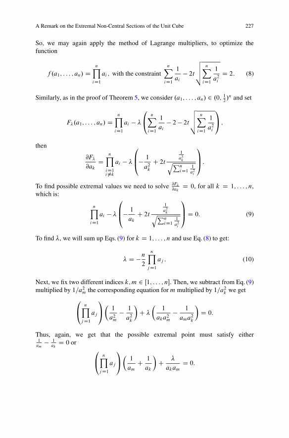
A Remark on the Extremal Non-Central Sections of the Unit Cube 227
So, we may again apply the method of Lagrange multipliers, to optimize thefunction
f .a1; : : : ; an/ DnY
iD1
ai ; with the constraintnX
iD1
1
ai
� 2t
vuut
nX
iD1
1
a2i
D 2: (8)
Similarly, as in the proof of Theorem 5, we consider .a1; : : : ; an/ 2 .0; 12/n and set
F�.a1; : : : ; an/ DnY
iD1
ai � �
0
@nX
iD1
1
ai
� 2 � 2t
vuut
nX
iD1
1
a2i
1
A ;
then
@F�
@ak
DnY
iD1i¤k
ai � �
0
B@� 1
a2k
C 2t
1
a3kqPn
iD11
a2i
1
CA :
To find possible extremal values we need to solve @F�
@akD 0, for all k D 1; : : : ; n,
which is:
nY
iD1
ai � �
0
B@� 1
ak
C 2t
1
a2kqPn
iD11
a2i
1
CA D 0: (9)
To find �, we will sum up Eqs. (9) for k D 1; : : : ; n and use Eq. (8) to get:
� D �n
2
nY
j D1
aj : (10)
Next, we fix two different indices k; m 2 Œ1; : : : ; n�. Then, we subtract from Eq. (9)multiplied by 1=a2
m the corresponding equation for m multiplied by 1=a2k we get
0
@nY
j D1
aj
1
A
�1
a2m
� 1
a2k
�
C �
�1
aka2m
� 1
ama2k
�
D 0:
Thus, again, we get that the possible extremal point must satisfy either1
am� 1
akD 0 or
0
@nY
j D1
aj
1
A
�1
am
C 1
ak
�
C �
akam
D 0:

228 J. Moody et al.
The above again gives ak C am D n�12
; which is only possible for n D 2. Thus, forn > 3 the only possible critical point is a1 D a2 D � � � D an. By arguments similarto those used in Theorem 5 (working with set C and ı), we may show f achieves a(constrained) maximum at a1 D a2 D � � � D an.
This yields the maximal � D . 1pn; : : : ; 1p
n/ and a D p
n.p
n
2� t/. This gives,
for t 2 .p
n�12
;p
n
2�,
jQn \ fx 2 Rn W jx � �j 6 tgj � 1 � 2n
n2
nŠ
�pn
2� t
�n
:
ut
Acknowledgements The Authors were supported in part by REU/NSF grant DMS-0755318. Thelast author was also supported in part by NSF grant DMS-0652684. We are indebted to FedorDragan, Jaegil Kim and Jenya Soprunova for valuable discussions.
References
1. S.A. Alvarez, Note on an n-dimensional Pythagorean theorem, www.cs.bc.edu/�alvarez/NDPyt.pdf
2. K. Ball, Cube slicing in Rn, Proc. Am. Math. Soc. 97, 465–473 (1986)
3. F. Barthe, A. Koldobsky, Extremal slabs in the cube and the Laplace transform. Adv. Math.174(1), 89–114 (2003)
4. F. Barthe, O. Guedon, S. Mendelson, A. Naor, A probabilistic approach to the geometry of thelnp -ball. Ann. Probab. 33(2), 480–513 (2005)
5. R.J. Gardner, The Brunn-Minkowski inequality, Bull. Am. Math. Soc. 39, 355–405 (2002)6. R.J. Gardner, in Geometric Tomography. Encyclopedia of Mathematics and its Applications,
vol. 58, 2nd edn. (Cambridge University Press, Cambridge, 2006)7. H. Hadwiger, Gitterperiodische Punktmengen und Isoperimetrie. Monatsh. Math. 76, 410–418
(1972)8. D. Hensley, Slicing the cube in R
n and probability. Proc. Am. Math. Soc. 73(1), 95–100 (1979)9. H. Konig, A. Koldobsky, Volume of low-dimensional slabs and sections in the cube, Adv. Appl.
Math. 47, 894–907 (2011)10. H. Konig, A. Koldobsky, Minimal volume of slabs in the complex cube, Proc. Am. Math. Soc.
140, 1709–1717 (2012)11. H. Konig, A. Koldobsky, On the maximal measure of sections of the n-cube, Proc. Southeast
Geometry Seminar, Contemp. Math., AMS (2013). http://analysis.math.uni-kiel.de/koenig/inhalte/CubeSlicing.pdf
12. A. Koldobsky, in Fourier Analysis in Convex Geometry. Mathematical Surveys and Mono-graphs, vol. 116 (American Mathematical Society, Providence, RI, 2005)
13. F. Nazarov, A. Podkorytov, Ball, Haagerup, and distribution functions. Complex analysis,operators, and related topics, Oper. Theory Adv. Appl. 113, 247–267 (Birkhauser, Basel, 2000)
14. K. Oleszkiewicz, A. Pełczynski, Polydisc slicing in Cn. Studia Math. 142(3), 281–294 (2000)
15. J.D. Vaaler, A geometric inequality with applications to linear forms. Pacific J. Math. 83,543–553 (1979)
16. C. Zong, What is known about unit cubes. Bull. Am. Math. Soc. (N.S.) 42(2), 181–211 (2005)17. A. Zvavitch, Gaussian measure of sections of dilates and shifts of convex bodies. Adv. Appl.
Math. 41/2, 247–254 (2008)

Universal Flows of Closed Subgroupsof S1 and Relative Extreme Amenability
L. Nguyen Van The
Abstract This paper is devoted to the study of universality for a particularcontinuous action naturally attached to certain pairs of closed subgroups of S1.It shows that three new concepts, respectively called relative extreme amenability,relative Ramsey property for embeddings and relative Ramsey property for struc-tures, are relevant in order to understand this property correctly. It also allowsus to provide a partial answer to a question posed in [2] by Kechris, Pestov andTodorcevic (Geom. Funct. Anal. 15(1), 106–189, 2005).
Key words Extreme amenability • Relative extreme amenability • Relative Ram-sey property • Fraısse theory • Ramsey theory • Universal flow
Mathematical Subject Classifications (2010): 37B05, 03C15, 03E02, 03E15,05D10, 22F50, 43A07, 54H20
1 Introduction
This note builds on the paper [2] by Kechris, Pestov and Todorcevic, and is devotedto the study of universality for a particular continuous action naturally attached tocertain pairs of closed subgroups of S1. Recall that if G is a topological group,a G-flow is a continuous action of G on a topological space X (in what follows,all topological spaces will be Hausdorff). For those, we will often use the notationG Õ X . The flow G Õ X is compact when the space X is. It is universal when
L. Nguyen Van The (�)Laboratoire d’Analyse, Topologie et Probabilites, Universite d’Aix-Marseille, Batiment HenriPoincare, Cour A, Avenue de l’escadrille Normandie-Niemen, 13397 Marseille Cedex 20, Francee-mail: [email protected]
M. Ludwig et al. (eds.), Asymptotic Geometric Analysis, Fields InstituteCommunications 68, DOI 10.1007/978-1-4614-6406-8 10,© Springer Science+Business Media New York 2013
229

230 L. Nguyen Van The
every compact minimal G Õ Y is a factor of G Õ X , which means that there exists� W X �! Y continuous, onto and G-equivariant, i.e., so that
8g 2 G 8x 2 X �.g � x/ D g � �.x/:
Finally, it is minimal when every x 2 X has dense orbit in X :
8x 2 X G � x D X:
It turns out that when G is Hausdorff, there is, up to isomorphism of G-flows, a unique G-flow that is both minimal and universal. This flow is calledthe universal minimal flow of G and is denoted by G Õ M.G/. When studyinguniversal minimal flows of closed subgroups of S1 (here and throughout the paper,S1 denotes the symmetric group of the natural numbers N, equipped with thepointwise convergence topology), the authors of [2] showed that certain flowsencode remarkable combinatorial properties, called the Ramsey property and theordering property. This connection also takes place in a slightly broader contextand it is in this more general framework that we will present it here, where pureorder expansions (i.e., order expansions where the language is enriched with a singlebinary relation symbol, which is always interpreted as a linear ordering) are replacedby precompact relational expansions and where the ordering property is replaced bythe expansion property (see [3]). Given closed subgroups G� � G of S1, thereare natural classes K and K� of finite objects attached to them, as well as a G-flow G Õ X�, where X� is the completion of the quotient G=G� equipped withthe projection of the right-invariant metric. When X� is compact, the followingproperties hold (cf [2] for pure order expansions and [3] for the precompact case):
(i) The flow G Õ X� is universal and minimal iff K� has the Ramsey propertyand the expansion property relative to K.
(ii) The flow G Õ X� is minimal iff K� has the expansion property relative to K.
Question 1 ([2], p.174). Assume that K� is a pure order expansion of K. Isuniversality of G Õ X� equivalent to the Ramsey property for K�?
More generally:
Question 2. Assume that K� is a precompact expansion of K. Is universality ofG Õ X� equivalent to the Ramsey property for K�?
Apart from the fact that they are very natural in view of the previous results,there is, at least, one other very good reason to study those problems. Indeed, givena class of finite objects, the Ramsey property is very often difficult to prove. Anynew tool that would allow to reach it is therefore welcome. However, [2] alreadyprovides a spectacular dynamical characterization of the Ramsey property for K�,as it shows that it is equivalent to M.G�/ being reduced to a single point for somesubgroup G� of G naturally attached to K�. So what is the real interest of the

Universal Flows of Closed Subgroups of S1 and Relative Extreme Amenability 231
questions? We started working on them when we realized that the Ramsey propertyimplies universality of G Õ X�. Our hope became then that universality wouldbe equivalent to a strictly weaker combinatorial condition for K�, call it weakRamsey property for the moment, and that this condition would be, in practice,easier to prove than the Ramsey property. This fact, together with the observationthat the expansion property is often much easier to prove than the Ramsey property,would then give an alternate combinatorial approach for further problems involvingRamsey property: in order to prove it for K�, instead of attacking the problemdirectly, it would suffice to prove that both the weak Ramsey property and theexpansion property are satisfied. Indeed, that would prove that the flow G Õ X�is both universal and minimal, and therefore that K� has the Ramsey property.So far, this approach is partially successful. It is successful in the sense thatuniversality is indeed equivalent to some combinatorial condition (finally not calledweak Ramsey property but, for reasons that should become clear later on, relativeRamsey property) which is, in general, strictly weaker than the Ramsey property.But the success is only partial in the sense that it is unclear whether in practice, thiscondition is much easier to prove than the Ramsey property.
Let us now turn to a concise description of the results presented in this paper. LetL be a countable first order signature and L� D L [ fRi W i 2 I �g a countablerelational expansion of L. We refer to Sect. 2 for all other undefined notions. Ourfirst result connects universality of G Õ X� to a dynamical statement involvingactions of G and G�.
Definition 1. Let H � G be topological groups. Say that the pair .G; H/ isrelatively extremely amenable when every continuous action of G on every compactspace admits an H -fixed point.
Theorem 1. Let F be a Fraısse structure in L and F� a Fraısse precompactrelational expansion of F in L�. The following are equivalent:
(i) The flow G Õ X� is universal.(ii) The pair .G; G�/ is relatively extremely amenable.
This result allows us to show that Question 2 has a negative answer by exhibitingconcrete examples of classes K and K� where the flow G Õ X� is universal but theRamsey property does not hold for K� (see Sect. 4). However, quite surprisingly,we are not able to settle the case of Question 1.
Next, we turn to a combinatorial reformulation of relative extreme amenability.Let K be a class of L-structures and K� an expansion of K in L�, that is, a classof L�-structures such that every element of K� is an expansion of an element of K.When A; B 2 K, the set of all embeddings from A into B is denoted by
BA
!Emb
:

232 L. Nguyen Van The
Let B� be an expansion of B in K� and a 2 �BA
�Emb
. The substructure of B�supported by a.A/ is an expansion of A in K�. Using a, we can then define anexpansion of A in K� as follows: for i 2 I , call ˛.i/ the arity of Ri . Then, set
8i 2 I � Rai .x1; : : : ; x˛.i// , RB�
i .a.x1/; : : : ; a.x˛.i///:
We will refer to .a.A/; Ra/ as the canonical expansion induced by a on A. Ifa0 2 �B
A
�Emb, write a ŠB� a0 when the canonical expansions on A induced by a and
a0 are equal (not only isomorphic).
Definition 2. Let K be a class of finite L-structures and K� an expansion of K inL�. Say that the pair .K; K�/ has the relative Ramsey property for embeddings whenfor every k 2 N, A 2 K, B� 2 K�, there exists C 2 K such that for every coloringc W �C
A
�Emb �! Œk�, there exists b 2 �C
B
�Emb such that:
8a0; a1 2
BA
!Emb
a0 ŠB� a1 ) c.ba0/ D c.ba1/:
Theorem 2. Let F be a Fraısse structure in L and let F� be a Fraısse precompactrelational expansion of F in L�. Then the following are equivalent:
(i) The pair .G; G�/ is relatively extremely amenable.(ii) The elements of Age.F�/ are rigid and the pair .Age.F/; Age.F�// has the
relative Ramsey property for embeddings.
Then, we investigate the properties of a weakening of the relative Ramseyproperty for embeddings, which involves only structures, as opposed to embeddings.
Definition 3. Let K be a class of finite L-structures and K� an expansion of K inL�. Say that the pair .K; K�/ has the relative Ramsey property for structures whenfor every k 2 N, A 2 K and B� 2 K�, there exists C 2 K such that for everycoloring c W �C
A
� �! Œk�, there exists b 2 �CB
�Emb such that:
8eA0;eA1 2
BA
! �eA0 ŠB�eA1 ) c.b.eA0// D c.b.eA1//
�:
Above,eA0 ŠB�eA1 means that B� � QA0 Š B� � QA1.
This weakening may be strictly weaker than the embedding version, but at thecombinatorial level, it is good enough to play the role of a “weak Ramsey property”as described above:
Theorem 3. Let F be a Fraısse structure in L and let F� be a Fraısse precompactexpansion of F in L� whose age consists of rigid structures. Assume that thepair .Age.F/; Age.F�// has the relative Ramsey property for structures and that

Universal Flows of Closed Subgroups of S1 and Relative Extreme Amenability 233
Age.F�/ has the expansion property relative to Age.F/. Then Age.F�/ has theRamsey property.
Finally, we show that in order to guarantee the existence of an expansion withboth the Ramsey and the expansion property, it is enough to prove the existence ofan expansion with the relative Ramsey property for structures:
Theorem 4. Let F be a Fraısse structure in L� and let F� be a Fraısse precompactrelational expansion of F in L�. Assume that Age.F�/ consists of rigid elements andthat the pair .Age.F/; Age.F�// has the relative Ramsey property for structures.Then Age.F�/ admits a Fraısse subclass with the Ramsey property and theexpansion property relative to Age.F/.
The paper is organized as follows: Sect. 2 contains all basic notions concerningFraısse theory, structural Ramsey property and precompact relational expansions.Section 3 contains a proof of Theorem 1. Section 4 exhibits concrete classesanswering Question 2. Section 5 provides a proof of Theorem 2. In Sect. 6, a moredetailed study of the relative Ramsey property for embeddings is carried. Finally,Sect. 7 concentrates on the relative Ramsey property for structures and contains theproofs of Theorem 3 and 4.
2 Ramsey Property, Expansion Property, PrecompactExpansions
The purpose of this section is to describe the global framework where our studyis taking place. Our main references here are [2] for Fraısse theory and structuralRamsey theory and [3] for precompact expansions.
2.1 Fraısse Theory
In what follows, N denotes the set f0; 1; 2; : : :g of natural numbers and for a naturalnumber m, Œm� denotes the set f0; : : : ; m � 1g. We will assume that the reader isfamiliar with the concepts of first order logic, first order structures, Fraısse theory(cf [2], sect. 2), reducts and expansions (cf [2], sect. 5). If L is a first order signatureand A and B are L-structures, we will write A � B when A embeds in B, A � Bwhen A is a substructure of B and A Š B when A and B are isomorphic. When L
is countable, a Fraısse class in L will be a countable class of finite L-structures ofarbitrarily large sizes, satisfying the hereditarity, joint embedding and amalgamationproperty, and a Fraısse structure (or Fraısse limit) in L will be a countable, locallyfinite, ultrahomogeneous L-structure.

234 L. Nguyen Van The
2.2 Structural Ramsey Theory
In order to define the Ramsey property, let k; l 2 N and A; B; C be L-structures.The set of all copies of A in B is written
BA
!D feA � B W eA Š Ag:
We use the standard arrow partition symbol
C �! .B/Ak;l
to mean that for every map c W �CA
� �! Œk�, thought as a k-coloring of the copies
of A in C, there is eB 2 �CB
�such that c takes at most l-many values on
�eBA
�. When
l D 1, this is written
C �! .B/Ak :
A class K of finite L-structures is then said to have the Ramsey property when
8k 2 N 8A; B 2 K 9C 2 K C �! .B/Ak :
When K D Age.F/, where F is a Fraısse structure, this is equivalent, via acompactness argument, to:
8k 2 N 8A; B 2 K F �! .B/Ak :
2.3 Precompact Expansions
Assume now that we have a first-order expansion of L, L� D L [ fRi W i 2 I �g,with I � countable and every symbol Ri relational and not in L. Let K� denote anexpansion of K in L� (that means that all elements of K� are of the form A� D.A; .RA�
i /i2I �/ and that every A 2 K can be enriched to some element A� D.A; .RA�
i /i2I �/ of K� by adding some relations on A). For A� 2 K�, the reductof A� to L is denoted by A� � L D A. Then, K� satisfies the expansion propertyrelative to K if, for every A 2 K, there exists B 2 K such that
8A�; B� 2 K� .A� � L D A ^ B� � L D B/ ) A� � B�:
Next, consider F, a Fraısse structure in L. For i 2 I �, the arity of the symbolRi is denoted by ˛.i/. We let F� be an expansion of F in L�. We assume that F� isalso Fraısse and write F� D .F; .R�
i /i2I �/, or .F; R�/. We also assume that F andF� have the set N of natural numbers as universe. The corresponding automorphism

Universal Flows of Closed Subgroups of S1 and Relative Extreme Amenability 235
groups are denoted by G and G� respectively. The group G� will be thought as asubgroup of G and both are closed subgroups of S1, the permutation group of Nequipped with the topology generated by sets of the form
Ug;F D fh 2 G W h � F D g � F g;
where g runs over G and F runs over all finite subsets of N. Note that the group S1admits two natural metrics: a left invariant one, dL, defined as
dL.g; h/ D 1
2m; m D minfn 2 N W g.n/ ¤ h.n/g;
and a right-invariant one, dR, given by
dR.g; h/ D dL.g�1; h�1/:
In what follows, we will be interested in the set of all expansions of F in L�,which we think as the product
P WDYi2I �
Œ2�F˛.i/
:
In this notation, the factor Œ2�F˛.i/ D f0; 1gF˛.i/
is thought as the set of all ˛.i/-aryrelations on F. Each factor Œ2�F
˛.i/is equipped with an ultrametric di , defined by
di .Si ; Ti / D 1
2m; m D minfn 2 N W Si � Œn� ¤ Ti � Œn�g
where Si � Œn� (resp. Ti � Œn�) stands for Si \ Œn�a.i/ (resp. Ti \ Œn�a.i/).The group G acts continuously on each factor as follows: if i 2 I �, Si 2 Œ2�F
˛.i/
and g 2 G, then g � Si is defined by
8y1 : : : y˛.i/ 2 F g � Si .y1 : : : y˛.i// , Si .g�1.y1/ : : : g�1.y˛.i///:
This allows us to define a continuous action of G on the product P equippedwith the supremum distance d P of all the distances di (where g �S is simply definedas .g � Si/i2I � whenever S D .Si /i2I � 2 P and g 2 G). As a set, G=G� can bethought as G � R�, the orbit of R� in P , by identifying Œg�, the equivalence classof g, with g � R�. The metric dR induces a metric on the quotient G=G�, whichcoincides with the restriction of d P on G � R� (see [3], Proposition 1). Therefore,we can really think of the metric space G=G� as the metric subspace G �R� of P andit can be shown that the space G=G� Š G � R� is precompact (i.e., has a compactcompletion, or, equivalently, a compact closure in P ) iff every element of Age.F/
has finitely many expansions in Age.F�/ (see [3], Proposition 2). In that case, wesay that Age.F�/ is a precompact expansion of Age.F/ (or that F� is a precompactexpansion of F).

236 L. Nguyen Van The
3 Relative Extreme Amenability and Universality
In this section, we prove Theorem 1:
Theorem 1. Let F be a Fraısse structure and F� a precompact relational expansionof F. The following are equivalent:
(i) The flow G Õ X� is universal for minimal compact G-flows.(ii) The pair .G; G�/ is relatively extremely amenable.
Proof (Proof of .i/ ) .i i/). Let G Õ X be a compact G-flow and let Y � X
be such that G Õ Y is compact minimal. By universality, find � W X� �! Y
continuous, G-equivariant and surjective. Denote � D �.Œe�/, where e denotes theneutral element of G (recall that X� D 1G=G�). Then, � is G�-fixed, because forg 2 G�:
g�� D g��.Œe�/ D �.g�Œe�/ D �.Œg�/ D �.Œe�/ D �: ut
Proof (Proof of .i i/ ) .i/). Let G Õ X be a compact minimal G-flow. Find� 2 X , G�-fixed. Then, let p W G �! X be defined by
p.g/ D g � �:
This map is G-equivariant, right uniformly continuous and constant on elementsof G=G�. Therefore, it induces Np W G=G� �! X , which is also G-equivariantand right uniformly continuous. Denote by � the continuous extension of Np to thecompletion X� D 1G=G�. Then � is G-equivariant and surjective because its rangeis a compact subset of X containing G � �, which is dense in X . ut
4 Universality vs Ramsey Property
A consequence of Theorem 1 is that for precompact expansions, universality ofG Õ X� is not equivalent to Ramsey property for Age.F�/. For example, considerthe class U<
S of finite ordered ultrametric spaces with distances in S , where S is afinite subset of R. The corresponding Fraısse limit is a countable ordered ultrametricspace, denoted by .Uult
S ; </. As a linear ordering, it is isomorphic to .Q; </. Hence,.Uult
S ; </ can be thought as a precompact relational expansion of .Q; </, and thegroup Aut.Uult
S ; </ can be thought as a closed subgroup of Aut.Q; </. Because thislatter group is extremely amenable (see [5]), the pair .Aut.Q; </; Aut.Uult
S ; <// isrelatively extremely amenable and the corresponding flow is universal. However, itis known that U<
S does not have the Ramsey property, see [4]. A similar situationoccurs with finite posets, considering .Q; </ and the Fraısse limit .P; </ of the classof all finite ordered posets. This class does not have the Ramsey property (cf [7,8]),but the corresponding flow is universal.

Universal Flows of Closed Subgroups of S1 and Relative Extreme Amenability 237
In the two previous examples, the pair of groups .G; H/ under consideration isproved to be relatively extremely amenable by producing an extremely amenableinterpolant, i.e., an extremely amenable closed subgroup K of G containing H . It isa natural question to ask whether every relatively extremely amenable pair of groupsadmits such an interpolant. The answer in general is negative, as witnessed by thepair .S1; Aut.Z; <//. This result is due to Gutman. [1] has been withdrawn due toan error in the main argument.
Finally, in view of the original question posed in [2], we do not know whetheruniversality of G Õ X� implies Ramsey property of Age.F�/ when F� is a pureorder expansion of F. We believe that the answer should be negative, but werenot able to construct any counterexample so far. In fact, results of Sokic (see[7, 9]) provide a positive answer in a number of cases. As a possible strategy fora counterexample, start with a Fraısse class Age.F/ with the Ramsey propertyand consisting of rigid elements. Consider then the class K< of all finite orderexpansions of elements of Age.F/ and try to find a Fraısse subclass K� � K<
without the Ramsey property. Then, calling F� the Fraısse limit of K� and denotingG� D Aut.F�/, we would have .G; G�/ relatively extremely amenable (becauseG is extremely amenable), hence G Õ X� universal, while K� does not have theRamsey property.
5 Relative Extreme Amenability and Relative RamseyProperty for Embeddings
In view of the two previous sections, it is natural to ask whether relative extremeamenability of a pair .G; G�/ as before can be seen at the level of Age.F/ andAge.F�/. The answer is positive, as shown by the following result. Note that theproof has the same pattern as the proof of Kechris-Pestov-Todorcevic theorem aspresented in [3], Theorem 1.
Theorem 2. Let F be a Fraısse structure and F� a Fraısse precompact relationalexpansion of F. Then the following are equivalent:
(i) The pair .G; G�/ is relatively extremely amenable.(ii) The elements of Age.F�/ are rigid and the pair .Age.F/; Age.F�// has the
relative Ramsey property for embeddings.
5.1 Proof of .i / ) .ii /
Assume that .G; G�/ is relatively extremely amenable. We first prove that allelements of Age.F�/ are rigid. To do so, consider the set of all linear orderings

238 L. Nguyen Van The
LO.F/, seen as a subspace of the space Œ2�F�F. The group G acts continuously onthis later space via the logic action. The set LO.F/ is then a G-invariant compactsubspace. Explicitly, G acts on LO.F/ as follows: if �2 LO.F/ and g 2 G, then
8x; y 2 F x.g� �/y , g�1.x/ � g�1.y/:
By relative extreme amenability of .G; G�/, there is a G�-fixed point in LO.F/,call it <�. Consider now a finite substructure A� � F� and let ' be an automorphismof A�. By ultrahomegeneity of F�, ' extends to an automorphism � of F�. Because<� is G�-fixed, it is preserved under '. Thus, on A, <� is preserved by ', whichmeans that ' is trivial on A. This proves that A� is rigid.
To prove that .Age.F/; Age.F�// has the relative Ramsey property for embed-dings, it suffices to show that F satisfies the property that is required for C inDefinition 2. A compactness argument allows then to find C. So consider k 2 N,A 2 Age.F/; B� � F� finite and a coloring
c W
FA
!Emb
�! Œk�:
Consider the compact space Œk�.FA/Emb, acted on continuously by G by shift: if
� 2 Œk�.FA/Emb, g 2 G and a 2 �F
A
�Emb
, then
g � �.a/ D �.g�1a/:
The set G � c is a G-invariant compact subspace. By relative extreme amenabilityof G, there is a G�-fixed point in G � c, call it c0. The fact that c0 is G�-fixed meansthat c0.a0/ D c0.a1/ whenever a0 ŠF� a1. Consider now the finite set
�BA
�Emb, where
B WD B� � L. Because c0 2 G � c, there is g 2 G so that
g � c �
BA
!Emb
D c0 �
BA
!Emb
:
So if a0; a1 2 �BA
�Emb
are such that a0 ŠB� a1 then
c.g�1a0/ D c.g�1a1/:
It follows that g�1 witnesses the relative Ramsey property for embeddings. ut

Universal Flows of Closed Subgroups of S1 and Relative Extreme Amenability 239
5.2 Proof of .ii / ) .i /
Assume that Age.F�/ consists of rigid elements and the pair .Age.F/; Age.F�//
has the relative Ramsey property for embeddings. For A � N finite, we denote byStab.A/ the pointwise stabilizer Stab.A/ in G and we can make the identification:
G=Stab.A/ D
FA
!Emb
:
Proposition 1. Let k 2 N, A � N finite and supporting a substructure A of F andF � G finite. Let Nf W G �! Œk� be constant on elements of G=Stab.A/. Then thereexists g 2 G such that
8h; h0 2 F h0h�1 2 G� ) Nf .gh/ D Nf .gh0/:
Proof. The map Nf induces a map f W G=Stab.A/ �! Œk�, which we may think as ak-coloring of
�FA
�Emb. Consider the set fŒh� W h 2 F g. It is a finite set of embeddings
from A to F. Therefore, we can find a finite substructure B � F large enoughso that the ranges of all those embeddings are contained in B. Let B� denote thesubstructure of F� supported by B . By relative Ramsey property for embeddingsapplied to A, B� and the coloring f , find g 2 G such that
8a0; a1 2
BA
!Emb
.a0 ŠB� a1 ) f .ga0/ D f .ga1// :
Consider now h; h0 2 F so that h0h�1 2 G�. Then Œh� ŠB� Œh0� and so
f .gŒh�/ D f .gŒh0�/:
At the level of Nf , that means Nf .gh/ D Nf .gh0/. �
Proposition 2. Let p 2 N, f W G �! Rp left uniformly continuous and bounded
(where Rp is equipped with its standard Euclidean structure), F � G finite, " > 0.
Then there exists g 2 G such that
8h; h0 2 F h0h�1 2 G� ) kf .gh/ � f .gh0/k < ":
Proof. Let m 2 N. Note that as subsets of G, elements of G=Stab.Œm�/ havediameter 1=2mC1 with respect to the left invariant metric d L on G. Thus, by leftuniform continuity, we can find m 2 N large enough so that f is constant up to" on each element of G=Stab.Œm�/. By local finiteness of F, let now A � N befinite, supporting a finite substructure A of F and such that Œm� � A. Then f is alsoconstant up to " on each element of G=Stab.A/. Because f is also bounded, wecan also find Nf W G �! R
p with finite range, constant on elements of G=Stab.A/

240 L. Nguyen Van The
and so that kf � Nf k1 < "=2. By Proposition 1, there exists g 2 G such thatNf .gh/ D Nf .gh0/ whenever h0h�1 2 G�. Then kf .gh/ � f .gh0/k < " whenever
h0h�1 2 G�. utWe can now show that the pair .G; G�/ is relatively extremely amenable. Let
G Õ X be a continuous action, with X compact. For p 2 N, � W G �! Rp
uniformly continuous and bounded, F � G finite, " > 0, set
A�;";F D fx 2 X W 8h 2 F \ G� k�.h � x/ � �.x/k � "g:
The family .A�;";F /�;";F is a family of closed subsets of X . We claim that ithas the finite intersection property. Indeed, if �1; : : : ; �l ; "1; : : : ; "l ; F1; : : : ; Fl aregiven, take
� D .�1; : : : ; �l /; " D min."1; : : : ; "l /; F D F �11 [ : : : [ F �1
l [ feg:
Fix x 2 X and consider the map f W G �! Rp1C:::Cpl defined by
8g 2 G f .g/ D .�1.g�1 � x/; : : : ; �l .g
�1 � x///:
Because the maps �i ’s are uniformly continuous and the map g 7! g�1 � x isleft uniformly continuous (cf [6], p40), the map f is left uniformly continuous. ByProposition 2, there exists g 2 G so that
8h; h0 2 F h0h�1 2 G� ) kf .gh/ � f .gh0/k < ":
Equivalently,
8i � l 8h; h0 2 F h0h�1 2 G� ) k�i .h�1g�1 � x/ � �i .h
0�1g�1 � x/k � "i :
Taking x0 D g�1 � x and h0 D e, we obtain
8i � l 8h 2 Fi k�i .h � x0/ � �i .x0/k � "i :
This proves the finite intersection property of the family .A�;";F /�;";F . Bycompactness of X , it follows that this family has a non empty intersection. Considerany element x of this intersection. We claim that x is fixed under the action of G�:if not, we would find g 2 G� so that g � x ¤ x. Then, there would be a uniformlycontinuous function �0 W X �! Œ0; 1� so that �0.x/ D 0 and �0.g � x/ D 1. Thatwould imply x … A�0;1=2;fgg, a contradiction. ut

Universal Flows of Closed Subgroups of S1 and Relative Extreme Amenability 241
6 Versions and Consequences of the Relative RamseyProperty
6.1 Canonical Expansions
Recall that when A; B 2 K, B� is an expansion of B in K� and a 2 �BA
�Emb
, thecanonical expansion induced by a on A is the structure .a.A/; Ra/ defined by
8i 2 I � Rai .x1; : : : ; x˛.i// , RB�
i .a.x1/; : : : ; a.x˛.i///:
Note that a is not completely characterized by the canonical expansion it induceson A when a.A/ possesses a non-trivial automorphism, but that it is when a.A/ isrigid. In the case where all expansions of A are rigid, then the ŠB�-equivalenceclasses are those sets of the form
�B�
A�
�Emb, where A� ranges over the set of all
expansions (possibly isomorphic, but based on A) of A in K�.
6.2 More on the Relative Ramsey Property for Embeddings
In this section, we present simple facts related to the concept of relative Ramseyproperty for embeddings.
Proposition 3. Assume that the pair .K; K�/ has the relative Ramsey property forembeddings, then so does the pair .K; K��/ whenever K�� is an expansion of K inL� such that K�� � K�.
Proof. Direct from the definition. utFor anyone familiar with Ramsey theory, this is a rather unexpected feature (most
of Ramsey type properties are not preserved when passing to subclasses).
Proposition 4. Let F be a Fraısse structure and F� a Fraısse expansion of F. Thenthe pair .Age.F/; Age.F�// has the relative Ramsey property for embeddings whenfor every k 2 N, A 2 Age.F/; B� � F� finite and c W �F
A
�Emb
�! Œk�, there existsg 2 G such that:
8a0; a1 2
BA
!Emb
a0 ŠB� a1 ) c.ga0/ D c.ga1/:
Proof. A standard compactness argument. utNote that because B� is a substructure of F�, a0 ŠB� a1 is equivalent to
a0 ŠF� a1, which is equivalent to the existence of g� 2 G� so that a1 D g�a0
(use ultrahomogeneity of F�).

242 L. Nguyen Van The
Proposition 5. Let F be a Fraısse structure and F� a Fraısse expansion of F suchthat Age.F�/ consists of rigid elements. Then, the following are equivalent:
(i) The pair .Age.F/; Age.F�// has the relative Ramsey property for embeddings.(ii) For every k 2 N, A 2 Age.F/, B� 2 Age.F�/, there exists C� 2 Age.F�/ such
that for every coloring c W �CA
�Emb �! Œk�, there exists b 2 �C
B
�Emb such that:
8a0; a1 2
BA
!Emb
a0 ŠB� a1 ) .ba0 ŠC� ba1 ^ c.ba0/ D c.ba1//:
Proof. Quite clearly, item i i/ implies the relative Ramsey property for embeddings.For the converse, use the standard trick of enriching the coloring c by the ŠC� -isomorphism type. Formally, fix k 2 N, A 2 Age.F/, B� 2 Age.F�/. Recall thatE.A/ denotes the set of all (possibly isomorphic) expansions of A in Age.F�/.Consider C provided by the relative Ramsey property for embeddings applied to A,B� and kjE.A/j. Let C� denote any expansion of C in Age.F�/. Let c W �C
A
�Emb
�!Œk� and define Nc by Nc.a/ D .c.a/; Œa�/, where Œa� denotes the ŠC� equivalence classof a. This is a kjE.A/j-coloring of
�CA
�Emb
, so we can find b 2 �CB
�Emb
so that
8a0; a1 2
BA
!Emb
a0 ŠB� a1 ) Nc.ba0/ D Nc.ba1/:
We are done since
Nc.ba0/ D Nc.ba1/ , .ba0 ŠC� ba1 ^ c.ba0/ D c.ba1//: ut
We now turn to a consequence of the relative Ramsey property for embeddings.Let A 2 Age.F/ and B� 2 Age.F�/. Recall that the set
�BA
�Emb is partitioned into
ŠB�-equivalence classes, which correspond to those sets of the form�B�
A�
�Emb, where
A� ranges over the set of all (possibly isomorphic) expansions of A in Age.F�/ thatare based on A. As a direct consequence:
Proposition 6. Let F be a Fraısse structure and F� a Fraısse expansion of F suchthat Age.F�/ consists of rigid elements. Assume that the pair .Age.F/; Age.F�//
has the relative Ramsey property for embeddings. Then, for every k 2 N, A�; B� 2Age.F�/, there exists C 2 Age.F/ such that for every coloring c W �C
A
�Emb �! Œk�,
there exists b 2 �CB
�Emb
such that the set b ı �B�
A�
�Emb
WD fba� W a� 2 �B�
A�
�Emb
g ismonochromatic.
Quite surprisingly, the converse to the previous proposition does not seem tohold. The main obstruction is that we only have a limited control on how b
behaves with respect to canonical expansions. As we have seen before, we canmake sure that b preserves ŠB� -equivalence. However, we cannot make sure that it

Universal Flows of Closed Subgroups of S1 and Relative Extreme Amenability 243
preserves canonical expansions. This detail appears to be problematic when tryingto deduce the relative Ramsey property for embeddings from a repeated applicationof item .i i/.
7 The Relative Ramsey Property for Structures
Let K be a class of L-structures and K� an expansion of K in L�. Recall that thepair .K; K�/ has the relative Ramsey property for structures when for every k 2 N,A 2 K and B� 2 K�, there exists C 2 K such that for every coloring c W �C
A
� �! Œk�,there exists b 2 �C
B
�Emb
such that:
8eA0;eA1 2
BA
! �eA0 ŠB�eA1 ) c.b.eA0// D c.b.eA1//
�;
where eA0 ŠB�eA1 means that B� � QA0 Š B� � QA1.
Again, when K and K� are of the form Age.F/ and Age.F�/ respectively, whereF and F� are Fraısse structures and F� is an expansion of F, a compactness argumentshows that .Age.F/; Age.F�// has the relative Ramsey property for structures whenfor every k 2 N, A 2 Age.F/, B� 2 Age.F�/ and c W �F
A
� �! Œk�, there existsg 2 G such that:
8eA0;eA1 2
BA
! �eA0 ŠB�eA1 ) c.g.eA0// D c.g.eA1//
�:
This property implies (but does not seem to be equivalent to) the followingweakening of the Ramsey property for Age.F�/: for every k 2 N, A�; B� 2Age.F�/ and c W �F
A
� �! Œk�, there exists g 2 G such that g ı �B�
A�
�is
monochromatic.Note that colorings of structures can be seen as particular cases of colorings of
embeddings, where elements with isomorphic (and not necessarily equal) canonicalexpansions receive the same color. For that reason, the relative Ramsey propertyfor embeddings implies the relative Ramsey property for structures. The conversedoes not seem to hold in general. The only instance for which we could check thatthe two notions agree is when the elements of Age.F/ are rigid, simply because thesets
�FA
�and
�FA
�Emb
can be identified. However, from the practical point of view, thefollowing results show that the relative Ramsey property for structures may havesome applications in the future.
Proposition 7. Assume that the pair .K; K�/ has the relative Ramsey property forstructures, then so does the pair .K; K��/ whenever K�� � K�.
Proof. Direct from the definition. ut

244 L. Nguyen Van The
Theorem 3. Let F be a Fraısse structure and F� a precompact expansion of Fwhose age consists of rigid structures. Assume that the pair .Age.F/; Age.F�// hasthe relative Ramsey property for structures and that Age.F�/ has the expansionproperty relative to Age.F/. Then Age.F�/ has the Ramsey property.
Proof. Because of the relative Ramsey property for structures, every A 2 Age.F/
has a finite Ramsey degree in Age.F/ whose value is at most equal to the number ofnon-isomorphic expansions of A in Age.F�/. Together with the expansion propertyrelative to Age.F/, this is known to imply the Ramsey property for Age.F�/ (for areference, see for example [3], Sect. 5, Proposition 8). ut
The preceding result could turn out to be useful in practice, where the Ramseyproperty is often difficult to prove and the expansion property generally moreaccessible.
Theorem 4. Let F be a Fraısse structure and let F� be a precompact relationalexpansion of F. Assume that Age.F�/ consists of rigid elements and that the pair.Age.F/; Age.F�// has the relative Ramsey property for structures. Then Age.F�/
admits a Fraısse subclass with the Ramsey property and the expansion propertyrelative to Age.F/.
Proof. Let S 2 G � R� be such that G Õ G � S is minimal. Note that Age.F; S/ �Age.F�/ because S 2 G � R� (cf [3], section on minimality). We claim thatAge.F; S/ is a required. This class clearly has the hereditarity property and the jointembedding property. The expansion property comes from minimality of G Õ G � S(cf [4], remark following Theorem 4 in Section 4). To prove the Ramsey property,notice first that because Age.F; S/ � Age.F�/, the pair .Age.F/; Age.F; S// alsohas the relative Ramsey property for structures (cf Proposition 7), which in turnimplies that every A 2 Age.F/ has a finite Ramsey degree at most equal to thenumber of non-isomorphic expansions of A in Age.F; S/. Because Age.F; S/ hasthe hereditary property, the joint embedding property and the expansion propertyrelative to Age.F/, it has the Ramsey property ([3], Sect. 5, Proposition 8). Finally,because of all the previous properties and because Age.F; S/ consists of rigidelements, it is Fraısse ([2] p.20, or [3] end of Sect. 6). ut
Further investigation about the practical status of the relative Ramsey propertyfor structures will decide on its value as a tool to derive the Ramsey property. Wehave to admit that, so far, we are not aware of any concrete application of any of thepreceding results of this section.
Acknowledgements I would like to sincerely thank Miodrag Sokic as well as the anonymousreferee for their comments which greatly improved the quality of the paper.

Universal Flows of Closed Subgroups of S1 and Relative Extreme Amenability 245
References
1. Y. Gutman and L. Nguyen Van The, Relative extreme amenability and interpolation, preprint,2011.
2. A. S. Kechris, V. G Pestov, and S. Todorcevic, Fraısse limits, Ramsey theory, and topologicaldynamics of automorphism groups, Geom. Funct. Anal. 15 (2005), no. 1, 106–189.
3. L. Nguyen Van The, More on Kechris-Pestov-Todorcevic correspondence: precompact expan-sions, Fund. Math., accepted.
4. L. Nguyen Van The, Structural Ramsey theory of metric spaces and topological dynamics ofisometry groups, Mem. Amer. Math. Soc. 206 (2010), no. 968, x+140.
5. V. G. Pestov, Ramsey-Milman phenomenon, Urysohn metric spaces, and extremely amenablegroups, Israel J. Math. 127 (2002), 317–357.
6. V. G. Pestov, Dynamics of infinite-dimensional groups, University Lecture Series, vol. 40,American Mathematical Society, Providence, RI, 2006, The Ramsey-Dvoretzky-Milmanphenomenon, Revised edition of Dynamics of infinite-dimensional groups and Ramsey-typephenomena [Inst. Mat. Pura. Apl. (IMPA), Rio de Janeiro, 2005; MR2164572].
7. M. Sokic, Ramsey properties of finite posets and related structures, Ph.D. thesis, University ofToronto, 2010.
8. M. Sokic, Ramsey properties of finite posets, Order 29(2012), no. 1, 1–30.9. M. Sokic, Ramsey property, ultrametric spaces, finite posets, and universal minimal flows,
preprint, 2011.

Oscillation of Urysohn Type Spaces
N.W. Sauer
Abstract A metric space M D .M I d/ is homogeneous if for every isometry ˛ ofa finite subspace of M to a subspace of M there exists an isometry of M onto Mextending ˛. The metric space M is universal if it isometrically embeds every finitemetric space F with dist.F/ � dist.M/. (dist.M/ being the set of distances betweenpoints of M.)
A metric space M is oscillation stable if for every � > 0 and every uniformlycontinuous and bounded function f W M ! < there exists an isometric copy M� D.M �I d/ of M in M for which:
supfjf .x/ � f .y/j j x; y 2 M �g < �:
Theorem. Every bounded, uncountable, separable, complete, homogeneous, uni-versal metric space M D .M I d/ is oscillation stable. (Theorem 12.)
Key words Partitions of metric spaces • Ramsey theory • Metric geometry •Urysohn metric space • Oscillation stability
Mathematical Subject Classifications (2010): 03E02, 22F05, 05C55, 05D10,22A05, 51F99
N.W. Sauer (�)Department of Mathematics and Statistics, University of Calgary,2500 University Dr. NW, Calgary, Alberta, Canada T2N 1N4e-mail: [email protected]
M. Ludwig et al. (eds.), Asymptotic Geometric Analysis, Fields InstituteCommunications 68, DOI 10.1007/978-1-4614-6406-8 11,© Springer Science+Business Media New York 2013
247

248 N.W. Sauer
1 Basic Notions and Facts
Find in this section some basic definitions and facts and in the next, introductorysection, a general background discussion about the topics of this article.
Definition 1. A metric space M D .M I d/ is homogeneous if for every isometry ˛
of a finite subspace of M to a subspace of M there exists an isometry of M onto Mextending ˛. A metric space M is universal if it embeds every finite metric space Fwith dist.F/ � dist.M/.
Definition 2. A metric space M is an Urysohn metric space if it is separable,complete, homogeneous and universal.
It follows easily from the general Fraısse theory and is stated explicitly asCorollary 2.2 of [1] that
Fact 1. An Urysohn metric space U embeds every separable metric space N withdist.N/ � dist.U /.
See [11] for further background information on homogeneous metric spaces andtheir partition theory. Two Urysohn metric spaces with the same set of distances areisometric. (Theorem 8). An Urysohn metric space with R as set of distances will bedenoted by UR.
In [8] a very general definition and discussion and applications for the notion thata function f W G=H ! < is oscillation stable is given. In there, G is a topologicalgroup and H a subgroup and f is uniformly continuous with respect to the leftuniformity of G. (See [8] for a more complete statement.) Further it is defined in[8] that a pair G; H for H a topological subgroup of a topological group G, isoscillation stable if every bounded left uniformly continuous function f W G=H !< is oscillation stable.
In the case of G being the group of isometries of a homogeneous metric spaceM D .M I d/ onto M with H the isotropy subgroup fixing a point v of M andf W M ! < (identified with f W G=H ! <) a uniformly continuous and boundedfunction, this general definition translates to: The function f is oscillation stableif there exists, for every � > 0, a copy M� D .M �I d/ of M in M for which:supfjf .x/ � f .y/j j x; y 2 M �g < �. (Again see [8] where this translation isoutlined in the case of the unit sphere of `2 or see [15] for a short proof.) Hence wemay define: A homogeneous metric space M D .M I d/ is oscillation stable if forevery � > 0 and every uniformly continuous and bounded function f W M ! <there exists a copy M� D .M �I d/ of M in M for which:
supfjf .x/ � f .y/j j x; y 2 M �g < �:
Because of the results in Sect. 9 it is natural to extend the use of the notion ofoscillation stability to metric spaces in general and to define:

Oscillation of Urysohn Type Spaces 249
Definition 3. A metric space M D .M I d/ is oscillation stable if for every � > 0
and every uniformly continuous and bounded function f W M ! < there exists acopy M� D .M �I d/ of M in M for which:
supfjf .x/ � f .y/j j x; y 2 M �g < �:
Definition 4. Let M D .M I d/ be a metric space. Then for � > 0 and A � M let:�A
��
D fx 2 M j 9y 2 A .d.x; y/ < �/g: (1)
The metric space M is approximately indivisible if for every � > 0 and n 2 ! andfunction � W M ! n there exist i 2 n and an isometric copy M� D .M �I d/ of Min M with
M � ����1.i/
��:
The metric space M is indivisible if for every n 2 ! and function � W M ! n thereexist i 2 n and an isometric copy M� D .M �I d/ of M in M with
M � � ��1.i/:
If R is finite then we obtain from Theorem 9.1 of [2]:
Theorem 1. Every Urysohn metric space UR for which the set of distances R isfinite, is indivisible.
Theorem 2. A metric space M D .M I d/ is oscillation stable if and only if it isapproximately indivisible.
Hence we can use the terms oscillation stable and approximately indivisibleinterchangeably to denote the same phenomenon. When citing theorems we willuse original terminology.
Definition 5. Let R � <, then:
a ˚ b WD supfx 2 R j x � a C bg:
2 Introduction
Sharpening and reformulating Dvoretzky’s Theorem, see [4, 5], Milman, see [10],proved, for Sk the unit sphere of the k C1-dimensional Euclidean space and for S1,the unit sphere of the Hilbert space `2:
Theorem 3 (Milman). Let n 2 ! and � W S1 ! n. Then for every " > 0 and
every k 2 !, there is i 2 n and an isometric copy .Sk/� of Sk in S1 such that
.Sk/� ����1.i/
��.

250 N.W. Sauer
This result then led naturally to the distortion problem, asking if the Hilbertsphere S
1 is approximately indivisible, that is oscillation stable. Which wassettled by:
Theorem 4 (Odell–Schlumprecht [13]). There is a number n 2 ! and a function
� W S1 ! n and � > 0 such for every i 2 n the set���1.i/
��
does not contain a
copy of S1. (That is S1 has distortion.)
The notion of oscillation stable topological groups was first introduced andstudied by Kechris, Pestov and Todorcevic in [8], see also Pestov [15]. Forhomogeneous metric spaces, their groups of isometries are oscillation stable if themetric spaces are oscillation stable in the sense of Definition 3. In the special caseof metric spaces it is more convenient to use the notion of oscillation stable as givenin Definition 3. It is shown in [8], see also [15], that homogeneous metric spaces areoscillation stable if and only if they are approximately indivisible. It follows fromTheorem 13 that this equivalence actually holds for all metric spaces.
The Hilbert Sphere S1 and the Urysohn Sphere UŒ0;1� share many interesting
topological properties. For example: The group Iso.S1/ is extremely amenable, asshown by Gromov and Milman [7]. The group Iso.UŒ0;1� is extremely amenable,as shown by Pestov [14]. Subsequently to the Odell–Schlumprecht result, it wastherefore natural to ask whether the Urysohn sphere UŒ0;1� has distortion as well.The first major step in resolving this question is the main result achieved by Lopez-Abad and Nguyen Van The in [9]: The Urysohn sphere is oscillation stable if allUrysohn metric spaces Un for n D f0; 1; : : : ; n � 1g are indivisible. This then wasproven in [12] by Nguyen Van The and Sauer, yielding the result that the Urysohnsphere UŒ0;1� is oscillation stable.
The main result in this paper, namely that bounded, uncountable Urysohn metricspaces are oscillation stable, required a sequence of results similar to the Abad andNguyen Van The and Sauer sequence of results.
The characterization of the distance sets of Urysohn metric spaces was achievedin [1], see Sect. 3 Theorem 8 of this article. In particular the set of distances R of anUrysohn metric space is closed and is closed under the operation ˚ which is thenassociative on R.
Let R be a closed set of numbers for which ˚ is associative. As a first stepwe need to approximate R with a finite subset for which ˚ is associative. Thisis accomplished in Sect. 7 Theorem 15. It follows from Theorem 9.1 of [2] thatUrysohn metric spaces with a finite set of distances are indivisible, extending theresult that the Urysohn metric spaces Un are indivisible.
An essential part of the proof in the Lopez-Abad–Nguyen paper is a clever treeconstruction. For this construction it was necessary to calculate certain distances.This was possible because the finite approximating sets of numbers for the intervalŒ0; 1� are sets of the form f m
nj 0 � m � ng, and hence explicitly available for the
calculation. In the general case dealt with in this article, the finite approximatingsets are not explicitly available and hence it is impossible to calculate the requireddistances. It follows that the existence of such distances has to be proven. Thisnecessitated the study of metric R-graphs in Sect. 5.
Oscillation of Urysohn Type Spaces 251
Finally we have to address the question: What are the closed subsets of the realshaving 0 as a limit and for which ˚ is associative? Some initial experiments seemedto indicate that such sets are just finite unions of closed intervals. If this wherethe case, then the oscillation theorem for Urysohn metric spaces could simply bederived from the Abad–Nguyen Van The–Sauer result. But, as will be shown inSect. 10, there are quite intricate examples, of such sets. (Generalized Cantor typesets for example.) A complete characterization of such sets seems to be beyond ourpresent abilities.
3 The 4-Values Condition
Let R � <�0 be a closed subset of the non negative reals. Then, according toDefinition 5, the operation ˚ or ˚R if the distinction is needed is given by:
a ˚ b WD supfx 2 R j x � a C bg
which, because R is closed as a subset of <, is a binary operation on R. A subsetfa; b; cg � R is metric if a � b C c and b � a C c and c � a C b. A triple .a; b; c/
of numbers in R is metric if its set of entries fa; b; cg is metric. Note the followingimmediate consequence:
Observation 1. maxfb; cg � b ˚ c 2 R and the triple .b ˚ c; b; c/ is metric, forall b; c 2 R. Also:
If .a; b; c/ is a metric triple of numbers in R, then b ˚ c � a and hence b ˚ c isthe largest number x 2 R for which the triple .x; b; c/ is metric. The operation ˚is commutative and if a � b then a ˚ c � b ˚ c.
Definition 6. The set of quadruples with entries in R and with maxfb; c; d g � a �bCcCd will be denoted by Q.R/. The arrow xÝ.a; b; c; d / means that the triples.a; b; x/ and .c; d; x/ are metric. The set R satisfies the 4-values condition if:
For all quadruples .a; b; c; d / 2 Q.R/ and all x 2 Rx Ý .a; b; c; d / implies that there exists y 2 R with y Ý .a; d; c; b/:
Theorem 5. A closed subset R � <�0 of the non negative reals satisfies the 4-values condition if and only if the operation ˚ on R is associative.
Proof. Let R satisfy the 4-values condition and fb; c; d g � R. We will prove thatd ˚ .c ˚ d/ D .d ˚ c/ ˚ b.
It follows from Observation 1 that d ˚ .c ˚ b/ D .b ˚ c/ ˚ d , that the triples.d ˚c; d; c/ and
�.d ˚c/˚b; d ˚c; b
�are metric and that d CcCb � .d ˚c/˚b �
maxfd; c; bg. Hence�.d˚c/˚b; b; c; d
� 2 Q.R/ and d˚cÝ�.d˚c/˚b; b; c; d
�.

252 N.W. Sauer
Because R satisfies the 4-values condition there exists y 2 R with y Ý�.d ˚
c/ ˚ b; d; c; b�. Then y � b ˚ c because the triple .y; b; c/ is metric and y ˚ d �
.d ˚ c/ ˚ b because the triple�.d ˚ c/ ˚ b; y; d
�is metric. Hence:
d ˚ .c ˚ b/ D .b ˚ c/ ˚ d � y ˚ d � .d ˚ c/ ˚ b;
and therefore:
.d ˚ c/ ˚ b D b ˚ .c ˚ d/ � .b ˚ c/ ˚ d D d ˚ .c ˚ b/ � .d ˚ c/ ˚ b;
implying d ˚ .c ˚ d/ D .d ˚ c/ ˚ b.Let ˚ be associative and .a; b; c; d / 2 Q.R/ with x 2 R and x Ý .a; b; c; d /.
Then d ˚ c � x and x ˚ b � a and
.b ˚ c/ ˚ d D d ˚ .c ˚ b/ D .d ˚ c/ ˚ b � x ˚ b � a:
It follows that b ˚ c Ý .a; d; c; b/.
Theorem 5 together with
Theorem 6 ([1] Theorem 2.2). Any two Urysohn metric spaces M and N withdist.M/ D dist.N/ are isometric.
and
Theorem 7 ([1] Theorem 4.4). Let 0 2 R � <�0 with 0 as a limit. Then thereexists an Urysohn metric space UR if and only if R is a closed subset of <�0 whichsatisfies the 4-values condition.
Let 0 2 R � <�0 which does not have 0 as a limit. Then there exists an Urysohnmetric space UR if and only if R is a countable subset of < which satisfies the4-values condition.
imply:
Theorem 8. Any two Urysohn metric spaces M and N with dist.M/ D dist.N/ areisometric.
Let 0 2 R � <�0 with 0 a limit of R. Then there exists an Urysohn metricspace UR with dist.UR/ D R if and only if R is a closed subset of <�0 with ˚Rassociative.
An Urysohn metric space with R as set of distances will be denoted by UR.
4 Ordered Urysohn Metric Spaces
The purpose of this section is to establish Lemma 1, which will be needed lateron. For readers familiar with the general Fraısse theory the Lemma is probably

Oscillation of Urysohn Type Spaces 253
quite obvious, but unfortunately it does not seem to be stated explicitly in theliterature. Using the tools of Fraısse theory one would use the fact that the class offinite induced substructures of a homogeneous structure has amalgamation and thenconclude from Proposition 1.3 of [3] or Theorem 5 of [11] that in the case of metricspaces the amalgamation property implies the disjoint amalgamation property. It isthen easily seen that the disjoint amalgamation property implies that every Katetovfunctions has infinitely many realizations. This then in turn implies Lemma 1 via astandard construction as for the special case proven in [9].
Avoiding Fraısse theory we use Theorem 2 of [6] which says that for everyhomogeneous structure for which the class of finite induced substructures hasdisjoint amalgamation, hence in particular for every Urysohn metric space U D.U I d/ and every finite subset F � U , the restrictionU�.U nF / is an isometric copyof U . A relational structure having this property is called strongly inexhaustible.Hence every Urysohn metric space is strongly inexhaustible.
Definition 7. LetU D .U I d/ be a countable Urysohn metric space with U D fui ji 2 !g an enumeration of U . The enumeration-order on U is the linear order givenby ui � uj if and only if i � j .
Lemma 1. Let U D .U I d/ be a countable Urysohn metric space with U D fui ji 2 !g an enumeration of U and let U � D .U �I d/ be an isometric copy of U in U .Then there exists an enumeration-order preserving isometry of U into U �.
Proof. For ˛0 the empty isometry we will construct an !-sequence of isometries˛0 � ˛1 � ˛2 � ˛3 � with ˛n W fui j i 2 ng ! U � which is enumeration-orderpreserving for each n 2 !. Then ˛ WD S
n2! ˛n will be an order preserving isometryof U into U �.
For ˛n constructed let l 2 ! such that ˛.n � 1/ D ul and let
F D ˚uj 2 U � j j < l and uj 62 f˛.ui / j i 2 ng�
and let NU D U � � .U � n F /. Let N be the subspace of U induced by the setfui j 0 � i � ng. Because U is strongly inexhaustible, the space NU is isometric toU and hence universal and therefore there exists an isometry ˇ of the space N intoNU . Let � be the restriction of ˇ to the set fui j i 2 ng. Then ��1 ı ˛n is an isometry
and because NU is homogeneous it has an extension ı to an isometry of NU onto NU .Let ˛nC1 D ı ı ˇ.
5 Metric R-Graphs
Let R � <�0 be a closed subset of the non negative reals satisfying the 4-valuescondition. Then the ˚ operation on R is commutative and associative according toTheorem 5. For .ai 2 RI i 2 n 2 !/ let
Li2n ai D a0 ˚ a1 ˚ a2 ˚ � � � ˚ an�1.

254 N.W. Sauer
Lemma 2. Let a 2 R and S � R. Then a ˚ inf.S/ D inffa ˚ s j s 2 Sg.
Proof. If a C inf.S/ D a ˚ inf.S/ then a C s � a ˚ s � a ˚ inf.S/ D a C inf.S/
for all s 2 S and hence a C inf.S/ D inffa C s j s 2 Sg � inffa ˚ s j s 2 Sg �a ˚ inf.S/ D a C inf.S/ implying a ˚ inf.S/ D inffa ˚ s j s 2 Sg.
Otherwise a C inf.S/ > a ˚ inf.S/. Because R is closed there exists an � > 0
with Œa ˚ inf.S/; a C inf.S/ C �� \ R D ;. Then a ˚ s D a ˚ inf.S/ for all s 2 Swith s � inf.S/ < �. Hence inffa ˚ s j s 2 Sg D a ˚ inf.S/.
A sequence V D .v0; v1; v2; : : : ; vn�1; vn/ of vertices of a graph is a walk from v0
to vn if fxi ; xiC1g is an edge of the graph for all i 2 n. The walk P is a trail from v0
to vn if vi D vj only for i D j . A path fv0; v1; : : : ; vng of a graph is a trail in whichtwo vertices xi and xj are adjacent if and only if ji � j j D 1. Note that every walkfrom a to b contains a path from a to b. The length of a path is the number of itsedges. A graph is connected if for all vertices a and b there is a path from a to b. Acycle is a connected graph in which every vertex is adjacent to exactly two points.(Hence, for our purposes, a single edge is not a cycle of length two.) It follows thatthe number of edges of a cycle is equal to the number of its vertices, the length of thecycle. If fa; bg is an edge of a cycle of length n then, after removing the edge fa; bgfrom the cycle, there is a path from a to b of length n�1. An isomorphic embeddingof a cycle into a graph is a cycle of the graph. That is, a cycle of a graph does nothave any secants. Note that the vertices of a cycle of a graph can be adjacent to morethan two points, just not in the cycle.
Definition 8. An R-graph G D .GI E; d/ is a triple, for which:
1. .GI E/ is a simple graph with G as set of vertices and E as set of edges.2. d W E [ f.x; x/ j x 2 Gg ! R, the distance function of H, is a function with
d.x; y/ D 0 if and only if x D y.3. d.x; y/ D d.y; x/ for all fx; yg 2 E .
The R-graph G D .GI E; d/ is connected if the graph .GI E/ is connected.
Note that if M D .M I d/ is a metric space with dist.M/ � R then G D .M I ŒM �2; d/
is an R-graph for which the underlying graph .M I ŒM �2/ is complete.For G D .GI E; d/ an R-graph and W D .v0; v1; v2; : : : ; vn�1; vn/ a walk let
d.W / D Li2n d.vi ; viC1/. Note that for every walk W from v0 to vn there exists a
trail P from v0 to vn with d.P / � d.W /. For G D .GI E; d/ and a; b 2 G let:
d.a; b/ WD inffd.W/ j W is a walk from a to bg:
Note that d.a; b/ D inffd.P/ j P is a trail from a to bg.
Definition 9. An R-graph G D .GI E; d/ is regular if d.a; b/ > 0 for all .a; b/ 2G2 with a 6D b. (Note that finite R-graphs are regular.)
An R-graph G D .GI E; d/ is metric if d.v0; vn/ � d.W / for every walk.v0; v1; : : : ; vn�1; vn/ from v0 to vn and every edge fv0; vng 2 E . That is if d.a; b/ Dd.a; b/ for every edge fa; bg 2 E .

Oscillation of Urysohn Type Spaces 255
It follows that a cycle C D .C I EC; d/ is metric if and only if for every edgee 2 EC:
d.e/ �M
h2ECnfegd.h/:
Lemma 3. A regular R-graph G D .GI E; d/ is metric if and only if all of its cyclesare metric.
Proof. If G contains a cycle induced by the set fvi j i 2 n 2 !g for whichd.v0; vn/ >
Li2n d.vi ; viC1/ then G is not metric because v0; v1; : : : ; vn is a walk
from v0 to vn. Assume that all cycles of R are metric and for a contradiction that theR-graph G is not metric.
Let n 2 ! be the smallest number for which there exists an edge fv0; v1g 2 E
and a trail T D .v0; v1; : : : ; vn/ with d.v0; v1/ > d.T /. Then fvi j i 2 ng does notinduce a cycle and hence there exists a secant, that is there are indices i; j withfi; j g 6D f0; ng and with i C 1 < j so that fvi ; vj g is an edge in E . Then
d.vi ; vj / � d.vi ; viC1/ ˚ d.viC1; viC2/ ˚ � � � ˚ d.vj �1; vj /
follows from j � i < n and the minimality condition on n. The trail S D.v0; v1; : : : ; vi ; vj ; vj C1; : : : ; vn/ is shorter than the trail T with d.S/ � d.T / <
d.v0; v1/ in contradiction to the minimality of n.
Corollary 1. Let M D .M I d/ be a metric space with dist.M/ � R. Then theR-graph G D .M I ŒM �2; d/ is metric and regular.
Proof. The only cycles of G are triangles, which are metric. Hence it follows fromLemma 3 that the R-graph G is metric and regular.
For two R-graphs G D .GI EG; dG/ and H D .GI EH; dH/ let G 2 H if EG �EH and dH restricted to EG is equal to dG. If G D .GI E; dG/ is an R-graph andM D .GI dM/ a metric space with dist.M/ � R and H the R-graph .GI ŒG�2; dM/
then we write G 2 M if G 2 H. Note that if G 2 H and H is metric and regular thenG is metric and regular.
Lemma 4. Let G D .GI E; dG/ be a connected and metric regular R-graph witha; b 2 G and a 6D b and fa; bg 62 E .
Then H D .GI E [ fa; bg; dH/ with G 2 H and dH.a; b/ D dG.a; b/ is a metricregular R-graph with dG.x; y/ D dH.x; y/ for all fx; yg 2 ŒG�2.
Proof. Let fx; yg 2 ŒG�2. In order to determine dH.x; y/ let P be the set of trailsin H from x to y. Let Q be the set of trails from x to y in G and let Z be the set oftrails in G from a to b. Let P D .x D v0; v1; v2; : : : ; vn�1; vn D y/ 2 P . If fa; bgis not an edge of P then dH.P/ D dG.P/ and P 2 Q. Otherwise there is exactly onei 2 n so that fvi ; viC1g D fa; bg. Let T be the trail v0; v1; : : : ; vi in G and S the trailviC1; viC2; : : : ; vn in G and let a D dG.T/ C dG.S/ D dH.T/ C dH.S/.

256 N.W. Sauer
Then, using Lemma 2
dH.P/ D a ˚ dG.a; b/ D inffa ˚ dG.Z/ j Z 2 Zg:
Hence there exists, for every � > 0, a trail Z 2 Z so that dG.Q/ � dH.P/ C � forQ the trail in G from x D v0 to y D vn which goes from v0 to vi along T and thento viC1 along Z and then to vn D y along S. Hence, for every � > 0 and for everytrail P 2 P there exists a trail QP 2 Q with dG.QP/ < dH.P/ C �. This together withQ � P implies that
dH.x; y/ D inffdH.P/ j P 2 Pg D inffdG.Q/ j Q 2 Qg D dG.x; y/:
It follows that H is metric and regular.
Lemma 5. Let G D .GI EG; dG/ be a metric regular R-graph. There exists aconnected, metric regular R-graph H D .GI EH; dH/ with G 2 H.
Proof. Let C be the set of connected components of G. For each C 2 C let vC bea vertex in the connected component C. Let 0 < r 2 R and V D fvC j C 2 Cg.Let H D .GI EH; dH/ the R-graph with EH D EG [ ŒV �2 and d.vC; vD/ D r for alledges fvC; vDg 2 ŒV �2 and with G 2 H.
A trail which contains points in different connected components contains an edgeof distance r > 0. Hence H is regular because each of the connected components isregular. If a cycle of H contains two vertices in V then it is a subset of V and hence ametric triangle. Otherwise the cycle is a subset of one of the connected componentsand by assumption metric.
Lemma 6. Let G D .GI E; d/ be a connected, regular, metric R-graph. Then M D.G;dG/ is a metric space on G with dG.a; b/ D dG.a; b/ for all edges fa; bg 2E.G/.
Proof. Let P be the partial 2-order of metric and regular 2-extensions H of theR-graph G D .GI E; d/ with dH.a; b/ D dG.a; b/ for all points a; b 2 G. LetC D �
Hi D .GI Ei ; di /I i 2 I�
be a chain of P and K D .GI EK; dK/ the R-graphwith EK D S
i2I Ei and dK.x; y/ D di .x; y/ for some i 2 I with fx; yg 2 Ei . LetV be a cycle of K. Because V is finite there is an i 2 I so that V is a cycle of Hi andhence is metric. It follows now from Lemma 3 that K is metric.
We have to check that K is regular. Assume for a contradiction that there are twovertices a; b 2 G with a 6D b and a sequence .Tn/ of trails in K from a to b so thatthe sequence dK.Tn/ tends to 0. For each of the trails Tn exists an i 2 I so that Tn isa trail in Hi and hence dK.Tn/ D dHi .Tn/ � dHi .a; b/ D dG.a; b/, a contradiction.
A simple application of Zorn’s Lemma to the partial order P together withLemma 4 shows that the metric R-graph G has a 2-extension to a metric spaceM on G.
Theorem 9. Let R � <�0 be a closed subset of the non negative reals satisfyingthe 4-values condition and let G D .GI EG; dG/ be an R-graph.

Oscillation of Urysohn Type Spaces 257
If there exists a metric space M D .GI dM/ with dG.a; b/ D dM.a; b/ for alledges fa; bg 2 EG, then the R-graph G is regular and metric.
If G is metric and regular, then there exists a connected, metric and regular R-graph H D .GI EH; dG/ with EG � EH and dG.a; b/ D dH.a; b/ for all edgesfa; bg 2 EG.
If G is connected, regular and every cycle of G is metric then M D .G;dG/ is ametric space on G with dG.a; b/ D dG.a; b/ for all edges fa; bg 2 EG.
Proof. If there exists a metric space M D .GI dM/ with dist.M/ � R and G 2 Mthen G 2 .GI ŒG�2; dM/ and the R-graph .GI ŒG�2; dM/, being metric and regularaccording to Corollary 1, implies that G is metric.
The second assertion follows from Lemma 5 and the third from Lemma 6together with Lemma 3.
6 A Construction
For this section, let: R � <�0 be a closed subset of the non negative reals satisfyingthe 4-values condition with 0 < r 2 R. Let U D .U I dU/ and V D .V I dV/ be twodisjoint, countable metric spaces with dist.U/ [ dist.V/ � R. Let .ui I i 2 !/ be anenumeration of U . Let I � ! and V D fvi j i 2 I g an indexing of V for whichj dU.ui ; uj / � dW.vi ; vj /j � r for all i; j 2 !.
Lemma 7. There exists a metric space W D .W I dW/ with dist.W/ � R andV � W D fwi I i 2 !g and wi D vi for all i 2 I and W \ U D ;, so thatj dU.ui ; uj / � dW.wi ; wj /j � r for all i; j 2 !.
Proof. Let G D .GI EG; dG/ be the R-graph determined by:
1. G D U [ V .2. G� U D U and G� V D V.3. EG D ŒU �2 [ ŒV �2 [ ˚fui ; vi g j i 2 I
�.
4. dG.ui ; vi / D r for all i 2 I .
Claim. Every cycle of G is metric. Let C D fci j i 2 n 2 !g induce a cycle of G.If C � U or C � V then, because the only cycles in metric spaces are triangles,the set C induces a triangle which is metric. If C \ U 6D ; and C \ V 6D ; thenjC \ U j D jC \ V j D 2. (Every subset P with jP j < n of a cycle of length n
induces a set of paths and hence a subgraph with fewer than jP j edges. Every finitesubset of U or V induces as many edges as it has elements.) Hence if C \ U 6D ;and C \ V 6D ; then there are indices i; j 2 I with i 6D j and C D fui ; uj ; vj ; vi g.This cycle is metric because j dU.ui ; uj / � dV.vi ; vj //j � r .
The R-graph G is regular because if a and b in G are not adjacent then oneof them is in V and the other in U and hence every walk from a to b containsan edge of length r . It follows from Theorem 9 that there exists a metric space

258 N.W. Sauer
M D .M D U [ V I d/ with G 2 M and dist.M/ � R. Let W D fwi j i 2 !g bea set of points with wi D vi for all i 2 I and W \ U D ;. Let f W W ! M begiven by:
f .wi / D(
vi for all i 2 I ;
ui otherwise:
Let W D .W I dW/ be the metric space on W for which f is an isometry of Winto M. Let i 2 I and j 2 ! n I then j dU.ui ; uj / � dW.wi ; wj /j D j dM.ui ; uj / �dM.vi ; uj /j � r because .ui ; vi ; uj / is a metric triangle in the metric space M. Hencej dU.ui ; uj / � dW.wi ; wj /j � r for all i; j 2 !.
We fix the metric space W given by Lemma 7.
For n 2 ! let Pn be the set of all order preserving injections ˛ Wf0; 1; 2; : : : ; ng ! ! for which the function ˛ W fui j 0 � i � ng ! U
with ˛.ui / D u˛.i/ is an isometry. That is d.u˛.i/; u˛.j // D d.ui ; uj / for all0 � i; j � n. Let P D S
n2! Pn. Let P! be the set of all order preservinginjections of ˛ W ! ! ! for which the function ˛ W U ! U with ˛.ui / D u˛.i/ isan isometry. Note that P! is the set of order preserving functions ˛ from ! into !
for which the set fu˛.i/ D ˛.ui / j i 2 !g induces a copy of U in U. This isometriccopy of U in U is denoted by U˛ D .U˛I dU/.
For ˛ 2 Pn and ˇ 2 Pm with n � m 2 ! let ˛ v ˇ if ˛.i/ D ˇ.i/ for all i 2 n.It follows that the partial order .P I v/ is a disjoint union of trees each one of whichhaving one element of P0 as a root. If B � P forms a maximal branch of .P I v/
thenSB is a function in P! . If ˛ 2 P! let ˛n 2 Pn be the element with ˛n v ˛.
Then B D f˛n j n 2 !g is a maximal branch.Let P D .PI EP; dP/ be the R-graph with:
1. EP D ˚.˛; ˇ/ 2 ŒP �2 j ˛ v ˇ
�.
2. dP.˛; ˇ/ D dW.wn; wm/ for all ˛ 2 Pn and ˇ 2 Pm with ˛ v ˇ.
Note that if B is a branch of .P I v/ then B induces a metric space in P and if B isan infinite maximal branch then B induces an isometric copy of W in P. (It is notdifficult to see that every maximal branch is infinite, but we do not need this fact.)
Lemma 8. Every induced cycle of the R-graph P D .P I EP; dP/ is metric.
Proof. Let C induce a cycle in P and n maximal so that there is a point ˛ 2 C \Pn.Let ˇ and � be the two points in C adjacent to ˛. It follows that n � 2 and that ˇ
and � are on the branch of the tree .P I v/ below ˛ and hence adjacent. HenceC D f˛; ˇ; �g is a triangle in the metric space induced by the branch below ˛.
Let H D .H I EH; dH/ be the R-graph with H D P [ U and EH D EP [ ŒU �2 [Sn2!
˚f˛; u˛.n/g j ˛ 2 Pn
�so that:
1. H�P D P and H� U D U.2. dH.˛; u˛.n// D r for all n 2 ! and ˛ 2 Pn.
Oscillation of Urysohn Type Spaces 259
Note that in H every point ˛ 2 P is adjacent to exactly one point in U . Namely, if˛ 2 Pn then it is adjacent to u˛.n/. Let uh˛i be the point in U adjacent to ˛ 2 P .Then dH.˛; uh˛i/ D r and for ˛ v ˇ two points in P :
j dH.˛; ˇ/ � dH.uh˛i; uhˇi/j � r; (2)
because for ˛ 2 Pn and ˇ 2 Pm:
j dH.˛; ˇ/ � dH.uh˛i; uhˇi/j D j dW.wn; wm/ � dU.u˛.n/; u˛.m//j Dj dW.wn; wm/ � dU.un; um/j � r . Inequality 2 implies that:
dH.˛; ˇ/ � r ˚ dH.uh˛i; uhˇi/ and dH.uh˛i; uhˇi/ � r ˚ dH.˛; ˇ/: (3)
Lemma 9. Let U� D .U �I dU/ be an isometric copy of U in U. Then there existsan isometric copy V� D .V�I d/ of V in H with:
V � � �U ��
r:
Proof. It follows from Lemma 1 that there exists an enumeration order preservingisometry ˛ of U into U with ˛.U / � U �. Let ˛ 2 P! be the order preservingfunction of ! into ! with ˛.ui / D u˛.i/ and let ˛n be the restriction of ˛ to n. thenB D f˛n j n 2 !g is an infinite maximal chain in .P I v/ and hence isometric toW. Because V is a subspace of W there exists an isometric copy V� D .V �I d/ ofV in B. For every point ˇ 2 B the distance dH.ˇ; uhˇi/ D r and hence: V � � B ��˛.U /
�r
� �U ��
r.
Lemma 10. The R-graph H is metric and regular.
Proof. Let C induce a cycle in H. It follows from Lemma 8 that if C � P then C ismetric. If L induces a metric subspace of H and C � L then C is a metric triangle.Hence we may assume that C is not a subset of any metric subspace of H. It followsthat jC \ Lj � 2 for every subset L of H which induces a metric subspace of H. Inparticular 1 � jC \ U j � 2 and jC \Bj � 2 for every branch B of P.
Let f˛i j i 2 l 2 !g be the set of points in C \P for which there does not exista point ˇ 2 C \ P with ˛i @ ˇ, that is those points in C \P which are maximalon their branches. LetB i the set of points ˇ 2 P with ˇ @ ˛i . Then jC \B i j � 2.Hence for each ˛i there is at most on other point, say ˇi in C \ P , which impliesthat the other point of C adjacent to ˛i is the point uh˛i i in U . That is the two pointsin C adjacent to ˛i are uh˛i i and ˇi .
Let c 2 C be the other point of C adjacent to ˇ0. If c 2 P then it is notpossible that c @ ˇ0 because otherwise ˛0 is adjacent to c. Hence if c 2 P thenˇ0 @ c. If there is an ˛i with c @ ˛i the branch below or equal to ˛i would containthree points of C . Hence c D ˛i for some i 2 l . Say i D 1 and then the otherpoint of C adjacent to ˇ0 is ˛1. That is, ˇ0 D ˇ1. Similar to before, the otherpoint of C adjacent to ˛1 is the point uh˛1i in U . The circle C contains the pathuh˛1i; ˛1; ˇ0; ˛0; uh˛0i. If uh˛1i 6D uh˛0i then C D fuh˛1i; ˛1; ˇ0; ˛0; uh˛0ig because
260 N.W. Sauer
fuh˛1i; uh˛0ig is an edge in H. In order to see that C induces a metric cycle we haveto check for each edge fx; yg induced by C that d.x; y/ is less than or equal tothe
L-sum over the other edges. Because d.˛0; uh˛0i/ D d.˛1; uh˛1i/ this will be
the case for the edges f.˛0; uh˛0ig and f.˛0; uh˛0ig. Using Inequality 3:
dH.uh˛0i; uh˛1i/ � dH.uh˛0i; uhˇ0i/ ˚ dH.uhˇ0i; uh˛1i/
� �r ˚ dH.˛0; ˇ0/
� ˚ �r ˚ dH.ˇ0; ˛1/
�
and
dH.˛0; ˇ0/ � r ˚ dH.uh˛0i; uhˇ0i/ � r ˚ dH.uhˇ0i; uh˛1i/ ˚ dH.uh˛0i; uh˛1i/
� r ˚ dH.ˇ0; ˛1/ ˚ r ˚ dH.uh˛0i; uh˛1i/
and similar for dH.˛1; ˇ0/.The remaining possibility is that c 2 U . Then C contains the path
uh˛0i; ˛0; ˇ0; uhˇ0i and hence C D fuh˛0i; ˛0; ˇ0; uhˇ0ig because uhˇ0i and uh˛0iare adjacent in H. The cycle induced by C is metric because:
dH.uh˛0i; uhˇ0i/ � dH.˛0; ˇ0/ ˚ r � dH.˛0; ˇ0/ ˚ r ˚ r and
dH.˛0; ˇ0/ � dH.uh˛0i; uhˇ0i/ ˚ r � dH.uh˛0i; uhˇ0i/ ˚ r ˚ r:
Let a and b be two non adjacent points in H . If one is an element of P and theother of U then every walk from a to b contains an edge of length r . If both arein U then every walk from a to b has length at least dH.a; b/. If both points are inP then every walk from a to b which contains a point of U has length at least r .The remaining case then is that a and b are two non adjacent points in the sameconnected component of P. This connected component is a tree. Let n 2 ! maximalwith � 2 Pn and � @ a and � @ b. Then dH.a; b/ � dH.a; �/.
Theorem 10. R � <�0 be a closed subset of the non negative reals satisfyingthe 4-values condition with 0 < r 2 R. Let U D .U I dU/ and V D .V I dV/ betwo disjoint metric spaces with dist.U/ [ dist.V/ � R and let .ui I i 2 !/ be anenumeration of U . Let I � ! and V D fvi j i 2 I g be an indexing of V . Let
j dU.ui ; uj / � dV.vi ; vj /j � r for all i; j 2 I .
Then there exists a countable metric space L D .LI dL/ with dist.L/ � R,containing the metric space U as a subspace, so that for every copy U� D .U �I dL/
of U in U there exists a copy V� D .V �I dL/ of V in L so that:
V � � �U ��
r:

Oscillation of Urysohn Type Spaces 261
Proof. The R-graph H is metric according to Lemma 10 and hence it follows fromTheorem 9 that there is a metric space L D .LI d/ with H 2 L and dist.L/ � R andL D U [P . Lemma 9 implies that for every copy U� D .U �I dL/ of U in U thereexists a copy V� D .V �I dL/ of V in L so that:
V � � �U ��
r:
7 Finite Approximations
Let R � <�0 be a closed and bounded subset of the non negative reals satisfyingthe 4-values condition and with 0 as a limit. We will write ˚ for ˚R. Let � > 0 begiven.
Definition 10. For A a finite subset of R with max A D max R and l 2 R let Nl hAior just Nl , if A is understood, be the smallest number in A larger than or equal to l .
A finite set A � R is a finite �-approximation of R if max A D max R and� > min A > 0 and Nl � l < � for all l 2 R.
Because R is compact there exists a finite �-approximation for every � > 0.
Definition 11. For A � R let C.A/ D fa ˚ b j a; b 2 Ag [ A and C.;/ D A. Theset A is subadditive closed if C.A/ D A.
Let C0.A/ D ; and C1.A/ D A and recursively CnC1.A/ D C.Cn.A//. (Hence ;is not subadditive closed unless A is empty.)
Note that min A D minC.A/ and if max A D max R then max A D maxC.A/
and if A is finite then C.A/ is finite. Hence if A is a finite �-approximation of Rthen Cn.A/ is a finite �-approximation of R. If Cn.A/ is subadditive closed thenCnC1.A/ D Cn.A/ is subadditive closed.
For Cn.A/ not subadditive closed let wnC1 WD min�CnC1.A/ n Cn.A/
�. (Hence
w1 D min A.)
Lemma 11. Let A be a finite �-approximation of R. Let 1 � n 2 ! so that Cn.A/
is not subadditive closed, then:
1. wnC1 � wn ˚ w1.2. wnC1 > wn
3. If wnC1 > wn ˚ w1 then wnC1 � wn C w1.
Proof. There exist t 0 2 Cn.A/ n Cn�1.A/ and t 00 2 Cn.A/ so that wnC1 D t 0 ˚ t 00.Hence wnC1 � t 0 ˚ t 00 � wn ˚ w1 � wn. It is not the case that wnC1 6D wn becausewnC1 2 CnC1.A/ n Cn.A/ and wn 2 Cn.A/. Hence wnC1 > wn.
There is no element x 2 R with wn ˚ w1 < x � wn C w1. Hence if wnC1 >
wn ˚ w1 then wnC1 � wn C w1.
Lemma 12. Let A be a finite �-approximation of R. There is a number n 2 ! sothat Cn.A/ is a subadditive closed �-approximation of R.

262 N.W. Sauer
Proof. The set Cn.A/ is an �-approximation of R for every 1 � n 2 !. Hence,because R is bounded above, it suffices to show: If n � 1 and CnC1.A/ is notsubadditive closed then wnC2 � wn C w1.
If wn ˚ w1 < wnC1 then wnC2 � wnC1 � wn C w1 according to Lemma 11.Because wn ˚ w1 � wnC1 the remaining case is wn ˚ w1 D wnC1.
Then using Lemma 11: wnC2 > wnC1 D wn ˚ w1. There is no element x 2 Rwith wn ˚ w1 < x < wn C w1 implying wnC2 � wn C w1.
Corollary 2. For every � > 0 and 0 < r < � with r 2 R exists a finite r-approximation S of R with r 2 A.
Lemma 13. Let A � R be finite and subadditive closed with max A D max R andfor x 2 A let Nx WD NxhAi. Then if fa; b; cg � R is metric the set f Na; Nb; Ncg is metric.
Proof. Let fa; b; cg be metric with a � b � c. Then Na C Nb � a C b � c and c 2 Rimplies Na ˚ Nb � c. This in turn implies that Nc � Na ˚ Nb because Na ˚ Nb 2 R. FinallyNc � Na ˚ Nb � Na C Nb.
Lemma 14. Let A � R be finite and subadditive closed with max A D max R.Then A satisfies the 4-values condition.
Proof. For l 2 R let Nl WD Nl hAi.Let .a; b; c; d / 2 Q.A/ with x 2 A so that x Ý .a; b; c; d /. Because A � R,
and A satisfies the 4-values condition, there is a number y 2 R with y Ý.a; d; c; b/
implying that the triples .y; c; b/ and .y; a; d/ are metric. It follows from Lemma 13that then the triples . Ny; Nc; Nb/ D . Ny; c; b/ and . Ny; Na; Nd/ D . Ny; a; d/ are metric andhence that Ny Ý .a; d; c; b/.
8 Oscillation Stability Theorems
Lemma 15. Let R � <�0 be a closed and bounded subset of the non negativereals satisfying the 4-values condition and with 0 as a limit. Let UR D .URI d/ bean Urysohn metric space with dist.UR/ D R and let V be a countable dense subsetof UR and UR � V be equal to the space V D .V I d/.
Then: There exists, for every � > 0, a finite set S � R satisfying the 4-valuescondition and a subset US of UR so that UR � US is the Urysohn metric space US .For every isometric copy U �
S D .U �S ; d/ of US in US there exists an isometric copy
VU�
S D .VU�
S I d/ of V in UR with:
VU�
S � �U �S
��:
Proof. Let � > 0 be given and let 0 < r 2 R with r < �. Using Corollary 2, let Sbe a subadditive closed and finite r-approximation of R with r 2 S. It follows fromLemma 14 that S satisfies the 4-values condition. Hence there exists a countableUrysohn metric space U D .U I dU/ with enumeration, say U D fui j i 2 !g.

Oscillation of Urysohn Type Spaces 263
We may assume that U \ UR D ;. For x; y 2 UR let Nd.x; y/ D NahSi 2 S ford.x; y/ D a. It follows from Lemma 13 that Nd is a metric on UR with distances inS. Hence, because of Definition 10:
j d.x; y/ � Nd.x; y/j � r for all x; y 2 UR: (4)
Because NV D .V I Nd/ is a countable metric space with dist. NV/ � S there exists anisometric embedding f of NV into U. Let I D fi 2 ! j 9v 2 V .f .v/ D ui /g. LetV D fvi j i 2 I g be the indexing of V with I so that f .vi / D ui for all i 2 I . Itfollows then from Inequality 4 that:
j dU.ui ; uj / � dV.vi ; vj /j � r for all i; j 2 I .
We are now in the position to apply Theorem 10 which yields a countable metricspace L D .LI dL/ with dist.L/ � R, containing the metric space U as a subspace,so that for every copy U� D .U �I dL/ of U in U there exists a copy V� D .V �I dL/
of V in L so that:
V � � �U ��
r:
There exists an isometric embedding g of L into UR, according to Fact 1. Let USbe the image of U under g. Then UR restricted to US is an Urysohn space US . IfU �S D .U �
S ; d/ is an isometric copy of US in US , the inverse isometry of g yieldsan isometric copy of U in U and hence a copy of V which projected via g into URgives a copy VU �
S D .VU�
S I d/ of V in UR with:
VU�
S � �U �S
�r
� �U �S
��:
Theorem 11. Every bounded, separable, complete, homogeneous, universal metricspace UR with 0 a limit of R is oscillation stable.
Proof. On account of Theorem 13 it suffices to prove that UR D .URI d/ isapproximately indivisible. Let � > 0 and the function � W UR ! n 2 ! be givenand let V be a dense subset of UR. Lemma 15 yields a finite set S � R satisfyingthe 4-values condition for which the Urysohn space US is a subspace of UR with:For every isometric copy U �
S D .U �S ; d/ of US in US there exists an isometric copy
VU�
S D .VU�
S I d/ of V in UR with:
VU�
S � �U �S
��2:
The restriction of � to US maps US to n. Because US is indivisible according toTheorem 1 there exists i 2 n and an isometric copyU �
S D .U �S I d/ of US in US with
U �S � ��1.i/ and hence a copy VU�
S D .VU�
S I d/ of V in UR so that
VU�
S � �U �S
��2
� ���1.i/
��2:

264 N.W. Sauer
The completion C of VU�
S in UR induces in UR a subspace C D .C I d/ isometric toUR with:
C � �VU�
S
��2
���
��1.i/�
�2
��2
� ���1.i/
��:
Let UR be a bounded, uncountable, separable, complete, homogeneous, universalmetric space. Because UR is separable, 0 is a limit of the set of distances R. Hencewe obtain:
Theorem 12. Every bounded, uncountable, separable, complete, homogeneous,universal metric space is oscillation stable.
9 Oscillation Stable and Approximately Indivisible
It follows from a general discussion of “oscillation stable” topological groups in[8,15] that a homogeneous metric space M D .M I d/ is oscillation stable if and onlyif it is approximately indivisible. We will prove in this section the more general factthat a metric space M D .M I d/ is oscillation stable if and only if it is approximatelyindivisible.
Lemma 16. If M D .M I d/ is an approximately indivisible metric space then M isoscillation stable.
Proof. Let f W M ! < be bounded and uniformly continuous and let � > 0 begiven.
Let ı > 0 be such that d.p; q/ < ı implies jf .p/�f .q/j < 13� for all p; q 2 M .
Let a; b 2 < be such that f .M / � Œa; b/ and let a D x0 < x1 < x2 < � � � < xn D b
be a partition of Œa; b/ with xiC1 � xi < 13� for all i 2 n. Let � W M ! n be the
function with �.p/ D i if f .p/ 2 Œxi ; xiC1/.Because M is approximately indivisible there exists an i 2 n and a copy M� D
.M �; d/ of M in M with M � � ���1.i/
�ı. Let p; q 2 M �. There exist u; v 2 ��1.i/
with d.p; u/ < ı and d.q; v/ < ı. Then:
jf .p/ � f .q/j � jf .p/ � f .u/j C jf .u/ � f .v/j C jf .v/ � f .q/j D �:
Lemma 17. Oscillation stable metric spaces are bounded.
Proof. Let M D .M I d/ be an oscillation stable metric space and assume for acontradiction that M is unbounded. Fix a sequence .pi I i 2 !/ of points in M with:
8.i 2 !/�
d.p0; pi / < d.p0; piC1/�
and limi!1 j d.p0; pi / � d.p0; piC1/j D 1:

Oscillation of Urysohn Type Spaces 265
Let l.i/ D d.p0; piC1 � d.p0; pi / and f W M ! < be the function so that ifd.p0; x/ 2 Œd.p0; pi /; d.p0; piC1/�, then:
f .x/ D 1
l.i/.d.p0; x/ � d.p0; pi / if i is even;
f .x/ D 1
l.i/.d.p0; piC1/ � d.p0; px/ if i is odd:
The function f is the composition of a uniformly continuous piecewise linearmap from < ! < with the uniformly continuous distance function d.p0; x/ andhence is uniformly continuous. The range of f is a subset of the interval Œ0; 1� withf .pi / D 0 if i is even and f .pi / D 1 if i is odd.
Note. If 0 � r 2 < and � > 0 then there exists an i 2 !, even, so that 0 � f .x/ < �
for all x with j d.p0; x/ � d.p0; pi /j � r . If 0 � r 2 < and � > 0 then there existsan i 2 !, odd, so that 0 � 1 � f .x/ < � for all x with j d.p0; x/ � d.p0; pi /j � r .
Given � > 0. Because M is oscillation stable there exists an isometric embedding˛ of M to a copy M� D .M �I d/ of M in M so that jf .x/ � f .y/j < 1
3� for
all x; y 2 M �. Let r D d.p0; ˛.p0// and i even be such that 0 � f .x/ < 13�
for all x with j d.p0; x/ � d.p0; pi /j � r . Then 0 � f .˛.pi // < 13� because
j d.p0; ˛.pi // � d.p0; pi /j D j d.p0; ˛.pi // � d.˛.p0/; ˛.pi //j � r . Let j be oddsuch that 0 � 1 � f .x/ < 1
3� for all x with j d.p0; x/ � d.p0; pj /j � r . Then
0 � 1 � f .˛.pj // < 13� because j d.p0; ˛.pj // � d.p0; pj /j D j d.p0; ˛.pj // �
d.˛.p0/; ˛.pj //j � r .But then we arrived at the contradiction jf .˛.pi // � f .˛.pj //j > 1
3�.
Lemma 18. If for every partition of M into two parts .X; Y / and for every � > 0
there exists a copy M� D .M �; d/ of M in M with M � � �X
��
or M � � �Y
��
then M is indivisible.
Proof. By induction on the number of parts in the partition. Let.B0; B1; B2; : : : ; Bn�1; Bn/ be a partition of M and � > 0 be given. LetX D S
i2n Bi and Y D Bn. If there exists a copy M� D .M �; d/ of M withM � �
Bn/ �2
we are done. Otherwise there exists a copy M� D .M �I d/ of M withM � � �
X�
�2.
Lemma 19. Let M D .M I d/ be a metric space and .X; Y / a partition of M andf W M ! < with
f .x/ D inffd.x; y/ j y 2 Y gand for all y 2 Y
f .y/ D inffd.x; y/ j x 2 Xg:then f is uniformly continuous.

266 N.W. Sauer
Proof. Let � > 0 and ı D 12� and let p; q 2 M with d.p; q/ � 1
2�. If p 2 X
and q 2 Y then f .p/ � 12� and f .q/ � 1
2� and hence jf .p/ � f .q/j � �.
If p; q 2 X there exists a point u 2 Y with d.p; u/ < f .p/ C 12� and hence
f .q/ � d.q; u/ < f .p/ C � implying jf .q/ � f .p/j < �.
Lemma 20. Let M D .M I d/ be a metric space and k > 0 and .X; Y / a partitionof M so that d.x; y/ � ı for all x 2 X and y 2 Y . Then the function f W M ! <with f .x/ D 0 for all x 2 X and f .y/ D 1 for all y 2 Y is uniformly continuous.
Proof. jf .x/ � f .y/j D 0 for all x; y 2 M with d.x; y/ < ı.
Theorem 13. A metric space M D .M I d/ is oscillation stable if and only if it isapproximately indivisible.
Proof. On account of Lemma 16 it remains to prove that if M is oscillation stablethen it is approximately indivisible.
Let � > 0 be given and .X; Y / a partition of M into two parts.Let f W M ! < be the function so that for all x 2 X
f .x/ D inffd.x; y/ j y 2 Y g
and for all y 2 Y
f .y/ D inffd.x; y/ j x 2 Xg:The function f is uniformly continuous because of Lemma 19.
Hence there exists a copy M� D .M �I d/ of M in M so that jf .p/ � f .q/j < �2
for all p; q 2 M �. If f .p/ < � for all p 2 X \ M � then M � � �Y
��.
Let p 2 X \ M � with f .p/ � �. If there is no q 2 Y \ M � then M � � X ��X
��. Let M � \ Y 6D ;. Let x 2 X \ M � and y 2 Y \ M � with d.x; y/ < �
2. Then
f .y/ < �2
and hence jf .p/�f .y/j > �2
a contradiction. It follows that d.x; y/ � �2
for all x 2 X \ M � and all y 2 Y \ M �.The function g W M � ! < with g.x/ D 0 for all x 2 X \ M � and g.y/ D 1
for all y 2 Y \ M � is uniformly continuous according to Lemma 20. It follows thatthere exists a copy M�� D .M��I d/ of M� in M� so that jg.a/ � g.b/j < 1
2for all
a; b 2 M ��. This in turn implies that g.a/ D g.b/ for all a; b 2 M �� and hencethat M �� � X or M �� � Y .
10 Cantor Sets and the 4-Values Condition
Let R � <�0. Theorem 5 states that if R is closed, then it satisfies the 4-valuescondition if and only if the operation ˚ is associative on R. If R is not a closedsubset of <�0 then R can satisfy the 4-values condition but might not be closedunder the operation ˚. Let for example R D Œ0; 1/ [ Œ2; 3� then R satisfies the 4-values condition. We aim to show that there are quite interesting closed subsets R ofthe reals which satisfy the 4-values condition and hence quite intricate homogeneous

Oscillation of Urysohn Type Spaces 267
metric spaces which are oscillation stable. Lemma 21 together with Lemma 22 arethe basic tools to generate subsets of the reals which satisfy the 4-values condition.The sets R � <�0 constructed below have 0 as a limit are closed and satisfy the4-values condition. Hence, according to Theorem 8, for each such set R there existsa unique Urysohn metric space UR.
The ordinary Cantor set obtained by successively removing the middle open thirdof the closed intervals does not satisfy the 4-values condition because . 1
3˚R 2
9/ ˚R
19
D 13
but 13˚R. 2
9˚R 1
9/ D 2
3. But if .l1; l2; l3; l4; : : : / is a finite or infinite sequence
of numbers with 13
< li < 1 for all i then the set obtained by successively removingthe middle open intervals of length li times the length of the interval, satisfies the4-values condition. See below for a more precise account.
Lemma 21. Let R be closed and satisfy the 4-values condition and let c > 0, then:The set cR D fcr j r 2 Rg satisfies the 4-values condition. The set fx 2 R jx � cg satisfies the 4-values condition. The interval Œ0; 1� satisfies the 4-valuescondition.
Proof. Let c > 0 and r; s 2 R. Then cr ˚cR cs D c.r ˚R s/, implying the firstassertion. Let r; s; t 2 fx 2 R j x � cg WD S and let m D max.S/. If r C s � m,then .r ˚S s/ ˚S t D m ˚S t D m and s ˚S t � s and hence r ˚S .s ˚S t/ D m.Similarly we obtain .r ˚S s/ ˚S t D r ˚S .s ˚S t/ if t C s � m or r C t � m.
Let r C s � m and r C t � m and s C t � m. Then r ˚S s D r ˚R s andr˚S t D r˚Rt and t˚S s D t˚Rs. Hence if .r˚S s/Ct � m and rC.s˚S t/ < m
then .r ˚R s/ ˚R t � m but r ˚R .s ˚R t/ < m. Hence if .r ˚S s/ C t � m thenr C .s ˚S t/ � m implying .r ˚S s/ ˚S t D m D r ˚S .s ˚S t/ � m. Similarly.r ˚S s/ ˚S t D m D r ˚S .s ˚S t/ � m if r C .s ˚S t/ � m. If .r ˚S s/ C t < m
and r C .s ˚S t/ < m then .r ˚S s/ ˚S t D .r ˚R s/ ˚R t D r ˚R .s ˚R t/ Dr ˚S .s ˚S t/.
The set <�0 satisfies the 4-values condition, because r ˚<�0 s D r Cs, implyingthat the set Œ0; 1� satisfies the 4-values condition.
Lemma 22. If R � <�0 is closed and satisfies the 4-values condition and l >
2 � max.R/ then the set fr C nl j n 2 ! and r 2 Rg is closed and satisfies the4-values condition.
Proof. Let n; m 2 ! and r; s 2 R. Then .nl Cr/C .ml Cs/ D .nCm/l Cr Cs <
.n C m/l C l . Hence .nl C r/ ˚ .ml C s/ D .n C m/l C .r ˚ s/ and we have, forn; m; k 2 ! and r; s; t 2 R:
�.nl C r/ ˚ .ml C s/
� ˚ .kl C t/ D �.n C m/l C .r ˚ s/
� ˚ .kl C t/
D .n C m C k/l C �.r ˚ s/ ˚ t
� D .n C m C k/l C �r ˚ .s ˚ t/
�
D .nl C r/ ˚ �.m C k/l C .s ˚ t/
� D .nl C r/ ˚ �.ml C s/ ˚ .kl C t/
�:

268 N.W. Sauer
Given an interval Œa; b� of the reals and 0 � w � 1 let Œa�w
�b� denote the subset
of Œa; b� obtained by removing the middle open interval of length w.b � a/ fromŒa; b�. Note that Œa
�0�b� D Œa; b� and Œa
�1�b� D ; and that:
Œa�w/b� D Œa; �.a; w; b/� [ Œı.a; w; b/; b�; for: (5)
�.a; w; b/ D 1
2
�.1 C w/a C .1 � w/b
�; (6)
ı.a; w; b/ D 1
2
�.1 � w/a C .1 C w/b
�: (7)
For finite sequences w D .wi I i 2 n 2 !/ we define recursively the set of disjointintervals Œa
�w
�b�. If w is the empty sequence then Œa
�w
�b� D Œa; b�. If w D .w/,
the sequence consisting of a single entry, then Œa�w
�b� D Œa
�w
�b�. In general, for
w� D .wi I 1 � i 2 n/:
Œa�w
�b� D Œa
�w�
��.a; l0; b
�� [ Œı.a; l0; b/; b�
�w�
�b�:
Note that the set Œ0�w
�b� is a scaled version of the set Œ0
�w
�c�, that is Œ0
�w
�b� D
bc
� Œ0�w
�c�. Hence:
Lemma 23. Let w D .wi I i 2 n 2 !/ be a sequence of numbers and b; c betwo positive numbers. Then Œ0
�w
�b� satisfies the 4-values condition if and only if
Œ0�w
�c� satisfies the 4-values condition.
Note that the set Œa�w
�bCa� is a translation of the set Œ0
�w
�b�, that is Œa
�w
�bCa� D
fx C a j x 2 Œ0�w
�b�g. Hence we obtain by induction on n:
Lemma 24. For all n 2 ! and sequences w D .wi I i 2 n 2 !/ with 13
< wi < 1
for all i 2 n, the set Œ0�w
�1� satisfies the 4-values condition.
Proof. The interval Œ0; 1� satisfies the 4-values condition. Let 13
< w < 1 and w D.wi I i 2 n 2 !/. If Œ0
�w
�1� satisfies the 4-values condition, the set Œ0
�w
�12.1 � w/�
satisfies the 4-values condition and Π12.1 C w/
�w
�1� is an 1
2.1 C w/ translation of
Œ0�w
�12.1 � w/�. Hence Œ0
�w
�12.1 � w/� [ Œ 1
2.1 C w/
�w
�1� satisfies the 4-values
condition, because 12.1 C w/ > 2 � 1
2.1 � w/ and therefore Lemma 22 applies.
Let v be the sequence .w; w0; w1; w2; : : : ; wn�1/. Then Œ0;�v�1� D Œ0
�w
�12.1 �
w/� [ Œ 12.1 C w/
�w
�1� and hence Œ0
�v�1� satisfies the 4-values condition.
Definition 12. Let w D .wi I i 2 !/ be a sequence with 0 < wi < 1 for all i 2 !.Then
Œ0�w
�1� D
\n2!
Wn for Wn D .wi i 2 n/:
Theorem 14. Let w be a finite or infinite sequence with 13
< wi < 1 for all indicesi . Then the Cantor type set Œ0
�w
�1� satisfies the 4-values condition.

Oscillation of Urysohn Type Spaces 269
Proof. If w is finite, the Theorem follows from Lemma 24. Let w D .wi I i 2 !/
and Wn D .wi i 2 n/. Let Rn D Œ0�Wn
�1� and ˚Rn WD ˚n and let R1 D Œ0
�w
�1�
and ˚ D ˚R1.
Note that if x is a boundary point of Rn for some n, then x 2 Rm and it isa boundary point of Rm for all m > n and hence an element of R1 and it is aboundary point of R1. This implies that for all a; b 2 R1 exists an index n so thata ˚n b D a ˚m b for all m � n and hence a ˚ b D a ˚n b. Therefore, for all triplesfa; b; cg of numbers in R1, there exists an index n so that ˚n agrees with ˚ on theset fa; b; cg. Because ˚n is associative:
.a ˚ b/ ˚ c D .a ˚n b/ ˚n c D a ˚n .b ˚n c/ D a ˚ .b ˚ c/:
We did not use the full strength of Lemma 22 when splitting closed intervals intotwo parts separated by an open interval. We could have instead split the intervalsinto finitely many parts separated by open intervals of the same length. Hence forinfinite sequences of the type w D �
.li ; mi/I i 2 !�, with mi giving the number of
parts, defined Cantor type sets of the form Œ0�w
�1�. Of course the construction can
then also be extended to any countable sequence of this type, yielding quite intricateUrysohn type spaces.
References
1. N. Sauer, Distance sets of Urysohn metric spaces, Canad. J. Math. 65(1), 222–240 (2013)2. N. Sauer, Vertex partitions of metric spaces with finite distance sets. Discrete Math. 312(1),
119–128 (2012)3. C. Delhomme, C. Laflamme, M. Pouzet, N. Sauer, Divisibility of countable metric spaces. Eur.
J. Combinatorics 28(6), 1746–1769 (2007)4. A. Dvoretzky, A theorem on convex bodies and applications to Banach spaces. Proc. Nat. Acad.
Sci. USA 45, 223–226 (1959)5. A. Dvoretzky, Some results on convex bodies and Banach spaces, in Proceedings International
Symposium on Linear spaces (Jerusalem Academic Press, Jerusalem, 1961), pp. 123–1606. M. El-Zahar, N.W. Sauer, Ramsey-type properties of relational structures. Discrete Math.
(North-Holland) 93, 1–10 (1991)7. M. Gromov, V.D. Milman, A topological application of the isoperimetric inequality. Am. J.
Math. 105, 843–854 (1983)8. A.S. Kechris, V. Pestov, S. Todorcevic, Fraısse limits, Ramsey theory, and topological
dynamics of automorphism groups. Geom. Funct. Anal. 15, 106–189 (2005)9. J. Lopez-Abad, L. Nguyen Van The, The oscillation stability problem for the Urysohn sphere:
a combinatorial approach. Topology Appl. 155(14), 1516–1530 (2008)10. V.D. Milman, A new proof of A. Dvoretzky’s theorem on cross-sections of convex bodies.
Funkcional. Anal. i Prilozen. 5(4), 28–37 (1971 in Russian)11. L. Nguyen Van The, Structural Ramsey theory of metric spaces and topological dynamics of
isometry groups. Mem. Am. Math. Soc. 968(206), 155 (2010)12. L. Nguyen Van The, N. Sauer, The Urysohn Sphere is oscillation stable. Goem. Funct. Anal.
19(2), 536–557 (2009)

270 N.W. Sauer
13. E. Odell, T. Schlumprecht, The distortion problem. Acta Math. 173, 259–281 (1994)14. V. Pestov, Ramsey-Milman phenomenon, Urysohn metric spaces, and extremely amenable
groups. Israel J. Math. 127, 317–358 (2002)15. V. Pestov, in Dynamics of infinite-dimensional groups, University Lecture Series, vol. 40
(American Mathematical Society, Providence, RI, 2006). The Ramsey–Dvoretzky–Milmanphenomenon, Revised edition of Dynamics of infinite-dimensional groups and Ramsey-typephenomena [Inst. Mat. Pura. Apl. (IMPA), Rio de Janeiro, 2005]

Euclidean Sections of Convex Bodies
Gideon Schechtman
Abstract This is a somewhat expanded form of a 4 h course given, with smallvariations, first at the educational workshop Probabilistic methods in geometry,Bedlewo, Poland, July 6–12, 2008 and a few weeks later at the Summer schoolon Fourier analytic and probabilistic methods in geometric functional analysis andconvexity, Kent, Ohio, August 13–20, 2008.
The main part of these notes gives yet another exposition of Dvoretzky’s theorem onEuclidean sections of convex bodies with a proof based on Milman’s. This materialis by now quite standard. Towards the end of these notes we discuss issues related tofine estimates in Dvoretzky’s theorem and there are some results that didn’t appearin print before. In particular there is an exposition of an unpublished result of Figiel(Claim 1) which gives an upper bound on the possible dependence on � in Milman’stheorem. We would like to thank Tadek Figiel for allowing us to include it here.There is also a better version of the proof of one of the results from Schechtman(Adv. Math. 200(1), 125–135, 2006) giving a lower bound on the dependenceon � in Dvoretzky’s theorem. The improvement is in the statement and proof ofProposition 2 here which is a stronger version of the corresponding Corollary 1 inSchechtman (Adv. Math. 200(1), 125–135, 2006).
Key words Dvoretzky’s theorem • Euclidean sections • Fine estimates
Mathematical Subject Classifications (2010): 46B07, 52A20, 46B09
G. Schechtman (�)Department of Mathematics, Weizmann Institute of Science, Rehovot 76100, Israel,e-mail: [email protected]
M. Ludwig et al. (eds.), Asymptotic Geometric Analysis, Fields InstituteCommunications 68, DOI 10.1007/978-1-4614-6406-8 12,© Springer Science+Business Media New York 2013
271

272 G. Schechtman
1 Lecture 1
By a convex, symmetric body K � Rn we shall refer to a compact set with non-
empty interior which is convex and symmetric about the origin (i.e., x 2 K impliesthat �x 2 K).
This series of lectures will revolve around the following theorem of Dvoretzky.
Theorem 1 (A. Dvoretzky, 1960). There is a function k W .0; 1/ � N ! N
satisfying, for all 0 < " < 1, k."; n/ ! 1 as n ! 1, such that for every0 < " < 1, every n 2 N and every convex symmetric body in K � R
n thereexists a subspace V � R
n satisfying:
1. dim V D k."; n/.2. V \ K is “"-euclidean,” which means that there exists r > 0 such that:
r � V \ Bn2 � V \ K � .1 C "/r � V \ Bn
2 :
The theorem was proved by Aryeh Dvoretzky [3], answering a question ofGrothendieck. The question of Grothendieck was asked in [8] in relation with apaper of Dvoretzky and Rogers [4]. Grothendieck [8] gives another proof of themain application (the existence, in any infinite-dimensional Banach space, of anunconditionally convergent series which is not absolutely convergent) of the resultof Dvoretzky and Rogers [4] a version of which is used bellow (Lemma 2).
The original proof of Dvoretzky is very involved. Several simplified proofs weregiven in the beginning of the 1970s, one by Figiel [5], one by Szankowski [17]and the earliest one, a version of which we will present here, by Milman [10]. Thisproof which turns out to be very influential is based on the notion of concentration ofmeasure. Milman was also the first to get the right estimate (log n) of the dimensionk D k."; n/ of the almost Euclidean section as the function of the dimension n. Thedependence of k on " is still wide open and we will discuss it in detail later in thissurvey. Milman’s version of Dvoretzky’s theorem is the following.
Theorem 2. For every " > 0 there exists a constant c D c."/ > 0 such that forevery n 2 N and every convex symmetric body in K � R
n there exists a subspaceV � R
n satisfying:
1. dim V D k, where k � c � log n.2. V \ K is "-euclidean:
r � V \ Bn2 � V \ K � .1 C "/r � V \ Bn
2 :
For example, the unit ball of `n1—the n-dimensional cube—is far from theEuclidean ball. It is easy to see that the ratio of radii of the bounding and the boundedball is
pn:
Bn2 � Bn1 � p
nBn2

Euclidean Sections of Convex Bodies 273
andp
n is the best constant. Yet, according to Theorem 2, we can find a subspace ofR
n of dimension proportional to log n in which the ratio of bounding and boundedballs will be 1 C ".
There is a simple correspondence between symmetric convex sets in Rn and
norms on Rn given by kxkK D inff� > 0 W x
�2 Kg. The following is an
equivalent formulation of Theorem 2 in terms of norms.
Theorem 3. For every " > 0 there exists a constant c D c."/ > 0 such that forevery n 2 N and every norm k�k in R
n `k2 .1 C "/-embeds in .Rn; k�k/ for some
k � c � log n.
By “X C -embed in Y ” I mean that there exists a one-to-one bounded operatorT W X ! Y with kT kk.TjTX /�1k � C .
Clearly, Theorem 2 implies Theorem 3. Also, Theorem 3 clearly implies a weakerversion of Theorem 2, with Bn
2 replaced by some ellipsoid (which by definition isan invertible linear image of Bn
2 ). But, since any k-dimensional ellipsoid easily seento have a k=2-dimensional section which is a multiple of the Euclidean ball, wesee that also Theorem 3 implies Theorem 2. This argument also shows that provingTheorem 2 for K is equivalent to proving it for some invertible linear image of K .Before starting the actual proof of Theorem 3 here is a very vague sketch of theproof: Consider the unit sphere of `n
2 and the surface of Bn2 , which we will denote
by Sn�1 D fx 2 Rn W kxk2 D 1g. Let kxk be some arbitrary norm in R
n. Thefirst task will be to show that there exists a “large” set Sgood � Sn�1 satisfying8x 2 Sgood: jkxk � M j < "M where M is the average of kxk on Sn�1. Moreover,we shall see that, depending on the Lipschitz constant of k�k, the set Sgood is “almostall” the sphere in the measure sense. This phenomenon is called concentration ofmeasure.
The next stage will be to pass from the “large” set to a large dimensional subspaceof Rn contained in it. Denote O.n/—the group of orthogonal transformations fromR
n into itself. Choose some subspace V0 of appropriate dimension k and fix an "-netN on V0\Sn�1. For some x0 2 N ,“almost all” transformations U 2 O.n/ will sendit into some point in Sgood. Moreover, if the “almost all” notion is good enough, wewill be able to find a transformation that sends all the points of the "-net into Sgood.Now there is a standard approximation procedure that will let us pass from the "-netto all points in the subspace.
In preparation for the actual proof denote by � the normalized Haar measureon Sn�1—the unique, probability measure which is invariant under the group oforthogonal transformations. The main tool will be the following concentration ofmeasure theorem of Paul Levy (for a proof see e.g. [14]).
Theorem 4 (P. Levy). Let f W Sn�1 �! R be a Lipschitz function with a constantL; i.e.,
8x; y 2 Sn�1 jf .x/ � f .y/j � Lkx � yk2:
Then,
�fx 2 Sn�1 W jf .x/ � Ef j > "g � 2e� "2n
2L2 :

274 G. Schechtman
Remark. The theorem also holds with the expectation of f replaced by its median.
Our next goal is to prove the following theorem of Milman which, gives somelower bound on the dimension of almost Euclidean section in each convex body.It will be the main tool in the proof of Theorem 3.
Theorem 5 (V. Milman). For every " > 0 there exists a constant c D c."/ > 0
such that for every n 2 N and every norm k�k in Rn there exists a subspace V � R
n
satisfying:
1. dim V D k, where k � c ��
Eb
�2
n.
2. For every x 2 V
.1 � "/E � kxk2 � kxk � .1 C "/E � kxk2:
Here E D RSn�1kxkd� and b is the smallest constant satisfying kxk � bkxk2.
The definition of b implies that the function k � k is Lipschitz with constant b onSn�1. Applying Theorem 4 we get a subset of Sn�1 of probability very close to one(� 1 � 2e�"2E2n=2), assuming E is not too small, on which
.1 � "/E � kxk � .1 C "/E: (1)
We need to replace this set of large measure with a set which is large in the algebraicsense: a set of the form V \ Sn�1 for a subspace V of relatively high dimension.The way to overcome this difficulty is to fix an "-net in V0 \ Sn�1 (i.e., a finite setsuch that any other point in V0 \Sn�1 is of distance at most " from one of the pointsin this set) for some fixed subspace V0 (of dimension k to be decided upon later)and show that we can find an orthogonal transformation U such that kUxk satisfiesEq. (1) for each x in the "-net. A successive approximation argument (the details ofwhich can be found, e.g., in [11], as all other details which are not explained here)then gives a similar inequality (maybe with 2" replacing ") for all x 2 V0 \ Sn�1,showing that V D U V0 can serve as the needed subspace.
To find the required U 2 O.n/ we need two simple facts. The first is to noticethat if we denote by � the normalized Haar measure on the orthogonal group O.n/,then, using the uniqueness of the Haar measure on Sn�1, we get that, for each fixedx 2 Sn�1, the distribution of Ux, where U is distributed according to �, is �. Itfollows that, for each fixed x 2 Sn�1, with �-probability at least 1 � 2e�"2E2n=2,
.1 � "/E � kUxk � .1 C "/E:
Using a simple union bound we get that for any finite set N � Sn�1, with �-probability � 1 � 2jN je�"2E2n=2, U satisfies
.1 � "/E � kUxk � .1 C "/E
for all x 2 N (jN j denotes the cardinality of N ).

Euclidean Sections of Convex Bodies 275
Lemma 1. For every 0 < " < 1 there exists an "-net N on Sk�1 of cardinality
��
3"
�k
.
So as long as 2
�3"
�k
e�"2E2n=2 < 1 we can find the required U . This translates
into k � c "2
log 3"
E2n for some absolute c > 0 as is needed in the conclusion of
Theorem 5.
Remark. This proof gives that the c."/ in Theorem 5 can be taken to be c "2
log 3"
for
some absolute c > 0. This can be improved to c."/ � c"2 as was done first byGordon in [7]. (See also [13] for a proof that is more along the lines here.) This laterestimate can’t be improved as we shall see below in Claim 1.
To prove the lemma, let N D fxi gmiD1 be a maximal set in Sk�1 such that for all
x; y 2 N kx � yk2 � ". The maximality of N implies that it is an "-net for Sk�1.Consider fB.xi ;
"2/gm
iD1—the collection of balls of radius "2
around the xi -s. Theyare mutually disjoint and completely contained in B.0; 1 C "
2/. Hence:
mVol
�B�x1;
"
2
��DX
Vol
�B�xi ;
"
2
��D Vol
�[B�xi ;
"
2
��
� Vol
�B�0; 1 C "
2
��:
The k homogeneity of the Lebesgue measure in Rk implies now that m ��
1C"=2
"=2
�k
D�
1 C 2"
�k
.
This completes the sketch of the proof of Theorem 5.
2 Lecture 2
In order to prove Theorem 3 we need to estimate E and b for a general symmetricconvex body. Since the problem is invariant under invertible linear transformationwe may assume that Sn�1 is included in K , i.e., b D 1. It remains to estimate E
from below. As we will see this can be done quite effectively for many interestingexamples (we will show the computation for the `n
p balls). However in general itmay happen that E is very small even if we assume as we may that Sn�1 touchesthe boundary of K . This is easy to see.
The way to overcome this difficulty is to assume in addition that Sn�1 is theellipsoid of maximal volume inscribed in K . An ellipsoid is just an invertiblelinear image of the canonical Euclidean ball. Given a convex body one can findby compactness an ellipsoid of maximal volume inscribed in it. It is known thatthis maximum is attained for a unique inscribed ellipsoid but this fact will not be

276 G. Schechtman
used in the reasoning below. The invariance of the problem lets us assume that thecanonical Euclidean ball is such an ellipsoid. The advantage of this special situationcomes from the following lemma.
Lemma 2 (Dvoretzky–Rogers). Let k�k be some norm on Rn and denote its unit
ball by K D Bk�k . Assume the Euclidean ball Bn2 D Bk�k2
is (the) ellipsoid ofmaximal volume inscribed in K . Then there exists an orthonormal basis x1; : : : ; xn
such that
e�1
�1 � i � 1
n
�� kxi k � 1; for all 1 � i � n:
Remark 1. This is a weaker version of the original Dvoretzky–Rogers lemma. Itshows in particular that half of the xi -s have norm bounded from below: for all1 � i � b n
2c kxi k � .2e/�1. This is what will be used in the proof of the main
theorem.
Proof. First of all choose an arbitrary x1 2 Sn�1 of maximal norm. Of course,kx1k D 1. Suppose we have chosen fx1; : : : ; xi�1g that are orthonormal. Choosexi as the one having the maximal norm among all x 2 Sn�1 that are orthogonalto fx1; : : : ; xi�1g. Define a new ellipsoid which is smaller in some directions andbigger in others:
E D8<:
nXiD1
ai xi Wj �1XiD1
a2i
a2C
nXiDj
a2i
b2� 1
9=; :
SupposePn
iD1 bixi 2 E . ThenPj �1
iD1 bixi 2 aBn2 ; hence kPj �1
iD1 bixi k � a.Moreover, for each x 2 spanfxj ; : : : ; xngTBn
2 we have kxk � kxj k and sincePniDj bi xi 2 bBn
2 , kPniDj bi xi k � kxj kb. Thus,
�����nX
iD1
bi xi
����� ������
j �1XiD1
bixi
�����C������
nXiDj
bi xi
������ � a C kxj k � b:
The relation between the volumes of E and Bn2 is Vol.E/ D aj �1bn�j C1Vol.Bn
2 /.If aCkxj k�b � 1, then E � K . Using the fact that Bn
2 is the ellipsoid of the maximalvolume inscribed in K we conclude that
8a; b; j s.t. a C kxj k � b D 1; aj �1bn�j C1 � 1:
Substituting b D 1�akxj k and a D j �1
nit follows that for every j � 2
kxj k � aj �1
n�j C1 .1 � a/ D�
j � 1
n
� j �1n�j C1
�1 � j � 1
n
�� e�1
�1 � j � 1
n
�:
ut

Euclidean Sections of Convex Bodies 277
We are now ready to prove Theorem 3 and consequently also Theorem 2.As we have indicated, using Theorem 5, and assuming as we may that Bn
2 is theellipsoid of maximal volume inscribed in K D Bk�k, it is enough to prove that
E DZ
Sn�1
kxkd x � c
rlog n
n; (2)
for some absolute constant c > 0.This will prove Theorems 2 and 3 with the bound k � c "2
log 1"
log n.
We now turn to prove Inequality (2). According to Dvoretzky–Rogers Lemma 2there are orthonormal vectors x1; : : : ; xn such that for all 1 � i � b n
2c kxi k � 1=2e
ZSn�1
kxkd�.x/ DZ
Sn�1
�����nX
iD1
ai xi
����� d�.a/
DZ
Sn�1
1
2
�����n�1XiD1
ai xi C anxn
����� C�����
n�1XiD1
ai xi � anxn
�����!
d�.a/
�Z
Sn�1
max
(�����n�1XiD1
ai xi
����� ; kanxnk)
d�.a/
�Z
Sn�1
max
(�����n�2XiD1
ai xi
����� ; kan�1xn�1k; kanxnk)
d�.a/ � : : :
�Z
Sn�1
max1�i�n
kai xi kd�.a/ � 1
2e
ZSn�1
max1�i�b n
2 cjai jd�.a/:
To evaluate the last integral we notice that because of the invariance of thecanonical Gaussian distribution in R
n under orthogonal transformation and (again!)the uniqueness of the Haar measure on Sn�1, the vector .
Pg2
i /�1=2.g1; g2; : : : ; gn/
is distributed �. Here g1; g2; : : : ; gn are i.i.d. N.0; 1/ variables. Thus
ZSn�1
max1�i�b n
2 cjai jd�.a/ D E
max1�i�b n2 cjgi j
.Pn
iD1 g2i /1=2
D Emax1�i�b n2 cjgi j
E.Pn
iD1 g2i /1=2
: (3)
(The last equation follows from the fact that the random vector .P
g2i /�1=2
.g1; g2; : : : ; gn/ and the random variable .P
g2i /1=2 are independent.)
To evaluate the denominator from above note that by Jensen’s inequality:
E
nX
iD1
g2i
!1=2
� E
nXiD1
g2i
!1=2
D pn:

278 G. Schechtman
The numerator is known to be of orderp
log n (estimate the tail behaviour ofmax1�i�b n
2 cjgi j).This gives the required estimate and concludes the proof of Theorems 2 and 3.As another application of Theorem 5 we will estimate the almost Euclidean
sections of the `np balls Bn
p D fx 2 RnI kxkp D .
PniD1 jxi jp/1=p � 1g.
Using the connection between the Gaussian distribution and � we can write
Ep DZ
Sn�1
kxkpd� D E.P jgi jp/1=p
.P
g2i /1=2
D E.P jgi jp/1=p
E.P
g2i /1=2
:
To bound the last quantity from below we will use the following inequality:
p2=� � n1=r D
�X.Ejgi j/r
�1=r � E
�Xjgi jr
�1=r ��E
Xjgi jr
�1=r D cr � n1=r
Hence:Ep � cp � n
1p � 1
2 :
For p > 2 we have kxkp � kxk2. For 1 � p < 2 we have kxkp � n1p � 1
2 � kxk2.It now follows from Theorem 5 that the dimension of the largest " Euclidean sectionof the `n
p ball is
k �(
cp."/n2p ; 2 < p < 1
c."/n; 1 � p < 2:
3 Lecture 3
In this section we will mostly be concerned with the question of how good theestimates we got are. We begin with the last result of the last section concerning thedimension of almost Euclidean sections of the `n
p balls.Clearly, for 1 � p < 2 the dependence of k on n is best possible. The following
proposition of Bennett, Dor, Goodman, Johnson and Newman [2] shows that this isthe case also for 2 < p < 1.
Proposition 1. Let 2 < p < 1 and suppose that `k2 C -embeds into `n
p , meaning
that there exists a linear operator T W Rk ! Rn such that
kxk2 � kT xkp � C kxk2;
then k � c.p; C /n2=p .

Euclidean Sections of Convex Bodies 279
Proof. Let T W Rk ! R
n, T D .aij /niD1
kj D1 be the linear operator from the
statement of the claim. Then for every x 2 Rk
0@ kX
j D1
x2j
1A
1=2
�0@ nX
iD1
ˇˇˇ
kXj D1
aij xj
ˇˇˇp1A
1=p
� C
0@ kX
j D1
x2j
1A
1=2
: (4)
In particular, for every 1 � l � n, substituting instead of x the l th row of T we get
0@ kX
j D1
a2lj
1A
p
�nX
iD1
ˇˇˇ
kXj D1
aij alj
ˇˇˇp
� C p
0@ kX
j D1
a2lj
1A
p=2
:
Hence, for every 1 � l � n
0@ kX
j D1
a2lj
1A
p=2
� C p:
Let g1; : : : ; gk be independent standard normal random variables. Then using thefact that
Pkj D1gi aj has the same distribution as .
Pkj D1a
2j /1=2g1 and the left-hand
side of the Inequality (4) we have
E
0@ kX
j D1
g2j
1A
p=2
� E
0@ nX
iD1
ˇˇˇ
kXj D1
gj aij
ˇˇˇp1A
DnX
iD1
E
0B@jg1jp
0@ kX
j D1
a2ij
1A
p=21CA � C p
Ejg1jpn:
On the other hand we can evaluate E.Pk
j D1g2j /p=2 from below using the
convexity of the exponent function for p=2 > 1:
E
0@ kX
j D1
g2j
1A
p=2
�0@E
kXj D1
g2j
1A
p=2
D kp=2:
Combining the last two inequalities we get an upper bound for k:
k � C 2.Ejg1jp/2=pn2=p: ut

280 G. Schechtman
Remarks.
1. There exist absolute constants 0 < ˛ � A < 1 such that ˛p
p � .Ejg1jp/1=p �A
pp. Hence the estimate we get for c.p; C / is c.p; C / � ApC 2. In particular,
for p D log n, we have
k � AC 2 log n
for an absolute A. `nlog n is e-isomorphic to `n1. Hence, if we C -embed `k
2 into`n1, then k � Ac2 log n, which means that the log n bound in Theorem 2 is sharp.
2. The exact dependence on " in Theorem 2 is an open question. From the proof wegot an estimation k � c"2
log.1="/log n. We will deal more with this issue below.
Although the last result doesn’t directly give good results concerning thedependence on " in Dvoretzky’s theorem it can be used to show that one can’t expectany better behaviour on " than "2 in Milman’s Theorem 5. This was observed byTadek Figiel and didn’t appear in print before. We thank Figiel for permitting us toinclude it here.
Claim 1 (Figiel). For any 0 < � < 1 and n large enough (n > ��4 will do), thereis a 1-symmetric norm, k � k, on R
n which is 2-equivalent to the `2 norm and suchthat if V is a subspace of Rn on which the k � k and k � k2 are .1 C �/-equivalent thendimV � C�2n (C is an absolute constant).
Proof. Given � and n > ��4 (say) let 2 < p < 4 be such that n1p � 1
2 D 2�. Put
kxk D kxk2 C kxkp
on Rn. Assume that for some A and all x 2 V ,
Akxk2 � kxk � .1 C �/Akxk2:
Clearly, 1 C �2
� 1Cn1p �
12
1C�� A � 2 and be get that for all x 2 V ,
.A � 1/kxk2 � kxkp � ..1 C �/A � 1/kxk2 D .A � 1 C �A/kxk2:
Since �A � n1p � 1
2 � 4.A � 1/, we get that, for B D A � 1,
Bkxk2 � kxkp � 5Bkxk2:
It follows from [BDGJN] that for some absolute C ,
dimV � C n2=p D C.n1p � 1
2 /2n D 4C�2n: ut

Euclidean Sections of Convex Bodies 281
Next we will see another relatively simple way of obtaining an upper bound onk in Dvoretzky’s theorem, which, unlike the estimate in Remark 1, tends to 0 as" ! 0. It still leaves a big gap with the lower bound above.
Claim 2. If `k2 .1 C "/-embeds into `n1, then
k � C log n
log.1=c"/;
for some absolute constants 0 < c; C < 1.
Proof. Assume we have .1�"/�1-embedding of `k2 into `n1, i.e., we have an operator
T D .aij /niD1
kj D1
satisfying, for every x 2 Rk ,
.1 � "/
0@ kX
j D1
x2j
1A
1=2
� max1�i�n
ˇˇˇ
kXj D1
aij xj
ˇˇˇ �
0@ kX
j D1
x2j
1A
1=2
: (5)
This means that there exist vectors v1; : : : ; vn 2 Rk such that for every x 2 R
k :
.1 � "/kxk2 � max1�i�n
< vi ; x >� kxk2: (6)
In particular, kvi k2 � 1 for every 1 � i � n.
Suppose x 2 Sk�1, then the left-hand side of Eq. (6) states that there exists an1 � i � n such that < vi ; x >� .1 � "/; hence
kx � vik22 D kxk2
2 C kvi k22 � 2 < vi ; x >� 2 � 2.1 � "/ D 2":
Thus, the vectors v1; : : : ; vn form ap
2"-net on the Sk�1, which means that n ismuch larger (exponentially) than k.Indeed, we have
n[iD1
B.vi ; 2p
2"/ Bk2 n .1 � p
2"/Bk2
) nVolB.0; 2p
2"/ � VolB.0; 1/ � VolB.0; 1 � p2"/
) n.2p
2"/k � 1 � .1 � p2"/k � p
2"k.1 � p2"/k�1:
This gives for " < 132
and k � 12
n � k
2
�1
4p
2"
�k�1
��
1
4p
2"
�k=2

282 G. Schechtman
or
k � 4 log n
log 132"
: ut
This shows that the c.�/ in the statement of Theorem 2 can’t be larger thanC
log.1=c"/.
Our last objective in this survey is to improve somewhat the lower estimate onc.�/ in the version of Dvoretzky’s theorem we proved. For that we will need theinverse to Claim 2.
Claim 3. `k2 .1 C "/-embeds into `n1 for
k D c log n
log.1=c"/
for some absolute constants 0 < c; C < 1.
The proof is very simple and we only state the embedding. Use Lemma 1 to findan �-net fxi gn
iD1 on sk�1 where k and n are related as in the statement of the claim.The embedding of `k
2 into `n1 is given by x ! fhx; xi igniD1.
4 Lecture 4
In this last section we will prove a somewhat improved version of Dvoretzky’stheorem, replacing the �2 dependence by � (except for a log factor).
Theorem 6. There is a constant c > 0 such that for all n 2 N and all � > 0,every n-dimensional normed space `k
2 .1 C "/-embeds in .Rn; k�k/ for some k �c�
.log 1� /2
log n.
The idea of the proof is the following: We start as in the proof of Milman’sTheorem 5, assuming Sn�1 is the ellipsoid of maximal volume inscribed in theunit ball of Bk�k . If E is large enough (so that �2E2n � �
.log 1� /2
log n) we get the
result from Milman’s theorem. If not, we will show that the space actually containsa relatively high dimensional `m1 and then use Claim 1 to get an estimate on thedimension of the embedded `k
2 .The main proposition is the following one which improves the main proposition
of [15]:
Proposition 2. Let .X; k � k/ be a normed space and let x1; : : : ; xn be a sequencein X satisfying kxi k � 1=10 for all i and
E
�k
nXiD1
gi xi k�
� Lp
log n: (7)

Euclidean Sections of Convex Bodies 283
Then, there is a subspace of X of dimension k � n1=4
CLwhich is CL-isomorphic to
`k1. C is a universal constant.
Let us assume the proposition and continue with the
Proof (Proof of Theorem 6). We start as in the proof of Theorem 2, assuming Bn2
is the ellipsoid of maximal volume inscribed in the unit ball of .Rn; k � k/. As
we already said we may assume �2E2n � �
.log 1� /2
log n or Ep
n �p
log np� log 1
�
. Let
x1; : : : ; xn be the orthonormal basis given by the Dvoretzky–Rogers lemma, so thatin particular kxi k � 1=10 for i D 1; : : : ; n=2. It follows from the triangle inequalityfor the first inequality and from the relation between the distribution of a canonicalGaussian vector and the Haar measure on the sphere that
E
0@k
n=2XiD1
gi xi k1A � E
k
nXiD1
gi xi k!
� CEp
n
So
E
0@k
n=2XiD1
gi xi k1A �
plog np
� log 1�
and by Proposition 2 there is a subspace of .Rn; k � k/ of dimension k � n1=4
CLwhich
is CL-isomorphic to `k1 where L D 1p� log 1
�
. It now follows from an iteration result
of James (see Lemma 3 below and Corollary 1 following it) that for any 0 < � < 1
there is a subspace of .Rn; k�k/ of dimension k � cnc�
log L which is 1C� - isomorphicto `k1. c > 0 is a universal constant. We now use Claim 1 to conclude that `k
2 embeds
in our space for some k � c log.cnc�
log L /
log.1=c"/D c0� log n
.log.1=c"//2 . utThe following simple lemma is due to R.C. James:
Lemma 3. Let x1; : : : ; xm be vectors in some normed space X such that kxi k � 1
for all i and �����mX
iD1
ai xi
����� � L max1�i�m
jai j
for all sequences of coefficients a1; : : : ; am 2 R. Then X contains a sequencey1; : : : ; ybp
mc satisfying kyi k � 1 for all i and
������bp
mcXiD1
ai yi
������ � pL max
1�i�bpmc
jai j
for all sequences of coefficients a1; : : : ; abpmc 2 R.

284 G. Schechtman
Proof. Let �j , j D 1; : : : ; bpmc be disjoint subsets of f1; : : : ; mg each of
cardinality bpmc. If for some j
������Xi2�j
ai xi
������ � pL max
i2�j
jai j
for all sequences of coefficients, we are done. Otherwise, for each j we can find avector yj D P
i2�jai xi such that kyj k D 1 and
pL maxi2�j jai j < 1. But then,
������bp
mcXj D1
bj yj
������ � L maxj; i2�j
jbj ai j � L maxj
jbj jp
L�1 D pL max
jjbj j: ut
Corollary 1. If `m1 L-embeds into a normed space X , then for all 0 < � < 1, `k11C�1��
-embeds into X for k m�= log L.
Proof. By iterating the lemma (pretending for the sake of simplicity of notationthat m2�s
is an integer for all the relevant s-s), for all positive integer t there is asequence of length k D m2�t
of norm one vectors x1; : : : ; xk in X satisfying
�����kX
iD1
ai xi
����� � L2�t
max jai j
for all coefficients. Pick a t such that L2�t D 1 C � (approximately); i.e., 2�t Dlog 1C�
log L �
log L. Thus k m�= log L and
�����kX
iD1
ai xi
����� � .1 C "/ max jai j:
To get a similar lower bound on kPkiD1 ai xi k, assume without loss of generality
that max jai j D a1. Then
kPkiD1 ai xi k D k2a1x1 � .a1x1 �Pk
iD2 ai xi /k� 2a1 � ka1x1 �Pk
iD2 ai xi k� 2a1 � .1 C �/a1 D .1 � �/ max jai j: ut
We are left with the task of proving Proposition 2. We begin with

Euclidean Sections of Convex Bodies 285
Claim 4. Let x1; : : : ; xn be normalized vectors in a normed space. Then for all reala1; : : : ; an,
Prob�i D˙1
�����nX
iD1
�i ai xi
����� < max1�i�n
jai j!
� 1=2:
Proof. Assume as we may a1 D max1�i�n jai j. If ka1x1 CPniD2 �i ai xi k < a1 then
�����a1x1 �nX
iD2
�i ai xi
����� � 2a1 ������a1x1 C
nXiD2
�i ai xi
����� > a1
and thus
P
�����nX
iD1
�i ai xi
����� > a1
!� P
�����nX
iD1
�i ai xi
����� < a1
!:
So1 � P.kPn
iD1 �i ai xi k 6D max jai j/D P.kPn
iD1 �i ai xi k < a1/ C P.kPniD1 �i ai xi k > a1/
� 2P.kPniD1 �i ai xi k < a1/: ut
Remark 2. If x1 D x2, a1 D a2 D 1 and a3 D � � � D an D 0 then the 1=2 in thestatement of Claim 4 cannot be replaced by any smaller constant.
Proposition 3. Let x1; : : : ; xn be vectors in a normed space with kxi k � 1=10 forall i and let g1; : : : ; gn be a sequence of independent standard Gaussian variables.Then, for n large enough,
P
�����nX
iD1
gi xi
����� <
plog n
100
!� 2=3:
Proof. Note first that it follows from Claim 4 that
P
�����nX
iD1
gi xi
����� < max1�i�n
jgi jkxi k!
� 1
2: (8)
This is easily seen by noticing that .g1 : : : ; gn/ is distributed identically to."1jg1j : : : ; "njgnj/ where "1 : : : ; "n are independent random signs independentof the gi -s. Now compute
P
�����nX
iD1
"i jgi jxi
����� < max1�i�n
jgi jkxi k!

286 G. Schechtman
by first conditioning on the gi -s. We use (8) in the following sequence ofinequalities:
P
�����nX
iD1
gi xi
����� <
plog n
100
!
� P
�����nX
iD1
gi xi
����� <
plog n
100&
plog n
100< max
1�i�njgi jkxi k
!
CP
max
1�i�njgi jkxi k �
plog n
100
!
� P
�����nX
iD1
gi xi
����� < max1�i�n
jgi jkxi k!
CP
max
1�i�njgi j �
plog n
10
!
� 1
2C .1 � e�c log n/n for n large enough
� 1
2C e�n1�c � 2
3: ut
In the proof of Proposition 2 we shall use a theorem of Alon and Milman [1](see [18] for a simpler proof) which has a very similar statement: Gaussians arereplaced by random signs and
plog n by a constant.
Theorem 7 (Alon and Milman). Let .X; k�k/ be a normed space and let x1; : : : ; xn
be a sequence in X satisfying kxi k � 1 for all i and
E�i D˙1
�����nX
iD1
�i xi
�����!
� L: (9)
Then, there is a subspace of X of dimension k � n1=2
CLwhich is CL-isomorphic to
`k1. C is a universal constant.
Proof of Proposition 2. Let �1; : : : ; �bpnc � f1; : : : ; ng be disjoint with j�j j D
bpnc for all j . We will show that there is a subset J � f1; : : : ; bp
ncg of cardinality
at leastp
n
4and there are fyj gj 2J with yj supported on �j such that kyj k D 1 for
all j 2 J and
E�i D˙1
0@������Xj 2J
�j yj
������1A � 80L:
We then apply the theorem above.

Euclidean Sections of Convex Bodies 287
To show this notice that the events kPi2�jgi xi k <
plog n
200, j D 1; : : : ; bp
nc,are independent and by Proposition 3 have probability at most 2=3 each. So with
probability at least 1=2 there is a subset J � f1; : : : ; bpncg with jJ j � bp
nc4
suchthat kPi2�j
gi xi k > 1200
plog n for all j 2 J . Denote the event that such a J exists
by A. Let frj gbpnc
j D1 be a sequence of independent signs independent of the originalGaussian sequence. We get that
Lp
log n � Eg
�kPbp
ncj D1
Pi2�j
gi xi k�
D ErEg
�kPbp
ncj D1 rj
Pi2�j
gi xi k�
� ErEg
�kPbp
ncj D1 rj
Pi2�j
gi xi k1A
�� 1
2Eg
��ErkPbp
ncj D1 rj
Pi2�j
gi eik�.
A�:
It follows that for some ! 2 A, there exists a J � f1; : : : ; bpncg with jJ j � bp
nc4
such that putting Nyj D Pi2�j
gi .!/xi , one has k Nyj k > 1200
plog n for all j 2 J
and
Er
0@������Xj 2J
rj Nyj
������1A � 2L
plog n:
Take yj D Nyj =k Nyj k.
Acknowledgements The work was supported in part by the Israel Science Foundation.
In the list of references below we included also some books and expositorypapers not directly referred to in the text above.
References
1. N. Alon, V.D. Milman, Embedding of lk1
in finite-dimensional Banach spaces. Israel J. Math.45(4), 265–280 (1983)
2. G. Bennett, L.E. Dor, V. Goodman, W.B. Johnson, C. Newman, On uncomplemented subspacesof Lp , 1 < p < 2. Israel J. Math. 26(2), 178–187 (1977)
3. A. Dvoretzky, Some results on convex bodies and Banach spaces, in Proceedings InternationalSymposium on Linear spaces, 1961 (Jerusalem Academic Press, Jerusalem; Pergamon, Oxford,1960), pp. 123–160
4. A. Dvoretzky, C.A. Rogers, Absolute and unconditional convergence in normed linear spaces.Proc. Nat. Acad. Sci. U.S.A. 36, 192–197 (1950)
5. T. Figiel, A short proof of Dvoretzky’s theorem on almost spherical sections of convex bodies.Compositio Math. 33(3), 297–301 (1976)
6. A.A. Giannopoulos, V.D. Milman, Euclidean structure in finite dimensional normed spaces.Handbook of the geometry of Banach spaces, vol. I (Elsevier, North-Holland, Amsterdam,2001), pp. 707–779
7. Y. Gordon, Some inequalities for Gaussian processes and applications. Israel J. Math. 50(4),265–289 (1985)

288 G. Schechtman
8. A. Grothendieck, Sur certaines classes de suites dans les espaces de Banach et le theoreme deDvoretzky-Rogers, (French) Bol. Soc. Mat. So Paulo 8, 1953, pp. 81–110 (1956)
9. W.B. Johnson, G. Schechtman, Finite dimensional subspaces of Lp . Handbook of the geometryof Banach spaces, vol. I (Elsevier, North-Holland, Amsterdam, 2001), pp. 837–870
10. V.D. Milman, A new proof of A. Dvoretzky’s theorem on cross-sections of convex bodies,(Russian) Funkcional. Anal. i Priloen. 5(4), 28–37 (1971)
11. V.M. Milman, G. Schechtman, in Asymptotic theory of finite-dimensional normed spaces.Lecture Notes in Mathematics, vol. 1200 (Springer, Berlin, 1986)
12. G. Pisier, The volumes of convex bodies and Banach space geometry (Cambridge UniversityPress, Cambridge 1989)
13. G. Schechtman, in A remark concerning the dependence on " in Dvoretzky’s theorem.Geometric aspects of functional analysis (19871988). Lecture Notes in Mathematics, vol. 1376(Springer, Berlin, 1989), pp. 274–277
14. G. Schechtman, Concentration, results and applications. Handbook of the geometry of Banachspaces, vol. 2 (Elsevier, North-Holland, Amsterdam, 2003), pp. 1603–1634
15. G. Schechtman, Two observations regarding embedding subsets of Euclidean spaces in normedspaces. Adv. Math. 200(1), 125–135 (2006)
16. R. Schneider, in Convex bodies: the Brunn-Minkowski theory, Encyclopedia of Mathematicsand its Applications, vol. 44 (Cambridge University Press, Cambridge, 1993)
17. A. Szankowski, On Dvoretzky’s theorem on almost spherical sections of convex bodies. IsraelJ. Math. 17, 325–338 (1974)
18. M. Talagrand, Embedding of l1
k and a theorem of Alon and Milman. Geometric aspects offunctional analysis (Israel, 1992–1994). Oper. Theory Adv. Appl. 77, 289–293 (1995)

Duality on Convex Sets in Generalized Regions
Alexander Segal and Boaz A. Slomka
Abstract Recently, the duality relation on several families of convex sets wasshown to be completely characterized by the simple property of reversing order.The families discussed in aforementioned results were convex sets in R
n. Our goalin this note is to generalize this type of results to regions in R
n bounded betweentwo convex sets.
Key words Duality of convex bodies • Fractional linear transformations • Orderisomorphism
Mathematical Subject Classifications (2010): 26B25, 06D50, 52A20
1 Introduction
Let A and B be two convex sets in Rn such that A � B . Denote by Kn.A; B/ the
class of all closed convex sets containing A and contained in B:
Kn.A; B/ D fK 2 Kn W A � K � Bg:Note that we may consider simply all sets contained in a given set B , or alternativelyall sets containing A, if we allow for A D � and B D R
n, so that for exampleKn D Kn.;;Rn/. Our goal is to determine all order-preserving isomorphisms andas a result order-reversing isomorphisms on this class. Note that characterizationsfor the special cases Kn.0;Rn/ and Kn.;;Rn/ were done by Artstein–Milmanin [1, 2]. In addition, the family of convex bodies with zero in the interior wasconsidered by Boroczky and Schneider in [4]. A special case of the aforementioned
A. Segal (�) • B.A. SlomkaSchool of Mathematical Science, Tel-Aviv University, Ramat Aviv, Tel Aviv 69978, Israele-mail: [email protected]; [email protected]
M. Ludwig et al. (eds.), Asymptotic Geometric Analysis, Fields InstituteCommunications 68, DOI 10.1007/978-1-4614-6406-8 13,© Springer Science+Business Media New York 2013
289

290 A. Segal and B.A. Slomka
family where the bodies are origin symmetric was considered by Gruber in [5].A somewhat different family of closed convex cones was also treated by Schneiderin [9]. We remark that in the aforementioned papers [4, 5, 9] the authors actuallyconsider a more general setting, namely the classification of the endomorphismsof corresponding lattices. In this paper we generalize these theorems to the classKn.A; B/ for any convex A; B such that A is compact. To state our first result, weintroduce the class of n-dimensional fractional linear maps, which will play a centralrole in this paper. In the sequel we assume we have some fixed Euclidean structure.Rn; h�; �i/.Definition 1. A map F W Rn ! R
n will be called fractional linear if
F.x/ D Ax C b
hc; xi C d;
where A is a n � n matrix, b; c 2 Rn and d 2 R, such that the matrix
OA D�
A b
c d
�
is invertible.
We denote the family of fractional linear maps by F:L.n/. Note that a fractionallinear map is actually the restriction of a projective map. For further information ofsuch maps, we refer the reader to [3, 10]. We will use a result by Shiffman, roughlystating that any injective map, that preserves, in some sense, most of the intervals,on some open set must be fractional linear. More precisely, given an open set U ,denote by L.U / the set of lines in R
n intersecting U . Then:
Theorem 1 (Shiffman). Let n � 2. Let U � Rn be an open connected set and
let L0 be an open subset of L.U / that covers U . Assume that F W U ! Rn is an
injective continuous map and that F.l \ U / is contained in a line for every l 2 L0.Then F is a fractional linear map.
Let us state our main result.
Theorem 2. Let n � 2 and A1; B1; A2; B2 2 Kn such that A1; A2 are compact andAi � Bi for i D 1; 2. Also, assume that int.B1/ ¤ ;. Let T W Kn.A1; B1/ !Kn.A2; B2/ be a bijective mapping satisfying for all K; L 2 Kn.A1; B1/:
K � L , T .K/ � T .K/:
Then there exists F 2 F:L.n/ such that T .K/ D F.K/ for all K 2 K. Moreover,A2 D F.A1/ and B2 D F.B1/.
As a corollary of Theorem 2 we get a characterization of duality on the classKn.A; B/ in case where 0 2 A. The result is presented in Sect. 3.6.

Duality on Convex Sets in Generalized Regions 291
Remark 1. A theorem in the spirit of Theorem 2 was proved for the case of convexfunctions by Artstein–Florentin–Milman in [3]. For the sake of completeness, westate the result here; given two compact sets K � T define the class
C vxT .K/ D ff W Rn ! R [ fC1g W f is convex ; 11T � f � 11
K g;
where 11K D � log 1K is the convex indicator function.
Theorem 3 (Artstein–Florentin–Milman). Let n � 2. Let A1 � B1 and A2 � B2
be compact convex sets. Let T W C vxA1.B1/ ! C vxA2.B2/ be an order-preservingbijection. Then, there exists a fractional linear map F W B1 � R
C ! B2 � RC such
that for every f 2 C vxA1.B1/ we have
epi.Tf / D F.epif /;
where epi.f / is the epigraph of f .
We remark that in the heart of all previous results (where B D Rn) lies the use of
extremal sets of the classes in hand that satisfy some useful properties. Using theseextremal sets leads to a construction of a point map, inducing the orderisomorphism.Then the use of the fundamental theorem of affine geometry (see [8]) essentiallycompletes the proof. In our setting, the use of extremal families is also centraland, in fact, an extremal property which holds in general for all of our cases isdescribed and proved in Sect. 2. Using Theorem 1 that generalizes the classicalfundamental theorem of projective geometry, we will conclude that the inducingmap is a fractional linear map.
2 Extremal Families
We will denote by A _ B the closed convex hull of A and B , i.e. convfA; Bg.
Definition 2. Let K be a closed convex set. A closed convex subset L � K is saidto be extremal in K if for every x 2 L; a; b 2 K ,
x 2 .a; b/ H) Œa; b� � L:
Definition 3. Let F be a family of closed convex sets. A set K 2 F is said to beextremal in F if for every A; B 2 F ,
K D A _ B H) A D K or B D K:
Characterization of extremal sets of Kn.A; B/ is given in Sect. 3.2.

292 A. Segal and B.A. Slomka
Recall Klee’s theorem [6, 7], which states that if a closed convex set in Rn does
not contain a full line, it is the convex hull of its extremal points and extremal rays(extremal subsets, which are a point/ray respectively).
Definition 4. Consider the set Kn.A; B/. Given two points x; y 2 B n A, we willsay that they are comparable if x 2 A _ fyg or y 2 A _ fxg.
3 Proof of Theorem 2
The plan of the proof is as follows. First, we will describe all the possibilities forextremal elements in Kn.A; B/. Then, we will show that they are preserved underT . This will provide us with a point map F that induces the map T . After that, wewill show that the point map preserves, in some sense, most of the intervals andapply a stronger version of the fundamental theorem of affine geometry to concludethat F is a fractional linear map.
3.1 Largest and Smallest Elements
Since A1 � K for all K 2 Kn.A1; B1/ it must hold that T .A1/ � T .K/. SinceT is onto we get that T .A1/ is a subset of every element of Kn.A2; B2/ and thusT .A1/ D A2. In the same way, T .B1/ D B2.
3.2 Extremal Elements
Remark 2. Several proofs in this section are based on separation of convex sets byhyperplanes. Unless stated otherwise, separation is assumed to be strict, i.e. if ahyperplane H separates sets X; Y then it is assumed that H , X and Y are disjoint.
Lemma 1. Let A 2 Kn be a compact convex set and B 2 Kn. Then, if K 2Kn.A; B/ is extremal, then either K D A _ fxg for some point x or K D A _ R forsome ray R.
Proof. Case 1: Assume that K contains some ray R. If K ¤ A_R, then there existssome point x 2 K n .A _ R/. Due to compactness of A there exists a hyperplane H
that separates x from A_R and contains no translate of R. Denote by H C the closedhalf-space that contains x and by H � the half-space that contains A _ R. Denoteby KC D A _ .K \ H C/ and K� D A _ .K \ H �/. Then, by the choice of H
we know that KC does not contain R, K� does not contain x and K D KC _ K�,which is a contradiction to extremality of K .

Duality on Convex Sets in Generalized Regions 293
Case 2: Assume that K contains no rays. In this case it is not hard to check thatK is a compact set (see e.g. [6]). Thus, K can be written as A _ E where E isthe set of extremal exposed points in K which are not in A. Take a point x1 2 E .If E n fx1g is empty, we are done. Otherwise, there exists a point x2 2 E n fx1g.Choose a hyperplane H that separates x2 from A_fx1g. Define H C the closed half-space containing x2 and H � the closed half-space containing A _ fx1g. ConsiderKC D A _ .K \ H C/ and K� D A _ .K \ H �/. Obviously, K D KC _ K�.It is also clear that KC does not contain x1. Indeed, since A and K \ H C are bothcompact, their convex hull is the union of all convex combinations of a 2 A andk 2 K \ H C. Since x1 is an extremal point of K it cannot be written as convexcombination of points in K . Thus x1 62 KC. Obviously x2 62 K�; hence we get acontradiction to extremality of K . ut
3.3 Segments Are Mapped to Segments
Let T W Kn.A1; B1/ ! Kn.A2; B2/ be an order-preserving isomorphism. As wealready noticed, T .A1/ D A2 and T .B1/ D B2. Since T is order isomorphism, it iseasy to see that the following holds:
1. T .K1 _ K2/ D T .K1/ _ T .K2/.2. T .K1 \ K2/ D T .K1/ \ T .K2/.
Thus, we conclude that extremal elements of Kn.A1; B1/ are mapped to extremalelements of Kn.A2; B2/.
Denote by Ei the set Bi n Ai , for i D 1; 2. Before we define our point map, let uscheck that an extremal element of the form A1 _ fxg cannot be mapped to A2 _ R
for some ray:
Lemma 2. For every point x1 2 E1 there exists x2 2 E2 such that T .A1 _ fx1g/ DA2 _ fx2g.
Proof. Assume the contrary: There exists a point x 2 E1 and a ray R such thatT .A1_fxg/ D A2 _fRg. Since E1 is open, there exists y 2 E1 such that A1 _fxg ¨A1 _fyg. The image of A1 _fyg must be an extremal element that contains A2 _R,but this is impossible, unless T .A1 _ fyg/ D A2 _ R and thus y D x, which is acontradiction. utNow, since T is bijective, we get a well-defined point map F W B1 n A1 ! B2 n A2
as follows:
T .A1 _ fxg/ D A2 _ fF.x/g:Clearly F is also bijective. Our main goal now is to show that F is a fractional linearmap.

294 A. Segal and B.A. Slomka
Lemma 3. Let a; b 2 E1 two points such that the line passing through them doesnot intersect A1. Then, the line passing through F.a/; F.b/ does not intersect A2.
Proof. First notice that F.a/ and F.b/ are not comparable since T �1 preservesorder. Assume the claim does not hold. Then, there exist two points a; b 2 E1,such that the line passing through a; b does not intersect A1, but the line throughF.a/; F.b/ does intersect A2. Since F.a/; F.b/ are not comparable it must holdthat the segment ŒF .a/; F.b/� intersects A2. Let us check that A2 _ F.a/ _ F.b/ D.A2 _F.a//[ .A2 _F.b//. Obviously, ŒF .a/; F.b/� � .A2 _F.a//[ .A2 _F.b//.Indeed, denote by z0 the point where ŒF .a/; F.b/� intersects the boundary of A2.Then, ŒF .a/; z0� � A2 _F.a/ and Œz0; F .b/ � A2 _F.b/. Consider a point z1 on theboundary of A2 _ F.b/ and denote by z2 the point where the line through F.b/ andz1 intersects the boundary of A2. Clearly, ŒF .b/; z2� � A2 _ F.b/ and Œz2; F .a/� �A2_F.a/. Thus, the triangle created by F.a/; F.b/; z2 is contained in .A2_F.a//[.A2 _F.b//, which implies that ŒF .a/; z1� � .A2 _F.a//[.A2_F.b//. Since A2 iscompact we get that the convex hull A2_F.a/_F.b/ D .A2_F.a//[.A2 _F.b//,which is a contradiction since A1 _ a _ b ¤ .A1 _ a/ [ .A1 _ b/. utLemma 4. Let a; b 2 E1 be two incomparable points. Then F.Œa; b�/ DŒF .a/; F.b/�.
Proof. By the previous argument ŒF .a/; F.b/� does not intersect A2. Define the setK D A1 _ fag _ fbg and consider some point z 2 .a; b/. Since T is an orderisomorphism, we have that T .K/ D T .A1 _ fag/ _ T .A1 _ fbg/ and since K DK _ .A _ fzg/ we have that T .K/ D T .K/ _ .A2 _ F.z//. Thus F.z/ 2 T .K/.If F.z/ 62 ŒF .a/; F.b/�, we could find some point z0 2 ŒF .a/; F.b/� such thatA2 _ F.z/ � A2 _ z0. Since T �1 preserves order, we know that the pre-image ofA2 _ z0 contains A1 _ z. On the other hand, A2 _ z0 � T .K/ and thus its pre-imageis contained in K . Since T �1.A2 _ z0/ is an extremal element, we conclude thatT �1.A2 _ z0/ D A1 _ z, which is a contradiction to injectivity. ut
At this stage we have a point map that induces T and sends, in some sense, a largeset of intervals to intervals. In order to show that F is a fractional linear map we mustshow that it is continuous. Since F is defined on some subset of .Rn; h�; �i/ with thestandard Euclidean structure, we get a naturally induced metric. The continuity wediscuss is with respect to this metric.
3.4 Continuity of F
Lemma 5. Let Kn 2 Kn.A1; B1/ be a decreasing sequence such that Kn & K .Then, T .Kn/ & T .K/.
Proof. Obviously, since T is order preserving it holds that T .Kn/ & M for someM 2 Kn.A2; B2/. Since K � Kn we have that T .K/ � T .Kn/ which implies that

Duality on Convex Sets in Generalized Regions 295
T .K/ � M . On the other hand, since T .Kn/ M and T �1 is order-preservingisomorphism, we know that Kn T �1.M /. Thus T �1.M / � \1
1 Kn and M �T .\1
1 Kn/, which implies that M D T .\11 Kn/ D T .K/. ut
Lemma 6. Let fKng � Kn.A1; B1/ be an increasing sequence such that Kn % K .Then, T .Kn/ % T .K/.
Proof. The proof is similar to the proof of Lemma 5. utLemma 7. Let fxng � E1 be a sequence that converges to some point x. For agiven n, consider the set
Kn D A1 _ fxn; xnC1; : : :g:Then,
A1 _ x D1\
nD1
Kn:
Proof. Denote by Kn;m D A1 _ xn : : : _ xm. Then, Kn D Sm�nC1 Kn;m. Assume
we have a point z 62 A1 _ x and z 2 T1nD1
S1mDnC1 Kn;m. This implies that for each
n there exists p such that z 2 Kn;p . Since z 62 A1 _ x, there exists �0 > 0 such thatd.z; A1 _ x/ > �0. On the other hand, since fxng converges to x, there exists n0
such that for all n > n0 jx � xnj < � and thus dH.Kn;p; A1 _ x/ < �0 for all p > n
(where dH stands for the Hausdorff distance). Since z 2 Kn;p for some p, we get acontradiction.
Now assume that x 62 T1nD1
S1mDnC1 Kn;m. Thus, there exists n0 such that x 62S1
mDn0C1 Kn0;m. This implies that d.x; Kn0;m/ > �0 for some �0 > 0 and for allm > n0. In particular, for all m > n0 we have that d.x; xm/ > �0, but this cannothold since the sequence fxng converges to x. Thus, since A1 � T1
nD1
S1mDnC1 Kn;m
and x 2 T1nD1
S1mDnC1 Kn;m we have that A1 _ x � T1
nD1
S1mDnC1 Kn;m: This
completes the proof. utLemma 8. The map F is continuous on E1.
Proof. We would like to show that for any sequence fxng � E1 such that xn ! x
we have that F.xn/ ! F.x/. For a given n, we may consider an increasing sequence(with respect to m) of convex sets defined in Lemma 7:
Kn;m WD A1 _ xn _ xnC1 : : : _ xm
and a decreasing sequenceKn D lim
m!1 Kn;m:
By Lemma 7 we have that Kn & K , where K D A1 _ x. By Lemma 5 T .Kn/ &T .K/ D A2 _ F.x/. Assume that F.xn/ converges to some point y. Since T is anorder isomorphism we have that T .Kn;m/ D A2 _ F.xn/ : : : _ F.xm/, T .Kn;m/ is

296 A. Segal and B.A. Slomka
a sequence increasing to T .Kn/ while T .Kn/ is a sequence decreasing to T .K/ DA2 _ F.x/. On the other hand, using Lemma 7 we get that T .Kn/ converges toA2_y. This implies that A2_F.x/ D T .K/ D A2_y which means that y D F.x/.
ut
3.5 Completing the Proof
Now we know that the map F W E1 ! E2 is continuous and maps intervalsconnecting non-comparable points to intervals. Since we do not know that anyinterval is mapped to interval under F we cannot apply the classical fundamentaltheorem of projective geometry. Thus, we would like to apply Theorem 1. Since weare considering open sets in a family of lines in R
n, we must discuss the relevanttopology. A line l 2 L.Rn/ is defined uniquely by its direction (up to a sign) andthe distance from the origin. Hence a line l can be determined by a non-negativenumber dl and a vector (ul) on the sphere Sn�1. The metric on L.Rd / is inheritedfrom the Grassmannian. A neighbourhood of the line defined by .d; u/ is given bya small perturbation of both d and u.
Consider the set QE1 D int.E1/ and L1 WD L. QE1/ n L.A1/. Notice that L1 is theset of lines that intersect the interior of E1 but do not intersect A1. Now, we willshow that the interior of L1 is an open set that covers the interior of E1.
Remark 3. The open set L01 D intL1 satisfies:
QE1 �[
l02L0
1
l:
Indeed, take some point x 2 QE1. Since QE1 is open, there exists a point y such thatthe line l0 passing through x and y does not intersect A1. Since both x; y 2 QE1 it isclear that l0 2 L0
1.Clearly, two points x; y 2 QE1 are comparable if and only if the line lx;y passing
through them is not in L01. Thus, applying Lemma 4 we get that for any l 2 L0
1,F.l \ QE1/ is contained in a line. Therefore, we have shown that on the interior ofE1, all the conditions of Theorem 1 are satisfied. Hence, we conclude that F j QE1
is afractional linear map. If the defining hyperplane of F j QE1
has no common points withE1, then it is obvious that F is fractional linear on E1 (two continuous functions thatcoincide on a dense subset are equal). If the defining hyperplane of F j QE1
has some
common point x with E1, then for any sequence fxng � QE1 that converges to x itmust hold that F.xn/ converges to 1 which is a contradiction to continuity. To seethat T .K/ D F.K/ for K 2 Kn.A1; B1/ notice that every K 2 Kn.A1; B1/ can bewritten as the convex hull of all the extremal elements contained in K .
Duality on Convex Sets in Generalized Regions 297
3.6 Duality
After we have a characterization of all known order-preserving isomorphism on theclasses mentioned above, we may easily write characterizations of duality on suchclasses. Recall that given a convex set K in R
n, the polar set is defined as follows:
Kı D fx 2 Rn W hx; yi � 1; 8y 2 Kg:
Theorem 4. Let n � 2, A1; A2; B1; B2 convex sets in Rn such that 0 2 A1. Let
T W Kn.A1; B1/ ! Kn.A2; B2/ be a bijection satisfying for all K; L 2 Kn.A1; B1/
K � L , T .K/ T .L/:
Then, there exists a fractional linear map F W Aı1 n Bı
1 ! B2 n A2 such that forevery K 2 Kn.A1; B1/ we have T .K/ D F.Kı/.
Proof. Consider the map T1.K/ D T .Kı/. Obviously, the domain of T1 isKn.Bı
1 ; Aı1/ and T is an order-preserving isomorphism. Thus, by Theorem 2, we
know that there exists a fractional linear map F W Aı1 n Bı
1 ! B2 n A2 such thatT1.K/ D F.K/ for all K 2 Kn.Bı
1 ; Aı1/. Hence T .K/ D F.Kı/. This means that
T .A1/ D B2 and T .B1/ D A2. ut
Acknowledgements The authors would like to thank Prof. Vitali Milman and Prof. Shiri Artsteinfor suggesting to consider this generalization of order isomorphisms for convex regions and theiruseful advice and comments. The first named author was partially supported by the ISF grantno. 387/09, and the second named author was partially supported by the ISF grant no. 247/11. Theresearch is supported in part by the Hermann Minkowski Minerva Center for Geometry at Tel AvivUniversity.
References
1. S. Artstein-Avidan, V. Milman, The concept of duality for measure projections of convexbodies. J. Funct. Anal. 254, 2648–2666 (2008)
2. S. Artstein-Avidan, V. Milman, The concept of duality in asymptotic geometric analysis, andthe characterization of the Legendre transform. Ann. Math. 169, 661–674 (2009)
3. S. Artstein-Avidan, D. Florentin, V. Milman, Order isomorphisms on convex functions inwindows. Geometric Aspects of Functional Analysis, Israel Seminar 2006–2010. pp. 61–122
4. K. Boroczky, R. Schneider, A characterization of the duality mapping for convex bodies. Geom.Funct. Anal. 18, 657–667 (2008)
5. P. Gruber, The endomorphisms of the lattice of norms in finite dimensions. Abh. Math. Sem.Univ. Hamburg 62, 179–189 (1992)
6. B. Grunbaum, Convex polytopes, 2nd edn. (Springer, New York, 2003)7. V.L. Klee Jr., Extremal structure of convex sets. Arch. Math. 8, 234–240 (1957) pp. [16] P8. V.V. Prasolov, V.M. Tikhomirov, Geometry (English summary). Translated from the 1997
Russian original by O.V. Sipacheva. Translations of Mathematical Monographs, vol. 200(American Mathematical Society, Providence, RI, 2001) pp. xiiC257, ISBN: 0-8218-2038-9

298 A. Segal and B.A. Slomka
9. R. Schneider, The endomorphisms of the lattice of closed convex cones. Beitr. Algebra Geom.49, 541–547 (2008)
10. B. Shiffman, Synthetic projective geometry and Poincare’s theorem on automorphisms of theball. Enseign. Math. 41(2), 201–215 (1995) no. 3–4

On Polygons and Injective Mappingsof the Plane
Boaz A. Slomka
Abstract We give an affirmative answer to a question asked by Gardner andMauldin (Geom. Dedicata 26, 323–332, 1988) about bijections of the plane takingeach polygon with n sides onto a polygon with n sides. We also state and provemore general results in this spirit. For example, we show that an injective mappingtaking each convex n-gon onto a non-degenerate n-gon (not necessarily convex oreven simple) must be affine.
Key words Polygons • Injective maps • Fundamental theorem of affine geometry
Mathematical Subject Classifications (2010): 52A10, 52A25
1 Introduction
1.1 Background and Definitions
In a paper by Gardner and Mauldin [2] the authors present a few problems in theend of their note. Problem 4 asks the following.
“Let f be a bijection of R2 onto itself taking polygons with n sides onto polygonswith n sides. Must f be affine?”
B.A. Slomka (�)School of Mathematical Science, Tel-Aviv University, Ramat Aviv, Tel-Aviv 69978, Israele-mail: [email protected]
M. Ludwig et al. (eds.), Asymptotic Geometric Analysis, Fields InstituteCommunications 68, DOI 10.1007/978-1-4614-6406-8 14,© Springer Science+Business Media New York 2013
299

300 B.A. Slomka
a
b
c
d
Fig. 1 Example of polygons:(a) convex polygons, (b)simple polygons, (c)non-degenerate polygons, (d)general polygons
However, the term “polygon” could be interpreted in several ways, where eachdefinition yields a different problem, not comparable with the others. The classes ofpolygons that we consider are: convex polygons, simple polygons, non-degeneratepolygons and general polygons (see Fig. 1), defined as follows.
Definition 1. A set P � R2 is said to be a general polygon if there exists a
continuous piecewise linear function l W Œ0; 1� ! R2, with l.0/ D l.1/, such that
P D l.Œ0; 1�/. If l is injective everywhere but a finite set then P is said to be a non-degenerate polygon. If l is injective on Œ0; 1/ then P is said to be a simple polygonand if P is also the boundary of a convex set then P is said to be a convex polygon.The sides of P are the images of the segments in which l is linear and its verticesare their endpoints.
The number of sides of a polygon may depend on its parametrization, unlessthe polygon is simple (this may imply that the original problem refers to simplepolygons), and so we will always mean for the minimal possible number of sides.As customary, a polygon with n sides will be called an n-gon.
We say that two sides of a polygon are adjacent if they share a vertex of thepolygon. Similarly, any two vertices of a polygon that share a side are said to beadjacent vertices.
Denote the family of all convex polygons by Polyconv, the family of all simplepolygons by Polysimp, the family of all non-degenerate polygons by Polynond, andthe family of all general polygons by Polygene. Obviously, we have that
Polyconv � Polysimp � Polynond � Polygene :
On Polygons and Injective Mappings of the Plane 301
Each polygon P divides the plane into finitely many open connected sets. In otherwords, the complement of P , denoted by P c D R
2 n P , is the union of a finitenumber of disjoint open (polygonally) connected components.
1.2 Main Results
For all of the above definitions of polygons, we give an affirmative answer forProblem 4 in [2]. In fact, for three of the cases, we prove a much stronger result.Let us state the first result about general n-gons.
Theorem 1. Let n > 2 be fixed. Let f W R2 ! R2 be a bijective mapping taking
each general n-gon onto a general n-gon. Then f is an affine transformation.
The remaining classes of polygons are dealt with in a single result which is muchstronger. We show that it is actually sufficient to assume only that each convex n-gonis mapped onto a non-degenerate n-gon. Moreover, we also remove the assumptionthat the function is onto. We prove the following.
Theorem 2. Let n > 2 be fixed. Let f W R2 ! R
2 be an injective mappingtaking each convex n-gon onto a non-degenerate n-gon. Then f is an affinetransformation.
The proof of Theorem 2 is reduced to the case where convex n-gons are mapped tosimple n-gons:
Theorem 3. Let n > 2 be fixed. Let f W R2 ! R2 be an injective mapping taking
each convex n-gon onto a simple n-gon. Then f is an affine transformation.
The proof of Theorem 3 is reduced to the case where convex n-gons are mapped toconvex n-gons:
Theorem 4. Let n > 2 be fixed. Let f W R2 ! R2 be an injective mapping taking
each convex n-gon onto a convex n-gon. Then f is an affine transformation.
In fact, the assumption in Theorem 4 that the image of a convex n-gon is a convexn-gon may be relaxed and replaced by the assumption that its image is a convexpolygon which is not necessarily an n-gon. We prove the following.
Theorem 5. Let n > 2 be fixed. Let f W R2 ! R2 be an injective mapping taking
each convex n-gon onto a convex polygon (not necessarily an n-gon). Then f isaffine.
Adding the assumption that f is onto, we provide a simpler proof to Theorem 5(conveniently restated as follows) that requires no further preparation besidesrecalling the classical fundamental theorem of affine geometry.

302 B.A. Slomka
Theorem 6. Let n > 2 be fixed. Let f W R2 ! R
2 be a bijection taking eachconvex n-gon onto a convex polygon (not necessarily an n-gon). Then f is an affinetransformation.
We remark here that often a simple polygon is defined as the area bounded bya closed simple polygonal path in the plane as opposed to Definition 1 where thepolygon is identified as the bounding curve itself. This alternative definition doesnot affect our results whatsoever, as explained in Remark 1.
This note is organised as follows. In Sect. 2 we gather some preliminary neededresults; in Sect. 2.1 we recall the well-known fundamental theorem of affinegeometry which, as in [2], plays a central role in our proofs. In Sect. 2.2 we provetwo geometric observations about simple polygons and in Sect. 2.3 we prove twostatements about polygon-preserving maps that we will later on use multiple times.In Sect. 3 we prove the main results, Theorems 1–6, in reversed order, and concludethe section with a few remarks.
2 Preliminary Results
In this section we recall some known results and prove some new ones.
2.1 The Fundamental Theorem of Affine Geometry
A mapping from Rn into itself is called a collineation if it maps any three collinear
points (that is, points on one straight line) to collinear points.As mentioned in [2], the classical fundamental theorem of affine geometry
states that a bijective collineation of Rn onto itself is an affine transformation.
This classical result has various strengthened variations, as well as versions for theprojective setting (in this case the theorem is referred to as the fundamental theoremof projective geometry). For a list of such results (as well as further related results)we refer the reader to [1]. In the sequel, we shall refer to the following version as“the fundamental theorem of affine geometry”.
Theorem [The fundamental theorem of affine geometry]. Let f W Rn ! Rn be
an injective collineation. Assume that the image of f is not contained in a straightline. Then f is an affine transformation.
2.2 Some Facts About Simple Polygons
We will need two geometric observations about simple polygons. Let us first recallsome basic facts about simple polygons and introduce more notations.

On Polygons and Injective Mappings of the Plane 303
βα p
q
Fig. 2 A simple 4-gon. Here, p is a convex corner with internal angle ˛ and q is a reflex cornerwith external angle ˇ. The grey area is the polygon’s interior and the white area is its exterior
Due to Jordan’s curve theorem, a simple polygon P divides the plane intotwo connected components; a bounded component and an unbounded component.Denote the union of P and its bounded component by P . Then its boundedcomponent is the interior of P , denoted by int P and its unbounded componentis the exterior of P , denoted by ext P . A simple polygon P will be called a convexpolygon if int P is a convex set.
There are two angles between two adjacent sides of a simple polygon P , oneinternal angle facing int P and one external angle facing ext P . If an internal anglehas measure less than � radians, then the common vertex (of the angle formingsides) is called a convex corner, and otherwise it is called a reflex corner (Fig. 2).
The following proposition is a self-evident fact (and thus its proof is left for thereader as an easy exercise).
Proposition 1. Let P be a convex n-gon and let a; b 2 intP (or a; b 2 ext P ).Then there exists an n-gon Q so that a; b 2 Q and P \ Q D ;.
Although not needed in this note, it is worth mentioning that Proposition 1 maybe proven even if the polygon P is only assumed to be a simple n-gon. Moreover,one may also ask how many points can be added to a and b (such that the polygonQ will pass through them as well). For example, it is not hard to check that for a4-gon, we may add one more point.
The following geometric observation is the key proposition for the proof ofTheorem 3.
Proposition 2. Let P and Q be two simple n-gons that satisfy
(i) either Q � int P [ P or Q � ext P [ P , and(ii) Q and P intersect at exactly n points, none of which are vertices of P .
Then Q � int P [ P and P and Q are convex n-gons.
Proof. Let us first give a brief sketch of the proof. We will see that Q must be thepath connecting the intersection points of P and Q that belong to adjacent sidesof P , each point from a different side of P (see Fig. 3). Consequently, as Fig. 3illustrates, Q would intersect both connected components of P c , unless P is convex.

304 B.A. Slomka
PP
Q Q
Fig. 3 A sketch of the proof:Q is the path orderlyconnecting the intersectionpoints of P and Q. Thus,only if P is convex,Condition (i) may hold
H+
H−p1 q1 qk p2
a
q2
D
qn
J+J−
q
G
b q
Fig. 4 The dotted segmentŒa; qk� lies in V and thedotted path connecting b, q0
and qn lies in W
Let U denote the connected component of P c for which Q � U [ P . Let U 0denote the other connected component of P c (later on in the proof we will show thatU D int P and U 0 D ext P ). Notice that since Q � U [ P , any polygonal path inU 0 has no intersection with Q. Let p1; : : : ; pn and q1; : : : ; qn be the (consecutive)vertices of P and Q, respectively.
First, it is easy to verify that all n intersecting points of P and Q are vertices ofQ. Indeed, otherwise Q would either intersect P at infinitely many points or wouldnot be contained in U [ P . Since Q is an n-gon, there are no other vertices of Q.
Next, we show that there must be exactly one vertex of Q on each side of P .To this end, assume that there exist two vertices, say q1 and qk , of Q that lie bothon one side of P , say (without loss of generality) Œp1; p2�. By assumption, q1; qk 62fp1; p2g. Moreover, notice that 2 < k < n as P and Q intersect at finitely manypoints. Without loss of generality we may also assume that q1 2 Œp1; qk� and thatno vertex of Q lies on Œq1; qk�. The infinite straight line containing Œp1; p2� dividesthe plane into two open half planes, denoted by H � and H C (see Fig. 4). SinceŒp1; p2� is a side of P , there exists an open convex set G containing Œq1; qk� sothat H � \ G � U and H C \ G � U 0. Hence, as Q � U [ P , we have thatq2; qn; qk�1; qkC1 2 H �. The line passing through Œq1; q2� divides the plane intotwo open half planes, denoted by J C and J �. Without loss of generality, assumethat qk 2 J � and qn 2 J C. The segment Œq1; q2� divides U [ P into two connectedcomponents. We claim that qk and qn belong to different components. Let q 2U \ Œq1; q2� and let D � G \ H � be an open ball around q. Take a 2 J � \ D andb 2 J C \ D, so that a belongs to one of the aforementioned components, denotedby V , and b belongs to the other component, denoted by W .
By our construction, the segment Œa; qk� is in G \ H � and so is in U [ P . Henceqk 2 V . Let q0 be a point on Œq1; qn� \ .G \ H �/ � U . Then both the segmentŒb; q0� and the segment Œq0; qn� belong to U [ P and so qn 2 W . By definition, there

On Polygons and Injective Mappings of the Plane 305
are two polygonal paths from qk to qn that lie entirely in Q. One contains Œq1; q2�
and the other does not, and since Q � U [ P , this is a contradiction to the fact thatqk 2 V whereas qn 2 W . Thus on each side of P lies only one vertex of Q.
Next, we show that any two vertices of Q lying on adjacent sides of P must sharea side of Q. To this end, assume that there exist two vertices of Q, say (without lossof generality) q1 and q2, connecting non-adjacent sides of P , denoted by A andB . Hence, the line segment Œq1; q2� � U [ P divides U [ P into two connectedcomponents, each containing a side of P different from both A and B , and so eachcomponent contains a vertex of Q different from both q1 and q2. Let q and q0 betwo vertices of Q, one from each component. Since Q is a simple polygon, it canbe decomposed into two polygonal paths from q to q0, intersecting only at q andq0. As one of these paths must contain Œq1; q2�, the second cannot intersect it, acontradiction to the fact that q and q0 belong to different connected componentsinto which Œq1; q2� divides U [ P .
Next, we show that U D int P . Assume that U D ext P . Let p0 be a convexcorner of P . Such a corner exists and in fact every simple polygon has at least 3
convex corners; see, for example, [3].1 Let A0 and B 0 be sides of P with p0 asa common vertex and assume that q0
1 2 A0 and q02 2 B 0 are the corresponding
adjacent vertices of Q that lie on A0 and B 0. Since q01 and q0
2 are not vertices of P ,it follows that the line segment Œq0
1; q02� � Q has non-empty intersection with int P ,
a contradiction to the fact that Q � ext P [ P . Thus, Q � int P [ P .Finally, we show that P is convex. Assume that P is not a convex n-gon. Then
it has reflex vertex Qp. Let QA and QB be sides of P with Qp as a common vertex and letQq1 2 QA and Qq2 2 QB be the adjacent vertices of Q that lie on QA and QB . Since Qq1 andQq2 are not vertices of P , it follows that the line segment Œ Qq1; Qq2� � Q has non-emptyintersection with ext P , a contradiction to the fact that Q � P . Thus, P and Q areconvex n-gons. ut
2.3 Polygon-Preserving Injective Maps
In this section we prove two statements about polygon-preserving injective maps,which we will repeatedly use in the proofs of the main results.
Lemma 1. Let n > 2. Let f W R2 ! R
2 be an injective mapping, taking eachconvex n-gon onto a general polygon. Let P be a convex n-gon, mapped ontoa polygon f .P /. Then f .int P / and f .ext P / are contained each in a singleconnected component of f .P /c .
1Alternatively, this can be easily seen by considering its convex hull whose boundary is a convexpolygon with at least 3 corners and observing that all its corners are convex corners of the originalpolygon.

306 B.A. Slomka
f(x)
K
f(P)
Fig. 5 f .T / (from the proofof Proposition 3) is containedin the cone K
Proof. Let a; b 2 int P . By Proposition 1, there exists a convex n-gon Q such thata; b 2 Q and Q \ P D ;. Moreover, since f is injective, f .Q/ \ f .P / D ;.Since f .Q/ is a polygon such that f .a/; f .b/ 2 f .Q/ it follows that there exists apolygonal path � connecting f .a/ and f .b/ and satisfying that � \ f .P / D ; andso f .a/ and f .b/ both belong to the same connected component of f .P /c . Thus,f .int P / is contained in the same connected component. Repeating the exact sameproof for ext P yields that f .ext P / is also contained in one connected componentof f .P /c . utProposition 3. Let n > 2. Let f W R2 ! R
2 be an injective mapping, taking eachconvex n-gon onto a convex polygon (not necessarily an n-gon). Then for everyconvex n-gon P , f .int P / � int f .P / and f .ext P / � ext f .P /. Moreover, givena convex n-gon P , if x; y 2 P are points such that f .x/ is not a vertex of f .P /
then f .x/ and f .y/ do not belong to a common side of f .P /.
Proof. Let P be a convex n-gon. Clearly, there exist many points in P that theirimages are not vertices of f .P /. Fix such a point x 2 P and fix a point y whichdoes not share a side of P with x. By Lemma 1, we have that f .int P / is containedin one of the two connected components of f .P /c , which we denote by U .
Let T � P be a convex n-gon such that T \ P D fx; yg. Then f .T / is aconvex polygon that intersects f .P / only at f .x/ and f .y/. Since f .int P / � U ,we have that f .T / � U [ f .P /. We claim that f .x/ is a vertex of f .T /.Indeed, assume that f .x/ is not a vertex of f .T / and let A be the side of f .T /
containing f .x/. Since f .x/ is not a vertex of f .P /, it follows that either A
intersects both connected components of f .P /c or A is contained in a side of P .The first possibility contradicts the fact that f .T / � U [ f .P / and the secondpossibility contradicts the fact that f .T / \ f .P / D ff .x/; f .y/g. Thus, f .x/ is avertex of f .T /.
Next, we show that U D intf .P /. To this end, denote the two vertices of f .T /
that are adjacent to f .x/ by w and z. Since f .T / is a convex polygon, it followsthat f .T / is contained in the cone
K D ff .x/ C ˛.w � f .x// C ˇ.z � f .x// W ˛; ˇ � 0g
as illustrated in Fig. 5. Since f .y/ 2 f .T / \ f .P / � K \ f .P /, it follows thatf .T / \ intf .P / ¤ ; which implies that U D intf .P /. Moreover, the fact that

On Polygons and Injective Mappings of the Plane 307
f .T / \ f .P / D ff .x/; f .y/g
implies that f .x/ and f .y/ cannot belong to a common side of f .P /.To show that f .extP / � extf .P /, take another convex n-gon Q ¤ P such
that P � Q. By the above arguments, we have that f .int Q/ � int f .Q/, and sof .P / � f .Q/. Since f .P / ¤ f .Q/, it follows that f .Q/ \ extf .P / ¤ ;. Thus,there exists a point z 2 Q \ extP such that f .z/ 2 extf .P /. Thus, by Lemma 1,f .extP / � extf .P /. ut
3 Proofs of the Main Results
Proof of Theorem 6. We show that f �1 is a bijective collineation. Let a0; b0; c0 2 R2
be collinear points, and assume that f �1.a0/; f �1.b0/ and f �1.c0/, respectivelydenoted by a; b; c, are not collinear. Construct a convex n-gon P as follows (seeFig. 6); take a triangle containing a; b; c, each on a different side, such that a; b; c
are not vertices of the triangle. Then trim the corners to get a 4-gon, a 5-gon, ora 6-gon. Repeat the trimming process until you get a convex n-gon P containinga; b; c, where none of them are its vertices.
In addition to a; b; c, pick n � 3 points v1; : : : ; vn�3 from the remaining n � 3
sides of P which do not contain a; b; c, one point from each side (none of which isa vertex of P ). Let Q denote the convex n-gon with vertices a; b; c; v1; : : : ; vn�3.By assumption, f .P / and f .Q/ are both convex polygons which intersect atexactly n points, including a0; b0; c0. Since a0; b0; c0 are collinear, it follows that thewhole (smallest) segment containing them is contained in both f .P / and f .Q/, acontradiction. Thus, f �1 is a bijective collineation. By the classical fundamentaltheorem of affine geometry, f �1, and so f , is an affine transformation. utProof of Theorem 5. We show that f is a collineation. To this end, let a; b; c 2 R
2
be collinear points. Let P be a convex n-gon containing a; b; c in one of its sides,where none of the three are vertices of P . Let I � P be a segment containing a; b; c
and let Q be a convex n-gon such that Q � ext P [ P and P \ Q D I , as in Fig. 7.By Proposition 3, it follows that f .Q/ � extP [ P and f .P / � extf .Q/ [ f .Q/.Since both f .P / and f .Q/ are convex, it follows that their intersection must be
a
b
c
P
Fig. 6 The construction of P
in the proof of Theorem 6

308 B.A. Slomka
P Q
a
b
c
Fig. 7 The construction of Q
in the proof of Theorem 5
contained in a segment in f .P / (just as P and Q intersect in Fig. 7). In particular,f .a/; f .b/; f .c/ are collinear.
Concluding the above, collinear points are mapped to collinear points and so, bythe fundamental theorem of affine geometry, f is affine. utProof of Theorem 4. We show that f is a collineation. To this end, let a; b; c 2 R
2
be collinear points. Let P be a convex n-gon containing a; b; c in one of its sides,where none of the three are vertices of P . Denote the sides of P by A1; : : : ; An.Without loss of generality, a; b; c 2 A1. Let x1; x2; : : : ; xn 2 P be additionaln points such that for all i 2 f1; : : : ; ng, xi 2 Ai and f .xi / is not a vertex off .P /. By Proposition 3, it follows that for i ¤ j , f .xi / and f .xj / do not belongto a common side of f .P / and so f .x1/; : : : ; f .xn/ belong to n different sidesof f .P /, respectively denoted by B1; : : : ; Bn. Since f .P / is an n-gon, replacingx1 by any member of fa; b; cg and repeating the previous argument yields thatf .a/; f .b/; f .c/ 2 B1. In particular, the three are collinear. Concluding the above,collinear points are mapped to collinear points and so, by the fundamental theoremof affine geometry, f is affine. utProof of Theorem 3. Let P be a convex n-gon, mapped to f .P /. Our goal is to showthat f .P / is a convex n-gon. Pick n points v1; : : : ; vn 2 P , each from a differentside of P , such that v1; : : : ; vn are not vertices of P and their images f .v1/; : : : f .vn/
are not vertices of f .P /. Let Q be the convex n-gon with vertices v1; : : : ; vn. ThenQ � P and P \Q D fv1; : : : ; vng. By Lemma 1, we have that either f .Q/ � f .P /
or f .Q/ � ext f .P / [ f .P /, and so f .P / and f .Q/ satisfy the assumptions ofProposition 2. This implies that f .P / is a convex n-gon. By Theorem 4, f is affine.
utProof of Theorem 2. Let P be convex n-gon, mapped to f .P /. Our goal is to showthat f .P / is a simple n-gon. By Lemma 1, f .int P / is contained in one of theconnected components of P , which we denote by U .
Next, we show that there exists another connected component V ¤ U of f .P /c
for which f .ext P / � V . To this end, choose n � 1 points x1; : : : ; xn�1 from n � 1
consecutive sides of P and another two points xn; xnC1 from the remaining nth sideof P , such that none of x1; : : : ; xnC1 are vertices of P and none of their imagesare vertices of f .P /. Construct a convex n-gon Q as in Fig. 8, so that P \ Q Dfx1; : : : ; xnC1g, Q\int P ¤ ; and Q\ext P ¤ ;. As f .Q/ is an n-gon, there must

On Polygons and Injective Mappings of the Plane 309
x1
x2
x3 x4
xn−2
xn−1
xnxn+1
P
Q
Fig. 8 The construction of Q
in the proof of Theorem 2
x
y
P
x
y
T T
Pz
z
Fig. 9 The construction of T
in the proof of Theorem 2
be a point f .a/ 2 ff .x1/; : : : ; f .xnC1/g which is not a vertex of f .Q/. Therefore,f .a/ is neither a vertex of f .P / nor a vertex of f .Q/, and so f .Q/ intersectsat least two different connected components of f .P /c . Thus, there exist a pointq 2 QnfP g and a connected component V ¤ U of f .P /c so that f .q/ 2 V . Sincef .intP / � U , q 2 ext P and so, by Lemma 1, f .ext P / � V .
To show that f .P / is a simple n-gon, assume towards a contradiction that it is aself-intersecting n-gon. Since f .P / is a non-degenerate polygon, there exists a thirdconnected component W ¤ U; V of f .P /c . Denote the closure of W by cl.W /.
By the definition of a non-degenerate polygon, only points that belong to multiplesides of f .P / may belong to the closure of more than two connected componentsof f .P /c . As there are only finitely many such points, we may choose two pointsx0; y0 2 f .P / \ cl .W / that belong to the closure of exactly two connectedcomponents of f .P /c , one of which is W . Let x; y 2 P be the correspondingpoints for which f .x/ D x0 and f .y/ D y0. Let T be a convex n-gon such thatT \ P D fx; yg, T \ int P ¤ ; and T \ ext P ¤ ;. Indeed, it is easy to constructsuch a convex n-gon T as in Fig. 9; pick any point z 2 int P that does not belong tothe segment Œx; y� and take two long enough segments emanating from z and passingthrough x and y as sides of T where the remaining n � 2 sides are constructed inext P . Since f .intP / � U and f .ext P / � V , we have that f .T / � U [V [f .P /.
Let s 2 int P \ T and t 2 ext P \ T . By the above, we have that f .s/ 2 U ,f .t/ 2 V and f .T / � U [ V [ f .P /. Let � W Œ0; 1� ! f .T / be a polygonal path

310 B.A. Slomka
connecting f .s/ and f .t/. That is, �.0/ D f .s/, �.1/ D f .t/ and �.�/ 2 f .T / forall 0 � � � 1. Define
�0 D supf� < 1 W �.�/ 62 V g:
Then �..�0; 1�/ � V and, for some 0 < ı < 1, �.Œ�0 � ı; �0// is contained ina connected component of f .P /c which is different from V . Obviously, �.�0/ 2f .P /, and as � � f .T /, it follows that �.�0/ 2 f .P / \ f .T / D ff .x/; f .y/g.Since both f .x/ and f .y/ are in the closure of exactly two connected componentsof f .P /c , one of which is W , it follows that
�.Œ�0 � ı; �0// � W;
a contradiction to the fact that f .T / � U [ V [ f .P /. Thus, f .P / is a simplen-gon. By Theorem 3, f is affine. ut
We remark that under the further assumption that f is onto, the above proof ofTheorem 2, which reduces to Theorem 3, becomes almost trivial, as one can verify.
Proof of Theorem 1. The plan of the proof if to show that each convex n-gon ismapped to a simple n-gon and apply Theorem 3 to complete the proof.
Let P be a convex n-gon. First, we show that f .P / divides the plane into at leasttwo connected components. To this end, assume that f .P /c is connected. Then forany two points x; y 2 f .P / there exists a single path � � f .P / connecting x andy. This means that every closed path in f .P / must pass through each point an evennumber of times, and so f .P / has an even number of sides, that is n D 2m. LetP1 � P be the union of m consecutive sides of P , and let P2 � P be the union ofthe remaining m sides of P . Then P1 and P2 are (degenerate) n-gons that intersectat exactly two points, say a; b, and so f .P1/ and f .P2/ are two n-gons that intersectexactly at f .a/ and f .b/. Thus, there exists a path
�1 � f .P1/ � f .P /
connecting f .a/ and f .b/, and another path
�2 � f .P2/ � f .P /
connecting f .a/ and f .b/, where �1\�2 D ff .a/; f .b/g, a contradiction to the factthat f .P /c is connected. Therefore, f .P /c has at least two connected components.
Next, we show that f .P / is simple. Since f is onto and since f .P /c has atleast two connected components, it follows by Lemma 1 that U WD f .int P / andV WD f .ext P / are the only two connected components of f .P /c . To show thatf .P / is simple, we need to prove that each point in f .P / is contained in the closureof both U and V . This fact will follow by, essentially, the same argument used in thelast part of the proof of Theorem 2; assume that there exists a segment I � f .P /

On Polygons and Injective Mappings of the Plane 311
which is contained in the closure of exactly one connected component of f .P /c ,denoted by W , which is either U or V .
Choose two points x0; y0 2 I . Let x; y 2 P be the corresponding points forwhich f .x/ D x0 and f .y/ D y0. Let T be a convex n-gon such that T \ P Dfx; yg, T \ int P ¤ ; and T \ ext P ¤ ;. The construction of T is the same as inthe proof of Theorem 2 (see Fig. 9).
Let s 2 int P \ T and t 2 ext P \ T . Then f .s/ 2 U and f .t/ 2 V . Let � WŒ0; 1� ! f .T / be a polygonal path connecting f .s/ and f .t/. That is, �.0/ D f .s/,�.1/ D f .t/ and �.�/ 2 f .T / for all 0 � � � 1. Define
�0 D supf� < 1 W �.�/ 62 V g:
Then �..�0; 1�/ � V and, for some 0 < ı < 1, �.Œ�0 � ı; �0// is contained in U .Obviously, �.�0/ 2 f .P /, and as � � f .T /, it follows that
�.�0/ 2 f .P / \ f .T / D ff .x/; f .y/g:
Since both f .x/ and f .y/ are in the closure of only one connected component off .P /c , we get a contradiction. Thus, f .P / is a simple n-gon. By Theorem 3, f isaffine. ut
Note that for a fixed odd number of sides 2n C 1, one can verify that the aboveproof of Theorem 1 actually proves a stronger statement, namely that if a bijection f
maps each convex .2n C 1/-gon onto a general .2n C 1/-gon then f must be affine.This statement probably holds also for even number of sides, however proving itseems quite technical.
Remark 1. As mentioned in Sect. 1.2, sometimes a simple polygon is defined asthe area bounded by a closed simple polygonal path in the plane as opposed toDefinition 1. This alternative definition for polygons does not affect the validity ofTheorems 3, 4, 5, 6 since one may easily show that a bijection f W R2 ! R
2 thatmaps each simple polygon (in the alternative sense) onto a polygon must map itsboundary onto the boundary of its image. Indeed, for any point x on the boundaryof a simple polygon P , there exists a simple polygon Q intersecting P only at x.Thus f .P / and f .Q/ intersect only at f .x/ and so f .x/ must be on the boundaryof f .P /.
One may consider yet another class of polygons, namely general polygons with alocally injective parametrization. Such polygons will be called locally injective. Itcan be proven that a bijection of the plane taking each convex n-gon onto a locallyinjective n-gon must be affine. In fact, it can be checked that every locally injectivepolygon divides the plane into at least two connected components, and then one canrepeat verbatim the second part of the proof of Theorem 1 to complete the proof.
We remark that it is worth thinking about other problems posed in [2]. Inparticular, Problems 1, 3 and 6 which are closely related to the problem settledin this note, ask the following (respectively.)

312 B.A. Slomka
1. Are there bijections of Rn which map each circle onto a finite union of line
segments? Or even polygonal arcs?2. Let f be a bijection of R2 onto itself which maps polygons onto polygons. Is f
piecewise affine on every bounded set?3. Is there a bijection of R2 onto itself taking each circle into a triangle (or into a
square)?
Acknowledgements The author would like to thank his advisor, Prof. Shiri Artstein–Avidan, forbringing the problems presented in [2] to his attention and for fruitful discussions. The authorwould also like to thank the anonymous referee for numerous helpful comments. This work hasbeen partially supported by ISF grant No. 247/11.
References
1. S. Artstein-Avidan, B.A. Slomka, A new fundamental theorem of affine geometry and applica-tions, preprint
2. R.J. Gardner, R.D. Mauldin, Bijections of Rn onto itself. Geom. Dedicata 26, 323–332 (1988)3. A.S. Jones, An elementary theorem for simple polygons. Math. Gaz. 59, 266–268 (1975)

Abstract Approach to Ramsey Theoryand Ramsey Theorems for Finite Trees
Sławomir Solecki
Abstract I will give a presentation of an abstract approach to finite Ramsey theoryfound in an earlier paper of mine. I will prove from it a common generalization ofDeuber’s Ramsey theorem for regular trees and a recent Ramsey theorem of Jasinskifor boron tree structures. This generalization appears to be new. I will also show, inexercises, how to deduce from it the Milliken Ramsey theorem for strong subtrees.
Key words Ramsey theory • Ramsey theorems for trees
Mathematical Subject Classifications (2010): 05D10, 05C55
1 Introduction
The first result of pure finite Ramsey theory and a prototype of the many later resultsof this area (see [5]) is the theorem proved by Ramsey in 1930. We recall it now toremind the reader of the flavor of pure finite Ramsey theory. We will also refer tothis statement later on. For a natural number n, let Œn� D f1; : : : ; ng; in particular,Œ0� D ;. The classical Ramsey theorem says that given natural numbers d , l , andm, there exists a natural number n such that for each d -coloring, that is, a coloringwith d colors, of all l element subsets of Œn�, there exists an m element subset z ofŒn� such that all l element subsets of z have the same color.
In Sect. 2, we give an exposition of the abstract approach to pure finite Ramseytheory developed in [7]; the main theorem, saying that a general pigeonhole
S. Solecki (�)Department of Mathematics, University of Illinois, Urbana, IL 61801, USA, and Instituteof Mathematics, Polish Academy of Sciences, ul. Sniadeckich 8, Warsaw, Polande-mail: [email protected]
M. Ludwig et al. (eds.), Asymptotic Geometric Analysis, Fields InstituteCommunications 68, DOI 10.1007/978-1-4614-6406-8 15,© Springer Science+Business Media New York 2013
313

314 S. Solecki
principle implies a general Ramsey property, is stated as Theorem 9 (see alsoAppendix 1). Most pure finite Ramsey theoretic results can be viewed as instancesof the machinery presented here. In the exposition, we make an effort to motivatethe main abstract notions and we also illustrate them with examples.
In Sects. 3, 4, 5, using arguments consisting mostly of formulating appropriatedefinitions, we show that certain Ramsey-theoretic results for finite trees, one ofwhich is new, are particular instances of the general Theorem 9. These applicationsof Theorem 9 to concrete situations are similar to each other, with the maindifferences lying in the derivations used (more on it in the next paragraph). There-fore, in the first two applications (the illustrations in Sect. 2 and Illustration 10),we explicitly check all the details and provide pictures; in the third application(a generalization of Deuber’s and Jasinski’s theorems, Sect. 4), we give all thedefinitions, but carefully check the pigeonhole principle only; in the last application(Milliken’s theorem, Sect. 5), we state all the definitions, but leave checking thedetails to the reader in exercises. Recall that in [7], it is shown how, for example,the classical Ramsey theorem, the Graham–Rothschild theorem, and a new self-dualRamsey theorem can be obtained as instances of Theorem 9.
In each of the many concrete Ramsey theorems (considered here and in [7]), thesame underlying algebraic structure turns out to be present, the structure of a normedbackground given by Definition 1 (see also Appendix 1). A crucial element of suchstructures is a truncation operator, which forms a basis for inductive arguments. Inthe concrete situations involving trees and considered in the present paper, there isa close connection between truncation operators and derivations on trees. Roughlyspeaking there are two natural derivations on trees: cutting off the rightmost branchand cutting off the highest leaves. These two derivations give rise to two types oftruncation operators, which lead to two types of normed backgrounds, which inturn lead to two Ramsey theorems. Namely, the branch cutting derivation gives ageneralization of Deuber’s and Jasinski’s theorems, while the leaf cutting derivationgives Milliken’s theorem.
For convenience, we adopt the following modification to the notation for theoperation of subtracting 1 among natural numbers: we set 0 � 1 to be equal to0; for k > 0, k � 1 retains its usual meaning.
2 Abstract Approach with Illustrations
2.1 Abstract Ramsey Theory
A typical Ramsey-type theorem has the following form. We start with two familiesF and P . (Elements of F and P are usually finite sets of functions, most frequentlysome type of morphisms.) A set P from P and a number of colors d are given. Theconclusion of the theorem then asserts that there is a set F from F with a givenmapping (usually a type of composition) defined on F � P ,

Abstract Ramsey Theory and Ramsey Theorems for Trees 315
F � P 3 .f; x/ ! f : x;
such that for each d -coloring of the image ff : xW f 2 F; x 2 P g of F � P underthe mapping there exists f0 2 F with ff0 : xW x 2 P g monochromatic.
Below in the paper, we formalize this vague idea and we also give severalconcrete examples that should convince the reader that Ramsey-type theorems doindeed have this form. Here, as an illustration, we only phrase the classical Ramseytheorem in a way that is compatible with the general framework above. It may beuseful for the reader to recall here the Ramsey theorem from the first paragraphof the introduction. In the restatement of the Ramsey theorem to which we nowproceed, for natural numbers p and q, we identify p element subsets of Œq� withincreasing injections from Œp� to Œq� so that a subset z is identified with the uniqueincreasing injection whose range is equal to z. One can take F D P to be the familyof all sets produced as follows: fix natural numbers p and q and form the set ofall increasing injections from Œp� to Œq�. Fix natural numbers d , l , and m, and letP 2 P be the set of all increasing injections from Œl � to Œm�. Then the classicalRamsey theorem says that there is an n with the following property. For the setF 2 F of all increasing injections from Œm� to Œn�, if we d -color the set
ff ı xW f 2 F; x 2 P g D all increasing injections from Œl � to Œn�;
then there exists f0 2 F such that ff0 ı xW x 2 P g is monochromatic.Now we start the description of the abstract approach. Let A and X be sets.
Assume we are given a partial function from A � X to X :
.a; x/ ! a : x:
Such a function : will be called an action (of A on X ). No properties of the function: are assumed to hold at this point. For F � A and P � X , we say that F : P isdefined if a : x is defined for all a 2 F and x 2 P , and we let
F : P D fa : xW a 2 F; x 2 P g:
We also write a : P for fag : P .We will give a sequence of illustrations that contain the most rudimentary
examples of the general notions being introduced. The illustrations depend on eachother and lead to the classical Ramsey theorem.
Illustration 1 Let A D X be the set of all (strictly) increasing functions fromŒk� D f1; : : : ; kg to N n f0g, where k ranges over N. Given a; x 2 A D X withaW Œl � ! N n f0g and xW Œk� ! N n f0g, let a : x be defined precisely when Œl �
contains the image of x and put
a : x D a ı x:

316 S. Solecki
Going back to the general situation, let F and P be families of non-empty subsetsof A and X , respectively. Assume we have a partial function from F � P to P :
.F; P / ! F � P
such that if F � P is defined, then it is given by the point-wise action of F on P ,that is, F : P is defined and
F � P D F : P:
In such a situation, we say that .F ; P ; � / is a pair of families over .A; X; : /.Introducing a restriction � of the point operation of sets in F on sets in P makesthe Ramsey condition (R) below more flexible, while a careful calibration of theresteriction makes it possible to satisfy condition (�) of the next subsection. Inconcrete situations, definitions of restrictions � are very natural.
Illustration 2 For k; l 2 N with 0 < k � l , let�
lk
�stand for the set of all (strictly)
increasing functions from Œk� to Œl �. Let also�
0
0
�consist of one element—the empty
function. Since an increasing function from Œk� to Œl � is determined by its range,�
lk
�
can be identified with the set of all k element subsets of Œl �. Let F D P be the setof all
�lk
�with 0 < k � l or k D l D 0. Declare
�nm
���
lk
�to be defined precisely
when m D l , and let
n
l
!
�
l
k
!
D
n
k
!
:
It is clear that�
nl
���
lk
� D �nl
�:�
lk
�. Note, however, that
�nm
�:�
lk
�is defined if we
assume only m � l .
The following condition is our Ramsey statement, which is just a formalizationof the statement from the beginning of this subsection:
(R) given d > 0, for each P 2 P , there is an F 2 F such that F � P is defined,and for every d -coloring of F � P there is an f 2 F such that f : P ismonochromatic.
Illustration 3 In the special case of Illustrations 1 and 2, condition (R) says inparticular that given d > 0 and 0 < k � l there exists m � l such that for eachd -coloring of
�ml
���
lk
� D �mk
�there exists a 2 �m
l
�such that the set
(
a ı xW x 2
l
k
!)
is monochromatic. This is the classical Ramsey theorem.

Abstract Ramsey Theory and Ramsey Theorems for Trees 317
2.2 Abstract Pigeonhole Principle
We introduce here our pigeonhole principle. The name is purely conventional asthe principle is not a simple abstraction of the well known pigeonhole principleof Dirichlet. Rather it is a condition that is easy to check in concrete situationsand that implies, through inductive arguments encoded in Theorem 9, the Ramseycondition (R).
We will need an important additional piece of structure. Let A; X , and an action: be as above. Let @W X ! X be a function such that for a 2 A and x 2 X , if a : x
is defined, then a : @x is defined and
@.a : x/ D a : @x: (1)
Such a function @ is called a truncation. For P � X , we write
@P D f@xW x 2 P g: (2)
Introduction of the operator @ equips X with an additional structure and Eq. (1)states that the action of A on X is implemented by homomorphism of this structure.In applications to concrete Ramsey theorems, @ is always a form of derivationleading from an object in X to another, less complex object in X . In this fashion, inproofs, @ provides a foothold for inductive arguments.
Illustration 4 We continue the pervious illustrations, in particular, our notation isas in Illustration 1. For x 2 X with xW Œk� ! N n f0g, define
@x D x � Œk � 1�:
(Recall here the convention for the notation k � 1 adopted in the introduction.) It iseasy to check that condition (1) is satisfied. Note also that, by Eq. (2), @
�lk
� D �l�1k�1
�,
if k > 1, and @�
lk
� D �00
�, if k � 1.
Let .F ; P ; � / be a pair of families over .A; X; : / equipped with a truncation @.We are ready to formulate our pigeonhole principle. For P � X and y 2 X , put
Py D fx 2 P W @x D yg: (3)
So Py is the set consisting of those elements of P that truncate to the same simplerobject y. Given a; b 2 A, we say that b extends a if for each x with a : x defined,we have that b : x is defined and that it is equal to a : x. For F 2 F and a 2 A, let
Fa D ff 2 F W f extends ag: (4)
The Ramsey statement (R) above requires, upon coloring of F � P , stabilizingthe coloring on a copy f : P of P obtained by acting on P by some element f

318 S. Solecki
kk −1
x
y id
l l
l
f
m
[l] [m][k]
Fig. 1 Condition (P) inIllustration 5
of F . Pigeonhole principle (P) below asks us to perform the following much easiertask. We fix an object y 2 X , which can be assumed to be simpler than objects in P .We consider the elements of P that truncate to this fixed y, that is, we consider Py ,and require stabilizing the coloring only on a copy f : Py of Py obtained by actingon Py by an element f from F . The price to pay is that f has to act on y in a wayprescribed by an element a 2 A chosen in advance, that is, f is actually taken fromFa for some a for which a : y is defined.
It is surprising that various concrete pigeonhole principles occurring in thefinite pure Ramsey theory have this form. We illustrate it below by the classicalpigeonhole principle used to prove the classical Ramsey theorem. In the followingsections, we will give more complex examples involving trees. Paper [7] contains anumber of further examples.
The following criterion on .F ; P ; � / is our pigeonhole principle:
(P) given d > 0, for all P 2 P and y 2 @P , there are F 2 F and a 2 A suchthat F � P is defined, a : y is defined, and for every d -coloring of Fa : Py
there is an f 2 Fa such that f : Py is monochromatic.
Note that in the condition above Fa : Py is defined since F � P is assumed to bedefined and Fa � F and Py � P . Also, of course, the condition would not havechanged if we required the coloring to be defined on F : Py or even on F : P . It is,however, crucial that f be found in Fa.
Illustration 5 In our special case from the earlier illustrations, a moment of thoughtand a picture convince one that condition (P) boils down to the classical pigeonholeprinciple. For the sake of practice, however, let us look at it carefully in detail. Wewill be helped by Fig. 1.
For notational simplicity, in the argument below, we assume that k > 1 and leavechecking that the same argument works for k � 1 to the reader. We state condition(P) in our special case:

Abstract Ramsey Theory and Ramsey Theorems for Trees 319
let d > 0, 1 < k � l and y 2 �l�1k�1
�be given; let l 0 be the maximum of the range
of y; there exists m � l and an increasing function aW Œl 0� ! N n f0g such that foreach d -coloring of
(
f ı xW f 2
m
l
!
; f � Œl 0� D a; x 2
l
k
!
; x � Œk � 1� D y
)
there exists f 2 �ml
�with f � Œl 0� D a and such that
(
f ı xW x 2
l
k
!
; x � Œk � 1� D y
)
is monochromatic.We claim that the condition above holds with a being the identity function from
Œl 0� to itself. Indeed, with this choice of a, the conclusion of the condition reads:there exists m � l such that for each d -coloring of
(
f ı xW f 2
m
l
!
; f .i/ D i for i 2 Œl 0�; x 2
l
k
!
; x � Œk � 1� D y
)
there exists f 2 �ml
�with f .i/ D i , for i 2 Œl 0�, and with
ff ı xW x 2
l
k
!
; x � Œk � 1� D yg
monochromatic.The elements of the set
(
f ı xW f 2
m
l
!
; f .i/ D i for i 2 Œl 0�; x 2
l
k
!
; x � Œk � 1� D y
)
differ only in the single value f .x.k// and this value comes from the set Œm� n Œl 0�.Also x.k/ is an arbitrary element of Œl � n Œl 0�. So, in essence, we are d -coloringŒm� n Œl 0� and are looking for an increasing function from Œl � n Œl 0� to Œm� n Œl 0� whosevalues take the same color. This is just the classical pigeonhole condition, and wecan take m to be any number strictly bigger than l 0 C d .l � l 0 � 1/.
Our goal is to state a theorem that condition (P) implies condition (R). Achievingthis goal, in Theorem 9, will require introducing more structure on .A; X; : ; @/ andimposing additional conditions on .F ; P ; � /.

320 S. Solecki
2.3 Additional Structure and Additional Conditions
Let A; X , an action : , and a truncation @ be as above.Let again .F ; P ; � / be a pair of families over .A; X; : /. Recall the notion
of extension for elements of A defined in the discussion preceding (4). We firststate two conditions on .F ; P ; � / that do not require introducing any additionalstructure:
(A) if P 2 P , then @P 2 P ;(B) if F 2 F , P 2 P , and F � @P is defined, then there is G 2 F such that G � P
is defined and for each f 2 F there is g 2 G extending f .
Strictly speaking conditions (A) and (B) are not needed to prove Theorem 9; onecan dispense with them at the expense of strengthening condition (P) slightly. (Weelaborate on it in Appendix 1.) However, in some situations, for example, in all thesituations in this note, conditions (A) and (B) hold, and whenever they hold they doso in an obvious way (and they make strengthening of (P) unnecessary). Condition(A) simply requires closure of P under truncation. As for condition (B), note that ifF : P is defined, then F : @P is defined. The reverse implication is false in general.Condition (B) gives a substitute for this reverse implication: assuming somethingstronger, namely that F � @P is defined, we can infer that G � P is defined for a G
that can simulate the action of every element of F .
Illustration 6 Recall that we have
F D P D(
n
m
!
W 0 < m � n or m D n D 0
)
:
We check conditions (A) and (B). It follows from the remark in Illustration 4 that Pis closed under @, so (A) holds. To check (B), let F D �
nm
�and P D �
lk
�. We assume
k > 1 and leave the trivial case k � 1 to the reader. We have
F � @P D
n
m
!
�
l � 1
k � 1
!
is defined precisely when m D l � 1, and we can take G D �nC1
l
�to witness the
conclusion of (B) since�
nC1l
���
lk
�is defined and each element of
�n
l�1
�is extended
by an element of�
nC1l
�. We elaborate on this last point. Note that for each f 2 � n
l�1
�,
that is, for each increasing f W Œl � 1� ! Œn�, there is increasing gW Œl � ! Œn C 1�
with g � Œl � 1� D f . In this situation, for each x 2 X (recall that X is the set ofall increasing functions from some Œk� to N), if f : x is defined, then the image of x
is included in Œl � 1�, and so g : x is defined and obviously
g : x D g ı x D f ı x D f : x:

Abstract Ramsey Theory and Ramsey Theorems for Trees 321
So, in our example, g extending f as an increasing function is equivalent to g
extending f as an element of A. A similar coincidence will be present also in thesubsequent illustrations.
To make the partial function : from A�X to X into an honest action, we assumethat we also have a partial function from A � A to A:
.a; b/ ! a b;
such that for a; b 2 A and x 2 X if a : .b : x/ and .a b/ : x are both defined, then
a : .b : x/ D .a b/ : x: (5)
The operation as above will be called multiplication. Equation (5) is the usualequation defining, say, a group action on a set. As before, for F; G � A, we saythat F G is defined if a b is defined for all a 2 F and b 2 G and we let
F G D fa bW a 2 F; b 2 Gg:
Now, again as before, in addition to the partial function � from F � P to P ,assume that we have a partial function � from F � F to F with the property that ifG � F is defined, then it is given point-wise, that is, G F is defined and
G � F D G F:
We now call .F ; P ; � ; �/ a pair of families over .A; X; : ; /.We can now state our final condition on F , P , � and �:
(�) if F; G 2 F , P 2 P , and F � .G � P / is defined, then so is .F � G/ � P .
This condition is crucial. It says that F � .G � P / is never defined “by chance;” ifit is defined, then the product F � G is defined, as is its action on P . In concretesituations, this condition is guaranteed by a natural calibration of the domains of theoperations � and �. Note that under the assumptions of (�), from Eq. (5), we have
F � .G � P / D .F � G/ � P:
In [7], a pair of families .F ; P ; � ; �/ over .A; X; : ; / fufilling condition (�) is calledan actoid of sets.
Illustration 7 Recall again that
F D P D(
n
m
!
W 0 < m � n or m D n D 0
)
:

322 S. Solecki
Declare�
nm
� � �lk
�on F to be defined precisely when m D l and let
n
l
!
�
l
k
!
D
n
k
!
:
So � is equal to � defined earlier in Illustration 2. It follows that � is given pointwise.To check (�), note that if
q
p
!
�
n
m
!
�
l
k
!!
is defined, then m D l and p D n, but in this situation
q
p
!
�
n
m
!!
�
l
k
!
is defined.
We require one more piece of structure that, roughly speaking, measurescomplexity of objects in X . A function j jW X ! D, where .D; �/ is a linearorder, is called a norm if for x; y 2 X , jxj � jyj implies that for all a 2 A
a : y defined ) .a : x defined and ja : xj � ja : yj/: (6)
Illustration 8 In our special case, X is the set of all increasing injections xW Œk� !Nnf0g for k 2 N. Define j jW X ! N, where N is taken with its natural linear order,to be
jxj D(
max image.x/ D x.k/; if k > 0I0; if k D 0:
We check that this definition gives a norm. Let a 2 A, aW Œl � ! N n f0g. Note that,for x 2 X , a : x is defined precisely when jxj � l and ja : xj D a.jxj/, if jxj > 0,and ja : xj D 0, if jxj D 0. So given x1; x2 2 X with jx1j � jx2j, it is clear that ifa : x2 is defined, then so is a : x1 and
ja : x1j D a.jx1j/ � a.jx2j/ D ja : x2j; if jx1j > 0;
or
ja : x1j D 0 � ja : x2j; if jx1j D 0:
The additional conditions required to prove our theorem were stated as (A), (B),and (�). The additional structure introduced above is consolidated in the followingnotion.

Abstract Ramsey Theory and Ramsey Theorems for Trees 323
Definition 1. A normed background is a pair of sets A; X equipped with amultiplication and an action : fulfilling (5), with a truncation @ fulfilling (1), andwith a norm j j fulfilling (6).
With some abuse of notation, a normed background as above will be denoted by.A; X/.
2.4 The Theorem
Now we can phrase our theorem. To see how it follows from the somewhat moregeneral results of [7], the reader should consult Appendix 1. We write @t P , t 2 N,for the result of applying truncation @ to P t times.
Theorem 9. Let .F ; P ; � ; �/ be a pair of families over a normed backgroundfulfilling conditions (A), (B), and (�). Assume that each P 2 P is finite and foreach P 2 P there is t 2 N such that @t P consist of one element. If .F ; P/ fulfills(P), then it fulfills (R).
Note that the theorem above gives the classical Ramsey theorem on the basis ofIllustrations 1–8. In them, we checked all the assumptions of Theorem 9 except: forP 2 P , P is finite and @t P has one element for some t 2 N. Finiteness of P isclear. Note that @k
�lk
� D �00
�, so this last assumption is also fulfilled.
3 Trees and Another Illustration
Trees and Embeddings We state here basic definitions concerning trees. By a treewe understand a finite, possibly empty, partial order such that each two elementshave a common predecessor and the set of predecessors of each element is linearlyordered. So trees for us are finite trees. If a tree is non-empty, it has a smallestelement, which we call the root. Maximal elements of a tree are called leaves. Byconvention, we regard every node of a tree as one of its own predecessors and asone of its own successors.
Each tree T carries a binary function ^T that assigns to each v; w 2 T the largestelement v ^T w of T that is a predecessor of both v and w. After Deuber [2], we saythat a function f W S ! T , for trees S and T , is a morphism if for all v; w 2 S ,
f .v ^S w/ D f .v/ ^T f .w/:
So strictly speaking f is a morphism from the functional structure .S; ^S / to thefunctional structure .T; ^T /.
For a tree T and v 2 T , let imT .v/ be the set of all immediate successors of v,and we do not regard v as one of them. Let T .v/ be the tree whose elements are all

324 S. Solecki
the successors of v (with v among them, of course). Let htT .v/ be the cardinality ofthe set of all predecessors of v (including v), and let
ht.T / D maxfhtT .v/W v 2 T g:
For a non-empty tree T , let br.T / be the maximum of cardinalities of imT .v/ forv 2 T .
We will occasionally suppress the subscripts from various pieces of notationintroduced above if we deem them clear from the context.
A tree T is called ordered if for each v 2 T there is a fixed linear order of im.v/.Such an assignment allows us to define the lexicographic linear order �T on all thenodes of T by stipulating that v �T w if v is a predecessor of w and, in case v is nota predecessor of w and w is not a predecessor of v, that v �T w if the predecessor ofv in im.v ^ w/ is less than or equal to the predecessor of w in im.v ^ w/ in the givenorder on im.v ^ w/.
The simplest ordered trees are Œn� for n 2 N with their natural successor relationand the unique ordering of the immediate successors of each vertex.
An embedding f from an ordered tree S to an ordered tree T is an injectivetree morphism such that
(i) It is order preserving between �S and �T ;(ii) For each v 2 S , the set fw 2 imT .f .v//W w is a predecessor of f .v0/ for some
v0 2 imS .v/g forms an initial segment with respect to �T of imT .f .v//.
Note that preservation of order by f is equivalent to saying that for every v 2 S
and all w1; w2 2 imS .v/ with w1 �S w2 if w01; w0
2 in imT .f .v// are predecessors off .w1/ and f .w2/, respectively, then w0
1 �T w02. An embedding is leaf preserving if
each leaf of the domain is mapped to a leaf of the range. An embedding f W S ! T iscalled strong if for v; w 2 S with ht.v/ D ht.w/ we have that ht.f .v// D ht.f .w//.Note that each embedding from Œn�, n 2 N, to an ordered tree is a strong embedding.
Derivations on Trees There are two natural ways to trim an ordered tree. Let anordered tree T be given. Put
T � D fv 2 T W ht.v/ < ht.T /g; (7)
that is, T � is obtained from T by removing all of its highest leaves. Note that T �with �T restricted to it is an ordered tree, and that the inclusion from T � to T is astrong embedding.
Let x be the rightmost with respect to �T leaf of T , that is, x is the �T -largestelement of T , and let
T 0 D fv 2 T W T .v/ has a leaf different from xg; (8)

Abstract Ramsey Theory and Ramsey Theorems for Trees 325
that is, T 0 is obtained from T by removing from it a final segment of its rightmostbranch. The tree T 0 with �T restricted to it forms an ordered tree and the inclusionT 0 � T is a leaf preserving embedding. If T 6D ;, then the set T n T 0 with theinherited tree structure can be identified with Œp� for some p 2 N, p > 0, with itsnatural tree order. If T 0 6D ;, there is a unique node v0 2 T 0 that has an immediatesuccessor in T n T 0. We call v0 the splitting node of T .
Examples of Trees and Embeddings We fix some notation concerning trees. AfterDeuber [2], a non-empty tree T is called regular if for each v 2 T that is not a leaf,jim.v/j D br.T / and for each leaf x 2 T , ht.x/ D ht.T /. Of course, each such treeis fully determined by the value of two parameters: br.T / and ht.T /. For k; n 2 N,k > 0, n > 1, let T k;n be the regular tree of height n and with branching numberk. By convention, for k 2 N, let T k;1 have exactly one node and T k;0 be equal tothe empty tree, and for n 2 N, n > 1, let T 0;n have exactly one node. We considerT k;n to be an ordered tree with some linear order �T k;n . (All possible orders makingT k;n into an ordered tree lead to isomorphic ordered trees.) The tree T 1;n can beidentified with Œn� as an ordered tree.
We fix two natural ways of embedding T k;n into T k;nC1. First, there is a uniqueembedding �� of T k;n into T k;nC1 with
��.imT k;n .v// � imT k;nC1 .��.v//;
for v 2 T k;n, and with �� mapping the root of T k;n to the root of T k;nC1, if T k;n isnon-empty. Note that htT k;n .v/ D htT k;nC1 .��.v// for v 2 T k;n. We write
T k;n �� T k;nC1 (9)
to indicate that we consider T k;n identified with its image under ��. There is also aunique embedding �0 of T k;n into T k;nC1 with
�0.imT k;n .v// � imT k;nC1 .�0.v//;
for v 2 T k;n, and with �0 mapping the �T k;n -smallest leaf of T k;n to the �T k;nC1-smallest leaf of T k;nC1, if T k;n is non-empty. This embedding comes from theisomorphism between T k;n and T k;nC1.v0/, where v0 is the �T k;nC1-smallestimmediate successor of the root of T k;nC1. Note that the image of the set of allleaves of T k;n under �0 is an initial segment with respect to �T k;nC1 of the set ofleaves of T k;nC1. We write
T k;n �0 T k;nC1 (10)
to indicate that we consider T k;n identified with its image under �0.We give one more illustration. Its conclusion will be used in the sequel.

326 S. Solecki
Illustration 10 We prove the following, possibly folklore, generalization of theclassical Ramsey theorem.
Given d > 0, s 2 N, and a non-empty ordered tree S , there is a non-empty orderedtree T with br.T / D br.S/ such that for each d -coloring of all leaf preservingembeddings of Œs� to T there exists a leaf preserving embedding g0W S ! T suchthat
fg0 ı f W f W Œs� ! S a leaf preserving embeddinggis monochromatic.
The proof below consists essentially of stating definitions. All the checking thatneeds to be done is routine and would be probably best left to the reader. However,since this is the first example involving trees, we will perform all the verificationscarefully and explicitly.
Let k D br.S/. Since there is a leaf preserving embedding from S to T k;m withm D ht.S/, we can assume that S D T k;m for some m. For n 2 N, set
T n D T k;n:
Normed Background Let X be the set of all (not necessarily leaf preserving)embeddings from some Œm� to some T n. Let A consist of all strong embeddingsfrom some T m to some T n. (Strong embeddings were defined earlier in this section.We will need this more restrictive notion of embedding for the normed backgroundwe are defining to work.) For f 2 X and g; g1; g2 2 A declare that g : f is definedif the image of f is included with respect to �� (as defined in Eq. (9)) in the domainof g, and similarly declare that g2 g1 is defined if the image of g1 is included withrespect to �� in the domain of g2, and let
g : f D g ı f and g2 g1 D g2 ı g1:
Define @� on X be letting for f W Œm� ! T n,
@�f D f � Œm � 1�:
Note, after recalling the derivation (7), that @�f D f � Œm��. Let
jf j D(
ht.f .m//; if m > 0I0; if m D 0:
(11)
It is checked without any difficulty that .A; X/ with the operations defined above isa normed background. The requirement that embeddings in A be strong is used inchecking that j j is a norm.

Abstract Ramsey Theory and Ramsey Theorems for Trees 327
A Pair of Families Over (A, X ) Let S; T be ordered trees. Let
T
S
!s
and
"T
S
#s
(12)
stand for the set of all strong embeddings and strong, leaf preserving embeddings,respectively, from S to T . Since all embeddings from Œm�, m 2 N, to an orderedtree are strong, we simplify our notation by setting
T
m
!
D
T
Œm�
!s
and
"T
m
#
D"
T
Œm�
#s
; (13)
that is,�
Tm
�and
�Tm
�stand for the set of all embeddings from Œm� to T and for the set
of all leaf preserving embeddings from Œm� to T , respectively.Let F consist of sets of the form
�T n
T m
�sand
�T n
T m
�swith 0 < m � n or m D n D
0. Declare � to be defined precisely in the following situations:�
T n
T m
�s � �T m
T l
�sand
�T n
T m
�s � �T m
T l
�s, and define them to be
T n
T m
!s
�
T m
T l
!s
D
T n
T l
!s
and
"T n
T m
#s
�"
T m
T l
#s
D"
T n
T l
#s
:
Let P consist of sets of the form�
T n
m
�and
�T n
m
�with 0 < m � n or m D n D
0. Declare � to be defined precisely in the following situations:�
T n
T m
�s ��
T m
l
�and
�T n
T m
�s ��T m
l
�, and let
T n
T m
!s
�
T m
l
!
D
T n
l
!
and
"T n
T m
#s
�"
T m
l
#
D"
T n
l
#
:
It is easy to see that these � and � when defined are given point-wise. This checkingboils down to showing that each strong embedding from T l to T n factors throughT m, and the same for strong, leaf preserving embeddings. Such factorizations areeasy to produce. Arguing by induction, we see that it is suffices to show theirexistence for l < m D l C 1 � n. Since l < n, given a strong (leaf preserving,respectively) embedding gW T l ! T n, there is 1 � j � n such that ht.g.v// 6D j ,for each v 2 T l . Fix the largest 1 � i � l such that ht.g.v// < j for all v 2 T l withht.v/ D i , or let i D 0 if no such i exists. Let g1W T l ! T lC1 be an arbitrary strong(leaf preserving, respectively) embedding such that for v 2 T l
ht.g1.v// D(
ht.v/; if ht.v/ � i ;
ht.v/ C 1; if ht.v/ � i C 1.

328 S. Solecki
So there is no element of T l that gets mapped to a w 2 T lC1 with ht.w/ D i C 1.Now it is easy to find a strong (leaf preserving, respectively) embedding g2W T lC1 !T n such that g D g2 ı g1. (We do it so that ht.g2.w// D j for all w 2 T lC1 withht.w/ D i C 1.)
Note that
@�
T n
m
!
D @�"
T n
m
#
D8<
:
�T n�1
m�1
�; if m > 1;
�T 0
0
�; if m � 1.
(14)
Using Eq. (14), we verify that F and P is a pair of families over .A; X/ fulfillingconditions (A) and (B). Condition (A) is clear from Eq. (14). We verify condition(B) for k > 1 in the calculation below, and leave the trivial case k � 1 to the reader.Note that by Eq. (14), if
T n
T m
!s
� @�
T l
k
!
D
T n
T m
!s
�
T l�1
k � 1
!
is defined, then l D m C 1, so�
T nC1
T mC1
�s��
T l
k
�is defined and each g 2 �
T n
T m
�sis
extended by some h 2 �T nC1
T mC1
�s(that is, for each f 2 X if g : f is defined, then so
is h : f and h : f D g : f ); simply view T m as included in T mC1 via �� and takehW T mC1 ! T nC1 to be any strong embedding with h � T m D g, that is, h extendsgW T m ! T n as an embedding. We handle the situation when
T n
T m
!s
� @�"
T l
k
#
D
T n
T m
!s
�
T l�1
k � 1
!
is defined in the same way, except that in this case�
T nC1
T mC1
�switnesses that (B) holds.
To see condition (�), note that if
T q
T p
!s
�
T n
T m
!s
�
T l
k
!!
is defined, then m D l and p D n, so
T q
T p
!s
�
T n
T m
!s!
�
T l
k
!
is defined, as required. We handle the situation when
"T q
T p
#s
� "
T n
T m
#s
�"
T l
k
#!
is defined in the same way.

Abstract Ramsey Theory and Ramsey Theorems for Trees 329
Condition (R) for the above defined pair of families clearly gives the statement
from the beginning of this illustration. Since for�
T n
m
� 2 P we have .@�/n�T n
m
� D �T 0
0
�
and�
T 0
0
�has exactly one element, by Theorem 9, it suffices to see condition (P).
Condition (P) We carefully check condition (P). Fix an element of P , which mustbe of the form
�T q
p
�or�
T q
p
�. We consider the first case first. We assume p > 1
and leave p � 1 to the reader. To check (P), recall the pieces of notation set up
in Eqs. (3) and (4). Fix f0 2 @��T q
p
� D �T q�1
p�1
�. We need to find an element
�T r
T q
�s
of F (it suffices, of course, to find r) and g0 2 A so that for each d -coloring of�T r
T q
�sg0
:�
T q
p
�f0
there is g 2 �T r
T q
�sg0
such that g :�
T q
p
�f0
is monochromatic. Note that�
T r
T q
�s ��
T q
p
�is automatically defined.
We claim that g0 2 A equal the identity function T jf0jC1 ! T jf0jC1 does thejob, where jf0j is defined by Eq. (11). Checking (P) boils down to stating preciselywhat elements the sets
�T q
p
�f0
,�
T r
T q
�sg0
, and g :�
T q
p
�f0
, for g 2 �T r
T q
�sg0
, consist of. Let
v0 be the smallest with respect to �T q element of the set imT q .f0.p � 1//, and keepin mind that we are looking for r .
The set�
T q
p
�f0
consists of all f 2 �T q
p
�with @�f D f0. This last condition is
equivalent to saying that f � Œp � 1� D f0 and
f .p/ 2 T q.v0/; (15)
where Eq. (15) is a consequence of point (ii) in the definition of embedding betweenordered trees. Each such embedding f is completely determined by the value off .p/. Fix r � q, arbitrary for the moment. Let g be a strong embedding in
�T r
T q
�sg0
.
It is equal to the identity on T jf0jC1 and it is determined by strong embeddings gv
from T q.v/ to T r.v/, where v varies over the nodes of T q with ht.v/ D jf0j C 1.Now, elements of g :
�T q
p
�f0
are embeddings g ı f W Œp� ! T r with f for which
Eq. (15) holds. Each such embedding is completely determined by the value
.g ı f /.p/ D gv0 .f .p// 2 T r.v0/:
Therefore, solving the problem of fixing the color on g :�
T q
p
�f0
amounts to the
following: d -color T r.v0/ (this is where the values of .g ı f /.p/ are coming from),then find a strong embedding (this is gv0) of T q.v0/ (this is where the values f .p/
are located) to T r.v0/ so that the image of T q.v0/ is monochromatic. This can bearranged using a form of the Halpern–Lauchli theorem ((HL2) with t D 1 fromAppendix 2) by taking r large enough since T q.v0/ and T r.v0/ are isomorphic toT m and T n, where m D q � .jf0j C 1/ and n D r � .jf0j C 1/, respectively.For v 6D v0, after identifying T q.v/ with T q.v0/ and T r.v/ with T r.v0/ via theunique isomorphisms, we let gv be equal to gv0 . Note that so defined g is strong(Fig. 2).

330 S. Solecki
[p]
p
f0
T q T r
id
f0 (p−1)v0
T q (v0)
f
T q(v)
v
T r(v0) T r(v)
p−1
v0 v
gv0 gv
|f 0|+
1
|f 0|+
1
Fig. 2 Condition (P) in Illustration 10
The case P D �T q
p
�is handled analogously with the exception that for F one
takes�
T r
T q
�sfor large enough r and one uses another form of the Halpern–Lauchli
theorem ((HL1) from Appendix 2). We leave it to the reader to re-check the details.
4 A Ramsey Theorem for Finite Trees
We prove the following theorem that extends the results of Deuber [2] and ofJasinski [3]. Our proof differs from the arguments of these two papers.
Proposition 1. For non-empty ordered trees S; T and d > 0, there exists a non-empty ordered tree V with br.V / D br.T / such that for each d -coloring of all leafpreserving embeddings from S to V there is a leaf preserving embedding g0W T !V such that
fg0 ı f W f W S ! T a leaf preserving embeddinggis monochromatic.
As a direct consequence of the above result, one gets its version for embeddingsthat are not necessarily leaf preserving by the following argument. Given orderedtrees S; T , let SC; TC be the trees obtained from S and T by adding one node ontop of each leaf of S and T , respectively. Apply now the above statement to SC; TCobtaining V . Let V� be gotten from V by deleting from it all of its leaves. It is easyto check that V� works by using the obvious observation that embeddings from S

Abstract Ramsey Theory and Ramsey Theorems for Trees 331
to T , from S to V�, and from T to V� are precisely restrictions of leaf preservingembeddings from SC to TC, from SC to V , and from TC to V , respectively.
Deuber’s theorem [2] is the above result for embeddings that are not necessarilyleaf preserving and under the additional assumptions that br.S/ D br.T / and thatS is regular as defined in Sect. 3. Jasinski’s theorem is originally [3] stated forboron structures as defined in [1], but can easily be rephrased in terms of trees, andthen it becomes equivalent to the above result with the additional assumptions thatbr.S/ D br.T / and that for each v 2 S that is not a leaf jim.v/j D 2.
We show now how to derive Proposition 1 from Theorem 9.Let k D br.T / and set T n D T k;n. Note that it is enough to prove the theorem
for T equal to some T n since every ordered tree T with br.T / D k embeds leaf-preservingly into some T n.
We define an analogue of the set of natural numbers for the present Ramseysituation. We view T n as an ordered subtree T nC1 via the inclusion �0 defined byEq. (10). This convention gives an increasing sequence .T n/n2N of ordered trees. Letthe direct limit (that is, the union, if T n is identified with its image in T nC1) of thissequence be denoted by T 1. Observe that T 1 carries a linear order induced fromthe linear orders �T n on the T n-s. We denote this linear order by �1. Each elementv of T 1 belongs to some T n. We call v a leaf if v is a leaf in some, or equivalentlyall, T n to which it belongs. For an ordered tree S , each function f W S ! T 1 hasits range included in some T n. We call f a leaf preserving embedding if f is aleaf preserving embedding to some, or equivalently all, T n in which the image of f
is included. Further, gW D ! T 1 for a subset D of T 1 is called a leaf preservingembedding if the restriction of g to each D \ T n, n 2 N, is a leaf preservingembedding, where D \ T n is taken with the tree order inherited from T n. For a leafx 2 T 1, let
Tx D fv 2 T 1W v �1 xg:Note that Tx is an infinite set.
Normed Background Let Y consist of all leaf preserving embeddings f W S !T 1, where S is an ordered tree. Let B consist of the empty function and of all leafpreserving embeddings gW Tx ! T 1, where x is a leaf of T 1. It is easy to see thatfor such a gW Tx ! T 1, we have g.Tx/ � Tg.x/. As always, for f 2 Y and g 2 B ,let g : f to be defined precisely when the image of f is included in the domain of g
and letg : f D g ı f:
Similarly for g1; g2 2 B , define g2 g1 to be defined precisely when the image of g1
is contained in the domain of g2 and let
g2 g1 D g2 ı g1:
We define a truncation using the branch cutting derivation on trees given by Eq. (8).For f 2 Y with f W S ! T 1 define
@0f D f � S 0;

332 S. Solecki
where S 0 is given by Eq. (8). We define a norm j jW Y ! T 1 [ f�1g, where T 1is considered as a linear order with �1 and �1 is an element that is less than allthe elements of T 1, by letting for f 2 Y with f W S ! T 1
jf j D(
max image.f /; if S 6D ;I�1; if S D ;.
Observe that if S 6D ;, then jf j is the �1-minimal leaf x 2 T 1 such thatimage.f / � Tx. It is easy to check that with so defined operations, .B; Y / becomesa normed background.
A Pair of Families Over (B, Y ) For n 2 N, let xn 2 T 1 be the rightmost leaf ofT n and let vn 2 T 1 be the root of T n. Note that
Txn D T n [ fvnCkW k 2 N; k > 0g:
Define for 0 < m � n
"T n
T m
#1D fg 2 BWgW Txm ! Txn; g.T m/ � T n; and
g.vmCk/ D vnCk for all k 2 N; k > 0g:
Additionally, let�
T 0
T 0
�1consist of the empty function. Observe that the function
"T n
T m
#13 g ! g � T m
is a bijection from�
T n
T m
�1to all leaf preserving embeddings from T m to T n.
Let G consist be the family of all subsets of B of the form�
T n
T m
�1, where n; m 2 N
and 0 < m � n or m D n D 0. Let Q be the family of all non-empty finite setsQ � Y of the following form: there is an ordered tree S such that Q consists ofsome leaf preserving embeddings from S to T 1. In such a situation, we say that Q
is based on S . As usual, declare�
T n
T m
�1 � �T l
T k
�1to be defined precisely when m D l
and let
"T n
T l
#1�"
T l
T k
#1D"
T n
T k
#1:
Declare�
T n
T m
�1 � Q to be defined precisely when m is the smallest natural numberwith the property that the images of all elements of Q are included in T m, and let

Abstract Ramsey Theory and Ramsey Theorems for Trees 333
"T n
T m
#1� Q D
"T n
T m
#1: Q:
We leave to the reader the easy check that .F ; Q; � ; �/ is a pair of families over.B; Y /, that is, the operations � and � are given pointwise. The pair of familiesfulfills conditions (A), (B), and (�). Condition (A) is clear. To see condition (B),assume that
�T n
T m
�1 � @Q is defined, that is, m is smallest such that the image of allelements of @Q is included in T m. Let l 2 N be smallest such that the image of each
element of Q is included in T mCl . Then�
T nCl
T mCl
�1witnesses that (B) holds since
�T nCl
T mCl
�1� Q is defined and, as is easy to check, each leaf preserving embedding
from�
T n
T m
�1extends (as a function) to a leaf preserving embedding from
�T nCl
T mCl
�1.
Condition (�) follows immediately from an easy observation that if m is the smallestnatural number such that the image of each function in Q is included in T m, thenn is the smallest natural number with each function in
�T n
T m
�1: Q having its image
included in T n.Note that condition (R) in this case is the theorem we are proving. Observe also
that if Q 2 Q is based on S , then @Q is based on S 0, and S 0 has one leaf fewerthan S if S 6D ;. Thus, @t Q has exactly one element (the empty function) for t
equal to the number of leaves in S . It follows that to get (R) it remains to checkcondition (P).
Condition (P) Let Q 2 Q be based on S and let q 2 N be smallest such that allelements of Q have ranges included in T q . The set @Q is based on S 0. We assumeS 0 is not the empty tree. (The case S 0 D ; is easier, and we ask the reader to handleit after reading the current argument.) Let u0 2 S 0 be the splitting node of S , andidentify S n S 0 with Œp� for some non-zero p 2 N. (Recall here the discussionfollowing (8).) Fix f0 2 @0Q. Then f0W S 0 ! T q , f0 2 Y . Let
v0 D f0.u0/ 2 T q: (16)
To check (P), we need to find r 2 N and g0 2 B such that for each d -coloringof�
T r
T q
�1g0
: Qf0 there is g 2 �T r
T q
�1g0
with g : Qf0 monochromatic. We will show thatlarge enough r works. Fix r � q. Now, we define g0. Find the �1-smallest leaf x
in T q such that the image of f0 is included in Tx. Note that v0 is a predecessor of x.First we define g0W Tx ! T 1. Note that
Tx D .Tx \ T q/ [ fvqCkW k 2 N; k > 0g:
For the moment, we view T q as a subset of T r in the sense T q �� T r , as defined byEq. (9), and we let g0 be the identity on the elements of Tx \ T q that are not leaves.Let g0 map leaves of Tx \ T q to leaves of T r in such a way that g0 on Tx \ T q is aleaf preserving embedding to T r . Let g0.vqCk/ D vrCk for k 2 N, k > 0. It is clearthat g0 2 B .

334 S. Solecki
Consider the set E of all w 2 T q such that w is an immediate successor of apredecessor of x and x <1 w. The set T q n T
qx is partitioned into trees T q.w/ with
w 2 E . Therefore, each g 2 �T r
T q
�1g0
is equal to g0 in Tx and is completely determinedby leaf preserving embeddings
gw D g � T q.w/W T q.w/ ! T r.w/; w 2 E:
Note that v0 given by Eq. (16) has an immediate successor in E . Let w0 be the�1-smallest among them. For each f 2 Qf0 , f � S 0 is equal to f0 whose imageis included in Tx, while the image of f � .S n S 0/ is included in T q.w0/. So eachelement of g : Qf0 being of the form g ı f W S ! T r is completely determined by
gw0 ı .f � .S n S 0//W S n S 0 ! T r.w0/:
Note that the identification of S n S 0 with Œp� makes f � .S n S 0/ into a leafpreserving embedding from Œp� to T q.w0/. Thus, fixing the color on g : Qf0 amountsto the following (with notation as in Eq. (13)): d -color
�T r .w0/
p
�, find a leaf preserving
embedding gw0 W T q.w0/ ! T r.w0/ so that gw0 :�
T q.w0/p
�is monochromatic. This can
be achieved from Illustration 10 by taking r large enough as T r.w0/ and T q.w0/ areisomorphic to T n and T m, where n D r � ht.w0/ and m D q � ht.w0/. We can letgwW T q.w/ ! T r.w/ be arbitrary leaf preserving embeddings for w 2 E , w 6D w0.
5 Milliken’s Theorem in Exercises
We prove in this section the following result due to Milliken [4]. The reader mayconsult [6] for another purely finitary proof of Milliken’s theorem.
Proposition 2. Let S and T be ordered trees. Assume that all leaves in T have thesame height. For d > 0, there exists an ordered tree V with br.V / D br.T / suchthat for each d -coloring of all strong, leaf preserving embeddings from S to V thereis a strong, leaf preserving embedding g0W T ! V such that
fg0 ı f W f W S ! T a strong, leaf preserving embeddingg
is monochromatic.
The proof of Proposition 2 that we will give yields also the statement obtainedfrom Proposition 2 by replacing strong, leaf preserving embeddings by strongembeddings in all places. This statement can also be obtained from Proposition 2by a proof that is identical to the argument following Proposition 1. It suffices tonotice that, with the notation as in that argument, strong embeddings from S to T ,from S to V�, and from T to V� are precisely restrictions of strong, leaf preservingembeddings from SC to TC, from SC to V , and from TC to V , respectively.

Abstract Ramsey Theory and Ramsey Theorems for Trees 335
The proof of Proposition 2 is a somewhat more sophisticated version of theargument in Illustration 10. Let k D br.T /. As before set T n D T k;n. View T n asa subtree of T nC1 via the inclusion �� defined in Eq. (9). This inclusion is a strongembedding. This way we obtain an increasing sequence .T n/n2N of ordered trees.Let T1 be the union (direct limit) of this sequence. The range of each functionf W S ! T1 on an ordered tree S is included in some T n. We call f a strongembedding if f is a strong embedding as a function from S to T n for some, orequivalently all, T n in which the image of f is included. For v 2 T1, let ht.v/ beequal to htT n.v/ for some, or equivalently, all T n with v 2 T n.
Normed Background Let Z consist of all strong embeddings f W S ! T1, whereS is an ordered tree. Let C consist of all strong embeddings gW T m ! T n, for somem � n. For f 2 Z and g 2 C , let g : f be defined precisely when the image of f
is included in the domain of g and let
g : f D g ı f:
Similarly for g1; g2 2 C , let g2 g1 be defined precisely when the image of g1 iscontained in the domain of g2, and let
g2 g1 D g2 ı g1:
For f 2 Z with f W S ! T n define
@�f D f � S�:
Define a norm j jW Z ! N, by letting for f 2 Y with f W S ! T1
jf j D maxv2S
ht.f .v//:
Exercise. Check that .C; Z/ is a normed background.
A Pair of Families Over (C;Z ) The pair of families described below extends theone described in Illustration 10. Recall the sets
�TS
�sand
�TS
�sdefined in Eq. (12). Let
H consist of all�
T n
T m
�sand
�T n
T m
�swhere m; n 2 N and 0 < m � n or m D n D 0. Let
R consist of all non-empty sets of the form�
T n
S
�sand
�T n
S
�s, where S is an ordered
tree. Declare�
T n
T m
�s � �T l
T k
�sand
�T n
T m
�s � �T l
T k
�sto be defined precisely when m D l ,
and let
T n
T l
!s
�
T l
T k
!s
D
T n
T k
!s
and
"T n
T l
#s
�"
T l
T k
#s
D"
T n
T k
#s
:
Similarly, declare�
T n
T m
�s ��
T l
S
�sand
�T n
T m
�s ��
T l
S
�sto be defined precisely when m D
l , and let

336 S. Solecki
T n
T l
!s
�
T l
S
!s
D
T n
S
!s
and
"T n
T l
#s
�"
T l
S
#s
D"
T n
S
#s
:
The operations � and � are undefined in situations not specified above.
Exercise. Check that .H; R; � ; �/ is a pair of families over .C; Z/ fulfillingconditions (A), (B), and (�). (Hint. This is almost identical to the argument inIllustration 10.)
Exercise. Note that it suffices to prove Proposition 2 for T of the form T n (this iswhere the assumption that all leaves in T have the same height is used) and checkthat condition (R) for .H; R; � ; �/ implies Proposition 2 (as well as the statementobtained from Proposition 2 by replacing strong, leaf preserving embeddings bystrong embeddings).
Exercise. Check condition (P) for .H; R; �; � /. (Hint. This follows from theHalpern–Lauchli theorem for strong subtrees (HL1) and (HL2) from Appendix 2and is similar to the argument for (P) in Illustration 10.)
6 Appendix 1: Conditions (A) and (B) Removed and theFinal Word on Normed Backgrounds
1. The following criterion (PC) is the strengthening of condition (P) allowing us toget rid of conditions (A) and (B). It is obtained from (P) by replacing all occurrencesof P , except the one in F � P , by @t P for a fixed but arbitrary t 2 N.
(PC) given d > 0 and t , for all P 2 P and x 2 @tC1P , there are F 2 F anda 2 A such that F � P is defined, a : x is defined, and for every d -coloringof Fa : .@t P /x there is f 2 Fa such that f : .@t P /x is monochromatic.
The following result is [7, Corollary 4.4].
Theorem 11. Let .F ; S; � ; �/ be a pair of families with (�) over a normedbackground. Assume that each P 2 P is finite and for each P 2 P there is t 2 N
such that @t P consist of one element. If .F ; P/ fulfills (P+), then it fulfills (R).
To see that Theorem 9 is a consequence Theorem 11, we note that (P) in thepresence of (A) and (B) implies (PC). To see this implication, we proceed byinduction on t . Condition (PC) for t D 0 is just (P). Assuming that (PC) holds fort , we prove it for t C 1. Let P 2 P and x 2 @tC2P . By condition (A), @P 2 P .So condition (PC) for t applied to @P and x gives F 2 F and a 2 A such thatF � @P is defined, a : x is defined, and for every d -coloring of Fa : .@tC1P /x thereis f 2 Fa such that f : .@tC1P /x is monochromatic. Now condition (B) givesG 2 F such that G � P is defined and such that each element of F is extended byan element of G. It follows that each element of Fa is extended by an element of

Abstract Ramsey Theory and Ramsey Theorems for Trees 337
Ga. Now it is clear that G and a witness that (PC) holds for t C 1.
2. The main algebraic structures in the paper are normed backgrounds. We list belowconditions that are more symmetric than those defining normed backgrounds. Asindicated by Lemma 1, they give a notion that is in essence equivalent to normedbackground. All the normed backgrounds in the present paper and in [7] fulfill theconditions below.
Let .A; X; ; : ; @; j j/ be such that is a partial function from A � A to A, : is apartial function from A � X to X , @ is a function from X to X and j j is a functionfrom X to a set with a linear order �. Assume the following axioms hold for alla; b 2 A and x; y 2 X :
(i) if a : .b : x/ and .a b/ : x are defined, then a : .b : x/ D .a b/ : x;(ii) if a : x and a : @x are defined, then @.a : x/ D a : @x;(iii) j@xj � jxj;(iv) if jxj � jyj and a : x and a : y are defined, then ja : xj � ja : yj;(v) if jxj � jyj and a : y is defined, then so is a : x.
The following result is [7, Lemma 4.5].
Lemma 1. (a) Assume .A; X; ; : ; @; j j/ fulfills conditions (i)–(v) above, then.A; X/ with , : , @ and j j is a normed background
(b) If .A; X/ with , : , @ and j j is a normed background, then there is a functionj j1 on X such that .A; X; ; : ; @; j j1/ fulfills conditions (i)–(v) above.
7 Appendix 2: The Halpern–Lauchli Theorem for StrongSubtrees as a Restatement of the Hales–Jewett Theorem
We point out here that the Halpern–Lauchli theorem for strong subtrees (thereare other, more difficult, versions) and the Hales–Jewett theorem are identicalstatements phrased in different languages. The importance of this translation forthe presentation here comes from the fact that the Hales–Jewett theorem is shown in[7] to be one of the results that follow from the abstract approach to Ramsey theory.So when using the Halpern–Lauchli theorem in the present paper we stay within thisapproach. Justin Moore remarks that equivalence of these two statements (that is,of the Hales–Jewett and the Halpern–Lauchli theorems) has been known for sometime.
We set up a dictionary for translating the Hales–Jewett theorem to the Halpern–Lauchli theorem. Let S and T be ordered trees. Let f W leaves.S/ ! leaves.T / bestrictly increasing with respect the orders �S and �T (restricted to the leaves), andbe such that for each v 2 S there is w 2 T such that for any two leaves x; y of S
with v D x ^ y we have w D f .x/ ^ f .y/. Then there is a unique leaf preservingembedding from S to T whose restriction to leaves.S/ is equal to f . We, therefore,refer to such an f itself as a leaf preserving embedding. If in the above definition

338 S. Solecki
ht.w/ depends only on ht.v/, then the induced embedding is strong and again we callf strong. A sequence f1; : : : ; fr W leaves.S/ ! leaves.T / of strong embeddings iscalled a strong sequence if for x; y 2 leaves.S/ and 1 � i; j � r
ht.fi .x/ ^ fi .y// D ht.fj .x/ ^ fj .y//:
Fix a linearly ordered finite set A that is disjoint from N. For n 2 N, we considerordered trees
A�n D fvW Œl � ! AW l � ng;where the tree relation is equal to the extension relation and the order relation is theone coming from the linear order on A. So A�n is a version of the trees T k;n definedin Sect. 3, where k D jAj. Note that the set of leaves of this tree is equal to the setAn of all functions from Œn� to A.
For any function vW Œl � ! A, let v0W A [ Œl � ! A be equal to the identity functionon A and to v on Œl �. Assume we have a function wW Œn� ! A [ Œm� such that
(i) Œm� is included in the image of w;(ii) w.Œl�/ \ Œm� is an initial segment of Œm�, for each l � n.
Such w gives rise to a strong embedding gwW Am ! An (recall that Am and An arethe sets of leaves of A�m and A�n, respectively) defined by
gw.x/ D x0 ı w;
for x 2 Am. It is easy to check, using property (ii) of w, that gw preserves thelexicographic order. Property (i) ensures that gw is injective. Further note that forx; y 2 Am, if x ^ y D v0 with ht.v0/ D i0, then gw.x/ ^ gw.y/ D v1 withht.v1/ D i1, where
i1 D maxfi W w.Œi �/ \ Œm� � Œi0�g and v1.i/ D v00.w.i//; for i 2 Œi1�: (17)
Note that i1 depends only on i0. Thus, gw is indeed a strong embedding.Now assume that for r 2 N, we have wW Œn� ! Ar [Œm� with properties (i) and (ii)
above. Such a w gives rise to r functions wi D �i ıw, where �i W Ar [Œm� ! A[Œm�
is the i -th projection on Ar and the identity on Œm�, also fulfilling conditions (i)and (ii). We therefore get a sequence of strong embeddings g1
w; : : : ; grwW Am ! An
defined bygi
w.x/ D x0 ı wi ;
where x 2 Am. Formulas (17) imply that this is a strong sequence.The following result is a version of the Halpern–Lauchli theorem (for strong
subtrees). Recall the definition of the trees T k;n from Sect. 3. Fix k and letT n D T k;n. Note that we can take T n D A�n for A with jAj D k.
(HL1) Given d > 0, t and m there exists n such that for each d -coloring ofleaves.T n/ � � leaves.T n/ (t factors) there exists a strong sequence of leaf

Abstract Ramsey Theory and Ramsey Theorems for Trees 339
preserving embeddings gi W T m ! T n, for i D 1; : : : ; t , such that the set
g1.leaves.T m// � � gt .leaves.T m//
is monochromatic.
(HL2) Given d > 0, t and m there exists n such that for each d -coloring of
f.w1; : : : ; wt /W w1; : : : ; wr 2 T n; ht.wi / D ht.wj /; for 1 � i; j � tg
there exists a strong sequence of embeddings gi W T m ! T n for i D 1; : : : ; t suchthat the set
f.g1.v1/; : : : gt .vt //W v1; : : : ; vt 2 T m; ht.vi / D ht.vj /; for 1 � i; j � tg
is monochromatic.We show that the above statements are re-phrasings of the Hales–Jewett theorem.
The Hales–Jewett theorem can be stated as below in points (a) and (b). (It is statedthis way in [7, Sect. 7], and it is proved there using the abstract approach to Ramseytheory.)
(a) Let B be a finite set not including any natural numbers. Given d > 0 and m
there is n such that for each d -coloring of functions from Œn� to B there is afunction w0W Œn� ! B [ Œm� with properties (i) and (ii) such that the set
fv ı w0W vW B [ Œm� ! B; v � B D idBg
is monochromatic.(b) Let B be a finite set not including any natural numbers. Given d > 0 and m
there is n such that for each d -coloring of functions from Œq� to B for all q � n
there is n0 � n and a function w0W Œn0� ! B [ Œm� with properties (i) and (ii)such that the set
fv ı w0W vW B [ Œp� ! B; p � m; v � B D idBg
is monochromatic.
By the discussion at the beginning of this appendix, it is clear that (HL1) and(HL2) follow from (a) and (b), respectively, by taking B D At .
Acknowledgements Research supported by NSF grant DMS-1001623. I thank Kostya Slutsky forpreparing for me the two wonderful drawings, and Alekos Kechris, Justin Moore, Miodrag Sokic,Min Zhao, and the referee for their comments on earlier versions of the paper.

340 S. Solecki
References
1. P.J. Cameron, Some treelike objects. Quart. J. Math. Oxford 38, 155–183 (1987)2. W. Deuber, A generalization of Ramsey’s theorem for regular trees. J. Combin. Theor. B 18,
18–23 (1975)3. J. Jasinski, Properties of boron tree structures (2011, preprint)4. K. Milliken, A Ramsey theorem for tress. J. Combin. Theor. A 26, 137–148 (1979)5. J. Nesetril, Ramsey theory, in Handbook of Combinatorics, ed. by R. Graham, M. Grotschel,
L. Lovasz, (Elsevier Science, 1995), pp. 1331–14036. M. Sokic, Bounds on trees. Discrete Math. 311, 398–407 (2011)7. S. Solecki, Abstract approach to finite Ramsey theory and a self-dual Ramsey theorem (2011,
preprint)

Some Affine Invariants Revisited
Alina Stancu
Abstract We present several sharp inequalities for the SL.n/ invariant ˝2;n.K/
introduced in our earlier work on centro-affine invariants for smooth convex bodiescontaining the origin. A connection arose with the Paouris-Werner invariant ˝K
defined for convex bodies K whose centroid is at the origin. We offer two alternativedefinitions for ˝K when K 2 C 2C. The technique employed prompts us toconjecture that any SL.n/ invariant of convex bodies with continuous and positivecentro-affine curvature function can be obtained as a limit of normalized p-affinesurface areas of the convex body.
Key words Affine surface area • Brunn-Minkowski-Firey theory • Centro-affinecurvature • Centro-affine surface area • p-affine surface area
Mathematical Subject Classifications (2010): 52A40, 52A38, 52A20, 53A07
1 Introduction
Besides the intrinsic interest in affine invariants originating in Felix Klein’s ErlangenProgram, the extension to the Brunn-Minkowski-Firey theory [20, 21], and veryrecent connections between affine invariants and fields like stochastic geometry[3, 7] and information theory [17, 27, 30], led to an intense activity in this areaof geometric analysis. The renewed interest in affine invariants has benefited alsofrom a systematic approach classifying them, as for example in [8, 15, 16, 18], and
A. Stancu (�)Department of Mathematics and Statistics, Concordia University,1455 de Maisonneuve Blvd. West, Montreal, Quebec, Canada, H3G 1M8e-mail: [email protected]
M. Ludwig et al. (eds.), Asymptotic Geometric Analysis, Fields InstituteCommunications 68, DOI 10.1007/978-1-4614-6406-8 16,© Springer Science+Business Media New York 2013
341

342 A. Stancu
from their use in affine and affine Sobolev inequalities [10,11,19,23–26,28,39,40]and problems arising in differential geometry [4–6, 9, 22, 35–38] which rely onisoperimetric-type functional inequalities. The study of such inequalities constitutesone of our primary goals of an on-going project.
The present paper spun as a follow-up of [34] in which we introduced newSL.n/-invariants for smooth convex bodies. We started by searching for sharpaffine inequalities satisfied by one such invariant derived, in a certain sense, fromthe centro-affine surface area. The resulting inequalities are the subject of the nextsection. In the process, we encountered a connection to another SL.n/ invariant ofconvex bodies defined by Paouris and Werner who also related it to informationtheory [30]. In Sect. 3, we present two alternative definitions of this invariant.We noted that an additional SL.n/ invariant of convex bodies of class C 2C is definedwith analogous techniques. This prompted us to conjecture that SL.n/ invariantsfor convex bodies with continuous and positive centro-affine curvature function canbe obtained as limits of normalized p-affine surface areas of the convex body.
The setting for this paper is the Euclidean space Rn; n � 2; in which we considerconvex bodies containing the origin in their interior. Most of the time, we will alsorequire that the convex bodies have smooth boundary, i.e. C 1, with positive Gausscurvature. We will denote the set of such convex bodies by Kreg. However, onseveral occasions, we will relax the regularity of the boundary to class C 2 withpositive Gauss curvature and we will use the notation C 2C to indicate this latterclass of convex bodies. The preferred parametrization of a convex body K will bewith respect to the unit normal vector, u 7! XK.u/, making many functions on theboundary @K to be considered as functions on the unit sphere Sn�1.
We will denote the Gauss curvature of a convex body by K and its centro-affine curvature by K0. Geometrically, K�1=2
0 at a given point of @K is, up toa dimension dependent constant, the volume of the centered osculating ellipsoidat that point. Note that the centro-affine curvature is constant if and only if K
is a centered ellipsoid. This can also be seen from a lemma due to Petty [31]since, analytically, as a function on the unit sphere, the centro-affine curvature is
the ratio K0.u/ D K.u/
hnC1.u/; u 2 S
n�1, where h is the support function of K:
h.u/ D maxfx � u j x 2 Kg with x � u denoting the usual inner product in Rn.
Two additional notations are deemed necessary. First, N0.u/ WD K0� 1
nC1 .u/N .u/ isthe centro-affine normal which is, pointwise, proportional to the (classical) affinenormal N .u/, [14]. Finally, we will use d�K to denote the cone measure of@K which, given that the Gauss curvature of K is positive, can be expressed by
d�K.x/ D h.�.x//1
K .�.x// d�Sn�1.�.x//, where � W @K ! Sn�1 is the Gauss
map of the boundary of K , hence the inverse of the parametrization X .

Some Affine Invariants Revisited 343
2 Inequalities for a Second Order Centro-Affine Invariant
In [34], we introduced a class of SL.n/ invariants for smooth convex bodies inR
n. For a fixed convex body K , these invariants were the first, second, and, for anarbitrary integer k, the k-th variation of the volume of K while the boundary of thebody was subject to a pointwise deformation in the direction of the centro-affinenormal by a speed equal to a power of the centro-affine curvature at each specificpoint. The p-affine surface areas introduced by Lutwak [21] for p greater than one(later extended to the range 0 � p < 1 by Hug [13], to �n � p < 0 by Meyer-Werner [29], and to �1 � p < n by Schutt-Werner [33]) are, via this method,part of this class of invariants. To exemplify, and also bring the reader’s attentionto a particular such invariant which is one of the main objects of this paper, let usconsider the following deformation of a convex body K with smooth boundary:
8
<
:
@X.u; t/
@tDK0
12 .u; t/ N0.u; t/
X.u; 0/ D XK.u/:
(1)
Then, the first variation of Vol.K/ is the centro-affine surface area of K:
d
dt.Vol.K//tD0 D �
Z
@K
K12
0 .�.x// d�K.x/ D �˝n.K/ DW ˝1;n.K/; (2)
see [34]. Recall that the centro-affine surface area of a convex body is the only one
among the p-affine surface areas, ˝p.K/ DZ
@K
Kp
nCp
0 d�K; invariant under GL.n/
transformations of the Euclidean space. Moreover, pursuing an additional variation,we obtain:
˝2;n.K/
WD ��
d 2 Vol.K.t/
dt2
�
jtD0
(3)
D n.n � 1/
2Vol.Kı/ � n � 1
2
Z
Sn�1
hp
K0 s.hp
K0; h; : : : ; h/ d�Sn�1 ;
where s.f1; f2; � � � ; fn�1/ is an extension of the mixed curvature function usuallydefined on C 2, here smooth, support functions to arbitrary smooth functionson the unit sphere S
n�1, see [32] page 115 and also [34]. For the readerfamiliar with mixed determinants, the following can be taken as definitionfor the function s.f1; f2; � � � ; fn�1/.u/ WD D...f1/ij C ıij f1/.u/; ..f2/ij Cıij f2/.u/; : : : ; ..fn�1/ij C ıij fn�1/.u//; u 2 S
n�1; where D is a mixed determinantand . : /i represents the covariant differentiation with respect to the i -th vector of apositively oriented orthonormal frame on the unit sphere Sn�1.

344 A. Stancu
We will show in Proposition 1 that, in a certain sense, ˝2;n.K/ measures how farK is from being a centered ellipsoid. In preparation, we call the Aleksandrov body,Af , associated with a continuous positive function f on the unit sphere the convexbody whose support function hf is the maximal element of
fh � f j h W Sn�1 ! R support function of a convex bodyg:If f is itself a support function of a convex body L, then Af is precisely the body L.Moreover, in general, f D hf almost everywhere with respect to the surface areameasure of Af . We could not find where this notion first surfaced in the literature,yet the work [9] gives an excellent background on this notion. We are now ready tostate the following comparison result which we will use in analyzing ˝2;n:
Lemma 1 (Monotonicity Lemma). Suppose that f is a strictly positive smoothfunction on the unit sphere Sn�1 and that h is the support function of a convex body
K � Rn which belongs to Kreg. Then, denoting by m WD min
Sn�1
f
h, respectively,
M WD maxSn�1
f
h, we have
m � n Vol.K/ �Z
Sn�1
f s.h; h; : : : ; h/ d�Sn�1 � M � n Vol.K/ (4)
and, if the Aleksandrov body associated with f has continuous positive curvaturefunction, then
m2 � n Vol.K/ �Z
Sn�1
f s.f; h; : : : ; h/ d�Sn�1 � M 2 � n Vol.K/: (5)
Proof. Since K belongs to Kreg, s.h; h; : : : ; h/ > 0 on Sn�1, thus mh � f � M h
implies directly (4). In fact, we will show that we also have
m � V.h; g; h; : : : ; h/ � V.f; g; h; : : : ; h/ � M � V.h; g; h; : : : ; h/; (6)
for any g support function of a convex body, denoted for later use by K2. Indeed,if f itself would be a support function of a convex body, this claim is simplydue to the monotonicity of mixed volumes. If f is not a support function, thenthere exists a large enough constant c so that f C ch is a support function of aconvex body, say L, with the Gauss parametrization. Moreover, L � K1, wherethe latter is the dilation of K by the factor M C c. Then, from the monotonicityof mixed volumes, we have that V.L; K2; K; : : : ; K/ � V.K1; K2; K; : : : ; K/.Choosing to represent these mixed volumes through the notation emphasizing thesupport functions of the two convex bodies, we have V.f C ch; g; h; : : : ; h/ �V..M C c/h; g; h; : : : ; h/. Finally, using the linearity of mixed volumes, we obtainV.f; g; h; : : : ; h/ C cV.h; g; h; : : : :; h/ � .M C c/V .h; g; h; : : : ; h/ which is,after a trivial simplification, the right-hand side inequality of Eq. (6). Similarly,

Some Affine Invariants Revisited 345
by considering the dilation K of factor .m C c/, we obtain a convex body K3
such that K3 � L and an argument analogous with the one above will implymV.h; g; h; : : : ; h/ � V.f; g; h; : : : ; h/.
We will now proceed to prove Eq. (5). Note again that if f would be a supportfunction of a convex body, the claim follows from the monotonicity of mixedvolumes. If f is not a support function, consider the Aleksandrov body associatedto f , Af , whose support function we denote by hf . Thus M h � f � hf � mh
and, SAf-a.e., f ı �Af
.x/ D hf .x/, where �Afis the Gauss map of @Af . As, by
hypothesis, Af has a continuous positive curvature function, and by using Eq. (6),we haveZ
Sn�1
f s.f; h; :::; h/ d�Sn�1 DZ
@Af
f .��1Af
.x//s.f; h; : : : ; h/.��1Af
.x// dSAf.x/
DZ
@Af
hf .��1Af
.x//s.f; h; : : : ; h/.��1Af
.x// dSAf.x/
DZ
Sn�1
hf s.f; h; :::; h/ d�Sn�1
D nV.f; hf ; h; :::; h/
� m � n V.h; hf ; h; : : : ; h/
D m
Z
Sn�1
hf s.h; h; :::; h/ d�Sn�1
� m
Z
Sn�1
m hs.h; h; :::; h/ d�Sn�1
D m2 � n Vol.K/: (7)
The second inequality can be proved similarly. utConsequently, we obtain the following inequalities for ˝2;n.K/.
Proposition 1. Let K 2 Kreg with the usual notations of h and K0 for the supportfunction, respectively, the centro-affine curvature of K as functions on the sphereS
n�1. Then
1. ˝n;2.K/ � 0 with equality if and only if K is a centered ellipsoid.2. If, in addition, the Aleksandrov body associated with f WD h
pK0 has continuous
positive curvature function, then ˝n;2.K/ � .n � 1/n
2.M � m/Vol.K/, where
M; m are the maximum and minimum of the centro-affine curvature of K .The equality occurs if and only if K is a centered ellipsoid.

346 A. Stancu
Proof. 1. The first claim follows immediately from the Minkowski-type inequalitywe detailed in Lemma 4.3 of [34]
�Z
Sn�1
f s.f; h; : : : ; h/ d�Sn�1
��Z
Sn�1
hs.h; h; : : : ; h/d�Sn�1
�
��Z
Sn�1
f s.h; h; : : : ; h/ d�Sn�1
�2
;
where f is an arbitrary smooth function on the sphere, while h is a smoothsupport function of a convex body. It suffices to apply this inequality to thesecond term of ˝n;2.K/ with f WD h
pK0 to obtain
˝2;n.K/ � n.n � 1/
2Vol.Kı/ � n � 1
2n
˝2n.K/
Vol.K/
from which the result follows by Holder’s inequality
Vol.Kı/ � Vol.K/
D 1
n2
�Z
@K
K0 d�K
�
��Z
@K
d�K
�
� 1
n2
�Z
@K
pK0 d�K
�2
: (8)
Note that the equality is attained if and only if K0 is constant on Sn�1, hence if
and only if K is a centered ellipsoid.2. By taking f D h
pK0 with m � K0 � M , we can apply Eq. (5),
˝2;n.K/ D n.n � 1/
2Vol.Kı/
�n � 1
2
Z
Sn�1
hp
K0 s.hp
K0; h; : : : ; h/ d�Sn�1 ;
� n.n � 1/
2
1
n
Z
@K
K0 d�K � n.n � 1/
2m Vol.K/
� n.n � 1/
2.M � m/ Vol.K/: (9)
Equality is attained if and only if M D m which implies, as before, that K isa centered ellipsoid. Note that we have only used the left-hand side inequalityof Eq. (5). It so happens that the right-hand side inequality of Eq. (5) follows forthis choice of function f from the positivity of ˝2;n.K/ for any K 2 Kreg. utFurther, the previous result implies additional isoperimetric-type inequalities.
Theorem 1. If K 2 Kreg, the following Gl.n/-invariant inequality holds

Some Affine Invariants Revisited 347
1
n2˝2
n.K/ � Vol.K/ � Vol.Kı/
� 2
n.n � 1/minfVol.K/ � ˝n;2.K/; Vol.Kı/ � ˝n;2.K
ı/g C 1
n2˝2
n.K/;
and equality occurs if and only if K is a centered ellipsoid.If, in addition, K is such that the Aleksandrov body associated with f WD h
pK0
has continuous positive curvature function andM
m� 1 C p
5
2, the golden ratio,
then the following Gl.n/-invariant inequality holds:
1
n2˝2
n.K/ � Vol.K/ � Vol.Kı/ � 1
n2˝2
n.K/
�
1 � M � mpM m
��1
with equality if and only if K is a centered ellipsoid.
Proof. The left-hand inequality follows immediately from Holder’s inequality. Infact, this easy remark motivated a search for an upper bound of the volume productVol.K/ � Vol.Kı/ in terms of the centro-affine surface area or, in other words, areverse isoperimetric-type inequality.
Toward this goal, note that the sign of ˝2;n.K/ translates into the followingGl.n/-invariant inequality:
1
n2˝2
n.K/ � Vol.K/ � Vol.Kı/ � 2
n.n � 1/Vol.K/ � ˝n;2.K/ C 1
n2˝2
n.K/;
with equality if and only if K is a centered ellipsoid. Apply the same inequality withthe roles of K and Kı reversed and use the fact that ˝n.K/ D ˝n.Kı/, [12,18,39].Therefore,
1
n2˝2
n.K/ � Vol.K/ � Vol.Kı/
� 2
n.n � 1/minfVol.K/ � ˝n;2.K/; Vol.Kı/ � ˝n;2.K
ı/g C 1
n2˝2
n.K/;
with equality if and only if K is a centered ellipsoid.From Proposition 1,
2
n.n � 1/Vol.K/ � ˝n;2.K/ � .M � m/ Vol2.K/
and2
n.n � 1/Vol.Kı/ � ˝n;2.K
ı/ � .M ı � mı/ Vol2.Kı/;

348 A. Stancu
thus
2
n.n � 1/minfVol.K/ � ˝n;2.K/; Vol.Kı/ � ˝n;2.K
ı/g
� p.M � m/.M ı � mı/ Vol.K/ � Vol.Kı/:
Here mı and M ı are the minimum, respectively, the maximum of the centro-affinecurvature of @Kı.
For any point of @K , x, there exists a point y on @Kı such that K0.x/�Kı0.y/ D 1,
see [12], thus M � mı D 1 and m � M ı D 1 otherwise a contradiction with one ofthe definitions of mı; M ı occurs. Hence
p.M � m/.M ı � mı/ D
s
.M � m/
�1
m� 1
M
�
D M � mpM m
;
which is less or equal to 1 if and only if M=m is less or equal to the golden ratioabove.
Thus
Vol.K/ � Vol.Kı/ � M � mpM m
� Vol.K/ � Vol.Kı/ C 1
n2˝2
n.K/
which implies the right-hand side inequality. The equalities follow as before fromM D m equivalent to constant centro-affine curvature along the boundary @K . ut
Note that in the next proposition we drop the smoothness assumption on theboundary of K to class C 2.
Proposition 2. For any p > 1, and any K 2 C 2C with the origin in its interior,we have
˝nCpp .K/
Voln�p.K/� np�1
�Vol.K/ � Vol.Kı/
�p�1 � ˝nC1.K/
Voln�1.K/: (10)
The equality holds if and only if p D 1 or K is a centered ellipsoid.The opposite inequality holds for p < 1, p ¤ �n.
Proof. Note that, for any p ¤ �n,
˝p.K/ DZ
@K
Kp
nCp
0 d�K DZ
@K
�K
nnC1
0
p�1nCp
d�K; (11)
where d�K is the affine surface area measure, in other words the Blaschke metric,
of K . As the function x 7! xp�1nCp ; x > 0, is concave for p � 1 and convex
for p � 1, we apply the appropriate Jensen’s inequality for each range and the
normalized measure1
˝.K/d�K . If p � 1, we obtain

Some Affine Invariants Revisited 349
�nVol.Kı/
˝.K/
� p�1nCp
� ˝p.K/
˝.K/, ˝p.K/ � �
n Vol.Kı/� p�1
nCp �˝ nC1nCp .K/ (12)
with equality if and only if p D 1 or K is a centered ellipsoid. A re-arrangementof terms, gives Eq. (10). The proof of the reverse inequality in the case p � 1 isperfectly similar. utCorollary 1. For any convex body K 2 Kreg,
nn
�2
n � 1Vol.K/ � ˝n;2.K/ C 1
n˝2
n.K/
�
� ˝nC1.K/
Voln�1.K/� ˝2n
n .K/
Œ.2=.n � 1// ˝n;2.K/Vol.K/ C ˝2n.K/=n�
n�1;
with equality iff K is a centered ellipsoid.
Proof. Apply the previous result for p D 0 and, respectively, p D n, and use thebounds on Vol.K/ � Vol.Kı/ from Theorem 1. utCorollary 2 (Isoperimetric-like Inequality). For any K 2 C 2C with the centroidat the origin, and any T 2 Sl.n/,
Sn.TK/
Voln�1.K/� n
!2n�3n
max
(˝2n
n .K/
˝nC1.K/=Voln�1.K/;
�˝nC1.K/
Voln�1.K/
�n�1)
; (13)
where S.TK/ stands for the surface area of TK and !n is the volume of the unitball x2
1 C : : :Cx2n D 1 in R
n. Equality occurs if and only if K is a centered ellipsoidand T is the linear transformation of determinant one such that TK is a ball.
Hence
Proof. Consider p D n in the inequality of Proposition 2 to obtain
˝2nn .K/ � nn�1ŒVol.K/ � Vol.Kı/�n�1 � ˝nC1.K/
Voln�1.K/: (14)
From the classical isoperimetric inequality,
Voln�1.K/ � �Voln�1.B/=Sn.B/
�Sn.K/;
where B is the unit ball as above. On the other hand, by Blaschke-Santalo inequality,Vol.K/ � Vol.Kı/ � .Vol.B//2.
Therefore
˝2nn .K/ � nn�1 Vol3.n�1/.B/
Sn.B/
Sn.K/
Voln�1.K/� ˝nC1.K/
Voln�1.K/; (15)

350 A. Stancu
where all quantities, except S.K/, are invariant under linear transformations of
determinant one. Hence, the conclusion follows as nn�1 Vol3.n�1/.B/
Sn.B/D !2n�3
n
n:
To analyze the equality case one needs to take T to be the linear transformation ofdeterminant one minimizing the surface area of K and note that all other equalitieshold if and only if K is a centered ellipsoid.
We will now use p D 0 in Proposition 2, to obtain
˝nC1.K/
Voln�1.K/� n Vol.K/ � Vol.Kı/ � n
V.B/
S.B/n=.n�1/� S.K/n=.n�1/ � Vol.Kı/
� nV.B/3
S.B/n=.n�1/� S.K/n=.n�1/
Vol.K/D n1� n
n�1 !3� n
n�1n
S.K/n=.n�1/
Vol.K/;
(16)
relying again on Blaschke-Santalo inequality.From here,
Sn.TK/
Voln�1.K/� n
!2n�3n
�˝nC1.K/
Voln�1.K/
�n�1
; (17)
with the same condition for the equality case as above. utOne can use K. Ball’s reverse isoperimetric ratio which gives an upper bound on
Sn.TK/
Voln�1.K/by the corresponding ratio for the regular solid simplex in R
n (or the
solid cube in the centrally-symmetric case), [1,2], in the above corollary to get lowerbounds on the affine isoperimetric ratio of bodies in C 2C. However, these bounds willnot be sharp.
As in Corollary 1, one can drop the requirement that the centroid of K is at theorigin, consider K 2 Kreg, and use the upper bound on the volume product fromTheorem 1 instead of Blaschke-Santalo inequality, to obtain SL.n/ invariant lowerbounds on the isoperimetric ratio S.TK/n=Vol.K/n�1.
Finally, we include the next corollary, due to [30], which follows immediatelyfrom Proposition 2.
Corollary 3. For any convex body K of class C 2C containing the origin in itsinterior,
˝K � ˝nC1.K/
.nVol.Kı//nC1;(18)
where ˝K WD limp!1
�˝p.K/
nVol.Kı/
�nCp
is the affine invariant introduced by Paouris
and Werner in [30]. The equality occurs if and only if K is a centered ellipsoid.

Some Affine Invariants Revisited 351
Note that in [30], for certain considerations, the invariant ˝K has been defined forconvex bodies whose centroid is at the origin, yet the above definition makes sensefor any convex body K of class C 2C containing the origin in its interior for whichone can show as in [30] that the limit exists.
3 More on the Paouris-Werner Invariant
Motivated by the earlier occurrence of ˝K , we would like to give here a coupleof other definitions of this invariant when K belongs to C 2C. To do so, let us alsorecall that Paouris and Werner showed in [30] that ˝K is related to the Kullback-Leibler divergence DKL of two specific probability measures P , Q on @K via the
relation DKL.P kQ/ D ln
�Vol.K/
Vol.Kı/˝
�1=nK
�
; where, in slightly different terms
than in [30],
DKL.P kQ/ WD 1
nVol.Kı/
Z
@K
K0 ln
�
K0
Vol.K/
Vol.Kı/
�
d�K:
Hence, it is useful to note the identity
ln.˝K/ D � 1
Vol.Kı/
Z
@K
K0 ln K0 d�K; (19)
and note that, in this paper, we assume only that the origin is contained in the interiorof the convex body K .
Proposition 3. For any K of class C 2C containing the origin in its interior, and anyinteger p > 1, the following Gl.n/-invariant inequalities hold
˝2n.K/ �
�˝n=3.K/
�4
.nVol.K//2��˝n=7.K/
�8
.nVol.K//6� : : : �
�˝n=.2p�1/.K/
�2p
.nVol.K//2p�2� : : : ; (20)
or, alternately,
˝2n.K/ � .˝3n.Kı//4
.nVol.K//2� .˝7n.Kı//8
.nVol.K//6� : : : �
�˝n.2p�1/.K
ı/�2p
.nVol.K//2p�2� : : : ; (21)
˝2n.K/ � .˝3n.K//4
.nVol.Kı//2� .˝7n.K//8
.nVol.Kı//6� : : : �
�˝n.2p�1/.K/
�2p
.nVol.Kı//2p�2� : : : : (22)
In all sequences, all equalities hold if and only if K is a centered ellipsoid (which isthe only reason why we did not include p D 1 in the statement).

352 A. Stancu
Proof. Note that Eqs. (20) and (21) are equivalent through the equality ˝q.K/ D˝n2=q.Kı/, [12, 18, 39]. The same goes for Eq. (22) due to ˝n.K/ D ˝n.Kı/ andinterchanging the roles of K and Kı in the previous sequence of inequalities. Thus,it suffices to prove (20).
We will use the concavity of the function x 7! px on .0; 1/ and Jensen’s
inequality as follows:
�˝n.K/
nVol.K/
�1=2
D�Z
@K
pK0
d�K
n Vol.K/
�1=2
�Z
@K
4p
K0
1
n Vol.K/d�K; (23)
thus�
˝n.K/
nVol.K/
�1=2
� ˝n=3.K/
nVol.K/;
which is, after raising both sides to power four, the first inequality of Eq. (20).Re-iterate now the same argument for ˝n=3.K/:
�˝n=3.K/
nVol.K/
�1=2
D�Z
@K
4p
K0
d�K
n Vol.K/
�1=2
�Z
@K
8p
K0
1
n Vol.K/d�K; (24)
which translates into�
˝n=3.K/
nVol.K/
�1=2
� ˝n=7.K/
nVol.K/:
Hence
˝n.K/ � ˝2n=3.K/
nVol.K/� ˝4
n=7.K/
.nVol.K//3
and so on, the sequence is obtained by iterating the argument. utTheorem 2 (Alternative Definition of ˝K). For any K of class C 2C containing theorigin in its interior, the scaling invariant sequence
( �˝n.2p�1/.K/
�2p
.nVol.Kı//2p
)
p2N; p�1
converges and
limp!1
�˝n.2p�1/.K/
nVol.Kı/
�2p
D ˝K: (25)
Proof. By Eq. (22), the positive sequence
�˝n.2p�1/.K/
�2p
.nVol.Kı//2p�2is decreasing, thus
converges. Therefore, so does the sequence above whose general term differs fromgeneral term of the former sequence by a factor of .nVol.Kı//�2.

Some Affine Invariants Revisited 353
Let q WD n.2p � 1/; and, similarly with Proposition 3.6 in [30], consider
ln
"
limp!1
�˝n.2p�1/.K/
�2p
.nVol.Kı//2p
#
D limp!1 2p ln
�˝n.2p�1/.K/
nVol.Kı/
�
D � 2p
ln 2
ddp
�˝n.2p�1/.K/
�
˝n.2p�1/.K/
D � limp!1
2p
ln 2
ddq
�R
@Kexp
�
ln Kq
nCq
0
�
d�K
�dq
dp
˝n.2p�1/.K/
D � limp!1 22p
ddq
�R
@Kexp
�
ln Kq
nCq
0
�
d�K
�
˝n.2p�1/.K/
D � limp!1 22p
�R
@K exp
�
ln Kq
nCq
0
�
ln.K0/ n.nCq/2 d�K
�
˝n.2p�1/.K/
D �n limp!1
R
@KK
2p�12p
0 ln.K0/ d�K
˝n.2p�1/.K/
D �n
R@K K0 ln.K0/ d�K
n Vol.Kı/D ln.˝K/:
The last equality, due to Eq. (19), completes the proof. utFollowing from the monotonicity of the sequence (22), we have
Corollary 4. For any K of class C 2C containing the origin in its interior, and anyinteger p � 1,
˝K � .nVol.Kı//2 � .˝n.2p�1/.K//2p
.nVol.Kı//2p�2; (26)
in particular ˝K � .nVol.Kı//2 � ˝2n.K/, with equalities everywhere if and only if
K is a centered ellipsoid.
Corollary 5. For any K of class C 2C containing the origin in its interior, and anyinteger p � 1,
˝K � ˝Kı � .˝n.2p�1/.K/ � ˝n.2p�1/.Kı//2p
.n2Vol.K/ � Vol.Kı//2p ; (27)

354 A. Stancu
in particular ˝K � ˝Kı � ˝2n.K/ � ˝2
n.Kı/
.n2Vol.K/ � Vol.Kı//2, with equalities everywhere if
and only if K is a centered ellipsoid in which case the right-hand sides of the twoinequalities are equal to 1.
The definition of ˝K can be extended to affine surface areas of negative exponentusing a similar result with Proposition 3:
Theorem 3 (Second Alternative Definition of ˝K). For any K of class C 2Ccontaining the origin in its interior, the sequence
(�˝�.nC2p/.K
ı/
nVol.K/
�2p)
p2N; p�1
converges and
limp!1
�˝�.nC2p/.K
ı/
nVol.K/
�2p
D ˝�1K : (28)
Proof. By applying again Jensen’s inequality for the concave function x 7! px,
x > 0, we have, for any integer p � 1,
Z
@K
K� n2
0 d�K ��R
@KK� n
4
0 d�K
2
n Vol.K/��R
@KK� n
8
0 d�K
4
.n Vol.K//3
� : : : ��R
@KK� n
2p
0 d�K
2p
.n Vol.K//2p�1� : : : (29)
therefore the sequence of general term
�˝�.nC2p/.K
ı/
nVol.K/
�2p
D�
˝�n2=.nC2p/.K/
nVol.K/
�2p
D
1
n Vol.K/� .˝�n2=.nC2p/.K//2p
.nVol.K//2p�1
!
is monotone. Interchanging K with Kı, we conclude that the sequence(�˝�.nC2p/.K/
nVol.Kı/
�2p)
p2N; p�1
is monotone.
We now proceed as in the previous theorem with
ln
"
limp!1
�˝�.nC2p/.K/
�2p
.nVol.Kı//2p
#
D limp!1 2p ln
�˝�.nC2p/.K/
nVol.Kı/
�

Some Affine Invariants Revisited 355
D � 2p
ln 2
ddp
�˝�.nC2p/.K/
�
˝�.nC2p/.K/
D � limp!1
2p
ln 2
ddp
�R
@Kexp
�ln K
n2p C1
0
d�K
˝�.nC2p/.K/
D n limp!1
�R
@K exp
�
ln KnC2p
2p
0
�
ln.K0/ d�K
�
˝�.nC2p/.K/
D n
R@K K0 ln.K0/ d�K
n Vol.Kı/D � ln.˝K/;
and, using Eq. (19), we complete the proof of the theorem. ut
While it is known that integrals of the formZ
@K
�.K0/ d�K are SL.n/-invariant,
see also [16, 18], considering the results in [30], and others, including for examplethe next theorem, we conjecture that the set of p-affine surface areas, with algebraicoperations, can generate, by taking the closure, all integrals of the above form.
Theorem 4. For any K of class C 2C containing the origin in its interior, the SL.n/-
invariant �.K/ WD exp
�1
nVol.K/
Z
@K
ln.K0/ d�K
�
is the limit, as p ! C1, of
the sequence
8<
:
˝� n
2p.K/
n Vol.K/
!2p9=
;p2N; p>1
:
Proof. The claim follows directly from
ln
"
limp!1
�˝�n=2p .K/
�2p
.nVol.Kı//2p
#
D limp!1 2p ln
�˝�n=2p .K/
nVol.Kı/
�
D � 2p
ln 2
ddp
�˝�n=2p .K/
�
˝�n=2p .K/
D � limp!1
2p
ln 2
ddp
�R
@Kexp
�
ln K� 12p�1
0
�
d�K
�
˝�n=2p .K/
D limp!1
22p
.2p � 1/2
�R
@Kexp
�
ln K� 12p�1
0
�
ln.K0/ d�K
�
˝�n=2p .K/

356 A. Stancu
D limp!1
22p
.2p � 1/2
�R
@KK� 1
2p�1
0 ln.K0/ d�K
�
˝�n=2p .K/
DR
@Kln.K0/ d�K
n Vol.K/D ln.�K/: �
Acknowledgements I am thankful to Monika Ludwig, Vitali Milman and Nicole Tomczak-Jaegermann, the organizers of the 2010 Workshop on Asymptotic Geometric Analysis andConvexity, for the invitation to participate, to the Fields Institute for the hospitality and, to allof the above, for the stimulating atmosphere during my stay there.
References
1. K.M. Ball, in Volumes of Sections of Cubes and Related Problems, Israel Seminar on G.A.F.A.,1987–88, ed. by Lindenstrauss and Milman, Lecture Notes in Mathematics, Vol. 1376,(Springer, Berlin, 1989) pp. 251–260
2. K.M. Ball, Volume ratios and a reverse isoperimetric inequality. J. London Math. Soc. 44,351–359 (1991)
3. I. Barany, Affine perimeter and limit shape. J. Reine Angew. Math. 484, 71–84 (1997)4. K. Boroczky, E. Lutwak, D. Yang, G. Zhang, The logarithmic Minkowski problem, to appear
in J. Amer. Math. Soc.5. K. Chou, X.-J. Wang, The Lp-Minkowski problem and the Minkowski problem in centroaffine
geometry. Adv. Math. 205, 33–83 (2006)6. A. Cianchi, E. Lutwak, D. Yang, G. Zhang, Affine Moser-Trudinger and Morrey-Sobolev
inequalities. Calc. Var. Partial Diff. Equations 36, 419–436 (2009)7. P.M. Gruber, Asymptotic estimates for best and stepwise approximation of convex bodies II.
Forum Math. 5, 521–538 (1993)8. C. Haberl, M. Ludwig, A characterization of Lp intersection bodies. Int. Math. Res. Not. 2006,
1–29 (2006). doi:10:1155/imrn/2006/10548.9. C. Haberl, E. Lutwak, D. Yang, G. Zhang, The even Orlicz Minkowski problem. Adv. Math.
224, 2485–2510 (2010)10. C. Haberl, F. Schuster, Asymmetric affine Lp Sobolev inequalities. J. Funct. Anal. 257,
641–658 (2009)11. C. Haberl, F. Schuster, General Lp affine isoperimetric inequalities. J. Differential Geom. 83,
1–26 (2009)12. D. Hug, Curvature Relations and Affine Surface Area for a General Convex Body and its Polar.
Results in Math. 29, 233–248 (1996)13. D. Hug, Contributions to affine surface area, Manuscripta Math. 91, 283–301 (1996)14. K. Leichtweiss, Affine Geometry of Convex Bodies (John Wiley and Sons, New York, 1999)15. M. Ludwig, Minkowski valuations. Trans. Amer. Math. Soc. 357, 4191–4213 (2005)16. M. Ludwig, General affine surface areas. Adv. Math. 224, 2346–2360 (2010)17. M. Ludwig, Fisher information and matrix-valued valuations. Adv. Math. 226, 2700–2711
(2011)18. M. Ludwig, M. Reitzner, A classification of SL.n/ invariant valuations. Annals of Math. 172,
1223–1271 (2010)19. M. Ludwig, J. Xiao, G. Zhang, Sharp convex Lorentz-Sobolev inequalities. Math. Ann. 350,
169–197 (2011)
Some Affine Invariants Revisited 357
20. E. Lutwak, The Brunn-Minkowski-Firey theory. I: Mixed volumes and the Minkowskiproblem. J. Differential Geom. 38, 131–150 (1993)
21. E. Lutwak, The Brunn-Minkowski-Firey theory II: Affine and geominimal surface areas. Adv.Math. 118, 244–294 (1996)
22. E. Lutwak, V. Oliker, On the regularity of solutions to a generalization of the Minkowskiproblem. J. Differential Geom. 41, 227–246 (1995)
23. E. Lutwak, D. Yang, G. Zhang, Lp affine isoperimetric inequalities. J. Differential Geom. 56,111–132 (2000)
24. E. Lutwak, D. Yang, G. Zhang, Sharp affine Lp Sobolev inequalities. J. Differential Geom.62, 17–38 (2002)
25. E. Lutwak, D. Yang, G. Zhang, Volume inequalities for subspaces of Lp . J. Differential Geom.68, 159–184 (2004)
26. E. Lutwak, D. Yang, G. Zhang, Optimal Sobolev norms and the Lp Minkowski problem. Int.Math. Res. Not. IMRN 62987, 1–10 (2006)
27. E. Lutwak, D. Yang, G. Zhang, Cramer-Rao and moment-entropy inequalities for Renyientropy and generalized Fisher information. IEEE Trans. Inform. Theory 51, 473–478 (2005)
28. E. Lutwak, G. Zhang, Blaschke–Santalo inequalities. J. Differential Geom. 47, 1–16 (1997)29. M. Meyer, E. Werner, On the p-affine surface area. Adv. Math. 152, 288–313 (2000)30. G. Paouris, E. Werner, Relative entropy of cone measures and Lp centroid bodies. Proc.
London Math. Soc. Vol. 104, 253–286 (2012)31. C.M. Petty, Affine isoperimetric problems, in Discrete Geometry and Convexity ed. by
J.E. Goodman, E. Lutwak, J. Malkevitch, R. Pollack. Proceedings Conference New York 1982.Annals of the New York Academic of Sciences, vol. 440, 1985, pp. 113–127
32. R. Schneider, Convex bodies: The Brunn-Minkowski theory (Cambridge Univ. Press, NewYork, 1993)
33. C. Schutt, E. Werner, Surface bodies and p-affine surface area. Adv. Math. 187, 98–145 (2004)34. A. Stancu, Centro-Affine Invariants for Smooth Convex Bodies. Int. Math. Res. Notices 2012,
2289–2320 (2012) doi: 10:1093/imrn/rnr110.35. N.S. Trudinger, X.-J. Wang, The Bernstein problem for affine maximal hypersurfaces. Invent.
Math. 140, 399–422 (2000)36. N.S. Trudinger, X.-J. Wang, Affine complete locally convex hypersurfaces. Invent. Math. 150,
45–60 (2002)37. N.S. Trudinger, X.-J. Wang, The Affine Plateau Problem. J. Amer. Math. Soc. 18, 253–289
(2005)38. N.S. Trudinger, X.-J. Wang, Boundary regularity for the Monge-Ampere and affine maximal
surface equations. Ann. of Math. 167, 993–1028 (2008)39. E. Werner, D. Ye, New Lp affine isoperimetric inequalities. Adv. in Math. 218, 762–780
(2008)40. E. Werner, D. Ye, Inequalities for mixed p-affine surface area. Math. Annalen 347, 703–737
(2010)

On the Geometry of Log-Concave ProbabilityMeasures with Bounded Log-Sobolev Constant
P. Stavrakakis and P. Valettas
Abstract Let LSlc.�/ denote the class of log-concave probability measures � onRn which satisfy the logarithmic Sobolev inequality with a given constant � > 0.
We discuss LSlc.�/ from a geometric point of view and we focus on related openquestions.
Key words Log-Sobolev inequality • .�/-property • 2-measures
Mathematical Subject Classifications (2010): 52A20, 52A40, 60E15
1 Introduction
The general setting of this article is the class of log-concave probability measureson R
n; these are the Borel probability measures � on Rn with the property that
�..1 � �/AC �B/ � .�.A//1��.�.B//�: (1)
for any pair of Borel subsets A;B of Rn and any � 2 .0; 1/. The study of geometricproperties of log-concave probability measures is a central topic in asymptoticgeometric analysis and several questions asking for universal bounds for importantgeometric parameters of these measures remain open. Let us briefly introduce twoof them, the hyperplane conjecture and the Kannan-Lovasz-Simonovits conjecture.
A log-concave probability measure � on Rn is called isotropic if the barycentre
of � is at the origin and its covariance matrix Cov.�/ with entries
P. Stavrakakis (�) • P. ValettasDepartment of Mathematics, University of Athens, Panepistimioupolis 157 84, Athens, Greecee-mail: [email protected]; [email protected]
M. Ludwig et al. (eds.), Asymptotic Geometric Analysis, Fields InstituteCommunications 68, DOI 10.1007/978-1-4614-6406-8 17,© Springer Science+Business Media New York 2013
359

360 P. Stavrakakis and P. Valettas
Cov.�/ij WDZRn
xi xj f�.x/ dx (2)
is the identity matrix. Then the isotropic constant of � is defined by f .0/1=n wheref is the density of � with respect to Lebesgue measure. The hyperplane conjectureasks if there exists an absolute constant C > 0 such that L� � C for all n � 1
and all isotropic log-concave probability measures �. Bourgain in [9] proved thatone always has L� � C 4
pn logn, and Klartag [14] improved this bound to L� �
C 4pn; a second proof of this estimate appears in [15]. On the other hand, one of
the equivalent versions of the Kannan–Lovasz–Simonovits conjecture asks if thereexists an absolute constant C > 0 such that the Poincare inequality
Z'2d� � C
Zkr'k22d� (3)
holds true (with constant C ) for all isotropic log-concave probability measures andall smooth enough functions ' satisfying
R'd� D 0.
Both questions are known to have an affirmative answer if we restrict ourattention to special classes of log-concave probability measures. One way tointroduce such a class is to impose some assumption of uniform boundedness on onegeometric parameter for this subclass and to study other main geometric parametersof the measures in this subclass, trying to obtain uniform estimates for them whichshould depend on the bound for the chosen parameter only.
The purpose of this article is to provide a survey on the basic geometric propertiesof the class LS.�/ of probability measures � on R
n which satisfy the logarithmicSobolev inequality with a given constant � > 0. We obtain bounds in terms of �,but independent of the dimension, for several of these parameters and we emphasizesome questions which remain open even if we impose this additional assumption.
A Borel probability measure � on Rn is said to satisfy the logarithmic Sobolev
inequality with constant � > 0 if for any (locally) Lipschitz function f W Rn ! R
one has,
Ent�.f 2/ � 2�
Zkrf k22 d�; (4)
where Ent�.g/ D E�.g logg/ � E�g log.E�g/ is the entropy of g with respectto �. It is well-known (see e.g. [18, Chap. 5]) that the log-Sobolev inequalityimplies normal concentration. For every measurable function f on R
n consider thelogarithmic Laplace transform
Lf .u/ D log
�Zeuf d�
�; u 2 R: (5)
Then, the Herbst argument shows that if f is 1-Lipschitz and E�.f / D 0, one hasLf .u/ � �u2=2 for all u 2 R, and hence, from Markov’s inequality,

Geometry of Log-Concave Probability Measures 361
�.x W jf .x/j � t/ � 2e�t 2=2�; t > 0: (6)
It is also known that the log-Sobolev inequality implies Poincare inequality, namely:if � belongs to the class LS.�/, then for any (locally) Lipschitz function f W Rn !R we have
Var�.f / � �
Zkrf k22 d�; (7)
where Var�.g/ D E�.g2/ � .E�.g//
2 denotes the variance of g with respect to �.We denote the class of probability measures satisfying Poincare inequality with agiven constant � > 0 by P.�/.
We are mainly interested in the subclasses LSlc.�/ and Plc.�/ of isotropiclog-concave probability measures that belong to LS.�/ and P.�/ respectively.In particular, we study the dependence on � of various parameters that play a crucialrole in recent works about isotropic log-concave measures—see the next section fordefinitions and background information. It turns out that, from this point of view,LSlc.�/ is a rather restricted class with very nice properties:
Theorem 1. Let � be an isotropic log-concave probability measure on Rn which
satisfies the logarithmic Sobolev inequality with constant � > 0. Then,
(i) All directions are sub-Gaussian: � is a 2-measure with constant c1p�.
(ii) The isotropic constant of � is bounded: L� � c2p�.
(iii) Let Iq.�/ D �R kxkq2d��1=q
, �n < q < 1, q ¤ 0. Then, Iq.�/ � I2.�/Cp�pq for all 2 � q < 1. In particular, Iq.�/ � c3
pn for all q � c4n=�.
Also, I�q.�/ � c5pn for all q � c6n=�.
(iv) Most directions are “regular” and super-Gaussian: there exists a subset Aof Sn�1 with measure �.A/ > 1 � e�c7n=� such that for any � 2 A we have
�Zjhx; �ijq d�.x/
�1=q� c8
p�pq=p
�Zjhx; �ijp d�.x/
�1=p(8)
for any 1 � p � c9n=� and any q � p, and also,
�.x W jhx; �ij � t/ � e�c10t2=�; (9)
for all 1 � t � c11pn=�.
The proofs of the previous statements are given in Sect. 3. Our basic tools are theclassical Herbst argument and the theory of Lq-centroid bodies as it is developedin [10, 12, 27–29]. All these assertions show that measures belonging to LSlc.�/(with � ' 1) share many of the properties of the standard n-dimensional Gaussianmeasure �n (recall that �n satisfies the log-Sobolev inequality with � D 1). We closeSect. 3 with a strengthened version of a recent result of Latała (see [16]) about the

362 P. Stavrakakis and P. Valettas
tails of order statistics of log-concave isotropic probability measures� in Rn: Latała
showed that
�.x W x�m � t/ � exp.�p
mt=c/ (10)
for all 1 � m � n and t � log.en=m/, where .x�1 ; : : : ; x
�n / is the decreasing
rearrangement of .jx1j; : : : ; jxnj/. We show that if � 2 LS.�/ is centered then, forevery 1 � m � n and for any t � C
p� log.en=m/, we have
�.x W x�m � t/ � e�cmt2=�: (11)
In fact, using a recent result from [1], one can obtain a similar estimate in the settingof log-concave isotropic probability measures with bounded 2-constant, but for aslightly different range of t’s.
According to Theorem 1 (i), if � 2 LSlc.�/ then � is a 2-measure. It is naturalto ask what is the exact relation of 2-measures with this class: more precisely,what is the best upper boundm.b; n/—with respect to b and the dimension n—thatone can have for the log-Sobolev constant of an isotropic measure on R
n with 2constant less than or equal to b. In Sect. 4 we show that a transportation of measureargument from [17] allows one to show that the log-Sobolev constants of the `nq ballsfor 2 � q � 1 are uniformly bounded. It is well known that these bodies are 2(actually, the list of known 2 measures is also rather poor).
Theorem 2. There exists an absolute constant C > 0 such that for every n andevery 2 � q � 1 one has �q;n 2 LSlc.C /, where �q;n is the Lebesgue measure onthe normalized `nq ball B
n
q .
In Sect. 5 we discuss the infimum convolution conjecture of Latała and Woj-taszczyk for the class LSlc.�/. We first recall property .�/ which was introducedby Maurey in [21]. If � is a probability measure on R
n and ' W Rn ! Œ0;1 is ameasurable function, then the pair .�; '/ is said to have property .�/ if
Zef�' d�
Ze�f d� � 1 (12)
for any bounded measurable function f W Rn ! R, where
.f�g/.x/ WD infff .x � y/C g.y/ W y 2 Rng (13)
is the infimum convolution of two functions f; g W Rn ! R. Since (12) is clearlysatisfied with ' � 0, the question is to find the largest cost function ' for which itis still true. In [17] it is proved that if � is symmetric and .�; '/ has property .�/for some convex cost function ', then
'.y/ � 2��.y=2/ � �
�.y/; (14)
where

Geometry of Log-Concave Probability Measures 363
��.y/ D L�.y/ D sup
x2Rn
�hx; yi � log
Zehx;zid�.z/
�(15)
is the Legendre transform of the logarithmic Laplace transform� of�. Thus,�� is
the best cost function that might satisfy property .�/ with a given measure �. Latałaand Wojtaszczyk conjecture that there exists an absolute constant b > 0 such that.�;�
�.�b// has property .�/ for every symmetric log-concave probability measure
� on Rn. This is a very strong conjecture. If true in full generality, this optimal
infimum convolution inequality would imply a positive answer to the Kannan–Lovasz–Simonovits conjecture and the hyperplane conjecture.
We study the conjecture of Latała and Wojtaszczyk for the class of log-concaveprobability measures with log-Sobolev constant �. It is not hard to check that
��.y/ � kyk22
2�. Therefore, a weaker answer would be to show that, for any bounded
measurable function f we have (12) for a function ' which is proportional to kyk22.At this point we are able to give a proof of this fact using the equivalence of thelogarithmic Sobolev inequality and the Gaussian isoperimetric inequality in thecontext of log-concave measures, first established by Bakry and Ledoux (see [3]).
Theorem 3. Let � be a log-concave probability measure which satisfies the log-Sobolev inequality with constant � > 0. Then, .�; '/ has property .�/, where'.y/ D c
�kyk22 and c > 0 is an absolute constant.
Theorem 3 is close in spirit to a result due to Maurey proved in [21] stating that if
.�; '/ has property .�/ with '.y/ D kyk222�
, then � satisfies Poincare inequality withconstant � (see Sect. 5 for the exact statement).
2 Notation and Background Material
We work in Rn, which is equipped with a Euclidean structure h�; �i. We denote
by k � k2 the corresponding Euclidean norm, and write Bn2 for the Euclidean unit
ball, and Sn�1 for the unit sphere. Volume is denoted by j � j. We write !n for thevolume of Bn
2 and � for the rotationally invariant probability measure on Sn�1. TheGrassmann manifold Gn;k of k-dimensional subspaces of Rn is equipped with theHaar probability measure �n;k . Let k � n and F 2 Gn;k . We will denote by PF theorthogonal projection from R
n onto F . We also write A for the homothetic imageof volume 1 of a compact set A � R
n of positive volume, i.e. A WD A
jAj1=n . The
letters c; c0; c1; c2 etc. denote absolute positive constants which may change fromline to line. Whenever we write a ' b, we mean that there exist absolute constantsc1; c2 > 0 such that c1a � b � c2a.
A convex body in Rn is a compact convex subset C of R
n with non-emptyinterior. We say thatC is symmetric if x 2 C implies that �x 2 C . We say thatC iscentered if it has barycentre at the origin, i.e.
RC
hx; �i dx D 0 for every � 2 Sn�1.The support function hC W R
n ! R of C is defined by hC .x/ D maxfhx; yi W

364 P. Stavrakakis and P. Valettas
y 2 C g. We define the mean width of C by w.C / D RSn�1 hC .�/�.d�/, and more
generally, for each �1 < q < 1, q ¤ 0, we define the q-mean width of C by
wq.C / D�Z
Sn�1
hqC .�/�.d�/
�1=q: (16)
The radius of C is the quantity R.C/ D maxfkxk2 W x 2 C g and, if the origin is aninterior point of C , the polar body C ı of C is
C ı WD fy 2 Rn W hx; yi � 1 for all x 2 C g: (17)
Let C be a symmetric convex body in Rn. Define k�.C / as the largest positive
integer k � n for which
1
2w.C /.Bn
2 \ F / � PF .C / � 2w.C /.Bn2 \ F / (18)
with probability greater than nnCk with respect to the Haar measure �n;k on Gn;k .
It is known (see [23, 26]) that the parameter k�.C / is completely determined byw.C / and R.C/: There exist c1; c2 > 0 such that
c1nw.C /2
R.C /2� k�.C / � c2n
w.C /2
R.C /2(19)
for every symmetric convex body C in Rn. The same parameter is crucial for the
behavior of the q-mean width of C : it is proved in [19] that for any symmetricconvex body C in R
n one has (1) wq.C / ' w.C / if 1 � q � k�.C /, (2) wq.C / 'pq=nw.C / if k�.C / � q � n and (3) wq.C / ' R.C/ if q � n.
Recall that a Borel probability measure � on Rn is called log-concave if
�..1 � �/AC �B/ � .�.A//1��.�.B//� for any pair of Borel subsets A;B of Rn
and any � 2 .0; 1/. It is known that if � is log-concave and if �.H/ < 1 for everyhyperplane H , then � is absolutely continuous with respect to Lebesgue measureand its density f� is a log-concave function, i.e. logf is concave (see [8]).
A well-known consequence of Borell’s lemma (see [25, Appendix III]) states thatif f W Rn ! R is a seminorm and � is a log-concave probability measure on R
n,then, for any 1 � p < q,
kf kLq.�/ � cq
pkf kLp.�/; (20)
where c > 0 is an absolute constant. In particular, (20) holds true for any linearfunctional f .x/ D hx; �i and any norm f .x/ D kxk.
Let ˛ 2 Œ1; 2. The ˛-norm of f is defined by
kf k ˛ D inf
�t > 0 W
Zexp.jf j=t/˛ d� � 2
�: (21)

Geometry of Log-Concave Probability Measures 365
One can check that kf k ˛ ' supq�˛kf kLq.�/q1=˛
. We say that a log-concave probabilitymeasure � on R
n satisfies a ˛-estimate with constant b˛ in the direction of � if
kh�; �ik ˛ � b˛kh�; �ik2: (22)
The measure � is called ˛ with constant b D b˛ if it satisfies a ˛ estimate withconstant b in every direction � 2 Sn�1. The following are equivalent:
1. � satisfies a ˛-estimate with constant b in the direction of � .2. For all t > 0 we have �.x W jhx; �ij � tkh�; �ik2/ � 2e�ta=b˛ .
From (20) we see that every log-concave probability measure has 1constant b � C , where C > 0 is an absolute constant.
Let � be a probability measure on Rn. For every q � 1 and � 2 Sn�1 we define
hZq.�/.�/ WD�Z
Rn
jhx; �ijqd�.x/�1=q
: (23)
Note that if � is log-concave then hZq.�/.�/ < 1. We define the Lq-centroid bodyZq.�/ of � to be the centrally symmetric convex set with support function hZq.�/.Lq-centroid bodies were introduced in [20]. Here we follow the normalization(and notation) that appeared in [27]. The original definition concerned the classof measures 1K where K is a convex body of volume 1. In this case, we also writeZq.K/ instead of Zq.1K/. Additional information on Lq-centroid bodies can befound in [28, 29].
An absolutely continuous (with respect to Lebesgue measure) probability mea-sure � on R
n with density f� is called isotropic if it is centered and Z2.�/ D Bn2 .
Equivalently, ifR hx; �i2 d�.x/ D 1 for all � 2 Sn�1. In the log-concave case we
define the isotropic constant of � by L� WD f�.0/1n . We refer to [11, 24, 29] for
additional information on isotropic convex bodies and measures.For every �n < q � 1, q ¤ 0, we define
Iq.�/ WD�Z
Rn
kxkq2d�.x/�1=q
: (24)
Observe that if � is isotropic then I2.�/ D pn. Next, we consider the parameter
q�.�/ D maxfk � n W k�.Zk.�// � kg: (25)
The main result of [28] asserts that the moments of the Euclidean norm on log-concave isotropic measures satisfy a strong reverse Holder inequality up to the valueq�: for every q � q�.�/,
Iq.�/ � CI�q.�/; (26)

366 P. Stavrakakis and P. Valettas
where C > 0 is an absolute constant. In other words, Iq.�/ ' pn if 1 � jqj �
q�.�/. Moreover, one has a non-trivial estimate for the parameter q�: if � is a ˛-measure with constant b˛, then
q�.�/ � cn˛=2=b˛˛ ; (27)
where c > 0 is an absolute constant. In particular, q�.�/ � cpn for every isotropic
log-concave probability measure � in Rn.
3 Isotropic Log-Concave Measures with BoundedLogarithmic Sobolev Constant
3.1 Geometric Properties
In this section we assume that � is an isotropic log-concave measure on Rn
with logarithmic Sobolev constant � and provide short proofs of the statements inTheorem 1. In some cases the results hold true under weaker assumptions on �.
Let us first recall the classical Herbst argument (for a proof see [18]):
Lemma 1 (Herbst). Let � be a Borel probability measure on Rn such that � 2
LS.�/. Then, for any 1-Lipschitz function f W Rn ! R with E�.f / D 0, we have
Lf .t/ � �
2t2; (28)
for any t 2 R. �
Proposition 1. Let � be an isotropic measure in LS.�/. Then, for any � 2 Sn�1we have:
kh�; �ik 2 � cp�; (29)
where c > 0 is an absolute constant.
Proof. From Herbst’s Lemma and Markov’s inequality we conclude that �.x Wjf .x/j � t/ � 2e�t 2=2� for every 1-Lipschitz function f with E�.f / D 0. Since �is assumed isotropic,� is centered and this result applies to the function x 7! hx; �i,where � 2 Sn�1. Thus, we get
�.x W jhx; �ij � t/ � 2e�t 2=2� (30)
for every t > 0, and this implies that
kh�; �ik 2 � cp�: (31)

Geometry of Log-Concave Probability Measures 367
In other words,� is a 2-measure with constantO.p�/. Note that the log-concavity
of � is not necessary for this claim. utNext we prove that the isotropic constant of � is bounded in terms of �.
Proposition 2. Let � 2 LSls.�/. Then, one has
L� � cp�; (32)
where c > 0 is an absolute constant.
Proof. It is known that 2-isotropic log-concave measures have bounded isotropicconstant. Actually, it was recently proved in [15] that the dependence on the 2-constant is linear. This follows from the following main result of [15]: if q � q�.�/then
jZq.�/j1=n � c
rq
n: (33)
Since � is a 2-measure with constantp� we have q�.�/ � cn=�. Thus, using
also the fact that jZn.�/j1=nŒf�.0/1=n ' 1 (see [28]) we get
L� D Œf�.0/1=n ' 1
jZn.�/j1=n � 1
jZq.�/j1=n � C
rn
q; (34)
for all q � cn=� and the result follows. utRemark. Let � be a measure which satisfies Poincare inequality with constant �.Note that
hCov.�/.u/; ui D Var�.f / � �
Zkrf k22 d� D �kuk22; (35)
where f .x/ D hx; ui. Thus, for any probability measure � 2 P.�/ we have
L� WD k�k 1n1Œdet Cov.�/
12n � k�k1=n1
pk; (36)
where k�k1 D supx f�.x/ and f� is the density of �.
Proposition 3. Let � 2 LS.�/. Then, � satisfies the following moment estimate:For any q � 2 one has
Iq.�/ � I2.�/C p�pq: (37)
In particular, if � is isotropic then we have:
Iq.�/ � .1C ı/I2.�/; (38)
for 2 � q � ı2n=� and ı > .2�=n/1=2.

368 P. Stavrakakis and P. Valettas
Proof. We prove a more general result following [2]: if � satisfies the logarithmicSobolev inequality with constant � > 0 then, for any Lipschitz function f on R
n
and for any 2 � p � q, we have
kf k2q � kf k2p � �kf k2Lip.q � p/: (39)
For the proof we may assume that kf kLip D 1. Let g.p/ D kf kp . Differentiatingg we see
g0.p/ D kf kp�1
p
R jf jp log jf j d�R jf jp d� � 1
p2log
Zjf jp d�
: (40)
On the other hand using the logarithmic Sobolev inequality for jf jp=2; p > 2, aftersome calculations we arrive at:
1
p
Rf p logf d�Rf p d�
� 1
p2log
Zjf jp d� � �
2
R jf jp�2 d�R jf jp d� : (41)
That is
g0.p/g.p/
� �
2
g.p � 2/p�2
gp.p/: (42)
Then, using Holder’s inequality, we get
2g0.p/g.p/ � � (43)
for all p > 2. Thus, for any 2 � p � q we get g.q/2�g.p/2 � �.q�p/. Choosingf .x/ D kxk2 and using the elementary inequality
pa C b � p
aCpb, we see that
Iq.�/ � I2.�/C p�pq (44)
for all 2 � q < 1. Note that the log-concavity assumption is not needed for theproof of this claim. utProposition 4. Let � be an isotropic measure in LSlc.�/. Then,
I�q.�/ � c1I2.�/ (45)
for all q � c2n=�, where c1; c2 > 0 are absolute constants.
Proof. For the negative values of q we use the fact that q�.�/ � c6n=�. Thisis a consequence of (27) because � is a 2-measure with constant O.
p�/ from
Proposition 1. Then, from (26) we conclude that I�q.�/ � C�1Iq.�/ � c5pn for
all 2 � q � c6n=�. utProposition 5. Let � be an isotropic measure in LSlc.�/. Then, most directionsare “regular” and super-Gaussian: There exists a subset A of Sn�1 with measure�.A/ > 1 � e�c7n=� such that for any � 2 A we have

Geometry of Log-Concave Probability Measures 369
�Zjhx; �ijq d�.x/
�1=q� c8
p�pq=p
�Zjhx; �ijp d�.x/
�1=p(46)
for any 1 � p � c9n=� and any q � p, and also,
�.x W jhx; �ij � t/ � e�c10t2=� ; (47)
for all 1 � t � c11pn=�.
Proof. Under the weaker assumption that � is an isotropic log-concave 2-measurewith constant b in R
n, we show that there exists a subset A of Sn�1 of measure�.A/ > 1� e�c1n=b2 such that for any � 2 A and for any 1 � p � c2n=b
2 we have:
�Zjhx; �ijp d�.x/
�1=p' p
p: (48)
The argument has more or less appeared in [12] (see also [29]). Since � has 2constant b, from (27) we have q�.�/ � cn=b2. Let k � cn=b2. Then, if we fixp � k, applying Dvoretzky’s theorem for Zp.�/ we have
1
2w.Zp.�//.B
n2 \ F / � PF .Zp.�// � 2w.Zp.�//.B
n2 \ F / (49)
for all F in a subset Bk;p of Gn;k of measure
�n;k.Bk;p/ � 1 � e�c3k�
.Zp.�// � 1 � e�c4n=b2: (50)
Applying this argument for p D 2i , i D 1; : : : ; blog2 kc, and taking into accountthe fact that, by (20), Zq.�/ � cZp.�/ if p < q � 2p, we conclude that thereexists Bk � Gn;k with �n;k.Bk/ � 1 � e�c5n=b2 such that (48) holds true for everyF 2 Bk and every 1 � p � k. On the other hand, since Ip.�/ ' I2.�/ D p
n forall 2 � p � q�.�/, we see that
w.Zp.�// ' pp (51)
for all p � cn=b2. Therefore, (48) can be written in the form
hZp.�/.�/ ' pp (52)
for all F 2 Bk , � 2 SF and 1 � p � k. To conclude the proof, let k D bcn=b2c.Then, if we set A D f� 2 Sn�1 W hZp .�/ ' p
p; for all 1 � p � kg, Fubini’stheorem gives:
�.A/ DZGn;k
�F .A \ F / d�n;k.F / �ZBk
�F .A \ F / d�n;k.F /
� 1 � e�cn=b2 : (53)
370 P. Stavrakakis and P. Valettas
Now, let � 2 A and let p � cn=b2 and q � p. From (48) we have kh�; �ikp ' pp.
Since � is a 2 measure we have kh�; �ikq � cbpq for all � 2 Sn�1 and all q � 1.
This shows that
kh�; �ikq � cbpq=p kh�; �ikp: (54)
In the case � 2 LSlc.�/ we know that b D O.p�/, and this proves Proposition 5.
For the second part we use an argument which has essentially appeared in[12]. Using the fact that for all � 2 A and for all 1 � q � cn=b2 we havehZq.�/.�/ ' p
q, we write
�
�x W jhx; �ij � 1
2kh�; �ikq
�� .1 � 2�q/2
kh�; �ik2qqkh�; �ik2q2q
� e�cq; (55)
where we have used Paley–Zygmund inequality and (20). Therefore, for all � 2 A
and all q � cn=b2, we get
�.x W jhx; �ij � c1pq/ � e�c2q: (56)
Writing c1pq D t we have that for all 1 � t � c3
pn=b one has �.x W jhx; �ij � t/
� e�ct2 for all � 2 A, and �.A/ � 1 � e�cn=b2 . utRemark. For a general measure � 2 LSlc.�/ one cannot expect that every direction� will be super-Gaussian (with a constant depending on �). To see this, considerthe uniform measure �1;n on the unit cube Cn D � 1
2; 12
�n. This is a product
log-concave probability measure, and hence, it satisfies the logarithmic Sobolevinequality with an absolute constant � (see [18, Corollary 5.7]). On the other hand,it is clearly not super-Gaussian in the directions of ei , because hCn.ei / ' 1. Thesame is true for all � 2 Sn�1 for which hCn.�/=
pn D on.1/.
3.2 Tail Estimates for Order Statistics
The starting point for the next property is a result of Latała from [16]: if � is alog-concave isotropic probability measure on R
n then
�.x W x�m � t/ � exp.�p
mt=c/ (57)
for all 1 � m � n and t � log.en=m/, where .x�1 ; : : : ; x
�n / is the decreasing
rearrangement of .jx1j; : : : ; jxnj/. We will show that if � 2 LS.�/ and is centered,then a much better estimate holds true. The idea of the proof comes from [16,Proposition 2].
Proposition 6. Let � be a centered probability measure on Rn which belongs to
the class LS.�/. For every 1 � m � n and for any t � Cp� log.en=m/, we have
Geometry of Log-Concave Probability Measures 371
�.x W x�m � t/ � e�cmt2=�: (58)
Proof. Since � satisfies the log-Sobolev inequality with constant �, the followingisoperimetric inequality holds (for a proof see [18]): if �.A/ � 1=2, then for anyt > 0 one has
1 � �.AC tBn2 / � e�t 2=8�: (59)
Applying Herbst’s argument to the function x 7! xi (that is (30) for � D ei ) we have
�.x W jxi j � t/ � 2e�t 2=2� (60)
for t > 0. Given 1 � m � n, for any t > 0 we define the set
A.t/ WD fx W card.i W jxi j � t/ < m=2g: (61)
Claim. For every t � p6� log.en=m/ we have �.A.t// � 1=2.
Indeed, using Markov’s inequality and (60) we obtain:
1 � �.A.t// D �.x W card.i W jxi j � t/ � m=2/
D �
x W
nXiD1
1fjxi j�tg.x/ � m
2
!
� 2
m
nXiD1
�.x W jxi j � t/
� 4n
me� t2
2� � 4n
m
�enm
�3<1
2: (62)
Now, let t0 WD p6� log.en=m/. For any s > 0, if we write z D x C y 2 A.t0/C
spmBn
2 then less thanm=2 of the jxi j’s are greater than t0 and less thanm=2 of thejyi j’s are greater than s
p2. Using the isoperimetric inequality once again, we get:
�.x W x�m � t0 C p
2s/ � 1 � �.A.t0/C spmBn
2 / � e�ms2=8� : (63)
Choosing s � 2t0 we get the result with C D 2p6 and c D 1=64. ut
Note that for previous argument neither isotropicity nor log-concavity is needed.Nevertheless, one can actually obtain the strong estimate of Proposition 6 in thesetting of log-concave isotropic probability measures with bounded 2-constant,using a more general result from [1, Theorem 3.3]: For every log-concave isotropicprobability measure � in R
n, for every 1 � m � n and every t � c log.en=m/,one has
�.x W x�m � t/ � exp
���1� .
pmt=c/
; (64)

372 P. Stavrakakis and P. Valettas
where
��.p/ D max�2Sn�1
kh�; �ikp D R.Zp.�//; p � 1: (65)
Assuming that � is a 2-measure with constant b > 0, we have ��.p/ � c1bpp,
and hence ��1� .
pmt=c/ � c2mt
2=b2. Then, we get the following.
Proposition 7. Let � be a log-concave isotropic probability measure on Rn with
2-constant b > 0. For every 1 � m � n and for any t � C log.en=m/, we have
�.x W x�m � t/ � e�cmt2=b2 : (66)
�Similarly, we can state [1, Theorem 3.4] in the setting of 2-measures with
constant b (in particular, for all � 2 LSlc.�/):Proposition 8. Let � be a log-concave isotropic probability measure on R
n with 2-constant b > 0. For every 1 � m � n and for any t � 1, we have
�
�x W max
j� jDmkP�.x/k2 � ct
pm log.en=m/
�
� exp��cmt2 log2.en=m/=b2 logb
�; (67)
where P� denotes the orthogonal projection onto R� and the maximum is over all
� � f1; : : : ; ng with j� j D m. �
4 Log-Sobolev Constant of 2-Measures
The question whether log-concave probability measures with bounded 2-constantexhibit a good behavior with respect to the Poincare or log-Sobolev constant seemsto be open. In fact, the Kannan–Lovasz–Simonovits conjecture, which asks if thePoincare constants of all log-concave probability measures are uniformly bounded,has been verified only in some special cases: these include the Euclidean ball, theunit cube and log-concave product measures (see [22] for a complete picture of whatis known). The “KLS-conjecture” was also confirmed for the normalized `np ballsby S. Sodin [30] in the case 1 � p � 2 and by Latała and Wojtaszczyk [17] in thecase p � 2.
It is well-known (see [4]) that the 2-constants of the `nq-balls, 2 � q � 1, areuniformly bounded. Below we show that the argument of [17] allows one to showthat their log-Sobolev constants are also uniformly bounded.
Proof of Theorem 2. Recall that if �; � are Borel probability measures on Rn and
T W Rn ! Rn is a Borel measurable function, we say that T transports � to � if,
for every Borel subset A of Rn,

Geometry of Log-Concave Probability Measures 373
�.T �1.A// D �.A/: (68)
Equivalently, if for every Borel measurable function f W Rn ! R,Zf .T x/ d�.x/ D
Zf .x/ d�.x/: (69)
Let 1 � q < 1. We consider the probability distribution �q on R with density.2ıq/
�1 exp.�jxjq/, where ıq D � .1C 1=q/, and write �nq for the product measure�˝nq on R
n, with density .2ıq/�n exp.�kxkqq/. We define a function wq W R ! R bythe equation
1p2
Z 1
x
e�t 2=2 dt D 1
2ıq
Z 1
wq .x/e�jt jq dt: (70)
We also define Wq;n W Rn ! Rn by Wq;n.x1; : : : ; xn/ D .wq.x1/; : : : ;wq.xn//. It
is proved in [17] that Wq;n transports �n to �nq : for every Borel subset A of Rn wehave �n.W �1
q;n .A// D �nq .A/. Moroever,Wq;n is Lipschitz: for any r � 1 and for allx; y 2 R
n we have
kWq;n.x/ �Wq;n.y/kr � 2ıqp2
kx � ykr : (71)
Next, we consider the radial transformation Tq;n, which transports �nq to �q;n—the
uniform probability measure onBn
q , the normalized ball of `nq . For every 1 � q < 1and n 2 N we define fq;n W Œ0;1/ ! Œ0;1/ by the equation
1
.2ıq/n
Z s
0
rn�1e�rq dr DZ fq;n.s/
0
rn�1 dr (72)
and Tq;n W Rn ! R
n by Tq;n.x/ D fq;n.kxkq/ xkxkq . One can check that Tq;n
transports the probability measure �nq to the measure �q;n.In the case 2 � q < 1, the composition Sq;n D Tq;n ı Wq;n transports the
Gaussian measure �n to �p;n and is a Lipschitz map with respect to the standardEuclidean norm, with a Lipschitz norm which is bounded by an absolute constant:for every Borel subsetA of Rn we have �n.S�1
q;n.A// D �nq.A/, and for all x; y 2 Rn
we have:
kSq;n.x/ � Sq;n.y/k2 � Ckx � yk2; (73)
where C > 0 is an absolute constant.Now, we use the following simple Lemma.
Lemma 2. Let �; � be two Borel probability measures on Rn. Assume that �
satisfies the log-Sobolev inequality with constant � and that there exists a Lipschitzmap T W .Rn; �/ ! .Rn; �/, with respect to the Euclidean metric, that transports� to �. Then, � satisfies the log-Sobolev inequality with constant �kT k2Lip.

374 P. Stavrakakis and P. Valettas
Proof. Let f W Rn ! R be a Lipschitz map. Then, f ı T is Lipschitz. Since, �satisfies the log-Sobolev inequality with constant �, we get:
Ent�..f ı T /2/ � 2�
Zkr.f ı T /k22 d�: (74)
From (69) we obtain:
Ent�..f ı T /2/ D Ent�.f 2/; (75)
while for the right-hand side we have:Z
kr.f ı T /k22 d� � kT k2Lip
Zk.rf / ı T k22 d� D kT k2Lip
Zkrf k22 d�: (76)
Combining the above, we conclude the proof. utWe can now complete the proof of Theorem 2. The Gaussian measure �n satisfies
the log-Sobolev inequality with constant 1: for any Lipschitz function f in Rn
we have
Ent�n.f2/ � 2
Zkrf k22 d�n: (77)
Then, the result follows from (73) and Lemma 2. �
Problem 1. Determine the smallest constantm.b; n/ such that every isotropic log-concave probability measure � on R
n, which is 2 with constant less than or equalto b, satisfies the log-Sobolev (resp. Poincare) inequality with constant m.b; n/.
Remark 1. At this point we should mention that Bobkov [5] has proved that if � isa log-concave, centered probability measure on R
n, then � satisfies the log-Sobolevinequality with constantO.d2/, where
d D inf
�t > 0 W
Zexp.kxk2=t/2 d�.x/ � 2
�; (78)
that is, the 2 norm of the Euclidean norm x 7! kxk2 with respect to the measure�. In [5] he also proves that any log-concave, centered probability measure satisfiesPoincare inequality with constant I 22 .�/, where
I2.�/ D�Z
kxk22 d�.x/�1=2
: (79)
Thus, ifK is an isotropic convex body in Rn and� D �K is the uniform measure on
K , then by Alesker’s theorem (see for example [11, Theorem 2.2.4]) we have thatd ' p
nLK D I2.K/, thus we obtain that � satisfies the log-Sobolev inequalityand Poincare inequality with constantO.nL2K/. Actually a better dependence for thePoincare constant is known, due to recent developments on the central limit theoremfor convex bodies (see [6]).

Geometry of Log-Concave Probability Measures 375
5 Infimum Convolution
In this paragraph we discuss the relation between the logarithmic Sobolev inequalityand the infimum convolution conjecture, as formulated by Latała and Wojtaszczykin [17]. By the classical Herbst’s argument we can easily verify that if � is centeredand satisfies the log-Sobolev inequality with constant �, then
e�.�/ DZehx;�i d�.x/ � e�k�k22=2; (80)
for all � 2 Rn. (Actually, this can be easily verified for all log-concave, isotropic,
2 probability measures with 2 constantp� without the assumption on the log-
Sobolev constant). This in turn gives that
��.�/ � k�k22
4�; (81)
for all � 2 Rn. The main question is the following:
Problem 2. We say that � has the infimum convolution property with constant ˛(which we denote by IC.˛/) if the pair .�;�
�.�˛// has property .�/. Given � > 0,
determine if there is a positive constant c.�/ such that every isotropic, log-concaveprobability measure � on R
n which belongs to LSlc.�/ satisfies IC.c.�//.
Since the infimum convolution property is of “maximal” nature, one could ask, inview of (81), if a probability measure � which satisfies the log-Sobolev inequalitywith constant � also has property .�/ with a cost function w of the form w.y/ Dc�kyk22 for some absolute constant c > 0. Below we give a proof of this fact under
the assumption that � is a log-concave probability measure. We first recall somewell known facts.
Let � be a Borel probability measure on Rn. For every Borel subset A of Rn we
define its surface area as follows:
�C.A/ D lim inft!0C
�.At / � �.A/t
; (82)
where At D AC tBn2 is the t-extension of A with respect to k � k2. In other words,
At � AC tBn2 D
�x 2 R
n W infa2A kx � ak2 < t
�: (83)
We say that � satisfies a Gaussian isoperimetric inequality with constant c > 0 if
�C.A/ � cI.�.A// (84)
376 P. Stavrakakis and P. Valettas
for every Borel subset A of Rn, where I is the Gaussian isoperimetric function
I.x/ D � ı ˚�1.x/: (85)
Here, ˚ is the standard normal distribution function
˚.x/ D 1p2
Z x
�1e�t 2=2 dt (86)
and � D ˚ 0 is its density. Assuming that � satisfies (84) with constant c D c.�/
we will show that .�; '/ has property .�/, where '.x/ D c2
4kxk22. Note that this
condition is in general more restrictive than the condition � 2 LSlc.�/: It isknown that if � satisfies (84) with constant c > 0 then � 2 LS.1=c2/ (see [5]).Nevertheless, in the context of log-concave probability measures on R
n, (84) andthe log-Sobolev inequality are equivalent. This was first established by Bakry andLedoux in [3]. Below, we first sketch an argument for the sake of completeness.
Assume that � is a log-concave probability measure on Rn. Then, the density
of � with respect to the Lebesgue measure is of the form e�U , where U W Rn !Œ�1;1/ is a convex function. If we consider the differential operator
Lu D �u � hrU;ruifor u 2 C2 and u 2 L2.�/, then using integration by parts we easily check that thelog-Sobolev inequality can be written in the form
Ent�.f2/ � 2�
Zf .�Lf / d�: (87)
Using a hypercontractivity result of Gross [13] and semigroup arguments we canarrive at the following parametrized variant of the log-Sobolev inequality:
Theorem 4 (Bakry-Ledoux, 1996[3]). Let � be a probability measure with den-sity e�U with respect to Lebesgue measure, where U W Rn ! Œ�1;1/ is a convexfunction. If � satisfies the log-Sobolev inequality with constant � > 0 then, for anyt � 0 and any smooth function f , we have
kf k22 � kf k2p.t/ � p2tkf k1
Zkrf k2 d�; (88)
where p.t/ D 1C e�t=� .
Using this Theorem we can derive the Gaussian isoperimetric inequality withconstant c D O.��1=2/.
Proposition 9. Let � be a probability measure with density e�U with respect to theLebesgue measure, where U W Rn ! Œ�1;1/ is a convex function. If � satisfiesthe log-Sobolev inequality with constant � > 0 then, for any Borel set A in R
n
we have

Geometry of Log-Concave Probability Measures 377
�C.A/ � c.�/I.�.A//: (89)
Furthermore, we can have c.�/ D c=p�, where c > 0 is an absolute constant.
Proof. LetA be a Borel set in Rn. It is enough to consider the case 0 < �.A/ � 1=2.
For any t � 0, approximating �A with smooth functions f" W Rn ! Œ0; 1 and
passing to the limit, from Theorem 4 we get
�.A/�1 � �.A/
2p.t/�1
� p
2t�C.A/: (90)
Note that
2
p.t/� 1 D tanh
�t
2�
�� t
2�tanh.1/; (91)
for all 0 � t � 2�. Therefore, we have
�.A/�1 � e� c1t
2� log.1=�.A//
� p2t�C.A/: (92)
Computing at time t0 D �log.1=�.A// 2 .0; 2�/ we see that
�C.A/ � 1 � e�c1=2p2
1p��.A/
slog
1
�.A/: (93)
Using the fact that I.x/ � c2xp
log.1=x/ for all x 2 .0; 1=2/ and some absolute
constant c2 > 0, we get the result with constant c D 1�e�c1=2
2c2��1=2. ut
Proof of Theorem 3. Let � denote the standard 1-dimensional Gaussian measure.It is known that .�;w/ has property .�/, where w.x/ D x2=4—see [21]. Let f be abounded measurable function on R
n. We consider a function g W R ! R which isincreasing, continuous from the right, and such that, for any t 2 R,
�.f < t/ D �.g < t/: (94)
Then, for the proof of (12) we just need to verify thatZef�' d� �
Zeg�w d�: (95)
To this end, it suffices to prove that for any u > 0,
�.f�' < u/ � �.g�w < u/: (96)
Since g is increasing we get that g�w is also increasing, thus the set Du D fx W.g�w/.x/ < ug is a half-line. For every x 2 Du there exist x1; x2 2 R such thatx1Cx2 D x and g.x1/Cw.x2/ < u. By a limiting argument, for the proof of (96) it is

378 P. Stavrakakis and P. Valettas
enough to prove that for any x 2 Du and for any x1; x2 2 R with g.x1/Cw.x2/ < uwe have
�.f�' < u/ � �.�1; x1 C x2 D ˚.x1 C x2/: (97)
For any g.x1/ < s1 < u � w.x2/ the definition of g implies that: �.f < s1/ D�.g < s1/ � �.�1; x1 D ˚.x1/. Moreover, the inclusion
ff < s1g C ˇjx2j2Bn2 � ff�' < ug (98)
is valid with '.x/ D kxk22=ˇ2 for any ˇ > 0.
In order to get the result, we ought to verify an inequality of the followingform: if �.A/ � ˚.x1/ one has �.A C ˇ
2jx2jBn
2 / � ˚.x1 C x2/:
Equivalently, for any t > 0 and any Borel subset A in Rn we would like to
have �.AC tBn2 / � ˚.˚�1.�.A//C 2
ˇt/.
To finish the proof we just observe that our assumption is equivalent to �C.A/ �c.�/I.�.A// for any Borel subset A of Rn and this in turn to the fact that for anyBorel subset A of Rn and any t > 0 we have
�.AC tBn2 / � ˚.˚�1.�.A//C tc.�//: (99)
A proof of this last assertion can be found in [18]. Thus, we have proved Theorem 3
with '.y/ D c.�/2
4kyk22 D c
�kyk22, where c > 0 is an absolute constant. �
Remark. We should mention here that Maurey has proved in [21] that if .�;w/ hasproperty .�/ and w W Rn ! R
C is a convex function such that w.x/ � 12�
kxk22 insome neighborhood of 0, then � satisfies Poincare inequality with constant �. Thus,the previous Theorem shows that in the context of log-concave measures, the classLSlc.�/ is contained in the class of measures � satisfying .�/ with a convex costfunction which satisfies this hyperquadratic condition near zero, and in turn, thisclass is contained in Plc.c�/, where c > 0 is an absolute constant.
A weaker version of Problem 2 is the following:
Problem 3. We say that� has comparable weak and strong moments with constant˛ (which we denote by CWSM.˛/) if for any norm k � k in R
n and any q � p � 2
one has:
"Z ˇˇkxk �
�Zkxkp d�.x/
�1=p ˇˇq#1=q
� ˛ supkzk
�
�1
�Zjhz; xijp d�.x/
�1=p:
(100)Determine if every measure � 2 LSlc.�/ satisfies CWSM.c/ for some constantc D c.�/.
It was communicated to us by R. Latała that a positive answer to Problems 2 and 3is not known even if we restrict our attention to the following case:

Geometry of Log-Concave Probability Measures 379
Problem 4. Given a probability measure � of the form d�.x/ D e�W.x/ dx withW W Rn ! R a convex function such that HessW � ˛�1I for some given constant˛ > 0, determine if Problems 2 and 3 have a positive answer up to constants c.˛/.
This class of measures has been studied systematically, and it is well known thatit is a subclass to LSlc.˛/ (see for example [7]).
Acknowledgements We would like to thank A. Giannopoulos for many interesting discussions.We also thank E. Milman and R. Latała for useful references on the subject of this work.
References
1. R. Adamczak, R. Latała, A.E. Litvak, A. Pajor, N. Tomczak-Jaegermann, Tail estimates fornorms of sums of log-concave random vectors. Submitted.
2. S. Aida, T. Masuda, I. Shigekawa, Logarithmic Sobolev inequalities and exponential integra-bility. J. Funct. Anal. 126, 83–101 (1994)
3. D. Bakry, M. Ledoux, Levy-Gromov’s isoperimetric inequality for an infinite dimensionaldiffusion generator. Invent. Math. 123, 259–281 (1996)
4. F. Barthe, O. Guedon, S. Mendelson, A. Naor, A probabilistic approach to the geometry of the`np-ball. Ann. Probab. 33, 480–513 (2005)
5. S.G. Bobkov, Isoperimetric and analytic inequalities for log-concave probability measures.Ann. Probab. 27, 1903–1921 (1999)
6. S.G. Bobkov, On isoperimetric constants for log-concave probability distributions, GAFA,Lecture Notes in Math. vol. 1910 (Springer, Berlin 2007), pp. 81–88
7. S.G. Bobkov, M. Ledoux, From Brunn-Minkowski to Brascamp-Lieb and to Logarithmic-Sobolev inequalities. Geom. Funct. Anal. 10, 1028–1052 (2000)
8. C. Borell, Convex set functions in d-space. Period. Math. Hung. 6(2), 111–136 (1975)9. J. Bourgain, On the distribution of polynomials on high dimensional convex sets, Geom.
Aspects of Funct. Analysis (Lindenstrauss-Milman eds.), Lecture Notes in Math. 1469 (1991),127–137.
10. N. Dafnis, G. Paouris, Small ball probability estimates, 2-behavior and the hyperplaneconjecture. J. Funct. Anal. 258, 1933–1964 (2010)
11. A.A. Giannopoulos, Notes on isotropic convex bodies, Lecture Notes, Warsaw 2003, availableat http://users.uoa.gr/�apgiannop/. Accessed January 2013.
12. A. Giannopoulos, G. Paouris, P. Valettas, �˛-estimates for marginals of log-concave probabil-ity measures. Proc. Am. Math. Soc. 140, 1297–1308 (2012)
13. L. Gross, Logarithmic Sobolev inequalities. Am. J. Math. 97, 1061–1083 (1975)14. B. Klartag, On convex perturbations with a bounded isotropic constant. Geom. Funct. Anal.
16, 1274–1290 (2006)15. B. Klartag, E. Milman, Centroid bodies and the logarithmic laplace transform—A unified
approach. J. Funct. Anal. 262, 10–34 (2012)16. R. Latała, Order statistics and concentration of `r -norms for log-concave vectors. J. Funct.
Anal. 261, 681–696 (2011)17. R. Latała, J.O. Wojtaszczyk, On the infimum convolution inequality. Studia Math. 189, 147–
187 (2008)18. M. Ledoux, The concentration of measure phenomenon, in Mathematical Surveys and
Monographs, vol. 89 (American Mathematical Society, Providence, 2001)19. A. Litvak, V.D. Milman, G. Schechtman, Averages of norms and quasi-norms. Math. Ann. 312,
95–124 (1998)

380 P. Stavrakakis and P. Valettas
20. E. Lutwak, G. Zhang, Blaschke-Santalo inequalities. J. Differ. Geom. 47, 1–16 (1997)21. B. Maurey, Some deviation inequalities. Geom. Funct. Anal. 1, 188–197 (1991)22. E. Milman, On the role of convexity in isoperimetry, spectral gap and concentration. Invent.
Math. 177, 1–43 (2009)23. V.D. Milman, A new proof of A. Dvoretzky’s theorem in cross-sections of convex bodies,
(Russian). Funkcional. Anal. i Prilozen. 5(4), 28–37 (1971)24. V.D. Milman, A. Pajor, Isotropic positions and inertia ellipsoids and zonoids of the unit ball of
a normed n-dimensional space, in Geometric Aspects of Functional Analysis (Lindenstrauss-Milman eds.) Springer Lecture Notes in Math., vol. 1376 (1989), pp. 64–104
25. V.D. Milman, G. Schechtman, in Asymptotic Theory of Finite Dimensional Normed Spaces.Lecture Notes in Math., vol. 1200 (Springer, Berlin, 1986)
26. V.D. Milman, G. Schechtman, Global versus Local asymptotic theories of finite-dimensionalnormed spaces. Duke Math. J. 90, 73–93 (1997)
27. G. Paouris, Concentration of mass on convex bodies. Geom. Funct. Anal. 16, 1021–1049(2006)
28. G. Paouris, Small ball probability estimates for log-concave measures. Trans. Am. Math. Soc.364, 287–308 (2012)
29. G. Paouris, On the existence of supergaussian directions on convex bodies. Mathematika 58,389–408 (2012)
30. S. Sodin, An isoperimetric inequality on the `np balls. Ann. Inst. H. Poincare, Probab. Statist.44, 362–373 (2008)

f -Divergence for Convex Bodies
Elisabeth M. Werner
Abstract We introduce f -divergence, a concept from information theory andstatistics, for convex bodies in R
n. We prove that f -divergences are SL.n/ invariantvaluations and we establish an affine isoperimetric inequality for these quantities.We show that generalized affine surface area and in particular the Lp affine surfacearea from the Lp Brunn Minkowski theory are special cases of f -divergences.
Key words f -divergence • Relative entropy • Affine surface area
Mathematical Subject Classifications (2010): 52A20, 53A15
1 Introduction
In information theory, probability theory and statistics, an f -divergence is afunction Df .P;Q/ that measures the difference between two probability dis-tributions P and Q. The divergence is intuitively an average, weighted by thefunction f , of the odds ratio given by P andQ. These divergences were introducedindependently by Csiszar [2], Morimoto [36] and Ali & Silvey [1]. Special casesof f -divergences are the Kullback Leibler divergence or relative entropy and theRenyi divergences (see Sect. 1).
E.M. Werner (�)Department of Mathematics, Case Western Reserve University, Cleveland, OH 41106 USA
UFR de Mathematique, Universite de Lille 1, 59655 Villeneuve d’Ascq, Francee-mail: [email protected]
M. Ludwig et al. (eds.), Asymptotic Geometric Analysis, Fields InstituteCommunications 68, DOI 10.1007/978-1-4614-6406-8 18,© Springer Science+Business Media New York 2013
381

382 E.M. Werner
Due to a number of highly influential works (see, e.g., [4–11, 14, 15, 18, 19, 21–27, 29, 31, 34, 35, 37, 41–53, 55–57]), the Lp-Brunn–Minkowski theory is now acentral part of modern convex geometry. A fundamental notion within this theory isLp affine surface area, introduced by Lutwak in the ground breaking paper [26].
It was shown in [51] that Lp affine surface areas are entropy powers of Renyidivergences of the cone measures of a convex body and its polar, thus establishingfurther connections between information theory and convex geometric analysis.Further examples of such connections are e.g. several papers by Lutwak, Yang, andZhang [28, 30, 32, 33] and the recent article [38] where it is shown how relativeentropy appears in convex geometry.
In this paper we introduce f -divergences to the theory of convex bodies andthus strengthen the already existing ties between information theory and convexgeometric analysis. We show that generalizations of the Lp affine surface areas, theL� and L affine surface areas introduced in [20, 22], are in fact f -divergences forspecial functions f . We show that f -divergences are SL.n/ invariant valuationsand establish an affine isoperimetric inequality for these quantities. Finally, we givegeometric characterizations of f -divergences.
Usually, in the literature, f -divergences are considered for convex functions f .A similar theory with the obvious modifications can be developed for concavefunctions. Here, we restrict ourselves to consider the convex setting.
1.1 Further Notation
We work in Rn, which is equipped with a Euclidean structure h�; �i. We write Bn
2 forthe Euclidean unit ball centered at 0 and Sn�1 for the unit sphere. Volume is denotedby j � j or, if we want to emphasize the dimension, by vold .A/ for a d -dimensionalset A.
Let K0 be the space of convex bodies K in Rn that contain the origin in their
interiors. Throughout the paper, we will only consider such K . For K 2 K0, Kı Dfy 2 R
n W hx; yi � 1 for all x 2 Kg is the polar body ofK . For a point x 2 @K , theboundary of K , NK.x/ is the outer unit normal in x to K and �K.x/, or, in short �,is the (generalized) Gauss curvature in x. We write K 2 C2C, if K has C2 boundary@K with everywhere strictly positive Gaussian curvature �K . By � or �K we denotethe usual surface area measure on @K and by � the usual surface area measure onSn�1.
Let K be a convex body in Rn and let u 2 Sn�1. Then hK.u/ is the support
function of K in direction u 2 Sn�1, and fK.u/ is the curvature function, i.e. thereciprocal of the Gaussian curvature �K.x/ at the point x 2 @K that has u as outernormal.

f -Divergence for Convex Bodies 383
2 f -Divergences
Let .X;�/ be a measure space and let dP D pd� and dQ D qd� be probabilitymeasures on X that are absolutely continuous with respect to the measure �. Letf W .0;1/ ! R be a convex function. The �-adjoint function f � W .0;1/ ! R off is defined by (e.g. [16])
f �.t/ D tf .1=t/; t 2 .0;1/: (1)
It is obvious that .f �/� D f and that f � is again convex if f is convex.Csiszar [2], and independently Morimoto [36] and Ali & Silvery [1] introducedthe f -divergenceDf .P;Q/ of the measuresP andQ which, for a convex functionf W .0;1/ ! R can be defined as (see [16])
Df .P;Q/ DZ
fpq>0gf
�p
q
�qd�C f .0/ Q .fx 2 X W p.x/ D 0g/
Cf �.0/ P .fx 2 X W q.x/ D 0g/ ; (2)
where
f .0/ D limt#0f .t/ and f �.0/ D lim
t#0f �.t/: (3)
We make the convention that 0 � 1 D 0.Please note that
Df .P;Q/ D Df �.Q;P /: (4)
With (3) and as
f �.0/ P .fx 2 X W q.x/ D 0g/ DZ
fqD0gf �
�q
p
�pd� D
ZfqD0g
f
�p
q
�qd�;
we can write in short
Df .P;Q/ DZX
f
�p
q
�qd�: (5)
For particular choices of f we get many common divergences. E.g. forf .t/D t ln t with �-adjoint function f �.t/ D � ln t , the f -divergence is the classicalinformation divergence, also called Kullback–Leibler divergence or relative entropyfrom P to Q (see [3])
DKL.P kQ/ DZX
p lnp
qd�: (6)
For the convex or concave functions f .t/ D t˛ we obtain the Hellinger integrals(e.g. [16])
H˛.P;Q/ DZX
p˛q1�˛d�: (7)

384 E.M. Werner
Those are related to the Renyi divergence of order ˛, ˛ ¤ 1, introduced by Renyi[40] (for ˛ > 0) as
D˛.P kQ/ D 1
˛ � 1ln
�ZX
p˛q1�˛d��
D 1
˛ � 1 ln .H˛.P;Q// : (8)
The case ˛ D 1 is the relative entropyDKL.P kQ/.
3 f -Divergences for Convex Bodies
We will now consider f -divergences for convex bodies K 2 K0. Let
pK.x/ D �K.x/
hx;NK.x/in njKıj ; qK.x/ D hx;NK.x/in jKj : (9)
Usually, in the literature, the measures under consideration are probability measures.Therefore we have normalized the densities. Thus
PK D pK �K and QK D qK �K (10)
are measures on @K that are absolutely continuous with respect to �K . QK is aprobability measure and PK is one if K is in C2C.
Recall that the normalized cone measure cmK on @K is defined as follows: Forevery measurable set A � @K
cmK.A/ D 1
jKjˇˇ˚ta W a 2 A; t 2 Œ0; 1��
ˇˇ: (11)
The next proposition is well known. See e.g. [38] for a proof. It shows that themeasures PK and QK defined in (10) are the cone measures of K and Kı. NK W@K ! Sn�1, x ! NK.x/ is the Gauss map.
Proposition 1. Let K be a convex body in Rn. Let PK and QK be the probability
measures on @K defined by (10). Then
QK D cmK;
or, equivalently, for every measurable subset A in @K QK.A/ D cmK.A/.If K is in addition in C2C, then
PK D N�1K NKıcmKı
or, equivalently, for every measurable subset A in @K
PK.A/ D cmKı
�N�1Kı
�NK.A/
��: (12)

f -Divergence for Convex Bodies 385
It is in the sense (12) that we understand PK to be the “cone measure” of Kı andwe write PK D cmKı .
We now define the f -divergences of K 2 K0. Note that hx;NK.x/i > 0 for allx 2 @K and therefore fx 2 @K W qK.x/ D 0g D ;. Hence, possibly also using ourconvention 0 � 1 D 0,
f �.0/ PK .fx 2 @K W qK.x/ D 0g/ D 0:
Definition 1. Let K be a convex body in K0 and let Let f W .0;1/ ! R be aconvex function. The f -divergence of K with respect to the cone measures PK andQK is
Df .PK;QK/ DZ@K
f
�pK
qK
�qKd�K
DZ@K
f
� jKj�K.x/jKıjhx;NK.x/inC1
� hx;NK.x/injKj d�K: (13)
Remarks. By (4) and (13)
Df .QK;PK/ DZ@K
f
�qK
pK
�pKd�K D Df �.PK;QK/
DZ@K
f ��pK
qK
�qKd�K
DZ@K
f
� jKıjhx;NK.x/inC1
jKj�K.x/�
�K.x/ d�K
njKıjhx;NK.x/in : (14)
f -divergences can also be expressed as integrals over Sn�1,
Df .PK;QK/ DZSn�1
f
� jKjjKıjfK.u/hK.u/nC1
�hK.u/fK.u/
njKj d� (15)
and
Df .QK;PK/ DZSn�1
f
� jKıjfK.u/hK.u/nC1
jKj�
d�K
njKıjhK.u/n : (16)
Examples. If K is a polytope, the Gauss curvature �K of K is 0 a.e. on @K . Hence
Df .PK;QK/ D f .0/ and Df .QK;PK/ D f �.0/: (17)
For every ellipsoid E ,
Df .PE ;QE/ D Df .QE ; PE/ D f .1/ D f �.1/: (18)

386 E.M. Werner
Denote by Conv.0;1/ the set of functions W .0;1/ ! .0;1/ such that isconvex, limt!0 .t/ D 1, and limt!1 .t/ D 0. For 2 Conv.0;1/, Ludwig[20] introduces the L affine surface area for a convex bodyK in R
n
˝�.K/ DZ@K
��K.x/
hx;NK.x/inC1
�hx;NK.x/id�K: (19)
Note that in (19) the densities corresponding to pk and qK of (9) are not normalized.However, we could equally have used non-normalized densities in Definition 1.Thus, in this sense, L affine surface areas are special cases of (non-normalized)f -divergences for f D .
For 2 Conv.0;1/, the �-adjoint function � is convex, limt!0 .t/ D 0,and limt!1 .t/ D 1. Thus � is an Orlicz function (see [17]), and gives rise tothe corresponding Orlicz-divergencesD � .PK;QK/ andD � .QK;PK/.
Let p � 0. Then the function f W .0;1/ ! .0;1/, f .t/ D tp
nCp ,is convex. The corresponding (non-normalized) f -divergence (which is also anOrlicz-divergence) is the Lp affine surface area, introduced by Lutwak [26] forp > 1 and by Schutt and Werner [46] for p < 1; p ¤ �n. See also [12].
It was shown in [51] that all Lp affine surface areas are entropy powers of Renyidivergences.
For p � 0, the function f W .0;1/ ! .0;1/, f .t/ D tp
nCp is concave.
The corresponding Lp affine surface areasR@K
�
pnCpK d�K
hx;NK.x/in.p�1/nCp
are examples of L�
affine surface areas which were considered in [22] and [20]. Those, in turn arespecial cases of (non-normalized) f -divergences for concave functions f .
Let f .t/ D t ln t . Then the �-adjoint function is f �.t/ D � ln t . Thecorresponding f -divergence is the Kullback Leibler divergence or relative entropyDKL.PKkQK/ from PK to QK
DKL.PKkQK/ DZ@K
�K.x/
njKıjhx;NK.x/in ln
� jKj�K.x/jKıjhx;NK.x/inC1
�d�K:
(20)
The relative entropyDKL.QKkPK/ fromQK to PK is
DKL.QKkPK/ D Df �.PK;QK/
DZ@K
hx;NK.x/injKj log
� jKıjhx;NK.x/inC1
jKj�K.x/�d�K: (21)
Those were studied in detail in [38].

f -Divergence for Convex Bodies 387
Similar to (15) and (16), one can define mixed f -divergences for n convex bodiesin R
n. We will not treat those here but will concentrate on f -divergence for oneconvex body. We also refer to [54], where they have been investigated for functionsin Conv.0;1/.
The observation (17) about polytopes holds more generally.
Proposition 2. Let K be a convex body in K0 and let f W .0;1/ ! R be a convexfunction. If K is such that �K .fpK > 0g/ D 0, then
Df .PK;QK/ D f .0/ and Df .QK;PK/ D f �.0/:
Proof. �K .fpK > 0g/ D 0 iff QK .fpK > 0g/ D 0. Hence the assumption impliesthat QK .fpK D 0g/ D 1. Therefore,
Df .PK;QK/ DZ@K
f
�pK
qK
�qKd�K
DZ
fpK>0gf
�pK
qK
�qKd�K C
ZfpKD0g
f
�pK
qK
�qKd�K
D f .0/:
By (4), Df .QK;PK/ D Df �.PK;QK/ D f �.0/.
The next proposition complements the previous one. In view of (18) and (24), itcorresponds to the affine isoperimetric inequality for f -divergences. It was provedin [16] in a different setting and in the special case of f 2 Conv.0;1/ by Ludwig[20]. We include a proof for completeness.
Proposition 3. Let K be a convex body in K0 and let f W .0;1/ ! R be a convexfunction. If K is such that �K .fpK > 0g/ > 0, then
Df .PK;QK/ � f
�PK .fpK > 0g/QK .fpK > 0g/
�QK .fpK > 0g/C f .0/ QK .fpK D 0g/
(22)and
Df .QK;PK/ � f ��PK .fpK > 0g/QK .fpK > 0g/
�QK .fpK > 0g/Cf �.0/ QK .fpK D 0g/:
(23)If K is in C2C, or if f is decreasing, then
Df .PK;QK/ � f .1/ and Df .QK;PK/ � f �.1/ D f .1/: (24)
Equality holds in (22) and (23) iff f is linear or K is an ellipsoid. If K is in C2C,equality holds in both inequalities (24) iff f is linear or K is an ellipsoid. If f isdecreasing, equality holds in both inequalities (24) iff K is an ellipsoid.

388 E.M. Werner
Remarks.
(i) It is possible for f to be decreasing and linear without having equality in (24).To see that, let f .t/ D at C b, a < 0, b > 0. Then, for polytopesK (for which�K .fpK > 0g/ D 0), Df .PK;QK/ D f .0/ D b > f .1/ D a C b. But, alsoin the case when 0 < �K .fpK > 0g/ < 1, strict inequality may hold.
Indeed, let " > 0 be sufficiently small and let K D Bn1."/ be a “rounded”cube, where we have “rounded” the corners of the cube Bn1 with sidelength2 centered at 0 by replacing each corner with "Bn
2 Euclidean balls. ThenDf .PK;QK/ D b C a PK .fpK > 0g/ > b C a D f .1/.
(ii) Proposition 3 corresponds, in a sense, to the isoperimetric inequality. This canbe seen, e.g., from Eq. (24), which, by (18), for any ellipsoid E can be written as
Df .PK;QK/ � Df .PE ;QE/ and Df .QK;PK/ � Df .QE ; PE /:
Proof of Proposition 3. Let K be such that �K .fpK > 0g/ > 0, which isequivalent to QK .fpK > 0g/ > 0. Then, by Jensen’s inequality,
Df .PK;QK/ D QK .fpK > 0g/Z
fpK>0gf
�pK
qK
�qKd�K
QK .fpK > 0g/Cf .0/ QK .fpK D 0g/
� QK .fpK > 0g/ f�PK .fpK > 0g/QK .fpK > 0g/
�C f .0/QK .fpK D 0g/ :
Inequality (23) follows by (4), as Df .QK;PK/ D Df �.PK;QK/.
If K is in C2C, QK .fpK > 0g/ D 1, QK .fpK D 0g/ D 0, PK .fpK > 0g/ D 1
and PK .fpK D 0g/ D 0. Thus we get that Df .PK;QK/ � f .1/ andDf .QK;PK/ � f �.1/ D f .1/.
If f is decreasing, then, by Jensen’s inequality
Df .PK;QK/ DZ@K
f
�pK
qK
�qKd�K � f
�Z@K
pKd�K
�� f .1/:
The last inequality holds asR@KpKd�K � 1 and as f is decreasing.
Equality holds in Jensen’s inequality iff either f is linear or pKqK
is constant.Indeed, if f .t/ D at C b, then
Df .PK;QK/ DZ
fpK>0g
�apK
qKC b
�qKd�K C f .0/ QK .fpK D 0g/
D aPK .fpK > 0g/C f .0/:

f -Divergence for Convex Bodies 389
If f is not linear, equality holds iff pKqK
D c, c a constant. By a theorem of Petty[39], this holds iff K is an ellipsoid. Note that the constant c is different from 0, aswe assume that �K .fpK > 0g/ > 0.
The next proposition can be found in [16] in a different setting. Again, we includea proof for completeness.
Proposition 4. Let K be a convex body in K0 and let f W .0;1/ ! R be a convexfunction. Then
Df .PK;QK/
� f .0/C f �.0/C f .1/
�QK.f0 < pK � qKg/C PK.f0 < qK � pKg/
�
and
Df .QK;PK/
� f .0/C f �.0/C f .1/
�QK.f0 < pK � qKg/C PK.f0 < qK � pKg/
�:
If f is decreasing, the inequalities reduce to Df .PK;QK/ � f .0/ respectively,Df .QK;PK/ � f �.0/.
Proof. It is enough to prove the first inequality. The second one follows immediatelyfrom the first by (4).
Df .PK;QK/ DZ@K
f
�pK
qK
�qKd�
DZ
fpK>0gf
�pK
qK
�qKd�C f .0/ QK.fpK D 0g/
D f .0/ QK.fpK D 0g/CZ
f0<pKg\ff 0�0gf
�pK
qK
�qKd�
CZ
f0<pKg\ff 0<0gf
�pK
qK
�qKd�
� f .0/
�QK.fpK D 0g/CQK
�fpK > 0g \ ff 0 < 0g��
CZ
f0<pK�qKg\ff 0�0gf
�pK
qK
�qKd�
CZ
f0<qK�pKg\ff 0�0gf
�pK
qK
�qKd�
� f .0/C f .1/ QK
�f0 < pK � qKg \ ff 0 � 0g�

390 E.M. Werner
CZ
f0<qK�pKg\ff 0�0gf �
�qK
pK
�pKd�
D f .0/C f .1/ QK
�f0 < pK � qKg \ ff 0 � 0g�
CZ
f0<qK�pKg\ff 0�0g\f.f �/0�0gf �
�qK
pK
�pKd�
CZ
f0<qK�pKg\ff 0�0g\f.f �/0<0gf �
�qK
pK
�pKd�
� f .0/C f .1/ QK
�f0 < pK � qKg \ ff 0 � 0g�Cf �.1/ PK
�f0 < qK � pKg \ ff 0 � 0g \ f.f �/0 � 0g�Cf �.0/ PK
�f0 < qK � pKg \ ff 0 � 0g \ f.f �/0 < 0g�� f .0/C f �.0/ PK
�f0 < qK � pKg \ ff 0 � 0g�
Cf .1/�QK.f0 < pK � qKg \ ff 0 � 0g/
CPK.f0 < qK � pKg \ ff 0 � 0g/�:
It follows from the last expression that, if f is decreasing, the inequality reduces toDf .PK;QK/ � f .0/.
The next proposition shows that f -divergences are GL.n/ invariant and thatnon-normalized f -divergences are SL.n/ invariant valuations. For functions inConv.0;1/, this was proved by Ludwig [20].
For functions in Conv.0;1/ the expressions are also lower semicontinuous, asit was shown in [20]. However, this need not be the case anymore if we assume justconvexity of f . Indeed, let f .t/ D t2 and let K D Bn
2 be the Euclidean unit ball.Let .Kj /j2N be a sequence of polytopes that converges to Bn
2 . As observed above,Df .PKj ;QKj / D f .0/ D 0 for all j . But Df .PBn2 ;QBn2
/ D f .1/ D 1.
Let QPK D �K�Khx;NK.x/in and QQK D hx;NK.x/i�K . Then we will denote by
Df . QPK; QQK/ and Df . QQK; QPK/ the non-normalized f -divergences. We will alsouse the following lemma from [46] for the proof of Proposition 5.
Lemma 1. Let K be a convex body in K0. Let h W @K ! R be an integrablefunction, and T W Rn ! R
n an invertible, linear map. Then
Z@K
h.x/d�K D j det.T /j�1Z@T .K/
f .T �1.y//kT �1t .NK.T �1.y///kd�T.K/:
Proposition 5. Let K be a convex body in K0 and let f W .0;1/ ! R be aconvex function. Then Df .PK;QK/ and Df .QK;PK/ are GL.n/ invariant andDf . QPK; QQK/ andDf . QQK; QPK/ are SL.n/ invariant valuations.

f -Divergence for Convex Bodies 391
Proof. We use (e.g. [46]) that
hT .x/;NT.K/.T .x/i D hx;NK.x/ikT �1t .NK.x//k ;
and
�K.x/ D kT �1t .NK.x//knC1 det.T /2�T .K/.T .x//
and Lemma 1 to get that
Df .PK;QK/ DZ@K
f
�pK.x/
qK.x/
�qK.x/d�.x/
D 1
j det.T /jZ@T .K/
fpK.T
�1.y//
qK .T�1.y//
qK.T
�1.y//d�T.K/kT �1t .NK.T �1.y///k
D Df .PT.K/;QT.K//:
The formula for Df .QK;PK/ follows immediately from this one and (4).The SL.n/ invariance for the non-normalized f -divergences is shown in the sameway.
Now we show thatDf . QPK; QQK/ andDf . QQK; QPK/ are valuations, i.e. for convexbodiesK and L in K0 such that K [L 2 K0,
Df . QPK[L; QQK[L/CDf . QPK\L; QQK\L/ D Df . QPK; QQK/CDf . QPL; QQL/: (25)
Again, it is enough to prove this formula and the one for Df . QQK; QPK/ followswith (4). To prove (25), we proceed as in Schutt [43]. For completeness, we includethe argument. We decompose
@.K [L/ D .@K \ @L/ [ .@K \ Lc/ [ .Kc \ @L/;
@.K \L/ D .@K \ @L/ [ .@K \ intL/ [ .intK \ @L/;
@K D .@K \ @L/ [ .@K \ Lc/ [ .@K \ intL/;
@L D .@K \ @L/ [ .@Kc \ @L/ [ .intK \ @L/;
where all unions on the right hand side are disjoint. Note that for x such that thecurvatures �K.x/, �L.x/, �K[L.x/ and �K\L.x/ exist,
hx;NK.x/i D hx;NL.x/i D hx;NK\L.x/i D hx;NK[L.x/i (26)
and
�K[L.x/ D minf�K.x/; �L.x/g; �K\L.x/ D maxf�K.x/; �L.x/g: (27)
To prove (25), we split the involved integral using the above decompositionsand (26) and (27).

392 E.M. Werner
4 Geometric Characterization of f -Divergences
In [51], geometric characterizations were proved for Renyi divergences. Now,we want to establish such geometric characterizations for f -divergences as well.We use the surface body [46] but the illumination surface body [53] or the meanwidth body [13] can also be used.
Let K be a convex body in Rn. Let g W @K ! R be a nonnegative, integrable,
function. Let s � 0.The surface body Kg;s, introduced in [46], is the intersection of all closed half-
spaces HC whose defining hyperplanes H cut off a set of f�K -measure less thanor equal to s from @K . More precisely,
Kg;s D\
R@K\H� gd�K�s
HC:
For x 2 @K and s > 0
xs D Œ0; x� \ @Kg;s:
The minimal functionMg W @K ! R
Mg.x/ D inf0<s
R@K\H�.xs;NKg;s .xs//
g d�K
voln�1�@K \H�.xs; NKg;s .xs//
� (28)
was introduced in [46]. H.x; �/ is the hyperplane through x and orthogonal to �.H�.x; �/ is the closed halfspace containing the point x C �, HC.x; �/ the otherhalfspace.
For x 2 @K , we define r.x/ as the maximum of all real numbers so thatBn2 .x � NK.x/; / � K . Then we formulate an integrability condition for the
minimal function Z@K
d�K.x/�Mg.x/
� 2n�1 r.x/
< 1: (29)
If g is bounded, then Mg is bounded as well. Therefore condition (29) is satisfied,if, e.g., g is bounded and K is in C2C.
The following theorem was proved in [46].
Theorem 1. Let K be a convex body in Rn. Suppose that f W @K ! R is an
integrable, almost everywhere strictly positive function that satisfies the integrabilitycondition (29). Then
cn lims!0
jKj � jKg;sjs
2n�1
DZ@K
�1
n�1
K
g2
n�1
d�K;
where cn D 2jBn�12 j 2
n�1 .

f -Divergence for Convex Bodies 393
Theorem 1 was used in [46] to give geometric interpretations ofLp affine surfacearea and in [51] to give geometric interpretations of Renyi divergences. Now we usethis theorem to give geometric interpretations of f -divergence for cone measures ofconvex bodies.
For a convex function f W .0;1/ ! R, let gf ; hf W @K ! R be defined as
gf .x/ D
264njKıjnnjKjn pKqK
fpKqK
n�1
375
12
(30)
and
hf .x/ D gf �.x/ D
264njKıjnnjKjn qnK=p
n�2K
fpKqK
n�1
375
12
: (31)
Corollary 1. LetK be a convex body in K0 and let f W .0;1/ ! R be convex. Letgf ; hf W @K ! R be defined as in (30) and (31). If gf and hf are integrable, almosteverywhere strictly positive functions that satisfy the integrability condition (29),then
cn lims!0
jKj � jKgf ;sjs
2n�1
D Df .PK;QK/
and
cn lims!0
jKj � jKhf ;s js
2n�1
D Df .QK;PK/:
Note that if, e.g., K 2 C2C and f is bounded, then gf and hf are bounded andcondition (29) is satisfied.
Proof of Corollary 1. The proof of the corollary follows immediately fromTheorem 1.
Acknowledgements Prof. Werner’s work was partially supported by an NSF grant, a FRG-NSFgrant and a BSF grant.
References
1. M.S. Ali, D. Silvey, A general class of coefficients of divergence of one distribution fromanother. J. Royal Stat. Soc. Ser. B 28, 131–142 (1966)
2. I. Csiszar, Eine informationstheoretische Ungleichung und ihre Anwendung auf den Beweisder Ergodizitat von Markoffschen Ketten. Publ. Math. Inst. Hungar. Acad. Sci. ser. A 8,84–108 (1963)

394 E.M. Werner
3. T. Cover, J. Thomas, Elements of Information Theory, 2nd edn. (Wiley, Hoboken, 2006)4. R.J. Gardner, A positive answer to the Busemann-Petty problem in three dimensions. Ann.
Math. 140(2), 435–47 (1994)5. R.J. Gardner, The dual Brunn-Minkowski theory for bounded Borel sets: Dual affine quermass-
integrals and inequalities. Adv. Math. 216, 358–386 (2007)6. R.J. Gardner, G. Zhang, Affine inequalities and radial mean bodies. Am. J. Math. 120(3),
505–528 (1998)7. E. Grinberg, G. Zhang, Convolutions, transforms, and convex bodies. Proc. London Math. Soc.
78(3), 77–115 (1999)8. R.J. Gardner, A. Koldobsky, T. Schlumprecht, An analytical solution to the Busemann-Petty
problem on sections of convex bodies. Ann. Math. 149(2), 691–703 (1999)9. C. Haberl, Blaschke valuations. Amer. J. Math. 133, 717–751 (2011)
10. C. Haberl, F. Schuster, General Lp affine isoperimetric inequalities. J. Differ. Geom. 83, 1–26(2009)
11. C. Haberl, E. Lutwak, D. Yang, G. Zhang, The even Orlicz Minkowski problem. Adv. Math.224, 2485–2510 (2010)
12. D. Hug, Curvature Relations and Affine Surface Area for a General Convex Body and its Polar.Results Math. V. 29, 233–248 (1996)
13. J. Jenkinson, E. Werner Relative entropies for convex bodies, to appear in Transactions of theAMS.
14. D. Klain, Star valuations and dual mixed volumes. Adv. Math. 121, 80–101 (1996)15. D. Klain, Invariant valuations on star-shaped sets. Adv. Math. 125, 95–113 (1997)16. F. Liese, I. Vajda, On Divergences and Information in Statistics and Information Theory. IEEE
Trans. Inf. Theory 52, 4394–4412 (2006)17. J. Lindenstrauss, L. Tzafriri, in Classical Banach spaces. I. Sequence spaces. Ergebnisse der
Mathematik und ihrer Grenzgebiete, vol. 92 (Springer, Berlin, 1977)18. M. Ludwig, Ellipsoids and matrix valued valuations. Duke Math. J. 119, 159–188 (2003)19. M. Ludwig, Minkowski areas and valuations. J. Differ. Geom. 86, 133–162 (2010)20. M. Ludwig, General affine surface areas. Adv. Math. 224, 2346–2360 (2010)21. M. Ludwig, M. Reitzner, A Characterization of Affine Surface Area. Adv. Math. 147, 138–172
(1999)22. M. Ludwig, M. Reitzner, A classification of SL.n/ invariant valuations. Ann. Math. 172 ,
1223–1271 (2010)23. E. Lutwak, Dual mixed volumes. Pacific J. Math. 58, 531–538 (1975)24. E. Lutwak, Intersection bodies and dual mixed volumes. Adv. Math. 71, 232–261 (1988)25. E. Lutwak, The Brunn-Minkowski-Firey theory I : Mixed volumes and the Minkowski
problem. J. Differ. Geom. 38, 131–150 (1993)26. E. Lutwak, The Brunn-Minkowski-Firey theory II : Affine and geominimal surface areas. Adv.
Math. 118, 244–294 (1996)27. E. Lutwak, G. Zhang, Blaschke-Santalo inequalities. J. Differ. Geom. 47, 1–16 (1997)28. E. Lutwak, D. Yang, G. Zhang, A new ellipsoid associated with convex bodies. Duke Math. J.
104, 375–390 (2000)29. E. Lutwak, D. Yang, G. Zhang, Sharp Affine Lp Sobolev inequalities. J. Differ. Geom. 62,
17–38 (2002)30. E. Lutwak, D. Yang, G. Zhang, The Cramer–Rao inequality for star bodies. Duke Math. J. 112,
59–81 (2002)31. E. Lutwak, D. Yang, G. Zhang, Volume inequalities for subspaces of Lp . J. Differ. Geom. 68,
159–184 (2004)32. E. Lutwak, D. Yang, G. Zhang, Moment-entropy inequalities. Ann. Probab. 32, 757–774 (2004)33. E. Lutwak, D. Yang, G. Zhang, Cramer-Rao and moment-entropy inequalities for Renyi
entropy and generalized Fisher information. IEEE Trans. Inf. Theory 51, 473–478 (2005)34. M. Meyer, E. Werner, The Santalo-regions of a convex body. Trans. AMS 350(11), 4569–4591
(1998)35. M. Meyer, E. Werner, On the p-affine surface area. Adv. Math. 152, 288–313 (2000)

f -Divergence for Convex Bodies 395
36. T. Morimoto, Markov processes and the H-theorem. J. Phys. Soc. Jap. 18, 328–331 (1963)37. F. Nazarov, F. Petrov, D. Ryabogin, A. Zvavitch, A remark on the Mahler conjecture: local
minimality of the unit cube. Duke Math. J. 154, 419–430 (2010)38. G. Paouris, E. Werner, Relative entropy of cone measures and Lp-centroid bodies. Proc.
London Math. Soc. (2011). DOI 10.1112/plms/pdr03039. C. Petty, Affine isoperimetric problems, discrete geometry and convexity. Ann. NY. Acad. Sci.
441, 113–127 (1985)40. A. Renyi, On measures of entropy and information, in Proceedings of the 4th Berkeley
Symposium on Probability Theory and Mathematical Statistics, vol.1 (University of CaliforniaPress, California 1961), pp. 547–561
41. B. Rubin, G. Zhang, Generalizations of the Busemann-Petty problem for sections of convexbodies. J. Funct. Anal. 213, 473–501 (2004)
42. F. Schuster, Crofton measures and Minkowski valuations. Duke Math. J. 154, 1–30 (2010)43. C. Schutt, On the affine surface area. Proc. Am. Math. Soc. 118, 275–290 (1990)44. C. Schutt, E. Werner, The convex floating body. Math. Scand. 66, 275–290 (1990)45. C. Schutt, E. Werner, Random polytopes of points chosen from the boundary of a convex body,
in GAFA Seminar Notes. Lecture Notes in Mathematics vol. 1807 (Springer-Verlag 2002),241–422.
46. C. Schutt, E. Werner, Surface bodies and p-affine surface area. Adv. Math. 187, 98–145 (2004)47. A. Stancu, The Discrete Planar L0-Minkowski Problem. Adv. Math. 167, 160–174 (2002)48. A. Stancu, On the number of solutions to the discrete two-dimensionalL0-Minkowski problem.
Adv. Math. 180, 290–323 (2003)49. E. Werner, Illumination bodies and affine surface area. Studia Math. 110, 257–269 (1994)50. E. Werner, On Lp -affine surface areas. Indiana Univ. Math. J. 56(5), 2305–2324 (2007)51. E. Werner, Renyi Divergence and Lp-affine surface area for convex bodies. Adv. Math. 230,
1040–1059 (2012)52. E. Werner, D. Ye, NewLp affine isoperimetric inequalities. Adv. Math. 218(3), 762–780 (2008)53. E. Werner, D. Ye, Inequalities for mixed p-affine surface area. Math. Ann. 347, 703–737 (2010)54. D. Ye, Inequalities for general mixed affine surface areas. J. London Math. Soc. 85, 101–120
(2012)55. G. Zhang, Intersection bodies and Busemann-Petty inequalities in R
4. Ann. Math. 140,331–346 (1994)
56. G. Zhang, A positive answer to the Busemann-Petty problem in four dimensions. Ann. Math.149, 535–543 (1999)
57. G. Zhang, New affine isoperimetric inequalities, in International Congress of Chinese Mathe-maticians (ICCM), Hangzhou, China, vol. II, pp. 239–267 (2007)