MAGNETIC FIELDS
636
MAGNETIC FIELDS
-
Upload
khangminh22 -
Category
Documents
-
view
1 -
download
0
Transcript of MAGNETIC FIELDS

MAGNETIC FIELDS
MAGNETIC FIELDS A Comprehensive Theoretical Treatise
for Practical Use
Heinz E. Knoepfel
A Wiley-Interscience Publication
JOHN WILEY & SONS, INC.
New York Chichester. Weinheim Brisbane Singapore Toronto

This book is printed on acid-free paper
Copyright 0 2000 by John Wiley & Sons, Inc. All rights reserved
Published simultaneously in Canada.
No part of this publication may be reproduced, stored in a retrieval system or transmitted in any form or by any means, electronic, mechanical, photocopying, recording, scanning or otherwise, except as permitted under Section 107 or 108 ofthe 1976 United State Copyright Act, without either the prior written permission of the Publisher, or authorization through payment of the appropriate per-copy fee to the Copyright Clearance Center, 222 Rosewood Drive, Danvers, MA 01923, (978) 750-8400, fax (978) 750-4744. Requests to the'publisher for permission should be addressed to the Permissions Department, John Wiley & Sons, Inc., 605 Third Avenue, New York. NY 10158-0012, (212) 850-601 I , fax (212) 850-6008. E-Mail: PERMREQ@ WILEY.COM.
For ordering and customer service, call I-800-CALL WILEY.
Library of Congress Cataloging-in-Publication Data:
Knoepfel, Heinz, 193 I - Magnetic fields : A comprehensive theoretical treatise for
practical use / Heinz E. Knoepfel. p. cin.
Includes bibliographical references and index. ISBN 0-471-32205-9 (cloth: alk. paper) 1, Magnetic fields. I . Title.
QC754.2M3 K63 1999 537--dc21
99-058796
Printed in the United States of America 10 9 8 7 6 5 4 3 2

To the Memory of my Parents, Elsa and Arthur KnoepfeCBossarl
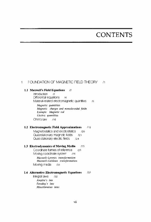
CONTENTS
1 FOUNDATION OF MAGNETIC FIELD THEORY / I
1.1 Maxwell's Field Equations / Z
Introduction / z Differential equations 14
Material-related electromagnetic quantities 15
Magnetic quantities Magnetic charges and nonsolenoidal fields Example: Magnetic rod Electric quantities
Ohm's law 116
1.2 Electromagnetic Field Approximations Magnetostatics and electrostatics 120 Quasistationary magnetic fields / z 1
Quasistationary electric fields /24
/ I 9
1.3 Electrodynamics of Moving Media Coordinate frames of reference 125
Moving coordinate system 126
125
Maxwell-Lorentz transformation Maxwell-Galilean transformation
Moving media 131
1.4 Alternative Electromagnetic Equations /32
Integral laws /3z
AmpPre's law Faraday's law Miscellaneous laws
vii
viii CONTENTS
Diffferential laws /37
Current densities 138
Magnetic circuits 140
1.5 Boundary Conditions /43
Field condifions 144
General conditions Nonsupercondiicting media Example: Calculation of the conditions
Current densily condtions 149
Moving boundaries 151
2 MAGNETIC POTENTIALS 1.55
2.1 Magnetic Scalar Potential /55
Potential in empty space 156 Definitions and solutions Boundary conditions
Axsymmetric systems /60
General equations Expansion near the axis Example: Diamagnetic sphere
Two-dimensional plane systems 164
General equations Example: Transverse field on diamagnetic rod The conformal transformation method Example: Parallel lines
Example: Permanent spherical magnet Example: Magnetized sphere Method of images
Potential in and outside magnetized material 170
2.2 Magnetic Vector Potential /76
Basic equations and soluCons /76
Equations Solutions Boundary conditions Retarded potentials
Axxisymmetric systems 184
Plane two-dimensional systems /86 Biot-Savart law 186
Filamentary conductor Multipole expansion Magnetic dipole

CONTENTS ix
2.3 Fields in Cylindrical and Straight Conductors 191
Circular loop /Q 1
Multiloop system 194
Coil pair Field shaping
Thin solenoid /97
Thick solenoid / I 00 Bitter solenoid /I 04
Toroidal magnets / I 05
Straight conductors /I 07
Example: Rectangirlar bar conditctor Example: Strip condiictor Example: Two-dimensional miiltipole configitrations
Short f i lamentary coil Saddle-shaped coils / I 14
Long coils
2.4 Inductance of Conductors / I 17
Self-inductance I 1 17
Filamentary approximation Fnradny law Example: Wire transmission line
Mutual inductance / I 2 1
Filamentary approxiniation General expressions
2.5 Structure of Magnetic Fields Magnetic field lines I1 26
Magnetic surfaces 11 28
I t 25
Toroidal sitrfaces
3 PERIODIC FIELDS AND WAVE PHENOMENA / i 3 3
3.1 Complex Functions 1133
Sinusoidal functions /I 34
Complex variables and functions
Complex vectors I I 38
11 35 Example: Conformal transformations
3.2 Sinusoidal and Rotating Electromagnetic Fields I1 40
Electromagnetic equations / I 40 Generalized wave equations 11 42
Magnetic potential 11 42
Rotating magnetic fields / I 44

X CONTENTS
Two-phased coil arrangement Three-phased coil arrangement
3.3 Wave Phenomena 1146
Wave equations / I 47
Plane waves in a uniform medium Plane waves in a conducting medium
Example: Radiation f rom a Hertzian dipole / I 49
/ I 50
4 MAGNETIC FIELD DIFFUSION AND EDDY CURRENTS / I 53
4.1 Magnetic Diffusion Theory /153
General equations for a solid conductor Quasistationary diffusion equations / I 56
Solutions to the diffusion problem
/ I 54
/ I 58
Solutions and analogies Response to a step-function field Generalization Dflusion time
4.2 Field Diffusion into Plane Conductors I165
Half-space conductor 11 65
S tep-fu nct ion field General solution Characteristic diffusion parameters
Transient polynomial fields Transient sinusoidal field Steady sinusoidal field Exponential field
Step-function field Steady sinusoidal field
Special boundary fields on half-space 11 7 1
Slab conductor / I 79
4.3 Field Diffusion in Cylindrical Geometry 1183
Equations in simple geometry 11 84
One-dimensional equations Axisymmetric equations Two-dimensional equations
Diffusion of axial fields 1187
Step-function field on a rod Steady sinusoidal field on a rod Diffusion through a hollow conductor

CONTENTS
Diffusion of transverse fields 11 94
Transverse step-function field on a rod Steady and rotating transverse fields Transverse diffiision through a hollow conductor
4.4 Eddy Currents 1201
The eddy current approach Two-dimensional currents in sheets 1203
The thin-sheet approximation 1207
120 I
Field equations Vector potential equations Example: Thin disc Example: Moving thin disc Example: Moving sheet
Limiting cases The thin-walled shell The magnetically thin shell Example: Transverse field on thin shell with gaps
Eddy currents in cylindrical shells 12 I 4
Magnetic shielding 1220
Example: Shielding of a steady sinusoidal field Example: Shielding by a thick hollow conductor Example: Shielding by a thin hollow conductor
4.5 Diffusion in Electric Circuits 1225
Lumped circuits 1225
Skin-effect impedance Example: Step-function current on plane conductor Example: Step-function current on a rod
Generalization of the resuits and equhalent circuits Alternating currents 1232
1230
5 ELECTROMAGNETIC AND THERMAL ENERGIES 1235
5.1 Electromagnetic Energy Equations 1235
Electromagnetic energy 1236
Field equations Potential equations Sinrtsoidal fields Inductive energy Example: Coaxial transmission line
Example: Thermal diffusion in slab Thermal energy 1244
xii CONTENTS
5.2 Magnetic Heating in Constant Conductivity Conductors /248
Dffusion heating 1249
loule's law Energy equations
Polynomial field Step-function field Sinusoidal field Energy skin depth
Slab Rod Hollow cylindrical conductor
Heating in the conducting haif-space 1252
Heating of thick sheets and cylindrical conductors 1260
5.3 Heating in Thin Conductors /264
Plane and cylindrical geometries /264
Thin slab Thin rod Thin disc
Electric c o n d u c t i law /268
Temperatiire-dependent conductivity Current integral
Diffusion and heating in hollow conductors 1270
Example: Step-function field diffusion Example: Transient sinusoidal field diffsion Example: Steady sinusoidal heating
5.4 Nonlinear Magnetic Diffusion /277
Nonlinear diffusion equations 1278
One-dimensional diffusion 1279
An approximated solution Energy skin depth
Diffusion and heating in magnetic materials 1285
Steady sinusoidal magnetic field heating Ferromagnetic induction heating Ferromagnetic hysteresis heating
6 MAGNETIC FORCES AND THEIR EFFECTS / Z Q ~
6.1 Electromagnetic Forces 1295
Elemental forces 1296
Lorentz force

CONTENTS Xiij
Biot-Savart force Electromagnetic force density
Magnetic force density Example: Axisymmetric force density Maxwell's magnetic stress tensor Magnetic multipole expansion More on electromagnetic forces and torques
Forces on finite bodies 1300
6.2 Magnetic Forces on Rigid Conductors 13 i 1
Inductive forces 13 1 1
Virtual work formalism Loops and solenoids
Magnetic dipole suspension Magnetic braking Example: Moving disc Example: Moving sheet Example: Rotating sheet Homopolar generator
Magnetic suspension and braking 13 1 5
Magnetic levitation 1326
Ferromagnetic track Conducting track
Magnetomechanical machines 1333
Rotating machines Synchronous machines Induction machines More on magnetomechanical machines
Forces within a conductor 1339
6.3 Magnetic Propulsion Effects in Conducting Sheets 1342
Plane sheet propulsion 1343
Equation of motion Thermal velocity limitation for thin conductors Shock waves Ablation effect Velocity limitation for thick conductors
Implosion of a cylindrical sheet 1352
General equations Constant current driver
6.4 Acceleration and Trajectories of Particles Equation of motion 1357
Pellet acceleration methods 1359
1356

xiv CONTENTS
Magnetic acceleration 136 I Magnetic dipole acceleration Diamagnetic sphere Example: Toroidal coil Magnetic rail gun
Particle trajectories in electromagnetic fields Cartesian equations Motion in static, uniform fields Motion in variable fields Motion in axisymmetric fields Example: Trajectories in toroidal fields Electromagnetic optics
7 MAGNETOMECHANICAL STRESSES
7.1 Stress-Strain Relations and their Limits The stress tensor 1388
Elastic stress-strain relations 1392
The displacement vector 1395
Effects of thermal expansion /397
Thermoelasticlty in dynamic system 1398
Failure criteria /399
7.2 Stresses in Solenoidal Magnets Thick cylinder and disk 1404
Solenoidal coils 1407
Yielding in cylindrical containers Thin-walled cylindrical magnet 141 4
Dynamic containment /4 i 5
/404
141 2
7.3 Stresses in Toroidal Magnets I 4 17
Container shell of general shape Toroidal magnet /420
141 7
Toroidal magnet with constant stress 1423
I370
1387
/388
7.4 Force-Free Fields and Current Distributions /427
General formulation 1428
Force-free contigurations A28
Plane geometry

CONTENTS xv
Cylindrical geometry Spherical geometry Variable-pitch solution
8 MAGNETOHYDRODYNAMICS AND PROPERTIES OF MATTER 1435
8.1 Magnetohydrodynamic Equations /436
General formulation 1436
Eirlerian frame Lagrangian frame
Magnetic diffusion /44z
Field diffusion Vector potential diffusion Limiting cases Cylindrical one-dimensional geometry
8.2 Magnetic Flux Compression /450
Flux compression circuit Flux compression by incompressible plane conductors
Current generators 1451
Implosion of an ideal flux compressing shell 1458
Field diffusion Ideal f l u x compression
Ultrahigh field generators 1463
Incompressible shell with finite conductivity Compressible shell with infinite conductivity Cylindrical frirx compression
8.3 Some Properties of Matter /471
Electric conductivity /47z
Conductivity in the solid state Conductivity in liquid, vapor, and plasma states Superconductivity
Magnetic matter 1484
Diamagnetism Paramagnetism Ferromagnetism Permanent magnets
Quantum parameters Critical magnetic fields and monopoles Nuclear magnetic resonance
High-energy densities 1503

xvi CONTENTS
Equation of state Specific heat and phase transitions Shock waves
9 NUMERICAL AND ANALOG SOLUTION METHODS / 5 i 3
9.1 Numerical Computation Methods /514
Poisson's difference equation Difference solution method
Shape functions Example: Leakage field in an electromagnet
Network definit ion Network solution Magnetic reluctance network
Finite-difference method 15 I 4
Finite-element method /5 I 8
Finite-element network methods /5z3
9.2 Approximation by Filamentary or Simple Elemental Conductors /530
Circular loops and solenoids 1530
Approximation by filamentary straight sections Inductance and magnetic energy 1533
Force and field lines 1534
/532
9.3 Analog Methods 1535
Electromagnetic model scaling 1535
General formulation Quasis ta t ionary approximation
Magnetomechanical model scaling /538
APPENDICES mi
A.l Electromagnetic Units and Equations /542
A.2 Mathematical Functions /545
The errorfunction /545
Bessel functions of integer order Functions in series formulation 1553
Vector formulae 1555
1547
A 3 Coordinate Systems, Vector and Tensor Relations /555

CONTENTS xvii
Definitions Vector operators Differential relations Integral relations
Various coordinates and transformations Differential expressions Laplacian of a vector
Vectors in Cartesian, cytindrical, and spherical coordinates 1558
Vectors in orthogonal curvilinear coordinates /56z
Definitions Differential expressions Direction of the curl vector
Matrices and tensors /564
Definitions Transformations between coordinate systems
A.4 Some Solutions of Second-Order Differential Equations /567
Pertinent differential equations /568
Laplace equation 1569
Separation in Cartesian coordinates Separation in cylindrical coordinates Example: Solution in R periodic geometry Separation in spherical coordinates
Simple and double series solution Example: Infinitely permeable, rectangular boundary Example: Axisymmetric, superconducting boundary
Poisson equation 1576
Helmhok equation /581
Diffusion equation 1583
Separation in Cartesian coordinates Separation in cylindrical coordinates Separation in spherical coordinates
BIBLIOGRAPHY 1587
PREFACE
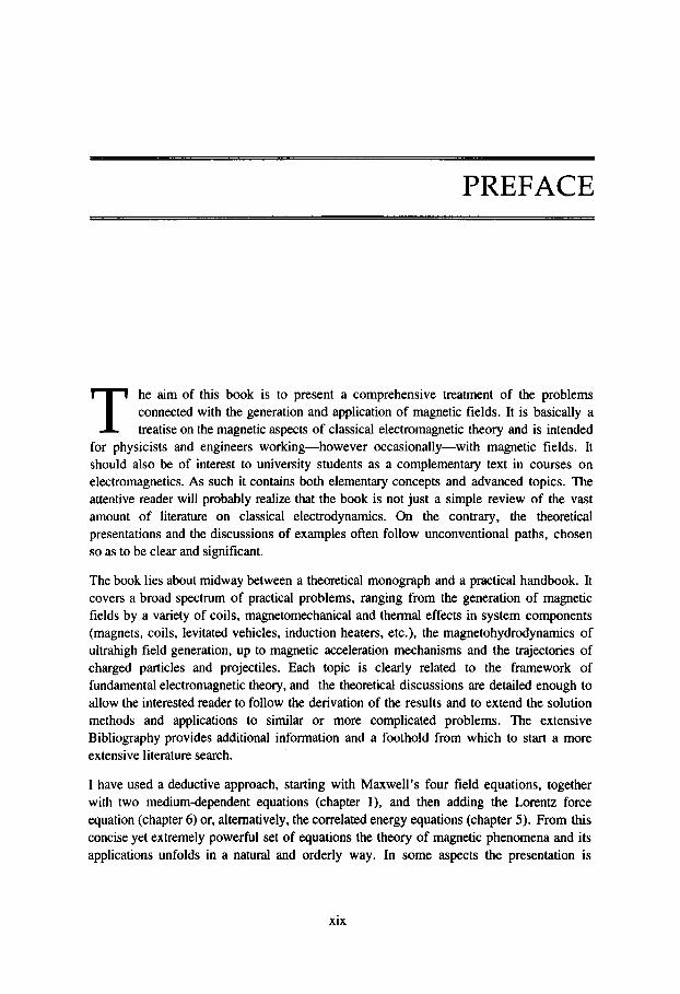
T he aim of this book is to present a comprehensive treatment of the problems connected with the generation and application of magnetic fields. It is basically a treatise on the magnetic aspects of classical electromagnetic theory and is intended
for physicists and engineers working-however occasionally-with magnetic fields. It should also be of interest to university students as a complementary text in courses on electromagnetics. As such it contains both elementary concepts and advanced topics. The attentive reader will probably realize that the book is not just a simple review of the vast amount of literature on classical electrodynamics. On the contrary, the theoretical presentations and the discussions of examples often follow unconventional paths, chosen so as to be clear and significant.
The book lies about midway between a theoretical monograph and a practical handbook. It covers a broad spectrum of practical problems, ranging from the generation of magnetic fields by a variety of coils, magnetomechanical and thermal effects in system components (magnets, coils, levitated vehicles, induction heaters, etc.), the magnetohydrodynamics of ultrahigh field generation, up to magnetic acceleration mechanisms and the trajectories of charged particles and projectiles. Each topic is clearly related to the framework of fundamental electromagnetic theory, and the theoretical discussions are detailed enough to allow the interested reader to follow the derivation of the results and to extend the solution methods and applications to similar or more complicated problems. The extensive Bibliography provides additional information and a foothold from which to start a more extensive literature search.
I have used a deductive approach, starting with Maxwell’s four field equations, together with two medium-dependent equations (chapter l), and then adding the Lorentz force equation (chapter 6) or, alternatively, the correlated energy equations (chapter 5) . From this concise yet extremely powerful set of equations the theory of magnetic phenomena and its applications unfolds in a natural and orderly way. In some aspects the presentation is
xix
xx PREFACE
similar to my previous 1970 book Pulsed High Magnetic Fields, which remains a useful complementary source for solving some specific problems.
It is assumed that the reader has the mathematical background required by most textbooks on electrodynamics; in particular, ordinary differential calculus and equations, vector algebra, and differential relations. In any case, helpful reminders are given in the Appendices, which contribute to making the book largely self-sufficient. The International System of Units (SI) is used in text and formulae; but in deference to still widespread laboratory practice, the ghost of the practical cgs units (cm, g, s, dyn, erg, oersted, gauss, together with ampere, volt, henry, coulomb, etc.) lingers on through some duplicated basic equations, clearly marked by an asterisk. In addition, two comprehensive tables provide the basic equations written in different systems (SI, Gaussian, emu, esu, practical cgs).
This book has evolved gradually through the years and is largely based on notes taken during my long involvement in activities specifically related to magnetic fields. In the following are listed some of the projects I have worked on and just a few of the teachers, colleagues and scholars to whom I express my gratitude for their direct or indirect contributions and scientific enlightenment: In the 1950s, a gamma-ray spectrometer based on a highly uniform NMRcontrolled magnet (with Peter Stoll and Willy Wolfli), this thesis work was carried out at the Swiss Federal Institute of Technology (ETH) in Zurich under Paul Scherrer, whilst I was also writing up and editing (with Fritz Herlach) Wolfgang Pauli’s lecture on Wave Mechanics for publication; in the 1960s magnetic flux compression experiments and theory at Frascati with Jirka Linhart, Fritz Herlach and Riccardo Luppi; in the 1970s, electron runaway studies in the Ormak magnetic tokamak at Oak Ridge National Laboratory with John Clarke, Don Spong and Stewart Zweben; still in the 1970s, design of an experimental magnetic tokamak machine for relativistic electron- beam studies at the Massachusetts Institute of Technology (MIT) with Bruno Coppi, and later, in the 1990s involvement in his superhigh-magnetic-field Ignitor project; back in the 1980s. I was engaged, as chairman of the European Advisory Group on Fusion Technology, in establishing the technology base for the European Fusion Program-in particular, with regard to superconducting magnet technology; since the end of this period I have been following these problems also as director of the School of Fusion Reactor Technology founded by Bruno Brunelli at the “Ettore Majorana” Center for Scientific Culture in Erice, Sicily.
I am grateful to Roberto Andreani, the present and long-time director of the Euratom-ENEA Fusion Program, for the hospitality extended to me at the Frascati Research Center of the Italian Agency for New Technologies, Energy and the- Environment (ENEA) well beyond my employment there by the European Commission. Last but not least, it is a pleasure to acknowledge the substantial technical help received from many persons at Frascati, above all from Lucilla Crescentini for the dedicated and professional management of the many drafts of the manuscript, and from Peter Riske for the artwork. I would also like to thank Carolyn Kent for the English editing, Nadia Gariazzo for typing the final camera-ready copy, and Maria Polidoro for the secretarial help over all these years.
PREFACE xxi
Finally, 1 apologize for any errors in the text, equations, or figures that have been overlooked despite careful proofreading, and would greatly appreciate their being called to my attention.
HEINZ E. KNOEPFEL
March 2000
Association EURATOM-ENEA ENEA Rrsrarch Crnler. Frasiati. ltulv

MAGNETIC FIELDS
FOUNDATION OF MAGNETIC FIELD THEORY
War es ein Gott der diese Gleichungen schrieb? (“Was it a god who wrote these equations?’) Thus wrote L.E. Boltzmann, one of the great scientists of the 19th century, at the beginning of the introduction to his Lectures on Maxwell’s Theory of Electricity and Light (Munich, 1893). This motto well reflects the powerful beauty and conciseness of the so-called Maxwell equations, particularly when presented (as below) in vectorial form. These equations, which had been published in final form about ten years earlier, represent the concluding highlight of centuries of discoveries and studies in electromagnetism and set the comprehensive foundation of classical electromagnetic theory.
In contrast to the historical approach used in many textbooks (where the fundamental effects are gradually developed into the final set of the electromagnetic equations), in this book, Maxwell’s equations are used as the starting point for presenting and discussing the mathematical and physical aspects of electromagnetism, with particular reference to magnetic phenomena. The presentation of various (simplified) forms of Maxwell’s equations and some related mathematical constraints is the main aim of this chapter.
Nore. Equations are referred to by their designation, for example, (1.5-23) means the equation labeled (1.5-23) in section 1.5 The International System of Units (SI) applies throughout the book; however, an asterisk added to the equation designation-for example, (l.l-l7)*-indicates that equation (1.1-17) is written in practical cgs units, which are defined in table A.l- I I of appendix A.l. Superscripts refer to the Bibliography, which is subdivided per chapter and given at the end of the book.
1
M4GNETICFIELDS: A Comprehensive Theoretical Treatise for Practical Use Heinz E. Knoepfel
Copyright Q 2000 by John Wiley & Sons, Inc

2 CHAPTER 1 FOUNDATION OF MAGNETIC FIELD THEORY
1.1 MAXWELL’S FIELD EQUATIONS
Introduction
The history of the study of magnetic and electric effects is as old as that of physics, which originated in the Ionian Greek culture as an offspring of philosophy about 600 BC.
The philosopher Thales of Miletus, who is credited as the founder of science and thus of physics (“the study of nature”), knew about the peculiar properties of lodestone as attracting iron or assuming a north-south orientation. A large deposit of lodestone is known to have existed near the ancient town of Magnes (today’s Manissa, near Izrnir, Turkey), from which, in fact, the word “magnetism” is derived. These simple magnetic, as well as some electrostatic, phenomena remained a curiosity for centuries.
The year 1600 AD saw the publication of De magnete, the first elementary treatise (in Latin) on magnetism, by W. Gilbert, who was an influential medical doctor at the English Court. The birth in the 17th century of the inductive-deductive science of J. Kepler, G . Galilei, and I. Newton led in the 18th century to numerous and ordered observations of magnetic and electric phenomena by D. Bernoulli, H. Cavendish, Ch. A. Coulomb, B. Franklin, A. Galvani, and A. Volta, just to name a few of the many scientists involved. A fundamental contribution to the progress of science, and to the study of electromagnetic phenomena in particular, was the refinement of mathematical analysis through the differential and variational calculus introduced by I. Newton and G.W. Leibniz in 1670-75, and extended by L. Euler and J.L. Lagrange in 1744-55.
In the pioneering first half of the 19th century, it became possible to study magnetic and electric phenomena more systematically. Electricity and magnetism, which previously were entirely separate subjects (the former dealt with such things as cat’s fur, glass rods, batteries, frog’s legs, lightning; the latter with bar magnets, compass needles, the Earth’s poles) rapidly merged into electromagnetism. The beginning of this period coincides with H.Ch. Oersted’s discovery in 1819 that a compass needle is deflected if placed near a current-carrying conductor. Mathematician A. M. AmNre’s interest in physics was stimulated by this discovery, and within a few months (1820) he extended both experimentally and theoretically the understanding of magnetic effects related to electric currents. For this work, he can be considered the “father” of electromagnetism.
In the same year, J.B. Biot and F. Savart formulated the law that gives magnetic fields as generated by filamentary currents, and in 1826 G.S. Ohm established the relation between electric field and current. In 1831 M. Faraday described the law of induction and introduced the concept of magnetic lines of force. (He also revived the concept of Ether, “the vacuum-filling medium”; see remarks in the introduction to section 2.5.) In the following two decades, electromagnetic phenomena were gradually formulated in more exact mathematical-theoretical terms by the contributions of C.F. Gauss, W.E. Weber, W. Thomson, R. Kohlrausch, H. Helmholtz, and others.
1.1 MAXWELL'S FIELD EQUATIONS 3
In 1855 J.C. Maxwell further extended the ideas about field lines; seven years later he introduced the concept of displacement currents, which self-consistently completed the electromagnetic equations. His Treatise on Electricity and Magnetism, I . ' first published in 1873, and the contributions in 1884-85 by H. Hertz and 0. Heaviside gave Maxwell's equations their final form. After J.P. Joule stated the equivalence of heat and mechanical energy in 1845, H.A. Lorentz (who formulated the electromagnetic force on an electric charge in 1879), J.H. Poynting, and P.N. Lebedev gradually introduced the concepts of electromagnetic force and energy into the theoretical framework in the second half of the 19th century. Clearly, a large number of other important physicists and mathematicians contributed substantially to establishing electrodynamics. Many of them are mentioned in the text in connection with their fundamental work (full names and dates are listed in the Index).
In the first half of the 20th century, classical electromagnetic theory was coupled with quantum mechanics into quantum electrodynamics. As one of the four fundamental fields of forces-thus of energy-in Nature [gravitation, electromagnetism, weak interaction (nuclear beta-decay), strong interaction (nuclear reactions)], electrodynamics was blended in the second half of the century with the field of weak interactions into the unified electro- weak theory, one important step toward including all four fields in the so-called Grand Unification.
The great applications of electricity started while classical electromagnetic theory was being completed. In 1879 the first railway vehicle was driven by electric power in Berlin, and three years later Th. A. Edison built the first electric power station to partly supply lighting to New York City. This marks the beginning of a new evolution, which characterizes the 20th century, since the availability of electricity introduced increasingly sophisticated and efficient applications of it in industry, transport, and communications.
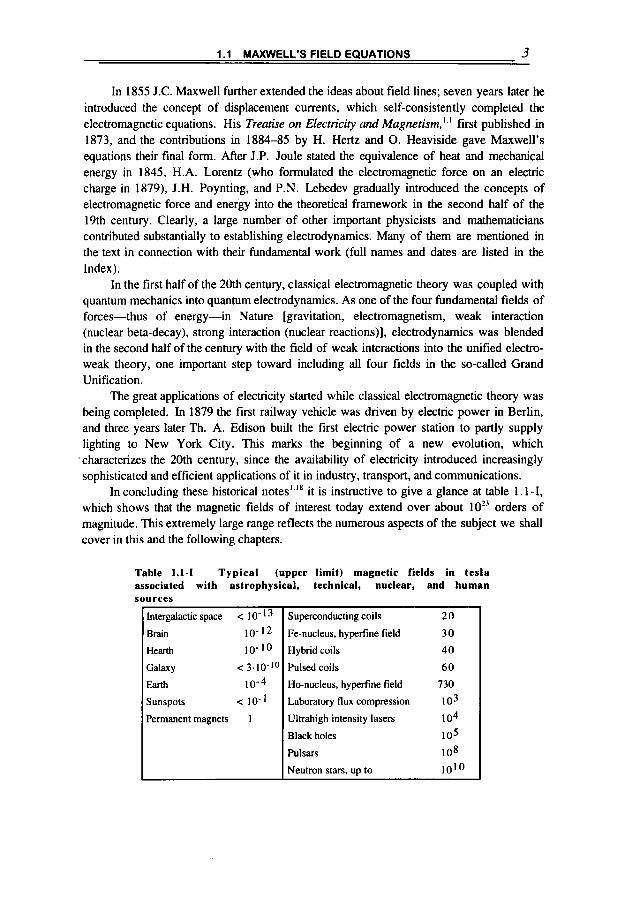
In concluding these historical notes'.'' it is instructive to give a glance at table 1.1 -I, which shows that the magnetic fields of interest today extend over about lo2-' orders of magnitude. This extremely large range reflects the numerous aspects of the subject we shall cover in this and the following chapters.
Table 1.1-1 Typical (upper limit) magnetic fields in tesla associated with astrophysical, technical, nuclear, and human sources
~ntergaiactic space < I 0- 1 3
Brain 10-12
Hearth 10-10
Earth 10-4
Sunspots < 10-1
Galaxy < 3.10-I'
Permanent magnets 1
Superconducting coils
Fe-nucleus, hyperfine field
Hybrid coils
Pulsed coils
Ho-nucleus, hyperfine field
Laboratory flux compression
Ultrahigh intensity lasers
Black holes
Pulsars
Neutron stars, up to
20
30
40
60
730
103
104
I 05
108
1010

4 CHAPTER 1 FOUNDATION OF MAGNETIC FIELD THEORY
Differential equations
MaxwellSfield equations in SI units (International System of Units) are here written in the vectorial form
dl, dt
V x H = j + - ,
w dt
V X E = - - ,
V . B = O ,
(1.1-1)
(1.1-2)
(1.1-3)
(1.1-4)
where the five vectors, one scalar function, and one operator are:
H, magnetic field strength (or magnetic intensity) [dimension: ampere.m"; for the electromagnetic units see table A. 1-II in appendix A.11;
B , magnetic flux density (or magnetic induction) [tesla]; D , electric flux density (or electric induction or displacement) [c~ulomb.m-~]; E , electric field strength (or electric intensity) [volt.m*']; j , free current density (that is, the current density related to the transport of free electric
charges) [amperem'*]; pe, volume density of free electric charges [ c~u lombm~~] ;
V, nabla operator (defining the operation curl, divergence, and so on; see table A.3-I1 in appendix A.3) [m-'I.
The equations are also known as the laws of Amp&re-Maxwell (1.1- l), Faraday ( 1.1-2), Gauss-Faraday (1.1-3), and Gauss (1.1-4), but these denominations are used more appropriately in connection with the corresponding integral forms presented in section 1.4.
In the previous differential equations, j and pe can be considered as the sources that determine the electromagnetic fields H, B, E , D . They are related by the charge or current conservation eqwtion,
V . j + - - a P e - 0 , at
(1.1-5)
which is obtained by taking the divergence of (1.1 - 1) and using (1.1-4) and the fact that divergence of a curl is zero, thereby commuting the V and dldt operators (because we assume a space where, at each point, the field vector and all its derivatives are continuous).
To make a general solution possible, three more equations are required, which are known as constitutive equations, that is, Ohm's law

1.1 MAXWELL'S FIELD EQUATIONS 5
j = o E , (1.1-6)
and the relations
B = p H , (1.1-7)
D = E E , (1.1-8)
where cr is the electric conductivity [dimension: ohm-l.m-'],
P = POPR (1.1-9)
is the magnetic permeability with PO = 41c10-~ [henrym-I], and
& = &o&R (1.1- 10)
is the dielectric constant (or permittivity) with €0 = 8.854 x 10⁻¹² [farad.m-l] (the dimensionless parameters PR and E R are discussed below). These which characterize the medium, can themselves be functions of various parameters (for example, the temperature, or even H itself), in addition to space and time. For the more general case, when the medium has nonisotropic properties with respect to electromagnetic phenomena, these parameters actually become tensors (see the end of appendix A.3)3.2. The whole problem then becomes formally quite cumbersome, but nowadays such cases can be treated by numerical computation (see chapter 9). In this book, however, we shall limit our attention to isotropic media and nearly always assume the electric conductivity a, relative magnetic permeability pR, and dielectric permittivity E~ to be constants.
quantities,
Material-related electromagnetic quantities
We have seen that the magnetic field H is related to the free current density j through Amplxe's law (1.1-l), whereas the magnetic induction or flux density B is related to the electric field E through Faraday's law (1.1-2). We shall see throughout the book that B is the dominant magnetic vector quantity because it appears explicitly in all magnetically induced effects: electric fields, magnetic forces, moments, and so on. For this reason, and for simplicity, B is often also called the magnetic field, which well matches the electric field E, the dominant electric quantity (rather than the electric flux density D ) since it appears in all electrically induced effects: currents, forces, moments, and so on.
The magnetic and electric properties of a medium can be described with the help of two vectors, the magnetic (M) and electric (P) polarization vectors:
B M = - - H , PO
(1.1-11)

6 CHAPTER 1 FOUNDATION OF MAGNETIC FIELD THEORY
P = D - € o E , (1.1- 12)
which exist only in a medium since they actually vanish in free space where B = poH, D = EOE. Introducing them into (1.1-1,4) yields
(1.1-13)
EOV. E = pe +(-V .P) . ( 1 .1 - 14)
These equations formally show that when material is present in an electromagnetic field, internal sources of currents and charges appear. In fact, the terms
(1.1- 15)
may be interpreted as material-related equivalent mgmtiurtion or electric-polarimtbn current densities, whereas
p = - V . P ( 1.1 - 16) P
may be interpreted as an equivalent electric charge density introduced by the electric polarization.
In the following we shall give further relations and information on these macroscopic magnetic and electric properties of material. Then, in chapter 8 these quantities are put in relation with some microscopic elements of material.
Magnetic quantities
It is an experimental fact that in most materials, when subjected to a (current generated) magnetic field H, an additional magnetic field component M is generated locally (defined as magnetic polarization or magnetization), and the two add together to give the total local induction
B = h f l ~ H = h H + h M , ( 1 . 1 - 17)
or, in the practical cgs system [B in gauss; H in oersted; M in erg . G-’ . ~ m - ~ ] ,
B = H + 4 x M . (1.1- 17)*
Sometimes, the magnetic polarization is also defined as
IM =poM . (1.1-18)

I .l MAXWELL’S FIELD EQUATIONS 7
By introducing the magnetic susceptibility
we can write
M = xmH (1.1-20)
Note that if a given outer magnetic field Ho is applied to a finite body of magnetic material, the local magnetic behavior is not, in general, described by the above relations containing the substitution Ho + H; for example, the magnetic induction in the body is not B = p H o but B=pHi, where the internal local field Hi (which determines the local magnetization M=xmHi) is itself the result of the addition of the outer field and the magnetization component. For the same reason, the induction outside the body is B = poHe, where the external local field He is co-determined by the magnetic effect of the body. To determine Hi at any point within the body and He outside it requires solving a magnetic (potential) problem, as outlined in sections 2.1 and 2.2. The example of a magnetic rod is dealt with later in this section and will help to get a better understanding of these magnetic field components. A simple case is given by a closed magnetic circuit or a ring of magnetic material (as discussed in section 1.4 in connection with figure 1.4-3a, with x = 0) with an evenly wound coil around it, which generates a magnetic field HO within the structure. In this idealized situation it is simply He = 0 and Hi = Ho. thus B =pHo everywhere. The magnetic properties of materials, expressed by the magnetization M, depend on two main atomistic effects, which can give rise to large local magnetic fields, as we will discuss in more detail in section 8.3 [see, in particular (8.3-26,36)]: (1) the orbital motion of electrons around the nucleus, which can be seen as current loops of atomistic dimensions or as small magnetic dipole moments; (2) the intrinsic spin of the electrons (or nuclei) with the related magnetic dipole moment. The relative magnetic permeability p~ or the magnetic susceptibility xm. which define M through (1.1-19, 20). vary widely, as shown in table 1.1-11. In the so-called diamagnetic materials the susceptibility is negative; in paramagnetic, positive; and in ferromagnetic, very large ( x , = lo4). Moreover, it can depend in a complicated way on H (see in section 8.3).
We have already seen in ( 1.1 - 15) that from a macroscopic point of view magnetization may be expressed in terms of an equivalent magnetization current density by
j , = V x M . (1.1-21)
Alternatively we will see in (1.1-23) that it may also be described as a volume density of magnetic dipole moments, to which we will relate in (1.1-27,29) a magnetic charge density. These three macroscopic models are obviously equivalent and justified by the atomistic explanation of the magnetization given above.
When M is uniform there are no such currents in the medium; instead, a magnetization sugace current density as defined in (1.4-39,
i ,= lim j,Ah , &+O
(1.1 -22a)

8 CHAPTER I FOUNDATION OF MAGNETIC FIELD THEORY
Table 1.1-11 Magnetic susceptibilitiesa
Material
Diamagnetic: Bismuth Silver
Water
Carbon dioxide
Copper
Paramagnetic: Oxygen Sodium Aluminum Tungsten Gadolinium
Iron Iron-nickel
Ferromagnetic (max.values):
Magnetic susceptibility x,,
-17.6 x -2.4 x 10⁻⁵ -0.88 x 10⁻⁵
-0.90 x 10⁻⁵ - 1 . 2 x 10⁻⁵
0.19 x 10⁻⁵
0.85 x 10⁻⁵
2.3 x 10⁻⁵
7 .8 x 10-5 4 8 ' 0 0 0 ~
3 0 x lo3 80-300 x lo3
OSee section 8.3 (tables 8.3-VI. VII) for more detailed information.
appears, which, on the boundary of the medium (e.g., surrounded by free space), has the value [see in (1.5-6)]
(1.1-22b) i, = -n x M ,
where n is the unit normal vector to the boundary, pointing outwards. Ampkre already suggested that magnetic properties might be described by such formal currents. They are considered to be made up of elementary cells that include circulating, whirling currents, as depicted in figures 1.1-1 and 1.1-2, which is in qualitative agreement with the above expressions. In fact, when M is constant and the whirling current cells equal, all the currents, except those on the surface of the medium, cancel each other out at the common boundaries of the cells, thus giving rise to the surface current density. These equivalent Ampkrian currents, pictured as flowing without dissipation in a magnetized medium, are an artifact that can be used to describe magnetization effects in simple physical terms. In section 8.3 we show that qualitative support of this picture is provided by the atomistic explanation of magnetization, i.e., by microscopic, inaccessible currents of atomic origin.
The magnetization M can be seen as the magnetic moment per unit volume in the form
(1.1-23)
where rpQ is the coordinate vector with respect to a point of origin P of the current density jm,Q. The total magnetic moment pm of a given volume of material is thus'
I .I MAXWELL'S FIELD EQUATIONS 9
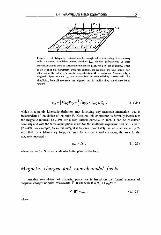
Figure 1.1-1 Magnetic material can be thought of as consisting of elementary cells containing Ampkrian current densities jm; addition (subtraction) of these
currents provides a bound surface current density i, flowing on the boundary, which
exists even if the elementary amperian currents are identical and thus cancel each other out in the interior (when the magnetization M is uniform). Alternatively, a magnetic dipole moment p, can be associated to each whirling current cell. (For
simplicity, here all moments are aligned, but in reality they could also be at random.)
which is a purely kinematic definition (not involving any magnetic interaction) that is independent of the choice of the point P. Note that this expression is formally identical to the magnetic moment (2.2-49) for a free current density. In fact, it can be calculated similarly and with the same assumptions made for the multipole expansion that will lead to (2.2-49). For example, from this integral it follows immediately [as we shall see in (2.2- 45)] that for a filamentary loop, carrying the current I and enclosing the area S, the magnetic moment is
(1.1-25)
where the vector S is perpendicular to the plane of the loop.
Magnetic charges and nonsolenoidal fields
Another formulation of magnetic properties is based on the formal concept of magnetic charges or poles. We rewrite V. B = 0 with B = poH + poM as
V . H " = p , , (1.1-26)
where

10 CHAPTER I FOUNDATION OF MAGNETIC FIELD THEORY
I
Figure 1.1-2 Magnetization M and related current density j, = V x M.
p , = - V . M . (1.1-27)
in analogy to the electric polarization charge density (1.1-16), can be considered as a magnetic charge density, which is the source of the nonsolenoidal field component Hn. We use the magnetic field decomposition (1.1-35), where for the solenoidal component it is v.Hs =o.
When M is uniform, there are no such charges in the bulk of the material under consideration; however, a magnetic sugace charge density defined as in (1.4-36),
r,= lim pmdh , (1.1-28) d h + O
still exists at the boundary, which is given in (1.5-1 l),
r, = -n * (M2 - MI), (1.1-29)
and the relative nonsolenoidal field component (for simplicity we drop the superscript n) is defined in (1.5-10).
n.(Hz-H1)=rm , (1.1-30)
where n is again the outward pointing unit vector, from medium 1 to 2, normal to the boundary. These relations show that a magnetized material has at its surface formal magnetic charge densities r,, which arise whenever the normal component of M goes through a discontinuity. The magnetic charges generate in the interior of the material a so- called demagnetizing field & that by definition points from the north (+) to the south (-)
1 .l MAXWELL’S FIELD EQUATIONS 11
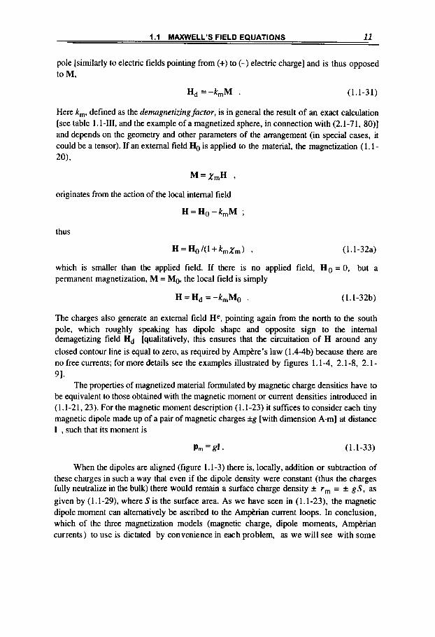
pole [similarly to electric fields pointing from (+) to (-) electric charge] and is thus opposed to M,
Hd =-k,M . (1.1-31)
Here k,, defined as the demagnetizing factor, is in general the result of an exact calculation [see table 1.1-111, and the example of a magnetized sphere, in connection with (2.1-71, 80)] and depends on the geometry and other parameters of the arrangement (in special cases, it could be a tensor). If an external field HO is applied to the material, the magnetization (1.1- 201,
M=XmH 9
originates from the action of the local internal field
H=Ho-k,M ;
thus
H=Ho/(I+k,Xm) 7 ( 1.1 -32a)
which is smaller than the applied field. If there is no applied field, H o = 0, but a permanent magnetization, M = Mo. the local field is simply
H=Hd =-k,Mo . (1.1-32b)
The charges also generate an external field He, pointing again from the north to the south pole, which roughly speaking has dipole shape and opposite sign to the internal demagetizing field Hd [qualitatively, this ensures that the circuitation of H around any closed contour line is equal to zero, as required by Ampkre’s law (1.4-4b) because there are no free currents; for more details see the examples illustrated by figures 1.1-4, 2.1-8, 2.1 -
The properties of magnetized material formulated by magnetic charge densities have to be equivalent to those obtained with the magnetic moment or current densities introduced in (1.1-21,23). For the magnetic moment description (1.1-23) it suffices to consider each tiny magnetic dipole made up of a pair of magnetic charges *g [with dimension A.m] at distance I , such that its moment is
91.
P m =gJ . (1.1-33)
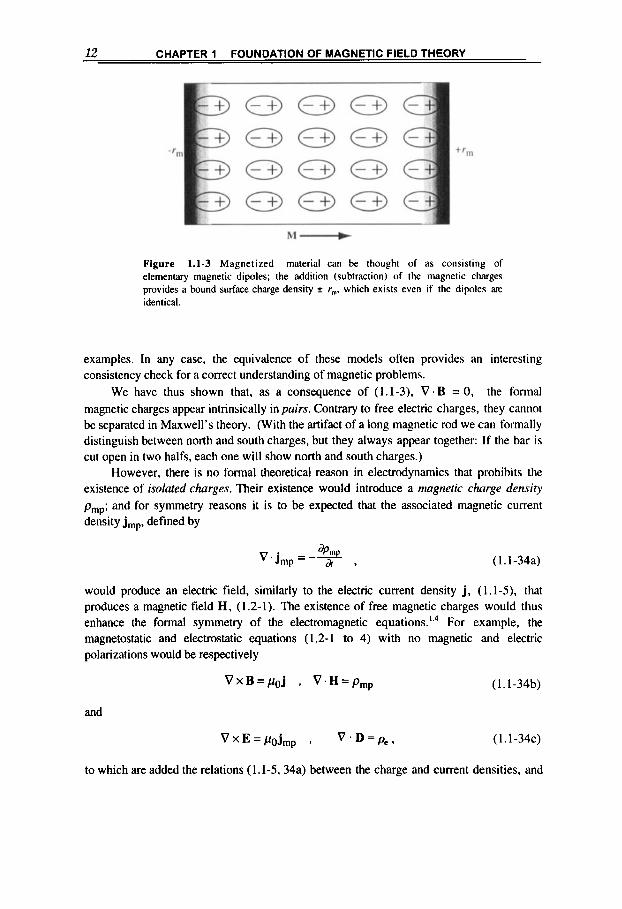
When the dipoles are aligned (figure 1.1-3) there is, locally, addition or subtraction of these charges in such a way that even if the dipole density were constant (thus the charges fully neutralize in the bulk) there would remain a surface charge density f rm = f g S, as given by (1.1-29), where S is the surface area. As we have seen in (1.1-23), the magnetic dipole moment can alternatively be ascribed to the Amphian current loops. In conclusion, which of the three magnetization models (magnetic charge, dipole moments, Amfirian currents) to use is dictated by convenience in each problem, as we will see with some
12 CHAPTER 1 FOUNDATION OF MAGNETIC FIELD THEORY
Figure 1.1-3 Magnetized material can be thought of as consisting of elementary magnetic dipoles; the addition (subtraction) of the magnetic charges provides a bound surface charge density i r,. which exists even if the dipoles are identical.
examples. In any case, the equivalence of these models often provides an interesting consistency check for a correct understanding of magnetic problems.
the formal magnetic charges appear intrinsically in pairs. Contrary to free electric charges, they cannot be separated in Maxwell's theory. (With the artifact of a long magnetic rod we can formally distinguish between north and south charges, but they always appear together: If the bar is cut open in two halfs, each one will show north and south charges.)
However, there is no formal theoretical reason in electrodynamics that prohibits the existence of isolated charges. Their existence would introduce a magnetic charge density
pmp; and for symmetry reasons it is to be expected that the associated magnetic current density j,, defined by
We have thus shown that, as a consequence of (1.1-3), V . B = 0,
(1.1-34a)
would produce an electric field, similarly to the electric current density j, (1.1-5), that produces a magnetic field H , (1.2-1). The existence of free magnetic charges would thus enhance the formal symmetry of the electromagnetic equations.' For example, the magnetostatic and electrostatic equations (1.2-1 to 4) with no magnetic and electric polarizations would be respectively
and
(1.1-34b)
(1.1-34~)
to which are added the relations (1.1-5,34a) between the charge and current densities, and
1.1 MAXWELL'S FIELD EQUATIONS l3
we would also add the force densities to be introduced in (6.1-12) and derivable from (8.3- 65) .
Despite experimental investigations lasting decades, the existence of free magnetic charges, sometimes called magnetic monopoles, has not been established. But extensive theoretical work in quantum electrodynamics and general relativity, more in general in the domain of elementary particle physics, have outlined some of the characteristics of magnetic monopoles, if they exist at all, which will be presented in connection with (8.3-64).
It is useful to recall at this point Helmholtz's theorem, according to which any static vector field at any point in space (which, together with its derivative, is finite, continuous, and vanishes at infinity) may be decomposed into'.' [see also ( 1 .I-54)]
H = H" + H S , (1.1-35)
where ~n =-v@ is the irrotational component and HS = V x A is the rotational or solenoidal component. The first component can be directly related to the magnetization M through (1.1-27.29); the second, to free and displacement currents through the Ampkre-Maxwell equation (1 . I - 1).
Because from (A.3-7, I I ) we have for these scalar and vector fields
V X V @ = O , V . ( V x A ) = O ,
we obtain
V . H = V . H n . V x H = V x H S . (1.1-36)
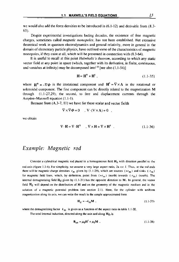
Example: Magnetic rod
Consider a cylindrical magnetic rod placed in a homogeneous field H, with direction parallel to the
rod axis (figure 1.1-4). For simplicity, we assume a very large aspect ratio, 2a << 1. Thus, at the rod ends there will be magnetic charge densities r m given by ( I . 1-29), which are sources (+ r , ) and sinks ( - r , )
for magnetic field lines, which, by definition, point from (+r , ) (north) towards ( -r , , , ) (south). The
internal demagnetizing field H,j given by (1.1-31) has the opposite direction to M. In general, the vector
field Hd will depend on the distribution of M and on the geometry of the magnetic medium and is the
solution of a magnetic potential problem (see section 2.1). Here, for the cylinder with uniform
magnetization along its axis. we can write the result in the simple approximated form
Hd =-k,M , (1.1-37)
where the demagnetizing factor k, is given as a function of the aspect ratio in table I . 1-111.
The total internal induction, directed along the axis and along Ho. is
(1.1-38)
14 CHAPTER I FOUNDATION OF MAGNETIC FIELD THEORY
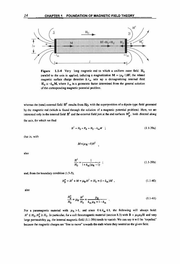
Figure 1.1-4 Very long magnetic rod to which a uniform outer field HO parallel to the axis is applied, inducing a magnetization M = (pR-l)Hi; the related magnetic surface charge densities f rm sets up a demagnetizing internal field H, P -k,M, where k, is a geometric factor determined from the general solution of the corresponding magnetic potential problem.
whereas the (total) external field He results from Ho. with the superposition of a dipole-type field generated
by the magnetic rod (which is found through the solution of a magnetic potential problem). Here, we are
interested only in the internal field Hi and the external field just at the end surfaces q, both directed along
the axis, for which we find
H’ = Ho + H(j = Ho - k,M ; ( I . I-39a)
that is, with
also
and, from the boundary condition (1.5-3),
H ; = H i + M = p R H i = H o + ( l - k , ) M ,
(1. I-39b)
(1.1-40)
also
!LPR-= Hi PR (1.1-41) HO HO k m f l R + l - k m
For a paramagnetic material with pR > I , and since 0 < k, < I, the following will always hold:
H’ 5 Ho. Hi 2 Ho. In particular, for a soft ferromagnetic material (section 8.3) with B = p 0 f l ~ H and very
large permeability p ~ , the internal magnetic field (1.1-39b) tends to vanish: We can say it will be “expelled”
because the magnetic charges are “free to move” towards the ends where they neutralize the given field.

1.1 MAXWELL'S FIELD EQUATIONS 15
1/2a
km
0 I 2 5 10 100
I 0.27 0.14 0.040 0.0172 0.00036
For a permanently magnetized rod with M = MO independent of H and with no applied outer field,
HO = O (figure 1.1-4). from (1.1-39.40) follows
H d = H i =-k,Mo, H i =(I-k,)Mo . ( I . 1-42)
Only when the rod is very long, 2a << I, and thus k, << 1, will the outer field at the magnet poles be
ti; 3 M o , We can formally express these properties also with the equivalent description involving the
(bound) surface current density i , . Since just outside the cylindrical surface of the (very long) magnetic md
the field is zero, from the boundary condition (1.5-5) we derive
i m = ~ = H i + M o = ( l - k , ) M o . ( I .I-43) PO
The magnetic field in the external free space produced by a permanently magnetized rod is equivalent to the
dipole-type field generated by a solenoidal coil with the same cylindrical geometry and the current density i , . The internal fields are quite different, as required to satisfy the integral conditions (1.4-4): In the rod
H' = Hd = - k , ~ ~ ; in the equivalent cylindrical coil H~ = H; = ( I - k , ) M ~ .
Electric quantities
For completeness' sake, we also present the analogous quantities relative to dielectric material. Similarly to (1.1-17), for the electric displacement vector, from experience and in relation to (1.1-12), we write
D = E ~ & R E = E o E + P , ( 1.1-44)
where the electric polarization is
P = E O X ~ E 1
and the electric susceptibility is
X e = & R - 1
(1.1-45)
(1.1-46)
The electric polarization P is directly related to the electric properties of materials (which can thus be expressed through the parameters xe and E R ) and, according to

16 CHAPTER 1 FOUNDATION OF MAGNETIC FIELD THEORY
(1.1-16), can be interpreted as deriving from an equivalent polarization charge density through
p = - V . P . (1.1-47) P
Somewhat analogously to magnetic material [see in connection with (1.1-29)], when P is uniform there are no such charges in the medium. However, a bound polarization surface charge density (1.4-36) is still present, rp = lim(Ah O)ppAh, and on the boundary of the medium (e.g., surrounded by free space) it has the value (1.5-14),
rp =-n.(P2 - 5 ) , (1.1-48)
and the electric fields on the boundary are defined in (1.5-13),
n . ( E 2 - E I ) & ~ = r p . (1.1-49)
The model to interpret this polarization effect considers that the medium contains electric dipole charges that align under the action of an electric field. When the dipole density is constant, the f charges neutralize, but there is still a surface charge density, qualitatively like the magnetic dipoles shown in figure 1.1-3. We recall that molecules or ions can have permanent dipoles, or dipoles generated through an applied electric field that displaces the center of positive charges with respect to that of negative charges.
The electric polarization P can be seen as the electric moment per unit volume [somewhat analogously to the magnetization (1.1-23)],
(1.1-50)
where pp,Q is the net, locally bound polarization charge density and 9,Q is the coordinate
vector with respect to a point of origin P. The total electric moment of a given volume of material is
(1.1-51)
which is independent of the choice of the origin P.
Ohm's law
Under the action of a force, an electric charge moves in a conductor, thereby establishing a current. We write
j=d, (1.1-52)
1 .l MAXWELL'S FIELD EQUATIONS 17
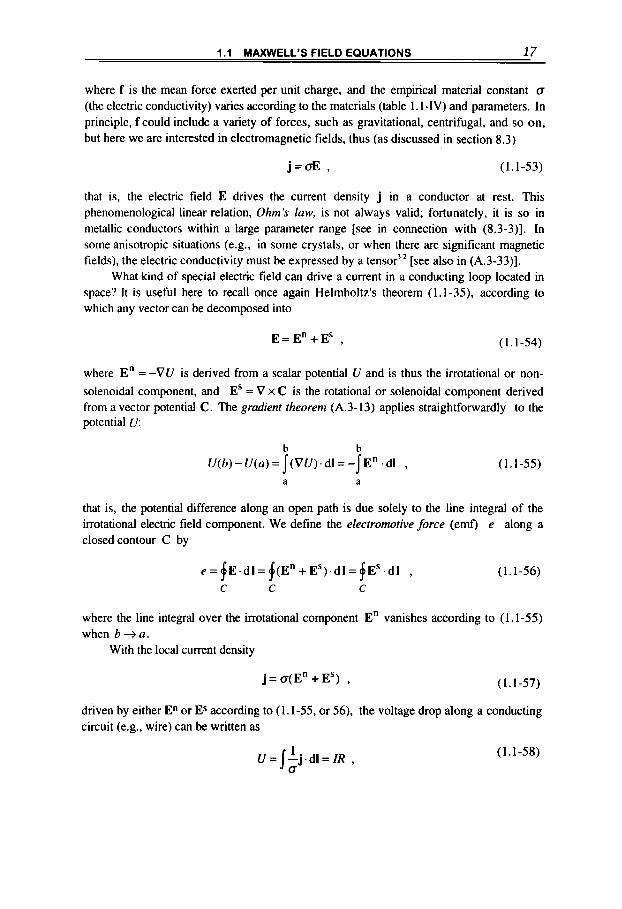
where f is the mean force exerted per unit charge, and the empirical material constant Q
(the electric conductivity) varies according to the materials (table 1.1-IV) and parameters. In principle, f could include a variety of forces, such as gravitational, centrifugal, and so on, but here we are interested in electromagnetic fields. thus (as discussed in section 8.3)
j = u E , ( 1.1-53)
that is, the electric field E drives the current density j in a conductor at rest. This phenomenological linear relation, Ohm's law, is not always valid; fortunately, it is so in metallic conductors within a large parameter range [see in connection with (8.3-3)]. In some anisotropic situations (e.g., in some crystals, or when there are significant magnetic fields), the electric conductivity must be expressed by a tensor'' [see also in (A.3-33)].
What kind of special electric field can drive a current in a conducting loop located in space? It is useful here to recall once again Helmholtz's theorem (1.1-35), according to which any vector can be decomposed into
E = E n + E S , (1.1-54)
where En = -VU is derived from a scalar potential U and is thus the irrotational or non- solenoidal component, and ES = V x C is the rotational or solenoidal component derived from a vector potential C. The gradient theorem (A.3-13) applies straightforwardly to the potential u:
b b
U(b) - U ( a ) = j ( V U ) . dl = - j E n . dl , (1.1-55) a a
that is, the potential difference along an open path is due solely to the line integral of the irrotational electric field component. We define the electromotive force (emf) e along a closed contour C by
e = E d l = ( E n + E S ) . d l = $ E S . d l , ( 1.1 -56) C
4 . 4 C C
where the line integral over the irrotational component En vanishes according to (1.1-55) when b + a .
With the local current density
j = o ( E n + E S ) , (1.1-57)
driven by either En or Es according to (1.1-55, or 56). the voltage drop along a conducting circuit (e.g., wire) can be written as
U = j - j . d l = 1 IR , 0
(1.1-58)

18 CHAPTER I FOUNDATION OF MAGNETIC FIELD THEORY
Table 1.1-IV Resistivities at 20°C
Material
Conductors: Silver
Gold Aluminum Nichrome
Semiconductors:
Copper
Salt water (saturated) Germanium Silicon (depending on purity)
Water (pure) Wood Glass
Quartz Sulfur Rubber
Insulators:
Resistivity n = l/a (ohmmeter)
1.59 x 1.67 x 2.35 x l o 8 2.65 x 100 x 10-8
0.044 0.46
3oO400
2.5 x 10⁵ 108-10" 1010-1014
1013
2~ 1015
1013-1016
where
R = ( - dl ox
(1.1-59)
is the resistance of the whole conducting circuit, I = jZ is the total current, and we have assumed that j and 0 are constant across any cross-sectional area Z: (filamentary conductor andor stationary current approximations).
For a stationary as well as a quasistationary current, from (1.1-5, 57) and because V . E n = O follows
V . j = V . (as) = 0 (1.1-60)
[see also in (1.2-2,21)], which means that the current paths close on themselves or extend to infinity and that a stationary or quasistationary current in a closed circuit is driven by an emfdue to a rotational electric field extending in space [such a field can be provided, e.g., by a time varying magnetic flux, as shown by (1.1-2), or more explicitly by (1.4-9)]. Often the emf in a circuit is generated by a local source, such as an electronic voltage generator, a battery, a charge separating device, or a thermocouple.
The previous expressions applied to filamentary conductors give rise to Kirchhoffs two laws for an electric circuit. Consider, for example, the triple junction of figure 1.1-5. By integrating (1.1-60) with Gauss' theorem (A.3-16) over a space delimited by a closed surface S surrounding the junction, we get
1.2 ELECTROMAGNETIC FIELD APPROXIMATIONS 19
'I
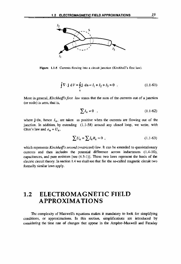
Figure 1.1-5 Currents flowing into a circuit junction (Kirchhoff s first law).
(1.1-61)
More in general, KirchhofSsfirst law states that the sum of the currents out of a junction (or node) is zero, that is,
where j-ds, hence I,, are taken as positive when the currents are flowing out of the junction. In addition, by extending (1.1-58) around any closed loop, we write, with Ohm's law and en = U,,
Xu, = CInRn =o , (1.1-63)
which represents Kirchhoffs second (restricted) law. It can be extended to quasistationary currents and then includes the potential difference across inductances (1.4- lo), capacitances, and pure resistors [see (4.5-l)]. These two laws represent the basis of the electric circuit theory. In section 1.4 we shall see that for the so-called magnetic circuit two formally similar laws apply.
1.2 ELECTROMAGNETIC FIELD APPROXIMATIONS
The complexity of Maxwell's equations makes it mandatory to look for simplifying conditions, or approximations. In this section, simplifications are introduced by considering the time rate of changes that appear in the Amp&re-Maxwell and Faraday
20 CHAPTER 1 FOUNDATION OF MAGNETIC FIELD THEORY
equations (1.2- 1, 2): if there is no time dependence, the static equations with the related phenomena apply; if the rate of changes is sufficiently slow with respect to the dynamic phenomena of interest, the quasistationary approximation is valid. In fact, this book is mostly devoted to the study of static and quasistationary magnetic field approximations.
Magnetostatics and electrostatics
In the cases where there is no time dependence, the displacement current term dDl dt in (1.1-1) drops out, andAmp6re's law is simply
V x H = j , (1.2-1)
or, in practical cgs units (oersted, ampere, cm),
V x H = 0 . 4 d . (1.2-1)*
As a consequence (since the divergence of any curl vanishes), the current conservation equation ( 1.1-5) reduces to
V . j = O , (1.2-2)
which expresses the fact that all current lines either close on themselves or extend to infinity, with no charge accumulation (dp, / dt =O). In addition, from (1.1-3) we know that
V . B = O , with B = p H , (1.2-3)
meaning the magnetic flux lines are solenoidal (they either close on themselves or go to infinity; see also section 2.5).
In mgnetostatics, basically three groups of problems are solved (see also the schematic in figure 2.2-3, chapter 2). (a) Given H, find j [a relatively simple problem, particularly in the integral form for the
total current I, as in Amptre's law (1.4-3)]. (b) Given the currents, find H (this problem is the main subject of the first two chapters
and basically requires the solution of a second-order differential equation). (c) Given the magnetostatic fields, determine the inductances, forces, and energies
related to it (treated in the following chapters). Note that the analogous electrostatic equations,
V x E = O , (1.2-4a)
V.D=p,, with D = & E , (1.2-4b)
are obtained by requiring no magnetic flux density variation, dB I at = 0 and dp, I dt = 0 ,
1.2 ELECTROMAGNETIC FIELD APPROXIMATIONS 21
that is, the charge density pe to remain constant at each point in space. As a consequence of these equations, there is no interdependence between magnetostatic and electrostatic fields and they can be treated separately.
Quasistationary magnetic fields
In the quasistationary (or quasistatic) approximation, some time dependences of the fields are explicitly allowed. This obviously requires the conditions for tollerable time variations to be defined with respect to the dynamic processes of interest. For this purpose we rewrite the time-dependent Maxwell equations (1.1- 1.2) in a dimensionless form, with quantities marked by an asterisk (*), by introducing a Characteristic system dimension and a characteristic dynamic time T (e.g., for a harmonic time variation it would be z = l / w ) ,
r = lor* (i.e., x = lox* , etc.), t = Tt* , ( 1.2-5)
which also yields
a l a -+-- 1 v + - v * , 10 aI T a t *
and a characteristic magneticfield Ho,
H = H ~ H * .
We want to preserve Faraday's equation in the form
* * w* at*
V X E =-- ,
which implies
With this and Ohm's law (1.1-6),
j=uE ,
Ampkre's equation (1.1- 1) is
* * * 2;dlE* z 2 aI*
V x H = k E +-- ,
(1.2-6)
(1.2-7)
(1.2-8)
(1.2-9a)
( 1.2-9b)
(1.2- 10)
where
22 CHAPTER 1 FOUNDATION OF MAGNETIC FIELD THEORY
lo 112 20 = - , c = (p&)-
C (1.2-11)
is the time required by an electromagnetic (plane) wave to propagate down the characteristic system dimension b at the light velocity c;
2, =pC& (1.2-12)
is the magnetic or current density dirusion time (that is, the characteristic time an electromagnetic field tied to a current density requires to diffuse into a conductor, as will be discussed in chapter 4); and
E
0 r e = - , (1.2-13a)
whereby 2 Term = 20
is a formal electricjield or charge relaxation time in the conductor-that is, a characteristic time after which a variation of the electric charge density, or its related electrostatic field, settles to stationary conditions. In fact, from the continuity equation (1.1-5). Gauss' law (1.1-4), and Ohm's law (1.2-9b) we obtain the equation for the free electric charge density
Pe.
-+%pe=O I
dr (1.2-13b)
which has the exponential solution
(1.2-13~) = e-'/Tc e co .
The inconsistency introduced by the charge relaxation time Te will be discussed below.
neglected with respect to the conduction current (first term on right-hand side), provided Within a conductor, the displacement current [that is, the last term in (1.2-lo)] can be
Neglecting the displacement term in free space, (a = 0, z, = 0), requires
20 I2a 1 ,
(1.2- 14)
where there is no conduction current
(1.2-15a)
which, by introducing the wavelength of the imposed (harmonic) electromagnetic field,A = 27rcc7, and with (1.2-1 I), yields
nm4. (1.2-15b)

1.2 ELECTROMAGNETIC FIELD APPROXIMATIONS 23
This means that the whole conductor system is subject to the same quasistationary field; there is no lag effect in the field propagation, whose velocity may be regarded as infinite. This conclusion is well known from antenna theory, where currents, whose wavelength is long compared to the largest dimension of the antenna conducting circuit, do not give rise to appreciable radiation [see in (3.3-16)].
In electric conductors, where the effects of magnetic fields predominate over those of electrostatic fields, conditions (1.2-14, 15) are generally well satisfied. For example, for a copper conductor (d = 6 107 ohm-] m- l , l= 0.3 m) the times are typically 70 = 10-9 s, z,
However, Ohm’s law (1.2-9b), which has been used here to establish both the dimensionless Amp&re equation (1.2- 10) and the charge equation (1.2-13). is valid only for time scales much larger than the average time between collisions of the free electron (with electric charge e and mass me) in the conductor
= 7 s, re = 1.5 1049 s .
(1.2- 16)
as will be shown in connection with (8.3-4); for copper it is typically q = 5 .lO-14 s (table 8.3-1). For the above considerations to remain valid in a good conductor, it is at least necessary that z be long compared to z,, in which case the current will be in phase with the electric field. It is, therefore, physically meaningful to take, instead of z,, the much longer relaxation time z, as a limit in most situations. The physical phenomena, which define the effective charge relaxation time in a good electrical conductor, are more subtle, but the rough estimate of re+% remains fairly valid.’.23 In any case, for typical quasistationary magnetic-dominated phenomena, where z 2 10-6 s, it follows that
T > > 2 0 ” T r , (1.2- 17)
whereas z can be of the same order as z, . We conclude that the quasistationary magnetic field approximation holds at least for all frequencies up to those corresponding to the infrared spectrum.
Consequent to these conditions, the displacement term in Amphe’s equation (1.1 - 1) [as well as the charge density variation term in (1.1-5), which directly derives from it] drops out, and the magnetoquasistationary equations are
V x H = j , (1.2-18)
w dr
V X E = - - , (1.2- 19)
V . B = O , (1.2-20)
where B = p H and j = oE. The equation
V . j = O (1.2-21)
24 CHAPTER 1 FOUNDATION OF MAGNETIC FIELD THEORY
is a result of (1.2-18). as was pointed out in connection with (1.2-2). The dynamics in this magnetoquasistationary approximation enters through the Faraday law (1.2- 19). There is also the equation
V.D=p, , with D = & , ( 1.2-22)
for the unlikely circumstance of wanting to know aposteriori the very small free charge density pe in a magnetic problem.
In conclusion, the magnetquasistationary approximation is a powerful and very useful theoretical formalism because it holds for the majority of fields used in electromechanical engineering and for some in radioengineering.
Quasistationary electric fields
It is instructive to present the electroquasistationary equations pertinent to an electric- field-dominated problem, which is typically found in a dielectric or very poorly conducting medium. For example, in a glass insulator (a= 10l2 ohm-' m-', 1 =0.3 m) we find
zo = 19 s, z, = 1.1 10- s, z, = 9 s; that is,
zn To )) 7, , ( 1.2-23)
whereas z can be of the same order as z, . Using similar considerations and procedure to that for the magnetquasistationary case, we get the electroquasistationary equations:
V.D=pe , ( 1.2-24)
(1.2-25)
V x E = O , ( 1.2-26)
where D = &E and j = oE. There are also the equations
dD V x H = j + -
dt
[this one being consistent with (1.2-24,25)] and
V . B = O .
(1.2-27)
( 1.2-28)
which can be used in the unlikely circumstance that the extremely weak magnetic field must be known a posteriori in the electric quasistationary approximation. Note that here the dynamics enters through the charge conservation equation (1.2-25).
1.3 ELECTRODYNAMICS OF MOVING MEDIA 25
1.3 ELECTRODYNAMICS OF MOVING MEDIA
In this section we introduce two generalizations regarding the study of electrodynamic phenomena: First, we consider two coordinate frames moving with velocity v with respect to each other, and we study how the electromagnetic quantities transform in the two systems; second, we allow the medium (to which the electrodynamic phenomena refer) to flow with velocity u = u(x,y,z) and study its effects. This study provides the basic equations of magnetohydrodynamic theory, a subject that is expanded in chapter 8.
Coordinate frames of reference
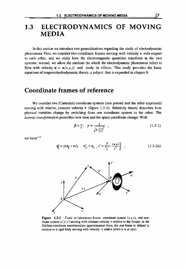
We consider two (Cartesian) coordinate systems (one primed and the other unprimed) moving with relative, constant velocity v (figure 1.3-1). Relativity theory describes how physical variables change by switching from one coordinate system to the other. The Lorentz transformation prescribes how time and the space coordinate change: With
(1.3- 1)
we have'-12
q;=r(ql-vt), r i = r l , t * = Y [ t - y ] , ( 1.3-2a)
Figure 1.3-1 Fixed or laboratory-frame coordinate system (x ,y ,z ) . and rest- frame system (x',y',z'J moving with constant velocity v relative to the former, in the Galilean coordinate transformation approximation (here, the rest frame is defined in relation to a rigid body moving with velocity v within which it is at rest).

26 CHAPTER 1 FOUNDATION OF MAGNETIC FIELD THEORY
where the subscripts 11 and I indicate components of the position vector parallel and perpendicular to v. For example, for Cartesian coordinates with the primed system moving with velocity v along the z-direction:
z’=y(z-pct), x ’ = x , y ’ = y , ct’=y(ct-Pz) , (1.3-2b)
or
z=y(z’+@t’), x = x ’ , y = y ’ , ct=y(ct ’+pz’ ) . (1.3-2~)
WhenP << 1-that is, y 2 1 (or, formally, c + -)-these relations reduce to the Galilean transfomtion:
r‘ = r - vt , f ’ = t , (1.3-3a)
or, as above,
z ’ = z - v t , x ’ = x , y ’ = y , t ’ = t . (1.3-3b)
The Galilean transformation applies to the quasistationary electromagnetic equations, since in both formalisms the same assumption applies ( c + -a). Both Lorentz and Galilean transformations are based on the approximation of a nonaccelerated movement- that is, approximately constant v . They are applied within the special theory of relativity and express the relation between the quantities given in nonaccelerated, or so-called inertial, frames of reference.”.e’ Otherwise, Einstein’s general theory of relativity applies. However, objects moving with velocity Ti within each frame can be accelerated.
Moving coordinate system
We are concerned in general about the relationship between two entities, electromagnetic fields and media with electromagnetic properties (conductors, magnetic materials, etc.), so we must understand how the properties expressed by them change when viewed within two frames of reference in relative motion.
With respect to the second entity, we consider first a medium that presents itself as a rigid body. We define as the rest-frame (or moving) coordinate system, characterized by primed parameters (figure 1.3-l), the one where the body and any observer P placed on it are at rest, but moving with relative constant velocity v with respect to the &oratory or fued frame (labeled with unprimed parameters).
We want to determine the differences in the electromagnetic quantities and properties perceived by an observer P at rest in the moving frame versus those perceived by an observer P in the laboratory frame, with respect to the same phenomena.

1.3 ELECTRODYNAMICS OF MOVING MEDIA 27
Max w el 1 -Lo yen t z t ra n sfor ma t ion
Fortunately, Maxwell‘s equations (1.1-1 to 4) remain the same in all frames, regardless of their relative (nonaccelerated) motion. In fact, it is a postulate of special relativity that physical laws must be the same in any inertial coordinate system. In parallel to the unprimed equations (1.1-1 to 4) valid in the laboratory frame, we have the identical primed equations valid in the moving frame
V’-B’=O , (1.3-6)
V ’ . D ’ = p i , (1.3-7)
where the primed nabla operator is v‘ E (dldx’,dldy‘,d/&’). The constitutive equations (1.1-6 to 8) are strictly valid for the medium only in its rest frame, so
j’=aE , (1.3-8)
B’=pH‘, D = E E ’ . (1.3-9)
The parameters a , p , ~ of the medium should also be primed, since they could be dependent of the relative velocity; but this effect is neglected here.
The problem then is to determine the transformation rules that must be applied to switch from the one set of equations to the other, For example, an observer P in the laboratory frame wants to know the primed electromagnetic quantities in the moving frame, but expressed as a function of the unprimed quantities of his frame (which he can measure). In the general formulation these transformation rules can be found by applying the Maxwell-Loren?. transformations [i.e., the Lorentz transformation ( 1.3-2) for the coordi- nates, plus the condition that Maxwell’s equations remain invariant to it]. For the operators from ( 1.3-2b) follows [for frames moving along the z-axis (v, = 0, v,. = O)]
We are now in the position to show under which conditions the unprimed Maxwell equations (1.1- 1 to 4) transform into the primed ones (1.3-4 to 7). For this purpose we

28 CHAPTER 1 FOUNDATION OF MAGNETIC FIELD THEORY
write the former in their components and apply the above operators.8.' We find that the resulting primed equations are identical to (1.3-4 to 7). provided that we set [the subscripts I and 11 refer to the normal ( x , y ) , and parallel (z) components relative to the constant (z- component) velocity]
H i = y ( H - v x D ) , , H i = H , (1.3- 12)
E i = y ( E + v x B ) L , q = q , ( 1.3- 14)
Di = ~ ( D + I v x H ) ~ , 2 9i=91 ' (1.3-15)
From these relations we note the relative nature of magnetic and electric fields: Their magnitude can be different in different reference systems. For example, even if it were H = 0 in the unprimed system, we can have a finite H', (1.3-12), in the primed system. This is in contrast to the constancy of Maxwell's equations-that is, the laws governing these fields.
Max w el 1 -Ga 1 ilea n t ra ns fo r ma t io n
Fortunately, the operations are easier for nonrelativistic velocities since they remain invariant to the simpler Galilean transformation (1.3-3). In addition to the space transformation, the following rules [which derive from (1.3-10, l l ) ] apply to the derivatives of a scalar function @, or vector A:
V ' + V , (1.3-17a)
( 1.3- 1 7b)
where the last operator is called the convective or Lugragian time derivative (which can also standfor a total time derivative). The first rule states that the spatial derivatives are the

1.3 ELECTRODYNAMICS OF MOVING MEDIA 29
same, irrespective of the frame in which they are taken. This follows logically from the fact that an instan: physical picture of the phenomenon must show up identical in the two frames. Clearly, the situation is different with the time derivative taken in the two frames (second rule). For an observer P in the primed rest frame, by definition, the time derivative is taken with the primed special coordinates held fixed; but in the laboratory frame, on the contrary, any function @, or vector A, which is in the position r = (x,y,z) at time r moves into position r+ vAt during the following time interval A t . This implies the application of the chain rule differentiation, which, when applied to a scalar function @ = @ ( x , y , z, t) with
and which, analogously, when applied to a vector A P (A,,A,.,AZ), is
In particular, using (A.3-5,9) we get
D @ - d o + V . ( * ) , Dr dr
(1.3-19)
( 1.3-20)
if V.v = 0 [i.e., for a constant velocity or an incompressible body, see (8.1-4)]; and
D A dA Dt dr - = - + v(V . A ) - V x ( V x A) , (1.3-2 1)
if in addition ( A . V ) v = 0 [i.e., for a rigid body translating with constant velocity, see, e.g., (8.1-43)].
With respect to the Maxwell-Galilean transformation (where c+ 00, y z I ) , the relations (1.3-12 to 16) can be rewritten in the form
E ’ = E + v x B , (1.3-22)
H ’ = H - v x D , (1.3-23)
j ‘ = j - p , v , ( I .3-24)
and
B ’ = B , D ’ = D , p:=pe. (1.3-25)
plus the constitutive equations (1.3-8,9). For example, to determine H’, E’ from Maxwell’s

30 CHAPTER 1 FOUNDATION OF MAGNETIC FIELD THEORY
equations (1.3-4 to 7) and using (1.3-17,21) we obtain
V x H’ = o(E+ v xB) +-- dD V X (V x D)+ pev , (1.3-26) at
(1.3-27) dB V x E‘ = --+ V X ( V x B) , at
The magnetic quasistationary approximation (1.2-18 to 20) is compatible with the Galilean transformation (both formally assume c+ =), and in this case the set of relations (1.3-22 to 25) reduce to
E = E + v x B , (1.3-29)
(1.3-30)
remain untouched. Equation (1.3-29) is also intuitively deduced from the Lorentz force (6.1-1). In fact,
an observer moving through a magnetic field and carrying a charge q will experience a force q(E + v x B), which is formally equivalent to saying that in his frame of reference he sees the electric field (1.3-29). A direct consequence of (1.3-29, 30) is that [by substituting into (1.3-6)] Ohm’s law must be written as
j = a ( E + v x B ) . (1.3-31)
In practice we can say that this law applies in any frame of reference thar nzoves across magneticflux lines (or in which the body carrying the current j moves with respect to the magnetic field source).
For completeness’ sake we point out that the Galilean transformation rules (1.3-3,17) are also consistent with the transformation of the primed into the unprimed electric quasistationary equations (1.2-24,25,26), provided that
j’= j-p,v (1.3-32)
H ’ z H - v x D , (1.3-33)
whereas
E ’ = E , D ’ = D , ph=pe (1.3-34)
remain untouched. The current density is here affected by a convection current that in the magnetic approximation is implicitly negligible with regard to the conduction current.
I .3 ELECTRODYNAMICS OF MOVING MEDIA 31
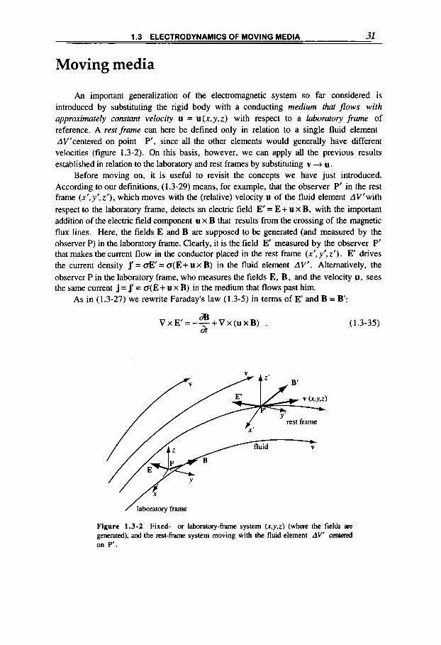
Moving media
An important generalization of the electromagnetic system so far considered is introduced by substituting the rigid body with a conducting medium that flows with approximately constant velociry u = u(x ,y , z ) with respect to a laboratory frame of reference. A rest frame can here be defined only in relation to a single fluid element AV‘centered on point P‘, since all the other elements would generally have different velocities (figure 1.3-2). On this basis, however, we can apply all the previous results established in relation to the laboratory and rest frames by substituting v + u.
Before moving on, it is useful to revisit the concepts we have just introduced. According to our definitions, (1.3-29) means, for example, that the observer P’ in the rest frame (x’ ,y ’ , z ’ ) , which moves with the (relative) velocity u of the fluid element AV‘with respect to the laboratory frame, detects an electric field E’ = E+ u x B, with the important addition of the electric field component u x B that results from the crossing of the magnetic flux lines. Here, the fields E and B are supposed to be generated (and measured by the observer P) in the laboratory frame. Clearly, it is the field E’ measured by the observer P’ that makes the current flow in the conductor placed in the rest frame (x’,y’, z ’ ) . E drives the current density j’ = aE’ = a(E+ ux B) in the fluid element AV‘. Alternatively, the observer P in the laboratory frame, who measures the fields E, B, and the velocity u, sees the same current j = j’ = a(E + u x B) in the medium that flows past him.
As in (1.3-27) we rewrite Faraday’s law (1.3-5) in terms of E’ and B = B‘:
6% a V x E’= -- + V x (U x B) . (1.3-35)
B‘ A z ’
E‘
rest frame
X
/ laboratory frame
Figure 1.3-2 Fixed- or laboratory-frame system (x,y,z) (where the fields are generated), and the rest-frame system moving with the fluid element AV’ centered on P’.
32 CHAPTER I FOUNDATION OF MAGNETIC FIELD THEORY
It is customary to introduce the Lagrangian derivative (1.3-21), so that
VxE’=-- . DB (1.3-36) Dt
These equations, together with
V x H = j ,
V . B = O ,
E ’ = E + u x B ,
j=oE‘, B = p H ,
(1.3-37)
provide the set of electromagnetic equations used by magnetohydrodynamic theory (in the magnetic quasistationary approximation).
By considering a&’= D I Dt + d I dt as a total time derivative and having introduced E , the above equations are written in Lugrangian form, i.e., with respect to rest frames (x’,y’, z‘) moving with the fluid (a form often convenient in computational evaluations). If, on the contrary, we reintroduce the electric field E and take into account the form (1.3- 21), then the equations return to the Eulerian form-that is, with respect to the laboratory frame fixed in the (x, y, z) space.
1.4 ALTERNATIVE ELECTROMAGNETIC EQUATIONS
It may sometimes be convenient to use Maxwell’s relations in different forms to those presented at the beginning of this chapter. This is particularly true for the integral form, which introduces the overall, lumped parameters of voltage, current, flux, and electric charge, with which an understanding of electromagnetic phenomena is often more straightforward.
Integral laws
Ampire’s law
By integrating (1.1-1) over any (open) cap surface S bounded by a closed contour C (figure 1.4-1) and applying Stokes’ theorem (A.3-14).

1.4 ALTERNATIVE ELECTROMAGNETIC EQUATIONS 33
Figure 1.4-1 Surface S limited by a contour line C.
we get
(1.4-1)
(1.4-2a)
that is, the circuitation (line integral) of H around any closed contour C is equal to the total normal current flowing across the corresponding cap surface S bounded by C,
is=jj.ds , S
(1.4-2b)
plus the time rate change of the normal D-flux across S. The positive direction around C and of the normal unit vector n on S follow the right-hand-screw convention. Note that if the surface and contour move with velocity v , only the last term in (1.4-2a) is affected, similarly to the magnetic flux, as will be indicated in (1.4-9). In the quasistationary magnetic approximation (when the last term can be neglected), this reduces to Ampkre's law
fH .d l=Zs , (1.4-3) C
or, in practical cgs units (oersted, ampere, cm), to
f H . d I = 0 . 4 ~ 1 ~ C
If we separate
H = H " + H ~
(1.4-3)*

34 CHAPTER 1 FOUNDATION OF MAGNETIC FIELD THEORY
as in (1 .l-35) into the irrotational component H" and rotational component HS , we find from Amp&re's law (1.4-3)
because
f H" dl = Z,
fH".d l=O ,
( 1.4-4a)
(1.4-4b)
according to the gradient theorem (A.3-13). The solenoidal component HS is completely independent of whether magnetic materials are present or not along the path (there is simply no pR factor in these equations).
Faraday 's law
Similarly, by applying Stokes' theorem (1.4-l), the F a r m law follows from ( 1.1 - 2):
or, in practical cgs units (voltlcm, gauss, cm),
e = E.dl=-lO -8 -1B.ds
&S f C
(1.4-5)
(1.4-5)*
(Note that the partial differentiation can be exchanged with the integral over the surface.) The induced electric field along C produces in the circuit the (inductive) electromotive force e (1.1-56), which here is due to the time variation of the magnetic flux
y l = j B . & S
within the fixed contour C; so, we write
.=-[%I . v=o
(1.4-6)
(1.4-7)
More in general, when the circuit C moves with velocity v, the emf along C from (1.3-29) is
e = f E . dl = $(E + v x B) . dl C C
(1.4-8a)

I .4 ALTERNATIVE ELECTROMAGNETIC EQUATIONS 35
For the last integral term, with the definitions v = d r / dt, d r x dl = ds, and the trivector relation (A.3-ld), we write
f (v x B).dl= -fB.(v x dl) = - B.dslAr = -[%I C C
. (1.4-8b)
Slat B=const.
To obtain this integral, the following remarks are useful (figure 1.4-2):
(a) A lateral surface Slat is defined as the contour C moves to C’ in the time interval At. (b) The differential area element of this lateral surface is I v x dl I At, and consequently
(1.4-8b) represents the increment Ayl of the magnetic flux through the surface Slat during time At.
(c) Since B is a solenoidal field [see (1.4-13)], the total flux through the closed surface S+Slat+S’ is zero; therefore (1.4-8b) is equal to the difference Ayl of the fluxes through the open surfaces S and S’ (the outward pointing ds is opposite on S and S’).
(d) The resulting Ayl/At term is expressed by the last equality, since the partial time derivative stands for the rate of change of flux due to the motion of the contour C in a constant field B.
In conclusion, by adding the contributions from (1.4-7,8), for the electromotive force e or the induced voltage U in a closed circuit in the general case, we obtain
(1.4-9)
where the total time derivative now stands for the total rate of change of the magnetic flux through the moving contour C. By introducing the inductance parameter L, which will be
Figure 1.4-2 The contour C moving with velocity v = drldr defines after a time Ar a cylindrical surface with lateral, top, and bottom surfaces.

36 CHAPTER 1 FOUNDATION OF MAGNETIC FIELD THEORY
defined in more detail in section 2.4, the Faraday law can also be written in the form
(1.4-10)
This result could have been obtained directly by using the generalized Leibniz rule,A.‘ valid for a vector F.
( 1.4- 1 1)
and applied to the magnetic induction, F B , where V . B = 0. In any case, the positive direction around C and of the normal unit vector n on S follow the right-hand-screw convention. The integral form of the Faraday law thus states that the emf, or the circuitation of E, around any closed contour C is equal to the negative time rate of change of the total normal B-flux across any cap surface S bounded by C, whether this change is due to a time variation of B or to motion of the contour C. The negative sign is determined by Lenz’s law: The current is (or would be) driven by the emf and will be in such a direction that the magnetic field it produces tends to counteract the change in flux that induced the emf.
Faraday’s law (1.4-8) is the basis for the generation of an inductive emf and electric current in an associated circuit. Two fundamental methods follow from (1.4-8a): either by magnetic flux variation as applied in an alternator generator, or by movement within a magnetic field (by “cutting field lines”) as in a homopolar generator. Both applications will be discussed in section 6.2, in connection with figures 6.2-9 and 13.
Miscellaneous laws
By applying Gauss‘ theorem (A.3-16) over any volume V bounded by a closed surface S ,
j(V.B)dV = f B . & , V S
(1.4-12)
we get with (1.1-3)
~ B . & = o , (1.4- 13) S
that is, the total outward normal B-flux across any closed surface S vanishes. (This is evidently a general consequence of the rotational nature of B.) Similarly, the current conservation (1.2-2 or 1.2-21) yields
+ = o , S
(1.4-14)

1.4 ALTERNATIVE ELECTROMAGNETIC EQUATIONS 37
see Kirchhoff s law (1.1-62). Integration of (1.1-4) gives, for the electric flux density,
$ D . d s = jpedV . S V
(1.4-15)
These integral laws remain unaffected when the surface moves across the electromagnetic field lines.
Differential laws
Maxwell’s differential laws in a fluid moving with quasiconstant velocity u are given in (1.3-26,27). As an example of the many possible variations, we introduce explicitly the magnetic and electric polarizations (1.1- 1 1, 12) in the fluid,
B z ~ ( o H + p o M , (1.4- 16)
D=EoE+P , (1.4- 17)
and require that the current density j include only the terms that in the frame-transformation are related to free electrical charges,
j = o(E+ u x k H ) - peu , (1.4- 18)
thus excluding the additional term u x p,,M deriving from the atomistic currents, as required by (1.3-22). This particular formulation of Maxwell’s equation is sometimes called the Chu-f~rmulation.’.’~ We deduce from (1.4-18) that on this basis the Galilean transformation relations, instead of (1.3-22,23), are
E ’ = E + u x k H , (1.4- 19)
H’=H-uxEoE . (1.4-20)
By inserting them into (1.3-26.27). we obtain a fully consistent set of equations:
(1.4-2 1) d dt
V x H = j+ -(E,E + P) + V x (P x u) ,
( 1.4-22) d dt
V x E =-po-(H + M) - poV x (M x U) ,
and from (1.1-3 to 5)
38 CHAPTER I FOUNDATION OF MAGNETIC FIELD THEORY
V.H=-V.M . (1.4-23)
&,,V.E=-V.P+p, , (1.4-24)
In addition, from (1.3-25) we have
B ’ = B , D ’ = D , p:=pe ;
(1.4-25)
(1.4-26)
hence with c = (po&~) -”* also we obtain
p , , ~ ’ = &M+ 41 x E, P’ = P - u x p o ~ . (1.4-27) c2
These equations easily can be reduced into the magnetic or electric quasistationary forms, similarly to (1.3-29 to 31) or (1.3-32 to 34). When u = 0 we obtain the original Maxwell equations (1.1-1 to 8).
Current densities
As mentioned in section 1.1, it can be useful to formally express some terms in Maxwell‘s equations as current densities. In analogy to the vacuum displacement current density,
a3 j, =&o-
dt (1.4-28)
(already recognized by Maxwell as a necessary term to complete the nonstationary electromagnetic equations even in empty space), in (1.1-15) we have introduced, by analogy, the magnetic and electric polarization current densities defined as
j, = V x M , j, =&o- a . (1.4-29) dt
The component
(1.4-30)
can be defined, by its very nature, as a capacitive current density, whereas

1.4 ALTERNATIVE ELECTROMAGNETIC EQUATIONS 39
j , = j + j , =- [ v;B1 (1.4-31)
is an inductive current density, where j is the current density sustained by free charges. The total current density is
.ko t=kh+jd 9 (1.4-32)
where
jch =.i+j, +jP (1.4-33)
represents the current densities that can be considered as being generated by the motion of free and/or bound electric charges, since they are related to the respective charge densities by
( 1.4-34)
[see also in (1.1-5); note that the current and charge densities corresponding to free charges are designated throughout the book as j,p,, the latter to be distinguished from the mass density p].
dPi - v . ji + - - 0 , i = nil,d, m,p, or a combination of them, dr
For later use we introduce the concept of a sugace current density ii defined as
i i = lim jiAh ; A h j O
(1.4-35)
that is, the current flowing as current density ji in a layer of depth Ah from the conductor surface is compressed into an infinitesimal surface thickness Ah + 0 [see comments in connection with (1.5-33) for the free surface current density]. Clearly, the same definition can be applied to the charge densities,
5 = lim p i A h , A h j O
so that
( I .4-36)
(1.4-37)
where the index i is the same as in (1.4-34). The surface vector i is defined by two surface coordinates (for example, for a plane
sheet and Cartesian coordinates) by ( x , y ) . Consequently, here the nabla operator V, is a surface operator with derivatives along its surface only [see also in (4.4-12)]. For example, in Cartesian coordinates with the unit vectors e,,ey along the x, y axes, we obtain
d d a x dy
V,+e,-+ey- . (1.4-38)

40 CHAPTER 1 FOUNDATION OF MAGNETIC FIELD THEORY
Magnetic circuits
For the study of magnetic systems composed of ferromagnetic components that almost entirely confine the magnetic flux, it is very convenient to resort to the magnetic- circuit concept, which is analogous to the electric (resistive) circuit. The circuits shown in figure 1.4-3 and the listing of the corresponding parameters in table 1.4-1 illustrate this concept. In fact, the application of Ampi?re’s law (1.4-3) to an appropriately chosen mean contour line C in the magnetic circuit of figure 1.4-3a gives the so-called magnetomotive force (mmf) or magnetomotance
VH=Hl+H,X , (1.4-39a)
where
V, = Nclc (1.4-39b)
is induced here by the Nc windings carrying the current I,. Since the normal magnetic flux through any cross section S is constant [because of (1.4-13)],
y = B S = B , S , or y = p H S = p , H , S , , ( 1.4-40)
4 1
Figure 1.4-3 Analogy between magnetic (a), and electric circuit (b).
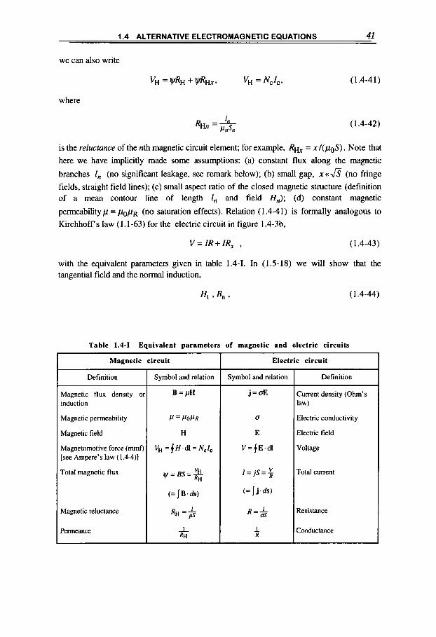
I .4 ALTERNATIVE ELECTROMAGNETIC EQUATIONS 41
RHn ='. ( 1.4-42) P"%
is the reluctance of the nth magnetic circuit element; for example, = x / ( p o S ) . Note that here we have implicitly made some assumptions: (a) constant flux along the magnetic
branches I,, (no significant leakage, see remark below); (b) small gap, xccz/s (no fringe fields, straight field lines); (c) small aspect ratio of the closed magnetic structure (definition of a mean contour line of length I,, and field H,,); (d) constant magnetic
permeability p = pop^ (no saturation effects). Relation (1.4-4 1) is formally analogous to Kirchhoff s law (1.1-63) for the electric circuit in figure 1.4-3b.
V=IR+IR, , (1.4-43)
with the equivalent parameters given in table 1.4-1. In (1.5-18) we will show that the tangential field and the normal induction,
Ht 9 Bn 7 (1.4-44)
Table 1.4-1 Equivalent parameters of magnetic and electric circuits
Magnetic circuit
Definition
Magnetic flux density 01
induction
Magnetic permeability
Magnetic field
Magnetomotive force (mmfl [see Ampere's law (1.4-4)]
Total magnetic flux
Magnetic reluctance
Perrneance
Symbol and relation
Electric circuit
Symbol and relation Definition
Current density (Ohm's law)
Electric conductivity
Electric field
Voltage
Total current
Resistance
Conductance

42 CHAPTER 1 FOUNDATION OF MAGNETIC FIELD THEORY
remain steady when crossing the boundary of the magnetic material. The first boundary condition implies that there is also some magnetic flux (leakage flux) external to the magnetic branches (for example, as shown in figure 9.1-7; see section 9.1); however, the assumption of constant flux (1.4-40) is in most cases sufficiently c o m t because the ratio of internal (p&) over external @OH,) induction is very large for a ferromagnetic material,
since p/& B 1. (Note the difference to the eleceric circuit, where no current is present
outside the conductor, because there Q= 0.) The second boundary condition, B , constant,
is expressed by (1.4-40), which in combination with the flux determined by (1.4-4 1) defines the magnetic field in the gap,
(1.4-45)
This field can be relatively large for a narrow gap width x in a ferromagnetic core ( p ~ n 1). [In an electric circuit a gap would fully stop the current, here it only introduces a large reluctance R H ~ = x/(poS) in the magnetic circuit, giving rise to the large magnetic
field.] By applying these laws to two closed loops and one junction of the circuit shown in
figure 1.4-4, and on the basis of the assumptions made before, we obtain
vHI + vH2 = wlRHl + w 2 R H 2 ,
vHI = w l R H l + w 3 ( R H 3 + R H 4 + R H x ) 7 ( 1.4-46)
w l = v / 3 + w 2 9
where
and for the tapered branch leading to the gap (from S, to S3) we find
(1.4-48) 0
From these relations it is easy to find all the required quantities; in particular, the field in the gap will have a form somewhat similar to (1.4-45) but with an additional amplifying factor
S/Sr [For the magnetic forces acting in the gap, see in connection with (6.2-50).]
The rules established before in (1.4-40,41) can be extended to more complicated circuits by applying the magnetic version of Kirchhoff s laws (1.1-62, 63) concerning the magnetic flux w and motive force VH in a junction and around a magnetic loop, respectively:
( 1.4-49)
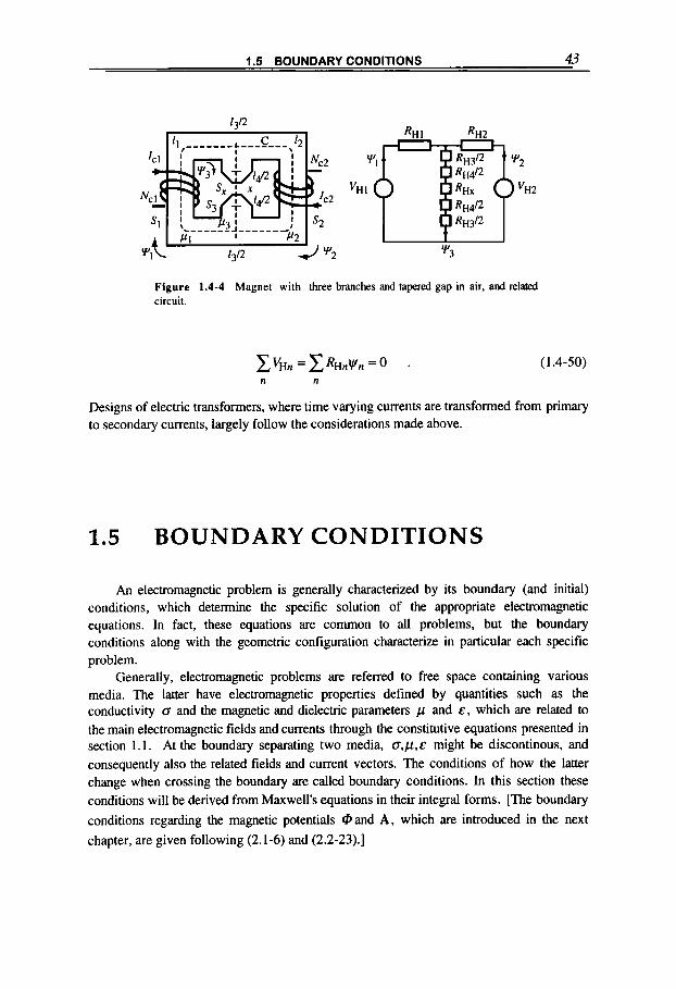
1.5 BOUNDARY CONDITIONS 43
Figure 1.4-4 Magnet with three branches and tapered gap in air, and related circuit.
( 1.4-50)
Designs of electric transformers, where time varying currents are transformed from primary to secondary currents, largely follow the considerations made above.
1.5 BOUNDARY CONDITIONS
An electromagnetic problem is generally characterized by its boundary (and initial) conditions, which determine the specific solution of the appropriate electromagnetic equations. In fact, these equations are common to all problems, but the boundary conditions along with the geometric configuration characterize in particular each specific problem.
Generally, electromagnetic problems are referred to free space containing various media. The latter have electromagnetic properties defined by quantities such as the conductivity d and the magnetic and dielectric parameters p and E , which are related to the main electromagnetic fields and currents through the constitutive equations presented in section 1 . 1 . At the boundary separating two media, o , ~ , E might be discontinous, and consequently also the related fields and current vectors. The conditions of how the latter change when crossing the boundary are called boundary conditions. In this section these conditions will be derived from Maxwell’s equations in their integral forms. [The boundary conditions regarding the magnetic potentials @and A , which are introduced in the next chapter, are given following (2.1-6) and (2.2-23).]

44 CHAPTER 1 FOUNDATION OF MAGNETIC FIELD THEORY
Field conditions
General conditions
The fundamental boundary conditions for the tangential and normal electromagnetic field components between two media will be derived in ( 1 .5-24,25,26,29, 32); they are
nx(H2 - H I ) = i , (1.5-1)
n x ( E 2 - E l ) = 0 , ( 1 5 2 )
n . ( B 2 - B I ) = 0 , (1.5-3)
n . (D2 - D,) = re , (1.5-4)
where n is the unit normal vector on the boundary pointing from medium I to medium 2 (see figure 1.5-1); i and re are the surface current and charge densities related to free electric charges [according to definitions (1.4-35, 36)], which can exist in superconductors where the electric conductivity is infinite, CT + OQ. Note that if in medium 2, 0 2 +-, then H, = 0, and the boundary field HI is purely tangential.
It is instructive to rewrite the boundary condition (1.5-1) by introducing the magnetization M through (1.1-17), B = p0H + poM, and obtain
n x ( B 2 : - B l ) l p o = i + i , ,
where
i, = n x ( M 2 - M I )
is the surface magnetization current density defined by (1.4-35). By inserting
B=pH , p=pOPR
into (1.5-1), an alternative to (1.5-6) is
n x ( B 2 /pz -BI / p l ) = i ,
since, in fact,
M = ( P R - l ) H .
Also, condition (1.5-3) can be separated with (1.5-26b) into the form
n.(H2-H1)=r , ,
(1.5-5)
( 1.5-6)
(1.5-7)
(1.5-8)
(1.5-9)
(1.5-10)
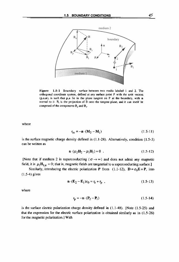
1.5 BOUNDARY CONDITIONS 45
Figure 1.5-1 Boundary surface between two media labeled 1 and 2. The orthogonal coordinate system, defined at any surface point P with the unit vectors (p,s,n), is such that p,s lie in the plane tangent on P at the boundary, with n normal to it. B, is the projection of B onto the tangent plane, and it can itself be composed of the components B,, and B,.
where
r, =-n.(M2 -M1) (1.5-1 1)
is the surface magnetic charge density defined in (1.1-28). Alternatively, condition (1 5 3 ) can be written as
n . ( P 2 H 2 -P@1)=0 . (1.5-12)
[Note that if medium 2 is superconducting ( Q -+ =) and does not admit any magnetic field, it is pIH1, , = 0; that is, magnetic fields are tangential to a superconducting surface.]
Similarly, introducing the electric polarization P from (1.1-12), D = EOE + P, into (1.5-4) gives
n . ( E 2 - E 1 ) ~ o = r e + r p , (1 5 1 3 )
where
rp=-n.(P2-Pl) (1.5- 14)
is the surface electric polarization charge density defined in (1.1-48). [Note ( I .5-25) and that the expression for the electric surface polarization is obtained similarly as in (1 5 2 6 ) for the magnetic polarization.] With

46 CHAPTER 1 FOUNDATION OF MAGNETIC FIELD THEORY
D = € E , E = E O E R , (1.5-15)
a modified form of (1 5 4 ) is
n . ( q E 2 -EIEI)EO =re, ( 1.5- 16)
and a modified form of (1 5 2 ) is
n x ( D 2 / €2 - DI /q ) = 0 . (1 5 1 7 )
Non s u percond uct ing media
In the magnetic quasistationary approximation and for normally conducting media (where i and re vanish), conditions (1.5-1 to 4) mean that the tangential (t) and normal (n) components
and (1.5- 18)
(1.5- 19)
remain steady when crossing the boundary. This also means that the other components Hn. Bt, and En, Dt, in conforming with (1.5-8, 12) and (1.5-16, 17), may jump according to the magnetic and electric properties of the adjoning media 1,2 according to
(1.5-20)
a)
1 I medium2
X
Figure 1.5-2 Refraction of a magnetic field line when crossing the boundary between two magnetic media (here. qualitatively p 2 < p1 ), and (b) decomposition of
the related field vectors.
I .5 BOUNDARY CONDITIONS 47
and
(1.5-21)
These conditions determine a refraction of thefield lines as they cross the boundary between media 1 and 2, which is similar to Snell’s refraction law in optics (figure 1.5-2). For example, for the magnetic field, conditions (1.5- 18) can be rewritten in scalar form as
H2 sin q$ = HI sin $1 and
from which, by eliminating H I , H2, follows
p 2 H 2 cos $2 = p1 HI cos $1 ,
(1.5-22)
and analogously for the electric field from conditions (1.5-19). This means that if a H(or E) field line enters a medium with a smaller magnetic or dielectric coefficient, it is refracted towards the normal. We also see (figure 1.5-2b) that when crossing the boundary, the tangential component Ht remains untouched [see (1.5-18)], but the normal component increases by the amount r, given in (1.5-10). Also note that if for medium 2, p 2 = =, then $I = 0, or = 0; that is, the field at the boundary is purely normal. Conversely, if p 2 = 0, the field at the boundary is purely tangential, which is formally analogous to the superconducting case 02 == [in both cases, medium 2 is fully diamagnetic; see also comments made in relation to (1.5- l).]
Example: Calculation of the conditions
It is instructive to derive the boundary conditions (1.5-1.3) [and by similarity (1.5-2,4)] by using
the integral forms of Maxwell’s equations near the boundary. Consider (1.4-13), which is the integral form of V B = 0, that is,
f B . d s = O ,
applied over the surface of the sufficiently small cylinder shown in figure 1.5-3 with height A h , and end surfaces As, and cut by the boundary surface separating the media 1 and 2, so as to obtain
( n l . B l + n 2 . B 2 ) A s + j B w . d s = O , (1 5 2 3 ) W
where the first term represents the f lux leaving the end surfaces ( BI, B,,Bw are taken to be the mean values
over their respective surfaces) and the integral gives the flux leaving the side wall W of the cylinder.
We let the cylinder height shrink towards the boundary surface, that is, Ah + 0, in which case the
flux contribution from the side wall W vanishes because it depends on the wall surface, which with Ah + 0

48 CHAPTER 1 FOUNDATION OF MAGNETIC FIELD THEORY
Figure 1.5-3 Boundary surface between media I and 2 with elemental cylinder and loop used to derive the boundary conditions for B. D and H, E, respectively.
also goes to zero. As the ends can remain finite, though small (AT f 0). from the above equation with an appropriate labeling (n = n2 = -nl) follows
n . ( B 2 - B I ) = 0 . (1 5 2 4 )
Similarly, from ( I . 1-4). V D = pe, follows
(nl . D I + n2 .D2)AT + I D w .ds = jp,dV . W
( I .5-25a)
The last integral represents the free electric charges contained in the cylinder and is = p,AhAT. As Ah + 0,
it vanishes, unless on the boundary there exists a surface charge density re as defined in (1.4-36). and we
obtain
n . ( D 2 - D , ) = r e . ( I .5-25b)
When the cylindrical body has magnetization M or electric polarization P, we proceed in the same way. For example, with B = &H + p o M we obtain, instead of (1.5-23).
(n l .Hl+n2.H2)AT+ j H w . d s + f M . d s = O . W
( I .5-26a)
The last integral, by introducing the magnetic charge density pm = - V . M , transforms with Gauss'
theorem into = pmATAh: and, as above, letting Ah -+ 0 we find
n.(H2-H1)=rm , (1.5-26b)
where the surface magnetic charge density (1.1-28) can also be written in the form (1.5-1 I). To demonstrate the boundary condition (1.5- I ) we apply Ampbre's integral law ( I .4-2).
1.5 BOUNDARY CONDITIONS 49
( 1 5 2 7 )
over the small rectangular loop C with surface S shown in figure 1.5-3. We introduce the orthogonal coordinate system with unit vectors (p, s, n) such that p = s x n, A = pAl (parallel branches), Ah = Rdh
(vertical branches), p = pz = - P I . n = n2 = -nI and use, as before, the appropriate labeling
p = p2 = -p i , n = n2 = -nI . The above integral relation can thus be rewritten approximately as
p,(H2 -Hl)Al+n. (H2 -Hl)Ah= ( 1 5 2 8 )
We let the loop height shrink towards the boundary, Ah + 0, whereas A I , though small, can remain finite
( A 1 # 0). in which case the second term (deriving from the vertical branches) vanishes and this relation
reduces to
n x ( H z - H I ) = i . ( I 5 2 9 )
To obtain this boundary condition we have: (a) used with the vector identity (A.3-Id) the relation
p' H = (s x n) . H = s . ( n x H) ; ( 1 5 3 0 )
(b) introduced the surface current density i defined in (1.4-35); and (c) assumed that D remains bounded; that is, for Ah + O , lim(DAh)+O. More in general, we could have introduced two components, is + is, + 4 2 , as both media could, in principle, cany surface currents on their common
boundary.
By proceeding similarly, from Faraday's integral law ( I .4-5) we obtain
p ~ ( E 2 - E l ) A l + n ~ ( E 2 - E l ) A h = - (s .B) AlAh , [: 1 from which we get the boundary condition
n x ( E 2 - E l ) = 0 ,
(1.5-3 I)
(1.5-32)
provided [like in point (c)] that B remains bounded while Ah + 0.
Current density conditions
From the current conservation equation (1.1-5) and by the procedure used for (1 5 2 4 , 26), we get
b, n .(j2 - j I ) b = (V, . i ) b + - dt
only that here the surface integral over the side wall W of the elemental cylinder [see (1.5- 23,25)] gives a contribution, providing a surface current density

50 CHAPTER 1 FOUNDATION OF MAGNETIC FIELD THEORY
i = lim (jAh) Ah+O
exists. In fact, note that Gauss' theorem (A.3-16),
g j . d s = j V . j d V ,
W
with ds z nAhdf, dV z AhAs can be transformed into the related surface relation
f j . d s-f(n. i)d I = j ( V s . i)ds 2 (V, . i)As , W
Ah+o
(1.5-33)
(1.5-34)
where V, is the surface operator (1.4-42). By letting Ah + 0, the above main equation reduces to
n . ( j 2 - j l ) = V s . i + - dr, , (1.5-35) dt
where reis the surface density of free charges defined in (1.4-36). Note that the last term derives directly from the displacement term in (1.1-1) and is thus canceled out in the quasistationary magnetic approximation. In any case, in a situation where there are no currents crossing the boundary, there must be
(1 5 3 6 )
as we know from (1.4-37). Whenever there are no surface currents or charges, or in any case if this relation holds, it follows that
n.( j2- j l )=o , (1.5-37)
that is, the nonnal component j, remains steady when crossing the boundary. The condition for the tangential component jt follows with j = oE directly from (1.5-2),
n x (: fl)- - 0
that is
(1.5-38)
(1.5-39)
With regard to the surface current density i = i s used in (1.5-29,33) (that is, we chose the unit vectors along i), we note that its existence, because of j + 00, also implies Q + .=+, . Nevertheless, this concept is also useful when the current-carrying layer has finite thickness Ah, provided that it is much smaller than the extension of the conductor, Ah c< Al. With (1.5-29) and (A.3-lc) we obtain
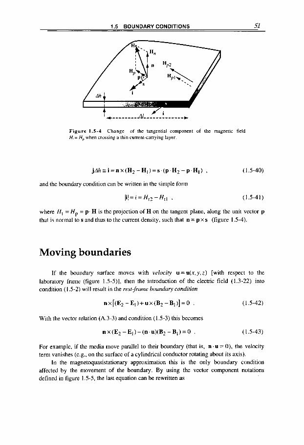
1.5 BOUNDARY CONDITIONS 51
Figure 1.5-4 Change of the tangential component of the magnetic field H,= H, when crossing a thin current-carrying layer.
jAh s i = nx(H2 - H ! ) = s . ( p . H 2 - p . H , ) , (1.5-40)
and the boundary condition can be written in the simple form
lil= i = H,, - Htl , ( 1 5 4 1 )
where H, = Hp = p. H is the projection of H on the tangent plane, along the unit vector p that is normal to s and thus to the current density, such that n = p x s (figure 1.5-4).
Moving boundaries
If the boundary surface moves with velocity u = u(x,y,z) [with respect to the laboratory frame (figure 1.5-5)], then the introduction of the electric field (1.3-22) into condition ( 1 5 2 ) will result in the rest-frunze boundary condition
nx[(E2 - E l ) + ux(B2 -BI ) ] = 0 . (1.5-42)
With the vector relation (A.3-3) and condition (1.5-3) this becomes
nx(E2 -El ) - (n .u) (B2 -B l )=O . (1.5-43)
For example, if the media move parallel to their boundary (that is, n . u = 0). the velocity term vanishes (e.g., on the surface of a cylindrical conductor rotating about its axis).
In the magnetoquasistationary approximation this is the only boundary condition affected by the movement of the boundary. By using the vector component notations defined in figure 1.5-5, the last equation can be rewritten as

52 CHAPTER 1 FOUNDATION OF MAGNETIC FIELD THEORY
Figure 1.5-5 Boundary moving with velocity u; here B and E are decomposed into the orthogonal system with unit vectors (p,s,n) chosen so that E,s = n x E.
or, in analogy to (1.518, 19), we can also say that
Er-UnBu, UnByl 9 (1.5-44)
(as well as unBn) are steady when crossing the moving boundary. ( BPis the tangential component parallel to Et , whereas B, is normal to it.)
If we consider, for completeness' sake, a moving dielectric medium to which the velocity-dependent quasistationary electric equations (1.3-17, 19) apply, then the boundary conditions (1.5-1,37,38) will change into
n x [ ( H 2 - H I ) + ux ( D 2 - DI)] = n x ( H 2 - H l ) + ( n . u ) ( D 2 - D I ) = is, (1.5-45)
n . ( j 2 - j l ) = ( n . ~ ) ( ~ ~ 2 -Pel) (1.5-46)
(1.5-47)
from which follow, like before, the conditions for the tangential or normal components of the parameters involved, in particular those concerning the convective current term peu. which is typical for the electric quasistationary approximation.
In the following chapter we shall determine the boundary conditions for other electromagnetic quantities, namely, for the magnetic scalar and vector potentials, all of which are summarized in table 1.5-1.
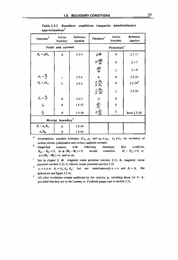
1.5 BOUNDARY CONDITIONS 53
E, -u,& 0
un 4, 0
Table 1.5-1 Boundary condi t ions (magnet ic quas is ta t ionary approximation)'
1.5-44
1.5-44
h Across Reference boundary equation
Parameter
Fields and currents
1.5-3
1.5- 1
1.5-4
1.5-2
1.5-37
I .5-39
I Across Reference boundary equation
Paramete:
Potentials' I 0
0
4
0
0
4
0
0
re
2.1-7
2.1-9
2.2-23
" Assumptions: possible existence ofi,, ps and ~2 # &, €2 # no existence of surface electric polarization and surface magnetic moment. Simplified notation with following meanings: first condition, Bn2 - 41 = 0, or n'(B2 - 91) = 0; second condition, H, - H,, = 0, or n x (Hz -HI) = i , and so on.
See in chapter 2: 0, magnetic scalar potential (section 2.1); A, magnetic vector potential (section 2.2): U, electric scalar potential (section 2.2).
xi = s, p , n; A; = As, Ap . A,,; but not simultaneously x; = n and Ai = A, (for
definitions see figure 2.2-4). All other conditions remain unaffected by the velocity u. including those for U, A, provided that they are in the Lorentz or Coulomb gauge (see in section 2.2).
d
54 CHAPTER 1 FOUNDATION OF MAGNETIC FIELD THEORY
The arzwork here and at the end of each chapter was done by Sergio Costa during a course on Magnetic Tokamak Problems held in July 1985 at the E k e (Sicily) Center of Scientijk Culture: Simple but elegant impressions from the Mediterranean ambience (within which the study of magnetism began more than 2600 years ago).
s *AMC€SCO. ERicF
Chapter 2
MAGNETIC POTENTIALS
The basic problem tackled in this chapter is that of establishing an explicit relation between static or quasistationary magnetic fields and the related current distributions, including the effects of magnetized materials. The study of this re1ation';s logically based on the solution of Maxwell's equations written in magnetic and electric fields, which is often a formidable mathematical task. A powerful alternative approach consists in introducing the magnetic scalar potential @ or vector potential A , together with the electric potential U where necessary, and in establishing their related differential equations. The introduction and handling of these potentials is the main subject of this chapter, and it will be shown that their application allows a more convenient description of magnetic phenomena in specific circumstances. Several analytical solution methods are presented; then useful solutions are provided that are related to magnetic fields produced by some geometrically simple, current-carrying conductors or magnetized materials; finally, the structure of magnetic fields is discussed in general terms.
Applications. The theory developed in this chapter gives the relations between magnet structures and the related magnetic field configurations. Solenoidal, toroidal, homogeneous, gradient, multipole, maximum, and variously shaped magnetic fields are calculated from ~ o l e n o i d a l , ~ ~ ~ toroidal, variable-winding, race-track, Bitter-type,' l7 and other current-carrying coil structures and also from magnetized These results are then used in other chapters to analyze the connected energies, forces, and mechanical stresses.
2.1 MAGNETIC SCALAR POTENTIAL
A relation between magnetic fields and current distribution can be conveniently established by introducing the magnetic scalar potential 0. The advantage of using this
55
M4GNETICFIELDS: A Comprehensive Theoretical Treatise for Practical Use Heinz E. Knoepfel
Copyright Q 2000 by John Wiley & Sons, Inc
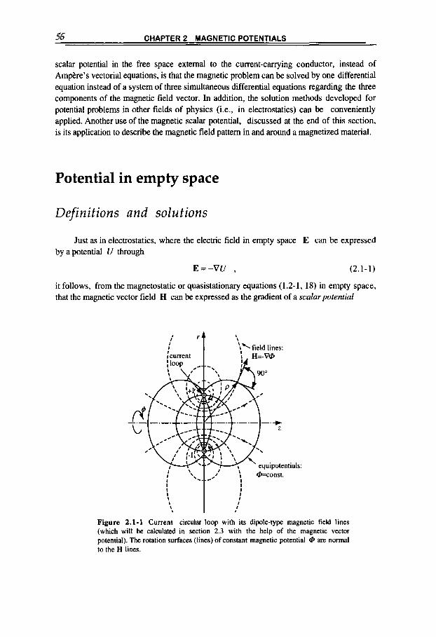
56 CHAPTER 2 MAGNETIC POTENTIALS
scalar potential in the free space external to the current-carrying conductor, instead of AmNre’s vectorial equations, is that the magnetic problem can be solved by one differential equation instead of a system of three simultaneous differential equations regarding the three components of the magnetic field vector. In addition, the solution methods developed for potential problems in other fields of physics (i.e., in electrostatics) can be conveniently applied. Another use of the magnetic scalar potential, discussed at the end of this section, is its application to describe the magnetic field pattern in and around a magnetized material.
Potential in empty space
Definitions and solutions
Just as in electrostatics, where the electric field in empty space E can be expressed by a potential U through
E=-VU , (2.1-1)
it follows, from the magnetostatic or quasistationary equations (1.2-1, 18) in empty space, that the magnetic vector field H can be expressed as the gradient of a scalarpotential
Figure 2.1-1 Current circular loop with its dipole-type magnetic field lines (which will be calculated in section 2.3 with the help of the magnetic vector potential). The rotation surfaces (lines) of constant magnetic potential 0 are normal to the H lines.

2.1 MAGNETIC SCALAR POTENTIAL 57
H = - V @ . (2.1-2)
In fact, taking the curl of this equation leads to V x H = 0 because of (A.3-1 l) , as also obtained from (1.2-1,18) inempty space wherej=O. Since also p V . H = O from (1.1-3), the magnetic field problem reduces to a potential problem described by Laplace's equation
A@=O , (2.1-3)
together with the appropriate boundary conditions (2.1-7, 9, 11). In general this gives rise to a Dirichletproblem [(see in connection with (A.4-6)], where the boundary conditions are defined by a given surface potential or field.
The advantages in using the magnetic potential @ and its related Laplace equation instead of the amperian equation (1.2-18) written in the magnetic field H have already been mentioned in the introduction to this section. But what are the merits of using @ instead of the magnetic vector potential A (which is introduced in section 2.2)? The answer depends on many aspects of the specific problem, as we shall see in this chapter. The vector potential is of more general usefulness because it applies to both current-carrying and empty space, whereas the scalar potential is limited only to the latter. But if there are no symmetries that eliminate one or two of the three vector components in A, the one- valued scalar potential can be more practical; it is also easier to visualize, because the surfaces of constant @ are normal to H with their spacing inversely proportional to IHI, according to the well-known properties of the gradient of a scalar potential (figure 2.1-1).
The scalar potential can be used only in simply connected, current-free space regions; the properties of the currents that flow beyond these regions can, in general, be taken care of by appropriate boundary conditions. However, one must be careful to avoid a multiple- valued potential function, and it often is tricky to relate @ to the current density j , which is present in most cases.
Figure 2.1-2 Integration paths for determining the scalar potential @.
58 CHAPTER 2 MAGNETIC POTENTIALS
For the potential defined by (2.1-3), the grudienf theorem
@(r)-@(a)= J V 4 . d l
‘i
(2.1-4)
applies, where the integration is from a reference point P(a) along a path Ci up to the
variable point P(r) (figure 2.1-2). With (2.1-2) this is
@ ( r ) = - j H . d l + D ,
‘i
(2.1-5)
since the potentials defining H can differ by a constant D. Some care must be taken in choosing the correct path. In figure 2.1-2, C, and C, are acceptable paths, even if they differ by a constant; in fact, with (1.4-2) we get
which shows that the change in @ around the closed path C,-C, is proportional to the encircled constant current, even when j = 0 along the path. Path C, should be avoided; it can be used only if one is sure that the current flowing between it and any outside path remains constant with changing position of P(r).
Most often, however, the magnetic potential problem is conveniently solved through the Laplace equation (2.1-3). which can be tackled with various methods, as we shall see in this chapter (reference is also made to appendix A.4 and to the extensive literature on mathematical physics).
Boundary conditions
Before dealing with some solutions of the magnetic potential problem, we shall introduce the boundary conditions on the magnetic scalar potential 4. These conditions follow directly from those given in section 1.5. For example, noting that
from (1 5 3 ) we obtain
(2.1-6)
(2.1-7)
The orthogonal coordinate system defined by the unit vectors p,s,n is oriented so that (p, s) are tangential to the boundary and, in particular, that p is in the direction of the vertical projection of H = - V 4 (figure 2.1-3). Hence
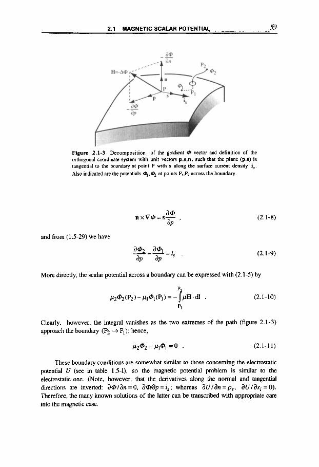
2.1 MAGNETIC SCALAR POTENTIAL 59
Figure 2.1-3 Decomposition of the gradient @ vector and definition of the orthogonal coordinate system with unit vectors p,s,n, such that the plane (p,s) is tangential to the boundary at point P with s along the surface current density is. Also indicated are the potentials q,q at points PI,PI across the boundary.
and from (1 5 2 9 ) we have
(2.1-8)
(2.1-9)
More directly, the scalar potential across a boundary can be expressed with (2.1-5) by
p2
pi
~2@2(P2) - P I @ I ~ ( P ~ ) = - JPH. dl . (2.1-10)
Clearly, however, the integral vanishes as the two extremes of the path (figure 2.1-3) approach the boundary (P2 + Pl); hence,
P2@2 - P A = o . (2.1-11)
These boundary conditions are somewhat similar to those concerning the electrostatic potential U (see in table 1.5-I), so the magnetic potential problem is similar to the electrostatic one. (Note, however, that the derivatives along the normal and tangential directions are inverted: a@Ian = 0, a W p = is; whereas aUIan = ps, a U / a x i = 0). Therefore, the many known solutions of the latter can be transcribed with appropriate care into the magnetic case.

60 CHAPTER 2 MAGNETIC POTENTIALS
Axisymmetric systems
General equations
In axisymmetric systems there is rotational symmetry about the z-axis, the currents are purely azimuthal,
j = j p g , (2.1- 12)
and consequently the related magnetic field is purely poloidal; that is, it has no component along e+ [see also the discussion in connection with (2.2-27)]. In this case it is convenient to resort to cylindrical coordinates (z,r); or in special cases, to spherical coordinates (p,8). Many magnetic field configurations of practical importance have this symmetry, such as those generated by currents flowing in loops or cylindrical coils (figure 2.1-4).
The Laplace equation (2.1-3) for the potential @(z,r ) in cylindrical coordinates is, according to (A.4-15),
Figure 2.1-4 Poloidal magnetic field H(z,r)=H(p,@ generated by an axisymmetric current distribution j = j+e+, with field components in cylindrical
(z,r,$) coordinates; the on-axis component is Hg(z = p) = H,(z,O) = H,(p,O).
2.1 MAGNETIC SCALAR POTENTIAL 61
and the field H(z,r) (2.1-2) has the components (table A.3-11)
(2.1 - 14)
In spherical coordinates the corresponding expressions for @(p,8) and H(p,8) are
(2.1-15)
(2.1-16)
The general solutions of these equations are given by (A.4-21, 22) in appendix A.4. A simple example in spherical coordinates will be discussed with the solution (2.1-26). The series expansion technique is applied below to present some properties of the magnetic field and its potential near the axis of symmetry. On the contrary, the fields far from the generating current sources can be conveniently described by the multipole expansion, which will be described starting from the vector potential form (2.2-42).
Expansion near the axis
For the scalar magnetic potential we set the polynomial series in r
m
(2.1 - 17) 2 @(z,r) = %(z)+ a2(z)r + ... = CaZnr2" n=O
(uneven terms in r vanish because of symmetry), and by introducing it into the two- dimensional Laplace equation (2.1-13) obtain
[ah2) + 4a2] + [ui2) + 16a4]r2 + ... = 0 ,
where for the differentiation we use the notation ah2) = d2[uo(z)]/dz2. Because this
equation holds for any value of r, the expressions contained in each pair of brackets must be zero, and by defining
@An) = -, with q ( z ) = ajA0)(z) = [@(~,r)] , ,~ , (2.1 - 18) dz"
we find

a CHAPTER 2 MAGNETIC POTENTIALS
thus the series representation of the solution is
(2.1 - 19)
By normalizing with the axial field on axis and in analogy to (2.1-18), we obtain
(2.1-20)
The axisymmetric magnetic field components follow from (2.1-14):
(2.1-21)
(2.1-22)
[Note that the substitution n - 1 + n in (2.1-22) will have the series starting again at n = 0.1 These solutions, which are a direct and general consequence of the rotational nature of H, (i.e.,V.H = O ) , provide the magnetic field around the symmetry axis, in a volume not containing any current, by knowing just the component H J z ) = H,(z ,O) , which can be found independently [see, e.g., in (2.3-7, 12, 19, 35)].
In first-order approximation (n = 0), from (2.1-22) we get
(2.1-23)
and differentiating (2.1-21) in the approximation n = 1 with respect to r yields
where we have used the definition of a differential (substitute H + H l ’ ) )

2.1 MAGNETIC SCALAR POTENTIAL 63
d N z ) - lim H ( z + E ) - H ( z ) -- m E+O &
The latter approximation shows that around a point on axis z = zo in axial symmetry (where dH, ld r vanishes), the increment of the gradient of the axial field component along the axis is twice as large in absolute value as the one perpendicular to it.
Example: Diamagnetic sphere An example conveniently treated in spherical coordinates (figure 2.1-5) is that of a fully diamagnetic
sphere with radius a (e.g., a superconducting sphere that fully excludes magnetic fields) immersed in a uniform outer field H, (const.). whose spherical components are
(2.1-25)
The general solution of the differential equation (2.1-15) is given in (A.4-25).
m
ow. 0 ) = x[ A,P" + (8) . (2.1-26) n=O
where P,,(e) are the Legendre polynomials (A.4-25). For the radial field component (2.1-16) we calculate
- H, = - C [ A,np"-' - sn(n + I ) ~ - ~ - * ] P ~ ( S ) . (2.1-27)
n=I
The boundary conditions require the following: (a) At infinity. Hp(p + -; any 8 ) + HO cose. which
implies that only the term A, = - H o remains; and (b) on the surface of the diamagnetic sphere,
H,(p = a; any 8) = 0; thus B , = -Hw3/2 (the boundary conditions for H e are then also automatically
fullfilled). Consequently, the potential is
o ~ p , e ~ = - ~ o p ~ ~ ~ e - ~ ~ ~ ~ ~ ~ e , (2.1-28) 2,
where the first term represents the potential
0" =-Ho p
d.. Z
FiguFe 2.1-5 Magnetic field around a diamagnetic sphere.
(2.1-29)
64 CHAPTER 2 MAGNETIC POTENTIALS
of the uniform magnetic field (2.1-25), and the second term represents the potential (2.2-52)
(2.1-30)
of the magnetic dipole with moment
p=-2aa3Ho . (2.1-3 I )
The spherical components of the poloidal field H(p,O)are calculated f?om (2.1-16) to be
H~ = ~ ~ [ 1 - ( ~ ~ / p ~ ) i ~ ~ ~ e , H~ = - ~ ~ [ i + ( a ~ / 2 p ~ ) i s i n e . (2.1-32)
On the equator, ( p = a,@ = a /2). the magnetic field increases independently of the radius a by a factor of 1.5: we can say that the diamagnetic sphere acts there as a flux concentrator. On the surface of the superconducting (diamagnetic) sphere, there flows a surface current (151 .41)
(2.1-33) 3 2
i,=He=--HosinO
that prevents the magnetic field from penetrating, and thus turns left-hand with respect to the vector Ho. When the elecmc conductivity is finite, the induced current penetrates into the sphere, and the
potential is modified. In chapter 4 we show that it is then convenient to resort to other solution methods; in particular, in appendix A.4 we discuss this problem by providing the appropriate equation (A.4-74) for its solution.
Two-dimensional plane systems
General equations
When the currents are purely axial, j = j,e,, the scalar potential @ and the related magnetic field H = -V@ become two-dimensional functions that can be described, e.g., by Cartesian (x,y) or polar ( r ,@) coordinates (figure 2.1-6). The Laplace equation and the field components take the form
or, respectively,
a2aj a2Q 7 + 7 = 0 , ax ay (2.1-34a)
(2.1-34b)
(2.1-35a)

2.1 MAGNETIC SCALAR POTENTIAL 65
Figure 2.1-6 Two-dimensional magnetic field H ( x . y ) = H(r , 4) generated by the orthogonal current density j = j,e,, with field components in Cartesian ( x , y )
and cylindrical (polar) ( r , $)-coordinates.
(2.1-35b)
For the general solution of these equations we refer again to appendix 4 and, in particular, to (A.4-14,21). For example, the two-dimensional magnetic potential and field on the outside (r 2 a ) of a very long cylindrical conductor carrying the total current I within the radius a is calculated in Cartesian coordinates from (2.1 -34),
2 2 2 (2.1-36a) @(x,y)=&arctan" , r = x + y , Y
H = - ' L x 2 x ,2 ' H = ' L Y 211 r 2 ' (2.1-36b)
or in cylindrical coordinates from (2.1-35),
@ ( r . # ) = - x # I , (2.1-37a)
(2.1-37b)
[This is also obtained directly from Amp2re's law (1.4-3).] When the current flows uniformingly in the cross-section, ( r l a ) , the results inside the conductor are obtained by the substitution I + Ir2la2 in the above expressions.
66 CHAPTER 2 MAGNETIC POTENTIALS
Many solution methods developed for other fields (in particular electrostatic) can conveniently be taken over for solving magnetic problems-for example, the methods of images [see at the end of this section and in connection with (6.2-51)]*' and conformal transformation (introduced below).
Example: Transverse field on diamagnetic rod
We briefly discuss a cylindrical problem that is directly solved by applying the solution (A.4-21): A uniform magnetic field HO is applied transversally to a perfectly conducting (Le., fully diamagnetic) cylinder. This arrangement, discussed in more detail in connection with figure 4.3-4, requires the following boundary conditions: (a) at infinity, Hr(r+-; any @)+ Hocos@; and (b) on the surface of the
diamagnetic cylinder, Hr(r = 0; any @) = 0. Using a procedure similar to that of the spherical solution (2.1-28). from (A.4-21) we get
(2.1-38)
with
(2.1-39)
The conformal transformation method
For the analytical solution of the potential problems defined by the two-dimensional potential or Laplace equations (2.1-34a,35a), it is often convenient to apply the method based on conformal transformation with complex function^.*.^.^.^ (Complex variables and functions are introduced and defined in section 3.1 .)
The basic theorems here are that,firsrly, any analytical function (3.1-20),
(2.1-40)
of the complex variable
z = x + i y , (2.1-4 1)
and, secondly, the real functions u, v in the variables x, y satisfy the potential equation (2.1-34a). In fact, for the complex function w, from
2.1 MAGNETIC SCALAR POTENTIAL 67
we calculate
and summation shows the first theorem,
- aZE + " = o . a2 ax2 ay2
whereas introducing (2.1-40) into this equation gives
( s + g ) + i [ s + g ) = o a2u a2u a2v a2v '
(2.1-42)
(2.1-43)
(2.1-44)
and, since each bracket term must vanish, this shows the second theorem. Similarly, introducing (2.-40) into (2.1-42) results in the so-called Cauchy-Riemann differential equations
(2.1-45)
which represent a necessary and sufficient condition for ~ ( 2 ) to be an analytical function. As later discussed in section 3.1 [see in connection with (3.1-20)], the complex
function ~ ( 2 ) transforms the (x,y)-plane into the (u,v)-plane. The interest here is that this formalism makes it possible in many cases to transform a potential problem from the real (x,y)-plane into the (u,v)-plane, where the analytical solution may be much easier for geometrical reasons.2s The final solution is then obtained by transforming back into the original (xy)-plane. A typical example is when one wants to determine the magnetic field generated by currents flowing in a group of circular conductors, or conductors with polynomial boundaries, with or without the presence of ferromagnetic rnaterials2.2'. The application of numerical techniques to conformal transformation has added interesting possibilities to this solution method.2.'
Example: Parallel lines An example where the conformal transformation method can be conveniently applied is represented
by the parallel transmission line problem illustrated in figure 2.1-7a, where two identical (superconducting) wires of radius a, at distance d, each cany on their surface the opposite total current f I. Due to field-current interaction (proximity efecr), the magnetic pattern is not obtained by simply adding the undisturbed vector field deriving from each wire taken separately. The azimuthal magnetic field around one
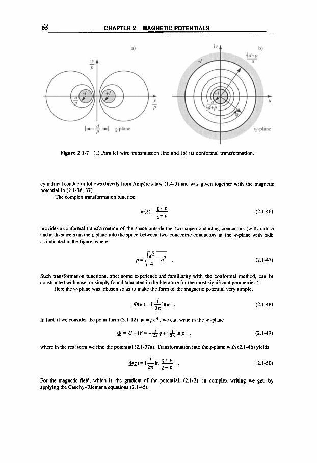
68 CHAPTER 2 MAGNETIC POTENTIALS
Figure 2.1-7 (a) Parallel wire transmission line and (b) its conformal transformation.
cylindrical conductor follows directly from Amphe's law (1.4-3) and was given together with the magnetic potential in (2.1-36, 37).
The complex transformation function
(2.1-46)
provides a conformal transformation of the space outside the two superconducting conductors (with radii u and at distanced) in the r-plane into the space between two concentric conductors in the w-plane with radii as indicated in the figure, where
(2.1-47)
Such transformation functions, after some experience and familiarity with the conformal method, can be constructed with ease, or simply found tabulated in the literature for the most significant geometries.2-'
Here the w-plane was chosen so as to make the form of the magnetic potential very simple,
(2.1-48)
In fact, if we consider the polar form (3.1-12) E= pew, we can write in the -plane
~p = U + i V = - & $ + i & l n p , (2.1-49)
where in the real term we find the potential (2.1-37a). Transformation into the z-plane with (2.1-46) yields
1 b + P 2X z - P
- @(z)=i-in - (2.1-50)
For the magnetic field, which is the gradient of the potential, (2.1-2). in complex writing we get, by applying the Cauchy-Riemann equations (2.1-45).

2.1 MAGNETIC SCALAR POTENTIAL 69
- H = H , + i H Y = - C - i & = - d ( u - i ax ay ax V ) = - d Z ' dz . ' (2.1-5 I )
that is, we do not need to determine the real part of Q and calculate the gradient, but we can differentiate directly the complex potential with respect to z and obtain [taking again the conjugate (3. I - 14)j
P I -
H * = H -iH =-=i-&=" d@ I - I dz " z 2 - p 2 x : x 2 - y 2 - p 2 + i 2 x y .
The magnetic field in the 2-plane outside the (superconducting) conductors thus has the components
The magnitude of the field becomes
On the conductor surface, described by the equation
(2.1-52)
(2.1-53)
(2.1-54)
(2.1-55)
(2.1-56)
we have
(2.1-57) 1 P i 2 n m '
141 = --
which also means that the linear current density on the conductor surface flowing parallel to the axis, where d d - - a 5 x < - + a, has the value ( I 5 4 1 ) ; that is, 2 2
i = H = L ! ! . (2.1-58) 21r M
z s
The magnetic field between the two wires is perpendicular to the x-axis, and its magnitude becomes, from (2.1-54) for y=O,
H =--/A 1 . Y 1r p 2 - x 2 '
whereas from (2.1-37) and ignoring the proximity effect, we obtain the smaller value
(2.1-59)
(2.1-60)
For the increase of the magnetic field between the two conductors there is a corresponding current density concentration on the conductor sides facing each other. Consequently, the apparent resistance and inductance vary, as will be shown by (2.4-15) for the inductance.
70 CHAPTER 2 MAGNETIC POTENTIALS
Potential in and outside magnetized materials
The magnetic scalar potential concept can be useful in describing the magnetic field in and around magnetized material. To illustrate this problem, let us consider the case of a permanent (but space dependent) magnetization M ( r ) , such as represented by hard ferromagnets where the magnetization is permanent and independent of any applied magnetic field (see in chapter 8). Taking the divergence of (2.1-2),
H = - V O , (2.1-61)
and, because of the definition (1.1-17), V‘BIp,, =V.(H+M)=O,results in the Poisson equation
A @ = V . M , (2.1-62)
and from (1.1-27) we can introduce the magnetic charge density
pm = - V * M . (2.1-63)
With this formulation the general solution for O at point P of the inhomogeneous differential equation can be found by various methods, for example it can be obtained similarly to the electrostatic potential (2.2-20):
The last expression is obtained by applying Gauss’ theorem (A.3- 16); it is important when M is uniform, because then in the whole volume V . M = 0, and only the surface gives a contribution through the magnetic surface charge density introduced in ( 1.1-29):
r , = n . M . (2.1-65)
Example: Permanent spherical magnet We illustrate the magnetic potential method with a permanent spherical magnet with fixed uniform
magnetization M = Mo (const.) and radius a (figure 2.1-8). We now have
r, = McosO , (2.1-66)
and the solution integral (2.1-64) is
(2.1-67)
Where
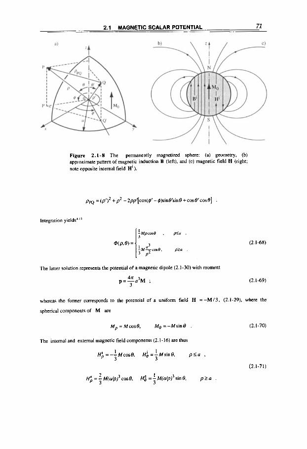
2.1 MAGNETIC SCALAR POTENTIAL 71
Figure 2.1-8 The permanently magnetized sphere: (a) geometry, (b) approximate pattern of magnetic induction B (left), and (c) magnetic field H (right; note opposite internal field H’ ).
ppQ = ( P # ) ~ +p2 -2pp~[cos(q’-~~sin0’sin0+cose~co~e] .
Integration yields” ’’ LMpcosO , p5u , 3
ww= , u3 pzu .
(2.1-68)
The latter solution represents the potential of a magnetic dipole (2.1-30) with moment
41r
3 p=-u3M ; (2.1-69)
whereas the former corresponds to the potential of a uniform field H = - M / 3 , (2.1-29). where the
spherical components of M are
Mp=McosO, MO=-MsinO .
The internal and external magnetic field components (2.1-16) are thus
1 I H i ---McosO, HL=-MsinO, p l u ,
p - 3 3
(2.1-70)
(2.1-7 1 )

72 CHAPTER 2 MAGNETIC POTENTIALS
Note that according to the definitions (1.1-37), the demagnetizing field here is Hd = Hi = - 1/3 M and the demagnetizing factor k, = 1/3: the internal field is antiparallel to M and to the z-axis. The
induction
B = (H + M) (2.1-72)
in the sphere has the components
(2.1-73) ' 2 ' 2 p 3 3
B' =-poMcos0 , Bh =--poMsinB ;
it is uniform and parallel to the z-axis (and opposite to the magnetic field), whereas outside i t is Be = h H e .
Example: Magnetized sphere In thesecond. more general example described in figure 2.1-9, a uniform outer field Ho, derivable
from a potential
0" = -Hopcose (2.1-74)
and with components
H~~ = H~ case , Hoe = -HosinB , (2.1-75)
induces in the sphere the magnetization
M=XH', x = ( p R - i ) . (2.1-76)
where Hi is the internal, as yet unknown, field, although it is plausible to assume that it is parallel to H,,. We can proceed formally, as before, because M remains uniform and constant, and the field thus results
from the superposition of solution (2.1-71) on the outer field (2.1-75). but we need an equation that relates M or Hi to Ho. This equation is provided by the boundary condition (1.5-18) requiring the normal (i.e.
radial) component of the magnetic induction to remain steady at the boundary p = a , that is,
pH;=pH; 3 (2.1-77)
from which follows
(2.1-78)
or, from (2.1-76).

2.1 MAGNETIC SCALAR POTENTIAL 73
Figure 2.1-9 Paramagnetic sphere ( p ~ > I ) in uniform magnetic field H, with approximate pattern of (a) magnetic induction B (left) and (b) magnetic field H (right; note reduced internal field H’ ).
‘ 3 HI=- H o = ( l - a ) H o .
PR + 2 (2.1-79)
The second boundary condition, requiring the tangential @component of the magnetic field (2.1-71) to remain steady, is automatically satisfied; also note that if the medium surrounding the sphere is not empty space but has a P R 2 # 1, then the above expressions change according to the substitution pR 4 pR /pRz. The solution, resulting from the superposition of the fields (2.1-71, 75). with a given in (2.1-78). is
H; = ~ ~ ( ~ - a ) c o s ~ , H; = - ~ , ( ~ - a ) s i n ~ for p ~ a , (2.1-80)
H; = H0[I+2a(a /p ) ’ ] cosB , H i =-H0[I-a(a/p)’]sinB for p’a . (2.1-81 )
According to the definitions (1.1-37) the demagnetizing field here is H, =-&I0 and the demagnetizing factor is k, =a. Similarly, the total potential here is obtained by superposition of the potentials (2.1-68,
74). For a fully diamagnetic sphere (i.e.. p~ + 0 and a + -1 I2 ), we find that the field He(p,B) and the
dipole moment p are as in (2.1-31. 32). In a paramagnetic material WithpR > 1, the internal field H i is always smaller than Ho. but
(2.1-82)
is always larger, and for p~ very large (ferromagnetic materials) it approaches 3H0; because of the
boundary condition (2.1-77) this Bi/&= pRfi = He is also the field just outside the poles.
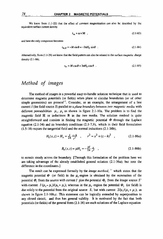
74 CHAPTER 2 MAGNETIC POTENTIALS
We know from (1.1-22) that the effect of constant magnetization can also be described by the equivalent surface current density
i , = n x M , (2.1-83)
and here the only component becomes
i,,@ = -M sine = -304, sine . (2.1-84)
Alternatively, from ( I .I-29) we know that the field pattern can also be related to the surface magnetic charge
density (2.1-66),
r,,, = M C O S ~ = ~ ~ H ~ C O S ~ . (2.1-85)
Method of images
The method of images is a powerful easy-to-handle solution technique that is used to determine magnetic potentials (or fields) when plane or circular boundaries (or of other simple geometries) are present'.'. Consider, as an example, the arrangement of a line current I (the field source S) parallel to aplane boundary between two magnetic media with different permeabilities p,, p 2 as shown in figure 2.1-10a. The problem is to find the magnetic field H or inductions B in the two media. The solution method is quite straightforward and consists in finding the magnetic potential 0 through the Laplace equation (2.1-34) and its boundary conditions (2.1-7,9), which in their field formulation (1.5-18) require the tangential field and the normal inductions (2.1-36b),
2 2 2 H t ( x , z ) = H, = L 2rr z-h r 2 , r = x + ( z - h ) . (2.1-86a)
(2.1-86b)
to remain steady across the boundary. [Through this formulation of the problem here we are taking advantage of the already established general solution (2.1 -36a); but note the difference in the coordinates.]
The result can be expressed formally by the image method, ' ' which states that the magnetic potential 0 (or field) in the &-region is obtained by the summation of the potential 0' from the source with current I plus the potential O2 from the image source S' with current I &- pl)I(pz t p,); whereas in the p2 -region the potential o2 (or field) is due solely to the potential from the original source S, but with current 21pl/(p2 + pl), as shown in figure 2.1-10b,c. This statement can be logically extended by superposition to any closed circuit, and thus has general validity. It is motivated by the fact that both potentials (or fields) of the general form (2.1-36) are each solutions of the Laplace equation
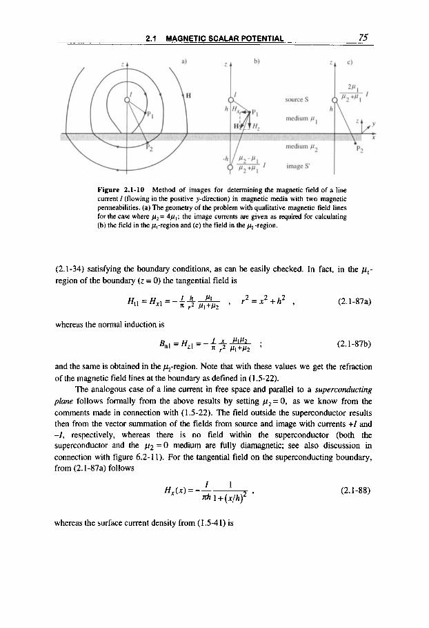
2.1 MAGNETIC SCALAR POTENTIAL 75
Figure 2.1-10 Method of images for determining the magnetic field of a line current I (flowing in the positive y-direction) in magnetic media with two magnetic permeabilities. (a) The geometry of the problem with qualitative magnetic field lines for the case where p2 = 4p,: the image currents are given as required for calculating (b) the field in the p,-region and (c) the field in the -region.
(2.1-34) satisfying the boundary conditions, as can be easily checked. In fact, in the p,- region of the boundary (z = 0) the tangential field is
2 2 2 r = x + h ,
whereas the normal induction is
(2.1-87a)
(2.1-87b)
and the same is obtained in the &-region. Note that with these values we get the refraction of the magnetic field lines at the boundary as defined in (1 322) .
The analogous case of a line current in free space and parallel to a superconducting plane follows formally from the above results by setting p2 = 0, as we know from the comments made in connection with (1.5-22). The field outside the superconductor results then from the vector summation of the fields from source and image with currents +I and -I, respectively, whereas there is no field within the superconductor (both the superconductor and the j4 = O medium are fully diamagnetic; see also discussion in connection with figure 6.2-1 1). For the tangential field on the superconducting boundary, from (2.1-87a) follows
I 1 H x ( x ) = --
&l+(x/h)2 ' (2.1-88)
whereas the surface current density from (1 5 4 1) is
76 CHAPTER 2 MAGNETIC POTENTIALS
that is, it falls off rapidly away from the projection point x=O (the total current flowing on the surface is obtained by summation and amounts to -0. In this ideal system of a line conductor parallel to the plane superconducting return conductor we find the current density concentration typical for the so-called proximiry effect. We have calculated this effect already for the parallel transmission lines shown in figure 2.1-7.
When the conductors have finite electrical conductivity a, the problem becomes more complicated. In relation to a line current parallel to a conducting plane, we find in (5.4-32b) the approximate mean heating power deposited in the plane by an oscillating line current; and we find in (6.2-62) the drag and suspension forces on the line current moving normally over the plane.
2.2 MAGNETIC VECTOR POTENTIAL
To deal with quasistationary magnetic problems, it is often convenient to introduce a magnetic vector potential A as done in this section. This vector potential is generally useful because it applies both to currentcarrying and to empty space (whereas the scalar potential introduced in the previous section is limited only to the latter) and is particularly convenient when the symmetry allows one to eliminate two of its three vector components, as for two-dimensional plane or axisymmetric magnetic field problems.
Basic equations and solutions
Equations
For the solution of the quasistationary magnetic field equation
V x H = j (2.2-1)
within a space where the current density is not everywhere zero, it is often convenient to introduce the vector potential A, defined through
B = V X A ; (2.2-2)

2.2 MAGNETIC VECTOR POTENTIAL 77
this is in agreement with (1.1-3), which requires B = p H to be the curl of some vector field; that is, the divergence of B vanishes according to (A.3-7). One of the physical meanings of A is related to the magnetic f lux y across any arbitrary curved surface S bounded by a contour line C (figure 2.2-1); in fact, applying Stokes’ theorem, (A.3-14), yields
(2.2-3)
From Faraday’s law (1.1-2) through insertion of (2.2-2) we get
V x (E + 9) = 0 ;
because the curl vanishes, the vector in parentheses can be derived from a scalar potential
U defined by (A.3-11).
- V U = E + a at . (2.2-4a)
This potential U can be identified as an electric scalar potential due to electrostatic charges or to external voltage sources. The total current density can thus include two components,
j = oE= j, + j, (2.2 -4b)
where
j, = - 8 U (2.2-4~)
is the one given by external electric sources, whereas
j. =-o& (2.2-4d) at
is the inductive component generated by a time-dependent magnetic vector potential or field.
Figure 2.2-1 Magnetic flux and vector potential.

78 CHAPTER 2 MAGNETIC POTENTIALS
We shift now briefly our attention to the general formulation, which takes care of the displacement current term in (1.1 - 1). Taking the divergence of (2.2-4a) and using (1.1-4) (thereby assuming p, E to be constants) yields
then inserting (2.2-2,4a) into Maxwell's equation (1.1-1) gives
AA = -pj + V(V . A) + p a + p & Y at2
(2.2-5)
(2.2-6)
where the Laplace operator A = V . V has different meanings, according to whether it operates on a scalar or on a vector [see in connection with (A.3-10,23)]:
AU=V.(VU) , (2.2-7)
AA = (V.V)A = V(V.A) - V x V x A . (2.2-8)
According to the definition of A in (2.2-2) and of the vector relation (A.3-1 l), it is possible to add a vector A', A -+ A + A', without changing the value of the magnetic induction B , provided that V x A' = 0-that is, provided that A' is the gradient of some scalar function V (plus a constant vector), A'=VV. This freedom to introduce a so-called gauge transformation can be used to simplify (2.2-5,6) by adjusting V . A : The Lorentz gauge
V . A = - p - au (2.2-9) at
leads to the symmetric d'Alembert equations
(2.2-10)
[For the solution of these equations see (2.2-26).] In the quasistationary magnetic approximation, where the last two terms in (2.2-6)
vanish because they derive from the displacement term aDl& it is convenient to use the Coulomb gauge
V * A = Q (2.2-1 1)
to obtain
AU=-& E , (2.2- 12)
A A = - K / . (2.2- 13)
It is useful to point out the significance of this formalism: The system of equations (2.2-10) [or of (2.2-12, 13) in the quasistationary approximation] can substitute Maxwell's

2.2 MAGNETIC VECTOR POTENTIAL 79
equations (1.1-1 to 4). Once the potentials A , U are determined, the electric and magnetic fields are found through (2.2-2,4),
p H = V x A , (2.2-14)
E = - a A - V U . at (2.2-15)
Which of these two options (i.e., the potential or the Maxwell equations) is more convenient for the solution depends on the specific electromagnetic problem to be tackled, as we shall see from some examples later on.
In conclusion we note that in the stationary case, the potential A follows from the given stationary current density j = js
AA=-pj . (2.2- 16)
[As we will see in the following problems of this section, j, is taken as given, without bothering about its origin (2.2-4~1.1 In the quasistationary case, the current density (2.2- 4b), j = j, + ji , includes in addition the inductive component (2.2-4d).
such that
dA dt
AA - p a - = -pjs (2.2-17)
[i.e., we obtain the diffusion equation (4.1-13). which will be discussed in chapter 41.
Solutions
The stationary or quasistationary solutions of the above differential equations in the potentials U , A follow standard rules. In particular, the general solution of (2.2-13) must be Looked for separately in the spaces with and without currents; in the latter case the vectorial Laplace-type equation
AA=O (2.2- 18)
has to be solved. Finally, the two subsolutions must be matched at the boundaries. For the solution of the vectorial equations presented so far [e.g., (2.2-13, 18)], it is
necessary to decompose them into equations for the components of the unknown vector field. This requires correctly interpreting the Laplacian operator, A = V . V = V2, as pointed out in (2.2-7,8). The result is straightforward (A.3-23) in Cartesian coordinates with A e (Ax, Ay, Az). For example, the vectorial equation (2.2-13) decomposes into three normal Poisson equations

80 CHAPTER 2 MAGNETIC POTENTIALS
AAi =-pji , i=x,p,z , (2.2-19)
where the Laplacian A is applied here to the scalar component-function Ai and has the well-known form given, for example, in table A.3-11. In other coordinate systems, the decomposition of the vectorial Laplace or Poisson equation into component equations is more complicated, as shown, for example, by the Laplacian (A.3-23b) in cylindrical coordinates.
On the other hand, as is well known from mathematical physics, and in particular from electrostatic problems, the solutions of (2.2-12, 13) in an unbounded space can also be expressed directly by integral formulaeA”: The electric potential becomes
and the vector potential yields
from which the magnetic field
(2.2-20)
(2.2-21)
(2.2-22)
is obtained in the quasistationary approximation; here P denotes the point in which the magnetic field is to be established, and Q the variable integration point within the conductor (figure 2.2-2). The last expression is called the Biot-Savart law. The transformation from (2.2-21) to (2.2-22) is obtained using the vector relation
v x - d V X j Q + v- X j Q (3 rPQ ( r d p ) and noting that V x jQ = 0, since the V operator is related only to point P. From (2.2-2 1) we easily find that the condition V.A = 0 requires VQ.j, = 0: (2.2-22) is therefore strictly correct only for closed conductors or conductors extending to infinity. The general time-dependent formulation of (2.2-2 1, 22) has the substitution jQ + jQ + a/& in the
integrals, which requires the calculation of the displacement current term; therefore, the formulation given in (2.2-26b) is to be preferred.
Figure 2.2-2 Spatial current distribution.

2.2 MAGNETIC VECTOR POTENTIAL 81
In figure 2.2-3 the relations between the current density j, the magnetic flux B, and the scalar and vector potentials 4 , A are represented schematically. The magnetic vector potential is very attractive for two-dimensional plane problems or axisymmetric magnetic field problems (where the current is purely axial j = jle, or azimuthal j = j4e,) because it then has only one component (Az, or Ah), which is orthogonal to the plane containing the magnetic field vector, as we shall see. For three-dimensional problems, all three components of the vector potential must in general be computed [from a system of three coupled, partial differential equations derived from the vectorial Poisson equation (2.2-13)], and thus the vector potential becomes less useful than the magnetic scalar potential (whenever the latter exists). The vector potential has the merit, in any case, of being applicable both in free space and within current-carrying conductors and avoiding the multiple-valued problem of the scalar potential.
n
Figure 2.2-3 The magnetostatic equations relating current density j , magnetic induction B = p H , scalar and vector potentials 0, A , with the equations shown (with reference to their position in the chaptery; the potentials can be convenient intermediate functions for simplifying the solution [CP is defined in free space, so there is no general meaningful relation to j in the conductor].
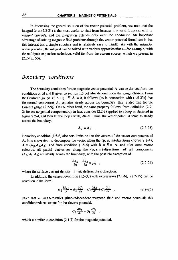
82 CHAPTER 2 MAGNETIC POTENTIALS
In discussing the general solution of the vector potential problem, we note that the integral form (2.2-21) is the most useful to start from because it is valid in spaces with or without currents, and the integration extends only over the conductor. An important advantage of solving magnetic field problems through the vector potential formalism is that this integral has a simple structure and is relatively easy to handle. As with the magnetic scalar potential, the integral can be solved with various approximations-for example, with the multipole expansion technique, valid far from the current source, which we present in (2.2-42, 50).
Boundary conditions
The boundary conditions for the magnetic vector potential A can be derived from the conditions on H and B given in section 1.5 but also depend upon the gauge chosen. From the Coulomb gauge (2.2-ll), V . A = 0, it follows [as in connection with (1.5-23)] that the normal component An remains steady across the boundary [this is also true for the Lorentz gauge (2.2-9)]. On the other hand, the same property follows from definition (2.2- 2) for the tangential component A,; in fact, consider (2.2-3) applied to a loop as depicted in figure 2.2-4, and then let the loop shrink, &+O. Thus, the vector potential remains steady across the boundary,
A 2 = A l . (2.2-23)
Boundary condition (1.5-6) also sets limits on the derivatives of the vector components of A . It is convenient to decompose the vector along the (p, s, n)-directions (figure 2.2-4), A I (Ap,As,An); and from condition (1.5-5) with B = V X A , and after some vector calculus, all partial derivatives along the (p, s, n)-directions of all components (A,, As, An) are steady across the boundary, with the possible exception of
(2.2-24)
where the surface current density i = si, defines the s-direction.
rewritten in the form In addition, the current condition (1.5-37) with expressions (2.1-6), (2.2-15) can be
(2.2-25)
Note that in magnetostatics (time-independent magnetic field and vector potential) this condition reduces to one for the electric potential,
which is similar to condition (2.1-7) for the magnetic potential.
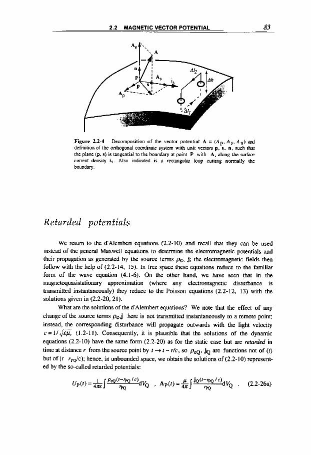
2.2 MAGNETIC VECTOR POTENTIAL 83
Figure 2.2-4 Decomposition of the vector potential A E ( A p , A s , A n ) ad definition of the orthogonal coordinate system with unit vectors p, s, n. such that the plane (p. s) is tangential to the boundary at point P with A , along the surface current density i s . Also indicated is a rectangular loop cutting normally the boundary.
Retarded potentials
We return to the dAlembert equations (2.2-10) and recall that they can be used instead of the general Maxwell equations to determine the electromagnetic potentials and their propagation as generated by the source terms Pe. j ; the electromagnetic fields then follow with the help of (2.2-14, 15). In free space these equations reduce to the familiar form of the wave equation (4.1-6). On the other hand, we have seen that in the magnetoquasistationary approximation (where any electromagnetic disturbance is transmitted instantaneously) they reduce to the Poisson equations (2.2-12, 13) with the solutions given in (2.2-20,21).
What are the solutions of the dAlembert equations? We note that the effect of any change of the source terms Pe j here is not transmitted instantaneously to a remote point; instead, the corresponding disturbance will propagate outwards with the light velocity c = 1/& (1.2-11). Consequently, it is plausible that the solutions of the dynamic equations (2.2-10) have the same form (2.2-20) as for the static case but are retarded in time at distance r from the source point by t + t - r/c, so peq, jQ are functions not of (t)
but of ( t -r,&); hence, in unbounded space, we obtain the solutions of (2.2- 10) represent- ed by the so-called retarded potentials:
84 CHAPTER 2 MAGNETIC POTENTIALS
By taking the curl of the last equation, i.e. proceeding as for the transition 2 2 21 to 22), we obtain the generalized Biot-Savart law (valid for any time dependence):
z s o . -
(2.2-26b)
here for simplicity we indicate the retardation through a square bracket, [ j ~ ] = j(r - 'pa / c ) , and have used (A.3-4) and the relation
v X [ j Q ] = -[%I x V(t - 'pa /c) = - x - [?] ?
Axisymmetric systems
In a cylindrical vector-potential problem, the cylindrical field components of pH = V x A are deduced from table A.3-11:
(2.2-27)
When the given, stationary currents are azimuthal or toroidal, j = jGe4 [i.e., flowing in circular paths perpendicular to the z-axis and centered on it (see figure 2.1-4 or 2.4-5)], we know from the rule (A.3-3 1) established in connection with the curl of a vector, j = V x H, that the field is purely poloidal, meaning Hq = 0. Similarly, from pfl = A x A it follows that the vector potential is azimuthal. This is also consistent with the expression for the H4- component in (2.2-27), which shows for H4 = 0 that A, can depend, if at all, only on r, and A, only on z; and since A,, A, do not appear in the other field components of (2.2- 27), it can be safely assumed that A, = A,. = 0. In conclusion, only the A#-component is relevant in axisymmetric geometry.
By taking the @-component of (A.3-24b), or by expressing the equation (V x H)# = j 4 with the help of table A.3-11, we obtain
(2.2-28)
The general solution of this Poisson equation referred to a space containing axisymmetric currents is obtained as usual: First, the solution of the homogeneous ( j 4 = 0) equation must be found [it is given in general form in (A.4-30)]; then, a particular solution of the full equation (2.2-28) must be added; finally, the solutions must be matched at the boundaries (including the condition + = 0 for r = 0, =) and for the initial conditions. Other solution
2.2 MAGNETIC VECTOR POTENTIAL 85
methods exist, such as the interesting double series method presented and discussed in (A.4-41). Note that (2.2-28) in free space differs formally by a term -AJr2 from the analogous (2. I - 13) referred to the scalar magnetic potential 0. When solving by numerical computation, however, both the A4 or 0 approaches require roughly the same effort.
The series expansion around the axis of symmetry can be applied as a solution method to give $ in a space not containing any current. From (2.1-21 or 22) and (2.2-27)
we get
(2.2-29) n=O
where the differential of the axial magnetic field denoted with the symbol Hi2"', which is a
function of 2 , is defined in (2.1-20); near the axis, a valid approximation is obtained by considering the n = 0 term only,
2A$ E prHo(z) . (2.2-30)
Finally, there is the integral solution (2.2-21), which is particularly useful in axisymmetric geometry. It will be applied in the next section, starting with the solution (2.3-1) for calculating the field produced by circular coils.
In concluding this discussion on axisymmetric systems, we reintroduce the poloidal magnetic flux function w(z , r ) , here taken across any surface S bounded by a concentric circle with radius r (see in figure 2.5-4). Definition (2.2-3) leads to
w k r ) = 2 x r 4 , (2.2-31)
with which the differential equation (2.2-28) can be written in the form
as easily checked. The magnetic field components (2.2-27) become
H =-1!!!!! I av r 2Kpr az 7 H z = - - 2npr ar
they can be expressed by the poloidal field defined as
H p = H r e r + H z e z = & e ~ x V ~
(2.2-32)
(2.2-33)
(2.2-34)
where e , , e r , e4 are the orthogonal unit vectors in cylindrical geometry [the last expression can be checked by inserting eg ,e , , e r and applying the trivectoral relation (A.3-3), then
taking the vector components of V w from table A.3-111. We shall take up the last expression again in section 2.5 and show in (2.5-12) that the v/ = const. lines are the Hp-field lines.

86 CHAPTER 2 MAGNETIC POTENTIALS
Plane two-dimensional systems
We consider here the two-dimensional geometry where the given, stationary current density is parallel to the z-axis, j = j z e , (figure 2.1-6), and hence the magnetic vector potential has the A,-component only. [As with the axisymmetric system, this is obtained by applying the rule established in connection with (A.3-31) to j = V x H and H = V x A .] This problem, where A is translationally invariant in z, can be handled, for example, in Cartesian coordinates with A,(x,y), or in cylindrical polar coordinates with A,(r,$), the choice being dictated by geometric convenience. Contrary to what we found in axisymmetric geometry, the A,component of the vector potential and the scalar potential @ both obey formally identical differential equations.
The Poisson equation (2.2-13), which here includes the axial component of (A.3- 24b) only, reduces in polar coordinates to
and the magnetic field components are
(2.2-35)
(2.2-36)
The homogeneous form of (2.2-35) is identical to (A.4-15) with the last term neglected, so the homogeneous solution A,(r,$) can be transcribed from (A.4-21). If there is also axial symmetry in jt(r,$) = j,(r), which implies Hr = 0, the result is a toroidal field HT = H4eg. As usual, the complete solution of (2.2-35) requires a particular solution to be added to the homogeneous solution.
It is often convenient to use Cartesian coordinates (x,y) in solving for A,(x,y) in plane problems. This case is discussed in section A.4. A simple Fourier series solution of the related Laplacian equation (A.4-27) is given in (A.4-28). Of particular interest, however, is the double Fourier series solution (A.4-31) because it directly gives the solution of the Poisson equation (A.4-27). Finally, there is the integral solution (2.2-21). which is particularly interesting in two-dimensional geometry [see the example in connection with (2.3-41) at the end of the next section].
Biot-Savart law
Filamentary conductor
In filamentary conductors (wires), the linear dimension of the cross section is much smaller than all the other dimensions, such that approximately
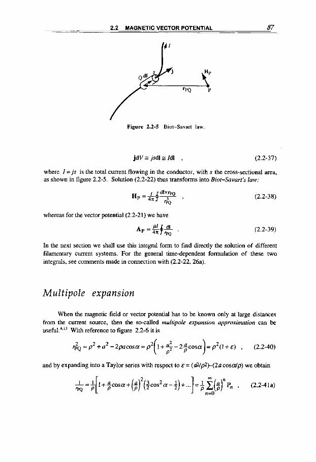
2.2 MAGNETIC VECTOR POTENTIAL 87
Figure 2.2-5 Biot-Savart law.
jdV G jsdl E Id1 , (2.2-37)
where I = j s is the total current flowing in the conductor, with s the cross-sectional area, as shown in figure 2.2-5. Solution (2.2-22) thus transforms into Biot-Savart’s law:
whereas for the vector potential (2.2-21) we have
(2.2-38)
(2.2-39)
In the next section we shall use this integral form to find directly the solution of different filamentary current systems. For the general time-dependent formulation of these two integrals, see comments made in connection with (2.2-22,26a).
M u It ipo 1 e expans ion
When the magnetic field or vector potential has to be known only at large distances from the current source, then the so-called multipole expansion approximation can be useful.*.” With reference to figure 2.2-6 it is
2 2 ’ p ~ = p + a2 - 2pacosa = p (1 + E ) , (2.2-40)
and by expanding into a Taylor series with respect to E = (dlp2)-(2acoscr/p) we obtain
m
1 = 1[1+ a c o s a + (a)2($cos2 P a - 3) + ...I = c($)” P,, , (2.2-4 1 a) rpp P P
n=O

88 CHAPTER 2 MAGNETIC POTENTIALS
Figure 2.2-6 Geometry for the multipole expansion of the magnetic vector potential at point P generated by a current loop.
where P, = Pn(cos a) are the Legendre polynomials,A,' the first five of which are given in (A.4-25). This could have been developed directly in vector form6' for ' p ~ = p - a:
(2.2-41b)
Insertion into (2.2-39) yields
A = &I[ $f(p. a)dl+ ...I = &+ gf[ $ P,, dl ; (2.2-42) n=l
here we have neglected the n = 0 (magnetic monopole) term because the total vector displacement around a closed loop is always zero:
+0 . (2.2-43)
The remaining n = 1.2,. . . terms correspond to the magnetic dipole, quadrupole. . . . terms.
Magnetic dipole
The dominant first n = 1 term in (2.2-42), called the dipole term, can be transformed into
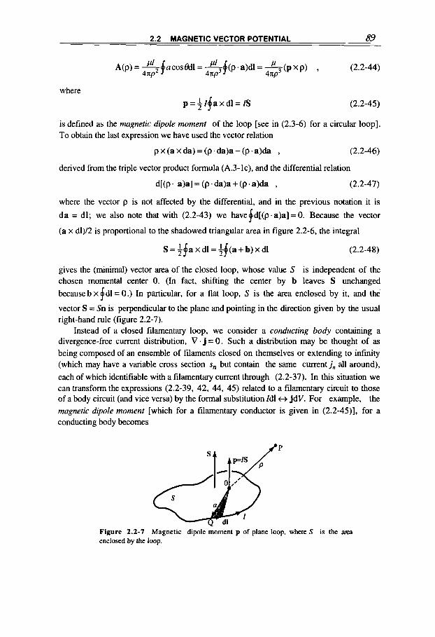
2.2 MAGNETIC VECTOR POTENTIAL 89
where p = + I f a x dl = Is
(2.2-44)
(2.2-45)
is defined as the magnetic dipole moment of the loop [see in (2.3-6) for a circular loop]. To obtain the last expression we have used the vector relation
p x (a x da) = (p.da)a - (p.a)da , (2.2-46)
derived from the triple vector product formula (A.3-lc), and the differential relation
d[(p. a)a] = (p . da)a + (p . a)da , (2.2-47)
where the vector p is not affected by the differential, and in the previous notation it is
d a = dl; we also note that with (2.2-43) we havefd[(p.a)a]=O. Because the vector
(a x d1)/2 is proportional to the shadowed triangular area in figure 2.2-6, the integral
S = +fa x d l = +$(a+ b) x dl (2.2-48)
gives the (minimal) vector area of the closed loop, whose value S is independent of the chosen momental center 0. (In fact, shifting the center by b leaves S unchanged becausebxfdl= 0.) In particular, for a flat loop, S is the area enclosed by it, and the
vector S = Sn is perpendicular to the plane and pointing in the direction given by the usual right-hand rule (figure 2.2-7).
Instead of a closed filamentary loop, we consider a conducting body containing a divergence-free current distribution, V. j = 0. Such a distribution may be thought of as being composed of an ensemble of filaments closed on themselves or extending to infinity (which may have a variable cross section s, but contain the same current j,, all around), each of which identifiable with a filamentary current through (2.2-37). In this situation we can transform the expressions (2.2-39, 42, 44, 45) related to a filamenmy circuit to those of a body circuit (and vice versa) by the formal substitution Id1 t) jdV. For example, the magnetic dipole moment [which for a filamentary conductor is given in (2.2-45)], for a conducting body becomes
P
Figure 2.2-7 Magnetic dipole moment p of plane loop, where S is the area enclosed by the loop.
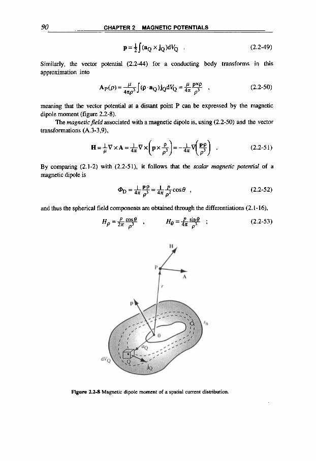
90 CHAPTER 2 MAGNETIC POTENTIALS
Similarly, the vector potential (2.2-44) for a conducting body transforms in this approximation into
(2.2-50)
meaning that the vector potential at a distant point P can be expressed by the magnetic dipole moment (figure 2.2-8).
The magneticfield associated with a magnetic dipole is, using (2.2-50) and the vector transformations (A.3-3,9),
H = $V x A = &V x(px#)= -&V($) . (2.2-51)
By comparing (2.1-2) with (2.2-51), it follows that the scalar magnetic potential of a magnetic dipole is
q, 4 H p3 = l L c o s ~ 4H p2 , (2.2-52)
and thus the spherical field components are obtained through the differentiations (2.1-16),
(2.2-53)
Figure 2.2-8 Magnetic dipole moment of a spatial current distribution.

2.3 FIELDS IN CYLINDRICAL AND STRAIGHT CONDUCTORS 91
herep is associated with the dipole moment of the specific problem, as given in (2.2-45) or (2.2-49) and also in (2.3-6).
We recall that a stark electric dipole with moment
Pe = 4 (2.2-54)
(that is, referred to an idealized electric field source having two equal and opposite point charges *q at some vanishing distance I apart) formally possesses the same potential
(2.2-55) ,y - I Pe’P D - X T 9
and hence the same field pattern
E = -VUD (2.2-56)
as that given by (2.2-53).
2 3 FIELDS IN CYLINDRICAL AND STRAIGHT CONDUCTORS
The general quasistationary magnetic field theory developed so far is now applied to the calculation of magnetic fields produced by some of the most simple currentcarrying conductors.
Circular loop
The filamentary circular current-loop is a fundamental element for the analytic and numeric computation of axisymmetric magnetic field configurations, so we will look at the various ways of calculating the magnetic field and its approximations.
From the comments made in connection with the cylindrical field components (2.2- 27), we know that the magnetic vector potential of the concentric circular current-loop with radius a of figure 2.3-1 has only the azimuthal component $. In the spherical coordinates (p.4.0) and with r& = p2 +a2 - 2pasinOcos@, the integral (2.2-39) is
2s
(2.3- 1)

92 CHAPTER 2 MAGNETIC POTENTIALS
I
Figure 2.3-1 Current loop and coordinate system.
where E = 2apsin e l ( p 2 + a 2 ) . For small E , requiring either p w a or p << a or sin 8 G 1,
with (1 -&cos@)-”’ z 1 +;&cos$, we obtain
(2.3-2)
The spherical magnetic field components of pH = V x A are deduced from table A.3-11,
and become in this approximation
(2.3-3)
(2.3-4)
In particular, at large distances (p >) a) they reduce to the dipole field [figure 2.3-2 and relations (2.2-53)],
(2.3-5)
where
(2.3-6) 2 p = m I
is the magnetic dipole moment (2.2-45 or 49). The on-axis field
~ ~ ( p = z,e = 0) = H,(~,o) = /a2 3 (2. 3-7) 2(z2+a2 )?
is a precise (not approximated) expression and could have been obtained directly by a straight integration of (2.2-38). Knowing the on-axis axial field, it is possible (in a current
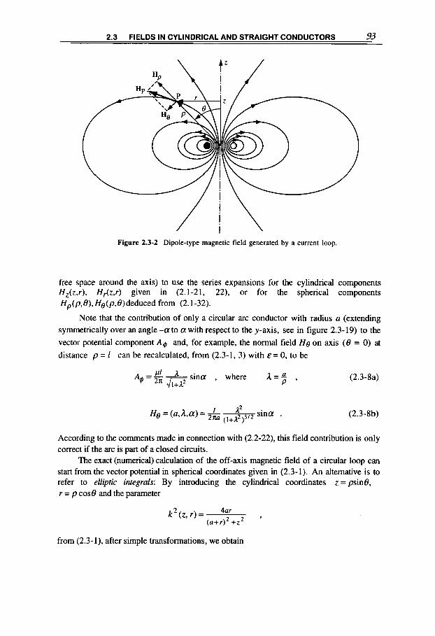
2.3 FIELDS IN CYLINDRICAL AND STRAIGHT CONDUCTORS 93
\ /
2.3 FIELDS IN CYLINDRICAL AND STRAIGHT CONDUCTORS 93
Figure 2.3-2 Dipole-type magnetic field generated by a current loop.
free space around the axis) to use the series expansions for the cylindrical components HZ(z,r) , H,.(z,r) given in (2.1-21, 22), or for the spherical components Hp (p, 6), He (p. 6') deduced from (2.1-32).
Note that the contribution of only a circular arc conductor with radius a (extending symmetrically over an angle -a to a with respect to the y-axis, see in figure 2.3- 19) to the vector potential component A4 and, for example, the normal field He on axis (6' = 0) at distance p = I can be recalculated, from (2.3-1, 3) with E = 0, to be
A - '' A sina , where A=" (2.3-8a) @ - E m P '
(2.3-8b)
According to the comments made in connection with (2.2-22), this field contribution is only correct if the arc is part of a closed circuits.
The exact (numerical) calculation of the off-axis magnetic field of a circular loop can start from the vector potential in spherical coordinates given in (2.3-1). An alternative is to refer to elliptic integrals: By introducing the cylindrical coordinates z = p i n e , r = p cose and the parameter
2 4ar k ( z , r ) = ( a + r ) 2 + z 2 '
from (2.3-1). after simple transformations, we obtain

94 CHAPTER 2 MAGNETIC POTENTIALS
(2.3-9)
where X X - - 2 2
K(k) = I( 1 - k2sin2y)-'I2 d y , E(k)= 1(1-k2sin2y)1'2dy , (2.3-10)
are the complete ellbtic integrals of the first and second kind, whose tabulated values and functional properties are well known and published.A" After differentiation of (2.3-9) and some rearrangement, the magnetic field components are obtained:
0 0
(2.3-1 1)
For small values of k (that is, r u a or r u a) the expansions
hold.A.' On axis (r+O. k+O). the result (2.3-7) is confirmed. In conclusion, the off-axis magnetic field of a filamentary circular current loop can be
found through the exact solution (2.3-11) by using the tabulated values for the elliptic integrakA3 In certain situations, it can be more convenient to take advantage of the approximations (2.3-4, 5) or expansions (2.1-21, 22), with the field on-axis being given by (2.3-7). Finally, there are tables that provide the field distribution as a function of normalized loop ~ararneters.'.~
Multiloop system
By adding one or more coaxial current ~ o p s to the original one, the axial magnetic field can be modified according to special requirements. A powerful method of analysis is to expand the magnetic potential that results from the m a y of loops in spherical harmonics, similarly as with the multipole expansion in (2.2-42).2.25 In the following, instead, we will take advantage of the single loop results obtained above.
Coil pair
In the case of a symmetric coil pair (figure 2.3-3), the sum of the axial fields (2.3-7) gives
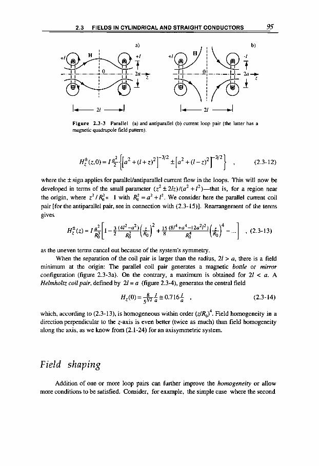
2.3 FIELDS IN CYLINDRICAL AND STRAIGHT CONDUCTORS 95
Figure 2.3-3 Parallel (a) and antiparallel (b) current loop pair (the latter has a magnetic quadruple field pattern).
where the k sign applies for paralleVantiparalle1 current flow in the loops. This will now be developed in terms of the small parameter (z2 f21z)l(a2 +12)-that is, for a region near the origin, where z2 / %<< 1 with % = u2 + 1 2 . We consider here the parallel current coil pair [for the antiparallel pair, see in connection with (2.3-15)]. Rearrangement of the terms gives
as the uneven terms cancel out because of the system's symmetry. When the separation of the coil pair is larger than the radius, 21 > a, there is a field
minimum at the origin: The parallel coil pair generates a magnetic bottle or mirror configuration (figure 2.3-3a). On the contrary, a maximum is obtained for 21 c a. A Helmholtz coil pair, defined by 21 = a (figure 2.3-4), generates the central field
H z ( 0 ) = &! z 0.716i , (2.3-14)
which, according to (2.3-13), is homogeneous within order (~4,)~. Field homogeneity in a direction perpendicular to the z-axis is even better (twice as much) than field homogeneity along the axis, as we know from (2.1-24) for an axisymmetric system.
Field shaping Addition of one or more loop pairs can further improve the homogeneify or allow
more conditions to be satisfied. Consider, for example, the simple case where the second
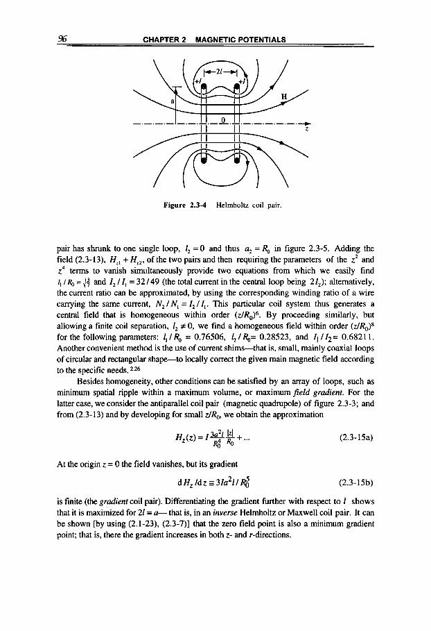
96 CHAPTER 2 MAGNETIC POTENTIALS
Figure 2.3-4 Helmholtz coil pair.
pair has shrunk to one single loop, l2 = 0 and thus a2 = R,, in figure 2.3-5. Adding the field (2.3-13), Hi, + Hz,, of the two pairs and then requiring the parameters of the z2 and z4 terms to vanish simultaneously provide two equations from which we easily find I, I R,, = 44 and I2 I I, = 32 I 49 (the total current in the central loop being 24); alternatively, the current ratio can be approximated, by using the corresponding winding ratio of a wire carrying the same current, N, I N, = I, I I,. This particular coil system thus generates a central field that is homogeneous within order ( Z / R ~ ) ~ . By proceeding similarly, but allowing a finite coil separation, 1, # 0, we find a homogeneous field within order (zlR0)* for the following parameters: 1, I = 0.76506, l2 I R,,= 0.28523, and I , I I,= 0.682 1 1. Another convenient method is the use of current shims-that is, small, mainly coaxial loops of circular and rectangular shape-to locally correct the given main magnetic field according to the specific needs. 2.26
Besides homogeneity, other conditions can be satisfied by an array of loops, such as minimum spatial ripple within a maximum volume, or maximum field gradient. For the latter case, we consider the antiparallel coil pair (magnetic quadrupole) of figure 2.3-3; and from (2.3-13) and by developing for small dR0, we obtain the approximation
Hz(z) = ... & “ R o
(2.3-15a)
At the origin z = 0 the field vanishes, but its gradient
d Hz Idz E 3h21 I @ (2.3-15b)
is finite (the gradient coil pair). Differentiating the gradient further with respect to I shows that it is maximized for 21 = a- that is, in an inverse Helmholtz or Maxwell coil pair. It can be shown [by using (2.1-23), (2.3-7)] that the zero field point is also a minimum gradient point; that is, there the gradient increases in both z- and r-directions.
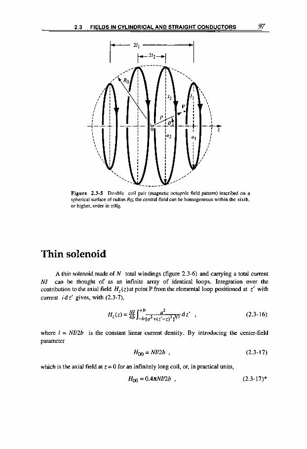
2.3 FIELDS IN CYLINDRICAL AND STRAIGHT CONDUCTORS 97
Figure 2.3-5 Double coil pair (magnetic octupole field pattern) inscribed on a spherical surface of radius Ro; the central field can be homogeneous within the sixth, or higher, order in dRo.
Thin solenoid
A thin solenoid made of N total windings (figure 2.3-6) and carrying a total current NI can be thought of as an infinite array of identical loops. Integration over the contribution to the axial field Hz(z)at point P from the elemental loop positioned at z’ with current idz‘ gives, with (2.3-7),
where i = Nll2b is the constant linear current density. By introducing the center-field parameter
Hm = Nll2b , (2.3-17)
which is the axial field at z = 0 for an infinitely long coil, or, in practical units,
Hm = 0.4nNll2b , (2.3-17)*
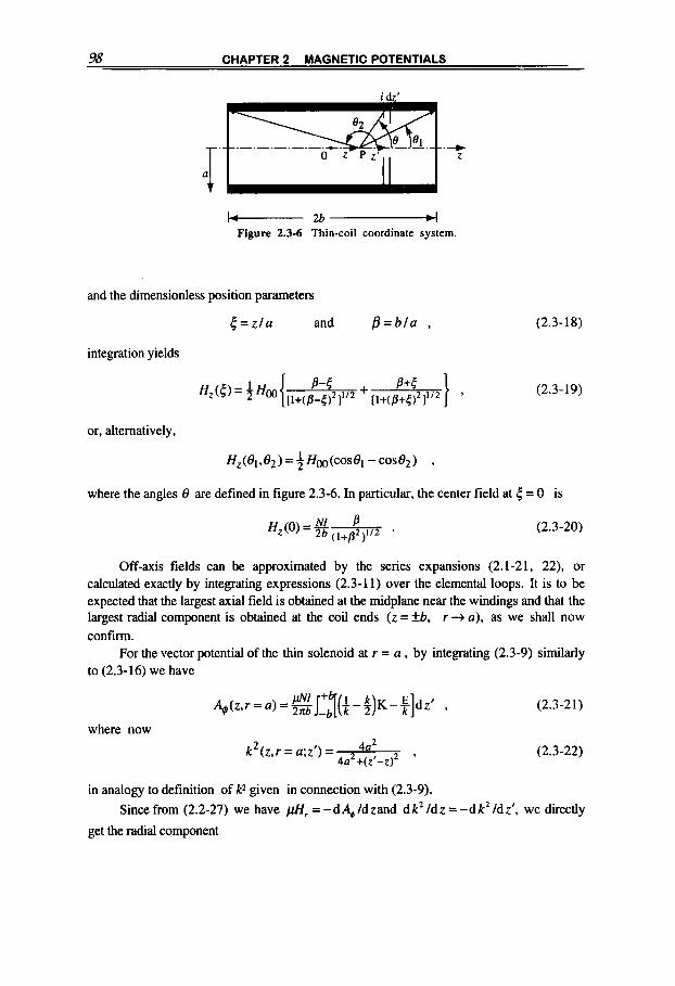
98 CHAPTER 2 MAGNETIC POTENTIALS
i dz’
. - 2 b h Figure 2.3-6 Thin-coil coordinate system.
and the dimensionless position parameters
t = z l a and P = b l a ,
integration yields
(2.3-18)
(2.3- 19)
or, alternatively,
H,(e,,e2)=+HOO(COSe, - c o s ~ ~ ) ,
where the angles 8 are defined in figure 2.3-6. In particular, the center field at 5 = 0 is
(2.3-20)
Off-axis fields can be approximated by the series expansions (2.1-21, 22), or calculated exactly by integrating expressions (2.3- 11) over the elemental loops. It is to be expected that the largest axial field is obtained at the midplane near the windings and that the largest radial component is obtained at the coil ends (z = fb, r + a), as we shall now confirm.
For the vector potential of the thin solenoid at r = a , by integrating (2.3-9) similarly to (2.3-16) we have
(2.3-21)
where now
(2.3-22) k 2 ( z , r = ax’) = 4a2 4a2+(z’-z)* ’
in analogy to definition of k* given in connection with (2.3-9).
get the radial component
Since from (2.2-27) we have pH, =-dA,ldzand dk21dz=-dk21dz’, we directly

2.3 FIELDS IN CYLINDRICAL AND STRAIGHT CONDUCTORS 99
k=k+(z'=b)
k=k- ( 2' =- 6 ) (2.3-23)
which can be determined for any z value with the help of the K and E elliptic integral tablesA.'. We explore the field behavior near the end of the coil, at r = a and z = b + 2 a ~ where E is a small number, and obtain from (2.3-22) with f l = b/a
k - ( z , r=a; z '= -b )=- 1 1+p2 .
When c2 cc 1 , and since
K ~ l n 4 - ~ l n ( l - k 2 ), E g l ,
2 for k z 1 up to order (1 - k ), the approximation
H,(z = b + 2 a ~ , r = a) z &[-In€ - C]
is obtained from (2.3-23). where C(k-)is the contribution from k = k- which vanishes for a very long coil, f l ~ 1, k- z 0 [as obtained from the approximations given in connection with (2.3-1 111. In this extreme case, H , diverges around the coil ends, as one would have expected.
0.5 0 0.5 I 1 .o
b
Figure 2.3-7 Current distribution in an idealized single-turn solenoid.

100 CHAPTER 2 MAGNETIC POTENTIALS
In a single-turn solenoid (made of one conducting sheet), the linear current distribution i(z) will establish itself by interaction with the field and in accordance with the geometry and conductivity of the conductor. Let us consider an ideal (superconducting) thin solenoid, which again can be considered to be an array of filamentary loops, each carrying a current i(z)dz, where i(z) is not constant but must be determined. This problem can be solved by considering the vector potential with the appropriate boundary condition or, more simply, by using the loop formulae (2.3-1 1). In fact, the contribution to the radial field H,. at the point (z,r = a), due to the infinitesimal loop located in the plane z’, can be written as
d H,(z - z’,a) = f (z - z’,a)i(z’)d z‘ , (2.3-24)
wheref(z - z’,Q) is clearly determined from (2.3-1 1). The boundary condition requires H,. = 0 all along the solenoid; that is, the integral equation
+b j -b f (~ -z ’ , a ) i (z‘)dz’=O (2.3-25)
determines the unknown i(z). The numerically calculated re~ult~.~’is shown in figure 2.3-7. The current density diverges at the end point as (b* -~~) -~ /* . This case is an example of the general problem of field behavior around sharp comers of (superconducting) conductors.’.“
Thick solenoid
After the filamentary loop and the thin sc-:noid, the next logical extension is the thic c cylindrical solenoid (figure 2.3-8). We assume that the azimuthal current is characterized by the mean constant-current density 8, where j is related to the cross section 1 of each of the N total windings and f is the filling factor defined as
f = conductor vol. - NE coil volume 2b(a2-al) . (2.3-26)
We start by looking for the general case-hat is, the off-axis magnetic field. Consider the vector potential A = (Ax,A,,,Az), (2.2-21), in Cartesian coordinates. We know that in this axisymmetric case, it will have only the azimuthal component A$, which
in the system of figure 2.3-8 (where P lies in the y = 0 plane- that is, the plane including the x,z-axes) is identical to its component A,,:
(2.3-27)
with
jy = jcosip

2.3 FIELDS IN CYLINDRICAL AND STRAIGHT CONDUCTORS 101
Figure 2.3-8 Vector potential for a thick, axisymmetric coil at point P in the y = 0 plane (for practical reasons, the decomposition of the current density j'4 flowing at point Q is made in the z = 0 plane of the drawing).
and
which is determined through the triangle PP'Q. The solution is
with the magnetic field components (2.2-27)

102 CHAPTER 2 MAGNETIC POTENTIALS
For a general discussion of these analytic results we refer to the l i t e r a t ~ r e . ~ . ' ~ ~ ~ . ~ ~ Nowadays, numeric integration of this result is relatively straightforward; care must
be taken near the axis ( r + 0), where it might be better to use approximations of the type shown in (2.1-21,22). If a computer is unavailable'or when the fields have to be calculated only in a few points, it might be convenient to use tabulated fields given as a function of the dimensionless parameters r l a , and la,.^.'^ In fact, figure 2.3-9 makes it clear that any regular solenoid with constant current density can be considered the resultant superposition (with appropriate signs) of four semi-infinite solenoids with zero inner radius (al + 0, b + -). We see from (2.3-29.30) that the normalized fields for each such coil,
(2.3-3 1)
depend only on the dimensionless parameters r lu , and z l a , and can thus be tabulated conveniently.
The on-axis field component, Hz(P) , can be obtained by extending, as before, the loop or thin solenoid expressions (2.3-7, or 16), or by calculation from the general result (2.3-30) with r + 0. The latter, however, needs some tedious transformations, using partial integrations to avoid singularities. We prefer to return to the original integral (2.2- 22) and write the axial field component at point P as (figure 2.3-10)
I
+ Z
- - - . - . - . - . I I I I
2b _+I
Figure 2.3-9 Rectangular coil with constant current density as superposition of four semi-infinite coils with zero inner radius.
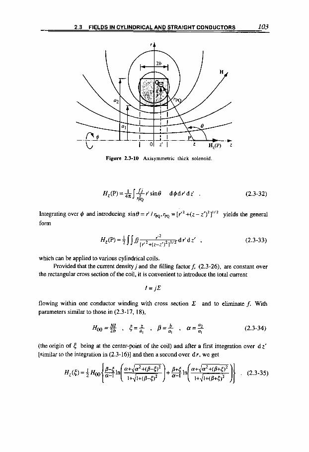
2.3 FIELDS IN CYLINDRICAL AND STRAIGHT CONDUCTORS 103
Figure 2.3-10 Axisymmetric thick solenoid.
H z ( P ) = L j q r ' s i n O dGdr'dz' . (2.3-32) 'pa
4r
Integrating over 4 and introducing sin0 = I' lrw.rw = [r'* +(z - z t ) 2 ] 112 yields the general
form
, 3,2 dr 'dz' , (2.3-33) HAP) = 3jsqrJ+(z-z r' 2 ) J
which can be applied to various cylindrical coils.
the rectangular cross section of the coil, it is convenient to introduce the total current Provided that the current densityj and the filling factorf. (2.3-26), are constant over
flowing within one conductor winding with cross section Z and to eliminate f. With parameters similar to those in (2.3-17, 18),
(the origin of { being at the center-point of the coil) and after a first integration over dz' [similar to the integration in (2.3-16)] and then a second over d r , we get

104 CHAPTER 2 MAGNETIC POTENTIALS
In particular, the center field at 4 = 0 is
(2.3 -3 6)
This expression can be simplified for various limiting cases. For example, for a thin disk coil, where p (( 1, it reduces (for uniform current density) to
H,(O) = H m a l n a P (2.3-37)
Bitter solenoid
Instead of the multiturn arrangement considered so far, a thick solenoid can be made from sheet windings or conducting disks. The disk magnets were introduced by Bitte?.* and are particularly suitable as high-field generators because they are mechanically strong and easy to cool (figure 2.3-1 1).
The steady-state, resistively determined current distribution within a disk is described by the nonuniform radial dependence
j = j , T 01 , (2.3-38)
2b I+
Figure 2.3-11 (a) Bitter magnet made of a stack of conducting disks; in practice, the stack can be obtained from machining along a helical pattern from a solid thick solenoid [schematically shown in (b)], or the single disks are cut open along a radius and connected to adjacent disks as indicated in (c).
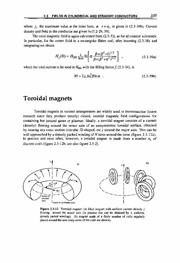
2.3 FIELDS IN CYLINDRICAL AND STRAIGHT CONDUCTORS 105
where j , , the maximum value at the inner bore, at r = a, , is given in (2.3-39b). Current density and field in the conductor are given in (7.2-29,30).
The axial magnetic field is again calculated from (2.3-33), as for all coaxial solenoids. In particular, for the center field in a rectangular Bitter coil, after inserting (2.3-38) and integratingwe obtain
(2.3-39a)
where the total current to be used in Hm with the filling factorf, (2.3-34), is
NI = 2jIfafplncu . (2.3-39b)
Toroidal magnets
Toroidal magnets in various arrangements are widely used in thermonuclear fusion research since they produce (nearly) closed, toroidal magnetic field configurations for containing hot ionized gases or plasmas. Ideally, a toroidal magnet consists of a current (density) flowing around the minor axis of an axisymmetric toroidal surface, obtained by rotating any cross section (circular, D-shaped, etc.) around the major axis. This can be well approached by a densely packed winding of N turns around the torus (figure 2.3- 12a). In practice and most often, however, a toroidal magnet is made from a number n, of discrete coils (figure 2.3-12b; see also figure 2.5-2).
a) I I _
I malor or s yrnmetry axis I
Figure 2.3-12 Toroidal magnet: (a) Ideal magnet with uniform current density j flowing around the minor axis (in practice this can be obtained by a uniform, densely packed winding); (b) magnet made of a finite number of coils regularly placed around the axis (only some o f the coils are shown).
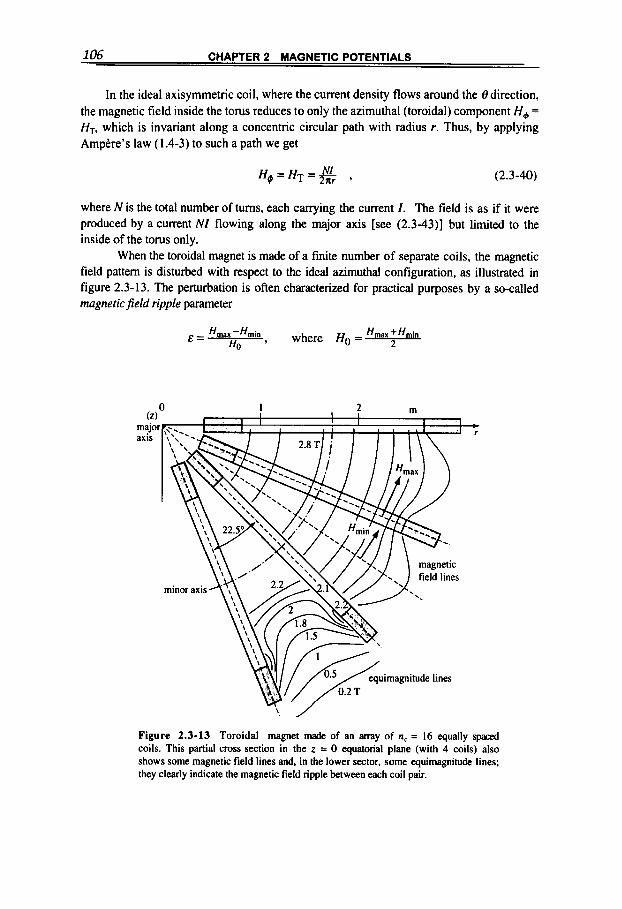
106 CHAPTER 2 MAGNETIC POTENTIALS
In the ideal axisymmetric coil, where the current density flows around the 8 direction, the magnetic field inside the torus reduces to only the azimuthal (toroidal) component H+ =
HT, which is invariant along a concentric circular path with radius r . Thus, by applying Ampere’s law (1.4-3) to such a path we get
where N is the total number of turns, each canying the current I. The field is as if it were produced by a current NI flowing along the major axis [see (2.3-43)] but limited to the inside of the torus only.
When the toroidal magnet is made of a finite number of separate coils, the magnetic field pattern is disturbed with respect to the ideal azimuthal configuration, as illustrated in figure 2.3-13. The perturbation is often characterized for practical purposes by a so-called magnetic field ripple parameter
H ax+Hmin where HO = ” Hmx -Hmin Ho ’ E =
majoi axis
-D r
Figure 2.3-13 Toroidal magnet made of an may of n, = 16 equally spaced coils. This partial cross section in the z = 0 equatorial plane (with 4 coils) also shows some magnetic field lines and, in the lower sector, some equimagnitude lines; they clearly indicate the magnetic field ripple between each coil pair.
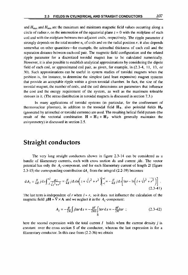
2.3 FIELDS IN CYLINDRICAL AND STRAIGHT CONDUCTORS 107
and H,,, and H,,,, are the maximum and minimum magnetic field values occurring along a circle of radius r, on the intersection of the equatorial plane z = 0 with the midplane of each coil and with the midplane between two adjacent coils, respectively. The ripple parameter E
strongly depends on the total number n, of coils and on the radial position r; it also depends somewhat on other quantities-for example, the azimuthal thickness of each coil and the separation distance between each coil pair. The magnetic field configuration and the related ripple parameter for a discretized toroidal magnet has to be calculated numerically. However, i t is also possible to establish analytical approximations by considering the dipole field of each coil, or approximated coil pair, as given, for example, in (2.3-4, 11, 13, or 30). Such approximations can be useful in system studies of toroidal magnets when the problem is, for instance, to determine the simplest (and least expensive) magnet systems that provide an acceptable ripple within a given toroidal chamber. In fact, the size of the toroidal magnet, the number of coils, and the coil dimensions are parameters that influence the cost and the energy requirement of the system, as well as the maximum tolerable stresses in it. (The stress distribution in toroidal magnets is discussed in section 7.3.)
In many applications of toroidal systems (in particular, for the confinement of thermonuclear plasmas), in addition to the toroidal field HT, also poloidal fields HP (generated by azimuthal or toroidal currents) are used. The resulting helical field pattern (the result of the vectorial combination H = H T + H P which generally maintains the axisymmetry) is discussed in section 2.5.
Straight conductors
The very long straight conductors shown in figure 2.3-14 can be considered as a bundle of filamentary currents, each with cross section ds and current jds. The vector potential has only the A,-component, and for each filamentary current of length 21 (figure 2.3- 15) the corresponding contribution dA: from the integral (2.2-39) becomes
dA, = & j d s j -/=-- +' d z - d l , j d ~ l n ( z + ~ r 2 + r ? ) ~ ~ ~ = - & j d s [ l n r - l n ( l + ~ ) ] .
(2.3-41)
The last term is independent of r when 1 )) r, so i t does not influence the calculation of the magnetic field pH = V x A and we neglect it in the A,-component:
P i A, = -61 j lnrds = -- 2% lnrds = --lnr 2rr: ; S
(2.3-42)
here the second expression with the total current I holds when the current density j is constant over the cross section S of the conductor, whereas the last expression is for a filamentary conductor. In this case from (2.2-36) we obtain

108 CHAPTER 2 MAGNETIC POTENTIALS
Figure 2 .3 - 14 (a) Cross sections of a rectangular bar 'with current flowing uniformingly along the positive z-axis towards the reader, and (b) the related isomagnetic lines.
which is the azimuthal magnetic field (2.1-37b) outside a very long cylindrical conductor.
conductor extending symmetrically from -1 to +f (figure 2.3-15) When the limit 1 B r does not apply, we obtain from (2.3-41) for a filamentary
A = @In[ + p] = g[ -In1 + In( 1 + d z ) ] , where 1 = f (2.3-44) z 2A 2
( r being the radial distance from the conductor), with the azimuthal field at point P of
(2.3-45)
More in general, we will show in (9.2-4) that the contribution to the azimuthal field H4,,2 at point P of a straight section defined by the vectors rl,r2 (figure 2.3-15) amounts
to (2.3-46a) - I ClX'2 r2+r, .
' ~ 2 - 4n rzr, r.r,+q.r. 9
that is,
In particular, the contribution of a conductor extending from points 0 to 1 is [compare with (2.3-45)]
(2.3-46~)

2.3 FIELDS IN CYLINDRICAL AND STRAIGHT CONDUCTORS 109
O1 P I2
+ Z
A 2 p 101 4 2
Z
I I 102 *
I I I - t
Figure 2.3-15 Straight, long filamentary current.
with which we can also write
H4,12 = H@,Q2 - H&Ol ’
Example: Rectangular bar conductor The vector potential component (2.3-42) for the rectangular straight conductor shown in figure
2.3-14a is
112 u b
-u -b A,(x.y)=-&& I jln[x’-x)2 + ( y ’ - ~ ) ~ ] dx’dy’ . (2.3-47)
which can be integrated to give2 ’ A, = -&{(a - x)(b- y)ln[(a - x)’ + (b - Y ) ~ ] + (a +x)(b - y)ln[(a + x ) ~ + (b - Y ) ~ ]
+(a-x)(b+y)ln[(a-x)2 + ( b + ~ ) ’ ] + ( a + x ) ( b + y ) l n [ ( a + x ) ~ +(b+y)’] (2.3-48)
arc tan 2 +arc tan 21
b-y b+Y I1 +(b - Y ) ~ [ arc tan f$ + arc tan -1 + (b + y)’[arc tan + arc tan (1+x .
The magnetic field components are calculated from = V x A with table A.3-11,
After differentiation of the above result and then defining the boundary comer by the polar coordinates
(figure 2.3-14a) such that
In[(a - x)’ + (b - y)’] = 21nr4, .... arc tan b-y = &,, ..., a-x
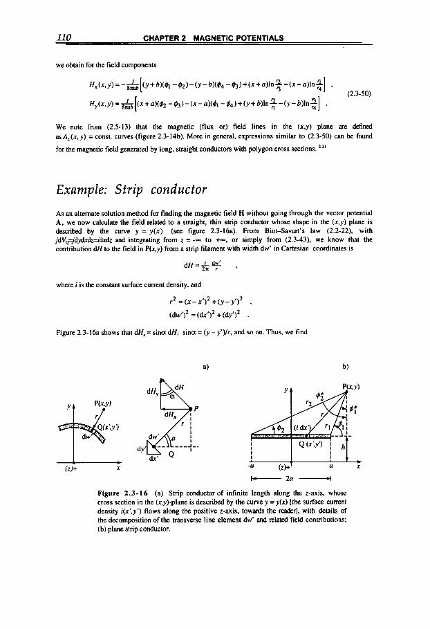
110 CHAPTER 2 MAGNETIC POTENTIALS
we obtain for the field components
We note from (2.5-13) that the magnetic (flux or) field lines in the (x,y) plane are defined asAz(x,y) = const. curves (figure 2.3-14b). More in general, expressions similar to (2.3-50) can be found
for the magnetic field generated by long, straight conductors with polygon cross sections. ’”
Example: S t r i p conductor As an alternate solution method for finding the magnetic field H without going through the vector potential A , we now calculate the field related to a straight, thin strip conductor whose shape in the (x,y) plane is described by the curve y = y(x) (see figure 2.3-16a). From Biot-Savart’s law (2.2-22). with jdVejdybidz=idrdz and integrating from z = -- to +m, or simply from (2.3-43), we know that the contribution dH to the field in P(x,y) from a strip filament with width dw’ in Cartesian coordinates is
where i is the constant surface current density, and
r z = ( x - x * ) ~ +(y-y’)’ ,
(dw’)* = (cLx’)~ +(dy’)2 .
Figure 2.3-16a shows that dH,= sina dH, sina = (y - y’)/r, and so on. Thus, we find
a)
I I 1 I L
+ 2a - Figure 2.3-16 (a) Strip conductor of infinite length along the z-axis, whose cross section in the (x,y)-plane is described by the curve y = y(x) [the surface current density i(x’,y’) flows along the positive z-axis, towards the reader], with details of the decomposition of the transverse line element dw’ and related field contributions; (b) plane strip conductor.
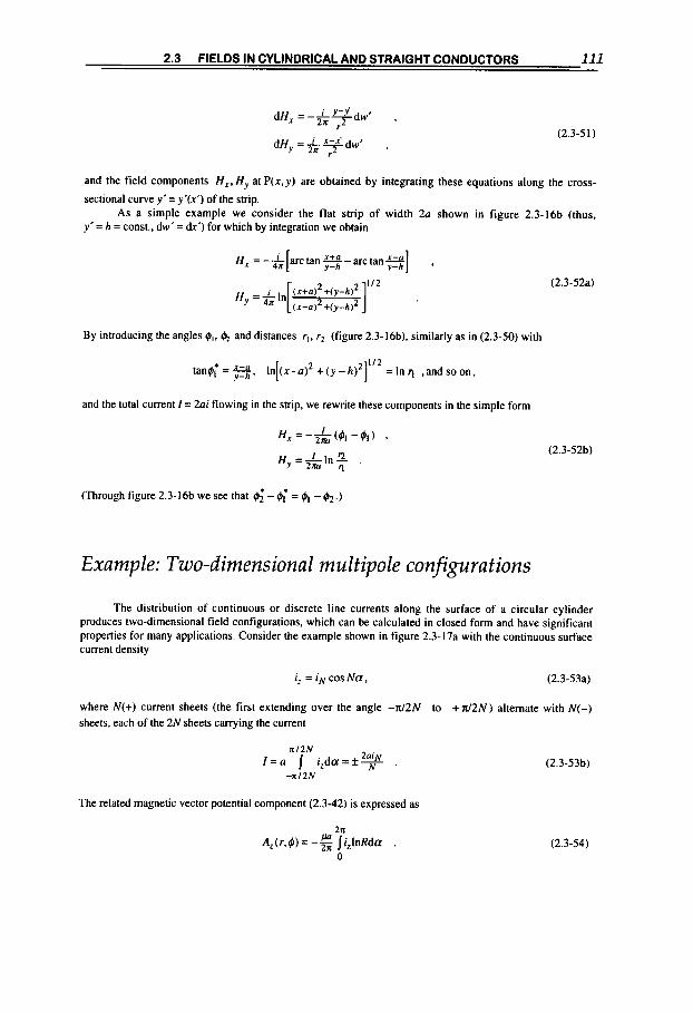
2.3 FIELDS IN CYLINDRICAL AND STRAIGHT CONDUCTORS 111
(2.3-51)
and the field components H,. H y at P(x,y) are obtained by integrating these equations along the cross-
sectional curve y' = y'(x') of the strip. As a simple example we consider the flat strip of width 2a shown in figure 2.3-16b (thus,
y' = h = const., dw' = dr') for which by integration we obtain
H y =&In (x+o)* + ( y - h ) 2
( + - o ) 2 + ( y - h ) 2
By introducing the angles $,, & and distances r,. r, (figure 2.3-16b). similarly as in (2.3-50) with
1 / 2 tan$; =-, Y-h I n [ ( x - a ) 2 + ( y - h ) 2 ] = I n 4 ,andsoon,
and the total current I = 2ni flowing in the sfrip, we rewrite these components in the simple form
(2.3-52a)
(2.3-52b)
(Through figure 2.3-16b we see that $; - 4; = $1 - $ 2 . )
Example: Two-dimensional multipole configurations
The distribution of continuous or discrete line currents along the surface of a circular cylinder produces two-dimensional field configurations, which can be calculated in closed form and have significant properties for many applications. Consider the example shown in figure 2.3-17a with the continuous surface current density
iz = iN cos N a , (2.3-53a)
where N(+) current sheets (the first extending over the angle -W2N to +W2N) alternate with N(-) sheets, each of the 2N sheets carrying the current
2 a i ~ n 1 2 N
-n12N I = a i , d c r = f T .
The related magnetic vector potential component (2.3-42) is expressed as
(2.3-53b)
(2.3-54)
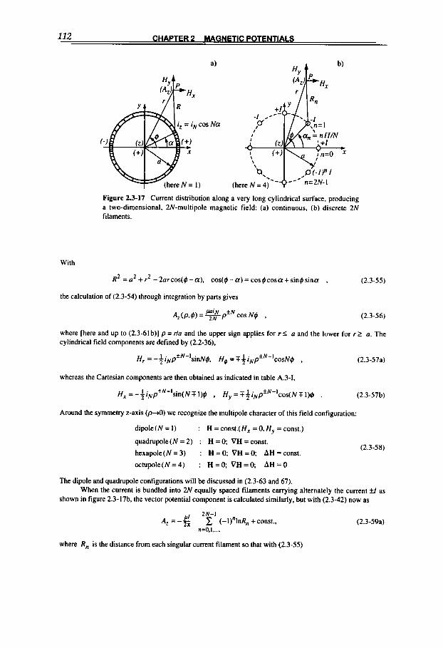
112 CHAPTER 2 MAGNETIC POTENTIALS
Na
Figure 2.3-17 Current distribution along a very long cylindrical surface, producing a two-dimensional, 2N-multipole magnetic field: (a) continuous, (b) discrete 2N filaments.
With
R' = a 2 + r 2 -2arcos(#-a), cos(@-a)=cos#cosa+s in#s ina , (2.3-55)
the calculation of (2.3-54) through integration by parts gives
A,(p.@) = +pfN cos Nq , (2.3-56)
where [here and up to (2.3-61 b)] p = rla and the upper sign applies for r I a and the lower for r t a. The cylindrical field components are defined by (2.2-36).
H , =-+iNpiN- ' s i~4 , H# =r+iNpiN-'cos,v# , (2.3-57a)
whereas the Cartesian components are then obtained as indicated in table A.3-I.
H , = -+iNpfN-'sin(NT I)# , H , = T+iNp"-'cos(Nr I)@ . (2.3-57 b)
Around the symmetry z-axis ( p 4 ) we recognize the multipole character of this field configuration:
dipole(N = I ) : H = const.( H , = 0, H y = const.)
quadrupole(N = 2) : H = 0; VH = const.
hexapole(N = 3) : H = 0 VH = 0 AH = const.
octupole(N=4) : €I=& V H = 0 A H = O
(2.3-58)
The dipole and quadrupole configurations will be discussed in (2.3-63 and 67).
shown in figure 2.3-17b, the vector potential component is calculated similarly, but with (2.3-42) now as When the current is bundled into 2N equally spaced filaments carrying alternately the current fl as
2N-1
n=0.1. ..., A =-& 2n C ( - I )"I~R, +const., (2.3-59a)
where R, is the distance from each singular current filament so that with (2.3-55)

2.3 FIELDS IN CYLINDRICAL AND STRAIGHT CONDUCTORS 1U
21nRn = I n ( l + p 2 ) + l n (2.3-59b)
For the calculation of the summation at r l a use repeatedly the expansion In( I f z ) = * z - ?/2 f z3/3 - z4/4+.. .valid for z < 1 ; the final result is
+ const. I -pzN - 2 p N cosNq9 1 (2.3-60)
Note that this expression and (2.3-61a) are valid at r 2 a as well as r 5 a, since they do not change when substituting p with Ilp.
The cylindrical field components are calculated again from (2.2-36)
(2.3-61a)
In first-order approximation by neglecting peN z 0 , we obtain
where again the upper sign applies for r < a and the lower for r > a . Around the symmetry axis ( p = r/a+O) we find the multipole pattern (2.3-58). whereas at large distances @ = r/a >> 1) the multipole field decreases as l/p'.
Magnetic fields resulting from other current distributions along the circular cylinder surface have been calculated-for example, the filamentary arrangement of figure 2.3-17b but with all currents flowing in the same direction'", or the 2N equally spaced sheet conductors' ' 2 that represent an azimuthal extension of the filamentary conductors in figure 2.3- 17b. The magnetic fields of toroidal multipole configurations have also been presented as closed analytic expressions. * '4
In this type of problem, it is often convenient to use series expansion for the current distribution. The solutions for the vector potential and the field components are then also in the form of infinite series.223 In addition, the calculation of two-dimenionsional magnetic fields with complex variables and functions (as introduced in section 3.1) is often particularly
Figure 23-18 Uniform magnetic fields in relatively large volumes can be produced by a pair of long racetrack coils. It is, however, convenient to bend the ends along the surface of a cylinder to have optimal access to the uniform field-hence the name saddle-shaped.

114 CHAPTER 2 MAGNETIC POTENTIALS
Saddle-shaped coils
Saddle-shaped coils are used to produce uniform, transverse magnetic fields over a relatively large and long volume (figure 2.3-18), as, for instance, required in particle accelerators for bending charged particle beams. We first discuss a filamentary coil with finite length and then analyze the two-dimensional field pattern produced by filamentary, sheet, and bulk straight conductors.
Short filamentary coil
The saddle-shaped coil shown in figure 2.3-19 consists of two identical filamentary conductors wound on the surface of a circular cylinder with radius a and length 21. The field anywhere in space may be calculated by applying the Biot-Savart law (2.2-38, 39). At the center of the coil (and of the coordinate system) it consists (because of symmetry) only of the vertical H@-component, which is
(2.3-62)
The first term comes from the four straight sections [each contributes a component HI sina; see (2.3-45)], and the second term comes from the four circular arcs extending over the arc 2 a [see (2.3-8)].
Figure 2.3-19 Filamentary saddle-shaped coil producing a dipole-type magnetic field. [In the cross section, the (+) sign means, as always, that the quantity pointslflows out of the page towards the reader; the opposite applies for the (-) sign.]

2.3 FIELDS IN CYLINDRICAL AND STRAIGHT CONDUCTORS 115
The position and extension of all the arcs and straight sections contribute to the homogeneity of the central field. This can be analyzed similarly to the loop pair conductors discussed in connection with (2.3-15). For example, it can be that good homogeneity (where all second derivatives of H,, with respect to the coordinates x,y,z vanish) can be obtained with A = 0.5 and 2 a = 120'.
Long coils
We now consider very long straight conductor arrangements, where the contributions of the connecting ends becomes negligible. The question here is: Are there any conductor arrangements (that is, current distributions) that provide uniform, purely transverse magnetic fields in such two-dimensional configurations? The answer is yes; in fact we have already found them. For the dipole current sheet with N = 1 in figure 2.3-17a, from (2.3-57) we find a homogeneous field within the whole cylindrical space r l a :
H x = O , H y = - i l / 2 = 1 / 4 a , (2.3-63)
where I is the total current carried in the sheet in the (+) direction, as well as in the (-) direction. The same applies for the filamentary current with N = 1 in figure 2.3-17b, but limited to a small space around the symmetry axis, where from (2.3-61b) we obtain
H , = O , H , ~ - N l l n ~ l . (2.3-64)
k S 4
Figure 2.3-20 Two overlapping cylindrical conductors carrying the opposite, uniform current density j , = -j2 for the production of a uniform magnetic field H,. In the overlapping region the currents cancel out, so we can consider this a conductor- free aperture.
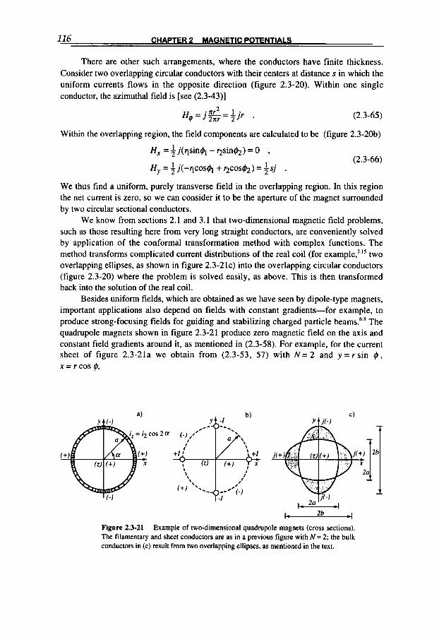
116 CHAPTER 2 MAGNETIC POTENTIALS
There are other such arrangements, where the conductors have finite thickness. Consider two overlapping circular conductors with their centers at distance s in which the uniform currents flows in the opposite direction (figure 2.3-20). Within one single conductor, the azimuthal field is [see (2.3-43)]
(2.3-65)
Within the overlapping region, the field components are calculated to be (figure 2.3-20b)
(2.3-66)
We thus find a uniform, purely transverse field in the overlapping region. In this region the net current is zero, so we can consider it to be the aperture of the magnet surrounded by two circular sectional conductors.
We know from sections 2.1 and 3.1 that two-dimensional magnetic field problems, such as those resulting here from very long straight conductors, are conveniently solved by application of the conformal transformation method with complex functions. The method transforms complicated current distributions of the real coil (for example,2 '' two overlapping ellipses, as shown in figure 2.3-21c) into the overlapping circular conductors (figure 2.3-20) where the problem is solved easily, as above. This is then transformed back into the solution of the real coil.
Besides uniform fields, which are obtained as we have seen by dipole-type magnets, important applications also depend on fields with constant gradients-for example, to produce strong-focusing fields for guiding and stabilizing charged particle The quadrupole magnets shown in figure 2.3-21 produce zero magnetic field on the axis and constant field gradients around it, as mentioned in (2.3-58). For example, for the current sheet of figure 2.3-21a we obtain from (2.3-53, 57) with N = 2 and y = r s i n 4, x = r cos @,
b 26 4 Figure 2.3-21 Example of two-dimensional quadrupole magnets (cross sections). The filamentary and sheet conductors are as in a previous figure with N = 2; the bulk conductors in (c) result from two overlapping ellipses, as mentioned in the text.

2.4 INDUCTANCE OF CONDUCTORS 117
~ , = - 1 y / 2 a 2 , ~ ~ = - 1 1 / 2 a ? , (2.3-67)
which provide the properties just mentioned.
2.4 INDUCTANCE OF CONDUCTORS
The magnetic properties of a conductor system are conveniently expressed by the inductance parameter L, which (at least in steady conditions) is a purely geometric quantity. In this section, its relation with the magnetic field-and, in particular, with the magnetic flux-is established and its properties then illustrated with different examples.
Self -inductance
The magneticflux v / referred to a closed filamentary loop C subtending a surface S is defined in (2.2-3) as
v / = I B . d s = $ A . d l . (2.4-1) S C
When the flux refers instead to a finite closed conductor with volume V (figure 2.4-I), straightforward extension with the relation (2.2-37) yields
v / = f l A . j d V . V
(2.4-2)
Figure 2.4-1 Inductance of a closed conductor.
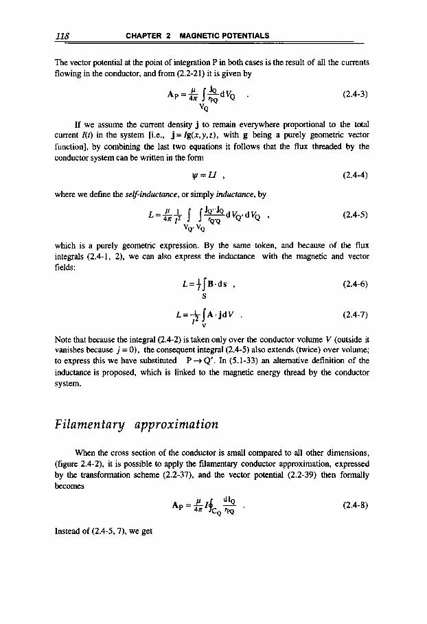
118 CHAPTER 2 MAGNETIC POTENTIALS
The vector potential at the point of integration P in both cases is the result of all the currents flowing in the conductor, and from (2.2-21) it is given by
(2.4-3)
If we assume the current density j to remain everywhere proportional to the total current Z(t) in the system [i.e., j = Zg(x,y,z), with g being a purely geometric vector function], by combining the last two equations it follows that the flux threaded by the conductor system can be written in the form
v = H . (2.4-4)
where we define the self-inductance, or simply inductance, by
(2.4-5)
which is a purely geometric expression. By the same token, and because of the flux integrals (2.4-1, 2), we can also express the inductance with the magnetic and vector fields:
L = f I B . d s , (2.4-6) S
L = + I A . j d V . (2.4-7) 1 .
Note that because the integral (2.4-2) is taken only over the conductor volume V (outside it vanishes because j = O), the consequent integral (2.4-5) also extends (twice) over volume; to express this we have substituted P + Q'. In (5.1-33) an alternative definition of the inductance is proposed, which is linked to the magnetic energy thread by the conductor system.
Filamentary approximation
When the cross section of the conductor is small compared to al l other dimensions, (figure 2.4-2), it is possible to apply the filamentary conductor approximation, expressed by the transformation scheme (2.2-37), and the vector potential (2.2-39) then formally becomes
Instead of (2.4-5,7), we get
(2.4-8)
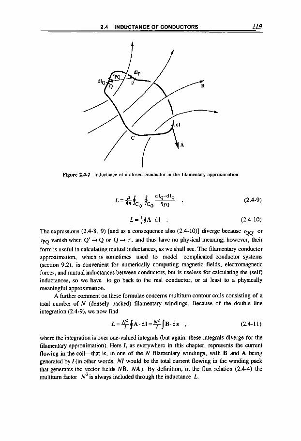
2.4 INDUCTANCE OF CONDUCTORS 119
Figure 2.4-2 Inductance of a closed conductor in the filamentary approximation.
L={fA.dl .
(2.4-9)
(2.4-10)
The expressions (2.4-8, 9) [and as a consequence also (2.4-lo)] diverge because rQQ, or ' p ~ vanish when Q' + Q or Q + P, and thus have no physical meaning; however, their
form is useful in calculating mutual inductances, as we shall see. The filamentary conductor approximation, which is sometimes used to model complicated conductor systems (section 9.2). is convenient for numerically computing magnetic fields, electromagnetic forces, and mutual inductances between conductors, but is useless for calculating the (self) inductances, so we have to go back to the real conductor, or at least to a physically meaningful approximation.
A further comment on these formulae concerns multitum contour coils consisting of a total number of N (densely packed) filamentary windings. Because of the double line integration (2.4-9), we now find
(2.4-1 1)
where the integration is over one-valued integrals (but again, these integrals diverge for the filamentary approximation). Here I, as everywhere in this chapter, represents the current flowing in the coil-that is, in one of the N filamentary windings, with B and A being generated by I (in other words, NI would be the total current flowing in the winding pack that generates the vector fields NB, NA). By definition, in the flux relation (2.4-4) the multitum factor N2 is always included through the inductance L.

120 CHAPTER 2 MAGNETIC POTENTIALS
In conductor systems where there are only surface currents, the formulae based on the filamentary approximation can also be very useful. The integration paths Cp, CQare
now any lines lying on the conductor surface and appropriately encircling it (figure 2.4-l), and by avoiding their intersection, one can eliminate any divergence in (2.4-9). [This follows directly by physics arguments but it can also be formally established by rewriting (2.4-5) into surface integrals with the transformation scheme used in connection with (2.3- 161.1
Faraday law The inductance represents a lumped parameter (in addition to the similar resistance
and capacitance parameters; see in connection with figure 4.5-1) that can be convenient for describing (inductive) circuit behavior. The inductance of a conductor system is also practical for expressing the magnetic energy linked to it, as we shall see in section 5 . 1 . Through the magnetic flux expression (2.4-4). it also provides a simple expression for Faraday's law (1.4-9): The emf, or induced voltage, in a closed (filamentary) circuit is
(2.4-12)
Example: Wire transmission line
As a simple example, we calculate the inductance of the parallel wire transmission line of figure 2.1-
7 in section 2.1. In the high-frequency limit (surface currents only), the flux linked to the system is
represented by the flux lines crossing the x-axis between the two wires, and we find, with (2.1-59).
After a simple transformation with
p 2 = $ d 2 - a 2 ,
we derive, for the inductance,
or in second-order approximation (when d d N 1)
(2.4- 13)
(2.4-14)
(2.4- 15)
~ = + l [ 1 n t - ( s ) 2 ] . (2.4-16)
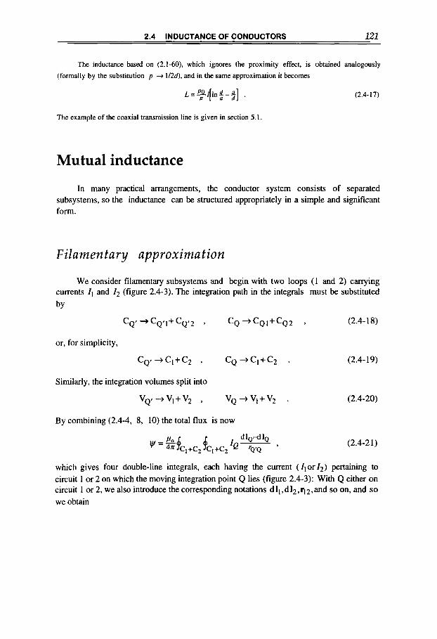
2.4 INDUCTANCE OF CONDUCTORS El
The inductance based on (2.1-60), which ignores the proximity effect, is obtained analogously (formally by the substitution p + 1/26), and in the same approximation it becomes
The example of the coaxial transmission line is given in section 5.1
Mutual inductance
In many practical arrangements, the conductor system consists of separated subsystems, so the inductance can be structured appropriately in a simple and significant form.
Filamentary approximation
We consider filamentary subsystems and begin with two loops (I and 2) carrying currents Il and I , (figure 2.4-3). The integration path in the integrals must be substituted
by
c Q ’ j c Q ’ I + c Q ’ 2 9 CQ + C Q l + c Q 2 9 (2.4-18)
or, for simplicity,
cQ’+cI+c2 , CQ+Cl+C2 . (2.4- 19)
Similarly, the integration volumes split into
vQ’+VI+v* , vQ+vl+v2 . (2.4-20)
By combining (2.4-4, 8, 10) the total flux is now
(2.4-21)
which gives four double-line integrals, each having the current ( I1or 12) pertaining to circuit 1 or 2 on which the moving integration point Q lies (figure 2.4-3): With Q either on circuit 1 or 2, we also introduce the corresponding notations dll,dl2,rl2,and so on, and so we obtain

l22 CHAPTER 2 MAGNETIC POTENTIALS
subsystem 2
QI
\ Figure 2.4-3 Mutual inductance between two loops
with
where bl = b2 = M is the so-called mutual inductance between the two circuits (often labeled with M); the (+) sign holds for currents Zl ,Z2 turning in the same direction, and the (-) sign holds for the opposite [the practical meaning of this will be explained in connection with (2.4-3 I)]. The self-inductance
and the analogous 4 2 form, which also results from (2.4-21), diverge, as we know from the comments on (2.4-lo), and in this form they have no physical meaning. Self- inductances can be calculated by referring to finite conductors or current distributions as expressed by (2.4-5, 6,7).
When the subsystems have 4 and N2 windings, respectively, by applying the reasoning relative to (2.4-1 l), the mutual inductance becomes
(2.4-25)
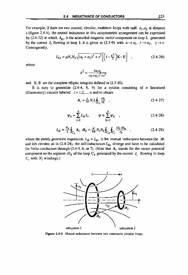
2.4 INDUCTANCE OF CONDUCTORS 123
For example, if there are two coaxial, circular, multitum loops with radii q , a 2 at distance s (figure 2.4-4), the mutual inductance in this axisymmetric arrangement can be expressed by (2.4-32) in which A#,I is the azimuthal magnetic vector component on loop 2, generated by the current I , flowing in loop 1; it is given in (2.3-9) with a + q, r + a 2 , z + s. Consequently,
L12 =pN1N2d/[(l-g)K-E] , (2.4-26)
where
and K, E are the complete elliptic integrals defined in (2.3-10).
(filamentary) circuits labeled i = 1,2, ..., n and to obtain It is easy to generalize (2.4-4, 8, 9) for a system consisting of n linearized
A, = L N . ~ . $ , 4n I I ci % qk ’ (2.4-27)
n n (2.4-28)
where the purely geometric expression Lik = Lki is the mutual inductance between the ith and kth circuits; as in (2.4-24), the self-inductances Lkk diverge and have to be calculated for finite conductors through (2.4-5,6, or 7). (Note that Ai stands for the vector potential component on the segment d 1, of the loop ck generated by the current I , flowing in loop Ci with Ni windings.)
I S
subsystem 1 ’ subsystem2
Figure 2.4-4 Mutual inductance between two concentric circular loops.

124 CHAPTER 2 MAGNETIC POTENTIALS
General expressions
The mutual inductance (2.4-7) between two not necessarily filamentary circuits with notation (2.4-23) is
(2.4-30)
When at least one (subsystem 2) is a filamentary conductor (figure 2.4-5) from (2.4-6, 10) we get, instead,
where S2 is a surface subtended by C2. The last expression shows that the mutual inductance between two conductor systems 1,2 (figure 2.4-3) is defined as the magnetic flux through circuit 2 produced by the unit current in system 1 (or vice versa). The (+) or (-) sign applies in (2.4-22) according to whether the flux integral is positive or negative, that is, whether or not the inducing flux in circuit 2 has the same sign as the one generated by its own current 12.
For an axisymmetric system (figure 2.4-5), where an azimuthal current distribution in subsystem 1 with total current 11 produces the azimuthal vector potential around loop 2 with radius a2, the simple form
4 2 = 2m2 %.I (2.4-32)
- ,
Figure 2.4-5 Mutual inductance of an axisymmetric conductor system, where at least subsystem 2 i s a filamentary circular loop.

2.5 STRUCTURE OF MAGNETIC FIELDS 125
is obtained from (2.4-3 1). The vector potential components A+ generated by a loop, a thin
solenoid, or a thick one are given in (2.3-9,21,29). If there are N, (density packed) total windings in subsystem 1 and N2 in subsystem
2, then for the same reasons that led to (2.4-25) the above mutual-inductance formulae (2.4-31,32) will include an additional factor N2(the other factor NI is implicitly expressed by the ratio A1 / I 1 or BI / I l ) . For later use we also note that with the magnetic field expressions (2.2-27). which are valid in an axisymmetric conductor system, the components of the magnetic induction on the loop ( z = s, r = a2) can, through (2.4-32), be written also in the form
(2.4-33)
(2.4-34)
2.5 STRUCTURE OF MAGNETIC FIELDS
Studies on the magnetic confinement of hot plasmas of thermonuclear interest and, more in general, on magnetohydrodynamics, as well as on modem electromechanical engineering have extended our practical knowledge of the structure and properties of magnetic fields. A magnetic field is a single quantity that can be related (as shown in this chapter) to a scalar or vector potential extending generally to infinity. Study of its morphology not only helps to understand the basic aspects of the field itself but also can lead to important practical benefits.* These considerations are conveniently expressed if we base them on the concepts of magnetic lines and surfaces.
There is an interesting historical and philosophical-physical evolution, which can be characterized by the idea of Ether (the medium filling the vacuum) and the related specific concept of electromagnetic field lines or lines of force.'.'* Not surprisingly, this was already a subject of debate in the Greek culture: Aristotle thought that "Nature abhors a vacuum." Much later, Newton believed in a continuous medium filling all space, but his equations did not in fact require it. In the 19th century, Faraday and then Maxwell revived the idea that space was filled with a medium having physical properties in itself, but again their equations could stand by themselves. The advent of special relativity at the very beginning of the 20th century started to change these ideas, but initially the Faraday-Maxwell concept of electric and magnetic fields as media filling all space was still retained. However, the concept of Ether in classical electromagnetic theory was then gradually abandoned, or just forgotten, because of its uselessness, whereas it continued to evolve and to motivate important laws of physics via general relativity and quantum field theory .

126 CHAPTER 2 MAGNETIC POTENTIALS
Magnetic field lines
The lines of force of a magnetic field (i.e., the field lines) provide an intuitive and useful view of the magnetic vector field H, which can be defined in space, for example, through its Cartesian components H,, H y , H z . Magnetic field lines are lines in space that are everywhere tangent to the magnetic field (figure 2.5-1). They are therefore described, in Cartesian coordinates, by the equations
= const. ,
or, in cylindrical coordinates, by
(2.5-1)
(2.5-2)
Note that these relations can also be written in vector form as H = const.dr, or H x d r = 0, where r is the position vector of point P from the origin, and d r is thus a differential vector tangent to the field lines.
It is convenient to introduce the arc length s as an independent variable, such that the field lines in space are described by the s-dependent functions
x=x(s), y=y(s), z = z(s) . (2.5-3)
These functions are clearly defined by (2.5- l), where now
dS = cosa, = + = h*(s) ,
H - 2 = cosay = + = hy(s) ,
H L!L = cosaz = $ = hJs) , ds
H(s)=,/- ,
and the initial conditions are
Note that with (2.5-4) we can also write
(2.5-4)
(2.5-5)
(2.5-6)
Formally, knowing the field lines (2.5-3) and the field magnitude H = [HI, (2.5-5), is uniquely equivalent to knowing the vectorfield H. In practice, there is quite a difference;
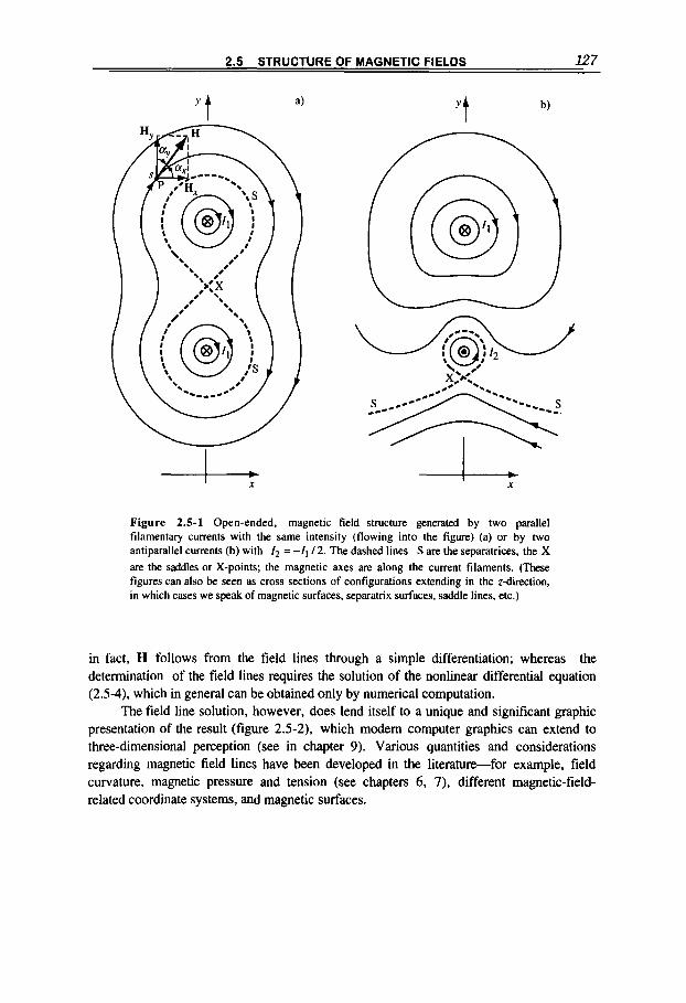
2.5 STRUCTURE OF MAGNETIC FIELDS 127
I I X
b
Figure 2.5-1 Open-ended, magnetic field structure generated by two parallel filamentary currents with the same intensity (flowing into the figure) (a) or by two antiparallel currents (b) with /2 = - I , 12. The dashed lines S are the separatrices, the X are the saddles or X-points; the magnetic axes are along the current filaments. (These figures can also be seen as cross sections of configurations extending in the zdirection, in which cases we speak of magnetic surfaces, separatrix surfaces, saddle lines, etc.)
in fact, H follows from the field lines through a simple differentiation; whereas the determination of the field lines requires the solution of the nonlinear differential equation (2.5-4), which in general can be obtained only by numerical computation.
The field line solution, however, does lend itself to a unique and significant graphic presentation of the result (figure 2.5-2). which modem computer graphics can extend to three-dimensional perception (see in chapter 9). Various quantities and considerations regarding magnetic field lines have been developed in the literature-for example, field curvature, magnetic pressure and tension (see chapters 6, 7), different magnetic-field- related coordinate systems, and magnetic surfaces.
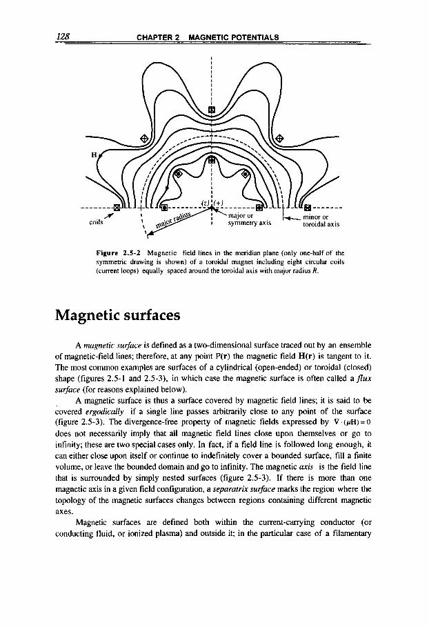
128 CHAPTER 2 MAGNETIC POTENTIALS
I
Figure 2.5-2 Magnetic field lines in the meridian plane (only one-half of the symmetric drawing is shown) of a toroidal magnet including eight circular coils (current loops) equally spaced around the toroidal axis with major radius R.
Magnetic surfaces
A magnetic surfuce is defined as a two-dimensional surface traced out by an ensemble of magnetic-field lines; therefore, at any point P(r) the magnetic field H(r) is tangent to it. The most common examples are surfaces of a cylindrical (open-ended) or toroidal (closed) shape (figures 2.5-1 and 2.5-3), in which case the magnetic surface is often called a f lux surfuce (for reasons explained below).
A magnetic surface is thus a surface covered by magnetic field lines; it is said to be covered ergodicully if a single line passes arbitrarily close to any point of the surface (figure 2.5-3). The divergence-free property of magnetic fields expressed by V . (pH) = 0 does not necessarily imply that all magnetic field lines close upon themselves or go to infinity; these are two special cases only. In fact, if a field line is followed long enough, it can either close upon itself or continue to indefinitely cover a bounded surface, fill a finite volume, or leave the bounded domain and go to infinity. The magnetic axis is the field line that is surrounded by simply nested surfaces (figure 2.5-3). If there is more than one magnetic axis in a given field configuration, a sepurutrix surfuce marks the region where the topology of the magnetic surfaces changes between regions containing different magnetic axes.
Magnetic surfaces are defined both within the current-canying conductor (or conducting fluid, or ionized plasma) and outside it; in the particular case of a filamentary
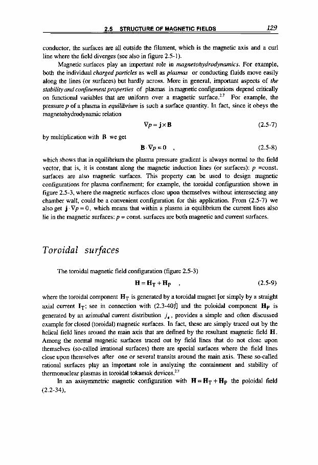
2.5 STRUCTURE OF MAGNETIC FIELDS 129
conductor, the surfaces are all outside the filament, which is the magnetic axis and a curl line where the field diverges (see also in figure 2.5-1).
Magnetic surfaces play an impcrtant role in magnetohydrodynamics. For example, both the individual charged particles as well as plasmas or conducting fluids move easily along the lines (or surfaces) but hardly across. More in general, important aspects of the stability and con3nement properfies of plasmas in magnetic configuI.dtiors depend critically on functional variables that are uniform over a magnetic surface.'-' For example, the pressurep of a plasma in equilibrium is such a surface quantity. In fact, since it obeys the magnetohydrodynamic relation
V p = j x B (2.5-7)
by multiplication with B we get
B . V p = O , (2.5-8)
which shows that in equilibrium the plasma pressure gradient is always normal to the field vector, that is, it is constant along the magnetic induction lines (or surfaces): p =const. surfaces are also magnetic surfaces. This property can be used to design magnetic configurations for plasma confinement; for example, the toroidal configuration shown in figure 2.5-3, where the magnetic surfaces close upon themselves without interesecting any chamber wall, could be a convenient configuration for this application. From (2.5-7) we also get j V p = 0, which means that within a plasma in equilibrium the current lines also lie in the magnetic surfaces: p = const. surfaces are both magnetic and current surfaces.
Toroida 1 surfaces
The toroidal magnetic field configuration (figure 2.5-3)
H = H T + H P , (2.5-9)
where the toroidal component HT is generated by a toroidal magnet [or simply by a straight axial current IT; see in connection with (2.3-40yl and the poloidal component Hp is generated by an azimuthal current distribution j , , provides a simple and often discussed example for closed (toroidal) magnetic surfaces. In fact, these are simply traced out by the helical field lines around the main axis that are defined by the resultant magnetic field H . Among the normal magnetic surfaces traced out by field lines that do not close upon themselves (so-called irrational surfaces) there are special surfaces where the field lines close upon themselves after one or several transits around the main axis. These so-called rational surfaces play an important role in analyzing the containment and stability of thermonuclear plasmas in toroidal tokamak devices.*
In an axisymmetric magnetic configuration with H = HT + Hp the poloidal field (2.2-34).
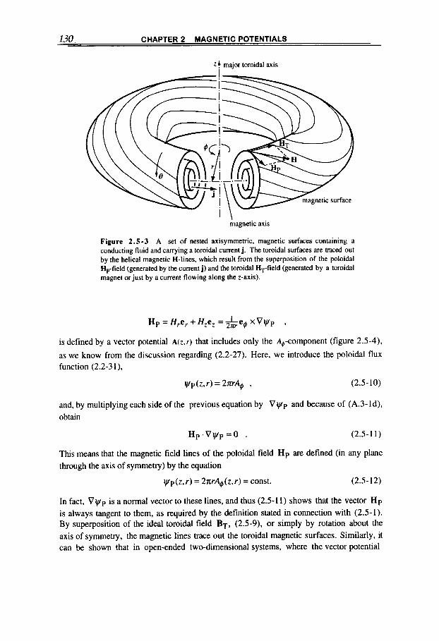
130 CHAPTER 2 MAGNETIC POTENTIALS
z! major toroidal axis I
I
magnetic axis
Figure 2.5-3 A set of nested axisymmetric, magnetic surfaces containing a conducting fluid and carrying a toroidal current j. The toroidal surfaces are &aced out by the helical magnetic H-lines, which result from the superposition of the poloidal Hp-field (generated by the current j) and the toroidal HT-field (generated by a toroidal magnet or just by a current flowing along the z-axis).
Hp = Hre, + Hzez = h e g x Vyp ,
is defined by a vector potential A ( z , r ) that includes only the A#-component (figure 2.5-4), as we know from the discussion regarding (2.2-27). Here, we introduce the poloidal flux function (2.2-3 1).
vp(z,r) = 2mA4, . (2.5-10)
and, by multiplying each side of the previous equation by V y p and because of (A.3- Id), obtain
Hp.Vt//p=O . (2.5-1 1)
This means that the magnetic field lines of the poloidal field Hp are defined (in any plane through the axis of symmetly) by the equation
vp(z,r) = 2~rA4,(z,r) = const. (2.5 - 12)
In fact, V y p is a normal vector to these lines, and thus (2.5-1 I ) shows that the vector Hp is always tangent to them, as required by the definition stated in connection with (2.5-1). By superposition of the ideal toroidal field BT, (2.5-9). or simply by rotation about the axis of symmetry, the magnetic lines trace out the toroidal magnetic surfaces. Similarly, it can be shown that in open-ended two-dimensional systems, where the vector potential

2.5 STRUCTURE OF MAGNETIC FIELDS U1
maior toroidal axis Z 4 poloidal flux: external to magnetic
toroidal flu:yl '4 ' \ T magnetic axis
Figure 2.5-4 Toroidal magnetic surface defining a toroidal flux and two poloidal fluxes, external Sp, and internal SP,. The fluxes remain constant with respect to a magnet- ic surface-hence the possible labeling of magnetic surfaces through the related flux.
A(r.9) (here in polar coordinates) is translationally invariant and has only the A, -component [see figure 2.1-6; and calculate w from (2.2-36)], the field lines are defined by the equation
Az(r ,@) = const. , (2.5-13)
and the corresponding surfaces are obtained by translating them along the z-direction. Magnetic fluxes defined with respect to a magnetic surface are preserved because by
definition (2.5-1 1) the magnetic field is tangent and thus does not cross the surface; hence, magnetic surfaces can also be labelled as flux surfaces. In an axisymmetric toroidal field there is a toroidal flux related to the cross section ST (figure 2.5-4),
and there are poloidal fluxes
h = p l H p . d s , SP
(2.5-14)
(2.5-15)
which are defined to be either outside the magnetic surface [wpe; this is the flux (2.5-12) obtained by integrating over the disk-like surface through any point M on the magnetic surface] or inside [ wpi; this follows by integration over the ribbon-like surface extending

0 2 CHAPTER 2 MAGNETIC POTENTIALS
Figure 2.5-5 Computer graphics presenting the nonaxisymmetric toroidal arrangement of some of the nonplanar coils for the stellarator-experiment WENDELSTEIN 7-X located at Greifswald (Germany); also shown is the outermost magnetic flux surface that will contain the hot plasma of thermonuclear interest (the major, mean radius is 5.5 m). (Courtesy of Max-Planck-Institut fur Plasmaphysik, Garching, Germany.)
from the magnetic axis to MI. It obviously is lype + lypi = lyptot, where the total poloidal flux is obtained by integrating over the disk defined by the magnetic axis. As mentioned before, the, values of the so-defined fluxes can be used to label the magnetic surfaces.
In this chapter we have mainly discussed simple arrangements of coils and magnetic configurations that to a large extent could be treated analytically. In practice, more complicated configurations are often used which, based on the concepts presented in this chapter, have to be calculated numerically (see in chapter 9). Such an example is shown in figure 2.5-5.

Chapter 3
PERIODIC FIELDS AND WAVE PHENOMENA
In this chapter we discuss some theoretical behavior of fields that are harmonic in time-that is, expressible in steady sine or cosine functions. These fields are important in physics, particularly in electromagnetic theory, because sinusoidal time dependence is a fundamental variation in nature. Electromagnetic wave phenomena are also introduced, but the discussion is limited to the most basic concepts only since such phenomena play a limited role in the topics treated in this book.
Applications. The formalism concerning sinusoidal time varying and rotating fields is applied extensively throughout the book and is the basis for many application~~-~-for example, motors and current generators (discussed in chapter 6).
3.1 COMPLEX FUNCTIONS
Complex variables and functions represent a very useful and powerful set of tools for dealing with phenomena that have sinusoidal time dependence. They are also used conveniently in other applications throughout the book so we shall briefly review some of their basic properties. We then extend some of these concepts to steady and nonsteady phenomena through the Fourier transformation formalism.
133
M4GNETICFIELDS: A Comprehensive Theoretical Treatise for Practical Use Heinz E. Knoepfel
Copyright Q 2000 by John Wiley & Sons, Inc
u4 CHAPTER 3 PERIODIC FIELDS AND WAVE PHENOMENA
Sinusoidal functions
It is convenient to express any function H (e.g., a magnetic field component) that has a harmonic time dependence through the complex exponential notation
H(x,y,z; o = &(x,y,z)eiw , (3.1-1)
(3.1-2)
is the imaginary unit or number. This notation implies that the physically meaningful component of the function (e.g., of the field) is the real part of it. If H = H(x,y,z) is a real function, the real part is
Re &x,y,z; t ) = H(x,y,z)cosot . (3.1-3)
because
eiw =cosm+isinm , (3.1-4)
as can be shown by writing the series expansions for eiw,cosot, i sinm. Here, w is the angular frequency, which is related to the time period T by
w = 2 ~ l T . (3.1-5)
More in general, Hcan itself be a complexfunction,
- W , Y , Z ) = H'(x,y,z)+i H''ky,z) , (3.1-6)
with H' being its real component and H" its imaginary one: .
H(x,y,z; t) = ~ ( x , y , z ) P = (H'+ ~ " ) ( c o s o t + i sinot). (3.1-7)
The real, meaningful component of the function is then
ReH= H'cosot-H"sinw .
For later use, note the relation
& = ( 1 + i ) / & ,
which derives from
& i = ( l f i ) 2 / 2 .
(3.1-8)
(3.
(3.1
-9)

3.1 COMPLEX FUNCTIONS us
Complex variables and functions
It is useful to recall some basic concepts and rules regarding complex variables and functions. A complex variable z may be represented in the Cartesian form
z = x + i y , (3.1- 11)
or in the polar form
= p - = pi@ = p(cosg+ising) , (3.1-12)
where e is the base of nautral logarithms and
p = ,/= = lz~, @ = arctan , (3.1-13)
as is evident from the representation in a Gaussian plane (figure 3.1-1), where L can be taken as a vector from the origin to point P(x,y). The conjugate variable,
L = x - i y = p e - i @ , (3.1 - 14)
is obtained by the substitution i + 4, and it lies symmetrically about the x-axis. With these definitions in mind, the basic algebraic operations follow in a logical
manner. Depending on the calculus to be made, it is convenient to use either the Cartesian or the polar form.
Addition (subtraction) of two complex variables,
zl+z2=x1+x2+i(Yl+Y2) 9
11 +12 =(p1cosq$ +p2cos&)+i(plsinq$ +p2sin&) , (3.1 - 15)
corresponds in the polar form to the addition (subtraction) of two vectors. A special case is
z + z * = 2 x ,
z + I* = 2pcosg ; (3.1-16)
that is, addition of a complex variable with its conjugate gives twice the real component. Multiplication (division) of two complex variables,
z1z2 = ( X I +iYl)(X2 +iyz)=(qx2 -YIY2)+i(xIY2 + X 2 Y I )
Z l Z 2 = PlP2e i(@l+@2) = p,p2[cos(gl + g2) + i sin(& +&)I ,
9
(3.1- 17)
corresponds to multiplication (division) of the absolute values and addition (subtraction) of the arguments. Special cases are
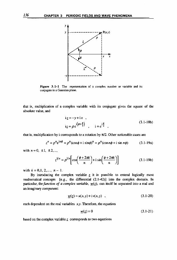
U6 CHAPTER 3 PERIODIC FIELDS AND WAVE PHENOMENA
't
Figure 3.1-1 The representation of a complex number or variable and its conjugate in a Gaussian plane.
that is, multiplication of a complex variable with its conjugate gives the square of the absolute value, and
i c = - y + i x , (3.1 - 1 8b)
that is, multiplication by i corresponds to a rotation by d 2 . Other noticeable cases are
zn = p"ei"$ = pfl(cos#+ i sin#)" = p"(cosn#+ i sin n ~ ) (3.1-19a)
withn=O, f 1 , f 2 ,...,
(3.1-19b)
with k = 0,1, 2 ,..., n - 1. By introducing the complex variable L it is possible to extend logically most
mathematical concepts [e.g., the differential (2.1-42)] into the complex domain. In particular, thefunction of a complex variable, ~ ( j : ) , can itself be separated into a real and an imaginary component:
- w(z ) = 4 x . y ) + i v(x,y) , (3.1-20)
each dependent on the real variables x,y. Therefore, the equation
W k ) = 0 (3.1-21)
based on the complex variable z corresponds to two equations
3.1 COMPLEX FUNCTIONS u7
u(x,y)=O , v(x,y)=O (3.1-22)
in the variables x,y. This shows that at any couple of values (x ,y) [which define a point P in the (x,y)-plane] the function w determines a point Q in the (u,v)-plane, which means that the Z(x,y)-plane is transformed into the w(u,v)-plane. It is easy to show that such a transformation keeps the angles unaltered; it is a conformal transformation.2~' Therefore, u,v are conjugated functions-that is, the family of curves
where c = const. intersect at normal angles. In fact, the orthogonal family of lines
u = c , v = c (3.1-24)
in the (u,v)-plane are conformally transformed into the orthogonal family of curves (3.1- 23). Similar expressions are obtained, and considerations applied, for the polar form (3.1- 12) of the complex variable.
Example: Conformal transformations
Consider as an example the function
Insertion of (3.1-1 I. 20) leads to
u + i v = x 2 - y 2 + i 2 x y . u = x 2 - y 2 , v=2xy .
that is,
(3.1-25)
(3.1-26)
This function determines a well-defined conformal transformation of problems. curves, and so on, from the z(x,y)-plane into the &(u,v)-plane. and vice versa. For example, the family of orthogonal lines u = c .
v = c in the w-plane transforms into the orthogonal family of curves u(x,y) = c , v(x.y) = c-that is.
hyperboles, x 2 - y 2 = c , 2xy=c , (3.1-27)
in the 2-plane. Conversely, the orthogonal lines x = c, y = c in the =lane transform conformally into the
orthogonal curves x(u,v) = c, y(u,v) = c-that is, parabolas,
u = c2 - (v2 1 4 2 ) . u = $142)- c2 , (3.1-28)
in
conformal transformation are discussed in section 2. I , i n connection with (2.140).
the &-plane (figure 3.1-2). Important properties of the &u,v-functions and a further example of a
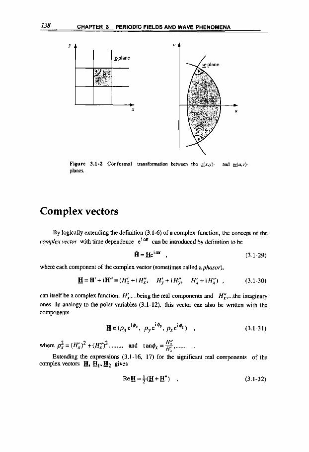
US CHAPTER 3 PERIODIC FIELDS AND WAVE PHENOMENA
“ t
X
Figure 3.1-2 Conformal transformation between the ~ ( x , y ) - and K(u,v)- planes.
Complex vectors
By logically extending the definition (3.1-6) of a complex function, the concept of the complex vector with time dependence e i m can be introduced by definition to be
H = H e i m , (3.1-29)
where each component of the complex vector (sometimes called a phasor),
- H=H‘+iH”=(Hi+ iH; , H;+iHy”, Hi+iH,“) , (3.1-30)
can itself be a complex function, Hi, ... being the real components and H,”, ... the imaginary ones. In analogy to the polar variables (3.1-12), this vector can also be written with the components
H=(pxeigx, pyei’y, pzei@z) , (3.1-31)
H;I where p: =(Hi)’ + ( H I ) 2 ,...,..., and tan& = -
H: ’...’... .
complex vectors €€, HI, H2 gives Extending the expressions (3.1-16, 17) for the significant real components of the
ReIJ=+(IJ+H*) , (3.1-32)
3.1 COMPLEX FUNCTIONS U9
R e g I .ReHz =@I +H;)$4, +HI;) = $(€I, .€I2 +_H; ._H; +€I;. Il2 +€II .€I;) ,
(3.1-33)
where the asterisk indicates, like in (3.1-141, that the substitution i+-i is performed in the vector components (3.1-30 or 3 l),
I ,, I It I ,, I ,
- H * = H - i H =(HI - iHx , Hy -iHy , Hi-iH, ) , (3.1-34)
(3.1-35)’
(3.1 -36)
All these expressions also hold when substituting
- H+H=IJeiUX ,
because this implies only a phase change #x + +OX,...
For later use, we calculate the time average over one period T = 2 a l w of
T ReH, .ReHz = (ReHI .ReH2)d?lT . (3.1-37)
By noting that the time average of HI . H 2 (or of H2) with the same harmonic time dependence o vanishes and that H: . H 2 = ( H I .HI;)* (to confirm this, we recall the
trigonometric relations: 2cos wt = 1 + cos2wt and sin2m = 2sinwtcosm), we obtain the time average theorem
2
and, in particular,
It is also easy to understand these relations with the polar form (3.1-31), especially if we assume the same phase angle for all components, thus
fj =&(mi$) - (3.1 -40a)
Then, for example, for (3.1-31, 37) we write

140 CHAPTER 3 PERIODIC FIELDS AND WAVE PHENOMENA
T (ReH)2 = + j p 2 c o s 2 ( m + @ ) d r = i p 2 , (3.1 -40b)
since
I, T 2 cos (Wt+@)dt=$ ;
the same result is obtained from (3.1-39.40).
ReH2 = l f i . H * =l 2 2 P .
When there is a phase angle for each component, writing the above becomes a little more tedious, but the procedure is the same. Obviously, all these relations also remain formally valid when, instead of a complex vector H, we simply have a complex function H . We shall apply the formalism of imaginary functions and vectors in sections 4.3.4.5, 5.1, 5.4.
3.2 SINUSOIDAL AND ROTATING ELECTROMAGNETIC FIELDS
The calculation of electromagnetic phenomena with a steady harmonic (cosine, sine) time dependence by means of complex variables and functions is a powerful method that allows direct time dependence to be eliminated from the equations. Consequently, the solutions become simpler and are based on the fact that at the end only the real parts have a physical meaning and will be used.
Electromagnetic equations
The source terms in Maxwell's equations (1.1-1 to 4), j and pe, and accordingly the resultant electromagnetic fields, are assumed to vary harmonically with the angular frequency w, (3.1-5), as expressed by the complex notation (3.1-1,29), that is,
iw j= . j e iW , pe = p e e i W , H = H e i W , E = E e ...., (3.2-1)
where j, pe, H, and E can themselves be time-independent complex phasors (vectors) or
scalar functions. - -
141 _. -~ 3.2 SlNUSOlDAL ELECTROMAGNETIC EQUATIONS
Inserting into the time-dependent equations (1.1- 1 to 5) immediately gives the time-independent equations
V x H = j + i w D - , (3.2-2)
V x E = - i w B , (3.2-3)
V.B=O , (3.2-4)
W = p e 7 (3.2-5)
V . j = i o p -e ' (3.2-6)
where all sources and vector field terms, according to notation (3.2-l), can be space- and &dependent, but are independent of time.
The same simplifying formalism can conveniently be applied to all other relevant equations where there is a time derivative-for example, to the quasistationary electric equations (1.2-24 to 27), or quasistationary magnetic equations (1.2-18 to 21), which then become
V x H = j - , (3.2-7)
V x E = - i o B , (3.2-8)
V.B=O , (3.2-9)
V . j = i w p - , -e
(3.2- 1 0)
The solution of these systems of complex electromagnetic differential equations, together with relations (3.2- 1 l), requires the application of the appropriate boundary conditions accompanying the geometrical configuration of each problem. These conditions remain formally identical to those determined in section 1.5 and summarized in table 1.5-1.
Up to now we have assumed the parameters o,p,& included in the constitutive equations (1.1-6 to 8),
j = o E - , B=p€J , D = E & (3.2-1 1 )
to be time-independent, meaning that any change in the magnetic or electric fields immediately induces a proportional change in the conduction current and in the volume densities of magnetization and polarization, (1.1 - 1 1,12). In reality, the response of the underlying physical phenomena is characterized by a time lag, which in the above time- independent equations can be taken care of by considering the parameters written in complex form
g = a ' + i o " , p = p , ( p k + i p i , , g = c , ( ~ k + i & j i ) , (3.2-12)
where o ' , p k , ~ k are the real components and o",pi,&i are the imaginary ones. We shall take up this argument in section 5.4, starting from (5.4-44).

142 CHAPTER 3 PERIODIC FIELDS AND WAVE PHENOMENA
Generalized wave equations
The system of differential equations (3.2-2 to 6) can be rendered more compact by taking the curl of (3.2-2,3) and then uniforming with the constitutive equations (3.2-1 l), where the parameters a,p,&, are assumed to be space-independent, to obtain the time- independent equations
A€J+ki€J=O , (3.2- 13)
AE+k$E=O , (3.2-14)
where
(3.2- 15) &;=pa 2 ( l - i a /Ew) .
These equations can also be deduced directly, with the formulations (3.2-1),
f i = H e ' u , f i = E e i m ,
from the differential time-dependent equations (4.1-2, 3), with the substitution of the double curl as in (4.1-5).
The first term on the right-hand side of (3.2-15) stems from the displacement-current term iwD in (3.2-2), thus it vanishes in the quasistationary approximation. In this case from (3.2-13) we obtain the magnetic digision equation
2 2 A€J=i--H, S2=- ,
62 - =Pw (3.2- 16)
(see section 4.1). where 6 is the diffusion skin depth (4.2-21).
Magnetic potential
The formalism expressed by the time dependence (3.2-1) can also be applied to the magnetic vector potential and to the electric scalar potential introduced in chapter 2; thus,
A = Aeiu, - 0 = - ueiw. (3.2- 17)
The time-dependent d'Alembert equations (2.2-10) then transform into the time-independent equations
A(I+k2(I=-p / E , (3.2- 1 8) -e
A A + k 2 A = - p j - , (3.2-19)

- - 3.2 SlNUSOlDAL ELECTROMAGNETIC EQUATIONS 143
provided that the Lorentz gauge (2.2-9) holds, that is,
A A = -iWpEu = - i k@u ;
here the wave number of the medium is expressed by
k = w @ = w = & = B , c Tc A
with
(3.2-20)
(3.2-21)
(3.2-22)
being the velocity at which any electromagnetic disturbance travels in the medium; in particular, c = 1 / 4 / is the speed of light in vacuum, A = Tc is the wavelength of
this disturbance, and T = 2 n / w its period. [The present discussion anticipates somewhat the argument of the next section; in fact, in free space, where j and p vanish, the above
equations assume the form of the wave equation that will be discussed in connection with
The solutions of (3.2-18.19) can be based on the retarded potentials (2.2-26),
- -e
(3.3-l).]
whereby the time delay t + t - r / c (i.e., eiwr + ei(w-kr) ) shows up such that
(3.2-23)
(3.2-24)
As already pointed out in connection with (2.2-15), the solution of an electromagnetic problem through the use of the potentials A. is in some cases a convenient alternative to solving the system of Maxwell's equations (3.2-2, to 5). The time-dependent magnetic and electric fields (3.2-1) are then obtained from the potentials through (2.2-14,15), that is,
p H = V x A , (3.2-25)
- E=-iwA-VU . (3.2-26)
In the quasistationary magnetic approximation, where
k + O (3.2-27)
because of relation (1.2-17). the above equations reduce, as in (2.2-12,13), to the Poisson equations
Ar/=-p I E , (3.2-28)
(3.2-29)
-e
AA = -p - j
and to the Coulomb gauge
V . A = O ,
whereas the field relations (3.2-25, 26) remain unaffected.
(3.2-30)
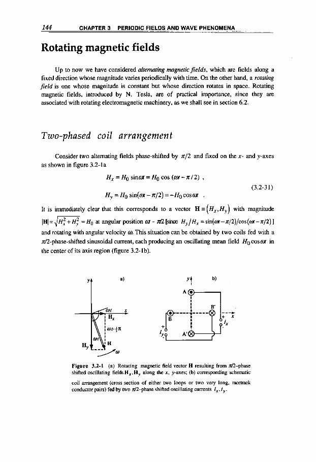
144 CHAPTER 3 PERIODIC FIELDS AND WAVE PHENOMENA
Rotating magnetic fields
Up to now we have considered alternating magneticfields, which are fields along a fixed direction whose magnitude varies periodically with time. On the other hand, a rotaring field is one whose magnitude is constant but whose direction rotates in space. Rotating magnetic fields, introduced by N. Tesla, are of practical importance, since they are associated with rotating electromagnetic machinery, as we shall see in section 6.2.
Two-phased coil arrangement
Consider two alternating fields phase-shifted by ~ / 2 and fixed on the x- and y-axes as shown in figure 3.2-la
H, = HO sinm= HO cos ( w t - ~ / 2 ) ,
Hy = HO sin(m - n/2) = -Ho cosot . (3.2-3 1)
It is immediately clear that this corresponds to a vector H I (H,, Hy) with magnitude
IHI = Jw = H~ at angular position u - n~ [sim H ~ / H ~ = sin(w - rrp)/cos (ox - rrp) 1 and rotating with angular velocity W. This situation can be obtained by two coils fed with a d2-phase-shifted sinusoidal current, each producing an oscillating mean field HO cosot in the center of its axis region (figure 3.2-lb).
a)
'1
Figure 3.2-1 (a) Rotating magnetic field vector H resulting from d2-phase shifted oscillating fields H,,H, along the x . y-axes; (b) corresponding schematic
coil arrangement (cross section of either two loops or two very long, racetrack conductor pairs) fed by two d2-phase shifted oscillating currents I x . I , .
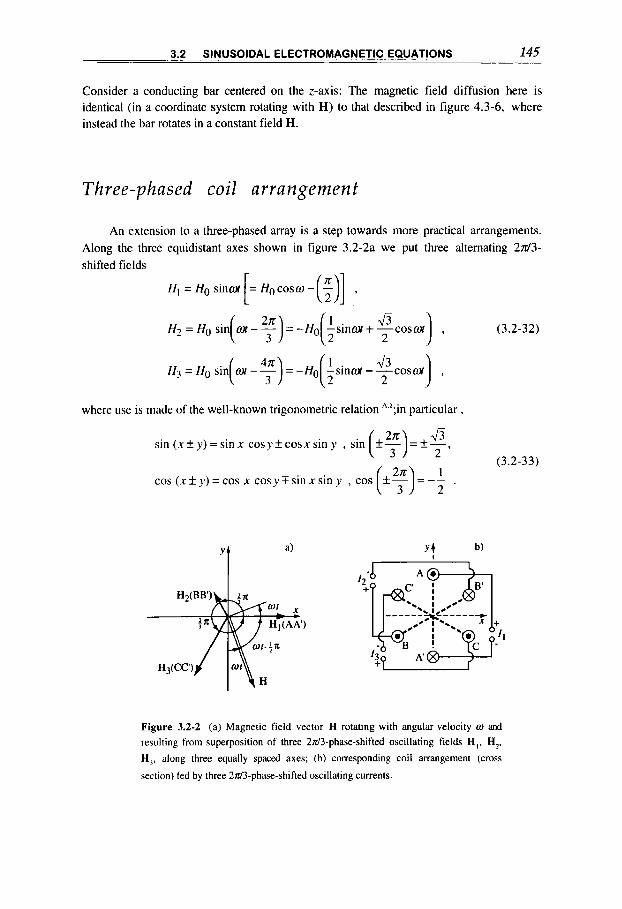
3.2 SINUSOIOAL ELECTROMAGNETIC EQUATIONS 145
Consider a conducting bar centered on the z-axis: The magnetic field diffusion here is identical (in a coordinate system rotating with H) to that described in figure 4.3-6, where instead the bar rotates in a constant field H.
Three-phased coil arrangement
An extension to a three-phased array is a step towards more practical arrangements. Along the three equidistant axes shown in figure 3.2-2a we put three alternating 2d3- shifted fields
H I = Ho sinW [ = Ho cosw -(:)I ,
(3.2-32)
where use is made of the well-known trigonometric relation A.';in particular,
s in (x+y)=s inx cosyfcosxs iny ,
cos (x+y)=cos x cosyTsinxsiny ,
(3.2-33)
a)
yI
Figure 3.2-2 (a) Magnetic field vector H rotating with angular velocity o and resulting from superposition of three 2ld3-phase-shifted oscillating fields H ,, H,, H,, along three equally spaced axes; (b) corresponding coil arrangement (cross
section) fed by three 2d3-phase-shifted oscillating currents.

146 CHAPTER 3 PERIODIC FIELDS AND WAVE PHENOMENA
Figure 3.2-3 The 2d3-phase-shifted currents I , , I,, I,. feeding the three coils A, B, C; and qualitative picture of the f current flow in the coils at three instants I, 11.111. clearly indicating the rotation of the resultant magnetic vector H (as usual, the symbols indicate the following: current flowing towards the reader, x away from reader, 0 negligible current).
Summing the components along the x- and y-axes gives
2 a 4x 3 3 3 2
2 a 47t 3 3 3 2
H, = HI + H2 cos- + H3 cos- = - Hosinwt ,
H =O+H2sin -+H3sin - = - - H Q c o s ~ ~ , Y
(3.2-34)
which define similarly as before in (3.2-21) the magnetic field vector H = (H,, H y ) with constant magnitude H = 1.5 HO at angular position wt - 4 2 and rotating with angular
velocity 0. This situation can be obtained, as before, by three equally spaced coils fed with f 2d3-shifted sinusoidal currents (with respect to the adjacent coils), as shown in figures 3.2-2b and 3.2-3.
3.3 WAVE PHENOMENA
In this section we shall introduce some concepts relating to electromagnetic waves. They are an important subject in electromagnetic theory and practice','. 3.3; however, they play a limited role as regards the main subject of this book, so only some basic concepts are presented and discussed. (On the contrary, electromagnetic diffusion phenomena, which are included in the same equations, are amply discussed in the next two chapters.)
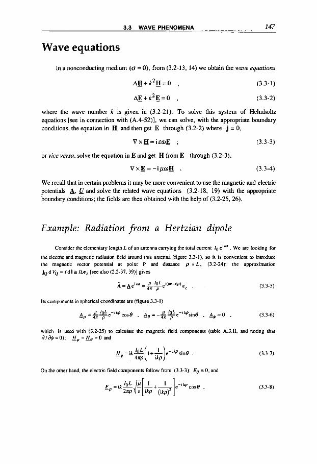
3.3 WAVE PHENOMENA 147
Wave equations
In a nonconducting medium (a = 0), from (3.2-13, 14) we obtain the wave equurions
A H + k 2 H = 0 , (3.3-1)
A E + k 2 E = 0 , (3.3-2)
where the wave number k is given in (3.2-21). To solve this system of Helmholtz equations [see in connection with (A.4-52)], we can solve, with the appropriate boundary conditions, the equation in B and then get E through (3.2-2) where j = 0,
V x H = i & @ ; (3.3-3)
or vice versu, solve the equation in E and get from E through (3.2-3),
V x E = - i p w H . (3.3-4)
We recall that in certain problems it may be more convenient to use the magnetic and electric potentials A, u and solve the related wave equations (3.2-18, 19) with the appropriate boundary conditions; the fields are then obtained with the help of (3.2-25.26).
Example: Radiation from a Hertzian dipole
Consider the elementary length L of an antenna carrying the total current I0 e i w . We are looking for
the electric and magnetic radiation field around this antenna (figure 3.3-1). so it is convenient to introduce the magnetic vector potential at point P and distance p N L, (3.2-24); the approximation jQ d VQ = I d l 3 ILe , [see also (2.2-37,39)] gives
Its components in spherical coordinates are (figure 3.3-1)
A -P = L l g L e - i ~ p c o s e 4H p , A g = - z ~ e P IoL -ikpsine , A q = O , (3.3-6)
which is used with (3.2-25) to calculate the magnetic field components (table A.3.11. and noting that d l d q = O ) : H p = H g = O a n d
On the other hand, the electric field components follow from (3.3-3): Eg = 0. and
(3.3-7)
(3.3-8)
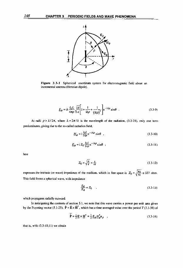
148 CHAPTER 3 PERIODIC FIELDS AND WAVE PHENOMENA
Figure 3.3-1 Spherical coordinate system for electromagnetic field about an incremental antenna (Hertzian dipole).
(3.3-9)
At radii p > u 2 n . where I. = 2 a / k is the wavelength of the radiation, (3.2-21). only one term
predominates, giving rise to the so-called radiation field,
-4 - H - i G e 'OL -ikpsine (3.3-10)
hem
q = & L E CE (3.3-12)
expresses the intrinsic (or wave) impedance of the medium, which in free space is ZO =
This field forms a spherical wave, with impedance
e , z o , (3.3- 13) %
which propagates radially outward.
In anticipating the contents of section 5.1, we note that this wave carries a power per unit area given by the Poynting vector (5.1-25). P = E X H', which has a time-averaged value over the period T(3.1-38) of
that is, with (3.3-10,ll) we obtain

3.3 WAVE PHENOMENA 149
- - zo IOL P=- 2 (2J - sin2e e P (3.3- 15)
The total mean power irradiated is obtained by integrating over a spherical surface with fixed p and d s = 2 n p s i n e p d @ ep.
This mean power loss from the antenna can be compared formally with an ohmic loss
- 1 i R w, =2
( lo is the peak current), and thus a radiation resistance of the antenna,
(3.3- 17)
(3.3- 18)
can be defined. This shows that an efficient antenna must have a length L comparable with the radiated wavelength. Note that the terms (ikp)-' ,...,that have been neglected for large enough p i n (3.3-7 to 9)
will not contribute to the irradiated power because in (3.3-14) they will either not appear, be small, or be
imaginary: They form the so-called induction field, with its reactive energy alternatively stored in the field
and returned to the antenna during each time cycle [see comments in connection with the reactive power
equation (5.1-26)].
Plane waves in a uniform medium
Plane electromagnetic waves are among the simplest wave types and are presented here as an example. In such a wave (figure 3.3-2), the magnetic and electric vectors are orthogonal to each other and lie in a plane perpendicular to the propagation direction, with their field magnitude being constant over this plane.
'J Figure 3.3-2 Plane wave propagating in the z-direction
150 CHAPTER 3 PERIODIC FIELDS AND WAVE PHENOMENA
The magnetic field is here taken along the y-direction, H = aye , , where I f y is
independent of the x-and y-coordinates; thus (3.3-1) reduces to
with the solution
Tikz - H, = Hoe
Inserting into (3.3-3) gives Ey = Ez = 0 and
HO Tikz Ec
Ex =f-e
(see table A.3. II), where by definition we have
(3.3- 19)
(3.3-20)
(3.3-21)
(3.3-22)
that is, respectively. the wave number (3.2-21) and the wave impedance [equal to the intrinsic impedance of the medium, as in (3.3-13)]. Consequently, for a plane wave traveling along the z-axis, and by reintroducing the time dependence, we can write
fi = - HeiW = Hoei(w-k.z) eY ’ (3.3-23)
(3.3 -24)
where -k. z = Tkz and the upper sign applies to the positive z-direction, and the lower sign applies to the negative. This shows that E , H , and the propagation vector k = ke, follow the right-hand rule, which is a general rule not limited to the plane wave case.
Plane waves in a conducting medium
The pertinent equations for a medium with finite conductivity CJ are given in (3.2-13 to 15). In the quasistationary approximation (where the displacement term is neglected versus the conductive term),
CJ,, EW , (3.3-25)
thus
(3.3-26)

3.3 WAVE PHENOMENA 151
where K = 1/p0 is the magnetic diffusivity (4.1-9). Consequently, (3.2-13) reduces to the diffusion equation
AH-*H=O K - , (3.3-27)
[which could also have been obtained directly from the magnetic diffusion equation (4.1- 8) presented in the next chapter].
The wave number (3.3-26) transforms into
k, z ( l - i ) / S , (3.3-28)
where
(3.3-29)
is the skin depth-that is, the depth to which the electromagnetic fields and waves penetrate substantially [see also (4.2-29)]. The solution of (3.3-27). in the simple plane wave geometry used for (3.3-19), is the same as in (3.3-20) but with this imaginary ka value; thus
-J i(m-i) H , , = H o e 6e (3.3 -30)
This equation describes the field as it penetrates the conductor (we have omitted the alternative + sign in front of z for an opposite traveling wave). The same solution applies for E x , connected by (3.3-21). We will return to this type of solution in chapter 4, in relation to different magnetic diffusion problems. We can define a formal penetration velocity in the conductor by writing [see also (4.2-18c), where lo = 8/21
Vd=21r6/T=w6=4- , (3.3-31)
that is, vd z 400 m/s in copper at 1 MHz.
Ciapter 4
MAGNETIC FIELD DIFFUSION AND EDDY CURRENTS
The previous chapter dealt mainly with the magnetic field generated in vacuum by a given current distribution; this chapter deals mostly with the interaction between time- varying magnetic fields (in the quasistationary approximation) and the related current density in conductors with constant electrical conductivity and incompressible mass. Depending on the formulation of the problems, the interaction effect in the conductor can be treated either as a magnetic diffusion process or as the induction of an eddy current distribution, the two solutions being related through Ampbre's law. Both are addressed here.
Applicarions. The finite penetration into a conductor of diffused, time-varying fields or of the related eddy currents gives rise to effects of practical importance-for example, modified resistances and impedances, or magnetic shielding4.13. These fields and currents are also the starting point for calculating (in chapters 5 and 6) locally limited or concentrated heat deposition (conductor damage) and force application (magnetic levitation). The strong modification (concentration) of the diffused fields and currents around an abrupt change in the conductor geometry (around a micro-crack) is the basis of magnetically sensitive, nondestructive testing4.'*.
4.1 MAGNETIC DIFFUSION THEORY
The interaction of a quasistationary magnetic field with a solid conductor can be described as a diffusion process. In this section the diffusion equation is established and
153
M4GNETICFIELDS: A Comprehensive Theoretical Treatise for Practical Use Heinz E. Knoepfel
Copyright Q 2000 by John Wiley & Sons, Inc
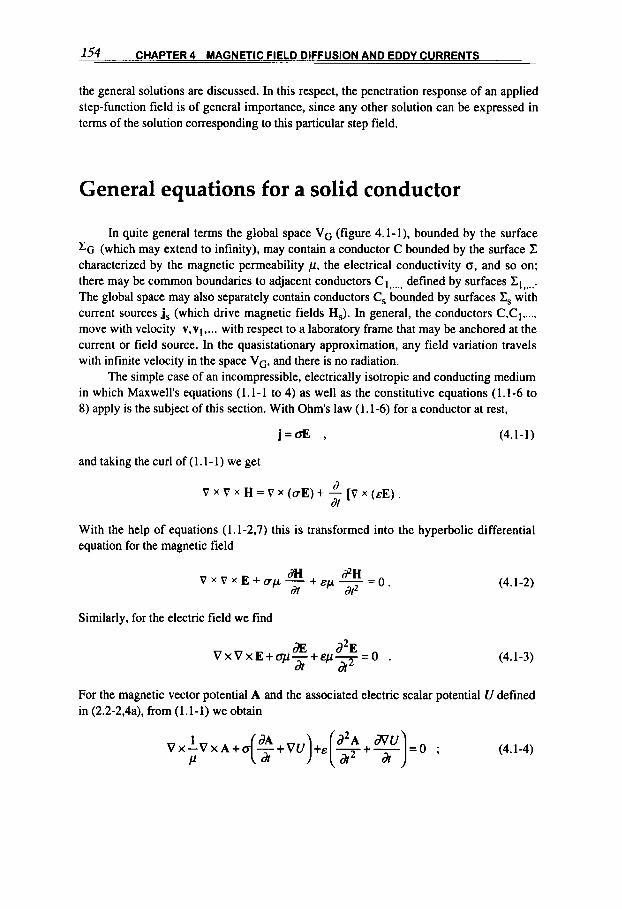
154 CHAPTER 4 MAGNETIC FIELD DIFFUSION AND EDDY CURR ENTS
the general solutions are discussed. In this respect, the penetration response of an applied step-function field is of general importance, since any other solution can be expressed in terms of the solution corresponding to this particular step field.
General equations for a solid conductor
In quite general terms the global space VG (figure 4.1-1). bounded by the surface ZG (which may extend to infinity), may contain a conductor C bounded by the surface C characterized by the magnetic permeability p, the electrical conductivity 6, and so on; there may be common boundaries to adjacent conductors Cl,,, , , defined by surfaces XI,.... The global space may also separately contain conductors C, bounded by surfaces C, with current sources j, (which drive magnetic fields HJ. In general, the conductors C,C move with velocity V,VI, ... with respect to a laboratory frame that may be anchored at the current or field source. In the quasistationary approximation, any field variation travels with infinite velocity in the space VG, and there is no radiation.
The simple case of an incompressible, electrically isotropic and conducting medium in which Maxwell's equations (1.1-1 to 4) as well as the constitutive equations (1.1-6 to 8) apply is the subject of this section. With Ohm's law (1.1-6) for a conductor at rest,
j=aE 9 (4.1-1)
and taking the curl of (1.1-1) we get
a d t
V x V X H = V X (uE) + - [V x (EE) .
With the help of equations (1.1-2,7) this is transformed into the hyperbolic differential equation for the magnetic field
Similarly, for the electric field we find
dE d2E V X V X E + OF- + &p- = 0 dt &*
(4.1-2)
(4.1-3)
For the magnetic vector potential A and the associated electric scalar potential U defined in (2.2-2,4a), from (1.1- 1) we obtain
V x 'V x A + 4% + VU) +E [ d2A + 7) dvU = 0 ;
P (4.1-4)
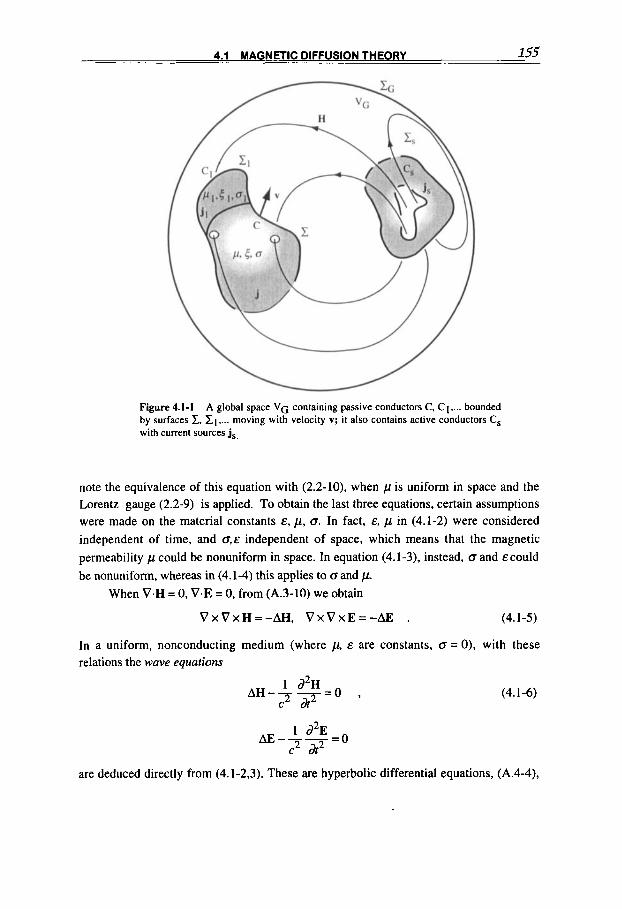
4.1 MAGNETIC DIFFUSION THEORY 155
Figure 4.1-1 A global space VG containing passive conductors C, C1 .... bounded by surfaces 1, 11 .... moving with velocity v; i t also contains active conductors Cs with current sources js,
note the equivalence of this equation with (2.2-lo), when p is uniform in space and the Lorentz gauge (2.2-9) is applied. To obtain the last three equations, certain assumptions were made on the material constants E , p, Q. In fact, E, p in (4.1-2) were considered independent of time, and Q,E independent of space, which means that the magnetic permeability p could be nonuniform in space. In equation (4.1-3), instead, Q and could be nonuniform, whereas in (4.1-4) this applies to CT and p.
When V.H = 0, V.E = 0, from (A.3-10) we obtain
V X V X H = - A H , V X V X E = - ~ . (4.1-5)
In a uniform, nonconducting relations the wave equations
medium (where p, E are constants, d = 0) , with these
1 d2H AH-T-=O ,
c dt2
1 d2E AE - - - - 0 c2 d t 2 -
(4.1-6)
are deduced directly from (4.1-2,3). These are hyperbolic differential equations, (A.4-4),
156 CHAPTER 4 MAGNETIC FIELD DIFFUSION AND EDDY CURRENTS
and imply that any electromagnetic field disturbance travels with the lighr velocity
1 c=- . f i
(4.1-7)
Quasistationary diffusion equations
In the magnetic quasistationary approximation, the third term in (4.1 -2), as well as in equations (4.1-3,4), drops out because it derives from the displacement term aD&. Because V . B = pV . H = 0, when p is uniform in space, relation (4.1-5) reduces (4.1-2) to the parabolic magnetic difluusion equation
1dH A H - - - = O , K d t
where
is the magnetic diffusivify, which in practical cgs units is
(4.1-8)
(4.1-9)
(4.1-9*)
The K-nOtatiOn is used throughout this book with the implicit understanding (if not otherwise stated) that a p are space-independent, with p, in addition, time-independent, as noted above. In (8.1-48) it will be shown that when the conductor moves with velocity v, additional terms must be added on the right-hand side of the diffusion equation. The diffusivity contains the product ap, where the permeability can be very large for ferromagnetic materials. With respect to magnetic diffusion, a ferromagnetic conductor behaves as if its electric conductivity were increased by a factor p ~ .
The magnetic diffusion equation could have been obtained more directly by considering, in the first place, the equations of the magnetoquasistationary approximation. Taking the curl of Amptre's law (1.2-1 8),
V x H = j , (4.1-10)
then using Ohm's law (4.1-1) and Faraday's law (1.1-2).
(4.1-lla)
gives, with the vector relations (A.3-8) and (4.1-5).

4.1 MAGNETIC DIFFUSION THEORY 157
(4.1-llb)
which, when a i s also constant, leads directly to (4.1-8) with the Laplacian given as
As easily checked, the diffusion equation (4.1-8) could have been written as well for the magnetic induction B. Similarly, by taking the curl of (4.1-8) and using (4.1- lo), the same formal diffusion equation can be deduced for the current density:
A = V.V.
Proceeding under the same assumptions as before, reduces to
(4.1- 12)
the vector potential equation (4.1-4)
A A = a p - + V U =-pj (: 1 (4.1- 13)
(where now p , but not 0, has been assumed uniform in space). Note that the right-hand side can be expressed with the total current density (2.2-4b),
j = j , + j i , (4.1-1 4a)
which includes two components: the one due to electric sources (2.2-4c),
j , = - o V U (4.1- 14b)
(typically this current density is nonzero only in active conductors-for example; the coils, which produce the magnetic field in the first place) and the other due to the so- called eddy currents (2.2-4d).
j. = -0dA (4.1 - 1 4 ~ ) d t '
Depending on the given problem, the potential U may or may not be zero; but the current conservation (1.2-2 1). V.j = 0, requires the additional condition
v . [ 0( 2 + vu)] = 0. (4.1 - 14d)
Together with the Coulomb gauge (2.2-1 1). V.A=O, these equations provide a unique solution to the magnetic diffusion or eddy current problem defined through the vector potential A . Note that actually the vector potential equation (4.1-13) can be decomposed into a set of three equations, depending on the domain under consideration (figure 4.1- 1):
(a) In the conductors C without sources, the reduced equation is defined by j, = 0. (b) In nonconducting space, we get a Poisson equation (2.2-16) as a consequence of o=O. (c) In the conductors C, with sources, the full equation (4.1-13) applies.

158 CHAPTER 4 MAGNETIC FIELD DIFFUSION AND EDDY CURRENTS
The solutions corresponding to the domains must be matched at the boundaries. The above equations and related solutions can be appreciably simplified when there
are important symmetries, as shown in connection with the cylindrical (r,z)-equations (4.3-8), (A.4-29, 41); the polar (r, #)-equations (4.3-1 1, 40, 48); the Cartesian (x,y)-
equations (A.4-27,31); and the spherical (p, @-equations (A.4-74). When the conductor moves with velocity v, it will be shown in (8.1-53) that these
equations, as a consequence of (1.3-14), include additional terms and b e c ~ m e ~ . ’ ~
, 1 (4.1 - 15)
+ (v . V)A - ( A . V)v + VU . 1
Solutions to the diffusion problem
From a physical and practical point of view, the following comments can be made regarding the solution to the magnetic field-conductor interaction problem defined so far in this section (see also figure 4.1-1).
(a) A pulsed magnetic field H, is imposed on the conductor C (as generated by the current j, flowing in the conductor C,), which reacts (passively) by setting up an eddy current distribution; this problem is best treated as a magnetic diffusion process by solving (4.1-8), as will be done in sections 4.2 and 4.3. [If required, the eddy currents can then be calculated through (4.1-lo).]
(b) The overall time varying current in the conductor C, is imposed, and the system reacts (actively) by rearranging, within C,, the current density distribution; this problem will be discussed in section 4.5.
(c) When the penetration of the magnetic field distribution is large with respect to the normal conductor dimensions (i.e.. when we can speak of a thin conductor) it is often more convenient to solve the problem directly in terms of the eddy current distribution because useful simplifications can be introduced, as shown in section 4.4.
With regard to the first comment, the diffusion process is described in this chapter primarily in terms of the magnetic field H, and not through the current density j, the vector potential A, or the magnetic induction B, although they all satisfy the same type of parabolic differential equation. It is a somewhat arbitrary decision. In its favor speaks the boundary condition for the main tangential component of H (table 1.5-I), which is formally identical to that of the scalar quantities of other diffusion problems, as will be pointed out shortly.
4.1 MAGNETIC DIFFUSION THEORY 159
In general terms, the field-conductor interaction problem requires the solution to be found for the conductors and the free space surrounding them, which then must be coupled by appropriate boundary conditions. In free space it is generally convenient to solve the problem in terms of the magnetic scalar potential 0 (2.1-2,3). We thus have only one unknown function (0); whereas in the conductor, in general, all three components of the magnetic vector field H must be considered. Of particular interest is the use of the vector potential A when there are symmetries in the problem, because the general solution is then valid in the whole space, including the conductors, as pointed out at the beginning of sections 2.1 and 2.2. The boundary conditions between conductors and free space are summarized in table 1.5-1.
Numerical techniques, which will be reviewed in chapter 9, are nowadays an important tool for tackling the inherently complex diffusion problems. Here, we deal with analytic solutions of typical diffusion problems by introducing some significant simplifications. This will allow some useful solutions to be presented and will give an idea of the relevant physical effects involved in the magnetic diffusion process.
S o h tions and analogies To solve the vectorial diffusion equations presented so far, it is necessary to
decompose them into equations for the components of the unknown vector field. As mentioned in connection with (2.2- 19). this is straightforward in Cartesian coordinates but requires attention in other coordinate systems. For example, for Cartesian components H I [H,(x, y,z) , H,,(x,y,z) , H , (x . y , r ) ] , the equations (4.1-8,l Ib) each decompose into
three equations:
(4.1- 16) 1 dHi - A H . - - - - O , i = x , y , z . ' K &
It is immediately clear that in this component form the magnetic diffusion equations are formally identical to the thermal conduction equations to be presented in section 5.1; in particular, (4.1-16) is similar to (5.1-37,43),
la A T - - - = O , a &
where T is the temperature, (Y = Wcv the thermal diffusivity (5.1-38), k the thermal conductivity, and cv the specific heat per unit volume. This formal analogy is very useful because thermal conduction theory has been studied for more than a century and has produced powerful mathematical solution methods for solving the related differential

160 CHAPTER 4 MAGNETIC FIELD DIFFUSION AND EDDY CURRENTS
equation^^.^. Thus, many solutions of the thermal equations can be transcribed directly into the corresponding magnetic diffusion solution (the same as for many of those discussed in this chapter) by application of the substitution scheme:
Hi t t T , i=x ,y , z ,
K H ~ ,
(4.1-17)
since the boundary conditions are often formally identical. The parabolic differential equation (4.1-16) is also found in other fields of physics-for example, in ordinary diffusion t h e ~ r y . ~ . ' ~
For the solution of diffusion equations like those indicated in (4.1-16), there exists a vast literature, and different mathematical methods are well known-for example, variable separation, Laplace transformation, Green's function, Galerkin integral, and so 0n4.4. Some information on the variable separation method is given in section A.4-in particular, starting from equation (A.4-60). The powerful Green's function method is briefly introduced in section 5.1 with the general solution (5.1-47). in connection with the heat conduction problem. This chapter mainly deals with the variable separation merhod, with some attention given to the transient step-function boundary condition because of its significance in magnetic field diffusion.
Response to a step function field
Knowledge of a conductor's response to an externally (subscript e) applied step- function magnetic field is of particular interest in diffusion problems. To simplify our discussion we use Cartesian, one-dimensional formulae for the rest of section 4.1; extension to other coordinate systems, or to vectorial relations, can be obtained by appropriate transformations. The problem here is to know how an applied so-called step- function boundary (subscript b) field (Heaviside step function), defined by
for - c t < 0,
Ho(xb) (const.), for 0 2 t < -, He(xb; 1 ) = (4.1-18)
where the initial condition at any internal (subscript i) point xi is generally
H , ( x , ; I ) = 0, fort I 0, (4.1- 19)
diffuses into the conductor system. The solution for the field at any internal point xi for t 2 0 can be written in the form
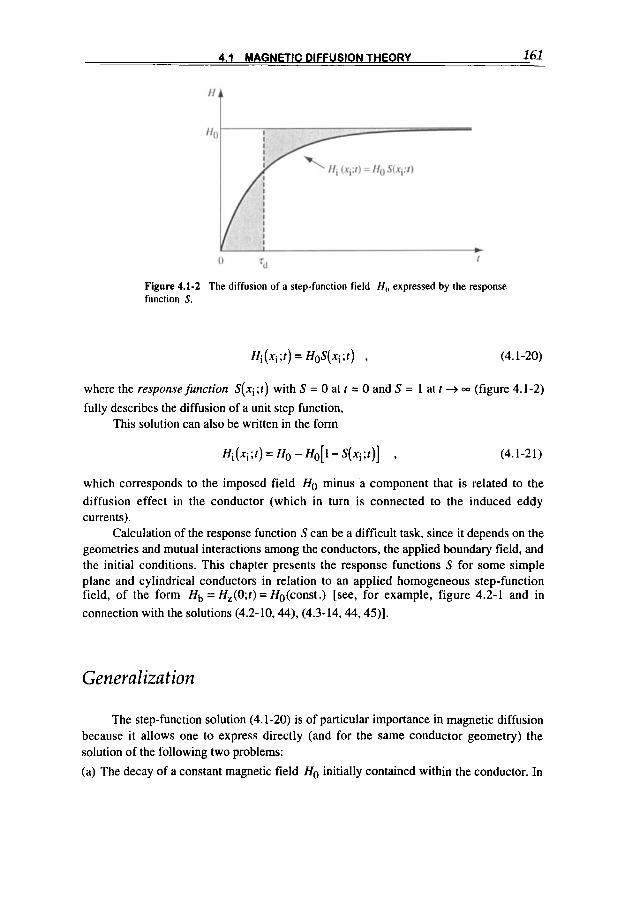
4.1 MAGNETIC DIFFUSION THEORY 161
Figure 4.1-2 The diffusion of a step-function field H, , expressed by the response function S.
Hi(xi;t)= HoS(xi;t) , (4.1-20)
where the response function S(xi;t) with S = 0 at t = 0 and S = 1 at t + m (figure 4.1-2)
fully describes the diffusion of a unit step function, This solution can also be written in the form
Hi(xi;r)= Ho - H0[1-S(xi;t)] , (4.1-2 1)
which corresponds to the imposed field HO minus a component that is related to the diffusion effect in the conductor (which in turn is connected to the induced eddy currents).
Calculation of the response function S can be a difficult task, since it depends on the geometries and mutual interactions among the conductors, the applied boundary field, and the initial conditions. This chapter presents the response functions S for some simple plane and cylindrical conductors in relation to an applied homogeneous step-function field, of the form Hb = H,(O;t)= HO(const.) [see, for example, figure 4.2-1 and in connection with the solutions (4.2-10,44), (4.3-14,44,45)].
Generalization
The step-function solution (4.1-20) is of particular importance in magnetic diffusion because it allows one to express directly (and for the same conductor geometry) the solution of the following two problems:
(a) The decay of a constant magnetic field HO initially contained within the conductor. In
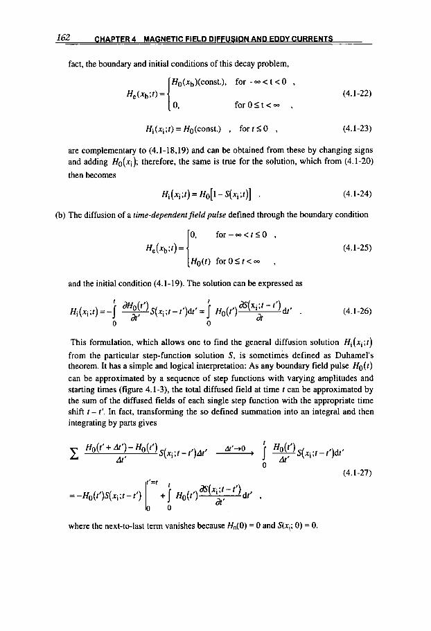
162 CHAPTER 4 MAGNETIC FIELD DIFFUSIO N AND EDDY CURRENTS
fact, the boundary and initial conditions of this decay problem, { ;(xb)(const.), for - < t < 0 ,
f o r O I t < = , He (Xb it) = (4.1-22)
Hi(.q;t) = HO(const.) , fort I 0 , (4.1-23)
are complementary to (4.1-18.19) and can be obtained from these by changing signs and adding H g ( 3 ) ; therefore, the same is true for the solution, which from (4.1-20)
then becomes
Hi(xi;t) = Ho[l - S(xi;t)] . (4.1-24)
(b) The diffusion of a time-dependentfield pulse defined through the boundary condition
0, f o r - - < t I O ,
Ho(t) f o r O I t < = , (4.1-25) He(Xb;t) =
and the initial condition (4.1-19). The solution can be expressed as
dS(X$ - 1’) 1 I
dt’ . at
Hi(xi;t) = -I W S ( 3 ; t - t’)dt’ =I Ho(t’) 0
at 0
(4.1-26)
This formulation, which allows one to find the general diffusion solution Hi(xi;t)
from the particular step-function solution S, is sometimes defined as Duhamel’s theorem. It has a simple and logical interpretation: As any boundary field pulse Ho(t) can be approximated by a sequence of step functions with varying amplitudes and starting times (figure 4.1-3), the total diffused field at time t can be approximated by the sum of the diffused fields of each single step function with the appropriate time shift t - t’. In fact, transforming the so defined summation into an integral and then integrating by parts gives
Af-to S(.q;t -f’)At’ - j m ( f ( x i ; t -t’)dt’ HO(t’+ At‘)-Ho(t’)
At’ 0
c At’ (4.1-27)
dS(xi;t - t’) dt’ ,
dt’ 0 0
where the next-to-last term vanishes because Ho(0) = 0 and S(xi.; 0) = 0.
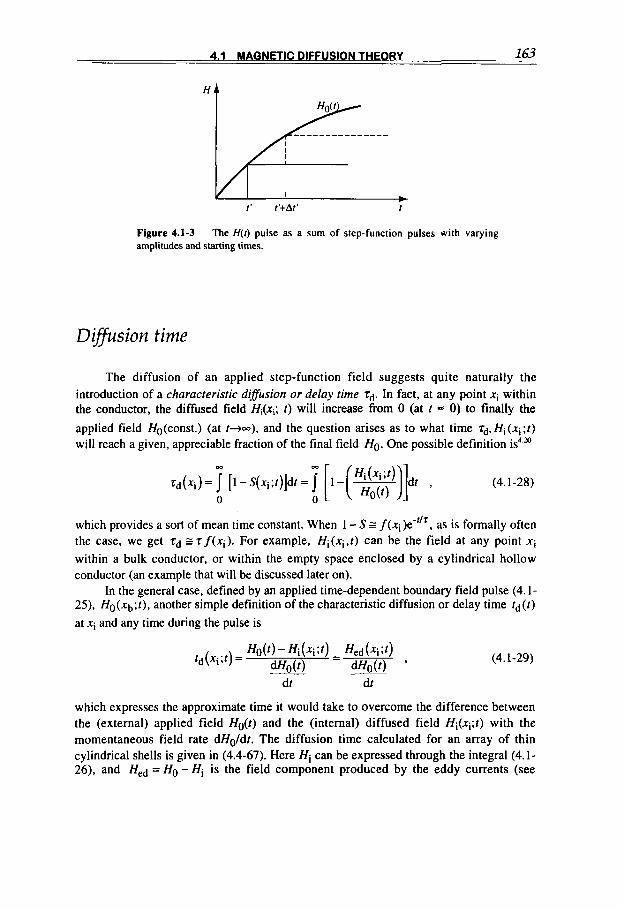
4.1 MAGNETIC DIFFUSION THEORY 163
Figure 4.1-3 amplitudes and starting times.
The H(r) pulse as a sum of step-function pulses with varying
Difision time
The diffusion of an applied step-function field suggests quite naturally the introduction of a characteristic diffusion or delay time z,+ In fact, at any point x; within the conductor, the diffused field Hi(.q; t ) will increase from 0 (at t = 0) to finally the
applied field Ho(const.) (at t+m), and the question arises as to what time rd, Hi(xi;t) will reach a given, appreciable fraction of the final field Ho. One possible definition is4.*’
(4.1-28)
which provides a sort of mean time constant. When 1 - S E f(q)e-f’7, as is formally often the case, we get Zd z r f (x , ) . For example, Hi(q,t) can be the field at any point xi
within a bulk conductor, or within the empty space enclosed by a cylindrical hollow conductor (an example that will be discussed later on).
In the general case, defined by an applied time-dependent boundary field pulse (4.1- 25), Ho(xb; t ) . another simple definition of the characteristic diffusion or delay time td(t) at xi and any time during the pulse is
(4.1-29)
dt dt
which expresses the approximate time it would take to overcome the difference between the (external) applied field Ho(t) and the (internal) diffused field Hi(q;r) with the momentaneous field rate dHoldt. The diffusion time calculated for an array of thin cylindrical shells is given in (4.4-67). Here Hi can be expressed through the integral (4.1- 26), and Hed = HO -Hi is the field component produced by the eddy currents (see

c 164 CHAPTER4 MA
section 4.4). Note that for a step function (4.1-18), HO = Ho(const.), integration of the
above definition up to t -+ m,
leads to definition (4.1-28). It is interesting to consider the special case
Ho(l)=& . for which the solution (4.1-26) becomes
r t Hi(3; t )= -h,JS(+;f -t’)dt‘= bIS(xi;t’)dt‘ ,
0 0
which, when inserted into the definition (4.1-29), yields
(4.1-30)
(4.1-3 1)
(4.1-32)
Here S(xi;t) is the response function defined in (4.1-20) and figure 4.1-2. This figure makes it clear that the right-hand side tends, after a long enough time, to a time- independent (but space-dependent) constant, thus
Zd =a- (4.1-33) ho --Onst.
This also means that here the eddy currents, which determine Hed, become stationary for t B Zd. The diffusion parameters of this case are illustrated in figure 4.1-4. Bhe result 7d = const. is obtained more in general, as shown in (4.4-67).]
H
‘d t
Figure 4.1-4 Diffusion of the linear field pulse He(I) = hot, which leads, after long enough times (t+-), to a characteristic delay time 7d, and to a stationary eddy current distribution with field component Hcd.
4.2 FIELD DIFFUSION INTO PLANE CONDUCTORS 165
4.2 FIELD DIFFUSION INTO PLANE CONDUCTORS
In this section the diffusion problem is solved in the plane one-dimensional case. Although this geometry is somewhat idealized, its simplicity allows one to find relatively simple analytical solutions and thus obtain a useful insight into the diffusion process. The analogous solutions of the equivalent thermal problem (4.1-17) are well known in the l i terat~re.~ ’
Half-space conductor
The coordinate system is chosen with the x-axis pointing into the conductor and the y- and z-axes placed on its surface so that H = (0.0, H z ) , E I (O,EY,O), and j = (0, jY.O), as shown in figure 4.2-1. The Amptre and Faraday laws (4.1-10.1 la) simplify with the expressions given in table A.3-I1 to the one-dimensional form
dH Z=-’ JY ’
or, in practical cgs units (A, V, Oe, cm, s),
and the diffusion equations (4.1-16) for the magnetic field
or, when p is constant in time and o i n space,
with K given in (4.1-9). These equations could have
(4.2-1)
(4.2-2)
(4.2-2)*
(4.2-3)
been obtained directly from differentiating (4.2-1) and then inserting Ohm’s law (4.1-1) and (4.2-2). For (4.2-3) and similar forms there exists a vast array of solutions, as already mentioned.

166 CHAPTER 4 MAGNETIC FIELD DIFFUSION AND EDDY CURRENTS
Figure 4.2-1 Diffusion into a conducting half-space.
In the following, various aspects of the solution to the diffusion equation (4.2-3) will be presented. By introducing the similarity variable
X 6 = - , 2&
(4.2-4)
where is the magnetic diyusivity given in (4.1-9), the above equation transforms into
dh dH -+26h=O , where h = - , 86 36
and the solution becomes
H,(t) = Ae-{*d{ + C ; (4.2-5)
here A and Care constants in 6 (but they can depend separately on x or t ) that must satisfy the appropriate initial and boundary conditions.
Step-function field
With the step-function boundary condition (4.1-18) (figure 4.2-2, case n = 0),
1" HO(const.),for 0 S t < -,
written here as
for - - < t < 0, H,(O,t) = (4.2-6)
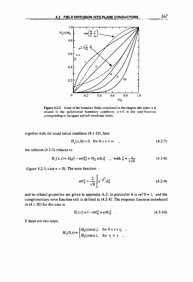
167 4.2 FIELD DIFFUSION INTO PLANE CONDUCTORS
0.8 -
I l l 1
0 0.2 0.4 0.6 0.8 1.0 rho
Figure 4.2-2 Some of the boundary fields considered in this chapter (the index n is related to the polynomial boundary condition; n = 0 is the step-function corresponding to the upper and left coordinate lines).
together with the usual initial condition (4.1-19). here
H,(x ,O) = 0, for 0 < x < - ,
the solution (4.2-5) reduces to
H,( x, t ) = Ho( 1 - erft) = HO erfct , with 5 = X 2&
(figure 4.2-3, case n = 0). The error function
(4.2-7)
(4.2-8)
(4.2-9)
and its related properties are given in appendix A.2: In particular it is erf 0 = 1, and the complementary error function erfc is defined in (4.2-8). The response function introduced in (4.1-20) for this case is
S ( x ; t ) = 1 - erft = erfct . (4.2-10)
If there are two steps,
HO(const.), for 0 < t < tl ,
Hl(const.), for tl < t , H, (0, t ) =

168 CHAPTER 4 MAGNETIC FIELD DIFFUSION AND EDDY CURRENTS
5 Figure 4.2-3 Diffused magnetic fields corresponding to the boundary fields labeled n=0.1,2.4,6 in the previous figure. The magnetic flux skin depth ~ 4 , ~ is indicated by a bar with arrow for each case.
the solution is as in (4.2-8) for the time interval 0 < t < t l ; thereafter, t > t l , and by linear combination it becomes
HZ(x,t)=Hoerfc-+(H1-Ho)erfc- 2 4 2 2 4 % . *
General solution
The solution (4.1-27) corresponding to the applied field pulse Ho(t)-that is, to the
I Ho(r), for 0 5 t < 00,
transient boundary condition 0, for - = < t < 0,
(4.2-1 1 ) H,(O,t) =
[where, however, Ho(t = 0) = 01 and initial condition (4.2-7)-can, with (4.2-lo), be given directly as

169 - ._ - -_ 4.2 FIELD DIFFUSION INTO PLANE CONDUCTORS
X 2 -~ f =-I X Ho(t’)e 4 K ( t - f ’ ) dt‘ 2 G 0 (t-t‘)3/2 ,
f -~ X 2 =-I X Ho(t’)e 4 K ( t - f ’ ) dt‘ 2 G 0 (t-t‘)3/2 ,
(4.2- 12)
Alternatively, by introducing the retarded similarity variable (4.2-4), 5* = x/2,/-,
the latter transforms into
This integral can be split into the components
X I
(4.2- 13)
(4.2-14)
The first integral gives the stationary solution [for a boundary field that extends from -- to +-; see, e.g., (4.2-30)], whereas the second integral depends on the transient nature of the boundary condition (4.2-1 1) and vanishes when t + -.
Alternatively, the general solution of the diffusion equation (4.2-3) relative to the half-space and defined by the boundary and initial conditions that are complementary to conditions (4.2-6,7)-that is,
H,(OJ) = 0, Hz(X,O) = Ho(x) (4.2-15)
(corresponding to a field distribution Ho(x) in the conductor that is allowed to decay from t = 0 on)-is found similarly to (4.2-12), or more directly from solution (A.4-65) by splitting the integral into two components from the x = 0 rigi in^.^:
Hz(x,t) = - 2Jxm 1 poiXt)[ 0 .--LTldd (4.2-16a)
( X - x y (x+x ’ )2
When Ho(x) = Ho(const.), with the variable transformation
and the definition (4.2-9), this solution simplifies into
2 4 z Hz(x,t) = Hoerf- . (4.2-16b)

170 CHAPTER 4 MAGNETIC FIELD DIFFUSION AND EDDY CURRENTS
In fact, it correctly satisfies the initial and boundary conditions, and from (4.2-5) we know that the error function is a solution of the plane diffusion equation (4.2-3).
When the boundary and initial conditions include a mixture of conditions (4.2- 7,11,15), the general solution will be a linear combination of solutions (4.2-12,16).
Characteristic dif is ion parameters
The diffusion equations can be rewritten into a dimensionless form by introducing [see also in connection with (1.2-5)] a characteristic time to (duration of the field pulse), conductor dimension lo, and field amplitude H o , such that H* = Hf Ho, t* = t / tO,
1* = 1/10, A* = A 1 6 :
(4.2-17)
This shows that the characteristic (penetration) diffusion depth SO down to which the magnetic field is still appreciable is
and that the field penetrates or decays away on a diffusion time scale
and with a formal diffusion velocity [see also in (3.3-31)]
(4.2-1 8a)
(4.2- 18b)
(4.2-18~)
[See (8.1-46) for an extension to moving conductors.] In practice, more precisely defined skin depths are of interest. The skin depth can be
related to the decay down to a specified amplitude of the diffused field; or, for example, the depth s, at which the diffused field H(x, t ) [as given by one of the solutions (4.2-8,12)] amounts to the e-fold decrease of the surface field H(0, t), which is thus defined by
H(s,,t) = H(O,t)/e . (4.2-19)
Another useful concept is the so-called magneticflux skin depth s@ defined in such a way that the total diffused magnetic flux fit) can be expressed by the surface magnetic induction spreading over s o that is,
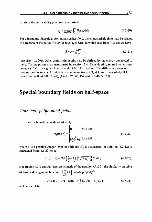
4.2 FIELD DIFFUSION INTO PLANE CONDUCTORS 171
or, since the permeability p is taken as constant,
For a harmonic sinusoidal oscillating surface field, the characteristic time may be related to a fraction of the period T = 2n/o (e.g.. to = T h ) , in which case from (4.2-18) we have
(4.2-21)
[see also (4.2-29)]. Other useful skin depths may be defined by the energy connected to the diffusion process, as mentioned in section 5.4. Skin depths, related to various boundary fields, are given later in table 5.2-11. Extension of the diffusion parameters to moving conductors and fluids is made in sections 4.3, 4.4 and particularly 8.1, in connection with (4.3-8, 11,47), (4.4-21,25,40,45), and (8.1-46,53,67).
Special boundary fields on half-space
Transient polynomial fields
For the boundary condition (4.2-1 1).
fo r t<O ,
H,(O,t;n) = (4.2-22)
where n is a positive integer (even or odd) and HO is a constant, the solution (4.2-12) is calculated from (4.1-27) to be
(4.2-23)
(see figures 4.2-2 and 3). Here use is made of the notation (A.2-7), the similarity variable
(4.2-4), and the gamma function r , whose propertyA '
r(z + 1) = zr(t) with r(+) = ,hi, r(i) = I
will be used later.
(4.2-24)

172 CHAPTER 4 MAGNETIC FIELD DIFFUSION AND EDDY CURRENTS
Four comments can be made regarding the polynomial solution: (a) The case n = 0 corresponds to the step-function boundary condition and related
solution given in (4.2-6,8). Application of this particular solution requires some caution since it gives rise to an infinite surface current density and temperature, as shown later in (5.2-22).
(b) Since the dirusion equation is a linear differential equation, the more general solution related to a linear combination of conditions (4.2-22) with n = 0,1,2, ... can be given as a linear combination of the corresponding solutions; in this way the diffusion of nearly any field pulse can be given in analytic form.
(c) The parabolic boundary field corresponding to n = 1, and whose diffused component is written immediately from (4.2-23) with the help of one of the relations (A.2-7). approximates fairly well the transient sinusoidal quarter period, whose exact solution in integral form is given in (4.2-28). Since, as we will see in the following sections, most phenomena depending on magnetic diffusion are relatively insensitive to the boundary pulse form, this case can be used to give good approximations for the important problem with a transient sinusoidal boundary condition.
(d) For the skin depth (4.2-20), we calculate - sq,n = &J ,, Hz(x,t;n)dr = 2"r(3n+1)2fiIn ,
0
where m
is determined with the help of (A.2-7, 9). Finally (figure 4.2-3),
(4.2-25)
Transient sinusoidal field
A case often encountered in practice, since it approximates the field diffusion in a LC circuit, is represented by the boundary condition
for t c 0,
("' Hosinux, for t 2 0, Hz(O,t) = (4.2-26)

173 _. 4.2 FIELD DIFFUSION INTO PLANE CONDUCTORS - .. - ~. - .
I- -I n= 1 .oo ob-] _**- -----------
.__-***
-0.5 I I I I I 1 0 1 2 3 4 5
X I 6
Figure 4.2-4 and comparison with the steady-state solution at three different times.
Diffusion of the transient magnetic field H,(x,r) = Hosinm (dashed line)
with w = 27cIT. Using the integral relation
(4.2-27)
the solution (4.2- 14) becomes
H , ( x , t ) = Hoe-x/6sin ( CB! - - i) - - 2 f sin[ - &)e-5*2 d t * (4.2-28)
where the harmonic skin depth (or depth of penetration), already mentioned in (4.2-21), is expressed as
(4.2-29)
here v = 1/T is the frequency and p~ the relative magnetic permeability (1.1-9), p = 47c 10-7 p ~ . This is the depth (measured from the surface of the half-space conductor) at which the amplitude of the magnetic field, electric field, and current density falls to l/e = 0.368 of their surface values, as we will see in (4.2-32, 33). The first term in (4.2- 28) is the solution (4.2-32) of the steady oscillation. In figure 4.2-4 the solution, calculated numerically, is plotted for three different times ( t /T = 0.25, 0.5, 1 ) and compared with the corresponding steady-state solution. The qualitative difference between the two solutions is expressed by the number of zeros: no zero point for the transient cases tlT= 0.25,0.5; only one zero for tlT= 1; infinite zeros for the steady-state

174 CHAPTER 4 MAGNETIC FI ELD DIFFUSION AND EDDY CURRENTS
solution. As a consequence of the strong decay of the solution over the distance 6, the quantitative difference is, however, rather small.
The numerically calculated magnetic flux skin depths (4.2-20) for the transient

4.2 FIELD DIFFUSION INTO PLANE CONDUCTORS 175
cases tlT= 0.25.0.5, 1 are
S# = 0.7806, 0.7236, - 0.3686 ,
whereas those corresponding to the steady case are given in (4.2-37). The value of the transient sB at field maximum t = 0.25T is also given in the nomogram of figure 4.2-5.
Steady sinusoidal field
The first term in (4.2-28), corresponding to the steady sinusoidal boundary condition
Hz(O,t) = Hosinun, for - m < t < +m , (4.2-30)
applied to a conducting half-space, can also be found directly from the diffusion equation
(4.2-3) by looking for a solution of the form
H , ( x , t ) = H(x)sin(wt - 4) (4.2-31)
or, alternatively, of the complex form (4.3-21b). The
4.2-4),
H, (x, t ) = Hoe-XJGsin
and the corresponding current density (4.2- 1) becomes
solution is straightforward (figure
j y ( x , t ) = joe-x/6sin wt - - + --IC ,
(4.2-32)
(4.2-33)
where
jo =a-; HO (4.2-34) 6
the dassical skin depth 6 is defined in (4.2-29) and given in the nomogram of figure 4.2-5. For both magnetic field and current, we find an exponential amplitude decrease and
a phase shift that depend only on x/6. Note that in this steady-state solution, the current precedes the field by a phase 0.25 R . Thus, when the outer field is zero at t = 0, the current density on the surface already has a finite value. However, the total current per unit width iy must disappear at t = 0, since, upon integrating (4.2-1) along a convenient rectangular path [with one side outside the conductor, parallel to the field, and the opposite side deep in the conductor where Hz(x + m,?) + 01, we calculate
H,(O,t) = i y ( t ) . (4.2-35)
176 CHAPTER 4 MAGNETIC FIELD DIFFUSION AND EDDY CURRENTS
In fact, integration of (4.2-33) yields
that is, the current has the same time dependence as required by (4.2-35).
The total magnetic$ux per unit width is
(4.2-36)
Thus, the flux disappears at a time when the field on the surface does not vanish (as always, hysteresis effects are neglected) because the flux trapped within the conductor adds algebraically with f signs. It seems appropriate to define the flux skin depth with respect to the maximum surface field H, [and not to H,(O,t)]. Thus setting vz(t) = N o s # , at t/T = 0.25,0.5, 1 , we get
(4.2-37)
These skin depths do not differ very much from those calculated in the transient solution, although there is a qualitative difference between the two cases. Note that the electric field on the surface of the half-space conductor can be obtained either from (4.2- 33), E,,(O,t) = jy(O,t)/o, or from (4.2-36), Ey(O, t ) = dv( t ) /d t .
The heating of various conductors subjected to a sinusoidal boundary magnetic field are calculated in chapter 5 with the results given in (5.2-26,44), (5.3-4,9,10) and table 5.4-11. These results are important in induction-heating applications.
Exponential field
The solution corresponding to the steady boundary field
Hz(O,t) = Hoe'/'. for - 00 < t < 00 , (4.2-38)
applied to a conducting half-space (see figure 4.2-2), is found directly from (4.2-3) by looking for a solution of the form e'/* f(x). For this function we obtain the equation
from which the general solution follows:
H , ( x , t ) = Hoer/'(Ale-x/Xo + A2e+'/'O) , (4.2-39)

4.2 FIELD DIFFUSION INTO PLANE CONDUCTORS 177
where Al, A2 are constants and
x o = G .
Here the only physically acceptable solution is
H,(x,t)= Hoexp . (: ;I For the magnetic flux skin depth defined in (4.2-20) we find
s @ = x o = G .
When the parameter
is time-dependent, we have z = ~ ( t ) , because f now follows the equation
Thus, the former relations remain approximately valid, provided that
d r z dt "7 -
(4.2-40a)
(4.2-40b)
(4.2-41a)
(4.2-4 1 b)
The exponential field increase is often obtained approximately in flux compression devices, and the simple solution (4.2-40) is useful for estimating the field diffusion in such experiments.
The solution corresponding to the transient boundary field
(4.2-42a)
with z positive or negative, is obtained again from the general solution (4.2-12):
(4.2-42b)
The error function of complex argument, obtained when 7 is negative, is well defined and t a b ~ l a t e d . ~ . ~
Note that for z + m, we obtain the step function and its related solution (4.2-8). A further solution corresponding to the transient exponential boundary field applied to a cylindrical conductor is discussed in connection with (4.3- 19,20).

Tab
le 4
.24
Ste
p-f
un
ctio
n fi
eld
dif
fusi
on 1
Ste
p bo
unda
ry
m
H=
Ho
(con
st.)
So
lutio
n H
z(f;
r)=
HO
eige
nfun
ctio
n qn
I
geom
etry
co
nsta
nts
I I I
h
5a
5b
2a
-
5c
M
.b-$E- t I
-sin
@
-sin
@
sin[
nn($
+ +)I/
n
sin[
nn($
+
+)]
/n
2l
diff
usio
n tim
e co
nst.
r,,
Rem
arks
sum
mat
ion
over
n=
1,3,
... (o
dd) o
nly
n=1,
2,3,
4,
sum
mat
ion
over
2=
2.4,
... (e
ven)
onl
y
doub
le s
umm
. ove
r n,
m=1
,3,..
(odd)
only
Jo,J
l,a,
, :
see
app.
A.2
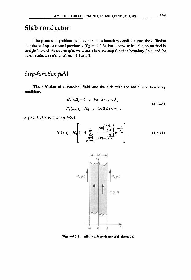
4.2 FIELD DIFFUSION INTO PLANE CONDUCTORS 179
Slab conductor
The plane slab problem requires one more boundary condition than the diffusion into the half-space treated previously (figure 4.2-6), but otherwise its solution method is straightforward. As an example, we discuss here the step-function boundary field, and for other results we refer to tables 4.2-1 and 11.
S tep-fu n ct ion field
The diffusion of a transient field into the slab with the initial and boundary conditions
H , ( x , O ) = O , for-d<x<d,
H,( fd , r )= HO , for O l r < - , (4.2-43)
is given by the solution (A.4-66)
(4.2-44)
Figure 4.2-6 Infinite slab conductor of thickness 2d.
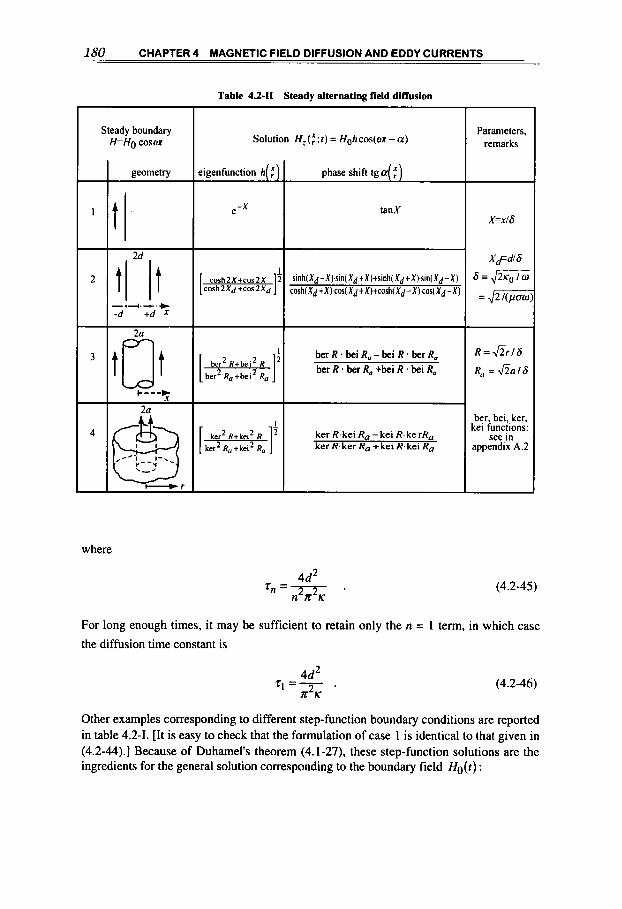
CHAPTER 4 MAGNETIC FIELD DIFFUSION AND EDDY CURRENTS - 180 __
Table 4.241 Steady alternating field diffusion
Steady boundary H=Ho C O S ~
geometry
t
-.+.-I-.+
-d +d X
2a
eigenfunction h(
e-'
cosh2 X tcos 2 X [ COSh2Xd t C O S 2xd ]
I ber2 Rtbei2 R
ber2 R, tbe i2 R,
ker2 R,+kei2 Ru
phase shift tga(:)
tanY
ber R * bei R,-be i R 1 ber R, ber R . ber R, +bei R. bei Ra
ker R. kei R, - kei R. ke rR, ker R.ker R, +kei R.kei R,
Parameters, remarks
R = & r l G
R, = G a l s
ber, bei, ker, kei functions:
see in appendix A.2
where
(4.2-45)
For long enough times, it may be sufficient to retain only the n = I term, in which case
the diffusion time constant is
4d2 7 1 ' 2 .
K K (4.2-46)
Other examples corresponding to different step-function boundary conditions are reported in table 4.2-1. [It is easy to check that the formulation of case 1 is identical to that given in (4.2-44).] Because of Duhamel's theorem (4.1-27), these step-function solutions are the ingredients for the general solution corresponding to the boundary field Ho(t ) :

4.2 FIELD DIFFUSION INTO PLANE CONDUCTORS 181
where
__ m e ‘n
H,(x,t) = -lo Ho(t’)cc qn-dt’ = cc An(r)qn(x)e ‘, , m
t (4.2-47)
n=l r n n=l
t‘
‘F dt’ An(t) = lloH(t’)e - ,
r n
and the other parameters are defined for some examples in table 4.2-1.
the initial and boundary conditions The decay of a magnetic field initially contained within the slab, characterized by
H,(x,O)=Ho , f o r - d < x c d ,
H,(fd,r)=O , f o r - O I t < w , (4.2-48)
is complementary to the diffusion of the step-function field. These conditions can be obtained from (4.2-43) by adding the term -Ho to the right-hand side and changing sign, as is the case for the solution
The solution of the two-dimensional form in (x,y) of the diffusion equation (4.1-8), related to an infinitely long rectangular conductor, is the product of the solutions of the respective one-dimensional diffusion equations with appropriate initial and boundary conditions; this follows directly from the general formulation of solution (A.4- 10.60). Case 4 in table 4.2-1 gives the solution corresponding to the step-function boundary condition.
As explained in connection with the conditions (4.2-43,48), this solution can be used to describe the decay of a longitudinal magnetic field H,, initially imbedded in a rectangular bar with sides 2a and 2b. When only the m,n = 1 terms are retained, the solution transcribed from (4.2-49) simplifies to
4 NI rcy -+ H,(x,y,t) =-HHgcos-cos-e .
n 2a 2b
Here the diffusion (decay) time (4.2-46) is
(4.2-50)
4
= n2( l/a2 + l/b2)K *
(4.2-5 1 )
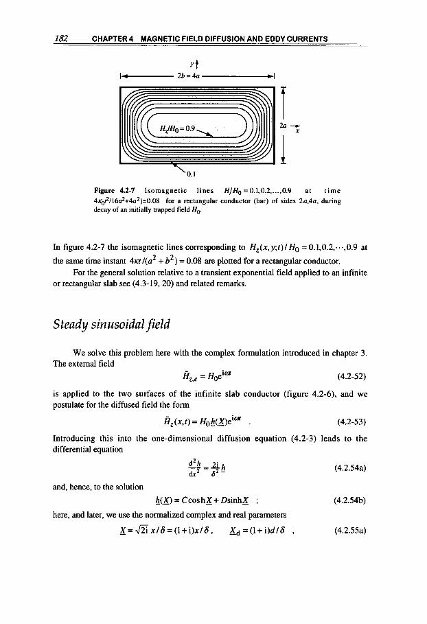
182 CHAPTER 4 MAGNETIC FIELD DIFFUSION AND EDDY CURRENTS
T
Figure 4.2-7 Isomagnet ic lines H / H o =0.1.0.2. ..., 0.9 a t t i m e 4@/16a2+4a2)=0.08 for a rectangular conductor (bar) of sides 2a.4a, during decay of an initially trapped field H,,.
In figure 4.2-7 the isomagnetic lines corresponding to H,(x,y;t)/ HO = 0.1,0.2,...,0.9 at
the same time instant 4a / ( a2 + b2) = 0.08 are plotted for a rectangular conductor. For the general solution relative to a transient exponential field applied to an infinite
or rectangular slab see (4.3-19,20) and related remarks.
Steady sinusoidal field
We solve this problem here with the complex formulation introduced in chapter 3. The external field
Hz,e = HoeiW (4.2-52)
is applied to the two surfaces of the infinite slab conductor (figure 4.2-6), and we postulate for the diffused field the form
f i z ( x , t ) = Hob(x)eiw . (4.2-53)
Introducing this into the one-dimensional diffusion equation (4.2-3) leads to the differential equation
and, hence, to the solution
- h ( 2 ) = Ccos h_X + DsinhX ;
(4.2.54a)
(4.2.54b)
here, and later, we use the normalized complex and real parameters
- X = J Z ; x / 6 = ( 1 + i ) x / 6 , Xd=(1+ i )d /6 , (4.2.55a)
4.3 FIELD DIFFUSION IN CYLINDRICAL GEOMETRY 183
x = X / 6 , x d = d / 6 , 6 = - (4.2.55b)
where 6 is the harmonic skin depth (4.2-29), and use is made of (3.1-9). The boundary conditions
l G - 3
(4.2-56)
define the constants C and D, and we find the solution
(4.2-57) cosh X h(X) = - COShXd '
The hyperbolic cosine with complex argument can be written asA ' coshX = cosh( X + ix) = coshxcos X + i sinhXsinX ,
sinhx = sinh(X+ ix) = sinhXcosX + icoshXsinX .
Thus the solution can be obtained in the form
(4.2-58)
+ sinhxsinXsinhxdsinXd + i(sinhXsinXcosh Xd cosxd - cosh Xcos XsinhXdsinXd)] .
After applying a few relations of the hyperbolic cosine and sine functionsA.', for example
2cosh2 X = cosh2X + 1 , 2sinh2X = cosh2X - 1 ,
we obtain the real functions h(X) and a(X) as given in table 4.2-11 [see the definitions
(4.2-59)
(3.1-1 I , 12)].
4.3 FIELD DIFFUSION IN CYLINDRICAL GEOMETRY
The diffusion of magnetic fields through cylindrical conductors is a process often encountered in practice-for instance, in the transmission of high-frequency currents. Because of the cylindrical geometry, the exact analytic solutions are generally very clumsy. In some cases, however, it is possible to give useful approximations; the most obvious is attained when the skin depth is much smaller than the radius, since the problem then reduces to the plane case, and the solutions given in the previous sections can be used.
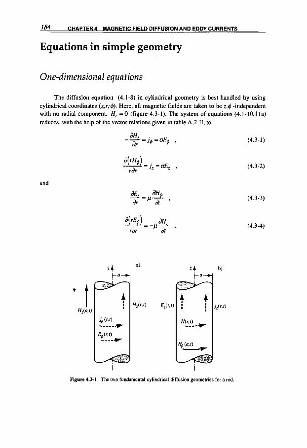
184 CHAPTER 4 MAGNETIC FIELD DIFFUSION AND EDDY CURRENTS
Equations in simple geometry
One-dimensional equations
The diffusion equation (4.1-8) in cylindrical geometry is best handled by using cylindrical coordinates (z,r;@). Here, all magnetic fields are taken to be z,@ -independent with no radial component, Hr = 0 (figure 4.3-1). The system of equations (4.1-10,l la) reduces, with the help of the vector relations given in table A.2-II, to
(4.3-1) dH dr
- - = j q = o E q ,
and
dH -- - - p a t . rdr
(4.3-2)
(4.3-3)
(4.3-4)
Figure 4.3-1 The two fundamental cylindrical diffusion geometries for a rod.
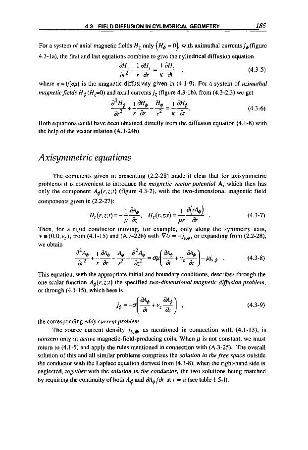
4.3 FIELD DIFFUSION IN CYLINDRICAL GEOMETRY 185
For a system of axial magnetic fields Hz only ( H4 = 0), with aximuthal currentsjO (figure
4.3-la), the first and last equations combine to give the cylindrical diffusion equation
(4.3-5)
where K = I/(o~) is the magnetic diffusivity given in (4.1-9). For a system of azimuthal magneticfields H @ (Hz=O) and axial currentsjZ (figure 4.3-lb), from (4.3-2.3) we get
(4.3-6) -+ a2H@ laH@ H@ - 1 aH@ h2 r & r2 ~ d t ’
Both equations could have been obtained directly from the diffusion equation (4.1-8) with the help of the vector relation (A.3-24b).
Axisymmetric equations The comments given in presenting (2.2-28) made it clear that for axisymmetric
problems it is convenient to introduce the magnetic vector potential A, which then has only the component %(r,Z;t) (figure 4.3-2), with the two-dimensional magnetic field
components given in (2.2-27):
”, Hz(r , z ;r )=- - 1 . H,(r,z;t) = P h Pr i+
(4.3-7)
Then, for a rigid conductor moving, for example, only along the symmetry axis, v = (O ,O,v , ) , from (4.1-15) and (A.3-22b) with VU = - jS,@, or expanding from (2.2-28), we obtain
This equation, with the appropriate initial and boundary conditions, describes through the one scalar function A@( r, z ; t ) the specified two-dimensional magnetic difSusion problem, or through (4.1-15), which here is
(4.3-9)
the corresponding eddy current problem. The source current density jS ,+ as mentioned in connection with (4.1-13), is
nonzero only in active magnetic-field-producing coils. When p is not constant, we must return to (4.1-5) and apply the rules mentioned in connection with (A.3-25). The overall solution of this and all similar problems comprises the solution in thefree space outside the conductor with the Laplace equation derived from (4.3-8), when the right-hand side is neglected, together with the solution in the conductor, the two solutions being matched by requiring the continuity of both A#and d ! / & at r = a (see table 1.5-1).

186 CHAPTER 4 MAGNETIC FIELD DIFFUSION AND EDDY CURRENTS
Figure 4.3-2 Conductor C moving with velocity vz in an axisymmetric magnetic field configuration generated by the source current density is, @ in the conductor D and defined by the vector potential component A@
The diffusion of an axisymmetric magnetic field in spherical coordinates is discussed in connection with (A.4-74).
Two-dimensional equations Another two-dimensional magnetic field distribution is obtained when there is a
purely axial current density, j = jzez. We know from the discussion in connection with (2.2-35) that the corresponding field distribution is conveniently described through the A z ( r , @ ; f ) component of the vector potential, with the two-dimensional magnetic field components given by
1 dA 1 dA ffr(r,$;r) = -2, H4(r,@;r) = ---1 .
P 34 Clh (4.3-10)
Similarly to (4.3-8), from (4.1-15) with VU and (A.3-22b, 24b) for a rigid conductor rotating about its symmetry axis in the azimuthal velocity v = (O,v@,O), we obtain

4.3 FIELD DIFFUSION IN CYLINDRICAL GEOMETRY 187
(4.3-1 1 )
As before, the source current density often neglected. The eddy current density is
is nonzero only in active conductors, so it is
(4.3-12)
The general solution corresponding to this equation, with vq = 0, jssz = 0, is given in
(A.4-72).
Diffusion of axial fields
Step-function field on a rod
The diffusion into a conducting rod of a transient axial magneticfield, which is characterized by (4.3-5) and the usual initial and boundary conditions
H,(r,O)=O, f o r O l r < a , (4.3-13)
for--<t<O ,
("' Ho(const.), for 0 I t < - ,
H,(a,f) =
is
(4.3-14)
Here Jo, J 1 are the Bessel functions of the first kind of order v = 0,1, and the aa, = x t are the positive roots of the equation
Jo(x$) = 0 (4.3-15)
[see table A.2-I and (A.2-19)]. This solution follows directly from the general solution (A.4-69), where 4, B,, = 0 since H, remains finite at r = 0; aan = x$, 4 = HO because
of the boundary condition, and An = -2Ho / ( x [ J ~ ( x t ) ) because of the initial condition

188 CHAPTER 4 MAGNETIC FIELD DIFFUSION AND EDDY CURRENTS
and (A.2-21). The solution also ensures that dH, ldr = 0 at r = 0, and Hz(r,t) = Ho for
t + - or when cT+ 0. The diffusion (decay) time constants are
For long enough times-that is, when t ~ ~ 1 , where
2 1 a ml K
= 7 = 0.173- = 2.18 x 10-'a20
(4.3-16a)
(4.3-16b)
is the predominant diffusion time (p = &)-it may be sufficient to retain the first term only, in which case the diffused field on axis is described by the approximation
I -- Hz(O,t)G Ho(1-e ' 1 ) (4.3- 17)
The decay of an axial magnetic field initially trapped within the rod is complementary to the above diffusion process, and the solution can be transcribed directly from (4.3-14) by adding a term (-H,-,) to the right-hand side and changing sign [as discussed in connection with (4.2-49) for similar diffusion into or from a bar]. For example, the magnetic flux remaining in the bar is calculated to be
(4.3-18a)
Here the uniformly convergent series was integrated term by term and evaluated with the integral relation (A.2-25b); note that with (A.2-21) one correctly obtains y,(t + 0) = Worn2. A coil of N turns wound on the bar will pick up an induced voltage (1.4-9), U, during the field decay, which in the approximation of (4.3-17) is given by
(4.3-18b)
This arrangement allows the measurement of Q ; it is an example of the electrodeless method of measuring electrical conductivity or other related parameters through the inductive response of metallic samples in the form of ~phe res~ . '~ . 4.29,
hollow cylinders. In the latter, the method is particularly effective, because the simultaneous measurement of the external and internal magnetic field permits a more direct correlation to the diffusion parameters (see formulae in the subsections on hollow cylinders in this and the following chapters).
The general diffusion solution Hz(r,f) related to the diffusion of a general transient boundary field Ho(t) can be found through Duhamel's theorem (4.1-27) with the parameters defined in (4.3-14), or in table 4.2-1, case 5 . As an example, we mention the transient exponential boundary field

4.3 FIELD DIFFUSION IN CYLINDRICAL GEOMETRY 189
I
Hz = Ho(1- e-7) (4.3-19)
(where the field rises from 0 at t = 0 to the asymptotic value Ho). which approximates fields obtained in many experiments, notably in magnetically contained fusion experiments. This transient ( t 2 0) boundary field comprises a step function added to a (negative) transient exponential function; the related solution of the diffusion equation, obtained through the theorem (4.1 -27), (4.2-47), will reflect these two component^^.^^:
m
(4.3-20)
Note that for z + 0 we obtain the solution corresponding to a step function, and thus the expressions for the constants c,, the eigenfunctions qn (r), and the diffusion (decay) times Z, are in this case given by (4.3-14, 15, 16). As a matter of fact, this solution can be extended to the cases 1,4, and 6 described in table 4.2-1 and also in (4.2-44, SO), (4.3-14, 4 1) (infinite and rectangular slab, and transverse rod) by inserting the appropriate parameters. For the eddy-current heating corresponding to this boundary field see (5.2-39, 40).
Steady sinusoidalfield on a rod
The solution of the difSuusion into a rod of the steady boundary field
Hz(a,t) = Ho coswt, for - m < t < +oo , (4.3-2 I a)
is treated extensively in the literature4.' as an eddy current problem, which will be discussed specifically at the end of this chapter. Therefore, analysis here is limited to a brief outline that makes use of the complex formalism developed in section 3.1, and already applied in (4.2-52).
Assuming the boundary field in the complex writing to be
Hz(a,r) = HoeiUX , (4.3-21b)
and looking for a solution of the form
HZ(r,t) = Hol-z(/?)eiUX , (4.3-22)
the diffusion equation (4.3-5) transforms into
(4.3-23)
Here and in the following, for the normalized complex and real radii we use the notations

190 CHAPTER 4 MAGNETIC FIELD DIFFUSION AND EDDY CURRENTS
- R = f i r / 6 = ( 1 + i ) r / 6 , _R,=f ia /6 ,
R = f i r / 6 . R , = f i a / 6 , 6=@ , (4.3-24)
with 6 the harmonic skin depth (4.2-29), and use is made of (3.1-9). This equation is solved by modified Bessel functions (A.2-13) of the first and second kind and of order zero:
where the constants C,D are determined by the boundary conditions of the specific problem.
For a solid cylindrical conductor we have D = 0, since H , remains finite for r = 0 and &(O) = 00; on the other hand, the constant C is determined by the boundary condition (4.3-21):
(4.3-25b)
Introducing the Kelvin functions (A.2- 15),
i-,(_R) = berR + ibeiR , (4.3-2%)
and rearranging gives
(4.3-25d) ia - berRberR, +beiRbeiR, +i(beiRberR, -berRbeiR, ) h(B)=he -
ber2 R, +hi2 Ru
thus we obtain the functions h and tana as given in table 4.2-11 [see the definitions (3.1- 11, 12)].
cylindrical conductor than in the plane case. In fact, due to cylindrical geometry, current filaments tend to penetrate more as they become shorter and therefore "less resistive". As a result, the current skin depth is larger than in the plane case. The opposite is true for the cylindrical hole, where the current will be concentrated close to the surface.
It can be expected that the surface current density is, for instance, smaller on the
Difision through a hollow conductor
The diffusion problem related to a hollow infinitely long cylindrical conductor requires, in addition to the usual boundary condition at the outer surface, a particular boundary condition at the inner surface (figure 4.3-3). This condition follows from Faraday's induction law (1.4-5)

4.3 FIELD DIFFUSION IN CYLINDRICAL GEOMETRY 191
I I I I
I I I I
I I I I I I
I I I I I l
inner boundary
Figure 4.3-3 The hollow cylindrical conductor.
d dt A
f E . d l = --I B.ds C
(4.3-26)
applied over the curve C resulting from the intersection of a normal plane with the inner surface, and A is the surface bounded by it. Since the tangential component Et is steady across the boundary, it is
(4.3-27a)
For a cylindrical conductor with outer radius b and inner radius a (figure 4.3-3). the inner boundary condition becomes
(4.3-27b)
where in analogy to (4.1-9) the magnetic diffusivity
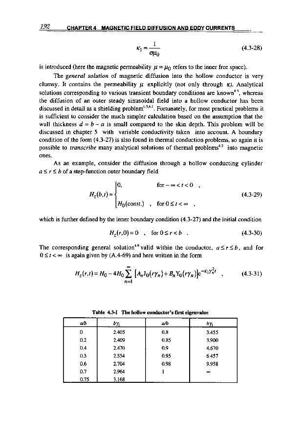
192 CHAPTER 4 MAGNETIC FIELD DIFFUSION AND EDDY CUR RENTS
a/b
0
0.2
0.4
0.5 0.6
0.7
0.75
(4.3-28)
by, a/b by, 2.405 0.8 3.455
2.409 0.85 3.900
2.470 0.9 4.670
2.554 0.95 6.457
2.704 0.98 9.958 2.964 1 m
3.168
is introduced (here the magnetic permeability p = & refers to the inner free space). The general solution of magnetic diffusion into the hollow conductor is very
clumsy. It contains the permeability p explicitly (not only through K). Analytical solutions corresponding to various transient boundary conditions are known4 ', whereas the diffusion of an outer steady sinusoidal field into a hollow conductor has been discussed in detail as a shielding Fortunately, for most practical problems i t is sufficient to consider the much simpler calculation based on the assumption that the wall thickness d = b - a is small compared to the skin depth. This problem will be discussed in chapter 5 with variable conductivity taken into account. A boundary condition of the form (4.3-27) is also found in thermal conduction problems, so again it is possible to transcribe many analytical solutions of thermal problems4.* into magnetic ones.
As an example, consider the diffusion through a hollow conducting cylinder a I r 2 b of a step-function outer boundary field
f o r - m < t < O , (4.3-29) (" Ho(const.) , f o r O I t < m ,
H,(b,f) =
which is further defined by the inner boundary condition (4.3-27) and the initial condition
HZ(r,O)=O , f o r O I r < b . (4.3-30)
The corresponding general s ~ l u t i o n ~ . ~ valid within the conductor, a I r I b , and for 0 I t < m is again given by (A.4-69) and here written in the form
Table 4.34 The hollow conductor's first eigenvalue
(4.3-3 1)
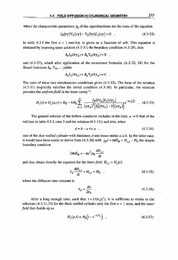
4.3 FIELD DIFFUSION IN CYLINDRICAL GEOMETRY 193
where the characteristic parameters yn of the eigenfunctions are the roots of the equation
J o ( b y ) Y 2 ( 4 - Y o ( b y ) J 2 ( 4 = 0 . (4.3-32)
In table 4.3-1 the first n = 1 root by1 is given as a function of d b . This equation is obtained by imposing upon solution (4.3-3 1) the boundary condition (4.3-29). thus
A,Jo(by,)+ B,Yo(bY,)=O ,
and (4.3-27), which after application of the recurrence formulae (A.2-22, 24) for the Bessel functions Jo. YO,.. ., yields
A,J,(by,)+ B,Y2(byn)=0 .
The ratio of these two simultaneous conditions gives (4.3-32). The form of the solution (4.3-3 1) implicitly satisfies the initial condition (4.3-30). In particular, the solution provides the uniform field in the inner cavity' 4:
The general solution of the hollow conductor includes in the limit a 0 that of the
rod [see in table 4.2-1, case 5 and the solution (4.3-14)] and also, when
d = b - a < < a , (4.3-34)
that of the fhin-walled cylinder with thickness d and mean radius a b. In the latter case, it would have been easier to derive from (4.3-26) with j4d = odE4 = Hz,i - HO the simple boundary condition
and thus obtain directly the equation for the innerfield Hz,i = H z ( f ) :
dHz'i + Hz, i = Ho , 5d dt
where the diffusion time constant is
(4.3-35)
(4.3-36)
After a long enough time, such that f > l / ( ~ ~ y t ) , it is sufficient to retain in the solutions (4.3-3 1,33) for the thick-walled cylinder only the first n = 1 term, and the inner field then builds up as
H z ( a , t ) = Ho(1- e-f/rl (4.3-37)
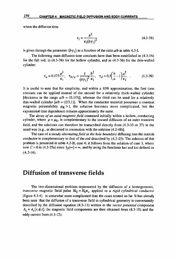
194 CHAPTER 4 MAGNETIC F IELD DIFFUSION AND EDDY CURRENTS
where the diffusion time
(4.3-38)
is given through the parameter ( b y l ) as a function of the ratio a/b in table 4.3-1. The following main diffusion time constants have thus been established in (4.3-16)
for the full rod, in (4.3-38) for the hollow cylinder, and in (4.3-36) for the thin-walled cylinder:
It is useful to note that for simplicity, and within a 10% approximation, the first time constant can be applied instead of the second for a relatively thick-walled cylinder [thickness in the range a/b = (0,1/3)], whereas the third can be used for a relatively thin-walled cylinder [ a h = (213, l)]. When the conductor material possesses a constant magnetic permeability p~ > 1, the solution becomes more complicated, but the exponential time dependence remains approximately the same.
The decay of an axial magnetic field contained initially within a hollow, conducting cylinder, where p = po, is complementary to the inward diffusion of an outer transient field, and the solutions can therefore be transcribed directly from (4.3-33 or 37) in the usual way [e.g., as discussed in connection with the solution (4.2-48)].
The case of a steady alternatingfield at the hole boundary diffusing into the outside conductor is complementary to that of the rod described by (4.3-25). The solution of this problem is presented in table 4.2-11, case 4; it follows from the solution of case 3, where now C = 0 in (4.3-25a) since Io(-) = -, and by using the functions ker and kei defined in (A.2-16).
Diffusion of transverse fields
The two-dimensional problem represented by the diffusion of a homogeneous, transverse magnetic field pulse Ho = Hoe, applied to a rigid cylindrical conductor (figure 4.3-4) is somewhat more complicated than the cases treated so far. It has already been seen that the diffusion of a transverse field in cylindrical geometry is conveniently described by the diffusion equation (4.3-1 1) written in the vector potential component A, = A,(r,&t); the magnetic field components are then obtained from (4.3-10) and the eddy current from (4.3-12).

4.3 FIELD DIFFUSION IN CYLINDRICAL GEOMETRY 195
Figure 4.3-4 Diffusion of a transverse, homogeneous magnetic field Ho = Hoe, into a conducting rod (the qualitative field pattern implies a negligible rotation of the rod about its z-axis); here and in all other similar cross sections the z-axis is pointing towards the reader, when not stated otherwise.
Transverse step-function field on a rod
Consider first a cylindrical rod at rest (vq = 0 ) to which a transverse, homogeneous
stepfunction field Ho = Hoe, (const.) is applied at t 1 0 . The solution must be
established simultaneously in free space ( r > a ) and in the conducting rod (r l a ) . The solution of the diffusion equation (4.3-1 1 ) relative to the rod with v+= 0 and js,z = 0, that
is, of the equation
- + - - + T - = Q p - d2A 1 dA 1 d 2 A dA ,
dr2 r dr r a@2 dt (4.3-40)
is established in (A.4-72) and, with the appropriate constants for this problem, is
The corresponding solution in free space of the Laplace equation [(4.3-40) where Q = 01 is given in (A.4-21), and with the constants chosen so as to be consistent with our geometry is
Az(r,@;t) = pHor [ 1 - - a2rt(t']sin@, r 1 a . (4.3 -42)
Here the constant Q (constant in r, @, but not in t ) and the characteristic parameters a" of the eigenfunctions are determined by the boundary conditions on r = a, which require [see 1.5-18). (4.3-lo)] dAz/rd@ and dAz ldr to remain steady across the surface (because the same applies for H, and H4). We find for a nonmagnetic rod, p = h,

196 CHAPTER 4 MAGNETIC FIELD DIFFUSION AND EDDY CURRENTS
(4.3-43)
and also [by making use of (A.2-21 to 26)] that the an are again positive roots of (4.3-15).
This means that here the field diffusion time constants l/Ka; are exactly the same as those corresponding to the diffusion of an axial magnetic field into the rod; in particular, the main time constant determined by n = 1 is again given by (4.3-16), in which case (4.3-
43) is approximated by a t ) z e-Kff:r = e-5.78ro’a2. For the field components (4.3-10) in the external free space r 2 a, from (4.3-42) we get
H#,e = -Ho 1 + T Q ( t ) sin4 , [ : ‘ I (4.3-44a)
(4.3-44b)
with Q(t) given in (4.3-43).
The precise solutions (4.3-4 1.42) already take care of the boundary conditions, as well as the initial condition requiring H,., H4 to vanish within the conductor at r = 0; they
also ensure that at r 4 m, or t 4 00, or CT = 0 (K + -.Q + 0), the uniform magnetic field is correctly described by H,. = Hgcos4, H# = -Hosing. For a completely diamagnetic
rod (a + -,K + 0) from (4.3-43) we get Q = I , and the solution (4.3-44), identical to (2.1-39). then shows that at the equator (at I$ = zd2, r = a) there is a flux concentration effect that doubles the field to 2H0, independently of the rod radius [as found similarly for the sphere in (2.1-32)].
The magnetic field components H,.(r, 4;r) and H#(r,$;r) are easily calculated through (4.3-lo), and are given in table 4.2-1 case 6. The related current density (4.3-12) in the rod is
(4.3-45)
For the general solution relative to a transient, transverse exponential field, see (4.3- 19,20) and related remarks.
Steady and rotating transverse fields
The steady alternating solution corresponding to the outer field (4.3-2 la), H = Hocoswt, can be obtained through the equations given before‘.’. The right-hand side

4.3 FIELD DIFFUSION IN CYLINDRICAL GEOMETRY 197
of the diffusion equation (4.3-40) for a cylindrical conductor with radius a at rest (v = 0) then reduces to opd, = 2A,/B, where we have introduced the diffusion skin depth (4.2-
2%
s = g 1 (4.3-46a)
here related to the vector potential A,, but which equally well applies to the corresponding magnetic field and eddy current components (4.3-10, 12); the same can be said of the diffusion time (4.2-1 8b),
r d = o , 2 . (4.3-46b)
In anticipating the definition (8.1-47c) we also introduce the magnetic Reynolds number
R m ~ ( 2 ) =r 2opm2 9 (4.3-46~)
which characterizes the strength of the diffusion process: larger R, mean that the transverse field penetrates less into the conductor, and, conversely, that the conductor represents a stronger disturbance to the applied uniform field configuration. Figure 4.3-5 shows a time sequence of the qualitative magnetic field pattern: it results from the superposition of the impressed field plus the dipole-type field related to the induced eddy current jz.
For the interesting case6.'-"of a conducting rigid rod rotating with a steady angular velocity R = v $ / r and immersed in a uniform constant magnetic field Ho, the right-hand
side of (4.3-1 1) reduces, instead, to Rop(dA,/d$) = 2(dA, /r3$)/6;. In analogy to the above expressions we find for the rotating bar the following skin depth, diffusion time, and Reynolds number [as defined in (8.1-47c)I:
2
(4.3-47)
Figure 4.3-5 Diffusion of a H,(t) = H,, cos(wt)e, transverse and homogeneous magnetic field into a conducting stationary rod (Reynolds number R, = 5; p~ = 1 ) at four different moments (semiqualitative pictures; in the first, the field is only due to the previously induced eddy current density, the imposed field being zero).
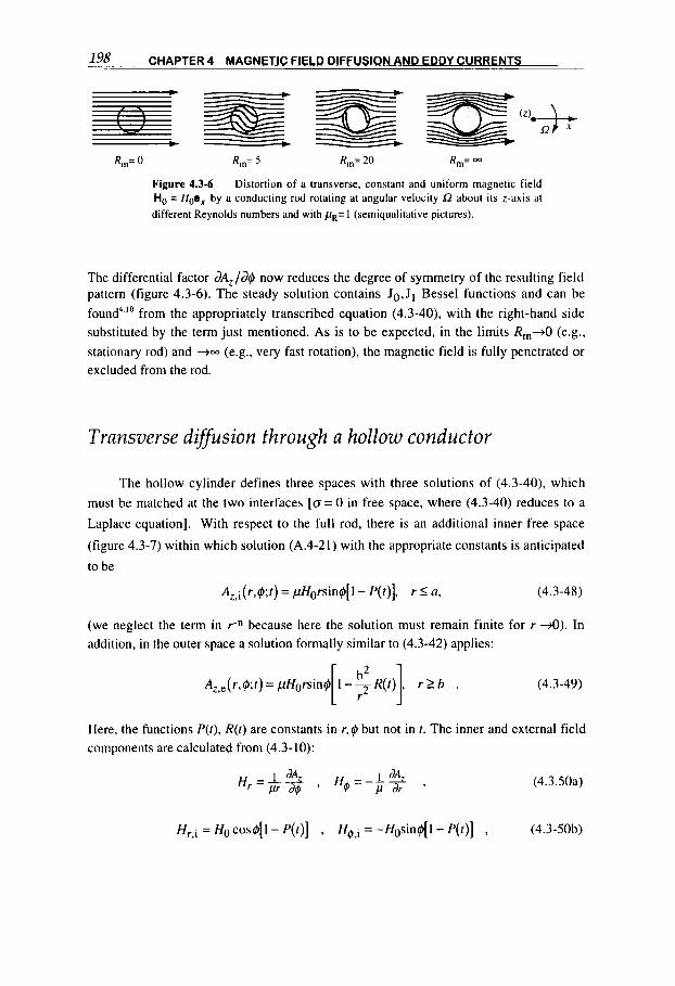
198 CHAPTER 4 MAGNETIC FIELD DIFFUSION AND EDDY CURRENTS
R,= 0 R,= 5 R,= 20 R,= 00
Figure 4.3-6 Distortion of a transverse, constant and uniform magnetic field Ho = Hoe, by a conducting rod rotating at angular velocity R about its z-axis at
different Reynolds numbers and with pR=l (semiqualitative pictures).
The differential factor aA,/a@ now reduces the degree of symmetry of the resulting field pattern (figure 4.3-6). The steady solution contains Jg,J, Bessel functions and can be found4 l o from the appropriately transcribed equation (4.3-40), with the right-hand side substituted by the term just mentioned. As is to be expected, in the limits Rm+O (e.g., stationary rod) and +aJ (e.g., very fast rotation), the magnetic field is fully penetrated or excluded from the rod.
Transverse diffusion through a hollow conductor
The hollow cylinder defines three spaces with three solutions of (4.3-40). which must be matched at the two interfaces [6= 0 in free space, where (4.3-40) reduces to a
Laplace equation]. With respect to the full rod, there is an additional inner free space
(figure 4.3-7) within which solution (A.4-2 1) with the appropriate constants is anticipated
to be
Az,i(r,@;f) = pHOrsin@[l- P(r) ] , r I a, (4.3-48)
(we neglect the term in r-n because here the solution must remain finite for r 4). In addition, in the outer space a solution formally similar to (4.3-42) applies:
(4.3-49)
Here, the functions P(t ) , R(r) are constants in r,@ but not in t. The inner and external field components are calculated from (4.3-10):
(4.3.504
H , i = H ~ c o s @ [ ~ - P ( ~ ) ] , H0.i =-Hgsin$[l-P(t)] , (4.3-50b)

4.3 FIELD DIFFUSION IN CYLINDRICAL GEOMETRY 199
Figure 4.3-7 field H, = Hoe, at t 2 0 into a hollow conducting cylinder.
Diffusion of a transverse and homogeneous step-function magnetic
The first term in these expressions corresponds to the imposed step-function field H,= H o , whereas the second term expresses the diffusion process caused by the conductor through the functions P ( f ) , R( f ) . Note that solution (4.3-50b) describes a homogeneous innerfield, parallel to the imposed external field, whose amplitude varies in time as Ho[ 1 - P(f) l .
The functions P, R can be determined from solution (A.4-72), valid within the conductor, a I r I b, which here takes the
. (4.3-51) I m
Az(r,q5;f) =Wosinq5 r + C[c , J~ ( ry , )+ D,Yl(ry,)]e -K,Y3 i n=l
The magnetic field components are calculated with (4.3-50a). The eigenfunctions y, are again the roots of (4.3-32), as can be shown by imposing,
on solutions (4.3-48, 49, 51), the boundary conditions at r = b,a, which require both H g and H , to remain steady across the boundary, and then making use of the recurrence formulae (A.2-26). In fact, from these operations, it follows that
c,Jo(bY,)+~,Yo(bYn)=O 9
CnJ2(ayfl)+ D,Y2(ay,) = O ,
requiring Jo(by,)Y2(ay,)- J2(aY,)Yo(bY,) = 0 9 (4.3-52)
which is identical to condition (4.3-32). The parameters C, and D, are found from the appropriate conditions of the problem.
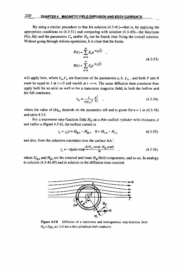
200 CHAPTER 4 MAGNETIC FIELD DIFFUSION AND EDDY CURRENTS
By using a similar procedure to that for solution (4.3-41)-that is, by applying the appropriate conditions to (4.3-5 1) and comparing with solution (4.3-49)-the functions P(r), R(r) and the parameters Cn and/or Dn can be found, thus fixing the overall solution. Without going through tedious operations, it is clear that the forms
m
n=l m
(4.3-53)
n=l
will apply here, where En,Fn are functions of the parameters a, b, y n , and both P and R must be equal to 1 at t = 0 and vanish at t + m. The same diffusion time constants thus apply both for an axial as well as for a transverse magnetic field, in both the hollow and the full conductor,
(4.3 -54)
where the value of (byn, depends on the parameter alb and is given for n = 1 in (4.3-38) and table 4.3-1.
For a transverse step-function field Ho on a thin-walled cylinder with thickness d and radius a (figure 4.3-8), the surface current is
iz = j z d = Hg.e - H4,i, 0 = Hr+e - Hr*i (4.3-55)
and also, from the inductive constraint over the surface AA’,
(4.3-56)
where Hg,e and H4,i are the external and inner Hg-field components, and so on. In analogy to solution (4.3-44,45) and in relation to the diffusion time constant
X
Figure 4.3-8
Ho = Hoe, at t 2 0 into a thin cylindrical shell conductor. Diffusion of a transverse and homogeneous step-function field
4.4 EDDY CURRENTS 201
(4.3-57) da zd == I
found through (4.3-35), the solution
-'/")sin$ , (4.3-58)
iz = j zd = -2Hoe-'J'dsin~ , (4.3-60)
is established, which satisfies all the necessary boundary and initial conditions.
4.4 EDDY CURRENTS
The concept of eddy currents is closely tied through Maxwell's equation to the concept of diffused magnetic fields; and, in fact, in the quasistationary approximation, the two are described formally by the same type of parabolic differential equations. In addition, when the diffused magnetic field is known, through Ampbre's law (4.1-10) it is easy to calculate the corresponding eddy current distribution, and vice versa. There are situations, however, where the use of the eddy current as the explicit electromagnetic quantity is of greater practical convenience, as for example when studying the reaction of conducting sheets to time-dependent magnetic fields. Also, evaluating Joule's heating losses is easier when the diffusion is expressed in eddy current terms.
The eddy current approach
The quasistationary current density conservation equation (1.2-2 l),
V . j = O , (4.4- 1)
with Ohm's law (4.1-1) transforms into
V . E = O , (4.4-2)
meaning that the electric field E (in addition to j ) is irrotational and thus expressible as
202 CHAPTER 4 MAGNETIC FIELD DIFFUSION AND EDDY CURRENTS
E = I = v X C , (4.4- 3) 0
where C is called the current stream vector field. With Faraday's law (4.1- 1 l), it also follows that
a-I f3t
AC=/f- , (4.4-4)
where, because of Amp2re's law (4.1-lo), there remains the relation C = aH. However, the eddy current approach, represented by the last differential equation, becomes convenient when it is possible to consider the magnetic field separable into
H = H O + H ' , (4.4-5)
where H o ( t ) is the imposed outerfield that induces the eddy currents obtained from the equations
j = o V x C , (4.4-6)
dHo AC=p-
dt ' (4.4-7)
and where the small perturbation field H' is then obtained through the integral (2.2-22).
(4.4-8)
The eddy current approach based on this formalism can be useful when dealing with conductors that represent a relatively small perturbation to the applied magnetic field. This is the case when the diffusion skin depth s [see, e.g., (4.2-18a)I is large with respect to the conductor dimensions in the direction normal to the applied magnetic field
s>>d, . (4.4-9)
Such a conductor is called a thin sheet (for example, the slab in figure 4.2-6 when the thickness d is much smaller than s, or the disk in figure 4.4-5 when the radius a is much smaller than s). Note that, in general, the skin depth s(t ) relative to an applied transient field pulse is s + 0 when t - + O [see, e.g., in (4.2-25)]. Thus, the thin-sheet approximation, characterized by the formulation of the eddy current problem through (4.4-6,7), is, in general, valid only at times
t"Td 9 (4.4- 10)
where Td is acharacteristic difision or delay time for the specific field pulse to penetrate into the given conductor system, as, for example, defined in (4.1-29) and (4.2-18b) and

4.4 EDDY CURRENTS 203
given for many problems in sections 4.2 and 4.3. The eddy current problem can be useful, however, in a more general formulation (not limited to the thin-sheet approximation), as will be shown next.
Two-dimensional currents in sheets
Consider a conductor whose thickness d (even if variable) is small with respect to all relevant characteristic lengths, particularly in comparison to the diffusion skin depth. We call such a conductor a sheet, which may be defined by a surface S of any shape delimited by the borderline r (figure 4.4-1). The current density j (and all other parameters) is thus considered to be nearly uniform across the conductor thickness, and it can be expressed by a mean surface current density
i = j d (4.4- 1 1)
[see also in connection with (1.5-4)] acting on the mid sugace between the two surfaces delimiting the conductor. Because of the assumption that the normal component jn has no sources or sinks, 3, /&I = 0, i is everywhere tangent to the (mid) surface, and from (1.5- 36) we get the solenoidality or conservation condition
V , . i = O . (4.4-12)
Figure 4.4- 1 vacuum with magnetic field H(I).
Eddy currents in plane conducting sheet moving with velocityv in a
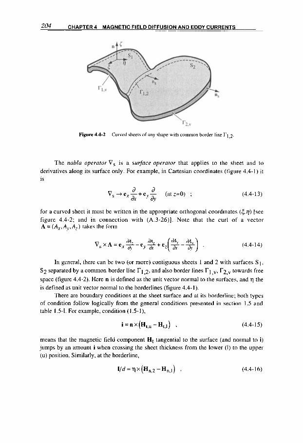
204 CHAPTER 4 MAGNETIC FIELD DIFFUSION AND EDDY CURRENTS
Figure 4.4-2 Curved sheets of any shape with common border line r1.2
The nahla operator Vs is a surface operator that applies to the sheet and to derivatives along its surface only. For example, in Cartesian coordinates (figure 4.4-1) i t is
(4.4- 13)
for a curved sheet it must be written in the appropriate orthogonal coordinates (&q) [see figure 4.4-2; and in connection with (A.3-26)]. Note that the curl of a vector A = (A, ,A, , ,A , ) takes the form
V , x A = e , - - e , ~ + e , ( ~ - $ ) dA. dA. dA,. dA . ?Y
(4.4-14)
In general, there can be two (or more) contiguous sheets I and 2 with surfaces S1, S2 separated by a common border line r1,2, and also border lines r2,v towards free
space (figure 4.4-2). Here n is defined as the unit vector normal to the surfaces, and q the is defined as unit vector normal to the borderlines (figure 4.4-1).
There are boundary conditions at the sheet surface and at its borderline; both types of condition follow logically from the general conditions presented in section 1.5 and table 1.5-1. For example, condition (IS-I) ,
i = n x (Ht,u - H,,J) , (4.4- 15)
means that the magnetic field component Ht tangential to the surface (and normal to i ) jumps by an amount i when crossing the sheet thickness from the lower (1) to the upper (u) position. Similarly, at the borderline,
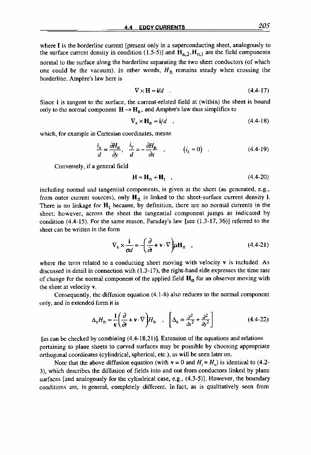
4.4 EDDY CURRENTS 205
where I is the borderline current [present only in a superconducting sheet, analogously to the surface current density in condition (1.5-5)] and Hn,2,Hn,l are the field components
normal to the surface along the borderline separating the two sheet conductors (of which one could be the vacuum). In other words, Hn remains steady when crossing the borderline. Arnptre's law here is
V x H = i l d . (4.4-17)
Since i is tangent to the surface, the current-related field at (within) the sheet is bound only to the normal component H + H,, and Amphre's law thus simplifies to
V, x H, = i/d , (4.4- 18)
which, for example in Cartesian coordinates, means
(4.4-19)
Conversely, if a general field
H = H , + H , , (4.4-20)
including normal and tangential components, is given at the sheet (as generated, e.g., from outer current sources), only H n is linked to the sheet-surface current density i. There is no linkage for H, because, by definition, there are no normal currents in the sheet; however, across the sheet the tangential component jumps as indicated by condition (4.4-15). For the same reason, Faraday's law [see (1.3-17, 36)] referred to the sheet can be written in the form
v, X-=-(&+v.V)pH, i , od
(4.4-21)
where the term related to a conducting sheet moving with velocity v is included. As discussed in detail in connection with (1.3-17), the right-hand side expresses the time rate of change for the normal component of the applied field Hn for an observer moving with the sheet at velocity v.
Consequently, the diffusion equation (4.1-8) also reduces to the normal component only, and in extended form it is
(4.4-22)
[as can be checked by combining (4.4-18,21)]. Extension of the equations and relations pertaining to plane sheets to curved surfaces may be possible by choosing appropriate orthogonal coordinates (cylindrical, spherical, etc.), as will be seen later on.
Note that the above diffusion equation (with v = 0 and H, = H,) is identical to (4.2- 3), which describes the diffusion of fields into and out from conductors linked by plane surfaces [and analogously for the cylindrical case, e.g., (4.3-5)]. However, the boundary conditions are, in general, completely different. In fact, as is qualitatively seen from
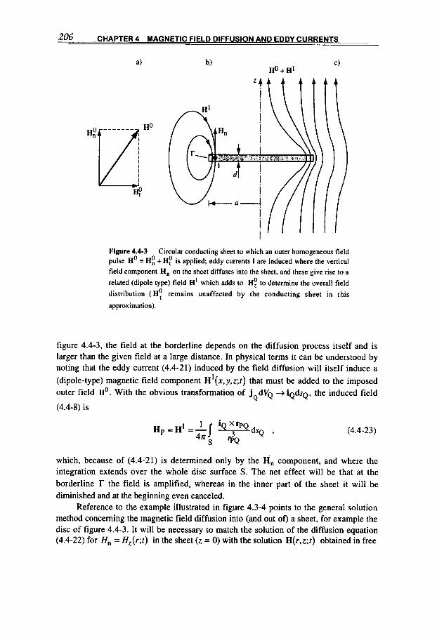
206 CHAPTER 4 MAGNETIC FIELD DIFFUSION AND EDDY CURRENTS
Figure 4.4-3 Circular conducting sheet to which an outer homogeneous field pulse Ho = H: + HF is applied; eddy currents i are induced where the vertical field component H, on the sheet diffuses into the sheet, and these give rise to a
related (dipole type) field H' which adds to Hg to determine the overall field
distribution ( H y remains unaffected by the conducting sheet in this
approximation).
figure 4.4-3, the field at the borderline depends on the diffusion process itself and is larger than the given field at a large distance. In physical terms it can be understood by noting that the eddy current (4.4-21) induced by the field diffusion will itself induce a (dipole-type) magnetic field component H'(x, y,z;r) that must be added to the imposed outer field Ho. With the obvious transformation of JQdVQ + iQdsQ, the induced field
(4.4-8) is
(4.4-23)
which, because of (4.4-21) is determined only by the Hn component, and where the integration extends over the whole disc surface S. The net effect will be that at the borderline r the field is amplified, whereas in the inner part of the sheet it will be diminished and at the beginning even canceled.
Reference to the example illustrated in figure 4.3-4 points to the general solution method concerning the magnetic field diffusion into (and out of) a sheet, for example the disc of figure 4.4-3. It will be necessary to match the solution of the diffusion equation (4.4-22) for Hn = H,(r;r) in the sheet (z = 0) with the solution H(r,z;r) obtained in free

4.4 EDDY CURRENTS 207
Figure 4.4-4 The conducting sheet in a time-varying homogeneous magnetic field HO(t) = Hoe,, with the perturbation H' established by the induced eddy current and thus with the total field H = Ho + HI.
space from the Laplace equation AH=O. [For an axisymmetric problem, as in the case of a disc, it would clearly be more convenient to introduce the azimuthal component A, of the vector potential and solve the equations that can be derived from the form of (4.3-8).] An example of such a problem, in cylindrical geometry, will be described later on.
The thin-sheet approximation
The relative complexity encountered above in handling field diffusion into sheets strongly suggests, once again, searching for reasonable approximations. The thin-sheet approximation is an important simplification obtained when the skin depth s is large in comparison to the sheet extension, s >) 1 (and not only to its thickness,^ >> d). In this case, diffusion even of the normal field is a minor effect and one is entitled to introduce the separation (4.4-3,
H = H O + H ' , (4.4-24)
between the outer applied field Ho and the perturbation field HI (figure 4.4-4).
Field equations
The thin-sheet approximation consists in calculating the eddy current i in the sheet by using, for example, Faraday's law (4.4-21), where Hn 4 H t , and then calculating the
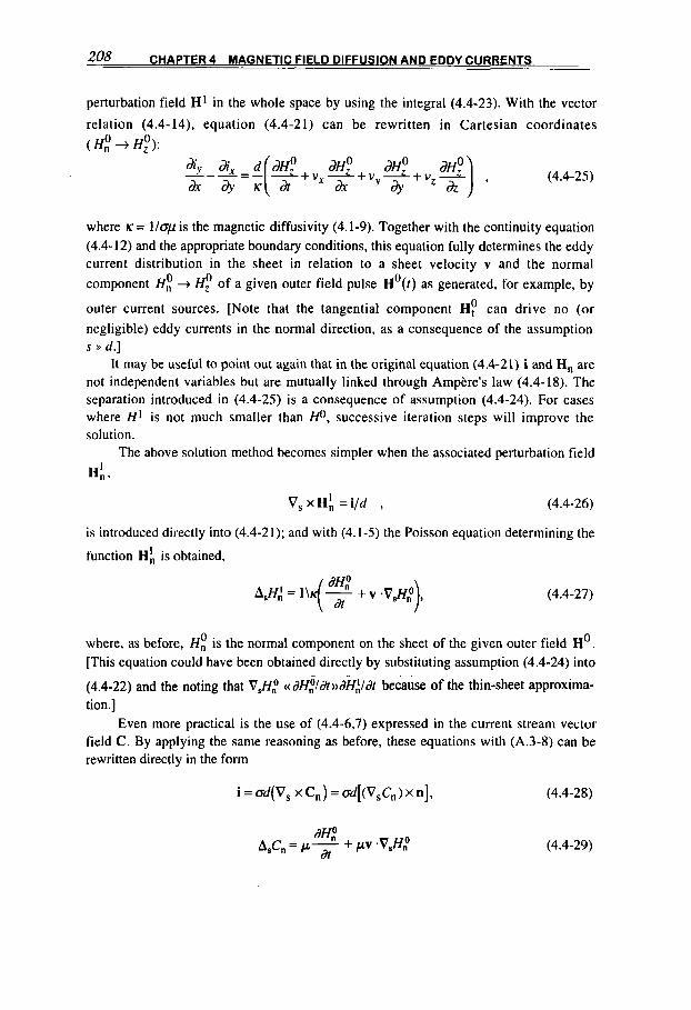
208 CHAPTER 4 MAGNETIC FIELD DIFFUSION AND EDDY CURRENTS
perturbation field H 1 in the whole space by using the integral (4.4-23). With the vector
relation (4.4-14), equation (4.4-21) can be rewritten in Cartesian coordinates (Hf + H:):
(4.4-25)
where K = 1/0p is the magnetic diffusivity (4.1-9). Together with the continuity equation (4.4- 12) and the appropriate boundary conditions, this equation fully determines the eddy current distribution in the sheet in relation to a sheet velocity v and the normal component Hf + H: of a given outer field pulse Ho(t) as generated, for example, by
0 outer current sources. [Note that the tangential component H, can drive no (or negligible) eddy currents in the normal direction, as a consequence of the assumption s )> d.]
It may be useful to point out again that in the original equation (4.4-21) i and H, are not independent variables but are mutually linked through Ampbre's law (4.4- 18). The separation introduced in (4.4-25) is a consequence of assumption (4.4-24). For cases where HI is not much smaller than m, successive iteration steps will improve the solution.
The above solution method becomes simpler when the associated perturbation field
Hf, 9
V, x Hf, = i/d , (4.4-26)
is introduced directly into (4.4-21); and with (4.1-5) the Poisson equation determining the
function Hf, is obtained,
(4.4-27)
where, as before, Hf is the normal component on the sheet of the given outer field Ho . [This equation could have been obtained directly by substituting assumption (4.4-24) into
(4.4-22) and the noting that V&' (( dH~ldtm3H~lat because of the thin-sheet approxima- tion.]
Even more practical is the use of (4.4-6.7) expressed in the current stream vector field C. By applying the same reasoning as before, these equations with (A.3-8) can be rewritten directly in the form
i = od(V, x C,) = od[(V,C, ) x n], (4.4-28)
(4.4-29)

4.4 EDDY CURRENTS 209
[Note the relation d,, t H,!, for the normal component of C at the sheet C, = C,n.] The eddy current problem in the thin-sheet approximation is thus determined by
solving a two-dimensional Poisson equation in the scalar C, current stream function within the sheet only, with the Dirichlet condition on the borderline towards free space of
C, = 0 on r (because along r it is everywhere i.q = 0; see figure 4.4-1). The stream
function lines C, = const. define the flow direction of the current, and its magnitude is inversely proportional to the local distance among the lines. The perturbation field HI set up in free space by the eddy currents can be determined through (4.4-23).
When Ho and/or v include an explicit time dependence, HI will also become a function of time; this means that the eddy current distribution will in general change as time progresses. It can be said that the change occurs instantaneously when the thin-sheet conditions (4.4-9.10) apply. For example, if the field depends linearly on time, H, = br, the eddy current will tend towards a stationary distribution for t"'td [see, e.g., the cylindrical case described by (4.4-66,67)].
0
Vector potential equations
It may be useful to express the eddy current i also in terms of the vector potential
A = A, + A , , (4.4-30)
which is here split up into the components that are normal and tangential to the sheet [as in (4.4-20)], and thus obtain from (4.1-15)
- i = -(&+ v . v),, - v,u. od
(4.4-3 1)
This vector relation directly gives, through its two equations, the two components of the surface current densityi when A, and the potential U are given [see the analogous expressions (4.1-14)]. The solenoidality of i (4.4-12) can formally be assured by the scalar electric potential U , which is fixed by the Laplace equation
A U = O (4.4-32)
and the appropriate conditions along the boundary line r1.2 delimiting two conducting sheets that might have different surface conductivities od. The continuity across the border line for the components normal to r1.2 of i, A or H provides the condition
"2 - [(od)2 - (ad ) , ]$ =-($-+).q. dA dA a h (4.4-33)
In the thin-sheet approximation, besides the attention to be paid to U , the vector
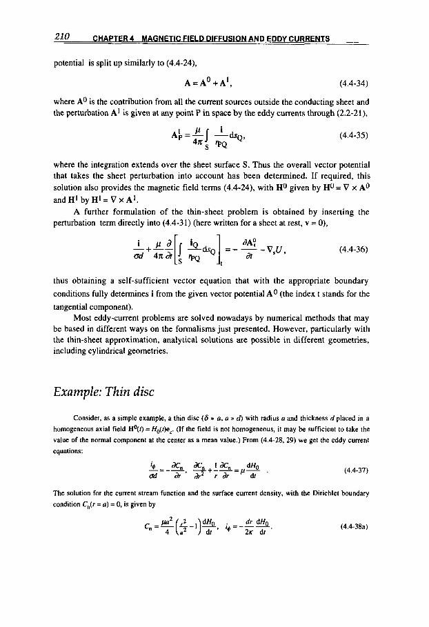
210 CHAPTER 4 MAGNETIC FIELD DIFFUSION AND EDDY CUR RENTS
potential is split up similarly to (4.4-24),
A = AO + A ~ , (4.4-34)
where A0 is the contribution from all the current sources outside the conducting sheet and the perturbation A1 is given at any point P in space by the eddy currents through (2.2-21),
(4.4-35)
where the integration extends over the sheet surface S. Thus the overall vector potential that takes the sheet perturbation into account has been determined. If required, this solution also provides the magnetic field terms (4.4-24), with Ho given by Ho= V x A0
and HI by HI = V x A ] . A further formulation of the thin-sheet problem is obtained by inserting the
perturbation term directly into (4.4-31) (here written for a sheet at rest, v = 0),
(4.4-36)
thus obtaining
conditions fully
a self-sufficient vector equation that with the appropriate boundary
determines i from the given vector potential A0 (the index t stands for the
tangential component). Most eddy-current problems are solved nowadays by numerical methods that may
be based in different ways on the formalisms just presented. However, particularly with the thin-sheet approximation, analytical solutions are possible in different geometries, including cylindrical geometries.
Example: Thin disc
Consider, as a simple example, a thin disc (6 * a. a * d) with radius a and thickness d placed in a homogeneous axial field Ho(f) = Ho(f)e,. (If the field is not homogeneous, it may be sufficient to take the
value of the normal component at the center as a mean value.) From (4.4-28.29) we get the eddy current equations:
(4.4-37)
The solution for the current stream function and the surface current density, with the Dirichlet boundary
condition C,(r = a ) = 0, is given by
(4.4-38a)
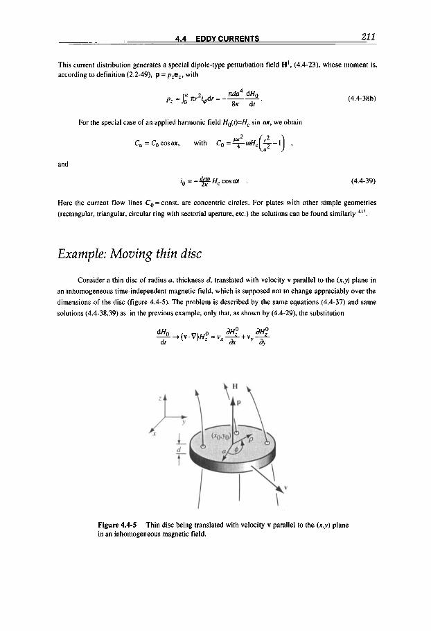
4.4 EDDY CURRENTS 211
This current distribution generates a special dipole-type perturbation field HI. (4.4-23). whose moment is, according to definition (2.2-49). p = prez, with
pz =6 Rr2iqdr=---. &a4 dHO SK dr
(4.4-38b)
For the special case of an applied harmonic field Ho(r)=Hc sin 01, we obtain
and
i4 = -* Hc cosm . (4.4-39)
Here the current flow lines Co = const. are concentric circles. For plates with other simple geometries
(rectangular, triangular, circular ring with sectorial aperture, etc.) the solutions can be found similarly 4.17.
Example: Moving thin disc Consider a thin disc of radius a. thickness d, translated with velocity v parallel to the (x.y) plane in
an inhomogeneous time-independent magnetic field, which is supposed not to change appreciably over the dimensions of the disc (figure 4.4-5). The problem is described by the same equations (4.4-37) and same
solutions (4.4-38.39) as in the previous example, only that, as shown by (4.4-29). the substitution
Figure 4.4-5 i n an inhomogeneous magnetic field.
Thin disc being translated with velocity v parallel to the (x ,y ) plane
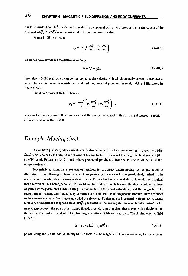
212 CHAPTER4 M AGNETIC FIELD DIFFUSION AND EDDY CURRENTS
has to be made; here, H; stands for the vertical z-component of the field taken at the center (x,,y,) of the
disc, and dH;/dx, dH;/& are considered to be constant over the disc.
From (4.4-38) we obtain
where we have introduced the diffusion velocity
w = 2 K - 2 d - / loti (4.4-40b)
[see also in (4.2-18c)I. which can be interpreted as the velocity with which the eddy currents decay away,
as will be seen in connection with the receding-image method presented in section 6.2 and illustrated in figure 6.2- 12.
The dipole moment (4.4-38) here is
(4.4-41)
whereas the force opposing this movement and the energy dissipated in this disc are discussed in section
6.2 in connection with (6.2-23).
Example: Moving sheet
As we have just seen, eddy currents can be driven inductively by a time-varying magnetic field (the dH/& term) and/or by the relative movement of the conductor with respect to a magnetic field gradient [the
(v.V)H term]. Equation (4.4-21) and others presented previously describe this situation with all the
necessary details.
Nevertheless, attention is sometimes required for a correct understanding, as for the example
illustrated by the following problem, where a homogeneous, constant vertical magnetic field, limited within
a small zone, threads a sheet moving with velocity v. From what has been said above, it would seem logical
that a movement in a homogeneous field should not drive eddy currents because the sheet would either lose
or gain any magnetic flux (lines) during its movement. If the sheet extends beyond the magnetic field
region, the movement will induce eddy currents even if the field is homogeneous because there are sheet
regions where magnetic flux (lines) are added or subtracted. Such a case is illustrated in figure 4.4-6, where a steady, homogeneous magnetic field pH;, generated in the rectangular zone with sides 2 ~ x 2 6 in the
narrow gap between the poles of a magnet, threads a conducting thin sheet that moves with velocity along
the y-axis. The problem is idealized in that magnetic fringe fields are neglected. The driving electric field
( I .3-29)
E = V y X pH: = vypH;e, (4.4-42)
points along the x-axis and is strictly limited to within the magnetic field region-that is, the rectangular
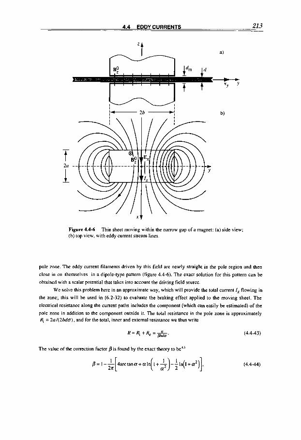
4.4 EDDY CURRENTS 213
2a -
Figure 4.4-6 (b) top view, with eddy current stream lines.
Thin sheet moving within the narrow gap of a magnet: (a) side view;
pole zone. The eddy current filaments driven by this field are nearly straight in the pole region and then
close in on themselves in a dipole-type pattern (figure 4.4-6). The exact solution for this pattern can be
obtained with a scalar potential that takes into account the driving field source.
We solve this problem here in an approximate way, which will provide the total current I, flowing in
the zone; this will be used in (6 .2-32) to evaluate the braking effect applied to the moving sheet. The
electrical resistance along the current paths includes the component (which can easily be estimated) of the
pole zone in addition to the component outside it. The total resistance in the pole zone is approximately Ri = 2 a / ( 2 b d o ) , and for the total, inner and external resistance we thus write
R = R , + R -A (4.4-43) e - p b d f J .
The value of the correction factor /3 is found by the exact theory to be4'
(4.4-44)
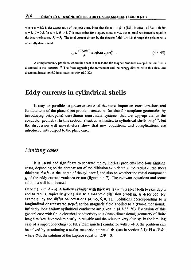
214 CHAPTER 4 MAGNETIC FI EL0 DIFFUSION AND EDDY CURRENTS
where a=b/aistheaspect ratioofthepolezone. Notethatforaw I , p+(1 .5+Ina) /a+ l /a+0; for
a = 1, p = 0.5; for a M 1, /3 + 1. This means that for a square zone, a = b. the external resistance is equal to
the inner resistance, R, = Ri . The total current driven by the electric field (4.4-42) through the pole zone is
now fully determined:
(4.4-45)
A complementary problem, where the sheet is at rest and the magnet produces a step-function flux is
discussed in the literature4 I*. The force opposing the movement and the energy dissipated in this sheet are discussed in section 6.2 in connection with (6.2-32).
Eddy currents in cylindrical shells
It may be possible to preserve some of the most important considerations and formulations of the plane sheet problem treated so far also for nonplane geometries by introducing orthogonal curvilinear coordinate systems that are appropriate to the conductor geometry. In this section, attention is limited to cylindrical shells ~ n l y ~ . ~ ' , but the discussion will nevertheless show that new conditions and complications are introduced with respect to the plane case.
Limiting cases
It is useful and significant to separate the cylindrical problems into four limiting cases, depending on the comparison of the diffusion skin depth s, the radius a, the sheet thickness d = b - a, the length of the cylinder 1, and also on whether the radial component j , of the eddy current vanishes or not (figure 4.4-7). The relevant equations and some solutions will be indicated.
Case u (s E( d; d - a). A hollow cylinder with thick walls (with respect both to skin depth and to radius) typically giving rise to a magnetic diffusion problem, as described, for example, by the diffusion equations (4 .3-5,6,8, 1 1 ) . Solutions corresponding to a longitudinal or transverse step-function magnetic field applied to a (two-dimensional) infinitely long hollow cylindrical conductor are given in (4.3-33.50). Extension of this general case with finite electrical conductivity to a (three-dimensional) geometry of finite length makes the problem nearly intractable and the solution very clumsy. In the limiting case of a superconducting (or fully diamagnetic) conductor with s + 0, the problem can be solved by introducing a scalar magnetic potential @ (see in section 2.1): H = -V@ , where @ is the solution of the Laplace equation A@ = 0.
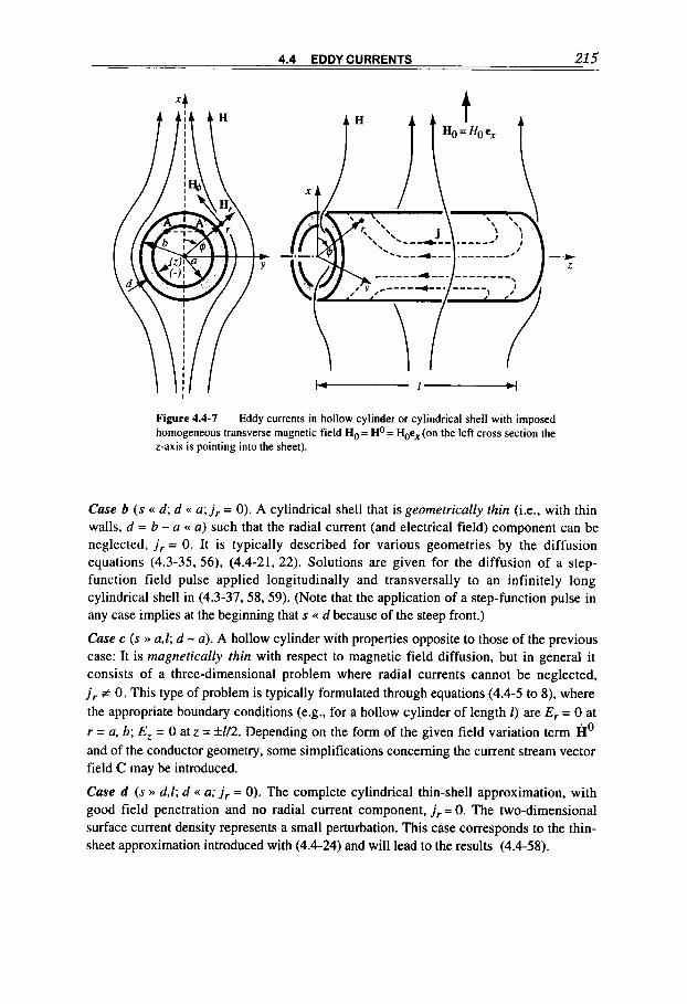
4.4 EDDY CURRENTS 215
-f-
Figure 4.4-7 Eddy currents in hollow cylinder or cylindrical shell with imposed homogeneous transverse magnetic field Ho= Ho= h e , ( o n the left cross section the z-axis is pointing into the sheet).
Case b (s (c d; d (( a; j , = 0) . A cylindrical shell that is geometrically thin (i.e., with thin walls, d = b - a G a ) such that the radial current (and electrical field) component can be neglected, j , = 0. It is typically described for various geometries by the diffusion equations (4.3-35, 56) , (4.4-21, 22). Solutions are given for the diffusion of a step- function field pulse applied longitudinally and transversally to an infinitely long cylindrical shell in (4.3-37,58,59). (Note that the application of a step-function pulse in any case implies at the beginning that s (( d because of the steep front.)
Case c (s )) a,l; d - a). A hollow cylinder with properties opposite to those of the previous case: It is magnetically rhin with respect to magnetic field diffusion, but in general it consists of a three-dimensional problem where radial currents cannot be neglected, j , # 0. This type of problem is typically formulated through equations (4.4-5 to 8), where the appropriate boundary conditions (e.g., for a hollow cylinder of length I) are E, = 0 at r = a, b; Ez = 0 at z = W 2 . Depending on the form of the given field variation term Ho and of the conductor geometry, some simplifications concerning the current stream vector field C may be introduced.
Case d (s )) d,l; d (( a; j , = 0). The complete cylindrical thin-shell approximation, with good field penetration and no radial current component, j , = 0. The two-dimensional surface current density represents a small perturbation. This case corresponds to the thin- sheet approximation introduced with (4.4-24) and will lead to the results (4.4-58).
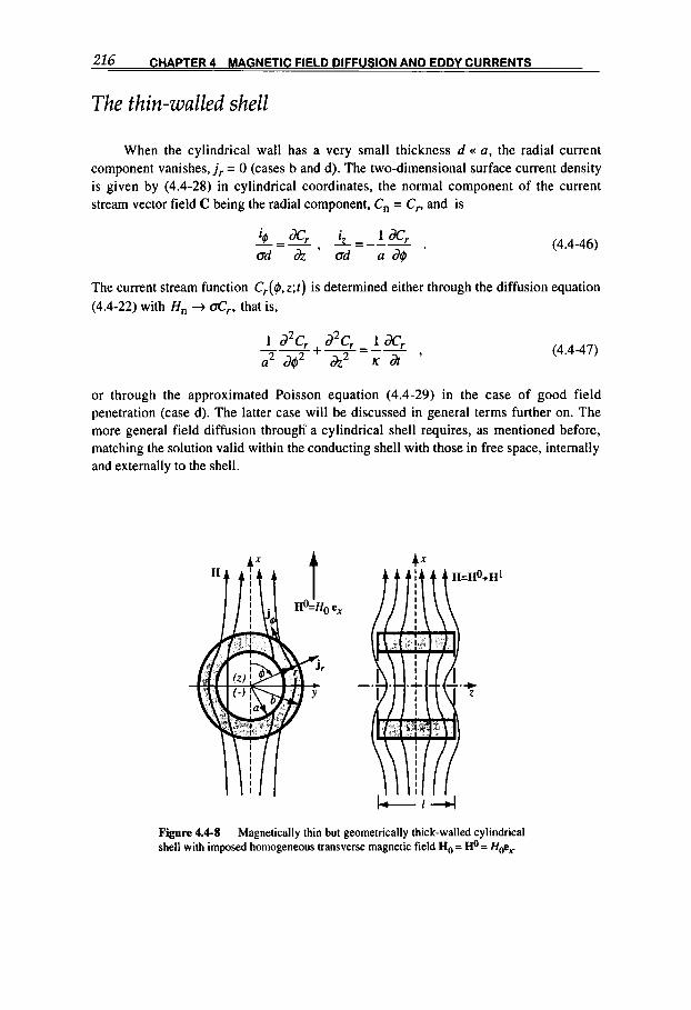
216 CHAPTER 4 MAGNETIC FIELD DIFFUSION AND EDDY CURRENTS
The thin-walled shell
When the cylindrical wall has a very small thickness d c( a, the radial current component vanishes, j , = 0 (cases b and d). The two-dimensional surface current density is given by (4.4-28) in cylindrical coordinates, the normal component of the current stream vector field C being the radial component, Cn = C,., and is
(4.4-46) iq aC, i IaC, -=- --L=--- od dz ’ od a a$ ‘
The current stream function C,($,z;t) is determined either through the diffusion equation (4.4-22) with H, 4 K,.. that is,
(4.4-47)
or through the approximated Poisson equation (4.4-29) in the case of good field penetration (case d). The latter case will be discussed in general terms further on. The more general field diffusion througli a cylindrical shell requires, as mentioned before, matching the solution valid within the conducting shell with those in free space, internally and externally to the shell.
A x
Figure 4.4-8 shell with imposed homogeneous transverse magnetic field Ho = Ho = Hoer
Magnetically thin but geometrically thick-walled cylindrical

4.4 EDDY CURRENTS 217
The magnetically thin shell
The eddy current problem becomes simpler when the imposed magnetic field penetrates easily into the conductor-that is, for a magnetically thin shell. There are then two limiting cases (as mentioned at the beginning of this section), which will be considered now: case c, thick-walled shell with d - u and a three-dimensional current density (figure 4.4-8); case d, thin-walled shell with d (c u and a two-dimensional current density, where j , = 0 (figure 4.4-9).
In case c, the eddy current density (4.4-6),
j = o V x C ,
is defined through the vector Poisson equation (4.4-7). It is often convenient to write that equation in its Cartesian components [see comments in connection with (A.4-26)],
(4.4-48) AC, =- PdH,o , ACs=- PddHyo , AC, =- wfo , dt dt dt
but then to solve each equation in cylindrical coordinates (r,@,z), with the Laplacian given in (A.4-15) and elements of the general solution indicated thereafter. Because of the magnetically thin shell approximation, the eddy current would change, in accordance with the delay-time condition (4.4-10). with the same time dependence; only if Ho depended linearly on time, thus d H ldt = const ., would the current tend towards a stationary distribution. The vector components C, = CX(r,q,z);.. resulting from the solution are transformed into their cylindrical components as indicated in table A.3-I:
0
Cr = C, cos@ + Cssin@; Cq = -C,sin@ + Cs cos@; C, = C, . (4.4-49)
t Ho = H o ex
'4 d r
Figure 4.4-9 transverse homogeneous magnetic field H, = Ho = Hoe,
Infinite array of thin-walled cylindrical shells with imposed

218 CHAPTER 4 MAGNETIC FIELD DIFFUSION AND EDDY CURRENTS
Finally, the eddy current components j I ( j r , j$ , jz ) are calculated from (4.4-6) with the help of table A.3-11.
In the thin-walled shell approximation (case d), the two-dimensional eddy surface current density I, (4.4-28,29), in cylindrical geometry with the current stream function Cn+C, as in (4.4-46,47) is simply given by
where C, is now defined by the Poisson equation
(4.4-50)
(4.4-5 1 )
with the last term being the time derivative of the radial component of the imposed magnetic field. The eddy-current-related field perturbation H1 in the surrounding space is calculated through (4.4-23). It is useful to recall that (4.4-51) results from a combination of the definition (4.4-50) with the current conservation (4.4-12).
and Faraday's law (4.4-21) for the radial component at r = a
d dH: K dt
(Vxi),=--- ,
that is
where 1 / ~ = ap and table A.3-I1 is used for writing the components.
Example: Transverse field on thin shell with gaps
(4.4-52)
(4.4-53)
To an infinite periodic array of magnetically and geometrically thin cylindrical shells (case d) of
length 1 at distance L and radius a, a transverse variable magnetic field pulse Ho = Ho(t)e, is applied (figure
4.4-9). [We recall from (A.4-23) the substantial simplification introduced for the solution, when the basic
geometry is multiplied into an infinite array.] The stationary solution of (4.4-51), where the radial
component of the applied field is

4.4 EDDY CURRENTS 219
H," = H ~ C O S # . (4.4-54)
and which satisfies the boundary condition iz = 0 at z = fU2 and i$ = 0 at # = fn/2 (i.e., C, = 0 at these
boundaries), is obtained by variable separation [see in connection with (A.4-15,26)],
dr
and thus from (4.4-50) we get
da dH sinh(z/a) K dr cosh(l/2a) '
i$ =-A cos # -
iz . =--sin da dHo . 4 I-- cosh(z/a)] K dr cosh( 1/2a)
In a very long, I + m, cylindrical shell, the current reduces to
da dHo i# =0, iz =--sin#
K dr
(4.4-55)
(4.4-56)
(4.4-57)
(4.4-58)
This could have been obtained more directly through the electric field that results from the inductive constraint in the plane AA ' normal to the imposed transverse field H! [see figure 4.3-8; or simply from
(4.4-53)]:
The total current thus flowing along one shell quadrant,
(4.4-59)
(4.4-60)
is reconnected at the (infinitely) far ends to the other quadrant by a total azimuthal current f@= I, It is instructive to apply these results to a discussion on magnetic field penetration into the bore of
the cylindrical conductor arrangement with gaps shown in figure 4.4-9. The transverse field H,(z;r)
established on the z-axis can be. written in the form (4.4-24),
Hx(z;f)= H:(t)+ H;(z;r) = Ho(f)+ Hd(z;t) , (4.4-61)
where H:(r) = Ho(r) is the externally applied, transverse field (4.4-54). and the eddy component
Hi(2;r) = Hed(Z;r) is derived through the integral (4.4-23) from the eddy currents (4.4-56, 57). In many
applications (e.g., confinement of charged particles, or of a plasma column), what counts is the geometric mean transverse field Z,(r) along the axis,
- HI(!)= Ho(r)+Zed(r) . (4.4-62)
where, by definition,

220 CHAPTER 4 MAGNETIC FIELD DIFFUSION AND EDDY CURRENTS
(4.4-63)
In the present geometrical arrangement, zed is determined in (4.4-23) only by the average component of
the current density iz. which is parallel to the axis, and not by the component i@ which has opposite
directions in the upperllower half-shells. There are also no contributions from harmonic components along the interval L of the type i,,n = cos(nz/l). Finally,
Hence. the mean component on axis zed is solely the result of the axial current i,(@,z;r) [given in (4.4-57)]
that flows in this infinite array of cylindrical shells each with length / (figure 4.4-9). and from (4.4-23) we
get
(4.4-65)
Finally, the mean penetrated transverse field (4.4-62) is calculated from (4.4-57,65) to be - H , ( r ) = H o ( r ) - q f $ i ( l - F t a n h & ) . (4.4-66)
[Note that (tanhx)/x 5 1 for any value of xA !] The mean diffusion or delay time defined in (4.1-30) with
which the external field penetrates into the bore of this infinite array of thin cylindrical conductos (case d;
figure 4.49) is thus
r,, = f $ i ( l - u t a n h & ) , (4.4-67)
which depends only on the magnetic diffusivity K = I/(up) and the geometric parameters, but is
independent of the form of the externally applied, transverse field pulse Ho(r); it is attained after a time
t >> rd from the beginning.
On the other hand, if the conductor were superconducting or fully diamagnetic (with surface currents
only, case a), a fraction of the applied field would penetrate promptly, without delay ( K+ -), through the
gaps. This problem4." could be solved through a magnetic scalar potential @ as introduced in section
2.1: H = -V@, where @ is the solution of the Laplace equation A@ = 0.
Magnetic shielding
Shielding from magnetic fields is one of the important applications of the magnetic- diffusion and eddy-current theories that we have developed in this chapter. The reduction of a time-dependent magnetic field by a conducting sheet that surrounds a useful space can be characterized by the shieldingfuctor (or transfer function)
(4.4-68) transmitted inner magnetic field amplitude = external magnetic field amplitude in absence of shield '
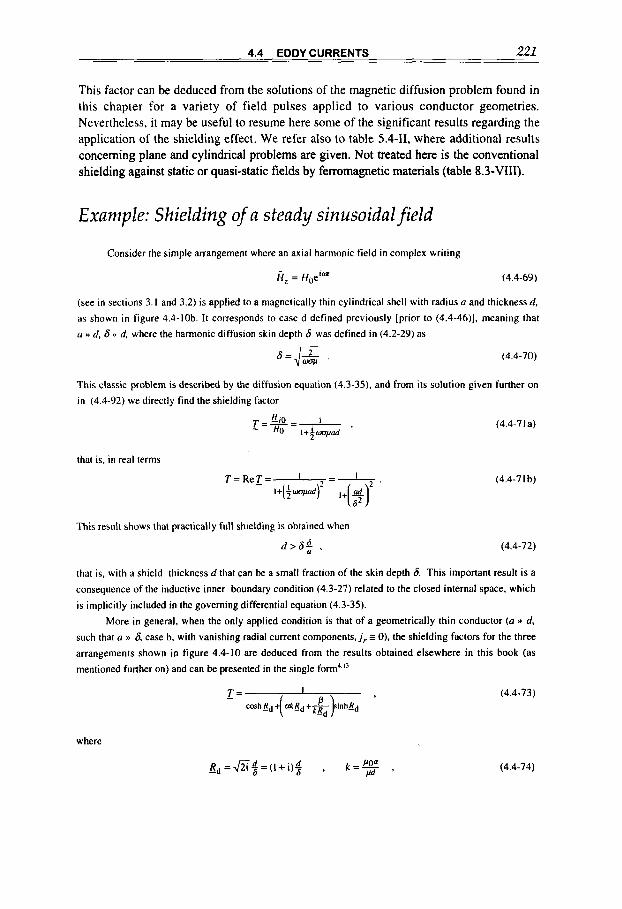
4.4 EDDY CURRENTS 221
This factor can be deduced from the solutions of the magnetic diffusion problem found in this chapter for a variety of field pulses applied to various conductor geometries. Nevertheless, it may be useful to resume here some of the significant results regarding the application of the shielding effect. We refer also to table 5.4-11, where additional results concerning plane and cylindncal problems are given. Not treated here is the conventional shielding against static or quasi-static fields by ferromagnetic materials (table 8.3-VIII).
Example: Shielding of a steady sinusoidal field
Consider the simple arrangement where an axial harmonic field in complex writing
I-r: = (4.4-69)
(see in sections 3. I and 3.2) is applied to a magnetically thin cylindrical shell with radius a and thickness d.
as shown in figure 4.4-lob. It corresponds to case d defined previously [prior to (4.4-46)]. meaning that
(I P) d, 6 >) d, where the harmonic diffusion skin depth 6 was defined in (4.2-29) as
(4.4-70)
This classic problem is described by the diffusion equation (4.3-35). and from its solution given further on
i n (4.4-92) we directly find the shielding factor
that is, in real terms
This result shows that practically full shielding is obtained when
d > 6 : ,
(4.4-71 a)
(4.4-7 I b)
(4.4-72)
that is, with a shield thickness d that can be a small fraction of the skin depth 6. This important result is a
consequence of the inductive inner boundary condition (4.3-27) related to the closed internal space. which
is implicitly included in the governing differential equation (4.3-35). More in general, when the only applied condition is that of a geometrically thin conductor (a s d,
such that a M 6, case b, with vanishing radial current components. j , z 0). the shielding factors for the three
arrangements shown in figure 4.4-10 are deduced from the results obtained elsewhere in this book (as
mentioned further on) and can be presented in the single form4 I'
where
(4.4-73)
(4.4-74)
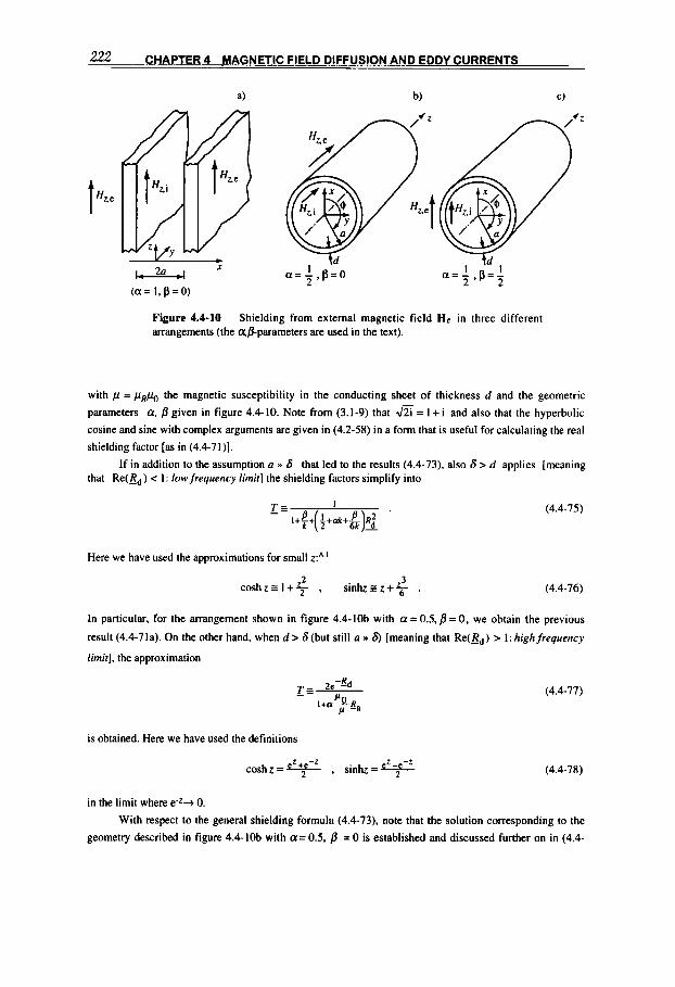
2 2 CHAPTER 4 MAGNETIC FIELD DIFFUSION AND EDDY CURRENTS
a) b) C )
1 a= - 1 , p = l 2 2
a=- ,P=O 2 (a= I , p = O )
Figure 4.4-10 arrangements (the @-parameters are used in the text).
Shielding from external magnetic field He i n three different
with p = pRpo the magnetic susceptibility in the conducting sheet of thickness d and the geometric
parameters a. p given in figure 4.4-10. Note from (3.1-9) that f i = I + i and also that the hyperbolic
cosine and sine with complex arguments are given in (4.2-58) in a form that is useful for calculating the real
shielding factor [as in (4.4-71)].
If in addition to the assumption a n 6 that led to the results (4.4-73). also 6 > d applies [meaning that Re(Bd) < 1 : lowfrequency limit] the shielding factors simplify into
- T Z I (4.4-75) I + l+ k ( 2 Ltak+- &]2 R
'
Here we have used the approximations for small z?'
coshznI+$ , s i n k z z + $ (4.4-76)
In particular, for the arrangement shown in figure 4.4-10b with a = 0.5, p = 0, we obtain the previous
result (4.4-71a). On the other hand, when d > 6(but still a n 6) [meaning that Re(_Rd) > I : highfrequency
limit]. the approximation
(4.4-77) 2e-&d
I + a A R B
T G - - P
is obtained. Here we have used the definitions
in the limit where e-Z+ 0. With respect to the general shielding formula (4.4-73), note that the solution corresponding to the
geometry described in figure 4.4-10b with a= 0.5, p = 0 is established and discussed further on in (4.4-
4.4 EDDY CURRENTS 223
88.90.92). To find the solution of the transverse field shielding (figure 4.4-I&) we can proceed as in the
subsection following (4.3-48) but with the assumption a D 6. Finally. to find the result for the plane
geometry shown in figure 4.4-IOa, we refer to the field diffusion into a slab given in (4.2-53). where the
constants in the general solution (4.2-54) are now determined [instead as in (4.2-56)) by the boundary conditions at x = a + d,
fiz,e = Hoeiw or h z ( X u + d ) = 1 ; (4.4-79)
and the inductive condition at x = a [similarly to (4.3-27)],
or
where
(4.4-8Oa)
(4.4-80b)
(4.4-80~)
Example: Shielding by a thick hollow conductor
The shielding problem defined in figure 4.4-IOb is formulated and solved here in complex writing,427 similarly as with the diffusion into a rod [see in (4.3-21 to 25).] The applied axial external field
HZ*= = Hoeiw (4.4-81a)
leads to the solution in the conductor:
hZ(r,i) = Hoh,(_R)eiw
where, as in (4.3-25a). the solution is expressed in the modified Bessel functions.
h, (E)=ao( t? )+ DKo(_R)
(4.4-81 b)
(4.4-82)
with
R = = (1 + i ) $ and t?, = _R(r =a). = E(r = b), Bd = l?(r = d ) . (4.4-83) 6 -
The constants C and D are determined with the boundary conditions, which here are
at r = b , i.e.A=_Rb: h z ( E b ) = l ; (4.4-84)
at r = a, i.e.. _R = I?,, from (4.3 - 27), =+iwahah,(_R,) (4.4-85a)
224 CHAPTER 4 MAGNETIC FIELD DIFFUSION AND EDDY CURRENTS
(4.4-85b) R =yLz(e,)
The solution (4.4-82) satisfying conditions (4.4-84.85) is calculated to be
here we have used the following modified Bessel relations derived from (A.2-22.23, and 25.26):
(4.4-86)
(4.4-87)
For the shielding factor (4.4-68). by applying these relations again, we obtain
Hob,(, ) 2 T = =!!,@,)= - H o R o 2 [ I O ( B b ) K Z ( E u )-KO(,b) l2(!! , ) ] '
The first step to obtain the shielding factor in real terms is to express these Bessel functions with the related Kelvin functions, as in (4.3-2%).
A substantial simplification is obtained when (I n 6, in which case with the approximations (A.2-37, 38) for large 2, the Bessel functions can be eliminated. However, in this case where Re ( B ) N 1 it would be
more convenient to neglect the second term in the diffusion equation (4.3-23) from the beginning and thus obtain
the solution of which is
&(I?) = CcoshB+ D sinhe .
(4.4-89)
(4.4-90)
The constants are easily determined through the boundary conditions (4.4-84.85). To obtain the solution in
real terms, the relations (4.2-58) will have to be applied.
Example: Shielding by a thin hollow conductor
We calculate here the diffusion of an axial steady harmonic field He= Ho coswf through a thin-
walled hollow cylinder (figure 4.4- lob) by applying the appropriate complex formalism introduced in
chapter 3. Similar calculations for determining magnetic diffusion are presented for a cylindrical rod,
starting from (4.3-2 1); and for a thin-walled cylindrical conductor, starting from (4.4-69).
Taking the boundary field in the complex writing to be, as in (4.4-81a).
tie(ro,r) = Hoeim , (4.4-9 1)
(4.4-92a)
we look for the inner field

4.5 DIFFUSION IN ELECTRIC CIRCUITS 225
By inserting into the appropriate differential equation (4.3-35). we immediately get
(4.4-92b)
(4.4-93)
where d c 6 because of the thin-sheet approximation, and the harmonic skin depth 6 is given in (4.4-70).
The surface current density s = jd [see also (4.4- I I ) ] , constant through the conductor because of the thin-
sheet approximation, is consequently
(4.4-94)
(here we indicate the surface current density with s instead of i to avoid confusion with the imaginary unit).
4.5 DIFFUSION IN ELECTRIC CIRCUITS
The question addressed in this section concerns the current density distribution within a conductor when a time varying total current I ( r ) [or voltage V(t)] is imposed at its end. This problem will also allow us to establish a relation between the current-field diffusion processes presented in this chapter and the global parameters characterizing current conduction in a conductor, namely, its impedance Z , resistance R, capacitance C, and inductance L.
Lumped circuits
For the study of the electromagnetic properties resulting from electric currents flowing in conductor systems, it is often convenient (as we have already seen) to reduce the system to a circuit of lumped elements to which Kirchhoff s laws (1.1-62, 63) are applied. For example, the series circuit shown in figure 4.5-1 is described by the equation
(4.5-1)
where V is the voltage (emf) source, R the resistance (1.1-59), L the inductance (2.4-5), and C the capacitance, and we have introduced separately a time-dependent skin-effect impedance Z(r), which will be the subject of the following discussion. For completeness'

- - 226 CHAPTER 4 MAGNETIC FIELD DIFFUSION AND EDDY CURRENTS
sake we recall that the definition of the capacitance between two conducting bodies (e.g.. the two plates in a capacitor) with known electric field E and flux D distribution is
C = Q l V (4.5-2a)
where the potential difference (taken along any path between the surfaces of the two bodies) is
V = j E . d l , (4.5-2b)
and the accumulated electrical charge on either one of their surfaces is [from (1.1-4) and (A.3- 16)]
Q=$D.ds . (4.5-2~)
The simplicity of this circuit de~cription'. '~ (in comparison to the more general field theory) is mainly due to the approximations implicitly made in establishing it:
(a) Wires connecting the lumped circuit elements are assumed to be ideal conductors. (b) Circuit dimensions are small enough for wave propagation to be negligible
[magnetoquasistationary approximation with closed current filaments according to (1.2-21) in all elements except in the capacitor].
(c) Magnetic flux change d(Ll)ldt is negligible everywhere except in connection with the inductor.
(d) Displacement current term dD/dr is negligible everywhere except in the capacitor.
Often the circuits are operated at near dc conditions with uniform current distribution throughout the conductors. There are, however, operating ranges where the impedance Z due to skin effect in some circuit elements can be comparable to or larger than the lumped impedances of other element^^.^.
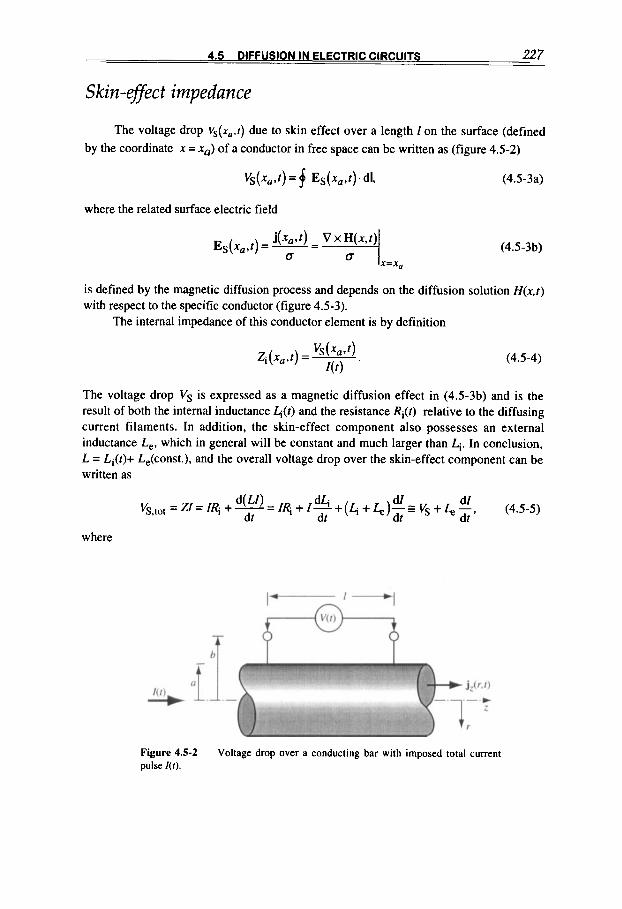
; 227
Skin-effect impedance
The voltage drop Vs(xa.r) due to skin effect over a length 1 on the surface (defined by the coordinate x = xa) of a conductor in free space can be written as (figure 4.5-2)
Vs(xu,t)=f Es(x,,t).dl, (4.5-3a)
where the related surface electric field
(4.5-3b)
is defined by the magnetic diffusion process and depends on the diffusion solution H(x,t) with respect to the specific conductor (figure 4.5-3).
The internal impedance of this conductor element is by definition
(4.5 -4)
The voltage drop Vs is expressed as a magnetic diffusion effect in (4.5-3b) and is the result of both the internal inductance h(t) and the resistance Ri(t) relative to the diffusing current filaments. In addition, the skin-effect component also possesses an external inductance Le, which in general will be constant and much larger than I!+,. In conclusion, L = Li(r)+ Le(const.), and the overall voltage drop over the skin-effect component can be written as
where
Figure 4.5-2 pulse I ( ! ) .
Voltage drop over a conducting bar with imposed total current
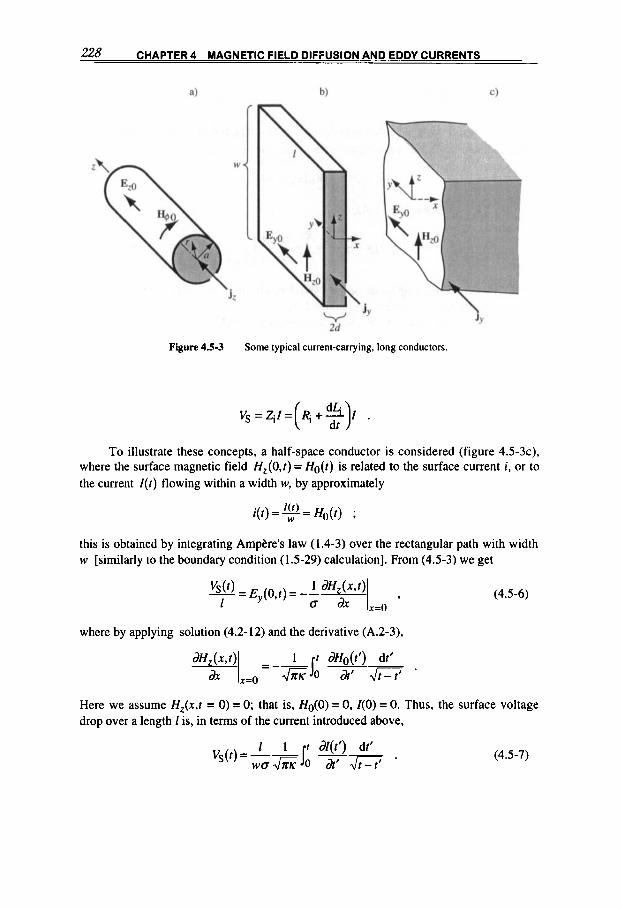
228 CHAPTER 4 MAGNETIC FIELD DIFFUSION AND EDDY CURRENTS
Figure 4.5-3 Some typical current-carrying. long conductors.
To illustrate these concepts, a half-space conductor is considered (figure 4.5-3c), where the surface magnetic field H,(O,f ) = H o ( f ) is related to the surface current i, or to the current I ( r ) flowing within a width w, by approximately
I ( t ) i ( r ) = = Ho(t ) ;
this is obtained by integrating Amptre’s law (1.4-3) over the rectangular path with width w [similarly to the boundary condition (1.5-29) calculation]. From (4.5-3) we get
(4.5-6)
where by applying solution (4.2-12) and the derivative (A.2-3),
x=o
Here we assume H,(x,r = 0) = 0; that is, Ho(0) = 0, I(0) = 0. Thus, the surface voltage drop over a length 1 is, in terms of the current introduced above,
(4.5-7)
4.5 DIFFUSION IN ELECTRIC CIRCUITS 229
With this, the circuit equation (4.5-1) becomes a Fredholm integral equation in I, whose solution can be found with numerical techniques; in some simple cases even analytic solutions exist.A xA 27 The particular plane geometry used here can be an approximation to more complicated conductor geometries provided that the skin depth remain much smaller than the radius of curvature of the surface or thickness of the conductor.
In the following, the internal impedance with respect to a specific current pulse, i.e., a step-function current pulse, is calculated for three simple conductor geometries (figure 4.5-3). [Extension to any transient pulse form can be made on the basis of Duhamel's theorem (4.1-27).]
Example: Step-jhction current on plane conductor
For the step-function current pulse
0. for - - < t < 0,
/,(const.), for 0 5 r < -, (4.5-8)
applied to the half-space, the solution procedure is similar to that for the general solution (4.5-6). which refers to the same conductor geometry (figure 4.5-3c). We have I = wHo(const.), and by referring to the
simple step-function-related solution (4.24). we get
and thus
I V , ( t ) = Z i l , = ~
w u & l U '
(4.5-9)
As a second example of a plane conductor, consider a conducting slab with thickness 2d and width
w H 2d (figure 4.5-3b). which limits a step-function field pulse Ho(const.) on one side only, thus carrying a current (4.5-8). I, = WHO. Here, (4.5-6) is
and from the solution given by case 2 in table 4.2-1 we calculate
(4.5-10)
(4.5- I I )

2.30 CHAPTER 4 MAGNETIC FIELD DIFFUSION AND EDDY CURREN TS
Example: Step-function current on a rod
A typical current-carrying conductor geometry is the rod (figure 4.5-3a), whose H$-field diffusion is
described by (4.3-6) with the solution [similar to (A.4-72)]
(4.5-12)
where (a&) are the roots of the Bessel function Jl(a&) = 0 [see table A.2-I and (A.2-20)]. The related
current density (4.3-2) is
and because of the imposed current pulse (4.5-8), the condition (for 0 I I c m)
2x j,(r,I)dr = lo = 2naH+o(const.) i 0
(4.5-13)
(4.5- 14)
must hold. Note that this problem can also be described by the related diffusion equation (4.1-12) for the
axial current density
(4.5-15)
By using a similar procedure to that in connection with (4.5-10). with E,(a,r) = j,(a,r)/uo calculated from
(4.5- 12.13). the voltage drop over the rod is
(4.5-16)
Generalization of the results and equivalent circuits
The internal impedances of the various slab geometries and of the rod with respect to a step-function boundary condition, found with solutions (4.5-1 1,16), have all the characteristic form
(4.5-17)
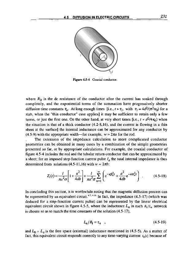
4.5 DIFFUSION IN ELECTRIC CIRCUITS 231
Figure 4.5-4 Coaxial conductor
where Ro is the dc resistance of the conductor after the current has soaked through completely, and the expontential terms of the summation have progressively shorter diffusion time constants z,,. At long enough times [i.e., t >> 71, with TI = 4&/(7C2Kg) for a slab, when the "thin conductor" case applies] it may be sufficient to retain only a few terms, or just the first one. On the other hand, at very short times [i.e., t (< &/4rg) when the situation is that of a thick conductor (4.2-8.16). and the current is flowing in a thin sheet at the surface] the internal inductance can be approximated for any conductor by (4.5-9) with the appropriate width-for example, w = 2 m for the rod.
The extension of the impedance calculation to more complicated conductor geometries can be obtained in many cases by a combination of the simple geometries presented so far, or by appropriate calculations. For example, the coaxial conductor of figure 4.5-4 includes the rod and the tubular return conductor that can be approximated by a sheet; for an imposed step-function current pulse I , the total internal impedance is thus determined from solutions (4.5-1 1,16) with w = 2nb:
In concluding this section, it is worthwhile noting that the magnetic diffusion process can be represented by an equivalent c i r c ~ i t . ~ . ' . ~ . ' ~ In fact, the impedance (4.5-17) (which was deduced for a step-function current pulse) can be represented by the linear electrical equivalent circuit shown in figure 4.5-5, where the inductance L, in each R,/L,, network is chosen so as to match the time constants of the solution (4.5-17),
and = L , is the free space (external) inductance mentioned in (4.5-5). As a matter of fact, this equivalent circuit responds correctly to any time-varying current / , ,(t) because of

232 CHAPTER 4 MAGNETIC FIELD DIFFUSION AND EDDY CURRENTS
Figure 4.5-5 current conduction and diffusion problems.
Electric equivalent circuit for representing some time-dependent
the arguments mentioned following theorem (4.1-27). This circuit simulates the physical diffusion process, and the magnetic diffusion can generally be described also by ordinary circuit analy~is.~ 23
A1 ternating currents
We now discuss an example of the steady, alternating current problem, where the total current
l ( t ) = la COSUX, for - m < t < +oo , (4.5-20)
is imposed on the rod (figure 4.5-3a). This example is discussed in many textbooks' thus our presentation is limited to only some significant aspects. The related current density distribution j z ( r , t ) , and hence its impedance, can be calculated using a similar formalism to that introduced in (4.3-21) for the magnetic field diffusion, where we applied the complex functions defined in section 3.1. Putting
I(r)= Iaeiwr , (4.5-21)
and looking for a solution of the complex quantities
the diffusion equation (4.5-15) transforms into
(4.5-22)
(4.5-23)
where the normalized radius the solution is the modified Bessel function b of order 0,
was given in (4.3-24). According to (4.3-25) and (A.2-13),
f=CIo(!z) 9 (4.5-24)

4.5 DIFFUSION IN ELECTRIC CIRCUITS 233
where the constant C is fixed by the boundary condition (4.5-14), which in its complex form is
- i l r a s 2 C e i o x ~ ~ IO(/?)_Rd/?= Iaeiw ,
where
- R = f i i = ( l + i ) i , = / ? ( r = a ) = ( l + i ) ” 6 ,
and the skin depth (4.2-29) is
S=m=Jm .
The application of the integral formula in (A.2-26) yields
f i r , C = 2n0a6 I, (& ) ’
and the electric field (4.5-22,24), &(r,f), is thus fully determined. In analogy to (4.5-5). the complex internal impedance is defined as
(4.5-25)
(4.5-26)
(4.5-27)
(4.5-28)
where Ri(o) is the effective resistance of the conductor and h ( w ) the internal self- inductance [with w,!+(w) the internal reactance]. Introducing the Kelvin function (A.2-15) from (4.5-28) we obtain, by decomposing into real and imaginary parts,
1 berRabei’Ru - beiRuber’Ra (4.5-29) 2 ’ R(w) = ~
- h d a (ber’R,)* + (bei’Ru)
1 berRuber’Ru + beiRabei’Ra wh(w) = ~ (4.5-30) fim60 (ber’R,)’ +(bei’Ra)2
where Ru = d u l 6 and the prime denotes derivation with respect to R = f i rI6.
their derivatives, and by excluding te&s;of order (u/6)* and higher, we calculate
At low frequencies (i.e., when a < 4, from the series expansions (A.2-29, 30) and
(4.5-3 1)
(4.5-32)
On the contrary, at high frequencies-that is, where u N 6, and the current is flowing in a

234 CHAPTER 4 MAGNETIC FIELD DIFFUSION AND EDDY CURRENTS
thin sheet only-with the approximations (A.2-39,40,4 1 ) we get
(4.5-33)
(4.5-34)
In the lowest nonvanishing order we get R G ~ 4 , and in this limit the resistance is as if the uniform current flowed in a conductor sheet of thickness 6.
Cfiupter 5
ELECTROMAGNETIC AND THERMAL ENERGIES
Electromagnetic fields give rise to an energy density, and time-varying fields give rise to an energy flow; these have to be considered in studying electromagnetic problems: They can represent significant energy storage (investment) and a loss (heating) mechanism. In addition, there are secondary effects: The current flow induced in an electric conductor generates heat that affects the thermal behavior of the associated mass; the increasing temperature in a conductor will diminish the electric conductivity, and, in turn, this will change the magnetic diffusion and eddy currents, and so on, resulting in a nonlinear magnetic diffusion process. As is evident from the general definition of energy, electromagnetic energy is related to electromagnetic forces, which will be the subject of the next chapter.
Applicafions. The topics in this chapter support several examples of practical importance: operational limitations, introduced in a magnetic systems as a result of energy dissipation; inductive energy storage through SMES systems’ ” (superconducting magnetic energy storage); induction heating’ I , an industrial process to heat work pieces directly or indirectly; and, more in general, electromagnetic processing of
5.1 ELECTROMAGNETIC ENERGY EQUATIONS
In a closed electromagnetic system, including fields, electric conducting, and nonconducting masses, the energy sources and flow include several components, as will be shown in this section. In addition, the relation between electromagnetic energy and the
235
M4GNETICFIELDS: A Comprehensive Theoretical Treatise for Practical Use Heinz E. Knoepfel
Copyright Q 2000 by John Wiley & Sons, Inc
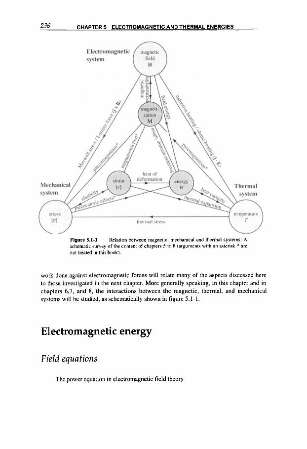
236 CHAPTER 5 ELECTROMAGNETIC AND THERMAL ENERGIES
Figure 5.1-1 Relation between magnetic, mechanical and thermal systems: A schematic survey of the content of chapters 5 to 8 (arguments with an asterisk * are not treated in this book).
work done against electromagnetic forces will relate many of the aspects discussed here to those investigated in the next chapter. More generally speaking, in this chapter and in chapters 6,7, and 8, the interactions between the magnetic, thermal, and mechanical systems will be studied, as schematically shown in figure 5.1-1.
Electromagnetic energy
Field equations
The power equation in electromagnetic field theory
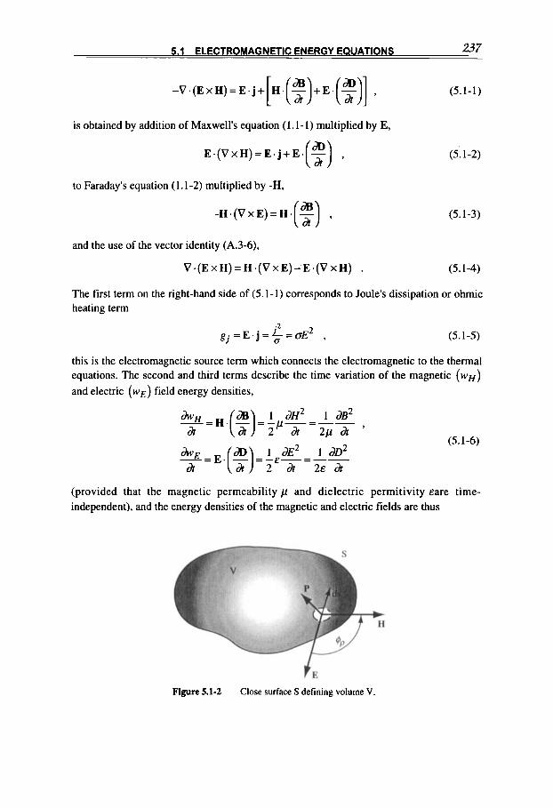
5.1 ELECTROMAGNETIC ENERGY EQUATIONS 237
- V . ( E x H ) = E . j + H . - + E . - , [ (3 (31 is obtained by addition of Maxwell's equation (1.1- I ) multiplied by E,
E .(V x H) = E . j + E . - (3 ' to Faraday's equation (1.1-2) multiplied by -H,
and the use of the vector identity (A.3-6),
v .(E x H) = H . (v x E) - E . (v x H)
(5.1-1)
(5: 1-2)
(5.1-3)
(5.1-4)
The first term on the right-hand side of (5.1-1) corresponds to Joule's dissipation or ohmic heating term
.2 g . I = ~ . j = l = C7 oE2 , (5.1-5)
this is the electromagnetic source term which connects the electromagnetic to the thermal equations. The second and third terms describe the time variation of the magnetic (WH)
and electric (WE) field energy densities,
(5.1-6)
(provided that the magnetic permeability p and dielectric permitivity &are time- independent), and the energy densities of the magnetic and electric fields are thus
Figure 5.1-2 Close surface S defining volume V.
238 CHAPTER 5 ELECTROMAGNETIC AND THERMAL ENERGIES
or, in practical cgs units,
H2 W H = P R ~ ,
and WE=-&&- 1 D2 .
2 2 E
(5.1-7)
(5.1 -7)*
(5.1-8)
This last term, which derives through E.(dD/&) from the displacement term in Maxwell's equation, can be neglected in the magnetoquasistationary approximation.
Integration of (5.1-1) over the volume V delimited by a closed surface S (figure 5.1- 2) and using Gauss' theorem (A.3- 16) yields the integral power equation
-Is P . d s = I - d V + I j2 --(-pH2+-&E2)dV d 1 1 ,
a 1 2 2 V O V
where the Poynting vector
P = E x H ,
or, in practical cgs units,
lo8 P=-(ExH) ,
4K
(5.1-9)
(5.1-10)
(5.1 -lo)*
represents the power flow crossing the boundary per unit surface. Note that these power and energy expressions can be extended to the cases where
p, €are time dependent and/or where the conducting mass is moving with velocity u. In the first case, the terms
H2* , E d t 2
dr (5.1-1 1)
must be added on the right-hand sides of (5.1-6, 9). In the second case, the transformations presented in section 1.3 must be introduced. This will lead, in the magnetoquasistationary approximation, to the magnetohydrodynamic energy equations (8.1-8,13,35) that will be introduced in section 8.1.
Potential equations
The power equations can also be expressed in terms of the magnetic vector potential A and the electric scalar potential U, which, through (2.2-2, 4), express the
5.1 ELECTROMAGNETIC ENERGY EQUATIONS 239
magnetic and electric fields
B = V x A ,
(5.1 - 12)
Multiplication of the last expression with the current density vector j and using the vector identity (A.3-5).
V.(Uj)=U V . j + j . V U ,
and the current conservation equation (1.1-5).
V . j+- dPe -0 - , a gives
(5.1 - 13)
This corresponds to the power equation (5.1-1). In particular, we see that the time variation of the magnetic field energy density is, instead of (5.1-6).
h = j . ( $ ) dr , (5.1-14)
and that the last term vanishes in the magnetic quasistationary approximation, where V . j = O , (1.2-21). Integration of (5.1-13) over the volume V and application of Gauss' theorem (A.3-16) leads to the power equation
(5. I 15)
Although this current-potential equation resembles the current-field equation (5. -9). there are, however, fundamental differences. The integration here is only over the volume
in which j and pe are finite. Al l terms vanish in free space, making it impossible to think of an energy flow from this space into the conductor across its surface. [For the total magnetic field energy expressed in terms of magnetic vector potential and/or current densities, see (5.1-31, 33).]
240 CHAPTER 5 ELECTROMAGNETIC AND THERMAL ENERGIES
Sinusoidal fields
A case often encountered in practice (e.g., induction heating applications'.' treated in section 5.4) is where the fields are sinusoidal in time, for which it is convenient to use the complex vector formalism introduced in chapter 3. Accordingly, any electromagnetic vector (e.g., the magnetic field) is presented in the form (3.2-1).
(5.1 - 16) H=Hei",P,=Eei", - j = j e iwr ,
where the complex vectors H, E, and - j, which are called phasors, can be written in the
forms (3.1-30 or 3 1 )-for example,
H = H' + iH" I ( H ; + i H,",H; + iH;,H; + i H y ) . (5.1 - 17)
At the end of the calculation with this formalism, we have to return to the real component of the significant parameters, because only this component has a real physical meaning (this is evident when comparing results of a conventional calculation with those of a complex calculation). The real parameter, or vector, is easily obtained by the relation (3.1-32).
(5.1-18) 1
ReH=-(H+H*) , 2 -
where H* is the conjugate vector defined in (3.1-34,35). Also, from (3.1-36) it is
- H . H * = I H f = H 2 = H t 2 + H t P 2 . (5.1 - 19)
Another useful relation when resolving problems with this formalism is the theorem (3.1- 381,
(5.1-20) ReH, .ReHz =-Re(& 1 .H;) ; 2
and, in particular,
(5.1-2 1) - 2 1 1
2 - - 2 (ReH) = - H . H * = - H 2 ,
which provides the time average (over a period r ) of the product of two real functions (e.g., field quantities).
We have to rewrite the power equations (5.1-2 to 4) in a suitable form for applying the above rules. For this purpose' ' I . ' I , Maxwell's equation (3.2-2) is rewritten in the form
VXH*=j* - imD* , (5.1-22)
which is obtained by taking the conjugate quantities (5.1-16), and Faraday 's equation
5.1 ELECTROMAGNETIC ENERGY EQUATIONS 241
(1.1-2) is rewritten in the form
V x E = - i w i i
(see also in section 3.2). Multiplying the first equation by E, multiplying the second by - H *, and then adding them up [as in (5.1-1 to 4)] provides the power equation
-v. (E x H *) = E . j * -iw -H * .B + E . fi *) . (5.1-23) - - ( - This expression is convenient because, by applying (5. I-19,20), it allows us to obtain the time average over one period T = 2R/O by simply introducing the factor 1/2. For the terms on the right-hand side with (5.1-16) we obtain
Similarly, for the complex Poynting vector (5.1-10) we write
with @p = @E - @H the phase angle between E, u, and nEH the unit vector normal to the
(E,H) plane. [Note that i* = 4, (H *)* = H, etc.] Inserting (5.1-24.25) in (5.1-23) and
then integrating over the volume V delimited by the surface S as in (5.1-9) provides the mean power flowing over a period T into the volume
I j 2 w - S = S'+ is" = -IEHe' Qp (nEH .ds) = - 1 -dV + i- I ( E E ~ - pH2)dV. (5.1-
S 2 v = 2 V
26)
The separation of the complex power equation with ei'" = C O S @ ~ + i sin@p, (3.1-4).
into a real and an imaginary part provides the real power equation
(5.1-27a)
which describes the mean ohmic power dissipated over the time T, and a reactive power equation
(5.1 -27b) S" = -1EH sin$,,(nEH .ds) = - , ( E E ~ w -pH2)dV , S 2 V
which represents the energy flowing in and out of the electromagnetic energy storage,

242 CHAPTER 5 ELECTROMAGNETIC AND THERMAL ENERGIES
without dissipation. Note that the mean energies stored in the fields within the volume V are
Since (5.1-26) shows that the power dissipated in the volume V goes exclusively into ohmic heating, we must have
- WH +WE = Const. (5.1-29)
within this volume. Also, provided that the vectors E,€J on the surface S are such that the conditions
q5,,=0 andlor nEH.ds=O
hold, from (5.1-26) it follows that
that is, the energy inflow over a period T (which is dissipated as Joule's heat) is equal to twice the mean magnetic or electric stored energy. Magnetization effects (e.g., damping mechanisms) with related energy losses are conveniently expressed with a complex magnetic permeability, wich will be introduced in (5.4-44).
Inductive energy
The total magnetic field energy linked to a conductor system (figure 5.1-3) can be written in the magnetoquasistationay approximation (5.1-7) as
W H = j - p H 2 d V = j 1 -A.(VxH)dV 1 . 2
V 2
V
(5.1-3 1)
In fact, by using the vector potential A, (5.1-12), and (A.3-6) we obtain
(H , B)dV = H . (V x A)dV = A . (V x H)dV + V. (A x H)dV ; (5.1-32)
the last integral can, however, be neglected since, through Gauss' theorem (A.3-16) applied to the vector (A x H),
[V. (AxH)]dV=f ( A x H ) . d s , V S
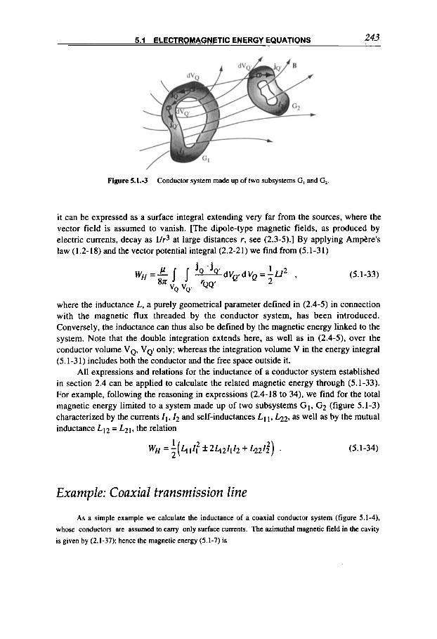
5.1 ELECTROMAGNETIC ENERGY EQUATIONS 243
Figure 5.1.4 Conductor system made up of two subsystems G, and G,.
it can be expressed as a surface integral extending very far from the sources, where the vector field is assumed to vanish. [The dipole-type magnetic fields, as produced by electric currents, decay as llr3 at large distances r, see (2.3-5).] By applying Amp5re’s law (1.2-18) and the vector potential integral (2.2-21) we find from (5.1-31)
(5.1-33)
where the inductance L, a purely geometrical parameter defined in (2.4-5) in connection with the magnetic flux threaded by the conductor system, has been introduced. Conversely, the inductance can thus also be defined by the magnetic energy linked to the system. Note that the double integration extends here, as well as in (2.4-5), over the conductor volume VQ, VQ‘ only; whereas the integration volume V in the energy integral (5.1-31) includes both the conductor and the free space outside it.
All expressions and relations for the inductance of a conductor system established in section 2.4 can be applied to calculate the related magnetic energy through (5.1-33). For example, following the reasoning in expressions (2.4-18 to 34). we find for the total magnetic energy limited to a system made up of two subsystems GI, G2 (figure 5.1-3) characterized by the currents I I , ~ and self-inductances L I 1. L22, as well as by the mutual inductance L12 = L21, the relation
(5.1-34)
Example: Coaxial transmission line As a simple example we calculate the inductance of a coaxial conductor system (figure 5.1-4).
whose conductors are assumed to cany only surface currents. The azimuthal magnetic field in the cavity
is given by (2.1-37); hence the magnetic energy (5.1-7) is
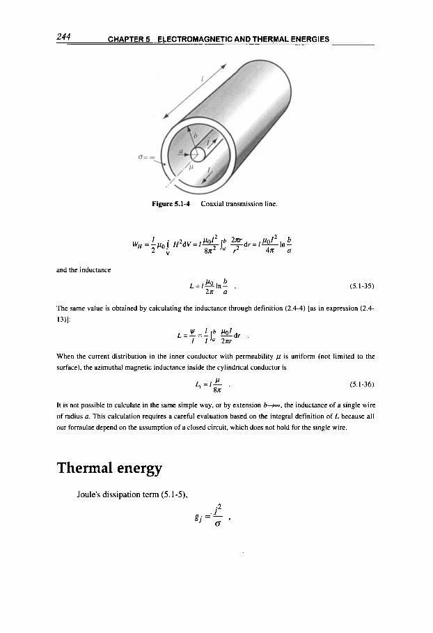
244 CHAPTER 5 ELECTROMAGNETIC AND THERMAL ENERGIES
Figure 5.1-4 Coaxial transmission line.
and the inductance
Po b L=l-In- . 2n a
(5.1-35)
The same value is obtained by calculating the inductance through definition (2.4-4) [as in expression (2.4-
I3)]:
VI - I b Pol L = - - - j -dr . I I 21rr
When the current distribution in the inner conductor with permeability p is uniform (not limited to the
surface), the azimuthal magnetic inductance inside the cylindrical conductor is
(5.1-36)
It is not possible to calculate in the same simple way, or by extension b-, the inductance of a single wire
of radius a. This calculation requires a careful evaluation based on the integral definition of L because all
our formulae depend on the assumption of a closed circuit, which does not hold for the single wire.
Thermal energy
Joule's dissipation term (5.1-5),
. j 2 ' 0 '
g. = -
5.1 ELECTROMAGNETIC ENERGY EQUATIONS 245
links the electromagnetic energy to the thermal energy in the conductor. Heating of the conductor gives rise to a flow of thermal energy and can entail local melting with variation in the electrical conductivity (chapter 8), which in turn influences the electromagnetic quantities.
The heat balance and the related temperatures must be studied by the thermal dirusion equation
I l a k a &
A T + - g = - - , (5.1-37)
where the temperature T(x,y,z;t) [measured in kelvin] and the source term g(x,y,z;r) = gj [rate of energy generation per unit volume, measured, e.g., in watt/m3] may be space- and time-dependent, k is the thermal conductivity [W/(m.K)], assumed here to be a constant, and
k a=- CV
(5.1-38)
is the thermal diffusivity [m2/s], where c v is the specific heat per unit volume [J/(m3.K)].
The diffusion equation (5.1-37) is the result of the (thermal) power balance in the elemental volume Ax Ay Az (figure 5.1-5):
net heat flow into + energy generation rate within = energy accumulation rate . (5.1-39)
In fact, the heat flux q. a vector quantity measured in [W/m*], according to Fourier’s law of heat conduction, is determined by the temperature gradient and is expressed for an isotropic body by the components (in Cartesian coordinates)
(5.1-40)
Consequently, the net rate of heat flowing (e.g., along the y-direction) into the elemental volume Ax Ay Az is
The accumulation rate of the internal (thermal) energy density Q is defined by the change in the specific internal energy ~ [ J k g ] , or PE [J/m3] where p is the mass density [kg/m3]; in solid bodies (neglecting phase changes, compression energy, etc.) a good approximation is
such that the rate becomes
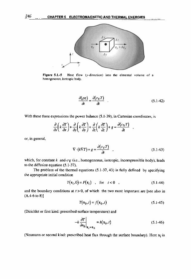
246 CHAPTER 5 ELECTROMAGNETIC AND THERMAL ENERGIES
Figure 5.1.4 Heat f low (y-direction) into the elmental volume of a homogeneous, isotropic body.
(5.1-42)
With these three expressions the power balance (5.1 -39), in Cartesian coordinates, is
or, in general,
(5.1-43)
which, for constant k and c v (i.e., homogeneous, isotropic, incompressible body), leads to the diffusion equation (5.1-37).
The problem of the thermal equations (5.1-37.43) is fully defined by specifying the appropriate initial condition
T ( X ~ , ~ > = F ( X ~ ) , for r < O , (5.1-44)
and the boundary conditions at t > 0, of which the two most important are [see also in (A.4-6 to S ) ]
T( X b , t ) = f( Xb, t ) (5.1-45)
(Dirichlet or first kind: prescribed surface temperature) and
(5.1-46)
(Neumann or second kind: prescribed heat flux through the surface boundary). Here xi is

5.1 ELECTROMAGNETIC ENERGY EQUATIONS 247
a coordinate vector covering the whole body in Cartesian coordinates xi I (x,y,z); xb is a coordinate vector delimiting its surface; and nb denotes an outward pointing, normal vector on the boundary surface.
For the solution of the so-defined thermal conduction problem, which is similar to the magnetic diffusion problem (see in chapter 4). there exists a vast body of literature. The solutions of the heat conduction equations (5.1-37,43) follow standard methods 4.2,44
(e.g., variable separation, Laplace transformation, Green’s function method, etc.) as well as numerical method^'.^. In particular, for the variable separation method, we refer to the solution of the similar magnetic diffusion equation analyzed in chapter 4 and appendix A.4.
Example: Thermal difision in slab
I t may be instructive to briefly illustrate the powerful Green‘sfunclion method, by giving the general
solution of the one-dimensional Cartesian equation (5.1-37).
(5.1-47)
defined with conditions (5.1-44 to 46) within two plane, parallel boundaries ( b = 1.2) at distance 2d4’4:
2d
r’=O T(x,t)= J G(x,t~x’,O)F(x’)dr’ for the initial condition,
+ aJll,=, dt’ [MG(&?lih.tl)] for the second-kind boundary condition. (5.1-48) h=1,2 ‘ b
Here, G(x,t lx’ , t ’ ) is the Green function, which depends on the geometry and type of boundary condition;
it is found tabulated for a large variety of problems.44
For example, the one-dimensional Green function for a sheet of thickness 2d with boundary
conditions of the first kind (figure 5.1-6) is
which is convenient for small a(? -f1)/4d2 values; whereas for large values the alternative form
(5.1-49)
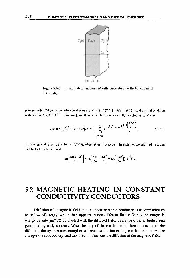
248 CHAPTER 5 ELECTROMAGNETIC AND THERMAL ENERGIES
Figure 5.1-6 Infinite slab of thickness 2d with temperatures at the boundaries of
T , (0, T2W.
is more useful. When the boundary conditions are T(0.r) = T(2d.r) = f i ( r ) = f2(t) = 0, the initial condition
in the slab is T ( x . 0 ) = F ( x ) = To(const.), and there are no heat sources g = 0, the solution (5.1-48) is
(5.1-50)
(n=odd)
This corresponds exactly to solution (4.2-49). when taking into account the shift d of the origin of the x-axis
and the fact that for n = odd,
nn(x - d ) n-l sin [ ~ 2d ] = sin( 5 - y ) = cos( z)(-l)T
5.2 MAGNETIC HEATING IN CONSTANT CONDUCTIVITY CONDUCTORS
Diffusion of a magnetic field into an incompressible conductor is accompanied by an inflow of energy, which then appears in two different forms: One is the magnetic energy density pH2 / 2 connected with the diffused field, while the other is Joule’s heat generated by eddy currents. When heating of the conductor is taken into account, the diffusion theory becomes complicated because the increasing conductor temperature changes the conductivity, and this in turn influences the diffusion of the magnetic field.

5.2 MAGNETIC HEATING IN CONSTANT CONDUCTIVITY CONDUCTORS 249
We shall first study the energy dissipation, as derived from the constant conductivity diffusion theory dealt with in the last chapter, and then discuss the more general diffusion theory, which takes into account the temperature effects.
Diffusion heating
Joule's law
The increase in the internal energy density (heat) Q in a conductor carrying a current density j was found in (5.1-41,43) to be
& - J 2 +kAT , a t 0
(5.2-1)
where k is the thermal conductivity, 0 the electrical conductivity, and T(x,t) the temperature of the conductor, generally given here in degrees Celsius. The first term on the right-hand side is the heat source as given by Joule's dissipation term; the second represents heat conduction. For a solid conductor below the melting temperature we can generally write, with good approximation (neglecting phase changes, compression energies, etc.), that
Q = c J , (5.2-2)
where the specific heat c, (per unit volume) remains approximately constant in the temperature range from 0 "C to melting point (see figure 8.3-13).
During the melting process the temperature remains constant, but since Q is increased by the melting heat, (5.2-2) has to be corrected. In the first part of this section we will explicitly introduce the temperature instead of the internal energy density Q , with the limitations just mentioned. For practical purposes we do not include the initial values of the internal energy and the temperature in the formulae, so Q and Tactually represent increments in a given parameter interval rather than absolute values.
The heat-conduction term ( k A T ) can generally be neglected in magnetic field diffusion problems. For example, compare the normal electromagnetic skin depth &, (4.2-29) related to a boundary field oscillating with angular frequency o, to the corresponding thermal skin depth
(5.2-3a)
which is found immediately from the analogy of the two diffusion equations (4.1-16) and (5.1-37) and the substitution scheme (4.1-17). As seen in table 5.2-1, the ratio
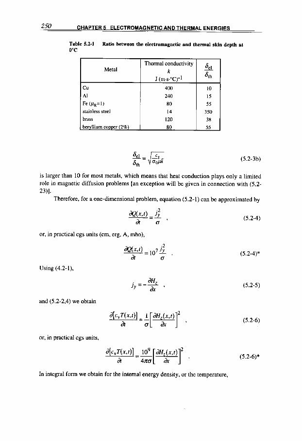
250 CHAPTER 5 ELECTROMAGNETIC AND THERMAL ENERGIES
Table 5.2-1 Ratio between the electromagnetic and thermal skin depth at
Metal
0°C
& Thermal conductivity k ,.
cu A1
Fe (pR= I ) stainless steel
brass
400 240
80
14
I20
10
15
55 350 38
(5.2-3 b)
is larger than 10 for most metals, which means that heat conduction plays only a limited role in magnetic diffusion problems [an exception will be given in connection with (5.2-
Therefore, for a one-dimensional problem, equation (5.2- 1) can be approximated by 2311.
or, in practical cgs units (cm, erg, A, mho),
Using (4.2-I),
(5.2-4)
(5.2-4)*
(5.2-5) dH
Y d x j = - - ,
and (5.2-2,4) we obtain
(5.2-6) dt
or, in practical cgs units,
(5.2-6)* h
In integral form we obtain for the internal energy density, or the temperature,
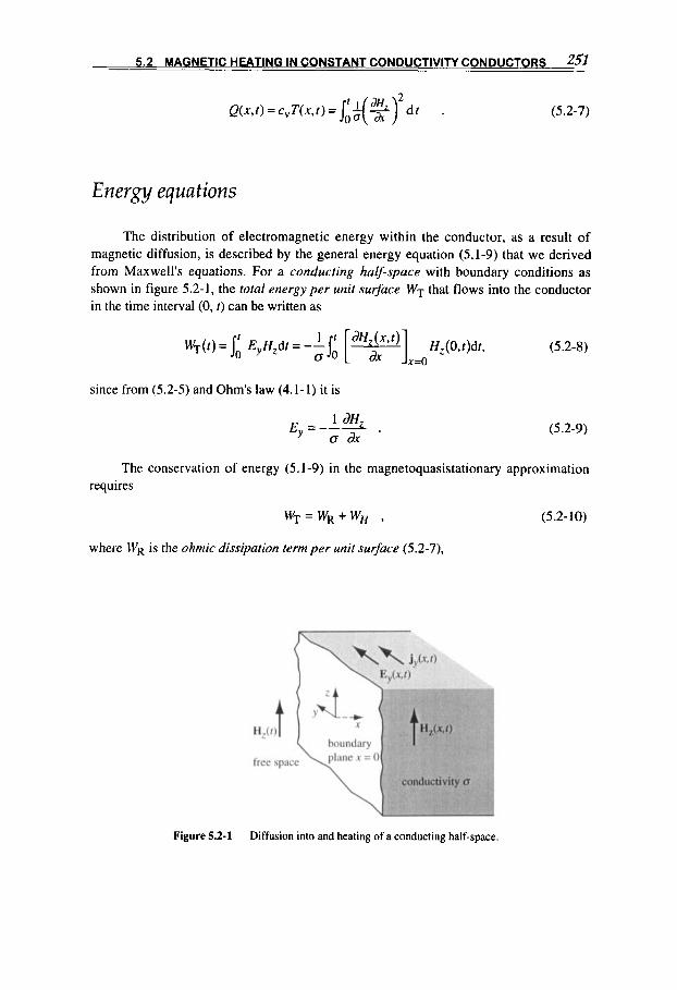
c 2 5 1
2 Q(x,t)=c,T(x,t)=/:$(%) d t . (5.2-7)
Energy equations
The distribution of electromagnetic energy within the conductor, as a result of magnetic diffusion, is described by the general energy equation (5.1-9) that we derived from Maxwell's equations. For a conducting half-space with boundary conditions as shown in figure 5.2-1, the total energyper unit surface WT that flows into the conductor in the time interval (0, t) can be written as
since from (5.2-5) and Ohm's law (4.1-1) it is
1 dH Ey = - a 2 .
(5.2-8)
(5.2-9)
The conservation of energy (5.1-9) in the magnetoquasistationary approximation requires
W T = W R + W H , (5.2-10)
where WR is the ohmic dissipation term per unit surface (5.2-7),
Figure 5.2-1 Diffusion into and heating of a conducting half-space.

252 CHAPTER 5 ELECTROMAGNETIC AND THERMAL ENERGIES
(5.2-1 I )
and WH represents thefield energy per unit surface
WH ( f ) = pj; [ Hz (X, t)f? d~ . (5.2- 1 2)
As usual, the magnetic permeability p = pop^ is considered here a material constant. We define, as in (4.1-9), the constant magnetic diffusivity
1
OOP K O = - ,
or, in practical cgs units,
(5.2-13)
(5.2-13)*
Heating in the conducting half-space
Assuming the conductivity to be constant, we will calculate the temperature and the dissipated energy for two of the most typical examples of magnetic field diffusion in the conducting half-space (figure 5.2-1) dealt with in chapter 4. The solutions of many other cases are summarized in table 5.2-11. As an example of the calculation method involved we will consider in some detail the problem represented by the polynomial boundary field.
Polynomial field
The general solution of the diffusion problem defined by the boundary condition
1
, f o r O I f < - , withn=0,1,2 .... (5.2-14)
has been given in (4.2-23) as
2fi)n(iflerfct} ,

5.2 MAGNETIC HEATING IN CONSTANT CONDUCTIVITY CONDUCTORS 253
where
With the help of (A.2-9,10) we calculate
Using these expressions we find, from (5.2-S), the total energy absorbed per unit surface by the conductor,
(5.2- 16) 1 2 n + l
n + - 2 2
WT(r;n) = - H , (O,t;n)q,,, 7 ,
where use is made of the flux skin depth (4.2-25).
(5.2- 17)
and the surface field (5.2- 14). For the magnetic field energy per unit surface (5.2-12) we readily find
and for the ohmic loss per unit surface (5.2-1 1) we get
here we have introduced the function
2 I,, = 1; (i"erfc6) d 5 , (5.2-20)
already used in (4.2-25). Applying (A.2-S), we transform this integral into the form
f,, = -I 1 - [(i"-2erfcC} - 2~(i"-'erfc5)]{inerfc5jd5 ,
2n 0
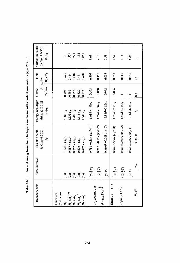
Tab
le 5
2-11
F
lux
and
en
ergy
loss
es fo
r a
hal
f-sp
ace c
ond
uct
or w
ith
con
stan
t con
du
ctiv
ity [q,= l/(a
&)l
Fiel
d
ition
WH
j WT
Bou
ndar
y fi
eld
Sur
face
en.
fac
tor
[def
in (5
.2-3
0)l
fl/PR
Ste
ady
(-
c r
< c=
.)
Hos
in(2
a / T
)r
0.56
3.56
44 (K
"T/~
)
0.56
=0.
4&
(KO
T/2
)
0.56
3.2
824
(xan
( K,, r)
H
o ed
r
1.28
6=2.
57s,
1.57
6=3.
14s,
3.14
6=6.
28s,
S@
Tim
e in
terv
al
1.12
8 .j (Kd)
0.88
7 d (~d)
0.75
2 d
( Kor
)
0.60
2 d (~d)
0.41
7 d
(iC
or)
0.78
63.8
84 (
KJ/
~)
0.71
6 =0
.57d
(K
,T/~
)
0.36
96 3
.20
84
(KJ)
2.00
0 so
1.33
3 so
1.20
0 so
1.11
1 S
$
1.04
8 so
1.08
6=1.
39s,
1.27
6 =I
.94s
,
2.88
6=7.
8%,
3hm
ic
~R
~W
T
diss
i
-
1.70
7
1.58
6
1.55
2 1.
529
1.5 1
2
0.59
3
0.85
0
0.96
2
0.806
1 1 1.5 - 0.
293
0.41
4
0.44
8
0.47
1
0.48
8
0.40
7
0.15
0
0.03
8
0.29
2
0.08
0
0.040
0.5
m
1.57
1
1.27
3
1.13
2 1.
051
1.63
2.18
5.51
2.57
3.14
6.28
1
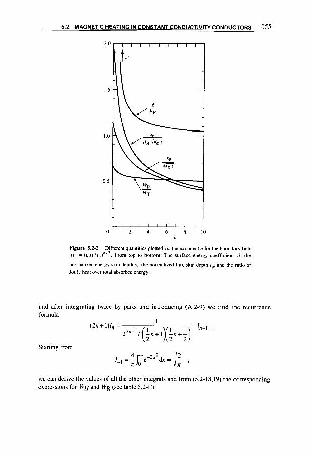
5.2 MAGNETIC HEATING IN CONSTANT CONDUCTIVITY CONDUCTORS 255
2.0
I .5
I .0
0.5
0 2 4 6 8 1 0 n
Figure 5.2-2 Different quantities plotted vs. the exponent n for the boundary field H b = HO(r/ro)"'*. From top to bottom: The surface energy coefficient 8, the
normalized energy skin depth se, the normalized flux skin depth sp. and the ratio of Joule heat over total absorbed energy.
and after integrating twice by parts and introducing (A.2-9) we find the recurrence formula
Starting from
1 (2n + 1)In =
22n-IT(;n+ 1x;.+;) -'n-*
we can derive the values of all the other integrals and from (5.2-18,19) the corresponding expressions for WH and WR (see table 5.2-11).
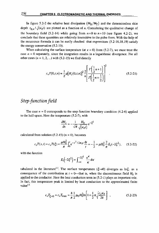
256 CHAPTER 5 ELECTROMAGNETIC AND THERMAL ENERGIES ___
In figure 5.2-2 the relative heat dissipation (WR/WT) and the dimensionless skin depth s4,. lm are plotted as a function of n. Considering the qualitative change of
the boundary field (5.2-14) while going from n=O to n=10 (see figure 4.2-2), we conclude that these quantities are relatively insensitive to the pulse form. With the help of the recurrence formula it can be easily checked that expressions (5.2-16,18,19) satisfy the energy conservation (5.2-10).
When calculating the surface temperature (at x = 0) from (5.2-7), we must treat the case n = 0 separately, since the integration results in a logarithmic divergence. For all other cases (n = 1.2, ...) with (5.2-15) we find directly
S t e p f u n c t ion fie1 d
The case n = 0 corresponds to the step-function boundary condition (4.2-6) applied to the half-space. Here the temperature (5.2-7), with
calculated from solution (5.2-15) ( n = 0), becomes
with the function
tabulated in the literature’.?. The surface temperature ( 6 - 9 ) diverges as ln5, as a consequence of the contribution at t = 0-that is, when the discontinuous field Ho is applied to the conductor. Here the heat conduction term in (5.2-1) plays an important role. In fact, this temperature peak is limited by heat conduction to the approximated finite value’
(5.2-23)
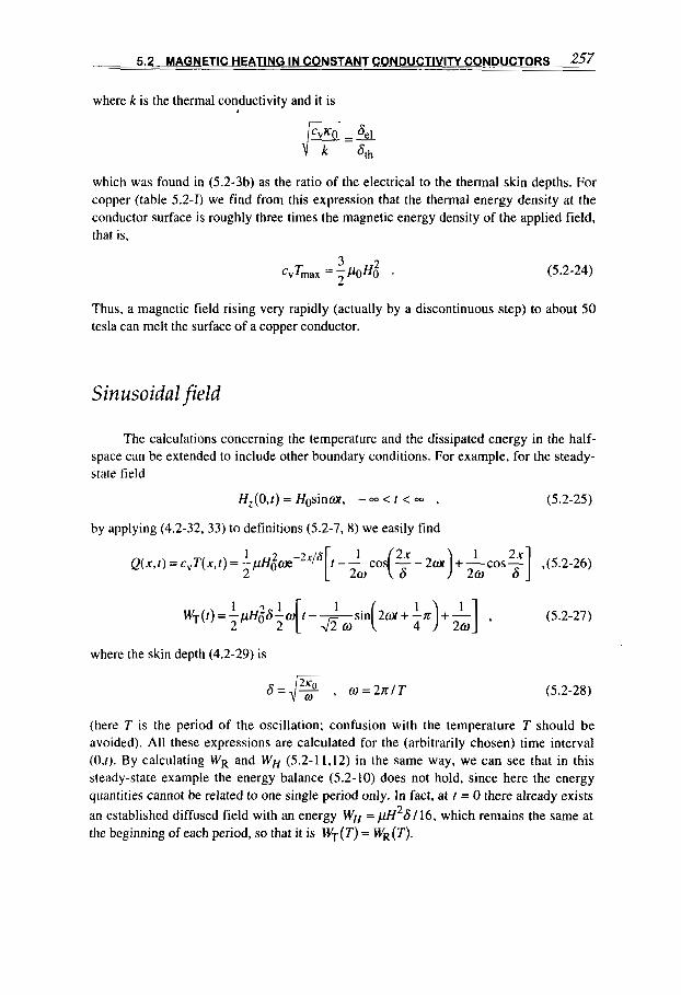
m 5 7
where k is the thermal conductivity and it is
which was found in (5.2-3b) as the ratio of the electrical to the thermal skin depths. For copper (table 5.2-1) we find from this expression that the thermal energy density at the conductor surface is roughly three times the magnetic energy density of the applied field, that is,
(5.2-24) 3 2 CvTmax = p H 0 ’
Thus, a magnetic field rising very rapidly (actually by a discontinuous step) to about 50 tesla can melt the surface of a copper conductor.
Sinusoidal f ield
The calculations concerning the temperature and the dissipated energy in the half- space can be extended to include other boundary conditions. For example, for the steady- state field
H,(O,t) = Hosinwt, - m < t < m , (5.2-25)
by applying (4.2-32, 33) to definitions (5.2-7, 8) we easily find
Q ( x , f ) = cvT( x , t ) =
where the skin depth (4.2-29) is
(5.2-27)
6=J% , w = 2 n / T (5.2-28)
(here T is the period of the oscillation; confusion with the temperature T should be avoided). All these expressions are calculated for the (arbitrarily chosen) time interval (0,f). By calculating WR and WH (5.2-11,12) in the same way, we can see that in this steady-state example the energy balance (5.2-10) does not hold, since here the energy quantities cannot be related to one single period only. In fact, at t = 0 there already exists an established diffused field with an energy WH = pY26/16, which remains the same at the beginning of each period, so that it is WT(T) = W,(T).

- 258 . . . . CHAPTER 5 ~ ELECTROMAGNETIC __ AND THERMAL ENERGIES
These formulae are important for induction heating applications. They will be taken up again at the end of this chapter and presented with other results in table 54-11. The single most relevant parameter is the mean heating power FR that is deposited [over a time interval (O, r ) ] per unit surface of the conductor under consideration, in this case in the whole thickness of the half-space (x+m). Since, as we have seen, WR(O,T) = W,(O,T), from (5.2-27) we find
(5.2-29a)
where we have also introduced the amplitude j o of the surface current density (4.2-33). The mean heating power deposited within a depth x is
and with (5.2-26) we obtain
(5.2-29b)
This shows that nearly P R ( ~ ) = 0.865P~(-). - all the heating occurs in a skin depth 6: in fact,
In surface-heating applications (surface hardening, etc.) an appropriately small 6 will be chosen; on the contrary, if bulk heating is the goal, a large 6 is convenient, since the material beyond 6 will be heated only by heat conduction. Through (5.2-28), the most convenient skin depth 6 can be determined by the choice of the frequency v = d 2 a of the induction heating apparatus. Furthermore, (5.2-29a) shows that large heating densities can be obtained with small 6.
The heating of thick and thin slabs, rods, and hollow cylindrical conductors immersed in a harmonic, steady sinusoidal field will be calculated in (5.2-44) and (5.3-4, 6,9 , 10, 39), and the heating in a transient sinusoidal field will be calculated in (5.3-35,36).
Energy skin depth
In all these examples, the surface temperature can be expressed in the general form
where the surface energy factor 19 depends on the pulse form (i.e., on both its shape and duration) but remains of the order of unity. Similarly, the total dissipated energy per unit

- 5.2 MAGNETIC HEATING IN CONSTANT CONDUCTIVITY CONDUCTORS 259
surface can be written, as in (5.2-16),
(5.2-31)
where s,( t ) is defined as the energy skin depth. The corresponding definition in the
practical cgs system is obviously obtained by the substitution poH2 I 2 + H 2 1 8 ~ . The quantities t?/& and se I&, as well as the flux skin depth s4 and the ratios
WR I W, and W, I WT, are given in table 5.2-11 for different boundary fields. The results of the transient sinusoidal case have been computed numerically using (4.2-1.28). It is interesting to note that all the monotonically increasing magnetic field pulses (the first six cases of table 5.2-11, with the exception of the step function; see also figure 4.2-3) give rise to relatively similar results. We can conclude that the quantities represented in this table are rather insensitive to the pulse form. A second remark concerns the comparison between the transient and the steady sinusoidal cases. As one would expect, there is a noticeable difference at the first quarter period, particularly for the surface temperature, which for the steady wave train is nearly 1.6 times larger than for the transient train. In both cases a large part of the energy dissipated during one period is already lost at t = T l 4 . For a copper conductor we find from table 5.2-11, for instance, that at the end of the transient quarter period the surface temperature has increased by
T = 0.2ti2( O C , tesla) ,
meaning that the surface (initially at O O C ) reaches the melting temperature (table 8.3-11) when the applied field amplitude is 75 tesla.
Using the energy skin depth concept defined by (5.2-31), it is possible to estimate in a crude but practical manner the energy losses related to plane conductors or conductors whose main radius of curvature is large compared to s,. For example, in a long single- turn solenoid, whose inner radius a is large compared to s,, the ratio qw of the total energy loss to the energy stored inductively in the bore is approximately given by
The Qosc, factor of this solenoid can then be written for a periodic field with s, = n6 (table 52-11) in the form
(&sc, = 27rIqw = a16 . (5.2-32)
[The Qosc. factor of a periodic system is here the ratio of 27r times the average energy stored in the system divided by the energy dissipated per cycle.] This formalism, as well as (5.2-31). is valid for a "thick" conductor-that is, a conductor whose thickness d is much larger than se. On the other hand, we will see in section 5.3 that for a "thin"
conductor ( d a , ) the energy losses are larger by a factor of about ( s , / d ) than in the
corresponding thick case.
2

260 CHAPTER 5 ELECTROMAGNETIC AND THERMAL ENERGIES
Heating of thick sheets and cylindrical conductors
The magnetic heating of bounded thick conductors, such as plane sheets and rods with circular cross section, follows from (5.2-7) with the help of the magnetic diffusion solutions HZ(x,t) found in chapter 4 with regard to various boundary fields. It is obvious that as long as the thickness of the sheet or the radius of curvature of the curved surface is much larger than the magnetic flux skin depth, the solutions corresponding to the half- space found previously are good approximations.
We start by considering a step-function boundary field, which, through Duhamel's theorem (4.1-27). is the basis of more general solutions and also gives the practical result of the complementary problem-the heating caused by the decay of a magnetic field initially trapped within the conductor. For cylindrical conductors we shall also consider a harmonic sinusoidal field because this is approximately obtained when discharging a capacitor bank current source into a conductor system.
Slab
From (4.2-1) and the general solution function field we obtain for the current density
j y ( x , t ) = - - = - H dH c a9n 5, ox,. ' n=l dx
given in table 4.2-1 for an applied step-
t m . --
(5.2-33)
where the parameters c, qn, and 2, are defined by the boundary conditions. Because of the orthogonality of the series, the power dissipated per unit volume in the conductor is simply
(5.2-34)
The mean energy per unit volume dissipated at the end of the diffusion process in the whole slab and calculated for the geometry given in figure 4.2-6 and case no. 1 in table 4.2-1 is easily found to be

5.2 MAGNETIC HEATING IN CONSTANT CONDUCTIVITY CONDUCTORS 261
in fact*.4, the value of the series is l r 2 / 8 . This is an obvious result, particularly if we think about the complementary problem-the decay of an initially trapped internal field Ho [see also in connection with (5.3-15)]. The extension of these considerations to a rectangular bar [see (4.2-50) and general solution in table 4.2-11 is straightforward. In particular, for the mean energy density we obtain
- 32pH; - 1 1 pH; Q = -
lr4 n=1.3 .... m=1.3 ,... (5.2-36)
(n,m. odd)
Rod
The solution of the magnetic diffusion equation (4.3-5) for an applied step-function field parallel to the axis of a cylindrical conductor (figure 5.2-3a) is given in table 4.2-1 and (4.3-14); the related eddy current density (4.3-1) and dissipated power density j$ /rs are formally as in (5.2-33,34) but with the substitution x + r . With the parameters for this case defined in table 4.2-1, the mean energy density dissipated in the conductor over the complete diffusion process is easily calculated to be
a)
_rL,
Figure 5.2-3 outer axial magnetic field.
Heating of a bar (a) or a hollow cylinder (b) by the diffusion of an

c 262
(5.2-37)
where use is made of (A.2-21). For a transverse magnetic step-function field (figure 4.3-4). the solution in terms of
the field components H,(r,@;t), H$(r,@;t) is again found in table 4.2-1 and can be
calculated from (4.3-10,41,42). With the related current density given in (4.3-45) we calculate for the dissipated mean energy density
(5.2-38)
That the dissipated energy be greater in this case could have been expected. In fact, consider the complementary case, the outward diffusion of the transverse flux trapped by the rod when the outer uniform field Ho suddenly disappears: The dissipated energy stems not only from the decay of the field trapped within the conductor but also from the dipole-type outer field bound to it.
It is interesting to extend this expression to the transient exponential boundary field (4.3- 19).
and its solution (4.3-20). Proceeding as above, for the mean dissipated energy we obtain in this case
(5.2-39)
which for T C C zn [with the diffusion time constant T~ given in (4.3-16)] tends to the step- function solution (5.2-37). When rn zn-that is, TB rI-we obtain
(5.2-40)
which can be approximated (with a slight overestimate in the overall result) by substituting zn + z1 [see (4.3-16b)l; thus
- T I P Qz--H . T 2
(5.2-4 1 )
Similar results can be obtained for the infinitely long rectangular slab and the transverse rod.
The steady sinusoidal boundary field

5.2 MAGNETIC HEATING IN CONSTANT CONDUCTIVITY CONDUCTORS 263
HZ=HOsinwt , for -m<t<m , (5.2-42)
results in the solution, case 3, given in table 4.2-11, and the relevant energy components can be calculated with it. However, the limiting case where the radius a is much smaller than the characteristic skin depth s is approximated with sufficient precision by the heating in the half-space already considered in this section.
Hollow cylindrical conductor
Conceptually, magnetic diffusion heating here is similar to that for the circular bar, but the dissipated energy is provided by the energy not only of the field in the conductor but also of the energy trapped in the hollow interior (plus the outer dipole-type field in the "transverse" field case). Instead of proceeding to the calculation of the total dissipated energy with the corresponding diffusion solutions (4.3-3 1,33) for the "parallel" field case (figure 5.2-3b) and (4.3-50) for the "transverse" case, we refer to the next section, where these problems are solved in the approximation of thin-walled cylindrical conductors, but with temperature-dependent electrical conductivity.
Let us now consider the complementary problem to the rod represented by a thick single-turn solenoid (figure 5.2-4b) to whose cylindrical inner surface of radius a the boundary condition (5.2-42) applies. From the solution, case 4 given in table 4.241, and with the approximation found in (A.2-33,34), ker z = -ln(z/2), keiz = -0.25xvalid in the limitz + 0, we find for a << 6
(5.2-43)
Figure 5.2-4 (a) Infinite conductor with a cylindrical hole of radius a; in practice, this geometry is approximated by a thick single-turn solenoid (b), or in irregularities with the form of (c).

264 CHAPTER 5 ELECTROMAGNETIC AND THERMAL ENERGIES
hence, the temperature can be written as
(5.2-44) 1 2 1
c,T(a,t) - Ho [ (aa/s)ln(Jza/s)]
Since lirn,,o(zlnz)=O, the temperature on the inner surface of a solenoid, where a/6al , can be appreciably higher than in a conductor whose radius of curvature is larger than the skin depth. This effect is to be expected from the comments made following (4.3- 25). In irregularities of the type shown in figure 5.2-4c, the bottom can thus attain very high temperatures (above melting point) and the result will be a gradual cut through the conductor (saw effect).
5.3 HEATING IN THIN CONDUCTORS
Plane and cylindrical geometries
Thin conductors exposed to variable magnetic fields, as introduced and defined in section 4.4 following (4.4- 1 1 and 24), represent important arrangements encountered in praxis. The calculation of their heating effects allow us to obtain simple, but significant results, which we will present now for three examples based on different geometries.
Thin slab
Let us consider, as in section 4.2, figure 4.2-6, a slab of thickness 2d, which we suppose here to be thin-that is, d much smaller than the corresponding skin depth SQ. The surface temperature then differs from that of a half-space conductor, and it strongly depends on the boundary conditions.
(a) The slab is immersed in a magnetic field, the boundary conditions being the same on We study three different problems of practical importance (figure 5.3- 1):
both planes. [We shall see that for s# D d the temperature is proportional to ( d / ~ $ ) ~ . ]
(b) On one side the slab limits a given magnetic field; that is, the surface field on the other side is zero. [Here, we shall find that for s# N d the temperature is proportional
to ( ~ @ / d ) ~ . ]
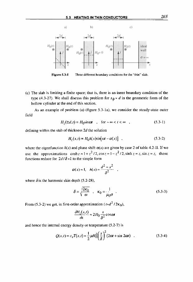
5.3 HEATING IN THIN CONDUCTORS 265
Figure 5.3-1 Three different boundary conditions for the “thin” slab.
(c) The slab is limiting a finite space; that is, there is an inner boundary condition of the type (4.3-27). We shall discuss this problem for s$ D d in the geometric form of the hollow cylinder at the end of this section.
As an example of problem (a) (figure 5.3-la), we consider the steady-state outer field
H,(+d,t) = Hosinm , for - 0 0 < f < 00 , (5.3-1)
defining within the slab of thickness 2d the solution
H,(x,r) = H&(x)sin[m-a(x)] , (5.3-2)
where the eigenfunction h(x) and phase shift a(x) are given by case 2 of table 4.2-11. If we 2 2 use the approximations coshz = 1 + z /2, cosz = 1 - z 12, sinh z = z, sin z = z, these
functions reduce for 2d /6 <( 1 to the simple form
2 2 a ( x ) = 1, h(x) = ~
d - X
62 ’
where 6is the harmonic skin depth (5.2-28),
2 From (5.3-2) we get, in first-order approximation ( rvd / ~ K o ) .
and hence the internal energy density or temperature (5.2-7) is
Q ( x , f ) = c ,T(x , f ) =
(5.3-3)
(5.3-4)
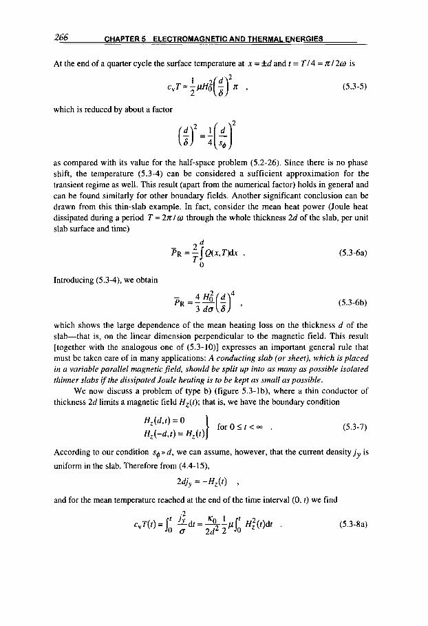
266 CHAPTER 5 ELECTROMAGNETIC AND THERMAL ENERGIES
At the end of a quarter cycle the surface temperature at x = +d and t = T 14 = X I 2 0 is
(5.3-5)
which is reduced by about a factor
as compared with its value for the half-space problem (5.2-26). Since there is no phase shift, the temperature (5.3-4) can be considered a sufficient approximation for the transient regime as well. This result (apart from the numerical factor) holds in general and can be found similarly for other boundary fields. Another significant conclusion can be drawn from this thin-slab example. In fact, consider the mean heat power (Joule heat dissipated during a period T = 2 n / w through the whole thickness 2d of the slab, per unit slab surface and time)
(5.3-6a) - 2 d PR = - J Q ( ~ , T u x .
T o Introducing (5.3-4). we obtain
(5.3-6b)
which shows the large dependence of the mean heating loss on the thickness d of the slab-that is, on the linear dimension perpendicular to the magnetic field. This result [together with the analogous one of (5.3-lo)] expresses an important general rule that must be taken care of in many applications: A conducting slab (or sheet), which is placed in a variable parallel magnetic field, should be split up into as many as possible isolated thinner slabs if the dissipated Joule heating is to be kept as small as possible.
We now discuss a problem of type b) (figure 5.3-lb), where a thin conductor of thickness 2d limits a magnetic field H z ( t ) ; that is, we have the boundary condition
(5.3-7)
According to our condition sq D d , we can assume, however, that the current density j , is
uniform in the slab. Therefore from (4.4-15),
2djy = - H , ( t ) ,
and for the mean temperature reached at the end of the time interval (0, t ) we find
(5.3-8a)
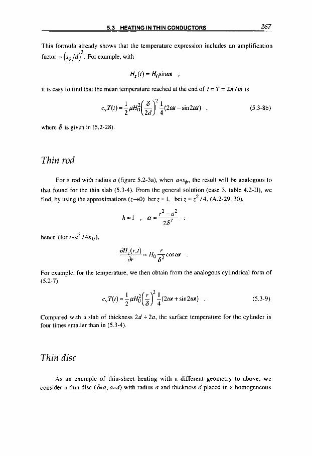
5.3 HEATING IN THIN CONDUCTORS 267
This formula already shows that the temperature expression includes an amplification
factor - ( s g / d ) . For example, with 2
H,(t) = Hosinw5 ,
it is easy to find that the mean temperature reached at the end of t = T = 2 K / U is
(5.3-8b)
where 6 is given in (5.2-28).
Thin rod
For a rod with radius a (figure 5.2-3a), when a<ag, the result will be analogous to
that found for the thin slab (5.3-4). From the general solution (case 3, table 4.2-II), we find, by using the approximations (z+O) berz = 1, bei
r2 - a 2 h = 1 , a=-
2 s 2
2 hence (for t m 1 4 ~ 0 ) .
For example, for the temperature, we then obtain from (5.2-7)
z = z 2 14, (A.2-29, 30),
the analogous cylindrical form of
(5.3-9)
Compared with a slab of thickness 2d + 2a, the surface temperature for the cylinder is four times smaller than in (5.3-4).
Thin disc
As an example of thin-sheet heating with a different geometry to above, we consider a thin disc (&MI, a d ) with radius a and thickness d placed in a homogeneous
268 CHAPTER 5 ELECTROMAGNETIC AND THERMAL ENERGIES
field H ( t ) = HO sinwt that is parallel to its axis (see figure 4.4-5). The induced surface
eddy current from (4.4-39) is
drw i4 = -- Ho coswt
2KO
and the related Joule heating per unit time and disc surface is calculated to be
(5.3- 1 Oa)
The mean dissipated heating power per unit disc surface over a period T = 27r / w is
(5.3-lob)
[see also (3.1-38)]. This equation shows the large dependence of the mean heating power on the sheet's surface dimension (radius a)- that is, the linear dimension perpendicular to the magnetic field. This result is again similar to that expressed by (5.3-6b) and here states: A conducting sheet, which is placed in a variable, perpendicular magnetic field, should be split up into as many as possible isolated smaller and thinner sheets if the dissipated Joule heuting is to be kept as small as possible.
Electric conductivity law
The argument to be introduced in the following links, in a way, the first part of the chapter to the second, since we shall now allow the conductivity to be heat-dependent.
Tempera ture-dependen t conductivity
For the conductivity we choose the simple form
0=- 0 0
l+pQ ' (5.3-1 I )
where 00 is the conductivity at O'C, is the heat factor [dimension m3/joule], and Q is the increase of internal energy or heat content relative to O'C, which in the solid phase is related to the temperature T by (5.2-21,
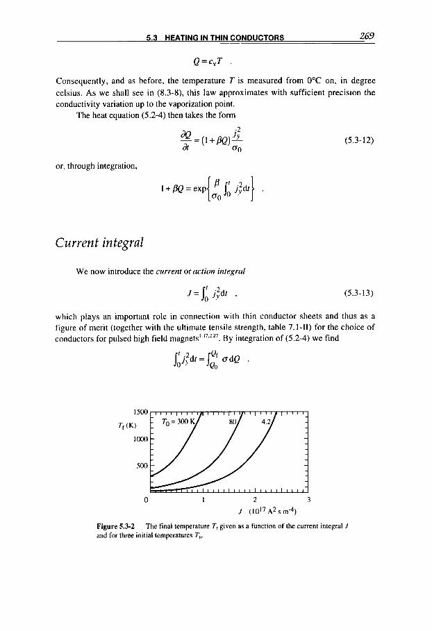
5.3 HEATING IN THIN CONDUCTORS 269
Q = c v T .
Consequently, and as before, the temperature T is measured from 0°C on, in degree Celsius. As we shall see in (8.3-8). this law approximates with sufficient precision the conductivity variation up to the vaporization point.
The heat equation (5.2-4) then takes the form
or, through integration,
I+PQ=exp{$Ji j;dt} .
Cu rren t integral
We now introduce the current or action integral
J = I : j;dt ,
(5.3- 12)
(5.3-13)
which plays an important role in connection with thin conductor sheets and thus as a figure of merit (together with the ultimate tensile strength, table 7.1-11) for the choice of conductors for pulsed high field magnets' '7.227. By integration of (5.2-4) we find
Jij;dt = 5"' Qo o d e .
0 1 2 3
J (1017 A* s m-4)
Figure 5.3-2 and for three initial temperatures T,,.
The final temperature Tt given as a function of the current integral J
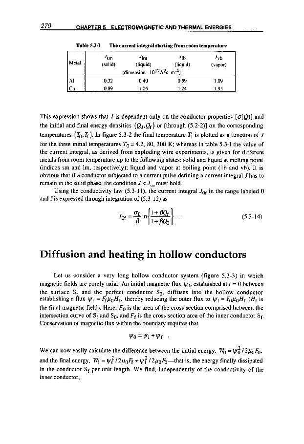
2 70 CHAPTER 5 ELECTROMAGNETIC AND THERMAL ENERGKS.
Table 5.3-1 The current integral starting from raom temperature
(solid) (liquid) (liquid) (vapor) Metal
dimension 1017A2s m-4
0.32 0.40 0.59
cu 0.89 1.05 1.24 1.95
This expression shows that J is dependent only on the conductor properties [b(Q)] and the initial and final energy densities (&,Qf) or [through (5.2-2)] on the corresponding
temperatures (T0,Tf). In figure 5.3-2 the final temperature Tf is plotted as a function of J
for the three initial temperatures To = 4.2, 80, 300 K; whereas in table 5.3-1 the value of the current integral, as derived from exploding wire experiments, is given for different metals from room temperature up to the following states: solid and liquid at melting point (indices sm and lm, respectively); liquid and vapor at boiling point ( 1 b and vb). It is obvious that if a conductor subjected to a current pulse defining a current integral J has to remain in the solid phase, the condition J < J, , must hold.
Using the conductivity law (5.3-1 l), the current integral Jof in the range labeled 0 and f is expressed through integration of (5.3-12) as
(5.3- 14)
Diffusion and heating in hollow conductors
Let us consider a very long hollow conductor system (figure 5.3-3) in which magnetic fields are purely axial. An initial magnetic flux yo, established at t = 0 between the surface Sf and the perfect conductor S O , diffuses into the hollow conductor establishing a flux yf = FfpOHf, thereby reducing the outer flux to y1 = FOpoHf (Hf is the final magnetic field). Here, FO is the area of the cross section comprised between the intersection curve of Sf and So, and Ff is the cross section area of the inner conductor Sp Conservation of magnetic flux within the boundary requires that
vlo=V/l+wf . We can now easily calculate the difference between the initial energy, WO = YO 2 12pOFo.
2 and the final energy, Wf = yf2 12~04 + yl 12poFo-that is, the energy finally dissipated in the conductor Sf per unit length. We find, independently of the conductivity of the inner conductor,
5.3 HEATING IN THIN CONDUCTORS 2 71
Figure 5.3-3 closed surface So.
Thin hollow conductor S, enclosed by an infinitely conducting
(5.3- 15)
This equation shows that for FO )) l$ (i.e., for an outer field that remains nearly constant during diffusion) the dissipated energy equals the final magnetic energy in the hollow conductor.
The same result applies when the flux yo, initially trapped within the hollow conductor, diffuses outwards. If we retain the previous notations, we have simply to interchange Ff with Fo in the last equation. For the special case FO lFf + -, we find the obvious result that all the energy related to the initial trapped flux is finally converted into ohmic heat.
Now we shall consider in some detail the diffusion of an axial magnetic field through a hollow, very long cylindrical conductor (figure 5.3-4), by including from the beginning the electric conductivity law given in (5.3-1 1). The magnetic field is purely axial and has the same magnitude everywhere in the bore. For simplicity we assume the current density j, to be constant through the conducting sheet, a condition that holds when the conductor thickness d is small compared with the flux skin depth sk With this assumption, which is approximately valid for many of the interesting experimental problems, it is possible to reduce the cylindrical diffusion equation coupled to the inner boundary condition of type (4.3-26) to an ordinary differential equation. The solution is, therefore, appreciably simplified.
According to these assumptions, we can write with (4.4-15)
i = j & = H i - H , , (5.3-16)
where i is the linear current density and Hi, He are the inner and outer magnetic fields respectively. On the other hand, we have, for the induced voltage,
(5.3-17)
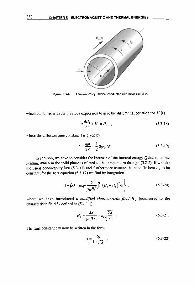
2 72 CHAPTER 5 ELECTROMAGNETIC AND THERMAL ENERGIES
Figure 5.3-4 Thin-walled cylindrical conductor with mean radius r,, .
which combines with the previous expression to give the differential equation for Hi(t)
(5.3- 18) dHi
r---+Hi=H, , dt
where the diffusion time constant z is given by
rod 1 z = - = -poroda . 2K 2
(5.3- 19)
In addition, we have to consider the increase of the internal energy Q due to ohmic heating, which in the solid phase is related to the temperature through (5.2-2). If we take the usual conductivity law (5.3-1 1 ) and furthermore assume constant, for the heat equation (5.3-12) we find by integration
the specific heat cv to be
(5.3-20)
where we have introduced a modified characteristic field Hc [connected to the characteristic field hc defined in (5.4-1 l)]
H, =- POP ‘0
The time constant can now be written in the form
(5.3-21)
7=- 70
l+PQ ’ (5.3-22)

5.3 HEATING IN THIN CONDUCTORS 2 73
where
(5.3-23)
The numerical solution of the system of (5.3-18,20,22) for any applied transient external field HJr) is relatively simple, and later on we shall discuss the example corresponding to the sinusoidal boundary field He = Hgsinon. In the limiting case where H, D He, the problem reduces simply to the differential equation (5.3-18), with z = zO. The solution of the most importance cases can then be found by straightforward integration.
Example: Step-function field diflusion If the external field He (parallel to the axis, figure 5.3-4) is described by the usual step function
He = Ho(const.), for 0 s r < -,
He =0, for t < 0 , (5.3-24)
it is even possible to find an analytical solution for the temperature dominated problem. In fact, in this case, multiplying (5.3-18) by (Hi - Ho) and with the help of (5.3-20,22). we get the equation [ i n (Hi - Ho) 2 ]
which. through partial integration, can easily be transformed into
( H , - H o ) 2 -HOZ=-HZ
Eliminating the integral term through (5.3-25) and integrating, we obtain
hence the solution
(5.3-25)
(5.3-26)
(5.3-27)
which is plotted in figure 5.3-5. When H, <( Hc, this formula reduces to
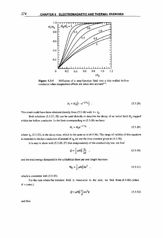
2 74 CHAPTER 5 ELECTROMAGNETIC AND THERMAL ENERGIES
I .o HilHo
0.8
0.6
0.4
0.2
0 0.2 0.4 0.6 0.8 1.0 1.2
Ur0
Figure 5.3-5 conductor when temperature effects are taken into account4 I".
Diffusion of a step-function field into a thin-walled hollow
Hi = Ho(I -e-'/ro) . (5.3-28)
This result could have been obtained directly from (5.3-18) with 7 = ro.
within the hollow conductor. In the limit corresponding to (5.3-28) we have
Both solutions (5.3-27. 28) can be used directly to describe the decay of an initial field H, trapped
Hi = Hoe-"rO , (5.3-29)
where ro. (5.3-23). is the decay time, which is the same as in (4.3-36). The range of validity of this equation
is extended to thicker conductors if instead of 7, we use the time constant given in (4.3-38).
It is easy to show with (5.3-20, 27) that independentIy of the conductivity law. we find
and the total energy dissipated in the cylindrical sheet per unit length becomes
(5.3-30)
(5.3-3 I )
which is consistent with (5.3-15). For the case where the transient field is transverse to the axis, we find from (4.3-60) (when
d = const.)
Q = pHi :sin2$ (5.3-32)
and thus

5.3 HEATING IN THIN CONDUCTORS 275
confirming that, as for the circular rod (5.2-37.38). the totally dissipated energy in the "transverse" case
amounts to twice that of the "parallel" case.
Example: Transient sinusoidal field difusion
If the transient axial boundary field is sinusoidal,
He = Hosinwr, for 0 5 I < - . H , =0, for I < 0 ,
(5.3-34)
the system of equations (5.3-18.20.22) has to be solved numerically. Like in the previous case, the results
depend on the two parameters
where T = 2 x 1 ~ is the period and H, the critical field defined in (5.3-21). In figure 5.3-6 we have plotted the inner field corresponding to the particular case r0 = T14. The limiting case Ho"H, can be solved
analytically from (5.3-18) without difficulty, since ?= ?o (figure 5.3-6b).
0 0.5 1.0 , 1.5 2.0 - TI4
I .o HilHa
0.8
0.6
0.4
0.2
0
HdHc = 0
L 1
I
TI4 TI4
Figure 5.3-6 Diffusion of a transient sinusoidal field into a thin-walled hollow conductor: (a) when temperature effects are taken into account, for the case r0 = 4T; (b) in the limit HO 1 Hc = 0.

276 CHAPTER 5 ELECTROMAGNETIC AND THERMAL ENERGIES
The heat content in the conductor at maximum internal field H, is obtained from (5.3-20).
m = / k , T = e x p -Ifm (Hi -He) 1' roHz 6 3 - 3 9
and is plotted in figure 5.3-7 versus the reduced time constant. As can be seen. the hollow conductor system
can be used to generate very high temperatures in a metal. However, i t is not possible to exceed appreciably
the boiling point, since the thin conductor then simply explodes. Therefore, this experiment is intimately connected with the domain of exploding conductors ".
For the energy factor 19, (5.2-30). we get
(5.3-36)
One of the practical meanings of the curves in figure 5.3-7 is the following. If with a given energy source
(capacitor bank) we want to fill a given thin-walled cylindrical conductor (defining fo) with the largest
possible magnetic field H,, we must choose the electric circuit ( i t . . in practice the inductance of the coil) in such a way that the period T of the system is far from the values of fo 10.25 T corresponding to the
maximum of /@ (i.e.. the maximum of the dissipated energy).
Example: Steady sinusoidal heating The diffusion of a steady, axial sinusoidal magnetic field through a thin-walled hollow cylinder
(figure 5.3-4) was discussed in section 4.4 following (4.4-91) by applying complex formalism, in which the
boundary field is written in the form
he( ro . l ) = HoeiW ,
As a result of the diffusion process the linear current density, constant through the conductor because of the
thin-sheet approximation, was found in (4.4-94) to be
i = S e i W , w i t h S = H i o - H o = - = ( m + i ) , 1 + 0 2 2 2
where
(5.3-37)
(5.3-38)
the harmonic skin depth 6 is given in (5.2-28). and d (c &because of the thin-sheet approximation. (Here we
indicate the linear current density with s instead of i to avoid confusion with the imaginary unit.) When u is
a constant, the mean ohmic power deposited (during one period T ) in the cylindrical conductor (per unit
surface) is calculated from (5.2-4) with theorems (5.1-20,24) to be

2 77 - ~
5.4 NONLINEAR MAGNETIC DIFFUSION 2 77
PQ
10
I
0.1 0. I I ‘0 10 -
TI4
Figure 5.3-7 transient sinusoidal external field.
Dimensionless heat content i n a thin-walled hollow conductor for a
0.1 I I I I I I I l l I I I I l l 1
0. I I ‘0 10 - TI4
Figure 5.3-7 transient sinusoidal external field.
Dimensionless heat content i n a thin-walled hollow conductor for a
The total heat deposited per unit volume of the conductor during a time of n periods, t = nT, is thus
(5.3-40) - I
d Q ( / ) = n T P R - .
The total dissipated energy in the cylindrical shell (per uni t length) is, by using (5.3-40) and w = 2mT
(5.3-4 1)
where the value in parentheses is the nominal maximum magnetic energy within the cylinder. The
dissipated energy is highest when w r = I and decreases for higher or lower values of it. When the
conductivity is temperature-dependent, as in (5.3-1 I ) . the heat deposited is given instead by (5.3-20). The
integral in this form can again be approximated by expression (5.3-39). but the whole calculation can now
be done only approximately by iteration steps, since ‘also becomes temperature dependent, as in (5.3-22).
5.4 NONLINEAR MAGNETIC DIFFUSION
One possible limitation of the diffision theory considered so far (with the exception of the last part of the previous section) is due to the assumption that the electric conduc-
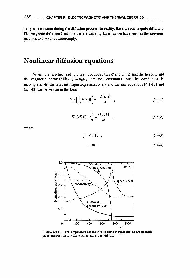
278 CHAPTER 5 ELECTROMAGNETIC AND THERMAL ENERGIES
tivity u is constant during the diffision process. In reality, the situation is quite different. The magnetic diffision heats the current-carrying layer, as we have seen in the previous sections, and u varies accordingly.
Nonlinear diffusion equations
When the electric and thermal conductivities Q and k , the specific heat cv, and the magnetic permeability p = p o p ~ are not constants, but the conductor is incompressible, the relevant magnetoquasistationary and thermal equations (4.1- 1 1) and (5.1-43) can be written in the form
where
j = V x H ,
j = a E .
1 .o
- 5 0.8 8 a ," 0.6 8
$ 0.4 2
.- -
0.2
I 1 I I I I I I l l I I
0 200 400 600 800 lo00 O C
Figure 5.4-1 parameters of iron (the Curie temperature is at 746 "C).
The temperature dependence of some thermal and electromagnetic
(5.4-1)
(5.4-2)
(5.4-3)
(5.4-4)
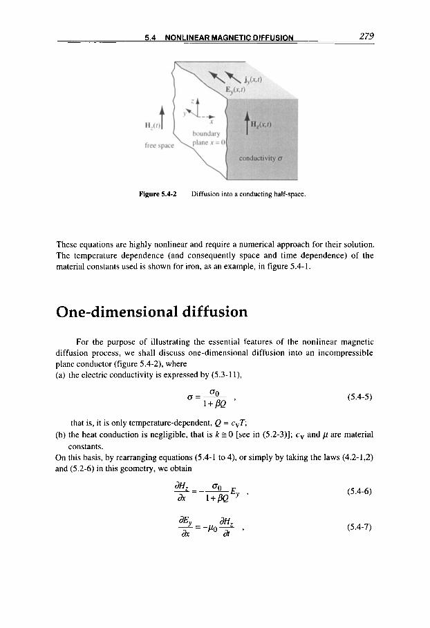
5.4 NONLINEAR MAGNETIC DIFFUSION 2 79
Figure 5.4-2 Diffusion into a conducting half-space.
These equations are highly nonlinear and require a numerical approach for their solution. The temperature dependence (and consequently space and time dependence) of the material constants used is shown for iron, as an example, in figure 5.4-1.
One-dimensional diffusion
For the purpose of illustrating the essential features of the nonlinear magnetic diffusion process, we shall discuss one-dimensional diffusion into an incompressible plane conductor (figure 5.4-2), where (a) the electric conductivity is expressed by (5.3-1 I ) ,
(5.4-5)
that is, it is only temperature-dependent, Q = cvT;
constants. (b) the heat conduction is negligible, that is k z 0 [see in (5.2-3)]; cv and p are material
On this basis, by rearranging equations (5.4-1 to 4), or simply by taking the laws (4.2-1,2) and (5.2-6) in this geometry, we obtain
(5.4-6)
(5.4-7)
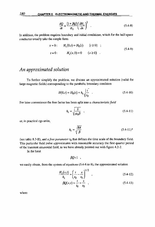
280 CHAPTER 5 ELECTROMAGNETIC AND THERMAL ENERGIES
(5.4-8)
In addition, the problem requires boundary and initial conditions, which for the half-space conductor usually take the simple form
x = o : H , ( O , t ) = H o ( r ) ( t 2 0 ) ;
r = O : H , ( x , O ) = O ( x 2 0 ) . (5.4-9)
An approximated solution
To further simplify the problem, we discuss an approximated solution (valid for large magnetic fields) corresponding to the parabolic boundary condition
7
H(0 , r ) = Ho(r) = h, - d:, For later convenience the free factor has been split into a characteristicfield
hc=E ,
or, in practical cgs units,
(5.4- 1 0)
(5.4-1 1 )
(5.4-1 1)*
(see table 8.3-11), and a free parameter to that defines the time scale of the boundary field. This particular field pulse approximates with reasonable accuracy the first quarter period of the transient sinusoidal field, as we have already pointed out with figure 4.2-2.
In the limit
PQ,l ,
we easily obtain, from the system of equations (5.4-6 to 8), the approximated solution
(5.4-12)
(5.4-1 3)
where
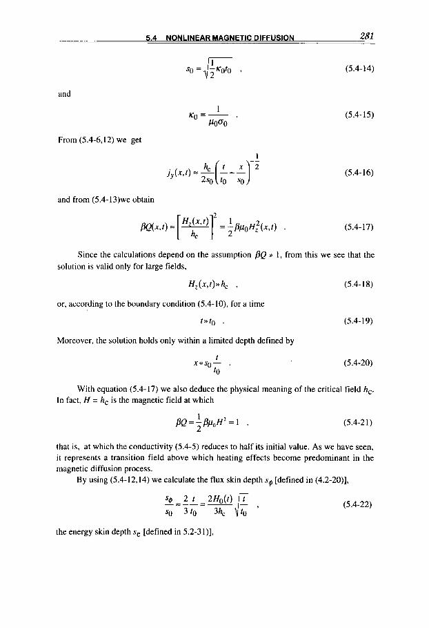
5.4 NONLINEAR MAGNETIC DIFFUSION 281
and
1
PO% KO = -
From (5.4-6.12) we get
and from (5.4-13)we obtain
(5.4- 15)
(5.4-16)
(5.4-17)
Since the calculations depend on the assumption PQ M 1 , from this we see that the solution is valid only for large fields,
H,(XJ)*h, 7 (5.4- 1 8)
or, according to the boundary condition (5.4-lo), for a time
t ) ) t O .
Moreover, the solution holds only within a limited depth defined by
t x<<s()- .
t0
(5.4- 19)
(5.4-20)
With equation (5.4-17) we also deduce the physical meaning of the critical field hc. In fact, H = hc is the magnetic field at which
(5.4-2 1 ) I 2
PQ = -PpoH' = 1 ,
that is, at which the conductivity (5.4-5) reduces to half its initial value. As we have seen, it represents a transition field above which heating effects become predominant in the magnetic diffusion process.
By using (5.4-12,14) we calculate the flux skin depth s$ [defined in (4.2-20)],
(5.4-22)
the energy skin depth Se [defined in 52-31)],
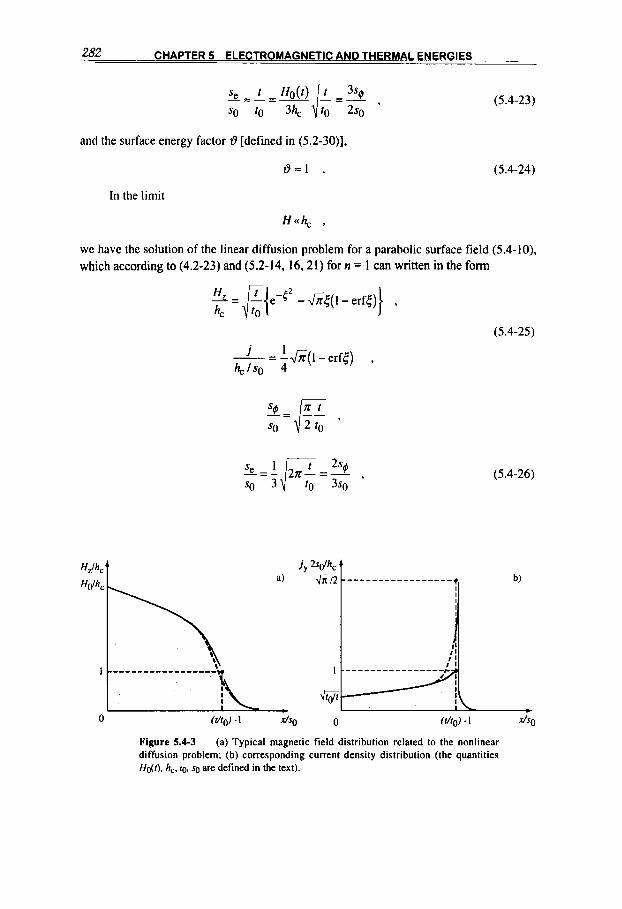
282 CHAPTER 5 ELECTROMAGNETIC AND THERMAL ENERGIES
and the surface energy factor 19 [defined in (5.2-30)],
8=1 . (5.4-24)
In the limit
H . 4 ,
we have the solution of the linear diffusion problem for a parabolic surface field (5.4-10). which according to (4.2-23) and (5.2-14, 16,21) for n = 1 can written in the form
(5.4-25)
a)
(5.4-26)
0 (tho) - 1 0 (r/rg) ~ 1
Figure 5.4-3 (a) Typical magnetic field distribution related to the nonlinear diffusion problem; (b) corresponding current density distribution (the quantities HOW. h,. 10, SO are defined in the text).

5.4 NONLINEAR MAGNETIC DIFFUSION 283
1 i Y = - - K ,
2
where
(5.4-27)
The magnetic field distribution in the conductor, as shown in figure 5.4-3a, is divided into two parts by the characteristic field hc (i.e., H , / h , -- l ) , to which corresponds the depth, from (5.4- 12).
(5.4-28) X t _ - _ _ - 1 . so to
The front shape is determined by classical diffusion (5.4-25), whereas the tail is dominated by the high field diffusion and increases slowly up to the boundary value Ho(f) /hc according to (5.4- 12). Correspondingly, the current density (figure 5.4-3b) shows a front peak determined essentially by classical diffusion (5.4-25). whereas the surface value decreases in proportion to m a c c o r d i n g to (5.4-16).
These distributions are typical for a large variety of boundary fields and we can say that the nonlinear diffusion process is characterized by a current concentration at the leading front, which "eats" its way into the conductor, thereby appreciably increasing the amount of diffused flux. This peak effect is apparent also in figure 5.4-4, which shows the current distribution relative to a step-function boundary condition H: = H, (const.),
for 0 I t * .Note that with this boundary field the nonlinear magnetic diffusion reduces (as in the linear case) to an ordinary differential equation containing only the similarity variable tdefined in (5.4-27) [see also in connection with (4.2-6), (5.2-22)].
0.4
0.2
10 t 8 0 2 4
Figure 5.4-4 Dimensionless current density corresponding to the nonlinear diffusion of a step-function boundary field H(r) = Ho (const.) as a function of the similarity variable 5 defined in the text.
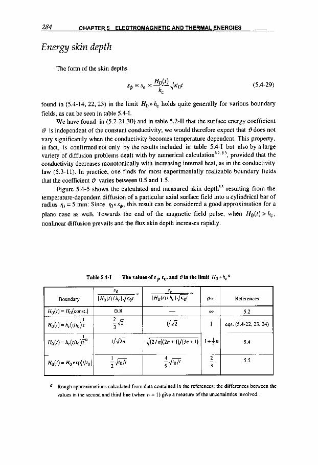
284 CHAPTER 5 ELECTROMAGNETIC AND THERMAL ENERGIES
Boundary
H o ( t ) = Ho(const.)
I
HoO) = k(f/fo)?
Energy skin depth
Se
[Ho(f) /hc]&-r = IHo(f)lh,lJK,r = I9= References
0.8 m 5.2
245 1/45 1 eqs. (S.4-22.23.24) 3
-
The form of the skin depths
(5.4-29)
found in (5.4-14,22,23) in the limit HO.hc holds quite generally for various boundary fields, as can be seen in table 5.4-1.
We have found in (5.2-21,30) and in table 52-11 that the surface energy coefficient 19 is independent of the constant conductivity; we would therefore expect that t? does not vary significantly when the conductivity becomes temperature dependent. This property, in fact, is confirmed not only by the results included in table 5.4-1 but also by a large variety of diffusion problems dealt with by numerical calculation8” 8 3 , provided that the conductivity decreases monotonically with increasing internal heat, as in the conductivity law (5.3-1 1). In practice, one finds for most experimentally realizable boundary fields that the coefficient 0 varies between 0.5 and 1.5.
Figure 5.4-5 shows the calculated and measured skin depth’.’ resulting from the temperature-dependent diffusion of a particular axial surface field into a cylindrical bar of radius ro = 5 mm: Since rO”sq, this result can be considered a good approximation for a
plane case as well. Towards the end of the magnetic field pulse, when no(‘) > hc,
nonlinear diffusion prevails and the flux skin depth increases rapidly.
Table 5.4-1 The values of sp se, and I9 in the limit Ha n hca
I
Rough approximations calculated from data contained in the references; the differences between the
values in the second and third line (when n = I ) give a measure of the uncertainties involved.
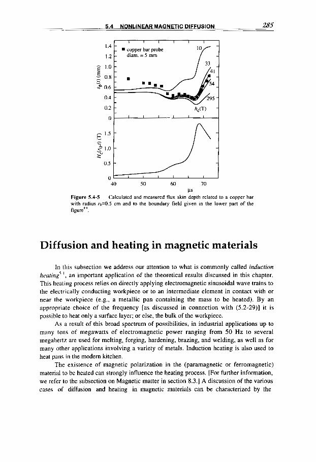
5.4 NONLINEAR MAGNETIC DIFFUSION 285
I I I 1 I I 1.4 - - copper bar probe 1.2 - diam. = 5 mm
0.2 t
- 1.5 t P 1.0
zw 0.5
0
- -- v
40 50 60 70 PS
Figure 5.4-5 Calculated and measured flux skin depth related to a copper bar with radius r0=0.5 cm and to the boundary field given in the lower part of the figure4 ’.
Diffusion and heating in magnetic materials
In this subsection we address our attention to what is commonly called induction heating’.’, an important application of the theoretical results discussed in this chapter. This heating process relies on directly applying electromagnetic sinusoidal wave trains to the electrically conducting workpiece or to an intermediate element in contact with or near the workpiece (e.g., a metallic pan containing the mass to be heated). By an appropriate choice of the frequency [as discussed in connection with (5.2-29)] i t is possible to heat only a surface layer; or else, the bulk of the workpiece.
As a result of this broad spectrum of possibilities, in industrial applications up to many tens of megawatts of electromagnetic power ranging from 50 Hz to several megahertz are used for melting, forging, hardening, brazing, and welding, as well as for many other applications involving a variety of metals. Induction heating is also used to heat pans in the modem kitchen.
The existence of magnetic polarization in the (paramagnetic or ferromagnetic) material to be heated can strongly influence the heating process. [For further information, we refer to the subsection on Magnetic matter in section 8.3.1 A discussion of the various cases of diffusion and heating in magnetic materials can be characterized by the

286 CHAPTER 5 ELECTROMAGNETIC AND THERMAL ENERGIES
L
Figure 5.4-6 B - H magnetization (hysteresis) curve of ferromagnetic material.
a typical hard
properties of the magnetic permeability p, and thus of the magnetic induction
B = p H , P = P o P R , (5.4-30)
as follows: (a) p is constant. We have seen in this and the previous chapter that the reaction of a
conducting material with constant magnetic permeability to an applied outer magnetic field pulse is as if the electric conductivity were increased by a factor pR. In particular, for the energy factor (i.e., surface temperature) and the energy and flux skin depths defined in table 5.2-11 we found the following dependence on the relative permeability:
(5.4-3 1)
[For ferromagnetic conductors the total dissipated energy, and particularly the surface temperature, can thus be appreciably higher than for nonmagnetic conductors.]
(b) p is a function of various parameters (e.g., magnetic field, temperature, etc.). Qualitatively, the same considerations as in the previous case can be made; but an exact solution must be based on the appropriate equations [see comments in connection with (4.1-4), and also (5.4-1,2)] and it will be nonlinear.
(c) p is a function with hysteresis, as is typically the case for ferromagnetic materials (figure 5.4-6).
(d) p is a matrix, meaning that the vectors H and B are not aligned, as can be the case in crystals.

5.4 NONLINEAR MAGNETIC DIFFUSION 287
Figure 5.4-7 Magnetization curve of a soft ferromagnetic material. typically iron- nickel or magnetically soft iron; a constant, mean magnetic permeability pRa can be defined, which allows an approximate description of the eddy current effects up to about H s / 2 .
In the following we shall discuss three typical cases: Induction heating with constant p; or with approximately constant p without hysteresis up to a fraction of the saturation field H s for ferromagnetic materials (figure 5.4-7); and magnetic hysteresis heating in ferromagnetic materials (which does not imply finite electric conductivity).
An exact appreciation of the heating in the workpiece requires evaluation not only of the localized electromagnetic induction heating but also of the heat conduction in the bulk through the thermal diffusion equation (5.1-37.43) and the cooling of its surface through radiation loss, as given by the Stefan-Bolfzmann law,
Here, Ps is in W/mZ; E is the dimensionless emissivity coefficient of the surface; Ts is the surface temperature of the body under consideration; and T A is the temperature of the ambient or of surfaces surrounding it , both in kelvin. For example, for a surface with Ts = 1300 K (-lO0O'C) radiating into room temperature (TA = 300 K), the T' term can be neglected and PR = 180 kW/m2.
Steady sin usoida 1 magnetic field heating
Induction heating is based on the diffusion of a steady sinusoidal (harmonic) field through an electric conductor, a process we have studied in great detail in this and the previous chapters. We briefly recall here the main results, although this linear theory, where the magnetic permeability p is a constant as in relation with (5.4-31). does not strictly pertain to this section.

288 CHAPTER 5 ELECTROMAGNETIC AND THERMAL ENERGIES
Table 54-11 Induction heating by harmonic field HoeiW
-
-
I
2
2a
2t
3
-
4
42
4t
5
51
5t
-
Seometry
Plane Geometry
Half-space with parallel field
Slab with parallel field :thickness 2d)
thick
rhin (6d)
rhin disc :6*aa,d)wlth normal field :thickness 2d, radius (I)
Cylindrical geometry
Cylinder with axial field [radius (I):
thick
lhin (6 n u )
Hollow Eylinder with axial field (radii b. a, wa lhickness d):
lhick
lh in ( 6 o u d)
)iffused magnetic fielda (complex writing)
cosh X coshXd
W1,e'W - q(,,exp{i(w- X: + x')}
e -
Hue,w berRt i beiR berR, + i bed?,
Mean heating power, per ur :xposed surface
Hi sinh2Xd -sin2Xd daxd cosh2Xd -cos2Xd
__ I H,' 2 (10 R' ber2R,+bei2R,,
berR,,brr'R, + beiR0bei
I H i __ 32 ao R,"
f
_ - I H i (R,RdJ2)2
2 do 1t(R,Rd/2)2
a For the fields in real terms see also table 4.2-11. Other energy relations for the half-space are given in table 5.2-11. See also, for example, eqs. 12.22 and 12.38 in ref. 5.1. For uniformity to slab, here thickness is 2d in contrast to (5.3-10). The related surface current density is given in (4.4-39).
f Cumbersome formula; see, for example, ref. 5.1 (eq. 12.55).
Quations n text
(4.2-32) (5.2-29)
(4.2-
53.57)
(5.3-2.6)
(4.4-39) (5.3-10)
-
(4.3-25)'
related I( (5.3-9)
(4 4-86)
(4.4-92) (5.3-39) -
Reduced fariable and Jarameters
X = x / 6 Xd =d16
X = ( l t i ) X / I X ,= ( l t i ) d / _
6 = W JT;=l+i

5.4 NONLINEAR MAGNETIC DIFFUSION 289
These results were found in a straighforward manner from the appropriate differential equations by taking real steady boundary conditions HO sin wt (or the
equivalent form HOCOS wf) . However, in these problems it is convenient to use the complex functions and vectors introduced and discussed in chapter 3, which represent a widely used formalism in electromagnetic theory whenever there is an imposed frequency w. Table 5.4-11 gives an overview of some of the analytic results and refers to the equations in chapters 4 and 5 where they were obtained. The second column presents the mean power that within an oscillation period T = 2 d w flows through the surface of the conductor (workpiece) and dissipates into heat. However, we recall from the discussion of the complex Poynting vector in (5.1-25,26,27) that during a period T there is an additional power flow in and out of the surface without dissipation. These are the magnetic (inductive) and electric field energies (5.1-28) bound to the electromagnetic energy storage of the conductor. They represent a reactive term in the circuit which generates the oscillating electromagnetic fields.
Note that in more complicated conductor systems (e.g., the parallel transmission lines with proximity effects, figure 2.1-7), induction heating can be approximately calculated by substituting some of the idealized solutions presented throughout this book with the concept of the current flowing within a finite skin depth. For example, application of the image method to the line conductor carrying the current I = Iosinwt parallel to a (superconducting) plane return conductor, figure 6.2- 1 1 a, gives the tangential boundary field (2.1-88),
Ho = -- 10 1 nh l + ( x / h ) 2
(5.4-32a)
If the plane now has finite conductivity Q with skin depth 6, (5.2-28), and if h N 6, the approximate mean heating power per unit surface deposited over an oscillation time on the plane conductor (as a consequence of the oscillating current in the line conductor) is obtained directly from (5.2-29a):
- 1 lo" 1 PR(X) = --
2n2Q6 h2 [ I + ( ~ l h ) ~ ] ~ '
(5.4-32b)
This result is of significance in applications where the heating source (e.g., single-turn conductors carrying large currents) is placed near the surface of the component under treatment for local heating, hardening, and so on.
Ferromagnetic induction heating
In a ferromagnetic material the relative permeability p~ is not constant but is a

290 CHAPTER 5 ELECTROMAGNETIC AND THERMAL ENERGIES
function of H, as can be seen in the hysteresis loop relating B and H of figures 5.4-6 and 7 [see also section 8.3 (figure 8.3-8)]. Moreover, the alignment of the elementary magnetic domains becomes saturated at magnetic fields pHs of typically 1-20 mT, and the saturation induction Bs (typically 1 to 2 T) is itself temperature-dependent (figure 5.4- 1). Above the so-called Curie temperature (e.g., for iron 746°C; figure 5.4-1) ferromagnetism disappears completely (see section 8.3, subsection on Ferromagnetism). Consequently, magnetic diffusion becomes a highly nonlinear process, and the linear diffusion theory presented previously in chapters 4 and 5 cannot be applied.
This is a typical nonlinear situation, which must be handled by numerical computation. If an analytical approximation is looked for, we can proceed in two different ways, according to whether the applied outer field is smaller or larger than the saturation field Hs. In thefirst case, when HO < Hs, it is convenient to determine an approximate, mean (constant) magnetic permeability over the range of interest as shown in figure 5.4-7, and this then allows the linear diffusion theory to be applied again. This procedure has been developed quite extensively, in order to obtain significant result’.’.
In the second case, when HO > Hs, the situation becomes more i n t r i ~ a t e ~ . ~ ~ . Consider the ferromagnetic half-plane of figure 5.4-8 to the surface of which a steady magnetic field
H, = HO sinm
is applied. A skin with depth 6of magnetic induction saturation Bs forms early on in each half-cycle (as soon as Hosinwt > Hs) and propagates into the ferromagnetic material
(where actually it annihilates the region with maximum depth 6, of negative saturation -Bs left over by the previous half-cycle). This situation is illustrated in figure 5.4-8 with the assumption that the magnetic induction BS is constant in the skin depth and changes from k values according to the half-cycle of the surface field. With this we want to calculate 6, 6,, H,(x,t) = H,o(xl)sinm, E y ( x , t ) andjy(x,t).
Application of Faraday’s law (1.4-5) to the quadrilateral curve C in figure 5.4-8 gives
thus
d6 dt
jy(x,t) = OEy = -204 - (5.4-3 3)
(as the magnetization front advances by A6, the saturation induction jumps from -Bs to +Bs; hence a factor of 2 in the flux variation). In addition, from Amptre’s law (1.4-3) taken over D we get
AlH,(x,t) = -jyAl(6 - x) (5.4-34a)

5.4 NONLINEAR MAGNETIC DIFFUSION 291 -.
I I
Bs + I I I I I I
I
I I
st l 6 m l I I I I I I
Figure 5.4-8 Magnetic diffusion into a ferromagnetic conductor
or with (5.4-33)
d6 dt
H , ( x , t ) = H , o ( x ) sinm = 20Bs(6 - x)- ,
which can be integrated at n = 0,
(5.4-34b)
t 6 Holsin wt dt = 20Bs16 d6 ,
0 0
to obtain
292 CHAPTER 5 ELECTROMAGNETIC AND THERMAL ENERGIES
- ( l -cosa)=ol@ HO 2 . w
(5.4-35)
Thus, the magnetic induction skin depth at full saturation is [with the relation 1 - cosx = 2sin x / 2 ] 2
WI 6 = 6s sin- (5.4-36)
2
where the maximum attained at the end of each half-cycle t = T/2 is
(5.4-37)
this skin depth has an analogous form to the classical skin depth (5.2-28). From (5.4- 33.34) in the range 0 I x 5 6 , as shown in figure 5.4-8 we obtain the current density
(5.4-38)
and the magnetic field
Hz(x,t)=-jy(6-x)= (5.4-39)
The mean heating power flowing (during one half-cycle) through the unit surface is calculated to be, with (5.4-36,38),
2 8 Ho2 T I 2
- 2 1 P = - - j6 jydt=- - ,
3n &a 0
(5.4-40)
where use has been made of the integral relation jcos2x sinr dx = -(cos3x)/3. Note that
this expression is formally similar to (5.2-29), where the mean dissipated power is obtained with a constant magnetic permeability, with the substitution p -) Bs/Ho. The surface temperature at the end of each cycle is
(5.4-4 1 )
which is again similar to (5.2-26), but it can be very large because of the saturation induction Bs. It can easily become larger than the Curie temperature (e.g., for iron 746"C), in which case the ferromagnetic properties vanish. Where this is the case, the diffusion process would fall back on the linear theory and the results presented in tables 5.2-11 and 5.4-11.
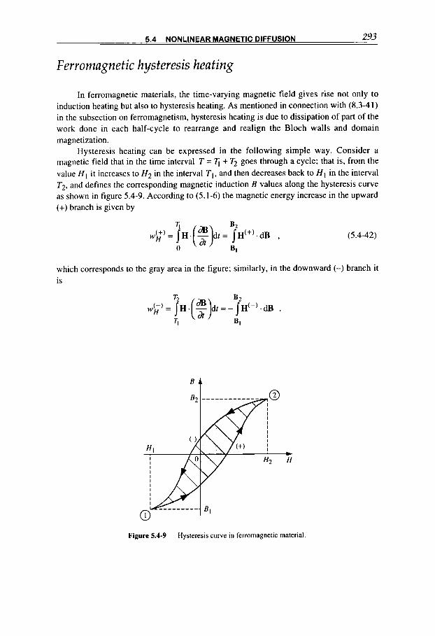
5.4 NONLINEAR MAGNETIC DIFFUSION 293
Ferromagnetic hysteresis heating
In ferromagnetic materials, the time-varying magnetic field gives rise not only to induction heating but also to hysteresis heating. As mentioned in connection with (8.3-41) in the subsection on ferromagnetism, hysteresis heating is due to dissipation of part of the work done in each half-cycle to rearrange and realign the Bloch walls and domain magnetization.
Hysteresis heating can be expressed in the following simple way. Consider a magnetic field that in the time interval T = TI + T2 goes through a cycle; that is, from the value H I it increases to H 2 in the interval TI, and then decreases back to H I in the interval T2, and defines the corresponding magnetic induction B values along the hysteresis curve as shown in figure 5.4-9. According to (5.1-6) the magnetic energy increase in the upward (+) branch is given by
(5.4-42)
which corresponds to the gray area in the figure; similarly, in the downward (-) branch it is
Figure 5.4-9 Hysteresis curve in ferromagnetic material.

294 CHAPTER 5 ELECTROMAGNETIC AND THERMAL ENERGIES
The total energy dissipated in one cycle (during the time interval r ) is thus
B2 B2
Bl BI
wH = jH(+) .dB- /H'-'.dB , (5.4-43)
which is expressed by the hatched area enclosed by the two branches of the hysteresis
In complex writing, the hysteresis effect can be handled in an elegant formal way. As mentioned in connection with (3.2- 12). microscopic physical phenomena, which may introduce a time lag between the application of a magnetic field H and its related induction field B, can be expressed by a complex magnetic permeability
curve.
where, as we know from (3.1-13),
(5.4-45)
[ pR, pi, pi, a are all real, positive parameters, and the negative sign we have given to pg in (5.4-44) anticipates the physics results]. In fact, from
B = - p B = pOpRHOe(iW-a) , where B=kiW , H =&", (5.4-46)
we see that the induction field lags behind the magnetic field by the phase angle a. The magnetization power per unit volume was shown in (5.1-6) to be
dWH = H . (5) dt
(5.4-47)
With our complex formalism the mean power per unit volume dissipated in the material (within a period 7') can be written with (5.1-20) in the form
- P R = ReH . Re- a 1 = -Re[H.(-iwpH *)] = WI-J. I-J * Re[-i(ph + ip;)] = - pomp: H 2 , d t 2 2 2
(5.4-48) which shows that p i represents the dissipative term in the complex magnetic permeability (5.4-44). The total heat deposited by the polarization-depolarization cycles per unit volume of the magnetic material during a time of n periods, t = nT, is given by
(5.4-49)

Chpter 6
MAGNETIC FORCES AND THEIR EFFECTS
In this chapter, the theoretical introduction of basic electromagnetic forces leads to several magnetic problems of practical importance. In fact, technically feasible magnetic-field forces and energy densities are much larger than those of electric fields. This is why the Amphe and the Biot-Savart magnetic forces are the basic elements in practical applications of electromagnetism; they drive electric motors and determine the mechanical stresses in magnets.
Applications. This is the most important chapter when it comes to applications. Besides the vast subject of electric motors'7763a, some selected discussions here refer to the acceleration and, in some cases, guidance of massive conductors [magnetically levitated vehicles (MAGLEV)6 24, magnetic braking, magnetic suspension'^", magnetic bearing6 42],
of pellets (magnetic suspension for diagnostic purposes, magnetic separation' 17,
electromagnetic launchers' "), and of single particles (accelerators6'.' 19, electron microscopes' ', electron beam technology for welding and melting6 20, electronic devices).
6.1 ELECTROMAGNETIC FORCES
In this section we present the elemental electromagnetic forces that are applied on electric charges and currents.
295
M4GNETICFIELDS: A Comprehensive Theoretical Treatise for Practical Use Heinz E. Knoepfel
Copyright Q 2000 by John Wiley & Sons, Inc
296 CHAPTER 6 MAGNETIC FORCES AND THEIR EFFECTS
Elemental forces
Loren tz force One of the basic relations of electromagnetism (together with Maxwell's four
equations) is given by the Lorentz force
F = q ( E + v x B ) , (6.1 - 1 a)
or in practical cgs units (dyn, coulomb, Vkm, c d s , gauss),
F = q(107E + 0 . 1 ~ x B) , (6.1 - 1 a)*
which is the force that govems a particle with an electric charge q moving with velocity v in an electric field E and in a magnetic flux density B = pH. Note that since the magnetic force
F B = q v x B (6.1 - 1 b)
is perpendicular to the displacement ds = vdt,it does not do any work; from (A.3-ld) indeed,
FB .ds = qv . (v x B)dt = 0 .
Expression (6.1-1) is also valid for time-dependent quantities and for any velocity (even one approaching the velocity of light c). The force (6. I-1), which was determined in its basic structure by H.A. Lorentz, establishes a relation between electromagnetic theory and mechanics. (Note: There are no dimensional parameters because it is from this expression that the SI units of q. E, and B are determined; see tables A.3-I and 11.)
It is sometimes convenient to express the Lorentz force with the magnetic vector potential A (2.2-2),
B = V x A ,
and the electrostatic potential U which in (2.2-4) contributes to expressing the general (static plus inductive) electric field,
dA dr
E = - V U - - ,
Application of the vector relation (A.3- 12). thereby noting that only A(rp) (determined at
the particle's position rp) and ~ ( t ) are subject to the Vaperator, gives
v x B = v x V x A = V(V . A) - ( v . V)A ;
and from (1.3-17,19), by considering the total time derivative,
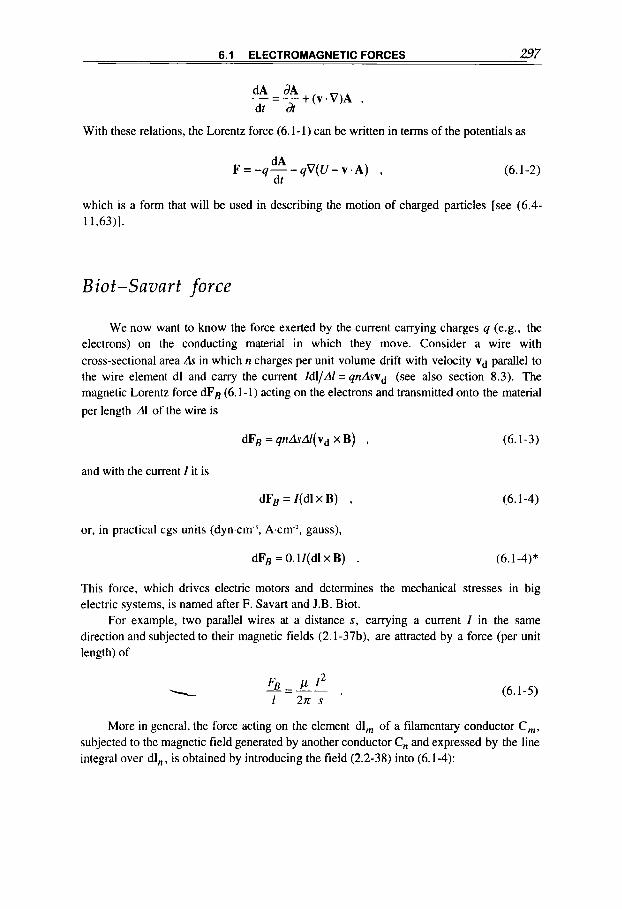
6.1 ELECTROMAGNETIC FORCES 297
dA -'A + ( v . V ) A . dt dt
With these relations, the Lorentz force (6.1-1) can be written in terms of the potentials as
(6.1-2) dA
F = -4- - qV(U - v . A ) , dt
which is a form that will be used in describing the motion of charged particles [see (6.4- 1 1,63)].
Biot-Savart force
We now want to know the force exerted by the current carrying charges q (e.g., the electrons) on the conducting material in which they move. Consider a wire with cross-sectional area As in which n charges per unit volume drift with velocity Vd parallel to the wire element dl and carry the current Idl/Al= qndsvd (see also section 8.3). The rnagnetic Lorentz force dFs (6.1-1) acting on the electrons and transmitted onto the material per length Al of the wire is
dFB = qndsAl( V d X B) , (6.1-3)
and with the current I it is
dFB = I(dl X B) , (6.1-4)
or, in practical cgs units (dyntm.), A.cm-2, gauss),
dFB = 0. Il(dl X B) . (6.1 -4)*
This force, which drives electric motors and determines the mechanical stresses in big electric systems, is named after F. Savart and J.B. Biot.
For example, two parallel wires at a distance s, carrying a current I in the same direction and subjected to their magnetic fields (2.1-37b), are attracted by a force (per unit length) of
(6.1-5)
More in general, the force acting on the element dl, of a filamentary conductor C,, subjected to the magnetic field generated by another conductor C, and expressed by the line integral over dl,, is obtained by introducing the field (2.2-38) into (6.1-4):

298 CHAPTER 6 MAGNETIC FORCES AND THEIR EFFECTS
A
Figure 6.1-1 Elemental Biot-Savart forces between filamentary conductors (the angle a , , is defined by dl,dl, COSCC,,, = dl, 'dl,,).
(6.1-6)
where r,,, = r, - r, (figure 6.1 - 1). From this we define the elemental Biot-Savart force,
which with (A.3-lc) can be written as
or, by referring to the notation in figure 6.1-1, also as
d F,,m - 'f" (r,,,, cosa,dl,dl, - cosan,,dl,dl,rn,,) . (6.1-8) 4 8 rn,m
The first term in these two expressions will give no contribution when integrated over the closed circuits C, or C, . In fact, with (A.3-4,13) for the integration over the closed curve c,, follows
f *.dim= 3 f V
c,, rwn Cm
Then, the total force exerted on this circuit by the circuit C, (or vice versa) becomes

6.1 ELECTROMAGNETIC FORCES 299
(6.1-9)
These expressions can be useful in numerical computations; they can often be transformed and simplified for specific needs (see in connection with figure 9.2-2). In the literature, a different elemental force law, originally proposed by Amphe' I , is sometimes mentioned. Discussion on this laws uncovered interesting theoretical aspect^^.^^, which are, however, of limited importance in practice.
Electromagnetic force density
The Biot-Savart force concept (6.1-4) can be extended to the force per unit volume exerted on a conductor element A V = AsAl, which canies a current density j = Idl/AsAl across the surface As and along dl, to obtain Ampkre's force density or volume force
AF dF - + - = f B = j x B , A V dV
or, in practical cgs units (dyn.cm-), A.cm-2, gauss),
fB =O.l(jxB)
(6.1 - 10)
(6.1-lo)*
With the obvious addition from (6.1-1) of the electric force density
f E = P e E , (6.1- 11)
the total force exerted by a (quasistationary) electromagnetic field on a unit volume of isotropic matter becomes
f = p , E + ( j x B ) . (6.1- 12)
This simple force expression is based on various assumptions; in this connection the following comments can be made:
(a) Magnetic permeability p and dielectric permittivity E. They are taken to be space constants; otherwise the terms' '
fs = - - E 1 2 V&--H2Vp 1 2 2
(6.1-13)
expressing the polarization and magnetization force densities have to be added to (6.1 - 12); also, there is no dependence on the mass density6'-that is, no electro- or magnetostrictive forces (they anyway produce deformation but no net body force), which would be represented by the terms

300 CHAPTER 6 MAGNETIC FORCES AND THEIR EFFECTS
(6.1-14)
and no dependence on the fields themselves, no hysteresis.
(b) Neither permanent polarization P (1.1-45) nor magnetization M (1.1-20) are considered; otherwise, in the latter case, a term (1.1-21)
fM = j, x B = ( V x M ) x B (6.1-15)
must be added.
(c) Expression (6.1-12) is valid for static and quasistationary timedependent fields B(r), E( t ) (where the latter now also includes the induced electric field), since otherwise, the electromagnetic pressure term
J( D x B) dr
foe = ~ (6.1- 16)
must be included (D x B is the electromagnetic momentum density).
(d) Expression (6.1-12), in analogy to the Lorentz force (6.1-l), is valid for any frame of reference. This is not true, in general, for the other terms mentioned here.
Forces on finite bodies
Magnetic force density The magnetic volume force that results from (6.1-10,13),
f e = j x B (6.1-17a)
or
(6.1 - 17 b) 1 2 2
f e = j x B - - H V p
when p is not constant, (6.1-13), can be written, by eliminating the quasistationary current density
j = V x H ,
in the form
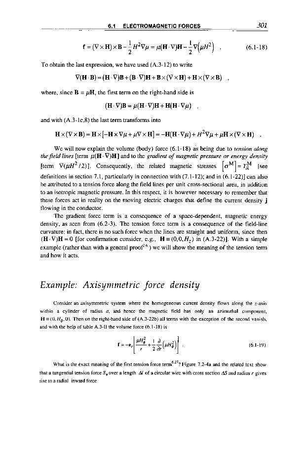
6.1 ELECTROMAGNETIC FORCES 301
(6. I - 18) 1 1 2 2
To obtain the last expression, we have used (A.3-12) to write
f = (V x H) x B - -H2Vp = p ( H . V)H - -V(pH2) .
V(H . B) = (H . V)B+ (B . V)H + B x (V x H) + H x (V x B) ,
where, since B = pH, the first term on the right-hand side is
(H . V)B = p ( H . V)H + H(H . Vp) ,
and with (A.3-lc,8) the last term transforms into
H x (V x B ) = H x[-H x Vp + p V x H] = - H ( H . V p ) + H2Vp + p H x(V x H) .
We will now explain the volume (body) force (6.1-18) as being due to tension along thefield lines [term p(H . V)H] and to the gradient of magnetic pressure or energy density [term V(pH2 /2)] . Consequently, the related magnetic stresses [aM]= i$ [see
definitions in section 7.1, particularly in connection with (7.1-12); and in (6.1-22)] can also be attributed to a tension force along the field lines per unit cross-sectional area, in addition to an isotropic magnetic pressure. In this respect, it is however necessary to remember that these forces act in reality on the moving electric charges that define the current density j flowing in the conductor.
The gradient force term is a consequence of a space-dependent, magnetic energy density, as seen from (6.2-3). The tension force term is a consequence of the field-line curvature; in fact, there is no such force when the lines are straight and uniform, since then (H”i’)H = 0 [for confirmation consider, e.g., H = (O,O,Hz) in (A.3-22)]. With a simple example (rather than with a general proof’ ) we will show the meaning of the tension term and how it acts.
Example: Axisymmetric force density Consider an axisymmetric -system where the homogeneous current density flows along the z-axis
within a cylinder of radius a, and hence the magnetic field has only an azimuthal component,
H I (0. [email protected]). Then on the right-hand side of (A.3-22b) all terms with the exception of the second vanish,
and with the help of table A.3-I1 the volume force (6. I - 18) is
(6. I - 19)
What is the exact meaning of the first tension force term6.*’? Figure 7.2-4a and the related text show
that a tangential tension force S, over a length A/ of a circular wire with cross section AS and radius r gives
rise to a radial inward force

302 CHAPTER 6 MAGNETIC FORCES AND THEIR EFFECTS
or force per unit volume of the wire of
Comparison with the first term on the right-hand side of (6.1-19) indicates that pH$ (which compares with
S+ /AS) can be interpreted as the magnetic tension force per unit cross-sectional area and also that this
tension force density gives rise to a volume force plf; / r that acts radially inward.
For the magnetic volume forcef, acting outside and inside the conducting cylinder we easily calculate
from (2.1-37b) and (6.1-19)
w; w; +-=o , I
r > a , H q = g , f,=-- r r
(6.1-20a)
(6.1-20b)
Outside the conducting cylinder the tension and gradient-pressure terms cancel out, as required, since there is no current ] = Ax H flowing; whereas inside, both terms compress the conducting cylinder (so-
called pinch effect)
Maxwell’s magnetic stress tensor
We now go back to the general force density (6.1-18) and by integration obtain the total magnetic force acting on the finite body with volume Vdelimited by the surface S:
F = fdV = I p ( H . V)HdV - -I 1 V(pH2)dV = 9 pH(H. ds) - -fpH2ds 1 ,(6.1-21) 2 2
where (A.3-18,19a) and V . B = 0 have been applied to transform the volume integrals into surface integrals. This result shows that the magnetic force acting on a finite body can be expressed by an integral over the field on the surjime bounding the body. The field is seen as the stress-transmitting medium from the inner portions of the body to the surface. These ideas had already been developed in relation to the field concept by Maxwell, whose opinion was that the transmission of the magnetic volume force acting in a given volume to the surface bounding that volume can be formulated in terms of the magnetic stress tensor.
In fact, by introducing ds = nds , with n the unit normal vector on the body surface, the total magnetic body force (6.1-21) can be written as
F = $ T ~ & , (6.1 -22a)

6.1 ELECTROMAGNETIC FORCES 303
-(H: - H," - H : ) H ~ H ~
-(H," 1 - H: - H:) H ~ H ~
- (H: 1 - H: - H ; )
HXHZ
2
where the vector
H ( H . n ) - - H 2 n } = p T ["I . n (6.1-22b) 2
can be seen as the result of the multiplication [as defined in (A.3-37, 38)] of the column vector n with the so-called Maxwell stress tensor
(6. I-23a)
or, in element-writing,
(6.1-23b)
and H 2 = H : + H : + H : .
comparing (6.1-21, and 22) and using the notation (A.3-38) we have The magnetic volume force density can also be expressed through this tensor, and by
f.=V.[T"] (6.1-24a)
or, in component writing,
(6.1-24b)
The Maxwell tensor is symmetric and of second rank, so by following the procedure outlined in (A.3-50,51) it can be reduced through diagonalization to principal axes,
H 2 0 0
(6.1-25) [T M I=&[: 2 ; H 2 ",,2] ,
where the first axis is parallel to H and the other two are perpendicular to it. The magnitude
of the surface force density is TM = p H 2 /2, and figure 6.1-2 shows that H bisects the
angle between n and TM. In fact, consider the stress Tds related to the surface element ds=nds, with n making an angle a with the x-axis, which is chosen to be the principal axis aligned with H . The stress component parallel to H is T'dsx = T'sinor ds, and the one perpendicular to it is Tyyds = Tyy cosa ds: this shows that the angle between T and H is
I I

304 CHAPTER 6 MAGNETIC FORCES AND THEIR EFFECTS
Figure 6.1-2 Surface magnetic force density.
also equal to a. In conclusion, we have tension along the field line (figure 6.1-2b) and a compression force normal to it (figure 6.1-2c). In the particular case shown in figure 6. I - 2d, we have shear (always with the same magnitude p H 2 / 2 ) . These results can be expressed qualitatively by saying that magnetic flux lines act like stretched elastic bands, which behave as bands under tension that mutually repel each other.
The stress tensor can be extended to include electrostatic forces as well. In accordance with the electrostatic volume force that results from (6.1-12, 13).
(6.1-26) fE=p ,E- -E 1 2 V E , 2
the electric stress tensor is calculated analogously' 5 :
The properties of the magnetic stress tensor are valid for this tensor as well.
Magnetic multipole expansion
(6.1-27)
The total force resulting from integration of the volume force (6.1-10) over the volume of a finite body can often be simplified because some terms may drop out or transform into simpler ones. For example, (6.1-21) shows that the total magnetic force can

6.1 ELECTROMAGNETIC FORCES 305
be expressed by an integral over the body surface.
approximation) the total force Here we present another useful integrated form by simplifying (in first-order
(6.1-28)
exerted by an outer field B on a finite conductor containing a divergence-free current distribution [see remarks on such a current flow in connection with (1.2-2 1) and (2.2-22)]. Here and in the remaining part of this section, the field B is taken to be generated by outside currents (that have nothing in common with j); however, the following results would not change if, instead, the total field, including also the self-field generated by j , is used, because the self-field cannot result in a net force on the current. We know from (2.2- 42) and the comments following (2.2-45) that the magnetic vector potential of such a current distribution can be expanded into multipole terms, and we expect here a similar expansion for the force (6.1-28). with the first-order (dipole) term dominating. We obtain the magnetic field BQat the point Q(a) within the conductor in first-order approximation by expanding the field in a Taylor series about its value Bo at a point 0 that is firmly attached to the coordinate system of the conductor (figure 6.1-3); in vector form and using the simple notation B = Bo (we omit the index zero), we write
BQ = B+(a .V)B+. . . . (6.1-29)
Insertion into the force integral (6.1-28) gives
Figure 6.1-3 Force F acting on the dipole moment p derived from a divergence- free current distribution j flowing in the conducting body.
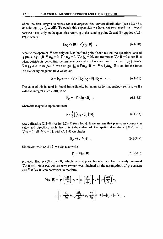
306 CHAPTER 6 MAGNETIC FORCES AND THEIR EFFECTS
where the first integral vanishes for a divergence-free current distribution [see (2.2-43), considering jQdVQ 2 Idl]. To obtain this expression we have: (a) rearranged the integral
because it acts only on the quantities referring to the running point Q; and (b) applied (A.3- 12) to obtain
(a, .V)B = v(aQ .B) , (6.1-30)
because the operator V acts only on B at the fixed point 0 and not on the quantities labeled Q [thus, e.g., (B.V)aQ = 0, V x aQ = 0, V x jQ = 01, and moreover V x B = 0 since B is taken outside its generating current sources (which have nothing to do with jQ). Since V x jQ = 0, from (A.3-8) we also get jQ x V(aQ .B) = -V x jQ(aQ .B); so, for the force
in a stationary magnetic field we obtain
F = F P +... = -v XjjQ(aQ.B)dvQ +*.. . (6.1-3 1)
The value of this integral is found immediately, by using its formal analogy (with p + B ) with the integral in (2.2-50). to be
Fp =-VX(pxB) , (6.1 -3 2)
where the magnetic dipole moment
(6.1-33) 1
P = - j (aQ 2 jQ)dVQ
was defined in (2.2-49) [or in (2.2-45) for a loop]. If we assume that p remains constant in value and direction, such that it is independent of the spatial derivatives [ v X p = 0, V . p = 0, (B . V)p = 01, with (A.3-9) we obtain
Fp=(p.V)B . (6.1-34a)
Moreover, with (A.3-12) we can also write
Fp = V(p.B) (6.1-34b)
provided that p x (V x B) = 0, which here applies because we have already assumed V x B = 0. Note that the last term (which was obtained on the assumptions of p constant and v x B = 0 ) can be written in the form

6.1 ELECTROMAGNETIC FORCES 307
which is quite different from the form of (p.V)B given in (A.3-22). Accordingly, the translational force Fp acts predominantly in the direction of the prevailing field gradient. In
addition, it is maximum when p is aligned with B, and it points towards increasing B when p.B is positive (and vice versa).
There is also a torque
(6.1-35)
exerted by the magnetic field on the current distribution about the moment center 0 (figure 6.1-4). The first term in the Taylor expansion (6.1-29) is generally the dominant one in this expression, and the only term effective in a uniform magnetic field (in such a field no translational force exists). Expansion of the triple vector product (A.3-lc) gives
(6.1-36)
where the last integral vanishes (in fact, any current tubule, which according to the comments made following (2.2-48) describes the current distribution, can be decomposed into segments along the azimuthal rA4, radial Ar, axial Az directions; in the first direction aQ . j, = 0, whereas any contribution to the integral on the second and third has always an identical negative counterpart along a tubule closing upon itself). The first integral is identical to that in (6.1-3 I), and the torque on a magnetic dipole is thus
T = p x B . (6.1-37) P
Equation (6.1-34) shows that the translational force can be expressed by the potential energy
Figure 6.1-4 Torque T, on a magnetic dipole moment p.
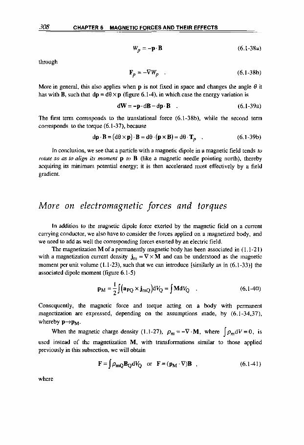
308 CHAPTER 6 MAGNETIC FORCES AND THEIR EFFECTS
W - -p .B (6.1-38a) P -
through
F,, = -VWP . (6.1-38b)
More in general, this also applies when p is not fixed in space and changes the angle 8 it has with B, such that dp = de x p (figure 6.1-4), in which case the energy variation is
dW=-p.dB-dp.B . (6.1-39a)
The first term corresponds to the translational force (6.1-38b), while the second term corresponds to the torque (6.1-37), because
dp . B = (do x p) . B = de .(p x B) = do. Tp . (6.1-39b)
In conclusion, we see that a particle with a magnetic dipole in a magnetic field tends to rotate so as to align its moment p to B (like a magnetic needle pointing north), thereby acquiring its minimum potential energy; it is then accelerated most effectively by a field gradient.
More on electromagnetic forces and torques
In addition to the magnetic dipole force exerted by the magnetic field on a current carrying conductor, we also have to consider the forces applied on a magnetized body, and we need to add as well the corresponding forces exerted by an electric field.
The magnetization M of a permanently magnetic body has been associated in ( 1.1-2 1) with a magnetization current density j, = V x M and can be understood as the magnetic moment per unit volume ( I . 1-23), such that we can introduce [similarly as in (6.1-33)] the associated dipole moment (figure 6.1-5)
(6.1-40)
Consequently, the magnetic force and torque acting on a body with permanent magnetization are expressed, depending on the assumptions made, by (6.1-34,37), whereby p + p ~ .
When the magnetic charge density (1.1-27), pm =-V-M. where IpmdV=O, is
used instead of the magnetization M, with transformations similar to those applied previously in this subsection, we will obtain
(6.1-41)
where

6.1 ELECTROMAGNETIC FORCES 309
Figure 6.1-5 Force F acting on a body with permanent magnetization M and dipole moment pH in a magnetic field B.
PM PmQ dvQ . (6.1-42)
However, ongoing discussions show6 28.b 29 that there can be subtle differences between the magnetic dipole models based on magnetic charges (or magnetization) and the current loop.
For some applications6” it may be convenient to express the magnetic force
F = I j x BdV (6.1-43)
with the (externally generated) magnetic scalar (0) or vector (A) potentials (2.1-2). (2.2-2), B = -pV@, B = V x A . In the first case, by applying (A.3-8) we get (here p = const.)
F=-pjjxV@dV=pjVx(@j)dV-pI@VxjdV, (6.1-44a)
and with the use of (A.3-17) this can also be written as
F = -pf@(j xds)- p/@V x j dV . (6.1-44b)
In the second, vector potential case, by applying (A.3-19b) and noting that V. j = 0, V . A = 0 , and j . ds = 0 (because the current must be parallel to the surface), we get
F = I j x (V x A)dV = f ( A . j)ds - f j(A . ds) - I A x (V x j)dV ; (6.1 -45a)
by using (A.3-19a) to transform the second surface integral we can also write
F = f ( A . j)ds - I ( A . V)jdV -/A x (V x j)dV . (6.1-45b)
310 CHAPTER 6 MAGNETIC FORCES AND THEIR EFFECTS
When j is constant, the expressions (6.1-44,45) reduce to the first term on the right-hand side only.
Similar considerations and expressions also apply to the force Fe and torque Te exerted by an electric field E on a body possessing permanent electric polarization P or an electric charge density distribution They are obtained by substituting B+E and
p+pe in (6.1-34), where the electric dipole moment for zero net charge (I pedV = 0) is
(6.1-46)
In conclusion, the total force and torque exerted by a stationary electromagnetic field on a body with divergent-free current and zero net charge but having electric and magnetic dipole moments pe, p can be written in the form
F = ( ~ , . v ) E + ( ~ . v ) B , (6.1-47)
T = p , x E + p x B , (6.1-48)
where p includes the contributions both from the free current (6.1-33) and from the magnetization (6.1-40). and similarly, pe includes the contributions of the charge distribution and permanent polarization (6.1-46). Note that if a divergent current component is present (e.g., with currents flowing into and out from a finite conductor through gliding contacts; see example shown in figure 6.4-6), a force component obtainable by integrating the magnetic force densities (6.1-4 or 10) must be added in (6.1-42). that is,
F e = Z 4 d l x B , or = I jxBdV . (6.1-49) V
Similarly, if the net electric charge is not zero, we must take into account an electric force component
(6.1-50)
which is derived by integrating (6.1-1 1).
When the fields B(t), E(t) are time-dependent, there is no explicit change in the magnetic force terms, provided that B(t) remains within the limits set by the quasistationary approximation. [Otherwise a term -d(p x Elc) ldt must be added on the right-hand side of (6.1-341.1 Of course, the electric forces must also take into account the induced electric field components. In fact, even the B(t) could be influenced indirectly through a variation of the current distribution that determines the magnetic dipole moment p [see the example in connection with figure 6.4-5, which is a consequence of a magnetic diffusion effect].

6.2 MAGNETIC FORCES ON RIGID CONDUCTORS 311
6.2 MAGNETIC FORCES O N RIGID CONDUCTORS
Magnetic forces determined by electric currents flowing in finite conductors are at the basis of magnetomechanical applications Is. We now give a few examples that represent a broad range of applications, and we will be using various calculation methods and approximations. We will start by introducing the virtual work concept for idealized point masses (i.e., having no torques).
Inductive forces
Virtual work formalism
Let us assume that the potential (magnetic) energy W, which a current-carrying or magnetized body possesses with respect to other bodies in the system, depends on several independent parameters x;. i = 1 , 2, ..., n. When the parameters change by an amount
6xj , the energy increment is expressed by
dW my=c-&j . d X ;
On the other hand, this increment can correspond to the work
6 A = Fxi6xi
(6.2- 1 a)
(6.2- lb)
done by the generalized force components Fxi related to the change in the parameters x i .
Since xi are independent parameters and conservation of energy in a closed system requires
6 W + 6 A = O , (6.2-2)
from comparison of the last two expression we get
dw F =-- . xi
(6.2-3a)
In particular, the parameters can be ordinary space variables (e.g., XI = x, x2 = y, x3 = z ) in which case we write
F = - V W . (6.2-3b)
The magnetic force acting on the system is thus obtained as the negative gradient of its

312 CHAPTER 6 MAGNETIC FORCES AND THEIR EFFECTS
magnetic energy, which, for example, for current-carrying conductors can be expressed by the inductance integrals (5.1-33). for magnetic matter by the magnetic flux energy (6.2-49), and for a magnetic dipole by the potential energy (6.1-38a).
A body is in equilibrium when the sum of all forces is zero,
Z F j = O , (6.2-4a)
which also means that [by multiplying with H a n d noting (6.2-lb)]
&=ZF,,GXi=O . (6.2-4b)
In this case we find from (6.2-2)
m = o , (6.2-4~)
that is, a body is in equilibrium when its potential energy with respect to the system has an extreme value (minimum, inflection, or maximum). A free system characterized by a po- tential energy W (in addition to kinetic and heat energies) tends towards attaining a stable equilibrium characterized by a minimum in its potential energy.
For a conductor system with current I and self-inductance L, the magnetic energy, from (5.1-33). is given as
(6.2-5a)
and the inductive force Fx, , pointing towards decreasing inductance along the virtual
displacement hi, can be expressed as
1 2 w = - L I , 2
(6.2-5b)
-3-
Figure 6.2-1 Forces acting on a current-carrying rigid loop and on a coaxial loop pair, and torque acting on a inclined loop pair.
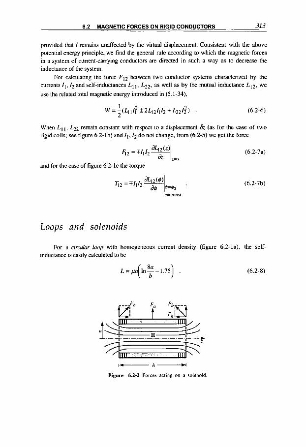
6.2 MAGNETIC FORCES ON RIGID CONDUCTORS 3u
provided that I remains unaffected by the virtual displacement. Consistent with the above potential energy principle, we find the general rule according to which the magnetic forces in a system of current-carrying conductors are directed in such a way as to decrease the inductance of the system.
For calculating the force F12 between two conductor systems characterized by the currents 11, 12 and self-inductances L ~ I . L22, as well as by the mutual inductance L12, we use the related total magnetic energy introduced in (5.1-34),
(6.2-6)
When L , rigid coils; see figure 6.2-lb) and I I , ~ do not change, from (6.2-5) we get the force
L22 remain constant with respect to a displacement 6.. (as for the case of two
and for the case of figure 6.2-lc the torque
(6.2-7a)
(6.2-7b)
s=const.
Loops and solenoids
For a circular loop with homogeneous current density (figure 6.2-la), the self- inductance is easily calculated to be
L = p a In--1 75 ( ? 4 (6.2-8)
I
a h -
Figure 6.2-2 Forces acting on a solenoid.
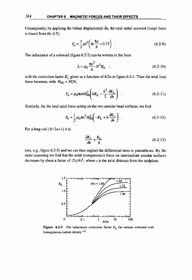
314 CHAPTER 6 MAGNETIC FORCES AND THEIR EFFECTS
Consequently, by applying the virtual displacement &, the total radial outward (loop) force is found from (6.-2-5):
The inductance of a solenoid (figure 6.2-2) can be written in the form n
(6.2-9)
(6.2-10)
with the correction factor KL given as a function of W2a in figure 6.2-3. Thus the total loop force becomes, with H m = Nl/h ,
Fa = &mhH& ( hK L-$%).
Similarly, for the total axial force acting on the two annular head surfaces, we find
Fh =-&ni12H&(-KL+h%) 1 2 dh ‘
For a long coil ( h / 2 a n 1) it is
<& dh h
(6.2-1 1 )
(6.2- 12)
(6.2-13)
(see, e.g., figure 6.2-3) and we can thus neglect the differential term in parentheses. By the same reasoning we find that the axial (compression) force on intermediate annular surfaces decreases by about a factor of ( 2 ~ / h ) ~ , where z is the axial distance from the midplane.
1.0 -
0 0.1 10 100 I h12a
Figure 6.2-3 homogeneous current density I.’”.
The inductance correction factor K, for various solenoids with
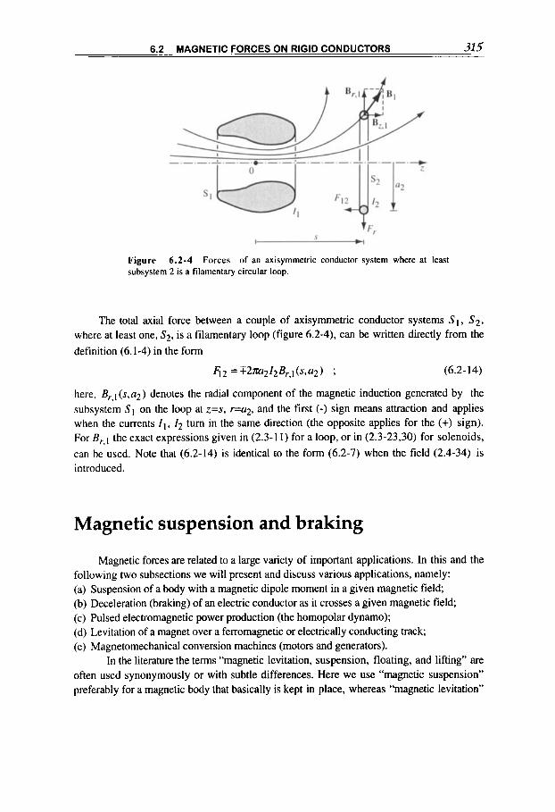
6.2 MAGNETIC FORCES ON RIGID CONDUCTORS 315
Figure 6.2-4 Forces of an axisymmetric conductor system where at least subsystem 2 is a filamentary circular loop.
The total axial force between a couple of axisymmetric conductor systems SI, S2. where at least one, S2, is a filamentary loop (figure 6.2-4). can be written directly from the definition (6.1-4) in the form
42 =T2m2I2Br,1(s,a2) ; (6.2- 14)
here, Br,] (s,a2) denotes the radial component of the magnetic induction generated by the subsystem SI on the loop at z=s, r=q, and the first (-) sign means attraction and applies when the currents 11, I2 turn in the same direction (the opposite applies for the (+) sign). For Br,l the exact expressions given in (2.3-1 1) for a loop, or in (2.3-23.30) for solenoids, can be used. Note that (6.2-14) is identical to the form (6.2-7) when the field (2.4-34) is introduced.
Magnetic suspension and braking
Magnetic forces are related to a large variety of important applications. In this and the following two subsections we will present and discuss various applications, namely: (a) Suspension of a body with a magnetic dipole moment in a given magnetic field; (b) Deceleration (braking) of an electric conductor as it crosses a given magnetic field; (c) Pulsed electromagnetic power production (the homopolar dynamo); (d) Levitation of a magnet over a ferromagnetic or electrically conducting track; (e) Magnetomechanical conversion machines (motors and generators).
In the literature the terms “magnetic levitation, suspension, floating, and lifting” are often used synonymously or with subtle differences. Here we use “magnetic suspension” preferably for a magnetic body that basically is kept in place, whereas “magnetic levitation”
316 CHAPTER 6 MAGNETIC FORCES AND THEIR EFFECTS
is related to magnetic bodies that can move freely in some directions. The basic applications mentioned before also lead to various arrangement used in
practice. A typical example is frictionless magnetic bearings used in ultracentrifuges and for diagnostic^^.^^, where the rapidly spinning body (shaft) is suspended magnetically. This can be obtained in principle by a variety of combinations between the supporting field base (permanent, normal conductive, or superconductive magnets) and the suspended body (superconductor, ferromagnetic material, electric conductor, and superconductive, normal conductive, or permanent magnets); the characteristics of some of these arrangements can be inferred from the discussion of the following examples.
Magnetic dipole suspension
The suspension in a magnetic field of a magnetized body or of a current-canying conductor can be determined by applying the appropriate force expressions found in section 6.1. One convenient way to tackle this problem is to attribute a magnetic dipole moment p to the body or conductor and determine the force through (6.1-34),
F = (p.V)B = V(p.B) . (6.2- 15)
Let us recall that (figure 6.2-5):
this force acts predominantly in the direction of the prevailing field gradient (6.1-34); it is maximum when p is aligned with B , and points towards increasing B when p . B is positive, and vice versa (6.1-34); however, the dipole tends to rotate as a result of the torque T = p x B, so as to align
on the axis of an axisymmetric field system, as the dipole becomes aligned (p+p,), the
force (6.1-34) reduces to the only component
p to B (6.1-37);
(6.2- 16)
(derivatives with respect to z will be indicated by a dash); the dipole moment of a sphere with permanent uniform magnetization M is (2.1-69)
4 p = - m 3 M 3 , (6.2-17a)
but if the magnetization M due to the susceptibility (1.1 - 19). zrn = pR - 1, is induced by a (homogeneous) field HO it is (2.1-78),
or approximately
(6.2- I7b)

6.2 MAGNETIC FORCES ON RIGID CONDUCTORS 317
P E V X m H O (6.2-17~)
3 where V is the volume of the (approximately spherical) magnetic body (V = 4m /3)
and we have neglected the factors ( l+~ , , / 3 ) ; - ' on the right-hand side because (x,,(<< 1 for para- or diamagnetic materials (table 1.1-11); in particular, for a superconducting or fully diamagnetic sphere ( p ~ 3 0) we obtain [see also (2.1-31)]
(6.2-17d) 3 2
p = - - V H o .
With these elements, various magnetic suspension arrangements can be described, as used in practice or in demonstration experiments. Here we choose to analyze in particular diamagnetic suspension, which is an interesting method applying to practically any mater- iaP4' because diamagnetism is a general property of atoms and molecules, as we will see in section 8.3. We consider a diamagnetic object placed on the axis of an axisymmetric field configuration (figure 6.2-5) having the axial component B,. The magnetic force (6.2-16,17),
Figure 6.2-5 Suspension force Fz (here acting against the gravity force -me) in the field gradient of a loop, for a diamagnetic (or superconducting) and a magnetized (para- or ferromagnetic) sphere. Since the field gradient increases towards the center of the loop, the diamagnetic sphere can have an equilibrium position where FZ = -mg (however, stability is attained only near z = 0.5a from the center); on the contrary, the position of the magnetized sphere is unstable and can be held in position only by a feedback mechanism acting on the field strength (i.e.. the current in the loop).
318 CHAPTER 6 MAGNETIC FORCES AND THEIR EFFECTS
must be balanced against its gravity F = pVg (g is the gravitational acceleration, p the material density) so that we have the equilibrium condition
Diamagnetic materials typically have pll~,,, I z lo8 kg. m-3 [water 1.13, graphite (the smallest value) 0.131, so that with a high field magnet producing B, = 10 - 15 T over Al = 0.1 m at the muzzle (see later on) it may be possible to suspend practically any (diamagnetic) object (plastic, water, live animals, etc.).
Practical suspension requires stability around the equilibrium point z, defined by (6.2-18b): Vertical or radial deviations must induce restoring forces, that is, the total energy of the object,
W(z)=pVgz+lXml VB:/2& . (6.2- 19a)
must be at a minimum (i.e., increase away from the equilibrium point):
fi > 0 (vertical stability) - d2W > 0 (radial stability) . (6.2-19b) dZ2 ' &2
[For the magnetic energy obtained as the field is increased in the diamagnetic object from 0 to B2 see (6.1-38, 39).]
The stability conditions are thus:
(Bi)2 + BzBY> 0, for vertical stability , (6.2-20a)
and, with (2.1-24),
(B;)2 - 2BzBg> 0, for radial stability . (6.2-20b)
We probe these conditions with a loop as in figure 6.2-5. From (2.3-7) we get
(6.2-21)
which is maximum at the inflection point zi = a / 2 defined by B;(zi) = 0, where obviously both stability conditions are satisfied. Introducing the expressions of BE, B;, B: and solving (6.2-20a,b) we find that the stability zone extends around zi from the lower value z,
6.2 MAGNETIC FORCES ON RIGID CONDUCTORS 319
determined by vertical stability to the upper radial stability value z , : z,< z < z,, where I, = a / J ? =0.378a, z , =a&% = 0 .633~ ; that is, stability is attained over an axial length of only 0 .255~.
Similarly, calculations can be performed with the magnetic field expressions given for the thin solenoid in (2.3-19), (6.4-28), thick solenoid in (2.3-35), Bitter solenoid in (2.3- 39). disc in (2.3-37), multiloop systems in (2.3-13,14,15), and for other simple conductor arrangements through the theory presented in section 2.3. It will be found, as for the loop, that the stability ranges are very small in comparison to the coil dimensions.
The above analysis is idealized in various aspects, in particular, it is assumed that the variation of the field be small over the dimension of the object. Nevertheless, it defines some necessary conditions for obtaining diamagnetic suspension. For example, it requires that the equilibrium point z, [obtained through (6.2-18b) by an appropriate field magnitude] be placed within the stability range (rv,rr) [derived from a purely geometric condition of the specific magnet]. If z, is below z,, the object falls; if z, is above z,, the object moves radially away from the axis, where it experiences a smaller field gradient (2.1- 24), and then eventually falls.
Comparable suspension of a paramagnetic object in the axisymmetric configuration of figure 6.2-5 is unstable. In this case, from (6.1-38) we find that the magnetic energy term in (6.2-19a) has a negative sign, and so have the left-hand sides of (6.2-20a,b); thus (at least at the inflection point where B c = 0) there can be no stability. The instability of para- or ferromagnetic objects in a magnetic field can be expressed in the form of a general
(we will find a further example in the levitation shown by figure 6.2-10).
The direct dependence of the magnetic force from the field gradient, as shown in (6.2- 15,16,18), is the base of the High-Gradient Magnetic Separation (HGMS) technique643, which makes it possible to separate para- or weakly ferromagnetic materials from nonmagnetic (diamagnetic) materials in a magnetic field region possessing large gradients. [Another, more selective but less powerful process will be mentioned in connection with (6.4-99).] Various arrangements are used, according to the separation process under ons side ration^^^. In a typical setup, a transverse magnetic field is applied to grids of thin magnetic wires. Paramagnetic particles are attracted and stick on the wire surface where the field gradient is highest (see qualitatively in figure 2.1-9). In this way it is possible, for example, to extract unwanted magnetic impurities from a feed pumped through the grids. After the collection surface on the wires is saturated, the magnetic impurities are flushed away with the magnet switched off.
Magnetic bra king
Consider an electrically conducting sheet permeated with a magnetic field (figures 6.2- 6,7). When the sheet moves, eddy currents are induced that interact with the field to give
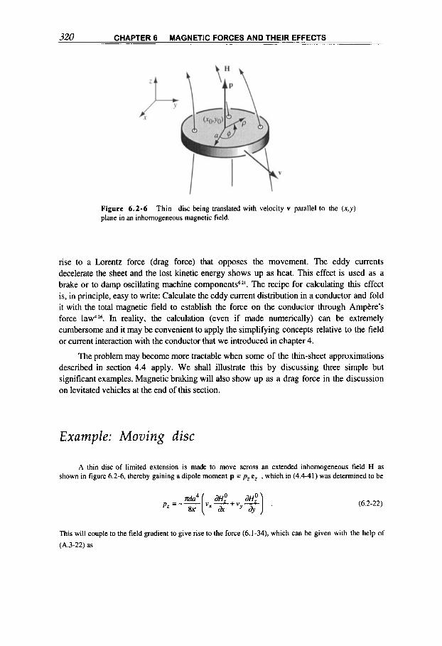
320 CHAPTER 6 MAGNETIC FORCES AND THEIR EFFECTS
Figure 6.2-6 Thin disc being translated with velocity v parallel to the (x ,y ) plane in an inhomogeneous magnetic field.
rise to a Lorentz force (drag force) that opposes the movement. The eddy currents decelerate the sheet and the lost kinetic energy shows up as heat. This effect is used as a brake or to damp oscillating machine components621. The recipe for calculating this effect is, in principle, easy to write: Calculate the eddy current distribution in a conductor and fold it with the total magnetic field to establish the force on the conductor through Ampkre's force law426. In reality, the calculation (even if made numerically) can be extremely cumbersome and it may be convenient to apply the simplifying concepts relative to the field or current interaction with the conductor that we introduced in chapter 4.
The problem may become more tractable when some of the thin-sheet approximations described in section 4.4 apply. We shall illustrate this by discussing three simple but significant examples. Magnetic braking will also show up as a drag force in the discussion on levitated vehicles at the end of this section.
Example: Moving disc
A thin disc of limited extension is made to move across an extended inhomogeneous field H as shown in figure 6.2-6, thereby gaining a dipole moment p = p,e, , which in (4.4-41) was determined to be
p =-- z4( v,-+v,- d z o dHo]
?Y (6.2-22)
This will couple to the field gradient to give rise to the force (6.1-34). which can be given with the help of
(A.3-22) as

6.2 MAGNETIC FORCES ON RIGID CONDUCTORS 321
(6.2-23)
Since V x H = O in current free space, so from table A.3-11. dHx/& =dH,Idx, ...., and the force
components can be rewritten into a braking force parallel to the (x,y) plane
(6.2-24) dH dH
Fp.K = MZ 2 ' Fp.v =wz -$ '
and a [evitation force normal to it
JH Fp,z = Wr -$
The dissipated Joule heat per unit time is
and with the solutions (4.4-38.40) yields
(6.2-25)
(6.2-26)
(6.2-27)
With no other forces involved and with (4.4-41), this corresponds exactly to the work done per unit time
against the braking force
-W" =Fp . V = Fp,x~c + Fp.y~y , (6.2-28)
that is, the braking energy shows up as Joule heat. If the coordinate system is chosen so as to align v with the y-axis (v = 0). then from (6.2-27)
If, furthermore, we assume the gradient of H! also to align with this axis, then from (6.2-22,24)
Fp,y = - L A 2 d vy[%] 2
8kK
(6.2-29)
(6.2-30)
This expression clearly points out the dependence of the braking force and the dissipated energy on the disc
area A = no2, on the thickness and velocity, and on the field gradient.
Example: Moving sheet The complementary example, where an extended sheet moves across a well-defined and limited
magnetic field area A = 4ab. is shown in figure 6.2-7. The total induced current flowing in the x-direction
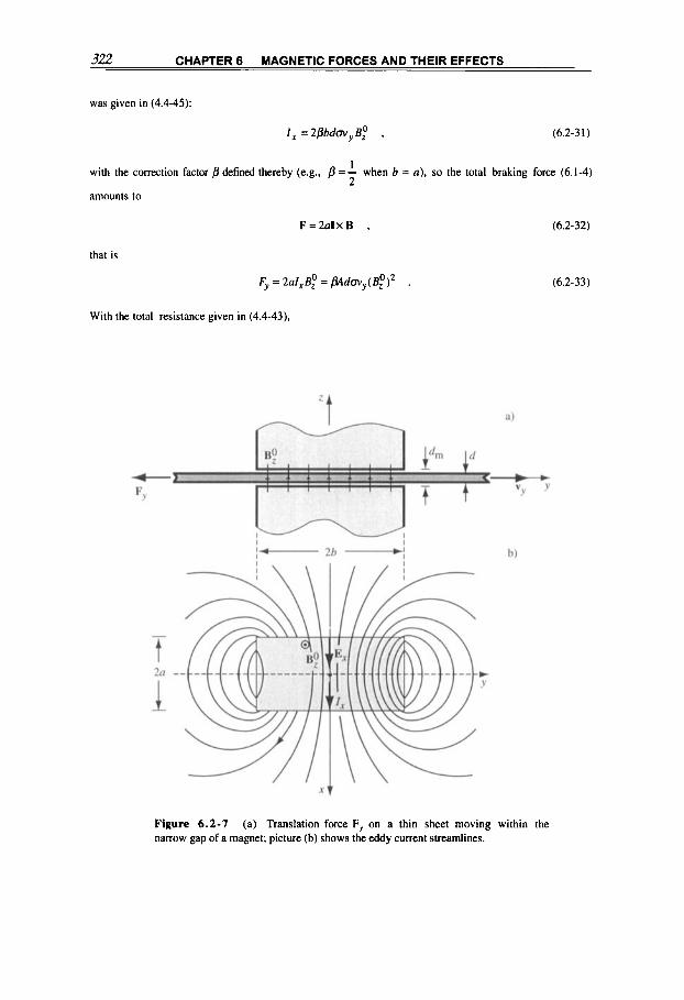
322 CHAPTER 6 MAGNETIC FORCES AND THEIR EFFECTS
was given in (4.4-45):
I , = 2pbdrn7, B," . (6.2-31)
1
2 with the correction factor p defined thereby (e.g., p = - when b = a), so the total braking force (6.1-4)
amounts to
P=2aIxB , (6.2-32)
that is
Fy = 2aIxB: = ~ d a v , ( B ~ ) *
With the total resistance given in (4.4-43).
(6.2-33)
Figure 6.2-7 (a) Translation force F,, on a thin sheet moving within the narrow gap of a magnet; picture (b) shows the eddy current streamlines.

323 6.2 MAGNETIC FORCES ON RIGID CONDUCTORS .-
the total dissipated Joule heat per unit time is
W, = RI: = pAdm;(B:)2 ,
that is, exactly the braking work done per unit time W, =F. v = Fyvy .
(6.2-34)
Example: Rota t ing sheet The concepts and results of the previous example can easily be applied to a disc with radius ro
rotating with angular velocity w = v / r , a geometry that more directly reflects many braking and damping
applications.
Consider first the example shown in figure 6.2-8, where an axial field threads a small rectangular zone
of the disc with area A = 4ab at distance r from the axis (obtainable from a magnet with a small gap, as in
the previous figure). From the equation of angular momentum [see also (6.4-21)]
dw dt '
M - = T (6.2-35)
where the moment of inertia M of the homogeneous disc with mass density p and the torque T with (6.2-31)
are
Figure 6.2-8 Braking of a rotating disc by a magnetic field B," applied by a magnet in a rectangular zone 2a x 26.

324 CHAPTER 6 MAGNETIC FORCES AND THEIR EFFECTS
n M = - p d '2 '0 * (6.2-36a)
2 T = -rQ = -2ar / ,E f = -w2@ do(B:) , (6.2-36b)
we find the solution describing the reduction of angular velocity o with time:
(6.2-37) 1 M p r2A d a ( B f ) 2 '
O=Ooe-"r , ,r=-
Here, the correction factor p will be only slightly different from that given in (4.4-44) for the infinite sheet; if it is required precisely, it can be calculated similarly as for the sheet43.
Homopolar generator
The principle of the homopolar generator or dynamo is again based on Faraday's law (1.4-8a); that is, a voltage V appears between the center and the rim of a metallic disc (rotor) in an axial field B, rotating with angular frequency w = v / r :
a 2 a
2 0 V = J ( v x B ) .dr=--wB, . (6.2-38a)
Of the many arrangements in use, we will consider here the case of a self-excited generator (figure 6.2-9a), where the field B, is produced by the current output of the generator itself, so that for the emf generated across the rotor we write
(6.2-38b) V = a I w , B z = 2 a I / a 2 ,
where a is a machine constant and I the total current. Specifically, we are looking for the power pulse fed into a lumped, constant R , L-
circuit by a rotor turning at initial frequency u g after the switch S is closed at time t = O .
(For the startup an externally generated small magnetic field is necessary, but this field plays no role after the generator comes to power, as we will see.) The equation describing the electric circuit is then
(6.2-39) dl dt
L - + I ( R - ~ ~ ) = O .
The mechanical aspect of the problem is taken care of by the angular momentum equation (6.2-35). Here the torque with (6.2-38b) is
a T=-JIB,rdr=-ct!l 2 ,
0 (6.2-40)
so that we have

6.2 MAGNETIC FORCES ON RIGID CONDUCTORS 325
b)
0 time
Figure 6.2-9 Homopolar generator: (a) Schematic rendering, indicating the electric circuit with total. constant resistance R and inductance L of the system; (b) current pulse output from a rotor initially turning at frequency wg.
M - = - d 2 , dw dr
(6.2-41)
where M is the moment of inertia of the rotating structure.
wo > w,, where From (6.2-39) we see that a current rise ( I - ' dlldt > 0) can be obtained only if
W, = R l a (6.2-42)
is the critical angular frequency of the system. After eliminating t from (6.2-39.41) and integrating, we find
(6.2-43) 2 M 2 I +-(w-w,) = A ; L
here A is an integration constant, which is determined by the initial condition ( t = 0): w = mu, I = I , (as has been mentioned, to start the generator we must assume an initial current I0 or an outer field H 0 ) . From (6.2-39,41,43)
I = (6.2-44a) cosh{a(r - tm),/(A/ML}
with
(6.2-44b)
Clearly, maximum current Im is obtained for t = t,-that is, when the hyperbolic cosine is at its minimum*-' and equal to one. Then, assuming the initial current to be small,

326 CHAPTER 6 MAGNETIC FORCES AND THEIR EFFECTS
so that A = M(w0 - w,)~ 1 L , we find (figure 6.2-9b)
(6.2-45a)
(6.2-45 b)
For the system efficiency (transformation of kinetic energy into magnetic energy in the load inductance h) we have
(6.2-46)
The last three equations show (at least approximately) the influence of the various parameters on the performance of the machine. For example, a satisfactory efficiency is obtained only when the inductance of the generator and the leads (where L = & + LL) is small when compared to the load inductance LL and when wc << wo . A more quantitative
discussion requires the machine parameter a to be known. The two main problems limiting the performance of this generator type are low output
voltage and contact problems, mostly at the peripheral brush, caused by the high speed of the rotor. The advantage lies in the solid mechanical structure of the rotor, which can be identical to the flywheel. In high-performance systems, it is convenient to separate the two elements because the peripheral velocity on the rotor is limited to about 200 m / s by contact problems (even if liquid metal contacts and jets are used). This velocity is about an order of magnitude lower than the limit imposed by mechanical stress.
The most common magnetomechanical pulse generator however is the alternator, which will be discussed later, in connection with figure 6.2-13. Although it is basically an oscillating emf generator, by appropriate electrotechnical means it can also be used as unidirectional current pulse generator. The problem can then be treated similarly to that of the homopolar circuit. The advantage of such a machine over a homopolar generator is that no gliding or liquid contacts (which can seriously limit the power output) are present in the main circuits and that a high-voltage output is possible. On the other hand, the machine, and in particular the rotor, is generally more complicated.
Magnetic levitation
Various arrangements for high-speed ground transportation based on magnetically levitated vehicles (MAGLEV) over a fixed magnetic or conducting track have been proposed and tested experimentally, and a few are ready to enter commercial application622.
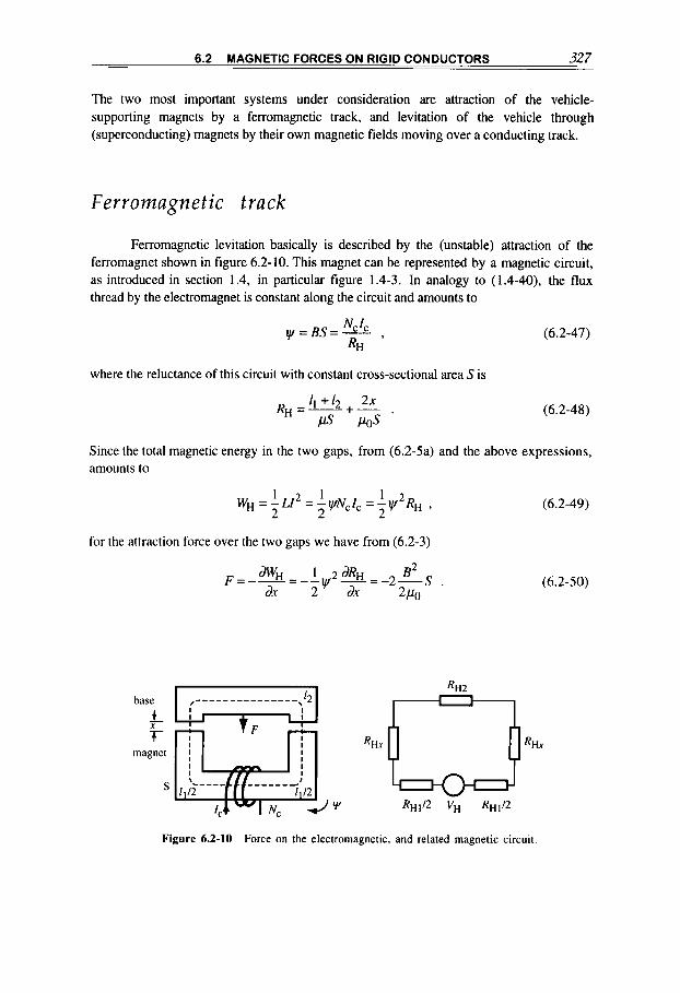
6.2 MAGNETIC FORCES ON RIGID CONDUCTORS 327
The two most important systems under consideration are attraction of the vehicle- supporting magnets by a ferromagnetic track, and levitation of the vehicle through (superconducting) magnets by their own magnetic fields moving over a conducting track.
Ferro m a p et ic track
Ferromagnetic levitation basically is described by the (unstable) attraction of the ferromagnet shown in figure 6.2-10. This magnet can be represented by a magnetic circuit, as introduced in section 1.4, in particular figure 1.4-3. In analogy to (1.4-40), the flux thread by the electromagnet is constant along the circuit and amounts to
where the reluctance of this circuit with constant cross-sectional area S is
(6.2-47)
(6.2-48)
Since the total magnetic energy in the two gaps, from (6.2-5a) and the above expressions, amounts to
WH =-W2 1 =-vNcIc 1 =-v 1 2 RH , 2 2 2
for the attraction force over the two gaps we have from (6.2-3)
(6.2-49)
(6.2-50)
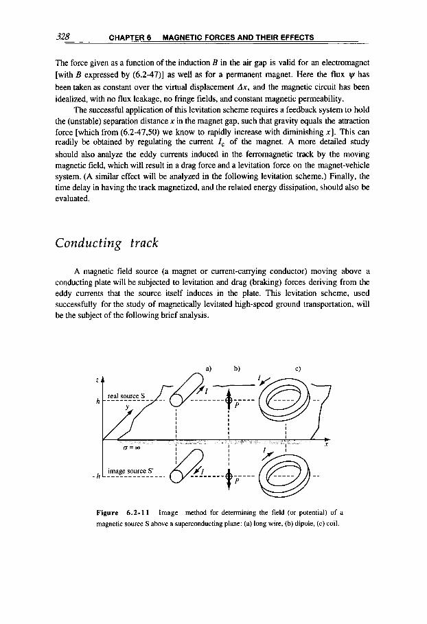
328 CHAPTER 6 MAGNETIC FORCES AND THEIR EFFECTS
The force given as a function of the induction B in the air gap is valid for an electromagnet [with B expressed by (6.2-47)] as well as for a permanent magnet. Here the flux I/ has been taken as constant over the virtual displacement Ax, and the magnetic circuit has been idealized, with no flux leakage, no fringe fields, and constant magnetic permeability.
The successful application of this levitation scheme requires a feedback system to hold the (unstable) separation distance x in the magnet gap, such that gravity equals the attraction force [which from (6.2-47,SO) we know to rapidly increase with diminishing XI. This can readily be obtained by regulating the current I , of the magnet. A more detailed study should also analyze the eddy currents induced in the ferromagnetic track by the moving magnetic field, which will result in a drag force and a levitation force on the magnet-vehicle system. (A similar effect will be analyzed in the following levitation scheme.) Finally, the time delay in having the track magnetized, and the related energy dissipation, should also be evaluated.
Conducting track
A magnetic field source (a magnet or current-carrying conductor) moving above a conducting plate will be subjected to levitation and drag (braking) forces deriving from the eddy currents that the source itself induces in the plate. This levitation scheme, used successfully for the study of magnetically levitated high-speed ground transportation, will be the subject of the following brief analysis.
Figure 6.2-1 1 Image method for determining the field (or potential) of a
magnetic source S above a superconducting plane: (a) long wire, (h) dipole, (c) coil.
6.2 MAGNETIC FORCES ON RIGID CONDUCTORS 329
To start with, we consider the levitation of a field source S over a superconducting plane, as shown in figure 6.2-1 1, a classical example which is solved by the image method2': The magnetic field (or the scalar or vector potentials) in this configuration is obtained by substituting the plane with a negative source image S', thus vectorially adding the fields (or the potential) of the two sources taken independently. With the resulting tangential field at the surface [as also required by the boundary condition (1.5-12)], the surface eddy current density can be calculated (but often, as we shall see below, it will not be necessary).
Consider the levitation force of the first two sources shown in figure 6.2-1 1. We can avoid calculating the eddy currents by giving the field component H, generated by the image source S' at the position S, thus obtaining the force acting on S. For the long conductor carrying the current I at height h above the superconducting plane, from (2.1- 37). (6.1-4,5) we obtain
(6.2-51)
whereas for the dipole with moment p aligned to the z-axis from (2.2-53), (6.2-15) we obtain
For the coil we use (6.2-7a) to formally write
(6.2-53)
where L12 is the mutual inductance between the coil at S and its image at S'. It can be calculated with (2.4-5), or in the case of the filamentary approximation with (2.4-9). Analytic expressions for 4 2 can be founded for coils with simple geometries-for example, rectangular coils6 12 or circular filamentary coils, see (2.4-26).
The situation changes if the supporting sheet has finite electric conductivity, since the eddy currents (whether generated by the source S with a time dependent field or by moving along the sheet) will decay away.
A general solution, which follows in a natural way from the idealized image method, was proposed by Maxwell and leads to the so called receding i m g e method. Consider an arbitrary (time-dependent or moving) magnetic source S, characterized (for example) by its given magnetic scalar potential @ S ( x , y , z ; t ) , which induces the eddy current pattern i(x,y;r) in the thin conducting sheet. It can be shown6" that the potential generated by these currents at the position of the source is
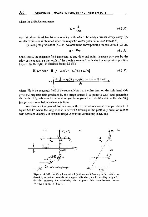
330 CHAPTER 6 MAGNETIC FORCES AND THEIR EFFECTS
where the diffusion parameter
(6.2-55)
was introduced in (4.4-40b) as a velocity with which the eddy currents decay away. (A similar expression is obtained when the magnetic vector potential is used instead'".)
By taking the gradient of (6.2-54) we obtain the corresponding magnetic field (2.1-2),
H = - V @ . (6.2-56)
Specifically, the magnetic field generated at any time and point in space (x,y,z;f) by the eddy currents that are the result of the moving source S with the time-dependent position [ xo( t ) , yo(t), zo( t ) ] is obtained from (6.2-54):
H(x,y,z;t) = -H,[x - xo(t),y - y0(t),z + Z O ( ~ ) ] (6.2-57)
m
d H ~ [ x - ~ O ( r ) , y - y ~ ( r ) , z + z o ( t - z ) + w z ] dz , -4 0 dz
where H s is the magnetic field of the source. Note that the first term on the right-hand side gives the magnetic field produced by the image source S' at point (x,y,z;t) and generating the fields -Hs; whereas the second integral term gives the reduction due to the receding images (as shown below) when w is finite.
We illustrate this general formulation with the two-dimensional example shown in figure 6.2-12, where the long wire with current I flowing in the positive y-direction moves with constant velocity v at constant height h over the conducting sheet, thus
Figure 6.2-12 (a) Very long wire S (with current I flowing in the positive y- direction, away from the reader) moving over thin sheet, and its receding images S': (b) the geometry for calculating the magnetic field contributions, where r2 =(2h+nwAt)' + ( r ~ v A t ) ~ .
6.2 MAGNETIC FORCES ON RIGID CONDUCTORS 331
x o ( t ) = v t , yo = o , Q = h . (6.2-58)
In this coordinate system, the field components of the source term H s ( x . 2 ) are from (2.1-
36b)
(6.2-59)
The magnetic field generated by the eddy currents (i.e., by the receding image source -Hs .x) at the position of the wire ( x = vr , z = h) thus follows from (6.2-57),
Hx = -[ H s , x ] x = o -wI%] x=vr d7 , (6.2-60a)
z=2h z=2h+w7
dz , (6.2-60b) x=vr
z=2h z=2h+wr
and finally we obtain
(6.2-61) I vw , H =-- ~
I v2 H =--- 4 ~ h v 2 + w 4nh v 2 + w 2 '
The levitation ( FL) and drag ( FD) force components exerted by the field of the receding image source on the current carrying and sidewise moving wire are, from (6.1-4),
(6.2-62a) p l L v L 4 7 r h V 2 + , 2 '
FL = F, = -I/.I,Hx = --
When the sheet is superconducting ( w + O), we obtain the levitation without drag already established in (6.2-51).
The forces on other magnetic sources can be calculated similarly by starting from (6.2-60), with the appropriate source term Hs6.34. For example, for a dipole source with moment p (figure 6.2-1 lb) moving with constant velocity v at constant height h over a thin sheet, the lift force632 is
(6.2-63)
[see (6.2-52)]. According to the receding image method, the eddy current configuration (induced by

332 CHAPTER 6 MAGNETIC FORCES AND THEIR EFFECTS
the source S) can be replaced by a (continuous) set of image sources S' that lag behind and recede away as a wake from the sheet with velocity w , as shown in figure 6.2-12a. In our example of the uniformingly moving wire, it can, in fact, be shown that summing up the field contributions (6.2-59) of the receding image wire S' at the place of the real wire S (figure 6.2-12b) gives the result (6.2-60). In this connection it can also be seen that with the virtual displacements Ax = vAr, Az = wAr and because of the summation process, we find quite in general (valid for any type of source)
F H & w &=A=-=- FL H, AX v '
(6.2-64)
as already obtained in the special case (6.2-62b): The ratio of drag over levitation force diminishes with increasing velocity v.
The previous levitation results are based on the assumption of a thin sheet d (< h, d <( 6, where the appropriate approximation for the skin depth (4.2-29) (see in figure 4.2- 5) here is
V , v = - . 1
h (6.2-65)
A vehicle levitating at h = 10 cm above a d = 1 cm-thick aluminum track [ o = 36 x lo6 (52. m)-'] will give rise to a diffusion velocity (6.2-55) of w = 4.5 m / s ; at the typical upper and lower-limit velocities of v = 150 m/s (+ 540 km/h) and 30 m/s (+ 110 km/h), the skin depths (6.2-65) are 2.2 and 5 mm, respectively. These figures show that in practice the thin sheet approximation condition d <( 6is most often not satisfied; the correct picture is rather that of a very (infinitely) thick track.
How will the thick sheet results differ from the thin sheet formulae given above? At high velocities the lift force FL (6.2-62a) will not differ much (for v M w it is anyway at nearly its ideal image-maximum), contrary to the drag Fo (6.2-62b). It is to be expected that a reasonable approximation for Fo is obtained by substituting 26 + d (what counts is the current-carrying sheet of thickness 26, the rest of the conductor plays practically no role) in the diffusion velocity (6.2-55), such that from (6.2-64) we obtain
(6.2-66)
and, in fact, this expression is confirmed (in the high-velocity limit) by an analyt~c calculation for a long wire moving over a conducting half-space6 33. These considerations on the FL, Fo- forces in relation to a thick sheet are valid in general (for the reason mentioned before) and not limited to the moving long wire arrangement.
6.2.- MAGNETIC FORCES ON RIGID CONDUCTORS 333 ~ .- - - - .- . .-
Magnetomechanical machines
One of the main reasons for the extensive penetration of electricity in today's world is the relative simplicity and compactness of the machines that convert mechanical power into electricity and vice versa. The most widely used electromechanical device is the magnetic- field-type rotating machine. We have already discussed one particular example, the dc homopolar generator, in connection with figure 6.2-9. Here we look at the more general arrangement of a rotating machine, which implicitly includes both the magnetomechanical power generators and motors but limit our discussion to a few basic considerations only. The variety of generator types and particularly of motors is very large, as is the range of more than 10" over the magnetomechanical power they handle and transform: from the near-to-one gigawatt of alternating generators coupled to steam turbines down to the very small fraction of one watt absorbed by micromotors. Even an elementary discussion of this subject is well beyond the scope of this book, and we refer to the extensive literature for the specific subjects: for example, conversion principled I . large power systems' ', small motors' ' 6 , and electric drive systems6 37.
Rotating machines
In our model, a stator or armature (index s) supports two perpendicular coil pairs (indices a and b) with magnetic fluxes, ySa, y s b , and includes a rotor (index r) rotating
with angular velocity w, which also support two perpendicular coil pairs, as shown in figure 6.2-13. For this balanced two-phase machine we write:
(a) For the imposed currents
I,, = I , cosw,t , Isb = I,sinw,t , (6.2-67 a)
I , = I , cosw,t , lrb = I,sinw,t ; (6.2-67 b)
this system produces (as we know from figure 3.2-1) a resultant magnetic vector H, rotating with angular velocity w, with respect to the stator, and a vector H, rotating
with 0, with respect to the rotor, which itself rotates with w with respect to the stator. (b) For the magneticflues
(6.2-68)

334 CHAPTER 6 MAGNETIC FORCES AND THEIR EFFECTS
where L,, L, are the (constant) self-inductances of the windings, and
Msr=Moc0s@ , @ = a r + @ o (6.2-69)
is the mutual inductance between the coil (a) of the stator and the coil (a) of the rotor [as will be discussed following (6.2-73)], but note that the mutual inductance between (a,b) coils is, according to the notation in figure 6.2-13, given by M,, = Mo COS(@ - K 12).
(c) For the mechanical rorque
Tsr = (Iralsb - IrbIsa)MO cOs@ - (IraIsu - IrbIrb)MOsin@ 1 (6.2-70)
considering that the mechanical torque between the (sa) stator coil and the (ra) rotor coil is given, according to (6.2-7b), by
(d) For the mechanical power
P = wq,
(6.2-7 1)
(6.2-72)
With the use of the above equations and of well-known trigonometric identities* ' [see also in (3.2-33)] the torque (6.2-70) can be rewritten in the form
q, = -MO I,I, sin [<w - w, + w, )t + h] . (6.2-73)
Note that the assumption (6.2-69), according to which the mutual inductance M,, varies sinusoidally with rotor position, follows qualitatively from the coil arrangement shown in figure 6.2-13; but in real machines, with the stator racetrack coils wound on the surface and with a small rotor-to-stator air gap (i.e., approximately radial flux density lines), it implies that the stator .windings are arranged in such a way as to produce a radial air-gap flux density that varies sinusoidally with the rotation angle.
Because we have considered an ideal system with neither mechanical (friction) nor electric (Joule) losses, the mechanical power equals the total electric power at the stator and rotor terminals,
P = p , , p , = P , + P , . (6.2-74a)
With V,, and Vsb the induced voltages at the stator terminals, it is
(6.2-74b) ps = Isa -t Isb Vsb 9
where, for example with the magnetic flux ySa given in (6.2-68),
(6.2-74~)
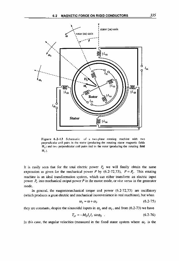
6.2 MAGNETIC FORCE ON RIGID CONDUCTORS 335 ~ _ _
Figure 6.2-13 Schematic of a two-phase rotating machine with two perpendicular coil pairs in the stator (producing the rotating stator magnetic fields H,) and two perpendicular coil pairs tied to the rotor (producing the rotating field
H r ) .
It is easily seen that for the total electric power P, we will finally obtain the same expression as given for the mechanical power P by (6.2-72,73), P = 4. This rotating machine is an ideal transformation system, which can either transform an electric input power P, into mechanical output power P in the motor mode, or vice versa in the generator mode.
In general, the magnetomechanical torque and power (6.2-72,73) are oscillatory (which produces a great electric and mechanical inconvenience in real machines), but when
w, = w + w , (6.2-75)
they are constants, despite the sinusoidal inputs in w, and w,, and from (6.2-73) we have
T,, = -MoI,I, sin& . (6.2-76)
In this case, the angular velocities (measured in the fixed stator system where 0, is the
336 CHAPTER 6 MAGNETIC FORCES AND THEIR EFFECTS
velocity with respect to the rotor, which itself rotates with w) of the resultant rotating magnetic field vectors of the stator and rotor H, and H, are identical to the angle $0 between them, and this correctly results in the above torque.
The most important generator or motor-type rotating machines can be reconducted to the model described by the above equations, in particular by the angular velocity condition (6.2-75).
Synchronous machines
The synchronous machine is defined in our model by having direct current applied to the (ra) winding of the rotor only, thus with respect to (6.2-67) it is: w, = 0, I,, = I , (const.), I r b = 0. This machine, with constant torque (6.2-76). converts the constant mechanical or electric power (6.2-72)
P = P, = -W~l,l, sin&, (6.2-77)
at the synchronous angular velocity (6.2-75),
w = w , ,
only. It is easy to understand the motor or generator operation mode (according to whether
the primary input power source is electric or mechanical) in the synchronous machine, where a constant magnetic (dipole) moment pr rotates with the rotor at the angular velocity w. The magnetic moment pr is produced by the rotor windings as in (2.2-45) and can also be associated to a permanent magnet with a northkouth pole pair (1.1-33), or to a magnetic flux iy,. In the motor mode, the rotor with its magnetic moment locks with the stator’s rotating field B, through the torque (6.1-37), T,., = pr x B,, so that w = w,, and trails this field by the angle 40, which increases with the mechanical load up to a limiting value. When this value is exceeded, the rotor falls out of synchronous operation and produces vibrating alternating torques, a detrimental situation for any type of machine.
Alternatively, in the generator mode, the magnetic flux iy, rotating with the rotor past the stator windings induces in them the emf that drives the output currents Is,, I,b, oscillating with w, = W . This generator type, called alternator, is the most common application of the synchronous-type machine and comes in large power units (from 100 up to lo00 MW electric output power) driven by steam turbines.
Induction machines
Induction machines are defined with respect to the model of figure 6.2-13 by having

6.2 MAGNETIC FORCE ON RIGID CONDUCTORS 337
the rotor circuits (ra) and (rb) each short-circuited at the terminals by a resistance R,, with the currents in these closed circuits induced from the stator. The one lumped R L circuit (ra) coupled through the mutual inductance (6.2-69). M,, , to the stator windings is described
by the differential equation
d dt dt L, + R,I, = -MoI, -[cosw,tcos(wt + 40) +sinw,t sin(m + 40)] , (6.2-78a)
which can be transformed with the trigonometric identities (3.2-33) into
dlra L, - + R,I, = -MI,(w, - w ) sin[(@, - w)t - 401 . dt
The solution is
1 7r I,=Ircos (w , -w) t - - -& ) -P [ 2
(6.2-78b)
(6.2-79)
where
and the so-called slip parameter is defined as
w, - w
U S
s=- (6.2-81)
The second RL circuit of the rotor (rb) gives rise to the identical but a/2-phase-shifted current I,b [i.e., with cos substituted by sin in (6.2-79)]. Note that the currents Ira, I r b oscillate with w, = w, - w , (6.2-75), as in the forced case (6.2-67b), but with a phase shift (-n/2-1$0 --a), whereas the stator currents Isa. Isb are as in (6.2-67a). The
induced currents Ira, I,, build up in the rotor circuits when the rotor velocity w is slower (or faster) than the rotating field velocity w,, thus W , # O : synchronous running of the rotor, w, = 0, is not possible because no rotor currents would be induced.
We are now in a position to calculate all the relevant parameters of this rotating machine as before. The simplification of the torque (6.2-70) is more tedious, and after successive application of the trigonometric identities (3.2-33) we find
T,r = (6.2-82)
which is a constant value, as was to be expected because the angular velocity condition (6.2-75) holds. The power balance in this rotating system,
P, = P+ P, , (6.2-83)
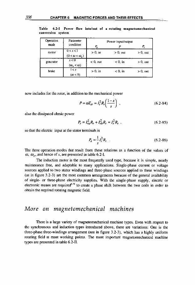
338 CHAPTER 6 MAGNETIC FORCES AND THEIR EFFECTS
Operation mode
motor
generator
brake
Table 6.2-1 Power flow intolout of a rotating magnetomechanical conversion system
Parameter Power input/output condition
P pr pe O C s < ' > 0, in > 0, out > 0, out
O < 0, out < 0. in > 0. out
(0 c 0 c W,)
(0, c 0)
> 0. i n < 0, in > 0, out I < ,
(0 < 0)
now includes for the rotor, in addition to the mechanical power
P = wq, = I;R,(?) , (6.2-84)
also the dissipated ohmic power
P, = I : ~ R , + I;~,R, = I;R, ,
so that the electric input at the stator terminals is
(6.2-85)
(6.2-86) P , = - I , R , 1 2 . S
The three operation modes that result from these relations as a function of the values of w, w,, and hence of s, are presented in table 6.2-1.
The induction motor is the most frequently used type, because it is simple, nearly maintenance free, and adaptable to many applications. Single-phase current or voltage sources applied to two stator windings and three-phase sources applied to three windings (as in figure 3.2-3) are the most common arrangements because of the general availability of single- or three-phase electricity supplies. With the single-phase supply, electric or electronic means are. r e q ~ i r e d ~ . ~ ~ to create a phase shift between the two coils in order to obtain the required rotating magnetic field.
More on magnetomechanical machines
There is a large variety of magnetomechanical machine types. Even with respect to the synchronous and induction types introduced above, there are variations: One is the three-phase three-windings arrangement (see in figure 3.2-3), which has a highly uniform rotating field at most working points. The most important magnetomechanical machine types are presented in table 6.2-11.

. - -. - - - 6.2 MAGNETIC FORCE ON RIGID CONDUCTORS 339 -
Table 6.2-11 Magnetomechanical machines
Arrangement and coupling
rotating field in stator (torque T = p x B
linear (force F = ( p . V ) B , or F = jxB:
Type
permanent magnetic moment
reluctance
(a) synchronous (figure 6.2 - 13)
(b) induction (figure 6.2 - 13)
(c) commutator
(d) homopolar (figure 6.2 -9)
(e) linear motor
(0 rail gun (figure 6.4- 6)
(g) magnetic pump
In the synchronous machine (a), we have also included the rotors based on hysteresis and reluctance effects, since they are often used as motors636. In the first case the rotor is made of permanent-magnet material with small coercive force so that the material is magnetized cyclically by the rotating stator field. The reluctance rotor6 38 is characterized by radial entrances, thus varying magnetic resistances or reluctances, which seek (as with a permanent magnet) to align with the rotating field and to rotate with it.
The commutator types (c) comprise the large group of dc machines where the inherent ac characteristics of rotating machines are converted into dc operation by the appropriate arrangement of the contact segments (commutator) on the rotor shaft, which are in contact with the brushes on the stator. Typically, a dc motor is driven by the torque that results from the interaction of current-carrying loops on the rotor with a constant magnetic field fixed with the stator. The change in current direction (for the torque to always result in the same direction) is operated by the commutator that alternatively connects the loops with an outer dc voltage source. Often dc motors use permanent magnets for the stator magnetic field source6 393 5 ' .
The linear motor (e) is basically a linear deployment of the rotating machine; for example, there are linear induction motors625 and linear dc motors640. For a simple arrangement of the magnetic pump (g) consider a conducting fluid in an insulating duct, where a transverse field B is applied and a transverse perpendicular current j is made to flow. The resulting force F will force the fluid to flow along the duct.
Forces within a conductor
At this point it is instructive to find out how the magnetic Lorentz force (6.1-1) and, consequently, the volume force (6.1-10) act on a conductor. By its very nature, the volume
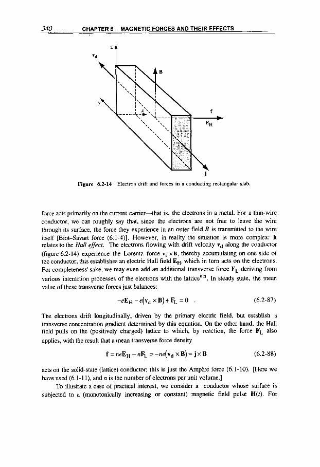
340 CHAPTER 6 MAGNETIC FORCES AND THEIR EFFECTS
vd
Figure 6.2-14 Electron drift and forces in a conducting rectangular slab.
force acts primarily on the current carrier-that is, the electrons in a metal. For a thin-wire conductor, we can roughly say that, since the electrons are not free to leave the wire through its surface, the force they experience in an outer field B is transmitted to the wire itself [Biot-Savart force (6.1-4)]. However, in reality the situation is more complex: It relates to the Hull effect. The electrons flowing with drift velocity vd along the conductor (figure 6.2-14) experience the Lorentz force vd xB, thereby accumulating on one side of the conductor; this establishes an electric Hall field EH, which in turn acts on the electrons. For completeness' sake, we may even add an additional transverse force FL deriving from various interaction processes of the electrons with the lattice' 2 ' . In steady state, the mean value of these transverse forces just balances:
- e E H - e ( v d xB)+FL = O . (6.2-87)
The electrons drift longitudinally, driven by the primary electric field, but establish a transverse concentration gradient determined by this equation. On the other hand, the Hall field pulls on the (positively charged) lattice to which, by reaction, the force FL also applies, with the result that a mean transverse force density
f = n e E H - n F L = - n e ( v d X B ) = j X B (6.2-88)
acts on the solid-state (lattice) conductor; this is just the Amp&re force (6.1-10). [Here we have used (6.1-1 l), and n is the number of electrons per unit volume.]
To illustrate a case of practical interest, we consider a conductor whose surface is subjected to a (monotonically increasing or constant) magnetic field pulse H(t). For

6.2 MAGNETIC FORCE ON RIGID CONDUCTORS 341
simplicity we take the plane case, where an outer magnetic field is applied parallel to an infinitely thick conductor (figure 6.2- 15) and the (monotonically decreasing) current density
(6.2-89) JHz ( X J ) j y ( x , t ) = - dX
is induced. In the infinitesimal layer between x and x + Ax beneath the surface, there is the current density j , ( x , f ) carried by electrons (and kept to this position by the diffusion
process), which drift at velocity
and are subject to the transverse Hall force
1 dH F,(x,r) = -evyBz = - Bz 2
n d x
or force density
dH dx
f,(x,r) = -nFx = - B 2
(6.2-90)
(6.2-91 a)
(6.2-9 1 b)
Each layer contributes with a force component per unit surface (or pressure)f,dx.
depth x that results from interaction of the magnetic field with an incompressible body Integration of the force density along the x-axis gives the hydrodynnntic pressure at
dH 1 p x ( x . f ) = -I -BZ& = p~ - - p H 2 ( x , t ) ,
o d x 2 (6.2-92)
Figure 6.2-15 The conducting half-space, to which a surface magnetic field pulse H Z ( t ) is applied.

342 CHAPTER 6 MAGNETIC FORCES AND THEIR EFFECTS
where
1 pH = ~W2(0")
dPx(xJ) = -flz- dH
is the (full) magnetic pressure related to the surface field. conductor is
dr d x .
(6.2-93)
The pressure gradient within the
(6.2-94)
Whereas the force density can be maximum at the surface layer, the full pressure appears by summation only at a certain depth, which in most practical problems can be considered approximately se the flux skin depth defined in (4.2-20).
As a further example, consider the parabolic boundaryfield (5.4- lo),
applied on a plane, infinitely thick conductor. For very high magnetic fields in the nonlinear domain [ Ho > h,, where h, is the characteristic field (5.4-1 l)], we find from (5.4- 12,16) the constant force density
whereas the surface temperature (5.4- 17) continues to increase
T(O,t)=-- Mi t . 2cv to
(6.2-96)
(6.2-97)
At a certain time the surface layer will boil off violently (see in connection with figure 6.3- 5). At low fields ( HO < hc), the surface force density obtained from (5.4-25) is also finite, but will increase with time:
(6.2-98)
6.3 MAGNETIC PROPULSION EFFECTS IN CONDUCTING SHEETS
In the previous section some overall effects related to the forces exerted by a magnetic field on rigid conductors were presented. This subject will be taken up again and extended
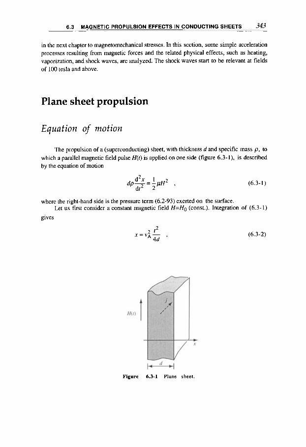
6.3 MAGNETIC PROPULSION EFFECTS IN CONDUCTING SHEETS 343
in the next chapter to magnetomechanical stresses. In this section, some simple acceleration processes resulting from magnetic forces and the related physical effects, such as heating, vaporization, and shock waves, are analyzed. The shock waves start to be relevant at fields of 100 tesla and above.
Plane sheet propulsion
Equation of motion
The propulsion of a (superconducting) sheet, with thickness d and specific mass p. to which a parallel magnetic field pulse H(t) is applied on one side (figure 6.3- I), is described by the equation of motion
(6.3-1)
where the right-hand side is the pressure term (6.2-93) exerted on the surface.
gives Let us first consider a constant magnetic field H=Ho (const.). Integration of (6.3- 1)
(6.3-2)
Figure 6.3-1 Plane sheet.
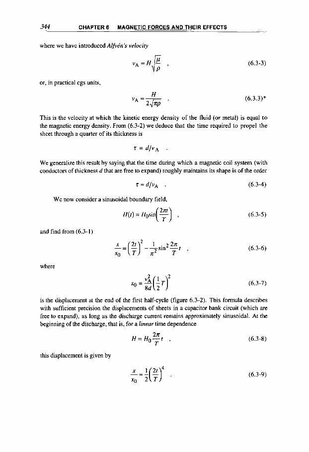
344 CHAPTER 6 MAGNETIC FORCES AND THEIR EFFECTS
where we have introduced Alfvin's velocity
,
or, in practical cgs units,
(6.3-3)
(6 .3 .3) *
This is the velocity at which the kinetic energy density of the fluid (or metal) is equal to the magnetic energy density. From (6.3-2) we deduce that the time required to propel the sheet through a quarter of its thickness is
5 = d/VA .
We generalize this result by saying that the time during which a magnetic coil system (with conductors of thickness d that are free to expand) roughly maintains its shape is of the order
z = d / v A . (6.3 -4)
We now consider a sinusoidal boundary field,
H(t) = Hos in (T) ,
and find from (6.3-1)
where
(6 .3-5)
(6 .3-6)
(6 .3-7)
is the displacement at the end of the first half-cycle (figure 6.3-2). This formula describes with sufficient precision the displacements of sheets in a capacitor bank circuit (which are free to expand), as long as the discharge current remains approximately sinusoidal. At the beginning of the discharge, that is, for a linear time dependence
2 a T
H=Ho-t ,
this displacement is given by
(6 .3-8)
"_'(")I xo 2 T (6.3-9)
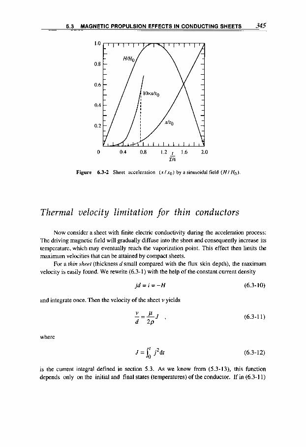
6.3 MAGNETIC PROPULSION EFFECTS IN CONDUCTING SHEETS 345
0.4 0.8 1.2 1 1.6 2.0 - 0 T/4
Figure 6.3-2 Sheet acceleration ( X / X O ) by a sinusoidal field ( H l H o )
Thermal velocity limitation for thin conductors
Now consider a sheet with finite electric conductivity during the acceleration process: The driving magnetic field will gradually diffuse into the sheet and consequently increase its temperature, which may eventually reach the vaporization point. This effect then limits the maximum velocities that can be. attained by compact sheets.
For a thin sheet (thickness d small compared with the flux skin depth), the maximum velocity is easily found. We rewrite (6.3-1) with the help of the constant current density
j d = i = - H (6.3-10)
and integrate once. Then the velocity of the sheet v yields
where
J = j2dt 0
(6.3-1 1)
(6.3-12)
is the current integral defined in section 5.3. As we know from (5.3-13), this function depends only on the initial and final states (temperatures) of the conductor. If in (6.3-1 1)
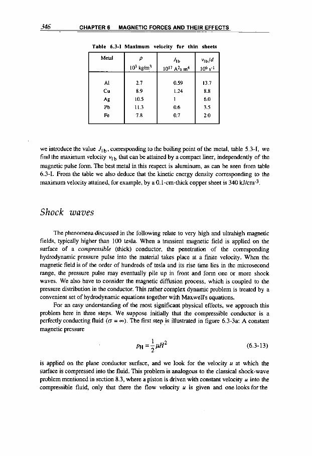
346 CHAPTER 6 MAGNETIC FORCES AND THEIR EFFECTS
Table 6.3-1 Maximum velocity for thin sheets
we introduce the value J I b , corresponding to the boiling point of the metal, table 5.3-1, we find the maximum velocity vl b that can be attained by a compact liner, independently of the magnetic pulse form. The best metal in this respect is aluminum, as can be seen from table 6.3-1. From the table we also deduce that the kinetic energy density corresponding to the maximum velocity attained, for example, by a 0.1-cm-thick copper sheet is 340 kJhn-3.
Shock waves
The phenomena discussed in the following relate to very high and ultrahigh magnetic fields, typically higher than 100 tesla. When a transient magnetic field is applied on the surface of a compressible (thick) conductor, the penetration of the corresponding hydrodynamic pressure pulse into the material takes place at a finite velocity. When the magnetic field is of the order of hundreds of tesla and its rise time lies in the microsecond range, the pressure pulse may eventually pile up in front and form one or more shock waves. We also have to consider the magnetic diffusion process, which is coupled to the pressure distribution in the conductor. This rather complex dynamic problem is treated by a convenient set of hydrodynamic equations together with Maxwell's equations.
For an easy understanding of the most significant physical effects, we approach this problem here in three steps. We suppose initially that the compressible conductor is a perfectly conducting fluid (a = -). The first step is illustrated in figure 6.3-3a: A constant magnetic pressure
(6.3-13) 1 2
is applied on the plane conductor surface, and we look for the velocity u at which the surface is compressed into the fluid. This problem is analogous to the classical shock-wave problem mentioned in section 8.3, where a piston is driven with constant velocity u into the compressible fluid, only that there the flow velocity u is given and one looks for the
pH = - p H 2
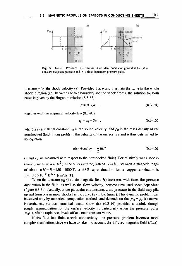
6.3 MAGNETIC PROPULSION EFFECTS IN CONDUCTING SHEETS 347
Figure 6.3-3 Pressure distribution in an ideal conductor generated by (a) a constant magnetic pressure and (b) a time-dependent pressure pulse.
pressure p (or the shock velocity V S ) . Provided that p and u remain the same in the whole shocked region (i.e., between the free boundary and the shock front), the solution for both cases is given by the Hugoniot relation (8.3-85),
P = POVSU 9 (6.3-14)
together with the empirical velocity law (8.3-93)
vs = c o + S u , (6.3-15)
where S is a material constant, co is the sound velocity, and po is the mass density of the nonshocked fluid. In our problem, the velocity of the surface is u and is thus determined by the equation
(6.3-16)
(u and v s are measured with respect to the nonshocked fluid). For relatively weak shocks
(SucccO),we have u 0~ H2 ; in the other extreme, instead, u = H. Between a magnetic range
of about pH=B=150-1OOOT, a f8% approximation for a copper conductor is
u = 1.45 x When the pressure PH (i.e., the magnetic field H) increases with time, the pressure
distribution in the fluid, as well as the flow velocity, become time- and space-dependent (figure 6.3-3b). Actually, under particular circumstances, the pressure in the fluid may pile up and form one or more shocks [as the curve ( S ) in the figure]. This dynamic problem can be solved only by numerical computation methods and depends on the p~ = m(t) curve. Nevertheless, various numerical results show that (6.3- 16) provides a useful, though rough, approximation for the surface velocity u, particularly when the pressure pulse pH ( t ) , after a rapid rise, levels off at a near-constant value.
If the fluid has finite electric conductivity, the pressure problem becomes more complex than before, since we have to take into account the diffused magnetic field H(x,t).
B3’* [ c d p , TI.

348 CHAPTER 6 MAGNETIC FORCES AND THEIR EFFECTS
In an incompressible conductor we found in (6.2-92) that the hydrodynamic pressure is
p = -p[HZ(O,r)- 1 H2(x,t)] . 2
(6.3-17)
For a real, compressible conductor (figure 6.3-4) the pressure does not substantially deviate from this distribution but extends, of course, only to a finite depth. The exact calculation of the field and pressure distribution in such a case can be done only numerically and requires a complete MHD code. We shall discuss the formulation of this general problem in chapter 8.
It is now reasonable to apply the previous results (see figure 6.3-3b) to the plane at the depth xp-that is, where (most of) the pressure appears (figure 6.3-4). Consequently, this plane acts as a piston moving at the velocity u given by (6.3-16), and it drives a pressure peak (eventually a shock) into the fluid. It should be noted that for nonlinear field diffusion ( H > h,) characterized by a relatively flat-topped diffused field, xp is about equal to the flux skin depth, xp = sq [ h, is the characteristic field (5.4-1 l)].
What happens to the layers between the surface and the plane at xp is less clear, at least on the basis of our qualitative picture. They also move into the fluid, but the velocity is dependent on their position. In addition, this part of the conductor is heated up by the diffusion process and the surface may start boiling off. Fortunately, in most practical cases the thickness of the surface layer is much smaller than the penetration depth of the pressure pulse (sq << xs) . As an example, let us consider again the parabolic surface field (6.2-95) for which at high fields ( HO > h,) from (5.4-14,22) we obtain
(6.3- 18)
whereas u and v s are approximately given by (6.3-15,16). For a copper conductor (tables 8.3-11 and VIII) with to = 1 p and at poH0 = 500 T (and poh, = 43 T ) we find
Figure 6.3-4 Pressure distribution in a fluid with finite conductivity.
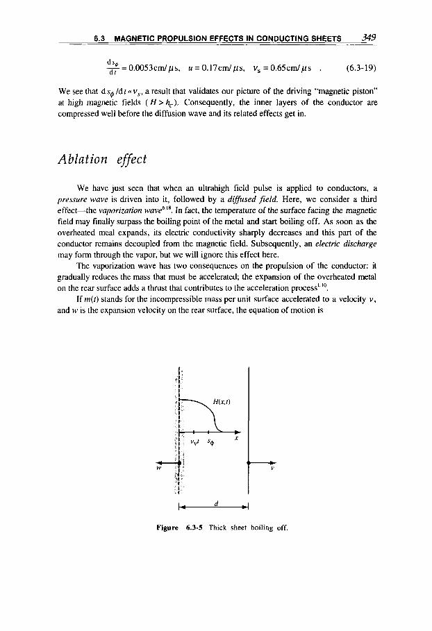
6.3 MAGNETIC PROPULSION EFFECTS IN CONDUCTING SHEETS 349
9 = O.O053cm/ps, u = 0.17cm/ps, V, = 0.65cm/ps . (6.3- 19) dr
We see that ds4 ldtccv,, a result that validates our picture of the driving “magnetic piston” at high magnetic fields ( H > hc), Consequently, the inner layers of the conductor are compressed well before the diffusion wave and its related effects get in.
Ablat ion effect
We have just seen that when an ultrahigh field pulse is applied to conductors, a pressure wave is driven into it, followed by a diffused field. Here, we consider a third effect-the vaporization wave6 In fact, the temperature of the surface facing the magnetic field may finally surpass the boiling point of the metal and start boiling off. As soon as the overheated meal expands, its electric conductivity sharply decreases and this part of the conductor remains decoupled from the magnetic field. Subsequently, an electric discharge may form through the vapor, but we will ignore this effect here.
The vaporization wave has two consequences on the propulsion of the conductor: it gradually reduces the mass that must be accelerated; the expansion of the overheated metal on the rear surface adds a thrust that contributes to the acceleration process’ lo.
If m(t) stands for the incompressible mass per unit surface accelerated to a velocity v , and w is the expansion velocity on the rear surface, the equation of motion is
Figure 6.3-5 Thick sheet boiling off,

350 CHAPTER 6 MAGNETIC FORCES AND THEIR EFFECTS
d o + ( w - V ) - = - p H h 1 2 , dt dt 2
which, after differentiation and separation, becomes
(6.3-20)
(6.3-21)
If the vaporization wave creeps into the sheet at a constant velocity vv, the accelerated mass
is reduced according to
m(t)=p(d-vvt) . (6.3-22)
Then for the special case H = Ho(const.), by integrating (6.3-21). the mass velocity
becomes
v = w+- In- , [ 2) :) (6.3-23)
where rno = pd is the initial mass and VA is Alfvtn's velocity (6.3-3). We assume that the
metal in front of the vaporization wave is heated by magnetic field diffusion to a constant temperature,
1 C, T = zw: (6.3-24)
300
E 8 ",
> a
100
t // -4
0 4ooo 8000 I2000
T (K) Figure 6.3-6 Theoretical estimate of vaporization wave velocity ' "'.
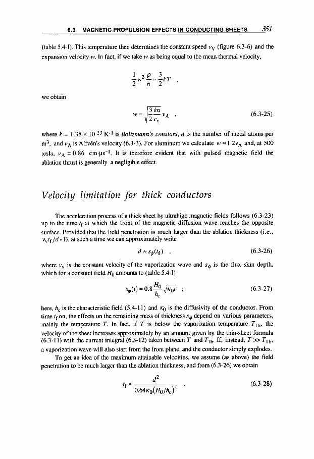
6.3 MAGNETIC PROPULSION EFFECTS IN CONDUCTING SHEETS 351
(table 5.4-1). This temperature then determines the constant speed vv (figure 6.3-6) and the
expansion velocity w. In fact, if we take w as being equal to the mean thermal velocity,
we obtain
(6.3-25)
where k = 1.38 x 10⁻²³ K-1 is Boltzmann's constant, n is the number of metal atoms per m3, and V A is AlfvCn's velocity (6.3-3). For aluminum we calculate w = 1.2vA and, at 500
tesla, V A = 0.86 cm.ps-1. It is therefore evident that with pulsed magnetic field the ablation thrust is generally a negligible effect.
Velocity limitation for thick conductors
The acceleration process of a thick sheet by ultrahigh magnetic fields follows (6.3-23) up to the time If at which the front of the magnetic diffusion wave reaches the opposite surface. Provided that the field penetration is much larger than the ablation thickness (i.e., v,tf / d (( 1). at such a time we can approximately write
d Z s $ ( t f ) , (6.3-26)
where v , is the constant velocity of the vaporization wave and s$ is the flux skin depth, which for a constant field HO amounts to (table 5.4-1)
s g ( t ) =: 0.8--JKof HO ; (6.3-27) h,
here, h, is the characteristic field (5.4-1 1) and KO is the diffusivity of the conductor. From time t f on, the effects on the remaining mass of thickness SQ depend on various parameters, mainly the temperature T . In fact, if T is below the vaporization temperature Tlb. the velocity of the sheet increases approximately by an amount given by the thin-sheet formula (6.3-1 1) with the current integral (6.3-12) taken between T and Tlb. If, instead, T >> Tlb,
a vaporization wave will also start from the front plane, and the conductor simply explodes. To get an idea of the maximum attainable velocities, we assume (as above) the field
penetration to be much larger than the ablation thickness, and from (6.3-26) we obtain n

352 CHAPTER 6 MAGNETIC FORCES AND THEIR EFFECTS
This assumption seems reasonable at least for magnetic fields smaller than 200 tesla and larger than 500 tesla, since at low temperatures we have v , = 0 and at very high temperatures the vaporization velocity tends to become constant (figure 6.3-6). In this case, also (6.3-23) can be simplified:
(6.3-29)
To obtain the maximum velocity of the thick sheet accelerated by a constant field H o . we introduce in this expression the time t f and obtain approximately
- V = 0.8p- hc2 d PKO
(6.3-30)
Note that the maximum velocity in first-order approximation [ ~ , . ( H o / h , ) ~ ~ g / d ] is independent of the magnetic field and formally very similar to that of the thin sheet. For aluminum it amounts to v = 9.6 x 10⁶ d (m.s-l)-that is, less than the thin-sheet velocity v = 13.7 x 10⁶ d (m.s-1).
Implosion of a cylindrical sheet
The implosion of a cylindrical sheet driven by an outer magnetic field is an arrangement of practical importance that is used in different experiments mainly as an energy concentrator. Ultimately, the magnetically driven implosion* 53 (and even more so, the explosive-driven implosion discussed in section 8.2) is a powerful scheme for bringing an internally trapped and heated material (plasma) to extremely high densities and temperature'.'', as studied in very high energy density p h y s i d 3 and as required in inertial confinement f i s i ~ n ~ . ~ ~ .
Compared to plane sheet propulsion, the cylindrical implosion is characterized by: (1) afixed time scale depending on the time required by the conductor to implode on its axis; ( 2 ) a minimum pressure, which is necessary to overcome the structural strength of the cylindrical shell; (3) the energy dissipation due to deformation of the imploding metal; (4) the confluence of the conductor, which towards the end of the implosion dictates the dynamics of the leading front. Most of the effects reported for the plane sheet also apply here, at least for the first half of the implosion; later, the typical implosion effects in point (4) dominate.
Here we are interested in thin conductors ( d M ' 0 ) and relatively large fields [of the order of the yield field defined by (7.2-46)], so we can neglect the effects in points (3) and (4). In section 8.2 we shall consider the implosion dynamics in more detail.

6.3 MAGNETIC PROPULSION EFFECTS IN CONDUCTING SHEETS 353
General equations
We consider a cylindrical sheet coupled to a capacitor bank in one of the two geometries shown in figures 6.3-7, 8 . If we neglect cohesion forces, in both cases the shell implodes according to the equation of motion
d2r 1 2 - m - = - p H 2 m ,
dt2 2 (6.3-31)
where m = 2nrodop is the mass of the incompressible shell per unit length. In one case (figure 6.3-7), the relation between magnetic field and total current I is
whereas, for the +implosion (figure 6.3-8) of a relatively long coil ( h N r), it is
I H = H o = h . (6 .3-33)
The equation of motion is coupled through (6.3-32,33) to the general circuit equation (see in connection with figures 4.5-1 and 8.2-1)
Figure 6.3-7 z-implosion geometry.

354 CHAPTER 6 MAGNETIC FORCES AND THEIR EFFECTS
Figure 6.3-8 $-implosion geometry.
d2(LI) d(RI) I dt2 dt C
+-+-=o , (6.3-34)
where in general both the inductance L and the resistance R contain a time-dependent component related to the implosion dynamics. This problem can be solved only by numeric methods, even when the resistance is negligible, that is R a m (although analytic approximations can be f o ~ n d ~ . ~ ~ in special cases).
Constant current driver
To get a rough idea of the implosion dynamics in the two arrangements, we shall deal with the idealized case in which the current in the circuit remains constant ( I = I,.); that is, we neglect the circuit equation (6.3-34) in order to obtain for the z-implosion (6.3-3 1,32)
(6.3- 35) d2r p I:
r - - - - - 9
dt2 - 4 R m
which, for the initial conditions t = 0, r = ro, vo = 0, and noting that dvldt = v(dv/dr), can be integrated easily:

6.3 MAGNETIC PROPULSION EFFECTS IN CONDUCTING SHEETS 355
(6.3-36)
The final speed is obtained when the shell has collapsed completely, at which point for the (outer) radius rf we get
nrf2 =2mid0 . (6.3-37)
The final velocity
(6.3-38)
following from (6.3-36) by the substitution r + ry, is to be compared to the maximum value (6.3-1 1)
(6.3-39)
which in this form also approximately holds in cylindrical geometry. From the comparison it is possible to optimize the circuit parameters and the foil dimensions.
For the @implosion under the same conditions, we use (6.3-31,33) to obtain
d2r 2 - + A r = O , with A = dt2
the solution is
r=rOcosAt ,
(6.3-40)
(6.3-41)
IvI = rOA sin A t . The final velocity, vf = QA, is clearly smaller than in the previous case (6.3-38), as to be
expected. The expressions of both cases are approximately valid also for oscillating currents
when at least one current reversal occurs and provided that we replace p with its mean value. For example, with a current of the form I = ImsinWt for tf > 2 a / w (i.e., w > 4A), we obtain the new value
(6.3-42)
A typical experimental set of parameters for each of the two implosion types is shown in table 6.3-11 (in both cases, the imploding shell is used to compress an initially trapped magnetic flux so as to obtain high magnetic fields; see section 8.2).
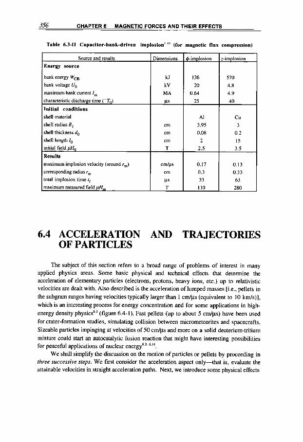
356 CHAPTER 6 MAGNETIC FORCES AND THEIR EFFECTS
Pimplosion
136
20
0.64
25
Al
3.95
0.08
2
2.5
0.17
0.3
33
I10
Table 63-11 Capacitor-bank-driven implosion' "' (for magnetic flux compression)
z-implosion
570
4.8
4.9
40
cu 3
0.2
15
3.5
0.13
0.33
63
280
Source and results
Energy source
bank energy Wcs
bank voltage U, maximum bank current I ,
characteristic discharge time ("To)
Initial conditions
shell material
shell radius R, shell thickness do
shell length I, initial field pHo
Results
maximum implosion velocity (around r,)
corresponding radius rm
total implosion time tf maximum measured field pH,,,
Dimensions
kJ
kV
MA
CLS
cm cm cm T
6.4 ACCELERATION AND TRAJECTORIES OF PARTICLES
The subject of this section refers to a broad range of problems of interest in many applied physics areas. Some basic physical and technical effects that determine the acceleration of elementary particles (electrons, protons, heavy ions, etc.) up to relativistic velocities are dealt with. Also described is the acceleration of lumped masses [i.e., pellets in the subgram ranges having velocities typically larger than 1 c d p s (equivalent to 10 kds)] , which is an interesting process for energy concentration and for some applications in high- energy density physics6.3 (figure 6.4-1). Fast pellets (up to about 5 c d p s ) have been used for crater-formation studies, simulating collision between micrometeorites and spacecrafts. Sizeable particles impinging at velocities of 50 c d p and more on a solid deuterium-tritium mixture could start an autocatalytic fusion reaction that might have interesting possibilities for peaceful applications of nuclear energy6.', 6.14.
We shall simplify the discussion on the motion of particles or pellets by proceeding in three successive steps. We first consider the acceleration aspect only-that is, evaluate the attainable velocities in straight acceleration paths. Next, we introduce some physical effects
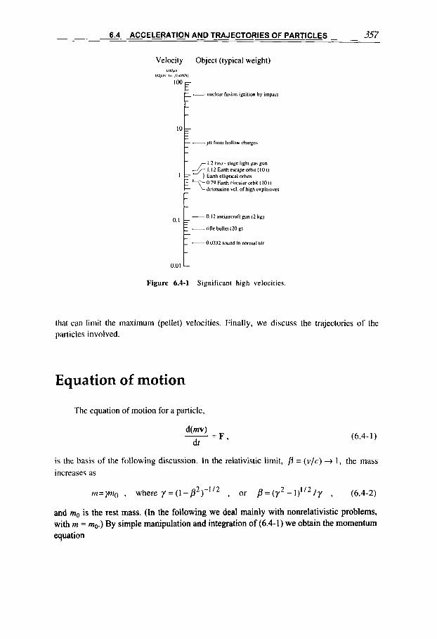
6.4 ACCELERATION AND TRAJECTORIES OF PARTICLES 357
Velocity Object (typical weight) c n I / p
(eq"1" I<> Ill MI1
- nucledr furion lgnlllon by impdcl
-)el from hollow charger
1.2 lwo - slage light gas gun 1.12 Eanh cscdpc orbil (101)
0.79 Eanh circular orbil (10 I) ?detonation vel. of high explosives
- 0. I ? antiaircraft gun (2 kg)
- rifle bullel (20 g)
- 0 0332 sound in normal air
0. I
0.01 t Figure 6.4-1 Significant high velocities.
that can limit the maximum (pellet) velocities. Finally, we discuss the trajectories of the particles involved.
Equation of motion
The equation of motion for a particle,
(6.4-1)
is the basis of the following discussion. In the relativistic limit, p = ( v / c ) + 1, the mass increases as
m = p o , where y = (1 - p2)-1'2 , or p = ( y 2 - 1)1'2 / y , (6.4-2)
and mo is the rest mass. (In the following we deal mainly with nonrelativistic problems, with m = mo.) By simple manipulation and integration of (6.4-1) we obtain the momentum equation
358 CHAPTER 6 MAGNETIC FORCES AND THEIR EFFECTS
mv = IFdt (6.4-3)
and, by noting that v . d(mv) = v2dm + mdv212, the energy equation
(m - mo)$ = IF . dl (= mo$/2, when v (( c). (6.4-4)
When a constant force F acts during a time t along a straight path with length I, these equations reduce to
m v = t F , -mv 1 2 = I F . 2
(6.4-5)
The outcome of the general equations is a large variety of trajectories and acceleration processes, according to the type of force that acts on the particle. In addition to driving forces, we also have retaining forces, such as the Stokes' drag force for a spherical particle with radius a moving in a fluid with viscosity 17 '.I2,
F = - 6 m a v , (6.4-6)
or the radiation damping force (for nonrelativistic velocities, v (( c)' .~,
F = - - . P09* d2v (6.4-7) 67rc dr2
Here, we are mainly interested in the motion in electromagnetic fields of particles having an electric charge q. With the Lorentz force (6.1-1). the equation of motion is
-= d(mv) q(E + v x B) , dt
(6.4-8)
and from (6.4-4) it follows that the total energy of motion
W = (m - mo)c2 + qU = const. (= mo3/2 + qU, when v (( c) (6.4-9)
is conserved, where U is the electric potential, E = -vU , that is,
U = - I E . d l (6.4-10)
(see section 2.2).
as B = V x A ; and with the Lorentz force in the form (6.1-2), the equation of motion is
d -(mv + qA) = -qV(U - v .A) , dr
It is often convenient to introduce the magnetic vector potential A , defined in (2.2-2)
(6.4-1 1 )
where A and U can be dependent on time. To be exact, these equations should be

6.4 ACCELERATION AND TRAJECTORIES OF PARTICLES 359
completed by the radiative force (6.4-7), but this is nearly always small and can fortunately be neglected. Note that in the so-called conjugate momentum
p = m v + q A (6.4-12)
appearing on the left-hand side of (6.4-1 l) , the term qA represents a stored magnetic field momentum available to the particle and, like the kinetic momentum mv, can be changed whenever the particle experiences gradients in the interaction energy q(U - v . A ) . We see that the magnetic field can change the momentum but not the energy (6 .4-9) of the charged particle.
Pellet acceleration methods
A large variety of processes for accelerating pellets exists or has been p r ~ p o s e d ~ . ' ~ . The most common acceleration device for a pellet or projectile is a gun, where a compressed and heated gas drives the projectile down a barrel of length 1. If the pressure were to exert a constant force Fp on the projectile, the velocity v attained at the muzzle would be given directly by (6.4-5). However, as the projectile travels down the barrel, the pressure of the driving gas diminishes, and this realistic consideration will introduce a velocity limit. The maximum pellet velocity will remain smaller than the velocity of expansion of the gas into vacuum, which is roughly equal to the sound velocity co or, more precisely, to
(6.4-13)
where TO is the initial temperature in kelvin of the driving gas, y its adiabatic factor, A its
mean atomic weight, and m~ = 1.67 x 10⁻²⁷ kg the mass of the hydrogen atom. In practice, the projectile velocities are much smaller than vexp and depend on various other parameters, such as the length of the gun and the mass ratio of the driving gas over pellet. High-performance guns use helium or hydrogen as driving gas and have this heated in special ways (by electric discharges, or a preliminary driver gas in a two-stage gun, etc.). Velocities of up to 1.2 c d p s with a 1-g pellet have been thus obtained.
Before discussing the performance and limitations of magnetic propulsion, we should mention as a useful reference the electrostatic acceleration method, which is effective on electrically charged particles. Here the driving force in an electric field E is F = q E , where there is a physical limit on the electric charge q that can be placed on a pellet. Introducing the surface electric field established by q on a spherical pellet with radius a in free space,
(6.4-14) 4 Eo = ~
4Z&oa2 '
360 CHAPTER 6 MAGNETIC FORCES AND THEIR EFFECTS
we note that for a negatively charged pellet it is limited by field emission to E i I lo9 V/m,
whereas for a positively charged pellet it is limited by the tensile strength 0, of the material to a value of about
that is, typically E t I 1 0 " V/m (for 0, z 500 N/m2, see comments further on). From
(6.4-4) with rn = 4 m 3 p / 3 we get the (ideal) velocity attained over the acceleration length I :
(6.4-15)
For example, a pellet with a = 10-3 m, p = 3000 kg/m3 and charged to a maximum field of Eo = 1010 V/m, is accelerated by a IE = 10 MV potential to a velocity of 1300 d s ; for E = 1 MV/m (which is about 1/5 of the practical, technical electric field limit in linear accelerators) we have 1 = 10 m.
However, the effectiveness of acceleration by electric fields is generally inferior to that by magnetic fields (considered later). This is because magnetic fields produced in practical arrangements give rise to larger stored energy densities and driving forces when compared to those produced by practical electrostatic fields. In fact, comparing the electric and
112 magnetic energy densities (5.1-7,8), B2/2p = &E2/2, gives E =cB, where c = (&p)- is the velocity of light (3.2-22). On this basis, an electric field of E = 3 x 10'0 V/m, which is well beyond the technical limit given above and even beyond the physical limits mentioned in connection with (6.4- 14), corresponds to a technically easy-to-produce induction of B = 10 T. From (6.4-15) we can see that electrostatic acceleration is most suitable for small pellets, also because it is relatively easy to handle and charge them with this method.
The strong accelerations considered here cause a large inertial pressure on the pellet, which may eventually overcome the strength limit op of its material, thus leading to its disintegration. This strength problem must be analyzed for each specific arrangement, but in a rough approximation, for the maximum tolerable force on a spherical pellet, we may take the expression F = M oP and set oP P oU, where 0, is the ultimate tensile strength
of the material. Values of 0, in MPa are typically (see also tables 7.1-1 and 11): 0.5 for frozen hydrogen, 600 for duraluminum, 1200 for cold-rolled stainless steel, and 1O'OOO for whiskers single crystals. By inserting this force into (6.4-3,4), we obtain the corresponding, possible maximum velocities for a spherical pellet:
2
2 3 0 3 0 v 2 1 2 , v s t - .
2aP 4ap (6.4- 16)
In addition, the application of the accelerating force must be sufficiently smooth to avoid generating shockwaves that could easily destroy the pellet (shock reflections, spallation; see section 8.3). This means that the risetime of the force must be large
6.4 ACCELERATION AND TRAJECTORIES OF PARTICLES 361
compared to the sound transit time in the pellet ah,.
Finally, if the material of a pellet to be used for certain applications does not possess the requisites of the acceleration process (material strength, electric conductivity, or permanent magnetization), one could consider composite pellets where one or more active components are introduced in addition to the useful payload. For example, the deuterium ice pellet in inertial thermonuclear fusion applications could be reinforced by a steel jacket and be placed on top of a superconducting loop, which is more suitable for powerful acceleration (as we shall see later).
Magnetic acceleration
Acceleration by magnetic fields represents a powerful method for driving massive pellets to velocities well in excess of 1 c d p s . This type of acceleration can be used for
launching systems that in themselves allow further concentration of energy (e.g., by convergent shocks or hydrodynamic flows, as reported above).
To get an idea of the (lower limit) velocities obtained by magnetic acceleration, consider the simple system shown in figure 6.4-2, in which a cylindrical, perfectly conducting projectile of radius a is expelled by a magnetic field contained within an ideal hollow conductor. If end effects are neglected, the energy balance before and after the projectile is expelled from the magnetic-flux-conserving solenoid of radius a l gives
1 2 2 1 2 2 1 2 2 -pHfn(al - a ) - - p H o m , =-m pv 2 2 2
.
Therefore, for the velocity we find
(6.4-17)
If a /a l <( 1 (i,e., for a constant field H I = H o ) . the final velocity is independent of the particle size and equal to AlfvCn's velocity V A (6.3-3). For example, a compact aluminum pellet expelled from a 100-T magnetic field will acquire a maximum velocity of
On the basis of the various magnetic forces discussed in the previous sections, we can distinguish between two main magnetic acceleration methods:
(a) Dipole acceleration, where a magnetic field gradient accelerates a pellet having a magnetic moment due either to a source-free current distribution (V. j = 0) or to permanent or induced magnetization.
(b) External current source acceleration, where a magnetic field accelerates a pellet in which a current is driven by an external source through gliding contacts (typically, a rail gun launcher, see figure 6.4-6).
V G V A ~ 1 . 7 ~ 1 0 ~ m/~.
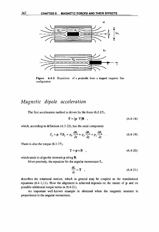
362 CHAPTER 6 MAGNETIC FORCES AND THEIR EFFECTS
f f 2a
Figure 6.4-2 Expulsion of a projectile from a trapped magnetic flux configuration.
Magnetic dipole acceleration
The first acceleration method is driven by the force (6.2-15),
F=(p .V)B ,
which, according to definition (A.3-22). has the axial component
There is also the torque (6.1-37),
T = p x B ,
which tends to align the moment p along B. More precisely, the equation for the angular momentum L,
dL dt -=T
(6.4- 18)
(6.4- 19)
(6.4-20)
(6.4-21)
describes the rotational motion, which in general may be coupled to the translational equations (6.4-1,ll). How the alignment is achieved depends on the nature of p and on possible additional torque terms in (6.4-21).
An important well-known example is obtained when the magnetic moment is proportional to the angular momentum,
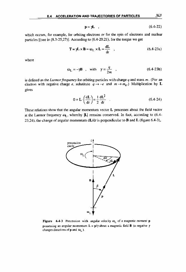
6.4 ACCELERATION AND TRAJECTORIES OF PARTICLES 363
P=& 9 (6.4-22)
which occurs, for example, for orbiting electrons or for the spin of electrons and nuclear particles [(see in (8.3-25.27)]. According to (6.4-20,21), for the torque we get
(6.4-23a) dL
T = & x B = c o L x L = - , dt
where
C O L = - @ , with y=- 4 , (6.4-23 b) 2m
is defined as the Larmor frequency for orbiting particles with charge q and mass m. (For an electron with negative charge e, substitute q + -e and m + me.) Multiplication by L gives
(6.4-24)
These relations show that the angular momentum vector L precesses about the field vector at the Larmor frequency q, whereby ILI remains conserved. In fact, according to (6.4- 23,24), the change of angular momentum dLldt is perpendicular to B and L (figure 6.4-3),
Figure 6.4-3 Precession with angular velocity oL of a magnetic moment p
possessing an angular momentum L = ply about a magnetic field B (a negative y changes directions of p and OL).
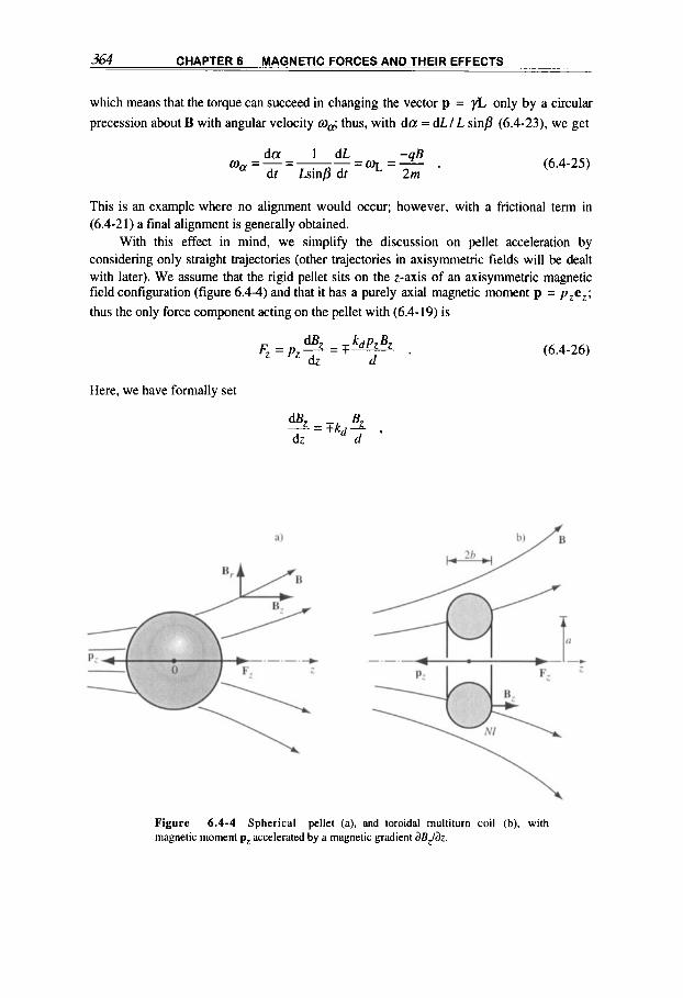
364 CHAPTER 6 MAGNETIC FORCES AND THEIR EFFECTS
which means that the torque can succeed in changing the vector p = $ only by a circular precession about B with angular velocity w,; thus, with d a = dL/ L sinp (6.4-23), we get
-@ WL =- dt LsinP dt 2m
- d a - 1 -= dL w, (6.4-25)
This is an example where no alignment would occur; however, with a frictional term in (6.4-21) a final alignment is generally obtained.
With this effect in mind, we simplify the discussion on pellet acceleration by considering only straight trajectories (other trajectories in axisymmetric fields will be dealt with later). We assume that the rigid pellet sits on the z-axis of an axisymmetric magnetic field configuration (figure 6.4-4) and that it has a purely axial magnetic moment p = p z e z ; thus the only force component acting on the pellet with (6.4-19) is
Here, we have formally set
(6.4-26)
Figure 6.4-4 Spherical pellet (a), and toroidal rnultiturn coil (b), with magnetic moment pz accelerated by a magnetic gradient &J&.
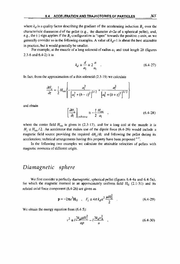
6.4 ACCELERATION AND TRAJECTORIES OF PARTICLES 365
where kd is a quality factor describing the gradient of the accelerating induction B, over the characteristic dimension d of the pellet (e.g., the diameter d=2a of a spherical pellet), and, e.g., the (-) sign applies if the B,-configuration is “open” towards the positive z-axis, as we generally consider so in the following examples. A value of kd= 1 is about the best attainable in practice, but it would generally be smaller.
For example, at the muzzle of a long solenoid of radius a1 and total length 2b (figures 2.3-6 and 6.4-2) it is
In fact, from the approximation of a thin solenoid (2.3-19) we calculate
and obtain
(6.4-27)
(6.4-28)
where the center field H,, is given in (2.3-17), and for a long coil at the muzzle it is H, s H,, 12. An accelerator that makes use of the dipole force (6.4-26) would include a magnetic field source providing the required dB,/dz and following the pellet during its acceleration; technical arrangements having this property have been proposed 1 3 .
In the following two examples we calculate the attainable velocities of pellets with magnetic moments of different origin.
Diamagnetic sphere
We first consider a perfectly diamagnetic, spherical pellet (figures 6.4-4a and 6.4-5a). for which the magnetic moment in an approximately uniform field Ho (2.1-31) and its related axial force component (6.4-26) are given as
We obtain the energy equation from (6.4-5):
(6.4-30)
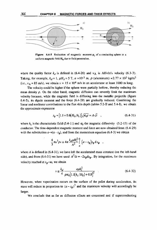
366 CHAPTER 6 MAGNETIC FORCES AND THEIR EFFECTS
Figure 6.4-5 Reduction of magnetic moment pz of a conducting sphere in a
uniform magnetic field €I,, due to field penetration.
where the quality factor kd is defined in (6.4-26) and VA is Alfvtn's velocity (6.3-3).
Taking, for example, k d = 1 , pHz = 5 T, a =lO-3 m, p (aluminum) =2.77 x 10³ kg/m3
(i.e., vA = 85 d s ) , we obtain v = 15 x 104 d s in an accelerator at least 1000 m long. The velocity could be higher if the sphere were partially hollow, thereby reducing the
mean density p. On the other hand, magnetic diffusion can severely limit the maximum velocity because, while the magnetic field is diffusing into the metallic projectile (figure 6.4-5). its dipole moment and the force (6.4-29) are gradually reduced. Combining the linear and nonlinear contributions to the flux skin depth (tables 52-11 and 5.4-I), we obtain the approximate expression
~4 .- [ 1 . 1 + 0.8( Ho/h,-)]J.ot = A& , (6.4-3 1 )
where hc is the characteristic field (5.4-1 1) and 16 the magnetic diffusivity (5.2-13) of the conductor. The time-dependent magnetic moment and force are now obtained from (6.4-29) with the substitution a+(a - s4), and from the momentum equation (6.4-3) we obtain
-m 4 3 p z 4 n kdpHz2 7 (a - s4)so dsg , 3 a
where A is defined in (6.4-3 l), we have left the accelerated mass constant (on the left-hand side), and from (6.4-31) we have used A2dt = - 2 s @ ~ ~ . By integration, for the maximum
velocity reached at s p , we obtain
V S - kd a*: (6.4-32) p K ~ [ ~ . ~ ( h c / ~ o ) + o . 8 ] 2 '
However, when vaporization occurs on the surface of the pellet during acceleration, its
mass will reduce in proportion to (a - 4 ) and the maximum velocity will accordingly be
larger. We conclude that as far as diffusion effects are concerned and if superconducting
3

6.4 ACCELERATION AND TRAJECTORIES OF PARTICLES 367
projectiles are excluded, it is convenient to use fields in excess of 100 T for the acceleration process. At still higher fields, HO >> h, , the maximum velocity is independent of the field and we are free to choose the most suitable value. For example, for a copper projectile, taking k, = 1 and a = 0.01 m, we obtain v E 60 x 103 m/s.
Example: Toroidal coil
The pellet here is a toroidal coil with major and minor radii a and b (figure 6.4-4b) and containing N
windings such that with the filling factorf. (2.3-26). we have
N I = j n b 2 f .
Such a projectile has a relatively large magnetic moment over mass ratio and is thus very convenient for
magnetic acceleration. We can approximate the toroid with a mass m= 2malrb'p and a magnetic moment
(2.3-6)
pz = - m 2 N I = -n2a2b2B ;
this results in the force (6.4-26).
5 = mkdNIBz = a2k,pb2f iBz . and for the energy equation (6.4-5) we thus obtain the maximum velocity
"2 - ! fkdjBz P
(6.4-33)
(6.4-34)
In a superconducting coil the tolerable maximum values ofj. R . and of the product j B are limited, as
mentioned in section 8.3. For example, for the smcalled type 11 Nb3Sn superconductor, the maximum
applicable values are approximately (see in table 8.3-V and figure 8.3-5)
j , S 10" A h 2 , Bc I 20 T , ( j R ) , I 5 X 10" AT/m2 .
With the latter value and taking f = 0.1, k, = 1. p = 5 x lo3 kg/m3, a pellet velocity of lo4 m/s is
reached in an ideal magnetic accelerator at least 100 m long. Note that for a superconducting pellet, the
minimum accelerator length or the maximum pellet velocity are independent of its size [a small dependem
comes only through the quality factor (6.4-27)].
Note that, for the accelerating force of the loop or toroid, instead of (6.4-33) we could have taken the
expression resulting from (6.1-4) with the radial field component B , ,
F = 2 M N I B r ,
which implies in comparison with (6.4-27.33) that 28, = kdt?, = a(dE/dz); this is also consistent with
(2.1-23).

368 CHAPTER 0 MAGNETIC FORCES AND THEIR EFFECTS
Magnetic rail gun
The second magnetic acceleration method [mentioned in conjunction with (6.4-18)] is illustrated typically by a rail gun launcher' 16.6 I' (figure 6.4-6), where the projectile (here with rectangular dimensions a, 6, d) is driven by the inductive force (6.2-33,
F = - - . 2 dz
(6.4-35)
To estimate the acceleration process, it may be appropriate in many cases to assume the current I to remain constant and the inductance of the rail gun to be given by
L = I ! Q + P ~ L Z , (6.4-36)
where Lo is the constant source inductance and kL depends on the geometry of the rail gun. For example, for two thin plates, it is k L = Kab b/a where KAb is a parameter given in figure 6.4-7 as a function of bla and typically amounts to Kab = 0.5 forb = a.
In this approximation, from (6.4-4) we get
that is, the kinetic energy of the projectile equals the inductive energy stored by the rails left behind. This expression also directly provides the velocity attained over a distance 1 (with constant current r ) for the rectangular pellet with mass abdp
(6.4-37)
Figure 6.4-6 Rail gun launcher for a rectangular projectile ( A x b x d)

6.4 ACCELERATION AND TRAJECTORIES OF PARTICLES 369
There is, however, an upper velocity limit due to the eventual melting of the projectile as a result of ohmic heating. To estimate this limit, we assume, similarly to (6.3-1 I), the rectangular pellet to be thin. From (6.4-3, 35, 36) we obtain
m v = Fdt = -pkL I 12dt (6.4-38a) 2
and with I = jad = const. and m = abdp we find the velocity limit
V K a b ( c ) @I b 9
d (6.4-38b)
where Kab = k lb /a is found in figure 6.4-7 and Jlb is defined in (6.3-12) and given for some metals in table 6.3-1.
The maximum velocity also depends on the dimensions of the projectile and will further increase if vaporization causes mass loss during acceleration; the thin-conductor approximation may require the projectile to be composed of a package of thin sheets. For an aluminum projectile with a = b = d = 1 cm and thus Kab E 0.5, we obtain the velocity limit
of 7 c d p s . From (6.4-37) we know that this velocity would be reached in a rail gun with, for example, a current of I = 1 MA and a length of at least 20 m. The kinetic energy of the projectile amounts to 6.6 MJ, the same as the inductive energy left behind in the system, as we know from (6.4-36). These figures, however rough and optimized, clearly show the effectiveness of a rail gun launcher.
f bT
h a d
Figure 6.4-7 Inductance L and
I .o
0.8
0.6
0.4
0.2
n
20 nH cm -
16
12
8
4
0 0. I 1 10 -
b/a correction factor Kab for parallel thin-plate
transmission line with homogeneous current density ' "'.

3 70 CHAPTER 6 MAGNETIC FORCES AND THEIR EFFECTS
Particle trajectories in electromagnetic fields
The trajectory of a particle in space, determined by the forces that act on it, is described by the solution of the equation of motion (6.4- 1). In Cartesian coordinates, the trajectory can be given by the solution x = x ( f ) , y = y ( t ) , z = z( t ) or, eliminating time when this information is not required, by a parametric form of the type x = x(z), y = y(z ) .
We shall now discuss the motion, in electromagnetic fields, of particles possessing an electric charge q and, later, of particles with a magnetic moment p. Plenty of literature is available on the former68.6 1 9 , since it is the basis for understanding electron and ion accelerators, mass spectrometers, electronic tubes, electron microscopes, and so on; it is also a fundamental subject in the kinetic theory of plasmas6 lo.
Cartesian equations
The nonrelativistic equation of motion (6.4-1) for a particle with mass rn (= mo) and (positive) electric charge q is
rnv=qE+q(vxB)+F , (6.4-39a)
where we have introduced the Lorentz force (6.1-1) and any non-electromagnetic force F experienced by the particle: for example, the gravity F = rn g . We note that formally we can cancel F in this equation provided that the substitution for the electric field
E + E + F / q (6.4-39b)
is made at any required step of calculation. With this in mind, in the following formulae the general nonelectromagnetic force F is. for simplicity, not carried on.
The Cartesian component equations of motion are thus
(6.4-40)
where the dot stands for differentiation with respect to time. We also have the energy equation (6.4-9), written here in the form
(6.4-41)
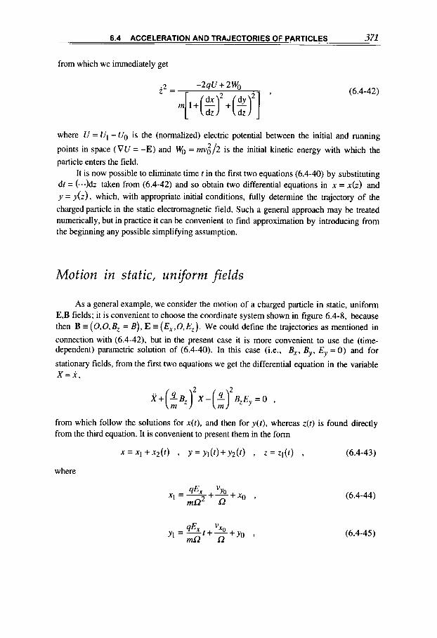
6.4 ACCELERATION AND TRAJECTORIES OF PARTICLES 371
from which we immediately get
(6.4-42)
where U = Ul - UO is the (normalized) electric potential between the initial and running
points in space ( V U = -E) and WO = m$/2 is the initial kinetic energy with which the particle enters the field.
It is now possible to eliminate time t in the first two equations (6.4-40) by substituting df = (...)dz taken from (6.4-42) and so obtain two differential equations in x = x(z ) and y = At), which, with appropriate initial conditions, fully determine the trajectory of the charged particle in the static electromagnetic field. Such a general approach may be treated numerically, but in practice it can be convenient to find approximation by introducing from the beginning any possible simplifying assumption.
Motion in static, uniform fields
As a general example, we consider the motion of a charged particle in static, uniform E,B fields; it is convenient to choose the coordinate system shown in figure 6.4-8, because then B = (O,O,Bz = B ) , E = (E,,O,Ez). We could define the trajectories as mentioned in
connection with (6.4-42). but in the present case it is more convenient to use the (time- dependent) parametric solution of (6.4-40). In this case (i.e., B,, By, Ey = 0) and for
stationary fields, from the first two equations we get the differential equation in the variable X = X ,
X + -B, X- - BzE,,=O , (: s (9 from which follow the solutions for x( t ) , and then for y ( t ) , whereas z(f) is found directly from the third equation. It is convenient to present them in the form
x = x I + x 2 ( t ) , Y = y l ( r ) + y 2 ( t ) , z = z l ( t ) . (6.4-43)
where
(6.4-44)
(6.4-45)
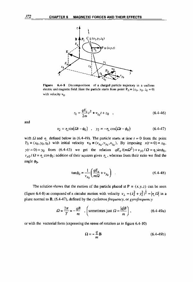
372 CHAPTER 6 MAGNETIC FORCES AND THEIR EFFECTS
Figure 6.4-8 Decomposition of a charged particle trajectory in a uniform electric and magnetic field: Here the particle starts from point Po = (xo. yo. zo = 0) with velocity vo.
(6.4-46)
with f, and q defined below in (6.4-49). The particle starts at time t = 0 from the point Po = (xo,yo,zo) with initial velocity v0 =(vxo,v , ,o ,vzo) . By imposing x(t =O)=xo,
y ( t = 0) = yo from (6.4-43) we get the relation qEx / ( m a ) + v Y o / R = qsin-0, vXo / R = T cos 40 : addition of their squares gives q , whereas from their ratio we find the
2
angle 40,
(6.4-48)
The solution shows that the motion of the particle placed at P = ( x , y , z ) can be seen (figure 6.4-8) as composed of a circular motion with velocity v l = (4 2 + y;); = ITRI in a
plane normal to B, (6.4-47), defined by the cyclotron frequency, or gyrofrequency
sometimes just l2 = m
a=-=-@ 21r
T m
or with the vectorial form (expressing the sense of rotation as in figure 6.4-10)
(6.4-49a)
(6.4-49b)

6.4 ACCELERATION AND TRAJECTORIES OF PARTICLES 373
and the Lurmor radius
(6.4-49~)
about a guiding center C = (xl ,yl ,q) that itself moves along a parabola (6.4-45.46) placed in the (y,z)-plane. The overall result in space is a helical path around the parabola. We recall that the cyclotron frequency R = v l / is found from equating the centrifugal force
v:m/rL with the centripetal magnetic force (6.1-1b), - 4 v l B . Note that the sign in all these expressions is determined for a particle with positive electric charge 4 by the usual right-hand-screw convention.
The particle, with mass m and velocity v l moving on the circular orbit projection with Larmor radius in a plane parallel to the (x,y)-plane and perpendicular to the given (uniform) magnetic field B, creates its own mean current I and related magnetic moment (2.3-6), p (with direction opposite to B for any charge such that p' B = - p B ) ,
(6.4-50a)
(6.4-50b)
where vI is given as a function of the initial parameters in (6.4-49), and we have also
introduced the magnetic flux v / = K $ B enclosed by the orbit. Note that the magnetic moment is a constant of motion and that B is the (uniform) field given by outer sources, not the (negative, diamagnetic) field generated by the current I , which according to (2.3-7) on axis is Bow" = pI/2%-that is, negligibly small.
The guiding-center's parabolic trajectory, on the other hand, is the result of two velocities (6.4-45.46): the increasing velocity 71 parallel to the magnetic field lines, driven by the parallel electric field component (along the z-axis)
E V I I =il = 4 2 1 + v ~ o ,
m (6.4-51a)
and the constant, so-called E-cross-B drijt velocify normal to the E, B fields
(6.4-51b)
(along the negative y-axis, independently of the sign of the charge). This trajectory can be traced, in analogy to an example from classical mechanic^'-'^,
by a point P on the circle of radius rL (6.4-49c), rigidly connected to another circle of radius X I (6.4-44) rolling without slipping through the contact point R along a parallel to the y-axis at x = X I - % (figure 6.4-9). The pattern of the trajectory depends on the relative magnitude of r~ and xl-that is, on the value of the initial velocity vo versus the electroma-

374 CHAPTER 6 MAGNETIC FORCES AND THEIR EFFECTS
I I I
Figure 6.4-9 Projection on the (x.y)-plane normal to B of the trajectories of a negatively charged particle P in uniform fields E = E, e, , B = Bzez , which can be described
by rolling over the contact point R two rigidly connected circles (see text): (a) prolate cycloid ( x, < rL); (b) cycloid ( uo = 0); (c) curtate cycloid (x l > rL). (For a positively charged particle, the trajectories are mirrored about the y-axis but still move towards negative y.)
gnetic parameters. For example, when vxo = 0 and for vyo = -Vd = E,/B, from (6.4-49c) we find q = 0 and a straight trajectory is obtained. Variations around this critical velocity result in quite different, curved trajectories, which is an effect used in the so-called velocity spectrograph or filter to sort out particles with fixed velocities, independently from their charge or mass.
Note that for a negatively charged particle (for example an electron with negative charge e), in all the above equations we have to substitute
q + -[el , l2+ lelB/rn ; (6.4-52)
the relations between directions and signs are illustrated in figure 6.4-10.
Motion in variable fields
The above exact results for uniform electric and magnetic fields E, B remain

6.4 ACCELERATION AND TRAJECTORIES OF PARTICLES 375
a) b)
-9 +9 -9 +9
Figure 6.4-10 Rotation of a charged particle about a magnetic field at the cyclotron frequency 0. Since the current I produced by the orbiting particles has by definition the same direction as the moving (+) charge, the consequence is a diamagnetic effect: the positive particle rotates in a direction opposite to the current Is producing the magnetic field B from outer coils.
approximately valid for time-dependent and nonuniform fields, provided that the variations of these fields remain small over time Tor length rL (6.4-49). As to be expected, however,
there will be additional contributions in relation to the finite E and VB terms. Under this udiabaticify assumption6" the trajectory of a charged particle in an electromagnetic field consists of the following:
(a) The fast gyration about a guiding center at velocity vI in a plane normal to (the local) B described by (6.4-49), with its magnetic moment
(6.4-53)
a constant of motion [analogously as in (6.4-50b)I.
described by (b) The motion of the guiding center at velocity vII = ds/dr along the magnetic field lines
iiB m v - E - p - , II - 4 as (6.4-54)
where the last term means differentiation along the field lines; this equation is related to (6.4-51a), but here it is extended by the force due to nonuniform fields on a magnetic dipole (6.4- 18,19).
In addition, there are various drift velocities of the guiding center C across the field lines, defined as follows:
VE=- (E-cross-B drift), B2
(6.4-55)
which is the general form of (6.4-5 lb);
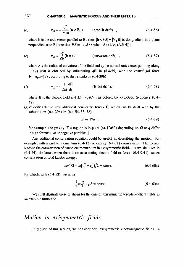
376 CHAPTER 6 MAGNETIC FORCES AND THEIR EFFECTS
2 V B = -- '' (bx V B ) (grad-B drift) , (6.4-56)
2- (4
where b is the unit vector parallel to B, thus Ib x V q = IV,q is the gradient in a plane perpendicular to B [note that V B = -e,B/ r when B 0~ l l r , (A.3-4)];
2
Rr vR = x ( b x e,) (curvature drift) , (6.4-57) (e)
where r is the radius of curvature of the field and e, the normal unit vector pointing along r [this drift is obtained by substituting qE in (6.4-55) with the centrifugal force F = e,m# / r , according to the remarks in (6.4-39b)l;
1 dE vE = - z i d r (E-dot drift), (6.4-58)
where E is the electric field and R = -qB/m, as before, the cyclotron frequency (6.4- 49).
(g)Velocities due to any additional nonelectric forces F, which can be dealt with by the substitution (6.4-39b) in (6.4-54, 55, 58)
E -j F / q . (6.4-59)
for example, the gravity, F = mg, or as in point (e). [Drifts depending on R or q differ in sign for positive or negative particles!]
Any additional conservation equation could be useful in describing the motion-for example, with regard to momentum (6.4-12) or energy (6.4-1 1) conservation. The former leads to the conservation of canonical momentum in axisymmetric fields, as we shall see in (6.4-64); the latter, when there is no accelerating electric field or force, (6.4-9,41), states conservation of total kinetic energy,
mv2/2 = m( vf + v:) /2 = const. , (6.4-60a)
for which, with (6.4-53), we write
(6.4-60b) 1 2 -myI + p B = const. 2
We shall illustrate these relations for the case of axisymmetric toroidal-helical fields in an example further on.
Motion in axisymmetric fields
In the rest of this section, we consider only axisymmetric electromagnetic fields. In
6.4 ACCELERATION AND TRAJECTORIES OF PARTICLES 377
the appropriate cylindrical coordinate system, where the components of the velocity and force are v = ( t , r & i ) , F =(Fr,F#,F,) , the general equation of motion (6.4-1) separates
into the components (radial comp.) , ' 2 m r - m r @ = F,
--(mr2qi) I d = F@ r dt
mi'= F, (axial comp.) .
(azimuthal comp.) , (6.4-61)
[To obtain these equations, consider that with r = re, we have r = i0, + r+,, but e , = Ae,/Ar = ( A @ / A t ) e g , etc., where e , , e g , e , are the cylindrical unit vectors; see table
A.3-111 and figure A.3-1.1 Note that the second term in the first equation can be read as the centrifugal force; the second equation can be read as the change of angular momentum caused by the toque rF+ (where the split term 2 4 , in particular, is the Coriolis acceleration). The components of the Lorentz force (6.1-1) in an axisymrnetric magnetic field (where Bo = 0) are
Fr = qEr + q d B Z ,
F4 = qE4 + q(iBr - tB,) , (6.4-62)
F, = qEz - qr$B, .
Expressing B, and B, by the only vector potential component A4 through (2.2-27) and setting Eo = 0 gives
(6.4-63)
(the sum of the partial derivatives of % ( r , z ) is indeed equal to the total derivative on the
right-hand side). This combined with the azimuthal equation (6.4-61) results in the angular momentum equation
(6.4-64) 2 ' mr @+qrA$ = pq = const.
(Note the equivalence rd = vl = vo with the previous notations.) Equation (6.4-64) expresses the conservation of the so-called canonical angular
momentum p q of a charged particle in axisymrnetric fields and gives the relation between
the mechanical angular momentum ( = mr2 4 ) and the magnetic flux encircled by the motion of the particle, v / = 27~7% . It also shows [analogously to what has been said in connection
with (6.4-12)] that a particle entering a magnetic field will acquire an angular momentum, but this is lost again when leaving the field. On the other hand, a particle born in a magnetic field will attain angular momentum on leaving the field.

378 CHAPTER 6 MAGNETIC FORCES AND THEIR EFFECTS
We also have the energy equation (6.4-41)
(6.4-65)
from which we can determine dr = (...)dz and eliminate time from (6.4-61) [similarly to (6.4-42)]. In particular, by eliminating time and 4 from the radial equation, we obtain the trajectory r = r(z) in a meridian plane, which itself rotates with an angle @ = @ ( z )
determined by integration of (6.4-64). These general relations may be suitable for a numerical solution, but in many practical
situations it is probably more convenient to proceed with the guiding-center approximation outlined in (6.4-53 to 60).
Example: Trajectories in toroidal fields We apply the previous theoretical considerations in order to study the trajectories of charged particles
in a toroidal-helical magnetic field6.9 (so-called tokamak magnetic configuration2.’), which is the result of
the superposition
B = B, + B (6.4-66)
of a toroidal field BT = h e , (where ST = I I R is generated by a toroidal magnet or just a current flowing
along the z-axis; see figure 2.3- 12) and a poloidal field B p = Bpeg generated by a current distribution with
total current I flowing along the toroidal magnetic axis (figure 6.4-1 I ) . (In a tokamak there is also a control field BV = -Bve, generated by outer coils that can often be neglected because BV < Bp << 4; i n a configuration where the toroidally circulating particles are in equilibrium, Bv vanishes inside it.)
As we know from the discussion relative to figure 2.5-3, this magnetic configuration gives rise to
nested toroidal flux surfaces (i.e., surfaces defined by the family of helical field lines), which are ideally suited to containing the toroidal current-carrying plasma.
We shall show in the following that the orbit of a charged particle (figure 6.4-12) in such a configuration consists of a fast gyration at the toroidal field gyrofrequency R,, (6.4-49). about a guiding
center that moves, not on the flux surfaces, but on a set of nested, so-called drift surfaces, which are the
result of the movement along the helical field lines plus the various drift movements. We shall now proceed to establish and locate the drift surfaces for negatively charged particles (electrons) and then add other
properties of charged particles moving in this toroidal magnetic-field configuration. Although it is a three- dimensional field configuration, we shall see that the properties of the guiding center trajectory depend on the poloidal field B, only, and in this sense the configuration is axisymmetric. On the other hand, the
toroidal (azimuthal) field BT = e# &&/R guides the center around the torus, contributes to determining
the fast rotation at the gyrofrequency RT, and introduces the gradient lV&l= & / R (but this does not
eliminate the fundamental axisymmetric nature of our problem). In this magnetic configuration, where for simplicity we assume negligible Bv and no electric field,
by following what was said for (6.4-53 to 59), the guiding-center velocity for the negatively charged
electron, q = -e, moving as in figure 6.4-1 l a may be broken down approximately as
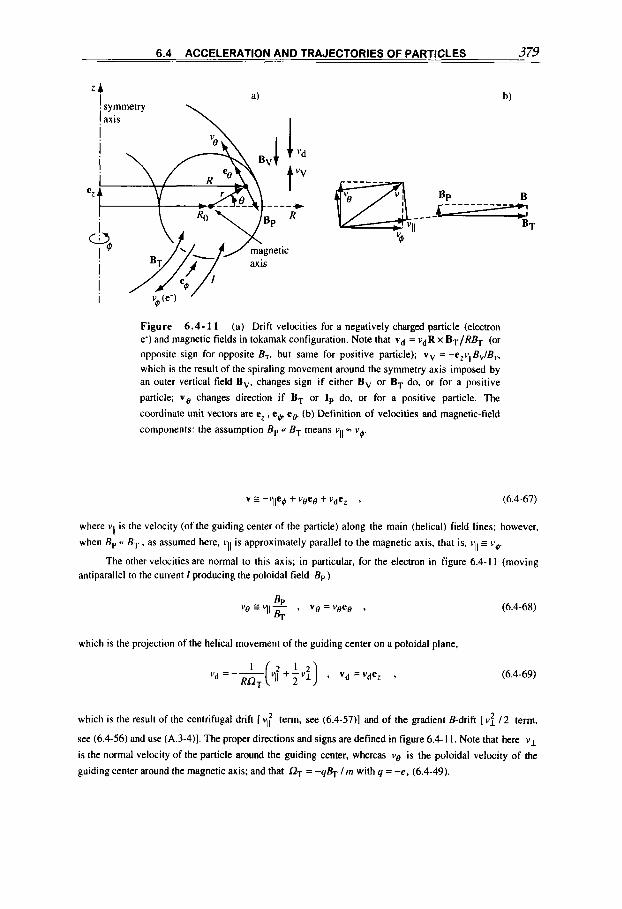
6.4 ACCELERATION AND TRAJECTORIES OF PARTICLES 379
a) Z A ' symmetry
I axis
b)
Figure 6.4-1 1 (a) Drift velocities for a negatively charged particle (electron e-) and magnetic fields in tokamak configuration. Note that vd = VdR x BT/RB, (or opposite sign for opposite BT. but same for positive particle); v v = -e,v,,E,/B,,
which is the result of the spiraling movement around the symmetry axis imposed by an outer vertical field Bv, changes sign if either B, or B, do, or for a positive
particle; v o changes direction if B, or I, do, or for a positive particle. The
coordinate unit vectors are e, , eC eg (b) Definition of velocities and magnetic-field
components: the assumption B , <( BT means vII = V~
V I - V ~ +vgeg+vdeZ , (6.4-67) 11 @
where vll is the velocity (of the guiding center of the particle) along the main (helical) field lines; however,
when B , (< B, , as assumed here, VII is approximately parallel to the magnetic axis, that is, vII P vc
The other velocities are normal to this axis; in particular, for the electron in figure 6.4- I 1 (moving antiparallel to the current I producing the poloidal field Bp)
which is the projection of the helical movement of the guiding center on a poloidal plane,
(6.4-68)
(6.4-69)
which is the result of the centrifugal drift [ v,f term, see (6.4-57)l and of the gradient B-drift [ v: / 2 term,
see (6.4-56) and use (A.3-4)]. The proper directions and signs are defined in figure 6.4- 1 I . Note that here vI is the normal velocity of the particle around the guiding center, whereas vo is the poloidal velocity of the
guiding center around the magnetic axis; and that L?, = - 4 4 / m with q = -e, (6.4-49).

380 CHAPTER 0 MAGNETIC FORCES AND THEIR EFFECTS
Figure 6.4-12 Electron particle moving inside a helical field that is the superposition of a toroidal field BT (produced by outer coils, not shown) and a
poloidal field B, (produced by the toroidal current flowing inside the minor radius a).
The displacement of the drift (orbit) surfaces with respect to the magnetic surfaces (figure 6.4-12) can be made plausible by combining the vd and v o velocities ( Y O w vd) starting where vole,. A quantitative
evaluation is obtained by using the conservation of the canonical angular momentum (6.4-64) with respect
to an orbit passing through point P at radius r (figure 6.4-1 1). which we rewrite in the form
(6.4-70)
where yp is. according to (2.2-31), the relevant poloidal flux function, (2.5-15). defined between this orbit
and the magnetic axis,
r
i y p ( r ) = 2 s j BpRdr
0
(6.4-7 1 )
To calculate the exact value we need to know the current distribution that in turn determines the exact form of Bp(r ) .
To illustrate a simple case, we assume that the current I flows homogeneously within a torus with major and minor radii Ro and a; that is, we consider within this torus a flat current profile that defines. with
R = Ro t r,
(6.4-72)
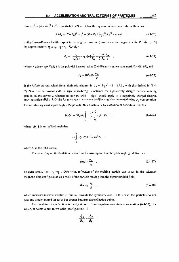
6.4 ACCELERATION AND TRAJECTORIES OF PARTICLES 381
Since r2 = ( R - 4)’ + z 2 , from (6.4-70,72) we obtain the equation of a circular orbit with radius r
2Rd, + ( R - RO)* + z 2 z ( R - R,, +Idy()’ + z 2 = const. (6.4-73)
shifted inwardoutward with respect to its original position (centered on the magnetic axis R = &, z = 0) by approximately ( V I I s V g . V I I B v ~ . Ro )> d, )
(6.4-74)
where rLp(n) = vllm/(qBp) is the poloidal Larmor radius (6.4-49) at r = a. we have used (6.4-68.69). and
I, = (6.4-75) 9
is the Alfvtn current, which for a relativistic electron is I , = 1 7 6 [kA] , with p.y defined in (6.4-
2). Note that the inward shift [+ sign in (6.4-73)] is obtained for a positively charged particle moving
parallel to the current I, whereas an outward shift (- sign) would apply to a negatively charged electron moving antiparallel to 1. Orbits for more realistic current profiles may also be treated using p$ conservation.
For an arbitrary current profile j ( r ) . the poloidal flux function is. by extension of definition (6.4-71).
(6.4-76)
where j ( r ’ ) is normalized such that
2n r’j(r’)dr’=m2I0 , i 0 where I, is the total current.
The preceding orbit calculation is based on the assumption that the pitch angle x , defined as
t a n X = k , (6.4-77) VII
be quite small, i t . , vI svll . Otherwise, reflection of the orbiting particle can occur in the tokamak
magnetic field configuration as a result of the particle moving into the higher toroidal field,
B=B0- Ro , (6.4-78) R
which increases towards smaller R . that is, towards the symmetry axis. In this case, the particles do not
pass any longer around the torus but bounce between two reflection points.
The condition for reflection is easily deduced from angular-momentum conservation (6.4-53), for
which, at points A and B, we write (see figure 6.4-13)
2 2 “LA - ‘ I B
BA
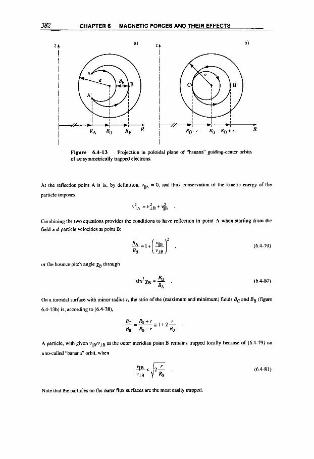
382 CHAPTER 6 MAGNETIC FORCES AND THEIR EFFECTS
I
I
I 1
1 ! I I- I
@ A’ I I I I I I I I I
I I ! I I
!
i i i i i i i- i
I @ I I I I I I
+ R
I i Figure 6.4-13 Projection in poloidal plane of “banana” guiding-center orbits of axisymmetrically trapped electrons.
At the reflection point A it is, by definition, vllA = 0. and thus conservation of the kinetic energy of the
particle imposes
“2 - 2 lA -V*,+Y#Z, ’
Combining the two equations provides the conditions to have reflection in point A when starting from the
field and particle velocities at point B:
(6.4-79)
or the bounce pitch angle xB through
(6.4-80) . 2 BB BA
sin X B =- .
On a toroidal surface with minor radius r, the ratio of the (maximum and minimum) fields B, and B, (figure
6.4- I3b) is, according to (6.4-78),
A particle, with given vlle/vlB at the outer meridian point B remains happed locally because of (6.4-79) on
a so-called “banana” orbit, when
(6.4-81)
Note that the particles on the outer flux surfaces are the most easily trapped
6.4 ACCELERATION AND TRAJECTORIES OF PARTICLES 383
Electromagnetic optics
So far we have given the trajectories as solutions obtained by integrating the equation of motion with respect to time. We have also presented the useful guiding-center approximations and indicated the general procedure for eliminating time so as to obtain the trajectories in space. However, there are less tedious approaches for directly obtaining the underlying differential equations for the trajectories. The easiest is by means of “Hamilton’s principle”, or “the principle of least action” *. This then leads us directly to the optics of chargedparticles in electromagnetic fields, which is of practical interest and widely covered in the literature s.6 6.6 7.6 *O.
We introduce this subject in relation to stationary axisymmetric magnetic fields only, first for particles having an electric charge, then for particles with a magnetic moment, by assuming the trajectories to be:
(a) paraxial (small rand drldz, i.e., small inclination of the trajectories to the axis); (b) meridian (i.e., with the initial velocity vector vo lying in a meridian plane, with
2 vo = 2Wo/m).
The approximation resulting from (a) is known as “Gaussian optics” and provides the “Gaussian trajectories”. These assumptions imply that in (6.4-64) the integration constant is zero and [from (2.2-30)] that 2% E rBz; the meridian plane therefore rotates at angular
velocity
(6.4-82)
(also called the Larmor frequency, (6.4-23b), half the cyclotron frequency), which by integration and using dz = dtJzw,/m from (6.4-85) gives the corresponding angle
@ = - ‘ IB,(z)dz 24%
(6.4-83)
Substituting (6.4-82) into the radial component equations (6.4-61,62) with no electric field yields
mi: = --rBz q2 2
4m
The paraxial assumption also implies mi’ = r2 E 0 and
(6.4-84)
(6.4-85)
With (6.4-85) we can eliminate time in (6.4-84) and obtain the trajectory defined by
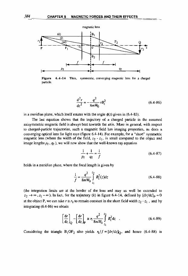
384 CHAPTER 6 MAGNETIC FORCES AND THEIR EFFECTS
magnetic lens
I
F ,I+ f f Pf 9f 4+ I- +
4 I
Figure 6 .4-14 Thin, symmetric. converging magnetic lens for a charged particle.
(6.4-86)
in a meridian plane, which itself rotates with the angle Nz) given in (6.4-83). The last equation shows that the trajectory of a charged particle in the assumed
axisymmetric magnetic field is always bent towards the axis. More in general, with respect to charged-particle trajectories, such a magnetic field has imaging properties, as does a converging optical lens for light rays (figure 6.4-14). For example, for a “short” symmetric magnetic lens (where the width of the field, 22 - z1, is small compared to the object and image lengths p f , qf ), we will now show that the well-known ray equation
(6.4-87) 1 1 1
-+-=7 Pf 4f
holds in a meridian plane, where the focal length is given by
(6.4-88)
(the integration limits are at the border of the lens and may as well be extended to 22 + 00 , z1 - =). In fact, for the trajectory (k) in figure 6.4-14, defined by [dr/dzIp = 0
at the object P, we can take r G r1 to remain constant in the short field width z2 - z1 , and by integrating (6.4-86) we obtain
(6.4-89)
Considering the triangle BIOFz also yields q/f = [d r /dz ]~ , and hence (6.4-88) is
6.4 ACCELERATION AND TRAJECTORIES OF PARTICLES 385
confirmed. For reasons of symmetry, the trajectories (1) and (m) are similarly confirmed, and this proves (6.4-87), which is a geometric consequence of figure 6.4-14.
The similarity of the imaging properties of certain electromagnetic fields on charged particles to those of geometric optics is more general than implied by our simple example. In fact, it also refers, for example, to thick nonsymmetric electrostatic and magnetic lenses, up to and including, similarly, the aberration theory 6 1 1 .
We now extend these optical concepts to include the trajectories in axisymmetric magnetic fields of particles with no net electric charge but with a magnetic moment. In particular, we consider the trajectories in a field with cylindrical components B,, B, of a
spherical pellet with volume V = 4m3/3 and mass m = pV and having a magnetic moment (1.1-24)
p = j M d V s V q B , for M = q B ; (6.4-90)
for example, for an induced-field-proportional magnetization M (2.1-78) it is
From (6.4-18) the force on the spherical pellet becomes
F=Vq(B.V)B ,
which has the cylindrical components (A.3-22b).
m F $ = O ,
(6.4-9 1)
(6.4-92)
(6.4-93)
We introduce assumption (a) for a paraxial trajectory in an axisymmetric magnetic field by eliminating B, and d( ...) /& through the first-order approximation calculated from (2.1- 21, 23) and then obtain from (6.4-61) the approximated equations of motion
(6.4-94)
(6.4-95) 2 ' r $=const ,
(6.4-96)
where the constant is zero for a meridian trajectory; that is, there is no rotation in this case,

386 CHAPTER 6 MAGNETIC FORCES AND THEIR EFFECTS
4=0. We now determine the trajectory deflected by a thin magnetic lens in a meridian plane.
Integration of (6.4-96) and noting that 2 = i(di/dz) gives
(6.4-97)
where the last term vanishes for z l r z 2 taken outside the lens. If even inside the (weak) lens
this term remains small, we have dddt 2 vo and time can be eliminated from (6.4-94):
(6.4-98)
We are now at the same point as we were with (6.4-86) for a charged particle, and we can thus proceed similarly to obtain the optical imaging equation (6.4-87) for a thin and weak magnetic lens extending from z1 to 22. Integrating once with respect to z, with the same assumptions as made in (6.4-89), gives the approximate focal length5
(6.4-99)
for a pellet with induced magnetic moment (6.4-90) (here we have integrated by parts and taken z1 , z 2 to be located outside the lens). We find that in a thin and weak magnetic lens, only diamagnetic pellets [with q < 0, because p~ < 1 in (6.4-91)] are converging and can be focused cf> 0) ; whereas pellets with paramagnetic materials [ q > 0, p~ > 1) are diverging with virtual image cf< 0). These arrangements can be used to separate pellets according to their magnetism. In practice, the pellets would probably be suspended in a fluid, and in the underlying theory one would have to include gravity, Stokes' drag (6.4-6), and so on.

MAGNETOMECHANICAL STRESSES
The volume force exerted by an electromagnetic field on a current-carrying conductor links the theory of electrodynamics to structural mechanics. Since magnetic fields in technical applications are often at levels that imply stresses near or above the tensile strength of electrical conductors, the mechanical stress problems that result from this situation have important practical consequences. With the exception of a few simple cases, the magnetic stress problem is tractable only through numerical computation. The procedure generally starts with determining the local current density and magnetic field through the magnetostatic or dynamic relations presented in chapters 1 and 2, and then tying the resulting magnetic volume force to the mechanical yield-stress relations. To illustrate the concepts and problems introduced in the first section we shall discuss two relatively simple conductor geometries: cylindrical and toroidal coils.
Applications. The practical aspects in this chapter mainly concern the performance limits of some solenoidal and toroidal high-field magnets' 'j. These considerations can also be helpful in designing super-high-field, pulsed, or quasi-steady solenoidal magnets' 27 of, for example, the hybrid' (external superconducting solenoidal coil with internal cryogenic coil) or split-pair type' l7 (allowing a diagnostic access at the mid plane). An ideal situation is achieved with force-free magnetic fields7'*, which is the concluding subject of discussion.
387
M4GNETICFIELDS: A Comprehensive Theoretical Treatise for Practical Use Heinz E. Knoepfel
Copyright Q 2000 by John Wiley & Sons, Inc
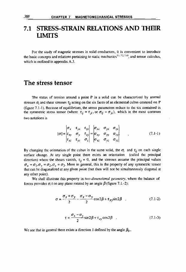
388 CHAPTER 7 MAGNETOMECHANICAL STRESSES
o x r y x z, Qxx c y x Qn
7 x 2 7 y z Qz Qxz Qyz Qzz
[a]= r x y Qy r z y = Qxy Qyy Qzy
7.1 STRESSSTRAIN RELATIONS AND THEIR LIMITS
(7.1-1)
For the study of magnetic stresses in solid conductors, it is convenient to introduce I" , and tensor calculus, the basic concepts and relations pertaining to static mechanics'
which is outlined in appendix A.3.
The stress tensor
The status of tension around a point P in a solid can be characterized by normal stresses oi and shear stresses rQ acting on the six faces of an elemental cubus centered on P (figure 7.1-1). Because of equilibrium, the stress parameters reduce to the six contained in the symmetric stress tensor (where zQ = z,;, or QQ = Q,;), which in the most common
two notations is
By changing the orientation of the cubus in the same solid, the oi and TQ on each single surface change. At any single point there exists an orientation (called the principal direction) where the shears vanish, rQ = 0, and the stresses assume the principal values ox = Q ~ , Q ~ = 0 2 . 0 , = a3. More in general, this is the property of any symmetric tensor that can be diagonalized at any given point (but then will not be simultaneously diagonal at any other point).
We shall illustrate this property in two-dimensional geometry, where the balance of forces provides cr, z on any plane rotated by an angle p (figure 7.1 .-2):
o,+oy o,-oy Q=--- cos2P + zxysin2P ,
2 2
0 , - Q y . z=- sin2P + zxy cos2P . 2
(7.1-2)
(7.1-3)
We see that in general there exists a direction 1 defined by the angle P o ,
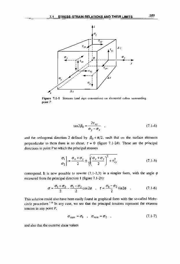
7.1 STRESS-STRAIN RELATIONS AND THEIR LIMITS 389
Figure 7.1-1 point P.
Stresses (and sign convention) on elemental cubus surrounding
(7.1-4)
and the orthogonal direction 2 defined by Po + nJ2, such that on the surface elements
perpendicular to them there is no shear, T = 0 (figure 7.1-2d). These are the principal directions in point P to which the principal stresses
(7.1-5)
correspond. It is now possible to rewrite (7.1-2,3) in a simpler form, with the angle 4 measured from the principal direction 1 (figure 7.1-2b):
(7.1-6)
This solution could also have been easily found in graphical form with the so-called Mohr- circle procedure.' lo In any case, we see that the principal tensions represent the extreme tension in any point P,
Omax =Q1 9 bmin =(T2 9 (7.1-7)
and also that the extreme shear values

390 CHAPTER 7 MAGNETOMECHANICAL STRESSES
Figure 7.1-2 Stresses on two-dimensional elemental square centered at point P, and their transformation by rotation.
rmax} = *O' ;"2 (7.1-8) rmin
are attained along surfaces inclined by 45" with respect to the principal directions 1,2, defined by 4 = 0 and 6 = 90".
In three-dimensional geometry similar results are found for the stress and shear distribution: (a) Generally, there also exist principal directions and related stresses ol ,o2,03 such that along their normal surface elements there is no shear. (b) The principal directions and stresses are determined analytically or graphically in a procedure similar to the two-dimensional one. (c) If we assume the directions labeled such that 01 > 02 > 03, we find analogously
(7.1-9)
These considerations pertain to the tensor-diagonalization procedure, which is outlined more in general in (A.3-41,42).
Let us now consider a solid that is subject to a position-dependent body force density with components
f(x*y,z) = ( fx . fyJz) (7.1-10)
and in which the stresses will in general also depend on position, for example,

7.1 STRESS-STRAIN RELATIONS AND THEIR LIMITS 391
oXY =o,(x,y,z). [We are now using the second notation of the stress tensor (7 .1- l ) . ]
For the force component along the x-axis, where the stress alone gives the component [a, + dx(do,/&) - a,]Ay&, we find from figure 7.1-3, in static equilibrium,
(7.1- 11)
and similarly from the force balance along the y,z-axes,
do, do,, do, -+-+-+fy=0 , $v dz dx
Introducing the stress tensor [o]. [(7.1-1). see also (A.3-381, these equations can be written (but only in Cartesian coordinates) by the vector equation of elastic equilibrium
V . [ a ] + f = o . (7.1- 12)
[Temperature effects are included in the extension (7.1-35).] As a further example, we extend these equilibrium equations to cylindrical geometry,
which is particularly useful for magnetic field applications. Let us consider first the simple case where the body force reduces to the radial force density f,(r) (it is useful to look at figures 7.2-2 and 7.2-4). The balance of the radial force components that act on a cylindrical volume element AV = rA@Ar& include, in addition to the body force AFf = f , A V , the following two contributions: the net radial stress component
J aa, ax+ --d* ax
F i g u r e 7 .1 -3 All the shear and stress components along the x-axis of an elemental cubus.
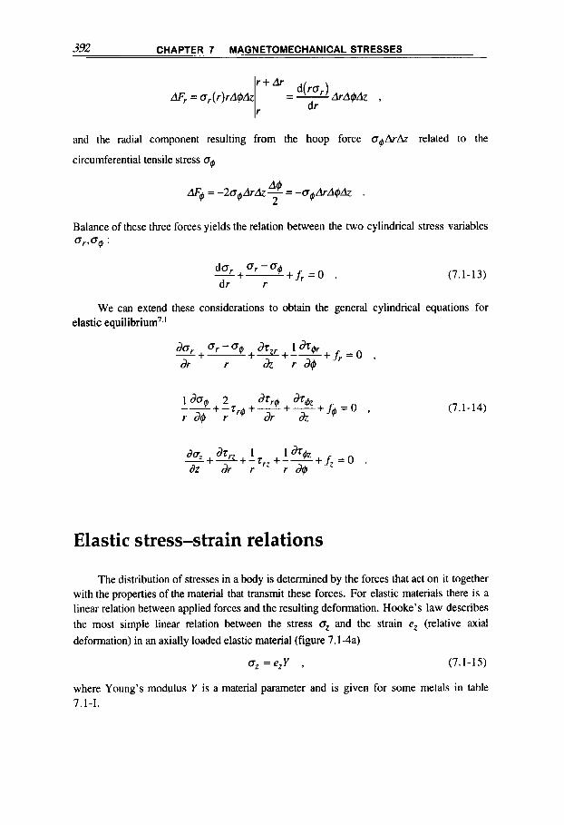
392 CHAPTER 7 MAGNETOMECHANICAL STRESSES
dF, = o,(r)rA@Az = - d(ror) ArA@& , dr
and the radial component resulting from the hoop force D @ A ~ related to the
circumferential tensile stress 04
dF4 = - 2 0 ~ Ar& - A@ = -64 ArA4Az 2
Balance of these three forces yields the relation between the two cylindrical stress variables b r , Q @ :
(7.1-13)
We can extend these considerations to obtain the general cylindrical equations for elastic equilibrium’.’
do, O r e 0 4 & -+- + +-- dr r & r d@
(7.1 - 14)
dt I 1 dz dr r r d@ - daz + J + - z r z +--+f, = 0 .
Elastic stress-strain relations
The distribution of stresses in a body is determined by the forces that act on it together with the properties of the material that transmit these forces. For elastic materials there is a linear relation between applied forces and the resulting deformation. Hooke’s law describes the most simple linear relation between the stress O, and the strain eZ (relative axial deformation) in an axially loaded elastic material (figure 7.1-4a)
O, =e,Y , (7.1 - 15)
where Young’s modulus Y is a material parameter and is given for some metals in table 7.1-1.

7.1 STRESS-STRAIN RELATIONS AND THEIR LIMITS 393
[el =
Table 7.1-1 Tensile and electric properties of some metals at room temaera t )"(.)I I 0
ex Yxy Yxz exx exy exz
Yzr YZ) ez ezr ezy '22
Y y x ey Y y z = eyx eyy eyz . (7. I - 16)
Metal I steel (Aq 42, UNI i
SS (AISI 304)
steel (AISI 9840)
(heat treatment)
anticorodal (AC-11,
3571, TA-16) (heat treatment)
copper I / 2 hard
{$led
brass 112 hard
1::aled
Hidural ( C u Z r )
(forgings)
Berilbronz (Cu. I %
Density Yield Ultimate Young's Resistivity Figure of strength strength moduli merit
6 0, 0" Y rl 0yl rl (g/cm3)' ( M P a t (MPa) (MPa) (@cm)' (MPdFCLcm
7.8 220 4W500 207'000 10 22
6 240-300 550-650 199.000 72 3 .34 .2
1.9 850-1000 1000-1200 206'000 -
2.1 260-330 310-370 69'000 3.2-3.8 -74-94
300 340
6.9 200 270 I18'000 1.67 120
70 210
120-300 520
8.4 120-300 410 98'000 6.2 - 19-50
120-300 350
8.9 270-300 41W50 123'000 2.1 130-140
8.3 620-670 730-800 113'000 3.4-3.8 -170-190
I Co) ( h y t treatment
M p a = lo6 newton/m2 = lo7 dyn/crn2 = 10 bar = 0.102 kp/mm2 = 0.102 a i m . = 145 PSI.
The deformation (strain) of a volume element of the solid under consideration (figure 7.1-4) can be described, similarly to stress, by a symmetric strain tensor, given here with two of the most usual notations,
As can be seen from the figure, the ex = em, ... represent elongations along the three axes, and the yyx = e Y x , ... represent the angles of deformation. Again we have the properties of a
symmetric tensor. For example, the sum of the diagonal components is an invariant. As can easily be shown, the sum is here equal to the relative volume change
AV - = e x + e y + e z = e .
V (7.1- 17)

394 CHAPTER 7 MAGNETOMECHANICAL STRESSES
a)
Figure 7.1-4 Pictorial definition of strain-stress relations: (a) ez ,(T, , normal
strain and stress; (b) yzx,rzx, shear strain and stress (e , = 67. / Az. yzy = 67. / A y ) .
We shall limit the following discussion on the elastic stress-strain relation to a solid with isotropic mechanical properties. For later use, we will give the relations between the single components of the stress and strain tensors. As sketched in figure 7.1-4a, an elongation (e.g., in the z-direction) entails a (negative) elongation in the y- and x-directions (as expressed by the Poisson ratio v), and Hooke's law becomes
e,Y = (T, - v(oY + 0,) ,
eyY = oY - V(Q, +ox) ,
e,Y = ( T ~ - v((T, +ay) ,
(7.1 - 1 8)
which can be rearranged, for example, in the practical form
(T, = 2G ex +- ( 1 3 '
where e = e, + e y + e , and
(7.1 - 19)
Y G=- 2(1+v)
(7.1-20)
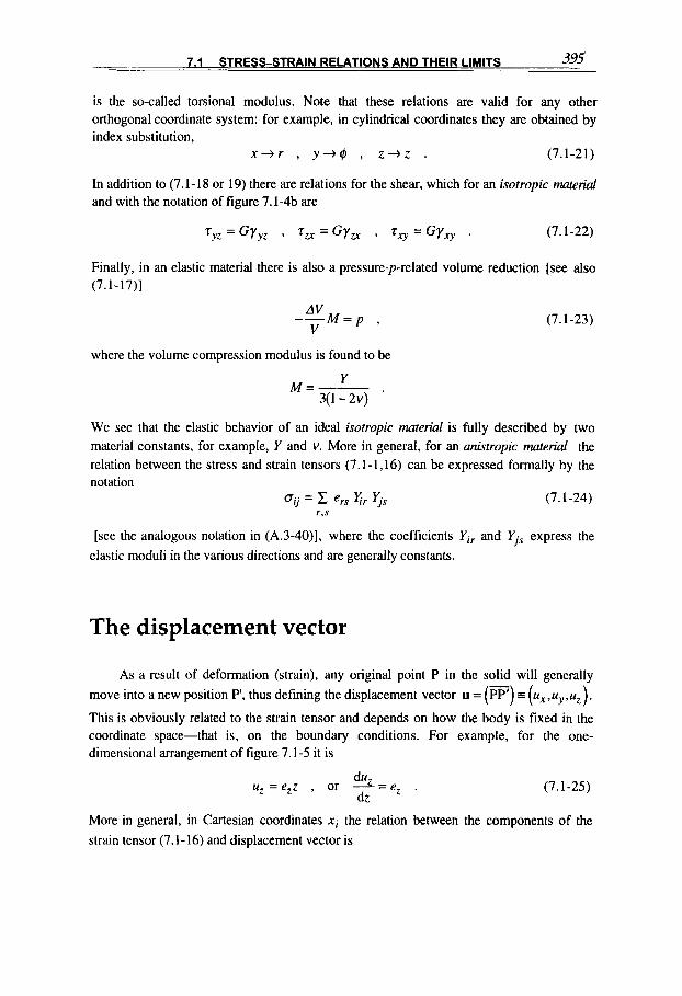
7.1 STRESSSTRAIN RELATIONS AND THEIR LIMITS 395
is the so-called torsional modulus. Note that these relations are valid for any other orthogonal coordinate system: for example, in cylindrical coordinates they are obtained by index substitution,
x + r , y + $ , z + z . (7.1-21)
In addition to (7.1-18 or 19) there are relations for the shear, which for an isotropic material and with the notation of figure 7.1-4b are
ryz = Gy,, , 7, =Gy, , z,, = GY, . (7.1-22)
Finally, in an elastic material there is also a pressure-p-related volume reduction [see also (7.1 - 17)]
AV -_ V M = p , (7.1-23)
where the volume compression modulus is found to be
Y M=- 3(1- 2 ~ )
We see that the elastic behavior of an ideal isotropic material is fully described by two material constants, for example, Y and v. More in general, for an anistropic material the relation between the stress and strain tensors (7.1-1,16) can be expressed formally by the notation
(7.1-24)
[see the analogous notation in (A.3-40)], where the coefficients Yir and Yjs express the elastic moduli in the various directions and are generally constants.
The displacement vector
As a result of deformation (strain), any original point P in the solid will generally move into a new position P , thus defining the displacement vector u = (PP') I (ux,uy.uZ). This is obviously related to the strain tensor and depends on how the body is fixed in the coordinate space-that is, on the boundary conditions. For example, for the one- dimensional arrangement of figure 7.1-5 it is
du
dz uz = e , z , or ez . (7.1-25)
More in general, in Cartesian coordinates xi the relation between the components of the strain tensor (7.1-16) and displacement vector is

396 CHAPTER 7 MAGNETOMECHANICAL STRESSES
Figure 7.1-5 Axial strain e, and displacement uZ. caused by an axial force S, or thermal expansion in a thin bar with cross-section area F.
(7.1-26)
As we shall see, introduction of the displacement vector is of great practical value. It is usually convenient to use it in the coordinate system most appropriate to the geometry of the solid under consideration. For example, the cylindrical (ur, urn, u,) components of the displacement vectors obtained from the equations
(7.1-27)
whereas in spherical coordinates (p, 44) they are
(there are also the spherical components of yeg, ype, ygp not given here' I ) . For example,
in the simple axisymrnetric cylinder (which will be used later in the discussion related to figure 7.2- 1). for the radial displacement ur of any point we can write
which could also have been obtained directly from (7.1-27).

7.1 STRESS-STRAIN RELATIONS AND THEIR LIMITS 397
Effects of thermal expansion
In many applications it is important to take into consideration the stresses caused by thermal expansion. We recall that most engineering materials will expand when heated. For the range of normal working temperatures, the unrestrained linear deformation (figure 7.1 - 5 ) can be expressed with sufficient precision by the strain
e, = a T , (7.1-31)
where a is the coefficient of thermal expansion and T stands for a temperature difference; that is, T is measured from a reference temperature To. which is generally 0°C. In most
applications, the coefficient acan be considered a constant, although it slightly depends on various physical parameters. For example, it is itself affected by stress; at the tension yield stress it can be as much as 10% greater for steel than it is with no load applied.
If the principle of superposition for the temperature- and stress-caused strains is applied, then the temperature expansion effect is introduced into (7.1-18 or 19) by the following strain substitution:
e x + e x - c r T , e y + e y - a T , e,+e,-crT . (7.1-32)
For example, from (7.1-19), in Cartesian coordinates we obtain
ve = e x + - - a * T , etc.
v(e - 3aT) X = e , - a T + 2G 1-2v 1-2v
(7.1-33)
where e = ex + ey + e, and
I + v 1-2v
a* = a -
is the reduced thermal expansion coefficient. On the other hand, the shear relations (7.1-22) remain unaffected by these thermal effects. Similarly, in cylindrical coordinates from (7.1 - 19), with the index substitution (7.1-21). we obtain
ve ve 0 ve -- 0, - e , + - - a * ~ , 2 = e 4 + - - a * T , A = e , + - - a * T , 2G 1-2v 2G 1-2v 2G 1-2v
(7.1-34)
where now e = e, + e4 + e,. The two sets of equations (7.1-33,34), in addition to the
assumption of a being with good approximation a constant factor even in an anisotropic material, indicate that the temperature effect is taken into account by the substitution for the main stress components in (7.1-1 1.12)
bjj + 0 j j + k,T ,

398 CHAPTER 7 MAGNETOMECHANICAL STRESSES
(where k , = 2 G a *). For example, the equation of elastic equilibrium (7.1-12) expands
into the vector form V.[o]+k,VT+f = o . (7.1-35)
This makes it necessary to know the temperature distribution in the solid, which is obtained from the heat diffusion equation (5.1-37),
kAT+g=cvT+@ , (7.1-36)
where g is the source term (here, typically g = j*/o), k is the thermal conductivity, cv is the specific heat per unit volume, and the dot means differentiation with respect to time. In extending the heat equation (5.1-37), we have added the last transient term describing heat transport as a consequence of dilation (7.1-17) of the solid, where p = P(T) is a temperature-dependent material constant. This term connects the transient aspects of the mechanical stresses to the heat diffusion problem 7.6; but in practice it can nearly always be neglected. In most cases, therefore, the temperature problem can be decoupled from the stress problem: One first calculates the space- and time-dependent temperature distribution T ( x , r ) from the given heat source g and initial and boundary conditions, which then determines the stress distribution- for example, through (7.1-33 or 35).
Thermoelasticity in dynamic systems
We now present some further elements of a general thermoelastic theory that might be of interest in formulating and solving magnetomechanical problems ’ I . Specifically, we want to establish the relation between the displacement vector u and the temperature effects and body forces that cause it, and we also include dynamic effects. The latter is accomplished by introducing the acceleration force density pu into all the forces given in (7.1-1 1.12) such as to obtain the equation of motion; for example, along the x-axis this becomes
Introducing the displacement components (7.1-26) into (7.1-22.33) yields
dux ve =x - 2G dx I-2v
01 * T , etc.,
(7.1-37)
(7.1-38)
(7.1-39)
with which (7.1-37) transforms into
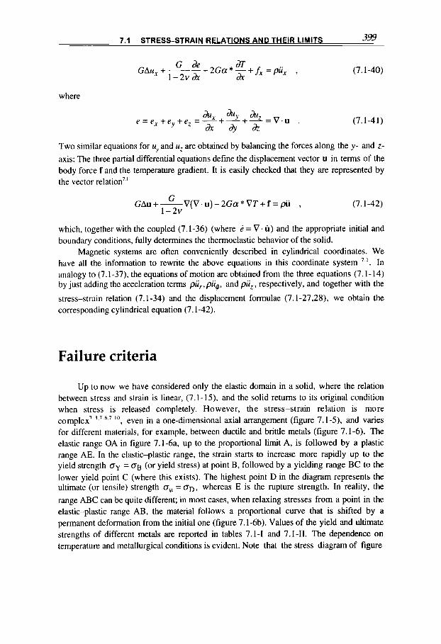
7.1 STRESS-STRAIN RELATIONS AND THEIR LIMITS 399
G de a 1-2vdx dx
GAuX+---2Ga*-+ fx=pUx ,
where
& A & e = e , + e Y + e Z = ~ + Y + - = V . U .
(7.1-40)
(7.1-41)
Two similar equations for uy and uz are obtained by balancing the forces along the y - and z- axis: The three partial differential equations define the displacement vector u in terms of the body force f and the temperature gradient. It is easily checked that they are represented by the vector relation7.'
(7.1-42) G
1-2v GAu +-V(V.u) - 2Ga * VT + f = pii ,
which, together with the coupled (7.1-36) (where e = V . u) and the appropriate initial and boundary conditions, fully determines the thermoelastic behavior of the solid.
Magnetic systems are often conveniently described in cylindrical coordinates. We have all the information to rewrite the above equations in this coordinate system I . In analogy to (7.1-37), the equations of motion are obtained from the three equations (7.1-14) by just adding the acceleration terms pii,,pug, and puz, respectively, and together with the
stress-strain relation (7.1-34) and the displacement formulae (7.1-27,28), we obtain the corresponding cylindrical equation (7.1-42).
Failure criteria
Up to now we have considered only the elastic domain in a solid, where the relation between stress and strain is linear, (7.1-15), and the solid returns to its original condition when stress is released completely. However, the stress-strain relation is more complex7 ',' 6 7 I" , even in a one-dimensional axial arrangement (figure 7.1-3, and varies for different materials, for example, between ductile and brittle metals (figure 7.1-6). The elastic range OA in figure 7.1-6a. up to the proportional limit A, is followed by a plastic range AE. In the elastic-plastic range, the strain starts to increase more rapidly up to the yield strength oY = OB (or yield stress) at point B, followed by a yielding range BC to the lower yield point C (where this exists). The highest point D in the diagram represents the ultimate (or tensile) strength 8, = OD, whereas E is the rupture strength. In reality, the range ABC can be quite different; in most cases, when relaxing stresses from a point in the elastic-plastic range AB, the material follows a proportional curve that is shifted by a permanent deformation from the initial one (figure 7.1-6b). Values of the yield and ultimate strengths of different metals are reported in tables 7.1-1 and 7.1-11. The dependence on temperature and metallurgical conditions is evident. Note that the stress diagram of figure

CHAPTER 7 MAGNETOMECHANICAL STRESSES __ 400 ~.
/" I I I I I I I I I I I I
I I
strain e~
elastic - C)
elastic P
------ I
4 time d)
k e creep strain ec
Figure 7.1-6 Stress-strain diagrams: (a) ductile material (with ABCD portion not to scale); (b) hysteresis or work hardening range (typically for a brittle material); (c) approximated diagram; (d) creep curve at constant load and temperature.
7.1-7 is related to an alloy mentioned in table 7.1-11. For calculations it can be convenient to approximate the stress-strain diagram in this range by two linear relations, one in the elastic range and the other in the elastic-plastic range, with a yield stress defined as in figure
Compressional loading gives rise to a somewhat similar and fairly smooth diagram up to the elastic-plastic range, but final failure, related to an ultimate yield strength, is generally caused by shear at an angle of 45" to the axial compression.
The concepts and theories of practical importance in magnetomechanical systems are complex and numerous, and their description lies well beyond the scope of this book. For example, in a simplified way we can say that the total strain
7 .1-6~.
e = e e + e +ec+eT (7.1-43) P
is made up of the creep component ec, in addition to the elastic ee, (7.1-15), (istantaneous) plastic ep. and temperature eT components (7.1-32). Creep is obtained under tensile loads and depends on three main parameters' 4: stress, time, and temperature (figure 7.1-6d).

7.1 STRESS-STRAIN RELATIONS AND THEIR LIMITS 401 ~
temperatures
Alloy
I 55-hard ' I
I 55-annealed
IO4hard ' I
- - - - - - - - - - - IWannealed
h 3ycon 3HPTM
;lidcop@'
4L-IS + NBIOOOThf
lanl
innwled
Temperature Yield Ultimate Rupture Figure of strength strength elongation merit
T 0, 0" EE ad rl (K) (MPa) (MPa) (%) (MPd~ '2 . c ml
4 490 560 28 2410
76 460 500 19 1 I60
_ - - - - - - - - - _ - - - ~ ~ 5 - - - - - ~ ~ - - - - - - - - - - - _ - - - - - - - - - _ - - - 410 8 200
4 81 460 62 230
76 81 380 55 I40
295 65 240 44 31
4 430 5 10 32 I I 'OOO
76 400 440 19 1680
9 190 - - - 2?5- - - - - 243- - - - 3 0 - - - - - - - - - - - - - - - - - - 4 31 410 76 3'000
76 31 340 57 I50
295 23 210 48 0.6
76 X I4 9 I9 - 7x0
295 723 X O 6 5-8 280
473 655 725 - I90
295 7x6 862 10 360
295 345 503 1 0 I50
A topic of great practical importance concerns the failure ~riteria'~---that is, the criteria that indicate when a solid structure (a magnet for example) can rupture under tensile or compressional loads (caused by magnetic forces). Failures of specimen under loads result mainly from the complex growth process of cracks and are initially caused by a variety of mechanisms, among which are surface defects, microcracks, and slip regions; cyclic loadings; stress corrosion; creep deformations.
Under dynamic single-pulse loading, the strength limits generally tend to increase. However, for a sequence of stress cycles (cyclic loadings), most materials will be affected
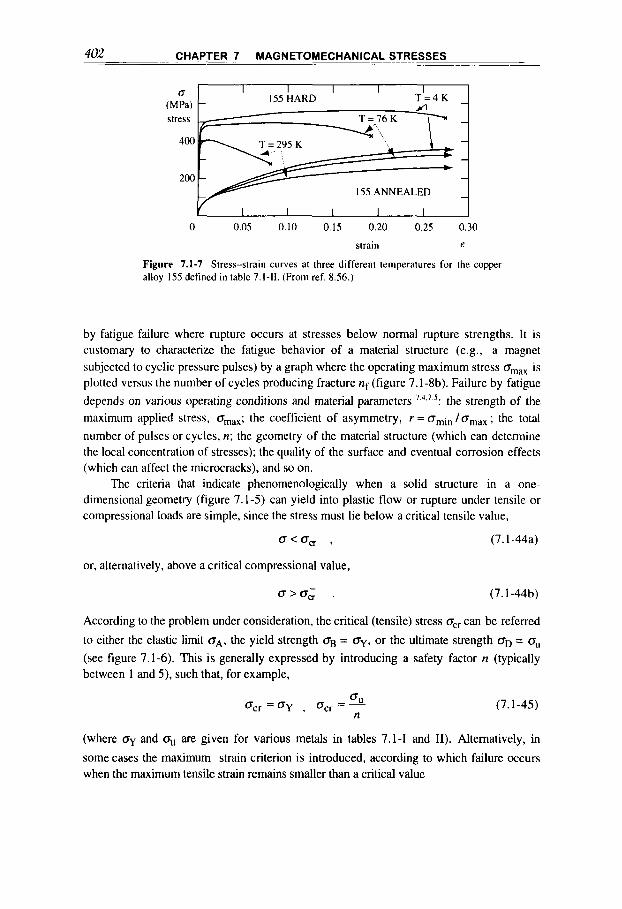
- _. ~ -. CHAPTLR _ _ 7 MAGNETOMECHANICAL ~- STRESSES . - 402
I I I I I 155 HARD T = 4 K
Y
U
(MPa) r? -
- , C -
b - I55 ANNEALED -
I
0 0.05 0.10 0.15 0.20 0.2s 0.30
strain e
Figure 7.1-7 Stress-strain curves at three different temperatures for the copper alloy 155 defined in table 7.1-11. (From ref. 8.56.)
by fatigue failure where rupture occurs at stresses below normal rupture strengths. It is customary to characterize the fatigue behavior of a material structure (e.g., a magnet subjected to cyclic pressure pulses) by a graph where the operating maximum stress omax is plotted versus the number of cycles producing fracture nf (figure 7.1-8b). Failure by fatigue depends on various operating conditions and material parameters ' 4.7 ': the strength of the maximum applied stress, omax; the coefficient of asymmetry, r = omin /omax ; the total
number of pulses or cycles, n; the geometry of the material structure (which can determine the local concentration of stresses); the quality of the surface and eventual corrosion effects (which can affect the microcracks), and so on.
The criteria that indicate phenomenologically when a solid structure in a one- dimensional geometry (figure 7.1-5) can yield into plastic flow or rupture under tensile or compressional loads are simple, since the stress must lie below a critical tensile value,
O<O, 7 (7.1-44a)
or, alternatively, above a critical compressional value,
O>O& . (7.1-44b)
According to the problem under consideration, the critical (tensile) stress ocr can be referred
to either the elastic limit a,, the yield strength OB = OY, or the ultimate strength OD = 0, (see figure 7.1-6). This is generally expressed by introducing a safety factor n (typically between I and 5) . such that, for example,
(7.1-45)
(where OY and O, are given for various metals in tables 7.1-1 and 11). Alternatively, in
some cases the maximum strain criterion is introduced, according to which failure occurs when the maximum tensile strain remains smaller than a critical value

7.1 STRESS-STRAIN RELATIONS AND THEIR LIMITS 403
Omin -
I I I I )
e < ecr . (7.1-46)
But what is a meaningful criterion in a more complex two- or three-dimensional problem, where there are mixed compressional and tensile stresses? There are different criteria, based on a variety of physical arguments. In a predominantly tensile domain, where the major of the principal stresses (01) is much larger than the others (O2,03), the
one-dimensional criterion (7.1-448) can make sense:
01 <0,, . (7.1-47)
Experience shows that the shear stress plays an important role in limiting the mechanical strength of materials, particularly when compressional loads apply, as already mentioned. Consequently, it is required that the maximum shear, as given in (7.1-8 or 9), be smaller than a critical yield value (Tresca criterion)79
(7.1-48)
In a one-dimensional arrangement we have
(7.1-49) - Dcr . 2 .
rcr = ~
this value can be used as a rough approximation, particularly for metals. In structures with complicated stress distributions (in which one at least of the principal stresses is compressional), a more satisfactory criterion requires the von Mises equivalent stress 6 . ''
(7.1-50)
defined on the basis of the principal stresses, 01, 02, and 03, to be less than a critical value
O M < < a . (7.1-51)

404 CHAPTER 7 MAGNETOMECHANICAL STRESSES
This Huber-von Mises-Hencky criterion is obtained by considering the distortion work of the material, and o,, can be taken here to be roughly equal to the tensile yield strength 0,.
A practical approach to the analysis of mechanical strength would start by applying the proportional, elastic theory [see (7.1-18 or 19)], which is relatively well-defined and clear’ 14. The resulting principal stresses will indicate when and where the proportional limits or, more in general, the failure criteria are reached. An important and interesting problem then is how the structure behaves in the elastic-plastic range up to the yield strength 0,. The simplest approximation is to treat the structure with the elastic
stress-strain relations up to the point where the principal stress reaches the yield strength
61 = (7.1-52)
and to assume that in the domain where o > oB, the material adapts with any necessary
strain to the surrounding mechanical constraints. In this way and with appropriate design, dangerously high stresses in certain regions of the magnetomechanical structure (as will be localized in the following studies on solenoidal and toroidal magnets) may be shifted to other more relaxed regions. Precompressing some of the critical components through external hydrostatic presses can further improve the overall containment. With such means, magnets for the Ignitor”’ and Omitron’” controlled fusion experiments were designed for the generation of toroidal fields from 13 up to 20 T o n the toroidal axis with radii from 0.5 to 1.4 m.
Interesting copper alloys are available today for the construction of high-performance magnets’ (for some examples see table 7.1-11).
7.2 STRESSES IN SOLENOIDAL MAGNETS
Thick cylinder and disk
The stress problem of a thick-walled elastic cylinder subjected to a radial force density f = f, ( r ) and to the constant radial pressures p I and p2 at the inner and outer surfaces
(figure 7.2-1) introduces the similar problems of a cylindrical magnet that is subjected to the Lorentz force densityf = j B , which we shall analyze later. This problem has, in fact, already been formulated above in general terms in connection with the expressions concerning stress, strain, and displacements caused by body forces or temperature effects

7.2 STRESSES IN SOLENOIDAL MAGNETS 405
in the cylindrical coordinate system [see (7.1-14,27,28,35,36)]. Many stress and failure problems concerning cylindrical magnets are similar to what is found in the theory of pressure vessels' '.
To simplify the solution we consider an axisymmetric [ (d(...)/d@ + O)] solid (figure
7.2-2), meaning that either oz = 0 or eZ = 0, thus leaving only the u,-displacement as a variable with the relations (7.1-30),
a4 U e =r e g = I ,
d r ' r
In the plane stress approximation, defined by 6, = 0 , from (7.1- 19) with relations
(7.1-30) we obtain
V I + V
I - v (e, +eg)--aT e2 =-- I -v (7.2- 1)
and consequently
du dr r r dr
2 I - v 2 1 - v -dur u - - + V' - (1 + v ) f f T , o q y = 3 + VL - ( I + v)ffT (7.2-2) o r y
with which (7.1-13) transforms into
dT d2u 1 du u d 1 d(ru,) - I - v dr2 r dr 3 dr[ r dr 1 Y d r
2 L + - L - L = - -- f + ( I + v ) a - . (7.2-3)
Figure 7.2-1 and internal force density$
Thick-walled cylinder subjected to external pressures p , and p 2
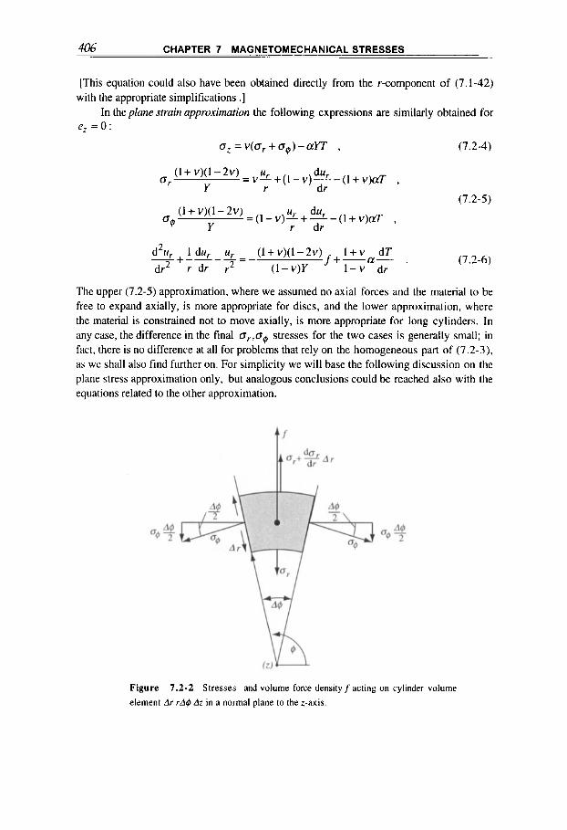
406 CHAPTER 7 MAGNETOMECHANICAL STRESSES
[This equation could also have been obtained directly from the r-component of (7.1-42) with the appropriate simplifications .]
In the plane strain approximarion the following expressions are similarly obtained for e, = 0 :
o , = v ( o r + o d ) - a Y T , (7.2-4)
(1 + v)(l - 2v) u du Y r d r
OtJ Y r dr
= v L + (1 - v)--L - (1 + v)aT , or
(7.2-5) (1 + v)(l - 2v) = (1 - v ) L + L - du (1 + v)aT , u
d2u 1 du ( 1 + ~ ) ( 1 - 2 ~ ) I + v dT l + - L - 5 = - f+-a- . (7.2-6) dr2 r dr r2 (1 - v)Y 1 - v dr
The upper (7.2-5) approximation, where we assumed no axial forces and the material to be free to expand axially, is more appropriate for discs, and the lower approximation, where the material is constrained not to move axially, is more appropriate for long cylinders. In any case, the difference in the final o,,otJ stresses for the two cases is generally small; in fact, there is no difference at all for problems that rely on the homogeneous part of (7.2-3), as we shall also find further on. For simplicity we will base the following discussion on the plane stress approximation only, but analogous conclusions could be reached also with the equations related to the other approximation.
Figure 7.2-2 Stresses and volume force densityf acting on cylinder volume element Ar r A @ & in a normal plane to the z-axis.

407 .~
7.2 STRESSES IN SOLENOIDAL MAGNETS ~ _ _ _
The general solution of the Eulerian differential equation (7.2-3) can be found easily. Indeed, a direct integration provides
1 d(rur) - (1 - v 2 ) j -~ f d r + ( I + v ) a T + 2 C , r d r Y
and then integrating once again yields the solution
D ur(r) = U(r) + Cr + - ,
r
where
rTdr U ( r ) = - l _ y ? j r d r j f d r f P r (1 + v)a
rY r
(7.2-7)
(7.2-8)
(7.2-9)
"I al
is a particular solution of (7.2-3), and the constants C, D are fixed by appropriate boundary conditions. The stress components or, 04 are calculated through (7.2-2). For free boundaries subjected to only the external pressures p l , p2 (figure 7.2-1). the integration constants are found from the conditions
and the solution is then fully determined. For example, the solution
D ur(r)=-- - r - +- r + C r + -
Y ( 8 3 r
2 1-v c 3 d (7.2-1 1 )
is found for T = 0 and a force density of the form
f ( r ) = c r + d , (7.2-12)
which, as we shall see in (7.2-18,19), is pertinent to a solenoidal coil with constant current density. (With d = 0 it also describes the centrifugal forcef = p d r in a spinning disk or cylinder with mass density p and angular frequency w.)
Solenoidal coils
We now apply the previous results to some typical cylindrical magnet structures. The special case f = 0 provides the stress distribution in an thick elastic cylindrical shell subjected to intemaVexternal pressures p l , p2 . This case can describe a magnet with the current j limited to within a very thin layer of thickness d, at the inner boundary r = a ] .
From (6.2-92) we know that the electromagnetic force per unit surface exerted on the layer
408 CHAPTER 7 MAGNETOMECHANICAL STRESSES
d, is, independently of the current distribution in d , ,
(7.2-13)
From the general solution (7.2-8 or 11) with U = 0 and C,D fixed by conditions (7.2- lo), we calculate the stress components (7.2-2)
and the constant axial strain
(7.2- 14)
(7.2- 15)
(7.2- 16)
On the other hand, it is easily checked that in this problem the plane strain approximation provides the same (T,.,(T~ stresses, but with constant axial stress
.:( $ - I] = 2+ - $ P 2 ) (7.2- 17)
If we were applying this stress with opposite sign on a free cylinder (as in fact we have in the former approximation), we would just obtain the strain (7.2-16); this also shows the correspondence between the two approximations.
The second example concerns the evenly wound long solenoidal magnet with uniform current density in its cross section of
. . dH H 2 - H l J = J =--=-- dr a2-a1
and the decay of the axial midplane fields from H ( a l ) = H I to H(u2) = H2 of
( H 2 - Hl ) r - H 2 q + H1u2
a2 - a1 H(r) =
(index z is omitted in this section). By fixing the constants of (7.2-12) through
f = p j H ,
the force density, and using the conditions (7.2-10) and the symbols
(7.2- 18)
(7.2- 19)
(7.2-20)
(7.2-21)

7.2 STRESSES IN SOLENOIDAL MAGNETS 409
2 0 - P H:
4
2
u 1.0 1 . 1 1.2 1.3
t I I 1 I I 1 I 1 I I I I 1 1 - 1
I 2 3 4 p = r/ul normalized radius p = r/ul
Figure 7.2-3 Hoop and radial stress distributions in two long solenoidal coils with constant current density, H, = 0 and a = 1.3.4. U~ up compact elastic structure; u:. wide independent-turn approximation; u;, thin-sheet approximation.
[from here to (7.2-3 1 ) this a must not be confused with the thermal expansion coefficient used up t o (7.2-9)], the general solution (7.2-1 1) is obtained in the explicit form
(1 + a)p (aHI - H2) . (7.2-22) 1 11 + ({>+=(]+“+a I-v 2 )I--- 2 + v I - v 3 3
The hoop stress q and the radial stress 0,. are calculated with the help of (7.2-2 or 5). For example, with free boundaries, pI = p2 = 0 , from (7.2-2) with T = 0 we obtain for the
hoop stress’ ‘’
In figure 7.2-3 we have plotted these normalized stresses for two very long solenoidal coils
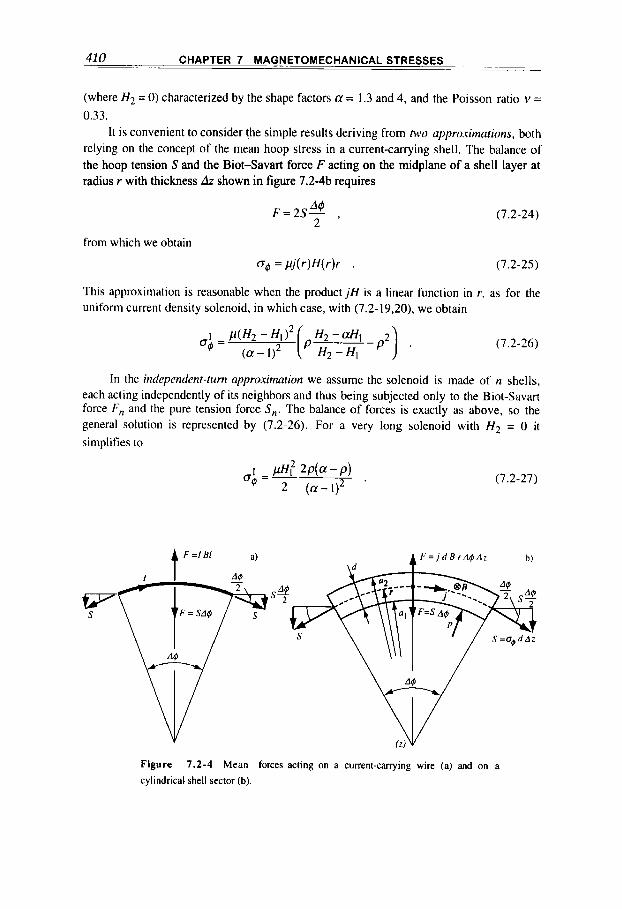
410 CHAPTER 7 MAGNETOMECHANICAL STRESSES
(where H2 = 0) characterized by the shape factors a = 1.3 and 4, and the Poisson ratio v = 0.33.
It is convenient to consider the simple results deriving from two approximations, both relying on the concept of the mean hoop stress in a current-canying shell. The balance of the hoop tension S and the Biot-Savart force F acting on the midplane of a shell layer at radius r with thickness dr shown in figure 7.2-4b requires
4 2
F=2S- ,
from which we obtain
(7.2-24)
(7.2-25)
This approximation is reasonable when the product j H is a linear function in r , as for the uniform current density solenoid, in which case, with (7.2-19,20). we obtain
(7.2-26)
In the independent-turn approximation we assume the solenoid is made of n shells, each acting independently of its neighbors and thus being subjected only to the Biot-Savart force I., and the pure tension force S,,. The balance of forces is exactly as above, so the general solution is represented by (7.2-26). For a very long solenoid with H2 = 0 it simplifies to
(7.2-27)
Figure 7.2-4 Mean forces acting on a current-canying wire (a) and on a
cylindrical shell sector (b).

7.2 STRESSES IN SOLENOIDAL MAGNETS 411
In the fhin-shref approximation (which will be treated in more detail later) the solenoid is taken to be one single sheet. The result is again approximated by (7.2-25) with r = (a2 + a l ) /2 , that is, p = (a + l)/2; in particular, from (7.2-27):
(7.2-28)
The last two approximations are introduced for a = 1.3 and 4 into figure 7.2-3 for an interesting comparison with the general elastic solution (7.2-25). For a relatively thin coil the radial stress or is compressive and helps in making the hoop stress og more uniform
and smaller in its maximum value than the independent turn stress og . However, in fatter
coils the radial stress or becomes negative (i.e., tensile) and the situation worsens. The
transition between the two cases [i.e., where (dor/dp)p,l = 01 happens at a = 1.85 for
very long coils. We conclude that radial stresses, as long as they are compressive, are beneficial in reducing the maximum hoop stresses. Qualitatively, this effect works because the inner layers, subjected to the maximum Biot-Savart forces, can lean on outer layers, thereby limiting the strain and its related stress.
High-field Bitter coils (see figure 2.3-1 1) have a current density distribution in the conductor of
I
and a corresponding axial midplane field of
H ( r ) = HI -(HI - H2)- In P In a
(7.2-29)
(7.2-30)
These expressions are obtained from the Bitter current distribution j = j l /p , (2.3-38).
where p,a are as in (7.2-21). Introducing the related force densityf= pjH into the integral expression (7.2-9) (where T = 0) provides the particular solution
lnp] . (7.2-31) H1(2 lna+ l ) - H2
HI - H2
1 - v2 (HI - H2I2 W P ) = y l n 2 a
The general solution (7.2-8) and the stresses (7.2-2) can then be calculated, as before (for additional calculations see ref. 2.9 and ref. 1.17, p. 349).
Up to now we have assumed a homogeneous coil material and smooth current density. But a coil is generally made from layers of metallic conductor and of dielectric materials (figure 7.2-5). We can extend the above solutions to include multilayered coils (where each layer i = l,2, ..., n may or may not carry a current density j; and may possess
different mechanical properties v; , Yi) by rewriting for each layer the appropriate solution,
and all the solutions are then matched at their boundaries. Take the example of (7.2-22), which is rewritten for the ith layer with the following logical substitutions:

412 CHAPTER 7 MAGNETOMECHANICAL STRESSES
Figure 7.2-5 The multilayered solenoid. Each layer i=1,2 ..., may carry a constant current densityjiand may possess different mechanical parameters v, , V, .
(7.2-3 2)
Referred to the n layers, this general expression provides the system of 2n equations for the 2n variables u; , pi (noting that at the boundary of two adjacent layers the ui , pi must be the same). Elimination of pi leads to a system of n + 1 linear equations for the n + 1 unknown displacements u; or, alternatively, through (7.1-30), strains ei.
Yielding in cylindrical containers
The merit of the elastic stress-strain calculations discussed above in connection with some examples is to describe the elastic behavior of electromechanical systems, and particularly to show when and where the strength limit of the material is reached, so that failures can be avoided by appropriate structural changes in the system.
We will now explore the containment limit for thick-walled cylinders, which anticipates the strength problem of cylindrical magnets. According to criteria (7.1 -47,48), here transcribed to cylindrical geometry, yielding (marked by the superscript Y) occurs when

7.2 STRESSES IN SOLENOIDAL MAGNETS 4 u
(7.2-33) Y Y o4 =o,, , or o$ -a, =25,, .
The first may be a sufficient criterion for thin discs; the second, more refined criterion may be more appropriate for long solenoids. By introducing these values into (7.1-13) we obtain, respectively, the two equations
(7.2-34)
and by direct integration the solutions
1 , r
a, Y =a,, --I rfdr+G , or a? = 2rJnr- I f d r + G . (7.2-35) r
To simplify our reasoning, we assume the function f in such a way that yielding extends from a l to radius r = rc, with the constant G fixed by the boundary condition at a l . From rc
to u1 the material is in the elastic domain where the radial stress a, is described by (7.2-2)
and the general solution (7.2-8), with the constants C,D now fixed by the boundary conditions at u2 and r = r,, this condition being as in (7.2-33): a@(r,)= acr or
04(r,) - a,(rc) = 25,, . These three conditions at r = a1 ,rc, u2 determine the constants
C. D. G; and the matching condition 0,. ( rc )=ar ( rc ) finally provides the radius re at
which transition occurs from the elastic to the plastic domain.
As an example, we consider the mechanical strength of a cylindrical shell containing the pressure pI (with no other force around: f = 0, 112 = 0, T = 0) by applying the right- hand yielding criterion (7.2-33). In the plastic domain r = a1 to re, the normalized radial
stress (7.2-35) is
Y
(7.2-36)
whereas in the elastic domain, r = rc to a2, from (7.2-14,15) with the substitutions uI + r,, p1 + pc we find
having imposed on r = r, the condition
(7.2-37)
(7.2-3 8)
414 . CHAPTER 7 -MAGNETOMECHANICAL STRESSES - - _ _ .. ._
The last expression also shows that yielding in such a container starts at its inner surface r = u I when the contained pressurepl exceeds the critical value
(7.2-39)
When the pressurepl is above this value the yielding interface is located at a radius rc inside
the container material and is found from (7.2-34,35) through the condition Y
or (rc) = or (rc 1 :
(7.2-40) ~ + 2 l n ! L = P I - l r L .
“22 a1 rcr
As long as rc < a 2 , the outer elastic domain still sustains the yielded domain as well.
Thin-walled cylindrical magnet
When the thickness d = u2 - a1 of the container is small compared to its mean radius of curvature a = (a2 + q ) / 2 (say, typically smaller than M), it is convenient to adopt the thin-wall or membrane approximation, which appreciably simplifies the formulation and the results of the problem. In this approximation it is assumed that there are only stresses tangential at any point to the surface and constant across the thickness d , the stress normal to the surface being negligible. Any load acting on the membrane, such as a pressure pl
internal to the container or the j x B force of a thin coil, must be resisted by these tangential stresses.
A case of interest, because of its analogy to a thin solenoidal coil, is the containment of a pressure p by a thin-walled cylindrical shell. Balance of the forces acting on a shell sector (figure 7.2-4) gives (7.2-24) and since here F = pad4 we find a mean tangential stress of
(7.2-4 1 ) U
o+b=p- 7
d
which could also have been obtained from (7.2-25) in the limit a2 - a1 = d << a ] , or from (7.1-13) with or = 0 andf = p/d. Introducing the radial displacement up (7.1-30), with
Hooke’s law (7.1-15) gives
U q = ’ Y .
a
Here, a simple criterion for containment is obtained from (7.1-47):
(7.2-42)
o+b<Qcr 7 (7.2-43)

~~~~ ~~ 7.2 STRESSES IN SOLENOIDAL MAGNETS 415
where o,, is the critical yield strength defined in connection with (7.1-45), with oy and o, given for various metals in tables 7.1.1 and II.
We can transcribe these formulae for the containment of a static magnetic field by taking from (7.2- 13)
p=- N2 2
For example, the criterion for static containment of a magnetic field is therefore
1 2 d -pH <D,,- . 2 N
We can define LI yieldfield by the relation
(7.2-44)
(7.2-45)
(7.2-46)
whose practical meaning clearly results from (7.2-45). For example, for a,, = lo00 MPa,
we find H y = 50 T.
Dynamic containment
For rapidly pulsed magnets it is sometimes necessary to consider dynamic containment, where the inertia of the structure plays an important role. This effect refers to the termpii in the more general theory expressed by (7.1-42). Here, we limit the
discussion to the simple case of a thin cylindrical container (figure 7.2-6). If the time duration of the pressure pulse p(f) is short compared to the oscillating period
(7.2-47)
of the container' I", the momentum transferred to its wall is
1
P = 21~ahj p(f)dr ,
0
(7.2-48)
where p is the mass density. (The period TM is typically 100 ps for a container of 10-cm diameter.) For the resulting dilatation we calculate
(7.2-49)

.- . 416 .. CHAPTER 7 MAGNETOMECHANICAL STRESSES - .
Figure 7.2-6 Cylindrical magnetic field container.
p = - M - , where M = 2modlip K: is the container mass. The criterion for dynamic containrnent therefore becomes
I - p j 1 H 2 d t c j s .
2 o
(7.2-50)
(7.2-51)
As an example we consider a sinusoidal field
2n T
H = Hosin-t
limited to the first half cycle. By integration and use of the mechanical period TM (7.2-47), the criterion transforms into the simple form
(7.2-52)
Since our calculation is based on the assumption T (( T,, this expression shows that dynamic containment is better than static containment (7.2-45) by a factor TMIT. In
addition, the dynamic oCr value is somewhat larger than the usual static value given in table
In the case just treated, the material of the wall acts as both the inertial mass and the retaining elastic bound More often these two roles are overtaken by two distinct elements: this situation can easily be dealt with by extending this simple calculation accordingly ’.”.
7.1-1.
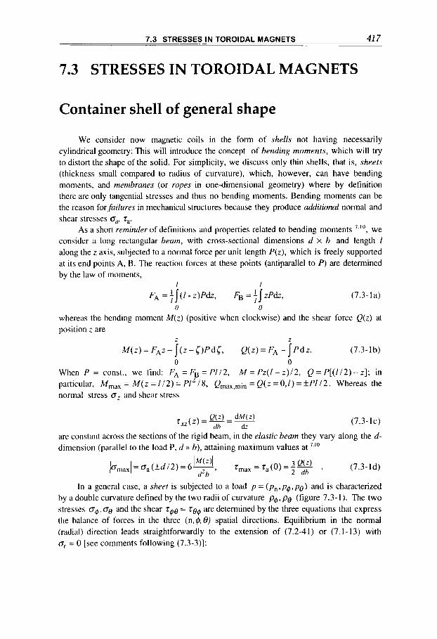
7.3 STRESSES IN TOROIDAL MAGNETS 417 ._ . - ~. - _ _
~
7.3 STRESSES IN TOROIDAL MAGNETS
Container shell of general shape
We consider now magnetic coils in the form of shells not having necessarily cylindrical geometry: This will introduce the concept of bending moments, which will try to distort the shape of the solid. For simplicity, we discuss only thin shells, that is, sheets (thickness small compared to radius of curvature), which, however, can have bending moments, and membranes (or ropes in one-dimensional geometry) where by definition there are only tangential stresses and thus no bending moments. Bending moments can be the reason for failures in mechanical structures because they produce additional normal and shear stresses o,, r,.
As a short reminder of definitions and properties related to bending moments ' I", we consider a long rectangular brani, with cross-sectional dimensions d x b and length 1 along the z axis, subjected to a normal force per unit length P(z) , which is freely supported at its end points A, B. The reaction forces at these points (antiparallel to P) are determined by the law of moments,
I I FA = i j ( 1 - z)fdz., FB = ' I z P d z , (7.3-la)
I 0 0
whereas the bending moment M(z) (positive when clockwise) and the shear force Q(z ) at position z are
2
M ( z ) = - j ( z - c)f dc , Q(z ) = FA - If d z. (7.3-lb) 0 0
When P = const., we find: FA = FB = P112, M = Pz(1 - z ) / 2 , Q = f [ ( 1 / 2 ) - z ] ; in particular, M,,, = M ( z = 1 / 2 ) = P I 18, Qmax,,in = Q ( z = O , I ) = f P I / 2 . Whereas the normal stress oz and shear stress
L
(7.3- 1 C)
are constant across the sections of the rigid beam, in the elasric beam they vary along the d- dimension (parallel to the load P, d )) b), attaining maximum values at ' l o
(7.3-ld)
In a general case. a sheet is subjected to a load 11 = ( p n , p ~ , p o ) and is characterized by a double curvature defined by the two radii of curvature pq, pe (figure 7.3- I ) . The two stresses oq, 00 and the shear ~ $ 0 = are determined by the three equations that express the balance of forces in the three (n ,@,O) spatial directions. Equilibrium in the normal (radial) direction leads straightforwardly to the extension of (7.2-41) or (7.1-13) with or = 0 [see comments following (7.3-3)]:

418 CHAPTER 7 MAGNETOMECHANICAL STRESSES
t pnp,$ A@* d B
Figure 7.3-1 Stresses on thin-walled shell of thickness d with double curvature and subjected to normal pressure load pn (no shear is indicated, since uF a, are supposed lo be principal stresses).
Figure 7.3-1 Stresses on thin-walled shell of thickness d with double curvature and subjected to normal pressure load pn (no shear is indicated, since uF a, are supposed lo be principal stresses).
(7.3-2)
For establishing the other two equilibrium equations we refer, for simplicity, to an axisymmetric shell with constant thickness d- that is, a surface obtained by a generating curve rotating about a given axis (figure 7.3-2). For example, equilibrium along the 8- direction must consider the following four forces: the ogstress increment (dSe/d8)A8; the z,,+,cincrement ( f l&j /d@) A @ ; the projection S@A$ cos8 of the oG-stress normal component S @ A @ ; and the load component Pe Introducing the expressions for the forces given in figure 7.3-2 results in the differential equation 7.7
and similarly, from the equilibrium along the +direction we obtain
(Note that pg,pe do not vary with d@, but can vary with 38.) An important remark concerns the principal directions along the principal stresses,
ol(= og), 6 2 ( = GO), o3(= on), as defined in (7.1-5). In a membrane, the principal directions 1, 2 lying in the tangential plane with direction 3 normal to it. follow directly
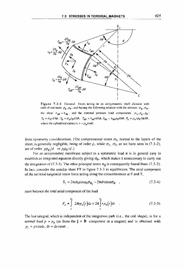
419 . ..
~. . 7.3 - STRESSES IN TOROIDAL MAGNETS ~- - _
A
Figure 7 .3-2 General forces acting on an axisymmetric shell element with radii of curvature p9 . p e , and having the following relation with the stresses 09, uo ,
the shear ?w ='sw. and the external pressure load components p n , p O , p , :
S, = oerdA4 I Sq = 09podA0 . Tq, = ?gordAQ, Toe = TWpedAO, P, = pnrpoA@AO.
where the cylindrical radius is r = pgsinO.
from symmetry considerations. [The compressional stress 03, normal to the layers of the sheet, is generally negligible, being of order p , while 01, 02, as we have seen in (7.3-2), are of order p p g l d or p p o l d .]
For an axisymmetric membrane subject to a symmetric load it is in general easy to establish an integrated equation directly giving 0 0 , which makes it unnecessary to carry out
the integration of (7.3-3). The other principal stress 04 is consequently found from (7.3-2).
In fact, consider the annular sheet FT in figure 7.3-3 in equilibrium: The axial component of the net total tangential stress force acting along the circumferences at F and T,
S, = 2ndrgsina00g~ - 2ndrsina00 , (7.3-4)
must balance the total axial component of the load
'0 '0
F, = I 2mp,(r)dv = 2nIrpn(r )dr . (7.3-5) r r
The last integral, which is independent of the integration path (i.e., the coil shape), is for a rionnal loud p = pn (as from the j x B component in a magnet) and is obtained with pz = p c o s a , dr = dscosa .
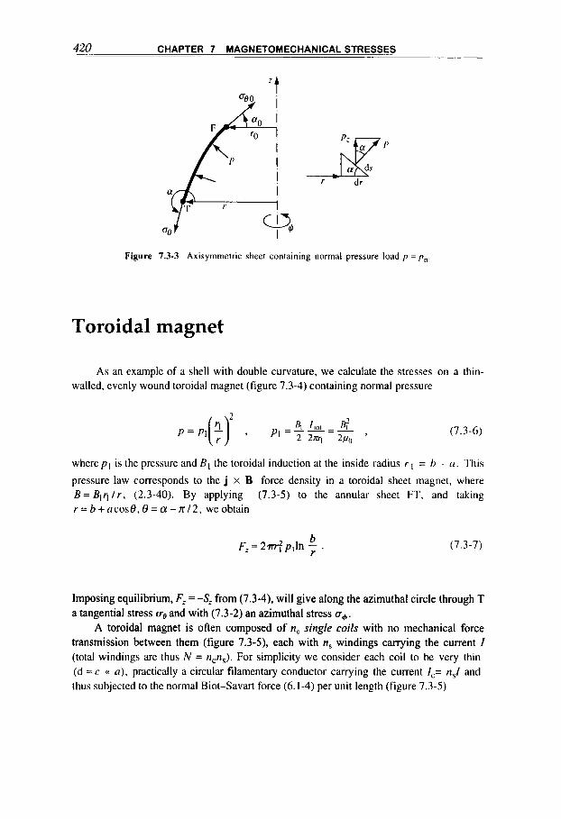
420 CHAPTER 7 MAGNETOMECHANICAL STRESSES
Figure 7.3-3 Axisymmetric sheet containing normal pressure load p = pn
Toroidal magnet
As an example of a shell with double curvature, we calculate the stresses on a thin- walled, evenly wound toroidal magnet (figure 7.3-4) containing normal pressure
(7.3-6)
wherepl is the pressure and Bl the toroidal induction at the inside radius r I = h - ~ i . This
pressure law corresponds to the j x B force density in a toroidal sheet magnet, where B = BIq / r , (2.3-40). By applying (7.3-5) to the annular sheet FT, and taking r = b+ucosO, 8 = a - 7 r / 2 , we obtain
(7.3-7) b F z = 2m:p,ln - r .
Imposing equilibrium, Fz = -Sz from (7.3-4), will give along the azimuthal circle through T a tangential stress a, and with (7.3-2) an azimuthal stress u4.
A toroidal magnet is often composed of n, single coils with no mechanical force transmission between them (figure 7.3-5), each with n, windings carrying the current I (total windings are thus N = ncns). For simplicity we consider each coil to be very thin (d = c (( a ) , practically a circular filamentary conductor carrying the current I,= n,I and thus subjected to the normal Biot-Savart force (6.1-4) per unit length (figure 7.3-5)
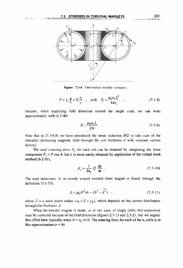
~- 7.3 STRESSES IN TOROIDAL MAGNETS 421
Figure 7.3-4 Thin-walled ioroidal container
(7.3-8)
because, when neglecting field distortion around the single coils, we can write approximately with (2.3-40)
(7.3-9)
Note that in (7.3-6.8) we have introduced the mean induction B/2 to take care of the (linearly) decreasing magnetic field through the coil thickness d with constant current density.
The totul cmtrringforce Fc for each coil can be obtained by integrating the force component P, = P cos 8, but it is more easily obtained by application of the virtual work method (6.2-5b),
The total inductance of an evenly wound toroidal definition (5.1-33).
(7.3-10)
sheet magnet is found through the
L = p o ~ * ( h - 4 7 7 ) , (7.3-1 1)
where U is a mean minor radius ( a , c zi < 122) . which depends on the current distribution through the thickness d.
When the toroidal magnet is made, as in our case, of single coils, this expression must be corrected because of the field distorsion (figures 2.3-13 and 2.5-2), but we neglect this effect here, typically when N = n, 3 10. The entering force for each of the n, coils is in this approximation (r = 6)
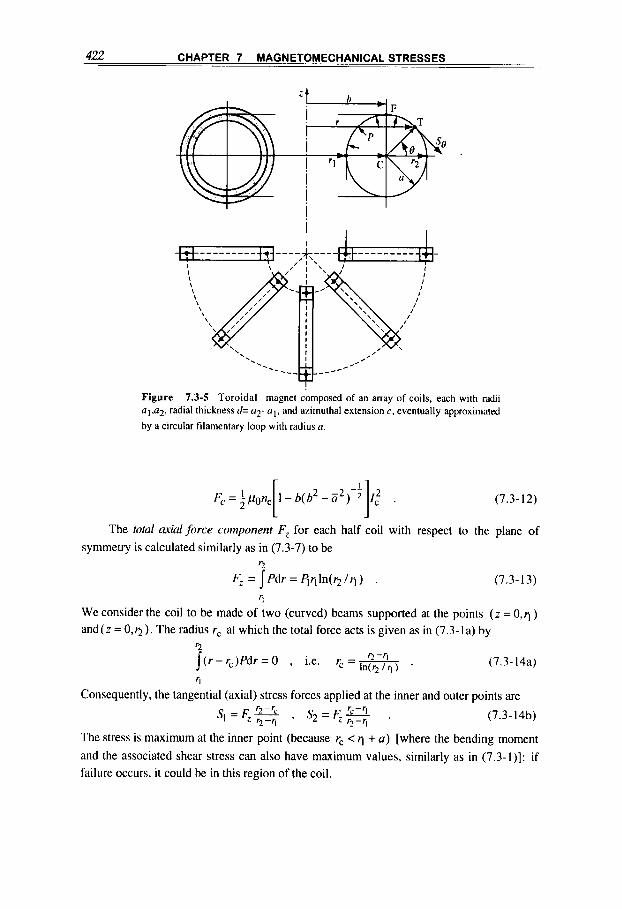
422 CHAPTER 7 MAGNETOMECHANICAL STRESSES
Figure 7.3-5 Toroidal magnet composed of an array of coils, each with radii ~ 1 . ~ 2 . radial thickness d= a2- al. and azimuthal extension c, eventually approximated
by a circular filamentary loop with radius a.
(7.3-12)
The total axiul force component F, for each half coil with respect to the plane of symmetry is calculated similarly as in (7.3-7) to be
'2
F, = I P d r = F j q l n ( ~ l r l ) . (7.3-13)
4 We consider the coil to be made of two (curved) beams supported at the points (z = 0,rI) and(z = 0 , ~ ) . The radius r, at which the total force acts is given as in (7.3-la) by
(7.3-14a) ( r - r c ) P d r = O , i.e. rc =--- '2 -'I 7 In(r2/rL) ' 'I
Consequently, the tangential (axial) stress forces applied at the inner and outer points are
(7.3-14b) S - F '2-'C S - F 'C-q I - Z " 1 ' 2 - z " I .
The stress is maximum at the inner point (because rc < q + a ) [where the bending moment and the associated shear stress can also have maximum values, similarly as in (7.3-l)]: if failure occurs, it could be in this region of the coil.

423 -. ~
7.3 .STRESSES IN TOROIDAL MAGNETS - - . ~ .~ - __ -
Toroidal magnet with constant stress
In a bubble at equilibrium, a constant surface tension counteracts the pressure drop at the bubble’s membrane, thereby defining its shape”. Similarly, a flexible toroidal coil can adapt its cross-sectional shape so as to obtain constant stress and become bending free. This problem is discussed here for the two cases treated before, which are appropriate approximations for toroidal magnet structures: the toroidal sheet magnet and the filamentary coil.
As in connection with (7.3-7), the balance of the axial component forces acting on the annular membrane FT (figure 7.3-6) of the toroidal sheet magnet yields
(7.3- 15)
where the toroidal magnet pressure (7.3-6) has been used, b is the radial distance of the maximum (where dz/dr = tana = 0) . and
-~ I di[ (:ckr]y 1
2 s ina=+tana( l+ tan a ) 2 =f- I + - dr
By imposing the constant stress condition 00 = OO(const.) in S, = F, we get
I F \
I 7 - y !
(7.3- 1 6)
Figure 7.3-6 Upper-half cross section of the toroidal sheet magnet or the filamentary coil.
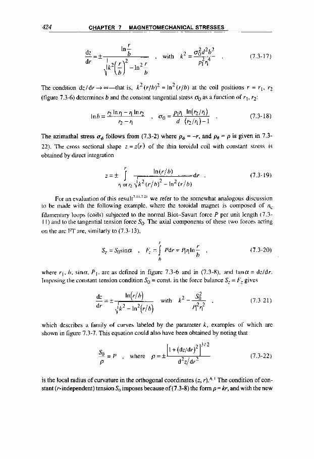
424 CHAPTER 7 MAGNETOMECHANICAL STRESSES
The condition dzldr + --that is, k2(r/b)2 = ln2(r/h) at the coil positions r = r l , r2
(figure 7.3-6) determines h and the constant tangential stress 0, as a function of r l , ‘2:
Inh = 1 00 =- Plq W 2 l r l ) (7.3-18) r2 lnq - q Inr2
‘2 - ‘I d (r2/rd-l .
The azimuthal stress ud follows from (7.3-2) where pd = -r, and pe = p is given in 7.3-
22). The cross sectional shape z = z ( r ) of the thin toroidal coil with constant stress is obtained by direct integration
(7.3-19)
For an evaluation of this result’ ‘ I ’’I we refer to the somewhat analogous discussion to be made with the following example, where the toroidal magnet is composed of nc filamenlary loops (coils) subjected to the normal Biot-Savart force P per unit length (7.3- 1 I ) and to the tangential tension force So. The axial components of these two forces acting
on the arc FT are. similarly to (7.3- 13).
r
(7.3 -20) r h
S, =Sosinor , F- = I P d r = Fjqln- , h
where ‘1. 0, sina, PI, are as defined in figure 7.3-6 and in (7.3-8), and tana = dz/dr. Imposing the constant-tension condition So = const. i n the force balance S, = Fz gives
(7.3-21) 2 s,2 $ti2
with k =- , dz
which describes a family of curves labeled by the parameter k , examples of which are shown in figure 7.3-7. This equation could also have been obtained by noting that
[ I + ( d ~ / d r ) ~ ] ~ ” so= P , where p = + (7.3-22) P d2z/dr2
is the local radius of curvature in the orthogonal coordinates (z, r).*.I The condition of con- stant (r-independent) tension So imposes because of (7.3-8) the form p= kr, and with the new

425 - . __ _ _ 7.3 STRESSES IN-TOJOJDAL MAGNETS
. ._ . . - . . . - -
;t !
1 I I
a)
z A
PP
- I I
! I
Figure 7.3-7 ( a ) T w o possible solution curves z = z (r ) of the constant stress filarnentary coil in a toroidal magnet; (b) a family of D-shaped. filamentary coils (upper halfonly) with the sarne outer radius
variable ii = dz /d r and separation we obtain
. . du d r
which by simple integration between h and r leads to (7.3-21). This also makes it evident that this coil is hmciing,free, because at any arc portion ds the normal force Pds is fully equilibrated by the tension force So, in the way shown by figure 7.2-4.
By requiring as in (7.3- 17) dz/dr + ..-that is, k L = InL ( r / h ) at the coil positions r = r l , ‘2 , we obtain [because In (r1 / b ) = In (Q / / I ) ]
L L
h = f i , k = l n J r 2 / r l , and S ~ ~ = q r , I n ~ , (7.3-23)
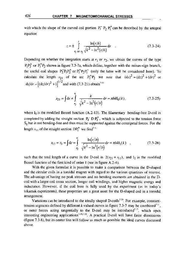
426 CHAPTER 7 MAGNETOMECHANICAL STRESSES
with which the shape of the curved coil portion P; P2 PTcan be described by the integral
equation
(7.3-24) z = f -\i--dr W l b ) . q or r2 k 2 - ln2(r/b)
Depending on whether the integration starts at rI or 1-2, we obtain the curves of the type
PIP; or PTP2 shown in figure 7.3-7a, which define, together with the minus-sign branch,
the useful coil shapes PFP1Pz or PTP2P; (only the latter will be considered here). To
calculate the length 321 of the arc PTP2 we note that (ds) = (dz)2 +(dr)2 or 2
112 ds/dr = [(dz/dq2 + 11 and with (7.3-21) obtain7 'I
(7.3-25)
where 10 is the modified Bessel function (A.2-13). The filamentary bending-free D-coil is
completed by adding the straight section P; D PT, which is subjected to the tension force So but is not bending-free and thus must be supported against the centripetal forces. For the
length sI I of the straight section DP: we find7 I'
r, In(r/b)
9 k -In ( r /h) "1 1 = ZI = dz = \iT dr = xhkI 1 ( k ) , (7.3-26)
such that the total length of a curve in the D-coil is 2(s21 + ~ 1 1 ) . and 11 is the modified Bessel function of the first kind of order I (see in figure A.2-4).
With the given formulae it is possible to make a comparison between the D-shaped and the circular coils in a toroidal magnet with regard to the various quantities of interest. The advantage of having no peak stresses and no bending moments are obtained in the D- coil with a larger coil cross section, longer coil windings, and higher magnetic energy and inductance. However, if the coil bore is fully used by the experiment (as in today's tokamak experiments), these properties are a great asset for the D-shaped coil in a toroidal arrangement.
Variations can be introduced to the ideally shaped D-coils7 20. For example, constant- tension segments defined by different k-valued curves in figure 7.3-7 may be combined7 ", or outer forces acting tangentially to the D-coil may be i n t r o d ~ c e d ~ ' ~ , which open interesting engineering applications7 ''.7 '*. A practical D-coil will have finite dimensions (figure 7.3-8), but its center line will follow as much as possible the ideal curves discussed above.
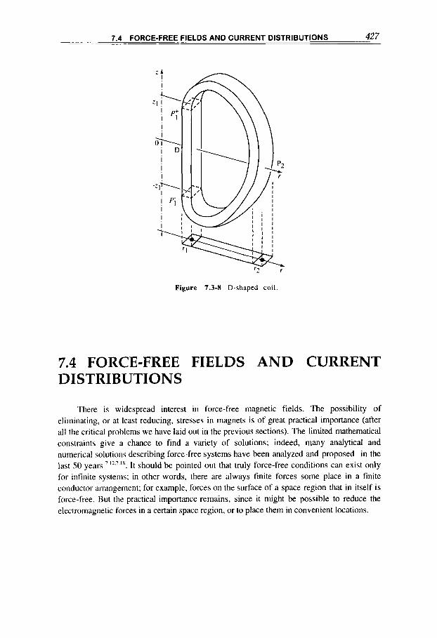
7.4 FORCE-FREE FIELDS AND CURRENT DISTRIBUTIONS 427
Figure 7.3-8 D-shaped coil
7.4 FORCE-FREE FIELDS AND CURRENT DISTRIBUTIONS
There is widespread interest in force-free magnetic fields. The possibility of eliminating, or at least reducing, stresses in magnets is of great practical importance (after all the critical problems we have laid out in the previous sections). The limited mathematical constraints give a chance to find a variety of solutions; indeed, many analytical and numerical solutions describing force-free systems have been analyzed and proposed in the last 50 years la. It should be pointed out that truly force-free conditions can exist only for infinite systems; in other words, there are always finite forces some place in a finite conductor arrangement; for example, forces on the surface of a space region that in itself is force-free. But the practical importance remains, since it might be possible to reduce the electromagnetic forces in a certain space region, or to place them in convenient locations.

428 CHAPTER 7 MAGNETOMECHANICAL STRESSES
General formulation
According to Ampkre's force density (6.1-10). there is a force-free conducting matter if everywhere
f = j x B = O , (7.4- 1)
that is, if the local current density j is parallel to the magnetic induction,
which also means that
j x H = O . (7.4- 3)
Here a is a scalar function (which might be a constant, o r otherwise depend on space and/or on time), which must satisfy the equation
H V a = O , (7.4-4)
but otherwise is arbitrary. This equation is obtained by taking the divergence of the quasistationary Ampkre equation (1.2-18). here rewritten in the form
V x H = a H , (7.4-5)
applying (A.3-5), and assuming the magnetic permeability p to be a constant in space, V , B = PV. H = 0.
Similarly, by taking the curl of this vector relation, we obtain with (A.3-8,lO)
AH +a2H = H x ( V a ) , (7.4-6)
and when the magnetic field and current density are linearly related (i.e., a = const.), this reduces to the Helmoltz, or wave, equation
A H + a 2 H = 0 . (7.4-7)
For some solutions describing linear force-free configurations we refer to the mathematical considerations made in section A.4, starting from (A.4-52).
Force-free configurations
Here, we shall discuss some simple solutions of the force-free configuration problem for the purpose of illustrating its most important features.
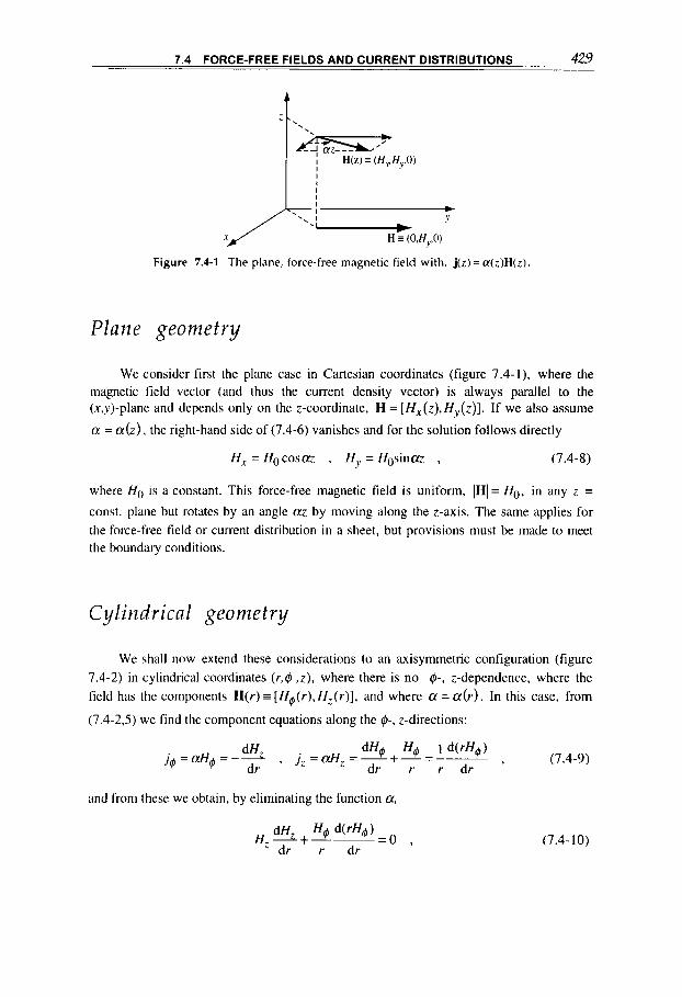
7.4 FORCE-FREE FIELDS AND CURRENT DISTRIBUTIONS 429
t
'- H = (O,H,,O)
Figure 7.4-1 The plane, force-free magnetic field with, j ( z ) = a ( z ) H ( z ) .
Plane geometry
We consider first the plane case in Cartesian coordinates (figure 7.4-1). where the magnetic field vector (and thus the current density vector) is always parallel to the (x,y)-plane and depends only on the z-coordinate, H = [H,(z), Hy(z)]. If we also assume
a = a(z), the right-hand side of (7.4-6) vanishes and for the solution follows directly
H , = Hocosaz , H,, = Hosinaz , (7.4-8)
where H, is a constant. This force-free magnetic field is uniform, [HI = H", in any z =
const. plane but rotates by an angle 012 by moving along the z-axis. The same applies for the force-free field or current distribution in a sheet, but provisions must be made to meet the boundary conditions.
C y 1 ind r ica 1 geometry
We shall now extend these considerations to an axisymmetric configuration (figure 7.4-2) in cylindrical coordinates (r,@ , z ) , where there is no @-, z-dependence, where the field has the components H(r) = [HG(r), Hz(r)], and where a = a(r). In this case, from
(7.4-2,5) we find the component equations along the @-, z-directions:
and from these we obtain, by eliminating the function a,
(7.4- 10)
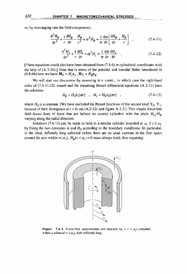
430 CHAPTER 7 MAGNETOMECHANICAL STRESSES
or, by rearranging into the field components,
d2H I d H I d a d H
dr2 r dr a dr dr 2 + -2 + (r2Hz = --I (7.4- 12)
[These equations could also have been obtained from (7.4-6) in cylindrical coordinates with the help of (A.3-24).] Note that in t e r n of the poloidal and toroidal fields introduced in (6.4-66) here we have Hp = Hzez , HT = H#eg.
We will start our discussion by assuming a = const., in which case the right-hand sides of (7.4- I1,12) vanish and the remaining Bessel differential equations (A.2-11) have the solutions
H4 = HoJl(ar) , H, = HoJo(ar) , (7.4- 13)
where Ho is a constant. [We have excluded the Bessel functions of the second kind Yo, Y I , because of their divergence at r = 0; see (A.2-12) and figure A.2-3.1 This simple force-free field draws lines of force that are helices on coaxial cylinders with the pitch H,/H@ varying along the radial direction.
Solutions (7.4-13) can be made to hold in a tubular cylinder bounded at al I r I a2
by fixing the two constants a and Ho according to the boundary conditions. In particular, in the ideal, infinitely long solenoid (when there are no axial currents in the free space around the axis within r< al), H4(r = q ) = 0 must always hold, thus requiring
Figure 7.4-2 Force-free axisyrnrnetric coil structure (a , < r < a2) contained within a solenoid ( r _>a,), both infinitely long.
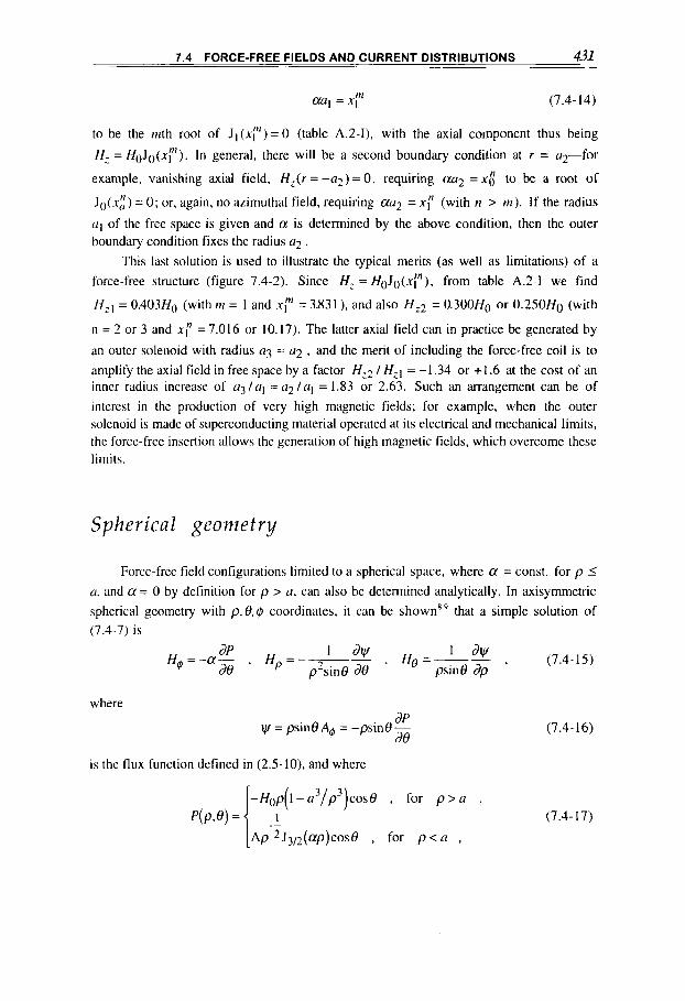
7.4 FORCE-FREE FIELDS AND CURRENT DISTRIBUTIONS 431
aq = x ? (7.4- 14)
to be the nith root of Jl(x;)1)=0 (table A.2-I), with the axial component thus being
H,. = HoJo(x;)l). In general, there will be a second boundary condition at r = a2-for
example, vanishing axial field, H Z ( r = -9) = 0, requiring au2 = x$ to be a root of
Jo(x;;) = 0; or, again, no azimuthal field, requiring 0ra2 = x; (with n > m). If the radius
u1 of the free space is given and a is determined by the above condition, then the outer boundary condition fixes the radius a2 .
This last solution is used to illustrate the typical merits (as well as limitations) of a
force-free structure (figure 7.4-2). Since H,- = HoJo(x?), from table A.2-I we find
HZI = 0.403Ho (with rn = 1 and x;” = 3.83 1 ), and also Hz2 = 0.300H0 or 0.250Ho (with
n = 2 or 3 and x; = 7.016 or 10.17). The latter axial field can in practice be generated by
an outer solenoid with radius a3 = a2 , and the merit of including the force-free coil is to amplify the axial field in free space by a factor HZ2 / Hzl = -1.34 or +1.6 at the cost of an inner radius increase of q / a l = q / q = 1.83 or 2.63. Such an arrangement can be of interest in the production of very high magnetic fields; for example, when the outer solenoid is made of superconducting material operated at its electrical and mechanical limits, the force-free insertion allows the generation of high magnetic fields, which overcome these limits.
Spherica 1 geometry
Force-free field configurations limited to a spherical space, where a = const. for p I (1, and a = 0 by definition for p > N , can also be determined analytically. In axisymmetric
spherical geometry with p, 0.6 coordinates, it can be shown’ that a simple solution of (7.4-7) is
where dP
y / = psino$ = -psin0- d0
is the tlux function defined in (2.5-lo), and where
-H(,p(l-a3/p3)cose , for p > a ,
Ap 2 J 3 / 2 ( a p ) ~ o ~ B , for p < a , _-
(7.4- 1 6)
(7.4- 17)
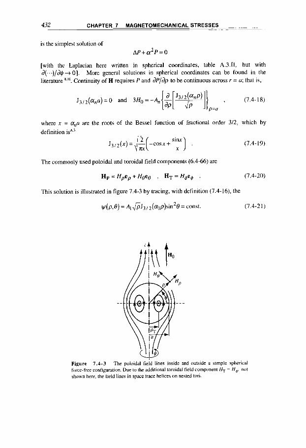
432 CHAPTER 7 MAGNETOMECHANICAL STRESSES
is the simplest solution of hp + a2 P = 0
[with the Laplacian here written in spherical coordinates, table A.3.11, but with d(...)/dG -+ 01. More general solutions in spherical coordinates can be found in the literature 'I". Continuity of H requires P and dP/@ to be continuous across r = a; that is,
J 3 , 2 ( a n a ) = 0 and 3Ho=-An (7.4- 18)
p=u
where x = a,p are the roots of the Bessel function of fractional order 3/2, which by
(7.4- 19)
The commonly used poloidal and toroidal field components (6.4-66) are
H p = Hpep+Hoeg , HT = H$e+ . (7.4-20)
This solution is illustrated in figure 7.4-3 by tracing, with definition (7.4-16), the
yl(p.8) = ~ ~ f i ~ ~ , 2(alp)sin 2 8 = const. (7.4-21)
Figure 7 .4-3 The poloidal field lines inside and outside a simple spherical force-free configuration. Due to the additional toroidal field component H , = H p not shown here, the field lines in space trace helices an nested tori.
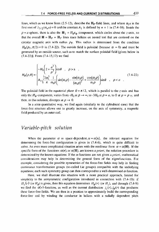
7.4 FORCE-FREE FIELDS AND CURRENT DISTRIBUTIONS 433
lines, which as we know from (2.5-12), describe the Hp-field lines, and where ala is the first root of J3/2(a,1u)=0 and theconstantA, is defined by n = 1 in (7 .4-18) . Inside the
p = a sphere, there is also the HT = H4e4 component, which circles about the z-axis, so
that the overall H = H p + H T lines trace helices on nested tori that are centered on the
circular magnetic axis with radius p ~ . This radius is determined from the condition
H @ ( p ~ , 7 r / 2 ) = 0 in (7 .4-22) . The outside field is poloidal (because a = 0) and must be
generated by an outside source, such as to match the surface poloidal field [given below in (7 .4-22)] . From (7.4-15,17) we find
The poloidal field in the equatorial plane 0 = n / 2 , which is parallel to the z-axis and has only the H o -component, varies from -Ho at p + -, to -3Ho at p = a, to 0 at p = p T, and
then, in this solution, diverges at p + 0. In a semi-quantitative way, we find again (similarly to the cylindrical case) that the
force-free structure allows one to greatly increase, on the axis of symmetry, a magnetic field produced by an outer coil.
Variable-pitch solution
When the parameter a is space-dependent, a = a ( x ) , the relevant equation for determining the force-free configuration is given in (7 .4-6) , which is quite difficult to solve. An even more complicated situation arises with the nonlinear form a = a ( H ) . If the specific form of the functions a(r), or a(H), are known a priori, the solution procedure is determined by the known equations. If the a-functions are not given u priori, mathematicid considerations may help in determining the general form of the eigenfunctions. For example, considering the possible symmetries of the force-free fields may help in finding continuous transformation groups (so-called Lie groups) compatible with the underlying equations; each such symmetry group can then correspond to a well-determined a-function.
Here, we shall illustrate this situation with a more practical approach, limited for simplicity to the axisymmetric configuration introduced in connection with (7.4- 10): if H,(r) (or H 4 ) is given, then this equation determines H @ ( r ) (or Hi), and through (7 .4-9) we find the &)-function, as well as the current distribution j z ( r ) , j 4 ( r ) that produces these force-free fields. We are then in a position to approximately build the corresponding force-free coil by winding the conductor in helices with a radially dependent pitch
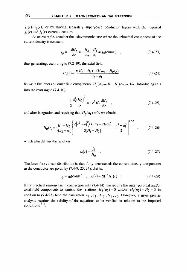
434 CHAPTER 7 MAGNETOMECHANICAL STRESSES
j z ( r ) / j#(r) , or by having separately superposed conductor layers with the required jz ( r ) and j#(r) current densities.
As an example, consider the axisymmetric case where the azimuthal component of the current density is constant:
(7.4-23)
thus generating, according to (7.2- 19). the axial field
(7.4-24) - H I ) - ( H ~ ~ I -Hla2) Hz (r) =
a2 - a1
between the inner and outer field components Hz(al) = HI , Hz(a2) = H2. Introducing this
into the rearranged (7.4- lo),
(7.4-25)
and after integration and requiring that Ho(al) = 0, we obtain
which also defines the function
a ( r )= - j# . %
(7.4-27)
The force-free current distribution is thus fully determined: the current density components in the conductor are given by (7.4-9,23,24), that is,
j 4 = jg(const.) , j z ( r ) = a(r)H,(r) . (7.4-28)
If for practical reasons [as in connection with (7.4-14)] we require the outer poloidal and/or axial field components to vanish, the relations Hq(a2) = 0 and/or H , ( q ) = H2 = 0 in
addition to (7.4-23) bind the parameters a1 , a2 , H2 , HI , j o . However, a more precise analysis requires the validity of the equations to be verified in relation to the imposed conditions ' . I 3 .
Chpte r 6
MAGNETOHYDRODYNAMICS AND PROPERTIES OF MATTER
In previous chapters we discussed the heating and pressure effects that appear when electromagnetic fields and currents are large enough, and which can give rise to complicated interaction processes in the field-conductor system. As the fields become even stronger, the high temperature and pressure may influence the parameters of the conductor, and the equation of state and other matter-related functions have to properly describe the phenomena. There are also remarkable effects when conductors or electrically conducting fluids move within electromagnetic fields. This situation is described in the first section by combining the equations of (quasistationary) magnetodynamics and fluidodynamics to obtain the equations of magnetohydrodynamics. The final section describes some of the most important properties of conducting and magnetic matter which are of relevance to the subjects treated in this book.
Applications. Magnetohydrodynamic applications range from the astrophysical scale'.'' (magnetic activity in the Earth, the Sun, and intergalactic space) down to the laboratory scale (MHD current generators' ', electromagnetic processing of material^^.^', controlled thermonuclear fusion The second section in this chapter is wholly devoted to magnetic flux compression' '" because this peculiar method produces the highest fields on the stellar scale and in the laboratory and is substantially different from conventional high magnetic field generators'.''. The classical and quantum physics of magnetized material, as presented in the third section, leads the way to the magnetic resonance method which is used today in a wide spectrum of applications, from the noninvasive inspection of solid state, biological, and molecular structures'" up to the human body imaging techniques used in clinical medicines4'. Finally, permanent magnetsB5* are another important subject in applicationss4", since with the new magnetic materials they can be a convenient substitute for current-driven magnets.
435
M4GNETICFIELDS: A Comprehensive Theoretical Treatise for Practical Use Heinz E. Knoepfel
Copyright Q 2000 by John Wiley & Sons, Inc
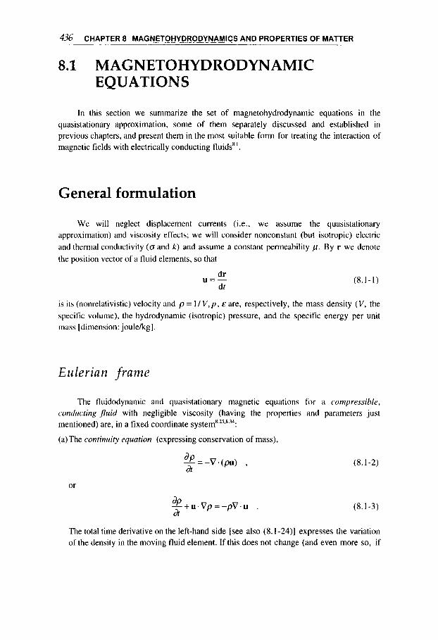
436 CHAPTER 8 MAGNETOHYDRODYNAMICS AND PROPERTIES OF MATTER
8.1 MAGNETOHYDRODYNAMIC EQUATIONS
In this section we summarize the set of magnetohydrodynamic equations in the quasistationary approximation, some of them separately discussed and established in previous chapters, and present them in the most suitable form for treating the interaction of magnetic fields with electrically conducting fluids' I.
General formulation
We will neglect displacement currents (i.e., we assume the quasistationary approximation) and viscosity effects; we will consider nonconstant (but isotropic) electric and thermal conductivity (CT and k ) and assume a constant permeability p . By r we denote the position vector of a fluid elements, so that
dr dt
u = - (8. I - I )
is its (nonrelativistic) velocity and p = 1/ V , p , E are, respectively, the mass density ( V , the specific volume), the hydrodynamic (isotropic) pressure, and the specific energy per unit mass [dimension: joulekg].
Eulerian frame
The fluidodynamic and quasistationary magnetic equations for a compressible, conducting jluid with negligible viscosity (having the properties and parameters just mentioned) are, in a fixed coordinate system' *',' 34:
(a)The contirzuity equation (expressing conservation of mass),
* = - v . ( p u ) , (8.1-2) at
or
+ + u . v p = - p v . u . (8.1-3) at
The total time derivative on the left-hand side [see also (8.1-24)] expresses the variation of the density in the moving fluid element. If this does not change (and even more so, if

8.1 MAGNETOHYDRODYNAMIC EQUATIONS 437
the fluid is incompressible), we have
v . u = o . (8.1-4)
(b) The equation of motion or Euler 's equation (expressing conservation of momentum),
p -+(u.V)u =-vp+fM + f , [: 1 (8.1-5)
where p is the hydrodynamic (isotropic) pressure and f is the volume density of external forces (for example, a gravitational force f = p g ) . The electromagnetic volume force density fB from (6.1-18) is
f B = j x B = ( V x H ) x B = p ( H . V ) H - - V ( p H 1 2
2 P
which is related to Maxwell's stress tensor (6.1-23). The form of (8.1-5) applies strictly only for an iderrl fluid, in which, by definition, no energy dissipation processes are taken into account-in particular, no viscosity and no heat exchange. [In a viscous flow there would be an additional term on the right-hand side of the form k l V ( V . u ) + k2Au,
where for an incompressible fluid k l = 0, and typically for mercury k2 = 1.6 x 1 0 - 3
kg/m,s.] I t can be shown that in an ideal fluid V x u = 0, which according to (A.3-11) means that u is derivable from a scalar velocity potential u = V@". If in addition the
fluid flow obeys (8.1-4), the scalar function is defined through Laplace's equation
V . V @ , , = A q , = 0 . (8.1-7)
(c) The general therrtiodynurnic equation (expressing heat balance)
+ u . V ( p ) = g + V . ( k V T ) + r3t
(8.1-8)
where k is the thermal conductivity, and for the source term (the energy term generated by external sources), Joule heating is taken:
(8.1-9)
where 0 is the electric conductivity. Note that (8.1-8) is obtained from (5.1-42,43) by adding the compressibility term - ( p / V)dV/dt-that is, the (negative) work done by the overall pressure on the elemental volume V = 1 / p ; however, the compressibility is negligible for a fluid in normal conditions. A further approximation step toward making (8.1-8) consistent with the presence of a quasistationary magnetic field would add the
term 3 ( p H 2 ) / 2 d on the left hand and extend the hydrodynamic pressure with the term
p + p + pH2 / 2 . [It is useful to mention that in these fluidodynamic equations each

.. - 4-38 CHAPTER 8 MAGNETOHYDRODYNAMICS AND PROPERTIES OF MATTER .. . - - . -
time derivative has been extended by a term ( u . V ) ... with respect to a nonflowing situation, as motivated by the calculation leading to (1.3-18); in a viscous flow, on the right-hand side of (8.1-8) there would be an additional term of the form V.([Z]u), where [4 is the viscous stress tensor, see (A.3-36).]
(d) The energy conservation equarion (as an alternative to the previous thermodynamic equation). In hydrodynamics a convenient conservation equation is expressed as
1 *( dr P E + pu2) = -v . 9 , (8.1 - 10)
which states that the increase in the internal plus kinetic energy density is equal to the negative divergence of the energy flux density
(8.1-11)
[In a viscous flow there would be here an additional term [Zlu. see the previous point (c).] Equations (8.1-10, 11) are obtainable from (8.1-8) with g = 0 when the equations of motion (8.1-5) and continuity (8.1-2) and the appropriate vector transformations are applied. When a magnetic field is present, the internal energy density on the left-hand side includes the field energy density pH2 /2 , and the energy flux density on the right -hand side includes the Poynting flux V.P, (S. l - lO), where
1
a P = E X H =[E'-(U xB)]x H = H X ( U x p H ) - - H X ( V X H) ; (8.1-12)
here the field E'= j /a = V x H l o , (1.3-37), has been introduced because it is the one that drives the current density j on the moving conductor. Consequently, the energy conservation equation with a quasistationary magnetic field in the conducting fluid becomes
(8.1-13)
where now
1
o - k V T + H x ( u x p H ) - - H x ( V x H ) . (8.1-14a)
This energy equation is equivalent to (8.1-8,9), as can be verified by appropriate calculation834. For later use, note that in the approximation with a very large Reynolds number [as defined in (8.1-47a)l it is E' = 0, (8.1-61), and the last term in (8.1-12,14a) thus vanishes. The second last term, with the trivectoral relation (A.3- Ic), is
H x (U x = w2u- ~ ( H . u ) H . (8. I - 14b)
8.1 MAGNETOHYDRODYNAMIC EQUATIONS 439
(e) In addition, the tyrcrfioru of state of the fluid are required-for example, given in the form (8.3-79,80)
11 = 1 0 , p ) , (8.1-15a)
E=&(T ,p ) . (8. I - 15b)
(0 Finally, the quasistationary mcignetic equutions must be added. With the assumptions made in connection with (1.2-18 to 21), (1.3-37), they are
V x H = j , (8.1 - 1 6 )
dB f3t
V x E = - - , (8.1-17)
V . B = O , B = p H , (8.1 - 18)
and also
j = o E ’ = o ( E + u x B ) ,
and from (8.1-16)
V . j = O .
(8.1 - 19)
(8.1-20)
It is often convenient to use combinations of the above equations-for example, the general magnetic diffusion equation (8.1-39) as a combination of (8.1-16 to 19). With an appropriate set of initial and boundary conditions, and provided thato and k are known functions, for example (5.3-1 I ) , (8.3-10,15),
o = o ( T , p ) 7 (8.1-21)
k = k ( T , p ) , (8.1-22)
the niugnrtohydrodynaniic (MHD) problem is then fully deterniined. It should be remembered that all these equations are given here in an Euleriun frume-that is, with respect to a coordinate system fixed in space. For a general comment on the set of these MHD equations see further on, in connection with (8.1-58).
Lagra ngia n f r ame
As we know from section 1.3, when considering a fluid moving with velocity u, it is often more convenient to solve the magnetohydrodynamic problem in a Lagrungiun frame-that is, with respect to a coordinate system moving with the fluid (figure 8.1-1).
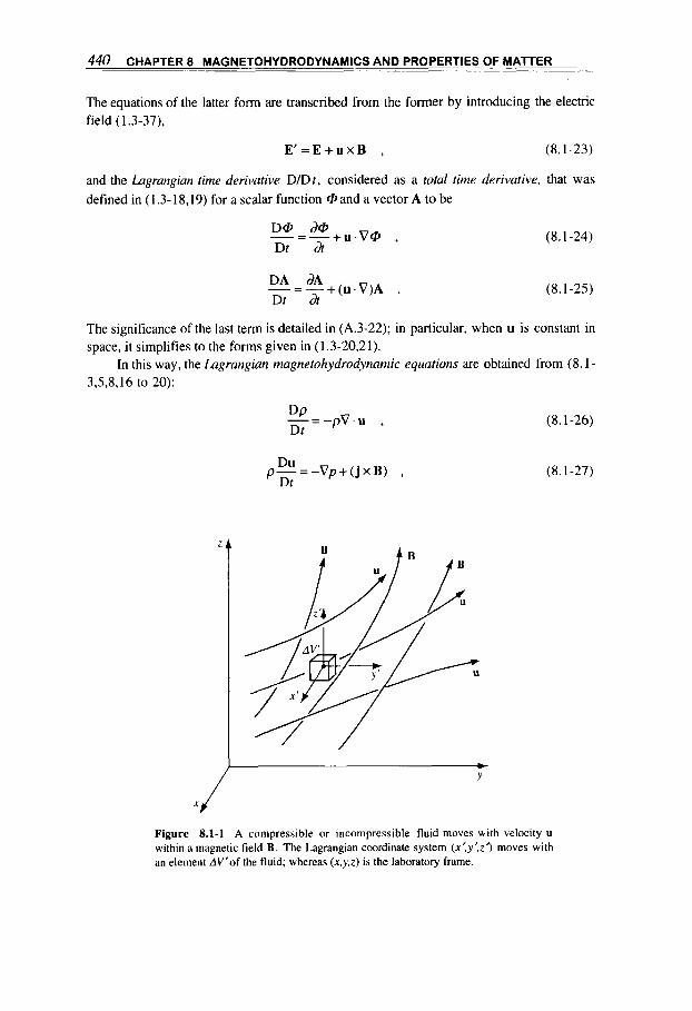
440 CHAPTER 8 MAGNETOHYDRODYNAMICS AND PROPERTIES OF MATTER
The equations of the latter form are transcribed from the former by introducing the electric field (1.3-37).
E ’ = E + u x B , (8.1-23)
and the Lagrangian time derivative DIDt , considered as a total time derivative, that was defined in (1.3- 18,19) for a scalar function 0 and a vector A to be
DA d A Dt at
- = - + ( u . V ) A .
(8.1-24)
(8.1-25)
The significance of the last term is detailed in (A.3-22); in particular, when u is constant in space, it simplifies to the forms given in (1.3-20,2 1).
In this way, the Lagrangian magnetohydrodynamic equations are obtained from (8.1- 3,5,8,16 to 20):
-- D p - - p V . u , Dt
Du Dt
p - = - V p + ( j x B ) ,
V
(8.1-26)
(8.1-27)
Figure 8.1-1 A compressihle or incompressible fluid moves with velocity u within a magnetic field B . The Lagrangian coordinate system (x’,y’,z’) moves with an element AV’of the fluid; whereas (x ,y ,z ) is the laboratory frame.
8.1 MAGNETOHYDRODYNAMIC EQUATIONS 441
V x H = j ,
(8.1-28)
(8.1-29)
(8.1 -30) DB Dt
V x E’ = -- - B(V . U) + (B . V)U ,
V . B = O , B = p H , (8.1-31)
j = & ’ , (8.1-32)
and
V . j = O . (8.1-33)
With the appropriate equations of state [ e g , (8.1-15)], the electric and thermal conductivity functions [e.g., (8.1-2 1,22)], and the specific initial and boundary conditions, the prohleni is fully determined.
(a) The electric field E’ is the field measured by an observer moving with the fluid and is the one that drives the current density j in the moving fluid [see in connection with (1.3- 29,30)]; otherwise, if the E field as measured by a laboratory apparatus is required, the substitution (8.1-23) must be made.
(b) For later use, the explicit source ( g ) and force ( f B ) terms, as given in (8.1-6,9), are used in (8.1-27.28); no other external force is considered, f = 0.
(c) The thermodynamic equation (8.1-28) indicates that the increase in the internal volume energy density (PE) is determined by joule heating, the gradient of the heat flux density, and the work done against the hydrodynamic pressure.
(d) The inductive equation (8.1-30) indicates that the (negative) electric field E‘ is determined by the total field derivative in time, and by the field amplification due to a convergent flow and to a compressible fluid [see in connection with (8.1-45)].
(e) For a fluid, for which the continuity equations (8.1-4,26) reduce to V ’ u = 0, the last term in (8.1-28) plus the second last in (8.1-30) drop out.
(f) For a viscous flow there are additional ternis in (8.1-27.28). as mentioned in connection with (8.1-6,9,11).
For the energy consentation equation for a fluid where Dp / Dt = 0, V . u = 0 , from
The following remarks might be helpful:
(8.1-13.14) and (A.3-5) we obtain
Dt (8.1-34)

442 CHAPTER 8 MAGNETOHYDRODYNAMICS AND PROPERTIES OF MATTER
Finally, integrating over a volume V delimited by a closed surface S of a moving fluid in a quasistationary magnetic field yields
D J ( E + i u 2 + I@H2)dM = ${ -(E’ x H) + kVT - pu Dr 2 P
M S (8.1-35)
+ [p(u.H)H-&pH*u] }ds ,
where we have used Gauss’ theorem (A.3- 16) and have transformed the integration over the volume into one over the mass (dM = pdV). This equation expresses the energy conservation. In fact, it shows that the increase in the total energy (thermal, kinetic, and magnetic field energies) in the moving fluid of mass M (left-hand side) is given by (right- hand side, in order) the Poynting flux, thermal diffusion, work done by the hydrodynamic and magnetic pressure with respect to the moving surface S [in analogy to (6.1-22b), the last bracket represents the vector resulting from the multiplication of u by Maxwell’s stress tensor (6.1-23)]. For a general comment on the set of these MHD equations see further on, in connection with (8.1-58).
Magnetic diffusion
Fie 1 d d i;ff u s ion
The presence of conducting jluids moving with velocity u causes new effects for the diffusion of magnetic fields as introduced in section 4.1. Ohm’s law is now
j = o ( E + u x p H ) , (8.1-36)
and in the quasistationary approximation and for a fixed coordinate system, by taking the curl of
V x H = j (8.1-37)
and using
V X E = - - &H a t ’
we get the generalized difusion equation
(8.1-38)
a-I at
l c h H = - - V x ( ~ x H ) , (8.1-39)
443 _ _ -
8.1 MAGNETOHYDRODYNAMIC EQUATIONS _ _ --
where
(8.1-40)
is the magnetic diffusivity (4.1-9), and the same assumptions that led to the static diffusion equation (4.1-8) apply. In particular, if K were not uniform in space there would be the additional term -VK x ( V x H) on the right-hand side, (4.1-1 Ib). Using the vector identity (A.3-9) and with
V . p H = O , (8.1-4 1 )
this equation is rewritten as
(8.1-42) &I dr
KAH = - + ( u . V ) H - (H .V)U + H ( V . u ) .
By switching to a Lagrangian coordinate system with the Lagrangian time derivatives (8.1-24,25), we obtain
- DH = K ~ H + ( H . V ) U - H ( V . U ) , Dt
(8.1-43)
which is sometimes termed the conzplete induction equation, and in this form it refers, as we know, to a frame moving with the fluid element. The first term on the right-hand side of this equation represents the increase in the magnetic field by diffusion, as we know from (4.1-8); the second tern1 determines magnetic field amplification due to the curvature of the flow (it can vanish in certain circumstances-for example, in the case of a rigid body translating with constant velocity parallel to itself); the third term gives magnetic amplification due to the compressibility of the fluid because, in fact, with the continuity equations (8.1-3 or 26) i t can be written in the form
It vanishes when the fluid is incompressible, (8.1-4),
v . u = o .
(8.1-44)
(8.1-45)
The complete induction equation (8.1-43) thus describes the balance of magnetic fields in a moving conducting fluid. The amplification of magnetic fields by fluid motion is referred to as a dynurno processR9: It is positive when the mentioned amplification terms prevail over the diffusion term. By virtue of this process 3 3 , the kinetic energy of the fluid can be converted into magnetic energy, and through diffusion and dissipation it can be converted into heat, as was discussed in chapter 5.
Here again as in (1.2-5). (4.2-17) it can be convenient to consider dimensionless equations and rehted quantities. We mark them with an asterisk by normalizing to

444 CHAPTER 8 MAGNETOHYDRODYNAMICS AND PROPERTIES OF MATTER -
characteristic parameters: time r, , length I,, velocity u, = Idto, magnetic field H , . For example, the generalized diffusion equation (8.1-39) or the complete induction equation (8.1-43) can be rewritten in the forms
Here,
&I* 1 -= -A * H * + V * X(U * xH*) , & * R,,,
(8.1-46a)
(8.1-46b)
(8. I-47a)
is defined as the magnetic Reynolds number, which is the ratio of the u-dependent terms to the first term on the right-hand side and can also be understood as the ratio of the diffusion time (4.2-18b),
to the transition or displacement time 10 = 10 l u ~ in the system. In analogy to this primary dcfinition related to a moving electric fluid, it is also
customary to introduce a Reynolds number for a conductor at rest ("0 = 0) but exposed to a
harmonic field oscillating at the frequency w = 2 n / T , where it is, accordingly, the ratio of the diffusion time rd to a characteristic period of excitation-for example, t0 = T l r r = 2 / w asin(4.2-21)-thus
Figure 8.1-2 A rigid body moving with velocity v across a magnetic field B .

8.1 MAGNETOHYDRODYNAMIC EQUATIONS 445
(8.1-47b)
112 Furthermore, by introducing the diffusion skin depth SO = to)''^ or so = 6 = ( 2 ~ / w )
from (4.2- I8,2 1 ), we can also write
(8.1-47~)
which does not contain the velocity or time explicity. [An example of this formulation is used in (4.3-47).] Because of its I"-dependence, the magnetic Reynolds number can be
very large in astrophysics; for example, it is 106-1012 on the Sun. The significance of R,,, for magnetic systems is discussed in connection with (8.1-58).
Finally, we consider the simple case of a nondejbrmahle, incompressible conductor translating with velocity u = v with respect to the magnetic field configuration (figure 8.1 - 2). As a consequence of the remarks just made, the right-hand side of (8.1-42), which refers to the fixed laboratory coordinate system, will include only the first two terms
~ H = - + ( v . V ) H dH ,
dr
where, according to (A.3-22),
d H & & ( v . V ) H = V ~ - + V - + v ~ - . dx J ? y az
Vector potential difftlsion
By introducing the vector potential A defined in (2.2-2).
V x A = B = p H ,
into (8.1-36,37,38) we get in analogy to (4.1-4)
. 1
(8.1-48)
(8.1-49)
(8.1-50)
(8.1-5 1)
With the vector relations (A.3-9) and when u = VOis expressible as the gradient of a scalar
function [thus, for an ideal fluid, V x u = 0, see in connection with (8.1-7)] and since
V.A = 0, (2.2-1 I ) , we obtain
u x(V x A) = -AV. u + ( A . V ) u - ( u . V ) A . (8.1-52)

446 CHAPTER 8 MAGNETOHYDRODYNAMICS AND PROPERTIES OF MATTER
Finally, when p is uniform and the fluid is incompressible [thus V . u = 0, (8.1-4)], equation (8.1-5 1 ) transforms into a similar form to (4.1 - 13),
-pjs . 1 (8.1-53)
The right-hand side expresses, in addition to the current source term j, = - f lu , (4.1- 14b), the eddy current term
1 With respect to (4.1-14c), it is extended by the term (8.1-52),
u x B = (A . V ) U - (U .V)A ,
(8.1-54)
(8.1-55)
which expresses the balance of the entering/exiting field lines with respect to the moving rigid conductor.
As we know from section 2.2, the vector potential formulation can be convenient in plane or axisymmetric geometries because in these cases only one (scalar) component of A must be considered. For example, in a plane geometry with currents flowing normal to the plane, j = [O,O, j z ( x , y ) ] , only the A,-component exists A I [O,O,A,(x,y)] and the magnetic field has the components B,, B y , solely (see figure 2.1-6). In Cartesian coordinates, (A.3-22,23), the vector equation (8.1-53) for a rigid cylindrical body moving with constant velocity v = ( v , , v y ) reduces in this case to the only z-component equation
(8.1-56)
An example of a corresponding, axisymmetric equation is given in (4.3-1 1).
Limiting cases
In a typical MHD problem, which combines electromagnetism with fluid mechanics, the vectors B and u are the primary variables, together with two or more of the
thermodynamic functions: fluid density p, pressure p , internal energy per unit mass E ,
temperature T. The determination of B and u requires two vectorial equations (that is, six equations for the six components of B, u)-for example, the equation of motion (8.1-5 or 27) and the generalized diffusion equation (8.1-39 or 43). In addition, each thermodynamic function present in the problem requires one additional equation-for example, the continuity equation (8.1-3). one of the energy equations (8.1-8 or 13), or the equations of state (8.1-15).

8.1 MAGNETOHYDRODYNAMIC EQUATIONS 447 -
To reduce the complexity of this general set of MHD equations, it is convenient to estimate the relative importance of the many competing physics effects and related terms and to eliminate them from the beginning. Dimensionless parameters can help in this ordering, as we have seen with the introduction of the magnetic Reynolds number (8.1-47),
(8.1-57) R , = - - / L o ~ ~ u 10. - . K
Another such parameter is the fluid beta
p=- 2 P p H 2 ’
(8.1-58)
which is the ratio of the fluid pressure to the magnetic field pressure (6.2-93): At p (( 1, the magnetic equations and effects predominate over the fluid ones. The Alfvtn Mach number
is the ratio of the fluid velocity u to Alfvtn’s velocity (6.3-3),
V A = H - . d::
(8.1-59)
(8.1-60)
I f the Reynolds number is extremely lurge-that is, R, + 00, which can mean CT + (a perfectly conducting fluid)-the effective electric field E’= E + u x B is
negligible compared with IEl or IE x BI because the current j = oE‘ must remain finite, thus
E z - u x B . (8.1-61)
In this case, a simple set of ideal MHD equations follows from (8.1-3,5,17,19); for example,
* + v . ( p u ) = o , (8.1-62) dt
Du dt
p - = -Vp + ( v x H) x B , (8.1-63)
w - = V X ( U X B ) , at
(8.1-64)
V . B = O , (8.1-65)
which provide the eight equations for the eight components and functions involved of B, u,
p, p . Note that in this case there is the possible presence of a nonnegligible charge density
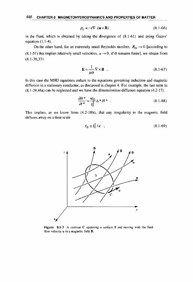
448 CHAPTER 8 MAGNETOHYDRODYNAMICS AND PROPERTIES OF MATTER
pe =-EV. (UXB) (8.1-66)
in the fluid, which is obtained by taking the divergence of (8.1-61) and using Gauss’ equation (1.1-4).
On the other hand, for an extremely small Reynolds number, R, -+ 0 [according to
(8.1-57) this implies relatively small velocities, u -+ 0, if d remains finite], we obtain from (8.1-36,37)
1
PO E = - V x B . (8.1-67)
In this case the MHD equations reduce to the equations governing induction and magnetic diffusion in a stationary conductor, as discussed in chapter 4. For example, the last term in (8.1-39,46a) can be neglected and we have the dimensionless diffusion equation (4.2- 17).
(8.1-68)
This implies, as we know from (4.2-18b), that any irregularity in the magnetic field diffuses away on a time scale
(8.1-69) 2 Zd E ! o / K ,
Figure flow velocity u in a magnetic field B.
8.1-3 A contour C spanning a surface S and moving with the fluid
8.1 MAGNETOHYDRODYNAMIC EQUATIONS 449
where K = 1 / WCT is the magnetic diffusivity. A further interesting comment concerns the balance of magnetic flux
t,//=IB.ds S
(8.1-70)
relative to an open surface S delimited by the contour C which moves with the fluid (figure 8.1-3). In the case of a perfectly conducting fluid ( R,,, + 00, (T + -, K + 0) the frozen f lux fheoreni applies, which states that the magnetic flux ythreading the open surface S remains constant as the contour C moves within the fluid. To show this statement, we integrate (8.1-64) over S to obtain with Stokes’ theorem (A.3-14) and (A.3-ld)
6% J,. ds + $ B . (U x dl) = 0 ,
S C
By comparison with (1.4-8) we can write this equation in the form
- = o , dW df
(8.1-7 1 )
(8.1-72)
which states that the total time derivative of the magnetic flux through a moving surface is zero. Since the surface S in the proof that led to (1.4-9) can be arbitrarily small, we can say that the magnetic fields lines are frozen in: that is, they are tied to the infinitely conducting fluid and move with it.
Cylindrical one-dinzensional geometry
It may be useful to adapt some of the general magnetohydrodynamic equations to a simple, but for many applications significant, geometry; namely, to the cylindrical one- dimensional geometry (radius and time; see, e.g., figure 5.2-3) for a purely axial magnetic field, with the variables HZ,E4,j,#,,ur. relative to a Lagrangian frame moving with the fluid. With the use of the Lagrangian time derivative (8.1-24,25),
D d d - = -+ ur - Df dt dr ’
and the vector relations contained in table A.3-11, for this geometry we obtain from (8. I - 23,26 to 32) the fluid equations
(8.1-73)
(8.1-74)
450 CHAPTER 8 MAGNETOHYDRODYNAMICS AND PROPERTIES OF MATTER
p-=-P- d(rur)+*+-- .2 l a kr- dT , DE Dt r b CT r & ( d r )
and the electrodynamic equations [similar to (4.3-1,4)]
dH Z=-' &. Jg, '
(8.1-75)
(8.1-76)
(8.1-77)
j g , = a E i , (8.1-78)
where
EG = Eg, -pHzur . (8.1-79)
From these expressions it is easy to obtain, for example, the corresponding energy and magnetic flux conservation relations (8.1-30,34) or, by eliminatingjg, and E',P from the last three equations, calculate
(8.1-80) DH 1 d r d H H Dp A=-- -3 +A- . Dt p & ( o b ) p Df
This expression is the generalized diffusion equation (8.1 -43,44) for the axial magnetic field with the additional term representing the field increase due to fluid compression. In this case, the term (H . V)u vanishes [see (A.3-22)], because of the cylindrical coordinates.
8.2 MAGNETIC FLUX COMPRESSION
Magnetic flux compression is an interesting method for generating large electromagnetic power pulses, of the order of 101 1 watts and above' 3.' 4.8 . In flux compression systems, a closed electric conductor linking a magnetic flux v / is compressed by external forces, thereby converting mechanical into magnetic energy. This transformation method is very efficient as long as flux losses remain limited (typically smaller than 50%). Therefore, problems regarding magnetic flux diffusion (chapter 4) are here of major concern.
Flux compression systems can be divided roughly into two classess6:
(a) The current or energy generators, in which the compression volume is usually separated

8.2 MAGNETIC FLUX COMPRESSION 451
from the inductive load. Typical maximum magnetic energies in the 1 - to 10-MJ range are generated and transferred into low-inductance loads' (see also in table 8.2-1).
(b) The energy detzsity generators, in which ultrahigh magnetic fields are generated by radial implosion of a cylindrical hollow conductor. With such devices, 1000-T fields with good homogeneity in volumes of order 1 cm' are actually being produced' '' (see also table 8.2-11) and used in a large variety of physics applications' 1 4 .
Current generators
Flux compression circuit
We describe the flux compression system by the simple circuit shown in figure 8.2- 1, which includes a total time-dependent inductance
U t ) = + LL (8.2-1)
made up of the constant load inducfutzce LL and the compression inductance & ( t ) . The resistance R ( t ) formally represents the magneticflux leakage. The current I flowing in the circuit is determined by the differential equation
d o + R I = ( ) . dt
(8.2-2)
Figure 8.2-1 Idealized flux compression circuit
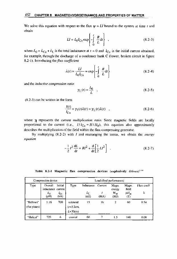
452 CHAPTER 8 MAGNETOHYDRODYNAMICS AND PROPERTIES OF MATTER
We solve this equation with respect to the flux w = LI bound to the system at time r and obtain
LI = L&-,exp -1 -dt , 11: 1 (8.2-3)
where = f.po + LL is the total inductance at t = 0 and fco is the initial current obtained,
for example, through the discharge of a condenser bank C (lower, broken circuit in figure 8.2- 1). Introducing theflux coeficient
LI ;l(t)=-=exp
h k o (8.2-4)
and the inductive compression ratio
(8.2-3) can be written in the form
(8.2-6)
where fi represents the current multiplication ratio. Since magnetic fields are locally proportional to the current (i.e., I / I,, = H / H o ) , this equation also approximately describes the multiplication of the field within the flux-compressing generator.
By multiplying (8.2-2) with I and rearranging the terms, we obtain the energy equation
2 dt (8.2-7)
Table 8.2-1 Magnetic flux compression devices (explosively driven)’.’”
I Compression device I Load (final performance)
TY Pe
“Bellows”
(tlat plates)
“Helical”
Overall Initial inductance current
Lo 6, (W) (kA)
1.16 700
125 6
Type Inductance Current Magn. Magn. Flux coeff. energy field
(nH) (MA) (MJ) (T) LL I wM pHtn ?l
solenoid 15 16 2 60 0.54
(r=3.2cm.
L=30cm)
coaxial 60 7 I .5 I 40 0.08
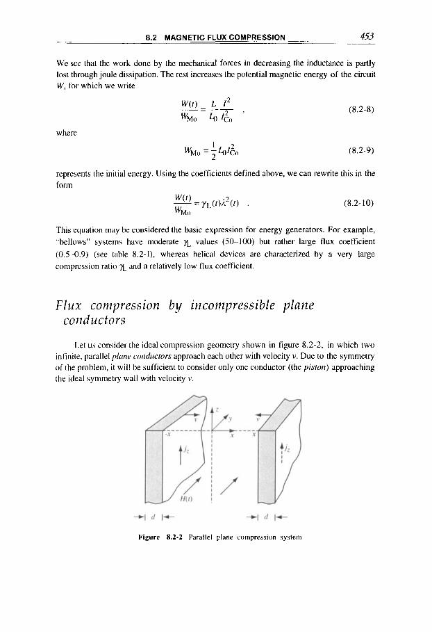
453 -
8.2 MAGNETIC FLUX COMPRESSION . _. ~
- -
We see that the work done by the mechanical forces in decreasing the inductance is partly lost through joule dissipation. The rest increases the potential magnetic energy of the circuit W, for which we write
(8.2-8)
where
(8.2-9) 1 2 wMo = 5 h l C o
represents the initial energy. Using the coefficients defined above, we can rewrite this in the form
(8.2-10)
This equation may be considered the basic expression for energy generators. For example, “bellows” systems have moderate values (50-100) but rather large flux coefficient
(0.5-0.9) (see table 8.2-I), whereas helical devices are characterized by a very large compression ratio and a relatively low flux coefficient.
Flux compression by incompressible plane conductors
Let us consider the ideal compression geometry shown in figure 8.2-2, in which two infinite, parallel plnnr condrctors approach each other with velocity v. Due to the symmetry of the problem, i t wil! be sufficient to consider only one conductor (the piston) approaching the ideal symmetry wall with velocity v.
Figure 8.2-2 Parallel plane compression system

454 CHAPTER 8 MAGNETOHYDRODYNAMICS AND PROPERTIES OF MATTER
Usually, a compression system is characterized by the initial kineric energy of its piston (with thickness d, see in figure 8.2-3),
WK, = 2 p d v o 1 2 .
and the initial magnetic energy in the compression volume
(8.2- 1 1)
Assuming we have an ideal conductor (a+,..), we can write the flux and energy conservation in the form
-poH 1 2 1 2 x+-pdv = WM, + WK, . 2 2
(8.2-14)
Differentiation of the former yields
and from the latter we finally obtain
(8.2- 15)
Figure 8.2-3 Plane piston.
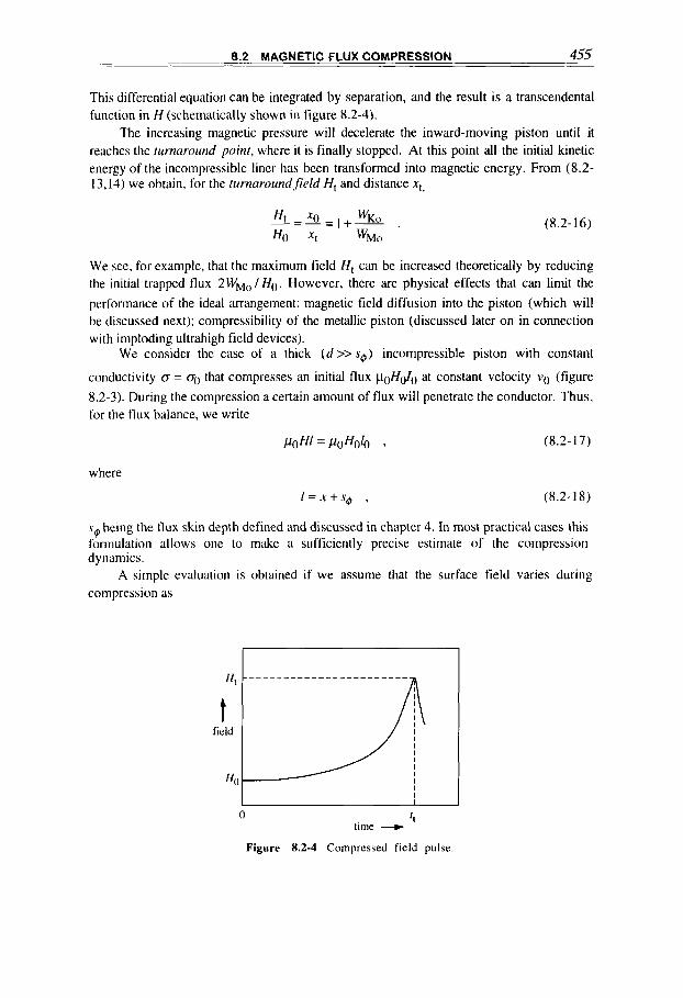
8.2 MAGNETIC FLUX COMPRESSION 455
This differential equation can be integrated by separation, and the result is a transcendental function in H (schematically shown in figure 8.2-4).
The increasing magnetic pressure will decelerate the inward-moving piston until it reaches the turnaround poinf, where it is finally stopped. At this point all the initial kinetic energy of the incompressible liner has been transformed into magnetic energy. From (8.2- 13,14) we obtain, for the turnaroundfield Ht and distance xt,
(8.2-16)
We see. for example, that the maximum field H , can be increased theoretically by reducing the initial trapped flux 2 WM, / H o . However, there are physical effects that can limit the
performance of the ideal arrangement: magnetic field diffusion into the piston (which will be discussed next); compressibility of the metallic piston (discussed later on in connection with imploding ultrahigh field devices).
We consider the case of a thick (d >> so) incompressible piston with constant
conductivity (T = q) that compresses an initial flux p ~ H d o at constant velocity vo (figure 8.2-3). During the compression a certain amount of flux will penetrate the conductor. Thus, for the flux balance, we write
(8.2-17)
where
I = x + s ( $ , (8.2-18)
.so being the flux skin depth defined and discussed in chapter 4. In most practical cases this formulation allows one to make a sufficiently precise estimate of the compression dynamics.
A simple evaluation is obtained if we assume that the surface field varies during compression as
0 I t time -
Figure 8.2-4 Compressed field pulse
456 CHAPTER 8 MAGNETOHYDRODYNAMICS AND PROPERTIES OF MATTER
H(0,t) = Hoet1' , (8.2- 19)
where the characteristic time 5 can be approximated within the limitation mentioned in connection with (4.2-41) by
(8.2-20)
Here, we have implicitly assumed that the flux loss and the penetration velocity of the diffused field remain limited; that is sg M x and dsgldt(c v. This approach, in which the
field increase is considered as a time sequence of exponential functions with variable 5, is sometimes called the skin-layer method 8 4 . Its physical motivation is based on the fact that the parameters of field diffusion, such as the skin depth, are dominated by the ever- increasing field, so the contribution of the previous (initial) condition ( HO exp(- t /s@), see
next equation and figure 8.2-3) gets rapidly lost. For the final distribution in the conductor, from (4.2-40) we have
and for the current density we get
here,
(8.2-21)
S,#, = JK"5 (8.2-22)
is the flux skin depth and KO is the magnetic diffusivity (8.1-40). With the help of the induction law (1.4-9, for the surface electric field we can write
from which with (8.2-21) we obtain
(8.2-23)
whcre i+v = poHx is the flux per unit height in the compression volume. When the factor S@V/Kg is a constant, for the relative flux reduction we obtain by direct integration
(8.2-24)

8.2 MAGNETIC FLUX COMPRESSION 457
For the case where the piston moves at a constant velocity v = vo , we calculate from (8.2-
20,22,23)
(8.2-25)
Here, we have introduced the magnetic Reynolds number (8.1-47)
(8.2-26) R, - %”O
KO ’
which can be considered as the ratio of the diffusion decay-time (= x i / K ~ ) over the compression time ( x g / v o ) . Thus, a large R , means that diffusion losses are relatively
unimportant. For example. for a copper piston with xo = 10 cm and vo = 0.2 cm/ps, we have R, = 15’000.
We now want to establish a relation between the field-diffusion concept and the formal circuit equations given at the beginning of this chapter. With the approximation just
used, we calculate for the mean resistance
while the total inductance is
L = p o l .
Introducing these approximations in (8.2-3). for the field amplification we obtain
When the piston velocity is constant, that is,
”() = - = - f I ’
we calculate with (8.2-20,22) the field amplification
(8.2-27)
(8.2-28)
(8.2-29)
(8.2-30)
Besides the fact that here we have introduced the ratio lol l instead of xo/x (which
remains within the tolerances of our approximation), we find the same result as in (8.2-25).
We calculate the rnaritnunijeld nniplijication H , / Ho that can be attained for x + 0, in which case the minimum distance 1 follows from (8.2-18,20,22):

458 CHAPTER 8 MAGNETOHYDRODYNAMICS AND PROPERTIES OF MATTER
J"'.. v '
that is,
lmin =xu . (8.2-31) vn
Introducing this value in (8.2-30), the maximum amplification for large R, values becomes
H , = R , + & , (8.2-32) Hn 2 e2
where e = 2.7 1828 is the base of natural logarithms.
Implosion of an ideal flux compressing shell
The generation of magnetic fields of 100 and more tesla by flux compression requires pistons with very large kinetic energy densities. These can be obtained by resorting to explosive-driven cylindrically converging shells, with the result that the energy is concentrated near the implosion axis where the ultrahigh fields are generated.
Analysis of a cylindrical Compression system is rather complex and involves formidable theoretical methods and numerical solution procedures. Fortunately, in most cases o f practical interest, it is possible to separate the acceleration phase of the imploding cylindrical shell from the flux Compression phase. This siniplification is generally possible in explosive-driven systems, since acceleration of the shells by explosive action is essentially terminated a few centimeters from the initial radius, when the magnetic pressure is still negligible.
Fie 1 d d ff u s ion
We shall begin our study of cylindrical generators by discussing the implosion of a cylindrical shelf, characterized by an initial velocity vo. Here, we consider typical velocities of 0.1-1 c m / p (1-10 k d s ) , as can easily be obtained with chemical explosives' lo. For our analysis of the implosion dynamics we shall assume that the shell is an incompressible frictionless fluid confined within two concentric cylindrical surfaces. From the general continuity equation (8.1 -4,73) we derive, for the axisymmetric and incompressible fluid (see table A.3-11), the condition
&rv) -=o , dr
(8.2-33)

8.2 MAGNETIC FLUX COMPRESSION 459
Figure 8.2-5 Imploding ideal shell: (a) initial and (b) intermediate position
from which, by integration, we obtain
r v = A ( t ) ; (8.2-34)
here, r is the radius, v the radial velocity, p the mass density, and A ( t ) an integration constant, which will be defined by a convenient set of the two boundary conditions. The incompressibility also results in conservation of the volume (figure 8.2-5). that is,
Q 2 - r f = R 2 - R : = R i , (8.2-35)
where Ro is the (outer) radius of the fully collapsed and incompressible shell (q -+ 0). For the kinetic energy of the shell (per unit of axial length) comprised between the radii rI and r
we calculate
From the equation expressing conservation of momentum [see (8.1-63,74)],
(8.2-36)
(8.2-37)
we can easily derive by integration with respect to r the pressure law within the shell:
(8.2-38)
where A ( t ) is defined in (8.2-34). To gain some insight into the peculiarities of the cylindrical implosion, let us first
discuss the freely imploding shell. This most simple case is defined by the boundary
460 CHAPTER 8 MAGNETOHYDRODYNAMICS AND PROPERTIES OF MATTER
conditions (at r = rl ,r2)
PI = P2 = 0
and the initial condition (at t = 0, rl = R, )
(8.2-39)
v1 = vo . (8.2-40)
The velocity vo also defines, through (8.2-36) extended to the initial radii R , , R 2 . the initiuf
kinetic energy
w,, = l r p 2 v i ~ f In(?) . (8.2-4 1 )
The relation between the implosion velocity v1 and the inner radius ‘1 follows from the
conservation of (kinetic) energy
WK =WKo . (8.2-42)
We finally obtain
( r ~ v ~ ) ~ In( 1 + $1 = ( R I V ~ ) ~ In( 1 + $1 .
For the case where the liner is initially very thin, that is,
we derive the simple expression
(8.2-43)
(8.2-44)
(8.2-45)
We see that the velocity of the inner boundary gradually increases and at rl + 0 diverges
as ( r~~lnr ,~) -1’2 . Thus, this behavior also means that during implosion of an incompressible shell the (constant) kinetic energy concentrates more and more towards the inner boundary.
Another substantial difference with respect to the plane case is the pressure distribution within the converging fluid, which is found from (8.2-38):
(8.2-46)
Here, we have used the expression
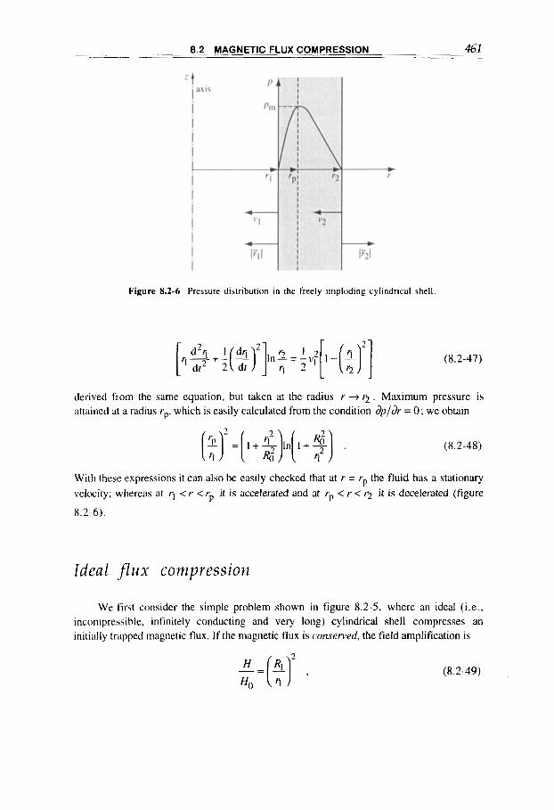
~ 8.2 MAGNETIC FLUX COMPRESSION 461
Figure 8.2-6 Pressure distribution in the freely imploding cylindrical shell
(8.2-47)
derived from the same equation, but taken at the radius r + Q . Maximum pressure is attained at a radius rp. which is easily calculated from the condition dp/dr = 0 ; we obtain
(8.2-48)
With these expressions it can also be easily checked that at r = rp the fluid has a stationary velocity; whereas at rI < Y < Y it is accelerated and at rP < Y < “2 it is decelerated (figure P 8.2-6).
Ideal f lux compression
We first consider the simple problem shown in figure 8.2-5, where an ideal (i.e., incompressible, infinitely conducting and very long) cylindrical shell compresses an initially trapped magnetic flux. If the magnetic flux is conserved, the field amplification is
2 -=($ H . Ho
(8.2-49)

462 CHAPTER 8 MAGNETOHYDRODYNAMICS AND PROPERTIES OF MATTER
so the magnetic pressure and energy density increase as
!$(;) 4
HO (8.2-50)
The field increases until the imploding conductor has transformed all its initial kinetic energy (per unit length) W K , into magnetic energy:
1 2 2 W K O + ~ M O = ? P O ~ ~ 9
where
(8.2-5 1 ) 1 2 2 w M ~ = 5 PO HO nRl
is the initial magnetic energy. For the tumuroundfield Ht and radius rt we derive with (8.2-
49). similarly to the plane case (8.2-16),
(8.2-52)
The problem of magnetic flux compression by the incompressible, ideal conductor is fully determined if, in addition to the initial condition (8.2-40,41), we fix the boundary conditions
P2 = o (8.2-53)
and
The latter takes care of the magnetic pressure exerted by the initial field Ho on the inner boundary and is obtained from flux conservation (8.2-50). Much in the same way as in (8.2-45) for the free shell, here we obtain the relation between the implosion velocity Y I
and the radius '1 of the flux compressing shell. We must now add to the left-hand side of the energy balance (8.2-42 or 43) the potential magnetic energy
where WM, is given in (8.2-51). In analogy to the approximation (8.2-45) we then obtain
[$) (rf/Rg)ln(l+$/q2) .
2
1 -(q/q)* (8.2-55)

463 ~. -
8.2 MAGNETIC FLUX COMPRESSION -~ - . . - ~.
Here, in addition to condition (8.2-44), we require
wMo <<wKo 3
and rt is the turnaround radius given in (8.2-52):
(8.2-56)
(8.2-57)
Approximation (8.2-55) includes some previously established results. Note that for v 1 = 0
we have r I = rt, and for rt -+ 0, (8.2-55) is identical to (8.2-45). If, in addition, the shell also remains thin in the vicinity of the turnaround radius, so
that
- < < 1 4; ,
r: (8.2-55) reduces to
from which we calculate the deceleration
(8.2-58)
(8.2-59)
(8.2-60)
Assumption (8.2-58) is, however, rather artificial since the shell generally becomes thick towards compression end. If, for example, we have r2 / c - 3 , an exact calculationR7
shows that the maximum deceleration v i / q obtained from this approximation is
underestimated by a factor of four.
Ultrahigh field generators
To understand cylindrical flux compression systems, particularly with regard to their maximum performance, we must at least include the compressibility and the electric conductivity of the imploding shell. A flux compression experiment can be properly described only within the framework of riiugnetohydrnd.ynumic theory (MHD) and we refer to the basic equations presented in section 8.1, notably the fluidodynamic equations (8.1- 2,3,5) and the electromagnetic equations (8.1-16 to 20). However, the set of these equations can be solved, even for the simplest cases, only by numerical methods. It is outside the scope of this book to report on the numerous results found in this respect.
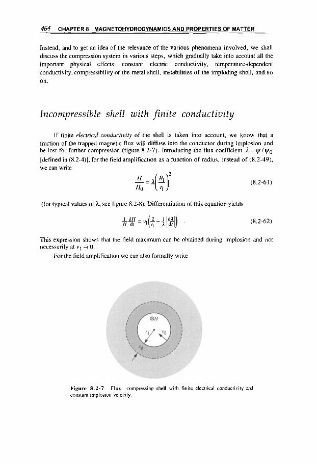
6 4 CHAPTER 8 MAGNETOHYDRODYNAMICS AND PROPERTIES OF MATTER
Instead, and to get an idea of the relevance of the various phenomena involved, we shall discuss the compression system in various steps, which gradually take into account all the important physical effects: constant electric conductivity, temperature-dependent conductivity, compressibility of the metal shell, instabilities of the imploding shell, and so on.
Incompressible shell with finite conductivity
If finite electricul conductivity of the shell is taken into account, we know that a fraction of the trapped magnetic flux will diffuse into the conductor during implosion and be lost for further compression (figure 8.2-7). Introducing the flux coefficient A = I ~ / I ~ O
[defined in (8.2-4)], for the field amplification as a function of radius, instead of (8.2-49), we can write
L A ( ? ) 2
HO
(for typical values of h, see figure 8.2-8). Differentiation of this equation yields
(8.2-6 1 )
(8.2-62)
This expression shows that the field maximum can be obtained during implosion and not necessarily at v I -+ 0.
For the field amplification we can also formally write
Figure 8 .2-7 Flux compressing shell with finite electrical conductivity and constant implosion velocity.

8.2 MAGNETIC FLUX COMPRESSION 465
(8.2-63)
where sQ is the flux skin depth defined in (4.2-20). For a reasonable description of the compression dynamics it will, in general, be sufficient to use appropriate approximations for so, such as those given by (8.2-22) or in tables 5.2-11 and 5.4-1.
More refined approximations make use of the skin-layer method [see in connection with (8.2-19)]. For example, we could easily extend the calculations made for a plane piston from (8.2-19) to cylindrical geometry and thereby obtain an estimate of the flux coefficient A as a function of rI (8.2-24 or 25), or of the maximum field amplification
It may be instructive to give a simple, if only qualitative, physical meaning to the maximum field amplification. We know from (4.3-39) that the characteristic magnetic diffusion time out of a cylindrical cavity with radius r is
H m 1 4).
(q): constant magnetic diffusivity); whereas the remaining compression time, at constant implosion velocity vo, is
r
"0 Tcompr. =- .
0.5
0
A
0.5
0 0.2 0.4 0.6 0.8 1.0
Figure 8.2-8 Flux coefficient during compression as calculated numerically"'. Note that R,, = IO'OOO is obtained, for example, for a copper shell having R , = 5 cm and 11, = 0.25 c d p s
466 CHAPTER 8 MAGNETOHYDRODYNAMICS AND PROPERTIES OF MATTER
The two time values become equal at radius
rmd VO
Consequently, in the first part of the implosion (from R , to rmd), we have
where
RI vo Rm =- KO
(8.2-64)
(8.2-65)
(8.2-66)
is the rnugnetic Reynolds number. The value of the constant a1 must be determined with an exact calculation. (From numerical calculations * ’, based on a constant implosion velocity VO, we obtain a1 = 0.04.)
When the surface magnetic field exceeds the characteristic field
I? (8.2-67)
(see also table 8.3-11), the assumption of constant conductivity is no longer reasonable. In fact, we know from (5.4-29) that if we use a conductivity law of the form
(8.2-68)
the flux skin depth SQ increases drastically, roughly by a factor Ho/h, with respect to the value based on constant conductivity.
We now give an estimate of the maximum attainable fields. It was also shown in connection with (5.4-29) that the equipartition law
(8.2-69) 1 2
2 Q = c,O = t?-jioH ,
where 19 = 1 is the surface energy factor, holds even for a conductivity law as given above. Thus for H N h, we can write
(8.2-70)
Since the flux is lost mainly toward the end of compression, when the conductivity is lowest,
8.2 MAGNETIC FLUX COMPRESSION 467
(8.2-7 1 ) 2 -2 O = Omin = Ooh, Hmd ,
we can extend the approximation for the maximum amplification found in (8.2-65) to
that is, we obtain
(8.2-72)
(8.2-73)
where the constant R, is defined by (8.2-66) and a2 is a parameter. The radius r d at field
maximum Hmd can be obtained through the condition rmdH,d = &,dRt Ho, where &d is the flux coefficient at Hn,d :
2
(8.2-74)
Magnetohydrodynamic calculations8’ confirm these forms and for the parameters find a2 =
1, I , = 0.6. They also confirm the equipartition law (8.2-69) with 8 = 1.
It is instructive to rewrite (8.2-74) with the help of (8.2-66) in the form
(8.2-75)
We then clearly see that the maximum attainable fields, obtained from the implosion of an incompressible shell with variable conductivity, can be influenced, but only weakly, by the initial velocity I J ~ or the initial trapped flux (nR1 p 0 H 0 ) . For example, for a copper conductor (table 8.3-11) and the very good initial values pH0 = 10 T , R , = 5 cm, vo = 0.5
c d p (i.e., R, = 20’000). from (8.2-75) and from (8.2-74), we obtain pHmd = 1800 T, rmd = 0.1 cm.
2
Compressible shell with infinite conductivity
By taking the cotnpressihilify of the shell into account we make a further important step toward reality. For the purpose of separating this problem for the time being from magnetic field diffusion, we will assume that the shell is an ideal conductor (0 + m) . The
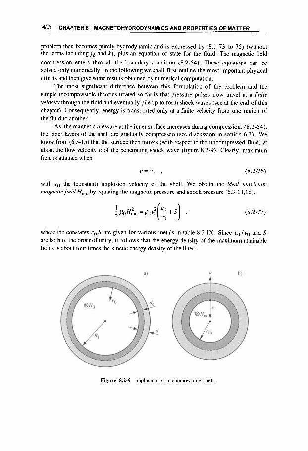
a8 CHAPTER 8 MAGNETOHYDRODYNAMICS AND PROPERTIES OF MATTER
problem then becomes purely hydrodynamic and is expressed by (8.1-73 to 75) (without the terms includingj4 and k ) , plus an equation of state for the fluid. The magnetic field compression enters through the boundary condition (8.2-54). These equations can be solved only numerically. In the following we shall first outline the most important physical effects and then give some results obtained by numerical computation.
The most significant difference between this formulation of the problem and the simple incompressible theories treated so far is that pressure pulses now travel at a finite velocity through the fluid and eventually pile up to form shock waves (see at the end of this chapter). Consequently, energy is transported only at a finite velocity from one region of the fluid to another.
As the magnetic pressure at the inner surface increases during compression, (8.2-54). the inner layers of the shell are gradually compressed (see discussion in section 6.3). We know from (6.3-15) that the surface then moves (with respect to the uncompressed fluid) at about the flow velocity u of the penetrating shock wave (figure 8.2-9). Clearly, maximum field is attained when
u = v o , (8.2-76)
with vo the (constant) implosion velocity of the shell. We obtain the ideal maximum magtietic field H,, by equating the magnetic pressure and shock pressure (6.3- 14,16),
(8.2-77)
where the constants c0.S are given for various metals in table 8.3-IX. Since c0 /vo and S are both of the order of unity, it follows that the energy density of the maximum attainable fields is about four times the kinetic energy density of the liner.
Figure 8.2-9 Implosion of a compressible shell.

- 469 . . _. .. - 8.2 ___ MAGNETIC FLUX COMPRESSION . _ _
0. I 0. I 1 10
iUde
Figure 8.2-10 Maximum field obtained hy a compressible. infinitely conducting cylindrical shell (after Somon"'). The field amplification due to plane pistons is reported in the same variables for comparison. Note that according to the definition of effective thickness we would have (a,) plane/(d,)cyl. = 2.vI/R, , where
x l is the distance of the plane piston from the symmetry plane of implosion.
Due to the finite velocity of the shock wave, only a fraction of the initial kinetic energy is therefore transformed into magnetic energy of the compressed field. This effect can be expressed by the effective thickness de, which we define as the thickness of an inner skin of the shell at the initial position whose kinetic energy is transformed totally into the magnetic energy of the final field. According to this definition we have (ford, cc R l )
L
where rm0 is the radius corresponding to maximum field. Hence, by using (8.2-77) and
the flux conservation relation ( Hmor20 = HoRt ), we obtain
(8.2-78)
As long as the initial thickness of the shell is small compared to de , all the kinetic energy of the flux compressing shell is taken up for compressing the field. From (8.2-52) we then directly obtain the maximum dynamic field H,
(8.2-79)
When d 2 (Ie we formally expect Hlnc E H,, [as in fact is the case in plane geometry (see in figure 8.2- lo)] ; however, the velocity V I of the inner boundary of the imploding shell increases rapidly with respect to v o [see in (8.2-45) for an incompressible shell], and this
leads to a further energy concentration effect and thus an increase in the maximum attainable field Hmc. The results of the numerical calculation are shown in figure 8.2-10.

470 CHAPTER 8 MAGNETOHYDRODYNAMICS AND PROPERTIES OF MATTER
Table 8.2-11 Ultrahigh field implosion generator'.'"
Initial condition
magnetic field shell internal radius shell kinetic energy
Maximum performance
magnetic field shell internal radius magnetic energy flux coefficient
pH,= 12T R , = 7.5 cm WRo = 1.5 MJ/cm
pH,= IIOOT rm = 0.5 cm WMm = 380 H/cm A, = 0.4
Considering the same example treated in connection with (8.2-75), we now obtain by dynamic limitation for a copper conductor (table 8.3-11) of thickness d = 0.3 cm: de = 0.1
cm, p H,,, = 1130 T, p H,, = 1650 T, rmc = 0.4 cm. Thus, we obtain about the same maximum field (8.2-75) as by considering the magnetic diffusion limit. Here, however, the limit is more stringent than for magnetic diffusion alone. In fact, we have available only one
typical set of parameters is given in table 8.2-11; however, maximum fields of 3000 tesla have been claimed in large implosion devices".'.
"free" parameter, v0; whereas in (8.2-75) we have, in addition, the flux (p0Ho~Rl 2 ). A
Cylindrical f l u x compression
A realistic evaluation of compression dynamics requires that field diffusion and the compressibility of the conductor be simultaneously taken into account. This general problem, which therefore includes the complete set of MHD-equations with an appropriate equation of state and an electrical conductivity law, can be solved only numerically. As an example, we can mention the one-dimensional MAGPIE codes8 with which axisymmetric compression problems, both in E# and in E , geometry, can be solved.
From the previous discussions on the most significant effects playing a role near turnaround, we can draw the following conclusions.
(a) Maximum field H, is determined principally by the implosion dynamics of the compressible piston; that is, H , = Hmc. In fact, if a flux skin depth sg is taken into account (figure 8.2-1 I), the conclusions we have drawn with respect to the cylindrical surface of radius rmc following (8.2-77) remain valid; they are simply extended to an inner surface of an approximated radius rm + s#, to which the magnetic pressure is substantially applied (figure 6.3-4).
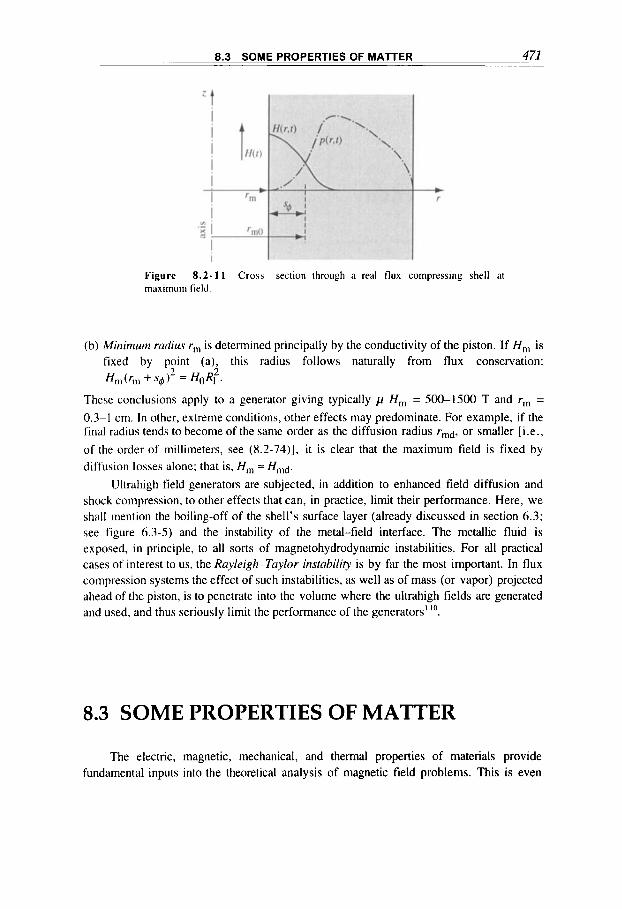
8.3 SOME PROPERTIES OF MATTER 471
Figure 8.2-1 1 Cross section through a real flux compressing shell at maximum field.
(b) Miriirizurn radius rm is determined principally by the conductivity of the piston. If H, is fixed by point (a), this radius follows naturally from flux conservation:
2 2 Hm(rm +so) = HoRl . These conclusions apply to a generator giving typically p H, = 50&1500 T and rm =
0.3-1 cm. In other, extreme conditions, other effects may predominate. For example, if the final radius tends to become of the same order as the diffusion radius rmd, or smaller [i.e.,
of the order of millimeters, see (8.2-74)], it is clear that the maximum field is fixed by diffusion losses alone; that is, Hm = Hmd.
Ultrahigh field generators are subjected, in addition to enhanced field diffusion and shock compression, to other effects that can, in practice, limit their performance. Here, we shall mention the boiling-off of the shell’s surface layer (already discussed in section 6.3; see figure 6.3-5) and the instability of the metal-field interface. The metallic fluid is exposed, in principle, to all sorts of magnetohydrodynamic instabilities. For all practical cases of interest to us, the Ruyleigh-Taylor insfability is by far the most important. In flux compression systems the effect of such instabilities, as well as of mass (or vapor) projected ahead of the piston, is to penetrate into the volume where the ultrahigh fields are generated and used, and thus seriously limit the performance of the generators’ lo.
8.3 SOME PROPERTIES OF MATTER
The electric, magnetic, mechanical, and thermal properties of materials provide fundamental inputs into the theoretical analysis of magnetic field problems. This is even

472 CHAPTER 8 MAGNETOHYDRODYNAMICS AND PROPERTIES OF MATTER
more so when engineering structures, such as magnets, have to be designed and built8 49.8 50 . Here we will present some fundamental data (when not already given throughout the chapters) and order them around some elementary physical models.
Electric conductivity
According to Ohm’s law (1.1-53),
j = a E , (8.3-1)
the electric conductivity Q is a physical parameter relating the electric field E to the current density j . In the most general cases the conductivity can have the form of a tensor [see also in (A.3-33)]. Here, we shall consider only cases where j and E are aligned, such that o reduces to a scalar function, which varies with the material considered (see table 8.3-11) and can depend on various physical quantities.
The conduction mechanism can be interpreted formally as the flow of free electrons that is inhibited by various interaction processes*”.”’. If we introduce, in accordance with transport theory, a relaxation rime r for scattering such that the overall mean electron drift velocity can be expressed as
1 eE (v )=- r - , 2 me
the current density yields
I e2
2 me j = nee(v) = -ne -rE .
(8.3-2)
(8.3-3)
Ohm’s law thus results from an average balance between the momentum gained by each free electron from the electric field and the momentum lost in collisions. According to (8.3- l), the conductivity can therefore be written formally as
here, n, is the density of free electrons (there is about one free electron per atom), and e and
me are the charge and mass of the electron. Instead of z, we can also introduce the mean
free path
1 ke=r(v)=- , ni se
(8.3-5)
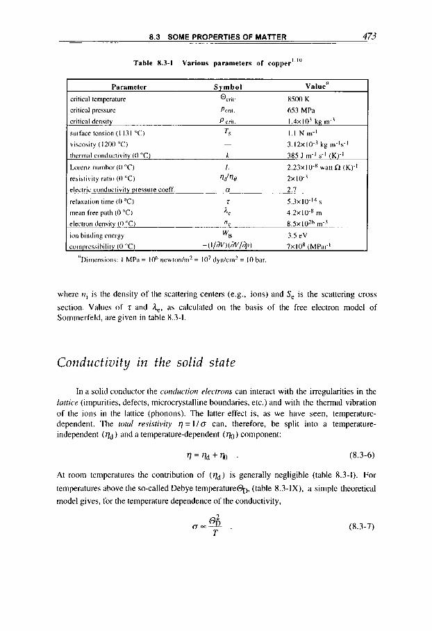
8.3 SOME PROPERTIES OF MATTER 473
Table 8.3-1 Various parameters of copper' lo
Parameter S y m b o l Value'
critical temperature 'cnt. 8500 K
critical pressure Pcnt. 653 MPa
critical density P crit. I .4x lo3 kg m-3
surface tension ( I I3 I "C) TS 1 . 1 N m-I
viscosity (1200 " C ) - 3.12x10-' kg m-ls-l
thermal conductivity (0 "C) k 385 J m-I s-I ( K ) - '
Loren/ number (0 "C) L 2 . 2 3 ~ 1 0 - ~ watt R (K)-I
resistivity ratio (0 " C ) rld/r78 2x10⁻³
electricconductivity pressure coeff. ~ a--. 2.7
relaxation time (0 "C) r 5 . 3 ~ 1 0 - ' ~ s
mean free path (0 "C) 4 4 . 2 ~ I W8 m
electron density (0 "C) " e 8 . 5 ~ 1 0 ~ ~ m - j
ion binding energy w, 3.5 eV
compressibility (0 "C) - ( I / d v ) (dv/d'J) 7 ~ 1 0 ~ (MPai-l
"Dimensions: 1 MPa = lo6 newton/m2 = l o 7 dyn/cm2 = 10 bar.
where ni is the density of the scattering centers (e.g., ions) and Se is the scattering cross
section. Values of z and A,, as calculated on the basis of the free electron model of Sommerfeld, are given in table 8.3-1.
Conductivity in the solid state
In a solid conductor the conrfuctioti elcctrotzs can interact with the irregularities in the lattice (impurities, defects, microcrystalline boundaries, etc.) and with the thermal vibration of the ions in the lattice (phonons). The latter effect is, as we have seen, temperature- dependent. The ford resistiviry q = I l o can, therefore, be split into a temperature- independent ( qd ) and a temperature-dependent ( ~ 0 ) component:
At room temperatures the contribution of ( q d ) is generally negligible (table 8.3-1). For
temperatures above the so-called Debye temperature%, (table 8.3-IX), a simple theoretical
model gives, for the temperature dependence of the conductivity,
(8.3-7)
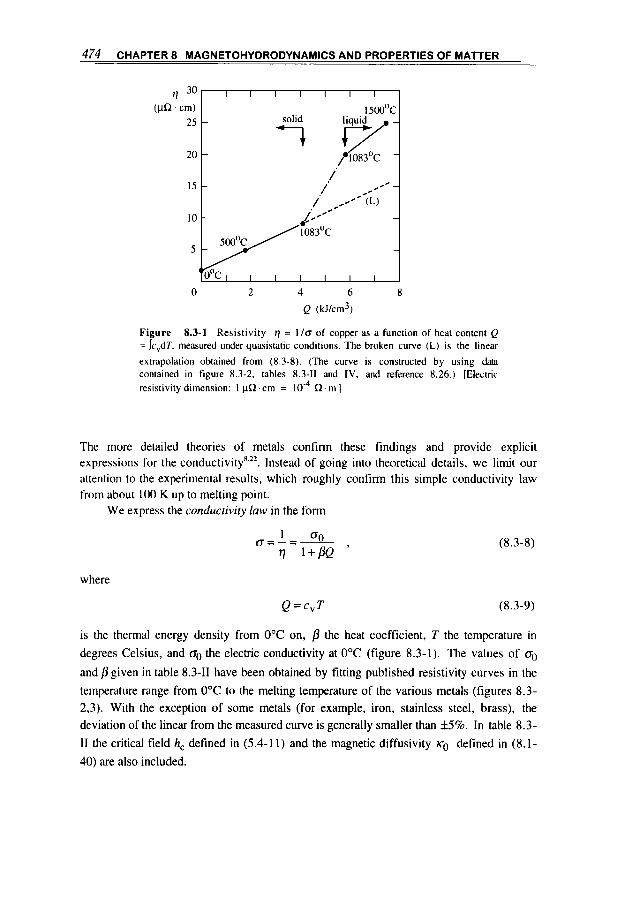
474 CHAPTER 8 MAGNETOHYDRODYNAMICS AND PROPERTIES OF MATTER
v 3 0 -
(PQ. cm) 25
20
I I I I I I ' - q y 1 5oooc
- 1083OC -
/
extrapolation obtained from (8.3-8). (The curve is constructed by using dara contained in figure 8.3-2, tables 8.3-11 and IV, and reference 8.26.) [Electric resistivity dimension: I p Q . c m = R.m 1
The more detailed theories of metals confirm these findings and provide explicit expressions for the conductivity' 22. Instead of going into theoretical details, we limit our attention to the experimental results, which roughly confirm this simple conductivity law from about 100 K up to melting point.
We express the conducfiviry law in the form
(8.3-8)
where
Q = c v T (8.3-9)
is the thermal energy density from 0°C on, p the heat coefficient, T the temperature in
degrees Celsius, and 00 the electric conductivity at 0°C (figure 8.3-1). The values of O,
and p given in table 8.3-11 have been obtained by fitting published resistivity curves in the
temperature range from 0°C to the melting temperature of the various metals (figures 8.3- 2,3). With the exception of some metals (for example, iron, stainless steel, brass), the deviation of the linear from the measured curve is generally smaller than f5%. In table 8.3- I1 the critical field h, defined in (5.4-1 1) and the magnetic diffusivity KO defined in (8.1-
40) are also included.

8.3 SOME PROPERTIES OF MATTER 475
D (PQ ' cm)
30
25
20
15
10
5
0 -200 0 500 loo0 1500 2000
T ('(3
Figure 8.3-2 Resistivity of electrolytic copper and aluminum, brass, and aluminum-silicon as a function of temperature, measured under quasistatic conditions. I n the transient case' ', the temperature range 500-2000 OC is swept through in about 2 p. (Curves up to melting point are from reference 8.27; curves of the liquid phase are from reference 8.26.)
The electrical conductivity in conductors for practical applications also depends critically on the exact composition and the manufacturing condition of the alloys. An example of this is presented in table 8.3-111, which moreover shows the temperature dependence of the resistivity qH '* at two cryogenic temperatures of practical interest (76 K obtained by liquid nitrogen cooling, 4 K by liquid helium) compared to the value at room temperature (295 K). In high-field applications, the tensile strength of the conductor is also very important; the two qualities are expressed by the figure of merit CSY / q , where OY is
the yield strength given in table 7.1-11. The electric conductivity also depends on several other physical quantities. Here, we
mention only pressure and magnetic field, since their influence on the conduction mechanism can be of some importance in very particular problems. The conductivity law (8.3-9) can be extended to include the compression effect in the form
(8.3-10)
where p = 1 / V is the mass density, and the experimentally determined pressure coefficient 01 is given, for copper, in table 8.3-1.
When a magnetic field H is applied, the conducting electrons move, between collisions, in circular (or helical) orbits with a Lurmor radius (6.4-49c),
(8.3-1 I )
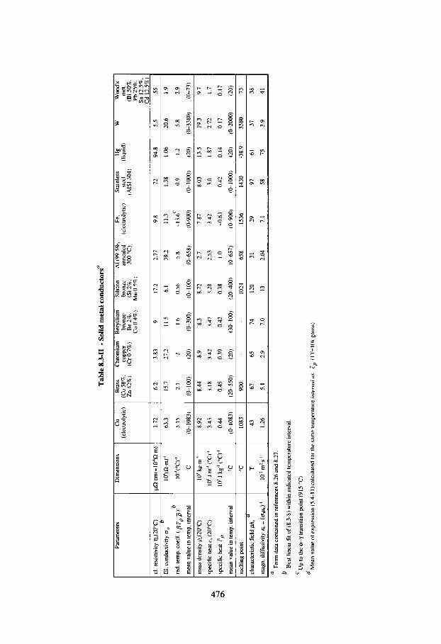
Tab
le 8
.3-1
1 - S
olid
met
al c
ond
uct
ors'
Par
amet
en
Dim
ensi
ons
cu
Brass
Chr
omiu
m
Ber
ylliu
m
Silic
on
Al(
99
.54
. Fe
. S
mnl
ess
Hg
w
woo
d's
(ele
ctro
lytic
) (Cu 5
8%.
copp
er
bron
ze
bron
ze
anne
aled
(e
lect
roly
uc)
stee
l (l
iqui
d)
mef
. Z
n4
24
) (C
r07
%)
Be2
B.
tSi2
4.
300°
C)
(A
N 30
4)
(Bi
50%
. C
o0
.4%
) M
nOS
%)
pb 2
5%.
Sn
12.5
4.
I I
Cd
12.5
%)
2
El.
cond
uctiv
ity u
, 10
h(R
.m)-
' 63
.3
15.7
27
2
I1 5
61
39
.2
11.3
1.
38
I06
20
.6
I .9
red.
tem
p. c
wff
. ( p
cP 5
J' m
ean
valu
e in
tem
p. in
terv
al
"C
(0-1
083)
(0
-100
) (2
0)
(0-300)
(&I0
01
(0-6
58)
(0-9
00)
(O-IOOO)
(20)
(0
-338
0)
(0-7
3)
lo-?
"C
) ' 5
15
2. I
?
I .6
03
6
5.8
-13.
6'
09
I .2
5.
8 2.
9
mas
s de
nsity
p,,(
20"C
) 10
' kg-m '
8.92
8.
44
8.9
8.3
8 72
2.
7 7.
87
8.03
13
.5
19.3
9.
7
b
spec
ific
hea
t c,
(20°
C)
lb J
m.'.
("C
)-'
3.43
3.
18
3 42
3.
47
3.28
2.
53
3.42
3.
0 1.
87
2 72
I .
7
spec
ific
hea
t Tp
10
' J-k
g.' (
T)'
0.44
0 45
0.
39
0.42
0
38
10
-0
63
0.42
0.
14
0.17
0.
17
mea
n va
lue
in te
mp
inte
rval
"C
(0
-108
3)
(20-
550)
(2
0)
(30-
100)
(2
W00
1 (0
-657
) 10
-900
) (0
-lOO
O)
(20)
(C
-2M
H))
(20)
mel
ting
poin
t
char
acte
rist
ic f
ield
phc
mag
n. d
iffu
sivi
ty &
= (u
&
"C
1083
90
0 I0
24
65
8 15
36
1430
-3
8.9
3380
73
T 43
67
6.5
74
12
0 31
29
97
61
37
38
I .26
5.
1 2.
9 7.
0 13
2.
04
7.1
58
75
3.9
41
m2
I
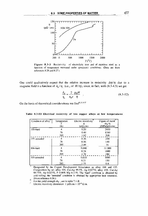
8.3 SOME PROPERTIES OF MATTER 477
Condition of alloy"
155-hard
-200 0 500 loo0 1500 2000
T (OC)
F i g u r e 8.3-3 Resistivity of electrolytic iron and of stainless steel as a function of temperature measured under quasistatic conditions. (Data are from references 8.26 and 8.27.)
Temperature Electric resistivity" Figure of meritr T v flK/rl
(K) (pR-cm) (MPa/pR.cm) 4 0.20 2410
One could qualitatively expect that the relative increase in resistivity A q / q due to a magnetic field is a function of he (i.e., of H / q ) , since, i n fact, with (834.5) we get
I Wannealed
- he--- - 2 P 0 H . 'L nee 17
On the basis of theoretical considerations we findR ", "
- - - _ - - - - - - - - - - _ 2 9 r _ _ - - - - - - ~ - - - - - - - - - - - ~ ~ 0 - - - - . I .79 4 0.0 I0 3000 76 0.2 I I50 295 I .75 0.6
(8.3- 12)
Table 8.3-111 Electrical resistivity of two copper alloys a t low temperatures
- - - - - - - - - - 155-annealed
IWhard
76 0.40 1160 I .92
4 0.36 230 76 0.56 I40 295 2.09 31 4 0.040 I I 'OOO
76 0.24 1680
- - - -225- - - - - - - - - - - - - - - - - - - - - 220- - - -
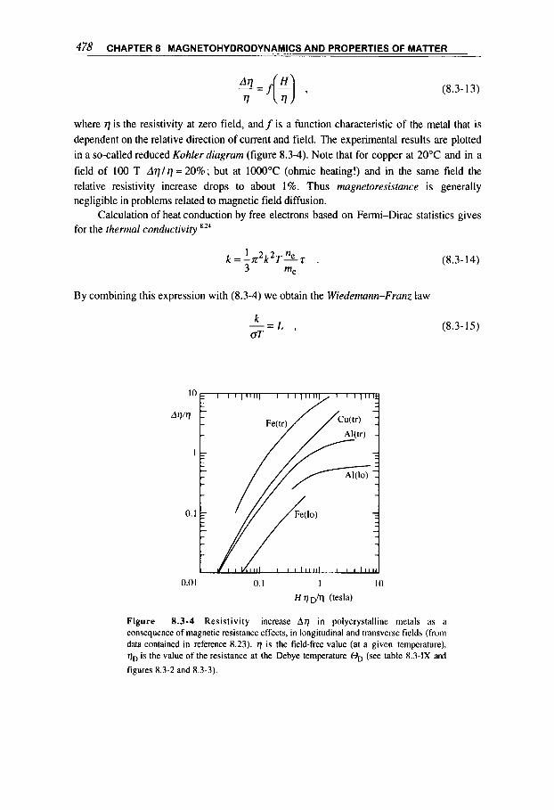
478 CHAPTER 8 MAGNETOHYDRODYNAMICS AND PROPERTIES OF MATTER
(8.3-13)
where q is the resistivity at zero field, and f is a function characteristic of the metal that is dependent on the relative direction of current and field. The experimental results are plotted in a so-called reduced Kohler diagram (figure 8.3-4). Note that for copper at 20°C and in a field of 100 T A q / q = 20%; but at 1OOO"C (ohmic heating!) and in the same field the relative resistivity increase drops to about 1 %. Thus magnetoresistance is generally negligible in problems related to magnetic field diffusion.
Calculation of heat conduction by free electrons based on Fermi-Dirac statistics gives for the thermal conductivity 8.24
By combining this expression with (8.3-4) we obtain the Wiedemann-Franz law
k - = L d T '
(8.3- 14)
(8.3-15)
0.0 I 0. I 1 10
H q D/V (tesla)
Figure 8.3-4 Resistivity increase A q in polycrystalline metals as a consequence of magnetic resistance effects, in longitudinal and transverse fields (from data contained in reference 8.23). q is the field-free value (at a given temperature), qD is the value of the resistance at the Debye temperature 0, (see table 8.3-IX ard figures 8.3-2 and 8.3-3).

Tab
le 8
3-IV
M
etal
con
duct
ors
abov
e m
elti
ng p
oint
(1
Para
met
ers
Dim
ensi
ons
el. c
ondu
ctiv
ity
(at
T,"C
)oI
lo'(Q
.m)-
l
redu
ced
tem
p. c
wff
.(!3
1.cp
.pl)
b
10-3
(~c)p
cu
AI
Fe
Woo
d's
H
g N
a (e
lect
roly
tic)
(9
9.5%
) (e
lect
roly
tic)
m
etal
4.7
5.0
0.7
1.15
1.1
10.4
3.2
0.38
0.
53
-
8.7
-
cond
uctiv
ity d
ecre
ase
q/u,
(at T
,)
P sp
ecif
ic h
eat c
(mea
n va
lue
with
in te
mp.
inte
rval
)
mel
ting
poin
t T
,
boili
ng p
oint
T, (
760
mm
Hg)
late
nt h
eat o
f m
eltin
g
late
nt h
eat o
f va
pori
zatio
n
heat
of
subl
imat
ion
(fro
m 0
°C)
-
0.48
0.
6 I
0.92
0.
74
-0.2
5
0.47
I .
08
0.79
-
0.13
7
(0-3
00)
(108
3-15
00)
(660
-1O
OO
) (1
550-
2O0o
) -
I083
65 8
15
36
73
-38.
9
357
2500
24
50
3070
0.21
0
38
0.27
-
0.01
17
4.7
10.5
-
0.29
2
5.6
12.1
7.
5
-
-
-
-
0.7
0.92
8
I .35
(IOC-350)
97.8
883
0.1
13
4.2 -
Man
ly f
rom
ref
eren
ces
8.26
and
8.27
.
In a
nalo
gy t
o (8
.3-9
). n
ear
the
mel
ting
poin
t we
wri
te u =
o,[I +
Plc
V(T
- T, )
I-'.

480 CHAPTER 8 MAGNETOHYDRODYNAMICS AND PROPERTIES OF MATTER
where L = r2 k2 /3e2 = 2.45 x lo-’ W U K is the Lorenz constant. (The exact value for copper is given in table 8.3-1.) By taking into account (8.3-7) we see, for example, that the thermal conductivity is independent of temperature.
Conductivity in liquid, vapor, and plasma states
A decrease in electric conductivity is found for most metals on melting (table 8.3-IV and figures 8.3-2,3). This effect depends on the decrease in the mean free path of the electrons resulting from additional disorder in a liquid. Nevertheless, in the rapid heating caused by field diffusion, there may not be enough time for the liquid to settle for its quasistatic structure. It is expected, therefore, that the conductivity decrease on transient melting not be so pronounced as measured in quasistatic conditions (figure 8.3-2).
As the temperature of the ohmically heated conductor becomes higher than the boiling point, the surface starts boiling off; the dense vapor then expands and is gradually transformed into a highly conducting plasma”‘. Study of the properties of the electric conductivity and, in general, of transport coefficients across these phase changes is a rather arduous problem. In general one tries to approach it from a practical side by giving empirical laws.
Superconduct ivi ty
There are certain materials in which dc electric currents can be transported with (practically) zero resistanceX45.X 55. This property is attained when:
the temperature of the material is less than a critical temperature T,;
the magnetic field to which the material is exposed is less than a critical magnetic field
the density of the current flowing in the material is less than a criticul current densityj,.
These critical parameters vary with the material. For a given material, they also depend on the form of the specimen, its orientation with respect to the magnetic field, and so on. The three critical parameters are related, as shown for two superconductors in figure 8.3-5; in particular, there is the empirical relation
H, ;
(8.3-16)
where HCo denotes the critical field at zero temperature and T,o is the critical temperature at
zero field (table 8.3-V).
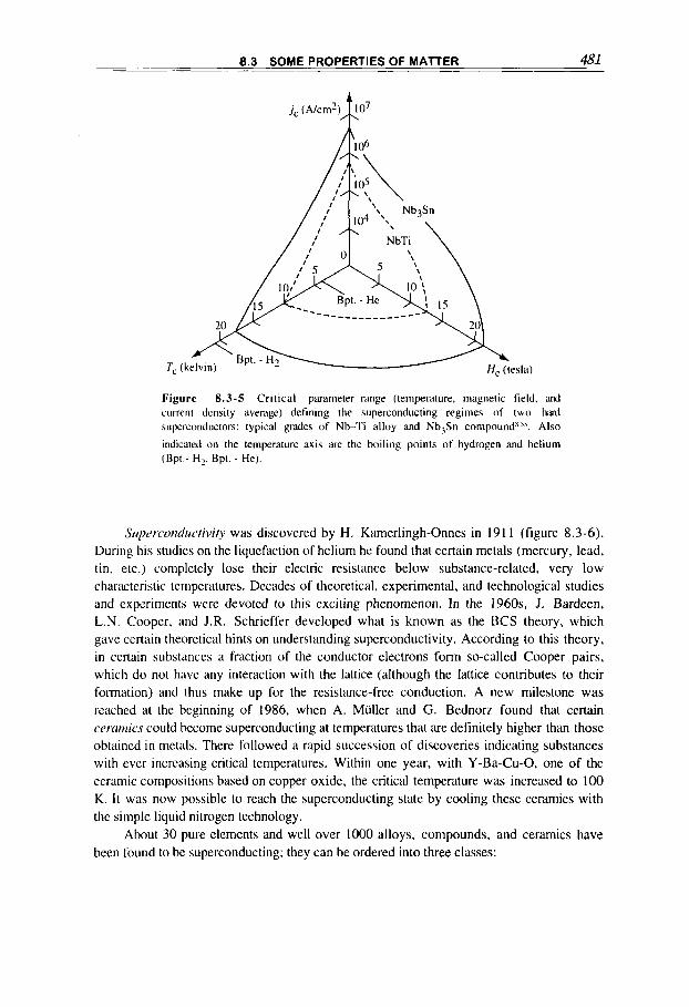
8.3 SOME PROPERTIES OF MATTER 481
jc (ARm2)&
Figure 8.3-5 Cr i t ica l parameter range (temperature. magnetic field, and current density average) defining the superconducting regimes of two hanl superconductors: typical grades of Nb-Ti alloy and Nb3Sn compound" ss. Also
indicated on the temperature axis are the boiling points of hydrogen and helium (Bpt.- H2. Bpt. - He).
SIrp"r~"iicIi".tiv;ry was discovered by H. Kamerlingh-Onnes in I9 1 1 (figure 8.3-6). During his studies on the liquefaction of helium he found that certain metals (mercury, lead, t in , etc.) completely lose their electric resistance below substance-related, very low characteristic temperatures. Decades of theoretical, experimental, and technological studies and experiments were devoted to this exciting phenomenon. In the 1960s, J. Bardeen, L.N. Cooper, and J .R. Schrieffer developed what is known as the BCS theory, which gave certain theoretical hints on understanding superconductivity. According to this theory, in certain substances a fraction o f the conductor electrons form so-called Cooper pairs, which do not have any interaction with the lattice (although the lattice contributes to their formation) and thus make up for the resistance-free conduction. A new milestone was reached at the beginning of 1986, when A. Muller and G. Bednorz found that certain crrcirnics could become superconducting at temperatures that are definitely higher than those obtained i n metals. There followed a rapid succession of discoveries indicating substances with ever increasing critical temperatures. Within one year, with Y-Ba-Cu-0, one of the ceramic compositions based on copper oxide, the critical temperature was increased to 100 K. It was now possible to reach the superconducting state by cooling these ceramics with the simple liquid nitrogen technology.
About 30 pure elements and well over 1000 alloys, compounds, and ceramics have been found to be superconducting; they can be ordered into three classes:

CHAPTER 8 MAGNETOHYDRODYNAMICS AND PROPERTIES OF MATTER . - ~ - -. -~
~~~~
Superconductivity
Nb-Ti (46.5%) Nb3Sn
V,Ga
Nb,(AI0., Geo 2)
Table 8.3-V Properties of some (commercial) hard superconductorsN 2’ .1 ’’ ~ ~~ ~~ ~
Critical temp.(K) Upper critical field (T) Crjrical currentdensity (A.mm-*) .-
T C O H,, H , at 4.2 K j, at 8T,4.2K at 12T, 2K 12T, 4.2K
9.1 14 11.5 800 400 0
18.3 24.5 22.5 I000 700 500
15 23.0 21.0 600 700 500
21 40 - - - -
Type 1 superconductors. They are characterized by a very sharp transition to normal conduction when the magnetic field reaches Hc. They mostly include metals (mercury, lead, etc.) and have limited technical applications.
Type 2 (or “hard”) superconductors. In this group, certain physical superconducting characteristics are gradually lost, starting from a field H c l up to Hc2
(called the “upper critical field’, or just “critical field”) where the substantial transition to normal conduction occurs. These superconducting materials are capable of supporting high current densities at high magnetic fields, and are thus of technical interest. They include the two superconductors mostly used today in technical applications: Nb-Ti, a niobium-titanium alloy (generally near a 5&50% weight share), and Nb3Sn, a niobium- 3-tin compound pertaining to the so-called A-1 5 cubic crystal structural type compounds [which has a better high-field performance (figure 8.3-5 and table 8.3-V), but is a brittle compound and thus more difficult to form into filamentary conductors].
High-temperature superconductors. These new ceramic compositions are mostly based on copper oxide with critical temperatures above the liquid nitrogen temperature (-1 90°C) (and in future hopefully increasing up to room temperature). At present there are still some technical difficulties in using them in practical, high-field generators. However, there can be no doubt that within a few years, these high-temperature superconductors will be used c~mmerciallyl-~~-for example, in energy related products, as in cables, transformers, and inductive energy storage.
There are several remarks to be made in connection with the practical application of hurd superconductorsB 18. As already mentioned, the critical parameters depend on various facts, such as the geometry of the superconductor, its manufacturing procedure, and so on. This is why in practice Nb3Sn superconductors are good up to only about 12 T, and Nb-Ti
superconductors up to 8 T, although their critical fields measured on specimens are about 24 and 14 T, respectively (table 8.3-V).

8.3 SOME PROPERTIES OF MATTER 483
HgBa2Ca2Cu308+,sj
T12Ba2Ca2Cu30 IO+6 - Bi2Sr2Ca2Cu3010+,sj 1
100
YBa2CujO7-g
80
70
30 (La. B a)2Cu04
Nb- AI-Ge
N bO 10 -
- J H ~ Metals and compounds Oxides
1910 1930 1950 1970 1990 0 1 1
I I I
Year
Figure 8.3-6 Evolution of the critical temperature with the discovery of new superconductors.
An important effect to be taken into account in the practical application of hard superconductors is related to a series of local microheating mechanisms that can increase locally the temperature to above the critical temperature. [The temperature excursions are enhanced by the fact that specific heats of all materials (except helium) are extremely small at the low temperature under consideration.] When this happens, the resistance rises suddenly to the high values of the normal state (for Nb-Ti at around 10 K, about 40 times the resistance of copper at room temperature), and through local joule heating (Rp) a nearly explosive deposition of the inductive energy tied to the system can take place: The normal state propagates through the whole superconductor, a process called a “quench’. The local heating in hard superconductors can derive from a variety of sources, from purely mechanical friction (the superconducting wires moving slightly under the influence of the
4% CHAPTER 8 MAGNETOHYDRODYNAMICS-AND PROPERTIES OF MAlTER . .- ~. - -~
j x B forces) to magnetic diffusion effects, which are related to the physics of the superconducting state in hard superconductors.
The most significant diffusion effects are caused by so-called “flux jumps” in connection with an increasing magnetic field. As a consequence, in ac fields, the heating effects depend on the frequency, amplitude, and direction of the magnetic fields. It can be shown that flux heating effects are proportional to the surface of the superconducting wire. Thus, in practical applications the superconductor is subdivided into filaments with diameters typically 10 to 50 pn (required for field variations of 1 to 5 T/s).
To cope with these dangerous heating effects, further stabilizution means are introduced. The most important is to embed the filaments in a matrix of copper or aluminum to form integrated, composite conductor strands. The coolant for hard superconductors is liquid helium; in some applications it is used in the supeguid state at about 2 K, where thermal conductivity is very high. This coolant then prevents localized transient heat accumulation by rapidly conducting and dissipating the dangerous thermal energy into the surrounding matrix.
Magnetic matter
As mentioned in section I . I , in most materials when subjected to a magnetic field H , an additional field component, or magnetization M, is generated locally such that (1.1-17)
and the magnetic susceptibility (1.1 - 19),
(8.3-17)
(8.3-18)
can have positive or negative values, according to the material (table 1.1-11). For the purpose of illustration, we shall briefly and in simple terms describe the
atomistic effects induced by the application of a magnetic field H to diamagnetic, paratnugnefic, and ferrornugnetic materials‘ 19.’ *”. We shall show that the magnetic properties of these materials are associated with the magnetic moment and the ungular momentum (spin) possessed by elementary particles (electron, proton, neutron, etc.) and the orbits @the electrons in the atomB5’.
Diamagnet ism
Diamagnetism, which is obtained when a magnetic field is switched on over certain materials, will manifest itself as a negative susceptibility and as a tendency to push the
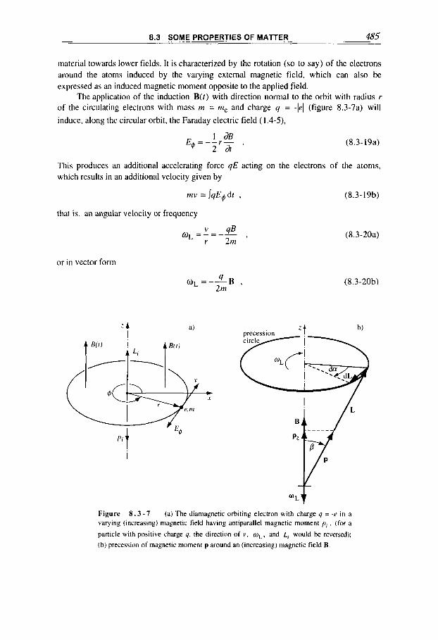
8.3 SOME PROPERTIES OF MATTER 485
material towards lower fields. It is characterized by the rotation (so to say) of the electrons around the atoms induced by the varying external magnetic field, which can also be expressed as an induced magnetic moment opposite to the applied field.
The application of the induction B(r) with direction normal to the orbit with radius r of the circulating electrons with mass M = me and charge 4 = -1el (figure 8.3-7a) will induce, along the circular orbit, the Faraday electric field (1.4-5).
1 dB 2 d r
E q = - - r - . (8.3-19a)
This produces an additional accelerating force q E acting on the electrons of the atoms, which results in an additional velocity given by
tizv = j 4Eqd t , (8.3- 19b)
that is, an angular velocity or frequency
or in vector form
t I
(8.3-20a)
(8.3-20b)
Figure 8 . 3 - 7 (a) The diamagnetic orbiting electron with charge q = -r in a varying (increasing) magnetic field having antiparallel magnetic moment p , , (for a
particle with positive charge 4. the direction of v , q,, and L, would be reversed); (b) precession of magnetic moment p around an (increasing) magnetic field B.
486 CHAPTER 8 MAGNETOHYDRODYNAMICS AND PROPERTIES OF MAlTER
and this in turn yields a current flowing clockwise with respect to B:
(8.3-21)
Note that the Larrnor frequency W L , already found in (6.4-23) as a precession frequency, is half the cyclotron frequency (6.4-49),
a=-- 4B , rn
(8.3-22)
that is, the frequency of a charged particle orbiting in a steady magnetic field. For each ith electron on an orbit normal to B with radius ri. application of the induction yields a (negative) magnetic moment (2.2-45),
(8.3-23)
In other words, the induced angular velocity results in a magnetic moment pi that is antiparallel to the applied field B (independent from the sign of the charge). By introducing the mechanical angular momentum
(8.3-24) 2 L;=w~;rn';: ,
this magnetic moment can also be written as
4 2rn
p i = $ ; , with y=- . (8.3-25)
[Since the so-called gyromagnetic ratio y is independent of the form of the angular momentum, this relation also applies to the cyclotron rotation (8.3-22) as shown in (6.4-
We are now in a position to express the magnetization M in terms of atomistic parameters because according to (1.1-23) it can be given as the mean magnetic moment per unit volume. For a spherically symmetric charge distribution in the atom, the electron orbits with radii Ri will in general lie at random positions with respect to the plane normal to B . By evaluating the mean square value we find that (8.3-23) can be applied directly with the
substitution q2 + -Rf . What is left is the summation over all Z orbits of the n atoms per
unit volume to obtain (with the electron charge e and mass rn,)
2 3 ~
2- 3
(8.3-26a)
and thus from definition (8.3- 18) the diamagnetic susceptibility is
8.3 SOME PROPERTIES OF MATTER 487
(8.3-26b)
since in general M N H , that is, B E p@ . The diamagnetic susceptibility Xmd is negative
(table 1.1-11) and is a direct consequence of the electron cloud surrounding the atomic nucleus; it increases with the radius square of the orbits and has no explicit temperature dependence.
It follows implicitly from (8.3-25) that a diamagnetic effect is obtained also from particles that have no orbital movement but an internal magnetic moment p s with collinear
angular momentum or spin L,
Ps=YL ' (8.3-27)
For example, for the internal magnetic and angular momentum (spin) of the electron, it is
e y=- - me
(8.3-28)
which is twice as large as for the orbital moment (8.3-25). If we apply a magnetic field B (see in figure 8.3-7b), we know from the equation of the gyroscope (6.4-23) that under the action of a torque, which here is
T = p , x B = - y B x L , (8.3-29)
the angular momentum vector L begins to precess, here about B, at frequency
OL =-yB ; (8.3 -30)
and the reasoning then continues formally as in (8.3-23). If p is the angle between B , or the collinear z-axis, and ps (which in figure 8.3-7b is shown parallel to L, contrary to the
left figure), then the mean magnetic moment is now reduced to
1': = ps c o s p . (8.3-31)
I f there are n atoms each with magnetic moments ps,free to rotate und distributed ut rundoni
in space, may have any value, and for the magnetization component along R we have
M. = n C pscospj = O . i
(8.3 -32)
The permanent magnetic moments p s all precess independently of the angle pj at the same
angular frequency (8.3-30) and consequently in this case the mean components of M perpendicular to B also vanish,
M,=M,=O . (8.3-33)
A diamagnetic effect exists only when there is a resultant finite permanent moment (8.3-

488 CHAPTER 8 MAGNETOHYDRODYNAMICS AND PROPERTIES OF MATTER
23), but there is no such effect for permanent magnetic moments distributed at random. [On the contrary, the diamagnetic magnetization (8.3-26) calculated with the inductively driven electron cloud model is due to the resultant magnetic moments pi. (8.3-23), all being
antiparallel to B.] Diamagnetism is thus a general property of materials, but it is so small that it generally
goes unnoticed. It is clear that more precise calculations must be based on quantum mechanical theory; in particular, they must consider the particular interaction effects and the quantization of the angular momentum L and magnetic moment p [see (8.3-47,50)].
Paramagnetism
If the atoms have permanent magnetic moments, application of a flux B will try to align them through the action of the torque (8.3-29). There will also be the diamagnetic precession, but the alignment effect, contrasted only by the kinetic movement, will strongly predominate. In contrast to the freely precessing magnetic moments that in (8.3-26) led to diamagnetism, here the magnetic moment ps are energetically coupled to the structure of the
surrounding material (which we call the “lattice”), thus providing the so-called paramagnetism. A simple classical calculation made below (Langevin’s theory) gives the so-called Curie low for paramagnetic susceptibility
(8.3 -34)
where ps is the overall magnetic dipole moment of each of the total n atoms per unit volume and Tis the temperature of the material. This expression is found on assuming p s B (( kT,
which means that there is deviation from this law at very low temperatures and in very strong fields. In sufficiently strong fields, B 2 kT/p, , all magnetic moments tend to be
aligned along the field and the magnetization saturates at
M+p,n . (8.3-35)
It is worth pointing out that in dielectric substances, with permanent electric dipoles pe
(2.2-54), analogous effects and formulae apply, as with paramagnetism. For the calculation of the paramagnetic susceptibility we start by noting that the
magnetic potential energy of a magnetic moment ps making an angle p towards B (figure
8.3-7b) is given in (6.1-38a) as
W = -ps . B = -p,BcosP . (8.3-36)
From thermodynamics we know that the number dn of atoms (in thermodynamic equilibrium with the lattice at temperature 7‘) having moments lying between pand p + d p is proportional to exp(- WlkT), more precisely it is
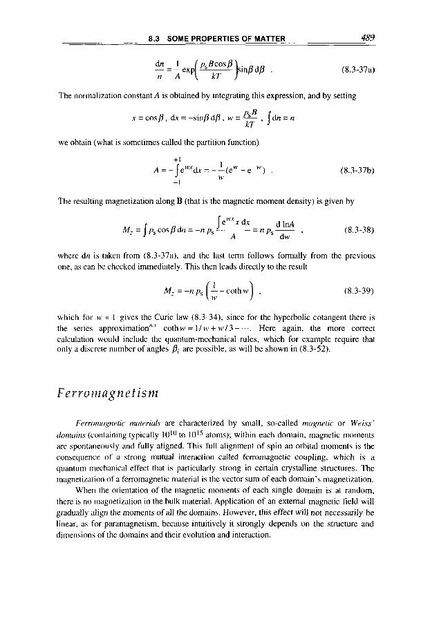
8.3 SOME PROPERTIES OF MAlTER 4-89
-=-exp( dn 1 p,Bcosp kT )slnpd/3 . n A
(8.3-37a)
The normalization constant A is obtained by integrating this expression, and by setting
x = c o s p , dr=-s in /3dp , w=-, PSB I d n = n kT
we obtain (what is sometimes called the partition function)
(8.3-37 b) -I
The resulting magnetization along B (that is the magnetic moment density) is given by
where dn is taken from (8.3-37a), and the last term follows formally one, as can be checked immediately. This then leads directly to the result
(8.3-38)
from the previous
(8.3-39)
which for to (( I gives the Curie law (8.3-34). since for the hyperbolic cotangent there is the series approximation" ' coth w = 1 / cv + w / 3 - .... Here again, the more correct calculation would include the quantum-mechanical rules, which for example require that only a discrete number of angles p, are possible, as will be shown in (8.3-52).
F e r romagn e t is m
Frrrorruignrtic tiuitrriuls are characterized by small, so-called tnugnetic or Weiss ' chiuins (containing typically 101() to 10's atoms); within each domain, magnetic moments are spontaneously and fully aligned. This full alignment of spin an orbital moments is the consequence o f a strong mutual interaction called ferromagnetic coupling, which is a quantum mechanical effect that is particularly strong in certain crystalline structures. The magnetization o f a fcrromagnetic material is the vcctor sum of each domain's magnetization,
When the orientation of the magnetic moments of each single domain is at random, there is no magnetization in the bulk material. Application of an external magnetic field will gradually align the moments of all the domains. However, this effect will not necessarily be linear, as for paramagnetism, because intuitively it strongly depends on the structure and dimensions of the domains and their evolution and interaction.

490 CHAPTER 8 MAGNETOHYDRODYNAMICS AND PROP_ERTIES OF-MA-rER - ~- .- - ~-
Orientation and dimensions of the domains, and the so-called Bloch walls separating them, are generally dictated by minimum energy state. When a magnetic field is applied, the domains change and the walls are displaced correspondingly across the crystal, unless they are blocked by an imperfection of the lattice, or by a grain boundary in polycrystalline substances. These imperfections also introduce a resistance to falling back to the initial state when the field is removed. This is the source of hysteresis. In addition, ferromagnetism depends on the size of the specimen, the magnitude and frequency of the applied field, etc. Above the so-called Curie feniperature, the kinetic movement overcomes the spontaneous alignment within the magnetic domains, the alignment gets lost, and thus the ferromagnetic property of the material disappears, to leave only the paramagnetic effect. (For example, the Curie temperature of iron is at 746 "C, whereas the melting occurs at 1530 "C; see table 83-11 and figure 5.4-1 .)
The behavior of ferromagnetic substances under the action of an applied magnetic field is typically described by the so-called B - H or magnetization curves. Some basic parameters are illustrated in figure 8.3- 10b and defined herewith:
Saturation. Practical: maximum induction B , when the curve starts to level off.
Theoretical: the asymptotic maximum of the magnetization term M , = lim ( B - p,,bH).
The value depends on temperature.
Rematience: The induction B, remaining after H has returned to zero.
Coercivity: The field H , required to cancel the remaining induction.
Domains of magnetization: As the magnetic field H is applied up to point 4 , the process remains reversible; then extensive domain wall movements set in, so if at P2 the field is reduced, a new hysteresis curve is traced out; at 4 the material is brought to near saturation with almost complete alignment of the domains.
H+m
Energy losses in ferromagnetic materials are a topic of particular interest in applications. The two main electromagnetic losses in these materials can be characterized as follows:
Eddy current loss: results from ohmic heating by induced currents flowing within the skin depth (as widely discussed in chapter 5).
Hysteresis loss: the result of the rearrangement of Bloch walls and domain niagnctization, when B and H vary through the hysteresis loop. The energy lost in going around the loop is given in (5.4-43),
(8.3-40)
which corresponds to the area of the loop (when the velocity of variation is large, the rearrangement process may not be complete, and this loss therefore depends on the velocity, or frcquency, of field variation).
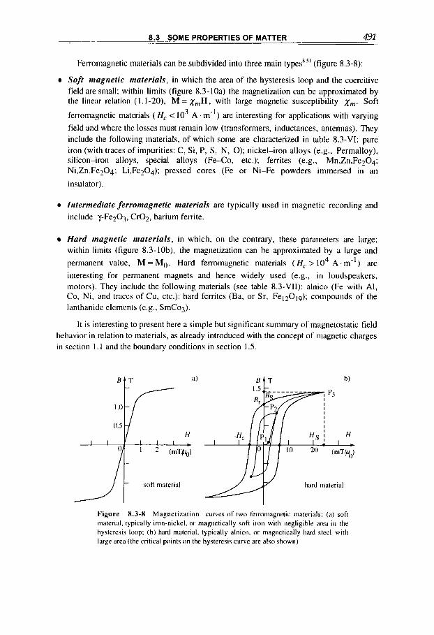
8.3 SOME PROPERTIES OF MATTER 491
Ferromagnetic materials can be subdivided into three main types' '' (figure 8.3-8):
Soft magnetic materials, in which the area of the hysteresis loop and the coercitive field are small; within limits (figure 8.3-10a) the magnetization can be approximated by the linear relation (l.I-20), M = x , ~ H , with large magnetic susceptibility x,,,. Soft
ferromagnetic materials ( H, < 10- A . rn-') are interesting for applications with varying field and where the losses must remain low (transformers, inductances, antennas). They include the following materials, of which some are characterized in table 8.3-VI: pure iron (with traces of impurities: C, Si, P, S, N, 0); nickel-iron alloys (e.g.. Permalloy), silicon-iron alloys, special alloys (Fe-Co, etc.); fenites (e.g., Mn,Zn,Fe204; Ni,Zn,Fe204; Li,Fe204); pressed cores (Fe or Ni-Fe powders immersed in an insulator).
3
Intermediate ferromagnetic materials are typically used in magnetic recording and include y-Fe203, Cr02, barium ferrite.
Hard magnetic maferials, in which, on the contrary, these parameters are large; within limits (figure 8.3-10b), the magnetization can be approximated by a large and permanent value, M = Mo. Hard ferromagnetic materials ( H , > lo4 A ' m - l ) are interesting for permanent magnets and hence widely used (e.g., in loudspeakers, motors). They include the following materials (see table 8.3-VII): alnico (Fe with Al, Co, Ni, and traces of Cu, etc.): hard ferrites (Ba, or Sr, Fe12019); compounds of the lanthanide elements (e.g., SmCo3).
It is interesting to present here a simple but significant summary of magnetostatic field behavior in relation to materials, as already introduced with the concept of magnetic charges in section I . 1 and the boundary conditions in section 1.5.
B I T B I T
Figure 8.3-8 Magnetization curves of two ferromagnetic materials: (a) soft material. typically iron-nickel, or magnetically soft iron with negligible area in the hysteresis loop; (b) hard material, typically alnico, or magnetically hard steel with large area (the critical points on the hysteresis curve are also shown).
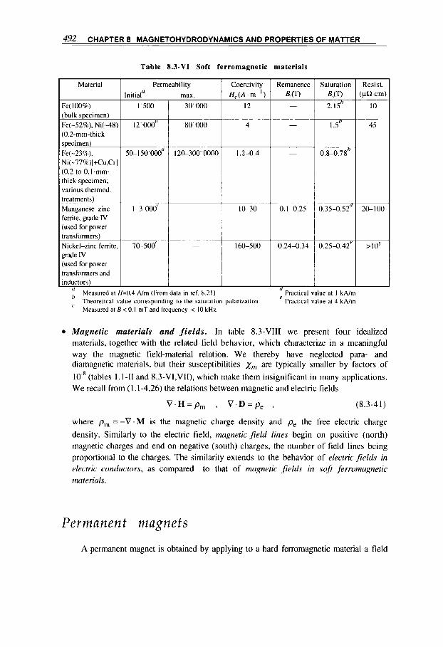
4% CHAPTER 8 MAGNETOHYDRODYNAMICS AND PROPERTIES OF MATTER .- .. . -
Material
Fe( 100%) (bulk specimen) Fe(-52%). Ni(-48) (0.2-mm-thick specimen) Fe(-23%), Ni(-77%)[+Cu,Cr] (0.2 to 0. l-mm- thick specimen; various thermod. treatments) Manganese-zinc ferrite, grade IV (used for power transformers) Nickel-zinc ferrite, grade IV (used for power transformers and inductors)
Table 8.3-VI Soft ferromagnetic materials
Permeability Initial" max.
1'500 1 30'000
70-500' I
Coercivity H J A . m-' )
12
4
I .2-0.4
I S 3 0
16O-500
" b '
Measured at H=0.4 Nin (From data in ref. h.21) Theoretical value corresponding to the saturation polarization Measured at B < 0.1 mT and lrequcncy < 10 kHz
Remanence BAT) -
-
-
0.1-0.25
0.24-0.34
-
Saturation B,(T) 2 . 1 f
I .Sh
0.84.78'
0.35-0.52'
0 .254.42 '
Practical value at 1 kA/m ' Practical value at 4 kA/m
Resist. IpR-cm:
10
45
20-100
Magnetic materials and f i e l d s . In table 8.3-VIII we present four idealized materials, together with the related field behavior, which characterize in a meaningful way the magnetic field-material relation. We thereby have neglected para- and diamagnetic materials, but their susceptibilities xIN are typically smaller by factors of
(tables 1.1-11 and 8.3-VI,VII), which make them insignificant in many applications. We recall from (1.1-4,26) the relations between magnetic and electric fields
V . H = p , , V . D = p e , (8.3-41)
where pi,, = -V . M is the magnetic charge density and pe the free electric charge
density. Similarly to the electric field, rnugnetic field lines begin on positive (north) magnetic charges and end on negative (south) charges, the number of field lines being proportional to the charges. The similarity extends to the behavior of electric ,fields in rlecrric conductors, as compared to that of niugnetic ,fields in so f t ferrotnugnetic rmteriuls.
Per 111 a n en t nz ag n e t s
A permanent magnet is obtained by applying to a hard ferromagnetic material a field

8.3 SOME PROPERTIES OF MATTER 493
Material (from rels. I .17,8.40,8.42)
Ferrite ( Fez03 ), isotropic Strontium ferrite ( S,O + hFe203) , ceramic Alnico 4 Lanthanide elein. comp. (Sm,Co). metallic NdFeB. metallic
pulse that runs from zero up to when saturation induction is obtained, and back to zero. It is interesting to recall that the alignment of the domain, and thus the polarization 1, = p o M 0 ,
is determined by the local field H i , which is generally smaller than the applied field H0 . Consider, as a first example, a long magnetic bar (as the one shown in figure 1.1-4 in
section 1.1 ) to which a magnetic field H0 is applied, and from (1.1-39a) the internal field is
given by
H' = H0 - kmMo . (8.3-42)
As Ho returns gradually to zero, the induction B in the bar follows the hysteresis' upper branch in figure 8.3-8b, and when H0 = 0 , it reaches a point in the left upper quadrant
defined by H i = -kmMo. (Note that the branch is in general defined and labeled by the maximum applied field H0, unless, as in our case, the saturation branch is considered.)
The obtainable remnant induction, and thus the polarization, 1~ = poMo, is obtained from
the definition ( l . l - l7) , . .
p,@ + p O ~ o = B ' ( H ' ) o r
p o M o ( l - k m ) = ~ ~ ( - k ~ ~ ~ o ) , (8.3-43)
which determines Mo when the (saturation) magnetization curve is known. In a second example, a magnetic circuit of total length L = 1 +x with a short gap in
air of length x and cross-sectional area S (the rectangular circuit shown in figure 1.4-3, or a ring circuit) is surrounded by an evenly spaced winding, which produces the field Ho all
along L. The magnetic circuit equations (1.4-39,40) give
H ~ L = H ' I + ~ , ~ x ~ (8.3-444
Remanencz R , ( T )
0.27
0.39
I .o 1 . 1
I .4
B'S = p"H,S., . (8.3-44b)
880 370
iaterials for permanent magnets
Energy product I

- 494 CHAPTER 8 MAGNETOHYDRODYNAMICS AND PROPERTlEs OF MATTER-_
-. -~
Material type characteristic
Nonmagnetic __ Hard ferromagnets Magnetization M = Mn is large
and permanent
Soft ferromagnets Magnetization M = x m H with large magnetic susceptibility x,, Magnetic charges accumulate on its surface [see comments in relation with (8.3-41)]
Electric conductivity u -+ - Large electric surface currents
Superconductors
Magnetostiltic field H behavior
Field penetrates as if no material
Field penetrates as if no material
Internal field is expelled External field is perpendicular to the surface
No internal field External field is parallel to the
When Ho = 0 from these equations we obtain
(8.3-45)
In referring to the energy expression (5.1-7) we can say that the square of the magnetic fields produced near the poles of a permanent magnet is proportional to the magnetic energy density in the ferromagnetic material; we also can say that the total magnetic energy in the
gap, po H, xS, / 2, is equal to the total magnetic energy in the magnet, H B 1 9 2 .
For a closed magnetic circuit, x = 0, with field lines closed within the material, it is always Hi = H o . As the outer field Ho is gradually reduced to zero, the induction Bi
again follows the hysteresis curve upper branch (figure 8.3-8b) until at Ho = Hi = 0 the remnant induction B, is attained. The obtainable permanent magnetization Mo in this case is given by
I i I 2
P O M O = ~ ' (8.3-46)
The great advantage of permanent magnets is that they maintain a magnetic field without any power input, as on the contrary is required in current driven magnets. For practical reasons, the field must remain as much as possible unaffected by time, temperature, and imposed outer field variations. These properties can be obtained by the correct choice of the ferromagnetic material, which must possess among other properties: (a) a large energy product (HiBi),,,ax defined in the upper left quadrant of the hysteresis curve [see in (8.3.45)]; (b) a large value of magnetization M or remnant induction Br [see (8.3-46)]; (c) a large value of the coercive field Hc (to avoid canceling the remaining
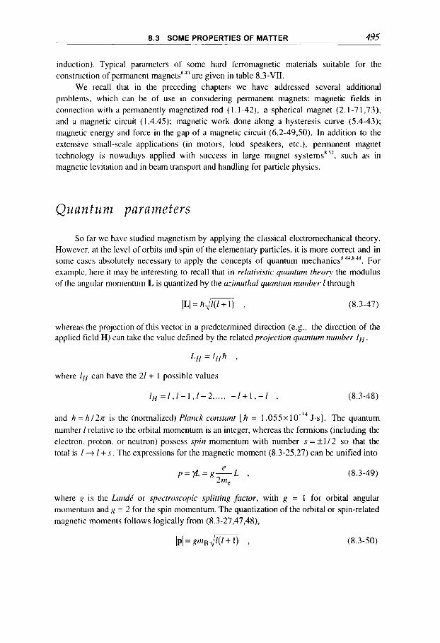
8.3 SOME PROPERTIES OF MATTER 495 ~~ ~~
induction). Typical parameters of some hard ferromagnetic materials suitable for the construction of permanent magnet?") are given in table 8.3-VII.
We recall that in the preceding chapters we have addressed several additional problems, which can be of use in considering permanent magnets: magnetic fields in connection with a permanently magnetized rod ( I . 1-42), a spherical magnet (2.1-7 1,73), and a magnetic circuit ( I .4.45); magnetic work done along a hysteresis curve (5.4-43); magnetic energy and force in the gap of a magnetic circuit (6.2-49.50). In addition to the extensive small-scale applications (in motors, loud speakers, etc.), permanent magnet technology is nowadays applied with success in large magnet systems'", such as in magnetic levitation and in beam transport and handling for particle physics.
Quantum parameters
So far we have studied magnetism by applying the classical electromechanical theory. However, at the level of orbits and spin of the elementary particles, i t is more correct and in some cases absolutely necessary to apply the concepts of quantum mechanic^^^^^"^. For example, here it may be interesting to recall that in relativistic quanfuni theory the modulus of the angular momentum L is quantized by the a5niuf/zal quontuni nuttiher 1 through
[I,[ = hJl(I+ 1) , (8.3-47)
whereas the projection of this vector in a predetermined direction (e.g., the direction of the applied field H) can take the value defined by the related projection qurrntirrti tiuriiber I,,
L H = I H W ,
where If, can have the 21 + 1 possible values
1H = [ , / - I , 1 - 2 ,..., - ! + I , - / , (8.3-48)
and h = / I / 27c is the (normalized) Plmck cotrstant [ W = 1 . 0 5 5 ~ 1 0-34 J.s]. The quantum number 1 relative 10 the orbital momentum is an integer, whereas the fermions (including the electron, proton. or neutron) possess spin momentum with number s = *I / 2 so that the total is 1 + 1 + s , The expressions for the magnetic moment (8.3-25,27) can be unified into
(8.3-49)
where R is the kind6 or spectroscopic splitfinR factor, with g = 1 for orbital angular momentum and g = 2 for the spin momentum. The quantization of the orbital or spin-related magnetic moments follows logically from (8.3-27,47,48),
IpI = gmg &K) , (8.3-SO)
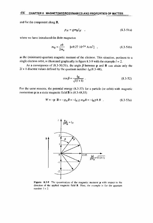
4% CHAPTER 8 MAGNETOHYDRODYNAMICS AND PROPERTIES OF MATTER
and for the component along B,
P H = gmBIH (8.3-51a)
where we have introduced the Bohr magneton
eA
2me mg = - [=9.27 A.m2] , (8.3-51b)
as the (minimum) quantum magnetic moment of the electron. This situation, pertinent to a single electron orbit, is illustrated graphically in figure 8.3-9 with the example 1 = 2.
As a consequence of (8.3-50,51), the angle p between p and B can attain only the 21 + 1 discrete values defined by the quantum number 1~(8.3-48),
(8.3 -5 2 ) 1, cosp = ~ J q i K ) ‘
For the same reasons, the potential energy (8.3-37) for a particle (or orbit) with magnetic momentum p in a static magnetic field B is (8.3-48,55)
Figure 8.3-9 The quantization of the magnetic moment p with respect to the direction of the applied magnetic field B . Here, the example is for the quantum number 1 = 2.

8.3 SOME PROPERTIES OF MATTER 497 ~ _ _ _ _
The energy levels of an electron in the atom are defined in general by the four quantum numbers ti,1,/H,s, where n is the principal quantum number (such that 1 = 1,2 ,..., n - I ) ; in particular, when there is a magnetic field, (8.3-53a), its otherwise degenerate energy levels are split into 21 + 1 discrete so-called Zeeman energy levels separated by
A W = f l B . (8.3-53b)
For example, for the orbital case 1 = 2 shown in figure 8.3-9 there are five levels labeled lH = -2, - 1 , 0, + I , +2; for a particle with spin 3/2 there are four levels, 1~=-3/2, -1/2, +1/2, +3/2. We also recall that the quantized photon energy corresponding to a radiation with frequency w = V / ~ K is
W = w h = v h . (8.3-53~)
In analogy to the Bohr magneton (8.3-5 1 b), the nuclear magneton is defined as
eft
2nzp tnN = ~ [= 5.05 x A . m2] (8.3-54)
The Lrrmwrfreyueticy remains as before in (8.3-30), but since the gyromagnetic ratio is
e
2 ni, y = -g- , for electron orbit (g = 1) or spin (g = 2) , (8.3-55a)
e , for nuclear spin (g z from 0.3 to 4) , (8.3-55b)
we find
= 14.0 g B GHz, tesla; for an electron ,
= 15.3 g B MHz, tesla; for a nucleon . ( 8.356a)
( 8. S56b)
In general, an atom contains many electrons and related orbits. In this case the various orbital and spin momenta of the single atom add vectorially, and this result is then quantized, formally as above. Consequently, for the total atomic magnetic moment the same rules as in (8.3-47,50) apply, where 1 is an integer or half-integer, and g now lies between 1 and 2, since it is a measure of the relative mix in the resultant momentum of orbital and spin components. [Here we recall the Pauli exclusion principle, which states that in an atom at the same time only one electron (fernion) can occupy the same (n,l,lH,s)-defined quantum level.]
In the nuclear domain the relation between resultant spin and magnetic moment is not so simple, as even the single proton (hydrogen nucleus) with spin 1 = 1/2 has the magnetic moment p~ = +2.79 niN. or the single neutron with the same spin has PH = -1.91 mN.
This can be taken care of by attributing to each situation the appropriate yor g value, where the above quantization rules remain of course valid.
498 CHAPTER 8 MAGNETOHYDRODYNAMICS AND PROPERTIES OF MATTER
Critical magnetic fields and monopoles
Starting from the magnetic quantum moment mg (8.3-51b), we obtain the (minimum) quantization of the Lannor radius 'L (6.4-49c) and the nrngnetic f l u x ym relative to an electron orbiting with the cyclotron frequency R(8.3-22) in a plane normal to the induction
B. From trig = 7rk I with 1 = -ef i /2K [similarly to (8.3-21)] we obtain 2
and V / , , , = z r ~ 2 h B = - [ = 2 . 0 7 ~ 1 0 - ' ~ T . m 2 ]
2e
(8.3-57)
(8.3-58)
Here h = h / 2 ~ is the normalized Planck constant and e, m, are the electron charge and mass. If in addition we introduce the Bohr radius ( E is the dielectric constant)
4K & h2 rB = ~ [= 0.53 x IO-"' m]
nree (8.3-59)
(i.e., the fundamental orbit radius of the electron in the hydrogen atom) and the electron Cortrpton wavelength
& = - [= 2 . 4 3 ~ m] tnec
(8.3-60)
(i.e., the wavelcngth-shift resulting from the 90" scattering of a light quantum by an electron), we can define two critical magnetic fields" ''A 19:
(a) Criticd yuanfunr field, from & = 2K r j , at which classical electrodynamics becomes invalid:
2 2 [= 4.42 x 10' T] . l?le c
BQ =7 (8.3-61)
(b) Critical nzugneticfield, from rB = 'L, at which magnetic effects prevail over Coulomb effects:
3
BM =(:) (*y 4KE [=2.36x10⁵ T] . (8.3-62)
In section 1.1, following (1.1-33), we have shown that in Maxwell's electromagnetic theory formal magnetic charges appear intrinsically in pairs, but we also mentioned that there is no physical reason prohibiting the existence of isolated magnetic charges, sometimes also called monopoles. Dirac in his fundamental work of 1931"' showed that quantum physics allows the existence of nlagnetic monopoles carrying a magnetic charge g = Ngo, which is an integral multiple N of the fundamental charge
(8.3-63)

8.3 SOME PROPERTIES OF MATTER 499
[This writing, which includes the magnetic permeability PO, is consistent with the
definition of magnetic charges in (1.1-26,29,33).] I f monopoles exist at all, there is no reason to suppose them all identical; that is, different N-values could be possible. For simplicity, in the following we set N = 1. Note that the monopole induction charge expressed as pogo corresponds to twice the magnetic flux quantum introduced in (8.3-
58). In analogy to the electric field produced by a free electric charge, (6.4-14), a magnetic charge go at rest is the source of a radial magnetic field
( 8.3 - 64)
whereas when moving with velocity v in an electromagnetic field it experiences a force which with (1.3-23) we write
(8.3-65)
similarly to the Lorentz force (6.1-1) for an electric charge. where c = ( ~ o E o ) - " ~ is the velocity of light in vacuum (1.2-1 I ) . The energy gain W, of a monopole in a magnetic induction B over a distance 1 is thus
%=go [ = 3 . 2 9 ~ 1 0 - ~ J . m - l . T - l or = 2 0 . 6 G e V . m - ' . T - l ] . (8.3-66) IB
For example, a magnetic field of 10 T over 1 m confers 206 GeV on a monopole. [In a
comparable, practical electric field of 1 MV.m-l-see comments in connection with (6.4- 15)-an electron acquires only 1 MeV]. By any practical comparison, the magnetic monopole is thus very strongly interacting with magnetic fields. No other intrinsic property of the monopole other than its magnetic charge is predicted by Dirac's 1931 theory, but since then other speculative characleristics have been attribuited to it by theoretical work' ". For example, the mass of the lightest monopole could be between lo1* and 1017 eV-that is about 103 to 108 times the proton mass-and thus be far more massive than presently observed elementary particles. As a consequence of the large mass and strong interaction, the monopoles should be exceedingly rare, and perhaps were produced only very early during the Big Bang, at the birth of the Universe.
Nuclear magnetic resonance
Over the last thirty years magnetic resonance based on nuclear magnetic moments and spins (nuclear magnetic resonance, NMR) has been the subject of many applicationsB4', mainly for diagnostic radiology in medicines4' (magnetic resonance imaging, MRI), for the study of chemical species (magnetic resonance spectroscopy) and the structure of solid state. This technique is based on (a) the Larmor frequency (8.3-56b) in the focal field B,
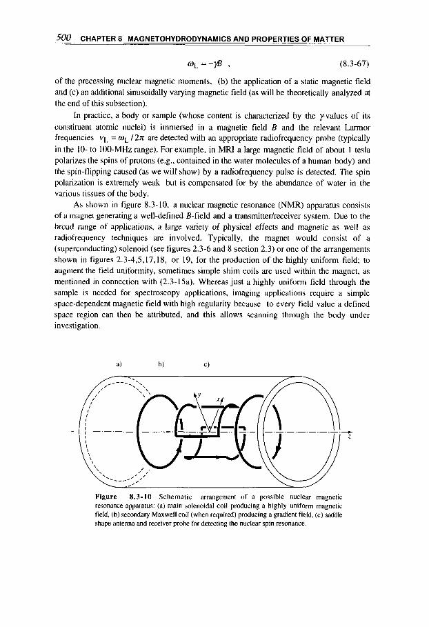
500 CHAPTER 8 MAGNETOHYDRODYNAMICS AND PROPERTIES OF MATTER
W L =-p 3 (8.3-67)
of the precessing nuclear magnetic moments, (b) the application of a static magnetic field and (c) an additional sinusoidally varying magnetic field (as will be theoretically analyzed at the end of this subsection).
In practice, a body or sample (whose content is characterized by the yvalues of its constituent atomic nuclei) is immersed in a magnetic field B and the relevant Larmor frequencies vL = W L / 2 a are detected with an appropriate radiofrequency probe (typically in the 10- to 100-MHz range). For example, in MRI a large magnetic field of about 1 tesla polarizes the spins of protons (e.g., contained in the water molecules of a human body) and the spin-flipping caused (as we will show) by a radiofrequency pulse is detected. The spin polarization is extremely weak but is compensated for by the abundance of water in the various tissues of the body.
As shown in figure 8.3-10, a nuclear magnetic resonance (NMR) apparatus consists of a magnet generating a well-defined B-field and a transmitter/receiver system. Due to the broad range of applications, a large variety of physical effects and magnetic as well as radiofrequency techniques are involved. Typically, the magnet would consist of a (superconducting) solenoid (see figures 2.3-6 and 8 section 2.3) or one of the arrangements shown in figures 2.3-4,5,17,18, or 19, for the production of the highly uniform field; to augment the field uniformity, sometimes simple shim coils are used within the magnet, as mentioned in connection with (2.3-1Sa). Whereas just a highly uniform field through the sample is needed for spectroscopy applications, imaging applications require a simple space-dependent magnetic field with high regularity because to every field value a defined space region can then be attributed, and this allows scanning through the body under investigation.
Figure 8.3-10 Schematic arrangement of a possible nuclear magnetic resonance apparatus: (a) main solenoidal coil producing a highly uniform magnetic field, (6) secondary Maxwell coil (when required) producing a gradient field, (c) saddle shape antenna and receiver probe for detecting the nuclear spin resonance.
8.3 SOME PROPERTIES OF MATTER 501
A convenient way to obtain large-volume magnetic fields with these properties (figure 2.3-4) is to superpose on the fundamental uniform field a much weaker gradient field, which can be generated by a Maxwell or inverse Helmholtz coil pair [see (2.3-15b)I or by other arrangements as discussed in connection with figures 2.3-3 and 21. Finally, the radiofrequency antenna and receiving probe must transmit the radiofrequency power from the generator to the sample and detect the response of a local Larmor precession resonance. This can be achieved with one single coil, or with separated coils. The receiving coil must possibly be perpendicular to the main field direction since this ensures the maximum induced electromotive force (emf) signal by the fluctuating (perpendicular) magnetic field generated by the resonantly precessing nuclei.
For the presentation of the classic NMR model, we extend the considerations made in connection with paramagnetism. Here we have again permanent magnetic moments p,, not of the atoms but of the nuclei in the magnetic material, that start to precess at the Larmor frequency (8.3-67) under the action of an applied outer field B . By introducing the magnetization M, which by definition (1.1-23) is the density of magnetic moments,
M = nps (8.3-68)
(where n is the number of magnetic moments p, per unit volume), the gyroscope equation (6.4-23) is transformed into
M = @ I x B . (8.3 -69)
This shows that the vector M [as p, in (6.4-231 precesses with the Larmor frequency wL around the magnetic field. We know from (8.3-32,39) that if the moments p, are distribuited at random an effect appears only if there are interaction processes with external elements. These processes are taken care of formally by the so-called Bloch equation
(8.3-70)
through two characteristic time constantsE4': 71 relaxes the longitudinal Mz component and is also called the spin-lattice relaxation time because it is due mainly to the thermalization process between the spin and surrounding material; z2 relaxes the transverse M,,M,, components and is usually called spin-spin relaxation time because it is mainly due to the interactions among spins (typical values for TI, z2, for example for metallic Fe at room temperature, are 1 to 5 ms); in addition, ex,ey,e, , are the Cartesian unit vectors with e,
taken along the B vector, and Mo is the equilibrium magnetization along the z-axis of the spin system obtained at the end of the process.
As we know from the introduction, Nh4R techniques require, in addition to a static magnetic field Bo, an oscillating field B1 which may be represented by a magnetic field
rotating with frequency win the (x,y)-plane normal to B [see in (3.2-31) and figure 3.2-1 in section 3.21:
B1 = BI coswt ex + Blsinwt e y . (8.3-71)
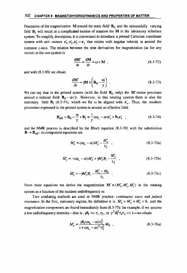
502 CHAPTER 8 MAGNETOHYDRODYNAMICS AND PROPERTIES OF MATTER
Precession of the magnetization M around the static field Bo and the sinusoidally varying field B, will result in a complicated motion of nutation for M in the laboratory reference system. To simplify description, it is convenient to introduce a primed Cartesian coordinate system with unit vectors ei,e;,e; = ez that rotates with angular velocity w around the
common z-axis. The relation between the time derivatives for magnetization (as for any vector) in the two system is
dM’ dM dt dr
- = - + u x M ,
and with (8.3-69) we obtain
dM’ = W X ( Bo-- ;) . dr
(8.3-72)
(8.3-73)
We can say that in the primed system (with the field BO only) the M‘vector precesses around a reduced field Bo -a/ y . However, in this rotating system there is also the stationary field B1 (8.3-71), which we fix to be aligned with e;. Thus, the resultant precession expressed in the primed system is around an effective field
(8.3-74)
and the NMR process is described by the Bloch equation (8.3-70) with the substitution B + B,ff : its component equations are
(8.3-75a)
M’
72 h; =-(OIL - w ) M ~ + @ ; B l - A , (8.3-75b)
(8.3-75 C)
From these equations we derive the magnetization M’ = (Mi, M;, Mi) in the rotating
system as a function of the incident radiofrequency w. Two irradiating methods are used in NMR practice: continuous wave and pulsed
resonance. In the first, stationary regime, by definition it is M; = M; = hi = 0, and the
magnetization components are found immediately from (8.3-75): for example, if we assume a low radiofrequency intensity-that is ,@I << 71 , ~ 2 , or y B1 2172 << 1-we obtain 2 2
(8.3-76a)

8.3 SOME PROPERTIES OF MATTER 503
(8.3-76b)
M ; = M o . (8.3-76~)
The dependence of M;,Mi3 versus (WL -w) t2 give rise to typical dispersion and
absorption behaviors around the resonance w = w ~ . The nuclear equilibrium magnetization Mo, first introduced in (8.3-70). appears in all three components, and thus is a measure of the NMR signal intensity. It is expressed, analogously to the Curie law (8.3-36a), but with (8.3-5054) Ips/ = flJm, as
y2A21(1+ 1) MO = xmn H = n h
3kT (8.3-77a)
In the more widely used pulsed-resonance technique, the NMR effect is probed with a pulse of radiofrequency w applied during a time f,, that is short compared to the relaxation times ~ 1 . r ~ . At resonance w = W L , we see from (8.3-74) that in the rotating primed system, the movement of the vector M simplifies to the precession around Bl = Ble; at angular velocity w1 = only, so that the corresponding angle of rotation is
41 = 7 4 f p . (8.3-77b)
For example, the application of a pulse of duration such that 41 = n / 2 will rotate M into the x,y-plane (normal to Bo). After the pulse is over, this transverse magnetization will decay with the characteristic time r2 , and the longitudinal component will recover with z1, as defined in (8.3-70).
Finally, we note that in the alternative quantum-mechanical NMR model, the calculation makes direct reference to the Zeeman energy levels (8.3-53), and with AW = CI$I = f l B we reconfirm the Larmor frequency condition (8.3-67).
High-energy densities
Interaction of a high magnetic field with a metal conductor may increase the lattter’s internal energy to densities up to and, eventually, well above the chemical binding energy of solids. At these energy levels the properties of the metal (the atoms or ions in the lattice), as well as the transport properties of the electrons, may well be different from their behavior under normal conditions-that is, at room temperature and atmospheric pressure. In the following we discuss and illustrate some of the properties of solids at these extreme conditions that have been applied previously in this book.

504 CHAPTER 8 MAGNETOHYDRODYNAMICS AND PROPERTIES OF MATTER
1 .O 1.2 I .4 1.6 1.8
density p/pg
Figure 8.3-11 Energy density in shock-compressed copper: E, is the cold compression (lattice) contribution; E~ and E, are the thermal contributions of ions and electrons. (The curves have been obtained from data given in reference 8.29.)
Equation of state
In the pressure and temperature range of interest to us (up to the order of 105 MPa and lo4 K), we may consider the metallic conductor to be in the form of an isotropic condensed state, and hence thermodynamically defined by three independent variables, such as the specific volume V = 1 / p , the pressure p , and the temperature T (here and in the following in kelvin). They can be reduced to two independent variables by introducing an equalion of stute-that is, a relation between the variables themselves andor between related thermodynamic quantities, such as the internal energy E, or the enthalpy (heat function) h = QV = E + pV. For example, we can give an equation of state in the form
& = & ( p , V ) , or p = p ( V , T ) . (8.3-78a)
Experimental results and physical arguments show that it is reasonable to consider the internal energy density (per unit mass) of the metal in the form
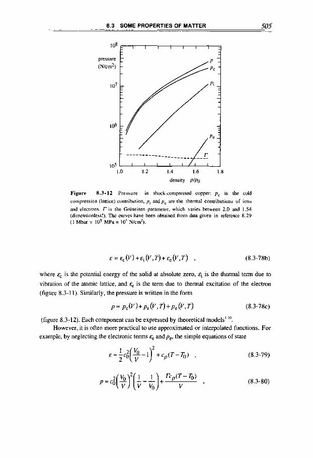
8.3 SOME PROPERTIES OF MATTER 505
pressure (N/cm2)
I 07
I 06
I .o 1.2 I .4 1.6 1.8
density p/po
Figure 8.3-12 Pressure in shock-compressed copper: pc is the cold
compression (lattice) contribution, pi and p e are the thermal contributions of ions and electrons. r is the Griineisen parameter, which varies between 2.0 and 1.54 (dimensionless!). The curves have been obtained from data given in reference 8.29 ( 1 Mbar = 10' MPa = 10' N/cm*).
& = &,(V)+Ei(V,T)+&,(V,T) , (8.3-78b)
where E, is the potential energy of the solid at absolute zero, q is the thermal term due to
vibration of the atomic lattice, and E, is the term due to thermal excitation of the electron (figure 8.3-1 1). Similarly, the pressure is written in the form
P = p c ( ~ )+ pi (V 9 T) + P e (v, T) (8.3 - 7 8 ~ )
(figure 8.3-12). Each component can be expressed by theoretical models' lo.
example, by neglecting the electronic terms ee and pe, the simple equations of state However, it is often more practical to use approximated or interpolated functions. For
(8.3-79)
(8.3 -80)

506 CHAPTER 8 MAGNETOHYDRODYNAMICS AND PROPERTIES OF MATTER
density po at 0°C
density poo = V1 at 0 K mole weight
sound velocity co shock parameter C
Table 8.3-IX Equation of state of metals'
gem-3 2.71 7.8 8.5 8.93 11.3 19.3 g ~ m - ~ 2.746 - - 9.024 11.60 19.40
63.5 207.2 183.9
cm.ps-l 0.52 0.39 0.37 0.40 0.20 0.40
g.mo1-l 27.0 55.8 - cm,ps-' 0.52 -0.45 - 0.39 0.19 -
Parameter I Dimensions I Al Fe Brass Cu Pb W
shock parameter S I 1.4 I .6 1.5 1.50 1.52 1.27
mean spec. heat c,, at 20°C
electron param. a, Debye temp. 0, at 0°C
Griineisen param. np0)
Fermi temp. 4
J.g-l ("C)-l 0.90 - - 0.38 0.129 0.136 1.98 2.46 -
lo-' J,g-l(°C)-2 500 - - 110 140 60 K 390 420 320 320 88 350
2.08 1.95 -
K -13'000 -30'000 8200 8200 -11'000 -
Mainly from references 8.28.8.29, and 8.30
can be proposed, where r ( t h e so-called Griineisen parameter, see figure 8.3-12) and c,, (the specific heat at constant pressure) can be approximated by their (constant) values at normal conditions (table 8.3-IX).
Specific heat and phase transitions
In tables 8.3-11 and IX, we give the mean value of the spec@c heat of various metals. Actually, the specific heat is temperature-dependent, even within the small temperature range (from about 0°C to 1000°C) considered here (see figure 8.3-13). Nevertheless, for most metals in the solid phase, the cp values remain within f10% of their mean value. Note
that according to our definition it is cv = pcp , where cv is the specific heat per unit volume and cp is the specific heat per unit mass.
In metal conductors interacting with fields above 100 T, the temperature can increase by ohmic dissipation well above IO'OOO K. We must, therefore, also consider the phase transitions that can take place in the metal (figure 8.3-14).
The first transition is from solid to liquid. In most problems of interest to us, it plays a limited role. For example, from a quantitative, energetic viewpoint, we note that the latent heat of melting E, (table 8.3-IV) is small compared to the other energy densities (5, E ~ ; see
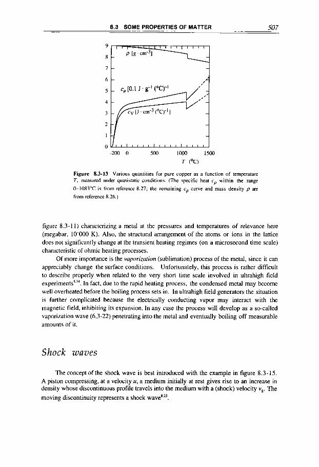
8.3 SOME PROPERTIES OF MATTER 507
' t 1
-200 0 500 lo00 1500
T (OC)
Figure 8.3-13 Various quantities for pure copper as a function of temperature T , measured under quasistatic conditions. (The specific heat cp within the range
0-1083°C is from reference 8.27; the remaining cp curve and mass density p are from reference 8.26.)
figure 8.3- 1 1) characterizing a metal at the pressures and temperatures of relevance here (megabar, 1O'OOO K). Also, the structural arrangement of the atoms or ions in the lattice does not significantly change at the transient heating regimes (on a microsecond time scale) characteristic of ohmic heating processes.
Of more importance is the vaporization (sublimation) process of the metal, since it can appreciably change the surface conditions. Unfortunately, this process is rather difficult to describe properly when related to the very short time scale involved in ultrahigh field experiment^"^. In fact, due to the rapid heating process, the condensed metal may become well overheated before the boiling process sets in. In ultrahigh field generators the situation is further complicated because the electrically conducting vapor may interact with the magnetic field, inhibiting its expansion. In any case the process will develop as a so-called vaporization wave (6.3-22) penetrating into the metal and eventually boiling off measurable amounts of it.
Shock waves
The concept of the shock wave is best introduced with the example in figure 8.3-15. A piston compressing, at a velocity u, a medium initially at rest gives rise to an increase in density whose discontinuous profile travels into the medium with a (shock) velocity v,. The moving discontinuity represents a shock wave' 25.
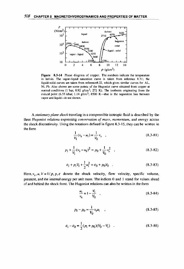
508 CHAPTER 8 MAGNETOHYDRODYNAMICS AND PROPERTIES OF MATTER
(kelvin)
hugoniot
liquid
(kelvin)
1.. - r
." 0 2 4 6 8 1 0 1 2 1 4
P (g/cm3)
Figure 8.3-14 Phase diagram of copper. The numbers indicate the temperature in kelvin. The vapor-liquid saturation curve is taken from reference 8.31; the liquid-solid curves are taken from reference8.32, which gives similar curves for AL, Ni, Pb. Also shown are some points of the Hugoniot curve obtained from copper at normal conditions ( 1 bar; 8.92 g/cm3; 272 K). The isotherm originating from the critical point (6.53 kbar; 1.14 g/cm3; 8500 K-that is the separation line between vapor and liquid-is not shown.
A stationary plane shock traveling in a compressible isotropic fluid is described by the three Hugoniot relations expressing conservation of mass, momentum, and energy across the shock discontinuity. Using the notations defined in figure 8.3-15, they can be written in the form
(8.3-81)
(8.3 -82)
(8.3-83) E I + p I v , + Z U I 1 2 = E o + p O V O .
Here, vs, u, V = I / p , p , E denote the shock velocity, flow velocity, specific volume, pressure, and the internal energy per unit mass. The indices 0 and 1 stand for values ahead of and behind the shock front. The Hugoniot relations can also be written in the form
(8.3-84)
p1 - P o = -VsUl 1 ' (8.3-85) VO

8.3 SOME PROPERTIES OF MATTER 509
Figure 8.3-15 Piston driving an ideal shock wave into a medium at rest
From (8.3-84.85) we can eliminate u or vs and get the simpler expressions
2 2 ( P I - P o ) vs = vo (VO - 4) ’
(8.3-87)
~ : = ( P I - P o ) ( v O - w . (8.3 -8 8)
For the case in which the initial pressure is negligible (PI >> PO), we obtain from (8.3- 5 133)
El -&o =-u1 1 2 . , (8.3-89) 2
this equation expresses the equipartition of kinetic and internal energy in a shock- compressed medium.
In order to solve the shock problem completely, one more equation must be added to the three general dynamic relations. This fourth expression is obviously an equation of state characterizing the thermodynamic properties of the medium. We suppose it to be known in the form [see, e.g., (8.3-80)]
p = P ( v , E ) . (8.3-90)
Elimination of the internal energy E through (8.3-83) reduces this equation to the simpler expression
p=FH,(v) * (8.3-91)
where FHl, is the Hugoniot function related to the initial state (p0,Vo). Alternatively, with
(8.3-86) we can obtain

510 CHAPTER 8 MAGNETOHYDRODYNAMICS AND PROPERTIES OF MATTER
10
P (M bar)
8
6
4
2
0 I .o I .5 2.0 2.5 3.0
P'PO
Figure 8 . 3 - 16 contained in references 8.28.8.29. and 8.30.) ( 1 Mbar = lo5 MPa).
(plpo)-Hugoniots of various metals. (Mainly from data
For example, this last equation defines the Hugoniot-Rankine curve in the ( u , p ) plane, that is, the locus of all ( u , p ) points that can be reached by a shock starting from the initial state (uo,po). Hugoniot curves have been determined for many solids (figures 8.3-16 and 8.3- 17).
The measured shock and flow velocities of most metals fit, within a few percent, into the linear relation
vs =c+su , (8.3-93)
where Cis (almost) the value of the sound velocity co in the non-shocked fluid and S is a material constant (see table 8.3-IX). Within the range covered by this relation, and provided that the assumptions made in connection with (8.3-85) are valid, the Hugoniots take the simple parabolic form
1
p = q c o + Su)u , VO
or (8.3-94)
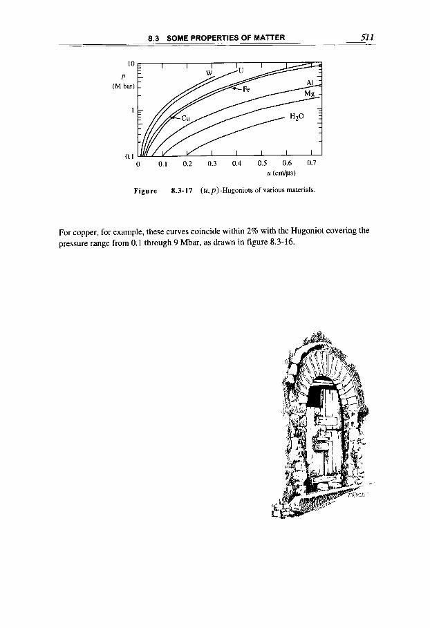
8.3 SOME PROPERTIES OF MATTER 511
0 0.1 0.2 0.3 0.4 0.5 0.6 0.7 u ( C d P S )
Figure 8.3-17 (u,p)-Hugoniots of various materials.
For copper, for example, these curves coincide within 2% with the Hugoniot covering the pressure range from 0.1 through 9 Mbar, as drawn in figure 8.3-16.

Chpter 9
NUMERICAL AND ANALOG SOLUTION METHODS
Only a few simple problems can be solved exactly or with sufficient approximation by analytic methods, as documented throughout this book. The problem of calculating and describing magnetic-field and current distributions in relation to complicated conductor geometries having variable electrical conductivity andor to materials having variable magnetic permeability can be solved by using a large variety of computer programs. An in- depth coverage of numerical solution methods is beyond the scope of this book; discussion is limited to presenting some of the basic theoretical considerations underlying numerical methods and referring to the extensive literature. In general, analog solution methods applied to magnetic Dirichlet problems are no longer used. However, in a way the most straightforward analog method is to measure currents and magnetic fields either in the actual apparatus or in a scaled-down model. The latter procedure can have distinct advantages, as discussed in the last section of this chapter.
Applications. The practical aspects related to the subject treated in this chapter are numerous, in the sense that proven, commercially available software for the solution of electromagnetic problems (for example, solvers of Maxwell’s or magnetic-potential equations) covers a broad range of possible applications. This aspect is further supported by today’s widespread access to powerful computers, ranging from desktop PCs to massively parallel superconducting arrays.
513
M4GNETICFIELDS: A Comprehensive Theoretical Treatise for Practical Use Heinz E. Knoepfel
Copyright Q 2000 by John Wiley & Sons, Inc
514 CHAPTER 9 NUMERICAL AND ANALOG SOLUTION METHODS
9.1 NUMERICAL COMPUTATION METHODS
The creation of computation programs can be facilitated by the widely diversified electromagnetic theory base presented in the previous chapters. The general problem concerns the complete solution of Maxwell’s equations for the electromagnetic fields or of the Laplace or Poisson equations for the electromagnetic potentials, with the appropriate boundary and initial conditions. In practice, and in view of specific applications, we obviously try to simplify the problem by choosing the most convenient theoretical formulations, of which many are deduced in this book.
The most general and flexible numerical solution techniques used today are the powerful finite-element method and to a lesser extent the finite-dtflerence method. These methods allow us to treat problems that include ferromagnetic materials and are also useful for calculating the diffusion of magnetic fields and the associated eddy currents. Another method, which is particularly convenient for the study of eddy current problems, is the finite-element network method, which takes advantage of the development of the general network theory that has developed separately over the last 25 years.
The approximation of complicated, iron-free magnet systems by jlumentury or simple elemental conductors makes it possible to apply relatively fast and convenient numerical solution procedures. In particular, axisymmedc current distributions can be approximated by an array of circular loops, in which case computation is reduced to solving for the elemental loop and then adding the various components.
With the sophisticated software available today, any desired result, such as field lines, contour lines, current flow lines, can easily be displayed in useful and appealing graphical form. We can obtain stereoscopic pictures that give a three-dimensional view of the field- line pattern, or have an artist’s multicolor impression of complicated coil structures. A historically based review on the development of numerical methods-in particular, of the finite-element method-can be found in the literature’.*’.
Finite-dif f erence method
The numerical solution of partial differential equations such as found in the previous chapters can be calculated in a natural way with respect to a finite number of points pertaining to the region of interest. For this solution, the diflerentiul equation is transformed into a difference equation, which is particularly suitable for numerical treatment. This solution technique, based on thefinite-dtference method, since the end of the 1970s has given way to the method of finite elements. Nevertheless, it is still used with continuing success, particularly in the form of the finite-difference time-domain techniques, which are applied for the solution of Maxwell’s equation in relation to microwave problem^^.'^^'.'^.
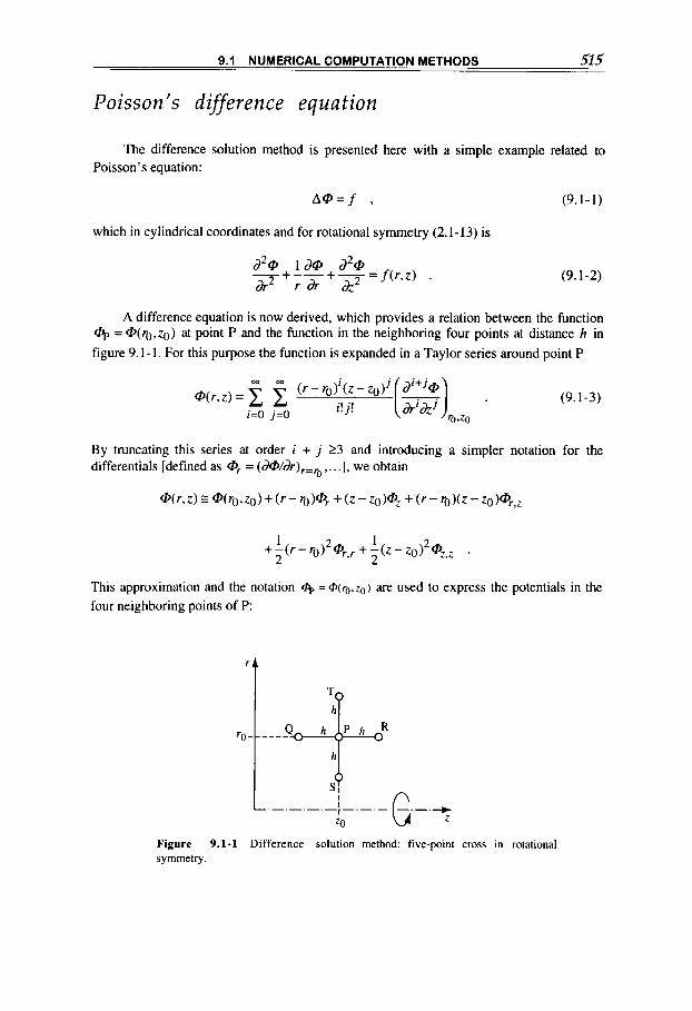
9.1 NUMERICAL COMPUTATION METHODS 515
Poisson's difference equation
The difference solution method is presented here with a simple example related to Poisson's equation:
A @ = f , (9.1-1)
which in cylindrical coordinates and for rotational symmetry (2.1-13) is
d2@ Id@ 3% dr2 1 dr &2
f ( r , z ) . -+--+-= (9.1-2)
A difference equation is now derived, which provides a relation between the function cQ, = @(rO,z0) at point P and the function in the neighboring four points at distance h in figure 9.1-1. For this purpose the function is expanded in a Taylor series around point P
(9.1-3)
By truncating this series at order i + j 2 3 and introducing a simpler notation for the differentials [defined as Or = (d@/dr),=, ,. . .], we obtain
@(r. Z) 5 @(fig, Zo) + ( r - '0 )Or + ( Z - Z o + (1. - a)( Z - ZO)@',~
This approximation and the notation 3 = @(rO.zo) are used to express the potentials in the four neighboring points of P:
't
Figure 9.1-1 Difference solution method: five-point cross in rotational symmetry.

516 CHAPTER 9 NUMERICAL AND ANALOG SOLUTION METHODS
I - hOZ + - h2@z,z 2
= @(rg, 10 - h ) =
% = @(ro,zO + h ) = % +haz + - h 1 2 4z,z
% = @ ( r g - h , z g ) = % - h Q i , + - h 1 2 Or,,
2
2
q =@(rg+h.zO)=@++hdjr+yh 1 2
To obtain the required difference equation, we must eliminate
(9.1-4)
the four differentials, for which purpose we need a further equation taken from (9.1-2) with fp = f ( ro,zo):
(9.1-5) 1
‘0 @r,r + -9 + @,,z = f p .
By straightforward algebra, we finally obtain the (local) Poisson difference equation
(9.1-6)
Proceeding similarly, it is possible to deduce the difference equation related to two or more points Q,R, ... with unequal distances to P. In particular, with P on the axis of symmetry (ro + 0), the difference equation (9.1-6) is not applicable. To establish the appropriate difference equation9-’, we rewrite (9.1-5) in the limit r0 -+ 0 [where cDrs/rg + see (2.1-2411.
and by proceeding as before we obtain, for points P, Q, R on axis and T at radial distance h from it,
(9.1-8) 1 p K@Q - @P) + (@R - @PI + 4(@T - @P)l =h .
Poisson’s difference equation in the Cartesian two-dimensional (x.y)-plane can easily be found by proceeding as above. Formally, it can also be directly obtained from the previous expressions by the coordinate substitution r + x and z + y and by letting r, + 03.
In particular, we find from (9.1-6) the five-point difference equation in Cartesian coordi- nates:

9.1 NUMERICAL COMPUTATION METHODS 517
Difference solution method
A potential problem in three dimensions with rotational symmetry can be defined by Poisson’s equation (9.1-2) and the potential on the boundary (figure 9.1-2). For the solution of this Dirichlet problem by the difference method we first draw a network of, for example, square meshes inside the region of interest, which define internal points (full circles in figure 9.1-2). In addition, the mesh lines define boundary points where they intersect the boundary (open circles).
At each internal point P an appropriate difference equation relates the potential % to
the potentials @Q, %, 0s. ... of neighboring internal or boundary points Q , R, S, ... For example, the difference equation (9.1-6) can be taken at regular internal mesh points; (9.1- 8) must be used for points on the axis; and in general a four- or five-point difference equation with unequal distances to P must be considered when boundary points are included.
The significance of the difference solution method is that if overall there are N internal points, the appropriate difference equations provide N linear equations for the N unknown potentials at each point (the fixed potentials at the boundary points being taken as constants).
The solution of the Dirichlet problem through the difference method thus reduces to solving a large set of simultaneous linear equations, which can be written in the matrix form (A. 3-36)
[MI@ = f , (9.1 - 10)
where in general [w is a square matrix, @ is the unknown potential column vector, and f is a column vector with known components. This is a well-known central problem in numerical computation and is treated in most books on numerical methods.
The numerical solution of the system (9.1-10) can follow either direct or iterative procedures. The direct niethod gives (in principle) the exact answer in a finite number of steps, but the algorithm is often complicated and nonrepetitive; it requires relatively large computer memory for the storage of intermediate results.
Figure 9.1-2 Difference solution method: determining the potential with given boundary conditions within a network of square meshes.

518 CHAPTER 9 NUMERICAL AND ANALOG SOLUTION METHODS
Iterative methods are more frequently used to solve the system (9.1-10) because they are based on a relatively simple and straightforward algorithm’.’. One starts with an initial set of arbitrarily approximated potentials for the internal points. A first round of computation will produce potentials that displace those assumed. A second round can further improve the consistency of the resulting potentials with Poisson’s equation, and so on. Considerations on the stability and on the velocity of convergence of the procedure are analyzed extensively in the references mentioned. The success of the difference method strongly depends on the appropriate choice of the network of internal points- that is, of the size and form of the mesh, which must be adapted to the nature and sensitivity of the problem in the different regions of interest. Regular mesh spacing is preferred in numerical computing because it improves computation speed and simplifies programming. In this respect the only regular polygons that can completely fill the plane are triangles, rectangles, and hexagons.
Here we have introduced the difference method with some simple considerations pertaining to the elliptic Poisson differential equation (9.1-1). (See also section A.3.) The method can be extended equally well to parabolic and hyperbolic differential equations. It has been developed in recent years to a high degree of specialization to treat quite complicated physical problems’.’.
Finite-element method
Since the 1970s, the finite-element solution method has been a very successful numerical method for solving boundary and initial value problems, such as found in structural mechanical and electromagnetic problems. It is more flexible than the difference method-for example, in satisfying boundary conditions, facilitating mesh grading, and
Figure 9.1-3 The plane region defined by the contour C subdivided into triangular finite elements.
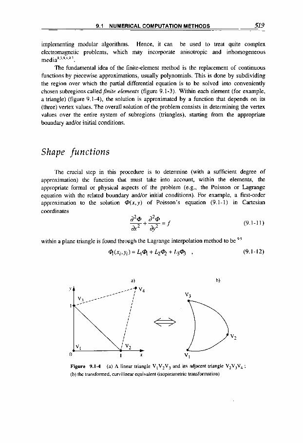
9.1 NUMERICAL COMPUTATION METHODS 519
I '
implementing modular algorithms. Hence, it can be used to treat quite complex electromagnetic problems, which may incorporate anisotropic and inhomogeneous
The fundamental idea of the finite-element method is the replacement of continuous functions by piecewise approximations, usually polynomials. This is done by subdividing the region over which the partial differential equation is to be solved into conveniently chosen subregions calledfinite elements (figure 9.1-3). Within each element (for example, a triangle) (figure 9.1-4), the solution is approximated by a function that depends on its (three) vertex values. The overall solution of the problem consists in determining the vertex values over the entire system of subregions (triangles), starting from the appropriate boundary andor initial conditions.
media9 1.9 4.9 7
I I v3
_--- y3- _ - - - - - - - \I -Dv2 -
.Vl ; v 2 -
Shape functions
The crucial step in this procedure is to determine (with a sufficient degree of approximation) the function that must take into account, within the elements, the appropriate formal or physical aspects of the problem (e.g., the Poisson or Lagrange equation with the related boundary and/or initial conditions). For example, a first-order approximation to the solution 9 ( x , y ) of Poisson's equation (9.1-1) in Cartesian coordinates
(9.1-11)
within a plane triangle is found through the Lagrange interpolation method to be 9 5
q ( X i t Y i ) = L ~ q +4%+-%.34 7 (9.1 - 12)
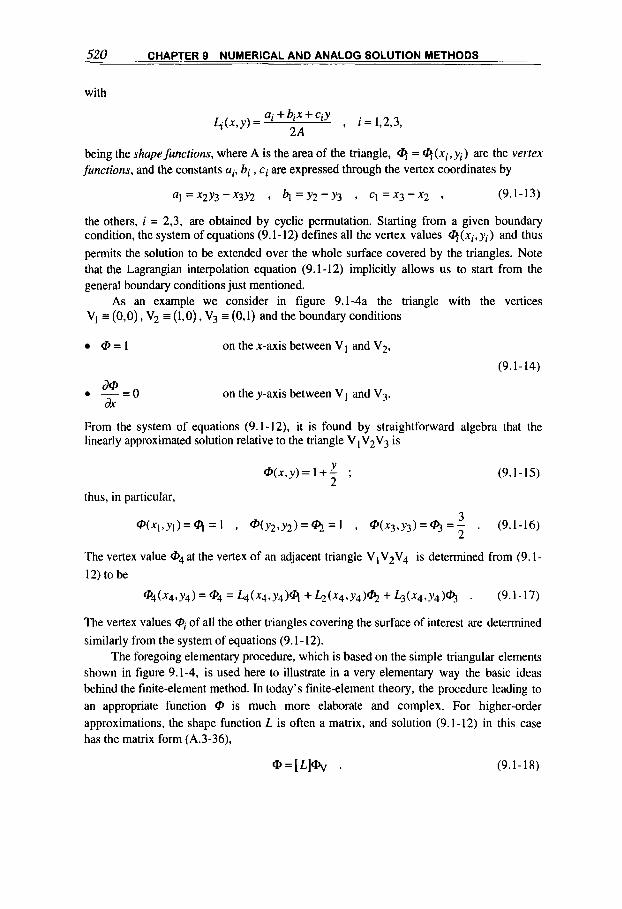
520 CHAPTER 9 NUMERICAL AND ANALOG SOLUTION METHODS
with
being the shapefunctions, where A is the area of the triangle, at = d.+(x;,y;) are the vertex
functions, and the constants ai, bi , ci are expressed through the vertex coordinates by
a1 =x2y3 -x3y2 , 4 =y2 -y3 , ~1 =x3 -x2 , (9.1- 13)
the others, i = 2,3, are obtained by cyclic permutation. Starting from a given boundary condition, the system of equations (9.1-12) defines all the vertex values Qf(xi,y;) and thus permits the solution to be extended over the whole surface covered by the triangles. Note that the Lagrangian interpolation equation (9.1-12) implicitly allows us to start from the general boundary conditions just mentioned.
As an example we consider in figure 9.1-4a the triangle with the vertices VI I (0,O) , V2 = (1,0), V3 = (0,l) and the boundary conditions
@ = l on the x-axis between V 1 and V2,
(9.1 - 14)
0 -= 0 on the y-axis between V I and V3.
From the system of equations (9.1-12). it is found by straightforward algebra that the linearly approximated solution relative to the triangle V I V2V3 is
dx
Y 2
@(x,y) = 1 + - ;
thus, in particular,
(9.1- 15)
@(x1,y1)= q = 1 1 @(y2.y2)= 3 = 1 7 @(X3,Y3) = % = 2 . (9.1-16)
The vertex value a4 at the vertex of an adjacent triangle V1V2V4 is determined from (9.1- 12) to be
@4(4(X4J4) = 4 = L4(x4,Y4)q + tr(X49Y413 + MX4.Y4)QI . (9.1-171
The vertex values Qi of all the other triangles covering the surface of interest are determined similarly from the system of equations (9.1 - 12).
The foregoing elementary procedure, which is based on the simple triangular elements shown in figure 9.1-4, is used here to illustrate in a very elementary way the basic ideas behind the finite-element method. In today’s finite-element theory, the procedure leading to an appropriate function @ is much more elaborate and complex. For higher-order approximations, the shape function L is often a matrix, and solution (9.1-12) in this case has the matrix form (A.3-36),
@=[L]* . (9.1- 18)
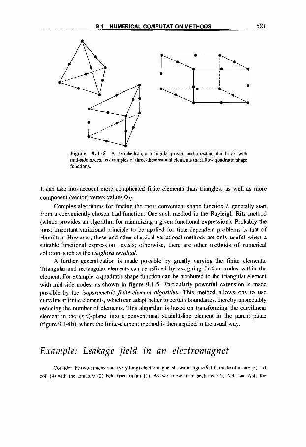
9.1 NUMERICAL COMPUTATION METHODS 521
Figure 9 . 1 - 5 A tetrahedron, a triangular prism, and a rectangular brick with mid-side nodes, as examples of three-dimensional elements that allow quadratic shape functions.
It can take into account more complicated finite elements than triangles, as well as more component (vector) vertex values a".
Complex algorithms for finding the most convenient shape function L generally start from a conveniently chosen trial function. One such method is the Rayleigh-Ritz method (which provides an algorithm for minimizing a given functional expression). Probably the most important variational principle to be applied for time-dependent problems is that of Hamilton. However, these and other classical variational methods are only useful when a suitable functional expression exists; otherwise, there are other methods of numerical solution, such as the weighted residual.
A further generalization is made possible by greatly varying the finite elements. Triangular and rectangular elements can be refined by assigning further nodes within the element. For example, a quadratic shape function can be attributed to the triangular element with mid-side nodes, as shown in figure 9.1-5. Particularly powerful extension is made possible by the isoparumetric finite-element algorithm. This method allows one to use curvilinear finite elements, which can adapt better to certain boundaries, thereby appreciably reducing the number of elements. This algorithm is based on transforming the curvilinear element in the (x,y)-plane into a conventional straight-line element in the parent plane (figure 9.1-4b). where the finite-element method is then applied in the usual way.
Example: Leakage f ie ld in an electromagnet Consider the two-dimensional (very long) electromagnet shown in figure 9.1-6, made of a core (3) a d
coil (4) with the armature (2) held fixed in air ( 1 ) . As we know from sections 2.2, 4.3, and A.4, the

522 CHAPTER 9 NUMERICAL AND ANALOG SOLUTION METHODS
resulting two-dimensional magnetic field is described by the one A, -component of the vector potential,
(9. I- l9a)
for which the following equations hold (4.1-13, A.4-27):
poi , , in region 4. and I with j, = 0 d 2 A d2A z+_i=- , (9.1- l9b) dX2 &2
d 2 A d 2 A dA . _Zr+-=-pd-, in regions 2 and 3 ,
?Y2 a (9.1 - 19c)
where the constants p, dare the magnetic permeability and electric conductivity of the E4l-steel of core and armature, and the uniform current density flowing in the coil is taken to be
j , = jo( 1 - e-%o) .
We know from (2.2-23) that A remains steady when crossing the boundaries between the regions, whereas
the magnetic field is refracted according to the laws (1.5-20 to 22); the initial condition is set as A , ( f = O ) = O .
The high-density triangular mesh used to solve this problem through the finite-element method'*' is
shown in figure 9. I-6b. The magnetic steady-state field distribution is shown in figure 9.1-7a. whereas the transient distribution for f = r o = 10 ms is in figure 9.1-7b. Note that field lines emerge from the
ferromagnetic structure at practically 90". as required by the refraction law (1.5-22) for p R >> I .
Figure 9.1-6 ( a ) Cross section of (very long) electromagnet, symmetric about the y-axis with: (b) the high density triangular mesh used to apply the finite- element solution method.

9.1 NUMERICAL COMPUTATION METHODS 523
I
l a ) I
\
/
Figure 9.1-7 Magnetic field distribution in the magnet shown in the previous figure: (a) Steady state, t s to; (b) transient, f = to = 10 ms (courtesy of S . Sikora. Finite-Element and Boundary-Element Methods in reference 9.27).
Finite-element network methods
The jinite-element electric network method is a convenient procedure for numerical calculation of the eddy currents induced by pulsed magnetic fields in complicated conductor systems. It is useful when the conductor is thin (i.e., when the conductor thickness is smaller than the field penetration skin depth) and when the permeability ,u is constant (no iron). In contrast to the finite-difference solution method described at the beginning of this section, basically only the conductor volume and not the entire space is modeled (the magnetic field in space, distorted by the diffusion process, is calculated separately by a simple approximation).
The basic idea of the finite-element electric network m e t h ~ d ~ . " . ~ . ' ~ is to represent the electric conductor through an appropriate network of circuit branches, which define an ensemble of M rectangular meshes labeled m or n, each with an associated lumped resistance R , and inductance Ln,m towards any other mesh n. The eddy currents, which are induced by a pulsed magnetic field, are then given approximately by the mesh currents i,n; these are found by numerically solving the system of M simultaneous differential equations with their initial or boundary conditions.
The general procedure for solving the eddy current problem in a thin conductor can be characterized by the following steps:
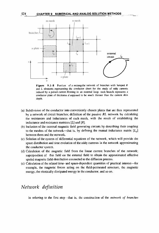
CHAPTER 9 NUMERICAL AND ANALOG SOLUTION METHODS _ _ - -_ ~ 524- -
external ,
0 Figure 9.1-8 Portion of a rectangular network of branches with lumped R and L elements representing the conductor sheet for the study of eddy currents induced by a pulsed current flowing in an external loop; each branch represents a conductor plate of thickness d supposed to be much thinner than the current skin depth.
(a) Subdivision of the conductor into conveniently chosen plates that are then represented by a network of circuit branches; definition of the passive RL network by calculating the resistances and inductances of each mesh, with the result of establishing the inductance and resistance matrices [L] and [R] .
(b) Inclusion of the external magnetic field generating circuits by describing their coupling to the meshes of the network-that is, by defining the mutual inductance matrix [L,] between them and the network.
(c) Solution of the system of differential equations of the network, which will provide the space distribution and time evolution of the eddy currents in the network approximating the conductor system.
(d) Calculation of the magnetic field from the linear current branches of the network; superposition of this field on the external field to obtain the approximated effective spatial magnetic field distribution connected to the diffusion process.
(e) Calculation of the related time- and space-dependent quantities of practical interest-for example, the magnetic forces acting on the field-permeated structure, the magnetic energy, the ohmically dissipated energy in the conductor, and so on.
Network definition
In referring to the first step-that is, the construction of the network of brunches

- .- 9.1 .-NUMERICAL COMPUTATION METHODS 525
representing the conductor (figure 9.1-8)-it is necessary and logical to attribute to each branch a rectangular conductor portion (a plate of thickness d) , with the branch lying at its center line. Since the branches are conveniently arranged in two directions represented by the coordinates u , v , normal to each other, one accordingly speaks of u- and v-plates. (When the conductor thickness is of the order of the diffusion skin depth or larger, it may be necessary to consider a three-dimensional network, see figure 9.1-9). For calculating the current if,, in the mth mesh we have to determine first the inductance and resistance of each mesh.
The mutual (and self-) inductances L,,m between two meshes n,m (figure 9.1-10) are defined on the basis of the flux bound to the rectangular area delimited by the four branches of mesh m and produced by the unit current flowing in the four plates defining mesh n [the basic reason for not simply taking branches also for mesh n is to avoid computational singularities in the Neumann integral when it comes to a self-inductance L,,,,,,, see remarks following (2.4-lo)]. From (2.4- 10) we find
(9.1 -20a)
The vector potential A,, at any point Q on the four branches of mesh in is obtained by integrating over the four rectangular plates of mesh n, each with volume V,, / 4 = ld,,b, and constant current density j,, = i,/(d,,b,,) (figure 9.1-10). (Branches and plates could have different dimensions, in which case the correct figures must be considered.) It can be found easily in closed analytical form from definition (2.2-21) that
(9.1-20b)
Both equations decompose in a straightforward way into four integrals, such that the
'" t V /v
Figure 9.1-9 When the conductor sheet thickness is of the order of the current skin depth or more, a multilayer network must be used to correctly describe the eddy current distribution in the conductor; here, a portion of a three-layered network is shown. However, in general the computation becomes intractable if conceptual simplifications are not introduced.
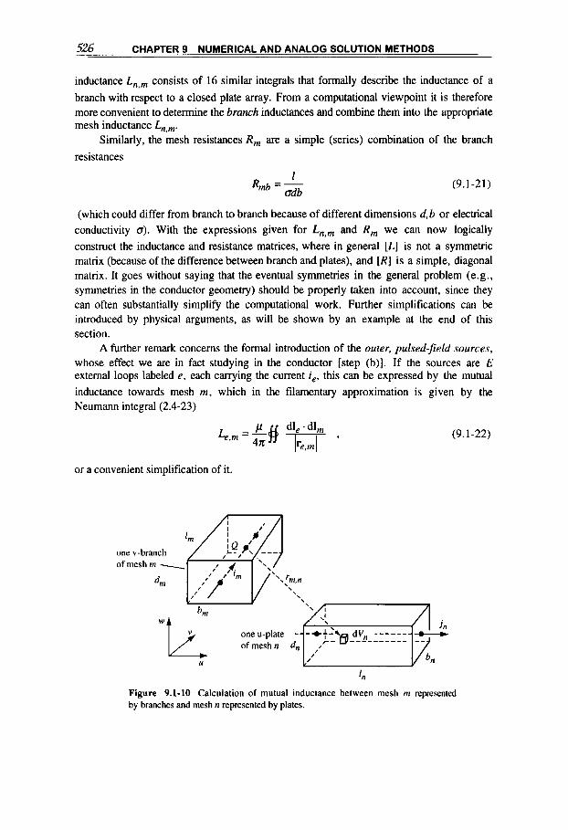
526 CHAPTER 9 NUMERICAL AND ANALOG SOLUTION METHODS
inductance Ln,, consists of 16 similar integrals that formally describe the inductance of a branch with respect to a closed plate array. From a computational viewpoint it is therefore more convenient to determine the brunch inductances and combine them into the appropriate mesh inductance Ln,,.
Similarly, the mesh resistances R , are a simple (series) combination of the branch resistances
1 odb
Rmb = - (9.1-21)
(which could differ from branch to branch because of different dimensions d,b or electrical conductivity 0). With the expressions given for Ln,tn and R , we can now logically construct the inductance and resistance matrices, where in general [L] is not a symmetric matrix (because of the difference between branch and plates), and [ R ] is a simple, diagonal matrix. It goes without saying that the eventual symmetries in the general problem (e.g., symmetries in the conductor geometry) should be properly taken into account, since they can often substantially simplify the computational work. Further simplifications can be introduced by physical arguments, as will be shown by an example at the end of this section.
A further remark concerns the formal introduction of the outer, pulsed-field sources, whose effect we are in fact studying in the conductor [step (b)]. If the sources are E external loops labeled e , each carrying the current i,, this can be expressed by the mutual inductance towards mesh m, which in the filamentary approximation is given by the Neumann integral (2.4-23)
(9.1-22)
or a convenient simplification of it.
one v-branch of mesh rn .
of mesh n
U
Ill
Figure 9.1-10 Calculation of mutual inductance between mesh m represented by branches and mesh n represented by plates.
9.1 NUMERICAL COMPUTATION METHODS 52 7
Network solution
The numerical solution of the network problem [step (c)] can take advantage of the general network theory developed particularly in the last 20 years' 8.9 9; together with the most advanced, new generation of computers it has become a powerful tool that can handle the most complicated and extended electric network systems. The problem here is relatively simple, since we have branches with lumped L- and R-elements only, but it is characterized by a large number of meshes. To solve for the M mesh currents i,, we have a total of M linear coupled differential equations, of which the one for the current i, is from Kirchhoff s law (1.1-63)
(9.1-23)
with the inductances and resistances defined in (9.1-20 to 22). The problem represented by the system of the m = 1, .... M equations (9.1-23) is fully determined when M independent initial conditions are given. In matrix notation the system of differential equations can be written in the form (A.3-36.37). with the rules (A.3-34.35).
or
(9.1-24)
(9.1-25)
There are different, well-known numerical techniques to solve such a transient system-for example, the Runge-Kutta method or the Predictor-Corrector methodg2'. Note that the eigenvalues of the product matrix [L]-I[R] are the inverse of the charucrenstic decay times qn of each of the M meshes representing a conductor portion or plate.
Many eddy current problems are related to alternating external magnetic field sources, varying as eiW in complex writing. In this case the system is described by the equation in matrix notation
[R+ iwL]I = [iwLe]I, , (9.1-26)
where the matrices [L], [L,], [R] are defined as before, and I and I, are the complex phasor vectorsq8. By solving for I in this system of ordinary equations, we obtain the mesh eddy currents and their phase relation with respect to the alternating currents I, in the outer circuits.
If we return to the picture of a field diffusion process [step (d) defined at the beginning of this subsection], the overall magnetic field distribution can easily be found in a first approximation by superposition of the original (unperturbed) field on the field generated by the induced currents flowing in the network branches. Calculation of the latter field, generated by the known currents flowing in the filamentary straight branches of the

__ __ 528 CHAPTER 9 NUMERICAL AND ANLLCG SOLUTION METHODS
network, is formally a simple procedure that will be discussed in connection with (9.2-2) in the next section. Similarly, numerical calculation of other related quantities [step (e)]-for example, forces exerted on the conductor, and potential or dissipated energies-is straightforward. In conclusion, the finite-element network method allows a step-by-step approach for numerically solving complicated eddy current or magnetic field diffusion problems in a relatively logical and convenient way.
In some cases it is important to model the conductor system as simply as possible to reduce the subdivisions [step (a)] to a minimum; here, physical intuition in predetermining the dominant eddy current paths and exploitation of all recognizable symmetries will help. We want to illustrate these concepts with an example.
In the operation of some devices for the study of controlled thermonuclear fusion, the penetration of a vertical equilibrium magnetic field into the toroidal magnet and vacuum containers plays an important role9.’’ (the equilibrium field serves to center the hot plasma ring and confer-together with the other magnetic fields-the necessary stability). An example of such an arrangement with the eddy current stream lines calculated for each of the nine thin-walled toroidal sectors with an extended network mesh is shown in figure 9.1 - 1 1. (This model serves to study the motion of the plasma ring located at the center of
Figure 9.1-11 Eddy current stream lines on a thin conducting toroidal sheet (subdivided into nine segments by highly resistive wedges) induced by a vertical field H , ; this example has been calculated with the network mesh method presented in the text’ l5 (courtesy of Princeton Plasma Physics Laboratory).

9.1 NUMERICAL COMPUTATION METHODS 529
Figure 9.1-12 The calculation of the eddy current distribution induced by an axial magnetic field on a sectored toroidal sheet (as shown in the previous figure) could be simplified appreciably by premodeling each of the nine sectors through six saddle-shaped loops (for simplicity, only two of the nine sectors are shown).
the toroidal chamber in reaction to a varying outer axial magnetic field that is disturbed by the induced eddy currents.) But even not knowing this picture, we expect the eddy currents in each sector to have a saddle-shaped pattern, either by intuition or, in this case, from the result of the cylindrical case discussed in section 4.4 in connection with figure 4.4-9. Instead of representing the toroidal sector by an extensive electric network as indicated in figure 9.1-8, each sector could also be modeled roughly by six saddle-shaped loops (three on the upper half and three on the lower half), each composed of two toroidal and two poloidal branches (the“u” and “v”-plates), as shown in figure 9.1-12.
Magnetic reluctance network
From the similarity between electric and magnetic circuits (table 1.4-1), and Kirchhoff s laws (1.1-62.63) and (1.4-49,50) governing them, we derive the magnetic reluctance network method (RNM) for finding the flux lines and related parameters in magnetic materials, which is formally identical to that applied previously to electrically conducting materials. Here the magnetic material is subdivided (as in figure 9.1-8) into
CHAPTER 9 NUMERICAL AND ANALOG SOLUTION METHODS ~ - - -- 530 . __
u,v-plates with their related magnetic fluxes ( i , + y,) and reluctances (R, + RH,) . The necessary equations for defining these parameters in the grid of branches and nodes are derived from the magnetic Kirchhoff laws (1.4-49,50). The system of equations is formally similar to (9.1-23 to 25) and is solved correspondingly. We refer to the literature for further detail^^.^'.
9.2 APPROXIMATION BY FILAMENTARY OR SIMPLE ELEMENTAL CONDUCTORS
Circular loops and solenoids
An axisynimetric current system can be approximated for computational purposes to any required degree of precision by a sufficiently dense array of filamentary, coaxial, circular loops, each one characterized by its own current and radius. The magnetic field distribution generated by this current system in space is then given as the vectorial sum of the contributions of all the loops. On the same computational basis, we can handle a more general current system composed of an array of axisymmetric subsystems (such as the one just mentioned), where each of these subsystems may have any position and orientation in space. In fact, the results calculated for each subsystem in its axisymmetric frame of reference can be linearly transformed into the one common frame of reference for the general system.
The magnetic field generated by one loop is described in terms of the complete elliptic integrals in (2.3-1 1). and similar expressions apply for the mutual inductance (2.4-26) and the axial force (6.2-14) between two loops'.''. In numerical calculations it is convenient to recompute the elliptic integrals contained in these equations on the basis of appropriate approximations, rather than take tabulated values.
In the previous chapters we gave the most important electromagnetic relations regarding axisymmetric current distributions. We saw, in particular, that it is convenient to introduce the magnetic vector potential A, because it has only the azimuthal component A 4. Its relation with the magnetic field components is found in (2.2-27) and with the mutual inductance in (2.4-32), and hence with the magnetic forces in (6.2-14).
An alternative method for calculating magnetic fields generated by (iron-free) axisymmetric current distributions is based on the expansion in polynomiuls9~'* (2.1-17), with the solution given by (2.1-21,22). The coefficients a& of this expansion (2.1-18,20) are determined from the on-axis magnetic field (and its derivatives), which is given for the
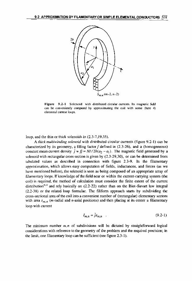
9.2 APPROXIMATION 6Y-FILAMENTARY OR SIMPLE ELEMENTAL CONWCTORsl31 - ~ . - _ _ _ _
Sm,n (m=2, n=2)
Figure 9.2-1 Solenoid with distributed circular currents. Its magnetic field can be conveniently computed by approximating the coil with some (here 4) elemental current loops.
loop, and the thin or thick solenoids in (2.3-7,19,35). A thick multiwinding solenoid with distributed circular currents (figure 9.2- 1) can be
characterized by its geometry, a filling factorf defined in (2.3-26), and a (homogeneous) constant mean current density = fi = NI/2b(a2 - q). The magnetic field generated by a solenoid with rectangular cross section is given by (2.3-29,30), or can be determined from tabulated values as described in connection with figure 2.3-9. In the filamentary approximation, which allows easy computation of fields, inductances, and forces (as we have mentioned before), the solenoid is seen as being composed of an appropriate array of filamentary loops. If knowledge of the field near or within the current-carrying system (the coil) is required, the method of calculation must consider the finite extent of the current distribution’ l 3 and rely basically on (2.2-22) rather than on the Biot-Savart law integral (2.2-38) or the related loop formulae. The filiform approach starts by subdividing the cross-sectional area of the coil into a convenient number of (rectangular) elementary sectors with area s ~ , ~ (m-radial and n-axial positions) and then placing at its center a filamentary loop with current
(9.2- 1)
The minimum number m,n of subdivisions will be dictated by straightforward logical considerations with reference to the geometry of the problem and the required precision; in the limit, one filamentary loop can be sufficient (see figure 2.3-1).
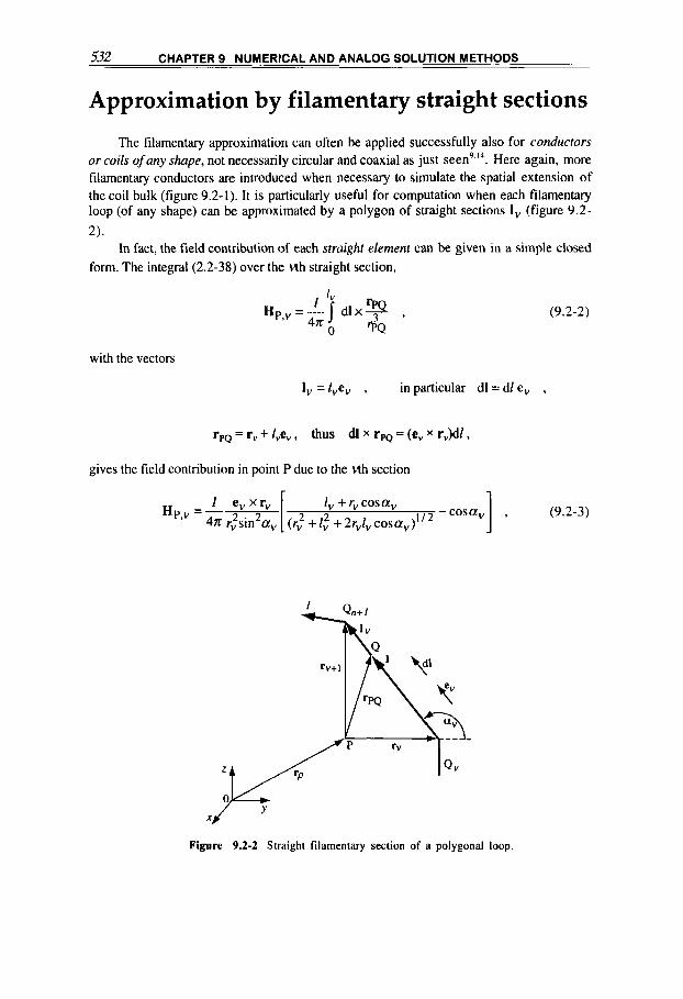
532 CHAPTER 9 NUMERICAL AND ANALOG SOLUTION METHODS
Approximation by filamentary straight sections
The filamentary approximation can often be applied successfully also for conductors or coils ofany shape, not necessarily circular and coaxial as just seen9 1 4 . Here again, more filamentary conductors are introduced when necessary to simulate the spatial extension of the coil bulk (figure 9.2-1). It is particularly useful for computation when each filamentary loop (of any shape) can be approximated by a polygon of straight sections I, (figure 9.2-
2). In fact, the field contribution of each straight element can be given in a simple closed
form. The integral (2.2-38) over the vth straight section,
'pa dlx- , Hp,, =-I I
4x0 dQ (9.2-2)
with the vectors
I, =I,e, , in particular d l = d l e, ,
rpQ = r, + l,e,, thus dl x rpQ = (e, x r,)dl ,
gives the field contribution in point P due to the Mh section
, , 2 --osa, , (9.2-3) 1 1 e, xr, 1, + rv cosa, HP,v =- 4~ r,sin 2 2 01, [ 2 (r, +I, 2 +2r,l,cos01,)
X J '
Figure 9.2-2 Straight filamentary section of a polygonal loop.
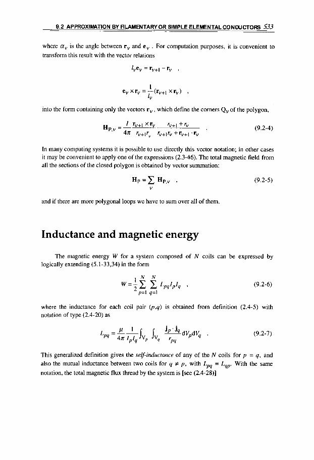
9.2 APPROXIMATION BY FILAMENTARY OR SIMPLE ELEMENTAL CONDUCTORS 533
where 01, is the angle between rv and e , . For computation purposes, it is convenient to transform this result with the vector relations
lyev = rv+l - rv ,
I ev x r, = --(rV+l x rv) ,
1,
into the form containing only the vectors rv , which define the corners Qv of the polygon,
(9.2-4) I %+I x r v %+I + r v
4n %+IT" %+I% + rv+1 . rv H P , ~ =--
In many computing systems it is possible to use directly this vector notation; in other cases i t may be convenient to apply one of the expressions (2.3-46). The total magnetic field from all the sections of the closed polygon is obtained by vector summation:
(9.2-5)
and if there are more polygonal loops we have to sum over all of them.
Inductance and magnetic energy
The magnetic energy W for a system composed of N coils can be. expressed by logically extending (5.1-33,34) in the form
(9.2-6) L p = l q=l
where the inductance for each coil pair @,q) is obtained from definition (2.4-5) with notation of type (2.4-20) as
(9.2-7)
This generalized definition gives the self-inductance of any of the N coils for p = q, and also the mutual inductance between two coils for q # p , with Lpq = L,. With the same
notation, the total magnetic flux thread by the system is [see (2.4-28)]
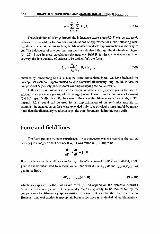
534 CHAPTER 9 NUMERICAL AND ANALOG SOLUTION METHODS
N N w = c c L P d 4 * (9.2-8)
p=l q=l
The calculation of Wor ylthrough the inductance expression (9.2-7) can be extremely tedious. It is mandatory to look for simplifications or approximations; and following what has already been said in this section, the filamentary conductor approximation is the way to go. The inductance of any coil pair can then be calculated through the double-line integral (9.1-22). Since in these calculations the magnetic field B is already available (as it is, anyway, the first quantity of interest to be looked for), the form
(9.2-9)
obtained by transcribing (2.4-31), may be more convenient. Here, we have included the concept that each coil (approximated by one elemental filamentary loop) could, in fact, be composed of N (densely packed) total windings carrying the coil current I .
In this way it is easy to calculate the mutual inductances Lpq (where p # q), but not the self-inductances (where p = q), which diverge [as we know from the comments following (2.4-10); specifically, here B,, becomes infinite on the filamentary element ds ] The
p : integral (9.2-9) could still be used for an approximation of the self-inductance if, for example, the integration surface were extended only to a physically meaningful boundary other than the filamentary conductor (e.g., the outer boundary delimiting each coil).
Force and field lines
The force per unit volume experienced by a conductor element carrying the current density j in a magnetic flux density B = pH was found in (6.1-10) to be
dF d F - + - = j x B . AV dV
If across the elemental conductor surface sm,n (which is normal to the current density) both
j and B can be substituted by a mean value, then with A V = s , , , ~ dl and = j sm,n , we get, in the limit,
which, as expected, is the Biot-Savart force (6.1-4) applied on the elemental sections. Since B is known (because it is generally the first quantity to be looked for by the computation) the filamentary approximation is convenient also for the force calculation. However, a note of caution is appropriate because the force is evaluated at the filamentary

9.3 ANALOG METHODS 535
conductor element, where the magnetic field of the latter diverges. In theory, the field produced by a straight section does not generate any resultant force on it, but because of the divergence, large errors are possible. From a computational viewpoint this difficulty can simply be avoided by subtracting from the overall flux density the component produced by the straight element for which the force is computed.
Magneticfield lines are an integral expression of the magnetic vector field H, as defined in section 2.5. They are determined by the solution of the system of nonlinear differential equations (2.5-4). With the exception of a very few simple cases, this problem can be solved only numerically.
9.3 ANALOG METHODS
Many analog methods have been applied in the past for the solution of the Dirichlet problem, or for determining and eventually plotting magnetic fields derived from a given current distribution. Examples are the electrolytic tank or the resistance network, where the potential is obtained by measuring voltage over a continuous or discrete resistance distribution' lo. However, with the advent of modem digital computers, these types of analog methods are not in practical use any longer.
Clearly, the most direct analog method is to measure the magnetic field distribution by magnetic probes around the real coil or conductor system.
Electromagnetic model scaling
General formulation
When the real conductor system is large and complex, it may be convenient to use scaled-down models, which must, however, correctly and in a well-defined way transform all the relevant electromagnetic parameters and phen~mena~ .~ ' . The problem here is to determine the transformation rules by finding the proportionality parameters aj between the model and the real system parameters (the former being marked by the superscript m):
r"' =arr , t"'=a,t ,

536 CHAPTER 9 NUMERICAL AND ANALOG SOLUTION METHODS
(9.3-1) j m = a j j , bm=a,d ,
Pe? = app, *
where all the quantities have the usual meaning, as defined in section 1.1 and throughout the book. The nabla operator and the time derivative transform as
a l a
a r atm a t & 1
v m = - v , -- (9.3-2)
The a-parameters are determined by the requirement that Maxwell's equations remain invariant with these linear transformations. For example, from (1.1-1).
(9.3-3) m, at
V x H = j + - ,
follows by inserting relations (9.3- 1.2) and rearranging
The invariance is assured when
aH = arai
(9.3 -4)
(9.3-5)
and
aHar =araD . (9.3-6)
Proceeding as above, from the laws of Faraday, Gauss, and Ohm (1.1-2,4,6),
ds dr
V X E = - - , (9.3 -7)
V.D=p, , (9.3- 8)
j=aE , (9.3-9)
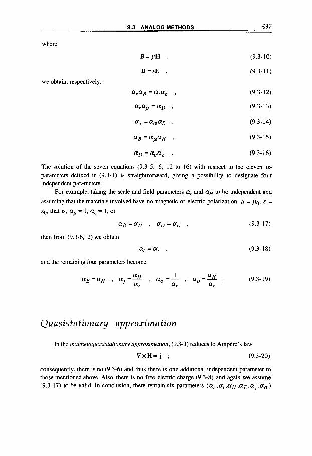
9.3 ANALOG METHODS 537
where
B = p H ,
D=& ,
we obtain, respectively,
araB =ataE ,
arap =aD ,
(9.3-10)
(9.3-1 1)
(9.3 - 12)
(9.3-13)
aj =aOaE , (9.3- 14)
aB=apaH , (9.3-15)
aD =aEaE . (9.3- 16)
The solution of the seven equations (9.3-5, 6, 12 to 16) with respect to the eleven a- parameters defined in (9.3-1) is straightforward, giving a possibility to designate four independent parameters.
For example, taking the scale and field parameters ar and aH to be independent and
assuming that the materials involved have no magnetic or electric polarization, p = po, E =
E ~ , that is. ap = I , aE = 1, or
ag =aH , aD = aE , (9.3-17)
then from (9.3-6,12) we obtain
at = ar ,
and the remaining four parameters become
aH , a6=- 1 , ap=- " H . aE=aH , a ' = - ar ar a,
(9.3-18)
(9.3-19)
Q uas is ta t ion a ry approxima t ion
In the magnetoquasistationary approximation, (9.3-3) reduces to Amp6re's law
V x H = j ; (9.3 -20)
consequently, there is no (9.3-6) and thus there is one additional independent parameter to those mentioned above. Also, there is no free electric charge (9.3-8) and again we assume (9.3-17) to be valid. In conclusion, there remain six parameters (ar,at,aH,aE,aj,aO)

538 CHAPTER 9 NUMERICAL AND ANALOG SOLUTION METHODS
three of which are independent. For example, if we choose ar , aH, a. to be independent, from (9.3-5, 12,14) the three remaining parameters become
(9.3-21)
The scaling laws can be extended to include an electrically conducting fluid moving with velocity u, for which the parameter a,,, defined by
u'"=a,,u , a,=a,ta, , (9.3-22)
is related to the already known ar, at . In the magnetohydrodynamic approximation ( 1.3- 35, 37), the Faraday law
(9.3-23) ds at
V x E' = - - + V x (U x B)
has an additional term with respect to (9.3-7), which, however, introduces a condition that is identical to (9.3-12). Thus, the situation of independent and dependent parameters remains unchanged by the introduction of a velocity in the MHD-approximation.
Many other considerations can be made and conditions applied. For example, a significant quantity in magnetic field generation is the skin depth (4.2-18a).
for which we find, with (9.3-21),
s'"=a,&s . (9.3-24)
It would be convenient for the skin depth to scale as the linear dimension, and for the free parameter a. we thus set a. = 1. Modeling of fields and losses in ferromagnetics is
another example of practical importance9-*'.
The fact that only one time parameter at (or frequency parameter a;') is admitted in
the transformations [e.g., (9.3-18,21)] requires the model to be supplied with a current or field pulse that must be similar to the pulse in the original system-that is, with the same reduced Fourier spectrum.
Magnetomechanical model scaling
The scaling considerations made previously can be extended to include other domains
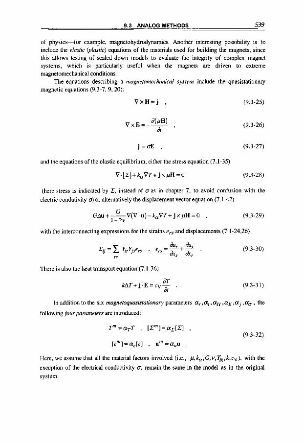
9.3 ANALOG METHODS 539
of physics-for example, magnetohydrodynamics. Another interesting possibility is to include the elastic @lasfic) equations of the materials used for building the magnets, since this allows testing of scaled down models to evaluate the integrity of complex magnet systems, which is particularly useful when the magnets are driven to extreme magnetomechanical conditions.
The equations describing a magnetomechanical system include the quasistationary magnetic equations (9.3-7,9,20):
V x H = j , (9.3-25)
(9.3-26)
j = o E , (9.3-27)
and the equations of the elastic equilibrium, either the stress equation (7.1-35)
V .[,TI+ k,VT+ j x pH = 0 (9.3-28)
(here stress is indicated by 1, instead of cras in chapter 7, to avoid confusion with the electric condutivity a) or alternatively the displacement vector equation (7.1-42)
(9.3-29) G
1-2v GAu+-V(V.u)-k,VT+jxpH=O ,
with the interconnecting expressions for the strains ers and displacements (7.1-24,26)
(9.3 -30)
There is also the heat transport equation (7.1-36)
(9.3-3 1 ) ar dt
k A T + j . E = c v - .
In addition to the six magnetoquasistationary parameters a;, a,, a H , aE ,a j , a. , the
following four parameters are introduced:
T m = a ~ T , [ Z m ] = a z [ C ] ,
[ e r n ~ = a , [ e 1 , urn =auu . (9.3-32)
Here, we assume that all the material factors involved (i.e., p,k,,G,v,Xk,k,cv), with the
exception of the electrical conductivity 0, remain the same in the model as in the original system.
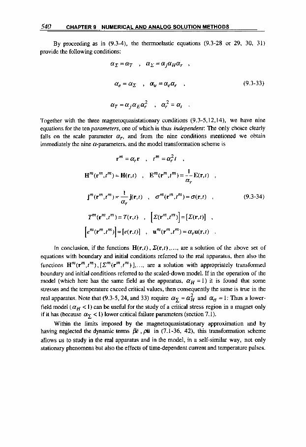
540 CHAPTER 9 NUMERICAL AND ANALOG SOLUTION METHODS
By proceeding as in (9.3-4), the thermoelastic equations (9.3-28 or 29, 30, 31) provide the following conditions:
az=aT , az=ajaHar ,
ae = az , a, =sear , (9.3-33)
aT =ajaEar 2 , a,?=a,
Together with the three magnetoquasistationary conditions (9.3-5,12,14), we have nine equations for the ten parameters, one of which is thus independent: The only choice clearly falls on the scale parameter ar, and from the nine conditions mentioned we obtain immediately the nine a-parameters, and the model transformation scheme is
2 rm =ar' , t m = a r t ,
Hm(rm,tm) = H(r,t) , Em(rm,tm) = -E(r,t) , 1
a r
(9.3-34)
In conclusion, if the functions H(r.r) , Z(r,r) ,. .., are a solution of the above set of equations with boundary and initial conditions referred to the real apparatus, then also the functions Hm(rm,tm), [C"(r",f") I, ..., are a solution with appropriately transformed boundary and initial conditions referred to the scaled-down model. If in the operation of the model (which here has the same field as the apparatus, a H = 1) it is found that some stresses and the temperature exceed critical values, then consequently the same is true in the real apparatus. Note that (9.3-5,24, and 33) require aE = a H and aa = 1: Thus a lower- field model ( a H < 1) can be useful for the study of a critical stress region in a magnet only if it has (because ax < 1) lower critical failure parameters (section 7.1).
Within the limits imposed by the magnetoquasistationary approximation and by having neglected the dynamic terms @ , pii in (7.1-36, 42), this transformation scheme allows us to study in the real apparatus and in the model, in a self-similar way, not only stationary phenomena but also the effects of time-dependent current and temperature pulses.
2
APPENDICES
These appendices present, after a review on electromagnetic units, a collection of mathematical notes on functions (A.2), on vector and tensor analysis (A.3), and on second-order differential equations (A.4). Although it is assumed that the reader possesses a broad knowledge of fundamental mathematical tools, these Appendices are useful reminders related to the theoretical analysis in the text. For a complete discussion, the reader is referred to the extensive literature on mathematical physics at the end of the book.
54 1
M4GNETICFIELDS: A Comprehensive Theoretical Treatise for Practical Use Heinz E. Knoepfel
Copyright Q 2000 by John Wiley & Sons, Inc

542 APPENDICES
A.l ELECTROMAGNETIC UNITS AND EQUATIONS
Table A.1-I gives some of the most important electromagnetic relations, written in four different systems of units; table A.1-I1 specifies the units of six different electromagnetic systems and gives the conversion factors for obtaining SI units (International System of Units)*.*'. Finally, tables A. 1-111 and A. 1-IV report the values of some of the most frequently used constants and conversion factors.
Table A . l - I Electromagnetic relations
Rela tion I- Maxwell
Fields in matte
Biot-Savart
Lorentz
Poynling vect
Cyclolron freq
S1 system V x H = j + y
V x E = - W a v B = O V D=p,
B = p H D=EE
V x E = -IO-sW/dr V B=O
V ( ~ ~ E ) = 1 . 1 3 ~ 1 0 ' ~ p ,
B = ~ R H
Emu system
V x H = 4@+& a v x E = - m a V . B = O V . D = 4npe
B = P R H
D=(eR / c 2 ) E
P = [ E x H] P = g [ E xH1 P=&IExHI P = f [ E xHI
1. R = - q B l m R = -qB/ m R = - q B / m R = - q B / m c
In some texthooks (e.g.. reference 1.5) the equations contain j instead of j/c.
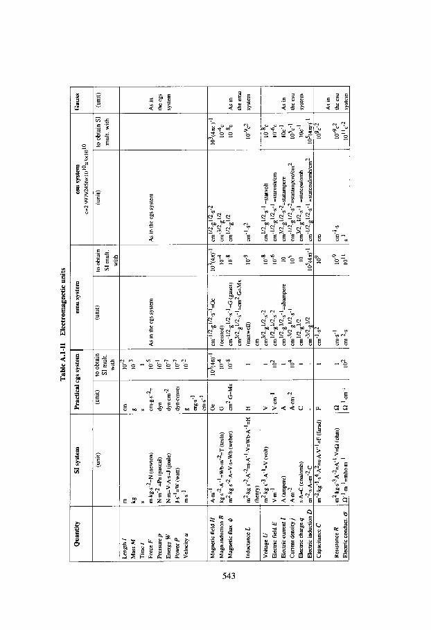
Tab
le A
.l-I
1 E
lect
rom
agn
etic
units
Qua
ntit
y
Len
gth
I M
ass M
T
ime
f
Forc
e F
Ene
rgy
W
Pow
er P
Vel
ocity
u
Pres
sure
p
Mag
netic
fie
ld H
M
agn.
indu
cnon
B
Mag
netic
flu
x @
Indu
ctan
ce L
Vol
tage
U
Ele
ctri
c fi
eld
E E
lecu
ic c
urre
nt I
C
urre
nt d
ensi
ty j
Ele
cmc
char
ge q
E
lect
ric
indu
ctio
n D
Cap
acita
nce
C
Res
ista
nce R
Ele
ctri
c co
nduc
t. U
SI s
yste
m
(uni
t)
m.k
g.s-
'=N
(n
ewto
n)
N.m
-' =P
a (p
asca
l)
N.m
=V.A
.s=J
(jou
le)
1-
s-
L~
(w
an)
m.s
-1
Pra
ctic
al c
gs sy
stem
(uni
t)
o o
btai
n SI
mult.
w
ith
10-2
10-3
10-5
10-1
10.'
10-7
10-2
I
103(
4rr)
-l
10
4
10-8
I 1 I02
I o4 1 I I I 102
emu
syst
em
(uni
t)
As
in t
he c
gs s
yste
m
o ob
tain
SI m
ult.
wit
h
103(
4n)-
I
10
4
10-8
I 0-9
10-8
10-6
I 05
I 09
10-9
loll
10
10
105(
41r)
-l
I Gauss
esu
syst
em
c=?.
9979
24S
6~
1 O1
od
x 10
"
(uni
t)
As
in h
e cg
s sy
stem
mu
lt. w
ith
As
in
the
cgs
syst
em
the
emu

544 APPENDICES
Table A.l-111 Selected physical constantsA.'*
Ouantitv
Magnetic permeability
Dielectric constant
Velocity of light
Planck constant
Electron charge
Electron rest mass
Proton rest mass
Atomic mass unit
Gravitation constant
Boltzmann constant
Avogadro number
Bohr magneton (eh / 4R me )
Nuclear magneton (eh/41rmp)
Magnetic flux quantum (h/2e)
Quantity
Magnetic field (H)
Value
p, = 4 ~ x l O - ~ =1.2566370614~10"H.m-~
E, =8.854187817~10- '~ F.rn-I
c = (p0&,)
h = 6.62607 x J. s
h = 1.05457 X lo-" J . s
e = -1.602 177 x C
me = 9 . 1 0 9 3 8 ~ 1 0 - ~ ~ k g
mp = 1.67262 x kg
% . m u = I .66054x 10-27kg
g = 9.807 m. s - ~
k = R / N = 1 . 3 8 0 6 ~ 1 0 - ~ ~ J.K-'
N = 6.02213~ 1023(mol)-1
mg = 9 . 2 7 4 0 1 ~ 1 O - ~ ~ A ~ m ~ ( = J f I J
mN = 5.05078~ A.m2(= Jm)
yrn = 2.067834~ lo-!' Wb(= V.s)
1 -_ = 2.99792458~ lo8 ms- '
Table A.1-IV Some conversion factors
Value
I Oe = 79.58 A.m-l
I gamma magn. field unit = lo-' Oe
Magnetic induction ( B )
Energy
Pressure
Temperature
El. conductivitv'
I G =
1 eV = 1 . 6 0 2 ~ 1 0 - ~ ~ J
1 erg = 10-7 J I cal = 4.184 J 1 ton(eq.TNT)= 109cal=4.18x10⁹J
I Pa = bar
1 bar = 16 N . d = 1@dyn/cm2
1 atm = 0.980x10⁵Nm2
0 "C +273.16 K
1 eV t1.16 lo4 K
100% IACS+58x106(Rm)-' I
Wb.m-2 = lo4 tesla
'Intern. Annealed Copper Standard; conductivity of pure copper with density 8.89 g/cm3 at 20°C.

A.2 MATHEMATICAL FUNCTIONS 545
A.2 MATHEMATICAL FUNCTIONS
The error function
The error function, which frequently appears in plane diffusion problems, is defined byA.4
so that
erf 0 = 0 ,
erf - = 1 ,
erf (-x) = -erfx ,
and
derfx - 2 e - ~ 2 dx-x For small values of x, it can be expressed by the convergent series
and hence approximated by
For large values of x, the semiconvergent series
(A.2- 1)
(A.2-2)
(A.2-3)
(A.2-4)
(A.2-5)
can be used with an error which is in absolute value less than the last term retained. Defining the complementary error function as
m
erfcx = 1 -erfx = j=jX e-x2dx , (A. 2-6)
the integrals related to the notation
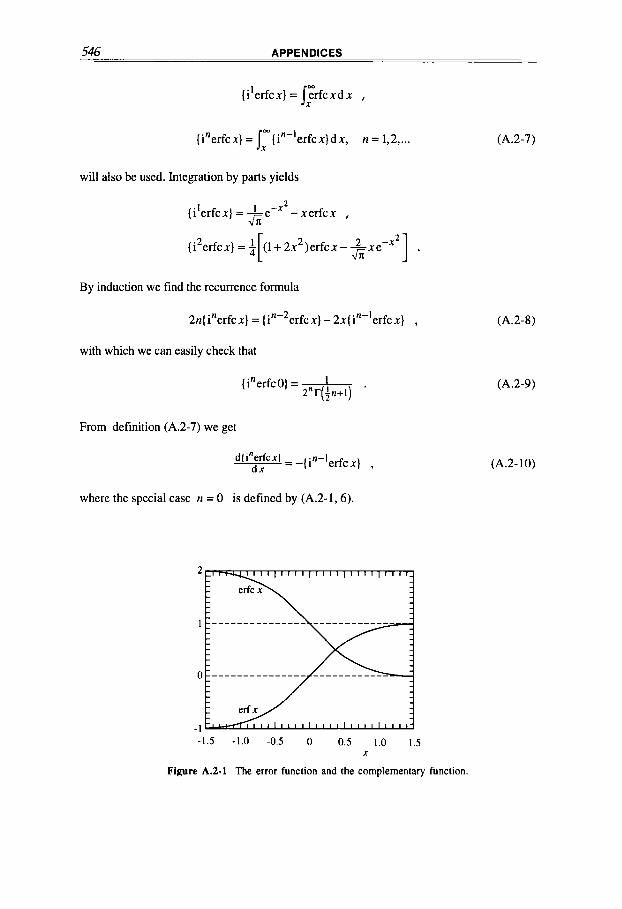
546 APPENDICES
(i'erfcx) = 1Frfcxdx ,
m
(i"erfcx) = I {in-lerfcx)dx, n = 42, ...
will also be used. Integration by parts yields
2 1 t i erfcx) = L e e ' -xerfcx , J;;
x' ] .
By induction we find the recurrence formula
2n{ inerfc x l = { in-2erfc x) - 2x( ifl-'erfc x ) ,
with which we can easily check that
Ii"erfc0) = * 2"r(fn+1) '
From definition (A.2-7) we get
d(i'eerfcx1 = -(in-lerfcx) d x
where the special case n = 0 is defined by (A.2-1,6).
-1.5 -1.0 -0.5 0 0.5 1.0 1.5 X
1 1 1 1 1 1 1 1 1 1 1 1 1 1 1 1 1 1
-1.5 -1.0 -0.5 0 0.5 1.0 1.5 X
(A.2-7)
(A.2-8)
(A.2-9)
(A.2-10)
Figure A.2-1 The error function and the complementary function.

A.2 MATHEMATICAL FUNCTIONS 547
The functions erf x and erfc x are shown in figure A.2-1; the normalized functions {in erfc x ) for n = 0,l ...., 6 are shown in figure 4.2-3.
Bessel functions of integer order
We present some basic definitions and relations regarding the Bessel functions used
The solutions of the differential equation in the main text; for further information we refer the reader to the l i t e r a t ~ r e ~ . ” ~ . ~ .
(A.2-11) Z 2 ~ + Z ~ + ( ( f Z 2 2 - v ) F = O d z 2 d z
are, for the (+)-sign case,
F$+’=AJ,(z)+ BY,(z)
and, for the (-)-sign case,
F$-) = A I , ( z ) + B K , ( z ) ,
I .o
0.8
0.6
0.4
0.2
0
-0.2
-0 A -. . 0 2 4 6 8 1 0 1 2 1 4
X
Figure A.2-2 First-kind Bessel functions of order v = 0.1.2.
(A.2- 12)
(A.2-13)

548 APPENDICES
0.6
0.4
0.2
0
-0.2
-0.4
-0.6
-0.8
-1.0
0 2 4 6 8 1 0 1 2 1 4
X
Figure A.2-3 Second-kind Bessel functions of order v = 0, 1, 2. (Note that for x 2 2.5, Yo and J I are nearly coincident. whereas Y I I -Jo)
Figure A.2-4 v = 0.1.
functions of order
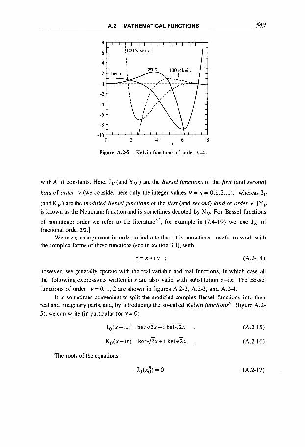
A.2 MATHEMATICAL FUNCTIONS 549
0 2 4 6 8 X
Figure A.2-5 Kelvin functions of order v=O.
with A , B constants. Here, J v (and Y ) are the Bessel functions of the first (and second)
kind of order v (we consider here only the integer values v = n = 0,1,2, ...), whereas I,
(and K , ) are the modified Bessel functions of the first (and second) kind of order v. [Yv is known as the Neumann function and is sometimes denoted by N,. For Bessel functions
of noninteger order we refer to the literatureA3, for example in (7.4-19) we use J,,, of fractional order 312.1
We use z as argument in order to indicate that it is sometimes useful to work with the complex forms of these functions (see in section 3. l), with
z = x + i y ; (A.2- 14)
however, we generally operate with the real variable and real functions, in which case all the following expressions written in z are also valid with substitution z+x. The Bessel functions of order v = 0, 1, 2 are shown in figures A.2-2, A.2-3, and A.2-4.
It is sometimes convenient to split the modified complex Bessel functions into their real and imaginary parts, and, by introducing the so-called Kelvin functionsA.' (figure A.2- 5), we can write (in particular for v = 0)
IO(x+ix)=ber f ix+ibe i& , (A.2- 15)
Ko(x+ir)= ker f ix+ i keifix . (A.2-16)
The roots of the equations
Jo(xlf) = 0 (A.2-17) ,

550 APPENDICES
n
1 2
3
4
5
roots values roofs values
4 Jl(& 4 JOC.1") 2.405 +0.5 19 3.831 +0.403
5.520 -0.340 7.016 -0.300
8.654 +0.27 1 10.17 +0.250
11.79 -0.232 13.32 -0.2 I8
14.93 +0.207 16.47 -0.196
and
J ~ ( x ; ) = 0 (A.2- 18)
are given for all n's by
x;f s n(n - 0.25 + y) (to within f 0.03%) (A.2- 19)
x; z n(n + 0.25 - y) (to within f 0.06%) . (A.2-20)
The associated values of Jo(x;) and Jl(x:) of the first five roots are reported in table A.2-I.
The following summation holds A *:
(A.2-2 1)
Denoting by Fv either J,, Y , I, or (-1)" K , we have the recurrence formulaA'
but without the factor (-1) when Fv = J,, or = Yv; and we also have the differential
relations (with k = 0, 1, 2, ...)
(A.2-23)
but without the factor (-1) when Fv = I, , or = (-1)" Kv For example, with k = 1 and
v = n and denoting the derivative with respect to z by a prime, we get
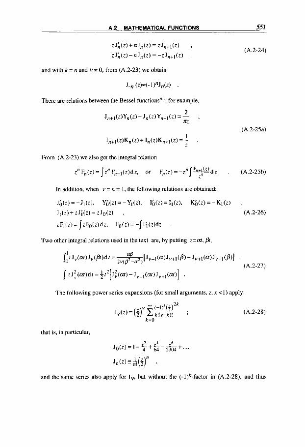
A.2 MATHEMATICAL FUNCTIONS 551
and with k = n and v = 0, from (A.2-23) we obtain
There are relations between the Bessel functions* '; for example,
2
In J ~ + I ( z ) ~ , ( z ) - J ~ ( z ) Y ~ + ~ ( z ) = - 9
1 I,,I(Z)K,(Z)+ I,(Z)K,+I(Z) = - .
Z
From (A.2-23) we also get the integral relation
zn F,(z) = j z " F,-l(z)dz, or F,(z) = -zfljddz F ( z n
(A.2-24)
(A.2-25a)
(A.2-25b)
Two other integral relations used in the text are, by putting z=M, Pt,
ji t J (at) J, (Pr d t = 2 v ( p 2 -a2) [Jv-l(a)Jv+l(P) - Jv+l(a)Jv-l(P)] . (A.2-27)
t J ~ ( a r ) d t = ~ r 2 [ J ~ ( a r ) - J v - l ( ~ ) J , + l ( ~ ) ] .
The following power series expansions (for small arguments, z, x <1) apply:
(A.2-28)
that is, in particular,
2 4 J o ( z ) = l - $ + L - L + 64 2304 ".'
Jn (z ) a( 1 L n 2 ) ,
and the same series also apply for I,. but without the (-l$-factor in (A.2-28), and thus

552 APPENDICES
with only (+)-signs in the latter series; andA.'
2 4 ( i X 2 ) ($2)
berx=l--+-- (2!)2 (4!)2 '.*'
3 5
beix=;Cx 1 2 --+-- (ax') (ax') ... (3!? (S!?
(A.2-29)
(A.2-30)
The following approximations for very small arguments (z, x c( 1) can also be useful for calculating functions of the second kind:
YJz) 5 $ln( 5 z ) JJz) + ... , (A.2-3 1)
ker x z -In(ix) ber x + i n beix + ... ,
keixE-In ( 2 Lx 1 beix-$nberx+ ... .
(A.2-33)
(A.2-34)
For very large arguments ( z , x ))I), the following approximations are usefulA.':
J,(z) E ECOS( z - +vX - i n ) , (A.2-35)
yV(z) z G s i n ( z - ivn -in) , (A.2-36)
(A.2-37)
(A.2-38)
in particular, the following combinations of the Kelvin functions can be approximately calculated for large
(A.2-39) (ber'x) 2 +(bei'x)2 =A(x)
berxber'x + bei' xbeix E A ( x ) (A.2-40)
ber x bei' x + ber' x bei x f (A.2-41)
where the prime denotes derivation with respect to x, and A(x) = eX'/?/(2m).

A.2 MATHEMATICAL FUNCTIONS 553
Functions in series formulation
For the analytic or numerical solution of many magnetic field problems it is convenient to express given functions in them with series of well-known and simpler functions. As we have seen throughout the book, there are different reasons for this representation, but probably the most interesting is the possibility of approximating the solution with a very limited number of functions in the series which are well suited to the problem and relative geometry under investigation. The polynomial Taylor series is the most used [e.g., (2.1-17), (2.2-29), (2.3-13), (9.1-3), (A.2-4), (A.2-28)]. But since polynomials are often poor functions to use for approximating many given functions of interest, other more appropriate sets are used in practice, as for example the series in Bessel functions, which are useful in cylindrical field problems [e.g., (4.3-31). (4.3-41), (4.3- 51), (4.5-12), (A.4-19). (A.4-30)], or even double series where two different series representations are folded into expressing a given function [e.g., (A.4-13), (A.4-41)].
Among the many other complete series (meaning that they can approximate any continuous function in a closed interval), the most known and useful is the Fourier series based on the harmonic functions cos nx and sin nx [e.g.. (4.2-44). (A.4-13). (A.4-21b), (A.4-3 l), (A.4-66)]. Any steady periodic function At) in the period T = 2 a / w such that flt)=f(t+nT) can, in fact, be expressed by the Fourier series
m
f ( t ) = x u , , cosnwt+ b,sinnwt n=O
(A.2-42)
(n = 0 corresponds to the only term q), where
The an,bn parameters are obtained by multiplying (A.2-42) by cos(bwt) and sin(bot), respectively, and integrating, thereby noting the orthogonality of the sin and cos functions:
0 b # n
T b = n = O
T 2 - I rcos(bwt)cos(nm)dr= _ _
2
I - I: sin(bwr)sin(nwt)dt = _-
2
- T
sin(bwt)cos(nwt)dt = 0 _-
2
b # n
b = n # O ’

554 APPENDICES
In fact, this formalism can be extended to a nonperiodic functionfit), in which case (with TI 2 + +-) we have the double Fourier integrals
m m
f ( t ) = IA(w)cos(wr)do+fB(w)sin(wt)dw , (A.2-44) 0 0
They are generally presented in the symmetric, complex form
m
(A.2-46)
00
1 F(w) = jf(t) e-iwdt , (A.2-47)
-00
where F(w) is referred to as the Fourier transform off(?), and flt) is the inverse transform of F(w) . (These expressions may be extended to multiple dimensions in a natural manner.) Here we have introduced the basic elements of the Fourier transfonn method for solving differential equationsA 23. The idea is to transform the original equation (ordinary or partial) into a simpler equation (algebraic or ordinary differential) where the solution is easier; the required solution of the original differential equation is then obtained by finding the inverse transform of the solution of the simpler equation. In the literature one can find extensive tables where numerous Fourier transforms and their inverse are tabulatedA.20, making the application of this method easy and convenient for a large number of problems.
The Luplace transform of a functionat) of the real variable t is by definition
m
F( s) = f ( t ) e-s'dt 0
(A .2-48)
where s is a parameter that can be complex. This transformation results from the Fourier integral (A.2-47), provided that iw = s andflt) is zero for t < 0 and different from zero for t 2 0. The Laplace transfonn method is widely used, similarly to the Fourier transform, to solve partial differential equations. We refer to the extensive literatureA 24~A.25
and to the tables that list the transforms of a large variety of functions, together with the inverse transformsA.'.
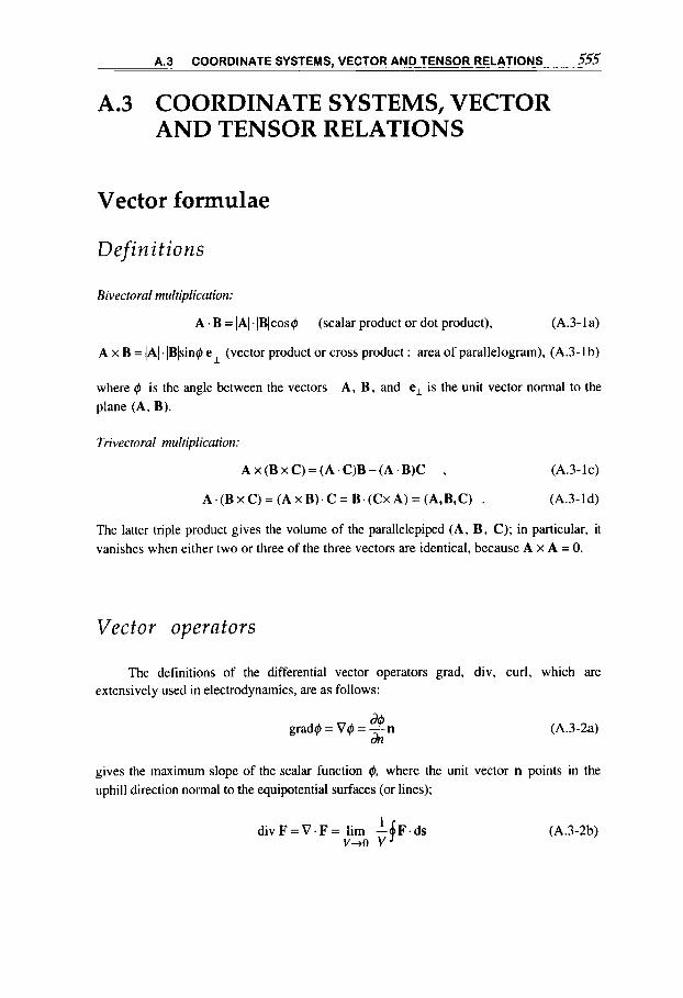
A.3 COORDINATE SYSTEMS, VECTOR AND TENSOR RELATIONS 555
A.3 COORDINATE SYSTEMS, VECTOR AND TENSOR RELATIONS
Vector formulae
Defini t ions
Bivectoral multiplication:
A . B = IAl.IBlcos@ (scalar product or dot product), (A.3-la)
A x B = (AI.IBlsin@ el (vector product or cross product : area of parallelogram), (A.3-lb)
where @ is the angle between the vectors plane (A, B).
A , B , and e, is the unit vector normal to the
Trivectoral multiplication:
A x (B x C) = ( A . C)B - (A . B)C , (A.3-lc)
(A.3-ld) A . (B x C) = (A x B) . C = B , (CX A) = (A, B, C) .
The latter triple product gives the volume of the parallelepiped (A, B, C); in particular, it vanishes when either two or three of the three vectors are identical, because A x A = 0.
Vector opera tors
The definitions of the differential vector operators grad, div, curl, which are extensively used in electrodynamics, are as follows:
grad@ = V@ = - a@ n (A.3-2a) h
gives the maximum slope of the scalar function @, where the unit vector n points in the uphill direction normal to the equipotential surfaces (or lines);
(A.3-2b) I
v+o v d i v F = V . F = lim - fF .ds
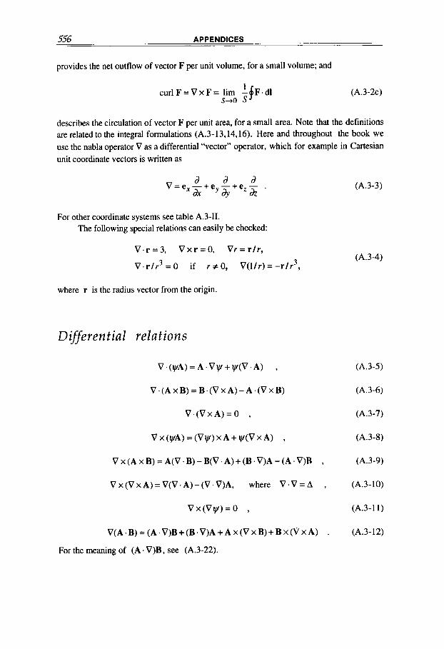
556 APPENDICES
provides the net outflow of vector F per unit volume, for a small volume; and
1 s+o s c u r l F = V x F = lim - fF .d l (A.3-2~)
describes the circulation of vector F per unit area, for a small area. Note that the definitions are related to the integral formulations (A.3-13,14,16). Here and throughout the book we use the nabla operator V as a differential “vector” operator, which for example in Cartesian unit coordinate vectors is written as
a a a dx y d y dz
V = e x - + e -+ee,-
For other coordinate systems see table A.3-11. The following special relations can easily be checked:
V . r = 3 , V x r = 0 , V r = r / r ,
v . r / r 3 = O if r #o, V ( l / r ) = - r / r , 3
(A.3-3)
(A. 3-4)
where r is the radius vector from the origin.
Differential relations
V . ( v A ) = A . V v + v ( V . A ) , (A.3-5)
V .(A x B) = B.(V x A)- A . (V X B) (A. 3 -6)
V . ( V x A ) = O , (A.3-7)
v x (vA) = (V v) x A + y ( V x A) , (A. 3-8)
V x (A x B) = A(V .B) - B(V . A ) + (B.V)A - (A .V)B , (A.3-9)
V x ( V x A ) = V ( V . A ) - ( V . V ) A , where V . V = A , (A.3- 10)
V x ( V y ) = O , (A.3-11)
V( A * B) = ( A . V)B + (B . V)A + A x (V x B) + B x (V x A ) . (A.3- 12)
For the meaning of (A. V)B, see (A.3-22).

A.3 COORDINATE SYSTEMS, VECTOR AND TENSOR RELATIONS 557
In tegral relations
Along a curve limited by two points in space A, B:
y V y . d l = y ( B ) - y ( A ) (gradient theorem) . A
Over a surface S bounded by a closed curve C:
j ( V x A ) . d s = f A . d l (Stokes' theorem) , S C
Over a volume V bounded by a closed surface S:
I ( V . A ) d V = f A . d s (Gauss' theorem) , V S
j ( V x A)d V = f d s x A , V S
(A.3-13)
(A.3-14)
(A.3-15)
(A.3- 16)
(A.3-17)
(A.3- 18)
(A.3-19a)
j [ A x (V x B) + B x (V x A) - A(V .B) - B(V . A)]dV = $(A. B)ds V S
- fB(A.ds) - fA(B.ds) , (A.3-19b) S S
I(vt//.v$ + yA$)dV = f J,V&ls (Green's theorems) V S
(A.3-20a)
[from (A.3-5) with A = V$ and (A.3-16)],
(A.3-20b)
[from (A.3-20a) subtracting the same with y, $ interchanged].
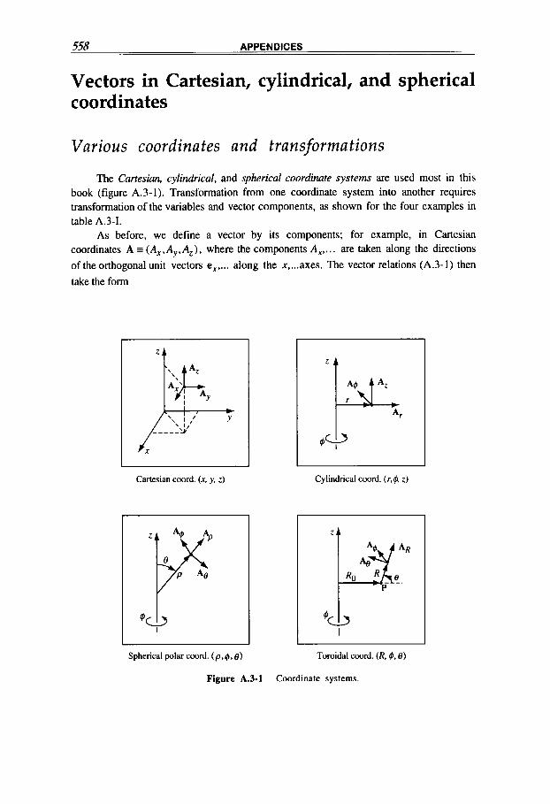
558 APPENDICES
Vectors in Cartesian, cylindrical, and spherical coordinates
Various coordinates and transformations The Cartesian, cylindrical, and spherical coordinate systems are used most in this
book (figure A.3- 1). Transformation from one coordinate system into another requires transformation of the variables and vector components, as shown for the four examples in table A.3-I.
As before, we define a vector by its components; for example, in Cartesian coordinates A = (Ax,Ay,Az) , where the components Ax, ... are taken along the directions of the orthogonal unit vectors e x , ... along the x , ... axes. The vector relations (A.3-1) then take the form
Cartesian coord. (x. Y, Z )
Spherical polar coord. ( p . $ . e )
Cylindrical coord. ( r ,4 z )
I
Toroidal coord. (R. $, 0)
Figure A.3-1 Coordinate systems.

A.3 COORDINATE SYSTEMS, VECTOR AND TENSOR RELATIONS 559
A x B = (AyBZ - ByAz)ex + (A , Bx - BzAx)ey + (A, By - BxAy)ez =
A . B = AxBx + A , B y +AzBz ,
ex ey
A, A,
Bx By
A.(BxC)=(A,B ,C)= Ax A, A,
c x c y cz B, By Bz .
(A.3-21a)
(A .3-2 1 b)
(A.3-21~)
Table A.3-I Transformations of coordinates and vector components
Cartesian (x.y,z) to cylindrical (r,@.z)
x = r c o s q
y=rs in@
z = z
A, = A, cosQ+ A, sin 4 A+ =-A, sin 4 +A, cos4
A, = A 2
Cartesian (x,v.z) to spherical ( p , @ , @
x = p i n e cos@
y = psino sin4
Ap = A,sinBcosO+A,sinBsinO+A,cose
A, =A,cos8cos4+Avcos8sing-A,sinB
A$ = -A,sin@+A,cosg
= p o s e
Cylindrical ( r .4 , z ) to Cartesian (x ,y ,z )
r = ( x 2 + y 2 ) ' / 2
tan 4 = y I x
z = z A, = A , + - A $ ~
A, = A, f + A@ 4 A, = A ,
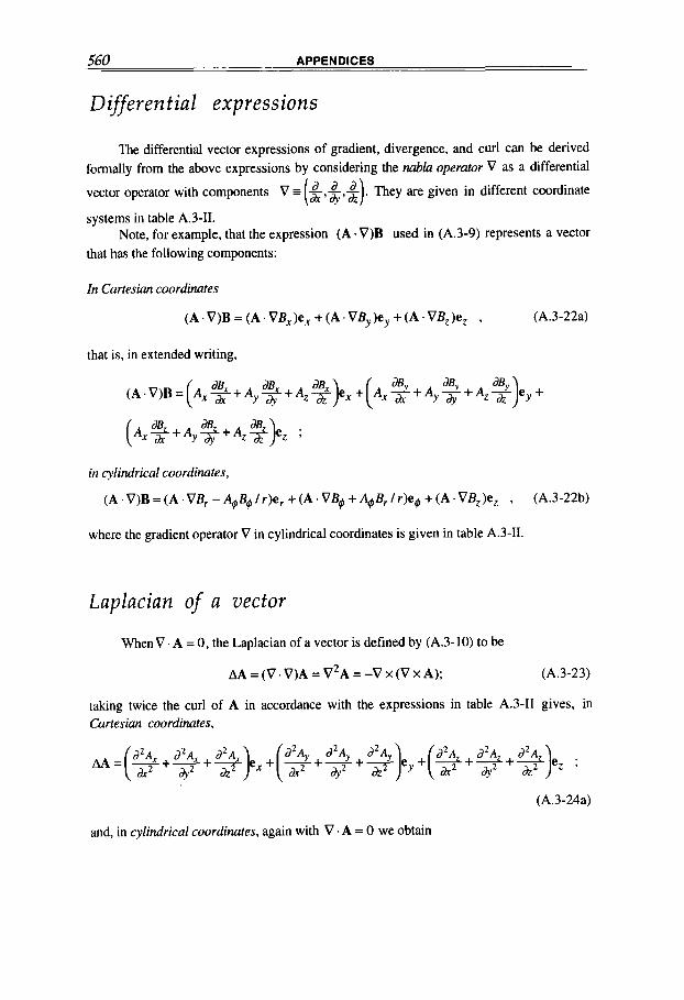
560 APPENDICES
Differential expressions
The differential vector expressions of gradient, divergence, and curl can be derived formally from the above expressions by considering the nabh operator V as a differential
vector operator with components V = (&,$,-$). They are given in different coordinate
systems in table A.3-11. Note, for example, that the expression ( A . V ) B used in (A.3-9) represents a vector
that has the following components:
In Cartesian coordinates
( A . V ) B = ( A . V B , ) e , + ( A . V B y ) e y + ( A . V B , ) e , , (A.3-22a)
that is, in extended writing,
( A . v ) B = ( A ~ % + A - + A - e x + A,$+A Y a y Y + A z m ey+ Y a y dBx Z d z ( dB dB dB 1
(A, 2 + Ay% + A, %)ez ;
in cylindrical coordinates,
( A . V ) B = ( A . V B , -%B#lr)e, + ( A . V B @ ++B,lr)eg + (A .VB, )e , , (A.3-22b)
where the gradient operator V in cylindrical coordinates is given in table A.3-11.
Laplacian of a vector
WhenV. A = 0, the Laplacian of a vector is defined by (A.3-10) to be
AA = ( v . V ) A = V ~ A = -V x (V X A ) ; (A.3-23)
taking twice the curl of A in accordance with the expressions in table A.3-I1 gives, in Cartesian coordinates,
(A.3-24a)
and, in cylindrical coordinates, again with V . A = 0 we obtain
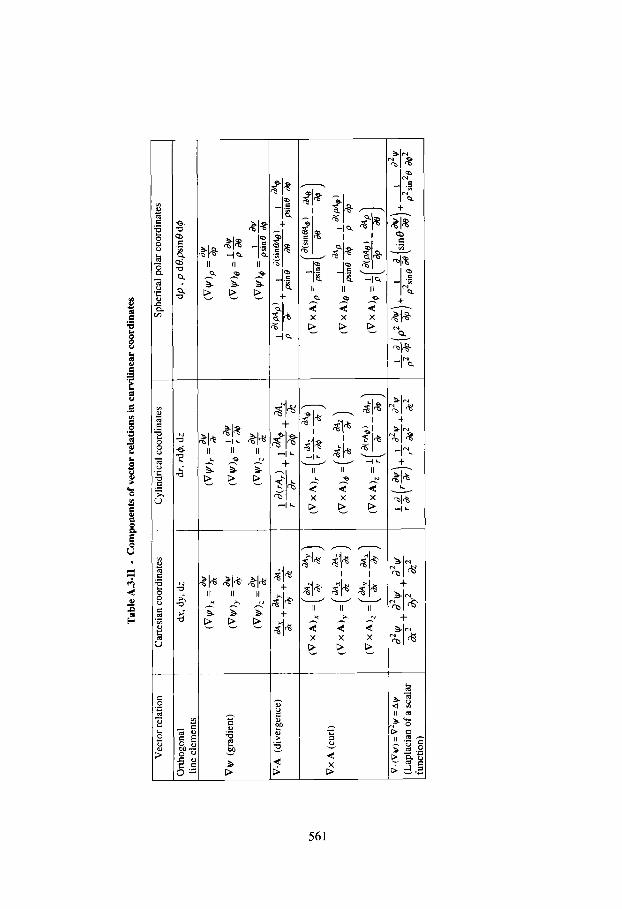
Tab
le A
.3-1
1 - C
ompo
nent
s of ve
ctor
rel
atio
ns i
n cu
rvili
nea
r coo
rdin
ates
Vec
tor
rela
tion
Ort
hogo
nal
line
elem
ents
Vly
(gr
adie
nt)
V.A
(di
verg
ence
)
Vx
A (
curl
)
V.(
Vv
) = V
2v =
Aly
(Lap
laci
an of a
scal
ar
func
tion
)
Car
tesi
an c
oord
inat
es
dx, d
y, d
:
Cyl
indr
ical
coo
rdin
ates
dr, r
d@
, dz
Sphe
rica
l pol
ar c
oord
inat
es
dp
. p d
@,p
sin€
Jd@
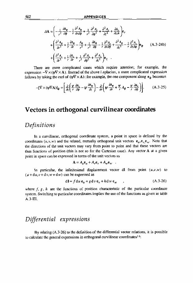
562 APPENDICES
+
+($+j-$ JA +1 r2
+
(A.3-24b)
There are more complicated cases which require attention; for example, the expression -V x (@ x A ) . Instead of the above Laplacian, a more complicated expression follows by taking the curl of (fl x A): for example, the one component along eg becomes
Vectors in orthogonal curvilinear coordinates
Def i n i t io n s
In a curvilinear, orthogonal coordinate system, a point in space is defined by the coordinates (u,v, w) and the related, mutually orthogonal unit vectors e,,e,,e,. Note that the directions of the unit vectors may vary from point to point and that these vectors are thus functions of position (this is not so for the Cartesian case). Any vector A at a given point in space can be expressed in terms of the unit vectors as
A = Aueu + Avev + Awew .
In particular, the infinitesimal displacement vector dl from point (u,v,w) to ( u + du,v + d v,w + dw) can be expressed as
d l = f d u e, + g d v e v + h d w e w , (A.3-26)
where f, g , h are the functions of position characteristic of the particular coordinate system. Switching to particular coordinates implies the use of the functions as given in table A.3-111.
Differential expressions
By relating (A.3-26) to the definition of the differential vector relations, it is possible to calculate the general expressions in orthogonal curvilinear coordinates'?
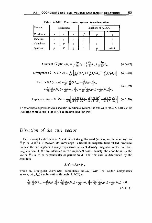
A.3 COORDINATE SYSTEMS, VECTOR AND TENSOR RELATIONS 563
System Coordinates Functions of position I I Curvilinear
Cylindrical r 2 r
Spherical P e I P psino
(A.3-27) Gradient : Vyl(u,v,w) = --e, 1 J y l +--e, 1 dy/ +L*ew f d u g d v h &
Divergence : V.A(u,v,w) = ~ [ ~ ( g h A , ) + $ ( F A , ) + $ ( f g A , ) ] (A.3-28)
Curl : V x A(u,v,w) = &[$(hA,) - x ( g A , ) ] e , d
(A.3-29)
L a p l a c i a n : A y / = V . V y l = l [ - d ( g h d V ) -- +- d ( j h d V ) -- +- d ( fgdV)] -- (A.3-30) f g h d u f d u d v g d v A h &
To refer these expressions to a specific coordinate system, the values in table A.3-111 can be used (the expressions in table A.3-I1 are obtained like this).
Direction of the curl vector Determining the direction of V x A is not straightforward (as it is, on the contrary, for
Vyl or A x B). However, its knowledge is useful in magnetic-field-related problems because the curl appears in many expressions (current density, magnetic vector potential, magnetic force). We are interested in two important cases, namely, the conditions for the vector V x A to be perpendicular or parallel to A. The first case is determined by the condition
A . ( V x A ) = O ,
which in orthogonal curvilinear coordinates (u,v,w) with the vector components A I (Au,AL,,Aw) can be written through (A.3-29) as
d fs
(A.3-3 I)
A d A d $[ z(M, - $(gA, I] + $[ x ( f A u ) - a4 (M,)] + - z ( f A u ) ] = 0.

564 APPENDICES
It is immediately clear that this equation is satisfied when any two of the three components A,,A,,A, simultaneously vanish. In other words, V x A is orthogonal to any vector field A whose direction coincides with one of the unit vectors e,,e,, or e, of any orthogonal curvilinear coordinate system (for example, in cylindrical coordinates, if A = $eq is purely azimuthal). If this is not the case, there may still exist surfaces in space at every point on which the orthogonality is obtained; in fact, consider A I A(u,v,w), then (A.3- 3 1) may transform into the equation of such a surface.
The vector V x A is parallel to A when
A x ( V X A ) = O . (A.3-3 2)
This case is discussed in section 7.4, since it pertains to the concept of force-free fields.
Matrices and tensors
Definitions
A rectangular array of parameters (real or complex) ordered in m rows and n columns is called a mafrix. For example, for a square, tridimensional matrix with m,n = 3 we write
(A.3-33)
and the element in the ith row andjth columns is written Su. Matrices occur in our book in
the solution of systems of linear equations and in the transformation of vectors. As an example of the matrix algebra, we recall the rules for addition and multiplication of two matrices. The sum
involves two matrices with the same order m x n and defines a matrix [ A ] whose ijth elements are the sum of the ijth elements of the matrices [Sl and [ B ] :
A,. = S. . + B.. (A.3-34b) 0 'J I / '
The multiplication of two matrices
[Almxp = [Slmxn[Blnxp (A.3-35a)
results in a matrix where the Au element is the sum of the products of the corresponding
elements of the ith row of [Sl and thejth column of [B] :
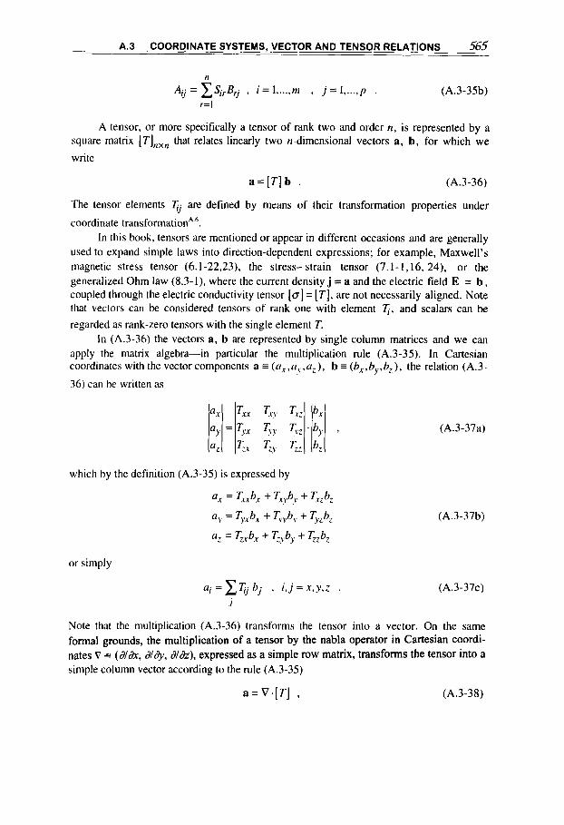
A.3 COORDINATE SYSTEMS, VECTOR AND TENSOR RELATIONS 565
n
A- rl = C S ; , B ~ ~ , i = I ,..., m , j = I ,.... p , (A.3-35b) r=l
A tensor, or more specifically a tensor of rank two and order n, is represented by a square matrix [TI,,, that relates linearly two n-dimensional vectors a, b, for which we
write
a = [ T ] b . (A.3-36)
The tensor elements qj are defined by means of their transformation properties under
coordinate transformationA '. In this book, tensors are mentioned or appear in different occasions and are generally
used to expand simple laws into direction-dependent expressions; for example, Maxwell's magnetic stress tensor (6.1-22,23), the stress- strain tensor (7.1-1,16, 24), or the generalized Ohm law (8.3-1). where the current density j = a and the electric field E = b , coupled through the electric conductivity tensor [o] = [TI, are not necessarily aligned. Note that vectors can be considered tensors of rank one with element q, and scalars can be regarded as rank-zero tensors with the single element T.
In (A.3-36) the vectors a, b are represented by single column matrices and we can apply the matrix algebra-in particular the multiplication rule (A.3-35). In Cartesian coordinates with the vector components a = (ax,av,az), b = (bx,by,bz), the relation (A.3-
36) can be written as
which by the definition (A.3-35) is expressed by
a, = T,, b, + Txy by + TXz bz
a,, = Tyxbx + Tvyby .. + Tvzbz aZ = T3bX + cyby + czbz . ,
or simply
(A.3-37b)
(A.3-37~)
Note that the multiplication (A.3-36) transforms the tensor into a vector. On the same formal grounds, the multiplication of a tensor by the nabla operator in Cartesian coordi- nates v = (d&, d/o?y, a/&), expressed as a simple row matrix, transforms the tensor into a simple column vector according to the rule (A.3-35)
a = V . [ T ] , (A.3-38)

566 APPENDICES
as detailed, for example, by the elastic equilibrium equations (7.1-1 1,12).
Transformations between coordinate systems
A vector a is related to a coordinate system through its components. If the coordinate system changes (for example, through rotation) into a primed system, also the vector components change, although the vector remains the same. It is to be expected that this transformation is described by a matrix [S] and that we can write, similarly to (A.3-36,37),
a'= [S] a (A.3-39a)
or
(A.3-39b)
For example, in a two-dimensional Cartesian system changed by rotation through an angle qit is
(A.3-39~)
as can easily be checked.
system. For a second-rank tensor the new tensor elements are expressed as a double sum Similarly, also the elements of a tensor are transformed when changing coordinate
(A.3-40)
In particular, it can be shown that for a so-called Hermitian tensor (see definition at the end of this subsection) there exists in general a new coordinate system, and consequently a transformation matrix [Sl, where the tensor will be diagonalized. This means that the matrix array representing the new tensor has nonzero elements along its diagonal; for example, in three dimensions the matrix has only three elements
(A. 3-4 1 a)
where the ki are called the eigenvalues of the original tensor [a, prior to transformation. Due to its importance, we give here the recipe for obtaining the diagonalization of a
tridimensional tensor, and we refer to the for the proof and for further details on tensors. The eigenvalues Ai are (here) the roots of the third-order equation defined by the determinant

A.4 SOME SOLUTIONS OF SECOND-ORDER DIFFERENTIAL EQUATIONS 567
T I - n T12 T13
T21 T22 - T23
T31 ?32 ? 3 3 - n d e t ,
= O (A. 3-4 1 b)
[for the unfolding of a determinant see in (A.3-21b)l. But what is the transformation matrix [S] that transforms the original coordinate system into the final system, in particular transforms the unit vectors e; of the original system into the new e l , which in this case are called unit eigenvectors? The three elements Sc transforming the first unit vector,
T 1 1 - 4 T12 T13
T2 I T22 -A1 T23
T3 I T32 ? 3 3 - A l
(A. 3-42a)
SI 1
. 4 2 = O . (A. 3-42b)
s13
are obtained from the three linear homogeneous equations defined by the matrix notation
Normalization into unit vectors in addition requires
$1 + $2 + $3 = 0 . (A.3-42~)
The other matrix elements S 2 j , S3j and the two unit vectors e$,ej are obtained similarly.
The (three-dimensional ) diagonalization procedure is thus fully outlined (extension to other dimensions is straightforward).
The matrices of interest in this book are typically Hermitian square matrices defined in general by elements that are equal to their complex conjugate transpose: = _T:; (see
section 3.1). In particular, when the elements are real, the Hermitian matrices are symmetric, qj = Ti;. The eigenvalues A; of a Hermitian or symmetric matrix are always
real numbers and the related eigenvectors are orthogonal (these properties can be useful in the diagonalization procedure).
A.4 SOME SOLUTIONS OF SECOND-ORDER DIFFERENTIAL EQUATIONS
In consideration of the frequent reference made in the main text to specific solutions of some differential equations, we present a brief (neither complete nor rigorous) review regarding the most important. We refer to the extensive literature on mathematical physics for a complete discussion.

568 APPENDICES
Pertinent differential equations
Some of the most important quantities or functions U considered in the main text-in particular, the magnetic field components-can be found as solutions of second-order, linear, partial differential equations. In two-dimensional Cartesian coordinates these equations can be written in the general form
a- a2u + b- a2u + c- a2u + d - + du e - au + jU = F ( x , y ) d x 2 hay J y 2 ?v
(A.4-1)
(The extension of this equation to more variables is straightforward.) The equation is said to be linear if it is linear in U and all its derivatives; it is termed as homogeneous if F = 0, otherwise it is nonhomogeneous.
The classification is determined by the coefficients a,b,c of the highest partial derivatives, and the equation is said to be
elliptic, if b2 < 4ac ,
hyperbolic, if b2 > 4ac ,
parabolic, if b =4ac . 2
(A.4-2)
More in general, these coefficients can be functions of x and y ; they may even contain U explicitly, in which case the equations are nonlinear.
Elliptic di$erential equations are generally associated with steady-state problems and require the boundary condition to be fixed, that is, they require the function U or its derivatives to be predetermined on the boundary of interest [see (A.4-6, to 8)]. Relatively simple examples are the Laplace equation (2.1-3) for the magnetic scalar potential, or the Poisson equation (2.2- 19) for the magnetic vector potential components; for example, the latter relates to the general form (A.4-1) by taking a, c = 1, and b, d , e f = 0:
d2U d2U -+2= F ( x , y ) . dx2 ?v
(A.4-3)
Hyperbolic equations are generally related to propagation problems and require a knowledge of certain initial values and often of boundary values as well. A typical example is the electromagnetic wave equation (3.3-1,2). With reference to (A.4-1) and with the time variable g t = y , the simplest hyperbolic (wave) equation is
(A.4-4)
where p 2 is a coefficient. Parabolic equations are typically associated with diffusion problems and define a
(penetration) velocity that is small compared to the time variation of the main quantity and its associated velocity. An example is the magnetic diffusion equation (4.2-3), with the

A.4 SOME SOLUTIONS OF SECOND-ORDER DIFFERENTIAL EQUATIONS 569
slow penetration velocity of the field into the current-canying conductor and the propagation velocity of the field in the surrounding space (which is infinite in the quasistationary approximation). With reference to (A.4-1) the simplest parabolic (diffusion) equation takes the form
q 7 - z - o 2a2u au - , (A.4-5) dx
where q2 is a coefficient. For the solution of parabolic as well as hyperbolic equations, a knowledge of a
mixture of initial and boundary values is generally required. In fact, it is most convenient to solve the partial differential equations (A.4- I ) in direct conjunction with the associated initial and boundary value conditions. The general form of the boundary conditions can be specified as
Dirichlet boundary condition U = f ( 1 )
(first kind), (A.4-6)
Neumann boundary condition
0 mixed boundary (or Robin) condition 2 + rn(f)U = k(1)
= h(1) (A.4-7)
(second kind),
(A.4- 8) (third kind),
where n denotes the normal to the boundary, and f is a length measurement along the boundary. When h, k vanish, homogeneous conditions are obtained.
Laplace equation
The solution of the Laplace equation
A U = O (A.4-9)
can be tackled through various methods. For magnetic scalar potential problems, some useful methods are:
(a) the method of separation of variables; (b) the method of conformal transformation (for two-dimensional plane geometries); (c) the method of series expansions (for approximated solutions); (d) Green’s function ~nethod~.~.~.’.
The method of conformal transformation [method (b)] is illustrated with the parallel transmission line problem in section 2.1. Method (c) is appropriate at small distances, where the potential is developed into a series and in this form inserted into the Laplace
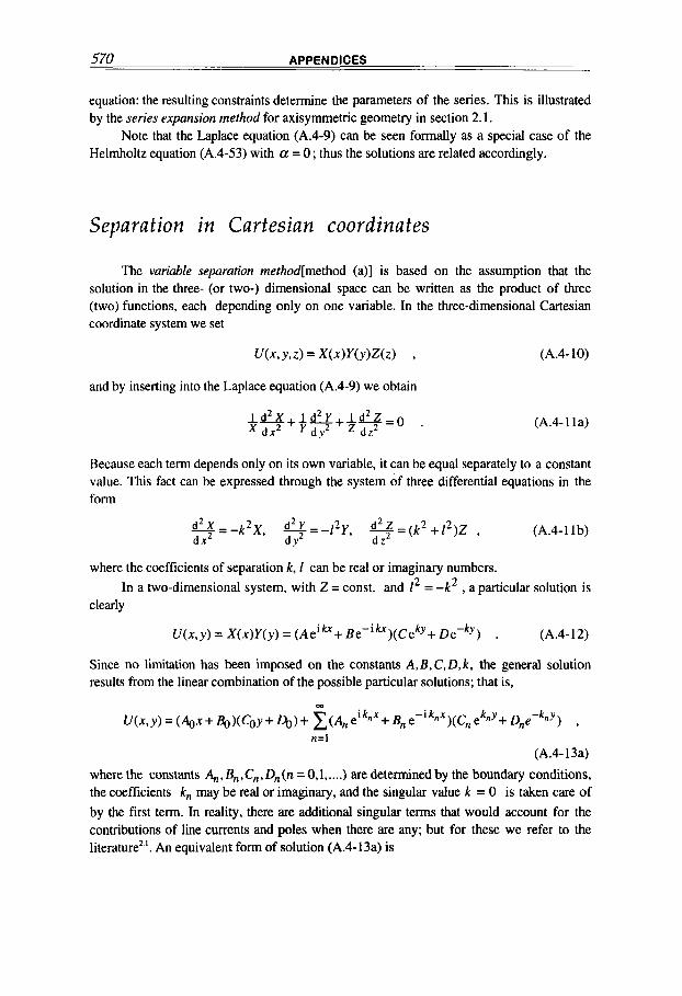
570 APPENDICES
equation: the resulting constraints determine the parameters of the series. This is illustrated by the series expansion method for axisymmetric geometry in section 2.1.
Note that the Laplace equation (A.4-9) can be seen formally as a special case of the Helmholtz equation (A.4-53) with a = 0; thus the solutions are related accordingly.
Separation in Cartesian coordinates
The variable separation rnethod[method (a)] is based on the assumption that the solution in the three- (or two-) dimensional space can be written as the product of three (two) functions, each depending only on one variable. In the three-dimensional Cartesian coordinate system we set
and by inserting into the Laplace equation (A.4-9) we obtain
I d 2 X ; l d 2 1 ' + L & = o . dx2 l ' d y 2 d z 2
(A.4-1 la)
Because each term depends only on its own variable, it can be equal separately to a constant value. This fact can be expressed through the system of three differential equations in the form
where the coefficients of separation k, 1 can be real or imaginary numbers.
clearly
2 In a two-dimensional system, with Z = const. and 1 = -k2 , a particular solution is
U(x ,y ) = X(x)Y(y) = (Aeih+ Be-ih)(Ceky+ De-ky) . (A.4-12)
Since no limitation has been imposed on the constants A,B,C,D,k, the general solution results from the linear combination of the possible particular solutions; that is,
m
U(x,y)=(Agx+Bg)(Coy+&)+ ~ ( A n e i k n x + B , e - i k , * ) ( C , e k n y + D n e - k n Y ) , n=l
(A.4- 13a)
where the constants An,Bn,C,,,Dn(n = O,l, .... ) are determined by the boundary conditions, the coefficients kn may be real or imaginary, and the singular value k = 0 is taken care of by the first term. In reality, there are additional singular terms that would account for the contributions of line currents and poles when there are any; but for these we refer to the literature2.'. An equivalent form of solution (A.4-13a) is

A.4 SOME SOLUTIONS OF SECOND-ORDER DIFFERENTIAL EQUATIONS 571
m
U ( x , y ) = (Aox+Bo)(CO~+&)+ C(A,sinnx+ B,,cosnx)(C,,sinhny+ D,,coshny) , n=l
(A.4- 1 3 b) where in this special case (for a problem periodic along x) we have substituted k,, + n ,
and have thus obtained a Fourier series periodic in x for any value of y in the range 0 I y < m . Clearly, the complementary solution, where x and y are interchanged, is also valid.
The constants A,,, B,,, C,, , Dn can be given in closed form. For a Dirichlet problem on a rectangle 0 I x I a, 0 I y I b , where, for example, we have U = f ( x ) on side y = 0 and U = 0 on the other three, we obtain the solution
m
(A.4- 1 3 ~ )
The constant A,, is determined from the condition
00
so that, as shown in (A.2-42,43),
A, = (A.4-13d) a sinh( n a $ ) IJ
When boundary conditions are given on more than one side, the solution of the Dirichlet problem is obtained by adding solutions of the type (A.4-13c,d).
It is easy to show that among the fundamental solutions of Laplace’s equation (A.4-9) we have
U = A In r , in two - dimensional geometry,
U = A- , in three - dimensional geometry, r
1 (A.4-14)
where r is the distance from the origin, in Cartesian coordinates r = J J x + y + z
Separation in cylindrical coordinates
The variable separation method can be similarly applied to other coordinate systems. In cylindrical coordinates, where the Laplace equation is
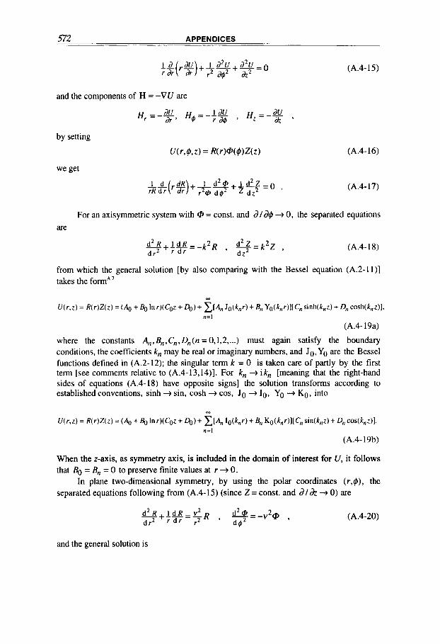
572 APPENDICES
and the components of H = -VU are
(A.4-15)
(A.4-16)
For an axisymmetric system with Q, = const. and d / d @ + 0, the separated equations are
(A.4- 18)
from which the general solution [by also comparing with the Bessel equation (A.2-1 I ) ] takes the formA.’
- U(r,z) = R(r)Z(z) = + BO Inr)(Coz + 4) + C [ A , , JO(k,r) + B, Yo(k,,r)l[C,, sinh(k,,z) + D,, cosh(k,,z)l.
,,=I
(A.4-19a)
where the constants A,, B,, C, , Dn (n = 0, I, 2, ...) must again satisfy the boundary conditions, the coefficients k, may be real or imaginary numbers, and Jo. YO are the Bessel functions defined in (A.2-12); the singular term k = 0 is taken care of partly by the first term [see comments relative to (A.4-13,14)]. For k, + i k, [meaning that the right-hand sides of equations (A.4- 18) have opposite signs] the solution transforms according to established conventions, sinh + sin, cosh + cos, JO + 10, YO + KO, into
- U(r,z) = R(r)Z(z) = (4 + 4 Inr)(Coz + DO)+ Z [ A , IO(k,r)+ B,, Ko(k,r)l[C,, sin(k,,z) + Dn cos(k,z)l.
, = I
(A.4- 19b)
When the z-axis, as symmetry axis, is included in the domain of interest for U, it follows that 4 = B, = 0 to preserve finite values at r + 0.
In plane two-dimensional symmetry, by using the polar coordinates ( r , @ ) , the separated equations following from (A.4-15) (since Z = const. and a / & + 0) are
(A.4-20)
and the general solution is
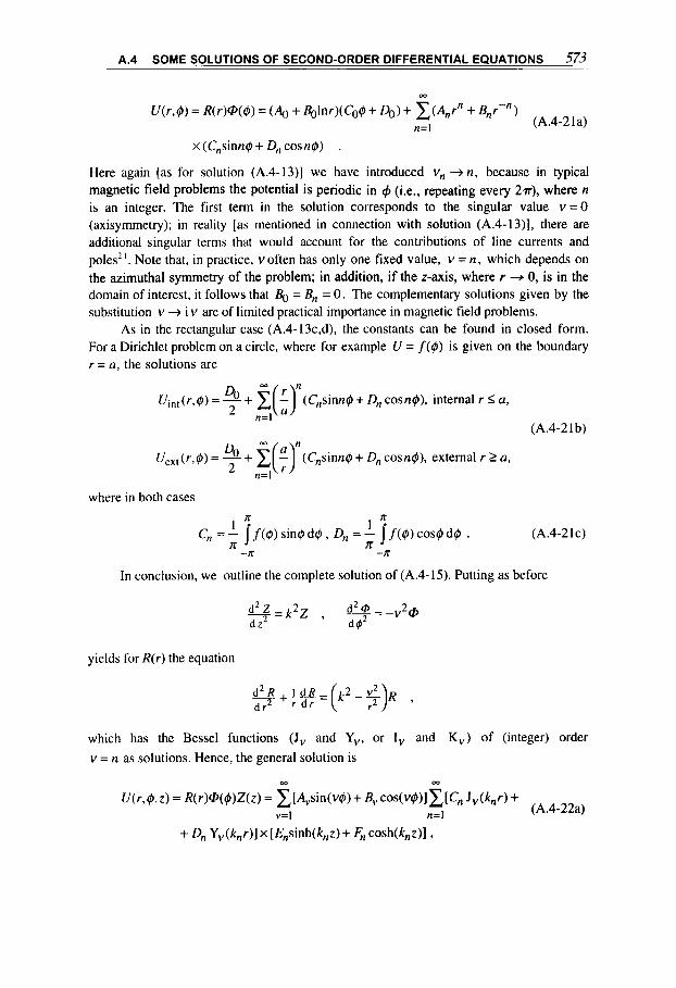
A.4 SOME SOLUTIONS OF SECOND-ORDER DIFFERENTIAL EQUATIONS 573
m
U ( r , @ ) = R(r)@(@) = (4 + Bolnr)(Co@+ &)+ C ( A n r n + B,,r-") n=l (A.4-2 la)
x(C,sinn@+ D,cosn@) .
Here again [as for solution (A.4-13)] we have introduced v,, -+ n , because in typical magnetic field problems the potential is periodic in 4 (i.e., repeating every 274 where n is an integer. The first term in the solution corresponds to the singular value v = O (axisymmetry); in reality [as mentioned in connection with solution (A.4-13)], there are additional singular terms that would account for the contributions of line currents and poles2 I . Note that, in practice, v often has only one fixed value, v = n , which depends on the azimuthal symmetry of the problem; in addition, if the z-axis, where r + 0, is in the domain of interest, it follows that & = Bn = 0. The complementary solutions given by the substitution v + i v are of limited practical importance in magnetic field problems.
As in the rectangular case (A.4-13c,d), the constants can be found in closed form. For a Dirichlet problem on a circle, where for example U = f(@) is given on the boundary r = a, the solutions are
(C,sinn@ + Dn cosn@), internal r I a, n=l 2
(A.4-21b)
where in both cases
(A.4-21~)
In conclusion, we outline the complete solution of (A.4-15). Putting as before
-- d 2 Z - k 2 2 , d 2 0 = v2@ d z 2 d G 2
yields for R(r) the equation
which has the Bessel functions (J, and Y,, or I, and K,) of (integer) order v = n as solutions. Hence, the general solution is
m m
U ( r , @ , z ) = R(r)@(@)Z(z) = x[A ,s in (v@)+ B,cos (v@)]~[C J (k ,=I n=l " "I' (A.4-22a)
+ D,, Y,(knr)]x [E,sinh(k,z)+ F, cosh(k,z)] ,
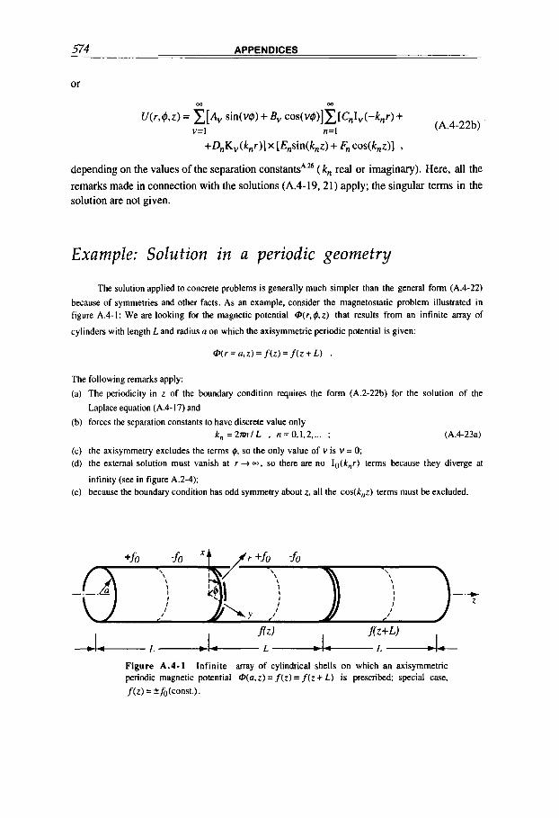
574 APPENDICES
or
m m
U(r,@,z) = C [ A V sin(@) + Ev c o s ( v @ ) ] ~ [ C n I v ( - k , , ~ ) ~ v=l n=l (A.4-22b)
+DnKv(knr)] x [Ensin(knz) + Fn cos(k,,z)] ,
depending on the values of the separation constantsA26 (k,, real or imaginary). Here, all the remarks made in connection with the solutions (A.4-19,21) apply; the singular terms in the solution are not given.
Example: Solution in a periodic geometry The solution applied to concrete problems is generally much simpler than the general form (A.4-22)
because of symmetries and other facts. As an example, consider the magnetostatic problem illustrated in figure A.4-1: We are looking for the magnetic potential dVr,@z) that results from an infinite array of
cylinders with length Land radius a on which the axisymmetric periodic potential is given:
O ( r = a , z ) = f ( z ) = f ( z + L ) .
The following remarks apply:
(a) The periodicity in z of the boundary condition requires the form (A.2-22b) for the solution of the Laplace equation (A.4- 17) and
(b) forces the separation constants to have discrete value only k n = 2 m l L , n=O,1,2 ,... ; (A.4-23a)
(c) the axisymmetry excludes the terms 4, so the only value of v is v = 0; (d) the external solution must vanish at r + -, so there are no Ig(k,r) terms because they diverge at
infinity (see in figure A.2-4); (e) because the boundary condition has odd symmetry about z, all the cos(k,z) terms must be excluded.
Figure A.4-1 Infinite array of cylindrical shells on which an axisymmetric periodic magnetic potential @(a.z) = f(z) = f ( z + L ) is prescribed; special case, f(z) = *fO(const.).
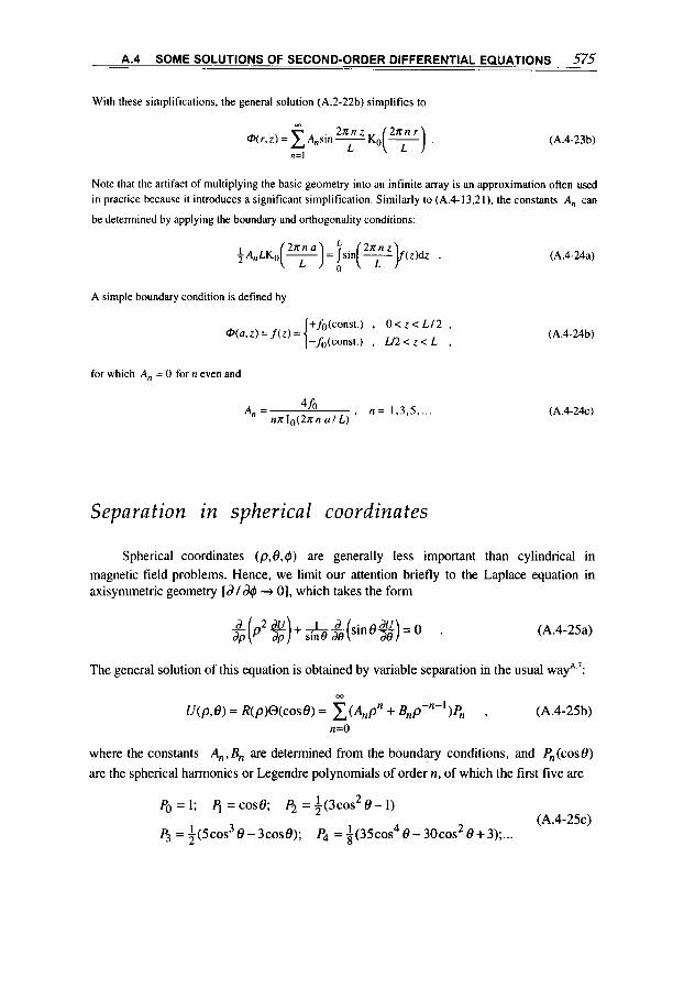
A.4 SOME SOLUTIONS OF SECOND-ORDER DIFFERENTIAL EQUATIONS 575
With these simplifications, the general solution (A.2-22b) simplifies to
m
O(r,z) = Ansin - L
n=I
(A.4-23b)
Note that the artifact of multiplying the basic geometry into an infinite array is an approximation often used in practice because it introduces a significant simplification. Similarly to (A.4-13.21). the constants An can
be determined by applying the boundary and orthogonality conditions:
A simple boundary condition is defined by
+fo(const.) , O < z < L 1 2 ,
-fo(const.) , U2 < z < L , O(a,z) = f(z) =
for which A, = 0 for n even and
n = 1.3.5, A, = 4f0 ni710(2xn u / L ) '
(A .4-24a)
(A.4-24b)
(A.4-24c)
Separation in spherical coordinates
Spherical coordinates (p , &#) are generally less important than cylindrical in magnetic field problems. Hence, we limit our attention briefly to the Laplace equation in axisymrnetric geometry [aid# + 01, which takes the form
(A.4-25a)
The general solution of this equation is obtained by variable separation in the usual wayA7:
m
U(p,O) = R(p)O(cose) = C ( A n p n + B,P-~-')P, , (A.4-25b) n=O
where the constants A,, Bn are determined from the boundary conditions, and P,(cos8) are the spherical harmonics or Legendre polynomials of order n, of which the first five are
2 p0 = 1; 4 = case; p2 = +OS 8- 1)
4 = +(5c0s3 e - ~ c o s ~ ) ; p4 = $(35c0s4 e - 3 0 ~ 0 s ~ 8 + 3); ... (A.4-25~)
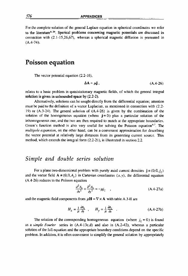
576 APPENDICES
For the complete solution of the general Laplace equation in spherical coordinates we refer to the literatureA.26. Sperical problems concerning magnetic potentials are discussed in connection with (2.1-15,26,67), whereas a spherical magnetic diffusion is presented in (A.4-74).
Poisson equation
The vector potential equation (2.2-16).
AA= p i , (A.4-26)
relates to a basic problem in quasistationary magnetic fields, of which the general integral solution is given in unbounded space by (2.2-2).
Alternatively, solutions can be sought directly from the differential equation; attention must be paid to the definition of a vector Laplacian, as mentioned in connection with (2.2- 19) or (A.3-24). The general solution of (A.4-26) is given by the combination of the solution of the homogeneous equation (where j = 0) plus a particular solution of the inhomogeneous one, and the two are then required to match at the appropriate boundaries. Green’s function method is also very useful for solving the Poisson equationA7. The multipole expansion, on the other hand, can be a convenient approximation for describing the vector potential at relatively large distances from its generating current source. This method, which extends the integral form (2.2-21). is illustrated in section 2.2.
Simple and double series solution
For a plane two-dimensional problem with purely axial current densities j I (O,O, j ,) and the vector field A a (O.O,A,) in Cartesian coordinates ( x , y ) , the differential equation (A.4-26) reduces to the Poisson equation
and the magnetic field components from pH = V x A with table A.3-I1 are
(A.4-27a)
(A.4-27b)
The solution of the corresponding homogeneous equation (where j z = 0) is found as a simple Fourier series in (A.4-13c,d) and also in (A.2-42), whereas a particular solution of the full equation and the appropriate boundary conditions depend on the specific problem. In addition, it is often convenient to simplify the general solution by appropriately

A.4 SOME SOLUTIONS OF SECOND-ORDER DIFFERENTIAL EQUATIONS 577
choosing the coordinate system in accordance with the symmetries of the problem. For example, if the solution (A.4-13) does not involve uniform fields in either the x- or y- direction, we put 4 = Co = 0, and since the origin of A, is arbitrary we take 4. L& = 0; if A, is to be odd along the x-direction it is Bn = O . Thus, the general solution of the
homogeneous equation would reduce in this case to
m
A,(x,y) = Csinnkx(G, enky+ Hn e-nky) . (A.4-28) n=l
For the same plane problem, but defined in polar coordinates (r, @), the differential equation is given in (2.2-35), and the general solution is discussed thereafter.
On the other hand, for a purely axisymmetric, azimuthal vector field, A = (O,Ag,O) with A4 = Ag(z,r) , the vector Laplacian reduces to the @component in
(A.3-24) and the corresponding Poisson equation becomes, as in (2.2-28).
(A.4-29)
The general solution results, as we know, from a combination of the solution of the homogeneous equation (where jq = 0) with a particular solution of the inhomogeneous
one. In comparing the homogeneous equation with the equivalent (A.4-15) (where did$+ 0 ) , we note the additional term - A g / r z . By proceeding as with (A.4-19), the
general homogeneous solution becomes
00
A~(z,~)=R(~)Z(Z)=(A~~+B~~-')(COZ+DD)+ C [ A n JI(knr)+BnY,(knr)lx n=l
x [Cnsinh(knz) + D, cosh(knz)] . (A.4-30)
Of more practical interest is the double Fourier series solution, sometimes called Roth's method' I. Here, one single function, represented by a double series, provides the solution over the whole domain containing free space and conductors. In fact, the method consists in establishing the solution in the form of a double series, and then fixing its constants so as to satisfy the complete equation (A.4-26), including the current sources. We illustrate this method by sketching the solution of two different problems, the first expressed in Cartesian (x ,y ) coordinates and the second in axisymmetric (r,z) cylindrical coordinates.
Example: Infinitely permeable, rectangular boundary
Consider the problem described in Cartesian (x,y)-coordinates in figure A.4-2: Find the vector potential A Z ( x , y ) within an infinitely permeable (p + -), rectangular boundary containing a current-

578 APPENDICES
carrying conductor. For the solution of the differential equation (A.4-27) we postulate the product of two
simple Fourier series, in cosines only2 I.
(A.4-31)
(the general solution would include four such double series resulting from the additional cos.sin, sincos,
and s in4n terms) so that the field components are
(A.4-32)
(A.4-33)
The boundary conditions are determined here by the fact that there are no tangential field components
at the infinitely impermeable boundary [see in (1.5-22)],
H,(any x ; y = O , b ) = O , H , , ( ~ = O , a ; a n y y ) = O , (A.4-34)
which implies
k , = ( n - l ) a / b , k , = ( rn- l )x la . (A.4-35)
The still undetermined a,,,,-coefficients are fixed by requiring the solution (A.4-31. 35) to satisfy the
Poisson equation (A.4-27): By differentiating twice we obtain
m m
1 x&, +k,2)am,, cos(k,x)cos(k,,y) = pj, . (A.4-36) m=l n=l
Figure A.4-2 Infinitely long, current-carrying conductor contained within an infinitely permeable rectangular boundary.

A.4. SOME SOLUTIONS OF SECOND-ORDER DIFFERENTIAL EQUATIONS 579
Explicit expressions for are obtained by applying the orthogonality rule of Fourier series [see, in
comparison, the orthogonality of the simple Fourier series in the integrals following (A.2-43)].
Multiplying each side by cos(kpx)cos(k,y) and integrating over the space ( u x 6 ) , which reduces to the
conductor cross section S on the right-hand side where j z is finite, yields
that is,
umqn T(ki + k i ) = p j j j z cos(k,x)cos(k,y)dxdy S
(A.4-38)
because on the left-hand side, only the integrals with the terms p = rn and s = n remain finite. The integral on the right-hand side depends on the form of S and on the functional dependence of j z , but when these are given, i t is fully determined, and so are the a,,,,-coefficients. For example, when S is rectangular with
sides (a2 - ul) x (b2 - 61). and j z constant, the result is
The first three parameters corresponding to the singular rn, n = I values require, however, both integrals to
be recalculated in the appropriate form, to obtain
(A.4-40)
and we are free to set al.1 = 0 (because a constant term in A, is irrelevant). In conclusion, the one solution
(A.4-31) with the nowdefined parameters a,,,n.k,.k, in (A.4-35, 39, 40) is valid in the whole space
( a x 6 ) . including the conductor.
Example: Axisymmetric, superconducting boundary
We now apply the double series solution method (also defined as Roth's method2.') to the problem
described in cylindrical coordinates by the Poisson equation (A.4-29) and figure A.4-3: Find the
axisymmetric vector potential A#(z,r) within an infinitely conducting (a + =) cylindrical boundary
containing a toroidal current-carrying conductor.
We proceed as we did in the previous example, only that here we postulate for the solution of (A.4-
29) the double series solution [it can be shown to represent any given function of the type of A#(z.r)]
(A.4-4 I )

580 APPENDICES
Figure A.4-3 Axisymmetric curent distribution contained in a perfectly conducting, cylindrical box.
so that the field components (2.2-27) are
m m
pHr(z,r)=---- - Ca,,,,k,, cos(knfz)Jl(knr) (A.4-42) ' m=l n=l
a(rAq) m p H Z ( z . r ) = $ 7 = Ca,,,,k,sin(k,,z)Jo(k,r) . (A.4-43)
m=I n=l
where J,. J, are the Bessel functions (A.2-12) and we have used (A.2-23), that is, J ( r J l ) l d r = rJo.
The boundary conditions require the field to be tangential on the superconducting boundary [see (1.5-
12)]; that is, they require the normal field components on the boundary to vanish,
H, (anyz; r=a)=O . H,(z=O,b;any r ) = O ,
which implies
(A.4-44)
kna = x ; , knfb = ( m - 1)n , (A.4-45)
where xfare the roots of J l [ i s . Jl(x;) = 01, given in table A.2-I. (Note that the symmetry requirements
about the axis and the midplane are implicitly taken care of by this solution.) The a,,,-coefficients are determined, as in (A.4-36). by requiring the solution (A.4-41.45) to satisfy
the Poisson equation (A.4-29): Differentiating twice and using the differential equation (A.2- I I ) with
v = l,z = knr gives
(A.4-46)
The explicit forms of the a,,,-parameters are obtained again by applying the orthogonality rule. By
multiplying each side by rsin(kpz)Jl(k,r). then integrating over the whole cylindrical space (which reduces
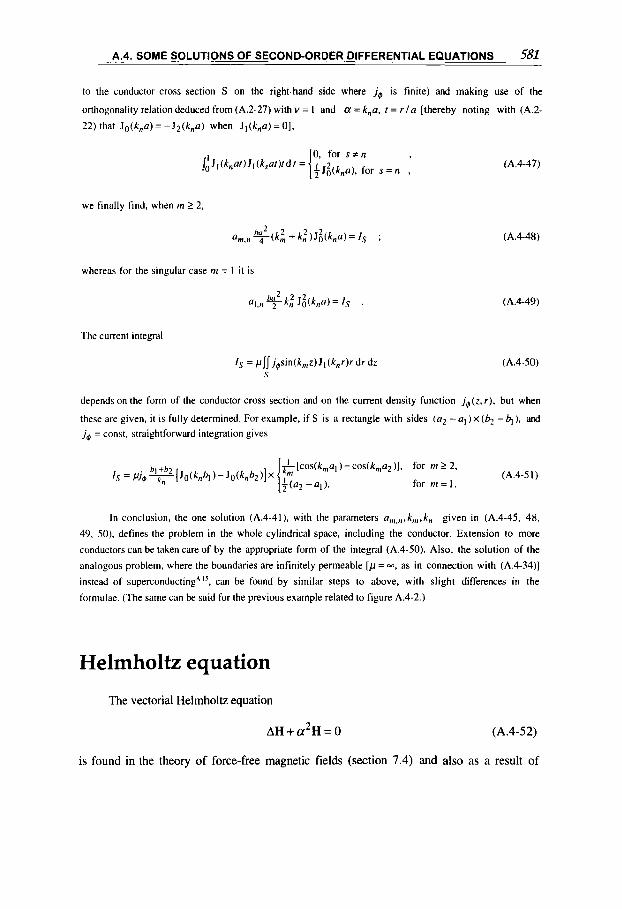
A.4. SOME SOLUTIONS OF SECOND-ORDER DIFFERENTIAL EQUATIONS 581
to the conductor cross section S on the right-hand side where j # is finite) and making use of the
orthogonality relation deduced from (A.2-27) with v = I and a = k,a, t = r / a [thereby noting with (A.2-
22) that Jo(kfln)=-J2(k,a) when J l (k ,a )=O] ,
we finally find, when m t 2,
(A.4-47)
(A.4-48)
whereas for the singular case m = 1 i t is
2 ~ 1 . ~ %k: J;(k,a)= 1s . (A.4-49)
The current integral
depends on the form of the conductor cross section and on the current density function j # ( z , r ) , but when
these are given, il is fully determined. For example, if S is a rectangle with sides (a2 - al ) x (62 - 4 ) , and j, = const, straightforward integration gives
In conclusion, the one solution (A.4-41), with the parameters ufl,,,,kn1,kn given in (A.4-45. 48,
49, 50). defines the problem i n the whole cylindrical space, including the conductor. Extension to more
conductors can be taken care of by the appropriate form of the integral (A.4-50). Also, the solution of the
analogous problem. where the boundaries are infinitely permeable [ p = -, as in connection with (A.4-34)]
instead of superconductingA Is, can be found by similar steps to above, with slight differences in the
formulae. (The same can be said for the previous example related to figure A.4-2.)
Helmholtz equation
The vectorial Helmholtz equation
A H + ~ H = O (A.4-52)
is found in the theory of force-free magnetic fields (section 7.4) and also as a result of
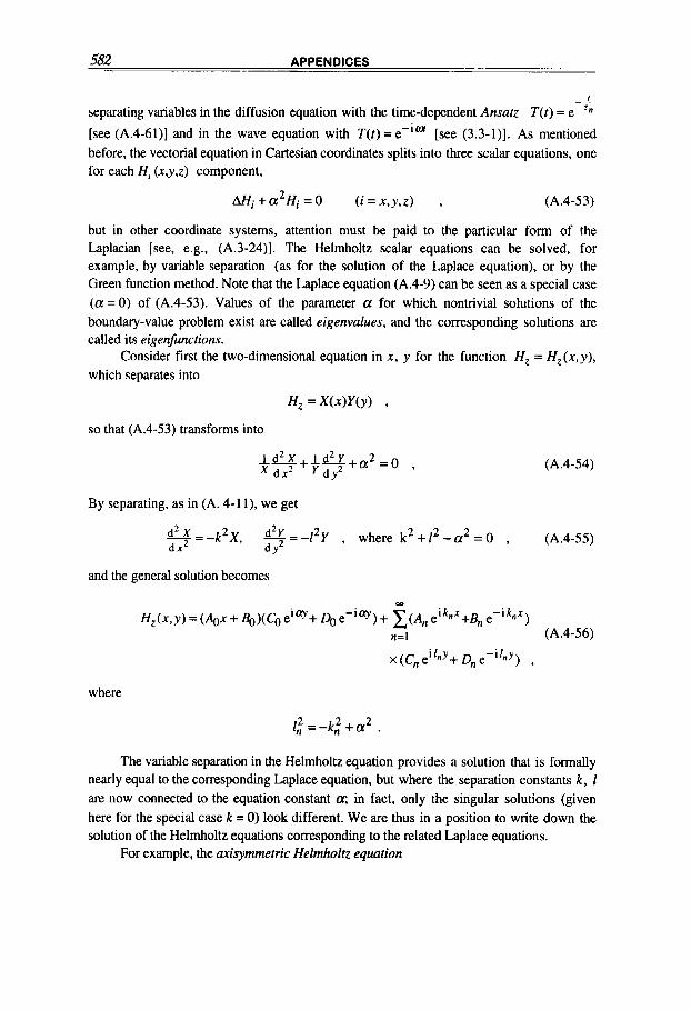
582 APPENDICES
-_ separating variables in the diffusion equation with the time-dependent Ansatz T ( t ) = e ' n
[see (A.4-61)] and in the wave equation with T(t)=e-iW [see (3.3-l)]. As mentioned before, the vectorial equation in Cartesian coordinates splits into three scalar equations, one for each Hi (x,y,z) component,
A H i + a L H i = O ( i = x , y , z ) , (A.4-53)
but in other coordinate systems, attention must be paid to the particular form of the Laplacian [see, e.g., (A.3-24)]. The Helmholtz scalar equations can be solved, for example, by variable separation (as for the solution of the Laplace equation), or by the Green function method. Note that the Laplace equation (A.4-9) can be seen as a special case (a=0) of (A.4-53). Values of the parameter a for which nontrivial solutions of the boundary-value problem exist are called eigenvulues, and the corresponding solutions are called its eigenfunctions.
Consider first the two-dimensional equation in x, y for the function H , = H,(x,y) , which separates into
Hz = X(X)Y(Y) 9
so that (A.4-53) transforms into
-- 1 d 2 X I 1 d 2 Y + a 2 = 0 , d x 2 y d y 2
(A.4-54)
By separating, as in (A. 4-1 ), we get
2 2 2 - d 2 Y --12Y , where k + I -a = O , (A.4-55) d y 2 -
and the general solution becomes
m
H,(x ,y ) = (&x + Bg) ( Co ei q+ 4 e-i q, + c ( A n ei knX+Bn e-i knx n=l (A.4-56)
where
1; =-k: +a2 .
The variable separation in the Helmholtz equation provides a solution that is formally nearly equal to the corresponding Laplace equation, but where the separation constants k , 1 are now connected to the equation constant a; in fact, only the singular solutions (given here for the special case k = 0) look different. We are thus in a position to write down the solution of the Helmholtz equations corresponding to the related Laplace equations.
For example, the misymmetric Helmholtz equation
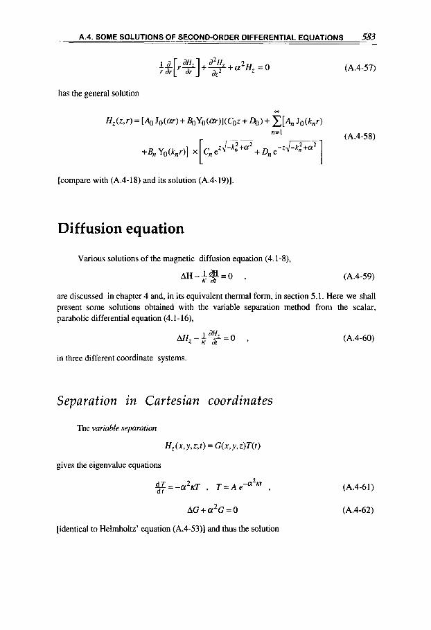
A.4. SOME SOLUTIONS OF SECOND-ORDER DIFFERENTIAL EQUATIONS 583
(A.4-57)
has the general solution
[compare with (A.4-18) and its solution (A.4-19)].
Diffusion equation
Various solutions of the magnetic diffusion equation (4.1-8),
AH--!-&=() K d r (A.4-59)
are discussed in chapter 4 and, in its equivalent thermal form, in section 5.1. Here we shall present some solutions obtained with the variable separation method from the scalar, parabolic differential equation (4.1- 16),
AHz---=o I , (A.4-60) K d f
in three different coordinate systems.
Separation in Cartesian coordinates
The variable separation
H , ( x , y , z ; r ) = G ( x , y , z ) T ( t )
gives the eigenvalue equations
dT - a 2 ~ , T = A e-a2a dr
AG+ C X ~ G = o
[identical to Helmholtz’ equation (A.4-53)] and thus the solution
(A.4-6 1 )
(A.4-62)

584 APPENDICES
m
H,(x,y,z;t) = b x + Boy + Cgz + 4 + ~AnG,,e-":' , (A.4-63) n=l
where Gn(x,y,z) are the eigenfunctions of the Helmholtz equation related to the
characteristic separation parameters a,, and the first terms represent the singular solution for a = 0. The parameters A,-J,B,J,CO,L+,,A,, and a, are fixed by the specific boundary and initial conditions. For example, with the initial condition given by H,(x,y,z;t = 0) = H,(x,y,z) within a space V it isA.'
An = jHoGndrdy& . (A.4-64) V
If the initial field H, is prescribed in the entire space, by the combination of the last two expressions we obtain the solution in closed formA.':
(A.4-65)
For the diffusion of a step-function field Ho= const. applied at time t = 0 on both
surfaces delimiting a slab at x = k d (figure 4.2-6). it is convenient to use the eigenfunction solution (A.4-63), which in the general one-dimensional case becomes
m
Hz(x,t) = &x + L& + x(Ans inanx+ Bn cosa,x)e-Kffi' . (A.4-66) n=l
Because the solution must be steady at x = 0 (i.e., [aHz/dx]x,o =0)
we f i n d 4 = 0, An = O ; and because of the boundary condition H,(fd,t) = HO for 0 I t 2 m it is +and = n a / 2 , n = 1,3, ...( odd), and L+, = Ho. Finally, the initial condition
H,(x,O) = 0 determines Bn = ( - 1 ) T 4 H ~ /na through Fourier-series summation. The solutions to other and time-dependent boundary conditions for the slab problem are given in table 4.2-1 and in (4.2-47), (5.1-47).
n+l
Separation in cylindrical coordinates
The solution of the diffusion equation in other than Cartesian coordinates requires the separated equation (A.4-63) to be applied accordingly. For example, consider the simple one-dimensional diffusion equation in the cylindrical coordinate r, (4.3-9,
(A.4-67)
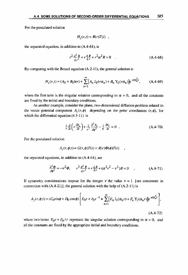
. .. A.4. SOME SOLUTIONS OF SECOND-ORDER DIFFERENTIAL EQUATIONS 585 -~
For the postulated solution
the separated equation, in addition to (A.4-61), is
2 d 2 R 2 2 r - + r Q R + r a R = O . dr2 d r
(A.4-68)
By comparing with the Bessel equation (A.2-1 l), the general solution is
m
H z ( r , f ) = (4 + Bglnr)+ c [ A n J o ( r a , ) + B,, Y ~ ( r a , ) ] e - ~ ~ ~ ' , (A.4-69) n=l
where the first term is the singular solution corresponding to a = 0, and all the constants are fixed by the initial and boundary conditions.
As another example, consider the plane, two-dimensional diffusion problem related to the vector potential component A z ( r , @ ) depending on the polar coordinates (r ,$) , for which the differential equation (4.3-1 1) is
For the postulated solution
the separated equations, in addition to (A.4-61), are
(A.4-70)
(A.4-7 1)
If symmetry considerations impose for the integer v the value v = 1 [see comments in connection with (A.4-21)], the general solution with the help of (A.2-11) is
r -.
(A.4-72)
where two terms Eor + Fo I r represent the singular solution corresponding to a = 0, and all the constants are fixed by the appropriate initial and boundary conditions,
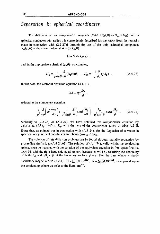
586 APPENDICES
Separation in spherical coordinates
The diffusion of an anisymmetric magnetic field H(p,@ = ( Hp,O, H e ) into a
spherical conductor with radius a is conveniently described [as we know from the remarks made in connection with (2.2-27)] through the use of the only azimuthal component %(p,f3) of the vector potential A = (O,%,O):
H = V x ( % e g ) . and, in the appropriate spherical (p,O)- coordinates,
I d Hp =-- (A@@ , He =----(p%) .
psino df3 P dP (A .4-73)
In this case, the vectorial diffusion equation (4.1- 13),
reduces to the component equation
Similarly to (2.2-28) or (A.3-24). we have obtained this axisymmetric equation by calculating (AA)@ = -(V x H)g with the help of the components given in table A.3-11.
[Note that, as pointed out in connection with (A.3-24), for the Laplacian of a vector in spherical or cylindrical coordinates we obtain (AA)@ # % . I
The solution of this diffusion problem can be found through variable separation by proceeding similarly to (A.4-24.61): The solution of (A.4-74). valid within the conducting sphere, must be matched with the solution of the equivalent equation in free space [that is, (A.4-74) with the right-hand side equal to zero because Q = 01 by requiring the continuity of both Ag and 3% lap at the boundary surface p = a. For the case where a steady
oscillatory magnetic field (3.2-1). H = Ho(p,B)eim, A = Ao(p.f3)eim, is imposed upon the conducting sphere we refer to the literatureA.I4.

BIBLIOGRAPHY
This section contains the references ordered by the chapter in which they are of relevance or are first mentioned. It also includes books, not necessarily referred to in the text, that might be useful for a general introduction or more extensive study on each chapter's subject or on magnetic fields in general (the choice of these titles is subjective and may not give appropriate credit to similar books).
Chapter 1: FOUNDATION OF MAGNETIC FIELD THEORY
1.1. J.C. Maxwell, A Treatise on Electricity and Magnetism, Vol. 1 and 2 (Clarendon Press, Oxford, 1892; Dover, New York, 1954) [Part I, Electrostatics; Part 11, Electrokinematics; Part III, Magnetism; Part IV, Electromagnetism]
1.2. A. Sommerfeld, Electrodynamics (Academic Press, New York, 1975)
1.3. W.R. Smythe, Static and Dynamic Electricity (McGraw-Hill, New York, 1950) [In particular: Chs. 4 and 5 , Two- and Three-Dimensional Potential Distributions; Ch. 7 , Magnetic Interaction of Currents; Ch. 8, Electromagnetic Induction; Ch. 11, Eddy Currents; Ch. 12, Magnetism; Ch. 16, Special Relativity and the Motion of Charged Particles]
1.4. J.D. Jackson, Classical Electrodynamics (Wiley, New York, 1962)
1.5. W.K.H. Panofsky and M. Phillips, Classical Electricity and Magnetism (Addison- Wesley, Reading, Massachusetts, 1962)
1.6. D.J. Griffiths, Introduction to Electrodynamics (Prentice-Hall, Englewood Cliffs, New Jersey, 1989)
1.7. G.P. Harnwell, Principles of Electricity and Electromagnetism (McGraw-Hill, New York, 1949) [In particular: Ch. 5, Nonohmic Circuit Elements and Alternating
5 87
M4GNETICFIELDS: A Comprehensive Theoretical Treatise for Practical Use Heinz E. Knoepfel
Copyright Q 2000 by John Wiley & Sons, Inc

588 BIBLIOGRAPHY
Currents; Ch. 9, Electromagnetic Effects of Steady Currents; Ch. 10, Changing Electric Currents and Electromagnetic Reactions; Ch. 11, Magnetic Properties of Matter; Ch. 12, Electromagnetic Machinery]
1.8. R.S. Elliott, Electromagnetics-History, Theory, and Applications (LEEE Press, New York, 1995) [In particular: Ch. 2, The Special Theory of Relativity; Ch. 4 , Magnetostatics in Free Space; Ch. 5, Electromagnetics in Free Space; Ch. 7 , Magnetic Materials; Ch. 8, Conductive Materials]
1.9. J.A. Stratton, Electromagnetic Theory (McGraw-Hill, New York, 1941) [In particular: Ch. 1, The Field Equations; Ch. 2, Stress and Energy; Ch. 4, The Magnetostatic Field]
1.10. H. Knoepfel, Pulsed High Magnetic Fields (North-Holland, Amsterdam, 1970; now available at UMI, University Microfilms International, POB 1346, Ann Arbor, Michigan 48 106-1346)
I . 1 1. R.W.P. King and S . Prasad, Fundamental Electromagnetic Theory and Applications (Prentice-Hall, Englewood Cliffs, New Jersey, 1986)
1.12. B. Di Bartolo, Classical Theory of Electromagnetism (Prentice Hall, Englewood Cliffs, New Jersey, 1991) [In particular: Ch. 4, Induction and Quasi-Stationary Phenomena; Chs. 6 and 7, Theory of Relativity; Ch. 8, Radiation from a Moving Point Charge; Ch. 12, Electromagnetic Properties of Matter]
1.13. J.R. Melcher, Continuum Electromechanics (MIT Press, Cambridge, 198 I ) [In particular: Ch. 3, Electromagnetic Forces, Force Densities, and Stress Tensors; Ch. 6, Magnetic Diffusion and Induction Interactions; Ch. 7, Laws, Approximations and Relations of Fluid Mechanics]
1.14. J. Vanderlinde, Classical Electromagnetic Theory (Wiley, New York, 1993) [In particular: Ch. 4, Energy and Momentum; Ch. 5, Static Potentials in Vacuum-Laplace's Equation; Ch. 6, Static Potentials with Sources-Poisson's Equation; Ch. 7, Static Electromagnetic Fields in Matter; Appendix B, Vectors and Tensors]
1.15. H.F. Tiersten, A Development of the Equations of Electromagnetism in M a t e d Continua (Springer, New York, 1990) [In particular: Ch. 7, Magnetic Field Equations in Magnetized Regions Carrying Steady Currents; Ch. 8, Forces and Torques Exerted by the Magnetic Induction Field on Magnetized Matter Carrying Current; Ch. 11, Energy and Momentum in the Electromagnetic Field; Ch. 12, The Influence of Motion on the Electromagnetic Field Equations]
1.16. D. Baldomir and P. Hammond, Geometry of Electromagnetic Systems (Clarendon Press, Oxford, 1996) [In particular: Ch. 2, A Geometrical Approach to Maxwell's Equations; Ch. 5, Symmetries of Space and Time; Ch. 6, Electromagnetic Radiation; Ch. 7, The Relationship between Electricity and Magnetism in Electrodynamics]
1.17. H.J. Schneider-Muntau (ed.), High Magnetic Fields: Applications, Generation, Materials (World Scientific, Singapore, 1997) [In particular: J.R. Miller, Large Magnet Systems at the National High Magnetic Field Laboratory, p. 3 I 1; S. Ito, K. Inoue, T. Kiyoshi and H. Maeda, Development of a 40T Class Hybrid Magnet, p. 333; J. Brown, P. Daniels, N. Kerley, and K. Tirnms, Aspects of Superconducting Split Pair Magnet, p. 297; C.A. Luongo, D.W. Lieurance, and D. Madura, Superconducting Storage Systems, p. 117; A.K. Kalafala, F.S. Murray, M.B. Parizh, M.W. Sampson, E.A. Scholle, and R.E. Wilcox, Superconducting Magnetic Energy Storage for Power Quality Applications, p. 127; H.T. Coffey, Electromagnetic Suspension and Propulsion, p. 183; P. Pernambuco-Wise, Pulse Magnets at the National High Magnetic Field Laboratory, p. 371; J.R. Sims, G.J .
BIBLIOGRAPHY 589
Naumovich, T. Hoang, and P. Dent, Quasi-Continuous Magnets, p. 381; Y.M. Eyssa, M.D. Bird, B.J. Gao, and H.J. Schneider-Muntau, Design and Stress Analysis of Florida-Bitter Resistive Magnets, p. 349; T. Ohara, Feasibility of Using Magnetic Chromatography for Ultra-Fine Particle Separation, p. 431
I . 18. E.T. Whittaker, History of the Theories of Aether and Electricity (Nelson, London, 195 3)
1.19. G.E. Vekstein, Physics of Continuous Media-A Collection of Problems with Solutions for Physics Student (Adam Hilger, Bristol, 1992) [In particular: Part I , Electrodynamics of Continuous Media]
1.20. H.A. Haus and J.P. Penhune, Case Studies in Electromagnetism, Problems with Solutions and Laboratory Experiments (Wiley, New York, 1960) [In particular: Ch. 7, Electromagnetic Energy and Power; Ch. 8, The Sinusoidal Steady State; Ch. 9 , Electromagnetic Fields in the Presence of Moving Matter]
1.2 1. C.M. Lemer, Problems and Solutions in Electromagnetic Theory (Wiley, New York, 1985)
I .22. R.M. Bozorth, Ferromagnetisnius (Van Nostrand, New York, 1955)
1.23. E.J. Bochove and J.F. Walkup, Am. J. Phys. 58,131 (1990): A Communication on Electrical Charge Relaxation in Metals
Chapter 2: MAGNETIC POTENTIALS
2.1.
2.2.
2.3.
2.4.
2.5.
2.6.
2.1.
K.J. Binns, P.J. Lawreson. and C.W. Trowbridge, The Analytical and Nunierical Solution of Electric and Magnetic Fields (Wiley, Chichester, 1992) [In particular: Ch. 2, Images; Ch. 3, The Solution of Laplace's Equation by Separation of the Variables; Ch. 5, Conformal Transformation-Basic Ideas; App. 3, Table of Transformations]
N. Morita, N. Kumagai, and J.R. Mautz, Integral Equation Methods for Electronzagnetics (Artech House, Boston, 1990) [In particular: Ch. 2, Integral Representations; Ch. 4, The Numerical Solution of Integral Equations]
F. Losch, Tables of Higher Functions (McGraw-Hill, New York, 1960)
P.J. Hart, Universal Tables for Magnetic Fields of Filamentary and Distributed Circular Currents (Elsevier, Amsterdam, 1967)
V.I. Ivanov and M.K. Trubetskov, Hundbook of Conformal Mapping with Computer Aided Visualization (CRC Press, Boca Raton, Florida, 1995) [In particular: Ch. 1 , Mathematics-The Theory of Conformal Mappings; Ch. 2 , Physics-Applications of Conformal Mappings; Ch. 3, Practice-Catalog of Conformal Mappings]
W.D. D'haeseleer, W.N.G. Hitchon, J.D. Callen, and J.L. Shohet, Flux Coordinates and Magnetic Field Structure (Springer, Berlin, 199 1) [In particular: Ch. 2, Vector Algebra and Analysis in Curvilinear Coordinates; Ch. 3, Tensorial Objects; Ch. 4, Magnetic-Field-Structure-Related Concepts; Ch. 6, Toroidal Flux Coordinates]
J. Wesson, Tokamaks (Clarendon Press, Oxford, 1997)

590 BIBLIOGRAPHY
2.8. F. Bitter, Rev. Sci. Instrum. 7,482 (1936): The Design of Powerful Electromagnets
2.9. D.B. Montgomery, Solenoid Magnet Design (Wiley, New York, 1969) [In particular: Ch. 1, Uniform Current Density Solenoids; Ch. 2, Non-Uniform Current Density Solenoids; Ch. 3, General Cooling Considerations; Ch. 5, Magnetic Stresses; Ch. 6, Superconducting Magnets; Ch. 7, Pulse Magnets]
2.10. D.B. Montgomery, Proceedings of the EEE 69, 977 (August 1981): Magnet Development [A review of magnet development in the magnetic fusion energy program, relative to both superconducting and resistive magnets]
2.1 1. J. Van Bladel, Singular Electromagnetic Fields and Sources (Clarendon Press, Oxford, 1991) [In particular: Ch. 2, Concentrated Sources; Ch. 3 , Green's Dyadics; Ch. 4, Singularities at an Edge]
2.12. M.N. Wilson, Superconducting Magnets (Clarendon Press, Oxford, 1983)
2.13. S.T. Lin and A.R. Kaufmann, Rev. Mod. Phys. 25, 182 (1953): Helmholtz Coils for Production of Powerful and Uniform Fields and Gradients
2.14. D.M. Ginsberg and M.J. Melchner, Rev. Sci. Instrum. 41, 122 (1970): Optimum Geometry of Saddle Shaped Coils for Generating a Uniform Magnetic Field
2.15. R.D. Hazeltine and J.D. Meiss, P h m a Confinement (Addison-Wesley, Redwood City, California, 1992)
2.16. G.V. Brown and L. Flax, J. Appl. Phys. 35, 1764 (1964): Superposition of Semi- Infinite Solenoids for Calculating Magnetic Fields of Thick Solenoids. Also in Report NASA TN D 2494 (September 1964): Superposition Calculation of Thick Solenoid Fields from Semi-Infinite Solenoid Tables
2.17. G. Bardotti, B. Bertotti, and L. Gianolio, J. Math. Phys. 5, 1387 (1964): Magnetic Configuration of a Cylindre with Infinte Conductivity
2.18. V.I. Danilov and M. Ianovici, Nucl. Instrum. Methods 94, 541 (1971): Magnetic Field of Thick Finite DC Solenoids
2.19. J. Caldwell, J. Appl. Phys. 53, 1273 (1982): The Magnetic Field Due to a Number of Toroidal Conductors
2.20. D.J. Griffiths and M.A. Heald, Am. J. Phys. 59, 11 1 (1991): Time-Dependent Generalizations of the Biot-Savart and Coulomb Laws
2.21. R.A. Beth, J. Appl. Phys. 37, 2568 (1966): Complex Representation and Computation of Two-Dimensional Magnetic Fields
2.22. J.P. Boris and A.F. Kuckes, Nucl. Fusion 8, 323 (1968): Closed Expressions for the Magnetic Field in Two-Dimensional Multipole Configurations
2.23. D.E. Lobb, Nucl. Instrum. Methods 64, 251 (1968): Properties of Some Useful Two-Dimensional Magnetic Fields
2.24. G.V. Sheffield, Nucl. Fusion 23, 1039 (1983): Closed Expressions for the Magnetic Field of Toroidal Multipole Configurations
2.25. L.W. McKeehan, Rev. Sci. Instrum. 7, 150 (1936): Combination of Circular Currents for Producing Uniform Magnetic Fields
2.26. W.A. Anderson, Rev. Sci. Instrum. 32, 241 (1961): Electrical Current Shims for Correcting Magnetic Fields
2.27. F. Herlach, Rep. Prog. Phys. 62, 859 (1999): Pulsed Magnets [An extensive review with updated bibliography]

BIBLIOGRAPHY 591
Chapter 3: PERIODIC FIELDS AND WAVE PHENOMENA
3.1. J.A. Kong, Electromagnetic Wave Theory (Wiley, New York, 1986) [In particular: Ch. 2, Propagation in Homogeneous Media; Ch. 3, Reflection, Transmission, Guidance, and Resonance: Ch. 5, Scattering; Ch. 7, Electromagnetic Theory and Special Relativity]
3.2. D.B. Melrose and R.C. McPhedran, Electromagnetic Processes in Dispersive Media (Cambridge University Press, Cambridge, 1991) [In particular: Ch. 2, Cartesian Tensors; Ch. 3, The Stress Tensor and Multiple Moments; Ch. 4; Fourier Transforms; Ch. 5, Green's Functions; Ch. 6, The Response of a Medium; Ch. 7 , General Properties of Response Tensors; Ch. 8, Analytical Properties of Response Functions; Ch. 9, Response Tensors for Some Idealized Media; Ch. 11, Wave Dispersion and Polarization; Ch. 12, Waves in Anisotropic Crystals]
3.3. D.H. Staelin, A.W. Morgenthaler, and J.A. Kong, Electromagnetic Waves (Prentice- Hall, Englewood Cliffs, New Jersey, 1994) [In particular: Ch. 2, Radiation by Currents and Charges in Free Space; Ch. 3, Waves in Media; Ch. 9, Antennas]
3.4. P.R. Karmel, G.D. Colef and R.L. Camisa, Introduction to Electromagnetic and Microwave Engineering (Wiley, New York, 1998) [In particular: Ch. 9 , Transmission Lines; Ch. 13, Microwave Networks; Ch. 14, Radiation and Antennas]
3.5. S.Seely and A.D. Poularikas, Electromagnetics-Classical and Modem Theory and Applications (Dekker, New York, 1979) [In particular: Ch. 4, Analytical Solution of Boundary Value Problems (Laplace's and Poisson's Equations); Ch. 6, Static and Quasi-Static Magnetic Fields; Ch. 7, Interactions of Charged Particles with Electric and Magnetic Fields; Ch. 8, Description of Wave Phenomena; Ch. 10, Waves in Unbounded Mediums; Ch. 11, Guided Waves; Ch. 14, Radiation]
3.6. Ph.C. Magnusson, G.C. Alexander and V.K. Tripathi, Transmission Lines and Wave Propagation (CRC Press, Boca Raton, Florida, 1991) [In particular: Ch. 10, Plane Electromagnetic Waves; Ch. 12, Fields in Hollow Rectangular Waveguides; Ch. 13, Fields in Hollow Cylindrical Waveguides; Ch. 14, Skin Effect in Coaxial Conductors]
Chapter 4: MAGNETIC FIELD DIFFUSION AND EDDY CURRENTS
4.1. H. Kaden, Wirbelstrome und Schirmung in der Nachrichtentechnik (Springer, Berlin, 1959) [A comprehensive treatise (in German) on eddy currents and magnetic field screening, for applied steady sinusoidal fields]
4.2. H.S. Carslaw and J.C. Jaeger, Conduction of Heat in Solids (2nd ed., Oxford University Press, London, 1959)
4.3. M.A. Heald, Am. J. Phys. 56,521 (1988): Magnetic Braking-Improved Theory
4.4. J.V. Beck, K.D. Cole, A. Haji-Sheikh, and B. Litkouhi, Heat Conduction Using Green's Functions (Hemisphere Publishing, London, 1992)
592 BIBLIOGRAPHY
4.5. J.C. Jager, Philos. Mag. 29, 18 (1940): Magnetic Screening by Hollow Circular Cylinders
4.6. N.M. Ozisik, Heat Conduction (Wiley, New York, 1980)
4.7. D.W. Kerst and J.C. Sprott, University of Wisconsin Plasma Physics Report UC-20 (Madison, Wisconsin, March 1986): Electrical Circuit Modelling of Conductors with Skin Effect
4.8. S.V. Putvinskii, Sov. Phys.-Techn. Phys. (English translation) 24, 103 1 (1980): Penetration of Magnetic Field Through Slits in an Ideal Shield
4.9. K. Khalaf-Allah, Report CLM-R 141 (UKAEA, Culham Lab., Culham UK, 1974): Time Constant for Magnetic Field Diffusion Into a Hollow Cylindrical Conductor
4.10. M.P. Perry and Th.B. Jones, EEE Trans. Magn. MAG-14, 227 (1978): Eddy Current Induction in a Solid Conducting Cylinder with a Transverse Magnetic Field
4.1 1. H.L. Libby, Introduction to Electromagnetic Nondestructive Test Methods (Krieger, Huntington, New York, 1979)
4.12. J. Blitz, Electrical and Magnetic Methods of Nondestructive Testing (Adam Hilger, Bristol, 1991) [In particular: Ch. 3, Magnetic Methods; Ch. 5. Eddy Current Methods; Ch. 7, Miscellaneous Methods]
4.13. K.S.H. Lee, Electromagnetic Shielding, in: H.N. Kritikos and D.L. Jaggard (eds.), Recent Advances in Electromagnetic Theory (Springer, Berlin, 1990) [Introduction of a general theory of magnetic diffusion which then is applied to calculate the effects of simple shields]
4.14. R.C. Callarotti and P.E. Schmidt, J. Appl. Phys. 54 , 2940 (1983): Inductive Response of Metallic Spheres and Spherical Shells
4.15. R. Spa1 and A.H. Kahn, J. Appl. Phys. 50, 6135 (1979): Eddy Currents in a Conducting Cylinder with a Crack
4.16. N. Gauthier, Am. J. Phys. 54, 649 (1986): Explaining the Skin Effect Simply, with V=RI+L (dYdt)
4.17. R. Sikora, J. Purczynski, W. Lipinski, and M. Gramz, LEEE Trans. Magn. MAG- 14,383 (1978): Use of Variational Methods to the Eddy Currents Calculation in Thin Conducting Plates [The plates have the following shapes: rectangular, triangular, circular ring, sector of circular ring, circular ring with radial cut]
4.18. D. Schieber, IEEE Trans. Magn. MAG-8, 775 (1972): Transient Eddy Currents in Thin Metal Sheets
4.19. R.Ghez, A Primer of Diffusion Problems (Wiley-Interscience, New York, 1988)
4.20. W.G.F. Core and P. Noll, Report R(88)03 (JET Joint Undertaking, Abingdon, 1988): Transverse Magnetic Field Penetration Through the JET Toroidal Coil and Support Structure
4.2 1. A. Krawczyk and J.A. Tegopoulos, Numerical Modelling of Eddy Currents (Clarendon Press, Oxford, 1993)
4.22. R.L. Stoll, The Analysis of Eddy Currents (Clarendon Press, Oxford, 1974)
4.23. A.J. Pointon and H.M. Howarth, AC and DC Network Theory (Chapman and Hall,
4.24. K. Khalaf-Allah, Report CLM-R 139 (UKAEA, Culham Lab., Culham UK, 1974):
London, 1991)
Eddy Current Loss in Pulsed Magnetic Field

BIBLIOGRAPHY 593
4.25. R.D. Medford and M. Pelovitz, Br. J. Appl. Phys. (J. Phys. D) 1, 901 (1968): The Analysis of Transients in Pulsed LCR Circuits with Appreciable Skin Impedance
4.26. J.-L. Boulnois and J.-L. Giovachini, J. Appl. Phys. 49, 2241 (1978): The Fundamental Solution in the Theory of Eddy Currents and Forces for Conductors in Steady Motion
4.27. S. Fahy, Ch. Kittel, and S.G. Louie, Am. J. Phys. 56, 989 (1988): Electromagnetic Screening by Metals
4.28. F.J. Young, IEEE Trans. Magn. MAG-13, 1776 (1977): Induction Heating for Case Hardening Applications
4.29. J.A. Delaney and A.B. Pippard, Rep. Prog. Phys. 35, 677 (1972): Electrodeless Methods for Conductivity Measurement in Metals
Chapter 5: ELECTROMAGNETIC AND THERMAL ENERGIES
5.1. J. Davies and P. Simpson, Induction Heating Handbook (McGraw-Hill, London, 1979)
5.2. R.E. Kidder, Report UCRL 5467 (Livermore, 1959): Nonlinear Diffusion of Strong Magnetic Fields into a Conducting Half-Space
5.3. H. Knoepfel and R. Luppi, in: Exploding Wires, Vol. 4, p. 233 (Plenum Press, New York, 1968): The Electrical Conductivity of Metals at Very High Temperatures
5.4. G.A. Shneerson, Soviet Phys.-Tech. Phys. (English translation) 12, 368 (1967): Surface Effect in Strong Magnetic Fields, I
5.5. J.D. Lewin and P.F. Smith, Rev. Sci. Instrum. 35, 541 (1964): Production of Very High Magnetic Fields by Flux Compression
5.6. H.A. Haus and J.R. Melcher, Electronlagnetic Fields and Energy (Prentice-Hall, Englewood Cliffs, New Jersey, 1989) [In particular: Ch. 9, Magnetisation; Ch. 1 I , Energy, Power Flow and Forces]
5.7. A.H. Kahn, R. Spal, and A. Feldman, J. Appl. Phys. 48, 4454 (1977): Eddy- Current Losses Due to a Surface Crack in Conducting Material
Chapter 6: MAGNETIC FORCES AND THEIR EFFECTS
6.1. H.H. Woodson and J.R. Melcher, Electromechanical Dynamics, (Wiley, New York, 1968): Part I, Discrete Systems; Part 11, Fields, Forces, and Motion; Part 111, Elastic and Fluid Media
6.2. E.J. Konopinski, Electromagnetic Fields and Relativistic Particles (McGraw-Hill, New York, 1981) [In particular: Ch. 5, Nonrelativistic Motions in Static Fields; Ch. 10, Fields of a Moving Point Charge; Ch. 11, Einstein’s Special Theory of Relativity; App. E, The Magnetostatics of Materials]

594 BIBLIOGRAPHY
6.3. P. Caldirola and H. Knoepfel (eds.), Physics of High Energy Density (Academic Press, New York, 1971)
6.4. A. Septier, Applied Charged Parlicle Optics, Part A (Academic Press, New York, 1980)
6.5. H. Wollnik, Optics of Charged Particles (Academic Press, Orlando, 1987)
6.6. P.W. Hawkes and E. Kasper, Principles of Electron Optics, Vols 1, 2, 3 (Academic Press, London, 1989)
6.7. L. Reimer, Transmission Electron Microscopy (Springer, Berlin, 1984)
6.8. S . Humphries, Charged Particle Beams (Wiley, New York, 1990)
6.9. H. Knoepfel and D.A. Spong, Nucl. Fusion 19, 785 (1979): Runaway Electrons in Toroidal Discharges
6.10. W.B. Thomson, An Introduction to Plasma Physics (Pergamon Press, Oxford, 1962)
6.11. Ximen Jiye, Aberration Theory in Electron and Ion Optics (Academic Press, Orlando, 1986)
6.12. N.I. Shtepa, Sov. Phys.-Techn. Phys. (English translation) 24, 1034 (1979): Focusing of Small Spherical Particles by Axisymmetric Magnetic Fields
6.13. F. Winterberg, Nucl. Fusion 6 , 152 (1966): Nuclear Fusion by Magnetic Acceleration of a Superconducting Solenoid [The proposed accelerator is a lumped LC transmission line which generates a travelling magnetic wave]
6.14. B.M. Manzon, Sov. Phys.-Uspekhi (English translation) 24, 662 (1982): Acceleration of Macroparticles for Controlled Thermonuclear Fusion
6.15. W.M. Saslow, Am. J. Phys. 55, 986 (1987): Electromechanical Implications of Faraday's law-A Problem Collection
6.16. IEEE Trans. Plasma Science (June 1989): Electromagnetic Launchers (Various authors with numerous contributions)
6.17. IEEE Trans. Magn. MAG-35, 1 (1999): Electromagnetic Launch Technology [Various authors with numerous contributions]
6.18. S.I. Anisimov and V.A. Khokhlov, Instabilities in her-Matter Interaction (CRC Press, Boca Raton, Florida, 1995)
6.19. H. Wiedemann, Particle Acceleration Physics (Springer, Berlin, 1993) [In particular: Ch. 3, Circular Accelerators; Ch. 4, Charged Particles in Electromagnetic Fields; Ch. 9, Synchrotron Radiation]
6.20. R. Bakish (ed.), Introduction to Electron Beam Technology (Wiley, New York, 1962) [In particular: Ch.2, Physics of Electron Beam Fundamentals; Ch. 7, Electron Beam Melting; Ch. 9, Electron Beam Welding; Ch. 10, Electron Beams in Electron Microscopes; Ch. 11, Electron Beam Machining; Ch. 16, High Energy Electron Beams for Radiation Applications]
6.21.K. Nagaya, H. Kojima, and Y. Karube, IEEE Trans. Magn. MAG-20, 2136 (1984): Braking Forces and Damping Coefficients of Eddy Current Brakes Consisting of Cylindrical Magnets and Plate Conductors of Arbitrary Shape
6.22. P.K. Sinha, Electromagnetic Suspension-Dynamics and Control (P. Peregrinus, London, 1987) [In particular: Ch. 2, Superconducting System; Ch. 3, Ferromagnetic Suspension; Ch. 4, Suspension Stability]

BIBLIOGRAPHY 595
6.23. V.N. Bondaletov, Sov. Phys.-Techn. Phys. (Engl. translation) 12, 198 (1967):
6.24. R.G. Rhodes and B.E. Mulhall, Magnetic Levitation for Rail Transport (Clarendon
6.25. J.F. Gieras, Linear Induction Drives (Clarendon Press, Oxford, 1993)
6.26. R.D. Guenther, Modern Optics (Wiley, New York 1989)
6.27. R.C. Cross, Am. J. Phys. 57 , 722 (1989): Magnetic Lines of Force and Rubber
6.28. T.H. Boyer, Am. J. Phys. 56,688 (1988): The Force on a Magnetic Dipole
6.29. L. Vaidman, Am. J. Phys. 58,978 (1990): Torque and Force on a Magnetic Dipole
6.30. O.D. Jefimenko, Am. J. Phys. 58, 625 (1990): Direct Calculation of Electric and
6.3 1. L.C. Davis and D.F. Wilkie, J. Appl. Phys. 42, 4779 (1971): Analysis of Motion of
6.32. J.R. Reitz, J. Appl. Phys. 41, 2067 (1970): Forces on Moving Magnets due to Eddy
6.33. L.T. Klauder, Am.J. Phys. 37, 323 (1969): A Mangetic Field Diffusion Problem
6.34. J.R. Reitz and L.C. Davies, J. Appl. Phys. 43, 1547 (1972): Force on a Rectangular Coil Moving above a Conducting Slab
6.35. C. Christodoulides, Am. J. Phys. 56, 357 (1988): Comparison of the Arnpkre and Biot-Savart Magnetostatic Force Laws in their Line-Current-Element Form
6.36. H. Moczala, J . Draeger, H. Krauss, H. Schock, and S. Tillner, Small Electrical Motors (The Institution of Electrical Engineers, London, 1988)
6.37. R.M. Crowder, Application of Electric Drive Systems (Clarendon Press, Oxford, 1995)
6.38. I. Boldea, Reluctance Synchronous Machines and Drives (Oxford University Press, Oxford, 1995)
6.39. J.R. Hendershot and T.J.E. Miller, Design of Brushless Permanent-Magnet Motors (Oxford University Press, Oxford, 1994)
6.40. A. Basak, Permanent-Magnet dc Linear Motors (Oxford University Press, Oxford, 1996)
6.41. M.V. Berry and A.K. Geim, Eur. J. Phys. 18, 307 (1997): On Flying Frogs and Levitrons
6.42. J. Tani and T. Tagaki (eds.), Electromagnetic Forces and Applications (Elsevier, Amsterdam, 1992) [An extensive review of magnetic field applications, grouped in particular under the following headings: Magnetic Fluids and Melted Steel, Magnetic Bearings, Nondestructive Testing Using Electromagnetic Phenomena, Magnetic Levitation and Application of Superconductivity ]
6.43. H. Kolm, J. Oberteuffer and D.R. Kelland, Sci. Am., p. 47 (Nov. 1975): High- Gradient Magnetic Separation
6.44. R.R. Oder, E E E Trans. Magn. MAG-12, 428 (1976): High Gradient Magnetic Separation-Theory and Applications
Induction Acceleration of Conductors
Press, Oxford)
Bands
Magnetic Forces from Potentials
Magnetic Levitation Systems
Currents
596 BIBLIOGRAPHY
Chapter 7: MAGNETOMECHANICAL STRESSES
7.1. W. Nowacki, Thermoelasticity (Pergamon Press, Oxford, 1986)
7.2. L.D. Landau and E.M. Lifshitz, Theory of Elasticity (Pergamon Press, London, 1959)
7.3. J.N. Cernica, Strength of Materials (Holt, Rinehart and Winston, New York, 1977)
7.4. R.K. Penny and D.L. Marriott, Design for Creep (Chapman and Hall, London, 1995)
7.5. H. L. D. Pugh, Mechanical Behaviour of Materials Uqder Pressure (Elsevier, Amsterdam, 1970)
7.6. W. Johnson and P.B. Mellor, Engineering Plasticity (Van Nostrand-Reinhold, London, 1973)
7.7. J. Heyman, Equilibrium of Shell Structures (Clarendon Press, Oxford, 1977)
7.8. N.W. Murray, Introduction to the Theory of Thin- Walled Structures (Clarendon Press, Oxford, 1986)
7.9. J.F. Harvey, Theory and Design of Pressure Vessels (Chapman and Hall, New York, 1991)
7.10. H. Favre, Cours de Mkcanique. Vols I, I1 (Dunod, Paris, 1946)
7.1 1. S.L. Gralnick and F.H. Tenney, J. Appl. Phys. 47, 2710 (1976): Analytic Solutions
7.12. K. Lust and A. Schliiter, Z. Astrophysik 34, 263 (1954): Kraftfreie Magnetfelder
7.13. G.A. Shneerson, Sov. Phys.-Techn. Phys. (English translation) 31, 20 (1986): Long Solenoids with a Force-Free Winding Without External Stress-Relieving Conductors
7.14. A. Blake, Pratical Stress Analysis in Engineering Design (Dekker, New York, 1996) [Ch. I , Elements of Static Strength; Ch. 2, Dynamic and Thermal Effects; Ch. 3 , Straight Members; Ch. 4, Curved Members, Ch. 5, Plates and Flanges]
7.15. Y. Yamamoto and K. Miya (eds.), Electromagneto-Mechanical Interactions in Deformable Solids and Structures (North-Holland, Amsterdam, 1987)
7.16. R.J. Thome and J.M. Tarrh, MHD and Fusion Magnets - Field and Force Design Concepts (Wiley-Interscience, New York, 1982)
7.17. C.T. Welch, Bending-Free Shapes for Toroidal Magnet Field Coils with Concentated Symmetric Reactions, p. 910 in: Proc. 6th Symp. on Eng. Probl. of Fusion Res. , San Diego 1975 (IEEE, The Inst. of Electrical and Electronic Engineering, New York, NY 10017)
7.18. H. Zaghloul and 0. Barajas, Am. J. Phys. 58, 783 (1990): Force-Free Magnetic Fields [An excellent review with updated bibliography]
7.19. M. Soell, IEEE Trans. Magn. MAG15, 752 (1979): Maximum Attainable Toroidal Magnetic Fields for Tokamaks
7.20. R.W. Moses and W.C. Young, Analytic Expressions for Magnetic Forces on Sectored Toroidal Coils, p. 917 in: Proc. 6th Symp. on Eng. Probl. of Fusion Res . , San Diego 1975 (IEEE, The Inst. of Electrical and Electronic Engineering, New York, NY 10017)
for Constant-Tension Coil Shapes

BIBLIOGRAPHY 597
7.2 1. G. Bosia and H. Knoepfel, Report TOR.TEC 74.1 (Euratom-ENEA, Frascati,
7.22. P. Bonanos, Rev. Sci. Instrum. 52,609 (1981): Bow-Shaped Toroidal Coils
7.23. B. Coppi, Report RLE-PTP 96/03 (Res. Lab. Electronics, MIT, Cambridge, Massachusetts, 1996): Ignitor Program-Engineering Design Description
7.24. U. Barberis, L. Lanzavecchia, R. Palmieri, M. Pirozzi, A. Pizzuto, and A. Sestero, Engineering Feasibility Study of the Omitron Device, p. 1616 in: C. Ferro, M. Gasparotto, H. Knoepfel (eds.), Fusion Technology (SOFT 1992) (Elsevier Science Publ., Amsterdam, 1993)
January 1974): On a Flexible Toroidal Machine of the Tokamak Type
Chapter 8: MAGNETOHYDRODYNAMICS AND PROPERTIES OF MATTER
8.1.
8.2.
8.3.
8.4.
8.5.
8.6.
8.7.
8.8.
8.9.
W.F. Hughes and F.J. Young, The Electromagnetodynamics of Fluids (Wiley, New York, 1966)
H. Knoepfel and F. Herlach (eds.), Megagauss Magnetic Field Generation b y Explosives and Related Experiments (EUR 2750.q Euratom, Brussels, 1966)
Proceedings of the Second to Seventh International Conference on Megagauss Magnetic Fields and Related Topics, 1979 to 1996. In particular: P.J. Turchi (ed.), Megagauss Physics and Technology (Plenum Press, New York, 1980); C.M. Fowler, R.S. Caird, and D.J. Erickson (eds.), Megagauss Technology and Pulsed Power Applications (Plenum Press, New York, 1987); V.M. Titov and G.A. Shvetsov (eds.), Megagauss Fields and Pulsed Power Systems (Nova Science, New York, 1990)
A.D. Sakharov, Soviet Phys.-Uspekhi (English translation) 9,294 (1966): Magneto- Implosive Generators
C.M. Fowler, W.B. Garn, and R.S. Caird, J. Appl. Phys. 31, 588 (1960): Production of Very High Magnetic Fields by Implosion
F. Herlach and H. Knoepfel, Rev. Sci. Instrum. 36, 1088 (1965): Megagauss Fields Generated Through Explosive Driven Flux Compression Devices
J.P. Somon, Report EUR 4197f (Euratom, Brussels, 1968): Sur l'obtention de Champs MagnCtiques Intense au Moyen dune Implosion Cylindrique
D. Steinberg, R.E. Kidder and A.B. Cecil, Report UCRL 1493 1 (Livermore, June 1966): A One -Dimensional Magnetohydrodynamics Code
H.K. Moffat, Magnetic Field Generation in Electrically Conducting Fluids (Cambridge University Press, London, 1987)
8.10. V.C.A. Ferraro and C. Plumpton, An Introduction to Magneto-Fluid Mechanics (Oxford University Press, London, 1961)
8.1 1. Ya. B. Zel'dovich, A.A. Ruzmaikin, and D.D. Sokoloff, Magnetic Fields in Astrophysics (Gordon and Breach, New York, 1983)
8.12. L.D. Landau and E.M. Lifshitz, Fluid Mechanics (Pergamon Press, London, 1959) [In particular: Ch. 1, Ideal Fluids; Ch. 2, Viscous Fluids; Ch. 9, Shock Waves]
598 BIBLIOGRAPHY
8.13. A.I. Pavlovskii, N.P. Kolokolchikov, O.M. Tatsenko, A.I. Bykov, M.I. Dolotenko, and A.A. Karpikov, Reproducible Generation of Multimegaugass Magnetic Fields, p. 627 in: P.J. Turchi (ed.), Megagauss Physics and Technology (Plenum Press, New York, 1980)
8.14. C.A. Ekdahl, C.M. Fowler, and J.C. Solem, Phys. Today, p. 11 (October 1996): Magnetic Fields are Getting Higher on Research Lab Agendas
8.15. A.C. Eringen and G.A. Maugin, Electrodynamics of Continua, Vols I and I1 (Springer, New York, 1990) [In particular: Ch. 1, Kinematics of Material Continua; Ch. 2, Microscopic Electromagnetic Theory; Ch. 3, Macroscopic Electromagnetic Theory; Ch. 4, Elementary Properties of Electromagnetic Continua; Ch. 5, Constitutive Equations; Ch. 8, Magnetoelasticity; Ch. 9, Elastic Ferromagnets; Ch. 10, Magnetohydrodynamics; Ch. 12, Ferrofluids; Ch. 15, Relativistc Electrodynamics of Continua]
8.16. P. Schmelcher and W. Schweizer (eds.), Atoms and Molecules in Strong External Fields (Plenum Press, New York, 1998)
8.17. Z. Fisk, L. Gor'kov, D. Meltzer, and R. Schrieffer (eds.), Physical Phenomena a High Magnetic Fields I1 (World Scientific, Singapore, 1996)
8.1 8. R. Wesche. High-Temperature Superconductors: Materials, Properties, and Applications (Kluwer Academic Publishers, Dordrecht, The Netherlands, 1998)
8.19. D.J. Craik, Magnetism: Principles and Applications (Wiley, New York, 1995)
8.20. D. Jiles, Introduction to Magnetism and Magnetic Materials (Chapman and Hall, London, 1991) [In particular: Ch. 2, Magnetization and Magnetic Moment; Ch. 4, Magnetic Materials; Ch. 5, Magnetic Properties; Ch. 6, Magnetic Domains; Ch. 10, Electronic Magnetic Moments; Ch. 11, Quantum Theory of Magnetism; Ch. 12, Soft Magnetic Materials; Ch. 13, Hard Magnetic Materials; Ch. 16, Magnetic Methods for Materials Evolution]
8.21. Ph. Robert, Electrical and Magnetic Properties of Materials (Artech House, Norwood, Maryland, 1988) [In particular: Ch. 2, Electrical Conductivity; Ch. 3, Magnetic Properties; Ch. 4, Dielectric Properties]
8.22. R.G. Chambers, Electrons in Metals and Semiconductors (Chapman and Hall, London, 1990)
8.23. V.G. Bashtovoy, B.M. Berkovsky, and A.N. Vislovich, Introduction to Thennomechanics of Magnetic Fluids (Hemisphere Publishing, Washington, 1988; and Springer, Berlin, 1988) [Part I, Equilibrium Magnetization; Part 11, Nonequilibrium Magnetization]
8.24. R.V. Polovin and V.P. Demutsii, Fundamentals of Magnetohydrodynamics (Consultants Bureau, New York) [In particular: Ch. 3, Magnetohydrostatics; Ch.5, Shock Waves and Discontinuities; Ch. 6, Stationary Flows; Ch. 8, Hydromagnetic Dynamos; Ch. 9, Non-Newtonian Media]
8.25. Ya.B. Zel'dovich and Yu.P. Raizer, Physics of Shock Waves and High-Temperature Hydrodynamic Phenomena, Vol. I and I1 (Academic Press, New York, 1967).
8.26. Landolt and Bornstein, Zahlenwerte and Funktionen, Bande IV/2a, b,c; I V l 3 (Springer, Berlin, 1963, 64, 65, and 57).
8.27. Y.S. Touloukian, Thennophysical Properties of Matter (Plenum Press, New York, 1969)
8.28. R.G. McQueen and S.P. Marsh, J. Appl. Phys. 31, 1253 (1960): Equation of State for 19 Metallic Elements from Shock-Wave Measurements to 2 Megabars

BIBLIOGRAPHY 599
8.29. R.F. Trunin, Shock Compression of Condensed Materials (Cambridge University
8.30. M.L. Wilkings, Report UCRL 6797 (Livermore, 1962): Shock Hydrodynamics
8.3 1. E. Morris, A.W.R.E. Report No. 0-36/64 (Aldermaston, 1964): The Equation of State of Copper and of Other Metals Near Their Critical Points
8.32. V.D. Urlin, Soviet Phys.-JETP (English translation) 2 2 , 341 (1966): Melting at Ultra-High Pressures in a Shock Wave
8.33.M.R.E. Proctor and A. D. Gilbert, Lectures on Solar and Planetary Dynamos (Cambridge University Press, London, 1994)
8.34. O.N. Krokhin, Generation of High-Temperature Vapors and Plasmas by Laser Radiation; in: F.T. Arecchi and E.O. Schul-Du Bois (eds.), Laser Handbook (North- Holland, Amsterdam, 1972)
8.35. J.F. Shackelford (ed.), The CRC Materials Science and Engineering Handbook (CRC Press, Boca Raton, Florida, 1992)
8.36. S.O. Pillai, Solid State Electronic Engineering Materials (Wiley, New York, 1994) [In particular: Ch. 6 , Electric Properties of Metals; Ch. 7, Thermal Properties of Solids]
8.37. R.W. Cahn, P. Haasen, and E.J. Kramer (eds.), Material Science and Technology: Vol. 3A, Electronic and Magnetic Properties of Metals and Ceramics (VCH, Weinheim, Germany, 1992) [In particular: Ch. 2, Magneto-Optical Properties of Metals, Alloys and Compounds; Ch. 3, Electronic Transport Properties of Normal Metals; Ch. 4. Superconductivity; Ch. 5, Magnetic Properties of Metallic Systems]
8.38. R.P. Reed and A.F. Clark (eds.), Materials at Low Temperatures (American Society for Metals, Metals Park, Ohio, 1991) [In particular: Ch.1, Elastic Properties; Ch.2, Specific Heat; Ch. 3, Thermal Expansion; Ch. 5, Electrical Properties; Ch. 6 , Magnetic Properties; Ch. 7, Mechanical Properties; Ch. 12, Composites; Ch. 13, Superconductors; Sect. 14.5, Magnetic Field Measurements]
8.39. H.E. Boyer (ed.), Atlas of Stress-Strain Curves (American Society for Metals, Metals Park, Ohio, 1994)
8.40. K.H.J. Buschow, Pernlanent-Magnet Materials and Their Applications (Trans Tech Publications, Uetikon-Zurich, 1998)
8.4 I . G.L. Trigg (ed.), Encyclopedia of Applied Physics, Vol. 9 (VCH Publishers, New York, 1994) [In particular: J.F. Emerson and P.J. Bray, Magnetic Resonance and Quadrupole Resonance, Nuclear, p. 31; J.J. Attard and L.D. Hall, Magnetic Resonance Imaging, p. 47; B.H. Suits, Magnetic Resonance Spectrometers, p. 711
8.42. A.P. Guimaries, Magnetism and Magnetic Resonance in Solids (Wiley-Interscience, New York, 1998) [In particular: Ch. 2, Atomic Magnetic Moments; Ch.5, The Magnetization Curve; Ch. 7, Nuclear Magnetic Resonance; Ch. 8, Magnetic Resonance in Magnetic Materials]
8.43. C.-N. Chen and D.I. Hoult, Biomedical Magnetic Resonance Technology (Adam and Hilger, Bristol, 1989)
8.44. P. Strange, Relativisric Quantum Mechanics (Cambridge University Press, Cambridge, 1998) [In particular: Ch.1, The Theory of Special Relativity; Ch. 2 , Aspects of Angular Momentum; Ch. 8, One-Electron Atoms; Ch. 9, Potential Problems; Ch. 13, Superconductivity]
Press, Cambridge, 1998)

600 BIBLIOGRAPHY
8.45. T. Tsuneto, Superconductivity and Superfluidity (Cambridge University Press, Cambridge, 1998)
8.46. A.S. Goldhaber and W.P. Trower, Am. J. Phys. 58, 429 (1990): Resource Letter- Magnetic Monopoles
8.47. P.A.M. Dirac, Proc. Roy. SOC. A133, 60 (1931): Quantized Singularities in the Electromagnetic Field
8.48. W. Pauli, F. Herlach, and H. Knoepfel, Wellenmechanik (ETH, Zurich, 1959). English translation (Ch. Enz, ed.): Wave Mechanics (MIT Press, Cambridge, 1973)
8.49. W.D. Callister, Material Science and Engineering (Wiley, New York, 1997) [In particular: Ch. 6, Mechanical Properties of Metals; Ch. 12, Metal Alloys; Ch. 19, Electrical Properties; Ch. 20, Thermal Properties; Ch. 21, Magnetic Properties; App. A, The International System of Units (SI)]
8.50. R.A. Flinn and P.K. Troyan, Engineering Materials and Their Applications (Wiley, New York, 1995) [In particular: Ch. 6, Processing Metals into Components; Ch. 19, Analysis and Prevention of Failure; Ch. 20, Electrical and Optical Properties of Materials; Ch. 2 I , Magnetic properties of Materials; Ch. 22, Processing of Electrical, Magnetic, and Optical Materials and Components]
8.5 1. N. Braithwaite and G. Weaver (eds.), Electronic Materials (Butterworths, London, 1994) [In particular: Ch.3, Something About Magnets (Describing magnetic materials; Permanent magnet motors; Transformer cores; Magnetism and microstructure; Magnetic energies; Magnetic recording)]
8.52. Z.J.J. Stekly, in Ref. 1.17, p.83: Permanent Magnet Devices for Magnetic Resonance Imaging, Science, Defense, and Transportation
8.53. J.G. Linhart, H. Knoepfel, and C. Gourlan, Nucl. Fusion, Suppl. 2, 733 (1962): Amplification of Magnetic Fields and Heating of Plasma by Collapsing Metallic Shell
8.54. J.G. Linhart, Magnetically Imploded Plasma as a Driver for ICF, p. 485 in: G . Velarde, Y. Ronen and J.M. Martinez-Val (eds.), Nuclear Fusion by Inertial Conjinenzent (CRC Press, Boca Raton, Florida, 1993)
8.55. M. Tinkham, Introduction to Superconductivity (McGraw-Hill, New York, 1996)
8.56. R.P. Reed, R.P. Walsh, and F.R. Fickett, Report NBSIR (National Bureau of Standards, Boulder, Colorado, 1990): Properties of CDA 104, 155, and 175 Copper
8.57. R. Boca, Theoretical Foundation of Molecular Magnetism (Elsevier, Amsterdam,
Alloys
1999)
Chapter 9: NUMERICAL AND ANALOG SOLUTION METHODS
9.1. A.R. Mitchell and D.F. Griffiths, The Finite DifSerence Method in Partial Diyerential Equations (Wiley, Chichester, 1980)
9.2. K.H. Huebner, E.A. Thornton, and T.G. Byrom, The Finite Element Method for Engineers (Wiley-Interscience, New York, 1995)
BIBLIOGRAPHY 601
9.3.
9.4.
9.5.
9.6.
9.7.
9.8.
9.9.
J. Jin, The Finite Element Method in Electromagnetics (Wiley, New York, 1993) [In particular: Ch. 2, Introduction to the Finite Element Method; Chs. 3-5, One-, Two-, Three-Dimensional Finite Element Analysis: Ch. 6, Variational Principles for Electromagnetics]
P.P. Silvester and R.L. Ferrari, Finite Elements for Elecm'cal Engineers (Cambridge University Press, Cambridge, 1996)
A.J. Davies, The Finite Element Method: A First Approach (Clarendon Press, Oxford, 1980)
H.-Ch. Huang and A S . Usmani, Finite Element Analysis for Heat Transfer (Springer, London, 1994)
D.W. Pepper and J.C. Heinrich, The Finite Element Method-Basic Concepts and Applications (Hemisphere Publishing, Washington, 1992)
ThS. Huang and R.R. Parker, Network Theory, An Introductory Course (Addison- Wesley, Reading, Massachusetts, 1971)
L.P. Huelsman, Basic Circuit Theory, with Digital Computations (Prentice-Hall, Englewood Cliffs, New Jersey, 1972)
9.10. D.W. Weissenburger and U.R. Christensen, LEEE Trans. Magn. MAG-18, 422 (1982): A Network Mesh Method to Calculate Eddy Currents on Conducting Surfaces
9.1 1. M.W. Garrett, J. Appl. Phys. 34, 2567 (1963): Calculation of Fields, Forces and Mutual Inductances of Current Systems by Elliptic Integrals
9.12. M.W. Garrett, J. Appl. Phys. 38, 2563 (1967): Thick Cylindrical Coil Systems for Strong Magnetic Fields with Field or Gradient Homogeneities of the 6th to 20th Order
9.13. J.C. Whitson and W.I. van Rij, J. Appl. Phys. 47, 3291 (1976): Magnetic Field due to a Uniformly Wound Untwisted Flat Coil of Rectangular Cross Section
9.14. H. Preis, Archiv fur Elektrotechnik 69, 359 (1986): The Calculation of Eddy Currents and Magnetic Forces in Nuclear Fusion Experimental Devices (in German). Also in: H. Preis, Report IPP IIV24 (Max-Planck-Inst. fur Plasmaphysik, Garching, 1976): Calculation of the Magnetic Field, Magnetic Forces and Behaviour of Large Coil Systems for Fusion Experiments (in German)
9.15. D.W. Weissenburger, Report PPPL-2494 (Plasma Physics Laboratory, Princeton, New Jersey, 1988): SPARK Version 1.1 User Manual
9.16. A. Taflove, Computational Electrodynamics-The Finite-Digerence Time-Domain Method (Artech House, Boston, 1995)
9.17. K.S. Kunz and R.J. Luebbers, The Finite Digerence Time Domain Method For Electromagnetics (CRC Press, Boca Raton, Florida, 1993)
9.18. H. Preis, Archiv fur Elektrotechnik 65, 233 (1982): The Finite Element Network Method for the Calculation of Tridimensional Eddy Currents in Nuclear Fusion Experimental Devices (in German)
9.19. J. DeLucia, M. Bell, and K.-L. Wong, Fusion Techn. 10, 124 (1986): Vacuum Vessel Eddy Current Modeling for Tokamak Fusion Test Reactor Adiabatic Compression Experiments
9.20. Proceedings of the COMPUMAG Conference series and of the Biannual IEEE Conferences on Electromagnetic Field Computation (CEFC) published in IEEE Transactions on Magnetics [For updated information concerning the computation of

602 BIBLIOGRAPHY
electromagnetic fields]. For example: 8th COMPUMAG, (Sorrento, 199 l), IEEE Trans. Magn. MAG-28, 1044 (1992); 6th CEFC (Grenoble, 1994), IEEE Trans. Magn. MAG-31, 1307 (1995)
9.2 1. S.S.M. Wong, Computational Methods in Physics and Engineering (Prentice-Hall, Englewood Cliffs, New Jersey, 1992)[In particular: Ch. 5, Matrices; Ch. 8, Ordinary and Partial Differential Equations]
9.22. M.N.O. Sadiku, Numerical Techniques in Electromagnetics (CRC Press, Boca Raton, Florida, 1992) [In particular: Ch. 2, Analytical Methods, Ch. 3, Finite Difference Method; Ch. 4, Variational Methods; Ch. 5, Moment Methods; Ch. 6 Finite Element Method; Ch. 8, Monte Car10 Method; App. D, Solutions of Simultaneous Equations]
9.23. K. Umashankar and A. Taflove, Computational Electromagnetics (Artech House, Boston, 1993) [In particular: Ch. 3, Two-Dimensional Perfectly Conducting Objects-TM Polarization; Ch. 5, Two-Dimensional Homogeneous Dielectric Object-TM and TE Polarizations]
9.24. P. Zhou, Numerical Analysis of Electromagnetic Fields (Springer, Berlin, 1993) [In particular: Ch. 3, Finite Difference Method; Ch. 4, Fundamentals of Finite Element Method; Ch. 5, Variational Finite Element Method; Ch. 7, Charge Simulation Method; Ch. 9, Boundary Element Method; Ch. 10, Moment Methods; Ch. 1 1 , Methods of Applied Optimization]
9.25. D.G. Dudley, Mathematical Foundations for Electromagnetic Theory (IEEE Press, New York, 1994) [In particular: Ch. 2, Green's Function Method; Ch. 4 , Electromagnetic Sources; Ch. 5 , Electromagnetic Boundary Value Problems]
9.26. R.C. Booton, Computational Methods for Electromagnetics and Microwaves (Wiley, New York, 1992) [In particular: Ch. 2, Finite-Difference Method; Ch. 5, Variational and Related Methods; Ch. 6 , Finite Element Method; Ch. 7, Method of Moments]
9.27. J.K. Sykulski (ed.), Computational Magnetics (Chapman and Hall, London, 1995) [In particular: Ch. 2 Finite-Difference Methods; Ch. 3, Finite-Element and Boundary-Element Methods; Ch. 4, Reluctance Networks; Ch. 5 , Field Synthesis; Ch. 6, Coupled Fields; Ch. 7, Computer Aided Design in Magnetics; Ch. 8 , Experimental Methods]
9.28. J.R. Brauer (ed.), What Every Engineer Should Know About Finite Element Analysis (Dekker, New York, 1988) [In particular: Ch. 2, Basic Finite Element Concepts; Ch. 4, Thermal Analysis; Ch. 5, Electromagnetic Analysis]
9.29. M. Salazar-Palma, T.K. Sarkar, L.-E. Garcia-Castillo, T. Roy, and A. Djordjevic', Iterative and Self-Adaptive Finite-Elements in Electromagnetic Modeling (Artech House, Boston, 1998)
9.30. Ch.W. Steele, Numerical Computation of Electric and Magnetic Fields (Chapmann and Hall, New York, 1997) [In particular: Ch. 6 , Finite Element Method for Interior Problems; Ch. 9, Integral Equation Method; Ch. 10, Static Magnetic Problems; Ch. 1 1, Eddy Current Problems]
9.31. R. Albanese, E. Coccorese, F. Esposito, L. De Menna, R. Martone, G.Milano, R. Rubinacci, and A. Sestero, Scaling Laws and Design Criteria for a Press-Supported Compact Tokamak, p. 1791 in: A.M. Van Ingen, A. Nijsen-Vis, and H.T. Klippel (eds.), Fusion Technology (SOFT 1988) (Elsevier, Amsterdam, 1989)
BIBLIOGRAPHY 603
A.1.
A.2.
A.3.
A.4.
AS.
A.6.
A.7.
A.8.
A.9.
A. 10.
A . l l .
A. 12.
A.13.
A. 14.
A. 15.
APPENDICES
, I
1005 in: Fusion kechnology (SOFT 1980) (Pergamon Press, Oxford, 1981)
J . Spanier and K.B. Oldham, An Atlas of Functions (Hemisphere Publishing, Washington, 1987) [In particular: Ch. 8, The Unit-Step Function; Ch. 21, The Legendre Polynomials; Ch. 40, The Error Function; Ch. 43, The Gamma Function; Chs. 49, 50, 51, 52, 53, 54, The Bessel Functions; Ch. 55, The Kelvin Functions; Ch. 59, The Legendre Functions; Ch. 61, The Complete Elliptic Integrals]
C.E. Pearson, Handbook of Applied Mathematics (Van Nostrand Reinhold, New York, 1983)
M. Abramowitz and LA. Stegun, Handbook of Mathematical Functions with Formulas, Graphs, and Mathematical Tables (Dover, New York, 1965) [In particular: Ch. 6, Gamma Function; Ch. 7, Error Function; Ch. 8, Legendre Functions; Chs. 9,10, Bessel Functions; Ch. 11, Integrals of Bessel Functions; Ch. 17, Elliptic Integrals; Ch. 29, Laplace Transforms]
H.B. Dwight, Tables of Integrals and Other Mathematical Data (MacMillan, New York, 1957) [In particular on: Trigonometric functions; error function; elliptic functions; Kelvin and Bessel functions]
L.C. Andrews, Special Functions of Mathematics for Engineers (Oxford University Press, Oxford, 1998) [In particular: Ch.3, Other Functions Defined by Integrals (Error Function, Elliptic Integrals, etc.); Ch. 4, Legendre Polynomials and Related Functions; Chs. 6.7, 8, Bessel Functions]
A.W. Joshi, Matrices and Tensors in Physics (Wiley Eastern, New Delhi, 1975)
S.G. Mikhlin (ed.), Linear Equations of Mathemtical Physics (Holt, Rinehart and Winston, New York, 1967)
R. Courant and D. Hilbert, Methods of Mathematical Physics, Vol. I (Wiley- Interscience, New York, 1953)
H. Bateman, Partial Dizerential Equations of Mathematical Physics (Cambridge University Press, London, 1964)
D. Zwillinger, Handbook of Dij$erential Equations (Academic Press, Boston, 1989) [In particular: Ch. I B, Transformations; Ch. I1 B , Exact Methods for Partial Differential Equations; Ch. 111, Approximate Analytical Methods]
D. Zwillinger (ed.), Standard Mathematical Tables and Formulae (30th ed., CRC Press, Boca Raton, Florida, 1996)
E.R. Cohen and B.N. Taylor, Physics Today, p. 7 (August 1997): The Fundamental Physical Constants
H.W. Wyld, Mathematical Methods for Physics (Benjamin, Reading, Massachusetts, 1976) [In particular: Ch. 2, Separation of Variables and Ordinary Differential Equations; Ch. 3, Spherical Harmonics and Applications; Ch. 4, Bessel Functions and Applications; Ch. 6, Spherical Bessel Functions and Applications; Ch. 7, Dielectric and Magnetic Media; Ch. 10, Complex Variables-Basic Theory]
W.N. Hugrass, J. Appl. Phys. 54, 4280 (1983): The Nonlinear Generation of a Steady Magnetic Field in a Conducting Sphere Placed in an Oscillatory Magnetic Field
S. Bobbio. Analvtical Evaluation of the Inductances and aWaR Matrices in JET. D.

604 BIBLIOGRAPHY
A.16. N.Watson, A Treatise on the Theory of Bessel Function (Cambridge University Press, Cambridge, 1966)
A.17. Ph.M. Morse and H. Feshbach, Methods of Theoretical Physics, Part 1 & 11 (McGraw Hill, New York, 1953) [In particular: Ch. 4 Functions of a Complex Variable; Ch. 5, Ordinary Differential Equations; Ch. 7, Green's Functions; Ch. 10, Solutions of Laplace's and Poisson's Equations; Ch. 11, The Wave Equation; Ch. 13, Vector Fields]
A.18. P.B. Kahn, Mathematical Methods for Scientists and Engineers - Linear and Nonlinear Systems (Wiley, New York, 1990) [In particular: Ch. 1, Matrix Theory; Ch. 6, Differential Equations; Ch. 12, The Method of Averaging-MOA; Ch. 13, The Method of Multiple Times Scales - MMTS]
A. 19. H. Knoepfel, Very High Electromagnetic Energy Density Research at Frascati up to the Seventies and Beyond, in: C.M. Fowler, R.S. Caird, and D.J. Erickson (eds.), Megagauss Technology and Pulsed Power Applications (Plenum Press, New York, 1987)
A.20. L.D. Kovach, Boundary-Value Problems (Addison-Wesley, Reading, Massachusetts, 1984) [In particular: Ch. 4, Fourier Series; Ch. 5, Fourier Integrals and Transforms; Chs. 6 and 7, Boundary-Value Problems in Rectangular and Other Coordinate Systems; Appendix, Laplace and Fourier Transforms]
A.21. N.K. Sinha, Linear Systems (Wiley, New York, 1991) [In particular: Ch. 3, Fourier Analysis; Ch. 5, Laplace Transforms; Ch. 6, z-Transforms]
A.22. P. Kraniauskas, Transforms in Signal and Systems (Addison-Wesley, Wokingham, England, 1992) [In particular: Ch. 2, Fourier Transform; Ch. 3 , Laplace Transform]
A.23. J.S. Walker, Fast Fourier Tranvforms (CRC Press, Boca Raton, Florida, 1991)
A.24. P.B. Guest, Laplace Transforms and an Introduction to Distributions (Ellis Horwood, New York, 1991)
A.25. D.A. Meador, Laplace Circuit Analysis and Active Filters (Prentice-Hall, Englewood Cliffs, New Jersey, 1991
A.26. B. Kusse and E. Westwig, Mathematical Physics (Wiley-Interscience, New York, 1998) [In particular: Ch. 2, Differential and Integral Operations on Vector and Scalar Fields; Ch. 4, Introduction to Tensors; Ch.6, Introduction to Complex Variables; Ch. 10, Differential Equations; Ch. 1 1, Solutions to Laplace's Equation; Ch. 12, Integral Equations]
A.27. Encyclopaedia of Mathematics, Vols 1-10 (Kluwer Academic Publ., Dordrecht, Holland, 1989)
A.28. E.R. Cohen and P. Giacomo, Physica A146, 1 (1987): Symbols, Units, Nomenclature and Fundamental Constants in Physics
INDEX
This Index also lists the full name, life span, nationality, and professional characterization of the most important mathematicians, physicists, scientists, and engineers mentioned in the text (from antiquity to the present).
ac machine, 339
acceleration, - dipole, magnetic, 361-367 - electrostatic, 360 - magnetic, 361 - material limits, 360 - rail gun, 368 action integral, 269 Alfve'n, Hannes (Olof Costa) (1908-), Swedish astrophys.; 344
AlfvCn -current, 381 - Mach number, 447 - velocity, 344
alternating current, see: ac
alternators, 326, 333-339 AmpPre, Andre'-Marie ( 1 775-1836), French phys., brilliant and inspired, founded the science of electromagnetism; 2 ampere (A), unit, 543 Ampbre force density, 299,428
Ampbre law, 33 - cylindrical geometry, 184 - differential, 23, 32 - integral, 33 - plane geometry, 165
- thin sheet, 205 Ampkrian current densities, 9
angular momentum, 486 antenna, Hertzian, 147 approximation by elemental conductors,
Aristotle (384-322 BC), Greek philospher and scient,, characterized the orientation and content of all that is termed Western civilization; 125 armature, see: stator Avogardo, Amedeo (I 776-1856), Italian phys.; 544 Avogardo number, 544
531-534
banana orbit, 382 Bardeen, John (1908-), American phys.; 481
base of natural logarithms, 135,458 BCS theory, superconductivity, 48 1
beam, elastic, 417
bearings, magnetic, 3 16 Bednorz, Ceorg J . (1950-), German phys.; 481 bending-free coils, 425-426
605
M4GNETICFIELDS: A Comprehensive Theoretical Treatise for Practical Use Heinz E. Knoepfel
Copyright Q 2000 by John Wiley & Sons, Inc
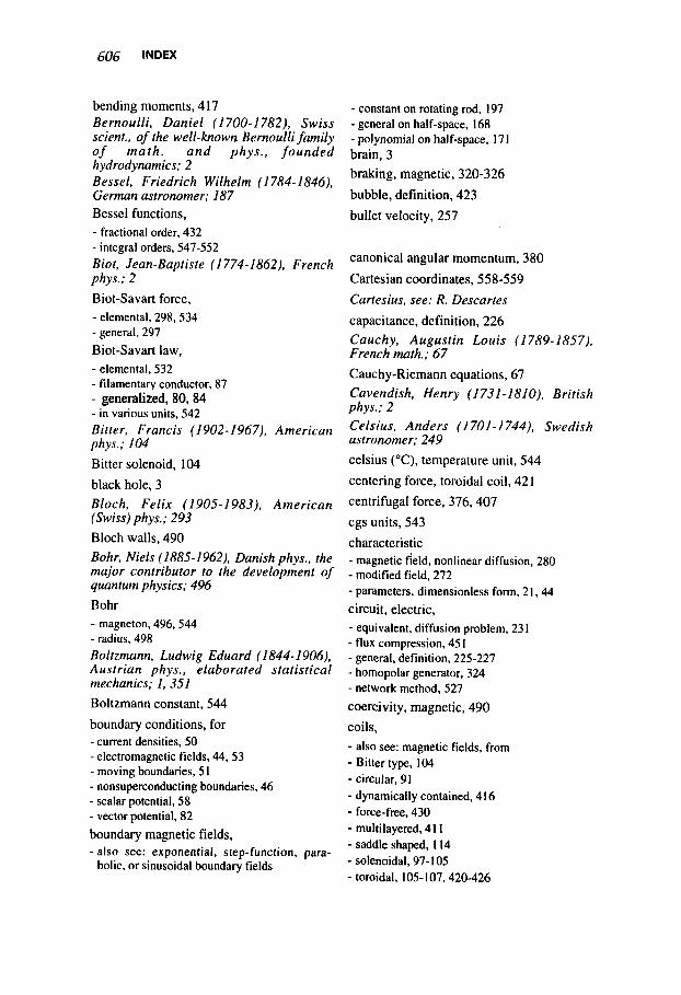
bending moments, 4 17 Bernoulli, Daniel (I 700-1 782), Swiss scient., of the well-known Bernoulli family o f math . and phys . , founded hydrodynamics; 2 Bessel, Friedrich Wilhelm ( I 784- 1846), German astronomer; 187 Bessel functions, - fractional order, 432 - integral orders, 547-552 Biot, Jean-Baptiste ( I 774-1862), French phys.; 2 Biot-Savart force, - elemental, 298,534 - general, 297 Biot-Savart law, - elemental, 532 - filamentary conductor, 87 - generalized, 80,84 - in various units, 542 Bitter, Francis (1902-1967), American phys.; 104 Bitter solenoid, 104
black hole, 3 Bloch, Felix (1905-1983), American (Swiss) phys.; 293 Bloch walls, 490 Bohr, Niels (1885-1962), Danish phys., the major contributor to the development of quantum physics; 496 Bohr - magneton, 496,544 - radius, 498 Boltzmann, Ludwig Eduard (1844-1906), Austrian phys., elaborated statistical mechanics; 1, 351 Boltzmann constant, 544
boundary conditions, for - current densities, 50 - electromagnetic fields, 44.53 - moving boundaries, 51 - nonsuperconducting boundaries, 46 - scalar potential, 58 - vector potential, 82 boundary magnetic fields, - also see: exponential, step-function, para-
bolic, or sinusoidal boundary fields
- constant on rotating rod, 197 - general on half-space, 168 - polynomial on half-space, 17 1 brain, 3 braking, magnetic, 320-326
bubble, definition, 423 bullet velocity, 257
canonical angular momentum, 380
Cartesian coordinates, 558-559
Cartesius, see: R. Descartes
capacitance, definition, 226 Cauchy, Augustin Louis ( I 789-1857), French math. ; 67 Cauchy-Riemann equations, 67 Cavendish, Henry (1731-1810), British phys.; 2 Celsius, Anders ( I 701- 1744), Swedish astronomer; 249
Celsius ("C), temperature unit, 544
centering force, toroidal coil, 42 1
centrifugal force, 376,407
cgs units, 543 characteristic - magnetic held, nonlinear diffusion, 280 - modified field, 272 - parameters, dimensionless form, 2 1.44 circuit, electric, - equivalent, diffusion problem, 23 I - flux compression, 45 1 - general, definition, 225-227 - homopolar generator, 324 - network method, 527 coercivity, magnetic, 490 coils, - also see: magnetic fields, from - Bitter type, 104 - circular, 91 - dynamically contained, 416 - force-free, 430 - multilayered. 41 1 - saddle shaped, 114 - solenoidal, 97-105 - toroidal, 105- 107,420426

INDEX 607
commutator-type machines, 339
complex - functions 134, I36 - variable, 135 - vectors, 138
compressional loading, 400 Compton, Arthur Holly (1892-1962), American phys.; 498 Compton wavelength, 498
condenser bank, 356,452
conductivity, - also see: resistivity - electric, 17,474 - electric, pressure-dependent, 473 - electric, temperature-dependent, 268 - thermal, 245
conformal transformation, 66, 137 conjugate - function, 137 - momentum, 359 - variable, 135
conservation of - canonical angular momentum, 377 - energy in MHD, 438,441 -442 - kinetic energy, 376 - magnetic moment, 375
constant-stress coils, 423-426 containment, dynamic, 416 Cooper, Leon N . (1930-), American phys.; 481 coordinate systems, - definitions, 558 - transformations, 559,563
copper, parameters, 473-476,
copper alloys, parameters, 393,401,477 Coriolis, Gustave-Gaspard ( I 792-1843), French eng. and math.; 377 Coulomb, Charles-Augustin ( I 736-1 806), French phys.; 2
coulomb (C), unit, 543
Coulomb gauche, 78
Coulomb law, 542
critical angular frequency, 325 critical field, magnetic, 498
creep, 400
cryogenic temperatures, 40 1 Curie, Pierre (1859-1906), French phys.; 290 Curie - law, 488,503 - temperature, 490
curl vector, - definition, 556 - direction of, 563
current density, surface, - boundary condition, 204 - definition, 39 - from magnetic field, 175 - from vector potential, 209 - mean, 203
current density, volume, - boundary conditions, 50 - capacitive 38 - displacement, 38 - electric polarization, 38 - electric sources, 157 - inductive 39,77 - magnetization, 7.38
current distribution, series expansion, 11 3 current integral, 269
current stream vector field, 202, 208, 216- 219
curvature
- radius, 425
cyclic loading of materials, 403
cyclotron frequency, 372-373,486,542 cylindrical shell, - geometrically thin-walled, 2 16 - limiting cases, 214 - magnetically thin, 2 17-2 18
- drift, 376
d’Alembert, Jean le Rond (1 71 7-1 783), French math. and phys.; 78
d’Alembert equations, 78
D-coil, 425-426 Debye, Peter (Joseph William) (1884- 1966), German (American) phys.; 473 Debye temperature, 473
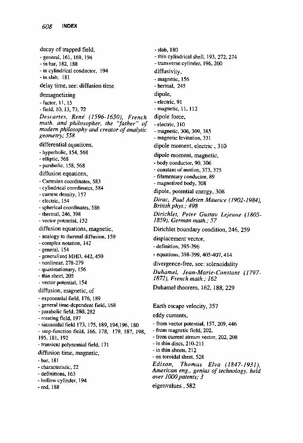
decay of trapped field, - general, 161, 169, 194 - i n bar, 182,188 - in cylindrical conductor, 194 - in slab, 181
delay time, see: diffusion time
demagnetizing -factor, 11, 15 - field. 10, 13. 73, 72 Descartes, RenC (1596-1650), French math. and philosopher, the ‘yather” of modern philosophy and creator of analytic geometry; 558
differential equations, - hyperbolic, 154,568 - elliptic, 568 - parabolic, 158,568 diffusion equations, - Cartesian coordinates, 583 - cylindrical coordinates, 584 - current density, 157 - electric, 154 - spherical coordinates, 586 - thermal, 246,398 - vector potential. 152 diffusion equations, magnetic, - analogy to thermal diffusion, 159 - complex notation, 142 - general, 154 - generalized MHD, 442,450 - nonlinear, 278-279 - quasistationary, 156 - thin sheet, 205 - vector potential, 154
diffusion, magnetic, of - exponential field, 176, 189 - general time-dependent field, 168 - parabolic field, 280,282 - rotating field. 197 - sinusoidal field 173, 175, 189, 194,196, 180 - step-function field, 166, 178, 179, 187, 198, 195, 181, 192 - transient polynomial field, 171
diffusion time, magnetic, -bar, 181 - characteristic, 22 - definitions, 163 - hollow cylinder, 194
- slab, 180 - thin cylindrical shell, 193,272,274 - transverse cylinder, 196, 200 diffusivity , - magnetic, 156 - hermal, 245
dipole, - electric, 91 - magnetic, 11, 112 dipole force, - electric, 310 - magnetic, 306,309,385 - magnetic levitation, 331 dipole moment, electric , 310
dipole moment, magnetic, - body conductor, 90,306 - constant of motion, 373,375 - filamentary conductor, 89 - magnetized body, 308 dipole, potential energy, 308 Dirac, Paul Adrien Maurice ( I 902- 1984), British phys.; 498 Dirichlet, Peter Gustav Lejeune (1805- 1859), German math.; 57 Dirichlet boundary condition, 246,259
displacement vector, - definition, 395-396 - equations, 398-399,405-407,414
divergence-free, see: solenoidality
Duhamel, Jean-Marie-Constant ( 1 797- 1872), French math.; 162 Duhamel theorem, 162, 188,229
Earth escape velocity, 357
eddy currents, - from vector potential, 157, 209,446 - from magnetic field, 202, - from current stream vector, 202,208 - in thin discs, 210-21 1 - in thin sheets, 212 - on toroidal sheet, 528 Edison, Thomas Elva (1847-1931), American eng., genius of technology, held over 1000patents; 3
-rod, 188- eigenvalues , 5 8 2

Einstein, Albert (1879-1955), American (German) phys., one of the great - in cylindrical coordinates, 377,385 personalities in the physics of the 20th century, elaborated the theory of relativity; 26
- in Cartesian coordinates, 370
- in fluidodynamics, 437 equation of state, 504-506
elastic equilibrium equations, 391-392
electric charge, relaxation time, 22 electric circuits, see: circuits
electric dipole moment, 91
electric force density, 299, 304
electric moment, 16
electric potential, 56.77, 358 - complex notation, 143
electric stress tensor, 304
electromotive force, 17.34-35
electron collision time, 23
electroquasistationary equations, 24, 30 electrostatic acceleration, 358
electrostatics, 20 elliptic differential equations, 568 elliptic integrals, 93
emf, see: electromotive force
emu units, 543
energy conservation, see: conservation
energy density, in - electric field, 238 - heat, 249 - magnetic field, 238 energy, electromagnetic, - also see: Joule dissipation - in half-space, 252 - total magnetic, 242 energy equation, 358, 370, 378 energy factor, surface, 258, 276, 282, 284, 466 energy skin depth, 259,282, 284
energy units, 544
enthalpy, 504 equation of motion, - for charged particle, 358, 370 - general, relativistic, 357
equilibrium condition, 3 12
error function, 545-546
esu units, 543 Ether, 125 Euler, teonhard (1707-1 783), Swiss math., one of the most productive mathematicians ever; 2 Eulerian - conservation equation, 437 - differential equation, 407 - frame of equations, 32,439 exclusion principle, 497
exponential boundary field, on - plane, half-space, I76 - rod, 189 - slab, 189
failure criteria, 399-404 Faraday, Michael (1791-1867). British phys., one of the great experimentalists of all times; 2, 125
Faraday law, - cylindrical geometry, 184 - differential, 34 - hollow cylinder, 191 - integral, 35, 120 - plane geometry, 165 - rotating cylinder, 324 - thin sheet, 205 farad (F), unit, 543
fatigue of materials, 403 Fermi, Enrico (1901-1954), Italian phys., one of the most brilliant physicists of the first half of the 20th century and great architect of the nuclear age; 478
Fenni-Dirac statistics, 478
ferromagnetic materials, 492-494
ferromagnetism, 489-49 1 field emission limit, 358
filamentary conductor approximation, 86. 91,114, 118, 121,424
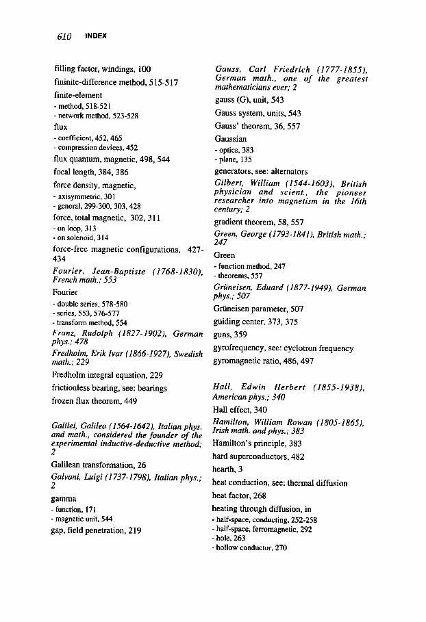
filling factor, windings, 100
fininite-difference method, 5 15-5 17 finite-element -method, 518-521 - network method, 523-528
flux - coefficient, 452.465 - compression devices, 452
flux quantum, magnetic, 498,544 focal length, 384, 386
force density, magnetic, - axisymmetric, 301 - general, 299-300, 303,428 force, total magnetic, 302,3 11 -on loop, 313 - on solenoid, 3 I4 force-free magnetic configurations, 427- 434 Fourier, Jean-Baptiste (I 768-1830), French math.; 553 Fourier - double series, 578-580 - series, 553,576-577 - transform method. 554 Franz, Rudolph (1827-1902), German phys.: 478 Fredholm, Erik Ivar (1866-1927), Swedish math.: 229 Fredholm integral equation, 229 frictionless bearing, see: bearings
frozen flux theorem, 449
Galilei, Galileo (1564-1642), Italian phys. and math., considered the founder of the experimental inductive-deductive method: 2 Galilean transformation, 26 Galvani, Luigi (1737-1 798), Italian phys.; 2 gamma - function. 17 1 - magnetic unit, 544
gap, field penetration, 219
Gauss, Carl Friedrich ( 1 777-1855), German math., one of the greatest mathematicians ever; 2 gauss (G), unit, 543
Gauss system, units, 543 Gauss’ theorem, 36,557
Gaussian - optics, 383 - plane, 135
generators, see: alternators Gilbert, William (1544-1603), British physician and scient., the pioneer researcher into magnetism in the 16th century; 2 gradient theorem, 58,557 Green, George (I 793-1841), British math.; 247 Green - function method, 247 - theorems, 557
Griineisen, Eduard (1877-1949). German phys.; 507 Griineisen parameter, 507 guiding center, 373, 375
guns, 359 gyrofrequency, see: cyclotron frequency
gyromagnetic ratio, 486,497
Hall, Edwin Herbert (1855-1938), American phys.; 340 Hall effect, 340 Hamilton, William Rowan (1805-1865), Irish math. andphys.; 383 Hamilton’s principle, 383
hard superconductors, 482
hearth, 3
heat conduction, see: thermal diffusion
heat factor, 268
heating through diffusion, in - half-space, conducting, 252-258 - half-space, ferromagnetic, 292 - hole, 263 - hollow conductor, 270
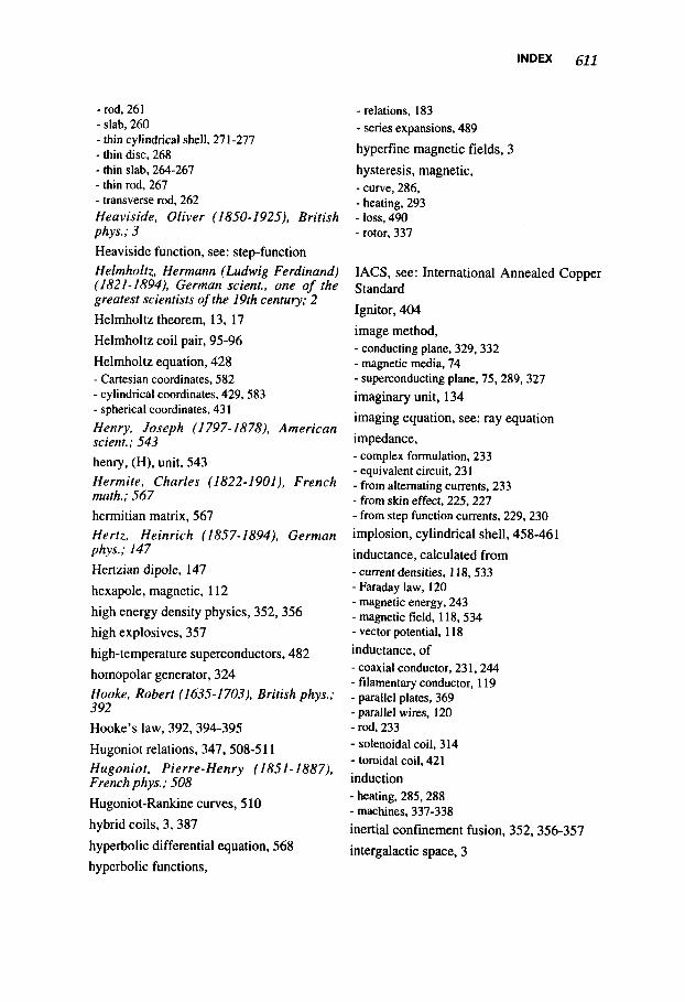
- rod, 261 - slab, 260 - thin cylindrical shell, 271 -277 - thin disc, 268 - thin slab, 264-267 - thin rod, 267 -transverse rod, 262 Heaviside, Oliver (1850- I925), British phys.; 3
- relations, 183 - series expansions, 489
hyperfine magnetic fields, 3
hysteresis, magnetic, - curve, 286, - heating, 293
- rotor, 337 - IOSS, 490
Heaviside function, see: step-function Helmholtz, Hermann (Ludwig Ferdinand) (1821-1894), German scient., one of the greatest scientists of the 19th century; 2
Helmholtz theorem, 13, 17 Helmholtz coil pair, 95-96
Helmholtz equation, 428 - Cartesian coordinates, 582 - cylindrical coordinates, 429, 583 - spherical coordinates, 43 1
Henry, Joseph (1 797-1878), American scient.; 543 impedance,
IACS, see: International Annealed Copper Standard
Ignitor, 404
image method, - conducting plane, 329,332 - magnetic media, 74 - superconducting plane, 75,289,327 imaginary unit, 134 imaging equation, see: ray equation
- complex formulation, 233 - equivalent circuit, 231 - from alternating currents, 233 - from skin effect, 225,227
henry, (H), unit, 543 Hermite, Charles (1822-1901), French math.; 567
hermitian matrix, 567 Hertz, Heinrich (1857-1894), German implosion, cylindrical shell, 458-461 phys.; 147
Hertzian dipole, 147
- from step function currents, 229, 230
inductance, calculated from - current densities, 118.533
hexapole, magnetic, 112 high energy density physics, 352,356
- Faraday law, 120 - magnetic energy, 243 - magnetic field, 118,534 -
high explosives, 357 - vector potential, 118
high-temperature superconductors, 482 inductance- of - coaxial conductor, 23 1,244 - filamentary conductor, 119
homopolar generator, 324
Hooke, Robert (1635-1703), British phys.; - parallel plates, 369 392 -parallel wires, 120 Hooke’s law, 392,394-395 - rod. 233
Hugoniot relations, 347,508-5 1 1 Hugoniot, Pierre-Henry (1851-1887), French phys.; 508 induction
- solenoidal coil, 314 - toroidal coil, 421
- - Hugoniot-Rankine curves, 5 10
hybrid coils, 3, 387
- heating, 285,288 - machines, 337-338 inertial confinement fusion, 352,356-357
intergalactic space, 3 hyperbolic differential equation, 568 hyperbolic functions,

International Annealed Copper Standard, 544
International System of Units, 542-543
isomagnetic lines, 182
Joule, James Prescott (1818-1889), British phys.; 3 Joule dissipation, 237,244,249
joule (J), unit, 543
Kamerlingh-Onnes, Heike (1853-1926), Dutch phys.; 481 Kelvin, Lord, see: W. Thomson Kelvin functions, 549,552 kelvin (K), temperature unit, 544 Kepler, Johannes (1571-1630), German (Czech) astronomer; 2 Kirchhoff, Gustav Robert (1824-1887), Gemtan phys.; 19 Kirchhoff laws, 19,42 Kohlrausch, Rudolph Hermann Arnd (1809-1858), German phys.; 2 Kohler diagram, 478
Lagrange, Joseph-Louis ( I 736-1813), French math.; 2 Lagrangian - time derivative, 28,440,449 - frame of equations, 32,440 - interpolation method, 519 LandP, Alfred ( I 888-1 975), German (American) phys.; 495 Land6 factor, 495 Langevin, Paul (1872-1946), French phys.; 488 Langevin theory, 488 Laplace, Pierre Simon (1 749- 1827), French math.; 57 Laplace equation, - Cartesian coordinates, 64,570 - cylindrical coordinates, 60.572 - spherical coordinates, 61.575 Lurmor, Joseph (1857-1942), British phys.; 363
Larmor - frequency, 383,485,491,500 - radius, 373,475.498
laser, 3 leakage field, 522 Lebedev, Pyotr Nikolayevich (1866-1912)- Russian phys.; 3 Legendre, Adrien-Marie ( I 752-1833), French math.; 88 Legendre polynomials, 88,575 Leibniz (sometimes written Leibnitz), Gottfried Wilhelm (1646-1 716), German math. and scient., a master of knowledge of his time, founder with Newton of digerential and integral calculus; 2 Leibniz rule, 36 lens, magnetic, 384 Lenz, Heinrich Friedrich Emil (1804- 1865), German phys.; 36 Lenz law, 36
levitation, magnetic, over - ferromagnetic track, 327 - conducting thin sheet, 329 - conducting thick sheet, 332 - superconducting plane, 329 linear machines, 339 logarithm, series approximation, 1 13 Lorentz, Hendrik Antoon ( I 853- 1928), Dutch phys.; 3 Lorentz force, - general, 296 - in Hall effect, 340 - various units, 542
Lorentz gauge, 78 lumped circuits, see: circuits, electric
Lorentz transformation, 25 Lorenz, Ludwig Valentin (1829-1891), Danish phys.; 480 Lorenz constant. 480
MAGLEV, see: magnetic levitation
magnetic axis, 127, 130- 13 1
magnetic charge density, - from dipoles, 10
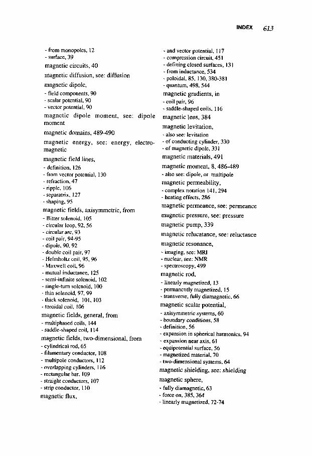
INDEX &73
- from monopoles. 12 - surface, 39
magnetic circuits, 40
magnetic diffusion, see: diffusion
magnetic dipole, - field components, 90 - scalar potential, 90 - vector potential, 90 magnetic dipole moment, see: dipole moment
magnetic domains, 489-490
magnetic energy, see: energy, electro- magnetic
magnetic field lines, - definition, 126 - from vector potential, 130 - refraction, 47 - ripple, 106 - separatrix. 127 - shaping, 95 magnetic fields, axisymmetric, from - Bitter solenoid, 105 - circular loop, 92,56 - circular arc, 93 - coil pair, 94-95 - dipole, 90, 92 - double coil pair, 97 - Helmholtz coil, 95,96 - Maxwell coil, 96 - mutual inductance, 125 - semi-infinite solenoid, 102 - single-turn solenoid, 100 - thin solenoid, 97, 99 - thick solenoid, 101, 103 - toroidal coil, 106
magnetic fields, general, from - multiphased coils, 144 - saddle-shaped coil, 114 magnetic fields, two-dimensional, from - cylindrical rod, 65 - filamentary conductor, 108 - multipole conductors, 112 - overlapping cylinders, 116 - rectangular bar, 109 - straight conductors, 107 - strip conductor, 110
magnetic flux,
- and vector potential, 117 - compression circuit, 45 1 - defining closed surfaces, - from inductance, 534 - poloidal, 85, 130.380-38 - quantum, 498,544 magnetic gradients, in - coil pair, 96 - saddle-shaped coils, 116 magnetic lens, 384
magnetic levitation, - also see: levitation - of conducting cylinder, 330 - of magnetic dipole, 33 I magnetic materials, 49 1
magnetic moment, 8,486-489 - also see: dipole, or multipole magnetic permeability, - complex notation 141,294 - heating effects, 286 magnetic permeance, see: permeance
magnetic pressure, see: pressure
magnetic pump, 339
magnetic relucatance, see: reluctance
magnetic resonance, - imaging, see: MRI - nuclear, see: NMR - spectroscopy, 499
magnetic rod, - linearly magnetized, 13 - permanently magnetized, 15 - transverse, fully diamagnetic, 66
magnetic scalar potential, - axisymmetric systems, 60 - boundary conditions, 58 - definition, 56 - expansion in spherical harmonics, 94 - expansion near axis, 61 - equipotential surface, 56 - magnetized material, 70 - two-dimensional systems, 64 magnetic shielding, see: shielding
magnetic sphere, - fully diamagnetic, 63 - force on, 385.364 - linearly magnetized, 72-74
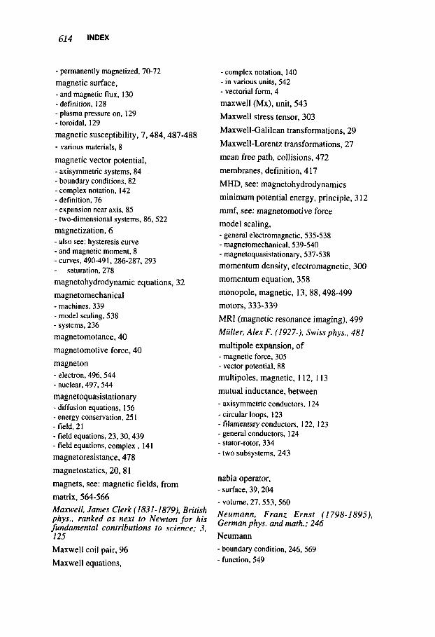
- permanently magnetized, 70-72
magnetic surface, - and magnetic flux, 130 - definition, 128 - plasma pressure on, 129 - toroidal, 129 magnetic susceptibility, 7,484,487-488 - various materials, 8
magnetic vector potential, - axisyrnmetric systems, 84 - boundary conditions, 82 - complex notation. 142 - definition, 76 - expansion near axis, 85 - two-dimensional systems, 86,522 magnetization, 6 - also see: hysteresis curve - and magnetic moment, 8 - curves, 490491,286-287, 293 - saturation, 278 magnetohydrodynamic equations,
magnetomec hanical - machines, 339 - model scaling. 538 - systems, 236
32
magnetomotance, 40
magnetomotive force, 40
magneton - electron, 496,544 - nuclear, 497,544 magnetoquasistationary - diffusion equations, 156 - energy conservation, 251 - field, 2 I - field equations, 23, 30,439 - field equations, complex , 141 magnetoresistance, 478
magnetostatics, 20, 81
magnets, see: magnetic fields, from
matrix, 564-566 Maxwell, James Clerk (1831-1879), British phys., ranked a s next to Newton f o r his fundamental contributions to science; 3, I25 Maxwell coil pair, 96
Maxwell equations,
- complex notation, 140 - in various units, 542 - vectorial form, 4
maxwell (Mx), unit, 543
Maxwell stress tensor, 303
Maxwell-Galilean transformations, 29
Maxwell-Lorentz transformations, 27
mean free path, collisions, 472
membranes, definition, 417
MHD, see: magnetohydrodynamics
minimum potential energy, principle, 3 12
mmf, see: magnetomotive force
model scaling, - general electromagnetic, 535-538 - magnetomechanical, 539-540 - magnetoquasistationary, 537-538 momentum density, electromagnetic, 300
momentum equation, 358
monopole, magnetic, 13,88,498-499 motors, 333-339
MRI (magnetic resonance imaging), 499
Miiller, Alex F. (1927-), Swiss phys., 481
multipole expansion, of - magnetic force, 305 - vector potential, 88 multipoles, magnetic, 112, 113
mutual inductance, between - axisymmetric conductors, 124 - circular loops, 123 - filamentary conductors, 122, I23 - general conductors, 124 - stator-rotor, 334 - two subsystems, 243
nabla operator, - surface, 39,204
- volume, 27,553,560
Neumann, Franz Ernst ( I 798-1 895), German phys. and math.; 246 Neumann
- boundary condition. 246,569 - function, 549

neutron star, 3 Newton, Isaac (1642-1 727), British math. and phys., one of the dominating personalities in the history of science, discoverer of the gravitation law (together with R. Hooke); 2, 125 newton (N), unit, 543
NMR (nuclear magnetic resonance), - apparatus, 500 - classical model, 501-503 - continuous wave method, 502-503 - pulsed resonance method, 503 - quantum mechanical model, 503 nonlinear magnetic diffusion, - ferromagnetic, 290 - general formulation, 278 - temperature dependent, 279
peak effect, current diffusion, 283
permanent magnets, - machines, 339 - materials, 493-495
permeance, 41
perturbation, - magnetic field, 202 - vector potential, 210
phase transitions, 506-507 phasor, 138,240 pitch angle, 381
Planck, Max (Karl Ernst Ludwig) (1858- 1947), German phys., originated quantum physics; 495 Planck constant, 495 plane wave, 149- 15 1
French math.; 80
octupole, magnetic, 112 Oersted, Hans Christian ( 1 777-1851), Poisson, Simian-Denis (1781-1840), Danish phys.; 2 oersted (Oe), unit, 543 Poisson equation, Ohm, Georg Simon (1787-1854), German - cylindrical 84,577 phys.; 2 Ohm law, 17,472 ohm (Q), unit, 543
- difference equation, 5 16 - vectorial, 576 Poisson integral solution, - quasistationary, 80
ohmic heating, see: Joule dissipation
Omitron, 404 optics of charged particles, 383
orbit, see: trajectory
parabolic - boundary field, 342 - differential equations, 568 paramagnetic suspension, 3 19
paramagnetism, 488-489 Pascal, Blaise (1623-1662), French math. and philosopher; 543 pascal (Pa), unit, 543 Pauli. Wolfgang (1900-1958), Swiss (Austrian) phys., the “conscience” of physics, formulated the exclusion principle and invented the neutrino; 497 Pauli exclusion principle, 497
- retarded, 83 polarization - also see: magnetization - electric, 6, 15 - magnetic, 6
potential energy, - equilibrium condition, 312 - magnetic dipole, 308 - magnetic inductive, 312 - stability condition, 318
power, electromagnetic equations, - complex, 241 - differential, 237. 239 - integral, 238, 239 Poynting, John Henry (1852-1914), British phys.; 3 Poynting vector, - complex notation, 241 - definition, 238 - in MHD, 400

- in various units, 542 - time averaged, 148
pressure, - electromagnetic, 300 - hydrodynamic, 341 - magnetic, 342
pressure units, 544 pressure vessels, 405
principal stresses, 389-390 projectile velocity, 359
propulsion, magnetic, - also see: acceleration by ablation thrust, 351 - cylindrical sheet, 352-356 - thick conductor, 35 1 -thin sheet, 343 proximity effect, 69,76
pulsar, 3
pulse loading, 402
Q-factor, defininition, 259
quadrupole, - fields, 112 - magnets, 96, 116 quantum - fields, magnetic, 498 - numbers, 495-497 - theory, 495-498 quasistationary, see: magnetoquasistation- ary and electroquasistationary
radiation damping, 358 Rankine, Willkiam John Macquorn (1820- 1872), British eng. andphys.; 510 rail gun, magnetic, 368 rationale magnetic surface, 129
Rayleigh, Lord, see: J. W. Strutt
ray equation, optical, 384 reactance, inductive, 233
receding image method, 329
refraction, magnetic field lines, 46 relativistic limit, 357
relativity,
- general theory, 26 - special theory, 26 relaxation time, - collisions, 47 - electric charge, 22
reluctance, - definition, 41 - network method, 529 - rotor, 339
remanence, magnetic, 490,494
remnant induction, see: remanence
resistance, total, 18
resistivity - of various materials, 18,393,474-479 - total, 473
response function, diffusion, 161 retarded - potentials, 83, 143 - similarity variable, 169 Reynolds, Osborne (1842-1912), British eng. andphys.; 197 Reynolds number, magnetic, 444-445,457, 466 Riemann, Bernhard (1826-1866), German math.; 67 ripple, magnetic field, 106
rope, definition, 417 rotating - magnetic fields, 144 - magnetomechanical machines, 333-339 - rod, 197
rotor, 333-339 Runge, Carl (David Tolmi) (1856-1927), German math. andphys.; 527
Runge-Kutta method, 527
saddle in field configuration, 127
saddle-shaped coil, 114
saturation, magnetic induction, 287 saw effect, 264
Savart, Felix (1791-1841), French phys.; 2 self-inductance, see: inductance

Scherrer, Paul (1890-1969), Swiss phys., great experimentalist and outstanding physics teacher; xx Schriefler, John Robert (1931-), American phys.; 481
series expansion of - Bessel functions, 551-552 - current distribution, I13 - error function, 545 - general functions, see: Fourier and Taylor
- hyperbolic functions, 489 - logarithm, 113 - multipole vector potential, 112
shear force, 4 17
sheet, definition, 417
shell, definition, 417
shielding factor, magnetic, 220-225
shock waves, 347,507-5 1 1
SI, see: International System of Units
similarity variable, 166, 169, 283
sinusoidal field diffusion, - cylindrical hole, 194 - overview, 180 - plane half-space, 172, 182 - rod, 189 - transverse rod, I96
skin depth, - energy, 259,282,284 -harmonic, 171, 173 - magnetic flux, 170,28 1,284,538 - nomogram, I74 -thermal, 249,257
skin-effect impedance, 227
slip parameter, 337 Snell van Rojen, Willebrord (Snellius) (1591-1626), Dutch astronomer and math.; 47
Snell refraction law, 47
solenoidality condition, of - current, 201,203,305 - electric field, 201 - magnetic field, 23 Sommerfeld, Arnold (Johannes Wilhelm) (1868-1951), German phys., patriarch of
series
German theoretical physics at the beginning of the 20th century; 473
specific heat, 245,249,278
sphere, see: magnetic sphere
stability condition, 3 18
stator, 333-339 Stefan, Josef (1835-1893), Austrian phys.; 125
Stefan-Boltzmann law, 287
step-function field diffusion, - cylindrical shell, 192 - overview, 178 - plane half-space, 166,229 - rod, 187,230 - slab, 179 - transverse shell, 198,200 - transverse rod, 187 Stokes, Georg Gabriel (1819-1903), British phys. and math.; 32 Stokes' - drag force, 358 - theorem, 32,557
Strutt, John William (Lord Rayleigh) (1842-1919), British phys.: 471
sunspots, 3
surface differential operators, 39, 204-205
surface temperature, see: heating through diffusion
susceptibility, - electric, 15 - magnetic, 7
suspension, magnetic, of - ferromagnet, 327 - magnetized sphere, 3 16 - superconducting sphere, 3 17 - also see: levitaton
synchronous machine, 336
Taylor, Brook (1685-1 73 l ) , British math.; 87
Taylor series, 61, 85, 87
- axisymmetric coordinates, 5 15
- in vector form, 305
temperature units, 544
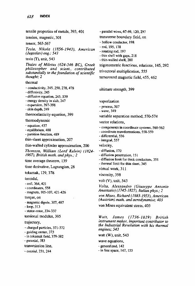
tensile properties of metals, 393,401 tension, magnetic, 301 tensor, 565-567 Tesla, Nikola ( I 856-1 943), American (Jugoslav) eng.; 543 tesla (T), unit, 543 Thales of Miletus (624-546 BC), Greek philosopher and scient., contributed substantially to the foundation of scientific thought; 2 thermal - conductivity, 245,250.278.478 - diffusivity, 245 - diffusion equation, 245.539 - energy density in slab, 247 - expansion, 397-398 - skin depth, 249
thermoelasticity equation, 399 thermodynamic - equation, 437 - equilibrium, 488 - partition function, 489 thin-sheet approximation, 207 thin-walled cylinder approximation, 200 Thomson, William (Lord Kelvin) (1824- 1907), British math. andphys.; 2 time average theorem, 139 time derivative, Lagrangian, 28 tokamak, 129,378 toroidal, - coil, 364,421 - coordinates, 558 -magnets, 105-107.421-426 torque, on - magnetic dipole, 307.487
- stator-rotor, 334-337
torsional modulus, 395 trajectory, - charged particles, 371-372 - guiding center, 373 - in tokamak field. 379-382 - paraxial, 383
transmission line,
- loop, 3 13
- parallel wires, 67-69, 120, 297
transverse boundary field, on - hollow conductor, 198 - rod, 195, 178 - rotating rod, 197 - thin shell with gaps, 218 - thin-walled shell, 200
trigonometric functions, relations, 145,292 trivectoral multiplication, 555 turnaround magnetic field, 455,462
ultimate strength, 399
vaporization - process, 507 - wave, 349 variable separation method, 570-574 vector relations, - components in coordinate systems, 560-562 - coordinate transformations, 558-559 - differential, 556 - integral, 557 velocity, - diffusion, 170 - diffusion penetration, 15 1 - diffusion limit for thick conductors, 35 I - thermal limit for thin sheet, 345 virtual work, 31 1
viscosity, 358 volt (V), unit, 543 Volta, Alessandro (Giuseppe Antonio Anastasio) (1 745-1827), Italian phys.; 2 von Mises, Richard (1883-1953), American (Austrian) math. and aerodynamist; 403
von Mises equivalent stress, 403
Watt, James (1736-1819) British instrument maker, important contributor to the Industrial Revolution with his thermal engines; 543 watt (W), unit, 543 wave equations, - generalized, 142 - in free space, 147. 155 - coaxial, 231,244
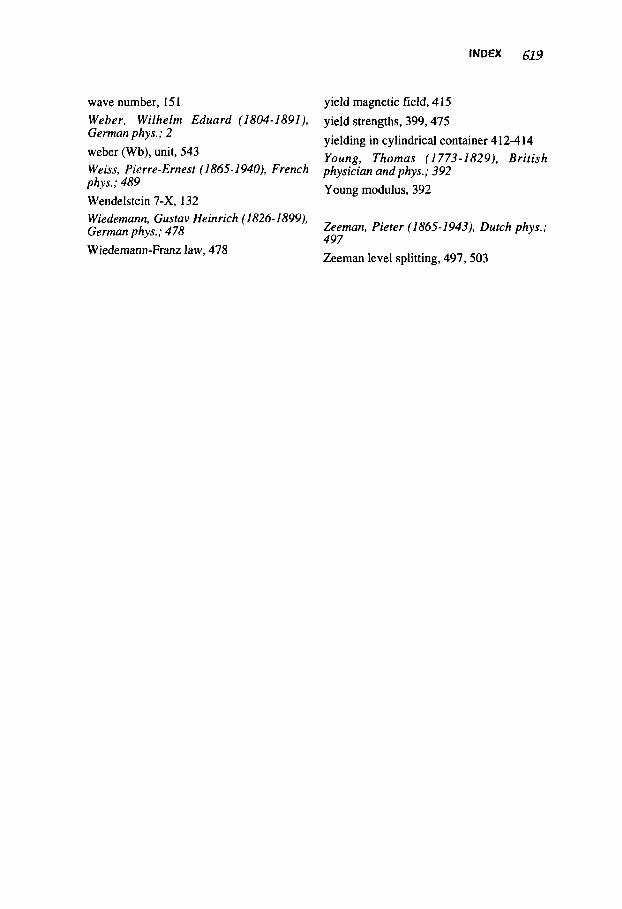
wave number, 151 Weber, Wilhelm Eduard (1804-1891), German phys.; 2
weber (Wb), unit, 543 Weiss, Pierre-Ernest (1865-1 940), French phys.; 489 Wendelstein 7-X, 132 Wiedemann, Gustav Heinrich (1826-1899), German phys.; 478 Wiedemann-Franz law, 478
yield magnetic field, 415
yield strengths, 399,475 yielding in cylindrical container 412-414 Young, Thomas (1773-1829), British physician and phys.; 392 Young modulus, 392
Zeeman, Pieter (1865-1943), Dutch phys.; 497 Zeeman level splitting, 497,503