CHAPTER

22

ELECTRIC FIELDS

22-1 What is Physics?

The physics of the preceding chapter tells us how to find the electric force on a particle 1 of charge

+q1 when the particle is placed near a particle 2 of charge +q2. A nagging question remains: How does

particle 1 “know” of the presence of particle 2? That is, since the particles do not touch, how can

particle 2 push on particle 1—how can there be such an action at a distance?

One purpose of physics is to record observations about our world, such as the magnitude and direction

of the push on particle 1. Another purpose is to provide a deeper explanation of what is recorded. One

purpose of this chapter is to provide such a deeper explanation to our nagging questions about electric

force at a distance. We can answer those questions by saying that particle 2 sets up an electric field in

the space surrounding itself. If we place particle 1 at any given point in that space, the particle

“knows” of the presence of particle 2 because it is affected by the electric field that particle 2 has

already set up at that point. Thus, particle 2 pushes on particle 1 not by touching it but by means of the

electric field produced by particle 2.

Our goal in this chapter is to define electric field and discuss how to calculate it for various

arrangements of charged particles.

Copyright © 2011 John Wiley & Sons, Inc. All rights reserved.

22-2 The Electric Field

The temperature at every point in a room has a definite value. You can measure the temperature at any

given point or combination of points by putting a thermometer there. We call the resulting distribution

of temperatures a temperature field. In much the same way, you can imagine a pressure field in the

atmosphere; it consists of the distribution of air pressure values, one for each point in the atmosphere.

These two examples are of scalar fields because temperature and air pressure are scalar quantities.

The electric field is a vector field; it consists of a distribution of vectors, one for each point in the

region around a charged object, such as a charged rod. In principle, we can define the electric field at

some point near the charged object, such as point P in Fig. 22-1a, as follows: We first place a positive

charge q0, called a test charge, at the point. We then measure the electrostatic force that acts on the

test charge. Finally, we define the electric field at point P due to the charged object as

(22-1)

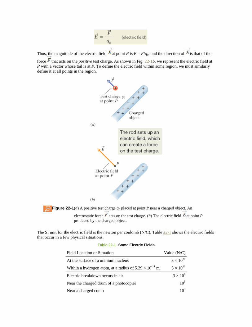
Thus, the magnitude of the electric field at point P is E = F/q0, and the direction of is that of the

force that acts on the positive test charge. As shown in Fig. 22-1b, we represent the electric field at

P with a vector whose tail is at P. To define the electric field within some region, we must similarly

define it at all points in the region.

Figure 22-1 (a) A positive test charge q0 placed at point P near a charged object. An

electrostatic force acts on the test charge. (b) The electric field at point P

produced by the charged object.

The SI unit for the electric field is the newton per coulomb (N/C). Table 22-1 shows the electric fields

that occur in a few physical situations.

Table 22-1 Some Electric Fields

Field Location or Situation Value (N/C)

At the surface of a uranium nucleus 3 × 1021

Within a hydrogen atom, at a radius of 5.29 × 10-11

m 5 × 1011

Electric breakdown occurs in air 3 × 106

Near the charged drum of a photocopier 105

Near a charged comb 103

In the lower atmosphere 102

Inside the copper wire of household circuits 10-2

Although we use a positive test charge to define the electric field of a charged object, that field exists

independently of the test charge. The field at point P in Figure 22-1b existed both before and after the

test charge of Fig. 22-1a was put there. (We assume that in our defining procedure, the presence of the

test charge does not affect the charge distribution on the charged object, and thus does not alter the

electric field we are defining.)

To examine the role of an electric field in the interaction between charged objects, we have two tasks:

(1) calculating the electric field produced by a given distribution of charge and (2) calculating the

force that a given field exerts on a charge placed in it. We perform the first task in Sections 22-4

through 22-7 for several charge distributions. We perform the second task in Sections 22-8 and 22-9

by considering a point charge and a pair of point charges in an electric field. First, however, we

discuss a way to visualize electric fields.

Copyright © 2011 John Wiley & Sons, Inc. All rights reserved.

22-3 Electric Field Lines

Michael Faraday, who introduced the idea of electric fields in the 19th century, thought of the space

around a charged body as filled with lines of force. Although we no longer attach much reality to these

lines, now usually called electric field lines, they still provide a nice way to visualize patterns in

electric fields.

The relation between the field lines and electric field vectors is this: (1) At any point, the direction of a

straight field line or the direction of the tangent to a curved field line gives the direction of at that

point, and (2) the field lines are drawn so that the number of lines per unit area, measured in a plane

that is perpendicular to the lines, is proportional to the magnitude of . Thus, E is large where field

lines are close together and small where they are far apart.

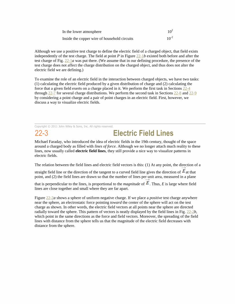
Figure 22-2a shows a sphere of uniform negative charge. If we place a positive test charge anywhere

near the sphere, an electrostatic force pointing toward the center of the sphere will act on the test

charge as shown. In other words, the electric field vectors at all points near the sphere are directed

radially toward the sphere. This pattern of vectors is neatly displayed by the field lines in Fig. 22-2b,

which point in the same directions as the force and field vectors. Moreover, the spreading of the field

lines with distance from the sphere tells us that the magnitude of the electric field decreases with

distance from the sphere.

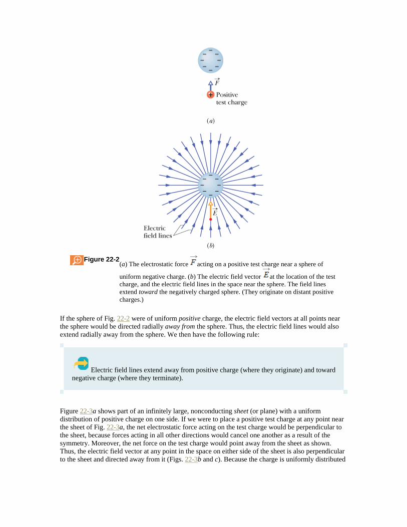
Figure 22-2 (a) The electrostatic force acting on a positive test charge near a sphere of

uniform negative charge. (b) The electric field vector at the location of the test

charge, and the electric field lines in the space near the sphere. The field lines

extend toward the negatively charged sphere. (They originate on distant positive

charges.)

If the sphere of Fig. 22-2 were of uniform positive charge, the electric field vectors at all points near

the sphere would be directed radially away from the sphere. Thus, the electric field lines would also

extend radially away from the sphere. We then have the following rule:

Electric field lines extend away from positive charge (where they originate) and toward

negative charge (where they terminate).

Figure 22-3a shows part of an infinitely large, nonconducting sheet (or plane) with a uniform

distribution of positive charge on one side. If we were to place a positive test charge at any point near

the sheet of Fig. 22-3a, the net electrostatic force acting on the test charge would be perpendicular to

the sheet, because forces acting in all other directions would cancel one another as a result of the

symmetry. Moreover, the net force on the test charge would point away from the sheet as shown.

Thus, the electric field vector at any point in the space on either side of the sheet is also perpendicular

to the sheet and directed away from it (Figs. 22-3b and c). Because the charge is uniformly distributed

along the sheet, all the field vectors have the same magnitude. Such an electric field, with the same

magnitude and direction at every point, is a uniform electric field.

Figure 22-3 (a) The electrostatic force on a positive test charge near a very large,

nonconducting sheet with uniformly distributed positive charge on one side. (b)

The electric field vector at the location of the test charge, and the electric field

lines in the space near the sheet. The field lines extend away from the positively

charged sheet. (c) Side view of (b).

Of course, no real nonconducting sheet (such as a flat expanse of plastic) is infinitely large, but if we

consider a region that is near the middle of a real sheet and not near its edges, the field lines through

that region are arranged as in Figs. 22-3b and c.

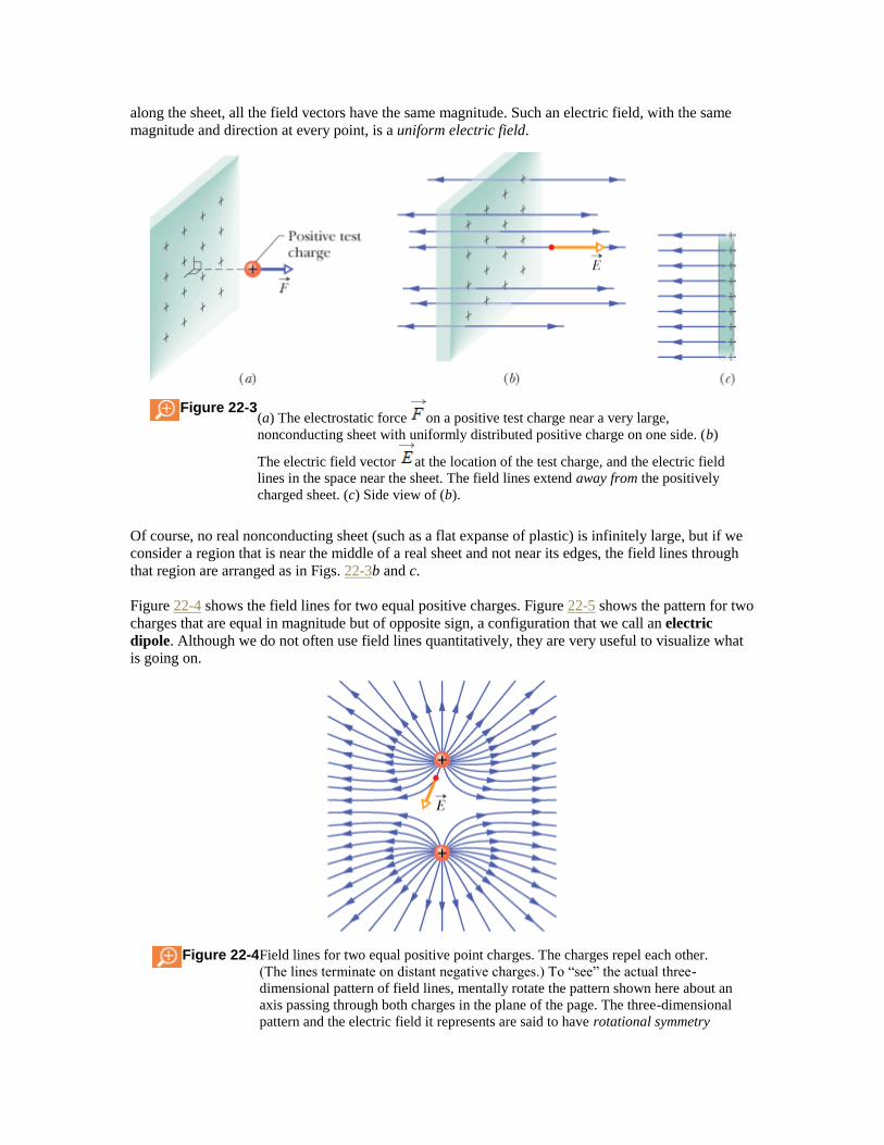
Figure 22-4 shows the field lines for two equal positive charges. Figure 22-5 shows the pattern for two

charges that are equal in magnitude but of opposite sign, a configuration that we call an electric

dipole. Although we do not often use field lines quantitatively, they are very useful to visualize what

is going on.

Figure 22-4 Field lines for two equal positive point charges. The charges repel each other.

(The lines terminate on distant negative charges.) To “see” the actual three-

dimensional pattern of field lines, mentally rotate the pattern shown here about an

axis passing through both charges in the plane of the page. The three-dimensional

pattern and the electric field it represents are said to have rotational symmetry

about that axis. The electric field vector at one point is shown;note that it is

tangent to the field line through that point.

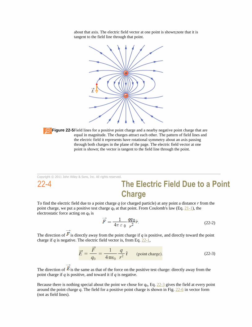
Figure 22-5 Field lines for a positive point charge and a nearby negative point charge that are

equal in magnitude. The charges attract each other. The pattern of field lines and

the electric field it represents have rotational symmetry about an axis passing

through both charges in the plane of the page. The electric field vector at one

point is shown; the vector is tangent to the field line through the point.

Copyright © 2011 John Wiley & Sons, Inc. All rights reserved.

22-4 The Electric Field Due to a Point Charge

To find the electric field due to a point charge q (or charged particle) at any point a distance r from the

point charge, we put a positive test charge q0 at that point. From Coulomb's law (Eq. 21-1), the

electrostatic force acting on q0 is

(22-2)

The direction of is directly away from the point charge if q is positive, and directly toward the point

charge if q is negative. The electric field vector is, from Eq. 22-1,

(22-3)

The direction of is the same as that of the force on the positive test charge: directly away from the

point charge if q is positive, and toward it if q is negative.

Because there is nothing special about the point we chose for q0, Eq. 22-3 gives the field at every point

around the point charge q. The field for a positive point charge is shown in Fig. 22-6 in vector form

(not as field lines).

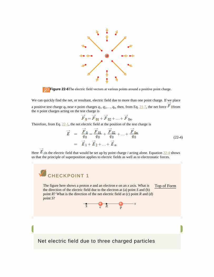
Figure 22-6 The electric field vectors at various points around a positive point charge.

We can quickly find the net, or resultant, electric field due to more than one point charge. If we place

a positive test charge q0 near n point charges q1, q2,…, qn, then, from Eq. 21-7, the net force from

the n point charges acting on the test charge is

Therefore, from Eq. 22-1, the net electric field at the position of the test charge is

(22-4)

Here is the electric field that would be set up by point charge i acting alone. Equation 22-4 shows

us that the principle of superposition applies to electric fields as well as to electrostatic forces.

CHECKPOINT 1

The figure here shows a proton π and an electron e on an x axis. What is

the direction of the electric field due to the electron at (a) point S and (b)

point R? What is the direction of the net electric field at (c) point R and (d)

point S?

Top of Form

Sample Problem

Net electric field due to three charged particles

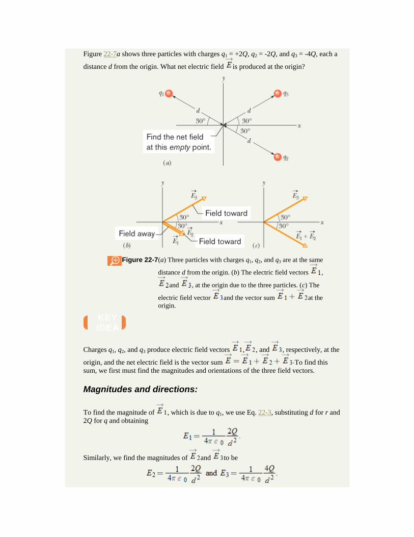
Figure 22-7a shows three particles with charges q1 = +2Q, q2 = -2Q, and q3 = -4Q, each a

distance d from the origin. What net electric field is produced at the origin?

Figure 22-7 (a) Three particles with charges q1, q2, and q3 are at the same

distance d from the origin. (b) The electric field vectors ,

and , at the origin due to the three particles. (c) The

electric field vector and the vector sum at the

origin.

KEY IDEA

Charges q1, q2, and q3 produce electric field vectors , , and , respectively, at the

origin, and the net electric field is the vector sum To find this

sum, we first must find the magnitudes and orientations of the three field vectors.

Magnitudes and directions:

To find the magnitude of , which is due to q1, we use Eq. 22-3, substituting d for r and

2Q for q and obtaining

Similarly, we find the magnitudes of and to be

We next must find the orientations of the three electric field vectors at the origin. Because

q1 is a positive charge, the field vector it produces points directly away from it, and

because q2 and q3 are both negative, the field vectors they produce point directly toward

each of them. Thus, the three electric fields produced at the origin by the three charged

particles are oriented as in Fig. 22-7b. (Caution: Note that we have placed the tails of the

vectors at the point where the fields are to be evaluated; doing so decreases the chance of

error. Error becomes very probable if the tails of the field vectors are placed on the

particles creating the fields.)

Adding the fields: We can now add the fields vectorially just as we added force

vectors in Chapter 21. However, here we can use symmetry to simplify the procedure.

From Fig. 22-7b, we see that electric fields and have the same direction. Hence,

their vector sum has that direction and has the magnitude

which happens to equal the magnitude of field .

We must now combine two vectors, and the vector sum , that have the

same magnitude and that are oriented symmetrically about the x axis, as shown in Fig. 22-

7c. From the symmetry of Fig. 22-7c, we realize that the equal y components of our two

vectors cancel (one is upward and the other is downward) and the equal x components add

(both are rightward). Thus, the net electric field at the origin is in the positive direction

of the x axis and has the magnitude

(Answer)

Copyright © 2011 John Wiley & Sons, Inc. All rights reserved.

22-5 The Electric Field Due to an Electric Dipole

Figure 22-8a shows two charged particles of magnitude q but of opposite sign, separated by a distance

d. As was noted in connection with Fig. 22-5, we call this configuration an electric dipole. Let us find

the electric field due to the dipole of Fig. 22-8a at a point P, a distance z from the midpoint of the

dipole and on the axis through the particles, which is called the dipole axis.

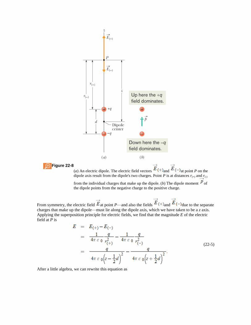
Figure 22-8

(a) An electric dipole. The electric field vectors and at point P on the

dipole axis result from the dipole's two charges. Point P is at distances r(+) and r(-)

from the individual charges that make up the dipole. (b) The dipole moment of

the dipole points from the negative charge to the positive charge.

From symmetry, the electric field at point P—and also the fields and due to the separate

charges that make up the dipole—must lie along the dipole axis, which we have taken to be a z axis.

Applying the superposition principle for electric fields, we find that the magnitude E of the electric

field at P is

(22-5)

After a little algebra, we can rewrite this equation as

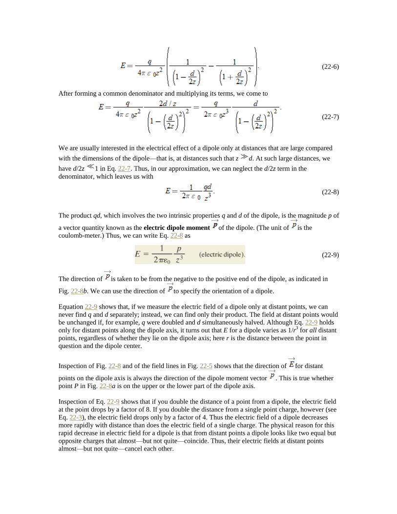
(22-6)

After forming a common denominator and multiplying its terms, we come to

(22-7)

We are usually interested in the electrical effect of a dipole only at distances that are large compared

with the dimensions of the dipole—that is, at distances such that z d. At such large distances, we

have d/2z 1 in Eq. 22-7. Thus, in our approximation, we can neglect the d/2z term in the

denominator, which leaves us with

(22-8)

The product qd, which involves the two intrinsic properties q and d of the dipole, is the magnitude p of

a vector quantity known as the electric dipole moment of the dipole. (The unit of is the

coulomb-meter.) Thus, we can write Eq. 22-8 as

(22-9)

The direction of is taken to be from the negative to the positive end of the dipole, as indicated in

Fig. 22-8b. We can use the direction of to specify the orientation of a dipole.

Equation 22-9 shows that, if we measure the electric field of a dipole only at distant points, we can

never find q and d separately; instead, we can find only their product. The field at distant points would

be unchanged if, for example, q were doubled and d simultaneously halved. Although Eq. 22-9 holds

only for distant points along the dipole axis, it turns out that E for a dipole varies as 1/r3 for all distant

points, regardless of whether they lie on the dipole axis; here r is the distance between the point in

question and the dipole center.

Inspection of Fig. 22-8 and of the field lines in Fig. 22-5 shows that the direction of for distant

points on the dipole axis is always the direction of the dipole moment vector . This is true whether

point P in Fig. 22-8a is on the upper or the lower part of the dipole axis.

Inspection of Eq. 22-9 shows that if you double the distance of a point from a dipole, the electric field

at the point drops by a factor of 8. If you double the distance from a single point charge, however (see

Eq. 22-3), the electric field drops only by a factor of 4. Thus the electric field of a dipole decreases

more rapidly with distance than does the electric field of a single charge. The physical reason for this

rapid decrease in electric field for a dipole is that from distant points a dipole looks like two equal but

opposite charges that almost—but not quite—coincide. Thus, their electric fields at distant points almost—but not quite—cancel each other.

Sample Problem

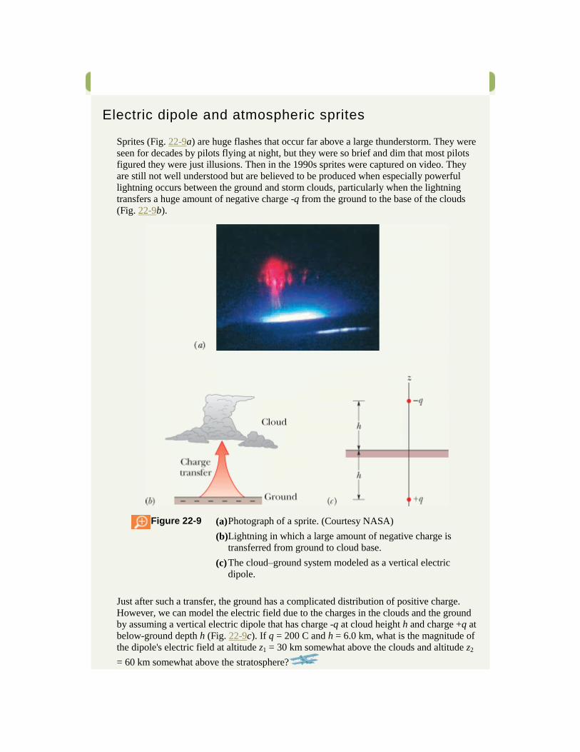
Electric dipole and atmospheric sprites

Sprites (Fig. 22-9a) are huge flashes that occur far above a large thunderstorm. They were

seen for decades by pilots flying at night, but they were so brief and dim that most pilots

figured they were just illusions. Then in the 1990s sprites were captured on video. They

are still not well understood but are believed to be produced when especially powerful

lightning occurs between the ground and storm clouds, particularly when the lightning

transfers a huge amount of negative charge -q from the ground to the base of the clouds

(Fig. 22-9b).

Figure 22-9

(a) Photograph of a sprite. (Courtesy NASA)

(b) Lightning in which a large amount of negative charge is

transferred from ground to cloud base.

(c) The cloud–ground system modeled as a vertical electric

dipole.

Just after such a transfer, the ground has a complicated distribution of positive charge.

However, we can model the electric field due to the charges in the clouds and the ground

by assuming a vertical electric dipole that has charge -q at cloud height h and charge +q at

below-ground depth h (Fig. 22-9c). If q = 200 C and h = 6.0 km, what is the magnitude of

the dipole's electric field at altitude z1 = 30 km somewhat above the clouds and altitude z2

= 60 km somewhat above the stratosphere?

KEY IDEA

We can approximate the magnitude E of an electric dipole's electric field on the dipole

axis with Eq. 22-8.

Calculations:

We write that equation as

where 2h is the separation between -q and +q in Fig. 22-9c. For the electric field at

altitude z1 = 30 km, we find

(Answer)

Similarly, for altitude z2 = 60 km, we find

(Answer)

As we discuss in Concept Module 22-6, when the magnitude of an electric field exceeds a

certain critical value Ec, the field can pull electrons out of atoms (ionize the atoms), and

then the freed electrons can run into other atoms, causing those atoms to emit light. The

value of Ec depends on the density of the air in which the electric field exists. At altitude

z2 = 60 km the density of the air is so low that E = 2.0 × 102 N/C exceeds Ec, and thus

light is emitted by the atoms in the air. That light forms sprites. Lower down, just above

the clouds at z1 = 30 km, the density of the air is much higher, E = 1.6 × 103 N/C does not

exceed Ec, and no light is emitted. Hence, sprites occur only far above storm clouds.

Copyright © 2011 John Wiley & Sons, Inc. All rights reserved.

22-6 The Electric Field Due to a Line of Charge

We now consider charge distributions that consist of a great many closely spaced point charges

(perhaps billions) that are spread along a line, over a surface, or within a volume. Such distributions

are said to be continuous rather than discrete. Since these distributions can include an enormous

number of point charges, we find the electric fields that they produce by means of calculus rather than

by considering the point charges one by one. In this section we discuss the electric field caused by a line of charge. We consider a charged surface in the next section. In the next chapter, we shall find the

field inside a uniformly charged sphere.

When we deal with continuous charge distributions, it is most convenient to express the charge on an

object as a charge density rather than as a total charge. For a line of charge, for example, we would

report the linear charge density (or charge per unit length) λ, whose SI unit is the coulomb per meter.

Table 22-2 shows the other charge densities we shall be using.

Table 22-2 Some Measures of Electric Charge

Name Symbol SI Unit

Charge q C

Linear charge density λ C/m

Surface charge density σ C/m2

Volume charge density ρ C/m3

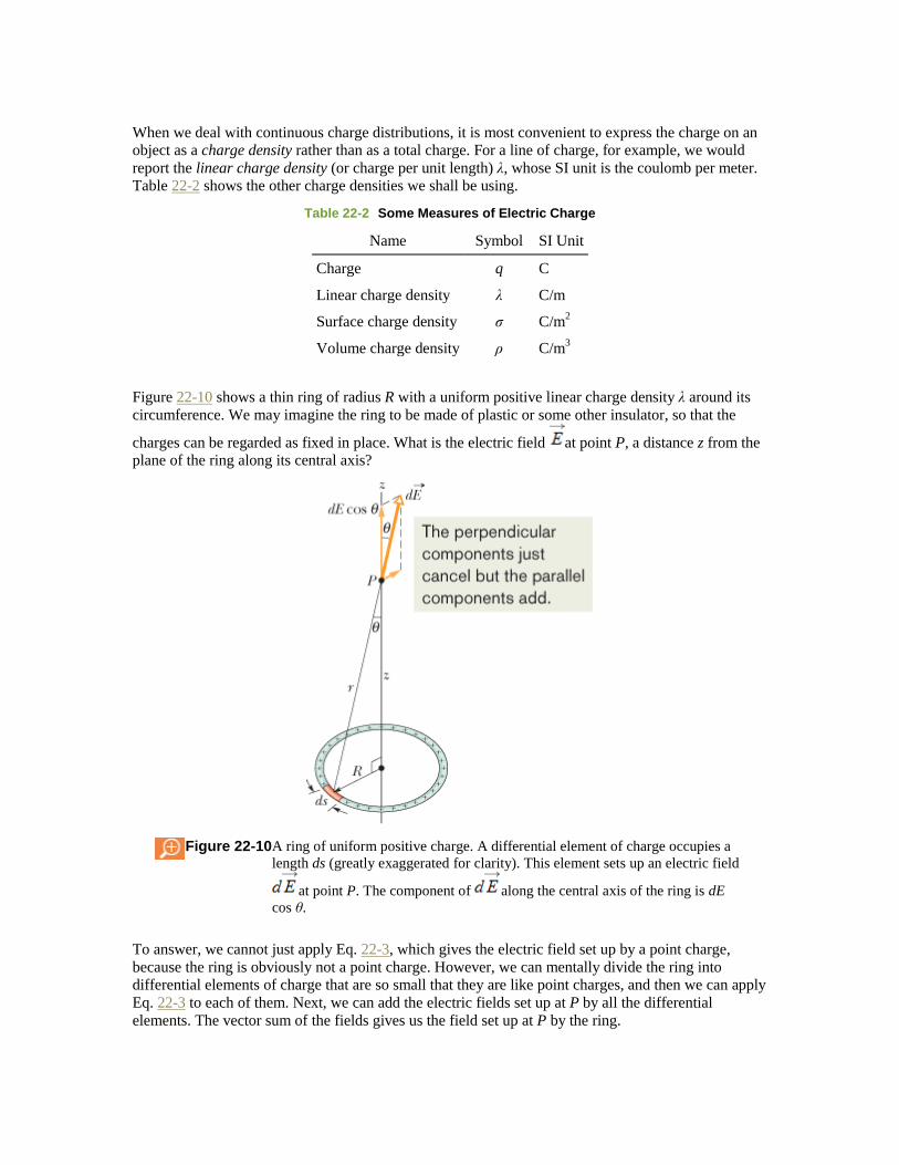
Figure 22-10 shows a thin ring of radius R with a uniform positive linear charge density λ around its

circumference. We may imagine the ring to be made of plastic or some other insulator, so that the

charges can be regarded as fixed in place. What is the electric field at point P, a distance z from the

plane of the ring along its central axis?

Figure 22-10 A ring of uniform positive charge. A differential element of charge occupies a

length ds (greatly exaggerated for clarity). This element sets up an electric field

at point P. The component of along the central axis of the ring is dE

cos θ.

To answer, we cannot just apply Eq. 22-3, which gives the electric field set up by a point charge,

because the ring is obviously not a point charge. However, we can mentally divide the ring into

differential elements of charge that are so small that they are like point charges, and then we can apply

Eq. 22-3 to each of them. Next, we can add the electric fields set up at P by all the differential

elements. The vector sum of the fields gives us the field set up at P by the ring.

Let ds be the (arc) length of any differential element of the ring. Since λ is the charge per unit (arc)

length, the element has a charge of magnitude

(22-10)

This differential charge sets up a differential electric field at point P, which is a distance r from

the element. Treating the element as a point charge and using Eq. 22-10, we can rewrite Eq. 22-3 to

express the magnitude of as

(22-11)

From Fig. 22-10, we can rewrite Eq. 22-11 as

(22-12)

Figure 22-10 shows that is at angle θ to the central axis (which we have taken to be a z axis) and

has components perpendicular to and parallel to that axis.

Every charge element in the ring sets up a differential field at P, with magnitude given by Eq. 22-

12. All the vectors have identical components parallel to the central axis, in both magnitude and

direction. All these vectors have components perpendicular to the central axis as well; these

perpendicular components are identical in magnitude but point in different directions. In fact, for any

perpendicular component that points in a given direction, there is another one that points in the

opposite direction. The sum of this pair of components, like the sum of all other pairs of oppositely

directed components, is zero.

Thus, the perpendicular components cancel and we need not consider them further. This leaves the

parallel components; they all have the same direction, so the net electric field at P is their sum.

The parallel component of shown in Fig. 22-10 has magnitude dEcos θ. The figure also shows us

that

(22-13)

Then multiplying Eq. 22-12 by Eq. 22-13 gives us, for the parallel component of ,

(22-14)

To add the parallel components dE cos θ produced by all the elements, we integrate Eq. 22-14 around

the circumference of the ring, from s = 0 to s = 2πR. Since the only quantity in Eq. 22-14 that varies

during the integration is s, the other quantities can be moved outside the integral sign. The integration

then gives us

(22-15)

Since λ is the charge per length of the ring, the term λ(2πR) in Eq. 22-15 is q, the total charge on the

ring. We then can rewrite Eq. 22-15 as

(22-16)

If the charge on the ring is negative, instead of positive as we have assumed, the magnitude of the

field at P is still given by Eq. 22-16. However, the electric field vector then points toward the ring

instead of away from it.

Let us check Eq. 22-16 for a point on the central axis that is so far away that z R. For such a point,

the expression z2 + R

2 in Eq. 22-16 can be approximated as z

2, and Eq. 22-16 becomes

(22-17)

This is a reasonable result because from a large distance, the ring “looks like” a point charge. If we

replace z with r in Eq. 22-17, we indeed do have Eq. 22-3, the magnitude of the electric field due to a

point charge.

Let us next check Eq. 22-16 for a point at the center of the ring—that is, for z = 0. At that point, Eq.

22-16 tells us that E = 0. This is a reasonable result because if we were to place a test charge at the

center of the ring, there would be no net electrostatic force acting on it; the force due to any element of

the ring would be canceled by the force due to the element on the opposite side of the ring. By Eq. 22-

1, if the force at the center of the ring were zero, the electric field there would also have to be zero.

Sample Problem

Electric field of a charged circular rod

Figure 22-11a shows a plastic rod having a uniformly distributed charge -Q. The rod has

been bent in a 120° circular arc of radius r. We place coordinate axes such that the axis of

symmetry of the rod lies along the x axis and the origin is at the center of curvature P of the

rod. In terms of Q and r, what is the electric field due to the rod at point P?

Electric field of a charged circular rod

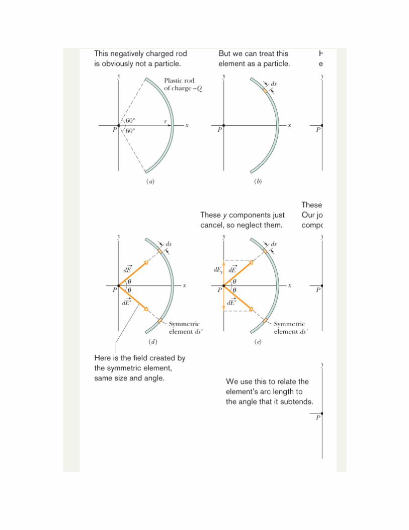
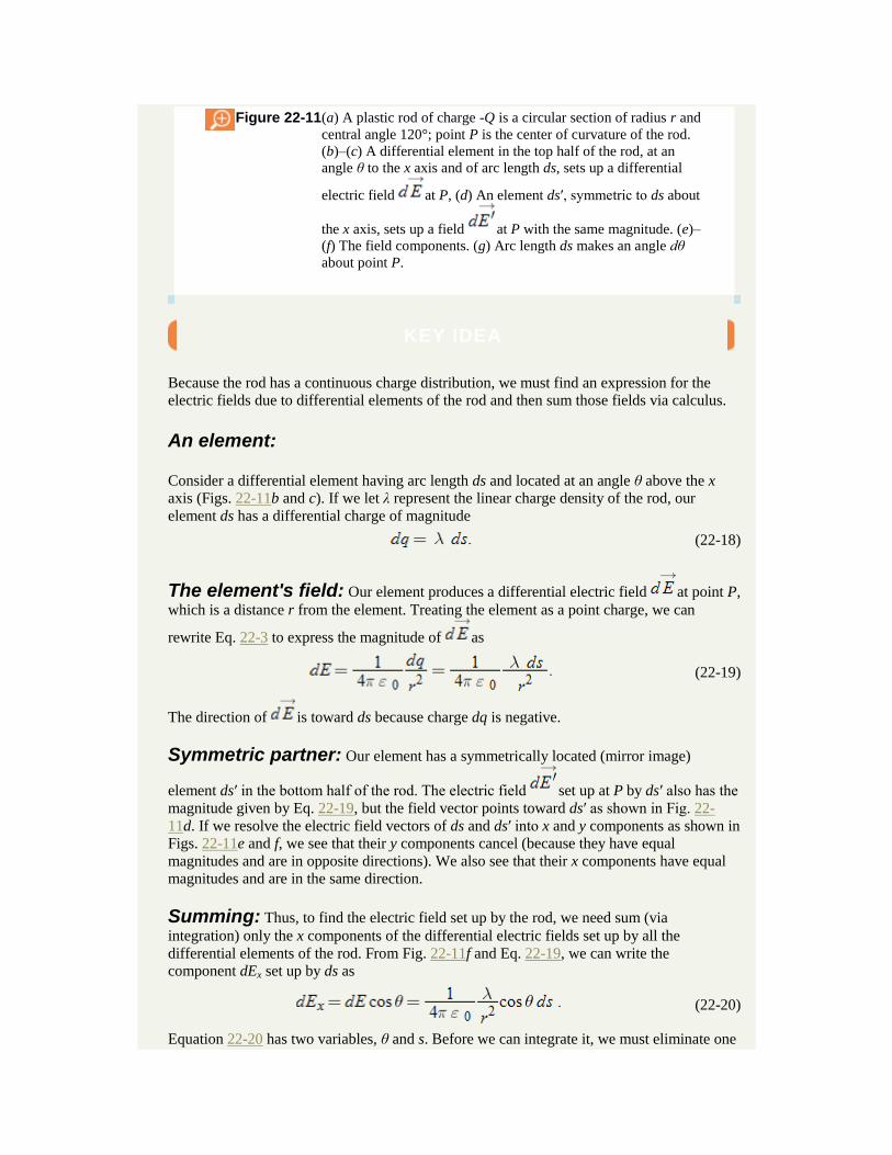
Figure 22-11 (a) A plastic rod of charge -Q is a circular section of radius r and

central angle 120°; point P is the center of curvature of the rod.

(b)–(c) A differential element in the top half of the rod, at an

angle θ to the x axis and of arc length ds, sets up a differential

electric field at P, (d) An element ds′, symmetric to ds about

the x axis, sets up a field at P with the same magnitude. (e)–

(f) The field components. (g) Arc length ds makes an angle dθ

about point P.

KEY IDEA

Because the rod has a continuous charge distribution, we must find an expression for the

electric fields due to differential elements of the rod and then sum those fields via calculus.

An element:

Consider a differential element having arc length ds and located at an angle θ above the x

axis (Figs. 22-11b and c). If we let λ represent the linear charge density of the rod, our

element ds has a differential charge of magnitude

(22-18)

The element's field: Our element produces a differential electric field at point P,

which is a distance r from the element. Treating the element as a point charge, we can

rewrite Eq. 22-3 to express the magnitude of as

(22-19)

The direction of is toward ds because charge dq is negative.

Symmetric partner: Our element has a symmetrically located (mirror image)

element ds′ in the bottom half of the rod. The electric field set up at P by ds′ also has the

magnitude given by Eq. 22-19, but the field vector points toward ds′ as shown in Fig. 22-

11d. If we resolve the electric field vectors of ds and ds′ into x and y components as shown in

Figs. 22-11e and f, we see that their y components cancel (because they have equal

magnitudes and are in opposite directions). We also see that their x components have equal

magnitudes and are in the same direction.

Summing: Thus, to find the electric field set up by the rod, we need sum (via

integration) only the x components of the differential electric fields set up by all the

differential elements of the rod. From Fig. 22-11f and Eq. 22-19, we can write the

component dEx set up by ds as

(22-20)

Equation 22-20 has two variables, θ and s. Before we can integrate it, we must eliminate one

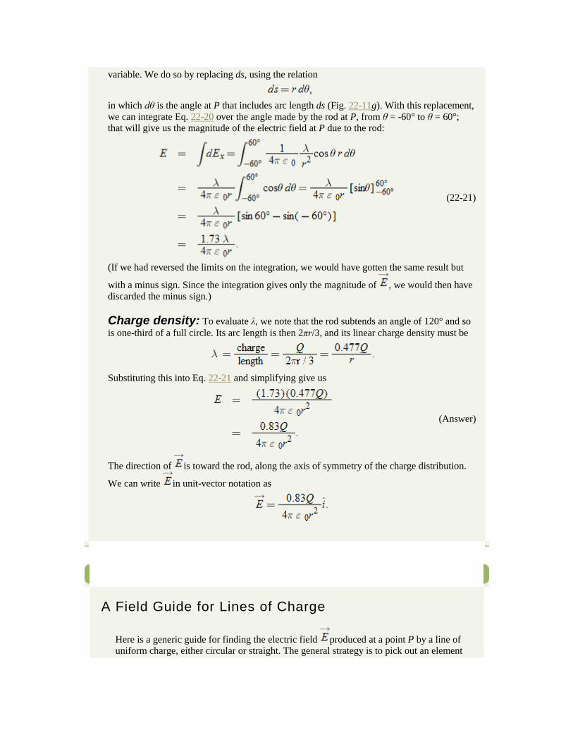
variable. We do so by replacing ds, using the relation

in which dθ is the angle at P that includes arc length ds (Fig. 22-11g). With this replacement,

we can integrate Eq. 22-20 over the angle made by the rod at P, from θ = -60° to θ = 60°;

that will give us the magnitude of the electric field at P due to the rod:

(22-21)

(If we had reversed the limits on the integration, we would have gotten the same result but

with a minus sign. Since the integration gives only the magnitude of , we would then have

discarded the minus sign.)

Charge density: To evaluate λ, we note that the rod subtends an angle of 120° and so

is one-third of a full circle. Its arc length is then 2πr/3, and its linear charge density must be

Substituting this into Eq. 22-21 and simplifying give us

(Answer)

The direction of is toward the rod, along the axis of symmetry of the charge distribution.

We can write in unit-vector notation as

Problem-Solving Tactics

A Field Guide for Lines of Charge

Here is a generic guide for finding the electric field produced at a point P by a line of uniform charge, either circular or straight. The general strategy is to pick out an element

dq of the charge, find due to that element, and integrate over the entire line of

charge.

Step 1. If the line of charge is circular, let ds be the arc length of an element of the

distribution. If the line is straight, run an x axis along it and let dx be the length of an

element. Mark the element on a sketch.

Step 2. Relate the charge dq of the element to the length of the element with either dq

= λ ds or dq = λ dx. Consider dq and λ to be positive, even if the charge is actually

negative. (The sign of the charge is used in the next step.)

Step 3. Express the field produced at P by dq with Eq. 22-3, replacing q in that

equation with either λ ds or λ dx. If the charge on the line is positive, then at P draw a

vector that points directly away from dq. If the charge is negative, draw the vector

pointing directly toward dq.

Step 4. Always look for any symmetry in the situation. If P is on an axis of symmetry

of the charge distribution, resolve the field produced by dq into components that

are perpendicular and parallel to the axis of symmetry. Then consider a second

element dq′ that is located symmetrically to dq about the line of symmetry. At P draw

the vector that this symmetrical element produces and resolve it into components.

One of the components produced by dq is a canceling component; it is canceled by the

corresponding component produced by dq′ and needs no further attention. The other

component produced by dq is an adding component; it adds to the corresponding

component produced by dq′. Add the adding components of all the elements via

integration.

Step 5. Here are four general types of uniform charge distributions, with strategies for

the integral of step 4.

Ring, with point P on (central) axis of symmetry, as in Fig. 22-10. In the expression

for dE, replace r2 with z

2 + R

2, as in Eq. 22-12. Express the adding component of

in terms of θ. That introduces cos θ, but θ is identical for all elements and thus is not a

variable. Replace cos θ as in Eq. 22-13. Integrate over s, around the circumference of

the ring.

Circular arc, with point P at the center of curvature, as in Fig. 22-11. Express the

adding component of in terms of θ. That introduces either sin θ or cos θ. Reduce

the resulting two variables s and θ to one, θ, by replacing ds with r dθ. Integrate over θ

from one end of the arc to the other end.

Straight line, with point P on an extension of the line, as in Fig. 22-12a. In the

expression for dE, replace r with x. Integrate over x, from end to end of the line of

charge.

Straight line, with point P at perpendicular distance y from the line of charge, as in

Fig. 22-12b. In the expression for dE, replace r with an expression involving x and y.

If P is on the perpendicular bisector of the line of charge, find an expression for the

adding component of . That will introduce either sin θ or cos θ. Reduce the

resulting two variables x and θ to one, x, by replacing the trigonometric function with an expression (its definition) involving x and y. Integrate over x from end to end of the

line of charge. If P is not on a line of symmetry, as in Fig. 22-12c, set up an integral to

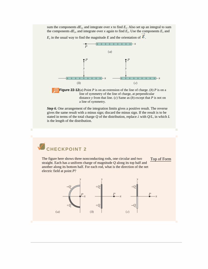
sum the components dEx, and integrate over x to find Ex. Also set up an integral to sum

the components dEy, and integrate over x again to find Ey. Use the components Ex and

Ey in the usual way to find the magnitude E and the orientation of .

Figure 22-12 (a) Point P is on an extension of the line of charge. (b) P is on a

line of symmetry of the line of charge, at perpendicular

distance y from that line. (c) Same as (b) except that P is not on

a line of symmetry.

Step 6. One arrangement of the integration limits gives a positive result. The reverse

gives the same result with a minus sign; discard the minus sign. If the result is to be

stated in terms of the total charge Q of the distribution, replace λ with Q/L, in which L

is the length of the distribution.

CHECKPOINT 2

The figure here shows three nonconducting rods, one circular and two

straight. Each has a uniform charge of magnitude Q along its top half and

another along its bottom half. For each rod, what is the direction of the net

electric field at point P?

Top of Form

Copyright © 2011 John Wiley & Sons, Inc. All rights reserved.

22-7 The Electric Field Due to a Charged Disk

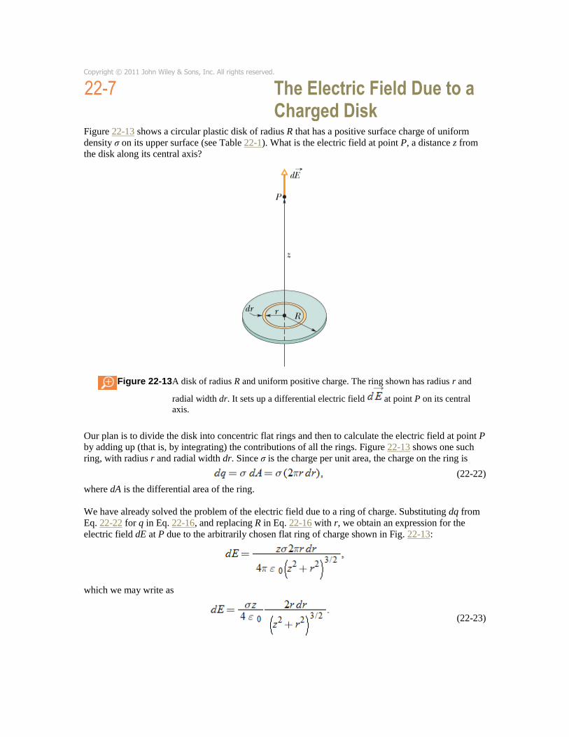
Figure 22-13 shows a circular plastic disk of radius R that has a positive surface charge of uniform

density σ on its upper surface (see Table 22-1). What is the electric field at point P, a distance z from

the disk along its central axis?

Figure 22-13 A disk of radius R and uniform positive charge. The ring shown has radius r and

radial width dr. It sets up a differential electric field at point P on its central

axis.

Our plan is to divide the disk into concentric flat rings and then to calculate the electric field at point P

by adding up (that is, by integrating) the contributions of all the rings. Figure 22-13 shows one such

ring, with radius r and radial width dr. Since σ is the charge per unit area, the charge on the ring is

(22-22)

where dA is the differential area of the ring.

We have already solved the problem of the electric field due to a ring of charge. Substituting dq from

Eq. 22-22 for q in Eq. 22-16, and replacing R in Eq. 22-16 with r, we obtain an expression for the

electric field dE at P due to the arbitrarily chosen flat ring of charge shown in Fig. 22-13:

which we may write as

(22-23)

We can now find E by integrating Eq. 22-23 over the surface of the disk—that is, by integrating with

respect to the variable r from r = 0 to r = R. Note that z remains constant during this process. We get

(22-24)

To solve this integral, we cast it in the form ∫ Xm dX by setting X = (z

2 + r

2), , and dX = (2r)

dr. For the recast integral we have

and so Eq. 22-24 becomes

(22-25)

Taking the limits in Eq. 22-25 and rearranging, we find

(22-26)

as the magnitude of the electric field produced by a flat, circular, charged disk at points on its central

axis. (In carrying out the integration, we assumed that z ≥ 0.)

If we let R → ∞ while keeping z finite, the second term in the parentheses in Eq. 22-26 approaches

zero, and this equation reduces to

(22-27)

This is the electric field produced by an infinite sheet of uniform charge located on one side of a

nonconductor such as plastic. The electric field lines for such a situation are shown in Fig. 22-3.

We also get Eq. 22-27 if we let z → 0 in Eq. 22-26 while keeping R finite. This shows that at points

very close to the disk, the electric field set up by the disk is the same as if the disk were infinite in

extent.

CHECKPOINT 3

(a) In the figure, what is the direction of the electrostatic force on the

electron due to the external electric field shown? (b) In which direction

will the electron accelerate if it is moving parallel to the y axis before it

encounters the external field? (c) If, instead, the electron is initially

moving rightward, will its speed increase, decrease, or remain constant?

Top of Form

Copyright © 2011 John Wiley & Sons, Inc. All rights reserved.

22-8 A Point Charge in an Electric Field

In the preceding four sections we worked at the first of our two tasks: given a charge distribution, to

find the electric field it produces in the surrounding space. Here we begin the second task: to

determine what happens to a charged particle when it is in an electric field set up by other stationary

or slowly moving charges.

What happens is that an electrostatic force acts on the particle, as given by

(22-28)

in which q is the charge of the particle (including its sign) and is the electric field that other charges

have produced at the location of the particle. (The field is not the field set up by the particle itself; to

distinguish the two fields, the field acting on the particle in Eq. 22-28 is often called the external field.

A charged particle or object is not affected by its own electric field.) Equation 22-28 tells us

The electrostatic force acting on a charged particle located in an external electric

field has the direction of if the charge q of the particle is positive and has the opposite

direction if q is negative.

Measuring the Elementary Charge

Equation 22-28 played a role in the measurement of the elementary charge e by American physicist

Robert A. Millikan in 1910–1913. Figure 22-14 is a representation of his apparatus. When tiny oil

drops are sprayed into chamber A, some of them become charged, either positively or negatively, in

the process. Consider a drop that drifts downward through the small hole in plate P1 and into chamber

C. Let us assume that this drop has a negative charge q.

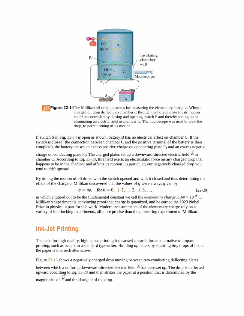
Figure 22-14 The Millikan oil-drop apparatus for measuring the elementary charge e. When a

charged oil drop drifted into chamber C through the hole in plate P1, its motion

could be controlled by closing and opening switch S and thereby setting up or

eliminating an electric field in chamber C. The microscope was used to view the

drop, to permit timing of its motion.

If switch S in Fig. 22-14 is open as shown, battery B has no electrical effect on chamber C. If the

switch is closed (the connection between chamber C and the positive terminal of the battery is then

complete), the battery causes an excess positive charge on conducting plate P1 and an excess negative

charge on conducting plate P2. The charged plates set up a downward-directed electric field in

chamber C. According to Eq. 22-28, this field exerts an electrostatic force on any charged drop that

happens to be in the chamber and affects its motion. In particular, our negatively charged drop will

tend to drift upward.

By timing the motion of oil drops with the switch opened and with it closed and thus determining the

effect of the charge q, Millikan discovered that the values of q were always given by

(22-29)

in which e turned out to be the fundamental constant we call the elementary charge, 1.60 × 10-19

C.

Millikan's experiment is convincing proof that charge is quantized, and he earned the 1923 Nobel

Prize in physics in part for this work. Modern measurements of the elementary charge rely on a

variety of interlocking experiments, all more precise than the pioneering experiment of Millikan.

Ink-Jet Printing

The need for high-quality, high-speed printing has caused a search for an alternative to impact

printing, such as occurs in a standard typewriter. Building up letters by squirting tiny drops of ink at

the paper is one such alternative.

Figure 22-15 shows a negatively charged drop moving between two conducting deflecting plates,

between which a uniform, downward-directed electric field has been set up. The drop is deflected

upward according to Eq. 22-28 and then strikes the paper at a position that is determined by the

magnitudes of and the charge q of the drop.

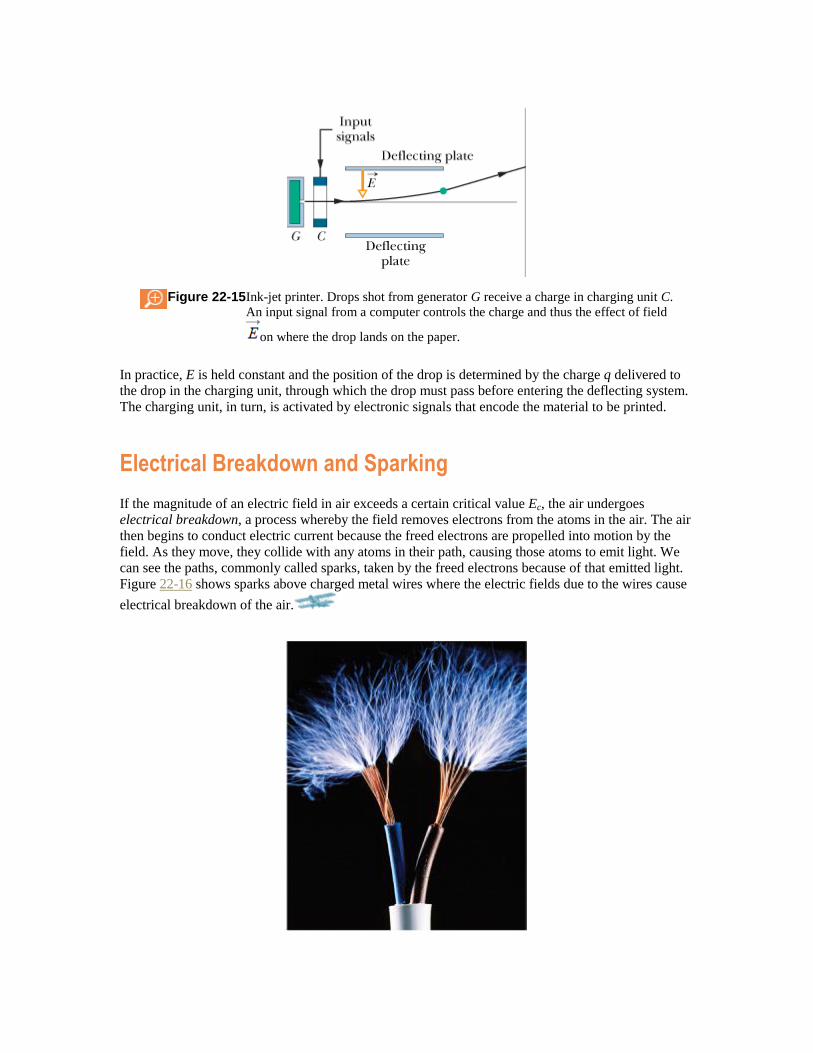
Figure 22-15 Ink-jet printer. Drops shot from generator G receive a charge in charging unit C.

An input signal from a computer controls the charge and thus the effect of field

on where the drop lands on the paper.

In practice, E is held constant and the position of the drop is determined by the charge q delivered to

the drop in the charging unit, through which the drop must pass before entering the deflecting system.

The charging unit, in turn, is activated by electronic signals that encode the material to be printed.

Electrical Breakdown and Sparking

If the magnitude of an electric field in air exceeds a certain critical value Ec, the air undergoes

electrical breakdown, a process whereby the field removes electrons from the atoms in the air. The air

then begins to conduct electric current because the freed electrons are propelled into motion by the

field. As they move, they collide with any atoms in their path, causing those atoms to emit light. We

can see the paths, commonly called sparks, taken by the freed electrons because of that emitted light.

Figure 22-16 shows sparks above charged metal wires where the electric fields due to the wires cause

electrical breakdown of the air.

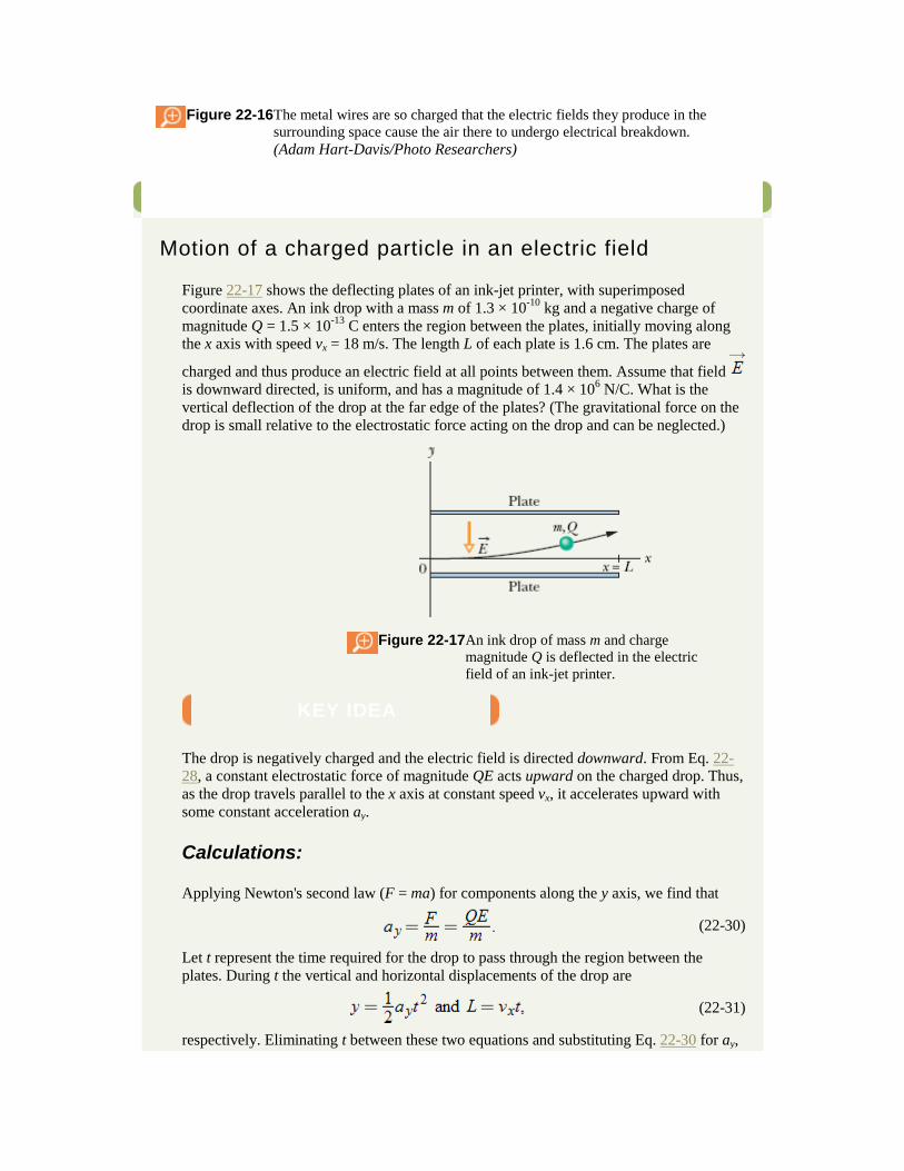
Figure 22-16 The metal wires are so charged that the electric fields they produce in the

surrounding space cause the air there to undergo electrical breakdown.

(Adam Hart-Davis/Photo Researchers)

Sample Problem

Motion of a charged particle in an electric field

Figure 22-17 shows the deflecting plates of an ink-jet printer, with superimposed

coordinate axes. An ink drop with a mass m of 1.3 × 10-10

kg and a negative charge of

magnitude Q = 1.5 × 10-13

C enters the region between the plates, initially moving along

the x axis with speed vx = 18 m/s. The length L of each plate is 1.6 cm. The plates are

charged and thus produce an electric field at all points between them. Assume that field

is downward directed, is uniform, and has a magnitude of 1.4 × 106 N/C. What is the

vertical deflection of the drop at the far edge of the plates? (The gravitational force on the

drop is small relative to the electrostatic force acting on the drop and can be neglected.)

Figure 22-17 An ink drop of mass m and charge

magnitude Q is deflected in the electric

field of an ink-jet printer.

KEY IDEA

The drop is negatively charged and the electric field is directed downward. From Eq. 22-

28, a constant electrostatic force of magnitude QE acts upward on the charged drop. Thus,

as the drop travels parallel to the x axis at constant speed vx, it accelerates upward with

some constant acceleration ay.

Calculations:

Applying Newton's second law (F = ma) for components along the y axis, we find that

(22-30)

Let t represent the time required for the drop to pass through the region between the

plates. During t the vertical and horizontal displacements of the drop are

(22-31)

respectively. Eliminating t between these two equations and substituting Eq. 22-30 for ay,

we find

(Answer)

Copyright © 2011 John Wiley & Sons, Inc. All rights reserved.

22-9 A Dipole in an Electric Field

We have defined the electric dipole moment of an electric dipole to be a vector that points from the

negative to the positive end of the dipole. As you will see, the behavior of a dipole in a uniform

external electric field can be described completely in terms of the two vectors and , with no

need of any details about the dipole's structure.

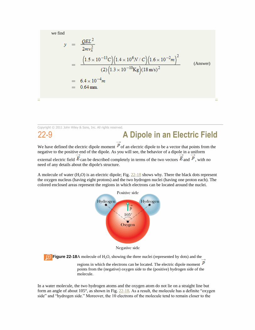
A molecule of water (H2O) is an electric dipole; Fig. 22-18 shows why. There the black dots represent

the oxygen nucleus (having eight protons) and the two hydrogen nuclei (having one proton each). The

colored enclosed areas represent the regions in which electrons can be located around the nuclei.

Figure 22-18 A molecule of H2O, showing the three nuclei (represented by dots) and the

regions in which the electrons can be located. The electric dipole moment

points from the (negative) oxygen side to the (positive) hydrogen side of the

molecule.

In a water molecule, the two hydrogen atoms and the oxygen atom do not lie on a straight line but form an angle of about 105°, as shown in Fig. 22-18. As a result, the molecule has a definite “oxygen

side” and “hydrogen side.” Moreover, the 10 electrons of the molecule tend to remain closer to the

oxygen nucleus than to the hydrogen nuclei. This makes the oxygen side of the molecule slightly more

negative than the hydrogen side and creates an electric dipole moment that points along the

symmetry axis of the molecule as shown. If the water molecule is placed in an external electric field, it

behaves as would be expected of the more abstract electric dipole of Fig. 22-8.

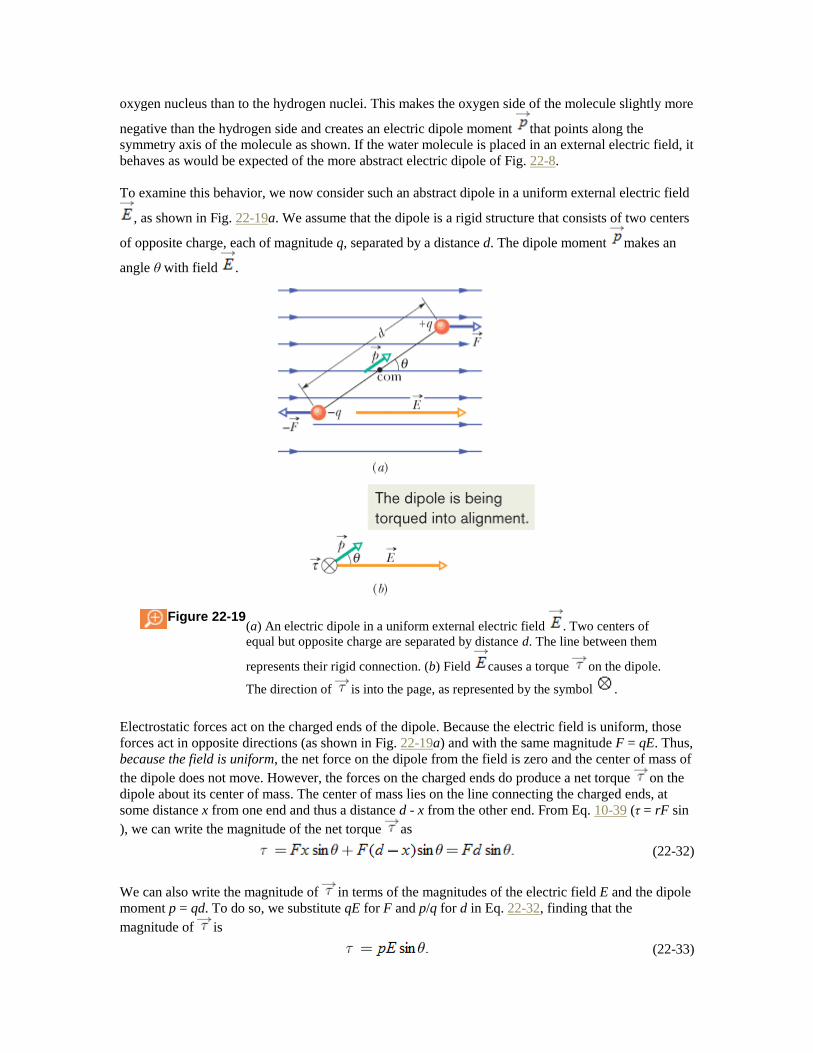
To examine this behavior, we now consider such an abstract dipole in a uniform external electric field

, as shown in Fig. 22-19a. We assume that the dipole is a rigid structure that consists of two centers

of opposite charge, each of magnitude q, separated by a distance d. The dipole moment makes an

angle θ with field .

Figure 22-19 (a) An electric dipole in a uniform external electric field . Two centers of

equal but opposite charge are separated by distance d. The line between them

represents their rigid connection. (b) Field causes a torque on the dipole.

The direction of is into the page, as represented by the symbol .

Electrostatic forces act on the charged ends of the dipole. Because the electric field is uniform, those

forces act in opposite directions (as shown in Fig. 22-19a) and with the same magnitude F = qE. Thus,

because the field is uniform, the net force on the dipole from the field is zero and the center of mass of

the dipole does not move. However, the forces on the charged ends do produce a net torque on the

dipole about its center of mass. The center of mass lies on the line connecting the charged ends, at

some distance x from one end and thus a distance d - x from the other end. From Eq. 10-39 (τ = rF sin

), we can write the magnitude of the net torque as

(22-32)

We can also write the magnitude of in terms of the magnitudes of the electric field E and the dipole

moment p = qd. To do so, we substitute qE for F and p/q for d in Eq. 22-32, finding that the

magnitude of is

(22-33)

We can generalize this equation to vector form as

(22-34)

Vectors and are shown in Fig. 22-19b. The torque acting on a dipole tends to rotate (hence the

dipole) into the direction of field , thereby reducing θ. In Fig. 22-19, such rotation is clockwise. As

we discussed in Chapter 10, we can represent a torque that gives rise to a clockwise rotation by

including a minus sign with the magnitude of the torque. With that notation, the torque of Fig. 22-19 is

(22-35)

Potential Energy of an Electric Dipole

Potential energy can be associated with the orientation of an electric dipole in an electric field. The

dipole has its least potential energy when it is in its equilibrium orientation, which is when its moment

is lined up with the field (then ). It has greater potential energy in all other

orientations. Thus the dipole is like a pendulum, which has its least gravitational potential energy in its

equilibrium orientation—at its lowest point. To rotate the dipole or the pendulum to any other

orientation requires work by some external agent.

In any situation involving potential energy, we are free to define the zero-potential-energy

configuration in a perfectly arbitrary way because only differences in potential energy have physical

meaning. It turns out that the expression for the potential energy of an electric dipole in an external

electric field is simplest if we choose the potential energy to be zero when the angle θ in Fig. 22-19 is

90°. We then can find the potential energy U of the dipole at any other value of θ with Eq. 8-1 (ΔU = -

W) by calculating the work W done by the field on the dipole when the dipole is rotated to that value

of θ from 90°. With the aid of Eq. 10-53 (W = ∫τ dθ) and Eq. 22-35, we find that the potential energy

U at any angle θ is

(22-36)

Evaluating the integral leads to

(22-37)

We can generalize this equation to vector form as

(22-38)

Equations 22-37 and 22-38 show us that the potential energy of the dipole is least (U = - pE) when θ =

0 ( and are in the same direction); the potential energy is greatest (U = pE) when θ = 180° (

and are in opposite directions).

When a dipole rotates from an initial orientation θi to another orientation θf, the work W done on the

dipole by the electric field is

(22-39)

where Uf and Ui are calculated with Eq. 22-38. If the change in orientation is caused by an applied

torque (commonly said to be due to an external agent), then the work Wa done on the dipole by the

applied torque is the negative of the work done on the dipole by the field; that is,

(22-40)

CHECKPOINT 4

The figure shows four orientations of an electric dipole in an external

electric field. Rank the orientations according to (a) the magnitude of the

torque on the dipole and (b) the potential energy of the dipole, greatest

first.

Top of Form

Microwave Cooking

Food can be warmed and cooked in a microwave oven if the food contains water because water

molecules are electric dipoles. When you turn on the oven, the microwave source sets up a rapidly

oscillating electric field within the oven and thus also within the food. From Eq. 22-34, we see that

any electric field produces a torque on an electric dipole moment to align with . Because the

oven's oscillates, the water molecules continuously flip-flop in a frustrated attempt to align with .

Energy is transferred from the electric field to the thermal energy of the water (and thus of the food)

where three water molecules happened to have bonded together to form a group. The flip-flop breaks

some of the bonds. When the molecules reform the bonds, energy is transferred to the random motion

of the group and then to the surrounding molecules. Soon, the thermal energy of the water is enough

to cook the food. Sometimes the heating is surprising. If you heat a jelly donut, for example, the jelly

(which holds a lot of water) heats far more than the donut material (which holds much less water).

Although the exterior of the donut may not be hot, biting into the jelly can burn you. If water

molecules were not electric dipoles, we would not have microwave ovens.

Sample Problem

Torque and energy of an electric dipole in an electric field

A neutral water molecule (H2O) in its vapor state has an electric dipole moment of magnitude

6.2 × 10-30

C·m.

(a) How far apart are the molecule's centers of positive and negative charge?

KEY IDEA

A molecule's dipole moment depends on the magnitude q of the molecule's positive or

negative charge and the charge separation d.

Calculation:

There are 10 electrons and 10 protons in a neutral water molecule; so the magnitude of its

dipole moment is

in which d is the separation we are seeking and e is the elementary charge. Thus,

(Answer)

This distance is not only small, but it is also actually smaller than the radius of a hydrogen

atom.

(b) If the molecule is placed in an electric field of 1.5 × 104 N/C, what maximum torque can

the field exert on it? (Such a field can easily be set up in the laboratory.)

KEY IDEA

The torque on a dipole is maximum when the angle θ between and is 90°.

Calculation:

Substituting θ = 90° in Eq. 22-33 yields

(Answer)

(c) How much work must an external agent do to rotate this molecule by 180° in this field,

starting from its fully aligned position, for which θ = 0?

KEY IDEA

The work done by an external agent (by means of a torque applied to the molecule) is

equal to the change in the molecule's potential energy due to the change in orientation.

Calculations:

From Eq. 22-40, we find

(Answer)

Copyright © 2011 John Wiley & Sons, Inc. All rights reserved.

REVIEW & SUMMARY

Electric Field To explain the electrostatic force between two charges, we assume that each charge

sets up an electric field in the space around it. The force acting on each charge is then due to the

electric field set up at its location by the other charge.

Definition of Electric Field The electric field at any point is defined in terms of the

electrostatic force that would be exerted on a positive test charge q0 placed there:

(22-1)

Electric Field Lines Electric field lines provide a means for visualizing the direction and

magnitude of electric fields. The electric field vector at any point is tangent to a field line through that

point. The density of field lines in any region is proportional to the magnitude of the electric field in

that region. Field lines originate on positive charges and terminate on negative charges.

Field Due to a Point Charge The magnitude of the electric field set up by a point charge q

at a distance r from the charge is

(22-3)

The direction of is away from the point charge if the charge is positive and toward it if the charge is

negative.

Field Due to an Electric Dipole An electric dipole consists of two particles with charges of

equal magnitude q but opposite sign, separated by a small distance d. Their electric dipole moment

has magnitude qd and points from the negative charge to the positive charge. The magnitude of the

electric field set up by the dipole at a distant point on the dipole axis (which runs through both

charges) is

(22-9)

where z is the distance between the point and the center of the dipole.

Field Due to a Continuous Charge Distribution The electric field due to a continuous

charge distribution is found by treating charge elements as point charges and then summing, via

integration, the electric field vectors produced by all the charge elements to find the net vector.

Force on a Point Charge in an Electric Field When a point charge q is placed in an

external electric field , the electrostatic force that acts on the point charge is

(22-28)

Force has the same direction as if q is positive and the opposite direction if q is negative.

Dipole in an Electric Field When an electric dipole of dipole moment is placed in an

electric field , the field exerts a torque on the dipole:

(22-34)

The dipole has a potential energy U associated with its orientation in the field:

(22-38)

This potential energy is defined to be zero when is perpendicular to ; it is least (U = -pE) when

is aligned with and greatest (U = pE) when is directed opposite .

Copyright © 2011 John Wiley & Sons, Inc. All rights reserved.

QUESTIONS

1 Top of Form

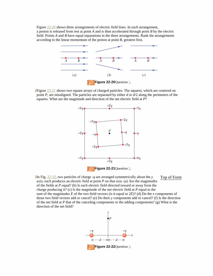
Figure 22-20 shows three arrangements of electric field lines. In each arrangement,

a proton is released from rest at point A and is then accelerated through point B by the electric

field. Points A and B have equal separations in the three arrangements. Rank the arrangements

according to the linear momentum of the proton at point B, greatest first.

Figure 22-20 Question 1.

2 Figure 22-21 shows two square arrays of charged particles. The squares, which are centered on

point P, are misaligned. The particles are separated by either d or d/2 along the perimeters of the

squares. What are the magnitude and direction of the net electric field at P?

Figure 22-21 Question 2.

3 In Fig. 22-22, two particles of charge -q are arranged symmetrically about the y

axis; each produces an electric field at point P on that axis. (a) Are the magnitudes

of the fields at P equal? (b) Is each electric field directed toward or away from the

charge producing it? (c) Is the magnitude of the net electric field at P equal to the

sum of the magnitudes E of the two field vectors (is it equal to 2E)? (d) Do the x components of

those two field vectors add or cancel? (e) Do their y components add or cancel? (f) Is the direction

of the net field at P that of the canceling components or the adding components? (g) What is the

direction of the net field?

Figure 22-22 Question 3.

Top of Form

4 Figure 22-23 shows four situations in which four charged particles are evenly spaced to the left

and right of a central point. The charge values are indicated. Rank the situations according to the

magnitude of the net electric field at the central point, greatest first.

Figure 22-23 Question 4.

5 Figure 22-24 shows two charged particles fixed in place on an axis. (a) Where on

the axis (other than at an infinite distance) is there a point at which their net electric

field is zero: between the charges, to their left, or to their right? (b) Is there a point

of zero net electric field anywhere off the axis (other than at an infinite distance)?

Figure 22-24 Question 5.

Top of Form

6 In Fig. 22-25, two identical circular nonconducting rings are centered on the same line. For three

situations, the uniform charges on rings A and B are, respectively, (1) q0 and q0, (2) -q0 and -q0,

and (3) -q0 and -q0. Rank the situations according to the magnitude of the net electric field at (a)

point P1 midway between the rings, (b) point P2 at the center of ring B, and (c) point P3 to the right

of ring B, greatest first.

Figure 22-25 Question 6.

7 The potential energies associated with four orientations of an electric dipole in an

electric field are (1) -5U0, (2) -7U0, (3) 3U0, and (4) 5U0, where U0 is positive.

Rank the orientations according to (a) the angle between the electric dipole moment

and the electric field and (b) the magnitude of the torque on the electric dipole,

greatest first.

Top of Form

8 (a) In the Checkpoint of Section 22-9, if the dipole rotates from orientation 1 to orientation 2, is

the work done on the dipole by the field positive, negative, or zero? (b) If, instead, the dipole

rotates from orientation 1 to orientation 4, is the work done by the field more than, less than, or the same as in (a)?

9 Top of Form

Figure 22-26 shows two disks and a flat ring, each with the same uniform charge Q.

Rank the objects according to the magnitude of the electric field they create at

points P (which are at the same vertical heights), greatest first.

Figure 22-26 Question 9.

10 In Fig. 22-27, an electron e travels through a small hole in plate A and then toward plate B. A

uniform electric field in the region between the plates then slows the electron without deflecting it.

(a) What is the direction of the field? (b) Four other particles similarly travel through small holes

in either plate A or plate B and then into the region between the plates. Three have charges +q1,

+q2, and -q3. The fourth (labeled n) is a neutron, which is electrically neutral. Does the speed of

each of those four other particles increase, decrease, or remain the same in the region between the

plates?

Figure 22-27 Question 10.

11 In Fig. 22-28a, a circular plastic rod with uniform charge +Q produces an electric

field of magnitude E at the center of curvature (at the origin). In Figs. 22-28b, c,

and d, more circular rods, each with identical uniform charges +Q, are added until

the circle is complete. A fifth arrangement (which would be labeled e) is like that in

d except the rod in the fourth quadrant has charge -Q. Rank the five arrangements according to the

magnitude of the electric field at the center of curvature, greatest first.

Top of Form

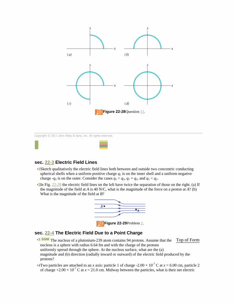
Figure 22-28 Question 11.

Copyright © 2011 John Wiley & Sons, Inc. All rights reserved.

PROBLEMS

sec. 22-3 Electric Field Lines

•1 Sketch qualitatively the electric field lines both between and outside two concentric conducting

spherical shells when a uniform positive charge q1 is on the inner shell and a uniform negative

charge -q2 is on the outer. Consider the cases q1 > q2, q1 = q2, and q1 < q2.

•2 In Fig. 22-29 the electric field lines on the left have twice the separation of those on the right. (a) If

the magnitude of the field at A is 40 N/C, what is the magnitude of the force on a proton at A? (b)

What is the magnitude of the field at B?

Figure 22-29 Problem 2.

sec. 22-4 The Electric Field Due to a Point Charge

•3 The nucleus of a plutonium-239 atom contains 94 protons. Assume that the

nucleus is a sphere with radius 6.64 fm and with the charge of the protons

uniformly spread through the sphere. At the nucleus surface, what are the (a)

magnitude and (b) direction (radially inward or outward) of the electric field produced by the

protons?

Top of Form

•4 Two particles are attached to an x axis: particle 1 of charge -2.00 × 10-7

C at x = 6.00 cm, particle 2

of charge +2.00 × 10-7

C at x = 21.0 cm. Midway between the particles, what is their net electric

field in unit-vector notation?

•5 What is the magnitude of a point charge whose electric field 50 cm away has

the magnitude 2.0 N/C?

Top of Form

•6 What is the magnitude of a point charge that would create an electric field of 1.00 N/C at points

1.00 m away?

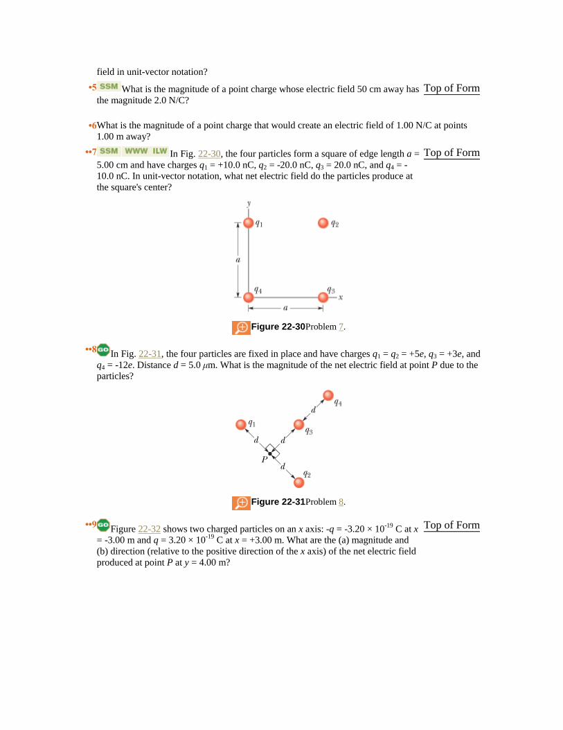
••7 In Fig. 22-30, the four particles form a square of edge length a =

5.00 cm and have charges q1 = +10.0 nC, q2 = -20.0 nC, q3 = 20.0 nC, and q4 = -

10.0 nC. In unit-vector notation, what net electric field do the particles produce at

the square's center?

Figure 22-30 Problem 7.

Top of Form

••8 In Fig. 22-31, the four particles are fixed in place and have charges q1 = q2 = +5e, q3 = +3e, and

q4 = -12e. Distance d = 5.0 μm. What is the magnitude of the net electric field at point P due to the

particles?

Figure 22-31 Problem 8.

••9 Figure 22-32 shows two charged particles on an x axis: -q = -3.20 × 10

-19 C at x

= -3.00 m and q = 3.20 × 10-19

C at x = +3.00 m. What are the (a) magnitude and

(b) direction (relative to the positive direction of the x axis) of the net electric field

produced at point P at y = 4.00 m?

Top of Form

Figure 22-32 Problem 9.

••10 Figure 22-33a shows two charged particles fixed in place on an x axis with separation L. The

ratio q1/q2 of their charge magnitudes is 4.00. Figure 22-33b shows the x component Enet,x of their

net electric field along the x axis just to the right of particle 2. The x axis scale is set by xs = 30.0

cm. (a) At what value of x > 0 is Enet,x maximum? (b) If particle 2 has charge -q2 = -3e, what is the

value of that maximum?

Figure 22-33 Problem 10.

••11 Two particles are fixed to an x axis: particle 1 of charge q1 = 2.1 10-8

C at x

= 20 cm and particle 2 of charge q2 = -4.00q1 at x 70 cm. At what coordinate on

the axis is the net electric field produced by the particles equal to zero?

Top of Form

••12 Figure 22-34 shows an uneven arrangement of electrons (e) and protons (p) on a circular arc of

radius r = 2.00 cm, with angles θ1 = 30.0°, θ2 = 50.0°, θ3 = 30.0°, and θ4 = 20.0°. What are the (a)

magnitude and (b) direction (relative to the positive direction of the x axis) of the net electric field

produced at the center of the arc?

Figure 22-34 Problem 12.

••13 Top of Form

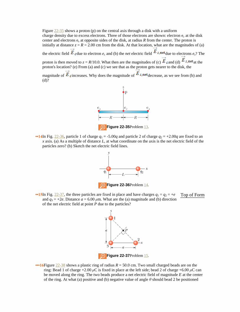
Figure 22-35 shows a proton (p) on the central axis through a disk with a uniform

charge density due to excess electrons. Three of those electrons are shown: electron ec at the disk

center and electrons es at opposite sides of the disk, at radius R from the center. The proton is

initially at distance z = R = 2.00 cm from the disk. At that location, what are the magnitudes of (a)

the electric field due to electron ec and (b) the net electric field due to electrons es? The

proton is then moved to z = R/10.0. What then are the magnitudes of (c) and (d) at the

proton's location? (e) From (a) and (c) we see that as the proton gets nearer to the disk, the

magnitude of increases. Why does the magnitude of decrease, as we see from (b) and

(d)?

Figure 22-35 Problem 13.

••14 In Fig. 22-36, particle 1 of charge q1 = -5.00q and particle 2 of charge q2 = +2.00q are fixed to an

x axis. (a) As a multiple of distance L, at what coordinate on the axis is the net electric field of the

particles zero? (b) Sketch the net electric field lines.

Figure 22-36 Problem 14.

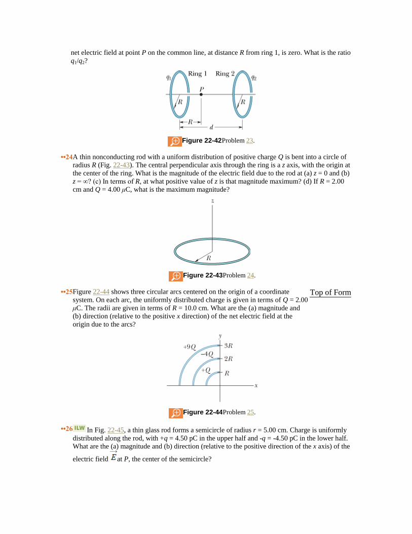
••15 In Fig. 22-37, the three particles are fixed in place and have charges q1 = q2 = +e

and q3 = +2e. Distance a = 6.00 μm. What are the (a) magnitude and (b) direction

of the net electric field at point P due to the particles?

Figure 22-37 Problem 15.

Top of Form

•••16 Figure 22-38 shows a plastic ring of radius R = 50.0 cm. Two small charged beads are on the

ring: Bead 1 of charge +2.00 μC is fixed in place at the left side; bead 2 of charge +6.00 μC can be moved along the ring. The two beads produce a net electric field of magnitude E at the center

of the ring. At what (a) positive and (b) negative value of angle θ should bead 2 be positioned

such that E = 2.00 × 105 N/C?

Figure 22-38 Problem 16.

•••17 Two charged beads are on the plastic ring in Fig. 22-39a. Bead 2, which is not

shown, is fixed in place on the ring, which has radius R = 60.0 cm. Bead 1 is

initially on the x axis at angle θ = 0°. It is then moved to the opposite side, at

angle θ = 180°, through the first and second quadrants of the xy coordinate

system. Figure 22-39b gives the x component of the net electric field produced at the origin by

the two beads as a function of θ, and Fig. 22-39c gives the y component. The vertical axis scales

are set by Exs = 5.0 × 104 N/C and Eys = -9.0 × 10

4 N/C. (a) At what angle θ is bead 2 located?

What are the charges of (b) bead 1 and (c) bead 2?

Figure 22-39 Problem 17.

Top of Form

sec. 22-5 The Electric Field Due to an Electric Dipole

••18 The electric field of an electric dipole along the dipole axis is approximated by Eqs. 22-8 and 22-

9. If a binomial expansion is made of Eq. 22-7, what is the next term in the expression for the

dipole's electric field along the dipole axis? That is, what is Enext in the expression

••19 Top of Form

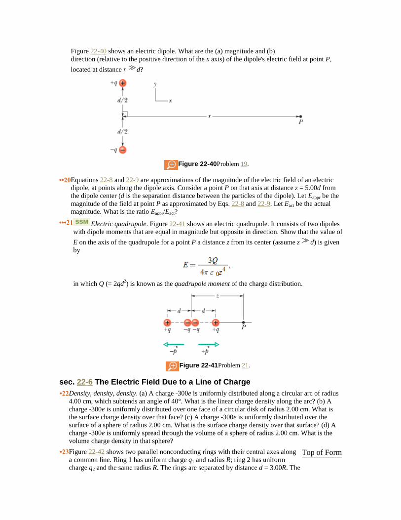
Figure 22-40 shows an electric dipole. What are the (a) magnitude and (b)

direction (relative to the positive direction of the x axis) of the dipole's electric field at point P,

located at distance r d?

Figure 22-40 Problem 19.

••20 Equations 22-8 and 22-9 are approximations of the magnitude of the electric field of an electric

dipole, at points along the dipole axis. Consider a point P on that axis at distance z = 5.00d from

the dipole center (d is the separation distance between the particles of the dipole). Let Eappr be the

magnitude of the field at point P as approximated by Eqs. 22-8 and 22-9. Let Eact be the actual

magnitude. What is the ratio Eappr/Eact?

•••21 Electric quadrupole. Figure 22-41 shows an electric quadrupole. It consists of two dipoles

with dipole moments that are equal in magnitude but opposite in direction. Show that the value of

E on the axis of the quadrupole for a point P a distance z from its center (assume z d) is given

by

in which Q (= 2qd2) is known as the quadrupole moment of the charge distribution.

Figure 22-41 Problem 21.

sec. 22-6 The Electric Field Due to a Line of Charge

•22 Density, density, density. (a) A charge -300e is uniformly distributed along a circular arc of radius

4.00 cm, which subtends an angle of 40°. What is the linear charge density along the arc? (b) A

charge -300e is uniformly distributed over one face of a circular disk of radius 2.00 cm. What is

the surface charge density over that face? (c) A charge -300e is uniformly distributed over the

surface of a sphere of radius 2.00 cm. What is the surface charge density over that surface? (d) A

charge -300e is uniformly spread through the volume of a sphere of radius 2.00 cm. What is the

volume charge density in that sphere?

•23 Figure 22-42 shows two parallel nonconducting rings with their central axes along

a common line. Ring 1 has uniform charge q1 and radius R; ring 2 has uniform

charge q2 and the same radius R. The rings are separated by distance d = 3.00R. The

Top of Form

net electric field at point P on the common line, at distance R from ring 1, is zero. What is the ratio

q1/q2?

Figure 22-42 Problem 23.

••24 A thin nonconducting rod with a uniform distribution of positive charge Q is bent into a circle of

radius R (Fig. 22-43). The central perpendicular axis through the ring is a z axis, with the origin at

the center of the ring. What is the magnitude of the electric field due to the rod at (a) z = 0 and (b)

z = ∞? (c) In terms of R, at what positive value of z is that magnitude maximum? (d) If R = 2.00

cm and Q = 4.00 μC, what is the maximum magnitude?

Figure 22-43 Problem 24.

••25 Figure 22-44 shows three circular arcs centered on the origin of a coordinate

system. On each arc, the uniformly distributed charge is given in terms of Q = 2.00

μC. The radii are given in terms of R = 10.0 cm. What are the (a) magnitude and

(b) direction (relative to the positive x direction) of the net electric field at the

origin due to the arcs?

Figure 22-44 Problem 25.

Top of Form

••26 In Fig. 22-45, a thin glass rod forms a semicircle of radius r = 5.00 cm. Charge is uniformly

distributed along the rod, with +q = 4.50 pC in the upper half and -q = -4.50 pC in the lower half.

What are the (a) magnitude and (b) direction (relative to the positive direction of the x axis) of the

electric field at P, the center of the semicircle?

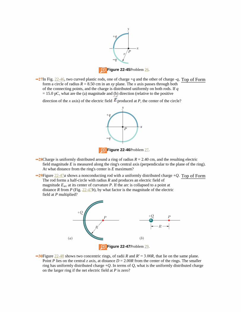
Figure 22-45 Problem 26.

••27 In Fig. 22-46, two curved plastic rods, one of charge +q and the other of charge -q,

form a circle of radius R = 8.50 cm in an xy plane. The x axis passes through both

of the connecting points, and the charge is distributed uniformly on both rods. If q

= 15.0 pC, what are the (a) magnitude and (b) direction (relative to the positive

direction of the x axis) of the electric field produced at P, the center of the circle?

Figure 22-46 Problem 27.

Top of Form

••28 Charge is uniformly distributed around a ring of radius R = 2.40 cm, and the resulting electric

field magnitude E is measured along the ring's central axis (perpendicular to the plane of the ring).

At what distance from the ring's center is E maximum?

••29 Figure 22-47a shows a nonconducting rod with a uniformly distributed charge +Q.

The rod forms a half-circle with radius R and produces an electric field of

magnitude Earc at its center of curvature P. If the arc is collapsed to a point at

distance R from P (Fig. 22-47b), by what factor is the magnitude of the electric

field at P multiplied?

Figure 22-47 Problem 29.

Top of Form

••30 Figure 22-48 shows two concentric rings, of radii R and R′ = 3.00R, that lie on the same plane.

Point P lies on the central z axis, at distance D = 2.00R from the center of the rings. The smaller

ring has uniformly distributed charge +Q. In terms of Q, what is the uniformly distributed charge

on the larger ring if the net electric field at P is zero?

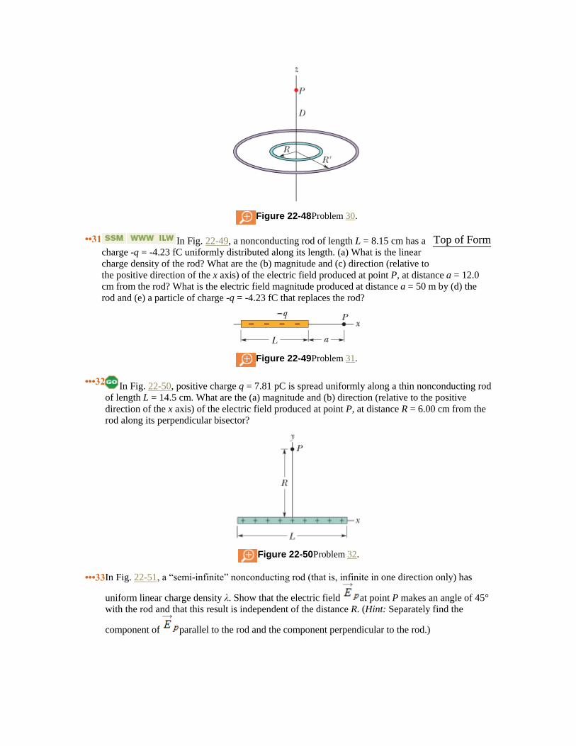
Figure 22-48 Problem 30.

••31 In Fig. 22-49, a nonconducting rod of length L = 8.15 cm has a

charge -q = -4.23 fC uniformly distributed along its length. (a) What is the linear

charge density of the rod? What are the (b) magnitude and (c) direction (relative to

the positive direction of the x axis) of the electric field produced at point P, at distance a = 12.0

cm from the rod? What is the electric field magnitude produced at distance a = 50 m by (d) the

rod and (e) a particle of charge -q = -4.23 fC that replaces the rod?

Figure 22-49 Problem 31.

Top of Form

•••32 In Fig. 22-50, positive charge q = 7.81 pC is spread uniformly along a thin nonconducting rod

of length L = 14.5 cm. What are the (a) magnitude and (b) direction (relative to the positive

direction of the x axis) of the electric field produced at point P, at distance R = 6.00 cm from the

rod along its perpendicular bisector?

Figure 22-50 Problem 32.

•••33 In Fig. 22-51, a “semi-infinite” nonconducting rod (that is, infinite in one direction only) has

uniform linear charge density λ. Show that the electric field at point P makes an angle of 45°

with the rod and that this result is independent of the distance R. (Hint: Separately find the

component of parallel to the rod and the component perpendicular to the rod.)

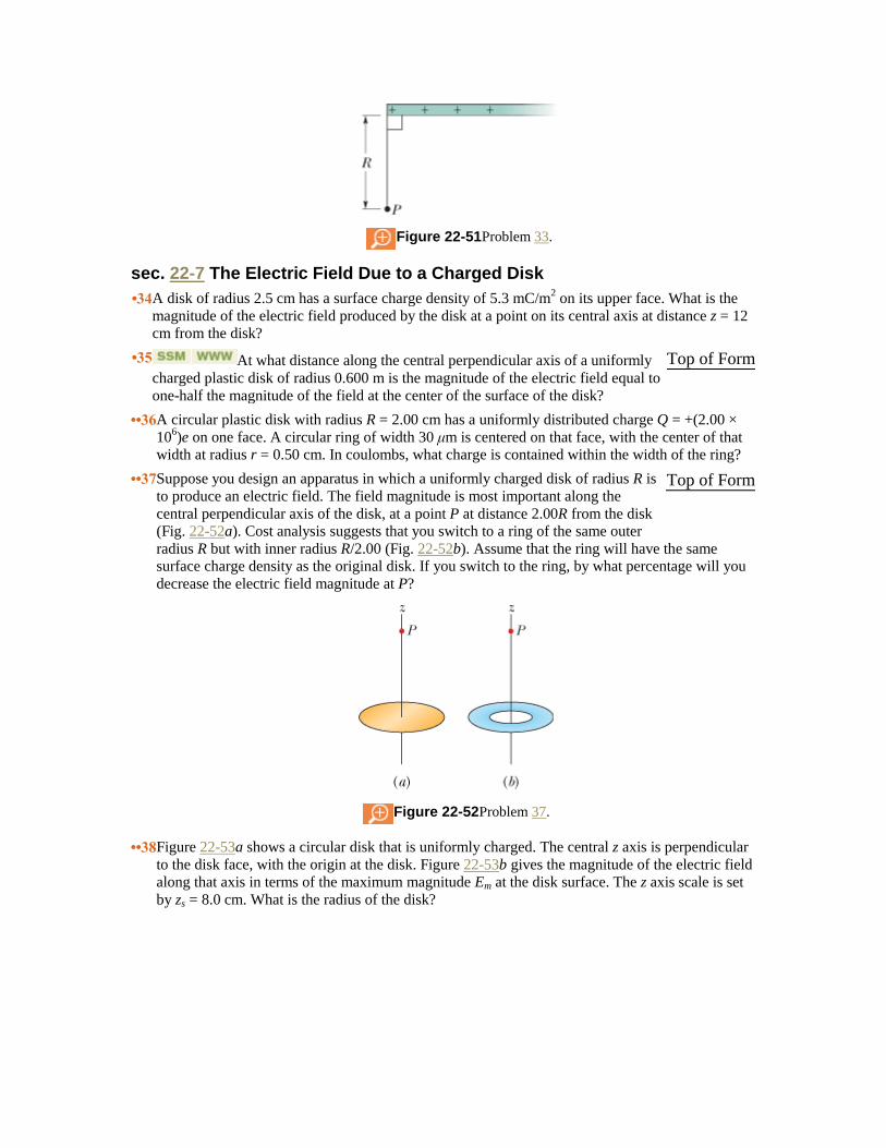
Figure 22-51 Problem 33.

sec. 22-7 The Electric Field Due to a Charged Disk

•34 A disk of radius 2.5 cm has a surface charge density of 5.3 mC/m2 on its upper face. What is the

magnitude of the electric field produced by the disk at a point on its central axis at distance z = 12

cm from the disk?

•35 At what distance along the central perpendicular axis of a uniformly

charged plastic disk of radius 0.600 m is the magnitude of the electric field equal to

one-half the magnitude of the field at the center of the surface of the disk?

Top of Form

••36 A circular plastic disk with radius R = 2.00 cm has a uniformly distributed charge Q = +(2.00 ×

106)e on one face. A circular ring of width 30 μm is centered on that face, with the center of that

width at radius r = 0.50 cm. In coulombs, what charge is contained within the width of the ring?

••37 Suppose you design an apparatus in which a uniformly charged disk of radius R is

to produce an electric field. The field magnitude is most important along the

central perpendicular axis of the disk, at a point P at distance 2.00R from the disk

(Fig. 22-52a). Cost analysis suggests that you switch to a ring of the same outer

radius R but with inner radius R/2.00 (Fig. 22-52b). Assume that the ring will have the same

surface charge density as the original disk. If you switch to the ring, by what percentage will you

decrease the electric field magnitude at P?

Figure 22-52 Problem 37.

Top of Form

••38 Figure 22-53a shows a circular disk that is uniformly charged. The central z axis is perpendicular

to the disk face, with the origin at the disk. Figure 22-53b gives the magnitude of the electric field

along that axis in terms of the maximum magnitude Em at the disk surface. The z axis scale is set

by zs = 8.0 cm. What is the radius of the disk?

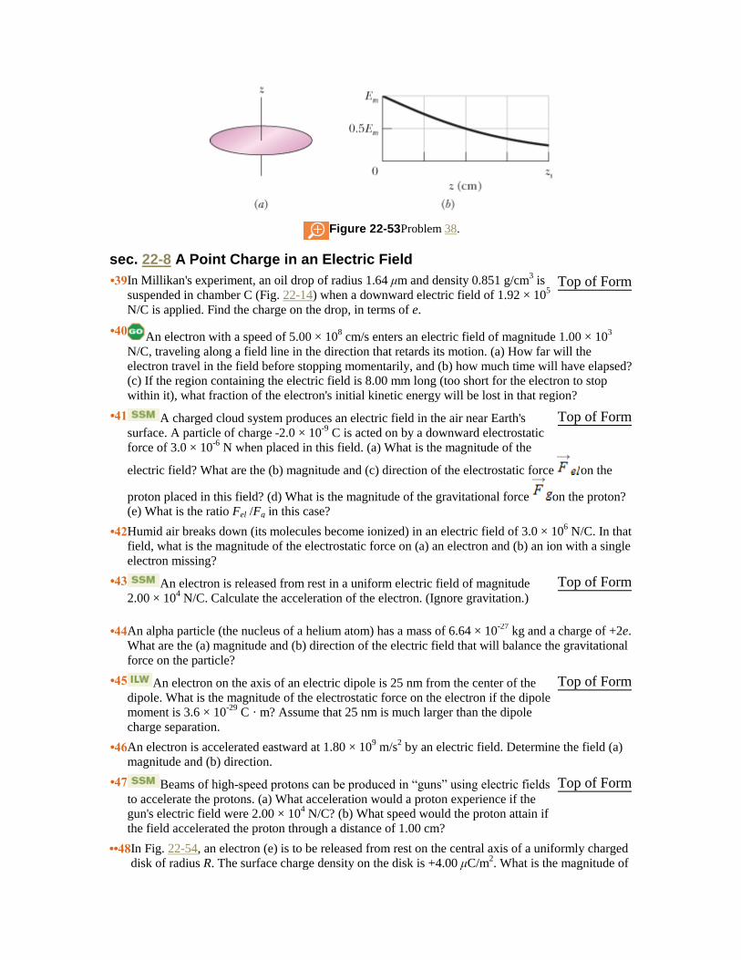
Figure 22-53 Problem 38.

sec. 22-8 A Point Charge in an Electric Field

•39 In Millikan's experiment, an oil drop of radius 1.64 μm and density 0.851 g/cm3 is

suspended in chamber C (Fig. 22-14) when a downward electric field of 1.92 × 105

N/C is applied. Find the charge on the drop, in terms of e.

Top of Form

•40 An electron with a speed of 5.00 × 10

8 cm/s enters an electric field of magnitude 1.00 × 10

3

N/C, traveling along a field line in the direction that retards its motion. (a) How far will the

electron travel in the field before stopping momentarily, and (b) how much time will have elapsed?

(c) If the region containing the electric field is 8.00 mm long (too short for the electron to stop

within it), what fraction of the electron's initial kinetic energy will be lost in that region?

•41 A charged cloud system produces an electric field in the air near Earth's

surface. A particle of charge -2.0 × 10-9

C is acted on by a downward electrostatic

force of 3.0 × 10-6

N when placed in this field. (a) What is the magnitude of the

electric field? What are the (b) magnitude and (c) direction of the electrostatic force on the

proton placed in this field? (d) What is the magnitude of the gravitational force on the proton?

(e) What is the ratio Fel /Fg in this case?

Top of Form

•42 Humid air breaks down (its molecules become ionized) in an electric field of 3.0 × 106 N/C. In that

field, what is the magnitude of the electrostatic force on (a) an electron and (b) an ion with a single

electron missing?

•43 An electron is released from rest in a uniform electric field of magnitude

2.00 × 104 N/C. Calculate the acceleration of the electron. (Ignore gravitation.)

Top of Form

•44 An alpha particle (the nucleus of a helium atom) has a mass of 6.64 × 10-27

kg and a charge of +2e.

What are the (a) magnitude and (b) direction of the electric field that will balance the gravitational

force on the particle?

•45 An electron on the axis of an electric dipole is 25 nm from the center of the

dipole. What is the magnitude of the electrostatic force on the electron if the dipole

moment is 3.6 × 10-29

C · m? Assume that 25 nm is much larger than the dipole

charge separation.

Top of Form

•46 An electron is accelerated eastward at 1.80 × 109 m/s

2 by an electric field. Determine the field (a)

magnitude and (b) direction.

•47 Beams of high-speed protons can be produced in “guns” using electric fields

to accelerate the protons. (a) What acceleration would a proton experience if the

gun's electric field were 2.00 × 104 N/C? (b) What speed would the proton attain if

the field accelerated the proton through a distance of 1.00 cm?

Top of Form

••48 In Fig. 22-54, an electron (e) is to be released from rest on the central axis of a uniformly charged

disk of radius R. The surface charge density on the disk is +4.00 μC/m2. What is the magnitude of

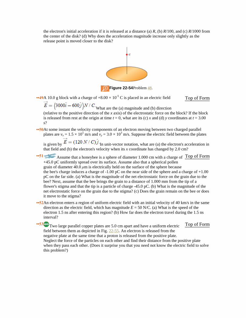
the electron's initial acceleration if it is released at a distance (a) R, (b) R/100, and (c) R/1000 from

the center of the disk? (d) Why does the acceleration magnitude increase only slightly as the

release point is moved closer to the disk?

Figure 22-54 Problem 48.

••49 A 10.0 g block with a charge of +8.00 × 10-5

C is placed in an electric field

What are the (a) magnitude and (b) direction

(relative to the positive direction of the x axis) of the electrostatic force on the block? If the block

is released from rest at the origin at time t = 0, what are its (c) x and (d) y coordinates at t = 3.00

s?

Top of Form

••50 At some instant the velocity components of an electron moving between two charged parallel

plates are vx = 1.5 × 105 m/s and vy = 3.0 × 10

3 m/s. Suppose the electric field between the plates

is given by In unit-vector notation, what are (a) the electron's acceleration in

that field and (b) the electron's velocity when its x coordinate has changed by 2.0 cm?

••51 Assume that a honeybee is a sphere of diameter 1.000 cm with a charge of

+45.0 pC uniformly spread over its surface. Assume also that a spherical pollen

grain of diameter 40.0 μm is electrically held on the surface of the sphere because

the bee's charge induces a charge of -1.00 pC on the near side of the sphere and a charge of +1.00

pC on the far side. (a) What is the magnitude of the net electrostatic force on the grain due to the

bee? Next, assume that the bee brings the grain to a distance of 1.000 mm from the tip of a

flower's stigma and that the tip is a particle of charge -45.0 pC. (b) What is the magnitude of the

net electrostatic force on the grain due to the stigma? (c) Does the grain remain on the bee or does

it move to the stigma?

Top of Form

••52 An electron enters a region of uniform electric field with an initial velocity of 40 km/s in the same

direction as the electric field, which has magnitude E = 50 N/C. (a) What is the speed of the

electron 1.5 ns after entering this region? (b) How far does the electron travel during the 1.5 ns

interval?

••53 Two large parallel copper plates are 5.0 cm apart and have a uniform electric

field between them as depicted in Fig. 22-55. An electron is released from the

negative plate at the same time that a proton is released from the positive plate.

Neglect the force of the particles on each other and find their distance from the positive plate

when they pass each other. (Does it surprise you that you need not know the electric field to solve

this problem?)

Top of Form

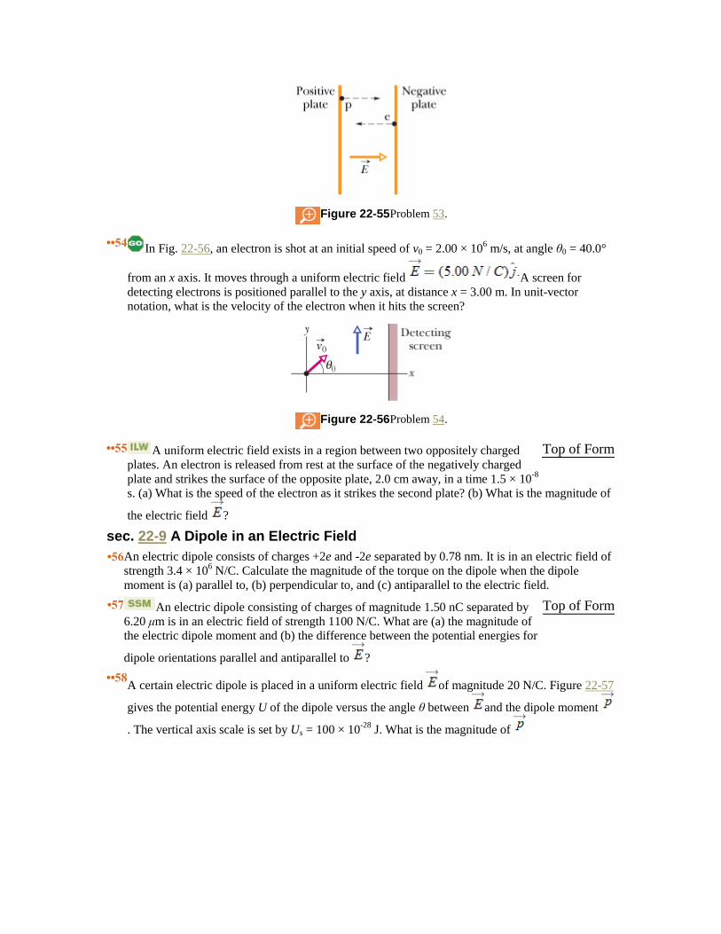
Figure 22-55 Problem 53.

••54 In Fig. 22-56, an electron is shot at an initial speed of v0 = 2.00 × 10

6 m/s, at angle θ0 = 40.0°

from an x axis. It moves through a uniform electric field A screen for

detecting electrons is positioned parallel to the y axis, at distance x = 3.00 m. In unit-vector

notation, what is the velocity of the electron when it hits the screen?

Figure 22-56 Problem 54.

••55 A uniform electric field exists in a region between two oppositely charged

plates. An electron is released from rest at the surface of the negatively charged

plate and strikes the surface of the opposite plate, 2.0 cm away, in a time 1.5 × 10-8

s. (a) What is the speed of the electron as it strikes the second plate? (b) What is the magnitude of

the electric field ?

Top of Form

sec. 22-9 A Dipole in an Electric Field

•56 An electric dipole consists of charges +2e and -2e separated by 0.78 nm. It is in an electric field of

strength 3.4 × 106 N/C. Calculate the magnitude of the torque on the dipole when the dipole

moment is (a) parallel to, (b) perpendicular to, and (c) antiparallel to the electric field.

•57 An electric dipole consisting of charges of magnitude 1.50 nC separated by

6.20 μm is in an electric field of strength 1100 N/C. What are (a) the magnitude of

the electric dipole moment and (b) the difference between the potential energies for

dipole orientations parallel and antiparallel to ?

Top of Form

••58 A certain electric dipole is placed in a uniform electric field of magnitude 20 N/C. Figure 22-57

gives the potential energy U of the dipole versus the angle θ between and the dipole moment

. The vertical axis scale is set by Us = 100 × 10-28

J. What is the magnitude of

Figure 22-57 Problem 58.

••59 How much work is required to turn an electric dipole 180° in a uniform electric

field of magnitude E = 46.0 N/C if p = 3.02 × 10-25

C·m and the initial angle is

64°?

Top of Form

••60 A certain electric dipole is placed in a uniform electric field of magnitude 40 N/C. Figure 22-58

gives the magnitude τ of the torque on the dipole versus the angle θ between field and the

dipole moment . The vertical axis scale is set by τs = 100 × 10-28

N·m. What is the magnitude of

?

Figure 22-58 Problem 60.

••61 Find an expression for the oscillation frequency of an electric dipole of dipole

moment and rotational inertia I for small amplitudes of oscillation about its

equilibrium position in a uniform electric field of magnitude E.

Top of Form

Additional Problems

62 (a) What is the magnitude of an electron's acceleration in a uniform electric field of magnitude

1.40 × 106 N/C? (b) How long would the electron take, starting from rest, to attain one-tenth the

speed of light? (c) How far would it travel in that time?

63 A spherical water drop 1.20 μm in diameter is suspended in calm air due to a

downward-directed atmospheric electric field of magni-tude E = 462 N/C. (a) What

is the magnitude of the gravitational force on the drop? (b) How many excess

electrons does it have?

Top of Form

64 Three particles, each with positive charge Q, form an equilateral triangle, with each side of length

d. What is the magnitude of the electric field produced by the particles at the midpoint of any side?

65 In Fig. 22-59a, a particle of charge +Q produces an electric field of magnitude Epart

at point P, at distance R from the particle. In Fig. 22-59b, that same amount of

charge is spread uniformly along a circular arc that has radius R and subtends an

angle θ. The charge on the arc produces an electric field of magnitude Earc at its

center of curvature P. For what value of θ does Earc = 0.500Epart? (Hint: You will probably resort

to a graphical solution.)

Top of Form

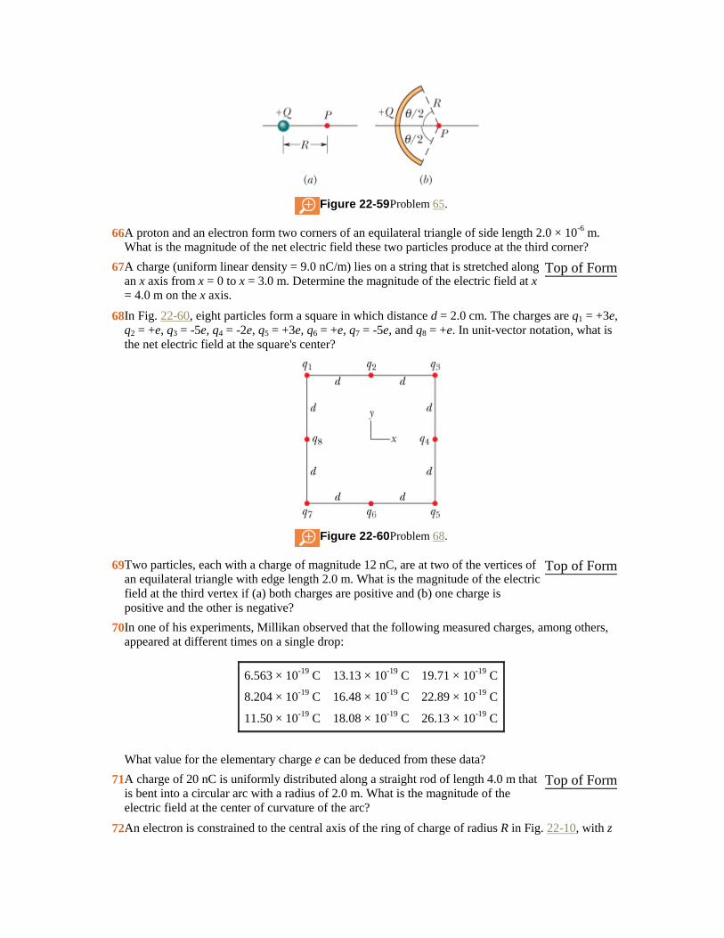
Figure 22-59 Problem 65.

66 A proton and an electron form two corners of an equilateral triangle of side length 2.0 × 10-6

m.

What is the magnitude of the net electric field these two particles produce at the third corner?

67 A charge (uniform linear density = 9.0 nC/m) lies on a string that is stretched along

an x axis from x = 0 to x = 3.0 m. Determine the magnitude of the electric field at x

= 4.0 m on the x axis.

Top of Form

68 In Fig. 22-60, eight particles form a square in which distance d = 2.0 cm. The charges are q1 = +3e,

q2 = +e, q3 = -5e, q4 = -2e, q5 = +3e, q6 = +e, q7 = -5e, and q8 = +e. In unit-vector notation, what is

the net electric field at the square's center?

Figure 22-60 Problem 68.

69 Two particles, each with a charge of magnitude 12 nC, are at two of the vertices of

an equilateral triangle with edge length 2.0 m. What is the magnitude of the electric

field at the third vertex if (a) both charges are positive and (b) one charge is

positive and the other is negative?

Top of Form

70 In one of his experiments, Millikan observed that the following measured charges, among others,

appeared at different times on a single drop:

6.563 × 10-19

C 13.13 × 10-19

C 19.71 × 10-19

C

8.204 × 10-19

C 16.48 × 10-19

C 22.89 × 10-19

C

11.50 × 10-19

C 18.08 × 10-19

C 26.13 × 10-19

C

What value for the elementary charge e can be deduced from these data?

71 A charge of 20 nC is uniformly distributed along a straight rod of length 4.0 m that

is bent into a circular arc with a radius of 2.0 m. What is the magnitude of the

electric field at the center of curvature of the arc?

Top of Form

72 An electron is constrained to the central axis of the ring of charge of radius R in Fig. 22-10, with z

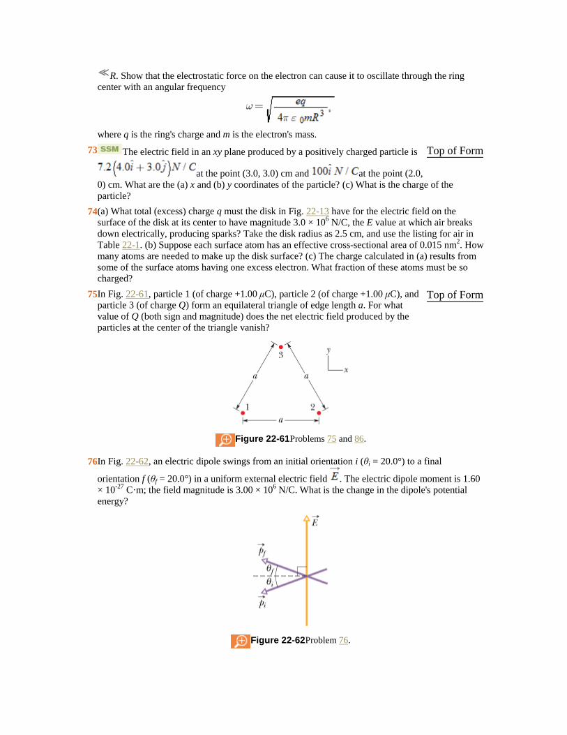
R. Show that the electrostatic force on the electron can cause it to oscillate through the ring

center with an angular frequency

where q is the ring's charge and m is the electron's mass.

73 The electric field in an xy plane produced by a positively charged particle is

at the point (3.0, 3.0) cm and at the point (2.0,

0) cm. What are the (a) x and (b) y coordinates of the particle? (c) What is the charge of the

particle?

Top of Form

74 (a) What total (excess) charge q must the disk in Fig. 22-13 have for the electric field on the

surface of the disk at its center to have magnitude 3.0 × 106 N/C, the E value at which air breaks

down electrically, producing sparks? Take the disk radius as 2.5 cm, and use the listing for air in

Table 22-1. (b) Suppose each surface atom has an effective cross-sectional area of 0.015 nm2. How

many atoms are needed to make up the disk surface? (c) The charge calculated in (a) results from

some of the surface atoms having one excess electron. What fraction of these atoms must be so

charged?

75 In Fig. 22-61, particle 1 (of charge +1.00 μC), particle 2 (of charge +1.00 μC), and

particle 3 (of charge Q) form an equilateral triangle of edge length a. For what

value of Q (both sign and magnitude) does the net electric field produced by the

particles at the center of the triangle vanish?

Figure 22-61 Problems 75 and 86.

Top of Form

76 In Fig. 22-62, an electric dipole swings from an initial orientation i (θi = 20.0°) to a final

orientation f (θf = 20.0°) in a uniform external electric field . The electric dipole moment is 1.60

× 10-27

C·m; the field magnitude is 3.00 × 106 N/C. What is the change in the dipole's potential

energy?

Figure 22-62 Problem 76.

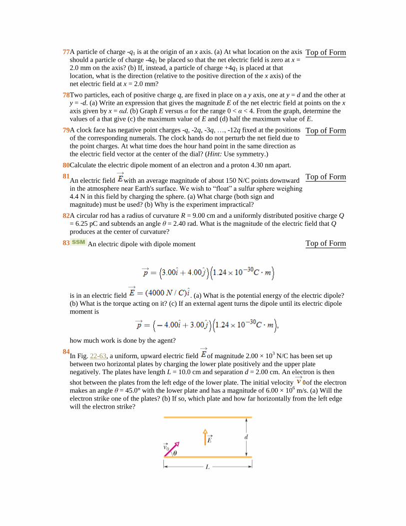
77 A particle of charge -q1 is at the origin of an x axis. (a) At what location on the axis

should a particle of charge -4q1 be placed so that the net electric field is zero at x =

2.0 mm on the axis? (b) If, instead, a particle of charge +4q1 is placed at that

location, what is the direction (relative to the positive direction of the x axis) of the

net electric field at x = 2.0 mm?

Top of Form

78 Two particles, each of positive charge q, are fixed in place on a y axis, one at y = d and the other at

y = -d. (a) Write an expression that gives the magnitude E of the net electric field at points on the x

axis given by x = αd. (b) Graph E versus α for the range 0 < α < 4. From the graph, determine the

values of a that give (c) the maximum value of E and (d) half the maximum value of E.

79 A clock face has negative point charges -q, -2q, -3q, …, -12q fixed at the positions

of the corresponding numerals. The clock hands do not perturb the net field due to

the point charges. At what time does the hour hand point in the same direction as

the electric field vector at the center of the dial? (Hint: Use symmetry.)

Top of Form

80 Calculate the electric dipole moment of an electron and a proton 4.30 nm apart.

81 An electric field with an average magnitude of about 150 N/C points downward

in the atmosphere near Earth's surface. We wish to “float” a sulfur sphere weighing

4.4 N in this field by charging the sphere. (a) What charge (both sign and

magnitude) must be used? (b) Why is the experiment impractical?

Top of Form

82 A circular rod has a radius of curvature R = 9.00 cm and a uniformly distributed positive charge Q

= 6.25 pC and subtends an angle θ = 2.40 rad. What is the magnitude of the electric field that Q

produces at the center of curvature?

83 An electric dipole with dipole moment

is in an electric field . (a) What is the potential energy of the electric dipole?

(b) What is the torque acting on it? (c) If an external agent turns the dipole until its electric dipole

moment is

how much work is done by the agent?

Top of Form

84 In Fig. 22-63, a uniform, upward electric field of magnitude 2.00 × 10

3 N/C has been set up

between two horizontal plates by charging the lower plate positively and the upper plate

negatively. The plates have length L = 10.0 cm and separation d = 2.00 cm. An electron is then

shot between the plates from the left edge of the lower plate. The initial velocity of the electron

makes an angle θ = 45.0° with the lower plate and has a magnitude of 6.00 × 106 m/s. (a) Will the

electron strike one of the plates? (b) If so, which plate and how far horizontally from the left edge

will the electron strike?

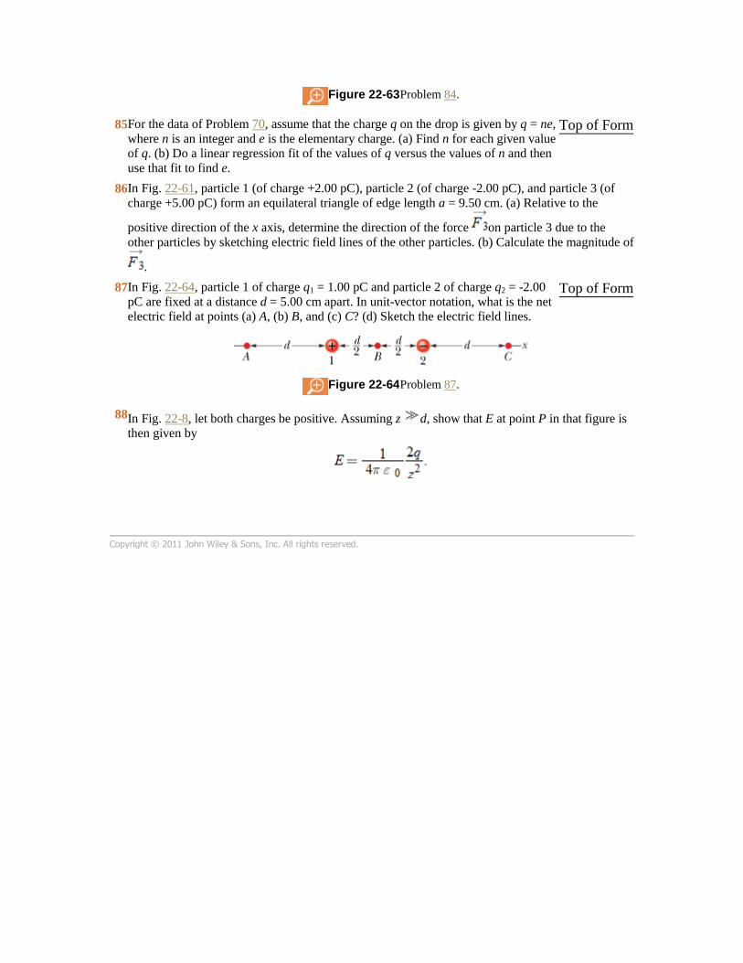
Figure 22-63 Problem 84.

85 For the data of Problem 70, assume that the charge q on the drop is given by q = ne,

where n is an integer and e is the elementary charge. (a) Find n for each given value

of q. (b) Do a linear regression fit of the values of q versus the values of n and then

use that fit to find e.

Top of Form

86 In Fig. 22-61, particle 1 (of charge +2.00 pC), particle 2 (of charge -2.00 pC), and particle 3 (of

charge +5.00 pC) form an equilateral triangle of edge length a = 9.50 cm. (a) Relative to the

positive direction of the x axis, determine the direction of the force on particle 3 due to the

other particles by sketching electric field lines of the other particles. (b) Calculate the magnitude of

.

87 In Fig. 22-64, particle 1 of charge q1 = 1.00 pC and particle 2 of charge q2 = -2.00

pC are fixed at a distance d = 5.00 cm apart. In unit-vector notation, what is the net

electric field at points (a) A, (b) B, and (c) C? (d) Sketch the electric field lines.

Figure 22-64 Problem 87.

Top of Form

88 In Fig. 22-8, let both charges be positive. Assuming z d, show that E at point P in that figure is

then given by

Copyright © 2011 John Wiley & Sons, Inc. All rights reserved.