Time-Varying Fields and Electromagnetic Waves
97
Arlon T. Adams Jay K. Lee Principles of Electromagnetics 4—Time-Varying Fields and Electromagnetic Waves
-
Upload
khangminh22 -
Category
Documents
-
view
3 -
download
0
Transcript of Time-Varying Fields and Electromagnetic Waves
Arlon T. AdamsJay K. Lee
Principles of Electromagnetics 4—Time-Varying Fields and Electromagnetic Waves
9781606507186_Cover.indd 1 19/12/14 3:51 PM

Principles of Electromagnetics 4— Time-Varying Fields and Electromagnetic Waves
Arlon T. Adams Jay K. Lee
Adams-Book4_FM.indd 1 16/12/14 12:11 AM

Electromagnetics 4—Time-Varying Fields and Electromagnetic Waves
Copyright © Cognella Academic Publishing 2015 www.cognella.com
All rights reserved. No part of this publication may be reproduced, stored in a retrieval system, or transmitted in any form or by any means—electronic, mechanical, photocopy, recording, or any other except for brief quotations, not to exceed 400 words, without the prior permission of the publisher.
ISBN-13: 978-1-60650-718-6 (e-book)
www.momentumpress.net
Trademark Notice: Product or corporate names may be trademarks or registered trademarks, and are used only for identification and explanation without intent to infringe.
A publication in the Momentum Press Electrical Power collection
Cover and interior design by S4Carlisle Publishing Services Private Ltd., Chennai, India
Adams-Book4_FM.indd 2 16/12/14 12:11 AM

Brief Contents
Preface ..................................................................................................ixChapter 1 Time-Varying Fields and Electromagnetic Waves ..............1Chapter 2 Principles of Magnetic Waves ..........................................39
Adams-Book4_FM.indd 3 16/12/14 12:11 AM

Adams-Book4_FM.indd 4 16/12/14 12:11 AM

Contents
Chapter 1 Time-Varying Fields and Electromagnetic Waves ..............11.1 Introduction ............................................................11.2 Laws of Electrostatics and Magnetostatics – A
Summary .................................................................21.3 Faraday’s Law ...........................................................4
1.3.1 General Forms of Faraday’s Law ........................41.3.2 The Effects of Motion Through Magnetic
Fields ...............................................................61.3.3 Non-Relativistic Integral Forms of
Faraday’s Law ................................................. 91.3.4 Lenz’s Law ......................................................13
1.4 Michael Faraday’s Famous Experiments of 1831 .....141.5 Maxwell’s Equations ...............................................18
1.5.1 Displacement Current ....................................191.5.2 Maxwell’s Equations .......................................241.5.3 The Wave Equation – Electromagnetic
Waves! ............................................................261.5.4 James Clerk Maxwell (1831-1879) .................29
1.6 Boundary Conditions for Time-Varying Fields .......321.7 Flow of Electromagnetic Power: Poynting’s
Theorem ................................................................35Chapter 2 Principles of Magnetic Waves .........................................39
2.1 Introduction ..........................................................392.2 The Wave Equation in a Source-Free Region ..........40
2.2.1 One-Dimensional Wave Solutions ..................412.3 Time-Harmonic Electromagnetic Fields .................43
2.3.1 Phasor Representation of Time-Harmonic Fields.............................................................44
2.3.2 Maxwell’s Equations for Time-Harmonic Fields.............................................................46
Adams-Book4_FM.indd 5 16/12/14 12:11 AM

2.3.3 Complex Poynting Theorem – Real Power Flow................................................................47
2.4 Uniform Plane Waves in Lossless Media .................512.4.1 Uniform Plane Waves Propagating in Arbitrary
Direction........................................................ 592.5 Uniform Plane Waves in Lossy Media ....................61
2.5.1 Attenuation of Waves .....................................622.5.2 Good Dielectric vs. Good Conductor .............67
2.6. Dispersion of Waves – Group Velocity ..................722.7. Polarization of Waves ............................................76
vi CONTENTS
Adams-Book4_FM.indd 6 16/12/14 12:11 AM
List of Figures
Figure 1-1. A conducting bar moving through a magnetic field ...........7Figure 1-2. Voltage in a moving system. ..............................................8Figure 1-3. How to tap off a voltage ....................................................8Figure 1-4. A conducting loop C, with a small gap a-b, moving
through magnetic fields. Velocities are non-relativistic and the loop is non-radiative. Vab(t) is the open-circuit voltage as measured by a moving observer. The velocity of the moving observer is that of the terminals a-b. Path C is closed through the gap from a to b ...............................................................................10
Figure 1-5. Induced voltage and current in a moving loop .................12Figure 1-6. Faraday’s experiments (a) general form, (b) iron core
experiment, (c) short-circuit current. ...............................16Figure 1-7. Displacement current and induced magnetic field in
a parallel-plate capacitor. .................................................21Figure 1-8. Conduction current and displacement current ................23Figure 1-9. Boundary conditions at an interface between two
different media ................................................................33Figure 2-1. Gaussian pulse moving with velocity v ............................42Figure 2-2. Time-harmonic electromagnetic field ..............................53Figure 2-3. Electric and magnetic fields as a function of space at
fixed time. .......................................................................56Figure 2-4. Uniform plane wave propagating in an arbitrary
direction..........................................................................60Figure 2-5. Time-harmonic electromagnetic field with attenuation ...64Figure 2-6. Group velocity of a wave packet ......................................74Figure 2-7. Wave polarization ............................................................78
Adams-Book4_FM.indd 7 16/12/14 12:11 AM

Adams-Book4_FM.indd 8 16/12/14 12:11 AM

Electromagnetics is not an easy subject for students. The subject presents a number of challenges, such as: new math, new physics, new geometry, new insights and difficult problems. As a result, every aspect needs to be presented to students carefully, with thorough mathematics and strong physical insights and even alternative ways of viewing and formulating the subject. The theoretician James Clerk Maxwell and the experimental-ist Michael Faraday, both shown on the cover, had high respect for physi-cal insights.
This book is written primarily as a text for an undergraduate course in electromagnetics, taken by junior and senior engineering and phys-ics students. The book can also serve as a text for beginning graduate courses by including advanced subjects and problems. The book has been thoroughly class-tested for many years for a two-semester Electromagnet-ics course at Syracuse University for electrical engineering and physics students. It could also be used for a one-semester course, covering up through Chapter 8 and perhaps skipping Chapter 4 and some other parts. For a one-semester course with more emphasis on waves, the instructor could briefly cover basic materials from statics (mainly Chapters 2 and 6) and then cover Chapters 8 through 12.
The authors have attempted to explain the difficult concepts of elec-tromagnetic theory in a way that students can readily understand and follow, without omitting the important details critical to a solid under-standing of a subject. We have included a large number of examples, sum-mary tables, alternative formulations, whenever possible, and homework problems. The examples explain the basic approach, leading the students step by step, slowly at first, to the conclusion. Then special cases and limiting cases are examined to draw out analogies, physical insights and their interpretation. Finally, a very extensive set of problems enables the instructor to teach the course for several years without repeating problem assignments. Answers to selected problems at the end allow students to check if their answers are correct.
Preface
Adams-Book4_FM.indd 9 16/12/14 12:11 AM

x PREFACE
# 156104 Cust: MP Au: Adams Pg. No. x Title: Principles of Electromagnetics 1—
K Short / Normal
DESIGN SERVICES OF
S4CARLISLEPublishing Services
During our years of teaching electromagnetics, we became interested in its historical aspects and found it useful and instructive to introduce stories of the basic discoveries into the classroom. We have included short biographical sketches of some of the leading figures of electromagnetics, including Josiah Willard Gibbs, Charles Augustin Coulomb, Benjamin Franklin, Pierre Simon de Laplace, Georg Simon Ohm, Andre Marie Ampère, Joseph Henry, Michael Faraday, and James Clerk Maxwell.
The text incorporates some unique features that include:
• Coordinate transformations in 2D (Figures 1-11, 1-12). • Summary tables, such as Table 2-1, 4-1, 6-1, 10-1. • Repeated use of equivalent forms with R (conceptual) and
|r−r′| (mathematical) for the distance between the source point and the field point as in Eqs. (2-27), (2-46), (6-18), (6-19), (12-21).
• Intuitive derivation of equivalent bound charges from polarization sources, including piecewise approximation to non-uniform polarization (Section 3.3).
• Self-field (Section 3.8). • Concept of the equivalent problem in the method of images
(Section 4.3). • Intuitive derivation of equivalent bound currents from
magnetization sources, including piecewise approximation to non-uniform magnetization (Section 7.3).
• Thorough treatment of Faraday’s law and experiments (Sections 8.3, 8.4).
• Uniform plane waves propagating in arbitrary direction (Section 9.4.1).
• Treatment of total internal reflection (Section 10.4). • Transmission line equations from field theory (Section
11.7.2). • Presentation of the retarded potential formulation in Chapter
12. • Interpretation of the Hertzian dipole fields (Section 12.3).
Finally, we would like to acknowledge all those who contributed to the textbook. First of all, we would like to thank all of the undergraduate
Adams-Book4_FM.indd 10 16/12/14 12:11 AM

PREFACE xi
# 156104 Cust: MP Au: Adams Pg. No. xi Title: Principles of Electromagnetics 1—
K Short / Normal
DESIGN SERVICES OF
S4CARLISLEPublishing Services
and graduate students, too numerous to mention, whose comments and suggestions have proven invaluable. As well, one million thanks go to Ms. Brenda Flowers for typing the entire manuscript and making corrections numerous times. We also wish to express our gratitude to Dr. Eunseok Park, Professor Tae Hoon Yoo, Dr. Gokhan Aydin, and Mr. Walid M. G. Dyab for drawing figures and plotting curves, and to Professor Mahmoud El Sabbagh for reviewing the manuscript. Thanks go to the University of Poitiers, France and Seoul National University, Korea where an office and academic facilities were provided to Professor Adams and Professor Lee, respectively, during their sabbatical years. Thanks especially to Syracuse University where we taught for a total of over 50 years. Comments and suggestions from readers would be most welcome.
Arlon T. Adams
Jay Kyoon [email protected]
June 2012Syracuse, New York
Adams-Book4_FM.indd 11 16/12/14 12:11 AM

Adams-Book4_FM.indd 12 16/12/14 12:11 AM

# 156104 Cust: MP Au: Adams Pg. No. 1 Title: Principles of Electromagnetics 1—
K Short / Normal
DESIGN SERVICES OF
S4CARLISLEPublishing Services
CHAPTER 1
Time-Varying Fields and Electromagnetic Waves
1.1 Introduction
In previous chapters we explored the very rapid progress made in magne-tostatics by Oersted, Ampère, Biot-Savart, Arago and others during the 1820’s following Oersted’s dramatic discovery of the relationship between electric current and magnetism. By the end of the 1820’s the formula-tion of magnetostatics was nearly complete. Such a rapid development of basic theory was virtually unheard of in those days. James Clerk Maxwell (1831-1879), studying at a later time the development of magnetostatics, said of Ampère’s work, “the whole, theory and experiment, seem to have burst forth in full vigor and completely formed from the brain of this Newton of electricity.” High praise from Maxwell!!
The problems of time-varying fields, however, were much more subtle and much more difficult to crack. Some first steps were made in 1831 when Michael Faraday (1791-1867) carried out in ten days a famous set of experiments in which he discovered (a) magnetic induction, (b) the similarity of permanent magnets and electromagnets, and (c) the first electric generator (Faraday disk generator). He continued to work on magnetic induction for over twenty years and expressed his conclusions in words equivalent to what we now call Faraday’s Law. The first half of the time-varying problem was thus completed by about 1850.
The other half of the time-varying problem was of a more abstract na-ture. There were no simple experiments which could be carried out to de-termine the solution. Maxwell, who was 40 years younger than Faraday, made his first step when he translated Faraday’s results into mathematical form. The search for the complete formulation of electromagnetics was

2 PRINCIPLES OF ELECTROMAGNETICS 4
# 156104 Cust: MP Au: Adams Pg. No. 2 Title: Principles of Electromagnetics 1—
K Short / Normal
DESIGN SERVICES OF
S4CARLISLEPublishing Services
an international affair. It was widely known that a piece of the puzzle was missing. Virtually all of the leading physicists of the time had a crack at the problem but it was unyielding. Finally Maxwell, after decades of study, reported his complete theory in 1865, at the end of the American Civil War. He continued to work on electromagnetics for the rest of his life, publishing his great work, A Treatise on Electricity and Magnetism, in 1873. He died in 1879. About ten years after his death Heinrich Hertz (1857-1894) built some of the first antennas and decisively confirmed Maxwell’s theory. About fifteen years after that Albert Einstein (1879-1955) showed that Maxwell’s equations were valid in any moving system and that they were in fact the basis for relativity. Since then, the twenti-eth century has not revealed any flaws in Maxwell’s equations. We now recognize them as the crowning achievement of electromagnetics. R. P. Feynman has said,
“Twenty thousand years from now, Maxwell’s equations will be recognized as a pinnacle of 19th century science, while the Ameri-can Civil War will be regarded as an insignificant brush fire …”
1.2 Laws of Electrostatics and Magnetostatics – A Summary
We recall that the basic laws of electrostatics are
∇ × =E 0 ∇ ⋅ =D ρv
(Electrostatics) (1-1)
The first law (∇ × E = 0) states the conservative (curl free) nature of
the electrostatic field. It implies that the line integral of E EC
d∫ ⋅
is
zero around any closed path C, and that the voltage between any two points is independent of path. It thus implies that the sum of the voltages around a loop is zero, which is known as the Kirchhoff voltage law (KVL) in circuit theory. The second law (∇ · D = ρv), known as Gauss’ law, states the divergence relationship between the source ρv and the electrostatic
field. It implies that the electric flux ' D s⋅
∫∫ dS
through any closed sur-face S is equal to the total charge enclosed within the volume.
TIME-VARyING FIELdS ANd ELECTROMAGNETIC WAVES 3
# 156104 Cust: MP Au: Adams Pg. No. 3 Title: Principles of Electromagnetics 1—
K Short / Normal
DESIGN SERVICES OF
S4CARLISLEPublishing Services
The basic laws of magnetostatics are
∇ × =H J ∇ ⋅ =B 0 (Magnestostatics) (1-2)
The first law (∇ × H = J), known as Ampère’s law, states the curl relationship between the source J and the magnetostatic field. Oersted’s
discovery was the first indication of this relationship. It implies that the
circulation of the magnetic field HC
d∫ ⋅
along any closed contour
C is equal to the total current passing through the surface bounded by C. The first law also implies ∇ · J = 0 and thus the sum of the currents into a junction or loose end ' J s⋅
∫∫ dS
is zero, which is known as the Kirchhoff current law (KCL) in circuit theory. The second law (∇ · B = 0) states the solenoidal (divergenceless) nature of the magnetostatic field. It implies that the surface integral ' B s⋅∫∫ d
S
over any closed surface S is
zero and that the flux B s⋅∫∫ dS
of the vector B through any open surface
S bounded by C is independent of the surface S.The laws for electrostatics and magnetostatics are uncoupled. The
electrostatic field arises from its divergence-type source ρv. The magne-tostatic field arises from its curl-type source J. The electric field E is de-termined solely by its sources (ρv and ρpv); B is determined solely by its sources (J and Jm). Each represents a canonical form. The electrostatic field represents all conservative vector fields; the magnetostatic field rep-resents all solenoidal vector fields.
For time-varying fields, some basic changes are required in the laws above. The two divergence laws, ∇ · D = ρv and ∇ · B = 0, are valid for the time-varying as well as for the static cases, and therefore no changes are necessary for those laws. However, the two curl equations, ∇ × E = 0 and ∇ × H = J, do require drastic revision, which is the subject of Faraday’s law and Maxwell’s equations, respectively. These revisions will upset all of our previous concepts. You may be surprised to learn that, in the general time-varying case, the sum of the voltages around a loop is not necessar-ily zero, the voltage is not independent of path, and that the sum of the currents into a junction or loose end is not zero. A completely new ball game!! However, despite those drastic changes in the characteristics of the

4 PRINCIPLES OF ELECTROMAGNETICS 4
# 156104 Cust: MP Au: Adams Pg. No. 4 Title: Principles of Electromagnetics 1—
K Short / Normal
DESIGN SERVICES OF
S4CARLISLEPublishing Services
fields, the mathematical changes required are relatively simple. The addi-tion of a single term to each of the two curl equations, ∇ × E = 0 and ∇ × H = J, will be sufficient to complete the formulation for time-varying fields.
1.3 Faraday’s Law
Faraday’s law appears in various forms and involves some very subtle ef-fects. It is important, therefore, that the different forms and their particu-lar limitations be clearly defined. We will start with the general forms, which are valid in all cases and then we will look at the special forms which are of particular interest to electrical engineers.
1.3.1 General Forms of Faraday’s Law
Faraday’s law in differential form is
∇ × = − ∂
∂E
Bt
(1-3)
(Faraday’s law in differential form)
We may conclude that a time-varying magnetic field creates an electric field. Referring to Helmholtz’s theorem we note that E may arise from ∇ × E or ∇ · E. In the electrostatic case, ∇ × E = 0, and the only pos-sible source is the free and bound charge densities since ∇ · E = (ρv +
ρpv)/ε0. In the time-varying case, however, ∂∂Bt
acts as an additional source. We note that Eq. (1-3) reduces to the static case, ∇ × E = 0, if ∇ × = ∂
∂=E
B0 0, if
t. Equation (1-3) is valid at all times at any point in
space in all situations. It is our first general law of electromagnetics since our previous laws were limited to the electrostatic case (charges are nailed down) or to the magnetostatic case (currents are steady).
Integrating both sides of Eq. (1-3) over an open surface S, we obtain the integral form of Faraday’s law
∇ × ⋅ = ⋅ = ∂∂
⋅∫∫ ∫ ∫∫E s EB
sd dt
dS C S
where the first equality is due to Stokes’ theorem. Therefore, we have
TIME-VARyING FIELdS ANd ELECTROMAGNETIC WAVES 5
# 156104 Cust: MP Au: Adams Pg. No. 5 Title: Principles of Electromagnetics 1—
K Short / Normal
DESIGN SERVICES OF
S4CARLISLEPublishing Services
C S
dt
d
(Faraday’s law in integral form)
∫ ∫∫⋅ = − ∂∂
⋅EB
s
)
(1-4)
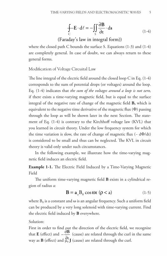
where the closed path C bounds the surface S. Equations (1-3) and (1-4) are completely general. In case of doubt, we can always return to these general forms.
Modification of Voltage Circuital Law
The line integral of the electric field around the closed loop C in Eq. (1-4) corresponds to the sum of potential drops (or voltages) around the loop. Eq. (1-4) indicates that the sum of the voltages around a loop is not zero, if there exists a time-varying magnetic field, but is equal to the surface integral of the negative rate of change of the magnetic field B, which is equivalent to the negative time derivative of the magnetic flux (Φ) passing through the loop as will be shown later in the next Section. The state-ment of Eq. (1-4) is contrary to the Kirchhoff voltage law (KVL) that you learned in circuit theory. Under the low frequency system for which the time variation is slow, the rate of change of magnetic flux (− dΦ/dt) is considered to be small and thus can be neglected. The KVL in circuit theory is valid only under such circumstances.
In the following example, we illustrate how the time-varying mag-netic field induces an electric field.
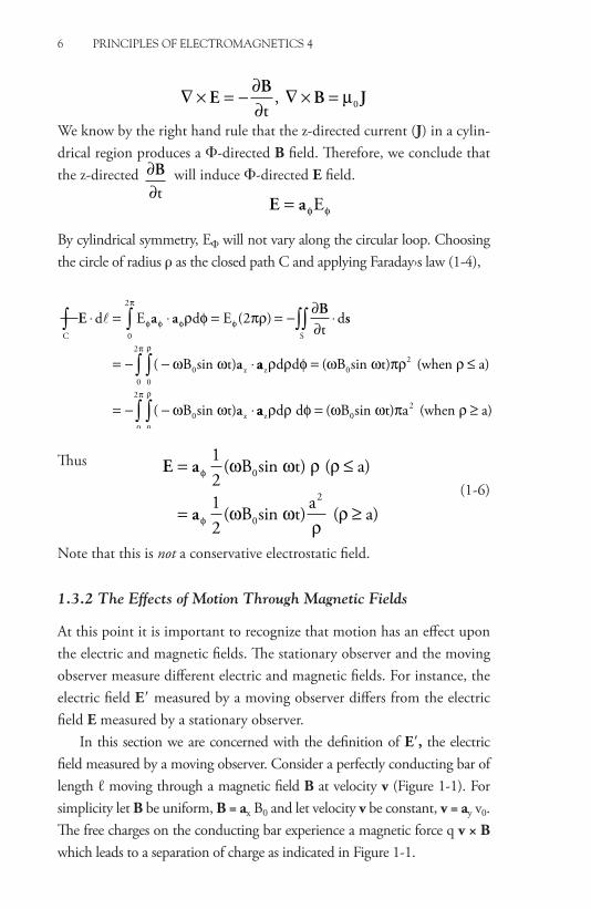
Example 1-1. The Electric Field Induced by a Time-Varying Magnetic Field
The uniform time-varying magnetic field B exists in a cylindrical re-gion of radius a:
B a= <zB t ( a)0 cosω ρ (1-5)
where B0 is a constant and ω is an angular frequency. Such a uniform field can be produced by a very long solenoid with time-varying current. Find the electric field induced by B everywhere.
Solution:First in order to find out the direction of the electric field, we recognize that E (effect) and − ∂
∂Bt
(cause) are related through the curl in the same way as B (effect) and μ0 J (cause) are related through the curl.
6 PRINCIPLES OF ELECTROMAGNETICS 4
# 156104 Cust: MP Au: Adams Pg. No. 6 Title: Principles of Electromagnetics 1—
K Short / Normal
DESIGN SERVICES OF
S4CARLISLEPublishing Services
∇ × = − ∂
∂∇ × =E
BB J
t 0, µ
We know by the right hand rule that the z-directed current (J) in a cylin-drical region produces a Φ-directed B field. Therefore, we conclude that the z-directed ∂
∂Bt
will induce Φ-directed E field.
E a= φ φE
By cylindrical symmetry, EΦ will not vary along the circular loop. Choosing the circle of radius ρ as the closed path C and applying Faraday›s law (1-4),
C 0 S
0 z
d E d Et
d
( B sin t)
∫ ∫ ∫∫⋅ = ⋅ = = − ∂∂
⋅
= − − ⋅
E a aB
s
a
φ φ φ
π
φρ φ πρ
ω ω
2
2( )
aa
a
z0
02
0 z
d d ( B sin t) (when a)
( B sin t)
ρ ρ φ ω ω πρ ρ
ω ω
ρπ
∫∫ = ≤
= − − ⋅
0
2
aa z0
02d d ( B sin t) a (when a)ρ ρ φ ω ω π ρ
ρπ
∫∫ = ≥0
2
Thus
E a
a
= ≤
= ≥
φ
φ
ω ω ρ ρ
ω ωρ
ρ
12
( B sin t) ( a)
12
( B sin t)a
( a)
0
0
2 (1-6)
Note that this is not a conservative electrostatic field.
1.3.2 The Effects of Motion Through Magnetic Fields
At this point it is important to recognize that motion has an effect upon the electric and magnetic fields. The stationary observer and the moving observer measure different electric and magnetic fields. For instance, the electric field E′ measured by a moving observer differs from the electric field E measured by a stationary observer.
In this section we are concerned with the definition of E′, the electric field measured by a moving observer. Consider a perfectly conducting bar of length ℓ moving through a magnetic field B at velocity v (Figure 1-1). For simplicity let B be uniform, B = ax B0 and let velocity v be constant, v = ay v0. The free charges on the conducting bar experience a magnetic force q v × B which leads to a separation of charge as indicated in Figure 1-1.

TIME-VARyING FIELdS ANd ELECTROMAGNETIC WAVES 7
# 156104 Cust: MP Au: Adams Pg. No. 7 Title: Principles of Electromagnetics 1—
K Short / Normal
DESIGN SERVICES OF
S4CARLISLEPublishing Services
B
++++×
++
a
b
E
v B
Bv
v
z
y
x
Figure 1-1. A conducting bar moving through a magnetic field
See the Hall effect for a similar charge-separation process. The separation of charge leads to an electric field E. The charge buildup continues until the electric force Fe = q E exactly cancels the magnetic force Fm = q v × B and equilibrium is reached. The process is nearly instantaneous. The charge distributes itself in such a manner as to produce a uniform field E = − v × B = az (v0 B0) throughout the conductor.
· See the discussion in Section 1.6 for the definition of a perfect conductor.
The moving bar therefore acts like a voltage source. If we could make contact with the moving ends of the bar we could tap off a voltage −B0 v0 ℓ. This voltage arises from the electric field since
V d d B v labb
a
b
a
0 0= − ⋅ = × ⋅ = −∫ ∫E v B
This voltage produced by a conducting bar moving through magnetic field is the basis of electric generators. It may be considered a linear gen-erator. Note that E is not zero inside the moving perfect conductor. This may be somewhat surprising. It is an indication that a new definition of the electric field is required for the moving observer.
Now consider the non-relativistic velocities (|v| c where c is the speed of light in vacuum) and let
′ = + +E E v B
(| | )v c
(1-7)
Then the field E′ as seen by the moving observer is zero in the conductor. Furthermore both the stationary and moving observers calculate the same force on a test charge, in the conductor, i.e., F = q (E + v × B) = q E′ = 0.

8 PRINCIPLES OF ELECTROMAGNETICS 4
# 156104 Cust: MP Au: Adams Pg. No. 8 Title: Principles of Electromagnetics 1—
K Short / Normal
DESIGN SERVICES OF
S4CARLISLEPublishing Services
Figure 1-2 shows a system (a black box with terminals a and b) mov-ing at velocity v with respect to a stationary coordinate system. The voltage V′ab measured by the moving observer is
′ = ′ ⋅∫V d
c
abb
a
E
v
(| | )
(1-8)
SYSTEM v(x,y,z,t)abV
x
y
z
a
abb
V d
=
= − E
+ a
− b
voltage measured by a moving observer
Figure 1-2. Voltage in a moving system
Equation (1-8) represents the work done in moving a unit charge from b to a while in motion at velocity v. If v varies throughout the sys-tem, then the velocity of the terminals a-b is the velocity of the observer. It is important to point out the difference between V dab
b
a
= − ⋅∫E
and ′ = − ′ ⋅∫V dab
b
a
E
. Usually we are interested in V′ab which is the open-circuit voltage measured in the system at the terminals a-b. If stationary conducting rails are added to our system as in Figure 1-3, i.e, if the input terminals of the moving part of the system make contact with stationary conducting rails, then we can tap off an induced voltage. In this case the terminals a-b are not moving and V′ab and Vab are identical.
(x,y,z,t)v
(x,y,z,t)v
moving partof the system stationary conducting
rails
ab abV =V
z
y
x
+ a
− b
Figure 1-3. How to tap off a voltage

TIME-VARyING FIELdS ANd ELECTROMAGNETIC WAVES 9
# 156104 Cust: MP Au: Adams Pg. No. 9 Title: Principles of Electromagnetics 1—
K Short / Normal
DESIGN SERVICES OF
S4CARLISLEPublishing Services
1.3.3 Non-Relativistic Integral Forms of Faraday’s Law
There are several non-relativistic integral forms of Faraday’s law which are quite useful in treating problems involving motion of circuits through magnetic fields. These forms are theoretically limited only by the non-relativistic restriction |v| c, but in order to apply them to network problems of interest we need the quasistatic restriction Dmax λ as well. Dmax is the maximum dimension of the circuit and λ is the wavelength of the time-varying field. The quasistatic restriction ensures that significant radiation does not occur and that the circuit theory assumptions apply. Thus the results of this section and their application to network problems are limited only by two simple restrictions (a) |v| c and (b) Dmax λ.
We now consider the general non-relativistic integral forms of Fara-day’s law. Substitute E′ = E + v × B in Eq. (1-4) to obtain the first form:
C S C
dt
d d
c
∫ ∫∫ ∫′ ⋅ = − ∂∂
⋅ + × ⋅EB
s v B
v
( )
(| | ) (1-9)
where C bounds S. Equation (1-9) applies to any path C in space whether or not it coincides with a circuit. We may think of
C
d∫ ′ ⋅E as a voltage
around the path C. We call it the induced voltage.It is often called an electromotive force or emf.The right-hand side of Eq. (1-9) can be manipulated to obtain − dΦ/
dt, thus yielding the second form:
C S
dddt
ddt
d
c
∫ ∫∫′ ⋅ = − = − ⋅E B s
v
Φ
(| | ) (1-10)
where C bounds S. The derivation* is lengthy and is omitted here. Equa-tion (1-10) also applies to any path C in space. It states that the induced voltage (emf ) around the closed path C is equal to the negative rate of change of magnetic flux (Φ) passing through the surface S bounded by C.*See D. K. Cheng, Field and Wave Electromagnetics, Addison-Wesley, 1989, 2nd ed., Chapter 7.
10 PRINCIPLES OF ELECTROMAGNETICS 4
# 156104 Cust: MP Au: Adams Pg. No. 10 Title: Principles of Electromagnetics 1—
K Short / Normal
DESIGN SERVICES OF
S4CARLISLEPublishing Services
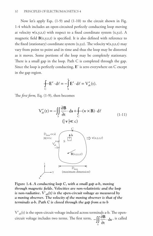
Now let’s apply Eqs. (1-9) and (1-10) to the circuit shown in Fig. 1-4 which includes an open-circuited perfectly conducting loop moving at velocity v(x,y,z,t) with respect to a fixed coordinate system (x,y,z). A magnetic field B(x,y,z,t) is specified. It is also defined with reference to the fixed (stationary) coordinate system (x,y,z). The velocity v(x,y,z,t) may vary from point to point and in time and thus the loop may be distorted as it moves. Some portions of the loop may be completely stationary. There is a small gap in the loop. Path C is completed through the gap. Since the loop is perfectly conducting, E′ is zero everywhere on C except in the gap region.
C
abb
a
d d V t∫ ∫′ ⋅ = − ′ ⋅ = ′E E ( ).
The first form, Eq. (1-9), then becomes
′ = − ∂∂
⋅ + × ⋅∫∫ ∫V tt
d d
c
abS C
( ) ( )
(| | )
Bs v B
v
(1-11)
+a
−b
ds
S
B(x,y,z,t)
abV
C
v(x,y,z,t)
(maximum dimension)Dmax
Dmaxc<<
<<v
z
y
x
Figure 1.4. A conducting loop C, with a small gap a-b, moving through magnetic fields. Velocities are non-relativistic and the loop is non-radiative. V′ab(t) is the open-circuit voltage as measured by a moving observer. The velocity of the moving observer is that of the terminals a-b. Path C is closed through the gap from a to b
V′ab(t) is the open-circuit voltage induced across terminals a-b. The open-circuit voltage includes two terms. The first term, − ∂
∂⋅∫∫
Bs
td
S
, is called

TIME-VARyING FIELdS ANd ELECTROMAGNETIC WAVES 11
# 156104 Cust: MP Au: Adams Pg. No. 11 Title: Principles of Electromagnetics 1—
K Short / Normal
DESIGN SERVICES OF
S4CARLISLEPublishing Services
the transformer emf. It is the only term present if v = 0. The second term,
C
d∫ × ⋅( )v B , called the flux-cutting emf or the motional emf, is the only term present if ∂
∂=B
t0 . In general, both terms are needed and both
contributions must be considered.Similarly, the second form, Eq. (1-10), becomes
′ = − = − ⋅∫∫V tddt
ddt
d c (Faraday’s law in circuiabS
( ) (| | )Φ
B s v tt form)
(1-12)
Equation (1-12) may already be familiar to you. ′ = −V tddtab( )Φ
is es-sentially the network model mentioned in Volume 3. There is one differ-ence in that a negative sign appears in Eq. (1-12). This merely implies that the voltage-current relationships are reversed. We can switch the sign in Eq. (7-22) simply by reversing voltage or current definitions and we can also switch the sign in Eq. (1-12) by reversing the definitions of V′ab or C. For simplicity, the plus sign is used in network theory. In electromagnetic theory we retain the negative sign because it is indicative of a negative or opposing effect as expressed in Lenz’s law. Therefore the definition of C is important. It passes through the gap from a (the positive reference for V′ab) to b.Here the three different forms of Faraday’s law are summarized in Table 1-1. Table 1-1. Faraday’s Law
(1) differential Form: ∇ × = − ∂∂
EBt
• Time-varying magnetic field induces an electric field.• The induced electric field circles around the changing magnetic field.
(2) Integral Form:
C S
dt
d∫ ∫∫⋅ = − ∂∂
⋅EB
s
(3) Circuit Form: V = − ddtΦ
• V = ′ ⋅∫
C
dE = induced voltage or emf
• Φ = ⋅∫∫B sdS
= magnetic flux passing through S

12 PRINCIPLES OF ELECTROMAGNETICS 4
# 156104 Cust: MP Au: Adams Pg. No. 12 Title: Principles of Electromagnetics 1—
K Short / Normal
DESIGN SERVICES OF
S4CARLISLEPublishing Services
Example 1-2. Induced Voltage in a Moving LoopA perfectly conducting square loop of side ℓ with small air gap is at a dis-tance d away from a very long straight wire which carries a steady current I, as shown in Figure 1-5(a).(a) When you pull the loop away from the straight wire (to the right) at
constant speed v, calculate open-circuit voltage V′ab induced across terminals a-b.
(b) Now if you pull the loop upwards at speed v (parallel to the wire), what is the induced voltage V′ab?
abV ab
+
−
d
I v
d
I vi(t)
resistance R
(a) (b)
z
x y
Figure 1-5. Induced voltage and current in a moving loop
Solution:(a) We can calculate V′ab using Eq. (1-11) or (1-12). Since the magnetic
field B produced by the steady current I in a straight wire is not time-varying, the first term in Eq. (1-11) doesn’t yield any emf, but the second term yields a flux-cutting emf. Assuming the rectangular coordinate system as shown in Fig. 1-5(a),I a v a= =z yI, v
The magnetic field B of a filament is given
B a a= = −φµπρ
µπ
0x
0I2
I2 y
(into the paper)
Then the magnetic flux passing through the loop in the direction of ds (out of the paper because C is chosen counterclockwise) is
Φ = ⋅ = −
⋅
= [ ]
∫∫ ∫∫+
+
B s a adI
2 ydydz
I2
y l
Sx
0x
d
d ll
0d
d l
µπ
µπ
0
ln ( ) == − +
µπ0I
2l ln
d ld

TIME-VARyING FIELdS ANd ELECTROMAGNETIC WAVES 13
# 156104 Cust: MP Au: Adams Pg. No. 13 Title: Principles of Electromagnetics 1—
K Short / Normal
DESIGN SERVICES OF
S4CARLISLEPublishing Services
Now when the loop is pulled to the right with constant velocity v, d should be replaced by d + vt. Then
Φ( ) lntIl
2(d vt) l
(d vt)0= − + +
+
µπ
Thus, from Eq. (1-12), the induced voltage is
′ = − = + + − +
=+ +
V tddt
Il2
ddt
d vt l) d vt)
Il2
vd vt l
ab0
0
( ) ln( ln(Φ µ
πµ
πvv
d vtIl v
2 (d vt l)(d vt)0
2+
=−
+ + +µ
π
(b) When the loop is pulled parallel to the wire, the separation d does not change and consequently the magnetic flux Φ does not change, i.e. Φ = constant. Thus
′ = − =VddtabΦ
0
There is no induced voltage.
1.3.4 Lenz’s Law
Lenz’s law, stated below, is often useful in determining the direction of an induced effect in a magnetic system of conductors, magnetic materials, moving objects, sources, etc. It was deduced in 1834 by Heinrich F. Lenz.
Lenz’s Law
When there is a change in magnetic flux in a magnetic system, the resulting effect (induced emf) is such as to oppose the change.
For example, if we try to increase the flux through a closed loop of wire, then the induced emf tends to have currents flow in the loop in such a direc-tion as to decrease the flux. Lenz’s law is included already in Faraday’s law

14 PRINCIPLES OF ELECTROMAGNETICS 4
# 156104 Cust: MP Au: Adams Pg. No. 14 Title: Principles of Electromagnetics 1—
K Short / Normal
DESIGN SERVICES OF
S4CARLISLEPublishing Services
through a negative sign in Eq. (1-3). However, it is very useful in indicating the sign of a change in current or flux and in checking calculations.
Example 1-3. Induced Current in a Moving LoopFor the configuration of Example 1-2, consider a closed square loop
of finite conducting wire of resistance R [Ω] as shown in Fig. 1-5(b). When the loop is pulled to the right at velocity v, the induced emf causes a current to flow through the loop. Find the induced current i(t) and the direction of the current.
Solution:The induced emf V(t) is obtained in a manner similar to that of Ex-
ample 1-2 and is related to the current by Ohm’s law (V = Ri):
V(t)= dIl v
2 (d vt l)(d vt)R i(t)
C
02
∫ ′ ⋅ = −+ + +
=E
µπ
where the direction of i(t) is taken to be CCW according to the right-hand rule. Therefore,
i(t)Il v
2 R(d vt l)(d vt)0
2
= −+ + +µ
π
The negative sign indicates that the current induced flows in a clockwise (CW) direction. We can also check the direction of induced current by Lenz’s law. When the loop moves to the right, the magnetic flux passing through the loop (Φ) into the paper decreases because B decreases as 1/ρ. According to Lenz’s law, the current is induced in such a direction as to oppose the change, i.e., to increase the magnetic flux (into the paper). A clockwise current of the loop would generate the B field into the paper in the region within the loop (or the surface S). It is assumed in this example that velocities are slow, that frequencies generated are low, and that the resistance of the loop is large compared to its reactance.
1.4 Michael Faraday’s Famous Experiments of 1831
By 1825, Michael Faraday (1791-1867) had become a very well-known chemist. He had discovered benzene, carried out important research on steel alloys, and been elected a Fellow of the Royal Society. He had also begun

TIME-VARyING FIELdS ANd ELECTROMAGNETIC WAVES 15
# 156104 Cust: MP Au: Adams Pg. No. 15 Title: Principles of Electromagnetics 1—
K Short / Normal
DESIGN SERVICES OF
S4CARLISLEPublishing Services
research in electromagnetics, repeating many of the basic experiments of Oersted and Ampère. He had also discovered an interesting rotating device described by some as the first motor. Unfortunately, he had been wrongly accused with stealing the idea from his senior colleague Wollaston, an accusa-tion that caused great pain to the honest, upright Faraday.
Faraday was scrupulously honest in his dealings with colleagues. He had a very careful way of raising questions about the research of others that usually led to friendships rather than antagonism. One is reminded of Franklin and his disarming frankness when Faraday writes: “I am by no means decided that there are currents of electricity in the common magnet … until the presence of electrical currents be proved in the mag-net … . I shall remain in doubt about Ampère’s theory” Faraday was a supporter of Ampère’s theory in some respects, but he would not accept assumptions until he had seen them proven through experiment. Ampère replied to Faraday at length and the two became friendly correspondents.
Faraday expressed his disappointment at his lack of opportunity for fundamental research when he wrote Ampère in 1825, “Every letter you write me states how busily you are engaged and I cannot wish it otherwise knowing how well your time is spent. Much of mine is unfortunately occupied in very commonplace employment and this I may offer as an excuse … for the little I do in original research.” Faraday’s thoroughness and reliability were too well-known. If Faraday did it, one knew that it would be well done, and Faraday, who worked at the Royal Institution, could not turn down governmental requests.
In 1831, when he carried out his experiments in magnetic induction, Faraday was 40 years old. He had come a long way from the impover-ished, uneducated bookbinder’s apprentice who, looking for a job in sci-ence in 1812, had written to a friend after being turned down: “I am now working at my old trade …, with respect to the progress of the sciences I know but little and am now likely to know still less. … I must resign philosophy (science) entirely to those who are more fortunate … . I am at present in very low spirits …”. Shortly afterward, Faraday accepted a job as assistant at the Royal Institution and proceeded rapidly in the interven-ing years to build up his reputation. Now he had come to another similar turning point in his life. He was discouraged about his opportunities for original research, as shown by his letter to Ampère. Now, at 40, was his
16 PRINCIPLES OF ELECTROMAGNETICS 4
# 156104 Cust: MP Au: Adams Pg. No. 16 Title: Principles of Electromagnetics 1—
K Short / Normal
DESIGN SERVICES OF
S4CARLISLEPublishing Services
best work behind him? He would try to answer a basic question: If an electric current causes a magnetic field, will a magnetic field in turn cause an electric current? Perhaps the answer to that question would be as basic and important as Oersted’s remarkable discovery of 1820.
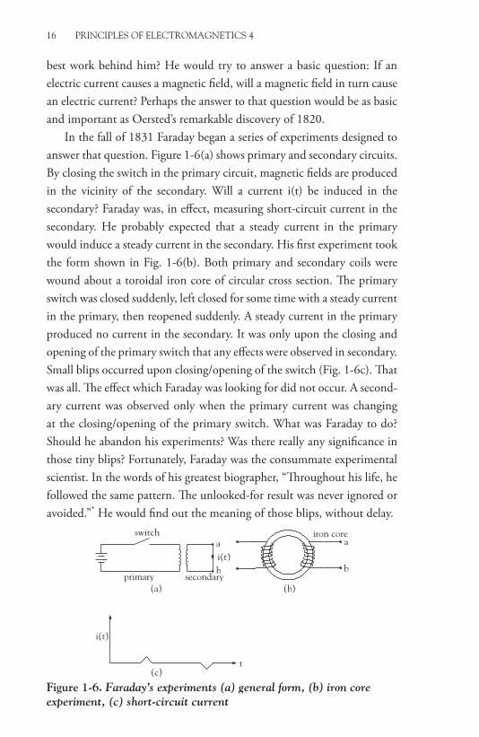
In the fall of 1831 Faraday began a series of experiments designed to answer that question. Figure 1-6(a) shows primary and secondary circuits. By closing the switch in the primary circuit, magnetic fields are produced in the vicinity of the secondary. Will a current i(t) be induced in the secondary? Faraday was, in effect, measuring short-circuit current in the secondary. He probably expected that a steady current in the primary would induce a steady current in the secondary. His first experiment took the form shown in Fig. 1-6(b). Both primary and secondary coils were wound about a toroidal iron core of circular cross section. The primary switch was closed suddenly, left closed for some time with a steady current in the primary, then reopened suddenly. A steady current in the primary produced no current in the secondary. It was only upon the closing and opening of the primary switch that any effects were observed in secondary. Small blips occurred upon closing/opening of the switch (Fig. 1-6c). That was all. The effect which Faraday was looking for did not occur. A second-ary current was observed only when the primary current was changing at the closing/opening of the primary switch. What was Faraday to do? Should he abandon his experiments? Was there really any significance in those tiny blips? Fortunately, Faraday was the consummate experimental scientist. In the words of his greatest biographer, “Throughout his life, he followed the same pattern. The unlooked-for result was never ignored or avoided.”* He would find out the meaning of those blips, without delay.
a
b
iron core
(b)
a
bi(t)
switch
primary secondary(a)
i(t)
t(c)
Figure 1-6. Faraday’s experiments (a) general form, (b) iron core experiment, (c) short-circuit current

TIME-VARyING FIELdS ANd ELECTROMAGNETIC WAVES 17
# 156104 Cust: MP Au: Adams Pg. No. 17 Title: Principles of Electromagnetics 1—
K Short / Normal
DESIGN SERVICES OF
S4CARLISLEPublishing Services
Next, Faraday removed the iron. He wound both primary and sec-ondary on a common cylindrical wooden core. At first, no effects were noted. Then, upon increasing the voltage by a factor of ten and increasing the number of turns, the small blips of Figure 1-6(c) were again observed upon closing and opening the switch. Now, what is happening here? A steady primary current produces a steady magnetic field in the vicinity of the secondary and no effect is observed during the steady magnetic field. When the switch is closed, the primary current, and the associated mag-netic field, rapidly increase towards their steady values. Similarly, upon opening the switch, the primary current/magnetic field rapidly decrease from their steady values toward zero. Thus the induced current is obtained only when the magnetic field is changing.
Faraday’s next experiment was designed to change the time variation completely. Both primary and secondary were mounted on separate broad boards, the switch was closed, and the primary was moved first towards, then away from the secondary. Thus the primary current would remain steady, or approximately so, but the magnetic field at the vicinity of the secondary would increase/decrease as the primary board approached/re-ceded. When the experiment was performed, the induced secondary cur-rent was of one polarity, say positive, as the primary board approached, and negative as the board receded.
Now Faraday placed great emphasis on the magnetic lines of force, the magnetic field, associated with the electric current and displayed by the pattern of iron filings, for instance. Doubtless, he could “see” the mag-netic field rise up as the switch was thrown, and increase at the secondary as the primary board approached. Thus the common thread of all these experiments was a changing magnetic field at the secondary whenever an induced current was observed in the secondary.
Next Faraday replaced the primary board with a permanent magnet, which was moved towards the secondary circuit board and then moved away from it. The results were identical in form to those obtained with the primary board, the induced secondary current being positive/negative as the magnet approached/receded.
*L. Pierce Williams, Michael Faraday: A Biography, p. 119, Da Capo Press, NY ,1987, Reprint from Basic Books, NY, 1965.

18 PRINCIPLES OF ELECTROMAGNETICS 4
# 156104 Cust: MP Au: Adams Pg. No. 18 Title: Principles of Electromagnetics 1—
K Short / Normal
DESIGN SERVICES OF
S4CARLISLEPublishing Services
Notice how Faraday moves inexorably toward the conclusion that current is induced in the secondary when the magnetic field in the vicin-ity of the secondary is changing. This conclusion leads to Faraday’s law, the first law governing time-varying fields. Faraday knew his abilities and his ambitions, but did he suspect that he was on the verge of such a great discovery during the famous ten days of fall 1831? Did he suspect that his greatest work was ahead of him, that he would eventually stand in the front rank of English scientists, and that many would rank him, in our own time, as one of the greatest scientists who had ever lived?
During the ten day period mentioned above, Faraday performed a number of additional experiments. One of these involved the discovery of the first generator, the Faraday disk generator. Faraday also discovered the flux-cutting principle outlined in Section 1.3.3. He read his results on November 24, 1831 to the Royal Society. Later Faraday would show that induced current was proportional to the area of the secondary loop. He also showed that the induced current was proportional to the conductiv-ity of the wire used in the secondary. These results lead us closer to the mathematical form of Faraday’s law given in Eq. (1-12).
1.5 Maxwell’s Equations
We have mentioned earlier that Faraday’s law was first discovered in 1831. It was expressed in its present form, ∇ × E = − ∂B/∂t, by Maxwell in the 1850s.
There were, at that time, a number of important unanswered ques-tions concerning electromagnetic effects. For instance, Faraday’s law de-scribes accurately the voltages and currents induced in a secondary circuit by changes in a primary circuit. However, they do not describe how en-ergy is transferred from primary to secondary or how rapidly. Experiment indicated that the process was nearly instantaneous and instantaneity is implied in the network equations. However, doubt persisted. Is it re-ally instantaneous or is there a finite time delay before the effect on the secondary?
There were also some basic questions at that time concerning the propagation of light. The speed of light was known fairly accurately and with a high degree of confidence since it has been determined by many

TIME-VARyING FIELdS ANd ELECTROMAGNETIC WAVES 19
# 156104 Cust: MP Au: Adams Pg. No. 19 Title: Principles of Electromagnetics 1—
K Short / Normal
DESIGN SERVICES OF
S4CARLISLEPublishing Services
different methods. It had first been calculated 175 years previously, in 1676, by Ole Roemer (1644-1710), a Danish astronomer. Roemer esti-mated the speed of light at 2.3 × 10⁸ m/sec, using an astronomical method related to the eclipse of the moons of Jupiter. Later corrections of Roemer’s calculations by Isaac Newton in 1704 indicated a velocity of about 2.7 × 10⁸ m/sec. In 1728, J. Bradley (1693-1762), an English astronomer, used an astronomical method related to stellar aberration to estimate the speed of light at 3.05 × 10⁸ m/sec. Finally H. L. Fizeau and L. Foucault made direct measurements of the speed of light by two different methods in 1849 and 1852, yielding values of 3.15 × 10⁸ m/sec and 2.98 × 10⁸ m/sec, respectively. Although the speed of light was fairly well established, the nature of light and the mechanism of propagation were unknown. How-ever, the propagation of sound waves was well understood, having been investigated by many researchers. In particular, D’Alembert had shown in 1750 that sound waves satisfied a scalar wave equation,
∇ = ∂∂
22
ψ ψ1v tx
2 2 (1-13)
where ψ and vs are sound pressure and sound velocity, respectively.Another question which would naturally have been raised during the
1850’s and 1860’s was the following: Faraday’s law implies that a chang-ing magnetic field produces an electric field. Is the inverse true, i.e., does a changing electric field produce a magnetic field?
1.5.1 Displacement Current
To answer the question just raised we consider the curl equations of elec-trostatics and magnetostatics. The first curl equation, ∇ × E = 0, becomes ∇ × E = − ∂B/∂t in the time-varying case. What, if anything, happens to the second curl equation, ∇ × H = J, in the time-varying case? We recall the equation of continuity,
∇ ⋅ = −∂∂
Jρv
t (1-7)
which relates J and ρv in general, including non-steady (time-varying) currents. For magnetostatics

20 PRINCIPLES OF ELECTROMAGNETICS 4
# 156104 Cust: MP Au: Adams Pg. No. 20 Title: Principles of Electromagnetics 1—
K Short / Normal
DESIGN SERVICES OF
S4CARLISLEPublishing Services
∇ × =H J (1-2a)
We take the divergence of Eq. (1-2a) above
∇ ⋅ ∇ × = ∇ ⋅ = −∂∂
( )H Jρv
t (1-14)
The left-hand side, the divergence of the curl, is always zero, whereas the right-hand side clearly is non-zero in the general time-varying case. Therefore the curl equation ∇ × H = J is incorrect for the time-varying case and requires modification at least. How can we modify the curl equa-tion so that there is no contradiction? One simple resolution would be to modify Eq. (1-14) by adding ∂
∂ρv
t to the right-hand side.
∇ ⋅ ∇ × = ∇ ⋅ = −∂∂
=( )H Jρv
t0
To see how this changes the curl equation, we substitute ρv = ∇ · D to obtain
∇ ⋅ ∇ × = ∇ ⋅ + ∂
∂
=( )H JDt
0 (1-15)
which is satisfied by
∇ × = + ∂
∂H J
Dt
(1-16)
One could also add a divergenceless (solenoidal) vector to the right-hand side of Eq. (1-16), but the result would not yield the proper static form in Eq. (1-2a) when ∂/∂t = 0. The term ∂
∂≡DJ
t d added to the second curl
equation has the units of volume current density (amps/m2). It is called displacement current density even though it may not actually represent current flow. This is a major contribution of Maxwell. He introduced this term on a purely theoretical basis. Maxwell’s theory was confirmed about 20 years later by Heinrich Hertz’s experiments on electromagnetic radia-tion in 1888. As will be shown later, inclusion of ∂
∂Dt
in the curl equation is crucial in predicting the propagation of electromagnetic waves, without which we would not live in a “communication” age today.
TIME-VARyING FIELdS ANd ELECTROMAGNETIC WAVES 21
# 156104 Cust: MP Au: Adams Pg. No. 21 Title: Principles of Electromagnetics 1—
K Short / Normal
DESIGN SERVICES OF
S4CARLISLEPublishing Services
Integrating both sides of Eq. (1-16) over an open surface S and apply-ing Stokes’ theorem, we obtain the integral form:
C S
dt
d∫ ∫∫⋅ = + ∂∂
⋅H JD
s (1-17)
Eqs. (1-16) and (1-17) are now known as the generalized Ampère’s law.
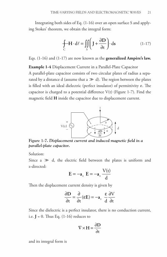
Example 1-4 Displacement Current in a Parallel-Plate CapacitorA parallel-plate capacitor consists of two circular plates of radius a sepa-rated by a distance d (assume that a d). The region between the plates is filled with an ideal dielectric (perfect insulator) of permittivity ε. The capacitor is charged to a potential difference V(t) (Figure 1-7). Find the magnetic field H inside the capacitor due to displacement current.
a
tD
d
z
+
−V(t)
Figure 1-7. Displacement current and induced magnetic field in a parallel-plate capacitor.
Solution:Since a d, the electric field between the plates is uniform and z-directed:
E a E a= − = −z z V(t)d
Then the displacement current density is given by
∂∂
= ∂∂
= − ∂∂
DE a
t t d
Vtz( )ε ε
Since the dielectric is a perfect insulator, there is no conduction current, i.e. J = 0. Thus Eq. (1-16) reduces to
∇ × = ∂∂
HDt
and its integral form is

22 PRINCIPLES OF ELECTROMAGNETICS 4
# 156104 Cust: MP Au: Adams Pg. No. 22 Title: Principles of Electromagnetics 1—
K Short / Normal
DESIGN SERVICES OF
S4CARLISLEPublishing Services
∇ × ⋅ = ⋅ = ∂
∂⋅∫∫ ∫ ∫∫H s H
Dsd d
td
S C S
(1-17a)
We recognize that the z-directed displacement current ( )∂∂Dt
induces the Φ-directed magnetic field H by the right hand rule:
H a= φ φH
Applying Eq. (1-17a) over the circle of radius ρ:
C S
z 2
z
d Ht
dt
Ht d
∫ ∫∫⋅ = ∂∂
⋅ =∂∂
=∂∂
⋅ = −
HD
sD
D
φ
φ
πρ πρ
ρ ε
( ) ( ) ( )2
2∂∂∂
⋅ ≤Vt 2
aρ ρ( )
Thus a magnetic field HΦ , proportional to ∂∂Vt
and increasing with ρ, is induced within the capacitor.
Modification of Current Circuital Law
The vector (J + ∂D/∂t) is divergenceless, i.e., ∇ · (J + ∂D/∂t) = 0 from Eq. (1-15). Integrating Eq. (1-15) over volume V we obtain
∇ ⋅ + ∂∂
= + ∂∂
⋅ =∫∫∫ ∫∫JD
JD
st
dvt
dV S
' 0 (1-18)
Thus
− ⋅ = ∂
∂⋅∫∫ ∫∫' 'J s
Dsd
td
S S
(1-19)
Equation (1-18) states that the sum of current and displacement current flowing into (or out of ) a closed surface is zero. Thus J + ∂D/∂t plays the same role in time-varying problems as did J in magnetostatic problems (∇ · J = 0 for the steady currents of magnetostatics). Equation (1-19), on the other hand, indicates that the current I d
S
= − ⋅∫∫' J s flowing into a surface S is not zero but is equal to the displacement current ' ∂
∂⋅∫∫
Ds
td
S
flowing out of S. Thus the sum of the currents flowing into a junction is not zero but is equal to the displacement current flowing out of the junction. This is contrary to the Kirchhoff current law (KCL) you learned in circuit theory.

TIME-VARyING FIELdS ANd ELECTROMAGNETIC WAVES 23
# 156104 Cust: MP Au: Adams Pg. No. 23 Title: Principles of Electromagnetics 1—
K Short / Normal
DESIGN SERVICES OF
S4CARLISLEPublishing Services
Figure 1-8(a) shows conduction current and displacement current at the open end of a conducting wire of radius a. The current at the end of the wire does not go to zero but terminates in displacement current. Con-sider the closed surface S. The current I d
S
= − ⋅∫∫' J s flowing in from the left equals the displacement current flowing out on the right.
Figure 1-8(b) shows two fat open-ended wires close together, separated by a distance d, forming a capacitor. Current J flows in from the left and out on the right in the wires; only displacement current flows in the gap region.
J
J J
JtD
tD
(b) Two adjacent open-ended wires.
S
J
J
tD
tD
(a) An open-ended conducting wire.
tD
tD
tD
tD
1I 3I
2I
4I
S
(c) A junction of four current-carrying wires.
Figure 1-8. Conduction current and displacement currentFigure 1-8(c) shows a junction of four current-carrying wires. The
sum of the currents flowing into the junction is not zero but is equal to the displacement current flowing out. So if we consider any closed surface S such as that of Fig. 1-8(c), the current
I I I I I d1 2 3 4S
= + + + = − ⋅∫∫' J s flowing into S equals the dis-
placement current '∂∂
⋅∫∫D
st
dS
flowing out.

24 PRINCIPLES OF ELECTROMAGNETICS 4
# 156104 Cust: MP Au: Adams Pg. No. 24 Title: Principles of Electromagnetics 1—
K Short / Normal
DESIGN SERVICES OF
S4CARLISLEPublishing Services
The effects of displacement current depend on frequency and geom-etry. For instance, consider the isolated open-ended wire with radius a in Fig. 1-8(a). For a λ (corresponding to low frequency because wave-length is inversely proportional to frequency) the current at the open end (and the displacement current) is very small and the effect of displace-ment current is not significant at low frequencies. If, however, another conductor is brought into close proximity, as shown in Fig. 1-8(b), then the effects of displacement current may become significant. In Fig. 1-8(b) for any a/λ, no matter how small, we can choose d (gap) such that the capacitive reactance is small and the circuit looks more like a short circuit rather than an open circuit. In Fig. 1-8(c), we can assume that displace-ment current is negligible if a λ and the junction is isolated. If how-ever, other conductors, for instance, another junction, are brought into close proximity, then the displacement current may become significant even if a λ.
It may be necessary then to take into account the so-called stray ca-pacitance to the nearby object. Including the stray capacitance allows an additional path for current flow in the circuit and permits the currents to be balanced. Thus displacement current upsets the Kirchhoff current law that the sum of currents into a junction is zero. The addition of stray or mutual capacitances helps but makes the circuit more complex. There is, however, no end to the various stray capacitances which can be taken into account. Eventually the circuit representation breaks down as frequency increases.
1.5.2 Maxwell’s Equations
As discussed earlier Eqs. (1-3) and (1-16) are generalizations of the two curl laws in Eqs. (1-1) and (1-2). While the latter two are valid only for static fields, the former two are valid for general time-varying fields. The two divergence laws in Eqs. (1-1) and (1-2) are still valid for time-varying fields. We collect the four equations, (1-3), (1-16), and the two diver-gence equations in (1-1), (1-2), for general time-varying fields:
∇ × = − ∂∂
EBt
(Faraday’s law) (1-20a)

TIME-VARyING FIELdS ANd ELECTROMAGNETIC WAVES 25
# 156104 Cust: MP Au: Adams Pg. No. 25 Title: Principles of Electromagnetics 1—
K Short / Normal
DESIGN SERVICES OF
S4CARLISLEPublishing Services
∇ × = + ∂∂
H JDt
(Generalized AmpŁre’s law)
(1-20b)
∇ ⋅ =D ρv (Gauss’ law for electric field) (1-20c)
∇ ⋅ =B 0 (Gauss’ law for magnetic field) (1-20d)
(Maxwell’s equations in differential form)
The four basic equations above are called Maxwell’s equations and are the basis of electromagnetics. They apply in any and all macroscopic situ-ations and cover the general time-varying case. They are also valid in any and all moving systems as was shown by Einstein. They are valid in any media including non-linear, anisotropic and non-reciprocal media.
For completeness we need to add the additional relationships among the field quantities of Maxwell’s equations. For instance, J and ρv are not independent but are related by the equation of continuity,
∇ ⋅ =∂∂
Jρv
t
For linear isotropic media one can add the constitutive relations to express D in terms of E and B in terms of H:
D E B H= =ε µ, (1-21)
For other media, one merely adds the appropriate relations among the field quantities:
D E P B H M= + = +ε µ µ0 , 0 0 (1-22)
Finally, one should add the Lorentz force law
F E v B= + ×q( ) (1-23)
for calculation of electric and magnetic forces. It is important to notice that Maxwell’s equations describe the action of charges on fields (how charges produce fields), and the Lorentz force law explains the action of fields on charges (how fields affect charges). Their combination summa-rizes the entire set of electromagnetic laws.

26 PRINCIPLES OF ELECTROMAGNETICS 4
# 156104 Cust: MP Au: Adams Pg. No. 26 Title: Principles of Electromagnetics 1—
K Short / Normal
DESIGN SERVICES OF
S4CARLISLEPublishing Services
Note also that the two divergence relations, ∇ · D = ρv and ∇ · B = 0 do not have to be established separately because they can be deduced from the two curl equations (1-20a), (1-20b) and the equation of conti-nuity. This is done merely by taking the divergence of the curl equations and using the equation of continuity.
Maxwell’s equations may also be stated in integral form. The first two integral forms may be derived by integrating the two curl equations (1-20 a,b) over surfaces and applying Stokes’ theorem. The last two forms are obtained by integrating the two divergence equations (1-20 c,d) over vol-ume V and applying the divergence theorem. The results are:
C S
dt
d∫ ∫∫⋅ = − ∂∂
⋅EB
s (1-24a)
C S
S
dt
d
It
d
∫ ∫∫
∫∫
⋅ = + ∂∂
⋅
= + ∂∂
⋅
H JD
s
Ds
(1-24b)
D s⋅ = =∫∫ ∫∫∫d dv Q
Sv
V
ρ (1-24c)
B s⋅ =∫∫ d
S
0 (1-24d)
(Maxwell’s equations in integral form)
Comparing the equations with the static forms, we note that there are
only two changes, i.e., the additions of the terms −∂∂
⋅ ∂∂
⋅∫∫ ∫∫B
sD
st
d t
dS S
,
to the first, second equations, respectively. However, all vectors and sca-
lars are now functions of time, i.e., E(x,y,z,t), B(x,y,z,t), Q(t), etc.
1.5.3 The Wave Equation – Electromagnetic Waves!
The addition of the displacement current term (∂D/∂t) ties in electromag-netics with wave action and light. It also answers a number of questions

TIME-VARyING FIELdS ANd ELECTROMAGNETIC WAVES 27
# 156104 Cust: MP Au: Adams Pg. No. 27 Title: Principles of Electromagnetics 1—
K Short / Normal
DESIGN SERVICES OF
S4CARLISLEPublishing Services
raised in the beginning of this section. Consider the electric and magnetic fields in free space (or open air), which require
ρv (in a source-free region)= =J 0
D E B H= =ε µo o (in free space or air),
Then Maxwell’s equations (1-20) reduce to
∇ × = − ∂∂
EHµ0 t
(1-25a)
∇ × = ∂
∂H
Eε0 t (1-25b)
∇ ⋅ = ∇ ⋅ =( )ε0 or E E0 0 (1-25c)
∇ ⋅ = ∇ ⋅ =( )µ0 or H H0 0 (1-25d)
Taking the curl of Eq. (1-25a)
∇ × ∇ × = ∇ ∇ ⋅ − ∇ = −∇ × ∂∂
= − ∂∂
∇ ×E E EH
H( ) ( )2 µ µ0 0t t
Using Eqs. (1-25b) and (1-25c),
−∇ = − ∂∂
∂∂
= − ∂∂
22
EH Eµ ε µ ε0 0 0 0 2t t t
Therefore, we have
∇ = ∂
∂2
2
EEµ ε0 0 2t
(1-26)
(Helmholtz’s wave equation)
Equation (1-26) is a vector form of the scalar wave equation (1-13) men-tioned earlier. We can also replace E with H in Eq. (1-26). Thus the com-ponents of E, H satisfy the scalar wave equation, which indicates wave propagation at velocity c:
c10
m/sec0 0
7= =× × ×
≈ ×−
1 14 8 85 10
3 1012 1 28
µ ε π( . )[ ]/

28 PRINCIPLES OF ELECTROMAGNETICS 4
# 156104 Cust: MP Au: Adams Pg. No. 28 Title: Principles of Electromagnetics 1—
K Short / Normal
DESIGN SERVICES OF
S4CARLISLEPublishing Services
Maxwell could thus predict the velocity of electromagnetic waves. His calculation, with some error in μ0, ε0, yielded a velocity of 3.11 × 10⁸ m/sec, which was very close to the measured speed of light. Later more precise measurements showed that the speed of light c is 2.998 × 10⁸ m/sec. So Maxwell was able to conclude that there are electromagnetic waves with a given velocity of propagation in free space, that all components of E, H propagate at that velocity, and that light is an electromagnetic phenomenon. All of this was possible only because of the addition of the displacement current term.
Example 1-5 Field Solutions of Maxwell’s EquationsThe electric field of an electromagnetic wave in air, free of sources, is given by
E a= −( )x oE t kzcos ω
where ω and k are constants.(a) Find the corresponding magnetic field H of the electromagnetic wave.(b) Confirm that E satisfies Gauss’ law, Eq. (1-20c).
Solution:(a) If you consider this problem as one in which the electric field (or equiva-
lently the displacement current) induces a magnetic field, you would be tempted to use the integral form of Ampere’s law to find the magnetic field. However, the difficulty lies in the prediction of how the magnetic field (H) will behave in terms of its direction and spatial dependence. For a source-free problem like this, it is much easier to use the differential form of Maxwell’s equations. Knowing E, we can calculate H, by using the differential form of Faraday’s law, Eq. (1-20a) and integrating with respect to time.
− ∂∂
= ∇ × = ∂∂
∂∂
∂∂
∂∂
= ∂∂
=
= =
BE
a a a
x x y zE E E
Note that x yE E
x y z
x y zy z
0
0
==∂∂
= ∂∂
−( ) = −( )
a a
a
yx
y 0
y 0
Ex z
E t kz
E k t kz
cos
sin
ω
ω

TIME-VARyING FIELdS ANd ELECTROMAGNETIC WAVES 29
# 156104 Cust: MP Au: Adams Pg. No. 29 Title: Principles of Electromagnetics 1—
K Short / Normal
DESIGN SERVICES OF
S4CARLISLEPublishing Services
Since B = μo H in air,
HB
a
a
= ∂∂
= − −( )
= −( )
∫ ∫1
tdt
1E k t kz dt
E k
t kz
0 0y 0
y 00
µ µω
µ ωω
sin
cos
Note that E and H should also satisfy Ampère’s law if they represent elec-tromagnetic fields.(b) In air, free of sources, Gauss’ law becomes
∇ ⋅ = =
∇ ⋅ =∂∂
+∂∂
+∂∂
=∂∂
D D E
D
0 and
Ex
Ey
Ez
Ex
E
0
0x y z
0x
0
ε
ε
ε ωcos tt kz−( ) = 0
Thus Gauss’ law is satisfied. One can also show that Gauss’ law for B, Eq. (1-20d), is satisfied.
1.5.4 James Clerk Maxwell (1831-1879)
In the previous sections of this Chapter, we outlined some of Maxwell’s and Faraday’s contributions to time-varying electromagnetic fields. Now let’s go back to Maxwell’s origins and describe briefly his upbringing, edu-cation, and his scientific contributions leading up to his complete formu-lation of electromagnetic theory.
Maxwell was born in 1831. His only sibling, Elizabeth, died in in-fancy before James was born. James spent most of his childhood on the family estate called Glenlair, which is 3 miles south of the village Corsock and about 50 miles west of Carlisle, in southwestern Scotland. His par-ents were John Clerk Maxwell and Francis Cay Maxwell, both of whom took a serious interest in his upbringing and education.. His mother took up his education and soon he was reading very widely, including large number of works in literature and history. It would have been difficult to find a better background for his early upbringing and education. James, like many a bright young lad, took a great interest in the world around

30 PRINCIPLES OF ELECTROMAGNETICS 4
# 156104 Cust: MP Au: Adams Pg. No. 30 Title: Principles of Electromagnetics 1—
K Short / Normal
DESIGN SERVICES OF
S4CARLISLEPublishing Services
him. He was especially interested in learning exactly how things worked and often wanted to perform complex tasks without help.
James’ mother died when he was eight. At the age of ten, he was sent to live with his aunt Jane and attend Edinburgh Academy. For complete-ness, let’s list here the schools which James attended:
Edinburgh Academy (1841-1847)Edinburgh University (1847-1850)Cambridge University (1850-1856)
and those at which he taught:
Marischal College (1856-1860)King’s College, London (1860-1865)Cambridge University (1871-1879)
After a period of adjustment, James made rapid progress in his studies at Edinburgh Academy. He published a mathematical paper at age 15. He was becoming a person of a very kind and generous spirit. He loved animals and rode horses but he did not go hunting. He was strong and athletic but did not participate in school boy games. He did a lot of walk-ing, swimming, and exercising. He could defend himself but did not pick fights. He could be critical, usually in a whimsical way. He had his own world of his projects and simple toys, often of his own making, and his ideas which he shared with a few friends. He wrote poetry, mostly of a whimsical nature.
At Edinburgh University, James took to the very broad education offered in subjects such as philosophy and logic. He also had access to Professor Ed-ward Forbes’ laboratory. He became interested in polarized light and the strain patterns which it revealed; this led to an excellent paper on elastic solids.*
James found Cambridge University to be a very convivial place. He made many friends and joined in discussions on every subject imaginable. Often he could offer his peers a new approach to a subject because of his wide reading. He had no interest whatsoever in institutional discussions of the conflict between science and religion, categorizing this issue as of a personal nature. In his senior year (1854) there were two important mathematical exams: the tripos and the Smith’s prize exam. James took second in the tripos and shared first in the Smith’s prize.

TIME-VARyING FIELdS ANd ELECTROMAGNETIC WAVES 31
# 156104 Cust: MP Au: Adams Pg. No. 31 Title: Principles of Electromagnetics 1—
K Short / Normal
DESIGN SERVICES OF
S4CARLISLEPublishing Services
He would stay on for two more years at Cambridge, working on elec-tromagnetics among other things and publishing a paper entitled, “On Faraday’s Lines of Force,” in which he developed a fluid analogy for static electric and magnetic problems.
Maxwell reminds us of Benjamin Franklin and Michael Faraday in his careful and generous way of discussing the research of others. We have already seen how generous Maxwell was with Gibbs’, Coulomb’s, and Ampère’s work. James praises Faraday’s work in particular because he carefully delineates all steps he has taken. Maxwell particularly ad-mired Faraday’s “lines of force.” Faraday had sensed something of great importance. It was the beginning of field theory, fields that may occupy all space. Faraday was criticized by some for “fuzzy ideas” but received support from Maxwell. Maxwell was a great contributor to the concept of field theory but Faraday also deserves credit.
In 1856, Maxwell was appointed Professor at Marischal College in Aberdeen. He was there for four years, was married to Katherine Mary Dewar in 1858, and then was appointed Professor at King’s College, London in 1860.
In 1861-62, James published a paper called “On Physical Lines of Force.” This paper used a very complex mechanical model with springy, spinning cells, and much else. The springyness led to the existence of displacement current in the electromagnetic system and electromagnetic waves (as shown in Section 1.5.3).
James had a complete model for electromagnetics, but he was not at all content. He wanted a more transparent system, namely a set of equa-tions of motion which could then be solved by LaGrange’s methods, a set of mathematical equations rather than the spinning cells. He worked for several more years on this project and published it in 1865, under the title, “A Dynamical Theory of the Electromagnetic Field.” This was also a complex system, consisting of 20 equations in 20 unknowns, which was reduced to the four equations with which we are familiar, namely, equa-tions (2-20a) to (2-20d). A few years after Maxwell’s death the reduction was completed by Oliver Heaviside, using the vector notation system of Josiah Willard Gibbs.
· Basil Mahon, The Man Who Changed Everything: The Life of James Clerk Maxwell, Chapter 3, John Wiley and Sons, Hoboken, NJ, 2003.

32 PRINCIPLES OF ELECTROMAGNETICS 4
# 156104 Cust: MP Au: Adams Pg. No. 32 Title: Principles of Electromagnetics 1—
K Short / Normal
DESIGN SERVICES OF
S4CARLISLEPublishing Services
So now Maxwell had two separate solutions to electromagnetic prob-lems, but he was still not satisfied. He had benefitted from the respective models in developing his own understanding but he did not want the models to play a dominant role. They were sufficient but not necessary. It was time to downplay the models and so he wrote, “I have on a former occasion attempted to describe a particular kind of strain …. In the pres-ent paper I avoid any hypothesis of this kind.”* Thus Maxwell focused attention on the mathematical steps and the final results. This was a dif-ficult but wise choice. Nowadays we set aside the springy cells as well as LaGrange’s system and start with Maxwell’s equations. But in order to understand how Maxwell arrived at his results, we need to recall the scaf-folding and the steps he took. Yet, in 1865, Maxwell’s results were just too deep and too complicated to be fully accepted. They were, in a sense, held in abeyance. Maxwell went back to work and in 1873 published his monumental, 1,000-page, A Treatise on Electricity and Magnetism. Eight years after Maxwell died, Heinrich Hertz observed electromagnetic waves in 1887 and verified Maxwell’s theory.
Einstein said, “One scientific epoch ended and another began with James Clerk Maxwell.”
1.6 Boundary Conditions for Time-Varying Fields
The boundary conditions for static electric fields were derived in Volume 2 and those for static magnetic fields were derived in Volume 3. The boundary conditions for time-varying fields are shown to be the same as those for static fields and they are given below:
E E1t 2t= (1-27a)
a H H Jn2 1 2 s× = =( ) (1-27b)
D D1n 2n S− = ρ (1-27c)
*R.A.R. Tricker, The Contributions of Faraday and Maxwell to Electrical Science, p. 266, Pergamon Press, NY, 1966.

TIME-VARyING FIELdS ANd ELECTROMAGNETIC WAVES 33
# 156104 Cust: MP Au: Adams Pg. No. 33 Title: Principles of Electromagnetics 1—
K Short / Normal
DESIGN SERVICES OF
S4CARLISLEPublishing Services
B B1n 2n= (1-27d)
The subscripts t and n denote the tangential and normal components, re-spectively. Note that an2 is a unit vector normal to the boundary interface, pointing from region 2 into region 1. The boundary conditions at the interface between two different media are derived using procedures quite similar to those used for static problems (see Figure 1-9).
an2
1 1 1μ
μ
, ,
2 2 2, ,
E1,D1,H1,B1
E2,D2,H2,B2
s s,J
2
1
Figure 1-9. Boundary conditions at an interface between two different media
We start with Maxwell’s equations in integral form, Eqs. (1-24a) - (1-24d), and apply them to the closed contour C and the Gaussian pillbox. The integral forms, Eqs. (1-24c) and (1-24d), are identical to the static forms and so the process is identical, yielding the boundary conditions, Eqs. (1-27c) and (1-27d). The integral forms, Eqs. (1-24a) and (1-24b), have the additional terms, − ∂
∂⋅∫∫
Bs
td
S
and ∂∂
⋅∫∫D
st
dS
, respectively, which are not present in the static case. The corresponding additional terms are integrated over a surface whose area vanishes in the limit (α → 0), so these additional terms do not contribute to the boundary conditions,. Hence we again have the same boundary conditions, Eqs. (1-27a) and (1-27b), as before. Therefore, four boundary conditions are identical in form to the static boundary conditions.
There are two special cases for boundary conditions which will prove to be useful in later chapters.
Case 1: dielectric – Perfect Conductor Interface
When the medium 2 is a perfect conductor which has an infinite conductiv-ity (σ = ∞), in order to support a finite current (J = σE) the electric field E
inside the perfect conductor must approach zero. Thus E2 = 0, which also
leads to H2 = 0 for the time-varying fields, because ∇ × = − ∂∂
=EHµt
0 and H is assumed to be not a static field. Inside a perfect conductor (σ

34 PRINCIPLES OF ELECTROMAGNETICS 4
# 156104 Cust: MP Au: Adams Pg. No. 34 Title: Principles of Electromagnetics 1—
K Short / Normal
DESIGN SERVICES OF
S4CARLISLEPublishing Services
= ∞), all time-varying fields are zero: E = H = 0. The first two boundary conditions, Eqs. (1-27a) and (1-27b), reduce to
Ea H J
1t
n2 1 S
=× =
0 (1-28)
at a dielectric-perfect conductor interface.These boundary conditions will be used in the waveguide problems in Volume 5. Here we have written only the boundary conditions for the tangential components because for time-varying field problems it is suf-ficient to use these two conditions.
Case 2: dielectric – dielectric Interface
When both media are not perfect conductors, the current can not flow on the surface, i.e., Js = 0. If the media have finite conductivity, a volume current J can flow inside the media but not on the surface. In this case, the first two boundary conditions become
E EH H
1t 2t
1t 2t
== (1-29)
at dielectric-dielectric interface.
These boundary conditions will be used in the wave reflection and trans-mission problems in Volume 5.
Finally, the boundary condition for the current density J at an inter-face differs in form from that of the steady-current case. It can be derived directly from the equation of continuity whose integral form is
∇ ⋅ = ⋅ = −∂∂∫∫∫ ∫∫ ∫∫∫J J s dv dt
dvV S
v
V
'ρ
When it is applied to the pillbox S, the result is
J Jtln 2nS= = −
∂∂ρ
(1-30)
It is useful to note the boundary condition for normal J. It is not neces-sary to include it in our basic set, Eq. (1-27), since J can be determined from E and ρs(t) can be determined from D.

TIME-VARyING FIELdS ANd ELECTROMAGNETIC WAVES 35
# 156104 Cust: MP Au: Adams Pg. No. 35 Title: Principles of Electromagnetics 1—
K Short / Normal
DESIGN SERVICES OF
S4CARLISLEPublishing Services
1.7 Flow of Electromagnetic Power: Poynting’s Theorem
In this last section we derive the theorem that illustrates conservation of electromagnetic energy and also shows the direction of electromagnetic power flow. We start with Maxwell’s equations. If we dot-multiply Eq. (1-20a) with H and Eq. (1-20b) with E and subtract the second equation from the first equation, we have
H E E H
E H HB
ED
E J
⋅ ∇ × − ⋅ ∇ ×
= ∇ ⋅ × = − ⋅ ∂∂
− ⋅ ∂∂
− ⋅
( ) ( )
( )t t
(1-31)
Here we have used a vector identity in Table 1-5. If the medium is linear (permittivity ε and permeability μ) and ε and μ do not depend on time (such a medium is called non-dispersive), then
ED
E E EE
E E
E E E
⋅ ∂∂
= ⋅ ∂∂
( ) = ⋅ ∂∂
= ∂∂
⋅
= ∂∂
⋅ = ∂∂
⋅
t t t t
t t
ε ε ε
ε
12
12
12
( ) DD (1-32a)
Similarly,
H
BH H H H H B⋅ ∂
∂= ⋅ ∂
∂( ) = ∂
∂⋅ = ∂
∂⋅ t t t t
µ µ12
12
(1-32b)
Substituting Eq. (1-32) in Eq. (1-31), we obtain
∇ ⋅ ×( ) = − ∂
∂⋅ + ⋅ − ⋅E H E D H B J E
t12
( ) (1-33)
Equation (1-33) is called Poynting’s theorem in differential form. The first term on the right side is the negative time rate of change of the sum of electric and magnetic energy densities (or energy per unit volume). The second term is, if J = σE, the negative of the Joule heat power per unit volume. The quantity on the left is in question. In order to interpret this equation in terms of power flow, we integrate both sides of Eq. (1-33) over volume V bounded by closed surface S:

36 PRINCIPLES OF ELECTROMAGNETICS 4
# 156104 Cust: MP Au: Adams Pg. No. 36 Title: Principles of Electromagnetics 1—
K Short / Normal
DESIGN SERVICES OF
S4CARLISLEPublishing Services
∇ ⋅ ×( ) = − ⋅ + ⋅ − ⋅∫∫∫ ∫∫∫ ∫∫∫E H E D H B J E dvddt
dv dvV V V
12
( )
Applying the divergence theorem to the left side:
' E H s E D H B J E×( ) ⋅ = − ⋅ + ⋅ − ⋅∫∫ ∫∫∫ ∫∫∫dddt
dv dvS V V
12
( )
Rewriting:
− ⋅ = ⋅ + ⋅ + ×( ) ⋅∫∫∫ ∫∫∫ ∫∫J E E D H B E H s dvddt
dv dV V S
12
( ) ' (1-34)
This is Poynting’s theorem in integral form. Let us interpret each term.
Case 1: If there are no sources of emf in the volume V, then − ⋅∫∫∫ J E dvV
is the negative of the Joule heat or power dissipation in V. Note that when J is a conduction current (Jc = σE), Jc · E = σE · E = σ|E|2 is positive.
Case 2: If there is a source, then this term becomes positive and it is equal to the power generated by the source in V. Note that when J is a source current (Ji), it is anti-parallel to E and Ji · E is negative.
The first term on the right side of Eq. (1-34) is the rate of change (in-crease) of electromagnetic energy stored in V, i.e.,
ddt
W We m( )+ . The second term on the right can then be interpreted as the power flowing out of the volume V through the surface S, carried by the electromag-netic fields. In other words, in the case of a source present in V (Case 2), Poynting’s theorem, Eq. (1-34), states that
The net power generated by the source in a certain volume equals the sum of the rate of increase of electromagnetic energy storage and the electromagnetic power flowing out of the volume.
This represents the conservation of electromagnetic energy in V. If the medium in V is dissipative (J = σE is present), the interpretation is differ-ent but electromagnetic energy is still conserved. Thus the special quantity
S E H= × (1-35)

TIME-VARyING FIELdS ANd ELECTROMAGNETIC WAVES 37
# 156104 Cust: MP Au: Adams Pg. No. 37 Title: Principles of Electromagnetics 1—
K Short / Normal
DESIGN SERVICES OF
S4CARLISLEPublishing Services
denotes the power (or energy per unit time) per unit area carried by the electric and magnetic fields (E, H). It is called the Poynting vector which gives us the direction of electromagnetic energy flow. We will see many applications of the Poynting vector later.
Example 1-6 Power Flow in a Parallel-Plate CapacitorConsider the parallel-plate capacitor in Example 1-4.(a) Find the magnitude and direction of the Poynting vector S at a point
on the cylindrical surface (ρ = a) of the dielectric.(b) Integrate S over the cylindrical surface of the dielectric and show
that it is equal to the rate of change of the stored electrostatic energy.
Solution:(a) In Example 1-4, we have obtained
E a H a= − = − =zV(t)d
d
dVdt
a2
(at a), φε ρ
Thus
S E H a a a= × = × = −z 2
V(t)d d
dVdt
a2d
VdVdtφ ρ
ε ε
The electromagnetic power flows in a radial direction.Noting that ds = aρ a dΦ dz, the power following out of the capacitor is
' ( ) da
2dV
dVdt
a d dz
a2d
VdVdt
S2
d
2
E H s a a× ⋅ = − ⋅
= ⋅
∫∫ ∫∫ε φ
ε
ρ ρ
π
0
2
0
(( )2π π εa d
ad
VdVdt
2
2= −
The power flowing into the capacitor is π εad
VdVdt
2
2 . The electrostatic energy stored in the capacitor is
W dv | dv ( is uniform in V)
V(t)d
eV V
= ⋅ =
=
∫∫∫ ∫∫∫12
12
12
2E D E Eε
ε
|
=2
( )π π εa d
a2d
V (t)22
2

38 PRINCIPLES OF ELECTROMAGNETICS 4
# 156104 Cust: MP Au: Adams Pg. No. 38 Title: Principles of Electromagnetics 1—
K Short / Normal
DESIGN SERVICES OF
S4CARLISLEPublishing Services
and dW
dta2d
ddt
V (t)a2d
VdVdt
e2
22
= =π ε π ε
Therefore, the power flowing into the capacitor is equal to the rate of increase of the stored electrostatic energy. This is the illustration of Poynting’s theorem. For this problem, there is no source between the plates (in volume V). The medium is a perfect dielectric; thus there is no power dissipation. Then Eq. (1-34) reduces to
− ×( ) ⋅ = ⋅ + ⋅ = +∫∫ ∫∫∫' E H s E D H Bdddt
dvddt
W WS V
e m12
( ) ( )
Assuming low frequency, the magnetic energy associated with H is negli-gible compared to the electric energy. To describe the energy conservation more accurately, we should recalculate E and H, including all time-vary-ing effects.

# 156104 Cust: MP Au: Adams Pg. No. 39 Title: Principles of Electromagnetics 1—
K Short / Normal
DESIGN SERVICES OF
S4CARLISLEPublishing Services
CHAPTER 2
Principles of Magnetic Waves
2.1 Introduction
In the previous chapter we learned the two fundamental laws for time-varying electric and magnetic fields, namely, Faraday’s law and Maxwell’s correction on Ampere’s law. Combined with the laws for static fields, a set of four laws, known as Maxwell’s equations, govern all electromag-netic phenomena involving both static and dynamic (time-varying) elec-tric and magnetic fields. In particular, we showed briefly in Section 1.5.3 that a combination of Faraday’s law (time-varying magnetic field induces an electric field) and Maxwell’s displacement current effect (time-varying electric field induces a magnetic field) leads to the wave equation, whose solution will represent the “electromagnetic wave.”
In this chapter and next chapter we study the electromagnetic waves as solutions of Maxwell’s equations and their properties in detail—propa-gation, attenuation, dispersion, polarization, reflection, and transmission. We begin by deriving the wave equation from Maxwell’s equations in a source-free region and show that the solutions represent a “wave,” called an electromagnetic wave. Then we introduce the complex phasor to treat the time-harmonic (or sinusoidal) electromagnetic fields.
First, we consider the propagation of electromagnetic waves in an unbounded, lossless medium. We study the solutions for electric and magnetic fields, the direction of propagation, the time-average power and other various properties for a so-called uniform plane wave. Next we con-sider what happens when the wave propagates in a lossy or conducting medium. It will be shown that the wave will attenuate as it propagates through a lossy medium. We then discuss the dispersion and polarization
40 PRINCIPLES OF ELECTROMAGNETICS 4
# 156104 Cust: MP Au: Adams Pg. No. 40 Title: Principles of Electromagnetics 1—
K Short / Normal
DESIGN SERVICES OF
S4CARLISLEPublishing Services
of waves. The polarization is a unique property that the electromagnetic wave has but the acoustic wave does not.
2.2 The Wave Equation in a Source-Free Region
We first derive the wave equation that governs the propagation of electro-magnetic waves and find the solutions for the simplest one-dimensional wave. Let’s consider the fields in a source-free region where there is no free charge or no free current, i.e., ρv = 0 and J = 0. Why do we consider such a situation? It’s because in many practical problems of interest such as reflection, transmission, guidance and resonance of waves we deal with the wave solutions in a region free of sources. When we later consider the radiation of waves in the antenna problem, we will need to include the sources, ρν and J.
Electromagnetic fields in a source-free region where ρν = J = 0 satisfy the following Maxwell’s equations from Eq. (2-20):
∇ × = − ∂∂
∇ ⋅ =
∇ × = − ∂∂
∇ ⋅ =
EB
D
HD
B
t
t
0
0 (2-1)
If the medium is linear, isotropic*, homogeneous, and nonconducting (also called lossless),
D E B H J E= = = =ε µ σ, , c 0 (2-2)
where Jc is the conduction current density. In such medium, Maxwell’s equations (2-1) reduce to
∇ × = − ∂
∂E
Hµt
(2-3a)
∇ × = ∂
∂H
Eεt
(2-3b)
∇ ⋅ =E 0 (2-3c)
∇ ⋅ =H 0 (2-3d)
* Isotropic means that ε and μ do not depend on the orientation or direction of the fields, E and H. In an isotropic medium, ε and μ are scalars. In an anisotropic medium, ε and μ become tensors.
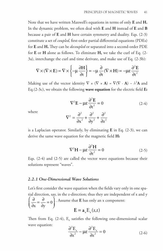
PRINCIPLES OF MAGNETIC WAVES 41
# 156104 Cust: MP Au: Adams Pg. No. 41 Title: Principles of Electromagnetics 1—
K Short / Normal
DESIGN SERVICES OF
S4CARLISLEPublishing Services
Note that we have written Maxwell’s equations in terms of only E and H. In the dynamic problem, we often deal with E and H instead of E and B because a pair of E and H have certain symmetry and duality. Eqs. (2-3) constitute a set of coupled, first-order partial differential equations (PDEs) for E and H. They can be decoupled or separated into a second-order PDE for E or H alone as follows. To eliminate H, we take the curl of Eq. (2-3a), interchange the curl and time derivate, and make use of Eq. (2-3b):
∇ × ∇ × = ∇ × − ∂∂
= − ∂∂
∇ × = − ∂∂
( ) )EH
HEµ µ µε
t t(
t2
2
Making use of the vector identity ∇ × (∇ × A) = ∇(∇ · A) − ム2A and Eq.(2-3c), we obtain the following wave equation for the electric field E:
∇ − ∂∂
=22
0EEµε
t2 (2-4)
where
∇ = ∂
∂+ ∂
∂+ ∂
∂2
2 2 2
x y z2 2 2
is a Laplacian operator. Similarly, by eliminating E in Eq. (2-3), we can derive the same wave equation for the magnetic field H:
∇ − ∂∂
=22
0HHµεt2 (2-5)
Eqs. (2-4) and (2-5) are called the vector wave equations because their solutions represent “waves”.
2.2.1 One-Dimensional Wave Solutions
Let’s first consider the wave equation when the fields vary only in one spa-tial direction, say, in the z-direction; thus they are independent of x and y
∂∂
= ∂∂
=
x y
0 . Assume that E has only an x component:
E a= x xE z,t( )Then from Eq. (2-4), Ex satisfies the following one-dimensional scalar wave equation:
∂∂
−∂∂
=2 2
0Ez
Ez
x2
x2µε
(2-6)

42 PRINCIPLES OF ELECTROMAGNETICS 4
# 156104 Cust: MP Au: Adams Pg. No. 42 Title: Principles of Electromagnetics 1—
K Short / Normal
DESIGN SERVICES OF
S4CARLISLEPublishing Services
Now we try the solutions for Ex(z,t) of the following form:
E z,t f(z t)x ( ) = ± v (2-7)Letting u = z ± νt and making use of the chain rule,
∂∂
=∂∂
∂∂
= ′ = ′ ±
∂∂
= ∂∂
∂∂
∂∂
= ′
Ez
Eu
uz
f u f (z t)
Ez
uz u
Ez
x x
x2
x
( ) v
2
′′ = ′′ ±f u f (z t)( ) v
(2-8a)
Similarly,
∂∂
=∂∂
∂∂
= ′ ± = ± ′ ±
∂∂
= ∂∂
∂∂
∂∂
Et
Eu
ut
f u f (z t)
Et
ut u
Et
x x
x2
x
( )( )v v v
2
= ± ′′ = ′′ ±( ) ( )v v v2 2f u f (z t)
(2-8b)
Substituting Eqs. (2-8a) and (2-8b) into Eq. (2-6), it is shown that the wave equation (2-6) is satisfied if
v = 1µε (2-9)
Therefore, any function whose argument is of the form z ± νt or z ± 1µε
satisfies Eq. (2-6).Physically Ex(z,t) = f(z − vt) represents a “wave” of constant shape f(u)
traveling in the positive z direction with velocity v. Consider f(z) being a Gaussian pulse with a peak at the origin. If we plot Ex(z,t) as a function of z at two successive instants, t = 0 and t = t0 (t0 > 0), then it is given by f(z) and f(z − vto) as shown in Figure 2-1.
z0
At t = t0At t = 0
z
vt)Ex(z,t)= f(z
Figure 2-1. Gaussian pulse moving with velocity v

PRINCIPLES OF MAGNETIC WAVES 43
# 156104 Cust: MP Au: Adams Pg. No. 43 Title: Principles of Electromagnetics 1—
K Short / Normal
DESIGN SERVICES OF
S4CARLISLEPublishing Services
The Gaussian pulse has traveled a distance vto ≡ zo in the +z direction as time progresses. The velocity of travel is of course given by
zt
o
o
= =v1µε
. It is also clear that Ex(z,t) = f(z + vt) represents a wave traveling in the negative z direction with velocity v. In summary,
E a a= ± = ±x xf z t f(z t)( )v1µε
(2-10)
is the simple form of a one-dimensional wave. Electromagnetic waves propagate through a linear homogeneous medium (μ,ε) with a velocity v:
v = 1µε
In free space or vacuum,
v = ≈× ×
= ×
−
−
1 1
4 1036
3 1012
8
µ επ
πo o 710
msec
which is precisely the speed of light in vacuum. Note that we have used
a useful number: επo
Fm
= × ≈
−−
8 854 101036
129
. . This implies that
light is an electromagnetic wave. Moreover, electromagnetic waves at any
frequency propagate with the same velocity.
2.3 Time-Harmonic Electromagnetic Fields
In Section 2.2, we have shown that any function whose argument is of the form z ± vt satisfies the wave equation. Among all possible functions for sources and fields, the sinusoidal function is the most popular. Therefore, we will mainly deal with the fields that are sinusoidal in time. We often call them time-harmonic fields.
There are a few good reasons why we emphasize the time-harmonic fields. First of all, almost all the electric sources that produce charges and currents are sinusoidal (known as ac sources) with a single frequency. Sec-ondly, when the charges and currents are sinusoidal with frequency f in

44 PRINCIPLES OF ELECTROMAGNETICS 4
# 156104 Cust: MP Au: Adams Pg. No. 44 Title: Principles of Electromagnetics 1—
K Short / Normal
DESIGN SERVICES OF
S4CARLISLEPublishing Services
hertz, the fields and waves that they produce are also sinusoidal with the exact same frequency f in Hz in the steady state because a set of Maxwell’s equations are linear: for example, when ρ, is increased twice, Gauss’ law confirms that E is also increased twice. This fact will greatly simplify the mathematical complexity, using the concept of complex phasor as will be shown later. Thirdly, even when the sources are not sinusoidal, any function of time can be expanded as a linear combination of harmonic si-nusoidal functions according to Fourier analysis. Thus knowing the solu-tions for time-harmonic electromagnetic fields will help find the solutions for non-sinusoidal fields.
2.3.1. Phasor Representation of Time-Harmonic Fields
You may recall that in the analysis of AC circuits where voltages and cur-rents are sinusoidal, the complex phasor is introduced to represent the sinusoidal or ac voltages and currents.
We will do the same here. Suppose the volume charge density ρv is a sinusoidal function of the following form:
ρ ρ ωv ot t( , ) ( )cosr r= +( )φ (2-11)
where ρo(r) is the amplitude, ω is the angular frequency in radian(s) per second and Φ is called the phase. ω is related to the frequency f in Hz by
ω π= 2 f (2-12)
Using Euler’s formula e jsinjθ θ θ= +cos , ρv in (2-11) can be written as
ρ ρ ρω ωv o
j( t )o
j j tt e e e( , ) Re ( ) Re ( )r r r= = +φ φ
where Re means taking the real part of the quantity in the brackets .Eliminating the complex exponential time function ej tω , we define
ρ ρ φ
v oje( ) ( )r r= (2-13)
as the complex phasor of ρv (r, t). Thus the real time ρv(r, t) and its com-plex phasor ρv(r) are related by
ρ ρ ωv v
j tt e( , ) Re ( )r r= (2-14)

PRINCIPLES OF MAGNETIC WAVES 45
# 156104 Cust: MP Au: Adams Pg. No. 45 Title: Principles of Electromagnetics 1—
K Short / Normal
DESIGN SERVICES OF
S4CARLISLEPublishing Services
which represents a sinusoidal charge density. We can similarly define the complex phasors for all of the scalar and vector field quantities that are time-harmonic. For example, the time-harmonic electric field can be written as
E r E r( , ) Re ( )t ej t= ω (2-15)
Note that E(r,t) is a real function of t, whereas E(r) is a complex phasor and is no longer a function of t. Now consider the time derivative of the electric field in (2-15).
∂∂
= ∂∂
= ∂∂
=t
tt
et
e j ej t j t jE r E r E r E r( , ) Re ( ) Re ( ) Re ( )ω ω ω ωωt
(2-16)
Therefore, the complex phasor of ∂∂Et
is jωE(r), which is an algebraic multiplication of E(r), the phasor of E(r,t), by a simple factor jω. In other words, jω can replace the time derivative ∂
∂t in the phasor representation
of time-harmonic quantities:
∂∂
↔t
t jE r E r( , ) ( )ω (2-17)
(time domain)(phasor domain)
This identity simplifies Maxwell’s equations for time-harmonic fields be-cause the time derivatives can be eliminated.
Example 2-1. Phasor Representation of Time-Harmonic QuantitiesFind the complex phasors of the following quantities that are sinusoidal in time.(a) ρv(t) = ρo sin (106t)(b) E(z,t) = ax E1 cos (109t −3z + π/4) + ay E2 cos (109t −3z + 3π/4) Solution:
(a) ρ ρ ρ π ρ
ρ
πv o o o
j 10 t /2
o
t sin 10 t cos 10 t /2 e
e
( ) ( ) ( ) Re
Re
( )= = − = =
−6 6 6
jj /2 j10 teπ 6 Thus, the phasor of ρv(t) is given by ρv = ρo ej π/2 with ω = 106 rad/s .
(b)

46 PRINCIPLES OF ELECTROMAGNETICS 4
# 156104 Cust: MP Au: Adams Pg. No. 46 Title: Principles of Electromagnetics 1—
K Short / Normal
DESIGN SERVICES OF
S4CARLISLEPublishing Services
E a a
a
( ) Re
Re
( ) ( )z,t E e E e
E
x 1j t z /4
y 2j t z /4
x 1
= + =
− + − +10 3 10 3 39 9π π
ee e E e e e z ej z j /4y 2
j z j3 /4 j10 t j10 t9 9− − − − − −+( ) = 3 3π πa ERe ( )
Thus the phasor of E(z,t) is given by
E a a( )z E e E e e with rad/s.x 1j /4
y 2j3 /4 j z= + =−π π ω3 910
2.3.2. Maxwell’s Equations for Time-Harmonic Fields
When the sources – charges and currents – are sinusoidal with the angular frequency ω, Gauss’ law and Ampère’s law guarantee that all the electric and magnetic field quantities in a linear medium become sinusoidal or time-harmonic with the same angular frequency ω. Thus, if we define complex phasors for all scalar and vector field quantities that appear in Maxwell’s equations (1-20) as shown in Eqs. (2-14) and (2-15), then using the identity (2-17), Maxwell’s equations (1-20) in the most general form reduce to
∇ × = −E Bjω (2-18a)
∇ × = +H J Djω (2-18b)
∇ ⋅ =D ρv (2-18c)
∇ ⋅ =B 0 (2-18d)
(Maxwell’s equations for time-harmonic fields)
where E, H, D, B, J, ρv are complex phasor representations of their corre-sponding quantities and they now depend only on spatial variables. When the medium is linear, isotropic, homogeneous and lossless as character-ized by Eq. (2-2), time-harmonic electromagnetic fields in the source-free region where ρv = J = 0, satisfy the following Maxwell’s equations.
∇ × = −E Hjω (2-19a)
∇ × =H Ejωε (2-19b)
∇ ⋅ =E 0 (2-19c)

PRINCIPLES OF MAGNETIC WAVES 47
# 156104 Cust: MP Au: Adams Pg. No. 47 Title: Principles of Electromagnetics 1—
K Short / Normal
DESIGN SERVICES OF
S4CARLISLEPublishing Services
∇ ⋅ =H 0 (2-19d)
(Maxwell’s equations for time-harmonic fields in simple medium in the source-free region)
Note that Eq. (2-19) is the time-harmonic version of Eq. (2-3). In Maxwell’s equations, the time derivatives have been eliminated and re-placed by an algebraic multiplication of jω. This will greatly simplify find-ing solutions for the fields from Maxwell’s equations.
2.3.3. Complex Poynting Theorem – Real Power Flow
There is a complex version of Poynting’s theorem that was presented in Section 1.7, which illustrates the flow of real electromagnetic power in terms of complex phasor fields. If we dot-multiply Eq. (2-18a) with H* and the complex conjugate of Eq. (2-18b) with E, and subtract the sec-ond term from the first term, we obtain
H E E H
E H B H E D E J
* *
* * * *
( ) ( )
( )
⋅ ∇ × − ⋅ ∇ ×= ∇ ⋅ × = − ⋅ − ⋅ − ⋅j ( )ω
(2-20)
where we have used the vector identity (6). Eq. (2-20) is the complex Poynting’s theorem in differential form and is the complex version of Eq. (1-31). If we follow the same procedure as in Section 1.7, i.e., in-tegrate both sides of Eq. (2-20) over the volume V bounded by closed surface S and apply the divergence theorem to the left side, we obtain the complex Poynting’s theorem in integral form:
( ) ( )* * * *E H s E D H B E J× ⋅ = ⋅ − ⋅ − ⋅∫∫ ∫∫∫ ∫∫∫d j dv dvS V V
ω (2-21)
If the medium is linear and μ, ε are assumed to be real, the first term of the right side of Eq. (2-21) becomes purely imaginary. Suppose J consists of the source current Ji (often called the impressed current) and the con-duction current Jc, i.e.,
J J J J E= + = +i c i σ (2-22)
Taking the real part of Eq. (2-21), dividing by 2, and rearranging the terms, we obtain

48 PRINCIPLES OF ELECTROMAGNETICS 4
# 156104 Cust: MP Au: Adams Pg. No. 48 Title: Principles of Electromagnetics 1—
K Short / Normal
DESIGN SERVICES OF
S4CARLISLEPublishing Services
12
12
12
Re Re* * *− ⋅ = × ⋅ + ⋅∫∫∫ ∫∫ ∫∫∫E J E H s E Ji dv d dvV S
cV
'
(2-23)
where the last term is shown to be real because E J E E E⋅ = ⋅ =c |* * | .σ σ 2
The physical interpretation of each term is given as follows. The term on the left side is the real or time-average power supplied by the sinusoidal source current Ji in the volume V. The first term on the right side is the real or time-average power flowing out of the volume V and the second term is the real or time-average power dissipated as the Joule heat in the volume V as discussed in Volume 2. Thus Eq. (2-23) represents the con-servation of real electromagnetic power in V. If we define the complex quantity
S E H≡ × * (2-24)
half its real part gives the time-average power per unit area carried by the electric and magnetic fields (E, H). S is called the complex Poynting vector. In summary, it is important to recognize that
12
Re *E H s× ⋅ =∫∫ dTime-average power flowingthrough the sur
Sfface S
(2-25)
and12
12
2Re |*− ⋅ = ⋅ =∫∫∫ ∫∫∫E J EcV V
dv | dvTime-average powerdissi
σppatedin the volume V
(2-26)
Finally, we wish to explain why the real part of 12
E H×( )* gives the time-average of E(t) × H(t) for the time-harmonic (or sinusoidal) fields:
S E H E Hav (t) (t)≡ × = × 12
Re * (2-27)
where < > denotes the time average. Note that for time-harmonic fields, the Poynting vector S = E(t) × H(t) represents an instantaneous power density. In practice, we are more interested in time-average power rather than an instantaneous power. The relationship (2-27) is analogous to how the average power is calculated from the complex phasor voltage and cur-rent in the analysis of ac circuits in the sinusoidal steady state, that is,

PRINCIPLES OF MAGNETIC WAVES 49
# 156104 Cust: MP Au: Adams Pg. No. 49 Title: Principles of Electromagnetics 1—
K Short / Normal
DESIGN SERVICES OF
S4CARLISLEPublishing Services
P V(t) I(t) V Iav ≡ = × 1
2Re *
(2-28)
where V and I are complex phasors corresponding to V(t) and I(t), respec-tively. In order to prove Eq. (2-27), we write
E E E H H H= + = +R I R Ij j, (2-29)
where ER, HR are real parts and EI, HI are imaginary parts of E, H. Then
E E E E
H H H H
( ) Re cos sin
( ) Re cos sin
t e t t
t e t
j tR I
j tR I
= = −
= = −
ω
ω
ω ω
ω ωωt
(2-30)
E(t) × H(t) = ER × HR cos2 ωt + EI × HI sin2 ωt − (ER × HI + EI × HR) cos ωt sin ωt
Making use of the following identities on the time-averages of the sinusoidal functions with angular frequency ω π π= =2
2f
T (T is a
period):
cos cos cos
sin( )
2 21 1 12
1 2
1
ω ω ω
ωω
tT
tdtT
t dt
2Tt
12
2 t
0
T
0
T
≡ = +( )
= +
∫ ∫
=0
T 12
sin cos
sin cos sin ,
2 1 12
1 212
1 12
2 0
ω ω
ω ω ω
tT
t dt
t tT
tdt
0
T
0
T
= −( ) =
= =
∫
∫∫time-averaging both sides of Eq. (2-30) leads to
E H E H E H(t) (t) R R I I× = × + ×( )1
2 (2-31)
From Eq. (2-29),
E H E E H H
E H E H E H E H
× = + × − = × + ×( ) + × − ×( )
*R I R I
R R I I I R R I
j j
j (2-32)

50 PRINCIPLES OF ELECTROMAGNETICS 4
# 156104 Cust: MP Au: Adams Pg. No. 50 Title: Principles of Electromagnetics 1—
K Short / Normal
DESIGN SERVICES OF
S4CARLISLEPublishing Services
Taking the real part of Eq. (2-32) and comparing with Eq. (2-31) proves the time-average relationship in Eq. (2-27). Note also that a factor of ½ in Eq. (2-26) signifies the time average of the dissipated power.
Example 2-2 Calculation of Time-Average PowerConsider an electromagnetic wave propagating in air (free of sources) which has the following time-harmonic electric field
E a= −( )x o
9E cos 2 10 t zπ 3
where Eo = 10 [V/m].(a) Find the magnetic field H of this wave, using the complex phasors.(b) Find the time-average power density in watts/m2 carried by the elec-
tromagnetic wave.Solution:(a) First, we find the corresponding complex phasor of E:
E a a( ) Re Rez,t E e E e ex oj2 10 t z
x oj z j t9
= = − − −π β ω3
where ω = 2π×109 and β = 3. Then the complex electric field is given by
E a= −x o
j zE e β
The complex magnetic field H can be calculated from Faraday’s law for time-harmonic fields, Eq. (2-18a):
∇ × = − = − =
= ∇ ×−
=−
∂∂
=
E B H
HE
a a
j j [In air, ]
j jEz
o o
o oy
xy
ω ωµ µ µ
ωµ ωµ1 (−−
−=− −j
jE e E e
oo
j zy
oo
j zβωµ
βωµ
β β)a
The magnetic field in real time is given by
H H a
a
(z,t) e E e e
E t
j ty
oo
j z j z
yo
o
= =
= −
−Re Re
cos(
ω β ωβωµ
βωµ
ω ββ
π ππ π
z
3 102 10 10
cos(2 10 t 3z) cos(2 10y 9 79
y
)
.= ⋅⋅ ⋅ ⋅
− = ×−−a a
43 8 10 3 99t 3z) [A/m]−

PRINCIPLES OF MAGNETIC WAVES 51
# 156104 Cust: MP Au: Adams Pg. No. 51 Title: Principles of Electromagnetics 1—
K Short / Normal
DESIGN SERVICES OF
S4CARLISLEPublishing Services
(b) The time-average Poynting vector is given by
S E H a a
a
av y oj z
yo
oj z
z
E e E e
12
Re
= × = ×
=
− −12
12
Re Re [ ]* *β ββωµ
EE E12
Eoo
o zo
oβ
ωµβ
ωµ
=* | |a 2
The time-average power density is
12
E12
32 10 10
=1.9 [W/m ]o
o2
9 72β
ωµ π π=
⋅ ⋅ ⋅×−
−
410 102 2( )
2.4 Uniform Plane Waves in Lossless Media
We first consider an electromagnetic wave propagating in an unbounded lossless medium free of sources. Assume that the medium has permittivity ε and permeability μ and is lossless (σ = 0) and consider time-harmonic fields. In order to find solutions for the time-harmonic fields we again start from Maxwell’s equations (2-19) and derive the differential equation for E or H separately as we have done in Section 2.2. To eliminate H, we take the curl of Eq. (2-19a) and make use of Eq. (2-19b):
∇ × ∇ × = − ∇ × = − ( ) =( )E H E Ej ( ) j jωµ ωµ ωε ω µε2
Making use of the vector identity ∇ × (∇ × E) = ∇(∇ · E) − ∇2E and Eq. (2-19c), we obtain the following second-order partial differential equation (PDE) for the electric field E:
∇ + =2 2 0E Ek (2-33)
where
k2 2= ω µε (2-34)
or
k = ω µε (2-35)
Eq. (2-33) is called the Helmholtz equation or the wave equation for a (time-harmonic) complex field. Eq. (2-35) is called the dispersion rela-tion and k is called the propagation constant.
52 PRINCIPLES OF ELECTROMAGNETICS 4
# 156104 Cust: MP Au: Adams Pg. No. 52 Title: Principles of Electromagnetics 1—
K Short / Normal
DESIGN SERVICES OF
S4CARLISLEPublishing Services
Similarly, by eliminating E in Eq. (2-19), we can derive the same PDE for the magnetic field H:
∇ + =2 2 0H Hk (2-36)
A final note of caution is in order. In the equations above, we have used E and H without underbar although they represent complex phasor fields. From now on we will not use the separate notations (underbars) for complex phasor fields, because we will mainly consider time-harmonic fields and the reader is to understand that they are phasors from the absence of time derivatives in the equations.
Let’s consider a simple solution for time-harmonic electric field E which points in the x-direction and varies only in the z-direction, thus independent of x and y. The complex field E can be written as
E a= x xE z( ) (2-37)
Substituting Eq. (2-37) into Eq. (2-33) and removing the unit vector, we obtain
∇ + =
∂∂
+ =2 22
2 0E k EEz
k Ex xx
2 x (2-38)
This is a second-order constant-coefficient ordinary differential equation whose two independent solutions can be written as either sinusoidal func-tions (sin, cos) or complex exponential functions as follows.
E z A cos(kz) B sin(kz)x ( ) = + (2-39)
or
E z E e E ex 0+ jkz
0jkz( ) = +− − − (2-40)
where A, B, E E0+
0, − are arbitrary coefficients.A and B are related to E0
+ and E0− by using Euler’s formula (see
Problem 2-14). We will take the form (2-40) for our discussion because each term in Eq. (2-40) has a clear physical interpretation and is easier to manipulate mathematically. The first and second terms represent waves propagating in the positive and negative z direction, respectively. Let’s consider the first term and let
E a= −x 0
jkzE e (2-41)
Assuming that the constant E0 is real (E0 could be complex in general), the electric field in real time is given as

PRINCIPLES OF MAGNETIC WAVES 53
# 156104 Cust: MP Au: Adams Pg. No. 53 Title: Principles of Electromagnetics 1—
K Short / Normal
DESIGN SERVICES OF
S4CARLISLEPublishing Services
E E a a( ) Re Re cos( )z,t e E e E t kzj tx 0
j( t kz)x 0= == = −−ω ω ω
(2-42)
Rewriting Eq. (2-42),
E a a( ) cos ( ) cosz,t E k z
kt E k z
1tx 0 x 0= − −
= −
ωµε
(2-43)
where we have used Eq. (2-35). Since the field takes the form of z
1t−
µε where f is the cosine function for this case, Eq. (2-42), or
alternatively Eq. (2-41), represents an electromagnetic wave traveling in the positive z direction with velocity v
1=µε , as we have discussed in
Section 2.2.1. In fact, we can see this by plotting the x component of the electric field in Eq. (2-42) as a function of space (z) at two successive time instants, t = 0 and t
2= π
ω as shown in Figure 2-2 (a), (b).
z
E0
)2
kzcos(E)2
t,z(E 0x ==
coskzE)0t,z(E 0x ==
tcosE)t,0z(E 0x ==
k2 k k23
k20
z
E0
k2 k k23
k20
t
E0
2 23 20
T
(a)
(b)
(c)
Figure 2-2. Time-harmonic electromagnetic field

54 PRINCIPLES OF ELECTROMAGNETICS 4
# 156104 Cust: MP Au: Adams Pg. No. 54 Title: Principles of Electromagnetics 1—
K Short / Normal
DESIGN SERVICES OF
S4CARLISLEPublishing Services
We observe that the sinusoidal wave has traveled a distance z0 = π/2k in the +z direction over the period of time t0 = π/2ω. The velocity of the wave is given by
vzt k
10
0
= = =ωµε (2-44)
as expected. The velocity v is often called the phase velocity because it measures the velocity of the phase change (kz) in Eq. (2-41). It is striking to observe that when the fields are sinusoidal in time (see Figure 2-2(c)) the fields are also sinusoidal in space (see Figure 2-2(a), (b)), thus periodic as a function of space. This spatial period of the wave is called the wave-length and is given by
λ π= =2
kvf (2-45)
where vk
fk
= =ω π2 has been used in the second equality. Note that the
period in time of the wave is T1f
= = 2πω [Figure 2-2(c)]. For example,
if the wave has the frequency f = 1 GHz, the wavelength in free space is
λ = = ××
=vf
cm3 101 10
308
9 . On the other hand, for an AM signal of f =
1000 kHZ, λ = ××
=3 101 10
3008
6 m . The propagation constant k is re-
lated to the wavelength λ by
k
2= πλ (2-46)
indicating that k gives the number of wavelengths in a spatial distance of 2π. Thus, k is also called the wavenumber.
Given the electric field in Eq. (2-41), the complex magnetic field H of the wave can be calculated by using Faraday’s law (2-19a):
HE
a a a= ∇ ×−
=−
∂∂
=−
−=− −
j jEz
jkj )
E e E eyx
y ojkz
y ojkz
ωµ ωµ ωµεµ
1 ( )(
(2-47)
where k
ωµµεµ
εµ
= = has been used. The magnetic field in real time is given by

PRINCIPLES OF MAGNETIC WAVES 55
# 156104 Cust: MP Au: Adams Pg. No. 55 Title: Principles of Electromagnetics 1—
K Short / Normal
DESIGN SERVICES OF
S4CARLISLEPublishing Services
H H a(z,t) e E cos( t kz)j ty o= = −Re ω ε
µω
(2-48)
We note that the magnetic field takes the same form as the electric field both in time and space, except that H points in the y direction. It is in-teresting to find that the ratio of the amplitudes of E and H is given by
EH
E
E
x
y
o
o
= = ≡εµ
µε
η (2-49)
Thus the ratio depends only on the medium parameters. This quantity η is called the intrinsic impedance of the medium. In free space or air for which ε0 = 8.86 × 10⁻¹² ≈ 1/36π × 10−9, μ0 = 4π × 10−7, the phase velocity, wavelength, intrinsic impedance and wavenumber are given by
vms
c in free space or air
cf
free-s
0 0
0
= = ×
≡
= = =
13 108
µ ε
λ λ ppace wavelenth [m]
[ ]
kc
k
0
00
0 00
0
ηµε
π η
ω µ ε ω πλ
= = ≈ ≡
= = = ≡
377 120
2
Ω
[[ ]m−1
(2-50)
In the medium of permittivity ε = εrε0 and permeability μ = μrμ0,
vc c
n
vf n
k n
r r
0r
r0 0
= = = = =
= = = = = =
1 0
0 0
µε µ ελ
λ
η µε
ηµε
ω µε ω µ ε µεµ ε
, ,
, kk0
(2-51)
The wave slows down by a factor of n,
ncv r r≡ = =µε
µ εµ ε
0 0 (2-52)

56 PRINCIPLES OF ELECTROMAGNETICS 4
# 156104 Cust: MP Au: Adams Pg. No. 56 Title: Principles of Electromagnetics 1—
K Short / Normal
DESIGN SERVICES OF
S4CARLISLEPublishing Services
called the index of refraction or the refractive index, which will play an important role in the reflection and transmission of the wave. The instantaneous Poynting vector and the time-average Poynting vector can be calculated as
S E H a= × = −( ) cos ( )z,t (z,t)E
t kzzo2
ηω2 (2-53a)
S E H a aav z oo
zoE
E E= × =
=1
212 2
2
Re Re| |*
*
η η (2-53b)
As expected, S points in the direction of travel (+z). We can also show that the time-average of Eq. (2-53a) gives Eq. (2-53b). In summary, the wave has the electric field E in the x direction and the magnetic field H in the y direction, and propagates in the z direction.
E a H a S a= = =− −x 0
jkzy
0 jkzav z
0E e E
e |E
2, ,
|η η
2
(2-54)
It is important to note that
E H E S H S⊥ ⊥ ⊥, ,
and (E, H, S) make a right-handed orthogonal coordinate system. Using Eqs. (2-42) and (2-48), the electric and magnetic fields as a function of space at a fixed time (say, t = 0) are plotted in Figure 2-3.
direction of propagationS = Ε×Η
E
E
H
H
x
y
z
Figure 2-3. Electric and magnetic fields as a function of space at fixed time
PRINCIPLES OF MAGNETIC WAVES 57
# 156104 Cust: MP Au: Adams Pg. No. 57 Title: Principles of Electromagnetics 1—
K Short / Normal
DESIGN SERVICES OF
S4CARLISLEPublishing Services
The wave we have just described is called a uniform plane wave. The term “plane” indicates that the surface on which the phase of the wave is constant (called the constant-phase front) is a plane. For the wave shown in Figure 2-3, the constant-phase front is given by
kz const( C)= ≡Then z
Ck
= denotes a plane parallel to the xy plane (z = 0). The term “uniform” implies that amplitudes of the wave fields on the constant-phase fronts (planes) are uniform, or independent of the position. For the wave described above, at any given constant-phase plane, amplitudes of E and H, E0 and E0/η, are independent of x and y, i.e., uniform. When the wave is generated from a localized source, it will start as a spherical wave, but after it propagates some distance, the wave will behave like a plane wave at points far from the source. Thus, the uniform plane wave represents the simplest and most useful form of wave propagation.
As a final note, for the second term of the E field solution in Eq. (2-40), we can follow the similar procedure and obtain
E a= −x 0
jkzE e (2-55a)
E a( )z,t E cos( t kz)x 0= +− ω (2-55b)
H a= − y
0 jkzE e
η (2-56)
S aav z
0|E2
= −|2
η (2-57)
The wave has the electric field in the positive x direction and the mag-netic field in the negative y direction, and propagates in the negative z direction. The relationship of (E, H, S) still holds. It is important to note that the complex field e−jkz represents a wave traveling in the +z direction and ejkz represents a wave traveling in the −z direction.
Example 2-3 Uniform Plane Wave in a Lossless MediumA uniform plane wave is traveling in the positive x direction in a lossless medium, with the 10 V/m electric field in the z direction. The wavelength of the wave is 20 cm and the velocity of wave propagation is 2 × 10⁸ m/s.

58 PRINCIPLES OF ELECTROMAGNETICS 4
# 156104 Cust: MP Au: Adams Pg. No. 58 Title: Principles of Electromagnetics 1—
K Short / Normal
DESIGN SERVICES OF
S4CARLISLEPublishing Services
(a) Determine the frequency in Hz of the wave and the permittivity of the medium, assuming the medium is non-magnetic, i.e., μ = μo.
(b) Write the complete complex phasor expressions for the electric and magnetic field vectors. Discuss the relationship between the direction of E, H and S.
Solution:(a) The frequency can be obtained from the relationship (2-45):
fv
Hz= = × = ×λ
2 100 2
1 108
2
.[ ]
If we let the dielectric constant of the medium be εr, then
v1 c
o o r r
= = = = ×12 108
µε µ ε ε ε
ε ε εr 8 o
c2 10
=×
=××
= ∴ =
2 8
8
23 102 10
2 25 2 25. .
(b) According to the description of the uniform plane wave, the complex electric field can be written as follows:
E a= −z 0
jkxE e
where E0 = 10 [V/m] and the propagation constant k is determined by
k f 1 10 [m ].0 09 1= = = ⋅ × ⋅
×= −ω µε π µ ε π π2 2 25 2
1 53 10
108( . ).
The magnetic field can be obtained by Faraday’s law: H
Ea a a= ∇ ×
−=
−−
∂∂
= − =− −
j jEx
Ej )
jk e H eyx
yo jkx
y ojk
ωµ ωµ ωµ1
(( ) xx
where Hk
E10
A/mo0
0= = ⋅⋅ × ⋅ ×
=−ωµπ
π π10
2 1 10 4 100 03989 7 . [ ] .
Thus,

PRINCIPLES OF MAGNETIC WAVES 59
# 156104 Cust: MP Au: Adams Pg. No. 59 Title: Principles of Electromagnetics 1—
K Short / Normal
DESIGN SERVICES OF
S4CARLISLEPublishing Services
E a H a= = −− −
zj10 x
yj10 x e e10 0 0398π π, .
The fields in real time are given by
E a
H a
( ) cos( )
( ) . cos( )
x,t 10 t x
x,t 10 t xz
9
y9
= −= −
10 2 10
0 0398 2 10
π ππ π
We note that the electric field points in +z direction, the magnetic field points in − y direction, and the wave propagates in +x direction. It is clear that (E, H, S) make a right-handed orthogonal coordinate system. Mak-ing use of this fact and knowing that the ratio of amplitudes of E and H is equal to the intrinsic impedance (η) of the medium, we can simply calculate the magnetic field, without using Faraday’s law, as follows:
H a E a a a
a
= × = × = − ⋅
= −
− −1 2 25 1 510
15η
εµ ηx
0
0x z 0
jkxy
0
jkz
y
E e e
377 e
. .
−− −= −jkzy
j10 xea 0 0398. π
2.4.1 Uniform Plane Waves Propagating in Arbitrary Direction
So far we have considered the wave in a simple form, that is, a uniform plane wave propagating in a direction with one particular coordinate (z), so that the fields vary only as a function of one coordinate. Suppose the wave propagates in an arbitrary direction which involves all three coor-dinates. The fields of such a plane wave can be expressed in the following general form:
E e e( )r E e e e E e0jk x jk y jk z
0j(k x k y k z)x y z x y z= =− − − − + + (2-58)
where e is a unit vector in the direction of the electric field and E0 is a (complex) constant for a uniform plane wave. If we define a vector
k a a a= + +x x y y z zk k k (2-59)
and make use of a position vector r = axx + ayy + azz, Eq. (2-58) can be rewritten as
E e( )r E e0jk r= − ⋅
(2-60)
We note that ejk·r is the general form of the uniform plane wave that propagates in an arbitrary direction. The vector k gives the direction of

60 PRINCIPLES OF ELECTROMAGNETICS 4
# 156104 Cust: MP Au: Adams Pg. No. 60 Title: Principles of Electromagnetics 1—
K Short / Normal
DESIGN SERVICES OF
S4CARLISLEPublishing Services
propagation, thus we will call k the propagation vector or the wave vec-tor. Its magnitude gives the propagation constant k and is related to the angular frequency ω by Eq. (2-35). Substituting Eq. (2-58) into Eq. (2-33) and making use of
∂∂
= − =− −
ue jk u e u x, y, zjk u
ujk uu u( ) ,
we obtain
( ) ( ) ( )
| |
− + − + − + =
= + + = =
jk jk jk k
k k k kx y z
2
x2
y2
z2 2
2 2 2
2 2
0E
k ω µε (2-61)
The phase of the wave will be constant when
k r⋅ = constantThis defines a constant-phase front, which is a plane perpendicular to k as shown in Figure 2-4. Note that for all observation points r on this phase front (which is a plane), k · r is the same, i.e., is a constant.
Figure 2-4. Uniform plane wave propagating in an arbitrary direction
Now we write the corresponding magnetic field in a similar form:
H h h( )r H e H e0jk r
0j(k x k y k z)x y z= =− ⋅ − + + (2-62)
If we substitute Eqs. (2-58) and (2-62) into Maxwell’s equations (2-19), making use of the algebraic identity for plane waves
E k
H
r1
r2
x
y
z
constant-phase fronts

PRINCIPLES OF MAGNETIC WAVES 61
# 156104 Cust: MP Au: Adams Pg. No. 61 Title: Principles of Electromagnetics 1—
K Short / Normal
DESIGN SERVICES OF
S4CARLISLEPublishing Services
∇ = ∂∂
+ ∂∂
+ ∂∂
= − + − + −
= − +
a a a a a a
a a
x y z x x y y z z
x x y
x y zjk jk jk
j( k k
( ) ( ) ( )
yy z zk ) jk,+ = −a
(2-63)
we obtain
k E H k E
k H H k H
× = ⋅ =× = − ⋅ =
ωµωε
00
(2-64)
From Eq. (2-64) we conclude that for uniform plane wave, (E, H, k) are perpendicular to each other and they make a right-handed orthogonal coordinate system:
E H E k H k E H k⊥ ⊥ ⊥ ×, , //
Thus for a uniform plane wave, knowing E and the direction of propaga-tion, we can easily obtain magnetic field H without using one of Max-well’s equations as follows:
H k E a Ek= × = ×1 1
ωµ η (2-65)
where ak
k k= is a unit vector in the direction of the propagation vector
k and η is the intrinsic impedance of the medium. Similarly, we can also calculate E from H for a uniform plane wave by
E k H H ak=
−× = ×1
ωεη (2-66)
2.5 Uniform Plane Waves in Lossy Media
In Section 2.4, we have considered the field solutions for the wave in a lossless or nonconducting medium for which σ = 0. What happens to the wave when propagating in a lossy or conducting medium? The lossy medium could be either a good conductor or a dielectric with small conductivity. As discussed in Volume 2 (Joule’s law) and Section 2.3.3 (Poynting’s theorem), there will be power dissipation or loss due to con-duction current Jc = σE. Since the power is carried by the wave, we expect that the wave will attenuate in its amplitude as it propagates through a lossy medium.
62 PRINCIPLES OF ELECTROMAGNETICS 4
# 156104 Cust: MP Au: Adams Pg. No. 62 Title: Principles of Electromagnetics 1—
K Short / Normal
DESIGN SERVICES OF
S4CARLISLEPublishing Services
2.5.1 Attenuation of Waves
In a lossy medium with permittivity ε, permeability μ and conductivity σ, we need to correct Ampère’s law (2-3b) and (2-19b) by adding the conduction current density Jc:
J E Jc i (source free)= = −σ , 0
Ampère’s law now reads
∇ × = + ∂
∂H J
Ec t
(in real time)ε (2-67a)
∇ × = + = +H J E Ec j ( j )ωε σ ωε (2-67b)
(for time-harmonic fields)
Making use of Eq. (2-67a) along with Eq. (2-3a), the wave equation (2-4) in the time domain is modified to
∇ − ∂
∂− ∂
∂=2
2
0EE Eµσ µεt t2 (2-68)
Making use of Eq. (2-67b) along with Eq. (2-13a), the Helmholtz equa-tion (2-33) or the wave equation for a complex field is modified to
∇ − + =2 0E Ej ( j )ωµ σ ωε (2-69)
Without resolving the new PDE (2-68), we can find solutions of Eq. (2-69) from the solutions of Eq. (2-33) by redefining the propagation constant k as the complex propagation constant such that
k j j ) j22 = − + = − ωµ σ ωε ω µ ε σ
ω( (2-70a)
k j ( j ) j= − + = − ωµ σ ωε ω µ ε σ
ω (2-70b)
Then Eq. (2-69) takes the same form as Eq. (2-33) for lossless media and we can make use of the field solutions that we obtained in Section 2.4 with the understanding of k being a complex number. Eq. (2-70) can be simplified by introducing an effective permittivity

PRINCIPLES OF MAGNETIC WAVES 63
# 156104 Cust: MP Au: Adams Pg. No. 63 Title: Principles of Electromagnetics 1—
K Short / Normal
DESIGN SERVICES OF
S4CARLISLEPublishing Services
ε ε σ
ωeff j= −
(2-71)
for the lossy medium which has permittivity ε and conductivity σ. Note that εeff is complex. Then we have
k2 2
eff= ω µε (2-72a)
k eff= ω µε (2-72b)
Ampère’s law (2-67) reduces to a regular form
∇ × =H Ej effωε (2-73)
which is the same as Eq. (2-19b) with ε being replaced by εeff. This im-plies that if we take the solutions of Section 2.4 and replace ε by εeff, we find the solutions for the wave in lossy medium.
Now we again consider a simple solution for time harmonic field E which points in the x direction and varies only in the z direction, as for-mulated in Eq. (2-37). Then the solution for Ex(z) will be given by Eq. (2-40) except that k now becomes a complex propagation constant. If we define
k j j= −
≡ −ω µ ε σ
ωβ α (2-74)
where β, α are real, for a wave traveling in the positive z direction, the complex electric field E is written from Eq. (2-41) as
E a a a= = =− − − − −x 0
jkzx 0
j( j )zx 0
z j zE e E e E e eβ α α β (2-75)
Since e−αz
represents an exponential decay in +z direction, the wave at-tenuates in a lossy medium as it travels in +z direction. If we assume Eo is real (if it is complex, we can write E Aeo
j= φ ), the electric field in real time is given by
E a a(z,t) E e e e E e t zx 0z j z j t
x 0z= = −− − −Re cos( )α β ω α ω β (2-76)
At fixed time, say t = 0, the electric field is plotted as a function of space z in Figure 2-5.

64 PRINCIPLES OF ELECTROMAGNETICS 4
# 156104 Cust: MP Au: Adams Pg. No. 64 Title: Principles of Electromagnetics 1—
K Short / Normal
DESIGN SERVICES OF
S4CARLISLEPublishing Services
2 23 20
zcoseE)0t,z(E z0x ==
z
z
E0)envelope(eE0
zeE0
Figure 2-5. Time-harmonic electromagnetic field with attenuation
We observe that β plays the same role as k of the wave in lossless me-dium and α describes the rate of attenuation. Thus we call β the phase constant and α the attenuation constant. The unit of β is radians per meter and that of α is called nepers per meter, in short, Np/m. The wave-length and phase velocity are given by
λ πβ
= =2 vf (2-77)
v1= ≠ω
β µε (2-78)
Since β depends on the frequency (ω) as seen from Eq. (2-74), the phase velocity of the wave in a lossy medium is not a constant, but dependent on the frequency of the wave. Such a medium is called dispersive.
The complex magnetic field H can be calculated using Faraday’s law (2-19a):
H
Ea a= ∇ ×
−= ≡− − −
jk
E eE
e ey ojkz
yo z j z
ωµ ωµ ηα β
˘ (2-79)
where
EH k j
| |ex
y eff
j= = =−
≡˘/
˘η ωµ µε
µε σ ω
η θη (2-80)

PRINCIPLES OF MAGNETIC WAVES 65
# 156104 Cust: MP Au: Adams Pg. No. 65 Title: Principles of Electromagnetics 1—
K Short / Normal
DESIGN SERVICES OF
S4CARLISLEPublishing Services
The intrinsic impedance η becomes complex for lossy media. The “hat” symbol signifies that η is complex. The complex magnetic field can be rewritten as
H a= − − +
y0 z j( zE
| |e e˘
)
ηα β θη (2-81)
and the magnetic field in real time is given by
H a(z,t)E| |
e t zy0 z= − −−
˘ cos( )η
ω β θαη (2-82)
This implies that the electric and magnetic field in lossy media are out of phase by the phase angle θη. From Eqs. (2-75) and (2-79) or (2-81), the time-average Poynting vector is given by
S E H aav z oz j z 0
*z j( zE e e
E| |
e e= × =
− − − − +12
12
Re Re ˘ ]* ) *α β α β θ
ηη
= −a z0 z|E
2| |e
|˘ cos
22
ηθη
α (2-83)
The power density of the wave attenuates like (e−αz)2 = e−2αz as it travels in +z direction.
For a wave traveling in the negative z direction, we follow a similar procedure to obtain
E a a= =− + − −x 0
jkzx 0
z j zE e E e eα β (2-84a)
E a(z,t) E e t zx 0z= −− α ω βcos( ) (2-84b)
H a= − − −
−
y0 zE
| |e t z˘ cos( )
ηω β θα
η (2-84c)
S aav z
0 2 z|E2| |
e= −− |˘ cos
2
ηθη
α (2-84d)
How to find α, β, | η |, θη

66 PRINCIPLES OF ELECTROMAGNETICS 4
# 156104 Cust: MP Au: Adams Pg. No. 66 Title: Principles of Electromagnetics 1—
K Short / Normal
DESIGN SERVICES OF
S4CARLISLEPublishing Services
The values of the attenuation constant, the phase constant and the complex intrinsic impedance can be obtained by solving the two complex equations for k and η , given by Eqs. (2-70) and (2-80). For example, substituting Eq. (2-74) into Eq. (2-70a), we have
k j j2 j2 2 2= − = − − = −( ) ( )β α β α αβ ω µε ωµεσ2 2 (2-85)
Matching the real and imaginary parts on both sides and solving two equations for α and β (see Problem 9-23), we obtain the expressions for α and β in terms of ω, μ, ε, σ as follows.
α ω µε σωε
= = +
−
2
Npm
1 12
12
(2-86a)
β ω µε σωε
= = +
+
2
radm
1 12
12
(2-86b)
Although Eqs. (2-86) can be used for any lossy medium with (μ, ε, σ), in the cases of good conductors and good dielectric media with small loss, we can obtain much simpler approximate expressions for α, β, η . Another important parameter that is often used is the penetration depth dp. It is the distance over which the wave amplitude is attenuated by a factor of 1 1
ee= − , which is equivalent to 36.8%.
E z dE z 0
=E e
Ee dx p
x
0d
0
dp
p
p( )( )
==
= → =−
−α
α α 1
Thus the penetration depth is the inverse of the attenuation constant:
dp = 1α (2-87)
The penetration depth measures how far the wave can penetrate into the lossy medium. When the medium is very lossy, dp will be very short since the wave will attenuate fast. When the medium is slightly lossy, dp will be long and the wave can penetrate deep into the medium without much attenuation.
PRINCIPLES OF MAGNETIC WAVES 67
# 156104 Cust: MP Au: Adams Pg. No. 67 Title: Principles of Electromagnetics 1—
K Short / Normal
DESIGN SERVICES OF
S4CARLISLEPublishing Services
2.5.2 Good Dielectric vs. Good Conductor
Whether the medium is a good dielectric (with small loss) or a good con-ductor (highly conducting) is determined by comparing the real (ε) and imaginary (σ/ω) parts of the effective permittivity given in Eq. (2-71). If ε σ/ω, the medium is a good dielectric. If ε σ/ω, the medium is highly conducting. There is a parameter, which determines this criterion, called the loss tangent. It is the ratio of the imaginary and real parts of εeff and also the ratio of amplitudes of the conduction current density (Jc = σE) and the displacement current density (Jd = jωεE).
Loss tangent (L.T.) c
d
= =σωε
J
J (2-88)
The loss tangent is a measure of how lossy the medium is and helps to classify the media between good conductors and good dielectrics:
L.T. , good dielectric
L.T. ,
c d
c
= →
=
σωε
σ ωε
σωε
σ ωε
1
1
,
,
J J
J Jdd good conductor→
A. Waves in Slightly Lossy Dielectric (L.T. 1)
In a good dielectric with small loss, σ ωε or L.T. 1. The complex propagation constant can be approximated by
k j j j= −
= −
≈ −
ω µ ε σωε
ω µε σωε
ω µε σωε
1 12
12
where the last equality can be shown by using the Taylor expansion of the square root function or the binomial expansion (see Eq. (2-32b)) with
σωε
being a small parameter. Then
k j j≈ − = −ω µε σ µε
β α2
and

68 PRINCIPLES OF ELECTROMAGNETICS 4
# 156104 Cust: MP Au: Adams Pg. No. 68 Title: Principles of Electromagnetics 1—
K Short / Normal
DESIGN SERVICES OF
S4CARLISLEPublishing Services
η µ
ε σω
µε
σωε
ε=−
≈j
since .
Thus, for a slightly lossy dielectric, we have
β ω µε α σ µε
σεµ
η µε
ωε σ= =
= =
,
, ˘
d (Loss-loss dielectric)
p
22
(2-89)
Note that the phase constant and intrinsic impedance have not been af-fected much due to small loss.
Example 2-4An electromagnetic wave of 10 MHz propagates in a lossy medium of ε = 2 ε0, μ = μ0 and σ = 5 × 10⁻⁵ [S/m]. Determine the attenuation constant and the phase constant using both the approximate and exact expressions and compare the results.Solution:First, we calculate the loss tangent to determine whether the medium is slightly lossy or highly conducting or neither at the given frequency.
L.T.
2 f 2 2 10 100 6= =
⋅= ×
⋅ × ⋅= =
−
−σ
ωεσ
π ε ππ
5 10
21036
0 045 15
9 .
Thus the medium is slightly lossy and we can use the approximate result of Eq. (2-89):
α σ µε
σ µε
σ η
β ω µε
= = = = × × = ×
= =
−−
2 2 25 10
2 2377 6 66 100
0
53
2Npm
2
0 .
ππ µ ε π πf 2 f
c2 rad
m00
7
8
2 10 23 10
0 296⋅ = = × ⋅×
=
.
If we use the exact expressions in Eq. (2-86), we obtain

PRINCIPLES OF MAGNETIC WAVES 69
# 156104 Cust: MP Au: Adams Pg. No. 69 Title: Principles of Electromagnetics 1—
K Short / Normal
DESIGN SERVICES OF
S4CARLISLEPublishing Services
α
β
= + −
= ×
= +
−0 2962
1 0 045 1 6 61 10
0 2962
1 0
21 2
3.( . ) .
.(
/ Npm
.. ) ./
045 1 0 29621 2
−
=
radm
We observe that the approximate results agree well with the exact results; there is very little error.
B. Waves in Good Conductor (L.T. 1)
In a highly conducting medium, σ ωε or L.T. 1. In this case, the complex propagation constant can be approximated by dropping the real part of εff: k j j j j= −
≈ −
= −
≡ −ω µ ε σω
ω µ σω
ωεσ β α12
12
The complex intrinsic impedance is approximated by
˘/
η µ
ε σω
µσ ω
ωµσ
ωµσ
π
=−
≈−
= +
=j j
j ej1
212
4
Thus, for a highly conducting medium, we have
β α ωµσωµσ
η ωµσ
ωµσ
σ ω= =
= + =
= d2
j e (Good conductor)
p
j4
2
21
,
˘ ( ) εε
(2-90)
We observe that in very good conductors, the attenuation constant is approximately equal to the phase constant and E and H are out of phase by 45°. The penetration depth dp will be very small for good conductors, in particular, at high frequencies where ω is very large, so dp is often called the skin depth for good conductors. Since the field cannot penetrate much into the medium, most of the conduction current Jc concentrates

70 PRINCIPLES OF ELECTROMAGNETICS 4
# 156104 Cust: MP Au: Adams Pg. No. 70 Title: Principles of Electromagnetics 1—
K Short / Normal
DESIGN SERVICES OF
S4CARLISLEPublishing Services
on the surface of the conductor and flows very little inside. This phe-nomenon is known as the skin effect. For example, for copper which has σ = 5.8×10⁷ S/m, ε ≈ εo, μ ≈ μo, the penetration depth is 8.53 mm at f = 60 Hz and 2.09 μm at 1 GHz, which looks like a skin. We can use the skin effect in effectively shielding the electronic devices from interfer-ence caused by external fields, by highly conducting enclosures whose wall thickness is greater than a few skin depths since the external interfer-ing field attenuates to a negligible value after a skin depth. The exact and approximate expressions for α, β, dp and η are summarized in Table 2-1
Table 2-1. Waves in Lossy Media
Exact Approximate
Low-loss Dielectric(ω ε >> σ)
Good Conductor(ω ε << σ)
αattenuation constant
ω µε σωε2
1 12
12
+
−
σ µε2
ωµσ2
βphase constant ω µε σ
ωε21 1
212
+
+
ω µω ωµσ2
dp
penetration depth1α
2σ
εµ
2ωµσ
η
ntrinsic impedance
µε
µε σ ωeff j
=− /
µε
ωµσ2
1+( )j
Example 2-5A ship at the ocean surface is supposed to communicate with a submarine at the depth of 100 meters below the surface, using a ULF (ultra low fre-quency) electromagnetic signal at 1 kHz. How much attenuation in dB does the signal suffer at the location of the submarine when the sea water has permittivity ε = 81 ε0, permeability μ = μ0, and conductivity σ = 4 [S/m] at this frequency?
PRINCIPLES OF MAGNETIC WAVES 71
# 156104 Cust: MP Au: Adams Pg. No. 71 Title: Principles of Electromagnetics 1—
K Short / Normal
DESIGN SERVICES OF
S4CARLISLEPublishing Services
Solution:Since ocean water is a lossy medium, when the electromagnetic wave trav-els from the ship at the surface to the submarine at the depth z, its field amplitude will attenuate exponentially as follows:
| |E(z) E e0z= −α
where E0 is the amplitude at the surface (z = 0) and a is the attenuation constant. Thus we need to calculate α. First we calculate the loss tangent at f = 1 kHz:
L.T.2 1 10
13
= =⋅ × ⋅ ×
= ×−σ
ωε ππ
4
81 1036
8 9 1095. ?
Seawater is a highly lossy medium at ULF, thus we can use Eq. (2-90):
α ωµσ π π π≈ = ⋅ ⋅ × ⋅ = × =−
−
22 4
24
10 10 410 0 1257
3 72 .
The attenuation in dB at z = 100 [m] can be calculated from the field as follows:
20 20 20 109log log logE(z 100)
Ee e dB
0
z 0.126 100= = = =− − ×α
Note that the lower the frequency, the less the attenuation.
Dielectric Loss
The loss can be caused not only by the dc conduction current but also by the high frequency ac current in phase with the applied electric field. When the dielectric is placed in an appreciable alternating field, the polar-ized atoms and molecules go through the continuous process of switching their dipole orientation, which results in a damping effect.* To account for such dielectric loss, often permittivity of the lossy dielectric is described by the complex permittivity whose imaginary part accounts for the loss:
ε ε ε= ′ − ′′j (2-91)
*see D. J. Griffiths (1999), Introduction to Electrodymanics, pp. 398-404, or J. D. Kraus (1992), Electromagnetics, pp. 442-445 for further discussion.

72 PRINCIPLES OF ELECTROMAGNETICS 4
# 156104 Cust: MP Au: Adams Pg. No. 72 Title: Principles of Electromagnetics 1—
K Short / Normal
DESIGN SERVICES OF
S4CARLISLEPublishing Services
Comparing Eq. (2-91) with the effective permittivity in Eq. (2-71), ε′ plays the role of ε and ε″ plays the role of σ/ω, or equivalently, σ = ωε″ is the equivalent conductivity. The loss tangent is given by L.T. = ′′
′εε
.
2.6 Dispersion of Waves – Group Velocity
In Section 2.4, we have seen that the velocity of propagation of an elec-tromagnetic wave in a lossless medium of permittivity ε and permeability μ is given by the phase velocity
υ ωµεp k
= = 1 (2-44)
For most media, μ and ε are constants and do not depend on the fre-quency. The electromagnetic waves at different frequencies propagate with the same velocity. However, for some media μ or ε or the index of refraction (n) is not constant and depends on the frequency, or equiva-lently, the wavelength. For example, the refractive index of typical glass is dependent on the wavelength at optical frequencies. When the white light consisting of different frequencies enters a prism, the refracted light gives a rainbow of colors because the glass prism has different indices of refraction at different color wavelengths. The phenomenon is called dispersion. When the medium parameters (ε and/or μ) depend on fre-quency, the phase velocity of the wave in that medium depends on the frequency and the medium is called dispersive. A lossy medium we stud-ied in Section 2.5 exhibits a dispersive behavior because the phase velocity in a lossy medium is given by
υ ωβp = (2-92)
where for a highly conducting medium, βωµσ=
2 , as shown in Eq. (2-90), and υp will depend on frequency. We will also find dispersive behavior when the waves propagate through a waveguide, as will be shown in Volume 5.
In transmitting information such as speech, image, digital data, etc. in a “baseband” signal which ranges from dc to some kHz or MHz, we

PRINCIPLES OF MAGNETIC WAVES 73
# 156104 Cust: MP Au: Adams Pg. No. 73 Title: Principles of Electromagnetics 1—
K Short / Normal
DESIGN SERVICES OF
S4CARLISLEPublishing Services
translate the low-frequency baseband signal to higher “carrier” frequency because higher frequencies will permit more reasonable sizes of wave-guides and antennas. Hence a composite signal consists of a multitude of many different frequencies. If the medium or the system is not disper-sive, all different frequency components travel at the same velocity and the received signal in time domain will not be distorted. This is the case for a uniform plane wave in unbounded lossless medium. On the other hand, if the medium is dispersive, the individual frequency components travel at different phase velocities and the received signal will be distorted. Usually an information-bearing composite signal has a small spread of frequencies (narrow band signals) around a high carrier frequency. Such a signal forms a wave packet and changes shape as it propagates. While each individual frequency component travels at the phase velocity, the wave packet as a whole (the envelope) travels at a different velocity, called the group velocity.
In order to observe the behavior of the wave packet, let’s consider a simple case of a wave packet that consists of two travelling waves with the same amplitude and slightly different frequencies, ω1 = ωc − Δω and ω2 = ωc + δω where Δω ωc. The propagation constants (k) in lossless media or the phase constants (β) in lossy media that correspond to waves of two different frequencies will also be slightly different. We let k1 = kc − Δk and k2 = kc + Δk, respectively. Again Δk kc. Then a composite wave of two frequencies traveling in +z direction can be described by
E(z,t) E t k z E t k z
E t k z t
o 1 1 o 2 2
o 2 2 1
= −( ) + −( )= −( ) +
cos cos
cos
ω ω
ω ω212
−−( )
−( ) + −( )
=−
k z
t k z t k z
E
1
2 2 1 1
o2
cos
cos
12
2
ω ω
ω ω11 2 1 2 1 2 1
o
2t
k k2
z2
tk k
2z
E t kz
−−
+−
+
= −
cos
cos( )
ω ω
ω2 ∆ ∆ ccos( )ωc ct k z
1 4 4 2 4
4 3
1 44 2
4 43
−
envelop carrier
(2-93)

74 PRINCIPLES OF ELECTROMAGNETICS 4
# 156104 Cust: MP Au: Adams Pg. No. 74 Title: Principles of Electromagnetics 1—
K Short / Normal
DESIGN SERVICES OF
S4CARLISLEPublishing Services
It is seen that the composite wave consists of a carrier signal with high frequency ωc and an envelope with low frequency Δω (slowly varying in time) as shown in Figure 2-6. Each part travels with different velocity, namely, the carrier travels with the velocity υ
ωβp
c
c
= , which is the phase velocity, and the envelope travels with the velocity υ ω
g k= ∆
∆, which we
call the group velocity. Therefore, the group velocity of the wave in a dis-persive medium is given by
υ ω
ω
ωβ β
ω
gddk dk
d
or dd d
d
= =
=
1 1
(2-94)
yE
xE=t t = 0
4t =
43
t =
yE
xE
=t
0t =
4t =
43
t =
Ex0
2Ex0
x0E
yE
xE=t 0t =
4t =4
3t =
x0E
2t =Ex0
45
t =
23
t =4
7t =
yE
xE=t 0t =
7t
4=
Ex0
2t =
23
t =Ex02
4t =
)LP(0,2A)b( o==)LP(0A)a( =
)RHCP(90,1A)c( o== (d) A=2, =90º
(LHEP)
Figure 2-6. Group velocity of a wave packet
PRINCIPLES OF MAGNETIC WAVES 75
# 156104 Cust: MP Au: Adams Pg. No. 75 Title: Principles of Electromagnetics 1—
K Short / Normal
DESIGN SERVICES OF
S4CARLISLEPublishing Services
In the case of an AM signal, υp is the velocity of a carrier signal and υg gives the velocity of a modulation envelope. Eq. (2-93) can be rewritten as
E(z,t) E k(z t k (z to g c p= − + − 2 cos cos∆ υ υ (2-95)
Example 2-6 Dispersion in a Lossy MediumFind the group velocity of a wave in a lossy medium (ε, μ, σ). Consider both cases: (i) slightly lossy dielectric and (ii) highly conducting medium. Assume that ε, μ, σ are constants, i.e., independent of frequency.Solution:As shown in Section 2.5.2, for waves in a slightly lossy medium,
β ω µε= (2-89)
The group velocity is given by
υ ωβ β
ωµεg
dd d
d
= = =1 1
which is the same as the phase velocity, υ ωβ µεp = = 1
and no disper-sion occurs.
For waves in a highly conducting medium,
β ωµσ=2 (2-90)
The group velocity is given by
υ ωβ
ωωµσ ω µσ
ωµσg
dd d
d12 2
2 = =
= =−
1
2
1 21 2/
which is different from the phase velocity, υ ω
βω
µσp2
= = and disper-sion occurs.

76 PRINCIPLES OF ELECTROMAGNETICS 4
# 156104 Cust: MP Au: Adams Pg. No. 76 Title: Principles of Electromagnetics 1—
K Short / Normal
DESIGN SERVICES OF
S4CARLISLEPublishing Services
2.7 Polarization of Waves
Polarization (to be distinguished from dielectric polarization) is a unique fea-ture of an electromagnetic wave that the longitudinal acoustic wave does not have. At a fixed point in space, the E and H field vectors of a time-harmonic electromagnetic wave vary sinusoidally in time. Given the direction of propa-gation, the field vectors are in a plane perpendicular to the direction of propa-gation as discussed in Section 2.4. The orientation of these field vectors is an important characteristic of the electromagnetic wave. The wave polarization is defined or described by the orientation of the electric field vector E as a function of time, at a fixed point in space. Specifying the orientation for E is sufficient because the magnetic field H can be readily obtained from E by one of Maxwell’s equations or Eq. (2-65) for uniform plane wave. When the electric field vectors lie along a line as time progresses at any given point in space, the wave is said to be linearly polarized. The wave whose electric field is given by Eq. (2-41) is an example of linearly polarized wave. When the tip of E follows a circle as time progresses, the wave is called circularly polarized. If the tip follows an ellipse, the wave is elliptically polarized. When the E vector doesn’t follow any of these but moves around randomly, the wave is said to be unpolarized. Sunlight and light emitted from fluorescent lamps are unpolarized. The polarization of the wave becomes a very important char-acteristic, for example, when the wave is incident upon a different medium at an oblique angle. The reflection and transmit of the wave depends upon the polarization of the incident wave as will be discussed in Volume 5.
Let’s consider a time-harmonic uniform plane wave that propagates in the positive z direction in a lossless medium. Since the electric field has to lie in a plane perpendicular to the z axis, the electric field has only x and y components and, in general, the complex electric field can take the following form:
E a a= + −( )x x y yjkzE E e (2-96)
where Ex and Ey are complex constants. The wave polarization depends on the amplitude ratio and phase difference of Ex, Ey. For simplicity let
E E (real)
E E e E Ae (A, real)x x0
y y0j
x0j
=
= ≡φ φ φso that

PRINCIPLES OF MAGNETIC WAVES 77
# 156104 Cust: MP Au: Adams Pg. No. 77 Title: Principles of Electromagnetics 1—
K Short / Normal
DESIGN SERVICES OF
S4CARLISLEPublishing Services
EE
Aey
x
j= φ
(2-97)
where AEE
y
x
= is the amplitude ratio and Φ is the phase difference
between Ex and Ey.The electric field in real time is given by
E a a
a a
( ) Re ( )
cos( )
z,t E E Ae e e
E t zx x0 y x0
j j z j t
x x0 y
= + = − +
−φ β ω
ω β EE A t zx0 cos( )ω β φ− + (2-98)
At a fixed point in space, say z = 0,
E a a( ) cos cos( )z 0,t E t E A tx x0 y x0= = + +ω ω φ (2-99)
Let us examine different cases for orientations of the electric field.
Case 1: A = 0 [Ey = 0]
E a
E a
== −
−x x0
jkz
x x0
E ez,t E t kz( ) cos( )ω
At z = 0,
E a( ) cos0,t E t.x x0= ω
As time progresses, the electric field oscillates on a straight line – the horizontal axis – if we plot E(z = 0, t) on the Ex−Ey plane, as shown in Figure 2-7(a). So the wave is linearly polarized (LP) – x-polarized when Ey = 0 and y-polarized when Ex = 0.
Case 2: A = 2, Φ = 0 [Ex and Ey are in phase]
E a a= +( x y x0jkz)E e
At z = 0,E a a( ) ( cos0,t 2)E tx y x0= + ω
Again the E vector lies on a straight line as time progresses (see Figure 2-7(b)). Thus the wave is linearly polarized. Note that the wave is linearly polarized when Φ = 0 or 180°.
Case 3: A = 1, Φ = − 90° [Ex0 = Ey0, 90° out of phase]
E a a a a= + = + (x x0 y x0j /2 jkz
x y x0jkzE E e e 2)E eπ (2-100)
At z = 0,
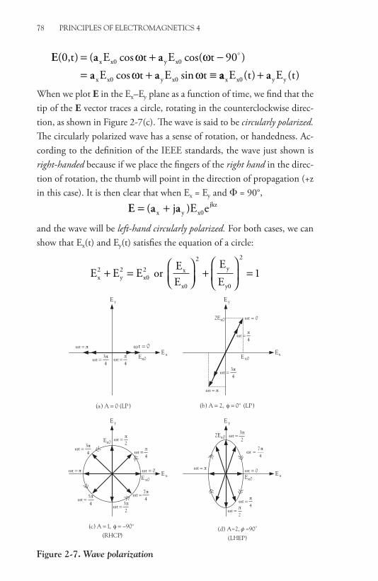
78 PRINCIPLES OF ELECTROMAGNETICS 4
# 156104 Cust: MP Au: Adams Pg. No. 78 Title: Principles of Electromagnetics 1—
K Short / Normal
DESIGN SERVICES OF
S4CARLISLEPublishing Services
E a a
a a
( ) ( cos cos( )cos sin
0,t E t E tE t E tx x0 y x0
x x0 y x0
= + −= + ≡
ω ωω ω
90
aa ax x0 y yE t E t( ) ( )+When we plot E in the Ex–Ey plane as a function of time, we find that the tip of the E vector traces a circle, rotating in the counterclockwise direc-tion, as shown in Figure 2-7(c). The wave is said to be circularly polarized. The circularly polarized wave has a sense of rotation, or handedness. Ac-cording to the definition of the IEEE standards, the wave just shown is right-handed because if we place the fingers of the right hand in the direc-tion of rotation, the thumb will point in the direction of propagation (+z in this case). It is then clear that when Ex = Ey and Φ = 90°,
E a a= +( x y x0jkzj )E e
and the wave will be left-hand circularly polarized. For both cases, we can show that Ex(t) and Ey(t) satisfies the equation of a circle:
E E E or EE
EEx
2y2
x02 x
x0
y
y0
+ =
+
=
2 2
1
yE
xE=t t = 0
4t =
43
t =
yE
xE
=t
0t =
4t =
43
t =
Ex0
2Ex0
x0E
yE
xE=t 0t =
4t =4
3t =
x0E
2t =Ex0
45
t =
23
t =4
7t =
yE
xE=t 0t =
7t
4=
Ex0
2t =
23
t =Ex02
4t =
)LP(0,2A)b( o==)LP(0A)a( =
)RHCP(90,1A)c( o== (d) A=2, =90º
(LHEP)
Figure 2-7. Wave polarization

PRINCIPLES OF MAGNETIC WAVES 79
# 156104 Cust: MP Au: Adams Pg. No. 79 Title: Principles of Electromagnetics 1—
K Short / Normal
DESIGN SERVICES OF
S4CARLISLEPublishing Services
Case 4: A E E out of phasex0 y0= = ≠2 90 90, [ , ]φ
E a a a a= + = + (x x0 y x0
j /2 jkzx y
kzE E e e 2j)eπ
(2-101)
At z = 0,
E a a( ) cos sin0,t E t E tx x0 y x0= −ω ω
In this case, we find that as time progresses the E vector traces an el-lipse and rotates in the clockwise direction. Hence the wave is said to be left-hand elliptically polarized. Ex(t) and Ey(t) satisfies the equation of an ellipse:
EE
EE
x
x0
y
y0
+
=
2 2
1
Note that the wave is elliptically polarized when Ex0 ≠ Ey0, Φ = ± 90° or Φ ≠ 0°, ±90°, 180° in which case the polarization ellipse will be tilted. All cases of wave polarization depending on A and Φ are summarized in Table 2-2. It is important to recognize that any wave having some general elliptical polarization can be decomposed into the superposition of two orthogonal, linearly polarized waves – for example, the x-polarized and y-polarized waves as shown in Eq. (2-105). Therefore, the analysis of a uniform plane wave having general polarization can be done by decom-posing it into two orthogonal, linearly polarized waves, analyzing each linearly polarized wave separately and combining the two solutions. This will greatly simplify the analysis of many complex wave problems. One immediate example will be shown in studying reflection and transmission of the wave in the next chapter. Table 2-2. Wave Polarization
E a a= + −( ,x x y yjkz y
x
jE E )e EE
Ae φ
Linear Polarization (i) Ex = 0, (ii) Ey = 0(iii) Φ = 0° or 180° (Ex and Ey are in phase)

80 PRINCIPLES OF ELECTROMAGNETICS 4
# 156104 Cust: MP Au: Adams Pg. No. 80 Title: Principles of Electromagnetics 1—
K Short / Normal
DESIGN SERVICES OF
S4CARLISLEPublishing Services
Circular Polarization
A 90 left-handed right-handed
E E 90 oux y
= = ±+−
= ±
1,
,
φ
tt of phase( )Elliptical Polarization (i) Φ ≠ 0°, ±90°, 180°
(ii)
φ
φφ
= ± ≠ ≠( )> →< →
90 A 1 E E
left-handed right-handed
x y ,
00
wwhen zk a//+
Sunlight is unpolarized or not polarized because although its electric field has two orthogonal components, each component is randomly vary-ing and Ex and Ey would not have any deterministic relationship. How-ever, when the sunlight is reflected from the road surface or snow on the ground, the reflected light known as the glare is partially polarized because one linearly polarized component is reflected more while the other com-ponent is mostly transmitted into the ground. A partially polarized wave can be viewed as a mixture of polarized waves and unpolarized waves. Skylight is another example of a partially polarized wave. Some species of ants and horseshoe crabs are known to be sensitive to polarized light and they use it for navigation.*
Linearly polarized waves are used in AM radio and TV broadcasting systems. AM broadcast stations operate at relatively low frequencies (f = 535−1605 kHz) and require large antenna towers in order to produce longer wavelengths (λ = 187−561m). These tall antennas generate verti-cally polarized waves, with the E field perpendicular to the ground and parallel to the antenna. For maximum reception of AM signals, receiv-ing antennas of the radio must be oriented parallel to the electric field, thus perpendicular (vertical) to the ground. On the other hand, most TV broadcasting signals are horizontally polarized, with the E fields parallel to the ground, so for good reception, rooftop TV antennas should be oriented horizontally and also perpendicular to the direction from which the signal comes. Most of the FM radio stations in the United States
*See T. H. Waterman, “Polarized light and animal navigation”, Scientific American, July 1955, pp. 88.

PRINCIPLES OF MAGNETIC WAVES 81
# 156104 Cust: MP Au: Adams Pg. No. 81 Title: Principles of Electromagnetics 1—
K Short / Normal
DESIGN SERVICES OF
S4CARLISLEPublishing Services
utilize circular polarization, which has the advantage that any orientation of an FM receiving antenna can detect a signal as long as the antenna is on the plane perpendicular to the direction of the signal propagation because a circularly polarized wave has two orthogonal, linearly polarized components.

# 156104 Cust: MP Au: Adams Pg. No. 83 Title: Principles of Electromagnetics 1—
K Short / Normal
DESIGN SERVICES OF
S4CARLISLEPublishing Services
INDEX
Ampère’s law, 3generalized, 21
Attenuation constant, 64Attenuation of waves, 62–66
Basic laws of electrostatics, 2Basic laws of magnetostatics, 3Boundary conditions, for time-
varying fields, 32–34Bradley, J., 19
Circularly polarized waves, 76, 78Complex permittivity, 71Complex Poynting theorem, 47–51Current circuital law,
modification of, 22–24
Dewar, Katherine Mary, 31Dielectric–dielectric interface, 34Dielectric–perfect conductor
interface, 33–34Dispersion of waves, 72–75
in lossy medium, 75Dispersion relation, 51Dispersive medium, 64, 72Displacement current, 19–24
in parallel-plate capacitor, 21–22Displacement current density, 20
Effective permittivity, 62–63Einstein, Albert, 2Electric field induced by time-varying
magnetic field, 5–6Electromagnetic waves, 26–29Electromotive force (emf), 9
flux-cutting or motional, 11transformer, 10–11
Elliptically polarized waves, 76
Faraday, Michael, 1experiments, 14–18
Faraday’s law, 1, 4–13, 18
general forms of, 4–6, 11motion effects through magnetic
fields, 6–8non-relativistic integral
forms of, 9–11voltage circuital law,
modification of, 5Feynman, R. P., 2Fizeau, H. L., 19Foucault, L., 19
Gauss’ law, 2Gibbs, Josiah Willard, 31Good dielectric vs. good conductor,
67–68Group velocity, 72–75
Heaviside, Oliver, 31Helmholtz equation, 51Helmholtz’s theorem, 4Hertz, Heinrich, 2, 20, 32Horizontally polarized waves, 80
Index of refraction. See Refractive index
Intrinsic impedance, 55
Kirchhoff current law (KCL), 3, 22Kirchhoff voltage law (KVL), 2, 5
Lenz, Heinrich F., 13Lenz’s law, 11, 13–14Linearly polarized waves, 76, 77Lorentz force law, 25Lossless media, uniform plane
waves in, 51–61Loss tangent, 67Lossy media, uniform plane
waves in, 61–72attenuation of waves, 62–66good dielectric vs. good
conductor, 67–68
9781606507186_index.indd 83 16/12/14 10:18 AM

# 156104 Cust: MP Au: Adams Pg. No. 84 Title: Principles of Electromagnetics 1—
K Short / Normal
DESIGN SERVICES OF
S4CARLISLEPublishing Services
84 INDEX
Magnetic fields, effects of motion through, 6–8
Maxwell, Francis Cay, 29Maxwell, James Clerk, 1–2, 29–32Maxwell, John Clerk, 29Maxwell’s equations, 18, 24–26
field solutions of, 28–29for time-harmonic electromagnetic
fields, 46–47Moving loop
induced current in, 13induced voltage in, 12–13
One-dimensional wave solutions, 41–43
Parallel-plate capacitordisplacement current in, 21–22power flow in, 37–38
Penetration depth, 66Phase constant, 64Phase velocity, 54Polarization of waves, 76–81Poynting’s theorem, 35–38Poynting vector, 37Propagation constant, 51Propagation vector, 60
Refractive index, 56Roemer, Ole, 19
Skin effect, 70Source-free region, wave
equation in, 40–43
Time-average power, 50–51Time-harmonic electromagnetic
fields, 43–51complex Poynting theorem, 47–51Maxwell’s equations for, 46–47phasor representation of, 44–46
Time-varying magnetic fieldsboundary conditions for, 32–34electric field induced by, 5–6
Uniform plane waves, 57in lossless media, 51–61lossy media, 61–72propagating in arbitrary
direction, 59–61Unpolarized waves, 76, 80
Voltage circuital law, modification of, 5
Wave equation, 26–29in source-free region, 40–43
Wavelength, 54Wavenumber, 54Wave vector, 60
9781606507186_index.indd 84 16/12/14 10:18 AM

EBOOKS FOR THE ENGINEERING LIBRARYCreate your own Customized Content Bundle—the more books you buy, the greater your discount!
THE CONTENT• Manufacturing
Engineering• Mechanical
& Chemical Engineering
• Materials Science & Engineering
• Civil & Environmental Engineering
• Advanced Energy Technologies
THE TERMS• Perpetual access for
a one time fee• No subscriptions or
access fees• Unlimited
concurrent usage• Downloadable PDFs• Free MARC records
For further information, a free trial, or to order, contact: [email protected]
Principles of Electromagnetics 4—Time-Varying Fields and Electromagnetic WavesArlon T. AdamsJay K. Lee
Arlon T. Adams (PhD, University of Michigan) is a Professor
Emeritus of Electrical and Computer Engineering at Syracuse
University, where he taught and conducted research in elec-
tromagnetics for many years, focusing on antennas and micro-
waves. He served as electronics officer in the U. S. Navy and
worked as an engineer for the Sperry Gyroscope Company.
Jay Kyoon Lee (Ph.D., Massachusetts Institute of Technology)
is a Professor of Electrical Engineering and Computer Science
at Syracuse University, where he teaches Electromagnetics,
among other courses. His current research interests are elec-
tromagnetic theory, microwave remote sensing, waves in aniso-
tropic media, antennas and propagation. He was a Research
Fellow at Naval Air Development Center, Rome Air Develop-
ment Center and Naval Research Laboratory and was an Invited
Visiting Professor at Seoul National University in Seoul, Korea.
He has received the Eta Kappa Nu Outstanding Undergraduate
Teacher Award (1999), the IEEE Third Millennium Medal (2000),
and the College Educator of the Year Award from the Technol-
ogy Alliance of Central New York (2002).
9781606507186_Cover.indd 2 19/12/14 3:51 PM