Second Harmonic Generation in Disordered Nonlinear Crystals
145
Second Harmonic Generation in Disordered Nonlinear Crystals: Application to Ultra- short Laser Pulse Characterization A thesis submitted for the degree of Doctor of Philosophy in Physical Science of Bingxia Wang Directors Dr. Jose Francisco Trull Dr. Crina Cojocaru and Dr. Hassan Akhouayri Barcelona, September, 2017
-
Upload
khangminh22 -
Category
Documents
-
view
1 -
download
0
Transcript of Second Harmonic Generation in Disordered Nonlinear Crystals

Second Harmonic Generation in Disordered
Nonlinear Crystals: Application to Ultra-
short Laser Pulse Characterization
A thesis submitted for the degree of Doctor of Philosophy in Physical Science of
Bingxia Wang
Directors
Dr. Jose Francisco Trull
Dr. Crina Cojocaru
and
Dr. Hassan Akhouayri
Barcelona, September, 2017


Aix-Marseille University
Polytechnic University of Catalonia
ECOLE DOCTORALE Physics Department / DONLL Group Institut Fresnel / Equipe ILM
Thèse présentée pour obtenir le grade universitaire de docteur Discipline : ED 352 – PHYSIQUE ET SCIENCES DE LA MATIERE Spécialité : Optique, Photonique et Traitement d’Image
Bingxia Wang
Génération du second harmonique dans des cristaux non-linéaires désordonnés: application pour la caractérisation d'impulsions laser
ultra-courtes
Second harmonic generation in disordered nonlinear crystals: application to ultra-short laser pulse characterization
Soutenue le 13/10/2017 devant le jury composé de :
Yannick Dumeige Dr. Rapporteur Fernando Silva Vázquez Dr. Rapporteur Georges Boudebs Prof. Examinateur Ramon Vilaseca Alavedra Prof. Examinateur Hassan Akhouayri Prof. Examinateur Co-directeur de thèse Crina Cojocaru Dr. Directeur de thèse
Numéro national de thèse/suffixe local : 2017AIXM0001/001ED62


To Youth


Acknowledgements
I do have a fabulous experience during my PhD study both in Barcelona and Marseille, which is undoubtedly attributed to all of my dearest advisors, friends, colleague, and also the bold, bloom and freedom environment.
It is really hard to send thanks properly to everyone who generously gave me
kindness and made this experience fabulous, but I will try to do it as much as I can.
In the first place, I would like to thank the advisors in Spain Crina and Jose to
give me this chance to start my PhD. I am very grateful for their help and teaching. It really means a lot. Without their help, this work would not been done.
Thanks to the advisor in France Hassan who kept giving me very positive
support and bring positive impact. Without his help, the stay in France would not have been so smooth.
特别感谢我的爸爸妈妈和弟弟。感谢一路支持帮助我的亲人,恩师,朋友。感
谢我学会克制。 I also want to thanks my friends and colleague in Barcelona and Marseille.
Their company relieved the pain of work and established a balance. Thanks to Andres, Carlos, Dario, Donatus, Daniel, Giulio, Hossam, Ignacio, Jin, Jordi, Judith, John, Lina, Lara, Maria M., Maria P., Pablo, Pepe, Sandro, Simone, SiYu, Shubham, Waqas and Yuchieh. Thanks to Cristina, Muriel, Carme, Ramon V., Kestutis, Ramon H. and Toni. Thanks to BoFei, Feng, Rui, ShiHe, Wei and Xin. Thanks to Alexandre, Konstantinos and Thibault.
Thanks to Iñigo for granting access into the facility at Centro de Láseres
Pulsados, CLPU, Salamanca, Spain. Thanks to Krzysztof for domain statistics measurements at Texas A&M University at Qatar. Thanks to Pablo Loza for domain pattern measurement with high-resolution SH imaging microscopy at ICFO - the Institute of Photonic Sciences. Thanks to Yan and Vito.
Thanks to the Erasmus Mundus Joint Doctorate Program Europhotonics 2013-
2016.
Finally, thanks to Wieslaw.


Contents
Abstract ................................................................................................................................................... i
Resum ..................................................................................................................................................... ii
Résumé .................................................................................................................................................. iii
Chapter 1: Introduction ........................................................................................................................ 1
1.1 Nonlinear optics in parametric processes .................................................................................. 1
1.1.1 Nonlinear Maxwell's equations and second order nonlinear interactions ...................... 2
1.2 Phase matching techniques ........................................................................................................ 7
1.2.1 Birefringent phase matching........................................................................................... 7
1.2.2 QPM in 1D periodic poled materials ............................................................................ 10
1.2.3 QPM in 2D quadratic nonlinear photonic crystals ....................................................... 11
1.3 Ultrashort pulse representation ................................................................................................ 16
1.3.1 Temporal intensity and phase ....................................................................................... 17
1.3.2 Spectrum and spectral phase ........................................................................................ 18
1.3.3 Pulse duration and spectral width ................................................................................. 19
1.3.4 Pulse propagation in dispersive media ......................................................................... 21
Chapter 2: Optical properties of SBN crystal ................................................................................... 24
2.1 Ferroelectric crystal: SBN crystal ........................................................................................... 24
2.1.1 Ferroelectric crystal ...................................................................................................... 24
2.1.2 SBN crystal................................................................................................................... 27
2.2 Linear refractive indices measurement .................................................................................... 29
2.2.1 Experimental setup ....................................................................................................... 29
2.2.2 Refractive indices measurement results ....................................................................... 31
2.3 Mathematical description of chromatic dispersion in SBN ..................................................... 33
2.3.1 The effect of GVD and TOD on pulse propagation ..................................................... 34
2.3.2 The combination effect of initial chirp and GVD on pulse propagation ...................... 37
2.4 Absorption spectrum of SBN .................................................................................................. 40
2.5 Phase mismatching curve of SBN ........................................................................................... 40
2.6 SHG in SBN ............................................................................................................................ 41
2.7 Conclusions ............................................................................................................................. 43
Chapter 3: Ultrashort pulse duration and chirp measurement via transverse auto-correlation
technique .............................................................................................................................................. 45
3.1 Introduction ............................................................................................................................. 45
3.2 Experimental setup and theoretical model .............................................................................. 49
3.2.1 Experimental setup ....................................................................................................... 49
3.2.2 TAC trace theoretical model ........................................................................................ 51
3.3 Results and discussions ........................................................................................................... 55
3.3.1 Measurement of 180 fs pulses ...................................................................................... 55
3.3.2 Measurement of a 30 fs pulse ....................................................................................... 56
3.3.3 Measurement of a 13 fs pulse ....................................................................................... 63
3.3.4 Measurement of a 13 ps pulse ...................................................................................... 65
3.4 Conclusions ............................................................................................................................. 69

Chapter 4: Ultrashort pulse duration and shape measurement via transverse cross-correlation
technique .............................................................................................................................................. 71
4.1 Introduction ............................................................................................................................. 71
4.2 Experimental setup and theoretical model .............................................................................. 74
4.2.1 Experimental setup ....................................................................................................... 74
4.2.2 TCC trace theoretical model ......................................................................................... 76
4.3 Experimental and simulation results ....................................................................................... 78
4.3.1 Parameters calibration .................................................................................................. 78
4.3.2 Pulse shape measurement ............................................................................................. 79
4.3.3 Effect of R0 and α on the pulse reconstruction ............................................................. 84
4.3.4 Explore the initial chirp parameter retrieve .................................................................. 87
4.4 Conclusions ............................................................................................................................. 88
Chapter 5: 2D solution for detecting domain statistics via analyzing second harmonic diffraction
............................................................................................................................................................... 90
5.1 Introduction ............................................................................................................................. 90
5.2 Initial study of domain statistics .............................................................................................. 91
5.2.1 Experimental setup and results ..................................................................................... 94
5.2.2 The limitation of the current model .............................................................................. 95
5.3 Study of domain statistics based on numerical simulation ...................................................... 98
5.3.1 Experimental setup and results ..................................................................................... 98
5.3.2 Numerical simulations ................................................................................................ 107
5.4 Effect of more complicated domain statistics on SH diffraction pattern ............................... 115
5.4.1 Design of the 2D domain structures ........................................................................... 115
5.4.2 Numerical simulations of SH diffraction pattern ....................................................... 116
5.5 Conclusions ........................................................................................................................... 120
Bibliography ........................................................................................................................................ 122
List of journal publications.................................................................................................................. 129
Other publications and participations .................................................................................................. 130

i
Abstract
The PhD project, entitled «Second harmonic generation in disordered nonlinear crystals: application to ultra-short laser pulse characterization», is devoted to the study of second harmonic generation in nonlinear ferroelectric crystals formed by a random distribution of domains with inverted quadratic nonlinear susceptibility (such as the Strontium Barium Niobate and Calcium Barium Niobate crystals) and its application to the single-shot characterization of ultrashort laser pulses. The basic principle of operation is related to the unique type of emission associated to those kinds of crystals where the second harmonic signal is emitted transversally to the beam propagation direction. Using the transverse second harmonic generation from these crystals we measure the pulse duration, the chirp parameter and the temporal profile in a single-shot configuration. This method has been implemented both in transverse auto-correlation and transverse cross-correlation schemes for the measurement of pulses with durations in the range from several tens up to several hundreds of femtoseconds. The main advantages gained with the developed techniques against other traditional methods include the removal of the requirement of thin nonlinear crystals for harmonic generation, the possibility to get automatic phase matching without angular alignment or temperature control over a very wide spectrum and a simplified operation process. Different types of pulses have been measured in different conditions and the limits of validity of the technique have been explored. Since this work relies strongly upon the characteristics of emission of the second harmonic signal by these random crystals, an important part of this work has been focused on the characterization of the distribution of domains of the random nonlinear ferroelectric crystals and its relation with the angular emission of the second harmonic signal. The domain distribution of the nonlinear polarization implies an associated distribution of reciprocal lattice vectors, which can compensate the phase mismatch in the nonlinear interaction. Any change in the domain distribution would have a direct impact in the second harmonic generated and in its intensity angular distribution. Based on these fundamental concepts we demonstrate an indirect non-destructive optical method for the characterization of nonlinear domain statistics based on the analysis of the second harmonic generation intensity angular distribution. This method has been implemented experimentally and tested in crystals with different types of distributions. To gain a deeper insight on these processes, numerical simulations have been performed using a split-step fast-Fourier transform beam propagation method. It has been demonstrated that the analysis of the dependence of the second harmonic generation angular emission with the fundamental beam wavelength can be used to obtain relevant information about complicated domain structures. This method could be used for real time monitoring of the unknown domain distribution during the poling or crystal growing process.
Keywords: Nonlinear optics, harmonic generation, nonlinear crystals,
ultrafast optics.
ii
Resum
Esta tesis doctoral es un estudio de la generación de segundo armónico en cristales no lineales compuestos por dominios ferroeléctricos que alternan el signo de la non linealidad de segundo orden y distribuidos de una forma aleatoria (como por ejemplo niobato de estroncio y bario o niobato de calcio y bario). Como primera aplicación proponemos una técnica de caracterización de pulsos laser ultracortos, cuyo principio de operación está relacionado con la manera singular en la que este tipo de cristal emite la señal de segundo armónico en una dirección transversal a la dirección de propagación del pulso a medir. Utilizando esta señal no lineal podemos determinar la duración del pulso, el parámetro de chirp y el perfil temporal en una configuración de single-shot. Hemos implementado este método en dos configuraciones distintas - auto correlación y correlación cruzada - para la medida de pulsos con duraciones entre 10 fs y 1 ps. Este método, en comparación con otros métodos tradicionales para la caracterización de pulsos ultracortos, permite obtener el ajuste de fase (phase matching) de forma automática sobre un rango espectral muy amplio, sin necesidad de aliñamiento crítico ni ajuste de temperatura, elimina el requisito de utilizar cristales delgados y tiene un proceso de operación más sencillo. Se han medido diferentes tipos de pulsos y se han explorado las limitaciones de la técnica. Como este trabajo se basa en las propiedades específicas de la emisión de segundo armónico en los cristales no lineales con distribución aleatoria de dominios, un objetivo importante ha sido la caracterización del tamaño y la distribución de los dominios ferroelectricos y su relación con la distribución angular específica del segundo armónico generado. La distribución espacial de los dominios implica una distribución correspondiente de vectores en la red recíproca que puede compensar el ajuste de fase en la interacción no lineal. Cualquier cambio en la distribución de dominios tendrá pues un impacto directo en la intensidad y distribución angular de la señal de segundo armónico generado. Basándolos en estos conceptos, demostramos un método óptico non destructivo indirecto para la caracterización estadística de los dominios no lineales basado en el análisis de la intensidad y la distribución angular del segundo armónico generado. Implementamos este método experimental en la caracterización de cristales con diferentes tipos de dominios. Para un estudio más detallado hemos desarrollado un modelo numérico basado en el método de “split-step fast-Fourier transform beam propagation” que simula el proceso no lineal observado experimentalmente. Demostramos que el análisis de la dependencia angular del segundo armónico puede aportar información relevante sobre estructuras con distribuciones complejas de dominios. Este método se puede utilizar para la monitorización en tiempo real de distribuciones desconocidas en el mismo proceso de crecimiento o del poling del cristal ferroelectrico.
Palabras clave: Óptica no lineal, generación de armónicos, cristales no
lineales, óptica ultrarrápida.

iii
Résumé
Ce projet de thèse de doctorat est intitulé « Génération du second harmonique dans des cristaux non-linéaires désordonnés: application pour la caractérisation d'impulsions laser ultra-courtes ». Il est consacré à l'étude de la génération de deuxième harmonique dans des cristaux ferroélectriques non linéaires formés par une distribution aléatoire de domaines. Ceci conduit à une distribution aléatoire de la susceptibilité non linéaire quadratique (Tels que le nitrate de baryum de strontium –SBN- et les cristaux de nitrate de calcium et de calcium) et son application à la caractérisation unique des impulsions laser ultra-courtes. Le principe de base de l'opération est lié au type unique d'émission associé à ces types de cristaux où le second signal harmonique est émis transversalement à la direction de propagation du faisceau. En utilisant la génération transversale de deuxième harmonique à partir de ces cristaux, nous mesurons la durée de l'impulsion, le paramètre chirp et le profil temporel dans une configuration à un seul pulse laser. Cette méthode a été mise en œuvre à la fois dans l'autocorrélation transversale et les schémas transversaux de corrélation croisée pour la mesure des impulsions avec des durées allant de plusieurs dizaines à plusieurs centaines de femtosecondes. Les principaux avantages obtenus avec les techniques développées par rapport à d'autres méthodes traditionnelles comprennent l'élimination de l'exigence de cristaux minces non linéaires pour la génération harmonique, la possibilité d'obtenir une correspondance automatique de phase sans alignement angulaire ou contrôle de la température sur un spectre très large et un processus d'opération simplifié. Différents types d'impulsions ont été mesurés dans différentes conditions et les limites de validité de la technique ont été explorées. Étant donné que ce travail repose fortement sur les caractéristiques de l'émission du second signal harmonique par ces cristaux ferroélectriques à distribution aléatoire des domaines, une partie importante de ce travail a été axée sur la caractérisation de la distribution des domaines des cristaux ferroélectriques non linéaires aléatoires et sa relation avec l'émission angulaire du signal de la deuxième harmonique. La distribution de la polarisation non linéaire implique une distribution associée de vecteurs de réseau réciproque, ce qui peut compenser le décalage de phase dans l'interaction non linéaire. Toute modification de la répartition des domaines aurait un impact direct dans la distribution angulaire de la deuxième harmonique et de sa distribution angulaire d'intensité. Sur la base de ces concepts fondamentaux, nous démontrons une méthode optique non destructive indirecte pour la caractérisation de statistiques des domaines non linéaire basées sur l'analyse de la distribution angulaire d'intensité de génération de la deuxième harmonique. Cette méthode a été mise en œuvre expérimentalement et testée dans des cristaux avec différents types de distributions. Pour obtenir une meilleure compréhension de ces processus, des simulations numériques ont été effectuées en utilisant une méthode de propagation de faisceau adaptée aux matériaux non linéaires. Il a été démontré que l'analyse de la dépendance de l'émission angulaire de la deuxième génération harmonique avec la longueur d'onde fondamentale du faisceau peut être utilisée pour obtenir des informations pertinentes sur les structures de

iv
domaines compliquées. Cette méthode pourrait être utilisée pour la surveillance en temps réel de la distribution de domaines inconnue pendant le processus de polling ou de croissance des cristaux.
Mots clés : Optique Non linéaire, génération du harmonique, cristal non
linéaire désordonné, Optique Ultra-rapide.
Chapter 1
Introduction
1.1 Nonlinear optics in parametric processes
Nonlinear optics (NLO) is the branch of optics that describes the behavior of light-matter
interactions induced by a strong laser in the regime where the dielectric polarization P responds
nonlinearly on the electric field of light. NLO remained unexplored until the discovery of second-
harmonic generation (SHG) by Peter Franken et al. [Fra61] in 1961, just one year after the laser
invention. In this experiment light at the doubled frequency was generated from the interaction of a
strong laser beam with the nonlinear medium (quartz crystal). This experiment marked the birth of the
field of NLO which complemented very fruitfully the technology development of lasers. Nonlinear
processes can be classified in two different categories, non-parametric process and parametric process.
In a nonlinear non-parametric process, the quantum state of the nonlinear material is changed because
of the transfer of energy, momentum or angular momentum between light and matter. In a nonlinear
parametric process, the quantum state of the nonlinear material is not changed by the interaction with
the light. As a consequence of this, the energy and momentum are conserved in the optical field,
making phase matching important and polarization-dependent. [Rüd08] [Rob08] Maxwell's equations
constitute the complete synthesis of the entire theory of classical electromagnetism and form the
foundation of classical optics.

2 Chapter 1: Introduction
In this introductory chapter, we will focus on the second-order nonlinear parametric process and
explore the corresponding solution of Maxwell’s equations and different phase-matching processes in
different nonlinear media.
1.1.1 Nonlinear Maxwell's equations and second order nonlinear interactions
We consider the form of the wave equation for the propagation of light through an optical
nonlinear medium. Maxwell’s equations in SI units can be written in the form of:
D (1.1)
0B (1.2)
B
Et
(1.3)
DH J
t (1.4)
Since, in general, we will not consider the presence of free charges and free currents we take 0 ,
0J . In non-magnetic media the magnetic field, B , and magnetic intensity, H , are related through
the relation: 0B H ; The electric field displacement vector 0D E P includes the nonlinearity of
the materials when the polarization density vector P depends nonlinearly upon the local value of the
electric field strength E . Combining Eq. (1.1)-Eq. (1.4) and the above supplementary equations we
obtain the expression:
2 2
2 2 2 2
0
1 1E E P
c t c t (1.5)
where c=(00)-1/2
is the speed of light in vacuum, 0 the electric permittivity and 0 the magnetic
permeability. This is the most general form of the wave equation both in linear and nonlinear optics.
The first term on the left-hand side of Eq. (1.5) can be written as:
2( )E E E (1.6)
In linear optics, E term vanishes when a plane wave propagates in an isotropic media. In
nonlinear parametric process, the E term is generally non-vanishing as a consequence of the more
general relation 0D , but in many cases the term ( )E can be small enough to be ignorable,
especially when the slowly varying amplitude approximation is valid. In this PhD work all the cases
discussed will be under the condition that the contribution of ( )E is negligible. Taking
( ) 0E and Eq. (1.6) into Eq. (1.5) the wave equation can be rewritten as:
2 22
2 2 2 2
0
1 1E E P
c t c t
(1.7)

Chapter 1: Introduction 3
The right term contains the polarization P and it describes the influence of the medium on the field as
well as the response of the medium. Splitting P into its linear and nonlinear parts as:
( , ) ( , ) ( , )L NLP r t P r t P r t (1.8)
The nonlinear materials under study can be considered as lossless and dispersionless in the
frequency range of interest. It can be considered as a monochromatic approximation. When a
monochromatic plane wave interacts with a second-order nonlinear medium, the linear part ( , )LP r t is
related to ( , )E r t through the linear susceptibility tensor 1
ij :
(1)
0
L
i ij j
j
P E
In isotropic media (1)
ij can be reduced to a constant(1) . With this constant
(1) the above equation
can be rewritten as:
(1)
0
LP E (1.9)
Substitution of Eq. (1.8) and Eq. (1.9) into the wave equation (1.7) gives:
2 22
0 02 2
NLEE P
t t
(1.10)
Eq. (1.10) is the nonlinear wave equation, where the nonlinear polarization acts as a source radiating
in a linear medium characterized by the dielectric function (1)
0 1 .
Here we consider the interaction of a light beam at the frequency ω1 with a medium possessing
quadratic nonlinearity. The field at 1 is written as:
1
1 1 01ˆ, . .
i tE r t e E e c c
(1.11)
E01 being its complex amplitude. For case of a lossless and dispersionless medium, the second-order
nonlinear polarization written in matrix form is as below:
(2)
0 1 1
,
. .NL
i ijk j k
j k
P E E c c (1.12)
It has two contributions: (a) Generate photons at ω2=2ω1, which is the so-called SHG process. (b)
Generate photons at the same frequency ω1. The term related to the SHG process can be written as:
22
2 0 0 1 0 1
,
. .i t
NL ijk j k
j k
P E E e c c
(1.13)
where 2
ijk is the second-order or quadratic susceptibility tensor.
It is convenient to introduce a change in notation defining the nonlinear coefficient, d,
proportional to the nonlinear susceptibility: 21
2ijk ijkd . Because the ijkd is symmetric in last two

4 Chapter 1: Introduction
indices, the contracted 3×6 matrix, ijd , is usually used. The second-order nonlinear polarization
leading to SHG in terms of ijd can be described by the matrix equation:
2
1
2
1
2 11 12 13 14 15 16 2
1
2 0 21 22 23 24 25 26
1 1
2 31 32 33 34 35 36
1 1
1 1
22
2
2
x
y
x
z
y
y z
z
x z
x y
E
EP d d d d d d
EP d d d d d d
E EP d d d d d d
E E
E E
(1.14)
where we have replaced the subscripts j and k by a single symbol according to the prescription:
xx=1, yy=2, zz=3, yz=zy=4, xz=zx=5, xy=yx=6.
Under Kleinman’s symmetry [Kle77], which states that when the interacting frequencies is far
from resonance conditions the susceptibility coefficients can be considered independent of frequency,
there are only 10 independent elements of ijd in Eq. (1.14). Moreover, any crystalline symmetries of
the nonlinear material can reduce this number further. For crystals belong to point group 4mm
symmetry, (SBN, for example) the ijd tensor is given by [Ric03] [Cha00]:
15
15
31 31 33
0 0 0 0 0
0 0 0 0 0
0 0 0
ij
d
d d
d d d
(1.15)
In practice, the highest component can be selected by using a specific polarized electric field.
Propagation of the SH beam in the medium can be described using Eq. (1.10) with P given by Eq.
(1.13):
2 2 22 2 (2)
02 2 02 0 0 01 01
,
i t i t i t
i i ijk j k
j k
E e k E e E E e
(1.16)
2 2
2 0 2 2k (1.17)
Eq. (1.16) can be simplified to a 1-D problem if:
(i) Diffraction effects can be neglected, i.e. in this case we take 0x y ;
(ii) Setting particular polarization states for the interaction the nonlinear process can be
described through an effective nonlinear coefficient, deff (the proper expression for deff in
different symmetries can be found in [ Boy03, Zer06];
(iii) Considering that the fields can be written as 01 1 1expE A z ik z and
02 2 2expE A z ik z .
With these assumptions Eq. (1.16) becomes:
2 1
2( 2 )2 2 2
2 0 0 2 122 e
i k k z
z eff
dk A d A
dz
(1.18)

Chapter 1: Introduction 5
When the changes in the amplitude of the field envelope over distances of the order of the wavelength
are small we can apply the slowly varying amplitude approximation (SVEA):
22
dAk
dz
2
2
2
d A
dz
Substituting this approximation into Eq. (1.18):
2022 1
2
i kz
eff
dAi d A e
dz
(1.19)
where 2 12k k k is the phase mismatch factor.
To obtain a similar equation for the fundamental field we must consider the interaction between
the fundamental and the SH field in the nonlinear medium. A similar procedure as that considered in
Eq. (1.13) leads to a nonlinear polarization oscillating at ω1, given by:
12 *
1 0 0 2 0 1
,
. .i t
NL ijk j k
j k
P E E e c c
(1.20)
Under the same assumptions applied to the SHG field, we can obtain the evolution equation for the
fundamental field as:
*011 2 1
1
2 kz
eff
dAi d A A e
dz
(1.21)
In most of the experimental conditions, the power lost by the input fundamental beam due to the
conversion to the SH frequency can be negligible, i.e., 1 0dA dz . This assumption takes the name of
undepleted pump approximation. In these conditions, the SHG process can be analyzed by taking into
account only Eq. (1.19). Its solution, in absence of an input SH beam, i.e. 2 0 0A , and for a
propagation length L inside the nonlinear crystal is:
202 2 1
2
1i kLeA L i dE
i k
which gives the expression of SHG intensity:
2
22 2 2 2 202 0 2 2 1 2
2
sin ( 2)2 2
( 2)eff
kLI L cn E L d E L
kL
The conversion efficiency can be calculated as:
2 2 2
12
3 2
1
sin ( 2)
( 2)
effd I LI L kLL
I n kL
(1.22)
where 2
1 2 0n .
If ∆k=0, the sinc(∆kL/2) function is equal to 1 and the conversion efficiency is directly
proportional to 2
effd , to L2 and to the total the intensity of the pumping beam. If ∆k0, Eq. (1.22)
predicts a dramatic decrease in the conversion efficiency as shown in Fig. 1.1 (Left). In this case, the

6 Chapter 1: Introduction
SH wave generated at a given point z1, having propagated to another point z2, is not in phase with the
SH wave generated at z2, which leads to the interference described by the sinc function. This sinc
function imposes an oscillating behavior on the SH intensity with the propagation distance which is
shown in Fig. 1.1 (Right). This figure reveals the effect of phase mismatch, ∆k, on SH intensity: the
larger the phase-mismatch the lower the SH intensity. When the propagation length equals the
coherence length LC the accumulated phase difference is and the nonlinear parametric process
reverses its direction transferring energy back from SH to fundamental wave. This is the origin of the
decrease of SH intensity for ∆k0. One half of the length separating two adjacent peaks of this
interference pattern is the coherence length, which expressed as:
2 1 2 12 4CL
k k k n n
(1.23)
where λ is the FF wavelength. The coherence length represents the maximum crystal length that is
useful in producing the SH power.
Fig. 1.1 SHG efficiency and intensity. (Left) Normalized conversion efficiency as a function of the phase
mismatch; (Right) SH intensity versus the propagation distance for different ∆k values.
According to the Eq. (1.22), the condition for an efficient SHG is ∆k=0, which means that k2=2k1.
This relation means that both the SH and FF beam have the same phase velocity and can be written
more generally for a 2D space as:
2 12k k (1.24)
It is the so called perfect phase matching (PM) condition. In the second-order nonlinear parametric
process the optical field obeys the energy conservation and momentum conservation and the
momentum conservation links to this PM condition. In this case, the SH is generated in the same
direction as the fundamental beam as shown in Fig. 1.2 (a). For phase mismatch process, Eq. (1.24) is
revised as:
2 12 0k k k (1.25)
Chapter 1: Introduction 7
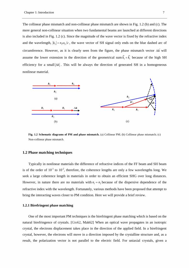
The collinear phase mismatch and non-collinear phase mismatch are shown in Fig. 1.2 (b) and (c). The
more general non-collinear situation when two fundamental beams are launched at different directions
is also included in Fig. 1.2 (c). Since the magnitude of the wave vector is fixed by the refractive index
and the wavelength, 2 2 2k n c , the wave vector of SH signal only ends on the blue dashed arc of
circumference. However, as it is clearly seen from the figure, the phase mismatch vector k will
assume the lower extension in the direction of the geometrical sum '
1 1k k because of the high SH
efficiency for a small k . This will be always the direction of generated SH in a homogeneous
nonlinear material.
Fig. 1.2 Schematic diagrams of PM and phase mismatch. (a) Collinear PM; (b) Collinear phase mismatch; (c)
Non-collinear phase mismatch.
1.2 Phase matching techniques
Typically in nonlinear materials the difference of refractive indices of the FF beam and SH beam
is of the order of 10-1
to 10-2
, therefore, the coherence lengths are only a few wavelengths long. We
seek a large coherence length in materials in order to obtain an efficient SHG over long distances.
However, in nature there are no materials with 1 2n n because of the dispersive dependence of the
refractive index with the wavelength. Fortunately, various methods have been proposed that attempt to
bring the interacting waves closer to PM condition. Here we will provide a brief review.
1.2.1 Birefringent phase matching
One of the most important PM techniques is the birefringent phase matching which is based on the
natural birefringence of crystals. [Gio62, Mak62] When an optical wave propagates in an isotropic
crystal, the electrons displacement takes place in the direction of the applied field. In a birefringent
crystal, however, the electrons will move in a direction imposed by the crystalline structure and, as a
result, the polarization vector is not parallel to the electric field. For uniaxial crystals, given a

8 Chapter 1: Introduction
propagation direction with respect to the crystallographic axis, , two normal modes of propagation
exist: the ordinary and extraordinary mode. Each of them propagates inside the crystal with a
particular value of index of refraction and polarization state. The ordinary index of refraction, no, is
isotropic, while the extraordinary index of refraction, ne, depends on the angle, , which can be written
as:
2 2
2
1 cos sin
( )e o en n n
Fig.1.3 (Left) shows the diagram of the varying refractive indices along the propagation direction
inside the birefringent crystal for both the ordinary and extraordinary polarizations and for both the
fundamental and SH wavelengths for the case of negative uniaxial crystals (ne<no). One can see that
for the particular propagation direction, θ, the ordinary polarized FF beam has the same refractive
index that the extraordinary polarized SH beam:
( ) (2 , )o en n (1.26)
Fig. 1.3 (Left) The refractive index ellipsoid projection of a negative uniaxial birefringent crystal. The red
and green ellipsoids and circles are corresponding to the varying refractive indices along the propagation direction
inside the crystal for both the fundamental and SH wavelengths. Propagation along the 𝜃 direction allows the PM
condition. (Right) Phase mismatch bandwidth. Bandwidth increases as the crystal gets thinner or the dispersion
decreases.
In some crystals, the refractive index depends on the temperature and ne change with temperature
is greater than the temperature dependence of no. Therefore, the temperature tuning can be used to
approach the PM condition. The major limitations of using birefringent crystals in nonlinear
parametric process are:

Chapter 1: Introduction 9
(i) PM condition is highly dependent on the wavelength (frequency), incidence angle, and
polarization state of the incident beam.
(ii) Usually, in the birefringent crystal only a narrow frequency band can reach PM condition at a
particular propagation direction. Since ultrashort pulses span over a broad frequency bandwidth,
achieving approximate phase matching for all frequencies can be a big issue.
In the nonlinear parametric process the range of wavelengths (frequencies) that can reach approximate
PM is the PM bandwidth. Generally, the PM bandwidth is very narrow, but as shown in Fig. 1.3
(Right) it increases as the crystal length decreases or as the wavelength increases due to the decreased
dispersion. Another phenomenon reducing the PM bandwidth is the group-velocity mismatch, arising
as a consequence of the different group velocities of the fundamental and SH inside the crystal. Fig.
1.4 shows the SHG of ultrashort pulse containing different frequency components ωi (i=1, 2, 3…) in
birefringent crystals. When the ultrashort pulse irradiates a thick nonlinear birefringent crystal along
the PM angle, because of the limited PM bandwidth the thick crystal generates SH wave for limited
frequencies, which is shown in Fig. 1.4 (Left). Fig. 1.4 (Right) shows the situation when the ultrashort
pulse irradiates a thin nonlinear birefringent crystal along the PM angle, the thin crystal generates SH
wave for all frequency components of the input pulse in the forward direction. To solve this ultrashort
pulse related issue and reach a large PM bandwidth, a thin nonlinear birefringent crystal is always
needed.
Fig. 1.4 SHG of ultrashort pulse in birefringent crystals. Left: A limited PM bandwidth of thick nonlinear
birefringent crystal allows limited frequencies to achieve approximate phase matching. Right: A large PM
bandwidth of thin nonlinear birefringent crystal allows all frequency components to achieve approximate phase
matching and the frequency components of SH wave are exactly the mapping of that of fundamental wave.
(iii) The PM in birefringent materials always occurs under the condition that FF and SH beams
have different polarization states. For extraordinary wave it is polarized in the principal plane and
propagates along the poynting vector resulting in a spatial walk-off problem.
Thick
SHG crystal
optical axis
ωi 2ω0
i=0,1,2,3…
Thin
SHG crystal
optical axis
ωi 2ωi
i=0,1,2,3… i=0,1,2,3…

10 Chapter 1: Introduction
1.2.2 QPM in 1D periodic poled materials
Another very important PM technique, proposed for the first time by Armstrong et al. in 1962
[Arm62] and experimentally proved in 1992 [Fej92], is the one dimensional (1D) quasi-phase-
matching (QPM) technique. As we have seen previously, the generated SH intensity will be low unless
the PM condition is satisfied. When the propagation length equals the coherence length LC, a phase
difference of π is accumulated by the interaction and then the nonlinear parametric process reverses its
direction transferring the energy back to the fundamental beam. By adding a phase shift of π
periodically every coherence length, the SH intensity will keep increasing monotonically with distance.
Fig. 1.5 (Top) illustrates with black and green arrows the complex amplitude contributions from
different parts of the nonlinear crystal to the SH wave. In the case without PM (Top Left), these
contributions cannot constructively add up over a significant distance in the crystal as shown by the
black line in the bottom figure. With QPM (Top Right), the sign of the contributions is reversed at
every coherence length. In that way, the total amplitude can keep increasing as shown by the green
line in the bottom figure. As a comparison, the gray line shows the SH intensity under the PM
condition.
Fig. 1.5 (Top): The complex amplitude contributions from different parts of the nonlinear crystal to the
harmonic wave. (Top Left): A low conversion efficiency without PM; (Top Right): With quasi-phase matching, a
high conversion efficiency can be achieved. (Bottom): The corresponding SH intensity under different
conditions. (Black Line): Without PM; (Green Line): With QPM; (Gray Line): with PM.

Chapter 1: Introduction 11
The realization process consists in periodically invert the sign of second-order NL susceptibility
χ(2)
of the material every coherence length. This can be done by periodic poling of ferroelectric
nonlinear crystal materials such as Lithium Niobate (LiNbO3), Lithium Tantalate (LiTaO3) or
Potassium Titanyl Phosphate (KTP, KTiOPO4). A strong electric field is applied to the crystal for
some time, using micro structured electrodes, so that the crystal orientation and thus the sign of the
nonlinear coefficient are permanently reversed only below the electrode fingers. The poling period
(the period of the electrode pattern) determines the wavelengths for which certain nonlinear processes
can be quasi-phase-matched. As shown in Fig. 1.6, the value of the period length, , is twice the
coherence length, LC. The periodically spatial distribution gives rise to a constant reciprocal lattice
vector 2G m . The phase mismatch can be compensated through this G and it applies directly in
the momentum conservation relation as:
2 12 0k k k G (1.27)
The benefits of the QPM technique are:
(1) It can be implemented for a very wide range of nonlinear interactions in crystals which do not
have birefringent properties.
(2) It can be implemented at a convenient temperature.
(3) Without spatial walk-off problem.
(4) The method of periodic poling can be applied to crystal materials with particularly high
nonlinearity, and makes possible to utilize the largest nonlinear coefficient that are not accessible
with birefringent PM.
Fig.1.6 QPM in 1D periodically poled nonlinear ferroelectric medium. QPM technique scheme for a typical
case of LiNbO3 crystal with G=∆k.
1.2.3 QPM in 2D quadratic nonlinear photonic crystals
When we extend the modulation of the χ(2)
to the two dimensional (2D) space, people usually talk
about quadratic nonlinear photonic crystals (NLPC), which can be divided into periodic/ quasi-
k(2w )
k(w ) k(w ) G
G
ω
ω
2ω
L = 2LC
+c (2)
-c (2)
0 1 2 3 4 5 6
# of c oherence length
SH
G i
nte
nsi
ty (
a.u
.)
A
B
C
800
600
400
0
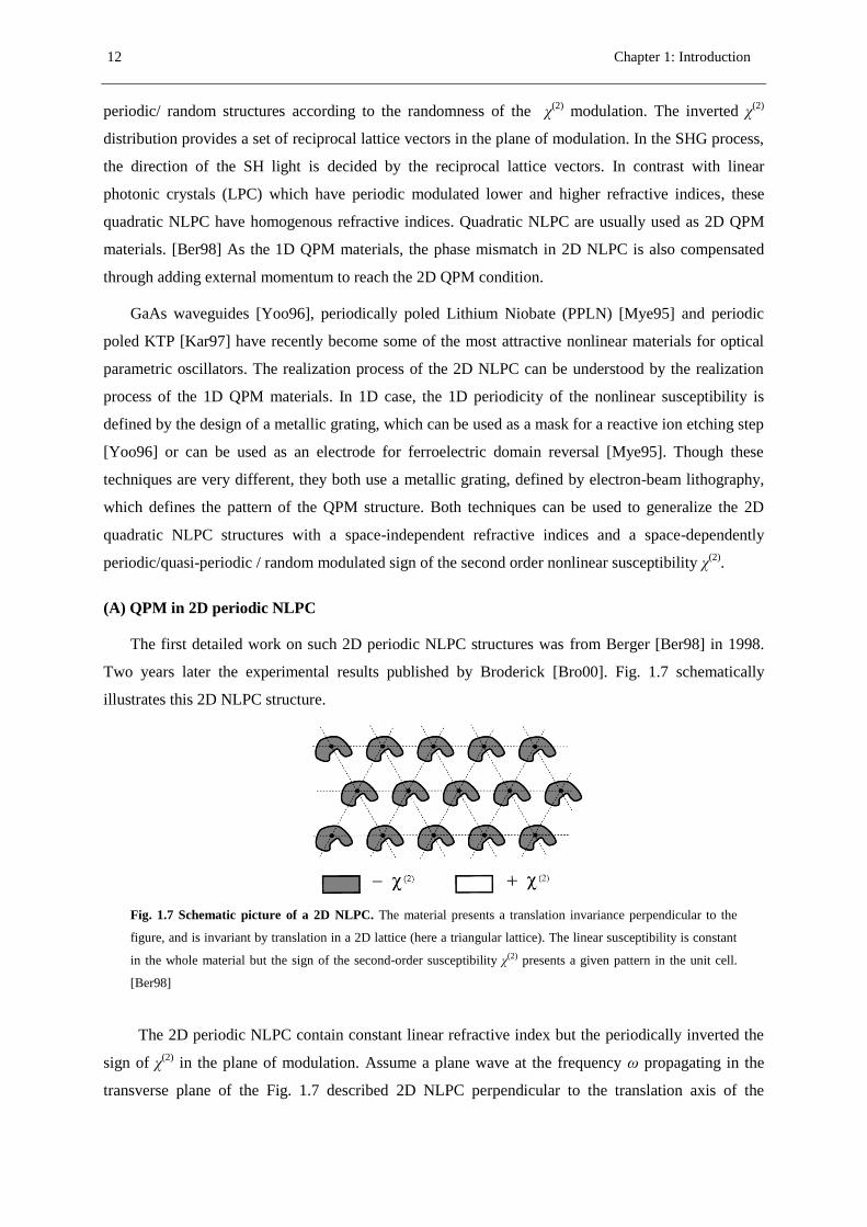
12 Chapter 1: Introduction
periodic/ random structures according to the randomness of the χ(2)
modulation. The inverted χ(2)
distribution provides a set of reciprocal lattice vectors in the plane of modulation. In the SHG process,
the direction of the SH light is decided by the reciprocal lattice vectors. In contrast with linear
photonic crystals (LPC) which have periodic modulated lower and higher refractive indices, these
quadratic NLPC have homogenous refractive indices. Quadratic NLPC are usually used as 2D QPM
materials. [Ber98] As the 1D QPM materials, the phase mismatch in 2D NLPC is also compensated
through adding external momentum to reach the 2D QPM condition.
GaAs waveguides [Yoo96], periodically poled Lithium Niobate (PPLN) [Mye95] and periodic
poled KTP [Kar97] have recently become some of the most attractive nonlinear materials for optical
parametric oscillators. The realization process of the 2D NLPC can be understood by the realization
process of the 1D QPM materials. In 1D case, the 1D periodicity of the nonlinear susceptibility is
defined by the design of a metallic grating, which can be used as a mask for a reactive ion etching step
[Yoo96] or can be used as an electrode for ferroelectric domain reversal [Mye95]. Though these
techniques are very different, they both use a metallic grating, defined by electron-beam lithography,
which defines the pattern of the QPM structure. Both techniques can be used to generalize the 2D
quadratic NLPC structures with a space-independent refractive indices and a space-dependently
periodic/quasi-periodic / random modulated sign of the second order nonlinear susceptibility χ(2)
.
(A) QPM in 2D periodic NLPC
The first detailed work on such 2D periodic NLPC structures was from Berger [Ber98] in 1998.
Two years later the experimental results published by Broderick [Bro00]. Fig. 1.7 schematically
illustrates this 2D NLPC structure.
Fig. 1.7 Schematic picture of a 2D NLPC. The material presents a translation invariance perpendicular to the
figure, and is invariant by translation in a 2D lattice (here a triangular lattice). The linear susceptibility is constant
in the whole material but the sign of the second-order susceptibility χ(2) presents a given pattern in the unit cell.
[Ber98]
The 2D periodic NLPC contain constant linear refractive index but the periodically inverted the
sign of χ(2)
in the plane of modulation. Assume a plane wave at the frequency ω propagating in the
transverse plane of the Fig. 1.7 described 2D NLPC perpendicular to the translation axis of the

Chapter 1: Introduction 13
cylinders. In the case of fundamental and harmonic waves are TM polarized with the electric field in
the translational direction. The parametric process can be written as :
22 2 2 (2) 2
2( ) 2 ( ) ( )exp ( 2 )k E r i E r i k k r
c
(1.28)
The periodically modulated χ(2)
can be rewritten as a Fourier series,
(2) expG
G RL
r iG r
(1.29)
where G are the available vectors from 2D reciprocal lattice (RL). G is its corresponding Fourier
coefficient. Substituting Eq. (1.29) into Eq. (1.28), the increase of the SH field appears to be related to
a sum of:
2exp 2i k k G r
The QPM condition appears then as the expression of the momentum conservation,
2 2 0k k G
The QPM in a 2D χ(2)
NLPC involves a momentum taken from the 2D RL to compensate the phase
mismatch ( 2 2k k ).
Two examples of 2D QPM processes are shown in Fig.1.8 (left). ( 1 2,e e ) compose the 2D basis of
the RL and the available G vector can be depicted as , 1 2m nG me ne . 2D QPM processes of 1,0G and
1,1G are represented in the figure. The related SH efficiencies depend on the Fourier coefficients of Eq.
(1.29), which depends on the shape of the χ(2)
pattern at the unit cell level. Using some trigonometry,
Fig.1.8 (Left) leads to:
2
2
2
2 2
21 4 sin
n n
G n n
(1.30)
where λ2ω is the SH wavelength inside the material and 2θ is the between kω and k2ω. If the medium has
no dispersion,2n n , Eq. (1.30) is reduced to the well-known Bragg law:
4sin 2 sind
G
where d is the period between two planes of scatters.
Fig. 1.8 (Right) shows the corresponding nonlinear Ewald construction. In the RL space, the
successful QPM can be achieved by the following steps:
(1) Draw 2k in the right direction but finishing at an origin;
(2) Draw a circle with radius at 2k with center CE,S. ;
(3)Where the circle passes through an origin, the ,m nG used to realize the QPM is marked in the
figure.

14 Chapter 1: Introduction
Fig. 1.8 Schematic picture of a 2D Reciprocal lattice. (Left) Reciprocal lattice of the structure of Fig.1.7, with
the 2D QPM processes of order [1, 0] and [1, 1] shown schematically. (Right) Nonlinear Ewald construction: the
center of the Ewald sphere is located 2k away from the origin of the RL and the radius of the sphere is
2k . If a
point of the RL is located on the Ewald sphere, PM occurs for the SHG process. [Ber98]
The advantages of 2D periodic NLPC can be summarized as:
(a) Can be used to compensate very large phase mismatches;
(b) Simultaneous phase matching of several parametric processes;
(c) Broad SHG bandwidth.
However, the limitation is that the available G value in the nonlinear parametric process is limited
by the 2D basis of the RL and the quantity of G is small.
(B) QPM in 2D quasi-periodic NLPC
In order to broaden the G distribution and increase the corresponding quantity, people resort to the
quasi-periodic NLPC. For example, in Ref. [She07] the authors Sheng et al. fabricated ferroelectric
domains in a short-range order. These quasi-periodic NLPC provide the possibility for broadband
QPM SHG in the visible range. The fabricated 2D ferroelectric domain pattern with electric field
poling method is shown in Fig. 1.9 (a) and the radius of the inverted domain is around 3.5 μm. The
plot in Fig. 1.9 (b) shows the values of the modulus of the reciprocal lattice vectors obtained by
Fourier transform of the spatial ferroelectric domain pattern. Fig. 1.9 (c) displays the calculated
Fourier spectrum of the ferroelectric domain pattern corresponding to the spectrum of reciprocal
vectors. The distribution of reciprocal vectors in a manner of concentric rings allows us to achieve an
efficient frequency conversion over a broad bandwidth. The structural short-range order plays an
important role in the observed high-efficiency broadband SHG and in other words the structural short-
range order provides a bigger flexibility to realize simultaneous PM in different nonlinear parametric
processes.

Chapter 1: Introduction 15
Fig. 1.9 2D quasi-periodic domain distribution and the corresponding discontinued reciprocal vectors. (a)
Micrograph of etched domain structure; (b) Modulus values of reciprocal vector obtained by Fourier transform of
the spatial ferroelectric domain pattern. Figure extracted from [She07].
(C) QPM in 2D random ferroelectric crystals
Random quasi phase matching (RQPM) is a very novel and interesting technique to achieve
broadband optical frequency conversion in disordered nonlinear ferroelectric crystals. The typical
disordered nonlinear ferroelectric crystals include the as-grown Strontium Barium Niobate (SBN),
Calcium Barium Niobate (CBN), etc. Moshe Horowitz first reported the broadband SHG from a
broadband input FF wave in disordered nonlinear ferroelectric crystal without any temperature or
angular tuning in 1993 [Hor93]. After that, the ferroelectric structure and other optical properties of
these disordered nonlinear ferroelectric crystals were reported [Tun03, Bau04, Ski04, Vid06].
Fig. 1.10 Random domain structure of disordered nonlinear ferroelectric crystal. (a). Optical micrograph
revealing the 2D distribution of the alternate ferroelectric domains in x-y plane after selective chemical etching
[Mol08]; (b) The domain structure along c axis with higher resolution [Rom01].
Fig. 1.10 (a) shows an optical microscope image of the ferroelectric domain in x-y plane of the as-
grown SBN crystal after conventional chemical etching. The image exhibits the disordered
ferroelectric domains with random diameter and random position. The ferroelectric domains align
parallel to the optical axis (c axis) as indicated in the figure. The domain cross-sections in x-y plane

16 Chapter 1: Introduction
are squares with rounded corners. [Mol08] The domain diameters in x-y plane are in the range 0.1–10
μm with a particular distribution with mean domain width at ~ 2–3 μm. [Mol08] The ferroelectric
domains have needle-like shape with the longest dimension parallel to the optical axis [Ram04]. Fig.
1.10 (b) shows the domain structure along optical c axis with higher resolution [Rom01].
For these as-grown crystals, the linear susceptibility is constant, while the second-order χ(2)
nonlinear susceptibility is spatially random modulated by the disordered ferroelectric domains as
shown in Fig.1.11 (a). The random inverted χ(2)
distribution provide a continuous set of reciprocal
lattice vectors in the plane of modulation as shown in Fig.1.11 (b). The simultaneous RQPM processes
as shown in Fig. 1.11 (c) yield the SHG in the xy plane.
Fig. 1.11 Continuous G distribution in disordered nonlinear ferroelectric crystal. (a) Random distributed χ(2)
domains; (b) Continuous distribution of reciprocal lattice vectors G in the x-y plane; (c) RQPM processes for the
SHG.
The limitation of this RQPM process is low SHG efficiency and the SHG intensity grows
linearly with distance. However, the advantages can be summarized as:
(a) A very large quantity of reciprocal lattice vectors G;
(b) Continuous G distribution;
(c) A very Broad SHG bandwidth.
1.3 Ultrashort pulse representation
In optics, an ultrashort pulse of light is an electromagnetic pulse whose time duration is usually of
the order of few tenth of femtoseconds (10−15
s), but in a larger sense this definition can be applied to
pulses with a duration of a picosecond (10−12
s) or less. Such short pulses have a broadband optical
spectrum, and can be created by mode-locked oscillators. The electric field of the pulses can be in
general a vector and it can be reduced to a scalar in the case of linear polarization, which is the case in
many situations and the case we are working in this thesis. In this research, polarization of ultrashort
laser pulse is always linear, either ordinary polarized or extraordinary polarized, and time independent,

Chapter 1: Introduction 17
which leads to the fact that a separate temporal characterization is sufficient to describe the ultrashort
pulse. The ultrashort pulse in the time domain is defined by a temporal amplitude and phase. The
relation between the pulse in the frequency and the temporal domain is the Fourier transform. In order
to have shorter pulses, it is necessary to have larger spectral bandwidths of emission.
This section is devoted to a general mathematical description of ultrashort laser pulses and their
temporal properties. Although the definitions provided in this section are well-suited to describe an
arbitrary temporal waveform, the analysis will focus on Gaussian temporal pulse profiles as they are
commonly encountered in a femtosecond laser laboratory.
1.3.1 Temporal intensity and phase
An optical wavepacket is generally defined by its electric field as a function of space and time
(x,y,z,t). A general treatment involving spatiotemporal coupling is relevant under specific situations
found for instance during propagation of ultrashort pulses [Ben12]. However, many problems
encountered in optics allow for a simplification of the problem in which the spatial and temporal
evolution of the fields can be decoupled, leading to the concepts of optical beam and optical pulse
respectively. If the polarization state of the fields is not changing we can also avoid a full vectorial
treatment and consider an scalar approximation [Tre00]. The spatial dependence is considered in
problems where the transverse spatial variation of the fields on propagation, i.e. diffraction effects
must be included. In the following no spatial dependence will be assumed (plane-wave approximation)
and the expresion for an optical pulse is given by:
cos ot I t t t (1.31)
where (t) is the temporal phase, O the pulse carrier frequency and I(t) is the temporal intensity.
2
I t t (1.32)
where the average is taken over times longer than the optical period. This representation, known as the
quasi-monochromatic pulse representation, is valid for pulses as short as few femtoseconds.
To simplify the mathematical treatment it is usually adopted a complex representation of the fields:
*1
exp exp2
o ot E t i t E t i t (1.33)
Expressed in terms of the analytical signal E(t)
exp exp oE t I t i t i t
Since we are only concerned about the temporal pulse shape and duration not the absolute magnitude
of the intensity, we omit the constants in the Eq. (1.32). The temporal phase can be expressed as
following:
18 Chapter 1: Introduction
Im( ( ))( ) arctan
Re( ( ))
E tt
E t (1.34)
The temporal phase, ϕ(t) contains frequency vs. time information, and the pulse instantaneous angular
frequency, ωinst(t), is defined as:
0
( )( )ins
d tt
dt (1.35)
The Taylor series for ϕ(t) about the time t=0:
2
0 1 2( ) 2t t t (1.36)
where only the first few terms are required to describe well-behaved pulses. The second order term ϕ2,
called the chirp coefficient (usual units expressed in fs-2
) gives an instantaneous frequency as shown in
Eq. (1.35), which varies linearly with time and results in up-chirped (if ϕ2>0) or down-chirped (ϕ2<0)
pulses. Higher order contributions lead to pulse distortions. The pulse can be alternatively expressed in
the spectral domain, through a Fourier transform of the temporal envelope, in terms of the frequency
Ω=ω-ωo.
1.3.2 Spectrum and spectral phase
The pulse field in the frequency domain is the Fourier transform of the time-domain field as
shown below:
( ) ( )exp( )t i t dt (1.37)
also, the inverse Fourier transform is:
1( ) ( )exp( )
2t i t d (1.38)
separating ε(ω) into its intensity and phase yields:
( ) ( ) exp( ( ))S i (1.39)
where S(ω) is the spectrum and φ(ω) is the spectral phase. We could have defined the spectrum and
spectral phase in terms of the Fourier transform of the complex pulse amplitude E(t):
0 0 0( ) ( ) exp( ( ))E S i (1.40)
where S(ω-ω0) would have been the spectrum, and φ(ω-ω0) would have been the spectral phase.
Most of the time, researchers don't do this simply in ultrafast optics. Generally, in the ultrafast
optics the time-domain field choose the complex field envelope, while the frequency-domain field is
the Fourier transform, not of the complex field envelope, but of the full real electric field. The reason
for this usage is that people like their spectra centered on the actual center wavelength not zero-but

Chapter 1: Introduction 19
they don't like their temporal waveforms rapidly oscillating, as would be required to be rigorously
consistent. The spectrum is given by:
2( ) ( )S (1.41)
The spectral phase is given by expressions analogous to those for the temporal phase:
Im( ( ))( ) arctan
Re( ( )) (1.42)
Like the temporal phase contains frequency and time information, the spectral phase contains time and
frequency information. So we define the group delay vs. frequency, tgroup (ω), given by:
( )groupt d d (1.43)
Correspondingly, the Taylor series for the φ(ω) about the time ω0 is follow:
2
0 0 1 0 2( ) ( ) ( ) 2 (1.44)
In the Eq. (1.36) and Eq. (1.44), the zeroth-order phase term is often called the absolute phase,
which is the phase of the carrier at the peak of the pulse envelope or some other reference time.
Usually, we don't care much about the lowest-order term, because when the pulse is many carrier-
wave cycles long, variation in the absolute phase shifts the carrier wave from the peak of the envelope
to a value only slightly different and hence changes the pulse field very little; The first-order phase is a
shift in time or frequency, which isn’t considered in this work with the reasons as follows: from the
Fourier Transform Shift Theorem, the first-order (linear term) in the spectral phase shown by the
second term in Eq. (1.44) corresponds to a delay representing when the pulse arrives, which is not
interesting for us. Also from the Fourier Transform Shift Theorem, the first-order (linear term) in the
temporal phase shown by the second term in Eq. (1.36) corresponds to a frequency shift, which is
often interesting but can be easily measured with a spectrometer. Since in this work we concentrate on
the time domain, we overlook this first-order phase; the second-order phase is often called the linear
chirp term. Quadratic variation of ϕ(t), that is, a nonzero value of ϕ2, represents a linear ramp of
frequency vs. time and so we say that the pulse is linearly chirped.
1.3.3 Pulse duration and spectral width
One of the most important goals of this thesis is to measure the temporal pulse duration (also
known as pulse length, or pulse width), unfortunately, no single definition of the pulse duration and
the spectral width is used. There are several definitions existing, such as full-width-half-maximum
(FWHM), half-width-l/e (HW1/e), root-mean-squared (RMS) width and equivalent pulse width.
[Tre00].
Unless specified otherwise, in this thesis we define the pulse duration T as the full-width-half-
maximum duration in intensity, which is the time between the most- separated points that have half of

20 Chapter 1: Introduction
the pulse's peak intensity (see Fig. 1.12). This is the most intuitive definition, and it's the rule in
experimental measurements, since it's easy to pull T off a plot. Fig. 1.12 (a) shows a Gaussian pulse
and its 200 fs FWHM duration and Fig. 1.12 (b) shows a pulse with double-peak structure and its 480
fs FWHM duration.
Fig. 1.12 FWHM duration. (a) A Gaussian pulse and its 200 fs FWHM duration; (b) A pulse with double-peak
structure and its 480 fs FWHM duration.
Analogously, the spectral full-width-half-maximum width (indicated by ∆ω) is the frequency
between the most-separated points that have half of the pulse's peak spectral intensity. Unless
specified otherwise, in this thesis we define the spectral width or spectral bandwidth ∆ω as the full-
width-half-maximum width.
Because the temporal and spectral characteristics of the electric field are related to each other
through Fourier transforms, the spectral width ∆ω and pulse duration T cannot vary independently of
each other. The product of temporal duration T and spectral width ∆ν of a pulse is called time-
bandwidth product (TBP) and there is a minimum TBP value written as: [Die06]:
2 2 BT T c (1.45)
The smaller the TBP, the "cleaner" or simpler the pulse, and the minimum TBP corresponding to the
simplest, and it increases with increasing pulse complexity. The equality holds for the case, where the
pulse spectral components are perfectly phase-locked (constant phase) and the pulse is called
bandwidth-limited or FTL, exhibiting the shortest possible duration at a given spectral width and pulse
shape. The dimensionless parameter cB depends on the actual pulse temporal shape and can be derived
analytically in each case.
For the phase-locked Gaussian pulse the corresponding electric field is expressed as bellow:
2
( ) exp(4 ln 2)
tt
T (1.46)
where T is the pulse duration. Submitting Eq. (1.46) to Eq. (1.37) and Eq. (1.39) we calculate the
spectral profile:
Inte
nsi
ty (
a.u
.) 1
0.5
0
Time (fs) Time (fs)-400 -200 0 200 400 -400 -200 0 200 400 600 800
Inte
nsi
ty (
a.u.)
1
0.5
0
(a) T=200 fs (b) T=480 fs

Chapter 1: Introduction 21
2
( ) exp(2 ln 2)
ST
(1.47)
where the spectral width 2
2 ln 2 T , which gives the minimal TBP value:
(2 ) 0.441 BT T c (1.48)
In a more general case, if the spectral components forming the Gaussian pulse carries a time-
dependent phase relation, due to chromatic dispersion for example, a longer temporal duration than the
bandwidth-limit (Eq. 1.48) can be generated. In general, a non-vanishing phase yields a larger time-
bandwidth product and a pulse with duration longer than a Fourier Transform Limited (FTL) pulse but
with the same spectrum.
1.3.4 Pulse propagation in dispersive media
The chromatic dispersion of an optical medium is the phenomenon that the phase velocity,
p k , and group velocity, 1
g k
, of light propagating in a transparent medium depend on
the optical frequency. The attribute “chromatic” is used to distinguish this type of dispersion from
other types, which are relevant particularly for optical fibers: intermodal dispersion and polarization
mode dispersion.
When propagating in transparent optical media, the properties of ultrashort pulses can undergo
complicated changes. Typical physical effects influencing pulses are: (a) Chromatic dispersion can
lead to pulse broadening, but also to pulse compression, chirping, phase changing, etc. (b) Various
nonlinearities can become relevant at high peak powers. For example, the Kerr effect can cause self-
phase modulation, and Raman scattering may e.g. induce Raman gain within the pulse spectrum
(Raman self-frequency shift). (c) Optical gain and losses can modify the pulse energy and the spectral
shape. (d) The spatial properties can change due to linear effects such as diffraction and waveguiding,
but also due to nonlinear effects such as self-focusing. In highly nonlinear interactions, filamentation
may occur. Of course, different effects can act simultaneously, and often interact in surprising ways.
For example, chromatic dispersion and Kerr nonlinearity can lead to soliton effects. [5 rp-
photonics.com] If we consider an ultrashort pulse with relatively low power propagation in a
dispersive media, the effects (b, c, d) can be ignored and the chromatic dispersion is the only effect
that dominates the propagation process.
The inherent dispersive character of any material media affects considerably the properties of
ultrashort optical pulses due to their intrinsic finite bandwidth. The direct consequence is that any
pulse propagating in a dispersive medium has a natural tendency to increase its pulse duration and
acquire a pulse chirp. Since this will be a predominant effect in the propagation through our crystals
let’s resume briefly some well-known aspects related to this phenomenon. We consider that the pulse

22 Chapter 1: Introduction
has a finite bandwidth centered at frequency 0, where the relation <<0 holds (this is valid for
pulses with durations as short as few tens of femtoseconds) and define the shifted frequency =-0.
Chromatic dispersion of second and higher order can be defined via the Taylor expansion of the
wavenumber k (change in spectral phase per unit length) as a function of the angular frequency ω
(around the central frequency 𝜔0, e.g. the mean frequency of the laser pulses):
0
2 32 3
2 3
1 1
2 6O O
O O
k k kk k k
2 33
1 1
2 6Ok g
u (1.49)
where 0
1u k
is the group velocity, 1/u contains the inverse group velocity (i.e., the group
delay per unit length) and describes an overall time delay without an effect on the pulse shape;
0
2 2g k
is the group velocity dispersion (GVD) coefficient and contains the second-order
dispersion or group delay dispersion (GDD) per unit length; 0
3 3
3 k
is the third order
dispersion (TOD) coefficient and contains the TOD per unit length. GVD and TOD coefficients, g and
β3, depend on the frequency or wavelength in transparent media. Different frequency components
travel at different group velocity in dispersive media, which leads to pulse chirping and consequently
results in lengthening or compression of the pulse.
The general propagation equation is in general quite involved [Die06], but we can obtain a
simplified propagation equation by truncating the dispersion effects up to second order and chose a
reference frame propagating with the pulse, the so called retarded frame of reference. In this case the
resulting equation constitutes the parabolic equation for pulse propagation:
2
2
( , ) ( , )0
2
A t z ig A t z
z t (1.50)
with
0 0( )( , ) ( , )
i k z tE t z A t z e (1.51)
where A(z,t) is the complex amplitude of the pulse. The solution to this equation can be obtained quite
straight forwardly in the frequency space in terms of the spectral complex amplitude A (z, ω):
21
20( , ) ( , ) ( ,0)e
i g z
A z A z A (1.52)
When both the GVD and TOD are considered, the above solution can be rewritten as:
2 33
1 1
2 60( , ) ( , ) ( ,0)e
i g z i z
A z A z A (1.53)
This result indicates two important consequences: (i) During pulse propagation the spectrum,
corresponding to the square modulus of E(z, ω), is not changed, i.e S(0, ω)=S(z, ω). (ii) The pulse

Chapter 1: Introduction 23
acquires a quadratic phase during propagation when GVD coefficient, g, dominates the dispersion
process, while a cubic phase during propagation when TOD coefficient, β3, dominates the dispersion
process. Direct Fourier Transform gives us the expression for the electric field of the pulse:
1( , ) ( , )
2
i tE t z E z e d (1.54)
More information about the effect of GVD and TOD on pulse propagation will further discussed in
Chapter 2.

Chapter 2
Optical properties of SBN crystal
2.1 Ferroelectric crystal: SBN crystal
2.1.1 Ferroelectric crystal
In this work, we are interested in materials showing a natural occurrence of nonlinear domain
inversion as well as in those with the artificially poled nonlinear domain inversion. All these nonlinear
domain structures exist in the ferroelectric crystals. Ferroelectric crystals are defined as crystals which
show a spontaneous electric polarization that can be reversed by the application of an external electric
field. [Wer57, Lin79] The ferroelectricity was first observed in 1920 in Rochelle salt by Valasek.
[Val21] In this section, we will briefly introduce a linear description of these crystals. The further
information can be found from DoITPoMS website (Dissemination of IT for the Promotion of
Materials Science), of the University of Cambridge, from which this paragraph draws on information
from.
Ferroelectric crystals are important basic materials for technological applications in capacitors and
in piezoelectric, pyroelectric, and optical devices. In many cases their nonlinear characteristics turn
out to be very useful, for example in optical second-harmonic generators and other nonlinear optical
devices. Possessing a spontaneous dipole moment that can be switched in an applied electric field is a
prerequisite for ferroelectric. The dipole moment μ of two particles of charge q separated by some
distance r is μ = qr. In a ferroelectric material, there is a net permanent dipole moment, which comes
from the vector sum of dipole moments in each unit cell, Σμ. This means ferroelectrics must be non-
Chapter 2: Optical properties of SBN crystals 25
centrosymmetric. There must also be a spontaneous local dipole moment which can lead to a
macroscopic polarization, but not necessarily if there are domains that cancel completely. This means
that the central atom must be in a non-equilibrium position. An inherent dipole moment in the
structure results in a polarization, which may be defined as the total dipole moment per unit volume,
i.e. P= Σμ/V. When the materials are polarized along a unique crystallographic direction, certain
atoms are displaced only along this axis, leading to a dipole moment along it. But, depending on the
crystal system, there may be few or many possible displacing axes.
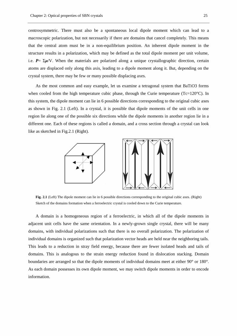
As the most common and easy example, let us examine a tetragonal system that BaTiO3 forms
when cooled from the high temperature cubic phase, through the Curie temperature (Tc=120°C). In
this system, the dipole moment can lie in 6 possible directions corresponding to the original cubic axes
as shown in Fig. 2.1 (Left). In a crystal, it is possible that dipole moments of the unit cells in one
region lie along one of the possible six directions while the dipole moments in another region lie in a
different one. Each of these regions is called a domain, and a cross section through a crystal can look
like as sketched in Fig.2.1 (Right).
Fig. 2.1 (Left) The dipole moment can lie in 6 possible directions corresponding to the original cubic axes. (Right)
Sketch of the domains formation when a ferroelectric crystal is cooled down to the Curie temperature.
A domain is a homogeneous region of a ferroelectric, in which all of the dipole moments in
adjacent unit cells have the same orientation. In a newly-grown single crystal, there will be many
domains, with individual polarizations such that there is no overall polarization. The polarization of
individual domains is organized such that polarization vector heads are held near the neighboring tails.
This leads to a reduction in stray field energy, because there are fewer isolated heads and tails of
domains. This is analogous to the strain energy reduction found in dislocation stacking. Domain
boundaries are arranged so that the dipole moments of individual domains meet at either 90° or 180°.
As each domain possesses its own dipole moment, we may switch dipole moments in order to encode
information.

26 Chapter 2: Optical properties of SBN crystals
Fig. 2.2 Free energy diagram. This scheme represents the potential barrier between the two stable positions (left
and right versus on the horizontal direction) of the dipole moments.
In an electric field, E, a polarized material lowers its (volume-normalized) free energy by -PE,
where P is the polarization. Any dipole moments which lie parallel to the electric field are lowered
in free energy, while moments that lie perpendicular to the field are higher in free energy and
moments that lie anti-parallel are even higher in free energy (+PE). This introduces a driving
force to minimize the free energy, such that all dipole moments align with the electric field. We
start by considering how dipole moments may align in zero applied field; since the horizontal
direction is crystallographically unique, the dipole moment is stable either aligned to the left of to
the right. These two moments are stable, because they sit in potential energy walls. The potential
barrier between them can be represented on a free energy diagram (Fig.2.2). This material is
considered to be homogenous. If the polarization points left then we have the situation in Fig.
2.2(a). The electric field consequently alters the energy profile, resulting in a “tilting” of the
potential well, Fig. 2.2(b). An increase in the electric field will result in a greater tilt, and lead to
the dipole moments switching, Fig. 2.2(c).
Fig. 2.3 Snapshot of the inhomogenous nucleation process that happen when a reversed external electric field Eext
is applied on a fully polarized crystal. The arrows represent the local direction of the polarization.
We can now look at the more realistic scenario in which domains form. Consider a material
which is fully polarized, so that all of the dipole moments are aligned in the same direction. Then
if we apply a reversed electric field over it, new domains with a reversed polarization start to
nucleate. This requires a certain amount of time, in the same manner as any nucleation process.
When the fluctuating nuclei reach a certain critical radius, they grow outwards, forming needle-

Chapter 2: Optical properties of SBN crystals 27
like structures. When they reach the other side of the ferroelectric, they begin to grow outwards (Fig.
2.3).
This dynamics explain the origin of the hysteresis loop. The removal of the field will leave some
polarization behind. Only when the field is reversed, also the polarization starts to lessen and new,
oppositely poled, domains form. They grow quickly however, giving a large change of polarization for
very little electric field. But to form an entirely reversed material, a large switching field is required.
This is mainly due to defects in the crystal structure but it also due to stray field energy. The
polarization of the material goes from a coupled pattern, with 180° boundaries, to a state in which
many heads and tails are separated. This leads to the increase in stray field energy. Therefore, to attain
this state, lots of energy has to be put in by a larger field. In Fig. 2.4 it is shown how a minor
hysteresis loop fits into the major loop above. There are three sections to this curve: 1) reversible
domain wall motion; 2) linear growth of new domains; 3) new domains reaching the limit of their
growth.
Fig. 2.4 Hysteresis loop due to the nucleation process. It is possible to distinguish three sections: 1)reversible
domain wall motion; 2) linear growth of new domains; 3) new domains reaching the limit of their growth.
2.1.2 SBN crystal
Strontium Barium Niobate crystals (SrxBa1-xNb2O6, noted SBN:100x or SBN) [Neu88] have
attracted much attention due to their potential applications in quasi-phase-matching second-harmonic
generation [Kew94], electro-optic modulation [Neu90], data storage [Kah94], pyroelectric detection
[Gla69], phase conjugation [Zha94], generation of photorefractive solitons [Wes01], and surface
acoustic wave devices [Neu80]. In this section, we will briefly introduce some basic information of
SBN crystals. Further information can be found in reference [Mic11].
The existence of SBN crystals was first reported in 1960 [Fra60]. In the mid 1960's, the first
SBN single crystals were grown over a range of compositions 0.25<x<0.75 [Bal67]. Czochralski
[Fur76], Stepanov [Ivl87], and vertical Bridgman [Lee98] techniques have been used to grow SBN
single crystals. However, because of their properties of low thermal conductivity and relatively large
latent heat, it is not easy to grow large size SBN crystals. To overcome this problem, a method for
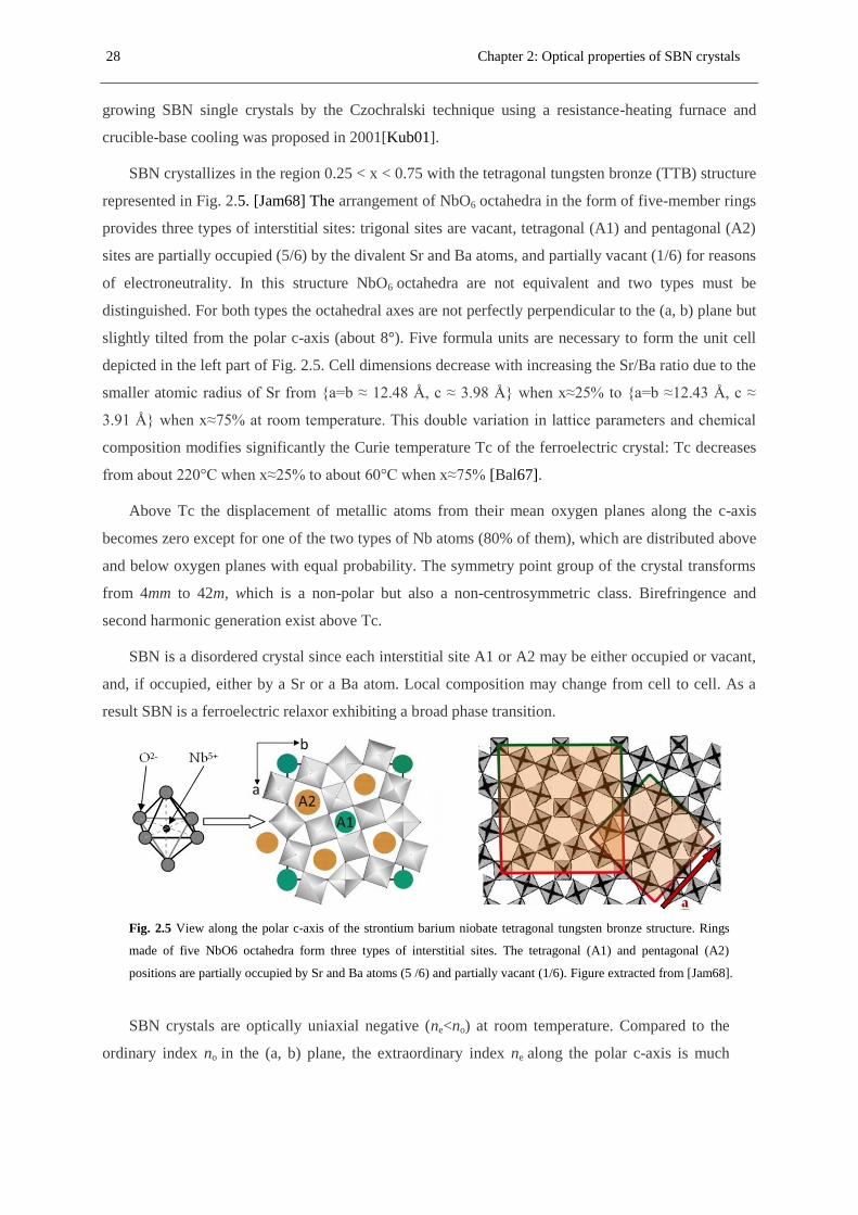
28 Chapter 2: Optical properties of SBN crystals
growing SBN single crystals by the Czochralski technique using a resistance-heating furnace and
crucible-base cooling was proposed in 2001[Kub01].
SBN crystallizes in the region 0.25 < x < 0.75 with the tetragonal tungsten bronze (TTB) structure
represented in Fig. 2.5. [Jam68] The arrangement of NbO6 octahedra in the form of five-member rings
provides three types of interstitial sites: trigonal sites are vacant, tetragonal (A1) and pentagonal (A2)
sites are partially occupied (5/6) by the divalent Sr and Ba atoms, and partially vacant (1/6) for reasons
of electroneutrality. In this structure NbO6 octahedra are not equivalent and two types must be
distinguished. For both types the octahedral axes are not perfectly perpendicular to the (a, b) plane but
slightly tilted from the polar c-axis (about 8°). Five formula units are necessary to form the unit cell
depicted in the left part of Fig. 2.5. Cell dimensions decrease with increasing the Sr/Ba ratio due to the
smaller atomic radius of Sr from {a=b ≈ 12.48 Å, c ≈ 3.98 Å} when x≈25% to {a=b ≈12.43 Å, c ≈
3.91 Å} when x≈75% at room temperature. This double variation in lattice parameters and chemical
composition modifies significantly the Curie temperature Tc of the ferroelectric crystal: Tc decreases
from about 220°C when x≈25% to about 60°C when x≈75% [Bal67].
Above Tc the displacement of metallic atoms from their mean oxygen planes along the c-axis
becomes zero except for one of the two types of Nb atoms (80% of them), which are distributed above
and below oxygen planes with equal probability. The symmetry point group of the crystal transforms
from 4mm to 42m, which is a non-polar but also a non-centrosymmetric class. Birefringence and
second harmonic generation exist above Tc.
SBN is a disordered crystal since each interstitial site A1 or A2 may be either occupied or vacant,
and, if occupied, either by a Sr or a Ba atom. Local composition may change from cell to cell. As a
result SBN is a ferroelectric relaxor exhibiting a broad phase transition.
Fig. 2.5 View along the polar c-axis of the strontium barium niobate tetragonal tungsten bronze structure. Rings
made of five NbO6 octahedra form three types of interstitial sites. The tetragonal (A1) and pentagonal (A2)
positions are partially occupied by Sr and Ba atoms (5 /6) and partially vacant (1/6). Figure extracted from [Jam68].
SBN crystals are optically uniaxial negative (ne<no) at room temperature. Compared to the
ordinary index no in the (a, b) plane, the extraordinary index ne along the polar c-axis is much

Chapter 2: Optical properties of SBN crystals 29
more sensitive to both Sr content and temperature [Ven68]. At λ=633 nm and room temperature, (no,
ne) vary from (2.314, 2.259) to (2.312, 2.299) when x varies from 25 to 75%, respectively.
Ferroelectric, dielectric and nonlinear optic properties of SBN crystals are very sensitive to the
Sr/Ba ratio consistently with the impact of this ratio on Curie temperature [Gla69, Len67]. Increasing
the Sr content reduces the interval between room and Curie temperatures, thus inducing a drastic
enhancement of the dielectric permittivity, pyroelectric coefficient and nonlinear optic properties.
Exceptionally large values of the linear electro-optic coefficient have been obtained (r33=1340 pm/V at
λ=633 nm) with a 75% Sr content [Len67].
Generally the tungsten bronze typed relaxation ferroelectric SBN crystals are grown by
Czochralski method. The Curie temperature of SBN crystals is in the range of 25~200℃ with the
variation of Sr content, that are lower than the familiar CaxBa1-xNb2O6(CBN)crystals, whose Curie
temperature is in the range of 124~347℃ with decreasing Ca content from 0.366 to 0.224. SBN
crystallizes in a wide solid solution rang in the tetragonal symmetry (space group P4bm). In
ferroelectric phase, SBN has the 4mm point group symmetry, which transforms to centrosymmetric
4/mmm point group above Curie temperature. With the same techniques of the 2D QPM, people
produces the artificially poled SBN crystals, which are χ(2)
modulated nonlinear photonic crystals.
Both the as-grown and artificially poled SBN crystals are our study interest in this PhD work.
2.2 Linear refractive indices measurement
A preliminary step to use these crystals in the different application is to characterize properly their
optical properties. We have performed some measurements and calculations for the characterization of
SBN which we will briefly review in this chapter. In this section we focus on the linear refractive
indices measurement. One of the first measurements of the refractive index of SrxBa1-xNb2O6 was
performed by Venturini et al in 1968 [Ven68] and the crystals with components at x=0.25, 0.50 and
0.75 were measured. Later, SBN crystals with other components were measured [Kip96, Woi01]
[Tun04]. In this work refractive index measurements for as-grown SBN with composition x=0.61
covering a wide wavelength region can be as a supplement and validation for the previous publications.
2.2.1 Experimental setup
The optical setup used to measure linear refractive indices is schematically shown in Fig. 2.6
(Top). The sample was placed on the sample stage which can be rotated along the rotation axis. A
CCD was used to record the light passing through the crystal. In order to measure the refractive index
we generated a vertical light line illuminating the SBN crystal along the selected direction. The upper
part of this light line passes above the crystal, while the bottom part of the light line passes through the
crystal. When the light line irradiates the crystal at normal incidence, no refraction is produced during

30 Chapter 2: Optical properties of SBN crystals
light passing through the crystal and the vertical light line is not distorted. A single straight line is
recorded by the CCD. As we rotate the crystal, the upper part of the light line is fixed while the bottom
part of the light line due to refraction is deviated by a distance, d, given by:
(sin cos cos sin )cos
ex in ex in
in
Ld
(2.1)
sin
sin
ex
in
n
(2.2)
where L=5 mm is the thickness of the SBN crystal, ex is the crystal rotation angle which is also the
external angle, in is the internal angles, n is refractive index to be measured which is dependent on
the wavelength of the light. Combination of Eq. (2.1) and Eq. (2.2) leads to the following equation:
2 2
cossin 1
sin
exex
ex
d Ln
(2.3)
The offset distance, d, can be clearly detected by the CCD as shown in Fig. 2.6 (bottom).
Fig. 2.6 Experimental setup and schematically shown the distance between refractive light and input light.

Chapter 2: Optical properties of SBN crystals 31
2.2.2 Refractive indices measurement results
We measured several wavelengths. The first wavelength is 532 nm from a diode pumped solid
state laser. To get a valid refractive index, three steps have been carried out in each measurement.
(1) Zeroing the position of output light.
The input light irradiating the crystal at normal incidence is used to calibrate the undeviated light
direction.
(2) Rotating the crystal in 1 degree steps and the CCD camera recorded offset distance, d, is
obtained as a function of rotation angle,ex .
(3) A fit is made over all the measured ex and d using Eq.(2.3). From this fit the refractive index
to be measured can be deduced.
Fig. 2.7 shows the measurement results corresponding to no (λ=532 nm). The blue dots show the
experimentally measured d value and the ex ; the red, green, and pink lines show the plots of Eq. (2.3)
with refractive index value at 2.31, 2.18, and 2.25 respectively. Comparing the three lines and the
experiment data we can see:
(1) The experiment data fits the pink line, which means no is close to 2.25;
(2) The red line corresponds a refractive index with a positive deviation, 0.06, from no=2.25;
(3) The pink line corresponds a refractive index with a negative deviation, -0.07, from no=2.25;
Fig. 2.7 Measurement result of no(λ=532 nm).
From the comparison, we can see the measurement error is around 5%, which is far from
precise. One important reason is: when we use camera to record the possition of each

32 Chapter 2: Optical properties of SBN crystals
refracive beam, we can not find a reference point due to the complex diffraction pattern.
Besides, the absence of camera lens in this measurement leads to the low accuracy of the
measurement.
Besides this wavelength at 532 nm, we also measured some other wavelengths at 400 nm, 574 nm,
580 nm, 633 nm, 667 nm, 769 nm, 800 nm, and 808 nm using supercontinuum generation in SCG-800
photonic crystal fiber. The corresponding measurement results are summarized in Table 2.1. All the
measurement results show the refractive index measurement error is around 5% with this method.
Table 2.1 λ (nm) 400 532 574 580 633 667 769 800 808
no (λ) 2.431 2.249 2.229 2.344 2.268 2.257 2.238 2.177 2.195
no positive deviation 0.04 0.06 0.06 0.06 0.06 0.05 0.06 0.07 0.05
no negative deviation -0.05 -0.07 -0.04 -0.06 -0.08 -0.06 -0.06 -0.06 -0.06
no tolerance deviation 0.09 0.13 0.10 0.12 0.14 0.11 0.12 0.13 0.11
Table 2.1 Measurement result of no at different wavelengths.
According to the two references [Woi01] and [Tun04], the value of (no-ne) is much less than 0.12,
so we can not distinguish ne and no using this method. The refractive index from reference [Woi01]
and [Tun04] are shown by the green and blue lines in Fig. 2.8. The +5% and -5% error of the two
refractive indices are plotted by the pink and red lines. The blue circle and blue bar represent the
refractive index and the error bar we measured in our experiments. According to these results, we can
see that the measured refractive index is closer to the results in [Woi01].
Fig. 2.8 Comparison of reference and experimental measurement.

Chapter 2: Optical properties of SBN crystals 33
2.3 Mathematical description of chromatic dispersion in SBN
The Sellmeier equation of unpoled SBN61 crystal is given by Ref. [Woi01]:
2
2( )
Bn A D
C (2.4)
where the parameters A, B, C and D for the refractive index of extraordinary ray are as following:
A=4.8592; B=0.1231; C=0.0567; D=0.0252.
The dispersion of the material can be described by either the frequency dependence of the
refractive index n or the wavelength dependence of the refractive index n . The derivatives of
the propagation constant 2 2 3 3, ,dk d d k d d k d used in pulse propagation process, expressed in
terms of the refractive index n [Die06], are:
' 1dk n dn dnk n
d c c d c d (2.5)
2 2 22
2 2 2
2 1
2
d k dn d n d ng
d c d c d c c d (2.6)
23 2 3 2 32 3
3 3 2 3 2 3
3 13
2
d k d n d n d n d n
d c d c d c c d d (2.7)
where, the first-order term 'k contains the inverse group velocity (i.e., the group delay per unit length)
and describes an overall time delay without an effect on the pulse shape; the second-order (quadratic)
term g is the group velocity dispersion (GVD) coefficient and contains the second-order dispersion or
group delay dispersion (GDD) per unit length; the third-order (cubic) term β3 is the third order
dispersion (TOD) coefficient and contains the TOD per unit length. GVD and TOD effects appear due
to the wavelength dependence of their associated parameters g and β3. Different frequency
components travel at different group velocity in dispersive media, which leads to pulse chirping and
consequently results in lengthening or compression of the pulse.
When substituting Eq. (2.4) into Eq. (2.6) and Eq. (2.7), we obtain the GVD value g and the TOD
coefficient value β3 as functions of the wavelength λ. The two curves are plotted in Fig. 2.9 (a) and (b).
For the unpoled SBN61 the typical value of GVD and TOD coefficients are 486 fs2/mm and 342
fs3/mm at 790 nm, 476 fs
2/mm and 337 fs
3/mm at 800 nm, and 301 fs
2/mm and 281.5 fs
3/mm at 1064
nm respectively.

34 Chapter 2: Optical properties of SBN crystals
Fig. 2.9 The GVD and TOD coefficients of unpoled SBN61. (a) The GVD coefficient of unpoled SBN61; (b)
The TOD coefficient of unpoled SBN61.
2.3.1 The effect of GVD and TOD on pulse propagation
As an important example let’s consider the particular case when an un-chirped incident pulse
possesses a Gaussian profile and propagates along z direction. The initial complex amplitude of the
electric field at z = 0 position can be written as:
2
2
0
1( ,0) exp
2 ( (2 ln 2))
tE t
T (2.8)
where T0 is the initial temporal FWHM duration in intensity.
According to Eq. (1.52) the GVD will impose a quadratic phase onto the initial pulse after
propagating a distance z as represented in Eq. (2.9) and Eq. (2.10):
21
2( , ) ( ( ,0))i g z
GE z E t e (2.9)
1( , ) ( ( , ))GE t z E z (2.10)
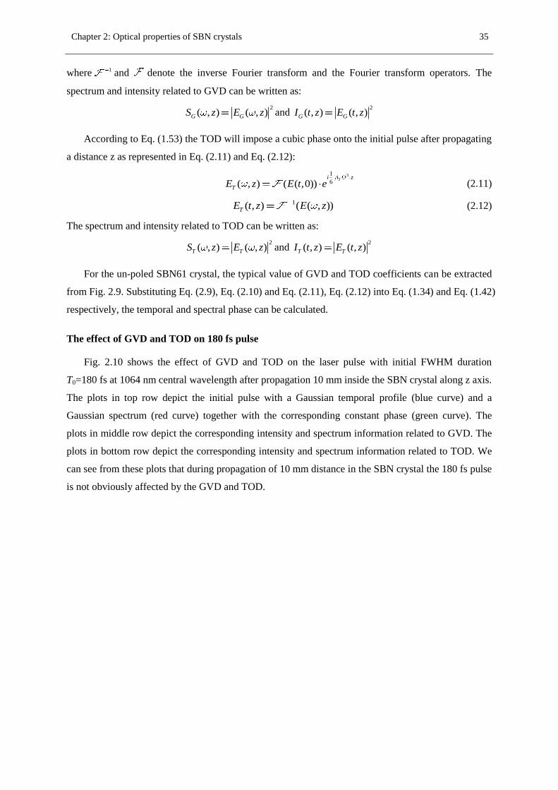
Chapter 2: Optical properties of SBN crystals 35
where 1 and denote the inverse Fourier transform and the Fourier transform operators. The
spectrum and intensity related to GVD can be written as:
2( , ) ( , )G GS z E z and
2( , ) ( , )G GI t z E t z
According to Eq. (1.53) the TOD will impose a cubic phase onto the initial pulse after propagating
a distance z as represented in Eq. (2.11) and Eq. (2.12):
33
1
6( , ) ( ( ,0))i z
TE z E t e (2.11)
1( , ) ( ( , ))TE t z E z (2.12)
The spectrum and intensity related to TOD can be written as:
2( , ) ( , )T TS z E z and
2( , ) ( , )T TI t z E t z
For the un-poled SBN61 crystal, the typical value of GVD and TOD coefficients can be extracted
from Fig. 2.9. Substituting Eq. (2.9), Eq. (2.10) and Eq. (2.11), Eq. (2.12) into Eq. (1.34) and Eq. (1.42)
respectively, the temporal and spectral phase can be calculated.
The effect of GVD and TOD on 180 fs pulse
Fig. 2.10 shows the effect of GVD and TOD on the laser pulse with initial FWHM duration
T0=180 fs at 1064 nm central wavelength after propagation 10 mm inside the SBN crystal along z axis.
The plots in top row depict the initial pulse with a Gaussian temporal profile (blue curve) and a
Gaussian spectrum (red curve) together with the corresponding constant phase (green curve). The
plots in middle row depict the corresponding intensity and spectrum information related to GVD. The
plots in bottom row depict the corresponding intensity and spectrum information related to TOD. We
can see from these plots that during propagation of 10 mm distance in the SBN crystal the 180 fs pulse
is not obviously affected by the GVD and TOD.
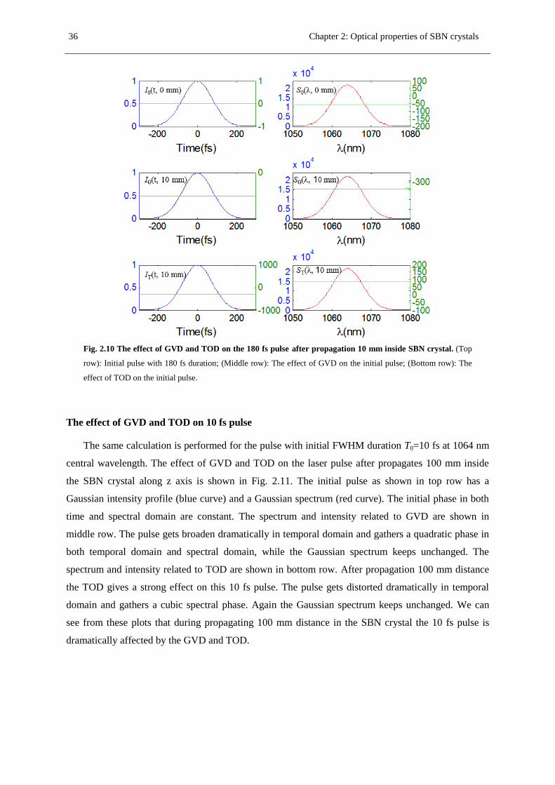
36 Chapter 2: Optical properties of SBN crystals
Fig. 2.10 The effect of GVD and TOD on the 180 fs pulse after propagation 10 mm inside SBN crystal. (Top
row): Initial pulse with 180 fs duration; (Middle row): The effect of GVD on the initial pulse; (Bottom row): The
effect of TOD on the initial pulse.
The effect of GVD and TOD on 10 fs pulse
The same calculation is performed for the pulse with initial FWHM duration T0=10 fs at 1064 nm
central wavelength. The effect of GVD and TOD on the laser pulse after propagates 100 mm inside
the SBN crystal along z axis is shown in Fig. 2.11. The initial pulse as shown in top row has a
Gaussian intensity profile (blue curve) and a Gaussian spectrum (red curve). The initial phase in both
time and spectral domain are constant. The spectrum and intensity related to GVD are shown in
middle row. The pulse gets broaden dramatically in temporal domain and gathers a quadratic phase in
both temporal domain and spectral domain, while the Gaussian spectrum keeps unchanged. The
spectrum and intensity related to TOD are shown in bottom row. After propagation 100 mm distance
the TOD gives a strong effect on this 10 fs pulse. The pulse gets distorted dramatically in temporal
domain and gathers a cubic spectral phase. Again the Gaussian spectrum keeps unchanged. We can
see from these plots that during propagating 100 mm distance in the SBN crystal the 10 fs pulse is
dramatically affected by the GVD and TOD.
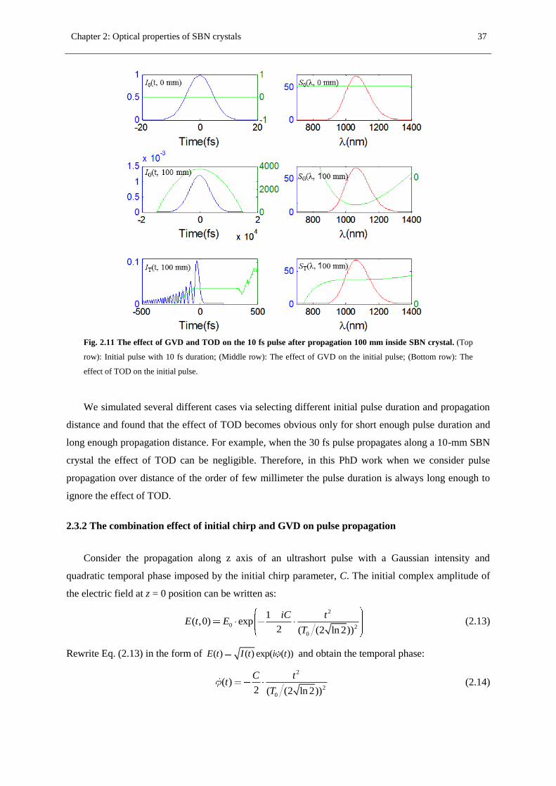
Chapter 2: Optical properties of SBN crystals 37
Fig. 2.11 The effect of GVD and TOD on the 10 fs pulse after propagation 100 mm inside SBN crystal. (Top
row): Initial pulse with 10 fs duration; (Middle row): The effect of GVD on the initial pulse; (Bottom row): The
effect of TOD on the initial pulse.
We simulated several different cases via selecting different initial pulse duration and propagation
distance and found that the effect of TOD becomes obvious only for short enough pulse duration and
long enough propagation distance. For example, when the 30 fs pulse propagates along a 10-mm SBN
crystal the effect of TOD can be negligible. Therefore, in this PhD work when we consider pulse
propagation over distance of the order of few millimeter the pulse duration is always long enough to
ignore the effect of TOD.
2.3.2 The combination effect of initial chirp and GVD on pulse propagation
Consider the propagation along z axis of an ultrashort pulse with a Gaussian intensity and
quadratic temporal phase imposed by the initial chirp parameter, C. The initial complex amplitude of
the electric field at z = 0 position can be written as:
2
0 2
0
1( ,0) exp
2 ( (2 ln 2))
iC tE t E
T (2.13)
Rewrite Eq. (2.13) in the form of ( ) ( ) exp( ( ))E t I t i t and obtain the temporal phase:
2
2
0
( )2 ( (2 ln 2))
C tt
T (2.14)

38 Chapter 2: Optical properties of SBN crystals
The instantaneous frequency can be expressed as following when substituting Eq. (2.14) into Eq.
(1.35):
0 2
0
( )( (2 ln 2))
ins
Ct t
T (2.15)
According to Eq. (1.37) the electric field in the frequency domain can be written as:
( ,0) ( ,0)exp( )E E t i t dt
2 2
0 00
2 (2 ln 2) ( (2 ln 2))exp
2(1 )1
T TE
iCiC (2.16)
After propagation z distance, according to Eq. (1.52) the electric field in the frequency domain can be
written as follow:
0
21( , ) ( ,0)exp
2E z E i g z
0
2 2 220 0 0 0
0 2 2
2 (2 ln 2) ( (2 ln 2)) ( (2 ln 2))exp exp
2(1 ) 2 11
T T T CE i g z
C CiC
(2.17)
Rewrite Eq. (2.17) in the form of Eq. (1.40) and obtain the spectral phase after propagate z distance:
0
22
0
2
( (2 ln 2))( , )
2 1
T Cz g z
C (2.18)
with Eq. (1.38) the corresponding pulse field in the temporal domain is:
1( , ) ( , )exp( )
2E t z E z i t d
1 2 2
2 2
0 2 222 202
0 2 2
(1 )
1exp exp
2( (2 ln 2))1 (1 ) 2( (2 ln 2)) 1 1
D
DD D D D
CC z
Lt tE i
z TzC z zC zi iC TL L L L L
(2.19)
Rewrite Eq. (2.19) in the form of ( ) ( ) exp( ( ))E t I t i t and obtain the temporal phase after propagate
z distance:
2
2
22 20
2
(1 )
( , )2( (2 ln 2))
1
D
D D
CC z
Ltt z
T zC z
L L
(2.20)

Chapter 2: Optical properties of SBN crystals 39
where 0
2
0( (2 ln 2))DL T g is the group velocity dispersion length, which is a characteristic length
of the medium (after propagate a distance LD the pulse gets broadened by a factor of 2 ); the
temporal phase evolution is represented in Eq. (2.20), which is a function of initial chirp and the group
velocity dispersion coefficient of the nonlinear material.
The initial phase is only related to the initial chirp and according to Eq. (2.13) and Eq. (2.16) the
initial phase can be described by a quadratic function. During pulse propagating inside the SBN
crystal the phase evolution is determined by the initial chirp and the material dispersion. Both the
GVD and initial chirp induced phase can be described by quadratic function.
Besides, the initial chirp and the group velocity dispersion coefficient also impose obvious effect
on the pulse shape which makes the pulse broadening or compression during propagation. To see this
clearly, Eq. (2.19) is rewritten in the same form with Eq. (2.13) and the expression as shown below:
2
0 2
1 ( )( , ) ( ) exp
2 ( ( ) 2 ln 2)
iC z tE t z E z
T z
21 2
2 2
0 2 222 202
0 2 2
1
1exp exp
2( (2 ln 2))1 (1 ) 2( (2 ln 2)) 1 1
D
DD D D D
CC z
Lt tE i
z TzC z zC zi iC TL L L L L
(2.21)
Here we define:
(i) Pulse duration (1/e intensity) at z position:
22
0 2
2( ) 1 (1 )e e
D D
Cz zT z T C
L L (2.22)
with 0 0 (2 ln 2)eT T , where Te0 and T0 are the pulse duration at 1/e intensity and FWHM
intensity at z=0 position.
(ii) Chirp parameter at z position:
2(1 )( )
D
CC z C z
L (2.23)
with 2
0( (2 ln2))DL T g . The chirp evolution inside a dispersive medium is determined by the
initial chirp, C, and the dispersion of the material, g. Since both C and g can have positive or
negative values, we find two different situations during pulse propagation in dispersive media: (a)
when the sign of GVD coefficient and of the initial chirp are the same the pulse broadens during
propagation; (b) For different signs of the GVD and chirp coefficients an initial compression of
the pulse is observed, until it is reached the point of minimum pulse duration (corresponding to a
Fourier transform limited pulse). From this point on the pulse will start broadening again.

40 Chapter 2: Optical properties of SBN crystals
2.4 Absorption spectrum of SBN
Theoretically, SBN crystals possess a very wide transparency window. The absorption spectrum
of SBN crystal was measured within the range of our interest and is plotted in Fig. 2.12, which shows
that signals with wavelengths less than 380 nm will be absorbed by SBN crystal.
Fig. 2.12 Absorption spectrum of SBN crystal.
2.5 Phase mismatching curve of SBN
Some nonlinear parametric process in disordered nonlinear crystals sensitively depends on the
phase mismatch value. For example, during the SHG process with collinear beams the phase mismatch
is given by ∆k =k2-2k1. Where k1 and k2 are the wavenumbers of the fundamental and second-
harmonic beam, respectively. The corresponding coherence length can be calculated via LC=π⁄∆k. The
phase mismatch evolution as a function of FF wavelength for oo-e (blue star) and ee-e (red circle) are
presented in Fig. 2.13 (a1) and Fig. 2.13 (b1) for SBN and CBN, respectively. [Tun04, EBr03] The
coherence length evolution along FF wavelength for oo-e (blue star) and ee-e (red circle) are presented
in Fig. 2.13 (a2) and Fig. 2.13 (b2) for SBN and CBN, respectively.

Chapter 2: Optical properties of SBN crystals 41
Fig. 2.13 Comparison of phase mismatch and coherence length for oo-e and ee-e interactions. (a1, b1): Phase
mismatch at different wavelengths for SBN and CBN crystals; (a2, b2): Coherence length at different wavelengths
for SBN and CBN crystals.
2.6 SHG in SBN
The as-grown ferroelectric SBN crystals exhibit a random-sized distribution of needle-like
oppositely oriented ferroelectric domains all aligned parallel to the optical axis (z axis). A schematic
representation of such domains is shown in Fig. 2.14 (a). While the reversed orientation of domains
corresponds to inversion of sign of the quadratic susceptibility χ(2)
, the refractive index of these
crystals remains practically homogeneous [Kaw98]. Unlike the typically used homogeneous nonlinear
crystals, SBN crystals are capable of achieving PM for frequency conversion processes over wide
angular and frequency bandwidths without angular or temperature tuning [Tun03, Rop13, Wan10].
PM can be obtained due to the continuous set of reciprocal lattice vectors, shown in Fig. 2.14 (b),
arising from the random size and distribution of the nonlinear domains. For the oo-e and ee-e
interactions in this 4mm point symmetry crystal the random nonlinear domains correspond to random
distribution of the χ(2)
. The reciprocal lattice vectors, with different modulus and orientations, lie in the
x-y plane. As a result, planar SH emission is observed when the input fundamental beam propagates in
the direction perpendicular to the optical axis (e.g. x axis). This effect constitutes the so-called
transverse second harmonic generation (TSHG) illustrated in Fig. 2.14 (c). Since the spectra of the
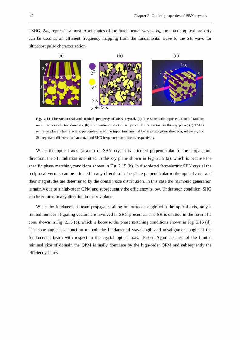
42 Chapter 2: Optical properties of SBN crystals
TSHG, 2ωi, represent almost exact copies of the fundamental waves, ωi, the unique optical property
can be used as an efficient frequency mapping from the fundamental wave to the SH wave for
ultrashort pulse characterization.
Fig. 2.14 The structural and optical property of SBN crystal. (a) The schematic representation of random
nonlinear ferroelectric domains; (b) The continuous set of reciprocal lattice vectors in the x-y plane; (c) TSHG
emission plane when z axis is perpendicular to the input fundamental beam propagation direction, where ωi and
2ωi represent different fundamental and SHG frequency components respectively.
When the optical axis (z axis) of SBN crystal is oriented perpendicular to the propagation
direction, the SH radiation is emitted in the x-y plane shown in Fig. 2.15 (a), which is because the
specific phase matching conditions shown in Fig. 2.15 (b). In disordered ferroelectric SBN crystal the
reciprocal vectors can be oriented in any direction in the plane perpendicular to the optical axis, and
their magnitudes are determined by the domain size distribution. In this case the harmonic generation
is mainly due to a high-order QPM and subsequently the efficiency is low. Under such condition, SHG
can be emitted in any direction in the x-y plane.
When the fundamental beam propagates along or forms an angle with the optical axis, only a
limited number of grating vectors are involved in SHG processes. The SH is emitted in the form of a
cone shown in Fig. 2.15 (c), which is because the phase matching conditions shown in Fig. 2.15 (d).
The cone angle is a function of both the fundamental wavelength and misalignment angle of the
fundamental beam with respect to the crystal optical axis. [Fis06] Again because of the limited
minimal size of domain the QPM is maily dominate by the high-order QPM and subsequently the
efficiency is low.

Chapter 2: Optical properties of SBN crystals 43
Fig. 2.15 SHG in disordered ferroelectric SBN crystal. (a). SH emission plane for the optical axis perpendicular
to the fundamental beam propagation direction; (b) Phase matching condition for case (a); (c) SH conical emission
for the z axis parallel to the fundamental beam propagation direction; (d) Phase matching condition for case (c).
The second-order parametric processes in this random structure have the following features: The
emitted SHG over a large spectral range which is limited only by transparency window of the crystal;
The non-collinear QPM interactions offer rich variety of phase matching possibilities, which enables
the SHG to occur at multiple directions; In the nonlinear parametric process there are no need of any
angular or temperature tuning. However, the limitation is that the SHG efficiency is always low and
intensity grows linearly with the propagation distance, which is a signature of the incoherent character
of the superposition of the SH emission from different domains. [Tru07]
2.7 Conclusions
In this chapter we systematically studied the optical properties of the SBN crystal. These
properties are closely related to the laser pulse propagation processes, which will study in the
following Chapters 3, 4 and 5. The study of these properties helps to understand the rest of the work.
Optical properties of the SBN crystal, such as, refractive indices, chromatic dispersion, linear
absorption and phase mismatching, can be found in literatures [Woi01, Tun04, Die06, Cal04],

44 Chapter 2: Optical properties of SBN crystals
however, they depend on the growing process or eventually doping component of the crystal. Since
these properties will strongly affect the laser pulse propagation process and impose effect on our
measurements, we have decided to test and validate them.
We built the setup and measured the linear refractive indices of SBN crystals, which can be as a
supplement and validation for the previous publications.
We studied the effects of group velocity dispersion and third order dispersion and the combination
effect of initial chirp and chromatic dispersion on pulse propagation, which is the preliminary study to
apply SBN crystal to ultrashort pulse characterization because dispersion in SBN crystal has a strong
effect on the initial chirp retrieving process.
We measured the linear absorption spectrum of SBN crystal. In this dissertation all the
measurements in different applications highly depend on the precise measurement of the output beam,
so the confirmation of the transparency window is the basis for efficient parameter estimation in the
rest of the work.
Some nonlinear parametric process in artificially poled random nonlinear crystals as discussed in
Chapter 5 sensitively depends on the phase mismatch value, so we calculated the phase-mismatching
curve of SBN crystal.
Since second-order nonlinearities are directly related to the domain distribution within the crystal,
in this chapter we briefly reviewed the ferroelectricity and second harmonic generation in SBN crystal.
The ferroelectric and optical properties of SBN make them suitable for poling and transverse second
harmonic generation.
Chapter 3
Ultrashort pulse duration and chirp
measurement via transverse auto-
correlation technique
3.1 Introduction
Ultrashort laser pulses, with their variety of peak powers and durations, are becoming an
important tool in an increasing number of applications in the fields of technology (materials
processing, etc.), biomedical sciences, and basic research, in general. As the pulses become shorter,
the dispersion effects that modify pulse properties during propagation through optical materials
become increasingly relevant so a precise characterization of the pulse properties is needed. The laser
pulses we are studying in this thesis are entirely defined by their electric field, which can be
represented either in temporal or spectral domain. Since the pulse parameters in temporal and spectral
domains are closely related by Fourier transform relations, the measurement of the pulse intensity and
phase in either temporal or spectral domain is sufficient to completely characterize the laser pulses.
Direct electronic detection methods are used to measure some basic information of a laser pulses.
For example, the energy detector detects pulse energy, spectrometer measures the spectrum, and the
temporal pulse duration of pulses longer than 1 nanosecond can be measured with a photodiode.
However, pulses in the sub-100 fs temporal regime are shorter than the temporal response of any
electronic detector, thus it becomes impossible to perform a direct measurement that could determine
their temporal profile [Won95]. The state-of-the-art technology that sets the temporal resolution limit
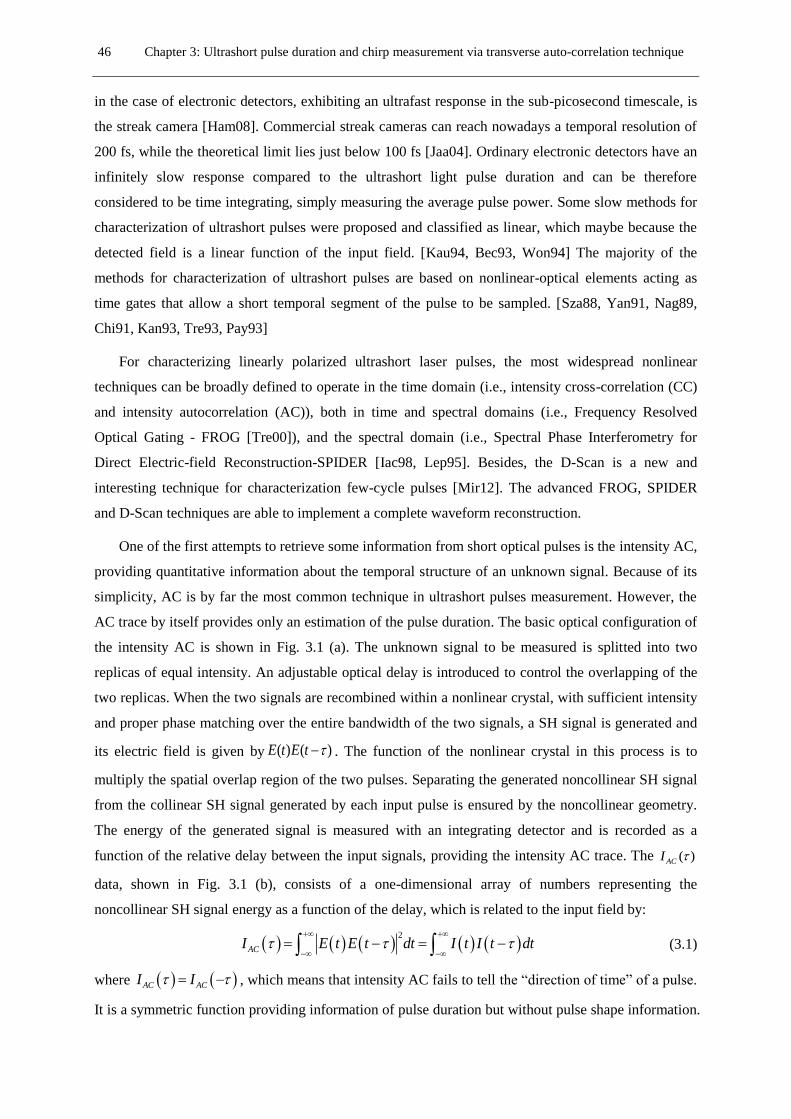
46 Chapter 3: Ultrashort pulse duration and chirp measurement via transverse auto-correlation technique
in the case of electronic detectors, exhibiting an ultrafast response in the sub-picosecond timescale, is
the streak camera [Ham08]. Commercial streak cameras can reach nowadays a temporal resolution of
200 fs, while the theoretical limit lies just below 100 fs [Jaa04]. Ordinary electronic detectors have an
infinitely slow response compared to the ultrashort light pulse duration and can be therefore
considered to be time integrating, simply measuring the average pulse power. Some slow methods for
characterization of ultrashort pulses were proposed and classified as linear, which maybe because the
detected field is a linear function of the input field. [Kau94, Bec93, Won94] The majority of the
methods for characterization of ultrashort pulses are based on nonlinear-optical elements acting as
time gates that allow a short temporal segment of the pulse to be sampled. [Sza88, Yan91, Nag89,
Chi91, Kan93, Tre93, Pay93]
For characterizing linearly polarized ultrashort laser pulses, the most widespread nonlinear
techniques can be broadly defined to operate in the time domain (i.e., intensity cross-correlation (CC)
and intensity autocorrelation (AC)), both in time and spectral domains (i.e., Frequency Resolved
Optical Gating - FROG [Tre00]), and the spectral domain (i.e., Spectral Phase Interferometry for
Direct Electric-field Reconstruction-SPIDER [Iac98, Lep95]. Besides, the D-Scan is a new and
interesting technique for characterization few-cycle pulses [Mir12]. The advanced FROG, SPIDER
and D-Scan techniques are able to implement a complete waveform reconstruction.
One of the first attempts to retrieve some information from short optical pulses is the intensity AC,
providing quantitative information about the temporal structure of an unknown signal. Because of its
simplicity, AC is by far the most common technique in ultrashort pulses measurement. However, the
AC trace by itself provides only an estimation of the pulse duration. The basic optical configuration of
the intensity AC is shown in Fig. 3.1 (a). The unknown signal to be measured is splitted into two
replicas of equal intensity. An adjustable optical delay is introduced to control the overlapping of the
two replicas. When the two signals are recombined within a nonlinear crystal, with sufficient intensity
and proper phase matching over the entire bandwidth of the two signals, a SH signal is generated and
its electric field is given by ( ) ( )E t E t . The function of the nonlinear crystal in this process is to
multiply the spatial overlap region of the two pulses. Separating the generated noncollinear SH signal
from the collinear SH signal generated by each input pulse is ensured by the noncollinear geometry.
The energy of the generated signal is measured with an integrating detector and is recorded as a
function of the relative delay between the input signals, providing the intensity AC trace. The ( )ACI
data, shown in Fig. 3.1 (b), consists of a one-dimensional array of numbers representing the
noncollinear SH signal energy as a function of the delay, which is related to the input field by:
2
ACI E t E t dt I t I t dt
(3.1)
where AC ACI I , which means that intensity AC fails to tell the “direction of time” of a pulse.
It is a symmetric function providing information of pulse duration but without pulse shape information.

Chapter 3: Ultrashort pulse duration and chirp measurement via transverse auto-correlation technique 47
Fig.3.1 Intensity autocorrelator. (a) Schematic representation of the intensity AC. (b) the intensity AC trace
calculated by different temporal delay τ.
Since the AC function depends on the assumed signal shape, to estimate the actual signal duration
through AC trace we should know the functional form for the temporal shape of the unknown signal.
If we consider a Gaussian-shaped signal 2 2( ) exp( ( (2 ln2)) )I t t T with the temporal intensity FWHM
duration T, the corresponding intensity AC trace can be expressed as 2 2( ) exp( ( (2 ln2)) )AC ACI t t T ,
where the relation between pulse duration T and AC duration TAC can be written as 2 ACT T . For a
Sech2 pulse the relation between pulse duration T and AC duration TAC becomes 1.54T=TAC.
The intensity AC is the simplest and the most common technique for measuring pulses with
durations above 150 – 200 fs. The AC profile can be only used for the estimate of the pulse duration,
which is actually enough in an important number of applications. However, the AC technique has
several limitations when ultrashort pulses below 100 fs have to be measured:
(a) Demand of multiple shots pulses. The AC technique depends on the measurement of SHG at
different pulse overlap region. In order to get a complete AC profile one has to keep changing the
delay time until it covers the entire pulse duration. In this way, one will always measure the
average pulse duration of a train of pulses. In order to overcome this limitation, a background-free
single-shot method to measure the intensity AC trace was developed by Janszky [Jan77]. In 1987
this method was used to measure pulses shorter than 100 fs [Sal87]. In this technique two replicas
of the pulse to be measured are overlapped with a given angle inside a NL crystal and the SH trace
is spatially recorded using a CCD. The recorded signal as a function of transverse dimension
provides naturally the AC trace of the two replicas of the pulse.
(b) Pulse distortion. Because the AC trace is measured in forward direction, one can only measure
the pulse duration at the output plane of the crystal. Compared with the pulse duration at the input

48 Chapter 3: Ultrashort pulse duration and chirp measurement via transverse auto-correlation technique
plane of the crystal, the pulse at this measurement place is already distorted after its propagation
through the dispersive nonlinear material.
(c) As described in Chapter 1, the PM condition is highly dependent on the PM angle and
wavelength. In order to get SHG efficiency, the optical path alignment is very critical to make
pulses propagate along the PM angle. For different pulses at different central wavelengths,
different nonlinear crystals are needed to realize phase matching.
(d) The demand of thin crystals. As described in Chapter 1, in order to get a large PM bandwidth
thin crystals are always needed. However, a thin crystal leads to a low SHG efficiency since the
efficiency is proportional to the square of crystal length.
As an alternative to the standard AC configurations it has been shown that parametric conversion
process in the as-grown ferroelectric SBN crystals can be used as an efficient and user-friendly
frequency mapping from infrared to visible for the femtosecond pulse monitoring. The non-collinear
SHG geometry in SBN crystals, shown schematically in Fig. 3.2 (a), was firstly proposed in Ref.
[Rop08] and later the corresponding transverse auto-correlation (TAC) trace simulation model is
reported in Ref. [Tru09]. The technique was initially applied to the measurements of around 200 fs
pulses. When the two pulse replicas represented by the black and red rectangles in Fig. 3.2 (b) overlap
inside the SBN crystal, different pulse overlap regions are automatically formed at different positions
along the transverse direction. The non-collinear second-order nonlinear interaction between the two
pulses within the SBN crystal, generates the TSHG which contributes to the TAC trace. In contrast to
the traditional single shot AC technique [Jan77] where the AC profile is recorded in the forward
direction at the output of the nonlinear crystal, the TAC technique captures the SHG signal at 90o with
respect to the propagation direction of the input beams and it allows for single-shot measurement of
the TAC profile evolution as a function of the propagation distance inside the crystal. This transverse
technique can be used for the determination of the pulse duration and of the initial chirp parameter of
the incident pulse when considering the dispersion effect during the pulse propagation inside the SBN
crystal.
We mentioned in the previous chapter there are some limitations in the random quasi phase
matching process, however, in the ultrashort pulse characterization process the limitations can be
transformed into advantages:
(a) The low efficiency can become an advantage in pulse characterization, because small pump
depletion can keep pulse characteristics unchanged during propagation inside the crystal.
(b) The large number of reciprocal lattice vectors, G, provided by the random crystal create broad
frequency bandwidth for full conversion at different wavelengths without need of alignment or
temperature control.
(c) Simultaneous PM of SHG process allows for nonlinear planar SHG other a large angular range
including the transverse SHG emission.
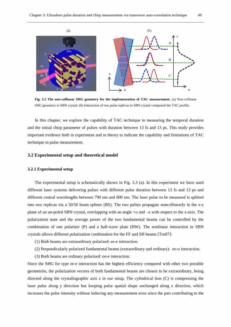
Chapter 3: Ultrashort pulse duration and chirp measurement via transverse auto-correlation technique 49
Fig. 3.2 The non-collinear SHG geometry for the implementation of TAC measurement. (a) Non-collinear
SHG geometry in SBN crystal; (b) Interaction of two pulse replicas in SBN crystal composed the TAC profile.
In this chapter, we explore the capability of TAC technique in measuring the temporal duration
and the initial chirp parameter of pulses with duration between 13 fs and 13 ps. This study provides
important evidence both in experiment and in theory to indicate the capability and limitations of TAC
technique in pulse measurement.
3.2 Experimental setup and theoretical model
3.2.1 Experimental setup
The experimental setup is schematically shown in Fig. 3.3 (a). In this experiment we have used
different laser systems delivering pulses with different pulse duration between 13 fs and 13 ps and
different central wavelengths between 790 nm and 800 nm. The laser pulse to be measured is splitted
into two replicas via a 50/50 beam splitter (BS). The two pulses propagate noncollinearly in the x-z
plane of an un-poled SBN crystal, overlapping with an angle +α and –α with respect to the x-axis. The
polarization state and the average power of the two fundamental beams can be controlled by the
combination of one polarizer (P) and a half-wave plate (HW). The nonlinear interaction in SBN
crystals allows different polarization combination for the FF and SH beams [Tru07]:
(1) Both beams are extraordinary polarized: ee-e interaction.
(2) Perpendicularly polarized fundamental beams (extraordinary and ordinary): eo-o interaction.
(3) Both beams are ordinary polarized: oo-e interaction.
Since the SHG for type ee-e interaction has the highest efficiency compared with other two possible
geometries, the polarization vectors of both fundamental beams are chosen to be extraordinary, being
directed along the crystallographic axis z in our setup. The cylindrical lens (C) is compressing the
laser pulse along y direction but keeping pulse spatial shape unchanged along z direction, which
increases the pulse intensity without inducing any measurement error since the part contributing to the

50 Chapter 3: Ultrashort pulse duration and chirp measurement via transverse auto-correlation technique
spatial TAC trace is the spatial shape along z direction which is undistorted after passing through the
cylindrical lens. A CCD camera in conjunction with a camera lens, placed above the crystal, is used to
record the spatially resolved nonlinear signal.
Fig. 3.3 Experimental setup, image system and background subtraction method for retrieving TAC trace set.
(a) Schematic representation of the TAC setup. P—polarizer, BS—50/50 beam splitter, M—mirror, HW—half-
wave plate, C—cylindrical lens; (b) The background subtraction method. The TAC trace set is retrieved by
subtracting the background signal when τ >>T0 from the total signal when τ = 0.
The Delay Control element is inserted into the setup to adjust optical delay as shown in Fig. 3.3
(a). When the delay time (τ) between the two optical paths is zero (the two pulses perfectly overlap),
the nonlinear interaction of the two fundamental beams gives rise to three well-differentiated SH
emissions shown in Fig. 3.3 (b) (bottom): two of them correspond to the conical SH emission from
each individual beam while the middle one is the SH emission coming from the non-collinear
interaction between the two pulse replicas. A clean background signal formed by the two conical SH
emission by each individual beam can be recorded when the delay τ>>T0, where T0 is the unknown
pulse initial duration. To get the TAC trace, one needs to subtract the background signal from the total
signal, which is the so-called background subtraction method. The TAC trace evolution along the
whole propagation distance within the crystal is composed by its spatial intensity profile at different

Chapter 3: Ultrashort pulse duration and chirp measurement via transverse auto-correlation technique 51
propagation distances (x0, x1…xn) as shown in the Fig. 3.4. Each TAC intensity profile IAC (z) is
directly related to the temporal intensity AC profile IAC (t) at this position inside the crystal. To
retrieve the temporal AC profile from the corresponding recorded spatial profile, a calibration factor
which depends on the geometry of the setup must be applied. This calibration can be properly obtained
with the following procedure:
(1) Image the whole SBN crystal surface to get the calibration factor between mm and pixel.
(2) Calculate the calibration factor between fs and mm with Eq. (3.2) [Rop08].
2 sin( )ACAC
zT
c (3.2)
The corresponding pulse duration can be calculated by 2ACT T . The factor 2 comes from
the assumption of Gaussian pulse profile for input pulses. Other pulse profiles should use different
factor.
(3) Combining the two calibration factors we finally get the relationship between space (pixel) and
time (fs), which can be used to retrieve the pulse duration evolution from the spatial width of TAC
trace set.
Fig. 3.4 TAC trace set obtained with the CCD imaging system. CCD recorded image of the TAC trace profile at
different propagation distances (x0, x1…xn) constitute the TAC trace set.
3.2.2 TAC trace theoretical model
As previously commented, an advantage of this technique is the possibility to record of SH signal
transversely to propagation direction. This allows to track the behavior of the input pulse along the
propagation direction. It is well known that any pulse will get broadened or compressed temporally
during propagation in dispersive media. Therefore the study of the evolution of the SH signal as a
function of the propagation distance can be used to obtain a measurement of the chirp parameter of the
input pulse.

52 Chapter 3: Ultrashort pulse duration and chirp measurement via transverse auto-correlation technique
We study the role of the broadening and compressing with a simplified theoretical model in which
we consider Gaussian pulses with initial chirp parameter C. The two Gaussian pulse replicas propagate
in the crystallographic plane x-z of an SBN crystal with the angles –α and +α with respect to the x-axis
as shown in Fig. 3.5.
Fig. 3.5 The schematic diagram of beam superposition inside SBN crystal. As beams propagate, the TSHG
emission region moves along x axis giving rise to the recorded TAC trace set.
The electric fields of the two replicas at x1=x2=0 mm can be written as:
2
1
1 1 0 2
0
1, 0 exp
2 2 ln 2
t x uiCE t x E
T
(3.3)
2
2
2 2 0 2
0
1, 0 exp
2 2 ln 2
t x uiCE t x E
T
(3.4)
where C is the initial chirp parameter, u is the speed of light in the crystal, T0 is the initial FWHM
duration of the unkown pulse. According to the Eq.(2.21), after propagate x1 and x2 distance inside the
SBN crystal, the electric fields of the two fundamental replicas at x1 and x2 position can be written as:
2
101 1 121 4
10 1
, exp exp
2 2 ln 2
t x uEE t x i t
F T F
(3.5)
2
202 2 221 4
20 2
, exp exp
2 2 ln 2
t x uEE t x i t
F T F
(3.6)
where

Chapter 3: Ultrashort pulse duration and chirp measurement via transverse auto-correlation technique 53
2
21 11 2
21 1
D D
Cx xF C
L L
(3.7)
2
22 22 2
21 1
D D
Cx xF C
L L
(3.8)
2
0 2 ln 2
D
TL
g
(3.9)
and g=486 fs2/mm is the group velocity dispersion (GVD) for SBN crystal at 790 nm central
wavelength (seen in Fig. 2.9 (a)), T0 is intensity FWHM duration and LD is GVD length over which the
initial pulse duration increases by factor of square root of 2. We can see from Eq. (3.9) that LD is
closely related to the pulse duration and the shorter the pulse the shorter the dispersion length, which
means the dispersive media has a stronger influence on short pulses than on the long pulses. The phase
term 1 t in Eq. (3.5) and 2 t in Eq. (3.6) can be ignored, because the phase term has no
contribution to the intensity TAC trace at particular position in this model. The following
transformation is used to change the variables to a common reference system:
1 sin cosin inx z x
(3.10)
2 sin cosin inx z x
(3.11)
If we consider that the ee-e interaction is phase-matched provided the available conversion
bandwidth of SBN then the generated TAC trace along the crystal can be simulated by:
1 2ACI t I I t d
(3.12)
where 2
1 1I E and 2
2 2I E . The spatial AC trace can be written as:
2 2
0 2 2
2 sinexpAC
zI I
u T x
(3.13)
where T(x) is the pulse duration evolution during propagation inside the SBN crystal and the
expression is represented as Eq. (1.57). During propagation the pulse duration T(x) is modified due to
the combination effect of initial chirp parameter and material dispersion characterized by the GVD
coefficient g. In normal GVD regime (g > 0), group velocity decreases with frequency and redder
frequencies travel faster than bluer ones. If C > 0, the pulse will become longer during the propagation.
If C < 0 instead, the pulse will be compressed until the different frequency components are in phase
and the pulse acquires its minimum FWHM duration (Tmin) corresponding to the Fourier transform
limited case. This minimum pulse duration occurs at the maximum compression distance xmin. In the
case of anomalous GVD regime (g < 0), when bluer frequencies travel faster than redder ones, the
pulse gets longer for C < 0 and is initially compressed if C > 0 (compression is obtained whenever C
and g have different signs).
54 Chapter 3: Ultrashort pulse duration and chirp measurement via transverse auto-correlation technique
For wavelengths corresponding to the normal GVD regime (λ < 2 μm for SBN crystal, seen in Fig.
2.9) one observes pulse compression when C < 0 as shown in Fig. 3.6. The minimum FWHM duration,
Tmin, and the corresponding maximum compression distance inside the crystal, xmin, can be obtained
from the condition:
min
min
min
( )0, ( )
x xx x
T xT T x
x (3.17)
The corresponding expression can be written as Eq. (3.18) and Eq. (3.19):
min 21
DC Lx
C (3.18)
0min
21
TT
C (3.19)
The value of initial chirp, C, and initial pulse duration (FWHM), T0, can be deduced from xmin and Tmin:
min
2
min
4ln(2) g xC
T (3.20)
2
2 min0 min
min
4ln(2) g xT T
T (3.21)
In the TAC technique, the dependence of the spatial TAC trace width, ∆z, with propagation
distance, x, allows the measurement of pulse temporal duration evolution T (x) as a function of
propagation distance. From the above analysis the duration evolution T (x) can be used to deduce the
initial pulse duration and initial chirp parameter.
Fig. 3.6 Effect of material dispersion on the negative chirped pulse during propagation inside the SBN
crystal. When the pulse propagates xmin distance, the dispersion induced chirp compensates the initial chirp and
where the pulse becomes Fourier transform limited pulse with the minimal pulse duration Tmin.

Chapter 3: Ultrashort pulse duration and chirp measurement via transverse auto-correlation technique 55
3.3 Results and discussions
3.3.1 Measurement of 180 fs pulses
In the first experiment we have measured pulses delivered by a Ti: Sapphire oscillator (Mira,
Coherent) operating at 800 nm with a repetition rate of 76 MHz. The average power of the laser
system was 1W and the initially unchirped pulse duration was around 180 fs. The two replicas of the
pulse propagated in the x-z plane of an SBN crystal (5×5×5 mm) forming angles +α and –α with
respect to the x-axis (external angle α=5.5º, internal angle αin=2.5o).
Fig. 3.7 (a) shows the experimentally recorded TAC trace set along the 5-mm propagation
distance along the SBN crystal with pulse propagation from left (x=0 mm) to right (x=5 mm). The
inset shows the AC trace intensity profile as a function of z at the position of the rectangular marker
(x=3 mm). From this plot we can measure the AC width at FWHM intensity, ∆zAC. To get a precise
width measurement we have to take into account that the measurements can be very irregular because
noise cannot be ignored in the detection of weak signals. In order to measure the AC width at FWHM
intensity we developed a MATLAB code based on the knife-edge technique. We calculated the total
area under the AC trace and calculate the positions (Z1, Z2) where area is (16%, 84%). This
measurement gives ∆zAC=Z2-Z1. With this method we can retrieve the TAC trace intensity profile and
calculate the FWHM width at each propagation distance. The space-time decoding factor can be
calculated from Eq. (3.22), with which the reference pulse duration at FWHM can be calculated and
the pulse duration evolution curve is shown in Fig. 3.7 (b).
2 sin( )ACzT
c (3.22)
The plot in Fig. 3.7 (b) shows the initial pulse FWHM duration at x=0 mm is around 170 fs. The
accuracy of the results in this configuration can be limited by the quality of the CCD camera image
(quantity of recorded pixels) and in the precision measurement of the incident angle α. We have
measured the pulse duration with an alternative auto-correlator and we have obtained the same result.
Thus, the alternative measurement can verify that the built setup and MATLAB code can work
properly.

56 Chapter 3: Ultrashort pulse duration and chirp measurement via transverse auto-correlation technique
Fig. 3.7 Experimental data process for reference pulse measurement. (a) Experimentally recorded TAC trace
set along SBN crystal. (b) The retrieved reference pulse temporal duration evolution along SBN crystal.
3.3.2 Measurement of a 30 fs pulse
After the measurement of pulses from conventional Ti: Sapphire oscillator, in this section we start
the innovative work and we move to measurements of pulses with durations below 50fs, where this
technique have not been previously tested. This work is the first complete research, to the best of our
knowledge, in detecting the chirp parameter and pulse duration with the TAC technique. This
experiment was performed in Centro de Láseres Pulsados, CLPU, Salamanca, Spain. We used a laser
source (Femtopower PRO HE CEP from Femtolaser) emitting pulses with FWHM duration around 30
fs at a repetition rate of 1 kHz and with 2 mJ energy per pulse, operating at 790 nm central wavelength.
The laser source can also provide shorter pulses, down to 6 fs, by the hollow-core fiber post-
compression technique [Nis96] using chirped mirrors to implement spectral phase compensation. An
acousto-optic device (Dazzler from Fastlite) was used to modulate the phase via imposing a selected
initial chirp on the FTL pulses with FWHM duration around 30 fs. The modulated pulses composed
the unknown pulses to be measured in our work. We have selected different negative values of initial
chirp parameter C in order to distinguish different unknown pulses. The two replicas of the unknown
pulse propagated in the x-z plane of the SBN crystal (5×5×10 mm) forming angles +α and –α with
respect to the x-axis (external angle α=3.4o and internal angle αin=1.5
o). Since different unknown
pulses own different initial chirp, the maximum compression distance for each pulse is different from
another. For an increased chirp parameter, the maximum compression distance inside the crystal
increases.

Chapter 3: Ultrashort pulse duration and chirp measurement via transverse auto-correlation technique 57
Before entering the TAC setup, each unknown pulse was carefully characterized using the
SPIDER [Iac98] technique. The initial chirp value C and initial FWHM duration T0 of the first
unknown pulse measured by SPIDER technique is [C= -7.9, T0=257 fs] and the corresponding
experimental results of TAC technique are presented in Fig. 3.8. Fig. 3.8 (a) shows the experimentally
recorded TAC trace set along the 10-mm SBN crystal with pulse propagation from left (x=0 mm) to
right (x=10 mm). The compression and broadening effect of the TAC trace during propagation can be
clearly seen in the plot. The retrieved spatial TAC trace profiles at position A (x=1.5 mm), B (x=3.3
mm), C (x=6.4 mm) and D (x=8.9 mm) marked by the dashed line are plotted in Fig. 3.8 (b). With the
space-time decoding factor (evaluated by Eq. (3.22)) we convert the spatial TAC profile width to
temporal pulse duration. The unknown pulse FWHM duration evolution is plotted in Fig. 3.8 (c). From
the pulse duration evolution curve the minimal time duration, Tmin=32 fs, and the corresponding
maximum compression distance, xmin=6.4 mm, can be extracted. We substitute the extracted Tmin and
xmin into Eq. (3.20) and Eq. (3.21) and consequently retrieve the initial chirp parameter C= -7.9 and
initial pulse FWHM duration T0 =257 fs.
Fig. 3.8 Experimental data process for the first measurement of 30 fs pulse with [C= -7.9, T0=257 fs]. (a)
Experimentally recorded TAC trace set along SBN crystal. (b) Spatial TAC trace profile at each position of the
dashed line. (c) The retrieved unknown pulse temporal duration evolution along SBN crystal.

58 Chapter 3: Ultrashort pulse duration and chirp measurement via transverse auto-correlation technique
With the retrieved initial chirp parameter C= -7.9 and initial pulse FWHM duration T0 =257 fs we
substitute Eq. (3.5)- Eq. (3.11) into Eq. (3.12) and obtain the TAC trace along the crystal. The
corresponding spatial TAC trace set along SBN crystal with pulse propagation from left (x=0 mm) to
right (x=10 mm) is shown in Fig.3.9 (a). The compression and broadening effect of the TAC trace
during propagation can be clearly visible in the plot. The retrieved spatial TAC trace profiles at
position A (x=1.5 mm), B (x=3.3 mm), C (x=6.4 mm) and D (x=8.9 mm) marked by the dashed line
are plotted in Fig. 3.9 (b). Using expression (3.2) the spatial TAC profile width can be directly related
to the unknown pulse FWHM duration. The retrieved temporal pulse duration evolution from the
simulated spatial TAC trace set is shown in Fig. 3.9 (c). From the pulse duration evolution curve the
minimal time duration, Tmin=35 fs, and the corresponding maximum compression distance, xmin=6.4
mm, can be extracted, which shows good agreement with the experimental results.
Fig. 3.9 Simulation results for the first measurement of 30 fs pulse with [C= -7.9, T0=257 fs]. (a) The
simulation of the spatial TAC trace set along SBN crystal with the initial conditions determined from the
experimental results. (b) Spatial TAC trace profile at each position of the dashed line. (c) The retrieved temporal
pulse duration evolution from the simulated spatial TAC trace set.
Chapter 3: Ultrashort pulse duration and chirp measurement via transverse auto-correlation technique 59
Since the spectrum of pulse was not modified by the Dazzler system in the experiment, according
to the theoretical analysis in the introduction the temporal phase and spectral phase at x position can be
written as:
0
22
0
2
( (2 ln 2))( , )
2 1
T Cx g x
C (3.23)
2
2
22 20
2
(1 )
( , )2( (2 ln 2))
1
D
D D
CC x
Ltt x
T xC x
L L
(3.24)
Expressions (3.23) and (3.24) can be used to plot the evolution of the temporal and spectral phases of
a Gaussian pulse with a particular value of initial chirp, C, and initial pulse duration, T0. Fig. 3.10 (a1,
b1, c1, d1) show the temporal intensity (blue line) and the corresponding temporal phase (green line)
at position A (x=1.5 mm), B (x=3.3 mm), C (x=6.4 mm) and D (x=8.9 mm). The plots in Fig. 3.10 (a1,
b1, c1) show the temporal pulse compression process where the dispersion induced positive chirp try
to compensate the initial negative chirp. When the dispersion induced positive chirp equals to the
initial negative chirp the pulse becomes FTL pulse with the minimal pulse duration and constant phase
shown in Fig. 3.10 (c1). The plots in Fig. 3.10 (c1, d1) show the pulse broadening process where the
dispersion induced positive chirp is already overcompensated the initial negative chirp. The
corresponding phase becomes a parabolic phase again but with opposite sign from the previous
parabolic. The plots in Fig. 3.10 (a2, b2, c2, d2) show the spectrum profile and spectral phase for each
case (a1, b1, c1, d1). We can see during pulse propagation the spectrum profile keeps unchanged but
the spectral phase has opposite sign from the temporal phase.

60 Chapter 3: Ultrashort pulse duration and chirp measurement via transverse auto-correlation technique
Fig. 3.10 The simulation of the temporal intensity and phase (left) and spectrum and spectral phase (right)
at position x=1.5 mm, 3.3 mm, 6.4 mm and 8.9 mm marked A, B, C and D in Fig. 9. (a1): temporal intensity
profile (blue line) and temporal phase (green) at x=1.5 mm; (b1): temporal intensity profile (blue line) and
temporal phase (green) at x=3.3 mm; (c1): temporal intensity profile (blue line) and temporal phase (green) at
x=6.4 mm; (d1): temporal intensity profile (blue line) and temporal phase (green) at x=8.9 mm; [(a2), (b2), (c2) and
(d2)] are the corresponding spectrum and spectral phase for each case [(a1), (b1), (c1) and (d1)].
With the same TAC setup we measured another six unknown pulses marked as A, B, C, D, E, and
F. Fig. 3.11 (a1, b1, c1, d1, e1, f1) show the CCD recorded spatial TAC trace set along the SBN
crystal for each pulse A, B, C, D, E, and F. We can see the increased initial chirp yields a larger
compression distance inside the SBN crystal. Fig. 3.11 (g1) shows the experimental retrieved
unknown pulse duration evolution along the SBN crystal for each pulse, which clearly displays the
minimal temporal FWHM duration, Tmin, and the corresponding maximum compression distance, xmin,
for each case. The measured minimal temporal FWHM duration and corresponding maximum
compression distance are as following:
A [Tmin =34 fs, xmin =0.9 mm], B [Tmin =32 fs, xmin =2.3 mm], C [Tmin =30 fs, xmin =3.2 mm]
D [Tmin =30 fs, xmin =4.0 mm], E [Tmin =30 fs, xmin =5.1 mm], F [Tmin =32 fs, xmin =6.4 mm]

Chapter 3: Ultrashort pulse duration and chirp measurement via transverse auto-correlation technique 61
We observe that in all cases the pulse duration at the maximum compression position is of the order of
30 fs. With Eq. (3.20) and Eq. (3.21) the initial chirp parameter C and initial pulse temporal FWHM
duration T0 can be retrieved as following:
A [C= -1.0, T0=48 fs], B [C= -2.8, T0=96 fs], C [C= -4.6, T0=142 fs],
D [C= -5.7, T0=175 fs], E [C= -7.2, T0=220 fs], F [C= -7.9, T0=257 fs].
Fig. 3.11 Comparison of experimental results and simulation results. (a1, b1, c1, d1, e1, f1): The
experimentally recorded TAC trace set along SBN crystal for pulse A [C= -1.0, T0=48 fs], pulse B [C= -2.8, T0=96
fs], pulse C [C= -4.6, T0=142 fs], pulse D [C= -5.7, T0=175 fs], pulse E[C= -7.2, T0=220 fs], and pulse F [C= -7.9,
T0=257 fs]; (g1): The experimental retrieved unknown pulse duration evolution along SBN crystal for each case
(a1, b1, c1, d1, e1, f1); (a2, b2, c2, d2, e2, f2): The simulation of the TAC trace set along SBN crystal with the
experimental retrieved initial chirp parameter and FWHM duration for each case (a1, b1, c1, d1, e1, f1); (g2) The
pulse duration evolution curve from the simulated TAC trace set for each case (a2, b2, c2, d2, e2, f2).

62 Chapter 3: Ultrashort pulse duration and chirp measurement via transverse auto-correlation technique
In addition to the method above, the value of initial pulse duration can be also obtained by
measuring the pulse duration directly at the entrance of the crystal, but the accurate measurement of
these long pulses requires the broader beams to provide complete overlap along the crystal length.
However, this condition can be relaxed by retrieving the initial pulse duration from the pulse duration
at the maximum compression point.
In order to check the validity of the experimental results obtained with this TAC technique, we
compared our results with the SPIDER measurement results and found a very good correspondence
between the results. The discrepancy between these two technique measured pulse duration is less than
2%. This discrepancy can be attributed to the measurement error of the CCD camera, the intersection
angle, and the Tmin and xmin. Besides, the intrinsic instabilities of the pulse train can also cause the un-
ignorable error.
In addition to the experimental studies of pulse evolution, we also analyzed these pulse evolution
with simulation. The simulated TAC traces set are shown in Fig. 3.11 (a2, b2, c2, d2, e2, f2). The
pulse duration evolution along the SBN crystal for each case is plotted in Fig. 3.11 (g2), which gives
the simulation results of minimal temporal FWHM duration, Tmin, and the corresponding maximum
compression distance, xmin, as following:
A [Tmin =35 fs, xmin =0.89 mm], B [Tmin =35 fs, xmin =2.27 mm], C [Tmin =30 fs, xmin =3.26 mm]
D [Tmin =30 fs, xmin =4.02 mm], E [Tmin =30 fs, xmin =5.12 mm], F [Tmin =35 fs, xmin =6.42 mm]
The simulation results have good agreement with experimental results.
The experimental and simulation results are summarized in Table 3.1. From the comparison
between experimental and simulation results, we see that this TAC technique works well for pulse
durations around 30 fs. This technique is capable of implement the real-time pulse duration and chirp
measurement, which provides the possibility to optimize the pulse parameters in real-time.
Experimental data Calculations Simulation data
xmin
(mm)
Tmin
(fs) C
T0
(fs)
GDD
(fs2)
xmin
(mm)
Tmin
(mm)
(a1) 0.9 34 -1.0 48 -411 (a2) 0.89 35
(b1) 2.3 32 -2.8 96 -1053 (b2) 2.27 35
(c1) 3.2 30 -4.6 142 -1511 (c2) 3.26 30
(d1) 4.0 30 -5.7 175 -1883 (d2) 4.02 30
(e1) 5.1 30 -7.2 220 -2384 (e2) 5.12 30
(f1) 6.4 32 -7.9 257 -2982 (f2) 6.42 35
Table. 3.1 The experimental and simulation results. Experimental data corresponding to situations (a1) – (f1) in
Fig.3.11 and retrieved values of C, T0 , and GDD. Results retrieved from simulation considering the calculated
values as initial conditions corresponding to the plots (a2) – (f2) in Fig.3.11.

Chapter 3: Ultrashort pulse duration and chirp measurement via transverse auto-correlation technique 63
3.3.3 Measurement of a 13 fs pulse
To check the capability of TAC technique in shorter pulse monitoring we performed the
measurements of pulses of decreased duration. Before implementing pulse measurement with our
TAC setup, the pulses were carefully characterized using the D-Scan and FROG techniques. As an
example, the minimal FWHM duration Tmin and the central wavelength of one of the unknown pulses
measured by D-Scan technique is [Tmin=13 fs, λ=790 nm].
The experimentally recorded TAC trace set along SBN crystal with our setup is shown in Fig.
3.12 (a). The retrieved unknown pulse duration evolution along the SBN crystal is shown in Fig. 3.12
(b), which gives a minimal temporal FWHM duration of 22 fs at x=0.84 mm position. The retrieved
pulse duration at positions between x=2 and x=5 mm is much smaller than that can be predicted by Eq.
(2.24). This is because the overlapping of the two beams is not complete at these positions. However
the measurement of [C, T0] can be performed properly as long as the two beans overlap completely at
the position of xmin.
Fig. 3.12 Experimental data process for the 13 fs pulse. (a) Experimentally recorded TAC trace set along SBN
crystal for pulse with 13 fs pulse duration. (b) The retrieved unknown pulse duration evolution along SBN crystal.
Several factors can cause the measurement error, such as pulse background subtraction error due
to pulse instabilities, resolution of the CCD camera, precision in the angle a measurement, non-
Gaussian temporal profile and the effect of higher order dispersion. We studied the effect of third-
order dispersion (TOD) of 5-mm SBN crystal on the pulse duration and found this TOD effect can be
overlooked for this 13 fs pulse. Besides, the other factors introduce some discrepancy but not such a
big difference between the real and measured pulse durations.
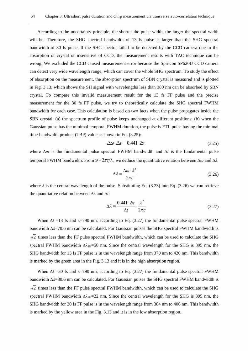
64 Chapter 3: Ultrashort pulse duration and chirp measurement via transverse auto-correlation technique
According to the uncertainty principle, the shorter the pulse width, the larger the spectral width
will be. Therefore, the SHG spectral bandwidth of 13 fs pulse is larger than the SHG spectral
bandwidth of 30 fs pulse. If the SHG spectra failed to be detected by the CCD camera due to the
absorption of crystal or insensitive of CCD, the measurement results with TAC technique can be
wrong. We excluded the CCD caused measurement error because the Spiricon SP620U CCD camera
can detect very wide wavelength range, which can cover the whole SHG spectrum. To study the effect
of absorption on the measurement, the absorption spectrum of SBN crystal is measured and is plotted
in Fig. 3.13, which shows the SH signal with wavelengths less than 380 nm can be absorbed by SBN
crystal. To compare this invalid measurement result for the 13 fs FF pulse and the precise
measurement for the 30 fs FF pulse, we try to theoretically calculate the SHG spectral FWHM
bandwidth for each case. This calculation is based on two facts when the pulse propagates inside the
SBN crystal: (a) the spectrum profile of pulse keeps unchanged at different positions; (b) when the
Gaussian pulse has the minimal temporal FWHM duration, the pulse is FTL pulse having the minimal
time-bandwidth product (TBP) value as shown in Eq. (3.25):
0.441 2t (3.25)
where ∆ω is the fundamental pulse spectral FWHM bandwidth and ∆t is the fundamental pulse
temporal FWHM bandwidth. From 2 λc , we deduce the quantitative relation between ∆ω and ∆λ:
2
2 c
(3.26)
where λ is the central wavelength of the pulse. Substituting Eq. (3.23) into Eq. (3.26) we can retrieve
the quantitative relation between ∆λ and ∆t:
20.441 2
2t c
(3.27)
When ∆t =13 fs and λ=790 nm, according to Eq. (3.27) the fundamental pulse spectral FWHM
bandwidth ∆λ=70.6 nm can be calculated. For Gaussian pulses the SHG spectral FWHM bandwidth is
2 times less than the FF pulse spectral FWHM bandwidth, which can be used to calculate the SHG
spectral FWHM bandwidth ∆λSH=50 nm. Since the central wavelength for the SHG is 395 nm, the
SHG bandwidth for 13 fs FF pulse is in the wavelength range from 370 nm to 420 nm. This bandwidth
is marked by the green area in the Fig. 3.13 and it is in the high absorption region.
When ∆t =30 fs and λ=790 nm, according to Eq. (3.27) the fundamental pulse spectral FWHM
bandwidth ∆λ=30.6 nm can be calculated. For Gaussian pulses the SHG spectral FWHM bandwidth is
2 times less than the FF pulse spectral FWHM bandwidth, which can be used to calculate the SHG
spectral FWHM bandwidth ∆λSH=22 nm. Since the central wavelength for the SHG is 395 nm, the
SHG bandwidth for 30 fs FF pulse is in the wavelength range from 384 nm to 406 nm. This bandwidth
is marked by the yellow area in the Fig. 3.13 and it is in the low absorption region.

Chapter 3: Ultrashort pulse duration and chirp measurement via transverse auto-correlation technique 65
Fig. 3.13 Wrong measurement analysis. The red line: Absorption spectrum of SBN crystal; The green area:
SHG spectral FWHM bandwidth for 13 fs FF pulse; The yellow area: SHG spectral FWHM bandwidth for 30 fs FF
pulse.
Combining the measured absorption spectrum of SBN crystal and the theoretically calculated
SHG spectral FWHM bandwidth, we can safely conclude that the SBN transparent window is the only
restriction for measuring the pulse of 13 fs duration but it has negligible effect on the 30 fs pulse
measurement. However, this is not the limitation of this TAC technique because we can measure
pulses with duration shorter than 13 fs with the same SBN crystal if laser central wavelength is longer
than 800 nm. Another solution is to choose other random nonlinear crystals (e.g. Calcium Barium
Niobate (CBN)) to avoid the absorption when implement the shorter pulse measurement. This TAC
technique can work for any fundamental wavelength within the transparency window of random
nonlinear crystal.
3.3.4 Measurement of a 13 ps pulse
To explore the capability of TAC technique in longer pulse monitoring, we have performed
measurements of pulses in the picosecond regime. As an example, we show in Fig. 3.14 the
measurement of 13 ps (FWHM) pulse. The experiment is performed using a CHEETAH-X Compact
Picosecond Laser (Radiantis Company) operating at 1064 nm central wavelength. This laser source
provides pulses with FWHM duration around 13 ps at a repetition rate of 80.8 kHz with maximum
output power at 13.2 W. The two replicas of the pulse overlapped within the SBN crystal forming
angles +α and –α with respect to the x-axis (external angle α=11.3o and αin=5.1
o). The CCD recorded
TAC trace set along the SBN crystal is shown in Fig. 3.14 (a) and the experimental retrieved unknown

66 Chapter 3: Ultrashort pulse duration and chirp measurement via transverse auto-correlation technique
pulse duration evolution along the SBN crystal is shown in Fig. 3.14 (b), which gives a temporal
FWHM duration of 1.4 ps but not 13 ps.
Fig. 3.14 Experimental data process for the 13 ps pulse. (a) Experimentally recorded TAC trace set along SBN
crystal for pulse with 13 ps pulse duration. (b) The retrieved unknown pulse duration evolution along SBN crystal
with average pulse duration around 1.4 ps.
To find the reason for this wrong measurement, we study the beam superposition process inside
SBN crystal. The schematic diagram is shown in Fig. 3.15. The SH signal is generated from the
volume overlap of the two fundamental beams and the width of the SH emission area ∆z (x=0 mm)
can be expressed as 0 cos inR .
0R is spatial FWHM width of the beam and in is the internal angle
inside the SBN crystal. In this case, the SH emission area ∆z has nothing to do with the TAC trace
FWHM width ∆zAC. This leads to the Eq. (3.22) fail to hold any more. This long pulse case is quite
different with the short pulse case as shown in Fig. 3.5. In this short pulse case, the SH emission area
is defined by the temporal overlap of both pulses and it is related with the spatial TAC trace FWHM
width of ( 2 sin ) ( 2 sin )AC inz Tu Tc , where u and c are the speed of light in the crystal and
vacuum and α is the external angle. This relation is valid for an identical Gaussian pulse with the
intensity FWHM duration T. Since the pulse measurement is directly related with the spatial width of
TAC trace in this technique, the upper limits of this technique is highly related with the crystal size (or
laser beam width) and incident angle. This discussion can be reasonable only for a fixed crystal size
(or laser beam width) or a fixed incident angle.
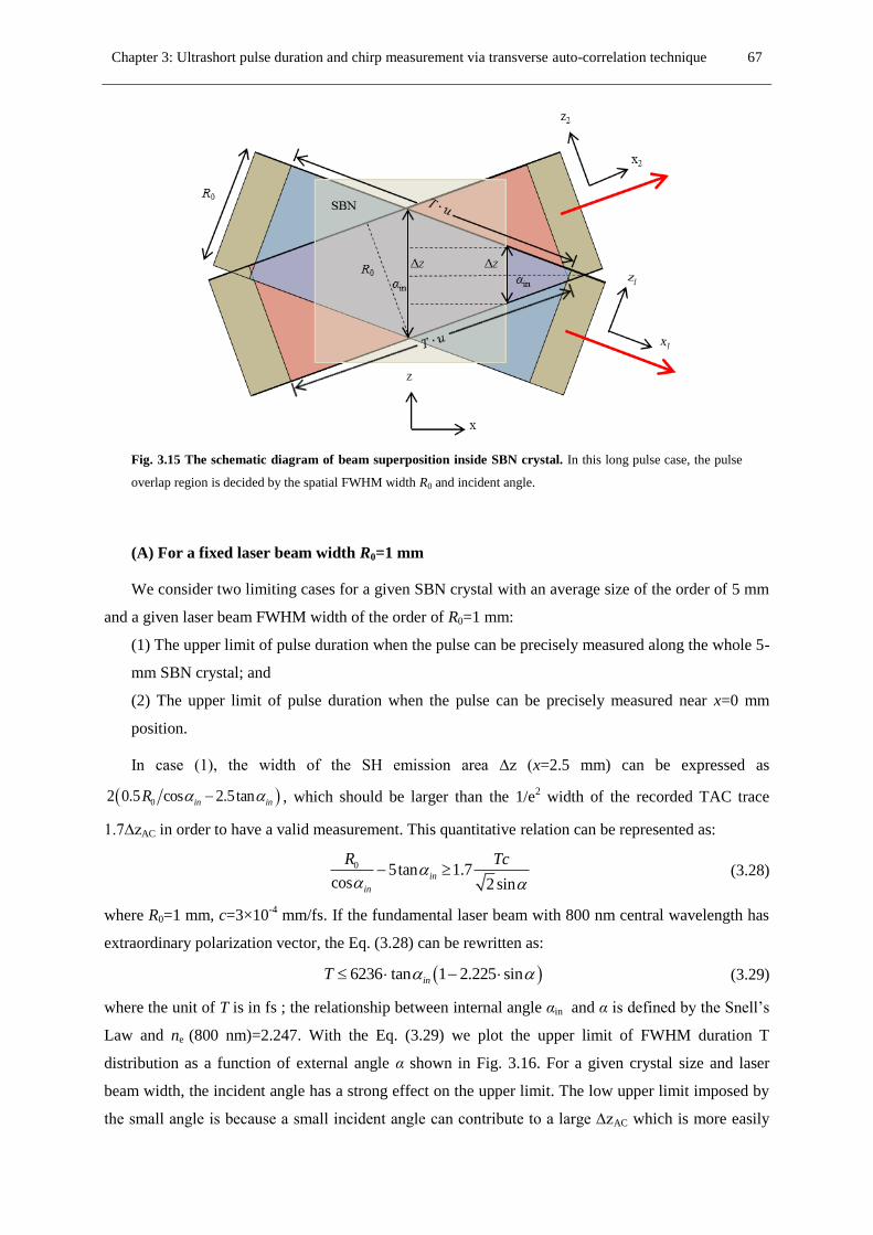
Chapter 3: Ultrashort pulse duration and chirp measurement via transverse auto-correlation technique 67
Fig. 3.15 The schematic diagram of beam superposition inside SBN crystal. In this long pulse case, the pulse
overlap region is decided by the spatial FWHM width R0 and incident angle.
(A) For a fixed laser beam width R0=1 mm
We consider two limiting cases for a given SBN crystal with an average size of the order of 5 mm
and a given laser beam FWHM width of the order of R0=1 mm:
(1) The upper limit of pulse duration when the pulse can be precisely measured along the whole 5-
mm SBN crystal; and
(2) The upper limit of pulse duration when the pulse can be precisely measured near x=0 mm
position.
In case (1), the width of the SH emission area ∆z (x=2.5 mm) can be expressed as
02 0.5 cos 2.5tanin inR , which should be larger than the 1/e2 width of the recorded TAC trace
1.7∆zAC in order to have a valid measurement. This quantitative relation can be represented as:
0 5tan 1.7cos 2 sin
in
in
R Tc
(3.28)
where R0=1 mm, c=3×10⁻⁴
mm/fs. If the fundamental laser beam with 800 nm central wavelength has
extraordinary polarization vector, the Eq. (3.28) can be rewritten as:
6236 tan 1 2.225 sininT (3.29)
where the unit of T is in fs ; the relationship between internal angle αin and α is defined by the Snell’s
Law and ne (800 nm)=2.247. With the Eq. (3.29) we plot the upper limit of FWHM duration T
distribution as a function of external angle α shown in Fig. 3.16. For a given crystal size and laser
beam width, the incident angle has a strong effect on the upper limit. The low upper limit imposed by
the small angle is because a small incident angle can contribute to a large ∆zAC which is more easily
68 Chapter 3: Ultrashort pulse duration and chirp measurement via transverse auto-correlation technique
exceed the width of the SH emission area ∆z. The low upper limit imposed by the large angle is
because a large incident angle leads to the sharp reduced ∆𝑧 which is more easily becomes less than
the ∆zAC. In order to get a large upper limit, the incident angle should be neither too big nor too small.
In this case, the largest upper limit of 313 fs can be obtained when the external angle α=13o.
Fig. 3.16 The upper limit of FWHM duration distribution as a function of external angle. The low upper limit
can be imposed by a small or large incident angle.
In case (2), the width of the SH emission area ∆z (x=0 mm) can be expressed as 0 cos inR , which
should be larger than the 1/e2 width of the recorded TAC trace 1.7∆zAC in order to have a valid
measurement. This quantitative relation can be represented as:
0 1.7cos 2 sinin
R Tc
(3.30)
where R0=1 mm, c=3×10⁻⁴
mm/fs. If the fundamental laser beam with 800 nm central wavelength has
extraordinary polarization vector, the Eq. (3.30) can be rewritten as:
4tan 1.6 10in T (3.31)
where the unit of T is in fs. From the above equation, we can see the 1 picosecond pulse can be
properly measured with this transverse technique if we select the experimental data near the x=0 mm
position. For a given SBN crystal with an average size of the order of 5 mm and a given laser beam
FWHM width of the order of 1 mm, the pulse duration range can be measured is from a couple of tens
of femtoseconds to one picosecond.
(B) For a fixed incident angle
We still consider the above two limiting cases. According to Eq. (3.28) and Eq. (3.30), the
measurement of long pulse duration always need a large laser beam width leading to the demand for
large crystal. The large spatial beam width and the yielded demand for large crystal are the restrictions
for measuring the pulse of 13 ps duration, but this is either not the limitation of this TAC technique
Chapter 3: Ultrashort pulse duration and chirp measurement via transverse auto-correlation technique 69
because such a long pulse still could be measured with this technique if we can find a large enough
crystal to propagate the broaden enough beam.
3.4 Conclusions
In this chapter we experimentally, theoretically and numerically explored the capability of
transverse autocorrelation technique for ultrashort laser pulse characterization.
The autocorrelation signal is given by the noncollinear planar SHG obtained in a random QPM
crystal (in our experiments an SBN crystal). These media have the unique property of emitting the SH
in a plane, perpendicular to the optical axis, when a fundamental beam propagates perpendicular to the
optical axis. The so-called transverse SHG is the SHG in the direction transverse to the propagation of
the fundamental beam.
By imaging the transverse SHG with respect to the pulse propagation we can record the AC trace
at the entrance of the crystal, which allows the measurement of the undistorted pulse duration. We
demonstrate that this technique can be implemented to the measurement of the temporal duration of
pulses between 22 fs and 1ps. However, this temporal window can be significantly enlarged by
replacing the SBN crystal with other random nonlinear crystals with a larger transparency window or
by working at longer wavelengths as explained in sections 3.3.3 and 3.3.4.
When a laser pulse propagates in a dispersive material it will be enlarged or compressed due to the
dispersion of the material and consequently the width of the AC trace will be modified. The
measurement of the AC trace evolution along the material gives information about the initial chirp
parameter of the pulse. For our interested pulse duration and propagation distance, the pulse duration
evolution along the material is modified by the combination effect of initial chirp and GVD. In normal
GVD regime (g > 0), If C < 0, the pulse will be compressed until the different frequency components
are in phase and the pulse acquires its minimum FWHM duration (Tmin). This minimum pulse duration
occurs at the maximum compression distance xmin. In the case of anomalous GVD regime (g < 0), the
similar phenomenon happens if C > 0. The value of initial chirp, C, and initial pulse duration (FWHM),
T0, can be deduced from xmin and Tmin.
With the TAC trace simulation model and experimental retrieved initial chirp and pulse duration
we simulated the TAC trace set and the corresponding pulse duration evolution curve, which have a
good match with the experimental results. We studied phase changing during pulse propagation and
simulated the temporal and spectral phase evolution along the crystal. Several different Gaussian
pulses over a broad initial chirp range were measured and the corresponding simulation results had
good match with experimental data.
As an important characteristic, the property of automatic PM without angular alignment or
temperature control makes the technique extensive to a very broad wavelength range and enormously

70 Chapter 3: Ultrashort pulse duration and chirp measurement via transverse auto-correlation technique
simplifies the operation process. In this chapter we worked on the Gaussian pulses but this TAC
technique is also suitable for measuring the non-Gaussian pulse chirp and duration evolution along the
crystal. This technique can be also used for real time monitoring of the chirp content at the
measurement position. Besides, in this technique the transverse emission of SHG removes the
requirement of thin nonlinear crystals and enables one to measure the undistorted pulse at the entrance
of the crystal.

Chapter 4
Ultrashort pulse duration and shape
measurement via transverse cross-
correlation technique
4.1 Introduction
In Chapter 3 we explored the intensity TAC techniques, as a simple and effective single-shot
method that can be used to measure the temporal duration and chirp parameter of pulses with duration
from hundreds of femtoseconds down to a couple of tens of femtoseconds [Tru15, Rop13, Wan10,
Tru09]. As the conventional intensity AC technique, our TAC method fails to measure the temporal
pulse shape, since in this technique the pulse is overlapped with its replica leading to the symmetric
distribution of the TAC trace. AC technique only can be used to characterize temporal pulse duration
of pulses with an already known pulse shape. Hence, cost-effective and simple methods of
measurement the pulse shape are still of potential interest. Different techniques have been proposed
and extensively adopted for temporal shape characterization [Die85, Aus71, Pri06, Liu02, Tre97,
Kan93, Alo10]. Cross-correlation (CC) and single-shot cross-correlation (SCC) [Ber04, Tun03] are
well-known techniques for the measurement of pulse temporal shape. Besides, more sophisticated
techniques, e.g., XFROG (cross-correlation FROG) which can be used for complete characterization
of optical pulses both in frequency and time domains [Gu02, Dud02, Akt03, Pal10]. Since these
methods depend on the detection of the SHG, the demand of thin crystals, the critical phase matching
(PM) angle and temperature tuning make them far from user-friendly. Since these sophisticated

72 Chapter 4: Ultrashort pulse duration and shape measurement via transverse cross-correlation technique
techniques are basically variants of the intensity CC measurement principle, it is necessary to review
this technique.
In the intensity CC technique, the temporal profile of unknown signal, Is(t), can be determined by
using a narrow temporal gate that can progressively sample the evolution of the pulse at discrete time
segments, by varying their relative timing. This process corresponds to measuring a convolution of the
unknown signal with the narrow temporal gate which is also called reference signal, Iref(t). The optical
configuration of the intensity CC is shown in Fig. 4.1 (a). An adjustable optical delay, , is
introduced into the unknown signal and reference signal. When the two delayed signals are
recombined within the SHG crystal, with sufficient intensity and proper phase matching over the
entire bandwidth of the two signals, a new optical signal is generated and its electric field is given by
s refE t E t . The function of the SHG crystal in this process is to multiply the spatial overlap
region of the two signals. The second-order intensity CC function uses the lowest-order nonlinear
process available, and therefore operates at the lowest power possible for a nonlinear process.
Separation of the generated new signal from the independent mixing of the input signals is ensured by
the noncollinear geometry. The energy of the generated signal is measured with a integrating detector
and is recorded as a function of the relative delay between the input signals, which composed the
intensity CC trace. The ( )CCI data, shown in Fig. 4.1 (b), consists of a one-dimensional array of
numbers representing the generated new signal energy as a function of the delay, which is related to
the input field by:
2
CC s ref s refI E t E t dt I t I t dt
Fig.4.1 Intensity cross-correlator. (a) Schematic representation of the intensity CC. (b) the intensity CC trace
calculated by different temporal delay τ.

Chapter 4: Ultrashort pulse duration and shape measurement via transverse cross-correlation technique 73
In an ideal case, if the reference signal is infinitely short compared to the unknown signal to be
characterized, the unknown temporal profile can be precisely determined by a CC measurement. As
the reference signal duration increases, the CC function will start to temporally smear and the
instrumental temporal resolution will decrease. With a prior knowledge of the temporal shape of the
reference signal, a deconvolution can extract the unknown temporal profile, corresponding to the
unknown signal. The deconvolution process fidelity relies on the assumed temporal shapes and the
degree that the reference signal is known. In practice, the reference signal has to be considerably
shorter than the pulse to be characterized and both pulses must be well overlapped, avoiding temporal
jitter during the temporal delay scan. When the first condition cannot be fulfilled, accurate knowledge
of the reference signal is necessary for a high-fidelity deconvolution.
As an extension of the TAC technique, TCC technique is also implemented using a non-collinear
SHG geometry. When the reference pulse and the unknown pulse represented by the red and blue
rectangles in Fig. 4.2 intersect inside the SBN crystal, different overlap regions are automatically
formed at different positions. During the second-order parametric process, the nonlinear crystal
multiplies the overlapped pulse and emits the TCC signal in the form of the TSHG, which is result
from the non-collinear second-order nonlinear interaction between the two pulses. The TCC technique
captures the SHG signal at 90o with respect to the propagation direction of the input beams and it
allows for single-shot measurement of the TCC profile evolution as a function of the propagation
distance inside the crystal. This technique can be used for the determination of the temporal shape and
duration evolution of the unknown pulse. As mentioned in Chapter 1, the three advantages in the
RQPM processes are also applied to the TCC technique.
Fig. 4.2 The non-collinear SHG geometry for the implementation of TCC measurement. Interaction of the
reference pulse and the unknown pulse in SBN crystal composed the TCC profile.
In this chapter, we are committed to the study of the transverse cross-correlation (TCC) technique
based on the detection of the TSHG signal resulting from the non-collinear interaction of an unknown

74 Chapter 4: Ultrashort pulse duration and shape measurement via transverse cross-correlation technique
pulse with the reference pulse in SBN crystal. We extended the theoretical model to include the beam
width of the pulses. We experimentally explored the effect of beam width and incidence angle on the
measurement error of this TCC technique in the characterization of pulses of the order of femtosecond
and picosecond.
4.2 Experimental setup and theoretical model
4.2.1 Experimental setup
The experimental setup is schematically shown in Fig. 4.3 (a). The laser pulse is splitted into two
replicas via a 50/50 beam splitter (BS1). One of the replicas serves as reference pulse (R) while the
second one passes through the “unknown pulse generator”. Since we want to explore and prove the
capability of our technique in temporal pulse shape measurement, we designed a controllable
“unknown pulse generator” based on the Michelson-type configuration. It provides the controlled
double pulses by overlapping two temporally delayed Gaussian pulses A and B. The temporal
separation between pulse A and pulse B, Tsep, is controlled by the M1 mirror's spatial offset distance,
Dsep. Mirror M1 is mounted on a motorized linear translation stage with 0.1 μm step resolution.
Tsep=2Dsep/c, where c is the speed of light. The two fields of pulse A and pulse B giving rise to the
unknown pulse (U). The unknown pulse and the reference pulse compose the two fundamental beams
in the nonlinear parametric processes, which propagate in the x-z plane of SBN crystal forming angles
+α and –α with respect to the x-axis. The polarization and transmission of the two fundamental beams
can be controlled by the combination of polarizer (P) and half-wave plate (HW). The polarization
vectors of both fundamental beams are chosen to be extraordinary, being directed along the
crystallographic axis z in our setup. The function of cylindrical lens (C) is compressing the two
fundamental beams along y direction but keeping pulse spatial shape unchanged along z direction,
which increases the pulse intensity without inducing any measurement error because in the setup the
part can contribute to the spatial TCC trace is the spatial shape along z direction which is undistorted
after passing through the cylindrical lens. An adjustable optical delay between unknown pulse and
reference pulse is also inserted into one of the arms by the Delay Control 1 element. When the delay (τ)
of the two optical path is zero, the nonlinear interaction of the two fundamental beams inside the SBN
crystal gives rise to three well-differentiated SH emissions, which compose the total signal: two of
them are corresponding to the conical SH emission from each individual beam; the middle one is the
TSHG from the non-collinear interaction between unknown pulse and reference pulse. When the delay
of the two optical path τ≠0 (to get a clean background signal the delay τ>>TR, where TR is reference
pulse duration), the nonlinear interaction only gives rise to the two conical SH emissions, which
compose the background signal. In order to record only the TCC trace one needs to subtract the
background signal from the total signal.

Chapter 4: Ultrashort pulse duration and shape measurement via transverse cross-correlation technique 75
Fig. 4.3 Experimental setup. (a) Schematic representation of the TCC setup. P—polarizer, BS1, BS2—beam
splitter, M1, M—mirror, HW—half-wave plate, C—cylindrical lens; (b) CCD recorded image of the TCC trace
profile at different propagation distances (x0, x1…xn) constitute the TCC trace set.
A CCD camera, placed above the crystal, is used to record the image of the spatially resolved total
signal when τ=0 and the background signal when τ>>TR. The TCC trace evolution along the whole
propagation distance within the crystal can be obtained with the background subtraction method. This
TCC trace gives the spatial CC profile at different propagation distances (x0, x1…xn) shown in the Fig.
4.3 (b). Each TCC trace profile ICC (z) is directly related to the temporal intensity CC profile ICC (t). To
retrieve the temporal CC trace profile from the corresponding recorded spatial TCC trace set, a space-
time decoding factor for mapping the spatial information to temporal information must be applied.
Since the intensity of TCC signal ICC(t) composed by the reference pulse IR(t) and the unknown pulse

76 Chapter 4: Ultrashort pulse duration and shape measurement via transverse cross-correlation technique
IP(t) can be mathematically represented by their convolution, the unknown pulse IP(t) can be
reconstructed with Eq. (4.1) if we assume the reference temporal profile is already known.
1 ( ( ))( )
( ( ))
CCp
R
I tI t
I t (4.1)
The CCD imaging system in TCC technique is the same with the one we used in Chapter 3. It is also
constituted by a camera lens and CCD camera.
4.2.2 TCC trace theoretical model
In the simulation we consider the reference pulse and the unknown pulse propagating in the
crystallographic plane x-z of an SBN crystal with the angles −α and +α with respect to the x-axis as
shown in Fig. 4.3. All the parameters used in the simulation were from the experimental results.
In Chapter 3 we discussed two extreme situations: (1) when pulse duration is short enough as
shown in Fig. 3.5, the spatial TAC trace width is decided by pulse duration and incident angle and the
spatial TAC trace width is the direct mapping of the temporal pulse duration for a particular incident
angle; (2) when pulse duration is long enough as shown in Fig. 3.15, the spatial TAC trace width is
decided by beam width and incident angle and the spatial TAC trace width has nothing to do with the
temporal pulse duration. These two extreme situations also apply to the TCC technique. However, the
pulse duration we measured in this chapter is either too short or too long, which introduces a third
situation between the two extreme situations as shown in Fig. 4.4. In this situation, the error-free TCC
trace is only restricted in particular area, where the spatial TCC trace width is decided by pulse
duration and incident angle as shown at position A and position B; At position C the spatial TCC trace
width is limited by the beam width and incident angle giving a wrong estimation of pulse information.
Fig. 4.4 The schematic diagram of beam superposition inside SBN crystal. As beams propagate, the TSHG
emission region moves along x axis giving rise to the recorded TCC trace set.

Chapter 4: Ultrashort pulse duration and shape measurement via transverse cross-correlation technique 77
In order to model the TCC trace properly, we extended the TAC trace simulation model to include
the spatial width of the electric field. In the experimental setup, the only part that can contribute to the
spatial TCC trace is the spatial shape along z direction. Therefore, in the new model the reference and
unknown pulses at x1=x2=0 mm can be written as:
2211
1 1 102 2
0 0
1, 0 exp exp
22 2 ln 2 2 ln 2
t x uz iCE t x E
R T
(4.2)
2
2
201 2
2 02
2 2 22
02
202 2
0
1exp
2 2 ln 2
, 0 exp
2 2 ln 21
exp2 2 ln 2
sep
t x uiCE
Tz
E t x
R t T x uiCE
T
(4.3)
where C is the initial chirp parameter, u is the speed of light in the crystal, T0 is the initial full-width-
half-maximum (FWHM) duration of output laser pulse.
According to Eq.(3.3)-Eq.(3.8), after propagate x1 and x2 distance inside the SBN crystal, the electric
fields of the two fundamental replicas at x1 and x2 position can be written as:
221101
1 1 12 21 4
10 0 1
, exp exp exp( ( ))
2 2 ln 2 2 2 ln 2
t x uEzE t x i t
FR T F
(4.4)
2
2201
21 4
22 0 22
2 2 222
02202
21 4
20 2
exp
2 2 ln 2
, exp exp( ( ))
2 2 ln 2
exp
2 2 ln 2
sep
t x uE
F T Fz
E t x i t
R t T x uE
F T F
(4.5)
where the expression of F1 and F2 are written as shown in Eq.(3.7)-Eq.(3.9); g=476 fs2/mm is the
group velocity dispersion (GVD) for SBN crystal at 800 nm central wavelength.
We can see from Eq. (3.9) LD is around 25 mm for the reference pulse of 180-fs duration, which
means the material dispersion induced pulse lengthening or compressing can be ignored. To simplify
the simulation, the phase terms are ignored in Eq. (4.4) and Eq. (4.5). It is because the phase term has
no contribution to the intensity of TCC trace at particular position in this model. Eq. (3.10) and Eq.
(3.11) are used to change the variables to a common reference system. We consider the ee-e
interaction is phase-matched and then the recorded TCC trace profile evolution can be simulated by:
33CC R PI t d I I t d
(4.6)
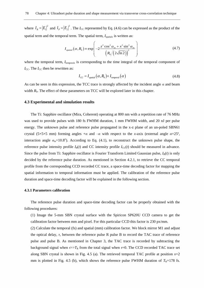
78 Chapter 4: Ultrashort pulse duration and shape measurement via transverse cross-correlation technique
where 2
1RI E and 2
2PI E . The ICC represented by Eq. (4.6) can be expressed as the product of the
spatial term and the temporal term. The spatial term, Ispatial, is written as:
2 2 2 2
0 2
0
cos sin, exp 2
2 ln 2
in inspatial
z xI R
R
(4.7)
where the temporal term, Itemporal, is corresponding to the time integral of the temporal component of
ICC. The ICC then be rewritten as:
0,CC spatial temporalI I R I
(4.8)
As can be seen in this expression, the TCC trace is strongly affected by the incident angle α and beam
width R0. The effect of these parameters on TCC will be explored later in this chapter.
4.3 Experimental and simulation results
The Ti: Sapphire oscillator (Mira, Coherent) operating at 800 nm with a repetition rate of 76 MHz
was used to provide pulses with 180 fs FWHM duration, 1 mm FWHM width, and 20 nJ per pulse
energy. The unknown pulse and reference pulse propagated in the x-z plane of an un-poled SBN61
crystal (5×5×5 mm) forming angles +α and –α with respect to the x-axis (external angle α=25º,
interaction angle αin=10.8o). According to Eq. (4.1), to reconstruct the unknown pulse shape, the
reference pulse intensity profile IR(t) and CC intensity profile ICC(t) should be measured in advance.
Since the pulse from Ti: Sapphire oscillator is Fourier Transform Limited Gaussian pulse, IR(t) is only
decided by the reference pulse duration. As mentioned in Section 4.2.1, to retrieve the CC temporal
profile from the corresponding CCD recorded CC trace, a space-time decoding factor for mapping the
spatial information to temporal information must be applied. The calibration of the reference pulse
duration and space-time decoding factor will be explained in the following section.
4.3.1 Parameters calibration
The reference pulse duration and space-time decoding factor can be properly obtained with the
following procedures:
(1) Image the 5-mm SBN crystal surface with the Spiricon SP620U CCD camera to get the
calibration factor between mm and pixel. For this particular CCD this factor is 230 px/mm.
(2) Calculate the temporal (fs) and spatial (mm) calibration factor. We block mirror M1 and adjust
the optical delay, τ, between the reference pulse R pulse B to record the TAC trace of reference
pulse and pulse B. As mentioned in Chapter 3, the TAC trace is recorded by subtracting the
background signal when τ>>TR from the total signal when τ=0. The CCD recorded TAC trace set
along SBN crystal is shown in Fig. 4.5 (a). The retrieved temporal TAC profile at position x=2
mm is plotted in Fig. 4.5 (b), which shows the reference pulse FWHM duration of TR=178 fs.

Chapter 4: Ultrashort pulse duration and shape measurement via transverse cross-correlation technique 79
Besides the reference pulse duration can be calibrated with this TAC measurement, the calibration
factor between the spatial (mm) and temporal (fs) domains can be calculated with Eq. (3.2).
(3) Combining the procedures (1) and (2), we finally get the space-time decoding factor between
pixel and fs of 19.4 fs/pixel (1 pixel equal to 19.4 fs), which can be directly used to map the CCD
recorded CC spatial profile to the CC temporal profile in this particular configuration.
Fig. 4.5 TAC measurement for parameter calibration. (a): The CCD recorded TAC trace set along 5 mm SBN
crystal; (b): The temporal TAC profile at x=2 mm.
To calibrate the unknown pulse generator we should find the ‘zero-delay position’ of M1 to make
pulse A and pulse B have zero delay. This zero delay calibration of pulses A and B was obtained by
scanning mirror M1 until the CCD recorded TAC trace formed by the reference pulse R and pulse A
completely overlapped with the CCD recorded TAC trace formed by reference pulse R and pulse B.
After this calibration the temporal separation between pulse A and pulse B can be precisely controlled
by the M1 mirror's spatial offset from this ‘zero-delay position’.
4.3.2 Pulse shape measurement
After calibrate the reference pulse duration, space-time decoding factor, and zero delay of pulses
A and B, in this section we will explain the pulse shape measurement procedure. We generated and
measured several “unknown” pulses. For the first “unknown” pulse the delay between the two sub-
pulses A and B, Tsep, was precisely adjusted and set to 300 fs [Tsep=300 fs]. The experimental results
are presented in Fig. 4.6.
The experimental recorded TCC trace set formed by the reference pulse and the unknown pulse
with Tsep=300 fs is shown in Fig. 4.6 (a). The temporal TCC profile at the position x=2 mm is retrieved
using the CCD recorded ICC(z) and the space-time decoding factor, which is shown by the blue dots in
Fig. 4.6 (b), where the two-peaked asymmetric CC trace can be clearly seen. The continuous red curve
in Fig. 4.6(b) is the fitted temporal CC profile. The unknown pulse temporal profile can be retrieved
by deconvolution between the experimental data ICC(t) and the reference pulse IR(t) using Eq. (4.1).
However, a direct use of the discrete experimental data leads to the appearance of oscillations in the

80 Chapter 4: Ultrashort pulse duration and shape measurement via transverse cross-correlation technique
profile of the retrieved signal. To retrieve a smooth unknown pulse temporal profile we have used the
following procedures:
1) Obtain a fit of the temporal CC profile in order to get a smooth function of ICC(t);
2) Obtain a fit of the reference pulse;
3) Use the fitting functions to obtain the unknown pulse temporal profile with Eq. (4.1). The
fitting function we used for the CC data corresponds to a superposition of two Gaussian functions
as follows:
2200
2 2(2 ln 2))
( )( )( ) e
(2xp exp
( ( ln 2)) cc cc
sepcc
CC A BT T
t t Tt tI t I I
(4.9)
where Tsepcc is the temporal pulse separation and Tcc is the individual pulse duration at FWHM in
intensity.
The red curve in Fig. 4.6(b) shows the well fitted temporal CC profile with Tcc=250 fs and Tsepcc=299
fs. From the previous measurement, the reference Gaussian pulse can be expressed as below:
2
0
2
(
(2 ln 2
)
)) ( ) exp
(R
RT
t tI t
(4.10)
where TR=178.5 fs.
Applying the deconvolution procedure with Eq. (4.9) and Eq. (4.10) we retrieved the unknown pulse
profile shown by the salmon area in Fig. 4.6 (c). The black curve in Fig. 4.6(c) is the corresponding fit
function which is represented by Eq. (4.1):
2222
2 2
( )( )( ) exp exp
( (2 ln 2)) ( (2 ln 2))
sepP
P C D
P P
t T x ut x uI t I I
T T (4.11)
where TsepP is unknown pulse peak separation and TP is the temporal duration of each individual
Gaussian pulse at FWHM in intensity. The fitted values are TsepP=299 fs and TP=175 fs. These values
are in very close agreement with the corresponding values set by the unknown pulse generator, Tsep
=300 fs and T=178.5 fs.
An estimated error ε between the experimental retrieved values, [TsepP=299 fs, TP=175 fs], and their
counterparts set by the unknown pulse generator, [Tsep=300 fs, T=178.5 fs], is calculated with the
following expression:
2 2
2 2
sep
sepP sep PT T T T
T T
(4.12)
where the calculated error is 1.9%. In order to intuitively display the measurement error, the original
“unknown” pulse composed by pulse A and pulse B is plotted by the continuous blue curve in Fig. 4.6
(c).
This transverse single-shot technique permits to observe the evolution of the CC trace (transverse
profile in z direction) along the propagation distance (x direction), which can be used to retrieve the

Chapter 4: Ultrashort pulse duration and shape measurement via transverse cross-correlation technique 81
unknown pulse temporal shape and duration and their evolutions along the crystal. Fig. 4.6 (d) shows
the evolution of unknown pulse duration along the 5 mm SBN crystal, corresponding to a stable
FWHM duration of ~471 fs.
Fig. 4.6 Experimental result for the first measured pulse with [T=178.5 fs, Tsep=300 fs]. (a): The CCD
recorded TCC trace set along SBN crystal; (b): ICC(t), the experimentally measured temporal TCC trace profile at
x=2 mm (blue dots), the corresponding fit function (continuous red curve). (c): IP(t), the experimentally retrieved
unknown pulse profile (salmon area), the corresponding fit function (continuous black curve), and the original
“unknown” pulse (continuous blue curve); (d): The retrieved unknown pulse duration evolution along SBN crystal.
For this few hundred of femtoseconds pulse the effect of the material dispersion is not obvious, so
the shape of pulse should remain unchanged during propagation along the 5-mm SBN crystal and the
spatial TCC trace profile as well, however Fig. 4.6 (a) shows the experimental recorded TCC trace set
has a distortion at both ends of the crystal and the corresponding error-free area is only restricted
between x=1 mm and x=2 mm of the crystal. This distorted TCC trace profile evolution can be
explained by Fig. 4.4: A long pulse yields a large spatial overlap region shown by the blue rectangle
area; in our measurement the blue rectangle area exceeds the laser beam overlap region at the both
ends of the crystal, which leads to the error-free area is restricted between x=1 mm and x=2 mm of the
crystal.

82 Chapter 4: Ultrashort pulse duration and shape measurement via transverse cross-correlation technique
Since the laser pulse from Ti: Sapphire oscillator (Mira, Coherent) in this measurement is the FTL
pulse, the chirp parameter C=0. With the experimentally retrieved reference pulse duration [TR=178.5
fs], unknown pulse parameters [TsepP=299 fs, TP=175 fs], and the experimental value of beam width
[R0=1 mm], we substituted Eq. (4.4) and Eq. (4.5) into Eq. (4.6) and finally plotted the spatial TCC
trace set along SBN crystal, which is shown in Fig. 4.7 (a). The values of E10, E201, and E202 are
retrieved from the CCD recorded TAC and TCC intensity distribution. The temporal TCC profile at
the position x=2 mm is retrieved using the corresponding ICC(z) and the space-time decoding factor,
which is shown by the blue dots in Fig. 4.7 (b), where the two-peaked asymmetric CC trace can be
clearly seen. The continuous red curve in Fig. 4.7 (b) is the fitted temporal CC profile. The unknown
pulse temporal profile can be retrieved by deconvolution between the ICC(t) and the reference pulse
IR(t) with Eq. (4.1). The retrieved unknown pulse is shown by the salmon area in Fig. 4.7 (c). The
black curve in Fig. 4.7 (c) is the fit function of IP(t). The simulated unknown pulse duration evolution
is plotted in Fig. 4.7 (d), which is around 471 fs during propagation along the 5-mm SBN crystal.
These simulation results are in very close agreement with the experimental results.
Fig. 4.7 Simulation result for the first measured pulse with [T=178.5 fs, Tsep=300 fs]. (a): The simulation of the
spatial TCC trace set along SBN crystal; (b): ICC(t), the temporal TCC trace profile at x=2 mm (blue dots) and the
corresponding fit function (continuous red curve); (c): IP(t), the retrieved unknown pulse profile (salmon area) and
the corresponding fit function (continuous black curve); (d):The retrieved unknown pulse duration evolution along
SBN crystal.

Chapter 4: Ultrashort pulse duration and shape measurement via transverse cross-correlation technique 83
With the same setup we generated four different “unknown” pulses marked as A, B, C, and D by
setting Tsep to 200 fs, 267 fs, 367 fs, and 1333 fs. Fig. 4.8 (a1, b1, c1, d1) shows the CCD recorded
TCC trace set along the 5 mm SBN crystal for each case. The corresponding temporal CC signals
selected at x=2 mm position are shown by the blue dots in Fig. 4.8 (a2, b2, c2, d2) together with the
fitted curves shown by the continuous red curve. The retrieved unknown pulses are shown by the
salmon area in Fig. 4.8 (a3, b3, c3, d3), which give the unknown pulse peak separation, TsepP, and the
temporal duration of each individual Gaussian pulse, TP. The measurement results for each pulse are
as following:
A [TsepP =203.7 fs, TP =185.7 fs], B [TsepP =269.7 fs, TP =176.9 fs]
C [TsepP =367.1 fs, TP =177.5 fs], D [TsepP =1206.7 fs, TP =169.4 fs]
Fig. 4.8 Comparison of experimental and simulation result. (a1, b1, c1, d1) The CCD recorded TCC trace set
along SBN crystal for unknown pulses A, B, C, and D; (a2, b2, c2, d2): The experimentally measured temporal
TCC trace profile at x=2 mm (blue dots) and the corresponding fit function (continuous red curve); (a3, b3, c3, d3):
The experimentally retrieved unknown pulse profile (salmon area) and the corresponding fit function (continuous
black curve; (a4, b4, c4, d4): the simulated TCC trace set along SBN crystal.

84 Chapter 4: Ultrashort pulse duration and shape measurement via transverse cross-correlation technique
The errors calculated by Eq. (4.12) are 4.4%, 1.4%, 0.6% and 10.8% respectively. For the few
hundred of femtoseconds pulse the error can be less than 5%, while for the picosecond pulse the
corresponding error can increase up to 10%. Again, because of the large pulse duration induced large
dispersion length, the pulse temporal shape and duration evolution in each case remains constant.
However, because of the long pulse duration induced large pulse overlap region, the experimental
recorded error-free TCC trace for each case is restricted between x=1 mm and x=2 mm of the crystal
as shown in Fig. 4.8 (a1, b1, c1, d1). With the experimentally retrieved reference pulse duration,
unknown pulse parameters [TsepP, TP], and the experimental value of beam width [R0=1 mm] and
incident angle, we substituted Eq. (4.4) and Eq. (4.5) into Eq. (4.6) and finally simulated the spatial
TCC trace set along SBN crystal shown in Fig. 4.8 (a4, b4, c4, d4), which is in good agreement with
the experimental result for each case.
4.3.3 Effect of R0 and α on the pulse reconstruction
As summarized in Chapter 3, the SBN transparency window is the restriction for measuring pulses
with duration less than a couple of tenths of femtosecond. In the opposite case of long pulses the factor
that cannot be overlooked in order to obtain a valid measurement is the effect of the beam width on the
recorded trace. In order to consider this effect we should study the effect imposed by the spatial and
temporal contributions to the resulting cross-correlation term given in Eq. (4.8).
To check the relevance of this effect in our particular configuration, we should consider the beam
size relative to the pulse duration. We find two extreme situations: when the condition TR/R0 <<tanα/c
holds (R0 is the spatial FWHM beam width in intensity, for our laser beam R0=1mm) the ICC provides
the direct mapping of the temporal pulse shape, with no limitation imposed by the finite beam size. In
the case TR/R0 >>tanα/c, the CCD recorded TCC trace sequence, ICC, does not give a proper mapping
of the temporal pulse shape because the beam size limits the overlapping region. Due to the duration
of our pulses we need to consider these effects in our actual setup
When TP/R0 << tanα/u, the spatial part can be safely approximated by 1 and the ICC is decided
solely by Itemporal which is the direct mapping of the temporal pulse shape. When TP/R0 >> tanα/u, the
TCC trace sequence ICC is strongly affected by Ispatial. As can be seen in Eq. (4.8), the influences of
this term will depend strongly on the incident angle of the overlapping beams.
In order to further analyze the effect of the incident angle and beam width on the TCC trace, we
simulated the particular case where TR=180 fs; TP=180 fs; Tsep=300 fs; IC/ID =0.8. The simulated
Itemporal, Ispatial and ICC traces for case A [α=12o, R0 =0.8 mm], case B [α=30
o, R0 =0.3 mm], and case C
[α=30o, R0 =0.8 mm] are shown in Fig. 4.9. The plots in the first column, (a1, b1, c1), show the
temporal CC of the pulse with no spatial contribution for two different incident angles 12º (a1) and 30º
(b1, c1). The Itemporal trace set corresponds to the blue rectangle area in Fig. 4.4, which represents the

Chapter 4: Ultrashort pulse duration and shape measurement via transverse cross-correlation technique 85
error-free CC trace evolution. Since the same pulses are used in these three cases, the width of Itemporal
trace along z-axis is decided by the incident angle. The effect of incident angle on the width of Itemporal
trace can be described as: the larger the incident angle, the narrower the width. Temporal broadening
is not observed during propagation due to the long pulses used in the simulation (notice that for such
pulse durations the group velocity dispersion length is LD=190 mm for the cross-correlation signal).
The plots in the second column, (a2, b2, c2), show the Eq. (4.7) represented spatial term, Ispatial, for
case A, B, and C. The finite size of the beam leads to a strong reduction of the overlapping region, so
the TCC trace remains unchanged only at a particular region where Ispatial is approximately 1. The
effect of the spatial part depends strongly on the beam diameter and incidence angle. The width of
Ispatial trace along z-axis is decided by the size of beam width. The length of Ispatial trace set along x-axis
is decided by the incident angle. The third column, (a3), (b3) and (c3) show the complete TCC trace
set, ICC, given by the product of Itemporal and Ispatial as shown in Eq. (4.8), which corresponds to the CCD
recorded TCC trace set in the measurement. In order to deduce the measurement error, we need
expand the beam width to get a wide enough Ispatial trace and increase the incident angle to get a
narrow enough Itemporal trace, but loss of length of ICC trace set is the price we must pay for error-free
measurement. The plots in the last column show the TCC trace profile at the position indicated by the
dashed white line of Itemporal (red line) and ICC (blue dots) for each one of the situations. As we can see
in plot (a4), a too small angle is limiting the capability to record properly the TSCC trace sequence so
the blue dots do not match the temporal CC signal given by the red line. For the case of plot (b4), a too
small beam size leads to a narrow Ispatial component, which also leads to a failure in the TCC
reconstruction. As the pulses to be measured become longer, one should increase the incident angle
or/and expand the beam size to get an error-free TCC trace set. The plot in (c4) shows that if the
conditions of beam size and incidence angle are adequate one can properly record the proper CC trace.
When using this TCC technique to implement pulse characterization, the experimental values of
incident angle and beam width should be carefully selected according to the above considerations in
order to properly record the TCC trace profile. As the pulse to be measured with duration in the range
between a few hundreds of femtoseconds and a couple of picoseconds, one should increase the
incident angle or / and expand the beam width to get an error-free TCC trace but at the expense of
length of ICC trace set. The previous conclusion that the measurement error increases when the
unknown pulse duration increases as shown in Fig. 4.8 could be due to the fact that the increased pulse
duration induced the higher demand for incident angle and beam width.

86 Chapter 4: Ultrashort pulse duration and shape measurement via transverse cross-correlation technique
Fig. 4.9 The simulation of the effect of the incident angle and beam width. Simulation of the temporal term of
the ICC trace: (a1) Itemporal (α=120, R0=0.8 mm); (b1) Itemporal (α=300, R0=0.3 mm); and (c1) Itemporal (α=300, R0=0.8
mm). Simulation of the spatial term of the ICC trace: (a2) Ispatial (α=120, R0=0.8 mm); (b2) Ispatial (α=300, R0=0.3
mm); and (c2) Ispatial (α=300, R0=0.8 mm). Total TCC trace set, ICC, for each cases [(a3), (b3) and (c3)]. TCC trace
profile at the position of the dashed line for Itemporal (red curve) and ICC (blue dots) [(a4), (b4) and (c4)].
From the plot in Fig. 3.16, we can see this transverse technique can be used to measure pulses
with duration around a couple of hundred femtoseconds when the incident angle is between 5o and 20
o.
However, in this chapter we extended the measurement capability to a couple of picoseconds by
considering the combination effect of incident angle and beam width. Besides, another important trick
is to restrict the error-free TCC trace in particular area and the loss of length of ICC trace set wins the
possibility of measuring longer pulses.

Chapter 4: Ultrashort pulse duration and shape measurement via transverse cross-correlation technique 87
4.3.4 Explore the initial chirp parameter retrieve
In the previous section, the laser pulse from Ti: Sapphire oscillator (Mira, Coherent) is Gaussian
shaped pulse with FWHM duration around 180 fs. For such a long pulse, the material dispersion
induced pulse broadening can be ignored and the initial chirp induced pulse broadening and changing
of pulse shape during propagation inside SBN crystal are not large enough to be used to detect the
chirp parameter. Therefore, the effect of pulse chirping on pulse evolution has not been studied with
this TCC technique so far.
To explore the capability of initial chirp parameter retrieval using this TCC technique, we resort to
the simulation of the evolution of TCC trace for short pulses with duration less than 100 fs. In the
simulation the reference pulse and unknown pulse at x=0 mm and x﹥0 mm position can be expressed
by Eq. (4.2, 4.3) and Eq. (4.4, 4.5), where T0=96 fs, Tsep=100 fs, E201/E202=0.9, α=15o and R0 =2 mm.
Three different chirp values are used to distinguish the three different unknown pulses A, B, and C.
The corresponding chirp parameter for each unknown pulse is: pulse A [C=-1], pulse B [C=-2.8], and
pulse C [C=-5]. Because of the appropriately selected incident angle and beam width for this particular
pulse duration, the simulated spatial ICC trace set along the 5 mm SBN crystal is the direct mapping of
the temporal CC trace. These three error-free TCC trace evolution formed by pulse A, pulse B, and
pulse C are shown in Fig. 4.10 (a1), (b1), and (c1) respectively with the same TCC trace profiles at
x=0 mm position due to the fact that initial chirp has no contribution on the initial pulse intensity
profile. The compression and broadening effect of the TCC trace during propagation in the 5 mm SBN
crystal can be clearly visible in the plots. The maximum compression distances, xmin, for each case can
be clearly seen from the plot and the corresponding values are: pulse A [xmin=3.6 mm], pulse B
[xmin=2.3 mm], and pulse C [xmin=1.3 mm]. The spatial TCC trace profiles at each maximum
compression distance marked by the dashed line are plotted in Fig. 4.10 (a2), (b2), and (c2)
respectively. To retrieve the unknown pulse temporal shape at these maximum compression distance,
we need to implement the deconvolution technique as explained previously between the reference
pulse IR(t) and the experimental data ICC(t). Combining the maximum compression distance and the
unknown pulse temporal duration at this position, we can finally retrieve the initial chirp value of
unknown pulse with Eq. (3.20). It can be seen that for such short pules, the spatial profile can be
completely changed during pulse propagation due to broadening of the pulses. At the plane close to
the shortest pulse duration where C=0, the temporal intensity profiles are fully recovered.

88 Chapter 4: Ultrashort pulse duration and shape measurement via transverse cross-correlation technique
Fig. 4.10 The simulation of the spatial TCC trace set along 5 mm SBN crystal for unknown pulses with
different chirp parameter. (A) ICC trace set for unknown pulse with chirp parameter C=-1; (B) ICC trace set for
unknown pulse with chirp parameter C=-2.8; (C) ) ICC trace set for unknown pulse with chirp parameter C=-5.
4.4 Conclusions
In this chapter we demonstrate the possibility of performing single-shot transverse cross-
correlation measurements using a nonlinear SBN crystal, for characterization of temporal shape and
duration of non-Gaussian ultrashort pulses.
We experimentally built the TCC setup. To explore the capability of the setup in pulse temporal
shape measurement, we build the controllable unknown pulse generator via overlapping two delayed
Gaussian pulses. The delay of the two pulses can be precisely controlled by a stage motor with 0.1 um
resolution. According to the setup the unknown pulse duration can be reach 1.5 ps. A CCD camera,
placed above the crystal, is used to record the spatial TCC trace. With a space-time decoding factor,
the spatial TCC trace can be converted to the temporal CC trace. The unknown pulse can be
reconstructed from the deconvolution between the temporal CC trace and reference pulse.
To build the TCC model, we extended the spatial TAC trace model in Chapter 3 to include the
effect of laser beam width. In the extended model the spatial TCC trace width is the function of laser

Chapter 4: Ultrashort pulse duration and shape measurement via transverse cross-correlation technique 89
beam width, incident angle and pulse duration. With the extended model we simulated the TCC trace
profile evolution.
We have studied the role played by factors such as the beam width or incident angle as error
sources for the final resolution of this technique. We showed that, if we want to perform
measurements in the long pulse duration range an increase of the incident angle or/and an expansion
of the beam width would be required.
This technique combines the capability of typical intensity CC methods in pulse shape
measurement, where the spatially resolved nonlinear signal generated by the overlap between a
reference and an unknown pulse provides information of the temporal CC signal, with the advantages
of the TAC technique in a wide range of pulse duration and chirp parameter measurement.
This work is the first research, to the best of our knowledge, in detecting pulse duration and pulse
shape with the transverse CC technique.

Chapter 5
2D solution for detecting domain
statistics via analyzing second harmonic
diffraction
5.1 Introduction
Nonlinear materials capable of broadband optical frequency conversion have attracted significant
interest recently due to their potential application in building ultrahigh-bandwidth devices and
ultrashort laser pulse characterization [She07, Tru09, Tru15, Wan16, Fis07]. As a very important
category of these nonlinear materials the ferroelectric nonlinear crystals with randomly distributed
antiparallel ferroelectric domains include Strontium Barium Niobate (SBN) [Kaw98], Calcium Barium
Niobate (CBN) [Mol09], Strontium Tetra Borate (SBO) [Ale08], etc. Due to the broadband quasi-
phase matching (QPM) condition, when a fundamental beam propagates perpendicular to the optical
axis of a random nonlinear crystal the generated second harmonic (SH) signal is spatially distributed
in a plane perpendicular to the optical axis with broad or narrow external emission angle [Fis06,
Tru07]. The dependence of SH signal on the particular domain size and distribution brings information
about these parameters. Direct visualization of random domain is not an easy task due to the
homogeneous character of the linear properties of the medium and the small size of these domains in
as-grown crystals combined with the limited resolution of conventional microscopy. Different
techniques including traditional method and time-consuming approaches with complex data
processing have been used for this purpose, such as chemical etching, Scanning Electron Microscopy
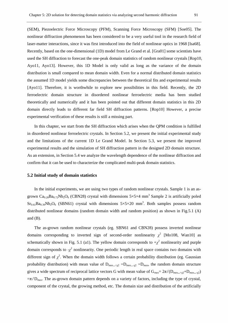
Chapter 5: 2D solution for detecting domain statistics via analyzing second harmonic diffraction 91
(SEM), Piezoelectric Force Microscopy (PFM), Scanning Force Microscopy (SFM) [Soe05]. The
nonlinear diffraction phenomenon has been considered to be a very useful tool in the research field of
laser-matter interactions, since it was first introduced into the field of nonlinear optics in 1968 [Isa68].
Recently, based on the one-dimensional (1D) model from Le Grand et al. [Gra01] some scientists have
used the SH diffraction to forecast the one-peak domain statistics of random nonlinear crystals [Rop10,
Ayo11, Ayo13]. However, this 1D Model is only valid as long as the variance of the domain
distribution is small compared to mean domain width. Even for a normal distributed domain statistics
the assumed 1D model yields some discrepancies between the theoretical fits and experimental results
[Ayo11]. Therefore, it is worthwhile to explore new possibilities in this field. Recently, the 2D
ferroelectric domain structure in disordered nonlinear ferroelectric media has been studied
theoretically and numerically and it has been pointed out that different domain statistics in this 2D
domain directly leads to different far field SH diffraction patterns. [Rop10] However, a precise
experimental verification of these results is still a missing part.
In this chapter, we start from the SH diffraction which arises when the QPM condition is fulfilled
in disordered nonlinear ferroelectric crystals. In Section 5.2, we present the initial experimental study
and the limitations of the current 1D Le Grand Model. In Section 5.3, we present the improved
experimental results and the simulation of SH diffraction pattern in the designed 2D domain structure.
As an extension, in Section 5.4 we analyze the wavelength dependence of the nonlinear diffraction and
confirm that it can be used to characterize the complicated multi-peak domain statistics.
5.2 Initial study of domain statistics
In the initial experiments, we are using two types of random nonlinear crystals. Sample 1 is an as-
grown Ca0.28Ba0.72Nb2O6 (CBN28) crystal with dimensions 5×5×4 mm3 Sample 2 is artificially poled
Sr0.61Ba0.39Nb2O6 (SBN61) crystal with dimensions 5×5×20 mm3. Both samples possess random
distributed nonlinear domains (random domain width and random position) as shown in Fig.5.1 (A)
and (B).
The as-grown random nonlinear crystals (eg. SBN61 and CBN28) possess inverted nonlinear
domains corresponding to inverted sign of second-order nonlinearity χ2 [Mo108, Wan10] as
schematically shown in Fig. 5.1 (a1). The yellow domain corresponds to +χ2 nonlinearity and purple
domain corresponds to -χ2 nonlinearity. One periodic length in real space contains two domains with
different sign of χ2. When the domain width follows a certain probability distribution (eg. Gaussian
probability distribution) with mean value of Dmax_+χ2 =Dmax_-χ2 =Dmax, the random domain structure
gives a wide spectrum of reciprocal lattice vectors G with mean value of Gmax= 2π ̸ (Dmax_+χ2+Dmax_-χ2)
=π ̸ Dmax. The as-grown domain pattern depends on a variety of factors, including the type of crystal,
component of the crystal, the growing method, etc. The domain size and distribution of the artificially
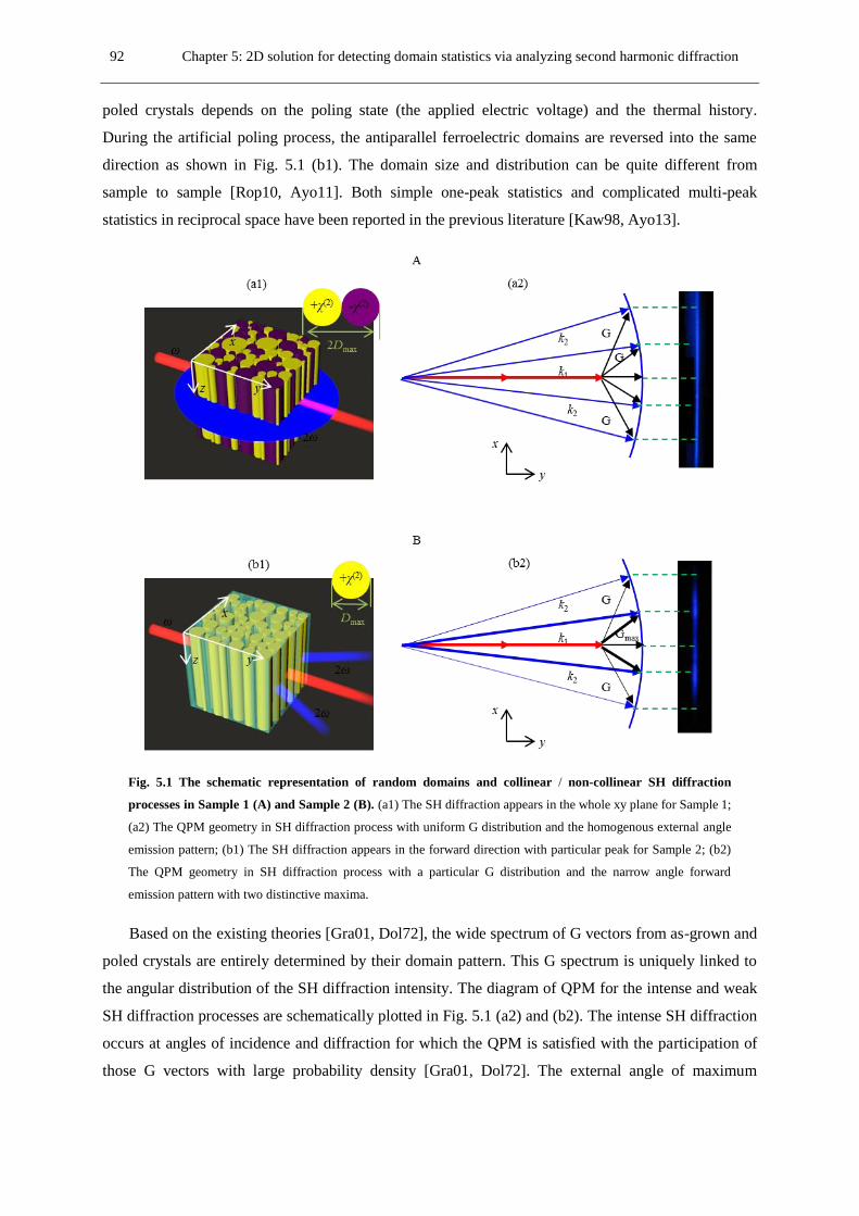
92 Chapter 5: 2D solution for detecting domain statistics via analyzing second harmonic diffraction
poled crystals depends on the poling state (the applied electric voltage) and the thermal history.
During the artificial poling process, the antiparallel ferroelectric domains are reversed into the same
direction as shown in Fig. 5.1 (b1). The domain size and distribution can be quite different from
sample to sample [Rop10, Ayo11]. Both simple one-peak statistics and complicated multi-peak
statistics in reciprocal space have been reported in the previous literature [Kaw98, Ayo13].
Fig. 5.1 The schematic representation of random domains and collinear / non-collinear SH diffraction
processes in Sample 1 (A) and Sample 2 (B). (a1) The SH diffraction appears in the whole xy plane for Sample 1;
(a2) The QPM geometry in SH diffraction process with uniform G distribution and the homogenous external angle
emission pattern; (b1) The SH diffraction appears in the forward direction with particular peak for Sample 2; (b2)
The QPM geometry in SH diffraction process with a particular G distribution and the narrow angle forward
emission pattern with two distinctive maxima.
Based on the existing theories [Gra01, Dol72], the wide spectrum of G vectors from as-grown and
poled crystals are entirely determined by their domain pattern. This G spectrum is uniquely linked to
the angular distribution of the SH diffraction intensity. The diagram of QPM for the intense and weak
SH diffraction processes are schematically plotted in Fig. 5.1 (a2) and (b2). The intense SH diffraction
occurs at angles of incidence and diffraction for which the QPM is satisfied with the participation of
those G vectors with large probability density [Gra01, Dol72]. The external angle of maximum

Chapter 5: 2D solution for detecting domain statistics via analyzing second harmonic diffraction 93
emission of the SH diffraction corresponds to the compensation of PM by the maximum G. It can be
calculated via the following formula theoretically:
max
max
GD
(5.1)
2 2 2
1 1 2 max
1 1 2
( )cos
2 ( )in
k k k G
k k k (5.2)
where 1
2sin( )ins nin is the external angle; θin is the internal angle; k1, k2 are the wave-vectors of
the fundamental and SH waves; n2 is the refractive index for the SH wave.
The weak SH diffraction occurs at angles of incidence and diffraction for which the QPM is satisfied
with the participation of those G vectors with small probability density.
According to Eq. (5.2), the G values needed to compensate the phase-mismatch in the first-order
QPM process is a function of FF wavelength and external emission angle. It can be written as:
2
2 11 1 2 1 1 22
2 2 2 2 2 2( , ) ( ) 2 ( )cos(sin (sin ))
2 2
n n n n n nG n
When fundamental wavelength ranges from 800 nm to 1600 nm and external angle ranges from 0
degree to 40 degree, a G (λ, θ) map is shown in Fig. 5.2 for ee-e interactions in SBN61 crystal.
Different colors from blue to red represent different G values from 0 μm-1
to 10 μm-1
.
Fig. 5.2 The theoretically calculated G (λ, θ) map in SBN61 crystal. Different colors from blue to red represent
different G values from 0 μm-1 to 10 μm-1.
94 Chapter 5: 2D solution for detecting domain statistics via analyzing second harmonic diffraction
5.2.1 Experimental setup and results
The initial experimental setup is schematically shown in Fig. 5.3. Two laser sources, a 180
femtosecond Ti: Sapphire oscillator (Mira, Coherent, repetition rate 76 MHz) and a 8 nanosecond
Nd:YAG system at 1064nm (repetition rate 10 Hz), were used to provide Gaussian pulses, propagating
at normal incidence onto the surface of the two samples as shown in the figure. The output FF beam
width at 1/e2 intensity was 400μm which was broad enough to cover at least N100 domains (the
average domain width for typical random nonlinear crystal is less than 3 μm from the reported
literature [Mol08, Ram04]). Since the typical length of the crystals used in the experiments range
between 10 and 20 mm, the emitted SH radiation will reflect an ensemble average of the domain
distribution, which can be used to analyze the dispersion of the domain width. Therefore, the ensemble
average over a large sample of domains can be realized in our experiment and the width of the SH
diffraction can be used to analyze the dispersion of the domain width with the first-order quasi-phase
matching condition in disordered ferroelectric domain structure [Rop10]. The polarization and
intensities of the incident fundamental beam can be controlled by the combination of a half-wave plate
(HW) and a polarizer (P). The samples were placed on a stage connected to a rotating arm (RA) whose
rotation axis was placed at the stage. A filter (F) and an analyzer (P) were mounted on the rotating arm
used to block the transmitted fundamental beam and select the polarized SH radiation generated by the
crystal, followed by a slit (S) selecting the SH radiation at a particular angle. A camera lens (L) was
used to focus the SH radiation onto the CCD camera. With the CCD camera the SH diffraction
intensity along different external emission angles can be captured.
Fig. 5.3 Schematic representation of the initial experimental setup. HW—half-wave plate, P—polarizer, RA—
rotating arm , F— filter, S— slit, L—camera lens.
In the initial experiments, Sample 1 and Sample 2 were measured for both oo-e and ee-e
interactions. As an example of the experimental results we show in Fig. 5.4 the corresponding SH
diffraction intensity as a function of external emission angle, θ, for Sample 1 (Figure A) and Sample 2
(Figure B) at wavelength 800 nm (blue line) and 1064 nm (green line) for the oo-e interaction. The
emission pattern of the SH diffraction from Sample 1 is very broad with external emission angle
ranging from -60o to 60
o as shown in Fig. 5.4 (A). The SH emission pattern from Sample 2 exhibits
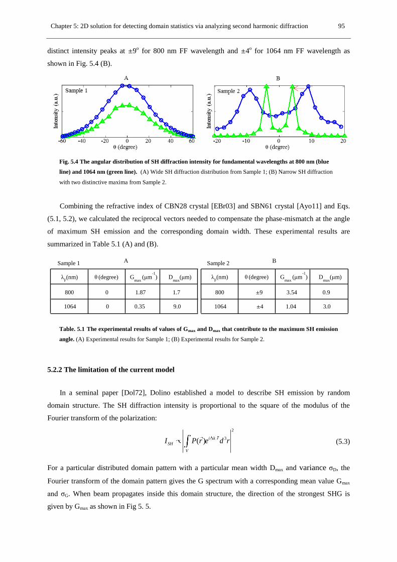
Chapter 5: 2D solution for detecting domain statistics via analyzing second harmonic diffraction 95
distinct intensity peaks at 9o for 800 nm FF wavelength and 4
o for 1064 nm FF wavelength as
shown in Fig. 5.4 (B).
Fig. 5.4 The angular distribution of SH diffraction intensity for fundamental wavelengths at 800 nm (blue
line) and 1064 nm (green line). (A) Wide SH diffraction distribution from Sample 1; (B) Narrow SH diffraction
with two distinctive maxima from Sample 2.
Combining the refractive index of CBN28 crystal [EBr03] and SBN61 crystal [Ayo11] and Eqs.
(5.1, 5.2), we calculated the reciprocal vectors needed to compensate the phase-mismatch at the angle
of maximum SH emission and the corresponding domain width. These experimental results are
summarized in Table 5.1 (A) and (B).
Table. 5.1 The experimental results of values of Gmax and Dmax that contribute to the maximum SH emission
angle. (A) Experimental results for Sample 1; (B) Experimental results for Sample 2.
5.2.2 The limitation of the current model
In a seminal paper [Dol72], Dolino established a model to describe SH emission by random
domain structure. The SH diffraction intensity is proportional to the square of the modulus of the
Fourier transform of the polarization:
2
3( ) i k r
SH
V
I P r e d r (5.3)
For a particular distributed domain pattern with a particular mean width Dmax and variance σD, the
Fourier transform of the domain pattern gives the G spectrum with a corresponding mean value Gmax
and σG. When beam propagates inside this domain structure, the direction of the strongest SHG is
given by Gmax as shown in Fig 5. 5.
λF(nm) θ
(degree)
G
max (μm
-1)
Dmax
(μm)
800 0 1.87 1.7
1064 0 0.35 9.0
B A
λF(nm) θ
(degree)
G
max (μm
-1)
Dmax
(μm)
800 9 3.54 0.9
1064 4 1.04 3.0
Sample 1 Sample 2
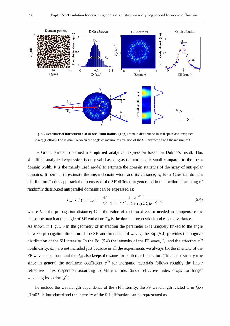
96 Chapter 5: 2D solution for detecting domain statistics via analyzing second harmonic diffraction
Fig. 5.5 Schematical introduction of Model from Dolino. (Top) Domain distribution in real space and reciprocal
space; (Bottom) The relation between the angle of maximum emission of the SH diffraction and the maximum G.
Le Grand [Gra01] obtained a simplified analytical expression based on Dolino’s result. This
simplified analytical expression is only valid as long as the variance is small compared to the mean
domain width. It is the mainly used model to estimate the domain statistics of the array of anti-polar
domains. It permits to estimate the mean domain width and its variance, σ, for a Gaussian domain
distribution. In this approach the intensity of the SH diffraction generated in the medium consisting of
randomly distributed antiparallel domains can be expressed as:
2 2
2 2 2 21 0 2 2
0
4 1( , , )
1 2cos( )
G
SH G G
L eI f G D
G e GD e (5.4)
where L is the propagation distance; G is the value of reciprocal vector needed to compensate the
phase-mismatch at the angle of SH emission; D0 is the domain mean width and σ is the variance.
As shown in Fig. 5.5 in the geometry of interaction the parameter G is uniquely linked to the angle
between propagation direction of the SH and fundamental waves, the Eq. (5.4) provides the angular
distribution of the SH intensity. In the Eq. (5.4) the intensity of the FF wave, Iω, and the effective χ(2)
nonlinearity, deff, are not included just because in all the experiments we always fix the intensity of the
FF wave as constant and the deff also keeps the same for particular interaction. This is not strictly true
since in general the nonlinear coefficient χ(2)
for inorganic materials follows roughly the linear
refractive index dispersion according to Miller’s rule. Since refractive index drops for longer
wavelengths so does χ(2)
.
To include the wavelength dependence of the SH intensity, the FF wavelength related term f2(λ)
[Tru07] is introduced and the intensity of the SH diffraction can be represented as:

Chapter 5: 2D solution for detecting domain statistics via analyzing second harmonic diffraction 97
2
1 0 2 1 0 4
2
( , , ) ( ) ( , , )SH
kI f G D f f G D
n n (5.5)
where 2 4
2 2( ) ( )f k n n , kω is the wave-vector of the FF wave, nω and n2ω are the refractive index
at FF wavelength and SH wavelength.
The plots in Fig. 5.6 illustrate the relation Eq. (5.5) as a function of emission angle and FF
wavelength. For a particular domain statistical distribution with D0=0.9 μm and σ=0.3 μm, the effect
of FF wavelength on the emission angle is plotted in Fig. 5.6 (A). When we increase the FF
wavelength the corresponding emission angle of intense SH is increased, which is determined by the
QPM condition. The angular distribution of SH diffraction intensity at different FF wavelengths from
800 nm to 1600 nm is represented in Fig. 5.6 (B). The decreased SH intensity with the increased
wavelengths can be clearly seen from the plots, which is due to f2(ω).
Fig. 5.6 Theoretically predicted angular distribution of the SH emission in Sample 2 (Eq.(5.5)). (A) The effect
of the FF wavelength on the SH emission angle for a particular domain the with D0=0.9 μm and σ=0.3 μm; (B) The
angular distribution of SH diffraction intensity at different FF wavelengths from 800 nm to 1600 nm.
As we increase the variance, σ, the width of the SH diffraction angular peaks get broadened,
leading to the merge between the two adjacent intensity peaks. In this limit Le Grand’s model gives a
single broad emission peak centered at the zero angular position. However, in this limit of large σ we
do not expect a quantitative prediction of the angular emission pattern, but it provides a qualitative
signature of the presence of large σ in the distribution. This large σ behavior is typical of as-grown
ferroelectric crystals as that shown from Sample 1. One expects this kind of structures always give a
broad emission pattern. The broader the emission, the larger G (or the smaller domain size) is needed.
The emission of Sample 2 with well-defined maxima should be consistent with a narrow σ distribution.
However, the study of the angular position of the maximum of SH as a function of the wavelength is
in conflict with this model since we experimentally observed a decrease of angular position of
maximum with increasing wavelength.

98 Chapter 5: 2D solution for detecting domain statistics via analyzing second harmonic diffraction
5.3 Study of domain statistics based on numerical simulation
Since the previous measurements clearly show that the simplified Le Grand’s model can not be
used to explain all the observed experimental patterns, we decided to implement a more detailed study
of the SH emission by random domain distributions of χ(2)
based on numerical simulation.
5.3.1 Experimental setup and results
Since the wavelength dependence of the SH intensity angular distribution gives important
information, we extended our experimental setup to measure the SH intensity angular distribution at
different fundamental wavelengths. The schematic representation of the experimental setup is shown
in Fig. 5.7. We used two tunable laser sources: femtosecond Ti:Sapphire oscillator (Coherent,
Chameleon Ultra II) and Optical Parametric Oscillator (APE Gmbh, Chameleon Compact OPO) to
provide femtosecond pulses at wavelengths ranges: 800 nm to 1000 nm and 1000 nm to 1600 nm,
respectively. The laser beam propagates at normal incidence onto the sample surface (Sample1: as-
grown CBN28, Sample 2: artificially poled SBN61). The polarization state and the average power of
the incident fundamental beam can be controlled by the combination of a half-wave plate and a
polarizer. The output average power for all wavelengths and for both polarizations (ordinary and
extraordinary) is fixed at the same value: 300 mW for CBN28 and 250 mW for SBN61. In the
experiment the polarization state is selected either perpendicular (oo-e) or parallel (ee-e) respectively.
The beam from the laser is weakly focused in the crystal by means of a plano-convex lens (beam waist
in the middle of the crystal). The beam width at 1/e2 intensity was 400 μm for both CBN28 and
SBN61. The temporal pulse duration at FWHM was around 180 fs (pulse width vary form 140 fs to
200 fs due to its source wavelength dependency). We projected the SH beam pattern on a diffusing
screen (Lee Filter) and imaged the pattern into a CCD. A high pass optical filter (Thorlabs FGB-37-A)
was used to block the strong IR fundamental beam before the CCD camera (Imaging Source
DMK31BU). We used a stripe of millimeter paper attached to the screen to calibrate spatial dimension
of the SHG profiles. Distance between screen and output facet of the crystal was measured by digital
caliper. From aforementioned experiment geometry we are able to calculate angular intensity profiles.
Fig. 5.7 Schematic representation of the deep experimental setup. HW—half-wave plate, P—polarizer, F - IR
blocking filter, S— diffusive screen,.
Chapter 5: 2D solution for detecting domain statistics via analyzing second harmonic diffraction 99
Besides the domain statistics, there are other factors impose effect on the SH diffraction intensity,
e.g., the intensity of the FF wave, the effective nonlinearity, the FF wavelength, the laser source
spurious emissions, etc. Eliminating these additional factors other than domain statistics is helpful to
reduce a complex analysis to a simpler one such that more detailed investigations can focus on the
domain statistics. Screening the angular distribution of the SH diffraction intensity is the first step to
have an effective experimental measurement.
(A) Eliminating the factors other than domain statistics (Factor screening)
Before performing this factor screening, we want to present the complete experimental
measurement results in order to find a safe way to eliminate the undesired factors. In the first
exploration, we measured the SH diffraction intensity distribution from Sample 1 for oo-e and ee-e
interactions. The complete SH diffraction intensity distribution as a function of external emission
angle, θ, at wavelength range from 800 nm to 1600 nm are plotted in Fig. 5.8. Since the output FF
beam width at 1/e2 intensity was 300μm (400μm), the FF beam was large enough to cover a sufficient
number of domains with different sizes. Besides, additional measurements were averaged over
different positions of the fundamental beam. Therefore the width of the SH diffraction can be used to
analyze the dispersion of the domain width assuming first-order quasi-phase matching compensation
in disordered ferroelectric domain structure [Rop10].
In the measurement results, there are two things we want to stress: the strong peak at zero angle
and the decreased SH intensity as increased wavelengths. For the strong peak at zero angular position,
we found that all data obtained by means of Chameleon laser (FF wavelength range from 800 nm to
950 nm) has that strong peak. It can not be caused by the collinear SHG process and neither the
fundamental beam leakage because the FF beam was filtered out by means of a stack of two Thorlabs
FGB-37 filters. Our investigation revealed that this peak most likely is from Ti: Saphire fluorescence.
To remove the effect of laser source imperfections all data around 0° were zeroed. The decreased SH
intensity at increased wavelengths is caused by the f2(λ) factor in Eq. (5.5) which has nothing to do
with the domain statistics. To focus on the effect of domain statistics on the SH diffraction intensity
distribution we normalized the SH diffraction intensity distribution. Since we always use the same
output average power for all FF wavelengths and we do not mix different interactions during the
domain statistics analysis, the normalization process can eliminate the effects of intensity of the FF
wave and the effective nonlinearity.

100 Chapter 5: 2D solution for detecting domain statistics via analyzing second harmonic diffraction
Fig. 5.8 The complete experimental measurement results for Sample 1. SH diffraction intensity distribution for
oo-e (blue line) and ee-e (red line) interactions when wavelengths range from 800 nm to 1600 nm.
(B) Experimental results
(B1) Experimental results of Sample 1 (natural CBN28)
The normalized SH diffraction intensity distribution as a function of the external emission angle, θ,
at different wavelengths ranging from 800 nm to 1600 nm are presented by the blue line (oo-e
interaction) and red line (ee-e interaction) in Fig. 5.9 (A). As we can see broad emission patterns are
observed for all wavelengths. The evolution of the SH intensity angular distribution from a single peak
to a double peak is very clear for both interactions.
The angles at peak intensity, θpeak, and angles at (1/e)2 intensity, θ(1/e)2, are summarized in Table
5.2 (A) and (B) for oo-e and ee-e interactions respectively.
The SH amplitude comparisons as a function of the external emission angle and of the FF
wavelength for oo-e and ee-e interactions are presented in Fig. 5.9 (b1) and Fig. 5.9 (b2). As discussed
in section 5.2.2, the decreased SH amplitude with increased FF wavelength can be explained by
Miller’s rule.
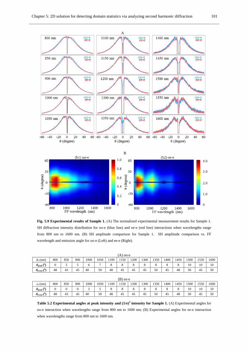
Chapter 5: 2D solution for detecting domain statistics via analyzing second harmonic diffraction 101
Fig. 5.9 Experimental results of Sample 1. (A) The normalized experimental measurement results for Sample 1.
SH diffraction intensity distribution for oo-e (blue line) and ee-e (red line) interactions when wavelengths range
from 800 nm to 1600 nm. (B) SH amplitude comparison for Sample 1. SH amplitude comparison vs. FF
wavelength and emission angle for oo-e (Left) and ee-e (Right).
(A) oo-e
λF (nm) 800 850 900 1000 1050 1100 1150 1200 1300 1350 1400 1450 1500 1550 1600
θpeak (o) 0 5 5 6 7 8 8 8 8 8 8 8 10 10 10
θ(1/e)2 (o) 48 43 45 40 50 48 45 45 45 50 45 48 50 45 50
(B) ee-e
λF (nm) 800 850 900 1000 1050 1100 1150 1200 1300 1350 1400 1450 1500 1550 1600
θpeak (o) 0 0 0 3 5 8 8 8 8 8 8 8 10 10 10
θ(1/e)2 (o) 48 43 45 40 50 48 45 45 45 50 45 48 50 45 50
Table 5.2 Experimental angles at peak intensity and (1/e)2 intensity for Sample 1. (A) Experimental angles for
oo-e interaction when wavelengths range from 800 nm to 1600 nm; (B) Experimental angles for ee-e interaction
when wavelengths range from 800 nm to 1600 nm.

102 Chapter 5: 2D solution for detecting domain statistics via analyzing second harmonic diffraction
The experimental observations are resumed in Fig.5.10 (a1) for oo-e and 5.10 (b1) for ee-e
together with the corresponding G (λ,θ) maps. The bars indicate the angular width of emission at 1/e2
intensity, while the circles represent the angle at peak intensity, θpeak. We can infer that a broad G
value distribution is necessary to compensate the phase mismatch over this broad angular and
frequency range. This large G range can be consistent with the type of emission observed from a
domain distribution with broad σ as discussed in section 5.2.2. This kind of behavior is usually
observed from as-grown ferroelectric crystals. In fact, the SH emission at 90 degree (the so-called
TSHG) has been the basis for the transverse auto-correlation and transverse cross-correlation
techniques developed in previous chapters.
Fig. 5.10 Summary of the experimental data and theoretically calculated G distribution for oo-e interaction.
(a1, b1) The theoretically calculated G (λ, θ) map and experimentally measured θpeak and θ(1/e)2; (a2, b2) The
theoretically calculated G values.
The theoretically calculated values of G are presented in Fig. 5.10 (a2) and Fig. 5.10 (b2) for oo-e
and ee-e interactions. Gpeak and G(1/e)2 are the theoretically calculated G values needed to compensate
the phase-mismatch at peak angle, θpeak, and 1/e2 intensity angle, θ(1/e)2; ∆kooe and ∆keee are the collinear
phase mismatch for oo-e and ee-e interactions. Under the first-order QPM condition, the value of G
which can be involved in the nonlinear process should be not smaller than the collinear phase
mismatch value for each interaction. Therefore, the effective FF wavelength can be used to measure

Chapter 5: 2D solution for detecting domain statistics via analyzing second harmonic diffraction 103
domain statistics are λFF800 nm for oo-e interaction and λFF 1000 nm for ee-e interaction. In these
wavelength region, the measured Gpeak remains stable (between 1.2 μm-1
and 1.8 μm-1
), with which we
deduce the G value with maximum probability density is Gmax=1.5 0.3 μm-1
. This Gmax corresponds
to the mean value of domain width around 2.0 μm for this as-grown CBN28 crystal. The dispersion σ
of the domain width is very large and the modulus value of G can be from |∆kooe|min to 11.7 μm-1
.
(B2) Experimental results of Sample 2 (artificially poled SBN61)
The normalized SH diffraction intensity distribution as a function of the external emission angle,
θ, at different wavelengths ranging from 800 nm to 1600 nm are presented by the blue line (oo-e
interaction) and red line (ee-e interaction) in Fig. 5.11 (A). The results of the measurements of Sample
2 show more remarkable wavelength dependence for both interactions. The peak angle dramatically
decreases as the wavelength increases, which is a totally different behavior with respect to the
experimental results observed for Sample 1. For the oo-e interaction, the evolution of the SH intensity
angular distribution changing from a double peak to a single peak are very clear. This behavior has
been also reported previously in the literature [Ayo11].
The angle at peak intensity, θpeak, and the angle at (1/e)2 intensity, θ(1/e)2, are summarized in Table
5.3 (A) and (B) for oo-e and ee-e interactions respectively.
SH amplitude comparisons as a function of the external emission angle and the wavelength for oo-
e and ee-e interactions are presented in Fig. 5.11 (b1) and Fig. 5.11 (b2). The SH amplitude first
decreases and then increases with increased FF wavelength for both interactions.

104 Chapter 5: 2D solution for detecting domain statistics via analyzing second harmonic diffraction
Fig. 5.11 Experimental results of Sample 2. (A) The normalized experimental measurement results for Sample 2.
SH diffraction intensity distribution for oo-e (blue line) and ee-e (red line) interactions when wavelengths range
from 800 nm to 1600 nm. (B) SH amplitude comparison for Sample 2. SH amplitude comparison vs. FF
wavelength and emission angle for oo-e (Left) and ee-e (Right).
(A) oo-e
λF (nm) 800 850 900 1000 1050 1100 1150 1200 1300 1350 1400 1450 1500 1550 1600
θpeak (o) 9 7.6 6 4.8 3.8 3.4 3 2.4 1.6 1.4 0 0 0 0 0
θ(1/e)2 (o) 16 12.4 11 8 7 6 5.2 5 4 4 3 3 2.2 2 2
(B) ee-e
λF (nm) 800 850 900 1000 1050 1100 1150 1200 1300 1350 1400 1450 1500 1550 1600
θpeak (o) 10 8.4 7.8 6 5.4 4.4 4 3.6 3.2 3 2.8 2.6 2.2 2.2 2
θ(1/e)2 (o) 18 14.6 13 10 9 8 7 7 6 5.8 5 5 4.8 4.8 4.8
Table 5.3 Experimental angles at peak intensity and (1/e)2 intensity for Sample 2. (A) Experimental angles for
oo-e interaction when wavelengths range from 800 nm to 1600 nm; (B) Experimental angles for ee-e interaction
when wavelengths range from 800 nm to 1600 nm
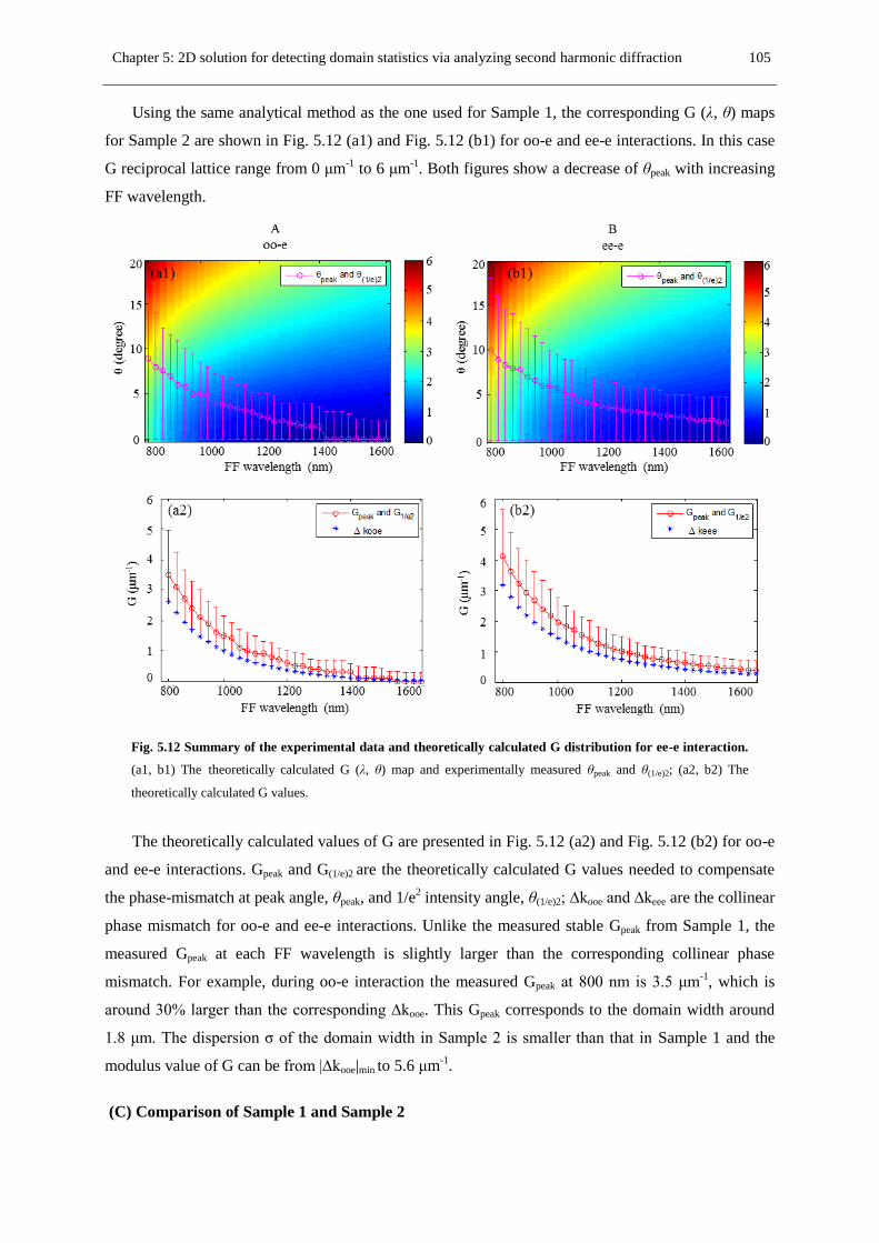
Chapter 5: 2D solution for detecting domain statistics via analyzing second harmonic diffraction 105
Using the same analytical method as the one used for Sample 1, the corresponding G (λ, θ) maps
for Sample 2 are shown in Fig. 5.12 (a1) and Fig. 5.12 (b1) for oo-e and ee-e interactions. In this case
G reciprocal lattice range from 0 μm-1
to 6 μm-1
. Both figures show a decrease of θpeak with increasing
FF wavelength.
Fig. 5.12 Summary of the experimental data and theoretically calculated G distribution for ee-e interaction.
(a1, b1) The theoretically calculated G (λ, θ) map and experimentally measured θpeak and θ(1/e)2; (a2, b2) The
theoretically calculated G values.
The theoretically calculated values of G are presented in Fig. 5.12 (a2) and Fig. 5.12 (b2) for oo-e
and ee-e interactions. Gpeak and G(1/e)2 are the theoretically calculated G values needed to compensate
the phase-mismatch at peak angle, θpeak, and 1/e2 intensity angle, θ(1/e)2; ∆kooe and ∆keee are the collinear
phase mismatch for oo-e and ee-e interactions. Unlike the measured stable Gpeak from Sample 1, the
measured Gpeak at each FF wavelength is slightly larger than the corresponding collinear phase
mismatch. For example, during oo-e interaction the measured Gpeak at 800 nm is 3.5 μm-1
, which is
around 30% larger than the corresponding ∆kooe. This Gpeak corresponds to the domain width around
1.8 μm. The dispersion σ of the domain width in Sample 2 is smaller than that in Sample 1 and the
modulus value of G can be from |∆kooe|min to 5.6 μm-1
.
(C) Comparison of Sample 1 and Sample 2

106 Chapter 5: 2D solution for detecting domain statistics via analyzing second harmonic diffraction
A comparison between the results in Sample 1 shown in Fig. 5.9 (b1) and (b2) and the results in
Sample 2 shown in Fig. 5.11 (b1) and (b2) reveals three main differences between these two samples:
(a) The emission pattern of the SH diffraction from Sample 1 has a much wider bandwidth than
that from Sample 2, which can be due to the larger dispersion of domain width in Sample 1;
(b) The SH intensity is decreased with the increased wavelengths for Sample 1, while the SH
intensity first decreases and then increases with increased FF wavelengths for Sample 2;
(c) The emission angle of intense SHG increases with increasing the FF wavelength for Sample 1,
while it decreases with increased FF wavelength for Sample 2. The emission pattern from Sample
1 is a typical result from an as-grown random nonlinear crystal, while the behavior of Sample 2 is
quite strange since as we discussed previously a SH emission pattern showing sharp peak
emission should have an increased θpeak as we increase the wavelength according to Le Grand
model.
To put some light into this difference a supplementary experiment was implemented in order to
directly visualize the ferroelectric domains pattern. This is not an easy task, since the domain size can
be very small and there is no refractive index contract between different domains, and the traditional
domain visualization methods are difficult to realize. In this work, the direct domain visualization was
performed with high-resolution SH imaging microscopy at ICFO – The Institute of Photonic Sciences.
The measured domain images of Sample 1 and Sample 2 are shown in Fig. 5.13 (A) and (B) with
122-nm and 204-nm resolution respectively. From the measurement we can see a very different
domain distribution. For Sample 1: The inverted nonlinear domains with bright and dark colors are
compactly arranged within the crystal; the typical domain size is much smaller than 1 μm but the
agglomeration of domains leads to a broad distribution of domain sizes. For the artificially poled
Sample 2: There is a large background (dark area) and the domains (bright island) have a very small
filling fraction around 6% from image calculation. These measurements can be used to check that:
(1) Sample 1 corresponds to an as-grown random distribution as expected.
(2) Sample 2 shows a quite uniform nonlinear background with a given orientation of the χ(2)
susceptibility together with a small portion of domains with inverted orientation of χ(2)
susceptibility.
As it occurs in any birefringent nonlinear crystal, the uniform nonlinear background imposes an
important effect on pulse propagation especially when the wavelength increases, because wavelength
increasing makes it closer to the phase matching condition and increases the coherence length. For
Sample 1 there is no uniform nonlinear background and the SH emission is entirely due to the phase
match compensation by reciprocal lattice G vectors. For Sample 2 we infer a plausible hypothesis that
the SH emission is due to the combination effect of quasi phase matching compensation by G vectors
and the role played by a finite phase mismatch in uniform nonlinear background.
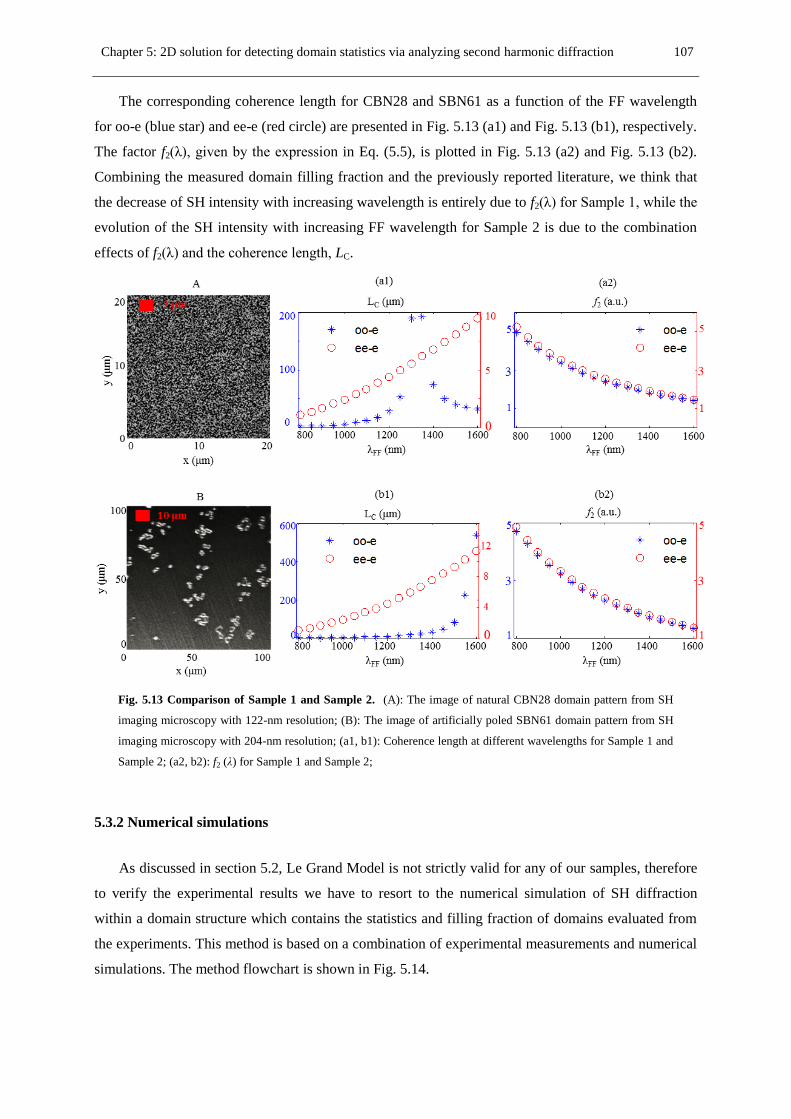
Chapter 5: 2D solution for detecting domain statistics via analyzing second harmonic diffraction 107
The corresponding coherence length for CBN28 and SBN61 as a function of the FF wavelength
for oo-e (blue star) and ee-e (red circle) are presented in Fig. 5.13 (a1) and Fig. 5.13 (b1), respectively.
The factor f2(λ), given by the expression in Eq. (5.5), is plotted in Fig. 5.13 (a2) and Fig. 5.13 (b2).
Combining the measured domain filling fraction and the previously reported literature, we think that
the decrease of SH intensity with increasing wavelength is entirely due to f2(λ) for Sample 1, while the
evolution of the SH intensity with increasing FF wavelength for Sample 2 is due to the combination
effects of f2(λ) and the coherence length, LC.
Fig. 5.13 Comparison of Sample 1 and Sample 2. (A): The image of natural CBN28 domain pattern from SH
imaging microscopy with 122-nm resolution; (B): The image of artificially poled SBN61 domain pattern from SH
imaging microscopy with 204-nm resolution; (a1, b1): Coherence length at different wavelengths for Sample 1 and
Sample 2; (a2, b2): f2 (λ) for Sample 1 and Sample 2;
5.3.2 Numerical simulations
As discussed in section 5.2, Le Grand Model is not strictly valid for any of our samples, therefore
to verify the experimental results we have to resort to the numerical simulation of SH diffraction
within a domain structure which contains the statistics and filling fraction of domains evaluated from
the experiments. This method is based on a combination of experimental measurements and numerical
simulations. The method flowchart is shown in Fig. 5.14.

108 Chapter 5: 2D solution for detecting domain statistics via analyzing second harmonic diffraction
Starting with the experimentally measured SH diffraction pattern from real crystals, we
numerically designed 2D domain structures and numerically simulated the laser beam propagation
through them using a split-step Fast Fourier Transform (FFT) beam propagation method. We
performed the above simulation process, until we obtained the similar SH diffraction pattern for both
numerical and experimental data, which means the designed domain pattern can truly reflect the main
aspects of nonlinear domain in real crystal. This numerical domain design process can be extremely
time consuming and fails to be applied to the analysis of big amount of domains in a normal computer
because each domain area needs at least 21 pixels 21 pixels to eliminate the domain shape induced
simulation error.
Fig. 5.14 Method Flowchart.
(A) Design the 2D domain structures
As shown in the Fig. 5.1, we consider the corresponding simulation when fundamental beam
propagates along y direction and SH diffraction emission in the x-y plane. Since the ferroelectric
domains have needle-like shape along z axis [Ram04], we only consider a 2D domain structure lying
in x-y plane during simulations.
We adopt the previously reported 2D solution for the simulation of disordered nonlinear
ferroelectric domains, which was demonstrated by V. Roppo et al. [Rop10]. We would like to review
this domain modelling again [Leg01, Rop10, Gai09, Mol08, Rom01]:
(a) Assume that the individual domains have form of rods with a circular transverse profile;
(b) We assume a particular distribution for the domain size and with this distribution a number of
domains is randomly generated and randomly placed in a rectangular area representing the size of
the sample;
(c) The domains number that takes part in the nonlinear process should be large compared to the
actual size of the input optical beam.

Chapter 5: 2D solution for detecting domain statistics via analyzing second harmonic diffraction 109
(A1) Design the 2D domain structures of Sample 1
In the 2D domain pattern simulation, the domain size was assumed to have a Gaussian distribution
with the experimental retrieved mean diameter (Dmax=2.0 μm). This assumption is based on the
processing of domain image as shown in Fig. 5.13 (A) using ImageJ program. The variance (σ) of the
Gaussian distribution is chosen as close as possible to the value retrieved from the experimental results.
As explained previously, compare with the total number of domains involved in the real experiment
the number of domains involved in this simulation is very limited. Therefore, the variance in each
simulation is always much smaller than the real variance in the crystal. But we can implement a
number of different simulations to average over these domains to realize the desired σ distribution.
The filling fraction of the anti-parallel domains used in the simulation is at least 90% and the rest is
linear background.
The simulated 2D domain structure in the x-y plane is shown in Fig. 5.15 (A). Fig. 5.15 (B) is the
corresponding Fourier spectrum of the domain structure in reciprocal space. Because of the randomly
distributed domain position, the sharp Bragg peaks shown in previous publications with quasi-periodic
structures [She07] did not appear in this simulation. The majority of reciprocal vectors are gathered
around a broad ring with radius Gmax=π/Dmax=1.5 μm-1
. The dispersion of the domain width gives
direct effect on the width of the SH diffraction but has nothing to do with the peak angle of the SH
diffraction. This peak angle is only related with the mean value of domain width.
Fig. 5.15 2D domain pattern simulation in real space and reciprocal space. (A) 2D random domain structure in
the real space with mean diameter Dmax=2.0 μm; (B) 2D spectrum of reciprocal vectors.
(A2) Design the 2D domain structures of Sample 2
For the artificially poled crystal the domain distribution can be quite different from sample to
sample since the resulting domain structure strongly depends on the history of the field and
temperature changes applied during the polling process. To simplify the 2D domain pattern simulation,
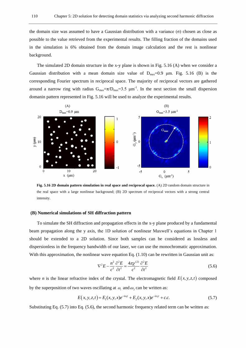
110 Chapter 5: 2D solution for detecting domain statistics via analyzing second harmonic diffraction
the domain size was assumed to have a Gaussian distribution with a variance (σ) chosen as close as
possible to the value retrieved from the experimental results. The filling fraction of the domains used
in the simulation is 6% obtained from the domain image calculation and the rest is nonlinear
background.
The simulated 2D domain structure in the x-y plane is shown in Fig. 5.16 (A) when we consider a
Gaussian distribution with a mean domain size value of Dmax=0.9 μm. Fig. 5.16 (B) is the
corresponding Fourier spectrum in reciprocal space. The majority of reciprocal vectors are gathered
around a narrow ring with radius Gmax=π/Dmax=3.5 μm-1
. In the next section the small dispersion
domanin pattern represented in Fig. 5.16 will be used to analyze the experimental results.
Fig. 5.16 2D domain pattern simulation in real space and reciprocal space. (A) 2D random domain structure in
the real space with a large nonlinear background; (B) 2D spectrum of reciprocal vectors with a strong central
intensity.
(B) Numerical simulations of SH diffraction pattern
To simulate the SH diffraction and propagation effects in the x-y plane produced by a fundamental
beam propagation along the y axis, the 1D solution of nonlinear Maxwell’s equations in Chapter 1
should be extended to a 2D solution. Since both samples can be considered as lossless and
dispersionless in the frequency bandwidth of our laser, we can use the monochromatic approximation.
With this approximation, the nonlinear wave equation Eq. (1.10) can be rewritten in Gaussian unit as:
2 2 (2) 22
2 2 2 2
4n E EE
c t c t
(5.6)
where n is the linear refractive index of the crystal. The electromagnetic field , , ,E x y z t composed
by the superposition of two waves oscillating at 1 and 2 can be written as:
1 2
1 2, , , ( , , ) ( , , ) . .i t i tE x y z t E x y x e E x y x e c c
(5.7)
Substituting Eq. (5.7) into Eq. (5.6), the second harmonic frequency related term can be written as:
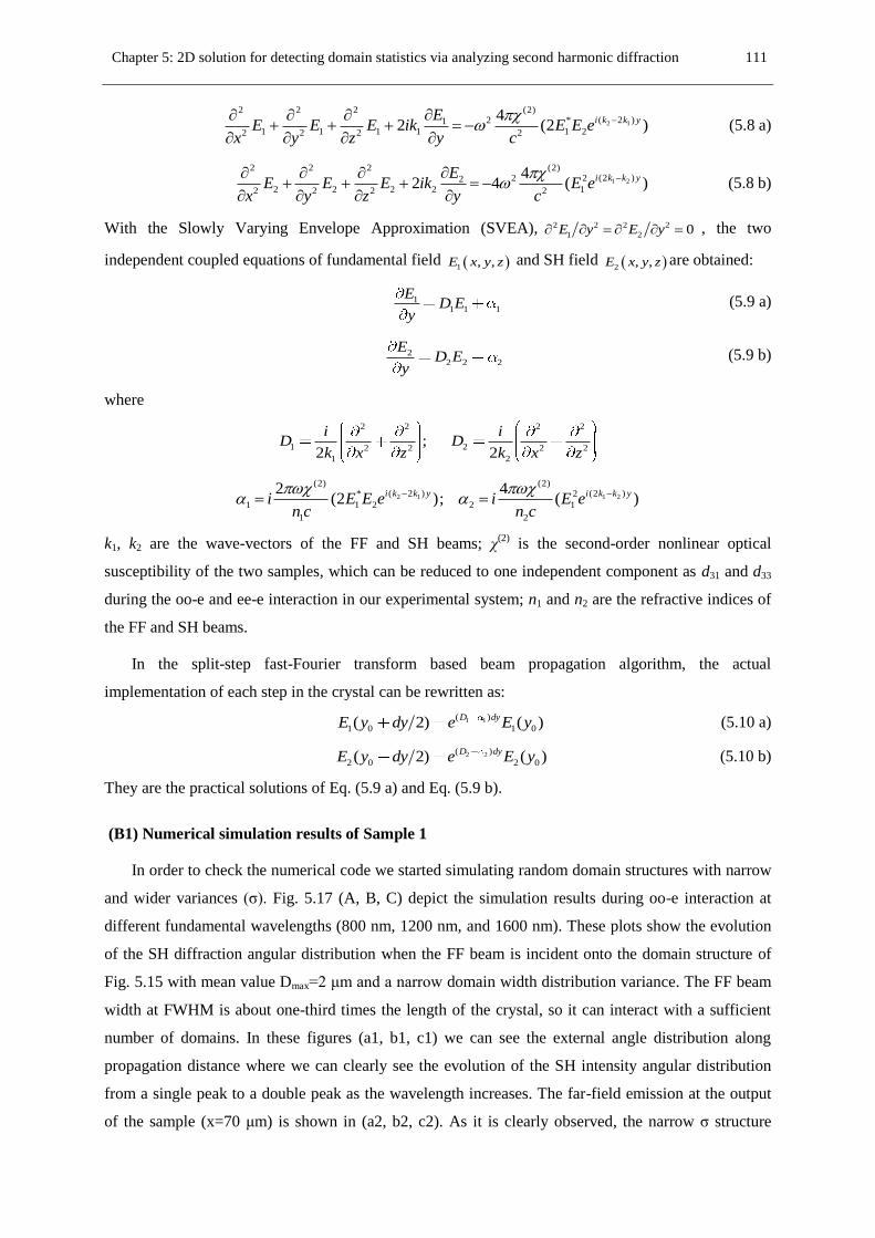
Chapter 5: 2D solution for detecting domain statistics via analyzing second harmonic diffraction 111
2 1
2 2 2 (2)( 2 )2 *1
1 1 1 1 1 22 2 2 2
42 (2 )
i k k yEE E E ik E E e
x y z y c
(5.8 a)
1 2
2 2 2 (2)(2 )2 22
2 2 2 2 12 2 2 2
42 4 ( )
i k k yEE E E ik E e
x y z y c
(5.8 b)
With the Slowly Varying Envelope Approximation (SVEA), 2 2 2 2
1 2 0E y E y , the two
independent coupled equations of fundamental field 1 , ,E x y z and SH field 2 , ,E x y z are obtained:
11 1 1
ED E
y (5.9 a)
22 2 2
ED E
y (5.9 b)
where
2 2 2 2
1 22 2 2 2
1 2
;2 2
i iD D
k x z k x z
2 1 1 2
(2) (2)( 2 ) (2 )* 2
1 1 2 2 1
1 2
2 4(2 ); ( )
i k k y i k k yi E E e i E en c n c
k1, k2 are the wave-vectors of the FF and SH beams; χ(2)
is the second-order nonlinear optical
susceptibility of the two samples, which can be reduced to one independent component as d31 and d33
during the oo-e and ee-e interaction in our experimental system; n1 and n2 are the refractive indices of
the FF and SH beams.
In the split-step fast-Fourier transform based beam propagation algorithm, the actual
implementation of each step in the crystal can be rewritten as:
1 1( )
1 0 1 0( 2) ( )D dy
E y dy e E y (5.10 a)
2 2( )
2 0 2 0( 2) ( )D dy
E y dy e E y (5.10 b)
They are the practical solutions of Eq. (5.9 a) and Eq. (5.9 b).
(B1) Numerical simulation results of Sample 1
In order to check the numerical code we started simulating random domain structures with narrow
and wider variances (σ). Fig. 5.17 (A, B, C) depict the simulation results during oo-e interaction at
different fundamental wavelengths (800 nm, 1200 nm, and 1600 nm). These plots show the evolution
of the SH diffraction angular distribution when the FF beam is incident onto the domain structure of
Fig. 5.15 with mean value Dmax=2 μm and a narrow domain width distribution variance. The FF beam
width at FWHM is about one-third times the length of the crystal, so it can interact with a sufficient
number of domains. In these figures (a1, b1, c1) we can see the external angle distribution along
propagation distance where we can clearly see the evolution of the SH intensity angular distribution
from a single peak to a double peak as the wavelength increases. The far-field emission at the output
of the sample (x=70 μm) is shown in (a2, b2, c2). As it is clearly observed, the narrow σ structure

112 Chapter 5: 2D solution for detecting domain statistics via analyzing second harmonic diffraction
results in the well resolved maxima separating when wavelength increases (0o for 800 nm, 9
o for
1200 nm, and 11o for 1600 nm). This emission is the main characteristic of Le Grand model as
shown in Fig. 5.6.
The simulation results of the SH diffraction pattern during oo-e interaction from Sample 1 with
large σ are shown in Fig. 5.17 (D, E, F). For this case, we performed an averaging over 25 different
domain realizations which give an equivalent effect as a wide domain width distribution but keeping
the same mean value as Dmax=2 μm. Each domain realization has a structure similar to that of Fig. 5.15.
In this case we can observe a much wider SH diffraction pattern along propagation distance as shown
in (d1, e1, f1). From the far-field angular distribution of SH diffraction in (d2, e2, f2), we can see that
intensity peaks appear at the external angles of 0o for 800 nm, 9
o for 1200 nm, and 11
o for 1600 nm
fundamental wavelengths respectively. This kind of emission corresponds to that experimental results
observed from Sample 1.
Fig. 5.17 SH diffraction simulation results during oo-e interaction when fundamental wavelength at 800 nm,
1200 nm, and 1600 nm. (A, B, C): SH diffraction simulation results with Dmax=2μm and small dispersion of
domain width; (D, E, F): SH diffraction simulation results with large dispersion of domain width. (a1, b1, c1, d1,
e1, f1): SH diffraction pattern along propagation distance; (a2, b2, c2, d2, e2, f2): Far-field angular distribution of
SH diffraction.

Chapter 5: 2D solution for detecting domain statistics via analyzing second harmonic diffraction 113
We also simulated the corresponding SH diffraction patterns during ee-e interaction, which have a
behavior very similar to that observed for oo-e interaction.
Fig. 5.18 shows a comparison between our simulated far-field angular distribution and the
experimental results for both oo-e interaction (blue line) and ee-e interaction (red line). The simulation
results are in good agreement with the experimental results. This agreement shows the process of
averaging over different realizations can be an efficient way to simulate the large variance distribution.
Fig. 5.18 Comparison between simulation results and experimental results both oo-e interaction (blue line)
and ee-e interaction (red line). (Top): Experimental far-field angular distribution; (Bottom): Simulated far-field
angular distribution.
(B2) Numerical simulation results of Sample 2
Fig. 5.19 shows the combined effects of domain distribution and nonlinear background on the SH
intensity angular emission during oo-e interaction. Top: The SH diffraction pattern along propagation
distance for different FF beams (at 800 nm, 1000 nm, 1200 nm and 1600 nm) incident onto the
domain structure depicted in Fig. 5.16(A). Bottom: the corresponding Far-field angular distribution.
From the far-field angular distribution, we can see that the external angle of the intensity peak is 9o
for 800 nm, 4o for 1000 nm, 3
o for 1200 nm, and 0
o for 1600 nm fundamental wavelengths
respectively. Comparing the external angle emission of SH at different wavelengths, we can see that
the nonlinear domain distribution dominates the parametric process at 800-1200nm, while the
nonlinear background dominates the parametric process at longer wavelengths and it completely
dominates at 1600 nm. These simulation results fit both the previous theoretical analysis as shown in
Fig. 5.13

114 Chapter 5: 2D solution for detecting domain statistics via analyzing second harmonic diffraction
Fig. 5.19 Combination effects of domain distribution and nonlinear background on the SH intensity angular
distribution during oo-e interaction. (Top): SH diffraction pattern along propagation distance; (Bottom): Far-
field angular distribution.
Fig. 5.20 shows the corresponding simulation results during ee-e interaction. Top: The SH
diffraction angular pattern as a function of propagation distance for fundamental beams of different
wavelengths incident onto the domain structure shown in Fig. 5.16(A). Bottom: the corresponding far-
field angular distribution at the end of the crystal. From the far-field angular distribution, we find SH
intensity peaks at the angles 11o for 800 nm, 6
o for 1000 nm, 5
o for 1200 nm, and 3
o for 1600
nm fundamental wavelengths respectively.
Fig. 5.20 Combination effects of domain distribution and nonlinear background on the SH intensity angular
distribution during ee-e interaction. (Top): SH diffraction pattern along propagation distance; (Bottom): Far-field
angular distribution.
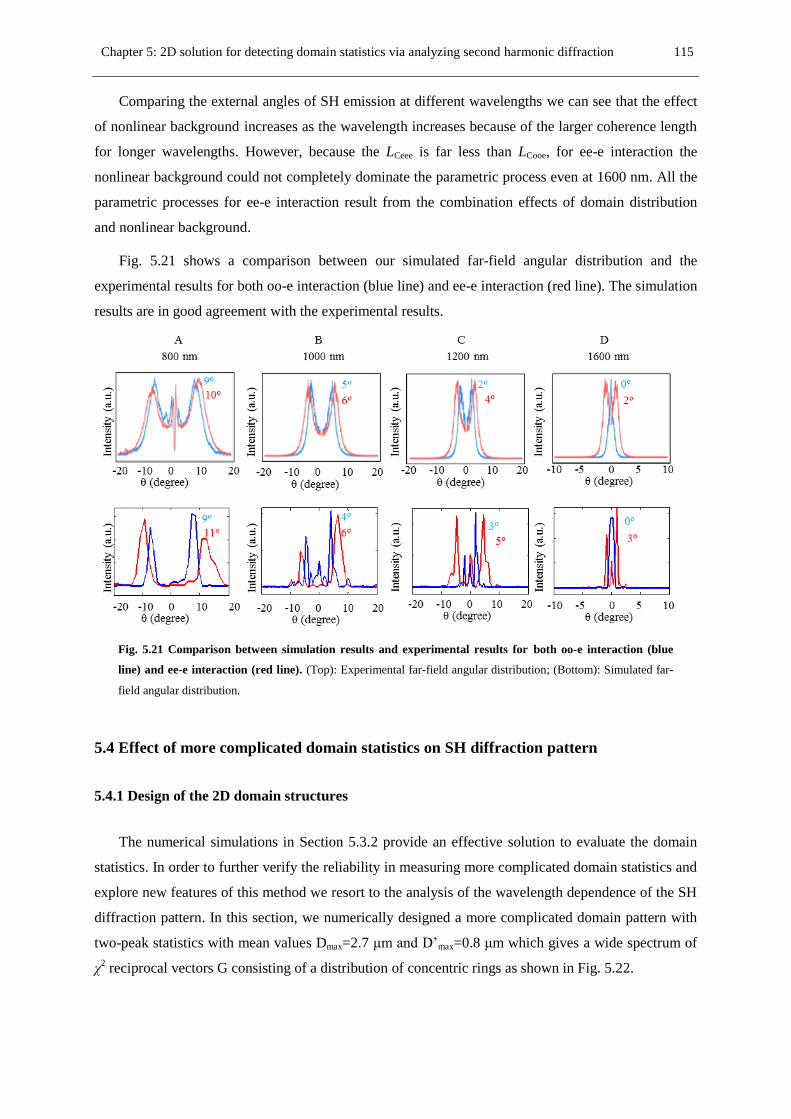
Chapter 5: 2D solution for detecting domain statistics via analyzing second harmonic diffraction 115
Comparing the external angles of SH emission at different wavelengths we can see that the effect
of nonlinear background increases as the wavelength increases because of the larger coherence length
for longer wavelengths. However, because the LCeee is far less than LCooe, for ee-e interaction the
nonlinear background could not completely dominate the parametric process even at 1600 nm. All the
parametric processes for ee-e interaction result from the combination effects of domain distribution
and nonlinear background.
Fig. 5.21 shows a comparison between our simulated far-field angular distribution and the
experimental results for both oo-e interaction (blue line) and ee-e interaction (red line). The simulation
results are in good agreement with the experimental results.
Fig. 5.21 Comparison between simulation results and experimental results for both oo-e interaction (blue
line) and ee-e interaction (red line). (Top): Experimental far-field angular distribution; (Bottom): Simulated far-
field angular distribution.
5.4 Effect of more complicated domain statistics on SH diffraction pattern
5.4.1 Design of the 2D domain structures
The numerical simulations in Section 5.3.2 provide an effective solution to evaluate the domain
statistics. In order to further verify the reliability in measuring more complicated domain statistics and
explore new features of this method we resort to the analysis of the wavelength dependence of the SH
diffraction pattern. In this section, we numerically designed a more complicated domain pattern with
two-peak statistics with mean values Dmax=2.7 μm and D’max=0.8 μm which gives a wide spectrum of
χ2 reciprocal vectors G consisting of a distribution of concentric rings as shown in Fig. 5.22.

116 Chapter 5: 2D solution for detecting domain statistics via analyzing second harmonic diffraction
Fig. 5.22 (a) is the reciprocal vector G spectrum of the domain structure. Most of the reciprocal
vectors are gathered around the first-order bright ring with radius Gmax=π/Dmax=1.2 μm-1
and the
second-order bright ring with radius G’max=π/D’max=4.0 μm-1
. These concentric rings could be
experimentally fabricated with the technique proposed in the reference [She07] where laser induced
writing of domains is studied, so this simulation could be of practical significance. The corresponding
intensity (probability density) at each value of the modulus of |𝐺| is calculated and the corresponding
plot is shown in Fig. 5.22 (b). From the plot we can see there are two intensity peaks at 1.2 μm-1
and
4.0 μm-1
. The reciprocal vectors at Gmax=1.2 μm-1
with the maximum probability density result from
domains with a mean diameter of Dmax=2.7 μm, while the reciprocal vectors at G’max=4 μm-1
correspond to a mean diameter of D’max=0.8 μm.
Fig. 5.22 2D two-peak statistics simulation. (a) 2D spectrum of reciprocal vector in a form of concentric rings; (b)
1D intensity distribution of the modulus of the reciprocal lattice vectors with two intensity peaks at 1.2 μm-1 and 4
μm-1.
5.4.2 Numerical simulations of SH diffraction pattern
When these two reciprocal vectors, Gmax=1.2 μm-1
and G’max=4 μm-1
, are involved in the nonlinear
parametric process for oo-e interaction, the corresponding SH emission angles can be theoretically
calculated via Eq. (5.2) and summarized in Table 5.4. λF is the fundamental wavelength; θ_Gmax and
θ_G’max are the theoretically calculated SH emission angle when Gmax and G’max are involved in the
non-collinear QPM process respectively. When there is no possibility of QPM the SH emission angle
is an invalid value and marked as NaN.
oo-e
λF (nm) 800 850 900 950 1000 1050 1100 1150 1200 1300 1350 1400 1450 1500 1550
θ_Gmax (o) NaN NaN NaN NaN 1.8 3.6 4.6 5.3 5.8 6.7 7.0 7.4 7.7 8.0 8.3
θ_G’max (o) 10.6 13.5 15.4 16.8 18.1 19.3 20.4 21.4 22.4 24.4 25.5 26.5 27.5 28.5 29.5
Table 5.4 Theoretical SH emission angles with Gmax and G’max. θ_Gmax and θ_G’max are the theoretically
calculated SH emission angle when Gmax and G’max involved in QPM process respectively.

Chapter 5: 2D solution for detecting domain statistics via analyzing second harmonic diffraction 117
During oo-e interaction the simulation of SH diffraction patterns along propagation distance for
different fundamental wavelengths are shown in Fig. 5.23 (a1-a2); the horizontal coordinates represent
the values of external angle from -20o to 20
o; the vertical coordinates represents the propagation
distance along y direction. The corresponding far-field angular distributions are shown in Fig. 5.23
(b1-b2); the horizontal coordinates represent the values of angle; the vertical coordinates represents
the intensity; the angles of the intensity peaks for each simulation are marked in black and pink in the
plots; the counterpart of the angles marked in black can be found in Table 5.4; the appearance of the
angles marked in pink are not from neither the Gmax nor G’max, which comes from simulation error.
Fig. 5.23 The wavelength dependence of the SH diffraction in oo-e interaction. (a1-a2) Simulation of the SH
diffraction pattern along propagation distance for different fundamental wavelengths; (b1-b2) The corresponding
far-field angular distribution of SH diffraction intensity.
A summary of the position of the peak angles is represented by the green and blue circles in Fig.
5.24. The blue circle represents the simulated external angle on the right side, while the green circle
represents the simulated external angle on the left side. The numerical simulation angles (blue and
green circles) can be fit with two curves represented by red star and pink star respectively. The red star

118 Chapter 5: 2D solution for detecting domain statistics via analyzing second harmonic diffraction
represents the theoretically calculated external angle when the reciprocal lattice vector Gmax =1.2μm-1
is involved in the QPM process. The absence of data when fundamental wavelengths are shorter than
1000 nm is because there is no possibility to obtain quasi phase matching at these wavelengths with
this value of G. The pink star represents the theoretical external angle when G’max=4μm-1
is involved
in the QPM process. The quantitative relation of probability density can be deduced from the fit in the
wavelength area where the QPM condition can be fulfilled for both reciprocal vectors. When λ≥1000
nm the trends of simulation and theoretical data calculated with Gmax fit well, which indicates that the
probability density of Gmax is larger than the probability density of G’max, P(Gmax)﹥P(G’max). The
degree of misfit (marked with the black dotted circles) reflect the difference between P(Gmax) and
P(G’max). A large value of P(Gmax)/ P(G’max) leads to a large misfit. For example, the appearance of
0.8º angle at 900 nm is because the quantity of the reciprocal vector can be used to compensate the
phase-mismatch at this process is more than the quantity of G’max.
Fig. 5.24 The comparison between theoretically calculated emission angle and simulated emission angle at
intensity peak for oo-e interaction.
We also explored the SH diffraction angular information during ee-e interaction. When Gmax and
G’max are involved in the nonlinear process for ee-e interaction, the SH emission angles were
theoretically calculated via Eq. (5.2) and are summarized in Table 5.5.

Chapter 5: 2D solution for detecting domain statistics via analyzing second harmonic diffraction 119
ee-e
λF (nm) 800 850 900 950 1000 1050 1100 1150 1200 1300 1350 1400 1450 1500 1550
θ_Gmax (o) NaN NaN NaN NaN NaN NaN 2.8 4.0 4.8 6.0 6.5 6.9 7.3 7.6 8.0
θ_G’max (o) 8.6 12.3 14.6 16.3 17.7 18.9 20.1 21.2 22.3 24.4 25.4 26.5 27.5 28.5 29.6
Table 5.5 Theoretical SH emission angles with Gmax and G’max. θ_Gmax and θ_G’max are the theoretically
calculated SH emission angle when Gmax and G’max involved in QPM process respectively.
The simulation of SH diffraction patterns along propagation distance for different fundamental
wavelengths are shown in Fig. 5.25 (a1-a2). The corresponding far field angular distribution are
shown in Fig. 5.25 (b1-b2); the angles of intensity peak for each simulation are marked in black and
pink in the plots; the counterpart of the angles marked in black can be found in Table 5.5; the
appearance of the angles marked in pink comes from the simulation error.
Fig. 5.25 The wavelength dependence of the SH diffraction in ee-e interaction. (a1-a2) Simulation of the SH
diffraction pattern along propagation distance for different fundamental wavelengths; (b1-b2) The corresponding
far-field angular distribution of SH diffraction.

120 Chapter 5: 2D solution for detecting domain statistics via analyzing second harmonic diffraction
The corresponding summary of the positions of the peak angle are plotted by the green and blue
circles in Fig. 5.26. The numerical simulation angles (blue and green circles) can be fit with two
curves represented by red star and pink star respectively. The red star represents the theoretically
calculated external angle when Gmax=1.2 μm-1
is involved in the QPM process. The absence of data
when fundamental wavelengths are shorter than 1000 nm is because there are no phase matching can
be fulfilled at these wavelengths. The pink star represents the theoretical external angle when
G’max=4.0 μm-1
is involved in the QPM process. The quantitative relation of probability density can be
deduced from the fit in the λ≥1100 nm area. Since the trends of simulation and theoretical data
calculated with Gmax fit well, we deduce P(Gmax)> P(G’max).
Fig. 5.26 The comparison between theoretically calculated emission angle and simulated emission angle at
intensity peak for ee-e interaction.
5.5 Conclusions
In this chapter we demonstrate an indirect non-destructive optical method for the characterization
of nonlinear domain statistics both in the as-grown random nonlinear crystals and in the artificially
poled random nonlinear crystals. This optical method is based on a combination of the experimental
measurements of the second harmonic diffraction intensity angular distribution and the corresponding
numerical simulation results.

Chapter 5: 2D solution for detecting domain statistics via analyzing second harmonic diffraction 121
In the experiments, we built the experimental setup and measured SH diffraction intensity angular
distribution at different wavelengths from 800 nm to 1600 nm.
In the simulations, we started with the designing and simulation of the two different domain
structures for the as-grown and artificially poled random nonlinear crystals. There are two different
ways to design the 2D domain structures. For the as-grown domain structure, there is a linear
background and the inverted nonlinear domains are compactly arranged within the crystal; for the
artificially poled domain structure, there is a nonlinear background and antiparallel domains, whose
filling fraction plays an important role in the second harmonic generation process. Besides, we
expanded the 1D solution of nonlinear Maxwell’s equation to 2D solution and numerically simulated
the SH diffraction and propagation in the simulated 2D domain structures with the split-step Fast-
Fourier Transform beam propagation method. We performed the above simulation processes, until we
obtained the similar SH diffraction pattern for both numerical and experimental data, which means the
designed domain pattern can truly reflect the nonlinear domain in real crystal.
This method has been implemented experimentally and tested in different crystals with different
types of distributions. It has been demonstrated that more complicated domain structures possess the
more complex second harmonic diffraction intensity angular emission pattern and the analysis of the
dependence of the second harmonic diffraction intensity angular distribution on the fundamental beam
wavelength can be used to obtain relevant information about complicated domain structures.
This method could be used for real time monitoring of the unknown domain distribution during
the poling or crystal growing process.

Bibliography
[Akt03] Akturk S, Kimmel M, O’Shea P, et al. Measuring spatial chirp in ultrashort pulses using
single-shot Frequency-Resolved Optical Gating[J]. Optics Express, 2003, 11(1): 68-78.
[Ale08] Aleksandrovsky A S, Vyunishev A M, Shakhura I E, et al. Random quasi-phase-matching in a
nonlinear photonic crystal structure of strontium tetraborate[J]. Physical Review A, 2008, 78(3):
031802.
[Alo10] Alonso B, Sola Í J, Varela Ó, et al. Spatiotemporal amplitude-and-phase reconstruction by
Fourier-transform of interference spectra of high-complex-beams[J]. JOSA B, 2010, 27(5): 933-940.
[Arm62] Armstrong J A, Bloembergen N, Ducuing J, et al. Interactions between light waves in a
nonlinear dielectric[J]. Physical Review, 1962, 127(6): 1918.
[Aus71] Auston D H. Measurement of picosecond pulse shape and background level[J]. Applied
Physics Letters, 1971, 18(6): 249-251.
[Ayo11] Ayoub M, Imbrock J, Denz C. Second harmonic generation in multi-domain χ 2 media: from
disorder to order[J]. Optics express, 2011, 19(12): 11340-11354.
[Ayo13] Ayoub M, Paßlick M, Koynov K, et al. Effect of the domain shape on noncollinear second-
harmonic emission in disordered quadratic media[J]. Optics express, 2013, 21(25): 31462-31468.
[Bal67] Ballman A A, Brown H. The growth and properties of strontium barium metaniobate,
Sr1−xBaxNb2O6, a tungsten bronze ferroelectric[J]. Journal of Crystal Growth, 1967, 1(5): 311-314.
[Bau04] Baudrier-Raybaut M, Haidar R, Kupecek P, et al. Random quasi-phase-matching in bulk
polycrystalline isotropic nonlinear materials[J]. Nature, 2004, 432(7015): 374-376.
[Bec93] Beck M, Walmsley I A, Wong V, et al. Chronocyclic tomography for measuring the
amplitude and phase structure of optical pulses[J]. Optics letters, 1993, 18(23): 2041-2043.
[Ben12] Benjamín Alonso Fernández, Spatiotemporal characterization of ultrashort laser pulses, (PhD
thesis, Universidad de Salamanca, Spain, 2012)
[Ber98] Berger V. Nonlinear photonic crystals[J]. Physical review letters, 1998, 81(19): 4136.

Bibliography 123
[Ber04] Berden G, Jamison S P, MacLeod A M, et al. Electro-optic technique with improved time
resolution for real-time, nondestructive, single-shot measurements of femtosecond electron bunch
profiles[J]. Physical review letters, 2004, 93(11): 114802.
[Boy03] Boyd R W. Nonlinear optics[M]. Academic press, 2003.
[Bro00] Broderick N G R, Ross G W, Offerhaus H L, et al. Hexagonally poled lithium niobate: a two-
dimensional nonlinear photonic crystal[J]. Physical review letters, 2000, 84(19): 4345.
[Cal04] Calin A. David, Optical and Dielectric Properties of SrxBa1−xNb2O6, (PhD thesis, Universität
Osnabrück, Germany, 2004)
[Cha00] F. Charra and G. Gurzadyan, Nonlinear Dielectric Susceptibilities, (Springer-Verlag, Berlin,
2000)
[Chi91] Chilla J L A, Martinez O E. Analysis of a method of phase measurement of ultrashort pulses
in the frequency domain[J]. IEEE Journal of quantum electronics, 1991, 27(5): 1228-1235.
[Die06] Diels J C, Rudolph W. Ultrashort laser pulse phenomena[M]. Academic press, 2006.
[Die85] Diels J C M, Fontaine J J, McMichael I C, et al. Control and measurement of ultrashort pulse
shapes (in amplitude and phase) with femtosecond accuracy[J]. Applied Optics, 1985, 24(9): 1270-
1282.
[Dol72] Dolino G. Effects of domain shapes on second-harmonic scattering in triglycine sulfate[J].
Physical Review B, 1972, 6(10): 4025.
[Dud02] Dudley J M, Gu X, Xu L, et al. Cross-correlation frequency resolved optical gating analysis
of broadband continuum generation in photonic crystal fiber: simulations and experiments[J]. Optics
Express, 2002, 10(21): 1215-1221.
[EBr03] Eßer M, Burianek M, Held P, et al. Optical characterization and crystal structure of the novel
bronzetype CaxBa1-xNb2O6 (x=0.28; CBN-28) [J]. Crystal Research and Technology, 2003, 38(6): 457-
464.
[Fej92] Fejer M M, Magel G A, Jundt D H, et al. Quasi-phase-matched second harmonic generation:
tuning and tolerances[J]. IEEE Journal of Quantum Electronics, 1992, 28(11): 2631-2654.
[Fis06] Fischer R, Saltiel S M, Neshev D N, et al. Broadband femtosecond frequency doubling in
random media[J]. Applied physics letters, 2006, 89(19): 191105.
[Fis07] Fischer R, Neshev D N, Saltiel S M, et al. Monitoring ultrashort pulses by transverse
frequency doubling of counterpropagating pulses in random media[J]. Applied Physics Letters, 2007,
91(3): 031104.
[Fra60] Francombe M H. The relation between structure and ferroelectricity in lead barium and
barium strontium niobates[J]. Acta Crystallographica, 1960, 13(2): 131-140.
[Fra61] Franken P A, Hill A E, Peters C W, et al. Generation of optical harmonics[J]. Physical Review
Letters, 1961, 7(4): 118.
[Fre68] Freund I. Nonlinear diffraction[J]. Physical Review Letters, 1968, 21(19): 1404.

124 Bibliography
[Fur76] Y. Furuhata. Growth of Single Crystal Materials for Electro-Optics[J]. Journal of the Japanese
Association for Crystal Growth, Vol. 3 (1976) No. 1-2 p. 1-47.
[Gai09] Gainutdinov R V, Volk T R, Lysova O A, et al. Recording of domains and regular domain
patterns in strontium–barium niobate crystals in the field of atomic force microscope[J]. Applied
Physics B: Lasers and Optics, 2009, 95(3): 505-512.
[Gio62] Giordmaine J A. Mixing of light beams in crystals [J]. Physical Review Letters, 1962, 8(1):
19.
[Gla69] Glass A M. Investigation of the electrical properties of Sr1− x Ba x Nb2O6 with special
reference to pyroelectric detection[J]. Journal of Applied Physics, 1969, 40(12): 4699-4713.
[Gra01] Le Grand Y, Rouede D, Odin C, et al. Second-harmonic scattering by domains in RbH2PO4
ferroelectrics[J]. Optics communications, 2001, 200(1): 249-260.
[Gu02] Gu X, Xu L, Kimmel M, et al. Frequency-resolved optical gating and single-shot spectral
measurements reveal fine structure in microstructure-fiber continuum[J]. Optics letters, 2002, 27(13):
1174-1176.
[Hor93] Horowitz M, Bekker A, Fischer B. Broadband second‐harmonic generation in SrxBa1−
xNb2O6 by spread spectrum phase matching with controllable domain gratings[J]. Applied physics
letters, 1993, 62(21): 2619-2621.
[Ham08] Hamamatsu Photonics. Guide to Streak Cameras. Technical report (2008).
[Iac98] Iaconis C, Walmsley I A. Spectral phase interferometry for direct electric-field reconstruction
of ultrashort optical pulses[J]. Optics letters, 1998, 23(10): 792-794.
[Ivl87] L.I. Ivleva, Yu.S. Kuz'minov, V.V. Osiko, N.M. Polozkov, The growth of multicomponent
oxide single crystals by stepanov's technique, Journal of Crystal Growth, Volume 82, Issue 1, 1987, p.
168-176.
[Jam68] Jamieson P B, Abrahams S C, Bernstein J L. Ferroelectric tungsten bronze-type crystal
structures. I. Barium Strontium niobate Ba0. 27Sr0. 75Nb2O5. 78[J]. The Journal of Chemical Physics,
1968, 48(11): 5048-5057.
[Jaa04] Jaanimagi P A. Breaking the 100-fs barrier with a streak camera[C]//Optical Science and
Technology, SPIE's 48th Annual Meeting. International Society for Optics and Photonics, 2004: 171-
182.
[Jan77] Janszky J, Corradi G, Gyuzalian R N. On a possibility of analysing the temporal
characteristics of short light pulses[J]. Optics Communications, 1977, 23(3): 293-298.
[Kah94] Kahmann F, Höhne J, Pankrath R, et al. Hologram recording with mutually orthogonal
polarized waves in Sr0.61Ba0.39Nb2O6: Ce[J]. Physical Review B, 1994, 50(4): 2474.
[Kan93] Kane D J, Trebino R. Characterization of arbitrary femtosecond pulses using frequency-
resolved optical gating[J]. IEEE Journal of Quantum Electronics, 1993, 29(2): 571-579.
[Kar97] Karlsson H, Laurell F. Electric field poling of flux grown KTiOPO 4[J]. Applied Physics
Letters, 1997, 71(24): 3474-3476.

Bibliography 125
[Kau94] Kauffman M T, Banyai W C, Godil A A, et al. Time‐to‐frequency converter for measuring
picosecond optical pulses[J]. Applied physics letters, 1994, 64(3): 270-272.
[Kaw98] Kawai S, Ogawa T, Lee H S, et al. Second-harmonic generation from needlelike ferroelectric
domains in Sr0. 6Ba0. 4Nd2O6 single crystals[J]. Applied physics letters, 1998, 73(6): 768-770.
[Kew94] A. S. Kewitsch, M. Segev, A. Yariv, G. J. Salamo, T. W. Towe, E. J. Sharp, and R. R.
Neurgaonkar. Tunable quasi-phase matching using dynamic ferroelectric domain gratings induced by
photorefractive space-charge fields. App. Phys. Lett., 64: 3068, 1994.
[Kip96] Kip D, Aulkemeyer S, Buse k, et al. Refractive Indices of Sr0.61Ba0.39Nb2O6 Single Crystals[J].
phys. stat. sol.(a), 1996, 154: K5.
[Kle77] Kleinman D A. Nonlinear dielectric polarization in optical media[J]. Physical Review, 1962,
126(6): 1977.
[Kub01] Kubota E, Yamazaki H, Ono M, et al. Large size SBN single crystal growth by the
resistance-heating Czochralski technique using crucible-base cooling[J]. Journal of crystal growth,
2001, 229(1): 217-222.
[Lee98] Lee H S, Wilde J P, Feigelson R S. Bridgman growth of strontium barium niobate single
crystals[J]. Journal of crystal growth, 1998, 187(1): 89-101.
[Len67] Lenzo P V, Spencer E G, Ballman A A. Electro-optic coefficients of ferroelectric strontium
barium niobate [J]. Applied Physics Letters, 1967, 11(1): 23-24.
[Lep95] Lepetit L, Cheriaux G, Joffre M. Linear techniques of phase measurement by femtosecond
spectral interferometry for applications in spectroscopy[J]. JOSA B, 1995, 12(12): 2467-2474.
[Lin79] M. Lines; A. Glass (1979). Principles and applications of ferroelectrics and related materials.
Clarendon Press, Oxford. ISBN 0-19-851286-4.
[Liu02] Liu T M, Huang Y C, Chern G W, et al. Triple-optical autocorrelation for direct optical pulse-
shape measurement[J]. Applied Physics Letters, 2002, 81(8): 1402-1404.
[Mak62] Maker P D, Terhune R W, Nisenoff M, et al. Effects of dispersion and focusing on the
production of optical harmonics[J]. Physical Review Letters, 1962, 8(1): 21.
[Mic11] Mickaël Lallart, ‘Ferroelectrics-Material Aspects’, book edited by Mickaël Lallart, ISBN
978-953-307-332-3, Published: August 24, 2011 under CC BY-NC-SA 3.0 license.
[Mir12] Miranda M, Arnold C L, Fordell T, et al. Characterization of broadband few-cycle laser
pulses with the d-scan technique[J]. Optics express, 2012, 20(17): 18732-18743.
[Mol08] Molina P, Ramirez M O, Bausa L E. Strontium Barium Niobate as a Multifunctional Two‐
Dimensional Nonlinear “Photonic Glass”[J]. Advanced Functional Materials, 2008, 18(5): 709-715.
[Mol09] Molina P, Alvarez-Garcia S, Ramírez M O, et al. Nonlinear prism based on the natural
ferroelectric domain structure in calcium barium niobate[J]. Applied Physics Letters, 2009, 94(7):
071111.
[Mye95] Myers L E, Bosenberg W R, Miller G D, et al. Quasi-phase-matched 1.064-μm-pumped
optical parametric oscillator in bulk periodically poled LiNbO 3[J]. Optics letters, 1995, 20(1): 52-54.
126 Bibliography
[Nag89] Naganuma K, Mogi K, Yamada H. General method for ultrashort light pulse chirp
measurement[J]. IEEE Journal of Quantum Electronics, 1989, 25(6): 1225-1233.
[Neu80] Neurgaonkar R R, Kalisher M H, Lim T C, et al. Czochralski single crystal growth of
Sr0.61Ba0.39Nb2O6 for surface acoustic wave applications[J]. Materials Research Bulletin, 1980, 15(9):
1235-1240.
[Neu88] R. R. Neurgaonkar, W. F. Hall, J. R. Oliver, et al. Tungsten brone Sr1-xBaxNb2O6:a case
history of versatility [J]. Ferroelectrics, 1988, 87: 167-179.
[Neu90] Neurgaonkar R R, Cory W K, Oliver J R, et al. Photorefractive tungsten bronze materials and
applications[C] 33rd Annual Techincal Symposium. International Society for Optics and Photonics,
1990: 2-6.
[Nis96] Nisoli M, De Silvestri S, Svelto O. Generation of high energy 10 fs pulses by a new pulse
compression technique[J]. Applied Physics Letters, 1996, 68(20): 2793-2795.
[Pal10] Palaniyappan S, Shah R C, Johnson R, et al. Pulse shape measurements using single shot-
frequency resolved optical gating for high energy (80 J) short pulse (600 fs) lasera)[J]. Review of
Scientific Instruments, 2010, 81(10): 10E103.
[Pay93] Paye J, Ramaswamy M, Fujimoto J G, et al. Measurement of the amplitude and phase of
ultrashort light pulses from spectrally resolved autocorrelation[J]. Optics letters, 1993, 18(22): 1946-
1948.
[Pri06] Priebe G, Janulewicz K A, Redkorechev V I, et al. Pulse shape measurement by a non-
collinear third-order correlation technique[J]. Optics communications, 2006, 259(2): 848-851.
[Ram04] Ramirez M O, Jaque D, Ivleva L, et al. Evaluation of ytterbium doped strontium barium
niobate as a potential tunable laser crystal in the visible[J]. Journal of applied physics, 2004, 95: 6185-
6191.
[Ric03] Richard L. Sutherland, Handbook of nonlinear optics by second edition, page 26.
[Rob08] Robert W. Boyd, Nonlinear Optics (3rd ed.), pp. 13–15.
[Rom01] Romero J J, Jaque D, Solé J G, et al. Diffuse multiself-frequency conversion processes in the
blue and green by quasicylindrical ferroelectric domains in Nd3+: Sr0.6Ba0.4(NbO3)2 laser crystal[J].
Applied Physics Letters, 2001, 78(14): 1961-1963.
[Rop08] Roppo V, Dumay D, Trull J, et al. Planar second-harmonic generation with noncollinear
pumps in disordered media[J]. Optics express, 2008, 16(18): 14192-14199.
[Rop10] Roppo V, Wang W, Kalinowski K, et al. The role of ferroelectric domain structure in second
harmonic generation in random quadratic media[J]. Optics express, 2010, 18(5): 4012-4022.
[Rop13] Roppo V, Kalinowski K, Sheng Y, et al. Unified approach to Čerenkov second harmonic
generation [J]. Optics express, 2013, 21(22): 25715-25726.
[Rüd08] Rüdiger P. Encyclopedia of laser physics and technology [J]. Handbook/Reference Book,
2008.

Bibliography 127
[Sal87] Salin F, Georges P, Roger G, et al. Single-shot measurement of a 52-fs pulse[J]. Applied
optics, 1987, 26(21): 4528-4531.
[She07] Sheng Y, Dou J, Ma B, et al. Broadband efficient second harmonic generation in media with a
short-range order[J]. Applied physics letters, 2007, 91(1): 011101.
[Ski04] Skipetrov S E. Nonlinear optics: Disorder is the new order[J]. Nature, 2004, 432(7015): 285-
286.
[Soe05] Soergel E. Visualization of ferroelectric domains in bulk single crystals[J]. Applied Physics B,
2005, 81(6): 729-751.
[Sza88] Szabó G, Bor Z, Müller A. Phase-sensitive single-pulse autocorrelator for ultrashort laser
pulses[J]. Optics letters, 1988, 13(9): 746-748.
[Tre00] Trebino R. Frequency-Resolved Optical Gating: The Measurement of Ultrashort Laser Pulses:
The Measurement of Ultrashort Laser Pulses[M]. Springer Science & Business Media, 2000.
[Tre93] Trebino R, Kane D J. Using phase retrieval to measure the intensity and phase of ultrashort
pulses: frequency-resolved optical gating[J]. JOSA A, 1993, 10(5): 1101-1111.
[Tre97] Trebino R, DeLong K W, Fittinghoff D N, et al. Measuring ultrashort laser pulses in the time-
frequency domain using frequency-resolved optical gating[J]. Review of Scientific Instruments, 1997,
68(9): 3277-3295.
[Tru07] Trull J, Cojocaru C, Fischer R, et al. Second-harmonic parametric scattering in ferroelectric
crystals with disordered nonlinear domain structures[J]. Optics express, 2007, 15(24): 15868-15877.
[Tru09] Trull J, Saltiel S, Roppo V, et al. Characterization of femtosecond pulses via transverse
second-harmonic generation in random nonlinear media[J]. Applied Physics B, 2009, 95(3): 609-615.
[Tru15] Trull J, Sola I, Wang B, et al. Ultrashort pulse chirp measurement via transverse second-
harmonic generation in strontium barium niobate crystal[J]. Applied Physics Letters, 2015, 106(22):
221108.
[Tun03] Tunyagi A R, Ulex M, Betzler K. Noncollinear optical frequency doubling in strontium
barium niobate[J]. Physical review letters, 2003, 90(24): 243901.
[Tun04] Tunyagi A R, “Non-Collinear Second Harmonic Generation in Strontium Barium Niobate,”
Unpublished doctoral dissertation, Universität Osnabrück, Osnabrück, Germany, 2004.
[Val21] Valasek J. Piezo-electric and allied phenomena in Rochelle salt[J]. Physical review, 1921,
17(4): 475.
[Ven68] Venturini E L, Spencer E G, Lenzo P V, et al. Refractive indices of strontium barium
niobate[J]. Journal of Applied Physics, 1968, 39(1): 343-344.
[Vid06] Vidal X, Martorell J. Generation of light in media with a random distribution of nonlinear
domains[J]. Physical review letters, 2006, 97(1): 013902.
[Wan10] Wang W, Kalinowski K, Roppo V, et al. Second-and third-harmonic parametric scattering in
disordered quadratic media [J]. Journal of Physics B: Atomic, Molecular and Optical Physics, 2010,
43(21): 215404.
128 Bibliography
[Wan16] Wang B, Cojocaru C, Krolikowski W, et al. Transverse single-shot cross-correlation scheme
for laser pulse temporal measurement via planar second harmonic generation[J]. Optics express, 2016,
24(19): 22210-22218.
[Wer57] Werner Känzig (1957). "Ferroelectrics and Antiferroelectrics". In Frederick Seitz; T. P. Das;
David Turnbull; E. L. Hahn. Solid State Physics. 4. Academic Press. p. 5. ISBN 0-12-607704-5.
[Wes01] Wesner M, Herden C, Pankrath R, et al. Temporal development of photorefractive solitons
up to telecommunication wavelengths in strontium-barium niobate waveguides[J]. Physical Review E,
2001, 64(3): 036613.
[Woi01] Woike, Th., Granzow, T., Dörfler, U., Poetsch, Ch., Wöhlecke, M. and Pankrath, R. (2001),
Refractive Indices of Congruently Melting Sr0.61Ba0.39Nb2O6. phys. stat. sol. (a), 186: R13–R15.
[Won94] Wong V, Walmsley I A. Analysis of ultrashort pulse-shape measurement using linear
interferometers[J]. Optics letters, 1994, 19(4): 287-289.
[Won95] Wong V, Walmsley I A. Linear filter analysis of methods for ultrashort-pulse-shape
measurements[J]. JOSA B, 1995, 12(8): 1491-1499.
[Yan91] Yan C, Diels J C. Amplitude and phase recording of ultrashort pulses[J]. JOSA B, 1991, 8(6):
1259-1263.
[Yoo96] Yoo S J B, Caneau C, Bhat R, et al. Wavelength conversion by difference frequency
generation in AlGaAs waveguides with periodic domain inversion achieved by wafer bonding[J].
Applied Physics Letters, 1996, 68(19): 2609-2611.
[Zer06] Zernike F, Midwinter J E. Applied nonlinear optics[M]. Courier Corporation, 2006.
[Zha94] Zhang H Y, He X H, Shih Y H, et al. Picosecond phase conjugation and two-wave coupling
in strontium barium niobate[J]. 1994.

129
List of journal publications
[1] B. Wang, C. Cojocaru, W. Krolikowski, Y. Sheng, and J. Trull, "Transverse single-shot cross-
correlation scheme for laser pulse temporal measurement via planar second harmonic generation," Opt.
Express 24, 22210 (2016).
[2] J. Trull, I. Sola, B. Wang, A. Parra, W. Krolikowski, Y. Sheng, R. Vilaseca, and C. Cojocaru,
"Ultrashort pulse chirp measurement via transverse second-harmonic generation in strontium barium
niobate crystal," Appl. Phys. Lett., 106, 221108 (2015).
[3] X. Chen, P. Karpinski, V. Shvedov, B. Wang, J. Trull, C. Cojocaru, A. Boes, A. Mitchell,
Wieslaw Krolikowski, and Y. Sheng, "Two-dimensional domain structures in Lithium Niobate via
domain inversion with ultrafast light," Photonics letters of Poland, 8, 33 (2016).
[4] X. Chen, P. Karpinski, V. Shvedov, K. Koynov, B. Wang, J. Trull, C. Cojocaru, W. Krolikowski
and Y. Sheng, "Ferroelectric domain engineering by focused infrared femtosecond pulses, "Appl. Phys.
Lett., 107, 141102 (2015).
Paper in preparation
B. Wang, K. Switkowski, C. Cojocaru, V. Roppo, Y. Sheng, M. Scalora, H. Akhouayri, R. Vilaseca,
W. Krolikowski, and J. Trull, "Domain statistics analysis of random nonlinear materials through the
wavelength dependence of second harmonic diffraction". Submitted to Optics Express.

130
Other publications and participations
Book Chapters
[1] C. Cojocaru, B. Wang, W. Krolikowski, Y. Sheng and J. Trull, "Single shot auto- and cross-
correlation schemes for ultrashort laser pulse measurement via transverse second harmonic generation
in random crystals," Advances in Optics: Reviews, Vol.1, Book Series. IFSA Publishing, S.L..
Conference with Proceedings
[1] B. Wang, C. Cojocaru, W. Krolikowski, K. Switkowski, Y. Sheng, H. Akhouayri, R. Vilaseca, M.
Scalora and J. Trull," Domain statistics analysis of random nonlinear crystals via second harmonic
generation," 19th International Conference on Transparent Optical Networks (ICTON), 2017. p.1-3.
[2] B. Wang, C. Cojocaru, J. Trull, "Pulse temporal shape and duration evolution determination via
transverse single-shot cross-correlation technique," IEEE Photonics Conference 2016. MF1.2, p. 154-
155.
[3] C. Cojocaru, B. Wang, and J. Trull. "Transverse cross-correlation scheme for pulse shape
measurement in random nonlinear crystals," 18th International Conference on Transparent Optical
Networks (ICTON), 2016. p. 1-3. DOI: 10.1109/ICTON.2016.7550424.
[4] C. Cojocaru, B. Wang, I. Sola, A. Parra, W. Krolikowski, Y. Sheng, R. Vilaseca, and J. Trull,
"Ultrashort pulse chirp measurement via transverse second-harmonic generation in random nonlinear
crystals," 17th International Conference on Transparent Optical Networks (ICTON), 2015. p. 1-3. DOI:
10.1109/ICTON.2015.7193436.
[5] J. Trull, B. Wang, I. Sola, W. Krolikowski, Y. Sheng, R. Vilaseca, C. Cojocaru, "Ultrashort pulse
chirp determination via transverse second harmonic generation in SBN crystal," Trobades Científiques
de la Mediterrània Josep Miquel Vidal. 2015. Published proceeding.
[6] C. Cojocaru, B. Wang, I. Sola, W. Krolikowski; Y. Sheng, R. Vilaseca, J. Trull, "Ultrashort pulse
chirp determination via transverse auto-correlation in SBN crystal," EOS Topical Meeting on Optics at
the NanoScale 2015. Published proceeding.

131
Conference Presentations
Oral Presentations
[1] B. Wang, C. Cojocaru, W. Krolikowski; Y. Sheng, H. Akhouayri, J. Trull, "Analysis of Domain
Statistics of Disordered Structures via Second Harmonic Diffraction," Conference on Lasers &
Electro-Optics / European Quantum Electronics Conference, 2017.
[2] B. Wang, C. Cojocaru, W. Krolikowski, K. Switkowski, Y. Sheng, H. Akhouayri, R. Vilaseca, M.
Scalora and J. Trull, "Domain Statistics Analysis of Disordered Structures via Second Harmonic
Generation," XXXVI Reunión Bienal de la Real Sociedad Española de Física 2017.
[3] B. Wang, C. Cojocaru, J. Trull, "Pulse temporal shape and duration measurement via transverse
single-shot cross-correlation technique," European Optical Society Annual Meeting 2016.
[4] B. Wang, C. Cojocaru, I. Sola, A. Parra, W. Krolikowski; Y. Sheng, R. Vilaseca, J. Trull, "Chirp
determination of ultrashort pulses via transverse second-harmonic generation random nonlinear
crystals," Conference on Lasers & Electro-Optics / European Quantum Electronics Conference, 2015.
Poster Presentation
[1] B. Wang, C. Cojocaru, I. Sola, W. Krolikowski; Y. Sheng, R. Vilaseca, J. Trull, "Ultrashort pulse
chirp determination via transverse auto-correlation in SBN crystal," International Conference on
UltraFast Optics, 2015.
Participations in Workshops and Schools
[1] Europhonics Spring School 5th edition with oral presentation in 2016 at Hyères, France.
[2] Europhonics Spring School 4th edition with poster presentation in 2015 at Paderborn, Germany.
[3] Europhonics Spring School 3th edition with poster presentation in 2014 at Hyères, France.
[4] I Benasque School on Quantum Optics and Nonlinear Optics with poster presentation in 2014 at
Benasque, Spain .
[5] Oral presentation at ‘PhD Days’ organized by Institut Fresnel in 2016 at Carry le Rouet, France.