Transmission of solitary pulse in dissipative nonlinear transmission lines

Author's personal copy

Transmission of solitary pulse in dissipative nonlinear transmission lines

E. Kengne a,b,*, R. Vaillancourt a

a Department of Mathematics and Statistic, University of Ottawa. 585 King Edward Avenue, Ottawa, ON, Canada K1N 6N5b Department of Mathematics and Computer Science, Faculty of Science, University of Dschang, P.O. Box 4509, Douala, Cameroon

a r t i c l e i n f o

Article history:Received 15 May 2008Received in revised form 21 August 2008Accepted 24 August 2008Available online 12 September 2008

PACS:03.75.Gg03.75.Nt03.75.Hh02.60.Cb

Keywords:Dissipative complex Ginzburg–LandauequationModified Hirota’s method

a b s t r a c t

A class of dissipative complex Ginzburg–Landau (DCGL) equations that govern the wavepropagation in dissipative nonlinear transmission lines is solved exactly by means of theHirota bilinear method. Two-soliton solutions of the DCGL equations, from which theone-soliton solutions are deduced, are obtained in analytical form. The modified Hirotamethod imposes some restrictions on the coefficients equations. Namely, the second-orderdispersion must be real. The physical requirement of the solutions imposes complementaryconditions on the combination of the dispersion and nonlinear gain/loss terms of the equa-tion, as well as on the coefficient of the Kerr nonlinearity. The analytical solutions for one-solitary pulses are tested in direct simulations.

� 2008 Elsevier B.V. All rights reserved.

1. Introduction

Since the 1970s, various investigators have discovered the existence of solitons in nonlinear transmission lines (NLTLs),through both mathematical models and physical experiments (see for example Refs. [1–5]). Scott’s classical monograph [6]was among the first to treat the physics of transmission lines. Scott showed that the Korteweg–deVries (KdV) equation de-scribes weakly nonlinear waves in a nonlinear LC transmission line containing a finite number of cells which consist of twoelements: a linear inductor in the series branch and a nonlinear capacitor in the shunt branch. If the nonlinearity is movedfrom the capacitor parallel to the shunt branch of the line to a capacitor parallel to the series branch, the nonlinear Schrö-dinger (NLS) equation is obtained instead [7].

Some years ago, the nonlinear propagation of signals in electrical transmission lines has been investigated, theoreticallyand experimentally [5,8,9]. It has been shown that the system of equations governing the physics of the considered networkcan be reduced either to single or coupled NLS equations or to the Ginzburg–Landau (GL) equations. The single and the cou-pled NLS equations admit the formation of envelope solitons, which have been observed experimentally [8,9].

More recently, Pelap et al. [10] presented a model for wave propagation on a discrete dissipative electrical transmissionline of Fig. 1 based on the complex Ginzburg–Landau (CGL) equation

ioAotþ P

o2Aox2 þ Q j Aj2A ¼ icA; ð1Þ

1007-5704/$ - see front matter � 2008 Elsevier B.V. All rights reserved.doi:10.1016/j.cnsns.2008.08.016

* Corresponding author. Present address: Department of Mathematics and Statistic, University of Ottawa. 585 King Edward Avenue,Ottawa, ON, Canada K1N 6N5.

E-mail address: [email protected] (E. Kengne).

Commun Nonlinear Sci Numer Simulat 14 (2009) 3804–3810

Contents lists available at ScienceDirect

Commun Nonlinear Sci Numer Simulat

journal homepage: www.elsevier .com/locate /cnsns


derived in the small amplitude and long wavelength limit using the standard reductive perturbation technique and complexexpansion [11] of the governing nonlinear equations. Here A is a complex amplitude, P ¼ Pr þ iPi and Q ¼ Q r þ iQ i are twocomplex constants, and c is a positive constant. Basically, the evolution of the complex wave envelope A is controlled by thecompetition of the dispersion ð� PÞ, nonlinearity ð� QÞ, and linear gain c. Physically, Pr measures the wave dispersion, Pi

measures the relative growth rate of disturbances whose spectra are concentrated near the fundamental wavenumberk;Q r determines how the wave frequency is amplitude modulated, Q i measures the saturation of the unstable wave, andthe positive constant c is the linear gain. The modulational instability of the Stokes waves Aðx; tÞ ¼ A0 exp½ik0x�iðPrk

20 � Qr j A0j2Þt�, where Qi j A0j2 ¼ cþ Pik

20, is considered in Ref. [10] and the modulational instability criterion

PrQ r þ PiQ i > 0 has been found.In this work, we study the transmission of solitary pulses, governed by the GL Eq. (1), propagating in the network of Fig. 1.

The paper is structured as follows. In Section 2, we show how the modified Hirota method is applied to construct the exactsolitary pulse solutions of the DCGL equation. In Section 3, we present some numerical results, and the paper is concluded inSection 4.

2. Derivation of explicit solitary pulse solutions

In order to prove that Eq. (1) can support envelope solitons, we use the Hirota bilinear technique [12]. Thus, we follow thedefinition of Nozaki and Bekki [13,14] and introduce the modified Hirota derivative

Dma;tD

na;xF:G ¼ o

ot0� a

o

ot

� �mo

ox0� a

o

ox

� �n

Fðx; tÞGðx0; t0Þ��x0¼x;t0¼t

: ð2Þ

We first note that Eq. (1), under the transformation Aðx; tÞ ¼ wðx; tÞ expðctÞ, takes the form

iwt þ Pwxx þ Q expð2ctÞ j wj2w ¼ 0: ð3Þ

The two-soliton solution of Eq. (3) is given by

wðx; tÞ ¼ u1ðx; tÞ þ u2ðx; tÞ; ð4Þ

where u1ðx; tÞu2ðx; tÞ ¼ 0 corresponds to the single soliton. Inserting Eq. (4) into Eq. (3), we obtain the system

iou1

otþ P

o2u1

ox2 þ Q expð2ctÞ j u1j2u1 þ Q expð2ctÞð2 j u1j2u2 þ u21u�2Þ ¼ 0;

iou2

otþ P

o2u2

ox2 þ Q expð2ctÞ j u2j2u2 þ Q expð2ctÞð2 j u2j2u1 þ u22u�1Þ ¼ 0;

ð5Þ

where ‘‘*” stands for the complex conjugate. To obtain exact solutions of system (5) we adopt the modified Hirota ansatz

u1ðx; tÞ ¼ Gðx; tÞF�aðx; tÞ; u2ðx; tÞ ¼ Hðx; tÞF�aðx; tÞ; ð6Þ

where G and H are two complex functions, F is a real function, and a is, in general, complex. Due to the presence of power �a,transformation (6) is different from that used in the case of the conventional nonlinear Schrödinger system. This differenceis, as a matter of fact, the main motivation for introducing these modified Hirota derivatives. Expression (6) is deduced fromthe truncation of the Puiseux expansions at the lowest level [15]. Using Eqs. (6), (5) is rewritten as a pair of bilinear equationsin terms of the modified Hirota derivative (2),

½iDa;t þ PD2a;x þ iPbþ 2ixbPDa;x�F:G ¼ 0; ½iDa;t þ PD2

a;x þ iPbþ 2ixbPDa;x�F:H ¼ 0; ð7Þ

D2x F:F ¼ 2Q expð2ctÞð2HG� þ GH� þ GG�Þ

Pað1þ aÞF2Rea� 2; D2

x F:F ¼ 2Q expð2ctÞð2GH� þ HG� þ HH�ÞPað1þ aÞF2Rea� 2

; ð8Þ

for GH–0. So the left-hand sides of Eq. (8) become equal. Hence the right-hand sides of Eq. (8) should also be equal which istrue only under the bilinear condition

ðH þ GÞðG� � H�Þ ¼ 0; ð9Þ

that is, H ¼ eG with e ¼ �1. In what follows, we consider that e 2 f�1;0;1g, e ¼ 0 corresponding to the single soliton prop-agating in the network. We then obtain

Fig. 1. Representation of a discrete nonlinear dissipative bi-inductance transmission line.

E. Kengne, R. Vaillancourt / Commun Nonlinear Sci Numer Simulat 14 (2009) 3804–3810 3805


½iDa;t þ PD2a;x�F:G ¼ 0; ð10Þ

D2x F:F ¼ 2Q expð2ctÞð1þ 3eÞ

Pað1þ aÞF2Rea� 2GG�: ð11Þ

For the special case a ¼ 1þ ig, with real g, (10), (11) is a system with time-dependent coefficients. For simplicity, we willrestrict ourselves to this special case. Having obtained the bilinear condition and bilinear forms, our next aim is to obtain thesoliton solutions. To generate the soliton solutions, we assume an expansion of the form

G ¼ expðxh1ðtÞ þ h0ðtÞÞ; F ¼ 1þ NðtÞ exp½xðh1ðtÞ þ h�1ðtÞÞ þ h0ðtÞ þ h�0ðtÞ�: ð12Þ

Instead of taking h0 and h1 constant as in the conventional nonlinear Schrödinger system, we take h0 and h1 to be func-tions of time t, because we want to solve a system with time-varying coefficients, or, in other words, for the waves propa-gating in an inhomogeneous medium. Inserting Eq. (12) into system (10), (11), we obtain

h01 ¼ 0; h00 � iPh21 ¼ 0;

N0

N¼ Pgðh1 þ h�1Þ

2; ð13Þ

Qð1þ 3�Þ expð2ctÞ ¼ að1þ aÞ2

PNðh1 þ h�1Þ2: ð14Þ

From Eq. (13) we obtain

h1ðtÞ ¼ k1; h0ðtÞ ¼ iPk21t þ n0; NðtÞ ¼ N0 exp½Pgðk1 þ k�1Þ

2t�; ð15Þ

where k1 and n0 are two complex constants and N0 a real constant. If N0;g, and NðtÞ are real, the definition of NðtÞ in Eq. (15)requires P to be real. If NðtÞ and P are reals, but a ¼ 1þ ig complex, Eq. (11) requires Q to the complex too. Working with realP means that we do not include diffusion, which would be represented by an imaginary part of P [16–19]. However, the non-linear coefficient Q which is complex allows the combination of the self-phase-modulation with the nonlinear loss/gain.Thus, the diffusion term P and the nonlinear gain/loss Q term are necessary ingredients for the applicability of the method.Form condition (14) we obtain

ðk1 þ k�1Þ2 ¼ 4cQ i

Pð�3Q r �ffiffiffiffiffiffiffiffiffiffiffiffiffiffiffiffiffiffiffiffiffiffiffiffi9Q 2

r þ 8Q 2i

qÞ; N0 ¼

ð1þ 3�ÞQ i

3c; g ¼

�3Q r �ffiffiffiffiffiffiffiffiffiffiffiffiffiffiffiffiffiffiffiffiffiffiffiffi9Q 2

r þ 8Q 2i

q2Q i

: ð16Þ

As it is seen from Eq. (16), the coefficient g, which determines the chirp of the pulse, depends only on the nonlinear gain/loss term. Because P ¼ Pr is real and c > 0, the physical solutions are those that make ðk1 þ k�1Þ

2 positive, that is, as one cansee from Eq. (16), P ¼ Pr and Q ¼ Q r þ iQ i must satisfy the condition

QiPr �3Q r �ffiffiffiffiffiffiffiffiffiffiffiffiffiffiffiffiffiffiffiffiffiffiffiffi9Q2

r þ 8Q 2i

q� �> 0: ð17Þ

Because of the transformation Aðx; tÞ ¼ wðx; tÞ expðctÞ, we obtain from Eq. (4) that

Aðx; tÞ ¼ u1ðx; tÞ expðctÞ þ u2ðx; tÞ expðctÞ ¼ A1ðx; tÞ þ A2ðx; tÞ:

From Eqs. (6), (12), (15), and (17), we obtain the following soliton

A1ðx; tÞ ¼exp½k1xþ ðiPk2

1 þ cÞt þ n0�

1þ N0 exp½ðk1 þ k�1Þxþ Pfgðk1 þ k�1Þ2 þ iðk2

1 � k�21 Þgt þ n0 þ n�0�� 1þig ;

A2ðx; tÞ ¼ eA1ðx; tÞ; e 2 f�1;0;1g

ð18Þ

where k1;N0, and g satisfy condition (16). Solution (18) contains two free parameters, namely, the complex parameter n0 andthe real constant k1i ¼ Imk1. It follows from Eq. (18) that the physical solutions are those that correspond to positive N0. Asone can see from Eq. (16), the physical solution then corresponds to positive Qi for e 2 f0;1g and Q i < 0 for e ¼ �1 (weremember that c > 0). By setting k1 ¼ k1r þ ik1i and n0 ¼ n0r þ in0i, it is seen from Eqs. (16) and (18) that the amplitude ofthe solitary pulse is given by

j A1ðx; tÞ j¼j A1ðz ¼ x� vtÞ j¼ expðn0rÞN0 expð2n0rÞ expðk1rzÞ þ expð�k1rzÞ

; v ¼ 2Pk1ik1r � ck1r

; ð19Þ

and this means that the solitary pulse moves with velocity v ¼ 2Pk1ik1r�ck1r

, which is an arbitrary constant. The wavenumber isthen k1r . If we take n0r ¼ � ln

ffiffiffiffiffiffiN0p

, Eq. (19) coincides with the moving soliton j A1ðzÞ j¼ 1= 2ffiffiffiffiffiffiN0p

cosh k1rz�

. It is seen from Eq.(19) that the soliton amplitude increases with n0r .

Note: According to Eq. (4), the one-soliton solutions of Eq. (1) are obtained for Eq. (15) as follows: If e ¼ 0, thenAðx; tÞ ¼ A1ðx; tÞ; if e ¼ 1, then Aðx; tÞ ¼ 2A1ðx; tÞ. These two solutions are distinct, not only because of the factor 2, but alsobecause of the expression for N0 appearing in the expression of A1ðx; tÞ (see Eq. (18)). We note that for e ¼ �1, we obtainfrom Eq. (4) the zero solution of Eq. (1).

3806 E. Kengne, R. Vaillancourt / Commun Nonlinear Sci Numer Simulat 14 (2009) 3804–3810


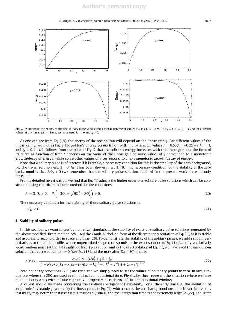
As one can see from Eq. (19), the energy of the one-soliton will depend on the linear gain c. For different values of thelinear gain c, we plot in Fig. 2 the soliton’s energy versus time t with the parameter values P ¼ 0:5;Q ¼ �0:25þ i; k1i ¼ 1,and n0 ¼ 0:1þ i. It follows from the plots of Fig. 2 that the soliton’s energy increases with the linear gain and the form ofits curve as function of time t depends on the value of the linear gain c: some values of c correspond to a monotonicgrowth/decay of energy, while some other values of c correspond to a non monotonic growth/decay of energy.

Note that a solitary pulse is of interest if it is stable, a necessary condition for this is the stability of the zero background,i.e., the trivial solution Aðx; tÞ ¼ 0. As it has been shown in work [10], the necessary condition for the stability of the zerobackground is that PrQ r < 0 (we remember that the solitary pulse solution obtained in the present work are valid onlyfor Pi ¼ 0Þ.

From a detailed investigation, we find that Eq. (1) admits the higher order one-solitary pulse solutions which can be con-structed using the Hirota bilinear method for the conditions

Pi ¼ 0;Q i > 0; Pr �3Q r �ffiffiffiffiffiffiffiffiffiffiffiffiffiffiffiffiffiffiffiffiffiffiffiffi9Q 2

r þ 8Q2i

q� �> 0: ð20Þ

The necessary condition for the stability of these solitary pulse solutions is

PrQ r < 0: ð21Þ

3. Stability of solitary pulses

In this section, we want to test by numerical simulations the stability of exact one-solitary pulse solutions generated bythe above modified Hirota method. We used the Crank–Nicholson form of the discrete representation of Eq. (1), as it is stableand accurate to second order in space and time [20]. To demonstrate the stability of the solitary pulses, we add random per-turbations to the initial profile, whose unperturbed shape corresponds to the exact solution of Eq. (1). Actually, a relativelyweak random noise (at the d % amplitude level) was added, and as the exact solution of Eq. (1), we have used the one-solitonsolution that corresponds to e ¼ 0 (see Eq. (18)and the note after Eq. (19)), that is,

Aðx; tÞ ¼ exp½k1xþ ðiPk21 þ cÞt þ n0�

ð1þ N0 exp½ðk1 þ k�1Þxþ Pfgðk1 þ k�1Þ2 þ iðk2

1 � k�21 Þgt þ n0 þ n�0�Þ1þig : ð22Þ

Zero boundary conditions (ZBC) are used and we simply need to set the values of boundary points to zero. In fact, sim-ulations where the ZBC are used need minimal computational time. Physically, they represent the situation where we havemetallic boundaries with infinite conductive properties at each end of the computational window.

A caveat should be made concerning the far-field (background) instability. For sufficiently small A, the evolution ofamplitude A is mainly governed by the linear gain c in Eq. (1), which makes the zero background unstable. Nevertheless, thisinstability may not manifest itself if c is reasonably small, and the integration time is not extremely large [21,22]. The latter

Fig. 2. Evolution of the energy of the one-solitary pulse versus time t for the parameter values P ¼ 0:5;Q ¼ �0:25þ i; k1i ¼ 1; n0 ¼ 0:1þ i, and for differentvalues of the linear gain c. Here, we have used k1r > 0 and g > 0.



circumstance helps make formally unstable solitary pulses stable and physically relevant objects [23]. In fact, the instabilityof a solution does not exclude its observation in experiments. If the time scale over which the onset of instability occurs farexceeds the duration of the experiments, then the formally unstable solution is as relevant for the experiment as is the stablesolution.

In what follows, we describe some sets of simulations which characterize the stability of the solitary pulses. These sim-ulations also show how the equation parameters affect the solitary pulses. For all the simulations, we take P and Q such thatthe necessary condition of the stability of the solitary pulses (21) is satisfied.

Remark. Because of the presence of the linear gain c, it is evident that the amplitude of the solitary pulses will increase asthe wave propagates.

3.1. Effect of the random perturbations

Now, we add random perturbations to the initial profile of the solitary pulses, whose unperturbed shape corresponds tothe exact solution (22) of Eq. (1). Relatively small random noise at 0.1% and 0.5% amplitude level were added in the case pre-sented in Fig. 3a and b, while a random noise at 3.75% amplitude level was added in the case presented in Fig. 3c. As we cansee from these figures, the evolution of the pulse is affected with strong noises (compare for example the maximal ampli-tudes of the solitary wave on Fig. 3a, b, and c).

3.2. Effect of the dispersion P

To observe the effect of the dispersion on the evolution of the solitary pulses, we consider six values of P, three negativevalues and three positive values. For all the plots of Fig. 4, we consider the same values of Q i ¼ 0:05; n0 ¼ 0:1þ i, and

Fig. 3. Propagation of the solitary pulse for P ¼ �0:5;Q ¼ 0:25þ 0:05i; c ¼ 0:025; n0 ¼ 0:1þ i; k1i ¼ 1;g < 0, and k1r > 0. The relative amplitude of the initialperturbation is 0.1% in (a), 0.5% in (b), and 3.75% in (c).

Fig. 4. Propagation of the solitary pulse for different values of the dispersion coefficient P for Qi ¼ 0:05; c ¼ 0:025; kr > 0; k1i ¼ 1, and n0 ¼ 0:1þ i. We haveused g > 0 and qr ¼ 1:2 for positive P, and g < 0 and Qr ¼ �1:2 for negative P. The relative amplitude of the initial perturbation is 0.1%. The values ofP ¼ �0:1; P ¼ �0:05; P ¼ �0:025; P ¼ 0:025; P ¼ 0:05, and P ¼ 0:1 are used for Fig. 4a, b, c, d, e, and f, respectively.



c ¼ 0:025. Because we need condition (21) to be satisfied, we will use different values of Q r : Qr ¼ 0:25 for negative P andQ r ¼ �1:2 for positive P. Fig. 4a, b, c, d, e, and f correspond to P ¼ �0:1; P ¼ �0:05; P ¼ �0:025; P ¼ 0:025; P ¼0:05; P ¼ 0:1. For all the plots of this figure, the relative amplitude of the initial perturbation 0.1% was added. The plots ofFig. 4 show that the width of the soliton increases with j P j and the amplitude of the solitary pulse depend on P, but, isnot monotone as function of P. The soliton sharpness is also affected by the dispersion coefficient P. One should note thattwo P with opposite sign do not correspond to the same evolution of the solitary pulse (this can be well observed fromFig. 4b and e).

3.3. Effect of the nonlinear gain

Here we present three plots to display the evolution of general wave packets for different values of nonlinear gain. Ran-dom noise (0.1%) is used. For all the plots of Fig. 5, we have used P ¼ �0:025;Qr ¼ 2:2; n0 ¼ �2þ 0:5i; k1i ¼ �1;c ¼ 0:025; k1r > 0 and g < 0. The plot of Fig. 5a, b, and c correspond to Qi ¼ 0:05;Qi ¼ 0:5, and Qi ¼ 1:5, respectively (weremember that the one-solitary pulse has been obtained only for positive Qi (see Eq. (20)). As the plots of Fig. 5 show,the width and the amplitude of the wave packets decrease as the nonlinear gain increases.

3.4. Effect of the linear gain

As we have mentioned above, for sufficiently small A, the evolution of amplitude A is mainly governed by the linear gain cin Eq. (1), which makes the zero background unstable, and this instability may not manifest itself if c is reasonably small, andthe integration time is not extremely large. In Fig. 6, we plot the evolution of the solitary pulses for different values of thelinear gain c when all the other parameters are maintained constant. Thus, we use for Fig. 6 the parameter values P ¼ 0:5,Q ¼ �2:2þ 2:5i; k1i ¼ �1; n0 ¼ �2� 0:5i;g > 0; k1r < 0. The relative amplitude of the initial perturbation is 0.1%. Plot (a)gives the propagation of the solitary pulse for the linear gain c ¼ 0:003, while plots (b) and (c) correspond to c ¼ 0:03and c ¼ 0:3, respectively. For all the plots of Fig. 6, the integration time is taken to be t ¼ 20. The plots of this figure showthat if the linear gain c is small, but not extremely small, instability manifests itself.

3.5. Effect of the solution parameter k1i on the solitary pulse

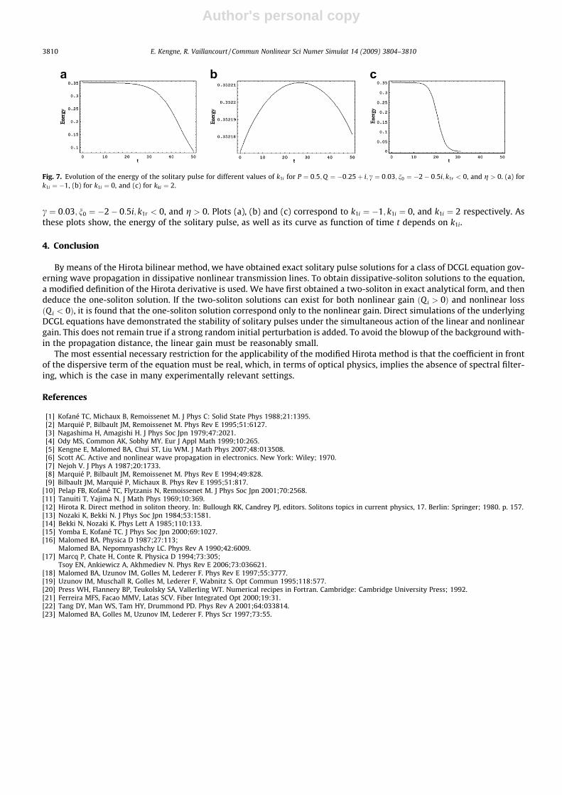
The three plots of Fig. 7 show the evolution of the density of the solitary pulses for different values of the parameter k1i.The solitary pulse we have used for these plots corresponds to the parameters P ¼ 0:5;Q ¼ �0:25þ i;

Fig. 5. Propagation of a general wave packet for different values of the nonlinear gain for P ¼ �0:025;Qr ¼ 2:2; n0 ¼ �2þ 0:5i; k1i ¼ �1; c ¼ 0:025; k1r > 0and g < 0. Plots (a), (b), and (c) correspond to Qi ¼ 0:05;Qi ¼ 0:5, and Qi ¼ 1:5, respectively.

Fig. 6. Plot of the propagation of the solitary pulse for the parameters P ¼ 0:5;Q ¼ �2:2þ 2:5i; k1i ¼ �1; n0 ¼ �2� 0:5i;g > 0; k1r < 0, with relativeamplitude of the initial perturbation 0.1%. Plots (a), (b), and (c) show the propagation of the solitary pulse for the linear gain c ¼ 0:003; c ¼ 0:03, and c ¼ 0:3,respectively.



c ¼ 0:03; n0 ¼ �2� 0:5i; k1r < 0, and g > 0. Plots (a), (b) and (c) correspond to k1i ¼ �1; k1i ¼ 0, and k1i ¼ 2 respectively. Asthese plots show, the energy of the solitary pulse, as well as its curve as function of time t depends on k1i.

4. Conclusion

By means of the Hirota bilinear method, we have obtained exact solitary pulse solutions for a class of DCGL equation gov-erning wave propagation in dissipative nonlinear transmission lines. To obtain dissipative-soliton solutions to the equation,a modified definition of the Hirota derivative is used. We have first obtained a two-soliton in exact analytical form, and thendeduce the one-soliton solution. If the two-soliton solutions can exist for both nonlinear gain ðQi > 0Þ and nonlinear lossðQ i < 0Þ, it is found that the one-soliton solution correspond only to the nonlinear gain. Direct simulations of the underlyingDCGL equations have demonstrated the stability of solitary pulses under the simultaneous action of the linear and nonlineargain. This does not remain true if a strong random initial perturbation is added. To avoid the blowup of the background with-in the propagation distance, the linear gain must be reasonably small.

The most essential necessary restriction for the applicability of the modified Hirota method is that the coefficient in frontof the dispersive term of the equation must be real, which, in terms of optical physics, implies the absence of spectral filter-ing, which is the case in many experimentally relevant settings.

References

[1] Kofané TC, Michaux B, Remoissenet M. J Phys C: Solid State Phys 1988;21:1395.[2] Marquié P, Bilbault JM, Remoissenet M. Phys Rev E 1995;51:6127.[3] Nagashima H, Amagishi H. J Phys Soc Jpn 1979;47:2021.[4] Ody MS, Common AK, Sobhy MY. Eur J Appl Math 1999;10:265.[5] Kengne E, Malomed BA, Chui ST, Liu WM. J Math Phys 2007;48:013508.[6] Scott AC. Active and nonlinear wave propagation in electronics. New York: Wiley; 1970.[7] Nejoh V. J Phys A 1987;20:1733.[8] Marquié P, Bilbault JM, Remoissenet M. Phys Rev E 1994;49:828.[9] Bilbault JM, Marquié P, Michaux B. Phys Rev E 1995;51:817.

[10] Pelap FB, Kofané TC, Flytzanis N, Remoissenet M. J Phys Soc Jpn 2001;70:2568.[11] Tanuiti T, Yajima N. J Math Phys 1969;10:369.[12] Hirota R. Direct method in soliton theory. In: Bullough RK, Candrey PJ, editors. Solitons topics in current physics, 17. Berlin: Springer; 1980. p. 157.[13] Nozaki K, Bekki N. J Phys Soc Jpn 1984;53:1581.[14] Bekki N, Nozaki K. Phys Lett A 1985;110:133.[15] Yomba E, Kofané TC. J Phys Soc Jpn 2000;69:1027.[16] Malomed BA. Physica D 1987;27:113;

Malomed BA, Nepomnyashchy LC. Phys Rev A 1990;42:6009.[17] Marcq P, Chate H, Conte R. Physica D 1994;73:305;

Tsoy EN, Ankiewicz A, Akhmediev N. Phys Rev E 2006;73:036621.[18] Malomed BA, Uzunov IM, Golles M, Lederer F. Phys Rev E 1997;55:3777.[19] Uzunov IM, Muschall R, Golles M, Lederer F, Wabnitz S. Opt Commun 1995;118:577.[20] Press WH, Flannery BP, Teukolsky SA, Vallerling WT. Numerical recipes in Fortran. Cambridge: Cambridge University Press; 1992.[21] Ferreira MFS, Facao MMV, Latas SCV. Fiber Integrated Opt 2000;19:31.[22] Tang DY, Man WS, Tam HY, Drummond PD. Phys Rev A 2001;64:033814.[23] Malomed BA, Golles M, Uzunov IM, Lederer F. Phys Scr 1997;73:55.

Fig. 7. Evolution of the energy of the solitary pulse for different values of k1i for P ¼ 0:5;Q ¼ �0:25þ i; c ¼ 0:03; n0 ¼ �2� 0:5i; k1r < 0, and g > 0. (a) fork1i ¼ �1, (b) for k1i ¼ 0, and (c) for kki ¼ 2.


Transmission of solitary pulse in dissipative nonlinear transmission lines

Documents

Transcript of Transmission of solitary pulse in dissipative nonlinear transmission lines