On the Dissipative Complex Ginzburg-Landau Equation Governing the Propagation of Solitary Pulses in...

CHINESE JOURNAL OF PHYSICS VOL. 47, NO. 1 FEBRUARY 2009

On the Dissipative Complex Ginzburg-Landau Equation Governing the

Propagation of Solitary Pulses in Dissipative Nonlinear Transmission Lines

E. Kengne,1, 2, ∗ C. Tadmon,2 and R. Vaillancourt1

1Department of Mathematics and Statistics,University of Ottawa, Ottawa, ON, K1N 6N5, Canada2Department of Mathematics and Computer Science,

Faculty of Science, University of Dschang,P.O. Box 4509, Douala, Republic of Cameroon

(Received May 15, 2008)

A class of dissipative complex Ginzburg-Landau (DCGL) equations that govern the wavepropagation in dissipative nonlinear transmission lines is solved exactly by means of theHirota bilinear method. Two-soliton solutions of the DCGL equations, from which the one-soliton solutions are deduced, are obtained in analytical form. The modified Hirota methodimposes some restrictions on the coefficients of the equations, namely, the second-orderdispersion must be real. The physical requirement of the solutions imposes complementaryconditions on the combination of the dispersion and nonlinear gain/loss terms of the equation,as well as on the coefficient of the Kerr nonlinearity. The analytical solutions for one-solitarypulses are tested in direct simulations.

PACS numbers: 03.75.Gg, 03.75.Nt, 03.75.Hh

I. INTRODUCTION

Nonlinear transmission lines (NLTLs) are very convenient tools for studying wavepropagation in nonlinear dispersive media [1]. They allow one to study qualitatively andquantitatively the properties of solitons [1, 2], provide a useful way to check how the non-linear excitations behave inside the nonlinear medium, and to allow one to model the exoticproperties of new systems [3]. For these reasons a growing interest has been devoted to theuse of NLTLs since the pioneering works by Hirota et al. [4] and Nagashima et al. [5] onsingle electrical lines simulating the Toda lattice [6] .

The multiplicative process in NLTLs is understood as a direct consequence of soliton-like propagation in this medium. Qualitatively, the origin of solitons in NLTLs is explainedby the balance between the effect of dispersion (due to the periodic location of capacitorsin the NLTL) and nonlinearity (due to the voltage dependence of the capacitances). Sincethe 1970s, various investigators have discovered the existence of solitons in NLTLs, throughboth mathematical models and physical experiments (see for example Refs. [5, 7–10]).Scott’s classical monograph [1] was among the first to treat the physics of transmissionlines. Scott showed that the Korteweg-deVries (KdV) equation describes weakly nonlinearwaves in a nonlinear LC transmission line containing a finite number of cells which consistof two elements: a linear inductor in the series branch and a nonlinear capacitor in the

http://PSROC.phys.ntu.edu.tw/cjp 81 c© 2009 THE PHYSICAL SOCIETYOF THE REPUBLIC OF CHINA

82 ON THE DISSIPATIVE COMPLEX . . . VOL. 47

shunt branch. If the nonlinearity is moved from the capacitor parallel to the shunt branchof the line to a capacitor parallel to the series branch, the nonlinear Schrodinger (NLS)equation is obtained instead [11].

Some years ago, the nonlinear propagation of signals in electrical transmission lineswas investigated, theoretically and experimentally [10, 12, 13]. It has been shown that thesystem of equations governing the physics of the considered network can be reduced eitherto single or coupled NLS equations or to the Ginzburg-Landau (GL) equations. The singleand the coupled NLS equations admit the formation of envelope solitons, which have beenobserved experimentally [12, 13].

More recently, Pelap et al. [14] presented a model for wave propagation on a discretedissipative electrical transmission line of Fig. 1 based on the complex Ginzburg-Landau(CGL) equation

i∂A

∂t+ P

∂2A

∂x2+Q |A|2A = iγA, (1)

derived in the small amplitude and long wavelength limit using the standard reductive per-turbation technique and complex expansion [15] of the governing nonlinear equations. HereA is a complex amplitude, P = Pr +iPi and Q = Qr +iQi are two complex constants, and γis a positive constant. Basically, the evolution of the complex wave envelope A is controlledby the competition of the dispersion (∼ P ) , nonlinearity (∼ Q) , and linear gain γ. Physi-cally, Pr measures the wave dispersion, Pi measures the relative growth rate of disturbanceswhose spectra are concentrated near the fundamental wavenumber k, Qr determines howthe wave frequency is amplitude modulated, Qi measures the saturation of the unstablewave, and the positive constant γ is the linear gain. The modulational instability of the

Stokes waves A (x, t) = A0 exp[

ik0x− i(

Prk20 −Qr |A0|2

)

t]

, where Qi |A0|2 = γ + Pik20 ,

was considered in Ref. [14] and the modulational instability criterion PrQr + PiQi > 0 hasbeen found.

The model shown in Fig. 1 is a lossy discrete nonlinear bi-inductance transmission linein which one cell consists of six elements: two linear inductors L1 and L2 (with L1 ≥ L2)in the series branch and two identical nonlinear capacitances C(V ) in the shunt branchesassociated with a conductance G. The losses due to the resistance of the inductors areneglected. The conductance (dissipative element) G accounts for the loss of the nonlinearcapacitor C. The line of Fig. 1 is an electrical equivalent of a diatomic lattice, in whichatoms interact with their first nearest neighbours through an interatomic potential withharmonic and cubic nonlinear interaction terms. As was shown in Ref. [14], the coefficientsP, Q, and γ of Eq. (1) are expressed in terms of the line parameters L1, L2, and G. Forexample, γ = G/ (2C0) , where the capacitance C0 is the value of the operating point, whichmay be adjusted by an external dc bias voltage V0.

In this work we study the transmission of solitary pulses, governed by the GL equation(1), propagating in the network of Fig. 1. This paper is structured as follows. In Section 2,we show how the modified Hirota method is applied to construct the exact solitary pulsesolutions of the DCGL equation. In Section 3, we present some numerical results, and thepaper is concluded in Section 4.

VOL. 47 E. KENGNE, C. TADMON AND R. VAILLANCOURT 83

FIG. 1: Representation of a discrete nonlinear dissipative bi-inductance transmission line.

II. DERIVATION OF EXPLICIT SOLITARY PULSE SOLUTIONS

In order to prove that Eq. (1) can support envelope solitons, we use the Hirota bilineartechnique [16]. Thus, we follow the definition of Nozaki and Bekki [17, 18] and introducethe modified Hirota derivative

Dmα,tD

nα,xF.G =

(

∂

∂t′− α

∂

∂t

)m (

∂

∂x′− α

∂

∂x

)n

F (x, t)G(

x′, t′)

∣

∣

∣

∣

x′=x,t′=t

. (2)

We first note that Eq. (1), under the transformation A (x, t) = ψ (x, t) exp (γt) , takesthe form

iψt + Pψxx +Q exp (2γt) |ψ|2 ψ = 0. (3)

The two-soliton solution of Eq. (3) is given by

ψ (x, t) = u1 (x, t) + u2 (x, t) , (4)

where u1 (x, t)u2 (x, t) = 0 corresponds to the single soliton. Inserting Eq. (4) into Eq. (3),we obtain the system

i∂u1

∂t+ P

∂2u1

∂x2+Q exp (2γt) |u1|2 u1 +Q exp (2γt)

(

2 |u1|2 u2 + u21u

∗

2

)

= 0,

i∂u2

∂t+ P

∂2u2

∂x2+Q exp (2γt) |u2|2 u2 +Q exp (2γt)

(

2 |u2|2 u1 + u22u

∗

1

)

= 0,

(5)

where “∗” stands for the complex conjugate. To obtain exact solutions of system (5) weadopt the modified Hirota ansatz

u1 (x, t) = G (x, t)F−α (x, t) , u2 (x, t) = H (x, t)F−α (x, t) , (6)

where G and H are two complex functions, F is a real function, and α is, in general,complex. Due to the presence of the power −α, the transformation (6) is different fromthat used in the case of the conventional nonlinear Schrodinger system. This difference is,as a matter of fact, the main motivation for introducing these modified Hirota derivatives.Expression (6) is deduced from the truncation of the Puiseux expansions at the lowest


level [19]. Using Eq. (6), Eq. ( 5) is rewritten as a pair of bilinear equations in terms of themodified Hirota derivative (2),

[

iDα,t + PD2α,x + iPβ + 2ixβPDα,x

]

F.G = 0,[

iDα,t + PD2α,x + iPβ + 2ixβPDα,x

]

F.H = 0,(7)

D2xF.F =

2Q exp (2γt) (2HG∗ +GH∗ +GG∗)

Pα (1 + α)F 2 Re α−2,

D2xF.F =

2Q exp (2γt) (2GH∗ +HG∗ +HH∗)

Pα (1 + α)F 2Re α−2,

(8)

for GH 6= 0. So the left-hand sides of Eq. (8) become equal. Hence the right-hand sides ofEq. (8) should also be equal, which is true only under the bilinear condition

(H +G) (G∗ −H∗) = 0, (9)

that is, H = εG with ε = ±1. In what follows, we consider that ε ∈ {−1, 0, 1}, ε = 0corresponding to the single soliton propagating in the network. We then obtain

[

iDα,t + PD2α,x

]

F.G = 0, (10)

D2xF.F =

2Q exp (2γt) (1 + 3ε)

Pα (1 + α)F 2Re α−2GG∗. (11)

For the special case α = 1+ iη with real η, (10)–(11) is a system with time-dependentcoefficients. For simplicity, we will restrict ourselves to this special case. Having obtainedthe bilinear condition and bilinear forms, our next aim is to obtain the soliton solutions.To generate the soliton solutions, we assume an expansion of the form

G = exp (xh1 (t) + h0 (t)) , F = 1+N (t) exp [x (h1 (t) + h∗1 (t)) + h0 (t) + h∗0 (t)] . (12)

Instead of taking h0 and h1 constant as in the conventional nonlinear Schrodinger system,we take h0 and h1 to be functions of time t, because we want to solve a system with time-varying coefficients, or, in other words, for the waves propagating in an inhomogeneousmedium. Inserting Eq. (12) into the system (10)–(11) we obtain

h′1 = 0, h′0 − iPh21 = 0,

N ′

N= Pη (h1 + h∗1)

2 , (13)

Q (1 + 3ε) exp (2γt) =α (1 + α)

2PN (h1 + h∗1)

2 . (14)

From Eq. (13) we obtain

h1 (t) = k1, h0 (t) = iPk21t+ ξ0, N (t) = N0 exp

[

Pη (k1 + k∗1)2 t

]

, (15)

where k1 and ξ0 are two complex constants and N0 is a real constant. If N0, η, and N (t)are real, the definition of N (t) in Eq. (15) requires P to be real. If N (t) and P are real,


but α = 1 + iη complex, Eq. (11) requires Q to be complex too. Working with real Pmeans that we do not include diffusion, which would be represented by an imaginary partof P [20–23]. However, the nonlinear coefficient Q, which is complex, allows a combinationof self-phase-modulation with nonlinear loss/gain. Thus, the diffusion term P and thenonlinear gain/loss Q term are necessary ingredients for the applicability of the method.From condition (14) we obtain

(k1 + k∗1)2 =

4γQi

P(

−3Qr ±√

9Q2r + 8Q2

i

) , N0 =(1 + 3ε)Qi

3γ, η =

−3Qr ±√

9Q2r + 8Q2

i

2Qi

.

(16)

As can be seen from Eq. (16), the coefficient η, which determines the chirp of the pulse,depends only on the nonlinear gain/loss term. Because P = Pr is real and γ > 0, thephysical solutions are those that make (k1 + k∗1)

2 positive, that is, as one can see fromEq. (16), P = Pr and Q = Qr + iQi must satisfy the condition

QiPr

(

−3Qr ±√

9Q2r + 8Q2

i

)

> 0. (17)

Because of the transformation A (x, t) = ψ (x, t) exp (γt) , we obtain from Eq. (4) that

A (x, t) = u1 (x, t) exp (γt) + u2 (x, t) exp (γt) = A1 (x, t) +A2 (x, t) .

From Eqs. (6), (12), (15), and (17), we obtain the following soliton

A1 (x, t) =exp

[

k1x+(

iPk21 + γ

)

t+ ξ0]

(

1 +N0 exp[

(k1 + k∗1) x+ P{

η (k1 + k∗1)2 + i

(

k21 − k∗21

)

}

t+ ξ0 + ξ∗0

])1+iη,

A2 (x, t) = εA1 (x, t) , ε ∈ {−1, 0, 1} ,(18)

where k1, N0, and η satisfy condition (16). Solution (18) contains two free parameters,namely, the complex parameter ξ0 and the real constant k1i = Im k1. It follows fromEq. (18) that the physical solutions are those that correspond to positive N0. As one cansee from Eq. (16), the physical solution then corresponds to positive Qi for ε ∈ {0, 1} andQi < 0 for ε = −1 (we remember that γ > 0). By setting k1 = k1r + ik1i and ξ0 = ξ0r + iξ0i,it is seen from Eqs. (16) and (18) that the amplitude of the solitary pulse is given by

|A1 (x, t)| = |A1 (z = x− vt)| =exp (ξ0r)

N0 exp (2ξ0r) exp (k1rz) + exp (−k1rz), v =

2Pk1ik1r − γ

k1r

,

(19)

and this means that the solitary pulse moves with velocity v = 2Pk1ik1r−γk1r

, which is an

arbitrary constant. The wavenumber is then k1r. If we take ξ0r = − ln√N0, Eq. (19)


FIG. 2: Evolution of the energy of the one-solitary pulse versus time t for the parameter valuesP = 0.5, Q = −0.25 + i, k1i = 1, ξ0 = 0.1 + i, and for different values of the linear gain γ. Here wehave used k1r > 0 and η > 0.

coincides with the moving soliton |A1 (z)| = 1/(

2√N0 cosh k1rz

)

. It can be seen fromEq. (19) that the soliton amplitude increases with ξ0r.

Note: According to Eq. (4), the one-soliton solutions of Eq. (1) are obtained fromEq. (15) as follows: If ε = 0, then A (x, t) = A1 (x, t) ; if ε = 1, then A (x, t) = 2A1 (x, t) .These two solutions are distinct, not only because of the factor 2 but also because of theexpression for N0 appearing in the expression of A1 (x, t) (see Eq. (18)). We note that forε = −1, we obtain from Eq. (4) the zero solution of Eq. (1).

As one can see from Eq. (19), the energy of the one-soliton will depend on the lineargain γ. For different values of the linear gain γ, we plot in Figure 2 the soliton’s energyversus time t with the parameter values P = 0.5, Q = −0.25 + i, k1i = 1, and ξ0 = 0.1 + i.It follows from the plots of Figure 2 that the soliton’s energy increases with the linear gainand the form of its curve as a function of time t depends on the value of the linear gainγ: some values of γ correspond to a monotonic growth/decay of energy, while some othervalues of γ correspond to a non-monotonic growth/decay of energy.

Note that a solitary pulse is of interest if it is stable, a necessary condition for thisis the stability of the zero background, i.e., the trivial solution A (x, t) = 0. As has beenshown in the work [14], the necessary condition for the stability of the zero background isthat PrQr < 0 (we remember that the solitary pulse solutions obtained in the present workare valid only for Pi = 0).


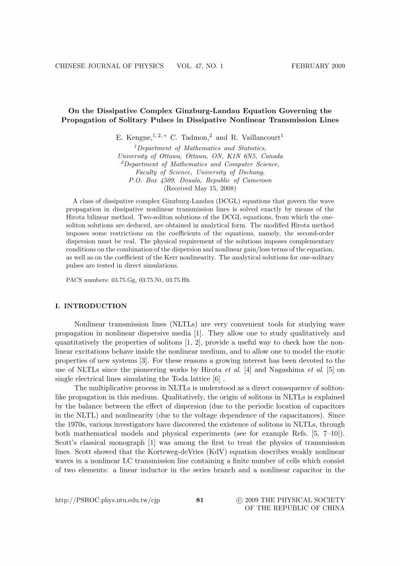
From a detailed investigation, we find that Eq. (1) admits the higher order one-solitary pulse solutions, which can be constructed using the Hirota bilinear method for theconditions

Pi = 0, Qi > 0, Pr

(

−3Qr ±√

9Q2r + 8Q2

i

)

> 0. (20)

The necessary condition for the stability of these solitary pulse solutions is

PrQr < 0. (21)

III. STABILITY OF SOLITARY PULSES

In this section, we want to test by numerical simulations the stability of the exactone-solitary pulse solutions generated by the above modified Hirota method. We used theCrank-Nicholson form of the discrete representation of Eq. (1), as it is stable and accurateto second order in space and time [24]. To demonstrate the stability of the solitary pulses,we add random perturbations to the initial profile, whose unperturbed shape correspondsto the exact solution of Eq. (1). Actually, a relatively weak random noise (at the δ %amplitude level) was added, and as the exact solution of Eq. (1), we have used the one-soliton solution that corresponds to ε = 0 (see Eq. (18) and the note after Eq. (19)). Zeroboundary conditions (ZBC) are used and we simply need to set the values of the boundarypoints to zero. In fact, simulations where the ZBC are used need minimal computationaltime. Physically, they represent the situation where we have metallic boundaries withinfinite conductive properties at each end of the computational window.

A caveat should be made concerning the far-field (background) instability. For suf-ficiently small A, the evolution of the amplitude A is mainly governed by the linear gainγ in Eq. (1), which makes the zero background unstable. Nevertheless, this instabilitymay not manifest itself if γ is reasonably small and the integration time is not extremelylarge [25, 26]. The latter circumstance helps make formally unstable solitary pulses stableand physically relevant objects [27]. In fact, the instability of a solution does not excludeits observation in experiments. If the time scale over which the onset of the instabilityoccurs far exceeds the duration of the experiments, then the formally unstable solution isas relevant for the experiment as is the stable solution.

In what follows, we describe some sets of simulations which characterize the stabilityof the solitary pulses. These simulations also show how the equation parameters affect thesolitary pulses. For all the simulations, we take P and Q such that the necessary conditionof the stability of the solitary pulses (21) is satisfied.

Remark. Because of the presence of the linear gain γ, it is evident that the amplitudeof the solitary pulses will increase as the wave propagates.

III-1. Effect of the random perturbations

Now we add random perturbations to the initial profile of the solitary pulses, whoseunperturbed shape corresponds to the exact solution of Eq. ( 1). Relatively small random


FIG. 3: Propagation of the solitary pulse for P = −0.5, Q = 0.25 + 0.05i, γ = 0.025, ξ0 = 0.1 + i,k1i = 1, η < 0, and k1r > 0. The relative amplitude of the initial perturbation is 0.1% in (a), 0.5%in (b), and 3% in (c).

FIG. 4: Propagation of the solitary pulse for different values of the dispersion coefficient P forQi = 0.05, γ = 0.025, kr > 0, k1i = 1, and ξ0 = 0.1+ i. We have used η > 0 and qr = 1.2 for positiveP, and η < 0 and Qr = −1.2 for negative P. The relative amplitude of the initial perturbation is0.1%. The values of P = −0.1, P = −0.05, P = −0.025, P = 0.025, P = 0.05, and P = 0.1 are usedfor Figs. 4(a), 4(b), 4(c), 4(d), 4(e), and 4(f), respectively.

noise at 0.1% and 0.5% amplitude level was added in the cases presented in Figs. 3(a)and 3(b), while a random noise at 3% amplitude level was added in the case presented inFig. 3(c). As we can see from these figures, the evolution of the pulse is affected with strongnoises (3%) (see Fig. 3(c) in comparison with Figs. 3(a) and 3(b)).


FIG. 5: Propagation of a general wave packet for different values of the nonlinear gain for P =−0.025, Qr = 2.2, ξ0 = −2 + 0.5i, k1i = −1, γ = 0.025, k1r > 0, and η < 0. Plots (a), (b), and (c)correspond to Qi = 0.05, Qi = 0.5, and Qi = 1.5, respectively.

III-2. Effect of the dispersion P

To observe the effect of the dispersion on the evolution of the solitary pulses, weconsider six values of P, three negative values and three positive values. For all the plotsof Fig. 4, we consider the same values of Qi = 0.05, ξ0 = 0.1 + i, and γ = 0.025. Becausewe need condition (21) to be satisfied, we will use different values of Qr: Qr = 0.25 fornegative P and Qr = −1.2 for positive P. Figs. 4(a), 4(b), 4(c), and 4(d) correspond toP = −0.1, P = −0.05, P = −0.025, P = 0.025, P = 0.05, and P = 0.1. For all the plots ofthis figure, the relative amplitude of the initial perturbation 0.1% was added. The plots ofFig. 4 show that the width of the soliton increases with |P | and the amplitude of the solitarypulse depends on P , but is not monotonic as a function of P . The soliton sharpness is alsoaffected by the dispersion coefficient P . One should note that two Ps with opposite signsdo not correspond to the same evolution of the solitary pulse (this can be well observedfrom Figs. 4(b) and 4(e)).

III-3. Effect of the nonlinear gain

Here we present three plots to display the evolution of general wave packets fordifferent values of nonlinear gain. Random noise (0.1%) is used. For all the plots ofFigure 5, we have used P = −0.025, Qr = 2.2, ξ0 = −2+0.5i, k1i = −1, γ = 0.025, k1r > 0,and η < 0. The plot of Figs. 5(a), 5(b), and 5(c) correspond to Qi = 0.05, Qi = 0.5, andQi = 1.5, respectively (we remember that the one-solitary pulse has been obtained only forpositive Qi (see Eq. 20). As the plots of Figure 5 show, the width and the amplitude of thewave packets decrease as the nonlinear gain increases.

III-4. Effect of the linear gain

As we have mentioned above, for sufficiently small A, the evolution of the amplitudeA is mainly governed by the linear gain γ in Eq. (1 ), which makes the zero backgroundunstable, and this instability may not manifest itself if γ is reasonably small and the inte-gration time is not extremely large. In Figure 6, we plot the evolution of the solitary pulsesfor different values of the linear gain γ when all the other parameters are maintained con-


FIG. 6: Plot of the propagation of the solitary pulse for the parameters P = 0.5, Q = −2.2 + 2.5i,k1i = −1, ξ0 = −2 − 0.5i, η > 0, and k1r < 0, with relative amplitude of the initial perturbation0.1%. Plots (a), (b), and (c) show the propagation of the solitary pulse for the linear gain γ = 0.003,γ = 0.03, and γ = 0.3, respectively.

FIG. 7: Evolution of the energy of the solitary pulse for different values of k1i for P = 0.5, Q =−0.25 + i, γ = 0.03, ξ0 = −2 − 0.5i, k1r < 0, and η > 0. (a) for k1i = −1, (b) for k1i = 0, and (c)for kki = 2.

stant. Thus, we use for Figure 6 the parameter values P = 0.5, Q = −2.2 + 2.5i, k1i = −1,ξ0 = −2 − 0.5i, η > 0, and k1r < 0. The relative amplitude of the initial perturbation is0.1%. Plot (a) gives the propagation of the solitary pulse for the linear gain γ = 0.003,while plots (b) and (c) correspond to γ = 0.03 and γ = 0.3, respectively. For all the plotsof Figure 6, the integration time is taken to be t = 20. The plots of this figure show that ifthe linear gain γ is small, but not extremely small, instability manifests itself.

III-5. Effect of the solution parameter k1i on the solitary pulse

The three plots of Figure 7 show the evolution of the density of the solitary pulsesfor different values of the parameter k1i. The solitary pulse we have used for these plotscorresponds to the parameters P = 0.5, Q = −0.25 + i, γ = 0.03, ξ0 = −2 − 0.5i, k1r < 0,and η > 0. Plots (a), (b), and (c) correspond to k1i = −1, k1i = 0, and k1i = 2, respectively.As these plots show, the energy of the solitary pulse, as well as its curve as a function oftime t, depends on k1i.


IV. CONCLUSION

By means of the Hirota bilinear method, we have obtained exact solitary pulse so-lutions for a class of DCGL equations governing wave propagation in dissipative nonlineartransmission lines. To obtain dissipative-soliton solutions to the equations, a modifieddefinition of the Hirota derivative is used. We have first obtained a two-soliton in ex-act analytical form, and then deduce the one-soliton solution. If the two-soliton solutionscan exist for both nonlinear gain (Qi > 0) and nonlinear loss (Qi < 0), it is found thatthe one-soliton solution corresponds only to the nonlinear gain. Direct simulations of theunderlying DCGL equations have demonstrated the stability of solitary pulses under thesimultaneous action of the linear and nonlinear gain. This does not remain true if a strongrandom initial perturbation is added. To avoid the blowup of the background within thepropagation distance, the linear gain must be reasonably small.

The most essential necessary restriction for the applicability of the modified Hirotamethod is that the coefficient in front of the dispersive term of the equation must be real,which, in terms of optical physics, implies the absence of spectral filtering, which is the casein many experimentally relevant settings.

References

∗ Electronic address: [email protected][1] A. C. Scott, Active and Nonlinear Wave Propagation in Electronics (Wiley, NewYork, 1970).[2] M. Remoissenet, Waves Called Solitons 2nd edn (Springer, Berlin, 1996).[3] K. E. Lonngren, Solitons in Action, edn K. E. Lonngren and A. C. Scott (Academic, New York,

1978).[4] R. Hirota and K. Suzuki, J. Phys. Soc. Jpn. 28, 1366 (1970); Proc. IEEE 61, 1483 (1973).[5] H. Nagashima and H. Amagishi, J. Phys. Soc. Japan 47, 2021 (1979).[6] M. Toda, J. Phys. Soc. Jpn. 23, 501 (1967).[7] T. C. Kofane, B. Michaux, and M. Remoissenet, J. Phys. C: Solid State Phys. 21, 1395 (1988).[8] P. Marquie, J. M. Bilbault, and M. Remoissenet, Phys. Rev. E 51, 6127 (1995).[9] M. S. Ody, A. K. Common, and M. Y. Sobhy, Eur. J. Appl. Math. 10, 265 (1999).

[10] E. Kengne, B. A. Malomed, S. T. Chui, and W. M. Liu, J. Math. Phys. 48, 013508 (2007).[11] V. Nejoh, J. Phys. A 20, 1733 (1987).[12] P. Marquie, J. M. Bilbault, and M. Remoissenet, Phys. Rev E 49, 828 (1994).[13] J. M. Bilbault, P. Marquie, and B. Michaux, Phys. Rev. E 51, 817 (1995).[14] F. B. Pelap, T. C. Kofane, N. Flytzanis, and M. Remoissenet, J. Phys. Soc. Jpn 70, 2568

(2001).[15] T. Tanuiti and N. Yajima, J. Math. Phys. 10, 1369 (1969).[16] R. Hirota, Direct method in soliton theory. Solitons (Topics in Current Physics vol 17) ed. R.

K. Bullough and P. J. Candrey (Springer, Berlin, 1980) p. 157.[17] K. Nozaki and N. Bekki, J. Phys. Soc. Jpn. 53, 1581 (1984).[18] N. Bekki and K. Nozaki, Phys. Lett. A 110, 133 (1985).[19] E. Yomba and T. C. Kofane, J. Phys. Soc. Jpn. 69, 1027 (2000).[20] B. A. Malomed, Physica D 27, 113 (1987); B. A. Malomed and L. C. Nepomnyashchy,

Phys. Rev. A 42, 6009 (1990).


[21] P. Marcq, H. Chate, and R. Conte, Physica D 73, 305 (1994); E. N. Tsoy, A. Ankiewicz, andN. Akhmediev, Phys. Rev. E 73, 036621 (2006).

[22] B. A. Malomed, I. M. Uzunov, M. Golles, and F. Lederer, Phys. Rev. E 55, 3777 (1997).[23] I. M. Uzunov, R. Muschall, M. Golles, F. Lederer, and S. Wabnitz, Opt. Commun. 118, 577

(1995).[24] W. H. Press, B. P. Flannery, S. A. Teukolsky, and W. T. Vallerling, Numerical Recipes in

Fortran (Cambridge University Press, Cambridge, 1992).[25] M. F. S. Ferreira, M. M. V. Facao, and S. C. V. Latas, Fiber Integrated Opt. 19, 31 (2000).[26] D. Y. Tang, W. S. Man, H. Y. Tam, and P. D. Drummond, Phys. Rev. A 64, 033814 (2001).[27] B. A. Malomed, M. Golles, I. M. Uzunov, and F. Lederer, Phys. Scr. 73, 55 (1997).

On the Dissipative Complex Ginzburg-Landau Equation Governing the Propagation of Solitary Pulses in...

Documents

Transcript of On the Dissipative Complex Ginzburg-Landau Equation Governing the Propagation of Solitary Pulses in...