Dynamics of defects in the vector complex Ginzburg–Landau equation

Physica D 174 (2003) 176–197

Dynamics of defects in the vector complexGinzburg–Landau equation

Miguel Hoyuelosa,b, Emilio Hernández-Garcıaa,∗, Pere Coleta, Maxi San Miguelaa Instituto Mediterráneo de Estudios Avanzados, IMEDEA (CSIC-UIB),Campus Universitat Illes Balears, E-07071 Palma de Mallorca, Spain

b Departamento de F´ısica, Facultad de Ciencias Exactas y Naturales, Universidad Nacional deMar del Plata, Funes 3350, 7600 Mar del Plata, Argentina

Received 3 October 2001; received in revised form 18 February 2002; accepted 15 May 2002

Abstract

Coupled Ginzburg–Landau equations appear in a variety of contexts involving instabilities in oscillatory media. Whenthe relevant unstable mode is of vectorial character (a common situation in nonlinear optics), the pair of coupled equationshas special symmetries and can be written as avector complex Ginzburg-Landau(CGL) equation. Dynamical propertiesof localized structures of topological character in this vector-field case are considered. Creation and annihilation processesof different kinds of vector defects are described, and some of them interpreted in theoretical terms. A transition betweendifferent regimes of spatiotemporal dynamics is described.© 2002 Elsevier Science B.V. All rights reserved.

Keywords:Vector Ginzburg–Landau equation; Topological defects; Spatiotemporal chaos; Optical instabilities; Light polarization

1. Introduction

Localized structures, objects with some kind of particle-like behavior, can be found in a variety of nonlinearlyevolving fields. Examples are vortices in fluids, superfluids and superconductors, propagating pulses of excitationin nerve systems, solitary waves in chemical media, in parametrically driven surfaces, and in granular media,among others[1]. An understanding of complex evolving configurations can be sometimes achieved in terms of theinteraction rules of the particle-like entities. In most cases, however, numerical integration of the evolution equationsis the most powerful tool to investigate the role of the localized structures.

Nonlinear optical cavities have been specially prolific in providing examples of localized structures[2]. Theyappear in the transverse profile of the field and can take the form of vortices, or of bright or dark dissipative spatialsolitons. It is usually considered that the polarization degree of freedom of the electromagnetic field is fixed eitherby material anisotropies or by experimental arrangement. Thus the description of the dynamics is done in terms

∗ Corresponding author. Fax:+34-971-173426.E-mail address:[email protected] (E. Hernandez-Garcıa).URL: http://www.imedea.uib.es/PhysDept/

0167-2789/03/$ – see front matter © 2002 Elsevier Science B.V. All rights reserved.PII: S0167-2789(02)00690-5

M. Hoyuelos et al. / Physica D 174 (2003) 176–197 177

of a scalar field. However, in the cases in which the polarization of the light is not fixed, the vector nature ofthe electromagnetic field leads to striking topological phenomena[3]. Recently reported examples of localizedstructures for which the polarization plays a fundamental role include points of zero amplitude in both componentsof the field in a periodic elliptically polarized background, found in type II OPO[4] and dots of low amplitude in acircularly polarized component of the field in an almost circularly polarized background found in self-defocusingvectorial Kerr resonators[5].

The scalar complex Ginzburg–Landau (CGL) equation is considered a paradigm model for the qualitative de-scription of general nonlinear oscillatory media (see, for example,[6–8]). The vector complex Ginzburg–Landau(VCGL) equation[9–13] plays the same role when the order parameter is of vector character, as is the case forthe electromagnetic field when the polarization is not fixed. For example, the VCGL equation is an appropri-ate model for laser emission from wide-aperture resonators close to the lasing threshold[13] in the absence ofpolarization-selecting cavity features. Different kinds of localized structures[9–12,14–16]are present in the dy-namic states of the two-dimensional VCGL equation. From a topological point of view, they aredefects, that is,places where the field state departs from some basic ordered state. These objects carry topological properties whichendorse them with a characteristic stability and robustness.

In this paper we study the dynamical properties of these defects for several dynamical regimes of the VCGLequation. In addition to reviewing and adding details to results previously presented, which address the synchro-nization properties of spatiotemporally chaotic states[14], the identification of a transition from aglassto agasphase[15], and the formation and annihilation processes leading to the different types of defects[16], we interpretsome of these findings in terms of the stability properties of the waves emitted by the defect cores, and in terms ofa recent perturbative analytic approach[17]. Since we are interested mostly in the dynamics of topological defects,we consider here just the two-dimensional VCGL case, for which point defects are topologically stable. For VCGLdynamics in one spatial dimension we refer the reader to[14,18,19].

Section 2presents the basic equations and properties. The different topological defects are described inSection 3,andSection 4is devoted to their dynamical properties. A description of agas-likephase is presented inSection 5.In Section 6we briefly discuss a situation of phase separation. Finally,Section 7summarize our conclusions.Appendix Aaddresses the stability of waves emitted by vector defects.

2. The vector complex Ginzburg–Landau equation

Extended systems close to a Hopf bifurcation at zero wavenumber are described by the CGL equation:

∂tA = A + (1 + iα)∇2A − (1 + iβ)|A|2A. (1)

For systems where the relevant unstable mode is of vectorial character,Eq. (1)is generalized to the VCGL equation

∂tA = A + (1 + iα)∇2A − (1 + iβ)[(A · A∗)A + 12(γ − 1)(A · A)A∗]. (2)

In the simplest caseA has two complex components. This is precisely the case of optical systems, for which,A = (Ax,Ay) describe the complex slowly varying amplitude of the electric field, whereAx andAy are theCartesian components. The right and left circularly polarized components(A+, A−) are related to them via therelationsAx = (A+ + A−)/

√2 andAy = (A+ − A−)/(i

√2). In terms of the circular components,Eq. (2)reads

∂tA± = A± + (1 + iα)∇2A± − (1 + iβ)(|A±|2 + γ |A∓|2)A±. (3)

The coefficientγ , which in general can be complex, gives the coupling between the components. Forγ = 0 werecover a pair of uncoupled equations of the form(1). We will often refer toEq. (1)as thescalarCGL, to contrast

178 M. Hoyuelos et al. / Physica D 174 (2003) 176–197

it with Eqs. (2)or (3). Forγ �= 0, Eq. (3)can be thought as a particularly symmetric example (for example, groupvelocity terms are absent) of a pair of coupled complex Ginzburg–Landau equations of the kind usually encounteredin wave competition situations[6].

WhenEq. (2) is derived for the Hopf bifurcation leading to laser emission[13], α is related to the strength ofdiffraction, andβ to the nonlinear frequency detuning. In this case, the so called Benjamin–Feir stability criterion1+ αβ > 0 is always satisfied, which means that there are always some plane waves which are stable against longwavelength perturbations. In addition, for laser systems,γ turns out to be a real parameter, andγ > −1. In thispaper, we will restrict our study to these ranges of parameters.

Eq. (3)has a family of plane-wave solutions of the form:

A± = Q± e−i(k±r−ω±t+φ0±). (4)

Within this family, the simplest solutions are the circularly polarized traveling waves, for which one of the compo-nents is identically 0

Q+ = 1 − k2, Q− = 0, ω+ = −β + (β − α)k2 (5)

or

Q+ = 0, Q− = 1 − k2, ω− = −β + (β − α)k2. (6)

Within the family (4) there are also solutions in which both components coexist. For wavevectors with the samemodulus,k+ = k− = k, we have

Q2+ = Q2

− = Q2 = 1 − k2

1 + γ, ω+ = ω− = ω = −β + (β − α)k2. (7)

We can have a linearly polarized traveling wave (k+ = k−) or a standing wave with periodic linear polarization(k+ = −k−). It is also possible to have depolarized solutions[13] with k+ �= k−

Q± = 1 − γ + γ k2± − k2∓1 − γ 2

, ω± = −αk2± − β(Q2

± + γQ2∓). (8)

The qualitative behavior for the VCGLequation (3)for |γ | < 1 is rather different from the one forγ > 1. Inthe second case the nonlinear competition betweenA+ andA− tends to favor one of them against the other, sothat in regions whereA+ is developed,A− generally vanishes, and vice versa. There are stable circularly polarizedsolutions of the form(5)or (6)while solutions of the form(7)which involve the coexistence of both fields are linearlyunstable. On the contrary, for|γ | < 1, wave coexistence is generally achieved. Circularly polarized solutions of theform (5) or (6) are linearly unstable while there are stable solutions of the forms(7) and (8). The character of thetopological defects in both cases is different[11,12]. In Sections 5 and 6we will consider the case|γ | < 1. Thecaseγ > 1 will be discussed inSection 6.

Forγ real, the point in parameter spaceα = β = 0 represents a special case of particularly simple dynamics. TheVCGL equation becomes then a potential system, or more precisely[20,21], a ‘relaxational gradient’ dynamicalsystem. Dynamics at long times approaches steady states that are identified as the minima of a Lyapunov potential.This is the case which is considered in greater detail in[11,12]. A more general situation isα = β. In this casethe system can be classified as ‘relaxational non-gradient’[20,21], and although a Lyapunov functional can be stillidentified, the attractor for the dynamics is no longer steady in general. The limiting ‘conservative case’α = β → ∞,also addressed in[11,12], leads to coupled nonlinear Schrödinger (or Gross–Pitaevskii) equations. This last limit isof great interest for the description of multicomponent Bose condensates[22] or the propagation of vector solitonsin optical fibers[23].


Fig. 1. Vectorial defects forγ = 0.1, α = 0.2 andβ = 2 (κ = 1.29). From left to right, top row:|A+|2, |A−|2, global phaseφg, and|Ax |2.Bottom row:φ+, φ−, relative phaseφr , and phase ofAx . Here and in the following figures, the values are coded in gray scale. In the imagesdisplaying amplitude values, black means zero amplitude, and thus the presence of a defect.

3. Scalar and vector defects for |γ | < 1

Starting from random initial conditions, even if the condition for existence of stable plane waves (1+ αβ > 0)is satisfied, solutions of(3) usually do not evolve to a simple plane wave(4) due to the presence of defects: pointswhere the phase ofA+ or A− is undefined and the corresponding amplitude is equal to 0. Around each defect, aspiral wave develops (except ifα = β) that, far from the defect core, approaches a plane wave with a particularwavenumber which has been dynamically selected by the presence of the defect. For example,Fig. 1shows differentviews of a configuration obtained after time evolution1 starting from random initial conditions, forα = 0.2,β = 2,andγ = 0.1. The configuration consist of wave domains separated by shock waves. There is a defect in bothcomponents (the black dot) in the center of each domain. Inhomogeneities and defects in just one of the componentshave been expelled away from the defect core with a given group velocity.

Therefore, two different kinds of defects are readily identified:Vector defectsare points at which the two com-ponentsA+ andA− simultaneously vanish (and thus the same happens forAx andAy at the same point).Scalardefects(mixed defectsin the nomenclature of[11,12]) are those at which only one of the two fields,A+ or A−vanish. In this case the vectorA is not 0, and the componentsAx andAy do not necessarily vanish, but they havestill a singular topological structure to be described below. The following ansatz describes the fieldA close to ascalar or to a vector defect

A±(r, θ) = R±(r)eiφ±(r,θ), (9)

where(r, θ) are the polar coordinates with the origin of coordinates at the defect core. The amplitude ofA+ and (or)A− go to zero at the core of a vector (scalar) defect:R+ and (or)R− → 0 for r → 0. The phase of the componentwhich vanishes atr = 0 is

φi(r, θ) = niθ + ψi(r) − ωit + φ0i , (10)

1 The integration algorithm is the one presented in[15], which is a generalization to the vector case of the pseudospectral in space andsecond-order in time algorithm for the CGL equation of[26]. We discretize with a 128× 128 square lattice a domain of 64× 64 space unitswith periodic boundary conditions. Animations of the different dynamic phenomena can be downloaded from website given in[24].


where the subindexi stands for+ or −. From expression(10), ni is seen to satisfy

ni = 1

2π

∮Γ

∇φi · dr, (11)

whereΓ is a closed path around the defect. This identifiesni as the topological charge associated to the singularityin the fieldAi . It necessarily takes integer values. In our numerical simulations we have never found for it a valuedifferent from 0,+1 or−1.ωi is the rotation frequency of the spiral wave inAi . Forr → ∞, ψ±(r) → kr.

It is possible to make a classification of defects using topological arguments[11,12]. Although this is not the wayin which it was originally introduced, the classification becomes particularly simple in terms of the charges(11).As stated before, avectordefect is the one at which both components of the field vanish. Thus, necessarily bothn+ andn− are nonvanishing. A vector defect is of typeargumentwhen the charges in the two field componentshave the same signs, i.e., whenn+ = n− = 1 or n+ = n− = −1. If the charges are of opposite signs, i.e., whenn+ = −n− = 1 or n+ = −n− = −1, the vectorial defect is ofdirector type. Ascalardefect is the one at whichjust one component of the field, but not the other, vanishes. This implies that only one of the two charges is differentfrom zero:n+ = ±1 andn− = 0, orn− = ±1 andn+ = 0 (seeFig. 2).

Numerically we observe that for vectorial defects both fields have identical modulus near the core:|A+| = |A−|,thusR+(r) = R−(r) = R(r). Then close to a vector defect,Eq. (3)becomes

∂tA± = A± + (1 + iα)∇2A± − (1 + iβ)(1 + γ )|A|2±A±. (12)

Each component is described by a scalar CGLequation (1)for a rescaled value of the common amplitude,A ≡√1 + γA±. In the rescaled variable, the shape and the size of the vectorial defect is independent ofγ . Furthermore,

we can use the arguments given by Hagan for the scalar CGL equation[25] to determine the wavenumbersk+ andk−. According to this the spiral wavenumber depends only on the parametersα andβ, thereforek+ = k− = kH ,wherekH (α, β) is the wavenumber of a spiral in the scalar CGL. Far from the defect core, asr → ∞, ψ+(r) =ψ−(r) = ψ(r) → kH r. The rotation frequencies areω+ = ω− = ω, whereω is given byEq. (7)usingk = kH . Itturns out[25] that the dependence ofkH onα andβ is always through the combination

κ =∣∣∣∣ α − β

1 + αβ

∣∣∣∣ , (13)

a parameter that will be important in the following. Ifκ = 0, kH = 0, so that whenα = β (the relaxational case) ahomogeneous state is found instead of a wave far from the vector defect core.

Fig. 2. Scheme showing the possible defects according to different combination of the chargesn+ andn−. White dots correspond to scalardefects, black dots to vectorial argument defects, and gray dots to vectorial director defects.


For an argument vectorial defect,n+ = n− = n = ±1, and we have

Ax =√

2R(r) cos(12�φ0)ei[nθ+ψ(r)−ωt+(φ0++φ0−)/2],

Ay =√

2R(r) sin(12�φ0)ei[nθ+ψ(r)−ωt+(φ0++φ0−)/2], (14)

where�φ0 = φ0+ − φ0− is the difference in initial phases ofA+ andA−. If A represents an optical field, itspolarization is linear, since the Cartesian componentsAx andAy oscillate in phase. The angle of polarization is theconstantξ = �φ0/2.

For a director vectorial defect,n+ = −n− = n = ±1, we have

Ax =√

2R(r) cos(nθ + 12�φ0)ei[ψ(r)−ωt+(φ0++φ0−)/2],

Ay =√

2R(r) sin(nθ + 12�φ0)ei[ψ(r)−ωt+(φ0++φ0−)/2]. (15)

The polarization in this case is also linear at each point, but the angle of polarization, given byξ = nθ + �φ0/2,rotates around the core of the defect (from here the name ofdirectordefect).

The defects just presented do indeed appear spontaneously in numerical simulations ofEq. (2) in appropriateparameter ranges. However, the classification by itself does not indicate much about the dynamics. It turns out that,when present, the vectorial defects dominate the dynamics, as shown inFig. 1. They generate a large exclusiondomain from which any inhomogeneity or scalar defect is expelled away. The scalar defects accumulate at thedomain limits. The modulus ofA+ andA− remain essentially frozen in time. The phasesφ+ andφ− displaycorotating spirals for the argument defects and counterrotating spirals for the director defects, in agreement with(10) for the appropriate values of the chargesni . We also show inFig. 1 the global phaseφg = φ+ + φ− and therelative phaseφr = φ+ −φ−. Argument and director defects are easily distinguished in the plot of the global phase:around an argument defect a two-armed spiral is formed (in a closed path around the defectφg changes in 4π ),while a target pattern is seen in the domain of a director defect (φg does not change). The relative phaseφr does notchange in a closed path around an argument defect while for a director defect it changes in 4π . The scalar defectsare identified as the points where the global or relative phase changes by 2π in a closed path around the point. Themodulus and phase ofAx are also plotted. In the domains of argument defects, the modulus ofAx is constant andthe phase is a spiral, in agreement withEq. (14). In the domains of the director defects,|Ax | has a characteristicradial structure that arises from the term cos(nθ + �φ0/2) in Eq. (15). The phase ofAx is a target pattern brokenby a straight line where there is a phase jump ofπ . This jump is produced by the change of sign of the cosine inEq. (15).

Fig. 3 shows a scalar defect present in theA+ component. It has been obtained at the same values ofα andβas before, butγ = 0.4. At these parameter values, vectorial defects do not appear (as discussed later), so that thescalar ones are allowed to generate wave domains, as the one shown inFig. 3. At the scalar defect-core, where oneof the component vanishes, the modulus of the other has a local maximum. Thus the object is circularly polarizedand imposes some elliptic polarization to its neighborhood. The phase ofA+ is a spiral wave whose wavenumbercannot be derived from the Hagan approach, since for scalar defects we have that|A+| �= |A−| (seeFig. 4) and noreduction to a single scalar CGL is possible. The wavenumber of the spiral wave is smaller thankH . The phase ofthe nonvanishing component is almost constant. More precisely, this phase slowly changes with radial symmetryas one moves away from the center, so that the lines of constant phase form a target pattern. In a similar set ofequations that include convective terms and a complex coupling, scalar defects have also been reported[27]. Inthat case, the phase of the nonvanishing field component presents a clearer target pattern. Phase target patterns inthe scalar CGL equation are also found under suitable boundary conditions[28,29] or inhomogeneities[30]. Theamplitudes and phases of thex andy linearly polarized components of the field around a scalar defect, also shown


Fig. 3. Different views of a scalar defect forγ = 0.4,α = 0.2 andβ = 2 (κ = 1.29), present in theA+ component. From left to right, top row:|A+|2, |A−|2, |Ax |2 and|Ay |2; bottom row:φ+, φ−, and phases ofAx andAy .

in Figs. 3 and 4, present spiral waves. Note that only phase waves, and not amplitude spiral waves, appear in thescalar CGL equation.

Fig. 5shows another view of scalar defects at two values ofγ . The maximum in the modulus of the nonvanishingcomponent, associated with the presence of the defect, is seen to grow with the value ofγ , if γ > 0. This is a

Fig. 4. Cross-sections of the intensities of a scalar defect (same parameters as inFig. 3). The top figure shows the defect in the+ component(solid line), and associated maximum in|A−|2 (dashed line). Bottom figure shows the spiral waves in thex andy amplitudes are out of phase(compare withFig. 3).


Fig. 5. Scalar defects at different values ofγ , as a function of the two spatial coordinates. First row:|A+|2 (left) and|A−|2 (right) atγ = 0.1.Second row: same as first row but forγ = 0.4. In both casesκ = 1.29, and the singular component isA+.

consequence of the coupling term inEq. (3), which favors anticorrelation ifγ > 0 (but positive correlation ifγ < 0). Notice also that the size of the scalar defect-core increases withγ .

4. Defect dynamics for |γ | < 1

We first discuss all the theoretically possible processes of creation and annihilation of defects. These processesare illustrated inFig. 6where we plot in the horizontal axis the topological charge of theA− component, and in thevertical axis the one ofA+. Open circles correspond to scalar defects, black circles to argument defects and graycircles to director defects as inFig. 2. The vectorial sum of arrows in the scheme implements the rule of topologicalcharge conservation. The possible processes are: (i) Creation of a vector defect by the coalescence of two scalardefects (illustrated inFig. 6(a) for an argument defect). This process is described inSection 4.1; (ii) Splitting ofa vector defect in two scalar defects, which is in fact the inverse process (seeSection 4.3); (iii) Annihilation of avector defect by collision with a scalar one.Fig. 6(b) represents the annihilation of an argument defect (the blackdot) by collision with a scalar defect in theA+ component (the open dot in the vertical axis), giving as a result ascalar defect in theA− component (the open dot in the horizontal).Fig. 6(c) shows a similar annihilation processfor a director defect (Section 4.2).


Fig. 6. Scheme showing some possible creation and destruction processes of defects in then+–n− plane. See text for details. (a) Creation ofan argument defect, (b) annihilation of an argument defect due to the collision with a scalar defect with chargen− = −1, (c) annihilation of adirector defect.

Aranson and Pismen performed recently[17] an analytical study of the interactions between scalar defects atdifferent field components, aiming at characterizing the stability properties of vector defects: if two scalar defects indifferent components attract each other, a vector defect will be formed in absence of other processes, whereas vectordefects will be unstable if their components repel. A first result is that the interaction is long ranged, in contrast to thecharacter of the interaction between defects in the same field. The approach in[17] is perturbative for small|γ |. Theresults depend on the value ofκ, the parameter fixing the asymptotic value of the wavenumber. According to[17]there is a critical valueκc � 0.52 such that ifκ > κc two scalar defects in different components attract each otherfor γ > 0.2 For γ < 0, two scalar defects in different components attract each other ifκ < κc. We find, however,numerically that forγ < 0 the vector defects have a short life time. The reason is that these defects generate a spiralwith a small wavenumberkH so that the group velocity at which perturbations are expelled awayvg = 2(α −β)kH

(seeAppendix A) is also small. It is then very likely that scalar defects in the neighborhood of the vector one(excluded from the analysis in[17]) approach its vector core and annihilate one of its components. In the followingwe focus our analysis of the dynamical properties of vector defects to the caseγ > 0. Creation, annihilation andsplitting of vector defects are described in the following three sections. The relaxational case (α = β) is discussedin Section 4.4.

4.1. Creation of vector defects forγ > 0

If γ = 0 both components of the field behave independently and vector defects are thus not formed. Forγ → 0the density of vector defects goes to 0 for any value ofα andβ. But the behavior for increasingγ depends on thevalues ofα andβ. It is useful to have in mind the different stability regions inα–β parameter space for the spiralsin the scalar CGL equation, as described, for example, in[31]. Spirals simply can be absent (forκ = 0), or ratherbe stable, convectively unstable (the spirals remain in place and look stable because perturbations are effectivelyejected away thanks to the group velocity on the spiral wave) or absolutely unstable. When the spirals are absolutelyunstable defect turbulence develops. The extent of these regions is altered here by the coupling between the fields,given by the parameterγ .

If κ �= 0, for a coupling 0< γ < γd (whereγd depends onα andβ), vectorial defects are formed at short timesstarting from a random initial condition. Initially, there is a high density of scalar defects. The density decreases asdefects of opposite charges collide and annihilate in pairs in each component of the field. At this point, two scalar

2 Earlier theoretical analysis[11] left open the possibility for the existence of vector defects below a critical value of the coupling,γc � 0.492,for α = β = 0, but the more recent work[17] rules out this possibility, or equivalentlyγc = 0.


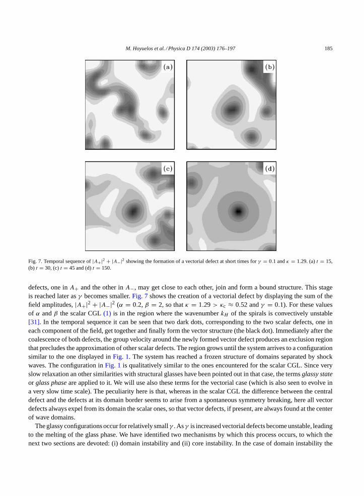
Fig. 7. Temporal sequence of|A+|2 + |A−|2 showing the formation of a vectorial defect at short times forγ = 0.1 andκ = 1.29. (a)t = 15,(b) t = 30, (c)t = 45 and (d)t = 150.

defects, one inA+ and the other inA−, may get close to each other, join and form a bound structure. This stageis reached later asγ becomes smaller.Fig. 7shows the creation of a vectorial defect by displaying the sum of thefield amplitudes,|A+|2 + |A−|2 (α = 0.2, β = 2, so thatκ = 1.29 > κc ≈ 0.52 andγ = 0.1). For these valuesof α andβ the scalar CGL(1) is in the region where the wavenumberkH of the spirals is convectively unstable[31]. In the temporal sequence it can be seen that two dark dots, corresponding to the two scalar defects, one ineach component of the field, get together and finally form the vector structure (the black dot). Immediately after thecoalescence of both defects, the group velocity around the newly formed vector defect produces an exclusion regionthat precludes the approximation of other scalar defects. The region grows until the system arrives to a configurationsimilar to the one displayed inFig. 1. The system has reached a frozen structure of domains separated by shockwaves. The configuration inFig. 1 is qualitatively similar to the ones encountered for the scalar CGL. Since veryslow relaxation an other similarities with structural glasses have been pointed out in that case, the termsglassy stateor glass phaseare applied to it. We will use also these terms for the vectorial case (which is also seen to evolve ina very slow time scale). The peculiarity here is that, whereas in the scalar CGL the difference between the centraldefect and the defects at its domain border seems to arise from a spontaneous symmetry breaking, here all vectordefects always expel from its domain the scalar ones, so that vector defects, if present, are always found at the centerof wave domains.

The glassy configurations occur for relatively smallγ . Asγ is increased vectorial defects become unstable, leadingto the melting of the glass phase. We have identified two mechanisms by which this process occurs, to which thenext two sections are devoted: (i) domain instability and (ii) core instability. In the case of domain instability the


domain around a vector defect becomes unstable and develops inhomogeneities. These irregularities lead to pathsthat permit the approach of a scalar defect that finally collides with the core and annihilates one of the componentsof the vector defect. In the core instability case the vector defect simply splits in two scalar defects. This processis described in[12] for the real coefficient case, where a greater symmetry between director and argument defectsseems to be present and both kind of defects become unstable for the same value ofγ . As we will see inSection 4.3,this is not the case for complex coefficients.

Finally, in the region of parameter spaceα–β where spirals are absolutely unstable[31] for the scalar CGLequation, no vectorial defects are formed. In this case we have what is called in the scalar case defect turbulence.Increasingγ does not change the qualitative behavior of each component, although anticorrelation between themodulus of both components increases.

4.2. Domain instability

By ‘domain instability’ we denote the situation in which the wave domain around a vector defect becomesunstable, begins to fluctuate, and develops inhomogeneities. Shortly afterwards, one of the two charges forming avector defect is annihilated by an external scalar defect. As a result a free scalar defect is left in the other componentof the field. The region of parameter spaceα–β where this process is observed corresponds approximately to theregion where for the scalar CGL equation the phase spirals are convectively unstable[31]. As γ is increased fromzero the stability of the spirals is modified: At a given value ofγ , the group velocity is not strong enough to

Fig. 8. Annihilation of an argument defect, forγ = 0.3 andκ = 1.29. The top figure shows the initial condition generated withγ = 0.1, thebox indicates the domain of the argument defect, and is amplified in the images below. First row:|A+|2, second row:|A−|2. From left to right:t = t0 + 30, t = t0 + 60, t = t0 + 90 andt = t0 + 120. At the final stage scalar defects approach the defect core annihilating then+ charge.


Fig. 9. Annihilation of a director defect, forγ = 0.35 andκ = 1.29. The top figure shows the initial condition generated withγ = 0.1, thebox indicates the domain of the director defect, and is amplified in the images below. First row:|A+|2, second row:|A−|2. From left to right:t = t0 + 50, t = t0 + 100,t = t0 + 200 andt = t0 + 300. As in the argument defect case, a scalar defect approach at the end the defect core,and annihilate one of the components of the director defect (the one inA+).

overwhelm the growth of the perturbations, the spirals becoming absolutely unstable. At this point the domainsaround the vectorial defects are ineffective as exclusion zones, so that scalar defects previously confined to thedomain border can approach the vectorial defect-core. Although this picture is valid for both kinds of vectorialdefects, director defects survive for largerγ than argument ones. For the parameter values ofFig. 1, argumentdefects become unstable atγ � 0.3 (seeFig. 8), while director defects remain stable up toγ � 0.35 (seeFig. 9).For largerγ only scalar defects are found numerically.

The different stability range of argument and director defects can be understood through a linear stability analysisof the vector spirals focusing in its plane-wave structure far from the core. This analysis is performed inAppendix A.The main point to be recognized is the difference between the phase structure between argument and director vectordefects. InFig. 10(a) and (b) we show constant-phase curves of both components for an argument defect and adirector defect. The wave vectors of the componentsA+ andA− in a pointx, k+(x) andk−(x) are perpendicularto the constant-phase curves. As discussed before,k+ = k− = kH , wherekH is the wavenumber of a scalar spiral.For the argument defects the difference of wave vectorskR = k+ − k− vanishes at any point of the plane whilefor the director defectskR �= 0. Far from the defect core,kR decreases for the director defect, however, it remainsdifferent from 0 within the exclusion island surrounding the defect.

The linear stability analysis of the wave in the two cases turns out to be different. It is shown inAppendix Athatfor argument defects, a wave withk+ = k− = kH becomes unstable ifkH > Kp, whereKp(α, β, γ ) is given inEq. (A.10), while in the case of director defects this happens ifkH > Ks , whereKs(α, β, γ ) is given inEq. (A.7).


Fig. 10. Lines of constant phase for (a) an argument defect and (b) a director defect. Solid curves correspond toφ+ = 0 andπ , and dashedcurves toφ− = 0 andπ . We can see that in (a)kR = 0 while in (b)kR �= 0.

In Fig. 11(a) and (b) we plot stability diagrams in theα–β plane, with the line 1+ αβ = 0 as a reference. InFig. 11(a) we show the curvesKp = kH andKs = kH for γ = 0.3. To the right of the curves, plane waves withk = kH are unstable. InFig. 11(b) we plot the curveKp = kH for different values ofγ (γ = 0,0.6,0.9 and 0.99).We can see that the curve moves left and upwards asγ is increased; the same happens with the curveKs = kH .Let us consider a point(α0, β0) such that plane waves withk = kH are stable forγ = 0. As γ is increasedthe curveKp = kH crosses the point turning the vectorial waves withkR = 0 unstable, this destabilizes thedomains of the argument defects. Ifγ is further increased, then the curveKs = kH crosses the point(α0, β0)

and waves withkR �= 0 become unstable, destabilizing the domains of the director defects. It should be saidthat the kind of stability analysis performed inAppendix Aconsiders extended perturbations. Since spiral waveshave a group velocity, it may happens that these instabilities are of convective type, that is, localized pertur-bations do not destroy the spiral wave but they are advected away from the defect core of the spiral with thegroup velocity[31]. Thus, we can still find stably looking spirals although the corresponding plane waves far

Fig. 11. Stability diagrams in theα–β plane showing different stability regions (the unstable regions are located to the right of the curves). Inboth figures the dashed curve is 1+αβ = 0. In figure (a) the curvesKp = kH andKs = kH are plotted forγ = 0.3 (seeEqs. (A.10) and (A.7)).The wave emitted by argument defects is unstable to the right of theKp curve. The wave emitted by director defects is unstable to the right oftheKs curve. In figure (b) we plot the curveKp = kH for different values ofγ : 0, 0.6, 0.9 and 0.99 as indicated.


from the core are unstable. The calculation of the limit ofabsolute instabilityto localized perturbations is quiteinvolved, but the result for the convective instability suggests that corotating spirals become absolutely unstablebefore counterrotating ones. We believe that the analysis presented here is an indication of the kind of insta-bilities that can affect the vectorial spirals and the order in which they appear as the coupling parameterγ isincreased.

4.3. Core instability

A core instability of a vector defect occurs when it splits in two scalar defects. This process is roughly presentin the region of parameter spaceα–β where the spirals are stable in the scalar case. The splitting of a direc-tor defect is shown inFig. 12 for κ = 0.54 andγ = 0.95. The size of the vectorial defect-core is muchnarrower than the size of the core of the two scalar defects that remain at the end of the process. This is aconsequence of two facts mentioned before, namely that the size of the vectorial defects does not depend onγ , whereas the size of scalar defects increases. Also in this case argument defects become unstable for smallerγ than director defects. For example, for the parameter values ofFig. 12 argument defects already split forγ = 0.75.

After the splitting, both scalar defects may form a bound pair that resembles a rotating molecule[17]. In Fig. 13a temporal sequence is plotted that shows a pair of scalar defects that rotate one around the other. For the particularvalues of the figure, however, the distance between the scalar defects increases and the angular velocity decreases,

Fig. 12. Splitting of a director defect, forα = 0.7, β = 2 (κ = 0.54) andγ = 0.95. The top figure shows the initial condition generated with avalue ofγ = 0.9, the square indicates the region amplified in the figures below. In the center of the square there is a director defect. First row:|A+|2, second row:|A−|2. From left to right:t = t0 + 50, t = t0 + 100,t = t0 + 150 andt = t0 + 200.


Fig. 13. Time sequence of a bounded pair of scalar defects after splitting of an argument defect, forκ = 1.29 andγ = 0.9. The pair rotates andthe bounding distance increases with time. The quantity plotted is|A+| for (a) t = t0, (b) t = t0 + 10, (c)t = t0 + 20 and (b)t = t0 + 30.

thus the molecule finally unbinds. Stable molecules, however, are found for other parameter values as reported in[17].

4.4. The relaxational case:α = β

Qualitative features distinguish the caseα = β (κ = 0) from the other cases. First, no spiral wave is formedaround vector defects (since, as stated before,kH = 0 if κ = 0). Second, the group velocity with which linearperturbations are expelled away from the neighborhood of a vector defect is 0 (the group velocity isvg = 2(α−β)kH ,as shown inAppendix A). Thus, perturbations and other defects are rather free to come arbitrarily close to vectordefects ifκ = 0 and we expect them to be frequently annihilated by processes such as the ones shown inFig. 6(b)or (c).

Starting from random initial conditions we do not find numerically the formation of vectorial defects inEq. (3)for α = β andγ > 0. In Fig. 14, the quantities|A+|2 and|A−|2 are plotted forα = β = 0 andγ = 0.1. It can beseen that there is no superposition of two defects in the same point. Starting with an initial condition with a slightlyperturbed vector defect, it spontaneously splits into two scalar defects for any positiveγ , as can be seen inFig. 15for γ = 0.2. This behavior is in agreement with the predictions of[17].

More in general, approaching the lineα = β, we observe numerically that director and argument defects of initialconfigurations such as the one inFig. 1 split spontaneously, even for very small values ofγ , again in agreementwith [17].


Fig. 14.|A+|2 and|A−|2 for α = 0, β = 0 (κ = 0, potential limit),γ = 0.1 andt = 100 starting from random initial conditions. There is nospontaneous formation of vectorial defects for real coefficients.

Fig. 15. Temporal sequence showing the splitting of a vectorial defect for real coefficients (α = β = 0) andγ = 0.2. First row:|A+|2, secondrow: |A−|2. From left to right:t = 50, 100, 150 and 200.

5. The gas phase

Forγ high enough, the vectorial defects always disappear following one of the two mechanisms described above.The system then presents a faster disordered dynamics compared with theglassyphase with vector defects. It is akind of gas-likephase, dominated by the scalar defects, which are conserved in number during very long times. Thescalar defects move faster than in the glassy phase, in a way reminiscent of atoms in a gas, from which we borrowthe name. Furthermore, the spiral wavelength around scalar defects increases withγ , so that well-developed spiralsdo not fit in the domains forγ close to 1. Domains are thus less effective as exclusion zones and defects even moremobile.

To distinguish the presence of these two different phases we can use the joint probability distribution of themodulus of the field components:p(|A+|, |A−|). Fig. 16shows a gray scale plot ofp(|A+|, |A−|) for γ = 0.1(glassy phase) andγ = 0.95 (gas phase); in both casesα = 0.2 andβ = 2. The plot is obtained taking the valuesof (|A+|,|A−|) at different space–time points. Forγ = 0.1 there is a broad maximum around|A+| � |A−| � 0.85with deviations from these values being rather uncorrelated, except for the points lying in the line|A+| = |A−|.


Fig. 16. Joint probability distributionp(|A+|, |A−|) for (a)γ = 0.1 and (b)γ = 0.95 (in both casesκ = 1.29). The histograms that are presentedin gray levels have been constructed by collecting the values of(|A+|, |A−|) at all space points of the simulation domain, and at 100 temporalsamples separated by�t = 1. The straight diagonal line in the first plot is a signature of the presence of vector defects (|A+| = |A−|), whereasthe curve in (b) displays the anticorrelation between components characteristic of scalar defects.

This line shows that the absolute values of both components take simultaneously the same value between 0 and1, situation identifying the core of vector defects. Forγ = 0.95 the line|A+| = |A−| has disappeared due to theabsence of vector defects. Instead, the probability distribution approaches the curve given by|A+|2 + |A−|2 = 1,which indicates anticorrelation between|A+| and|A−|. This anticorrelation is the fingerprint of the dominance ofthe scalar defects (seeFigs. 4 and 5). Similar qualitative behavior is observed for other values ofα andβ (giventhatκ > κc) asγ is increased.

The behavior in the glass and gas phases can be interpreted in terms of synchronization and generalized syn-chronization, respectively, of spatiotemporally chaotic configurations of the two field components[14,18]. In thiscontext, another interesting quantity that gives information about the transition from the glassy to the gas phase isthe mutual information between field components, that can be computed from the individual and joint probabilitydensities. In general, for two random discrete variablesX andY the mutual information

I (X, Y ) = −∑x,y

p(x, y) lnp(x)p(y)

p(x, y)

gives a measure of the statistical dependence between both variables, the mutual information being 0 if and only ifX andY are independent[32]. Numerical results presented in[14] show that there is a minimum ofI (|A+|, |A−|)(γ � 0.3 atα = 0.2 andβ = 2), where the variables have been adequately discretized, and that this value ofγ canbe interpreted as the transition point from the glassy to the gas phase. See[14,15]for more details about the vortexunbinding transition between the glassy and the gas-like phases.

6. Dynamics for γ > 1

Forγ > 1, as discussed inSection 2, linearly polarized states become unstable with respect to circularly polarizedstates. In this case the system segregates in two phases, one right circularly polarized and the other left circularlypolarized.Fig. 17is an example of a configuration that started from a random initial condition (γ = 1.1, α = 0.2,β = 2). Phase separation is clearly observed. As the system evolves, the length of the interface walls is reduced,in a domain-coarsening process. Despite the tendency of the concave domains to shrink, some defects remain atlong times. Vector point defects are no longer topologically allowed since the stable uniform states are such that


Fig. 17. Configuration of|A+|2 and|A−|2 (top row) and the corresponding phases (bottom row) forγ = 1.1,α = 0.2 andβ = 2 (κ = 1.29), att = 50. The system segregates into two circularly polarized phases, with some defects (the black dots in the amplitude plots, associated to thephase singularities in the phase plots).

the vanishing of one of the two polarizations in large areas, not just at points, is favored. However, we still havescalar point defects that are now lying on the domains of one circular polarization, and are points at which thecorresponding field amplitude goes to 0. Only one topological charge is defined, the associated to the componentwhich vanishes just at one point. They are of the type described in[11,12]as having a ‘repolarized core’ structure.In domains filled with one of the polarizations, say+, a defect is a place at which|A+| goes to 0, thus producinga phase singularity (seen inFig. 17) associated to a topological chargen+ = ±1; in response to this behaviorthe component which does not carry the topological charge takes nonzero values in the defect-core region. Otherstructures for the core are in principle possible, for example, a ‘punched core’ structure in which the componentthat does not carry the charge remains vanishing in the defect-core region. As discussed in[11,12], topologicalarguments imply that only the ‘repolarized core’ should be observed forγ slightly above 1, and this is indeed whatFig. 17shows. The differences in the sizes of the defect cores seen inFig. 17disappear at longer times.

We stress that the topological defects inFig. 17are different from the localized structures found in other sys-tems with coexistence of two equivalent homogeneous states, such as the Swift–Hohenberg equation in adequateparameter ranges or the parametrically forced CGL equation. In these systems the oscillating tails of the frontsconnecting the two equivalent homogeneous solutions are responsible for maintaining the existence of localizedstructures against the tendency of the domains to shrink[33]. These localized structures are not topological defects.Here, on the contrary, it is the topological character of the objects what prevents them to disappear after shrinkingto a point: defects can only disappear by combination with others of opposite charge.


7. Conclusions

We have numerically explored the conditions for the existence and stability of the different kinds of defects inthe two-dimensional VCGL equation: vector defects of argument or director type, and scalar defects. Dynamicphenomena associated with their creation and annihilation processes have been described. In particular, we haveidentified two mechanisms that lead to the destruction of the vector defects as the coupling parameter betweenfield components is increased: domain instability and core instability. One or the other takes place depending onparametersα andβ. For the domain instabilities of vector defects we have obtained analytic understanding in termsof the convective instability of the emitted spiral wave. For the core instability at a relatively large threshold valueof γ there is no available theory so far.

Our numerical results have been compared with the useful analytical studies by Aranson and Pismen[17]. Theystudied core instabilities as a function ofα andβ for smallγ . Their results explain our result that in the relaxationallimit (α = β) there are no vectorial defects forγ > 0. They also explain the existence of vector defects far from therelaxational limit and for smallγ . Our main interest, however, was on what happens far from the relaxational limitas function ofγ . In this regime we have found threshold values ofγ for the domain and core instabilities mentionedbefore. These instabilities are not accessible to the perturbative theoretical discussion of Aranson and Pismen andthere is need of further analytical studies.

Finally, the dominance of different types of defects at different parameter values leads to the identification ofdifferent dynamical regimes, such as the glassy and the gas phase.

Acknowledgements

Financial support from MCyT (Spain), project CONOCE BMF2000-1108, is acknowledged. MH acknowledgesfinancial support of Fundación Antorchas, Argentina, and of the National Council for Scientific and TechnicalResearch (CONICET) from Argentina.

Appendix A

We analyze in this appendix the stability of the wave emitted by vector defects. Far from the defect core wecan approximate the spiral waves by plane waves. The stability of plane waves with wavenumberkH will give usinformation about the stability of the spirals. The stability analysis presented here is an extension to two dimensionsof the analysis made in one dimension in[13] and it is valid for|γ | < 1. The effect of a perturbation on theplane-wave solution(4) can be written as

A± = (Q + a±)e−i(k±r−ω±t+φ0±), (A.1)

where|k+| = |k−| = kH for a vector defect.Q andω are given byEq. (7), anda± are the complex perturbations.Using the variables

s

sI

r

rI

=

R(a+ + a−)I(a+ + a−)R(a+ − a−)I(a+ − a−)

, (A.2)

whereR andI mean real and imaginary part, respectively, we obtain linearized equations fors, sI , r and rI .Instabilities appear first in the phase modes. They are identified as the linear combinations of the variables that in


the space-homogeneous case lead to zero eigenvalues. They areθ = −βs + sI andψ = −βr + rI . Performingthe change of variables(s, r, sI , rI) → (s, r, θ, ψ), and eliminating adiabatically the rapidly decaying amplitudevariabless andr in terms of the phases, we get the following phase equations:

∂t θ = (α − β)kS · ∇θ + (1 + αβ)∇2θ − 1 + β2

2(1 − k2)

[(kS · ∇)2θ + 1 + γ

1 − γ(kR · ∇)2θ

]

+(α − β)kR · ∇ψ − 1 + β2

(1 − k2)(1 − γ )(kS · ∇)(kR · ∇)ψ,

∂tψ = (α − β)kS · ∇ψ + (1 + αβ)∇2ψ − (1 + β2)(1 + γ )

2(1 − k2)(1 − γ )

[(kS · ∇)2ψ + 1 − γ

1 + γ(kR · ∇)2ψ

]

+(α − β)kR · ∇θ − 1 + β2

(1 − k2)(1 − γ )(kS · ∇)(kR · ∇)θ, (A.3)

wherekS = k+ + k− andkR = k+ − k−.As explained inSection 4.2, kR = 0 in the domain surrounding argument defects, butkR �= 0, although

small, for the domain around director defects. In both cases one can approximate|kS| ≈ 2kH . For smallkR, thedominant first-order derivative terms in(A.3) indicate that small perturbations on the waves travel at a group velocityvg = 2(α − β)kH .

We consider perturbations of small wave vectorq. The eigenvalues of the linear system(A.3) are

λ±q2

= −1 − αβ + 1 + β2

2Q2(1 − γ 2)

[(kR · q)2 + (kS · q)2

]±

√S

2q, (A.4)

whereq = |q|, q = q/q is the direction of the perturbation vector, andS = aq2 + ibq− c, with

a = (1 + β2)2

Q4(1 − γ 2)2{γ 2[(kR · q)2 − (kS · q)2]2 + 4(kR · q)2(kS · q)2},

b = 8(α − β)1 + β2

Q2(1 − γ 2)(kR · q)2kS · q, c = 4(α − β)2(kR · q)2. (A.5)

If kR �= 0, as is the case for director defects, we can approximate√S = i

√c(1− (ib/2c)q)+ O(q2). The real part

of the two eigenvalues are

R(λ±)q2

= −1 − αβ + 2(1 + β2)

Q2(1 − γ 2)k2 cos2χ± + O(q), (A.6)

whereχ± are the angles between the perturbation wave vectorq and the wave vectorsk+ andk−. Since|kR| isfinite the instability may arise for perturbation wavenumberq smallerthan|kR|. In this case, considering the mostdangerous longitudinal perturbations, i.e. whenχ+ = 0 orχ− = 0, we obtain a critical wavenumberKs such thatif k > Ks the plane waves become Eckhaus unstable. TakingR(λ±) = 0 in (A.6) we get

K2s = (1 + αβ)(1 − γ )

(1 + αβ)(1 − γ ) + 2(1 + β2). (A.7)

The equations for∂t θ and∂tψ (A.3) are coupled, and the eigenvector corresponding to the unstable eigenvaluemixes both variables. This means that the sum and the difference of the field perturbationsa+ anda−, becomeunstable simultaneously in this case.

If kR = 0, as appropriate around argument defects, we have thatk+ = k−, andχ+ = χ− = χ , and

S =((1 + β)γ kqcosχ

Q2(1 − γ 2)

)2

. (A.8)


We obtain for the real parts of the eigenvalues

R(λ±)q2

= −1 − αβ + 2(1 + β2)(1 ± γ )

Q2(1 − γ 2)k2 cos2χ + O(q). (A.9)

We consider again longitudinal perturbations corresponding toχ = 0. Taking the marginal stability condition in(A.9) for the most dangerous eigenvalue,R(λ+) = 0, we see that in this case plane waves become unstable fork > Kp, whereKp is given by

K2p = (1 + αβ)(1 − γ )

(1 + αβ)(1 − γ ) + 2(1 + β2)(1 + |γ |) . (A.10)

For kR = 0, Eqs. (A.3)for ∂t θ and∂tψ are decoupled. The most restrictive eigenvalue,λ+, is associated with thevariableψ , which is related to the difference of the field perturbations. Whenψ becomes unstable, the differencea+ − a− grows; in optical language this is called a polarization instability.

References

[1] H. Riecke, in: M. Golubitsky, D. Luss, S.H. Strogatz (Eds.), Pattern Formation in Continuous and Coupled Systems, Springer, New York,1999;L.M. Pismen, Vortices in Nonlinear Fields, Oxford University Press, New York, 1999.

[2] F.T. Arecchi, et al., Phys. Rev. Lett. 67 (1991) 3751;K. Staliunas, G. Slekys, C.O. Weiss, Phys. Rev. Lett. 79 (1997) 2658;C.O. Weiss, et al., Appl. Phys. B 68 (1999) 151;N.N. Rosanov, in: E. Wolf (Ed.), Progress in Optics, vol. 35, North-Holland, Amsterdam, 1996;M. Brambilla, et al., Phys. Rev. Lett. 79 (1997) 2042;D. Michaelis, U. Peschel, F. Lederer, Phys. Rev. A 56 (1997) R3366;M. Tlidi, P. Mandel, R. Lefever, Phys. Rev. Lett. 73 (1994) 640;W. Firth, A.J. Scroggie, Phys. Rev. Lett. 76 (1996) 1623;C. Etrich, U. Peschel, F. Lederer, Phys. Rev. Lett. 79 (1997) 2454;K. Staliunas, J.V. Sánchez-Morcillo, Phys. Rev. A 57 (1998) 1454;G.L. Oppo, A.J. Scroggie, W.J. Firth, J. Opt. B 1 (1999) 133.

[3] R. Bhandari, Phys. Rep. 281 (1997) 1.[4] M. Santagiustina, E. Hernández-Garcıa, M. San Miguel, A.J. Scroggie, G.-L. Oppo, Phys. Rev. E 65 (2002) 036610.[5] R. Gallego, M. San Miguel, R. Toral, Phys. Rev. E 61 (2000) 2241.[6] M.C. Cross, P.C. Hohenberg, Rev. Mod. Phys. 65 (1993) 851.[7] T. Bohr, M. Jensen, G. Paladin, A. Vulpiani, Dynamical Systems Approach to Turbulence, Cambridge University Press, Cambridge, 1998.[8] I.S. Aranson, L. Kramer, Rev. Mod. Phys. 74 (2002) 99.[9] L. Gil, Phys. Rev. Lett. 70 (1993) 162.

[10] L. Gil, Int. J. Bif. Chaos 3 (1993) 573.[11] L.M. Pismen, Phys. Rev. Lett. 72 (1994) 2557.[12] L.M. Pismen, Physica D 73 (1994) 244.[13] M. San Miguel, Phys. Rev. Lett. 75 (1995) 425.[14] E. Hernández-Garcıa, M. Hoyuelos, P. Colet, M. San Miguel, R. Montagne, Int. J. Bif. Chaos 9 (1999) 2257.[15] M. Hoyuelos, E. Hernández-Garcıa, P. Colet, M. San Miguel, Comp. Phys. Comm. 121–122 (1999) 414.[16] E. Hernández-Garcıa, M. Hoyuelos, P. Colet, M. San Miguel, Phys. Rev. Lett. 85 (2000) 744.[17] I.S. Aranson, L.M. Pismen, Phys. Rev. Lett. 84 (2000) 634.[18] A. Amengual, E. Hernández-Garcıa, R. Montagne, M. San Miguel, Phys. Rev. Lett. 78 (1997) 4379.[19] R. Montagne, E. Hernández-Garcıa, Phys. Lett. A 273 (2000) 239.[20] R. Montagne, E. Hernández-Garcıa, M. San Miguel, Physica D 96 (1996) 47.[21] M. San Miguel, R. Montagne, A. Amengual, E. Hernández-Garcıa, in: E. Tirapegui, W. Zeller (Eds.), Instabilities and Non-equilibrium

Structures V, Kluwer Academic Publishers, Dordrecht, 1996.[22] A.J. Leggett, Rev. Mod. Phys. 73 (2001) 307.[23] J. Yang, Y. Tan, Phys. Rev. Lett. 85 (2000) 3624, and references therein.[24] http://www.imedea.uib.es/PhysDept/Nonlinear/researchtopics/Vcgl2/.[25] P.S. Hagan, SIAM J. Appl. Math. 42 (1982) 762.

http://www.imedea.uib.es/PhysDept/Nonlinear/research_topics/Vcgl2/


[26] R. Montagne, E. Hernández-Garcıa, A. Amengual, M. San Miguel, Phys. Rev. E 56 (1997) 151.[27] J. Lega, C. R. Acad. Sci. Paris 309 (II) (1989) 1401.[28] V.M. Eguiluz, E. Hernández-Garcıa, O. Piro, Int. J. Bif. Chaos 9 (1999) 2209.[29] V.M. Eguiluz, E. Hernández-Garcıa, O. Piro, Phys. Rev. E 64 (2001) 036205.[30] M. Hendrey, K. Nam, P. Guzdar, E. Ott, Phys. Rev. E 62 (2000) 7627.[31] I.S. Aranson, L. Aranson, L. Kramer, A. Weber, Phys. Rev. A 46 (1992) R2992;

I.S. Aranson, L. Kramer, A. Weber, in: E. Tirapegui, W. Zeller (Eds.), Instabilities and Nonequilibrium Structures IV, Kluwer AcademicPublishers, Dordrecht, 1993, p. 259.

[32] R.J. McEliece, The theory of information and coding: a mathematical framework for communication, Encyclopedia of Mathematics andIts Applications, vol. III, Addison-Wesley, New York, 1977.

[33] P. Coullet, C. Elphick, D. Repaux, Phys. Rev. Lett. 58 (1987) 431;D. Gomila, P. Colet, G.-L. Oppo, M. San Miguel, Phys. Rev. Lett. 87 (2001) 194101.

Dynamics of defects in the vector complex Ginzburg–Landau equation

Documents

Transcript of Dynamics of defects in the vector complex Ginzburg–Landau equation