5D N = 1 super QFT: symplectic quivers - arXiv

arX

iv:2

112.

0469

5v1

[he

p-th

] 9

Dec

202

1

LPHE-MS-01-2021

5D N = 1 super QFT: symplectic quivers

E.H Saidi∗ and L.B Drissi†

1. LPHE-MS, Science Faculty, Mohammed V University in Rabat, Morocco

2. Centre of Physics and Mathematics, CPM- Morocco

December 10, 2021

Abstract

We develop a method to build new 5D N = 1 gauge models based on Sasaki-

Einstein manifolds Y p,q. These models extend the standard 5D ones having a unitary

SU(p)q gauge symmetry based on Y p,q. Particular focus is put on the building of a

gauge family with symplectic SP(2r,R) symmetry. These super QFTs are embedded

in M-theory compactified on folded toric Calabi-Yau threefolds X(Y 2r,0) constructed

from conical Y 2r,0. By using outer-automorphism symmetries of 5DN = 1 BPS quivers

with unitary SU(2r) gauge invariance, we also construct BPS quivers with symplectic

SP(2r,R) gauge symmetry. Other related aspects are discussed.

Keywords: SCFT5, 5D N = 1 super QFT on a finite circle, toric threefolds based on

Sasaki-Einstein manifolds, toric diagrams, BPS quivers, outer-automorphisms, folding.

1 Introduction

N = 1 supersymmetric gauge theories in five space time dimensions (super QFT5) are non

renormalizable field theories with eight supercharges. They are admitted to have UV fixed

points which can be deformed by relevant operators such that in the infrared they flow to

5D N = 1 super Yang-Mills (SYM5) coupled to hypermultiplets [1, 2]. A typical massive

∗[email protected]† [email protected]

1

http://arxiv.org/abs/2112.04695v1

deformation generating this type of flow is given by the SYM5 term tr(

F 2µν

)

/g2YM where

in 5D the inverse gauge coupling square 1/g2YM has dimension of mass. These 5D gauge

theories are somehow special compared to 6D gauge theories [3, 4, 5] including maximally

supersymmetric Yang-Mills theory believed to flow to N = (2, 0) supersymmetric 6D theory

in the UV [6, 7]. In the few last years, super QFT5s and their compactification, in particular

on a Kaluza-Klein circle with finite radius and to 3D, have been subject to some interest

in connection with their critical behaviour and specific properties of their gauge phases [8]-

[15]. Though a complete classification is still lacking [16, 5], several examples of such gauge

theories are known; and most of them can be viewed as deformations of 5D superconfor-

mal theories [17, 18, 19]. Simplest examples of SCFT5s are given by the so-called Seiberg

family possessing a rich flavor symmetry [20]; many others are obtained through embedding

in string theory. Generally speaking, this embedding can be achieved in two interesting

ways; either by using 5-brane webs in type IIB string theory [21]-[26]; or by using M-theory

compactification on Calabi-Yau threefolds [27]-[31]. Below, we comment briefly on these two

methods while giving some references which certainly are not the complete list since the

works in this matter are abundant.

The method of (p, q) 5-brane webs in type IIB string theory has led to several findings and

has several features; in particular the following: First, it gives evidence for the existence of

fix point of 5D gauge theories flowing to UV conformal points corresponding to collapsed

webs; and as such permits to study conditions for existence of critical fix points. This web

construction also indicates that not every 5D gauge theory can flow to a SCFT5 [1]; the

existence of a SCFT constraints the matter content of the theory. The 5-brane method

allows also to study gauge theory dualities in 5D. This is because a given SCFT5 can have

several gauge theory deformations; thus generating different (but dual) gauge theories in

infrared [21]. Also, the web method provides us with a tool to compute the instanton parti-

tion function that captures the BPS spectrum of the 5D theory by applying the topological

vertex formalism [32]-[37]. It also allows the study the global symmetry enhancements of

the SCFTs [7, 38] and UV-dualities [21], [39]-[41]. More interestingly, the 5-brane webs ap-

proach give a way to elaborate families of 5D gauge models with fix points closely related to

quivers with SU gauge in the shape of Dynkin diagrams. By introducing an orientifold plane

like O5-plane, the 5-brane webs can describe 5D super QFTs with flavors and gauge groups

beyond SU(N) such as SO(N) and Sp(2N) [42, 43] as well as exceptional ones like G2 [34].

2

Certain (p, q) 5-brane webs have interpretation in terms of toric diagrams [23] although, for

5D gauge theories with a large number of flavors, they lead to non- toric Calabi-Yau geome-

tries [44]. This brane based method is not used in this paper; it is described here as one of

two approaches to study 5D N = 1 super QFTs underlying SCFT5. For works using this

method, we refer to rich the literature in this matter; for instance [21]-[23],[45]-[50].

Regarding the M-theory method, to be used in this study, one can also list several interesting

aspects showing that it is a powerful higher dimensional geometric approach. First of all,

the 5D gauge theories are obtained by compactifying M-theory on Calabi-Yau threefolds

(CY3) X ( resolved X). Then, the effective prepotential F5D and its non trivial variations

δnF5D/δφn, characterising the Coulomb branch of the 5D super QFTs, have interesting CY3

interpretations; i.e. a geometric meaning in the internal dimensions. The F5D is given by the

volume vol(X) while its variations —describing magnetic string tensions amongst others—

are interpreted as volumes of p-cycles. Moreover, the calculation of F5D can be explicitly

done for a wide class of X ’s; in particular for the family of toric Calabi-Yau threefolds like

those based on the three following geometries: (a) The toric del Pezzo surfaces dPn with

n=1,2,3; these Kahler manifolds are toric deformations of the complex projective plane P2.

(b) The Hirzebruch surfaces Fn given by non trivial fibrations of a complex projective line

P1 over a base P1 [51]-[54]. (c) The family X (Y p,q) given by a crepant resolution of toric

threefolds realised as real metric cone on Sasaki-Einstein Y p,q spaces labeled by two positive

integers (p, q) constrained as p ≥ q ≥ 0 [55]-[59].

In this investigation, we focus on the particular class of 5D supersymmetric SU(p)q unitary

field models based on X (Y p,q) and look for a generalisation of these quantum field models to

other gauge symmetries. Our interest into the Sasaki-Einstein (EM) based CY3s has been

motivated by yet unexplored specific properties of Y p,q and also by the objective of general-

izing partial results obtained for the unitary family. In this context, recall that the toric 5D

super QFTs based on X (Y p,q) have unitary SU(p)q gauge symmetries with Chern-Simons

(CS) level q. Thus, it is interesting to seek how to generalize these unitary gauge models

based on X (Y p,q) for other gauge symmetries like the orthogonal and the symplectic. As a

first step in this exploration, we show in this study that the 5D unitary gauge theories based

on Y p,q have discrete symmetries that can be used to construct new gauge models. These

finite groups come from symmetries of p-cycles inside the X (Y p,q). By using specific prop-

erties of the unitary set and folding under outer- automorphisms of p-cycles, we construct a

3

new family of 5D SQFTs having symplectic SP(2r,R) gauge invariance.

To undertake this study, it is helpful to recall some features of the Sasaki-Einstein based

CY3: (i) They are toric and they extend the X (dP1) and the X (F0) . These geometries

appear as two leading members in the X (Y p,q) family. (ii) They have been used in the

past in the engineering of 4D supersymmetric quiver gauge theories [60]-[63]; and have been

recently considered in models building of unitary 5D N = 1 super CFTs [64]-[68]. (iii)

Being toric, the threefolds X (Y p,q)s and the unitary 5D super QFTs based on them can be

respectively represented by toric diagrams ∆X(Y p,q) and by BPS quivers QX(Y p,q) describing

the BPS particle states of the unitary supersymmetric theory.

The toric ∆X(Y p,q) and the BPS QX(Y p,q) are particularly interesting because they play a

central role in our construction; as such, we think it is useful to comment on them here. We

split the properties of these objects in two types: general and specific. The general proper-

ties, which will be understood in this investigation, are as in the geometric engineering of 4D

super QFTs [69]-[73]. They also concern aspects of the Sasaki-Einstein manifolds and the

brane tiling algorithms (a.k.a dimer model) [74]-[83]. Some useful general aspects for this

study are reported in the appendices A, B, C. The specific properties ∆X(Y p,q) and QX(Y p,q)

regard their outer-automorphisms and the implementation of the Calabi-Yau condition of

X as well as a previously unknown property of X (Y p,q) that we describe for the leading

members p = 2, 3, 4. By trying to exhibit manifestly the Calabi-Yau condition on the toric

diagram ∆X(Y p,q), we end up with the need to introduce a new graph representing X (Y p,q).

This new graph is denoted like GG

X(Y p,q)with G referring either to the gauge symmetry SU(p)

or to SP(2r,R). The construction of GG

X(Y p,q)will be studied with details in this paper; to

fix ideas, see eq(4.1) and the Figure 7, the Figure 8 and the Figure 9.

In the present paper, we contribute to the study of 5D N = 1 super QFT models based on

conical Sasaki-Einstein manifolds and their compactification on a circle with finite radius.

Using the above mentioned discrete symmetries, we develop a method to build new 5DN = 1

Kaluza-Klein quiver gauge models based on Sasaki-Einstein manifolds Y p,q. For that, we first

revisit properties of the internal X (Y p,q) geometries which are known to host gauge mod-

els with SU(p)q gauge symmetry. Then, we show that some of these Sasaki-Einstein based

threefolds have non trivial discrete symmetries that exchange p-cycles in X (Y p,q) and which

we construct explicitly. By using these finite symmetries and cycle- folding ideas, we build a

new set of 5D supersymmetric gauge models based on X (Y p,q) having symplectic SP(2r,R)

4

gauge invariance; thus extending the set of unitary gauge models for this family of CY3. We

also derive the associated BPS quivers encoding the data on the BPS states of the symplectic

theory. We moreover show that the cycle- folding by outer-automorphisms generate super

QFT models having no standard interpretation in terms of gauge phases. For a pedagogical

reason, we mainly focus on the leading members of the symplectic SP(2r,R) family; in par-

ticular on the 5D N = 1 super QFT with SP(4,R) invariance. The first SP(2,R) member is

isomorphic to the 5D N = 1 SU(2) model of the unitary series. To achieve this goal, we (i)

revisit the toric Calabi-Yau threefold X (Y 4,0) (p=4 and q=0), hosting a lifted SU(4)0 gauge

symmetry; and (ii) reconsider the BPS quiver QSU4

X(Y 4,0)of the underlying with 5D N = 1

super QFT compactified on a circle with finite size. After that we develop an approach to

construct toric Calabi-Yau threefolds with symplectic symmetry and a method to build the

BPS quiver QSP 4

X(Y 4,0)with SP(4,R) invariance. The extension of this construction to other

gauge symmetries is discussed in the conclusion section.

The organisation is as follows: In section 2, we review properties of the toric diagram

∆SU4

X(Y 4,0)of the Calabi-Yau threefolds X (Y 4,0). We show that ∆SU4

X(Y 4,0)has non trivial outer-

automorphisms Houter∆SU4

having a fix point. We also show that this discrete group Houter∆SU4

can

be interpreted as a parity symmetry in Z2 lattice. In section 3, we investigate the properties

of the BPS quiver QSU4

X(Y 4,0)associated with ∆SU4

X(Y 4,0). Here we show that QSU4

X(Y 4,0)has also

an outer-automorphism symmetry HouterQSU4

with fix points. This outer-automorphism group

has two factors given by (Z4)QSU4× (Zouter

2 )QSU4. In section 4, we introduce a new diagram

to represent the toric X (Y 4,0) . It is given by a graph G where the Calabi-Yau condition is

manifestly exhibited. To avoid confusion, we denote this graph like GSU4

X(Y 4,0)and refer to it

as the unitary CY graph of the toric X (Y 4,0) with SU(4) gauge symmetry. To deepen the

construction, we also give the unitary CY graphs GSU2

X(Y 2,0)and GSU3

X(Y 3,0)representing the toric

X (Y p,0) with p=2 and p=3. In section 5, we construct the symplectic CY graph GSP 4

X(Y 4,0)

and the associated symplectic BPS quiver QSP 4

X(Y 4,0). In section 6, we give a conclusion and

make comments. In the appendix, we give useful properties on the geometric properties of

the Coulomb branch of M-theory on CY3s and describe the building of BPS quivers.

5

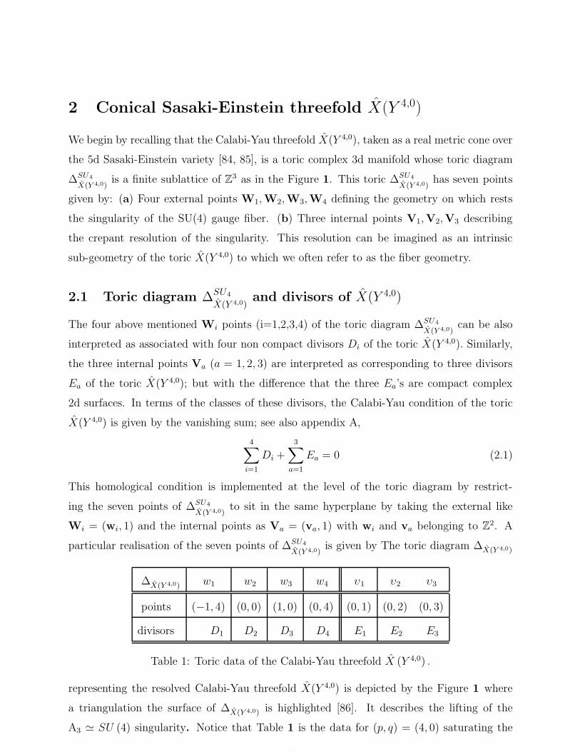
2 Conical Sasaki-Einstein threefold X(Y 4,0)

We begin by recalling that the Calabi-Yau threefold X(Y 4,0), taken as a real metric cone over

the 5d Sasaki-Einstein variety [84, 85], is a toric complex 3d manifold whose toric diagram

∆SU4

X(Y 4,0)is a finite sublattice of Z3 as in the Figure 1. This toric ∆SU4

X(Y 4,0)has seven points

given by: (a) Four external points W1,W2,W3,W4 defining the geometry on which rests

the singularity of the SU(4) gauge fiber. (b) Three internal points V1,V2,V3 describing

the crepant resolution of the singularity. This resolution can be imagined as an intrinsic

sub-geometry of the toric X(Y 4,0) to which we often refer to as the fiber geometry.

2.1 Toric diagram ∆SU4

X(Y 4,0)and divisors of X(Y 4,0)

The four above mentioned Wi points (i=1,2,3,4) of the toric diagram ∆SU4

X(Y 4,0)can be also

interpreted as associated with four non compact divisors Di of the toric X(Y 4,0). Similarly,

the three internal points Va (a = 1, 2, 3) are interpreted as corresponding to three divisors

Ea of the toric X(Y 4,0); but with the difference that the three Ea’s are compact complex

2d surfaces. In terms of the classes of these divisors, the Calabi-Yau condition of the toric

X(Y 4,0) is given by the vanishing sum; see also appendix A,

4∑

i=1

Di +

3∑

a=1

Ea = 0 (2.1)

This homological condition is implemented at the level of the toric diagram by restrict-

ing the seven points of ∆SU4

X(Y 4,0)to sit in the same hyperplane by taking the external like

Wi = (wi, 1) and the internal points as Va = (va, 1) with wi and va belonging to Z2. A

particular realisation of the seven points of ∆SU4

X(Y 4,0)is given by The toric diagram ∆X(Y 4,0)

∆X(Y 4,0) w1 w2 w3 w4 υ1 υ2 υ3

points (−1, 4) (0, 0) (1, 0) (0, 4) (0, 1) (0, 2) (0, 3)

divisors D1 D2 D3 D4 E1 E2 E3

Table 1: Toric data of the Calabi-Yau threefold X (Y 4,0) .

representing the resolved Calabi-Yau threefold X(Y 4,0) is depicted by the Figure 1 where

a triangulation the surface of ∆X(Y 4,0) is highlighted [86]. It describes the lifting of the

A3 ≃ SU (4) singularity. Notice that Table 1 is the data for (p, q) = (4, 0) saturating the

6

Figure 1: The toric diagrams ∆SU4

X(Y 4,0)having four external points (two blue and two green)

and three internal points (in red). These red points are associated with the lifting of the

SU(4) singularity of the gauge fiber. The surface of ∆SU4

X(Y 4,0)is divided into 4+4 triangles.

By merging the red points into the first point, one is left with 4 triangles.

lower bound of the constraint 0 ≤ q ≤ 4. For generic values of q constrained like 0 ≤ q ≤ p,

we have the following data This toric ∆X(Y p,q) has 3+p points and then 3+p divisors; p-1

∆X(Y p,q) w1 w2 w3 w4 {υa}1≤a≤p−1

points (−1, p− q) (0, 0) (1, 0) (0, p) (0, a)

divisors D1 D2 D3 D4 {Ea}1≤a≤p−1

Table 2: Toric data of X (Y p,q) with 0 ≤ q ≤ p.

of them are compact. They concern the divisor set {Ea}1≤a≤p−1. Notice also that the three

internal (red) points of ∆X(Y 4,0) represented by the Figure 1 form a (vertical) linear chain

A3 in the toric diagram with boundary points effectively given by the two (blue) external

w2 and w4. For convenience, we rename these two particular boundary points like w2 = υ0

and w4 = υ4 so that the above mentioned chain A3 can be put in correspondence with the

standard A3- geometry of the ALE space with resolved SU(4) singularity [87, 88]. With this

renaming, the Table 1 gets mapped to A similar description can be done for ∆X(Y p,0). For

simplicity of the presentation, we omit it. Having introduced the particular toric diagram

∆SU4

X(Y 4,0)hosting an underlying unitary SU(4) gauge symmetry, we turn now to explore one

of its exotic properties namely its outer-automorphism symmetries.

7

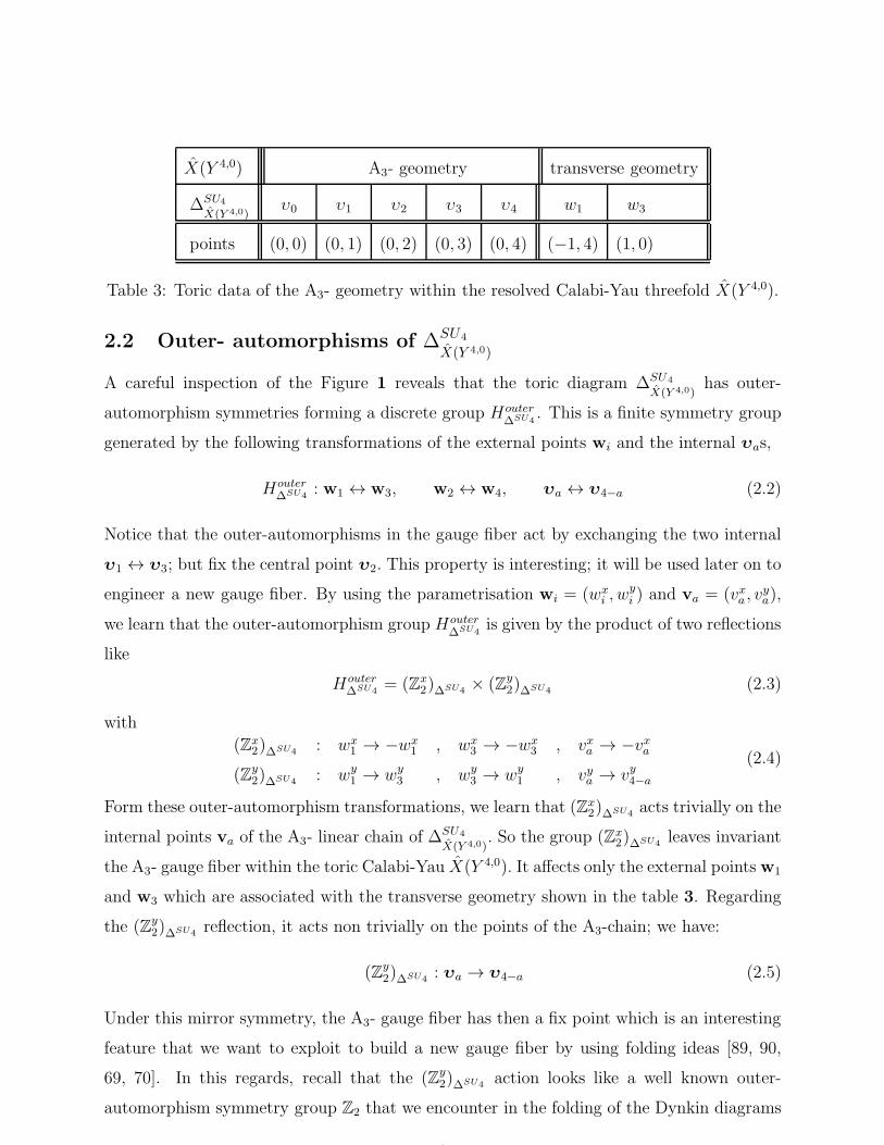
X(Y 4,0) A3- geometry transverse geometry

∆SU4

X(Y 4,0)υ0 υ1 υ2 υ3 υ4 w1 w3

points (0, 0) (0, 1) (0, 2) (0, 3) (0, 4) (−1, 4) (1, 0)

Table 3: Toric data of the A3- geometry within the resolved Calabi-Yau threefold X(Y 4,0).

2.2 Outer- automorphisms of ∆SU4

X(Y 4,0)

A careful inspection of the Figure 1 reveals that the toric diagram ∆SU4

X(Y 4,0)has outer-

automorphism symmetries forming a discrete group Houter∆SU4

. This is a finite symmetry group

generated by the following transformations of the external points wi and the internal υas,

Houter∆SU4

: w1 ↔ w3, w2 ↔ w4, υa ↔ υ4−a (2.2)

Notice that the outer-automorphisms in the gauge fiber act by exchanging the two internal

υ1 ↔ υ3; but fix the central point υ2. This property is interesting; it will be used later on to

engineer a new gauge fiber. By using the parametrisation wi = (wxi , w

yi ) and va = (vxa , v

ya),

we learn that the outer-automorphism group Houter∆SU4

is given by the product of two reflections

like

Houter∆SU4

= (Zx2)∆SU4

× (Zy2)∆SU4

(2.3)

with

(Zx2)∆SU4

: wx1 → −wx

1 , wx3 → −wx

3 , vxa → −vxa

(Zy2)∆SU4

: wy1 → wy

3 , wy3 → wy

1 , vya → vy4−a

(2.4)

Form these outer-automorphism transformations, we learn that (Zx2)∆SU4

acts trivially on the

internal points va of the A3- linear chain of ∆SU4

X(Y 4,0). So the group (Zx

2)∆SU4leaves invariant

the A3- gauge fiber within the toric Calabi-Yau X(Y 4,0). It affects only the external points w1

and w3 which are associated with the transverse geometry shown in the table 3. Regarding

the (Zy2)∆SU4

reflection, it acts non trivially on the points of the A3-chain; we have:

(Zy2)∆SU4

: υa → υ4−a (2.5)

Under this mirror symmetry, the A3- gauge fiber has then a fix point which is an interesting

feature that we want to exploit to build a new gauge fiber by using folding ideas [89, 90,

69, 70]. In this regards, recall that the (Zy2)∆SU4

action looks like a well known outer-

automorphism symmetry group Z2 that we encounter in the folding of the Dynkin diagrams

8

of the finite dimensional Lie algebras A2r−1. Here, we are dealing with the particular A3 ∼

SU (4) which is just the leading non trivial member of the A2r−1 series. As an illustration;

see the pictures of the Figure 2 describing the folding of the Dynkin diagram A3 giving

the Dynkin diagram of the symplectic C2 ≃ sp (4,R) which, thought not relevant for our

present study, it is also isomorphic to B2 ≃ so (5). Recall as well that the Dynkin diagrams

Figure 2: a) The Dynkin diagram of the Lie algebra A3. It has a mirror (Z2)∆SU4outer-

automorphism symmetry leaving one node fixed (in magenta color). b) The Dynkin diagram

of the symplectic Lie algebra C2. It is obtained by folding A3 under (Z2)∆SU4.

of finite dimensional Lie algebras g may be also thought of in terms of the Cartan matrices

K (g)ij = α∨i .αj defined by the intersection of simple roots αi and co-roots α∨

i = αi/α2i .

For the examples of A3 ≃ su (4) and C2 ≃ sp (4,R) , we have the following matrices

K (A3) =

2 −1 0

−1 2 −1

0 −1 2

, K (C2) =

2 −1

−2 2

(2.6)

Notice that the picture on the left of the Figure 2 can be put in correspondence with the

internal (red) points of the A3- linear chain of the Figure 1. At this level, one may ask what

about toric diagrams with a C2 type sub-diagram. We will answer this question later on after

highlighting another property of ∆SU4

X(Y 4,0). Before that, let us describe succinctly the BPS

quivers associated with the toric diagram of X(Y 4,0); and study its outer-automorphisms.

3 BPS quiver QSUp

X(Y p,0): cases p = 3, 4

In this section, we investigate two examples of unitary BPS quivers namely the QSU3

X(Y 3,0)and

the QSU4X(Y 4,0)

. These unitary BPS quivers are representatives of the families QSU2r−1

X(Y 2r−1,0)and

QSU2r

X(Y 2r,0)with r ≥ 1. They have intrinsic properties that we want to study and which will

be used later on. First, we consider the quiver QSU4

X(Y 4,0)with gauge symmetry SU(4) as this

quiver is one of the main graphs that interests us in this study. Then, we turn to the BPS

9

quiver QSU3

X(Y 3,0)with unitary symmetry SU(3). The QSU3

X(Y 3,0)quiver is reported here for a

matter of comparison with QSU4

X(Y 4,0). The results obtained for these quivers hold as well for

the families QSU2r−1

X(Y 2r−1,0)and QSU2r

X(Y 2r,0).

3.1 BPS quiver QSU4

X(Y 4,0)

The construction of the unitary BPS quiver QSU4

X(Y 4,0)of the 5D N = 1 super QFTs, com-

pactified on a circle with finite size and based on X(Y 4,0), follows from the brane tiling of

the so called brane-web ∆SU4

X(Y 4,0)(the dual of the toric diagram ∆SU4

X(Y 4,0)) by applying the

fast inverse algorithm [92, 93, 94]. Up to a Seiberg- type duality transformation, the repre-

sentative QSU4

X(Y 4,0)has a quiver- dimension dbps equals to 2× 3 + 2. Then the QSU4

X(Y 4,0)has 8

elementary BPS particles that generate the BPS spectrum of the 5D super QFT. For further

details; see the appendices A and B. To fix ideas, let us illustrate the numbers involved in

the dbps dimension which for QSUp

X(Y p,0)with p≥2 reads as follows; see also eqs(B.4-B.3),

dbps = 2 (p− 1) + 2 (3.1)

(i) the number 3 = 4 − 1 is precisely the rank of the SU(4) gauge fiber within the toric

X(Y 4,0). It is also the number of compact divisors —E1, E2, E3— of the threefold X(Y 4,0).

(ii) The product 2×3 = 6 designates the number of the electric/magnetic charged particles.

These 3+3 particles have interpretation in terms of M2– and M5-branes wrapping 2- and 4-

cycles in the internal threefold X(Y 4,0). (iii) The extra number 2=1+1 in the dbps- dimension

of QSU4

X(Y 4,0)refers to an instanton and to the elementary Kaluza-Klein D0 brane; for more

details see [64, 65, 66] and the appendix A.

The schematic structure of the BPS quiver QSU4

X(Y 4,0)is depicted by the Figure 3. It has 8 nodes

{1} , ..., {8} interpreted in terms of 8 elementary BPS particles. These nodes organise into

four Kronecker quivers (4 doublets of nodes) denoted like κc = {2c− 1, 2c}1≤c≤4; explicitly,

we have:

κ1 = {1, 2} , κ3 = {5, 6}

κ2 = {3, 4} , κ4 = {7, 8}(3.2)

As shown by the Figure 3, the 8 nodes of the BPS quiver are linked by 4×4 = 16 quiver- edges

〈j|l〉 interpreted in terms of chiral superfields in the language of supersymmetric quantum

mechanics (SQM) [65]. The unitary BPS quiver QSU4

X(Y 4,0)has been first considered in [66] (see

figure 25-a, page 61). For later use, we re-draw the Figure 3 as depicted by the equivalent

10

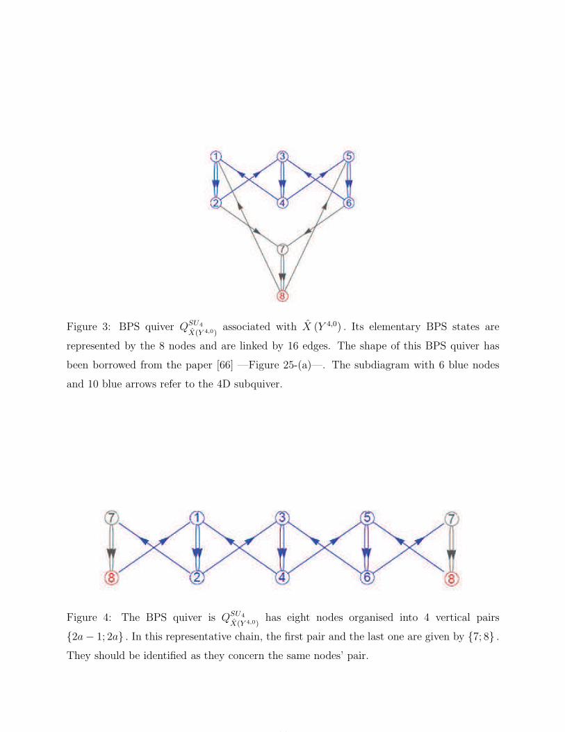
Figure 3: BPS quiver QSU4

X(Y 4,0)associated with X (Y 4,0) . Its elementary BPS states are

represented by the 8 nodes and are linked by 16 edges. The shape of this BPS quiver has

been borrowed from the paper [66] —Figure 25-(a)—. The subdiagram with 6 blue nodes

and 10 blue arrows refer to the 4D subquiver.

Figure 4: The BPS quiver is QSU4

X(Y 4,0)has eight nodes organised into 4 vertical pairs

{2a− 1; 2a} . In this representative chain, the first pair and the last one are given by {7; 8} .

They should be identified as they concern the same nodes’ pair.

11

Figure 4. In this redrawing, we have represented the Kronecker quiver {7, 8} twice. This

way of doing allows to think of the QSU4

X(Y 4,0)as a periodic chain of Kronecker quivers with

periodicity generated by a (Z4)QSU4outer-automorphism symmetry acting (i) on the quiver-

nodes {2c− 1}1≤c≤4 and {2c}1≤c≤4 as follows

(Z4)QSU4:

{2c− 1} → {2c+ 7}

{2c} → {2c+ 8}(3.3)

and (ii) on the Kronecker quivers like κc → κc+4. These outer-automorphisms, which act

also on the oriented arrows, have no fix node and no fix arrow. They play a secondary role

in our construction.

In addition to (Z4)QSU4, the unitary BPS quiver QSU4

X(Y 4,0)has another outer-automorphism

group factor namely (Zouter2 )QSU4

. It acts as a reflection symmetry mirroring nodes and

exchanging oriented arrows. Contrary to (Z4)QSU4, the mirror (Zouter

2 )QSU4has the remarkable

property of fixing four quiver- nodes and the associated arrows. It acts on the Kronecker

quivers as(

Zouter2

)

QSU4: κc → κ4−c (3.4)

thus exchanging κ1 ↔ κ3; but fixing κ2 and κ4 since κ4 ≡ κ0 due to the periodicity property

κc ≃ κc+4; thanks to (Z4)QSU4. By denoting the eight nodes like {1} , ..., {8} , the (Zouter

2 )QSU4

group is then generated by the double transposition ({1} {5}) ◦ ({2} {6}). Below, we refer

to this double transposition simply as (15) (26); so, we have:

(

Zouter2

)

QSU4=

{

s = (15) (26) | s2 = I}

(3.5)

From this description, we learn two interesting things: First, the (Zouter2 )QSU4

is a particular

subgroup of the symmetric (permutation) group S8 of eight elements (nodes) {1, ..., 8} .

Second the (Z4)QSU4is also a subgroup of S8; it generated by the product of two 4-cycles as

follows,

(Z4)QSU4=

{

t = (1357) (2468) | t4 = I}

(3.6)

So, both (Zouter2 )QSU4

and (Z4)QSU4are subgroups of the enveloping S8. Similar outer-

automorphism groups can be written down for the family QSU2r

X(Y 2r,0)with r ≥ 2.

3.2 BPS quiver QSU3

X(Y 3,0)

Here, we study the BPS quiver QSU3

X(Y 3,0)and some of its outer-automorphisms in order to

compare with QSU4

X(Y 4,0). The BPS quiver QSU3

X(Y 3,0)with gauge symmetry SU(3) has a quite

12

similar structure as QSU4

X(Y 4,0); but a different quiver dimension which is given by

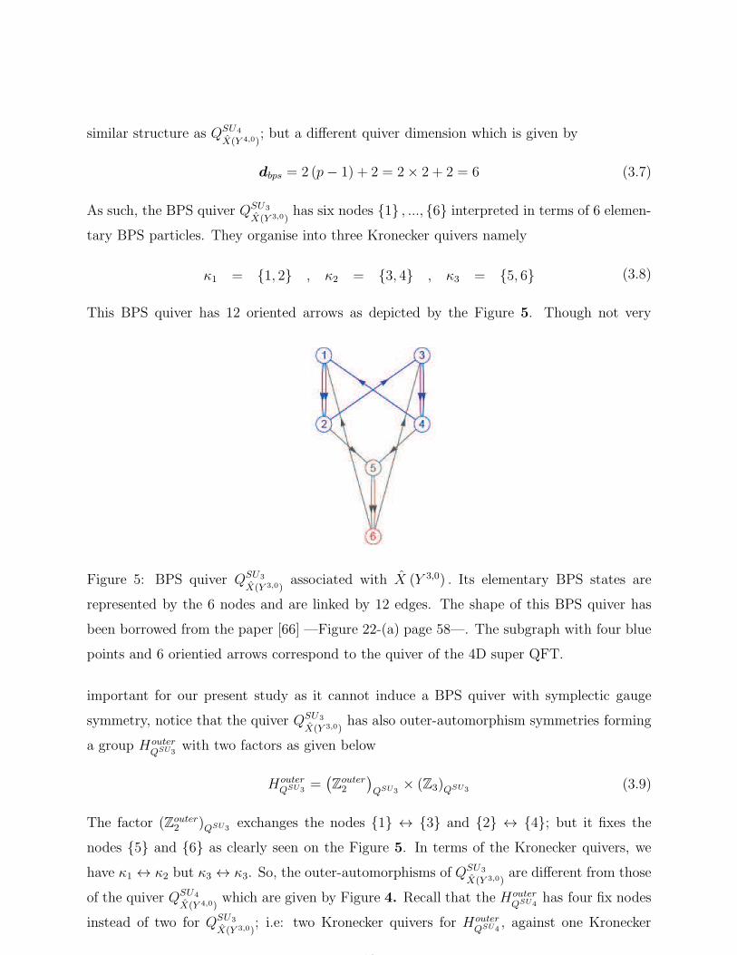
dbps = 2 (p− 1) + 2 = 2× 2 + 2 = 6 (3.7)

As such, the BPS quiver QSU3

X(Y 3,0)has six nodes {1} , ..., {6} interpreted in terms of 6 elemen-

tary BPS particles. They organise into three Kronecker quivers namely

κ1 = {1, 2} , κ2 = {3, 4} , κ3 = {5, 6} (3.8)

This BPS quiver has 12 oriented arrows as depicted by the Figure 5. Though not very



represented by the 6 nodes and are linked by 12 edges. The shape of this BPS quiver has

been borrowed from the paper [66] —Figure 22-(a) page 58—. The subgraph with four blue

points and 6 orientied arrows correspond to the quiver of the 4D super QFT.

important for our present study as it cannot induce a BPS quiver with symplectic gauge

symmetry, notice that the quiver QSU3

X(Y 3,0)has also outer-automorphism symmetries forming

a group HouterQSU3

with two factors as given below

HouterQSU3

=(

Zouter2

)

QSU3× (Z3)QSU3

(3.9)

The factor (Zouter2 )QSU3

exchanges the nodes {1} ↔ {3} and {2} ↔ {4}; but it fixes the

nodes {5} and {6} as clearly seen on the Figure 5. In terms of the Kronecker quivers, we

have κ1 ↔ κ2 but κ3 ↔ κ3. So, the outer-automorphisms of QSU3

X(Y 3,0)are different from those

of the quiver QSU4

X(Y 4,0)which are given by Figure 4. Recall that the Houter

QSU4has four fix nodes

instead of two for QSU3

X(Y 3,0); i.e: two Kronecker quivers for Houter

QSU4, against one Kronecker

13

quiver for HouterQSU3

. This difference holds as well for generic quivers QSU2r

X(Y 2r,0)and Q

SU2r−1

X(Y 2r−1,0)

with respective outer-automorphism groups HouterQSU2r

and Houter

QSU2r−1.

Regarding the factor (Z3)QSU3, it allows to represent the quiver QSU3

X(Y 3,0)as a periodic chain

as depicted by the Figure 6.



represented by the 6 nodes and are linked by 12 edges. The outer-automorphism group

(Zouter2 )QSU3

has no fix point.

4 Graphs GX(Y p,q) with manifest CY condition

In this section, we introduce a new graph to deal with the toric diagram ∆SU4

X(Y 4,0)with p=4

representing the Calabi-Yau threefold X(Y 4,0) with a resolved SU(4) gauge fiber. We refer

to this new graph as the unitary Calabi-Yau graph and we denote it like GSU4

X(Y 4,0). This graph

is explicitly defined by p − 1 vector qb with components given by the triple intersection

numbers

qbA = DA.E2b (4.1)

where the label A = (i, a) with i = 1, 2, 3, 4, for non compact divisors Di, and a = 1, 2, 3

for the compact Ea. Below, we refer to these qb’s as generalised Mori-vectors. Though this

CY graph GSU4

X(Y 4,0)looks formally different from the toric diagram, it is in fact equivalent

to it. It is just another way to deal with ∆SU4

X(Y 4,0)where the Calabi-Yau condition is mani-

festly exhibited. As we will show below, this is useful in looking for solutions of underlying

constraint relations required by the toric threefold X(Y 4,0).

4.1 Building the CY graph GSU4

X(Y 4,0)

To engineer the unitary Calabi-Yau graph GSU4

X(Y 4,0)of the toric X(Y 4,0), we start form the

Calabi-Yau condition given by eq(2.1) namely∑4

i=1Di +∑3

a=1Ea = 0. This constraint

14

relation is expressed in terms of the four non compact divisors Di and the three compact

Ea; but it is not the only constraint that must be obeyed by the divisors. There are two

other constraints that must be satisfied by the divisors. So, the seven divisors (Di, Ea) of

the toric Calabi-Yau threefolds X(Y 4,0) are subject to three basic constraints. They can be

collectively expressed as 3-vector equation like

4∑

i=1

WiDi +3

∑

a=1

VaEa = 0 (4.2)

where Wi = (wi, 1) and Va = (va, 1) are as in Table 1. To deal with the CY constraint

eq(2.1), we bring it to a relation between triple intersection numbers IABC = DA.DB.DC with

DA standing for the seven (Di, Ea). Multiplying formally both sides of eq(2.1) by E2b = Eb.Eb

with b = 1, 2, 3, we obtain the following relationships between the triple intersection numbers,

4∑

i=1

(

Di.E2b

)

+

3∑

a=1

(

Ea.E2b

)

= 0 (4.3)

These three relationships can be put into two convenient expressions; either as

4∑

i=1

J bi +

3∑

a=1

Iba = 0 (4.4)

where we have set J bi = Di.E

2b and Ib

a = Ea.E2b ; or into a more familiar form like

7∑

A=1

qbA = 0 (4.5)

with qbA =(

J bi , I

ba

)

standing three generalised Mori-vectors denoted below like qb (b = 1, 2, 3).

The second expression is precisely the relation that we have in gauged linear sigma model

(GLSM) realisation of toric Calabi-Yau threefolds [95]. Regarding the CY relation (4.5),

notice that it is quite similar to the well known relation

r∑

A=0

(

QbA

)

ADE= 0 (4.6)

giving the CY condition we encounter in the study of complex 2d ADE surfaces describing the

resolution of ALE spaces with ADE singularities. In this regards, recall that these complex

ADE surfaces play a central role in the geometric engineering of 4D N = 2 super QFTs from

type IIA string on Calabi-Yau threefolds given by ADE geometries fibered over the complex

line C [29, 30, 87, 96, 97, 98]. For these ADE geometries which can be imagined in terms

15

of orbifolds C2/Γ with Γ a discrete subgroup in SU(2), the expression the (Mori-) vectors

QbADE =

(

QbA

)

ADEcan be written down. For the example of the complex A3 surface, the

three Mori- vectors read as follows

(Qa)SU4=

1 −2 1 0 0

0 1 −2 1 0

0 0 1 −2 1

(4.7)

where the Cartan matrix K(SU4) of the Lie algebra of the SU(4) gauge symmetry appears

as a square sub-matrix of the above (Qa)SU4. Recall that K (SU4) is given by

K (SU4) = −

−2 1 0

1 −2 1

0 1 −2

(4.8)

For the case of the CY graph GSU4

X(Y 4,0)we are interested in this study, and depicted by the

Figure 7, the three generalised Mori- vectors (qa)SU4are given by

Figure 7: The graph of the CY threefolds geometry X (Y 4,0) exhibiting manifestly the CY

condition at each internal point. This graph has three (red) compact 4-cycles E1,E2,E3,

each with triple self intersection (−8), intersecting four non compact (blue) 4-cycles. The

Calabi-Yau threefolds condition is ensured by the vanishing sum of the total charge at each

red exceptional node. The underlying SQFT has an SU(4) gauge symmetry. Notice also

that this graph has a remarkable outer-automorphism symmetry to used later on.

16

(qa)SU4=

D1 D2 E1 E2 E3 D3 D4

2 2 −8 2 0 2 0

2 0 2 −8 2 2 0

2 0 0 2 −8 2 2

(4.9)

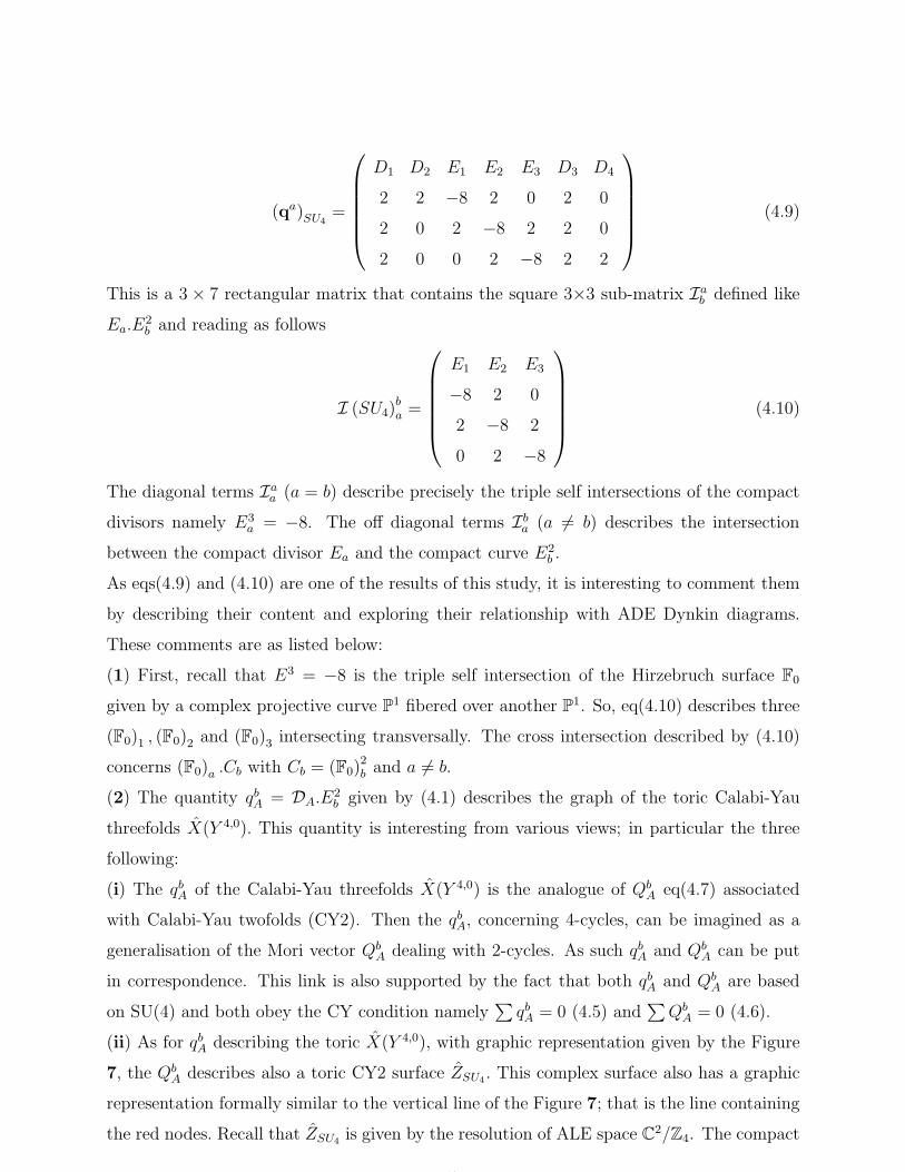
This is a 3 × 7 rectangular matrix that contains the square 3×3 sub-matrix Iab defined like

Ea.E2b and reading as follows

I (SU4)b

a =

E1 E2 E3

−8 2 0

2 −8 2

0 2 −8

(4.10)

The diagonal terms Iaa (a = b) describe precisely the triple self intersections of the compact

divisors namely E3a = −8. The off diagonal terms Ib

a (a 6= b) describes the intersection

between the compact divisor Ea and the compact curve E2b .

As eqs(4.9) and (4.10) are one of the results of this study, it is interesting to comment them

by describing their content and exploring their relationship with ADE Dynkin diagrams.

These comments are as listed below:

(1) First, recall that E3 = −8 is the triple self intersection of the Hirzebruch surface F0

given by a complex projective curve P1 fibered over another P1. So, eq(4.10) describes three

(F0)1 , (F0)2 and (F0)3 intersecting transversally. The cross intersection described by (4.10)

concerns (F0)a .Cb with Cb = (F0)2b and a 6= b.

(2) The quantity qbA = DA.E2b given by (4.1) describes the graph of the toric Calabi-Yau

threefolds X(Y 4,0). This quantity is interesting from various views; in particular the three

following:

(i) The qbA of the Calabi-Yau threefolds X(Y 4,0) is the analogue of QbA eq(4.7) associated

with Calabi-Yau twofolds (CY2). Then the qbA, concerning 4-cycles, can be imagined as a

generalisation of the Mori vector QbA dealing with 2-cycles. As such qbA and Qb

A can be put

in correspondence. This link is also supported by the fact that both qbA and QbA are based

on SU(4) and both obey the CY condition namely∑

qbA = 0 (4.5) and∑

QbA = 0 (4.6).

(ii) As for qbA describing the toric X(Y 4,0), with graphic representation given by the Figure

7, the QbA describes also a toric CY2 surface ZSU4

. This complex surface also has a graphic

representation formally similar to the vertical line of the Figure 7; that is the line containing

the red nodes. Recall that ZSU4is given by the resolution of ALE space C2/Z4. The compact

17

part of the associated toric diagram is given by the Figure 2-a where the nodes describe

three intersecting CP1 curves.

(iii) The above comments done for SU(4) holds in fact for the full SU(p) family with p ≥ 2.

So, the correspondence between qbA and QbA is a general property valid for SU(p)0 gauge

models in 5D. This correspondence holds also for the intersection matrices I (SUp)b

aand

K (SUp)b

aassociated with the compact parts in qbA and Qb

A respectively. However, the graph

of Kab is just the Dynkin diagram of the Lie algebra of SU(4). In this regards, recall that

we have Kab = α∨a .αb where the αa’s stand for the simple roots and the α∨

a = 2αa/α2a for

the co-roots. Clearly for SU(p), we have α2a = 2. The Cartan matrix Kab has also an in-

terpretation in terms of intersecting 2-cycles C(2)a in the second homology group H2; that is

C(2)a .C

(2)b = −Kab.

From this description, a natural question arises. Could the intersection matrix (4.10),

thought of as Iab = E∨a .Eb with E∨

a = E2a, also has a similar algebraic interpretation as

Kab = α∨a .αb? For example, could Iab be a generalized Cartan matrix K(gen)

ab [91] or a cousin

object of K(gen)ab ? In this regards, notice that like for −KSU4

, the matrix −ISU4is an integer

matrix with positive entries on the diagonal and non positive off diagonal entries. At first

sight one might suspect this matrix to be a generalised Cartan matrix. However, though

it is symmetric and has a positive determinant —det(−ISU4) > 0—, we have not found

an algebraic interpretation of this matrix. It is not either a generalised Cartan matrix of

Borcherds type. Progress in this direction will be reported in a future occasion.

We end this section by noticing that eq(4.9) is a particular solution of the Calabi-Yau con-

dition (4.5). It relies on the equality

Ea.E2b = E2

a.Eb ⇔ E∨a .Eb = E∨

b .Ea (4.11)

Other solutions of∑

A qbA = 0 violating the above symmetric property can be also written

down; they are omitted here.

4.2 Leading members of the GSUp

X(Y p,0)family

In the above subsection, we have focussed on the CY graph GSU4

X(Y 4,0)given by the Figure 7

which is based on exhibiting the triple intersection numbers of the compact divisors E1, E2, E2

amongst themselves and with the non compact D1, D2, D3, D4. This CY graph is however

the third member of the family GSUp

X(Y p,0)with p ≥ 2. Below, we give comments on the two

18

first CY graphs of this family.

The first member of the GSUp

X(Y p,0)family is given by GSU2

X(Y 2,0)(p=2). It has four (external) non

compact divisors D1, D2, D3, D4; but only one internal compact divisor that we denote E0.

So, there is one generalised Mori- vector given by

(q)SU2=

D1 D2 E0 D3 D4

2 2 −8 2 2

(4.12)

where the CY condition, given by the vanishing of the trace of (q)SU2, is manifestly exhibited.

The diagram representing the CY graph GSU2

X(Y 2,0)is given by the picture on the right side

of the Figure 8. On the left side of this figure, we have given the picture of the standard

A1 geometry of ALE space involving complex projective curves with self intersection −2.

Notice that the Calabi-Yau threefold X(Y 2,0) is precisely X(F0), the toric threefold based

Figure 8: On the left, the toric diagram of the A1 geometry. It has one compact 2-sphere,

with self intersection (−2), intersecting two transverse non compact (blue) 2-spheres once.

On the right, the graph GSU2

X(Y 2,0)geometry having one compact 4-cycle, with triple self inter-

section I000 = −8, intersecting four non compact (blue) 4-cycles. The Calabi-Yau threefolds

condition is ensured by the vanishing sum of the total charge.

on the Hirzebruch surface F0 which is known to have a triple self intersection (−8). Notice

also that this graph has outer-automorphisms given by the mirror (Zx2)∆SU2

×(Zy2)∆SU2

fixing

E0 and acting by the exchange D1 ↔ D3 and D2 ↔ D4.

Concerning the second member of the family namely GSUP

X(Y P,0)with p = 3, it has four external

non compact divisors D1, D2, D3, D4; but two compact divisors E1 and E2. For this case,

there are two generalised Mori- vectors given by

(qa)SU3=

D1 D2 E1 E2 D3 D4

2 2 −8 2 2 0

2 0 2 −8 2 2

(4.13)

19

The representative CY graph GSU3

X(Y 3,0)is depicted by the Figure 9. Notice that the graph

Figure 9: The CY graph GSU3

X(Y 3,0)of the toric threefolds X (Y 3,0) exhibiting manifestly the

Calabi-Yau condition at each internal point of the graph.

GSU3

X(Y 3,0)has an outer-automorphism symmetry group Houter

∆SU3given by (Zx

2)∆SU3× (Zy

2)∆SU3;

but with no fix divisor. The full Houter∆SU3

acts by the exchange E1 ↔ E2, D1 ↔ D3 and

D2 ↔ D4. This Houter∆SU3

is a subsymmetry of Z6. It is generated by the product of three

transpositions namely τ ◦ τ ′ ◦ τ ′′ with transpositions given by τ = (E1E2) , τ′ = (D1D3) and

τ ′′ = (D2D4).

5 Symplectic graphs and quivers

In this section, we first build the symplectic CY graph GSP 4

X(Y 4,0)by starting from the unitary

GSU4

X(Y 4,0)and using folding ideas under (Zx

2)∆SU4×(Zy

2)∆SU4. Then, we construct the symplectic

quiver QSP 4

X(Y 4,0)with symplectic SP(4,R) gauge symmetry by using the unitary BPS quiver

QSU4

X(Y 4,0)and outer-automorphisms (Zouter

2 )QSU4.

5.1 Symplectic CY graph GSP 4

X(Y 4,0)

We start by the toric data of ∆SU4

X(Y 4,0)given by Table 3. Because these data are defined up to

a global shift; we translate the points of ∆SU4

X(Y 4,0)by (0,−2). So the values of the wi and υa

points —Table 3— of the previous toric diagram gets mapped to new points that we present

as follows where we have set D−2 ≡ E−2 and D+2 ≡ E+2. With this parametrisation, the

internal point υ0 = (0, 0) is at the centre of the toric diagram. Moreover, the toric ∆SU4

X(Y 4,0)

is invariant under the outer-automorphism symmetry group Houter∆SU4

≃ (Zx2)∆SU4

× (Zy2)∆SU4

mapping the points w±i,υ0,υ±a into the symmetric ones namely w∓i,υ0,υ∓a. Because of

20

X(Y 4,0) A3- geometry transverse geometry

∆SU4

X(Y 4,0)υ−2 υ−1 υ0 υ+1 υ+2 w−1 w+1

points (0,−2) (0,−1) (0, 0) (0,+1) (0,+2) (−1,+2) (+1,−2)

divisors E−2 E−1 E0 E+1 E+2 D−1 D+1

Table 4: Toric data exhibiting manifestly outer-automorphism symmetry

the property w∓i = −w±i and υ∓a = −υ±a, the outer-automorphism Houter∆SU4

acts as a parity

symmetry of the toric diagram,

Houter∆SU4

: (w∓i, 0,υ∓a) → (−w±i, 0,−υ±a) (5.1)

Notice that the outer-automorphism parityHouter∆SU4

is isomorphic to the group product (Zx2)∆SU4

×

(Zy2)∆SU4

generated by the reflections in x- and y- directions acting as follows

(Zx2)∆SU4

: (nx, ny) → (−nx, ny)

(Zy2)∆SU4

: (nx, ny) → (nx,−ny)

(Zx2)∆SU4

× (Zy2)∆SU4

: (nx, ny) → (−nx,−ny)

(5.2)

where the (nx, ny)’s stand for the values of the external and the internal points of the toric

diagram. So, the triangulated ∆SU2r

X(Y 2r,0)is invariant under the outer-automorphism symmetry

group with the central point υ0 being the unique fix point of Houter∆SU4

.

By folding the CY graph GSU4

X(Y 4,0)under the parity symmetry (Zx

2)∆SU4× (Zy

2)∆SU4, we end

up with a new CY graph

GSP 4

X(Y 4,0)=

GSU4

X(Y 4,0)

(Zx2)∆SU4

× (Zy2)∆SU4

(5.3)

having 2 + 2 = 4 points given, up to identifications, by w−1 ≡ w+1, w−2 ≡ w+2; and υ0 as

well as υ−1 ≡ υ+1. The CY graph GSP 4

X(Y 4,0)is depicted by the Figure 10. The generalised

Mori- vectors q1 and q2 associated with the symplectic CY graph GSP 4

X(Y 4,0)have each four

components qaβ. They are given by

qaβ =

E±2 E±1 E0 D±1

2 −8 2 4

0 4 −8 4

(5.4)

21

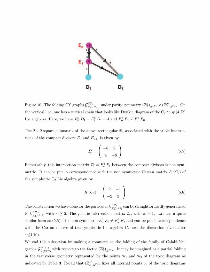
Figure 10: The folding CY graphs GSU4

X(Y 2r,0)under parity symmetry (Zx

2)∆SU4× (Zy

2)∆SU4. On

the vertical line, one has a vertical chain that looks like Dynkin diagram of the C2 ≃ sp (4,R)

Lie algebras. Here, we have E20 .D1 = E2

1 .D1 = 4 and E20 .E1 6= E2

1 .E0.

The 2× 2 square submatrix of the above rectangular qaβ , associated with the triple intersec-

tions of the compact divisors E0 and E±1, is given by

Iab =

−8 2

4 −8

(5.5)

Remarkably, this intersection matrix Iab = E2

a.Eb between the compact divisors is non sym-

metric. It can be put in correspondence with the non symmetric Cartan matrix K (C2) of

the symplectic C2 Lie algebra given by

K (C2) =

2 −1

−2 2

(5.6)

The construction we have done for the particular GSP 4

X(Y 4,0)can be straightforwardly generalized

to GSP 2r

X(Y 2r,0)with r ≥ 2. The generic intersection matrix Iab with a,b=1, ....r; has a quite

similar form as (5.5). It is non symmetric E2a.Eb 6= E2

b .Ea and can be put in correspondence

with the Cartan matrix of the symplectic Lie algebra Cr; see the discussion given after

eq(4.10).

We end this subsection by making a comment on the folding of the family of Calabi-Yau

graphs GSUp−1

X(Y p,0)with respect to the factor (Zx

2)∆SUp . It may be imagined as a partial folding

in the transverse geometry represented by the points w1 and w3 of the toric diagram as

indicated by Table 3. Recall that (Zx2)∆SUp fixes all internal points υa of the toric diagrams

22

∆SUp−1

X(Y p,0)as well as the two external w2 and w4; but exchanges the two other external w1

and w3. The folded

GSUp−1

X(Y p,0)/ (Zx

2)∆SUp (5.7)

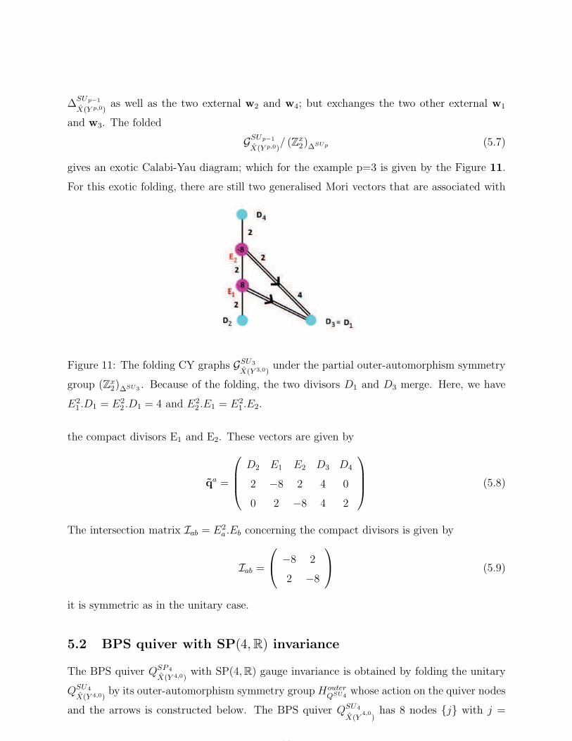
gives an exotic Calabi-Yau diagram; which for the example p=3 is given by the Figure 11.

For this exotic folding, there are still two generalised Mori vectors that are associated with

Figure 11: The folding CY graphs GSU3

X(Y 3,0)under the partial outer-automorphism symmetry

group (Zx2)∆SU3

. Because of the folding, the two divisors D1 and D3 merge. Here, we have

E21 .D1 = E2

2 .D1 = 4 and E22 .E1 = E2

1 .E2.

the compact divisors E1 and E2. These vectors are given by

qa =

D2 E1 E2 D3 D4

2 −8 2 4 0

0 2 −8 4 2

(5.8)

The intersection matrix Iab = E2a .Eb concerning the compact divisors is given by

Iab =

−8 2

2 −8

(5.9)

it is symmetric as in the unitary case.

5.2 BPS quiver with SP(4,R) invariance

The BPS quiver QSP 4

X(Y 4,0)with SP(4,R) gauge invariance is obtained by folding the unitary

QSU4

X(Y 4,0)by its outer-automorphism symmetry groupHouter

QSU4whose action on the quiver nodes

and the arrows is constructed below. The BPS quiver QSU4

X(Y4,0

)has 8 nodes {j} with j =

23

1, ..., 8; and 16 oriented arrows 〈j|l〉 as depicted by the Figure 4. Clearly, the BPS quiver

QSU4

X(Y4,0

)has a non trivial outer- automorphism symmetry group with two factors given by

HouterQSU4

= (Z4)QSU4×(

Zouter2

)

QSU4(5.10)

The factor (Z4)QSU4has no fix quiver-node and no fix quiver-arrows; while (Zouter

2 )QSU4has

fix nodes and arrows. The transformations under (Z4)QSU4are given eq(3.3); and the change

under (Zouter2 )QSU4

is as in eq(3.4). Thus, it is the symmetry (Zouter2 )QSU4

that is important

in our folding construction as it has fix nodes and arrows.

For the transformations under (Z4)QSU4, the nodes are transformed as follows

(Z4)QSU4:

{2a− 1} → {2a + 7}

{2a} → {2a + 8}(5.11)

This change indicates that the nodes {7} and {8} can be also denoted like {1} and {0}

respectively where the label 1 refers to −1 ≡ 7 and 0 ≡ 8. Regarding the action of the

(Zouter2 )QSU4

symmetry, we have the following transformations of the nodes

(

Zouter2

)

QSU4:

{2a− 1} → {7− 2a}

{2a} → {8− 2a}(5.12)

showing that four quiver- nodes amongst the eight ones are fixed. They concern the pair

{3} , {4} and the pair {7} , {8}.

By folding QSU4

X(Y4,0

)with respect to (Zouter

2 )QSU4, we obtain a BPS quiver interpreted as the

BPS quiver QSP 4

X(Y4,0

)with an SP(4,R) gauge symmetry. This folded BPS quiver has 6 nodes

namely {1, 2, 3, 4, 7, 8} (the old {5} and {6} omitted due to folding). This new set of nodes

can be also denoted as {1, 0, 1, 2, 3, 4} where we have renamed the Kronecker quiver {7, 8}

like {1, 0}. The resulting BPS quiver QSP 4

X(Y4,0

)is as depicted in the Figure 12. In addition

to the nodes, the folded BPS quiver has 16 oriented arrows distributed as in the Table 5

where the complex Xαa12 with α = 1, 2 and a = 1, 2 form a quartet; and where the Uα

∗ and

the Ua∗ are doublets with U standing for X, Y and Z. With these complex superfields, one

can write down the SQM superpotential of the theory; it will not be discussed here.

6 Conclusion and comments

In this paper, we have developed a method to construct a new family of 5D N = 1 super-

symmetric QFT models compactified on a circle with finite radius. This family of gauge

24

Figure 12: The BPS quiver QSP 4

X(Y4,0

)resulting by the folding of the QSU4

X(Y4,0

)under the mirror

(Zouter2 )Q . The nodes {1, 2, 3, 4} denote the elementary BPS particles associated with the

rank of the C2 Lie algebra.

arrows 〈1|2〉αa 〈3|4〉α 〈7|8〉α 〈2|3〉a 〈8|1〉a 〈4|1〉a 〈2|7〉a

matter Xαa12 Xα

34 Xα78 Za

23 Za81 Y a

41 Y a27

multiplicity 4 2 2 2 2 2 2

Table 5: Matter content of the BPS quiver QSP 4

X(Y4,0

).

models has symplectic SP(2r,R) gauge invariance and is embedded in M-theory on CY3s

based on Sasaki-Einstein manifolds Yp,0. Recall that gauge models engineered from M-theory

on X (Y p,q) are well known; and they have unitary symmetries. So, our construction can be

viewed as widening the family of unitary models based on X (Y p,q) to include the family of

symplectic invariant models. To engineer this new theory, we started from the 5D N = 1

super QFT, with unitary SU(4) gauge symmetry (corresponding to 2r=4), embedded in M-

theory compactification on the toric Calabi-Yau threefold X (Y 4,0) . This complex 3d variety

is a resolution of a conical singularity based on the Sasaki-Einstein manifold Y 4,0. Then, we

have proposed a graph to represent X (Y 4,0) by using the numbers Jiab and Iabc given by

triple intersections of the 7 divisors of X (Y 4,0); four non compact Di and three compact Ea.

This new graph, denoted as GSU4

X(Y 4,0), is given by a generalisation of the Mori-vectors of the

ADE geometries of ALE spaces. It is defined by eq(4.1) and, to our knowledge, it has not

been used before. We qualified the graph GSU4

X(Y 4,0)as a unitary CY graph, first because of

the unitary SU (4) symmetry of the gauge fiber within X (Y 4,0); and second to distinguish

it from the CY graph GSP 4

X(Y 4,0)having a symplectic SP (4,R) gauge symmetry. The use of

GSU4

X(Y 4,0)has the merit to (i) highlight the CY condition of the toric X (Y 4,0); (ii) extend the

usual complex A3 surface describing the resolution of an ALE space with an SU(4) singular-

25

ity; and (iii) to study non trivial outer-automorphisms Houter∆SU4

of the toric diagram ∆SU4

X(Y 4,0).

The outer-automorphism group Houter∆SU4

has a fixed internal point (a compact divisor); and is

used to build the symplectic CY graph GSP 4

X(Y 4,0)by using the folding GSU4

X(Y 4,0)/Houter

∆SU4. After

having set the basis for the CY graphs to represent the toric threefolds X (Y p,q), we turned

to investigating the BPS particles by constructing the symplectic BPS quiver QSP 4

X(Y 4,0)that

is associated with the symplectic CY graph GSP 4

X(Y 4,0). This BPS quiver is obtained by folding

the unitary BPS QSU4

X(Y 4,0)with respect to outer-automorphisms (Zouter

2 )QSU4. Recall that the

QSU4

X(Y 4,0)has 8 nodes and 16 oriented arrows respectively describing 8 elementary BPS par-

ticles and 16 chiral superfields in SQM. The mirror symmetry (Zouter2 )QSU4

fixes four nodes

of QSU4

X(Y 4,0)and exchanges the four others. It fixes four arrows and exchanges the 12 others.

We end this conclusion by making two more comments regarding extensions of the analysis

done in this paper.

The first extension concerns the building of symplectic BPS quivers QSP 2r

X(Y 2r,0)with generic

rank. This is achieved by starting from the unitary quiver QSU2r

X(Y 2r,0)with rank 2r-1 and

use folding ideas. The resulting symplectic quivers QSP 2r

X(Y 2r,0)are associated with the toric

threefolds obtained by folding the unitary QSU2r

X(Y 2r,0)with respect to the outer-automorphism

group (Zouter2 )QSU2r . The quiver series QSP 2r

X(Y 2r,0)is also related to the symplectic CY graphs

GSP 2r

X(Y 2r,0)obtained from the folding of the unitary GSU2r

X(Y 2r,0)under the outer-automorphism

symmetry Houter∆SU2r

. The explicit expression of the generalised Mori-vectors and representative

graph GSP 2r

X(Y 2r,0)as well as the associated quivers have been omitted for the sake of simplifying

the presentation of the underlying idea.

The second extension regards 5D super QFT models, based on conical Sasaki-Einstein mani-

folds Yp,q, with gauge symmetries beyond the unitary SU(r + 1) and the symplectic SP(2r,R)

groups. These gauge symmetries concern the orthogonal SO(2r) and SO(2r + 1) groups; and

eventually the three exceptional Lie groups E6,E7 and E8. For 5D super QFT models with

SO(2r) gauge symmetry embedded in M-theory on X (Y p,q), one needs engineering toric

Calabi-Yau threefolds Xp,q (Dr) with an SO(2r) gauge fiber. This might be nicely reached

by using the technique of the CY graphs GSO2r

X(Dr)used in this study although an explicit check

is still missing. This series of GSO2r

X(Dr)could be constructed by taking advantage of known

results from the so-called complex Dr surfaces describing the resolution of ALE space with

SO(2r) singularity. The family of the CY graphs GSO2r

X(Dr)might be also motivated from the

correspondence between eq(4.8) and eq(4.10) for simply laced case; see also the correspon-

26

dence between eq(5.5) and eq(5.6) for non simply laced diagrams. If this SO(2r) study can

be rigourously performed, one can also use outer-automorphisms of GSO2r

X(Dr), inherited for the

Dynkin diagram of so(2r) Lie algebra, as well as the outer-automorphisms of the associated

BPS QSO2r

X(Dr)to construct 5D supersymmetric QFT models with SO(2r − 1) gauge invariance.

Progress in these directions will be reported elsewhere.

Appendices

In this section, we give three appendices: A, B and C. They collect useful tools and give some

details regarding the study given in this paper. In appendix A, we recall general aspects of

the families of CY3s used in the geometric engineering of 5D N = 1 super QFTs and the 5D

N = 1 super CFTs. We also describe properties of the Coulomb branch of the 5D SQFTs.

In appendix B, we illustrate the derivation of the formula (3.1). In appendix C, we describe

through examples the relationship between the 5D Kaluza-Klein BPS quivers and their 4D

counterparts.

Appendix A

We begin by reviewing interesting aspects of M-theory compactified on a smooth non compact

Calabi-Yau threefold X. Then, we focus on illustrating these aspects for the class of CY3s

given by X (Y p,q) used in present study. We also use these aspects to comment on the

properties of the BPS particle and string states of the 5D gauge theory.

Two local CY3 families

Generally speaking, we distinguish two main families of local Calabi-Yau threefolds X de-

pending on whether they have an elliptic fibration or not. These two families are used in

the compactification of F-theory/M-theory/ type II strings leading respectively to effective

gauge theories in 6/5/4 space time dimensions. These compactifications have received lot

of interest in recent years in regards with the full classification of superconformal theories

in various dimensions and their massive deformations. Because of dualities and due to the

biggest 6D, the classification of 6D effective gauge theories has been conjectured to be the

mother of the classifications in the lower dimensional theories. What concerns us in this

27

appendix is not the study of the classification issue; but rather give some mathematical tools

developed there and which can also be applied to our study.

• Family of local CY3s admitting an elliptic fibration.

These local Calabi-Yau threefolds X are complex 3D spaces given by the typical fibration

E → B with building blocks as: (i) B a complex 2D base; this is a Kahler surface. (ii) a

complex 1D fiber E given by an elliptic curve. This genus zero curve is expressed by the

Weirstrass equation

E : y2z = x3 + fxz2 + gz3 (A.1)

where (x, y, z) are homogeneous coordinates of P2. Moreover, z is a function on the base B

and (x, y, f, g) are sections K−2B , K−3

B , K−4B , K−6

B with KB the canonical divisor class of B.

Depending on the nature of the base, one can preserve either preserve 16 supersymmetric

charges for bases B type T2 → P1; or eight supercharges in the case of bases B like for example

P1×P1 and in general Hirzebruch surfaces Fn. These elliptically fibered CY3 geometries X ∼

E × B have been used recently in the engineering of superconformal theories in dimensions

bigger than 4D. Regarding the SCFTs in 4D, the classification has been obtained a decade

ago by using type II strings. For the classification of the 5D SCFTs using M-theory on

elliptically fibered CY3 we refer to [4]. The graphs representing these theories are intimately

related with the Dynkin diagrams of affine Kac-Moody Lie algebras.

• Family of local CY3s not elliptically fibered.

As examples of local Calabi-Yau threefolds X , we cite the orbifolds of the complex 3- di-

mension space; i.e C3/Γ with discrete group Γ contained in SU(3). These orbifolds include

the conical Sasaki-Einstein threefolds X (Y p,q) we have considered in this paper. The local

CY3 geometries which are not elliptically fibered are used in the engineering of massive su-

persymmetric QFTs. The graphs representing these theories are related with the Dynkin

diagrams of ordinary Lie algebras.

In what follows, we focus on M-theory compactified on X (Y p,0) considered in this study and

on the corresponding U(1)p−1 Coulomb branch.

M-theory on X (Y p,0)

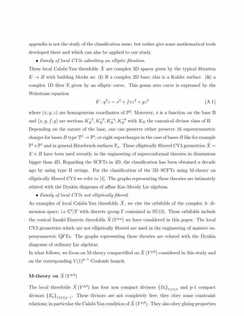
The local threefolds X (Y p,0) has four non compact divisors {Di}1≤i≤4 and p-1 compact

divisors {Ea}1≤a≤p−1. These divisors are not completely free; they obey some constraint

relations; in particular the Calabi Yau condition of X (Y p,0) . They also obey gluing properties

28

through holomorphic curves. The CY condition reads in terms of the divisor classes as in

eq(2.1). For a generic positive integer p; it reads as follows [64]

4∑

i=1

Di +

p−1∑

a=1

Ea = 0 (A.2)

In our study, this condition has been transformed as in eq(4.1); and has been used to intro-

duce the graphs given in section 4. Notice that the union of the compact divisors S = ∪p−1a=1Ea

is important in this investigation; it is a local surface made of a collection of irreducible com-

pact holomorphic surfaces Ea. The irreducible holomorphic surfaces intersect each other

pairwise transversally; this intersection is important and will be described below with de-

tails. Notice also that the Kahler parameters of the Ea’s are identified as the Coulomb

branch moduli φa; they appear in the calculation through the linear combination∑

φaEa

which also plays an important role in the construction.

Regarding the gluing properties of the compact divisors and their consequences; they need

introducing some geometric tools of the CY3. For a shortness and self contained of the

presentation, we restrict to giving only those main tools that are interesting for this study.

However, we take the occasion to also describe some particular geometric objects that are

relevant for the investigation of the Coulomb branch of the gauge theory. These geometric

objects are introduced through the four following points (a), (b), (c) and (d).

a) Gluing the compact divisors

The compact holomorphic surfaces {Ea} are complex surfaces in X. Neighboring surfaces Ea

and Eb are glued to each others while satisfying consistency conditions. Before giving these

conditions, recall that in our study, we have solved the CY condition by thinking of the Ea’s

as given by (F0)a. As the holomorphic surface F0 is given by a projective line P1f trivially

fibered over a base P1B, then we have

Ea =(

P1f

)

a×

(

P1B

)

a(A.3)

Notice that this is a particular solution of the CY on 4-cycles; it has been motivated by

looking for a simple solution to exhibit the CY condition as in the Figures 7-8-9 of section 4.

However, general solutions might be worked out by using other type of holomorphic compact

surfaces like the Hirzebruch surfaces (Fn)a of degree n and their blow ups at generic points.

To fix the ideas, we focus below on the surfaces Fn and on two lattices associated with Fn

namely: (1) the lattice Λl (Fn) of complex curves l in Fn; and (2) the Mori cone of curves

29

Ml (Fn); this is a particular sublattice of Λl (Fn) . To that purpose, recall that holomorphic

curves l in the compact surface Fn are generated by two basic (irreducible) curves e and f.

The base curve e is the zero section of the fibration; and the f is the fiber P1f . The intersection

numbers of these generators are given by

e2 = −n , f 2 = 0 , e.f = 1 (A.4)

Before proceeding forward, notice the four following interesting aspects: (i) The positivity

e.f ≥ 0 captures the irreducibility property of the generators e and f. In general, a given

curve l belonging to Λl (Fn) is said irreducible if we have l.e ≥ 0 and l.f ≥ 0. (ii) As far

compact holomorphic curves in Fn are concerned; one distinguishes two interesting curves

that play an important role in the study of Fn. These are the curve h = e + nf ; and the

canonical class KFn,g= −2h + (2g − 2 + n)f where we have moreover figured the genus

g. For the case of Fn, we have KFn= −2e + (n− 2) f ; it reduces for the case n = 0 to

KF0= −2e− 2f with triple intersection given by

(F0)3 = KF0

.KF0= 8e.f = 8 (A.5)

From the above relations, we can perform several computations. For example, we have

h2 = +n , h.e = 0 , h.f = 1

KF0.h = −2 , KF0

.e = 2n− 2 , KF0.f = −2

(A.6)

and(

KFn,g+ l

)

.l = 2g − 2 (A.7)

where g is the genus of l. Because the genus g ≥ 0, the above quantity is greater than −2

due to the constraint 2 (g − 1) ≥ −2. (iii) Holomorphic curves in Mori cone Ml (Fn) of the

surface Fn are given by the linear combination lne,nf= nee + nff with positive integers ne

and nf . These are particular curves of Λl (Fn) corresponding to ne and nf arbitrary integers.

Notice that with this notation, we have h =l1,n; and the particular curve l1,1 = e + f has

a self intersection l21,1 = 2 − n. (iv) If considering several surfaces Fna

with a=1,...,p-1;

then eq(A.4) extend as follows e2a = −na and f 2a = 0 as well as ea.fa = 1. Quite similar

relationships can be written down for the holomorphic curves in Λal = Λl (Fna

) and curves in

Mal = Ml (Fna

).

Returning to the gluing of curves la and lb inside two compact surfaces Sa and Sb; say the

30

divisor Ea and the divisor Eb. It is defined by using the following restrictions

lab = la|Eb, lba = lb|Ea

(A.8)

and imposing some consistency conditions coming from topology and geometry. The topology

requires the two curves la and lb to be identical in the following sense: (α) if the la is

irreducible; then the lb must be also irreducible; and (β) the genera of the two curves have

to be equal and positive; that is g (la) = g (lb) ≥ 0. The geometry requires moreover the

volumes vol(lab) and vol(lba) to be equal; these volumes are computed by using the dual

Kahler divisor as usual like −J.lab = −J.lba. Under these consistency conditions, the gluing

of the two curves is thought of in terms of the identification lab ≃ lba together with the CY

condition that reads as follows

(lab)2 + (lba)

2 = 2g − 2 (A.9)

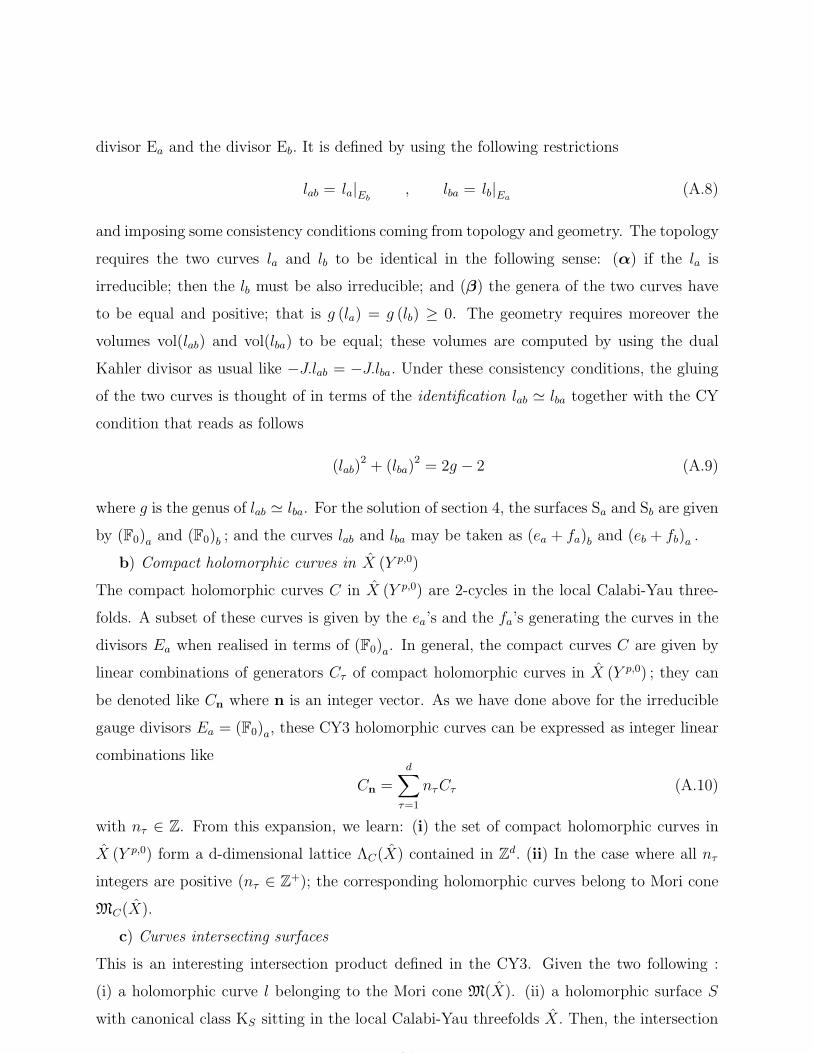
where g is the genus of lab ≃ lba. For the solution of section 4, the surfaces Sa and Sb are given

by (F0)a and (F0)b ; and the curves lab and lba may be taken as (ea + fa)b and (eb + fb)a .

b) Compact holomorphic curves in X (Y p,0)

The compact holomorphic curves C in X (Y p,0) are 2-cycles in the local Calabi-Yau three-

folds. A subset of these curves is given by the ea’s and the fa’s generating the curves in the

divisors Ea when realised in terms of (F0)a. In general, the compact curves C are given by

linear combinations of generators Cτ of compact holomorphic curves in X (Y p,0) ; they can

be denoted like Cn where n is an integer vector. As we have done above for the irreducible

gauge divisors Ea = (F0)a, these CY3 holomorphic curves can be expressed as integer linear

combinations like

Cn =

d∑

τ=1

nτCτ (A.10)

with nτ ∈ Z. From this expansion, we learn: (i) the set of compact holomorphic curves in

X (Y p,0) form a d-dimensional lattice ΛC(X) contained in Zd. (ii) In the case where all nτ

integers are positive (nτ ∈ Z+); the corresponding holomorphic curves belong to Mori cone

MC(X).

c) Curves intersecting surfaces

This is an interesting intersection product defined in the CY3. Given the two following :

(i) a holomorphic curve l belonging to the Mori cone M(X). (ii) a holomorphic surface S

with canonical class KS sitting in the local Calabi-Yau threefolds X. Then, the intersection

31

between l and S is given by

l.S = (l.KS)|S (A.11)

For the interesting case where the holomorphic surface S is given by the compact divisors

Ea, the above intersection reads as (l.KS)|Ea. The value of this intersection depends on two

possibilities:

(α) The case where l lives inside Ma(X); then, we have l.Ea = (l.KS)|Ea.

(β) The case where l lives inside another surface; say S = Eb; then we have

l.Ea = (l.lba)|Eb(A.12)

where lba is the curve participating in the gluing between Ea and Eb. The curve lab also sits

in Ma(X). From these relations, we learn that the intersections l.Ea can be recovered from

the intersection products on the Mori cones Ma.

d) Triple intersections

The triple intersections Ea.Eb.Ec of the holomorphic surfaces are numbers that can be ex-

pressed as intersection products of gluing curves inside any of the three surfaces. For that,

we use the typical curves Lab = Ea.Eb; these intersection curves appear as irreducible curves

lab from the Ea side; and as irreducible curves lba from the side of Eb. The intersection of

Ea and Eb is obtained as described before; that is by the identification lba = lab. Similar

identifications hold for the intersections of Eb.Ec and Ec.Ea. By taking the intersection curve

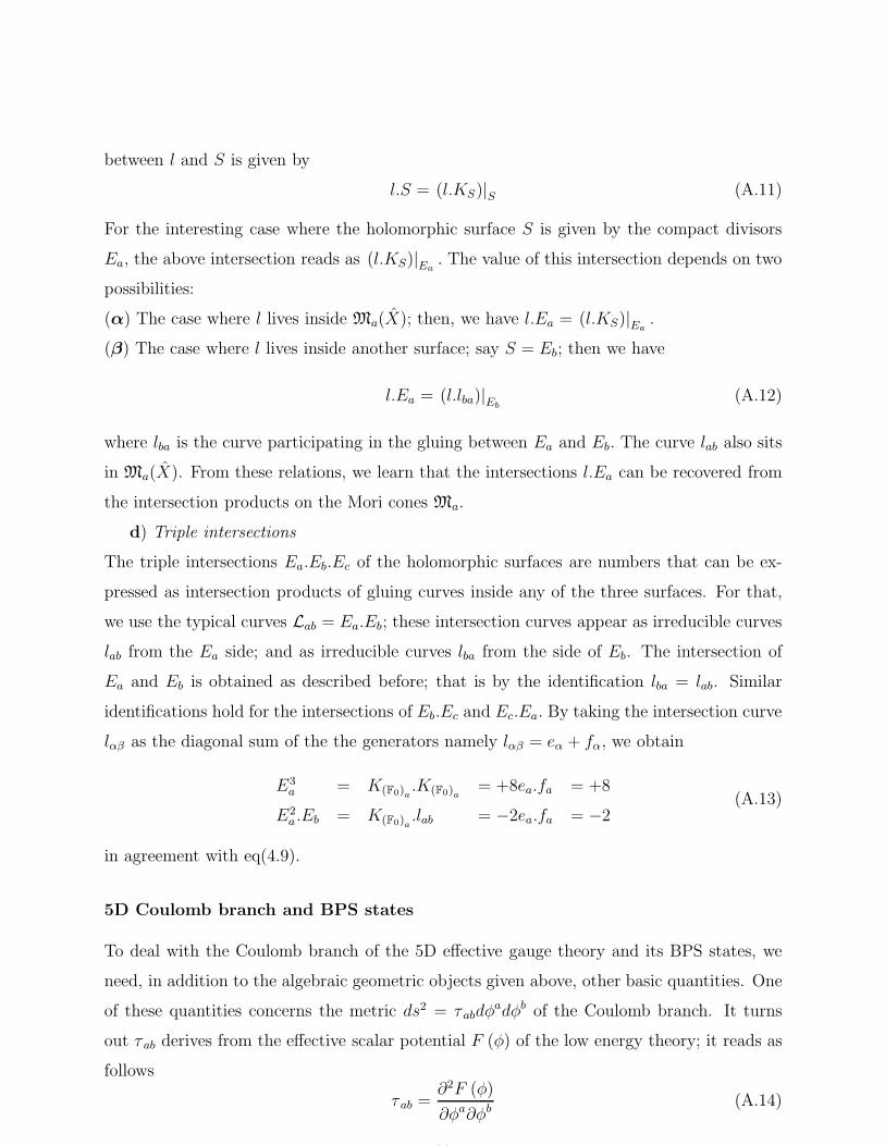
lαβ as the diagonal sum of the the generators namely lαβ = eα + fα, we obtain

E3a = K(F0)a

.K(F0)a= +8ea.fa = +8

E2a .Eb = K(F0)a

.lab = −2ea.fa = −2(A.13)

in agreement with eq(4.9).

5D Coulomb branch and BPS states

To deal with the Coulomb branch of the 5D effective gauge theory and its BPS states, we

need, in addition to the algebraic geometric objects given above, other basic quantities. One

of these quantities concerns the metric ds2 = τabdφadφb of the Coulomb branch. It turns

out τ ab derives from the effective scalar potential F (φ) of the low energy theory; it reads as

follows

τ ab =∂2F (φ)

∂φa∂φb(A.14)

32

Given F (φ) , one also has two other interesting quantities associated to it. (i) the gra-

dient ∂F (φ)∂φa which give the tensions Ta of BPS string states. (ii) the third derivatives as

∂3F (φ) /∂φa∂φb∂φc giving coefficient of the Chern-Simons term κabc = kdabc. The higher

derivatives vanish identically because F (φ) is a cubic function. Recall that the effective

potential of the 5D effective theory is exactly known; it reads as follows

F =1

2g20habφ

aφb +κ

6dabcφ

aφbφc +1

12

∑

roots α

|α.φ|3 −∑

f

∑

ω∈Rf

|ω.φ+mf |3

(A.15)

This function has the properties: (i) It is a cubic function of the gauge scalar field moduli

{φ1, ..., φr} parameterising the Coulomb branch. (ii) It depends on the mass parameters mf

of the 5D effective theory. (iii) It also depends on the roots α of Lie algebra and representa-

tions weights ω ∈ Rf of the underlying gauge symmetry group. From the geometric view, the

5D gauge theory has an interesting description in terms of even p-cycles in the CY3. These

cycles captures information whose some are presented through the four following poinst (a),

(b), (c) and (d).

(a) Dual of the Kahler 2-form

The dual of the Kahler 2-form of X (Y p,0) is a divisor of the CY3 reading in terms of the

generating divisors and the Coulomb branch moduli as follows

J =4

∑

i=1

miDi +

p−1∑

a=1

φaEa (A.16)

The compact complex surfaces Ea are in one to one with the U (1) factors of the Coulomb

branch of the 5D gauge theory. In the SU(4) gauge theory studied in the paper, we have

three φ’s.

(b) Volume of compact even p-cycles in X (Y p,0)

These compact cycles include: (i) the set of compact 2- cycles C belonging H2(X), (ii) the

set of compact 4- cycles S belonging H4(X); and (iii) the 6-cycle given by X (Y p,0).

The volume of a compact 2-cycles C is given by the intersection number

V ol (C) = −J.C (A.17)

For the particular compact holomorphic curves given by the p − 1 curves basic curves Ca

generating the Mori cone of X (Y p,0) ; we have the elementary volumes V ol (Ca) = υa.

The volume of a compact 4-cycles S is given by the intersection number

V ol (S) =1

2J.J.S (A.18)

33

For the particular compact holomorphic surfaces given by the basic p − 1 divisors Ea; we

have the elementary volumes V ol (Ea) = υa.

Finally, the volume of of X (Y p,0) ; it is given by the triple intersection number of the divisor

J. This is the prepotential of the low energy 5D theory

F (φ) = −1

3!J.J.J (A.19)

Notice that by putting (A.19) back into Ta, τ ab, κabc and using (A.16), we end up with the

following interpretation in terms of intersections

Ta ∼ Ea.J.J , τab ∼ Ea.Ea.J , κabc ∼ Ea.Eb.Ec (A.20)

(c) The BPS states of the 5D theory

In this effective gauge theory, we distinguish two kinds of BPS states:

(i) Massive particle states (M2/C) given by M2- branes wrapping the compact holomorphic

curves C. The masses of these particle states are given by V ol (C) . For the particular compact

curves Ca; it is associated p-1 electrically charged elementary BPS particles given by the

wrapping M2/Ca. The masses of these particles are given by υa.

(ii) String states M5/S arising from M5- brane wrapping the compact holomorphic surfaces

S. The tensions of these strings are given by V ol (S) . For the particular compact surfaces

given by the p-1 divisor Ea; it is associated p-1 magnetically charged elementary BPS strings

M5/Ea with tensions given by υa.

Notice that the BPS spectrum of 5D N=1 theories include gauge instantons I in addition

to the electrically charged particles and the magnetically charged monopole strings. The

central charges of these particles are given by

Zelc =

p−1∑

a=1

n(elc)a φa +m0I , Zmag =

p−1∑

a=1

n(mag)a

∂F

∂φa

(A.21)

where n(elc)a , n

(mag)a are integers. Notice that not every choice of these integers corresponds

to the central charge of a physical state whose mass or tension has to be positive. The

values of these n’s are obtained using BPS quivers and their mutations. Notice also that by

compactifying the 5D gauge theories on a finite circle; we generate a Kaluza Klein particle

states as described in the core of the paper.

(d) Dirac pairing

The intersection numbers Ca.Eb of compact curves Ca and compact surfaces Eb describe the

Dirac pairing between the BPS particles and the BPS strings.

34

Appendix B

Here, we consider M-theory compactified on X (Y 2,0) with SU(2) gauge symmetry and look

for the derivation of the quiver dimension dbps = 2 (p− 1) + 2 of eq(3.1). Because of the

choice p=2, we have dbps = 4 indicating that the BPS quiver QSU2

X(Y 2,0)has four nodes as

shown by the Figure 13-(b). Recall that the BPS quiver QSU2

X(Y 2,0)is related to the toric

diagram ∆SU2

X(Y 2,0)by the so-called fast inverse algorithm [92, 93, 94]. This algorithm involves

two main steps summarized as follows:

• Brane tiling BT

This step maps the toric ∆SU2

X(Y 2,0)into a brane tiling in the 2-torus to which we refer to as

BTX(Y 2,0). It uses the brane web ∆SU2

X(Y 2,0)(the dual of the toric diagram) to represent it by

the tiling as given by the Figure 13-(a). Recall that the toric graph representing ∆SU2

X(Y 2,0)is

Figure 13: (a) The brane tiling of ∆SU2

X(F0). (b) the BPS quiver QSU2

X(F0)with SU(2) gauge symmetry.

(c) the BPS subquiver of the 4d N = 2 pure SU(2)0 gauge theory.

a standard diagram; it can be drawn by using the Table 2 with p=2 and q=0. It has four

external points (next = 4), describing the four non compact divisors; and one internal point

(nint = 1) describing the compact divisor associated with the SU(2) gauge symmetry. For a

short presentation, we have omitted this graph.

• The BPS quiver

The second step maps the brane tiling BTX(Y 2,0) into the BPS quiver QSU2

X(Y 2,0)as shown by

the picture Figure 13-(b). This mapping is somehow technical, we propose to illustrate the

construction by giving some details.

35

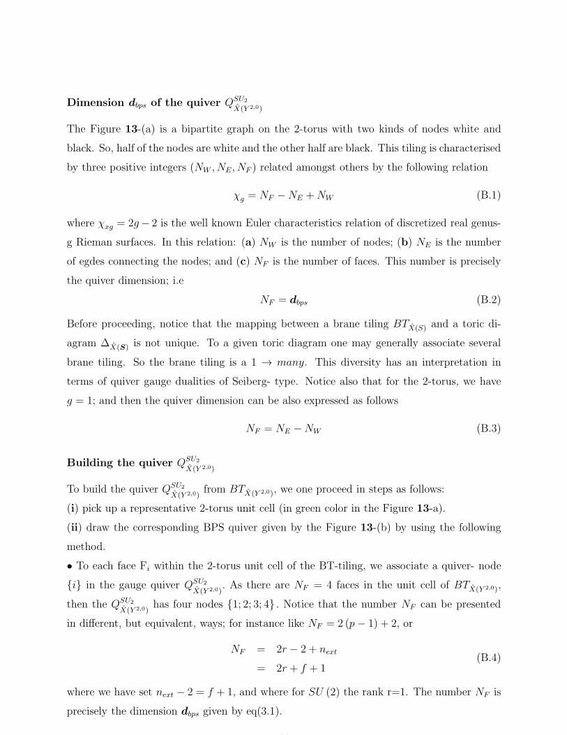
Dimension dbps of the quiver QSU2

X(Y 2,0)

The Figure 13-(a) is a bipartite graph on the 2-torus with two kinds of nodes white and

black. So, half of the nodes are white and the other half are black. This tiling is characterised

by three positive integers (NW , NE , NF ) related amongst others by the following relation

χg = NF −NE +NW (B.1)

where χxg = 2g− 2 is the well known Euler characteristics relation of discretized real genus-

g Rieman surfaces. In this relation: (a) NW is the number of nodes; (b) NE is the number

of egdes connecting the nodes; and (c) NF is the number of faces. This number is precisely

the quiver dimension; i.e

NF = dbps (B.2)

Before proceeding, notice that the mapping between a brane tiling BTX(S) and a toric di-

agram ∆X(S) is not unique. To a given toric diagram one may generally associate several

brane tiling. So the brane tiling is a 1 → many. This diversity has an interpretation in

terms of quiver gauge dualities of Seiberg- type. Notice also that for the 2-torus, we have

g = 1; and then the quiver dimension can be also expressed as follows

NF = NE −NW (B.3)

Building the quiver QSU2

X(Y 2,0)

To build the quiver QSU2

X(Y 2,0)from BTX(Y 2,0), we one proceed in steps as follows:

(i) pick up a representative 2-torus unit cell (in green color in the Figure 13-a).

(ii) draw the corresponding BPS quiver given by the Figure 13-(b) by using the following

method.

• To each face Fi within the 2-torus unit cell of the BT-tiling, we associate a quiver- node

{i} in the gauge quiver QSU2

X(Y 2,0). As there are NF = 4 faces in the unit cell of BTX(Y 2,0),

then the QSU2

X(Y 2,0)has four nodes {1; 2; 3; 4} . Notice that the number NF can be presented

in different, but equivalent, ways; for instance like NF = 2 (p− 1) + 2, or

NF = 2r − 2 + next

= 2r + f + 1(B.4)

where we have set next − 2 = f + 1, and where for SU (2) the rank r=1. The number NF is

precisely the dimension dbps given by eq(3.1).

36

• To each edge Eij of the brane tiling, separating the faces Fi and Fj , we associate a quiver-

arrow 〈ij〉 with direction determined by a traffic rule. In this rule, the circulation goes

clockwise around white BT- nodes; and counter-clockwise around black BT-nodes. In the

example QSU2

X(Y 2,0); we have 8 quiver- arrows organized into four pairs. The are given by

arrows 〈i (i+ 1)〉 with i = 1, 2, 3, 4 mod 4.

• To each BT-node in the brane tiling corresponds a superpotential monomial. So, the full

superpotential W SU2

X(Y 2,0)associated with the BPS quiver has four monomials; this is because

NW = 4. For simplicity, we omit the explicit expression of W SU2

X(Y 2,0).

In the end of this appendix, notice that the four nodes of the quiver QSU2

X(Y 2,0)are interpreted

in type IIA string as the elementary BPS particles. The particles sitting at the nodes {1, 2}

correspond to the electrically D2/C2 and the magnetically D4/C4 charged BPS particles

where Cn refers to n-cycles in X (Y 2,0). These two nodes form together a sub-graph of the

SU(2) gauge quiver QSU2

X(Y 2,0); it is given by the usual Kronecker diagram depicted by the

Figure 13-(c). The node {3} is associated with the elementary instanton I; and the node

{4} with the elementary Kaluza- Klein D0. These two nodes form together the Kronecker

sub-diagram {3, 4}.

Appendix C

In this appendix, we describe briefly helpful tools regarding the structure of BPS quivers in

4D N = 1 Kaluza-Klein while focussing on those relevant aspects for our study. The material

given below aims facilitating the reading of section 3. For a rigorous and abstract formulation

of BPS quivers using amongst others the central charges and the Coulomb branch moduli,

we refer to literature in this matter. For instance, the section 2.3 of [66] for 4D KK quivers

and [99]-[101], [90], [69]-[73] for 4D.

ADE gauge models

A short way to introduce the 4D KK BPS quivers is to go through the well studied BPS

quivers QG

X(4d) of 4D N = 2 gauge theories with ADE gauge symmetries. The use of these

4D quivers may be motivated from various views in particular from the three following:

(1) QG

X(4d) ⊂ QG

X(5d) . The quivers QG

X(4d), which are described below and mention in

the text, appear as sub-quivers of the 4D KK BPS quivers QG

X(5d) . For example, compare

the two pictures of the Figure 14 with the Figures 5 and 6 in the main text. This feature,

37

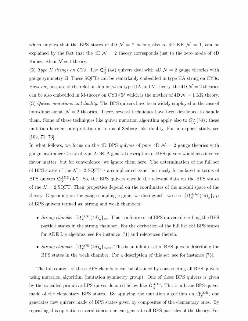
which implies that the BPS states of 4D N = 2 belong also to 4D KK N = 1, can be

explained by the fact that the 4D N = 2 theory corresponds just to the zero mode of 4D

Kaluza-Klein N = 1 theory.

(2) Type II strings on CY3. The QG

X(4d) quivers deal with 4D N = 2 gauge theories with

gauge symmetry G. These SQFTs can be remarkably embedded in type IIA string on CY3s.

However, because of the relationship between type IIA and M-theory, the 4D N = 2 theories

can be also embedded in M-theory on CY3×S1 which is the mother of 4D N = 1 KK theory.

(3) Quiver mutations and duality. The BPS quivers have been widely employed in the case of

four-dimensional N = 2 theories. There, several techniques have been developed to handle

them. Some of these techniques like quiver mutation algorithm apply also to QG

X(5d) ; these

mutation have an interpretation in terms of Seiberg- like duality. For an explicit study, see

[102, 71, 73].

In what follows, we focus on the 4D BPS quivers of pure 4D N = 2 gauge theories with

gauge invariance G; say of type ADE. A general description of BPS quivers would also involve

flavor matter; but for convenience, we ignore them here. The determination of the full set

of BPS states of the N = 2 SQFT is a complicated issue; but nicely formulated in terms of

BPS quivers QADE

X(4d). So, the BPS quivers encode the relevant data on the BPS states

of the N = 2 SQFT. Their properties depend on the coordinates of the moduli space of the

theory. Depending on the gauge coupling regime, we distinguish two sets {QADE

X(4d)n}I,II

of BPS quivers termed as strong and weak chambers:

• Strong chamber {QADE

X(4d)n}str. This is a finite set of BPS quivers describing the BPS

particle states in the strong chamber. For the derivation of the full list o3f BPS states

for ADE Lie algebras; see for instance [71] and references therein.

• Strong chamber {QADE

X(4d)n}weak. This is an infinite set of BPS quivers describing the

BPS states in the weak chamber. For a description of this set; see for instance [73].

The full content of these BPS chambers can be obtained by constructing all BPS quivers

using mutation algorithm (mutation symmetry group). One of these BPS quivers is given

by the so-called primitive BPS quiver denoted below like QADE

X. This is a basic BPS quiver

made of the elementary BPS states. By applying the mutation algorithm on QADE

X, one

generates new quivers made of BPS states given by composites of the elementary ones. By

repeating this operation several times, one can generate all BPS particles of the theory. For

38

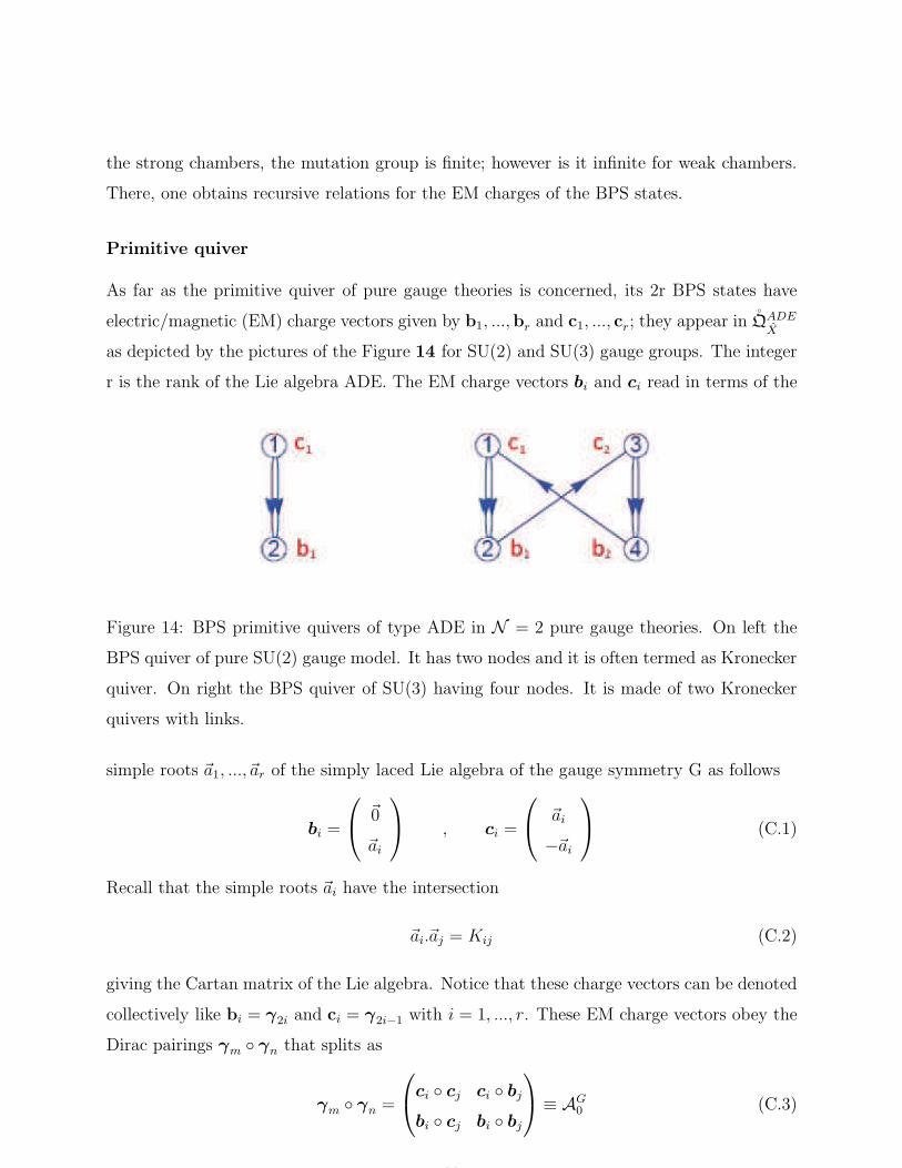
the strong chambers, the mutation group is finite; however is it infinite for weak chambers.

There, one obtains recursive relations for the EM charges of the BPS states.

Primitive quiver

As far as the primitive quiver of pure gauge theories is concerned, its 2r BPS states have

electric/magnetic (EM) charge vectors given by b1, ...,br and c1, ..., cr; they appear in QADE

X

as depicted by the pictures of the Figure 14 for SU(2) and SU(3) gauge groups. The integer

r is the rank of the Lie algebra ADE. The EM charge vectors bi and ci read in terms of the

Figure 14: BPS primitive quivers of type ADE in N = 2 pure gauge theories. On left the

BPS quiver of pure SU(2) gauge model. It has two nodes and it is often termed as Kronecker

quiver. On right the BPS quiver of SU(3) having four nodes. It is made of two Kronecker

quivers with links.

simple roots ~a1, ...,~ar of the simply laced Lie algebra of the gauge symmetry G as follows

bi =

~0

~ai

, ci =

~ai

−~ai

(C.1)

Recall that the simple roots ~ai have the intersection

~ai.~aj = Kij (C.2)

giving the Cartan matrix of the Lie algebra. Notice that these charge vectors can be denoted

collectively like bi = γ2i and ci = γ2i−1 with i = 1, ..., r. These EM charge vectors obey the

Dirac pairings γm ◦ γn that splits as

γm ◦ γn =

ci ◦ cj ci ◦ bj

bi ◦ cj bi ◦ bj

≡ AG0 (C.3)

39

Notice also that for simply laced Lie algebras, the primitive BPS quiver QADE

Xconsists of 2r

nodes and 3r − 2 links as described below:

A) nodes in QADE

X

The 2r nodes of QADE

Xare as depicted by the pictures of the Figure 14 corresponding to

SU(2) and SU(3) . They refer to the elementary BPS states with EM charges bi and ci.

Notice that in the case of pure gauge theories considered in this appendix, the bi’s are the

charges of r elementary monopoles Mi while the ci’s are the charges of r elementary dyons

Di. So the elementary BPS states of the theory are given by

Monopoles : M1, ...,Mr

Dyons : D1, ...,Dr

(C.4)

These BPS states have interpretation in terms of D2- and D4- branes wrapping 2- and 4-

cycles in the CY3. In M-theory language, they can be interpreted in terms of wrapped M2-

and M5- branes.

B) Links between nodes of QADE

X

There are r+(2r − 2) oriented links joining the nodes of QADE

X. These links are of two types

as described below:

• r vertical links l1, ..., lr joining the nodes (bi, ci) ; that is the r pairs (b1, c1) , ..., (br, cr).

They are oriented from the node ci to the node bi. These links carry a charge given by

the absolute value of the Dirac pairing bi ◦ ci which is equal to 2 due to the relation

bi ◦ ci = ~ai.~ai = 2 (C.5)

Recall that the Dirac pairing of the electric magnetic charge vectors is antisymmetric

γm ◦ γn = −γn ◦ γm; so we have

bi ◦ ci = −ci ◦ bi = Kij (C.6)

bi ◦ bj = ci ◦ cj = 0 (C.7)

• 2 (r − 1) oblique links lij joining two nodes of different pairs (bi, ci) and (bj , cj). This

reduced number of links is due to the constraint eqs(C.6-C.7). So, the intersection

matrix AG0 describing the primitive quiver QADE

Xis related to the Cartan matrix of the

Lie algebra as follows

AG0 =

0 −K

K 0

(C.8)

40

This construction extends to the BPS quivers with non simply laced gauge symmetries;

see for instance [90, 69, 70].

References

[1] G. Zafrir, Brane webs and O5-planes, JHEP03(2016)109, arXiv:1512.08114 [hep-th].

[2] G. Zafrir, Brane webs, 5d gauge theories and 6d N = (1, 0) SCFT’s, JHEP 12 (2015)

157 [arXiv:1509.02016].

[3] L. Bhardwaj, Classification of 6d N = (1, 0) gauge theories, JHEP 11 (2015) 002,

arXiv:1502.06594 [hep-th].

[4] Lakshya Bhardwaj, Patrick Jefferson, Classifying 5d SCFTs via 6d SCFTs: Rank one,

JHEP 01 (2020) 153, e-Print: 1809.01650.

[5] Patrick Jefferson, Sheldon Katz, Hee-Cheol Kim, Cumrun Vafa, On Geometric Classi-

fication of 5d SCFTs, JHEP04(2018)103, arXiv:1801.04036 [hep-th].

[6] M.R. Douglas, On D = 5 super Yang-Mills theory and (2; 0) theory, JHEP 02 (2011)

011, [arXiv:1012.2880].

[7] N. Lambert, C. Papageorgakis and M. Schmidt-Sommerfeld, M5-Branes, D4-branes

and Quantum 5D super-Yang-Mills, JHEP 01 (2011) 083 [arXiv:1012.2882].

[8] Fabio Apruzzi, Ling Lin, Christoph Mayrhofer, Phases of 5d SCFTs from M-/F-theory

on Non-Flat Fibrations, JHEP05(2019)187, arXiv:1811.12400 [hep-th]

[9] D. Xie and S.-T. Yau, Three dimensional canonical singularity and five dimensional

N = 1 SCFT, JHEP 06 (2017) 134, arXiv:1704.00799 [hep-th].

[10] S. Alexandrov, S. Banerjee, and P. Longhi, Rigid limit for hypermultiplets and five-

dimensional gauge theories, JHEP 01 (2018) 156, arXiv:1710.10665 [hep-th]

[11] P. Jefferson, H.-C. Kim, C. Vafa, and G. Zafrir, Towards Classiffication of 5d SCFTs:

Single Gauge Node, arXiv:1705.05836 [hep-th].

41

http://arxiv.org/abs/1512.08114










[12] Cyril Closset, Michele Del Zotto, Vivek Saxena, Five-dimensional SCFTs and gauge

theory phases: an M-theory/type IIA perspective, SciPost Phys. 6, 052 (2019),

arXiv:1812.10451 [hep-th].

[13] H. Hayashi, S.-S. Kim, K. Lee, M. Taki, and F. Yagi, A new 5d description of 6d

D-type minimal conformal matter, JHEP 08 (2015) 097, arXiv:1505.04439 [hep-th].

[14] J. J. Heckman, D. R. Morrison, and C. Vafa, On the Classification of 6D SCFTs and

Generalized ADE Orbifolds, JHEP 1405 (2014) 028, [arXiv:1312.5746].

[15] Matteo Sacchi, Orr Sela, Gabi Zafrir, Compactifying 5d superconformal field theories

to 3d, JHEP 09 (2021) 149, arXiv:2105.01497 [hep-th].

[16] L. Bhardwaj, On the classification of 5d SCFTs, JHEP 09 (2020) 007

[arXiv:1909.09635].

[17] Anton Kapustin, On the universality class of little string theories, Phys.Rev.D 63

(2001) 086005, e-Print: hep-th/9912044.

[18] Chi-Ming Chang, 5d and 6d SCFTs Have No Weak Coupling Limit, 10.1007/JHEP09

(2019) 016, arXiv:1810.04169 [hep-th].

[19] Lakshya Bhardwaj, Patrick Jefferson, Hee-Cheol Kim, Houri-Christina Tarazi, Cumrun

Vafa, Twisted Circle Compactifications of 6d SCFTs, arXiv:1909.11666 [hep-th].

[20] N. Seiberg, Five-dimensional SUSY field theories, nontrivial fixed points and string

dynamics, Phys. Lett. B 388 (1996) 753 [hep-th/9608111]

[21] O. Aharony and A. Hanany, Branes, superpotentials and superconformal fixed points,

Nucl. Phys. B 504 (1997) 239 [hep-th/9704170].

[22] O. Aharony, A. Hanany and B. Kol, Webs of (p,q) five-branes, five-dimensional field

theories and grid diagrams, JHEP 01 (1998) 002 [hep-th/9710116].

[23] N. C. Leung and C. Vafa, Branes and toric geometry, Adv.Theor.Math.Phys. 2 (1998)

91-118, [hep-th/9711013].

[24] S. Cabrera, A. Hanany and F. Yagi, Tropical Geometry and Five Dimensional Higgs

Branches at Infinite Coupling, JHEP 01 (2019) 068, [1810.01379].

42






http://arxiv.org/abs/hep-th/9912044







[25] A. Bourget, J. F. Grimminger, A. Hanany, M. Sperling and Z. Zhong, Magnetic Quivers

from Brane Webs with O5 Planes, JHEP 07 (2020) 204, [2004.04082].

[26] M. Akhond, F. Carta, S. Dwivedi, H. Hayashi, S.-S. Kim and F. Yagi, Five-brane webs,

Higgs branches and unitary/orthosymplectic magnetic quivers, JHEP 12 (2020) 164,

[2008.01027].

[27] D. R. Morrison and N. Seiberg, Extremal transitions and five-dimensional supersym-

metric field theories, Nucl. Phys. B483 (1997) 229-247,arXiv: hep-th/9609070 [hep-th].

[28] K. A. Intriligator, D. R. Morrison, and N. Seiberg, Five-dimensional supersymmetric

gauge theories and degenerations of Calabi-Yau spaces, Nucl. Phys. B497 (1997) 56-

100, arXiv:hep-th/9702198 [hep-th].

[29] S. H. Katz, A. Klemm, and C. Vafa, Geometric engineering of quantum field theories,”

Nucl. Phys. B497 (1997) 173-195, arXiv:hep-th/9609239 [hep-th].

[30] S. Katz, P. Mayr, and C. Vafa, Mirror symmetry and exact solution of 4-D N=2 gauge

theories: 1., Adv.Theor.Math.Phys. 1 (1998) 53-114, arXiv:hep-th/9706110 [hep-th].

[31] T. J. Hollowood, A. Iqbal, and C. Vafa, Matrix models, geometric engineering and

elliptic genera, JHEP 03 (2008) 069, arXiv:hep-th/0310272 [hep-th].

[32] S.-S. Kim and F. Yagi, Topological vertex formalism with O5-plane, Phys. Rev. D97

(2018) 026011, [arXiv:1709.01928].

[33] M. Aganagic, A. Klemm, M. Marino, and C. Vafa, The Topological vertex, Com-

mun.Math.Phys. 254 (2005) 425{478, [hep-th/0305132].

[34] A. Iqbal, C. Kozcaz, and C. Vafa, The Refined topological vertex, JHEP 0910 (2009)

069, [hep-th/0701156].

[35] H. Awata and H. Kanno, Refined BPS state counting from Nekrasov’s formula and

Macdonald functions, Int.J.Mod.Phys. A24 (2009) 2253-2306, [arXiv:0805.0191].

[36] Hirotaka Hayashi, Sung-Soo Kim, Kimyeong Lee, Futoshi Yagi, 5-brane webs for 5d

N = 1 G2 gauge theories, JHEP03(2018)125, arXiv:1801.03916 [hep-th].

43











[37] Lalla Btissam Drissi, Houda Jehjouh, El Hassan Saidi, Refining the Shifted Topological

Vertex, J.Math.Phys.50:013509,2009, arXiv:0812.0513 [hep-th].

[38] O. DeWolfe, A. Hanany, A. Iqbal and E. Katz, Five-branes, seven-branes and five-

dimensional En field theories, JHEP 03 (1999) 006 [hep-th/9902179].

[39] M.R. Gaberdiel and B. Zwiebach, Exceptional groups from open strings, Nucl. Phys.

B 518 (1998) 151 [hep-th/9709013].

[40] D. Gaiotto and H.-C. Kim, Duality walls and defects in 5d N = 1 theories, JHEP 01

(2017) 019 [arXiv:1506.03871].

[41] H. Hayashi, S.-S. Kim, K. Lee and F. Yagi, 6d SCFTs, 5d Dualities and Tao Web

Diagrams, JHEP 05 (2019) 203 [arXiv:1509.03300].

[42] Hirotaka Hayashi, Rui-Dong Zhu, More on topological vertex formalism for 5-brane

webs with O5-plane, JHEP04(2021)292, arXiv:2012.13303.

[43] H. Hayashi, S.-S. Kim, K. Lee, and F. Yagi, Discrete theta angle from an O5-plane,

JHEP 1711 (2017) 041, arXiv:1707.07181.

[44] F. Benini, S. Benvenuti, and Y. Tachikawa, Webs of five-branes and N=2 superconfor-

mal field theories, JHEP 0909 (2009) 052, [arXiv:0906.0359].

[45] I. Brunner and A. Karch, Branes and six-dimensional fixed points, Phys. Lett. B409

(1997) 109-116, [hep-th/9705022].

[46] O. Bergman and G. Zafrir, 5d fixed points from brane webs and O7-planes,

arXiv:1507.03860.

[47] H. Hayashi, S.-S. Kim, K. Lee, M. Taki, and F. Yagi, More on 5d descriptions of 6d

SCFTs, JHEP 10 (2016) 126, [arXiv:1512.08239].

[48] Xiaobin Li, Futoshi Yagi, Thermodynamic limit of Nekrasov partition function for

5-brane web with O5-plane, arXiv:2102.09482 [hep-th].

[49] Hirotaka Hayashi, Sung-Soo Kim, Kimyeong Lee, Futoshi Yagi, Rank-3 antisymmetric

matter on 5-brane webs, JHEP05(2019)133, arXiv:1902.04754 [hep-th].

44














[50] Mohammad Akhond, Federico Carta, Siddharth Dwivedi, Hirotaka Hayashi, Sung-Soo

Kime, Futoshi Yagi, Five-brane webs, Higgs branches and unitary/orthosymplectic

magnetic quivers, JHEP12(2020)164, arXiv:2008.01027 [hep-th].

[51] M. R. Douglas, S. H. Katz, and C. Vafa, Small Instantons, Del Pezzo Surfaces and

Type I’ Theory, Nucl. Phys. B497 (1997) 155-172, arXiv:hep-th/9609071

[52] C. P. Herzog, Exceptional collections and del Pezzo gauge theories, JHEP 04 (2004)

069, arXiv:hep-th/0310262.

[53] B. Feng, S. Franco, A. Hanany, and Y.-H. He, UnHiggsing the del Pezzo, JHEP 08

(2003) 058, arXiv:hep-th/0209228 [hep-th].

[54] S. Franco and A. Hanany, Geometric dualities in 4-D field theories and their 5-D

interpretation, JHEP 04 (2003) 043, arXiv:hep-th/0207006 [hep-th]

[55] J. P. Gauntlett, D. Martelli, J. Sparks, and D. Waldram, Sasaki-Einstein metrics on

S2 × S3, Adv. Theor. Math. Phys. 8 no. 4, (2004) 711-734, arXiv:hep-th/0403002.

[56] D. Martelli and J. Sparks, Toric Sasaki-Einstein metrics on S2 × S3, Phys. Lett. B621

(2005) 208-212, arXiv: hep-th/0505027 [hep-th].

[57] S. Benvenuti, S. Franco, A. Hanany, D. Martelli, and J. Sparks, An Infinite family of

superconformal quiver gauge theories with Sasaki-Einstein duals, JHEP 06 (2005) 064,

arXiv:hep-th/0411264 [hep-th].

[58] J. P. Gauntlett, D. Martelli, J. Sparks, S.-T. Yau, Obstructions to the existence of

Sasaki-Einstein metrics, Commun. Math. Phys. 273 (2007), 803–827.

[59] A. Futaki, H. Ono, G. Wang, Transverse Kahler geometry of Sasaki manifolds and

toric Sasaki-Einstein manifolds, J. Diff. Geom. 83 (2009), 585–636.

[60] Jiakang Bao, Grace Beaney Colverd, Yang-Hui He, Quiver gauge theories: beyond

reflexivity, JHEP06(2020)161, arXiv:2004.05295 [hep-th].

[61] Olaf Lechtenfeld, Alexander D. Popov, Marcus Sperling, Richard J. Szabo,

Sasakian quiver gauge theories and instantons on cones over lens 5-spaces,

10.1016/j.nuclphysb.2015.09.001, arXiv:1506.02786 [hep-th].

45











[62] D. Martelli and J. Sparks, Toric geometry, Sasaki-Einstein manifolds and a new infinite

class of AdS/CFT duals, Commun. Math. Phys. 262 (2006) 51–89, [hep-10201].

[63] A. Butti and A. Zaffaroni, From toric geometry to quiver gauge theory: The equiv-

alence of a-maximization and Z-minimization, Fortsch. Phys. 54 (2006) 309–316,

hep-th/0512240.

[64] C. Closset, M. Del Zotto, and V. Saxena, Five-dimensional SCFTs and gauge the-

ory phases: an M-theory/type IIA perspective, SciPost Phys. 6 no. 5, (2019) 052,

arXiv:1812.10451 [hep-th].

[65] Vivek Saxena, Rank-two 5d SCFTs from M-theory at isolated toric singularities: a

systematic study, J. High Energ. Phys. 2020, 198 (2020), arXiv:1911.09574 [hep-th].

[66] Cyril Closset, Michele Del Zotto, On 5d SCFTs and their BPS quivers. Part I: B-branes

and brane tilings, arXiv:1912.13502 [hep-th].

[67] Cyril Closset, Sakura Schafer-Nameki, Yi-Nan Wang, Coulomb and Higgs Branches

from Canonical Singularities: Part 0, JHEP02(2021)003, arXiv:2007.15600 [hep-th].

[68] Cyril Closset, Simone Giacomelli, Sakura Schafer-Nameki, Yi-Nan Wang, 5d and

4d SCFTs: Canonical Singularities, Trinions and S-Dualities, JHEP05(2021)274,

arXiv:2012.12827 [hep-th].

[69] R.Ahl Laamara, O.Mellal, E.H.Saidi, BPS N = 2 spectra of SO7 and SP4 models,

Nucl. Phys B914, 2017, 642-696

[70] R.Ahl Laamara, O.Mellal, E.H.Saidi, BPS states in supersymmetric G2 and F4 models,

Nucl. Phys B920, 2017, 157-191.

[71] Murad Alim, Sergio Cecotti, Clay Cordova, Sam Espahbodi, Ashwin Rastogi, Cumrun

Vafa, N=2 Quantum Field Theories and Their BPS Quivers, arXiv:1112.3984.

[72] E.H Saidi, Weak Coupling Chambers in N=2 BPS Quiver Theory, Nuclear Physics B

864 (2012), arXiv:1208.2887.

[73] E.H Saidi, Mutations Symmetries in BPS quiver theory: Building the BPS Spectra,

arXiv:1204.0395, Journal of High Energy Physics, (2012), Number 8, 18.

46










[74] A. Hanany and K. D. Kennaway, Dimer models and toric diagrams,


[75] S. Franco, A. Hanany, K. D. Kennaway, D. Vegh, and B. Wecht, Brane dimers and

quiver gauge theories, JHEP 01 (2006) 096, arXiv:hep-th/0504110 [hep-th]

[76] B. Feng, Y.-H. He, K. D. Kennaway, and C. Vafa, Dimer models from mirror sym-

metry and quivering amoebae, Adv. Theor. Math. Phys. 12 no. 3, (2008) 489-545,


[77] Y. Imamura, Anomaly cancellations in brane tilings, JHEP 06 (2006) 011,

arXiv:hep-th/0605097v2.

[78] A. Hanany and R.-K. Seong, Brane Tilings and Refexive Polygons, Fortsch. Phys.60

(2012) 695-803, arXiv:1201.2614 [hep-th].

[79] S. Franco, Y.-H. He, C. Sun, and Y. Xiao, A Comprehensive Survey of Brane Tilings,

Int. J. Mod. Phys. A32 no. 23n24, (2017) 1750142, arXiv:1702.03958 [hep-th]

[80] A. Hanany, C. P. Herzog, and D. Vegh, Brane tilings and exceptional collections, JHEP

0607 (2006) 001, arXiv:hep-th/0602041 [hep-th].

[81] M. Bender and S. Mozgovoy, Crepant resolutions and brane tilings II: Tilting bundles,

ArXiv e-prints (Sept., 2009) , arXiv:0909.2013 [math.AG].

[82] A. Hanany, P. Kazakopoulos, and B. Wecht, A New infinite class of quiver gauge

theories, JHEP 08 (2005) 054, arXiv:hep-th/0503177 [hep-th].

[83] M. Cvetic, H. Lu, D. N. Page, and C. N. Pope, New Einstein-Sasaki spaces in five and

higher dimensions, Phys. Rev. Lett. 95 (2005) 071101, hep-th/0504225.

[84] J. Qiu and M. Zabzine, Review of localization for 5d supersymmetric gauge theories,

J. Phys. A50 no. 44, (2017) 443014, arXiv:1608.02966 [hep-th].

[85] James Sparks, New Results in Sasaki-Einstein Geometry, Riemannian Topology and

Geometric Structures on Manifolds (Progress in Mathematics), Birkhauser (Nov 2008),

arXiv:math/0701518 [math.DG].

47












http://arxiv.org/abs/math/0701518

[86] L.B Drissi, E.H Saidi; Domain walls in topological tri-hinge matter, Eur. Phys. J. Plus

(2021) 136: 68

[87] M. R. Douglas and G. W. Moore, D-branes, quivers, and ALE instantons,

arXiv:hep-th/9603167.

[88] M. Ait Ben Haddou, A. Belhaj, E. H. Saidi, Geometric Engineering of N=2 CFT {4}s

based on Indefinite Singularities: Hyperbolic Case, Nucl.Phys. B674 (2003) 593-614,


[89] L.Bonora, R.Savelli, Non simply laced Liealgebras via Ftheory strings, JHEP 1011

(2010) 025, 1007.4668.

[90] Sergio Cecotti, Michele Del Zotto, 4d N = 2 Gauge Theories and Quivers: the Non-

Simply Laced Case. JHEP 10 (2012) 190, e-Print: 1207.7205 [hep-th].

[91] El Hassan Saidi, Hyperbolic Invariance in Type II Superstrings, Talk given at IPM

String School and Workshop, ISS2005, January 5-14, 2005, Qeshm Island, IRAN,


[92] Masahito Yamazaki, Brane Tilings and Their Applications, Fortsch.Phys.56:555-

686,2008, arXiv:0803.4474 [hep-th].

[93] S. Franco, A. Hanany, D. Martelli, J. Sparks, D. Vegh, B. Wecht, Gauge theories from

toric geometry and brane tilings, JHEP 01 (2006) 128, hep-th/0505211.

[94] A. Butti, D. Forcella, and A. Zaffaroni, The dual superconformal theory for L(p,q,r)

manifolds, JHEP 09 (2005) 018, hep-th/0505220.

[95] E. Witten, Phase transitions in M theory and F theory, Nucl. Phys. B471 (1996) 195–

216, arXiv:hep-th/9603150 [hep-th].

[96] R. Ahl Laamara, M. Ait Ben Haddou, A Belhaj, L. B Drissi, E. H Saidi, RG

Cascades in Hyperbolic Quiver Gauge Theories, Nucl.Phys. B702 (2004) 163-188,


[97] M. Ait Ben Haddou, A. Belhaj, E. H. Saidi, Classification of N=2 supersymmetric

CFT4s: Indefinite Series, J.Phys. A38 (2005) 1793-1806, arXiv:hep-th/0308005.

48










[98] Malika Ait Benhaddou, El Hassan Saidi, Explicit Analysis of Kahler Deformations in

4D N=1 Supersymmetric Quiver Theories, Physics Letters B575(2003)100-110 [hep-

th].

[99] Alim, M., Cecotti, S., Cordova, C., Espahbodi, S., Rastogi, A., Vafa, C.: BPS quivers

and spectra of complete N=2 quantum field theories. Commun. Math. Phys. 323, 1185

(2013). arXiv:1109.4941

[100] Cecotti, S., Del Zotto, M.: Y systems, Q systems, and 4D N = 2 supersymmetric QFT.

J. Phys. A 47, 474001 (2014). arXiv:1403.7613.

[101] Alim, M., Cecotti, S., Cordova, C., Espahbodi, S., Rastogi, A., Vafa, C. N = 2 quan-

tum field theories and their BPS quivers. Adv. Theor. Math. Phys. 18, 27 (2014).

arXiv:1112.3984

[102] G. Bonelli, F. Del Monte and A. Tanzini, BPS Quivers of Five-Dimensional SCFTs,

Topological Strings and q-Painleve Equations, Ann. Henri Poincare (2021).

49




5D N = 1 super QFT: symplectic quivers - arXiv

Documents

Transcript of 5D N = 1 super QFT: symplectic quivers - arXiv