HAL Id: hal-03551957https://hal.archives-ouvertes.fr/hal-03551957

Submitted on 2 Feb 2022

HAL is a multi-disciplinary open accessarchive for the deposit and dissemination of sci-entific research documents, whether they are pub-lished or not. The documents may come fromteaching and research institutions in France orabroad, or from public or private research centers.

L’archive ouverte pluridisciplinaire HAL, estdestinée au dépôt et à la diffusion de documentsscientifiques de niveau recherche, publiés ou non,émanant des établissements d’enseignement et derecherche français ou étrangers, des laboratoirespublics ou privés.

Taxonomy of Polar Subspaces of Multi-Qubit SymplecticPolar Spaces of Small Rank

Metod Saniga, Henri de Boutray, Frédéric Holweck, Alain Giorgetti

To cite this version:Metod Saniga, Henri de Boutray, Frédéric Holweck, Alain Giorgetti. Taxonomy of Polar Subspacesof Multi-Qubit Symplectic Polar Spaces of Small Rank. Mathematics, 2021, 9 (18), pp.2272 (18).�10.3390/math9182272�. �hal-03551957�

Taxonomy of Polar Subspaces of Multi-QubitSymplectic Polar Spaces of Small Rank*

Metod Saniga1, Henri de Boutray2,3, Frédéric Holweck2,4, and Alain Giorgetti2,3

1Astronomical Institute of the Slovak Academy of Sciences, SK-05960 TatranskáLomnica, Slovakia (msaniga@astro.sk)

2Université Bourgogne Franche-Comté, F-25030 Besançon, France3Institut FEMTO-ST (UMR 6174 - CNRS/UBFC/UFC/ENSMM/UTBM)

4Laboratoire Interdisciplinaire Carnot de Bourgogne (UMR 6303 - CNRS/ICB/UTBM)

Abstract

We study certain physically-relevant subgeometries of binary symplectic polar spaces W(2N−1, 2) of small rank N, when the points of these spaces canonically encode N-qubit observables.Key characteristics of a subspace of such a space W(2N − 1, 2) are: the number of its negativelines, the distribution of types of observables, the character of the geometric hyperplane thesubspace shares with the distinguished (non-singular) quadric of W(2N−1, 2) and the structureof its Veldkamp space. In particular, we classify and count polar subspaces of W(2N − 1, 2)whose rank is N − 1. W(3, 2) features three negative lines of the same type and its W(1, 2)’s areof five different types. W(5, 2) is endowed with 90 negative lines of two types and its W(3, 2)’ssplit into 13 types. A total of 279 out of 480 W(3, 2)’s with three negative lines are composite,i.e., they all originate from the two-qubit W(3, 2). Given a three-qubit W(3, 2) and any of itsgeometric hyperplanes, there are three other W(3, 2)’s possessing the same hyperplane. Thesame holds if a geometric hyperplane is replaced by a ‘planar’ tricentric triad. A hyperbolicquadric of W(5, 2) is found to host particular sets of seven W(3, 2)’s, each of them being uniquelytied to a Conwell heptad with respect to the quadric. There is also a particular type of W(3, 2)’s,a representative of which features a point each line through which is negative. Finally, W(7, 2)is found to possess 1908 negative lines of five types and its W(5, 2)’s fall into as many as 29types. A total of 1524 out of 1560 W(5, 2)’s with 90 negative lines originate from the three-qubitW(5, 2). Remarkably, the difference in the number of negative lines for any two distinct typesof four-qubit W(5, 2)’s is a multiple of four.

Keywords — N-qubit observables; binary symplectic polar spaces; distinguished sets ofdoilies; geometric hyperplanes; Veldkamp lines

1 IntroductionSome fifteen years ago, it was discovered (see, e.g., [2, 3, 4, 5]) that there exists a deep connectionbetween the structure of the N-qubit Pauli group and that of the binary symplectic polar space ofrank N, W(2N− 1, 2), where commutation relations between elements of the group are encodedin collinearity relations between points of W(2N − 1, 2). This connection has subsequently beenused to obtain a deeper insight into, for example, finite geometric nature of observable-basedproofs of quantum contextuality (for a recent review, see [6]), properties of certain black-holeentropy formulas [7] and the so-called black-hole/qubit correspondence [8], leading to a finite-geometric underpinningof four distinct Hitchin’s invariants and the Cartan invariant of form

*This paper is the author version of [1].

1

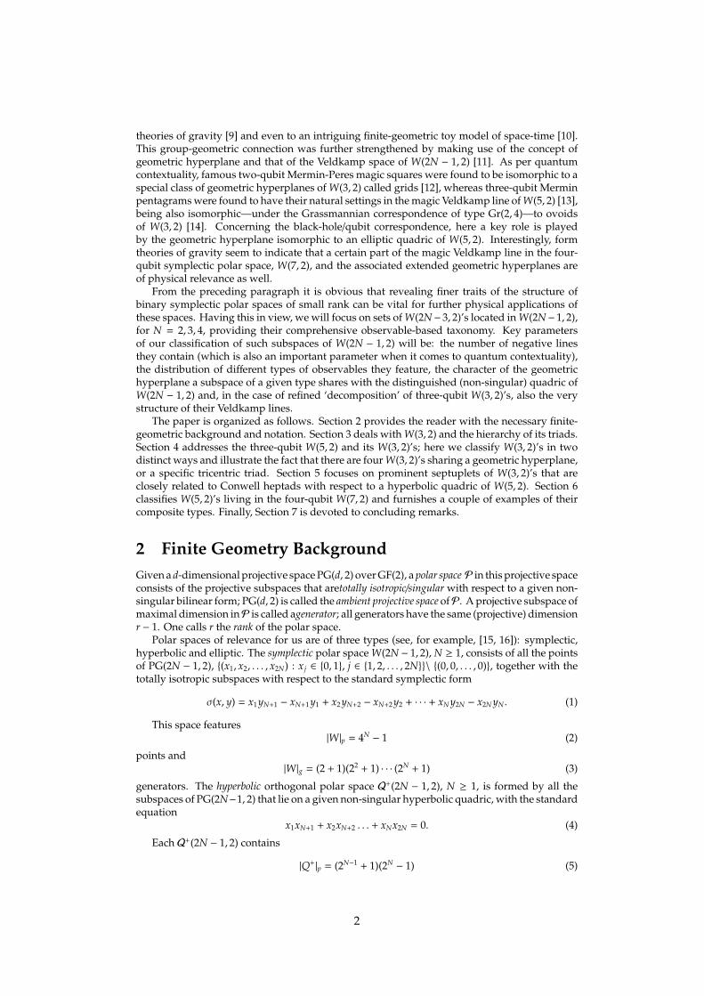
theories of gravity [9] and even to an intriguing finite-geometric toy model of space-time [10].This group-geometric connection was further strengthened by making use of the concept ofgeometric hyperplane and that of the Veldkamp space of W(2N − 1, 2) [11]. As per quantumcontextuality, famous two-qubit Mermin-Peres magic squares were found to be isomorphic to aspecial class of geometric hyperplanes of W(3, 2) called grids [12], whereas three-qubit Merminpentagrams were found to have their natural settings in the magic Veldkamp line of W(5, 2) [13],being also isomorphic—under the Grassmannian correspondence of type Gr(2, 4)—to ovoidsof W(3, 2) [14]. Concerning the black-hole/qubit correspondence, here a key role is playedby the geometric hyperplane isomorphic to an elliptic quadric of W(5, 2). Interestingly, formtheories of gravity seem to indicate that a certain part of the magic Veldkamp line in the four-qubit symplectic polar space, W(7, 2), and the associated extended geometric hyperplanes areof physical relevance as well.

From the preceding paragraph it is obvious that revealing finer traits of the structure ofbinary symplectic polar spaces of small rank can be vital for further physical applications ofthese spaces. Having this in view, we will focus on sets of W(2N−3, 2)’s located in W(2N−1, 2),for N = 2, 3, 4, providing their comprehensive observable-based taxonomy. Key parametersof our classification of such subspaces of W(2N − 1, 2) will be: the number of negative linesthey contain (which is also an important parameter when it comes to quantum contextuality),the distribution of different types of observables they feature, the character of the geometrichyperplane a subspace of a given type shares with the distinguished (non-singular) quadric ofW(2N − 1, 2) and, in the case of refined ‘decomposition’ of three-qubit W(3, 2)’s, also the verystructure of their Veldkamp lines.

The paper is organized as follows. Section 2 provides the reader with the necessary finite-geometric background and notation. Section 3 deals with W(3, 2) and the hierarchy of its triads.Section 4 addresses the three-qubit W(5, 2) and its W(3, 2)’s; here we classify W(3, 2)’s in twodistinct ways and illustrate the fact that there are four W(3, 2)’s sharing a geometric hyperplane,or a specific tricentric triad. Section 5 focuses on prominent septuplets of W(3, 2)’s that areclosely related to Conwell heptads with respect to a hyperbolic quadric of W(5, 2). Section 6classifies W(5, 2)’s living in the four-qubit W(7, 2) and furnishes a couple of examples of theircomposite types. Finally, Section 7 is devoted to concluding remarks.

2 Finite Geometry BackgroundGiven a d-dimensional projective space PG(d, 2) over GF(2), a polar space P in this projective spaceconsists of the projective subspaces that aretotally isotropic/singular with respect to a given non-singular bilinear form; PG(d, 2) is called the ambient projective space ofP. A projective subspace ofmaximal dimension inP is called agenerator; all generators have the same (projective) dimensionr − 1. One calls r the rank of the polar space.

Polar spaces of relevance for us are of three types (see, for example, [15, 16]): symplectic,hyperbolic and elliptic. The symplectic polar space W(2N − 1, 2), N ≥ 1, consists of all the pointsof PG(2N − 1, 2), {(x1, x2, . . . , x2N) : x j ∈ {0, 1}, j ∈ {1, 2, . . . , 2N}}\ {(0, 0, . . . , 0)}, together with thetotally isotropic subspaces with respect to the standard symplectic form

σ(x, y) = x1 yN+1 − xN+1 y1 + x2 yN+2 − xN+2 y2 + · · · + xN y2N − x2N yN. (1)

This space features|W|p = 4N

− 1 (2)

points and|W|g = (2 + 1)(22 + 1) · · · (2N + 1) (3)

generators. The hyperbolic orthogonal polar space Q+(2N − 1, 2), N ≥ 1, is formed by all thesubspaces of PG(2N−1, 2) that lie on a given non-singular hyperbolic quadric, with the standardequation

x1xN+1 + x2xN+2 . . . + xNx2N = 0. (4)

Each Q+(2N − 1, 2) contains

|Q+|p = (2N−1 + 1)(2N− 1) (5)

2

points and there are|W|Q+ = |Q+|p + 1 = (2N−1 + 1)(2N

− 1) + 1 (6)

copies of them in W(2N − 1, 2). Finally, the elliptic orthogonal polar space Q−(2N − 1, 2), N ≥ 2,comprises all points and subspaces of PG(2N − 1, 2) satisfying the standard equation

f (x1, xN+1) + x2xN+2 + · · · + xNx2N = 0, (7)

where f is an irreducible quadratic polynomial over GF(2). Each Q−(2N − 1, 2) contains

|Q−|p = (2N−1− 1)(2N + 1) (8)

points and there are|W|Q− = |Q−|p + 1 = (2N−1

− 1)(2N + 1) + 1 (9)

copies of them in W(2N− 1, 2). For both symplectic and hyperbolic polar spaces r = N, whereasfor the elliptic one r = N − 1. The smallest non-trivial symplectic polar space is the N = 2 one,W(3, 2), often referred to as the doily. It features 15 points (see Eq. 2) and the same number oflines (that are also its generators, see Eq. 3), with three points per line and three lines through apoint; it is a self-dual 153-configuration and the only one out of 245,342 such configurations thatis triangle-free, being, in fact, isomorphic to the generalized quadrangle of order two (GQ(2, 2)).This symplectic polar space features ten Q+(3, 2)’s (by Eq. 6)) and six Q−(3, 2)’s (by Eq. 9). AQ+(3, 2) contains nine points and six lines forming a 3 × 3 grid, so it is also called a grid. AQ−(3, 2) features five pairwise non-collinear points, hence it is an ovoid. A triple of mutually

non-collinear points of W(3, 2) is called a triad and a point collinear with all the three points ofa triad is called a center of the triad; W(3, 2) contains 60 unicentric and 20 tricentric triads.

The N-qubit observables we will be dealing with belong to the set

SN = {G1 ⊗ G2 ⊗ · · · ⊗ GN : G j ∈ {I,X,Y,Z}, j ∈ {1, 2, . . . ,N}}\{IN} (10)

where IN ≡ I(1) ⊗ I(2) ⊗ . . . ⊗ I(N),

X =(0 11 0

), Y =

(0 −ii 0

), and Z =

(1 00 −1

)(11)

are the Pauli matrices, I is the identity matrix and ‘⊗’ stands for the tensor product of matrices.SN, whose elements are simply those of the N-qubit Pauli group if the global phase is disre-garded, features two kinds of observables, namely symmetric(i.e., observables featuring an evennumber of Y’s) andskew-symmetric; the number of symmetric observables is (2N−1 + 1)(2N

− 1).We shall further employ a finer classification where an observable having N − 1, N − 2, N − 3,. . . I’s will be, respectively, of type A, B, C, . . . ; also, whenever it is clear from the context,G1 ⊗ G2 ⊗ · · · ⊗ GN will be short-handed to G1G2 · · ·GN.

For a particular value of N, the 4N− 1 elements of SN can be bijectively identified with

the same number of points of W(2N − 1, 2) in such a way that the images of two commutingelements lie on the same line of this polar space, andgenerators of W(2N − 1, 2) correspond tomaximal sets of mutually commuting elements. If we take the symplectic form defined by Eq.1, then this bijection acquires the form

G j ↔ (x j, x j+N), j ∈ {1, 2, . . . ,N}, (12)

assuming thatI↔ (0, 0), X↔ (0, 1), Y↔ (1, 1), and Z↔ (1, 0). (13)

Employing the above-introduced bijection (for more details see, e.g., [13]), it can be shownthat given an observable O, the set of symmetric observables commuting with O togetherwith the set of skew-symmetric observables not commuting with O will lie on a certain non-degenerate quadric of W(2N−1, 2), this quadric being hyperbolic (resp. elliptic) if O is symmetric(resp. skew-symmetric). We can express this important property by making, whenever appro-priate, this associated observable explicit in a subscript, Q±(O)(2N − 1, 2), noting that there existsa particular hyperbolic quadric associated with I:

Q+(I)(2N − 1, 2) := {(x1, x2, . . . , x2N) ∈W(2N − 1, 2) | x1xN+1 + x2xN+2+

. . . + xNx2N = 0}.(14)

3

Given a point-line incidence geometry Γ(P,L), a geometric hyperplane of Γ(P,L) is a subset of itspoint set such that a line of the geometry is either fully contained in the subset or has with it just asingle point in common. The Veldkamp spaceV(Γ) of Γ(P,L) is the space in which [17]: (i) a pointis a geometric hyperplane of Γ and (ii) a line is the collection, denoted H′H′′, of all geometrichyperplanes H of Γ such that H′ ∩H′′ = H′ ∩H = H′′ ∩H or H = H′,H′′, where H′ and H′′ aredistinct points of V(Γ). For a Γ(P,L) with three points on a line, all Veldkamp lines are of theform {H′,H′′,H′∆H′′} where H′∆H′′ is the complement of symmetric difference of H′ and H′′,i.e., they form a vector space over GF(2). As demonstrated in [11],V(W(2N− 1, 2)) � PG(2N, 2).Its points are both hyperbolic and elliptic quadrics of W(2N−1, 2), as well as its perp-sets. Givena point x of W(2N− 1, 2), theperp-set Q̂(x)(2N− 1, 2) of x consists of all the points collinear with it,

Q̂(x)(2N − 1, 2) := {y ∈W(2N − 1, 2) | σ(x, y) = 0}; (15)

the point x being referred to as the nucleus of Q̂(x)(2N − 1, 2).We shall briefly recall basic properties of the Veldkamp space of the doily, V(W(3, 2)) ≃

PG(4, 2), whose in-depth description can be found in [12]. The 31 points ofV(W(3, 2)) comprisefifteen perp-sets, ten grids and six ovoids—as also illustrated in Fig. 1. The 155 lines ofV(W(3, 2)) split into five distinct types as summarized in Table 1 and depicted in Fig. 2. (Table1, as well as Fig. 1 and 2, were taken from [18].)

Figure 1: The three kinds of geometric hyperplanes of W(3, 2). The 15 points of the doily arerepresented by small circles and its 15 lines are illustrated by the straight segments as well asby the segments of circles; note that not every intersection of two segments counts for a point ofthe doily. The upper panel shows grids (red bullets), the middle panel perp-sets (yellow bullets)and the bottom panel ovoids (blue bullets). Each picture—except that located in the bottomright-hand corner—stands for five different hyperplanes, the four others being obtained from itby its successive rotations through 72 degrees around the center of the pentagon.

Table 1: An overview of the properties of the five different types of lines of V(W(3, 2)) in termsof the core (i.e., the set of points common to all the three hyperplanes forming the line) and thetypes of geometric hyperplanes featured by a generic line of a given type. The last column givesthe total number of lines per each type.

Type Core Perps Ovoids Grids #

I Two Secant Lines 1 0 2 45II Single Line 3 0 0 15III Tricentric Triad 3 0 0 20IV Unicentric Triad 1 1 1 60V Single Point 1 2 0 15

4

Figure 2: An illustrative portrayal of representatives (rows) of the five (numbered consecutivelyfrom top to bottom) different types of lines ofV(W(3, 2)), each being uniquely determined by theproperties of its core (black bullets).

In what follows, we will mainly be focused on W(2N−3, 2)’s that are located in W(2N−1, 2).These are, in general, of two different kinds [11]. A W(2N − 3, 2) of the first kind, to be calledlinear, is isomorphic to the intersection of two perp-sets with non-collinear nuclei and theirnumber in W(2N − 1, 2) is

|W|Wl =13

4N−1(4N− 1). (16)

A W(2N − 3, 2) of the second kind, to be called quadratic, is isomorphic to the intersection ofa hyperbolic quadric and an elliptic quadric and W(2N − 1, 2) features

|W|Wq = 4N−1(4N− 1) (17)

of them. By way of example, in W(3, 2) a linear (resp. quadratic) W(1, 2) corresponds to atricentric (resp. unicentric) triad.

In the sequel, when referring to W(2N−1, 2) and its subspaces, we will always have in mindthe W(2N − 1, 2) and its subspaces whose points are labelled by N-qubit observables from theset SN as expressed by Eq. 12 and 13. Moreover, a linear subspace of such W(2N − 1, 2) willbe calledpositive or negative according as the (ordinary) product of the observables located init is +IN or −IN, respectively. Let us illustrate this point, taking again the N = 2 case. Up toisomorphism, there is just one type of the two-qubit doily. Its six observables of type A are IX,XI, IY, YI, IZ and ZI and its nine ones of type B areXX, XY, XZ, YX, YY, YZ, ZX, ZY and ZZ,the latter lying on a particular hyperbolic quadric, Q+(YY)(3, 2). Among the fifteen lines only thethree lines {XX,YY,ZZ}, {XY,YZ,ZX} and {XZ,YX,ZY} are negative, forming also one system ofgenerators of Q+(YY)(3, 2).

3 W(3,2) and Its Two-Qubit W(1,2)’sThis is a rather trivial case. As already mentioned in Section 2, the doily contains three negativelines, which are all of the same(B−B−B) type. Among its W(1, 2)’s, we find two types of linearones and three types of quadratic ones whose properties are summarized in Table 2.

5

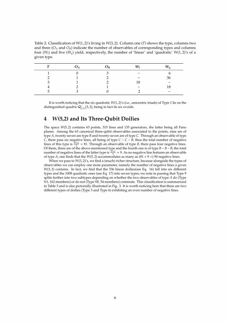
Table 2: Classification of W(1, 2)’s living in W(3, 2). Column one (T) shows the type, columns twoand three (OA and OB) indicate the number of observables of corresponding types and columnsfour (Wl) and five (Wq) yield, respectively, the number of ‘linear’ and ‘quadratic’ W(1, 2)’s of agiven type.

T OA OB Wl Wq

1 0 3 − 62 1 2 − 363 1 2 18 −

4 2 1 − 185 3 0 2 −

It is worth noticing that the six quadratic W(1, 2)’s (i.e., unicentric triads) of Type 1 lie on thedistinguished quadric Q+(YY)(3, 2), being in fact its six ovoids.

4 W(5,2) and Its Three-Qubit DoiliesThe space W(5, 2) contains 63 points, 315 lines and 135 generators, the latter being all Fanoplanes. Among the 63 canonical three-qubit observables associated to the points, nine are oftype A, twenty-seven are type B and twenty-seven are of type C. Through an observable of typeC, there pass six negative lines, all being of type C − C − B; thus the total number of negativelines of this type is 27×6

2 = 81. Through an observable of type B, there pass four negative lines.Of them, three are of the above-mentioned type and the fourth one is of type B−B−B; the totalnumber of negative lines of the latter type is 27×1

3 = 9.As no negative line features an observableof type A, one finds that the W(5, 2) accommodates as many as (81 + 9 =) 90 negative lines.

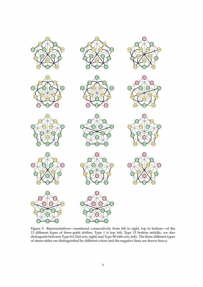
When we pass to W(3, 2)’s, we find a (much) richer structure, because alongside the types ofobservables we can employ one more parameter, namely the number of negative lines a givenW(3, 2) contains. In fact, we find that the 336 linear doilies(see Eq. 16) fall into six differenttypes and the 1008 quadratic ones (see Eq. 17) into seven types; we note in passing that Type 9splits further into two subtypes depending on whether the two observables of type A do (Type9A, 162 members) or do not (Type 9B, 54 members) commute. This classification is summarizedin Table 3 and is also pictorially illustrated in Fig. 3. It is worth noticing here that there are twodifferent types of doilies (Type 3 and Type 6) exhibiting an even number of negative lines.

6

ZYZ

YIY

XYZ XZY

ZXY

IXX

YYI

IZXXYX

ZYXZZY

IYY

XXYIXZ

IZZ

YZZ

IXX

IZY ZZI

XYI

ZIY

YXI

ZXZYYY

IYZXZX

YIX

ZYXXXY

XIZ

IIY

YYY

XYX ZZX

YZY

YXI

XIZ

YZIYYI

ZIZYXY

ZYX

ZXXXXX

XZX

ZXY

IYX

YII IIZ

XZI

YIZ

XZZ

YYYZZZ

YYXXXX

XXY

IYYZZI

ZXX

XIX

IYX

YII IIZ

XZI

YIZ

XZZ

IZXXYI

YYXZIY

XXY

YZXXYZ

ZXX

IXI

IXZ

ZZX XZZ

IXX

YIY

XYY

IIXIIZ

ZYYYXY

XZX

ZZIXZI

ZZZ

XZY

ZIZ

XIX XXI

YYI

IXX

ZZI

ZXYYZX

YIYXYZ

IZZ

YXZZYX

IYY

XIZ

YIY

YYI ZZI

IZZ

XXI

ZIZ

XZIZIX

IYYIXZ

XIX

ZXIIZX

IXX

IXI

YXY

XZY XYZ

ZIY

IXX

YYX

ZXYYIY

ZYIIIX

IZZ

YYIZYX

IYY

IYZ

ZII

ZXZ XZZ

XII

YYI

IZZ

XYZZYZ

IXZYIZ

ZZZ

YZIYXI

XXZ

IIZ

XZZ

ZIY XIX

ZZZ

YIZ

YZY

ZZIXZI

YZXYII

ZIX

IZYIZX

XIY

IYI

ZII

ZXZ XZZ

XII

YYI

IZZ

XYIZYI

IXZYII

ZZZ

YZZYXZ

XXZ

XIX

XZX

YYI ZZI

XYX

XXI

YXX

IYIIZI

ZXXIXX

ZYI

YIIZII

YZI

XII

XZI

YYI ZZI

XYI

XXI

YXI

IYIIZI

ZXIIXI

ZYI

YIIZII

YZI

Figure 3: Representatives—numbered consecutively from left to right, top to bottom—of the13 different types of three-qubit doilies; Type 1 is top left, Type 13 bottom middle; we alsodistinguish between Type 9A (3rd row, right) and Type 9B (4th row, left). The three different typesof observables are distinguished by different colors and the negative lines are drawn heavy.

7

Table 3: Classification of doilies living in W(5, 2). Column one (T) shows the type, column two(C−) the number of negative lines in a doily of the given type, columns three to five (OA to OC)indicate the number of observables of corresponding types and columns six (Dl) and seven (Dq)yield, respectively, the number of ‘linear’ and ‘quadratic’ doilies of a given type.

T C− OA OB OC Dl Dq

1 7 0 7 8 − 812 7 0 9 6 27 −

3 6 1 5 9 − 108

4 5 2 5 8 162 −

5 5 2 7 6 − 162

6 4 3 5 7 − 324

7 3 0 9 6 9 −

8 3 0 15 0 − 369 3 2 7 6 − 216

10 3 2 9 4 81 −

11 3 4 5 6 54 −

12 3 4 7 4 − 8113 3 6 9 0 3 −

The 27 observables of type B lie on an elliptic quadric of W(5, 2), which can be defined asfollows:

Q−

(YYY)(5, 2) := x21 + x1x4 + x2

4 + x22 + x2x5 + x2

5 + x23 + x3x6 + x2

6 = 0. (18)

Here, we took a coordinate basis of W(5, 2) in which the symplectic form σ(x, y) is given byEq. 1,

σ(x, y) = (x1 y4 − x4 y1) + (x2 y5 − x5 y2) + (x3 y6 − x6 y3),

so that the correspondence between the 63 three-qubit observables (see Eq. 10)

S3 = {G1 ⊗ G2 ⊗ G3 : G j ∈ {I,X,Y,Z}, j ∈ {1, 2, 3}}\I3

and the 63 points of W(5, 2) is of the form (see Eq. 12)

G j ↔ (x j, x j+3), j ∈ {1, 2, 3},

taking also into account Eq. 13.This special quadric Q−(YYY)(5, 2), as any non-degenerate quadric, is a geometric hyperplane of

W(5, 2). As a doily is also a subgeometry of W(5, 2), it either lies fully in Q−(YYY)(5, 2) (Type 8), orshares with Q−(YYY)(5, 2) a set of points that form a geometric hyperplane; an ovoid (Types 3, 4, 6and 11), a perp-set (Types 1, 5, 9 and 12) and a grid (Types 2, 7, 10 and 13). One also observesthat no quadratic doily shares a grid with Q−(YYY)(5, 2).

In addition to the distinguished elliptic quadric, there are also three distinguished hyperbolicquadrics in W(5, 2), namely: the quadric whose 35 observables feature either two X′s or no X,

Q+(ZZZ)(5, 2) := x2

4 + x25 + x2

6 + x1x4 + x2x5 + x3x6 = 0, (19)

the one whose 35 observables feature either two Y′s or no Y (see Eq. 14),

Q+(III)(5, 2) := x1x4 + x2x5 + x3x6 = 0, (20)

and the one whose 35 observables feature either two Z′s or no Z,

Q+(XXX)(5, 2) := x2

1 + x22 + x2

3 + x1x4 + x2x5 + x3x6 = 0. (21)

Accordingly, there are three distinguished doilies of Type 8, namely the ones the quadricQ−

(YYY)(5, 2) shares with these three hyperbolic quadrics.

8

Take the two-qubit doily. Add formally to each observable, at the same position, the samemark from the set {X,Y,Z}. Pick up a geometric hyperplane in this three-qubit labeled doilyand replace by I the added mark in each observable that belongs to this geometric hyperplane.One obviously gets a three-qubit doily. Now, there are 31 geometric hyperplanes in the doily,three possibilities (X,Y,Z) to pick up a mark and three possibilities(left, middle, right) where toinsert the mark; so there will be 31 × 3 × 3 = 279 doilies created this way. In particular, out ofthe 15 × 9 = 135 doilies ‘induced’ by perp-sets, 81 are of Type 10 and 54 of Type 11; out of the10 × 9 = 90 doilies ‘generated’ by grids, eighty-one are of Type 12 and nine of Type 8; finally,the 6 × 9 = 54 doilies stemming from ovoids are all of the same type 9B. So, if we look at Table3, all doilies of Types 1 to 7, 27 doilies of Type 8 and all doilies of Type 9A can be regarded as‘genuine’ three-qubit guys, nine doilies of Type 8 that originate from grids (henceforth referredto as Type 8′) and all doilies of Types 9B to 13 can be viewed as ‘built from the two-qubit guy’;with Type 13 doilies being even more two-qubit-like.

This stratification of three-qubit doilies can also be spotted in a different way. Take arepresentative doily of a particular type, for example, that of Type 3 depicted in Fig. 4, top.From its three-qubit labels, keep first only the left mark (bottom left figure), then the middlemark (bottom middle figure) and, finally, the right mark (bottom right figure). In each of thesethree ‘residual’ doilies it is easy to see that if you take the points featuring a given non-trivialmark (i.e., X, Y or Z) together with the points featuring I, these always form a geometrichyperplane and the whole set form a Veldkamp line of the doily where the points featuring Irepresent its core. Employing Table 1 we readily see that this Veldkamp line is of type V (thecore is a single point) for the left residual doily, type III (the core is a tricentric triad) for themiddle doily and of type IV (the core is a unicentric triad) for the right one. To account thisway for the 13 types of three-qubit doilies, we also need the concept of a trivial Veldkamp lineof the doily, i.e., a line consisting of a geometric hyperplane counted twice and the full doily,which exactly accounts for those doilies ‘generated’ by the two-qubit doily. This classification issummarized in Table 4. Here, columns two to six give the number of ordinary Veldkamp linesof a given type, columns seven to nine show the same for trivial Veldkamp lines and the lastcolumn corresponds to the degenerate case when all the points of a residual doily bear the labelI. Note that all doilies stemming from the two-qubit doily (i. e., Types 8′ to 13) feature ordinaryVeldkamp lines of the same type.

Using a computer, we have also found out a very interesting property that given a doilyand any geometric hyperplane in it, there are three other doilies having the same geometrichyperplane. Fig. 5 serves as a visualization of this fact when the common geometric hyperplaneis an ovoid. The four doilies sharing a geometric hyperplane, however, do not stand on thesame footing. This is quite easy to spot from our example depicted in Fig. 5. A point of the doilyis collinear with three distinct points of an ovoid, the three points forming a unicentric triad.Let us pick up such a triad, say {ZYI,XYI,YYI} and look for its centers in each of the four doilies.These are IYI (top doily), IIX (left doily), IIY (right doily) and IYZ (bottom doily). We see thatthe last three observables are mutually anticommuting, whereas the first observable commuteswith each of them. This property is found to hold for each of

( 53)= 10 triads contained in an

ovoid. Hence, the top doily of Fig. 5 has indeed a different footing than the remaining three.A similar 3 + 1 split up is also observed in any quadruple of doilies having a grid in commonbecause a point of the doily is also collinear with three points of a grid that form a unicentrictriad. However, when the shared hyperplane is a perp-set, one gets a different, namely a 2 + 2split, because in this case the corresponding triple of points forms a tricentric triad.

9

Table 4: A refined classification of doilies living in W(5, 2). We use the following abbreviationsfor the cores of Veldkamp lines: 2cl—two concurrent lines, le—line, ttr—tricentric triad, utr—unicentric triad, pt—point, ov—ovoid, ps—perp-set, gr—grid and fl stands for the full doily.

T 2cl le ttr utr pt ov ps gr fl

1 1 − − − 2 − − − −

2 − 3 − − − − − − −

3 − − 1 1 1 − − − −

4 − 1 2 − − − − − −

5 1 − − 2 − − − − −

6 1 − 1 1 − − − − −

7 − 3 − − − − − − −

8 3 − − − − − − − −

9A 1 − − 2 − − − − −

8′ − − 2 − − − − 1 −

9B − − 2 − − 1 − − −

10 − − 2 − − − 1 − −

11 − − 2 − − − 1 − −

12 − − 2 − − − − 1 −

13 − − 2 − − − − − 1

IX

X

I

Y

Y

XX

X

X

Y

I

Z Z

Y

XY

Y

Y

Y

X

XX

Z

Z

Z

Z

I I

I

YX

Z

Y

Y

Y

ZX

X

Z

Y

Y

Z X

I

XXX

XZX

YXY

ZYX

ZXX

YYI

YYY

ZIZ

XYX YXI ZZX

XIZ

YZY

YZI

IIY

Figure 4: A formal decomposition of a three-qubit doily (top) into three ‘single-qubit residuals’(bottom). In each doily of the bottom row, the three geometric hyperplanes forming a Veldkampline are distinguished by different color, with their common points being drawn black; also, thenuclei of perp-sets are represented by double circles.

A tricentric triad of a linear resp. quadratic doily of W(5, 2) defines a line resp. plane in theambient PG(5, 2). The latter type of a triad is found to be shared by four quadratic doilies. Giventhe three observables of such a triad, there are seven observables commuting with each of them,the corresponding seven points lying in a Fano plane (namely in the polar plane to the planedefined by the triad) in the ambient PG(5, 2). One of the seven observables has a distinguishedfooting as it commutes with each of the remaining six ones, with these six observables forming

10

three commuting pairs. Out of the six observables, one can form just four tricentric triads ofwhich each is complementary to the triad we started with and thus defines with the latter aunique quadratic doily. These properties are also illustrated in Fig. 6.

IYI

ZII

ZXZ XZZ

XII

YYI

IZZ

XYIZYI

IXZYII

ZZZ

YZZYXZ

XXZ

IIX

ZYX

ZZY XXY

XYX

YYI

IZZ

XYIZYI

IXZYYX

ZXY

YXYYZY

XZY

IIY

ZYY

ZZX XXX

XYY

YYI

IZZ

XYIZYI

IXZYYY

ZXX

YXXYZX

XZX

IYZ

ZIZ

ZXI XZI

XIZ

YYI

IZZ

XYIZYI

IXZYIZ

ZZI

YZIYXI

XXI

Figure 5: An illustration of the case when four different doilies share an ovoid (boldfaced). Thetop doily is of Type 11, the bottom one of Type 8, and both the left and right doilies are of Type 3.

Among the 13 different types of three-qubit doilies, there is one type, namely Type 3, whichhas two remarkable properties. The first property is that there is one point (to be called a deeppoint) such that all three lines passing through it are negative. Let us take a representative doilyof such a type shown in Fig. 3, 1st row right. The deep point is ZIZ. Then one sees that there arejust two points (to be called zero-points) such that neither of them lies on a negative line; one isIIY and the other is XIZ. These two points and the deep point form in the doily a tricentric triad,hence a copy of ‘linear’ W(1, 2). The second property is related to the fact that through eachobservable of type B there pass four negative lines. Three of them are such that each featuresone observable of type B and two observables of type C, whereas the remaining one consists ofall observables of type B. Written vertically, the four negative lines passing through our deeppoint ZIZ are:

ZIZ ZIZ ZIZ ZIZXXX XYX XZX XIXYXY YYY YZY YIY

We see that the three lines that are located in the doily are of the same type, viz. B − C − C.If we also include the fourth negative line, viz. the B − B − B one, we obtain what we cancall a ‘doily with a tail.’ Taking into account the above-mentioned four-doilies-per-hyperplaneproperty, we see that there are altogether 12 doilies, four per each observable, having the sametail and all being of Type 3.

11

IZX

XXY

ZIZ YIY

YII

XIX

IIY

YZXXYZ

YXXXZI

XXI

XZYZYX

IXX

IZX

XXY

XYX IYI

YII

XIX

YYI

YZXXYZ

IZZXZI

ZZY

ZXIXIZ

YZZ

YXZ

ZZI

XYX YIY

IYY

ZYZ

YYI

YZXXYZ

YXXXZI

XXI

ZXIZYX

YZZ

YXZ

ZZI

ZIZ IYI

IYY

ZYZ

IIY

YZXXYZ

IZZXZI

ZZY

XZYXIZ

IXXXYZYZX

XZI

XIZ

ZXI IZX

YXZ

ZYX

XZY

YYY

Figure 6: Four three-qubit doilies on a ‘planar’ tricentric triad (represented by hexagons). Theseven observables commuting with the three hexagonal ones are, for better illustration, coloreddifferently. The three red lines of the Fano plane that meet at the distinguished observable (gray)are totally isotropic, whilst the remaining four (depicted green) are not. The four complementarytriads (of observables) are illustrated by a full black circle and three half-circles.

5 ‘Conwell’ Heptads of Doilies in W(5,2)Recall Sylvester’s famous construction of W(3, 2), see [19]. Given a six-element set M6 ≡

{1, 2, 3, 4, 5, 6}, a duad is an unordered pair (i j) ∈ M6, i , j and a syntheme is a set of threepairwise disjoint duads, i.e., a set {(i j), (kl), (mn)} where i, j, k, l,m,n ∈ M6 are all distinct. Thepoint-line incidence structure whose points are duads and whose lines are synthemes, withincidence being inclusion, is isomorphic to W(3, 2), as also illustrated in Fig. 7.

23

26

16

15

35

14

36

45

12 34 56

24

13

46

25

Figure 7: A duad-syntheme model of W(3, 2).

Next, take a seven-element set, M7 ≡ {1, 2, 3, 4, 5, 6, 7}. One can form from it( 7

3)= 35

unordered triples (i jk), i , j , k , i. From each set of fifteen triples having the same element incommon, we can create a doily using the duad-syntheme construction on that six-element subsetof M7 where the common element is omitted. So, we achieve seven different doilies, one per eachelement, as depicted in Fig. 8. Any two of them have an ovoid in common; because each ovoidis characterized by two elements, say a and b, and it is of the form {(abc), (abd), (abe), (ab f ), (abg)},where a, b, c, d, e, f , g ∈ M7 are all different, hence it belongs to both the a-doily and the b-doily.Also, any triple is shared by three doilies.

12

1

2

34

5

6

7

147

136

157

146

135123

127

126

125

124

156145

134

137167

125

247126

257

246

234

123237

236

235

267

256 245

124

127

236

135

237

136

357

345

234

134

347

346

137

367

356235

123

347

246

134

247

146

456345

245

145

457

124147

467346

234

145

357

245

135257

567

456

356

256156

235

125

157

457 345

256

146

356

246

136

167

567

467

367

267

346

236126

156

456

367

257

467 357

247

127

167

157147

137457

347

237267

567

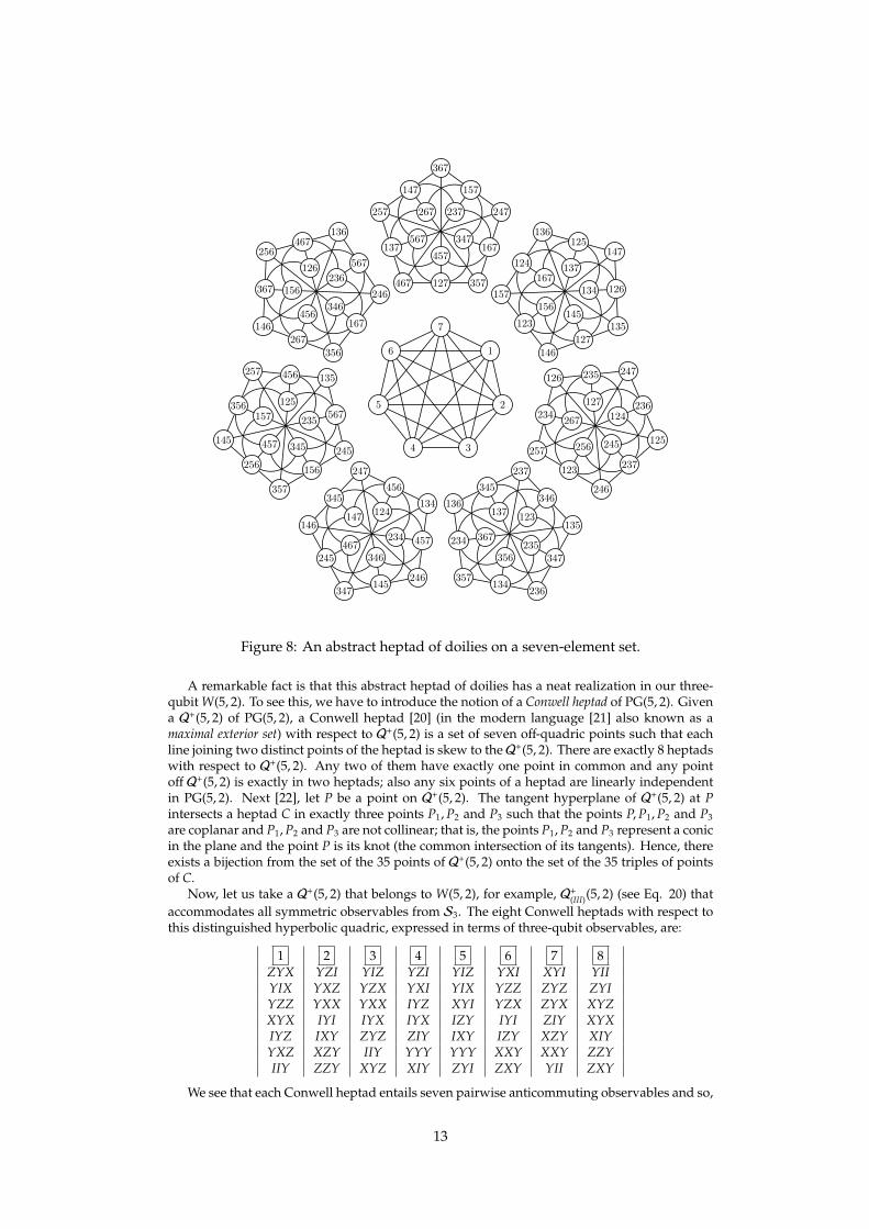
Figure 8: An abstract heptad of doilies on a seven-element set.

A remarkable fact is that this abstract heptad of doilies has a neat realization in our three-qubit W(5, 2). To see this, we have to introduce the notion of a Conwell heptad of PG(5, 2). Givena Q+(5, 2) of PG(5, 2), a Conwell heptad [20] (in the modern language [21] also known as amaximal exterior set) with respect to Q+(5, 2) is a set of seven off-quadric points such that eachline joining two distinct points of the heptad is skew to the Q+(5, 2). There are exactly 8 heptadswith respect to Q+(5, 2). Any two of them have exactly one point in common and any pointoff Q+(5, 2) is exactly in two heptads; also any six points of a heptad are linearly independentin PG(5, 2). Next [22], let P be a point on Q+(5, 2). The tangent hyperplane of Q+(5, 2) at Pintersects a heptad C in exactly three points P1,P2 and P3 such that the points P,P1,P2 and P3

are coplanar and P1,P2 and P3 are not collinear; that is, the points P1,P2 and P3 represent a conicin the plane and the point P is its knot (the common intersection of its tangents). Hence, thereexists a bijection from the set of the 35 points of Q+(5, 2) onto the set of the 35 triples of pointsof C.

Now, let us take a Q+(5, 2) that belongs to W(5, 2), for example, Q+(III)(5, 2) (see Eq. 20) thataccommodates all symmetric observables from S3. The eight Conwell heptads with respect tothis distinguished hyperbolic quadric, expressed in terms of three-qubit observables, are:

1 2 3 4 5 6 7 8ZYX YZI YIZ YZI YIZ YXI XYI YIIYIX YXZ YZX YXI YIX YZZ ZYZ ZYIYZZ YXX YXX IYZ XYI YZX ZYX XYZXYX IYI IYX IYX IZY IYI ZIY XYXIYZ IXY ZYZ ZIY IXY IZY XZY XIYYXZ XZY IIY YYY YYY XXY XXY ZZYIIY ZZY XYZ XIY ZYI ZXY YII ZXY

We see that each Conwell heptad entails seven pairwise anticommuting observables and so,

13

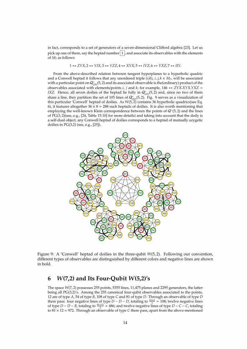
in fact, corresponds to a set of generators of a seven-dimensional Clifford algebra [23]. Let uspick up one of them, say the heptad number 1 , and associate its observables with the elementsof M7 as follows:

1↔ ZYX, 2↔ YIX, 3↔ YZZ, 4↔ XYX, 5↔ IYZ, 6↔ YXZ, 7↔ IIY.

From the above-described relation between tangent hyperplanes to a hyperbolic quadricand a Conwell heptad it follows that any unordered triple (i jk), i, j, k ∈ M7, will be associatedwith a particular point onQ+(III)(5, 2) and its associated observable is the(ordinary) product of theobservables associated with elements/points i, j and k; for example, 146 ↔ ZYX.XYX.YXZ =IXZ. Hence, all seven doilies of the heptad lie fully in Q+(III)(5, 2) and, since no two of themshare a line, they partition the set of 105 lines of Q+(III)(5, 2). Fig. 9 serves as a visualization ofthis particular ‘Conwell’ heptad of doilies. As W(5, 2) contains 36 hyperbolic quadrics(see Eq.6), it features altogether 36 × 8 = 288 such heptads of doilies. It is also worth mentioning thatemploying the well-known Klein correspondence between the points of Q+(5, 2) and the linesof PG(3, 2)(see, e.g., [24, Table 15.10] for more details) and taking into account that the doily isa self-dual object, any Conwell heptad of doilies corresponds to a heptad of mutually azygeticdoilies in PG(3,2) (see, e.g., [25]).

ZYX

YIX

YZZXYX

IYZ

YXZ

IIY

YIY

ZIX

ZII

IXZ

XZXZXZ

XYY

ZZZ

XIZ

IIX

XXXYYZ

IZZ

XXIXZI

XIZ

ZYYZZZ

YYI

XZZ

XXZ

ZXZIZI

YYX

IXX

IXI

IZX ZIZ

IIX

XYY

YYX

XZX

IZI

ZIX

YXY

ZZX

XXZ

IZZ

ZXI

XIX

XXI

IYY

IIZIXX

ZXZ

ZXI

XZZ

IZZ

ZYY

IXZ

ZXXZZX

ZIZ

YYZ

XII

IIXYIY

ZZIXIX

XXZ

YYZ

YXY

ZIZ

XZXYYI

YZY

ZXX

IIZ

IZXXXX

IXX

XIZ

ZII

XII ZZX

IZX

IXZ

IIZ

XZZ

ZIX

XZI

YZY

ZZI

IYY

IXI

XIX

YYXZZZ

XXX

ZXX

IYY

YYI

ZZI YXY

ZYY

XYY

XZI

ZIIYIY

XXIXII

ZXI

IZIIXI

YZY

Figure 9: A ‘Conwell’ heptad of doilies in the three-qubit W(5, 2). Following our convention,different types of observables are distinguished by different colors and negative lines are shownin bold.

6 W(7,2) and Its Four-Qubit W(5,2)’sThe space W(7, 2) possesses 255 points, 5355 lines, 11,475 planes and 2295 generators, the latterbeing all PG(3,2)’s. Among the 255 canonical four-qubit observables associated to the points,12 are of type A, 54 of type B, 108 of type C and 81 of type D. Through an observable of type Dthere pass: four negative lines of type D − D − D, totaling to 81×4

3 = 108; twelve negative linesof type D −D − B, totaling to 81×12

2 = 486; and twelve negative lines of type D − C − C, totalingto 81 × 12 = 972. Through an observable of type C there pass, apart from the above-mentioned

14

lines of type D − C − C, six negative lines of type C − C − B, totaling to 108×62 = 324. Through an

observable of type B there passes, apart from the already discussed two types of lines, a singlenegative line of type B−B−B, the total number of such lines being 54×1

3 = 18. Since no negativeline can contain an observable of type A, the four-qubit W(7, 2) thus exhibits five distinct typesof negative lines whose total number is (108 + 486 + 972 + 324 + 18 =) 1908.

When it comes to W(5, 2)’s, we find 11 types among their 5440 linear members and as manyas 18 types among their 16,320 quadratic cousins, as summarized in Table 5. It represents nodifficulty to check that 54 observables of type B and 81 of type D lie on a particular hyperbolicquadric in W(7, 2), to be referred to as the distinguished hyperbolic quadric Q+(YYYY)(7, 2), whichis also a geometric hyperplane in the latter space. A W(5, 2) either lies fully in this quadric(Types 2 and 21) or shares with it a set of points that forms a geometric hyperplane. Hence, thesum of OB and OD in each row of Table 5 must be one of the following numbers: 27 (when thehyperplane of W(5, 2) is an elliptic quadric), 31 (a perp-set) and/or 35 (a hyperbolic quadric); forthe reader’s convenience, the type of such geometric hyperplane is explicitly listed in column 9of Table 5. One sees that no linear W(5, 2) shares with Q+(YYYY)(7, 2) a perp-set and no quadraticW(5, 2) cuts this distinguished quadric in an elliptic quadric. Comparing Table 5 with Table 3,one readily discerns that whereas W(3, 2)’s in W(5, 2) are endowed with both an even and oddnumber of negative lines, for W(5, 2)’s in W(7, 2) this number is always even; in addition, thedifference in C− for any two distinct types of four-qubit W(5, 2)’s is a multiple of four.

Let us have a closer look at W(5, 2)’s featuring 90 (i.e., the smallest possible number of)negative lines. We can easily show that almost all of them originate from the three-qubitW(5, 2). First, by adding I to each three-qubit observable at the same position we achieve thefour trivial four-qubit W(5, 2)’s of Type 29. Next, adding to each observable at the same positiona mark from the set {X,Y,Z}, picking up a geometric hyperplane in this four-qubit labeled W(5, 2)and replacing by I the added mark of each observable in the geometric hyperplane one getsa four-qubit W(5, 2) with 90 negative lines. Now, there are 28 (# of elliptic quadrics) + 36 (#of hyperbolic quadrics) + 63 (# of perp-sets) = 127 geometric hyperplanes in the W(5, 2), threepossibilities (X,Y,Z) to pick up a mark and four possibilities (left, middle-left, middle-right,right) where to insert the mark. So, there will be 127 × 3 × 4 = 1524 four-qubit W(5, 2)’s createdthis way, which only falls short by 36 the total number of W(5, 2)’s endowed with 90 negativelines (the four guys of Type 29 being, of course, disregarded). A concise summary is given inthe last column of Table 5, where the type of geometric hyperplane is further specified by thecharacter/type of the associated (three-qubit) observable. One observes that Type 23 is the onlyirreducible type of W(5, 2)’s having 90 negative lines.

We shall illustrate this process by a couple of examples. Let us start with the perp-set of thethree-qubit W(5, 2) whose nucleus is an observable of type A, say XII. Out of 31 observablescommuting with this observable there are seven of type A(XII, IXI, IIX, IYI, IIY, IZI and IIZ),fifteen of type B (IXX, IXY, IXZ, XXI, XIX, IYX, IYY, IYZ, XYI, XIY, IZX, IZY, IZZ, XZI, andXIZ) and nine of type C (XXX, XXY, XXZ, XYX, XYY, XYZ, XZX, XZY, and XZZ). Hence,out of 32 observables off the perp, there will be 9 − 7 = 2 of type A, 27 − 15 = 12 of type B and27 − 9 = 18 of type C:

Q̂(XII) OA OB OC

on 7 15 9off 2 12 18

Next, each observable of the perp-set acquires a trivial mark I and hence goes into thefour-qubit observable of the same type. However, an observable lying off the perp-set gets anon-trivial label X, Y or Z and so yields the four-qubit observable of the subsequent type; thatis, O(3)

A → O(4)B , O(3)

B → O(4)C and O(3)

C → O(4)D . Hence, in our case, we get:

(Q̂(XII)) OA OB OC OD

(on – type intact) 7 15 9 0(off – type shifted) 0 2 12 18

Total 7 17 21 18

15

Table 5: Classification of W(5, 2)’s living in W(7, 2). Column one (T) shows the type, column two(C−) the number of negative lines in a W(5, 2) of the given type, columns three to six (OA to OD)indicate the number of observables featuring three I’s, two I’s, one I or no I, respectively, columnsseven (Wl) and eight (Wq) yield, respectively, the number of ‘linear’ and ‘quadratic’ W(5, 2)’s ofa given type, the last but one column depicts the type of intersection of a representative W(5, 2)with the distinguished hyperbolic quadric and the last column indicates the type of geometrichyperplane featuring the trivial mark(I) for composite W(5, 2)’s.

T C− OA OB OC OD Wl Wq Int GH

1 130 3 9 33 18 108 − ell − − −

2 126 0 24 0 39 − 108 full − − −

3 126 1 13 27 22 − 1944 hyp − − −

4 126 2 10 30 21 − 1620 perp − − −

5 122 1 15 27 20 972 − hyp − − −

6 122 2 10 30 21 − 648 perp − − −

7 118 0 16 32 15 − 324 perp − − −

8 118 3 9 33 18 648 − ell − − −

9 118 3 11 25 24 − 1296 hyp − − −

10 114 1 15 27 20 324 − hyp − − −

11 114 1 17 27 18 − 216 hyp − − −

12 114 3 13 25 22 1944 − hyp − − −

13 114 4 12 28 19 − 1944 perp − − −

14 110 3 15 25 20 − 1944 hyp − − −

15 110 5 11 23 24 648 − hyp − − −

16 106 5 13 23 22 − 1944 hyp − − −

17 102 1 21 27 14 − 648 hyp − − −

18 102 2 18 30 13 − 324 perp − − −

19 102 3 15 25 20 − 648 hyp − − −

20 102 4 12 28 19 − 1944 perp − − −

21 90 0 36 0 27 − 12 full ell: O = YYY22 90 2 22 30 9 − 108 perp hyp: all 9 O’s featuring two Y’s23 90 3 9 33 18 36 − ell − − −

24 90 3 21 25 14 324 − hyp perp: all 27 O’s of type C25 90 4 16 28 15 − 324 perp ell: all 27 O’s featuring one Y26 90 5 15 31 12 324 − ell perp: all 27 O’s of type B27 90 6 18 26 13 − 324 perp hyp: 26 O’s having no Y + III28 90 7 17 21 18 108 − hyp perp: all 9 O’s of type A29 90 9 27 27 0 4 − ell full W(5, 2)

Comparing with Table 5 we see that this is a four-qubit W(5, 2) of Type 28.As the second example we shall take the case when the geometric hyperplane of W(5, 2) is

an elliptic quadric generated by an antisymmetric observable of type B, say YXI. This quadric,Q−

(YXI)(5, 2), consists of all symmetric observables that commute with YXI and all antisymmetricobservables that anticommute with YXI. In particular, it contain 4 observables of type A (IXI,IIX, IIZ and IYI), 11 observables of type B (XZI, ZZI, YIY, IXX, IXZ, YZI, IYX, IYZ, XIY, ZIYand IZY) and 12 observables of type C(XZX, ZZX, XZZ, ZZZ, YXY, XYY, ZYY, YZX, YZZ,XXY, ZXYand YYY). So, out of 36 observables off the quadric, there will be 5, 16 and 15 of typeA, B and C, respectively. In a succinct form,

16

Q−

(YXI)(5, 2) OA OB OC

on 4 11 12off 5 16 15

From this it follows that the corresponding four-qubit W(5, 2) is of Type 25:

(Q−(YXI)(5, 2)) OA OB OC OD

(on – type intact) 4 11 12 0(off – type shifted) 0 5 16 15

Total 4 16 28 15

7 ConclusionsWe have introduced a remarkable observable-based taxonomy of subspaces of W(2N − 1, 2),2 ≤ N ≤ 4, whose rank is just one less than that of the ambient space. Alongside the distributionof various types of observables, an important parameter of the classification was the numberof negative lines contained in a subspace. As already mentioned in the introduction, this latterparameter is essential in checking whether a given finite geometric configuration is contextualor not. For example, our preliminary analysis shows that all three-qubit and four-qubit doiliesare, as their two-qubit sibling, contextual. In a separate paper we plan to address this questionin more detail, also employing the degree of contextuality for a variety of other symplecticsubspaces. However, when approaching subspaces of higher rank this way, it would be naturalto include as parameters the number of negative linear subspaces of every viable dimensionfrom 1 to N−2, i.e., consider negative lines, negative planes, . . . , negative generators; so, alreadyin the case of N = 4 we can add one more parameter, the number of negative planes a four-qubitW(5, 2) is endowed with, to achieve an interesting refinement of our Table 5. As the three-qubitW(5, 2) features 54 negative planes [26], each composite four-qubit W(5, 2) must have the samenumber of negative planes; in connection with this fact, it would be interesting to check whethereach irreducible four-qubit W(5, 2) having 90 lines (Type 23) also enjoys this property.

Another interesting extension/variation of our taxonomy would be to take into account thenumber of negative lines passing through a point of the subspace. Let us call this number theorder of a point and for each subspace W(2s − 1, 2) define the following string of parameters[p0, p1, p2, . . . , p4s−1−1], where pk, 0 ≤ k ≤ 4s−1

− 1 stands for the number of points of order kthe subspace contains. Applying this to three-qubit doilies (s = 2), we find the following fivepatterns (as readily discerned from Fig. 3): [0, 9, 6, 0] (Types 1 and 2), [2, 9, 3, 1] (Type 3), [5, 5, 5, 0](Types 4 and 5), [6, 6, 3, 0] (Type 6) and [6, 9, 0, 0] (Types 7 to 13).

A slightly different possibility of employing our strategy is to analyse other distinguishedsubgeometries of W(2N − 1, 2) such as, for example, the split Cayley hexagon of order two[27]. This generalized polygon can be embedded into W(5, 2), and in two different ways [28],classical and skew. We have already discerned two distinct kinds of the former and as manyas thirteen different types of the latter. Yet a full understanding of the case requires a morerigorous computer-assisted approach and will, therefore, be treated in a separate paper.

AcknowledgmentsThis work was supported by the Slovak VEGA Grant Agency, Project #2/0004/20, the French“Investissements d’Avenir” programme, project ISITE-BFC (contract ANR-15-IDEX-03) and bythe EIPHI Graduate School (contract ANR-17-EURE-0002).

The computations have been performed on the supercomputer facilities of the Mésocentrede calcul de Franche-Comté; the code is freely available at https://quantcert.github.io/Magma-contextuality/.

We are indebted to Zsolt Szabó and Petr Pracna for their help with the figures and thankPéter Vrana for providing us with a list of doilies of W(5, 2). We also appreciate constructiveremarks/suggestions from four anonymous referees.

17

References[1] Saniga M.; de Boutray H.; Holweck F.; Giorgetti A. Taxonomy of Polar Subspaces of Multi-

Qubit Symplectic Polar Spaces of Small Rank. Mathematics 2021, 9(18), 2272. [CrossRef]

[2] Saniga, M.; Planat, M. Multiple Qubits as Symplectic Polar Spaces of Order Two. Adv.Stud. Theor. Phys. 2007, 1, 1–4.

[3] Planat, M.; Saniga, M. On the Pauli Graph of N-Qudits. Quantum Inf. Comput. 2008, 8,127–146.

[4] Havlicek, H.; Odehnal, B.; Saniga, M. Factor-Group-Generated Polar Spaces and (Multi-)Qudits. SIGMA 2009, 5, 096. [CrossRef]

[5] Thas, K. The Geometry of Generalized Pauli Operators of N-qudit Hilbert Space, and anApplication to MUBs. Europhys. Lett. 2009, 86, 60005. [CrossRef]

[6] Holweck, F. Geometric constructions overC andF2 for quantum information. In QuantumPhysics and Geometry; Ballico, E., Bernardi, A., Carusotto, I., Mazzucchi, S., Moretti,V., Eds.; Lecture Notes of the Unione Matematica Italiana; Springer Nature: Cham,Switzerland, 2019; Volume 25, pp. 87–124.

[7] Lévay, P.; Saniga, M.; Vrana, P.; Pracna, P. Black Hole Entropy and Finite Geometry. Phys.Rev. D 2009, 79, 084036. [CrossRef]

[8] Borsten, L.; Duff, M.; Lévay, P. The Black-Hole/Qubit Correspondence: An Up-to-DateReview. Class. Quantum Grav. 2012, 29, 224008. [CrossRef]

[9] Lévay, P.; Holweck, F.; Saniga, M. The Magic Three-Qubit Veldkamp Line: A FiniteGeometric Underpinning for Form Theories of Gravity and Black Hole Entropy. Phys.Rev. D 2017, 96, 026018. [CrossRef]

[10] Lévay, P.; Holweck, F. Finite Geometric Toy Model of Spacetime as An Error CorrectingCode. Phys. Rev. D 2019, 99, 086015. [CrossRef]

[11] Vrana, P.; Lévay, P. The Veldkamp Space of Multiple Qubits. J. Phys. A Math. Theor. 2010,43, 125303. [CrossRef]

[12] Saniga, M.; Planat, M.; Pracna, P.; Havlicek, H. The Veldkamp Space of Two-Qubits.SIGMA 2007, 3, 075. [CrossRef]

[13] Lévay, P.; Szabó, Z. Mermin Pentagrams Arising from Veldkamp Lines for Three Qubits.J. Phys. A Math. Theor. 2017, 50, 095201. [CrossRef]

[14] Saniga, M.; Lévay, P. Mermin’s Pentagram as an Ovoid of PG(3,2). Europhys. Lett. 2012,97, 50006. [CrossRef]

[15] Hirschfeld, J.W.P.; Thas, J.A. General Galois Geometries; Oxford University Press: Oxford,UK, 1991.

[16] Cameron, P.J. Projective and Polar Spaces. In QMW Maths Notes 13; Queen Mary andWestfield College, School of Mathematical Sciences: London, UK, 1991.

[17] Buekenhout, F.; Cohen, A.M. Diagram Geometry: Related to Classical Groups and Buildings;Springer: Berlin/Heidelberg, Germany, 2013.

[18] Saniga, M.; Lévay, P.; Planat, M.; Pracna, P. Geometric Hyperplanes of the Near HexagonL3 × GQ(2, 2). Lett. Math. Phys. 2010, 91, 93–104. [CrossRef]

[19] Sylvester, J.J. Elementary researches in the analysis of combinatorial aggregation. Phil.Mag. 1844, 24, 285–296. [CrossRef]

[20] Conwell, G.M. The 3-space PG(3, 2) and its group. Ann. Math. 1910, 11, 60–76. [CrossRef]

[21] Thas, J.A. Maximal exterior sets of hyperbolic quadrics: The complete classification. J.Combin. Theory Ser. A 1991, 56, 303–308. [CrossRef]

[22] De Clerck, F.; Thas, J.A. Exterior sets with respect to the hyperbolic quadric in PG(2n−1, q).In Finite Geometries; Lecture Notes in Pure and Applied Mathematics; Dekker: New York,NY, USA, 1985; Volume 103, pp. 83–91.

[23] Lévay, P.; Planat, M.; Saniga, M. Grassmannian connection between three-and four-qubitobservables, Mermin’s contextuality and black holes. J. High Energy Phys. 2013, 9, 037.[CrossRef]

18

[24] Hirschfeld, J.W.P. Finite Projective Spaces of Three Dimensions; Oxford University Press:Oxford, UK, 1985.

[25] Edge, W.L. The Geometry of the Linear Fractional Group LF(4,2). Proc. Lond. Math. Soc.1954, 4, 317–342. [CrossRef]

[26] Saniga, M.; Holweck, F.; Jaffali, H. Taxonomy of Three-Qubit Mermin Pentagram. Sym-metry 2020, 12, 534. [CrossRef]

[27] Polster, B.; Schroth, A.E.; van Maldeghem, H. Generalized Flatland. Math. Intell. 2001, 23,33–47. [CrossRef]

[28] Coolsaet, K. The Smallest Split Cayley Hexagon Has Two Symplectic Embeddings. FiniteFields Their Appl. 2010, 16, 380–384. [CrossRef]

19