Central WENO schemes for hyperbolic systems of ... - Numdam

ESAIM: MODÉLISATION MATHÉMATIQUE ET ANALYSE NUMÉRIQUE

DORON LEVY

GABRIELLA PUPPO

GIOVANNI RUSSOCentral WENO schemes for hyperbolic systems of conservation lawsESAIM: Modélisation mathématique et analyse numérique, tome 33, no 3 (1999),p. 547-571<http://www.numdam.org/item?id=M2AN_1999__33_3_547_0>

© SMAI, EDP Sciences, 1999, tous droits réservés.

L’accès aux archives de la revue « ESAIM: Modélisation mathématique et analysenumérique » (http://www.esaim-m2an.org/) implique l’accord avec les conditionsgénérales d’utilisation (http://www.numdam.org/conditions). Toute utilisation com-merciale ou impression systématique est constitutive d’une infraction pénale. Toutecopie ou impression de ce fichier doit contenir la présente mention de copyright.

Article numérisé dans le cadre du programmeNumérisation de documents anciens mathématiques

http://www.numdam.org/

http://www.numdam.org/item?id=M2AN_1999__33_3_547_0

http://www.esaim-m2an.org/

http://www.numdam.org/conditions



Mathematical Modelling and Numerical Analysis M2AN, Vol 33, N° 3, 1999, p 547-571Modélisation Mathématique et Analyse Numérique

CENTRAL WENO SCHEMES FOR HYPERBOLIC SYSTEMSOF CONSERVATION LAWS

DORON LEVY1, GABRIELLA PUPPO 2 AND GIOVANNI RUSSO3

Abstract. We present a family of high-order, essentially non-oscillatory, central schemes for approx-imating solutions of hyperbolic Systems of conservation laws These schemes are based on a newcentered version of the Weighed Essentially Non-Oscillatory (WENO) reconstruction of point-valuesfrom cell-averages, which is then followed by an accurate approximation of the fiuxes viaa. natural con-tmuous extension of Runge-Kutta solvers We explicitly construct the third and fourth-order schemeand demonstrate their high-resolution properties m several numerical tests

Resumé. Nous présentons une famille de schémas centrés ENO d'ordre élevé pour des solutionsapprochées de systèmes hyperboliques de lois de conservation Ces schémas reposent sur une nouvelleversion centrée de la reconstruction ENO à poids (WENO) des valeurs ponctuelles à partir des moyennessur les cellules, ce qui conduit à une approximation précise des flux grâce à une extension naturellecontinue des solveurs Runge-Kutta Nous construisons explicitement les schémas d'ordre trois et quatreet nous provons leurs propriétés de haute précision à travers des essais numériques

AMS Subject Classification. 65M10, 65M05.

Received April 7, 1998 Revised July 1, 1998

1. INTRODUCTION

In recent years, a tremendous amount of research was done m developing and implementing modem high-resolution methods for approximating solutions of hyperbolic Systems of conservation laws. A review of suchnumerical methods can be found, e.gn in [7,16,30].

Among the variety of methods for approximating solutions of such problems we focus on finite-différencemethods, which can be divided into two mam catégories, namely upwmd schemes and central schemes.

The prototype of upwmd schemes is the first-order Godunov scheme in which a piecewise-constant interpolant(which is constructed based on previously computed cell-averages) is evolved exactly to the next time stepaccording to the conservation law. This évolution involves a solution of Riemann problems on the boundaries ofeach cell, which is mterpreted as an upwinding procedure, as one has to difTer between left-going and right-goingwaves m order to compute the flux in these non-smooth régions.

Keywords and phrases Hyperbolic conservation laws, central différence schemes, high-order accuracy, non-oscillatory schemes,WENO reconstruction, Runge-Kutta1 Département de Mathématiques et d'Informatique, École Normale Supérieure, 45 rue d'Ulm, 75230 Paris Cedex 05, Francee-mail dlevyQmath. berkeley. edu2 Dipartimento di Matematica, Pohtecnico di Tormo, Corso Duca degh Abruzzi 24, 10129 Tormo, Italy e-mail puppoQpolito. î t3 Dipartimento di Matematica, Università dell'Aquila, Via Vetoio, loc Coppito, 67100 L'Aquila, Italy e-mail russoQunxvaq.it

© EDP Sciences, SMAI 1999

548 D. LEVY ET AL.

For linear Systems, a gênerai procedure can be used, which is based on the characteristic décomposition ofthe field [16]. If the System is nonlinear, however, a genera! scheme for the (exact or approximate) solution ofthe Riemann problem is not known, and the upwind approach may be rather complicated and costly.

An alternative approach for quasilinear Systems is given by the so-called relaxation schemes [13]. Givena quasilinear hyperbolic system of conservation laws, a semilinear System with stiff relaxation is constructed.Under suitable conditions the solution of the latter converges to the solution of the quasilinear system, asthe relaxation parameter tends to zero. The numerical solution of the quasilinear system is obtained by asplitting procedure. During the convection step, a linear hyperbolic system is solved by upwind scheme. Therelaxation step is treated by an implicit scheme (which can be explicitly solved). The two steps are suitablycombined in order to obtain second order accuracy in time. They can be efïiciently implemented in one andseveral dimensions. However, they have the drawback that the intermediate semilinear system is larger thanthe original quasilinear system, and it is difficult to design a splitting strategy that allows higher (larger thansecond) order it time.

A gênerai procedure used to obtain high accuracy in space with upwind schemes is based on high orderreconstruction of the field variables. This is obtained by approximating the field at a given time by a piecewisepolynomial rather than by a piecewise constant. Generally, a piecewise reconstruction of degree r shouldguarantee spatial accuracy of order r+1 for a smooth solution. Since the drawback of a high-order reconstructionis the oscillations it might create, several methods were suggested to combine the upwinding framework with amechanism to prevent the création and évolution of such spurious numerical oscillations. In particular, a classof Essentially Non-Oscillatory (ENO) schemes was presented in [8] and studied in numerous works (see [26,27],and the références therein). ENO schemes are based on a reconstruction procedure (of either point-values orcell-averages) which involves a sélection of a stencil in each cell of the grid. This stencil sélection is based onminimizing the oscillations which can be created due to the approximation of the underlying function and/orits derivatives in non-smooth régions.

Recently, a new approach for the reconstruction procedure has been suggested in [21]. There, in the so-calledWeighted Essentially Non-Oscillatory (WENO) reconstruction, instead of selecting one stencil according to anon-oscillatory criterion, one reconstruction is created by taking a convex combinat ion of all the candidatestencils. The weights of this combination are determined through a non-linear computation which is based onthe local smoothness of the stencil. Every stencil is weighted according to the oscillations which it might create.In discontinuous régions, e.p., the weights will be biased towards the stencils in the smoother régions. Since,effectively, in smooth régions the linear combination of the different stencils can be interpreted as a wide stencil,a higher-order scheme can be constructed without using polynomials of a higher degree in the reconstructionprocedure [11]. An efficient implementation of WENO schemes and a new criterion for measuring the localsmoothness of the stencils were also presented in [11].

Central schemes on the other hand, can be viewed as a high-order extension to the first-order Lax-Friedrichsscheme (LxF) [6]. In its staggered version, the LxF scheme is based on constructing a piecewise-constant re-construction which is then evolved exactly in time and finally projected on its staggered cell-averages. Due tothe staggering, the approximation of the evolved fluxes is done in smooth régions (up to an appropriate CFLcondition). Hence, no characteristic décomposition is required and the upwinding is replaced by a straight-forward cent er ed computation of the quant ities involved. In such a way, no Riemann-solvers are required; aquality which is evident for a genera! one-dimensional system and in higher space dimensions where no suchRiemann-solvers exist,

The accuracy of the schemes can be increased by using a higher-order reconstruction and a sufficiently accuratequadrature rule for the approximation of the fluxes. The one-dimensional second-order Nessyahu-Tadmor schemeis presented in [23]. A different approach to second-order central differencing based on characteristics tracingwas introduced by Sanders and Weiser in [25]. Extensions to third-order can be found in [9,22]. For anextension of the second-order scheme to two space dimensions see [1,2,12]. In all of the above cases, a non-linear limiting augments the reconstruction in order to prevent oscillations. A third-order, two-dimensional

CENTRAL WENO SCHEMES 549

central scheme for the two-dimensional incompressible Euler équations is présentée! in [17jl9]. A central-schemeon unstaggered mesties was derived in [3,4],

We note in passing that staggering can be eliminated by transforming the staggered schemes into non-staggered schemes without loss of accuracy (see [10]).

A first step to combining the upwind and central approaches was taken in [5]. There, high-order, non-oscillatory central schemes were constructed based on a high-order ENO reconstruction step. These schemes wereshown to enjoy the desired properties of both approaches; the central framework provided the robustness andthe simplicity while the ENO reconstruction provided the required high-order, non-oscillatory reconstruction.In the same paper, Runge-Kutta schemes have been used for the time intégration of the flux on cell boundaries.Function évaluations are minimized by using the Natural Continuous Extension of Runge Kutta schemes [33].In particular, third and fourth-order schemes for gênerai Systems were presented and the expected accuracy hasbeen numerically confirmed.

In this work, which can be viewed as a natural extension of [5], we bring both the central and upwindapproaches even closer. Here, we construct a central scheme in which the main ingrediënt is a new, centeredversion of a WENO reconstruction. This new approach enables one to create, e.#., from a piecewise-parabolicreconstruction (based on cell-averages), a central, fourth-order accurate method.

In a future work [18], we will extend these ideas to the setup of two-dimensional Systems of conservationlaws.

The paper is organized as follows: In Section 2 we briefly overview the gênerai framework of central schemes forone-dimensional hyperbolic Systems of conservation laws. Our new central-WENO reconstruction is presentedin Section 3. The resulting method is then summarized in Section 4, and finally, several canonical numericalexamples can be found in Section 5. These numerical examples clearly demonstrate the accuracy, non-oscillatoryand robustness properties of our scheme.

2. CENTRAL SCHEMES - A SHORT OVERVIEW

We are concerned wit h the approximate solutions of Systems of hyperbolic conservation laws,

ut + f(u)x = 0, ueRd, d > 1, (2.1)

subject to the initial conditions, u(x,t = 0) = UQ(X).

To approximate solutions of (2.1) we discretize both space and time assuming uniform mesh spacings ofh := Ax and At, respectively. We dénote the spatial grid-points by Xj = jAx and the time steps by tn = nAt.Here and below À := At/Ax dénotes the usual fixed mesh-ratio. Since the solutions of (2.1) can developdiscontinuous solutions (shocks) even for smooth initial data, the quantities that will be used on the discretelevel are cell-averages. The numerical approximation of the cell-average in the cell Ij := [£j-i/2j xj+i/2) centeredaround Xj at time tn, is denoted by üj :

u(x,tn)àx.r-i/2

Assuming that the cell-averages at time £n, ü™, are known, our goal is to compute the cell-averages at the nexttime step tn+l. First, from ü™, we reconstruct a piecewise-polynomial interpolant

' • ( T W - (9 9}

taking into account conservation, accuracy and non-oscillatory requirements. Here, Xj 'IS ^he characteristicfunction of the interval i j , and Rj(x) is a polynomial of degree r which is defined in Ij.

550 D. LEVY ET AL.

—n+1u j l

FIGURE 2.1. Reconstruction and projection.

The interpolant P^a^f1) in (2.2) is then evolved to the next time step integrating (2.1) on its staggeredcells (see Fig. 2.1). Note that due to the staggering the time intégration of the fluxes is performed in a smoothrégion and therefore the intégral can be accurately approximated by a quadrature formula. The staggeredcell-averages, ü™+i/2

a r e obtained by

1=0

The parameters 7 and j3i are the weights and the nodes of the particular quadrature formula, and û areintermediate values predicted either by a Taylor approximation or by a Runge-Kutta (RK) method. For afourth-order method one can use, e.g., Simpson's rule. The staggered cell-averages at time tn, ü^+1/2, aregiven by

>r,n —xj+i/2 rx3+i

R3{x)dx+Jx3 + l/2

(2.4)

Given a spécifie reconstruction {R3}7 the intégrais on the RHS of (2.4) can be explicitly computed.In the case of Systems a RK method is simpler because it does not require the computation of the Jacobian

or the Hessian of the System. A great saving in function évaluation when using a RK method can be obtainedconstructing its Natural Continuons Extension (NCE) described below. The main idea is to advance to the lasttime node of the quadrature using a one-step RK method and computing the other intermediate values by asuitable polynomial reconstruction.

2.1. Time évolution: Runge-Kutta with natural continuous extension

Consider the Cauchy problem

y(to) = s/o-


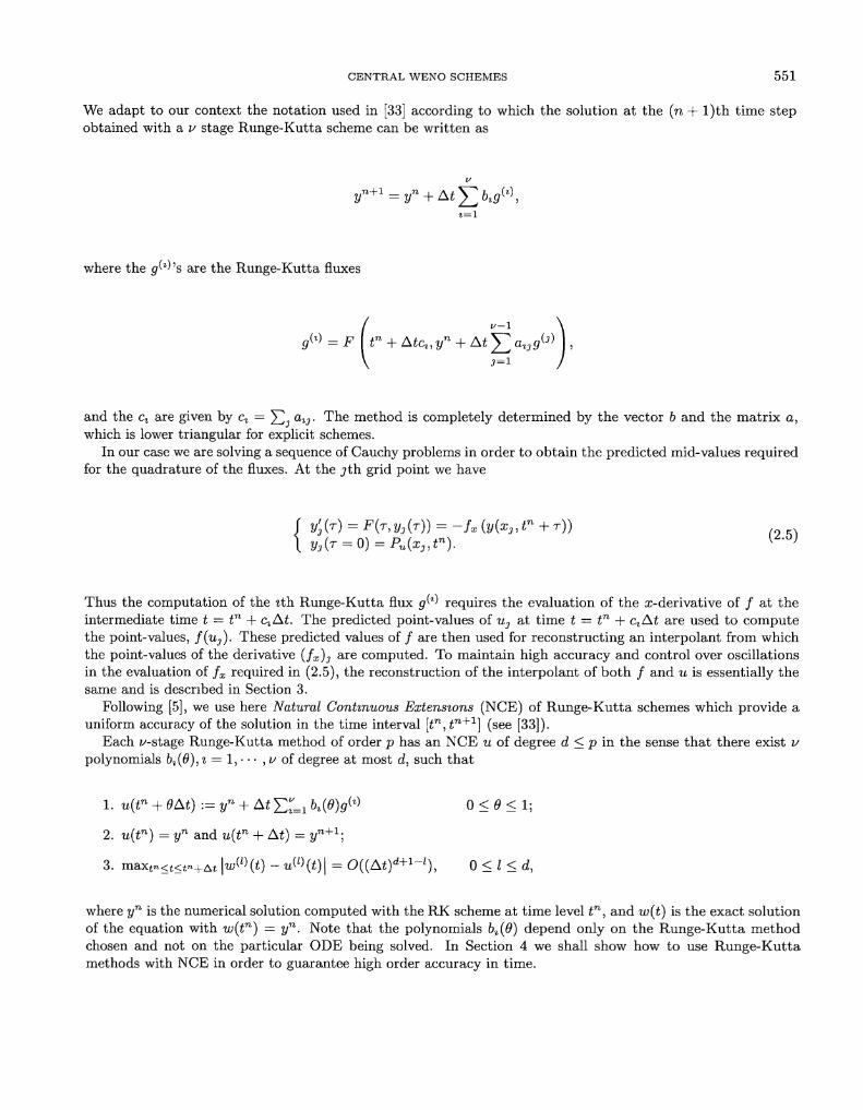
We adapt to our context the notation used in [33] according to which the solution at the (n + l)th time stepobtained with a v stage Runge-Kutta scheme can be written as

Z=l

where the g^'s are the Runge-Kutta fluxes

=F[ u y

and the c% are given by c% = Yl3 a%3- The method is completely determined by the vector b and the matrix a,

which is lower triangular for explicit schemes.In our case we are solving a séquence of Cauchy problems in order to obtain the predicted mid-values required

for the quadrature of the fluxes. At the jth grid point we have

y'3 (T) = F(T, y3 (r)) = -fx (y{x3, tn + r))

Thus the computation of the zth Runge-Kutta flux g^ requires the évaluation of the x-derivative of ƒ at theintermediate time t — tn -f c%At. The predicted point-values of u3 at time t = tn + czAt are used to computethe point-values, f(u3). These predicted values of ƒ are then used for reconstructing an interpolant from whichthe point-values of the derivative (fx)j are computed. To maintain high accuracy and control over oscillationsin the évaluation of fx required in (2.5), the reconstruction of the interpolant of both ƒ and u is essentially thesame and is described in Section 3.

Following [5], we use here Natura! Continuons Extensions (NCE) of Runge-Kutta schemes which provide auniform accuracy of the solution in the time interval [t71^71^1] (see [33]).

Each z -stage Runge-Kutta method of order p has an NCE u of degree d < p in the sense that there exist vpolynomials b%{9), % = 1, • • • , v of degree at most d, such that

1. u(tn + 0At) := yn + At^=l 6.(%w 0 < 9 < 1;

2. u(tn) = yn and u(tn + At) = yn+1;

3. maxtn<t<t-+At \wW(t) - u®(t)\ = O((At)d+l"1), 0 < l < d,

where yn is the numerical solution computed with the RK scheme at time level tn, and w(t) is the exact solutionof the équation with w(tn) = yn. Note that the polynomials bz(9) depend only on the Runge-Kutta methodchosen and not on the particular ODE being solved. In Section 4 we shall show how to use Runge-Kuttamethods with NCE in order to guarantee high order accuracy in time.

552 D. LEVY ET AL.

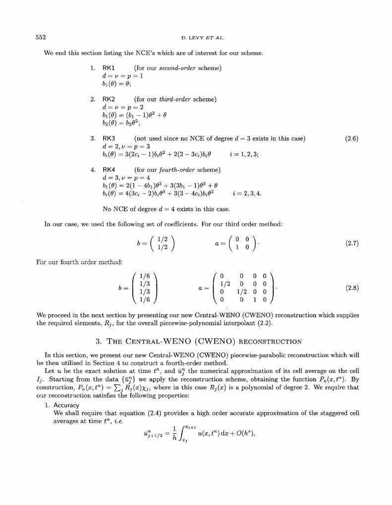
We end this section listing the NCE's which are of interest for our scheme.

1. RK1 (for our second-order scheme)d = v = p = 1

2. RK2 (for our third-order scheme)d=v= p =2b^O) = (bx - l)02 + 0

3. RK3 (not used since no NCE of degree d = 3 exists in this case) (2.6)d = 2,v = p = 3bi(0) = 3(2a - l)biO2 + 2(2 - 3c;)M i = 1,2,3;

4. RK4 (for our fourth-order scheme)d = 3,i/=p = 46i(fl) = 2(1 - 461JÖ3 + 3(36i - l)02 + (96.(0) = 4(3ci - 2)6ifl3 + 3(3 - 4ci)6i0

2 i = 2,3,4.

No NCE of degree d = 4 exists in this case.

In our case, we used the following set of coefficients. For our third order method:

For our fourth order method:

/ 1/6 \ /O 0 0 073 •I/O

1/31/6/

1/2 0 0y 1/0 / \ u 0 1 0

(2.8)

We proceed in the next section by presenting our new Central-WENO (CWENO) reconstruction which suppliesthe required éléments, Rj, for the overall piecewise-polynomial interpolant (2.2).

3. THE CENTRAL-WENO (CWENO) RECONSTRUCTION

In this section, we present our new Central-WENO (CWENO) piècewise-parabolic reconstruction which willbe then utilized in Section 4 to construct a fourth-order method.

Let u be the exact solution at time f1, and ü" the numerical approximation of its cell average on the celli j . Starting from the data {ü™} we apply the reconstruction scheme, obtaining the function Pu{x,tn). Byconstruction, Pu(x, tn) = Y2j Rj(x)Xji where in this case Rj(x) is a polynomial of degree 2. We require thatour reconstruction satisfies the following properties:

1. AccuracyWe shall require that équation (2.4) provides a high order accurate approximation of the staggered cellaverages at time £n, i.e.

1" h


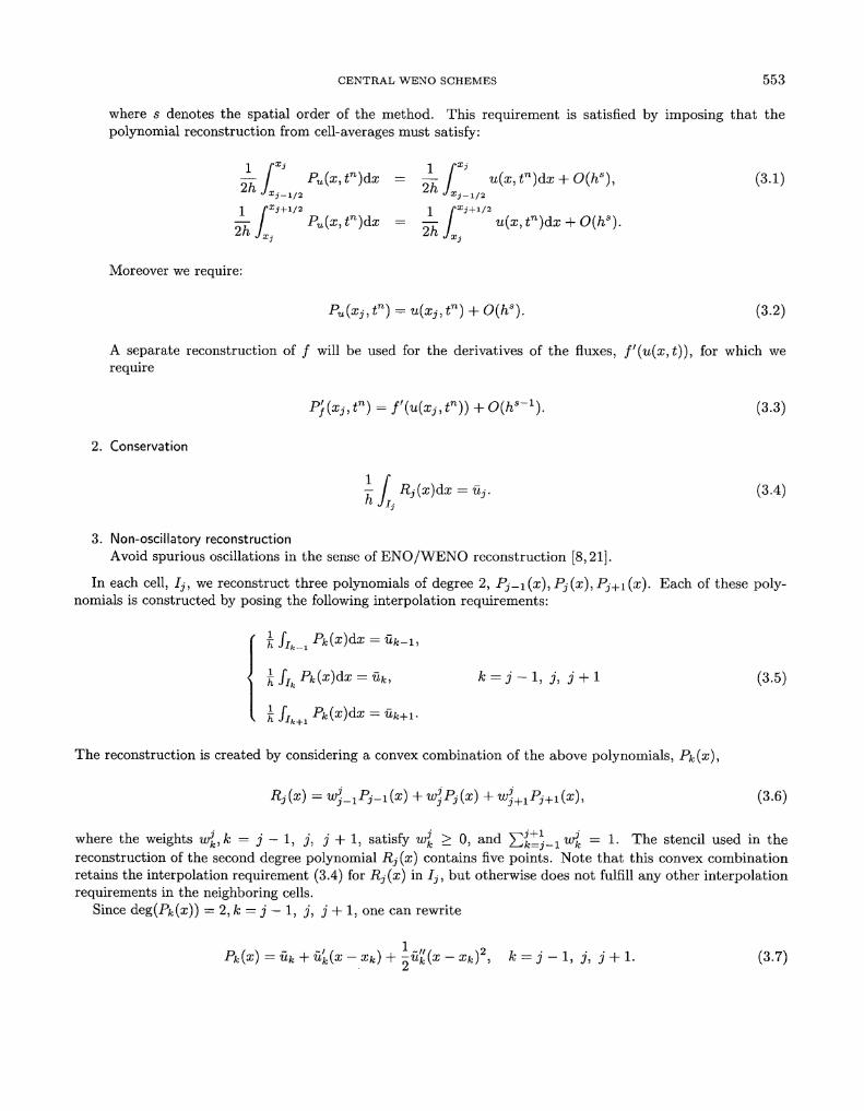
where s dénotes the spatial order of the method. This requirement is satisfied by imposing that thepolynomial reconstruction from cell-averages must satisfy:

^ r pu(x,ndx = i r u(x,tn)l fxj + l/2 1 fXj + 1/2

— J Pu(x,tn)dx = —J u(xytnJ

Moreover we require:

Pu(xj,tn) = u(xj,tn) + O(hs). (3.2)

A separate reconstruction of ƒ will be used for the derivatives of the fluxes, /'(u(x,£)), for which werequire

P'f(Xj,tn) = f'{u{Xj,t

n))+O{hs-1). (3.3)

2. Conservation

^J^Rj(x)dx = üj. (3.4)

3. Non-oscillatory reconstructionAvoid spurious oscillations in the sense of ENO/WENO reconstruction [8,21].

In each cell, Ij, we reconstruct three polynomials of degree 2, Pj-i(x)JPj(x)iPj^i(x). Each of these poly-nomials is constructed by posing the following interpolation requirements:

\ fIk Pk(x)dx = öfc, k = j - 1, j , j + 1 (3.5)

The reconstruction is created by considering a convex combination of the above polynomials,

i x ) + t^+ 1P j + 1(x) , (3.6)

where the weights w3k,k = j — 1, j , j + 1, satisfy w3

k > 0, and XlÜj-i fc = 1- ^he stencil used in thereconstruction of the second degree polynomial Rj(x) contains five points. Note that this convex combinationretains the interpolation requirement (3.4) for Rj(x) in ij-, but otherwise does not fulfill any other interpolationrequirements in the neighboring cells.

Since deg(Pfc(a;)) = 2, k = j - 1, j , j + 1, one can rewrite

Pk(x) =ük+ üfk(x - xk) + ~ül{x - xkf, k - j - 1, j , j + 1. (3.7)

554 D LEVY ET AL

The reconstructed point-values, ük, and the reconstructed discrete first and second derivatives, ük,ük, areuniquely determined by the interpolation requirements (3.5), as

üfc-

2h- 2uk

Hence, the interpolant R3 (x) can be written as

o („\ __ 7. _|_ , / f™ _ ™ \ i £ , , " (« _ -r ï2 ^ Qï

where its reconstructed point-values u3, and its reconstructed derivatives, uf3,u3\ are given by

7 / L / 1 l - 2 ~ / / x 7~ 7 / - , - / 1 , 2 - / / X

All that is left in order to end the reconstruction is to détermine the weights, w3kJk = j — 1,J,J + 1. Two

ingrédients are taken into account in their construction: the accuracy requirements and the non-oscillatoryrequirements.

Following the notations of [11], in order to guarantee convexity, Y^k=3-iw3k = 1' ^ e weights, wk, are

written as

< = - -j — ' k = j-1,3,3 + 1, (3.11)

where

The constants, C/c,€,p, and the smoothness indicator, JS^, will be determined below.Since we are in the framework of central schemes and not upwind schemes, our accuracy requirements are

different from those found in [11]. Here is exactly where the central philosophy enters. The constants Ckintroduced here, are computed such that they are symmetrie around the center of each cell. Consequently, wename our new centered reconstruction as Central-WENO (CWENO).

Since we can not satisfy all the accuracy requirements simultaneously, we split the computation into twoparts and by that we are led to two different sets of constants Ck. The first set corresponds to the accuracyrequirement in the reconstruction of the cell-averages (3.1), while the second set of constants corresponds tothe accuracy requirements in the reconstruction of the derivatives (3.3). Due to cancellation, any symmetriechoice of coefficients will result in a fourth-order approximation of the point-values in the center of the cells(5 — 4 in (3.2)). In order to satisfy (3.2) for 5 = 5 one has to use non-positive constants, namely a non-convexcombination of the stencils - see the remarks below. Clearly, the use of two separate sets of constants imposesabsolutely no problems on the implementation of the algorithm. We note that also in the original WENOpaper [21], two sets of (different) constants were suggested. There, the motivation was to adapt the constants

CENTRAL WENO SCHEMES

TABLE 3.1. The constants of the Central-WENO reconstruction.

555

II Ç,_i 1 C3cell- averagesderivativespoint-values

3/161/6

5/82/3

C3+\ || accuracy3/161/6

any symmetrie combination

hb

h4

to the upwinding and hence they were determined by the char act er ist ie variables. In our case, however, no suchcharacteristic décomposition is required. The simplicity of the central framework is projected onto our newCentral-WENO reconstruction.

A straightforward computation results with the desired constants which are displayed in Table 3.1.Several different ways to détermine the smoothness indicator were suggested in the literature (see, e.g.,

[11,21]). Here we use the measure taken from [11], which amounts to a measure on the L2-norms of thederivatives:

• ^ + 1/2

1 = 1 JX3-1/

(3.13)

where Pk dénotes the Zth derivative of -Pfc(x). An explicit intégration of (3.13) yields

IS]_X = r ^ fe -2 - 2ÜJ-1 + üj1 2

1 2 v

In smooth régions, a Taylor expansion of (3.14) gives

= (ü'h)2 + ~(üf/h2)2 + O(h%

3<1, (3.14)

(3.15)

Hence, IS3k = O(h2), and in critical points it is O(h4). In non-smooth régions, ISJ

k = O(l), and by that thenormalized weight of the corresponding stencil will be negligible. Therefore, our reconstruction follows theWENO methodology by automatically avoiding the information coming from non-smooth régions which arethe cause for spurious oscillations.

The remaining parameters to be determined in (3.12) are e and p. The constant e was inserted in thedenominator in order to prevent it from vanishing. In [11] ane = 10~6 was empirically selected. Here, we findthat the scheme is almost not sensitive to the value of e, and e = 10~6 proved adequate for the numerical resultsin Section 5. The value of p was determined in [21] as one above the degree of the reconstruction polynomial,which in our case amounts to 3. In [11] a p = 2 was empirically selected and here we use the same value p = 2.

In short, our reconstruction from cell averages routine accepts in input the values {ü3} of cell averages attime £n, and produces in output the point values u3,u

fvu" which completely détermine the reconstruction

polynomial R3 (x).A few modifications are needed to compute the reconstruction from point values for the flux f3 = f(u3)

which is needed in the Runge-Kutta step.

556 D. LEVY ET AL.

Her e the candidate polynomials P& satisfy the interpolation requirements (compare with (3.5)):

Pk(xk) = ƒ*, fc = j - 1, j , i + 1 (3-16)

Thus the reconstructed point values ƒ& and the reconstructed first and second dérivâtives ƒ£ and ƒ£' are givenby:

f = fk f = ^ =

For the évaluation of the int er médiat e values, all that will be needed is a pointwise reconstruction of the spacederivative /j which is given by:

The computation of the weights in (3.17) is the same as above (3.11-3.15). Here, we use the second set ofconstants CV s of Table 3.1, and the computation of the smoothness indicators IS3

k in (3.14) involves the pointvalues / j , instead of the cell averages.

Several remarks are in order.

Remarks.

1. In [5] the ENO reconstruction was first combined with central schemes. There? it was shown that an ENOreconstruction of degree 3 is required to obtain an overall third-order method (when the flux intégration isdone by a Runge-Kutta solver). Here we construct a piecewise-parabolic interpolant that is then utilizedto obtain a fourth-order accurate method.

2. The piecewise-parabolic upwind-WENO reconstruction is utilized in [11] to obtain a fifth-order method,which is more accurate than our fourth-order method. On the other hand, it suffers from the drawbacks ofthe upwind approach. We can also obtain a fifth-order method, requiring s = 5 in (3.1-3.3). Unfortunately,in (3.2), s = 5 leads to a non-convex combination. Such a combination does not fit in our framework. Itshould be possible to construct a fifth-order method which reduces to lower order convex reconstructionby taking a convex combination of the fifth-order method and the fourth-order method described above,but we do not describe it here.

3. Practically, we have observed that the scheme dépends very weakly on the value of e. The parameter emust be chosen such as to avoid cancellations in the significant digits and in that sensé it dépends on theorder of magnitude of the solution. However, since the weights are normalized, the magnitude of e hasvery littie effect on the scheme.

To summarize, our new Central-WENO reconstruction enjoyed the best of two worlds. On one hand, itfollows the WENO methodology by making use of the existing information in order to automate the sélection ofthe stencil and to increase the overall order of accuracy of the resulting reconstruction while retaining its non-oscillatory properties. On the other hand, since we are dealing with the central framework, our reconstructionmakes no use of characteristic décomposition and by that we are left with a simple and robust machinery.

4. THE METHOD

In this section we combine the central framework which was overviewed in Section 2 with our new CWENOreconstruction of Section 3. The dérivation of the resulting scheme is straightforward and is summarized in thefollowing algorithm, which applies to the scalar case.


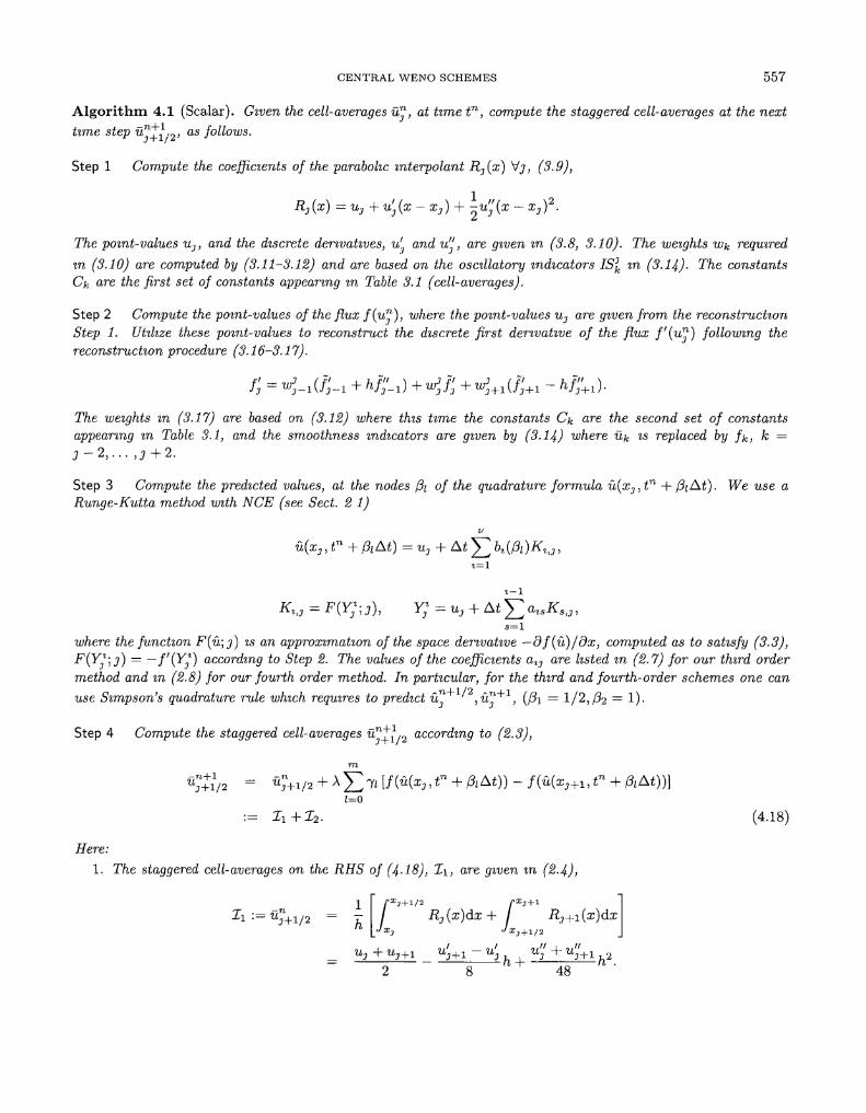
Algorithm 4.1 (Scalar). Given the cell-averages ü™, at time tn, compute the staggered cell-averages at the nexttime step ün^>2, as follows.

Step 1 Compute the coefficients of the parabohc interpolant R3(x) Vj, (3.9),

R3(x) = u3 + u'3(x - x3) + -u3'(x - x3f.

The pomt-values u3, and the discrete derivatzves, uf3 and u", are given m (3.8, 3.10). The weights Wk required

m (3.10) are computed by (3.11-3.12) and are based on the oscillatory indicators IS3k tn (3.14)- The constants

Ck ojre the first set of constants appearzng m Table 3.1 (cell-averages).

Step 2 Compute the pomt-values of the flux f(u™), where the pomt-values u3 are given from the reconstructionStep 1. Utihze these pomt-values to reconstruct the discrete first derivatwe of the flux ff(u^) followmg thereconstruction procedure (3.16-3.17).

The weights m (3.17) are based on (3.12) where this time the constants Ck o/re the second set of constantsappeanng m Table 3.1, and the smoothness indicators are given by (3.14) where ük is replaced by fk, k —

Step 3 Compute the predicted values, at the nodes pi of the quadrature formula û(x3,tn +/3^At). We use a

Runge-Kutta method with NCE (see Sect. 2 1)

KXI3 = F(Y;- J), Y; = Uj + At Y

where the function F(u\j) is an approximation of the space denvative —df(iï)/dx, computed as to satisfy (3.3),F(Y3]j) = —f{Y3

%) accordmg to Step 2. The values of the coefficients a%3 are hsted m (2.7) for our third ordermethod and m (2.8) for our fourth order method. In particular, for the third and fourth-order schemes one canuse Simpson's quadrature rule which requires to predict û™+1 , û™+1, (Pi = 1/2,/32 = 1)*

Step 4 Compute the staggered cell-averages û n ^ , 2 accordmg to (2.3),

1=0

(4.18)

Here:

1. The staggered cell-averages on the RHS of (4-18), I\, are gtven m (2.4),

Ü ; + 1 / 2 - - R3(x)dx + I R3+I(x)dx\

X3 + l U3 u , _2__J±1^28 48

558 D. LEVY ET AL.

The potnt-values and the derivatives, u3^uJ}u3f, wem computed in Step 1.

2. For a third and fourth-order schemes, X2 can be wrttten as Simpson}$ rule

•= £{[/(<£)+4/ (Ü ; + 1 / 2 ) + / (^+1)] - [/(Û?+1)+4/(û;

where the predtcted potnt-values u™+1^2 = u{x3,tn + 1/2At) and n^+1 = u{x3,t

n + At), are the result ofStep 3.

We end this section sketching the algorithm for the case of dx d Systems of conservation laws. In the following,u dénotes the vector with components u = (u1, - • • , ud).

Algorithm 4.2 (Systems). Gtven the cell-averages ü™, at time tn, compute the staggered cell-averages at thenext time step ün+h2, as foliotas.

Step 1: Compute the coefficients of the parabohc interpolant R3(x) Vj, applymg Step 1 of Algorithm 4-1 oieach component of the vector ü™. Note that the coefficients of the interpolant are now d component vector s. Forthe computation of the oscillatory indicators IS3

k several stratégies are possible. One can apply formulas (3.14)obtaining different smoothness indicators for each component. Alternatively, one can use information comingfrom all components as in the Global strategy defined %n (5.1) below. For more details, see the discussion inSection 5.2.

Step 2: Compute the point-values of the flux f(u"), where the potnt-values (uj, • • • ,Uj) are reconstructed mStep 1. Utilize these point-values to reconstruct the discrete derivative of each component of the flux functionf(u") applymg the reconstruction procedure (3,16-3.17) at each component of f. As in Step 1, the smoothnessindicators can be computed either by a componentwise or a global strategy.

Step 3: Compute the predicted values of f(u). at the nodes 3\ of the quadrature formula, vsing o Runge-Kuttamethod with NCE (see Sect. 2.1). Observe that now ÏL,U)K%) and Y* are d components vectors. In particular,note that each component ofY% must be updated bef ore f(Y*) can be computed. Each component of F(YJ;j)can be ihen computed applying our discrete differentiation scheme component by component to the vector f (Y*).

Step 4: Apply Step 4 of Algorithm 4-1 to each component of the conservation law.

Remark. The central framework is based on the assumption that the solution remains smooth at the boundariesof the staggered cell ( ^ ,x J + i ) , if the appropriate CFL condition is satisfied. The discontinuities arising fromthe generalized Riemann problems defined at xJ+i/2 do not have the time to reach the cell boundaries. Thus it isquite reasonable to assume that the degree of smoothness of the solution at x3 and x3+i will not change abruptlywithin one time step. Therefore the smoothness indicators can be computed only once per time step. Moreprecisely, we can compute the smoothness indicators from cell averages, as indicated in Step 1 of our algorithms,and utilize these same quantities when Computing the weights of our reconstruction at each intermediate stageof the RK step. We implemented this simplified technique in our numerical simulations in Section 5.2 below.We emphasize that this réduction in the complexity of the computation of the smoothness indicators is closelylinked to the central framework.

5. NUMERICAL RESULTS

In this section we test our third and fourth-order schemes summarized in Section 4. We start from a singlescalar équation where we numerically compute the order of accuracy of our schemes. We also demonstrate ona model problem how the smoothness indicators trigger the sélection of the correct stencil when discontinuitiesare present. We end the discussion of the scalar case with a linear problem proposed by Jiang and Shu in [11].


The construction of the smoothness indicators is more delicate for Systems of équations than in the scalarcase. We show with numerical examples that a naive component by component extension of the scalar schemedoes not yield the best results. We formulate and test two different algorithms to address this problem.

We then apply our scheme to some classical test problems of gas dynamics. Our results show that the use ofthe same smoothness indicator for all the components produces better results and is computationally cheapercompared with the componentwise indicator.

5.1. Scalar équation

We study the performance of our schemes by applying them to the following test problems:

Test 1.ut 4- ux = 0,u{x,t = 0) = sin(7rx),periodic boundary conditions on [—1,1],intégration time: T = 10.

This test is used to check the convergence rate at large times.

Test 2.ut + ux = 0,u(x, t = 0) = sin4(7nc),periodic boundary conditions on [—1,1],intégration time: T = 1.

This test is used to detect possible détériorations of accuracy due to strong oscillations in the parameters thatdétermine the stencil (such as in ENO schemes). See the discussion in [5] and références therein.

Test 3.

u(x} t = 0) = 1 + \ sin(7rx),periodic boundary conditions on [—1,1],intégration times: T = 0.33 and T = 1.5.

Here T = 0.33 is used for convergence tests, and T = 1.5 for the shock capturing test (the shock develops atTs = 2/TT).

Test 4.ut + ux = 0,u(x,t = 0) = UQ(X),

periodic boundary conditions on [—1,1],intégration time: T = 8.

This test is used to show the resolution properties of the scheme. The initial data UQ(X) is defined in theExample 1 of [11] as:

UQ(X) =

| (G(x, z-S) + G(x, z + ö) + 4(3(2;, z)), -0.8 < x < -0.6,1, -0.4 <x < -0.2,1 — |10(a; — 0.1)|, 0 < z <0.2,| (F(x, a - ö) + F(x, a + ö) + AF(x, a)), 0.4 < x < 0.6,0, otherwise,

whereG(x,z) = c-^(«-*)2,

F(x,a) = (max(l-a2(a;-a)2 ,0))1 /2 .

560 D. LEVY ET AL.

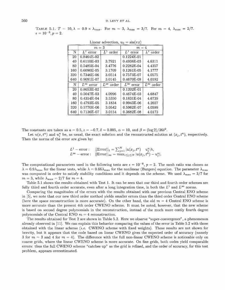
TABLE 5.1. T = 10, A = 0.9 x Amax. For m = 3, Amax = 3/7. For m = 4, Amax

Linear advection, UQ = sin(Trx)

= 2/7.

N204080

160320640

N204080

160320640

m =Ll error

0.8464E-020.6110E-030.5485E-040.6090E-050.7346E-060.9091E-07L°° error

0.8653E-020.5047E-030.4354E-040.4793E-050.5770E-060.7136E-07

= 3L1 order

3.79213.47763.17093.05143.0145

L°° order

4.09963.53503.18343.05423.0154

m =L1 error

0.1224E-010.4938E-030.2282E-040.1261E-050.7573E-070.4670E-08L°° error

0.1202E-010.4674E-030.1831E-040.9943E-060.5962E-070.3682E-08

= 4Ll order

4.63114.43574.17774.05754.0192

L°° order

4.68474.67394.20274.05994.0173

The constants are taken asa = 0.5, z = -0.7, S = 0.005, a = 10, and (3 = (Iog2)/36J2.Let u{X)tn) and u™ be, as usual, the exact solution and the reconstructed solution at (xj}t

n), respectively.Then the norms of the error are given by:

L1 - error : !|Errorjji = Ef=i \u(x37tn) u?\h,

L°° — error : 11Error||oo =

The computational parameters used in the following tests are e = 10~6} p = 2. The mesh ratio was chosen as

A — 0.9Amax for the linear tests, while A = 0.66Amax for the nonlinear (Burgers) équation. The parameter Amax

was computed in order to satisfy stability conditions and it dépends on the scheme. We used Amax = 3/7 form — 3, while Amax = 2/7 for m = 4.

Table 5.1 shows the resuit s obtained with Test 1. It can be seen that our third and fourth order schemes arefully third and fourth order accurate, even after a long intégration time, in both the L1 and L°° norms.

Comparing the magnitudes of the errors with the results obtained with our previous Central. ENO schemein [5], we note that our new third order method yields smaller errors than the third order Central ENO scheme(here the space reconstruction is more accurate). On the other hand, the old m = 4 Central ENO scheme ismore accurate than the present 4th order CWENO scheme. It must be noted, however, that the new schemeis based on second degree polynomials in the reconstruction, instead of the much more costly fourth degreepolynomials of the Central ENO m = 4 reconstruction.

The results obtained for Test 2 are shown in Table 5.2. Here we observe "super-convergence", a phenomenonalready observed in [11]. We can explain this behavior comparing the values of the error in Table 5.2 with thoseobtained with the linear scheme (Le. CWENO scheme*with fixed weights). These results are not shown forbrevity, but it appears that the code based on linear CWENO gives the expected order of accuracy (namely3 for m — 3 and 4 for m = 4). The différence with the full non-linear CWENO scheme is noticeable only oncoarse grids, where the linear CWENO scheme is more accurate. On fine grids, both codes yield comparableerrors: thus the full CWENO scheme "catches up" as the grid is refmed, and the order of accuracy, for this testproblem, appears overestimated.

CENTRAL WENO SCHEMES

TABLE 5.2. T = 1,A = 0.9 x Amax. For m = 3, Amax = 3/7. For m = 4, Amax = 2/7.

561

N204080160320640N204080160320640

Linearm =

L1 error0.5514E-010.6353E-020.5247E-030.2940E-040.2625E-050.3048E-06L°° error

0.6643E-010.8657E-020.9784E-030.3827E-040.2669E-050.2983E-06

advection, UQ — sin (nx)= 3

L1 order

3.11743.59814.15773.48533.1063

L°° order

2.93983.14544.67603.84213.1613

m =L1 error

0.9541E-010.7728E-020.8175E-030.3002E-040.1130E-050.6141E-07L°° error

0.10120.9660E-020.1510E-020.7870E-040.2185E-050.6022E-07

= 4L1 order

3.62583.24084.76734.73094.2023

L°° order

3.38962.67784.26185.17045.1814

TABLE 5.3. T = 0.33, A = 0.66 x Amax. For m = 3, Amax = 3/7. For m = 4, Amax = 2/7.

N204080160320640

N204080160320640

Burgers équation, UQ -m =


0.6699E-020.8913E-030.5859E-040.2624E-050.1542E-060.1338E-07

3L1 order

3.50524.11874.26923.80343.1126

L°° order

2.91003.92724.48094.08843.5273

= 14- l/2sin(7rx)m =


0.9462E-020.1139E-020.8631E-040.4461E-050.2296E-060.1269E-07

= 4L1 order

3.57284.11504.37874.40174.1916

L°° order

3.05493.72164.27424.28004.1779

We end the accuracy tests with a non linear problem (Test 3), computing the order of accuracy at T = 0.33,well before the shock formation time T — 2/n. The results appear in Table 5.3. Once again, we observe thecorrect order of accuracy.

The shock-capturing properties of the CWENO scheme are illustrated in Figure 5.1 for the Burgers équation(Test 3). The pictures on the left refer to the solution before shock formation (T = 0.5) and the pictures on theright refer to the solution after shock formation (T = 1.5). The bottom part of the picture shows the weightsvPk computed in the reconstruction from cell averages. In particular, the central weight corresponds to w3

3,

562 D. LEVY ET AL.

T=.5, N = 80 T = 1.5, N = 80

-1 -0.5 0 0.5 1Central weight

1

-0.5 0 0.5 1Left weight

-0.5 0.5 1

-1 -0.5 0 0.5 1Central weight

1

0.5

FIGURE 5.1. Burgers équation. Solution and weights. Weights computed from cell averages,m = 4.

while the left weight corresponds to Wj_x. Before the shock formation, the weights remain close to theirequilibrium values (given in Tab. 1). An abrupt change can be seen after the shock formation. Hère the stencilsthat would yield oscillations are assigned almost a zero weight. Thus the solution is oscillation-free even afterthe shock forms. The shock transition occurs within two cells.

Figure 5.2 shows the results obtained on Test 4, for m = 3 and two grid sizes, N = 200 and N = 400. Thesolution has no spurious oscillations: the scheme is able to control oscillations arising from discontinuities in thesolution and in its derivatives. The resolution of the contact discontinuities present in the square wave seemsbetter than the analogous results obtained in the ENO and WENO case with Roe flux by Jiang and Shu (seeFig. 1 in [11]). Their results are better if they couple their scheme with the artificial compression method byYang [32]. We have not yet tried to adapt Yang's algorithm to the central framework. This issue might beaddressed in future work. We also note that the resolution of the left peak in the wave train is not as sharp asin the WENO case.


0.6 0.8

1

0.8

0.6

0.4

0.2

o-

I I I 1 1 I I I I

A

S

i il itm il mm i il il il mu il muni I I I U M F ^fcuu H I M m imi mu m H i n m mi4-llililllllllillillililillliimilillnlllill11 "• •• 1 II ITIIII il III II 111III llllll! 1111 ni*

jmiiiiiitiiiiiiiiiiUp

f 4A j #kà f\

i l f 1

ï 1 \ i \^ymimiiiiiif" |mf f lF" ^ M I I I H I I I I I I I Î I " " " 1 " " " " " ^ rauniiiiiinm1" «nniiiinnninMniiinnnimmmiiiiiii

••iiiiiiiiiilllllllllllllllllllil •UiHiiiJiijiiiiiKilllllllllllllH ••iiiiHiiiiiiiitiiiiiiiiiiiiiifiiiiiiiiiiiiiiiiiiuiiiiiiiiiiuiiiiiHirii

1 1 1 1 1 1

0.8 0.6 0.4 0.2 0.2 0.4 0.6 0.8

FIGURE 5.2. Shu's linear test, with m = 3. TV = 200 (top), N = 400 (bottom).

There is a curious lack of symmetry appearing in the right hump of the figure in the N = 400 case, whichchanges according to the direction of the wind. It is less pronounced in the N = 800 case. The same featureappears for m = 4. This is the only test problem in which we observed this phenomenon. We did not observesimilar phenomenon in our non-linear tests and we leave its investigation for a future study.

We obtain very similar results if we compute the smoothness indicators only once per time step instead ofComputing them at e very stage of the RK scheme, as described in the Remark at the end of Section 4. We donot include these results because they appear identical to the plots we have already shown.

5.2. Systems of équations

We apply our schemes to the system of Euler équations of gas dynamics for a polytropic gas with constant7 = 1.4. The variables p,m, £7, and p below, dénote the density, momentum, total energy per unit volume

564 D. LEVY ET AL.

N=100, m=4 N=400, m=4

0.2 0.4 0.6 0.8

Central weight Central weight

1 0.6 0.8

FIGURE 5.3. Componentwise smoothness indicator. Density (top) and central weights(bottom) for Sod's problem: À = 0.1, T — 0.16. The weight shown is computed in the re-construct ion from cell-averages for the density component.

and the pressure, respectively. We consider the following test problems:

Test 5. Shock tube problem with Sod's initial data [28].

f (pi,mhEi) = (1,0,2.5), z<0 .5 ,\ (pr, m r, Er) = (0.125,0, 0.25), x > 0.5.

Test 6. Shock tube problem with Lax' initial data [14].

f {pumhEi) = (0.445,0.311,8.928), x < 0.5,\ (pr, m r, Er) - (0.5, 0,1.4275), x > 0.5.

In both cases the computational domain is [0,1]; we integrate the équations up to T = 0.16, Le. before theperturbations reach the boundary of the computational région. Following Liu and Tadmor [22], the CFL wastaken as À = 0.1. Note that À = 0.1 is the optimal CFL for Lax initial data since the maximal characteristic


N=100, m=4 N=400, m=4

0.8

0.6(

0.4

0.2

n

Central weighi

?

yPMIIIIIHI» «j taœ l ffl

/K (D 1 J 1 1 (

1

f

7

f™8

8—0.2 0.4 0.6 0.8 1

1

0.8

0.61

0.4

0.2

n

Central weight

• r PÔ

c

•

0.2 0.4 0.6 0.8

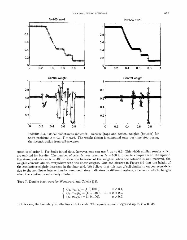
FIGURE 5.4. Global smoothness indicator. Density (top) and central weights (bottom) forSod's problem: À = 0.1, T = 0.16. The weight shown is computed once per time step duringthe reconstruction trom cell-averages.

speed is of order 5. For Sod's initial data, however, one can use A up to 0.2. This yields similar results whichare omitted for brevity. The number of cells, TV, was taken as N = 100 in order to compare with the upwindliterature, and also as TV" = 400 to show the behavior of the weights: when the solution is well resolved, theweights coincide almost everywhere with the linear weights. One can observe in Figure 5.6 that the height ofthe oscillations slightly decreases in the finer grid. We believe that this loss of self-similarity on coarse grids isdue to the non-linear interactions between oscillatory indicators in different régions, a behavior which changeswhen the solution is sufficiently resolved.

Test 7. Double blast wave by Woodward and Colella [31].

(pi,mi,PÜ = (1.0,1000), ar < 0.1,(Pc,rnc,Pc) = (1,0,0.01), O.K x < 0.9,(Pr,mr,pr) = (1,0,100), x>0 .9 .

In this case, the boundary is reflective at both ends. The équations are integrated up to T = 0.038.

566 D. LEVY ET AL.

Component-Wise Smoothness Indicator Global Smoothness Indicator

0.6 0.8 0.2 0.4 0.6 0.8


0.2 0.4 0.6 0.8 1

0.8

0.6

0.4

0.2

00 0.2 0.4 0.6 0.8 1

FIGURE 5.5. Componentwise and global smoothness indicators. Density (top) and centralweights (bottom) for Lax' problem: A = 0.1, T = 0.16, m = 4, N = 400. The weight shown iscomputed once per time step during the reconstruction from cell-averages for the density.

We start applying our scheme component by component to each équation of the Euler system, as described inSection 3. With this strategy the smoothness indicators are computed as in (3.14) using the formulas of the scalarcase for each component. The smoothness indicators are computed at each intermediate time level tn + ciAt ofthe Runge-Kutta intégration, applying again our scheme componentwise. We call this straightforward extensionto Systems of the scalar formulas for the computation of the weights "componentwise smoothness indicators". Inthe m — 4 case, we need 5 évaluations of the smoothness indicators for each component (one from cell averagesand one from point values at each of the four Runge-Kutta steps). Thus we have 15 évaluations of the quantitiesIS3

k at each time step, in the case of Euler équations.Applying this scheme with m = 4 to Sod's problem with a fixed value of A = 0.1, we find the results shown

in Figure 5.3, for TV = 200 and N = 400. We note that there are some small amplitude oscillations close to thecontact discontinuity.

The bottom part of the picture shows the behavior of the central weights obtained at the beginning of the lasttime step in the reconstruction from cell averages for the density. We note that the solution is oscillation freeclose to the shock, where the smoothness indicators sharply recognize the discontinuity, setting almost to zerothe weight of the "bad" stencils. The situation is more confused close to the contact discontinuity. The weights


N=100, m=4 N=400, m=4

0.2 0.4 0.6 0.8


0.8

0.6

0.4

0.2

0.2 0.4 0.6 0.8

FIGURE 5.6. Density smoothness indicator. Density (top) and central weights (bottom) forLax' problem: À = 0.1, T = 0.16, m = 4. The weight shown is computed once per time stepduring the reconstruction from cell-averages for the density.

of the "bad" stencils do not go to zero, because the contact discontinuity is spread on several cells (unlike theshock), and therefore it is not recognized as a discontinuity by the scheme.

The behavior of the weights becomes very irregular in the neighborhood of the contact wave, probably becausethe pressure and the velocity fields are continuous across the contact wave, and therefore each componentsélects a different stencil. This suggests that the scheme might improve if all components feel the présenceof a discontinuity through their smoothness indicators. This can be obtained, e.g., by using one smoothnessindicator for all the components:

(5.1)

568 D. LEVY ET AL.

N=400, m=4 N=800, m=4

0.8 0.2 0.4 0.6 0.8

N=400, m=3 N=800, m=3

0.2 0.4 0.6 0.8 1

: r0.2 0.4 0.6 0.8 1

FIGURE 5,7. Woodward and Colella bang. Density plot with global smoothness indicator.T ~ 0.038. The weight is computed once per time step during the reconstruction from cell-averages.

Here d is the number of équations, and Pk,r dénotes the feth polynomial for the rth component. The quantity\\ür\\2 is a scaling factor, and it is defined as the L2 norm of the cell averages of the rth component of u, namely:

1/2

2 =

\BX1J

The intégral in (5.1) can be exactly integrated [see (3.14)].We find that this strategy is effective even if the quantities IS3

k are computed at the beginning of the timestep in the reconstruction from cell averages, and are not changed at every level of the RK scheme. See theremark at the end of Section 4. This strategy will be called "global smoothness indicators" : its results on Sod'sproblem are shown in Figure 5.4. We note a slight improvement on the control of the spurious oscillations,and the oscillations in the weights are more localized. A more marked improvement can be observed on Lax'problem (see Fig. 5.5).


7

6

5

4

3

2

1

rv

N=400, m=4

V/

/

0.2 0.4 0.6 0.8

N=400, m=3

-7

6

5

4

3

2

1

N=800, m=4

\\V

fI

0 0.2 0.4 0.6 0.8 1

•7/

6

5

4

3

2

1

0

N=800, m=3

NV

1o 0.2 0.4 0.6 0.8 1

FIGURE 5.8. Woodward and Colella bang. Density plot with density smoothness indicator.T = 0.038. The weight is computed once per time step during the reconstruction from cell-averages.

To summarize, the "global smoothness indicators" strategy is much less expensive and gives better resultsthan the "componentwise smoothness indicators" strategy.

We can further improve our results if we take into account the particular structure of the system. Sincethe density jumps at both shocks and contact waves, we can use the density alone to compute the smoothnessindicators for all components.

Again, we find that it is enough to compute the smoothness indicators only once per time step. This strategyis slightly more diffusive than the previous one, because the biased stencils will be chosen more often. Theresults are slightly better than the "global smoothness indicators" strategy. The drawback of this approach isthat we use information about the particular structure of the system.

The application of the three stratégies that we are proposing to Lax' test problem (Test 6) are shown inFigures 5.5 and 5.6. The first figure shows the density and the central weight computed for the density componentfor the componentwise and the global stratégies, for m = 4 and N = 400. The second figure shows the resultsobtained with the density strategy with m = 4 and two grid sizes, N = 200 and N — 400. From Figure 5.6, wesee that the amplitude of the spurious wiggles near the contact discontinuity decays as the grid is refined.

570 D. LEVY ET AL.

In these pictures we see similar behavior as in Sod's problem. In all three stratégies, shock waves are wellresolved and oscillation free. Clearly, the global strategy produces a more reasonable sélection of the weights,compared with the componentwise approach. This behavior results in smaller wiggles in the numerical solution.It is remarkable that even the wild weights produced by the componentwise strategy resuit in a reasonablesolution. We believe that this fact illustrâtes the robustness of our scheme.

We end this section applying our scheme to Test 8: the blast wave problem of Woodward and Colella [31].Since in this problem the characteristic speeds change wildly with time, we used an adaptive évaluation of thetime step, namely:

At = C -j—[T, C = 0.9Amax,(cj + \Uj\)

where Cj and Uj are the local sound speed and velocity respectively. In our tests Amax dépends on the scheme,as already discussed for the scalar case.

We show the density component of the solution at T — 0.038 in Figure 5.7 and Figure 5.8, for the globaland the density stratégies respectively. The global strategy is clearly slightly less dissipative, especially on thecoarse grid, but there are small ENO-type wiggles. In both cases, the two peaks in the density are very wellresolved (compare with WENO schemes in [11]).

6. CONCLUSIONS

We have presented new third and fourth order central schemes which are based on a new central WENO(CWENO) reconstruction. The time marching scheme is constructed through Runge-Kutta intégration withnatural continuous extensions.

In particular, we develop simple and efficient techniques for the évaluation of the smoothness indicators inthe case of Systems.

Our results suggest that these schemes are fast and robust tools for the intégration of gênerai Systems ofconservation laws.

These new schemes require no approximate Riemann solvers, no projection along characteristic directions,no fancy splitting of the flux function in upwind and downwind directions, and finally no exact or approximateévaluation of eigenvalues and eigenvectors of the Jacobian of the flux.

A 2D extension of these schemes will be presented in a following paper [18].

Research was supported by Hyperbolic Systems of conservation laws TMR grant #ERBFMRXCT960033. Part of thiswork was done while the first and second authors were visiting L'Aquila, and while the third author was visiting ENS,Paris. We would like to thank G.-S. Jiang and S, Osher for their useful suggestions.

REFERENCES

[1] P. Arminjon, D. Stanescu and M.-C. Viallon, A Two-Dimensional Finite Volume Extension of the Lax-Priedrichs and Nessyahu-Tadmor Schemes for Compressible Flows, in Proc. 6th. Int. Syrnp. on CFD, Lake Tahoe, Vol. IV. M. Hafez and K. OshimaEds. (1995) 7-14.

[2] P. Arminjon and M,-C. Viallon, Généralisation du schéma de Nessyahu-Tadmor pour une équation hyperbolique à deuxdimensions d'espace. C.R. Acad. Sci. (Paris) Ser. I Math. 320 (1995) 85-88.

[3] P. Arminjon, M.-C. Viallon and A. Madrane, A Finite Volume Extension of the Lax-Friedrichs and Nessyahu-Tadmor Schemesfor Conservation Laws on Unstructured Grids. IJCFD 9 (1997) 1-22.

[4] P. Arminjon, M.-C. Viallon, A. Madrane and L. Kaddouri, Discontinuous Finite Eléments and Finite Volume Versions of theLax-Friedrichs and Nessyahu-Tadmor Schemes for Compressible Flows on Unstructured Grids. Computational Fluid DynamicsReview. M. Hafez and K. Oshima Eds., Wiley (1997).

[5] F. Bianco, G. Puppo and G. Russo, High Order Central Schemes for Hyperbolic Systems of Conservation Laws. SIAM J. Sci.Comp. (to appear.)

[6] K.O. Friedrichs and P.D. Lax, Systems of Conservation Equations with a Convex Extension. Proc. Nat. Acad. Sci. 68 (1971)1686-1688.


[7] E. Godlewski and P.-A. Raviart, Numerical Approximation of Hyperbolic Systems of Conservation Laws. Springer, New York(1996).

[8] A. Harten, B. Engquist, S. Osher and S. Chakravarthy, Uniformly High Order Accurate Essentially Non-oscillatory SchemesIII. JCP 71 (1987) 231-303.

[9] H.T. Huynh, A Piecewise-parabolic Dual-mesh Method for the Euler Equations. AIAA-95-1739-CP, The 12th AIAA CFDconference (1995).

[10] G.-S. Jiang, D. Levy, C.-T. Lin , S. Osher and E. Tadmor, High-Resolution Non-Oscillatory Central Schemes with Non-Staggered Grids for Hyperbolic Conservation Laws. SINUM 35 (1998) 2147-2168.

[11] G.-S. Jiang and C.-W. Shu, Efficient Implementation of Weighted ENO Schemes. JCP 126 (1996) 202-228.[12] G.-S. Jiang and E. Tadmor, Nonoscillatory Central Schemes for Multidimensional Hyperbolic Conservation Laws. SIAM J.

Sci. Comp. 19 (1998) 1892-1917.[13] S. Jin and Z.-P. Xin, The Relaxation Schemes for Systems of Conservation Laws in Arbitrary Space Dimensions. CPAM 48

(1995) 235-277.[14] P.D. Lax, Weak Solutions of Non-Linear Hyperbolic Equations and Their Numerical Computation. CPAM 7 (1954) 159-193.[15] B. van Leer, Towards the Ultimate Conservative Différence Scheme, V. A Second-Order Sequel to Godunov's Method. JCP

32 (1979) 101-136.[16] R.J. LeVeque, Numerical Methods for Conservation Laws. Lectures in Mathematics, Birkhauser Verlag, Basel (1992).[17] D. Levy, A Third-order 2D Central Schemes for Conservation Laws, Vol. I. INRIA School on Hyperbolic Systems (1998)

489-504.[18] D. Levy, G. Puppo and G. Russo, Central WENO Schemes for Multi-Dimensional Hyperbolic Systems of Conservation Laws

(in préparation).[19] D. Levy and E. Tadmor, Non-oscillatory Central Schemes for the Incompressible 2-D Euler Equations. Math. Res. Lett. 4

(1997) 1-20.[20] X.-D. Liu and S. Osher, Nonoscillatory High Order Accurate Self-Similar Maximum Principle Satisfying Shock Capturing

Schemes I. SINUM 33 (1996) 760-779.[21] X.-D. Liu, S. Osher and T. Chan, Weighted Essentially Non-oscillatory Schemes. JCP 115 (1994) 200-212.[22] X.-D. Liu and E. Tadmor, Third Order Nonoscillatory Central Scheme for Hyperbolic Conservation Laws. Numer. Math. 79

(1998) 397=425.[23] H. Nessyahu and E. Tadmor, Non-oscillatory Central Differencing for Hyperbolic Conservation Laws. JCP 87 (1990) 408-463.[24] P.L. Roe, Approximate Riemann Solvers, Parameter Vectors, and Différence Schemes. JCP 43 (1981) 357-372.[25] R. Sanders and A. Weiser, A High Resolution Staggered Mesh Approach for Nonlinear Hyperbolic Systems of Conservation

Laws. JCP 1010 (1992) 314-329.[26] C.-W. Shu, Numerical experiments on the accuracy of ENO and modified ENO schemes. J. Sci. Comp. 5 (1990) 127=149.[27] C.-W. Shu and S. Osher, Efficient Implementation of Essentially Non-Oscillatory S hoek-Capturing Schemes, II. JCP 83 (1989)

32-78.[28] G, Sod, A Survey of Several Finite Différence Methods for Systems of Nonlinear Hyperbolic Conservation Laws. JCP 22 (1978)

1-31.[29] P.K. Sweby, High Resolution Schemes Using Flux Limiters for Hyperbolic Conservation Laws. SINUM 21 (1984) 995=1011.[30] E. Tadmor, Approximate Solutions of Nonlinear Conservation Laws. CIME Lecture notes (1997), UCLA CAM Report 97-51.[31] P. Woodward and P. Colella, The Numerical Simulation of Two-Dimensional Fluid Flow with Strong Shocks. JCP 54 (1984)

115-173.[32] H. Yang, An Artificial Compression Method for ENO schemes: the SLOpe Modification Method. JCP 89 (1990) 125-160.[33] M. Zennaro, Natural Continuous Extensions of Runge-Kutta Methods. Math. Comp. 46 (1986) 119=133.

Central WENO schemes for hyperbolic systems of ... - Numdam

Documents

Transcript of Central WENO schemes for hyperbolic systems of ... - Numdam