THE HYPERBOLIC THEORY OF SPECIAL RELATIVITY
109
THE HYPERBOLIC THEORY OF SPECIAL RELATIVITY J.F. BARRETT --------------------------
Transcript of THE HYPERBOLIC THEORY OF SPECIAL RELATIVITY

THE HYPERBOLIC THEORY
OF SPECIAL RELATIVITY
J.F. BARRETT
--------------------------
2 2 2
J.F. BARRETT
THE HYPERBOLIC THEORY
OF SPECIAL RELATIVITY
--------------------------
A reinterpretation of the Special Theory in hyperbolic space.
'The principle of relativity corresponds to the hypothesis that the kinematic space is a space of constant negative curvature, the space of Lobachevski and Bolyai The value of the radius of curvature is the speed of light.'
Borel 1913
First issued October 2006, Southampton, UK © 2006 J.F.Barrett
Revised, corrected and reissued, November 2010
3 3 3
Preface This book can be considered as the outcome of my early interest in the theory of relativity when I felt uneasy at its presentation, particularly in its use of an imaginary fourth dimensional time coordinate. There seemed to be something basically wrong so that, many years later, when I saw by chance the work of Varićak expressing the theory in terms of Bolyai-Lobachevski geometry (or ‘hyperbolic geometry’), it came as a revelation. Being convinced that this was without doubt the correct approach, I started to work on it on my retirement publishing preliminary results at the conferences “Physical Interpretations of Relativity Theory ” (PIRT) held biannually in London. The present book collects together ideas described there expanded with additional material. It is intended to give an introductory systematic account of this theory intended for the reader well acquainted with the standard theory of special relativity. Most of the mathematics in this book is elementary and known. The novelty lies in arrangement of the material and showing inter-relationships. But there are also new formulations and much use is made of historical aspects which the author believes essential for a correct perspective. It is hoped that the book will demonstrate that, by keeping close to the historical development, advances can be made without going into sophisticated ideas even in such a well established field as the Special Theory of Relativity. I would like to record my gratitude to my family for their patience during the preparation of the book.
Autumn 2006, 2010 Evia, Greece & Southampton, UK
Contact address: Institute of Sound and Vibration, University of Southampton, Southampton UK [email protected]

4 4 4
Contents
Chapter 1
Comments on standard theory 6
Chapter 2
Product of Lorentz translations 18
Chapter 3
The spherical theory of Sommerfeld 26
Chapter 4
The hyperbolic theory 34
Chapter 5
Relative velocity 43
Chapter 6
Applications to optics 53
Chapter 7
Application to dynamics 60 Chapter 8
Differential Minkowski space and light propagation 72
General Bibliography 79
Appendix 1: Some historical notes 86
Appendix 2: Some mathematical notes 97

5 5 5
On the Hyperbolic Interpretation of Special Relativity The Special Theory of Relativity, which received its initial formulation by Poincaré and Einstein in 1905, gained general acceptance in 1908 about the same time as Minkowski's interpretation in terms of the 4 dimensional world Soon after, in the years 1910-1914, the Yugoslav mathematician Vladimir Varićak showed that this theory finds a natural interpretation in hyperbolic (or Bolyai-Lobachevski) geometry, an idea also put forward in less detail by a few other writers about the same time, notably Robb (1910, etc.) and Borel (1913). Despite its apparently fundamental nature, this hyperbolic interpretation remains little known and has not yet found its way into standard texts on relativity theory, even after nearly a century. This lack of interest has historical roots since hyperbolic geometry had from early times gained a reputation as an imaginary geometry of interest only in pure mathematics and its possible application to physical science therefore was, to most scientists, not seriously considered. The hyperbolic theory as put forward by Varićak in 1910 arose in connexion with the velocity composition law of Einstein. Sommerfeld in 1909 had shown how, using Minkowski's ideas, this law may be reinterpreted in an intuitively clear way in terms of spherical rotations in space time. But his interpretation relied essentially on Minkowski's imaginary complex coordinate ict and was not without its difficulties. Varićak reinterpreted Sommerfeld’s theory in hyperbolic space and so avoided the need for complex representation. His basic result is that the relativistic law of combination of velocities can be interpreted as the triangle of velocities in hyperbolic space and so the kinematic space of Special Relativity is hyperbolic. This view leads to the redefinition of velocity as a corresponding hyperbolic velocity more appropriate to relativity. It is needed for the correct definition of relative velocity which is fundamental to the theory. Although Varićak’s theory attracted some interest when it was first proposed, it soon became overshadowed by the appearance of the General Theory of Relativity which was of course also an interpretation using non-Euclidean geometry though in its Riemannian form. Afterwards the exposition of Special Relativity continued to follow the lines laid down by Einstein and Minkowski, the hyperbolic theory only being mentioned rarely. It was however used in cosmology by Milne (1934) and Fock (1955). Then, in the period just after the Second World War, ideas from hyperbolic geometry were found to be of use when discussing collisions by Special Relativity in atomic physics. Recently the hyperbolic theory appears to be set for a revival as shown by, for example, the historical review of Walter (1999) and the numerous publications of Ungar. The theory however has yet to become generally known and accepted by the majority of physicists.

6 6 6
CHAPTER 1 – Comments on Standard Theory 1. The Lorentz Translation The principle of relativity for mechanical phenomena dating from Galileo (1632)
applies to any frame of reference moving in uniform motion relative to an inertial system The theory of Special Relativity arose from the realization that light propagation must satisfy a similar principle of relativity. This led to the fundamental contributions of Lorentz, Larmor, Poincaré and Einstein establishing invariance of Maxwell's equations of light propagation under the Lorentz transformation The standard form of the Lorentz transformation and its inverse for translation along the x-axis is
t' = γ (t - v x/c2) t = γ (t' + v x'/c2) x' = γ (x - v t) x = γ (x' + v t') y' = y y = y' z' = z z = z'
(1) Here γ is the nondimensional constant (Lorentz factor)
γ = 1/√(1-v2/c2) (2) The choice of this initial multiplying factor means that the transformation and its inverse have similar form with only the sign change of v. These equations relate two Cartesian frames of reference here called S, S', with S' moving along the x-axis with velocity v relative to S (figure).
Fig: Frames S, S' ' The frame S may be considered to be the base frame (the rest frame or observer frame) and some phenomenon in the moving frame S' is to be referred back to S which means using the inverse transformation. Sometimes however the frame S' is taken to be that of a moving observer. The standard assumption is that both the frames are inertial frames of reference and that they move with constant velocity relative to one another along the x axis shown.

7 7 7
Associated with the frames of reference S, S' are the two local times t, t' The standard convention, introduced by Lorentz and used by Poincaré and Einstein, is that these times are both set at zero at the initial instant when it is also assumed that the two Cartesian frames coincide. This convention makes the equations homogenous. Time t will here be taken as first variable in view of its special importance relative to the space variables x,y,z. It is conveniently considered in the multiplied form ct, the transformation then taking the homogeneous form
ct' = γ (ct – β x) ct = γ (ct' + β x') x' = γ (x – β ct) x = γ (x' + β ct') y' = y y = y' z' = z z = z' (3)
β is here the nondimensional velocity v/c The above transformation for translation along the x-axis was originally named by Poincaré (1905, 1906) a ‘pure Lorentz transformation’ and by Minkowski (1909) a ‘special Lorentz transformation’. More recently the term 'boost' has been introduced. All these names are mathematically non descriptive. In this book the name used will be Lorentz translation this being the natural analogue of a Euclidean translation in the context of relativistic motion. * Historical note: The Lorentz translation, as used by Lorentz himself in a slightly different form and notation, included an arbitrary velocity dependent multiplier which was subsequently set equal to unity by Poincaré and Einstein for reasons of symmetry and of establishing the group property. The equations then took their now-familiar form. Lorentz's form of the transformation, which is slightly more general than the standard one, includes, for example, the transformation given by Voigt (1887) under which the wave equation remains invariant. The Lorentz multiplied form appears to have some importance in the theory (see Chapter 8).
2. The Differential Form of the Lorentz Translation The differential form of the Lorentz translation and its inverse is
dt = γ (dt' + v dx'/c2) dt' = γ (dt - v dx /c2) dx = γ (dx' + v dt') dx' = γ (dx - v dt) dy = dy' dy' = dy dz = dz' dz' = dz
(1) Or in homogeneous form,
c dt = γ (cdt' + β dx') c dt' = γ (cdt – β dx) dx = γ (dx' + β cdt') dx' = γ (dx – β cdt) dy = dy' dy' = dy dz = dz' dz' = dz
(2)

8 8 8
This form has several advantages. It avoids the initial assumptions that the velocity is uniform and that the origins coincide at time zero, assumptions which can be made if and when necessary. If the velocity v is constant the equations can be integrated to give the inhomogeneous form of the Lorentz translation. From the equations the following results can immediately be deduced: (a) Lorentz contraction: If two fixed points in the S' frame distance dx' apart are viewed simultaneously in the S frame then dt = 0 and from the inverse of the second equation of (1) follow the equations
dx' = γ dx (3)
dx = √(1-v2/c2) dx' (4) showing that the observed distance dx is contracted by the root factor. (b) Time dilation: If two events in the S' frame are observed at a fixed value x' then dx'=0 and from the first equation of (1) follows
dt = γ dt' = dt' /√(1-v2/c2) (5) So the time interval is dilated by the factor gamma, the Lorentz factor. Also
dt' = √(1-v2/c2) dt = dτ (6) This gives the time interval in frame S ' from the point of view of S. As indicated, it is normally denoted by dτ in the notation of Minkowski. 3. Velocity Composition A basic result, first clearly stated by Einstein (1905), is the composition rule for finding the magnitude of the resultant of inclined velocities. Einstein assumed that a point P has a uniform motion in frame S' which is Lorentz transformed to a uniform motion in frame S from which is found the relation between the velocity components ux, uy, uz in the S frame and the corresponding components u'x, u'y, u'z in the S' frame:
ux = u'x + v u'x = u x – v 1 + v u'x/c
2 (1 - v ux/c2)
uy = ____u'y____ u'y = u y . γ1 + v u'x/c
2 γ (1 - v ux/c2)
uz = ____u'z____ u'z = u z . γ1 + v u'x/c
2 γ (1 – v ux/c2)
(1)
9 9 9
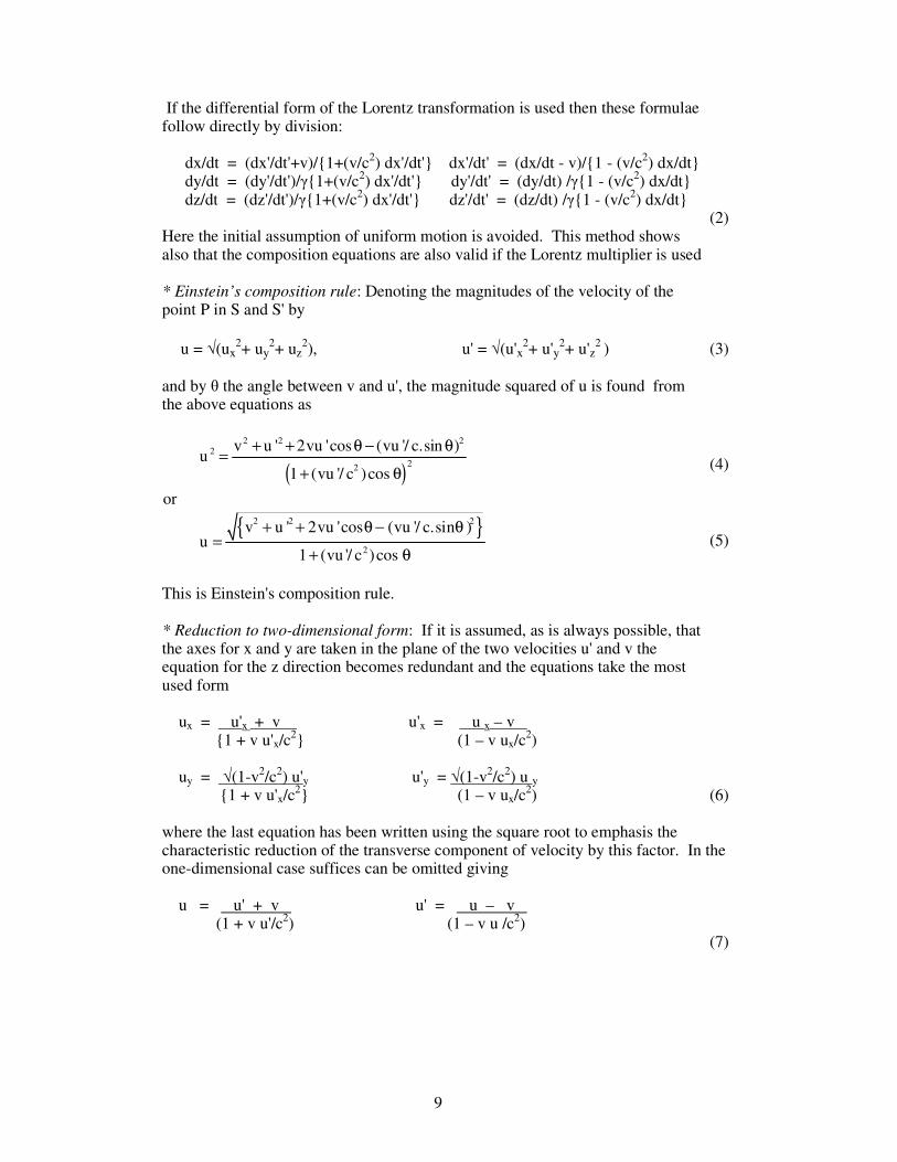
If the differential form of the Lorentz transformation is used then these formulae follow directly by division:
dx/dt = (dx'/dt'+v)/1+(v/c2) dx'/dt' dx'/dt' = (dx/dt - v)/1 - (v/c2) dx/dt dy/dt = (dy'/dt')/γ1+(v/c2) dx'/dt' dy'/dt' = (dy/dt) /γ1 - (v/c2) dx/dt dz/dt = (dz'/dt')/γ1+(v/c2) dx'/dt' dz'/dt' = (dz/dt) /γ1 - (v/c2) dx/dt
(2) Here the initial assumption of uniform motion is avoided. This method shows also that the composition equations are also valid if the Lorentz multiplier is used * Einstein’s composition rule: Denoting the magnitudes of the velocity of the point P in S and S' by
u = √(ux2+ uy
2+ uz2), u' = √(u'x
2+ u'y2+ u'z
2 ) (3) and by θ the angle between v and u', the magnitude squared of u is found from the above equations as
( )
2 2 22
22
v u ' 2vu 'cos (vu '/ c.sin )u
1 (vu '/ c )cos
+ + θ − θ=
+ θ (4)
or
2 2 2
2
v u ' 2vu 'cos (vu '/ c.sin )u
1 (vu '/ c )cos
+ + θ − θ=
+ θ (5)
This is Einstein's composition rule. * Reduction to two-dimensional form: If it is assumed, as is always possible, that the axes for x and y are taken in the plane of the two velocities u' and v the equation for the z direction becomes redundant and the equations take the most used form ux = u'x + v u'x = u x – v 1 + v u'x/c
2 (1 – v ux/c2)
uy = √(1-v2/c2) u'y u'y = √(1-v2/c2) u y 1 + v u'x/c
2 (1 – v ux/c2) (6)
where the last equation has been written using the square root to emphasis the characteristic reduction of the transverse component of velocity by this factor. In the one-dimensional case suffices can be omitted giving u = u' + v u' = u – v (1 + v u'/c2) (1 – v u /c2) (7)

10 10 10
4. The Lorentz Group The Lorentz group was at first defined by Poincaré (1905) for one dimensional motion and then (1906) as the group generated by the Lorentz translations in the x, y, and z directions. These generate also the group of spatial rotations which consequently is a subgroup of the Lorentz group. The group contains only homogeneous transformations in x, y, z, t and is what would now be called the restricted homogeneous Lorentz group. It only contains transformations retaining the sense of direction of t, i.e.it is orthochronos in current terminology. As defined by Poincaré, it may include optionally scalar multiplication (dilations) but following customary practice, this scalar will (for the present) be taken unity. Any transformation of this homogeneous group satisfies an equation
x'2+y'2+z'2-c2t'2 = x2+y2+z2-c2 t2 (1) This is because the generating transformations do and so it leaves invariant the quadratic form
x2+y2+z2 – c2t2 (2) The corresponding bilinear form is also left invariant. The homogeneous Lorentz group is nowadays frequently defined as the group of linear transformations leaving invariant the quadratic form (2). In this case the group may optionally be extended to include also time reversals and space reversals. Physically equation (1) implies that the sphere
x2+y2+z2 = (c t)2 (3) describing the outward expansion of a light wave starting from the origin at time t zero, becomes a similar sphere under Lorentz transformation. Any linear trans-formation having this property must be a homogeneous Lorentz transformation in the extended sense of Poincaré. This property leads to an algebraic derivation which has become standard for establishing the Lorentz transformation equations. Direct consideration of Maxwell’s equations is avoided this way. Apart from the linear transformations, nonlinear transformations also exist leaving invariant the quadratic form (2) (see the last chapter) If the Lorentz transformation is regarded as relating differential increments cdt, dx,
dy, dz then the group will include also nonhomogeneous transformations and will coincide with what is nowadays, rather unhistorically, called the Poincaré group. Under such transformations
dx'2+dy'2+dz'2- c2 dt'2 = dx2+dy2+dz2-c2 d t2 (4) which, interpreted physically, means that an infinitesimal sphere is transformed into itself by a Lorentz transformation. Such an infinitesimal sphere may be regarded as a Huyghens wavelet from which the finite wave (3) is generated. This approach analyses the physical situation at a more fundamental level (see Chapter 8).
11 11 11
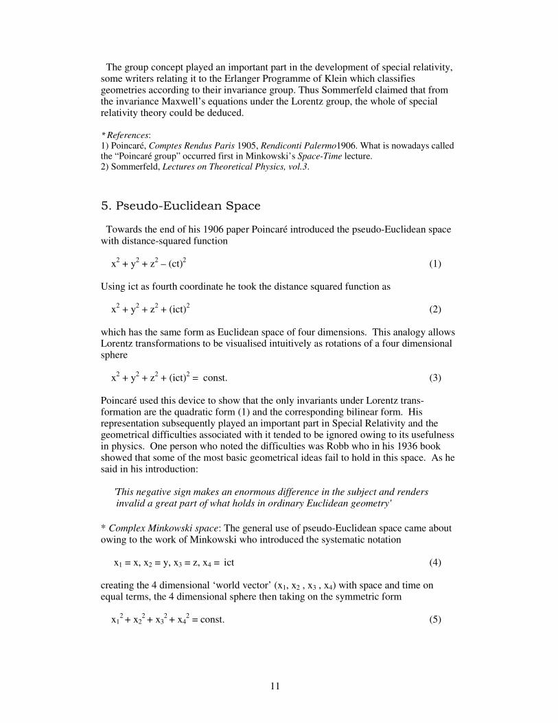
The group concept played an important part in the development of special relativity, some writers relating it to the Erlanger Programme of Klein which classifies geometries according to their invariance group. Thus Sommerfeld claimed that from the invariance Maxwell’s equations under the Lorentz group, the whole of special relativity theory could be deduced. * References: 1) Poincaré, Comptes Rendus Paris 1905, Rendiconti Palermo1906. What is nowadays called the “Poincaré group” occurred first in Minkowski’s Space-Time lecture. 2) Sommerfeld, Lectures on Theoretical Physics, vol.3.
5. Pseudo-Euclidean Space Towards the end of his 1906 paper Poincaré introduced the pseudo-Euclidean space with distance-squared function x2 + y2 + z2 – (ct)2 (1) Using ict as fourth coordinate he took the distance squared function as x2 + y2 + z2 + (ict)2 (2) which has the same form as Euclidean space of four dimensions. This analogy allows Lorentz transformations to be visualised intuitively as rotations of a four dimensional sphere x2 + y2 + z2 + (ict)2 = const. (3) Poincaré used this device to show that the only invariants under Lorentz trans-formation are the quadratic form (1) and the corresponding bilinear form. His representation subsequently played an important part in Special Relativity and the geometrical difficulties associated with it tended to be ignored owing to its usefulness in physics. One person who noted the difficulties was Robb who in his 1936 book showed that some of the most basic geometrical ideas fail to hold in this space. As he said in his introduction: 'This negative sign makes an enormous difference in the subject and renders
invalid a great part of what holds in ordinary Euclidean geometry'
* Complex Minkowski space: The general use of pseudo-Euclidean space came about owing to the work of Minkowski who introduced the systematic notation x1 = x, x2 = y, x3 = z, x4 = ict (4) creating the 4 dimensional ‘world vector’ (x1, x2 , x3 , x4) with space and time on equal terms, the 4 dimensional sphere then taking on the symmetric form x1
2 + x22 + x3
2 + x42 = const. (5)

12 12 12
In his 1908 paper ‘On the fundamental equations of electromagnetic processes in moving media’ Minkowski used this representation to give an impressive analysis of Maxwell’s equations, putting them in a form which made clear their complete four dimensional symmetry with respect to x1, x2, x3, x4. He used this symmetry to prove their invariance with respect to Lorentz transformations by a very simple argument: since they are clearly invariant under rotations of the space variables x1, x2, x3, they must, by symmetry, also be invariant under rotations involving the time variable x4, which typically would take the form x1' = x1 cos φ + x4 sin φ x4' = - x1 sin φ + x4 cos φ (6) When φ is a purely imaginary angle Minkowski defined as iψ where tanh ψ = v/c (7) Then equations (8) become the usual Lorentz equations. In his paper Minkowski also introduced the well known 4- and 6-vectors of the electromagnetic quantities and in the last part of the paper, he extended the four dimensional representation to dynamics. The methods and powerful analysis introduced by Minkowski exerted considerable influence on the subsequent development of special relativity. Sommerfeld in particular, followed and developed his line of thinking showing how the four dimensional representation can be used for vector analysis and the equations of mathematical physics. However, as we hope will be seen from the alternative view of this book, the Minkowski formulation has also had a negative influence Firstly in the promotion and use of pseudo-Euclidean space which, while being very useful for certain calculations, is unsatisfactory as a basis for theory. Secondly it has led to the view of the space of special relativity as flat and essentially Euclidean which overlooks the important relation with non-Euclidean space. Thirdly, putting time and space variables philosophically on equal terms is a view which cannot be maintained and is misleading, time being a distinguished variable as commonsense indicates. Notes: 1) Minkowski used the Lorentz form of the Maxwell-Herz equations which can be written concisely using modern suffix notation with summation convention as ∂fij = ρj ∂f*ij = 0 i, j = 1, 2, 3, 4 ∂xi ∂xi
where the arrays f and f* are skew symmetric matrices of the electromagnetic and magnetic vectors and the ρj give the four dimensional charge density vector. 2) Sommerfeld developed the Minkowski notation in his Ann. Phys 1909 paper, referred to in the next chapter, in his papers in Ann. Phys 1910 on vector analysis and vector calculus, and in his later book: Lectures on Mathematical Physics. 3) The view of Minkowski space as flat and essentially Euclidean of course also derives from General Relativity owing to the vanishing of the Riemann-Christoffel tensor. This however has no connexion with the non-Euclidean aspect referred to here as seen later.
13 13 13
6. Affine Minkowski Space In his famous 1908 lecture ‘Space and Time’, Minkowski presented his vision of a four dimensional space-time world without use of the complex representation but instead representing the variables x, y, z, t geometrically in a space of 'world events' by vectors (t,x,y,z). This representation is nowadays so familiar that it needs minimal description here but some comments are necessary. The structure of Minkowski space is determined by the group of affine trans-formations of the variables t, x, y, z. Such transformations preserve parallelism but make the coordinate axes oblique so distances are not preserved. For homogeneous Lorentz transformations which are special affine transformations, Minkowski showed that the obliqueness of the axes gives a geometrical explanation of the existence of the Lorentz contraction. The homogeneous Lorentz transformations conserve the family of hyperbolic surfaces x2 + y2 + z2 – c2 t2 = const. (1) which fill out the space and give it its characteristic structure. In the case when the constant is zero, the surface becomes the two sided light cone c2 t2 = x2 + y2 + z2 (2) which should perhaps properly be referred to as the Monge cone the properties of this cone having previously been described in detail by Monge (1808, 1850). Events are classified according to their relation with this cone as: (a) space-like if c2 t2 < x2+y2+z2
(b) null if c2 t2 = x2+y2+z2
(c) time-like if c2 t2 > x2+y2+z2 (3) these relationships being all Lorentz invariant. This classification is usually illustrated geometrically in reduced two dimensional form by the well known Minkowski diagram. In this diagram the naming ‘space-like’ is somewhat confusing since spatial events in physics are mostly determined by time-like events, these being mutually accessible by a signal of velocity less than that of light. Consequently time-like events, not space-like events, are important in physical phenomena. Time-like events all lie within the light cone, most evident geometrically in a 3-dimensional representation. * Scalar product: A scalar product of two event vectors (t, x, y, z), (t', x', y', z') may be defined in either a space-like or time-like manner. Using the time-like manner, it is ct ct' – x x' – y y' – z z' (4) It follows from the normal Cauchy inequality that the scalar product of two time-like events is positive: xx' + yy' + zz' ≤ √x2 + y2 + z2 √x '2 + y'2 + z '2 < ct ct' (5)

14 14 14
implying the strict inequality ct ct' – x x' – y y' – z z' > 0 (6) From this follows the impossiblity of having two orthogonal time-like events with ct ct' – x x' – y y' – z z' = 0 (7) If two events have such a property, one at least, must be space-like. * Convexity: The convexity property of the cone of time-like events means that for two time-like vectors (t,x,y,z), (t',x',y',z') the vector λ (t,x,y,z) + µ (t',x',y',z') where λ , µ > 0 is also time-like. This is deduced algebraically from c2 (λ t + µ t')2 – (λ x + µ x') 2 – ( λ y + µ y') 2 – (λ z + µ z')2 = λ2c2 t2 – (x2+y2+z2) + λµ ct.ct' – (xx'+yy'+zz') + µ2c2 t'2 – (x '2 + y'2 + z'2) (8) Here all terms on the right hand side are positive THEOREM: (Reversed Cauchy inequality): Time-like vectors (t, x, y, z), (t', x', y', z') satisfy ct ct' – xx' – yy' – zz' ≥ √(ct)2– x2 – y2 – z2 √(c t')2 – x' 2 – y' 2 – z' 2 (9) Equality holds only if the vectors are proportional. Proof: Consider the quadratic in λ f(λ) = λ 2(ct)2 – x2 – y2 – z2 + 2 λct ct' – xx' – yy' – zz'+ (ct')2 – x'2 – y'2 – z'2 = (λ ct-ct')2 – (λx-x')2 – (λy-y')2 – (λ z-z')2 (10) As λ tends to plus or minus infinity, f(λ) becomes positive while, when λ is t'/t f(λ) is negative or zero, being zero only if the vectors are proportional. So if the vectors are nonproportional, f(λ)=0 has two distinct real roots and the discriminant of the quadratic f(λ) is positive giving (ct ct' – xx' – yy' – zz')2 ≥ (ct)2 – x2 – y2 – z2(ct')2 – x' 2 – y'2 – z'2 (11) On taking positive square roots, inequality (9) follows from the positivity of the left hand side. There is equality only if the vectors are proportional ---------------------------------------------------------------------------------------------------- References: 1) On the Monge cone see Klein’s Die Entwicklung der Mathematik … 2) This proof of the reversed Cauchy inequality is due to Aczél (1956). Another proof is given later.

15 15 15
7. Ordering of Time-like Events In the cone of time-like events a partial ordering may be defined where the relation 'after' is interpreted as meaning that a light signal can pass from the first event to the second. Denoting the two events by (t1, x1, y1, z1), (t2, x2, y2, z2) the relation is (t2, x2, y2, z2) ≥ (t1, x1, y1, z1) (1) This has the meaning that c(t2 - t1) ≥ √(x2 - x1)
2 + (y2 - y1)2 + (z2 - z1)
2 (2) The inequality here is Lorentz invariant. This partial ordering breaks up the double sided cone of time-like events into the future and past cones of events (t, x,y,z) ≥ (0,0,0,0) (t,x,y,z) ≤ (0,0,0,0) (3) * Trajectories: A physically realizable motion is represented by a trajectory or ‘world-line’. This is a curve in the cone of time-like events where successive increments satisfy (c dt)2 > (dx2 + dy2 + dz2) (4) Then, with Minkowski, a variable τ may be defined having differential dτ = √dt2 - (dx2 + dy2 + dz2)/c2 (5) By differentiation of the moving point (t, x, y, z) with respect to variable τ there are derived Minkowski’s velocity and acceleration four vectors (dt/dτ, dx/dτ, dy/dτ, dz/dτ), (d2t/dτ2, d2x/dτ2, d2y/dτ2, d2z/dτ2) (6) These are important for his four dimensional formulation of dynamics. The components of the velocity vector satisfy the identity c2 (dt/dτ)2 - (dx/dτ)2 - (dy/dτ)2 – (dz/dτ)2 = c2 (7) showing that the four-velocity is time-like. This identity shows that the 4 velocity vector lies on a two sheeted hyperboloid and so is three dimensional. By differentiation follows c2 (dt/dτ) (d2t/dτ2) – (dx/dτ) (d2x/dτ2) – (dy/dτ) (d2y/dτ2) – (dz/dτ) (d2z/dτ2) = 0 (8) i.e. the scalar product of velocity and acceleration four-vectors is zero. Since the velocity vector has the time-like property the acceleration vector cannot also be time-like and so has the space-like property (although, like the velocity four-vector, it is not properly speaking an element in the Minkowski space).

16 16 16
* Reversed triangle inequality: A more precise definition of proper time follows from the reversed triangle inequality which is an immediate deduction from the reversed Cauchy inequality. THEOREM: If (t, x, y, z), (t', x', y', z') are two time-like vectors. √(ct)2-x2-y2-z2 + √(ct')2-x'2-y'2-z'2 ≤ √c2(t+t')2-(x+x')2-(y+y')2-(z+z')2 (9)
Proof: From the reversed Cauchy inequality follows [√(ct)2-x2-y2-z2 + √(ct')2-x'2-y'2-z'2]2
= (ct)2-x2-y2-z2 + 2√(ct)2-x2-y2-z2√(ct')2-x'2-y'2-z'2 + (ct')2-x'2-y'2-z'2 < (ct)2-x2-y2-z2 + 2ct.ct'-xx'-yy'-zz' + (ct')2-x'2-y'2-z'2 = c2 (t+t')2 - (x+x')2 - (y+y')2 – (z+z')2 (10) Taking the positive square root gives the reversed triangle inequality which may be written in terms of T(t, x, y, z) = √t2-(x2 + y2 + z2)/c2 (11) as T(t, x, y, z) + T(t', x', y', z') ≤ T(t+t', x+x', y+y', z+z') (12)
* Definition of proper time along a trajectory: Another statement of the theorem is in terms of intervals so that if e.g.
(t1, x1, y1, z1) ≤ (t2, x2, y2, z2) ≤ (t3, x3, y3, z3) (13)
then
T(t3 – t2, x3 – x2, y3 – y2, z3 – z2) + T(t2 – t1, x2 – x1, y2 – y1, z2 – z1) ≤ T(t3 – t1, x3 – x1, y3 – y1, z3 – z1) (14) This inequality immediately extends to a multiple division of a fixed interval by an ordered set of time-space values. If these values lie on a world line trajectory then it will be possible to take a minimum (or more precisely an infimum) as the number of points on the trajectory tends to infinity so giving a rigorous definition of the proper time for traversing the trajectory.

17 17 17
Notes: 1) The partial ordering of time-like events was observed by Robb (1913) and Carathéodory (1923) both of whom made it the basis of an axiomatic approach to relativity. Later the idea was mentioned by other writers: Birkhoff: Lattice Theory 1948, Andronov: Canad. J. Math.1957 and Zeeman: J Math. Phys.1960 the last two showing that ordering on the forward cone implies its Lorentz structure. 2) Bellman proved a generalization of the reversed triangle inequality for pth powers by a quite different method. See ‘On an inequality ...’, Amer. Math. Monthly, 1956

18 18 18
CHAPTER 2 - Product of Lorentz Translations
1. The Standard Form of a Lorentz Translation. The standard form for the Lorentz translation for a velocity v having components v1, v2, v3 will be taken to be
1 2 3
2
1 1 1 2 1 3
2
2 2 1 2 2 3
2
3 3 1 3 2 3
v / c v / c v / ccdt ' cdt
v / c 1 ( 1)n ( 1)n n ( 1)n ndx ' dx
dy ' dyv / c ( 1)n n 1 ( 1)n ( 1)n n
dz ' dzv / c ( 1)n n ( 1)n n 1 ( 1)n
γ −γ −γ −γ −γ + γ − γ − γ − = −γ γ − + γ − γ − −γ γ − γ − + γ − (1)
where n1, n2, n3 are components of the unit vector n in the direction of the velocity. The matrix of coefficients is symmetric and its inverse is obtained by changing v to –v. The relation can be written more concisely using partitioned matrices as
T
T
cdt ' cdt/ c
/ c I ( 1)
γ −γ = −γ + γ −
v
dr' drv nn (2)
Bold letters are used for 3x1 column vectors for emphasis. Using nondimensional parameters β (= v/c) and γ the transformation is
1 2 3
21 1 1 2 1 3
22 2 1 2 2 3
23 3 1 3 2 3
n n ncdt ' cdt
n 1 ( 1)n ( 1)n n ( 1)n ndx ' dx
n ( 1)n n 1 ( 1)n ( 1)n ndy ' dy
n ( 1)n n ( 1)n n 1 ( 1)ndz ' dz
γ −βγ −βγ −βγ −βγ + γ − γ − γ − = −βγ γ − + γ − γ − −βγ γ − γ − + γ −
(3) Equivalently, using partitioned matrices,
T
T
cdt ' cdt
I ( 1)
γ −γβ = −γβ + γ −
n
dr' drn nn
(4) The characteristic operator here is the 3x3 matrix I + (γ-1) nn
T = (I - nnT) + γ nn
T (5) This can also be considered vectorially as a dyadic (Silberstein 1914). When this matrix acts on any vector, the first term on the right forms the component of the vector perpendicular to n while the second term stretches the vector by a factor γ in the direction n. Thus if denotes component perpendicular to n, (I - nn
T) + γ nnTdr = dr
+ γ n (nTdr) (6)
19 19 19
2. The Product of Lorentz Translations. The explicit representation of the product of two Lorentz translations has been an enduring problem of Special Relativity. Since a Lorentz translation has a symmetric matrix it is clear that such a product will not also be a Lorentz translation. As is now well known, it is a Lorentz translation either followed or preceded by a spatial rotation. This important observation was apparently first made by Silberstein (1914) So that the composition of L1 followed by L2 may be written L2 L1 = R L r = Ll R (1) R is a spatial rotation matrix and L r and Ll the corresponding right and left Lorentz translations resulting from the composition. Here it is has been assumed that the rotation matrices for right and left multiplication are the same and this fact will be clear from the canonical form shown below. Note first that relations (1) imply on taking transposes that L1 L2 = L r R
-1 = R-1 Ll (2) since the Lorentz translation matrices are symmetric and the transpose of a rotation matrix gives its inverse. * The canonical form: The relation between right and left Lorentz translations can be more clearly demonstrated as follows. Using the right hand Lorentz translation, let us write the product as
T
T
1 0
0 I ( 1)
γ −βγ Ω −βγ + γ −
n
n nn (3)
Here Ω is a 3x3 rotation matrix. This product is
T
T( 1)(
γ −βγ −βγ Ω Ω + γ − Ω
n
n n)n
(4) It is now convenient to introduce the unit vector n'
n' = Ω n (5) so that Ω turns n into n'. From this follows, since transposition of Ω gives its inverse,
20 20 20
n = Ω -1 n' = ΩT n' (6) The matrix product can now be written in the more symmetric form
T
T( 1)
γ −βγ −βγ Ω + γ −
n
n' n'n (7)
It can now be transformed with the same rotation matrix into the left translation form
T
T
1 0
0I ( 1)
γ −βγ Ω−βγ + γ −
n'
n' n'n' (8)
The form (7) will be taken as the canonical form for the product of two Lorentz transformations. It represents the most general element of the Lorentz group as may be seen as follows. Given two such matrices, the first may be put in the form (3) and the second in the form (8). Their product then involves the product of two Lorentz translations which is again a canonical matrix. Such products generate the whole Lorentz group. Each element of the group is characterized by the angle of Ω which is additive on multiplication of the matrices.
3. The Explicit Product The explicit product can be found by the method of Silberstein. In obvious notation the product L2 L1 is
T T
2 2 2 2 1 1 1 1
T T
2 2 2 2 2 2 1 1 1 1 1 1I ( 1) I ( 1)
γ −β γ γ −β γ −β γ + γ − −β γ + γ −
n n
n n n n n n
T
T
1 0
0 I ( 1)
γ −βγ = Ω −βγ + γ −
n
n nn
(1) There is found after adjustments for sign, transposition, etc.
γ = γ1 γ2 1 + β1β2 n2Tn1
βγ n = γ2 ( I + (γ1-1) n1n1
T) β2 n2 + γ1 β1 n1 βγ Ωn = γ1 ( I + (γ2-1) n2n2
T) β1 n1 + γ2 β2 n2 Ω + (γ-1) (Ωn)nT
= β2 β1 γ2 γ1 n2n1T + (I + (γ2-1) n2n2
T)(I + (γ1-1) n1n1T)
(2)
From the 1st and 2nd of these equations follows

21 21 21
β n = (I + (γ1-1) n1 n1T) β2 n2 + γ1β1.n1
γ11 + β1β2 n1Tn2
= γ1
-1 (I - n1 n1T) + n1 n1
T β2 n2 + β1.n1
1 + β1β2 n1Tn2
= √(1 - β1
2) (I - n1 n1T) β2 n2 + n1
Tn2 β2 + β1n1
1 + β1β2 n1Tn2 (3)
Here the numerator is resolved into components orthogonal and parallel to n1 and the equation can be written, using the angle θ say between n1
and n2, as
β n = √(1 - β12) β2 sin θ
n1 + β2 cos θ + β1n1
1 + β1β2 cos θ (4) where n1
is the unit vector orthogonal to n1. In a similar way is found
β Ωn = β n' = √(1 - β22) β1 sin θ
n2 + β1 cos θ + β2n2
1 + β1β2 cos θ (5) * The Einstein composition formula: These expressions show the relation to velocity composition and there follows immediately for the magnitude squared
β 2 = (1 - β12) β2
2 sin2 θ + β2 cos θ + β1
2 1 + β1β2 cos θ2 = β1
2 + 2 β1β2 cos θ + β22 – (β1β2)
2 sin2 θ
1 + β1β2 cos θ2 (6) Or in terms of velocity,
v 2 = v12 + 2 v1v2 cos θ + v2
2 – (v1v2/c)2 sin2 θ
1 + v1v2/c2 .cos θ2 (7)
------------------------------------------------------------------------------------------------------ * Reference: The calculation here is its equivalent using matrices of Silberstein's 1914 calculation using vector and dyadic notation. 4. Composition of Orthogonal Motions The composition formulae may be simplified by taking the plane of the two velocities as the xy plane so that the z-axis then becomes redundant. The Lorentz matrices can then be written conveniently as 3 x 3 matrices transforming only the variables ct, x, y while the spatial rotation matrix Ω can be written as the 2x2 matrix
Ω = cos sin
si n cos
ψ ψ − ψ ψ
(1)
Ψ is the rotation angle, which is the angle Ω turns n through to give n'.

22 22 22
* Composition of orthogonal velocities: This is an important special case. The velocities may be taken along the x and y axes and then introducing as before β1, β2, β, for the ratios v1/c, v2/c, v/c the Lorentz matrices will be
L1 =
1 1 1
1 1 1
0
0
0 0 1
γ −γ β −γ β γ
(2)
L2 =
2 2 2
2 2 2
0
0 1 0
0
γ −γ β −γ β γ
(3) The product is
L2.L1 =
1 2 1 2 1 2 2
1 1 1
1 2 2 1 2 1 2 2
0
γ γ −γ γ β −γ β −γ β γ −γ γ β γ γ β β γ
(4) There follow the equations γ = γ1 γ2
γ β nT = [γ1 γ2 β1, γ2 β2] γ β (Ωn)T = [γ1 β1, γ1γ2 β2] (5) Here the value of β is given by β2 = β1
2 + β22/γ1
2 = β12/γ2
2 + β22 = β1
2 + β22 - β1
2 β22 (6)
The unit vectors n, n' for the two velocity compositions are nT = [β1, β2 /γ1] β
-1 = [β1, β2 √(1 - β12)] β-1
n' T = [β1/γ2, β2] β-1 = [β1√(1 - β2
2), β2] β-1 (7)
The resulting right hand Lorentz translation can be constructed using n and the product L2.L1 written as
1 2 1
21 1 1 2 1
22 1 2 1 1 2 1
1 0 0 ( / )
0 cos si n 1 ( 1)( / ) ( 1)( / )( / )
0 si n cos ( / ) ( 1)( / )( / ) 1 ( 1)( / )
γ −γβ −γ β γ ψ − ψ −γβ + γ − β β γ − β β β βγ ψ ψ −γ β γ γ − β βγ β β + γ − β βγ
(8) Similarly the left hand Lorentz translation can be constructed using n' and the product written

23 23 23
1 2 2
21 2 1 2 1 2 2
22 2 1 2 2
( / ) 1 0 0
( / ) 1 ( 1)( / ) ( 1)( / )( / ) 0 cos si n
( 1)( / )( / ) 1 ( 1)( / ) 0 si n cos
γ −γ β γ −γβ −γ β γ + γ − β βγ γ − β βγ β β ψ − ψ −γβ γ − β β β βγ + γ − β β ψ ψ
(9) The corresponding representation of L1 L2 is found by transposition which interchanges the Lorentz matrices and replaces Ψ by - Ψ. 5. Rotation Angle for Orthogonal Motions The rotation angle Ψ may be determined by forming scalar and vector products of n and n' which give cos Ψ and sin Ψ. In the case of composition of orthogonal motions there is found in this way, using values of n and n' found in the previous section, cosΨ = (√(1 - β2
2) β12 + √(1 - β1
2) β22)/ β2 = (γ2
-1 β12 + γ1
-1 β22)/ β2
sin Ψ = β1β2 (1 - √(1 - β12)(1 - β2
2))/ β2 = β1β2 (1 - γ1-1γ2
-1)/ β2 tan Ψ = β1β2 (γ1γ2 - 1)/ (γ1 β1
2+ γ2 β22)
(1) These may be expressed in various ways by algebraic transformation e.g. cos Ψ = (γ1 + γ2 )(1 - γ1 γ2 )/ β
2 = (γ1 + γ2 )/ (1 + γ1 γ2 ) sin Ψ = β1β2/ (1 + γ1
-1γ2-1) = β1γ1 β2γ2/ (1+ γ1γ2)
tan Ψ = β1γ1 β2γ2 / (γ1 + γ2 ) (2) Corresponding formulae may be given in terms of the velocities v1, v2, e.g. cos Ψ = v1
2 √(1- v2 2/c2) + v2
2 √(1- v12/c2)
v12 + v2
2 – (v1 v2 /c)2 (3) sin Ψ = v1 v2 1 – √(1- v1
2/c2)√ (1 – v22/c2)
v12 + v2
2 – (v1 v2 /c)2
= v1 v2 c2 1 + √(1- v1
2/c2)√(1 – v22/c2) (4)
tan Ψ = v1 v2 1 – √(1- v1
2/c2)√(1 – v22/c2)
v12 √(1- v2
2/c2) + v22 √(1- v1
2/c2) (5) * Half-angle formulae: The half-angle formulae for rotation angle Ψ take a simpler form. They appear to have some importance in the theory. They may be found from: cos2 Ψ/2 = 1 + cos Ψ = (γ1 + 1) (γ2 + 1) 2 2 (1 + γ1γ2) sin2 Ψ/2 = 1 - cos Ψ = (γ1 - 1) (γ2 - 1) 2 2 (1 + γ1γ2) tan2 Ψ/2 = sin2 Ψ/2 = (γ1 - 1) (γ2 - 1) cos2 Ψ/2 (γ1 + 1) (γ2 + 1) (6)
24 24 24
From the last follows a formula due to Liebmann (quoted by Varićak 1912) cot Ψ/2 = /(γ1 + 1) (γ2 + 1) √ (γ1 - 1) (γ2 – 1) (7) 6. The Thomas Precession The Thomas precession is a well known rotational effect occurring whenever acceleration α is in a different direction to velocity so that the velocities v, v + δv at successive instants t, t + δt do not have the same direction. The combination of the Lorentz matrices for these velocities results in an infinitesimal infinitesimal rotation δΨ. One method of calculating this is by the formulae which have been derived for combination of orthogonal velocities. If vector velocities v and δv are inclined at an angle θ, the increment δv has components parallel and orthogonal to v of δv cos θ, δv sin θ. Being infinitesimal, their effects may be superimposed, and to the first order of small quantities, the resulting infinitesimal rotation δΨ arises only from the orthogonal component. So the rotation angle may be found from the previous formula
sin Ψ = v1 v2 c2 1 + √(1- v1
2/c2) √(1 – v22/c2)
(1) On setting
v1 = v, v2 = δv sin θ = α δt sin θ, Ψ = δΨ (2) the following approximations will hold to first order:
√(1 - v1²/c²) ≈ √(1 - v²/c²) = γ -1, √(1 - v2²/c²) ≈ 1 (3)
The angular velocity relative to the observer is dΨ = v α sin θ . = 1 - √(1- v2/c2) v α sin θ dt c2 1 + √(1- v2/c2) v2 (4) Relative to the moving point it is dΨ = 1 - √(1- v2/c2) v α sin θ = γ - 1 v α sin θ dτ v2 √(1- v2/c2) v2 (5) This can be written as the vector equation dΨ = (γ - 1) v x α (6) d τ v² The rotation is about an axis perpendicular to v and α and in the direction of v x α.
25 25 25
* Approximation for v<<c: If the velocity v is small compared with that of light, δΨ ≈ sin δΨ = v1 v2 ≈ v1 v2 = v δv sin θ c2 1 + √(1- v1
2/c2) √(1 – v22/c2) 2 c2 2 c2
(7) resulting in dΨ = v α sin θ dt 2 c2 (8) dΨ = v x α d τ 2 c2 (9) ------------------------------------------------------------------------------------------------------- Note: The Thomas rotation was encountered in connexion with the accelerated motion of an electron in an electric field where the formula for spin of Goudschmidt and Uhlenbeck was corrected by Thomas (1926, 1927). Thomas’ first paper gave the approximate formula, the more accurate formula being given in his second paper. It is interesting that Borel had previously deduced in 1913 on purely mathematical grounds that such an effect would occur. Subsequent to Thomas’ work the spatial rotation associated with the composition of two general Lorentz translations also became known as the Thomas rotation even though the Thomas precession is only a special case. When, at a later period, the same phenomenon found application in quantum mechanics and particle physics, the name 'Wigner rotation' also came into use for the general rotation. ---------------------------------------------------------------------------------------------------------- References: Thomas: Nature 1926 p.514; Phil. Mag. 7 1927 1-23; Borel: C.R. Acad. Sci. Paris 1913; Wigner: Rev. Mod. Phys 1957; Borel’s observation is described by Scott-Walker 1999.
26 26 26
CHAPTER 3 – Sommerfeld’s Spherical Theory 1. The Lorentz Transformation as Rotation. In his fundamental 1909 paper ‘On the composition of velocities', Sommerfeld aimed
to show how the space-time view of Minkowski, then recently introduced, could be of real use to physicists. His spherical interpretation of Einstein’s composition formula led on directly to the hyperbolic theory. As previously described, Minkowski had, In his investigation of Maxwell’s equations, somewhat incidentally, represented the Lorentz transformation as a Euclidean rotation
x' = x cos φ + ict sin φ ict' = - x sin φ + ict cos φ (1)
The purely imaginary angle φ is defined by
tan φ = i v/c (2) implying
cos φ = 1 = γ sin φ = i (v/c) = i βγ (3) √(1 - v2/c2) √(1 - v2/c2)
Sommerfeld pointed out that this representation simplifies the composition rule for rectilinear motion since the result of two successive Lorentz transformations of angles φ1, φ2 is the Lorentz transformation with angle φ1 + φ2 given by
iv/c = tan (φ1 + φ2) = tan φ1 + tan φ2 = iv1/c + iv2/c 1 - tan φ1 tan φ2 1 – iv1/c iv2/c (4)
There follows the composition rule
v = v1 + v2 (5) 1 + v1 v2 /c
2 This new method of deriving the composition rule soon came into general use and was, for example, used by Einstein in his 1921 Princeton lectures replacing his earlier method. It is now well known. Not so well known however, is the generalization of this idea to the non-rectilinear case introduced by Sommerfeld in his 1909 paper and subsequent writings. ---------------------------------------------------------------------------------------------- Reference: Sommerfeld A: ‘Über die Zusammensetzung der Geschwindigkeiten’ Phys.Z. 1909 826-829.

27 27 27
2. Non-commutativity of Velocity Addition Einstein’s 1905 derivation of the composition rule gave the magnitude of the resultant of two velocities but had said nothing about its direction. Sommerfeld attempted to clarify this situation by combining two orthogonal velocities
v1 = (v1, 0), v2 = (0, v2) (1) This can be done in two possible ways - v1 followed by v2 and v2 followed by v1. He found, in agreement with Einstein's calculation (cf chapter 1), for the resultant velocities corresponding to these two ways the values
(v1, v2√(1 – v12/c2)), (v1√(1 – v2
2/c2), v2) (2) These have the same magnitude squared
v2 = v12 + v2
2 – (v1 v2 /c)2 (3) which can be written in either of two ways corresponding to the two resultants:
v2 = v12 + v2
2 (1 - v12/c²) = v1
2 (1 - v22/c²) + v2
2 (4) From these are found Pythagoras formulae corresponding to the figure below. The resultant velocities are represented by lines AC and C'A' of equal length.
Fig: Non-commutativity of velocity composition (Cartesian form) Multiplication of the transverse velocity components by contraction factors results in failure of the rectangular figure to close giving rise to what became known as non-commutativity of velocity addition. The angle Ψ between the resultants, which was already determined in the last chapter, is easily also found from this diagram by taking scalar and vector products of the vectors (2). As seen in the last chapter, composition of the Lorentz translations results in a rotation through the angle Ψ. The curious consequence of this is apparently to make an interchange of directions so that v1 followed by v2 results, not in vector AC, but in C'A' - this vector turned through angle Ψ. It is similar for v2 followed by v1.
28 28 28
3. The Spherical Representation Sommerfeld explained noncommutativity of velocity addition as arising from addition of displacements on a sphere determined by the Minkowski angles. In the case of addition of orthogonal velocities, the relation between the velocities v1, v2 and their resultant v may be written
(1 - v2/c2) = (1 - v12/c2) (1 - v2
2/c2) (1) This gives
1 = 1 1 √(1 - v2/c2) √(1 - v1
2/c2) √(1 – v22/c2 ) (2)
By using Minkowski angles φ, φ1, φ2, corresponding to v, v1, v2, the equation becomes
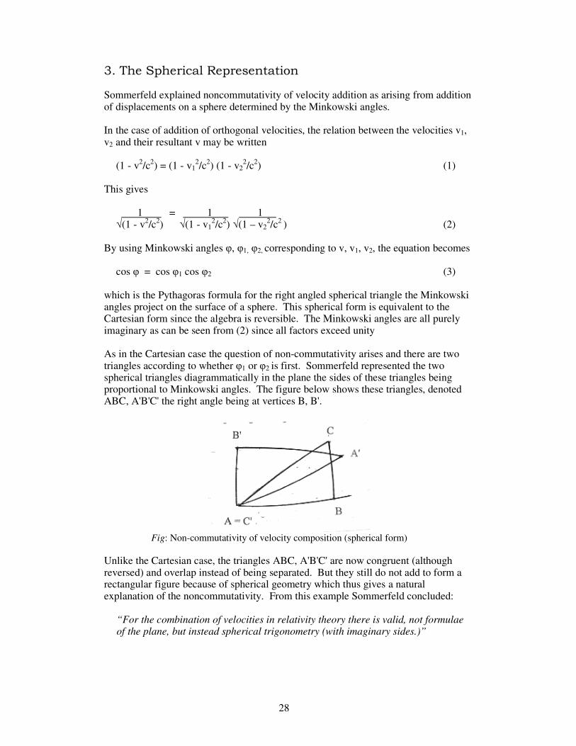
cos φ = cos φ1 cos φ2 (3) which is the Pythagoras formula for the right angled spherical triangle the Minkowski angles project on the surface of a sphere. This spherical form is equivalent to the Cartesian form since the algebra is reversible. The Minkowski angles are all purely imaginary as can be seen from (2) since all factors exceed unity As in the Cartesian case the question of non-commutativity arises and there are two triangles according to whether φ1 or φ2 is first. Sommerfeld represented the two spherical triangles diagrammatically in the plane the sides of these triangles being proportional to Minkowski angles. The figure below shows these triangles, denoted ABC, A'B'C' the right angle being at vertices B, B'.
Fig: Non-commutativity of velocity composition (spherical form) Unlike the Cartesian case, the triangles ABC, A'B'C' are now congruent (although reversed) and overlap instead of being separated. But they still do not add to form a rectangular figure because of spherical geometry which thus gives a natural explanation of the noncommutativity. From this example Sommerfeld concluded:
“For the combination of velocities in relativity theory there is valid, not formulae of the plane, but instead spherical trigonometry (with imaginary sides.)”
29 29 29
4. Spherical Form of the Einstein Composition Formula Extending these ideas, Sommerfeld derived the general composition law for inclined velocities. The Minkowski angle φ of the resultant velocity v is given by vector addition of the arcs on a sphere of the Minkowski angles φ1, φ2 for v1, v2 so that by the spherical cosine rule:
cos φ = cos φ1 cos φ2 + sin φ1 sin φ2 cos (π – θ) (4) where θ is the angle of inclination of velocities v1, v2. This is
cos φ = cos φ1 cos φ2 – sin φ1 sin φ2 cos θ (5) Changing from Minkowski angles to velocities gives
1 = 1 – (iv1/c) (iv2/c) cos θ √(1 – v2/c2) √(1 – v1
2/c2)√(1 – v22/c2) √(1 – v1
2/c2) √(1 – v22/c2)
(6) = (1 + v1 v2/c
2 cos θ) √(1 – v1
2/c2)√(1 – v22/c2)
(7) Inversion and squaring results in
(1 - v2/c2) = (1 – v12/c2) (1 – v2
2/c2) (1 + v1 v2 /c
2 cos θ)2 (8) Then solving for v gives Einstein’s composition law _________________________________
v = √v12 + v2
2 + 2 v1 v2 cos θ – (v1 v2/c sin θ)2 1 + (v1 v2 /c
2) cos θ (9) The algebra here is reversible so that starting from the composition formula the spherical cosine rule can be deduced.
30 30 30
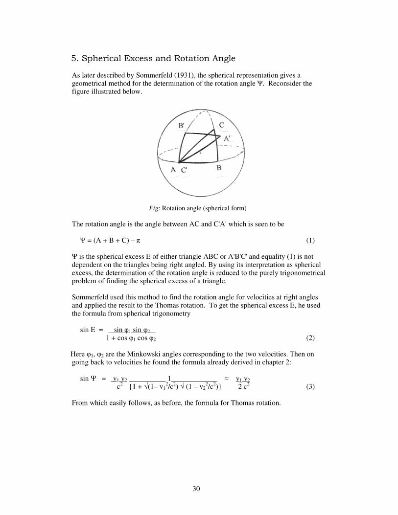
5. Spherical Excess and Rotation Angle As later described by Sommerfeld (1931), the spherical representation gives a geometrical method for the determination of the rotation angle Ψ. Reconsider the figure illustrated below.
Fig: Rotation angle (spherical form) The rotation angle is the angle between AC and C'A' which is seen to be
Ψ = (A + B + C) – π (1) Ψ is the spherical excess E of either triangle ABC or A'B'C' and equality (1) is not dependent on the triangles being right angled. By using its interpretation as spherical excess, the determination of the rotation angle is reduced to the purely trigonometrical problem of finding the spherical excess of a triangle. Sommerfeld used this method to find the rotation angle for velocities at right angles and applied the result to the Thomas rotation. To get the spherical excess E, he used the formula from spherical trigonometry
sin E = sin φ1 sin φ2 1 + cos φ1 cos φ2 (2)
Here φ1, φ2 are the Minkowski angles corresponding to the two velocities. Then on going back to velocities he found the formula already derived in chapter 2:
sin Ψ = v1 v2 1 ≈ v1 v2 c2 1 + √(1– v1
2/c2) √ (1 – v22/c2) 2 c2 (3)
From which easily follows, as before, the formula for Thomas rotation.

31 31 31
* Note: Sommerfeld did not give details of the derivation of the relation (2) dismissing it as elementary. Though elementary, the proof is somewhat tricky. It needs the use of sine, cosine and cotangent formulae in the forms
sin A = sin φ1/ sin φ , sin C = sin φ2 / sin φ cos φ = cos φ1 cos φ2 cot A cot C = cos φ
Then, since B is π/2,
sin E = sin (A + C – π/2) = – cos (A+C) = – cos A cos C + sin A sin C = sin A sin C (1 – cot A cot C) = (sin φ1/ sin φ) (sin φ2/ sin φ) (1 – cos φ) = sin φ1 sin φ2 (1 – cos φ) / (1 – cos2φ) = sin φ1 sin φ2 / (1 + cos φ) = sin φ1 sin φ2 / (1 + cos φ1 cos φ2) (4)
Quod erat demonstradum!
6. Central Projection and the Contraction Factor An interesting aspect of the Sommerfeld representation, which Sommerfeld himself did not analyse in detail is its relation with central projection of the sphere on to a tangential plane. Here is seen the possiblity, through non-Euclidean geometry, of explaining the contraction so typical of relativistic formulae. At the same time there is revealed a shortcoming of the spherical representation. The relation between velocities and their Minkowski angles, which may be written
v = R tan φ (1) with R equal to c/i ( = – ic), suggests the geometrical representation shown in the first figure below; it leads to the idea of projection of the spherical triangle ABC on to another triangle A1B1C1 in the tangential plane at one vertex (A in the second figure)
Fig. Geometric meaning of Fig. Central projection of a right- Minkowski angle -angled spherical triangle.

32 32 32
This geometrical representation of course ignores the fact that both R and φ are imaginary and R is even negative. Such a figure is only permissible in the spirit of the Sommerfeld representation which ignores all problems associated with geometrical representation of complex quantities in the attempt to provide an intuitive picture to aid thinking. The ultimate justification for doing this is that the resulting relationships become strictly valid in the hyperbolic version considered below. In this representation the tangential sides A1B1, A1C1, B1C1 are
R tan φ1 = v1 R tan φ = v (R sec φ1) tan φ2 = (R tan φ2) sec φ1 = v2 √(1– v1
2/c2) (2) The spherical triangle and its projection are shown below together for comparison.
ig. The spherical triangle
Fig. The projected triangle The Cartesian components vx, vy of the resultant velocity v are A1B1, B1C1 given by
vx = R tan φ1 = v1 _______ vy = (R tan φ2) sec φ1 = v2 √(1– v1
2/c2) (3) This explains the existence of the contraction factor affecting transverse velocity. While this calculation and its diagrammatic illustration are in principle correct, a contradiction arises from the geometrical representation. The figure above shows the third side OB1 greater than OA1 after multiplication by the factor sec φ1 whereas, because φ1 is purely imaginary, sec φ1 is less than unity and so OB1 should be less than OA1.
33 33 33
The contradiction can be avoided by adhering to the following derivation which however loses the geometrical picture. From the basic equations of spherical trigonometry applied to the right-angled spherical triangle ABC we get
tan φ1 = tan φ cos A sin φ2 = sin φ sin A cos φ = cos φ1 cos φ2 (4)
From the second and third of these equations follows
tan φ sin A = tan φ2 sec φ1 (5) so that the Cartesian components are, using these equations,
vx = v cos A = R tan φ cos A = R tan φ1 = v1 vy = v sin A = R tan φ sin A = R tan φ2 sec φ1 = v2 √(1 – v1
2/c2) (6) ------------------------------------------------------------------------------------------------------- References: 1) On Sommerfeld’s approach to relativity see especially his Lectures on Theoretical Physics. vol.3, Engl. tr. 1952 (Academic Press) See also the book of Rosenfeld: Non-Euclidean Geometry. 1988 (Springer) 2) Sommerfeld’s paper on Thomas rotation was 'Vereinfachte Ableitung des Thomasfactors'. Convegno di Fisica Nucleare, Rome 1931 reprinted in: Atombau und Spektrallinien 1931; Engl.tr. Atomic Structure and Spectral Lines,1952. He again described the method on pp 234-235 of vol.3 of his Lectures on Theoretical Physics. Engl. tr. New York 1952 (Academic Press) A review paper with valuable historical comment is Belloni & Reina: 'Sommerfeld's way to the Thomas precession', Eur. J. Phys. 1986. This paper credits the initial idea to Langevin.

34 34 34
CHAPTER 4 – The Hyperbolic Theory
1. Rapidity The basic quantity of the hyperbolic theory is the rapidity w defined in terms of the velocity by
th w = v/c (1) the principal value of the inverse hyperbolic tangent being used for the determination of w from this equation. Corresponding to any value of v less in magnitude to c this equation determines a value of w lying in the range - ∞ < w < ∞. Transforming the Minkowski rotational representation and its inverse
x' = x cos φ + ict sin φ x = x' cos φ - ict' sin φ ict' = - x sin φ + ict cos φ ict = x' sin φ + ict' cos φ (2)
by setting φ to be iw and using the identities
cos φ = cos iw = ch w sin φ = sin iw = i sh w (3)
there arises the symmetric transformation and its inverse
ct' = ct ch w - x sh w ct = ct' ch w + x' sh w x' = - ct sh w + x ch w x = ct' sh w + x' ch w (4)
which is the representation in terms of rapidity. Note that from (1) follows
ch w = 1 sh w = (v/c) (5) √(1- v2/c2) √ (1- v2/c2)
* Additivity: The characteristic property of rapidity is its additivity for velocity composition. This additivity is obvious from the relation with Minkowski's imaginary Euclidean form but can also be seen directly from the identity
th (w1+w2) = th w1 + th w2 1 + th w1 th w2 (6)
which immediately results in the composition law
v = v1 + v2 1 + v1 v2/c
2 (7)
for the velocity v corresponding to rapidity w1 + w2 so that for the rapidities w1,w2,w corresponding to v1,v2,v it is true that
w = w1 + w2 (8)
35 35 35
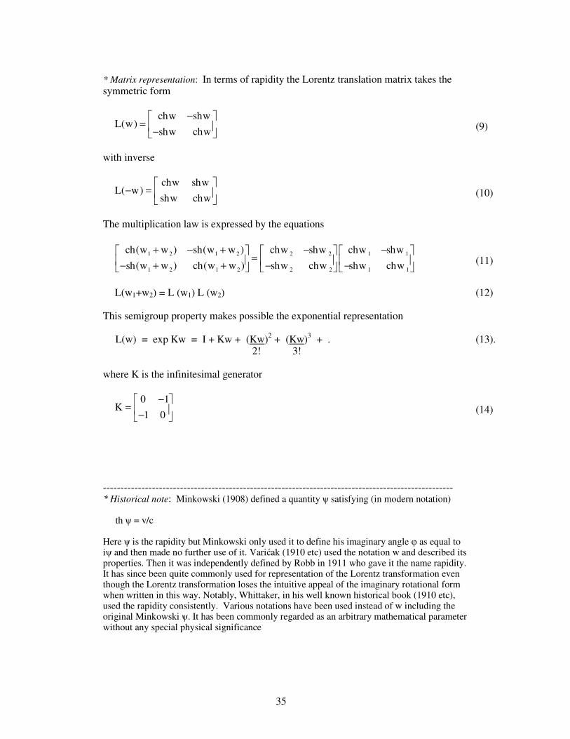
* Matrix representation: In terms of rapidity the Lorentz translation matrix takes the symmetric form
chw shwL(w)
shw chw
− = −
(9) (9)
with inverse
chw shwL( w)
shw chw
− =
(10)
The multiplication law is expressed by the equations
1 2 1 2 2 2 1 1
1 2 1 2 2 2 1 1
ch(w w ) sh(w w ) chw shw chw shw
sh(w w ) ch(w w ) shw chw shw chw
+ − + − − = − + + − −
(11)
L(w1+w2) = L (w1) L (w2) (12) (12)
This semigroup property makes possible the exponential representation
L(w) = exp Kw = I + Kw + (Kw)2 + (Kw)3 + . (13). (13) 2! 3!
where K is the infinitesimal generator
0 1K
1 0
− = −
(14)
---------------------------------------------------------------------------------------------------- * Historical note: Minkowski (1908) defined a quantity ψ satisfying (in modern notation)
th ψ = v/c Here ψ is the rapidity but Minkowski only used it to define his imaginary angle φ as equal to iψ and then made no further use of it. Varićak (1910 etc) used the notation w and described its properties. Then it was independently defined by Robb in 1911 who gave it the name rapidity. It has since been quite commonly used for representation of the Lorentz transformation even though the Lorentz transformation loses the intuitive appeal of the imaginary rotational form when written in this way. Notably, Whittaker, in his well known historical book (1910 etc), used the rapidity consistently. Various notations have been used instead of w including the original Minkowski ψ. It has been commonly regarded as an arbitrary mathematical parameter without any special physical significance
36 36 36
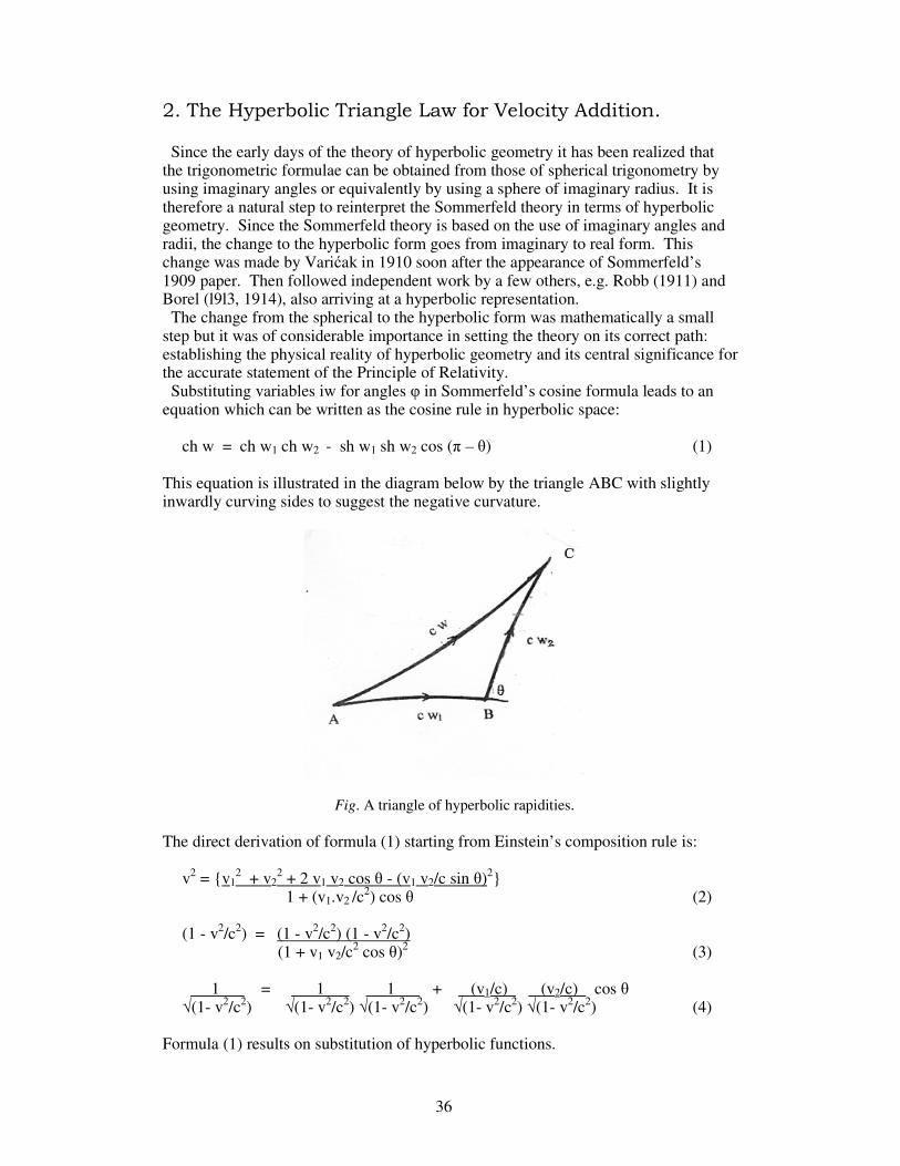
2. The Hyperbolic Triangle Law for Velocity Addition. Since the early days of the theory of hyperbolic geometry it has been realized that the trigonometric formulae can be obtained from those of spherical trigonometry by using imaginary angles or equivalently by using a sphere of imaginary radius. It is therefore a natural step to reinterpret the Sommerfeld theory in terms of hyperbolic geometry. Since the Sommerfeld theory is based on the use of imaginary angles and radii, the change to the hyperbolic form goes from imaginary to real form. This change was made by Varićak in 1910 soon after the appearance of Sommerfeld’s 1909 paper. Then followed independent work by a few others, e.g. Robb (1911) and Borel (l9l3, 1914), also arriving at a hyperbolic representation. The change from the spherical to the hyperbolic form was mathematically a small step but it was of considerable importance in setting the theory on its correct path: establishing the physical reality of hyperbolic geometry and its central significance for the accurate statement of the Principle of Relativity. Substituting variables iw for angles φ in Sommerfeld’s cosine formula leads to an equation which can be written as the cosine rule in hyperbolic space:
ch w = ch w1 ch w2 - sh w1 sh w2 cos (π – θ) (1) This equation is illustrated in the diagram below by the triangle ABC with slightly inwardly curving sides to suggest the negative curvature.
Fig. A triangle of hyperbolic rapidities.
The direct derivation of formula (1) starting from Einstein’s composition rule is:
v2 = v12 + v2
2 + 2 v1 v2 cos θ - (v1 v2/c sin θ)2 1 + (v1.v2 /c
2) cos θ (2)
(1 - v2/c2) = (1 - v2/c2) (1 - v2/c2) (1 + v1 v2/c
2 cos θ)2 (3)
1 = 1 1 + (v1/c) (v2/c) cos θ √(1- v2/c2) √(1- v2/c2) √(1- v2/c2) √(1- v2/c2) √(1- v2/c2) (4)
Formula (1) results on substitution of hyperbolic functions.

37 37 37
* Historical note: 1) The transition from spherical to hyperbolic trigonometry by the use of complex quantities is due to Taurinus (1826) and antedates much other work on hyperbolic geometry. See J. Gray: Ideas of Space, 1969 Oxford Univ. Press. The fact used in Varićak's transformation of the Sommerfeld form is that a pseudospherical sphere of imaginary radius is identical with a hyperboloid of revolution. 2) See the references to Varićak, Robb and Borel in the general bibliography. Vladimir Varićak (1865-1942) was professor of mathematics at Zagreb University. His biography was given by Kurepa (1965). Further contributions were made by Lewis & Tolman (1909), Ogura (1913), LeRoux(1922), Milne(1934), Karapetoff (1944), Patria (1956), Smorodinski (1963,1964). An extensive review has been given by Scott-Walker (1996, 1999)
3. Cartesian Projection from Hyperbolic Space The analogue of central projection of a sphere on to a tangential plane exists in hyperbolic geometry, the equivalent of the tangential plane at a point being a Euclidean plane called the limiting plane. As a result, many trigonometric formulae for hyperbolic space can be derived by projection in a similar way to the spherical case though the procedure is not intuitive. The equation corresponding to the imaginary R tan φ is
v = c th w (1) is regarded as showing velocity as a Euclidean projection of the rapidity w om hyperbolic space of negative radius of curvature c. Considering again the composition of two velocities v1,v2 at right angles, where a hyperbolic triangle ABC with a right angle at B is projected on to a plane triangle A1B1C1 tangential at A=A1. Transcribing the equations of the spherical case gives the to the sides a1, b1, c1 of the Euclidean triangle A1B1C1 the values
a1 = c th w2 sech w1 b1 = c th w c1 = c th w1 (2)
The hyperbolic triangle ABC and its Cartesian projection A1B1C1 are as illustrated below
Fig: The right-angled hyperbolic triangle.
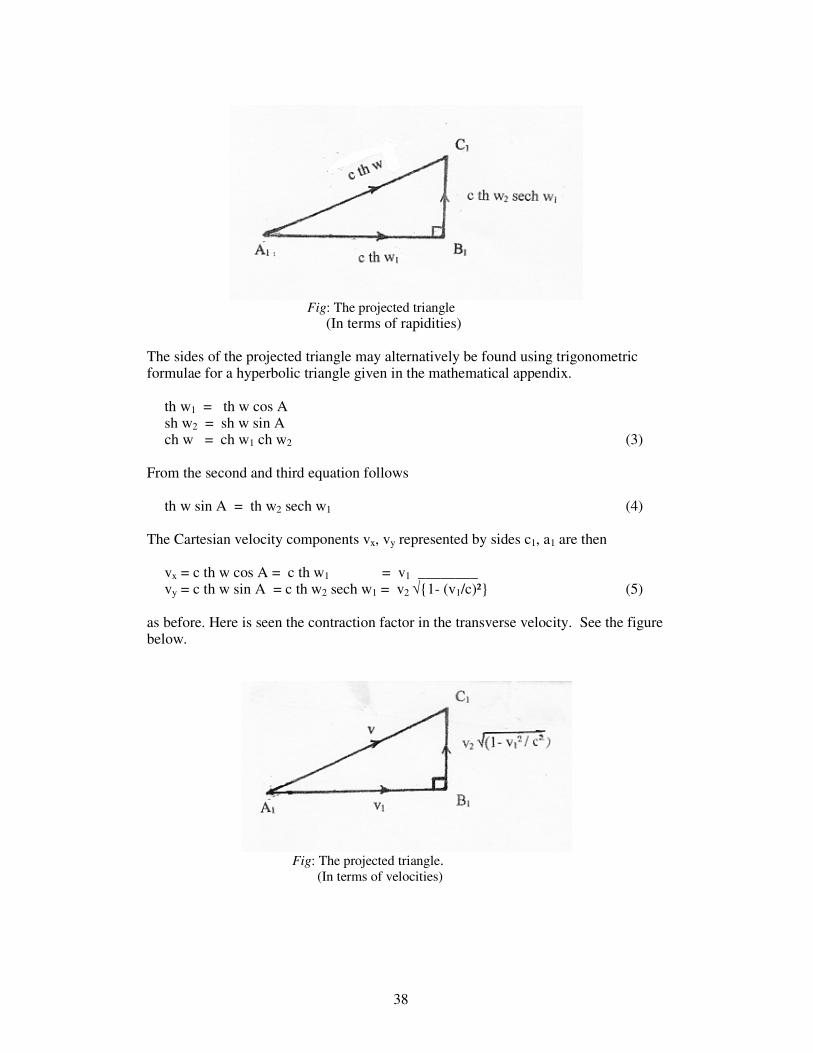
38 38 38
Fig: The projected triangle (In terms of rapidities)
The sides of the projected triangle may alternatively be found using trigonometric formulae for a hyperbolic triangle given in the mathematical appendix.
th w1 = th w cos A sh w2 = sh w sin A ch w = ch w1 ch w2 (3)
From the second and third equation follows
th w sin A = th w2 sech w1 (4) The Cartesian velocity components vx, vy represented by sides c1, a1 are then
vx = c th w cos A = c th w1 = v1 ________ vy = c th w sin A = c th w2 sech w1 = v2 √1- (v1/c)² (5)
as before. Here is seen the contraction factor in the transverse velocity. See the figure below.
Fig: The projected triangle. (In terms of velocities)

39 39 39
4. Hyperbolic Deficiency and Rotation Angle The interpretation of noncommutativity in hyperbolic geometry corresponding to that of Sommerfeld for the spherical case is shown in the figure below.
Fig: Non-commutativity (hyperbolic case)
Here the congruent triangles ABC, A'B'C' no longer overlap resulting in a difference in sign between this and the spherical case. As indicated by the figure, the rotation angle Ψ is the hyperbolic deficiency D of the triangle ABC
Ψ = π - (A+B+C) = D (1) * Calculation of rotation angle by trigonometry: The equality of rotation angle Ψ with deficiency D reduces determination of rotation angle to a trigonometrical problem of finding the deficiency of a triangle. EXAMPLE 1: Two velocities at right angles. The analogue of Sommerfeld’s formula proved in the last chapter is
sin D = sh w1 sh w2 1 + ch w1 ch w2 (2)
and it may be proved in a similar way merely transposing from spherical to hyperbolic form, replacing E by –D and φ1, φ2 by iw1, iw2. * Hyperbolic form of Liebmann’s half-angle formula: From Sommerfeld's formula may easily be deduced the Liebmann formula already proved in chapter 2.
sin D = √(ch w12 – 1) (ch w2
2 – 1) (1 + ch w1 ch w2) (3)
cos D = √(1 – sin2 D) = (ch w1 + ch w2) (1 + ch w1 ch w2) (4)
cos D + 1 = (ch w1 + 1)(ch w2 + 1) (1 + ch w1 ch w2) (5)

40 40 40
From this follows the required result:
cot D/2 = cos D + 1 = (ch w1 + 1)(ch w2 + 1) = (γ1 + 1)( γ2 + 1) sin D (ch w1 - 1)(ch w2 - 1) (γ1 – 1)( γ2 - 1) (6)
Now for any rapidity w
γ + 1 = ch w + 1 = 2 ch2(w/2) = coth2 (w/2) γ - 1 ch w - 1 2 sh2(w/2) (7)
So the result may also be written in the hyperbolic form (Varićak 1912).
cot D/2 = coth (w1/2) coth (w2/2) (8) EXAMPLE 2 Two velocities inclined at an angle. The formula for rotation angle is
cot Ψ/2 = C + cos θ (9) sin θ
θ being angle of inclination of velocities, and C the constant
C = (γ1 + 1)( γ2 + 1) = coth (w1/2) coth (w2/2) (γ1 – 1)(γ2 - 1) (10)
For orthogonal velocities, cos θ = 0, sin θ = 1 and the Liebmann formula.follows The derivation is immediate from transcribing a formula of Lagrange for spherical excess (see the mathematical appendix). The hyperbolic form of this formula is
cot (D/2) = ch (w1/2) ch (w2/2) + sh (w1/2) sh (w2/2) cos θ sh (w1/2) sh (w2/2) sin θ (11)
On division of numerator and denominator by the sinh half angles, there results formula (9). It may be transformed to the following symmetric form (see mathematical appendix)
cot D/2 = √(1 - ch2 w1 - ch2 w2 - ch2 w3 + 2 ch w1 ch w2 ch w3 ) 1 + ch w1 + ch w2 + ch w3 (12)
From there it is it transforms to the symmetrical formulae often quoted in the particle physics literature:
sin D = 1 + ch w1 + ch w2 + ch w3 2 (ch w1/2) (ch w2/2) (ch w3/2) (13)
cos D = √(1 - ch2 w1 - ch2 w2 - ch2 w3 + 2 ch w1 ch w2 ch w3 ) 2 4 (ch w1/2) (ch w2/2) (ch w3/2) (14)

41 41 41
* Note: The value of Ψ given by (10) was first given, using spinors, by van Wyk (1984) and, apparently using Silberstein's method, by Ben-Menahem (1985). Subsequently many papers have been devoted to its derivation by various methods. The present one by hyperbolic trigonometry was given by the writer (PIRT 2000) and has apparently not elsewhere appeared in the literature although Smorodinski (1962 etc.) used related formulae from which it could easily have been deduced. The symmetrical formulae (14), (15) were used in the physics literature from 1962. See Wick (1962), Smorodinski (1963) etc. On the derivation see Hestenes Space-time Algebra 1966
5. Hyperbolic Velocity Instead of the nondimensional rapidity w it is more natural in physical applications to use the corresponding dimensional quantity
V = c w = c th [-1] (v/c) (1) This was used by Varićak who regarded it as the true velocity from which the usual velocity v is found as a Euclidean projection. This is here accepted as a correct view although for the sake of conforming with customary usage as regards the word 'velocity' the term hyperbolic velocity will be used to denote velocity as defined by equation (1). Since v and V have the same physical dimensions the relation between them can be shown as below where the scales of v and V are the same.
Fig: The relation between velocity and hyperbolic velocity.
* Properties of hyperbolic velocity (a) Like rapidity, it can take any value from - ∞ to + ∞, the hyperbolic velocity of light being infinite. When v → c correspondingly V → ∞ (b) At low velocities (v << c) hyperbolic velocity V approximates v or more precisely, .
V = v 1 + 1/3 (v/c)2 + 1/5 (v/c)4 + ... (2) For rectilinear motion, hyperbolic velocities combine by the same rules of addition as do the proportional rapidities. So if the composition of velocities v1 and v2 gives velocity v then corresponding hyperbolic velocities are added:

42 42 42
V = V1 + V2 (3)
* The space of hyperbolic velocities: Hyperbolic velocity vectors V are defined by their magnitude V and direction. The space of such vectors forms a hyperbolic space of radius of curvature c and defines the kinematic space in Special Relativity. This provides the constant c with a natural meaning and leads to a very satisfactory view of the principle of relativity which was well expressed by Borel (1913)
'The principle of relativity corresponds to the hypothesis that the kinematic space is a space of constant negative curvature, the space of Lobachevski and Bolyai The value of the radius of curvature is the speed of light.'
The kinematic space approximates the classical velocity space locally for velocities small compared with the speed of light. The addition of hyperbolic velocities comes from rewriting the formula for the combination of rapidities. The cosine rule giving the magnitude V for the combination of V1 and V2 inclined at angle θ becomes
ch V/c = ch V1/c ch V2/c + sh V1/c sh V2/c cos θ (4) Use of V instead of rapidity w simplifies diagrams, e.g.the Sommerfeld diagram in hyperbolic space becomes a figure such as that shown below
----------------------------------------------------------------------------------------------------- Note: The addition law assumed in the present book follows the original idea of Varićak (1912). Addition of vectors in hyperbolic space by the method of parallel transport involves a rotational effect (See e.g. Richtermeyer: Hyperbolic Geometry, Springer 1992). This is due to the curvature of the space and occurs in relativity as the Thomson rotation. It leads to a result similar to the gyrovector as defined by Ungar except that it applies to hyperbolic vectors and not Cartesian vectors as does the gyrovector.

43 43 43
CHAPTER 5 – Relative Velocity 1. Relative Velocities in Rectilinear Motion All velocities are relative in Einstein’s form of the principle of relativity. But most frequently, expositions of the theory make only indirect reference to relative velocities which are defined tacitly through the velocity composition law. This law is usually thought of as in terms of group addition of velocities but is more properly interpreted as combining two relative velocities to form a new relative velocity. Group addition is most appropriate when all velocities are referred to the same origin. The usual one dimensional situation (frames S and S') is as shown. Origin O' moves away from origin O and the motion of a point P to the two frames is related Suppose that, relative to origin O, the points O' and P move with velocities v1, v2 and, relative to O', P has velocity u.(see fig.)
|…..u→….|
Fig. Moving frames and O O' P relative motions o------------o------------o-------------
v1 → v2 → Transferring the origin from O to the new origin O' gives, by the composition rule,
v2 = v1 + u . 1 + v1 u / c2 (1)
On solving for u,
u = v2 - v1 . 1 - v2 v1 / c
2 (2) This formula gives the relative velocity of two points (here O' and P) moving with velocities v1 and v2 relative to an origin (here O). It might at first appear that since v1 and v2 are dependent on the origin O, then u must also be dependent on this origin but it can be seen from the meaning that it is not. This fact can also be verified algebraically by substituting in (2) for v1 and v2 the expressions
v1 + u' , v2 + u' . 1 + v1 u' / c2 1 + v2 u' / c2 (3)
u' being a further arbitrary relative velocity, when it is found that the expression (2) remains unchanged. In this respect formula (2) differs from the composition formula (1) which is dependent on origin and for this reason formula (2) is preferable as a starting point to formula (1).

44 44 44
* Re-derivation of the composition rule: With formula (2) for relative velocities as a starting point it is possible to deduce the rule for composition of relative velocities in a more convenient way. Consider the situation in the figure where 3 points P1, P2, P3 are in motion relative to an origin O.
O P1 P2 P3
Fig: Composition of relative o----------o-----------o---------o--------- rectilinear velocities v1 → v2 → v3 →
The relative velocities u2/1 of P2 to P1 and u3/2 of P3 to P2, are u2/1 = v2 - v1 u3/2 = v3 – v 1 - v2 v1/c
2 1 - v3 v2/c2 (4)
The relative velocity u3/1 of P3 relative to P1 is u3/1 = v3 - v1
1 - v3 v1/c2 (5)
After some calculation, the composition rule follows purely algebraically as
u3/1 = u3/2 + u2/1
1 + u3/2 u2/1/c2 (6)
Reference: Prokhovnik: The Logic of Special Relativity, 1967 * Use of hyperbolic velocities: these relations simplify and become more transparent by the use of rapidities or hyperbolic velocities. Suppose, as before, there are three moving points P1, P2, P3 referred to an origin O. Then w2/1 = w2 - w1 U2/1 = V2 - V1 (7) w3/2 = w3 - w2 U3/2 = V3 - V2 (8) from which by addition, w3/2 + w2/1 = w3 - w1 = w3/1 U3/2 + U2/1 = V3 - V1 = U3/1 (9) * Galilean and Lorentzian translational invariance: The use of rapidity and hyperbolic velocity makes clearer the distinction between two forms of translation invariance. The two forms are
v → v + u (Galilean) (10)
V → V + U (Lorentzian) (11)
45 45 45
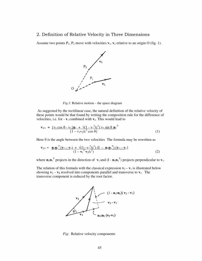
2. Definition of Relative Velocity in Three Dimensions Assume two points P1, P2 move with velocities v1, v2 relative to an origin O (fig. 1).
Fig.1: Relative motion – the space diagram
As suggested by the rectilinear case, the natural definition of the relative velocity of these points would be that found by writing the composition rule for the difference of velocities, i.e. for - v1 combined with v2. This would lead to
v2/1 = v2 cos θ - v1n1 + √(1 - v12/c2) v2 sin θ
n1
1 – v1v2/c2 cos θ (1)
Here θ is the angle between the two velocities The formula may be rewritten as
v2/1 = n1n1T (v2 – v1) + √(1– v1
2/c2) (I – n1n1T) (v2 – v1
(1 – v1T
v2/c2) (2)
where n1n1
T projects in the direction of v1 and (I - n1n1T) projects perpendicular to v1.
The relation of this formula with the classical expression v2 – v1 is illustrated below showing v2 – v1 resolved into components parallel and transverse to v1. The transverse component is reduced by the root factor.
Fig: Relative velocity components

46 46 46
* Fock's derivation: This expression (2) was derived by Fock (1955) by transfering the origin from O to P1 so considering P1 to be at rest. As in the classical case, the velocity of P2 with respect to this new origin is then defined as the velocity of P2 relative to P1. * Detail: Fock assumed uniform motions and wrote the Lorentz transformation for the the move to the new origin at P1 with coordinates r ', t '. This transformation has the differential form dt' = γ1 (dt – dr.v /c) dr' = dr – v1 dt + (γ1 – 1) n1 (n1.dr – v1 dt) (3) where n1 is a unit vector in the direction of v1 and factor γ1 refers to this velocity: By division Fock’s formula for the relative velocity v2/1 is found as v2/1 = dr' = v2 - v1 + (γ1 - 1) n1.(n1.v2)-v1 (4) dt' γ1(1 - v1.v2 / c
2) By rearrangement this may be written in the form v2/1 = n1n1
T ( v2 – v1) + √(1– v1
2/c2) (I – n1n1T) (v2 – v1
(1 – v1T
v2/c2) (5)
which is the same as formula (2). By the same definition the reverse relative velocity, found by interchange of suffixes, would be
v1/2 = v1 cos θ – v2n2 + √(1 – v22/c2) v1 sin θ
n2
1 – v1v2/c2 cos θ (6)
= n2 n2
T ( v1 - v2) + √(1 – v2
2/c2) (I – n2 n2T) (v1 – v2
(1 - v1T
v2/c2) (7)
What is surprising is that the two relative velocities are not negatives of one another as might have been expected. They do however have the same magnitude found by the difference form of Einstein’s composition rule:
v2/12 = v1/2
2 = (v12 – 2 v1v2 cos θ + v2
2 ) – (v1v2/c)2 sin2 θ 1 – v1v2/c
2 cos θ2 (8) The two relative velocities consequently differ only in direction. This rotational effect is taken into account in the matrix definition given in the next section. ---------------------------------------------------------------------------------------------- References: Fock: The Theory of Space, Time and Gravitation, Moscow 1955, Engl.tr. Oxford 1959. See also Møller: The Theory of Relativity 1955.

47 47 47
3. Matrix Representation of Relative Velocity Relative velocity may be defined by a similar idea to that used previously for the one dimensional case where all motions are referred to an observer O. For two moving points P1, P2 the relations between coordinate changes referred to observer O are, with use of appropriate suffices
[ ] [ ]0 01 2
1 2
0 01 2
cdt cdtcdt cdt( ) , ( )
= Λ = Λ
v v
dr drdr dr
(1) the matrices here being Lorentz translations. From these follows
[ ][ ] 12 1
2 1
2 1
cdt cdt( ) ( )
− = Λ Λ
v v
dr dr (2)
Although matrices L(v2), L (v1) are defined relative to O, their product L(v2)L (v1)
-1 is independent of O. For supposing that the relation between coordinate changes between the two different observers O, O' is
[ ]0 0
0
0 0
cdt cdt '( )
'
= Λ
v
dr dr (3)
the matrices L (v2), L (v1) will transform by
L(v2) → L (v2) Λ (v0), L (v1) → L (v1) Λ (v0) (4) leaving the product L (v2) L (v1)
-1 unchanged. The relative velocity matrix is consequently well defined independently of observer as
Λ2/1 = L(v2) L(v1) -1 (5)
from which follows for the inverse
Λ1/2 = L(v1) L(v2) -1 = (Λ2/1)
-1 (6) Note that a relative velocity of two moving points is represented by a Lorentz translation when and only when the origin is taken at one of the moving points. This was in fact what Fock had done which gave the incorrect impression that a relative velocity in general can be so represented.
48 48 48
4. Re-derivation of Fock’s Expression for Relative Velocity The product L (v2)L (v1)
-1 when written as L (v2)L (-v1) may be evaluated as a product of Lorentz translations and written in the form R L(v) where R is a spatial rotation and Λ(v) a Lorentz translation. More explicitly it will be
T
T
1 0 / c
0 / c I ( 1)
γ −γ Ω −γ + γ −
v
v nn (1)
where Ω is a 3x3 spatial rotation matrix. On forming the product there is found
γ = γ1γ2 1 - v1Tv2/c
2 γ v = γ2 (I + (γ1-1) n1n1
T) v2 - γ1 v1 γ (Ω v) = γ1 (I + (γ2-1) n2n2
T)(-v1)+ γ2 v2 (2) From the first and second of these equations is found
v = I + (γ1-1) n1 n1Tv2 - γ1 v1
γ1 1 – v1Tv2/c
2 (3) Slight rearrangement gives Fock’s expression
v = v2 - v1 + (γ1 - 1)n1(n1T v2)-v1 (4)
γ1 (1 - v1T
v2/c2)
so identifying v as v2/1 By further rearrangement this may be written as
v2/1 = n1n1T (
v2 - v1) + √(1– v12/c2) (I - n1n1
T) (v2 - v1 (1 - v1
T v2/c
2) (5)
This resolves the difference of velocities into longitudinal and transverse components. Interchange of suffixes gives the reverse relative velocity:
v1/2 = n2 n2T (
v1 - v2) + √(1– v22/c2) (I - n2 n2
T) (v1 - v2 (1 - v1
T v2/c
2) (6) From above it is seen that
Ω v2/1 = v1/ 2 (7) showing the relation between the two relative velocities which are not negatives of one another. The matrix (1) may be written symmetrically in canonical form as
T
T( 1)
γ −βγ −βγ Ω + γ −
2/1
1/2 1/2 2/1
n
n n n (8)

49 49 49
5. Composition of Relative Velocity Matrices Let there be three points P1, P2, P3 moving with velocities v1, v2, v3 relative to the observer O. The relative velocity matrices are with L() denoting Lorentz translation,
Λ2/1 = L(v2) L(v1)
-1 Λ3/2 = L(v3) L(v2)
-1 Λ3/1 = L(v3) L(v1)
-1 (1) from which follows the composition rule:
Λ3/1 = Λ3/2 Λ2/1 (2) which shows the transitivity of matrix multiplication for connected relative velocities. This equation can obviously be extended to any number of consecutive stages. * Moving frames of reference: In the standard situation of systems S and S' with S' moving with velocity v relative to S, consider the motion of a point P moving with velocities u, u' relative to S and S'. As seen by an observer at rest at the origin O of the S frame, the velocity of P relative to the origin O' in the S' frame is
Λ(u') = L(u) L(v)-1 (3)
where L(.) denotes a Lorentz translation matrix. Now the velocity u will be defined by the equation
L(u') L(v) = R L(u) (4) R being here a rotation matrix So the observed relative velocity of P is
Λ(u') = R-1 L(u') (5) The transformation law then takes the form
L(u) = R-1 L(u')L(v) = Λ(u') L(v) (6) which implies that it is not possible to find L(u) by just multiplying Lorentz translation matrices L(v) and L(u') as was done, for example, in the 1909 Sommerfeld paper discussed in chapter 3 While valid mathematically, this product would have no physical meaning. The multiplication must be done as explained here in which case the resultant has no rotation and addition takes place in the usual way for vectors. ---------------------------------------------------------------------------------------------------- * Remark: The writer believes that in this way a resolution can be found of the difficulty in multiplying Lorentz translations which has been much discussed in the literature following the work of Mocanu and Ungar (see bibliography).

50 50 50
6. Relative Velocity and Hyperbolic Geometry Fock (1955) deserves the credit for realizing the importance of hyperbolic space for the correct representation of relative velocity in Special Relativity. He also introduced the appropriate representation of this space - that of Beltrami-Klein. Since the magnitude of the relative velocity is given by the Einstein composition formula for the difference of velocities, the corresponding calculation for velocity addition given previously is easily modified to give the relation
1 - v2 = (1 - v12/c2)(1 - v2
2/ c2) c2 (1 - v1 v2 cos θ / c2) 2 (1)
between the velocities v1, v2 , the angle θ between them, and the relative velocity v. Taking square roots and inverting results in
1 = c2 – v1 v2 cos θ √(1 - v2/c2) √(c2 – v1
2)(c2 – v22) √(c2 – v1
2)(c2 – v22) (2)
which, using corresponding rapidities w, w1, w2, gives
ch w = ch w1 ch w2 – sh w1 sh w2 cos θ (3) or equally in terms of hyperbolic velocities V, V1, V2
ch V/ c = ch V1/c ch V2/c – sh V1/c sh V2/c cos θ (4)
The relationships between V, V1, V2 may consequently be represented by the sides of a triangle in hyperbolic space as shown.
Fig: Hyperbolic triangle of relative rapidities. This diagram may be interpreted as showing vector subtraction of hyperbolic velocities to form a relative hyperbolic velocity, as justified by the matrix form
L (v2) = Λ (v2/1) L (v1) (5) where the matrix Λ (v2/1) includes a correcting rotation so that there is no resulting turning angle in the right hand side.

51 51 51
7. The Beltrami Representation In Special Relativity, relative to a chosen origin and Cartesian frame, admissible velocities (vx, vy, vz) are restricted by the inequality v² = vx² + vy² + vz² < c² (1) The velocity space is consequently represented by vectors drawn from the origin to points inside this sphere which may be given by spherical coordinates:
vx = v n1 = v sin φ cos θ vy = v n2 = v sin φ sin θ vz = v n3 = v cos φ (2)
where n1, n2, n3 are direction cosines of the velocity direction and φ, θ spherical coordinates. On using rapidity w as radial parameter instead of v, these velocity components become
vx = c th w n1 = c th w sin φ cos θ vy = c th w n2 = c th w sin φ sin θ vz = c th w n3 = c th w cos φ (3)
The rapidity w takes values from zero to infinity so that in terms of w, φ, θ the space becomes infinite in extent. This is the Beltrami representation.of hyperbolic space in its normal parametrization The Riemannian metric in this space, due to Beltrami, can be introduced by considering the magnitude squared of the differential relative velocity of points having velocities v and v + dv. This magnitude squared is given by the Einstein composition rule for the difference which in this case results in the polar coordinate expression
dv² + 1 v² [dφ² + sin² φ dθ²] (1 – v²/c²)² (1 – v²/c²) (4)
On change to rapidity, this leads to a Riemannian metric c² dw² + c² sh² w [dφ² + sin² φ dθ²] (5) or, in terms of the corresponding hyperbolic velocity V it is, dV² + c² sh² V/c [dφ² + sin²φ dθ²] (6) which is the standard form of the Riemannian metric of a hyperbolic space. Equivalently the metric squared element can be written `
dV² + γ² [r² dφ² + r² sin²φ dθ²] (7) This expression shows clearly the deviation of the space from Euclidean form when expressed in spherical coordinates.

52 52 52
The (nondimensional) metric in this space is given by the magnitude of the relative rapidities w2/1, w2/1 satisfying the equation which follows from the last section
c ch w2/1 = c ch w2/1 = c² - v1.v2 √(c² - v1.v1)(c² - v2.v2) (8)
The equivalence of (12) with the composition rule for the relative velocity follows from the calculation in the previous section. Beltrami space has the convenience that velocities are represented by straight lines. This may be illustrated as below in the case of three moving points B, C, D with hyperbolic velocities V1, V2, V3 relative to a point A. The relative velocities are found by completing triangles as shown giving the triangular composition of two relative hyperbolic velocities V2/1 and V3/2 to give V3/1
Fig: Composition of relative hyperbolic velocities. This figure corresponds to the matrix composition rule for relative velocities given above. ----------------------------------------------------------------------------------------------------- * Notes: Further details on the Beltrami representation are given in the mathematical appendix. It was Milne (1934) who first used this representation in special relativity for his model of the expanding universe (a use made more explicit by Whitrow 1939) Application of the Beltrami representation to velocity space in special relativity is due to Fock (1955)
53 53 53
CHAPTER 6 – Applications to Optics
1. Aberration and Oblique Doppler Effect Here, starting from the original idea of Bradley on stellar aberration, the observer is commonly thought of as moving while the source of light is considered to be stationary. So frame S will represent the stationary source frame for emitted light and frame S’ the moving frame of the observer. * The principle of invariance of the phase: If the incoming wave has direction cosines (l, m, n) relative to the source frame S, the phase relative to S is
Φ = 2 π f t - (lx +my + nz)/c (1) f being frequency in Herz. Similarly if the wave has direction cosines (l', m', n') relative to the observer frame S' the phase relative to S' is
Φ = 2 π f ' t' - (l'x' +m'y' + n'z')/c (2) The basis of the calculation is that these two expressions must be the same. This is the 'Principle of invariance of the phase' used by Lorentz (1886,1895) with classical transformation formulae from which he found approximately correct formulae for both Doppler effect and aberration. Einstein (1905) used the same method with the corrected transformation and so found the relativistic formulae which have since become very much used. Varićak rephrased them in terms of rapidity If the incoming wave is inclined at an angle φ to the direction of motion of the observer relative to the source along the x-axis then the phase of the incoming wave relative to the two frames S can be written in the simpler form
Φ = 2 π f t - (x cos φ + y sin φ)/c Φ = 2 π f 't' - (x' cos φ' + y' sin φ ')/c (3)
so that the principle of invariance gives
f (ct - x cos φ - y sin φ ) = f ' (ct' - x' cos φ' - y' sin φ') (4) (a) True values in terms of observed values From invariance of the phase combined with
ct' = ct ch w - x sh w x' = - ct sh w + x ch w y' = y (5)
There follows

54 54 54
f = f ' (1 + v /c.cos φ') √(1-v²/c²) (6)
cos φ = cos φ' + v/c 1 + v/c.cos φ' (7)
sin φ = √(1-v²/c²) sin φ' 1 + v/c.cos φ' (8)
(b) Observed values in terms of true values Similarly, starting from
ct = ct' ch w + x' sh w x = ct' sh w + x' ch w y = y' (9)
there is found through substitution
f ' = f (ch w - sh w cos φ) = ch w f ( 1 - th w cos φ ) f ' cos φ' = f (ch w cos φ - sh w ) = ch w f ( cos φ - th w ) f ' sin φ' = f sin φ (10)
This gives the same formulae with change in sign for v
f ' = f (1 - v/c cos φ) (11) √(1-v²/c²)
cos φ' = cos φ - v/c 1 - v/c cos φ (12)
sin φ' = √(1-v²/c²) sin φ 1 - v/c cos φ (13)
* Transverse Doppler Effect: The transverse Doppler Effect occurs when the light source is observed at right angles to the direction of motion. This requires solving the equations for f ' when φ' is π/2. Using (7) to find cos φ in terms of cos φ' and substituting in (11) there is found observed frequency f ' in terms of observed angle φ'
f ' = f √(1-v²/c²) . (1 + v /c.cos φ') (14)
When φ' is π/2 this gives the formula for the transverse Doppler effect:as
f ' = f √(1-v²/c²) (15)
---------------------------------------------------------------------------------------------------- * References: 1) Lorentz's work on aberration and the Doppler Effect is well described by Miller (1998) 2) For history and interesting comments on the transverse Doppler Effect see the books of Stevenson & Kilminster (1958), and Prokhovnik (1969)
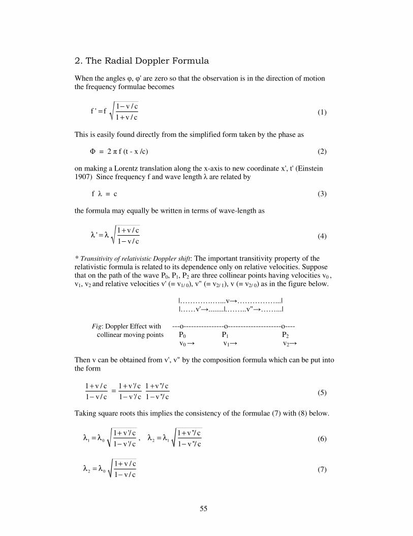
55 55 55
2. The Radial Doppler Formula When the angles φ, φ' are zero so that the observation is in the direction of motion the frequency formulae becomes
1 v / cf ' f
1 v / c
−=
+ (1)
This is easily found directly from the simplified form taken by the phase as Φ = 2 π f (t - x /c) (2) on making a Lorentz translation along the x-axis to new coordinate x', t' (Einstein 1907) Since frequency f and wave length λ are related by f λ = c (3) the formula may equally be written in terms of wave-length as
1 v / c'
1 v / c
+λ = λ
− (4)
* Transitivity of relativistic Doppler shift: The important transitivity property of the relativistic formula is related to its dependence only on relative velocities. Suppose that on the path of the wave P0, P1, P2 are three collinear points having velocities v0 , v1, v2 and relative velocities v' (= v1/ 0), v" (= v2/ 1), v (= v2/ 0) as in the figure below.
|………….…...v→……………...| |……v'→........|.……..v"→……...|
Fig: Doppler Effect with ---o----------------o---------------------o---- collinear moving points P0 P1 P2
v0 → v1→ v2→ Then v can be obtained from v', v" by the composition formula which can be put into the form
1 v / c 1 v '/ c 1 v ''/ c
1 v / c 1 v '/ c 1 v ''/ c
+ + +=
− − − (5)
Taking square roots this implies the consistency of the formulae (7) with (8) below.
1 0 2 1
1 v '/ c 1 v ''/ c,
1 v '/ c 1 v ''/ c
+ +λ = λ λ = λ
− − (6)
2 0
1 v / c
1 v / c
+λ = λ
− (7)

56 56 56
* A modified redshift formula: The classical linear Doppler formula as used in astronomy for nebula recession (Hubble 1936) arises from binomial theorem approximation to the relativistic formula (5):
λ ' = λ (1 + v/c) (8) This can be written as
z = v/c (9)
where z is the redshift
z = (λ ' - λ)/ λ (10)
This linearized Doppler formula does not have the transitivity property, implying for example, that in astronomy, all redshifts are Earth centred. However a modified form of the relativistic formula (5) may be found of similar form to the linearized Doppler formula which does have the desired transitivity property. This is found by taking logarithms of equation (5) and using the equation relating v to hyperbolic velocity V
[ 1]1 v / cln th (v / c)
1 v / c−+
=−
= V/c (11)
Then this may be written analogously to the classical linearized Doppler formula as
Z = V/c (12)
where Z is the modified redshift
Z = ln (λ '/ λ) (13)
This form of the Doppler shift law relates the quantities Z and V which are both additive over subintervals as illustrated in the fig. below.
|.……………...V→….…………..| |……V' →.…|..……...V"→……..|
P0 P1 P2
Fig. The additive relation between ----o--- ------------o-----------------------o-- hyperbolic velocity and logarithmic Doppler shift < ------Z'----- >< ---------Z"------- >
< ------------ Z = Z' + Z" ---------- > In this way the transitive property is restored to the linear Doppler formula.
57 57 57
* Logarithmic Doppler shift: The quantity Z which has been defined here provides an alternative and improved measure of Doppler shift. It may be called 'logarithmic measure of Doppler shift' or for short 'logarithmic Doppler shift’. It is a strictly increasing function of the wave-length ratio λ'/ λ reducing to normal redshift for low relative velocities since, when λ' differs little from λ,
Z = ln 1 + (λ' - λ)/ λ ≈ (λ' - λ)/ λ = ∆ λ / λ = z (14) The following properties of logarithmic Doppler shift Z contrast favourably with those of normal Doppler redshift z for which they fail to hold exactly: (a) Change from wave-length to frequency or vice versa merely involves change of sign
ln (λ '/ λ ) = - ln (f '/ f) (15) (b) Z has antisymmetry between emitter and receiver undergoing a simple sign change when these are reversed:
ln (λ '/ λ ) = - ln (λ / λ '), ln (f '/ f) = - ln (f / f ') (16) (c) Z is additive (transitive) as expressed by the equations
ln (λ '/ λ ) + ln (λ "/ λ ') = ln (λ "/ λ ), ln (f '/f ) + ln (f "/ f ') = ln (f "/ f ) (17) ------------------------------------------------------------------------------------------------------- * Notes: 1) The transitivity property of the radial Doppler formula was observed by Prokhovnik (1969) and Jánossy (1971). 2) The logarithmic Doppler shift measure can also be used in General Relativity. Using the known formulae for cosmological redshift and time-varying Hubble parameter H(t): λ2 = R(t2) , H(t) = 1 dR(t) λ 1 R(t1) R dt there is found the generalized logarithmic redshift law Z = ln (λ2 / λ 1) = ln R(t2)/ R(t1) = ln R(t2) – ln R(t1) = ∫ H(t) dt Further details are given in the writer’s 1992 PIRT paper.

58 58 58
3. The Hyperbolic Interpretation of Relativistic Aberration The wave theory interpretation of aberration loses contact with the simple picture of triangular velocity addition of the classical Bradley theory. This picture can be partially restored by using the velocity composition formulae. Consider an incoming photon moving with velocity components relative to the source frame S of ux = - c cos φ, uy = - c sin φ (1) Using the velocity composition formula the corresponding components relative to the observer frame S ' are ux' = - (c cos φ + v) (2) (1 + v/c. cos φ)
uy' = - c sin φ √(1 - v2/c2) (3) (1 + v/c. cos φ) Here ux'
2 + uy'
2 = c2 (4) so that it is permissible to put ux' = - c cos φ', uy' = - c sin φ' (5) when substitution leads directly to the aberration formulae. There is however a difficulty. Since both (ux, uy) and (ux', uy') have magnitude c it is not possible to form a Euclidean triangle of velocities. This difficulty is overcome in the non-Euclidean representation. The aberration formula resulting from the substitution (5) in (2) may be written
c.cos φ' = c cos φ + v 1 + cos φ. v/c (6)
and compounds the forward component of the light velocity c cos φ with v by the composition rule for rectilinear velocities. So introducing rapidity components w, w ', W by cos φ = th w, cos φ' = th w ', v = c th W (7) (6) becomes c cos φ' = c th w + c th W = c th (w + W) 1 + th w. th W (8)

59 59 59
The simple addition
w ' = w + W (9) of the x-components together with the fact that the y component of the light rapidity remains infinite makes it possible to reconstruct the triangle of rapidities as shown in
the figure. Fig: The triangle of rapidities in aberration.
Here the two sides representing velocity of light have become infinite, their components in the direction of motion remaining finite. The light paths are both Lobachevski parallels to the vertical line representing the transverse component of light velocity. Angles φ', φ are Lobachevski angles of parallelism as shown by the equations (5). In this way the triangle addition of Bradley’s theory is restored. ----------------------------------------------------------------------------------------------- Note: The use of Lobachevski parallels in light propagation was mentioned by Silberstein in his 1914 book but it did not appear in later literature.

60 60 60
CHAPTER 7 – Applications to Dynamics 1. Hyperbolic Acceleration Hyperbolic acceleration will be here defined as rate of change dV/dτ of hyperbolic velocity V with respect to proper time τ, the time observed relative to the moving body. In one dimension it coincides with the known expression for rectilinear acceleration given e.g. by Rindler 1991:
α = 1 dv (1) (1-(v/c)2) 3/2 dt = 1 1 dv = 1 d th [-1] v/c = dV (1- v2/c2)1/2 1 - v2/c2 dt (1- v2/c2)1/2 dt dτ (2)
Relative to the moving body v is zero and then from (2) the hyperbolic acceleration is represented by the normal derivative expression. Hyperbolic acceleration dV/dτ has a more familiar form than the expression (1) with its multiplying factor. It may also be defined more intuitively as follows. Consider the situation in the figure below representing an accelerating point P. v → v +δv → 0 |----------- P o ---------o P' --------------------------→ x x +δx x -axis
Fig: On the definition of rectilinear acceleration In any time increment δt, the increase in velocity δv of an accelerating body does not occur at a fixed value of x relative to an origin O but takes place over a certain interval x to x+δx. The increase of velocity relative the origin O should consequently be calculated by the relative velocity formula as (v+δv)-v = δv . 1 - (v+δv).v/c2 1 - (v+δv).v/c2 (3) which gives, as δt → 0 and δv→ 0, a first order increment of δv = c δ th[-1] v/c = δV (4) 1 – v2/c2 Taking account of the time change from the origin to the frame of the moving particle, the acceleration is found as the hyperbolic acceleration as defined above. The three dimensional hyperbolic acceleration can be defined using Fock's definition of relative velocity.

61 61 61
2. Motion under Constant Acceleration The relativistic motion of a particle under constant acceleration was analysed in detail by Born (1909) who called it 'hyperbolic motion' since the equation of the trajectory in the x, t plane is a hyperbola instead of the parabola of classical physics. To find the trajectory it is necessary to integrate the equation
2 2 3/ 2
dvdt
(1 v / c )= α
− (1)
for constant acceleration α. This gives, if v = 0 when t=0,
2 2
vt
(1 v / c )= α
− (2)
On solving for v and again integrating, there is found
02
0 0
t tt
x x v dt dt(1 ( t / c) )
α− = =
+ α∫ ∫ (3)
which gives
2 2 20 0x x (c / ) (1 ( t / c) ) 1 x t / 2 ... = + α + α − = + α −
(4) from which the trajectory is found as the hyperbola (x - x0 + b) ² - c² t² = b² (5) where b is the constant c²/ α. * The Minkowski interpretation: The current standard interpretation of the motion uses the ideas of Minkowski. The hyperbola is centralized by choosing x0 equal to b in which case. x² - c² t² = b² (6) and given the complex representation x² + (ict)² = b² (7) In polar coordinates using an imaginary angle φ this is x = b cos φ ict = b sin φ (8)

62 62 62
Since b is constant, differentiation gives: dx = - b sin φ dφ ic dt = b cos φ dφ (9) There follows dτ = √(dt ² - (dx /c)²) = bi /c. dφ (10) Consequently φ increases uniformly with τ giving the picture of constant angular speed circular motion which Sommerfeld called 'cyclic motion'. It has a constant (purely imaginary) central acceleration in the x, ict plane caused by the applied force. * The Lobachevski interpretation: Here it is not necessary to make the same rather artificial choice of initial condition but instead it is convenient to parametrize the trajectory as x = x0 - b + b ch u, ct = b sh u (11) from which dx / dt = c th u (12) so identifying u with rapidity. Further, __________ dτ = √dx2 – (cdt)2 = b du (13) again leading to the value of hyperbolic acceleration of dV/dτ =c du/dτ = c2/ b = α (14) By integration is found an analogue of Galileo’s law for velocity increase as used in elementary mechanics: V = V0 + ατ (15) ---------------------------------------------------------------------------------------------------- * References: On hyperbolic motion see e.g. Pauli: Theory of Relativity, Prokhovnik: Theory of Relativity. 1967. Original references are: Minkowski ‘Raum und Zeit’ 1908 (See p.84 in 'The Principle of Relativity' translation which is annotated on p.96 with Sommerfeld's 1923 notes) Born 'Die Theorie des starren Elektrons ...' Ann. Phys. 1909, Sommerfeld Atombau und Spektrallinien.1919 etc.320-.

63 63 63
3. Newton’s Second Law for Rectilinear Motion In 1906 Planck showed that Newton's second law of motion for rectilinear motion can be written in the relativistic form F = dp (1) dt F is applied force and p is momentum given by p = mv = mv 1 + 1/6 (v/c)2 + ... (2) √(1 – v2/c2) m being what is usually called the rest mass. Planck’s equation may easily be transformed to involve (hyperbolic) acceleration: dp = m d v = m 1 dv = m α (3) dt dt √(1-v2/c2) (1-v2/c2)3/2 dt This equation may also be written dp = m dV (4) dt dτ Then Newton's law takes the familiar form F = m α = m dV (5) dτ In words, (6) This relation may be derived even more directly from the representation p = mc sh V/c (7) Differentiation gives: F = dp = m ch V/c dV = m dV dt dt dτ (8) For constant force the acceleration is also constant and the motion is hyperbolic. -------------------------------------------------------------------------------------------------- * References: See Planck (1906a) and (1906b). The form of Newton’s Law given above was proposed by the writer at the 2000 PIRT conference. It avoids the concept of velocity dependent mass, velocity dependence being in the acceleration not the mass.
Force = Rest mass x (hyperbolic) acceleration
64 64 64
4. Remarks on Newton's Law of Motion in Three Dimensions In his 1905 paper Einstein wrote the relativistic 3 dimensional Newtonian equations of motion of a particle (an electron) in an electric field There were assumed inertial systems, here denoted S and S', with S for the observer and S' for the particle. S' moves with uniform velocity v relative to S along the x-axis and both S and S' are coincident with the particle at t = 0 in position and S' also in velocity. The basic assumption made is that Newton's law in its classical form applies in the frame S' instantaneously coincident with the electron so that relative to the electron: m d2x'/ dt ' 2 = F'x = e E' x m d2y'/ dt ' 2 = F'y = e E'y m d2z'/ dt ' 2 = F'z = e E'z (1) The accelerations in S' and in S are related by: d2x'/ dt ' 2 = γ3 d2x/ dt2
d2y'/ dt ' 2 = γ 2 d2y/ dt2
d2z'/ dt ' 2 = γ 2 d2z/ dt2 (2) The electric fields are related by E 'x = E x
E 'y = γ (Ey – v/c Hz) E 'x = γ (Ez + v/c Hz) (3) So from (1) it follows that to the observer in S the equations of motion are: m γ3 d2x/ dt2 = F x m γ 2 d2y/ dt2 = γ Fy
m γ 2 d2z/ dt2 = γ Fz (4) where on the right hand side are the components of the Lorentz force: F x = e E x
Fy = e (Ey – v/c Hz) Fz = e (Ez + v/c Hz) (5) On the appearance of the factor γ in the lateral force components see Møller (1955) * Planck’s form of Newton’s Law: Planck (1906) showed that for rectilinear motion, Newton's law may be written relativistically in terms of rate of change of momentum. Einstein (1907) rewrote the 3 dimensional equations in Planck's form and rederived the equations of his 1905 paper. The 3 dimensional Planck-Newton equations are [Fx, Fy, Fz] = | dpx dpy dpz | | dt dt dt | (6)

65 65 65
The components of vector momentum are [px, py, pz] = | mvx , mvy , mvz . | | √(1 – v2/c2) √(1 – v2/c2) √(1 – v2/c2) | (7) Differentiating the right hand side of (6) gives the components as
d m vx = m (1-vy2/c2-vz
2/c2) dvx + m vxvy /c2 dvy + m vxvz /c
2 dvz dt √ (1-(v/c)2) √(1-(v/c)2) 3/2 dt (1-(v/c)2)3/2 dt (1-(v/c)2)3/2 dt
d m vy = m vyvx /c2 dvx + m (1-vz
2/c2-vx2/c2 ) dvy + m vyvz /c
2 dvz dt √ (1-(v/c)2) √(1-(v/c)2) 3/2 dt (1-(v/c)2)3/2 dt (1-(v/c)2)3/2 dt
d m vz = m vzvx /c2 dvx + m vzvy /c
2 dvx + m (1-vx2/c2-vy
2/c2) dvz dt √ (1-(v/c)2) √(1-(v/c)2) 3/2 dt (1-(v/c)2)3/2 dt (1-(v/c)2)3/2 dt
(8) Applied to a particle with velocity components: vx = v, vy = 0, vz = 0 these give Fx = m 1 dvx = m γ3 dvx (1 – v2/c2)3/2 dt dt Fy = m 1 dvy = m γ dvy √(1 – v2/c2) dt dt Fz = m 1 dvz = m γ dvz √(1 – v2/c2) dt dt (9) On restoring the factor γ in the second and third equations there result equations agreeing with those above ------------------------------------------------------------------------------------------------------- * Note on variable mass: Einstein (1905) made no mention of the interpretation of the left hand side of the equations (4) as components of relativistic acceleration but interpreted these equations in terms of velocity dependent mass. Dividing by γ he wrote the equations as m γ3 d2x/dt2 = Fx m γ d2y/dt2 = Fy m γ d2z/dt2 = Fz Then he interpreted second derivatives as components of acceleration in the classical way and the multiplying factors m γ3 and mγ as giving velocity dependent longitudinal and lateral masses. In doing this Einstein was using the interpretation of Lorentz then current. The notion of the variable mass of an electron had been introduced by Lorentz in 1895 and modified by Abraham (1904) and Lorentz (1904c) to longitudinal and lateral masses. ------------------------------------------------------------------------------------------------------------ * References Lorentz 1995 ‘Versuch…’ ; Abraham-Föppl 1904 'Lehrbuch der Elektrizität ..' Lorentz 1904c. Planck 1906, Einstein Ann. Phys. 1905, Jahrb. Phys. 1907 ; Sommerfeld: 'Atombau ... ', 1933; Toulmin R.C. 'Note on the determination …', Phil. Mag. 21 1911 296-301. See also the historical appendix,

66 66 66
5. Three-dimensional Particle Dynamics in Vector Form The vector form of Planck’s equation giving Newton’s Law of Motion is F = dp dt (1) F is applied force and p is the momentum vector p = 1 (mvx, mvy, mvz) √(1 – v2/c2) (2) Following Einstein 1905, Planck's equation is usually discussed using the concept of velocity dependent mass. Here we follow a method suggested by electron optics (see e.g. Born & Wolf). The momentum is represented as
p = p n (3) n is a unit vector in the direction of v and p denotes the scalar value: p = mv . √(1 – v2/c2) (4) On differentiating the product Planck’s equation becomes F = dp n + p dn dt dt (5) The first term on the right, the tangential component, is in the direction of n while the second term, the normal component, is perpendicular to n. (a) The tangential component: This is F.n = dp = m dv dt 1 - v2/c2 )3/2 dt (6) On the right, there is the same expression as in the rectilinear case. As a result is deduced: (7)
Tangential force = Rest mass x tangential (hyperbolic) acceleration

67 67 67
(b) The normal component: this becomes more explicit by introducing differential arc length ds when we can put dn = dn ds = 1 n v dt ds dt ρ (8) Here ρ is radius of curvature, and n is the unit normal to the curve. Consequently the resolution of the force into tangential and normal components is F = dp.n + p v n (9) dt ρ The central force is p v n = γ mv2 n (10) ρ ρ * Work and energy: Work is done solely by the tangential component of force and the rate of doing work is F.v = Fx.vx+Fy.vy+Fz.vz = m v dv = dE (11) √(1 – v2/c2) dt dt It is seen to be equal to the rate of change of kinetic energy E E = m c2 . √(1 – v2/c2) (12) If a potential function V exists in the particular coordinate system used, then F.dx = - dV (13) and integration of (11) gives the energy equation V + E = const. (14) 6. Calculation of Central Force in Uniform Circular Motion In two dimensional circular motion referred to the centre p = mc sh (V/c) (-sin θ, cos θ) (1) θ being the polar angle. If angular velocity is uniform, dp = mc sh (V/c) (-cos θ, - sin θ) dθ dt dt (2) This becomes, on transforming the time on the right hand side,

68 68 68
dp = mc th (V/c) (-cos θ,-sin θ) dθ = m v (-cos θ,-sin θ) dθ dt dτ dτ (3) Resembling the usual expression for the centrifugal force i.e. mv dθ/dτ along the unit normal
Fig.1: The space diagram Fig.2: The velocity diagram (Hodograph)
The same calculation may be done by using the velocity diagram (hodograph) which in this case is a circle in the hyperbolic plane (fig.2). By the hyperbolic geometry of the circle the increment δV is related to incremental angle δθ by
δV = c sh (V/c) δθ (4) Then the central force can be calculated as mass times vector momentum change:
m dV = m dθ c sh (V/c) = m dθ c th (V/c) = m dθ v dt dt. dτ dτ (5) 7. The Energy-Momentum Four-Vector The energy-momentum four vector for a single particle of mass m and velocity v is defined here as
[E/c, px, py, pz]T = | mc m vx mvy mvz |
| √(1 - v2/c2) √(1 - v2/c2) √(1 - v2/c2) √(1 - v2/c2) | (1)
Being a multiple of [cdt, dx, dy, dz]T it transforms the same way. Expressing the components in terms of the unit vector n in the direction of the velocity there is found E/c = mc ch w = m ch V/c px = mc sh w n1 = m sh V/c n1 = mc sh V/c sin φ cos θ py = mc sh w n2 = m sh V/c n2 = mc sh V/c sin φ sin θ pz = mc sh w n3 = m sh V/c n3 = mc sh V/c cos φ (2)

69 69 69
The components satisfy identically the equation defining a hyperbolic surface invariant under Lorentz transformation: (E/c)2 - (px
2+py2+pz
2) = (mc)2 (3) In consequence the dimensionality is effectively three not four. On taking differentials it follows that identically (E/c) (dE/c) - (px dpx+py dpy+pz dpz) = 0 (4) So that the differential vector [dE/c, dpx, dpy, dpz]
T (5) is orthogonal to the energy-momentum vector and consequently space-like. The spherical parametrization of the surface (4) leads to the surface element squared of dpx
2 + dpy2 + dpz
2 – d (E/c)2 = (mc)2 dw2 + sh2 w (dφ2 + sin2φ dθ2) = (m)2 dV2 + c2 sh2 (V/c) (dφ2 + sin2φ dθ2) (6) - the standard Riemannian form for a hyperbolic space. The expression on the right corresponds to orthogonal incremental momentum components of m dV radially and of mc sh V/c dθ transversally. 8. Energy-Momentum of a System of Particles The energy - momentum vector of a system of particles is defined by summation over all particles. The energy and momentum may be written E/c = ∑ mc ch w p = ∑ mc n sh w (1) Superimposition of equations results in the same transformation equations as for a single particle. Energy and momentum are connected by the identity: (E/c)2 - p.p = (Mc)2 (2) With the help of suffices, M is seen to have the value M 2 = (∑ mi ch wi )
2 - (∑ mi ni sh wi ) . (∑ mj nj sh wj ) = ∑ ∑ m i m j ch wi ch wj - n i.n j sh wi sh wj = ∑ ∑ m i m j ch w j / i (3) Here M can be thought of as the total mass-energy of the particles. Associated with M a rapidity W can be defined by the equations M ch W = ∑ m ch W M n sh W = ∑ m n sh W (4)

70 70 70
Division gives n th W = ( ∑ mi ni sh w i) / (∑ mi ch w i) (5) So that th2 W = ( ∑ ∑ mi mj ni.n j sh w i sh w j)(∑ mi ch w i)
2 (6) The rapidity W here is similar to the classical velocity of the centre of mass. 9. Percussion The equations for percussion were established by Lewis & Tolman 1908 in the simple case of rectilinear collision. If the two particles have masses m1, m2 and velocities v1, v2 the basic equations are m1 + m2 = m1 + m2 . √(1-v1*
2/c2) √(1- v2*2/c2) √(1-v1
2/c2) √(1- v22/c2)
m1 v1* + m2 v2* = m1v1 + m2v2 . √(1- v1*
2/c2) √(1- v2*2/c2) √(1-v1
2/c2) √(1-v22/c2) (1)
The asterisk denotes value after collision. The first equation is for the conservation of mass equivalent of energy and the second equation is for conservation of momentum. These equations must hold independently of the frame of reference so if we take these equations to refer to inertial system S then they must also hold in a system S ' moving uniformly relatively to it. This property is most conveniently established using the hyperbolic representation when the conservation equations (1) become m1 ch w1* + m2 ch w2* = m1 ch w1 + m2 ch w2 m1 sh w1* + m2 sh w2* = m1 sh w1 + m2 sh w2 (2) In a system S ' moving with rapidity W relatively to S the equations will be m1 ch (w1* - W) + m2 ch (w2* - W) = m1 ch (w1 - W) + m2 ch (w2 - W) m1 sh (w1* - W) + m2 sh (w2* - W) = m1 sh (w1 - W)+ m2 sh (w2 - W) (3) On expanding the hyperbolic functions these equations are seen to be equivalent to the previous ones in (2). Further it can be seen that the validity of either of the equations (3) with respect to arbitrary translations W (i.e. the relativity principle) implies the validity of the other. It is convenient to write the relationships using the two-dimensional energy-momentum vector relating mass-energy E and momentum p: [E/c p ]T = [mc ch w mc shw ]T (4)
71 71 71
Moving from S to S ' expressed by w = W + w' (5) The energy-momentum vector obeys the usual Lorentz translation law, in matrix form
E / c chw shw E '/ c E '/ c chw shw E / c
p shw chw p ' p ' shw chw p
− = = −
(6)
By right matrix multiplication of the Lorentz translation w the equations (E1*/c) + (E2*/c) = (E1/c) + (E2/c) p1* + p2* = p1 + p2 (7) then immediately transform to the corresponding form in system S '. * Three-dimensional percussion: equations for conservation of mass-energy in normal form are: m1 + m2 = m1 + m2 √(1-v1* ²) √(1-v2* ²) √(1-v1²) √(1-v2²) (8) For conservation of momentum components they are: m1 vx1* + m2 vx2* = m1 vx1 + m vx2 √(1- v1* 2/c2) √(1- v2* 2/c2) √(1-v1
2/c2) √(1-v22/c2)
m1 vy1* + m2 vy2* = m1vy1 + m2vy2 . √(1- v1* 2/c2) √(1- v2* 2/c2) √(1-v1
2/c2) √(1-v22/c2)
m1 vz1* + m2 vz2* = m1vz1 + m2vz2 √(1- v1* 2/c2) √(1- v2* 2/c2) √(1-v1
2/c2) √(1-v22/c2) (9)
These can be written concisely as (E1*/c) + (E2*/c) = (E1/c) + (E2 /c) p1* n1* + p2* n2* = p1 n1 + p2 n2 (10) Here p is scalar momentum and n is the unit vector in the direction of the velocity
72 72 72
CHAPTER 9 – Differential Minkowski Space and Light Propagation
1. Differential Minkowski Space The use of the differential form of the Lorentz transformation leads naturally to the concept of the differential Minkowski space of four-vectors (dt, dx, dy, dz) where all the ideas of normal Minkowski space apply to these differential vectors. Thus differential vectors are classified as time-like or space-like according to whether or not they lie in the differential Monge cone
c2dt2 = dx2+dy2+dz2 (1) Only time-like vectors have significance for physical motion because the requirement
(dx/dt)2 + (dy/dt)2 + (dz/dt)2 < c2 (2)
that the velocity should not exceed c, implies that
dx2+dy2+dz2 < c2dt2 (3) So the differential vector (dt, dx, dy, dz) lies within the Monge cone. Usually it is the forward light-cone which is of most interest characterized by this last condition with dt > 0. The Monge cone and the system of associated hyperbolic surfaces remain invariant relative to differential changes brought about by any homogeneous Lorentz trans-formation.
(cdt', dx', dy', dz') = L (cdt, dx, dy, dz) (4) The use of the differential form here allows the variables t', x', y', z' to be related to t, x, y, z by nonhomogeneous as well as homogeneous Lorentz transformations. This possibility is exactly in accord with Minkowski’s original 1908 concept of the ‘absolute world’ as consisting of world vectors (t, x, y, z) invariant under the group of non-homogeneous Lorentz transformations. However the form of space he defined, i.e. the usual Minkowski space, is only invariant for homogeneous transformations corresponding to the chosen fixed origin. Differential Minkowski space gives more flexiblity permitting invariance also with respect to translations. It is consequently more in accord with Minkowski's conception of the absolute world.

73 73 73
2. The Cayley-Klein Metric in Differential Minkowski Space In his Theory of Relativity which first appeared in 1921, Pauli briefly observed that Varićak’s results could be derived from the Cayley-Klein theory of projective geometry but neither he nor others followed up this idea which will be described here in further detail The space of differential vectors written in either of the two forms (dt, dx, dy, dz), (c dt, dx, dy, dz) (1) gives rise to a projective space with the differential Monge cone c2 dt2 – dx2 – dy2 – dz2 = 0 (2) as absolute. Since this locus is a real conic, the resulting projective space is hyperbolic. Vectors in this space lie within the Monge cone representing physically feasible motions satisfying the condition dx2 + dy2 + dz2
< c2 d t2 (3) The Cayley-Klein projective distance between two differential vectors having suffices 1, 2 is ch [-1] (c2 dt1 dt2-dx1 dx2-dy1 dy2-dz1 dz2) . √(c2 dt1
2-dx12-dy1
2-dz12) √(c2 dt2
2-dx22-dy2
2-dz22) (4)
which is more conveniently written using vectors for the space part as
ch [-1] c2 dt1 dt2 – dr1.dr2 . √(c2dt1
2 – dr1.dr1) √(c2dt2 2 – dr2 .dr2) (5)
On dividing through by dt1 dt2 and denoting velocities dr/ dt by v and we see that the distance so defined is just the relative rapidity w of the two velocities v1, v2 given by ch w = c2 – v1.v2 . √ (c2 – v1.v1) √ (c2 – v2.v2) (6) so identifying the hyperbolic space as the Beltrami space of these velocity vectors. In this space the Beltrami parametric representation dx/dt = vx = c th w n1 = c th w sin φ cos θ dy/dt = vy = c th w n2 = c th w sin φ sin θ dz/dt = vz = c th w n3 = c th w cos φ (7)

74 74 74
can be viewed in a corresponding homogeneous form arising from (c dt, dx, dy, dz) = const. (ch w, sh w n1, sh w n2, sh w n3) (8) It implies c2 dt2 - dx2 - dy2 - dz2 = (const)2 (9) identifying the constant multiplier as c dτ. Thus c dt = c dτ ch w = c dτ ch w dx = c dτ sh w n1 = c dτ sh w sin φ cos θ dy = c dτ sh w n2 = c dτ sh w sin φ sin θ dz = c dτ sh w n3 = c dτ sh w cos φ (10) The parametrization (10) may also be written as giving the components of the Minkowski four-velocity
V0 = c dt/dτ = c ch w = c ch w V1 = dx/dτ = c sh w n1 = c sh w sin φ cos θ V2 = dy/dτ = c sh w n2 = c sh w sin φ sin θ V3 = dz/dτ = c sh w n3 = c sh w cos φ (11) Note that the space-time four-dimensionality arises from the use of homogeneous coordinates for three-dimensional motion. * Historical comment: In view of its importance for the history of the present subject the remarks of Pauli are here quoted in full. In a footnote (The Principle of Relativity, p.74 in Engl. trans.) he says:
“ Varićak establishes a formal connexion between the Lorentz transformation, as well as the relativistic formulae for the Doppler effect, aberration of light, and reflection in a moving mirror, with the Bolyai-Lobachevski geometry … This connexion with the Bolyai-Lobachevski geometry can be briefly described in the following way (this had not been noticed by Varićak): if one interprets dx1, dx2, dx3, dx4 as homogeneous coordinates in a three dimensional projective space, then the invariance of the equation dx1
2+dx22+dx3
2- dx42 = 0 amounts to
introducing a Cayley system of measurement based on a real conic section. The rest follows from the well known arguments of Klein (Math.Ann. 4 1871 12)”
Pauli only allows a ‘formal connexion’ and not a ‘real connexion’! As regards the reference to Klein, it is remarkable that Klein himself, the authority on both projective non-Euclidean geometry and relativity, had managed to miss the precise relation between the two, even in his 1910 paper: ‘Über die geometrische Grundlagen der Lorentz-gruppe’ devoted to exactly this question. The explanantion appears to be that, as shown both in Klein's paper and in Pauli's comment above, at that time it was customary to think in terms of the pseudo-Euclidean space-like metric which does not lend itself to the Cayley metric. The only place where the writer has found Klein using the appropriate time-like form is in a footnote of his book Die Entwicklung …. (p.131, vol.II) where he quoted the formula for Cayley-Klein distance for special relativity though using the Minkowski imaginary angle The reversed Cauchy inequality, the justification for this formula, was not mentioned.

75 75 75
3. The Light Cone Condition and Coordinate Invariance. Suppose that a transformation of frames of reference is made resulting in the relation [c dt', dx', dy', dz' ]T = Λ [c dt, dx, dy, dz ]T (1) Λ being a general Lorentz transformation. From this follows c2 dt'2 - dx'2 - dy'2 - dz'2 = (c2 dt2 - dx2 - dy2 - dz2) (2) So the Monge cones in the original and transformed spaces and their interiors correspond to each other (causality condition). More generally the same conclusion follows if there is a relation of the the type c2 dt'2 - dx'2 - dy'2 - dz'2 = κ2 (c2 dt2 - dx2 - dy2 – dz2) (3) where κ is any non-zero scalar multiplier. Such a relation may come about from the scalar multiplied form of the Lorentz transformation (e.g. the Voigt transformation) or from a nonlinear transformation of coordinates and time. Condition (3), fundamental to the theory; will be referred to as the light-cone condition. The following simple fact is basic. PROPOSITION: The light-cone condition implies absolute invariance of the Cayley-Klein metric. Proof: Any linear combination of two time-like differential vectors: (c dt, dx, dy, dz) = λ (c dt1, dx1, dy1, dz1) + µ (c dt2, dx2, dy2, dz2) (4) with λ, µ > 0 lies on the segment joining the two points with suffices 1 and 2 and so from the convexity of the Monge cone is also time-like. Under linear transformation of differentials it transforms to the vector (c dt', dx', dy', dz') = λ (c dt'1, dx'1, dy'1, dz'1) + µ (c dt'2, dx'2, dy'2, dz'2) (5) This similarly lies within the Monge cone in the transform space and is time-like. Applying the light-cone condition equating coefficients of λ2, λµ and µ2 we get c2 dt'1
2 – dx'12 – dy'1
2 – dz'12 = κ2 (c2 dt1
2 – dx12 – dy1
2 – dz12)
c2 dt'1dt'2 – dx'1dx'2 – dy'1dy'2 – dz'1 dz'2 = κ2 (c2 dt1 dt2 – dx1 dx2 – dy1 dy2 – dz1 dz2) c2 dt'2
2 – dx'22 – dy'2
2 – dz'22 = κ2 (c2 dt2
2 – dx22 – dy2
2 – dz22)
(6) From which follow invariance of the ratio giving Cayley-Klein metric and rapidity. The hyperbolic spaces in the original and transformed light-cones are correspondingly mapped on to one another isometrically. Rapidity and hyperbolic velocity are seen to be independent of the coordinate system under any differentiable coordinate transformation. Rapidity is an absolute invariant of the transformation and defines the hyperbolic geometry in Beltrami representation as described previously.

76 76 76
4. Normal Light Propagation In 1924 Carathéodory published a general derivation of the light cone condition starting from an initial set of axioms relating to light propagation. The background to the paper is that in 1908, 1910 Bateman and Cunningham had discovered that the equation of the wave surface as also Maxwell's equations were invariant under certain nonlinear transformations related to inversion which they called 'spherical wave transformations'. The papers of Cunningham and Bateman thus raised the question of the exact nature of the group of transformations under which Maxwell's equations remain invariant and the relation of this group with Special Relativity. This problem, ascribed to Pauli by Carathéodory, was investigated in the paper. Out of the initial axiomatic discussion Carathéodory established the existence of differentiable equations relating two systems of locally Euclidean coordinates and time of the form: x' = X(x,y,z,t), y' = Y(x,y,z,t), z' = Z(x,y,z,t), t' = T(x,y,z,t) (1) From these follow linear relations between corresponding differentials [ dx', dy', dz', dt' ]T = [ J ] [dx, dy, dz, dt ]T (2) [ J ] is the Jacobian matrix. Using these linear relations we may express as a quadratic in terms of dx, dy, dz, dt the quantity dx'2 + dy'2 + dz'2 - c2 dt'2 (3) For normal light propagation to be preserved by the transformation there must be satisfied a condition: dx' 2 + dy' 2 + dz' 2 - c2 dt' 2 = µ (x, y, z, t) (dx2 + dy2 + dz2 - c2 dt2) (4) - a similar condition to that previous found by Bateman in connexion with Maxwell's equations. It resembles the previous light cone condition but the multiplier µ (which should be positive) is a function of position and time instead of v. The condition is fundamental to Carathéodory’s theory. * Huyghens wavelets: The condition (4) can be given a physical interpretation for it implies that the infinitesimal spherical wave (a Huyghens wavelet) dx2 + dy2 + dz2 = c2 dt2 (5) transforms into a similar wavelet. These wavelets generate the wavefront which propagates according to equation of the wave-equation (∂V/∂x)2 + (∂V/∂y)2 + (∂V/∂z)2 - 1/c2 (∂V/∂t)2 = 0 (6) The light cone condition implies that this equation is also invariant under the transformation considered. This is because the dual equation of the Monge cone, giving the condition that a hyperplane with homogeneous coordinates (n0, n1, n2, n3) is tangential to the cone, is
77 77 77
n12 + n2
2 + n32 - (n0 /c)2 = 0 (7)
So the wave equation for V represents the condition that the vector [∂V/∂x, ∂V/∂y, ∂V/∂z, ∂V/∂t] (8) is tangential to the Monge cone. On transforming to new coordinates, there will be a condition dual to the light-cone condition: (n1'
2 + n2' 2 + n3'
2 – (n0' /c)2) = µ (x, y, z, t)–1 (n12 + n2
2 + n32 – (n0 /c)2) (9)
From this it immediately follows that the wave equation is satisfied in the new coordinates. Carathéodory proved the invariance of the wavefront equation using the theory of characteristics for a partial differential equation and showed that any piecewise linear light path becomes transformed into another piecewise linear light path.
------------------------------------------------------------------------------------ References: See Carathéodory: ‘On the axiomatics of special relativity …’ (German) Preuss. Akad Wiss. 1923 reproduced in his collected works. There is also a shorter version in German in his collected works which is the translation of an encyclopedia article published in Greek. The papers of Bateman and Cunningham are listed in the bibliography.
5. Conformal Transformation in Four Dimensions With l = ict, l' = ict' the light-cone condition can be written as dx' 2 + dy' 2 + dz' 2 + dl' 2 = µ (x, y, z, t) (dx2 + dy2 + dz2 + dl2) (1) This is the condition for a conformal transformation in 4 dimensions. One such conformal transformation is the Lorentz transformation. Another is the inversion: x' = x / (x2+y2+z2+l2) y' = y / (x2+y2+z2+l2) z' = z / (x2+y2+z2+l2) l' = l / (x2+y2+z2+l2) (2) When translated back to x, y, z, t variables this coincides with one of the spherical wave transformations of Bateman & Cunningham. The importance of inversion is seen from the following result: THEOREM (Liouville 1847): Every conformal transformation in a space of more than 2 dimensions is representable by a sequence of similarity transformations and inversions. The similarity transformations are those generated by orthogonal transformations and translations. A simplified proof of the theorem was given by Carathéodory in his 1923 paper.
78 78 78
Concerning the application of the spherical wave transformations to relativity, an important example is the following which arose in Bateman’s 1910 paper EXAMPLE Consider the infinitesimal transformation t' = t (1 + f x) x' = x (1 + f x) + ½ f (-x2 + c2t2 - y2 - z2) y' = y (1 + f x) z' = z (1 + f x) (3) f is here considered small so that only terms of the first order in f need be retained. The conformal condition is satisfied with µ (x,y,z,t) = 1 + 2 f x (4) On substituting for t from the first equation into the second we find x' = x + ½ f (x 2 + t' 2 – y 2 – z 2 ) (5) With x, y, z fixed, the point with coordinate x' moves with constant acceleration f. As Bateman observed, the relation between t and t' agrees with that given by Einstein (1907) in his attempt to extend the Special Theory to an accelerated system. This is an example of a non-Galilean transformation which nevertheless satisfies the condition of normal light propagation. Carathéodory considered that such transformations should be excluded from the invariance group of Special Relativity since he was understanding in his paper the principle of Special Relativity to include the principle of mechanical relativity, i.e. that all phenomena take place in an inertial frame. As a result the conclusion of Carathéodory is that the invariance group of Special Relativity is the non-homogeneous Lorentz group with scalar multiplication However, since those nonlinear transformations obey the light cone condition, it follows from above that the Cayley-Klein metric defining an invariant rapidity can be introduced leading to the Beltrami interpretation together with its consequences e.g. all those which follow from the composition of velocities. The writer’s opinion is that in view of this the status of the nonlinear transformations in the special theory must remain an open and important question. ----------------------------------------------------------------------------------------------- Reference: For further comments see the writer's paper at the congress 'Constantin Carathéodory ' Orestiada, Greece, Sept. 2000.

79 79 79
GENERAL BIBLIOGRAPHY References Aczél Ya: Some general methods in the theory of functional equations in one variable, Usp. Mat. Nauk 11 1956 3-68. Arzeliès H: La cinématique relativiste. Paris 1955 (Gauthier-Villars) Engl.tr Relativistic Kinematics. Oxford 1966 (Pergamon) Barrett J.F: Logarithmic redshift measure and a relativistic Hubble law. PIRT Conf., Imperial Coll. London, Sept. 1992; Proceedings, vol.2, pp.1-8 Barrett J.F: Hyperbolic geometry representation of velocity space in special relativity and Cayley-Klein metric. PIRT Conf. London, Sept. 1996; Proceedings (Supplementary papers) pp. 28-31 Barrett J.F: Special relativity and hyperbolic geometry PIRT Conf., London, Sept. 1998; Proceedings (Late papers), pp.18-31, ISBN: 1 873 757 530. Barrett J.F: Relativity by conformal transformation and hyperbolic geometry. PIRT Conf. London, Sept. 2000; Proceedings (Late papers): Univ. Liverpool (PD Publications), ISBN: 1-873 694-05-9, pp.16-25, http://www.physicsfoundations.org/PIRT_VII/texts/barrett.doc Barrett J.F: On Carathéodory's approach to relativity and its relation to hyperbolic geometry. Congress 'Constantin Carathéodory in his .. origins.' Orestiada, Greece, Sept. 2000. Proceedings: Palm Harbor FL 2001 (Hadronic Press) pp.81-90, ISBN 1-57485-053-9 Barrett J.F: Aberration and the luminosity-distance formula. PIRT Conf., London, Sept. 2000; Proceedings (Late papers) Univ. Liverpool (PD Publications) ISBN: 1-873-694-05-9, pp.26-32. Barrett J.F: Hyperbolic geometry in special relativity and its relation to the cosmology of Milne. pp. 27-33 in vol.1 of : M.Wegener & M.C. Duffy (eds.) 'Recent Advances in Relativity Theory', Palm Harbour, FL 2001, (Hadronic Press) ISBN 1-57485-047-4. Barrett J.F: Review of problems of dynamics in the hyperbolic theory of special relativity. PIRT Conf., London, Sept 2002, pp.17-30 in the Proceedings, Univ. Liverpool (PD Publications) ISBN 1 873 694 07 5. http://www.physicsfoundations.org/PIRT_VIII/texts/Barrett.doc Barrett J.F: Relative motion and hyperbolic geometry in special relativity. PIRT Conf. London, Sept. 2004 pp. 14-24 in Proceedings II, Univ. Liverpool (PD Publications) ISBN: 1 873 694 09 1, http://www.physicsfoundations.org/PIRT_IX/texts/barrett.doc

80 80 80
Barrett J.F: Using relative velocities and hyperbolic geometry in special relativity PIRT Conf. Budapest, Sept 2007, http://www.phil-inst.hu/~szekely/PIRT_Budapest/ft/Barrett_ft.pdf Bateman H: The transformation of the electrodynamical equations Proc. LMS 8 1910 223-264. Bellman R: On an inequality concerning an indefinite form. Amer. Math. Monthly, 63 1956 108-109. Ben-Menahem A. Wigner's rotation revisited. Amer. J. Phys. 53 1985 62-65. Belloni L.& Reina C: Sommerfeld's way to the Thomas precession. Eur. J. Phys. 7 1986 55-61. Birkhoff G.D. & Langer R.E: Relativity and Modern Physics Cambridge, Mass. 1927 (Harvard Univ. Press) Blumenthal O. (ed) Das Relativitätsprinzip Leipzig 19l3, 1923 (Teubner), Engl. tr. (W.Perrett & G.B. Jeffrey) The Principle of Relativity, London 1923 (Methuen); rpr. New York 1952 (Dover) Bondi H. Assumption and Myth in Physical Theory Cambridge 1967 (Univ. Press) Borel E. La théorie de la relativité et la cinématique. C.R. Acad. Sci. Paris, 156 1913 215-218. Borel E. La cinématique dans la théorie de la relativité. C.R. Acad. Sci. Paris, 157 1913 703-705. Borel E. Introduction geométrique a quelques théories physiques. Paris 1914 (Gauthier-Villars) Born M. & Wolf E Principles of Optics. Oxford 1959, 1965 (Pergamon) Carathéodory C.C. Zur Axiomatik der Speziellen Relativitätstheorie. Sitzb. Preuss. Acad. Wiss. 1924 12-27; Ges Math Schr. II 403-413. Carathéodory C.C. 'Xoroxronos' Megali Elliniki Encyclopedia, Athens 1934 (Eleftheroudakis); reprint in E. Spandagou ed. K.Karatheodori Athens 2000 (Aithra); German transl.by Stephanos Carathéodory: Der moderne Raum-Zeit-Begriff; Ges. Math. Schr. 403-413. Compte E: Relativity before relativity. Proc. PIRT Conf. Sept 1998. Cunningham E: The principle of relativity in electrodynamics. Proc. LMS 8 1910 77-98.

81 81 81
Einstein A. Zur Elektrodynamik bewegte Kırper. Ann. Physik 17 1905 891- 921; Coll. Papers II 275-306. Engl.tr. 'On the electrodynamics of moving bodies' in 'The Principle of Relativity' Miller 1998.and Coll.Papers (Engl. version trans. by Anna Beck) Einstein A. Őber die Relativitätsprinzip und die aus demselben gezogenen Folgerungen. Jahrb. Radioaktivitat 4 1907 411-462; Coll. Papers II, 433-484. Einstein A. Őber die spezielle und die allgemeine Relativitätstheorie. Braunschweig 1917 (Vieweg) Engl.tr 'Relativity, the Special and the General Theory', New York 1920 (Holt) Einstein A. The Meaning of Relativity (1921 Princeton Lectures.); Princeton 1921; London 1922 (Methuen) Einstein A: The Collected Papers of Albert Einstein, Vol. 2. The Swiss Years: Writings, 1900-1909, J. Stachel, ed. (Princeton: Princeton University Press, 1989). Engl.tr. (Anna Beck) Princeton Univ.Press 1989 ISBN 0-691-08549-8 Fock V.A: Teoriya prostranstva, vremeni i tyagoteniya. Moscow 1955 (Gosizdat fysmatlit.); Engl.tr 'The Theory of Space, Time and Gravitation', Oxford 1959 (Pergamon) Goldstein H: Classical Mechanics Reading Mass. etc 1980 (Addison-Wesley) Herglotz G: Über die Mechanik der deformierbaren Körpers vom Standpunkte der Relativitätstheorie, Ann. Phys. 36 1911 493-533 Hestenes D Space-time Algebra New York 1966 (Gordon & Breach) Jánossy L: Theory of Relativity based on Physical Reality. Budapest 1971 (Akademiai Kiado) Karapetoff V: Special Theory of Relativity in hyperbolic functions. Rev. Mod. Phys. 16 1944 33-52. Klein F: Über die sogenannte nichteuklidische Geometrie. Math Ann. 4 1871 573-625; Ges Math Abh I 254-; revised version: ibid. 6 1873 112-145. Klein F. Nicht-Euklidische Geometrie Rosemann (ed.) Berlin 1923, 1928 (Springer); rpr New York n.d. (Chelsea) [From lectures given in 1892] Klein F. Őber die geometrische Grundlagen der Lorentz-gruppe. Jahrb. dtsch. Math. Verein. 19 1910 533-552; Phys. Z. 12 1911 17-27.

82 82 82
Klein F. Vorlesungen őber die Entwicklung der Mathematik im neunzehnten Jahrhundert. Berlin 1926 (Springer) 2 vols; rpr New York 1956 (Chelsea) In 1 vol Kurepa D: First centenary of the birth of mathematician Vladimir Varićak. Informations scientifiques, Univ. Belgrade 1965, 61-67. (In Serbo-Croat) Le Roux J: Relativité restreinte et géometrie des systèmes ondulatoires. J de Math. 1 1922 205-253 esp 232-246; Paris 1922 (Gauthier-Villars). Lewis G.N: A revision of the fundamental laws of matter and energy. Phil.Mag. 16 1908 705-717. Lewis G.N. & Tolman R.C: The principle of relativity and non-Newtonian mechanics. Phil.Mag. 18 1909 510-523. Minkowski H. Das Relativitätsprinzip. Lecture to Math. Gesellschaft. Göttingen Nov 1907. Published posthumously in Ann. Phys. 47 1915 927-938; Jahrb. dtsch. Math. Verein. 24 1915 372-. Minkowski H Die Grundgleichungen für die elektromagnetischen Vorgänge in bewegten Körpern. Gött Nachr 1908 53-111, Math Ann 68 1910 472-525; Ges Abh II 352-404 Minkowski H: ‘Raum und Zeit’ (Address at 80th Assembly of German Natural Scientists and Physicists), Cologne, Sept 1908; Phys. Z. 10 1909 104-111; Jahrb. dtsch Math Verein 18 1909 75-88; Ges Abh II 431-446; Engl.tr. 'Space and Time' reprint. in The Principle of Relativity. Minkowski H Zwei Abhandlungen őber die Grundgleichungen der Elektrodynamik, Max Born (ed.) Leipzig 1910 (Teubner) (rpr. from Math. Ann. 68 1910) Minkowski H Gesammelte Abhandlungen (ed. A.Speiser, H.Weyl, D.Hilbert) 2 vols, Leipzig-Berlin 1911 (Teubner); rpr. New York 1967 (Chelsea) 2 vols in 1 Milne A.E. Relativity, Gravitation and World Structure Oxford 1935 (Clarendon Press) Mocanu C. On the relativistic velocity composition paradox and the Thomas rotation Foundations of Physics Letters, 5(5), 1992 Møller C. The Theory of Relativity, New York 1952, 1955, 1972 (Oxford Univ. Press) Ogura K. On the Lorentz transformation with some geometrical interpretations Sci. Rep. Tohuku Imp. Univ., 2 1913 95-116. Pathria R.K. Resultant momentum and kinetic energy in relativistic mechanics Amer J Phys. 24 1956 47-48; 411-413.

83 83 83
Pathria R.K. Relativity Dehli 1963, 1974 (Hindustan Pub. Corp.) Pauli W. Relativitätstheorie, Enz. math. Wiss. V.2(4) 19, Leipzig 1921 (Teubner); Engl. tr. 'Theory of Relativity' Oxford 1958 (Pergamon) Planck. M. Das Prinzip der Relativität und die Grundgleichungen der Mechanik. Verh. dtsch. Phys. Ges 8 1906 136-141. Planck M Zur Dynamik bewegter Systeme. Sitzb. Akad. Wiss. Berlin 13 1907 542-570; Ann. Physik 26 1908 1-34. Poincaré H. Sur la dynamique de l'electron. C.R. Acad. Sci. Paris 140 1905 1504-1508, Oeuvres IX 489-493. Poincaré H. Sur la dynamique de l'electron. Rend. Circ. mat. Palermo 21 1906 129-176, Oeuvres IX 494-550. Engl. tr. (Keswani G.H. & Kilminster C.W.) Brit. J. Phil. Sci. 34 1983 343-. Poincaré H. Oeuvres de Henri Poincaré, IX (ed. G.Darboux) Paris 1916-1956 (Gauthier-Villars) Prokhovnik S.J: The Logic of Special Relativity. Cambridge 1967 (Univ. Press) Rindler W: Introduction to Special Relativity. Oxford 1989 1991 (Univ. Press) Robb A.A: A Theory of Space and Time Cambridge 1910 (Heffers) Robb A.A: Optical Geometry of Motion, a New View of the Theory of Relativity Cambridge 1911, (Heffers) Robb A.A: The Geometry of Time and Space. Cambridge 1936 (Univ. Press) Rosenfeld B.A: Istoriya neevlidvoi Geometri, Moscow 1976, (Nauka) Engl. trans. A History of Non-Euclidean Geometry New York etc. 1988 (Springer) Scott-Walter: The non-Euclidean style of Minkowskian relativity pp. 91-127 The Symbolic Universe, J Gray (ed.), Oxford 1999 (Univ. Press) Silberstein L: The Theory of Relativity. London 1914, 1924 (MacMillan) Smorodinski Ya A: Parallel transfer of spin in Lobachevski space Soviet Physics 16(6) Jun 1963 1566-1570. Russian in JETP (USSR) 43 Dec 1962 2217-2223:

84 84 84
Smorodinski Ya A: Kinematika stolknovenii v geometriscom izlozhenia (Kinematics of collisions presented geometrically), Proc. Conf. 'Questions of the physics of elementary particles', Yerevan 1963 (Izdat. A.N. Arm. SSR) 242-271. Smorodinski Ya A: The theory of spiral amplitudes. Soviet Physics 18(2) Feb 1964 415-418. Russian in JETP 1963 604-609 Sommerfeld A. Őber die Zusammensetzung der Geschwindigkeiten in der Relativtheorie, Phys. Z. 10 1909 826-829; Ges. Schr. II 185-188. Sommerfeld A. Zur Relativitätstheorie, Ann. Phys. 1910, I Vierdimensionale Vectoralgebra. 32 749-776 II Vierdimensionale Vektoranalyse. 33 649-689 Sommerfeld A. Vereinfachte Ableitung der Thomasfactors. Convegno di Fisica Nucleare, Rome 1931; Proc 1932 (Atti Reale Accad.) 137-141 Sommerfeld A. Atombau und Spektrallinien, Braunschweig 1919, 1921, 1923 (Vieweg); Engl.trans: 'Atomic Structure and Spectral Lines' London 1923 (Methuen), rpr 1952 (Academic Press). Sommerfeld A. Vorlesungen őber theoretischen Physik. vol.3 Elektrodynamik. Engl. tr. Lectures on Theoretical Physics, vol.3 New York 1946, 1952 (Academic Press) Sommerfeld A. Gesammelte Schriften. 4 vols Braunschweig 1948 (Vieweg) Stachel J.J: History of Relativity Theory. L.M. Brown et al. (eds.) Twentieth Century Physics, New York 1995 (Amer. Inst. Phys) I 245-356. Stevenson G. & Kilminster: Special Relativity for Physicists. London 1958 (Longman-Green) Stillwell J: Sources of Hyperbolic Geometry. 1996 Amer Math Soc & Lond Math Soc Thomas L.H. The motion of a spinning electron Nature 1926 514 Thomas L.H: The kinematics of an electron with an axis Phil. Mag. 7 1927 1-23. Tolman R.C. Note on the determination from the Principle of Relativity of the fifth fundamental equation of the Maxwell theory. Phil. Mag. 21 1911 296-301. Tolman R.C: Non-Newtonian mechanics, the direction of force and acceleration. Phil. Mag. 22 1911 458-463.

85 85 85
Tolman R.C: Non-Newtonian mechanics, the mass of a moving body. Phil. Mag. 23 1912 375-380. Ungar A.A: Thomas rotation and the parametrization of the Lorentz group. Found. Physics Lett 1 1988 57-89. Ungar A.A: www.ndsu.edu/pubweb/~ungar/publications.html (Complete list of publications) Ungar A.A: Beyond Einstein’s Addition Law and its Gyroscopic Thomas Precession. The Theory of Gyrogroups and Gyrovector Spaces, Dordrecht 2001 (Kluwer Acad.); Reviewed by Scott Walker in Found. Phys. 33 2002 327-330. Varićak V. Anwendung der Lobatschefkijschen Geometrie in der Relativtheorie. Phys. Z. 11 1910 93-96. Varićak V. Die Relativtheorie und die Lobatschefskijsche Geometrie. ibid. 287-293. Varićak V. Őber die nichteuklidische Interpretation der Relativtheorie. Jahrb. dtsch. math. Verein 21 1912 103-127. Varićak V. Darstellung der Relativitätstheorie im dreidimensionalen Lobatschefskijschen Räume, Zagreb 1924 Wegener M. & Duffy M.C.(eds.) Recent Advances in Relativity Theory, 2 vols Palm Harbour FL 2001 (Hadronic Press) ISBN 1-57485-047-4, 1-57485-050-4 Weyl H. Raum, Zeit, Materie. Berlin 1918 (Springer) Engl.tr. Space, Time, Matter, from 4th ed., London 1922 (Methuen); from 5th German ed. New York 1952 (Dover) Whittaker E.T. A History of the Theories of the Aether & Electricity Edinburgh, (vol 1), London 1910 (Nelson), revised and enlarged edition 1951-3: (Nelson) vol.I: The Classical Theories 1951, vol. II: The Modern Theories 1953; reprint New York 1953 (Harper); New York 1973 (Humanities Press) Wick G.C. Angular momentum states for three relativistic particles, Annals Phys. 18 1962 65-80. Wigner E: Relativistic invariance and quantum phenomena. Rev. Mod.Phys. 29 1957 255-268. Whitrow G.J: On the Lobatschewskian trigonometry of a static substratum. Quart J Math 10 1939 313- Woodhouse N.M.J. Special Relativity London etc. 1949, 2003 (Springer) ISBN 1-85233-426-6 Wyk C. B.van Rotation associated with the product of two Lorentz transformations. Amer. J. Phys. 92, 1984, 853-854.
86 86 86
APPENDIX 1 – Some Historical Notes 1. Galilean Relativity and Newtonian Mechanics The origin of the principle of relativity is nowadays usually credited to Galileo. Following the publication in 1632 of his great book 'Dialogues on the two World Systems - Ptolemaic and Copernican', Galileo was put on trial by the Inquisition and found guilty of teaching “that the Earth moves and is not the centre of the World”. Aristotle had made a clear distinction between rest and motion Therefore it was natural to think if the Earth moved, either through rotation or by moving round the Sun, then this motion would be noticed. A falling body, for example, would not go straight down to Earth but fall askew. In the book the dialogue for the second day discusses at length the common observation that a person on a ship moving uniformly on a calm sea can be unaware of motion relative to the sea and can have the impression of being at rest. Further that, for example, a body dropped from the top of the mast falls straight down to the foot of the mast. This may be regarded as the first clear statement of the principle of relativity. It was used by Galileo in his later book 'Dialogues on two new Sciences' to show that the path of a projectile is a parabola. A similar principle of relativity for uniform motion was used by Huyghens (1656) to establish the law governing the impact of colliding bodies. Knowing the law of collision for direct impact gives the law for other impacts on referring the motion to the moving centre of gravity of the two colliding bodies. This principle of relativity was fundamental for the new mechanics which was then replacing the teaching of Aristotle. Aristotle, with his distinction between rest and motion, had actually stated that if left alone a body at rest will remain at rest and that a body in motion will remain in the same motion and his statements were apparently known to Newton. However in Newton's first law of motion of 1687- the law of inertia - uniform motion is seen as equivalent to being at rest although this is not apparent in the customary imprecise statement of the law which reads 'state of rest, or of uniform motion in a straight line' where the comma appears to separate distinct possibilities. As pointed out by Koyré, the more accurate translation of Newton's original Latin statement would read:
'A body perseveres in its state, at rest or in uniform motion in a straight line, unless compelled by an impressed force to change its state. '
Here the dynamical state is understood to be 'at rest or in uniform motion in a straight line'. Newton defined also absolute space and time. As illustrated by the well-known rotating bucket experiment, he considered absolute space necessary to explain centrifugal force in rotating systems. So Newtonian absolute space came to replace Aristotelian 'rest’. Newton offered no discussion regarding absolute time. His use of absolute space, subsequently criticised, was defended by Euler (1748) as a necessary foundation for the analytical mechanics he initiated so successfully. Maxwell (1877) subsequently stated that while Newtonian mechanics accepts that all motions must be defined relative to some origin and so are in this sense relative, the application of the
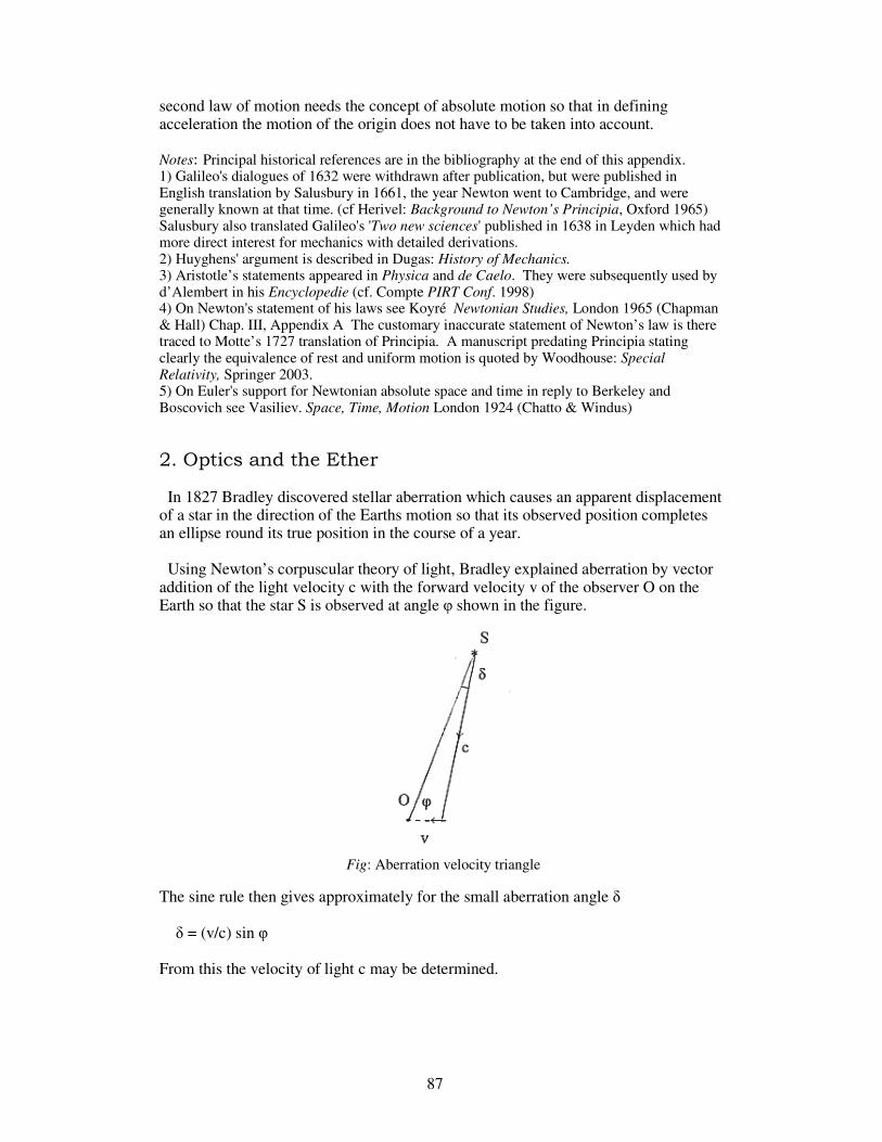
87 87 87
second law of motion needs the concept of absolute motion so that in defining acceleration the motion of the origin does not have to be taken into account. Notes: Principal historical references are in the bibliography at the end of this appendix. 1) Galileo's dialogues of 1632 were withdrawn after publication, but were published in English translation by Salusbury in 1661, the year Newton went to Cambridge, and were generally known at that time. (cf Herivel: Background to Newton’s Principia, Oxford 1965) Salusbury also translated Galileo's 'Two new sciences' published in 1638 in Leyden which had more direct interest for mechanics with detailed derivations. 2) Huyghens' argument is described in Dugas: History of Mechanics. 3) Aristotle’s statements appeared in Physica and de Caelo. They were subsequently used by d’Alembert in his Encyclopedie (cf. Compte PIRT Conf. 1998) 4) On Newton's statement of his laws see Koyré Newtonian Studies, London 1965 (Chapman & Hall) Chap. III, Appendix A The customary inaccurate statement of Newton’s law is there traced to Motte’s 1727 translation of Principia. A manuscript predating Principia stating clearly the equivalence of rest and uniform motion is quoted by Woodhouse: Special Relativity, Springer 2003. 5) On Euler's support for Newtonian absolute space and time in reply to Berkeley and Boscovich see Vasiliev. Space, Time, Motion London 1924 (Chatto & Windus)
2. Optics and the Ether In 1827 Bradley discovered stellar aberration which causes an apparent displacement of a star in the direction of the Earths motion so that its observed position completes an ellipse round its true position in the course of a year. Using Newton’s corpuscular theory of light, Bradley explained aberration by vector addition of the light velocity c with the forward velocity v of the observer O on the Earth so that the star S is observed at angle φ shown in the figure.
Fig: Aberration velocity triangle The sine rule then gives approximately for the small aberration angle δ δ = (v/c) sin φ From this the velocity of light c may be determined.

88 88 88
Bradley found the speed of light to be the same for all stars examined and close to the value found by Römer in1769 from eclipses of Jupiter’s satellites.Since in this derivation the angle of aberration δ depends on the speed of light, it might be expected to change if the light was passing through a material of refractive index greater than one which would reduce its speed correspondingly. The test was made by Arago in 1810 with a negative result. Being unable to find a simple explanation he asked Fresnel whether an explanation could be found using the wave theory of light which Young (1904) had shown could explain normal aberration. In reply Fresnel proposed his theory that the ether, at rest, is partially dragged by the Earth and as a result the velocity of the light in a medium moving with velocity v is given by the formula c' = c/N + kv Here N is the index of refraction and k is the dragging coefficient having the value. k = 1 – 1/N2 This formula was later experimentally investigated by Fizeau (1851) and found to be remarkably accurate. The result, strange at the time, subsequently found confirmation in the theory of relativity since the formula approximates addition of the velocities c/N and v by the composition rule when v/c is small (von Laue 1907, cf. Miller 1998) * The Doppler Effect: Another optical phenomenon which came to be important is the Doppler Effect which is by its nature a wave phenomenon. It was discussed in several papers from 1842 by Doppler who derived his formula and suggested it might be applied to the spectra of double stars. This was confirmed experimentally by Huggins and Miller in 1868 * Note: Boscovich, already in 1766, had proposed using a telescope filled with water but this was not tried out until about a century later by Airy with a negative result. 3. Maxwell’s Equations and the Lorentz Theory As remarked above, Maxwell, in his 1877 book ‘Matter and Motion’ stated that the concept of absolute motion is necessary for the foundations of Newtonian mechanics and he had assumed ether absolutely at rest when he established his electromagnetic theory of light (1873). The difference between systems at rest and in motion was emphasized in the Herz form of Maxwell’s equations which came into general use after 1890. * The work of Lorentz: Stokes in 1845 proposed a theory of aberration which assumed that the Earth dragged the ether in such a way that the relative velocity between them became zero on the surface. This theory led to results at variance with Fresnel’s hypothesis. Lorentz's earlier work aimed at reconciling Maxwell’s equations with Fresnel’s hypothesis. In connexion with this he developed a theory in 1886 covering both aberration and Doppler effect using what he called the principle of invariance of the phase which states that the phase Φ = 2πf (t - (lx + my + nz))

89 89 89
remains unaltered with change from rest to motion. Here f denotes frequency and (l, m, n) the direction cosines of the wave-normal. Later, with the appearance of the Herz form of Maxwell's equations and the discovery of the electron (1891), Lorentz developed his theory of electrons to study electrical phenomena in moving media. This theory explained electrical phenomena in terms of a free flow of electrons in the ether, the ether exerting a force on the electrons due to electric and magnetic fields, a force which became known as the Lorentz force. * Evolution of the Lorentz transformation: The history of the Lorentz transformation began with Voigt (1887) who, when investigating the Doppler Effect, showed that the three dimensional wave equation is unaltered by the change of variables x' = x - vt y' = y √(1-v2/c2) z' = z √(1-v2/c2) t' = t - (v/c2).x It differs only by a scalar multiple from the Lorentz transformation now used. The contribution of Voigt was however isolated and not followed up. Lorentz’s derivation of the transformation was in answer to the question:.given that Maxwell's equations are valid in a system S at rest relative to the ether, what equations are followed in a system S' moving relative to S ? Lorentz first made the transformation from coordinates in S to moving (‘relative’) coordinates coinciding with S' by x r = x – vt, y r = y, z r = z, t r = t He then found that the further transformation is necessary to ensure that Maxwell’s equations keep their form in S' given by x' = βl x r, y' = l y r, z' = l z r, t' = lt r /β – βl vx r /c
2
Here the variable t' is a fictitious ‘local time’, l is a positive constant multiplier, and β is the constant, nowadays usually denoted by γ and called the Lorentz factor, which was set at the approximate value β = 1 + v²/ 2c² With this theory it was found that, to the first order in v/c, light behaves in the moving system S' exactly as it does in the stationary system S. (Further details are given in the book of Miller (1998) from which this account is taken.) * The contraction hypothesis: The famous Michelson-Morley experiments of 1887, 1888 established that there is not any second order effect which enables a moving system to be distinguished from one that is at rest. The difficulty of explaining this fact resulted in the contraction hypothesis proposed independently by FitzGerald (1888) and Lorentz (1895). According to this hypothesis, motion of the electrons relative to the ether causes a length contraction in the direction of motion by the factor √(1-v²/c²), the electrons then becoming ellipsoidal. This hypothesis led on to a revision of the value of β to its exact value

90 90 90
β = 1/√(1-v²/c²) And to a revised theory by Lorentz (1904) * The standard Lorentz transformation: By substitution from Lorentz’s two sets of equations follows
x' = l β (x - vt) y' = l y z' = l z t' = l β (t - (v/c²)x)
Poincaré (1905) called these equations the Lorentz transformation observing that for the value l = 1 they combine and have an inverse of the same form so giving rise to a one dimensional group, the Lorentz group, which he then in 1906 extended to three dimensions. The scalar-multiplied form of this transformation includes that of Voigt as Lorentz (1909) later acknowledged saying that Voigt's paper had escaped him all those years and adding:
'The idea of the transformation might therefore have been borrowed from Voigt, and the proof that it does not alter the form of the equations for the free ether is contained in his paper'
From a slightly different point of view, the same transformation had also been used by Larmor in his 1900 book ‘Aether and Matter’ 4. The Principle of Relativity After the negative result of the Michelson-Morley experiments of 1887 and 1888 Poincaré, who had taken a close interest in the work of Lorentz commenting critically on underlying assumptions, was led to speculate that no difference would be found between Maxwell-Hertz equations for fixed and moving systems even for higher order approximations since electrical systems, like mechanical, depend only on relative motions. This view received further verification from the revised theory of Lorentz (1904) which accounted not only for second order effects and which demonstrated the invariance of Maxwell’s equations under the Lorentz transformation. In a lecture at St.Louis in 1904 Poincaré proposed several principles applying to all physical phenomena one of which was:
'The principle of relativity, according to which the laws of physical phenomena must be the same for a stationary observer as for an observer carried along in a uniform motion of translation so that we have not and can not have any means of discerning whether or not we are carried along in such a motion'

91 91 91
In his 1905 paper which appeared shortly before that of Einstein, Poincaré questioned the existence of absolute motion for linear motions although he had in his previous writings been careful to point out the exceptional nature of rotating systems. Einstein’s interest in the problem of relativity dates from his student days in Zürich where he had studied Herz-Maxwell theory in the form given to it by Lorentz in 1895 and then appears to have been influenced by Poincaré’s writings. His initial ideas formed in collaboration with his wife Mileva Marič appear to have been based on the theory of relative motions. Thus the introduction to his 1905 paper says
'..Maxwell's electrodynamics - as usually understood at the present time – when applied to moving bodies, leads to asymmetries which do not appear to be inherent in the phenomena. Take, for example, the reciprocal electrodynamic action of a magnet and a conductor. The observable phenomenon here depends only on the relative motion of the conductor and the magnet, whereas the customary view draws a sharp distinction between the two cases in which either the one or the other of these bodies is in motion.'
However the theory of the 1905 paper was not based on relative motions but followed on from the Lorentz theory. Einstein’s version of the Principle of Relativity denied absolutes both for space and, most remarkably, for time. All inertial systems in relative uniform motion were considered equivalent for the description of physical laws while each observer keeps his own time measured by personal clock. The status of rotating systems was left undefined and in fact, ignored. Einstein's paper 1905 was followed by a restatement with modifications in the 1907 paper in 'Jahrbuch der Physik'. In another series of papers Einstein followed up his growing interest in the relation between mass and energy. General recognition of the approach of the 1905 paper depended on experimental verification by measurements on fast moving electrons. After initial unclear results and an unsuccessful attempt to verify the theory using the transverse Doppler effect, final experimental proof was reported by Bücherer at the same time as Minkowski's famous 1908 lecture and established a general acceptance of the relativity principle in the form Einstein had given it. At the time, Einstein's contribution was regarded as a variation on the Lorentz theory although Lorentz himself later acknowledged the immense simplification Einstein's relativity hypothesis presented:
‘If I had to write the last chapter now, I should certainly have given a more prominent place to Einstein's theory of relativity by which the theory of electromagnetic phenomena in moving systems gains a simplicity that I had not been able to attain. The chief cause of my failure was my clinging to the idea that the variable t only can be considered as the true time and that my local time t' must be regard as no more than an auxiliary mathematical quantity. In Einstein's theory, on the contrary, t' plays the same part as t; if we want to describe phenomena in terms of x',y',z',t' we must work with these variables exactly as we could do with x,y,z,t’
Lorentz: 1915 note added to 'Theory of Electrons' (1906) p.321.)

92 92 92
Notes etc: 1) On Lorentz's work relating to Maxwell's equations see Miller A I: Einstein's Special Theory of Relativity. New York 1998 (Springer) 2) Detailed references for Poincaré’s contribution to the founding of the theory are given in Whittaker’s book. The above 1904 quotation is from Halstead’s English translation of Poincaré’s St Louis Lecture of 1904 as reprinted in Poincaré’s ‘Value of Science’. 3) Detailed biographic comments for Einstein including his indebtedness to others and use of texts such as those of Föppl and Drude may be found in his Collected Works, vol. II. Many of the comments are reproduced in Stachel’s ‘Einstein’s Miraculous Year’ 4) The early work of Einstein is recorded only by two letters of 1901 referring to ‘our work on relative motions’ to his wife Mileva Marič who appears to have made (at least) an initial contribution to the theory of relativity and its philosophy. Being from Croatia she came from the same region as Varićak and may well have been influenced by ideas originating from Boscovich. Varićak made an extensive study of Boscovich’s works and wrote many scholarly articles on them. He brought to notice Boscovich’s article of 1755 which contained ‘many clear and radical ideas regarding the relativity of space, time and motion’ (quoted from Silberstein 1914, p. 38) 5) The experimental evidence from electron measurements supporting Einstein’s theory was given by Bücherer ‘Die experimentalle Bestätigung der Lorentz-Einsteinsche Theorie‘.Phys. Z. 9 1908 Also in Ann. Phys. 1909.
5. Bibliography on the History of the Theory of Relativity These are in chronological order up to the appearance of the Poincaré-Einstein theory. 1632 Galilei G: Dialogo di Galileo Galilei Linceo doue nei congresso di quattro giornate se dicorre sopra i due massimi sistemi del mondo tolemaico e copernicano. Florence 1632; Withdrawn shortly after publication but republished Strasbourg 1637 in Latin; Engl. tr: 1665; G de Santillana (ed.) 'Dialogue on the Great World Systems', Chicago 1953 (Univ. Press); S. Drake (tr.) 'Dialogues concerning the two chief World Systems - Ptolemaic and Copernican', Berkeley Calif. 1967 (Univ. Calif. Press) 1656 Huyghens C De motu corporum ex percussione. [1656] (posth 1703) Oeuvres Complètes XVI 3-168; German transl. Über die Bewegung der Körper durch den Stoss Ostwald's Klassiker 138 1-34. F. Hausdorf (ed.) Described in Dugas. 1687 Newton I: Philosophiae Naturalis Principia Mathematica. London 1687 (Samuel Smith); 2nd ed. 1713; 3rd ed. 1726; Engl. tr. by Motte – Cajori: The Mathematical Principles of Natural Philosophy, Berkeley 1934 (Univ. Calif. Press) 1728 Bradley J: Letter to Dr Halley giving an account of a new discovered motion of the Fix'd Stars. Phil. Trans 35 1727/28 637- 661 1755 Bošković R.J. (Boskovich): De moto absoluto, an possit a relativo distingui, Rome 1755. Reprinted by Varićak (ed.) South Slavic acad. sci. 190 1912. 1804 T.Young: Experiments and Calculations relative to physical optics. Proc. Roy. Soc. 94 1804 1-16; Works I, 188- [Aberration explainable by wave theory]
93 93 93
1811 D.F-J.Arago Mémoire sur un modification remarkable qu'eprouvent les rayons lumineux dans leur passage a traverse certains corps diaphanes d'optique. Paris Mém. de l'Inst. 1811, 93-134; C.R. Acad. Sci Paris, 8 1829 326-; 36 1853 380- [Arago showed experimentally that in all respects light behaves as though it were coming from the direction of aberration.] 1818 Fresnel A.J. Sur l'influence du mouvement terrestre dans quelques phenomènes d'optique. Ann. Chimie Phys. 9 1818 57- ; Oeuvres complètes l II 627-. [Reply of Fresnel to Arago giving the Fresnel drag formula] 1841 Doppler C. Ueber das farbige Licht der Doppelsterne und einiger anderer Gestirne des Himmels. Bohm. Ges. Abh. 2 1841-42 467-490; Abhandlungen, Leipzig 1907 (Engelmann), Ostwald's Klassiker No. 161 pp 1-24. 1845 Stokes G.G. On the aberration of light Phil. Mag. 27 1845 9-15; 29 1846 62-63; Math & Phys Papers I 134-. [Stokes theory on ether drag by the Earth.] 1846 Doppler C: Bemerkungen zu meiner Theorie des farbigen Lichtes der Dopplesterne Pogg. Ann. 68 1846 1-34. 1846 Stokes G G: On Fresnel's theory of the aberration of light Phil Mag 28 1846 76-81 Math & Phys Papers I. 1847 Doppler C. Ueber den Einfluss der Bewegung des Fortpflanzungsmittels auf die Erscheinungen der Aether-, Luft- und Wasserwellen. Böhm. Ges. Abh. 5 1847 293-306. 1848 Stokes G.G. On the constitution of the luminiferous ether. Phil.Mag. 32 1848 343-349; Math.& Phys. Papers I. 1851 Fizeau H. Sur les hypothèses relatives .. l'aether lumineux, et sur une expérience qui parait démontrer que le mouvement des corps change le vitesse avec laquelle la lumière se propage dans leur intérieur. C.R. Acad. Sci. Paris 33 1851 349-355. 1868 Huggins W & Miller W.A: Notes on the lines in the spectra of some of the fixed stars, Proc Roy Soc.18 1868 444-445 [Experimental verification of Doppler shift for stellar motion] 1873 Maxwell J C: Treatise on Electricity and Magnetism, 2 vols Oxford 1873 (Univ. Press); rpr abridged 3rd ed. New York 1954 (Dover) 1877 Maxwell J C: Matter and Motion Cambridge 1877 (Univ. Press) rpr New York 1952 (Dover) 1878 Maxwell J.C: Ether Encyclopedia Britannica 1878: Scientific Papers 763-775. 1881 Michelson A.A:. The relative motion of the Earth and the luminiferous ether Amer. J. Sci. 22 120-129. [Michelson's first experiment]

94 94 94
1886 Lorentz H.A. Sur l'influence de la movement de la terre sur les phenomènes lumineux. Arch. néerl. Sci.21 1887 103-176. (Previously in Dutch in Versl Kon Akad Wet 2 1886 297-372); Coll. Papers IV 153-214. [Derivation of optical Doppler Effect and stellar aberration] 1887 Michelson A.A. & Morley E.W: On the relative motion of the Earth and the luminiferous aether, Amer. J. Sci. 34 333-345 1887; Phil. Mag. 24 1887 1887 Voigt M. Ueber das Doppler'sche Princip. Gött Nachr 1887 rpr in Phys. Z. 1915 1892 Herz H: Electric Waves Leipzig 1892 (Teubner); London 1893 (MacMillan); rpr New York 1962 (Dover) 1889 FitzGerald G F: The ether and the earth's atmosphere Science 1889 [The Lorentz contraction proposed in a nontechnical way] 1892 Lorentz HA La théorie electromagnetique de Maxwell et son application aux corps mouvants Arch néerl Sci 26 1892 363-; Leiden 1892 (Brill); Coll Papers II 164-343 [Lorentz-contraction] 1892 Lorentz H.A. De relatieve beweging van de Aarde en den Aether. Zitt. Verslag. Akad. Wet. Am'dam 1 Nov. 1892, 74-79; Coll.Papers IV 219-223. 1892 Lodge O.J. On the present state of our knowledge of the connexion between either and matter, Nature June 1892 p.164 [Refers to FitzGerald contraction] 1893 Lodge O J: A study on aberration Phil. Trans. 184 1893 727-804 [Refers to FitzGerald contraction on p.749] 1894 Föppl A: Einführung in die Maxwell'sche Theorie der Elektrizität. Leipzig 1894 (Teubner); republished 1904 as vol I of 'Theorie der Elektrizität' by Abraham. [Influential textbook based on Lorentz theory] 1895 Lorentz H.A. Versuch einer Theorie der electrischen und optischen Erscheinungen in bewegten Körpern. Leiden 1895 (Brill): Coll. Papers 5 1-137. [Chap. V: Second derivation of optical Doppler Effect and stellar aberration using principle of corresponding states. Local time defined in paras.89-92, p.122 refers to FitzGerald, acknowledging his independent proposal of the contraction hypothesis.] 1899 Lorentz H.A. Théorie simplifieé des phénomènes electriques et optiques dans les corps en mouvement. Proc. Acad. Sci. Amsterdam .1 1899 427-442. Coll. Papers IV 139-155 Previously in Dutch in Verslag. kon. Akad Wet 7 1899 507-522 [Lorentz transformation exact for square-root] 1900 Larmor J Aether and Matter Cambridge 1900 (Univ. Press) (Previously Cambridge 1898, Adams Prize Essay) [Wrote Lorentz transformation correct to second order terms and showed the Fitzgerald-Lorentz contraction as well as the slowing of clocks to be consequences. See pp.167-177 in the book, especially 173]
95 95 95
1900 Drude P.K.L. Lehrbuch der Optik 1900 Tr. as Textbook of Optics London 1902 [Limitation of Doppler formula emphasized] 1900 Poincaré H. La théorie de Lorentz et le principe de reaction. Arch. néerl. Sci. 1900; Oeuvres IX 464-488. 1901 Poincaré H. Electricité et optique. Paris (Sorbonne lectures to 1900) 1904 Lorentz H.A: Electromagnetic phenomena in a system moving with any velocity smaller than that of light. Proc Acad Sci Amsterdam 6 1904 809- 834; Coll Papers V 172-197; rpr in 'The Principle of Relativity' 1904 Poincaré H: Lecture to Congress of Arts and Sciences, St. Louis, USA Sept Bull. Sci. Math. 28 1904 302-; Engl. tr. (G.B. Halstead) Monist Jan 1905. [Stated ‘The principle of relativity’] 1904 Lorentz H.A. Maxwells Elektromagnetische Theorie. Enz. Math. Wiss. V(2) 13 Leipzig 1904 (Teubner), 63-144. 1904 Lorentz H.A. Weiterbildung der Maxwell'schen Theorie: Electronentheorie. Enz. Math. Wiss. V(2) 14 Leipzig 1904 (Teubner), 145-280. 1905 Poincaré H. Sur la dynamique de l'electron. C.R. Acad. Sci. Paris 140 1905 1504-1508, Oeuvres IX 489-493. 1905 Einstein A. Zur Elektrodynamik bewegte Kırper. Ann Physik 17 1905 891- 921; Engl.tr 'On the electrodynamics of moving bodies' in 'The Principle of Relativity' Coll. Works II 275- and 306 with extensive notes. 1906 Poincaré H. Sur la dynamique de l'electron. Rend. Circ. mat. Palermo 21 1906 129-176, Oeuvres IX 494-550. Engl. tr. (Keswani G.H. & Kilminster C.W.) Brit. J. Phil. Sci. 34 1983 343-. 1907 Einstein A. Őber die Relativitätsprinzip und die aus demselben gezogenen Folgerungen. Jahrb. Radioaktivitat 4 1907 411-462; Coll. Papers II 433-484. 1908 Bücherer A.H. Messungen an Becquerel strahlen. Die experimentalle Bestätigung der Lorentz-Einsteinsche Theorie. Phys. Z. 9 1908 755-762. Also in Ann. Phys. 1909 1909 Lorentz H.A. The Theory of Electrons (Columbia University Lectures 1906) Leipzig 1909 (Teubner); London 1909, 1915 (Nutt); rpr. New York 1952 (Dover) [cf. Chapter 5: Optical phenomena in moving bodies.]

96 96 96
6. Secondary Literature and Collected Works Doppler C. Abhandlungen Leipzig 1907 (Wilhelm Engelmann), Ostwald's Klassiker No. 161. Dugas R. Histoire de la mécanique. Neuchatel 1950 (Griffon); Engl. tr. London 1957 (Routledge & Paul); 1988 (Dover) Einstein A. The Collected Papers of Albert Einstein, ed J. Stachel et al. (Princeton Univ. Press 1989) [Relativity papers 1900-1909 are in vol. II] Lorentz H.A. Collected Papers, 9 vols, The Hague 1935-39 (Nijhoff) Miller A.I. Albert Einstein's Special Theory of Relativity New York 1998 (Springer) Poincaré H. Oeuvres de Henri Poincaré (ed. G.Darboux) Paris 1916-1956 (Gauthier-Villars) [Relativity papers are in vol. IX] Stachel J. Einstein's Miraculous Year Princeton 1998 (Univ.Press)
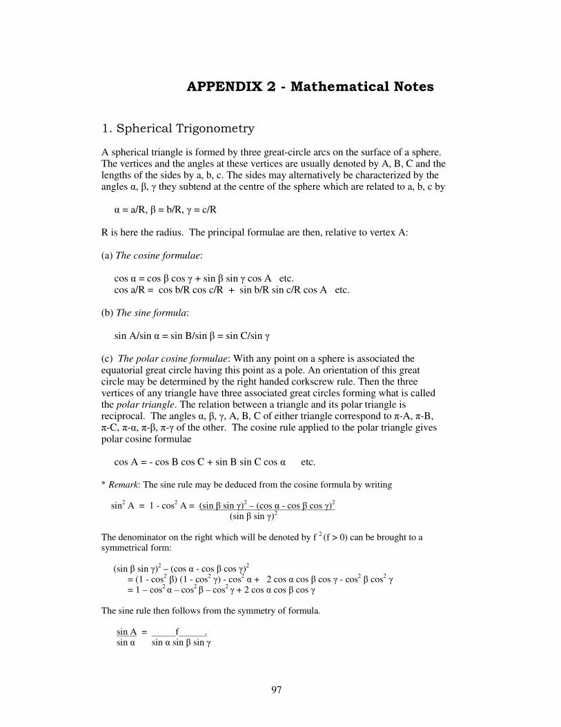
97 97 97
APPENDIX 2 - Mathematical Notes
1. Spherical Trigonometry A spherical triangle is formed by three great-circle arcs on the surface of a sphere. The vertices and the angles at these vertices are usually denoted by A, B, C and the lengths of the sides by a, b, c. The sides may alternatively be characterized by the angles α, β, γ they subtend at the centre of the sphere which are related to a, b, c by
α = a/R, β = b/R, γ = c/R R is here the radius. The principal formulae are then, relative to vertex A: (a) The cosine formulae:
cos α = cos β cos γ + sin β sin γ cos A etc. cos a/R = cos b/R cos c/R + sin b/R sin c/R cos A etc.
(b) The sine formula:
sin A/sin α = sin B/sin β = sin C/sin γ (c) The polar cosine formulae: With any point on a sphere is associated the equatorial great circle having this point as a pole. An orientation of this great circle may be determined by the right handed corkscrew rule. Then the three vertices of any triangle have three associated great circles forming what is called the polar triangle. The relation between a triangle and its polar triangle is reciprocal. The angles α, β, γ, A, B, C of either triangle correspond to π-A, π-B, π-C, π-α, π-β, π-γ of the other. The cosine rule applied to the polar triangle gives polar cosine formulae
cos A = - cos B cos C + sin B sin C cos α etc. * Remark: The sine rule may be deduced from the cosine formula by writing
sin2 A = 1 - cos2 A = (sin β sin γ)2 – (cos α - cos β cos γ)2 (sin β sin γ)2
The denominator on the right which will be denoted by f 2 (f > 0) can be brought to a symmetrical form:
(sin β sin γ)2 – (cos α - cos β cos γ)2
= (1 - cos2 β) (1 - cos2 γ) - cos2 α + 2 cos α cos β cos γ - cos2 β cos2 γ = 1 – cos2 α – cos2 β – cos2 γ + 2 cos α cos β cos γ
The sine rule then follows from the symmetry of formula.
sin A = f . sin α sin α sin β sin γ
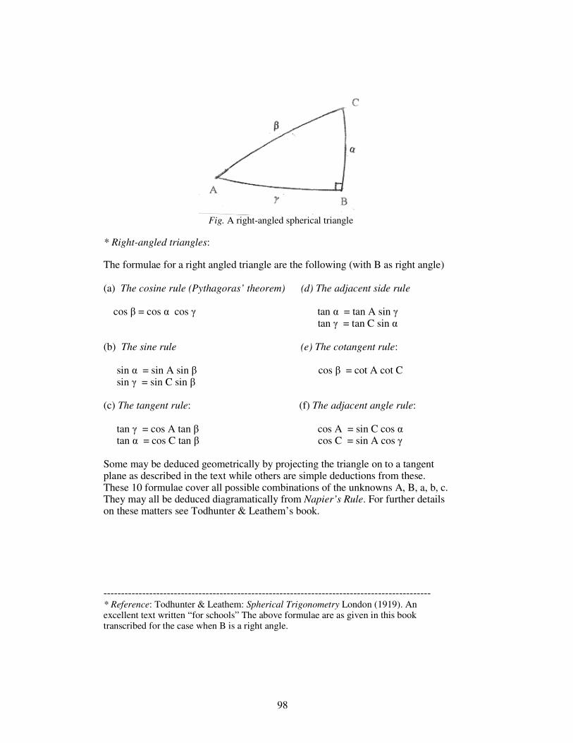
98 98 98
Fig. A right-angled spherical triangle * Right-angled triangles: The formulae for a right angled triangle are the following (with B as right angle) (a) The cosine rule (Pythagoras’ theorem) (d) The adjacent side rule
cos β = cos α cos γ tan α = tan A sin γ tan γ = tan C sin α
(b) The sine rule (e) The cotangent rule:
sin α = sin A sin β cos β = cot A cot C sin γ = sin C sin β
(c) The tangent rule: (f) The adjacent angle rule:
tan γ = cos A tan β cos A = sin C cos α tan α = cos C tan β cos C = sin A cos γ
Some may be deduced geometrically by projecting the triangle on to a tangent plane as described in the text while others are simple deductions from these. These 10 formulae cover all possible combinations of the unknowns A, B, a, b, c. They may all be deduced diagramatically from Napier’s Rule. For further details on these matters see Todhunter & Leathem’s book. --------------------------------------------------------------------------------------------- * Reference: Todhunter & Leathem: Spherical Trigonometry London (1919). An excellent text written “for schools” The above formulae are as given in this book transcribed for the case when B is a right angle.

99 99 99
* Spherical excess: From the polar cosine formula may be deduced that the sum of the angles of a spherical triangle is greater than π.
cos A = - cos B cos C + sin B sin C cos a/R < - cos B cos C + sin B sin C = - cos (B+C) = cos (π-B-C)
from which
A < π – B – C, i.e. A+B+C < π The spherical excess is the positive difference
E = (A+B+C) - π It gives the area of a spherical triangle by Giraud’s formula
area = E R2 * Lagrange’s formula for excess: numerous formulae have been given for finding the excess. The most appropriate for this book is that described by Lagrange (1799) which is
cot (E/2) = cos β/2 cos γ/2 + sin β/2 sin γ/2 cos A = cot β/2 cot γ/2 + cos A sin β/2 sin γ/2 sin A sin A
Lagrange’s derivation was the following
cot (E/2) = - tan (A + B + C)/2 = - tan A/2 + tan (B + C) 1 – tan A/2 tan (B + C)/2
Now use is made of the identity
tan (B + C)/2 = cos (β – γ)/2 cot A/2 cos (β + γ)/2
which is one of ‘Napier’s analogies’ ( SeeTodhunter & Leathem) Substituting for tan (B + C)/2, leads to the required expression
cot (E/2) = - tan A/2 cos (β + γ)/2 + cot A/2 cos (β - γ)/2 sin β/2 sin γ/2 sin A
= cos β/2 cos γ/2 + sin β/2 sin γ/2 cos A sin β/2 sin γ/2 sin A
Lagrange showed that this may be converted to a symmetric form as shown in the analogous hyperbolic case below. Reference: Lagrange’s paper: ‘Solution de quelques problèmes ...’ may be read in his Collected Works: Oeuvres VII 331-359 (see especially 339)
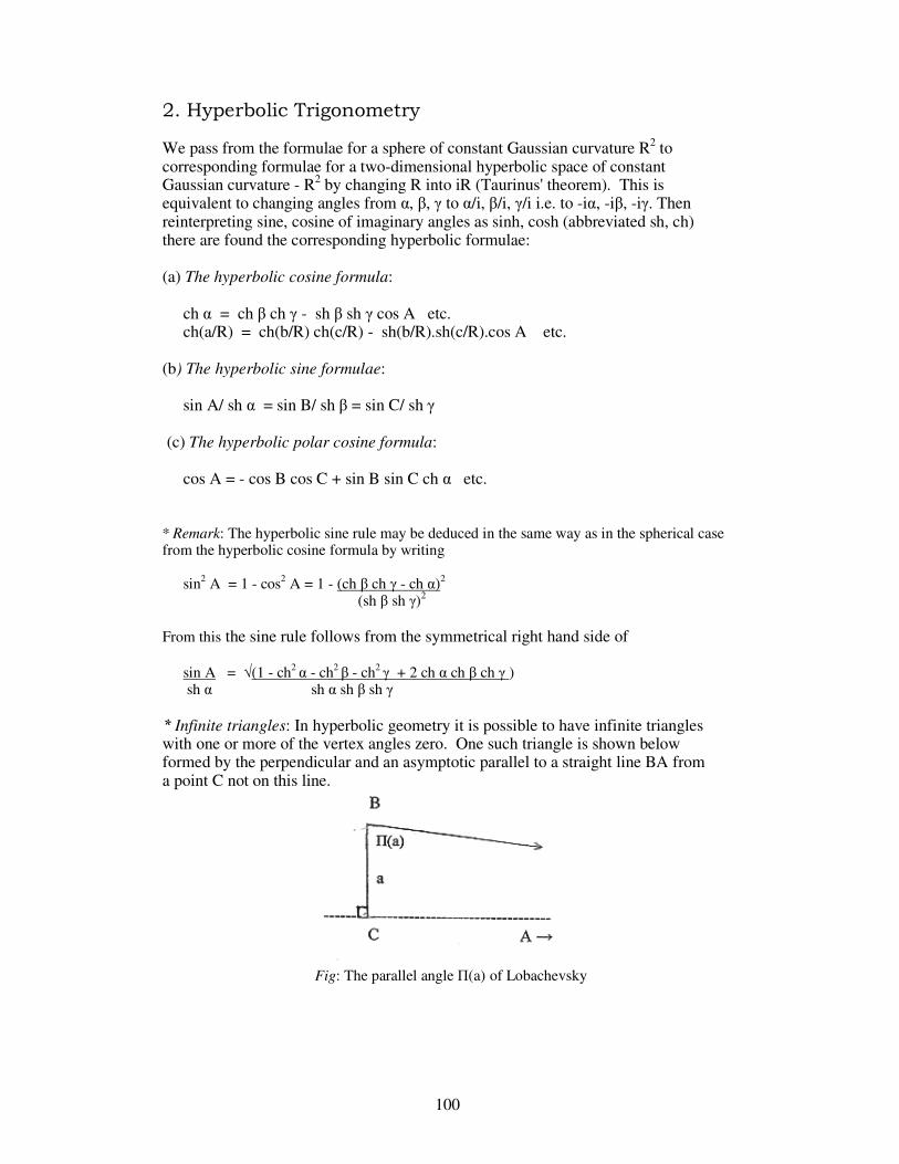
100 100 100
2. Hyperbolic Trigonometry We pass from the formulae for a sphere of constant Gaussian curvature R2 to corresponding formulae for a two-dimensional hyperbolic space of constant Gaussian curvature - R2 by changing R into iR (Taurinus' theorem). This is equivalent to changing angles from α, β, γ to α/i, β/i, γ/i i.e. to -iα, -iβ, -iγ. Then reinterpreting sine, cosine of imaginary angles as sinh, cosh (abbreviated sh, ch) there are found the corresponding hyperbolic formulae: (a) The hyperbolic cosine formula:
ch α = ch β ch γ - sh β sh γ cos A etc. ch(a/R) = ch(b/R) ch(c/R) - sh(b/R).sh(c/R).cos A etc.
(b) The hyperbolic sine formulae:
sin A/ sh α = sin B/ sh β = sin C/ sh γ (c) The hyperbolic polar cosine formula:
cos A = - cos B cos C + sin B sin C ch α etc. * Remark: The hyperbolic sine rule may be deduced in the same way as in the spherical case from the hyperbolic cosine formula by writing
sin2 A = 1 - cos2 A = 1 - (ch β ch γ - ch α)2
(sh β sh γ)2
From this the sine rule follows from the symmetrical right hand side of
sin A = √(1 - ch2 α - ch2 β - ch2 γ + 2 ch α ch β ch γ ) sh α sh α sh β sh γ
* Infinite triangles: In hyperbolic geometry it is possible to have infinite triangles with one or more of the vertex angles zero. One such triangle is shown below formed by the perpendicular and an asymptotic parallel to a straight line BA from a point C not on this line.
Fig: The parallel angle Π(a) of Lobachevsky

101 101 101
The angle B is the parallel angle of Lobachevsky denoted by him by Π(a) showing its dependence on the length a of the perpendicular CB. The right-angled triangle ABC has one zero angle and two infinite sides. On putting A = 0, B = Π(a), C = π/2 , b = ∞, c = ∞ in the above polar cosine formula for cos A follows,
1 = sin Π(a) ch α From this follows the formulae of Lobachevsky for the parallel angle:
sin Π(a) = 1/ ch (a/ R) cos Π(a) = th (a/ R) tan Π(a) = 1/ sh(a/R)
* References on hyperbolic geometry: The literature is considerable. Standard texts are those of Bonola, Sommerville while the books of Coxeter, Rosenfeld and Shirokov are to be recommended. Bonola includes a translation of Bolyai’s work. Not much of the original work of Lobachevski is easily available in translation Apart from a small introductory volume originally published in German, there is available one article in French, ‘Géometrie imaginaire’ and an English translation of a later work ‘Pangeometry’ both listed at the end of this appendix. * Right-angled hyperbolic triangles: With B as right angle the formulae corresponding to the spherical case are as follows (a) The hyperbolic cosine rule (d) The hyperbolic adjacent side rule
ch β = ch α ch γ th α = tan A sh γ th γ = tan C sh α
(b) The hyperbolic sine rule (e) The hyperbolic cotangent rule
sh α = sin A sh β ch β = cot A cot C sh γ = sin C sh β
(c) The hyperbolic tangent rule: (f) The hyperbolic adjacent angle rule
th γ = cos A th β cos A = sin C ch α th α = cos C th β cos C = sin A ch γ
As with spherical formulae, these 10 formulae cover all possible combinations of the unknowns A, B, a, b, c and may be set out by a modified form of Napier’s Rule. Certain of these formulae may be deduced by projection on to a tangential Euclidean plane (the limiting plane) as in the spherical case. --------------------------------------------------------------------------------------------------------- References: 1) For the hyperbolic Napier Rule, due to Engel, see Sommerville: Non-Euclidean Geometry 2) The method of projection on to the limiting plane is described in Shirokov: A sketch of the fundamentals of Lobachevskian geometry, (1964)

102 102 102
* Hyperbolic defect: From the polar cosine formula it may be shown that the sum of the angles of a hyperbolic triangle is less than π. Following a similar method to the spherical case we have
cos A = - cos B cos C + sin B sin C ch a/R > - cos B cos C + sin B sin C = - cos (B+C) = cos (π-B-C)
From which follows
A < π-B-C i.e. A+B+C < π The hyperbolic defect is defined as the positive difference
D = π - (A+B+C) It gives the area of a hyperbolic triangle by a formula due to Gauss (cf the spherical case)
area = D R2 * The Hyperbolic Form of Lagrange's Formula for Excess (Area): Lagrange's formula becomes cot (D/2) = ch β/2 ch γ/2 + sh β/2 sh γ/2 cos A sh β/2 sh γ/2 sin A LEMMA: In any hyperbolic triangle, tan (B + C) = ch (β-γ)/2 cot A 2 ch (β+γ)/2 2 This is the first of Napier's analogies for a hyperbolic triangle. Its proof is similar to the spherical case. From it the Lagrange formula follows easily: cot (D/2) = tan (A+B+C)/2 = tan A/2 + tan(B+C)/2 1 + tan A/2 tan(B+C)/2 By the lemma the right hand side is rhs = tan(A/2) ch(β+γ)/2 - cot(A/2) ch(β-γ)/2 ch(β+γ)/2 - ch (β-γ)/2 = ch β/2 ch γ/2 + sh β/2 sh γ/2 cos A sh β/2 sh γ/2 sin A ------------------------------------------------------------------------------------------------- Reference: See Sommerville (1914) for Gauss’ simple proof of his formula for area of a hyperbolic triangle.
103 103 103
* The symmetric form of the Lagrange formula: The formula may be further transformed by multiplying both denominator and numerator by 4 ch β/2 ch γ/2: rhs = 4 (ch β/2 ch γ/2)² + 4 ch β/2 ch γ/2 sh β/2 sh γ/2 cos A 4 ch β/2 ch γ/2 sh β/2 sh γ/2 sin A The numerator is then, converting to whole angles, (ch β + 1)(ch γ + 1) + sh β sh γ cos A = (ch β -1) (ch γ - 1) + ch α - ch β ch γ = 1 + ch α + ch β + ch γ while the denominator is, by the hyperbolic sine rule, sh β sh γ sin A = √(1 - ch2α - ch2β - ch2γ + 2 ch α ch β chγ ) resulting in the symmetric formula cot (D/2) = 1 + ch α + ch β + ch γ . √(1 - ch2α - ch2β - ch2γ + 2 ch α ch β ch γ ) Here cos (D/2) and sin (D/2) will be proportional to the numerator and denominator respectively. The constant of proportionality is easily identified by squaring and adding giving cos (D/2) = 1 + ch α + ch β + ch γ 4 (ch α/2)(ch β/2)(ch γ/2) sin (D/2) = √(1 - ch2α - ch2β - ch2γ + 2 ch α ch β ch γ ) 4 (ch α/2)(ch β/2)(ch γ/2)
104 104 104
3. Cayley-Klein Projective Metric Cayley (1869) showed how the concept of distance could be introduced into projective geometry relative to an absolute conic (or simply 'absolute') having equation a(x, x) = 0 Here a(x, y) is a bilinear form in the vectors x, y of a projective space.
a(x, y) = Σ Σ aij xi.yj i, j = 1 Projective distance ρ is defined relative to the absolute by the formula ρ = cos[-1] a(x,y) . √a(x,x) a(y,y) In three dimensions setting a(x, x) = x1
2 + x22 + x3
2 makes the absolute an imaginary locus and the Cayley definition gives the angle between the vectors x and y or, if these lie on a sphere with centre at the origin, the arc length on the surface of the sphere. Klein (1871) considerably developed Cayley's idea by a method based on cross-ratios leading to a unified treatment by projective geometry of Euclidean, spherical and Lobachevskian geometries according to the nature of the absolute conic. He introduced the terms parabolic, elliptic or hyperbolic respectively to denote the three basic geometries. In the hyperbolic case the quadratic a(x, x) is semi-definite so the absolute becomes a real ellipse and in view of the reversed Cauchy inequality the Cayley formula must be written as ρ = ch[-1] a(x,y) . √a(x,x) a(y,y) Ordinary Euclidean geometrical ideas apply in the interior of this ellipse but straight lines are considered to meet only if the meeting point lies in its interior. So lines do not necessarily meet and are then considered parallel. Lines meeting on the ellipse are defined as asymptotically parallel, the bounding conic thus representing infinity. With these conventions it is found that all Euclidean axioms are satisfied except those relating to parallels

105 105 105
* Relation to the Riemannian form: It is easy to show an equivalent formula for ρ is sh ρ = √a(x,y)²- a(x,x).a(y,y) √a(x,x) a(y,y) On putting y = x + dx there is found for the infinitesimal metric element squared: ds² = a(x,dx)² – a(x,x) a(dx,dx) = a(x,dx)² – a(dx,dx) a(x,x)² a(x,x)² a(x,x) It relates Cayley-Klein and Riemannian metrics. This formula shows that tangential elements to the surface a(x, x) = const (> 0) satisfying the constraint that a(x,dx) = 0 have metric element squared ds² = – a(dx, dx)/ const. Note the unexpected minus sign. * References: The original reference to Cayley's work is the last part of his 'Sixth Memoir on Quantics': Phil. Trans. 1859. Kleins' work was published in his elegantly written: Nicht Euklidische Geometrie reprinted by Chelsea 1927. See also Veblen & Young': Projective Geometry (Ginn) for a fine exposition. 4 The Beltrami-Klein Representation: Plane hyperbolic geometry is represented by the geometry of line segments within a circle as in fig.1. Two line segments are considered to be asymptotically parallel if they meet on the circle as in fig.2.
Fig.1 Intersecting and Fig.2: Asymptotic parallels
non-intersecting lines. * The Cayley-Klein metric: If the equation is centred at the origin and has radius R, its equation is x2 + y2 = R2 which may be put into homogeneous form by writing X/Z, Y/Z for x and y so that X2 + Y2 – R2 Z2 = 0
106 106 106
With this as absolute, the Cayley-Klein distance ρ is, ch ρ = (R2 Z1Z2 – X1X2 – Y1Y2) . R √(R2 Z1
2 – X12 – Y1
2 )(R2 Z22 – X2
2 – Y22 )
This in nonhomogeneous form is ch ρ = (R2- x1x2 - y1y2) . R √(R2- x1
2 – y12)(R2 - x2
2 – y22 )
From the last equation is found sh ρ = R√(x1 - x2)
2 + (y1 - y2)2 - (x1 y2 - x2 y1)
R √(R2 - x12 - y1
2)(R2 - x22 – y2
2) th ρ = R√(x1 - x2)
2 + (y1 - y2)2 - (x1 y2 - x2 y1)
R (R2- x1x2 - y1y2 ) * Polar formulae: Using the formula for th (ρ/R), the distance ρ from the origin (0,0) to a general point (x,y) at radial distance r is found from th ρ = r R R giving the parametric Beltrami form for the nonhomogeneous case as x = r cos θ = R th (ρ/R) cos θ y = r sin θ = R th (ρ/R) sin θ and for the homogeneous case, X = R sh (ρ/R) cos θ Y = R sh (ρ/R) sin θ Z = ch (ρ/R) The coordinates X, Y, Z (usually termed Weierstrass coordinates), satisfy identically -X 2 - Y 2 + R2 Z2 = R2 * The Riemannian form: The infinitesimal metric squared element (non-dimensional) is found from the formula for sh(ρ/R) or th (ρ/R) as
R2 (R2-y2) dx2 + 2xy dxdy + (R2-x2) dy2 (R2-x2-y2)2
R2 (R2-x2-y2) dx2 + (R2-x2-y2) dy2 + (xdy-ydx)2 (R2-x2-y2)2 R2 (dx2 + dy2) + (xdy – ydx)2
(R2-x2-y2) (R2-x2-y2)2
107 107 107
Changing to polar coordinates gives the metric element squared as
dr2 + r2 dθ2 1 - r2/R2 (1 – r2/R2)2
The further change to Beltrami coordinates gives it as
dρ2 + R2 sh2(ρ/R) dθ2
* The 3-dimensional case: The region within the circle now becomes the region x2+y2+z2 < R2 The radial distance from the origin (0, 0, 0) to point r = (x, y, z) is found as before as th (ρ/R) = r/R It gives the parametric form of the Beltrami representation in spherical coordinates: x = R th (ρ/R) sin φ cos θ y = R th (ρ/R) sin φ sin θ z = R th (ρ/R) cos φ The corresponding homogeneous form using Weierstrass coordinates (X, Y, Z, T) is T = ch (ρ/R) X = R sh (ρ/R) sin φ cos θ Y = R sh (ρ/R) sin φ sin θ Z = R sh (ρ/R) cos φ These parametrize the hyperboloid: – X 2 – Y 2 – Z2 + R2 T2 = R2
* The Cayley metric: Using r to denote vectors (x, y, z), equivalent forms for the nonhomogeneous Cayley metric giving distance from r1 to r2 are ch ρ = R2 – r1.r2 . √(R2 – r1.r1)(R
2 – r2.r2) sh ρ = √R2 (r2 – r1).(r2 – r1) – [(r1.r1) (r2.r2) – (r1.r2)
2] √(R2 – r1.r1)(R
2 – r2.r2) = R2(r2 - r1).(r2 - r1) – (r1 x r2).(r1 x r2) √(R2 – r1.r1)(R
2 – r2.r2) The last step used the Lagrange identity (r1.r1)(r2.r2) – (r1.r2)
2 = (r1 x r2).(r1 x r2) The formula for th ρ may be found from these by division.
108 108 108
* Riemannian metric: Using the formula for sh ρ or th ρ and putting r1 = r and r2 = r + dr, we find for the nondimensional metric element squared:
R2 (R2– r.r) (dr.dr) + (r.dr)2 (R2- r.r)2
.
Inside the bracket, using spherical coordinates,
r.r = r2
dr.dr = (dr)2 + r2 (dφ 2 + sin2 φ dθ2) r.dr = xdx+ydy+zdz = ½ d(r2) = r dr
and so
(R2– r.r)(dr.dr) + (r.dr) = R2 (dr)2 + (R2– r2 ) r2 (dφ 2 + sin2 φ dθ2) Now substitution results in
R2 dr2 + r2 (dφ 2 + sin2 φ dθ2) + R2 (r.dr)2 (R2-r2) (R2-r2)2 = (dr/R)2 + 1 (r/R)2dφ 2 + sin2 φ dθ2 (1–r2/R2)2 (1–r2/R2)
The further transformation to Beltrami coordinates gives the dimensional metric element squared in the standard Riemannian form.
dρ2 + R2 sh2 (ρ/R) dφ 2 + sin2 φ dθ2
----------------------------------------------------------------------------------------------------- * Note: Beltrami’s original papers were published in the same year as the posthumously published dissertation of Riemann in 1868. They were the first to consider the application of Riemann's ideas to spaces of negative curvature. The Beltrami space was soon afterwards treated by an alternative projective approach by Klein (1871) and became better known under his name.

109 109 109
5. References for Mathematics Appendix Beltrami E: Saggio di Interpretazione delle Geometria non-Euclidea. Giorn di Mat.8 1868 284-312; Opere Mat. I 374-405; Engl.tr.in Stillwell 1996 Beltrami E: Teoria fondamentale degli spazii di curvatura costante. Annali di Mat. Pura ed applicata, 11(2) 1868-69 2323-255; Engl.tr. In Stillwell 1996 Bonola R: La geometria non-euclidea, Bologna 1906 Engl.tr. Non-Euclidean Geometry, Chicago 1912 (Open Court); rpr New York 1955 Cayley A: Sixth memoir upon Quantics. Phil. Trans. 44 1859 61-90; Coll. Works II 561-592. Coxeter H.S.M: Non-Euclidean Geometry Washington 1942 (Math Assoc America) Klein F. Nicht-Euklidische Geometrie Rosemann (ed.), Berlin 1923, 1928 (Springer); rpr. New York n.d. (Chelsea) Lagrange J.L: Solution de quelques problèmes relatifs aux Triangles Sphériques J. Ecole Poly VI (II) 1799; Oeuvres VII 331-359 (see especially 339) Lobachevski N.I. Géometrie imaginaire. J. reine ang. Math. (Crelle) 17 1837 295-320. Lobachevski N.I. Pangeometriya Sci. Pub. Univ. Kazan 1855; Engl. tr. Smith D.E. Source Book in Mathematics, vol. II 360-374. Lobachevski N.I. Polnoe Sobranie Sochineni (ed. Kagan et al), 4 vols (Complete Collected Works) Moscow-Leningrad 1946-48 Rosenfeld B.A: Istoriya neevlidvoi Geometri, Moscow 1976, (Nauka) Engl.tr: A History of Non-Euclidean Geometry, New York etc. 1988 (Springer) Sommerville D. M. Y: The Elements of Non-Euclidean Geometry. London 1914 (Bell); rpr New York 1958 (Dover) Shirokov P. A: A Sketch of the Fundamentals of Lobachevskian Geometry. Engl tr. from Russian, Groningen 1964 (Noordhoff) Stillwell J: Sources of Hyperbolic Geometry. AMS & LMS 1996 Todhunter I & Leathem J. G: Spherical Trigonometry London 1901 etc. (MacMillan) Veblen O &Young J.W: Projective Geometry. Boston etc. 1910, 1913 (Ginn) ----------------------------------------------------------------------------------------------------