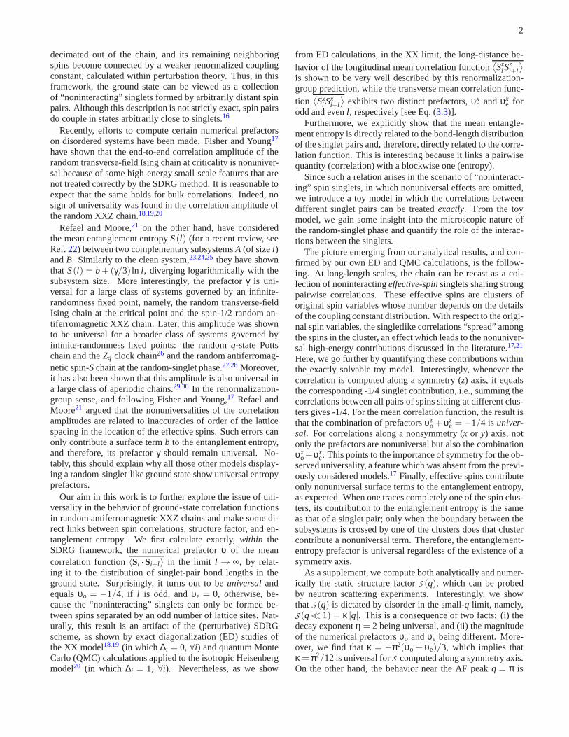
Correlation amplitude and entanglement entropy in random spin chains
17
arXiv:0704.0951v2 [cond-mat.dis-nn] 15 Nov 2007 Correlation amplitude and entanglement entropy in random spin chains José A. Hoyos, 1,2, ∗ André P. Vieira, 3, † N. Laflorencie, 4,5, ‡ and E. Miranda 1, § 1 Instituto de Física Gleb Wataghin, Unicamp, Caixa Postal 6165, 13083-970. Campinas, São Paulo, Brazil 2 Department of Physics, University of Missouri-Rolla, Rolla, Missouri 65409, USA 3 Departamento de Engenharia Metalúrgica e de Materiais, Universidade Federal do Ceará, 60455-760, Fortaleza, Ceará, Brazil 4 Institute of Theoretical Physics, École Polytechnique Fédérale de Lausanne, CH-1015 Lausanne, Switzerland 5 Department of Physics and Astronomy, University of British Columbia, Vancouver, British Columbia, Canada, V6T 1Z1 Using strong-disorder renormalization group, numerical exact diagonalization, and quantum Monte Carlo methods, we revisit the random antiferromagnetic XXZ spin-1/2 chain focusing on the long-length and ground- state behavior of the average time-independent spin-spin correlation function C(l )= υl −η . In addition to the well-known universal (disorder-independent) power-law exponent η = 2, we find interesting universal features displayed by the prefactor υ = υ o /3, if l is odd, and υ = υ e /3, otherwise. Although υ o and υ e are nonuniversal (disorder dependent) and distinct in magnitude, the combination υ o + υ e = −1/4 is universal if C is computed along the symmetric (longitudinal) axis. The origin of the nonuniversalities of the prefactors is discussed in the renormalization-group framework where a solvable toy model is considered. Moreover, we relate the average correlation function with the average entanglement entropy, whose amplitude has been recently shown to be universal. The nonuniversalities of the prefactors are shown to contribute only to surface terms of the entropy. Finally, we discuss the experimental relevance of our results by computing the structure factor whose scaling properties, interestingly, depend on the correlation prefactors. PACS numbers: 75.10.Pq, 75.10.Nr, 05.70.Jk I. INTRODUCTION Random low-dimensional quantum spin systems have been intensively investigated recently. The interplay between dis- order, quantum fluctuations, and correlations generates low- temperature phase diagrams with exotic phases. 1 In this con- text, one of the most investigated systems is the random an- tiferromagnetic (AF) quantum XXZ spin-1/2 chain, whose Hamiltonian reads H = ∑ i J i ( S x i S x i+1 + S y i S y i+1 + ∆ i S z i S z i+1 ) , (1.1) in which i labels the chain sites, S i are the usual spin-1/2 op- erators, J i ’s are positive uncorrelated random variables drawn from a probability distribution P 0 (J ), and ∆ i ’s are anisotropy parameters, also random uncorrelated variables. The clean system, J i ≡ 1 and ∆ i ≡ ∆, is a Tomonaga- Luttinger liquid for −1 < ∆ ≤ 1, with well-known asymptotic ground-state correlation functions, 2,3 C xx c (l )= S x i S x i+l =(−1) l Fl −η c − ˜ Fl −η c −1/η c , (1.2) C zz c (l )= S z i S z i+l =(−1) l Al −1/η c − 1 4π 2 η c l 2 , (1.3) as l → ∞. The clean-system exponent is 2 η c = 1 − (arccos ∆) /π. At the “free-fermion” point ∆ = 0, the pref- actors of the leading terms are known exactly, 4,5 being given by A = 1/ ( 2π 2 ) and F ≈ 0.147 09. 6 Away from this point (|∆| < 1), analytical forms for A and F were derived by Lukyanov and Zamolodchikov 7,8 and checked numerically later on. 9 Furthermore, the constant ˜ F , evaluated numeri- cally in Ref. 9, is at least 1 order of magnitude smaller than F . At the isotropic point ∆ = 1, irrelevant operators become marginal, yielding logarithmic corrections 10,11 C xx c (l )= C zz c (l )=(−1) l √ ln l (2π) 3/2 l . (1.4) For ∆ > 1, a spin gap opens and the system enters an anti- ferromagnetic Ising phase; otherwise, for ∆ < −1, the chain becomes a gapped Ising ferromagnet. Disorder strongly modifies the behavior in the clean criti- cal regime. It was shown that even the least amount of dis- order in J i destabilizes the Tomonaga-Luttinger phase, pro- vided −1/2 < ∆ i ≤ 1. 12 For −1 < ∆ i ≤−1/2, a finite amount of disorder is required to destabilize the clean phase. The low-energy behavior of the random AF spin-1/2 chain then corresponds to a random-singlet phase, characterized by ac- tivated dynamical scaling with a universal “tunneling” expo- nent ψ = 1/2, i.e., length (l ) and energy (Ω) scales are re- lated through Ω ∼ exp (−l ψ ), irrespective of P 0 (J ). 13 More- over, the transverse and the longitudinal mean spin-spin cor- relation functions decay as a power law ∼ υl −η for large dis- tances, both with the same universal exponent η = 2. 12,13 The mean value of the correlation function is dominated by rare widely separated spin pairs coupled in strongly-correlated sin- glet states. The remarkable fact that all correlations (xx, yy and zz) decay with the same exponent, irrespective of ∆, can be ascribed to the isotropy of the singlet state. In contrast, the typical value of the correlation function decays as a stretched exponential ∼ exp (−l ψ ). These results were obtained by us- ing the most successful theoretical tool to investigate such systems, the real-space strong-disorder renormalization-group (SDRG) method, first introduced in Refs. 14 and 15. The main idea behind the SDRG method is to gradually lower the energy scale by successively coupling the most strongly interacting spin pairs into singlet states. At each step of the renormalization transformation, one such pair is
-
Upload
independent -
Category
Documents
-
view
1 -
download
0
Transcript of Correlation amplitude and entanglement entropy in random spin chains
arX
iv:0
704.
0951
v2 [
cond
-mat
.dis
-nn]
15
Nov
200
7
Correlation amplitude and entanglement entropy in random spin chains
José A. Hoyos,1, 2,∗ André P. Vieira,3,† N. Laflorencie,4,5,‡ and E. Miranda1,§
1Instituto de Física Gleb Wataghin, Unicamp, Caixa Postal 6165, 13083-970. Campinas, São Paulo, Brazil2Department of Physics, University of Missouri-Rolla, Rolla, Missouri 65409, USA
3Departamento de Engenharia Metalúrgica e de Materiais,Universidade Federal do Ceará, 60455-760, Fortaleza, Ceará, Brazil
4Institute of Theoretical Physics, École Polytechnique Fédérale de Lausanne, CH-1015 Lausanne, Switzerland5Department of Physics and Astronomy, University of BritishColumbia, Vancouver, British Columbia, Canada, V6T 1Z1
Using strong-disorder renormalization group, numerical exact diagonalization, and quantum Monte Carlomethods, we revisit the random antiferromagnetic XXZ spin-1/2 chain focusing on the long-length and ground-state behavior of the average time-independent spin-spin correlation functionC(l) = υl−η. In addition to thewell-known universal (disorder-independent) power-law exponentη = 2, we find interesting universal featuresdisplayed by the prefactorυ = υo/3, if l is odd, andυ = υe/3, otherwise. Althoughυo andυe are nonuniversal(disorder dependent) and distinct in magnitude, the combinationυo +υe = −1/4 is universal ifC is computedalong the symmetric (longitudinal) axis. The origin of the nonuniversalities of the prefactors is discussed in therenormalization-group framework where a solvable toy model is considered. Moreover, we relate the averagecorrelation function with the average entanglement entropy, whose amplitude has been recently shown to beuniversal. The nonuniversalities of the prefactors are shown to contribute only to surface terms of the entropy.Finally, we discuss the experimental relevance of our results by computing the structure factor whose scalingproperties, interestingly, depend on the correlation prefactors.
PACS numbers: 75.10.Pq, 75.10.Nr, 05.70.Jk
I. INTRODUCTION
Random low-dimensional quantum spin systems have beenintensively investigated recently. The interplay betweendis-order, quantum fluctuations, and correlations generates low-temperature phase diagrams with exotic phases.1 In this con-text, one of the most investigated systems is the random an-tiferromagnetic (AF) quantum XXZ spin-1/2 chain, whoseHamiltonian reads
H = ∑i
Ji(
Sxi S
xi+1+Sy
i Syi+1 + ∆iS
zi S
zi+1
)
, (1.1)
in which i labels the chain sites,Si are the usual spin-1/2 op-erators,Ji ’s are positive uncorrelated random variables drawnfrom a probability distributionP0 (J), and∆i ’s are anisotropyparameters, also random uncorrelated variables.
The clean system,Ji ≡ 1 and ∆i ≡ ∆, is a Tomonaga-Luttinger liquid for−1< ∆ ≤ 1, with well-known asymptoticground-state correlation functions,2,3
Cxxc (l) =
⟨
Sxi S
xi+l
⟩
= (−1)l Fl−ηc − Fl−ηc−1/ηc , (1.2)
Czzc (l) =
⟨
Szi S
zi+l
⟩
= (−1)l Al−1/ηc − 14π2ηcl2
, (1.3)
as l → ∞. The clean-system exponent is2 ηc = 1 −(arccos∆)/π. At the “free-fermion” point∆ = 0, the pref-actors of the leading terms are known exactly,4,5 being givenby A = 1/
(
2π2)
and F ≈ 0.14709.6 Away from this point(|∆| < 1), analytical forms forA and F were derived byLukyanov and Zamolodchikov7,8 and checked numericallylater on.9 Furthermore, the constantF , evaluated numeri-cally in Ref.9, is at least 1 order of magnitude smaller thanF . At the isotropic point∆ = 1, irrelevant operators become
marginal, yielding logarithmic corrections10,11
Cxxc (l) = Czz
c (l) = (−1)l
√ln l
(2π)3/2 l. (1.4)
For ∆ > 1, a spin gap opens and the system enters an anti-ferromagnetic Ising phase; otherwise, for∆ < −1, the chainbecomes a gapped Ising ferromagnet.
Disorder strongly modifies the behavior in the clean criti-cal regime. It was shown that even the least amount of dis-order in Ji destabilizes the Tomonaga-Luttinger phase, pro-vided−1/2< ∆i ≤ 1.12 For−1< ∆i ≤−1/2, a finite amountof disorder is required to destabilize the clean phase. Thelow-energy behavior of the random AF spin-1/2 chain thencorresponds to a random-singlet phase, characterized by ac-tivated dynamical scaling with auniversal“tunneling” expo-nent ψ = 1/2, i.e., length (l ) and energy (Ω) scales are re-lated throughΩ ∼ exp(−lψ), irrespective ofP0 (J).13 More-over, the transverse and the longitudinalmeanspin-spin cor-relation functions decay as a power law∼ υl−η for large dis-tances, both with the same universal exponentη = 2.12,13 Themean value of the correlation function is dominated by rarewidely separated spin pairs coupled in strongly-correlated sin-glet states. The remarkable fact that all correlations (xx, yyandzz) decay with the same exponent, irrespective of∆, canbe ascribed to the isotropy of the singlet state. In contrast, thetypical value of the correlation function decays as a stretchedexponential∼ exp(−lψ). These results were obtained by us-ing the most successful theoretical tool to investigate suchsystems, the real-space strong-disorder renormalization-group(SDRG) method, first introduced in Refs.14and15.
The main idea behind the SDRG method is to graduallylower the energy scale by successively coupling the moststrongly interacting spin pairs into singlet states. At eachstep of the renormalization transformation, one such pair is
2
decimated out of the chain, and its remaining neighboringspins become connected by a weaker renormalized couplingconstant, calculated within perturbation theory. Thus, inthisframework, the ground state can be viewed as a collectionof “noninteracting” singlets formed by arbitrarily distant spinpairs. Although this description is not strictly exact, spin pairsdo couple in states arbitrarily close to singlets.16
Recently, efforts to compute certain numerical prefactorson disordered systems have been made. Fisher and Young17
have shown that the end-to-end correlation amplitude of therandom transverse-field Ising chain at criticality is nonuniver-sal because of some high-energy small-scale features that arenot treated correctly by the SDRG method. It is reasonable toexpect that the same holds for bulk correlations. Indeed, nosign of universality was found in the correlation amplitudeofthe random XXZ chain.18,19,20
Refael and Moore,21 on the other hand, have consideredthe mean entanglement entropyS(l) (for a recent review, seeRef.22) between two complementary subsystemsA (of sizel )andB. Similarly to the clean system,23,24,25 they have shownthat S(l) = b+ (γ/3) ln l , diverging logarithmically with thesubsystem size. More interestingly, the prefactorγ is uni-versal for a large class of systems governed by an infinite-randomness fixed point, namely, the random transverse-fieldIsing chain at the critical point and the spin-1/2 random an-tiferromagnetic XXZ chain. Later, this amplitude was shownto be universal for a broader class of systems governed byinfinite-randomness fixed points: the randomq-state Pottschain and theZq clock chain26 and the random antiferromag-netic spin-Schain at the random-singlet phase.27,28 Moreover,it has also been shown that this amplitude is also universal ina large class of aperiodic chains.29,30 In the renormalization-group sense, and following Fisher and Young,17 Refael andMoore21 argued that the nonuniversalities of the correlationamplitudes are related to inaccuracies of order of the latticespacing in the location of the effective spins. Such errors canonly contribute a surface termb to the entanglement entropy,and therefore, its prefactorγ should remain universal. No-tably, this should explain why all those other models display-ing a random-singlet-like ground state show universal entropyprefactors.
Our aim in this work is to further explore the issue of uni-versality in the behavior of ground-state correlation functionsin random antiferromagnetic XXZ chains and make some di-rect links between spin correlations, structure factor, and en-tanglement entropy. We first calculate exactly,within theSDRG framework, the numerical prefactorυ of the meancorrelation function〈Si ·Si+l 〉 in the limit l → ∞, by relat-ing it to the distribution of singlet-pair bond lengths in theground state. Surprisingly, it turns out to beuniversalandequalsυo = −1/4, if l is odd, andυe = 0, otherwise, be-cause the “noninteracting” singlets can only be formed be-tween spins separated by an odd number of lattice sites. Nat-urally, this result is an artifact of the (perturbative) SDRGscheme, as shown by exact diagonalization (ED) studies ofthe XX model18,19 (in which ∆i = 0, ∀i) and quantum MonteCarlo (QMC) calculations applied to the isotropic Heisenbergmodel20 (in which ∆i = 1, ∀i). Nevertheless, as we show
from ED calculations, in the XX limit, the long-distance be-havior of the longitudinal mean correlation function
⟨
Szi S
zi+l
⟩
is shown to be very well described by this renormalization-group prediction, while the transverse mean correlation func-tion
⟨
Sxi S
xi+l
⟩
exhibits two distinct prefactors,υxo andυx
e forodd and evenl , respectively [see Eq. (3.3)].
Furthermore, we explicitly show that the mean entangle-ment entropy is directly related to the bond-length distributionof the singlet pairs and, therefore, directly related to thecorre-lation function. This is interesting because it links a pairwisequantity (correlation) with a blockwise one (entropy).
Since such a relation arises in the scenario of “noninteract-ing” spin singlets, in which nonuniversal effects are omitted,we introduce a toy model in which the correlations betweendifferent singlet pairs can be treatedexactly. From the toymodel, we gain some insight into the microscopic nature ofthe random-singlet phase and quantify the role of the interac-tions between the singlets.
The picture emerging from our analytical results, and con-firmed by our own ED and QMC calculations, is the follow-ing. At long-length scales, the chain can be recast as a col-lection of noninteractingeffective-spinsinglets sharing strongpairwise correlations. These effective spins are clustersoforiginal spin variables whose number depends on the detailsof the coupling constant distribution. With respect to the origi-nal spin variables, the singletlike correlations “spread”amongthe spins in the cluster, an effect which leads to the nonuniver-sal high-energy contributions discussed in the literature.17,21
Here, we go further by quantifying these contributions withinthe exactly solvable toy model. Interestingly, whenever thecorrelation is computed along a symmetry (z) axis, it equalsthe corresponding -1/4 singlet contribution, i.e., summing thecorrelations between all pairs of spins sitting at different clus-ters gives -1/4. For the mean correlation function, the result isthat the combination of prefactorsυz
o + υze = −1/4 is univer-
sal. For correlations along a nonsymmetry (x or y) axis, notonly the prefactors are nonuniversal but also the combinationυx
o+υxe. This points to the importance of symmetry for the ob-
served universality, a feature which was absent from the previ-ously considered models.17 Finally, effective spins contributeonly nonuniversal surface terms to the entanglement entropy,as expected. When one traces completely one of the spin clus-ters, its contribution to the entanglement entropy is the sameas that of a singlet pair; only when the boundary between thesubsystems is crossed by one of the clusters does that clustercontribute a nonuniversal term. Therefore, the entanglement-entropy prefactor is universal regardless of the existenceof asymmetry axis.
As a supplement, we compute both analytically and numer-ically the static structure factorS (q), which can be probedby neutron scattering experiments. Interestingly, we showthatS (q) is dictated by disorder in the small-q limit, namely,S (q≪ 1) = κ |q|. This is a consequence of two facts: (i) thedecay exponentη = 2 being universal, and (ii) the magnitudeof the numerical prefactorsυo andυe being different. More-over, we find thatκ = −π2(υo + υe)/3, which implies thatκ = π2/12 is universal forS computed along a symmetry axis.On the other hand, the behavior near the AF peakq = π is
3
dominated by the characteristic divergence of the clean sys-tem. However, the true divergence atq = π is suppressed bydisorder and the peak width is broadened. Since there is no di-vergence in the case ofS (q) along thezaxis in the XX model,disorder universally determines its behavior near the AF peak,i.e.,S z(q = π− ε) = π−κ |ε| for ε ≪ 1. Only forq≈ π/2 isthe clean-system behaviorS z(q) = |q| found.
The remainder of this paper is as follows. We derive theuniversal SDRG expression for the mean correlation functionin Sec.II , reporting our numerical analyses in Sec.III . SectionIV discusses an exactly solvable model that yields instructiveresults on the origin of the universal behavior of correlationfunctions. In Sec.V, we derive the entanglement entropy andrelate it to the distribution of singlet lengths and to the corre-lation function. We discuss the experimental relevance of ourresults by computing the structure factor in Sec.VI. Finally,we make some concluding remarks in Sec.VII .
II. MEAN CORRELATION FUNCTION IN THESTRONG-DISORDER RENORMALIZATION-GROUP
FRAMEWORK
We start this section with a brief review of the SDRGmethod, followed by the derivation of the mean correlationfunction.
A. Strong-disorder renormalization-group method: A briefreview
The main idea behind the SDRG method is to reduce theenergy scale by integrating out the strongest couplings andrenormalizing the remaining ones. In the present case, onelocates the strongest coupling constantΩ = maxJi, say,J2, and then exactly treats the two-spin HamiltonianH0 =Ω(
Sx2Sx
3 +Sy2Sy
3 + ∆2Sz2Sz
3
)
, consideringH1 = H−H0 as a per-turbation.14 At low energies, spinsS2 andS3 “freeze” into a(nonmagnetic) singlet state, with the result that they can beeffectively removed from the chain, provided that the neigh-boring spinsS1 andS4 are now connected by a renormalizedcoupling constant
J =J1J3
(1+ ∆2)Ω, (2.1)
calculated within second-order perturbation theory. Theanisotropy parameter is also renormalized to∆ = ∆1∆3(1+∆2)/2. Note thatJ is smaller than eitherJ1, J3, or Ω, leadingto an overall decrease in the energy scale. After the decima-tion procedure, the distance betweenS1 andS4, which are nownearest neighbors, is renormalized to
l = l1 + l2+ l3 , (2.2)
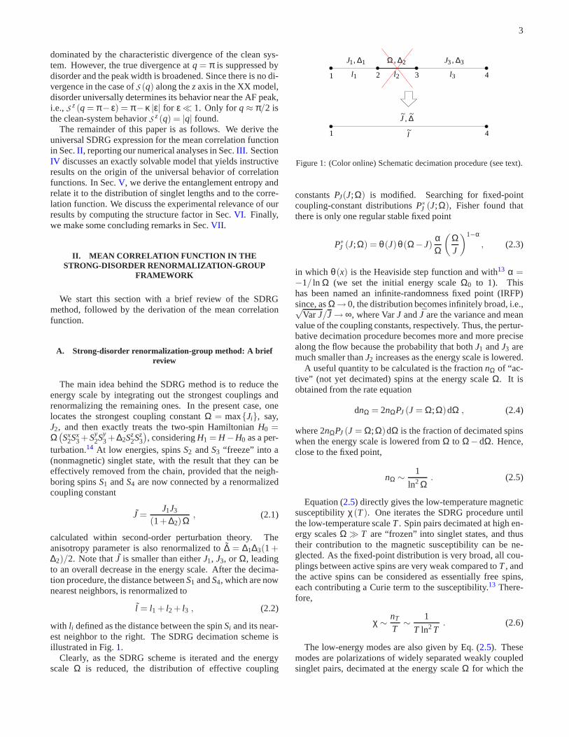
with l i defined as the distance between the spinSi and its near-est neighbor to the right. The SDRG decimation scheme isillustrated in Fig.1.
Clearly, as the SDRG scheme is iterated and the energyscale Ω is reduced, the distribution of effective coupling
l3l2l1
J1, ∆1 J3, ∆2Ω , ∆3
J~, ∆~
~l1 4
1 432
Figure 1: (Color online) Schematic decimation procedure (see text).
constantsPJ(J;Ω) is modified. Searching for fixed-pointcoupling-constant distributionsP∗
J (J;Ω), Fisher found thatthere is only one regular stable fixed point
P∗J (J;Ω) = θ(J)θ(Ω−J)
αΩ
(
ΩJ
)1−α, (2.3)
in which θ(x) is the Heaviside step function and with13 α =−1/ ln Ω (we set the initial energy scaleΩ0 to 1). Thishas been named an infinite-randomness fixed point (IRFP)since, asΩ→ 0, the distribution becomes infinitely broad, i.e.,√
Var J/J → ∞, where VarJ andJ are the variance and meanvalue of the coupling constants, respectively. Thus, the pertur-bative decimation procedure becomes more and more precisealong the flow because the probability that bothJ1 andJ3 aremuch smaller thanJ2 increases as the energy scale is lowered.
A useful quantity to be calculated is the fractionnΩ of “ac-tive” (not yet decimated) spins at the energy scaleΩ. It isobtained from the rate equation
dnΩ = 2nΩPJ (J = Ω;Ω)dΩ , (2.4)
where 2nΩPJ (J = Ω;Ω)dΩ is the fraction of decimated spinswhen the energy scale is lowered fromΩ to Ω−dΩ. Hence,close to the fixed point,
nΩ ∼ 1
ln2 Ω. (2.5)
Equation (2.5) directly gives the low-temperature magneticsusceptibilityχ(T). One iterates the SDRG procedure untilthe low-temperature scaleT. Spin pairs decimated at high en-ergy scalesΩ ≫ T are “frozen” into singlet states, and thustheir contribution to the magnetic susceptibility can be ne-glected. As the fixed-point distribution is very broad, all cou-plings between active spins are very weak compared toT, andthe active spins can be considered as essentially free spins,each contributing a Curie term to the susceptibility.13 There-fore,
χ ∼ nT
T∼ 1
T ln2T. (2.6)
The low-energy modes are also given by Eq. (2.5). Thesemodes are polarizations of widely separated weakly coupledsinglet pairs, decimated at the energy scaleΩ for which the
4
mean distance between spins wasl ∼ n−1Ω . Thus, the energy
costΩ to break a singlet of lengthl is
Ω ∼ exp(−lψ) , (2.7)
in which ψ = 1/2.13 This unusual exponential relation be-tweenΩ and l is named “activated” dynamical scaling andψ has been dubbed the “tunneling exponent.”
The scaling behavior of the mean correlation functionC(l)is cleverly obtained when one realizes thattypically two verydistant spins are not in a singlet state and thus are only weaklycorrelated. On the other hand, some rare and arbitrarily sep-arated spin pairs that were decimated together are stronglycorrelated and hence dominate the long-distance behavior ofC(l). Therefore, the mean correlation function must be pro-portional to the total number of spin singlets decimated at thelength scalel . Since the probability of decimating a spin pairis proportional to the probability that both spins have not beendecimated yet, it follows that
C(l) ∼ (−1)l n2Ω ∼ (−1)l
lη , (2.8)
with η = 2.13
In contrast, the typical correlation functionCtyp (l) behavesquite differently. Its long-distance behavior is obtainedby thefollowing argument. Suppose spinsS2 andS3 are those to bedecimated at a given SDRG step, as in Fig.1. In that case, thecorrelation betweenS2 andS3 equals−3/4+O (J3/Ω)2, whilethe correlation betweenS4 andS3 is of order−J3/Ω. Thus,the typical value of the correlation function will be propor-tional to the typical value ofJ/Ω. Using the fixed-point dis-tribution (2.3), one finds ln
∣
∣Ctyp (l)∣
∣ ∼ −ι√
l , i.e., the typicalcorrelation function decays as a stretched exponential, with anonuniversal prefactorι of order unity.13
B. Mean correlation function
We now derive the mean correlation function in a more for-mal calculation which allows us to compute its amplitude inaddition to its power-law decay. In the SDRG framework, themean correlation functionC(l) between spins separated by adistancel is obtained from the corresponding distribution ofsinglet-pair bond lengths in the ground statePs(l),
C(l) = −38
Ps(l) , (2.9)
since each singlet contributes a factor of−3/4 to C(l) andthere are two spins in each singlet.
The singlet-bond length distributionPs(l) can be calculatedfrom
Ps(l) = 2Z Ω0
0nΩP(J = Ω, l ;Ω)dΩ , (2.10)
whereP(J, l ;Ω)dJdl is the probability of finding a couplingconstant betweenJ andJ+dJ connecting spins separated bya distance betweenl andl +dl at the energy scaleΩ, and the
factor 2 comes from normalization. If we follow exactly thejoint probabilityP(J, l ;Ω) along the SDRG flow, then we canobtain an exact expression forPs(l). In fact, we only needP(J, l ;Ω) at J = Ω.
It turns out that we can carry out this task for∆i ≡ 0 andcouplings taken from the family of initial distributions,
P0(J) = θ(J)θ(Ω0−J)ϑ0
Ω0
(
Ω0
J
)1−ϑ0
, (2.11)
in which ϑ0 > 0 gauges the strength of the initial disorderandΩ0 sets the initial energy scale.31 We first calculate thedensity of active spinsnΩ. For that, we needPJ (J;Ω) =R
P(J, l ;Ω)dl , which is obtained from the flow equation14
−∂PJ
∂Ω=PJ(Ω;Ω)
Z
dJ1dJ3PJ (J1;Ω)PJ (J3;Ω)
× δ(
J− J1J3
Ω
)
. (2.12)
Introducing theAnsatz32,33
PJ (J;Ω) =ϑ(Ω)
Ω
(
ΩJ
)1−ϑ(Ω)
(2.13)
into Eq. (2.12) yields
ϑ(Ω) =ϑ0
1+ ϑ0Γ, (2.14)
whereΓ = ln(Ω0/Ω). Thus, from the rate equation (2.4), weobtain
nΩ =1
(1+ ϑ0Γ)2 , (2.15)
and Eq. (2.5) is recovered in the low-energy limitΓ → ∞.We now need to follow the SDRG flow of the joint distri-
butionP(J, l ;Ω), which is governed by the equation13
∂P∂Ω
=−Z
dl1dl2dl3dJ1dJ3P(J1, l1)P(Ω, l2)P(J3, l3)
× δ(l − l1− l2− l3)δ(
J− J1J3
Ω
)
. (2.16)
As shown in AppendixA, this can be done exactly byLaplace transformingP(J, l ;Ω) and using anAnsatzfor thecorresponding flow equation. The final result forP(Ω, l) ≡P(J = Ω, l ;Ω) is
P(Ω, l) =4π2
Ωa2Γ3
∞
∑n=1
(−1)n+1n2exp
−(nπ
aΓ
)2l
, (2.17)
wherea = ϑ0√
2l0, and l0 ≡ 1 is the “bare” lattice spacing.Although the leading term of Eq. (2.17) had been obtainedbefore,13 the explicit dependence on the initial disorder distri-bution encoded ina was not emphasized. As will be shownnext, this dependence is essential for our discussion.
5
Plugging Eqs. (2.15) and (2.17) into Eq. (2.10), we obtain
Ps(l) =8π2
a2
∞
∑n=1
(−1)n+1n2Z ∞
0
e−( nπaΓ )
2l
(1+ ϑ0Γ)2 Γ3dΓ
= 8l0l
∞
∑n=1
(−1)n+1
π2n2 f (l ,n) (2.18)
=2l03l2
1+O(
√
l0/l)
, (2.19)
where
f (l ,n) =1l0
Z ∞
0
e−εdε(√
2/(πn)+√
l/(l0ε))2 , (2.20)
and we usedf (l ≫ l0,n) → 1/l
1+O(
√
l0/l)
in the last
step. As explicitly shown in Eq. (2.18), the distribution ofsinglets in the ground state is independent of the initial disor-der parameterϑ0 at all length scales. Moreover, it follows auniversalpower law in the large-distance limit.
Finally, taking into account that singlets can only be formedbetween spins separated by distances corresponding to oddmultiples of l0, the mean correlation function takes theuni-versalform
Cu (l) = −υ(
l0l
)2
×
1, if l/l0 is odd,0, otherwise, (2.21)
whereυ = 1/4, irrespective of the initial disorder parameter.Note that Eq. (2.21) recovers Fisher’s scaling result Eq. (2.8).In view of the fact that correlations between the spins in asinglet state are isotropic, correlations between components ofthe spins along a given directionα = x, y, or z should behaveas
Cααu (l) = −1
3υ(
l0l
)2
×
1, if l/l0 is odd,0, otherwise, (2.22)
with a prefactor given by−υ/3 = −1/12.In order to check the prediction of Eq. (2.21), we calcu-
lated the mean correlation functionC(l) from numerical im-plementations of the SDRG algorithm on very large chains(2× 10⁷ sites), with initial couplings following probabilitydistributions of the form
P0 (J) =θ(J−Jmin)θ(Ω0−J)
1− (Jmin/Ω0)ϑ0
ϑ0
Ω0
(
Ω0
J
)1−ϑ0
, (2.23)
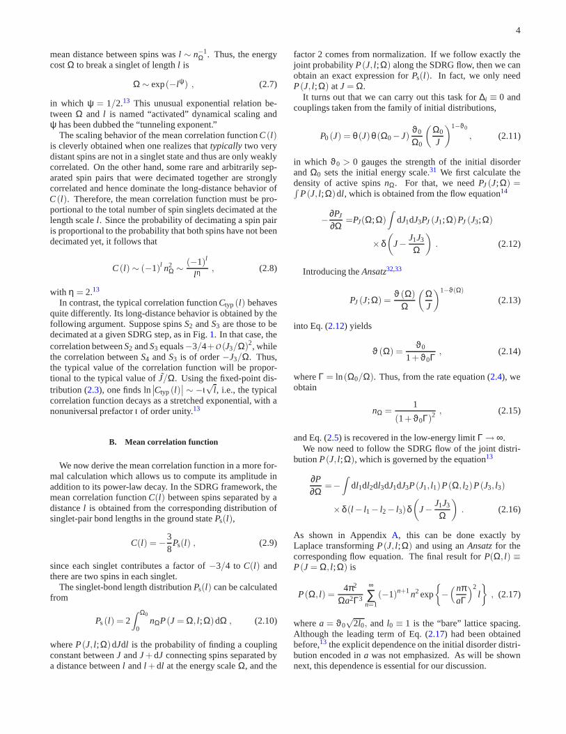
where Ω0 = 1, ϑ0 > 0, and Jmin ≥ 0. Figure 2 shows,for various chains, the relative difference between the calcu-lated correlation function and the universal prediction,δ(l) =C(l)/Cu (l)− 1, as a function ofl . We considered both theXX (∆i ≡ 0) and the isotropic Heisenberg (∆i ≡ 1) models,for which we averaged over 100 and 1000 disorder realiza-tions, respectively. In agreement with the previous analysis,the long-distance behavior of the correlation functions iswelldescribed by the universal predictionCu (l), regardless of themodel under consideration, within an error of less than 5%.
0 1 2 3 4 5log
10l
-0.2
-0.1
0
0.1
0.2
0.3
0.4
δ(l)
AXX
DXX
, FXX
, HXX
AXXX
DXXX
FXXX
HXXX
Figure 2: (Color online) Relative differenceδ = C/Cu −1 betweenthe mean correlation functionC and the universal predictionCu asa function of the distancel in the SDRG framework, for variouschoices of initial disorder, and both XX and isotropic Heisenberg(or XXX) models. Chains A, D, F, and H have couplings distributedaccording toP0(J) [see Eq. (2.23)] with (Jmin,ϑ0) equal to(0.5,1),(0,3), (0,1), and(0,0.3), respectively. The results for chains FXXand HXX (omitted for clarity) are statistically indistinguishable fromthose for chain DXX . Error bars (not shown for clarity) are of theorder of the statistical data fluctuations. Lines are guidesto the eyes.
Moreover, the mean correlation function of chains DXX , FXX ,and HXX (all of which haveJmin = 0, as described in the fig-ure caption) are statistically identical atall length scales, inagreement with Eq. (2.18), which predicts the same short-distance behavior for those spin chains whose coupling con-stants are distributed according to Eq. (2.11). Notice thatδ(l) approaches zero for largel even for distributions withJmin > 0, which clearly do not belong to the particular class ofdistributions [Eq. (2.11)] employed in the derivation ofCu(l).
The clear difference between the convergence rates of themean correlation functions in the XX and Heisenberg mod-els is due to the extra numerical prefactor of 1/2 presentin the recursion relation of the latter model [cf. Eq. (2.1)],which delays the convergence ofC(l) to the asymptotic formCu(l). This prefactor (which becomes negligible as the SDRGscheme proceeds) alters the relation between length and en-ergy scales, relevant for the derivation ofCu. However, at log-arithmically large energy scales,Γ = ln(Ω0/Ω) ≫ ln 2, thesimple relation between length and energy scales in Eq. (2.7)is recovered.
III. NUMERICAL RESULTS
We now confront the predicted long-distance form of themean correlation function, given in Sec.II , with numericalresults for XX chains, obtained through the mapping to freefermions, and for isotropic Heisenberg chains, obtained byquantum Monte Carlo (QMC) calculations.
6
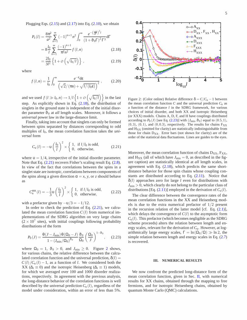
1 10 100l
0.0
0.1
0.2
0.3-l
2C
zz(l
)1/π2
1/12Box distribution, J
min = 0
Box distribution, Jmin
= 1/4Binary distribution, J
min = 1/10
Figure 3: (Color online) Dependence of−l2Czz(l) on the spin sepa-ration l in the XX model for three different probability distributionsof the couplings: a box distribution (ϑ0 = 1) with Jmin = 0, a box dis-tribution withJmin = 1/4, and a binary distribution withJmin = 1/10[see Eqs. (3.1) and (3.2)]. The orange solid line corresponds to thedisorder-free prediction (Ref.4) −l2Czz
c = 1/π2. For short-lengthscales, all chains approach the behavior of the uniform system. Aftera disorder-dependent crossover length, the data approach the univer-sal prediction of Eq. (2.22), which is indicated by the black dashedline. Statistical fluctuations increase withl , and so results forl ≥ 300,as well as error bars, are omitted for clarity.
A. XX chains
We analyzed disordered XX chains with periodic boundaryconditions, and coupling constants following box distributions
P0 (J) =θ(J−Jmin)θ(Ω0−J)
1− (Jmin/Ω0)ϑ0
ϑ0
Ω0
(
Ω0
J
)1−ϑ0
, (3.1)
with Ω0 = 1, ϑ0 > 0, andJmin > 0, or binary distributions
Q0 (J) =12
δ(J−Jmin)+12
δ(J−Ω0) . (3.2)
Below, we present results for different choices of parame-ters. Figure3 shows the mean longitudinal correlation func-tion Czz(l) =
⟨
Szi S
zi+l
⟩
as a function of the spin separationlfor a chain with 4000 sites and couplings taken from threeprobability distributions: two boxlike distributions (ϑ0 = 1)with Jmin = 1/4 andJmin = 0, and one binary distributionwith Jmin = 1/10, in which we average over 700, 1000, and800 disorder realizations, respectively. Other disorder dis-tributions give similar results. The short-length behavior ap-proaches the uniform-system result,4 Czz(l) =−(πl)−2. Aftera disorder-dependent crossover length,19,20 the mean longitu-dinal correlation function decays as a power law with expo-nentη = 2, and the prefactor clearly approaches the universalvalue−1/12 [see Eq. (2.22)]. Although not shown in the fig-ure, the typical longitudinal correlation functionCzz
typ (l), incontrast, has a nonuniversal prefactor.
1 10 100l
10-1
100
101
102
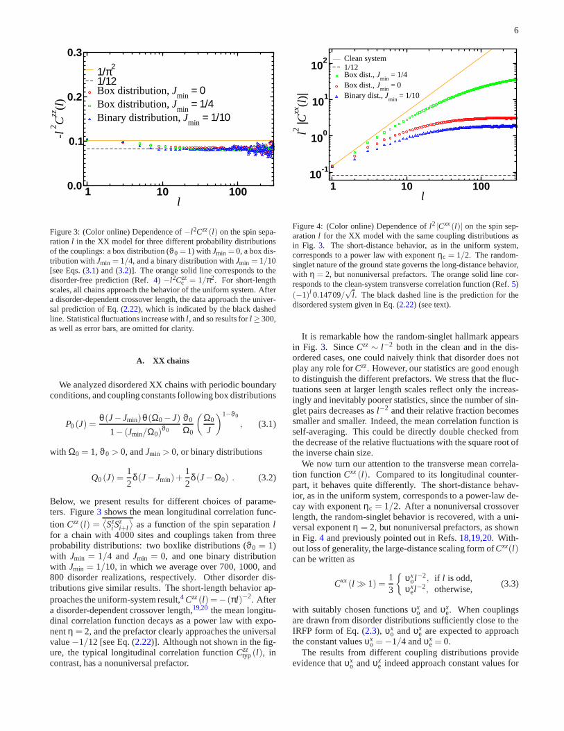
l2|C
xx(l
)|
Clean system1/12Box dist., J
min = 1/4
Box dist., Jmin
= 0Binary dist., J
min = 1/10
Figure 4: (Color online) Dependence ofl2 |Cxx(l)| on the spin sep-arationl for the XX model with the same coupling distributions asin Fig. 3. The short-distance behavior, as in the uniform system,corresponds to a power law with exponentηc = 1/2. The random-singlet nature of the ground state governs the long-distance behavior,with η = 2, but nonuniversal prefactors. The orange solid line cor-responds to the clean-system transverse correlation function (Ref.5)(−1)l 0.14709/
√l . The black dashed line is the prediction for the
disordered system given in Eq. (2.22) (see text).
It is remarkable how the random-singlet hallmark appearsin Fig. 3. SinceCzz∼ l−2 both in the clean and in the dis-ordered cases, one could naively think that disorder does notplay any role forCzz. However, our statistics are good enoughto distinguish the different prefactors. We stress that thefluc-tuations seen at larger length scales reflect only the increas-ingly and inevitably poorer statistics, since the number ofsin-glet pairs decreases asl−2 and their relative fraction becomessmaller and smaller. Indeed, the mean correlation functionisself-averaging. This could be directly double checked fromthe decrease of the relative fluctuations with the square root ofthe inverse chain size.
We now turn our attention to the transverse mean correla-tion functionCxx(l). Compared to its longitudinal counter-part, it behaves quite differently. The short-distance behav-ior, as in the uniform system, corresponds to a power-law de-cay with exponentηc = 1/2. After a nonuniversal crossoverlength, the random-singlet behavior is recovered, with a uni-versal exponentη = 2, but nonuniversal prefactors, as shownin Fig. 4 and previously pointed out in Refs.18,19,20. With-out loss of generality, the large-distance scaling form ofCxx(l)can be written as
Cxx(l ≫ 1) =13
υxol−2, if l is odd,
υxel−2, otherwise,
(3.3)
with suitably chosen functionsυxo andυx
e. When couplingsare drawn from disorder distributions sufficiently close totheIRFP form of Eq. (2.3), υx
o andυxe are expected to approach
the constant valuesυxo = −1/4 andυx
e = 0.The results from different coupling distributions provide
evidence thatυxo andυx
e indeed approach constant values for

7
1 10 100l
10-8
10-6
10-4
10-2
|Cxx
(l) +
Cxx
(l+1)
|
(1/12) l−2
Box dist., Jmin
= 1/4Box dist., J
min = 0
Binary dist., Jmin
= 1/10
Figure 5: (Color online) The summed transverse correlationfunc-tion Cxx
sum(l) = Cxx(l) + Cxx(l + 1) as a function of the distancel (for odd l ) for XX chains and the same coupling distributionsas in the previous figure. Although for sufficiently strong disor-der (circles and triangles) the curves approach a power law,corre-sponding to the random-singlet exponentη = 2 and to a prefactor(υx
o +υxe)/3 ≃ −1/12, the less disordered system (squares) shows
a different prefactor. Again, results forl > 400 and error bars areomitted for clarity.
arbitrary initial disorder, with−υxo and υx
e assuming close(but certainly distinct) values. Additionally, it seems thatthe quantityυx
o + υxe approaches an asymptotic value close
to −1/4 for sufficiently strong disorder. This can be seen inFig. 5, where we plot (forl odd) the combinationCxx
sum(l) ≡−[Cxx(l) +Cxx(l + 1)]. Notice that, for the box distributionwith Jmin = 0 and the binary distribution withJmin = 1/10,the curves forCxx
sum(l) are reasonably well described by thescaling form 1/
(
12l2)
in the long-distance limit. However,this is not the case for chains with couplings drawn from thebox distribution withJmin = 1/4, at least up to the sizes stud-ied (l = 1000, not shown). Indeed, we argue in Sec.IV thatdeviations from that scaling form should be expected for thetransversecorrelations in XX chains.
Finally, we report that we have considered also smallerchains (1000 sites) but with more disordered distributions(Jmin = 0, with ϑ0 = 0.3 or ϑ0 = 0.6). For the sake of clarity,we have omitted their data in Figs.3-5. The meanlongitudi-nal correlation function is remarkably well described by thenaive SDRG prediction (2.22). The meantransversecorrela-tion function, on the other hand, is well described by Eq. (3.3)with υx
o + υxe ≈−1/4.
B. XXX chains
We now present QMC results obtained for the SU(2) sym-metric model,
H =L0
∑i=1
JiSi ·Si+1 , (3.4)
1 10 100l
10-4
10-3
10-2
10-1
|Czz(l
)|
QMC (l even)QMC (l odd)
0.9/l2 (even)
0.98/l2 (odd)
SU(2) Heisenberg chain ; W=0.75 ; L0=200
Figure 6: (Color online) Correlation function(−1)lCzz(l) in theground state of isotropic random AF Heisenberg spin-1/2 chains[Eq. (3.4)] of lengthL0 = 200 with disorder strengthW = 0.75. Thequantum Monte Carlo results were obtained atT/J = 1.5×10⁻⁵ andaveraged overNsamples= 500 realizations. When the distancel be-tween spins is even (circles), the asymptotic regime is described byCzz(l) ≃ 0.9/l2 (black, solid line) whereas for oddl (squares), thebest fit givesCzz(l) ≃−0.98/l2 (red, dashed line).
with the random AF couplingsJi ’s distributed according to thebox distributions
P(J) =1
2JWθ(
J−J(1−W))
θ(
J(1+W)−J)
. (3.5)
The QMC algorithm we use is based on a stochastic seriesexpansion of the partition function.34,35 This is a finite tem-peratureT technique which, in principle, allows access toground-state properties, providedT is chosen to be muchsmaller than the finite-size gap of the systemΩ ∝ L−z
0 . Asalready discussed in several works (see, for instance, Refs. 20and36,37,38), the ground-state properties in random spin sys-tems can be very hard to access because extremely small en-ergy correlations might develop between distant spins or spinclusters. For random finite chains, the dynamical exponentzis formally infinite since we expect exponentially small cou-plings to develop at large distances between spins, so thatΩ ∝ exp(−√
L0). In order to accelerate the convergence to-ward the ground state, we used theβ-doubling scheme36 andthus performed the QMC measurements at temperatures assmall as 4× 10⁻⁶ in units of J. We show in Figs.6 and 7QMC results for the average spin-spin correlation functioninthe ground state,
Czz(l) =1
Nsamples
Nsamples
∑σ=1
2L0
L0/2
∑i=1
〈Szi S
zi+l 〉(σ), (3.6)
where we perform disorder averaging overNsamplesindepen-dent random samples, as well as space averaging along theperiodic chains. Note that the SU(2) symmetry of the Hamil-tonian ensures thatCzz(l) = Cyy(l) = Cxx(l).
As studied in great detail in Refs.19 and 20, there is acrossover phenomenon which is governed by the localization
8
1 10 100l
10-5
10-4
10-3
10-2
10-1
- ( C
zz(l
) +
Czz(l
+1)
)
W=0.75W=1
(1/12) l-2
SU(2) Heisenberg chain
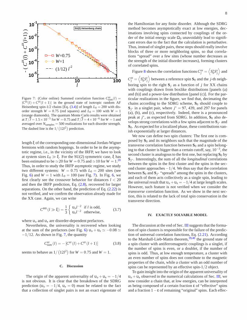
Figure 7: (Color online) Summed correlation functionCzzsum(l) =
|Czz(l) + Czz(l + 1)| in the ground state of isotropic random AFHeisenberg spin-1/2 chains [Eq. (3.4)] of lengthL0 = 200 with dis-order strengthW = 0.75 (red squares) andL0 = 100 with W = 1(orange diamonds). The quantum Monte Carlo results were obtainedatT/J = 1.5×10⁻⁵ for W = 0.75 andT/J = 4×10⁻⁶ for W = 1 andaveraged overNsamples= 500 realizations for each disorder strength.The dashed line is the 1/
(
12l2)
prediction.
lengthξ of the corresponding one-dimensional Jordan-Wignerfermions with random hoppings. In order to be in the asymp-totic regime, i.e., in the vicinity of the IRFP, we have to lookat system sizesL0 ≫ ξ. For the SU(2) symmetric case,ξ hasbeen estimated to be≃20 forW = 0.75 and≃10 forW = 1.20
Thus, in order to study the IRFP asymptotic regime, we studytwo different systems:W = 0.75 with L0 = 200 sites (seeFig. 6) andW = 1 with L0 = 100 (see Fig.7). In Fig. 6, wefirst clearly see the crossover behavior for distancesl < 20and then the IRFP prediction, Eq. (2.8), recovered for largerseparations. On the other hand, the prediction of Eq. (2.22) isnot verified, and we confirm the observation already made forthe XX case. Again, we can write
Cαα (l ≫ ξ) =13
υol−2 if l is odd,υel−2 otherwise,
(3.7)
whereυo andυe are disorder-dependent prefactors.Nevertheless, the universality is recovered when looking
at the sum of the prefactors (see Fig.6) υo + υe ≃ −0.08≃−1/12. As shown in Fig.7, the quantity
Czzsum(l) = − [Czz(l)+Czz(l +1)] (3.8)
seems to behave as 1/(
12l2)
for W = 0.75 andW = 1.
C. Discussion
The origin of the apparent universality ofυo + υe = −1/4is not obvious. It is clear that the breakdown of the SDRGprediction (υo = −1/4, υe = 0) must be related to the factthat a collection of singlet pairs is not an exact eigenstateof
the Hamiltonian for any finite disorder. Although the SDRGmethod becomes asymptotically exact at low energies, dec-imations involving spins connected by couplings of the or-der of the initial energy scaleΩ0 unavoidably lead to signifi-cant errors due to the fact that the calculation is perturbative.Thus, instead of singlet pairs, these steps should really involveblocks of three or more neighboring spins, so that correla-tions “spread” over a few sites (whose number decreases asthe strength of the initial disorder increases), forming clustersof correlated spins.
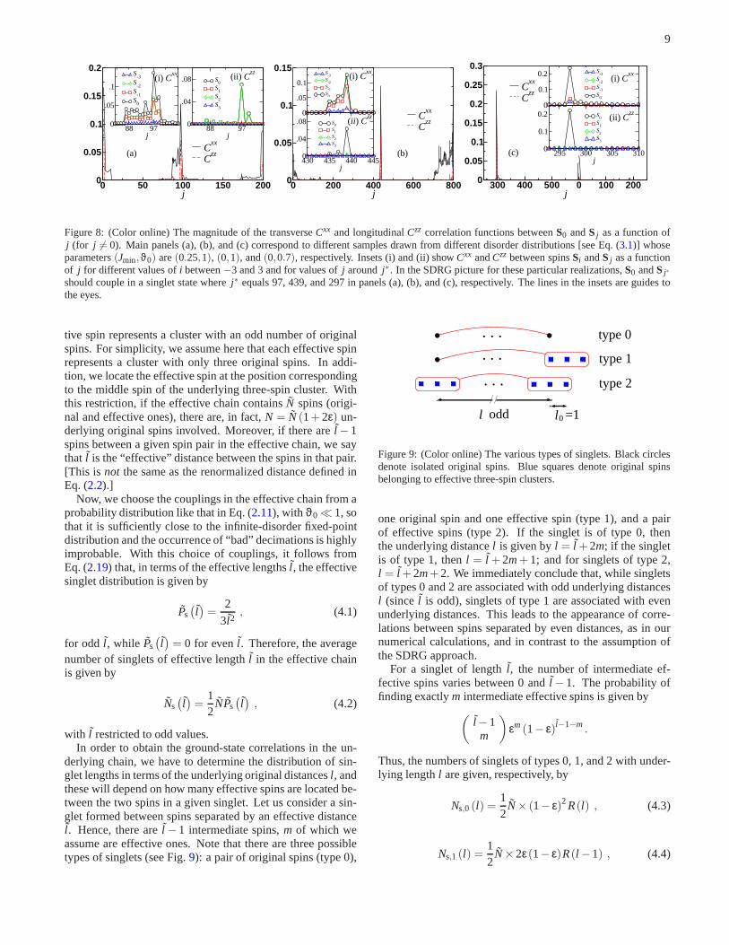
Figure8 shows the correlation functionsCxxj =
⟨
Sx0Sx
j
⟩
and
Czzj =
⟨
Sz0Sz
j
⟩
between a reference spinS0 and thej-th neigh-
boring spin to the rightS j as a function ofj for XX chainswith couplings drawn from boxlike distributions [panels (a)and (b)] and a power-law distribution [panel (c)]. For the par-ticular realizations in the figure, we find that, decimating thechains according to the SDRG scheme,S0 should couple toS j∗ in a singlet pair, wherej∗ = 97, 439, and 297 for panels(a), (b), and (c), respectively. Indeed, there is a pronouncedpeak atj∗, as expected from SDRG. In addition,S0 also de-velops strong correlations with a few spins adjacent toS j∗ andS0. As expected for a localized phase, these contributions van-ish exponentially at larger distances.
We now can define two spin clusters: The first one is com-posed byS0 and its neighbors such that the magnitude of thetransverse correlation function betweenS0 and a spin belong-ing to that cluster is bigger than a certain cutoff, say, 10−3, thesecond cluster is analogous to the first one, but replacingS0 byS j∗ . Interestingly, the sum of all thelongitudinalcorrelationsbetween the spins in the first cluster and the spins in the sec-ond cluster approaches−1/4. We thus say that the correlationbetweenS0 andS j∗ “spreads” among the spins in the clusters,and each of them acts collectively as a single spin, leading tothe universal result thatυo+υe =−1/4 at large length scales.However, such feature is not verified when we consider thetransversecorrelation function. As we show in the next sec-tion, this is related to the lack of total spin conservation in thetransverse direction.
IV. EXACTLY SOLVABLE MODEL
The discussion at the end of Sec.III suggests that the forma-tion of spin clusters is responsible for the failure of the predic-tion of universal correlation functions, Eq. (2.21). Accordingto the Marshall-Lieb-Mattis theorem,39,40 the ground state ofa spin cluster with antiferromagnetic couplings is a singlet, ifthe number of spins is even, or a doublet, if the number ofspins is odd. Thus, at low enough temperature, a cluster withan even number of spins does not contribute to the magneticproperties of the chain, while a cluster with an odd number ofspins can be represented by an effective spin-1/2 object.
To gain insight into the origin of the apparent universalityofυo + υe observed in the numerical calculations of Sec.III , wenow consider a chain that, at low energies, can be interpretedas being composed of a certain fractionε of “effective” spinsand a fraction 1−ε of remaining “original” spins. Each effec-
9
0 50 100 150 200j
0
0.05
0.1
0.15
0.2
Cxx
Czz
88 97j
0
.05
.1
S-3
S-2
S-1
S0
88 97j
0
.04
.08 S0
S1
S2
S3
(ii) Czz
(i) Cxx
(a)
0 200 400 600 800j
0
0.05
0.1
0.15
Cxx
Czz
0
.05
0.1
S-3
S-2
S-1
S0
430 435 440 445j
0
.04
.08 S0
S1
S2
S3
(i) Cxx
(ii ) Czz
(b)
300 400 500 0 100 200j
0
0.05
0.1
0.15
0.2
0.25
0.3
Cxx
Czz
0
0.1
0.2 S-3
S-2
S-1
S0
295 300 305 310j
0
0.1
0.2 S0
S1
S2
S3
(i) Cxx
(ii) Czz
(c)
Figure 8: (Color online) The magnitude of the transverseCxx and longitudinalCzz correlation functions betweenS0 andS j as a function ofj (for j 6= 0). Main panels (a), (b), and (c) correspond to different samples drawn from different disorder distributions [see Eq. (3.1)] whoseparameters(Jmin,ϑ0) are(0.25,1), (0,1), and(0,0.7), respectively. Insets (i) and (ii) showCxx andCzz between spinsSi andS j as a functionof j for different values ofi between−3 and 3 and for values ofj around j∗. In the SDRG picture for these particular realizations,S0 andS j∗
should couple in a singlet state wherej∗ equals 97, 439, and 297 in panels (a), (b), and (c), respectively. The lines in the insets are guides tothe eyes.
tive spin represents a cluster with an odd number of originalspins. For simplicity, we assume here that each effective spinrepresents a cluster with only three original spins. In addi-tion, we locate the effective spin at the position correspondingto the middle spin of the underlying three-spin cluster. Withthis restriction, if the effective chain containsN spins (origi-nal and effective ones), there are, in fact,N = N (1+2ε) un-derlying original spins involved. Moreover, if there arel −1spins between a given spin pair in the effective chain, we saythat l is the “effective” distance between the spins in that pair.[This is not the same as the renormalized distance defined inEq. (2.2).]
Now, we choose the couplings in the effective chain from aprobability distribution like that in Eq. (2.11), with ϑ0 ≪ 1, sothat it is sufficiently close to the infinite-disorder fixed-pointdistribution and the occurrence of “bad” decimations is highlyimprobable. With this choice of couplings, it follows fromEq. (2.19) that, in terms of the effective lengthsl , the effectivesinglet distribution is given by
Ps(
l)
=2
3l2, (4.1)
for odd l , while Ps(
l)
= 0 for evenl . Therefore, the averagenumber of singlets of effective lengthl in the effective chainis given by
Ns(
l)
=12
NPs(
l)
, (4.2)
with l restricted to odd values.In order to obtain the ground-state correlations in the un-
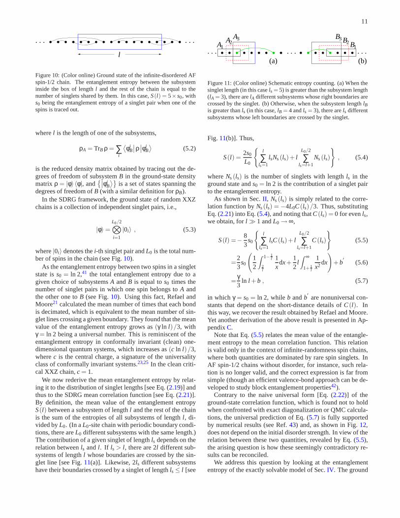
derlying chain, we have to determine the distribution of sin-glet lengths in terms of the underlying original distancesl , andthese will depend on how many effective spins are located be-tween the two spins in a given singlet. Let us consider a sin-glet formed between spins separated by an effective distancel . Hence, there arel − 1 intermediate spins,m of which weassume are effective ones. Note that there are three possibletypes of singlets (see Fig.9): a pair of original spins (type 0),
l odd l0 =1
type 0
type 1
type 2
. . .
. . .
. . .
Figure 9: (Color online) The various types of singlets. Black circlesdenote isolated original spins. Blue squares denote original spinsbelonging to effective three-spin clusters.
one original spin and one effective spin (type 1), and a pairof effective spins (type 2). If the singlet is of type 0, thenthe underlying distancel is given byl = l +2m; if the singletis of type 1, thenl = l + 2m+ 1; and for singlets of type 2,l = l +2m+2. We immediately conclude that, while singletsof types 0 and 2 are associated with odd underlying distancesl (sincel is odd), singlets of type 1 are associated with evenunderlying distances. This leads to the appearance of corre-lations between spins separated by even distances, as in ournumerical calculations, and in contrast to the assumption ofthe SDRG approach.
For a singlet of lengthl , the number of intermediate ef-fective spins varies between 0 andl −1. The probability offinding exactlym intermediate effective spins is given by
(
l −1m
)
εm(1− ε)l−1−m.
Thus, the numbers of singlets of types 0, 1, and 2 with under-lying lengthl are given, respectively, by
Ns,0 (l) =12
N× (1− ε)2R(l) , (4.3)
Ns,1 (l) =12
N×2ε(1− ε)R(l −1) , (4.4)

10
and
Ns,2 (l) =12
N× ε2R(l −2) , (4.5)
with
R(l) =23
l−13
∑m=0
(
l −2m−1m
)
εm(1− ε)l−3m−1
(l −2m)2 . (4.6)
In the limit of largel , the sum inR(l) can be written as anintegral, which can be calculated by Laplace’s method, usingStirling’s approximation. The final result is
R(l) =23
(1+2ε) l−2 +O(
l−3) . (4.7)
Consequently,
Ns,0 (l) =N3
(1− ε)2 l−2 +O(
l−3) (for odd l), (4.8)
Ns,1 (l) =2N3
ε(1− ε) l−2 +O(
l−3) (for evenl), (4.9)
and
Ns,2 (l) =N3
ε2l−2 +O(
l−3) (for oddl). (4.10)
In order to calculate the ground-state correlationsCαα (l) =⟨
Sαi Sα
i+l
⟩
, with α = x, y, z, let us focus on a fixed odd value ofl . There are contributions toCαα (l) andCαα (l +1) comingfrom singlets of type 0, with underlying lengthl ; from singletsof type 1, with lengthsl −1 andl + 1; and from singlets oftype 2, with lengthsl − 2, l , andl + 2. If we denote bycα
end(cα
mid) the “weight” of a spin in either end (in the middle) of athree-spin cluster to theα component of an effective spin (seeAppendixB), we can combine all contributions to write (seeFig. 9)
Cαα (l) =− 14N
Ns,0 (l)+ [Ns,1 (l −1)+Ns,1(l +1)]cαend
+ [Ns,2 (l −2)+Ns,2(l +2)](cαend)
2
+ Ns,2 (l)[
2(cαend)
2 +(cαmid)
2]
, (4.11)
and
Cαα (l +1) =− 14N
Ns,1 (l +1)cαmid
+ 2[Ns,2 (l)+Ns,2(l +2)]cαendc
αmid , (4.12)
so that, to leading order inl , we have
Cαα (l) =− 112
l−2
(1− ε)2 +4ε(1− ε)cαend
+ ε2[
4(cαend)
2 +(cαmid)
2]
(4.13)
and
Cαα (l +1) = − 112
l−22ε(1− ε)+4ε2cαend
cαmid. (4.14)
Note that the above results are significantly different fromthe bare SDRG results of Sec.II , most notably in that theaverage correlation is, in general, not zero for evenl . BothCαα (l) andCαα (l +1) decay with the random-singlet expo-nentη = 2, but with different prefactorsυα
o andυαe , respec-
tively. However, we have
13
(υαo + υα
e) = − 112
1− [1− (2cαend+cα
mid)]ε2 . (4.15)
For the XXZ chain, irrespective of the initial anisotropy∆,thez component of the total spin is a good quantum number,assuming the valueSz
tot = 0 in the (singlet) ground state. This
means that the sum of the ground-state correlations⟨
Szi S
zj
⟩
between a given spini and all other spinsj in the chain is equalto−1/4. Since this is also true for an effective spin, it followsthat 2cz
end+ czmid = 1 (as can be easily verified explicitly; see
AppendixB), and we must have
υzo + υz
e = −14
, (4.16)
irrespective of the concentrationε of effective spins (and thusof the initial disorder). Furthermore, in the Heisenberg limit(∆ = 1), owing to the SU(2) symmetry, we also have
υxo + υx
e = υyo + υy
e = υzo + υz
e = −14
. (4.17)
This last result, however, is not valid for∆ < 1. In particular,in the XX limit, for which 2cx
end+cxmid ≃ 0.9142, we obtain
υxo + υx
e ≃−14
(1−0.0858ε)2 , (4.18)
yielding a weak dependence onε.For the isotropic Heisenberg chain and forCzz(l), the an-
alytical results derived in this section are in agreement withthe numerical results in Sec.III , strengthening the conjectureof a universal behavior for sum of prefactors of the longitu-dinal ground-state correlations in random XXZ chains. Thepresence of larger effective-spin clusters (as typically occursfor weaker disorder; see Fig.8) should not change the con-clusions of this section concerning the universality ofυz
o+υze,
since the sum of all the weights of the original spins belong-ing to an effective cluster is identically 1 when computed withrespect to the symmetry axis.
V. ENTANGLEMENT ENTROPY AND ITS RELATION TOTHE CORRELATION FUNCTION
In this section, we discuss the relation between the entan-glement entropyS(l) and the ground-state mean correlationfunctionC(l).
The entanglement entropy between two complementarysubsystemsA andB is given by
S(l) = −TrρA ln ρA = −TrρB ln ρB , (5.1)
11
. . . . . .
l
Figure 10: (Color online) Ground state of the infinite-disordered AFspin-1/2 chain. The entanglement entropy between the subsysteminside the box of lengthl and the rest of the chain is equal to thenumber of singlets shared by them. In this case,S(l) = 5×s0, withs0 being the entanglement entropy of a singlet pair when one of thespins is traced out.
wherel is the length of one of the subsystems,
ρA = TrB ρ = ∑i
⟨
φiB
∣
∣ρ∣
∣φiB
⟩
(5.2)
is the reduced density matrix obtained by tracing out the de-grees of freedom of subsystemB in the ground-state densitymatrix ρ = |φ〉 〈φ|, and
∣
∣φiB
⟩
is a set of states spanning thedegrees of freedom ofB (with a similar definition forρB).
In the SDRG framework, the ground state of random XXZchains is a collection of independent singlet pairs, i.e.,
|φ〉 =
L0/2O
i=1
|0i〉 , (5.3)
where|0i〉 denotes thei-th singlet pair andL0 is the total num-ber of spins in the chain (see Fig.10).
As the entanglement entropy between two spins in a singletstate iss0 = ln 2,41 the total entanglement entropy due to agiven choice of subsystemsA andB is equal tos0 times thenumber of singlet pairs in which one spin belongs toA andthe other one toB (see Fig.10). Using this fact, Refael andMoore21 calculated the mean number of times that each bondis decimated, which is equivalent to the mean number of sin-glet lines crossing a given boundary. They found that the meanvalue of the entanglement entropy grows as(γ ln l)/3, withγ = ln 2 being a universal number. This is reminiscent of theentanglement entropy in conformally invariant (clean) one-dimensional quantum systems, which increases as(c ln l)/3,wherec is the central charge, a signature of the universalityclass of conformally invariant systems.23,25 In the clean criti-cal XXZ chain,c = 1.
We now rederive the mean entanglement entropy by relat-ing it to the distribution of singlet lengths [see Eq. (2.19)] andthus to the SDRG mean correlation function [see Eq. (2.21)].By definition, the mean value of the entanglement entropyS(l) between a subsystem of lengthl and the rest of the chainis the sum of the entropies of all subsystems of lengthl , di-vided byL0. (In aL0-site chain with periodic boundary condi-tions, there areL0 different subsystems with the same length.)The contribution of a given singlet of lengthls depends on therelation betweenls andl . If ls > l , there are 2l different sub-systems of lengthl whose boundaries are crossed by the sin-glet line [see Fig.11(a)]. Likewise, 2ls different subsystemshave their boundaries crossed by a singlet of lengthls≤ l [see
. . .(a)
AA A3
12
. . . . . .(b)
B3B2B1
Figure 11: (Color online) Schematic entropy counting. (a) When thesinglet length (in this casels = 5) is greater than the subsystem length(lA = 3), there arelA different subsystems whose right boundaries arecrossed by the singlet. (b) Otherwise, when the subsystem length lBis greater thanls (in this case,lB = 4 andls = 3), there arels differentsubsystems whose left boundaries are crossed by the singlet.
Fig. 11(b)]. Thus,
S(l) =2s0
L0
l
∑ls=1
lsNs(ls)+ lL0/2
∑ls=l+1
Ns(ls)
, (5.4)
whereNs(ls) is the number of singlets with lengthls in theground state ands0 = ln 2 is the contribution of a singlet pairto the entanglement entropy.
As shown in Sec.II , Ns(ls) is simply related to the corre-lation function byNs(ls) = −4L0C(ls)/3. Thus, substitutingEq. (2.21) into Eq. (5.4), and noting thatC(ls) = 0 for evenls,we obtain, forl ≫ 1 andL0 → ∞,
S(l) =− 83
s0
l
∑ls=1
lsC(ls)+ lL0/2
∑ls=l+1
C(ls)
(5.5)
=23
s0
(
12
Z 1− 1l
2l
1x
dx+12
lZ ∞
1+ 1l
1x2 dx
)
+b′
(5.6)
=γ3
ln l +b , (5.7)
in which γ = s0 = ln 2, while b andb′
are nonuniversal con-stants that depend on the short-distance details ofC(l). Inthis way, we recover the result obtained by Refael and Moore.Yet another derivation of the above result is presented in Ap-pendixC.
Note that Eq. (5.5) relates the mean value of the entangle-ment entropy to the mean correlation function. This relationis valid only in the context of infinite-randomness spin chains,where both quantities are dominated by rare spin singlets. InAF spin-1/2 chains without disorder, for instance, such rela-tion is no longer valid, and the correct expression is far fromsimple (though an efficient valence-bond approach can be de-veloped to study block entanglement properties42).
Contrary to the naive universal form [Eq. (2.22)] of theground-state correlation function, which is found not to holdwhen confronted with exact diagonalization or QMC calcula-tions, the universal prediction of Eq. (5.7) is fully supportedby numerical results (see Ref.43) and, as shown in Fig.12,does not depend on the initial disorder strength. In view of therelation between these two quantities, revealed by Eq. (5.5),the arising question is how these seemingly contradictory re-sults can be reconciled.
We address this question by looking at the entanglemententropy of the exactly solvable model of Sec.IV. The ground
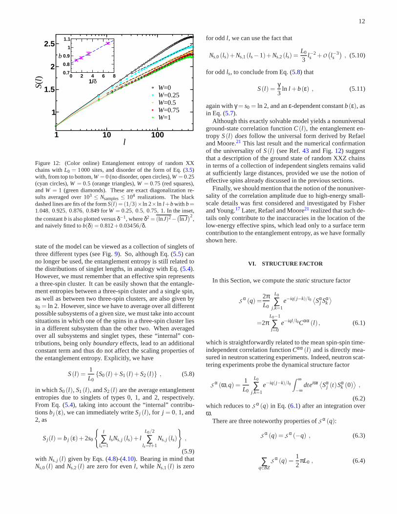
12
1 10 100l
1
1.5
2
2.5S(
l)
W=0W=0.25W=0.5W=0.75W=1
0 2 4 6 81/δ
0.7
0.8
0.9
1
1.1
b
Figure 12: (Color online) Entanglement entropy of random XXchains withL0 = 1000 sites, and disorder of the form of Eq. (3.5)with, from top to bottom,W = 0 (no disorder, open circles),W = 0.25(cyan circles),W = 0.5 (orange triangles),W = 0.75 (red squares),andW = 1 (green diamonds). These are exact diagonalization re-sults averaged over 103 ≤ Nsamples≤ 104 realizations. The blackdashed lines are fits of the formS(l) = (1/3)× ln 2× ln l +bwith b=1.048, 0.925, 0.876, 0.849 forW = 0.25, 0.5, 0.75, 1. In the inset,
the constantb is also plotted versusδ−1, whereδ2 = (lnJ)2−(
lnJ)2
,and naively fitted tob(δ) = 0.812+0.03456/δ.
state of the model can be viewed as a collection of singlets ofthree different types (see Fig.9). So, although Eq. (5.5) canno longer be used, the entanglement entropy is still relatedtothe distributions of singlet lengths, in analogy with Eq. (5.4).However, we must remember that an effective spin representsa three-spin cluster. It can be easily shown that the entangle-ment entropies between a three-spin cluster and a single spin,as well as between two three-spin clusters, are also given bys0 = ln 2. However, since we have to average over all differentpossible subsystems of a given size, we must take into accountsituations in which one of the spins in a three-spin cluster liesin a different subsystem than the other two. When averagedover all subsystems and singlet types, these “internal” con-tributions, being onlyboundaryeffects, lead to an additionalconstant term and thus do not affect the scaling properties ofthe entanglement entropy. Explicitly, we have
S(l) =1L0
S0 (l)+S1(l)+S2(l) , (5.8)
in whichS0(l), S1 (l), andS2(l) are the average entanglemententropies due to singlets of types 0, 1, and 2, respectively.From Eq. (5.4), taking into account the “internal” contribu-tionsb j (ε), we can immediately writeSj (l), for j = 0, 1, and2, as
Sj(l) = b j (ε)+2s0
l
∑ls=1
lsNs, j (ls)+ lL0/2
∑ls=l+1
Ns, j (ls)
,
(5.9)with Ns, j (l) given by Eqs. (4.8)-(4.10). Bearing in mind thatNs,0 (l) andNs,2 (l) are zero for evenl , while Ns,1 (l) is zero
for odd l , we can use the fact that
Ns,0 (ls)+Ns,1(ls−1)+Ns,2(ls) =L0
3l−2s +O
(
l−3s
)
, (5.10)
for odd ls, to conclude from Eq. (5.8) that
S(l) =γ3
ln l +b(ε) , (5.11)
again withγ = s0 = ln 2, and anε-dependent constantb(ε), asin Eq. (5.7).
Although this exactly solvable model yields a nonuniversalground-state correlation functionC(l), the entanglement en-tropy S(l) doesfollow the universal form derived by Refaeland Moore.21 This last result and the numerical confirmationof the universality ofS(l) (see Ref.43 and Fig.12) suggestthat a description of the ground state of random XXZ chainsin terms of a collection of independent singlets remains validat sufficiently large distances, provided we use the notion ofeffective spins already discussed in the previous sections.
Finally, we should mention that the notion of the nonuniver-sality of the correlation amplitude due to high-energy small-scale details was first considered and investigated by Fisherand Young.17 Later, Refael and Moore21 realized that such de-tails only contribute to the inaccuracies in the location ofthelow-energy effective spins, which lead only to a surface termcontribution to the entanglement entropy, as we have formallyshown here.
VI. STRUCTURE FACTOR
In this Section, we compute thestaticstructure factor
Sα (q) =
2πL0
L0
∑j ,k=1
e−iq( j−k)/l0⟨
Sαj Sα
k
⟩
=2πL0−1
∑l=0
e−iql/l0Cαα (l) , (6.1)
which is straightforwardly related to the mean spin-spin time-independent correlation functionCαα (l) and is directly mea-sured in neutron scattering experiments. Indeed, neutron scat-tering experiments probe the dynamical structure factor
Sα (ω,q) =
1L0
L0
∑j ,k=1
e−iq( j−k)/l0Z ∞
−∞dteiωt ⟨Sα
j (t)Sαk (0)
⟩
,
(6.2)which reduces toS α (q) in Eq. (6.1) after an integration overω.
There are three noteworthy properties ofS α (q):
Sα (q) = S α (−q) , (6.3)
∑q∈BZS
α (q) =12
πL0 , (6.4)
13
0 0.25 0.5 0.75 1q/π
0
0.25
0.5
0.75
1S
z(q
)/π
Box dist., Jmin
=1/4Box dist., J
min=0
Bin. dist., Jmin
=1/10
0 0.06q/π0
0.06
S z/π
S z= κq
S z= q
0.46 0.5 0.54q/π
0.46
0.5
0.54
S z/π
S z= q
(i)
(ii)
Figure 13: (Color online) The longitudinal structure factor in the XXmodel for various disordered chains of lengths up toL0 = 4000. Ascan be seen, they are practically indistinguishable. Inset(i) high-lights S z for small q in which the curves become somewhat distin-guishable nearq = 0.06π. Moreover, they slightly deviate from theclean system predictionS z
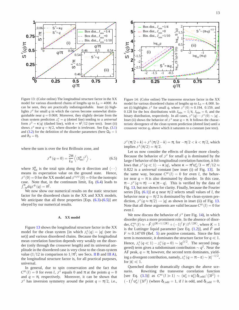
c = q (dotted line) tending to auniversalform S z = κ |q| (dashed line), withκ = π2/12 (see text). Inset (ii)showsS z nearq = π/2, where disorder is irrelevant. See Eqs. (3.1)and (3.2) for the definition of the disorder parameters (hereΩ0 = 1andϑ0 = 0).
where the sum is over the first Brillouin zone, and
Sα (q = 0) =
2πL0
⟨
(Sαtot)
2⟩
, (6.5)
whereSαtot is the total spin along theα direction and〈· · · 〉
means its expectation value on the ground state. Hence,S z(0) = 0 for the XX model andS x,y,z(0) = 0 for the isotropiccase. Note that, in the continuum limit, Eq. (6.4) leads toR π−π dqS α (q) = π2.
We now show our numerical results on the static structurefactor for the disordered chain in the XX and XXX models.We anticipate that all three properties [Eqs. (6.3)-(6.5)] areobeyed by our numerical results.
A. XX model
Figure13shows the longitudinal structure factor in the XXmodel for the clean system [in whichS z
c (q) = |q| (see in-set)] and various disordered chains. Because the longitudinalmean correlation function depends very weakly on the disor-der (only through the crossover length) and its universal am-plitude in the disordered case is very close to the clean-systemvalue (1/12 in comparison to 1/π2; see Secs.II B andIII A ),the longitudinal structure factor is, for all practical purposes,universal.
In general, due to spin conservation and the fact thatCzz(l) = 0 for evenl , S z equals 0 andπ at the pointsq = 0and q = π, respectively. Moreover, it can be shown thatS z has inversion symmetry around the pointq = π/2, i.e.,
0 0.25 0.5 0.75 1q/π
1
2
3
4
5
6
Sx (q
)/π
Box dist., Jmin
=1/4Box dist., J
min=0
Bin. dist., Jmin
=1/10
-2 -1.5 -1 -0.5
log10
q
-2.5
-2
-1.5
-1
log 10
(S
x(q
)-S
x(0
))
S x= κq
-2 -1 0log
10 (π-q)
0
0.5
1
1.5
2
log 10
Sx (q
)
S x~ (π-q)
-1/2
(i)
(ii)
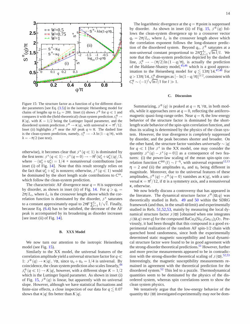
Figure 14: (Color online) The transverse structure factor in the XXmodel for various disordered chains of lengths up toL0 = 4,000. In-set (i) highlightsS z for small q, whereS x (0) ≈ 0.194, 0.159, and0.128 for the box distributions withJmin = 1/4, Jmin = 0, and thebinary distribution, respectively. In all cases,S x (q)− S x (0) ∼ |q| .Inset (ii) shows the behavior ofS x nearq = π. It follows the charac-teristic divergence of the clean system prediction (dottedline) until acrossover vectorqc above which it saturates to a constant (see text).
S z(π/2+k)+ S z(π/2−k) = π, for −π/2 < k < π/2, whichimpliesS z(π/2) = π/2.
Let us now consider the effects of disorder more closely.Because the behavior ofS z for small q is dominated by thelarge-l behavior of the longitudinal correlation function, it fol-lows thatS z(q≪ 1) → κ |q|, whereκ = π2υz
o/3 = π2/12≈0.822 is auniversalconstant [see inset (i) of Fig.13]. Inthe same way, becauseCzz(l) = 0 for even l , the behav-ior nearq = π is also dominated by disorder. In this case,π − S z(q≈ π) → κ |π−q|. This is verified by the data ofFig. 13, but not shown for clarity. Finally, because the Fourierseries [Eq. (6.1)] at q nearπ/2 selects small values ofl , thebehavior nearq = π/2 is dominated by the clean-system pre-diction, S z(q≈ π/2) → |q| as shown in inset (ii) of Fig.13.Note that all these arguments are valid becauseCzz(l) = 0 forevenl .
We now discuss the behavior ofS x (see Fig.14), in whichdisorder plays a more prominent role. In the absence of disor-der,Cxx
c (l) ≈ −F/l2K+1/(2K) +(−1)l F/l1/(2K), whereK = 1is the Luttinger liquid parameter [see Eq. (1.2)], and F andF ≈ 0.14709 (Ref.5) are positive constants. Since the firstterm is monotonic, it dominates the structure factor forq≪ 1.Hence,S x
c (q≪ 1)− S xc (q = 0) ∼ |q|3/2. The second (stag-
gered) term gives a subdominant contribution∼ q2. Near theAF peak,q = π; however, the second term dominates, yield-ing a divergent contribution, namely,S x
c (q = π− ε)∼ |ε|−1/2,for |ε| ≪ 1.
Quenched disorder dramatically changes the above sce-nario. Rewriting the transverse correlation function[see Eq. (3.3)] as Cxx(l ≫ 1) ∼ (υx
o + υxe)δl ,odd/
(
3l2)
+
(−1)l υxe/(
3l2)
(whereδl ,odd = 1, if l is odd, andδl ,odd = 0,
14
0 0.2 0.4 0.6 0.8 1q/π
0
0.5
1
1.5
2
2.5
3S
α(q
)/π
W=0.5W=0.75W=1
0 0.1 0.2 0.3q0
.1
.2
S α
Sα= Kq
Sα= κq -2 -1.5 -1 -0.5 0
log10
(1-q/π)
0
3
6
Sα
Sα= λln(1-q/π)
(i)
(ii)
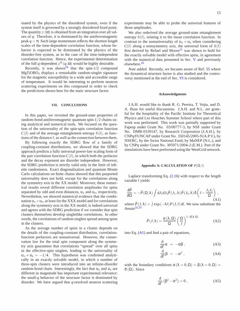
Figure 15: The structure factor as a function ofq for different disor-der parameters [see Eq. (3.5)] in the isotropic Heisenberg model forchains of lengths up toL0 = 200. Inset (i) showsS α for q≪ 1 andcompares it with the (field-theoretical) clean system predictionS α
c →K |q|, with K = 1/2 being the Luttinger liquid parameter, and thedisordered system predictionS α → κ |q|, with universalκ = π2/12.Inset (ii) highlightsS α near the AF peakq ≈ π. The dashed lineis the clean-system prediction, namely,S α
c →−λ ln(1−q/π), withλ = −π/2 (see text).
otherwise), it becomes clear thatS x (q≪ 1) is dominated bythe first term:S x (q≪ 1)−S x(q = 0)→−π2(υx
o + υxe) |q|/3,
where−(υxo + υx
e) = 1/4 + nonuniversal contributions [seeinset (i) of Fig.14]. Note that this result strongly relies onthe fact thatυx
o + υxe is nonzero; otherwise,S x (q≪ 1) would
be dominated by the short length scale contributions toCxx,which follow the clean-system prediction.
The characteristic AF divergence nearq = π is suppressedby disorder, as shown in inset (ii) of Fig.14. For q > qc =2π/Lc, whereLc is the crossover length above which the cor-relation function is dominated by the disorder,S x saturatesto a constant approximately equal to 2πF ∑Lc
l=11/√
l . Finally,because Eq. (6.4) has to be satisfied, the decrease of the AFpeak is accompanied by its broadening as disorder increases[see inset (ii) of Fig.14].
B. XXX Model
We now turn our attention to the isotropic Heisenbergmodel (see Fig.15).
Similarly to the XX model, the universal features of thecorrelation amplitude yield a universal structure factor forq≪1: S α (q) → κ |q| , ∀α, sinceυo + υe = 1/4 is universal. Bycoincidence, the clean system prediction also scales linearly,44
S αc (q≪ 1) → K |q|, however, with a different slopeK = 1/2
which is the Luttinger liquid parameter. As shown in inset (i)of Fig. 15, S α (q) is linear, but apparently with no universalslope. However, although we have statistical fluctuations andfinite-size effects, a close inspection of our data forq . 0.07shows thatκ |q| fits better thanK |q|.
The logarithmic divergence at theq= π point is suppressedby disorder. As shown in inset (ii) of Fig.15, S α (q) fol-lows the clean-system divergence up to a crossover vectorqc = 2π/Lc, whereLc is the crossover length above whichthe correlation exponent follows the long-distance predic-tion of the disordered system. Beyondqc, S α saturates at anon-universal constant proportional to 2π∑Lc
l=1
√ln l/l . We
note that the clean-system prediction depicted by the dashedline, S α
c → −(π/2) ln(1−q/π), is actually the predictionof the Haldane-Shastry model,45,46 which is a good approx-imation to the Heisenberg model forq . 13π/14.47,48 Forq> 13π/14,S α
c diverges as[− ln(1−q/π)]3/2, consistent withCα
c ∼ (−1)l√
ln l/l for l ≫ 1.
C. Discussion
Summarizing,S α (q) is peaked atq = π, ∀α, in both mod-els, while it approaches zero atq = 0, reflecting the antiferro-magnetic quasi-long-range order. Nearq = π, the low-energybehavior of the structure factor is dominated by the short-length scale behavior of the spin-spin correlation function, andthus its scaling is determined by the physics of the clean sys-tem. However, the true divergence iscompletelysuppressedby disorder, and the peak becomes shorter and broader. Onthe other hand, the structure factor vanishesuniversally∼ |q|for q ≪ 1 [for S x in the XX model, one may consider thequantity S x (q)− S x (q = 0)] as a consequence of two fea-tures: (i) the power-law scaling of the mean spin-spin cor-relation functionCαα (l) ∼ l−η, with universal exponent12,13
η = 2 and (ii) the amplitudesυo and υe being different inmagnitude. Moreover, due to the universal features of theseamplitudes,S α (q)− S α (q = 0) vanishes asκ |q|, with a uni-versalκ = π2/12, if α is a symmetry axis, and a nonuniversalκ, otherwise.
We now briefly discuss a controversy that has appeared inthe literature. The dynamical structure factorS α (ω,q) wastheoretically studied in Refs.49 and 50 within the SDRGframework (and thus, in the small-ω limit) and experimentallystudied in Refs.51,52,53, mainly by measuring the local dy-namical structure factorS (ω) [obtained when one integratesS (ω,q) overq] for the compound BaCu2(Si0.5Ge0.5)2O7. Pre-viously, it had been thought that this compound is a good ex-perimental realization of the random AF spin-1/2 chain withquenched bond randomness, since both the experimentallydetermined static magnetic susceptibility and local dynami-cal structure factor were found to be in good agreement withthe strong-disorder theoretical predictions.51 However, furtherand more precise measurements appeared to be in contradic-tion with the strong-disorder theoretical scaling ofS (ω).52,53
Interestingly, the magnetic susceptibility measurementsre-mained in agreement with the theoretical prediction for thedisordered system.52 This led to a puzzle. Thermodynamicalquantities seem to be dominated by the physics of the dis-ordered system, whereas spin correlations seem to show theclean system physics.
We tentatively argue that the low-energy behavior of thequantityωS (ω) investigated experimentally maynotbe dom-
15
inated by the physics of the disordered system, even if thesystem itself is governed by a strongly disordered fixed point.The quantityS (ω) is obtained from an integration over all val-ues ofq. Therefore, it is dominated by the antiferromagneticpeakq = π. Such large momentum reflects the shortest lengthscales of the time-dependent correlation function, whose be-havior is expected to be dominated by the physics of thedisorder-free system, as in the case of the time-independentcorrelation function. Hence, the experimental determinationof the full q-dependentS α (q,ω) would be highly desirable.
Recently, it was shown54 that the spin-1/2 compoundMgTiOBO3 displays a remarkable random-singlet signaturefor the magnetic susceptibility in a wide and accessible rangeof temperature. It would be interesting to perform neutronscattering experiments on this compound in order to checkthe predictions shown here for the static structure factor.
VII. CONCLUSIONS
In this paper, we revisited the ground-state properties ofrandom-bond antiferromagnetic quantum spin-1/2 chains us-ing analytical and numerical tools. We focused on the ques-tion of the universality of the spin-spin correlation functionC(l) and of the average entanglement entropyS(l), as func-tions of the distancel , as well as the connection between them.
By following exactly the SDRG flow of a family ofcoupling-constant distributions, we showed that the SDRGapproach predicts a fully universal power-law scaling formofthe pair correlation functionC(l), in which both the prefactorand the decay exponent are disorder independent. However,the SDRG prediction is strictly valid only in the limit of infi-nite randomness. Exact diagonalization and quantum MonteCarlo calculations on finite chains showed that this purporteduniversality does not hold, except for the correlations alongthe symmetry axis in the XX model. Moreover, these numer-ical results reveal different correlation amplitudes for spinsseparated by odd and even distances,υo andυe, respectively.Nevertheless, we showed numerical evidence that the combi-nationυo+υe, at least for the XXX model and for correlationsalong the symmetry axis in the XX model, is indeed universaland agrees with the SDRG prediction if we consider that spinclusters themselves develop singletlike correlations. Inotherwords, the correlations of random singlets spread among spinsin the clusters.
As the average number of spins in a cluster depends onthe details of the coupling-constant distribution, correlation-function prefactors are nonuniversal. However, the conser-vation law for the total spin component along the symme-try axis guarantees that correlations “spread” over all spinsin the effective-spin singlets, leading to the universality ofυo + υe = −1/4. This hypothesis was confirmed analyti-cally in an exactly solvable model, in which a number ofthree-spin clusters were introduced into an infinite-disorderrandom-bond chain. Interestingly, the fact thatυo andυe aredifferent in magnitude has important experimental relevance:the small-q behavior of the structure factor is dominated bydisorder. We have argued thatq-resolved neutron scattering
experiments may be able to probe the universal features ofthose amplitudes.
We also rederived the average ground-state entanglemententropyS(l), relating it to the mean correlation function. Incontrast to the nonuniversality ofυo + υe when consideringC(l) along a nonsymmetry axis, the universal form ofS(l)first derived by Refael and Moore21 was shown to hold forthe exactly solvable model with effective spins, in agreementwith the numerical data presented in Sec.V and previouslyelsewhere.43
Note added. Recently, we became aware of Ref.55 wherethe dynamical structure factor is also studied and the contro-versy mentioned at the end of Sec.VI is considered.
Acknowledgments
J.A.H. would like to thank R. G. Pereira, T. Vojta, and D.A. Huse for useful discussions. J.A.H. and N.L. are grate-ful for the hospitality of the Pacific Institute for TheoreticalPhysics and Les Houches Summer School where part of thiswork was performed. This work was partially supported byFapesp under Grant No. 03/00777-3, by NSF under GrantNo. DMR-0339147, by Research Corporation (J.A.H.), byCNPq/FUNCAP under Grant No. 350145/2005-9 (A.P.V.), byNSERC, by the Swiss National Fund, by MaNEP (N.L.), andby CNPq under Grant No. 305971/2004-2 (E.M.). Part of thesimulations have been preformed using the WestGrid network.
Appendix A: CALCULATION OF P(Ω, l)
Laplace transforming Eq. (2.16) with respect to the lengthvariablel yields
∂P∂Ω
= −P(Ω,λ)
Z
dJ1dJ3P(J1,λ) P(J3,λ)δ(
J− J1J3
Ω
)
,
(A1)whereP(J,λ) =
R
exp(−λl)P(J, l)dl . We now substitute theAnsatz32,33
P(J,λ) =α(λ,Ω)
Ω
(
ΩJ
)1−β(λ,Ω)
(A2)
into Eq. (A1) and find a pair of equations,
ddΓ
α = −αβ , (A3)
ddΓ
β = −α2 , (A4)
with the boundary conditionsα(λ = 0,Ω) = β(λ = 0,Ω) =ϑ(Ω). Since
ddΓ(
β2−α2)= 0 , (A5)
16
we find the solutions33
β =β0c+c2 tanh(cΓ)
c+ β0 tanh(cΓ), (A6)
α =c√
β20−c2
c cosh(cΓ)+ β0sinh(cΓ), (A7)
wherec= c(λ) is a constant of the flow, defined byc2 = β2−α2. Moreover,c is a real number sinceβ > α, which canbe shown by considering an explicit calculation of the meandistance between the “active” spins,
l =
Z
dl lZ
dJP(J, l)
= − limλ→0
ddλ
Z Ω
0dJP(J,λ)
= limλ→0
1λ
(
1− α(λ,Ω)
β(λ,Ω)
)
. (A8)
As l > 0, Eq. (A8) ensures thatα < β.The boundary conditions lead toc(λ → 0) ≪ 1, and so
c2 (λ ≪ 1) = a2λτ +O(
λτ+1)
. From
l = limλ→0
1λ
(
1−√
β2−c2
β
)
= limλ→0
c2
2λβ2 =a2
2ϑ20
(1+ ϑ0Γ)2
= l0 (1+ ϑ0Γ)2 , (A9)
one findsτ = 1, the last step coming from the definitionl = l0/nΩ, wherel0 is the initial mean distance between thesites. For simplicity, we consider that initially all spinsareuniformly separated, i.e.,l i = l0 = l0 is the lattice spacing.The constanta thus equalsϑ0
√2l0 and depends on the two
parameters of the problem, the initial length parameterl0 andthe initial disorder parameterϑ0. This is a consequence of thefact that the magnitude of a coupling constantJ shared by twospins a distancel apart is correlated withl , and thus the jointdistributionP(J, l) cannot be written asPJ (J)Pl (l).
We can finally obtainP(Ω, l) by Laplace invertingP(Ω,λ)in the appropriate scaling limit, i.e.λ → 0, Γ → ∞, andaλ1/2Γ ∼ O (1). Thus, Eqs. (A7) and (A6) become
α = a√
λcosech(
a√
λΓ)
, (A10)
β = a√
λcoth(
a√
λΓ)
, (A11)
respectively, yielding
P(Ω, l) =4π2
Ωa2Γ3
∞
∑n=1
(−1)n+1n2exp
−(nπ
aΓ
)2l
. (A12)
Appendix B: RENORMALIZATION OF A THREE-SPINCLUSTER
A cluster of three spinsS1, S2, andS3, connected by anti-ferromagnetic XXZ couplings, can be replaced at low energies
by an effective spin-1/2 object. If the three-spin Hamiltonianis given by
H123 = J(
Sx1Sx
2 +Sy1S
y2 + ∆Sz
1Sz2
)
+J(
Sx2Sx
3 +Sy2S
y3 + ∆Sz
2Sz3
)
, (B1)
with J > 0 and 0≤ ∆ ≤ 1, then the ground state is doublydegenerate. Thus, we can define an effective spinS0 such that,in the doublet subspace, the original spins are representedby“weights” defined by56
Sα1 = cα
1Sα0 , Sα
2 = cα2Sα
0 , Sα3 = cα
3Sα0 , (B2)
with α = x, y, zand
cx,yend≡ cx,y
1 = cx,y3 =
∆ +√
∆2 +8
2+ 14
(
∆ +√
∆2 +8)2 , (B3)
czend≡ cz
1 = cz3 =
14
(
∆ +√
∆2 +8)2
2+ 14
(
∆ +√
∆2 +8)2 , (B4)
cx,ymid ≡ cx,y
2 = − 1
1+ 18
(
∆ +√
∆2 +8)2 , (B5)
czmid ≡ cz
2 = −14∆(
∆ +√
∆2 +8)
1+ 18
(
∆ +√
∆2 +8)2 . (B6)
Appendix C: ANOTHER DERIVATION OF THEENTANGLEMENT ENTROPY IN THE STRONG-DISORDER
RENORMALIZATION-GROUP FRAMEWORK
Following Refael and Moore,21 we exactly calculate themean number of times a given bond is decimated, which cor-responds to the mean number of singlet linksMs crossing agiven point in the chain at the energy scaleΩ. Averaging overall the sites in the lattice, this is simply the sum of the lengthsof all bonds decimated until the energy scaleΩ, divided bythe chain length:
Ms(Ω) =
Z Ω0
ΩdΩ
Z ∞
0dl nΩP(Ω, l) l . (C1)
Using the results in Eqs. (2.15) and (2.17) we find that
Ms(Ω) =13
[
ln(1+ ϑ0Γ)+1
1+ ϑ0Γ−1
]
(C2)
=13
(
12
lnll0
+
√
l0l−1
)
, (C3)
where we have used the relation between length and energyscales in Eq. (A9). Again, the reader should be aware of an
17
extra 1/2 prefactor when integrating overl , due to the fact thatsinglet lengths are restricted to odd multiples ofl0. Finally,because any subsystem has two boundaries,
S(l) = 2s0Ms =γ3
ln l +b , (C4)
in which γ = s0 = ln 2 is a universal constant. Note that theconstantb=−1/3+O
(
l−1/2)
presented here has no physical
meaning. Although its value does not depend on the initialdisorder strength in this derivation, deviations from suchvalueare expected due to the spin clusters crossing the boundaries(see Sec.V).
∗ Electronic address:[email protected]† Electronic address:[email protected]‡ Electronic address:[email protected]§ Electronic address:[email protected] F. Iglói and C. Monthus, Phys. Rep.412, 277 (2005).2 A. Luther and I. Peschel, Phys. Rev. B12, 3908 (1975).3 F. D. M. Haldane, Phys. Rev. Lett.45, 1358 (1980).4 E. Lieb, T. Schultz, and D. Mattis, Ann. Phys.16, 407 (1961).5 B. M. McCoy, Phys. Rev.173, 531 (1968).6 There is an extra factor of 4 in Eq. (6.9) of Ref.5.7 S. Lukyanov and A. Zamolodchikov, Nucl. Phys. B493, 571
(1997).8 S. Lukyanov, Phys. Rev. B59, 11163 (1999).9 T. Hikihara and A. Furusaki, Phys. Rev. B58, R583 (1998).
10 I. Affleck, J. Phys. A31, 4573 (1998).11 S. Lukyanov, Nucl. Phy. B522, 533 (1998).12 C. A. Doty and D. S. Fisher, Phys. Rev. B45, 2167 (1992).13 D. S. Fisher, Phys. Rev. B50, 3799 (1994).14 S.-k. Ma, C. Dasgupta, and C.-k. Hu, Phys. Rev. Lett.43, 1434
(1979).15 C. Dasgupta and S.-k. Ma, Phys. Rev. B22, 1305 (1980).16 J. A. Hoyos and G. Rigolin, Phys. Rev. A74, 062324 (2006).17 D. S. Fisher and A. P. Young, Phys. Rev. B58, 9131 (1998).18 P. Henelius and S. M. Girvin, Phys. Rev. B57, 11457 (1998).19 N. Laflorencie and H. Rieger, Phys. Rev. Lett.91, 229701 (2003).20 N. Laflorencie, H. Rieger, A. W. Sandvik, and P. Henelius, Phys.
Rev. B70, 054430 (2004).21 G. Refael and J. E. Moore, Phys. Rev. Lett.93, 260602 (2004).22 L. Amico, R. Fazio, A. Osterloh, and V. Vedral (2007),
arXiv:quant-ph/0703044v1.23 C. Holzhey, F. Larsen, and F. Wilczek, Nucl. Phys. B424, 443
(1994).24 G. Vidal, J. I. Latorre, E. Rico, and A. Kitaev, Phys. Rev. Lett. 90,
227902 (2003).25 P. Calabrese and J. Cardy, J. Stat. Mech. p. P06002 (2004).26 R. Santachiara, J. Stat. Mech. p. L06002 (2006).27 A. Saguia, M. S. Sarandy, B. Boechat, and M. A. Continentino,
Phys. Rev. A75, 052329 (2007).28 G. Refael and J. E. Moore (2007), Phys. Rev. B 76, 024419
(2007).29 R. Juhász and Z. Zimborás, J. Stat. Mech. p. P04004 (2007).30 F. Iglói, R. Juhász, and Z. Zimborás, Europhys. Lett.79, 37001
(2007).31 Note that in this case the recursive SDRG procedure is equivalent
to that of the critical point of the random Ising chain in a trans-verse field, for which the coupling-constant distribution flow wasexactly obtained before by Iglói and coworkers.32,33
32 F. Iglói, R. Juhász, and P. Lajkó, Phys. Rev. Lett.86, 1343 (2001).33 F. Iglói, Phys. Rev. B65, 064416 (2002).34 A. W. Sandvik and J. Kurkijärvi, Phys. Rev. B43, 5950 (1991).35 O. F. Syljuåsen and A. W. Sandvik, Phys. Rev. E66, 046701
(2002).36 A. W. Sandvik, Phys. Rev. B66, 024418 (2002).37 S. Bergkvist, P. Henelius, A. Rosengren, Phys. Rev. B66, 134407
(2002).38 N. Laflorencie, S. Wessel, A. Läuchli, and H. Rieger, Phys. Rev.
B 73, 060403(R) (2006).39 W. Marshall, Proc. R. Soc. London. Ser. A232, 48 (1955).40 E. Lieb and D. Mattis, J. Math. Phys.3, 749 (1962).41 Notice we are using the logarithm in the natural basis in Eq. (5.1).42 F. Alet, S. Capponi, N. Laflorencie, and M. Mambrini, Phys. Rev.
Lett. 99, 117204 (2007).43 N. Laflorencie, Phys. Rev. B72, 140408(R) (2005).44 R. G. Pereira, J. Sirker, J.-S. Caux, R. Hagemans, J. M. Maillet,
S. R. White, and I. Affleck, J. Stat. Mech.: Theory Exp. 2007,P08022.
45 F. D. M. Haldane, Phys. Rev. Lett.60, 635 (1988).46 B. S. Shastry, Phys. Rev. Lett.60, 639 (1988).47 M. Karbach, K.-H. Mütter, and M. Schmidt, Phys. Rev. B50,
9281 (1994).48 M. Karbach, G. Müller, A. H. Bougourzi, A. Fledderjohann, and
K.-H. Mütter, Phys. Rev. B55, 12510 (1997).49 K. Damle, O. Motrunich, and D. A. Huse, Phys. Rev. Lett.84,
3434 (2000).50 O. Motrunich, K. Damle, and D. A. Huse, Phys. Rev. B63,
134424 (2001).51 T. Masuda, A. Zheludev, K. Uchinokura, J.-H. Chung, and S.
Park, Phys. Rev. Lett.93, 077206 (2004).52 T. Masuda, A. Zheludev, K. Uchinokura, J.-H. Chung, and S.
Park, Phys. Rev. Lett.96, 169908(E) (2006).53 A. Zheludev, T. Masuda, G. Dhalenne, A. Revcolevschi, C. Frost,
and T. Perring, Phys. Rev. B75, 054409 (2007).54 T. G. Rappoport, L. Ghivelder, J. C. Fernandes, R. B. Guimarães,
and M. A. Continentino, Phys. Rev. B75, 054422 (2007).55 Z. Xu, H. Ying, and X. Wan (2007), arXiv:cond-mat/0703772v1
[cond-mat.str-el].56 A. P. Vieira, Phys. Rev. B71, 134408 (2005).