
IS THE EFFICIENT FRONTIER EFFICIENT? - Casualty ...
51
IS THE EFFICIENT FRONTIER EFFICIENT? WILLIAM C. SCHEEL, WILLIAM J. BLATCHER, GERALD S. KIRSCHNER, AND JOHN J. DENMAN ! Abstract The paper defines plausible ways to measure sam- pling error within efficient frontiers, particularly when they are derived using dynamic financial analysis (DFA). The properties of an efficient surface are measured both using historical segments of data and using bootstrap samples. The surface was found to be diverse, and the composition of asset portfolios for points on the efficient surface was highly variable. The paper traces performance of on-frontier and off- frontier investment portfolios for different historical pe- riods. There was no clear cut superiority to the on- frontier set of portfolios, although lower risk-return on- frontier portfolios were generally found to perform bet- ter relative to comparable, off-frontier portfolios than those at higher risk levels. It is questionable whether practical deployment of optimization methods can occur in the presence of both high sampling error and the rela- tively inconsistent historical performance of on-frontier portfolios. The implications of this paper for DFA usage of ef- ficient frontiers is that sampling error may degrade the ability to effectively distinguish optimal and non-optimal points in risk-return space. The analyst should be cau- tious regarding the likelihood that points on an efficient frontier are operationally superior choices within that ! William C. Scheel, Ph.D., DFA Technologies, LLC; William J. Blatcher, AEGIS Insur- ance Services, Inc.; Gerald S. Kirschner, FCAS, MAAA, Classic Solutions Risk Man- agement, Inc.; and John J. Denman, AEGIS Insurance Services, Inc. 236
-
Upload
khangminh22 -
Category
Documents
-
view
0 -
download
0
Transcript of IS THE EFFICIENT FRONTIER EFFICIENT? - Casualty ...

job no. 1987 casualty actuarial society CAS journal 1987d04 [1] 09-12-02 2:43 pm
IS THE EFFICIENT FRONTIER EFFICIENT?
WILLIAM C. SCHEEL, WILLIAM J. BLATCHER,GERALD S. KIRSCHNER, AND JOHN J. DENMAN!
Abstract
The paper defines plausible ways to measure sam-pling error within efficient frontiers, particularly whenthey are derived using dynamic financial analysis (DFA).The properties of an efficient surface are measured bothusing historical segments of data and using bootstrapsamples. The surface was found to be diverse, and thecomposition of asset portfolios for points on the efficientsurface was highly variable.The paper traces performance of on-frontier and off-
frontier investment portfolios for different historical pe-riods. There was no clear cut superiority to the on-frontier set of portfolios, although lower risk-return on-frontier portfolios were generally found to perform bet-ter relative to comparable, off-frontier portfolios thanthose at higher risk levels. It is questionable whetherpractical deployment of optimization methods can occurin the presence of both high sampling error and the rela-tively inconsistent historical performance of on-frontierportfolios.The implications of this paper for DFA usage of ef-
ficient frontiers is that sampling error may degrade theability to effectively distinguish optimal and non-optimalpoints in risk-return space. The analyst should be cau-tious regarding the likelihood that points on an efficientfrontier are operationally superior choices within that
!William C. Scheel, Ph.D., DFA Technologies, LLC; William J. Blatcher, AEGIS Insur-ance Services, Inc.; Gerald S. Kirschner, FCAS, MAAA, Classic Solutions Risk Man-agement, Inc.; and John J. Denman, AEGIS Insurance Services, Inc.
236

job no. 1987 casualty actuarial society CAS journal 1987d04 [2] 09-12-02 2:43 pm
IS THE EFFICIENT FRONTIER EFFICIENT? 237
space. There are many possible frontiers that optimallyfit different empirical samples. Sampling error amongthem could cause the frontiers to traverse different re-gions within risk-return space, perhaps at points thatare disparate in a decision sense. What is an efficientpoint on one frontier may be inefficient when calculatedfrom a different sample. The paper finds the use of anefficient surface to be helpful in diagnosing the effectsof such sampling error.
ACKNOWLEDGEMENT
The authors gratefully acknowledge the very constructive com-ments of reviewers of the paper.
1. INTRODUCTION
Companies choose among investments often with the purposeof optimizing some goal and always limited by constraints. As-sets are divided among competing investment alternatives withthe hope that risk will be minimized for a desired level of re-turn, either investment return or overall return. When the alloca-tion fulfills the goals within the boundaries of constraints, it isthought to be efficient. The allocation is deemed to be a mem-ber of the efficient set at a point on an efficient frontier. It isefficient because it dominates off-frontier, interior points in therisk-return space.
This paper investigates this popular investment allocationstrategy in two ways. First, it seeks to determine what the sensi-tivity of the frontier is to possible sampling error in risk-returnspace. Second, both on-frontier and off-frontier portfolio alloca-tions for actual series of returns are tracked for their respectiveperformance. We begin with an apologue; it gives the readerboth a rationale and definition of what we mean by an efficientsurface.

job no. 1987 casualty actuarial society CAS journal 1987d04 [3] 09-12-02 2:43 pm
238 IS THE EFFICIENT FRONTIER EFFICIENT?
1.1. A Sampling Error Apologue
I walk into a casino with shaky knees and a rather small stake.Betting doesn’t come easily for me, and I expect to lose the stake.Ralph told me I would lose it. But I have a bevy of informationgleaned from experiments Ralph did with a computerized sim-ulation of a craps table. One of the items I call “knowledge” isthe efficient surface he made for me. Ralph said it would helpme understand the risk-return properties of the craps table andguide me in allocating my stake among the various bets that Ican make.
“There are many bets you can make at the table,” Ralph ex-plained, “‘Come,’ ‘Big-8’ and lots of others. I think of the gam-ing as a multivariate process. Of course, it has probabilities thatare objective and can be measured. Do you want me to figureout the combinatorics of the craps game and derive analytic so-lutions for optimal bet placement? My consulting fee might bea bit high because the math will take awhile, but I could do it.”
I mentally recalculated my meager stake and replied, “Is therea less expensive way?”
Ralph shrugged and said, “Sure. I can use a computer simu-lation I have and take a sample of game outcomes. I’ll use thesample to empirically develop a covariance matrix for some ofthe bets. Then, I’ll figure out which combinations of bets haveminimum variance for a particular payoff. You can choose whichrisk-return profile of bets is best for you. You’ll be able to al-locate your stake more efficiently. By the way, this is called anefficient frontier—it gives a profile of bets that are expected toproduce a given return with minimum variance. I’ll do a sampleof 25 games each with a combination of various bets. This willkeep the cost down.”
“Well, okay,” I replied, “but will this single efficient frontierreally work?”
“What do you mean, ‘single frontier’?” he asked.

job no. 1987 casualty actuarial society CAS journal 1987d04 [4] 09-12-02 2:43 pm
IS THE EFFICIENT FRONTIER EFFICIENT? 239
“What if the sample your computer simulation comes up withis unusual?” Ralph scratched his head, and I continued, “Youmeasure this thing you call a sample covariance matrix. But whatif you took a different sample? You’d get a different samplecovariance matrix, right?”
“Yes.”
“And it might be different?”
“Yes. Even materially different.”
“So, your efficient frontier (EF) is subject to sampling error—it was empirically derived from the sample of only 25 games.” Ithen asked, “What if you had a second sample of 25 games anddid another mathematical optimization. So we now have 2 dif-ferent EFs; both do the same thing, but the answers are different.Which one do I use when I walk into the casino?”
Ralph exclaimed, “I’ll take a sample, and then another, andanother. Each will have a different EF. Then, I’ll plot each pointof the samples’ EFs in risk-return space. I’ll count the numberof times the various EFs traverse a particular cell in that space.Maybe 10 EFs traverse the cell at the coordinates (10,15). Maybeonly 3 EFs traverse the cell at (1,3). Don’t you see? Just bycounting the number of times the sample EFs traverse a regionin risk-return space and normalizing the count to probabilities, Ican measure an efficient surface.”
I asked, “Why is the surface important?”
Ralph was now animated. He leaped to his feet. “Because,if the various sample EFs all traversed the same cells, the EFswould all be the same—there would no sampling error. What ifthe surface is spread out? Suppose some sectors of it are rel-atively flat? Then the efficiency of the EFs varies. Would youprefer to pick a point on the surface (with a particular combi-nation of bets) that appears most often among different EFs?Probably you would. You want the surface to be tightly peaked.
job no. 1987 casualty actuarial society CAS journal 1987d04 [5] 09-12-02 2:43 pm
240 IS THE EFFICIENT FRONTIER EFFICIENT?
In three dimensions, that’s a ridge or very pointy hill; in twodimensions, it is a probability distribution with little variance.”
He then went home to begin the chore of sampling and con-structing an efficient surface for me. I began to think, “A singleefficient frontier is measured from data. We often think of thedata being a sample from a replicable experiment. If a sampleof dice games is observed, the n-tuple bet outcomes for the cor-related bets are the empirical data source for an optimization. Itis easy to see how different samples can be drawn when talkingabout dice games. But the world of security returns is differentfrom a craps table. What is a sample there? What is the meaningof sampling error, and how might it affect the way I measure ef-ficient frontiers? Would an EF for securities really be efficient?”
These are important questions—ones addressed in this paper.It is difficult to think of how we’d repeat an experiment involvingsecurity returns. Is a series of experiments one that uses differenthistorical periods of returns? Is it a bootstrap of a broad segmentof history? These are the two approaches that are equivalent tosampling and measuring sampling error. The result of our mea-surements is an efficient surface.
1.2. Roadmap for the Paper
Section 2 of the paper lays the groundwork for measuringsampling error that affects efficient frontier measurement. Weexamine two approaches that seem particularly useful for dy-namic financial analysis. We also review the literature relating toEF efficiency. Section 3 introduces the notion of an efficient sur-face—this is a construct for understanding and measuring sam-pling error in EFs. In this section we describe the methodologyand data set used in our study.
The main body of results is presented in Sections 4, 5 and 6.We measure forecast performance of efficient frontiers in Section4. We are particularly concerned about the performance of off-frontier portfolios. Are they really inefficient? Do on-frontier

job no. 1987 casualty actuarial society CAS journal 1987d04 [6] 09-12-02 2:43 pm
IS THE EFFICIENT FRONTIER EFFICIENT? 241
portfolios dominate performance, as we might anticipate giventhat they are billed as “efficient”? The evidence we present inSection 4 shows instability in EFs derived both with historicalsegments and bootstrap samples. This leads us to conclude laterthat caution should be exercised when using efficient frontiers inDFA analysis.
On the road to this conclusion, we closely examine the effi-cient surface in Section 5. It portrays sampling error from twodifferent perspectives—historical and bootstrap sampling. Theefficient surface is a useful construct for visualizing samplingerror in EFs. We observe that such error is particularly large inthe high risk-return regions of the surface. This observation isreinforced in Section 6 by observing the diversity of portfoliocomposition as we compare different historical segments.
The final section is devoted to conclusions and cautions onthe use of EFs in DFA work. We conclude that EFs may notwarrant the term efficient. Their best use may be as advisorymeasurements concerning the properties of risk-return space.
2. SCENARIO GENERATION IN DFA
Dynamic financial analysis involves scenario generation.There are many types of scenarios that are simulated so thatthe model builder can measure a hypothetical state-of-the-worldwith accounting metrics. Asset generators typically create returnsfor invested assets. They model exogenous economic conditions.Each modeler sees the forces of the financial markets unfoldingaccording to a set of rules. The rule set is almost as diverse asthe number of modelers.
Some DFA model builders prefer stochastic differential equa-tions with various degrees of functional interrelatedness. Thetransition of returns over time, as well as the correlations amongdifferent asset components, always are represented in multiplesimultaneous equations. Other DFA modelers use multivariateNormal models, which conjecture a covariance matrix of invest-
job no. 1987 casualty actuarial society CAS journal 1987d04 [7] 09-12-02 2:43 pm
242 IS THE EFFICIENT FRONTIER EFFICIENT?
ment returns. These models do not have time-dependent transi-tion modeling information. Such an efficient frontier, by defini-tion, has no time transition properties. A sample taken from anysub-period within the time series would contain sampling error,but otherwise, the investment allocation would be unaffected.
Both approaches begin with a single instance of reality. Theyboth purport to model it. One approach, stochastic equations,uses largely subjective methods to parameterize the process.1
Another approach to modeling clings to assumptions that seemto be or are taken to be realistic.2 Both produce scenarios thatare deemed sufficiently similar to reality to represent it for thepurpose at hand.
The efficient frontier calculation can be a constrained opti-mization either based on a sample from a historic series of returnsor a derived series with smoothing or other ad hoc adjustment.Alternatively, an EF may be created from simulated DFA re-sults. Both the efficient frontier and DFA asset-based modelingare using the same set of beliefs regarding the manner by whichstatistically acceptable parameters are used.3 They both start witha single historic time series of returns for various component as-sets.
2.1. Two Viewpoints on the Use of Efficient Frontiers
The practitioner has a straightforward objective: define invest-ment allocation strategy going forward. Today’s portfolio alloca-tion leads to tomorrow’s result. The portfolio is then rebalancedrelative to expectations. The new one leads to new results. The
1The calibration may depend on examination of stylistic facts, but there seldom is formal-ized, statistical hypothesis testing to judge whether the facts can be accepted as such orwhether the representation of these facts in the model is really a scientific determination.2Some models use multivariate Normal simulation for rendering investment returns forconsecutive periods. There usually is an assumption that the covariance matrix used formultivariate Normal simulation is stationary from period to period in these models.3DFA and optimization do have a critical junction. Some DFA modelers believe theyunderstand time dependencies within period-to-period rates of return. EF attempts tooptimize expected return. If there is a time dependence conjectured, it should be factoredinto the expected returns used to build the EF for any period.
job no. 1987 casualty actuarial society CAS journal 1987d04 [8] 09-12-02 2:43 pm
IS THE EFFICIENT FRONTIER EFFICIENT? 243
cycle repeats. Where does the chicken end and the egg begin?In practice, the practitioner has only one instance of yesterday’sreality and tomorrow’s expectations from which to construct aportfolio and a model.
There are at least two approaches to using a DFA model todefine an investment allocation. In one, a DFA analyst might setup an initial allocation of assets using an efficient frontier ob-tained from quadratic optimization on a prior historical period.A DFA model would be run repeatedly—a different state-of-the-world would ensue each time, and a different reading ob-tained for the metric. These simulations produce endpoints inthe modeled risk-return space. In this approach, one beginningasset allocation leads to many different observations about end-points. The reason they are different is that, although each startswith the same state, the model simulates various outcomes. Eachhypothetical one probably leads to a different endpoint for theplanning horizon.
But, another viewpoint exists.4 We refer to it as the hybridapproach. Suppose that history serves a valid purpose in cali-brating a model but should not be used to define a beginningallocation. In this viewpoint, the investment mix is suggested bythe optimizer. DFA serves only to measure what could happenwith some hypothetical starting allocation.
The optimizer deals the cards in this deck, and DFA traceswhere the cards lead.5,6 The optimizer, not the modeler, submits
4Correnti, et al. review an approach similar to the hybrid model described here.5The optimizer posits a trial solution; it consists of a certain portfolio allocation. Thistrial allocation does not depend on any prior allocation of assets. Rebalancing that ensuesduring the optimization period (and under the control of the DFA model) also is unknownto the optimizer. The objective value that is returned by the model is driven by the initialtrial solution and model outputs that build on the trial solution.6Investment rates are forecasted by the DFA model, which might use multivariate Normalsimulation. There may be an overlap between what the optimizer uses and what theDFA model uses. For example, the covariance matrix used for the multivariate Normalsimulation is estimated from historical data and generally is assumed to be stationaryduring the forecast period. It is used both by the optimizer and by the DFA model.

job no. 1987 casualty actuarial society CAS journal 1987d04 [9] 09-12-02 2:43 pm
244 IS THE EFFICIENT FRONTIER EFFICIENT?
an initial allocation for review. In this hybrid approach, there isno initial portfolio based on optimization using prior history. Inthe hybrid model, the optimizer finds a portfolio, which leads toan ex post optimal result. The metric used in this optimizationis part of the DFA model—it is calculated by the accountingmethodology of the model as it generates future states of theworld. It may be difficult to reconcile the use of efficient fron-tiers for investments within hybrid-DFA modeling that, on theone hand, believes there is a historically dependent componentthat can be used for calibration, but rejects the use of data todefine a starting portfolio. Yet, on the other hand, simulations ofthat model are derived to construct an efficient frontier. It mayappear as though history has been rejected as information for thepurposes of decision making, yet indirectly it is used to repre-sent the future. The starting portfolio in the hybrid approach isbased at least indirectly on modeling and should represent an an-alyst’s expectations. These expectations are in theory built intothe model for return scenario generation, and that model wascalibrated to history in some fashion.
In DFA work, a performance metric is chosen. This metric ismeasured within a risk-return space. The metric must be measur-able according to the chosen accounting framework. Risk mightbe variance, semi-variance or some chance-constrained functionof the metric. In the real world, the corporate manager is re-warded for favorable performance of the metric and often penal-ized by unwanted risk in the metric. The volume of investmentin various stochastic components affects a metric’s performance.The operational question is how should an allocation be made toinvestments so that performance of the metric is optimized.
In the forecast period, the modeler generates a scenario of un-folding rates of return using, say, a multivariate, time-dependentasset model. An example would be any of the multi-factor meanreversion models in use today. The simulated progression of re-turns for a scenario generated by one of these models is affectedby an underlying mechanism that forces unusual deviations in
job no. 1987 casualty actuarial society CAS journal 1987d04 [10] 09-12-02 2:43 pm
IS THE EFFICIENT FRONTIER EFFICIENT? 245
the path back towards an expected trajectory of returns. The DFAmodel typically ties in some way the business operations to thesimulated economic environment.7 This economic scenario typi-cally generates other economic rates, such as the rate of inflation.A scenario that is generated by the economic model is taken to beexogenous; it is mingled with expectations about corporate per-formance. The company’s operations are tied to the exogenousinfluences of the economic scenario.
In the end, this modeling process is repeated many times forthe optimizer in the hybrid model. The optimizer requires ananswer to the question: Given an initial investment allocation,what is the end-horizon performance of the metric? The opti-mizer forces the model to measure the result of a simulation ex-periment given only an initial investment allocation. The modeltakes the allocation and produces an experimental point in risk-return space. All that is required of the model is its ability tomeasure the trajectory of the metric within the company’s busi-ness plan and a beginning allocation of assets. In this regard, thehybrid model is using a sort of dynamic programming approachto optimization. The possible outcomes are considered, and themost desirable traced back to the inputs (initial allocation). Thehope is that the optimized feasible set is robust relative to pos-sible stochastic outcomes in the model trajectory. The efficientfrontier traces the allocations necessary to achieve various pointsin this risk-return space. All of this raises the thorny question ofsubsequent performance dominance of the on-frontier portfoliosin the hybrid model. Do EF points truly dominate the perfor-mance of off-frontier frontier points—portfolios that are thoughtto be inefficient and have higher risk for the same return level?
The reason that this is a hybrid approach is that DFA mod-eling is not deployed on an optimal asset allocation derived di-rectly from the prior time series. Rather, DFA is combined with
7A typical behavioral pattern for business growth is modeling it as a function of inflation,which was generated by the economic scenario. Another is to tie severity in claims tounderlying inflation as unfolded in the economic model simulation.
job no. 1987 casualty actuarial society CAS journal 1987d04 [11] 09-12-02 2:43 pm
246 IS THE EFFICIENT FRONTIER EFFICIENT?
optimization to answer the single question: How should the port-folio be immediately rebalanced to achieve an optimal point inrisk-return space over the future DFA planning horizon?
Two portfolios can be devised through optimization proce-dures—one is based on historical results prior to the start of thesimulated future time periods. Another one involves allocationsthat are selected and tried by the optimizer—the DFA model isintegral to this second approach. The latter hybrid optimizationuses DFA-measured metrics in the optimizer goal function. Ifapplied over the course of the simulated future time periods, andaccording to the plan of the DFA model, the hybrid approachwould seem to yield optimal results at the end of the simulatedtime horizon. There is no reason to suppose that these two ap-proaches produce the same initial portfolios. Which one is thereal optimum?
During the planning horizon, the hybrid model may ignoreimperfections that, in real life, might have (and probably wouldhave) been dealt with by ongoing decision making. The EF couldhave been recalculated with realized data and the portfolio rebal-anced. The published state-of-the art in DFA modeling is unclearin this regard; but it may be that no intra-period portfolio opti-mization is done by DFA models between the time the analysisstarts with an allocation posited by the optimizer and when itends, say, five years later with a DFA-derived metric. It is in-conceivable that an organization would mechanically cling to aninitial, EF-optimal result for an operational period of this lengthwithout retesting the waters.8
8There is no reason other than a few computational programming complexities why intra-period optimizations cannot be done within DFA models. The question is whether theyare, or they are not, being done. For example, the DFA model can simulate a wide varietyof rebalancing strategies including the real-life one that involves a rebalancing trigger forsimulated portfolios whose allocation has deviated from a recent EF by some amount.Mulvey, et al. [1998, p. 160] describe an n-period simulation wherein such rebalancingis triggered. In addition, Mulvey, et al. describe the use of optimization constraints in aclever way to achieve an integration of strategic, long-term optimization with short-termtactical objectives. However, a DFA model that allows intra-period optimization must alsocapture the transaction and tax costs associated with the intra-period rebalancing and re-

job no. 1987 casualty actuarial society CAS journal 1987d04 [12] 09-12-02 2:43 pm
IS THE EFFICIENT FRONTIER EFFICIENT? 247
2.2. Limitations of this Study for Use of the Efficient Frontier inDFA
We do not do a complete DFA analysis—there is neither aliability component nor a conventional DFA metric such as eco-nomic value of a business enterprise. Rather, the data are limitedentirely to marketable, financial assets. Nevertheless, we believeour findings are of value to DFA work. If the efficient frontierproduced solely within a traditional investment framework hasunstable properties, these instabilities will apply to its use in DFAwork were it to be calculated and used in a similar way.
2.3. Other Investigations of the Efficacy of EF Analysis
Michaud has extensively investigated the use of EFs with par-ticular regard to general efficacy for forecasting. For example,he has shown [1998, pp. 115–126] that inclusion of pension li-abilities can substantially alter the statistical characteristics ofmean-variance (MV) optimization for investment portfolios.
Michaud’s book [1998] examines efficient frontiers both withrespect to their inherent uncertainty and what might be done toimprove their worthiness. He suggests that the effects of sam-pling error may be improved using a methodology described asa resampled efficient frontier. The motivation for some kind ofimprovement over classical EFs is that “: : :optimized portfoliosare ‘error maximized’ and often have little, if any, reliable in-vestment value. Indeed, an equally weighted portfolio may oftenbe substantially closer to true MV optimality than an optimizedportfolio.” [Michaud, 1998, p. 3].
The determination of a resampled efficient frontier is com-plex; Michaud has patented it. Although his book exposes thecore of the method that he believes improves on forecast er-ror, there is no empirical evidence provided in the book that aresampled efficient frontier has this desirable effect. Interested
optimization. See Rowland and Conde [1996] regarding the influence of tax policy onoptimal portfolios and the desirability of longer term planning horizons.
job no. 1987 casualty actuarial society CAS journal 1987d04 [13] 09-12-02 2:43 pm
248 IS THE EFFICIENT FRONTIER EFFICIENT?
readers are directed to his book. The concept of an efficient sur-face espoused in our paper is built on different constructs. Wewill readdress the important work of Michaud at a later point inthe paper. We now turn to the definition and measurement of anefficient surface.
3. THE EFFICIENT SURFACE
An efficient frontier consists of points within risk-return spacethat have minimum risk for a return. If there were a time-stationary, multivariate probability distribution for prior history,then history is a sample from it. History, therefore, would havesampling error.9
The concept of a conditional marginal probability distributioneither for return or risk emerges, and it, too, would have samplingerror. We discuss the properties of this marginal distribution, anequi-return slice of the efficient surface, in Section 5.1.
Were the instance of reality to be a sample, what is the sam-pling error?
Figure 1 shows efficient frontiers for random 5-year blocks ofhistory. The EFs were derived from monthly returns beginningin January 1988. Each curve in Figure 1 requires optimizationsfor a 5-year history of returns. The block of monthly returns waspicked at random from the entire time series. The points alongeach EF are obtained from separate passes through the data withthe optimizer. On each pass, one of the constraints differs. Thatconstraint is the requirement that the average portfolio return bea specified value in the return domain. The optimizer’s objec-tive function is the minimization of variance associated with thatportfolio expected return.
9If there were conjecture, the multivariate distribution would be subjective, and the effi-cient frontier would be the subjective frontier. A subjectively derived EF has no samplingerror, but it may lose operational appeal when represented in this manner, because sub-jectivity requires difficult reconciliation within a corporate, decision-making framework.

job no. 1987 casualty actuarial society CAS journal 1987d04 [14] 09-12-02 2:43 pm
IS THE EFFICIENT FRONTIER EFFICIENT? 249
FIGURE 1
Comparison of Efficient Frontiers for Different TimePeriods
Each EF in Figure 1 consists of nine points; each point in-volves a separate quadratic optimization. For example, one of theoptimization constraints is the portfolio expected return, which isset to an equality condition. There were nine different expectedreturns used in the study; one was a monthly return of 0.004.An examination of the figure at this value shows a point foreach of the four EFs. An empirically derived covariance matrixwas determined for each of the four time series illustrated inFigure 1 as well as for hundreds of others that are not shown.The juxtaposition of the EFs displays a tangle of overlapping,crisscrossing curves.10 This illustration can be viewed as sam-pling with replacement from a historical sample; it is appropriate,then, to view the figure as illustrative of a probability surface.It is a surface showing the extent of sampling error providedthere has been a stationary, multivariate distribution of compo-nents’ returns.11 Figure 1 indicates that it may be hazardous to
10Some segments of EFs such as those shown in Figure 1 can be indeterminate. This isbecause the quadratic optimizer could not identify a feasible set of investment alternativesfor all of the average returns chosen in the analysis. There is a small probability of overlapof data because the 5-year blocks of returns used for each EF could have overlappingsub-periods of time.11The population distribution is unknown, but it is estimated from the historical recordby calculation of an empirical covariance matrix for each historical block.
job no. 1987 casualty actuarial society CAS journal 1987d04 [15] 09-12-02 2:43 pm
250 IS THE EFFICIENT FRONTIER EFFICIENT?
accept any particular segment of history as the “best estimator.”This figure shows only several of the EF curves that build upan efficient surface. Examples of efficient surfaces appear laterin Figures 8 and 10. The distribution of risk in a cross-sectionalslice of this efficient surface also is reviewed in Section 5.
The positions and slopes of the EFs in Figure 1 are wildlydifferent, and were other historical EFs to be included, the com-plexity would be greater. This lack of historical stability castsdoubt on the operational validity of a particular efficient port-folio actually producing optimal performance. The figure alsohints that off-frontier portfolios may perform as well as or betterthan on-frontier portfolios. We examine this question of forecastreliability in detail in Section 4.
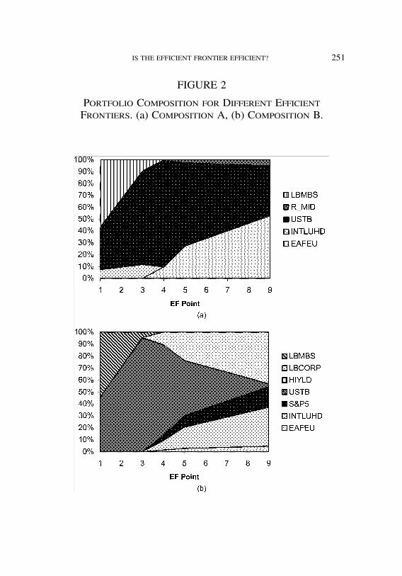
In addition to the positional changes in EFs over time, there isdramatic change in portfolio composition along the curve of eachEF in Figure 1. Examples of the change in portfolio compositionfor EFs appear in Figures 2a and 2b. Each chart is categorical—atic mark on the x-axis is associated with one of nine optimizationpoints. Each chart shows a stacked area rendering of the propor-tion of an asset component within the efficient set. If the readerviews either Figure 2a or 2b from left to right, the unfoldingchange, and possible collapse, of a particular component is illus-trated. This type of chart is a useful way to show a component’scontribution to the efficient set moving along the EF from lowrisk-return to high risk-return portfolios.
There is faint hope that the two different EF portfolio compo-sitions shown in Figures 2a and 2b will operationally produce thesame result when put in practice—were this to be a reasonablerepresentation of the effects of sampling error, the operationaluse of efficient frontiers would be questionable; sampling errorswamps operational usefulness and forecast responsiveness.
However, another illustration, Figure 3, indicates that if his-tory is a sample from a multivariate distribution, there shouldbe optimism that the efficient frontier evolves slowly, at leastmeasured in monthly metrics. This figure shows EFs calculated
job no. 1987 casualty actuarial society CAS journal 1987d04 [16] 09-12-02 2:43 pm
IS THE EFFICIENT FRONTIER EFFICIENT? 251
FIGURE 2
Portfolio Composition for Different EfficientFrontiers. (a) Composition A, (b) Composition B.

job no. 1987 casualty actuarial society CAS journal 1987d04 [17] 09-12-02 2:43 pm
252 IS THE EFFICIENT FRONTIER EFFICIENT?
FIGURE 3
Efficient Frontiers for Consecutive Time Periods
from consecutive, overlapping historical blocks of time. In thiscase, the time interval between between consecutive EFs is onemonth. The stability deteriorates fastest at higher risk-return lev-els. The result was found to hold for a wide variety of consecu-tive historical blocks starting at various points since 1977. Thisstability may provide an operational basis for investing in anon-frontier portfolio and seeing its performance prevail over off-frontier portfolios, at least for relatively short planning horizons.
There are other ways to use the historical record. The papershortly will turn to the use of the bootstrap as a method of mea-suring sampling error. First, the data and manipulation methodsare described in more detail.
3.1. Data Manipulation
This study uses the time series described in Appendix A: Re-view of Data Sources. Except where gaps were present in thehistorical record, the portfolio returns are actual.12,13
12The data represent returns for a selected group of investment components. There wasno attempt to filter or smooth the time series in any way. However, a few gaps in thehistorical record were interpolated.

job no. 1987 casualty actuarial society CAS journal 1987d04 [18] 09-12-02 2:43 pm
IS THE EFFICIENT FRONTIER EFFICIENT? 253
The data were used in two ways: (1) bootstrap samples weremade from the original time series in an attempt to approximatesampling error phenomena, and (2) various historical series ofthe data were used for performance analysis. The study exam-ines period segmentation and the performance of efficient andinefficient portfolios for different forecast durations.
3.1.1. Historical Performance Analysis
In this section of the paper, data for an efficient frontier areextracted for a historical period and used to evaluate the efficientfrontier. The on-frontier portfolios are minimum variance portfo-lios found using quadratic programming.14 Off-frontier portfo-lios also were calculated.15 The study is concerned with whetherthe performance of off-frontier portfolios really were inefficientcompared to the performance of on-frontier portfolios.
3.2. Bootstrap Sampling
A bootstrap sample of a data set is one with the same numberof elements, but random replacement of every element by draw-ing with replacement from the original set of data. When thisprocess of empirical resampling is repeated many times, the boot-strap samples can be used to estimate parameters for functionsof the data. The plug-in principle [Efron and Tibshirani, 1993,p. 35] allows evaluation of complex functional mappings from
13One technique for deploying efficient frontiers within DFA analysis involves removalof actual values from the data series used in optimization. These points in the actualtime series may be deemed abnormalities. The efficient frontier calculation does not useall available data or uses them selectively. See Kirschner [2000] for a discussion of thehazards of historical period segmentation.14All optimization was done using Frontline Systems, Inc. Premium Solver Plus V3.5 andMicrosoft Excel.15It is possible to restate a portfolio optimization problem to produce off-frontier portfo-lios. These are asset allocations for points in risk-return space that are within the concaveregion defined by the set of efficient points. They are portfolios with variance greaterthan the minimum variance points for the same expected returns. They were found bygoal equality calculation using the same constraints as were used for minimum varianceoptimization. However, the equality risk condition was set to a higher level than foundon the efficient frontier. Non-linear optimization was used for this purpose, whereasquadratic optimization was used for minimum variance optimization.
job no. 1987 casualty actuarial society CAS journal 1987d04 [19] 09-12-02 2:43 pm
254 IS THE EFFICIENT FRONTIER EFFICIENT?
examination of the same functional mapping on the bootstrapsamples. The function µ = t(F) of the probability distribution Fis estimated by the same function of the empirical distribution F,µ = t(F), where the empirical distribution is built up from boot-strap samples. This technique often is deployed for the derivationof errors of the estimate.
The plug-in features of a bootstrap enable inference from sam-ple properties of the distribution of bootstrap samples. The plug-in properties extend to all complex functions of the bootstrap,including standard deviations, means, medians, confidence inter-vals and any other measurable function. The EF is one of thesefunctions.
The bootstrap is used in this paper to illustrate the impact ofsampling error on the EF.16 EF is a complex function of the his-torical returns from which it was calculated. If the sample is froma larger, unknown domain, the bootstrap principles apply. In thecase of correlated investment returns, a segment of history mightbe thought of as a sample, but it may not be operationally mean-ingful because of sampling error. Yet, the use of the historicaldata in DFA applications treats it as though it were meaningful,representative, and not a sample.
The behavior of the EFs for our bootstrap samples is a non-parametric technique used to evaluate the effect of sampling er-ror, were history to be properly thought of as a sample. Becauseactuarial science is built largely on the precept that past history,even of seemingly unique phenomena, really is a sample, we tooproceed along this slippery slope.
3.2.1. Bootstrapping n-Tuples
The n-tuple observation of correlated observations at time tcan be sampled with replacement. This technique was used by
16The bootstrap has been used in connection with mean-variance optimization byMichaud and others in an attempt to improve performance of EF portfolios. See Michaud[1998].
job no. 1987 casualty actuarial society CAS journal 1987d04 [20] 09-12-02 2:43 pm
IS THE EFFICIENT FRONTIER EFFICIENT? 255
Laster [1998]. The experiment is similar to drawing packages ofcolored gum drops from a production lot. Each package containsa mixture of different colors that are laid out by machinery insome correlated manner. Suppose the lot that has been sampledoff the production line contains n packages. A bootstrap sampleof the lot also contains n observations. It is obtained by draws,with replacement, from the original sample lot. The n-tuple ofinvestment returns at time t is analogous to a package within thelot of gum drop samples. The historical sequence of correlatedreturns is analogous to the mix of different colors of gum dropsin a package. The analogy halts because we know the lot ofgum drop packages is a sample. We never will know whetherthe sequence of historical, n-tuple investment returns is a samplein a meaningful sense.
The data consist of a matrix of monthly returns; each row isan n-tuple of the returns during a common interval of time for thecomponent assets (columns of the matrix); the value of n was tenand measures the use of the ten investment categories describedin Appendix A: Review of Data Sources. The bootstrap methodinvolves sampling rows of the original data matrix. An n-tupledescribing the actual returns for asset components at an intervalof time is drawn and recorded as an “observation” in the boot-strap sample. Because this n-tuple can appear in another draw,the process involves sampling with replacement. This random-ized choice of an n-tuple is repeated for each observation in theoriginal sample. When the original sample has been replaced bya replacement sampling of the sample, the result is referred to asa bootstrap sample. This process of drawing a bootstrap samplecan be repeated many times, usually in excess of 2,000.
Each bootstrap sample has both a measurable covariance ma-trix and an efficient frontier that can be derived using that covari-ance matrix. It is unlikely that any two bootstrap samples willnecessarily have the same covariance matrix. Each sample canbe subjected to mathematical optimization to produce an efficientfrontier. The study asks whether this frontier is stable across the

job no. 1987 casualty actuarial society CAS journal 1987d04 [21] 09-12-02 2:43 pm
256 IS THE EFFICIENT FRONTIER EFFICIENT?
samples. Instability is measured in two ways. First, the boot-strapped efficient frontier may fluctuate from sample to sample.This means that the distribution of risk for a return point onthe EF is not a degenerate distribution that collapses to a singlepoint. Rather, there is a range of different portfolio risks amongthe bootstrap samples at a given return. There is a probabilitydistribution associated with risk, given a return among the boot-strap samples. In other words, the study attempts to measure thedistribution, and the study views that distribution as a measureof sampling error in risk-return space as it affects the calculationof an efficient frontier.
Second, the portfolio allocations may diverge qualitativelyamong bootstraps. Were portfolio allocations to be about thesame in an arbitrarily small region of risk-return space amongdifferent bootstrap samples, the practical effects of sampling er-ror would be small.
3.2.2. Extension of the Bootstrap Sample as a DFA Scenario
The bootstrap samples can be used in the way a DFA modelmight have used the original historical data, including their di-rect use within the calculation of the DFA results as a randominstance of investment results. They are the source of DFA sce-narios. This paper suggests how that direct use of the bootstrapmight unfold in a DFA liability-side simulation, but it does notdeploy it in that manner.17,18 The authors have a less ambitiousobjective of examining just the performance of the efficient fron-tier built from bootstrapping investment information.
17,Although the n-tuple used in this paper is a cross-sectional observation of returns, itcan be expanded to a cross-section of the entire business environment at time t. Thisincludes all economic aggregates, not just rates of return. Any flow or stock businessaggregate that can be measured for interval t is a candidate for the n-tuple. This wouldinclude inflation, gross domestic product, or any worldly observation of the businessclimate prevailing at that time. A bootstrap sample can be used as a component of alarger simulation requiring simulation of these worldly events.18DFA model builders spend time modeling empirical estimates of process and parameterrisk [Kirschner and Scheel, 1998]. Bootstrapping from the data removes much of thisestimation work and leaves the data to speak for themselves.

job no. 1987 casualty actuarial society CAS journal 1987d04 [22] 09-12-02 2:43 pm
IS THE EFFICIENT FRONTIER EFFICIENT? 257
3.3. Sampling Error within Risk-Return Space
There is no clear-cut method for estimating sampling errorthat may exist in risk-return space. We do not know the underly-ing distribution generating a historical sample. We do not knowwhether a population distribution, were it to exist, is stationaryover any time segment. We might, however, view history as anexperimental sample, particularly if we want to use it to forecastcorporate strategic decisions using DFA.
Sampling error can be envisioned and approximated in differ-ent ways for this hypothetical unfolding of reality. One way isto break the actual time series into arbitrary time segments andask whether a random selection among the subsets of time leadsto different, operationally disparate results—these would be EFsbased on the sub-segment of time that have portfolio allocationsdisparate enough to be viewed as operationally dissimilar. If theyare dissimilar enough to warrant different treatment, a samplingdistribution of interest is the one measured by the effects of thesetime-period slices.
Another approach is to envision prior history as an instanti-ation, period-to-period, from an unknown multivariate distribu-tion. The sampling error in this process is driven by a multivariatedistribution. Depending on our model, we may or may not placedependencies from prior realizations on this period’s realization.That is, for DFA investment return generation and intra-periodportfolio rebalancing, the multivariate model may be stationaryor non-stationary with respect to time.
3.3.1. Michaud’s Efficient Frontier
Michaud [1998] approaches the measurement of sampling er-ror effects on EF in a different way. Although his approach dif-fers, his overall conclusions are important and consistent withmany of our findings. He notes [1998, p. 33], “The operativequestion is not whether MV optimizations are unstable or un-intuitive, but rather, how serious is the problem. Unfortunately
job no. 1987 casualty actuarial society CAS journal 1987d04 [23] 09-12-02 2:43 pm
258 IS THE EFFICIENT FRONTIER EFFICIENT?
for many investment applications, it is very serious indeed.” Ourpaper will draw a similar conclusion.
He does not refer to an efficient surface but calculates a “re-sampled” portfolio that seems to capture some similar properties.Michaud uses multivariate Normal simulations from the same co-variance matrix used to calculate EFs. This covariance matrix isfrom a sample of data—the data observed during some historicalperiod. Just what definition of sampling error has been accom-modated in the Michaud resampled portfolio is unclear.
One of the Michaud simulations is not equivalent to a boot-strap sample used in this study. Michaud’s approach does not at-tempt to adjust for a primary source of sampling error—samplingerror in the covariance matrix. In our study, each bootstrap sam-ple has an independently measured covariance matrix. Usingthe DFA jargon of Kirschner and Scheel [1998, pp. 404–408],Michaud’s approach may not account for parameter risk in theunderlying returns generation mechanism. The ranking mecha-nism used by Michaud to combine EFs derived from variousmultivariate Normal simulations may distort risk-return space be-cause each EF is segmented in some non-linear fashion to iden-tify equally ranked points in risk-return space [Michaud, 1998,p. 46, footnote 11]. The portfolio profiles for identically rankedEF points are averaged, yet it is not clear that equi-ranked pointsfall within the same definition of risk-return space.
3.4. Importance to DFA Scenario Generation
This paper cannot and does not attempt to rationalize the pro-cess underlying investment yields over time.19 Rather, the modelbuilder should be careful to design the DFA model to be in accor-dance with perceptions about how a sampling methodology mayapply. The use of the model will invariably mimic that viewpoint.
19What if there were no common observable stationary probability measure for securityprices? Kane [1999, p. 174] argues we must use utility measurements.

job no. 1987 casualty actuarial society CAS journal 1987d04 [24] 09-12-02 2:43 pm
IS THE EFFICIENT FRONTIER EFFICIENT? 259
If, for example, one views history in the fashion imaginedby a bootstrap of n-tuples, and if that view does observe opera-tional differences, then one can create scenarios from bootstrapsamples. No more theory is required. Hypothetical investmentreturns are just a bootstrap sample of actual history.
Similarly, if EFs for historical periods produce superior per-formance in forecasting (compared to portfolios constructedfrom off-frontier portfolios derived from the same data), thenthe use of an empirically determined covariance model and mul-tivariate Normal simulation makes a great deal of sense.
3.5. Importance to DFA Optimization
Optimization often is used within DFA and cash flow testingmodels to guide portfolio rebalancing. The DFA model usuallygrinds through the process of business scenario and liability sce-nario simulations before the optimizer is deployed. But, account-ing within the model often is done while the optimizer seeks afeasible solution.
The sequence of model events runs like this:
1. Independently model many instances of exogenous statesof the business world (e.g., asset returns, inflation, mea-sures of economic activity, monetary conversion rates).Number these instances, B1,B2,B3, : : : ,Bn. Note that eachof these instances is a vector containing period-specificvalues for each operating fiscal period in the analysis.
2. Model many instances of the company’s performance.Number these instances C1,C2, : : : ,Cn. C1 often is depen-dent on B1 because it may use an economic aggregatesuch as inflation or economic productivity to influenceC1’s business growth or loss and expense inflation. EachC is a vector spanning the same fiscal periods as B.
3. Observe that in some DFA models neither B nor C isnecessarily scaled to the actual volume of business. Theyare unit rates of change for underlying volumes that areyet to be applied.

job no. 1987 casualty actuarial society CAS journal 1987d04 [25] 09-12-02 2:43 pm
260 IS THE EFFICIENT FRONTIER EFFICIENT?
4. Let the optimizer search mechanism posit a vector ofweights that distribute the volume of assets at t0, theinception point for a forecast period.
5. Apply the accounting mechanisms used by the DFAmodel to beginning assets and account for the unit activ-ities expressed in B and C.20 Do this accounting for eachvector pair "B1,C1#,"B2,C2#, : : : ,"BnCn# over the rangeof its time span.21
6. Calculate the metric used for the goal and any constraintsas of the end of the fiscal period, if it is a metric such aseconomic value or surplus. If it is a flow-based metricsuch as portfolio duration or discounted GAAP income,derive the metric for the holding period results. This cal-culation is done for each business/company scenario pair.There are n results; collectively they constitute a simu-lated sample.22
7. Return the required metrics for the sample to the opti-mizer. If the optimizer is deployed for EF calculation, thegoal will be a sample statistic for risk, such as variance,semi-variance, or chance-constrained percentile or range.The sample average for the distribution developed in step(6) for the metric will be used within the constraint set.
8. The optimizer will repeat steps (4)–(7) until it has ob-tained a feasible set.
The optimizer uses a sample. The optimizer results have sam-pling error. Steps (1) and (2) are experiments. Let there be 10
20At this stage, the derivation of taxes would occur. As noted by Rowland and Conde[1996], the determination of federal income taxes is convoluted by the combined ef-fect of discount rates, changes in loss reserves, varying underwriting results, and taxcarryforwards and carrybacks.21Some models may achieve computational efficiencies when economic scenarios arepaired with E(C) instead of with direct pairing to C1,C2, : : : ,Cn. When this is done,however, the variance of the metric being optimized will be reduced, and the minimumvariance portfolio is likely to be different.22If enough pairs are used, the chance that the model will converge improves.

job no. 1987 casualty actuarial society CAS journal 1987d04 [26] 09-12-02 2:43 pm
IS THE EFFICIENT FRONTIER EFFICIENT? 261
repetitions of this experiment. Application of steps (1)–(8) willresult in 10 efficient frontiers, each derived from a different ex-perimental sample. It is likely that they will have different char-acteristics.
In a DFA experiment there are many draws from the urn; eachsimulation is another draw. The modeler gets distributional infor-mation about the contents of the urn by the experimental group-ing of all the simulations. When enough simulations within eachexperiment are run, convergence of the distribution of resultscan be achieved. Since it is unlikely for the output distributionto be known, or necessarily capable of being parameterized, noa priori estimate is available. Instead, an empirical measure ofconvergence must be used.
The allocation of company assets among competing invest-ment alternatives using a single efficient frontier calculation(based on a single experimental result) may seem to be simi-lar to betting on the allocation among balls of different colorswithin the urn based on a single sample from the urn containingthem. One may, or may not, be lucky. But you improve yourluck by increasing the number of simulations.
One still may become victimized by a faulty decision whileignoring sampling error. This may arise in calibrating a modelto history. The historical record is a single draw from a trueunderlying probability distribution. We may be lucky that thenumber of periods in the historical realization contains sufficientinformation about the underlying process for unfettered decisionmaking. But we could be victims of sampling error, which weare unable to control or even limit.
4. HISTORICAL PERFORMANCE COMPARISON
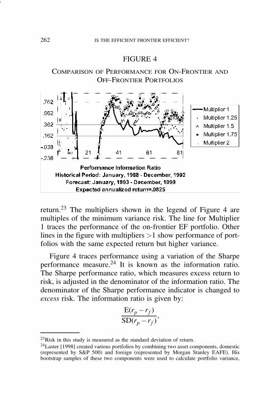
Figure 4 illustrates the performance of several portfolios overincreasingly longer forecast periods. It shows results for portfo-lios, which, a priori, have different levels of risk for the same
job no. 1987 casualty actuarial society CAS journal 1987d04 [27] 09-12-02 2:43 pm
262 IS THE EFFICIENT FRONTIER EFFICIENT?
FIGURE 4
Comparison of Performance for On-Frontier andOff-Frontier Portfolios
return.23 The multipliers shown in the legend of Figure 4 aremultiples of the minimum variance risk. The line for Multiplier1 traces the performance of the on-frontier EF portfolio. Otherlines in the figure with multipliers >1 show performance of port-folios with the same expected return but higher variance.
Figure 4 traces performance using a variation of the Sharpeperformance measure.24 It is known as the information ratio.The Sharpe performance ratio, which measures excess return torisk, is adjusted in the denominator of the information ratio. Thedenominator of the Sharpe performance indicator is changed toexcess risk. The information ratio is given by:
E(rp$ rf)SD(rp$ rf)
,
23Risk in this study is measured as the standard deviation of return.24Laster [1998] created various portfolios by combining two asset components, domestic(represented by S&P 500) and foreign (represented by Morgan Stanley EAFE). Hisbootstrap samples of these two components were used to calculate portfolio variance,
job no. 1987 casualty actuarial society CAS journal 1987d04 [28] 09-12-02 2:43 pm
IS THE EFFICIENT FRONTIER EFFICIENT? 263
whererp =monthly return on the portfolio,
rf =monthly return on the risk freecomponent of the portfolio,25
E = expectation operator, and
SD = standard deviation operator.
Although the information ratio was computed with monthly data,it is expressed as an annual measure in the paper.
4.1. EF Performance Is Better for Low Risk-Return Portfolios
The off-frontier portfolios, so-called inefficient portfolios,achieve performance that rivals or betters that of the EF port-folio.26 There is no concept of “significance” that can be at-tached to the observed differences. However, it is clear that theperformance differences are great and that inefficient portfoliosoutperform the efficient one in the Figure 4. When performanceis measured by geometric return, the underperformance of theEF portfolio can be more than 100 basis points, as shown inFigure 5. The underperformance shown in Figure 5 is measuredover a seven-year holding period, and there was no portfolio re-balancing during this time. Data for other time periods and theuse of intervening portfolio rebalancing might materially affectthis evidence of underperformance.
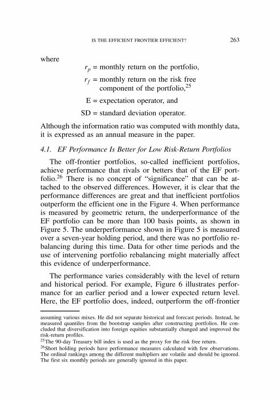
The performance varies considerably with the level of returnand historical period. For example, Figure 6 illustrates perfor-mance for an earlier period and a lower expected return level.Here, the EF portfolio does, indeed, outperform the off-frontier
assuming various mixes. He did not separate historical and forecast periods. Instead, hemeasured quantiles from the bootstrap samples after constructing portfolios. He con-cluded that diversification into foreign equities substantially changed and improved therisk-return profiles.25The 90-day Treasury bill index is used as the proxy for the risk free return.26Short holding periods have performance measures calculated with few observations.The ordinal rankings among the different multipliers are volatile and should be ignored.The first six monthly periods are generally ignored in this paper.

job no. 1987 casualty actuarial society CAS journal 1987d04 [29] 09-12-02 2:43 pm
264 IS THE EFFICIENT FRONTIER EFFICIENT?
FIGURE 5
Comparison of Geometric Return for On-Frontier andOff-Frontier Portfolios
portfolios for about ten years. Thereafter, it reverses, and perfor-mance falls below off-frontier portfolios. The Figure illustratesthat the contemplated holding period for use of an EF shouldprobably not be as long. The performance variance illustrated inFigure 6 is volatile; the differences in performance in on- andoff-frontier portfolios vary considerably with the choice of his-torical starting point and length of the holding period.
4.2. Overall Behavior of On-Frontier Portfolios for InformationRatio
The historical record was examined from several perspectivesto see whether an EF portfolio continues to outperform off-frontier portfolios. Equi-return portfolios were examined. Theseare portfolios whose returns are the same, but they have higherrisk. The forecast period immediately following the end of thehistorical segment was examined to determine how long the on-frontier portfolio maintained superior performance. This forecasthorizon extended to the end of the data, December 1999. His-torical segments consist of a 5-year block of 60 observations.
job no. 1987 casualty actuarial society CAS journal 1987d04 [30] 09-12-02 2:43 pm
IS THE EFFICIENT FRONTIER EFFICIENT? 265
FIGURE 6
EF Portfolio Performance at Low Risk-Return Levels
Several adjustments were made for this analysis. The first six-month period was ignored because the ratio is highly volatile andcomputed from few observations. The extreme low return levelsalso were removed from the analysis because higher ones shownin the table dominated them.27
Table 1 shows the relative behavior of the information ratioat the return level indicated at the top of the column. Each rowblock includes the time for subsequent row blocks. For example,the forecast beginning January 1980 covers the period endingDecember 1999. The interval of measurement is a month. All ofthe other blocks begin at a later point, but all forecast periodsend in December 1999.28
27The extreme low risk-return observations occur below where the EF curve has a positivefirst derivative. A portfolio with a higher return for the same risk can be found abovethis change in the curve.28Each block of rows uses a different set of on- and off-frontier portfolios—the respectiveEFs are derived from optimizations on different periods. For example, the January 1980forecast is based on the performance of EFs derived from a historical segment coveringthe 5-year period, January 1975–December 1979). However, the January 1995 forecastuses EFs derived from a different period, one covering the 5-year period, January 1989–

job no. 1987 casualty actuarial society CAS journal 1987d04 [31] 09-12-02 2:43 pm
266 IS THE EFFICIENT FRONTIER EFFICIENT?
TABLE 1
INFORMATION RATIO BEHAVIOR
Forecast Period Return Levels
Information Ratio (forecast begins 1/1980) 0.0066 0.0080 0.0085 0.0090 0.0095 0.0100
Periods until on-frontier point underperforms(max = 238)
6 6 6 6 6 6
Number of periods on-frontier pointoutperforms all others
10 142 148 153 154 151
Average on-frontier rank (5 is highest) 3.05 4.37 4.34 4.33 4.30 4.27
Information Ratio (forecast begins 1/1985) 0.0066 0.0080 0.0085 0.0090 0.0095 0.0100
Periods until on-frontier point underperforms(max = 178)
111 110 109 7 119 69
Number of periods on-frontier pointoutperforms all others
105 104 103 8 113 124
Average on-frontier rank (5 is highest) 3.46 3.40 3.38 1.92 3.72 3.90
Information Ratio (forecast begins 1/1990) 0.0066 0.0080 0.0085 0.0090 0.0095 0.0100
Periods until on-frontier point underperforms(max = 118)
40 6 9 9 9 9
Number periods on-frontier point outperformsall others
34 8 66 83 103 111
Average on-frontier rank (5 is highest) 4.18 4.05 4.57 4.72 4.89 4.96
Information Ratio (forecast begins 1/1993) 0.0066 0.0080 0.0085 0.0090 0.0095 0.0100
Periods until on-frontier point underperforms(max = 82)
19 6 6 6 6 10
Number of periods on-frontier pointoutperforms all others
15 3 5 6 2 4
Average on-frontier rank (5 is highest) 2.10 1.83 1.82 1.81 1.60 1.56
Information Ratio (forecast begins 1/1995) 0.0066 0.0080 0.0085 0.0090
Periods until on-frontier point underperforms(max = 58)
53 56 57 Never
Number of periods on-frontier pointoutperforms all others
47 50 51 53
Average on-frontier rank (5 is highest) 4.83 4.94 4.96 5.00
December 1994. The information in the blocks is not cumulative; the number of periodsthe on-frontier excels or outperforms off-frontier portfolios is a separate measurement foreach row block. The row blocks show performance for portfolios constructed at differentpoints in time.

job no. 1987 casualty actuarial society CAS journal 1987d04 [32] 09-12-02 2:43 pm
IS THE EFFICIENT FRONTIER EFFICIENT? 267
Missing cells in Table 1 indicate that a feasible set was notfound at that return level for one or more of the on- or off-frontierportfolios. There were five portfolios with risk up to two timesthe risk of the on-frontier point.
“Periods until on-frontier point underperforms” means thefirst period that an off-frontier portfolio beats the on-frontierefficient portfolio. “Number of periods on-frontier point outper-forms all others” means the last period where the efficient port-folio wins. Performance tends to hold up better for lower returnlevels. This effect is reinforced by the larger values shown forthe number of periods the on-frontier portfolio does outrank theoff-frontier portfolios. In general, the on-frontier portfolio rankswell compared to the others. The average rank is generally high,above 3 out of 5. But the performance is not consistent. The on-frontier portfolio did well during the long forecast period start-ing January 1980 and during the shorter forecast period startingJanuary 1995. However, the low average of the on-frontier forthe January 1993 period shows that the performance is greatlyinfluenced by the historical period and perhaps influenced bysampling error.
There also is great inconsistency in the number of periods be-fore an off-frontier portfolio has a higher information ratio. Thescan begins in period 6 of the forecast horizon, so the reversalshown in the table will either be never or a number between 6and n. In most cases, the reversal is early, but not permanent.There are many situations where the on-frontier portfolio wa-vers between highest rank and something less. This latter factis found in the rows, “Number of periods on-frontier point out-performs.” In most cases this number is larger than the num-ber of periods before reversion, indicating that the on-frontierwaffles in and out of superior performance. This could be an-other indication of sampling error. The choice of an on-frontierpoint may not, and probably does not, imply superior perform-ance.

job no. 1987 casualty actuarial society CAS journal 1987d04 [33] 09-12-02 2:43 pm
268 IS THE EFFICIENT FRONTIER EFFICIENT?
4.3. Behavior for Other Performance Measures
The information ratio is believed to be a valid measure ofperformance because it adjusts for variation in the return seriesduring the period of measurement. Were it applied to two consul-tants’ portfolio allocation recommendations, the consultant withlower excess returns could be ranked higher than the other con-sultant, because of proportionately lower risk in excess return.This may be small consolation to the holder of the lower wealthportfolio recommended by the higher ranked consultant. This iswhy it is important to assess other characteristics beyond the ap-petite for risk before making an allocation decision. The managerwith the higher information ratio has the better cost of risk perunit of return; yet, it is not of much use if a minimum returnlevel or ending wealth is required.
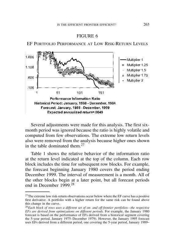
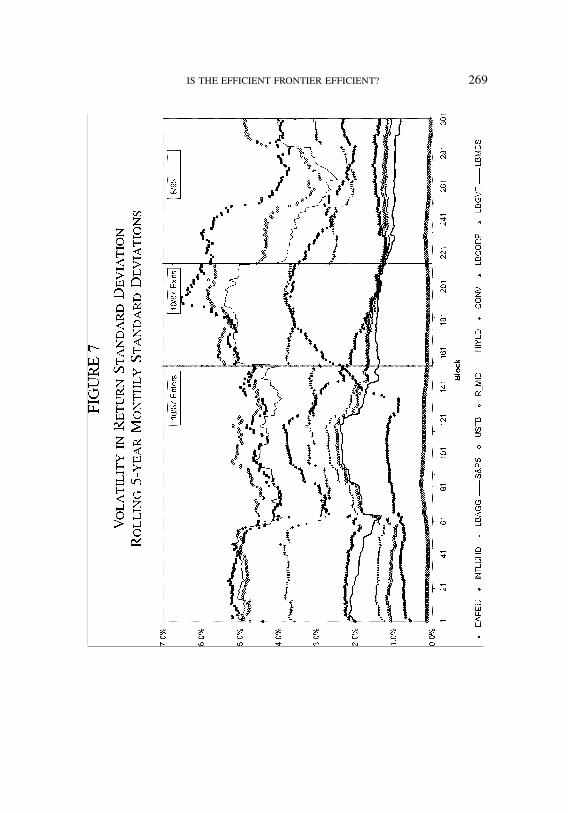
There is considerable historic instability in the standard de-viation of returns. This can be seen in Figure 7, which showsthe historic progression of changes in the standard deviation ofmonthly returns of the portfolio components used in this study.The lines show the change in standard deviation for rolling 5-yearblocks of data.29 Any performance measure that is a function ofthis risk proxy, such as the information index, will be inherentlysensitive to such volatility and, perhaps, exhibit similar historicinstability. This volatility in risk helps to explain why historicalEFs may lack forecast power.
One measure of performance that is not risk-adjusted is ge-ometric return during a holding period. Results are arrayed inTable 2. The layout of this table is similar to Table 1.
The forecast propensity of the on-frontier allocation ismarkedly changed. Wealth growth appears to be unrelated tothe on- or off-frontier portfolio choice, and often is worsefor the on-frontier allocation. The number of holding peri-
29There was significant volatility in the securities markets in 10/87 (“Black Monday”)and 8/98 (Long Term Capital crisis). These periods are highlighted in the figure.
job no. 1987 casualty actuarial society CAS journal 1987d04 [34] 09-12-02 2:43 pm
IS THE EFFICIENT FRONTIER EFFICIENT? 269

job no. 1987 casualty actuarial society CAS journal 1987d04 [35] 09-12-02 2:43 pm
270 IS THE EFFICIENT FRONTIER EFFICIENT?
TABLE 2
GEOMETRIC RETURN BEHAVIOR
Forecast Period Return Levels
Geometric Return (forecast begins 1/1980) 0.0066 0.0080 0.0085 0.0090 0.0095 0.0100
Periods until on-frontier point underperforms(max = 239)
6 6 6 6 6 6
Number of periods on-frontier pointoutperforms
0 107 106 102 102 105
Average on-frontier rank (5 is highest) 2.41 3.35 3.39 3.38 3.38 3.40
Geometric Return (forecast begins 1/1985) 0.0066 0.0080 0.0085 0.0090 0.0095 0.0100
Periods until on-frontier point underperforms(max = 179)
6 6 6 6 6 6
Number of periods on-frontier pointoutperforms
0 0 0 0 0 1
Average on-frontier rank (5 is highest) 1.00 1.00 1.00 1.00 1.03 1.04
Geometric Return (forecast begins 1/1990) 0.0066 0.0080 0.0085 0.0090 0.0095 0.0100
Periods until on-frontier point underperforms(max = 119)
21 6 74 89 111 119
Number of periods on-frontier pointoutperforms
15 7 68 85 105 113
Average on-frontier rank (5 is highest) 4.11 4.06 4.60 4.75 4.92 4.99
Geometric Return (forecast begins 1/1993) 0.0066 0.0080 0.0085 0.0090 0.0095 0.0100
Periods until on-frontier point underperforms(max = 83)
15 15 16 16 16 16
Number of periods on-frontier pointoutperforms
11 16 18 18 14 10
Average on-frontier rank (5 is highest) 1.99 2.19 2.22 2.22 1.92 1.73
Geometric Return (forecast begins 1/1995) 0.0066 0.0080 0.0085 0.0090
Periods until on-frontier point underperforms(max = 59)
6 6 6 6
Number of periods on-frontier pointoutperforms
0 2 9 30
Average on-frontier rank (5 is highest) 2.44 2.80 2.96 3.35
ods the efficient frontier portfolio dominates off-frontier port-folios is generally a lower proportion of the possible num-ber of holding periods in Table 2 than in Table 1. Michaud[1998, pp. 27–29] claims there is a portfolio within the

job no. 1987 casualty actuarial society CAS journal 1987d04 [36] 09-12-02 2:43 pm
IS THE EFFICIENT FRONTIER EFFICIENT? 271
EF, the “critical point,” below which single period mean-varianceefficient portfolios are also n-period geometric mean efficientand above which single period MV efficient portfolios are notn-period geometric mean efficient.
4.4. Performance Failure within CAPM
Work with beta has led to various criticisms [Malkiel, 1996,p. 271].30 For example, some low risk stocks earn higher returnsthan theory would predict. Other attacks on beta tend to mirrorwhat we see with EF:
1. The capital asset pricing model (CAPM) predicts risk-free rates that do not measure up in practice.31
2. Beta is unstable, and its value changes over time.32
3. Estimated betas are unreliable.33
4. Betas differ according to the market proxy they are mea-sured against.34
5. Average monthly return for low and high betas differsfrom predictions over a wide historical span.35
30Beta is a measure of systematic risk either for an individual security or for a portfolio.High beta portfolios, measured ex ante, in theory should have higher returns ex post thanlow beta portfolios.31When ten groups of securities, ranging from high to low betas, were examined forthe time period 1931–65, the theoretical risk free rate predicted by CAPM and actualrisk free rates significantly diverged. Low risk stocks earned more and high risk stocksearned less than theory predicted [Malkiel, 1996, pp. 256–7].32During short periods of time, risk and return may be negatively related. During 1957–65, securities with higher risk produced lower returns than low beta securities [Malkiel,1996, pp. 258–60].33The relationship between beta and return is essentially flat. Beta is not a good measureof the relationship between risk and return [Malkiel, 1996, pp. 267–8].34Predictions based on CAPM about expected returns both for individual stocks and forportfolios differ depending on the chosen market proxy. In effect, the CAPM approachis not operational because the true market proxy is unknown [Malkiel, 1996, pp. 266–7].35The ratio of price to book value and market capitalization did a better job of predictingthe structure of nonfinancial corporate share returns than beta during a 40-year period[Fama and French, 1992].

job no. 1987 casualty actuarial society CAS journal 1987d04 [37] 09-12-02 2:43 pm
272 IS THE EFFICIENT FRONTIER EFFICIENT?
Malkiel [1996, p. 270] concludes from his survey that, “One’sconclusions about the capital-asset pricing model and the useful-ness of beta as a measure of risk depend very much on how youmeasure beta.” This appears to be true of EFs too. The definitionof efficiency is what is important here—perhaps more importantbecause correct measurement requires precise definition.
The choice of an optimization mechanism couched in terms ofrisk-return trade-off may not lead to wealth maximization. Underthese pretenses one might wish to deploy a different optimizationmechanism, such as the one mentioned by Mulvey, et al. [1999,p. 153] in which the optimization seeks to maximize utility. Thechoice of a particular utility function may be framed in terms ofabsolute risk aversion—negative exponential utility works in thisregard.36 And if the behavior of security prices does not have anobservable stationary probability measure [Kane, 1999], utilityapproaches seem to be mandatory.
The subject of what is optimal is controversial and not aptto go away. The use of optimization within hybrid models andgeneration of metrics by DFA models has many subtle manifes-tations. One is the choice of planning horizon. Michaud [1998,p. 29] argues that investors with long-term investment objectivescan avoid possible negative long-term consequences of mean-variance efficiency by limiting consideration to EF portfolios ator below some critical point. There is a parallel in our paper, inwhat we refer to as sampling error and its effect on the shapeof the efficient surface. This surface appears to have propertiesat the lower risk-return areas of both lower dispersion, greatersimilarity in portfolio composition, and better on-frontier per-formance among different samples (either bootstrap or historicsegment).
36The recommendation of a utility-decision approach has great breadth in the insuranceliterature—beyond the use of utility as goal function in optimization, other venues find itappropriate where stochastic dominance is sought. For example, exponential utility usewas suggested in rate making by Freifelder [1976]. The choice of parameters for utilityfunctions is perhaps as much an art as the parameterization of claims generations in DFAmodels.

job no. 1987 casualty actuarial society CAS journal 1987d04 [38] 09-12-02 2:43 pm
IS THE EFFICIENT FRONTIER EFFICIENT? 273
5. CHARACTERISTICS OF THE EF SURFACE
The bootstrap-generated EF surface rises within the risk-return space. Views of this surface from two different anglesare shown in Figure 8.
The surface is constructed from monthly returns. Lookingdown on the surface of the views, one obtains a projectionon risk-return space. The surface is seen to curve as the effi-cient frontier curves. In the low risk-return sector, the surfaceis more peaked. The surface flattens and broadens in the risk-return space. Imagine yourself walking along the ridge startingin the southwest and proceeding northward and then northeast.You would first be descending a steep incline, and then a vistaof a vast plane would unfold along your right. This can be in-terpreted within the context of changes in the marginal distri-butions representing slices through the surface either along therisk or along the return dimensions. We refer to the latter as anequi-return slice, and its properties are examined in more detailat a latter point in the paper. In either case, the visualization isone of moving from less dispersed marginal distributions to oneswith greater variance as either dimension is increased.
There is an artifact of the intervalization that results in a sud-den rise in the surface at the highest risk level. This occurs be-cause higher risk observations were lumped into this final inter-val. Were higher levels of risk intervalized over a broader range,this ridge would flatten.
The surface shown in either of the views in Figure 8 isbuilt from many efficient frontiers, each produced from opti-mizations done on a bootstrap sample. We already have seenin Figure 1 a subset of EFs that tangle together—they can beorganized to produce a surface. The surface develops the sameway an empirical probability distribution is built from a sam-ple. Repeated sampling produces points that are intervalized andcounted.

job no. 1987 casualty actuarial society CAS journal 1987d04 [39] 09-12-02 2:43 pm
274 IS THE EFFICIENT FRONTIER EFFICIENT?
FIGURE 8
Views of EF Surface Created from Bootstrap Samples

job no. 1987 casualty actuarial society CAS journal 1987d04 [40] 09-12-02 2:43 pm
IS THE EFFICIENT FRONTIER EFFICIENT? 275
FIGURE 9
Distribution of Risk Given a Return Level
A frequency count can be made of observations for EFs fallingwithin an arbitrarily small, two-dimensional region of risk-returnspace. An example of this mapping for 5,000 bootstrap-simulatedEFs appears in Figure 8. Collectively, this mapping involvesthe two-dimensional intervalization of approximately 45,000quadratic optimizations constituting the EFs for the underlyingbootstrapped samples.37
5.1. Equi-Return Slice of the Efficient Surface
A slice through the efficient surface along the return planeproduces a histogram of the minimum risk points for a givenreturn in the EFs used for the EF Surface. As return increases,this marginal probability distribution becomes more disperse. Anexample appears in Figure 9.
37Equi-return minimum variance points for the 5,000 bootstrapped EFs were intervalizedbased on an overall evaluation of the range of risk among all points on all EFs. If anefficient set could not be identified for a return level, the observation was ignored. Themarginal probabilities (risk-return) were normalized to the number of viable observationsfor that risk level. The number of viable optimizations exceeded 4,500 at each return level.

job no. 1987 casualty actuarial society CAS journal 1987d04 [41] 09-12-02 2:43 pm
276 IS THE EFFICIENT FRONTIER EFFICIENT?
TABLE 3
Statistics for Equi-Return Slices of the EfficientSurface
Statistic Efficient Surface from Bootstrapped Efficient Frontiers
Return Level .0053 .0066 .0080 .0085 .0090 .0095 .0100Mean (times 1.0E4) .0125 .0533 3.76 8.86 17.9 33.6 50.7Standard Deviation .627 3.77 38.2 58.6 81.8 109.7 131.6(times 1.0E4)Skewness (times 1.0E8) .000123 .378 57.8 136. 275. 516. 779.
TABLE 4
Statistics for Equi-Return Slices of the SurfaceShown in Figure 10
Statistic Efficient Surface from Historical Samples
Return Level .0053 .0066 .0080 .0085 .0090 .0095 .0100Mean (times 1.0E4) .663 5.53 21.0 25.5 28.8 33.2 46.5Standard Deviation .080 .451 .861 .940 .995 1.06 1.23(times 1.0E2)Skewness (times 1.0E6) .00676 .769 2.92 3.54 4.00 4.62 6.46
The dispersion increases with return for both surfaces con-structed from bootstrap samples and from randomly selectedblocks of history. The distributions are positively skewed, in-creasingly so as return increases. The inset bars in Figure 9 iden-tify the intervals containing the mean and median points of thedistribution. Additional statistics both for bootstrapped and his-torical segment evaluations of sampling error appear in Tables 3and 4.
The statistics are visually apparent in the EF surface shown inFigure 8. The surface is partially bowl-like—sloping downwardin a concave fashion. Its rim encompasses a plane within therisk-return domain that is broad in the risk dimension. As onemoves from low to high return, the marginal distribution of EF
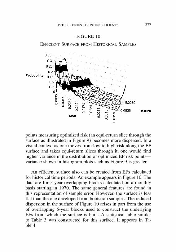
job no. 1987 casualty actuarial society CAS journal 1987d04 [42] 09-12-02 2:43 pm
IS THE EFFICIENT FRONTIER EFFICIENT? 277
FIGURE 10
Efficient Surface from Historical Samples
points measuring optimized risk (an equi-return slice through thesurface as illustrated in Figure 9) becomes more dispersed. In avisual context as one moves from low to high risk along the EFsurface and takes equi-return slices through it, one would findhigher variance in the distribution of optimized EF risk points—variance shown in histogram plots such as Figure 9 is greater.
An efficient surface also can be created from EFs calculatedfor historical time periods. An example appears in Figure 10. Thedata are for 5-year overlapping blocks calculated on a monthlybasis starting in 1970. The same general features are found inthis representation of sample error. However, the surface is lessflat than the one developed from bootstrap samples. The reduceddispersion in the surface of Figure 10 arises in part from the useof overlapping 5-year blocks used to construct the underlyingEFs from which the surface is built. A statistical table similarto Table 3 was constructed for this surface. It appears in Ta-ble 4.
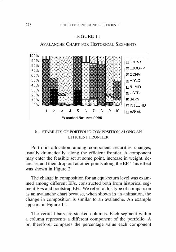
job no. 1987 casualty actuarial society CAS journal 1987d04 [43] 09-12-02 2:43 pm
278 IS THE EFFICIENT FRONTIER EFFICIENT?
FIGURE 11
Avalanche Chart for Historical Segments
6. STABILITY OF PORTFOLIO COMPOSITION ALONG ANEFFICIENT FRONTIER
Portfolio allocation among component securities changes,usually dramatically, along the efficient frontier. A componentmay enter the feasible set at some point, increase in weight, de-crease, and then drop out at other points along the EF. This effectwas shown in Figure 2.
The change in composition for an equi-return level was exam-ined among different EFs, constructed both from historical seg-ment EFs and bootstrap EFs. We refer to this type of comparisonas an avalanche chart because, when shown in an animation, thechange in composition is similar to an avalanche. An exampleappears in Figure 11.
The vertical bars are stacked columns. Each segment withina column represents a different component of the portfolio. Abr, therefore, compares the percentage value each component

job no. 1987 casualty actuarial society CAS journal 1987d04 [44] 09-12-02 2:43 pm
IS THE EFFICIENT FRONTIER EFFICIENT? 279
in the feasible set contributes across all components in the set.All bars are shown for a constant, equi-return level of an EF;but each bar is for a different historical segment. In Figure 11,each bar represents the portfolio composition for the equi-returnlevel point on the EF, which was calculated for a 5-year blockof monthly observations. The bars are for ten randomly chosenhistorical segments.38 Were the blocks within the bars to consistof the same components and were they to be about the samesize, the portfolio allocations would be the same regardless ofthe time frame. Examination of Figure 11 shows that the com-position of the bars and individual component allocations variesconsiderably.
The portfolio composition is much more stable at lower risk-return levels. This result is in accordance with other similar find-ings based on the EF surface. It, too, shows less disperse re-sults for lower return levels. This approach to measuring sam-pling error implies that performance of efficient frontiers maynot be optimal relative to off-frontier portfolios. If the mix andcomposition of portfolios fluctuates considerably both with re-spect to historical and bootstrap sampling methods, the perfor-mance expectations of an ex ante allocation are not apt to holdex post.
7. CONCLUSION
The behaviors shown in both Tables 1 and 2 illustrate amarked tendency towards randomness. The efficient surface builtfrom bootstrap samples is highly variable within the risk-returndomain. There appears to be some temporal dominance of on-frontier portfolios for lower risk-return levels, but the historicalrecord is mixed. The bootstrapping of the single sample of assetreturns provided by the historical data illustrates that sampling
38There is a small chance that two or more bars in an avalanche chart could be identical.However, there is a much larger probability that two or more bars have overlapping timeperiods in the calculation of their respective EFs.

job no. 1987 casualty actuarial society CAS journal 1987d04 [45] 09-12-02 2:43 pm
280 IS THE EFFICIENT FRONTIER EFFICIENT?
error could materially affect the position and shape of the effi-cient frontier.
7.1. Should Efficient Frontiers Be Used in DFA Models?
There is no strong support in this paper for the practical de-ployment of efficient frontiers in DFA. The risk in DFA mod-els stems from model, process, and parameter risk. It affects allaspects of DFA models of the insurance enterprise. The exis-tence of model and process risk [Kirschner and Scheel, 1998]thwarts the usual convergence to the true underlying distribu-tions gained by running large numbers of simulations. When allof these new risk elements are heaped on top of the samplingerror derived from asset model calibration or empirically mea-sured covariance matrices, one wonders whether EFs are reallyuseful in DFA analysis.
The work of Michaud [1998] bears on the issue of improvingthe performance of EF portfolios. He defines a measure of sta-tistical equivalence for mean-variance efficiency. Any portfoliowithin the efficient surface sufficiently close to the optimal port-folio is considered equivalent to it. The extension of his idea tothe efficient frontier surface is to identify a region on it whoseex ante chance-constrained probability both can be measured andhas desirable statistical properties in a forecasting sense. This isanalogous to acknowledging the existence of sampling error andspecifying an unknown population parameter only to within aninterval of statistical confidence. Unfortunately, the definition ofsufficiently close is constructive but difficult to implement in arigorous manner, particularly within the context of the hybridDFA model.
Future study will have to answer the question of whether on-frontier asset allocations that are measured from hybrid DFAmodels suffer a similar unreliability. But the problems with on-frontier asset portfolios raised in this paper are apt to be exacer-bated by inclusion of known sampling error in the liability sideof DFA models.

job no. 1987 casualty actuarial society CAS journal 1987d04 [46] 09-12-02 2:43 pm
IS THE EFFICIENT FRONTIER EFFICIENT? 281
7.2. How Can EFs Be Efficiently Deployed?
Users of this construct should be aware that the term “ef-ficient” in efficient frontiers has a good chance of being opera-tionally false. The efficiency of portfolio composition is unlikelyto be manifest in better performance of the on-frontier portfoliocompared to other, off-frontier portfolios. The risk-return sur-face is not adequately measured by a single EF, and samplingerror may lead to unwarranted conclusions about the efficacy ofportfolios measured in such singular optimizations.
The user of EFs should probably view them as containing pro-visional, useful information about risk-return relationships. But,any single EF has limited value in understanding the risk-returnsurface. The conceptual basis of an efficient surface is an orga-nized resampling of the data so that the decision process benefitsfrom better understanding of uncertainty that might arise just be-cause the EF is operationally derived from a sample. The misun-derstanding of this uncertainty may lead to erroneous decisions,and the practitioner must be alert to potential inefficiencies of asingle EF measurement. The authors recommend the elicitationof an efficient surface because the surface is apt to show a lackof statistical confidence in any single frontier on that surface.Under these circumstances, the practitioner must think in termsof confidence ranges. The sampling error shown in the efficientsurface emphasizes how careful one must be when drawing infer-ences derived from optimization. An optimized frontier is basedon an empirical covariance matrix, one that has sampling error.That error may be very important. It is easy to believe that strate-gic or tactical decisions motivated by so-called optimized DFAmeasurement will effectively move the organization to a betterposition in risk-return space. Unfortunately, there appears to bea broad region of “inefficiency” that may serve as well. An EFmay be better than a crystal ball; but there is a good chance thatit should not be taken too seriously.

job no. 1987 casualty actuarial society CAS journal 1987d04 [47] 09-12-02 2:43 pm
282 IS THE EFFICIENT FRONTIER EFFICIENT?
REFERENCES
[1] Chopra, Vijay, and William Ziemba, “The Effect of Errorsin Means, Variances, and Covariances on Optimal PortfolioChoice,” Worldwide Asset and Liability Management, Cam-bridge University Press, 1998, pp. 53–61.
[2] Correnti, Salvatore, Stephen M. Sonlin, and Daniel B. Isaac,“Applying a DFAModel to Improve Strategic Business De-cisions,” Casualty Actuarial Society Forum, Summer 1998,pp. 15–52.
[3] Davison, A. C., and D. V. Hinkley, Bootstrap Methods andTheir Application, Cambridge University Press, 1997, p.582.
[4] Efron, Gerald F., and Robert J. Tibshirani, An Introductionto the Bootstrap, Chapman & Hill, 1993, p. 436.
[5] Elton, Edwin J., and Martin J. Gruber, Modern PortfolioTheory and Investment Analysis, John Wiley & Sons, Inc,1995, p. 715.
[6] Fama, Eugene F., and Kenneth R. French, “The Cross-Section of Expected Stock Returns,” Journal of Finance,June 1992.
[7] Freifelder, Leonard R., A Decision Theoretic Approach toInsurance Ratemaking, Irwin, 1976, p. 141.
[8] Kane, S.A., “What Happened to the Utility Functions? Im-precise Expectations of Security Prices,” International Re-view of Financial Analysis, 8:2, 1999, pp. 165–175.
[9] Kirschner, Gerald S., “A Cost/Benefit Analysis of Alterna-tive Investment Strategies Using Dynamic Financial Anal-ysis Tools,” Casualty Actuarial Society Forum, Summer2000, pp. 21–54.
[10] Kirschner, Gerald S., and William C. Scheel, “The Me-chanics of a Stochastic Corporate Financial Model,” PCASLXXXV, 1998, pp. 404–454.

job no. 1987 casualty actuarial society CAS journal 1987d04 [48] 09-12-02 2:43 pm
IS THE EFFICIENT FRONTIER EFFICIENT? 283
[11] Laster, David S., “Measuring Gains from International Eq-uity Diversification: The Bootstrap Approach,” The Journalof Investing, Fall 1998, pp. 52–60.
[12] Levy, Haim, and Deborah Gunthorpe, “Optimal InvestmentProportions in Senior Securities and Equities Under Alter-native Holding Periods,” The Journal of Portfolio Manage-ment, Summer 1993, p. 31.
[13] Malkiel, Burton G., A Random Walk Down Wall Street, W.W. Norton & Company, Inc., 1996, pp. 227–276.
[14] Michaud, Richard O., Efficient Asset Management, HarvardBusiness School Press, 1998.
[15] Michaud, Richard O., “The Markowitz Optimization Enig-ma: is ‘Optimized’ Optimal,” Financial Analysts Journal,45:1, pp. 32–42.
[16] Mulvey, John M., Chris K. Madsen, and Francois Morin,“Linking Strategic and Tactical Planning Systems for Dy-namic Financial Analysis,” Casualty Actuarial Society Fo-rum, Summer 1998, pp. 149–167.
[17] Rowland, Vincent T., and Frank S. Conde, “Dynamic Fi-nancial Analysis Issues in Investment Portfolio Manage-ment,” Casualty Actuarial Society Forum, Spring 1996, pp.205–240.
[18] Sharpe, William F., “The Sharpe Ratio,” The Journal ofPortfolio Management, Fall 1994, pp. 49–58.

job no. 1987 casualty actuarial society CAS journal 1987d04 [49] 09-12-02 2:43 pm
284 IS THE EFFICIENT FRONTIER EFFICIENT?
APPENDIX A
Review of Data Sources
This paper uses monthly time series of asset class total returns.A selection of broad asset classes typical of P&C insurance com-pany asset portfolios was chosen for examination. The time seriesall begin January 1, 1970. However, certain asset classes (e.g.,mortgage backed securities) do not have a history that extendsback this far. For these classes, the time series were backfilledto the January 1, 1970 start date by an investment consultant.The backfill process was based on a consideration of the marketconditions of the time (e.g., interest rates, fixed income spreads,inflation expectations) and how the particular sector would haveperformed given those market conditions. The Start Date in Table5 refers to the date historical data begin.
TABLE 5
ASSET COMPONENTS
Class Code Source Start Date
International Equities EAFEU MSCI EAFE Index 1/1970International Fixed Income INTLHDG JP Morgan Non-US Traded Index 1/1970Large Cap Domestic Equities S&P5 S&P 500 Index 1/1970Cash USTB 90 Day US Treasury Bill 1/1970Mid Cap Domestic Equities RMID S&P Mid Cap 400 Index 1/1982High Yield HIYLD CSFB High Yield Bond Index 1/1986Convertible Securities CONV CSFB Convertible Index 1/1982Corporate Bonds LBCORP Lehman Brothers Corporate Bond
Index1/1973
Government Bonds LBGOVT Lehman Brothers Government 1/1973Bond Index
Mortgage Backed Securities LBMBS Lehman Brothers Mortgage BackedSecurities Index
1/1986

job no. 1987 casualty actuarial society CAS journal 1987d04 [50] 09-12-02 2:43 pm
IS THE EFFICIENT FRONTIER EFFICIENT? 285
APPENDIX B
Annualized Returns
The time series used in this study are monthly returns. Withthe exception of work relating to performance, all returns areexpressed as monthly returns.
For performance measurement purposes, returns have beenannualized using the following formulas.
Annualized Expected Return
Rp = (1+ rp)12$ 1,
where
Rp = annualized return, and
rp =monthly return.
Annualized Variance of Return
Vp = [vp+(1+¹p)2]12$ (1+Mp)2,
where
Vp = annualized variance of return,
vp =monthly variance of return,
¹p = expected monthly return, and
Mp = expected annualized return.

job no. 1987 casualty actuarial society CAS journal 1987d04 [51] 09-12-02 2:43 pm
286 IS THE EFFICIENT FRONTIER EFFICIENT?
Annualized Geometric Return
The growth rate, g, for a holding period of n years is givenby:
1+ g =!VnV0
"1=n,
where
Vn = portfolio value at the end of the holding period n, and
V0 = portfolio value at the beginning of holding period.