Casualty Actuarial Society
495
VOLUME LXXXVII NUMBERS 166 AND 167 PROCEEDINGS OF THE Casualty Actuarial Society ORGANIZED 1914 2000 VOLUME LXXXVII Number 166—May 2000 Number 167—November 2000
-
Upload
khangminh22 -
Category
Documents
-
view
1 -
download
0
Transcript of Casualty Actuarial Society

November 5, 2001 10:45 AM 1969fm.qxd
VOLUME LXXXVII NUMBERS 166 AND 167
PROCEEDINGS
OF THE
Casualty Actuarial SocietyORGANIZED 1914
2000
VOLUME LXXXVII
Number 166—May 2000
Number 167—November 2000

November 5, 2001 10:45 AM 1969fm.qxd
COPYRIGHT—2001
CASUALTY ACTUARIAL SOCIETY
ALL RIGHTS RESERVED
Library of Congress Catalog No. HG9956.C3
ISSN 0893-2980
Printed for the Society by
United Book Press
Baltimore, Maryland
Typesetting Services by
Minnesota Technical Typography, Inc.
St. Paul, Minnesota

FOREWORD
Actuarial science originated in England in 1792 in the early days of life insurance. Becauseof the technical nature of the business, the first actuaries were mathematicians. Eventually, theirnumerical growth resulted in the formation of the Institute of Actuaries in England in 1848.Eight years later, in Scotland, the Faculty of Actuaries was formed. In the United States, theActuarial Society of America was formed in 1889 and the American Institute of Actuaries in1909. These two American organizations merged in 1949 to become the Society of Actuaries.
In the early years of the 20th century in the United States, problems requiring actuarial treat-ment were emerging in sickness, disability, and casualty insurance—particularly in workerscompensation, which was introduced in 1911. The differences between the new problems andthose of traditional life insurance led to the organization of the Casualty Actuarial and StatisticalSociety of America in 1914. Dr. I. M. Rubinow, who was responsible for the Society’s forma-tion, became its first president. At the time of its formation, the Casualty Actuarial andStatistical Society of America had 97 charter members of the grade of Fellow. The Societyadopted its present name, the Casualty Actuarial Society, on May 14, 1921.
The purposes of the Society are to advance the body of knowledge of actuarial scienceapplied to property, casualty, and similar risks exposures, to establish and maintain standards ofqualification for membership, to promote and maintain high standards of conduct and compe-tence for the members, and to increase the awareness of actuarial science. The Society’s activ-ities in support of this purpose include communication with those affected by insurance, pre-sentation and discussion of papers, attendance at seminars and workshops, collection of alibrary, research, and other means.
Since the problems of workers compensation were the most urgent at the time of theSociety’s formation, many of the Society’s original members played a leading part in develop-ing the scientific basis for that line of insurance. From the beginning, however, the Society hasgrown constantly, not only in membership, but also in range of interest and in scientific andrelated contributions to all lines of insurance other than life, including automobile, liabilityother than automobile, fire, homeowners, commercial multiple peril, and others. These contri-butions are found principally in original papers prepared by members of the Society and pub-lished annually in the Proceedings of the Casualty Actuarial Society. The presidential address-es, also published in the Proceedings, have called attention to the most pressing actuarial prob-lems, some of them still unsolved, that have faced the industry over the years.
The membership of the Society includes actuaries employed by insurance companies,industry advisory organizations, national brokers, accounting firms, educational institutions,state insurance departments, and the federal government. It also includes independent consul-tants. The Society has three classes of members—Fellows, Associates, and Affiliates. BothFellowship and Associateship require successful completion of examinations, held in the springand fall of each year in various cities of the United States, Canada, Bermuda, and selected over-seas sites. In addition, Associateship requires completion of the CAS Course on Profes-sionalism. Affiliates are qualified actuaries who practice in the general insurance field and wishto be active in the CAS but do not meet the qualifications to become a Fellow or Associate.
The publications of the Society and their respective prices are listed in the Society’sYearbook. The Syllabus of Examinations outlines the course of study recommended for theexaminations. Both the Yearbook, at a charge of $40 (U.S. funds), and the Syllabus ofExaminations, without charge, may be obtained from the Casualty Actuarial Society, 1100North Glebe Road, Suite 600, Arlington, Virginia 22201.
I
November 5, 2001 10:45 AM 1969fm.qxd
November 5, 2001 10:45 AM 1969fm.qxd
JANUARY 1, 2000EXECUTIVE COUNCIL*
ALICE H. GANNON . . . . . . . . . . . . . . . . . . . . . . . . . . . . . . .PresidentPATRICK J. GRANNAN . . . . . . . . . . . . . . . . . . . . . . . . .President-ElectCURTIS GARY DEAN . . . . . . . . . . . . . .Vice President--AdministrationMARY FRANCES MILLER . . . . . . . . . . . . .Vice President--AdmissionsABBE S. BENSIMON . . . . . . . . .Vice President--Continuing EducationLEROY A. BOISON . . . . . . . . . . . . . . . .Vice President--InternationalDAVID R. CHERNICK . . .Vice President--Programs&CommunicationsGARY R. JOSEPHSON . . . . .Vice President--Research & Development
THE BOARD OF DIRECTORSOfficers*
ALICE H. GANNON . . . . . . . . . . . . . . . . . . . . . . . . . . . . . . .PresidentPATRICK J. GRANNAN . . . . . . . . . . . . . . . . . . . . . . . . .President-Elect
Immediate Past President†
STEVEN G. LEHMANN . . . . . . . . . . . . . . . . . . . . . . . . . . . . . . . .2000
Elected Directors†
PAUL BRAITHWAITE . . . . . . . . . . . . . . . . . . . . . . . . . . . . . . . . . .2000JEROME A. DEGERNESS . . . . . . . . . . . . . . . . . . . . . . . . . . . . . . .2000MICHAEL FUSCO . . . . . . . . . . . . . . . . . . . . . . . . . . . . . . . . . . . .2000STEPHEN P. LOWE . . . . . . . . . . . . . . . . . . . . . . . . . . . . . . . . . . .2000CHARLES A. BRYAN . . . . . . . . . . . . . . . . . . . . . . . . . . . . . . . . . .2001JOHN J. KOLLAR . . . . . . . . . . . . . . . . . . . . . . . . . . . . . . . . . . . .2001GAIL M. ROSS . . . . . . . . . . . . . . . . . . . . . . . . . . . . . . . . . . . . .2001MICHAEL L. TOOTHMAN . . . . . . . . . . . . . . . . . . . . . . . . . . . . . .2001AMY S. BOUSKA . . . . . . . . . . . . . . . . . . . . . . . . . . . . . . . . . . . .2002STEPHEN P. D'ARCY . . . . . . . . . . . . . . . . . . . . . . . . . . . . . . . . .2002FREDERICK O. KIST . . . . . . . . . . . . . . . . . . . . . . . . . . . . . . . . . .2002SUSAN E. WITCRAFT . . . . . . . . . . . . . . . . . . . . . . . . . . . . . . . . .2002
*Term expires at the 2000 Annual Meeting. All members of the ExecutiveCouncil are Officers. The Vice President–Administration also serves as theSecretary and Treasurer. † Term expires at Annual Meeting of year given.
II
2000 PROCEEDINGSCONTENTS OF VOLUME LXXXVII
Page
PAPERS PRESENTED AT THE MAY 2000 MEETING
The Direct Determination of Risk-Adjusted Discount Rates and Liability Beta
Russell E. Bingham . . . . . . . . . . . . . . . . . . . . . . . . . . . . . . . 1Risk and Return: Underwriting, Investment and LeverageProbability of Surplus Drawdown and Pricing for Underwriting and Investment Risk
Russell E. Bingham . . . . . . . . . . . . . . . . . . . . . . . . . . . . . . 31Estimating U.S. Environmental Pollution Liabilities by Simulation
Christopher Diamantoukos . . . . . . . . . . . . . . . . . . . . . . . . 79
DISCUSSION OF A PAPER PUBLISHED IN VOLUME LXXXIV
Application of the Option Market Paradigm to the Solution of Insurance Problems
Michael G. WacekDiscussion by Stephen J. Mildenhall . . . . . . . . . . . . . . . . 162
PAPER ORIGINALLY PRESENTED AT THE NOVEMBER 1999 MEETING
The 1999 Table of Insurance ChargesWilliam R. Gillam . . . . . . . . . . . . . . . . . . . . . . . . . . . . . . 188
ADDRESS TO NEW MEMBERS—MAY 8, 2000
Ruth E. Salzmann . . . . . . . . . . . . . . . . . . . . . . . . . . . . . . . . 219
MINUTES OF THE 2000 SPRING MEETING . . . . . . . . . . . . . . . . . . . 223
PAPERS PRESENTED AT THE NOVEMBER 2000 MEETING
Best Estimates for ReservesGlen Barnett and Ben Zehnwirth . . . . . . . . . . . . . . . . . . . 245
Applications of Resampling Methods in Actuarial PracticeRichard A. Derrig, Krzystof M. Ostaszewski, and Grzegorz A. Rempala . . . . . . . . . . . . . . . . . . . . . . . . . . . 322
III
November 5, 2001 10:45 AM 1969fm.qxd

November 5, 2001 10:45 AM 1969fm.qxd
Measuring the Interest Rate Sensitivity of Loss ReservesStephen P. D’Arcy and Richard W. Gorvett . . . . . . . . . . . 365
ADDRESS TO NEW MEMBERS—NOVEMBER 13, 2000
Charles C. Hewitt Jr. . . . . . . . . . . . . . . . . . . . . . . . . . . . . . . 401
PRESIDENTIAL ADDRESS—NOVEMBER 13, 2000
Alice H. Gannon . . . . . . . . . . . . . . . . . . . . . . . . . . . . . . . . . 407
MINUTES OF THE 2000 CAS ANNUAL MEETING . . . . . . . . . . . . . . 416
REPORT OF THE VICE PRESIDENT–ADMINISTRATION . . . . . . . . . . . 435
FINANCIAL REPORT . . . . . . . . . . . . . . . . . . . . . . . . . . . . . . . . . . . 442
2000 EXAMINATIONS—SUCCESSFUL CANDIDATES . . . . . . . . . . . . . 443
OBITUARIES
Olaf E. Hagen . . . . . . . . . . . . . . . . . . . . . . . . . . . . . . . . . . . 470Philip B. Kates . . . . . . . . . . . . . . . . . . . . . . . . . . . . . . . . . . . 471Norton E. Masterson . . . . . . . . . . . . . . . . . . . . . . . . . . . . . . 473Thomas E. Murrin . . . . . . . . . . . . . . . . . . . . . . . . . . . . . . . . 476John H. Rowell . . . . . . . . . . . . . . . . . . . . . . . . . . . . . . . . . . 478Irwin T. Vanderhoof . . . . . . . . . . . . . . . . . . . . . . . . . . . . . . . 480James M. Woolery . . . . . . . . . . . . . . . . . . . . . . . . . . . . . . . . 482
INDEX TO VOLUME LXXXVII . . . . . . . . . . . . . . . . . . . . . . . . . . 484
IV
2000 PROCEEDINGSCONTENTS OF VOLUME LXXXVII
Page

NOTICE
Papers submitted to the Proceedings of the Casualty Actuarial Society aresubject to review by the members of the Committee on Review of Papers and,where appropriate, additional individuals with expertise in the relevant topics. Inorder to qualify for publication, a paper must be relevant to casualty actuarialscience, include original research ideas and/or techniques, or have special edu-cational value, and must not have been previously copyrighted or published orbe concurrently considered for publication elsewhere. Specific instructions forpreparation and submission of papers are included in the Yearbook of theCasualty Actuarial Society.
The Society is not responsible for statements of opinion expressed in the arti-cles, criticisms, and discussions published in these Proceedings.
V
November 5, 2001 10:45 AM 1969fm.qxd

Editorial Committee, Proceedings Editors
ROBERT G. BLANCO, Editor-In-Chief
DANIEL A. CRIFO
WILLIAM F. DOVE
DALE R. EDLEFSON
RICHARD I. FEIN, (ex-officio)ELLEN M. GARDINER
JAMES F. GOLZ
KAY E. KUFERA
DALE REYNOLDS
DEBBIE SCHWAB
LINDA SNOOK
THERESA A. TURNACIOGLU
GLENN WALKER
VI
November 5, 2001 10:45 AM 1969fm.qxd

job no. 1969 casualty actuarial society CAS journal 1969D03 [1] 11-08-01 4:58 pm
Volume LXXXVII, Part 1 No. 166
PROCEEDINGSMay 7, 8, 9, 10, 2000
THE DIRECT DETERMINATION OF RISK-ADJUSTEDDISCOUNT RATES AND LIABILITY BETA
RUSSELL E. BINGHAM
Abstract
The development of a complete financial structure in-cluding balance sheet, income and cash flow statements,coupled with conventional accounting and economic val-uation rules, provides the foundation from which risk-adjusted discount rates and liability betas can be de-termined. Since liability betas cannot be measured di-rectly, a shift in focus is proposed to one based on mea-sures more readily available and better understood, suchas cost of capital, equity beta, leverage, etc. The risk-adjusted discount rate is shown as a function of thesevariables based on the developed financial structure andvaluation framework.The liability beta is then shown to follow as a con-
sequence, also to be calculated as a function of thesesame variables. The risk-adjusted discount rates that re-sult are less than the risk-free rate and the liability betasare negative to a greater degree than often suggested.
1

job no. 1969 casualty actuarial society CAS journal 1969D03 [2] 11-08-01 4:58 pm
2 RISK-ADJUSTED DISCOUNT RATES AND LIABILITY BETA
Several relationships are demonstrated including:risk/return versus leverage, equity beta versus liabilitybeta, and underwriting profit margin related in turn toloss payout, investment yield, market risk premium, andleverage.
1. SUMMARY
The original Myers–Cohn “model” [11] presented basic prin-ciples of discounted cash flow, with losses risk-adjusted, for usein the determination of a “fair” premium in ratemaking. Determi-nation of the risk adjustment to be used in discounting, a criticalmodel parameter, was based on the liability beta. Unfortunately,determination of liability beta has proven to be both elusive andcontroversial, since data does not exist to support its direct mea-surement. As a consequence, arguments in rate hearings regard-ing the value of liability beta have become influenced more bysubjective matters, such as one’s philosophical view of the roleof insurance in society, than by concrete facts. The ratemakingfocus must be brought back to one based on analytics and sup-ported by financially based, quantifiable assumptions and data.In the end, some means must be established for more rigorouslyincorporating underwriting risk and variability in the ratemakingprocess.
While elegant in many respects, what Myers–Cohn first pre-sented was more conceptual than substantive, and it lacked manyelements needed to permit its use in a ratemaking environment.Successful implementation of these concepts in a ratemakingcontext requires the development of a more complete and so-phisticated financial model structure. At a minimum, the meansto determine the rate of return implied by a particular insurancerate must be provided. In addition, the present overly subjectivepractice by which liability beta is selected in Massachusetts mustgive way to a more rigorous and quantifiable one.
The purpose of this paper is to first recap the essential changesthat need to be made to the Myers–Cohn model, presented in

job no. 1969 casualty actuarial society CAS journal 1969D03 [3] 11-08-01 4:58 pm
RISK-ADJUSTED DISCOUNT RATES AND LIABILITY BETA 3
detail in [3], to round it into a complete financial model con-taining the key components of total return. Second, the impor-tance of using after-tax discount rates and the equivalency of netpresent value rates of return and internal rates of return that fol-low as a consequence is reviewed (also discussed in detail in [1],[2] and [3]). This foundation provides the critical model struc-ture and valuation framework from which risk-adjusted discountrates and liability beta can be determined.
An important principle is introduced—that being that the risk-adjusted total rate of return must equal the risk-free rate. Thisfundamental principle provides a stepping stone from which adirect estimate of the liability beta becomes possible within thetotal return framework. Liability betas are shown in relationshipto the total return to shareholders, and the linkage with equitybetas demonstrated. The sensitivity of the underwriting profitmargin to variations in loss payout, investment yield, market riskpremium and leverage is demonstrated and discussed.
Liability betas cannot be directly measured, and Cumminsand Harrington [6] and Fairley [9] presented approaches to esti-mate them. Kozik [10] discussed the many problematic aspectsof the Capital Asset Pricing Model (CAPM) and liability betatheory, demonstrating why any estimate of liability beta is likelyto be subject to much debate. It is important to keep in mind,however, that the development of a liability beta is a secondaryobjective to that of determining the appropriate risk-adjusted dis-count rate. This paper proposes a shift in focus from liability betato one based on measures more readily available and better un-derstood, such as cost of capital, equity beta, leverage, etc. Therisk-adjusted discount rate will be shown as a function of thesevariables. While not essential to this ratemaking process, the lia-bility beta which must follow as a consequence can be calculatedas a function of these same variables, if one desires to do so.
The shift to a total return focus supported by equity betas andindicated cost of capital requirements, gives rise to the discussion

job no. 1969 casualty actuarial society CAS journal 1969D03 [4] 11-08-01 4:58 pm
4 RISK-ADJUSTED DISCOUNT RATES AND LIABILITY BETA
of another important principle—the need to maintain consistencyin financial leverage and equity beta due to the influence of lever-age on the magnitude and volatility in shareholder returns.
2. TOTAL RETURN MODEL
Practitioners recognize that a more rigorous financial modelframework is necessary to implement the basic Myers–Cohnprinciples (see [3] and [7]). A brief overview of Myers–Cohnand the “fair” premium determination is given in the Appendix.In addition to adding the missing elements needed to providethe complete total return model framework necessary to sup-port ratemaking, some of the more critical “shortcomings” ofthe original Myers–Cohn presentation which must be addressedinclude:
1. A single period focus, utilizing the rather simplisticpremium-to-surplus relationship, which avoids dealingwith more involved issues that follow from the need tolink surplus flows to policyholder liability flows over amulti-period timeframe.
2. The simplified view in which only losses are risky (i.e.,require use of a risk-adjusted discount rate). Other un-certain underwriting cash flows, and variables such asunderwriting income tax and surplus, which are depen-dent on losses, also require risk adjustment.
3. The reliance on a liability beta, needed within the CAPMframework to develop an estimate of the required riskadjustment, for which no direct measurement or actualdata exists.
As discussed in detail in [3], several changes listed below arerequired in order to convert the Myers–Cohn model into a totalrate of return model:
1. Introduce surplus flows into the model, including relatedinvestment income.

job no. 1969 casualty actuarial society CAS journal 1969D03 [5] 11-08-01 4:58 pm
RISK-ADJUSTED DISCOUNT RATES AND LIABILITY BETA 5
2. Separate and clearly delineate income from (a) under-writing, (b) investment of policyholder funds, and (c)investment of shareholder surplus.
3. Construct balance sheets and income statements, valuedon both a nominal and a present value basis, given therespective cash flows. The present values of liabilitiesand surplus are of particular importance.
4. Discount all flows using after-tax rates, whether risk-freeor risk-adjusted rates.
5. Develop rate-of-return measures from the net presentvalue income components (underwriting income, oper-ating income, and total income) by forming a ratio to therelevant balance sheet liability item. Display net presentvalue calculations both with and without risk adjustment.
6. Discount surplus and underwriting taxes, also on a risk-adjusted basis, to the degree they are influenced bylosses. Surplus is determined by use of a leverage ra-tio relative to liabilities inclusive of loss. Therefore, bothsurplus and underwriting taxes, which are both affectedby loss, must also be risk-adjusted for the portion so af-fected. As in the case of losses, display net present valuecalculations both with and without risk adjustment.
7. Control surplus flows through a linkage with liabilities,with respect to both amount and timing.
8. Distribute operating earnings in proportion to the liabil-ity exposure over the period for which exposures exist.Essentially this rule distributes operating earnings in pro-portion to the loss reserve over time.
The above changes are merely those that permit Myers–Cohnto enter into the discounted cash flow/net present value familyof models. The first six represent change with respect to modelstructure and analytics; the last two represent rules that specifythe pattern of surplus flows and earnings realization based on

job no. 1969 casualty actuarial society CAS journal 1969D03 [6] 11-08-01 4:58 pm
6 RISK-ADJUSTED DISCOUNT RATES AND LIABILITY BETA
relationships between risk and return. The Appendix provides arecap of these steps, converting Myers–Cohn into a net presentvalue total return model. D’Arcy and Dyer [8] review many im-portant principles with respect to discounted cash flow and othermodels in a broad economic context.
The introduction of surplus, via the leverage ratio, is necessaryif a total rate of return is to be calculated. This provides an indi-cation as to whether the cost of capital is being met, along withinsurance costs, as specified in the actuarial ratemaking princi-ples.
As a result of these steps, equivalency is achieved in rates ofreturn, whether determined on a net present value, internal rateof return, or shareholder return basis. This is reviewed in theAppendix and discussed in detail in [2] and [3]. An importantelement in this reconciliation is the proper reflection of taxeswith respect to discounting and the time value of money. Thisarea is worthy of review.
3. AFTER-TAX DISCOUNTING
The economic value that can be realized over time by holdingonto an asset is determined through the process of discounting.The reasonably risk-free, pre-tax rate at which an asset can beinvested, net of the tax payable on such implied investment in-come, is the rate that fully reflects the economics involved.
While it is common to see models that use pre-tax discounting(and some of these introduce taxes as a last step), this is incor-rect in principle. Insurance companies are tax-paying entities,obligated to pay taxes on income (including investment income)as earned. Thus insurers realize only an after-tax economic re-turn on their investments. Just as bottom-line net income fromunderwriting is top-line premium less underwriting expense andtax, bottom-line net income from investment is top-line pre-taxinvestment income less investment expense and tax. Simply put,taxes are a significant expense that cannot be ignored.
job no. 1969 casualty actuarial society CAS journal 1969D03 [7] 11-08-01 4:58 pm
RISK-ADJUSTED DISCOUNT RATES AND LIABILITY BETA 7
To illustrate this point, consider a $1,000 asset to be heldfor one year, with risk-free government yields available of 6%.At the end of a year $60 of pre-tax investment income will berealized, and be subject to tax. At a 35% tax rate, only $39 willremain, the net economic value generated from this asset. Theeffective earnings rate is thus 3.9%, or 6% taxed.
Now suppose a claim for $1,000 is to be paid in one year.If one assumes that the present value can be based on a pre-taxinterest rate of 6%, then only $943 need be set aside to cover it($1,000 discounted with a factor of 1.06). The $943 will growat 6% to $1,000; however, tax will have to be paid on the $57dollars of income, leaving the company short of the $1,000. Thenecessary amount that must be set aside to cover the claim isactually $962 ($1,000 discounted with a factor of 1.039). The$962 will earn interest of $58 dollars, less a tax of $20, leavingthe company with the necessary $1,000 to pay the claim. Thusthe economic value associated with the $1,000 loss payable inone year is $38, and the discounted loss reserve is $962 at thebeginning of the year.
While models that apply taxes to calculate the final answer ina last step may be reasonably accurate and simpler to construct,this is akin to assuming a life-insurance-like inside buildup, andthe degree of error will increase as the holding period extendsbeyond a single year.
4. DERIVATION OF RISK-ADJUSTED DISCOUNT RATE ANDLIABILITY BETA
The model framework supporting the calculation of a rate ofreturn, both with and without risk adjustment, with taxes fullyreflected in the discount rate, provides the key to being able todirectly estimate liability beta. The following principles will beutilized in conjunction with the rate of return model:
(i) If no adjustment is made for risk in the discount rate, thenthe total calculated rate of return must equal the required costof equity, whereas,

job no. 1969 casualty actuarial society CAS journal 1969D03 [8] 11-08-01 4:58 pm
8 RISK-ADJUSTED DISCOUNT RATES AND LIABILITY BETA
(ii) if all risk is taken into account in the discount process, thenthe total calculated rate of return must equal the risk-freerate.
These principles simply state that rates of return should normallyequal the cost of equity when no adjustment is made for risk inthe discount rate, but that they should equal the risk-free rate inthe absence of risk, as occurs when risk-adjusted discount ratesare used. The first principle is simply a statement that total returnshould equal the cost of capital.
The second principle is at the core of the risk adjustment pro-cess with respect to rate of return. The purpose of risk adjustmentis to adjust mathematically for risk such that the result becomescomparable to other such risk-adjusted rates of return. Usuallythis process targets the adjusted result to a common referencepoint represented by the risk-free rate of return. In the case ofdiscounted cash flow calculations, this involves an economically-based formula that reflects the time value of money. The impor-tant point is that the risk adjustment to the discount rate has theeffect of mathematically accounting for (i.e., eliminating) risk sothat the resulting risk-adjusted total return is the risk-free rate.If this were not the result, then by definition further risk wouldremain and the risk adjustment process would not have beencomplete.
The rate of return model formulation, both with and withoutrisk adjustment, will be used to demonstrate by way of sim-ple examples how the required risk adjustment and liability betacan be determined directly. For simplification in the examplespresented here, expenses will be assumed to be zero, premiumto be fully collected at policy inception (i.e., at time 0), taxespaid without delay, and losses fully paid on a single date. Onlylosses will be assumed to require risk adjustment. The formulasused below for calculating net present value rates of return arepresented in detail in [3], [4] and [5], and are reviewed in theAppendix.
job no. 1969 casualty actuarial society CAS journal 1969D03 [9] 11-08-01 4:58 pm
RISK-ADJUSTED DISCOUNT RATES AND LIABILITY BETA 9
First, given loss (L), tax (T), before-tax interest rate (Rb), losspayment date (N), liability/surplus leverage factor (F), equitybeta (¯e) and the market risk premium (Rp), a premium (P) isdetermined that generates a total return, without risk adjustment,equal to the CAPM-based cost of equity of Rb+¯eRp:
(P!L)(1!T) +L"1!1=(1+R)N#L"1!1=(1+R)N#=R F+R = Rb+¯eRp: (1)
Second, this premium (P) is used to determine the after-tax riskadjustment (RL) that produces a risk-adjusted total return equalto the risk-free rate:
(P!L)(1!T)+L"1! 1=(1+R+RL)N#L"1!1=(1+R+RL)N#=(R+RL)
F+R = Rb: (2)
Finally, the implied liability beta is determined using the rela-tionship:
¯L = RLb=Rp = "RL=(1!T)#=Rp,with required assumptions for:
Rb: Interest rate, before-tax
R: Interest rate, after-tax
L: Loss
F: Liability/surplus leverage factor
Rp: Market risk premium
¯e: Equity beta,
and the following derived by formula:
P: Premium
RL: Risk discount adjustment, after-tax
¯L: Liability beta
RLb: Risk discount adjustment, before-tax.
job no. 1969 casualty actuarial society CAS journal 1969D03 [10] 11-08-01 4:58 pm
10 RISK-ADJUSTED DISCOUNT RATES AND LIABILITY BETA
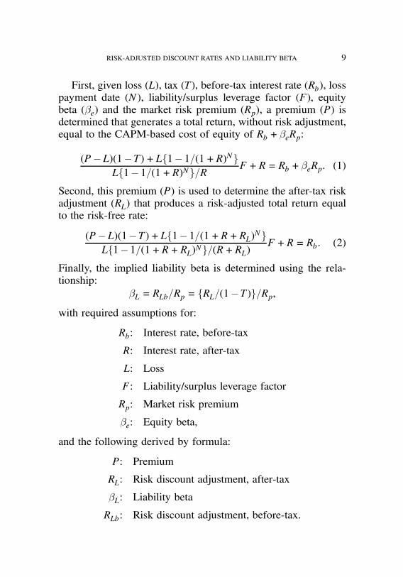
FIGURE 1
Baseline Risk/Return Line vs. Leverage
Average loss payout=3 yearsEquity beta=1.0Investment yield before-tax=6%Market risk premium=7%
Note: Each line will produce a 13% total return when the actual leverage is the sameas the base leverage was when the equity beta was determined to be 1.0.
Formula (1) expresses the sum of after-tax underwriting in-come and the present value of investment income on loss re-serves, in ratio to the present value of balance sheet loss reserveliabilities. This is the operating return, and it is multiplied byleverage and the investment return on surplus is added to producethe total return. Formula (2) differs only by the introduction ofthe risk discount adjustment. These formulas are simplified dueto the assumptions that premium is collected at policy inception,expenses are zero, there is no delay in tax payments, and thatlosses are paid in a single payment. Formulas (1) and (2) arereviewed in more detail in the Appendix.
These basic relationships were used to produce Figures 1–7, which demonstrate various relationships among the variables.Figure 1 establishes a base point of reference by demonstrat-

job no. 1969 casualty actuarial society CAS journal 1969D03 [11] 11-08-01 4:58 pm
RISK-ADJUSTED DISCOUNT RATES AND LIABILITY BETA 11
ing the relationship between leverage and return at three givenleverage levels. In practice, the measured equity beta and CAPMtarget cost of capital are at some “typical” leverage. If leveragewere to be higher, then the required return would be higher, andif leverage were to be lower, then the required return would belower. Presumably this would affect measured equity betas. Thisinterplay between leverage, return and risk should be consideredwhen solving for the target premium.
The actual leverage level is an extremely important, yet oftenoverlooked aspect of risk and return. Leverage simultaneouslyand similarly affects both return and risk, as measured by thevariability in return. All else being equal, higher leverage shouldproduce greater returns (i.e., higher cost of capital) and greatervariability in returns. Although one might expect higher betasto be produced when leverage is higher, this aspect is seldomconsidered when they are calculated and published. Given thesignificant impact of leverage, and since industry leverage hasbeen declining steadily over the past several years, three specificvalues were selected to represent this range and to reflect thisdynamic in the following discussion. The fact that insurance in-dustry equity betas today are around 1.0 is consistent with theeffect that large amounts of surplus and low leverage have in sup-pressing variability in return, and in making insurer returns alignmore closely to overall market returns. Both the cost of capitaland equity beta are expected to flex with leverage changes overtime.
Three base leverage levels (2.0, 3.0 and 4.0) have been as-sumed. These represent three possible levels of leverage in exis-tence at the point in time when the equity beta was determinedto be 1.0. Actual leverage may subsequently vary from these re-spective base points as shown by the three lines on the chart.Each of the lines, however, must produce a total return of 13%when the actual leverage matches the base level correspondingto the original calculation of the equity beta. This is the CAPMframework in which the cost of capital (13%) is equal to the

job no. 1969 casualty actuarial society CAS journal 1969D03 [12] 11-08-01 4:58 pm
12 RISK-ADJUSTED DISCOUNT RATES AND LIABILITY BETA
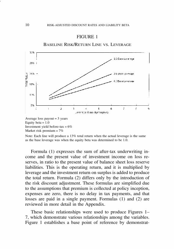
FIGURE 2
Equity vs. Liability Beta
Average loss payout=3 yearsInvestment yield before-tax=6%Market risk premium=7%
risk-free rate (6%) plus the market risk premium (7%) times theequity beta (1.0). These lines are used in the analysis to adjustthe total return target up or down if actual leverage increases ordecreases from the respective base.
5. LIABILITY BETA
Following the steps discussed above, the liability betas deter-mined by formula are shown in Figure 2 in relationship to equitybetas. The example shown is for a three-year loss payout, 7%market risk premium, and 6% risk-free yield. The liability beta isnegative in all cases. The magnitude shown here is substantiallymore negative than most of the literature has indicated. This islikely due to the fact that more sources of risk (i.e., variability)exist than may have been recognized by previous measures thathave assumed that losses alone are risky. This narrow assumptionexcludes sources of risk from the variability in the timing of loss
job no. 1969 casualty actuarial society CAS journal 1969D03 [13] 11-08-01 4:58 pm
RISK-ADJUSTED DISCOUNT RATES AND LIABILITY BETA 13
payout and the variability in the amount and timing of all othercash flows, including premium, expense, tax and investment.
One would hope that liability betas would be estimable withina more narrow range than that shown in Figure 2. Since totalreturns are affected by leverage, it would seem logical to ex-pect that equity betas would flex to some degree as leveragechanged, whereas liability betas should be relatively unaffectedand more stable. Increasingly more negative liability betas oc-cur when moving from the upper, higher leverage line to thelower, less leveraged line in Figure 2. More negative betas arewhat should be expected given the historical trends in declin-ing industry leverage and the likely delay in market response inforcing equity betas down proportionally in line with this.
The fact that the liability beta must be negative is intuitivelyobvious. Suppose that a $1,000 loss payable in one year is tobe reinsured (100%), with risk-free rates at 6%. If the amountand timing are both absolutely certain, it should be possible tofind a reinsurer who would agree to assume the loss obligationfor a premium of $962 ($1,000/1.039). If, on the other hand,losses are uncertain, the additional risk transfer that occurs fromthe insurer to the reinsurer requires that the reinsurer receiveadditional compensation. The reinsurer will require a premiumgreater than $962. In other words, the risk-adjusted discount ratemust be less than the risk-free rate, and liability beta must benegative.
The degree to which the risk-adjusted discount rate must beless than the risk-free rate is shown in Figure 3, for the sameexample, and also in relation to the equity beta.
Although low leverage would not generally be associated witha large equity beta, this extreme (lower right, bottom line in Fig-ure 3) would result in a negative risk-adjusted discount rate. Inother words, the discounted liability would be greater than thenominal liability. A sufficiently large surplus base, without cor-responding reductions in the equity beta and the cost of capital,

job no. 1969 casualty actuarial society CAS journal 1969D03 [14] 11-08-01 4:58 pm
14 RISK-ADJUSTED DISCOUNT RATES AND LIABILITY BETA
FIGURE 3
Equity Beta vs. Risk-Adjusted Discount Rate(After-Tax)
Average loss payout=3 yearsInvestment yield before-tax=6%Market risk premium=7%
impose an unrealistic burden on insurance pricing. This is thetrue essence of “surplus-surplus” as discussed at times in theratemaking context. This will be explored further below withrespect to the underwriting profit margin.
6. UNDERWRITING PROFIT MARGIN
The ultimate goal in ratemaking is to determine the premium,given assumptions on all costs and financial conditions, that insome way is “fair” to policyholders and owners of the companyalike. Figures 4–7 present the premium rate as an underwritingprofit margin as a function of loss payout, investment yield, mar-ket risk premium, and leverage, respectively.
In each of the examples, the base leverage cases (2.0, 3.0and 4.0) require liability betas of approximately !0:8, !0:5, and!0:4, respectively. Underwriting profit margins typically become

job no. 1969 casualty actuarial society CAS journal 1969D03 [15] 11-08-01 4:58 pm
RISK-ADJUSTED DISCOUNT RATES AND LIABILITY BETA 15
FIGURE 4
Underwriting Profit Margin vs. Loss Payout
Investment yield before-tax=6%Market risk premium=7%Equity beta=1.0
more negative (i.e., higher combined ratios) when loss payoutslengthen as shown in Figure 4, due to the greater investment in-come that will be generated prior to loss payment. This is shownin the lower two lines on the chart. However, as noted above,when leverage levels become so low as to create burdensomeamounts of surplus, the opposite can happen if cost of capitaland equity betas are not adjusted. This is the case in the upperline in Figure 4, in which the cost of equity and the equity betahave not been altered to reflect the lesser risk implied by thelower leverage. If the equity beta were to decline to at least 0.8(and the capital target return decline to 11.6% from 13.0%) inthis example, this effect would be avoided, with the resultingexpected downward sloping line.
As investment yields increase, underwriting profit margins de-teriorate as shown in Figure 5. While this sounds a bit like cashflow underwriting, if premium rates are to fully reflect the ben-
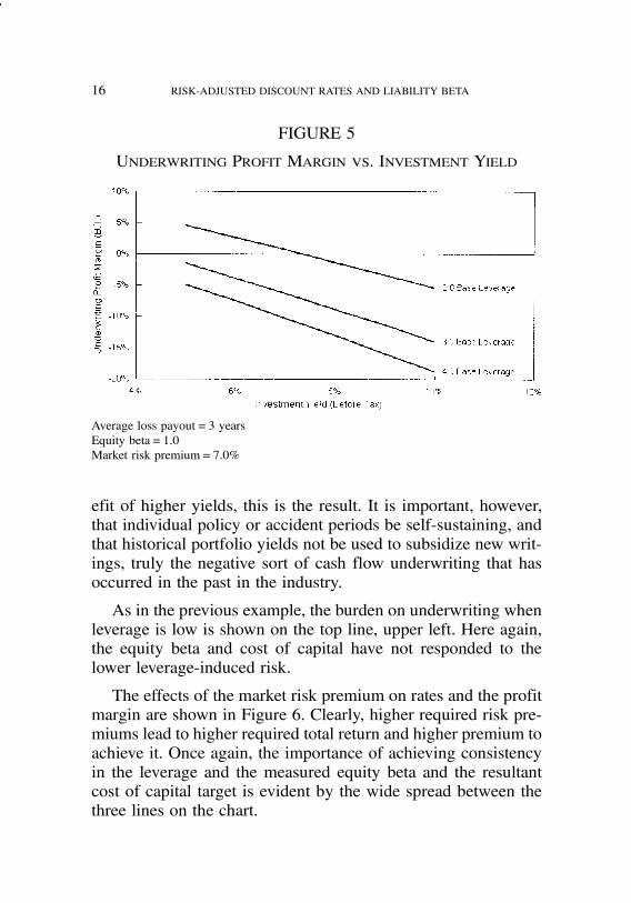
job no. 1969 casualty actuarial society CAS journal 1969D03 [16] 11-08-01 4:58 pm
16 RISK-ADJUSTED DISCOUNT RATES AND LIABILITY BETA
FIGURE 5
Underwriting Profit Margin vs. Investment Yield
Average loss payout=3 yearsEquity beta=1.0Market risk premium=7.0%
efit of higher yields, this is the result. It is important, however,that individual policy or accident periods be self-sustaining, andthat historical portfolio yields not be used to subsidize new writ-ings, truly the negative sort of cash flow underwriting that hasoccurred in the past in the industry.
As in the previous example, the burden on underwriting whenleverage is low is shown on the top line, upper left. Here again,the equity beta and cost of capital have not responded to thelower leverage-induced risk.
The effects of the market risk premium on rates and the profitmargin are shown in Figure 6. Clearly, higher required risk pre-miums lead to higher required total return and higher premium toachieve it. Once again, the importance of achieving consistencyin the leverage and the measured equity beta and the resultantcost of capital target is evident by the wide spread between thethree lines on the chart.

job no. 1969 casualty actuarial society CAS journal 1969D03 [17] 11-08-01 4:58 pm
RISK-ADJUSTED DISCOUNT RATES AND LIABILITY BETA 17
FIGURE 6
Underwriting Profit Margin vs. Market Risk Premium
Average loss payout=3 yearsEquity beta=1.0Investment yield before-tax=6%
The relationship between leverage and the profit margin isshown in Figure 7. Note the severe impact caused when lever-age is very low. If target returns are to be achieved when leveragedeclines to very low levels, significant increases in premium arerequired. Once again one has to question at what point surpluslevels become “excessive” in relation to current writings, andwhether it is reasonable to require target rates of return on thefull amount of surplus beyond this point. Perhaps the current lowlevels of industry leverage are now creating just such a dilemmain which it is becoming increasingly difficult to generate ade-quate returns on the entire amount of surplus available.
7. CONCLUSION
This paper has presented a methodology for the direct de-termination of risk-adjusted discount rates and liability betas.It involves the utilization of a “complete” total rate of return

job no. 1969 casualty actuarial society CAS journal 1969D03 [18] 11-08-01 4:58 pm
18 RISK-ADJUSTED DISCOUNT RATES AND LIABILITY BETA
FIGURE 7
Underwriting Profit Margin vs. Leverage
Average loss payout=3 yearsEquity beta=1.0Investment yield before-tax=6%Market risk premium=7%
model (albeit in simplified form) in which rates of return canbe determined both with and without risk adjustment. The to-tal return without risk adjustment must equal the target cost-of-capital-based return. The total return with risk adjustment mustequal the risk-free rate. Within this formulation it is importantthat taxes be reflected by utilizing discount rates on an after-taxbasis.
This formulation provides the capability to directly determinethe required risk-adjusted discount rate and liability beta, givenstandard underwriting financials, leverage factor, market risk pre-mium and equity beta. The risk-adjusted discount rates that resultare less than the risk-free rate and the liability betas are negative,

job no. 1969 casualty actuarial society CAS journal 1969D03 [19] 11-08-01 4:58 pm
RISK-ADJUSTED DISCOUNT RATES AND LIABILITY BETA 19
to a much greater degree than are often suggested. In no instanceare they positive.
The important influence of leverage, and the need for con-sistency with the cost of capital and equity beta measurements,are noted. Subsequent changes in leverage require adjustment tothese critical CAPM parameters. While the estimation and ap-plication of equity beta and the cost of capital are not withoutdebate, at least there is a wide body of comparative data avail-able to help judge the reasonableness of the results. This is notthe case with respect to liability beta.
Hopefully, in the future the conceptual dialogue over risk ad-justment and liability betas can be made more meaningful bycombining clearly specified parameter assumptions into a con-crete total return model framework, such as has been presentedin this paper.

job no. 1969 casualty actuarial society CAS journal 1969D03 [20] 11-08-01 4:58 pm
20 RISK-ADJUSTED DISCOUNT RATES AND LIABILITY BETA
REFERENCES
[1] Bingham, Russell E., “Surplus—Concepts, Measures of Re-turn, and Determination,” PCAS LXXX, 1993, pp. 55–109.
[2] Bingham, Russell E., “Rate of Return—Policyholder, Com-pany, and Shareholder Perspectives,” PCAS LXXX, 1993,pp. 110–147.
[3] Bingham, Russell E., “Cash Flow Models in Ratemaking:A Reformulation of Myers–Cohn NPV and IRR Modelsfor Equivalency,” Actuarial Considerations Regarding Riskand Return in Property-Casualty Insurance Pricing, ChapterIV, Casualty Actuarial Society, 1999, pp. 27–60.
[4] Butsic, Robert P., “Determining the Proper Interest Ratefor Loss Reserve Discounting: An Economic Approach,”Evaluating Insurance Company Liabilities, Casualty Actu-arial Society Discussion Paper Program, May 1988, pp.147–188.
[5] Copeland, Tom, Tim Koller, and Jack Murrin, Valuation—Measuring and Managing the Value of Companies II, JohnWiley & Sons, Inc., 1994.
[6] Cummins, J. David, and Scott E. Harrington, “Property-Liability Insurance Rate Regulation: Estimation of Under-writing Betas Using Quarterly Profit Data,” Journal of Riskand Insurance, March 1985.
[7] Cummins, J. David, “Multi-Period Discounted Cash FlowModels in Property-Liability Insurance,” Journal of Riskand Insurance, March 1990.
[8] D’Arcy, Stephen P. and Michael A. Dyer, “Ratemaking:A Financial Economics Approach,” PCAS LXXXIV, 1997,pp. 301–390.
[9] Fairley, William, “Investment Income and Profit Mar-gins in Property-Liability Insurance: Theory and Empiri-cal Results,” The Bell Journal of Economics, Spring 1979,reprinted in J. David Cummins and Scott E. Harrington(eds.), Fair Rate of Return in Property-Liability Insurance,Kluwer-Nijhoff, 1987.

job no. 1969 casualty actuarial society CAS journal 1969D03 [21] 11-08-01 4:58 pm
RISK-ADJUSTED DISCOUNT RATES AND LIABILITY BETA 21
[10] Kozik, Thomas J., “Underwriting Betas—The Shadows ofGhosts,” PCAS LXXXI, 1994, pp. 303–329.
[11] Myers, Stewart C. and Richard A. Cohn, “A DiscountedCash Flow Approach to Property-Liability Insurance RateRegulation,” J. David Cummins and Scott E. Harrington(eds.), Fair Rate of Return in Property-Liability Insurance,Kluwer-Nijhoff, 1987.

job no. 1969 casualty actuarial society CAS journal 1969D03 [22] 11-08-01 4:58 pm
22 RISK-ADJUSTED DISCOUNT RATES AND LIABILITY BETA
APPENDIX
The following example provides high-level balance sheet, in-come and cash flow statements. These are used to demonstratevarious rate of return calculations and to show the resultingequivalency between conventionally reported rates of return andnet present value rates of return, assuming certain rules are fol-lowed to control the flow of surplus and to distribute profits.The net present value rate of return is shown with and withoutrisk adjustment. Following this, the Myers–Cohn fair premiumapproach is briefly recapped, as modified to use after-tax dis-counting, shown in relation to this same example.
The following financial assumptions form the basis for theexample presented:
$ 103.85% combined ratio
$ $9,629 premium, collected without delay$ $10,000 loss, single payment at end of year 3$ $0 expense$ 35% income tax rate, no delay in payment
$ 6.0% investment interest rate before-tax, 3.9% after-tax
$ No loss discount tax$ 3.0 liability/surplus ratio.This example corresponds to the following:
$ 1.0 equity beta$ 7.0% market risk premium
$ 3.65% liability risk discount adjustment, before-tax
$ !0:521 liability beta.

job no. 1969 casualty actuarial society CAS journal 1969D03 [23] 11-08-01 4:58 pm
RISK-ADJUSTED DISCOUNT RATES AND LIABILITY BETA 23
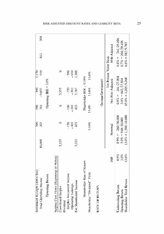
Simplified balance sheet, income and cash flow statements areshown for this example in Table A.1. The rules governing theflow of surplus are as follows: (1) the level of surplus is main-tained at a 1/3 ratio with loss reserves, (2) investment income onsurplus is paid to the shareholder as earned, and (3) operatingearnings are distributed in proportion to the level of insuranceexposures in each year, measured by loss reserve levels, relativeto the total exposure. Since loss reserves are equal at $10,000 ineach of the three years, operating earnings are distributed to theshareholder equally in each year.
Three “levels” of return exist within an insurance company.The first is the underwriting rate of return, which reflects whatthe company earns on pure underwriting cash flows, before re-flecting investment income on the float. This is a “cost of funds”to the company. The second, operating return, reflects what thecompany earns on underwriting when investment income onthe float is included. This is the “risk charge” to the policy-holder for the transfer of risk to the company. The third, thetotal return, is the net result of underwriting and investment in-come from operations together with investment income on sur-plus.
These rates of return can be determined by either a cash-flow-based internal rate of return (IRR) calculation or by relat-ing income earned to the amount invested. With regards to theshareholder total return perspective, the internal rate of return(IRR) based on cash flows from and to the shareholder indicatesa 13.0% return over the three-year period. The income versusinvestment approach (i.e., ROE) relates the income over the fullthree-year aggregate financial life of the business to the share-holder’s investment over this same period. This is shown in bothnominal (i.e., undiscounted) and in present value (discounted,but without risk adjustment) dollars to produce a 13.0% rateof return on investment. Furthermore, the return realized by theshareholder via dividends is also an identical 13.0% in each year.(This attribute follows from the rules used to control the flow of

job no. 1969 casualty actuarial society CAS journal 1969D03 [24] 11-08-01 4:58 pm
24 RISK-ADJUSTED DISCOUNT RATES AND LIABILITY BETA
job no. 1969 casualty actuarial society CAS journal 1969D03 [25] 11-08-01 4:58 pm
RISK-ADJUSTED DISCOUNT RATES AND LIABILITY BETA 25
job no. 1969 casualty actuarial society CAS journal 1969D03 [26] 11-08-01 4:58 pm
26 RISK-ADJUSTED DISCOUNT RATES AND LIABILITY BETA
surplus.) When risk-adjusted, the total net present valued rate ofreturn is 6.0%, which is identical to the risk-free rate.
The operating return, inclusive of underwriting and invest-ment income, is shown to generate a cash-flow-based internalrate of return of 3.0%. Equivalently, the operating income of$910 is a 3.0% return on the “investment equivalent” of $30,000,the total balance sheet policyholder supplied float upon whichthese earnings were generated. Also, $843 of present valued in-come is 3.0% on the present valued liability of $27,804.
The formulas that can be used to directly determine the netpresent value based rates of return, both without and with riskadjustment, are shown in Tables A.2 and A.3, respectively. Thefollowing variables are used in Tables A.2 through A.4:
P: Premium
Rb: Interest rate, before-tax
L: Loss
R: Interest rate, after-tax
N: Loss payment date
RL: Risk discount adjustment, after-tax
T: Tax rate
UWPT: Underwriting profit tax
NT: Underwriting tax payment delay
IBT: Investable balance investment income tax
F: Liability/surplus leverage factor
S: Initial surplus contribution (L=F):
Myers–Cohn Fair Premium With After-Tax Discounting
The $9,629 premium shown in the example can be derivedusing the traditional Myers–Cohn (MC) format, as long as all

job no. 1969 casualty actuarial society CAS journal 1969D03 [27] 11-08-01 4:58 pm
RISK-ADJUSTED DISCOUNT RATES AND LIABILITY BETA 27
TABLE A.2
NET PRESENT VALUE INCOME, BALANCE SHEET AND RATE OFRETURN DEFINITIONS, FORMULAS AND CALCULATIONS
WITHOUT RISK ADJUSTMENT
INCOME ITEMS FORMULAS
Underwriting Income (P!L)(1!T)(9,629! 10,000)(1! 0:35) =!241
Operating Income PV(P)!PV(L)!PV(UWPT)=P!L=(1+R)N!T(P!L)9,629! 10,000=(1+0:039)3! (0:35)(9,629! 10,000)= (P!L)!T(P!L)=(1+R)NT +L[(1!1=(1+R)N ](9,629! 10,000)! (0:35)(9,629! 10,000)=(1+ :039)0+10,000[1!1=(1+0:039)2]Underwriting Income+ Investment Income Credit on Policyholder Liabilities! 241+1,084 = 843
Surplus Investment Income R (Surplus)(0:039)(9,268) = 361
Total Income =Operating Income+ Investment Income on Surplus843+361 = 1,205
BALANCE SHEET ITEMS
Policyholder Liabilities L(1! 1=(1+R)N )=R10,000(1! 1=(1+0:039)3)=0:039 = 27,804
Surplus S(1!1=(1+R)N )=R3,333(1! 1=(1+0:039)3)=0:039 = 9,268
RATES OF RETURN
Underwriting Return on Underwriting Income /Policyholder LiabilitiesLiabilities (Cost of !241=27,804 =!0:9%Policyholder-SuppliedFunds)
Operating Return on Operating Income /Policyholder LiabilitiesLiabilities (Risk Charge 843=27,804 = 3:0%to Policyholder)
Total Return on Surplus Total Income /Surplus(ROS) 1,205=9,268 = 13:0%(Shareholder Return)
= (Operating Return on Liabilities)(Liability/Surplus)+R3:0%(3)+3:9%= 13:0%

job no. 1969 casualty actuarial society CAS journal 1969D03 [28] 11-08-01 4:58 pm
28 RISK-ADJUSTED DISCOUNT RATES AND LIABILITY BETA
TABLE A.3
NET PRESENT VALUE INCOME, BALANCE SHEET AND RATE OFRETURN DEFINITIONS, FORMULAS AND CALCULATIONS WITH
RISK ADJUSTMENT
INCOME ITEMS FORMULAS
Underwriting Income (P!L)(1!T)(9,629! 10,000)(1! 0:35) =!241
Operating Income PV(P)!PV(L)!PV(UWPT) = P!L=(1+R!RL)N!T(P!L)9,629! 10,000=(1+0:039! 0:024)3 ! (0:35)(9,629! 10,000)= (P!L)!T(P!L)=(1+R)NT +L[(1!1=(1+R!RL)N ](9,629! 10,000)! (0:35)(9,629! 10,000)=(1+0:039)0+10,000[1! 1=(1+0:039! 0:024)3]= Underwriting Income+ Investment IncomeCredit on Policyholder Liabilities!241+445 = 204
Surplus Investment Income R (Surplus)(0:039)(9,702) = 378
Total Income Operating Income+ Investment Income on Surplus204+378 = 582
BALANCE SHEET ITEMS
Policyholder Liabilities L(1! 1=(1+R!RL)N )=(R!RL)10,000(1! 1=(1+0:039! 0:024)3)=(0:039!0:024) =29,106
Surplus S(1!1=(1+R!RL)N )=(R!RL)3,333(1! 1=(1+0:039!0:024)3)=(0:039!0:024) =9,702
RATES OF RETURN
Underwriting Return on Underwriting Income /Policyholder LiabilitiesLiabilities (Cost of !241=29,106 =!0:8%Policyholder Supplied Funds)
Operating Return on Operating Income /Policyholder LiabilitiesLiabilities (Risk Charge 204=29,106 = 0:7%to Policyholder)
Total Return on Surplus Total Income /Surplus(ROS) 582=9,702 = 6:0%(Shareholder Return)
= (Operating Return on Liabilities)(Liability/Surplus)+R0:7%(3)+3:9%= 6:0%
job no. 1969 casualty actuarial society CAS journal 1969D03 [29] 11-08-01 4:58 pm
RISK-ADJUSTED DISCOUNT RATES AND LIABILITY BETA 29
discounting is on an after-tax basis, and given a liability beta thatis “consistent” with the equity beta. The traditional MC modelformat as shown in [1] is as follows:
P = PV(L)+PV(UWPT)+PV(IBT):
This states that the fair premium (P) is equal to the sum of thepresent value of the losses (L), the tax on underwriting profit(UWPT), and the tax on investment income derived from the in-vestable balance (IBT). The investable balance includes all pol-icyholder liabilities (net of premium, loss and expense) and sur-plus. Note that underwriting expense is combined with loss astotal liabilities in the example in the cited reference. It is sug-gested that the discount rates be adjusted for risk (i.e., uncer-tainty), particularly the rate applicable to losses. No mention ismade as to whether discount rates are on a before-tax or after-taxbasis.
The present example differs from the model in [1] to somedegree, first by extending from one to three periods, and thenby assuming that taxes on underwriting and investment are paidwithout delay. In [1] underwriting taxes were assumed to havea one year delay in their payment. The tax loss discount (TRA86) was excluded for simplification in both instances. In [1] Swas set equal to P for the single period example presented. Inthe present example, surplus was set at each point in time to anamount equal to L=F, where F is the liability/surplus leveragefactor. Since surplus is set as a function of liabilities, surplus isimplicitly risk-adjusted as well.
Table A.4 presents the derivation of the “fair” premium thatresults when the Myers–Cohn approach is reformulated to useafter-tax discounting and to control surplus via a linkage to liabil-ities over the multi-period timeframe. In this example the interestrate is 6%, the tax rate is 35%, and a risk adjustment of 3.65%before-tax (i.e., 2.4% after-tax) is made when discounting. Thisis the risk adjustment that results from a liability beta of !0:521.A liability/surplus ratio of 3-to-1 is used to determine the level
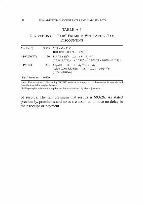
job no. 1969 casualty actuarial society CAS journal 1969D03 [30] 11-08-01 4:58 pm
30 RISK-ADJUSTED DISCOUNT RATES AND LIABILITY BETA
TABLE A.4
DERIVATION OF “FAIR” PREMIUM WITH AFTER-TAXDISCOUNTING
P = PV(L) 9,555 L=(1+R!RL)N10,000=(1+0:039! 0:024)3
+PV(UWPT) !130 T[P=(1+R)NT !L=(1+R!RL)NT ](0:35)[(9,629)=(1+0:039)0 !10,000=(1+0:039! 0:024)0]
+PV(IBT) 204 TRbS[(1! 1=(1+R!RL)N )=(R!RL)](0:35)(0:06)(3,333)[(1! 1=(1+0:039!0:024)3)=(0:039! 0:024)]
“Fair” Premium 9,629
Notes: Due to after-tax discounting PV(IBT) reduces to simply tax on investment income derivedfrom the investable surplus balance.Liability/surplus relationship implies surplus level affected by risk adjustment.
of surplus. The fair premium that results is $9,626. As statedpreviously, premiums and taxes are assumed to have no delay intheir receipt or payment.
job no. 1969 casualty actuarial society CAS journal 1969D02 [1] 11-08-01 4:58 pm
RISK AND RETURN: UNDERWRITING, INVESTMENTAND LEVERAGE
PROBABILITY OF SURPLUS DRAWDOWN AND PRICINGFOR UNDERWRITING AND INVESTMENT RISK
RUSSELL E. BINGHAM
Abstract
The basic components of the risk/return model appli-cable to insurance consist of underwriting return, invest-ment return and leverage. A pricing approach is pre-sented to deal with underwriting and investment risk,guided by basic risk/return principles, which addressesthe policyholder and shareholder perspectives in a con-sistent manner. A methodology to determine leverageis also presented, but as a distinct and separate ele-ment, enabling the pricing approach to be applied eitherwith or without allocation of surplus to lines of busi-ness. Since the leverage is also developed within a totalrisk/return framework, the approach provides a meansto integrate what are often disjointed rate and solvencyregulatory activities.Risk is controlled by a focus on the likelihood that
total return falls short of the target “fair” return by anamount which results in a specified drawdown of sur-plus. Thus rate adequacy and solvency are dealt with si-multaneously. A shift away from probability of ruin andexpected policyholder deficit approaches to solvency andratings is proposed and explained.An “Operating Rate of Return” is defined and sug-
gested as the appropriate rate of return measure thatshould be used for measuring the charge for risk transferfrom the policyholder to the company, rather than othermeasures such as profit margin, return on premium, etc.
31

job no. 1969 casualty actuarial society CAS journal 1969D02 [2] 11-08-01 4:58 pm
32 RISK AND RETURN: UNDERWRITING, INVESTMENT AND LEVERAGE
1. SUMMARY
Rate of return and risk in return represent the dimensions ofexpectation and uncertainty, respectively. The tradeoffs betweenthem are real and faced by individuals and businesses frequently.The decision to invest involves a choice among alternatives hav-ing anticipated variation in both return and risk. Being generallyaverse to risk, individuals and businesses choose the least riskyinvestment for a given level of anticipated return, or require agreater return when investments are riskier. The investor per-spective with respect to risk tends to be one of concern with thedegree to which returns might depart (or vary) from the expectedlevel.
The policyholder perspective, as represented by regulators andrating agencies, is typically more concerned with the dimensionof risk having to do with the occurrence of extreme and adverseevents, and whether the level of capital available is adequategiven the probability and magnitude of such events occurring.However, the risk transfer that occurs from the policyholder tothe company is governed by much the same risk/return principlesas those that govern the relationship between the company andthe shareholder. When viewed within the risk/return context, thelinkage between the policyholder and shareholder perspectivesbecomes clear, and the means for determining both fair premiumsto the policyholder and fair returns to the shareholder is provided.
In employing its equity and setting prices, insurance companymanagement is making an investment choice among alternativelines of business and investment asset classes based on knowl-edge of expected returns coincident with the risks associated withthose choices. These risks reflect both the shareholder and pol-icyholder perspectives. The assessment of the tradeoff betweenthese risks and returns and the level of surplus either required oravailable, is guided by the company’s desire to achieve a reason-ably balanced portfolio of businesses with a controlled risk/returnprofile for the company in aggregate.

job no. 1969 casualty actuarial society CAS journal 1969D02 [3] 11-08-01 4:58 pm
RISK AND RETURN: UNDERWRITING, INVESTMENT AND LEVERAGE 33
This paper will explain the basic components of the risk/return model applicable to insurance, as comprised of under-writing return, investment return and insurance leverage. It willdiscuss a pricing approach to deal with underwriting and invest-ment risk (i.e., variability) that addresses the concerns of boththe policyholders and the shareholders. A risk charge is shownas a function of underwriting and investment risk, and the sen-sitivity of price changes to them is demonstrated. Operating re-turn (i.e., return on underwriting and investment of policyholderfunds) coupled with the specification of “probability of surplusdrawdown” (PSD) is a focal point in this approach.
The PSD is a fundamental aspect of the risk/return relation-ship that is applicable to both the policyholder and the share-holder. Although consistent with the probability of ruin and ex-pected policyholder deficit concepts, it differs in that its focus ismore on the degree to which returns depart from expected levels,rather than simply on the extreme adverse outcomes.
The “operating return–probability of drawdown” method pre-sented in this paper is suggested as a replacement for the returnon premium concept by an operating return measure which ex-tends shareholder risk/return principles to the policyholder level.As a consequence, the method demonstrates how risk can be re-flected in the pricing mechanism without varying the allocationof surplus to individual lines of business, through the focus onoperating return. The result is a unified and consistent frame-work for establishing fair returns that reflects the transfer of riskfrom the policyholder to the company and from the company tothe shareholder.
Importantly, issues of leverage and surplus allocation are re-moved from the pricing process. The need for surplus is viewedprimarily as an overall company issue with respect to financialstrength and ratings. The result is a mechanism for establishingprices which recognizes the policyholder and shareholder per-spectives centered around their respective risk/return tradeoffs,without requiring that surplus be allocated to lines of business.

job no. 1969 casualty actuarial society CAS journal 1969D02 [4] 11-08-01 4:58 pm
34 RISK AND RETURN: UNDERWRITING, INVESTMENT AND LEVERAGE
Varying leverage ratios by line of business is shown to be anoptional risk adjustment step that translates rates of return to acommon level, such as a specified cost of capital.
With respect to style and focus, this paper will avoid anoverly-detailed and mathematically-oriented presentation in fa-vor of simpler demonstrations focused on the most basic of prin-ciples. These principles are essentially:
1. Functionally and mathematically, insurance is composedof underwriting, investment and leverage.
2. Interactions among the policyholder, company and share-holder are governed by the fundamental risk/return rela-tionship, in which higher risk requires higher return andvice versa.
3. The transfer of risk either from the insured to the com-pany or from the company to the shareholder are bothessentially investment-like decisions, which involve acharge for this transfer to occur. In the policyholder case,this results in a premium payment to the company; in thecase of the company, this results in an expected “pay-ment” to the shareholder via dividends or stock priceappreciation (i.e., the cost of capital).
4. The amount and timing of policyholder-related liabilitiesand cash flows that will eventually be paid are uncertain.The price for the transfer of this underwriting risk fromthe policyholder to the company must be incorporatedinto the premium charged when insurance is sold.
These fundamental principles apply broadly to all ratemakingmodels. Unfortunately, unnecessary confusion exists with respectto the many ratemaking models presented in the literature, fortwo basic reasons. First, because the relevance of these basicrisk/return principles may not be recognized in each of the mod-els, the assumptions and parameters used in them are determinedin various ways, causing their output to diverge substantially.
job no. 1969 casualty actuarial society CAS journal 1969D02 [5] 11-08-01 4:58 pm
RISK AND RETURN: UNDERWRITING, INVESTMENT AND LEVERAGE 35
Second, because many of the models differ in constructionand output, comparisons to one another are made difficult. Itis important to note that the many ratemaking models (such asunderwriting profit margin, target total rate of return, insurancecapital asset pricing model, discounted cash flow, Myers–Cohn,and internal rate of return, etc.) are all essentially equivalent. Asingle well-constructed total return model, supported by the fullcomplement of balance sheet, income and cash flow statements,and further valued both nominally and on a discounted basis,encompasses them all and will produce identical results when thesame input assumptions are used (as discussed in the material inthe References).
2. BACKGROUND
2.1. Rate of Return
Rate of return (often referred to more simply as return) reflectsthe amount of income produced on an investment in relation tothe investment itself. This ratio is usually expressed as an an-nual rate, although the investment period may be more or lessthan one year. Insurance decisions to invest in underwriting op-erations, in particular, usually involve a multi-year commitment(e.g., losses may take many years to settle) and the rate of returnthat results must reflect this timeframe as well. This is much likean investment with a holding period of several years, whereinboth the level of investment and return might vary over time,requiring that some form of composite annual percentage rate ofreturn (APR) be calculated.
Insurance companies deploy (i.e., invest) their surplus in ei-ther of two essential operating activities—underwriting or invest-ing. Each of these activities carries with it an anticipated rate ofreturn. The amount of insurance written on the one hand andthe amount of surplus/capital provided from financing activitieson the other, result in an operating leverage that magnifies theunderwriting and investment returns in relation to surplus. The

job no. 1969 casualty actuarial society CAS journal 1969D02 [6] 11-08-01 4:58 pm
36 RISK AND RETURN: UNDERWRITING, INVESTMENT AND LEVERAGE
following expression provides a simple yet accurate representa-tion of the way that underwriting and investment return, in con-junction with their respective leverage, contribute to total return:
R = (Ru)(L=S)+ (Ri)(L=S+1): (1)
Total return on surplus (R) is the sum of the respective prod-ucts of return and leverage from underwriting and investment.The return on underwriting (Ru) measures the profitability fromunderwriting operations (absent investment income). The returnon underwriting can be measured in various ways, dependingon whether the view is historical or prospective, or whether it isrelative to calendar or ultimate accident year. The return on in-vestment (Ri) is essentially a yield on total invested assets, whichinclude assets generated from both underwriting liability “float”and surplus.
Each of these returns is magnified by the leverage employedby the company. The underwriting leverage (L=S) is the net liabil-ity to surplus ratio. Liabilities consist primarily of loss reserves,but other liabilities must be considered, such as premiums receiv-able (a negative liability), reinsurance balances payable, taxes,etc. Since invested assets (I) are equal to net liabilities (L) plussurplus (S), L=S+1 in the above expression is equivalent to theratio of invested assets to surplus, or investment leverage. Viewedin this way, the total return is seen to be dependent simply on un-derwriting return, investment return, and insurance leverage. (It isnoted that statutory surplus and GAAP equity differ in their def-initions. For purposes of risk transfer pricing and in the contextof this paper, surplus is better thought of as a required risk-based“benchmark” amount. This is discussed in [3].)
Underwriting income (after-tax) is expressed as a rate of re-turn (Ru) and can be determined in either of two ways. The firstis to use a common finance tool, the internal rate of return (IRR),which is based on the underwriting cash flows that evolve overtime. The second is to relate underwriting income to the balancesheet investment that is derived from the same insurance liabilities
job no. 1969 casualty actuarial society CAS journal 1969D02 [7] 11-08-01 4:58 pm
RISK AND RETURN: UNDERWRITING, INVESTMENT AND LEVERAGE 37
that produce the underwriting income. This is approximately theratio of after-tax underwriting income to underwriting float (i.e.,primarily loss reserves). Both of these alternatives are demon-strated by way of example in the Appendix, and are discussedin detail in the reference material.
Underwriting return, Ru, is not the same as return on pre-mium. While return on premium may be a useful statistic, aratio to sales does not capture the dynamics as fully as a returnon funds invested statistic does, when the magnitude and timeperiods of the investment differ widely. Returns on premium arenot comparable between short- and long-tailed lines of business,since the magnitude and time commitment of supporting policy-holder funds are dramatically different. The underwriting rate ofreturn (Ru) fully reflects this dimension and presents a statisticthat is comparable across lines of business.
Investment return is dependent on returns (yields on fixedincome investments, stock market dividends and capital gains,etc.) available in financial markets, together with the selection ofvarious asset classes in which investments are made. In the caseof fixed income investments, investment return is also affectedby the maturity selected (which entails added interest rate riskas well).
Options exist within both underwriting and investment to se-lect lines of business and/or investments that entail varying re-turns and associated risks. The above formula (1) refers to asingle underwriting return and a single investment return when,in reality, there are numerous options within each of them.
2.2. Risk in Return
Risk is a measure of the uncertainty of achieving expectedreturns (which encompasses the possibility of a complete loss ofthe investment itself). The most common measure of risk is thestandard deviation statistic, which provides a means of quantify-ing the degree of likely variation of actual return relative to the

job no. 1969 casualty actuarial society CAS journal 1969D02 [8] 11-08-01 4:58 pm
38 RISK AND RETURN: UNDERWRITING, INVESTMENT AND LEVERAGE
return expected. The larger the standard deviation, the greaterthe chance that the actual return will deviate from the expectedreturn (either above or below it).
Underwriting and investment returns both involve a degree ofuncertainty (i.e., volatility). The expression below reflects howthe standard deviation in total return (¾R) is affected by the stan-dard deviation in underwriting return (¾Ru) and the standard de-viation in investment return (¾Ri). This formula makes use ofthe square of the standard deviation (known as the variance) forsimplicity:
¾2R = ¾2Ru(L=S)
2 +¾2Ri(L=S+1)2 +2r(L=S)(L=S+1)¾Ru¾Ri:
(2)
Leverage has a similar compounding effect on variability asit does on return. In addition, the interaction (i.e., correlation)between underwriting and investment is a critical component ofthe total risk, as captured by the last term in (2).
The correlation coefficient (r) measures the degree that under-writing and investment performance move in tandem with eachother. Underwriting and investment returns that move togetherin lock step in the same direction, both up or both down, willhave a perfect positive correlation (r =+1). Underwriting andinvestment returns that move in exact opposite directions, oneup and the other down, will have a perfect negative correlation(r =!1). When underwriting and investment returns are inde-pendent of one another, there is no correlation (r = 0). Thus,in terms of total variability, when underwriting and investmentmove together (positive correlation), risk is greater. Conversely,when underwriting and investment move opposite to one another(negative correlation), risk is less. The same principles apply at afiner level among the lines of business within underwriting andamong alternative investments.
In insurance circles, when the topic of a company’s surplusrequirements is discussed, the term covariance is often used. This

job no. 1969 casualty actuarial society CAS journal 1969D02 [9] 11-08-01 4:58 pm
RISK AND RETURN: UNDERWRITING, INVESTMENT AND LEVERAGE 39
is simply another term for describing the interaction among un-derwriting lines of business and investments, and the effect thismay have on the overall need for surplus and the risk to thecompany as described above (i.e., the benefit of diversification).
It is important to note that of the three basic factors affectingrisk and return, leverage stands alone in that it can be controlleddirectly by management; underwriting and investment, on theother hand, involve given levels of risk which are largely uncon-trollable. (This risk can be managed to some degree through di-versification.) The selected leverage at which a company choosesto operate has a significant influence on both the level and vari-ability of reported total returns, and is subject to practical regu-latory and rating agency constraints.
This process is more complex than can be reviewed here,especially if the correlations among many lines of business andalternative investments were to be considered simultaneously.
2.3. Leverage
The leverage employed by a company is subject to many con-straints, including ratings, cost of capital, and most importantlyin insurance, the probability of ruin. Insurance, unlike most otherbusinesses, involves selling a product whose costs can only be es-timated at the time the product is sold, and whose ultimate valuehas a significant potential to cause financial loss to an insurerwell in excess of premiums charged. Recognizing this financialexposure and the additional limits imposed on leverage by rat-ing agencies and financial markets, insurers have traditionallyconsidered the probability of ruin in determination of surplusrequirements. This concept results in the establishment of sur-plus levels in such a way as to keep to an acceptable minimumprobability the chance that surplus will be exhausted by unfa-vorable loss or other developments. More recently, the conceptof expected policyholder deficit (EPD) has been used to furtherquantify the amount of ruin.
job no. 1969 casualty actuarial society CAS journal 1969D02 [10] 11-08-01 4:58 pm
40 RISK AND RETURN: UNDERWRITING, INVESTMENT AND LEVERAGE
Leverage plays a direct role in the risk/return tradeoff as notedpreviously, since it simultaneously magnifies both return and riskas shown in formulas (1) and (2). To demonstrate this relation-ship, it is helpful to express formula (1) differently as follows:
R = Ri+(Ru+Ri)(L=S): (3)
This is the expression for a straight line, with an intercept of Ri(the return on investment) and a slope of (Ru+Ri). If no insur-ance were written (i.e., L=S = 0), the only return would be oninvestments, with a return equal to the average yield (Ri). As-suming a consistent level of profitability, as writings and leverageincrease, total return increases at a rate of (Ru+Ri). This termhas special meaning in that it represents the operating return frominsurance. Operating return reflects the income from underwrit-ing operations plus the investment income related to the assetsgenerated from underwriting operations (i.e., insurance liabilityfloat). It excludes income from investment of surplus, capturedin the above formula by the intercept Ri. The meaning and mea-surement of the underwriting, investment and operating returnsis discussed in the reference material and recapped briefly withan example in the Appendix.
Repeating the important point—leverage simultaneously af-fects both return (shown by formula 3) and variability in return(shown by formula 2). Apart from product or geographic diver-sification, returns cannot be increased by raising leverage with-out also increasing variability. Similarly variability cannot be re-duced without also reducing returns. Since insurance uncertaintycannot be eliminated, some combination of policyholder and/orshareholder pricing mechanisms is needed to deal with this risktransfer.
Predominant drivers of overall variability are: (1) variability inthe amount of liabilities, (2) variability in the timing of liabilitypayments, and (3) variability in interest rates. The greater thevariability in these three basic drivers, the greater the variabilityin return. While reinsurance and investment hedges can be used

job no. 1969 casualty actuarial society CAS journal 1969D02 [11] 11-08-01 4:58 pm
RISK AND RETURN: UNDERWRITING, INVESTMENT AND LEVERAGE 41
to reduce some of this variability, there will always be a degreeof variability remaining which cannot be eliminated, and thisshould be an important input into the pricing and leverage settingprocesses.
The following chart (Figure 1) presents key relationshipsamong balance sheet, income and cash flows and the risk transferactivities within the insurance firm. Within this structure the totalcompany is delineated into policyholder versus shareholder re-lated components. Note that the left side of the balance sheet con-sists of invested assets only. Non-invested assets are portrayedas a negative liability, and included within net liabilities on theright side of the balance sheet.
Several alternatives exist for setting leverage. As noted previ-ously, controlling the probability of ruin has been a traditionalapproach. More recently the expected policyholder deficit (EPD)has been developed. Controlling the variability in total return, ofmore interest to the shareholder, is another criterion that is oftenaddressed either by modifying the leverage ratio or by changingthe target rate of return.
2.4. The Probability of Ruin
The probability of ruin represents the likelihood that the com-bined effect of variability in liabilities and variability in the tim-ing of liability payments will cause surplus to be exhausted. Tokeep this probability to an acceptable minimum, surplus can beestablished at a level which is sufficient to cover the adverseconditions that can occur (e.g., losses larger than expected orpayable sooner than anticipated) all but, say, 1% of the time inan individual line of business.
Variability in the amount of loss and variability in the tim-ing of loss payments are most critical in terms of influencingthe leverage level and the variability in total return. Variabil-ity in loss has an even greater impact, due to a tendency to be
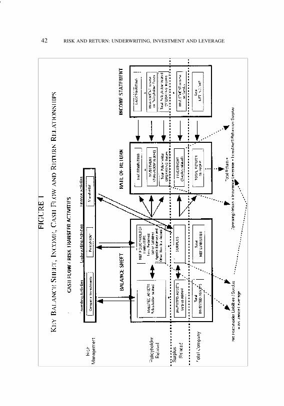
job no. 1969 casualty actuarial society CAS journal 1969D02 [12] 11-08-01 4:58 pm
42 RISK AND RETURN: UNDERWRITING, INVESTMENT AND LEVERAGE

job no. 1969 casualty actuarial society CAS journal 1969D02 [13] 11-08-01 4:58 pm
RISK AND RETURN: UNDERWRITING, INVESTMENT AND LEVERAGE 43
skewed, with the possibility of a very large loss (e.g., a natu-ral catastrophe). However, the probability of ruin approach hasshortcomings in that it does not typically reflect the impact oftaxes and other components of total net income, and may notconsider sources of variability other than from losses. A largeloss payable shortly after policy issuance is much more seriousthan is the same loss payable many years later, since, in the lattercase, substantial investment income is generated in the meantime.Also, the tax credit generated by losses reduces the out-of-pocketcost to the company. Variability in premium, expense and invest-ment are also potentially significant contributors to overall risk,which should be considered.
Furthermore, it should also be noted that control of probabilityof ruin does not result in a uniform variability in total return.Neither does it reflect the magnitude of policyholder deficit ifruin does occur. Note, for example, that a highly skewed lossdistribution may result in a greater policyholder shortfall thanwould a normal distribution, yet have the same probability ofruin.
2.5. Expected Policyholder Deficit (EPD)
EPD is a broader concept than is the probability of ruin, inthat it includes both the frequency and severity of extreme ad-verse consequence. Whereas the probability of ruin specifies thechance that company surplus may be exhausted, the EPD fur-ther estimates how much this amount is likely to be on average.Clearly policyholders and regulators are concerned with boththe probability and potential magnitude of loss, should surplusbe exhausted. While shareholders are concerned with the proba-bility of ruin, EPD is of little relevance since shareholder loss islimited to the amount of their investment.
The EPD concept has gained prominence in recent yearsand is being incorporated in some rating agency methodologies.However, this approach will have the same shortcomings as the

job no. 1969 casualty actuarial society CAS journal 1969D02 [14] 11-08-01 4:58 pm
44 RISK AND RETURN: UNDERWRITING, INVESTMENT AND LEVERAGE
probability of ruin, if it does not reflect the impact of taxes andother components of total net income.
Of more serious concern, however, is a basic principle ofstatistics and probability distributions that cautions against useof the “tail,” or low probability outcomes in frequency distri-butions. Most statistical methods rely on the “middle” of thedistribution, where the vast majority of the values occur. Theprobability of ruin and EPD approaches rely on the areas of thedata distribution having the least credibility and reliability. Whileof interest to policyholders, shareholders are instead concernedwith how returns might vary from that expected (that is, with themiddle of the distribution).
This shareholder perspective is one of risk versus return andis more appropriate within a context of risk transfer pricing. Theprobability of ruin and EPD, while important from a solvencystandpoint, are not as well-suited to this end.
2.6. Variability in Return
Shareholder investments reflect a tradeoff between the levelof return required and the uncertainty of such return. Sharehold-ers expect returns commensurate with uncertainty—if returns aremore variable, then investors will expect a higher absolute return,all else being equal. This in essence reflects the middle of thedistribution of returns about the expected value. In this regardthe shareholder perspective inherently embodies more statisticalcredibility.
Fortunately, the probability of ruin, EPD and variability inreturn viewpoints are connected. The concept of “probability ofsurplus drawdown” will be discussed in this regard.
2.7. Value at Risk and Probability of Surplus Drawdown (PSD)
The distribution of total return encompasses all financial com-ponents of an insurance company and the variability inherent in
job no. 1969 casualty actuarial society CAS journal 1969D02 [15] 11-08-01 4:58 pm
RISK AND RETURN: UNDERWRITING, INVESTMENT AND LEVERAGE 45
them. This is the distribution that is of concern to the share-holders, or investors, who provide capital to support the opera-tions of the company. In fact the traditional probability of ruinand EPD, when expanded to include all sources of underwrit-ing and investment income and taxes, are captured in the tailof this distribution. Ruin occurs when the total rate of returnis !100% or worse, with EPD being the average magnitude ofsuch events. Thus the first step in bridging the gap between thepolicyholder and shareholder measures is the conversion of ruinand EPD to a net income basis, and their expression as a rate ofreturn.
The second step is to view the distribution of returns asa continuum from the expected value downward to the ruinthreshold of !100% return. Economic surplus drawdown oc-curs along this continuum when total returns fall below the rateof return that could be achieved on alternative (typically risk-free) investments. Alternatively, this is equivalent to the point atwhich operating returns fall below 0% as shown in (3). Thisrate of return is most properly defined on an economic ba-sis to reflect the point at which investors lose money in eco-nomic terms. Thus the PSD represents the likelihood that aninvestor will experience an economic loss, when time valueis considered. This is a specific case within the more generalvalue at risk approach, which deals with a reduction in sur-plus of any specified amount (i.e., below zero) together withthe probability of its occurrence, rather than just simply thesingle threshold of 0% return at which surplus drawdown oc-curs.
It is important to note that the points of surplus drawdownand ruin, and their respective probabilities, both lie on the samedistribution. Actions which alter the return distribution will si-multaneously and similarly improve or worsen both the policy-holder and shareholder positions. This is shown more clearly byexamining the basic risk/return relationship.

job no. 1969 casualty actuarial society CAS journal 1969D02 [16] 11-08-01 4:58 pm
46 RISK AND RETURN: UNDERWRITING, INVESTMENT AND LEVERAGE
2.8. The Basic Risk/Return Tradeoff
The basic risk/return relationship is shown schematically inFigure 2. As variability in return increases along the x-axis, thereturn required to compensate for this risk also increases. Begin-ning at the origin (the point of “no risk, no return”), a risk/returnline exists such that the probability of a negative return, or sur-plus drawdown, is the same at all points along the line. Thisprobability is controlled by increasing or decreasing the slope ofthis line. A higher return (steeper slope) will reduce the probabil-ity of surplus drawdown by moving the distribution at each pointon the line farther up and away from negative return territory.
This essential relationship, that increased risk requires an in-creased return, is at work governing the risk transfer processthat takes place between the policyholder and the company andbetween the company and the shareholder. Referring back tothe basic relationship shown in (3), the operating return compo-nents, particularly its expected value and variability (i.e., meanand standard deviation) define the essentials of the risk/returnrelationship between the policyholder and the company. Whenleverage is applied and the investment of surplus (Ri) is included,the risk/return relationship between the company and the share-holder is established on a total return basis. Consistency in thesetwo risk transfer pricing activities is important in order to simul-taneously establish fair policyholder premiums and fair share-holder returns. A focus on operating return, in particular howrisk and variability are priced, will be presented first, with totalreturn following.
3. OPERATING RETURN–PRICING FOR RISK AND VARIABILITY
As shown previously, operating return on insurance opera-tions, driven by both its underwriting and investment componentsand coupled with the magnifying effect of leverage, defines thetotal risk and return profile of the insurance enterprise. The par-ticular characteristics of a line of business, such as the amount

job no. 1969 casualty actuarial society CAS journal 1969D02 [17] 11-08-01 4:58 pm
RISK AND RETURN: UNDERWRITING, INVESTMENT AND LEVERAGE 47
FIGURE 2
RISK VERSUS RETURN
and variability of its loss payouts, specify its operating returnprofile with respect to risk and return (i.e., the two dimensionsof expected value and variability). This profile has policyholderimplications, with respect to risk transfer and pricing, which canbe assessed separately from leverage.
3.1. The Policyholder Risk/Return Tradeoff
The traditional shareholder (investor) risk/return perspectiveis one that reflects the need to provide returns consistent with

job no. 1969 casualty actuarial society CAS journal 1969D02 [18] 11-08-01 4:58 pm
48 RISK AND RETURN: UNDERWRITING, INVESTMENT AND LEVERAGE
risk. Greater risk requires greater returns, which must be com-parable to other investment opportunities. The essence of thepolicyholder risk versus return relationship can be viewed sim-ilarly as reflected in Figure 3, which portrays variability in op-erating return and average operating return. Regardless of theunderlying underwriting or investment uncertainty, this basic re-lationship must hold. In fact, for a given PSD, all combinationsof loss variability and business tail length are shown here to lieon the same risk/return line. That is to say that all businessesconform to a uniform risk/return relationship, regardless of thevariety of characteristics possessed by them.
Since losses are assumed here to be normally distributed, eachline has a slope equal to the normal distribution “Z-value.” Thisis the number of standard deviations from the mean correspond-ing to specified probabilities from a normal distribution. For ex-ample, a Z-value of 1.645 corresponds to a 5% probability ofoccurrence (in each tail) from the mean. Thus using the Z-valueprovides an easy shortcut to determine the necessary operatingreturn required to compensate for risk, with a specified PSD.
In practice loss distributions are typically skewed, and thestandard deviation alone does not adequately describe risk. Insuch cases it is important that the area under the tail within eachrespective total return distribution be used to measure risk (i.e.,the PSD), and in turn be used in the pricing process. The Z-value shortcut based on the standard deviation is not appropriate.While Figure 3 would not appear as a straight line in such cases,the approach remains valid with the downside risk to surpluscontrolled consistently.
If the operating return above is converted to total return bymultiplying by a leverage factor and adding Ri to account forinvestment yield on surplus, Figure 4 emerges. In this scenariothat assumes no interest rate variability, the probability of surplusdrawdown is now the probability of a total return below Ri. Thisis the shareholder view that can be used to provide a comparisonto alternative investments, and guidance as to whether rates are

job no. 1969 casualty actuarial society CAS journal 1969D02 [19] 11-08-01 4:58 pm
RISK AND RETURN: UNDERWRITING, INVESTMENT AND LEVERAGE 49
FIGURE 3
POLICYHOLDER OPERATING RISK/RETURN TRADEOFF(WITH VARYING PSD)
adequate from a shareholder perspective. This will be discussedin more detail later.
In practical terms these steps equate to the use of a constantSharpe ratio to control risk. The Sharpe ratio, which is calculatedby dividing the difference between the total return and the risk-free return by the standard deviation in return, is in effect a Z-value.
It is important to note that the introduction of leverage doesnot change the probability of drawdown. (This is not true if risky
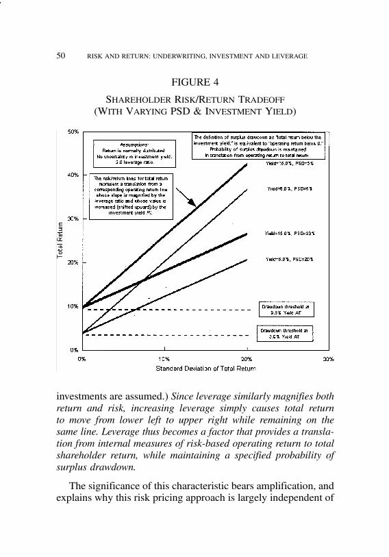
job no. 1969 casualty actuarial society CAS journal 1969D02 [20] 11-08-01 4:58 pm
50 RISK AND RETURN: UNDERWRITING, INVESTMENT AND LEVERAGE
FIGURE 4
SHAREHOLDER RISK/RETURN TRADEOFF(WITH VARYING PSD & INVESTMENT YIELD)
investments are assumed.) Since leverage similarly magnifies bothreturn and risk, increasing leverage simply causes total returnto move from lower left to upper right while remaining on thesame line. Leverage thus becomes a factor that provides a transla-tion from internal measures of risk-based operating return to totalshareholder return, while maintaining a specified probability ofsurplus drawdown.
The significance of this characteristic bears amplification, andexplains why this risk pricing approach is largely independent of

job no. 1969 casualty actuarial society CAS journal 1969D02 [21] 11-08-01 4:58 pm
RISK AND RETURN: UNDERWRITING, INVESTMENT AND LEVERAGE 51
the level of actual company surplus and does not require surplusallocation to lines of business as long as returns are sufficientlypositive. The premium necessary to generate a total return largeenough to keep the downside risk to surplus sufficiently low isthe same regardless of the leverage factor utilized, due to thebalanced and simultaneous effect leverage has on both risk andreturn. The stated total return (as well as the variability in totalreturn) will of course be higher as leverage increases, but the PSDwill remain the same. Reducing leverage does not improve the jointrisk/return profile, and increasing leverage does not worsen it.
Practically speaking, however, it is much easier to present arate filing based on a lower rate of return than a higher one,even if the premium is identical in both cases. In a total returnratemaking environment, the leverage utilized must be such soas to produce a rate of return within an acceptable range whilesatisfying other rating criteria. This is one of the considerationsin the determination of total company surplus requirements to re-flect the concerns of rating agencies and regulators. Furthermore,since premiums often are not sufficient to ensure fair profits, therisk of surplus loss is increased and a greater level of supportingsurplus (i.e., lower leverage) is necessary to provide an adequateruin safety margin.
The primary goals of state regulators, fair premiums and sol-vency, are simultaneously addressed by this risk transfer pricingprocess. Fair returns are determined which simultaneously guardagainst the probability of loss of surplus and ruin. As noted previ-ously, almost any reasonable risk-based level of operating returnprovides an adequate safety margin, and a very small probabilityof ruin. Fair risk-adjusted returns provide the direct connection tosolvency and the means by which solvency is ensured.
3.2. Policyholder Pricing for Underwriting Risk
Operating return is a financial measure which reflects the ba-sic nature of insurance—the fact that it incorporates the activities
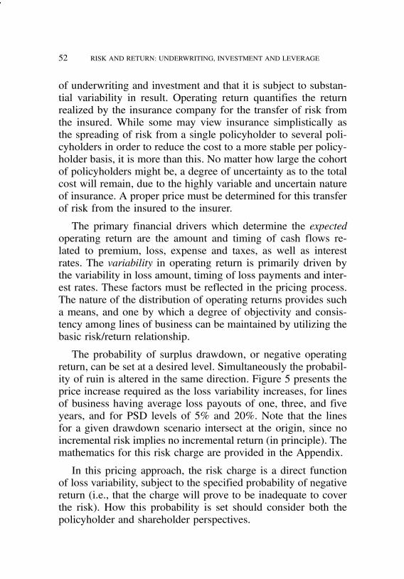
job no. 1969 casualty actuarial society CAS journal 1969D02 [22] 11-08-01 4:58 pm
52 RISK AND RETURN: UNDERWRITING, INVESTMENT AND LEVERAGE
of underwriting and investment and that it is subject to substan-tial variability in result. Operating return quantifies the returnrealized by the insurance company for the transfer of risk fromthe insured. While some may view insurance simplistically asthe spreading of risk from a single policyholder to several poli-cyholders in order to reduce the cost to a more stable per policy-holder basis, it is more than this. No matter how large the cohortof policyholders might be, a degree of uncertainty as to the totalcost will remain, due to the highly variable and uncertain natureof insurance. A proper price must be determined for this transferof risk from the insured to the insurer.
The primary financial drivers which determine the expectedoperating return are the amount and timing of cash flows re-lated to premium, loss, expense and taxes, as well as interestrates. The variability in operating return is primarily driven bythe variability in loss amount, timing of loss payments and inter-est rates. These factors must be reflected in the pricing process.The nature of the distribution of operating returns provides sucha means, and one by which a degree of objectivity and consis-tency among lines of business can be maintained by utilizing thebasic risk/return relationship.
The probability of surplus drawdown, or negative operatingreturn, can be set at a desired level. Simultaneously the probabil-ity of ruin is altered in the same direction. Figure 5 presents theprice increase required as the loss variability increases, for linesof business having average loss payouts of one, three, and fiveyears, and for PSD levels of 5% and 20%. Note that the linesfor a given drawdown scenario intersect at the origin, since noincremental risk implies no incremental return (in principle). Themathematics for this risk charge are provided in the Appendix.
In this pricing approach, the risk charge is a direct functionof loss variability, subject to the specified probability of negativereturn (i.e., that the charge will prove to be inadequate to coverthe risk). How this probability is set should consider both thepolicyholder and shareholder perspectives.
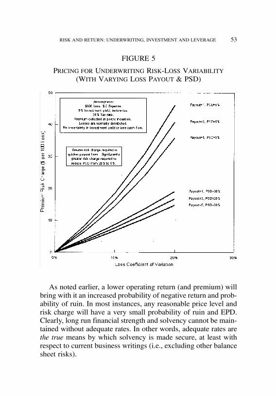
job no. 1969 casualty actuarial society CAS journal 1969D02 [23] 11-08-01 4:58 pm
RISK AND RETURN: UNDERWRITING, INVESTMENT AND LEVERAGE 53
FIGURE 5
PRICING FOR UNDERWRITING RISK-LOSS VARIABILITY(WITH VARYING LOSS PAYOUT & PSD)
As noted earlier, a lower operating return (and premium) willbring with it an increased probability of negative return and prob-ability of ruin. In most instances, any reasonable price level andrisk charge will have a very small probability of ruin and EPD.Clearly, long run financial strength and solvency cannot be main-tained without adequate rates. In other words, adequate rates arethe true means by which solvency is made secure, at least withrespect to current business writings (i.e., excluding other balancesheet risks).
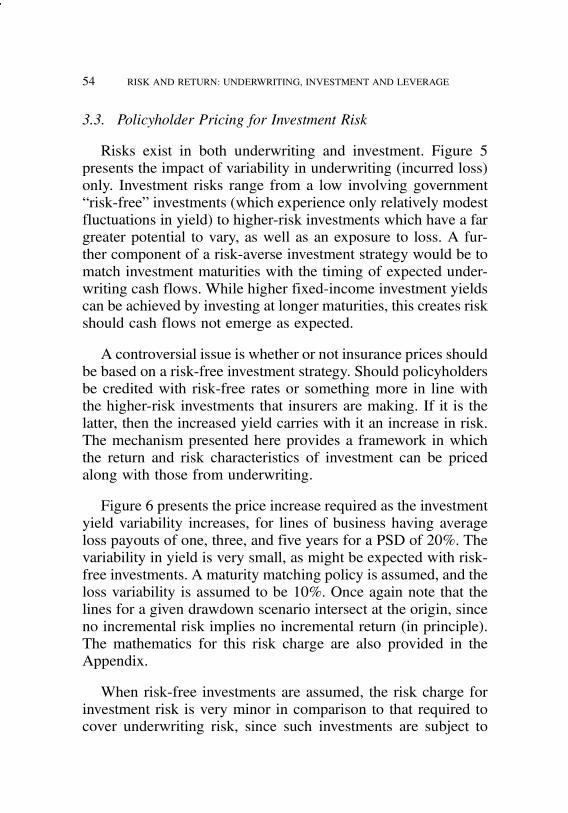
job no. 1969 casualty actuarial society CAS journal 1969D02 [24] 11-08-01 4:58 pm
54 RISK AND RETURN: UNDERWRITING, INVESTMENT AND LEVERAGE
3.3. Policyholder Pricing for Investment Risk
Risks exist in both underwriting and investment. Figure 5presents the impact of variability in underwriting (incurred loss)only. Investment risks range from a low involving government“risk-free” investments (which experience only relatively modestfluctuations in yield) to higher-risk investments which have a fargreater potential to vary, as well as an exposure to loss. A fur-ther component of a risk-averse investment strategy would be tomatch investment maturities with the timing of expected under-writing cash flows. While higher fixed-income investment yieldscan be achieved by investing at longer maturities, this creates riskshould cash flows not emerge as expected.
A controversial issue is whether or not insurance prices shouldbe based on a risk-free investment strategy. Should policyholdersbe credited with risk-free rates or something more in line withthe higher-risk investments that insurers are making. If it is thelatter, then the increased yield carries with it an increase in risk.The mechanism presented here provides a framework in whichthe return and risk characteristics of investment can be pricedalong with those from underwriting.
Figure 6 presents the price increase required as the investmentyield variability increases, for lines of business having averageloss payouts of one, three, and five years for a PSD of 20%. Thevariability in yield is very small, as might be expected with risk-free investments. A maturity matching policy is assumed, and theloss variability is assumed to be 10%. Once again note that thelines for a given drawdown scenario intersect at the origin, sinceno incremental risk implies no incremental return (in principle).The mathematics for this risk charge are also provided in theAppendix.
When risk-free investments are assumed, the risk charge forinvestment risk is very minor in comparison to that required tocover underwriting risk, since such investments are subject to
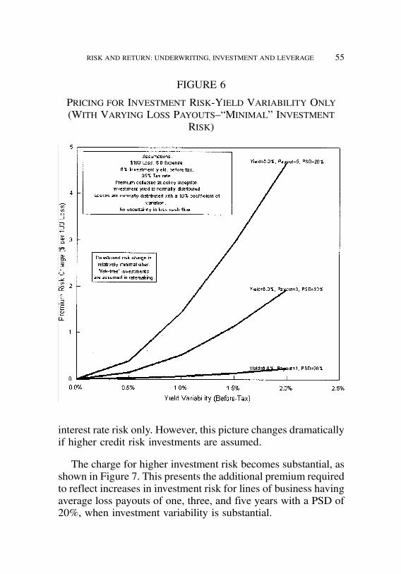
job no. 1969 casualty actuarial society CAS journal 1969D02 [25] 11-08-01 4:58 pm
RISK AND RETURN: UNDERWRITING, INVESTMENT AND LEVERAGE 55
FIGURE 6
PRICING FOR INVESTMENT RISK-YIELD VARIABILITY ONLY(WITH VARYING LOSS PAYOUTS–“MINIMAL” INVESTMENT
RISK)
interest rate risk only. However, this picture changes dramaticallyif higher credit risk investments are assumed.
The charge for higher investment risk becomes substantial, asshown in Figure 7. This presents the additional premium requiredto reflect increases in investment risk for lines of business havingaverage loss payouts of one, three, and five years with a PSD of20%, when investment variability is substantial.

job no. 1969 casualty actuarial society CAS journal 1969D02 [26] 11-08-01 4:58 pm
56 RISK AND RETURN: UNDERWRITING, INVESTMENT AND LEVERAGE
FIGURE 7
PRICING FOR INVESTMENT RISK-YIELD VARIABILITY ONLY(WITH VARYING LOSS PAYOUTS–RISKIER INVESTMENTS)
However, the key issue is to judge to what degree the in-creased benefit from higher yields (via a reduction in price) isoffset by the increase in price due to the higher risk. Figure8 presents an example of such an assessment. (Mismatching,which would increase risk and required premiums, has not beenfactored into this analysis.) A line of business with a three-yearaverage loss payout in which yields increase from a risk-free 6%to 15% (before-tax) will lose the entire benefit from this increase
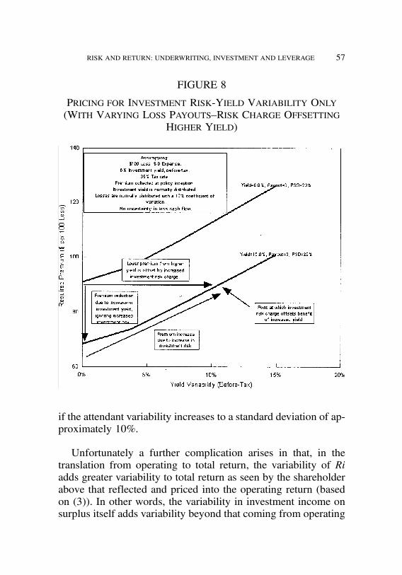
job no. 1969 casualty actuarial society CAS journal 1969D02 [27] 11-08-01 4:58 pm
RISK AND RETURN: UNDERWRITING, INVESTMENT AND LEVERAGE 57
FIGURE 8
PRICING FOR INVESTMENT RISK-YIELD VARIABILITY ONLY(WITH VARYING LOSS PAYOUTS–RISK CHARGE OFFSETTING
HIGHER YIELD)
if the attendant variability increases to a standard deviation of ap-proximately 10%.
Unfortunately a further complication arises in that, in thetranslation from operating to total return, the variability of Riadds greater variability to total return as seen by the shareholderabove that reflected and priced into the operating return (basedon (3)). In other words, the variability in investment income onsurplus itself adds variability beyond that coming from operating
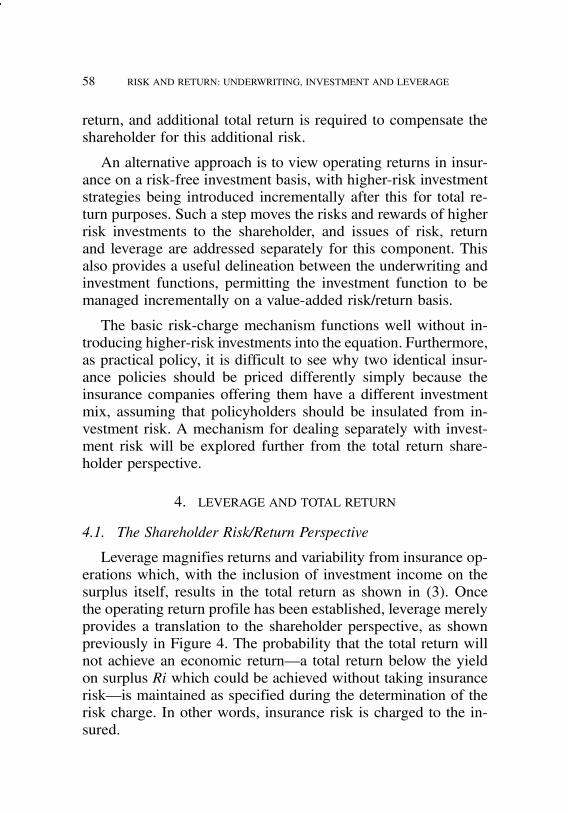
job no. 1969 casualty actuarial society CAS journal 1969D02 [28] 11-08-01 4:58 pm
58 RISK AND RETURN: UNDERWRITING, INVESTMENT AND LEVERAGE
return, and additional total return is required to compensate theshareholder for this additional risk.
An alternative approach is to view operating returns in insur-ance on a risk-free investment basis, with higher-risk investmentstrategies being introduced incrementally after this for total re-turn purposes. Such a step moves the risks and rewards of higherrisk investments to the shareholder, and issues of risk, returnand leverage are addressed separately for this component. Thisalso provides a useful delineation between the underwriting andinvestment functions, permitting the investment function to bemanaged incrementally on a value-added risk/return basis.
The basic risk-charge mechanism functions well without in-troducing higher-risk investments into the equation. Furthermore,as practical policy, it is difficult to see why two identical insur-ance policies should be priced differently simply because theinsurance companies offering them have a different investmentmix, assuming that policyholders should be insulated from in-vestment risk. A mechanism for dealing separately with invest-ment risk will be explored further from the total return share-holder perspective.
4. LEVERAGE AND TOTAL RETURN
4.1. The Shareholder Risk/Return Perspective
Leverage magnifies returns and variability from insurance op-erations which, with the inclusion of investment income on thesurplus itself, results in the total return as shown in (3). Oncethe operating return profile has been established, leverage merelyprovides a translation to the shareholder perspective, as shownpreviously in Figure 4. The probability that the total return willnot achieve an economic return—a total return below the yieldon surplus Ri which could be achieved without taking insurancerisk—is maintained as specified during the determination of therisk charge. In other words, insurance risk is charged to the in-sured.

job no. 1969 casualty actuarial society CAS journal 1969D02 [29] 11-08-01 4:58 pm
RISK AND RETURN: UNDERWRITING, INVESTMENT AND LEVERAGE 59
Surplus, and thus leverage, is set by balancing the policy-holder-related concerns of the regulators and insurance ratingagencies (i.e., lower leverage is better) with shareholder-relatedconcerns of the investment rating agencies and analysts (i.e., rea-sonably higher leverage is generally better). While shareholdersshould receive a higher return if risk is higher, changing leveragedoes not alter the probability of a negative economic downsiderisk. Although a leverage increase will raise returns to the share-holder, it also increases risk at the same time, with the result thatthe PSD remains unchanged.
If returns are low relative to risk and not consistent with otherinvestment alternatives available to the shareholder, then insur-ance companies will have difficulty raising capital. Essentially,the insurance company is not generating a sufficient return onoperations to pay for the transfer of risk from the company to theshareholder under such circumstances. This scenario exists whenthe risk/return relationship governing the company/shareholderrelationship is not supported by a similar risk/return relationshipbetween the company and its policyholders. The only recourseis to increase the underlying policyholder risk charge to bringthat risk/return relationship in line with that needed to supporta total company risk/return profile comparable to other externalinvestment choices. More specifically, the risk charge and returnmust be increased and the PSD reduced, so that the risk and re-turns are made consistent with other investments available to theshareholder.
One important benefit to the aggregate company, and thus tothe shareholder, is the reduction in risk and variability that comesfrom underwriting (line of business) and investment diversifica-tion (i.e., covariance). Companies benefit in many ways fromoffsetting factors which reduce aggregate variability, and thusrisk. These offsets occur: 1) in underwriting between lines ofbusiness, 2) in underwriting between variables such as expenseand loss within a line of business, 3) in investment between as-set classes, 4) between underwriting and investment, and 5) in

job no. 1969 casualty actuarial society CAS journal 1969D02 [30] 11-08-01 4:58 pm
60 RISK AND RETURN: UNDERWRITING, INVESTMENT AND LEVERAGE
reported calendar year financial results in longer-tailed lines ofbusiness (due to an averaging effect on the more volatile pol-icy/accident period results as they flow in). While very difficultto assess, these covariance benefits are of greater benefit to thelarger, more diversified insurers. Just how this effective reduc-tion in risk is reflected in the risk transfer pricing mechanismsis a topic that must be addressed at some point.
One of the interesting aspects of this is that surplus allocationto lines of business is not necessary for purposes of pricing, aslong as a uniform PSD is maintained among the various insur-ance products. The probability of ruin and EPD will be simi-larly controlled, and if prices are adequate, that probability willbe sufficiently small and negligible. While this may be a bit ofa simplification (since many loss distributions are skewed), thebasic principles are valid.
It should be noted that if risky investment strategies are in-cluded in the pricing mechanism, it is likely that the degree ofrisk will vary among the lines of business. For instance, longer-tailed lines might extend maturities to a greater degree thanshorter-tailed lines, thus adding more risk.
4.2. Investment Pricing for Investment Risk
The use of operating return, its expected value and distri-bution, together with the concept of the probability of surplusdrawdown provides a basis for setting fair premiums to the pol-icyholder, while at the same time permitting a fair return to theshareholder consistent with the amount of variability in total re-turn. The issue of investment risk remains as an additional com-ponent of overall total return variability. A mechanism for in-cluding higher investment and a related policyholder premiumrisk charge for the added investment risk entailed was presentedearlier. An alternative approach is to base policyholder premiumon an assumed risk-free investment strategy and separately re-flect investment in the shareholder total return, with the risks andrewards of investment kept within the shareholder domain.

job no. 1969 casualty actuarial society CAS journal 1969D02 [31] 11-08-01 4:58 pm
RISK AND RETURN: UNDERWRITING, INVESTMENT AND LEVERAGE 61
FIGURE 9
INVESTMENT RISK/RETURN(WITH VARYING LEVERAGE & TOTAL RETURN
VARIABILITY–TO MAINTAIN PSD)
This perspective recognizes that insurance company invest-ment activities are themselves subject to the same risk/returnprinciples that apply to policyholders and shareholders, facingthe same decisions that require greater compensation in returnwhen risk is higher. Investment activities are viewed as an in-cremental, value-added complement to underwriting activities,which together form insurance operations. Figure 9 presents thebasic tradeoff in investment risk and return. (The mathematics

job no. 1969 casualty actuarial society CAS journal 1969D02 [32] 11-08-01 4:58 pm
62 RISK AND RETURN: UNDERWRITING, INVESTMENT AND LEVERAGE
for the required increase in investment return are shown in theAppendix.) Here it is assumed that the policyholder premium hasbeen based on a risk-free investment strategy.
The straight line on this chart reflects the increase in returnrequired to compensate for increase in investment risk in orderto maintain a PSD of 20%, when investment is viewed apartfrom underwriting risk and leverage. Unfortunately, the inter-play between underwriting and investment risk and the effect ofleverage on total return variability must be considered. This re-sults in the other nonlinear examples shown on the chart. Notethat there is a benefit to the firm when investment risk is on thelower side, compared to the independent (i.e., linear) investmentrisk/return perspective. However, when investment risk contin-ues to increase while the underlying underwriting risk is smallor leverage is low, a greater investment return is required. Thispoints out the important connection between underwriting andinvestment risk and financial leverage.
Figure 10 presents the increase in investment return or “lift”required to maintain a given PSD, as investment return variabil-ity increases with the connection between underwriting and in-vestment risk and leverage considered in all cases. This figureprovides a frame of reference indicating the degree by whichinvestment returns must improve as investment risk increases.Importantly, the curves shown do not depend on the underlyinglevel of investment yield.
If the lift in investment returns is below those indicated, thenthe probability of surplus drawdown is increased. If investmentreturns cannot be improved, then perhaps the risks are too great.Furthermore, higher leverage requires a higher lift due to themagnifying effects of leverage on variability. Thus an alternativeto increasing investment return when investment risk increasesis to reduce leverage. In other words, increases in investmentrisk may embody elements of both higher investment return andmore conservative (i.e., lower) leverage.
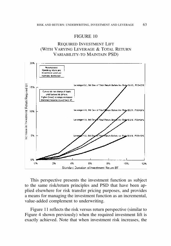
job no. 1969 casualty actuarial society CAS journal 1969D02 [33] 11-08-01 4:58 pm
RISK AND RETURN: UNDERWRITING, INVESTMENT AND LEVERAGE 63
FIGURE 10
REQUIRED INVESTMENT LIFT(WITH VARYING LEVERAGE & TOTAL RETURN
VARIABILITY–TO MAINTAIN PSD)
This perspective presents the investment function as subjectto the same risk/return principles and PSD that have been ap-plied elsewhere for risk transfer pricing purposes, and providesa means for managing the investment function as an incremental,value-added complement to underwriting.
Figure 11 reflects the risk versus return perspective (similar toFigure 4 shown previously) when the required investment lift isexactly achieved. Note that when investment risk increases, the
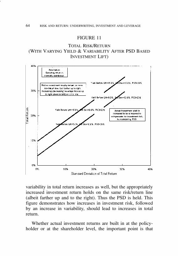
job no. 1969 casualty actuarial society CAS journal 1969D02 [34] 11-08-01 4:58 pm
64 RISK AND RETURN: UNDERWRITING, INVESTMENT AND LEVERAGE
FIGURE 11
TOTAL RISK/RETURN(WITH VARYING YIELD & VARIABILITY AFTER PSD BASED
INVESTMENT LIFT)
variability in total return increases as well, but the appropriatelyincreased investment return holds on the same risk/return line(albeit farther up and to the right). Thus the PSD is held. Thisfigure demonstrates how increases in investment risk, followedby an increase in variability, should lead to increases in totalreturn.
Whether actual investment returns are built in at the policy-holder or at the shareholder level, the important point is that

job no. 1969 casualty actuarial society CAS journal 1969D02 [35] 11-08-01 4:58 pm
RISK AND RETURN: UNDERWRITING, INVESTMENT AND LEVERAGE 65
the attendant increase in risk must be reflected. In the case ofthe policyholder, this means an increase in premium, possiblyby enough to outweigh the benefit of the higher investment re-turn. In the case of the shareholder, this means an increase in theoverall total return which recognizes the increase in total returnvariability.
4.3. Surplus Requirements and Allocation to Lines of Business
A long-running debate continues with regard to the need toallocate surplus to lines of business for the purposes of ratemak-ing. Those not in favor of surplus allocation and the total returnapproach to ratemaking usually suggest use of return on pre-mium (i.e., sales) as a preference. This statistic, however, is nota measure of return on investment, and it lacks a frame of refer-ence as to what is fair and on what basis it should be set. Alsoproblematic is the fact that it can and should differ markedlyamong lines of business, due to the length of the tail and thefloat-generating investment income that results. By way of alter-native, operating return as presented in this paper has importantattributes including:
1. Both of the operating return components of underwritingand investment rates of return, Ru and Ri, respectively,represent a return on supporting policyholder funds “in-vested.” Thus operating return is truly a return on invest-ment concept.
2. Operating return is an integral component of total return,since mathematically total return is calculated simply asthe product of operating return times leverage, plus theinvestment return on surplus.
3. Operating rate of return fully reflects the differing mag-nitude and cash flow timing characteristics of individuallines of business. Operating return represents an annu-alized rate of return, regardless of investment horizon,comparable across all lines of business.
job no. 1969 casualty actuarial society CAS journal 1969D02 [36] 11-08-01 4:58 pm
66 RISK AND RETURN: UNDERWRITING, INVESTMENT AND LEVERAGE
It is suggested here that, at a minimum, operating return be usedin place of return on premium.
Arguments which favor the use of total return include thefact that it is a widely recognized benchmark (e.g., 15% ROE)which is readily comparable to other industries in terms of therisk versus return relationship. (It is also clear that every addi-tional policy written entails an increase in risk to the insurancecompany, and requires some marginal increase in surplus.) Theapproach presented here extends the same risk (variability in re-turn) versus return principles that govern shareholder actions toa lower operating return level within the insurance company.
In essence the “operating return–probability of drawdown”method presented in this paper is a replacement of return onpremium by operating return, and an extension of shareholderrisk/return principles to the policyholder level. As a consequence,the method demonstrates how risk can be reflected in the pricingmechanism without varying the allocation of surplus to individ-ual lines of business, through the focus on operating return. Yetthis remains as a mathematical component of the total return,made complete simply by the application of leverage and theaddition of investment return on surplus. The PSD, driven bythe connected variability in operating and total return, providesa unifying and consistent framework for establishing fair returnsto reflect the transfer of risk from the policyholder to the com-pany and from the company to the shareholder. Furthermore, ifthe PSD is made the same when pricing the individual lines ofbusiness, then leverage can be set uniformly in each line equalto the overall company average for purposes of calculating totalreturn.
Were pricing models able to estimate all prospective finan-cial parameters sufficiently well, then adequate pricing wouldlay the foundation for financial strength and lessen the need forsurplus. However, many factors such as inflation, changing tortlaw, competitive pricing and catastrophic exposures, introduce

job no. 1969 casualty actuarial society CAS journal 1969D02 [37] 11-08-01 4:58 pm
RISK AND RETURN: UNDERWRITING, INVESTMENT AND LEVERAGE 67
uncertainty with respect to balance sheet value and require a sub-stantial surplus cushion. Furthermore, these risks and resultingsurplus needs are likely to differ among the lines of business.
The total surplus of an insurance company needs to be suf-ficient to provide an adequate financial cushion for the manybalance sheet risks. The approach presented in this paper sup-ports solvency with respect to current business writings, sincethe probability of ruin that results is extremely small (given anyreasonable PSD and operating return).
4.4. Application Steps to Put Concepts into Practice
The following overview presents the essential steps and capa-bilities that are necessary to put these concepts into practice.
1. Develop a model framework that provides key balancesheet, income, and cash flow components. If ratemak-ing is the primary focus, then modeling a single policyperiod may be sufficient, in which case a single pay-ment approach as presented in [2] and [3] may suffice. Ifcalendar year financials are needed, then a multi-periodcash flow model is needed, such as in DFA applications.Ideally this develops calendar period financials as thesum of current and prior policy/accident period contri-butions.
2. Develop a simulation capability built on top of thismodel, which can be applied to individual lines of busi-ness and then aggregated to a company total. The ca-pability to incorporate key correlations among lines ofbusiness and variables may be important.
3. Specify the expected values of all variables and distri-butions of key variables as necessary. Generally interestrates and the amount and timing of losses, coupled withdistributions that reflect the variability in them, are im-portant. Although difficult to determine, key correlations

job no. 1969 casualty actuarial society CAS journal 1969D02 [38] 11-08-01 4:58 pm
68 RISK AND RETURN: UNDERWRITING, INVESTMENT AND LEVERAGE
among lines of business and variables should be spec-ified. Omitting this (i.e., assuming independence) willtend to overstate the benefit of covariance (i.e., diver-sification) and understate company surplus needs, sincecorrelations are typically positive.
4. Set the (fixed) risk parameter to be used in each lineof business. This is the desired probability that the totalrate of return in an individual line of business will fallbelow the risk-free yield. A value in the range of 10%will probably be reasonable for starters. The number oflines of business, and the resultant diversification benefit,will affect this choice. The ruin probability for the totalcompany that results should be verified as sufficientlysmall.
5. Beginning with underwriting risk/return, initially set afixed leverage ratio (2 or 3 to 1 for liability to surplus) inall lines, and solve for the premium necessary to satisfythe specified risk parameter. The distributional outcomesfrom the simulation are used in this step. (A “risk-free”investment yield is suggested at this point.) This will in-dicate a required underwriting profit margin (i.e., com-bined ratio). At this point a risk/return line can be viewedfor the modelled lines of business.
6. Adjust leverage by line of business to achieve a targettotal return. Premium is unchanged by this step, sincethe process is one of simply sliding up or down therisk/return line depending on whether the initial return isbelow or above the target return. If initially below the tar-get return, leverage is increased (and decreased if above).The risk probability remains the same. The leverage ra-tios that result provide a risk adjustment mechanism, in-dicating relative line of business surplus requirementsthat permit all lines of business to be viewed relative tothe same risk-adjusted total return target.
job no. 1969 casualty actuarial society CAS journal 1969D02 [39] 11-08-01 4:58 pm
RISK AND RETURN: UNDERWRITING, INVESTMENT AND LEVERAGE 69
7. If higher risk investments are to be introduced, steps 5and 6 are repeated for investment risk/return. After esti-mated investment risk and variability are increased, solvefor the investment return necessary to satisfy the speci-fied risk parameter. This will indicate a required invest-ment margin. This should fall on the risk/return line butfarther up and to the right (i.e., greater risk, greater re-turn).
8. Adjust leverage by line of business to achieve the tar-get total return. Required investment yields (as well asoriginal premiums) are unchanged by this step, againsince the process is one of simply sliding up or downthe risk/return line, depending on whether the return isbelow or above the target return. The risk probability re-mains the same. The leverage ratios that result providea risk adjustment mechanism, indicating the relative lineof business surplus requirements for underwriting andinvestment risk combined. The difference from this sur-plus amount and that in step 6 is the amount required tocompensate for investment risk. The leverage ratios thatresult provide a risk adjustment mechanism that permitsall lines of business to be viewed on a comparable totalreturn basis, in which both underwriting and investmentrisk have been reflected.
The risk-based required premium and investment yield deter-mined in steps 5 and 7 may or may not be achievable. This thenbecomes part of the company’s portfolio investment decision asto whether certain lines of business and/or investments shouldbe written or undertaken.
In summary, this process provides a risk transfer pricingmechanism applicable to underwriting and investment activi-ties, by indicating the premiums and investment returns requiredgiven their respective risks. Necessary leverage and relative sur-

job no. 1969 casualty actuarial society CAS journal 1969D02 [40] 11-08-01 4:58 pm
70 RISK AND RETURN: UNDERWRITING, INVESTMENT AND LEVERAGE
plus amounts are also indicated in order to risk-adjust to a com-mon risk/return target.
5. CONCLUSION
It should be clear that the returns from underwriting and in-vestment (in terms of expectations and uncertainty) together withthe operating leverage employed by an insurance company, es-tablish the essential elements of the risk/return tradeoff. This pa-per has presented an approach based on the application of verybasic risk/return tradeoff principles to the risk transfer processthat occurs between the insured and the company and betweenthe company and the shareholder. Risk-based pricing algorithmshave been presented to deal consistently with underwriting riskamong lines of business and with investment risk. This processis apart from leverage, and does not require a varying surplusallocation to lines of business.
Operating return as presented in this paper is suggested asthe fundamental measure that should be used to judge the risktransfer activities and pricing with respect to the policyholder.It is noted that risk is a fundamental element of insurance andit cannot be eliminated. Variability in results is expected, andsimply throwing more surplus into the mix does not alter thebasic risk/return relationship. Therefore, whether it is underwrit-ing or investment based, some charge for risk transfer is neededwhenever it occurs.
The PSD has been introduced as a guide by which therisk/return tradeoff can be managed similarly for both the policy-holder and for the shareholder. This is suggested as the appropri-ate basis by which risk and return should be managed and pricesset. Furthermore it is suggested that, while consistent with theprobability of drawdown, the probability of ruin and EPD per-spectives are different and more appropriate as a means to satisfycompany solvency criteria than as a basis for risk transfer pric-ing. Instead, the risk transfer pricing approach presented here

job no. 1969 casualty actuarial society CAS journal 1969D02 [41] 11-08-01 4:58 pm
RISK AND RETURN: UNDERWRITING, INVESTMENT AND LEVERAGE 71
provides a single unified method which simultaneously satisfiesregulatory concerns with respect to both setting fair risk-adjustedpremiums and maintaining solvency.
Ultimately, insurance companies are faced with investmentdecisions with respect to the creation of optimum portfolio com-binations of underwriting lines of business and investments toincrease total return for a given level of risk. This involves ap-plication of the basic principles associated with the tradeoff be-tween risk and return, and in which aggregate company diversi-fication and covariance benefits play a role. While this paper hasattempted to present concepts in as simple a manner as possible,solutions must extend into those cases which reflect the many in-surance variables, how they relate to one another, and how theyevolve over time.
job no. 1969 casualty actuarial society CAS journal 1969D02 [42] 11-08-01 4:58 pm
72 RISK AND RETURN: UNDERWRITING, INVESTMENT AND LEVERAGE
REFERENCES
[1] Bingham, Russell E., “Fundamental Building Blocks of In-surance Profitability Measurement” and “Cash Flow Modelsin Ratemaking,” Actuarial Considerations Regarding Risk andReturn in Property-Casualty Insurance Pricing, Casualty Ac-tuarial Society, 1999, Chapters 2, 4.
[2] Bingham, Russell E., “Rate of Return—Policyholder, Com-pany, and Shareholder Perspectives,” PCAS LXXX, 1993,pp. 110–147.
[3] Bingham, Russell E., “Surplus—Concepts, Measures of Re-turn, and Determination,” PCAS LXXX, 1993, pp. 55–109.
[4] Bingham, Russell E., “Discounted Return—Measuring Prof-itability and Setting Targets,” PCAS LXXVII, 1990, pp. 124–159.
[5] Butsic, Robert P., “Solvency Measurement for Property-Liability Risk-Based Capital Applications,” The Journal ofRisk and Insurance 61, 1994, pp. 656–690.
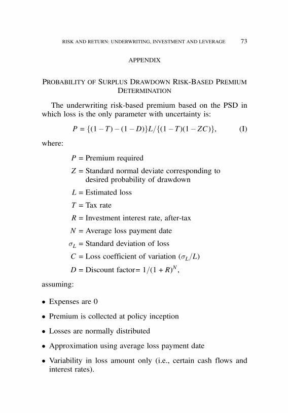
job no. 1969 casualty actuarial society CAS journal 1969D02 [43] 11-08-01 4:58 pm
RISK AND RETURN: UNDERWRITING, INVESTMENT AND LEVERAGE 73
APPENDIX
PROBABILITY OF SURPLUS DRAWDOWN RISK-BASED PREMIUMDETERMINATION
The underwriting risk-based premium based on the PSD inwhich loss is the only parameter with uncertainty is:
P = "(1!T)! (1!D)#L="(1!T)(1!ZC)#, (I)
where:
P = Premium required
Z = Standard normal deviate corresponding todesired probability of drawdown
L= Estimated loss
T = Tax rate
R = Investment interest rate, after-tax
N =Average loss payment date
¾L = Standard deviation of loss
C = Loss coefficient of variation (¾L=L)
D =Discount factor= 1=(1+R)N ,
assuming:
$ Expenses are 0$ Premium is collected at policy inception
$ Losses are normally distributed$ Approximation using average loss payment date$ Variability in loss amount only (i.e., certain cash flows andinterest rates).
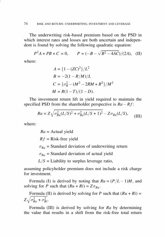
job no. 1969 casualty actuarial society CAS journal 1969D02 [44] 11-08-01 4:58 pm
74 RISK AND RETURN: UNDERWRITING, INVESTMENT AND LEVERAGE
The underwriting risk-based premium based on the PSD inwhich interest rates and losses are both uncertain and indepen-dent is found by solving the following quadratic equation:
P2A+PB+C = 0, P = (!B!!B2!4AC)=(2A), (II)
where:
A= "1! (ZC)2#=L2B =!2(1!R=M)=LC = "¾2R ! (M2!2RM+R2#=M2
M = R(1!T)=(1!D):The investment return lift in yield required to maintain the
specified PSD from the shareholder perspective is Ra!Rf:Ra= Z
"¾2Ru(L=S)
2 +¾2Ra(L=S+1)2!Z¾Ru(L=S), (III)
where:
Ra=Actual yield
Rf =Risk-free yield
¾Ru = Standard deviation of underwriting return
¾Ra = Standard deviation of actual yield
L=S =Liability to surplus leverage ratio,
assuming policyholder premium does not include a risk chargefor investment.
Formula (I) is derived by noting that Ru= (P=L!1)M, andsolving for P such that (Ru+Ri) = Z¾Ru.
Formula (II) is derived by solving for P such that (Ru+Ri) =
Z"¾2Ru+¾
2Ri.
Formula (III) is derived by solving for Ra by determiningthe value that results in a shift from the risk-free total return
job no. 1969 casualty actuarial society CAS journal 1969D02 [45] 11-08-01 4:58 pm
RISK AND RETURN: UNDERWRITING, INVESTMENT AND LEVERAGE 75
line, given by Rf+(Ru+Rf)(L=S) having a standard deviationof ¾Ru(L=S), to the riskier total return line, given by Ra+(Ru+Ra)(L=S) having a standard deviation of:"
¾2Ru(L=S)2 +¾2Ra(L=S+1)
2,
in order to satisfy the same PSD (i.e., Z-value).
The formulae presented here to demonstrate the concepts donot reflect all variables. While loss is generally the key driver interms of expected return and variability, a more complete exten-sion of this approach should reflect the impact of all parametersand multi-period cash flows (and the relationships among them)on return.
Demonstration Example
The following financial assumptions form the basis for theexample presented in Exhibit A-1:
$ 101.0% Combined ratio
$ $9,900 Premium, collected without delay$ $10,000 Loss, single payment after 3 years$ $0 Expense$ 35% Income tax rate, no delay in payment
$ 6.0% Investment interest rate before-tax, 3.9% after-tax
$ No loss discount tax$ 3.0 Liability/surplus ratio.Simplified balance sheet, income and cash flow statements
are shown for this example. The rules governing the flow ofsurplus are as follows: (1) the level of surplus is maintained at a1/3 ratio with loss reserves, (2) investment income on surplus ispaid to the shareholder as earned, and (3) operating earnings aredistributed in proportion to the level of insurance exposures in

job no. 1969 casualty actuarial society CAS journal 1969D02 [46] 11-08-01 4:58 pm
76 RISK AND RETURN: UNDERWRITING, INVESTMENT AND LEVERAGE
each year (measured by loss reserve levels) relative to the totalexposure. Since loss reserves are equal at $10,000 in each of thethree years, operating earnings are distributed to the shareholderequally in each year.
Three “levels” of return exist within an insurance company.The first is the underwriting rate of return, which reflects whatthe company earns on pure underwriting cash flows before re-flecting investment income on the float. This is a “cost of funds”to the company. The second, operating return, reflects what thecompany earns on underwriting when investment income on thefloat is included. This is the “risk charge” to the policyholderfor the transfer of risk to the company. Finally, the total returnis the net result of underwriting and investment income fromoperations together with investment income on surplus.
These rates of return can be determined either by a cash flow-based internal rate of return (IRR) calculation, or by relatingincome earned to the amount invested. With regard to the share-holder total return perspective, the IRR based on cash flows fromand to the shareholder indicates a 14.9% return over the three-year period. The income versus investment approach (i.e., ROE)relates the income over the full three-year aggregate financial lifeof the business to the shareholder’s investment over this sameperiod. This is shown in both nominal (i.e., undiscounted) andin present value (discounted) dollars to produce a 14.9% rateof return on investment. Furthermore, the return realized by theshareholder via dividends is also an identical 14.9% in each year.(This attribute follows from the rules used to control the flow ofsurplus.)
The operating return, inclusive of underwriting and invest-ment income, is most easily shown to generate a cash flow-basedinternal rate of return of 3.7%. Equivalently, the operating in-come of $1,100 is a 3.7% return on the “investment equivalent”of $30,000, the total balance sheet float upon which these earn-ings were generated.

job no. 1969 casualty actuarial society CAS journal 1969D02 [47] 11-08-01 4:58 pm
RISK AND RETURN: UNDERWRITING, INVESTMENT AND LEVERAGE 77

job no. 1969 casualty actuarial society CAS journal 1969D02 [48] 11-08-01 4:58 pm
78 RISK AND RETURN: UNDERWRITING, INVESTMENT AND LEVERAGE

job no. 1969 casualty actuarial society CAS journal 1969D01 [1] 11-08-01 4:58 pm
ESTIMATING U.S. ENVIRONMENTAL POLLUTIONLIABILITIES BY SIMULATION
CHRISTOPHER DIAMANTOUKOS
Things should be made as simple as possible, but notany simpler. —Albert Einstein
Abstract
The application of computer simulation to the estima-tion of environmental pollution costs for inactive haz-ardous waste sites is presented. The various modules ofthe pollution costs simulation model (PCSM) are de-scribed, with the flow of costs traced from remedialaction at EPA and state-administered sites through toinsureds in the form of potentially responsible parties(PRPs), and finally to the application of coverage de-fenses. Methods are presented for using precision (cred-ibility) estimates for state averages, and for projectingcosts for an insurance portfolio based on sampling pro-portions. Countrywide results are presented, includingthe characterization of variability and comparisons topublished insurance industry estimates of ultimate lossand expenses.
1. INTRODUCTION
The pollution costs simulation model (PCSM) described inthis paper represents in many respects a work in progress. Theremediation of pollution at inactive hazardous waste sites in theUnited States possesses a life cycle whose components are under-going continual change as regards their attributes and durations.A model designed to estimate the associated costs or liabilitiesof remediation must first learn to walk, or crawl. It is natural toexpect that, over time, changes and enhancements will be madeto such a model.
79

job no. 1969 casualty actuarial society CAS journal 1969D01 [2] 11-08-01 4:58 pm
80 ESTIMATING U.S. ENVIRONMENTAL POLLUTION LIABILITIES
This paper describes the status of the PCSM at a point intime: the PCSM will have undoubtedly changed by the time thispaper is read. The purpose of this paper is therefore to presentthe approach to solving these estimation problems through theapplication of simulation techniques and actuarial principles.
The model is used to perform two tasks. The first is a country-wide estimate for all environmental pollution costs and ultimateliabilities to the U.S. insurance market for abandoned sites. Thesecond is its application to a specific portfolio of insurance con-tracts in order to determine the liabilities to an individual insureror reinsurer.
It is assumed that the reader has some familiarity with the his-tory of the creation of environmental pollution liabilities throughthe Comprehensive Environmental Response, Compensation andLiability Act (CERCLA), Superfund Amendments and Reautho-rization Act of 1986 (SARA), and other federal, state, or locallaws. A thorough discussion of the governing laws and of the his-tory and evolution of pollution liabilities in the U.S. will not beoffered in this paper. The interested reader is directed to severalreferences that will serve to provide any needed background.
2. DESIGN OF MODEL
The PCSM is designed to trace and simulate the sequentialflow of pollution liabilities from the creation of costs at an indi-vidual hazardous waste site to the estimation of insurance liabil-ities at a contract (policy) level. The PCSM is best characterizedas an exposure model of insurance liabilities and costs, since it isbased on the construction of a model that attempts to measure theinsurable loss of a set of risks and then apply policy conditions inorder to estimate insured losses. The model does this through theestimation of population parameters and their interaction throughmodeling of the constituent databases. This process creates an“exposure measure”1 that relates the expected values and under-
1The term “exposure measure” reflects the usage afforded by [1, p. 5].
job no. 1969 casualty actuarial society CAS journal 1969D01 [3] 11-08-01 4:58 pm
ESTIMATING U.S. ENVIRONMENTAL POLLUTION LIABILITIES 81
lying distributions of the associated random variables, startingwith site remediation costs and ending with the potential attach-ment of insurance coverage. There are no actual insured lossesused in the construction of the PCSM as presented in this paper.
This form of exposure model is in sharp contrast to an extrap-olation, regression, or any other model which makes projectionsinto the future based on historical patterns and observations ofactual insured losses. Those types of models are normally ap-plied directly to empirical observations related to the liabilitiesbeing estimated.
One population invoked by the PCSM is the totality of inactivehazardous waste sites, where the great majority of the constituentsites do not have cleanup costs specifically associated with them.Some of these sites may be or may become National Priority List(NPL) sites in the future, and can be expected to command tensof millions of dollars in cleanup costs. Tens of thousands of thesesites are state sites or will be sites arising under individual statesupervision that do not have costs separately identified for them.
Another population is composed of those entities identifiedas potentially responsible parties (PRPs), which are presumed toform the bulk of what might better be termed ultimately respon-sible parties because they originally created the pollution. Thereare undoubtedly many more entities beyond those identified todate that will bear the cost for cleanup.
The PCSM constructs random variables that model costs at thesite level and that model the sharing of these costs among knownPRPs. Such estimates of costs in turn create exposures to lossfor policies that afford insurance to PRPs. The expectations anduncertainties of the costs modeled by the PCSM are aggregatedacross sites, PRPs, and the policy or incurred years over whichinsurance has been provided, and then extended to the entirepopulation of known sites in order to derive estimates of ultimatecleanup costs and insured liabilities.

job no. 1969 casualty actuarial society CAS journal 1969D01 [4] 11-08-01 4:58 pm
82 ESTIMATING U.S. ENVIRONMENTAL POLLUTION LIABILITIES
The statistical foundation of the PCSM is directly reflected bythe measures and distributions introduced throughout the modelthat reflect the uncertainty associated with each cost estimateelement.
The estimation of pollution liabilities from U.S. locations uti-lizes the inactive hazardous waste site information identified bythe Comprehensive Environmental Response, Compensation andLiability Information System (CERCLIS), as well as those iden-tified or estimated by state and territory site lists or data bases.The latter sources contain sites that did not originate with theEPA through CERCLIS. Over time, these lists will expand toinclude sites that originated in CERCLIS, but have been referredto individual state or local authorities for supervision and furtherremedial action.
The PCSM estimates cleanup costs (Capital, sometimes re-ferred to as Remediation, and Operation and Maintenance costs)as well as transaction costs (including allocated and unallocatedloss adjustment expenses for insurance coverage purposes) fornon-federal sites.2 The term “cost” will often be used to referto “cleanup costs” while “loss adjustment expense” has been re-served for transaction costs.
The PCSM performs five separate tasks in distinct, self-contained modules during each iteration of a simulation. The firstmodule simulates individual site cleanup costs for each of the ap-proximately 40,000 sites on the CERCLIS database (Section 3of this paper). The second module assigns a share of each site’sliability to each PRP for those sites identified with PRPs on theSite Enforcement Tracking System (SETS)3 database (Section4). The third module applies state specific estimated probabilities
2These sites are also referred to as “private sites” (see for example [15, p. 9]) althoughthere are private entities identified as potentially responsible parties on federal sites.3SETS is no longer the term used to identify this information as the EPA has restructuredits data bases, thereby integrating information that may have been provided by separatesources. The term is used here for historical reference and to convey the existence ofsuch information.
job no. 1969 casualty actuarial society CAS journal 1969D01 [5] 11-08-01 4:58 pm
ESTIMATING U.S. ENVIRONMENTAL POLLUTION LIABILITIES 83
of coverage defenses being upheld and state specific probabili-ties of exposure triggers in order to establish insurable costs orliabilities (Section 5). The fourth module associates loss adjust-ment expense with PRP cleanup costs and distributes both theindividually determined PRP insurable costs and loss adjustmentexpense across years of potential insurance coverage (Sections6 and 7). The fifth module performs different tasks dependingon whether the PCSM is being used for a countrywide simula-tion or a portfolio simulation. For the countrywide simulation itestimates the costs for those sites found only on state lists (allnon-CERCLIS sites in a state) or relegated to state enforcementfrom the CERCLIS database (Section 8). For an insurance port-folio it evaluates the potential indemnification afforded by thepolicies and coverages contained within (Section 9).
Any additional cost elements or modifications to any compo-nent of cost estimates associated with environmental pollutionliabilities that are not specifically mentioned are not estimatedby the PCSM. These include consideration of third party liabili-ties, collateral suit defendants, Natural Resource Damage claims,and orphan shares. As the goal of this paper is to convey con-cepts and approaches, such limitations of the PCSM as presentedherein should not detract from the achievement of that goal.
3. SITE COST ESTIMATES
Individual site cost estimates are performed for those sitescontained on the CERCLIS data base. The primary source ofcost information for an individual site in CERCLIS is containedin the Records of Decisions (RODs) issued by the United StatesEnvironmental Protection Agency (EPA). Specific cost informa-tion is available for only a small portion of these sites.
The estimation of site costs from RODs information is wor-thy of a paper in and of itself. One of the author’s associateswho contributed to the construction of the PCSM (Steven Finkel-stein) has written such a paper [2]. One key issue addressed
job no. 1969 casualty actuarial society CAS journal 1969D01 [6] 11-08-01 4:58 pm
84 ESTIMATING U.S. ENVIRONMENTAL POLLUTION LIABILITIES
therein is the extraction of cost information from the RODs in amanner that allows the transformation of present value costs, asshown in the RODs, into undiscounted (nominal) values. How-ever, an in-depth analysis of RODs reveals other issues includingthe identification of interim RODs (that presumably will be sup-plemented by final RODs), amendment RODs, the emergence offuture RODs applicable to additional operable units for a site,and the translation of cost estimates from the date of preparation(issuance) for a ROD to the time actual construction (remedia-tion) begins. The results of Finkelstein’s analysis of RODs costsare presented here in the form of cleanup costs and associatedpresent value factors without further explanation.
Exhibit 1 contains the distribution of CERCLIS sites at thetime the PCSM was constructed according to Active/Archived,Site Status, RODs information, and PRP information. Some sitesactually have more than one ROD issued while those identified asArchived, or No Further Remedial Action Planned (NFRAP), areunlikely to rise to the NPL. One of the ingredients to the modelis, therefore, an estimate of the respective probabilities that aNon-NPL CERCLIS site may become an NPL site in the future.It was assumed that only the balance of Non-NPL active sitesare eligible. All other sites, including all archived sites, wouldbe subject to state or local authority. Indeed, some of these sitesmay not require any cleanup as evidenced by the statistics shownin Exhibit 2.
The simulation of site costs is preceded by an analysis of costsby site that results in the construction of two fundamental databases:
! Sites with Variable Cost Estimates—contains information onthose CERCLIS sites where more than one cost estimate wasprovided in the RODs for one or more of a site’s operableunits.
! Sites Without Variable Cost Estimates—contains thoseCERCLIS sites with a single value of cost estimates from the

job no. 1969 casualty actuarial society CAS journal 1969D01 [7] 11-08-01 4:58 pm
ESTIMATING U.S. ENVIRONMENTAL POLLUTION LIABILITIES 85
RODs for each of its operable units or those CERCLIS siteswith no specific cost information.
Appendix A describes how these databases were used to con-struct site cost variability parameters. These parameters includeboth the analysis of the distribution of cleanup costs on a site ba-sis, as well as the variability or uncertainty of the cleanup costsfor a single site.
The variability of site costs is in addition to the EPA defaultaccuracy guideline of "30% to +50% of the published RODscosts [16, pp. 2–10]. Costs were randomized uniformly downto "30% or uniformly up to +50% and then normalized backto unity by dividing by 1.05, the expected value of the randomvariable so created4 during each iteration of the PCSM.
Appendix B includes the derivation of the frequency of fu-ture NPL sites and the associated average site costs by stateand category (NPL or state authority). It is of great value toidentify site characteristics that can be used in a predictive man-ner for estimating cleanup costs for those sites that currently donot carry such information. There were very few site charac-teristics sufficiently populated for this purpose at the time thePCSM was constructed. State name was always available anduseful to the extent it reflected differences among states result-ing from differing industrial or economic development and atti-tude to cleanup standards and enforcement. Precision weightingof average site cleanup costs that employed estimates of vari-ance was used in a manner consistent with actuarial estimates ofcredibility.
With these preliminary analyses completed, the sequence ofsteps employed by the PCSM to simulate a site cost during eachiteration is as follows:
4The expected value below unity is .85, while above unity it is 1.25, which results in anexpected value of 1.05 when they are equally weighted.

job no. 1969 casualty actuarial society CAS journal 1969D01 [8] 11-08-01 4:58 pm
86 ESTIMATING U.S. ENVIRONMENTAL POLLUTION LIABILITIES
1. For Sites With Variable Cost Estimates:
a) Randomly determine an EPA accuracy factor between"30% and +50%, or between .7 and 1.5, normalizedto unity for each separate cost. This is typically ap-plied to each individual total ROD present value cost.
b) Multiply each individual ROD total present value costby its random EPA accuracy factor.
c) Divide by the corresponding present value factor toobtain nominal costs.
d) Add the individual nominal costs for each ROD todetermine a total undiscounted site cleanup cost.
2. For Sites Without Variable Cost Estimates:
a) Randomly determine an EPA accuracy factor between"30% and +50%, or between .7 and 1.5, normalizedto unity.
b) Randomly determine a site cost uncertainty relativityas described in Appendix A.
c) Randomly assign NPL status to an individual eligibleactive CERCLIS site by state, assigning state author-ity status otherwise.
d) Assign state authority status to all non-eligible (ar-chived) CERCLIS sites.
e) Apply the individual ROD total present value cost ifapplicable; otherwise, apply the corresponding pres-ent value average state NPL site cost or the presentvalue average state authority site cost according tosite assignment.
f) Multiply by the random EPA accuracy factor and sitecost uncertainty relativity and, if a ROD cost was notused, also apply a normalized random factor from the

job no. 1969 casualty actuarial society CAS journal 1969D01 [9] 11-08-01 4:58 pm
ESTIMATING U.S. ENVIRONMENTAL POLLUTION LIABILITIES 87
TABLE 1
SIMULATION PROCEDURE FOR SITES WITHOUT VARIABLECOST ESTIMATES
Is this an NPL site? Y Y Y N N NDoes site have ROD present worth costs? Y Y N Y Y NDoes site (ROD) have specific PV Factor? Y N N Y N N
EPA accuracy factor X X X X X XSite cost uncertainty X X X X X XAverage NPL site cost for state XAverage state authority site cost for state XSite variability normalized factor X XROD present worth cost X X X XDefault PV Factor X X X XSpecific site (ROD) PV Factor X X
distribution of site cleanup costs to recognize differ-ences among site cleanup costs as described in Ap-pendix A.
g) Divide by the estimated present value factor whenavailable to determine the nominal (undiscounted)site cost; otherwise, divide by the separately deter-mined average present value factor (see Appendix B).
The decision logic table above summarizes the process forsimulating costs for sites without variable cost estimates. Thequestions on the left are answered for each site from top to bot-tom and left to right, until the bottom of a column is reachedin the upper half of Table 1. The actions applied to a site arethen identified with an “X” in that column in the bottom halfof the table. Note that the first question in the table is answeredafter randomly assigning NPL or state authority status to the in-dividual eligible active CERCLIS site as referred to in item 2.c)above.
One important reason for performing the simulation of costsat the site level is to provide the starting point of ground-up
job no. 1969 casualty actuarial society CAS journal 1969D01 [10] 11-08-01 4:58 pm
88 ESTIMATING U.S. ENVIRONMENTAL POLLUTION LIABILITIES
losses, which is used to estimate insurable losses for excess ofloss coverages. It is proper actuarial procedure to compare theexpected value of losses in excess of the attachment point forexcess of loss coverage; it is not proper to compare the expectedvalue of ground-up losses to the attachment point for excess ofloss coverage.
The simulation of ground-up losses therefore contributes tothe characterization of the uncertainty of pollution costs in theaggregate, as well as providing the vehicle to properly estimateinsurable losses for excess of loss coverage.
4. LIABILITY SHARES FOR POTENTIALLY RESPONSIBLE PARTIES
The estimate of individual liability shares for PRPs is per-haps the most difficult function performed by the PCSM. Actualshares are found in settlements that are contained in litigationfiles, claim files, or other records, all of which are proprietaryin nature. The only public information that is available for someCERCLIS sites is the actual name of a PRP from which the to-tal number of PRPs identified to date can be determined.5 Thisis subject to change, as Finkelstein’s paper clearly shows howPRPs emerge both prior and subsequent to the attainment of NPLstatus for an individual site [2]. The analysis is based on the datea site attained NPL status and the dates of the notification lettersfor the associated PRPs. Indeed, Exhibits 1-F and 1-H show thatonly 558 sites have PRP information out of a total of 803 siteswith RODs cost information, and Exhibit 1-G shows that a totalof 1,191 sites have PRP information.
The Beta distribution was employed as a modeling tool tovary PRP shares by utilizing the only available crude measure oftotal number of PRPs. This modeling of shares was performedin lieu of assigning equal shares to all PRPs for a site. Equalshares would appear to be a reasonable assumption, due to the
5The information presented in this paper related to PRPs is derived from the February1997 version of SETS.

job no. 1969 casualty actuarial society CAS journal 1969D01 [11] 11-08-01 4:58 pm
ESTIMATING U.S. ENVIRONMENTAL POLLUTION LIABILITIES 89
joint and several nature of the retroactive liability associated withpollution cleanup and the lack of any further information on thefinancial ability of the member PRPs to fund the cleanup efforts.Variable shares were modeled through the Beta distribution inorder to simulate the phenomenon of de minimis PRP shares.Appendix C presents the theory behind the structure of the Betadistribution used for this purpose.
This module of the PCSM assigns a share to each PRP fromthe appropriate Beta distribution for the site, and then normalizesthe shares so that they add to unity. Although this estimate mayexhibit a large degree of uncertainty for any individual PRP at anindividual site, it should offer reasonable results when consider-ing a portfolio of sites and PRPs as would be the case from aninsurance perspective. The process is performed as described inAppendix C. No attempt is made to reduce PRP shares for orphanshares, which should be considered a conservative assumption.However, this may not be so conservative as experience accruesfor the funding of pollution costs. It may very well be the casethat the application of joint and several liability theories servesto erode the limited savings offered by reduction for the recog-nition of orphan shares,6 resulting in a re-normalizing of sharesamong PRPs.
Those sites without PRP information are provided an estimateof the total number of PRPs based on an analysis of Site Cat-egory. This information can be used when a portfolio providesspecific information that relates a PRP to a site for which nosuch information appears on SETS.
One final consideration that has not been specifically modeledis the emergence of future PRPs at a given site. This shouldserve to reduce the shares of those PRPs currently identified ata site. Future PRPs also encompass the naming of collateral suitdefendants. This phenomenon would reflect both reductions to
6One estimate of these shares is 18% [23, p. 33].

job no. 1969 casualty actuarial society CAS journal 1969D01 [12] 11-08-01 4:58 pm
90 ESTIMATING U.S. ENVIRONMENTAL POLLUTION LIABILITIES
existing shares as well as increases resulting from the naming ofa PRP as a collateral suit defendant at another site.
These latter considerations from the preceding paragraph im-pact the equity of allocating pollution liability exposure amongPRPs rather than the total estimate of pollution costs. Such equityconsiderations clearly have the greatest bearing on the analysisof an individual insurance portfolio.
5. INSURANCE COVERAGE DEFENSE
The extent to which casualty insurance coverages provide in-demnification for pollution claims is a phenomenon that varieswith the period of time a given policy was in force. Case law hasbeen established to varying degrees by state that has upheld ordenied policy exclusions or conditions. The strongest defensesare those associated with the Absolute Pollution Exclusion in-troduced formally by ISO, Inc. beginning in 1986, with filingsintroduced among the various states over time.
The PCSM employs a Coverage Defense Module (CDM) thattranslates the information related to coverage exclusions or con-ditions into subjective estimates of probabilities that any specificcoverage defense by the insurer will be upheld. The initial ver-sion of this module was based on a review of two publications([13] and [14]).
The creation of these probabilities was founded on the basicprinciple that the higher the level of state court in which a rulinghas been rendered, the higher the probability that the ruling willbe upheld and applied in similar situations. The initial probabili-ties based on the type of court were as follows: 95% for supremecourts, 75% for appellate courts and 60% for any district or cir-cuit courts. The tempering at 95% of the highest court rulings fora state supreme court was used to eliminate absolute certainty forthe outcome of any particular coverage defense, thereby permit-ting the possibility of conditions that might cause an exceptionfor a given situation from that state’s ruling. Probabilities were

job no. 1969 casualty actuarial society CAS journal 1969D01 [13] 11-08-01 4:58 pm
ESTIMATING U.S. ENVIRONMENTAL POLLUTION LIABILITIES 91
also selected considering the number of cases related to the cov-erage defense that were similar, and the age of the cases reviewedfor a particular coverage defense.
These two final inputs to the probability selections enablethe CDM to be dynamic, accounting for changes in court deci-sions over time. Such an approach permits different probabilitiesdepending on when site cleanup costs are estimated or whenpollution insurance claims are settled. The approach can applydifferent levels of likely success for a coverage defense for siteswith cost estimates in the past versus those sites with yet to bedetermined costs and shares. Another approach is to reflect thephenomenon of when insurance claims are actually presented tocarriers and when they, in turn, are denied or, alternately, judgedto be valid and thereby represent indemnifiable losses.
The choice of state (venue) for any particular combinationof site and PRP must also be considered. The possible choicesinclude at least the state of domicile of the insurer, the state ofincorporation or domicile of the PRP, and the location of the site.The PCSM was run using the state of the site’s location, on theassumption that the state has a controlling, vested interest in theremediation of property within its jurisdiction and because thelocation of a risk (site) is often the controlling element for thesettlement of insurance claims. In the case of pollution, the authorhas been advised that the state of incorporation or domicile ofthe PRP is often used, but the issue of proper venue selectionis far from settled. In specific portfolio applications, the venueitself has been simulated by the author from several plausiblecandidates.
The PCSM incorporates the CDM by randomly determiningfor each site and PRP whether or not there will have been asuccessful defense (a favorable outcome to the insurer) for eachcategory analyzed for the particular state. A favorable outcometo the insurer translates to no indemnification for cleanup costsproper. Each such random determination is made by performing

job no. 1969 casualty actuarial society CAS journal 1969D01 [14] 11-08-01 4:58 pm
92 ESTIMATING U.S. ENVIRONMENTAL POLLUTION LIABILITIES
a Bernoulli trial (BT), with success measured by the probabil-ities described earlier. The interaction of several defenses mustalso be considered, that is, the possibility that an insurer willmove to deny coverage based on several exclusions contained inthe policy language. It was not practical, and perhaps not possi-ble, during the design of the CDM to perform such an analysisof all possible interactions. Instead, a hierarchy was employedthat placed greatest emphasis on the pollution exclusions and atmost one other defense, viz., Cleanup Costs as Damages. Threeseparate time periods were considered, responding to changingcoverage wording, to execute the planned hierarchy:
1. 1972 and prior used the BT for Cleanup Costs as Dam-ages defense (i.e., cleanup costs are not considered dam-ages and should therefore not be indemnified). The de-fault probability for Cleanup Costs as Damages was usedif the state did not have a ruling.
2. 1973 through 1986 considered several defenses by em-ploying the following hierarchy:
a) If there was a decision on the pollution exclusion re-quiring a “sudden and accidental event” that predatedthe Absolute Pollution Exclusion, and the BT resultedin no coverage, then no other defense was considered.
b) If the result described in a) was to provide cover-age (i.e., the defense was denied), then the BT of theCleanup Costs as Damages defense was used if avail-able, and if not available the BT using the defaultprobability for Cleanup Costs as Damages was used.
c) If there was no ruling on the pollution exclusion, thenthe BT of the Cleanup Costs as Damages defense wasused if available, and if not available the BT using thedefault probability for Cleanup Costs was used.
3. 1987 and subsequent focused on precedents for the Ab-solute Pollution Exclusion where available:

job no. 1969 casualty actuarial society CAS journal 1969D01 [15] 11-08-01 4:58 pm
ESTIMATING U.S. ENVIRONMENTAL POLLUTION LIABILITIES 93
a) If the state supreme court made a ruling upholdingthe Absolute Pollution Exclusion, then the BT forsuccessful denial of coverage used a probability of95%.
b) If the result of a) was to provide coverage, then the BTof the Cleanup Costs as Damages defense was used ifavailable, and if not available the BT using the defaultprobability for Cleanup Costs as Damages was used.
c) If there was a lower level ruling and BT indicated nocoverage, then that result was used.
d) If there was a lower level ruling and the result ofc) was to provide coverage then (similar to b) above)the BT of the Cleanup Costs as Damages defense wasused if available, and if not available the BT using thedefault probability for Cleanup Costs as Damages wasused.
e) If there were no rulings on the Absolute PollutionExclusion, the BT of the Cleanup Costs as Damagesdefense was used if available, and if not available theBT using the default probability for Cleanup Costs asDamages was used.
The following decision logic table (Table 2) summarizes theprocess used to determine a successful coverage defense, andoperates in similar fashion to Table 1. The abbreviations usedbelow are PE for pollution exclusion (sudden and accidental),APE for Absolute Pollution Exclusion, and, as used in the pre-ceding discussion, BT for performing a Bernoulli trial.
The default cleanup cost defense probability was based onthe average for those states that had respective rulings for thesedefenses. The reference “State (or default)” in Table 2 refers tothe use of the specific state ruling if available, and using thedefault probability if not available.
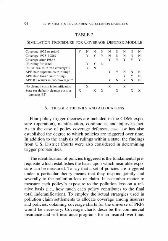
job no. 1969 casualty actuarial society CAS journal 1969D01 [16] 11-08-01 4:58 pm
94 ESTIMATING U.S. ENVIRONMENTAL POLLUTION LIABILITIES
TABLE 2
SIMULATION PROCEDURE FOR COVERAGE DEFENSE MODULE
Coverage 1972 or prior? Y N N N N N N N NCoverage 1973–1986? Y Y Y N N N N NCoverage after 1986? Y Y Y Y YPE ruling for state? Y Y NPE BT results in “no coverage”? Y NAPE state supreme court ruling? Y Y N N NAPE state lower court ruling? Y Y NAPE BT results in “no coverage”? Y N Y N N
No cleanup costs indemnification X X XState (or default) cleanup costs as X X X X X Xdamages BT
6. TRIGGER THEORIES AND ALLOCATIONS
Four policy trigger theories are included in the CDM: expo-sure (operation), manifestation, continuous, and injury-in-fact.As in the case of policy coverage defenses, case law has alsoestablished the degree to which policies are triggered over time.In addition to the analysis of rulings within a state, the findingsfrom U.S. District Courts were also considered in determiningtrigger probabilities.
The identification of policies triggered is the fundamental pre-requisite which establishes the basis upon which insurable expo-sure can be measured. To say that a set of policies are triggeredunder a particular theory means that they respond jointly andseverally to the pollution loss or claim. It is another matter tomeasure each policy’s exposure to the pollution loss on a rel-ative basis (i.e., how much each policy contributes to the finaltotal indemnification). To employ the actual strategies used inpollution claim settlements to allocate coverage among insurersand policies, obtaining coverage charts for the universe of PRPswould be necessary. Coverage charts describe the commercialinsurance and self-insurance programs for an insured over time.

job no. 1969 casualty actuarial society CAS journal 1969D01 [17] 11-08-01 4:58 pm
ESTIMATING U.S. ENVIRONMENTAL POLLUTION LIABILITIES 95
Instead, the PCSM assigns indemnified losses and loss adjust-ment expenses across years based on a simulation of the triggerapplied to that site and PRP combination. In the case of a man-ifestation trigger, only one year is involved. The year associatedwith manifestation is based on the date of a special notice letter,or general notice letter if the former is not applicable.
The PCSM uses a simple method of allocating pollution lossesover time according to the coverage trigger simulated. It is basedon the analysis of a large sample of claims at the insured andsite level that provided exposure (operation) dates and date ofnotice to the insurer. This permitted the estimation of the distri-bution of exposure to pollution loss over time for exposure andcontinuous triggers. Valid actual dates were employed whereverpossible, while simulated dates from the distribution of knownvalid dates were employed for CERCLIS sites without dates andon an aggregate basis for each set of state sites.
The continuous trigger distribution was translated to a condi-tional basis based on the manifestation year described earlier.7
The manifestation year serves as the endpoint for continuoustrigger assignments.
The resulting exposure and continuous trigger distributionswere heavily weighted towards more recent years, parallelingthe increased coverage afforded insureds in general as time goesby. This approach tends to create an element of conservatism tothe industry estimates as greater exposure is be generated fromthe more recent years that afford greater insurance coverage.
The injury-in-fact trigger used the continuous trigger distri-bution, normalized between the first discovery date of pollutionat a site and the notice date to a PRP pertaining to either a spe-cial or general letter from the EPA. This approach represents aconservative assumption as regards industry estimates, becauseit places the earliest date of injury at the first discovery date
7A more precise method would have been to decompose the distributions conditional ondiscovery dates, albeit with limited empirical information to do so.
job no. 1969 casualty actuarial society CAS journal 1969D01 [18] 11-08-01 4:58 pm
96 ESTIMATING U.S. ENVIRONMENTAL POLLUTION LIABILITIES
of pollution rather than the earliest default operation date of1950.
An alternative for measuring operation periods is to simplyemploy the operation dates of a site for those sites with RODscontaining cost estimates. This does not provide for variationamong PRPs for their involvement at a site. These dates and timeperiods must also be extrapolated over the entire population ofhazardous waste sites.
The PCSM does not employ an All Sums, or “Fountain”8
trigger. This trigger tends to create large concentrations of lossesfor a single insured in a single year. The losses may then beallocated or shared among other insurers or reinsurers consideredto be exposed to such losses through settlement of the pollutionclaims. There is less case law precedent on this trigger at thestate level in comparison to other triggers, thereby preventing areliable simulation of this relatively infrequently invoked trigger.However, the trigger is indeed employed by some specific PRPsand against some insurers.
7. LOSS ADJUSTMENT EXPENSE
The concept of duty to defend deals with whether or not aninsurer will incur legal expenses and other loss adjustment ex-penses (LAE) for a pollution claim, even though there is no in-demnification due to a successful coverage defense. Case lawon this subject is quite varied. The PCSM employed a conserva-tive assumption by including all LAE as costs to the insuranceindustry.
A summary of the LAE analysis is presented in Exhibit 3.It is based on analyses performed by the Rand Institute [9].The PCSM simulated the specific LAE to cleanup costs ratiouniformly within the ranges of 23.5% to 29.9%, and 29.9%to 37.0%, with equal probability associated with the lower and
8For example, see [8, p. 122].
job no. 1969 casualty actuarial society CAS journal 1969D01 [19] 11-08-01 4:58 pm
ESTIMATING U.S. ENVIRONMENTAL POLLUTION LIABILITIES 97
upper range. The simulated value was balanced to the estimatedaverage of 29.9% by dividing by the uniform average of 30.25%(i.e., the average of the expectation below and above the mean)in a manner analogous to the procedure employed for the EPAaccuracy factor discussed earlier in Section 3.
Another Rand Institute study [10, p. 51ff] also includes infor-mation that correlates total site transaction costs with the numberof PRPs. An enhancement to the modeling of LAE would beto include such variation with the additional constraint that thesimulated average balance to, or be consistent with, the originalestimate of the mean LAE to cleanup costs ratio.
8. COUNTRYWIDE RESULTS
In order to obtain countrywide results, the contribution fromstate sites must be estimated. The PCSM based these estimateson the frequency and cost figures contained in Exhibit 2. Thestate severities were also used for those CERCLIS sites that weredeemed to be excluded from NPL status, either through simula-tion or through identification as NFRAP. Note that these individ-ual sites were simulated according to the form of the distributionof site costs described earlier, but specific state average severitieswere employed.
Exposure triggers were weighted according to the expectationfor each trigger by state, rather than selecting a single trigger foreach iteration or for each state site. Costs were allocated overtime based on the simulation of default dates. Each iteration ofthe PCSM performed one random selection by state for aver-age site cost, each trigger default date, and the ratio of LAE tocleanup costs.
Exhibit 4 shows the estimates of pollution losses and the al-location over time. The distribution of insurance coverages wascensored at 1950 (i.e., the contributions to exposure for yearsprior to 1950 were added into 1950). It could be argued thatsome relevant coverage would have been provided by com-mercial general liability policies as early as 1940. However,
job no. 1969 casualty actuarial society CAS journal 1969D01 [20] 11-08-01 4:58 pm
98 ESTIMATING U.S. ENVIRONMENTAL POLLUTION LIABILITIES
although the author is aware of exposure for one type of site(manufactured gas plants) where exposure is claimed to exist asfar back as the 1840s, it is extremely unlikely that any propertyand casualty policies provided indemnification that far in thepast.
A few remarks concerning Exhibit 4 are in order. First andforemost is the magnitude of the estimate. It is approximately$70 billion (the total of the columns from all three pages ofExhibit 4), which is higher than the $56 billion estimate pub-lished in “BestWeek.”9 The difference is likely understated asthe “BestWeek” estimate presumably includes third party bodilyinjury claims and Natural Resource Damage claims.
Second, a comparison between the simulated mean of totalcleanup costs to indemnified costs indicates that very close to50% of costs were not insured as a result of the applicationof the parameters contained in the CDM. This compares withthe 40% reduction in insurable costs disclosed by “BestWeek”10
associated with successful coverage defense.
Third, no underlying limits were introduced, which wouldhave served to reduce the estimates. This is a conservative PCSMassumption. The author has witnessed insurance settlements thatbelie the conventional wisdom associated with the introductionof underlying deductibles, self-insured retentions, or the use ofunderlying limits for excess coverages. Underlying limits havespecific application to the analysis of reinsurance portfolios.
Fourth, the estimate of pollution losses over time permits oneto perform a more refined exposure analysis lacking specific in-sured information for a portfolio.11 For example, a market share
9See [21, p. P/C 6] and [22, p. 4].10See [20, p. P/C 7] where Insurers’ Liability %, footnote D, refers to “settlements andcases won by insurers.”11This is in lieu of another possible estimate based on the use of actual pollution claims,which the author has developed in a manner to remove the bias introduced by the emer-gence of the potentially most serious claims in the insured portfolio (nominally thoserelated to NPL sites).

job no. 1969 casualty actuarial society CAS journal 1969D01 [21] 11-08-01 4:58 pm
ESTIMATING U.S. ENVIRONMENTAL POLLUTION LIABILITIES 99
approach uses premiums as the exposure medium which can bematched against the relevant pollution estimates for the exposedyears.
Finally, the simulation of costs at the state level for non-CERCLIS sites tends to contribute greater variation than thatafforded by individual site simulation that is performed usingCERCLIS.
9. PORTFOLIO APPLICATIONS
The countrywide analysis and simulation form the kernel ofthe estimation for a specific portfolio. The simulation for a port-folio is streamlined somewhat by the initial restriction of sites tothose matched to the PRPs embedded in the portfolio. Specificinformation on such items as trigger theories, dates of operation,or PRP shares are used wherever possible at the site and PRPlevel.
The simulated costs by PRP, site, and year are normallymatched to the coverage parameters of the policies issued for thatinsured. The parameters can usually be limited to an attachmentpoint, limit or layer of coverage, and participation when directexcess insuranceor reinsurance is involved. Other coverage pa-rameters can also be included such as aggregate retentions forexcess policies. Deductibles can also be employed, although it isthe author’s experience that a limited amount of deductible cov-erages for Other Liability were offered through the mid 1980s.
The identification of the PRPs in the portfolio and the match-ing to those contained in SETS is the most time-consuming effortin a portfolio application. It is further complicated by the need toconsider the aggregation of costs for a single insured due to li-ability derived from subsidiaries, and the alternate identificationof an insured through aliases. The simulation proper is then seenas employing one of two possible representations of the portfo-lio. The first is where an exhaustive identification and match-ing of insureds and PRPs has been made that characterizes the

job no. 1969 casualty actuarial society CAS journal 1969D01 [22] 11-08-01 4:58 pm
100 ESTIMATING U.S. ENVIRONMENTAL POLLUTION LIABILITIES
portfolio. The other is where a sample of insureds within theportfolio has been identified.
In the case of a complete characterization of the portfolio, theextrapolation to an ultimate basis needs to consider the expectedcosts on sites that have not been specifically associated with theknown PRPs identified in the portfolio. This would include esti-mates related to sites found only on state lists and the potentialfor future NPL sites to be associated with the PRPs in the portfo-lio. It is also prudent in such circumstances to include additionalcosts related to RODs to be issued in the future on known NPLsites related to portfolio PRPs. Discussion of such estimates infurther detail is beyond the scope of this paper.
For the case where a sample of the portfolio has been simu-lated, Appendix D contains the derivation of a scalar that permitsthe extrapolation of the simulation results to the entire portfolio.Under these conditions the estimate will be biased downwardsdue to the inability to identify all PRPs embedded in a portfolioas discussed in Appendix D. This method may be enhanced byincluding some element of a market share exposure analysis asalluded to earlier.
10. WHERE DO WE GO FROM HERE?
There is a great deal of uncertainty surrounding the ultimatecost of pollution cleanup from inactive hazardous waste sites inthis country. Unfortunately, the model presented herein, as wellas any other, will for some considerable length of time sufferfrom model specification error of immeasurable magnitude.
The degree to which there are repeatable occurrences or eventsfrom which to base projections varies among the componentsand processes underlying the phenomenon of pollution cleanup.On the one hand, it took a study of only 18 Superfund sitesto provide enough material for the Rand Institute to publish aleading work in this area. On the other hand, there are on theorder of 1,000 CERCLIS sites with varying degrees of complete

job no. 1969 casualty actuarial society CAS journal 1969D01 [23] 11-08-01 4:58 pm
ESTIMATING U.S. ENVIRONMENTAL POLLUTION LIABILITIES 101
cost information; with such varying circumstances, the estimatedaverages must by necessity have a great deal of uncertainty.
There is considerable uncertainty in extrapolating any aver-ages, as many of the site characteristics that could serve as pre-dictive elements in a model are lacking from publicly availableinformation. For example, it is of limited predictive value to em-ploy average site cleanup costs by standard industry classification(SIC) if the thousands of sites that remain without cleanup costsare not identified by SIC.
At the end of the day, the task at hand is to project activitiesand costs that will take place in the future, without the familiarhistorical information that actuaries might use in development(extrapolation) estimates, regression models, or other methodsof estimation that rely to varying degrees on the observation ofactual insurance losses. Indeed, there is anecdotal evidence toshow that cost figures from RODs turn out to be quite differ-ent from actual expenditures,12 thereby casting additional doubton the reliability of some of the harder numbers that underliethese analyses. The costs of remedial investigations and feasibil-ity studies also increase costs and, if the decision by the Califor-nia Supreme Court in the Aerojet-General case on December 29,1997 sets a precedent, such costs will be subject to indemnifica-tion by insurance companies. Indeed, that decision also affectshow pollution losses would trigger insurance policies over timewhen self-insurance is involved.
The point of this brief discussion is that there are many signsindicating higher ultimate paid costs, and very few that pointin the other direction. The continuation of perceived downwardtrends in remediation costs may be altogether uncertain if fund-ing for the requisite continued research is discontinued, or if there
12According to an article on page B-1 from The Philadelphia Inquirer of August 14, 1997,the GEMS Landfill in New Jersey will require $62 million in capital costs to cleanup,well in excess of any readily available estimates from RODs and elsewhere that are onthe order of $27 million in capital costs.

job no. 1969 casualty actuarial society CAS journal 1969D01 [24] 11-08-01 4:58 pm
102 ESTIMATING U.S. ENVIRONMENTAL POLLUTION LIABILITIES
are disincentives for insureds to engage in voluntary cleanup ef-forts at reduced costs. In addition, the distribution of losses overtime for indemnification by insurance policies is a phenomenonthat continues to undergo change.
From an insurance perspective, the focus of the balance sheetis on liabilities. Given an estimate of ultimate insured costs, thequestion that remains to be answered is how much is there leftto be paid? From an economic perspective, the timing of thosepayments should provide insight as to their present value.
The matching of payments and ultimate costs cannot be doneby simply subtracting payments to date from the ultimate es-timates. It is more proper to subtract expected payments fromultimates. Failure to do so can lead to erroneous results suchas in the GEMS Landfill case alluded to earlier in a footnote.Further, there is some uncertainty as to the reliability of prop-erly matching payments against these liabilities. At a minimumthis is caused by the lack of separate identification of such earlycosts in the records of insurers. Models could be created to fab-ricate an answer, but it is a topic that requires further researchfor resolution.
Finally, some concerted efforts may be needed to obtain up-dated and reliable information on state administered sites [24].The evidence so far indicates substantial costs from this source,yet the level of available information does not approach thatavailable for many NPL sites. Indeed, the volume of such data,if available, would present a challenge to its use in the samemanner as that employed for NPL sites.

job no. 1969 casualty actuarial society CAS journal 1969D01 [25] 11-08-01 4:58 pm
ESTIMATING U.S. ENVIRONMENTAL POLLUTION LIABILITIES 103
REFERENCES
[1] Casualty Actuarial Society and Society of Actuaries, “Gen-eral Principles of Actuarial Science,” discussion draft datedAugust 15, 1998.
[2] Finkelstein, Steven J., “Dirty Words,” PCAS LXXXVI,1999.
[3] United States Environmental Protection Agency, Recordsof Decision (RODs)—downloaded directly from the EPAInternet site during calendar year 1997.
[4] Resources for the Future, RFF Database of Superfund NPLSites.
[5] United States Environmental Protection Agency, RemedialProgram Manager (RPM) Site Data Base and Users Guideto the RPM Site Data, January 1995.
[6] United States Environmental Protection Agency, Compre-hensive Environmental Response, Compensation, and Lia-bility Information System (CERCLIS) site lists, current andarchived, downloaded September 27, 1997.
[7] United States Environmental Protection Agency, Site En-forcement Tracking System (SETS) data base, accessedFebruary 1997.
[8] Bouska, Amy and TomMcIntyre, “Measurement of US Pol-lution Liabilities,” Casualty Actuarial Society Forum, Sum-mer 1994, pp. 73–160.
[9] Rand Institute for Civil Justice, Private Sector CleanupExpenditures and Transaction Costs at 18 Superfund Sites,1993.
[10] Rand Institute for Civil Justice, Superfund and TransactionCosts—The Experience of Insurers and Very Large IndustrialFirms, 1992.
[11] Association of State and Territorial Solid Waste Man-agement Officials and the U.S. Environmental ProtectionAgency, A Report on State/Territory Non-NPL HazardousWaste Site Cleanup Efforts for the Period 1980–1992, July1994.

job no. 1969 casualty actuarial society CAS journal 1969D01 [26] 11-08-01 4:58 pm
104 ESTIMATING U.S. ENVIRONMENTAL POLLUTION LIABILITIES
[12] Environmental Law Institute, An Analysis of State SuperfundPrograms: 50-State Study, 1995 Update, 1996.
[13] American Re-Insurance Company, A Review of Environmen-tal Coverage Case Law, 1997 and prior editions.
[14] General Reinsurance Company, 1997 Environmental ClaimsCase Law, 1997.
[15] Joint Institute For Energy & Environment, Resource Re-quirements for NPL Sites, 1996.
[16] Office of Emergency and Remedial Response, Guidance forConducting Remedial Investigations and Feasibility StudiesUnder CERCLA-Interim Final, October 1988.
[17] CERCLIS information from the Right to Know Network.
[18] American Academy of Actuaries, Costs Under Superfund,August 1995.
[19] The Congress of the United States Congressional BudgetOffice, The Total Costs of Cleaning Up Nonfederal SuperfundSites, January 1994.
[20] A.M. Best, “BestWeek Property/Casualty Supplement,”January 29, 1996.
[21] A.M. Best, “BestWeek Property/Casualty Supplement,”September 8, 1997.
[22] A.M. Best, “BestWeek Property/Casualty Supplement,”September 21, 1998.
[23] The Brookings Institution and Resources for the Future,Footing the Bill for Superfund Cleanups, 1995.
[24] Bhagavatula, R. R. and S. Sullivan, “What To Do With TheSuperfund Rejects” Contingencies, American Academy ofActuaries, March/April 1999, p. 36.

job no. 1969 casualty actuarial society CAS journal 1969D01 [27] 11-08-01 4:58 pm
ESTIMATING U.S. ENVIRONMENTAL POLLUTION LIABILITIES 105
EXHIBIT 1-A
SITE CHARACTERISTICS AND COST ANALYSES BY STATECERCLIS SOURCE: ARCHIVE
NUMBER OF SITESNPL STATUS
NFRAPState NPL Deleted Final Removed NFRAP NotID Site NPL NPL NPL Federal Federal Total
AK . . . . 131 130 261AL . . . . 12 563 575AR . . . 1 5 343 349AS . . . . 2 4 6AZ . . . 2 18 699 719CA . . . 8 92 2,434 2,534CM . . . . . 6 6CO . . . . 35 408 443CT . . . . 2 327 329DC . . . . 10 10 20DE . . . . 1 221 222FL . . . 2 34 552 588GA . . . . 11 723 734GU . . . . 10 3 13HI . . . 6 20 104 130IA . . . . 1 402 403ID . . . 1 67 134 202IL . 1 . 3 3 1,284 1,291IN . 5 . 2 2 1,433 1,442KS . . . . 2 339 341KY . . . . 4 487 491LA . . . . 14 525 539MA . . . . 8 516 524MD . . . . 11 309 320ME . . . . 8 103 111MI . 6 1 5 11 1,495 1,518MN . 12 . . 2 407 421MO . . . . 7 906 913MS . . . 2 6 374 382MT . . . . 16 177 193NC . . . . 8 687 695ND . . . . 7 58 65NE . . . . 4 235 239NH . . . . 3 62 65NJ 2 . . . 23 926 951NM . . . . 30 266 296
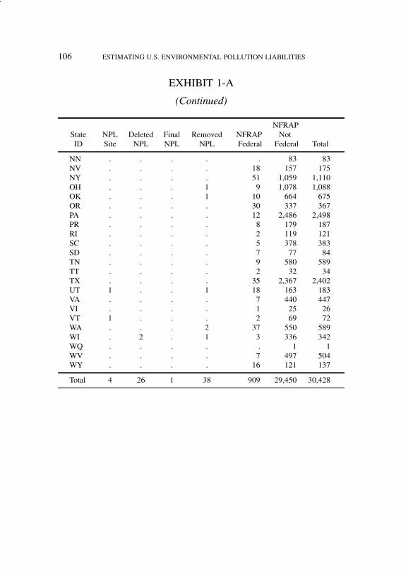
job no. 1969 casualty actuarial society CAS journal 1969D01 [28] 11-08-01 4:58 pm
106 ESTIMATING U.S. ENVIRONMENTAL POLLUTION LIABILITIES
EXHIBIT 1-A
(Continued)
NFRAPState NPL Deleted Final Removed NFRAP NotID Site NPL NPL NPL Federal Federal Total
NN . . . . . 83 83NV . . . . 18 157 175NY . . . . 51 1,059 1,110OH . . . 1 9 1,078 1,088OK . . . 1 10 664 675OR . . . . 30 337 367PA . . . . 12 2,486 2,498PR . . . . 8 179 187RI . . . . 2 119 121SC . . . . 5 378 383SD . . . . 7 77 84TN . . . . 9 580 589TT . . . . 2 32 34TX . . . . 35 2,367 2,402UT 1 . . 1 18 163 183VA . . . . 7 440 447VI . . . . 1 25 26VT 1 . . . 2 69 72WA . . . 2 37 550 589WI . 2 . 1 3 336 342WQ . . . . . 1 1WV . . . . 7 497 504WY . . . . 16 121 137
Total 4 26 1 38 909 29,450 30,428

job no. 1969 casualty actuarial society CAS journal 1969D01 [29] 11-08-01 4:58 pm
ESTIMATING U.S. ENVIRONMENTAL POLLUTION LIABILITIES 107
EXHIBIT 1-B
SITE CHARACTERISTICS AND COST ANALYSES BY STATECERCLIS SOURCE: ACTIVE
NUMBER OF SITESNPL STATUS
NotFederal Federal
State NPL Deleted Final Not Proposed Not RemovedID Site NPL NPL NPL NPL NPL NPL Total
AK 1 1 7 46 . 49 . 104AL . 1 12 15 1 110 . 139AR . 1 12 2 . 42 2 59AS . 1 . . . 1 . 2AZ 3 1 10 11 . 162 . 187CA 14 3 90 100 4 424 6 641CM . 1 . . . 2 . 3CO . 1 16 11 2 132 1 163CT 18 1 15 3 . 409 . 446DC . . . 8 . 9 1 18DE . 2 18 2 . 30 3 55FL 1 7 55 10 2 405 3 483GA . 1 15 6 1 243 1 267GU . . 2 12 . . . 14HI 6 . 4 22 . 37 . 69IA 5 4 16 15 1 189 6 236ID 4 1 8 17 2 29 . 61IL 7 . 38 9 3 339 . 396IN . . 30 9 1 157 1 198KS 1 5 10 7 1 202 1 227KY . . 20 13 . 90 . 123LA . . 14 3 3 70 . 90MA 7 1 30 9 . 459 . 506MD . 2 13 45 3 72 1 136ME . . 12 . . 88 . 100MH . . . . . 1 . 1MI . 4 71 9 2 148 1 235MN . 2 29 2 1 53 . 87MO 16 1 22 29 . 347 2 417MQ . . . 1 . . . 1MS . 2 1 5 2 58 1 69MT . . 8 8 1 31 1 49NC . 1 23 25 . 176 1 226ND . . 2 1 . 7 . 10NE 19 . 10 18 . 122 2 171NH 8 . 18 2 . 107 . 135

job no. 1969 casualty actuarial society CAS journal 1969D01 [30] 11-08-01 4:58 pm
108 ESTIMATING U.S. ENVIRONMENTAL POLLUTION LIABILITIES
EXHIBIT 1-B
(Continued)
NotFederal Federal
State NPL Deleted Final Not Proposed Not RemovedID Site NPL NPL NPL NPL NPL NPL Total
NJ 6 9 106 10 . 669 2 802NM . 1 10 17 1 61 . 90NN . . . . . 68 . 68NV . . 1 10 . 17 . 28NY . 10 78 11 1 521 . 621OH . 1 34 7 4 212 . 258OK . . 10 18 1 106 1 136OR 6 2 10 11 1 45 . 75PA . 10 100 16 2 394 2 524PR . . 9 4 1 72 . 86RI 24 . 12 7 . 150 . 193SC . 1 26 8 . 140 . 175SD . . 3 1 1 23 . 28TN . 1 17 18 1 260 1 298TT . 1 . . . 4 . 5TX . 5 26 21 1 175 2 230UT . . 12 4 4 122 2 144VA . 2 25 37 . 166 1 231VI . . 2 1 . 8 . 11VT 4 . 8 . . 64 . 76WA 52 10 48 24 2 43 . 179WI . . 40 20 . 92 . 152WQ . . . 1 . . . 1WV . 1 6 1 1 57 1 67WY . . 3 1 . 23 . 27
Total 202 98 1,217 723 51 8,292 46 10,629
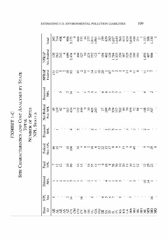
job no. 1969 casualty actuarial society CAS journal 1969D01 [31] 11-08-01 4:58 pm
ESTIMATING U.S. ENVIRONMENTAL POLLUTION LIABILITIES 109
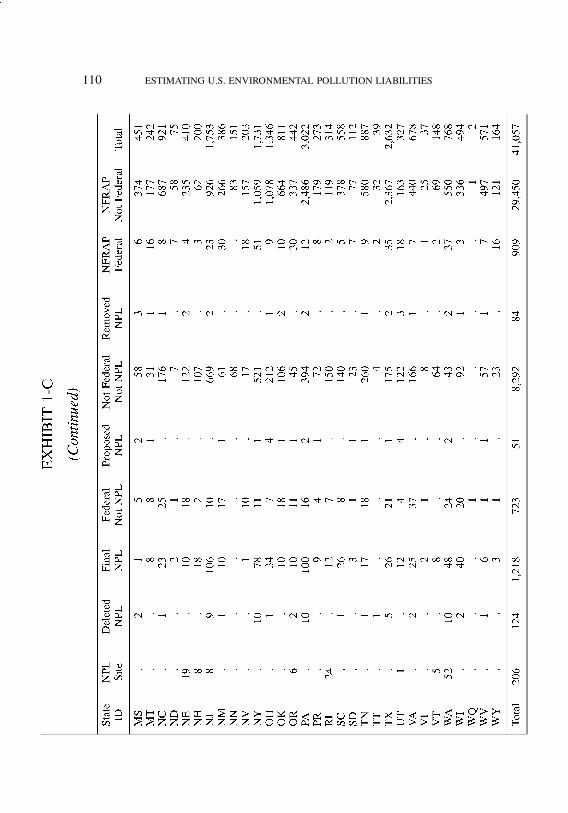
job no. 1969 casualty actuarial society CAS journal 1969D01 [32] 11-08-01 4:58 pm
110 ESTIMATING U.S. ENVIRONMENTAL POLLUTION LIABILITIES
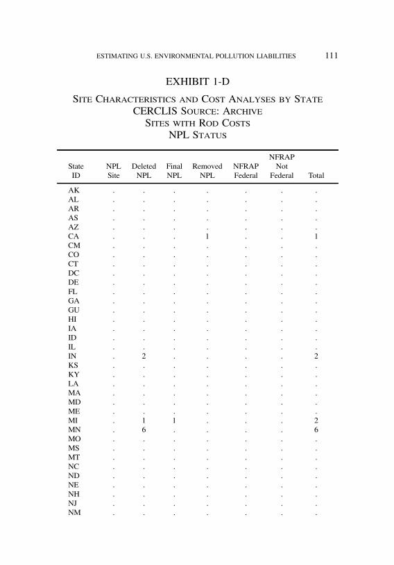
job no. 1969 casualty actuarial society CAS journal 1969D01 [33] 11-08-01 4:58 pm
ESTIMATING U.S. ENVIRONMENTAL POLLUTION LIABILITIES 111
EXHIBIT 1-D
Site Characteristics and Cost Analyses by StateCERCLIS Source: ArchiveSites with Rod Costs
NPL Status
NFRAPState NPL Deleted Final Removed NFRAP NotID Site NPL NPL NPL Federal Federal Total
AK . . . . . . .AL . . . . . . .AR . . . . . . .AS . . . . . . .AZ . . . . . . .CA . . . 1 . . 1CM . . . . . . .CO . . . . . . .CT . . . . . . .DC . . . . . . .DE . . . . . . .FL . . . . . . .GA . . . . . . .GU . . . . . . .HI . . . . . . .IA . . . . . . .ID . . . . . . .IL . . . . . . .IN . 2 . . . . 2KS . . . . . . .KY . . . . . . .LA . . . . . . .MA . . . . . . .MD . . . . . . .ME . . . . . . .MI . 1 1 . . . 2MN . 6 . . . . 6MO . . . . . . .MS . . . . . . .MT . . . . . . .NC . . . . . . .ND . . . . . . .NE . . . . . . .NH . . . . . . .NJ . . . . . . .NM . . . . . . .

job no. 1969 casualty actuarial society CAS journal 1969D01 [34] 11-08-01 4:58 pm
112 ESTIMATING U.S. ENVIRONMENTAL POLLUTION LIABILITIES
EXHIBIT 1-D
(Continued)
NFRAPState NPL Deleted Final Removed NFRAP NotID Site NPL NPL NPL Federal Federal Total
NN . . . . . . .NV . . . . . . .NY . . . . . . .OH . . . . . . .OK . . . . . . .OR . . . . . . .PA . . . . . . .PR . . . . . . .RI . . . . . . .SC . . . . . . .SD . . . . . . .TN . . . . . . .TT . . . . . . .TX . . . . . . .UT . . . . . . .VA . . . . . . .VI . . . . . . .VT . . . . . . .WA . . . . . . .WI . . . . . . .WQ . . . . . . .WV . . . . . . .WY . . . . . . .
Total . 9 1 1 . . 11
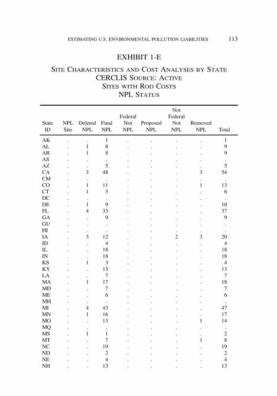
job no. 1969 casualty actuarial society CAS journal 1969D01 [35] 11-08-01 4:58 pm
ESTIMATING U.S. ENVIRONMENTAL POLLUTION LIABILITIES 113
EXHIBIT 1-E
Site Characteristics and Cost Analyses by StateCERCLIS Source: ActiveSites with Rod Costs
NPL Status
NotFederal Federal
State NPL Deleted Final Not Proposed Not RemovedID Site NPL NPL NPL NPL NPL NPL Total
AK . . 1 . . . . 1AL . 1 8 . . . . 9AR . 1 8 . . . . 9AS . . . . . . . .AZ . . 5 . . . . 5CA . 3 48 . . . 3 54CM . . . . . . . .CO . 1 11 . . . 1 13CT . 1 5 . . . . 6DC . . . . . . . .DE . 1 9 . . . . 10FL . 4 33 . . . . 37GA . . 9 . . . . 9GU . . . . . . . .HI . . . . . . . .IA . 3 12 . . 2 3 20ID . . 4 . . . . 4IL . . 18 . . . . 18IN . . 18 . . . . 18KS . 1 3 . . . . 4KY . . 13 . . . . 13LA . . 7 . . . . 7MA . 1 17 . . . . 18MD . . 7 . . . . 7ME . . 6 . . . . 6MH . . . . . . . .MI . 4 43 . . . . 47MN . 1 16 . . . . 17MO . . 13 . . . 1 14MQ . . . . . . . .MS . 1 1 . . . . 2MT . . 7 . . . 1 8NC . . 19 . . . . 19ND . . 2 . . . . 2NE . . 4 . . . . 4NH . . 13 . . . . 13

job no. 1969 casualty actuarial society CAS journal 1969D01 [36] 11-08-01 4:58 pm
114 ESTIMATING U.S. ENVIRONMENTAL POLLUTION LIABILITIES
EXHIBIT 1-E
(Continued)
NotFederal Federal
State NPL Deleted Final Not Proposed Not RemovedID Site NPL NPL NPL NPL NPL NPL Total
NJ . 5 74 . . . . 79NM . . 7 . . . . 7NN . . . . . . . .NV . . . . . . . .NY . 5 52 . . 1 . 58OH . . 24 . . . . 24OK . . 9 . . . . 9OR . 1 5 . . . . 6PA . 6 62 . . . . 68PR . . 6 . . 1 . 7RI . . 8 . . . . 8SC . 1 15 . . . . 16SD . . 1 . . . . 1TN . 1 11 . . . . 12TT . . . . . . . .TX . 3 20 . . . . 23UT . . 8 . . . . 8VA . 1 15 . . . . 16VI . . . . . . . .VT . . 2 . . . . 2WA . 4 20 . . 1 . 25WI . . 25 . . . . 25WQ . . . . . . . .WV . 1 3 . . . . 4WY . . . . . . . .
Total . 51 727 . . 5 9 792
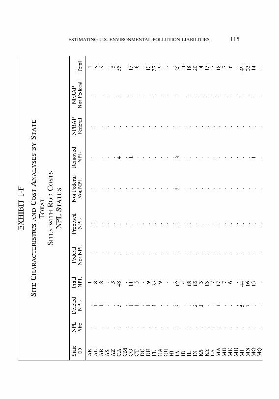
job no. 1969 casualty actuarial society CAS journal 1969D01 [37] 11-08-01 4:58 pm
ESTIMATING U.S. ENVIRONMENTAL POLLUTION LIABILITIES 115
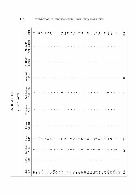
job no. 1969 casualty actuarial society CAS journal 1969D01 [38] 11-08-01 4:58 pm
116 ESTIMATING U.S. ENVIRONMENTAL POLLUTION LIABILITIES

job no. 1969 casualty actuarial society CAS journal 1969D01 [39] 11-08-01 4:58 pm
ESTIMATING U.S. ENVIRONMENTAL POLLUTION LIABILITIES 117

job no. 1969 casualty actuarial society CAS journal 1969D01 [40] 11-08-01 4:58 pm
118 ESTIMATING U.S. ENVIRONMENTAL POLLUTION LIABILITIES
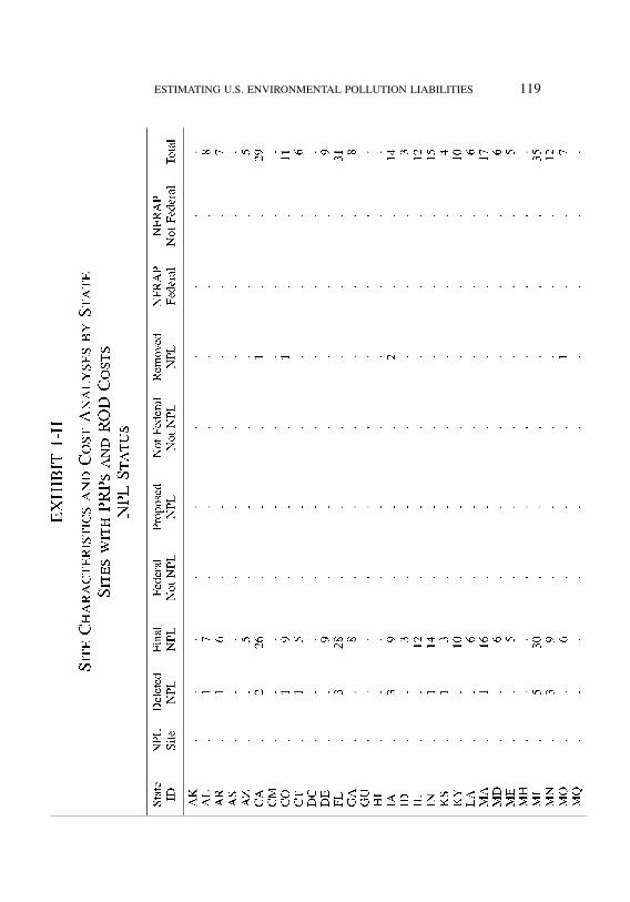
job no. 1969 casualty actuarial society CAS journal 1969D01 [41] 11-08-01 4:58 pm
ESTIMATING U.S. ENVIRONMENTAL POLLUTION LIABILITIES 119

job no. 1969 casualty actuarial society CAS journal 1969D01 [42] 11-08-01 4:58 pm
120 ESTIMATING U.S. ENVIRONMENTAL POLLUTION LIABILITIES

job no. 1969 casualty actuarial society CAS journal 1969D01 [43] 11-08-01 4:58 pm
ESTIMATING U.S. ENVIRONMENTAL POLLUTION LIABILITIES 121
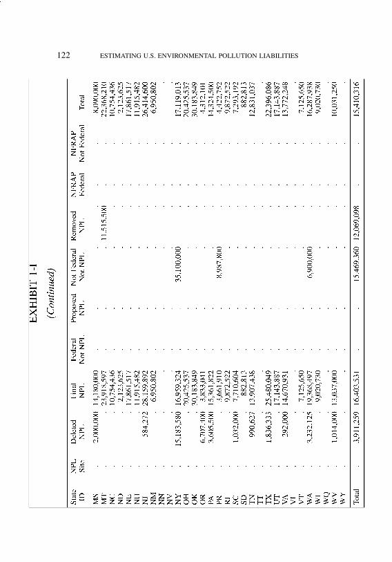
job no. 1969 casualty actuarial society CAS journal 1969D01 [44] 11-08-01 4:58 pm
122 ESTIMATING U.S. ENVIRONMENTAL POLLUTION LIABILITIES

job no. 1969 casualty actuarial society CAS journal 1969D01 [45] 11-08-01 4:58 pm
ESTIMATING U.S. ENVIRONMENTAL POLLUTION LIABILITIES 123
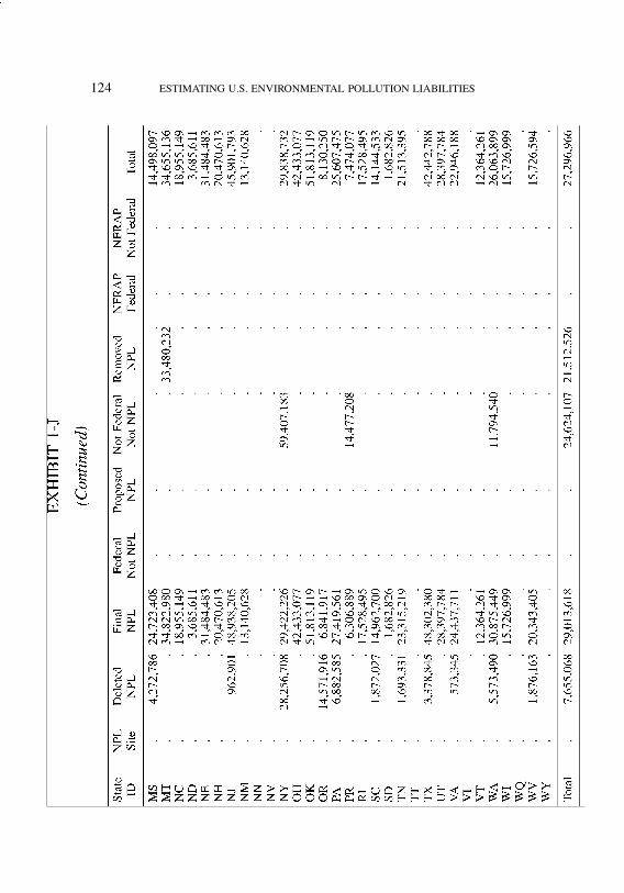
job no. 1969 casualty actuarial society CAS journal 1969D01 [46] 11-08-01 4:58 pm
124 ESTIMATING U.S. ENVIRONMENTAL POLLUTION LIABILITIES

job no. 1969 casualty actuarial society CAS journal 1969D01 [47] 11-08-01 4:58 pm
ESTIMATING U.S. ENVIRONMENTAL POLLUTION LIABILITIES 125
EXHIBIT 1-K
Site Characteristics and Cost Analyses by StateNon-Federal NPL Sites OnlyEstimated Nominal Cost
AverageNPL Status
StateID Deleted NPL Final NPL Total
AL 2,374,500 57,706,560 49,801,980AR 112,866 34,594,560 30,763,261AZ . 33,974,328 33,974,328CA 1,408,865 38,489,931 36,017,860CO 13,496,520 25,706,217 24,485,247CT 445,131 20,108,342 16,831,140DE 812,746 29,347,048 26,176,570FL 3,996,810 14,062,275 12,974,116GA . 14,475,330 14,475,330IA 4,676,223 5,311,589 5,184,516ID . 68,814,810 68,814,810IL . 22,546,175 22,546,175IN 180,613 31,098,616 28,006,816KS 2,773,107 12,351,631 9,957,000KY . 18,475,011 18,475,011LA . 47,050,720 47,050,720MA 738,864 31,503,896 29,694,188MD . 14,335,113 14,335,113ME . 13,215,305 13,215,305MI 7,992,494 28,797,108 26,674,188MN 19,681,607 8,985,890 12,194,605MO . 16,710,321 16,710,321MS 4,272,786 24,723,408 14,498,097MT . 34,822,980 34,822,980NC . 18,703,327 18,703,327ND . 3,685,611 3,685,611NE . 31,484,483 31,484,483NH . 19,524,436 19,524,436NJ 962,901 50,405,342 47,152,550NM . 14,949,158 14,949,158NY 28,256,708 29,828,770 29,688,407OH . 42,039,226 42,039,226OK . 55,356,542 55,356,542OR 14,571,916 7,180,084 8,658,451
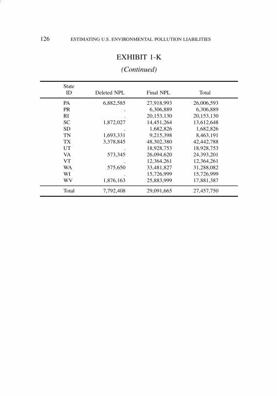
job no. 1969 casualty actuarial society CAS journal 1969D01 [48] 11-08-01 4:58 pm
126 ESTIMATING U.S. ENVIRONMENTAL POLLUTION LIABILITIES
EXHIBIT 1-K
(Continued)
StateID Deleted NPL Final NPL Total
PA 6,882,585 27,918,993 26,006,593PR . 6,306,889 6,306,889RI . 20,153,130 20,153,130SC 1,872,027 14,451,264 13,612,648SD . 1,682,826 1,682,826TN 1,693,331 9,215,398 8,463,191TX 3,378,845 48,302,380 42,442,788UT . 18,928,753 18,928,753VA 573,345 26,094,620 24,393,201VT . 12,364,261 12,364,261WA 575,650 33,481,827 31,288,082WI . 15,726,999 15,726,999WV 1,876,163 25,883,999 17,881,387
Total 7,792,408 29,091,665 27,457,750
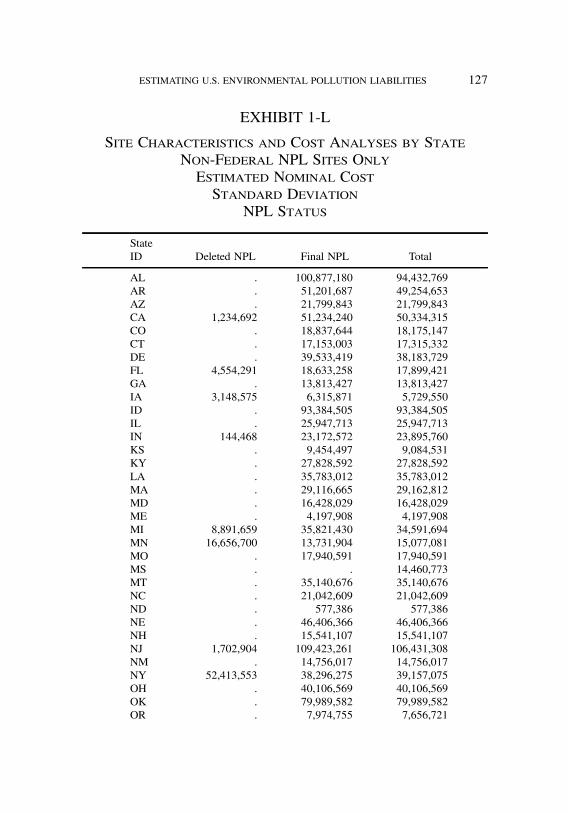
job no. 1969 casualty actuarial society CAS journal 1969D01 [49] 11-08-01 4:58 pm
ESTIMATING U.S. ENVIRONMENTAL POLLUTION LIABILITIES 127
EXHIBIT 1-L
Site Characteristics and Cost Analyses by StateNon-Federal NPL Sites OnlyEstimated Nominal CostStandard Deviation
NPL Status
StateID Deleted NPL Final NPL Total
AL . 100,877,180 94,432,769AR . 51,201,687 49,254,653AZ . 21,799,843 21,799,843CA 1,234,692 51,234,240 50,334,315CO . 18,837,644 18,175,147CT . 17,153,003 17,315,332DE . 39,533,419 38,183,729FL 4,554,291 18,633,258 17,899,421GA . 13,813,427 13,813,427IA 3,148,575 6,315,871 5,729,550ID . 93,384,505 93,384,505IL . 25,947,713 25,947,713IN 144,468 23,172,572 23,895,760KS . 9,454,497 9,084,531KY . 27,828,592 27,828,592LA . 35,783,012 35,783,012MA . 29,116,665 29,162,812MD . 16,428,029 16,428,029ME . 4,197,908 4,197,908MI 8,891,659 35,821,430 34,591,694MN 16,656,700 13,731,904 15,077,081MO . 17,940,591 17,940,591MS . . 14,460,773MT . 35,140,676 35,140,676NC . 21,042,609 21,042,609ND . 577,386 577,386NE . 46,406,366 46,406,366NH . 15,541,107 15,541,107NJ 1,702,904 109,423,261 106,431,308NM . 14,756,017 14,756,017NY 52,413,553 38,296,275 39,157,075OH . 40,106,569 40,106,569OK . 79,989,582 79,989,582OR . 7,974,755 7,656,721

job no. 1969 casualty actuarial society CAS journal 1969D01 [50] 11-08-01 4:58 pm
128 ESTIMATING U.S. ENVIRONMENTAL POLLUTION LIABILITIES
EXHIBIT 1-L
(Continued)
StateID Deleted NPL Final NPL Total
PA 5,105,863 37,916,318 36,661,725PR . 3,617,667 3,617,667RI . 17,108,656 17,108,656SC . 24,593,799 23,920,706SD . . .TN . 7,584,365 7,535,871TX 1,650,193 57,319,885 55,471,504UT . 13,778,021 13,778,021VA . 32,381,314 31,891,620VT . 17,044,091 17,044,091WA . 38,743,582 38,288,823WI . 13,016,710 13,016,710WV . 6,327,381 14,565,139
Total 17,610,317 49,742,140 48,371,328
Abbreviation: Delt = Deleted
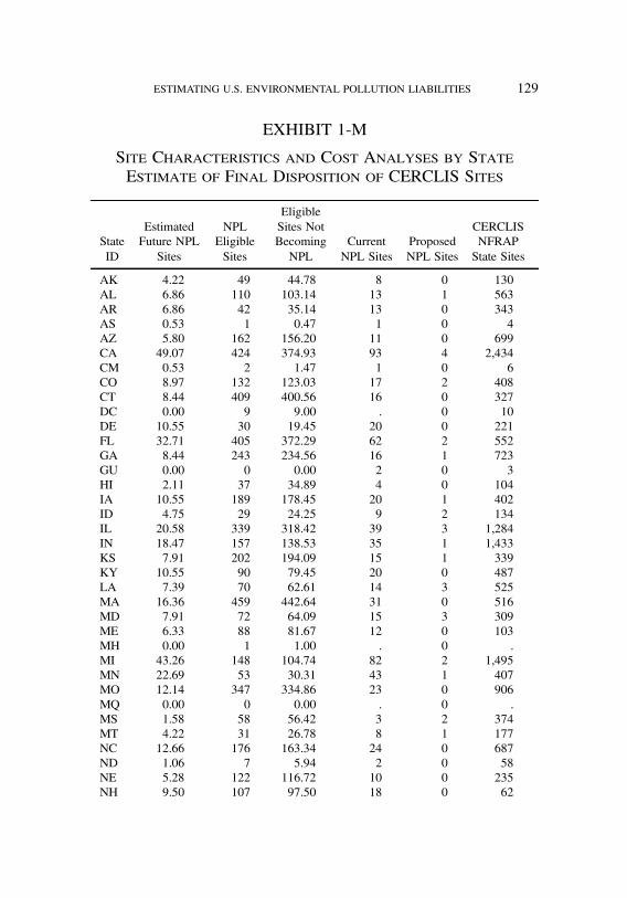
job no. 1969 casualty actuarial society CAS journal 1969D01 [51] 11-08-01 4:58 pm
ESTIMATING U.S. ENVIRONMENTAL POLLUTION LIABILITIES 129
EXHIBIT 1-M
Site Characteristics and Cost Analyses by StateEstimate of Final Disposition of CERCLIS Sites
EligibleEstimated NPL Sites Not CERCLIS
State Future NPL Eligible Becoming Current Proposed NFRAPID Sites Sites NPL NPL Sites NPL Sites State Sites
AK 4.22 49 44.78 8 0 130AL 6.86 110 103.14 13 1 563AR 6.86 42 35.14 13 0 343AS 0.53 1 0.47 1 0 4AZ 5.80 162 156.20 11 0 699CA 49.07 424 374.93 93 4 2,434CM 0.53 2 1.47 1 0 6CO 8.97 132 123.03 17 2 408CT 8.44 409 400.56 16 0 327DC 0.00 9 9.00 . 0 10DE 10.55 30 19.45 20 0 221FL 32.71 405 372.29 62 2 552GA 8.44 243 234.56 16 1 723GU 0.00 0 0.00 2 0 3HI 2.11 37 34.89 4 0 104IA 10.55 189 178.45 20 1 402ID 4.75 29 24.25 9 2 134IL 20.58 339 318.42 39 3 1,284IN 18.47 157 138.53 35 1 1,433KS 7.91 202 194.09 15 1 339KY 10.55 90 79.45 20 0 487LA 7.39 70 62.61 14 3 525MA 16.36 459 442.64 31 0 516MD 7.91 72 64.09 15 3 309ME 6.33 88 81.67 12 0 103MH 0.00 1 1.00 . 0 .MI 43.26 148 104.74 82 2 1,495MN 22.69 53 30.31 43 1 407MO 12.14 347 334.86 23 0 906MQ 0.00 0 0.00 . 0 .MS 1.58 58 56.42 3 2 374MT 4.22 31 26.78 8 1 177NC 12.66 176 163.34 24 0 687ND 1.06 7 5.94 2 0 58NE 5.28 122 116.72 10 0 235NH 9.50 107 97.50 18 0 62

job no. 1969 casualty actuarial society CAS journal 1969D01 [52] 11-08-01 4:58 pm
130 ESTIMATING U.S. ENVIRONMENTAL POLLUTION LIABILITIES
EXHIBIT 1-M
(Continued)
EligibleEstimated NPL Sites Not CERCLIS
State Future NPL Eligible Becoming Current Proposed NFRAPID Sites Sites NPL NPL Sites NPL Sites State Sites
NJ 60.68 669 608.32 115 0 926NM 5.80 61 55.20 11 1 266NN 0.00 68 68.00 . 0 83NV 0.53 17 16.47 1 0 157NY 46.43 521 474.57 88 1 1,059OH 18.47 212 193.53 35 4 1,078OK 5.28 106 100.72 10 1 664OR 6.33 45 38.67 12 1 337PA 58.04 394 335.96 110 2 2,486PR 4.75 72 67.25 9 1 179RI 6.33 150 143.67 12 0 119SC 14.25 140 125.75 27 0 378SD 1.58 23 21.42 3 1 77TN 9.50 260 250.50 18 1 580TT 0.53 4 3.47 1 0 32TX 16.36 175 158.64 31 1 2,367UT 6.33 122 115.67 12 4 163VA 14.25 166 151.75 27 0 440VI 1.06 8 6.94 2 0 25VT 4.22 64 59.78 8 0 69WA 30.60 43 12.40 58 2 550WI 22.16 92 69.84 42 0 336WQ 0.00 0 0.00 . 0 1WV 3.69 57 53.31 7 1 497WY 1.58 23 21.42 3 0 121
707.0 8,292 1,342 51 29,450
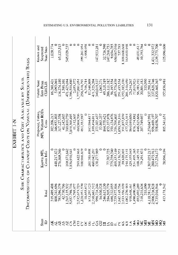
job no. 1969 casualty actuarial society CAS journal 1969D01 [53] 11-08-01 4:58 pm
ESTIMATING U.S. ENVIRONMENTAL POLLUTION LIABILITIES 131

job no. 1969 casualty actuarial society CAS journal 1969D01 [54] 11-08-01 4:58 pm
132 ESTIMATING U.S. ENVIRONMENTAL POLLUTION LIABILITIES
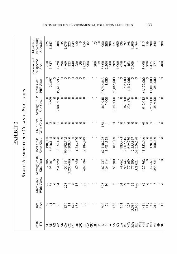
job no. 1969 casualty actuarial society CAS journal 1969D01 [55] 11-08-01 4:58 pm
ESTIMATING U.S. ENVIRONMENTAL POLLUTION LIABILITIES 133
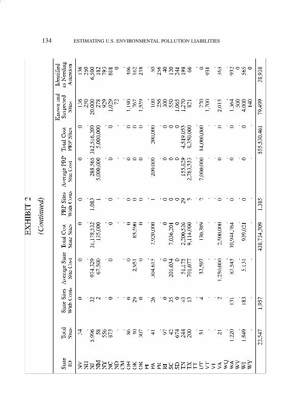
job no. 1969 casualty actuarial society CAS journal 1969D01 [56] 11-08-01 4:58 pm
134 ESTIMATING U.S. ENVIRONMENTAL POLLUTION LIABILITIES

job no. 1969 casualty actuarial society CAS journal 1969D01 [57] 11-08-01 4:58 pm
ESTIMATING U.S. ENVIRONMENTAL POLLUTION LIABILITIES 135

job no. 1969 casualty actuarial society CAS journal 1969D01 [58] 11-08-01 4:58 pm
136 ESTIMATING U.S. ENVIRONMENTAL POLLUTION LIABILITIES
EXHIBIT 4-A
Countrywide Estimates of Cleanup Costs andInsurance Liabilities Contribution from CERCLIS Sites
without PRP Information
Expected ExpectedIncurred Insured InsuredYear Indemnity Total LAE
1950 78,360,396 25,838,3151951 85,610,965 28,257,7891952 92,024,753 30,388,3371953 99,721,482 32,956,9941954 105,716,880 34,887,8191955 129,700,309 42,911,9901956 146,961,720 48,589,2931957 166,175,314 54,927,6401958 171,891,171 56,725,6361959 210,012,887 69,420,8291960 264,283,372 87,621,2641961 263,778,913 87,324,6481962 276,911,959 91,483,9721963 358,320,407 118,354,8731964 369,920,913 122,378,7401965 431,886,515 142,733,9361966 456,064,014 150,810,1161967 528,178,899 174,313,4371968 581,024,191 191,998,7461969 611,209,148 201,852,4261970 705,690,931 232,725,4761971 782,649,316 258,557,4431972 984,303,036 325,372,3951973 705,151,793 355,230,9311974 778,481,015 391,476,3551975 830,139,894 417,893,9861976 849,086,161 427,854,5941977 906,657,766 456,487,6881978 1,047,241,843 529,244,8811979 1,365,183,212 842,360,8961980 1,648,470,477 1,140,641,8411981 1,497,911,940 1,056,043,4501982 1,111,473,699 839,552,9381983 986,442,947 793,599,6381984 896,240,561 740,260,761
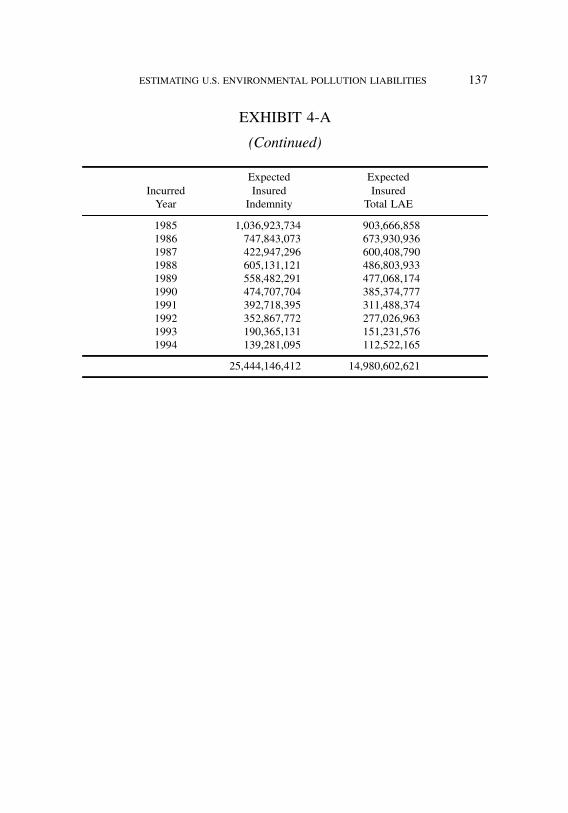
job no. 1969 casualty actuarial society CAS journal 1969D01 [59] 11-08-01 4:58 pm
ESTIMATING U.S. ENVIRONMENTAL POLLUTION LIABILITIES 137
EXHIBIT 4-A
(Continued)
Expected ExpectedIncurred Insured InsuredYear Indemnity Total LAE
1985 1,036,923,734 903,666,8581986 747,843,073 673,930,9361987 422,947,296 600,408,7901988 605,131,121 486,803,9331989 558,482,291 477,068,1741990 474,707,704 385,374,7771991 392,718,395 311,488,3741992 352,867,772 277,026,9631993 190,365,131 151,231,5761994 139,281,095 112,522,165
25,444,146,412 14,980,602,621
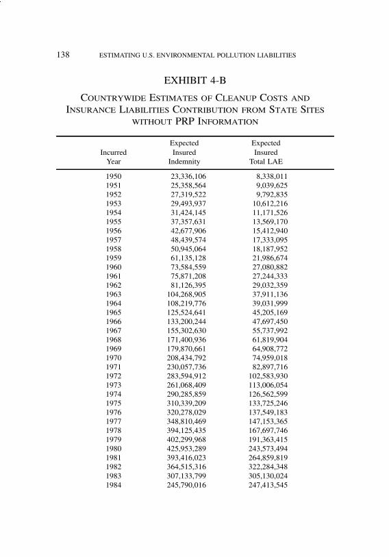
job no. 1969 casualty actuarial society CAS journal 1969D01 [60] 11-08-01 4:58 pm
138 ESTIMATING U.S. ENVIRONMENTAL POLLUTION LIABILITIES
EXHIBIT 4-B
Countrywide Estimates of Cleanup Costs andInsurance Liabilities Contribution from State Sites
without PRP Information
Expected ExpectedIncurred Insured InsuredYear Indemnity Total LAE
1950 23,336,106 8,338,0111951 25,358,564 9,039,6251952 27,319,522 9,792,8351953 29,493,937 10,612,2161954 31,424,145 11,171,5261955 37,357,631 13,569,1701956 42,677,906 15,412,9401957 48,439,574 17,333,0951958 50,945,064 18,187,9521959 61,135,128 21,986,6741960 73,584,559 27,080,8821961 75,871,208 27,244,3331962 81,126,395 29,032,3591963 104,268,905 37,911,1361964 108,219,776 39,031,9991965 125,524,641 45,205,1691966 133,200,244 47,697,4501967 155,302,630 55,737,9921968 171,400,936 61,819,9041969 179,870,661 64,908,7721970 208,434,792 74,959,0181971 230,057,736 82,897,7161972 283,594,912 102,583,9301973 261,068,409 113,006,0541974 290,285,859 126,562,5991975 310,339,209 133,725,2461976 320,278,029 137,549,1831977 348,810,469 147,153,3651978 394,125,435 167,697,7461979 402,299,968 191,363,4151980 425,953,289 243,573,4941981 393,416,023 264,859,8191982 364,515,316 322,284,3481983 307,133,799 305,130,0241984 245,790,016 247,413,545

job no. 1969 casualty actuarial society CAS journal 1969D01 [61] 11-08-01 4:58 pm
ESTIMATING U.S. ENVIRONMENTAL POLLUTION LIABILITIES 139
EXHIBIT 4-B
(Continued)
Expected ExpectedIncurred Insured InsuredYear Indemnity Total LAE
1985 221,688,995 308,149,0671986 167,065,353 242,846,7131987 147,908,737 207,374,9141988 100,667,233 178,889,3581989 114,491,815 196,030,8991990 103,059,409 179,970,5291991 56,352,816 104,414,8071992 80,054,797 121,425,4251993 47,295,950 56,371,5201994 28,727,347 24,120,406
7,439,273,244 4,851,467,183

job no. 1969 casualty actuarial society CAS journal 1969D01 [62] 11-08-01 4:58 pm
140 ESTIMATING U.S. ENVIRONMENTAL POLLUTION LIABILITIES
EXHIBIT 4-C
Countrywide Estimates of Cleanup Costs andInsurance Liabilities Contribution from CERCLIS Sites
with PRP Information
Expected ExpectedIncurred Insured InsuredYear Indemnity Total LAE
1950 36,124,737 11,703,7761951 39,506,765 12,817,4271952 42,448,887 13,762,3471953 46,031,092 14,925,5671954 48,753,261 15,791,9021955 60,158,527 19,509,8521956 68,064,319 22,068,2481957 76,910,460 24,920,0141958 79,313,796 25,698,2881959 97,223,613 31,532,7781960 123,313,666 40,014,7471961 122,378,154 39,685,5751962 128,044,863 41,521,8411963 165,888,464 53,808,1451964 171,093,073 55,490,1061965 199,990,444 64,901,4021966 210,998,983 68,455,3951967 244,062,943 79,115,8421968 268,320,314 87,024,9811969 282,348,869 91,501,1241970 325,723,414 105,569,1611971 362,557,962 118,592,2711972 457,508,944 149,594,4611973 269,598,311 162,800,2011974 297,117,698 179,762,0711975 316,655,982 191,861,3491976 323,322,688 196,260,1191977 344,114,604 209,185,6731978 399,958,117 248,706,3341979 417,433,372 284,561,6021980 455,593,706 348,004,6611981 442,254,551 348,295,1071982 521,449,186 465,396,4331983 395,828,330 340,207,5521984 384,771,459 336,795,444

job no. 1969 casualty actuarial society CAS journal 1969D01 [63] 11-08-01 4:58 pm
ESTIMATING U.S. ENVIRONMENTAL POLLUTION LIABILITIES 141
EXHIBIT 4-C
(Continued)
Expected ExpectedIncurred Insured InsuredYear Indemnity Total LAE
1985 329,896,771 397,563,7121986 379,020,264 350,773,7131987 157,298,911 238,182,9261988 241,992,415 156,616,1321989 245,765,651 187,123,4191990 233,338,009 190,450,9971991 185,971,174 128,735,5471992 194,457,021 141,657,3921993 131,508,517 79,163,6051994 137,295,225 93,503,327
10,461,407,514 6,463,612,567

job no. 1969 casualty actuarial society CAS journal 1969D01 [64] 11-08-01 4:58 pm
142 ESTIMATING U.S. ENVIRONMENTAL POLLUTION LIABILITIES
APPENDIX A
MEASURING SITE COST VARIABILITY
There are two sources of site variability that were analyzed.The first is that caused by differences among sites (i.e., the dis-tribution of site cleanup costs). The second is the variability inthe cleanup cost associated with the uncertainty in cleanup costsat the site level. Note that the latter is in addition to the EPAaccuracy guidelines of "30% to +50%.
To measure the first source of variability, a distribution ofcleanup costs was needed. The chosen source was the averagepresent worth by site from the RODs prepared by the EPA. Thesecosts are not at nominal values. Nominal, or undiscounted values,need to be estimated from present worth values, thereby intro-ducing additional uncertainty which detracts from the precisionof the measurement of variability that is sought.
The RODs costs were extracted directly from the text of thesedocuments. Where a range of costs was indicated then the av-erage was chosen, with a single cost effectively representing theaverage for the particular site.
The RODs used at the time covered the time period from1987 to approximately the end of 1993, with a few RODs actu-ally issued prior to 1987. In order to combine these data on aconsistent cost basis, parameters were extracted from the Univer-sity of Tennessee study [15, p. 15]. The specific parameters werea 2% trend in RODs cost annually plus a 46% increase in coststo represent cost growth as measured by the same study.14 Theaverage present worth values were trended by 2% from the yearof the date the ROD was issued to 1997. The results were thenaveraged by site, as there are many sites with multiple RODs.
14This uniform factor could have been omitted as it would not have affected the shapeof the distribution nor the estimated value of ¾. A colleague of the author advised as tothe potential misleading nature of this cost growth factor due to a mismatching of actualpaid costs and expected costs.

job no. 1969 casualty actuarial society CAS journal 1969D01 [65] 11-08-01 4:58 pm
ESTIMATING U.S. ENVIRONMENTAL POLLUTION LIABILITIES 143
Figure A-1 presents the resulting histogram for the 803 sitesincluded in the analysis. The statistic graphed is the natural log-arithm of the average present worth by site. Figure A-2 presentsa normal probability distribution plot for the same distributionusing the observed mean of 15.8135 and standard deviation of1.506764. Based on this plot and visual inspection of the his-togram, it was assumed that these costs could be reasonably de-scribed by a lognormal distribution with a coefficient of variation(CV) determined by the standard deviation:
CV = (e¾2 "1)1=2 = (e1:5067642 "1)1=2 = 2:9466 (A.1)
Most importantly, the resulting CV was chosen to apply to theestimated average site cost by state. This was accomplished bymultiplying the average cost by a randomly sampled value fromthe lognormal distribution (with the chosen CV of 2.9466 and amean of unity) every time a CERCLIS site cost was generated asa state enforced site. Since the mean of the lognormal is equal toe¹+(¾
2=2), the value of ¹ is solved directly as "1:135169 in orderto have a mean of 1 for the underlying ¾ of 1.506764.
To measure the second source of variability, an analysis wasperformed of those RODs that contained either a range of esti-mates or several alternate cost estimates. These ranges are sepa-rate and distinct from alternative remedies, and represent contin-gencies and additional uncertainties with regard to cleanup costestimates.
Figure A-3 presents a histogram of the relativities. The rel-ativities are measured by comparing a cost estimate to the av-erage for the ROD. A frequency is assigned to each estimatethat represents the reciprocal of the number of estimates in thatROD. In this fashion, the relativities from each ROD receivea total frequency (weight) of unity. The resulting histogram isnot symmetric because there are RODS with three or four esti-mates.

job no. 1969 casualty actuarial society CAS journal 1969D01 [66] 11-08-01 4:58 pm
144 ESTIMATING U.S. ENVIRONMENTAL POLLUTION LIABILITIES
Exhibit A-1 presents the table underlying the histogram. Theempirical relativities were used as shown when modeling thevariability of all site costs that did not have more than one costestimate (as described in Section 3).

job no. 1969 casualty actuarial society CAS journal 1969D01 [67] 11-08-01 4:58 pm
ESTIMATING U.S. ENVIRONMENTAL POLLUTION LIABILITIES 145
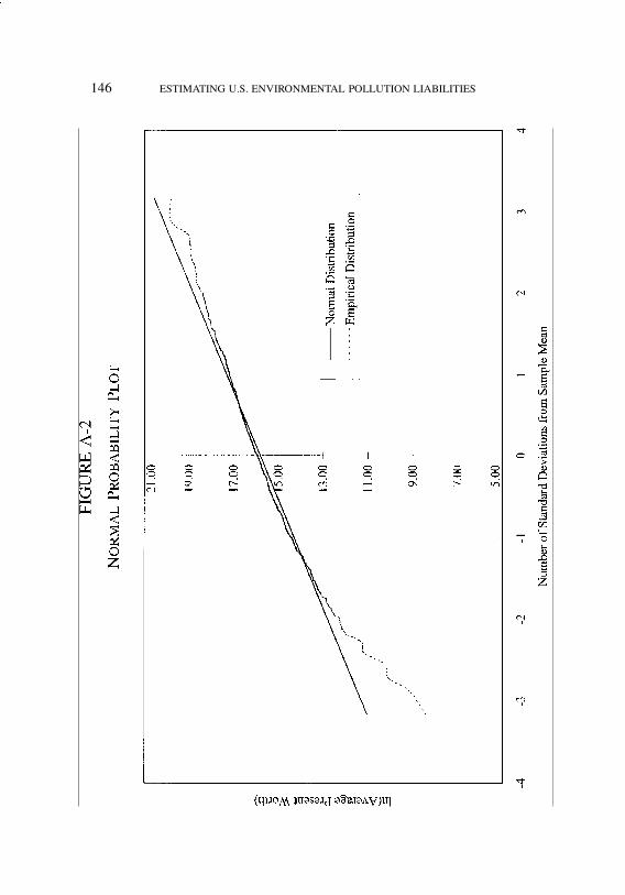
job no. 1969 casualty actuarial society CAS journal 1969D01 [68] 11-08-01 4:58 pm
146 ESTIMATING U.S. ENVIRONMENTAL POLLUTION LIABILITIES

job no. 1969 casualty actuarial society CAS journal 1969D01 [69] 11-08-01 4:58 pm
ESTIMATING U.S. ENVIRONMENTAL POLLUTION LIABILITIES 147

job no. 1969 casualty actuarial society CAS journal 1969D01 [70] 11-08-01 4:58 pm
148 ESTIMATING U.S. ENVIRONMENTAL POLLUTION LIABILITIES
EXHIBIT A-1
Analysis of Relativities for Multiple Cost RODs
Cumulative CumulativeRelativity to Number of Number of DistributionUnity Estimates Estimates of Relativity
0.05 3 3 0.01070.15 4 7 0.02500.25 2 9 0.03210.35 2 11 0.03930.45 9 20 0.07140.55 9 29 0.10360.65 13 42 0.15000.75 18 60 0.21430.85 29 89 0.31790.95 48 137 0.48931.05 50 187 0.66791.15 31 218 0.77861.25 19 237 0.84641.35 14 251 0.89641.45 11 262 0.93571.55 10 272 0.97141.65 1 273 0.97501.75 1 274 0.97861.85 4 278 0.99291.95 2 280 1.0000
Weighted Average Relativity 1.000357
job no. 1969 casualty actuarial society CAS journal 1969D01 [71] 11-08-01 4:58 pm
ESTIMATING U.S. ENVIRONMENTAL POLLUTION LIABILITIES 149
APPENDIX B
ESTIMATING AVERAGE SITE COSTS AND FREQUENCIES BYSTATE
The initial steps in this analysis involved obtaining an un-derstanding of the distribution of CERCLIS sites according toseveral characteristics. Exhibit 1 contains the tables that providethe requisite descriptive summaries.
The distribution by CERCLIS Source indicates that the greatmajority of sites are on the Archive file (30,428 out of a total of41,057). All but 69 of these have been identified as NFRAP bythe EPA. The other 69 sites were identified as NPL sites and haveapparently been removed due to cleanup or other reasons.15 Allof these NFRAP sites are assumed to be subject to remediationunder the respective state authorities.
Of the 10,629 Active sites, 1,217 are active NPL sites, 51are proposed NPL sites, 202 are sites identified or associatedwith NPL sites, 98 are deleted NPL sites, 46 have been removedfrom the NPL, and 723 are Federal non-NPL sites. This leaves abalance of 8,292 sites that are non-Federal sites that are eligiblefor assignment to the NPL in the future.
The estimate of the ultimate number of NPL sites was chosenas 2,100. This selection was based on work performed by theUniversity of Tennessee [15, p. 3] and the American Academy ofActuaries [18, p. i]. It was assumed that the future emergence ofNPL sites would conform to the existing NPL distribution of sitesby state. This assumption was based on the reasoning that statecharacteristics differ in their reflection of long-time industrialand manufacturing use or, alternatively, rapid industrializationand development since the Second World War are causal factorsin the emergence of NPL sites by state to date.
15One site is actually shown as an active NPL site.

job no. 1969 casualty actuarial society CAS journal 1969D01 [72] 11-08-01 4:58 pm
150 ESTIMATING U.S. ENVIRONMENTAL POLLUTION LIABILITIES
Likewise, when addressing the estimate of future average NPLcleanup costs by site, it is these same states’ densities of sites thatare likely to affect the inclusion of sites by state underlying thataverage. Individual state average cleanup costs for NPL siteswere precision (credibility) weighted with overall countrywideestimates in order to estimate future average NPL cleanup costsby site as described below.
Exhibit 1 also contains information on the distribution ofRODs with cost information, as well as the average present worthand average nominal cost of cleanup. All of the 803 sites dis-cussed in Appendix B have been associated with NPL sites atone time or another. The estimated nominal costs are based onthe analysis of present worth values by RODs and the direct es-timate of undiscounted values. The default value of .672 for thepresent value factor16 was used when insufficient informationwas available for a ROD to perform this estimate specifically.Values were trended to 1997 at an annual inflation rate of 2%,as performed in the analysis described in Appendix B.
The values used for the estimation of future NPL cleanupcosts weres based on the nominal costs for non-Federal Deletedand Final NPL sites. The averages and the standard deviationof these costs are shown on Exhibit 1. The following notationapplies to the estimation of the future average NPL cleanup costand estimate of the number of future NPL sites by state:
¹i = average (mean) of the nominal non-Federal Deletedor Final NPL cleanup costs for state i,
¹CW = the average of the state means of the nominalnon-Federal Deleted or Final NPL cleanup costs,
¾i = standard deviation of nominal non-Federal Deletedor Final NPL cleanup cost for state i,
16This value is the average present value factor obtained after removing outlier factorsof .4 or less and of .95 or greater.

job no. 1969 casualty actuarial society CAS journal 1969D01 [73] 11-08-01 4:58 pm
ESTIMATING U.S. ENVIRONMENTAL POLLUTION LIABILITIES 151
¾CW = standard deviation of the state averages (mean)of the nominal non-Federal Deleted or Final NPLcleanup costs,
zi = precision weight (credibility) estimated for state iaverage,
Ci = precision-weighted estimate of future averageNPL cleanup cost for state i,
Mi = final balanced estimate of future average NPLcleanup cost for state i,
NPLi = current number of NPL sites for state i. This iscomposed of CERCLIS sites identified as Deletedor Final NPL sites (NPL Status D or F) fornon-Federal sites,
Pi = number of Proposed NPL sites for state i(NPL Status P),
Qi = number of sites eligible for future NPL statusfor state i, defined as sites with current NPL Statusof Q (non-Federal and not NPL), and
FNPLi = estimated number of future NPL sites for state i.
The precision-weighted estimates of the mean future NPL sitecleanup cost are estimated as follows:
zi =
1¾2i
1¾2i+
1¾2CW
, and (B.1)
Ci = zi #¹i+(1" zi) #¹CW: (B.2)
The estimated means were balanced to the overall country-wide average by uniformly applying the ratio of the averagecountrywide NPL cleanup cost to the weighted average of the

job no. 1969 casualty actuarial society CAS journal 1969D01 [74] 11-08-01 4:58 pm
152 ESTIMATING U.S. ENVIRONMENTAL POLLUTION LIABILITIES
state-estimated average future NPL cleanup cost, using the num-ber of NPL sites by state as weights:
Mi = Ci #!$i¹i #NPLi!
$iCi #NPLi
: (B.3)
At the time of the analysis, Guam had two NPL sites and nosite eligible for future NPL status. With this restriction in mind,the number of future NPL sites for Guam was set at zero whilefor all other states it was estimated by:
FNPLi =NPLi!
$iNPLi"2
#"2100"
#$iNPLi"
#$iPi
$: (B.4)
The value of 2100 represents the estimated ultimate number ofNPL sites referred to earlier. The frequency with which a statusQ site becomes a future NPL site is the ratio of FNPLi to Qi bystate.
The last input to the estimation process is provided by thelimited aggregate information provided on state- and territory-administered cleanup efforts. Exhibit 2 shows the aggregate in-formation obtained from [11] and [12]. Integrating this infor-mation with the cost information obtained from the RODs textmade use of three important observations from review of thisEPA state and territory study:
! Federal Total Costs averaged $1.669 million per site at thattime but the expected future average is expected to be $25million [11, p. ES-10].
! The average state cost is $300,000 and the average PRP cost is$401,000 [11, p. ES-8], the latter representing approximatelyone-quarter of the aforementioned Federal cost.
! The total cost for the states is $1.205 billion on 3,395 sites[11, p. ES-8].

job no. 1969 casualty actuarial society CAS journal 1969D01 [75] 11-08-01 4:58 pm
ESTIMATING U.S. ENVIRONMENTAL POLLUTION LIABILITIES 153
It is important to note that these are actual paid costs thatcomprise a portion of ultimate total cleanup costs, the latter in-cluding operation and maintenance costs. This phenomenon islikely to influence the translation of average costs to an ultimatebasis for federal NPL sites to a greater extent than sites subjectto state-administered cleanup efforts. It is certainly an aspect thatmay point to a downward bias in total cost estimates.
This cost information includes enforcement as well as volun-tary cleanup efforts, creating an average that will likely tend tobe understated. Furthermore, there may be sites where both thestate and PRP costs are involved, yet only one of the parties re-ported its costs. This would also tend to understate any averagecost estimates.
The data by state as they appear in Exhibit 2 appear incom-plete, and countrywide statistics were used in the estimation pro-cess. Specifically, the following identity was employed:
Total Cost = State Average%State Sites+PRP Average%PRP Sites: (B.5)
Based on the national data summary from the EPA state andterritory study [11, p. ES-8], there were a total of 3,395 sitescountrywide, 2,167 state sites, and 1,385 PRP sites, the lattertwo quantities adding to 3,552. This relationship between thenumber of “total” countrywide sites (3,395 being less than 3,552,or what appears to be “the sum of its parts”) reflects the fact thatthere is an overlap between the state sites and the PRP sites (i.e.,there are sites that carry both state and PRP costs). The scalarreflecting this ratio (i.e., 3,395=3,552) was applied to the sum ofthe state and PRP sites by state in order to better estimate thetotal number of true separate and distinct sites.
Given the estimate of the number of sites by state, the av-erage cost per site is estimated as the total cost divided by thetotal number of sites by state. For those states without state andPRP site count information, the countrywide average was used
job no. 1969 casualty actuarial society CAS journal 1969D01 [76] 11-08-01 4:58 pm
154 ESTIMATING U.S. ENVIRONMENTAL POLLUTION LIABILITIES
($1,205,531,234=3,395 sites). The PRP insurable share is esti-mated as the ratio of the PRP cost to the total cost by state. Forstates without this cost information, the countrywide average wasused ($555,530,464=$1,205,531,234). Note that this componentof the model derives the insurable cost from state sites similar tothe CERCLIS estimate that includes non-Federal sites only.
The average state site cost is multiplied by the applicableCERCLIS sites that do not become future NPL sites (NFRAPsites plus the remaining eligible sites that do not become futureNPL sites) in order to estimate the total cleanup costs associatedwith state-administered programs. This average is not greaterthan the estimated average state PRP site cost, therefore permit-ting a measure of conservatism in some states for those sitesarising from CERCLIS. The average state PRP site cost is mul-tiplied by the sum of the number of known or suspected sitesby state and the expected number of future state sites. The latterquantity is implied by the difference between the total sites andthe estimated true number of sites, derived from the applicationof the countrywide site scalar mentioned above.
The dollar amounts included in this study are in nominal dol-lars. Average costs derived from these data are therefore notpresent value estimates, but rather nominal (undiscounted) costsat the level of the years in which they were spent. No inflationadjustments were made to the average cost estimates for futurecleanup costs.
The final results for insurable costs are shown in Exhibit 4.The total cleanup costs were simulated with a mean of $87.9 bil-lion. The histogram of the results is displayed in Figure B-1. Theeffects of the simulation from the CDM are to reduce the cleanupcosts that are indemnified by approximately 50%. Given an av-erage LAE factor to cleanup cost of 29.9% from Exhibit 3, theexpected value estimate of total insured costs is approximately$73.4 billion. This compares with the simulated mean of $69.6billion contained within the histogram of the results displayed inFigure B-2.
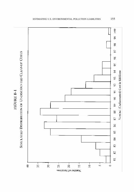
job no. 1969 casualty actuarial society CAS journal 1969D01 [77] 11-08-01 4:58 pm
ESTIMATING U.S. ENVIRONMENTAL POLLUTION LIABILITIES 155

job no. 1969 casualty actuarial society CAS journal 1969D01 [78] 11-08-01 4:58 pm
156 ESTIMATING U.S. ENVIRONMENTAL POLLUTION LIABILITIES

job no. 1969 casualty actuarial society CAS journal 1969D01 [79] 11-08-01 4:58 pm
ESTIMATING U.S. ENVIRONMENTAL POLLUTION LIABILITIES 157
APPENDIX C
PRP SHARES
Shares have been assigned to PRPs in one of two differentways when estimating pollution liabilities using the PCSM. Insome instances, a specific share was obtained from informationcontained in the claim files of an insurer or reinsurer when per-forming a portfolio analysis. In all other cases a simulated sharewas assigned to a PRP by using a Beta distribution. The totalof all shares for a site is balanced to unity, including both sim-ulated and specific shares. The remainder of this appendix willdiscuss the simulation of PRP shares that is used for the industryestimate.
The Beta distribution used in the simulation has the followingform:
B(x,®,¯) =
x%0t®"1(1" t)¯"1dt
¯(®,¯),
where ¯(®,¯) =¡ (®)¡ (¯)¡ (®,¯)
: (C.1)
The mean of this distribution is set equal to the reciprocalof the number of PRPs. In order to afford higher probabilitiesat or near zero, ® is equal to the reciprocal of the number ofPRPs whenever the number of PRPs is greater than one. Thereason for creating higher probabilities at or near zero is to af-ford a simulation of the de minimis shares phenomenon. Thisphenomenon results from the incidence of many PRPs on a sitethat have been determined to be minor (de minimis) contributorsto the pollution at the site. Setting ® equal to the reciprocal of thenumber of PRPs results in a value less than unity, thereby pro-viding the sought after shape of the distribution—a large modeat zero (0% share) and a much smaller secondary mode at unity(100% share).

job no. 1969 casualty actuarial society CAS journal 1969D01 [80] 11-08-01 4:58 pm
158 ESTIMATING U.S. ENVIRONMENTAL POLLUTION LIABILITIES
TABLE C-1
BALANCED SIMULATED AND SPECIFIC SHARES
Beta DistributionIndividual PRPs Simulated Share Balanced Share
1 0.2000 0.20002 0.8526 0.56443 0.0003 0.00024 0.0001 0.00015 0.2535 0.16786 0.0000 0.00007 0.0000 0.00008 0.0130 0.00869 0.0632 0.041810 0.0258 0.0171
Total Excluding PRP-1 1.2085 1.0000
If we let n be the number of PRPs and M be the mean of theBeta distribution, then we have the following relationships:
M =®
®+¯=1n, ®=
1n, and ¯ =
n"1n
= 1"®:
This distribution is used for each site for which shares weresimulated during each iteration of the PCSM simulation fora portfolio. To illustrate the process for ten PRPs on a site,the Table C-1 reproduces a sample iteration for ten PRPs withthe introduction of a fixed known share of 20% for PRP-1.PRP-1 represents a specific share assignment encountered duringa portfolio analysis as mentioned earlier.
Each of the nine other PRPs have shares simulated with a totalexcluding PRP-1 determined. The parameters of the Beta distri-bution in this case are ®= :1 and ¯ = :9. The shares of these othernine PRPs are then balanced to produce unity when including theknown fixed share of PRP-1. Note that this particular exampleincludes several PRPs with de minimis shares.
job no. 1969 casualty actuarial society CAS journal 1969D01 [81] 11-08-01 4:58 pm
ESTIMATING U.S. ENVIRONMENTAL POLLUTION LIABILITIES 159
APPENDIX D
DERIVATION OF SCALARS FOR SAMPLES
When estimating ultimate pollution losses for a portfolio, it isnecessary to determine a scalar that can be applied to the costssimulated by the PCSM. This is because only a sample of sitesand PRPs exists for the simulation employed for any portfolio.In the cases where there does not exist an exhaustive list of PRPsand policies exposed to pollution liabilities, which will often bethe case, a pro-rata scalar can be used of the following form:
InsT(P) =CUTCUN(S)
# InsN(S): (D.1)
The scalar represents the ratio shown on the right-hand sideof the formula above. This ratio will vary from one portfolio toanother. The following notation will be employed to show howthis scalar is derived:
CUX(Y) = total cleanup and operation and maintenance costsrelating to portfolio Y of potentially responsibleparties (PRPs) from subset X of all sites(cleanup costs),
InsX(Y) = Insured costs related to portfolio Y of PRPs fromsubset X of all sites,
N =NPL and CERCLIS (national) sites with potentiallyresponsible parties (PRPs) information,
T = all sites countrywide, including CERCLIS and state-and territory-administered sites, and
S = national sites included in the sample employed bythe PCSM.
If the PRP portfolio is not designated in a term, then the entirepopulation of PRPs is implied. In this presentation, the value ofP refers to the PRPs associated with the portfolio under analysis.
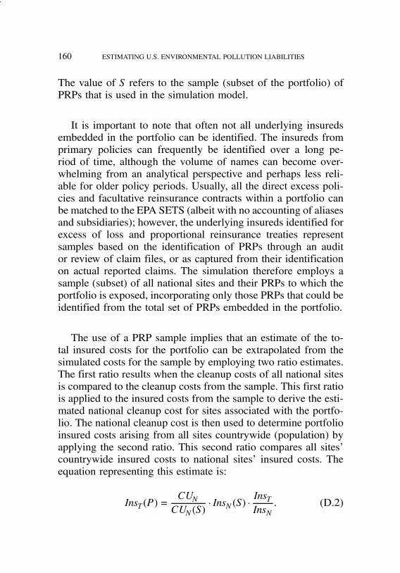
job no. 1969 casualty actuarial society CAS journal 1969D01 [82] 11-08-01 4:58 pm
160 ESTIMATING U.S. ENVIRONMENTAL POLLUTION LIABILITIES
The value of S refers to the sample (subset of the portfolio) ofPRPs that is used in the simulation model.
It is important to note that often not all underlying insuredsembedded in the portfolio can be identified. The insureds fromprimary policies can frequently be identified over a long pe-riod of time, although the volume of names can become over-whelming from an analytical perspective and perhaps less reli-able for older policy periods. Usually, all the direct excess poli-cies and facultative reinsurance contracts within a portfolio canbe matched to the EPA SETS (albeit with no accounting of aliasesand subsidiaries); however, the underlying insureds identified forexcess of loss and proportional reinsurance treaties representsamples based on the identification of PRPs through an auditor review of claim files, or as captured from their identificationon actual reported claims. The simulation therefore employs asample (subset) of all national sites and their PRPs to which theportfolio is exposed, incorporating only those PRPs that could beidentified from the total set of PRPs embedded in the portfolio.
The use of a PRP sample implies that an estimate of the to-tal insured costs for the portfolio can be extrapolated from thesimulated costs for the sample by employing two ratio estimates.The first ratio results when the cleanup costs of all national sitesis compared to the cleanup costs from the sample. This first ratiois applied to the insured costs from the sample to derive the esti-mated national cleanup cost for sites associated with the portfo-lio. The national cleanup cost is then used to determine portfolioinsured costs arising from all sites countrywide (population) byapplying the second ratio. This second ratio compares all sites’countrywide insured costs to national sites’ insured costs. Theequation representing this estimate is:
InsT(P) =CUNCUN(S)
# InsN(S) #InsTInsN
: (D.2)

job no. 1969 casualty actuarial society CAS journal 1969D01 [83] 11-08-01 4:58 pm
ESTIMATING U.S. ENVIRONMENTAL POLLUTION LIABILITIES 161
This formula can be rewritten by rearranging terms as:
InsT(P) =InsN(S)CUN(S)
# InsT #&CUNInsN
': (D.3)
It is assumed that the ratio of cleanup costs to insured costsis the same for national sites as it is for all sites, that is:&
CUNInsN
'&&CUTInsT
': (D.4)
Note that this assumption presumes that the insurance cover-age of insureds is commensurate with their hazard. As an exam-ple, a corporate entity that is not a Fortune 500 company maypurchase insurance that attaches at a lower amount due to itssmaller self-insurance capacity. However, that smaller entity’sinvolvement at a site with lower cleanup costs could still resultin an insured loss commensurate with, say, a Fortune 500 com-pany’s share of costs at an NPL site.
The formula now reduces to:
InsT(P) =InsN(S)CUN(S)
# InsT #&CUNInsN
': (D.5)
Cancellation of total sites’ insured costs results in the scalarequation cited earlier:
InsT(P) =CUTCUN(S)
# InsN(S): (D.6)
The scalar used for any given portfolio is the ratio from thesimulation of all sites’ countrywide cleanup costs to the samplednational sites’ cleanup costs.

job no. 1969 casualty actuarial society CAS journal 1969D06 [1] 11-08-01 4:58 pm
APPLICATION OF THE OPTION MARKET PARADIGM TOTHE SOLUTION OF INSURANCE PROBLEMS
MICHAEL G. WACEK
DISCUSSION BY STEPHEN J. MILDENHALL
ACKNOWLEDGEMENT
I would like to thank Bassam Barazi, David Bassi, Fred Kist,Deb McClenahan, David Ruhm, and Trent Vaughn for their helpfulcomments on the first draft of this review. I am also very gratefulto Ben Carrier for his persistent questioning of an earlier versionof Section 4 which helped me clarify the ideas.
1. INTRODUCTION
Michael Wacek’s paper is based on the well-known fact thatthe Black–Scholes call option price is the discounted expectedexcess value of a certain lognormal random variable.1 Specifi-cally, the Black–Scholes price can be written as
BS = e!r(T!t)E[(S(T)! k)+],where r is the risk-free rate of interest, T is the time when theoption expires, t is the current time, S(T) is a lognormal ran-dom variable related to the stock price S(T) at time T, k is theexercise price, and x+ :=max(x,0). In insurance terms, (L! k)+represents the indemnity payment on a policy with a loss of Land a deductible k. The Black–Scholes price can also be regardedas the discounted insurance charge (see Gillam and Snader [18]or Lee [25]). It is easy to compute the insurance charge under
1The formula is explicit in virtually all financial economics derivations, for example,Merton [27, p. 283], Cox and Ross [4, p. 154, equation 19, which is essentially theauthor’s Equation 1.3], Harrison and Kreps [19, Corollary to Theorem 3], Karatzas andShreve [23, p. 378], Hull [20, p. 223 (for forward contracts on a stock)], as well as moreovertly actuarial works, such as Gerber and Shiu [17, p. 104] and Kellison [24, AppendixX].
162

job no. 1969 casualty actuarial society CAS journal 1969D06 [2] 11-08-01 4:58 pm
APPLICATION OF THE OPTION MARKET PARADIGM 163
the lognormal assumption to arrive at—but not to derive—theexplicit Black–Scholes formula.2
Even without reference to the Black–Scholes formula, thereare obvious analogies between insurance and options becauseboth are derivatives. An insurance payment is a function of—isderived from—the insured’s actual loss; similarly, the terminalvalue of an option is a function of the value of some underlyingsecurity. To the extent that options and insurance use the samefunctions to derive value, there will be a dictionary between thetwo. As Wacek points out, this is the case. For example, the ex-cess function (L! k)+ is used to derive the terminal value of acall and an insurance payment with a deductible k; min(L, l) de-termines the value of an insurance contract with a limit l; and(k!L)+ = k!min(L,k) gives the terminal value of a put optionas well as the insurance savings function. There are several otherexamples given in the paper, including a cylinder. The author ex-plains how an insurance cylinder can be used to provide cheaperreinsurance and greater earnings stability for the cedent. The ideaof regarding an insurance payment as a function of the under-lying loss has been discussed previously in the Proceedings byLee [25] and [26], and Miccolis [28]. The connection betweeninsurance and options, based on the fact that both are derivatives,was also noted in D’Arcy and Doherty [9, p. 57].
Here are two other interesting correspondences between op-tion structures and insurance. The first is the translation fromput-call parity in options pricing to the relationship “one plussavings equals entry ratio plus insurance charge” from retrospec-tive rating. The put option is equivalent to the insurance savingsfunction and the call option to the insurance charge function(see Lee [25] and [26], which has the options profit diagrams,or Gillam and Snader [18] for more details).
The second correspondence applies Asian options to a modelof the rate of claims payment or reporting in order to price catas-
2Kellison [24, Appendix X] gives all the details.

job no. 1969 casualty actuarial society CAS journal 1969D06 [3] 11-08-01 4:58 pm
164 APPLICATION OF THE OPTION MARKET PARADIGM
trophe index futures and options. This example is too involvedto describe in detail here. The interested reader should look inthe original papers by Cummins and Geman [7] and [8].
Insurance can also be regarded as a swap transaction. Hull[20] defines swaps generically as “private agreements betweentwo companies to exchange cash flows in the future accordingto a prearranged formula.” In insurance language one cash flowis the known premium payment, generally consisting of one ormore installments during the policy period, and the other variesaccording to losses and continues for a longer period of time.Many recent securitization transactions have been structured asswaps. Indeed, in that context a swap is essentially insurancefrom a non-insurance company counter-party. Arguably, swapsare a better model for insurance than options because they in-volve a series of cash flows into the future rather than a singlepayment. Options, which involve a single payment when the op-tion is exercised, are not a good model for a per occurrenceinsurance product that could cover many individual claims.
Despite the title of the paper, Wacek is more concerned withoptions notation—puts, calls, profit diagrams and so forth—thanwith the options market paradigm. The dictionary definition ofa paradigm is a “philosophical and theoretical framework of ascientific school or discipline within which theories, laws, andgeneralizations: : :are formulated.” Wacek’s paper does not dis-cuss the assumptions underlying Black–Scholes nor the deriva-tion of the formula in any detail. Each is an important part ofthe options pricing paradigm. Moreover, the comments he offerson options prices tend to confuse a pure premium (loss cost)with a price (loss cost including risk charge, in this context). Herightly draws a distinction between the two but does not clearlystate whether the Black–Scholes formula gives the former or thelatter.
This review will focus on the theoretical framework, orparadigm, of options pricing. Section 2 will compare the Op-tion Pricing Paradigm with the corresponding actuarial notion,

job no. 1969 casualty actuarial society CAS journal 1969D06 [4] 11-08-01 4:58 pm
APPLICATION OF THE OPTION MARKET PARADIGM 165
and discuss how the former relies on hedging to remove riskwhile the latter relies on the law of large numbers to assume andmanage risk. The distinction between using hedging and diversi-fication to manage risk highlights an essential difference betweenthe capital and insurance markets. Section 3 will determine theactuarial price for a stock option under the lognormal distributionassumption, and will compare the result to the Black–Scholesformula. Section 4 then discusses why the Black–Scholes resultis different from the actuarial answer. It will also explain whythe Black–Scholes formula gives a price rather than a pure pre-mium. Section 5 will propose an application of the Option Pric-ing Paradigm to catastrophe insurance and discuss options onnon-traded instruments. Finally, Section 6 will compare marketprices with the Black–Scholes prices.
This review will only discuss applications of options pricingto individual contracts in a very limited way. The reader shouldbe aware that there are many other important applications, in-cluding the pioneering work of Cummins [6], revolving aroundvaluing the insurance company’s option to default. The ground-breaking paper by Phillips, Cummins and Allen [30] gives anapplication of these ideas to pricing insurance in a multi-linecompany. The reader should refer to the recent literature for moreinformation on these ideas.
2. OPTION PRICING PARADIGM AND ACTUARIALLY FAIR PRICES
The actuarial, or fair, value of an uncertain cash flow is de-fined to be its expected value. Insurance premiums are generallydetermined by loading the discounted actuarial value of the in-sured losses for risk and expenses. In this discussion it will beassumed that a risk charge is loaded into the pure premium bydiscounting at a risk-adjusted interest rate. Clearly this is neitherthe only choice nor is it necessarily the best choice. It will alsobe assumed that there are no expenses, and the word “price” willbe used to refer to a risk-loaded pure premium.

job no. 1969 casualty actuarial society CAS journal 1969D06 [5] 11-08-01 4:58 pm
166 APPLICATION OF THE OPTION MARKET PARADIGM
The Option Pricing Paradigm defines the price of an optionto be the smallest cost of bearing the risk of writing the option,which is completely different from the actuarial viewpoint. Inthis context, being able to bear the risk of writing an option(equivalent to writing insurance) means being able to respondto the holder of the option whatever contingency might occur.In actuarial-insurance language this implies a zero probabilityof ruin, for if there is a non-zero probability of ruin then thereis a contingency under which the option writer cannot respondto the holder, and hence the writer is not able to bear the risk(according to the definition).
The insurance company approach to bearing risk is to chargea pure premium plus risk load, to have a substantial surplus, andto pool a large number of independent risks. If stock prices fol-low an unbounded distribution, such as the lognormal, then itis not possible to write an option and achieve a zero probabil-ity of ruin using this insurance approach to bearing risk. Thus,unlike insurance, pricing and risk bearing in the Option PricingParadigm do not rely on the law of large numbers—a crucialdifference.
One way of bearing the risk of writing a stock option is to setup a hedging portfolio with the following four properties:
1. The portfolio consists of the stock underlying the optionand risk-free borrowing or lending.
2. The terminal value of the hedging portfolio equals theterminal value of the option for all contingencies.
3. The hedging portfolio is self-financing: once it has beenset up it generates no cash flows, positive or negative,until the option expires.
4. The hedging portfolio uses a deterministic trading strat-egy which only relies on information available wheneach trade is made. Trading only takes place betweenwhen the option is written and when it expires.

job no. 1969 casualty actuarial society CAS journal 1969D06 [6] 11-08-01 4:58 pm
APPLICATION OF THE OPTION MARKET PARADIGM 167
It is not clear that hedging portfolios exist. However, if theydo then the Option Pricing Paradigm price of an option can beno greater than the smallest amount for which it is possible toset up (i.e., purchase) a hedging portfolio. Indeed, by settingup a hedging portfolio the writer of the option is able to bearthe attendant risks, because the portfolio generates enough cashto respond to the holder no matter what contingency occurs. Bydefinition, the price of the option is the smallest amount of moneyfor which this is possible. Therefore, the actual option price canbe no greater than the cost of the cheapest hedging portfolio.
On the other hand, if there are no arbitrage opportunities,the Option Pricing Paradigm price must be at least as large asthe cost of setting up the cheapest hedging portfolio. Since thewriter can bear the risk of writing the option, it must have a port-folio, purchased with the proceeds of writing the option, with anending cash position at least as large as the terminal value ofthe option (and hence a hedging portfolio) in every contingency.Such a portfolio is said to dominate the hedging portfolio. Ifportfolio A dominates portfolio B then, in the absence of arbi-trage, A must cost more than B. Here, the option price is usedto purchase a portfolio which in turn dominates a hedging port-folio, and therefore the option price must be at least as great asthe cost of a hedging portfolio.3 Combining this with the previ-ous paragraph shows that in the absence of arbitrage, the OptionPricing Paradigm price equals the smallest amount for which itis possible to set up a hedging portfolio.
The above argument relies on the absence of arbitrage oppor-tunities in the market. An arbitrage is the opportunity to earn a
3The price of the option could simply be defined as the smallest cost of setting up a hedg-ing portfolio. For example, in Karatzas and Shreve [23] the fair price for a contingentclaim is defined as the smallest amount x which allows the construction of a hedgingportfolio with initial wealth x. However, it is generally not possible for an insurer toset up a hedging portfolio because it cannot trade in the security underlying the insur-ance contract option. Thus, a definition in terms of hedging portfolios would not havetransferred to insurance. On the other hand, “the cost of bearing the risk,” albeit with apossibly weaker notion of bearing risk, makes perfect sense in an insurance setting andis equivalent to the hedging portfolio definition for options.

job no. 1969 casualty actuarial society CAS journal 1969D06 [7] 11-08-01 4:58 pm
168 APPLICATION OF THE OPTION MARKET PARADIGM
riskless profit. In general, the existence of arbitrage opportunitiesis not compatible with an equilibrium model of security prices,since informed agents would engage in arbitrage and hence mod-ify market prices (see Dybvig and Ross [16, pp. 57–71] for anexplanation of the close connections between no-arbitrage andoptions pricing). In options pricing, no-arbitrage is used to justifydefining the price of an option as the smallest cost of a hedg-ing portfolio; if the option sold for more or less than the costof a hedging portfolio then risk-free arbitrage profits would bepossible. Put another way, the option and the hedging portfolioare comparables, and no-arbitrage implies that comparables musthave the same value. Since “the value of an asset is equal to thecombined values of its constituent items of cash flow” [3], if twoassets have the same cash flows then they are equivalent to aninvestor and must command the same price. The fact that one isan option and the other a synthetic option created from a portfo-lio of bonds and stocks is irrelevant. Obviously this only appliesin a world where the Black–Scholes assumptions hold—so inparticular there are no transaction costs, no discontinuous jumpsin stock prices, and continuous trading. Finally, no-arbitrage isa consequence of the model framework, not an assumption; po-tential arbitrages are ruled out through restrictions on admissibletrading strategies. This is a more advanced point; the interestedreader should see Harrison and Kreps [19], Dothan [14], andDelbaen and Schachermayer [10], [11] and [12] for more de-tailed information.
To conclude, this section has introduced the notions of no-arbitrage and hedging portfolios, and explained how the OptionPricing Paradigm defines price to be the smallest cost of settingup a hedging portfolio. These beginnings are enough to pointout some significant differences compared to actuarial methodsof pricing, one of which is that option pricing does not relyon the law of large numbers. The question of whether hedgingportfolios actually exist will be discussed in Section 4. First, wewill look at how an actuary would price an option.

job no. 1969 casualty actuarial society CAS journal 1969D06 [8] 11-08-01 4:58 pm
APPLICATION OF THE OPTION MARKET PARADIGM 169
3. AN ACTUARIAL APPROACH TO OPTION PRICING
It is instructive to compare the Black–Scholes price with theactuarial price—including risk-load—for a call option. Beforedefining terms we must fix the notation. Assume all interest ratesand returns are continuously compounded. Let r be the risk-freerate of interest, ¹ the expected return on the stock, S(t) or Stthe stock price at time t, and r" a risk-adjusted interest rate fordiscounting the option payouts. To keep the notation as simpleas possible, assume that the current time is t= 0 and that theoption expires at time t= T. Assume also that the stock priceprocess is a geometric Brownian motion,4 so that ln(S(t)=S(0))is normally distributed with mean t(¹!¾2=2) and variance t¾2for some ¾ > 0. Finally, let k be the exercise price.
The actuarial price for the option is the present value of theexpected payouts discounted at a risk-adjusted interest rate:
e!r"TE((S(T)! k)+): (3.1)
With r" = r, Equation 3.1 is Equation 1.3 from the paper.5 Anactuary could compute Equation 3.1 after estimating appropri-
4This means that over a very short time interval dt, the return on the stock dSt=St satisfiesthe stochastic differential equation dSt=St = ¹dt+¾dWt, where Wt is a Brownian motion.By definition Wt is normally distributed with mean zero and variance t¾
2. It followsfrom Ito’s Lemma that the solution to the stock price stochastic differential equationcan be written as St = S0exp((¹!¾2=2)t+¾Wt). Hence St has a lognormal distributionand ln(St=S0) is normal with mean (¹!¾2=2)t and variance t¾2. Since E(St) = S0e¹tit is reasonable to call ¹ the expected rate of return on the stock. See Hull [20], orKaratzas and Shreve [23], for more details. In particular, Hull [20, Chapter 10.3] discussesthe difference between expected returns over a short period of time and the expectedcontinuously compounded rate of return. If there is variability in the rate of return, so¾ > 0, then the former, ¹, is greater than the latter, ¹!¾2=2.5Wacek justifies assuming r" = r using the notion of a hedging portfolio. However, inthis section an actuarial viewpoint is taken instead. To the actuary—and the financialeconomics community as a whole prior to Black–Scholes—we should have r" > ¹> r,since the option is more leveraged than the stock and hence more risky. Brealey andMyers [2] point out that the option has a higher beta and a higher standard deviationof return than the underlying stock. Clearly ¹> r, since the stock is more risky than arisk-free bond. Note that r" > r assumes the actuary is buying an option and discountingthe payout as income; if the actuary were writing the option and pricing the payout as aloss, then r" < r would be appropriate.

job no. 1969 casualty actuarial society CAS journal 1969D06 [9] 11-08-01 4:58 pm
170 APPLICATION OF THE OPTION MARKET PARADIGM
ate values for ¹, ¾ and r". For ¹ the actuary might try using ahistorical average return, the Capital Asset Pricing Model price,or some other suitable tool. It is easy to estimate ¾ from a timeseries of stock prices. For the discounting rate, the actuary wouldmystically select some number r" > ¹ if buying an option (as isassumed here) or r" < r if writing one. Using Equation 3.1 theactuary would then arrive at the following expression for the callprice:
e(¹!r")TS0©
!ln(S0=k)+ (¹+¾
2=2)T
¾#T
"
! e!r"Tk©!ln(S0=k)+ (¹!¾2=2)T
¾#T
": (3.2)
This formula is identical to a pre–Black–Scholes result derivedby Samuelson [31] following the same logic used here. It is alsomentioned in Ingersoll [21, pp. 199–212], which includes a sur-vey of earlier attempts to determine a formula to price options.Comparing the actuarial Equation 3.2 to the Black–Scholes equa-tion
S0©
!ln(S0=k) + (r+¾
2=2)T
¾#T
"
! e!rTk©!ln(S0=k)+ (r!¾2=2)T
¾#T
", (3.3)
and relating the variables back to Equation 3.1 highlights twodifferences:
1. The Black–Scholes model appears to assume the stockearns the risk-free rate of return, that is ¹= r;
2. The Black–Scholes model discounts at the risk-free rateof interest, so r" = r.
Clearly, substituting ¹= r and r" = r into Equation 3.2 givesEquation 3.3. Section 6 compares option prices computed withthese two equations.
job no. 1969 casualty actuarial society CAS journal 1969D06 [10] 11-08-01 4:58 pm
APPLICATION OF THE OPTION MARKET PARADIGM 171
The expected rate of return ¹ on the stock is a function ofinvestor risk preferences. Individual investors could differ as totheir opinions of ¹ and yet the assumption underlying the firstdifference above says they will agree on the option price. In orderto underline how remarkable and counter-intuitive this assump-tion is, it is instructive to translate it into insurance language.Suppose S(T) is the value of a portfolio of losses at time T. Fur-ther, suppose S(T) is lognormal with parameters ¹ and ¾. Theinsurance analog of the call option pricing problem is to pricean aggregate stop loss on S(T) with attachment k. Assume allactuaries agree on ¾, that is, they agree on the coefficient ofvariation of aggregate losses.6 Now, the assumption discussedabove says different actuaries could disagree on ¹—and hencethe mean of S(T)—and yet agree on the price of the aggregatestop loss! Clearly there is something significant going on behindthe Black–Scholes formula.
No actuary would assume ¹= r and r" = r in pricing sincethey are not reasonable in the real world. In his paper, Wacekpoints out that option pricing discounts at the risk-free rate,r" = r, but he does not mention the first point. The next sec-tion examines why the two assumptions above can be made inthe Option Pricing Paradigm.
4. THE HEDGING PORTFOLIO IN DISCRETE TIME AND THEBLACK–SCHOLES FORMULA
The Black–Scholes formula is best understood by consideringa discrete time example. While the example may appear simplis-tic, it contains all of the key ideas in the Black–Scholes deriva-tion. Cox, Ross and Rubenstein [5] give an explanation of howto derive the full Black–Scholes result from a limit of the bi-nomial models considered here. Their explanation is consideredin more detail by Nawalkha and Chambers [29], who show that
6For a lognormal distribution, the coefficient of variation is#exp(¾2)! 1, a function of
¾ alone.

job no. 1969 casualty actuarial society CAS journal 1969D06 [11] 11-08-01 4:58 pm
172 APPLICATION OF THE OPTION MARKET PARADIGM
preference independence in [5] depends on a particular choiceof binomial parameters.
Consider writing a call option on a stock currently priced at$100. When the option expires, assume the stock price will beeither $120 or $90. The one period risk-free rate of interest is 5%;also, the option expires in one period and has an exercise priceof $105. Finally, assume the stock does not pay any dividends.
At this point it is important to understand what has, and whathas not, been assumed. Underlying our assumptions are two un-knowns: the probability p that the stock price will end at $120,and an expected return ¹ on the stock. The expected return ¹ is
¹= ln$120p+90(1!p)
100
%(using continuous compounding) or, equivalently,
100 = e!¹(120p+90(1!p)): (4.1)
Equation 4.1 expresses the current price as an expected presentvalue, discounted at a risk-adjusted interest rate. It gives onerelationship between the two unknowns p and ¹. It is impossiblefor us to know whether the current stock price is $100 becausethere is a very good chance of an upward price movement (highp) but investors are all very risk-averse (giving a high ¹), orbecause there is only a moderate chance of an upward movementin a largely risk-neutral market. The fact that the Black–Scholesformula is independent of the choice of ¹ and p, subject to theconstraint Equation 4.1, is one of its most remarkable featuresand it leads to the notion of risk-neutral valuation.
Return now to pricing the $105 call option under the OptionPricing Paradigm. From Section 2, the price of the call is thesmallest cost for which it is possible to set up a hedging port-folio. An explicit hedging portfolio for the option will now beconstructed, demonstrating that they exist, at least in this simplecase. Suppose the hedging portfolio consists of a stocks and b

job no. 1969 casualty actuarial society CAS journal 1969D06 [12] 11-08-01 4:58 pm
APPLICATION OF THE OPTION MARKET PARADIGM 173
dollars in bonds. The replicating property of a hedging portfoliorequires that, at expiration,
120a+b = 15 and
90a+b = 0:
The top line corresponds to an upward movement in the stockprice, when the option is worth max(120! 105,0) = 15 at expi-ration. The bottom line corresponds to a downward movement inthe stock price, when the option is worth max(90!105,0) = 0.Solving gives a= 1=2 and b =!45, meaning borrowing of $45.The cost today of setting up a portfolio which consists ofhalf of one stock plus $45 debt one period from now equals100=2! e!0:0545 = 7:19. The first term is the cost of buying halfa stock and the second term is the present value of a debt of $45one period from now.
It is easy to confirm that this portfolio hedges the option.If the stock price moves up, then selling the half-stock yields$60, exactly enough to pay off the $45 debt and pay the ownerof the option the $15 terminal value. If the stock price movesdown, then selling the half-stock realizes $45, which is exactlythe amount required to pay off the debt. There is nothing else topay since the option expires worthless.
Using the hedging portfolio it is also easy to see why no-arbitrage implies $7.19 is the appropriate price for the option. Ifthe option sold for more than $7.19, say $7.25, then arbitrageurswould write (sell) the over-priced options. With $7.19 of the pro-ceeds they could set up a hedging portfolio, effectively closingout their option position. They would make a risk-free profit ofsix cents per option written.
On the other hand, suppose the option sold for only $7.15.Then arbitrageurs would want to buy the under-price options.They could short one stock to get $100 and use the proceeds tobuy two options for $14.30, put $85.61 into bonds earning therisk-free rate, and skim off the remaining nine cents as arbitrage

job no. 1969 casualty actuarial society CAS journal 1969D06 [13] 11-08-01 4:58 pm
174 APPLICATION OF THE OPTION MARKET PARADIGM
profit. If the stock price rises to $120, they exercise the twooptions to yield a $30 profit, which combined with 85:61e0:05 =$90 in bonds gives $120—exactly enough to close out the shortposition in the stock. If the stock price falls to $90 then theoptions expire worthless, but the arbitrageurs still have $90 inthe bonds to close out the stock position.
To summarize, these arguments lead to essentially the sametwo conclusions already noted in Section 3 from comparingBlack–Scholes and the actuarial option price:
1. The option price is $7.19 regardless of the risk pref-erences of individuals, expressed through the unknownquantities ¹ and p, provided Equation 4.1 is satisfied;
2. The hedging portfolio consists of stock and risk-free bor-rowing only. Once it is set up there is no risk to the optionwriter because movements in the stock price and the op-tion price are perfectly correlated. A portfolio consistingof the hedge and the underlying option must thereforeearn, and hence be discounted at, the risk-free rate ofreturn.
Black and Scholes showed these two results are still true whenthe stock price is allowed to follow a more complex path incontinuous time. Under the lognormal stock price assumption,they proved the option price function is given by Equation 3.3,and derived the required trading strategy to use in the hedgingportfolio—the so-called “delta-hedging” strategy.
Cox and Ross [4] used the risk preference independence in thefirst conclusion above to argue that an option could be priced as-suming investors have any convenient risk preference. The sim-plest selection for preferences is risk-neutrality. In a risk-neutralworld, all stocks are expected to earn the risk-free return becauseinvestors do not require a premium for uncertainty. Thus ¹= ris determined. Of course, stocks do not earn the risk-free re-turn in the real, risk-averse, world. In our simple discrete model,

job no. 1969 casualty actuarial society CAS journal 1969D06 [14] 11-08-01 4:58 pm
APPLICATION OF THE OPTION MARKET PARADIGM 175
selecting risk-neutral preferences for investors is equivalent tosetting ¹= r, so now we can solve Equation 4.1 for p, to getp= (100er!90)=30 = 0:50424. A similar result holds in con-tinuous time: it is possible to explicitly adjust the stock priceprocess to that which would prevail in a risk-neutral world. Theadjusted process is denoted S(t). S(T) and S(T), the distributionof the actual stock price at time T, will be different since therisk-neutral assumption does not hold in the real world.
The adjustment that takes S to S is an adjustment of underly-ing probabilities. Risk preferences can be understood as a sub-jective assessment of probabilities for future events. Risk-averseindividuals will assign greater than actual probability to bad out-comes. The adjustment we are looking for will be an assessmentof these subjective probabilities. In order to reduce the return ona stock from ¹ to r, the probability of bad outcomes is increasedand the probability of good outcomes is decreased. The adjustedprobabilities are called an equivalent martingale measure, be-cause the discounted stock price process becomes a martingalewith respect to the new probabilities.
Wang’s proportional hazard transform method for computingrisk-loads also works by altering probabilities (see [34], [35]).Wang’s method is therefore in line with modern financial eco-nomic thinking and deserves serious consideration by actuaries.
In a risk-neutral world, an option will be valued as the presentvalue of its expected payouts, discounted at the risk-free rate. Fora call option with exercise price k this would be
e!rTE((S(T)! k)+): (4.2)
Equation 4.2 gives a pricing formula very similar to the author’sequation
e!rTE((S(T)! k)+): (4.3)
The difference between the two is the use of S, the real stockprice process, versus S, the process that holds in a risk-neutral

job no. 1969 casualty actuarial society CAS journal 1969D06 [15] 11-08-01 4:58 pm
176 APPLICATION OF THE OPTION MARKET PARADIGM
world. S will have an expected return equal to r < ¹ and is cer-tainly different from S, the “probability distribution of marketprices at expiry” which Wacek uses in his version of Equation4.3 on page 703. Section 6 gives a comparison of prices fromthese two formulae with actual market prices.
Finally, it is now clear that the Black–Scholes formula givesa price rather than a pure premium. Once the hedging portfoliohas been set up there is no risk to the option writer; thereforethere is no need for a risk load. In fact, adding a risk load tothe Black–Scholes price would create an arbitrage opportunity.Wacek makes this point in his footnote 2, but then obscures theissue by characterizing the rate as a pure premium to allow foran extra risk load when the hedging argument is not available.However, he does not discuss what conditions are necessary inorder to use a hedging argument. It turns out the condition isprecisely that there exists an equivalent martingale measure, asdiscussed above (see Duffie [15] for more details on this point).Also, see Gerber and Shiu [17], Cox and Ross [4] and Delbaen,Schachermayer and Schwizier [13] for a discussion of pricingoptions based on stock price processes other than the lognormalused in Black–Scholes.
5. TWO ACTUARIAL APPLICATIONS OF THE OPTION PRICINGPARADIGM
Catastrophe Insurance
I believe the Option Pricing Paradigm view is useful in a sit-uation where Black–Scholes will likely never apply: catastropheinsurance and reinsurance pricing. It tells us to price by com-puting the cost of being able to bear the risk for the contractperiod and not by loading the expected loss for risk. For catas-trophe reinsurance this means having access to a large, liquidpool of cash. The Option Pricing Paradigm also tells us to moveaway from a “bank” mentality where reinsurance is providing

job no. 1969 casualty actuarial society CAS journal 1969D06 [16] 11-08-01 4:58 pm
APPLICATION OF THE OPTION MARKET PARADIGM 177
inter-temporal smoothing, and consider the premium spent dur-ing the exposure period on bearing the risk. Most other linesof insurance are based on such a point-in-time, between-insuredrisk sharing, rather than inter-temporal, per-insured risk sharing.As noted in Jaffee and Russell [22], many institutional problemsarise for catastrophe insurance precisely because of the inter-temporal way it is currently handled.
Using the Black–Scholes model, the writer of an option usesthe option premium to maintain the hedging portfolio (the hedg-ing trading strategy for a call is buy high, sell low, so it is guar-anteed to lose money). When the option expires, the initial pre-mium has been exactly used up in stock trading losses whetherthe option ends up in or out of the money. Similarly, workingwithin this framework, a catastrophe insurance premium shouldbe spent during the policy term, perhaps on maintaining a line ofcredit, or paying a higher than market interest rate on a cat-bond.
Interestingly, it does not make sense to ask for a contingencyreserve with this viewpoint for two reasons. First because at theend of the contract period there is no remaining premium to putinto a reserve, and secondly because there is little or no taxableincome produced by the product. The need for catastrophe re-serves is largely a product of taxation of insurance companies. Inthis model, the catastrophe risk and premium would pass throughthe insurance company to an entity, such as a hedge fund, moreeconomically suited to bearing the risk and providing the neces-sary funding after a large event.
Options on Non-Traded Instruments
The Black–Scholes approach appears to rely on the possibilityof taking a position in the underlying stock. This is partially true.More important, however, is the fact that the stock represents theonly source of uncertainty, or stochastic behavior, in the system.Writing an option and maintaining a hedging portfolio cancelsout the pricing uncertainty, leaving a risk-free portfolio—as dis-cussed above.

job no. 1969 casualty actuarial society CAS journal 1969D06 [17] 11-08-01 4:58 pm
178 APPLICATION OF THE OPTION MARKET PARADIGM
Consider an option on an untraded quantity, such as inter-est rates or an insurance loss index. While, by definition, it isnot possible to take a position in the underlying, there is stillonly one source of uncertainty. Therefore, a Black–Scholes typeargument can be used to construct a risk-free portfolio consist-ing of two options with different exercise prices or expirationdates. The portfolio will use the fact that the two options haveinstantaneously perfectly correlated prices to cancel all the risk(stochastic behavior). The result is a partial differential equationsimilar to the Black–Scholes equation involving the prices of thetwo options as unknowns. Unfortunately, one equation betweentwo unknowns does not give a unique solution. When the under-lying is traded, its price is known already, giving one equation inone unknown, which is soluble. However, the partial differentialequation can be separated into an expression of the form
f(C1) = f(C2)
for some function f, where C1 and C2 are the unknown optionprices. Since the lefthand side depends on the expiration and ex-ercise price of C1 but not C2, both sides must be a function of therisk-free rate r and time t alone. This implies there are Black–Scholes-like partial differential equations for the prices of C1 andC2 each with one extra unknown, called the market price of riskfor the underlying index. Since all the option prices depend onthe same extra parameter, there are strong consistency conditionsput on the prices of a set of options on one underlying instru-ment. This approach could be useful in an insurance context tohelp price derivatives off an insurance-based index. For a moredetailed explanation of how the approach is applied to price in-terest rate derivatives, see Wilmot, Howison and Dewynne [36].
6. BLACK–SCHOLES IN ACTION
How well does the Black–Scholes formula perform in prac-tice? It is often asserted that the model is widely used in theindustry and also that traders are aware of its weaknesses; it is
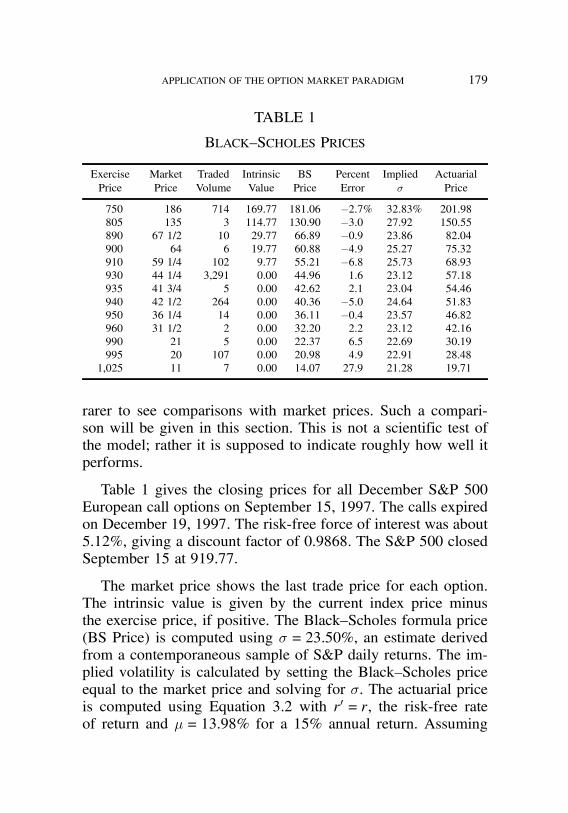
job no. 1969 casualty actuarial society CAS journal 1969D06 [18] 11-08-01 4:58 pm
APPLICATION OF THE OPTION MARKET PARADIGM 179
TABLE 1
BLACK–SCHOLES PRICES
Exercise Market Traded Intrinsic BS Percent Implied ActuarialPrice Price Volume Value Price Error ¾ Price
750 186 714 169.77 181.06 !2:7% 32.83% 201.98805 135 3 114.77 130.90 !3:0 27.92 150.55890 67 1/2 10 29.77 66.89 !0:9 23.86 82.04900 64 6 19.77 60.88 !4:9 25.27 75.32910 59 1/4 102 9.77 55.21 !6:8 25.73 68.93930 44 1/4 3,291 0.00 44.96 1.6 23.12 57.18935 41 3/4 5 0.00 42.62 2.1 23.04 54.46940 42 1/2 264 0.00 40.36 !5:0 24.64 51.83950 36 1/4 14 0.00 36.11 !0:4 23.57 46.82960 31 1/2 2 0.00 32.20 2.2 23.12 42.16990 21 5 0.00 22.37 6.5 22.69 30.19995 20 107 0.00 20.98 4.9 22.91 28.48
1,025 11 7 0.00 14.07 27.9 21.28 19.71
rarer to see comparisons with market prices. Such a compari-son will be given in this section. This is not a scientific test ofthe model; rather it is supposed to indicate roughly how well itperforms.
Table 1 gives the closing prices for all December S&P 500European call options on September 15, 1997. The calls expiredon December 19, 1997. The risk-free force of interest was about5.12%, giving a discount factor of 0.9868. The S&P 500 closedSeptember 15 at 919.77.
The market price shows the last trade price for each option.The intrinsic value is given by the current index price minusthe exercise price, if positive. The Black–Scholes formula price(BS Price) is computed using ¾ = 23:50%, an estimate derivedfrom a contemporaneous sample of S&P daily returns. The im-plied volatility is calculated by setting the Black–Scholes priceequal to the market price and solving for ¾. The actuarial priceis computed using Equation 3.2 with r" = r, the risk-free rateof return and ¹= 13:98% for a 15% annual return. Assuming

job no. 1969 casualty actuarial society CAS journal 1969D06 [19] 11-08-01 4:58 pm
180 APPLICATION OF THE OPTION MARKET PARADIGM
r" = r makes Equation 3.2 exactly the same as Equation 1.3 onpage 703 of the paper for a lognormal stock price distribution.Thus, the last column shows the impact on the option price ofusing the approximate expected rate of return of the underly-ing instrument rather than the risk-free rate of return; this isthe difference between using S and S as the stock price pro-cess. Clearly market prices are much closer to the Black–Scholesprice. Using a higher discount rate in place of r, but leaving ¹unchanged, would bring the actuarial price closer to the Black–Scholes value.
The results are really quite spectacular, especially when com-pared to the range of reasonable values determined by manyactuarial analyses. Remember there is only one free parameterunderlying all the model values, and even that is easy to esti-mate. As Hull [20] points out, the last option trade may haveoccurred well before the market closed, so the option price maycorrespond to a different S&P index value than the close. Hull isalso a good reference for more information on the mechanics ofoptions markets and for reasons why market prices diverge fromBlack–Scholes prices.
Finally, Table 1 only provides evidence that the market pricesusing Black–Scholes or a very similar formula. It does not nec-essarily follow that this is the “correct” price!
7. CONCLUSION
The thrust of Wacek’s paper is that options pricing and insur-ance pricing are essentially the same and that it should be possi-ble for each discipline to learn from the other. In many ways thisis true, particularly on a practical level. Examples include the au-thor’s sections on rate guarantees and multi-year contracts. Thephilosophy of “look for the option” is an important part of mod-ern finance, and is well illustrated by the many applications inBrealey and Myers [2]. Given its central role in finance, actuar-ies should understand the Option Pricing Paradigm and be able

job no. 1969 casualty actuarial society CAS journal 1969D06 [20] 11-08-01 4:58 pm
APPLICATION OF THE OPTION MARKET PARADIGM 181
to apply it, where relevant, in their own work. Wacek’s paper isvaluable because it helps point actuaries in this direction.
However there are some very significant differences betweenthe Option Pricing Paradigm and insurance which should notbe glossed over. The Option Pricing Paradigm is based on ar-bitrage and pricing comparables, and it relies on hedging to re-move risk. Insurance assumes and manages specific risk (seeTurner [33]). There are typically no liquid markets or close com-parables for the specific assets underlying insurance liabilities,and so option pricing techniques do not apply.7 The specializedunderwriting knowledge that insurance companies develop is akey part of their competitive advantage; what they do is bearthe resulting underwriting risk, they do not hedge it away.8 Thispoint is discussed by Santomero and Babbel [32] in their re-view of financial risk management by insurers. Obviously, howan individual company chooses to manage risk does not alterthe market price; the existence of a hedge-based pricing mecha-nism does, however, determine a market price in the absence ofarbitrage.
At a detailed level, Wacek’s transformation from the Black–Scholes formula to his supposedly more general Equation 1.3(Equation 4.3 here) is inappropriate. In this discussion, I haveshown how an actuarial approach to option pricing produces aresult similar to the Black–Scholes formula but with two im-portant differences: the assumed return on the stock (expectedmarket return compared to risk-free return) and the discount rate(a rate greater than the expected market return compared to therisk-free return). The Black–Scholes argument shows that writ-ing options is risk-free (in the conceptual model) because of thepossibility of setting up a self-financing hedging strategy withthe proceeds from writing an option. No-arbitrage then implies
7As Babbel says in [1]: “When it comes to the valuation of insurance liabilities, thedriving intuition behind the two most common valuation approaches—arbitrage andcomparables—fails us.”8Unless they can use their specialized knowledge to arbitrage the reinsurance markets!
job no. 1969 casualty actuarial society CAS journal 1969D06 [21] 11-08-01 4:58 pm
182 APPLICATION OF THE OPTION MARKET PARADIGM
the price of the option must be the smallest amount for which itis possible to set up a hedging portfolio. It follows that the optionprice is independent of an individual investor’s risk preferences.Cox and Ross [4] then argued that the option can be priced as-suming risk-neutrality. In a risk-neutral world stocks earn therisk-free return, thus explaining the first assumption. The hedg-ing portfolio argument also shows the risk-free rate is appro-priate for discounting, which explains the second assumption.Wacek makes the latter point but does not mention the former.As shown in Table 1, there is a significant difference betweenthe option prices with and without the former assumption. More-over, market prices are consistently closer to the Black–Scholesprices. The discussion of hedging and options pricing also makesit clear Black–Scholes gives a price, not a pure premium. Finally,Wacek’s assertion that “the pricing mathematics is basically thesame” for options and insurance is not really the case. Doubts asto this point can be dispelled by looking in any more advancedtext on options pricing, such as [14].
In this review, a simple discrete time example has been givento illustrate the hedging portfolio argument. It shows how theoption price is independent of risk preferences given the cur-rent stock price. While the example is often reproduced in fi-nance texts, the discussion of exactly how risk preferences fit in(through Equation 4.1) is less common. A new application of theOption Pricing Paradigm to catastrophe insurance was proposed,and how the paradigm works in the case of an underlying whichis not traded was discussed. Finally, a comparison of marketprices, Black–Scholes prices and actuarial prices for some S&Poptions has been given.
The Black–Scholes option pricing formula is an important andbeautiful piece of mathematics and financial economics. On thesurface the formula is just the discounted expected excess valueof a lognormal random variable—the tricky part is which lognor-mal variable! Understanding some of the paradigm lying behindthe formula, and some of its subtleties, gets us to the core of the

job no. 1969 casualty actuarial society CAS journal 1969D06 [22] 11-08-01 4:58 pm
APPLICATION OF THE OPTION MARKET PARADIGM 183
differences between how insurers and other financial institutionsbear and manage risk. Given the current convergence betweeninsurance and banking it is important for insurance actuaries tounderstand and to be able to exploit these differences—our futurelivelihoods could depend upon it.

job no. 1969 casualty actuarial society CAS journal 1969D06 [23] 11-08-01 4:58 pm
184 APPLICATION OF THE OPTION MARKET PARADIGM
REFERENCES
[1] Babbel, David F., “Review of Two Paradigms for the Mar-ket Value of Liabilities by R. R. Reitano,” North AmericanActuarial Journal 1, 4, 1997, pp. 122–123.
[2] Brealey, Richard A. and Stewart C. Myers, Principles ofCorporate Finance, 4th Edition, McGraw-Hill, 1981.
[3] Casualty Actuarial Society, “Statement of Principles Re-garding Property and Casualty Valuations, as adoptedSeptember 22, 1989,” Casualty Actuarial Society Yearbook,(1997), pp. 277–282.
[4] Cox, J. and S. Ross, “The Valuation of Options for Alterna-tive Stochastic Processes,” Journal of Financial Economics3, 1976, pp. 145–166.
[5] Cox, J., S. Ross, and M. Rubenstein, “Option Pricing: ASimplified Approach,” Journal of Financial Economics 7,1979, pp. 229–263.
[6] Cummins, J. David, “Risk-Based Premiums for InsuranceGuarantee Funds,” Journal of Finance 43, 1988, pp. 823–839.
[7] Cummins, J. David and Helyette Geman, “An Asian OptionApproach to the Valuation of Insurance Futures Contracts,”Review of Futures Markets 13, 2, 1994, pp. 517–557.
[8] Cummins, J. David and Helyette Geman, “Pricing Catas-trophe Insurance Futures and Call Spreads: An ArbitrageApproach,” Journal of Fixed Income 4, 4, 1995, pp. 46–57.
[9] D’Arcy, Stephen P. and Neil A. Doherty, The Financial The-ory of Pricing Property Liability Insurance Contracts, Home-wood, IL: Huebner Foundation/Irwin, 1988.
[10] Delbaen, F. and W. Schachermayer, “A General Version ofthe Fundamental Theorem of Asset Pricing,” Math. Ann.300, 1994, pp. 463–520.
job no. 1969 casualty actuarial society CAS journal 1969D06 [24] 11-08-01 4:58 pm
APPLICATION OF THE OPTION MARKET PARADIGM 185
[11] Delbaen, F. and W. Schachermayer, “Arbitrage Possibili-ties in Bessel Processes and Their Relation to Local Mar-tingales,” Probability Theory and Related Fields, 102, 1995,pp. 357–366.
[12] Delbaen, F. and W. Schachermayer, “Arbitrage and FreeLunch With Bounded Risk for Unbounded Continuous Pro-cesses,” Mathematical Finance 4, 4, 1994, pp. 343–348.
[13] Delbaen, F., W. Schachermayer and M. Schwizier, “Reviewof Option Pricing by Esscher Transforms,” Transactions ofthe Society of Actuaries XLVI, 1994, pp. 148–151.
[14] Dothan, Michael U., Prices in Financial Markets, OxfordUniversity Press, 1990.
[15] Duffie, Darrell, Dynamic Asset Pricing Theory, PrincetonUniversity Press, 1992.
[16] Dybvig, Philip H. and Stephen A. Ross, “Arbitrage,” TheNew Palgrave: Finance, (Eatwell, J., M. Milgate and P.Newman, eds.), W.W. Norton, 1987.
[17] Gerber, Hans U. and Elias S. W. Shiu, “Option Pricing byEsscher Transforms,” Transactions of the Society of Actuar-ies XLVI, 1994, pp. 99–191.
[18] Gillam, William R. and Richard H. Snader, Fundamentals ofIndividual Risk Rating, National Council on CompensationInsurance (Study Note), 1992.
[19] Harrison, J. M. and D. Kreps, “Martingales and Arbitragein Multiperiod Securities Markets,” Journal of EconomicTheory 20, 1979, pp. 381–408.
[20] Hull, John C., Options Futures and Other Derivative Secu-rities, Second Edition, Prentice-Hall, 1983.
[21] Ingersoll Jr., Jonathan E., “Options Pricing Theory,” TheNew Palgrave: Finance, (J. Eatwell, M. Milgate and P. New-man, eds.), W.W. Norton, 1987, pp. 199–212.
[22] Jaffee, Dwight M. and Thomas Russell, “Catastrophe In-surance, Capital Markets, and Uninsurable Risks,” Journalof Risk and Insurance 64, 2, 1997, pp. 205–230.
job no. 1969 casualty actuarial society CAS journal 1969D06 [25] 11-08-01 4:58 pm
186 APPLICATION OF THE OPTION MARKET PARADIGM
[23] Karatzas I. and S. Shreve, Brownian Motion and StochasticCalculus, New York: Springer-Verlag, 1988.
[24] Kellison, Stephen G., The Theory of Interest, 2nd Edition,Irwin, 1991.
[25] Lee, Yoong-Sin, “The Mathematics of Excess of Loss Cov-erage and Retrospective Rating—A Graphical Approach,”PCAS LXXV, 1988, pp. 49–77.
[26] Lee, Yoong-Sin, “On the Representation of Loss and In-demnity Distributions,” PCAS LXXVII, 1990, pp. 204–224.
[27] Merton, Robert C., “Theory of Rational Option Pricing,”Continuous Time Finance, Blackwell, 1990.
[28] Miccolis, Robert S., “On the Theory of Increased Limitsand Excess of Loss Pricing,” PCAS LXIV, 1977, pp. 27–59.
[29] Nawalkha, Sanjay K. and Donald R. Chambers, “The Bino-mial Model and Risk Neutrality: Some Important Details,”The Financial Review 30, 3, 1995, pp. 605–615.
[30] Phillips, Richard D., J. David Cummins and Franklin Allen,“Financial Pricing of Insurance in the Multiple-Line Insur-ance Company,” The Journal of Risk and Insurance 65, 4,1998, pp. 597–636.
[31] Samuelson, P. A., “Rational Theory of Warrant Pricing,”Industrial Management Review 6, 2, 1965, pp. 13–32.
[32] Santomero, Anthony M., and David F. Babbel, “FinancialRisk Management by Insurers: An Analysis of the Process,”Journal of Risk and Insurance 64, 2, 1997, pp. 231–270.
[33] Turner, Andrew L., “Insurance in an Equilibrium Asset-Pricing Model,” Fair Rate of Return in Property-LiabilityInsurance, (J. David Cummins and Scott A. Harrington,eds.), Boston: Kluwer-Nujhoff, 1987.
[34] Wang, S., “PremiumCalculation by Transforming the LayerPremium Density,” ASTIN Bulletin 26, 1995, pp. 71–92.

job no. 1969 casualty actuarial society CAS journal 1969D06 [26] 11-08-01 4:58 pm
APPLICATION OF THE OPTION MARKET PARADIGM 187
[35] Wang, S., “Ambiguity-aversion and the economics of insur-ance,” Proceedings of the Risk Theory Seminar, Wisconsin-Madison (1996).
[36] Wilmot, Paul, Sam Howison, and Jeff Dewynne, The Math-ematics of Financial Derivatives, A Student Introduction,Cambridge University Press, 1995.

job no. 1969 casualty actuarial society CAS journal 1945D09 [1] 11-08-01 4:58 pm
THE 1999 TABLE OF INSURANCE CHARGES
WILLIAM R. GILLAM
“The problem is all inside your head,She said to me.
The answer is easy if youTake it logically.
I’d like to help you in your struggleTo be free;
There must be fifty waysTo leave your lover.”
—Paul Simon
Abstract
This paper describes the development of the 1999Workers Compensation Table of Insurance Charges (Ta-ble M), filed in NCCI states to be effective November 1,1998.It presumes the reader knows what Table M is, and
how it is used in retrospective rating. Familiarity withthe NCCI Retrospective Rating Plan (the Plan) is help-ful.Development of the 1999 Table M is described in
steps, beginning with the sample data and how it wasmanipulated, followed by the algorithm used to modelloss ratios, methods for developing the loss ratio distri-bution, graduation of the excess ratios and derivation ofExpected Loss Size Ranges used in the Plan.The impact on premium of the proposed new Table M
is estimated.
1. BACKGROUND
At the heart of retrospective rating is a table of excess ratioscommonly called Table M. Details on the definition and use of
188

job no. 1969 casualty actuarial society CAS journal 1945D09 [2] 11-08-01 4:58 pm
THE 1999 TABLE OF INSURANCE CHARGES 189
Table M are provided much more fully elsewhere in the literature.See [1], [2], [3] and [4] among the references to this paper. Thereader is expected to know the vocabulary and basic significanceof the table.
The Workers Compensation Table of Insurance Charges, theproper name of Table M, was last changed in 1984. Derivation ofthe 1984 Table M was never documented in PCAS, as was donefor the 1964 Table M by LeRoy Simon, but it served well foralmost 15 years. Its passing is hereby lamented, if a bit satirically,in the song above, fittingly by another Simon. (One of fifty ways:“Don’t need to be coy, Roy.”)
Since 1984, annual updates have been made to account for in-flation in the average cost per case, which was quite significantduring the late 1980s. The body of Table M was not changed,but only the expected loss sizes necessary to qualify for specificcolumns of the table. Increasing skewness in the severity distri-bution, as discussed below, impacted the loss ratio distribution,and this needed to be reflected in the body of Table M; changesof this sort are not accounted for in inflationary updates. Evenif the table was approximately adequate in 1998, which our re-search verified, the need to update the body of Table M wasevident.
The changes in the loss size distribution were recognized earlyon and led to non-trivial updates in the calculation of excessloss factors (ELFs), also used in the retrospective rating plan.Three revisions were made (in 1987, 1992, and 1996) to themodel distributions used in the calculation of ELFs. The changesare documented in [5] and [6]. In general, each step involvedrecognition of increasing skewness in the distribution of seriousclaims by size.
The changes in loss severity are a sign of the times. Under-writing results in the workers compensation line of business dur-ing the last two decades of this century are a matter of record.

job no. 1969 casualty actuarial society CAS journal 1945D09 [3] 11-08-01 4:58 pm
190 THE 1999 TABLE OF INSURANCE CHARGES
Volatility in premium adequacy was driven by changes in le-gal rules, program administration, benefits, and salaries, as wellas a generally increasing feeling of entitlement among the pub-lic starting in the 1970s. During the late 1980s, this led to theneed for large rate increases, relatively more large compensationawards and a heavier tailed severity distribution.
2. OUTLINE
This is a short description of the basic steps in the creation ofthe 1999 Table of Insurance Charges. There is a section of thepaper for each step.
A. Sample Data—Premium and loss information was assembledfor a sample of 450,156 insureds from policy year 1988 atfifth report. The sample was grouped into 25 overlapping ad-justed expected loss size ranges. Risk expected loss size isadjusted by formula: a product of standard expected loss andthe appropriate state and hazard group relativity. The empir-ical loss ratio distribution of each group was normalized toa mean of unity.
B. Modeling Sample Excess Ratios—For each sample group, theempirical excess ratio distribution was fitted to excess ratiosbased on a Heckman–Meyers (HM) model distribution, asdescribed in [7] and [8]. The severity distribution used inthe model was exactly the one underlying the empirical fifthreport, and the frequency parameters were selected to effecta fit.
C. Development to Ultimate—The fifth report severity distribu-tion was replaced with one developed to ultimate. The sever-ity uncertainty parameter was increased to account for lossratio uncertainty, i.e., parameter risk. An ultimate excess ratiodistribution was produced for 26 groups. (The 26th distribu-tion was based on a hypothetically large expected number ofclaims and, as such, had no empirical sample.)
job no. 1969 casualty actuarial society CAS journal 1945D09 [4] 11-08-01 4:58 pm
THE 1999 TABLE OF INSURANCE CHARGES 191
D. Graduating the Table—Inverse exponential polynomials wereused to graduate 26 model excess ratio distributions.
E. The 1999 Table of Insurance Charges—This is it!
F. Derivation of Size Ranges—Sample risk average (formula)adjusted size and HM model frequency were used to derivenominal average severity by sample group. By selecting oneaverage severity, we were able to assign a 1988 expected losssize, frequency times severity, to each of 26 mother curves.Interpolation was used to create boundaries for (adjusted)expected loss size ranges, indexed by charges at entry ratiounity of 0.095 to 0.975. Estimated severity trend was used tomake size ranges appropriate for 1999.
G. Estimating the Impact—The algorithm described in [4] wasused to estimate premium recovered by using Table M.
3. THE PROCESS
Sample Data
We used the latest available statistical plan data at fifth reportfor the review. The unit statistical information includes the fol-lowing information for each policy in each state: payroll by class,manual premium (which is an extension of payroll along the re-spective class rates), experience modification, standard premiumand loss. We were able to group this information by risk to allowthe tabulation of standard expected loss (standard premium timespermissible loss ratio), actual loss, loss ratio and hazard groupof each risk (which can occasionally vary by state).
Exhibit 1 shows the actual policy periods by state used forthis analysis. These are close to policy year 1988, but vary bystate according to the filing schedules.
The exhibit also shows state and hazard group severity rela-tivities (S&HGRs), effective 10/1/91. In order to assign a risk toa column of Table M, the risk’s adjusted expected loss size is

job no. 1969 casualty actuarial society CAS journal 1945D09 [5] 11-08-01 4:58 pm
192 THE 1999 TABLE OF INSURANCE CHARGES
used. Starting with standard expected loss by state, the adjust-ment is accomplished by application of the appropriate S&HGR.This should account for known differences in scale of severitydistributions and is part of the current retrospective rating plan.Ideally, we would have used values calculated for 1988, but 1991was the first year the filing was effective and these were the ear-liest calculated, so we used these to adjust expected losses. Webelieve using the relativities is essential to be consistent with theuse of Table M in the retrospective rating plan, notwithstand-ing the discrepancy in effective date. Experience has shown theS&HGRs, which are relativities to the average, do not changemuch from year to year.
Using adjusted expected losses by risk, we grouped samplerisks into 25 size ranges. To maximize the number of risks ineach group, we allowed the size ranges to overlap, so somerisks fall into two different size ranges. Exhibit 2 shows the1988 expected loss size ranges used. Column 1 shows the ap-plicable indices for columns of the table. As described in [1],columns of Table M are indexed by the charge at entry ratio1, in percent. So for the third row, applicable columns havecharges at unity of 0.16 to 0.22. This corresponds to seven sizeranges:
1988 1988Expected Loss Expected Loss
Index Minimum Maximum
16 4,386,336 5,565,157...
......
21 1,544,131 1,872,49722 1,281,534 1,544,130
Risks with adjusted loss within the total range formed a sam-ple group of loss ratios from which empirical excess ratios werecalculated.

job no. 1969 casualty actuarial society CAS journal 1945D09 [6] 11-08-01 4:58 pm
THE 1999 TABLE OF INSURANCE CHARGES 193
Embedded in the 1988 risk data used is a fifth report sever-ity distribution, all states combined. This distribution became anintegral part of the next step.
Modeling Sample Excess Ratios
Each sample group of risks exhibited an empirical distributionof loss ratios, F[x]. The loss ratios x could easily be convertedinto entry ratios r by dividing x by the average, so that E[r] = 1:0.The excess ratios X(r) =
!!s=r(s" r)f(s), where f is the normal-
ized density, were calculated directly from the data. See [2] or[3] for a more detailed treatment of the topic of excess ratios.
This is a summary of the HM model as it pertains to this ap-plication: Using the collective risk model from risk theory, theHM algorithm creates a loss ratio distribution from underlyingfrequency and severity distributions. The algorithm uses the mo-ment generating function of the frequency and the characteristicfunction for the severity to derive the characteristic function ofthe loss ratio distribution, then inverts it to generate the aggre-gate distribution. Using simplifying assumptions, the input dataare an expected claim count ¸ and a contagion parameter c tomodel the frequency distribution, and a piecewise linear sever-ity distribution with a severity uncertainty parameter b to modelseverity. See [7], [8], and [9] for details.
We used the fifth report severity distribution along withchoices of ¸, c, and b to fit the empirical sample of excess ratios.
Each sample excess ratio distribution was fit directly to onebased on the HM model. Exhibit 3 shows results of the mod-eling process. (Each page shows results of 25 different fits atentry ratios 1.0 and 3.0.) There was no special technique used toeffect the fit. It turned out that using the appropriate frequencyto match the excess ratio at the entry ratio r = 1 assured a fairlygood fit to the entire sample excess ratio distribution. We startedwith ¸ proportional to the average adjusted expected loss size ofthe sample. A severity uncertainty parameter b = 0:001 worked

job no. 1969 casualty actuarial society CAS journal 1945D09 [7] 11-08-01 4:58 pm
194 THE 1999 TABLE OF INSURANCE CHARGES
well in the fit. Such a small value makes sense given that theempirical sample severity distribution and normalized loss ratioare determinate. There was more room to adjust the contagionparameter. We started with c= 0:30 for the small size groups. Tofit the distribution for larger risks, we needed to vary the con-tagion parameter c downward, as can be seen in Exhibit 3. Wemade fine-tuning adjustments to ¸ or c to extend the fit to allentry ratios for all 25-size groups.
Development to Ultimate
We did not change frequency parameters ¸ and c after fifthreport, assuming that change in the claim frequency distributionis insignificant after fifth report. This is a reasonable assump-tion, borne out by empirical evidence of very little frequencydevelopment from fourth to fifth report. In practice, of course,some claims may close with no payment or emerge as IBNR, butthis could be considered a matter of parameter risk as discussedbelow. We thus retained the fifth report model parameters ¸and c.
The development of the claim severity distribution is anothermatter. We had learned a lot about loss severity development inexcess loss factor (ELF) studies, first in 1992 and carried fur-ther in 1996, as described in [6]. Underlying the ELF procedureare three indemnity claim size distributions by injury group, de-veloped to ultimate. We also have one for medical-only claims.We were able to create an ultimate severity distribution consis-tent with the 1988 data by weighting scaled component distribu-tions. Each state has its own (estimated) ultimate scale and injuryweight for each of these distributions.
We created an ultimate severity distribution using techniquesmuch the same as in the ELF procedure [5]. We were able to de-velop average costs per case at ultimate and injury type weightsby state. We used those severities to scale the underlying distri-butions and the weights to combine them across injury group bystate and then across states.

job no. 1969 casualty actuarial society CAS journal 1945D09 [8] 11-08-01 4:58 pm
THE 1999 TABLE OF INSURANCE CHARGES 195
1. Empirical average severity by state and injury type wascalculated from the 1988 data.
2. Fifth to ultimate severity development factors were cal-culated for serious injury types by state. This was doneby attributing the fifth to ultimate loss development fac-tors from ratemaking entirely to serious injury claim size.
3. The development factors were applied respective of stateand injury type.
4. Developed permanent total (PT) and major permanentpartial (Major) claim types were combined, as well asfifth report minor permanent partial (Minor) and tem-porary total (TT), to obtain average severities for fatal,PT/Major, Minor/TT and medical-only injury groups bystate.
5. Loss weights by injury group and state were calculated.
6. Average severities and loss weights by injury group wereused with respective ultimate loss size distributions fromthe ELF procedure, and an associated distribution formedical-only, to make a weighted average severity dis-tribution for all claims combined by state.
7. All states were weighted together to create one ultimate1988 severity distribution. This was fit by a piecewiselinear model for use in the HM algorithm.
Now, using this derived ultimate severity distribution,1 we wereable to use HM to create an ultimate loss ratio distribution withcorresponding excess ratios. We did this first retaining b = 0:001as at fifth report. The impact of changing to an ultimate severitydistribution was considerable. This can be seen in Exhibit 4 bycomparing column 5 to column 4. We saw increases of up to 5
1Both the Table of Insurance Charges and the underlying severity distribution are prod-ucts for sale by NCCI; hence they are not included in this paper.

job no. 1969 casualty actuarial society CAS journal 1945D09 [9] 11-08-01 4:58 pm
196 THE 1999 TABLE OF INSURANCE CHARGES
percentage points in excess ratios for entry ratio 1, applicable torisks in the size ranges most impacted by retrospective rating (25to 60). We saw even larger increases at the higher entry ratios,reflecting the increased skewness of the loss ratio distributionbased on ultimate severity.
To account for parameter risk, we chose to increase the sever-ity uncertainty parameter b from 0.001 to 0.015. This is a judg-ment call, and based on our estimates of loss ratio uncertainty,not simply scale uncertainty. We needed to account for the factthat the expected loss ratio for each risk is only an estimate.The flexibility of the HM model to allow such an adjustment isa huge advantage of HM over competing models. Even thoughb = 0:015 represents a 12.2% uncertainty in expected loss ratio,which is large, the resulting increase in charges (about half apercentage point) did not seem that excessive. A comparison ofcolumns 7 and 5 shows the impact of this choice is much smallerthan the change from column 4 to 5.
The result of the process is 25 sample excess ratio tables basedon 25 loss ratio distribution models with underlying frequencyand severity distribution. A 26th sample was created using theultimate severity distribution and enough expected claims to pro-duce a charge at unity of less than 0.095.
Graduating the Table
Having 26 columns of an excess ratio table based on HMmodel loss distributions is a wonderful thing, but in practice thefunctional form of the associated insurance charges is more com-plex than practitioners may have wanted. They did want more ofother qualities: ease of data entry and at least 80 columns withcharges at unity in even percents. (The charges at unity of the26 models were not necessarily integral percents.)
The 1984 table could be generated by interpolating betweena sample of 19 inverse exponential polynomials, and two bound-ary functions. A similar algorithm to generate the new table
job no. 1969 casualty actuarial society CAS journal 1945D09 [10] 11-08-01 4:58 pm
THE 1999 TABLE OF INSURANCE CHARGES 197
was needed. This was accomplished in the following manner, aslightly simplified version of the prior technique.
1. Each sample HM excess ratio table was modeled. Thiswas done by catenating three models:
a. X(r) = 1" r for small values of r (at least for thelarger size groups).
The HM samples verified this simple expression forX, so it was better not to try and extend the fit furtherthan necessary.
b. X(r) = exp[!8k=1 akr
k] for medium values for r. Thecoefficients are derived from a regression on the HMmodel excess ratios, and of course differ by sizerange. By limiting the fit to these critical values ofr, very close approximations are possible.
c. X(r) = X(rl)k(r)X(ru)
1"k(r), where
k(r) ="ru" rru" rl
#, and rl # r # ru:
X(ru) is taken from the fitted curve in (b), and X(rl) istaken from the underlying HM sample tables. (rl,ru) isthe interval of (largest) entry ratios where this simpledecay works best.
These provide sample curves for interpolating the fi-nal table. For curves 29.35 and 33.16, Exhibit 5 showsresults of this modeling.
2. Two more mother curves were defined to be used asboundary values.
X0(r) =
$%&1" r 0# r # 10 for all r $ 1,
where r is the entry ratioX100(r) = 1 for all r $ 0
Now there are 28.
job no. 1969 casualty actuarial society CAS journal 1945D09 [11] 11-08-01 4:58 pm
198 THE 1999 TABLE OF INSURANCE CHARGES
3. Linear interpolation between the 28 mother curves wasused to generate the columns of the table with inte-gral percent p charge at unity entry ratio. For any en-try ratio r, the charge for the column indexed by pis:
Xp(r) = Xl(r)+
'Xp(1)"Xl(1)Xu(1)"Xl(1)
()Xu(r)"Xl(r)
*Exhibit 6 is a graph of the values used to interpolate X32.
The 1999 Table of Insurance Charges
After jumping through hoops, standing on our heads, and spit-ting wooden nickels to create this table, it is time to take a breakand enjoy a picture. Exhibit 7 is a three-dimensional graph of theTable (r,X,I). From the point of view of the reader, the graph isa concave surface. The vertical X axis is the charge. The entryratios r from 0.0 to 3.2 go from left to right coming towards thereader across the left half of the page, and the size group col-umn shows indices from 0 to 100, going away from left to rightacross the right half.
The surface is flat (planar) in the upper left, where entry ratiosare low and risks are large. In this region, X(r) = 1" r, whichimplies loss ratios are always at least rE. The curved isoclinesdenote constant charges of 0.90, 0.80, : : : ,0.10 from top to bot-tom. Note that there is an implied isocline for X = 0:0.
The foreground cross-section of the surface is concave andincreasingly so for larger and larger values of r, as it will tuckin closer and closer to the line (r,0,1) behind the surface onthe right hand side of the page. This is because for all sizegroups bigger than the boundary where X(1) = 1, the charge ap-proaches 0 as r increases. Within the contoured surface, there isa straight line where r = 1, and the charge is 1/100 of the index(1,X,100X).
job no. 1969 casualty actuarial society CAS journal 1945D09 [12] 11-08-01 4:58 pm
THE 1999 TABLE OF INSURANCE CHARGES 199
On Derivation of Size Ranges
Thus far we have developed a table with columns indexed bythe (percent) insurance charge at unity entry ratio. As explainedabove, this is based on 26 loss ratio distributions, complete withfrequency and severity parameters.
Table M was to be filed effective November 1, 1998. It wasnecessary to determine size ranges to be used for selection ofthe columns of the table applicable to an individual risk. Theseranges would of course be adjusted going forward for trend inaverage severity.
The HM model severity is scale free in the sense that the lossratio distribution, and consequent table of excess ratios, dependson the expected claim count and the shape, but not the size, ofthe severity distribution. If we could attach a scale to this distri-bution, we could use frequency times adjusted average severityto determine a dollar size corresponding to each model.
Exhibit 8 shows the first step in the estimation of the implicitaverage adjusted severity. We have already calculated the averageadjusted expected loss of each of 25 empirical sample groups inExhibit 2. Our modeling process assigned a frequency (expectedclaim count) to each group which was needed to match the sam-ple loss ratio distribution. In Exhibit 8, we simply divide theadjusted expected losses by the expected claim count to producean expected average adjusted severity. This of course varies witheach sample group, but, except for a small upward tick in thelargest size ranges, the estimated severity is remarkably flat.
We selected an average adjusted severity value consistent withthe 1988 samples. Using expected claim counts from the models(including the hypothetical model), the product is the point esti-mate of adjusted expected loss size for the 26 samples in 1988.This is shown in Exhibit 9.
Exhibit 10 shows how we developed 1988 size ranges. Inshort, we used interpolation between the 26 points to estimate

job no. 1969 casualty actuarial society CAS journal 1945D09 [13] 11-08-01 4:58 pm
200 THE 1999 TABLE OF INSURANCE CHARGES
adjusted expected losses corresponding to the boundaries of theranges (i.e., even percents +0:005).
We wanted to adjust these average sizes to a point in 1999.Using statistical plan data, we were able to determine that theactual severity trend between 1988 and 1994 was about +25%.Independent analysis of the most recent available data showedseverity trend to be nearly flat from 1993 through 1996, so weprojected no severity trend after 1994. Using the 1.25, we de-termined boundaries of expected loss size ranges applicable in1998/99. This is column 7 of Exhibit 10.
Estimating the Impact
The 1999 Table of Insurance Charges was filed effective11/1/98, replacing the 1984 Table. The aggregate impact on ex-pected retrospective rating premium was not great.
In the body of Table M, for the low entry ratios associatedwith the run of the mill retrospective rating contracts sold, thechanges in the table values were fairly small. The change to theexpected loss size ranges, although not a simple linear inflation,was also moderate. This can be seen in Exhibit 11. For the highcharge/small expected loss size columns, the inflationary impactwas minimal, with less than a 7% increase in the expected losssize ranges 72 to 46. This encompasses 1999 expected losses of$17,000 to $132,500. The size of a risk needed to qualify for thelower charge columns grew significantly, so that to qualify forcolumn 20, a risk had to be 60% larger ($5.9 vs. $3.7 million).We assume not many risks this size are written on a straight retro,even before this change.
Using methods described in [4], we were able to estimate animpact of about +1% on expected retrospectively rated premium.Exhibit 12 shows the evaluation. Assuming the new table is acorrect measure of excess ratios, we began with sample plans forrepresentatives of each range, calculated based on the old TableM and size groups. The expected retrospective premium written

job no. 1969 casualty actuarial society CAS journal 1945D09 [14] 11-08-01 4:58 pm
THE 1999 TABLE OF INSURANCE CHARGES 201
under those plans was evaluated with the proposed table andsize ranges applicable to actual losses. The estimated shortfall isabout 1% of premium which would (theoretically) be recoveredif the new table is implemented.
4. CONCLUSION
The new Table of Insurance Charges is a significant improve-ment to the former table. This is not a matter of pricing adequacy,as the estimated overall impact is small. What matters more isthe increase in individual risk equity due to the associated non-linear update of expected loss size ranges, but even this is onlypart of the story.
The use of explicit underlying frequency and severity dis-tributions is a great advance in the science, making the tablemore useful in new as well as standard applications. It allowsfor much more facile future updates, not only for inflation, butalso for changes in workers compensation law, administration orenvironment. There must be 50 ways.

job no. 1969 casualty actuarial society CAS journal 1945D09 [15] 11-08-01 4:58 pm
202 THE 1999 TABLE OF INSURANCE CHARGES
REFERENCES
[1] Simon, LeRoy J., “The 1965 Table M,” PCAS LII, 1965,p. 1.
[2] Gillam, William R., and Richard H. Snader, “Fundamentalsof Individual Risk Rating,” monograph published by NCCI,1992.
[3] Skurnick, David, “The California Table L,” PCAS LXI, 1974,p. 117.
[4] Gillam, Willam R., Discussion of Skurnick: “The CaliforniaTable L,” PCAS LXXX, 1993, p. 353.
[5] Gillam, William R., “Retrospective Rating: Excess Loss Fac-tors, PCAS LXXVIII, 1991 p. 1.
[6] Gillam, William R., “Retrospective Rating: 1997 ExcessLoss Factors,” PCAS LXXXIV, 1997, p. 450.
[7] Heckman, Philip E., and Glenn G. Myers, “The Calculationof Aggregate Loss Distributions from Claim Severity andClaim Count Distributions,” PCAS LXX, 1983, p. 22.
[8] Venter, Gary G., Discussion of Heckman and Myers: “TheCalculation of Aggregate Loss Distributions from ClaimSeverity and Claim Count Distributions,” PCAS LXX, 1983,p. 67.
[9] Klugman, Stuart A., Harry H. Panjer, and Gordon E. Will-mot, Loss Models: From Data to Decisions, New York: JohnWiley & Sons, Inc., 1998.
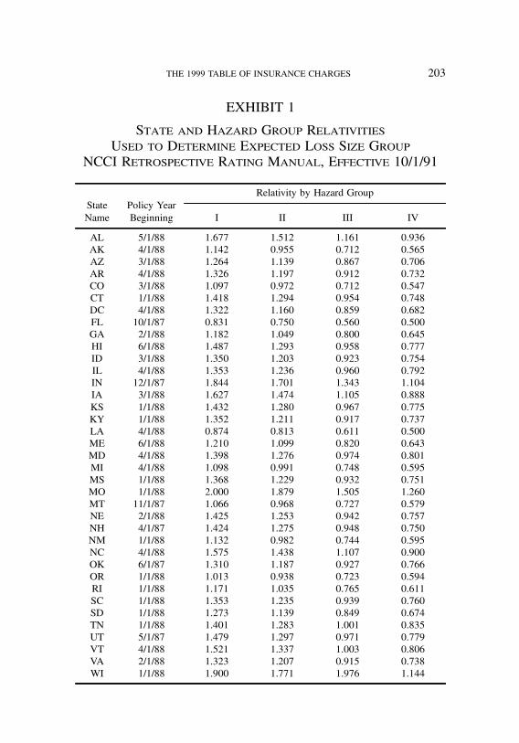
job no. 1969 casualty actuarial society CAS journal 1945D09 [16] 11-08-01 4:58 pm
THE 1999 TABLE OF INSURANCE CHARGES 203
EXHIBIT 1
State and Hazard Group RelativitiesUsed to Determine Expected Loss Size Group
NCCI Retrospective Rating Manual, Effective 10/1/91
Relativity by Hazard GroupState Policy YearName Beginning I II III IV
AL 5/1/88 1.677 1.512 1.161 0.936AK 4/1/88 1.142 0.955 0.712 0.565AZ 3/1/88 1.264 1.139 0.867 0.706AR 4/1/88 1.326 1.197 0.912 0.732CO 3/1/88 1.097 0.972 0.712 0.547CT 1/1/88 1.418 1.294 0.954 0.748DC 4/1/88 1.322 1.160 0.859 0.682FL 10/1/87 0.831 0.750 0.560 0.500GA 2/1/88 1.182 1.049 0.800 0.645HI 6/1/88 1.487 1.293 0.958 0.777ID 3/1/88 1.350 1.203 0.923 0.754IL 4/1/88 1.353 1.236 0.960 0.792IN 12/1/87 1.844 1.701 1.343 1.104IA 3/1/88 1.627 1.474 1.105 0.888KS 1/1/88 1.432 1.280 0.967 0.775KY 1/1/88 1.352 1.211 0.917 0.737LA 4/1/88 0.874 0.813 0.611 0.500ME 6/1/88 1.210 1.099 0.820 0.643MD 4/1/88 1.398 1.276 0.974 0.801MI 4/1/88 1.098 0.991 0.748 0.595MS 1/1/88 1.368 1.229 0.932 0.751MO 1/1/88 2.000 1.879 1.505 1.260MT 11/1/87 1.066 0.968 0.727 0.579NE 2/1/88 1.425 1.253 0.942 0.757NH 4/1/87 1.424 1.275 0.948 0.750NM 1/1/88 1.132 0.982 0.744 0.595NC 4/1/88 1.575 1.438 1.107 0.900OK 6/1/87 1.310 1.187 0.927 0.766OR 1/1/88 1.013 0.938 0.723 0.594RI 1/1/88 1.171 1.035 0.765 0.611SC 1/1/88 1.353 1.235 0.939 0.760SD 1/1/88 1.273 1.139 0.849 0.674TN 1/1/88 1.401 1.283 1.001 0.835UT 5/1/87 1.479 1.297 0.971 0.779VT 4/1/88 1.521 1.337 1.003 0.806VA 2/1/88 1.323 1.207 0.915 0.738WI 1/1/88 1.900 1.771 1.976 1.144
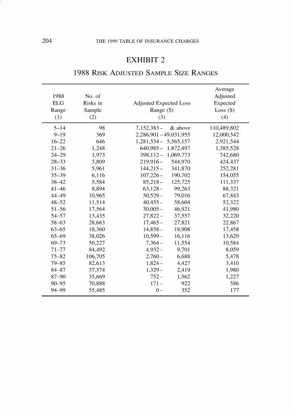
job no. 1969 casualty actuarial society CAS journal 1945D09 [17] 11-08-01 4:58 pm
204 THE 1999 TABLE OF INSURANCE CHARGES
EXHIBIT 2
1988 Risk Adjusted Sample Size Ranges
Average1988 No. of AdjustedELG Risks in Adjusted Expected Loss ExpectedRange Sample Range ($) Loss ($)(1) (2) (3) (4)
5–14 98 7,152,383 – & above 110,489,8029–19 369 2,286,901 – 49,031,955 12,000,54216–22 646 1,281,534 – 5,565,157 2,921,54421–26 1,248 640,985 – 1,872,497 1,385,52824–29 1,973 398,112 – 1,069,773 742,68028–33 3,809 219,916 – 544,970 424,43731–36 5,961 144,215 – 341,870 252,28135–39 6,116 107,226 – 190,702 154,05538–42 5,584 85,218 – 125,725 111,33741–46 8,894 63,128 – 99,263 88,32144–49 10,965 50,529 – 79,016 67,84348–52 11,514 40,455 – 58,604 52,32251–56 17,564 30,005 – 46,921 41,98054–57 13,435 27,822 – 37,557 32,22058–63 28,663 17,465 – 27,821 22,86763–65 18,360 14,858 – 18,908 17,45865–69 38,026 10,599 – 16,116 13,62969–73 50,227 7,364 – 11,554 10,58471–77 84,492 4,932 – 9,701 8,05975–82 106,705 2,760 – 6,688 5,47879–85 82,613 1,824 – 4,427 3,41084–87 37,374 1,329 – 2,419 1,98087–90 35,669 752 – 1,562 1,22790–95 70,888 171 – 922 58694–99 55,485 0 – 352 177
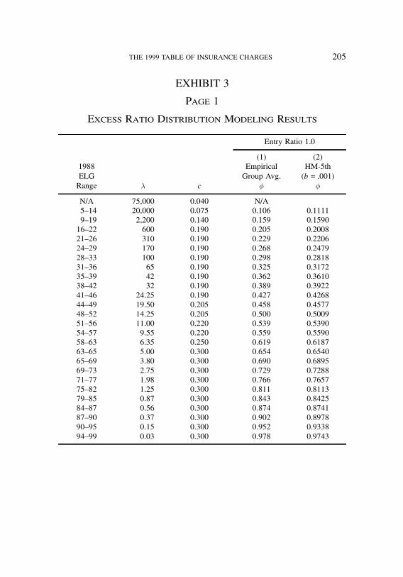
job no. 1969 casualty actuarial society CAS journal 1945D09 [18] 11-08-01 4:58 pm
THE 1999 TABLE OF INSURANCE CHARGES 205
EXHIBIT 3
Page 1
Excess Ratio Distribution Modeling Results
Entry Ratio 1.0
(1) (2)1988 Empirical HM-5thELG Group Avg. (b = :001)Range ¸ c Á Á
N/A 75,000 0.040 N/A5–14 20,000 0.075 0.106 0.11119–19 2,200 0.140 0.159 0.159016–22 600 0.190 0.205 0.200821–26 310 0.190 0.229 0.220624–29 170 0.190 0.268 0.247928–33 100 0.190 0.298 0.281831–36 65 0.190 0.325 0.317235–39 42 0.190 0.362 0.361038–42 32 0.190 0.389 0.392241–46 24.25 0.190 0.427 0.426844–49 19.50 0.205 0.458 0.457748–52 14.25 0.205 0.500 0.500951–56 11.00 0.220 0.539 0.539054–57 9.55 0.220 0.559 0.559058–63 6.35 0.250 0.619 0.618763–65 5.00 0.300 0.654 0.654065–69 3.80 0.300 0.690 0.689569–73 2.75 0.300 0.729 0.728871–77 1.98 0.300 0.766 0.765775–82 1.25 0.300 0.811 0.811379–85 0.87 0.300 0.843 0.842584–87 0.56 0.300 0.874 0.874187–90 0.37 0.300 0.902 0.897890–95 0.15 0.300 0.952 0.933894–99 0.03 0.300 0.978 0.9743

job no. 1969 casualty actuarial society CAS journal 1945D09 [19] 11-08-01 4:58 pm
206 THE 1999 TABLE OF INSURANCE CHARGES
EXHIBIT 3
Page 2
Excess Ratio Distribution Modeling Results
Entry Ratio 3.0
(1) (2)1988 Empirical HM-5thELG Group Avg. (b = :001)Range ¸ c Á Á
N/A 75,000 0.040 N/A5–14 20,000 0.075 0.000 0.00019–19 2,200 0.140 0.002 0.000116–22 600 0.190 0.015 0.002021–26 310 0.190 0.015 0.006824–29 170 0.190 0.054 0.015028–33 100 0.190 0.048 0.027231–36 65 0.190 0.053 0.043435–39 42 0.190 0.076 0.068838–42 32 0.190 0.089 0.090541–46 24.25 0.190 0.120 0.118344–49 19.50 0.205 0.147 0.145548–52 14.25 0.205 0.198 0.189851–56 11.00 0.220 0.237 0.233154–57 9.55 0.220 0.258 0.258158–63 6.35 0.250 0.335 0.337863–65 5.00 0.300 0.384 0.388065–69 3.80 0.300 0.444 0.443169–73 2.75 0.300 0.503 0.507171–77 1.98 0.300 0.568 0.569875–82 1.25 0.300 0.648 0.649379–85 0.87 0.300 0.705 0.704684–87 0.56 0.300 0.758 0.763187–90 0.37 0.300 0.807 0.808890–95 0.15 0.300 0.903 0.880494–99 0.03 0.300 0.954 0.9486
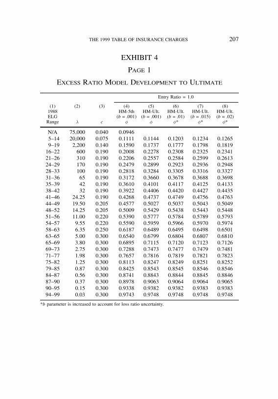
job no. 1969 casualty actuarial society CAS journal 1945D09 [20] 11-08-01 4:58 pm
THE 1999 TABLE OF INSURANCE CHARGES 207
EXHIBIT 4
Page 1
Excess Ratio Model Development to Ultimate
Entry Ratio = 1.0
(1) (2) (3) (4) (5) (6) (7) (8)1988 HM-5th HM-Ult. HM-Ult. HM-Ult. HM-Ult.ELG (b = :001) (b = :001) (b = :01) (b = :015) (b = :02)Range ¸ c Á Á Á* Á* Á*
N/A 75,000 0.040 0.09465–14 20,000 0.075 0.1111 0.1144 0.1203 0.1234 0.12659–19 2,200 0.140 0.1590 0.1737 0.1777 0.1798 0.181916–22 600 0.190 0.2008 0.2278 0.2308 0.2325 0.234121–26 310 0.190 0.2206 0.2557 0.2584 0.2599 0.261324–29 170 0.190 0.2479 0.2899 0.2923 0.2936 0.294828–33 100 0.190 0.2818 0.3284 0.3305 0.3316 0.332731–36 65 0.190 0.3172 0.3660 0.3678 0.3688 0.369835–39 42 0.190 0.3610 0.4101 0.4117 0.4125 0.413338–42 32 0.190 0.3922 0.4406 0.4420 0.4427 0.443541–46 24.25 0.190 0.4268 0.4737 0.4749 0.4756 0.476344–49 19.50 0.205 0.4577 0.5027 0.5037 0.5043 0.504948–52 14.25 0.205 0.5009 0.5429 0.5438 0.5443 0.544851–56 11.00 0.220 0.5390 0.5777 0.5784 0.5789 0.579354–57 9.55 0.220 0.5590 0.5959 0.5966 0.5970 0.597458–63 6.35 0.250 0.6187 0.6489 0.6495 0.6498 0.650163–65 5.00 0.300 0.6540 0.6799 0.6804 0.6807 0.681065–69 3.80 0.300 0.6895 0.7115 0.7120 0.7123 0.712669–73 2.75 0.300 0.7288 0.7473 0.7477 0.7479 0.748171–77 1.98 0.300 0.7657 0.7816 0.7819 0.7821 0.782375–82 1.25 0.300 0.8113 0.8247 0.8249 0.8251 0.825279–85 0.87 0.300 0.8425 0.8543 0.8545 0.8546 0.854684–87 0.56 0.300 0.8741 0.8843 0.8844 0.8845 0.884687–90 0.37 0.300 0.8978 0.9063 0.9064 0.9064 0.906590–95 0.15 0.300 0.9338 0.9382 0.9382 0.9383 0.938394–99 0.03 0.300 0.9743 0.9748 0.9748 0.9748 0.9748
*b parameter is increased to account for loss ratio uncertainty.
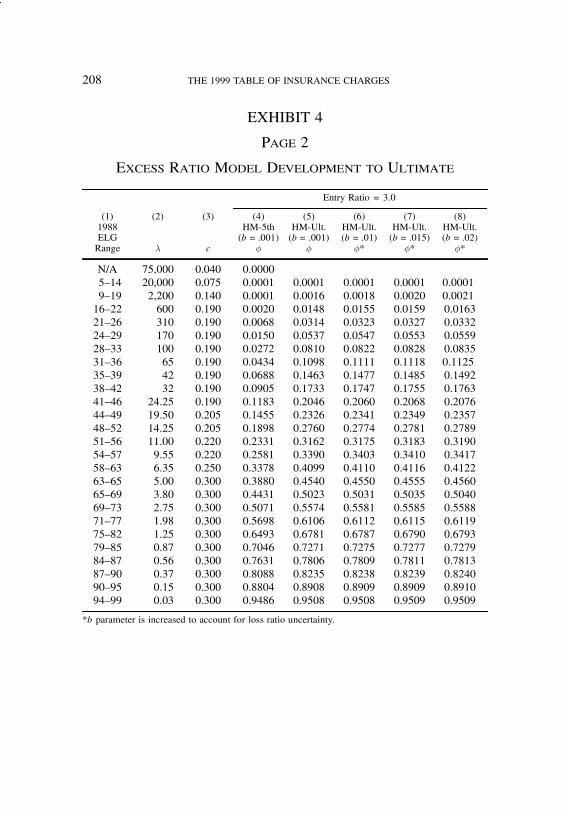
job no. 1969 casualty actuarial society CAS journal 1945D09 [21] 11-08-01 4:58 pm
208 THE 1999 TABLE OF INSURANCE CHARGES
EXHIBIT 4
Page 2
Excess Ratio Model Development to Ultimate
Entry Ratio = 3.0
(1) (2) (3) (4) (5) (6) (7) (8)1988 HM-5th HM-Ult. HM-Ult. HM-Ult. HM-Ult.ELG (b = :001) (b = :001) (b = :01) (b = :015) (b = :02)Range ¸ c Á Á Á* Á* Á*
N/A 75,000 0.040 0.00005–14 20,000 0.075 0.0001 0.0001 0.0001 0.0001 0.00019–19 2,200 0.140 0.0001 0.0016 0.0018 0.0020 0.002116–22 600 0.190 0.0020 0.0148 0.0155 0.0159 0.016321–26 310 0.190 0.0068 0.0314 0.0323 0.0327 0.033224–29 170 0.190 0.0150 0.0537 0.0547 0.0553 0.055928–33 100 0.190 0.0272 0.0810 0.0822 0.0828 0.083531–36 65 0.190 0.0434 0.1098 0.1111 0.1118 0.112535–39 42 0.190 0.0688 0.1463 0.1477 0.1485 0.149238–42 32 0.190 0.0905 0.1733 0.1747 0.1755 0.176341–46 24.25 0.190 0.1183 0.2046 0.2060 0.2068 0.207644–49 19.50 0.205 0.1455 0.2326 0.2341 0.2349 0.235748–52 14.25 0.205 0.1898 0.2760 0.2774 0.2781 0.278951–56 11.00 0.220 0.2331 0.3162 0.3175 0.3183 0.319054–57 9.55 0.220 0.2581 0.3390 0.3403 0.3410 0.341758–63 6.35 0.250 0.3378 0.4099 0.4110 0.4116 0.412263–65 5.00 0.300 0.3880 0.4540 0.4550 0.4555 0.456065–69 3.80 0.300 0.4431 0.5023 0.5031 0.5035 0.504069–73 2.75 0.300 0.5071 0.5574 0.5581 0.5585 0.558871–77 1.98 0.300 0.5698 0.6106 0.6112 0.6115 0.611975–82 1.25 0.300 0.6493 0.6781 0.6787 0.6790 0.679379–85 0.87 0.300 0.7046 0.7271 0.7275 0.7277 0.727984–87 0.56 0.300 0.7631 0.7806 0.7809 0.7811 0.781387–90 0.37 0.300 0.8088 0.8235 0.8238 0.8239 0.824090–95 0.15 0.300 0.8804 0.8908 0.8909 0.8909 0.891094–99 0.03 0.300 0.9486 0.9508 0.9508 0.9509 0.9509
*b parameter is increased to account for loss ratio uncertainty.

job no. 1969 casualty actuarial society CAS journal 1945D09 [22] 11-08-01 4:58 pm
THE 1999 TABLE OF INSURANCE CHARGES 209
EXHIBIT 5
Insurance Charges for Curve 29.35 Insurance Charges for Curve 33.16
Entry Heckman Entry HeckmanRatio Meyers Equation # Ratio Meyers Equation #(r) Model Graduated Used (r) Model Graduated Used
0.01 0.9900 0.9900 — 0.01 0.9900 0.9900 —0.02 0.9800 0.9800 0.02 0.9800 0.98000.03 0.9700 0.9700 0.03 0.9700 0.97000.04 0.9600 0.9600 0.04 0.9601 0.9600 1" r%0.05 0.9600 0.9500 0.05 0.9601 0.95000.06 0.9501 0.9400 1" r% 0.06 0.9502 0.94000.07 0.9401 0.9300 0.07 0.9403 0.93000.08 0.9302 0.9200 0.08 0.9304 0.9200 —0.09 0.9203 0.9100 0.09 0.9206 0.91020.10 0.9104 0.9000 0.10 0.9108 0.90050.11 0.9005 0.8900 — 0.25 0.7632 0.76290.25 0.7669 0.7580 0.50 0.5732 0.57330.50 0.5543 0.5543 0.75 0.4325 0.43260.75 0.4017 0.4016 1.00 0.3316 0.33161.00 0.2936 0.2935 1.25 0.2596 0.25951.25 0.2187 0.2188 1.50 0.2080 0.20791.50 0.1671 0.1672 1.75 0.1704 0.17041.75 0.1312 0.1312 2.00 0.1427 0.14272.00 0.1058 0.1058 2.25 0.1217 0.12172.25 0.0874 0.0874 2.50 0.1056 0.10562.50 0.0737 0.0737 IEP† 2.75 0.0930 0.0930 IEP†
2.75 0.0634 0.0634 3.00 0.0828 0.08283.00 0.0553 0.0553 3.25 0.0746 0.07463.25 0.0489 0.0489 3.50 0.0678 0.06783.50 0.0437 0.0437 3.75 0.0620 0.06203.75 0.0394 0.0394 4.00 0.0571 0.05714.00 0.0357 0.0357 4.25 0.0529 0.05294.25 0.0326 0.0326 4.50 0.0493 0.04934.50 0.0300 0.0300 4.75 0.0460 0.04604.75 0.0276 0.0276 5.00 0.0432 0.04325.00 0.0256 0.0256 5.25 0.0406 0.04065.25 0.0237 0.0237 5.50 0.0383 0.03835.50 0.0221 0.0221 5.75 0.0362 0.03625.75 0.0206 0.0206 6.00 0.0343 0.0343 —6.00 0.0192 0.0192 — 7.00 N/A 0.02887.00 N/A 0.0152 8.00 N/A 0.0242 ED‡
8.00 N/A 0.0120 ED‡ 9.00 N/A 0.02049.00 N/A 0.0095 10.00 N/A 0.0171 —10.00 N/A 0.0075 —%Equation (2)—Straight Line (see Appendix)†Equation (1)—Inverse Exponential Polynomial (see Appendix)‡Equation (3)—Exponential Decay (see Appendix)

job no. 1969 casualty actuarial society CAS journal 1945D09 [23] 11-08-01 4:58 pm
210 THE 1999 TABLE OF INSURANCE CHARGES
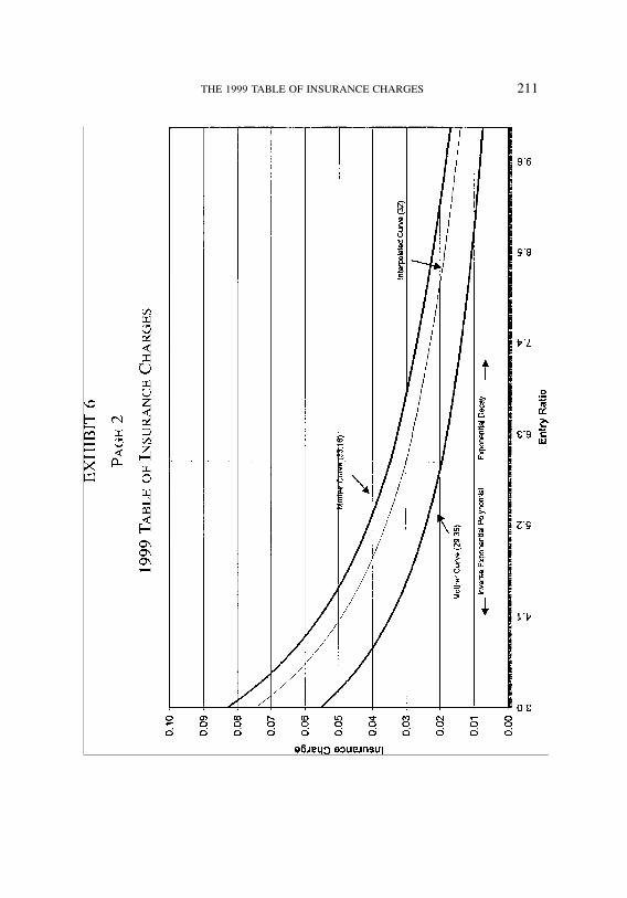
job no. 1969 casualty actuarial society CAS journal 1945D09 [24] 11-08-01 4:58 pm
THE 1999 TABLE OF INSURANCE CHARGES 211

job no. 1969 casualty actuarial society CAS journal 1945D09 [25] 11-08-01 4:58 pm
212 THE 1999 TABLE OF INSURANCE CHARGES

job no. 1969 casualty actuarial society CAS journal 1945D09 [26] 11-08-01 4:58 pm
THE 1999 TABLE OF INSURANCE CHARGES 213
EXHIBIT 8
Determination of 1988 Average Adjusted Severity
Average Model1988 Adjusted ExpectedELG Expected No. of AverageRange Loss Claims Severity(1) (2) (3) (4) = (2)=(3)
5–14 $110,489,802 20,000 $5,5249–19 $12,000,542 2,200 $5,45516–22 $2,921,544 600 $4,86921–26 $1,385,528 310 $4,46924–29 $742,680 170 $4,36928–33 $424,437 100 $4,24431–36 $252,281 65 $3,88135–39 $154,055 42 $3,66838–42 $111,337 32 $3,47941–46 $88,321 24 $3,64244–49 $67,843 20 $3,47948–52 $52,322 14 $3,67251–56 $41,980 11.00 $3,81654–57 $32,220 9.55 $3,37458–63 $22,867 6.35 $3,60163–65 $17,458 5.00 $3,49265–69 $13,629 3.80 $3,58769–73 $10,584 2.75 $3,84971–77 $8,059 1.98 $4,08175–82 $5,478 1.25 $4,38279–85 $3,410 0.87 $3,92084–87 $1,980 0.56 $3,54987–90 $1,227 0.37 $3,31790–95 $586 0.15 $3,80894–99 $177 0.03 $5,907
Overall Avg $4,031
Selected $4,000
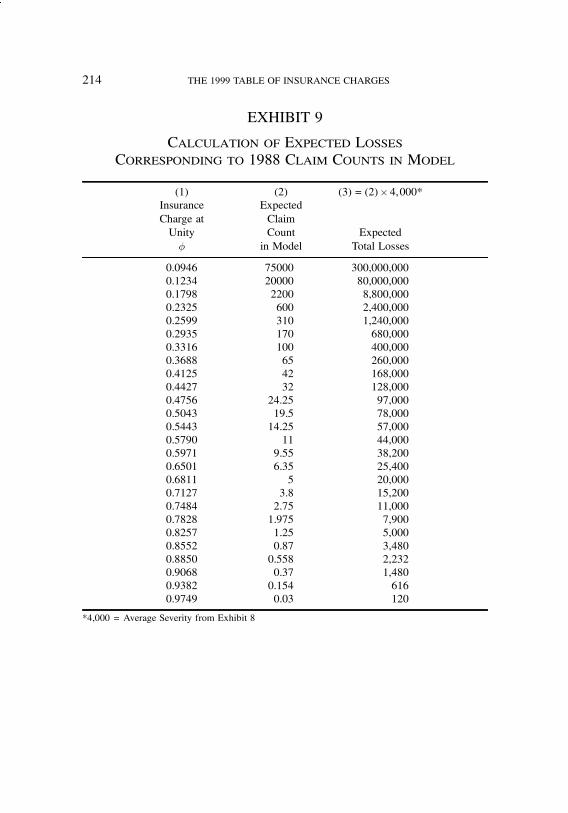
job no. 1969 casualty actuarial society CAS journal 1945D09 [27] 11-08-01 4:58 pm
214 THE 1999 TABLE OF INSURANCE CHARGES
EXHIBIT 9
Calculation of Expected LossesCorresponding to 1988 Claim Counts in Model
(1) (2) (3) = (2)& 4,000*Insurance ExpectedCharge at ClaimUnity Count ExpectedÁ in Model Total Losses
0.0946 75000 300,000,0000.1234 20000 80,000,0000.1798 2200 8,800,0000.2325 600 2,400,0000.2599 310 1,240,0000.2935 170 680,0000.3316 100 400,0000.3688 65 260,0000.4125 42 168,0000.4427 32 128,0000.4756 24.25 97,0000.5043 19.5 78,0000.5443 14.25 57,0000.5790 11 44,0000.5971 9.55 38,2000.6501 6.35 25,4000.6811 5 20,0000.7127 3.8 15,2000.7484 2.75 11,0000.7828 1.975 7,9000.8257 1.25 5,0000.8552 0.87 3,4800.8850 0.558 2,2320.9068 0.37 1,4800.9382 0.154 6160.9749 0.03 120
*4,000 = Average Severity from Exhibit 8

job no. 1969 casualty actuarial society CAS journal 1945D09 [28] 11-08-01 4:58 pm
THE 1999 TABLE OF INSURANCE CHARGES 215
EXHIBIT 10
Interpolation of 1998 Expected Loss Ranges
(1) (2) (3) (4) (5) (6) (7) =(6)&1:25*
Expected Total Losses Total Losses TrendedLoss Lower Upper for Lower for Upper Expected ExpectedGroup Point Point Point Point Losses LossesBoundary Used Used 1988 1988 1988 (1998)
0.095 0.0946 0.1234 300,000,000 80,000,000 294,542,927 368,178,6590.105 0.0946 0.1234 300,000,000 80,000,000 186,136,775 232,670,9690.115 0.0946 0.1234 300,000,000 80,000,000 117,629,371 147,036,7140.125 0.1234 0.1798 80,000,000 8,800,000 75,144,198 93,930,248... ... ... ... ... ... ...... ... ... ... ... ... ...... ... ... ... ... ... ...... ... ... ... ... ... ...
0.285 0.2599 0.2935 1,240,000 680,000 791,614 989,5180.295 0.2935 0.3316 680,000 400,000 665,942 832,4280.305 0.2935 0.3316 680,000 400,000 579,363 724,2040.315 0.2935 0.3316 680,000 400,000 504,041 630,0510.325 0.2935 0.3316 680,000 400,000 438,511 548,1390.335 0.3316 0.3688 400,000 260,000 384,557 480,6960.345 0.3316 0.3688 400,000 260,000 342,506 428,133
*severity trend from 1988 to 1998 = 1.250

job no. 1969 casualty actuarial society CAS journal 1945D09 [29] 11-08-01 4:58 pm
216 THE 1999 TABLE OF INSURANCE CHARGES
EXHIBIT 11
Page 1
Table of Expected Loss Size Range Comparison
Present Table Proposed Table
Expected Expected Expected ExpectedLoss Loss Loss LossGroup Range Group Range
80 6,922 – 7,773 80 7,795 – 8,67079 7,774 – 8,690 79 8,671 – 9,64678 8,691 – 9,681 78 9,647 – 10,64577 9,682 – 10,747 77 10,646 – 11,72076 10,748 – 11,891 76 11,721 – 12,90475 11,892 – 13,130 75 12,905 – 14,18074 13,131 – 14,452 74 14,181 – 15,52573 14,453 – 15,878 73 15,526 – 16,99672 15,879 – 17,406 72 16,997 – 18,60971 17,407 – 19,042 71 18,610 – 20,31470 19,043 – 20,802 70 20,315 – 22,15869 20,803 – 22,679 69 22,159 – 24,16868 22,680 – 24,696 68 24,169 – 26,20467 24,697 – 26,849 67 26,205 – 28,30466 26,850 – 29,162 66 28,305 – 30,57365 29,163 – 31,635 65 30,574 – 33,02164 31,636 – 34,280 64 33,022 – 35,66563 34,281 – 37,114 63 35,666 – 38,51962 37,115 – 40,149 62 38,520 – 41,60361 40,150 – 43,404 61 41,604 – 44,93360 43,405 – 46,884 60 44,934 – 48,54059 46,885 – 50,612 59 48,541 – 52,48358 50,613 – 54,610 58 52,484 – 56,66657 54,611 – 58,894 57 56,667 – 61,05556 58,895 – 63,490 56 61,056 – 65,78455 63,491 – 68,426 55 65,785 – 70,87954 68,427 – 73,720 54 70,880 – 76,64053 73,721 – 79,406 53 76,641 – 82,89152 79,407 – 85,521 52 82,892 – 89,65451 85,522 – 92,100 51 89,655 – 96,96650 92,101 – 99,181 50 96,967 – 104,63649 99,182 – 106,809 49 104,637 – 112,89548 106,810 – 115,032 48 112,896 – 121,86547 115,033 – 123,912 47 121,866 – 132,58346 123,913 – 133,498 46 132,584 – 144,24345 133,499 – 143,873 45 144,244 – 156,92844 143,874 – 155,101 44 156,929 – 171,48843 155,102 – 167,271 43 171,489 – 187,645
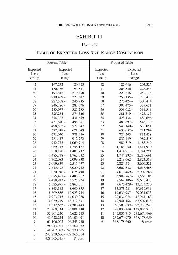
job no. 1969 casualty actuarial society CAS journal 1945D09 [30] 11-08-01 4:58 pm
THE 1999 TABLE OF INSURANCE CHARGES 217
EXHIBIT 11
Page 2
Table of Expected Loss Size Range Comparison
Present Table Proposed Table
Expected Expected Expected ExpectedLoss Loss Loss LossGroup Range Group Range
42 167,272 – 180,485 42 187,646 – 205,32541 180,486 – 194,841 41 205,326 – 226,34540 194,842 – 210,468 40 226,346 – 250,13439 210,469 – 227,507 39 250,135 – 276,42338 227,508 – 246,785 38 276,424 – 305,47437 246,786 – 283,076 37 305,475 – 339,62136 283,077 – 325,233 36 339,622 – 381,31835 325,234 – 374,326 35 381,319 – 428,13334 374,327 – 431,669 34 428,134 – 480,69633 431,670 – 498,861 33 480,697 – 548,13932 498,862 – 577,847 32 548,140 – 630,05131 577,848 – 671,049 31 630,052 – 724,20430 671,050 – 781,446 30 724,205 – 832,42829 781,447 – 912,772 29 832,429 – 989,51828 912,773 – 1,069,714 28 989,519 – 1,183,24927 1,069,715 – 1,258,177 27 1,183,250 – 1,414,91026 1,258,178 – 1,485,737 26 1,414,911 – 1,744,29125 1,485,738 – 1,762,082 25 1,744,292 – 2,219,66124 1,762,083 – 2,099,838 24 2,219,662 – 2,824,58323 2,099,839 – 2,515,497 23 2,824,584 – 3,609,32122 2,515,498 – 3,030,945 22 3,609,322 – 4,618,46821 3,030,946 – 3,675,490 21 4,618,469 – 5,909,76620 3,675,491 – 4,488,912 20 5,909,767 – 7,562,10519 4,488,913 – 5,525,974 19 7,562,106 – 9,676,42818 5,525,975 – 6,863,311 18 9,676,429 – 13,273,22017 6,863,312 – 8,609,855 17 13,273,221 – 19,630,98616 8,609,856 – 10,923,744 16 19,630,987 – 29,034,07315 10,923,745 – 14,039,278 15 29,034,074 – 42,941,16314 14,039,279 – 18,312,631 14 42,941,164 – 63,509,63813 18,312,632 – 24,300,443 13 63,509,639 – 93,930,24812 24,300,444 – 32,901,239 12 93,930,249 – 147,036,71411 32,901,240 – 45,622,243 11 147,036,715 – 232,670,96910 45,622,244 – 65,106,001 10 232,670,970 – 368,178,6599 65,106,002 – 96,243,920 9 368,178,660 – & over8 96,243,921 – 148,702,0227 148,702,023 – 243,230,6056 243,230,606 – 429,365,3145 429,365,315 – & over

job no. 1969 casualty actuarial society CAS journal 1945D09 [31] 11-08-01 4:58 pm
218 THE 1999 TABLE OF INSURANCE CHARGES
job no. 1969 casualty actuarial society CAS journal 1969MAY [1] 11-08-01 4:58 pm
ADDRESS TO NEW MEMBERS—MAY 8, 2000
THOUGHTS ON MY CAREER: THE SEQUEL
RUTH E. SALZMANN
When General Douglas MacArthur was relieved of his com-mand in the Pacific Theater by President Truman, he was askedto address the United States Congress. His famous line was: “Oldsoldiers never die; they just fade away.” In similar fashion, I cansay: “Old female actuaries never die; they just lose their figures.”
It is a pleasure to be here today to add my congratulations tothe 14 new Fellows and the 147 new Associates. How times havechanged from the “olden days;” 37 percent of you are women!
Last November, CAS Past-President LeRoy Simon addressedthe new members in San Francisco. One of his quotable lineswas: “It is easier to become an actuary than to be one.” To thatI will add: “But being one is a lot more fun!”
You now have the knowledge, at least to the satisfaction of theexamination committees, and you have the credentials to meet thechallenges that lie ahead in your actuarial careers. Progress willbe measured by solutions and answers that become less reflexiveand more reflective. It is this continuous transition from one tothe other that leads to wisdom.
As I looked back over my career, I wondered what would beof interest to actuaries who are looking forward to theirs. In mycase, it was the early years that set the course for a personallyrewarding career. Each of you, I know, is looking forward to thatsame goal.
When I became a Fellow in 1947, recent legislation made itpossible for one company to underwrite both casualty and firecoverages. This change allowed casualty companies to under-write auto, fire, and theft. When the transfer was made from thefire company to the casualty company where I worked, the loss
219
job no. 1969 casualty actuarial society CAS journal 1969MAY [2] 11-08-01 4:58 pm
220 ADDRESS TO NEW MEMBERS
ratios in both companies went down. Our CEO was a bit troubledover that.
More importantly, the new legislation created a need for acombined annual statement blank and later a uniform classifica-tion of expenses by account, function, and line of insurance. Tomake this happen, many industry committees were established.Actuaries as well as insurance accountants served on these com-mittees.
Subsequently, these same committee members served on In-surance Accounting and Statistical Association1 (IASA) panelsand workshops to communicate and discuss the new financial re-porting. I served on these committees and conducted IASA pre-sentations, and it was this involvement that shaped and helpedmy career. Based on this experience, I encourage all of you toserve on industry and society committees in those areas that in-terest you most.
In those earlier times, actuaries became regular participantson IASA panels. Let me tell you about one such panel. Thesubject was loss reserving methodologies for casualty lines. Mypresentation described the basic procedure of extrapolating a fi-nal incurred amount by accident year and then subtracting paidlosses to derive the liability. The next speaker, a renowned ac-tuary considerably senior to me, criticized that approach witha story about the village idiot who entered an archery contest.He shot his arrow into a wall and then painted a target aroundit. The point in his analogy was that the sequence was wrong.When the end result is determined first and the liability is then de-rived to support it, the objectivity of such a measurement may bequestionable. He likewise would have criticized the Bornhuetter–Ferguson method, as it incorporates a predetermined expectedloss ratio.
1Subsequently renamed Insurance Accounting and Systems Association.

job no. 1969 casualty actuarial society CAS journal 1969MAY [3] 11-08-01 4:58 pm
ADDRESS TO NEW MEMBERS 221
The better approach, in his opinion, was to measure the IBNRindependently and add it to the case reserves. This methodologywas the customary practice at the time. In all fairness to thisgentleman, the panel took place in the early fifties, an age thatpredated computers. As a result, it was difficult to produce so-phisticated measurements of loss liabilities on a timely basis.Also, the average life of claims was much shorter than it is to-day. Because of the latter, case reserve levels were undoubtedlymore dependable.
Over the years, I became a believer in the merits of estimatingloss liabilities on a basis other than by extrapolation, but I alsowanted to avoid the vagaries of case reserve levels. In my expe-rience, I seldom found case reserve levels to be dependably con-sistent from year to year, or measurably adjustable when they arebelieved to be inconsistent. I did finally produce two methods2
that independently measured the total liability, i.e., a combinedliability for both reported and unreported claims. At last I foundmethodologies that would satisfy me as well as my copanelist,and I could put this challenge behind me. I hope this story willencourage each of you to seek involvements where different ap-proaches are discussed. You, too, may end up with a challengethat won’t let you rest until you find a solution.
Recent legislation affecting your careers is the 1999 FinancialServices Modernization Act. This Act permits affiliations amongall types of financial firms, including insurance. As a result, therewill be newer alternative ways for customers to package all oftheir financial risks. What an enormous opportunity lies aheadfor each of you!
It is with a bit of humor that I predict what I believe to bethe biggest deterrent to mergers with insurance companies, andthat is the statutory annual statement blank. When I became aFellow, there were 34 pages in the blank. The last page in the
2Methods 5 and 6: Salzmann, Ruth E., Estimated Liabilities for Losses and Loss Adjust-ment Expenses, Prentice Hall, Englewood Cliffs, New Jersey, 1984.

job no. 1969 casualty actuarial society CAS journal 1969MAY [4] 11-08-01 4:58 pm
222 ADDRESS TO NEW MEMBERS
1999 blank is numbered 136; but if you add in all the pages thatare numbered in tenths, the number exceeds 200. This may be theinformation age, but I fear we may be putting the financial healthof the trees over the financial health of the forest. Doc Mastersononce said, “The annual statement needs only three pages: one forthe assets, the second for the liabilities and surplus, and the thirdfor the fingerprints of the officers.”
If any of you keep a list of “reminders” that you review nowand then, here are a few items to add:
1. Get involved in industry committees and meetings so asto benefit from the cross-fertilization of ideas.
2. When evaluating data, have the confidence to judge whatmay be random and what my not be. Paul Otteson oncesaid, “A normal number of abnormal losses is not ab-normal.”
3. Keep in mind that it still takes vision and imagination toharness data and information; technology is just a tool.
4. With any actuarial methodology, ask yourself: “Whymight I want to do it differently?”
5. Keep testing those assumptions.
6. Don’t give up on an elusive solution; sometimes a kindof irrational overconfidence is needed.
In conclusion, your new status should give you the confidenceto meet the challenges and to seek the opportunities in your fu-tures. Current social, economic, and environmental issues willaffect the measurement of financial risk and, therefore, will needthe expertise and knowledge of both the actuarial scholar and theactuarial practitioner.
Good luck to each of you!

October 30, 2001 11:24 PM 69maymin.qxd
MINUTES OF THE 2000 SPRING MEETING
May 7–10, 2000
BELLAGIO
LAS VEGAS, NEVADA
Sunday, May 7, 2000
The Board of Directors held their regular quarterly meetingfrom 9:00 a.m. to 5:00 p.m.
Registration was held from 4:00 p.m. to 6:00 p.m.
New Associates and their guests were honored with a specialpresentation from 5:30 p.m. to 6:30 p.m. Members of the 2000Executive Council discussed their roles in the Society with thenew members. In addition, Robert A. Anker, who is a past presi-dent of the CAS, gave a short talk on the American Academy ofActuaries’ (AAA) Casualty Practice Council.
A reception for all meeting attendees followed the new Associ-ates reception and was held from 6:30 p.m. to 7:30 p.m.
Monday, May 8, 2000
Registration continued from 7:00 a.m. to 8:00 a.m.
The 2000 Business Session, which was held from 8:00 a.m. to9:15 a.m., started off the first full day of activities for the 2000Spring Meeting. Alice H. Gannon introduced the CAS ExecutiveCouncil, the Board of Directors, and CAS past presidents whowere in attendance, including Robert A. Anker (1996), Phillip N.Ben-Zvi (1985), Ronald L. Bornhuetter (1975), Charles A. Bryan(1990), Michael Fusco (1989), Ruth E. Salzmann (1978), LeRoyJ. Simon (1971), Michael L. Toothman (1991), and Mavis A. Wal-ters (1997).
Ms. Gannon also recognized special guests in the audience:A. Norman Crowder III, President, Society of Actuaries; Curtis
223
224 MINUTES OF THE 1999 SPRING MEETING
E. Huntington, Executive Director, Actuarial Education and Re-search Fund; Stephen R. Kern, President, American Academy ofActuaries; Michael L. Toothman, President, Conference of Con-sulting Actuaries; and Stuart F. Wason, President, Canadian Insti-tute of Actuaries.
Abbe S. Bensimon, Gary R. Josephson, and Mary FrancesMiller announced the 147 new Associates and Patrick J. Grannanannounced the 14 new Fellows. The names of these individualsfollow.
NEW FELLOWS
October 30, 2001 11:24 PM 69maymin.qxd
Amy Petea AngellMark E. BohrerJulie BurdickRobert Neil CampbellMark Kelly EdmundsBrandon Lee Emlen
Christopher ToddHochhausler
Brandelyn C. KlennerElaine LajeunesseDiana Mary Susan
Linehan
Scott A. McPheeKathy PopejoyRichard A.
RosengartenMeyer Shields
NEW ASSOCIATES
Jodie Marie AganBrian M. AncharskiKevin L. AndersonDeborah Herman
ArdernPatrick BarbeauJody J. BembenekEllen A. BerningBrad D. BirtzMary Denise BoarmanVeronique BouchardThomas Leininger
Boyer IIDavid C. BrueckmanAngela D. Burgess
Patrick J. CharlesHarry Sigen ChenBrian Kenneth CiferriSusan M. CleaverRichard Jason CookKevin A. CormierJeffrey Alan CourcheneMary Elizabeth
Frances CunninghamPatricia A. Deo-Campo
VuongJean-François
DesrochersMark Richard
Desrochers
Michael DevineKevin George DonovanLouis-Christian DupuisDonna L. EmmerlingKeith Andrew
EngelbrechtLaura Ann EsboldtJuan de la Cruz
EspadasFarzad FarzanDonia Burris FreeseShina Noel FritzCynthia GalvinMichael Anthony
Garcia

MINUTES OF THE 2000 SPRING MEETING 225
Hannah GeeJames Brian GilbertJoseph Emmanuel
GoldmanAndrew Samuel
Golfin Jr.Olga GolodStacey C. GothamMark R. GreenwoodChantal GuillemetteJames Christopher
GuszczaDavid Bruce
HackworthDawn Marie S. HappJason Carl HeadPamela Barlow HeardKristina Shannon HeerHans HeldnerRobert C. HillDavid E. HodgesRichard Michael HoltzAllen J. HopeCarol Irene HumphreyRusty A. HustedMichael Stanley
JarmusikPatrice JeanCharles Biao JinSteven M. JokerstCheryl R. KelloggJames F. KingJill E. KirbyOmar A. KitchlewHenry Joseph
Konstanty
Darjen D. KuoChristine L. LackeBobb J. LackeyJean-François
LarochellePeter H. LatshawDoris LeeWendy Rebecca
LefersonWilliam Scott LennoxJoshua Yuri LigoskyErik Frank LivingstonRebecca Michelle
LocksRichard Paul LonardoWilliam F. Loyd IIIAlexander Peter
MaizysVictor MataDavid Michael MaurerTimothy C. McAuliffeRichard J. McElligottJennifer A. McGrathMartin MenardMitchel MerbergVadim Y. MezhebovskyEric Millaire-MorinRebecca E. MillerSuzanne A. MillsMatthew Kevin MoranLambert MorvanThomas M. MountRonald Taylor NelsonMichael Dale
NeubauerLoren J. Nickel
Ajay PahwaCosimo PantaleoMichael Thomas
PattersonWendy Wei-Chi PengJill E. PeppersMichael C. PetersenKevin Thomas
PetersonKraig Paul PetersonKristin Sarah
PiltzeckerSean Evans PorrecaWarren T. PrintzStephen Daniel
RiihimakiEzra Jonathan RobisonBryant Edward RussellFrederick Douglas
RyanLaura Beth SachsSalimah H. SamjiRachel SamoilJennifer Arlene ScherDaniel David
SchlemmerParr T. SchoolmanErnest C. SegalMichelle L. SheppardPaul O. ShupeLee Oliver SmithLora L. Smith-SarfoScott G. SobelMary Jane SperdutoChristine Steele-
Koffke
October 30, 2001 11:24 PM 69maymin.qxd
226 MINUTES OF THE 2000 SPRING MEETING
Gary A. SudbeckJonathan Leigh
SummersNeeza ThandiTanya K. ThielmanJohn David TraufferNathalie TremblayMatthew L. UhodaDennis R. Unver
Richard Alan Van Dyke
Josephine M. WaldmanColleen Ohle WalkerKristie L. WalkerTice R. WalkerWade Thomas
WarrinerKelly M. Weber
Petra Lynn WegerichChristopher John
WestermeyerKarin H. WohlgemuthTerry C. WolfeMihoko YamazoeNora J. Young
October 30, 2001 11:24 PM 69maymin.qxd
Ms. Gannon then introduced Ruth E. Salzmann, a past presi-dent of the Society, who presented the Address to New Members.
David R. Chernick, CAS vice president-programs and commu-nications, spoke to the meeting participants about the highlights ofthis meeting and what was planned in the program.
Richard I. Fein, chairperson of the Committee On Review ofPapers, announced that four Proceedings papers and one discus-sion of a Proceedings paper would be presented at this meeting. Inall, five papers were accepted for publication in the 2000 Proceed-ings of the Casualty Actuarial Society.
Robert S. Miccolis, chairperson of the Michelbacher PrizeCommittee, gave a brief description of this year’s Call Paper Pro-gram on Insurance in the Next Century. He announced that all ofthe call papers would be presented at this meeting. (The papers arepublished in the 2000 CAS Discussion Paper Program and can befound on the CAS Web Site.) Mr. Miccolis presented the Michel-bacher Prize to Sergei Esipov and Dajiang Guo for their paper,“Portfolio Based Pricing of Residual Basis Risk with Applicationto the S&P 500 Put Options.” The Michelbacher Prize commemo-rates the work of Gustav F. Michelbacher and honors the authorsof the best paper(s) submitted in response to a call for discussionpapers. The papers are judged by a specifically appointed commit-tee on the basis of originality, research, readability, and complete-ness.
MINUTES OF THE 2000 SPRING MEETING 227
Ms. Gannon then began the presentation of other awards. Sheexplained that the CAS Harold W. Schloss Memorial ScholarshipFund benefits deserving and academically outstanding students inthe actuarial program of the Department of Statistics and ActuarialScience at the University of Iowa. The student recipient is selectedby the Trustees of the CAS Trust, based on the recommendation ofthe department chair at the University of Iowa. Ms. Gannon an-nounced that Feng Sun is the recipient of the 2000 CAS Harold W.Schloss Memorial Scholarship Fund. Sun will be presented with a$500 scholarship.
Ms. Gannon then concluded the business session of the SpringMeeting.
Ms. Gannon next introduced the featured speaker, James Can-ton, who is one of the nation’s leading futurists, a digital entrepre-neur, and author.
The first General Session was held from 10:45 a.m. to 12:15p.m.
“Enterprise Risk Management”Moderator: Richard I. Fein
PrincipalPricewaterhouseCoopers LLP
Panelists: Michael L. AlbaneseGroup Vice PresidentA.M. Best CompanyJerry A. MiccolisPrincipalTillinghast-Towers PerrinThomas W. WronskiRisk DirectorFidelity Investments
After a luncheon, the afternoon was devoted to presentations ofconcurrent sessions, Proceedings papers, and call papers. The call
October 30, 2001 11:24 PM 69maymin.qxd

228 MINUTES OF THE 2000 SPRING MEETING
papers presented from 1:30 p.m. to 3:00 p.m. were:1. “Enterprise Risk Management: A Consultative Approach”
Authors: Edgar W. DavenportAdvanced Risk Management Services ofWillis North AmericaL. Michelle BradleyAdvanced Risk Management Services ofWillis North America
2. “Enterprise Technology Projects and the Role of the Actuary”Author: Paul C. Martin
Milliman & Robertson, Inc.Charlie CoonSt. Paul Companies, Inc.
The concurrent sessions presented from 1:30 p.m. to 3:00 p.m.were:
1. Financial Services RegulationModerator: Elise C. Liebers
Deputy Chief ActuaryNew York State Insurance Department
Panelists: Therese M. VaughanCommissionerIowa Insurance DivisionThomas A. OravezAssistant Vice PresidentFederal Reserve Bank of New YorkRobert PartridgeDirectorStandard & Poor’s Rating Group
2. CAS Research EffortsModerator/ Roger M. HaynePanelist: Consulting Actuary
Milliman & Robertson, Inc.
October 30, 2001 11:24 PM 69maymin.qxd
MINUTES OF THE 2000 SPRING MEETING 229
Panelists: Frederick F. CripeAssistant Vice PresidentAllstate Insurance CompanyRichard W. GorvettAssistant Professor of Actuarial ScienceUniversity of Illinois
3. CAS Membership SurveyModerator: David Skurnick
Senior Vice President and ActuarySt. Paul Re
Panelists: Roger A. SchultzAssistant Vice PresidentAllstate Insurance CompanyDavid J. OakdenConsulting ActuaryTillinghast-Towers Perrin
4. Technology and InsuranceModerator/ Robin A. HarbagePanelist: General Manager
Progressive CorporationPanelists: Richard Bishop
ConsultantRichard Bishop ConsultingJanet K. SilvermanSupervising Casualty ActuaryNew York State Insurance Department
5. Quality Assurance for the Actuarial Work ProductModerator: James E. Buck
Principal, Actuarial ConsultingInsurance Services Office, Inc.
Panelists: Mary D. MillerActuaryOhio Department of Insurance
October 30, 2001 11:24 PM 69maymin.qxd
230 MINUTES OF THE 2000 SPRING MEETING
Marc J. AdeeChief Financial Officer and Chief ActuaryBurlington Insurance Group
Proceedings papers presented during this time were:1. “Dirty Words: Interpreting and Using EPA Data in
Actuarial Analysis of an Insurer’s Superfund-Related Claim Costs”Author: Steven J. Finkelstein
Ernst & Young LLP2. “Estimating U.S. Environmental Liabilities by
Simulation”Author: Christopher Diamantoukos
Ernst & Young LLP
After a refreshment break, presentations of call papers, concur-rent sessions, and Proceedings papers continued from 3:30 p.m. to5:00 p.m. Call papers presented during this time were:
1. “The Last Few Obstacles on the Way to Digital Paradise”Author: Aleksey S. Popelyukhin
Sam Sebe LLC, Commercial Risk Re2. “Pricing Multiple Triggers—An Electrifying Example”
Author: Lawrence SchoberAssociated Electric and Gas Insurance Services
3. “Pricing for the Financial Risk of Uncollateralized Deductible Policies”Author: Robert F. Brown
Travelers Property Casualty
The concurrent sessions presented from 3:30 p.m. to 5:00 p.m.were:
1. Basics of Financial Risk ManagementPresenter: Richard W. Gorvett
Assistant Professor of Actuarial ScienceUniversity of Illinois
October 30, 2001 11:24 PM 69maymin.qxd

MINUTES OF THE 2000 SPRING MEETING 231
2. Current Accounting IssuesModerator: Patricia A. Teufel
PrincipalKPMG LLP
Panelists: Ralph S. BlanchardSecond Vice President and ActuaryTravelers Property Casualty CorporationAndrea M. SweeneyManagerArthur Andersen LLP
3. The Actuary and Earnings ManagementModerator/ Aaron HalpertPanelist: Principal
KPMG LLPPanelist: Martha Marcon
PartnerKPMG LLP
4. Questions and Answers with the CAS Board of DirectorsModerator: Patrick J. Grannan
PrincipalMilliman & Robertson, Inc.
Panelists: Frederick O. KistSenior Vice President and Chief ActuaryCNAGail M. RossVice PresidentAm-Re Consultants, Inc.Michael L. ToothmanPartnerArthur Andersen LLP
October 30, 2001 11:24 PM 69maymin.qxd
232 MINUTES OF THE 2000 SPRING MEETING
5. Proposals for Managing the Industry’s Catastrophe ExposureModerator: Wayne H. Fisher
Executive Vice President & Chief ActuaryZurich U.S.
Panelist: Ross J. Davidson Jr.Vice President, Industry AffairsUnited Services Automobile AssociationGordon K. HayActuarySAFECO Insurance CompaniesLee R. SteeneckVice President & ActuaryGeneral Reinsurance Corporation
The Proceedings paper presented during this time was:1. Discussion of “Application of the Option Market
Paradigm to the Solution of Insurance Problems”(by Michael G. Wacek, PCAS LXXXIV, 1997, p. 701)Discussion by Stephen J. Mildenhall
CNA Re
A reception for new Fellows and their guests was held from5:30 p.m. to 6:30 p.m., and the general reception for all membersand their guests was held from 6:30 p.m. to 7:30 p.m.
Tuesday, May 9, 2000
Registration continued from 7:00 a.m. to 8:00 a.m.
The General Session presented from 8:00 a.m. to 9:30 a.m.was:
“The Outsider’s View of the Actuary”Moderator: Jeanne M. Hollister
Consulting ActuaryTillinghast-Towers Perrin
October 30, 2001 11:24 PM 69maymin.qxd

MINUTES OF THE 2000 SPRING MEETING 233
Panelists: Nicholas M. BrownPresident and CEONAC Re CorporationRobert J. DellingerExecutive Vice President & Chief FinanceOfficerEmployers Reinsurance CorporationV. J. Dowling Jr.Dowling & Partners Securities, LLCPatrick W. KennyExecutive Vice President of Finance and Chief Finance OfficerFrontier Insurance Group, Inc.
Two limited attendance workshops, “Write Up Front” and “Ex-ecutive Presentation Skills,” were held from 8:00 a.m. to 5:00 p.m.and from 8:00 a.m. to noon, respectively.
Certain call papers that had been presented earlier during themeeting were repeated this morning from 10:00 a.m. to 11:30 a.m.The additional call paper presented during this time was:
1. “Portfolio Based Pricing of Residual Basis Risk with Application to the S&P 500 Put Options”Authors: Sergei Esipov
Centre SolutionsDajiang GuoCentre Risk Advisors and Centre Solutions
The concurrent sessions presented from 10:00 a.m. to 11:30a.m. were:
1. Actuaries in Nontraditional RolesModerator: Maribeth Ebert
PrincipalWilliam M. Mercer, Inc.
October 30, 2001 11:24 PM 69maymin.qxd

234 MINUTES OF THE 2000 SPRING MEETING
Panelists: James G. EvansInvestment ActuaryPrime Advisors, Inc.Regina M. BerensSenior Consulting ActuaryScruggs ConsultingRobert G. BlancoVice President and ActuaryNational Council on Compensation InsuranceDavid W. SimpsonManaging PrincipalD. W. Simpson & Company
2. Data StandardsModerator: Carole J. Banfield
Executive Vice PresidentInsurance Services Office
Panelists: Gary KnobleVice PresidentHartford Financial Services GroupArthur R. CadorineAssistant Vice PresidentInsurance Services OfficeBeth GrossmanDirector of Industry RelationsACORDChristine SickierskiVice PresidentWisconsin Compensation Rating BureauCharles E. WightManaging Consultant/Senior Vice PresidentMarsh USA Risk & Insurance Services
October 30, 2001 11:24 PM 69maymin.qxd
MINUTES OF THE 2000 SPRING MEETING 235
3. Recent Developments in Transferring RisksModerator/ John G. AquinoPanelist: Executive Vice President
Aon Re ServicesPanelist: Stephen J. Mildenhall
Vice PresidentCNA Re
4. Update on e-Commerce and its Use by InsurersModerator: J. Parker Boone
Senior Vice PresidentInsWeb
Panelists: Anthony L. AlfieriActuaryeCoverageCharles S. BrofmanPresident & Co-CEOCybersettle.comPaul J. FordSenior Vice President–Business DevelopmentInslogic.com
Various CAS committees met from noon to 5:00 p.m. Certaincall papers and concurrent sessions presented earlier were re-peated from 1:00 p.m. to 2:30 p.m. A limited attendance work-shop, “Executive Presentation Skills,” was held from 1:00 p.m. to5:00 p.m.
All members and guests enjoyed dinner and a show at LuxorLas Vegas from 5:30 p.m. to 9:30 p.m.
Wednesday, May 10, 2000
Certain call papers and concurrent sessions that had been pre-sented earlier during the meeting were repeated this morning from8:00 a.m. to 9:30 a.m. Additional concurrent sessions presented
October 30, 2001 11:24 PM 69maymin.qxd

236 MINUTES OF THE 2000 SPRING MEETING
were:1. Integrated Products and Holistic Financial Risk
ManagementModerator/ Shawna AckermanPanelist: Consulting Actuary
Miller, Herbers, Lehmann, & Associates, Inc.
Panelists: Ugur KoylougluOliver Wyman & CompanyEdmund S. ScanlonAssistant Vice PresidentZurich-American Specialties
2. Role of Regional AffiliatesModerator: Ramona C. Lee
ChairpersonRegional Affiliates Task Force
Panelists: James E. BuckVice PresidentCasualty Actuaries of Greater New YorkJulia L. PerrinePresidentCasualty Actuaries of Desert StatesTherese A. KlodnickiMemberRegional Affiliates Task Force
Proceedings papers presented from 8:00 a.m. to 9:30 a.m.were:
1. “Risk and Return: Underwriting, Investment and Leverage Probability of Surplus Drawdown and Pricing for Underwriting and Investment Risk”Author: Russell E. Bingham
The Hartford Financial Services Group
October 30, 2001 11:24 PM 69maymin.qxd
MINUTES OF THE 2000 SPRING MEETING 237
2. “The Direct Determination of Risk-Adjusted Discount Rates and Liability Beta”Author: Russell E. Bingham
The Hartford Financial Services Group
After a refreshment break, the final General Session was heldfrom 10:00 a.m. to 11:30 a.m.:
“The Actuary and the Insurance Industry of the 21st Century—What’s Ahead?”
Moderator: Phillip Ben-ZviPrincipal-In-ChargePricewaterhouseCoopers LLP
Panelists: Thomas N. AndersonPrincipalMcKinsey & CompanyRobert A. AnkerQuay QuestMichael DeGustaChief Technology OfficereCoverage
Alice H. Gannon officially adjourned the 2000 CAS SpringMeeting at 11:45 a.m. after closing remarks and an announcementof future CAS meetings.
Attendees of the 2000 CAS Spring Meeting
The 2000 CAS Spring Meeting was attended by 361 Fellows,278 Associates, and 52 Guests. The names of the Fellows and Associates in attendance follow:
October 30, 2001 11:24 PM 69maymin.qxd
FELLOWS
Rimma AbianShawna S. AckermanMark A. Addiego
Marc J. AdeeKristen M. AlbrightStephanie J. Albrinck
John P. AlltopDean R. AndersonRichard R. Anderson

238 MINUTES OF THE 2000 SPRING MEETING
Amy Petea AngellRobert A. AnkerJohn G. AquinoSteven D. ArmstrongTimothy J. BanickBruce C. BassmanPhilip A. BaumWilliam H. BelvinXavier BenaroschPhillip N. Ben-ZviRegina M. BerensLisa M. BesmanDavid R. BickerstaffRichard A. BillJames E. BillerRichard S. BiondiEverett G. BishopSuzanne E. BlackWayne E. BlackburnRalph S. BlanchardRobert G. BlancoDaniel David BlauBarry E. BlodgettMark E. BohrerLeRoy A. BoisonJ. Parker BooneRonald L. BornhuetterFrançois BoulangerAmy S. BouskaNancy A. BraithwaitePaul BraithwaiteMichael D. BrannonRobert S. BriereNicholas M. BrownLisa J. BrubakerJames E. Buck
Julie BurdickGeorge BurgerChristopher J.
BurkhalterJohn Frederick ButcherRobert Neil CampbellClaudette CantinJohn E. CaptainChristopher S. CarlsonKenneth E. CarltonSanders B. CathcartKevin J. CawleyDennis K. ChanScott K. CharbonneauDavid R. ChernickFrancis X. CorrMichael D. CovneyFrederick F. CripeAlan M. CroweMichael Kevin CurryRobert J. CurryDaniel J. CzabajKenneth S. DaileyGuy Rollin DanielsonRobert N. DarbyStephen P. D’ArcyEdgar W. DavenportJohn DawsonJerome A. DegernessJeffrey F. DeiglMichael L. DeMatteiChristopher
DiamantoukosAnthony M. DiDonatoMichael C. DolanJames L. Dornfeld
Robert B. DownerDenis DuboisJanet E. DuncanM. L. “Butch” DyeMaribeth EbertGrover M. EdieDale R. EdlefsonMark Kelly EdmundsValere M. EgnaskoDonald J. EldridgeEdward B. EliasonThomas J. EllefsonJohn W. EllingrodBrandon Lee EmlenPaul E. EricksenJames G. EvansPhillip A. EvensenSylvain FauchonRichard I. FeinRussell S. FisherWayne H. FisherKirk G. FlemingDaniel J. FlickBarry A. FranklinMichael FuscoScott F. GaliardoCecily A. GallagherThomas L. GallagherGary J. GanciAlice H. GannonKathy H. GarriganJames J. GebhardJohn F. GibsonWilliam R. GillamMichael Ambrose
Ginnelly
October 30, 2001 11:24 PM 69maymin.qxd

MINUTES OF THE 2000 SPRING MEETING 239
Gregory S. GirardMoshe D. GoldbergRichard W. GorvettJay C. GotelaerePatrick J. GrannanRussell H. GreigAnthony J. GrippaDavid Thomas GroffMarshall J. GrossackTerry D. GuslerGreg M. HaftJames A. HallRobert C. HallstromRobin A. HarbageMichael B. HawleyGordon K. HayMatthew T. HaydenRoger M. HayneBarton W. HedgesDennis R. HenryDavid E. HeppenSteven C. HermanKathleen A. HindsAlan M. HinesChristopher Todd
HochhauslerJeanne M. HollisterRandall D. HolmbergPaul E. HoughMarie-Josée HuardBrian A. HughesJames G. InkrottDaniel Keith JohnsonKurt J. JohnsonMark Robert JohnsonJeffrey R. Jordan
Gary R. JosephsonSteven W. JuddJeremy M. JumpKenneth R. KasnerHsien-Ming KehLowell J. KeithBrandon Daniel KellerAnne E. KellyRebecca Anne
KennedyMichael B. KesslerChangseob Joe KimDeborah M. KingFrederick O. KistMichael F. KleinBrandelyn C. KlennerFredrick L. KlinkerTimothy F. KoesterMikhael I. KoskiGary I. KoupfGary R. KratzerRodney E. KrepsDavid J. KretsAdam J. KreuserJeffrey L. KuceraAndrew E. KuderaDavid R. KunzeEdward M. KussPaul E. LackoBlair W. LaddusawSalvatore T. LaDucaElaine LajeunesseJohn A. LambR. Michael LambJames W. LarkinChristopher Lattin
Michel LaurinPierre Guy LaurinGuy LecoursRobert H. LeeSteven G. LehmannJennifer McCullough
LevineJohn J. LewandowskiMartin A. LewisElise C. LiebersOrin M. LindenDiana Mary Susan
LinehanBarry LiptonRichard Borge LordAileen C. LyleGary P. MaileDonald F. MangoDonald E. ManisPaul C. MartinSteven E. MathRobert W. MatthewsBonnie C. MaxieJeffrey H. MayerMichael G. McCarterLiam Michael
McFarlaneKelly S. McKeethanAllison Michelle
McManusKathleen A.
McMonigleDennis T. McNeeseM. Sean McPaddenJeffrey A. MehalicStephen V. Merkey
October 30, 2001 11:24 PM 69maymin.qxd

240 MINUTES OF THE 2000 SPRING MEETING
James R. MerzRobert E. MeyerRobert J. MeyerJerry A. MiccolisRobert S. MiccolisStephen J. MildenhallDavid L. MillerMary D. MillerMary Frances MillerPhilip D. MillerRonald R. MillerFrederic James MohlMark Joseph MoitosoDavid MolyneuxDavid Patrick MooreRoy K. MorellFrançois L. MorissetteMichelle M. MorrowRoosevelt C. MosleyKimberly Joyce
MullinsKenneth J. NemlickRichard T. NewellPatrick R. NewlinHiep T. NguyenMindy Y. NguyenJames R. NikstadJohn NissenbaumRay E. NiswanderRandall S. NordquistMichael A. NoriJonathan NortonKeith R. NystromDavid J. OakdenMelinda H. OostenRichard D. Pagnozzi
Donald D. PalmerM. Charles ParsonsNicholas H. PastorBruce PatersonMarc B. PearlJulia L. PerrineSarah Louise PetersenKristine E. PlickysRichard C. PlunkettKathy PopejoyRonald D. PridgeonArlie J. ProctorDavid S. PugelAlan K. PutneyAndre RacineJeffrey C. RaguseKara Lee RaiguelJohn J. ReynoldsDonald A. RigginsBrad M. RitterSteven Carl RominskeSheldon RosenbergRichard A. RosengartenGail M. RossBradley H. RoweJames B. RowlandStuart G. SadwinRuth E. SalzmannStephen Paul SauthoffEdmund S. ScanlonThomas E. SchadlerKaren L. SchmittRoger A. SchultzPeter R. SchwankeJeffery J. ScottKim A. Scott
Terry Michael SeckelMarie SellittiPeter SenakMichael ShaneHuidong Kevin ShangMark R. ShaplandDavid M. ShepherdLinda A. ShepherdOllie L. ShermanMeyer ShieldsBret Charles ShroyerLeRoy J. SimonDavid SkurnickChristopher M. SmeraldLee M. SmithMichael Bayard SmithRichard A. SmithPatricia E. SmolenTom A. SmolenJoanne S. SpallaAlan M. SpeertDavid SpieglerVictoria Grossack
StachowskiBarbara A. StahleyLee R. SteeneckJohn A. StenmarkMichael J. StewardThomas StruppeckJames SurragoBrian Tohru SuzukiChristian SvendsgaardScott J. SwanayAndrea M. SweenyChristopher C.
Swetonic
October 30, 2001 11:24 PM 69maymin.qxd

MINUTES OF THE 2000 SPRING MEETING 241
Steven John SymonSusan T. SzkodaKathleen W. TerrillPatricia A. TeufelMark L. ThompsonMichael ToledanoMichael L. ToothmanLinda Kay TorkelsonMichel TrudeauWarren B. TuckerPatrick N. TuresAlice M. UnderwoodJohn V. Van de Water
Oakley E. Van SlykeLeslie Alan VernonSteven M. VisnerRobert H. WainscottChristopher P. WalkerJoseph W. WallenMavis A. WaltersKimberley A. WardDominic A. WeberPatricia J. WebsterPeter A. WeisenbergerL. Nicholas WeltmannGeoffrey Todd Werner
Robin M. WilliamsTeresa J. WilliamsGregory S. WilsonBeth M. WolfeTad E. WomackArlene F. WoodruffPatrick B. WoodsFloyd M. YagerGerald Thomas YeungRichard P. YociusClaude D. YoderRonald J. ZaleskiBarry C. Zurbuchen
October 30, 2001 11:24 PM 69maymin.qxd
ASSOCIATES
Jodie Marie AganAnthony L. AlfieriNancy S. AllenAthula AlwisBrian M. AncharskiKevin L. AndersonDeborah Herman
ArdernCarl X. AshenbrennerCarole J. BanfieldBrian K. BellJody J. BembenekEllen A. BerningEric D. BesmanBrad D. BirtzLinda Jean BjorkMary Denise BoarmanChristopher David
BohnVeronique Bouchard
Thomas LeiningerBoyer
Lori Michelle BradleyRobert E. BrancelRichard Albert
BrassingtonLouis M. BrownRobert F. BrownDavid C. BrueckmanAngela D. BurgessMichelle L. BuschArthur R. CadorinePatrick J. CharlesTodd Douglas CheemaMichael Joseph
ChristianLouise Chung-Chum-
LamBrian Kenneth CiferriSusan M. Cleaver
Carolyn J. CoeKarl D. ColgrenVincent P. ConnorThomas P. ConwayRichard Jason CookKevin A. CormierMary Elizabeth F.
CunninghamRaymond V. DeJacoPatricia A. Deo-Campo
VuongJean-François
DesrochersMark Richard
DesrochersJonathan Mark
DeutschMichael DevineKevin George DonovanFrank H. Douglas

242 MINUTES OF THE 2000 SPRING MEETING
William A. DowellKevin Francis DownsStephen C. DuganLouis-Christian
DupuisDonna L. EmmerlingKeith Andrew
EngelbrechtLaura Ann EsboldtFarzad FarzanStephen Charles FieteSteven J. FinkelsteinWilliam P. FisanickSarah Jane ForeDonia Burris FreeseShina Noel FritzCynthia GalvinMichael Anthony
GarciaHannah GeeJames Brian GilbertSanjay GodhwaniSteven B. GoldbergJoseph Emmanuel
GoldmanAndrew Samuel GolfinOlga GolodStacey C. GothamGary GranoffDavid John GronskiJacqueline Lewis
GronskiChantal GuillemetteJames Christopher
GuszczaEwa Gutman
David BruceHackworth
Nasser HadidiAaron HalpertAlex A. HammettDawn Marie S. HappMichelle Lynne
HarnickEric Christian HasselJason Carl HeadPamela Barlow HeardPhilip E. HeckmanKristina Shannon HeerHans HeldnerDaniel J. HendersonJoseph A. HerbersRobert C. HillThomas Edward HindsJohn V. HintonDavid E. HodgesRichard Michael HoltzAllen J. HopeBrett HoroffDavid D. HuGloria A. HubermanJane W. HughesCarol Irene HumphreyMichael Stanley
JarmusikPatrice JeanCharles Biao JinSteven M. JokerstBryon Robert JonesCheryl R. KelloggChester T. KidoJohn Hun Kim
Ung Min KimMartin T. KingKelly Martin KingstonJill E. KirbyOmar A. KitchlewTherese A. KlodnickiHenry Joseph
KonstantyThomas F. KrauseDarjen D. KuoDavid W. LacefieldChristine L. LackeBobb J. LackeyJean-François
LarochelleAaron Michael LarsonPeter H. LatshawThomas V. LeDoris LeeRamona C. LeeWendy Rebecca
LefersonWilliam Scott LennoxCarl J. LeoKaren N. LevineCraig Adam LevitzJoshua Yuri LigoskyErik Frank LivingstonRichard Paul LonardoVictoria S. LuskJames P. LynchDavid J. MacesicJason K. MachtingerVahan A. MahdasianAlexander Peter
Maizys
October 30, 2001 11:24 PM 69maymin.qxd
MINUTES OF THE 2000 SPRING MEETING 243
Sudershan MalikGabriel O. MaravankinJanice L. MarksRosemary Marks-
SamuelsonJoseph MarracelloAnthony G. MartellaVictor MataDavid Michael MaurerTimothy C. McAuliffeJennifer A. McGrathVan A. McNealMartin MenardWilliam A. MendrallaMitchel MerbergVadim Y.
MezhebovskyEric Millaire-MorinRebecca E. MillerAin MilnerMatthew Kevin MoranStephen T. MorganMichael W. MorroLambert MorvanThomas M. MountCharles P. NeesonRonald Taylor NelsonMichael Dale
NeubauerHenry E. NewmanLynn NielsenDale F. OgdenKathleen Frances
O’MearaJohn A. PagliaccioAjay Pahwa
Cosimo PantaleoMichael Thomas
PattersonMichael A. PaulettiRosemary Catherine
PeckTracie L. PencakJill E. PeppersJudith D. PerrTimothy B. PerrKevin Thomas
PetersonKraig Paul PetersonRichard N. PiazzaKristin Sarah
PiltzeckerJordan J. PitzSean Evans PorrecaWarren T. PrintzAnthony E. PtasznikRichard B. PuchalskiPeter S. RaunerSteven J. RegnierKarin M. RhoadsBrad E. RigottyStephen Daniel
RiihimakiMarn RivelleEzra Jonathan RobisonRebecca L. RoeverScott J. RothPeter A. RoyekGeorge A. RudduckFrederick Douglas
RyanJohn P. Ryan
Shama S. SabadeLaura Beth SachsSalimah H. SamjiRachel SamoilMichael SanseveroJennifer Arlene ScherDaniel David
SchlemmerParr T. SchoolmanTimothy D. SchutzSteven George SearleErnest C. SegalMichelle L. SheppardPaul O. ShupeJanet K. SilvermanCharles Leo SizerJames J. SmagaLee Oliver SmithLora L. Smith-SarfoDavid C. SnowScott G. SobelMary Jane SperdutoMichael J. SperdutoJayme P. StubitzGary A. SudbeckLisa M. SukowJonathan Leigh
SummersCraig P. TaylorRichard Glenn TaylorJohn L. TedeschiMichael J. TempestaGlenda Oliver TennisNeeza ThandiJoseph P. TheisenTanya K. Thielman
October 30, 2001 11:24 PM 69maymin.qxd

244 MINUTES OF THE 2000 SPRING MEETING
Joseph O. ThorneJohn David TraufferNathalie TremblayMatthew L. UhodaDennis R. UnverJoel A. VaagRichard Alan Van DykeTherese M. VaughanRoger C. WadeJosephine M. WaldmanColleen Ohle WalkerKristie L. WalkerTice R. Walker
Wade ThomasWarriner
Monty JamesWashburn
Denise R. WebbKelly M. WeberPetra Lynn WegerichLynne Karyl
WehmuellerRobert G. WeinbergRussell B. WenitskyChristopher John
Westermeyer
David L. WhitleyMiroslaw (Mirek)
WieczorekDean M. WintersKarin H. WohlgemuthRobert F. WolfWindrie WongRick A. WorkmanMihoko YamazoeNora J. YoungSteven Bradley Zielke
October 30, 2001 11:24 PM 69maymin.qxd
job no. 1969 casualty actuarial society CAS journal 1969D05 [1] 11-08-01 4:58 pm
Volume LXXXVII, Part 2 No. 167
PROCEEDINGSNovember 12, 13, 14, 15, 2000
BEST ESTIMATES FOR RESERVES
GLEN BARNETT AND BEN ZEHNWIRTH
Abstract
Link ratio techniques can be regarded as weightedregressions. We extend these regression models to handledifferent exposure bases and modeling of trends in theincremental data, and we develop a variety of diagnostictools for testing the assumptions of these models.This “extended link ratio family” (ELRF) of regres-
sion models is used to test the assumptions made bystandard link ratio techniques, and compare their predic-tive power with modeling trends in the incremental data.Most loss arrays don’t satisfy the assumptions of stan-dard link ratio techniques. The ELRF modeling struc-ture creates a bridge to a statistical modeling frameworkwhere the assumptions are more consistent with actualdata. There is a paradigm shift from standard link ratiotechniques to the statistical modeling framework—theELRF models form a bridge from the “old” paradigmto the “new.”There are three critical stages involved in arriving at
a reserve figure: extracting information from the data
245

job no. 1969 casualty actuarial society CAS journal 1969D05 [2] 11-08-01 4:58 pm
246 BEST ESTIMATES FOR RESERVES
in terms of trends and stability, and distributions aboutthese trends; formulating assumptions about the futureleading to forecasting of distributions of paid losses; andconsideration of the correlations between lines and theireffect on the desired security level.Other benefits of the new statistical paradigm are dis-
cussed, including segmentation, credibility, and reservesor distributions for different layers.
1. INTRODUCTION AND SUMMARY
A model that is used to forecast reserves cannot include ev-ery variable that contributes to the variation of the final reserveamount. The exact future payment (being a random variable) isunknown and unknowable. Consequently, a probabilistic modelfor future reserves is required. If the resulting predictive distri-bution of reserves is to be of much use, or to have any meaning,the assumptions contained in that probabilistic model must besatisfied by the data. An appropriate probabilistic model will en-able the calculation of the distribution of the reserve that reflectsboth the process variability producing the future payments andthe parameter estimation error (parameter uncertainty).
The regression models based on link ratios developed by Bro-sius [2], Murphy [8], and Mack [6], [7] are described in Section2, and are extended to include trends in both the incremental dataand different exposure bases. We refer to that family of modelsas the extended link ratio family (ELRF). The ELRF providesboth diagnostic and formal tests of the standard link ratio tech-niques. It also facilitates the comparison of the relative predictivepower of link ratios vis-a-vis modeling the trends in the (log) in-cremental data.
Very often, for real data, even the best model within the ELRFis not appropriate, because the data doesn’t satisfy the assump-tions of that model. The common causes of this failure to satisfyassumptions motivate the development of the statistical modelingframework discussed in Section 3. The rich family of statistical

job no. 1969 casualty actuarial society CAS journal 1969D05 [3] 11-08-01 4:58 pm
BEST ESTIMATES FOR RESERVES 247
models in that framework contains assumptions more in keepingwith reality.
This statistical modeling framework is based on the analy-sis of the logarithms of the incremental data. Each model in theframework has four components of interest. The first three com-ponents are trends in each of the directions: development period,accident period, and payment/calendar period, while the fourthcomponent is the distribution of the data about the trends. Eachmodel fits a distribution to each cell in the loss development ar-ray and relates cell distributions by trend parameters. This richfamily of models we call the Probabilistic Trend Family (PTF).We describe how to identify the optimal model in the statis-tical modeling framework via a step by step model identifica-tion procedure, and illustrate that in the presence of an unstablepayment/calendar year trend, formulating assumptions about thefuture may not be straightforward. Because it is statistical, themodeling framework allows separation of parameter uncertaintyand process variability.
It also allows us to:
! check that all the assumptions contained in the model are sat-isfied by the data;
! calculate distributions of reserve forecasts, including the totalreserve;
! calculate distributions of, and correlations between, future pay-ment streams;
! price future underwriting years, including aggregate deduct-ibles and excess layers;
! easily update models and track forecasts as new data arrive.The final part of the paper discusses how the combination
of information extracted from the data and business knowledgeallows the actuary to formulate appropriate assumptions for thefuture in terms of predicting distributions of loss reserves. Corre-lations between different lines and a prescribed security level are

job no. 1969 casualty actuarial society CAS journal 1969D05 [4] 11-08-01 4:58 pm
248 BEST ESTIMATES FOR RESERVES
important inputs into a final reserve figure. Finally, other benefitsof the statistical paradigm are alluded to, including segmentation,credibility, and the pricing of different layers.
2. EXTENDED LINK RATIO FAMILY
2.1. Introduction
Brosius [2] points out that the use of regression in loss re-serving is not new, dating back to at least the 1950s, and saysthat using link ratio techniques corresponds to fitting a regres-sion line without an intercept term. Mack [6] derives standarderrors of development factors and forecasts (including the total)for the chain ladder regression ratios. He mentions the connec-tion to weighted least squares regression through the origin, andhe presents diagnostics that indicate that an intercept term maybe warranted on the data he analyses.
Working directly in a regression framework, Murphy [8] de-rives results for models without an intercept (such as the chainladder ratios), as well as models with an intercept.
Under the assumption of heteroscedastic (i.e., with non-constant variance) normality, we derive results for a more generalfamily of models (ELRF) that also include accident-year trendsfor each development year. We discuss calculations and diag-nostics for fitting and choosing between models and checkingassumptions. Standard errors of forecasts for both cumulativesand incrementals are also derived.
In the current section, we analyze a number of real loss de-velopment arrays. Diagnostics, including graphs of the data andformal statistical testing, indicate that models based on link ra-tios suffer several common deficiencies; and frequently even theoptimal model in the ELRF is inappropriate. Moreover, modelsbased on the log incremental data have more predictive powerthan the optimal model in the ELRF.
The standard link ratio models carry assumptions not usuallysatisfied by the data. This can lead to false indications and low

job no. 1969 casualty actuarial society CAS journal 1969D05 [5] 11-08-01 4:58 pm
BEST ESTIMATES FOR RESERVES 249
FIGURE 1
CUMULATIVE LOSS ARRAY
predictive power, so that the standard errors of forecasts becomemeaningless. Hence, we relegate the calculation of standard er-rors to the appendices to this paper.
2.2. Calculating Ratios Using Regressions
Suppose x(i), i= 1,2, : : : ,n, represent the cumulative valuesat development period j" 1 for accident periods i= 1,2, : : : ,n,and y(i) are the corresponding cumulative values at developmentperiod j. See Figure 1.
A graph of y versus x may appear as in Figure 2.
A link ratio y(i)=x(i) is the slope of a line passing through theorigin and the point [x(i),y(i)], so each ratio is a trend.
Accordingly, a link ratio (trend) average method is based onthe regression
y(i) = bx(i)+ "(i), (2.1.a)
whereVar["(i)] = ¾2x(i)±: (2.1.b)
The parameter b represents the slope of the “best” line throughthe origin and the data points [x(i),y(i)], i= 1,2, : : : ,n.
The variance of y(i) about the line depends on x(i), via thefunction x(i)±, where ± is a “weighting” parameter. The term
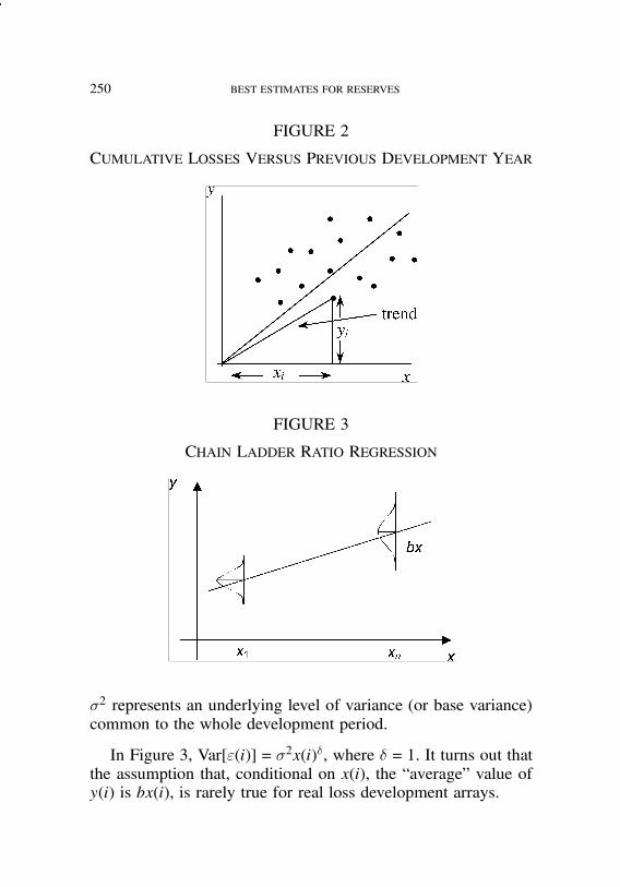
job no. 1969 casualty actuarial society CAS journal 1969D05 [6] 11-08-01 4:58 pm
250 BEST ESTIMATES FOR RESERVES
FIGURE 2
CUMULATIVE LOSSES VERSUS PREVIOUS DEVELOPMENT YEAR
FIGURE 3
CHAIN LADDER RATIO REGRESSION
¾2 represents an underlying level of variance (or base variance)common to the whole development period.
In Figure 3, Var["(i)] = ¾2x(i)±, where ± = 1. It turns out thatthe assumption that, conditional on x(i), the “average” value ofy(i) is bx(i), is rarely true for real loss development arrays.
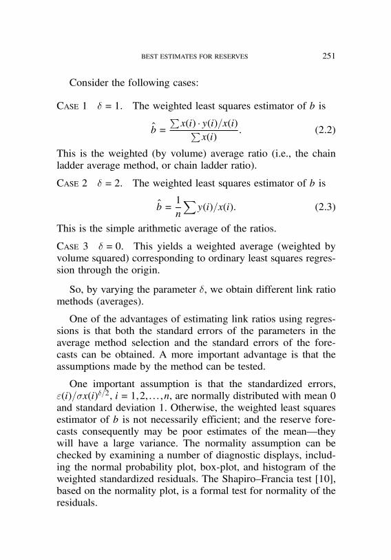
job no. 1969 casualty actuarial society CAS journal 1969D05 [7] 11-08-01 4:58 pm
BEST ESTIMATES FOR RESERVES 251
Consider the following cases:
CASE 1 ± = 1. The weighted least squares estimator of b is
b =!x(i) # y(i)=x(i)!
x(i): (2.2)
This is the weighted (by volume) average ratio (i.e., the chainladder average method, or chain ladder ratio).
CASE 2 ± = 2. The weighted least squares estimator of b is
b =1n
"y(i)=x(i): (2.3)
This is the simple arithmetic average of the ratios.
CASE 3 ± = 0. This yields a weighted average (weighted byvolume squared) corresponding to ordinary least squares regres-sion through the origin.
So, by varying the parameter ±, we obtain different link ratiomethods (averages).
One of the advantages of estimating link ratios using regres-sions is that both the standard errors of the parameters in theaverage method selection and the standard errors of the fore-casts can be obtained. A more important advantage is that theassumptions made by the method can be tested.
One important assumption is that the standardized errors,"(i)=¾x(i)±=2, i= 1,2, : : : ,n, are normally distributed with mean 0and standard deviation 1. Otherwise, the weighted least squaresestimator of b is not necessarily efficient; and the reserve fore-casts consequently may be poor estimates of the mean—theywill have a large variance. The normality assumption can bechecked by examining a number of diagnostic displays, includ-ing the normal probability plot, box-plot, and histogram of theweighted standardized residuals. The Shapiro–Francia test [10],based on the normality plot, is a formal test for normality of theresiduals.

job no. 1969 casualty actuarial society CAS journal 1969D05 [8] 11-08-01 4:58 pm
252 BEST ESTIMATES FOR RESERVES
FIGURE 4
The link ratio method also carries with it other assumptionsthat should always be tested.
Another basic assumption is that
E(y(i) $x(i)) = bx(i): (2.4)
That is, in order to obtain the mean cumulative at developmentperiod j, take the cumulative at the previous development period,j"1, and multiply it by the ratio. A quick diagnostic check ofthis assumption is given by the graph of y(i) versus x(i). Veryoften this shows that a (non-zero) intercept is also required. (SeeFigure 6.)
Equation 2.4 can be re-cast
E((y(i)" x(i)) $x(i)) = (b"1)x(i): (2.5)
That is, the mean incremental at development period j equals thecumulative at development period j" 1 multiplied by the link ra-tio, b, minus 1. What are the diagnostic tests for this assumption?
If the assumption underlying Equation 2.4 is valid, then theweighted standardized residuals versus fitted values should ap-pear random. Instead, what you will usually see is a downwardtrend like that depicted in Figure 4, representing the residuals
job no. 1969 casualty actuarial society CAS journal 1969D05 [9] 11-08-01 4:58 pm
BEST ESTIMATES FOR RESERVES 253
from the chain ladder ratios model for the Mack [7] data. (SeeExample 1 below.)
This indicates that large values are overpredicted and smallvalues are underpredicted, so that E(y $x) = bx is not true.Comparison of graphs of weighted standardized residuals
with graphs of the data will indicate that accident periods thathave “high” cumulatives are overfitted and those with “low” cu-mulatives are underfitted. Figure 5 shows the two displays forthe Mack [7] data. Note that as a result of the equivalence ofEquations 2.4 and 2.5, the residuals of the cumulative data arealso the residuals of the incremental data.
If you think of the way the incrementals are generated and thefact that there are usually payment-period effects, the cumulativeat development period j" 1 rarely is a good predictor of the nextincremental (after adjusting for accident period trends).
Murphy [8] suggested an extension of the regression modelrepresented by Equation 2.1 to include the possibility of an in-tercept:
y(i) = a+bx(i)+ "(i), (2.6a)
such thatVar["(i)] = ¾2x(i)±: (2.6b)
If the intercept a is non-zero and we do not include it in theregression model, then the estimate of the link ratio b (slope) isbiased. Note that in the graph in Figure 6 of cumulative values atdevelopment period 1 versus cumulative values at developmentperiod 0, the intercept appears to be different from zero (theorigin sits well below the graph). Indeed, it is significant betweenevery pair of contiguous development periods. See the data ofExample 1 below. We can rewrite Equation 2.6 thus:
y(i)" x(i) = a+(b" 1)x(i)+ "(i): (2.7)
So here, y(i)" x(i) is the incremental at development period j.

job no. 1969 casualty actuarial society CAS journal 1969D05 [10] 11-08-01 4:58 pm
254 BEST ESTIMATES FOR RESERVES
FIGURE 5
RAW DATA AND RESIDUALS FROM CHAIN LADDER MODEL
Consider the following two situations:
! b > 1 and a= 0.Here, to forecast the mean incremental at development pe-
riod j, we take the cumulative x at development period j"1and multiply it by (b"1).

job no. 1969 casualty actuarial society CAS journal 1969D05 [11] 11-08-01 4:58 pm
BEST ESTIMATES FOR RESERVES 255
FIGURE 6
CUMULATIVE IN DEVELOPMENT PERIOD 1 VERSUSCUMULATIVE IN DEVELOPMENT PERIOD 0
! b = 1 and a %= 0.In this case, x(i) has no predictive power in forecasting
y(i)" x(i). The estimate of a is a weighted average of the incre-mentals in development period j. We would therefore forecastthe next accident period’s incremental by averaging the incre-mentals down a development period. Accordingly, the stan-dard link ratio approach is abandoned in favor of averagingincrementals for each development period down the accidentperiods.
If b = 1 then the graph of y(i)" x(i) against x(i) should beflat, as depicted in Figure 7, which represents the incrementalsversus previous cumulatives (development period 0) for theMack [7] data. It is clear that the correlation is essentiallyzero. This is also true for every pair of contiguous developmentperiods.
In conclusion, if the incrementals y(i)" x(i) in developmentperiod j, say, appear random, it is very likely that the graphof y(i)" x(i) versus x(i) is also random. That is, there is zero
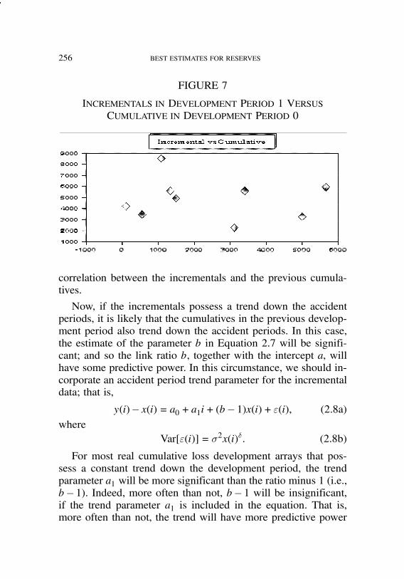
job no. 1969 casualty actuarial society CAS journal 1969D05 [12] 11-08-01 4:58 pm
256 BEST ESTIMATES FOR RESERVES
FIGURE 7
INCREMENTALS IN DEVELOPMENT PERIOD 1 VERSUSCUMULATIVE IN DEVELOPMENT PERIOD 0
correlation between the incrementals and the previous cumula-tives.
Now, if the incrementals possess a trend down the accidentperiods, it is likely that the cumulatives in the previous develop-ment period also trend down the accident periods. In this case,the estimate of the parameter b in Equation 2.7 will be signifi-cant; and so the link ratio b, together with the intercept a, willhave some predictive power. In this circumstance, we should in-corporate an accident period trend parameter for the incrementaldata; that is,
y(i)" x(i) = a0 + a1i+(b" 1)x(i)+ "(i), (2.8a)
whereVar["(i)] = ¾2x(i)±: (2.8b)
For most real cumulative loss development arrays that pos-sess a constant trend down the development period, the trendparameter a1 will be more significant than the ratio minus 1 (i.e.,b"1). Indeed, more often than not, b" 1 will be insignificant,if the trend parameter a1 is included in the equation. That is,more often than not, the trend will have more predictive power
job no. 1969 casualty actuarial society CAS journal 1969D05 [13] 11-08-01 4:58 pm
BEST ESTIMATES FOR RESERVES 257
than the ratio, and the residual predictive power of the ratio afterincluding the trend will be insignificant.
We use the following naming convention for the three param-eters:
a0 = intercept;
a1 = trend;
b = ratio (slope):
Here are some models included in the ELRF described byEquation 2.8.
! Chain Ladder Link RatiosIn this model, a0 = a1 = 0 and ± = 1.
! Cape Cod—intercept onlyHere it is assumed that b = 1 and a1 = 0. The Cape Cod
estimates a weighted average (with weights depending on ±) ofthe incrementals in each development period. The forecasts arealso based on a weighted average down the accident periodsfor each development period.
The model can be written as:
y(i)" x(i) = a0 + "(i), (2.9a)
whereVar["(i)] = ¾2x(i)±: (2.9b)
! Trend with b = 1The model estimates a weighted (depending on ±) trend
(parameters a0 and a1) down the accident periods for each de-velopment period. The forecasts are also based on a weightedtrend down the accident periods for each development period.
2.3. Example 1: The Mack Data
The data for the first example is fromMack [7] (see Table 2.1).The data are incurred losses for automatic facultative business
job no. 1969 casualty actuarial society CAS journal 1969D05 [14] 11-08-01 4:58 pm
258 BEST ESTIMATES FOR RESERVES
TABLE 2.1
INCURRED LOSS ARRAY FOR THE MACK DATA†
Accident Development YearYear 0 1 2 3 4 5 6 7 8 9
1981 5012 8269 10907 11805 13539 16181 18009 18608 18662 188341982 106 4285 5396 10666 13782 15599 15496 16169 167041983 3410 8992 13873 16141 18735 22214 22863 234661984 5655 11555 15766 21266 23425 26083 270671985 1092 9565 15836 22169 25955 261801986 1513 6445 11702 12935 158521987 557 4020 10946 123141988 1351 6947 131121989 3133 53951990 2063
†Note that 1982 accident year values are low.
in general liability, taken from the Reinsurance Association ofAmerica’s Historical Loss Development Study [9].
We first fit the chain ladder ratios regression model; that is,we fit Equation 2.1 with ± = 1 for every pair of contiguous de-velopment periods. The standardized residuals are displayed inFigure 8. Note that the equivalence of Equations 2.5 and 2.6means that the residuals of the model for the cumulative dataare identical to the residuals for the model of the incrementaldata.
We have already observed the downward trend in the fittedvalues (Figure 4), and that the high cumulatives are overpredictedwhereas the low cumulatives are underpredicted. This is mainlydue to the fact that intercepts are required.
So we now fit a model of the type given in Equation 2.6to each year (i.e., with intercepts, except for the last two pairsof contiguous development periods, as there is insufficient datathere). (See Table 2.2 for the regression output.) Note that noneof the slope (ratio) parameters are significantly different from 1and, if both parameters are insignificant, the slope (ratio) is less

job no. 1969 casualty actuarial society CAS journal 1969D05 [15] 11-08-01 4:58 pm
BEST ESTIMATES FOR RESERVES 259
TABLE 2.2
FIT OF THE MODEL WITH INTERCEPT† AND RATIO, WITH ± = 1
InterceptDevelop. Slope Slope"1 SlopePeriod Estimate Std. Error p value Estimate Estimate Std. Error p value
00–01 4,329 516 0.000 1.21445 0.21445 0.42131 0.62601–02 4,160 2,531 0.151 1.06962 0.06962 0.35842 0.85202–03 4,236 2,815 0.193 0.91968 "0:08032 0.24743 0.75903–04 2,189 1,133 0.126 1.03341 0.03341 0.07443 0.67704–05 3,562 2,031 0.178 0.92675 "0:07325 0.11023 0.55405–06 589 2,510 0.836 1.01250 0.01250 0.12833 0.93106–07 792 149 0.118 0.99110 "0:00890 0.00803 0.46707–08 — — — 1.01694 0.01694 0.01506 0.46308–09 — — — 1.00922 0.00922 — —
† Due to lack of observations in the tail, there is no intercept fitted for the last two years.
FIGURE 8
RESIDUAL PLOT FOR THE CHAIN LADDER RATIOS MODEL††
†† Note that the lines join the means at each period.
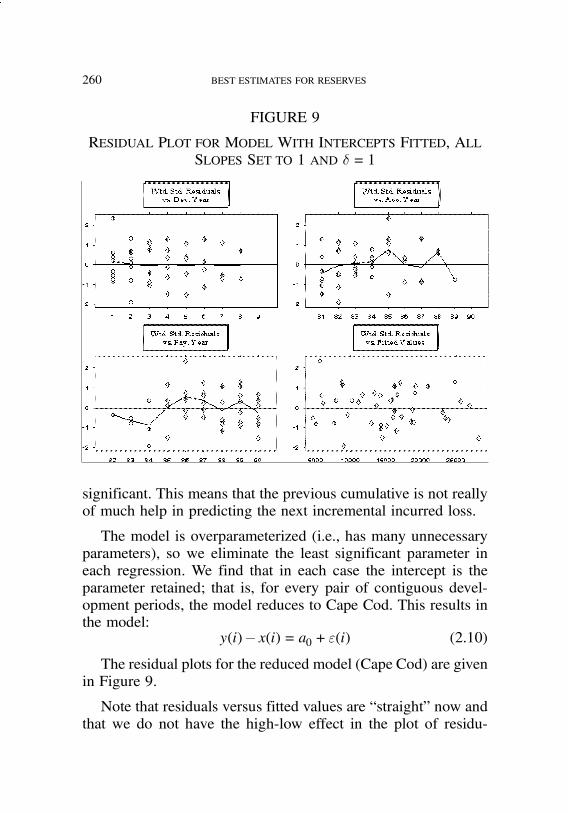
job no. 1969 casualty actuarial society CAS journal 1969D05 [16] 11-08-01 4:58 pm
260 BEST ESTIMATES FOR RESERVES
FIGURE 9
RESIDUAL PLOT FOR MODEL WITH INTERCEPTS FITTED, ALLSLOPES SET TO 1 AND ± = 1
significant. This means that the previous cumulative is not reallyof much help in predicting the next incremental incurred loss.
The model is overparameterized (i.e., has many unnecessaryparameters), so we eliminate the least significant parameter ineach regression. We find that in each case the intercept is theparameter retained; that is, for every pair of contiguous devel-opment periods, the model reduces to Cape Cod. This results inthe model:
y(i)" x(i) = a0 + "(i) (2.10)
The residual plots for the reduced model (Cape Cod) are givenin Figure 9.
Note that residuals versus fitted values are “straight” now andthat we do not have the high-low effect in the plot of residu-

job no. 1969 casualty actuarial society CAS journal 1969D05 [17] 11-08-01 4:58 pm
BEST ESTIMATES FOR RESERVES 261
TABLE 2.3
COMPARISON OF CAPE COD COEFFICIENTS OF VARIATIONWITH THOSE FOR THE CHAIN LADDER
Cape Cod Chain Ladder
AccidentYear
MeanForecast
StandardError
Coeff. ofVariation
MeanForecast
StandardError
Coeff. ofVariation
1981 0 0 — 0 0 —1982 172 41 0.244186 155 148 0.9548391983 483 465 0.899142 616 586 0.9512991984 1,113 498 0.385531 1,633 702 0.4298841985 1,941 1,218 0.512170 2,779 1,404 0.5052181986 4,200 1,555 0.408791 3,671 1,976 0.5382731987 6,878 1,677 0.271393 5,455 2,190 0.4014671988 10,252 3,247 0.308234 10,934 5,351 0.4893911989 14,874 3,657 0.253810 10,668 6,335 0.5938321990 19,336 4,532 0.215021 16,360 24,606 1.504034
Total 59,248 8,494 0.110347 52,272 26,883 0.514291
als versus accident period. The plot of residuals versus accidentyear does not exhibit a trend; if we were to include a trend, byestimating
y(i)" x(i) = a0 + a1i+ ", (2.11)
we would find that the estimate of a1 would not be significantlydifferent from zero.
We now present forecasts and coefficients of variation (meandivided by standard deviation) of forecasts based on the CapeCod (intercept-only) model with ± = 1, and compare this withthe forecasts and coefficients of variation for the chain ladderratios (see Table 2.3).
Note that, for the Cape Cod model, the standard errors aregenerally decreasing as a percentage of the accident-year fore-cast totals as we proceed down to the later years. This is be-cause the model relates the numbers in the triangle to a cer-tain degree—it assumes that the incremental values in the same

job no. 1969 casualty actuarial society CAS journal 1969D05 [18] 11-08-01 4:58 pm
262 BEST ESTIMATES FOR RESERVES
development period are randomly drawn from the same distribu-tion. This does not happen with the chain ladder ratios, becausethe model does not relate the incrementals in the triangle in anymeaningful way. For example, how are the values in the develop-ment period 0 related? Consequently, the coefficients of variationare substantially higher for the chain ladder ratios model. More-over, the coefficient of variation for 1990 is 150%, but for theprevious year it is 59%. Note that 1990 has one more incre-mental value to forecast than 1989; if anything, a good modelwill on average have smaller coefficients of variation for totalsof years with more observations. Since the 1990 accident-yeartotal pools one more uncertain value than 1989 and the remain-ing values (conditionally on the first) could be expected to havesimilar coefficients of variation to the corresponding values from1989, this appears to violate the fundamental statistical principleof insurance—risk reduction by pooling.
For the Mack data, the model with intercepts is reasonable,as there is no accident-year trend in the incrementals. For datawhere a constant trend (on a dollar scale) does exist, then thetrend will be significant, but very often the ratio will not besignificantly different from one.
2.4. Summary
We have so far considered two cases that can occur in realdata: incrementals for a particular development period have notrend, and incrementals have trend in the accident period direc-tion (after possibly adjusting the data by accident period expo-sures). In the first case, link ratios are often insignificant andso lack predictive power. In the second case, when incremen-tals versus accident periods for a particular development periodhave a constant trend, it is likely that the cumulatives in the pre-ceding development period also exhibit a trend so that the ratiohas some predictive power (equivalently, the ratio is significantlydifferent from one). However, more often than not, the accidentperiod trend has more predictive power than the ratio; and, once

job no. 1969 casualty actuarial society CAS journal 1969D05 [19] 11-08-01 4:58 pm
BEST ESTIMATES FOR RESERVES 263
FIGURE 10
RESIDUAL PLOTS FOR THE CHAIN LADDER RATIOS MODEL
it is included in the model, the term (b"1) is often insignificant(i.e., the ratio does not have any residual predictive power). Thesituation encountered most often in practice, however, involvesa trend change along the payment/calendar periods (diagonals).This means that as you look down each development period, thechange in trend will occur in different accident periods. Conse-quently, none of the above models in the ELRF can capture thesetrends.
The weighted standardized residual plots depicted in Figures10 and 11 are those of the chain ladder ratios and Equation2.8, respectively, applied to project ABC (Workers Compensa-tion Portfolio) discussed in Section 3. Note that the chain ladderratios indicate a payment-year trend change, and the model inEquation 2.8, which fits a constant trend down the accident yearsfor each development year, indicates that the trend before pay-

job no. 1969 casualty actuarial society CAS journal 1969D05 [20] 11-08-01 4:58 pm
264 BEST ESTIMATES FOR RESERVES
FIGURE 11
RESIDUAL PLOTS FOR TREND PLUS RATIO MODEL
ment year 1984 is lower than the trend after 1984. This project(ABC) is analyzed in more detail in Section 3.
The models subsumed by Equation 2.8 can be used to di-agnostically identify payment period trend changes but do notidentify these trend changes or forecast with them. The modelsin the ELRF form a bridge to models that also include paymentperiod trend parameters; that is, statistical models in the Proba-bilistic Trend Family (PTF) of the next section.
It is important to note that ELRF models also make the im-plicit assumption that the weighted standardized errors comefrom a normal distribution. If the assumption is true, the esti-mates of the regression parameters are optimal. If the assump-tion is not true, the estimates may be very poor. This normal-ity assumption is rarely true for loss reserving data. In fact,the weighted standardized residuals are generally skewed to theright, suggesting that the analysis should be conducted on the

job no. 1969 casualty actuarial society CAS journal 1969D05 [21] 11-08-01 4:58 pm
BEST ESTIMATES FOR RESERVES 265
FIGURE 12
RESIDUALS VERSUS FITTED VALUES FOR THE CHAIN LADDERRATIOS
logarithmic scale. The graph in Figure 12 illustrates the skew-ness of a set of weighted standardized residuals based on chainladder ratios for Project PAN6 (analyzed in detail in Example 4of Section 3). The positive-weighted standardized residuals arefurther from zero than the negative ones. If the normality as-sumption were correct, the plot would look roughly symmetricabout the zero line.
In summary, using the ELRF regression methodology youwill discover that, for any type of real loss development array,the standard development factor (link ratio) techniques are fre-quently inappropriate. Analyzing the incrementals on the loga-rithmic scale with the inclusion of payment period trend param-eters has more predictive power.
Finally, but importantly, the estimate of a mean forecastof outstanding (reserve) and corresponding standard deviationbased on a model may be quite meaningless, unless the assump-tions made by the model are supported by the data.
job no. 1969 casualty actuarial society CAS journal 1969D05 [22] 11-08-01 4:58 pm
266 BEST ESTIMATES FOR RESERVES
3. STATISTICAL MODELING FRAMEWORK
3.1. Introduction
Clearly, we require a model that is able to deal with changingtrends. Trends in the data on the original (dollar) scale are hardto deal with, since trends on that scale are not generally linearbut instead move in percentage terms—for example, 5% super-imposed (social) inflation in early years, and 3% in later years. Itis the logarithms of the incremental data that show linear trends.Consequently, we introduce a modeling framework for the loga-rithms of the incremental data that allows for changes in trends.The models of this type provide a high degree of insight into theloss development processes. Moreover, they facilitate the extrac-tion of a great deal of easily communicated information from theloss development array.
The details of the modeling framework and its inherent bene-fits are described in Zehnwirth [12]. However, given that there isa paradigm shift from the standard link ratio methodology to thestatistical modeling framework, we review the salient features ofthe statistical modeling framework.
3.2. Trend Properties of Loss Development Arrays
Since a model is supposed to capture the trends in thedata, it behooves us to discuss the geometry of trends inthe three directions; viz., development-year, accident-year andpayment/calendar-year.
Development years are denoted by j, j = 0,1,2, : : : ,s"1; ac-cident years by i, i= 1,2, : : : ,s; and payment years by t, t=1,2, : : : ,s. See Figure 13.
The payment-year variable t can be expressed as t= i+ j.This relationship between the three directions implies that thereare only two independent directions.
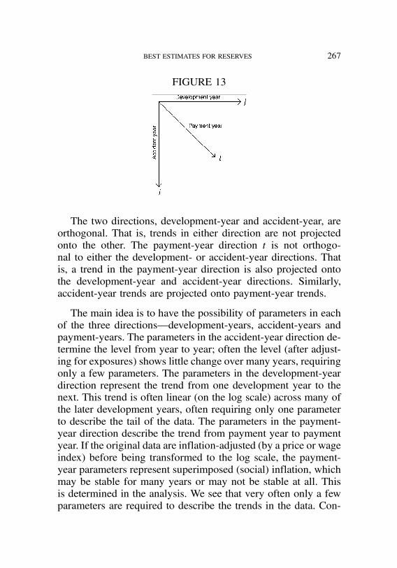
job no. 1969 casualty actuarial society CAS journal 1969D05 [23] 11-08-01 4:58 pm
BEST ESTIMATES FOR RESERVES 267
FIGURE 13
The two directions, development-year and accident-year, areorthogonal. That is, trends in either direction are not projectedonto the other. The payment-year direction t is not orthogo-nal to either the development- or accident-year directions. Thatis, a trend in the payment-year direction is also projected ontothe development-year and accident-year directions. Similarly,accident-year trends are projected onto payment-year trends.
The main idea is to have the possibility of parameters in eachof the three directions—development-years, accident-years andpayment-years. The parameters in the accident-year direction de-termine the level from year to year; often the level (after adjust-ing for exposures) shows little change over many years, requiringonly a few parameters. The parameters in the development-yeardirection represent the trend from one development year to thenext. This trend is often linear (on the log scale) across many ofthe later development years, often requiring only one parameterto describe the tail of the data. The parameters in the payment-year direction describe the trend from payment year to paymentyear. If the original data are inflation-adjusted (by a price or wageindex) before being transformed to the log scale, the payment-year parameters represent superimposed (social) inflation, whichmay be stable for many years or may not be stable at all. Thisis determined in the analysis. We see that very often only a fewparameters are required to describe the trends in the data. Con-
job no. 1969 casualty actuarial society CAS journal 1969D05 [24] 11-08-01 4:58 pm
268 BEST ESTIMATES FOR RESERVES
sequently, the (optimal) identified model for a particular lossdevelopment array is likely to be parsimonious. This allows usto have a clearer picture of what is happening in the incrementalloss process.
In this section, let y(i,j) be the natural log of the incrementalpayment data in accident year i and development year j. Thisis different from our use of y(i,j) in Section 2, but we do itfor consistency with the literature appropriate to the models ineach section. The mathematical formulation of the models in thestatistical modeling framework is given by Equation 3.5. We nowillustrate the geometry of trends with a simulation example.
3.3. Example 2—Simulated Data
To illustrate the trend properties of a loss development array,let us examine a situation where we know the trends (because wehave selected them). Consider a set of data where the underlyingpaid loss (at this point without any payment-year trends or evenrandomness—just the underlying development) is of the form
y(i,j) = ln(pij) = 11:51293"0:2j: (3.1)
On a log scale, this is a line with a slope of "0:2. The acci-dent years are completely homogeneous. Let’s add some pay-ment/calendar year trends: a trend of 0.1 from 1978 to 1982, 0.3from 1982 to 1983 and 0.15 from 1983 to 1991. Note that alinear trend of 0.1 per year on the log scale is about a 10% perannum increase on the original scale.
The trends are depicted in Figure 14. Patterns of change likethis are quite common in real data. Note that trends in the pay-ment/calendar year direction project onto the other two direc-tions, as they must. The resultant trends for the first six accidentyears are shown in Figure 15.
Note that each line in the graph is the resultant development-year trend for a single accident year. As you go down the acci-
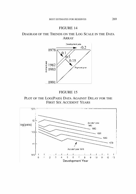
job no. 1969 casualty actuarial society CAS journal 1969D05 [25] 11-08-01 4:58 pm
BEST ESTIMATES FOR RESERVES 269
FIGURE 14
DIAGRAM OF THE TRENDS ON THE LOG SCALE IN THE DATAARRAY
FIGURE 15
PLOT OF THE LOG(PAID) DATA AGAINST DELAY FOR THEFIRST SIX ACCIDENT YEARS

job no. 1969 casualty actuarial society CAS journal 1969D05 [26] 11-08-01 4:58 pm
270 BEST ESTIMATES FOR RESERVES
FIGURE 16
TREND PLUS RANDOMNESS FOR THE FIRST SIX ACCIDENTYEARS
dent years (1978 to 1983), the 30% trend always kicks in onedevelopment-period earlier. The payment-year trends also projectonto the accident years, which is why the early years are at thebottom and the later years are at the top. Note how the “kink”moves back as we go up to the more recent accident years. Theresultant development-year trends are different for each accidentyear now. We can’t model even this simple situation with linkratios or any other ELRF model.
Of course, real data are never so smooth. On the same logscale, we add some noise—random numbers with mean 0 andstandard deviation 0.1, as shown in Figure 16.
Now the underlying changes in trends are not at all clear fortwo reasons—the payment-year trends project onto developmentyears, and the data always exhibits randomness that tends to ob-scure the underlying trend changes. It has many of the propertieswe observe in real data; and yet it is plain that, even with theextensions presented there, the regression models in ELRF fromSection 2 are inadequate for this data. We instead look to a model

job no. 1969 casualty actuarial society CAS journal 1969D05 [27] 11-08-01 4:58 pm
BEST ESTIMATES FOR RESERVES 271
FIGURE 17
PROBABILISTIC MODEL FOR DEVELOPMENT-YEAR TRENDS(LOG SCALE)
that incorporates the trends in the three directions and the vari-ability about those trends, measured on a log scale.
Consider a single accident year (dropping the i subscript forthe moment). We represent the expected level in the first de-velopment year by the parameter ®. We can model the trendsacross the development years by allowing for a (possible) pa-rameter to represent the expected change (trend) between eachpair of development years. We model the variation of the dataabout this process with a zero-mean, normally-distributed ran-dom error, represented as:
y(j) = ®+j"k=1
°k+ "j: (3.2)
This probabilistic model is depicted in Figure 17 (for the firstsix development years).
For this probabilistic model, ® is not the value of y observedat delay 0. It is the mean of y(0); indeed, y(0) has a normaldistribution with mean ® and variance ¾2. Similarly, °j is not
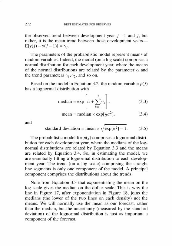
job no. 1969 casualty actuarial society CAS journal 1969D05 [28] 11-08-01 4:58 pm
272 BEST ESTIMATES FOR RESERVES
the observed trend between development year j"1 and j, butrather, it is the mean trend between those development years—E[y(j)" y(j" 1)] = °j.The parameters of the probabilistic model represent means of
random variables. Indeed, the model (on a log scale) comprises anormal distribution for each development year, where the meansof the normal distributions are related by the parameter ® andthe trend parameters °1,°2, and so on.
Based on the model in Equation 3.2, the random variable p(j)has a lognormal distribution with
median = exp
#$®+ j"k=1
°k
%& , (3.3)
mean =median& exp[12¾2], (3.4)
andstandard deviation =mean&
'exp[¾2]"1: (3.5)
The probabilistic model for p(j) comprises a lognormal distri-bution for each development year, where the medians of the log-normal distributions are related by Equation 3.3 and the meansare related by Equation 3.4. So, in estimating the model, weare essentially fitting a lognormal distribution to each develop-ment year. The trend (on a log scale) comprising the straightline segments is only one component of the model. A principalcomponent comprises the distributions about the trends.
Note from Equation 3.3 that exponentiating the mean on thelog scale gives the median on the dollar scale. This is why theline in Figure 17, after exponentiation in Figure 18, joins themedians (the lower of the two lines on each density) not themeans. We will normally use the mean as our forecast, ratherthan the median, but the uncertainty (measured by the standarddeviation) of the lognormal distribution is just as important acomponent of the forecast.

job no. 1969 casualty actuarial society CAS journal 1969D05 [29] 11-08-01 4:58 pm
BEST ESTIMATES FOR RESERVES 273
FIGURE 18
MODEL FOR TRENDS ALONG A DEVELOPMENT YEAR (DOLLARSCALE)
If we compute expected values of the logs of the develop-ment factors on the incremental data with this model, we obtainE[ln(p(j)=p(j"1))] = E[(°j + "j " "j"1)] = °j . That is, trend pa-rameters also underpin this new model, but in a way that willallow it to appropriately model the trends in the incremental data(in the three directions).
The model described so far only covers a single accident year;we have not yet accounted for the payment-year and accident-year trends. Let the mean of the (random) inflation between pay-ment year t and t+1 be represented by ¶t (iota-t).
Hence the family of models can be written:
y(i,j) = ®i+j"k=1
°k +i+j"t=1
¶t+ "i,j : (3.6)
We call this family of models the probabilistic trend family(PTF). Note that the mean trend between cells (i,j" 1) and (i,j)is °j + ¶i+j , and the mean trend between cells (i"1,j) and (i,j)is ®i+1"®i+ ¶i+j .

job no. 1969 casualty actuarial society CAS journal 1969D05 [30] 11-08-01 4:58 pm
274 BEST ESTIMATES FOR RESERVES
TABLE 3.1
PARAMETER ESTIMATES FOR THE MODEL WITH CONSTANTTRENDS
Parameter Estimate Standard Error t-ratio
® 11.4256 0.0302 378.57° "0:2062 0.0037 "55:08¶ 0.1563 0.0037 41.74
s= 0:1129 R2 = 97:0%
A member of this family of models relates the lognormal dis-tributions of the cells in the triangle. On a log scale, the distri-bution for each cell is normal, where the means of the normaldistributions are related by the “trends” described by the partic-ular model.
If the error terms "i,j (each coming from a normal distributionwith mean 0) do not have a constant variance, then the changesin variance must also be modeled. Note that there are numer-ous models in the PTF, even if we do not include the varying(stochastic) parameter models discussed in Section 3.7. The ac-tuary has to identify the most appropriate model for the lossdevelopment array being analyzed. The assumptions made bythe “optimal” model must be satisfied by the data. In doing so,one extracts information in terms of trends, stability of trends,and the distributions of the data about the trends.
3.3. Example 2 continued—Estimation
Let’s now try to identify the model that created the data. Webegin by fitting a model with all the development-year trendsequal to each other (one °), all payment-year trends equal toeach other (one ¶), and no accident-year trends (one ®); that is,with °k = °, ¶t = ¶, and ®i = ® for all parameters. The parameterestimates are given in Table 3.1.

job no. 1969 casualty actuarial society CAS journal 1969D05 [31] 11-08-01 4:58 pm
BEST ESTIMATES FOR RESERVES 275
FIGURE 19
PLOTS OF STANDARDIZED RESIDUALS VERSUS THE THREEDIRECTIONS AND FITTED VALUES FOR THE SINGLE
PAYMENT-YEAR TREND MODEL
The estimate of 0.1563 for ¶ (iota) is a weighted average ofthe three trends 0.1, 0.3 and 0.15.
Removing constant trends makes any changes in trend moreobvious; the residuals are shown in Figure 19.
The residuals need to be interpreted as the data adjusted forwhat has been fitted; accordingly, the residuals versus paymentyears represent the data minus the fitted value of 0.1563 peryear.
Immediately, the changes in trends in the payment-year di-rection become obvious. We can see that the trend in the earlyyears is substantially less than the estimated average of 0.1563;that the trend from 1982 to 1983 is much larger than it; and, after
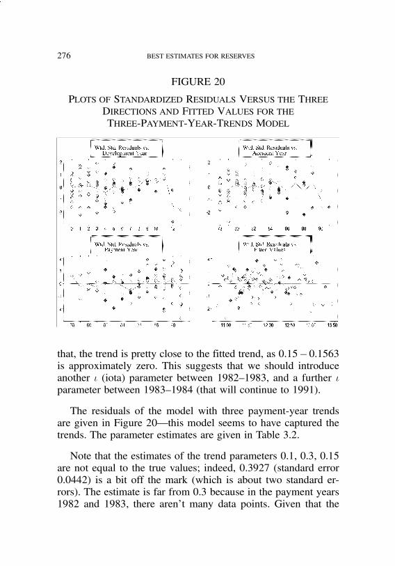
job no. 1969 casualty actuarial society CAS journal 1969D05 [32] 11-08-01 4:58 pm
276 BEST ESTIMATES FOR RESERVES
FIGURE 20
PLOTS OF STANDARDIZED RESIDUALS VERSUS THE THREEDIRECTIONS AND FITTED VALUES FOR THETHREE-PAYMENT-YEAR-TRENDS MODEL
that, the trend is pretty close to the fitted trend, as 0:15"0:1563is approximately zero. This suggests that we should introduceanother ¶ (iota) parameter between 1982–1983, and a further ¶parameter between 1983–1984 (that will continue to 1991).
The residuals of the model with three payment-year trendsare given in Figure 20—this model seems to have captured thetrends. The parameter estimates are given in Table 3.2.
Note that the estimates of the trend parameters 0.1, 0.3, 0.15are not equal to the true values; indeed, 0.3927 (standard error0.0442) is a bit off the mark (which is about two standard er-rors). The estimate is far from 0.3 because in the payment years1982 and 1983, there aren’t many data points. Given that the

job no. 1969 casualty actuarial society CAS journal 1969D05 [33] 11-08-01 4:58 pm
BEST ESTIMATES FOR RESERVES 277
TABLE 3.2
PARAMETER ESTIMATES FOR THETHREE-PAYMENT-YEAR-TRENDS MODEL
Parameter Estimate Standard Error t-ratio
® 11.5321 0.0612 188.34° "0:2062 0.0033 "61:91
¶: 78–82 0.0873 0.0209 4.18¶: 82–83 0.3927 0.0442 8.90¶: 83–91 0.1446 0.0046 31.72
s= 0:1005 R2 = 97:7%
TABLE 3.3
FORECASTS, STANDARD ERRORS, TREND ESTIMATES ANDTHEIR STANDARD ERRORS AS THE LATER PAYMENT YEARS
ARE REMOVED
StandardYears in Standard Standard Mean Error ofEstimation N ° (83–91) Error (°) ¶ (83–91) Error (¶) Forecast Forecast
78–91 105 "0:2062 0.0033 0.1446 0.0046 23,426,542 927,81078–90 91 "0:2075 0.0036 0.1527 0.0051 25,333,522 1,191,12978–89 78 "0:2086 0.0042 0.1512 0.0064 24,850,972 1,526,24678–88 66 "0:2119 0.0045 0.1575 0.0075 26,296,366 1,997,08978–87 55 "0:2131 0.0055 0.1563 0.0103 25,894,931 2,868,948
trend of 0.15 is in the data since 1983, we would expect sta-bility of forecasts, and trend parameter estimates as we removeyears.
The forecasts are stable—if we remove the most recent data,the forecasts of this model don’t change much relative to thestandard error in the forecast, as we can see in Table 3.3.
Note that the estimate of ° (recall that ° ="0:2) is prettystable, as we remove the latest years.

job no. 1969 casualty actuarial society CAS journal 1969D05 [34] 11-08-01 4:58 pm
278 BEST ESTIMATES FOR RESERVES
FIGURE 21
PREDICTION ERRORS FOR 1988–1991, FOR MODEL ESTIMATEDIN 1987
Figure 21 gives the prediction errors (on a log scale) for thefour payment years 1988–1991, based on the model estimated atyear end 1987.
The estimated model at the end of payment year 1987 slightlyover-predicts the payment periods 1988–1991. That is becausethe trend estimate since 1983 (see Table 3.4) is now 15:63%'1:03% (where we are writing mean' standard deviation as short-hand), in place of 14:46%'0:46% when we use all the years inthe estimation. Hence the forecast of $26M ('$2:9M) is “higher”than $23M ('$0:9M). When you test for a trend change be-tween 1987 and 1988, it is not significant (as we would ex-pect). Note that removal of recent payment years to check themodel’s ability to predict them (validation analysis) is part ofthe model identification procedure and extraction of informationprocess.

job no. 1969 casualty actuarial society CAS journal 1969D05 [35] 11-08-01 4:58 pm
BEST ESTIMATES FOR RESERVES 279
TABLE 3.4
VALIDATION RESULTS—PARAMETER ESTIMATES ANDFORECASTS AS PAYMENT YEARS ARE REMOVED FROM THE
SELECTED MODEL
Payment Years Estimate of Estimate of iota Forecast 'in Estimation gamma (83–91) Standard Error ($M)
1978–91 "20:62' 0:33 14:46' 0:46 23' 0:91978–90 "20:75' 0:36 15:27' 0:51 25' 1:21978–89 "20:86' 0:42 15:15' 0:64 25' 1:51978–88 "21:19' 0:45 15:75' 0:75 26' 2:01978–87 "21:31' 0:55 15:63' 1:03 26' 2:9
3.4. Example 3—Real Data With Major Payment-Year TrendInstability
We now analyze a real data array as presented in Table 3.5.
This loss development array has a major trend change betweenpayment years 1984 and 1985, even though the data and linkratios are relatively smooth. Indeed, it needs to be understoodthat, in general, trend instability has nothing to do with volatilityor smoothness of the data and link ratios. When there is a trendchange, formulation of the assumptions about the future trendwill depend on the explanation for that trend change.
The individual link ratios for the cumulated data are verystable, as can be seen in Figure 22. It is very dangerous to tryto make judgements about the suitability of development fac-tor techniques from the individual link ratios on the cumulateddata.
We first conduct some diagnostic PTF analysis, then showhow the ELRF modeling structure also indicates payment-yeartrend change, indeed that any method based on link ratios isquite meaningless for this data. Consequently, there is little to begained by forecasting any of the ELRF models. Figure 23 shows

job no. 1969 casualty actuarial society CAS journal 1969D05 [36] 11-08-01 4:58 pm
280 BEST ESTIMATES FOR RESERVES

job no. 1969 casualty actuarial society CAS journal 1969D05 [37] 11-08-01 4:58 pm
BEST ESTIMATES FOR RESERVES 281
FIGURE 22
PLOT OF INDIVIDUAL LINK RATIOS BY DELAY†
† The line joins Chain Ladder ratios.
FIGURE 23
STANDARDIZED RESIDUALS OF THE STATISTICAL CHAINLADDER MODEL
job no. 1969 casualty actuarial society CAS journal 1969D05 [38] 11-08-01 4:58 pm
282 BEST ESTIMATES FOR RESERVES
the standardized residuals of the statistical chain ladder in PTF(i.e., the statistical chain ladder fits all the gamma parametersand all the alpha parameters with no iotas). The residuals arejust the data (less the average level) adjusted for the (average)trend between every pair of contiguous development periods andevery pair of contiguous accident periods. This is why the plotsof standardized residuals versus development years and accidentyears are centered on zero! We use this model only as a di-agnostic tool to determine quickly whether there are payment-year trend changes that can be attributed solely to the paymentyears.
Contrast the smoothness of the ratios above with the plotof the residuals from this model. We can now see dramaticchanges in the payment-year direction. It might be very dan-gerous to use forecasts from any model assuming no changes inpayment-year trend, such as a model from the ELRF. There isa difference between Figures 23 and 10—the statistical chainladder shows the payment-year trends after adjusting for thetrends in the other two directions, while the chain ladder ra-tios (Figure 10) do not do that. But the change in trend is clearin either graph. In the current statistical modeling framework,we are able to model this change; we have a lot more con-trol over how we incorporate the trend changes into our modeland hence into the forecasts. Even the best ELRF model forthis data hardly uses ratios and is deficient because it givesus no control in the payment-year direction. It turns out thatthe trend before 1984 is approximately 10% whereas the trendafter 1984 is approximately 20%. So which trend should weassume for the future? This depends on the explanation forthe change. If the trend instability is due to new legislationthat applies retrospectively (to all accident periods), then onewould revert to the 10%—as a change to the level of pay-ments will be a single jump in level (possibly taking sev-eral years to be completely manifested). If there is no expla-nation for the trend change, except that the payments have

job no. 1969 casualty actuarial society CAS journal 1969D05 [39] 11-08-01 4:58 pm
BEST ESTIMATES FOR RESERVES 283
TABLE 3.6
PAID LOSS ARRAY FOR THE PAN6 DATA FOR EXAMPLE 4
Accident Development YearYear 0 1 2 3 4 5
1986 194324 571621 327880 249194 524483 17242741987 1469 57393 485791 169614 121410 5990211988 1860 161538 408008 314614 6744000 ****1989 23512 185604 260725 1134272 851099 21742001990 1044 70096 93600 1283752 1595466 9132151991 **** 3730 869959 187019 2764795 ****1992 **** 443205 180064 683407 8781171993 **** 12808 433511 1180171994 1431 77765 1511611995 51539 ****1996 ****
increased, then calling the future in terms of trends is more dif-ficult.
3.5. Example 4—Volatile Data With Stable Trends
We now consider an array where the paid losses are veryvolatile, but the trends are stable (see Table 3.6). Recall thattrend stability/instability is dependent on neither the volatility ofthe data nor the volatility of the link ratios. Since the randomcomponent is an integral part of the model, this model capturesthe behavior of this volatile data very well. We call this arrayPAN6.
A good model can be identified quickly for the logarithms ofthese data; it has no payment-year trends, and only two differentdevelopment-year trends—between development years 0–1 andfor all later years (the residual plot is given in Figure 24).
Note that the spread of the first two development years iswider than for the later years, and the spread for “small” fit-ted values is larger than the spread for “large” fitted values. Ifwe estimate the standard deviations in the two sections, we find

job no. 1969 casualty actuarial society CAS journal 1969D05 [40] 11-08-01 4:58 pm
284 BEST ESTIMATES FOR RESERVES
FIGURE 24
PLOT OF STANDARDIZED RESIDUALS FOR THE MODEL WITHTWO GAMMA PARAMETERS AND ONE ALPHA PARAMETER
that they are 3.0177 and 0.8015, respectively. This requires aweighted regression; development years 0 and 1 are given weight(0:8015=3:0177)2, and the other years (2+) have a weight of 1.The weighted, standardized residual plots now look fine (see Fig-ure 25). A check of the plot of residuals against normal scores(not presented here) indicates that the assumption of normalityof the logarithms of the data is very reasonable—the squaredcorrelation is greater than 0.99.
The normal distributions for this model have relatively largevariances—the estimate of ¾2 for development periods 0–1 is2.923, and for development periods 2+ is 0.80346. Note thatif a normal distribution has a variance ¾2, then the corre-sponding lognormal distribution has a coefficient variation of'exp(¾2)" 1> ¾.

job no. 1969 casualty actuarial society CAS journal 1969D05 [41] 11-08-01 4:58 pm
BEST ESTIMATES FOR RESERVES 285
FIGURE 25
PLOT OF WEIGHTED STANDARDIZED RESIDUALS AFTER THEWEIGHTED REGRESSION
This model also has forecasts that are stable as we remove themost recent data, as we see in Table 3.7. This is a very importantattribute of the identified model that captures the informationin the data—if the trends in the data are stable, then so are theforecasts based on the estimated model. In this case, we wereable to remove almost half the (most recent) data. The standarderrors of the forecasts are large because the lognormal distribu-tions are skewed—insurance is about measuring variance, notjust means.
While the variability of the data and hence the standard errorsof the forecasts are large, the message from the data has beenconsistent over many years. We are predicting the distributionof the data in each cell, not merely their mean and standarddeviation, so a large standard deviation does not imply a badmodel. Indeed, the model is very good. It captures the variances,indeed the distributions, in each cell.
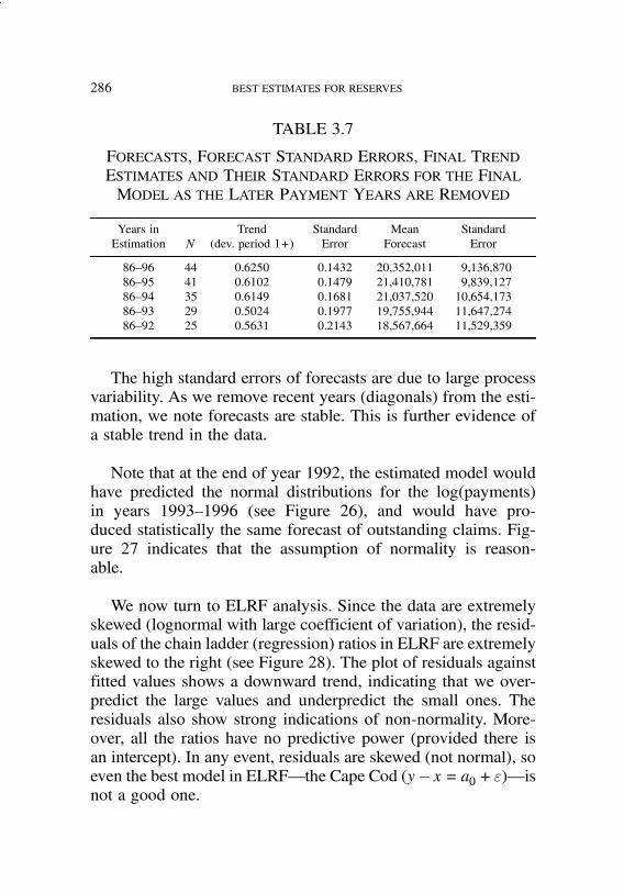
job no. 1969 casualty actuarial society CAS journal 1969D05 [42] 11-08-01 4:58 pm
286 BEST ESTIMATES FOR RESERVES
TABLE 3.7
FORECASTS, FORECAST STANDARD ERRORS, FINAL TRENDESTIMATES AND THEIR STANDARD ERRORS FOR THE FINALMODEL AS THE LATER PAYMENT YEARS ARE REMOVED
Years in Trend Standard Mean StandardEstimation N (dev. period 1+) Error Forecast Error
86–96 44 0.6250 0.1432 20,352,011 9,136,87086–95 41 0.6102 0.1479 21,410,781 9,839,12786–94 35 0.6149 0.1681 21,037,520 10,654,17386–93 29 0.5024 0.1977 19,755,944 11,647,27486–92 25 0.5631 0.2143 18,567,664 11,529,359
The high standard errors of forecasts are due to large processvariability. As we remove recent years (diagonals) from the esti-mation, we note forecasts are stable. This is further evidence ofa stable trend in the data.
Note that at the end of year 1992, the estimated model wouldhave predicted the normal distributions for the log(payments)in years 1993–1996 (see Figure 26), and would have pro-duced statistically the same forecast of outstanding claims. Fig-ure 27 indicates that the assumption of normality is reason-able.
We now turn to ELRF analysis. Since the data are extremelyskewed (lognormal with large coefficient of variation), the resid-uals of the chain ladder (regression) ratios in ELRF are extremelyskewed to the right (see Figure 28). The plot of residuals againstfitted values shows a downward trend, indicating that we over-predict the large values and underpredict the small ones. Theresiduals also show strong indications of non-normality. More-over, all the ratios have no predictive power (provided there isan intercept). In any event, residuals are skewed (not normal), soeven the best model in ELRF—the Cape Cod (y" x= a0 + ")—isnot a good one.
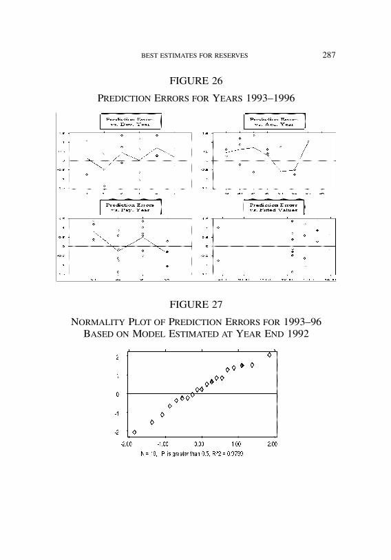
job no. 1969 casualty actuarial society CAS journal 1969D05 [43] 11-08-01 4:58 pm
BEST ESTIMATES FOR RESERVES 287
FIGURE 26
PREDICTION ERRORS FOR YEARS 1993–1996
FIGURE 27
NORMALITY PLOT OF PREDICTION ERRORS FOR 1993–96BASED ON MODEL ESTIMATED AT YEAR END 1992

job no. 1969 casualty actuarial society CAS journal 1969D05 [44] 11-08-01 4:58 pm
288 BEST ESTIMATES FOR RESERVES
FIGURE 28
RESIDUALS OF CHAIN LADDER RATIOS REGRESSION MODEL
Recall that if model assumptions are not satisfied by the data,then forecast calculations may be quite meaningless.
3.6. Example 5—Simulated Array Based on a Model With OnlyTwo Parameters
The following array, which we call SDF, is a simulated data setwhere the incremental paid losses have completely homogeneousaccident years. The actual model driving the data has one alpha(®) = 10, one gamma (°) ="0:3, and has ¾2 = 0:4. That is,
y(i,j) = 10" 0:3j+ "(i,j), (3.7)
where the "(i,j) are independent and identically distributed froma normal distribution with mean 0 and variance 0.4.
The simulated data is presented in Table 3.8.

job no. 1969 casualty actuarial society CAS journal 1969D05 [45] 11-08-01 4:58 pm
BEST ESTIMATES FOR RESERVES 289

job no. 1969 casualty actuarial society CAS journal 1969D05 [46] 11-08-01 4:58 pm
290 BEST ESTIMATES FOR RESERVES
The first thing to note with this data is that, once noise isadded, it looks like incremental paid data for a real array, eventhough it was generated from a very simple model.
The relatively large ¾2 (0.4) explains the high variability in theobserved paid losses. The incremental data displayed in Table 3.8appear volatile, but the values in the same development period areindependent realizations from the same lognormal distribution.
For example, in development period zero, the simulated val-ues 80,451 and 9,017 come from a lognormal distribution withmean 26,903 and standard deviation 18,867. Since a lognormaldistribution is skewed to the right, realizations larger than themean are typically further away from the mean compared to re-alizations less than the mean, which are bounded below by zero(and so are closer to the mean).
The apparent volatility in the data is not due to instability intrends; indeed, the reality is quite the opposite—though volatile,the incremental paid losses have stable trends. Since we know theexact probability distributions driving the data, we can computethe exact mean and exact standard deviation for each cell in therectangle and also the exact means and standard deviations ofsums.
The exact mean of the total outstanding is $284,125, with anexact standard deviation of $30,970, and so the process vari-ance is 30,9702. When we analyze the data in PTF, we identifyonly two significant parameters—®= 9:9667 (with standard er-ror 0.0847) and ° ="0:2867 (standard error 0.0126), and theestimate of ¾2 is 0.4085. Residuals from this estimated modelare displayed in Figure 29.
Table 3.9 gives forecasts of total outstanding, including vali-dation forecasts (note that the forecasts are stable, as expected).
We now study the cumulative array, displayed in Figure 30.Even though the incremental data was generated with homoge-neous accident years, the cumulated data have each accident year

job no. 1969 casualty actuarial society CAS journal 1969D05 [47] 11-08-01 4:58 pm
BEST ESTIMATES FOR RESERVES 291
FIGURE 29
RESIDUALS BASED ON THE ESTIMATED PARAMETERS OF THEMODEL FROM WHICH THE DATA WERE GENERATED
TABLE 3.9
ESTIMATES OF DEVELOPMENT-YEAR TRENDS AND TOTALOUTSTANDING WITH STANDARD ERRORS AS YEARS ARE
REMOVED FROM THE ANALYSIS
Payment Years Estimate Standard Error Mean Standard Errorin Estimation of Gamma of Gamma Forecast of Forecast
1978–94 "0:2867 0.0126 299,660 35,4871978–93 "0:2858 0.0146 303,980 37,8861978–92 "0:2865 0.0166 302,601 38,8431978–91 "0:2926 0.0195 304,711 42,1481978–90 "0:2940 0.0228 296,650 43,6251978–89 "0:2861 0.0271 313,604 50,001

job no. 1969 casualty actuarial society CAS journal 1969D05 [48] 11-08-01 4:58 pm
292 BEST ESTIMATES FOR RESERVES
FIGURE 30
CUMULATIVE DATA (SDF)†
†Accident year 1981 has high development; 1979 has low development.
at a completely different level. The plot against accident yearsjumps all over the place—the values along an accident year tendto be high or low. This is a common feature with cumulativearrays.
The cumulative values for 1979 lie entirely below those for1982 (see Figure 30), yet most of the incremental payments are“close” together. One “large” incremental value from the tail ofthe lognormal has a major impact on the cumulative data. Thelink ratio techniques assume that the next incremental paymentwill be high if the current cumulative is high, and this lookslike what is going on with the cumulative data. So the cumula-tives deliver a false indication, even for data where there are nopayment-year trend changes.
Note that for 1979, cumulative paid at development year 5is $45,750, whereas for 1981 it is $176,315. For this array, weknow that current emergence is not a predictor of future emer-gence.
The chain ladder ratios model gives a mean outstanding fore-cast of $254,130 and a standard error of the outstanding forecast
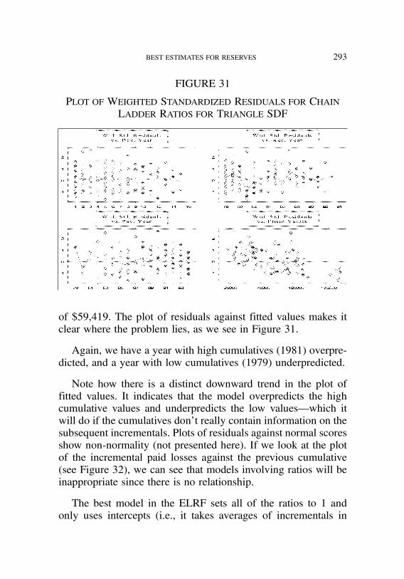
job no. 1969 casualty actuarial society CAS journal 1969D05 [49] 11-08-01 4:58 pm
BEST ESTIMATES FOR RESERVES 293
FIGURE 31
PLOT OF WEIGHTED STANDARDIZED RESIDUALS FOR CHAINLADDER RATIOS FOR TRIANGLE SDF
of $59,419. The plot of residuals against fitted values makes itclear where the problem lies, as we see in Figure 31.
Again, we have a year with high cumulatives (1981) overpre-dicted, and a year with low cumulatives (1979) underpredicted.
Note how there is a distinct downward trend in the plot offitted values. It indicates that the model overpredicts the highcumulative values and underpredicts the low values—which itwill do if the cumulatives don’t really contain information on thesubsequent incrementals. Plots of residuals against normal scoresshow non-normality (not presented here). If we look at the plotof the incremental paid losses against the previous cumulative(see Figure 32), we can see that models involving ratios will beinappropriate since there is no relationship.
The best model in the ELRF sets all of the ratios to 1 andonly uses intercepts (i.e., it takes averages of incrementals in

job no. 1969 casualty actuarial society CAS journal 1969D05 [50] 11-08-01 4:58 pm
294 BEST ESTIMATES FOR RESERVES
FIGURE 32
PLOT OF INCREMENTAL PAYMENTS AGAINST PREVIOUSCUMULATIVE
each development year). But, due to the non-normality, this isinsufficient. At least the ELRF analysis informs us that the in-crementals in a development period may be regarded as ran-dom values from the same distribution, and that these incre-mentals are not correlated with the previous cumulatives (justas the data were generated). It also tells us that the data areskewed, so we need to take a transformation. By way of sum-mary, the ELRF analysis informs us that the data were createdincrementally, accident years are homogeneous, and we shouldbe modeling the logs of the incremental data—it is telling us thetruth.
If you generate (simulate) data using link ratios, the ELRFwill tell you that ratios have predictive power and that the datawere generated cumulatively. Importantly however, for most realloss development arrays, ELRF analysis indicates that the datawere generated incrementally and that ratios have much less pre-dictive power than trends in the log incrementals. The ELRFanalysis also shows when there may be payment/calendar yeartrend changes.

job no. 1969 casualty actuarial society CAS journal 1969D05 [51] 11-08-01 4:58 pm
BEST ESTIMATES FOR RESERVES 295
3.7. Varying (Stochastic) Parameters
In view of the trend relationships between the development-year, accident-year, and payment-year directions, a model withseveral parameters in the payment-year and accident-year di-rections may suffer from multi-collinearity problems. Zehnwirth[12, Section 7.2] discusses the importance of varying (stochas-tic) parameter models, especially the introduction of a varyingalpha parameter (in place of adding parameters), to overcomemulti-collinearity. This is akin to exponential smoothing in theaccident-year direction. This approach is necessary, very pow-erful, and increases the stability of the model, especially if inthe more recent accident years there are some slight changes inlevels. The amount of stochastic variation in ® is determined bythe SSPE statistic, which is explained in Zehnwirth [12].
3.8. Model Identification
It is important to identify a parsimonious model in PTFthat separates the (systematic) trends from the random fluctu-ations, and moreover determines whether the trend in the pay-ment/calendar year direction is stable.
The model identification procedure is discussed in Section 10of Zehnwirth [12]. We start off with a model that only has oneparameter in each direction, model (sequentially) the trends inthe development-year direction, and follow that by looking at thetrends in the payment-year or accident-year directions (depend-ing on which direction exhibits more dramatic trend changes).Adjustments for different variances may also be necessary. Vali-dation analysis is an integral component of model identification,extraction of information, and testing for stability of trends.
3.9. Assumptions About the Future
Stability and assumptions about the future are discussed inSection 9.6.2 and 10.2 of Zehnwirth [12]. If payment/calendar

job no. 1969 casualty actuarial society CAS journal 1969D05 [52] 11-08-01 4:58 pm
296 BEST ESTIMATES FOR RESERVES
year trend has been stable in the more recent years, then theassumption about the future is relatively straightforward. For ex-ample, if the estimate in the last seven years of ¶ is ¶ with stan-dard error s:e:(¶), then we assume for the future a mean trendof ¶, with a standard deviation of trend of s:e:(¶); we do not as-sume the trend in the future is constant. Our model includes thevariability (uncertainty) in trend in the future, in addition to theprocess variability (about the trend).
If on the other hand, payment/calendar year trend has beenunstable, as was illustrated with Project ABC, assumptions aboutthe future will depend on the explanation for the instability—forProject ABC we revert to the 10% trend if the dramatic changeis explained by new legislation. Zehnwirth [12] also cites someother practical examples where special knowledge about the busi-ness is a contributing factor in formulating assumptions about thefuture, especially in the presence of trend instability. Importantly,however, that special knowledge is combined with the informa-tion that is extracted from past experience.
It is not possible to enumerate all feasible cases, though sev-eral cases are discussed in Zehnwirth [12]. The more experi-ence the actuary has with the new statistical paradigm, the betterhe/she is equipped to formulate assumptions about the future inthe presence of unstable trends. Bear in mind, of course, thatquite often trends are stable; but we only know this after per-forming an analysis like that described for the PTF.
3.10. How Do We Know That Real Data Triangles Can BeGenerated By the Members of the PTF?
Let’s conduct the following experiment. Begin with 100 dataarrays (triangles) and, for each triangle, the “best” model in thePTF is given. Recall that a fitted (best) model relates the distri-butions of each cell in terms of trends on the log scale. Thesemodels are tested to ensure they are good models. ELRF analysisis then conducted on each triangle. Now assume that some of thetriangles are real data from some companies, but some are not.
job no. 1969 casualty actuarial society CAS journal 1969D05 [53] 11-08-01 4:58 pm
BEST ESTIMATES FOR RESERVES 297
That is, for some triangles the data represent a sample path fromthe so-called “fitted” distributions. Which are the real data andwhich are simulated data from the model?
Both the real and simulated data display similar features toeach other, whether we analyze them using PTF models or ELRFmodels. For example, both usually indicate that once you fitan intercept (and accident-year trend, if present), ratios are notneeded. Both tend to display trends in the payment years. Sinceyou cannot distinguish between real triangles and simulated tri-angles generated from models in the PTF, these kinds of modelsmust be valid. That is, the rich family of models in PTF possessprobabilistic mechanisms for generating real data.
Of course, the models do not represent the underlying com-plex generation process that is driven by many variables. How-ever, the variables that drive the data are implicitly included inthe trends and the noise (¾2). We do the same thing when we fita loss distribution (e.g., Pareto) to a set of severities. The esti-mated Pareto did not create the severities, but it has probabilisticmechanisms for creating the data as a sample.
Suppose we now simulate (cumulative) loss development ar-rays from ratio models. The ELRF methodology applied to thesimulated arrays will inform us that ratios have predictive power(indeed more predictive power than using the trends in the in-crementals). If we now analyze the corresponding incremen-tal arrays using PTF models, we notice a phenomenon that isvery rarely observed for real data. After removing trends inthe development-year direction, there are distinct patterns in theaccident-year direction—the levels jump up and down dramati-cally, much more so than is typical for real data. This is becauseif an incremental value in development period zero is low, thenthe subsequent incrementals for the same accident period remainrelatively low, as all accident years are multiplied by the sameratios. Similarly, if the initial incremental value is high, the subse-quent incrementals from the model are high. This pattern occurseven when you include considerable randomness.
job no. 1969 casualty actuarial society CAS journal 1969D05 [54] 11-08-01 4:58 pm
298 BEST ESTIMATES FOR RESERVES
Finally, suppose an actuary is presented with many develop-ment arrays, some real, and the others simulated using mod-els based on ratio-techniques. By applying the ELRF and PTFmethodologies, the actuary is very frequently able to distinguishthe real arrays from the ones simulated from the ratio models.
4. THE RESERVE FIGURE
Loss reserves often constitute the largest single item in aninsurer’s balance sheet. An upward or downward 10%movementof loss reserves could change the whole financial picture of thecompany.
4.1. Prediction Intervals
We have argued for the use of probabilistic models, espe-cially in assessing the variability or uncertainty inherent in lossreserves. The probability that the loss reserve carried in the bal-ance sheet will be realized in the future is effectively zero, evenif the loss reserve is the true mean!
Future (incremental) paid losses may be regarded as a sam-ple path from the forecast (estimated) lognormal distributions,which include both process risk and parameter risk. Forecastingof distributions is discussed in Zehnwirth [12].
The forecast distributions are accurate provided the assump-tions made about the future are, and remain, true. For example, ifit is assumed that future payment/calendar year trend (inflation)has a mean of 10% and a standard deviation of 2%, and in twoyears time it turns out that inflation is 20%, then the forecastdistributions are far from accurate.
Accordingly, any prediction interval computed from the fore-cast distributions is conditional on the assumptions about thefuture remaining true. The assumptions are in terms of meantrends, standard deviations of trends, and distributions about thetrends.

job no. 1969 casualty actuarial society CAS journal 1969D05 [55] 11-08-01 4:58 pm
BEST ESTIMATES FOR RESERVES 299
It is important to note that there is a difference between afitted distribution and the corresponding predictive distribution.A predictive distribution necessarily incorporates parameter es-timation error (parameter risk); a fitted distribution does not. Ig-noring parameter risk can result in substantial underestimationof reserves and premiums (see the paper by Dickson, Tedescoand Zehnwirth [4] for more details).
Under the model, the distribution of a sum of payments (e.g.,accident-year outstanding payments) is the distribution of a sumof correlated lognormal variables. The lognormal variables arecorrelated because of the correlations between the estimated pa-rameters describing their mean level—indeed many forecasts willeven share some parameters. The distribution of the sum can beobtained by generating (simulating) samples from the estimatedmultivariate lognormal distributions. The same could be done forpayment-year totals (important for obtaining the distributions ofthe future payment stream) or for the overall total. This infor-mation is relevant to Dynamic Financial Analysis. Distributionsfor future underwriting years can also be computed—this infor-mation is useful for pricing, including aggregate deductibles andexcess layers.
An insurer’s risk can be defined in many different ways. Onecommon definition is related to the standard deviation of the risk,in particular a multiple of the standard deviation. If the reserveis based on a given percentile of the distribution of the totaloutstanding, the size of the loading as a multiple of the standarddeviation will be dependent on the skewness of the distribution.
If an insurer writes more than one long-tail line and aims fora 100 (1"®)% security level on all the lines combined, then therisk margin per line decreases the more lines the company writes,no matter which allocation principle is used. This is always true,even if there is some dependence (and so correlation) between thevarious lines. In the following example, the standard deviationprinciple is used.
job no. 1969 casualty actuarial society CAS journal 1969D05 [56] 11-08-01 4:58 pm
300 BEST ESTIMATES FOR RESERVES
Consider a company that writes n independent long-tail lines.Suppose that the standard error of loss reserve L(j) of line j iss:e:(j) (i.e., s:e:(j) is the standard error of the loss reserve variableL(j)). The standard error for the combined lines L(1)+ # # #+L(n)is
s:e:(Total) = [s:e:2(1)+ # # #+ s:e:2(n)]0:5: (4.1)
If the risk margin for all lines combined is k& s:e:(Total), where kis determined by the level of security required, then an allocationof the risk margin for line j is
k& s:e:(Total)& s:e:(j)=[s:e:(1)+ # # #+ s:e:(n)]< k& s:e:(j):(4.2)
The last inequality is true even when s:e:(Total) is not given bythe expression above.
If as a result of analyzing each line using the statistical mod-eling framework, we find that, for some lines, trends change inthe same years and the changes are of similar size, then the linesare not independent. (There may also be correlations between theresiduals, but that is generally only important when forecastingsums of lines.)
In that situation, if line i and j are correlated, say, then onecould use s:e:(i)+ s:e:(j) as the upper bound of the standard errorof L(i) +L(j). (Based on our experience, it is not often the casethat different lines are much correlated in terms of trends.)
Suppose we assume for the future payment/calendar years amean trend of ¶ with a standard deviation (standard error) s:e:(¶).Specifically, we are saying that the trend ¶, a random variable,has a normal distribution with mean ¶ and standard deviations:e:(¶). Recognition of the relationship between the lognormaland normal distributions tells us that the mean payment increasesas s:e:(¶) increases (and ¶ remains constant). The greater theuncertainty in a parameter (the mean remaining constant), themore money is paid out. The same argument applies to the otherestimated parameters in the model. This is known as Jensen’s
job no. 1969 casualty actuarial society CAS journal 1969D05 [57] 11-08-01 4:58 pm
BEST ESTIMATES FOR RESERVES 301
inequality (this concept is in many college finance texts—see forexample Brearley & Myers [1]). It is dangerous to ignore thisconcept.
4.2. Risk-Based Capital
There are a number of misconceptions regarding risk-basedcapital. It is important to note the following:
! The uncertainty in loss reserves (for the future) should bebased on a probabilistic model (for the future) that may bearno relationship to reserves carried by the company in thepast.
! The uncertainty for each line for each company should bebased on a probabilistic model, derived from the company’sexperience, that describes the particular line for that company.A model appropriate for one loss development array will usu-ally not be appropriate for another.
! The company’s experience may bear very little relationship tothe industry as a whole.
The approach discussed here allows the actuary to determinethe relationships within and between companies’ experiencesand their relationships to the industry in terms of simple, well-understood features of the data.
In establishing the loss reserve, recognition is often given tothe time value of money by discounting. The absence of dis-counting implies that the (median) estimate contains an implicitrisk margin. But this implicit margin may bear no relationship tothe security margin sought. The risk should be computed beforediscounting (at a zero rate of return).
4.3. Booking of the Reserve
There are no hard and fast rules here, but three very importantsteps are critical.
job no. 1969 casualty actuarial society CAS journal 1969D05 [58] 11-08-01 4:58 pm
302 BEST ESTIMATES FOR RESERVES
Step 1
Extract information, in terms of trends, stability of trends, anddistributions about trends, for the loss development array; in par-ticular, the incremental paid losses. Information is extracted byidentifying the best model in the PTF. Model identification andextraction of information necessarily involves validation analy-sis (re-analyzing and forecasting the array after removal of pastrecent payment/calendar years).
Step 2
Assumptions about the future are formulated. If payment/cal-endar year trend is stable, this is straightforward. If trends areunstable in more recent years, then an attempt is made to de-termine the cause by analyzing other data types and using anyrelevant business knowledge. A number of examples are givenin Zehnwirth [12], but it is impossible to give an exhaustive listas each case may be different.
Step 3
Using the distributions of reserves, the security margin soughton combined lines, and the risk capital available to the company,a percentile can be selected. Incidentally, the more uncertain thetrends are for the future, the higher the security margin that maybe called for.
4.4. Other Benefits of the Statistical Paradigm
Finally, the statistical modeling framework has other benefits,including:
! Credibility modelsIf a particular trend parameter estimate for an individual
company is not fully credible, it can be formally shrunk to-wards an industry estimate.
! Segmentation and layers

job no. 1969 casualty actuarial society CAS journal 1969D05 [59] 11-08-01 4:58 pm
BEST ESTIMATES FOR RESERVES 303
Very often the statistical model identified for a combinedarray of all payment types applies to some of the segments(by the same model, we mean the same parameter structure,not that the estimates are identical). Indeed, the variance ofthe normal distribution for a segment is larger than for thewhole—on the original scale, the coefficient of variation islarger for the components. These ideas can also be applied toterritories, etc., and to layers.
job no. 1969 casualty actuarial society CAS journal 1969D05 [60] 11-08-01 4:58 pm
304 BEST ESTIMATES FOR RESERVES
REFERENCES
[1] Brearly, Richard A. and Stewart C. Myers, Principles ofCorporate Finance, New York, NY: McGraw Hill Inc.,1991.
[2] Brosius, Eric, “Loss Development Using Credibility,” Ca-sualty Actuarial Society Part 7 Exam Study Kit, 1992.
[3] Cook, R. Dennis and Sanford Weisberg, Residuals and In-fluence in Regression, New York, NY: Chapman and Hall,1982.
[4] Dickson, David, Leanna Tedesco and Ben Zehnwirth, “Pre-dictive Aggregate Claims Distributions,” Journal of Riskand Insurance 65, 1998, pp. 689–709.
[5] Halliwell, Leigh, “Loss Prediction by Generalized LeastSquares,” PCAS LXXXIII, 1996, pp. 436–489.
[6] Mack, Thomas, “Distribution-Free Calculation of the Stan-dard Error of Chain Ladder Reserve Estimates,” ASTINBulletin, 23, 2, 1993, pp. 213–225.
[7] Mack, Thomas, “Which Stochastic Model is Underlying theChain Ladder Method?” Insurance Mathematics and Eco-nomics, 15, 2/3, 1994, pp. 133–138.
[8] Murphy, Daniel M., “Unbiased Loss Development Factors,”PCAS LXXXI, 144–155, 1994, pp. 154–222.
[9] Reinsurance Association of America, Historical Loss De-velopment Study, 1991 Edition, Washington, D.C.: R.A.A.,1991.
[10] Shapiro, Samuel S. and R. S. Francia, “Approximate Analy-sis of Variance Test for Normality,” Journal of the AmericanStatistical Association 67, 1972, pp. 215–216.
[11] Venter, Gary G., “Testing the Assumptions of Age-to-AgeFactors,” PCAS LXXXV, 1998, pp. 807–847.
[12] Zehnwirth, Ben, “Probabilistic Development Factor Mod-els with Applications to Loss Reserve Variability, Predic-tion Intervals and Risk Based Capital,” Casualty ActuarialSociety Forum, Spring 1994, 2, pp. 447–605.

job no. 1969 casualty actuarial society CAS journal 1969D05 [61] 11-08-01 4:58 pm
BEST ESTIMATES FOR RESERVES 305
APPENDIX A
WEIGHTED LEAST SQUARES ESTIMATES WITHOUT INTERCEPT
In this appendix, we give a brief outline of the simplest caseof the derivation of weighted least squares estimates. This cor-responds to the no-intercept models at the start of Section 2—including the standard chain ladder.
Consider the following model:
y(i) = bx(i)+ "(i), with (A.1a)
"(i)(Normal(0,¾2=w(i)): (A.1b)
The value w(i) is called the weight of observation i. Note thatweights are inversely proportional to variances. Estimation of theparameters via maximum likelihood corresponds to minimizingthe weighted sums of squared residuals:
n"i=1
w(i)(y(i)" bx(i))2: (A.2)
We find the minimum using calculus in a straightforwardmanner: taking derivatives with respect to b, and setting the resultequal to zero, we get
n"i=1
"2x(i)w(i)(y(i)" bx(i)) = 0; (A.3)
then solving for b we obtain:
b =n"i=1
w(i)x(i)y(i)
(n"i=1
w(i)x(i)2: (A.4)
When w(i) = x(i)"±, we obtain the estimates given near thestart of Section 2; specifically, with ± = 1 we obtain Equation2.2; and, with ± = 2, we obtain Equation 2.3.

job no. 1969 casualty actuarial society CAS journal 1969D05 [62] 11-08-01 4:58 pm
306 BEST ESTIMATES FOR RESERVES
APPENDIX B
CALCULATIONS FOR LINK RATIO MODELS WITH INTERCEPTSAND ACCIDENT-YEAR TRENDS
Let there be n accident years, numbering the most recent ac-cident year as 0, and the first as n"1, as in Murphy [8]. Let yijbe the cumulative amount paid in accident year i, developmentyear j, i= 0, : : : ,n"1, j = 0, : : : ,n"1, as in Figure 33. This sim-plifies many of the formulas. Let xij = yi,j"1, so that yij=xij is theobserved development factor from j"1 to j in accident year i.The only difference a more complex array shape (such as
missing early payment years, or with late development years cut-off) will make is to change the limits on summations.
Now let pij = ®j +¸jzij +(¯j " 1)xij + uij , where pij is the in-cremental paid loss in accident year i at development year j, xijis the cumulative paid in accident year i, up to development yearj"1, and zij is the count of accident years from the top, start-ing from 0. Since we number from the bottom, in the current
FIGURE 33
TRIANGULAR LOSS DEVELOPMENT ARRAY OF SIZE n, WITHACCIDENT YEARS LABELED IN REVERSE ORDER
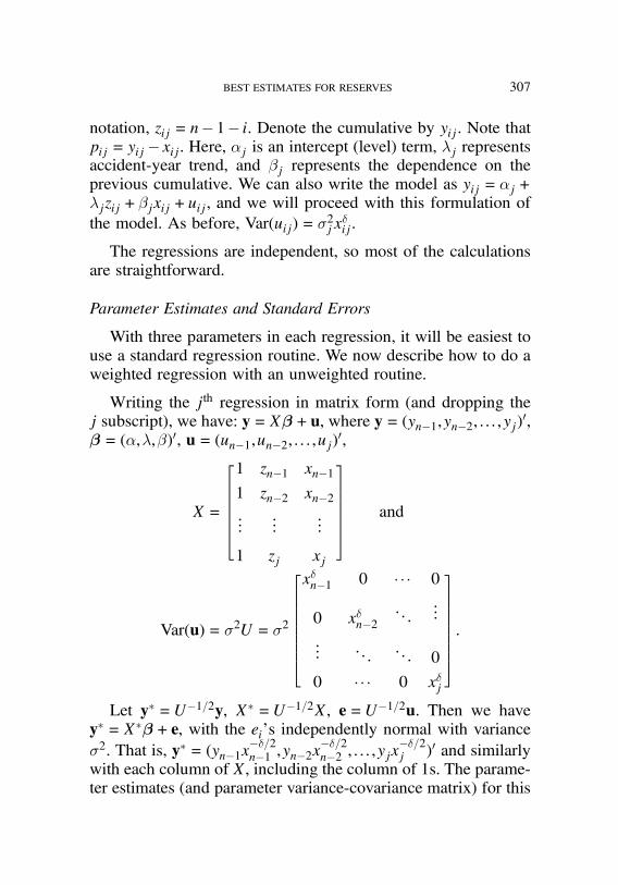
job no. 1969 casualty actuarial society CAS journal 1969D05 [63] 11-08-01 4:58 pm
BEST ESTIMATES FOR RESERVES 307
notation, zij = n"1" i. Denote the cumulative by yij . Note thatpij = yij " xij. Here, ®j is an intercept (level) term, ¸j representsaccident-year trend, and ¯j represents the dependence on theprevious cumulative. We can also write the model as yij = ®j +¸jzij +¯jxij +uij , and we will proceed with this formulation ofthe model. As before, Var(uij) = ¾
2j x±ij .
The regressions are independent, so most of the calculationsare straightforward.
Parameter Estimates and Standard Errors
With three parameters in each regression, it will be easiest touse a standard regression routine. We now describe how to do aweighted regression with an unweighted routine.
Writing the jth regression in matrix form (and dropping thej subscript), we have: y= X¯+u, where y= (yn"1,yn"2, : : : ,yj)),¯ = (®,¸,¯)), u= (un"1,un"2, : : : ,uj)),
X =
#)))))$1 zn"1 xn"11 zn"2 xn"2...
......
1 zj xj
%*****& and
Var(u) = ¾2U = ¾2
#)))))))$
x±n"1 0 # # # 0
0 x±n"2. . .
...
... . . . . . . 0
0 # # # 0 x±j
%*******&:
Let y* =U"1=2y, X* =U"1=2X, e=U"1=2u. Then we havey* = X*¯+ e, with the ei’s independently normal with variance¾2. That is, y* = (yn"1x
"±=2n"1 ,yn"2x
"±=2n"2 , : : : ,yjx
"±=2j )) and similarly
with each column of X, including the column of 1s. The parame-ter estimates (and parameter variance-covariance matrix) for this

job no. 1969 casualty actuarial society CAS journal 1969D05 [64] 11-08-01 4:58 pm
308 BEST ESTIMATES FOR RESERVES
new (unweighted) regression are the same as that of the oldregression; standard regression results give ˆ = (X*)X*)"1X*)y*(see, for example, Cook and Weisberg [3]).
Consequently, we will simply take ®, ˆ , ˆ and their estimatedvariances and covariances as being available. Note that in the fi-nal development years it isn’t possible to fit all three parameters;usually we would choose to fit ® and/or ¯ as appropriate.
Residuals
Note that the residuals, uij , are the same whether we con-sider incremental or cumulative values: uij = yij " yij = pij "pij . We now derive the variance of the residuals. Let H* =X*(X*)X*)"1X*). Note that y* = X* ˆ = X*(X*)X*)"1X*)y* =H*y*. Then Var(e) = Var(y* " y*) = Var((I"H*)y*) = (I"H*)#Var(y*)(I"H*)) = ¾2(I"H*)2. Note that H*2 =H*. HenceVar(e) = ¾2(I"H*). This is a standard regression result (see,for example, Cook and Weisberg [3]). Consequently Var(u) =U1=2Var(e)(U1=2)), from which we can find the variance ofan individual observation. Consider the regression for devel-opment year j, and suppress that subscript. Then Var(ei) =¾2[1" (x*i ))(X*)X*)"1x*i ], where x*i is the ith row of X*. ThereforeVar(ui) = ¾
2[1" (x*i ))(X*)X*)"1x*i ]x±i .
Forecasts and Standard Errors
Note that all forecasts and standard error calculations givenhere are conditional on the observed data.
! Forecasts: Clearly yi,i+k= ®i+k+ ˆ i+kzi,i+k+ ˆ i+kyi,i+k"1, whereyii = yii.
! Standard Errors:Var(yi,i+k " yi,i+k) = Var(yi,i+k "¹i,i+k+¹i,i+k " yi,i+k)
= Var(yi,i+k "¹i,i+k)+Var(yi,i+k "¹i,i+k)= vpi,i+k+ v
ei,i+k: (B.1)
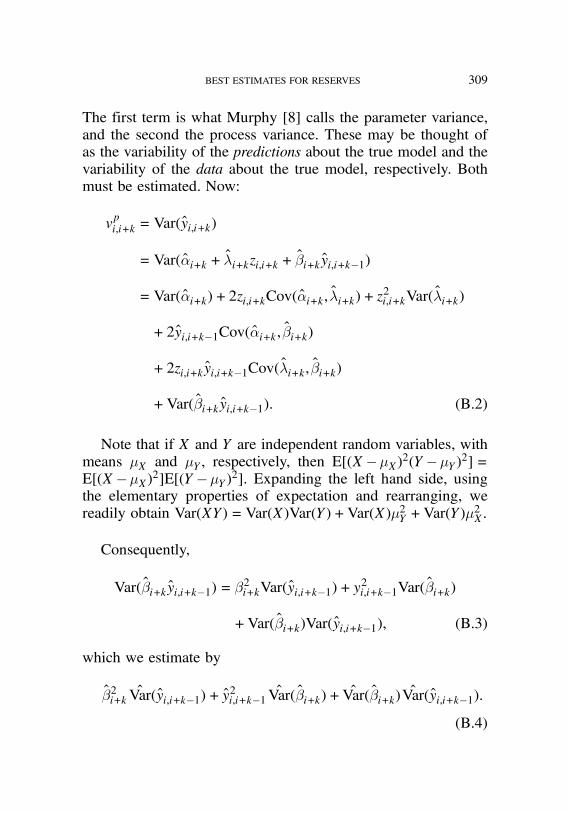
job no. 1969 casualty actuarial society CAS journal 1969D05 [65] 11-08-01 4:58 pm
BEST ESTIMATES FOR RESERVES 309
The first term is what Murphy [8] calls the parameter variance,and the second the process variance. These may be thought ofas the variability of the predictions about the true model and thevariability of the data about the true model, respectively. Bothmust be estimated. Now:
vpi,i+k =Var(yi,i+k)
= Var(®i+k+ˆi+kzi,i+k+
ˆi+kyi,i+k"1)
= Var(®i+k)+2zi,i+kCov(®i+k,ˆi+k)+ z
2i,i+kVar(
ˆi+k)
+ 2yi,i+k"1Cov(®i+k, ˆ i+k)
+ 2zi,i+kyi,i+k"1Cov( ˆ i+k, ˆ i+k)
+Var( ˆ i+kyi,i+k"1): (B.2)
Note that if X and Y are independent random variables, withmeans ¹X and ¹Y, respectively, then E[(X "¹X)2(Y"¹Y)2] =E[(X "¹X)2]E[(Y"¹Y)2]. Expanding the left hand side, usingthe elementary properties of expectation and rearranging, wereadily obtain Var(XY) = Var(X)Var(Y)+Var(X)¹2Y+Var(Y)¹
2X .
Consequently,
Var( ˆ i+kyi,i+k"1) = ¯2i+kVar(yi,i+k"1)+ y
2i,i+k"1Var( ˆ i+k)
+Var( ˆ i+k)Var(yi,i+k"1), (B.3)
which we estimate by
ˆ 2i+k Var(yi,i+k"1) + y
2i,i+k"1 Var( ˆ i+k)+ Var( ˆ i+k) Var(yi,i+k"1):
(B.4)

job no. 1969 casualty actuarial society CAS journal 1969D05 [66] 11-08-01 4:58 pm
310 BEST ESTIMATES FOR RESERVES
Hence we estimate
vpi,i+k = Var(®i+k)+2zi,i+kˆCov(®i+k,
ˆi+k)+ z
2i,i+k Var(
ˆi+k)
+ 2yi,i+k"1 ˆCov(®i+k,ˆi+k)+2zi,i+kyi,i+k"1 ˆCov( ˆ i+k,
ˆi+k)
+ y2i,i+k"1 Var( ˆ i+k) + [ ˆ2i+k +Var( ˆ i+k)]v
pi,i+k"1: (B.5)
Note that vpii is zero, since we are conditioning on the data. Fur-ther,
vei,i+k =Var(yi,i+k"¹i,i+k)= Var(®i+k +¸i+kzi,i+k"1 +¯i+kyi,i+k"1 +ui,i+k)
= ¯2i+kVar(yi,i+k"1)+Var(ui,i+k)
= ¯2i+kVar(yi,i+k"1"¹i,i+k"1)+¾2i+kx±i,i+k= ¯2i+kv
ei,i+k"1 +¾
2i+kx
±i,i+k, (B.6)
which we estimate as:
vei,i+k = Var(yi,i+k)
= ˆ 2i+k Var(yi,i+k"1)+ ¾2i+kE(y
±i,i+k"1)
= ˆ 2i+kvei,i+k"1 + ¾
2i+kf
±i,i+k"1, (B.7)
where f±i,j =E(y±i,j). We have
f±ij =
+,,,-,,,.1, ± = 0
yij , ± = 1
y2ij +Var(yij), ± = 2
, (B.8)
just as with Murphy [8]. With the normality assumption we canobtain estimates at other values of ±, but we omit details here.

job no. 1969 casualty actuarial society CAS journal 1969D05 [67] 11-08-01 4:58 pm
BEST ESTIMATES FOR RESERVES 311
Forecasts and standard errors on the incrementals can be ob-tained in similar fashion.
Forecasts and Standard Errors of Development-Year Totals
LetDj be the unknown future development-year total forecast,so
Dj =j"1"i=0
yij, (B.9)
and
Dj =j"1"i=0
yij: (B.10)
Note that
Var(Dj "Dj) = Var/0j"1"i=0
yij " yij12
=Var
/0j"1"i=0
yij "¹ij12+Var
/0j"1"i=0
yij "¹ij12
= Vpj +Vej : (B.11)
Taking Zj =!j"1i=0 zij , then
Vpj =Var
/0j"1"i=0
yij
12
=Var
/0j"1"i=0
®j + ˆ jzij + ˆj yi,j"1
12=Var(nj®j +Zj ˆ j + ˆj[Dj"1 + yj"1,j"1])
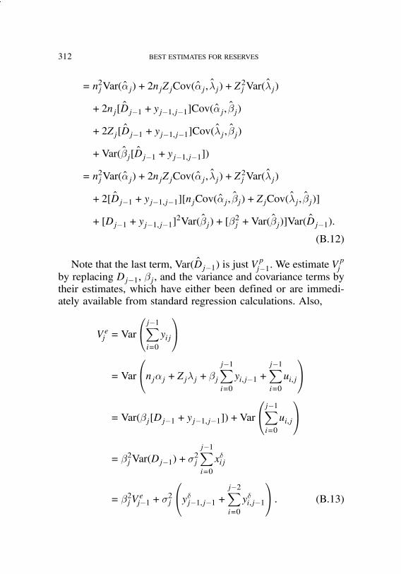
job no. 1969 casualty actuarial society CAS journal 1969D05 [68] 11-08-01 4:58 pm
312 BEST ESTIMATES FOR RESERVES
= n2jVar(®j)+ 2njZjCov(®j , ˆ j)+Z2jVar( ˆ j)
+2nj[Dj"1 + yj"1,j"1]Cov(®j, ˆ j)
+2Zj[Dj"1 + yj"1,j"1]Cov( ˆ j , ˆj)
+Var( ˆj[Dj"1 + yj"1,j"1])
= n2jVar(®j)+ 2njZjCov(®j , ˆ j)+Z2jVar( ˆ j)
+2[Dj"1 + yj"1,j"1][njCov(®j, ˆj)+ZjCov( ˆ j , ˆj)]
+ [Dj"1 + yj"1,j"1]2Var( ˆj)+ [¯
2j +Var(
ˆj)]Var(Dj"1):
(B.12)
Note that the last term, Var(Dj"1) is just Vpj"1. We estimate V
pj
by replacing Dj"1, ¯j , and the variance and covariance terms bytheir estimates, which have either been defined or are immedi-ately available from standard regression calculations. Also,
Vej =Var
/0j"1"i=0
yij
12
=Var
/0nj®j +Zj¸j +¯j j"1"i=0
yi,j"1 +j"1"i=0
ui,j
12
=Var(¯j[Dj"1 + yj"1,j"1])+Var
/0j"1"i=0
ui,j
12= ¯2jVar(Dj"1) +¾
2j
j"1"i=0
x±ij
= ¯2j Vej"1 +¾
2j
/0y±j"1,j"1 + j"2"i=0
y±i,j"1
12 : (B.13)

job no. 1969 casualty actuarial society CAS journal 1969D05 [69] 11-08-01 4:58 pm
BEST ESTIMATES FOR RESERVES 313
Due to independence across accident years, E(!j"2i=0 y
±i,j"1) =!j"2
i=0 E(y±i,j"1) =
!j"2i=0 f
±i,j"1, so the process variance term is esti-
mated by Vej =ˆ 2j V
ej"1 + ¾
2j (y
±j"1,j"1 +
!j"2i=0 f
±i,j"1). The estimated
standard error of Dj is then'Vpj + V
ej .
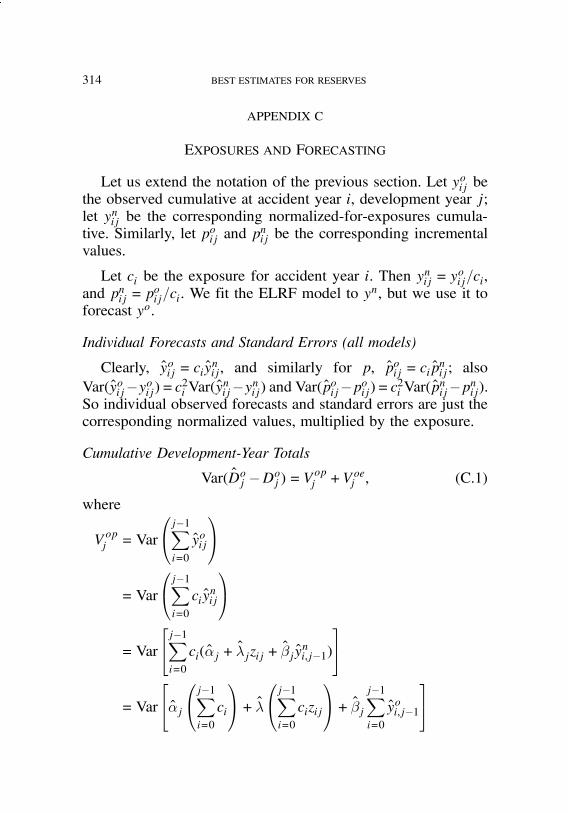
job no. 1969 casualty actuarial society CAS journal 1969D05 [70] 11-08-01 4:58 pm
314 BEST ESTIMATES FOR RESERVES
APPENDIX C
EXPOSURES AND FORECASTING
Let us extend the notation of the previous section. Let yoij bethe observed cumulative at accident year i, development year j;let ynij be the corresponding normalized-for-exposures cumula-tive. Similarly, let poij and p
nij be the corresponding incremental
values.
Let ci be the exposure for accident year i. Then ynij = y
oij=ci,
and pnij = poij=ci. We fit the ELRF model to y
n, but we use it toforecast yo.
Individual Forecasts and Standard Errors (all models)
Clearly, yoij = ciynij, and similarly for p, poij = cip
nij ; also
Var(yoij"yoij)=c2i Var(ynij"ynij) and Var(poij"poij)=c2i Var(pnij"pnij).So individual observed forecasts and standard errors are just thecorresponding normalized values, multiplied by the exposure.
Cumulative Development-Year Totals
Var(Doj "Doj ) = Vopj +Voej , (C.1)
where
Vopj =Var
/0j"1"i=0
yoij
12=Var
/0j"1"i=0
ciynij
12=Var
#$j"1"i=0
ci(®j +ˆjzij +
ˆjyni,j"1)
%&=Var
#$®j/0j"1"i=0
ci
12+ ˆ/0j"1"i=0
cizij
12+ ˆj j"1"i=0
yoi,j"1
%&
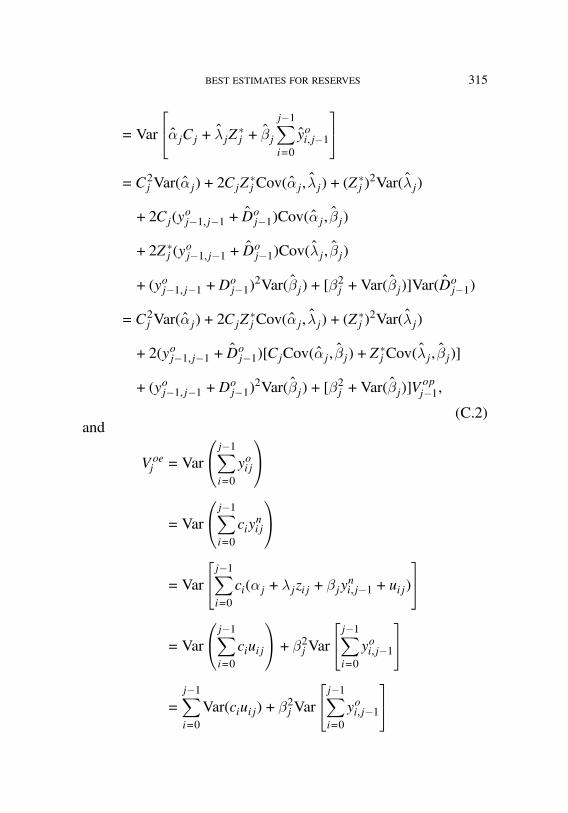
job no. 1969 casualty actuarial society CAS journal 1969D05 [71] 11-08-01 4:58 pm
BEST ESTIMATES FOR RESERVES 315
= Var
#$®jCj + ˆ jZ*j + ˆj j"1"i=0
yoi,j"1
%&= C2j Var(®j)+ 2CjZ
*jCov(®j, ˆ j)+ (Z
*j )2Var( ˆ j)
+2Cj(yoj"1,j"1 + D
oj"1)Cov(®j , ˆj)
+2Z*j (yoj"1,j"1 + D
oj"1)Cov( ˆ j , ˆj)
+ (yoj"1,j"1 +Doj"1)
2Var( ˆj)+ [¯2j +Var(
ˆj)]Var(D
oj"1)
= C2j Var(®j)+ 2CjZ*jCov(®j,
ˆj)+ (Z
*j )2Var( ˆ j)
+2(yoj"1,j"1 + Doj"1)[CjCov(®j , ˆj)+Z
*jCov( ˆ j , ˆj)]
+ (yoj"1,j"1 +Doj"1)
2Var( ˆj)+ [¯2j +Var(
ˆj)]V
opj"1,
(C.2)and
Voej =Var
/0j"1"i=0
yoij
12
=Var
/0j"1"i=0
ciynij
12
=Var
#$j"1"i=0
ci(®j +¸jzij +¯jyni,j"1 + uij)
%&
=Var
/0j"1"i=0
ciuij
12+¯2jVar#$j"1"i=0
yoi,j"1
%&
=j"1"i=0
Var(ciuij) +¯2jVar
#$j"1"i=0
yoi,j"1
%&

job no. 1969 casualty actuarial society CAS journal 1969D05 [72] 11-08-01 4:58 pm
316 BEST ESTIMATES FOR RESERVES
= ¾2j c2j"1(y
nj"1,j"1)
±+j"2"i=0
c2i vnei,j"1 +¯
2j V
oej"1
= ¾2j c2"±j"1(y
oj"1,j"1)
± +j"2"i=0
voei,j"1 +¯2j V
oej"1, (C.3)
where again we estimate this variance by replacing the D’s, ¯’s,variances and covariances by their estimates.

job no. 1969 casualty actuarial society CAS journal 1969D05 [73] 11-08-01 4:58 pm
BEST ESTIMATES FOR RESERVES 317
APPENDIX D
LIKELIHOOD AND CONDITIONAL REGRESSIONS
Let y(j) be the vector of data in development year j, andµ(j) be all the parameters for that development year. Let y=(y(0)), : : : ,y(n"1)))), so the development years are stacked oneon top of the other, and µ = (µ(1)), : : : ,µ(n"1)))). Then, straight-forward application of conditional probability and some simpli-fication gives us:
L(µ $ y)+ p[y $ µ]+ p[y(n"1) $ µ(n"1),y(n"2),y(n" 3), : : : ,y(0)]#p[y(n" 2) $ µ(n" 2),y(n"3),y(n"4), : : : ,y(0)]...
#p[y(1) $ µ(1),y(0)]#p[y(0)]
+ p[y(n"1) $ µ(n"1),y(n"2)]#p[y(n" 2) $ µ(n" 2),y(n"3)]# # # #p[y(1) $ µ(1),y(0)] #p[y(0)]: (D.1)
Since, for each regression, we are conditioning on the datafrom previous development years, the fact that the previous de-velopment data is stochastic and not fixed is not an issue—theconditional likelihoods still correspond to ordinary regressions.
The likelihood for y(0) doesn’t contain any of the parameters.At any value for µ, then, the likelihood of y(0) is just a constant;consequently, it cannot affect the location of the maximum of thelikelihood, nor its curvature there. So the way that the forecastsdepend on the parameters isn’t affected by y(0), apart from theway it enters the regression for y(1).

job no. 1969 casualty actuarial society CAS journal 1969D05 [74] 11-08-01 4:58 pm
318 BEST ESTIMATES FOR RESERVES
The model for the data says that the values in future devel-opment years depend on the earlier development years. We’veobserved the whole of y(0), so we know exactly how it willimpact the future runoff, because the model describes that. Ofcourse, the model may be wrong (and we argue that it is); but,given the model, the regressions may all be performed as ordi-nary regressions.
The forecasts are made conditionally on the data. We’ve ar-gued above that even the stochastic nature of y(0) can be ignoredin the forecasting because the model fully describes its impacton the future observations. However, this is not an importantpoint—if an argument were made that the stochastic nature ofy(0) should somehow affect the forecasts, it would not affect anyof our arguments about the unsuitability of these models.
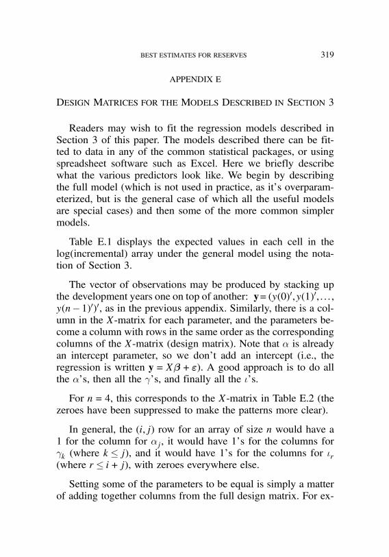
job no. 1969 casualty actuarial society CAS journal 1969D05 [75] 11-08-01 4:58 pm
BEST ESTIMATES FOR RESERVES 319
APPENDIX E
DESIGN MATRICES FOR THE MODELS DESCRIBED IN SECTION 3
Readers may wish to fit the regression models described inSection 3 of this paper. The models described there can be fit-ted to data in any of the common statistical packages, or usingspreadsheet software such as Excel. Here we briefly describewhat the various predictors look like. We begin by describingthe full model (which is not used in practice, as it’s overparam-eterized, but is the general case of which all the useful modelsare special cases) and then some of the more common simplermodels.
Table E.1 displays the expected values in each cell in thelog(incremental) array under the general model using the nota-tion of Section 3.
The vector of observations may be produced by stacking upthe development years one on top of another: y=(y(0)),y(1)), : : : ,y(n"1)))), as in the previous appendix. Similarly, there is a col-umn in the X-matrix for each parameter, and the parameters be-come a column with rows in the same order as the correspondingcolumns of the X-matrix (design matrix). Note that ® is alreadyan intercept parameter, so we don’t add an intercept (i.e., theregression is written y= X¯+"). A good approach is to do allthe ®’s, then all the °’s, and finally all the ¶’s.
For n= 4, this corresponds to the X-matrix in Table E.2 (thezeroes have been suppressed to make the patterns more clear).
In general, the (i,j) row for an array of size n would have a1 for the column for ®j , it would have 1’s for the columns for°k (where k , j), and it would have 1’s for the columns for ¶r(where r , i+ j), with zeroes everywhere else.Setting some of the parameters to be equal is simply a matter
of adding together columns from the full design matrix. For ex-

job no. 1969 casualty actuarial society CAS journal 1969D05 [76] 11-08-01 4:58 pm
320 BEST ESTIMATES FOR RESERVES
TABLE E.1
Expected Values of Log(Incremental) Under theGeneral Model
TABLE E.2
Design Matrix (X-Matrix) for the Full Model for aTriangle With 4 Years’ Data
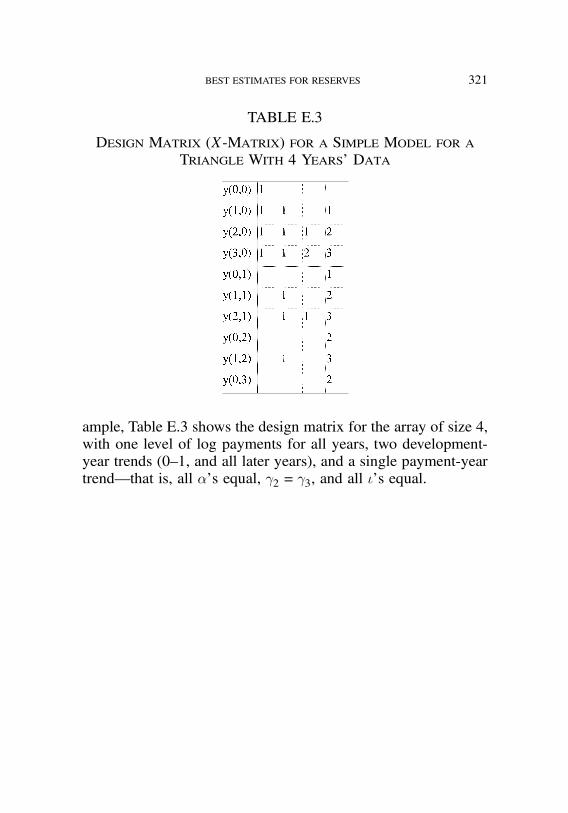
job no. 1969 casualty actuarial society CAS journal 1969D05 [77] 11-08-01 4:58 pm
BEST ESTIMATES FOR RESERVES 321
TABLE E.3
Design Matrix (X-Matrix) for a Simple Model for aTriangle With 4 Years’ Data
ample, Table E.3 shows the design matrix for the array of size 4,with one level of log payments for all years, two development-year trends (0–1, and all later years), and a single payment-yeartrend—that is, all ®’s equal, °2 = °3, and all ¶’s equal.

job no. 1969 casualty actuarial society CAS journal 1969D04 [1] 11-08-01 4:58 pm
APPLICATIONS OF RESAMPLING METHODS INACTUARIAL PRACTICE
RICHARD A. DERRIG, KRZYSZTOF M. OSTASZEWSKI,AND GRZEGORZ A. REMPALA
Abstract
Actuarial analysis can be viewed as the process ofstudying profitability and solvency of an insurance firmunder a realistic and integrated model of key input ran-dom variables such as loss frequency and severity, ex-penses, reinsurance, interest and inflation rates, and as-set defaults. Traditional models of input variables havegenerally fitted parameters for a predetermined familyof probability distributions. In this paper we discuss ap-plications of some modern methods of non-parametricstatistics to modeling loss distributions, and possibili-ties of using them for modeling other input variablesfor the purpose of arriving at an integrated companymodel. Several examples of inference about the sever-ity of loss, loss distributions percentiles and other re-lated quantities based on data smoothing, bootstrap es-timates of standard error and bootstrap confidence in-tervals are presented. The examples are based on real-life auto injury claim data and the accuracy of ourmethods is compared with that of standard techniques.Model adjustment for inflation and bootstrap techniquesbased on the Kaplan–Meier estimator, useful in the pres-ence of policies limits (censored losses), are also con-sidered.
ACKNOWLEDGEMENT
The last two authors graciously acknowledge support from theActuarial Education and Research Fund.
322
job no. 1969 casualty actuarial society CAS journal 1969D04 [2] 11-08-01 4:58 pm
APPLICATIONS OF RESAMPLING METHODS IN ACTUARIAL PRACTICE 323
1. INTRODUCTION
In modern analysis of the financial models of property-casualty companies the input variables can be typically classi-fied into financial variables and underwriting variables (e.g., seeD’Arcy, Gorvett, Herbers and Hettinger [6]). The financial vari-ables generally refer to asset-side generated cash flows of thebusiness, and the underwriting variables relate to the cash flowsof the liabilities side. The process of developing any actuarialmodel begins with the creation of probability distributions ofthese input variables, including the establishment of the properrange of values of input parameters. The use of parameters isgenerally determined by the use of parametric families of distri-butions. Fitting of those parameters is generally followed eitherby Monte Carlo simulation together with integration of all in-puts for profit testing and optimization, or by the study of theeffect of varying the parameters on output variables in sensitiv-ity analysis and basic cash flow testing. Thus traditional actuar-ial methodologies are rooted in parametric approaches, which fitprescribed distributions of losses and other random phenomenastudied (e.g., interest rate or other asset return variables) to thedata. The experience of the last two decades has shown greaterinterdependence of basic loss variables (severity, frequency, ex-posures) with asset variables (interest rates, asset defaults, etc.),and sensitivity of the firm to all input variables. Increased com-plexity has been accompanied by increased competitive pres-sures, and more frequent insolvencies. In our opinion, in orderto properly address these issues one must carefully address theweaknesses of traditional methodologies. These weaknesses canbe summarized as originating from either ignoring the uncertain-ties of inputs, or mismanaging those uncertainties. While earlyproblems of actuarial modeling could be attributed mostly to ig-noring uncertainty, we believe at this point the uncertain nature ofmodel inputs is generally acknowledged. Note that Derrig andOstaszewski [9] used fuzzy set techniques to handle the mix-ture of probabilistic and non-probabilistic uncertainties in asset/

job no. 1969 casualty actuarial society CAS journal 1969D04 [3] 11-08-01 4:58 pm
324 APPLICATIONS OF RESAMPLING METHODS IN ACTUARIAL PRACTICE
liability considerations for property-casualty claims. In our opin-ion it is now time to proceed to deeper issues concerning theactual forms of uncertainty. The Central Limit Theorem and itsstochastic process counterpart provide clear guidance for practi-cal uses of the normal distribution and all distributions derivedfrom it. But one cannot justify similarly fitting convenient dis-tributions to, for instance, loss data and expect to easily survivethe next significant change in the marketplace. What does workin practice, but not in theory, may be merely an illusion of ap-plicability provided by powerful tools of modern technology. Ifone cannot provide a justification for the use of a parametric dis-tribution, then a nonparametric alternative should be studied, atleast for the purpose of understanding the firm’s exposures. Inthis work, we will show such a study of nonparametric method-ologies applied to loss data, and will advocate the developmentof an integrated company model with the use of nonparametricapproaches.
1.1. Loss Distributions
We begin by addressing the most basic questions concerningloss distributions. The first two parameters generally fitted to thedata are average claim size and the number of claim occurrencesper unit of exposure. Can we improve upon these estimates byusing nonparametric methods?
Consider the problem of estimating the severity of a claim,which is, in its most general setting, equivalent to modeling theprobability distribution of a single claim size. Traditionally, thishas been done by means of fitting some parametric models froma particular continuous family of distributions (e.g., see Daykin,Pentikainen, and Pesonen [7, Chapter 3]). While this standardapproach has several obvious advantages, we should also realizethat occasionally it may suffer some serious drawbacks:
! Some loss data has a tendency to cluster about round num-bers like $1,000, $10,000, etc., due to rounding off the claim

job no. 1969 casualty actuarial society CAS journal 1969D04 [4] 11-08-01 4:58 pm
APPLICATIONS OF RESAMPLING METHODS IN ACTUARIAL PRACTICE 325
amount and thus in practice follows a mixture of continuousand discrete distributions. Usually, parametric models simplyignore the discrete component in such cases.
! The data is often truncated from below or censored from abovedue to deductibles and/or limits on different policies. In par-ticular, the presence of censoring, if not accounted for, mayseriously compromise the goodness-of-fit of a fitted paramet-ric distribution. On the other hand, trying to incorporate thecensoring mechanism (which is often random in its nature,especially when we consider losses falling under several in-surance policies with different limits) often leads to a cre-ation of a very complex model which is difficult to workwith.
! The loss data may come from a mixture of distributions de-pending upon some known or unknown classification of claimtypes.
! Finally, it may happen that the data simply does not fit any ofthe available distributions in a satisfactory way.
It seems, therefore, that there are many situations of practicalimportance where the traditional approach cannot be utilized, andone must look beyond parametric models. In this work we pointout an alternative, nonparametric approach to modeling lossesand other random parameters of financial analysis, originatingfrom the modern methodology of nonparametric statistics basedon the bootstrap or resampling method.
To keep things in focus we will be concerned here only withapplications to modeling the severity of loss, but the methodsdiscussed may be easily applied to other problems such as lossfrequencies, asset returns, asset defaults, and the combinationof variables into models of Risk Based Capital, Value at Risk,and general Dynamic Financial Analysis (DFA), including CashFlow Testing and Asset Adequacy Analysis.

job no. 1969 casualty actuarial society CAS journal 1969D04 [5] 11-08-01 4:58 pm
326 APPLICATIONS OF RESAMPLING METHODS IN ACTUARIAL PRACTICE
1.2. The Concept of Bootstrap
The concept of bootstrap was first introduced in the semi-nal piece of Efron [10], and relies on the consideration of thediscrete empirical distribution generated by a random sample ofsize n from an unknown distribution F. This empirical distribu-tion assigns equal probability to each sample item. In the dis-cussion which follows, we will write !Fn for that distribution. Bygenerating an independent, identically distributed (IID) randomsequence (resample) from the distribution !Fn or its appropriatelysmoothed version, we can arrive at new estimates of various pa-rameters and nonparametric characteristics of the original distri-bution F. This idea is at the very root of the bootstrap methodol-ogy. In particular, Efron [10] points out that the bootstrap givesa reasonable estimate of standard error for any estimator, and itcan be extended to statistical error assessments and to inferencesbeyond biases and standard errors.
1.3. Overview of the Article
In this paper, we apply bootstrap methods to two data setsas illustrations of the advantages of resampling techniques, es-pecially when dealing with empirical loss data. The basics ofbootstrap theory are covered in Section 2, where we show itsapplications in estimating standard errors and calculating con-fidence intervals. In Section 3, we compare bootstrap and tra-ditional estimators for quantiles and excess losses using sometruncated wind loss data. The important concept of smoothingthe bootstrap estimator is also covered in that section. Applica-tions of bootstrap to auto bodily injury liability claims in Section4 show loss elimination ratio estimates together with their stan-dard errors in a case of lumpy and clustered data (the data setis enclosed in Appendix B). More complicated designs that in-corporate data censoring and adjustment for inflation appear inSection 5. Sections 6 and 7 provide some final remarks and con-clusions. The Mathematica 3.0 programs used to perform boot-strap calculations are provided in Appendix A.

job no. 1969 casualty actuarial society CAS journal 1969D04 [6] 11-08-01 4:58 pm
APPLICATIONS OF RESAMPLING METHODS IN ACTUARIAL PRACTICE 327
2. BOOTSTRAP STANDARD ERRORS AND CONFIDENCEINTERVALS
As we have already mentioned in the previous section, thecentral idea of bootstrap lies in sampling the empirical cumula-tive distribution function (CDF) !Fn. This idea is closely relatedto the following, well-known statistical principle, henceforth re-ferred to as the “plug-in” principle. Given a parameter of interestµ(F) depending upon an unknown population CDF F, we esti-mate this parameter by µ = µ(!Fn). That is, we simply replace F inthe formula for µ by its empirical counterpart !Fn obtained fromthe observed data. The plug-in principle will not provide goodresults if !Fn poorly approximates F, or if there is informationabout F other than that provided by the sample. For instance,in some cases we might know (or be willing to assume) that Fbelongs to some parametric family of distributions. However, theplug-in principle and the bootstrap may be adapted to this lattersituation as well. To illustrate the idea, let us consider a paramet-ric family of CDF’s "F¹# indexed by a parameter ¹ (possibly avector), and for some given ¹0, let !¹0 denote its estimate calcu-lated from the sample. The plug-in principle in this case statesthat we should estimate µ(F¹0 ) by µ(F!¹0 ). In this case, bootstrap isoften called parametric, since a resample is now collected fromF!¹0 . Here and elsewhere in this work, we refer to any replicaof µ calculated from a resample as “a bootstrap estimate of µ(F)”and denote it by µ$.
2.1. The Bootstrap Methodology
Bickel and Freedman [2] formulated conditions for con-sistency of bootstrap, which resulted in further extensions ofEfron’s [10] methodology to a broad range of standard applica-tions, including quantile processes, multiple regression and strat-ified sampling. They also argued that the use of bootstrap did notrequire theoretical derivations such as function derivatives, influ-ence functions, asymptotic variances, the Edgeworth expansion,etc.

job no. 1969 casualty actuarial society CAS journal 1969D04 [7] 11-08-01 4:58 pm
328 APPLICATIONS OF RESAMPLING METHODS IN ACTUARIAL PRACTICE
Singh [19] made a further point that the bootstrap estimator ofthe sampling distribution of a given statistic may be more accu-rate than the traditional normal approximation. In fact, it turns outthat for many commonly used statistics the bootstrap is asymptot-ically equivalent to the one-term Edgeworth expansion estimator,usually having the same convergence rate, which is faster than thenormal approximation. In many more recent statistical texts thebootstrap is recommended for estimating sampling distributionsand finding standard errors and confidence sets. The extensionof the bootstrap method to the case of dependent data was con-sidered for instance by Kunsch [15], who suggested a movingblock bootstrap procedure which takes into account the depen-dence structure of the data by resampling blocks of adjacentobservations rather than individual data points. More recently,Politis and Romano [16] suggested a method based on circularblocks (i.e., on wrapping the observed time series values aroundthe circle and then generating the blocks of the bootstrap datafrom the circle’s “arcs”). In the case of the sample mean thismethod, which is known as circular bootstrap, again was shownto accomplish the Edgeworth correction for dependent, station-ary data.
The bootstrap methods can be applied to both parametric andnon-parametric models, although most of the published researchin the area is concerned with the non-parametric case since thatis where the most immediate practical gains might be expected.Let us note though that a simple, non-parametric bootstrap mayoften be improved by other bootstrap methods taking into ac-count the special nature of the model. In the IID non-parametricmodels, for instance, the smoothed bootstrap (bootstrap based onsome smoothed version of !Fn) often improves the simple boot-strap (bootstrap based solely on !Fn). Since in recent years sev-eral excellent books on the subject of resampling and relatedtechniques have become available, we will not be particularlyconcerned here with providing all the details of the presentedtechniques, contenting ourselves with making appropriate ref-
job no. 1969 casualty actuarial society CAS journal 1969D04 [8] 11-08-01 4:58 pm
APPLICATIONS OF RESAMPLING METHODS IN ACTUARIAL PRACTICE 329
erences to more technically detailed works. Readers interestedin gaining some basic background in resampling are referredto Efron and Tibisharani [11]. For a more mathematically ad-vanced treatment of the subject, we recommend Shao and Tu[17].
2.2. Bootstrap Standard Error Estimate
Arguably, one of the most important applications of bootstrapis to provide an estimate of the standard error of µ (seF(µ)). Itis rarely practical to calculate it exactly; instead, one usuallyapproximates seF(µ) with the help of multiple resamples. Theapproximation to the bootstrap estimate of standard error of µ(or BESE) suggested by Efron [10] is given by
!seB ="
B#b=1
[µ$(b)% µ$(&)]2=(B%1)$1=2
, (2.1)
where µ$(&) =%Bb=1 µ
$(b)=B, B is the total number of resamples(each of size n) collected with replacement from the plug-in es-timate of F (in the parametric or non-parametric setting), andµ$(b) is the original statistic µ calculated from the bth resample(b = 1, : : : ,B). By the law of large numbers
limB'(
!seB =BESE(µ),and, for sufficiently large n, we expect
BESE(µ)) seF(µ):Let us note that B, the total number of resamples, may be as largeas we wish since we are in complete control of the resamplingprocess. It has been shown that for estimating the standard error,one should take B to be about 250, whereas for different resam-pled statistics this number may have to be significantly increasedin order to reach the desired accuracy (see [11]).
job no. 1969 casualty actuarial society CAS journal 1969D04 [9] 11-08-01 4:58 pm
330 APPLICATIONS OF RESAMPLING METHODS IN ACTUARIAL PRACTICE
2.3. The Method of Percentiles
Let us now turn to the problem of using the bootstrap method-ology to construct confidence intervals. This area has been a ma-jor focus of theoretical work on the bootstrap, and several differ-ent methods of approaching the problem have been suggested.The “naive” procedure described below is not the most efficientone and can be significantly improved in both rate of conver-gence and accuracy. It is, however, intuitively obvious and easyto justify, and seems to be working well enough for the casesconsidered here. For a complete review of available approachesto bootstrap confidence intervals, see [11].
Let us consider µ$, a bootstrap estimate of µ based on a re-sample of size n from the original sample X1, : : : ,Xn, and let G$be its distribution function given the observed sample values
G$(x) = P"µ$ * x + X1 = x1, : : : ,Xn = xn#:Recall that for any distribution function F and p , (0,1) we de-fine the pth quantile of F (sometimes also called pth percentile)as F%1(p) = inf"x : F(x)- p#. The bootstrap percentiles methodgives G%1$ (®) and G%1$ (1%®) as, respectively, lower and upperbounds for the (1%2®) confidence interval for µ. Let us note thatfor most statistics µ, the distribution function of the bootstrap es-timator µ$ is not available. In practice,G%1$ (®) andG%1$ (1%®) areapproximated by taking multiple resamples and then calculatingthe empirical percentiles. In this case the number of resamples Bis usually much larger than for estimating BESE; in most casesB - 1000 is recommended.
3. BOOTSTRAP AND SMOOTHED BOOTSTRAP ESTIMATORS VSTRADITIONAL METHODS
In making the case for the usefulness of bootstrap methodol-ogy in modeling loss distributions, we would first like to compareits performance with that of the standard methods of inferenceas presented in actuarial textbooks.

job no. 1969 casualty actuarial society CAS journal 1969D04 [10] 11-08-01 4:58 pm
APPLICATIONS OF RESAMPLING METHODS IN ACTUARIAL PRACTICE 331
3.1. Application to Wind Losses: Quantiles
Let us consider the following set of 40 losses due to wind-related catastrophes that occurred in 1977. These data are takenfrom Hogg and Klugman [12], where they are discussed in de-tail in Chapter 3. The losses were recorded only to the nearest$1,000,000 and data included only those losses of $2,000,000or more. For convenience they have been ordered and recordedbelow.
2, 2, 2, 2, 2, 2, 2, 2, 2, 22, 2, 3, 3, 3, 3, 4, 4, 4, 55, 5, 5, 6, 6, 6, 6, 8, 8, 915, 17, 22, 23, 24, 24, 25, 27, 32, 43
Using this data set we shall give two examples illustratingthe advantages of applying the bootstrap approach to modelinglosses. The problem at hand is a typical one: assuming that allthe losses recorded above have come from a single unknowndistribution F, we would like to use the data to obtain somegood approximation for F and its various parameters.
First, let us look at an important problem of finding the ap-proximate confidence intervals for the quantiles of F. The stan-dard approach to this problem relies on the normal approxi-mation to the sample quantiles (order statistics). Applying thismethod, Hogg and Klugman [12] have found the approximate95% confidence interval for the 0.85th quantile of F to be be-tween X30 and X39, which for the wind data translates into theobserved interval (9,32). They also have noted that “this is awide interval but without additional assumptions this is the bestwe can do.” Is that really true? To answer this question let usfirst note that in this particular case the highly skewed binomialdistribution of the 0.85th sample quantile is approximated by asymmetric normal curve. Thus, it seems reasonable to expect thatnormal approximation could be improved here upon introducingsome form of correction for skewness. In the standard normal
job no. 1969 casualty actuarial society CAS journal 1969D04 [11] 11-08-01 4:58 pm
332 APPLICATIONS OF RESAMPLING METHODS IN ACTUARIAL PRACTICE
approximation theory this is usually accomplished by consider-ing, in addition to the normal term, the first non-normal term inthe asymptotic Edgeworth expansion of the binomial distribution.The resulting formula is messy and requires the calculation of asample skewness coefficient, as well as some refined form of thecontinuity correction (e.g., see Singh [19]). On the other hand,the bootstrap has been known to make such a correction auto-matically (Singh [19]) and hence we could expect that a boot-strap approximation would perform better here.1 Indeed, in thiscase (in the notation of Section 2) we have µ(F) = F%1(0:85) andµ = !F%1n (0:85)) X(34), the 34th order statistic, which for the winddata equals 23. For sample quantiles the bootstrap distribution G$can be calculated exactly (Shao and Tu [17, p.10]) or approxi-mated by an empirical distribution obtained from B resamples asdescribed in Section 2. Using either method, the (1%2®) confi-dence interval calculated using the percentile method is found tobe between X(28) and X(38) (which is also in this case the exactconfidence interval obtained by using binomial tables). For thewind data this translates into the interval (8,27), which is con-siderably shorter than the one obtained by Hogg and Klugman[12].
3.2. The Smoothed Bootstrap and its Application to ExcessWind Losses
As our second example, let us consider the estimation of theprobability that a wind loss will exceed a $29,500,000 threshold.In our notation that means that we wish to estimate the unknownparameter (1%F(29:5)). A direct application of the plug-in prin-ciple gives the value 0.05, the nonparametric estimate based onrelative frequencies. However, note that the same number is alsoan estimate for (1%F(29)) and (1%F(31:5)), since the relative
1This turns out to be true only for a moderate sample size (here, 40); for a binomialdistribution with large n (i.e., large sample size) the effect of the bootstrap correctionis negligible. In general, the bootstrap approximation performs better than the normalapproximation for large sample sizes only for continuous distributions.
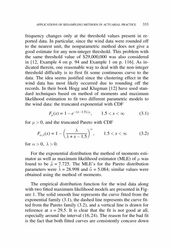
job no. 1969 casualty actuarial society CAS journal 1969D04 [12] 11-08-01 4:58 pm
APPLICATIONS OF RESAMPLING METHODS IN ACTUARIAL PRACTICE 333
frequency changes only at the threshold values present in re-ported data. In particular, since the wind data were rounded offto the nearest unit, the nonparametric method does not give agood estimate for any non-integer threshold. This problem withthe same threshold value of $29,000,000 was also consideredin [12, Example 4 on p. 94 and Example 1 on p. 116]. As in-dicated therein, one reasonable way to deal with the non-integerthreshold difficulty is to first fit some continuous curve to thedata. The idea seems justified since the clustering effect in thewind data has most likely occurred due to rounding off therecords. In their book Hogg and Klugman [12] have used stan-dard techniques based on method of moments and maximumlikelihood estimation to fit two different parametric models tothe wind data: the truncated exponential with CDF
F¹(x) = 1% e%(x%1:5)=¹, 1:5< x <( (3.1)
for ¹ > 0, and the truncated Pareto with CDF
F®,¸(x) = 1%&
¸
¸+ x%1:5'®, 1:5< x <( (3.2)
for ® > 0, ¸ > 0.
For the exponential distribution the method of moments esti-mator as well as maximum likelihood estimator (MLE) of ¹ wasfound to be ¹= 7:725. The MLE’s for the Pareto distributionparameters were ˆ = 28:998 and ®= 5:084; similar values wereobtained using the method of moments.
The empirical distribution function for the wind data alongwith two fitted maximum likelihood models are presented in Fig-ure 1. The solid smooth line represents the curve fitted from theexponential family (3.1), the dashed line represents the curve fit-ted from the Pareto family (3.2), and a vertical line is drawn forreference at x= 29:5. It is clear that the fit is not good at all,especially around the interval (16,24). The reason for the bad fitis the fact that both fitted curves are consistently concave down

job no. 1969 casualty actuarial society CAS journal 1969D04 [13] 11-08-01 4:58 pm
334 APPLICATIONS OF RESAMPLING METHODS IN ACTUARIAL PRACTICE
FIGURE 1
EMPIRICAL AND FITTED CDF’S FOR WIND LOSS DATA
for all the x’s and F seems to be concave up in this area.2 Thefit in the tail seems to be much better.
Once we determine the values of the unknown model param-eters, MLE estimators for (1%F(29:5)) may be obtained from(3.1) and (3.2). The numerical values of these estimates, theirrespective variances and their 95% confidence intervals are sum-marized in the second and third row of Table 1. All the confi-dence intervals and variances for the first three estimates shownin the table are calculated using the normal theory approxima-tion. The variance and confidence intervals for the fourth esti-mate based on the moving-average smoother are calculated by
2In practice, this drawback could be possibly remedied by fitting a mixture of the distri-butions shown in (3.1) and (3.2). However, this approach could considerably complicatethe parametric model and seems unlikely to provide much improvement in the tail fit,which is of primary interest here.
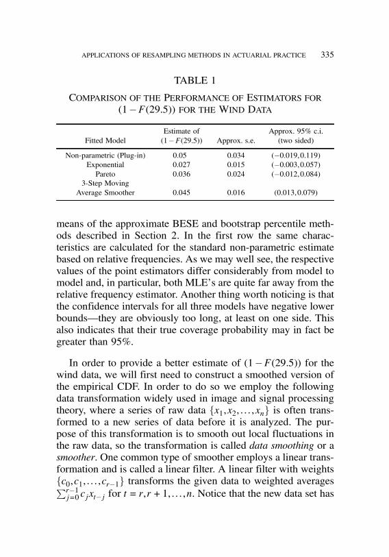
job no. 1969 casualty actuarial society CAS journal 1969D04 [14] 11-08-01 4:58 pm
APPLICATIONS OF RESAMPLING METHODS IN ACTUARIAL PRACTICE 335
TABLE 1
COMPARISON OF THE PERFORMANCE OF ESTIMATORS FOR(1%F(29:5)) FOR THE WIND DATA
Estimate of Approx. 95% c.i.Fitted Model (1%F(29:5)) Approx. s.e. (two sided)
Non-parametric (Plug-in) 0.05 0.034 (%0:019,0:119)Exponential 0.027 0.015 (%0:003,0:057)Pareto 0.036 0.024 (%0:012,0:084)
3-Step MovingAverage Smoother 0.045 0.016 (0:013,0:079)
means of the approximate BESE and bootstrap percentile meth-ods described in Section 2. In the first row the same charac-teristics are calculated for the standard non-parametric estimatebased on relative frequencies. As we may well see, the respectivevalues of the point estimators differ considerably from model tomodel and, in particular, both MLE’s are quite far away from therelative frequency estimator. Another thing worth noticing is thatthe confidence intervals for all three models have negative lowerbounds—they are obviously too long, at least on one side. Thisalso indicates that their true coverage probability may in fact begreater than 95%.
In order to provide a better estimate of (1%F(29:5)) for thewind data, we will first need to construct a smoothed version ofthe empirical CDF. In order to do so we employ the followingdata transformation widely used in image and signal processingtheory, where a series of raw data "x1,x2, : : : ,xn# is often trans-formed to a new series of data before it is analyzed. The pur-pose of this transformation is to smooth out local fluctuations inthe raw data, so the transformation is called data smoothing or asmoother. One common type of smoother employs a linear trans-formation and is called a linear filter. A linear filter with weights"c0,c1, : : : ,cr%1# transforms the given data to weighted averages%r%1j=0 cjxt%j for t= r,r+1, : : : ,n. Notice that the new data set has
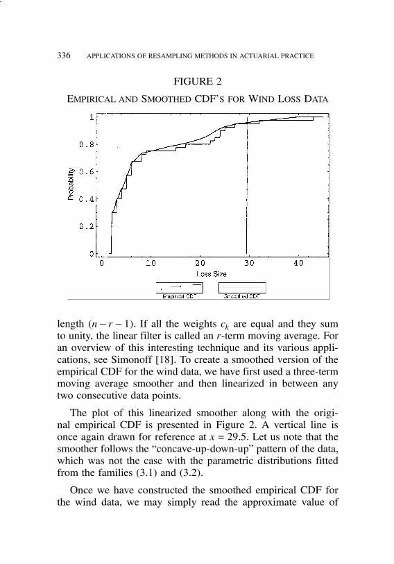
job no. 1969 casualty actuarial society CAS journal 1969D04 [15] 11-08-01 4:58 pm
336 APPLICATIONS OF RESAMPLING METHODS IN ACTUARIAL PRACTICE
FIGURE 2
EMPIRICAL AND SMOOTHED CDF’S FOR WIND LOSS DATA
length (n% r%1). If all the weights ck are equal and they sumto unity, the linear filter is called an r-term moving average. Foran overview of this interesting technique and its various appli-cations, see Simonoff [18]. To create a smoothed version of theempirical CDF for the wind data, we have first used a three-termmoving average smoother and then linearized in between anytwo consecutive data points.
The plot of this linearized smoother along with the origi-nal empirical CDF is presented in Figure 2. A vertical line isonce again drawn for reference at x= 29:5. Let us note that thesmoother follows the “concave-up-down-up” pattern of the data,which was not the case with the parametric distributions fittedfrom the families (3.1) and (3.2).
Once we have constructed the smoothed empirical CDF forthe wind data, we may simply read the approximate value of

job no. 1969 casualty actuarial society CAS journal 1969D04 [16] 11-08-01 4:58 pm
APPLICATIONS OF RESAMPLING METHODS IN ACTUARIAL PRACTICE 337
(1%F(29:5)) off the graph (or better yet, ask the computer todo it for us). The resulting numerical value is 0.045. What is thestandard error for that estimate? We again may use the bootstrapto answer that question without messy calculations. An approx-imate value for BESE (with B = 1000, but the result is virtuallythe same for B = 100) is found to be 0.016, which is only slightlyworse than that of the exponential model MLE and much bet-ter than the standard error for the Pareto and empirical models.Equivalently, the same result may be obtained by numerical in-tegration. Finally, the 95% confidence interval for (1%F(29:5))is found by means of the bootstrap percentile method with thenumber of replications set at B = 1000. Here the superiority ofthe bootstrap is obvious, as it gives an interval which is the sec-ond shortest (again exponential MLE model gives a shorter in-terval) but, most importantly, is bounded away from zero. Theresults are summarized in Table 1. Let us note that the resultbased on a smoothed empirical CDF and bootstrap dramaticallyimproves that based on the relative frequency (plug-in) estimatorand standard normal theory. It is perhaps of interest to note alsothat the MLE estimator of (1%F(29:5)) in the exponential modelis simply a parametric bootstrap estimator. For more detailson the connection between MLE estimators and bootstrap, see[11].
4. CLUSTERED DATA
In the previous section we have assumed that the wind datawere distributed according to some continuous CDF F. Clearlythis is not always the case with loss data, and in general we mayexpect our theoretical loss distribution to follow some mixtureof discrete and continuous CDF’s.
4.1. Massachusetts Auto Bodily Injury Liability Data
In Appendix B we present the set of 432 closed losses due tobodily injuries in car accidents, under bodily injury liability (BI)policies reported in the Boston Territory (19) for calendar year
job no. 1969 casualty actuarial society CAS journal 1969D04 [17] 11-08-01 4:58 pm
338 APPLICATIONS OF RESAMPLING METHODS IN ACTUARIAL PRACTICE
1995 (as of mid-1997). The losses are recorded in thousands andare subject to various policy limits but have no deductible. Pol-icy limits capped 16 out of 432 losses which are therefore con-sidered right-censored. The problem of bootstrapping censoreddata will be discussed in the next section; here we would liketo concentrate on another interesting feature of the data. Mas-sachusetts BI claim data are of interest because the underlyingbehavioral processes have been analyzed extensively. Weisbergand Derrig [20] and Derrig, Weisberg and Chen [8] describethe Massachusetts claiming environment after a tort reform asa “lottery” with general damages for non-economic loss (painand suffering) as the prize. Cummins and Tennyson [5] showedsigns of similar patterns countrywide, while Carroll, Abrahamseand Vaiana [3] and the Insurance Research Council [13] docu-mented the pervasiveness of the lottery claims in both tort andno-fault state injury claim payment systems. The overwhelmingpresence of suspected fraud and buildup claims3 allow for dis-torted relationships between the underlying economic loss andthe liability settlement. Claim negotiators can greatly reduce the“usual” non-economic damages when exaggerated injury and/orexcessive treatment are claimed as legitimate losses. Claim pay-ments in such a negotiated process with discretionary injuriestend to be clustered at some usual mutually-acceptable amounts,especially for the run-of-the-mill strain and sprain claims. Con-ners and Feldblum [4] suggest that the claim environment, ratherthan the usual rating variables, are the key elements needed tounderstand and estimate relationships in injury claim data. Allthe data characteristics above tend to favor empirical methodsover analytical ones.
Looking at the frequencies of occurrences of the particularvalues of losses in Massachusetts BI claim data, we may see thatseveral numerical values have especially high frequency. The loss
3In auto insurance, fraudulent claims are those in which there was no injury or the injurywas unrelated to the accident, whereas buildup claims are those in which the injury isexaggerated and/or the treatment is excessive.
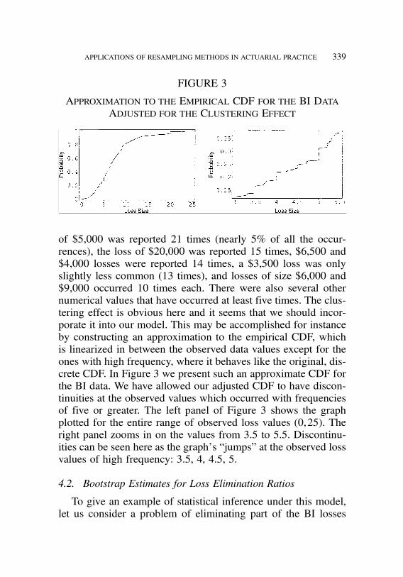
job no. 1969 casualty actuarial society CAS journal 1969D04 [18] 11-08-01 4:58 pm
APPLICATIONS OF RESAMPLING METHODS IN ACTUARIAL PRACTICE 339
FIGURE 3
APPROXIMATION TO THE EMPIRICAL CDF FOR THE BI DATAADJUSTED FOR THE CLUSTERING EFFECT
of $5,000 was reported 21 times (nearly 5% of all the occur-rences), the loss of $20,000 was reported 15 times, $6,500 and$4,000 losses were reported 14 times, a $3,500 loss was onlyslightly less common (13 times), and losses of size $6,000 and$9,000 occurred 10 times each. There were also several othernumerical values that have occurred at least five times. The clus-tering effect is obvious here and it seems that we should incor-porate it into our model. This may be accomplished for instanceby constructing an approximation to the empirical CDF, whichis linearized in between the observed data values except for theones with high frequency, where it behaves like the original, dis-crete CDF. In Figure 3 we present such an approximate CDF forthe BI data. We have allowed our adjusted CDF to have discon-tinuities at the observed values which occurred with frequenciesof five or greater. The left panel of Figure 3 shows the graphplotted for the entire range of observed loss values (0,25). Theright panel zooms in on the values from 3.5 to 5.5. Discontinu-ities can be seen here as the graph’s “jumps” at the observed lossvalues of high frequency: 3.5, 4, 4.5, 5.
4.2. Bootstrap Estimates for Loss Elimination Ratios
To give an example of statistical inference under this model,let us consider a problem of eliminating part of the BI losses
job no. 1969 casualty actuarial society CAS journal 1969D04 [19] 11-08-01 4:58 pm
340 APPLICATIONS OF RESAMPLING METHODS IN ACTUARIAL PRACTICE
by purchasing a reinsurance policy that would cap the losses atsome level d. Since the BI data is censored at $20,000, we wouldconsider here only values of d not exceeding $20,000. One of themost important problems for the insurance company consideringpurchasing reinsurance is an accurate prediction of whether sucha purchase would indeed reduce the experienced severity of lossand if so, by what amount. Typically this type of analysis is doneby considering the loss elimination ratio (LER) defined as
LER(d) =EF(X,d)EFX
, (4.1)
where EFX and EF(X,d) are, respectively, expected value andlimited expected value functions for a random variable X fol-lowing a true distribution of loss F. Since LER is only a theo-retical quantity unobservable in practice, its estimate calculatedfrom the data is needed. Usually, one considers the empirical losselimination ratio (ELER) given by the obvious plug-in estimate
ELER(d) =E!Fn(X,d)E!FnX =
n#i=1
min(Xi,d)
n#i=1
Xi
, (4.2)
where X1, : : : ,Xn is a sample.
The drawback of ELER is in the fact that (unlike LER) itchanges only at the values of d equal to the observed valuesof X1, : : : ,Xn. It seems, therefore, that in order to calculate anapproximate LER at different values of d, some smoothed ver-sion of ELER (SELER) should be considered. SELER may beobtained from Equation 4.2 by replacing the empirical CDF !Fnwith its smoothed version, obtained for instance by applying alinear smoother (as for the wind data considered in Section 3) ora cluster-adjusted linearization. Obviously, the SELER formulamay become quite complicated and its explicit derivation may betedious (as would be the derivation of its standard error). Again,the bootstrap methodology can be applied here to facilitate the

job no. 1969 casualty actuarial society CAS journal 1969D04 [20] 11-08-01 4:58 pm
APPLICATIONS OF RESAMPLING METHODS IN ACTUARIAL PRACTICE 341
FIGURE 4
APPROXIMATE GRAPH OF SELER(d)
computation of an approximate value of SELER(d), its standarderror and confidence interval for any given value of d. In Fig-ure 4 we present the graph of the SELER estimate for the BIdata calculated for the values of d ranging from 0 to 20 (lowestcensoring point) by means of a bootstrap approximation. Thisapproximation was obtained by resampling the cluster-adjusted,linearized version of the empirical CDF (presented in the leftpanel of Figure 3) a large number of times (B = 300) and repli-cating µ = SELER each time. The resulting sequence of boot-strap estimates µ$(b) for b = 1, : : : ,B was then averaged to givethe desired approximation of SELER. The calculation of stan-dard errors and confidence intervals for SELER was done bymeans of BESE and the method of percentiles, as described inSection 2. The standard errors and 95% confidence intervals ofSELER for several different values of d are presented in Ta-ble 2. The approximate BESE and bootstrap percentile methods

job no. 1969 casualty actuarial society CAS journal 1969D04 [21] 11-08-01 4:58 pm
342 APPLICATIONS OF RESAMPLING METHODS IN ACTUARIAL PRACTICE
TABLE 2
VALUES OF SELER(d)
Standard 95% Confidence Intervald SELER(d) Error (two-sided)
4 0.505 0.0185 (0:488,0:544)5 0.607 0.0210 (0:597,0:626)
10.5 0.892 0.0188 (0:888,0:911)11.5 0.913 0.0173 (0:912,0:917)14 0.947 0.0127 (0:933,0:953)18.5 0.985 0.00556 (0:98,0:988)
described in Section 2 were used to calculate the standard errorsand confidence intervals for the BI data in Table 2.
5. EXTENSIONS TO MORE COMPLICATED DESIGNS
So far in our account we have not considered any problemsrelated to the fact that often in practice we may have to deal withtruncated (e.g., due to deductible) or censored (e.g., due to policylimit) data. Another frequently encountered difficulty is the needfor inflation adjustment, especially with data observed over along period of time. We will address these important issues now.
5.1. Bootstrapping Censored Data for Policy Limits andDeductibles
Let us consider again the BI data presented in Section 4. Therewere 432 losses reported, of which 16 were at the policy lim-its.4 These 16 losses may therefore be considered censored fromabove (or right-censored), and the appropriate adjustment for thisfact should be made in our approach to estimating the loss dis-tribution F. Whereas 16 is less then 4% of the total number ofobserved losses for the BI data, these censored observations arecrucial in order to obtain a good estimate of F for the large lossvalues.
4Fifteen losses were truncated at $20,000 and one loss was truncated at $25,000.
job no. 1969 casualty actuarial society CAS journal 1969D04 [22] 11-08-01 4:58 pm
APPLICATIONS OF RESAMPLING METHODS IN ACTUARIAL PRACTICE 343
Since the problem of censored data arises naturally in manymedical, engineering, and other settings, it has received consid-erable attention in statistical literature. For the sake of brevitywe will limit ourselves to the discussion of only one of the sev-eral commonly used techniques, the so-called Kaplan–Meier (orproduct-limit) estimator.
The typical statistical model for right-censored observationsreplaces the usual observed sample X1, : : : ,Xn with the set ofordered pairs (X1,±1), : : : , (Xn,±n), where
±i =
"0 if Xi is censored,
1 if Xi is not censored
and the recorded losses are ordered X1 = x1 * X2 = x2 * && & *Xn = xn (with the usual convention that in the case of ties theuncensored values xi (±i = 1) precede the censored ones (±i = 0)).The Kaplan–Meier estimator of 1%F(x) is given by
!S(x) = (i :xi*x
&n% i
n% i+1'±i: (5.1)
The product in the above formula is that of i terms, where i isthe smallest positive integer less than or equal to n (the num-ber of reported losses) and such that xi * x. The Kaplan–Meierestimator, like the empirical CDF, is a step function with jumpsat those values xi that are uncensored. In fact, if ±i = 1 for all i,i= 1, : : : ,n (i.e., no censoring occurs), it is easy to see that Equa-tion 5.1 reduces to the complement of the usual empirical CDF.If the highest observed loss xn is censored, Equation 5.1 is notdefined for the values of x greater then xn. The usual practice isto then add one uncensored data point (loss value) xn+1 such thatxn < xn+1, and to define !S(x) = 0 for x- xn+1. For instance, forthe BI data the largest reported loss was censored at 25 and wehad to add one artificial “loss” at 26 to define the Kaplan–Meiercurve for the losses exceeding 25. The number 26 was pickedquite arbitrarily; in actuarial practice a more precise guess of

job no. 1969 casualty actuarial society CAS journal 1969D04 [23] 11-08-01 4:58 pm
344 APPLICATIONS OF RESAMPLING METHODS IN ACTUARIAL PRACTICE
FIGURE 5
THE KAPLAN–MEIER ESTIMATOR
the maximum possible value of loss (e.g., based on past expe-rience) should be easily available. The Kaplan–Meier estimatorenjoys several optimal statistical properties and can be viewedas a generalization of the usual empirical CDF adjusted for thecase of censored losses. Moreover, truncated losses or truncatedand censored losses may be easily handled by some simple mod-ifications of Equation 5.1. For more details and some examples,see Klugman, Panjer and Willmot [14, Chapter 2].
In the case of loss data coming from a mixture of discrete andcontinuous CDF’s as, for instance, the BI data, the linearizationof the Kaplan–Meier estimator with adjustment for clusteringseems to be appropriate. In Figure 5 we present the plots of alinearized Kaplan–Meier estimator for the BI data and the ap-proximate empirical CDF function (which was discussed in Sec-tion 4), not corrected for the censoring effect. It is interesting tonote that the two curves agree very well up to the first censoringpoint (20), where the Kaplan–Meier estimator starts to correct
job no. 1969 casualty actuarial society CAS journal 1969D04 [24] 11-08-01 4:58 pm
APPLICATIONS OF RESAMPLING METHODS IN ACTUARIAL PRACTICE 345
for the effect of censoring. It is thus reasonable to believe that,for instance, the values of SELER calculated in Table 2 shouldbe close to the values obtained by bootstrapping the Kaplan–Meier estimator. This, however, does not have to be the case ingeneral. The agreement between the Kaplan–Meier curve and thesmoothed CDF of the BI data is mostly due to the relatively smallnumber of censored values. The estimation of other parametersof interest under the Kaplan–Meier model (e.g. quantiles, proba-bility of exceedance, etc.) as well as their standard errors may beperformed using the bootstrap methodology outlined in the pre-vious sections. For more details on the problem of bootstrappingcensored data, see Akritas [1].
5.2. Inflation Adjustment
An adjustment for the effect of inflation can be handled quiteeasily in our setting. If X is the random variable modeling theloss which follows CDF F, when adjusting for inflation we areinterested in obtaining an estimate of the distribution of Z =(1+ r)X, where r is the uniform inflation rate over the period ofconcern. If Z follows a CDF G, then obviously
G(z) = F&
z
1+ r
'(5.1)
and the same relation holds when we replace G and F with theusual empirical CDF’s or their smoothed versions.5 In this set-ting, bootstrap techniques described earlier should be applied tothe empirical approximation of G.
6. SOME FINAL REMARKS
Although we have limited the discussion of resampling meth-ods to the narrow scope of modeling losses, we have presented
5Subclasses of losses may inflate at different rates (soft tissue versus hard injuries forthe BI data is an example). The theoretical CDF G may be then derived using multipleinflation rates as well.

job no. 1969 casualty actuarial society CAS journal 1969D04 [25] 11-08-01 4:58 pm
346 APPLICATIONS OF RESAMPLING METHODS IN ACTUARIAL PRACTICE
only some examples of modern statistical methods relevant tothe topic. Other important areas of application which have beenpurposely left out here include kernel estimation and the useof resampling in non-parametric regression and auto-regressionmodels. The latter includes, for instance, such important prob-lems as bootstrapping time-series data, modeling time-correlatedlosses and other time-dependent variables. Over the past severalyears some of these techniques, like non-parametric density esti-mation, have already found their way into actuarial practice (e.g.,Klugman, Panjer and Willmot [14]). Others, like bootstrap, arestill waiting. The purpose of this article was not to give a com-plete account of the most recent developments in non-parametricstatistical methods, but rather to show by example how easilythey may be adapted to real-life situations and how often theymay, in fact, outperform the traditional approach.
7. CONCLUSIONS
Several examples of the practical advantages of the boot-strap methodology were presented. We have shown by ex-ample that in many cases the bootstrap technique provides abetter approximation to the true parameters of the underly-ing distribution of interest than the traditional, textbook ap-proach relying on the MLE and normal approximation the-ory. It seems that bootstrap may be especially useful inthe statistical analysis of data which do not follow any ob-vious continuous parametric model (or mixture of models)or/and contain a discrete component (like the BI data pre-sented in Section 4). The presence of censoring and trunca-tion in the data does not present a problem for the boot-strap which, as seen in Section 5, may be easily incorpo-rated into a standard non-parametric analysis of censored ortruncated data. Of course, most of the bootstrap analysis istypically done approximately using a Monte Carlo simulation(generating resamples), which makes the computer an indis-pensable tool in the bootstrap world. Even more, accordingto some leading bootstrap theorists, automation is the goal

job no. 1969 casualty actuarial society CAS journal 1969D04 [26] 11-08-01 4:58 pm
APPLICATIONS OF RESAMPLING METHODS IN ACTUARIAL PRACTICE 347
[11, p. 393]:
One can describe the ideal computer-based statisticalinference machine of the future. The statistician en-ters the data: : :the machine answers the questions in away that is optimal according to statistical theory. Forstandard errors and confidence intervals, the ideal is insight if not in hand.
The resampling methods described in this paper can be used(possibly after correcting for time-dependence) to handle the em-pirical data concerning all DFA model input variables, includinginterest rates and capital market returns. The methodologies alsoapply to any financial intermediary, such as a bank or a life insur-ance company. It would be interesting, indeed it is imperative,to make bootstrap-based inferences in such settings and com-pare their effectiveness and applicability with classical paramet-ric, trend-based, Bayesian, and other methods of analysis. Thebootstrap computer program (using Mathematica 3.0 program-ming language; see Appendix A) that we have developed here toprovide smooth estimates of an empirical CDF, BESE, and boot-strap confidence intervals could be easily adapted to produce ap-propriate estimates in DFA, including regulatory calculations forValue at Risk and Asset Adequacy Analysis. It would also be in-teresting to investigate further all areas of financial managementwhere our methodologies may hold a promise of future appli-cations. For instance, by modeling both the assets side (interestrates and capital market returns) and the liabilities side (losses,mortality, etc.), as well as their interactions (crediting strategies,investment strategies of the firm), one might create nonparamet-ric models of the firm and use such a whole-company model toanalyze value optimization and solvency protection in an inte-grated framework. Such whole company models are more andmore commonly used by financial intermediaries, but we proposean additional level of complexity by adding the bootstrap estima-tion of their underlying random structures. This methodology is

job no. 1969 casualty actuarial society CAS journal 1969D04 [27] 11-08-01 4:58 pm
348 APPLICATIONS OF RESAMPLING METHODS IN ACTUARIAL PRACTICE
immensely computationally intensive, but it holds great promisenot just for internal company models but also for regulatory su-pervision, hopefully allowing for better oversight and avoidingproblems such as the insolvencies of savings and loans institu-tions in the late 1980s, the insolvencies of life insurance firmssuch as Executive Life and Mutual Benefit, or the catastrophe-related problems of property-casualty insurers.

job no. 1969 casualty actuarial society CAS journal 1969D04 [28] 11-08-01 4:58 pm
APPLICATIONS OF RESAMPLING METHODS IN ACTUARIAL PRACTICE 349
REFERENCES
[1] Akritas, Michael G., “Bootstrapping the Kaplan–Meier Es-timator,” Journal of the American Statistical Association 81,396, 1986, pp. 1032–1038.
[2] Bickel, Peter J. and David A. Freedman, “Some AsymptoticTheory for the Bootstrap,” Annals of Statistics 9, 6, 1981,pp. 1196–1217.
[3] Carroll, Stephen J., Allan Abrahamse, and Mary Vaiana,The Costs of Excess Medical Claims for Automobile PersonalInjuries, RAND, The Institute for Civil Justice, 1995.
[4] Conners, John and Sholom Feldblum, “Personal Automo-bile: Cost, Drivers, Pricing, and Public Policy,” CasualtyActuarial Society Forum, Winter 1997, pp. 317–341.
[5] Cummins, J. David and Sharon Tennyson, “Controlling Au-tomobile Insurance Costs,” Journal of Economic Perspec-tives 6, 2, 1992, pp. 95–115.
[6] D’Arcy, Stephen P., Richard W. Gorvett, Joseph A. Herbers,and T. E. Hettinger, “Building a Dynamic Financial Analy-sis Model that Flies,” Contingencies, November/December1997, pp. 40–45.
[7] Daykin, Chris D., Teivo Pentikainen, and Martti Pesonen,Practical Risk Theory for Actuaries, London: Chapman andHall, 1994.
[8] Derrig, Richard A., Herbert I. Weisberg, and Xiu Chen,“Behavioral Factors and Lotteries Under No-Fault with aMonetary Threshold: A Study of Massachusetts Automo-bile Claims,” Journal of Risk and Insurance 61, 2, 1994, pp.245–275.
[9] Derrig, Richard A. and Krzysztof M. Ostaszewski, “Manag-ing the Tax Liability of a Property-Liability Insurer,” Jour-nal of Risk and Insurance 64, 1997, pp. 695–711.
[10] Efron, Bradley, “Bootstrap: Another Look at Jackknife,”Annals of Statistics 7, 1, 1979, pp. 1–26.
job no. 1969 casualty actuarial society CAS journal 1969D04 [29] 11-08-01 4:58 pm
350 APPLICATIONS OF RESAMPLING METHODS IN ACTUARIAL PRACTICE
[11] Efron, Bradley and Robert J. Tibshirani, An Introduction tothe Bootstrap, New York: Chapman and Hall, 1993.
[12] Hogg, Robert V. and Stuart A. Klugman, Loss Distributions,New York: John Wiley & Sons, Inc., 1984.
[13] Insurance Research Council, Fraud and Buildup in Auto In-jury Claims—Pushing the Limits of the Auto Insurance Sys-tem, Wheaton, FL, 1996.
[14] Klugman, Stuart A., Harry H. Panjer, and Gordon E. Will-mot, Loss Models: From Data to Decisions, New York: JohnWiley & Sons, Inc., 1998.
[15] Kunsch, Hans R., “The Jackknife and the Bootstrap forGeneral Stationary Observations,” Annals of Statistics 17,3, 1989, pp. 1217–1241.
[16] Politis, D. and J. Romano, “A Circular Block-ResamplingProcedure for Stationary Data,” Exploring the Limits ofBootstrap (East Lansing, MI, 1990), New York: John Wi-ley & Sons, Inc., 1992, pp. 263–270.
[17] Shao, Jian and Dong Sheng Tu, The Jackknife and Bootstrap,New York: Springer-Verlag, 1995.
[18] Simonoff, Jeffrey S., Smoothing Methods in Statistics, NewYork: Springer-Verlag, 1997.
[19] Singh, Kesar, “On the Asymptotic Accuracy of Efron’sBootstrap,” Annals of Statistics 9, 6, 1981, pp. 1187–1195.
[20] Weisberg, Herbert I. and Richard A. Derrig, “MassachusettsAutomobile Bodily Injury Tort Reform,” Journal of Insur-ance Regulation 10, 1992, pp. 384–440.

job no. 1969 casualty actuarial society CAS journal 1969D04 [30] 11-08-01 4:58 pm
APPLICATIONS OF RESAMPLING METHODS IN ACTUARIAL PRACTICE 351
APPENDIX A
MATHEMATICA BOOTSTRAP FUNCTIONS
The following computer program written in Mathematica 3.0programming language was used to calculate bootstrap replica-tions, bootstrap standard errors estimates (BESE) and bootstrap95% confidence intervals using the method of percentiles.
(* Here we include the standard statistical libraries to be used inour bootstraping program *)
<<Statistics’DataManipulation’<<Statistics’ContinuousDistributions’
(* Here we define resampling procedure “boot” as well asempirical cdf functions: usual empirical cdf “empcdf” and itssmoothed version “cntcdf”. Procedure “inv” is used by “boot” *)
(* Arguments for the procedures are as follows:
“boot” has two arguments: “lst” (any data list of numeri-cal values) and , “nosam” (number of resamples, usually no-sum=Length[lst]
“empcdf” and “cntcdf” both have two arguments “lst” (any datalist of numerical values) and “x” -the numerical argument offunction *)
inv[x_, lstx_] :=Module[{nlx=Length[lstx]},If [x == 0 , lstx[[1]],If[x == 1, lstx[[nlx]], k=Floor[(nlx - 1) x];((nlx - 1) x - k ) (lstx[[k+2]] -
lstx[[k+1]])+lstx[[k+1]]]
]];

job no. 1969 casualty actuarial society CAS journal 1969D04 [31] 11-08-01 4:58 pm
352 APPLICATIONS OF RESAMPLING METHODS IN ACTUARIAL PRACTICE
boot[lx_, nosam_] := Module[{tt, i, a, n, lstx},lstx=Sort[lx]; n=Length[lx];lstx=Flatten[{{2 lstx[[1]] - lstx[[2]]},lstx, {2 lstx[[n]] - lstx[[n - 1]]}}];tt=RandomArray[UniformDistribution [0, 1], nosam];For[i=1, i <= nosam , i++, a[i] = inv[tt[[i]],
lstx]];Table[a[i], {i, 1, nosam}]];
cntcdf[lst_, x_] := Module[{ll=Sort[lst],n=Length[lst], i=1},
ll=Flatten[{{2 ll[[1]] - ll[[2]]}, ll, {2 ll[[n]] -ll[[n - 1]]}}];While[i <= n+2 && x > ll[[i]], i++];If[i == 1, 0,
If[i == n+3,1, ((x - ll[[i - 1]])/(ll[[i]] - ll[[i - 1]])+(i -2))/(n+1)]]];
empcdf[lst_, x_] :=Module[{ll=Sort[lst], n=Length[lst],i=1},While[i <= n && x > ll[[i]], i++];If[i == 1, 0, (i - 1)/ n]];
(* Here we define the bootstrap replications of statistic theta.Procedure “theta” calculates a statistic from the list of data “lst”.Procedure “replicate” replicates the statistic “theta” “norep”number of times using procedure “boot “ with parameters “lst”and “nosam”. As a result of this procedure we obtain a list ofreplicated values of “theta” *)
theta[lst_] := 1; (* define your Theta statistic here*)

job no. 1969 casualty actuarial society CAS journal 1969D04 [32] 11-08-01 4:58 pm
APPLICATIONS OF RESAMPLING METHODS IN ACTUARIAL PRACTICE 353
replicate[lst_, norep_, nosam_] := Module[{i, ll = },For [i=1, i <= norep, i++,
ll = Flatten[{ll, theta[boot[lst, nosam]]}]]; ll
];
(*Here we calculate BESE and 95% confidence interval basedon the method of percentiles for 1000 replications *)
(* run “replicate” procedure, store the results in variable“listofrep” *)
listofrep=replicate[lst, norep, nosam];
(* BESE*)
Variance[listofrep]
(* 95% confidence interval for number of replications (norep)=1000 *)
95ci = {listofrep[[25]], listofrep[[975]]}
Mathematica is a registered trademark of Wolfram Research, Inc.
job no. 1969 casualty actuarial society CAS journal 1969D04 [33] 11-08-01 4:58 pm
354 APPLICATIONS OF RESAMPLING METHODS IN ACTUARIAL PRACTICE
APPENDIX B
MASSACHUSETTS BI DATA
The table below presents a set of 432 closed auto BI losses inBoston Territory (19) for calendar year 1995 (as of mid-1997).For each loss we have provided the injury type classification codealong with the actual payment amount, as well as the correspond-ing policy limit. A description of the injury codes is provided onthe last page of the appendix.
No. Injury Type Total Amount Paid Policy Limit
1 5 $393 $20,0002 1 $500 $20,0003 6 $500 $20,0004 8 $900 $20,0005 6 $1,000 $20,0006 5 $1,000 $20,0007 5 $1,250 $20,0008 5 $1,500 $20,0009 5 $1,500 $20,00010 5 $1,525 $20,00011 5 $1,631 $100,00012 4 $1,650 $20,00013 5 $1,700 $20,00014 5 $1,700 $20,00015 5 $1,800 $20,00016 5 $1,950 $20,00017 5 $2,000 $20,00018 5 $2,000 $25,00019 5 $2,007 $20,00020 5 $2,100 $20,00021 5 $2,100 $20,00022 5 $2,100 $20,00023 5 $2,250 $20,00024 5 $2,250 $20,00025 5 $2,250 $20,00026 5 $2,250 $20,00027 5 $2,270 $20,00028 5 $2,300 $20,00029 6 $2,300 $20,00030 5 $2,375 $20,00031 5 $2,450 $20,000

job no. 1969 casualty actuarial society CAS journal 1969D04 [34] 11-08-01 4:58 pm
APPLICATIONS OF RESAMPLING METHODS IN ACTUARIAL PRACTICE 355
No. Injury Type Total Amount Paid Policy Limit
32 5 $2,500 $20,00033 5 $2,500 $100,00034 5 $2,500 $20,00035 6 $2,500 $20,00036 1 $2,600 $20,00037 5 $2,750 $20,00038 5 $2,800 $20,00039 5 $2,813 $20,00040 5 $2,900 $20,00041 5 $3,000 $20,00042 5 $3,000 $20,00043 5 $3,000 $20,00044 5 $3,000 $20,00045 5 $3,000 $20,00046 5 $3,000 $20,00047 5 $3,000 $20,00048 6 $3,000 $20,00049 6 $3,000 $50,00050 99 $3,000 $20,00051 6 $3,000 $20,00052 5 $3,000 $20,00053 5 $3,000 $20,00054 4 $3,000 $20,00055 5 $3,150 $20,00056 5 $3,250 $20,00057 5 $3,300 $20,00058 5 $3,300 $20,00059 5 $3,300 $20,00060 4 $3,500 $20,00061 4 $3,500 $1,000,00062 5 $3,500 $20,00063 1 $3,500 $20,00064 5 $3,500 $20,00065 5 $3,500 $20,00066 5 $3,500 $20,00067 5 $3,500 $20,00068 5 $3,500 $20,00069 4 $3,500 $20,00070 5 $3,500 $20,00071 5 $3,500 $50,00072 99 $3,500 $20,00073 5 $3,650 $20,00074 5 $3,700 $20,00075 5 $3,700 $20,00076 5 $3,700 $20,000
job no. 1969 casualty actuarial society CAS journal 1969D04 [35] 11-08-01 4:58 pm
356 APPLICATIONS OF RESAMPLING METHODS IN ACTUARIAL PRACTICE
No. Injury Type Total Amount Paid Policy Limit
77 5 $3,750 $20,00078 5 $3,750 $20,00079 5 $3,750 $20,00080 5 $3,750 $20,00081 6 $3,900 $20,00082 5 $4,000 $20,00083 5 $4,000 $1,000,00084 5 $4,000 $20,00085 5 $4,000 $20,00086 5 $4,000 $20,00087 4 $4,000 $20,00088 6 $4,000 $20,00089 5 $4,000 $20,00090 5 $4,000 $20,00091 5 $4,000 $20,00092 5 $4,000 $20,00093 5 $4,000 $20,00094 1 $4,000 $20,00095 5 $4,000 $25,00096 5 $4,250 $20,00097 6 $4,250 $20,00098 6 $4,278 $50,00099 5 $4,396 $25,000100 5 $4,400 $20,000101 5 $4,476 $20,000102 5 $4,500 $20,000103 5 $4,500 $20,000104 5 $4,500 $25,000105 5 $4,500 $20,000106 10 $4,500 $20,000107 5 $4,500 $20,000108 5 $4,521 $20,000109 5 $4,697 $20,000110 5 $4,700 $20,000111 5 $4,700 $20,000112 5 $4,700 $20,000113 4 $4,725 $20,000114 5 $4,750 $20,000115 5 $5,000 $20,000116 5 $5,000 $100,000117 5 $5,000 $20,000118 5 $5,000 $20,000119 5 $5,000 $20,000120 5 $5,000 $20,000121 5 $5,000 $20,000

job no. 1969 casualty actuarial society CAS journal 1969D04 [36] 11-08-01 4:58 pm
APPLICATIONS OF RESAMPLING METHODS IN ACTUARIAL PRACTICE 357
No. Injury Type Total Amount Paid Policy Limit
122 4 $5,000 $20,000123 5 $5,000 $20,000124 5 $5,000 $20,000125 5 $5,000 $20,000126 5 $5,000 $20,000127 5 $5,000 $20,000128 6 $5,000 $20,000129 4 $5,000 $20,000130 1 $5,000 $20,000131 5 $5,000 $20,000132 5 $5,000 $20,000133 5 $5,000 $20,000134 5 $5,000 $100,000135 5 $5,000 $20,000136 6 $5,100 $20,000137 5 $5,200 $20,000138 5 $5,200 $20,000139 5 $5,200 $20,000140 5 $5,200 $20,000141 5 $5,200 $20,000142 5 $5,200 $20,000143 5 $5,200 $20,000144 5 $5,225 $20,000145 5 $5,250 $20,000146 5 $5,250 $20,000147 5 $5,292 $20,000148 5 $5,296 $20,000149 5 $5,300 $20,000150 5 $5,300 $20,000151 4 $5,300 $20,000152 5 $5,333 $20,000153 5 $5,333 $20,000154 5 $5,333 $20,000155 5 $5,333 $20,000156 4 $5,344 $20,000157 5 $5,366 $20,000158 4 $5,400 $30,000159 5 $5,400 $20,000160 5 $5,415 $20,000161 5 $5,497 $100,000162 4 $5,500 $20,000163 5 $5,500 $20,000164 5 $5,500 $20,000165 5 $5,500 $20,000166 6 $5,500 $20,000

job no. 1969 casualty actuarial society CAS journal 1969D04 [37] 11-08-01 4:58 pm
358 APPLICATIONS OF RESAMPLING METHODS IN ACTUARIAL PRACTICE
No. Injury Type Total Amount Paid Policy Limit
167 5 $5,566 $20,000168 5 $5,600 $25,000169 5 $5,714 $20,000170 5 $5,714 $20,000171 5 $5,714 $20,000172 5 $5,714 $20,000173 5 $5,714 $20,000174 5 $5,714 $20,000175 5 $5,714 $20,000176 5 $5,725 $20,000177 6 $5,750 $20,000178 5 $5,750 $100,000179 5 $5,750 $20,000180 5 $5,852 $20,000181 6 $5,898 $20,000182 5 $5,900 $20,000183 5 $5,964 $20,000184 6 $5,990 $20,000185 5 $6,000 $25,000186 5 $6,000 $20,000187 5 $6,000 $20,000188 5 $6,000 $20,000189 1 $6,000 $20,000190 5 $6,000 $20,000191 5 $6,000 $20,000192 5 $6,000 $20,000193 5 $6,000 $20,000194 5 $6,000 $20,000195 4 $6,077 $20,000196 5 $6,078 $20,000197 5 $6,131 $20,000198 5 $6,166 $20,000199 5 $6,166 $20,000200 5 $6,169 $20,000201 5 $6,171 $20,000202 5 $6,208 $20,000203 5 $6,243 $20,000204 5 $6,318 $20,000205 5 $6,399 $20,000206 5 $6,413 $20,000207 5 $6,500 $20,000208 5 $6,500 $20,000209 5 $6,500 $20,000210 5 $6,500 $20,000211 5 $6,500 $20,000
job no. 1969 casualty actuarial society CAS journal 1969D04 [38] 11-08-01 4:58 pm
APPLICATIONS OF RESAMPLING METHODS IN ACTUARIAL PRACTICE 359
No. Injury Type Total Amount Paid Policy Limit
212 5 $6,500 $20,000213 5 $6,500 $20,000214 5 $6,500 $20,000215 99 $6,500 $20,000216 5 $6,500 $20,000217 5 $6,500 $50,000218 5 $6,500 $25,000219 5 $6,500 $20,000220 5 $6,500 $50,000221 5 $6,519 $20,000222 4 $6,536 $20,000223 5 $6,549 $20,000224 1 $6,558 $25,000225 6 $6,600 $20,000226 5 $6,600 $20,000227 6 $6,620 $20,000228 5 $6,700 $20,000229 6 $6,703 $20,000230 1 $6,743 $25,000231 5 $6,750 $20,000232 5 $6,800 $20,000233 4 $6,870 $20,000234 5 $6,893 $50,000235 5 $6,898 $50,000236 5 $6,907 $20,000237 5 $6,933 $20,000238 5 $6,935 $100,000239 5 $6,977 $100,000240 5 $7,000 $100,000241 5 $7,000 $20,000242 5 $7,000 $20,000243 5 $7,000 $20,000244 5 $7,000 $20,000245 5 $7,000 $20,000246 5 $7,000 $20,000247 5 $7,014 $20,000248 4 $7,043 $20,000249 5 $7,079 $20,000250 5 $7,118 $20,000251 5 $7,163 $20,000252 5 $7,191 $20,000253 5 $7,200 $20,000254 5 $7,200 $20,000255 5 $7,250 $20,000256 4 $7,252 $20,000
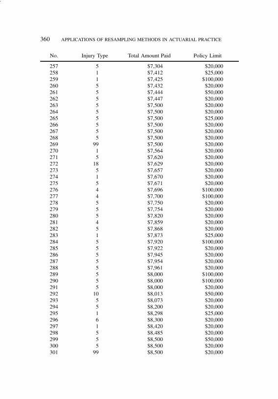
job no. 1969 casualty actuarial society CAS journal 1969D04 [39] 11-08-01 4:58 pm
360 APPLICATIONS OF RESAMPLING METHODS IN ACTUARIAL PRACTICE
No. Injury Type Total Amount Paid Policy Limit
257 5 $7,304 $20,000258 1 $7,412 $25,000259 1 $7,425 $100,000260 5 $7,432 $20,000261 5 $7,444 $50,000262 5 $7,447 $20,000263 5 $7,500 $20,000264 5 $7,500 $20,000265 5 $7,500 $25,000266 5 $7,500 $20,000267 5 $7,500 $20,000268 5 $7,500 $20,000269 99 $7,500 $20,000270 1 $7,564 $20,000271 5 $7,620 $20,000272 18 $7,629 $20,000273 5 $7,657 $20,000274 1 $7,670 $20,000275 5 $7,671 $20,000276 4 $7,696 $100,000277 4 $7,700 $100,000278 5 $7,750 $20,000279 5 $7,754 $20,000280 5 $7,820 $20,000281 4 $7,859 $20,000282 5 $7,868 $20,000283 1 $7,873 $25,000284 5 $7,920 $100,000285 5 $7,922 $20,000286 5 $7,945 $20,000287 5 $7,954 $20,000288 5 $7,961 $20,000289 5 $8,000 $100,000290 5 $8,000 $100,000291 5 $8,000 $20,000292 10 $8,013 $50,000293 5 $8,073 $20,000294 5 $8,200 $20,000295 1 $8,298 $25,000296 6 $8,300 $20,000297 1 $8,420 $20,000298 5 $8,485 $20,000299 5 $8,500 $50,000300 5 $8,500 $20,000301 99 $8,500 $20,000

job no. 1969 casualty actuarial society CAS journal 1969D04 [40] 11-08-01 4:58 pm
APPLICATIONS OF RESAMPLING METHODS IN ACTUARIAL PRACTICE 361
No. Injury Type Total Amount Paid Policy Limit
302 5 $8,500 $20,000303 5 $8,515 $20,000304 5 $8,612 $20,000305 5 $8,634 $100,000306 5 $8,686 $20,000307 5 $8,785 $20,000308 5 $8,786 $20,000309 5 $8,794 $20,000310 5 $8,805 $20,000311 5 $8,815 $20,000312 5 $8,856 $20,000313 5 $8,861 $20,000314 6 $8,882 $20,000315 5 $8,911 $20,000316 5 $8,914 $20,000317 5 $8,988 $20,000318 5 $9,000 $100,000319 5 $9,000 $20,000320 5 $9,000 $20,000321 5 $9,000 $20,000322 5 $9,000 $20,000323 5 $9,000 $0324 5 $9,000 $20,000325 5 $9,000 $20,000326 5 $9,000 $20,000327 5 $9,000 $20,000328 5 $9,009 $20,000329 5 $9,020 $20,000330 5 $9,030 $25,000331 5 $9,051 $20,000332 5 $9,053 $20,000333 5 $9,073 $100,000334 5 $9,100 $20,000335 1 $9,129 $20,000336 5 $9,200 $20,000337 5 $9,208 $20,000338 5 $9,300 $20,000339 5 $9,355 $20,000340 5 $9,356 $20,000341 5 $9,392 $20,000342 5 $9,395 $100,000343 5 $9,423 $20,000344 5 $9,428 $20,000345 5 $9,451 $100,000346 5 $9,500 $20,000

job no. 1969 casualty actuarial society CAS journal 1969D04 [41] 11-08-01 4:58 pm
362 APPLICATIONS OF RESAMPLING METHODS IN ACTUARIAL PRACTICE
No. Injury Type Total Amount Paid Policy Limit
347 5 $9,500 $20,000348 5 $9,602 $20,000349 5 $9,710 $20,000350 4 $9,881 $25,000351 5 $9,909 $20,000352 8 $10,000 $20,000353 6 $10,000 $20,000354 5 $10,000 $100,000355 6 $10,000 $20,000356 4 $10,106 $20,000357 5 $10,229 $20,000358 5 $10,330 $20,000359 5 $10,331 $20,000360 5 $10,400 $20,000361 5 $10,505 $100,000362 4 $10,555 $20,000363 1 $10,645 $20,000364 8 $10,861 $20,000365 5 $10,968 $20,000366 5 $11,000 $50,000367 4 $11,000 $100,000368 5 $11,032 $20,000369 5 $11,144 $20,000370 5 $11,166 $20,000371 1 $11,262 $25,000372 5 $11,344 $50,000373 99 $11,353 $20,000374 5 $11,385 $20,000375 1 $11,500 $20,000376 5 $11,626 $20,000377 5 $11,835 $20,000378 99 $11,986 $20,000379 5 $11,991 $20,000380 4 $12,000 $20,000381 5 $12,000 $20,000382 5 $12,000 $20,000383 5 $12,214 $100,000384 5 $12,274 $20,000385 5 $12,374 $20,000386 99 $12,380 $20,000387 3 $12,500 $20,000388 5 $12,509 $20,000389 5 $12,621 $100,000390 5 $12,756 $20,000391 5 $12,859 $20,000
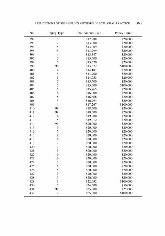
job no. 1969 casualty actuarial society CAS journal 1969D04 [42] 11-08-01 4:58 pm
APPLICATIONS OF RESAMPLING METHODS IN ACTUARIAL PRACTICE 363
No. Injury Type Total Amount Paid Policy Limit
392 5 $12,988 $20,000393 7 $13,000 $20,000394 5 $13,009 $20,000395 5 $13,299 $50,000396 4 $13,347 $20,000397 5 $13,500 $20,000398 5 $13,570 $20,000399 99 $13,572 $100,000400 4 $14,181 $20,000401 5 $14,700 $20,000402 5 $14,953 $20,000403 5 $15,500 $20,000404 5 $15,500 $100,000405 5 $15,765 $20,000406 18 $16,000 $20,000407 5 $16,668 $20,000408 5 $16,794 $20,000409 4 $17,267 $100,000410 99 $18,500 $20,000411 99 $18,500 $20,000412 18 $19,000 $20,000413 5 $19,012 $20,000414 99 $20,000 $20,000415 5 $20,000 $20,000416 7 $20,000 $20,000417 8 $20,000 $20,000418 8 $20,000 $20,000419 7 $20,000 $20,000420 7 $20,000 $20,000421 3 $20,000 $20,000422 6 $20,000 $20,000423 16 $20,000 $20,000424 5 $20,000 $20,000425 6 $20,000 $20,000426 5 $20,000 $20,000427 9 $20,000 $20,000428 5 $20,000 $20,000429 1 $22,692 $100,000430 5 $24,500 $50,000431 99 $25,000 $25,000432 2 $25,000 $100,000

job no. 1969 casualty actuarial society CAS journal 1969D04 [43] 11-08-01 4:58 pm
364 APPLICATIONS OF RESAMPLING METHODS IN ACTUARIAL PRACTICE
INJURY CODE DESCRIPTION
Injury InjuryType Description Type Description
1 MINOR LACERATIONS/ 13 PARALYSIS/PARESISCONTUSIONS
2 SERIOUS LACERATION 14 JAW JOINT DYSFUNCTION3 SCARRING OR
PERMANENTDISFIGUREMENT
15 LOSS OF A SENSE
4 NECK ONLY SPRAINSTRAIN
16 FATALITY
5 BACK OR NECK & BACKSPRAIN/STRAIN
17 DENTAL
6 OTHER SPRAIN/STRAIN 18 CARTILAGE/MUSCLE/TENDON/LIGAMENT INJURY
7 FRACTURE OR WEIGHTBEARING BONE
19 DISC HERNIATION
8 OTHER FRACTURE 20 PREGNANCY RELATED9 INTERNAL ORGAN
INJURY21 PRE-EXISTING CONDITION
10 CONCUSSION 22 PSYCHOLOGICALCONDITION
11 PERMANENT BRAININJURY
30 NO VISIBLE INJURY
12 LOSS OF BODY PART 99 OTHER

job no. 1969 casualty actuarial society CAS journal 1969D07 [1] 11-08-01 4:58 pm
MEASURING THE INTEREST RATE SENSITIVITY OFLOSS RESERVES
STEPHEN P. D’ARCY AND RICHARD W. GORVETT
Abstract
In order to apply asset-liability management tech-niques to property-liability insurers, the sensitivity of li-abilities to interest rate changes, or duration, must becalculated. The current approach is to use the Macaulayor modified duration calculations, both of which pre-sume that the cash flows are invariant with respect tointerest rate changes. Based on the structure of lia-bilities for property-liability insurers, changes in inter-est rates—given that interest rates are correlated withinflation—should affect future cash flows on existing li-abilities. This paper analyzes the effect that interest ratechanges can have on these cash flows, shows how tocalculate the resulting effective duration of these liabil-ities, and demonstrates the impact of failing to use thecorrect duration measure on asset-liability managementfor property-liability insurers.
1. INTRODUCTION
Property-liability insurance companies are exposed to a widevariety of risks. However, the focus of most insurers and reinsur-ers has been primarily on traditional insurance risks, such as le-gal, regulatory or catastrophic exposures. It is widely recognizedthat the potential impact of natural catastrophes on property-liability insurers is so severe that this area has been given exten-sive attention by the industry: sophisticated models have beendeveloped to quantify catastrophe exposure and securitized in-surance products are being designed to facilitate the trading ofsuch risks through the capital markets. Extensive attention has
365
job no. 1969 casualty actuarial society CAS journal 1969D07 [2] 11-08-01 4:58 pm
366 MEASURING THE INTEREST RATE SENSITIVITY OF LOSS RESERVES
also been paid to quantifying and predicting the underwritingcycle, although with considerably less success.
However, insurers are also exposed to a variety of financialrisks that have not received the same level of attention, despite thesuccess that other financial services firms have achieved in thisvenue. For example, with the rising level of globalization in theinsurance industry, the risk of fluctuations in foreign exchangerates is becoming an increasing concern for insurers. Neverthe-less, insurers lag well behind other financial institutions in for-eign currency hedging activity. Another critical area of risk facedby insurers involves fluctuations in value due to interest ratemovements. Banks, life insurers and other financial institutionshave developed sophisticated approaches to attempt to deal withinterest rate risk. Most property-liability insurers have neitheradopted the approaches of other financial institutions nor adaptedthose models to reflect the unique characteristics of this industry.This article seeks to address this area of concern. While interestrate risk is not as significant for the property-liability insuranceindustry as, for example, catastrophe risk, it does represent animportant source of risk and is one that can be effectively dealtwith through the use of accepted risk management techniques.
Similar to any other financial institution, the values of an in-surer’s assets and liabilities can be affected by changes in futureinterest rates. The reason for this is that the economic value of afinancial asset or liability is the discounted value of its future cashflows. Thus, if interest rates increase, the economic value of fu-ture cash flows will decrease; if interest rates decrease, economicvalue will increase. The direction of the movement in values ofboth the assets and the liabilities, according to this principle, willbe the same. The problem, however, is that asset and liability val-ues will generally not move by the same amount in response toa particular change in interest rates (unless specifically and ac-curately set up to do so). If they do not move similarly, the networth of an insurer will change over time due to the volatility ofinterest rates.

job no. 1969 casualty actuarial society CAS journal 1969D07 [3] 11-08-01 4:58 pm
MEASURING THE INTEREST RATE SENSITIVITY OF LOSS RESERVES 367
Asset-liability management (ALM), as used in the insuranceindustry, is a process by which insurers attempt to evaluate andadjust the exposure of the net value of the company (assets mi-nus liabilities) to interest rate changes. Although, in theory, thevolatility of other factors (e.g., catastrophes, changes in unem-ployment rates1) can also affect both asset and liability values,the current focus of ALM for insurers, as for most other financialinstitutions, is on interest rate risk. Life insurers were the first inthe industry to apply ALM techniques, since they have signifi-cant exposure to interest rate risk due to the long payout patternsof losses and their high leverage. However, this approach is nowbeing applied to the property-liability insurance industry as well.
The general approaches used by life insurers to measure thesensitivity of assets to interest rate risk are applicable to property-liability insurers to the extent that they have similar asset portfo-lios. In general, property-liability companies invest more heavilyin equities and less in mortgages, but the overall structure of theinvestment portfolio is roughly similar. However, the liabilitiesof property-liability insurers are different enough that the ap-proaches used by life insurers are simply not applicable to them,and new techniques must be developed.
Duration is a measure of the interest rate sensitivity of a fi-nancial instrument. The term duration, which seems to signifymore a measure of time than of interest rate sensitivity, is de-rived from early work on fixed income assets in which the inter-est rate sensitivity was found to correspond closely to a weightedaverage time value. The basic approach of ALM involves mea-suring the durations of assets and liabilities, and then adjustingone or both until the insurer is not significantly affected by inter-est rate changes (essentially, this involves setting the duration ofsurplus equal to zero). If the duration of liabilities is measuredincorrectly, then an insurer trying to immunize itself from inter-
1For example, an increase in the unemployment rate is likely to increase the severity ofworkers compensation losses and also alter the prepayment patterns on mortgage-backedsecurities.
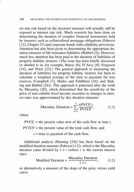
job no. 1969 casualty actuarial society CAS journal 1969D07 [4] 11-08-01 4:58 pm
368 MEASURING THE INTEREST RATE SENSITIVITY OF LOSS RESERVES
est rate risk based on the incorrect measure will actually still beexposed to interest rate risk. Much research has been done ondetermining the duration of complex financial instruments heldby insurers, such as collateralized mortgage obligations (Fabozzi[12], Chapter 27) and corporate bonds with callability provisions.Attention has also been given to determining the appropriate du-ration measure of life insurance liabilities (Babbel [3]). However,much less attention has been paid to the duration of liabilities ofproperty-liability insurers. (The issue has been briefly discussedor alluded to in, for example, Butsic [6]; D’Arcy [8]; Ferguson[14]; and Noris [23].) The general approach to measuring theduration of liabilities for property-liability insurers has been tocalculate a weighted average of the time to payment for lossreserves (Campbell [7], Hodes and Feldblum [16], and Stak-ing and Babbel [26]). This approach is patterned after the workby Macaulay [20], which determined that the sensitivity of theprice of non-callable fixed income securities to changes in inter-est rates was approximated by this duration measure:
Macaulay Duration =n!t=1
t(PVCFt)PVTCF
, (1.1)
where
PVCFt = the present value now of the cash flow at time t,
PVTCF = the present value of the total cash flow, and
t= time to payment of the cash flow.
Additional analysis (Panning [24]) has been based on themodified duration measure (Fabozzi [11]), which is theMacaulayduration value divided by 1+ r (where r is the current interestrate):
Modified Duration =Macaulay Duration
1+ r, (1.2)
or alternatively a measure of the slope of the price versus yieldcurve.
job no. 1969 casualty actuarial society CAS journal 1969D07 [5] 11-08-01 4:58 pm
MEASURING THE INTEREST RATE SENSITIVITY OF LOSS RESERVES 369
To illustrate Macaulay and modified duration, consider a bondwith a $1000 face value and an 8% annual coupon that maturesin 10 years. If interest rates are currently 8%, then the price ofthe bond would be $1000. The Macaulay duration of this bondis 7.25 and the modified duration is 6.71. To use duration tomeasure interest rate sensitivity, the expected change in the valueof a bond is equal to the negative of the change in interest ratestimes the modified duration (or Macaulay duration divided by(1+ r)). If interest rates were to increase slightly to 8.01%, thenthe price of the bond would drop to $999.33, which is a declineof 0.0671%. The predicted change in price based on durationwould be the negative of the change in interest rates, !:0001,times 6.71, or !0:0671%. For such a small change in interestrates for a bond with a fixed cash flow, duration measures theinterest rate sensitivity fairly accurately.
Both the Macaulay and modified duration calculations areonly accurate measures of interest rate sensitivity under the fol-lowing conditions:
" the yield curve is flat" any change in interest rates is a parallel yield curve shift" the cash flows do not change as interest rates change.In practice, none of these conditions is likely to be met. A numberof researchers have examined the effect of the first two condi-tions in general (see Klaffky, Ma, and Nozari [18]; Ho [15]; andBabbel, Merrill, and Panning [4]). In addition, the issue of vari-able cash flows has been widely recognized for specific classesof assets. Bonds with embedded options (such as call provisions)and mortgage-backed securities (where prepayments depend onthe interest rate level) are examples of assets on which the ex-pected cash flows change as interest rates change. A measuretermed effective duration has been developed to express the sen-sitivity of the present value of the expected cash flows with re-spect to interest rate changes; this measure specifically reflects

job no. 1969 casualty actuarial society CAS journal 1969D07 [6] 11-08-01 4:58 pm
370 MEASURING THE INTEREST RATE SENSITIVITY OF LOSS RESERVES
the fact that the cash flows can change as interest rates change(Fabozzi [11]). For assets with variable cash flows, it is appro-priate to calculate the effective duration rather than the modifiedduration.
The liabilities of property-liability insurers also vary with in-terest rates, due to the correlation of interest rates with inflation.As explained by Hodes and Feldblum [16, p. 558],
“Personal auto loss reserves are at least partially infla-tion sensitive. Medical payments in tort liability states,for instance, depend in part upon jury awards at thedate of settlement. The jury awards, in turn, are influ-enced by the rate of inflation, which is correlated (atleast in the long run) with interest rates.”
Thus, the appropriate measure of interest rate sensitivity of theliabilities of property-liability insurers is one that reflects thisinterest rate-inflation relationship, or effective duration. Hodesand Feldblum [16, p. 559] indicate that “A mathematical de-termination of the loss reserve (effective) duration is complex.”This is the task that is addressed in the remainder of this paper.The focus of this research is to develop a method to quantifythe sensitivity of economic surplus to parallel shifts in the yieldcurve.
In order to accommodate non-parallel yield curve shifts,stochastic interest rate models must be used. This approach hasbeen advocated for insurance applications by Tilley [28], Rei-tano [25], and Briys and de Varenne [5]. However, as pointedout by Litterman and Scheinkman [19], parallel shifts explainover 80% of historical yield curve movements. Although hypo-thetical portfolios can be constructed that show significant differ-ences in duration values under parallel versus non-parallel yieldcurve shifts, these differences are likely to be far less importantthan the impact of variable cash flows for the asset and liabilityportfolios of typical property-liability insurers. Thus, this paper

job no. 1969 casualty actuarial society CAS journal 1969D07 [7] 11-08-01 4:58 pm
MEASURING THE INTEREST RATE SENSITIVITY OF LOSS RESERVES 371
focuses on analyzing liability cash flows that vary with inter-est rate changes by recognizing that interest rate changes areimpacted by changes in the inflation rate. Further research willexplore the impact of stochastic interest models for both assetsand liabilities for representative property-liability insurers.
Section 2 of this paper discusses the nature and relative signif-icance of property-liability insurance company liabilities. Section3 examines the three major liability items, and discusses the tim-ings of cash flows for each of these items. The natures of thecash flows have important implications for the type and level ofimpact on liability durations of changes in interest rates. Section4 provides a mathematical derivation of a closed-form effectiveduration formula in a highly simplified framework. Section 5 de-scribes a more detailed numerical model used to estimate effec-tive durations. Section 6 summarizes the results of empirical es-timates and sensitivity tests of effective duration measures. Sec-tion 7 demonstrates the impact on asset-liability management ofusing modified versus effective duration measures of liabilities.
2. THE LIABILITIES OF PROPERTY-LIABILITY INSURERS
The three major balance sheet liability items of property-liability insurers are the loss reserve, the loss adjustment expensereserve, and the unearned premium reserve. As of 12/31/97, forthe industry in aggregate, these components totaled 84.8% of lia-bilities (A.M. Best [1]). All of these three reserves are subject tochange, via inflationary pressures, as interest rates change. Theremaining liabilities of property-liability insurers consist primar-ily of expenses payable, including taxes, reinsurance, contingentcommissions, and declared dividends. These cash flows are notlikely to be affected by interest rate changes so the interest ratesensitivity of these liabilities can be measured by Macaulay ormodified duration.2
2Panning [24] proposes that the present value of future business be considered in theasset-liability management of an insurer. This approach, though, is contrary to acceptedaccounting standards, both statutory and GAAP, and introduces significant, unverifiable

job no. 1969 casualty actuarial society CAS journal 1969D07 [8] 11-08-01 4:58 pm
372 MEASURING THE INTEREST RATE SENSITIVITY OF LOSS RESERVES
Since loss and loss adjustment expense reserve estimates arebased on historical development patterns, and the historical de-velopment patterns are affected by historical economic variablessuch as interest rates and inflation, the accuracy of the loss andloss adjustment expense reserves are, in essence, path depen-dent with respect to those economic variables. In other words,the level of loss and loss adjustment expense reserves calculatedat any point in time will depend upon how economic variableshave performed in prior years. However, it is not the accuracy ofthe current estimate that is of concern in measuring the effectiveduration, but how future cash flow patterns are influenced by fu-ture interest rate changes, which are in turn driven by changes ininflation. Reserving techniques that attempt to isolate the infla-tionary component from the other effects have been proposed byButsic [6] and Taylor [27], but these approaches are not widelyused currently.
Similarly, although the unearned premium reserve is calcu-lated based on the portion of written premiums that apply tounexpired policy terms, the cash flows that will emanate fromthe unearned premium reserve are essentially losses and loss ad-justment expenses on claims that occur after the evaluation datebut during the remaining policy term. Since these events havenot yet occurred, they are completely sensitive to changes in in-flation affecting the value of these future losses.
An added complication to the measurement of the sensitivityof insurer assets and liabilities to interest rate changes is the statu-tory accounting conventions of the insurance industry. Specifi-cally, bonds are valued on a book, or amortized, basis. Also, lossliabilities are not discounted to reflect the time value of moneyuntil payment. Thus, statutory valuations are often not directly
judgement factors about future premiums, losses, retention rates and pricing policies.Thus, this approach is not included here. The next step in asset-liability management forproperty-liability insurers should be to measure existing assets and liabilities accuratelyby recognizing the interest rate sensitivity of the cash flows from loss reserves, which isthe focus of the rest of this paper.
job no. 1969 casualty actuarial society CAS journal 1969D07 [9] 11-08-01 4:58 pm
MEASURING THE INTEREST RATE SENSITIVITY OF LOSS RESERVES 373
affected by changes in interest rates. However, the economic val-ues of these assets and liabilities are affected by interest ratechanges. (Under GAAP accounting, bonds not held to maturityare reported at market value and therefore would also be affectedby interest rates.) It is the economic values that are consideredhere, since these reflect the true worth of the company to itsowners.
Each of the three major liability items is discussed in greaterdetail below. More specifically, Section 3 sets the groundwork forevaluating the impact of future interest rate changes and inflationon the liabilities of property-liability insurers.
3. THE TIMING OF PROPERTY-LIABILITY INSURER LIABILITIES
Loss Reserves
A company’s aggregate loss reserve represents the totalamount to be paid in the future on all claims that have alreadybeen incurred. However, a variety of different situations can existwith respect to these claims:
1. A loss reserve can reflect a claim on which the insurer isin the process of issuing a check—the claim has alreadybeen fully investigated, and the insurer has agreed to asettlement amount with the claimant. The nominal valueof the claim amount will not be affected by changes ininterest rates, although the present value would changeslightly.
2. Alternatively, a loss reserve can represent a claim thathas caused a known amount of damage to property orto a person (the medical bills are complete). Thus, theamount of the loss to the claimant is determined andwill not change. However, the insurer and the claimantare still in dispute over whether the incident is covered,or over the extent of the insurer’s liability for payment.Again, the nominal amount of the payment should not

job no. 1969 casualty actuarial society CAS journal 1969D07 [10] 11-08-01 4:58 pm
374 MEASURING THE INTEREST RATE SENSITIVITY OF LOSS RESERVES
change if interest rates change.3 However, the economicvalue of the loss would change, since the future cashflow would be discounted by a different interest rate.
3. A third type of loss reserve is for damages that have yetto be discovered. The insurer will be liable for the losswhen the claimant experiences it, but the value of the losswill only be known in the future. On an occurrence-basedpolicy, this could apply for medical malpractice to a per-son who has not yet suffered the adverse consequencesof an injury caused by a negligent physician (e.g., im-proper diagnosis, long term adverse consequences fromprescribed medication, surgical errors that will lead to fu-ture complications). Or, in the case of workers compen-sation, if a former employee exposed to a work-relatedenvironmental hazard first manifests the ailment at somefuture date, the claim will be assigned to policies in ef-fect during the period of employment. For these claims,the nominal value of the loss payment will be affectedby interest rate changes to the extent that the interest ratechange is correlated with inflation on the goods or ser-vices related to the cost of the claim (property damage,medical expenses). The economic value of these losseswill also change with interest rates.
4. The most common type of loss reserve is for losses onwhich some of the damages have already been fixed invalue, but the remainder has yet to be determined. In ad-dition, the question of the extent of the insurer’s liabilitymay not have been settled. This could apply to an auto-mobile accident involving property damage and bodilyinjury in which the policyholder of the insurer may beliable. The damage to the claimant’s vehicle is prede-
3One way this could happen is if the insurer’s claim settlement philosophy were tochange with interest rates (e.g., if the financial condition of the insurer were to becomeimpaired in conjunction with an interest rate change and the company had to alter itsclaim settlement approach).

job no. 1969 casualty actuarial society CAS journal 1969D07 [11] 11-08-01 4:58 pm
MEASURING THE INTEREST RATE SENSITIVITY OF LOSS RESERVES 375
termined. The injured person has received some medi-cal care, but that care will continue at least up until thesettlement of the claim and perhaps beyond. The nom-inal value of a portion of these losses, termed “fixed,”will not be affected by interest rate changes, but the re-maining portion of the losses will be affected by futureinflation.
Calculating the effect of inflation on tangible losses, such asmedical expenses, wage losses, and property damage, althoughcomplicated, is relatively straightforward once the appropriateinflation indices are determined. However, quantifying the ef-fect of inflation on the value of intangibles in a liability claim,termed “general damages” in a legal context, presents additionalchallenges. These components include items such as pain andsuffering, loss of consortium, and hedonic losses. It is difficultto determine exactly how these values are established. Are theybased on the value at the time of the loss or the time of the ver-dict in a jury trial? Is the pain and suffering of a broken arm thatoccurred in 1986 evaluated the same as, or less than, a similarbroken arm that occurred in 1996, if both are being settled at thesame time?
Due to the difficulty in putting a numerical value on an in-tangible such as pain and suffering, general rules of thumb arisethat try to relate the pain and suffering award to the medical ex-penses incurred by the patient. Thus, a broken arm that generated$15,000 in medical bills is worth roughly three times as much asanother broken arm that generated only $5,000 in medical bills.(This does not mean that the pain and suffering from a soft-tissueinjury, such as a sore neck, which generated $15,000 in medicalexpenses would be worth as much as a broken arm with the sameamount of medical expenses.) On this basis, the general damageson liability claims will be impacted by interest rate changes tothe same extent that medical expenses are affected. However, atypical question asked by a plaintiff’s attorney in a bodily injurycase is how much a member of the jury would require to be

job no. 1969 casualty actuarial society CAS journal 1969D07 [12] 11-08-01 4:58 pm
376 MEASURING THE INTEREST RATE SENSITIVITY OF LOSS RESERVES
willing to undergo the same pain that the client has experienced.Since this is asked, rhetorically, near the end of the claim set-tlement process, conceivably the jury will implicitly adjust thevalue of the claim to the then-current cost of living. In this case,the entire loss reserve for general damages would be sensitive tofuture inflation changes.
Determining the effective duration of reserves will, therefore,depend on a model for dividing the future payments into a fixedcomponent, which is not sensitive to future inflation, and an infla-tion sensitive component, which will vary with subsequent infla-tion. This model is developed and described in Section 4 below.
Loss Adjustment Expense Reserves
Loss adjustment expense reserves are established for futurepayments in a manner similar to loss reserves. These expenseswill be paid over the time during which the remaining losses aresettled. Loss adjustment expenses are assigned to the accidentyear in which the loss that generated these expenses occurred;they are assigned either directly (for allocated loss adjustment ex-penses) or indirectly (for unallocated loss adjustment expenses).The same approach used for determining the proportion of lossreserves that are fixed in value can be used for loss adjustmentexpense reserves. However, since the rate with which these ex-penses become fixed in value can differ from the loss itself, theymay be modeled separately using different parameter values.
Loss adjustment expenses are different from loss reserves inthe following respect. As an insurer generates loss adjustmentexpenses, such as by hiring outside adjusters, it would generallypay these expenses shortly after the work is completed. The lossadjustment expense reserve, then, represents costs that are fixedin value to a much lower degree than loss reserves. Also, the legalcosts associated with defending a claim that goes to court will notbe established until the very end of the loss settlement process. Inaddition, the allocation process for unallocated loss adjustmentexpenses assigns a portion of the general claim department’s

job no. 1969 casualty actuarial society CAS journal 1969D07 [13] 11-08-01 4:58 pm
MEASURING THE INTEREST RATE SENSITIVITY OF LOSS RESERVES 377
expenses to the accident year of the claim when the loss is paid.Thus, for loss adjustment expense reserves, few of these costswill be fixed in value when the claim occurs and a relatively highportion of the total costs will be based on the cost of living whenthe claim is finally settled.
Unearned Premium Reserves
Since the unearned premium reserve essentially represents ex-posure to losses that have not even occurred yet, this liability isfully sensitive to future inflation. The expected cash flow ema-nating from the unearned premium reserve will shift to the extentthat any change in interest rates is correlated with inflation. If itis assumed that the insurer writes policies with terms not morethan one year, then all of the claims emanating from the unearnedpremium reserve will occur in the next accident year. The pay-ments on these losses will follow the claim payout pattern of theinsurer, except that losses will occur approximately in the mid-dle of the first half of the year (assuming annual policies writtenevenly throughout the year), as opposed to in the middle of thefull year as would be assumed for accident year data. Thus, theduration of the unearned premium reserve at the end of a fullyear would be the weighted average of the time until payment ofthe most recent accident year, plus 3/4 of a year. For example,the unearned premium reserve as of 12/31/99 covered losses thatoccurred, on average, on 4/1/00. For the loss reserve for accidentyear 1999, the average loss would have occurred at the middle ofthe year, or 7/1/99. Thus, the duration of the unearned premiumreserve as of 12/31/99 is 3/4 of a year more than the duration ofthe accident year 1999 loss reserves.
4. MATHEMATICAL MODEL OF THE EFFECTIVE DURATION OFRESERVES
In Section 5, we will present a detailed numerical modelfor determining effective duration. In this section, we develop

job no. 1969 casualty actuarial society CAS journal 1969D07 [14] 11-08-01 4:58 pm
378 MEASURING THE INTEREST RATE SENSITIVITY OF LOSS RESERVES
a simplified mathematical model of an effective duration for-mula based on the assumption of proportional decay of reserveliabilities. This assumption allows for a closed-form solution forduration when inflation is recognized. This formula will providea method to determine the general value of the effective dura-tion of insurance liabilities, as well as a point of reference forthe more detailed calculations discussed later. It should be notedthat other decay patterns are possible, but most would not leadto a closed-form solution, so caution should be used when thisapproach is applied in practice.
In this section, it is assumed that all payments are fully sensi-tive to inflation. In this case, the price level at which an insurermakes a claim payment depends only upon the date of that pay-ment. Put in the context of “fixed” costs described in the lastsection, here it is assumed that there are no fixed costs. Thisprovides a framework in which a closed-form solution can beeasily derived, assuming an appropriate payment pattern. Themeasurement of duration assuming partial fixed costs will bederived in Section 5.
Assume that the payout over time of property-liability re-serves is represented by a “proportional decay” model—eachyear, proportion c of the beginning reserve is paid out.4 Thus,
Rt = (1! c)Rt!1, (4.1)
where
Rt = the (correct) nominal reserve at time t,
c= the (constant) annual payout ratio, and
r = the relevant interest rate.
4Theoretically, this assumes that payouts are made forever, although after some yearsthey become negligible in size. Finite-length payout patterns are considered in Sec-tion 5.
job no. 1969 casualty actuarial society CAS journal 1969D07 [15] 11-08-01 4:58 pm
MEASURING THE INTEREST RATE SENSITIVITY OF LOSS RESERVES 379
Under this assumption, the present value of the initial reserve isexpressed as
PV(R0) =#!t=1
(1! c)t!1cR0(1+ r)t
=cR01! c
#!t=1
"1! c1+ r
#t=cR0r+ c
,
(4.2)
where the final form of the equation is derived from the for-mula for an infinite geometric progression.5 Now, we can derivean expression for the Macaulay duration by multiplying the nu-merator of each term in the present value calculation by t, anddividing the new summation by the original present value:
Macaulay Duration =D0 =
#!t=1
(1! c)t!1cR0t(1+ r)t
PV(R0): (4.3)
By again using the properties of infinite geometric progressions,the numerator of the Macaulay duration formula reduces to:
cR0(1+ r)(r+ c)2
: (4.4)
Dividing by the previous expression for PV(R0), the Macaulayduration is
D0 =1+ rr+ c
: (4.5)
Since the modified duration is the Macaulay duration divided by(1+ r), we have
Modified Duration =MD0 =1r+ c
: (4.6)
In order to determine the effective duration of property-liability insurer liabilities, we must calculate the present valueof those liabilities in three different ways: with the original in-terest rate, with an increased interest rate, and with a decreased
5For 0< x < 1, the value of x+ x2 + x3 + $ $ $= x=(1! x).
job no. 1969 casualty actuarial society CAS journal 1969D07 [16] 11-08-01 4:58 pm
380 MEASURING THE INTEREST RATE SENSITIVITY OF LOSS RESERVES
interest rate. Under this approach, after calculating the presentvalue assuming the original interest rate, we assume that the in-terest rate increases (e.g., by 100 basis points), and then that theinterest rate decreases (e.g., by 100 basis points). The effectiveduration is then calculated as:
Effective Duration = ED0 =PV! !PV+2PV0(¢r)
, (4.7)
where
PV! = the present value of the expected cash flowsif interest rates decline by ¢r,
PV+ = the present value of the expected cash flowsif interest rates increase by ¢r, and
PV0 = the initial present value of the expectedcash flows.
The key in calculating the effective duration is to account forthe impact of hypothetical changes in the interest rate on the fu-ture cash flows emanating from the liability items. For property-liability reserves, the primary impact on cash flows of a changein interest rates is due to the change in the inflation rate: sinceinterest rates are correlated with inflation, and inflation increasesfuture nominal claim payments, changes in interest rates will af-fect the level of future cash outflows, and thus the present valueof those outflows. Therefore, in order to calculate the effectiveduration, we need to adjust the formulas above to reflect thisinflationary impact.
Define the following additional variables:
r+ or ! = r +=! ¢r = the increased or decreasedinterest rate, and
i+ or ! = the inflationary adjustment after the changein interest rate:
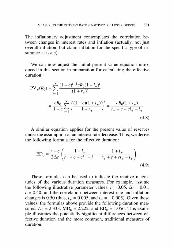
job no. 1969 casualty actuarial society CAS journal 1969D07 [17] 11-08-01 4:58 pm
MEASURING THE INTEREST RATE SENSITIVITY OF LOSS RESERVES 381
The inflationary adjustment contemplates the correlation be-tween changes in interest rates and inflation (actually, not justoverall inflation, but claim inflation for the specific type of in-surance at issue).
We can now adjust the initial present value equation intro-duced in this section in preparation for calculating the effectiveduration:
PV+(R0) =#!t=1
(1! c)t!1cR0(1+ i+)t(1+ r+)t
=cR01! c
#!t=1
"(1! c)(1+ i+)
1+ r+
#t=
cR0(1+ i+)r+ + c+ ci+! i+
:
(4.8)
A similar equation applies for the present value of reservesunder the assumption of an interest rate decrease. Thus, we derivethe following formula for the effective duration:
ED0 =r+ c2¢r
$1+ i!
r!+ c+ ci! ! i!! 1+ i+r+ + c+ ci+! i+
%:
(4.9)
These formulas can be used to indicate the relative magni-tudes of the various duration measures. For example, assumethe following illustrative parameter values: r = 0:05, ¢r = 0:01,c= 0:40, and the correlation between interest rate and inflationchanges is 0.50 (thus, i+ = 0:005, and i! =!0:005). Given thesevalues, the formulas above provide the following duration mea-sures: D0 = 2:333, MD0 = 2:222, and ED0 = 1:056. This exam-ple illustrates the potentially significant differences between ef-fective duration and the more common, traditional measures ofduration.
job no. 1969 casualty actuarial society CAS journal 1969D07 [18] 11-08-01 4:58 pm
382 MEASURING THE INTEREST RATE SENSITIVITY OF LOSS RESERVES
5. MODELING THE INTEREST RATE SENSITIVITY OF LOSS ANDLAE RESERVES
One of the difficulties in measuring the interest rate sensitivityof liabilities is the need for extensive data. What information isavailable, either publicly or within the company, to determine theimpact of interest rate changes on the cash flows of losses? Forthe loss and loss adjustment expense reserve, the expected nom-inal cost of these amounts at the end of each year are reported inaggregate, by accident year, by line of business, in the AnnualStatement. Internally, actuaries have access to this same informa-tion on a more frequent and more detailed basis. Although theexpected payment dates for future payments are not generallyrecorded, the actual payments made in each historical year—categorized by accident year (or month) and by line of business(or finer breakdown)—are available. This allows a comparisonof the actual payments with the expected payments and permitsthe generation of a profile of when the aggregate loss reservesare likely to be paid in the future. However, there is no publicinformation, and frequently not even any information within acompany, on when the value of an unpaid loss is set in value.To obtain such information, claim files would need to record thedate when each expenditure relating to a claim is made by theclaimant, not just when the insurer pays the claim. Since few, ifany, insurers currently maintain such detail, the only way to ob-tain this information is to perform a special study, as detailed inthe next section of the paper. Given the lack of data to measurethis effect precisely, this relationship needs to be modeled.
For this model, the following assumptions are made. At thetime the loss occurs, proportion k of the eventual cost of theclaim is “determined” (i.e., a proportion of the future cost is“fixed” and no longer open to change from interest rate andinflationary changes). In addition, proportion m of the loss willnot be determined until the time the claim is settled. Examplesof loss costs that will go into k are medical treatment soughtimmediately after the loss occurs, the wage loss component of

job no. 1969 casualty actuarial society CAS journal 1969D07 [19] 11-08-01 4:58 pm
MEASURING THE INTEREST RATE SENSITIVITY OF LOSS RESERVES 383
a bodily injury claim, and property damage. Examples of losscosts that will go into m are medical evaluations that are doneimmediately prior to determining the settlement offer, generaldamages to the extent they are based on the cost of living at thetime of settlement, and loss adjustment expenses connected withsettling the claim.
The remaining (1! k!m) portion of the expenses are mod-eled in three ways, to allow for differing rates at which the claimvalues could become fixed: these expenses could be fixed invalue linearly over the time period from loss to settlement, orin a manner that would represent either a concave function ora convex function. Figure 1 illustrates the three different func-tions proposed for the proportion of loss reserves that are fixedin value, and therefore not subject to inflation, over time.
A representative function that displays these attributes is:
f(t) = k+ %(1! k!m)(t=T)n&, (5.1)
where
f(t) = the proportion of ultimate paid claims “fixed”at time t,
k = the proportion of the claim that is fixed in valueimmediately,
m= the proportion of the claim that is not fixed invalue until the claim is settled,
n= 1 for the linear case,
n < 1 for the concave case,
n > 1 for the convex case, and
T = the time at which the claim is fully andcompletely settled.
For example, assume an insured causes an automobile acci-dent in the middle of 1997, and the victim requires immediate
job no. 1969 casualty actuarial society CAS journal 1969D07 [20] 11-08-01 4:58 pm
384 MEASURING THE INTEREST RATE SENSITIVITY OF LOSS RESERVES

job no. 1969 casualty actuarial society CAS journal 1969D07 [21] 11-08-01 4:58 pm
MEASURING THE INTEREST RATE SENSITIVITY OF LOSS RESERVES 385
medical attention. This is the k portion of the claim that is pre-determined immediately; assume that it represents 15% of thetotal cost of the claim. Further, assume that m is zero. After theaccident, the victim receives medical care on an ongoing basisuntil the claim is eventually settled in the middle of the year2000. These continuing care expenses will be influenced by in-flation. At the end of 1997, half of a year of continuing expenseshas been obtained. The total length of time before the claim willbe settled is three years (2000–1997). Thus, for the linear case(n= 1),
f(0:5) = 0:15+ %(1! 0:15)(0:5=3)1&:In this case, f(0:5) = 0:292, meaning that at the end of 1997,29.2% of the loss reserve for this 1997 accident year claim isfixed in value, with the remainder subject to future inflation.
This approach can be applied whether a particular claim hasbeen reported or whether it is a component of IBNR. As long asthe claim has been incurred, then some of portion of the loss isfixed in value, some portion will not be fixed in value until theclaim is settled, and the remaining portion is becoming fixed invalue over the intervening time. For example, even though theinsurer does not know of a particular injury on which it will beliable, the victim is likely to have received medical treatment atthe time of the loss.
6. DURATION MEASURES FOR INSURER LIABILITIES
Empirical Estimates
In order to implement our model of effective duration, valuesof several parameters must be determined:
" Loss payout pattern" Economic parameters" Interest rate" Correlation between interest and inflation

job no. 1969 casualty actuarial society CAS journal 1969D07 [22] 11-08-01 4:58 pm
386 MEASURING THE INTEREST RATE SENSITIVITY OF LOSS RESERVES
" Growth rate of insurance writings (g)" Cost determination parameters" k (the proportion of claim value that is fixed immediately)
" m (the proportion of claim value that is not fixed until theclaim is settled)
" n (the shape parameter of the fixed-claim-proportion func-tion).
Each of these parameter values is discussed in greater detail be-low.
A key component to determining effective duration is identi-fying the future cash flows. For property-liability insurance, thisinvolves determining the timing of future loss payments as lossreserves run off. For a particular corporate application of thiseffective duration procedure, the company’s historical loss pay-ment information by line of business can be used as a basis forestimating future claim payouts. For purposes of this paper, weused aggregate industry information available from A.M. Best[1]. Due to their size and importance, two lines of business wereused in our analysis: private passenger auto liability (PPAL) andworkers compensation (WC). An additional advantage of usingthese two lines of business is that their cash flows have differ-ent timing characteristics: WC pays out more slowly, in general,than PPAL. This distinction allows us to test the potential impactof calculating effective duration under different payout environ-ments.
Aggregate industry payout data for PPAL and WC were eachused in two different ways. First, the raw empirical data wereused. Empirical loss payment patterns were generated from anactuarial analysis of historical calendar and accident year pay-ment data. The second approach was to fit statistical distributions

job no. 1969 casualty actuarial society CAS journal 1969D07 [23] 11-08-01 4:58 pm
MEASURING THE INTEREST RATE SENSITIVITY OF LOSS RESERVES 387
TABLE 1
CUMULATIVE PROPORTION OF ULTIMATE ACCIDENT YEARLOSSES PAID
(Based on Age After Beginning of Accident Year)
PPA Liability Workers CompensationAge (Years) Empirical Smoothed Empirical Smoothed
1 .386 .398 .225 .3622 .701 .672 .486 .4963 .843 .827 .635 .5884 .919 .909 .727 .6585 .958 .953 .785 .7136 .977 .976 .822 .7577 .986 .988 .847 .7938 .991 .994 .867 .8239 .994 .997 .880 .84810 .995 .998 .891 .869
to the raw empirical payment patterns.6 For both PPAL and WC,a gamma distribution was used for illustrative purposes as the“smoothed alternative” to the raw empirical payment pattern.
The loss payment patterns used in our tests were as shownin Table 1. This table reflects the payout patterns through tenyears, which is the timeframe in which aggregate industry datais available in any particular edition of A.M. Best’s Aggregatesand Averages. For our purposes, the WC patterns are extrapolatedout to 30 years, and the PPAL patterns to 15 (empirical) and 19(smoothed) years.
The selected economic parameters are based largely on cur-rent and historical economic relationships. A “base case” 5%interest rate was selected in accordance with the level of short-term government rates in effect during the late 1990s. A 40% re-lationship between interest rates and claim inflation was selected
6In this case, the curve fitting was done using software called “BestFit” (a product ofPalisade Corporation), which provides best-fit parameter values to sample data for avariety of theoretical distributions.

job no. 1969 casualty actuarial society CAS journal 1969D07 [24] 11-08-01 4:58 pm
388 MEASURING THE INTEREST RATE SENSITIVITY OF LOSS RESERVES
based on the historical relationship between these two economicvariables.7 Finally, a 10% growth rate (g) is assumed, based onjudgment. This parameter reflects the fact that a typical insur-ance company carries reserves for a number of different accidentyears. The distribution of reserves by accident year is a functionof the growth rate in ultimate accident year incurred losses, andthe runoff patterns. The 10% growth assumption assumes that ul-timate accident year losses are growing at 10% per year, whichreflects the growth in both the number of policies written andclaim cost inflation.
The selection of cost determination parameters is very dif-ficult. Publicly available loss development information (e.g.,Best’s Aggregates and Averages or the NAIC data tapes) includesloss payments made each year, by accident year, on a by-linebasis. This is not sufficient to determine the fixed and variableportions of loss reserves. Even within a company, the data neededto determine these relationships is not generally maintained in aneasily accessible format. To address this issue, several large in-surers were approached and asked to participate in a study tohelp estimate the parameters used in this model. These compa-nies were asked to report information on a small sample of claimsthat were settled several years after the date of loss. None of thecompanies could provide an answer to the question of when thegeneral damages portion of a claim is fixed in value. It appearsthat there is simply too much uncertainty about the process usedto establish this figure to know if it is based on costs at the timeof the loss, the time of the settlement, or some interim time.
7The selected relationship is based upon the long-term (1926 through 1995) correlationcoefficient between U.S. Treasury Bill returns and the Consumer Price Index (CPI).Correlations and regressions were also estimated over other time periods, and betweenTreasury bill returns and a variety of inflation indices: CPI, private passenger auto bodilyinjury liability claim inflation, auto physical damage claim inflation, and other line ofbusiness inflation series. The correlation and regression coefficients varied greatly—byboth magnitude and statistical significance—according to the type of inflation and theperiod being tested. The 0.40 relationship in the text is used for illustrative purposesonly; the value used in any specific effective duration analysis would require furtherinvestigation and would depend upon the particular application. (Insurance claim inflationdata were taken fromMasterson [21]; T-bill and CPI data were taken from Ibbotson [17].)
job no. 1969 casualty actuarial society CAS journal 1969D07 [25] 11-08-01 4:58 pm
MEASURING THE INTEREST RATE SENSITIVITY OF LOSS RESERVES 389
One company did provide especially detailed reports on asample of auto liability insurance claims. These reports showedall the medical, wage loss, and property damage costs associatedwith the claims, the date any of these expenses were incurredby the claimant, and the total claim payment made by the com-pany. For most of these cases, the final claim paid exceededthe total costs the claimant had incurred. This is expected, sincethe itemized expenses represented special damages, and the fi-nal payment would also include the intangible general damages.However, there was one case in which the policyholder was notfully liable for the claim and the total payment was less than theplaintiff’s expenses.
The general pattern of the expenses was as follows. At thetime of the loss, the plaintiff incurred significant medical ex-penses, property damage, and wage loss. After the initial medi-cal treatment, the plaintiff incurred some continuing medical ex-penses, either for additional treatment or for rehabilitation. Theseexpenses most frequently ended before the claim was finally set-tled. This would suggest that the function for the value of thefixed claim is concave (n < 1), at least for the special damagesportion of the claim.
The results of this sample indicate that a more extensive anddetailed examination of this process would be very helpful in de-termining the appropriate parameters for measuring effective du-ration. For purposes of getting initial empirical estimates of effec-tive duration, we have chosen to begin with k = 0:15, m= 0:10,and n= 1:0. These values will be varied in the next subsection, inorder to determine the potential sensitivity of effective durationresults to the magnitude of these parameters.
Based on these selected parameters, a ¢r of 100 basis points,and using a spreadsheet model to implement the calculations, theeffective duration indications in Table 2 were derived. The essen-tial finding is that effective duration measures—which properlyaccount for the inflationary impact of interest rate changes on

job no. 1969 casualty actuarial society CAS journal 1969D07 [26] 11-08-01 4:58 pm
390 MEASURING THE INTEREST RATE SENSITIVITY OF LOSS RESERVES
TABLE 2
SUMMARY OF DURATION MEASURES FOR LOSS RESERVES(Based on “Base Case” Parameter Assumptions)
PPA Liability Workers CompensationEmpirical Smoothed Empirical Smoothed
Macaulay Duration 1.516 1.511 4.485 4.660Modified Duration 1.444 1.439 4.271 4.438Effective Duration 1.089 1.085 3.158 3.285
Convexity 5.753 5.214 50.771 45.060Effective Convexity 1.978 1.807 16.038 14.383
future loss reserve payments—are approximately 25% belowtheir modified duration counterparts. This relationship appearsto be consistent, based on the illustrative PPAL and WC testsabove, regardless of line of business, or whether empirical orsmoothed payout patterns are utilized.
In addition to duration, another quantity that is importantto asset-liability management—convexity—is also displayed inTable 2. Just as the impact of inflation on future cash flowsmust be measured via effective duration, the second derivativeof the price/interest rate relationship is appropriately measuredby effective convexity in an inflationary environment. The re-sults in Table 2 show that there is a significant difference be-tween the traditional and effective measures of convexity. Theeffective convexity formula used to derive the values in Table 2was:
Effective convexity =PV!+PV+!2PV0
PV0(¢r)2: (6.1)
Sensitivity of Effective Duration to Parameter Values
As indicated above, effective duration measures can providesignificantly different evaluations of property-liability insurer

job no. 1969 casualty actuarial society CAS journal 1969D07 [27] 11-08-01 4:58 pm
MEASURING THE INTEREST RATE SENSITIVITY OF LOSS RESERVES 391
interest rate sensitivity than the traditional modified durationmeasures. Use of the appropriate effective duration measureis therefore critical when utilizing asset-liability managementtechniques. Similarly, it is important to have an understand-ing of which parameter values have the greatest impact onthe magnitude of the effective duration calculation. In Table3, various parameters have been changed—one at a time—todemonstrate the level of sensitivity of effective duration val-ues with respect to those parameters. (Since the empirical andsmoothed pattern results were so similar above, to promote clar-ity only the empirical patterns were used for each line of busi-ness.)
The main result from Table 3 is the significant sensitivityof effective duration to the interest rate-inflation relationship.In particular, this parameter expresses how much inflationarypressure is associated with a 100 basis point change in interestrates. If there is no correlation between interest rates and infla-tion, the modified duration and effective duration are the same.If the correlation is as high as 80%, the effective duration isapproximately one-half the modified duration. The relationshipbetween changes in interest rates and changes in inflation—bothCPI and line of business claim inflation—has historically beenvery volatile. Our results suggest that additional efforts to deter-mine reasonable values for this relationship parameter would beworthwhile.
Another observation from the table is that the results are notoverly sensitive to some of the cost determination parameters.Given the difficulties mentioned above of determining valuesfor the parameters, this is a somewhat comforting finding. Forcompanies undertaking asset-liability management, simply usingeffective duration measures of their liabilities is more importantthan having the exact parameter values. However, these compa-nies should be encouraged to collect data that will allow them tomonitor the sensitivity of their results to different cost determi-nation function specifications.
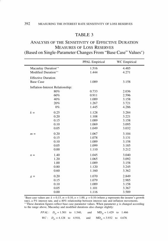
job no. 1969 casualty actuarial society CAS journal 1969D07 [28] 11-08-01 4:58 pm
392 MEASURING THE INTEREST RATE SENSITIVITY OF LOSS RESERVES
TABLE 3
ANALYSIS OF THE SENSITIVITY OF EFFECTIVE DURATIONMEASURES OF LOSS RESERVES
(Based on Single-Parameter Changes From “Base Case” Values')
PPAL Empirical WC Empirical
Macaulay Duration'' 1.516 4.485Modified Duration'' 1.444 4.271
Effective DurationBase Case 1.089 3.158
Inflation-Interest Relationship:80% 0.733 2.03660% 0.911 2.59640% 1.089 3.15820% 1.267 3.7210% 1.445 4.286
k = 0.25 1.128 3.2840.20 1.108 3.2210.15 1.089 3.1580.10 1.069 3.0950.05 1.049 3.032
m = 0.20 1.067 3.1040.15 1.078 3.1310.10 1.089 3.1580.05 1.099 3.1850.00 1.110 3.212
n= 1.40 1.045 3.0401.20 1.065 3.0921.00 1.089 3.1580.80 1.120 3.2450.60 1.160 3.362
g = 0.20 1.070 2.8490.15 1.079 2.9850.10 1.089 3.1580.05 1.101 3.3670.00 1.116 3.589
'Base case values are: k = 0:15, m = 0:10, n = 1:00, g = 0:10 (where g represents the insurer’s growthrate), a 5% interest rate, and a 40% relationship between interest rate and inflation movements.''These duration figures reflect base case parameter values. When parameter g is changed accordingto the range above, Macaulay and modified durations also change slightly:
PPAL : DO= 1:501 to 1:540, and MD
O= 1:429 to 1:466
WC : DO= 4:128 to 4:910, and MD
O= 3:932 to 4:676

job no. 1969 casualty actuarial society CAS journal 1969D07 [29] 11-08-01 4:58 pm
MEASURING THE INTEREST RATE SENSITIVITY OF LOSS RESERVES 393
7. USE OF EFFECTIVE DURATION IN ASSET-LIABILITYMANAGEMENT
In previous sections, the deficiencies of traditional measuresof duration in an inflationary world were identified, and an alter-native measure—effective duration—was described. In this sec-tion, the impact of using effective, as opposed to modified, dura-tion on a company’s asset-liability management process is illus-trated. The example used is a hypothetical workers compensationinsurer; it is assumed that this company has asset and liabilityvalues which are related in a manner consistent with aggregateindustry balance sheet figures.
The effective duration analysis in the prior section concen-trates on loss and allocated loss adjustment expense reserves andrunoffs. A complete asset-liability management analysis wouldalso consider unallocated loss adjustment expenses and unearnedpremium reserves (the timings of which are described in Section3 of this paper). For simplicity, and because they represent a rel-atively small part of an insurer’s liabilities, unallocated loss ad-justment expenses are considered together with losses and ALAEin the illustrative example in this section. However, the reason-ableness of this assumption would need to be evaluated in anyspecific corporate application of asset-liability management.
The duration of the unearned premium reserve was describedin Section 3. The one adjustment that must be made with re-spect to asset-liability management is to only consider the por-tion of the unearned premium reserve (UPR) which is associatedwith future losses and loss adjustment expenses—it is only thisportion which represents a liability for future cash flows whichmay be impacted by inflation. The duration for this portion ofthe UPR is calculated by determining the duration of the lossand LAE reserve for the most recent accident year, and adding0.75. The other portion of the UPR—the “equity” in the UPR—represents prepaid expenses associated with prior writings of in-surance policies, and is essentially an accounting construct which

job no. 1969 casualty actuarial society CAS journal 1969D07 [30] 11-08-01 4:58 pm
394 MEASURING THE INTEREST RATE SENSITIVITY OF LOSS RESERVES
is unrelated to future cash flows. Thus, this portion of the UPRis not considered in the following illustration.
For illustrative purposes, all other liability items on the in-surer’s balance sheet are considered to have a Macaulay durationof 1.0 (and thus, at an interest rate of 5%, a modified durationof 0.952).
The duration of an insurer’s surplus,DS, is as follows (Stakingand Babbel [26]):
DSS =DAA!DLL, (7.1)
where
S = surplus,
D = duration,
A= assets, and
L= liabilities.
In order to immunize its surplus (setting Ds = 0) from interestrate risk,8 an insurer needs to set the duration of its assets asfollows:
DA =DLL
A: (7.2)
Thus, the appropriate determination of the duration of liabilitiesis critical for asset-liability management.
Based on the aggregate industry balance sheet figures for WCinsurers reported in A.M. Best [1], Table 4 shows the liabilitydistribution for an insurer with assets of $1 billion.9 The liability
8In some cases, management would prefer to accept interest rate risk if an adequate returnwere provided for taking this risk. This alternative approach is to balance the generallyhigher returns from a longer term portfolio of assets against the risk of this position.Regardless of whether an insurer is attempting to immunize its portfolio or balance therisk-return trade-off, an accurate measure of duration for assets and liabilities is needed.9Workers compensation insurers tend to have a slightly higher proportion of their liabil-ities in loss and loss adjustment expenses, and a much lower proportion in the unearnedpremium reserve, than other insurers. In applications of this technique, the actual val-ues for these liabilities and the actual relationship between assets and liabilities for thecompany should be used.
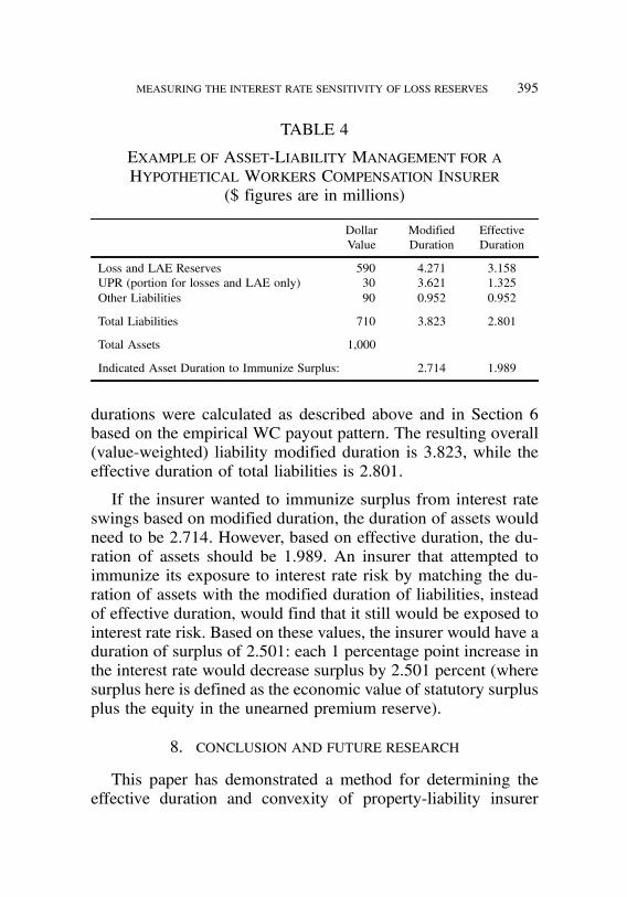
job no. 1969 casualty actuarial society CAS journal 1969D07 [31] 11-08-01 4:58 pm
MEASURING THE INTEREST RATE SENSITIVITY OF LOSS RESERVES 395
TABLE 4
EXAMPLE OF ASSET-LIABILITY MANAGEMENT FOR AHYPOTHETICAL WORKERS COMPENSATION INSURER
($ figures are in millions)
Dollar Modified EffectiveValue Duration Duration
Loss and LAE Reserves 590 4.271 3.158UPR (portion for losses and LAE only) 30 3.621 1.325Other Liabilities 90 0.952 0.952
Total Liabilities 710 3.823 2.801
Total Assets 1,000
Indicated Asset Duration to Immunize Surplus: 2.714 1.989
durations were calculated as described above and in Section 6based on the empirical WC payout pattern. The resulting overall(value-weighted) liability modified duration is 3.823, while theeffective duration of total liabilities is 2.801.
If the insurer wanted to immunize surplus from interest rateswings based on modified duration, the duration of assets wouldneed to be 2.714. However, based on effective duration, the du-ration of assets should be 1.989. An insurer that attempted toimmunize its exposure to interest rate risk by matching the du-ration of assets with the modified duration of liabilities, insteadof effective duration, would find that it still would be exposed tointerest rate risk. Based on these values, the insurer would have aduration of surplus of 2.501: each 1 percentage point increase inthe interest rate would decrease surplus by 2.501 percent (wheresurplus here is defined as the economic value of statutory surplusplus the equity in the unearned premium reserve).
8. CONCLUSION AND FUTURE RESEARCH
This paper has demonstrated a method for determining theeffective duration and convexity of property-liability insurer
job no. 1969 casualty actuarial society CAS journal 1969D07 [32] 11-08-01 4:58 pm
396 MEASURING THE INTEREST RATE SENSITIVITY OF LOSS RESERVES
liabilities, and has provided some general estimates of these val-ues. Based on the results derived, it appears that there can be sig-nificant differences between the traditional measures of duration(i.e., Macaulay and modified duration) and effective duration.Of these measures, only effective duration is capable of properlyaccounting for the impact of inflationary pressures on liabilitycash flows that are associated with potential changes in inter-est rates. This means that effective duration is the appropriatetool for measuring the sensitivity of the liabilities of property-liability insurers to interest rates when performing asset-liabilitymanagement. Use of the wrong duration measure can lead to anunintended mismatch of assets and liabilities, and an unwantedexposure to interest rate risk.
In addition to inflation, interest rate changes may also be cor-related with other financial and economic variables. For exam-ple, a decrease in interest rates is often—on average—associatedwith an increase in stock prices (since the discount rate on fu-ture dividends and capital gains is lower). Similarly, changes ininterest rates in the U.S. may certainly impact international fi-nancial relationships. To the extent to which these other variablesare factors in a jury’s damage award considerations, they mustalso be contemplated in an effective duration framework. Forexample, if the stock market has increased in value significantlybetween the time of an accident and the final jury verdict, a well-structured comment from the plaintiff’s attorney to the jury maylead to a higher award on the grounds that the plaintiff couldhave invested the monies lucratively if they had been availableat the time of the accident.10 These types of issues are beyondthe analytical scope of this paper, and are left for future research.
In this paper, we have approached the measurement of effec-tive duration from the standpoint of a shift in a constant interestrate. Future research should examine the impact of a stochastic
10The appropriate analytical framework in this case may involve option pricing theory—itis possible that the jury award may depend on the maximization of alternatives involvingsuch considerations as inflationary environment, stock market performance, etc.
job no. 1969 casualty actuarial society CAS journal 1969D07 [33] 11-08-01 4:58 pm
MEASURING THE INTEREST RATE SENSITIVITY OF LOSS RESERVES 397
interest rate model on effective duration and asset-liability man-agement. Interesting and important work in the non-insuranceliterature on effective duration, yield curves, and stochastic in-terest rates (e.g., Babbel, Merrill, and Panning [4]) has significantfuture applicability to the issues addressed in this paper. In ad-dition, stochastic interest rate models are beginning to appearin the property-liability insurance industry, especially within thecontext of dynamic financial analysis (D’Arcy and Gorvett, et al[9 and 10]). DFA models can connect underwriting experience,as well as loss development, to stochastically generated interestrate paths. In analyses in which assets are valued according toa stochastic rate assumption, it is appropriate to value liabilitieson the same basis. These will be an important areas for futureresearch.
job no. 1969 casualty actuarial society CAS journal 1969D07 [34] 11-08-01 4:58 pm
398 MEASURING THE INTEREST RATE SENSITIVITY OF LOSS RESERVES
REFERENCES
[1] A.M. Best, Aggregates and Averages, A.M. Best, 1998.
[2] Altman, Edward and Irwin Vanderhoof, The Financial Dy-namics of the Insurance Industry, Irwin, 1995.
[3] Babbel, David, “Asset Liability Matching in the Life In-surance Industry,” The Financial Dynamics of the InsuranceIndustry, Altman and Vanderhoof, Eds., 1995, Chapter 11.
[4] Babbel, David, Craig Merrill and William Panning, “De-fault Risk and the Effective Duration of Bonds,” FinancialAnalysts Journal, Jan./Feb. 1997, pp. 35–44.
[5] Briys, Eric and Francois de Varenne, “On the Risk of LifeInsurance Liabilities: Debunking Some Common Pitfalls,”Journal of Risk and Insurance, 64, 1997, pp. 673–694.
[6] Butsic, Robert, “The Effect of Inflation on Losses and Pre-miums for Property-Liability Insurers,” Inflation Implica-tions for Property-Casualty Insurance, Casualty ActuarialSociety Discussion Paper Program, 1981, pp. 58–102.
[7] Campbell, Frank, “Asset/Liability Management for Prop-erty/Casualty Insurers,” The Handbook of Fixed Income Se-curities, Fabozzi, Ed., 1997, Chapter 51.
[8] D’Arcy, Stephen, “Duration-Discussion,” PCAS LXXI,1984, pp. 8–25.
[9] D’Arcy, Stephen, Richard Gorvett, Joseph Herbers, ThomasHettinger, Steven Lehmann and Michael Miller, “Building aPublic-Access PC-Based DFA Model,” Casualty ActuarialSociety DFA Call Paper Program, 2, Summer 1997, pp. 1–40.
[10] D’Arcy, Stephen, Richard Gorvett, Thomas Hettinger andRobert Walling, “Using the Public-Access DFA Model: ACase Study,” Casualty Actuarial Society DFA Call PaperProgram, Summer 1998, pp. 53–118.
[11] Fabozzi, Frank, Valuation of Fixed Income Securities andDerivatives, Frank J. Fabozzi, Associates, 1995, Chapter 4.
job no. 1969 casualty actuarial society CAS journal 1969D07 [35] 11-08-01 4:58 pm
MEASURING THE INTEREST RATE SENSITIVITY OF LOSS RESERVES 399
[12] Fabozzi, Frank, The Handbook of Fixed Income Securities,McGraw-Hill, 1997.
[13] Fama, Eugene, “Term Structure Forecasts of Interest Rates,Inflation, and Real Returns,” Journal of Monetary Eco-nomics, 25, 1992, pp. 59–76.
[14] Ferguson, Ronald, “Duration,” PCAS LXX, 1983, pp. 265–288.
[15] Ho, Thomas Y., “Key Rate Durations: Measures of InterestRate Risk,” Journal of Fixed Income, September 1992, pp.29–44.
[16] Hodes, Douglas and Sholom Feldblum, “Interest Rate Riskand Capital Requirement for Property/Casualty InsuranceCompanies,” PCAS LXXXIII, 1996, pp. 490–562.
[17] Ibbotson Associates, Stocks, Bonds, Bills, and Inflation:1996 Yearbook, Chicago, IL: Ibbotson Associates, 1996.
[18] Klaffky, Thomas E., Y. Y. Ma and Ardavan Nozari, “Man-aging Yield Curve Exposure: Introducing Reshaping Dura-tions,” Journal of Fixed Income, December 1992, pp.1–15.
[19] Litterman, Robert and Jose A. Scheinkman, “Common Fac-tors Affecting Bond Returns,” Journal of Fixed Income, 1,1991, pp. 54–61.
[20] Macaulay, Frederick, Some Theoretical Problems Suggestedby the Movement of Interest Rates, Bond Yields, and StockPrices since 1856, National Bureau of Research, 1938.
[21] Masterson, Norton, “Economic Factors in Liability andProperty Insurance Claims Costs,” Best’s Insurance News,October 1968, pp. 12–18 (subsequent updates publishedperiodically in Best’s Review).
[22] Mishkin, Frederic, “The Information in the Longer MaturityTerm Structure About Future Inflation,” Quarterly Journalof Economics, 1990, pp. 815–828.
[23] Noris, P. D., Asset/Liability Management Strategies for Prop-erty and Casualty Companies, Morgan Stanley, 1985.
job no. 1969 casualty actuarial society CAS journal 1969D07 [36] 11-08-01 4:58 pm
400 MEASURING THE INTEREST RATE SENSITIVITY OF LOSS RESERVES
[24] Panning, William, “Asset-Liability Management for a Go-ing Concern,” The Financial Dynamics of the Insurance In-dustry, Altman and Vanderhoof, Eds., 1995, Chapter 12.
[25] Reitano, Robert R., “Non-Parallel Yield Curve Shifts andImmunization,” Journal of Portfolio Management, Spring1992, pp. 36–43.
[26] Staking, Kim and David Babbel, “The Relation BetweenCapital Structure, Interest Rate Sensitivity, and MarketValue in the Property-Liability Insurance Industry,” Jour-nal of Risk and Insurance, 62, 1995, pp. 690–718.
[27] Taylor, Gregory, Claim Reserving in Non-Life Insurance,North-Holland Press, 1986.
[28] Tilley, James A., “The Application of Modern Techniquesto the Investment of Insurance and Pension Funds,” Inter-national Congress of Actuaries, 1988.

job no. 1969 casualty actuarial society CAS journal 1969NOV [1] 11-08-01 4:58 pm
ADDRESS TO NEW MEMBERS—NOVEMBER 13, 2000
CHARLES C. HEWITT JR.
In preparing for this talk, I asked myself the question, “Is itrealistic for a person my age and so long away from actuarialwork to be giving advice to the successful young people whoare here this morning?”
I think not!
An axiom by which many of us “older statesmen” live is: “Ifyou have a question about your personal computer or the Inter-net, call the grandchildren.” However, there is a subject aboutwhich I have come to know a great deal: “What is it like to growold?”
Growing Old
Recently my wife has been making a novena. For the benefitof non-Catholics, a novena is a series of nine church serviceswhere each attendee has an intention. The intention is a wish orprayer that something will or will not happen.
Coming out of the service one day she recognized an ex-tremely elderly man and nodded to him. They struck up a conver-sation and at one point she said to him, “What is your intentionfor this novena?”
He replied as follows: “Recently I’ve heard that medical sci-ence may reach the time in this century when people will live tobe two hundred years old! I am asking the Lord, ‘Please do notlet me live beyond one hundred thirty!”’
Growing old is a boring subject to many. However, if you’regoing to live to 200 it’s still important. I’ll try to touch on itlightly.
First the bad news. Any knowledgeable physician will tellyou that the aging process, in many ways, reverses the growthprocess. Aptitudes that you acquired as a child growing up will
401

job no. 1969 casualty actuarial society CAS journal 1969NOV [2] 11-08-01 4:58 pm
402 ADDRESS TO NEW MEMBERS
weaken or disappear—both the physical and the mental and eventhe emotional. I’ll give you an example from my own experience.
In earlier years I was blessed with “instant recall.” So much sothat I actually qualified for and appeared on one of the ill-fatedTV quiz shows in the late fifties. And thereby hangs a tale.
When I was much younger and I did have instant recall, mymother-in-law persuaded me to go on the quiz show 21. This isthe one in which a contestant, Charles Van Doren, was fed theanswers and, when caught, lied about it to a grand jury and wasconvicted of perjury as a result.
My part in all of this was insignificant. I lost in my very firstturn to a woman named Elfrida Von Nardroff.
Shortly afterward I was sent as a consultant by Bowles, An-drews and Towne (a predecessor to Tillinghast) to Saudi Arabia.The Arabian-American Oil Company had requested a study ofworkmen’s compensation rates there.
While I was in Saudi Arabia, the quiz-show scandal broke.(As some of you may remember, a movie was made about thiswhole matter.)
The New York Daily News decided to do a follow-up with allof the contestants to see who else, if anyone, had been preppedwith answers before the show. My wife took the phone call fromthe Daily News, and explained that I was not home because myfirm had sent me to Saudi Arabia on a consulting job.
The following day the Daily News reported in essense that “wetried to reach Mr. Hewitt about this scandal but he had alreadyleft the country!”
Today I find that the “iters”—passages in the brain—do notalways respond as quickly as they used to. I’m not talking aboutmemory loss; my memory will ultimately respond. The bit ofmemory is still there—the forgetfulness is only temporary. InFlorida we call this having a “senior moment” but it is very

job no. 1969 casualty actuarial society CAS journal 1969NOV [3] 11-08-01 4:58 pm
ADDRESS TO NEW MEMBERS 403
common among older persons. Furthermore, I don’t listen “asfast” as I used to, and I’m not referring to hearing loss. Thathappens too.
Now the good news, growing old is not all bad. First thereis something called grandchildren and even great-grandchildren,who somehow manage to bring one pure joy.
Next there is the ability to look at one’s grown-up children—adult sons and daughters—and realize that the thing most re-sponsible for their well-being and self-assurance is the love thatthey received from their mother. Do you realize what a powerfulforce love is in this world of ours?
And, next to love, the most important thing we give to ourchildren is discipline. And I’m not talking about physical punish-ment. Discipline, properly exercised, promotes self-control. Andonce one achieves self-control, self-assurance follows. Don’t takemy word for it. This comes straight from the modern Dr. Spock,Dr. Berry Brazelton, who, incidentally, happens to be a collegeclassmate.
Enough about “old people”!
Pursuit of Excellence
Instead of advice, I’m going to issue to you two challenges.The first challenge has to do with the “pursuit of excellence”and is chosen because of the fact that our principal speaker thismorning is George Will.
George knows about excellence and the pursuit thereof. Infact, he has written a book about it entitled Men at Work. Thebook is about the game of baseball and those who play it orcoach.
Now, the pursuit of excellence has a handmaiden, and it isPREPARATION, PREPARATION, PREPARATION! Ask anysuccessful courtroom lawyer what the secret of trial work is andhe will tell you it is “preparation”. Ask any successful football

job no. 1969 casualty actuarial society CAS journal 1969NOV [4] 11-08-01 4:58 pm
404 ADDRESS TO NEW MEMBERS
coach how he expects to win next week’s game, and he will giveyou the same answer. There is no substitute for preparation un-less it is raw talent and, if you are blessed with raw talent, so be it!
But why am I telling you, today’s honorees, this? It was prepa-ration for exams that got you here today, unless you are one whois blessed with raw talent. If so, will you please stand and be rec-ognized.
Excellence is hard to define, but like the Supreme Court jus-tice said about pornography, you’ll know it when you see it.Every so often I see a tape of the great athlete, Wilma Rudolph,winning the Olympic 100-meter dash by more than ten meters.The hair on the back of my neck stands on end every time!
If you’re looking for nonsports-related evidence, try Sir AlecGuiness in The Bridge on the River Kwai or the less familiar Tunesof Glory. Or, how about Sir John Gielgud in anything!
In recent years we have been blessed with people like MichaelJordan and Tiger Woods. Are you thinking to yourself, “rawtalent”? Maybe so, but then why does Tiger spend two hourson the practice range after shooting a 66? Or, why does PeteSampras wonder howMichael Jordan got himself up emotionallyfor every game?
My first challenge today is that you continue to pursue excel-lence in your actuarial careers. That means, among other things,not accepting an important assignment without the determinationand the will to prepare yourselves fully for the task.
Planting of Trees (An Allegory)
My second challenge to you graduates is in the form of anallegory having to do with the planting of trees.
There is an old Greek proverb that says: “A society growsgreat when old men plant trees in whose shade they will neversit.”

job no. 1969 casualty actuarial society CAS journal 1969NOV [5] 11-08-01 4:58 pm
ADDRESS TO NEW MEMBERS 405
I will repeat: “A society grows great when old men plant treesin whose shade they will never sit.”
Now think about that one in a world in which the businessexecutive asks, “What have you done for me lately?” Or wherethe media deals in “thirty second sound bites.” Or where politi-cians govern by yesterday’s poll results. Or where the generalpublic asks to be entertained rather than to be informed. In theearly part of the twentieth century, the British historian, ArnoldToynbee, suggested that we are in the declining period of our civ-ilization. He pointed to the similarities between our own timesand ancient Rome with its circuses with gladiatorial combats,Christians being thrown to the lions, and other forms of whatwas then entertainment by public spectacle. What would Toyn-bee have thought about World Championship Wrestling or JerrySpringer?
I repeat: “A society grows great when old men plant trees inwhose shade they will never sit.”
Recently I found this proverb in the valedictory address givenin May of this year by a graduating senior at a well-known liberalarts university. I want to share a small portion of the valedicto-rian’s effort with you.
Now, in a sense, what we have here today is a graduation so,with a stretch, I will be your valedictorian.
As I speak from my platform you are seated on a large lawnin front of the administration building. I call your attention toour surroundings—handsome academic buildings and beautifulold trees. I point to the dean’s house.
Behind that house over there are two of the oldest trees oncampus. They were planted in 1766 to commemorate the repealby the British of the Stamp Act.
I was so taken with the beauty of our campus that I becameinterested in the care of the trees on campus and investigated the“tree situation.” I found that maintenance required a staff of 20

job no. 1969 casualty actuarial society CAS journal 1969NOV [6] 11-08-01 4:58 pm
406 ADDRESS TO NEW MEMBERS
groundsworkers and two full-time arborists. I worried about whatspecial steps were taken in times of drought and was told that,because the older trees have deeper roots and can draw waterfrom well below the surface, it was the young trees that werenurtured by whatever water was available. There we now havean allegory within an allegory!
And now comes the exhortation to your graduates.
With all that you have been given, now is the time to rise andto give of yourselves. It is only fitting at the moment of yourglory to thank all of those who have “nurtured” you through-out your whole lives—your parents, for their endless love andinspiration; your teachers (at every level of your education), fortheir willingness to cultivate your minds; your spouses or otherspecial persons who have encouraged you in your dreams and inyour preparation for this day by forgiving the many hours spentaway from them in that preparation; and finally, the “old men”who have gone before and who are not here any longer to joinyou and me in the shade in which we are living.
Now, I break the spell and remove my imaginary mortarboardand tell you that the young person who gave that address was anengineering major. Amazing!
So my second challenge is this: That some time during yourcareers or your lifetimes, you will stop and, figuratively speak-ing, plant a tree under whose shade you will never sit.
So I congratulate all of you and your families upon the ac-complishment being recognized today.
I can assure you that for the balance of your lives you willlook back on this accomplishment as one for which you willalways be proud!
Thank you for allowing an old actuary to be part of this cel-ebration.

job no. 1969 casualty actuarial society CAS journal 1969PRES [1] 11-08-01 4:58 pm
PRESIDENTIAL ADDRESS—NOVEMBER 13, 2000
THE MAIN THING
ALICE H. GANNON
“In any endeavor, the main thing is to keep the main thing themain thing. But you can’t keep the main thing the main thingif you don’t know what the main thing is.” Steve Goldberg, myfriend and colleague of 25 years and my boss for the last 11years, shared these words of wisdom with me shortly after heheard them at the opening ceremony of Black History Month atUSAA many years ago. They were the theme of the speech bythe featured speaker, an educator from Colorado, whose name isunfortunately long forgotten.
I believe these words to be true, both with regard to the focusthat should be given to one’s primary goal or objective and tothe importance of knowing what that goal or objective is. Whileit is possible for undirected activity to accidentally lead to a de-sired result, we are much more likely to achieve what we wantto achieve when we know what that is and work deliberatelytoward it.
I began my preparation for this, my presidential address, byreading a number of CAS documents. I read the original and cur-rent CAS constitution and bylaws. I read for the second dozenthtime this year our current strategic plan. I read the three historicalaccounts of the CAS: “The First 25 Years” written by FrancisPerryman; “The First 50 Years” written by Dudley Pruitt; and“The First 75 Years” written by Stanley Hughey. Following thetradition of many CAS presidents, I read about three dozen orso presidential addresses from prior years. I then reflected onwhat I had read in light of my experiences serving as presi-dent of the CAS—a job, which, at least for someone as inef-ficient as I am, entails spending part of every day, seven daysa week, working on or worrying about some CAS activity orissue.
407
job no. 1969 casualty actuarial society CAS journal 1969PRES [2] 11-08-01 4:58 pm
408 PRESIDENTIAL ADDRESS
I came to three major conclusions about the CAS. (ActuallyI came to a lot of conclusions about the CAS but only three thatI want to share with you today.) The first two concern our pastand the third our future. My first conclusion is that the CAS hasenjoyed a remarkable record of success throughout our 86-yearhistory. I will not take the time to provide even a partial listof the accomplishments that lead me to that conclusion. Any ofyou who doubt it should read the documents I named, and I amconfident that your conclusion will be the same as mine. In fact,I would encourage all members of the CAS to try to find time toread the historical accounts of the CAS. You will be impressedeither once again or for the first time by how rich a legacy wehave inherited. All of us can take great pride in being members ofan organization that has made so many contributions to actuarialscience, to the actuarial profession, to employers and clients ofactuaries, and to the public. We indeed have a heritage worthcelebrating!
My second conclusion is that an essential contributor to theCAS’s success has been that throughout those 86 years, the CAShas maintained an understanding of its purpose and has kept thatpurpose largely at the forefront of its planning and its activities.There has always been a statement of purpose in our constitution.What is really important, however, is that a large number of ac-tive CAS members have frequently engaged in discussion aboutthe meaning and implications of the CAS’s purpose, such that,despite linguistical limitations, the CAS’s purpose as an organi-zation has been well understood by most of the active members.In turn the leaders and volunteers of the CAS have, for the mostpart, maintained focus on that well-understood and accepted pur-pose as strategic directions have been debated and activities havebeen planned and carried out. In other words, for 86 years theCAS has known what its main thing is and has kept its mainthing the main thing.
Now my third conclusion, the one most relevant to us today,is that in recent years it has become more difficult for the CAS

job no. 1969 casualty actuarial society CAS journal 1969PRES [3] 11-08-01 4:58 pm
PRESIDENTIAL ADDRESS 409
to know and understand its purpose and keep that purpose asthe focus for our activities. And it will be even more difficult inthe years ahead. Knowing and keeping the main thing the mainthing will be as important to our continued success as it has beeninstrumental to the achievement of our past success. It is goingto be more difficult to do than ever before, however. I believe wemust become deliberate about keeping our purpose known andunderstood among our membership and very deliberate aboutkeeping it in focus as we carry out our work as a society.
Now let me be clear that I do not advocate that the CASforever cling to its current purpose. The CAS has very wiselythrough the years revised and expanded both the written state-ment of its purpose and its understanding of what that writtenstatement means. While strongly rooted in our origins, the CASis nevertheless not only a different organization today than whatit was in 1914, but it is much different and broader in scope thanwhat our visionary founders ever imagined it would become. Itwill be important for us and those who follow us to continue toexplore new applications and opportunities for our science andour profession. To paraphrase a statement from Bob Anker’s ad-dress: Change is our friend and we should embrace it. We should(forgive the cliches) push ourselves to think outside the box, tobreak down old paradigms, and to boldly go where no actuaryhas gone before! To do so effectively we must do so within thecontext of knowing who we are and what our current purposeand capabilities are, so that we can make well-considered andconscious changes to our direction when they are appropriate.
I am reminded of a discussion at a Board meeting earlier thisyear. I forget which agenda item we were on but, as is some-times the case at Board meetings, we had wandered off into adiscussion of whether we should launch a marketing campaignto convince employers and potential employers of all the won-derful skills and abilities actuaries possess, which the employersshould use to address a far greater range of business problemsthan what is currently the case. We perhaps got a little carried

job no. 1969 casualty actuarial society CAS journal 1969PRES [4] 11-08-01 4:58 pm
410 PRESIDENTIAL ADDRESS
away in our description of actuarial abilities. At one point SteveLowe spoke up and provided us with a reality check. He pointedout that a dog who tries to convince someone else that he is acat will probably only convince them that he is a foolish dog. Atthat point we got back to our agenda item.
So why do I think that it is getting increasingly difficult toknow our purpose and keep it at the center of our activities? Inpart it is a function of the growth in the size and diversity of ourmembership. There were 97 charter members of the CAS. Todaywe have almost 3,500 members and are adding about 200 newmembers a year.
In 1914 the members of the CAS were all men, 60 percent hada business address in New York City and another 20 percent inConnecticut or Massachusetts. Only six had an address west ofthe Mississippi. None had an address outside the U.S. As best Ican tell they all seemed to work directly for or with the insuranceindustry in some way.
Today a sizeable portion of our members are women andwe are much more geographically diverse. We have a signifi-cant number of members who live outside the U.S., particularlyCanada, but a growing number of members who live outside ofNorth America as well. While the insurance industry still domi-nates our members’ business activities, there is a growing numberof members who are spending at least part of their time workingon other than insurance matters.
The larger we become and the more diverse our membership,the more difficult it is to conduct the kind of communicationnecessary to achieve an ongoing consensus understanding of ourpurpose, especially as that purpose evolves. How to keep a fullrange of input from our diverse members as part of the evolu-tion of our purpose, and how to keep the majority of our mem-bers aware of and accepting of our evolving purpose will be achallenge that grows as our membership grows in numbers anddiversity.
job no. 1969 casualty actuarial society CAS journal 1969PRES [5] 11-08-01 4:58 pm
PRESIDENTIAL ADDRESS 411
There is also another reason why I believe it will be increas-ingly difficult for us to know and understand our purpose andkeep it the focal point of our activities. During the last 86 years,our purpose has grown in scope and in complexity. I believe thatis a trend that will continue. The broader and more complex ourpurpose becomes, the harder it will be to keep it defined and wellunderstood by even a small homogeneous group, let alone themembership as a whole. Thus, it will be harder for our volunteersto keep our purpose the focal point of activities.
Let me elaborate for a moment on two areas in which theCAS’s role is currently evolving and which potentially adds bothbreadth and complexity to our purpose—nontraditional practiceareas and globalization.
In 1999 the Task Force on Nontraditional Practice Areas ad-dressed the issue of how the CAS can better support its memberswho are currently working or who wish to work in nontraditionalpractice areas. Their excellent report was completed in Septem-ber 1999 and is available on the CAS web site. As a result oftheir work we have launched four new advisory committees thatwill help identify and direct significant new activity for the CASin nontraditional practice areas. I believe that the action the CAShas taken so far is very consistent with the CAS’s purpose state-ment as it currently exists and is understood by the majority ofour members. I had to give it some careful thought at the time,but I believe that these new activities are within the scope of “ac-tuarial science as applied to property, casualty and similar riskexposures.” However, with this step I believe we are headed in adirection that will ultimately challenge our current understandingof the definition of “similar risk exposures.”
In the background section of the task force’s report there isa discussion of the issue of defining “nontraditional practice ar-eas.” The task force reported that after some attempt to do so,they finally agreed that they would not define the term as itwas not critical to their charge. In fact they found that it is very
job no. 1969 casualty actuarial society CAS journal 1969PRES [6] 11-08-01 4:58 pm
412 PRESIDENTIAL ADDRESS
difficult to define “nontraditional practice area.” Some of the dif-ficulty is over what is traditional versus nontraditional. However,difficulty also arises over what falls within the scope of casualtyactuarial practice and what does not. What potential practice ar-eas are consistent with the purpose of the CAS and what practiceareas are not? That question becomes more complex as we movefurther away from the insurance context that was our historicalfocus.
Likewise, as the CAS tries to develop a clearer vision of itsrole in the worldwide actuarial profession, we are likely to con-front further complexity in defining our purpose. It took decadesfor the CAS to change from an organization whose purpose wassolely focused on the U.S. casualty actuary to one that also fo-cuses on the Canadian casualty actuary. I could not determinewhen the CAS first admitted a Canadian to membership, butI know it was long before 1987, the first year that the CAS’sexam syllabus differentiated U.S. and Canadian specialties. Go-ing from a U.S.-only organization to a U.S./Canadian organi-zation certainly increased the complexity of our mission. Eventoday we struggle with how best to support the needs of casualtyactuaries in both countries. Despite the complications involved,I think it has been highly beneficial for all parties for the CAS tobecome the learned body for casualty actuaries in both the U.S.and Canada. It was clearly the right thing to do despite the com-plication added to our purpose. Likewise, I strongly believe thatthe CAS should develop a significant and active role within theworldwide actuarial profession. We have so much to offer andthere is such a tremendous need for our knowledge and skillsin so many other countries. We are also observing that moreand more of the current CAS members’ employers and clientshave business interests in several countries, a trend that seemsinevitable to continue. Therefore, to best support even our U.S.and Canadian members properly, the CAS will need to developand maintain a prominent worldwide position in the profession.Yes, I think the CAS needs to be involved globally. But the addedcomplexity of that should not be underestimated.

job no. 1969 casualty actuarial society CAS journal 1969PRES [7] 11-08-01 4:58 pm
PRESIDENTIAL ADDRESS 413
And so as my term as president comes to an end, my advice toall future leaders of the CAS is to be mindful of the importanceof keeping the CAS’s purpose defined and well understood bythe membership, and keeping that purpose at the center of theCAS’s activities.
As the CAS moves into the new millennium (I had to workin a new millennium reference somewhere), it does so withconfidence and with purpose. We have an impressive recordof achievement to build upon. We have a current solid under-standing of our mission. And we have a wealth of commit-ted and capable volunteers dedicated to achieving that mission.I envision a CAS in the year 2086 that is even stronger andmore successful than the CAS of today. And I envision thatthe CAS president of 2086 will be able to say what I havesaid today. The CAS is an organization that has always knownwhat its main thing is and has kept the main thing the mainthing.
Now before I step down from the podium I would like spenda few more moments expressing my gratitude to a number ofpeople.
First I want to thank the Executive Council (EC). Pat, GaryDean, Abbe, Dave, Gary Josephson, LeRoy, and Mary Frances,you have all worked incredibly hard this past year on behalf ofall CAS members. You are outstanding examples of what servantleadership is all about. Thank you for your service.
Thanks also to the CAS Board of Directors. Many CAS mem-bers may not know how hard our Board works. They don’t justget together four times a year to rubberstamp whatever the ECputs before them. They spend significant time and energy devel-oping and debating all the policies and strategic direction of theCAS. As a Board they have been pretty tough on the EC thisyear, holding our feet to the fire. But as individuals they have allpitched in to help time and time again. They are a great groupof CAS volunteers and leaders.
job no. 1969 casualty actuarial society CAS journal 1969PRES [8] 11-08-01 4:58 pm
414 PRESIDENTIAL ADDRESS
I, of course, need to thank the hundreds of CAS memberswho have worked on committees, spoken at CAS seminars ormeetings, conducted research and wrote papers, or who servedthe CAS in some other way. I cannot name you all today but youknow who you are and you are indeed the heart and soul of theCAS.
Earlier today I recognized and thanked the CAS staff membersbut there is one staff member that I must mention again—TimTinsley, our outstanding executive director. There are not wordsfine enough to describe Tim Tinsley. He is intelligent, highly or-ganized, hard working, diplomatic, thorough, patient, cool underpressure, and I could go on and on. The CAS owes him ourthanks and appreciation. I also owe Tim my personal thanks. Inhis quiet but firm way, he kept me on track this past year and onschedule. He often made me look more prepared and in controlthan I really was, and he never failed to provide me wise councilwhen I was smart enough to ask for it. He has become not only ahighly respected colleague but a dear, dear friend as well. Thankyou, Tim.
If you will bear with me a few more moments I have a fewother personal thanks to offer. To my outstanding executive assis-tant, Debbie Seales, who is here with me today. She has enduredmuch from me this last year and has been invaluable in helpingme juggle my CAS responsibilities with my paid employmentresponsibilities. Thank you, Debbie. I am also grateful to myboss, Steve Goldberg, for his patience and support and to fouractuaries in my department at USAA who covered for me manytimes this past year when I was out on CAS business: Cather-ine Taylor, Rhonda Aikens, Geoff Werner and Tim Ungashick.Thanks for all your help.
I also need to thank some individuals whose advice on CASmatters was invaluable and whose encouragement often helpedme over the rough spots. Thanks to Mavis Walters who neverlet me forget it’s supposed to be fun to be the president ofthe CAS—and there were times I needed reminding. Thanks to

job no. 1969 casualty actuarial society CAS journal 1969PRES [9] 11-08-01 4:58 pm
PRESIDENTIAL ADDRESS 415
Chuck Bryan, Bob Anker, Jerry Degerness, Gail Ross, John Kol-lar, Pat Grannan, Mike Toothman, Dave Hartman, and so manyothers who provided me with great advice and assistance. Whatwould I have done without you?
And thanks to my wonderful family. To my beloved husband,David, and to the two best children a mother could have, Andrewand Zoe. This past year they were often without a wife and amother but they never complained and were always supportive.Now if I can just figure out how to get them to keep doing allthe laundry and other household chores I used to share in.
And finally thanks to God and thanks to all CAS memberswho gave me the opportunity to serve as president of the CAS.It has been such an honor and a privilege and an experience Iwill always cherish. Thank you very much.
October 30, 2001 11:49 AM 69novmin.qxd
MINUTES OF THE 2000 CAS ANNUAL MEETING
November 12–15, 2000
JW MARRIOTT
WASHINGTON, D.C.
Sunday, November 12, 2000
The Board of Directors held their regular quarterly meetingfrom 9:00 a.m. to 5:00 p.m.
Registration was held from 4:00 p.m. to 6:00 p.m.
From 5:30 p.m. to 6:30 p.m., there was a special presentation tonew Associates and their guests. All 2000 CAS Executive Councilmembers briefly discussed their roles in the Society with the newmembers. In addition, Steven G. Lehmann, who is a past presidentof the CAS, gave a short talk on the American Academy of Actu-aries’ (AAA) Casualty Practice Council.
A welcome reception for all members and guests was held from6:30 p.m. to 7:30 p.m.
Monday, November 13, 2000
Registration continued from 7:00 a.m. to 8:00 a.m.
CAS President Alice H. Gannon opened the business session at8:00 a.m. and introduced members of the Executive Council andthe CAS Board of Directors. Ms. Gannon also recognized pastpresidents of the CAS who were in attendance at the meeting, in-cluding: Robert A. Anker (1996), Phillip N. Ben-Zvi (1985),Ronald L. Bornhuetter (1975), Charles A. Bryan (1990), MichaelFusco (1989), David G. Hartman (1987), Charles C. Hewitt Jr.(1972), Frederick W. Kilbourne (1982), Steven G. Lehmann(1998), Michael L. Toothman (1991), Mavis A. Walters (1997),and Michael A. Walters (1986).
416

MINUTES OF THE 2000 CAS ANNUAL MEETING 417
Ms. Gannon also recognized special guests in the audience:Robert L. Brown, president of the Society of Actuaries; KennethA. Kent, president-elect of the Conference of Consulting Actuar-ies; W. James MacGinnitie, president-elect of the Society of Actu-aries; and David J. Oakden, president of the Canadian Institute ofActuaries.
Ms. Gannon then announced the results of the CAS elections.The next president will be Patrick J. Grannan, and the president-elect will be Robert F. Conger. Members of the CAS ExecutiveCouncil for 2000–2001 will be: Sheldon Rosenberg, Vice Presi-dent–Administration; Mary Frances Miller, Vice President–Ad-missions; Abbe Sohne Bensimon, Vice President–ContinuingEducation; LeRoy A. Boison, Vice President–International; DavidR. Chernick, Vice President–Programs and Communication; andGary R. Josephson, Vice President–Research and Development.New members of the CAS Board of Directors are Ralph S. Blan-chard III, Janet L. Fagan, Michael J. Miller, and Deborah M.Rosenberg.
Curtis Gary Dean announced the 33 new Associates and PatrickJ. Grannan announced the 134 new Fellows. The names of theseindividuals follow.
NEW FELLOWS
October 30, 2001 11:49 AM 69novmin.qxd
John Scott AlexanderMichele S. ArndtCarl Xavier
AshenbrennerDavid Steen AtkinsonEmmanuil Theodore
BardisMichael William
BarlowKeith M. BarnesPatrick BeaudoinNicolas BeaupreAndrew S. Becker
Michael J. BluzerSherri Lynn BorderVeronique BouchardErik R. BouvinTobe E. BradleyRobert F. BrownHugh E. BurgessAllison F. CarpJoseph G. CerretaPatrick J. CharlesKin Lun (Victor) ChoiAndrew K. ChuKuei-Hsia Ruth Chu
Wei ChuangSteven A. CohenLarry Kevin ConleeKathleen T.
CunninghamMary Elizabeth
CunninghamJonathan Scott CurleeLoren Rainard
DanielsonKris D. DeFrainMichael Brad DelvauxSean R. Devlin

418 MINUTES OF THE 2000 CAS ANNUAL MEETING
Tammi B. DulbergerLouis DurocherSophie DuvalKevin M. DykeJane EichmannGregory James EnglVicki A. FendleyKenneth D. FikesChauncey E. FleetwoodHugo FortinRonnie Samuel FowlerNoelle C. FriesSusan I. GildeaTodd Bennett GlassmanSanjay GodhwaniRebecca N. HaiKenneth Jay HammellAlex A. HammettMichelle Lynne
HarnickJeffery Tim HayQing HeAmy Louise HicksJay T. HiebAmy L. HoffmanTodd Harrison HoivikNancy Michelle HoppeWalter L. JedziniakCharles B. JinPhilippe JodinLori E. JulgaElina L. KoganskiClaudia A. KrucherChingyee Teresa LamTravis J. LappeRobin M. LaPreteLewis Y. Lee
Neal M. LeibowitzCharles LetourneauDengxing LinShu C. LinMichelle LuneauAndrea Wynne MalyonIan John McCrackenAin MilnerPaul D. MiotkeBenoit MorissetteKari S. MrazekKevin T. MurphySeth Wayne MyersKari A. NicholsonMihaela Luminita
O’LearyRichard A. OlsenRichard D. OlsenRebecca Ruth OrsiNathalie OuelletMichael G. OwenMark PaykinJulie PerronChristopher Kent PerryDaniel B. PerryAnthony George
PhillipsRichard Matthew
PilotteGlen-Roberts
PitruzzelloIgor PogrebinskyGregory J. PoirierRicardo A. RamotarChristopher David
RandallLeonid Rasin
Peter S. RaunerEllen J. ResplerRebecca L. RoeverDavid A. RosenzweigRomel G. SalamJames C. SantoJason Thomas SashStuart A. SchweidelWilliam Harold
Scully IIIErnest C. SegalChristopher M.
SteinbachCarol A. StevensonRoman SvirskyKarrie Lynn SwansonChester J. SzczepanskiVarsha A. TantriJonathan Garrett TaylorMichael J. TempestaRobert M. ThomasMichael J. TothMichael C. TranfagliaLaura M. TurnerKieh Tsung TyMartin VezinaNathan K. VoorhisClaude A. WagnerWilliam B. WestrateJerelyn S. WilliamsKendall P. WilliamsLaura Markham
WilliamsBrandon L. WolfJonathan Stanger
WoodruffYuhong Yang
October 30, 2001 11:49 AM 69novmin.qxd

MINUTES OF THE 2000 CAS ANNUAL MEETING 419
NEW ASSOCIATES
October 30, 2001 11:49 AM 69novmin.qxd
Katherine H. AntonelloMaura Curran BakerJeremy T. BensonNeil M. BodoffPeter R. DeMallieWilliam M. FinnDustin W. GaryAmy L. GebauerPatrick J. GilhoolMark D. HeyneKurt D. HinesPatricia A. Hladun
Derek R. HoymeCraig D. IsaacsGregory K. JonesSean M. KennedyDavid R. KennerudSusanlisa KesslerJing LiuKathleen T. LogueJulie MartineauJames J. Matusiak Jr.John R. McColloughRodney S. Morris
Brian C. NeitzelSean R. NimmSylvain NoletRodrick R. OsbornChristopher S.
ThrockmortonMark A. VerheyenShaun S. WangYa-Feng WangEric Zlochevsky
Ms. Gannon then introduced Charles C. Hewitt Jr., a past presi-dent of the Society, who presented the Address to New Members.
Following the address, David R. Chernick, Vice President–Programs and Communications, briefly highlighted the meeting’sprograms and thanked the CAS Program Planning Committee.Mr. Chernick then introduced John M. Kulik, Vice Chairperson ofthe CAS Committee on Review of Papers, who announced thattwo Proceedings papers would be presented at this meeting.
Mr. Kulik began the awards program by announcing that the2000 Woodward-Fondiller Prize was given to Stephen J. Milden-hall for his discussion of “Application of the Option Market Para-digm to the Solution of Insurance Problems” by Michael G.Wacek. Mr. Kulik then introduced LeRoy A. Boison, Vice Presi-dent–International, who presented the 2000 Charles A.Hachemeister Award to Uwe Schmock for his paper, “Estimatingthe Value of the WINCAT Coupons of the Winterthur InsuranceConvertible Bond: A Study of the Model Risk.” Mr. Mildenhall’spaper is published in this edition of the Proceedings. Mr.Schmock’s paper is published in the ASTIN Bulletin.

420 MINUTES OF THE 2000 CAS ANNUAL MEETING
Ms. Gannon presented the 2000 CAS Matthew S. RodermundService Award to Charles F. Cook, who was chosen for his out-standing contributions to the actuarial profession.
Ms. Gannon then requested a moment of silence in honor ofthose CAS members who passed away since November 1999.They are: J. Edward Faust Jr., Olaf E. Hagen, Phillip B. Kates,Paul S. Liscord Jr., Thomas E. Murrin, John H. Rowell, Irwin T.Vanderhoof, and James M. Woolery.
In a final item of business, Ms. Gannon acknowledged a dona-tion of $10,000 from D.W. Simpson & Company to the CAS Trust(CAST). The donation was made October 13, 2000.
Ms. Gannon then concluded the business session of the AnnualMeeting and introduced the featured speaker, George Will. Mr.Will is one of America’s leading political observers and is seenweekly on ABC’s This Week and read nationally in Newsweek andin his syndicated newspaper columns.
After a refreshment break, the first General Session was heldfrom 10:45 a.m. to 12:15 p.m.:
“Product Distribution in a Changing Business Environment”Moderator: Charles A. Bryan
Senior Vice President–Chief ActuaryNationwide Insurance Company
Panelists: Mark BensonExecutive Vice PresidentCybercompMark CisVice President, Strategy DevelopmentCUNA Mutual GroupSteven L. GrootPresidentAllstate International
October 30, 2001 11:49 AM 69novmin.qxd

MINUTES OF THE 2000 CAS ANNUAL MEETING 421
Waymon L. LynchAgency OwnerNationwide Insurance Company
Following the general session, CAS President Alice H. Gannongave her Presidential Address at the luncheon. At the luncheon’send, Ms. Gannon officially passed on the CAS presidential gavelto the new CAS president, Patrick J. Grannan.
After the luncheon, the afternoon was devoted to presentationsof concurrent sessions. The panel presentations from 1:30 p.m. to3:00 p.m. covered the following topics:
1. New Classes of Claims/Megatort UpdateModerator: Jennifer L. Biggs
Consulting ActuaryTillinghast-Towers Perrin
Panelists: Philip D. MillerConsulting ActuaryTillinghast-Towers PerrinBarbara K. MurrayAssistant Vice PresidentArgonaut Insurance Company
2. Emerging Nontraditional Products—Loss Mitigation Underwriting, Reps, and WarrantiesModerator/ Gary BlumsohnPanelist: Vice President
St. Paul RePanelists: Chris E. Nelson
Vice PresidentCNA ReMarvin PestcoeHead of Actuarial ServicesSwiss Re New Markets
October 30, 2001 11:49 AM 69novmin.qxd

422 MINUTES OF THE 2000 CAS ANNUAL MEETING
3. Non-U.S. DFA: Are They Doing That Too?Moderator: Susan E. Witcraft
Consulting ActuaryMilliman & Robertson, Inc.
Panelist: Stavros ChristofidesConsultantBacon & Woodrow
4. The Actuary’s Role in Due DiligenceModerator: Stuart G. Sadwin
Vice President & ActuaryCGU Insurance Companies
Panelists: Gayle E. HaskellChief Financial Officer and Chief ActuaryProvidence Washington Insurance CompanyGail M. RossVice PresidentAm-Re Consultants
5. Actuaries in an e-WorldModerator: John F. Gibson
PrincipalPricewaterhouseCoopers LLP
Panelists: John S. PetersDirector of Business DevelopmentOneShield.comB. C. VernieroVice President of Marketing and Internal DevelopmentHomesite InsuranceNancy P. WatkinsConsulting ActuaryMilliman & Robertson, Inc.
October 30, 2001 11:49 AM 69novmin.qxd

MINUTES OF THE 2000 CAS ANNUAL MEETING 423
6. The View from OverseasModerator: John C. Narvell
Chief ActuaryWinterthur International
Panelist: John C. BurvilleChief ActuaryACE Bermuda
7. Hachemeister Prize Paper: “Estimating the Value of the WINCAT Coupons of the Winterthur Insurance Convertible Bond: A Study of the Model Risk”Author: Uwe Schmock
ETH Zurich
After a refreshment break from 3:00 p.m. to 3:30 p.m., presen-tations of concurrent sessions continued and Proceedings paperswere presented. Certain concurrent sessions presented earlier wererepeated. Additional concurrent sessions presented from 3:30 p.m.to 5:00 p.m. were:
1. Prescription Drugs and the Workers Compensation SystemModerator/ Alex SwedlowPanelist: Consultant
California Workers Compensation Institute
Panelist: Laura Gardner, MDAxiomedics Research, Inc.
2. Current Trends in D&O and E&O InsuranceModerator/ Mark W. LarsenPanelist: Consultant
Tillinghast-Towers PerrinPanelists: Bernard R. Horovitz
Assistant Vice President and ActuaryChubb Executive Risk
October 30, 2001 11:49 AM 69novmin.qxd

424 MINUTES OF THE 2000 CAS ANNUAL MEETING
Cynthia TraczykVice PresidentCNA
3. AAA Securitization Task ForceModerator: Frederick O. Kist
Chief ActuaryKemper Insurance Companies
Panelists: Glenn G. MeyersChief of Actuarial Research and AssistantVice PresidentInsurance Services Office, Inc.William F. DoveVice PresidentCentre Solutions
Proceedings papers presented during this time were:1. “Applications of Resampling Methods in Actuarial
Practice”Authors: Richard A. Derrig
Automobile Insurers Bureau of MassachusettsKrzysztof M. OstaszewskiUniversity of IllinoisGrzegorz A. RempalaUniversity of Louisville
2. “Best Estimates for Reserves”Authors: Glen Barnett
Insureware Pty. Ltd.Ben ZehnwirthInsureware Pty. Ltd.
An Officers’ Reception for New Fellows and AccompanyingPersons was held from 5:30 p.m. to 6:30 p.m.
October 30, 2001 11:49 AM 69novmin.qxd

MINUTES OF THE 2000 CAS ANNUAL MEETING 425
A general reception for all attendees followed from 6:30 p.m.to 7:30 p.m.
Tuesday, November 14, 2000
Registration continued from 7:00 a.m. to 8:00 a.m.
The following General Sessions were held from 8:00 a.m. to9:30 a.m.:
“Auto Safety, Engineering, and Insurance—As We Begin the21st Century”
Moderator: Steven F. GoldbergSenior Vice PresidentUnited Services Automobile Association
Panelists: Brian O’NeillPresidentInsurance Institute of Highway SafetyRobert SheltonExecutive DirectorNational Highway Traffic Safety AdministrationRob StrassburgerVice President, Vehicle Safety HarmonizationAlliance of Automobile Manufacturers
“Financial Services Modernization: Information vs. Privacy Issues”
Moderator: Michael A. WaltersConsulting ActuaryTillinghast-Towers Perrin
Panelists: Debra BallenExecutive Vice President, Public Policy ManagementAmerican Insurance Association
October 30, 2001 11:49 AM 69novmin.qxd

426 MINUTES OF THE 2000 CAS ANNUAL MEETING
Jeffrey S. DuncanLegislative Director, Representative Edward J. MarkeyKevin RampeSpecial Deputy Superintendent and General CounselNew York Insurance Department
Two limited attendance workshops, “Negotiation Skills” and“Executive Presentation Skills,” were held from 8:00 a.m. to 5:00p.m. and from 8:00 a.m. to 12:00 p.m., respectively.
Following a break from 9:30 a.m. to 10:00 a.m., certain concur-rent sessions that had been presented earlier during the meetingwere repeated from 10:00 a.m. to 11:30 a.m. Additional concur-rent sessions presented were:
1. The e-volving CASModerator/ Therese A. KlodnickiPanelist: Committee On Online ServicesPanelist: Janet L. Dauber
WebmasterCasualty Actuarial Society
2. Report of CAS Advisory Committee on Enterprise Risk ManagementModerator: Andrew T. Rippert
Senior Vice PresidentDeloitte & Touche LLP
Panelists: Lawrence F. MarcusDirector & Associate ActuaryACE USAChris E. NelsonVice PresidentCNA Re
October 30, 2001 11:49 AM 69novmin.qxd
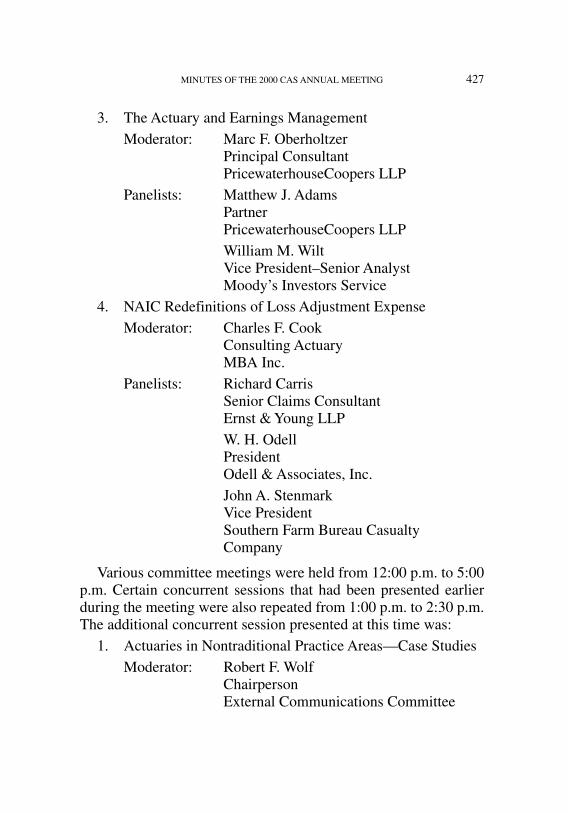
MINUTES OF THE 2000 CAS ANNUAL MEETING 427
3. The Actuary and Earnings ManagementModerator: Marc F. Oberholtzer
Principal ConsultantPricewaterhouseCoopers LLP
Panelists: Matthew J. AdamsPartnerPricewaterhouseCoopers LLPWilliam M. WiltVice President–Senior AnalystMoody’s Investors Service
4. NAIC Redefinitions of Loss Adjustment ExpenseModerator: Charles F. Cook
Consulting ActuaryMBA Inc.
Panelists: Richard CarrisSenior Claims ConsultantErnst & Young LLPW. H. OdellPresidentOdell & Associates, Inc.John A. StenmarkVice PresidentSouthern Farm Bureau Casualty Company
Various committee meetings were held from 12:00 p.m. to 5:00p.m. Certain concurrent sessions that had been presented earlierduring the meeting were also repeated from 1:00 p.m. to 2:30 p.m.The additional concurrent session presented at this time was:
1. Actuaries in Nontraditional Practice Areas—Case StudiesModerator: Robert F. Wolf
ChairpersonExternal Communications Committee
October 30, 2001 11:49 AM 69novmin.qxd

428 MINUTES OF THE 2000 CAS ANNUAL MEETING
Panelists: David FishbaumPrincipalWilliam M. Mercer, Inc.David MolyneuxAssistant Vice PresidentZurich ReRade T. MusulinVice President–ActuaryFlorida Farm Bureau Insurance Companies
Following the concurrent sessions, a special Capitol Hill Brief-ing on Catastrophe Issues was held from 2:30 p.m. to 4:00 p.m.
Entertainment and a buffet dinner were held from 7:00 p.m. to10:00 p.m.
Wednesday, November 15, 2000
Certain concurrent sessions were repeated from 8:00 a.m. to9:30 a.m. Additional concurrent sessions presented at this timewere:
1. Actuarial Statements of Opinion and ASOP 36Moderator: Patricia A. Teufel
PrincipalKPMG LLP
Panelists: Joseph A. HerbersPrincipal and Consulting ActuaryMiller, Herbers, Lehmann, & Associates, Inc.Robert S. MiccolisSenior Vice PresidentReliance Reinsurance CorporationRobert H. WainscottPrincipalErnst & Young LLP
October 30, 2001 11:49 AM 69novmin.qxd

MINUTES OF THE 2000 CAS ANNUAL MEETING 429
2. New Fellows’ PerspectivesModerator: Robert F. Conger
Consulting ActuaryTillinghast-Towers Perrin
Panelists: Sean R. DevlinAssistant Vice PresidentAmerican Re-Insurance CompanyChester J. SzczepanskiChief ActuaryPennsylvania Insurance Department
After a break from 9:30 a.m. to 10:00 a.m., the final GeneralSession was held from 10:00 a.m. to 11:30 a.m.:
“Worshipping at the Altar of Shareholder Value”Moderator: John J. Kollar
Vice PresidentInsurance Services Office, Inc.
Panelists: Weston M. HicksManaging DirectorJ. P. Morgan Securities, Inc.David B. KelsoChief Financial OfficerChubb Group of Insurance CompaniesStephen P. LoweChief ActuaryTillinghast-Towers PerrinKim D. ThorpeChief Financial OfficerFPIC Insurance Group, Inc.
Alice H. Gannon officially adjourned the 2000 CAS AnnualMeeting at 11:45 a.m. after closing remarks and an announcementof future CAS meetings.
October 30, 2001 11:49 AM 69novmin.qxd

430 MINUTES OF THE 2000 CAS ANNUAL MEETING
Attendees of the 2000 CAS Annual Meeting
The 2000 CAS Annual Meeting was attended by 353 Fellows,118 Associates, and 60 Guests. The names of the Fellows and Associates in attendance follow:
FELLOWS
October 30, 2001 11:49 AM 69novmin.qxd
Ralph L. AbellJonathan D. AdkissonMartin AdlerRebecca C. AmorosoRichard B. AmundsonScott C. AndersonRobert A. AnkerMichele Segreti ArndtNolan E. AschCarl Xavier
AshenbrennerRichard V. AtkinsonEmmanuil Theodore
BardisMichael William
BarlowBetty H. BarrowAndrea C. BautistaPatrick BeaudoinNicolas BeaupreAndrew Steven BeckerPhillip N. Ben-ZviAbbe Sohne BensimonCynthia A. BentleyRegina M. BerensDavid R. BickerstaffWilliam P. BiegajJennifer L. BiggsTerry J. Biscoglia
Ralph S. BlanchardMichael P. BlivessCarol BlomstromGary BlumsohnMichael J. BluzerLeRoy A. BoisonJoseph A. BoorSherri Lynn BorderRonald L. BornhuetterVeronique BouchardTheresa W. BourdonAmy S. BouskaTobias E. BradleyJames F. BranniganYaakov B. BraunerPaul J. BrehmWard M. BrooksRobert F. BrownRon BruskyCharles A. BryanGary S. BujauciusHugh Eric BurgessJeanne H. CampDouglas A. CarloneAllison Faith CarpJoseph Gerald CerretaLisa G. ChanzitPatrick J. CharlesDavid R. Chernick
Kin Lun (Victor) ChoiJames K. ChristieKuei-Hsia Ruth ChuAndrew K. ChuWei ChuangRita E. CiccarielloMark M. CisSteven A. CohenRobert F. CongerLarry Kevin ConleeEugene C. ConnellCharles F. CookMark CrawshawPatrick J. CroweKathleen T.
CunninghamMary Elizabeth
Frances CunninghamJonathan Scott CurleeRonald A. DahlquistCharles Anthony Dal
CorobboLoren Rainard
DanielsonLawrence S. DavisTimothy Andrew DavisThomas J. DeFalcoKris D. DeFrainCurtis Gary Dean

MINUTES OF THE 2000 CAS ANNUAL MEETING 431
Jerome A. DegernessCamley A. DelachMichael Brad DelvauxSean R. DevlinPatrick K. DevlinKurt S. DickmannBehram M. DinshawWilliam F. DoveMichael C. DubinDiane Symnoski DudaJudith E. DukatzTammi B. DulbergerLouis DurocherSophie DuvalKevin M. DykeRichard D. EastonBob D. EffingerGary J. EgnaskoJane EichmannMartin A. EpsteinJohn S. EwertMichael A. FalconeVicki Agerton FendleyKenneth D. FikesRussell S. FisherBeth E. FitzgeraldChauncey Edwin
FleetwoodClaudia S. FordeJohn R. ForneyHugo FortinRonnie Samuel FowlerNoelle Christine FriesJohn E. GainesAlice H. GannonRobert W. Gardner
David B. GelinneEric J. GesickJohn F. GibsonSusan I. GildeaTodd B. GlassmanSanjay GodhwaniSteven F. GoldbergAnnette J. GoodreauGregory S. GracePatrick J. GrannanEric L. GreenhillLinda M. GrohSteven L. GrootRebecca N. HaiLeigh Joseph HalliwellAlexander Archibold
HammettMichelle Lynne
HarnickDavid G. HartmanGayle E. HaskellJeffery Tim HayQing HeChristopher Ross HeimKirsten Costello
HernanCharles C. HewittAmy Louise HicksJay T. HiebAmy L. HoffmanTodd Harrison HoivikNancy Michelle HoppeRobert J. HopperBertram A. HorowitzMary T. HosfordDavid Dennis Hudson
Daniel B. IsaacRichard M. JaegerStephen JamesonWalter Leon JedziniakCharles B. JinPhilippe JodinJennifer Polson
JohnsonEric J. JohnsonWarren H. JohnsonThomas S. JohnstonGary R. JosephsonLori Edith JulgaFrank J. KarlinskiClive L. KeatingeAnne E. KellySteven A. KelnerAllan A. KerinFrederick W.
KilbourneMary Jean KingFrederick O. KistJoel M. KleinmanElina KoganskiJohn J. KollarIsrael KrakowskiSarah KrutovAndrew E. KuderaRonald T. KuehnKay E. KuferaJohn M. KulikJason Anthony
KundrotRobin M. La PreteMichael A. LaMonicaDavid A. Lalonde
October 30, 2001 11:49 AM 69novmin.qxd

432 MINUTES OF THE 2000 CAS ANNUAL MEETING
Chingyee Teresa LamDean K. LambJohn A. LambTravis J. LappeLewis Y. LeeMerlin R. LehmanSteven G. LehmannNeal Marev LeibowitzElizabeth Ann
LemasterCharles LetourneauKenneth A. LevineSiu K. LiPeter M. LichtJohn J. LimpertShu C. LinDengxing LinOrin M. LindenStephen P. LoweMichelle LuneauWilliam R. MaagW. James MacGinnitieAndrea Wynne MalyonLawrence F. MarcusLeslie R. MarloKelly J. MathsonJohn W. McClureMichael F. McManusWilliam T. MechDavid L. MenningMatthew P. MerlinoClaus S. MetznerStephen J. MeyerGlenn G. MeyersRobert S. MiccolisPhilip D. Miller
Mary Frances MillerDavid L. MillerDavid L. MillerAin MilnerNeil B. MinerCamille Diane
MinoguePaul David MiotkeDavid MolyneuxBruce D. MooreBenoit MorissetteKari Sue MrazekRobert V. MucciRaymond D. MullerTodd B. MunsonDonna S. MuntJohn A. MuradKevin T. MurphyThomas G. MyersSeth Wayne MyersJohn C. NarvellChris E. NelsonAaron West NewhoffKari A. NicholsonG. Chris NyceMargaret O’BrienMihaela Luminita S.
O’LearyDavid J. OakdenMarc F. OberholtzerRichard Alan OlsenRichard D. OlsenRebecca Ruth OrsiNathalie OuelletTimothy A. PaddockRudy A. Palenik
Robert G. PalmDonald W. PalmerJoseph M. PalmerMark PaykinHarry Todd PearceKathleen M. PechanDaniel Berenson PerryChristopher Kent PerryMarvin PestcoeJohn S. PetersMark W. PhillipsRichard Matthew
PilotteGlen-Roberts
PitruzzelloArthur C. PlacekIgor PogrebinskyGregory John PoirierDale S. PorfilioVirginia R. PrevostoMichael David PriceDeborah W. PriceRegina Marie PuglisiEduard J. PulkstenisMark S. QuigleyRicardo Anthony
RamotarChristopher David
RandallLeonid RasinEllen J. ResplerRebecca L. RoeverWilliam P. RolandA. Scott RomitoDeborah M. RosenbergDavid A. Rosenzweig
October 30, 2001 11:49 AM 69novmin.qxd
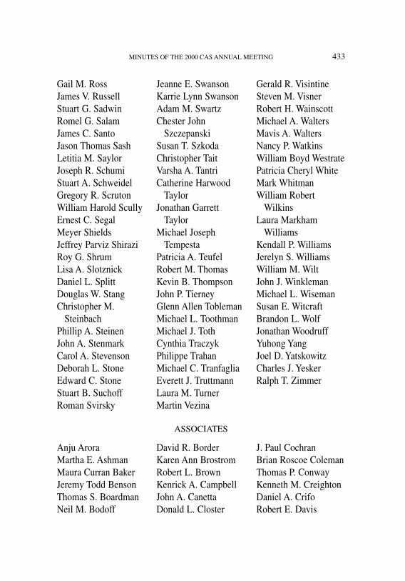
MINUTES OF THE 2000 CAS ANNUAL MEETING 433
Gail M. RossJames V. RussellStuart G. SadwinRomel G. SalamJames C. SantoJason Thomas SashLetitia M. SaylorJoseph R. SchumiStuart A. SchweidelGregory R. ScrutonWilliam Harold ScullyErnest C. SegalMeyer ShieldsJeffrey Parviz ShiraziRoy G. ShrumLisa A. SlotznickDaniel L. SplittDouglas W. StangChristopher M.
SteinbachPhillip A. SteinenJohn A. StenmarkCarol A. StevensonDeborah L. StoneEdward C. StoneStuart B. SuchoffRoman Svirsky
Jeanne E. SwansonKarrie Lynn SwansonAdam M. SwartzChester John
SzczepanskiSusan T. SzkodaChristopher TaitVarsha A. TantriCatherine Harwood
TaylorJonathan Garrett
TaylorMichael Joseph
TempestaPatricia A. TeufelRobert M. ThomasKevin B. ThompsonJohn P. TierneyGlenn Allen ToblemanMichael L. ToothmanMichael J. TothCynthia TraczykPhilippe TrahanMichael C. TranfagliaEverett J. TruttmannLaura M. TurnerMartin Vezina
Gerald R. VisintineSteven M. VisnerRobert H. WainscottMichael A. WaltersMavis A. WaltersNancy P. WatkinsWilliam Boyd WestratePatricia Cheryl WhiteMark WhitmanWilliam Robert
WilkinsLaura Markham
WilliamsKendall P. WilliamsJerelyn S. WilliamsWilliam M. WiltJohn J. WinklemanMichael L. WisemanSusan E. WitcraftBrandon L. WolfJonathan WoodruffYuhong YangJoel D. YatskowitzCharles J. YeskerRalph T. Zimmer
October 30, 2001 11:49 AM 69novmin.qxd
ASSOCIATES
Anju AroraMartha E. AshmanMaura Curran BakerJeremy Todd BensonThomas S. BoardmanNeil M. Bodoff
David R. BorderKaren Ann BrostromRobert L. BrownKenrick A. CampbellJohn A. CanettaDonald L. Closter
J. Paul CochranBrian Roscoe ColemanThomas P. ConwayKenneth M. CreightonDaniel A. CrifoRobert E. Davis

434 MINUTES OF THE 2000 CAS ANNUAL MEETING
Peter R. DeMallieSara P. DrexlerSharon C. DubinAlice H. EdmondsonEllen E. EvansFarzad FarzanWilliam M. FinnBrian C. FischerSean Paul ForbesMauricio FreyreTimothy J. FriersKai Y. FungDustin Wayne GaryAmy L. GebauerPatrick J. GilhoolBradley G. GipsonStewart H. GleasonTerry L. GoldbergChristopher David
GoodwinBruce H. GreenMonica A. GrilloNasser HadidiBrian D. HaneySusan Wadman HayesThomas F. HeadJoseph A. HerbersMark D. HeyneKurt D. HinesPatricia A. HladunJason N. HoffmanBernard R. HorovitzDerek Reid HoymeDavid D. HuJeffrey R. IllCraig D. Isaacs
Brian J. JanitschkeBrian E. JohnsonGregory K. JonesJames W. JonskeEdwin G. JordanScott A. KellySean M. KennedyDavid R. KennerudSusanlisa KesslerDavid Neal KightlingerJeffrey D. KimbleLinda S. KlenkTherese A. KlodnickiKaren Lee KrainzSteven M. LackeStephen E. LeheckaTodd William
LehmannJing LiuKathleen T. LogueWilliam F. LoydJulie MartineauJames J. MatusiakJohn R. McColloughDouglas H. MinRodney S. MorrisRade T. MusulinBrian C. NeitzelSean Robert NimmSylvain NoletLeigh S. OatesW. H. OdellLeo Martin OrthPrabha PattabiramanWillard W. PeacockClaude Penland
Sasikala RamanThomas O. RauJames E. RechMichael SanseveroJoshua Stewart SawyerMichael Robert
SchummerSteven George SearleBarbara A. SeifferttAhmad ShadmanHalina H. SmosnaDavid C. SnowCalvin C. SpenceMichael William
StarkeAvivya Simon StohlFrederick M. StraussEugene G. ThompsonJoseph O. ThorneChristopher S.
ThrockmortonFrederick A. UrschelEric VaithMark Alan VerheyenMary Elizabeth WaakRoger C. WadeDavid G. WalkerFelicia WangGregory S. WannerThomas J. WhiteRobert J. WhiteRobert F. WolfNora J. YoungYin Zhang
October 30, 2001 11:49 AM 69novmin.qxd

job no. 1969 casualty actuarial society CAS journal 1969VPR [1] 11-08-01 4:58 pm
REPORT OF THE VICE PRESIDENT–ADMINISTRATION
This report provides a one-year summary of CAS activitiessince the 1999 CAS Annual Meeting. I will first comment onthese activities as they relate to the following purposes of theCasualty Actuarial Society as stated in our Constitution:
1. Advance the body of knowledge of actuarial science appliedto property, casualty, and similar risk exposures;
2. Establish and maintain standards of qualifications for mem-bership;
3. Promote and maintain high standards of conduct and compe-tence for the members; and
4. Increase the awareness of actuarial science.
I will then provide a summary of other activities that may notrelate to a specific purpose, but yet are critical to the ongoingvitality of the CAS. Finally, I will summarize the current statusof our finances and key membership statistics.
The CAS discussion paper programs, Proceedings, and theForum contribute to the attainment of the first purpose. The win-ter, summer, and fall volumes of the Forum focused on top-ics in ratemaking, reserving, dynamic financial analysis, andhealth and managed care. The discussion paper program vol-ume addressed insurance in the next century. The Proceedingspapers addressed topics in workers compensation, residual mar-kets, and Superfund-related claims costs, as well as mathemati-cal/modeling techniques including the relationship between mini-mum bias and generalized linear models, a semiparametric modelfor loss distributions, and bias in loss development factors.
During the past year, members were able to receive the Fo-rum and discussion paper publications electronically via the CASWeb Site for the first time in lieu of hard copy. The cost sav-ings were shared with the members who elected this option bya reduction in their annual dues.
435

job no. 1969 casualty actuarial society CAS journal 1969VPR [2] 11-08-01 4:58 pm
436 REPORT OF THE VICE PRESIDENT–ADMINISTRATION
The Task Force on Fair Value of Liabilities, under the leader-ship of Ralph Blanchard, prepared a comprehensive report dis-cussing the issues surrounding fair valuing of property/casualtyinsurance liabilities, particularly in the United States. This is atimely subject because the issues are currently being reviewed bythe Financial Accounting Standards Board and the InternationalAccounting Standards Committee (IASC). Casualty actuaries arequalified through their education and experience to offer valuableinput on this topic and this report will support the CAS represen-tative to the International Actuarial Association, the internationalactuarial body working with the IASC.
In regards to purpose 2, there were a number of developmentsin the CAS education and examination system during the lastyear. Beginning with the Spring 2000 examinations, the CASinstituted a new system requiring nine exams for Fellowship andseven exams for Associateship. The first four exams are jointlyadministered with the Society of Actuaries (SOA); partial examswere discontinued. There was a rearrangement of material amongexams on the syllabus and topics were updated and sometimeschanged to reflect the current needs for CAS education. The newexamination Part 8, “Investments and Financial Analysis,” willprovide CAS actuaries with much broader exposure to the areaof investments and financial analysis.
The final report of the Task Force on Education and Exami-nation Process and Procedures, chaired by John Kollar, was pre-sented to the Executive Council and Board of Directors early inthe year. The task force reviewed the current education and exam-ination system to assess its strengths and weaknesses and maderecommendations to improve the process. Admissions commit-tees were assigned responsibility for implementing the recom-mendations. A professional educational consultant has been hiredon a contract basis to assist the CAS with defining learning ob-jectives and exam blueprints.
The CAS Task Force on Exams 3 and 4, chaired by HowardMahler, reevaluated examinations 3 and 4 addressing (1) whether

job no. 1969 casualty actuarial society CAS journal 1969VPR [3] 11-08-01 4:58 pm
REPORT OF THE VICE PRESIDENT–ADMINISTRATION 437
the learning objectives are appropriate for casualty actuaries andfor all actuaries and (2) whether the readings are appropriateto teach the learning objectives. A draft report was provided tothe Board in November 2000. The Board directed the ExecutiveCouncil (EC) to work with the SOA to make improvements intime for the Spring 2001 exams. The Board also directed the ECto commission the development of study notes for exams 3 and4 that are relevant to CAS learning objectives and appropriatefor self-study.
The Board approved waivers for CAS exams 1–4 for candi-dates who have received credit for specified Institute of Actu-aries’ exams. A reciprocal waiver policy for the Institute examshas been extended to the CAS.
A quality program of continuing education and a Code ofProfessional Conduct support purpose 3: “promote and main-tain high standards of conduct and competence for the mem-bers.”
The Board adopted a revised Code of Professional Conductto be effective January 1, 2001. This revised code has also beenadopted by the other four U.S. actuarial organizations and isthe result of the work of the Joint Committee on the Code ofProfessional Conduct, whose goal was to produce a uniform codefor the U.S. actuarial profession.
The CAS provides educational opportunities through the pub-lication of actuarial materials and the sponsorship of meetingsand seminars. This year’s sessions included the following, shownwith the number of CAS members in attendance:
Meetings:
Location CAS Members
Spring Las Vegas 639Annual Washington, D.C. 471

job no. 1969 casualty actuarial society CAS journal 1969VPR [4] 11-08-01 4:58 pm
438 REPORT OF THE VICE PRESIDENT–ADMINISTRATION
Seminars:
Topic Location CAS Members
Ratemaking San Diego 282Valuation of Insurance Operations St. Louis 77Reinsurance Boston 179Dynamic Financial Analysis New York 123Casualty Loss Reserves Minneapolis 316Funding Catastrophe Risks Providence 74Appointed Actuary—Joint CAS/CIA Toronto 357!
Course on Professionalism—Dec ’99 3 locations 82 studentsCourse on Professionalism—June ’00 2 locations 43 students
!Total attendance. Separate count for CAS members is not available.
Limited attendance seminars covered the following six top-ics: (1) Practical Applications of Loss Distributions, (2) Man-aging Asset and Investment Risk, (3) Principles of Finance, (4)Reinsurance, (5) Advanced Dynamic Financial Analysis, and (6)(Basic) Dynamic Financial Analysis. The CAS co-sponsored aspecial interest seminar in London with the Institute of Actuariesin June 2000.
Four new advisory committees in nontraditional practice ar-eas (i.e., nontraditional for CAS members) were formed: (1)Asset/Liability Management and Investment Policy, (2) Valua-tion of P&C Insurance Companies, (3) Enterprise Risk Manage-ment, and (4) Securitization/Risk Financing. These committeeswill identify research and education initiatives.
A program to offer training in general business skills to CASmembers was initiated at the 2000 Spring Meeting and repeatedat the Fall meeting. Sessions on executive presentation skills andbusiness writing skills were held.
To increase the awareness of opportunities in actuarial sci-ence, the CAS created a new web site, jointly sponsored withthe SOA, devoted entirely to recruiting and career development:www.BeAnActuary.org.

job no. 1969 casualty actuarial society CAS journal 1969VPR [5] 11-08-01 4:58 pm
REPORT OF THE VICE PRESIDENT–ADMINISTRATION 439
The CAS web site, now in its fifth year of existence, supportsall four purposes. Here are some highlights from the past yearthat have not been mentioned elsewhere in this report: (1) reg-istrations for meetings and payments of dues can be processedonline; (2) a collection of over 70 volumes and 600 articles fromthe ASTIN Bulletin was placed on the web site; and (3) a quicksearch function for the home page and all second-level pageswas added.
The CAS exercised an option to expand the size of the cur-rent CAS Office to provide needed facilities and for future staffgrowth. The CAS also exercised an option to extend the lease forfive years beyond the current expiration date in February 2001.
The Task Force on CAS Election Process chaired by John Pur-ple submitted its report in February 2000. The Board of Directorsacted on the recommendations in February and May, in time toimplement approved changes for the CAS 2000 elections. Thechanges included providing additional biographical informationon candidates for election in the ballot package, along with can-didates’ responses to two questions proposed by the NominatingCommittee. The questions asked for the 2000 elections were: (1)why do you want to be a member of the CAS Board?; and (2)what particular qualities and experience would you bring to theBoard? The Board also charged the EC with developing a com-munication plan to educate the membership about the electionprocess.
A Board Question & Answer Forum on the CAS web site wasapproved by the Board in September to enhance communicationbetween the membership and the Board.
A new CAS Committee on Investments was established fol-lowing Board agreement that the CAS investment strategy shouldbe expanded to allow investment of long-term funds in equitiesusing low expense, broadly diversified index funds. This rep-resents a shift from the conservative prior policy of investing

job no. 1969 casualty actuarial society CAS journal 1969VPR [6] 11-08-01 4:58 pm
440 REPORT OF THE VICE PRESIDENT–ADMINISTRATION
in intermediate-term U.S. Treasury fixed-income securities withstaggered maturity dates.
Membership growth continued with 183 new Associates, 149new Fellows, and 8 new Affiliates. (Affiliate is a nonvoting mem-bership category for qualified actuaries who have attained theiractuarial credentials in another actuarial organization.) The totalnumber of members as of November 2000 was 3,455, up 5.3%for the year.
New members elected to the Board of Directors for next yearare Ralph S. Blanchard III, Janet L. Fagan, Michael J. Miller, andDeborah M. Rosenberg. The membership elected Robert F. Con-ger to the position of President-Elect, while Patrick J. Grannanassumed the presidency.
The Executive Council, with primary responsibility for day-to-day operations, met either by teleconference or in person atleast once a month during the year. The Board of Directorselected the following Vice Presidents for the coming year: VicePresident–Administration, Sheldon Rosenberg; Vice President–Admissions, Mary Frances Miller; Vice President–ContinuingEducation, Abbe S. Bensimon; Vice President–International,LeRoy A. Boison; Vice President–Programs and Communica-tions, David R. Chernick; and Vice President–Research and De-velopment, Gary R. Josephson.
The CPA firm of Langan Associates has been engaged toexamine the CAS books for fiscal year 2000 and its findings willbe reported by the Audit Committee to the Board of Directors inFebruary 2001. The fiscal year ended with an unaudited net lossfrom operations of $183,280 compared to a budgeted net lossof $186,242. Fiscal year 2000 had been budgeted for a net lossbecause of the strong equity position that resulted from higherthan expected income in prior years.
Members’ equity now stands at $2,968,879. This representsa decrease in equity of $105,980 over the amount reported last

job no. 1969 casualty actuarial society CAS journal 1969VPR [7] 11-08-01 4:58 pm
REPORT OF THE VICE PRESIDENT–ADMINISTRATION 441
year. In addition to the net loss from operations, there was an un-realized gain of $17,766 recorded to adjust marketable securitiesto market value as of September 30, 2000. There was also a totalnet increase of $59,534 in various research, prize, and schol-arship accounts, arising from the difference between incomingfunds and interest earned less expenditures. These amounts arenot reflected in net income from operations.
For 2000–2001, the Board of Directors has approved a budgetof approximately $4.7 million, an increase of about $400,000over the prior fiscal year. Members’ dues for next year will be$300, an increase of $10, while fees for the Subscriber Programwill increase by $10 to $370. A $30 discount is available tomembers and subscribers who elect to receive the Forum andDiscussion Paper Program publications in electronic format fromthe web site.
Respectfully submitted,Curtis Gary DeanVice President–Administration
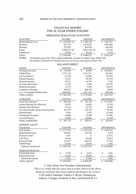
October 30, 2001 11:50 AM 1969FREP.QXD
FINANCIAL REPORTFISCAL YEAR ENDED 9/30/2000
OPERATING RESULTS BY FUNCTIONFUNCTION INCOME EXPENSE DIFFERENCEMembership Services $01,218,006 (a) $01,366,188 $0.(148,182)Seminars 921,739 1,030,025 (108,286)Meetings 767,087 807,849 (40,762)Exams 2,984,072 (b) 2,861,526 (b) 122,546Publications 39,594 30,424 9,170TOTAL $ 5,930,498 $ 6,096,012 $00,(165,514) (c)NOTES: (a) Includes gain of $17,766 to adjust marketable securities to market value (SFAS 124).
(b) Includes $1,865,955 of Volunteer Services for income and expense (SFAS 116).
BALANCE SHEETASSETS 9/30/1999 9/30/2000 DIFFERENCEChecking Accounts $00134,490 $000,30,029 $00(104,461)T-Bills/Notes 3,537,154 3,511,251 (25,903)Accrued Interest 51,708 43,006 (8,702)Prepaid Expenses 72,451 90,789 18,338Prepaid Insurance 16,871 16,719 (152)Accounts Receivable 11,255 2,980 (8,275)Textbook Inventory 8,174 3,499 (4,675)Computers, Furniture 386,873 406,702 19,829Less: Accumulated Depreciation (256,384) (307,174) (50,790)TOTAL ASSETS $ 3,962,594 $ 3,797,801 $00(164,793)
LIABILITIES 9/30/1999 9/30/2000 DIFFERENCEExam Fees Deferred $00,500,444 $00,325,339 $00 (175,105)Annual Meeting Fees Deferred 29,355 44,605 15,250Seminar Fees Deferred 27,441 42,750 15,309Accounts Payable and Accrued Expenses 263,779 349,159 85,380Deferred Rent 9,018 2,652 (6,366)Unredeemed Vouchers 19,800 14,400 (5,400)Accrued Pension 37,896 50,016 12,120TOTAL LIABILITIES $00,887,735 $00, 828,921 $00 (58,814)
MEMBERS' EQUITYUnrestricted 9/30/1999 9/30/2000 DIFFERENCECAS Surplus $02,727,393 $ 2,561,879 $00(165,514)Michelbacher Fund 105,861 110,185 4,324Dorweiler Fund 1,911 0 (1,911)CAS Trust 36,616 63,628 27,012Research Fund 133,207 160,972 27,765ASTIN Fund 52,046 54,910 2,864
Subtotal Unrestricted $03,057,034 $ 2,951,574 $0 (105,460)
Temporarily RestrictedScholarship Fund $00,006,738 $00,006,610 $00,00(128)Rodermund Fund 11,087 10,695 (392)
Subtotal Restricted 17,825 17,305 (520)TOTAL EQUITY $ 3,074,859 $ 2,968,879 $0,(105,980)
C. Gary Dean, Vice President–AdministrationThis is to certify that the assets and accounts shown in the above
financial statement have been audited and found to be correct.CAS Audit Committee: Charles A. Bryan, Chairperson;
Anthony J. Grippa; Frederick O. Kist; and Richard W. Lo
442 REPORT OF THE VICE PRESIDENT–ADMINISTRATION
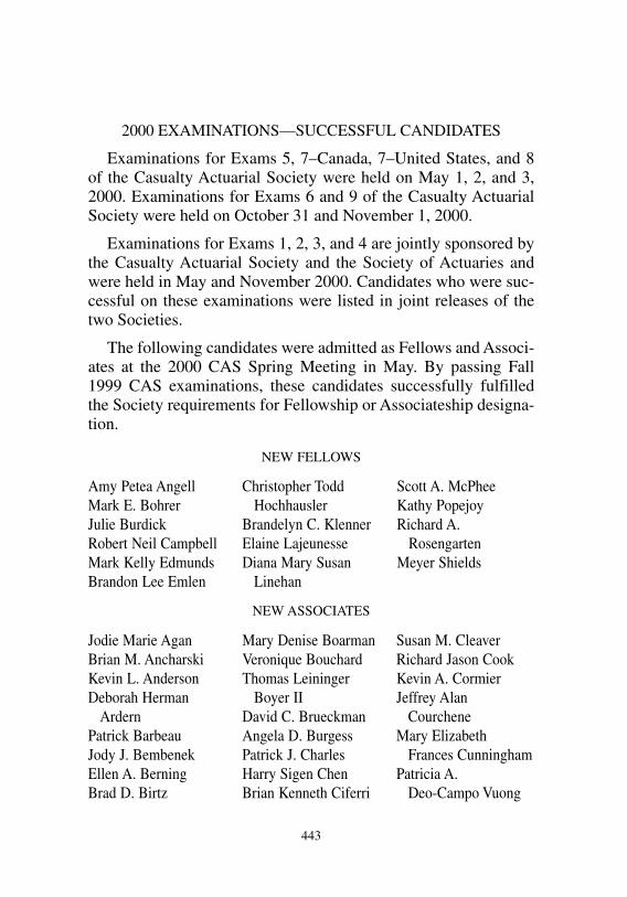
October 30, 2001 11:55 AM 1969cand.qxd
2000 EXAMINATIONS—SUCCESSFUL CANDIDATES
Examinations for Exams 5, 7–Canada, 7–United States, and 8of the Casualty Actuarial Society were held on May 1, 2, and 3,2000. Examinations for Exams 6 and 9 of the Casualty ActuarialSociety were held on October 31 and November 1, 2000.
Examinations for Exams 1, 2, 3, and 4 are jointly sponsored bythe Casualty Actuarial Society and the Society of Actuaries andwere held in May and November 2000. Candidates who were suc-cessful on these examinations were listed in joint releases of thetwo Societies.
The following candidates were admitted as Fellows and Associ-ates at the 2000 CAS Spring Meeting in May. By passing Fall1999 CAS examinations, these candidates successfully fulfilledthe Society requirements for Fellowship or Associateship designa-tion.
NEW FELLOWS
443
Amy Petea AngellMark E. BohrerJulie BurdickRobert Neil CampbellMark Kelly EdmundsBrandon Lee Emlen
Christopher ToddHochhausler
Brandelyn C. KlennerElaine LajeunesseDiana Mary Susan
Linehan
Scott A. McPheeKathy PopejoyRichard A.
RosengartenMeyer Shields
NEW ASSOCIATES
Jodie Marie AganBrian M. AncharskiKevin L. AndersonDeborah Herman
ArdernPatrick BarbeauJody J. BembenekEllen A. BerningBrad D. Birtz
Mary Denise BoarmanVeronique BouchardThomas Leininger
Boyer IIDavid C. BrueckmanAngela D. BurgessPatrick J. CharlesHarry Sigen ChenBrian Kenneth Ciferri
Susan M. CleaverRichard Jason CookKevin A. CormierJeffrey Alan
CourcheneMary Elizabeth
Frances CunninghamPatricia A.
Deo-Campo Vuong

444 2000 EXAMINATIONS—SUCCESSFUL CANDIDATES
Jean-FrançoisDesrochers
Mark RichardDesrochers
Michael DevineKevin George DonovanLouis-Christian DupuisDonna L. EmmerlingKeith A. EngelbrechtLaura Ann EsboldtJuan EspadasFarzad FarzanDonia Burris FreeseShina Noel FritzCynthia GalvinMichael Anthony
GarciaHannah GeeJames Brian GilbertJoseph Emmanuel
GoldmanAndrew Samuel
Golfin Jr.Olga GolodStacey C. GothamMark R. GreenwoodChantal GuillemetteJames Christopher
GuszczaDavid Bruce
HackworthDawn Marie S. HappJason Carl HeadPamela Barlow HeardKristina S. HeerHans Heldner
Robert C. HillDavid E. HodgesRichard Michael HoltzAllen J. HopeCarol Irene HumphreyRusty A. HustedMichael Stanley
JarmusikPatrice JeanCharles B. JinSteven M. JokerstCheryl R. KelloggJames F. KingJill E. KirbyOmar A. KitchlewHenry Joseph
KonstantyRebecca Michelle
KristalDarjen D. KuoChristine L. LackeBobb J. LackeyJean-François
LarochellePeter H. LatshawDoris LeeWilliam Scott LennoxJoshua Yuri LigoskyErik Frank LivingstonRichard Paul LonardoWilliam F. Loyd IIIAlexander Peter
MaizysVictor MataDavid Michael MaurerTimothy C. McAuliffe
Richard J. McElligottJennifer A. McGrathMartin MenardMitchel MerbergVadim Y. MezhebovskyEric Millaire-MorinSuzanne A. MillsMatthew Kevin MoranLambert MorvanThomas M. MountRebecca E. MoziRonald Taylor NelsonMichael Dale
NeubauerLoren J. NickelAjay PahwaCosimo PantaleoMichael Thomas
PattersonWendy Wei-Chi PengJill E. PeppersMichael C. PetersenKevin Thomas
PetersonKraig Paul PetersonKristin Sarah
PiltzeckerSean Evans PorrecaWarren T. PrintzStephen Daniel
RiihimakiEzra Jonathan RobisonBryant Edward RussellFrederick Douglas
RyanLaura Beth Sachs
October 30, 2001 11:55 AM 1969cand.qxd
2000 EXAMINATIONS—SUCCESSFUL CANDIDATES 445
Salimah H. SamjiRachel SamoilJennifer Arlene ScherDaniel David
SchlemmerParr T. SchoolmanErnest C. SegalMichelle L. SheppardPaul O. ShupeLee Oliver SmithLora L. Smith-SarfoScott G. SobelWendy Rebecca SpeertMary Jane Sperduto
Christine Steele-KoffkeGary A. SudbeckJonathan Leigh
SummersNeeza ThandiTanya K. ThielmanJohn David TraufferNathalie TremblayMatthew L. UhodaDennis R. UnverRichard Alan
Van DykeJosephine M. WaldmanColleen Ohle Walker
Kristie L. WalkerTice R. WalkerWade Thomas
WarrinerKelly M. WeberPetra Lynn WegerichChristopher John
WestermeyerKarin H. WohlgemuthTerry C. WolfeMihoko YamazoeNora J. Young
October 30, 2001 11:55 AM 1969cand.qxd
The following candidates successfully completed the followingSpring 2000 CAS examinations.
Exam 5
Keith P. AllenTanuja S. AlwarVagif AmstislavskiyJulie A. AndersonAmy J. AntenenKatherine H. AntonelloMelissa J. AppenzellerKevin J. AtinskyJoel E. AtkinsNicki C. AustinGregory K. BangsDanielle L.
BartosiewiczThomas C. BatesRick D. BeamEsther BeckerChad M. Beehler
James H. BennettAndrew W. BernsteinNebojsa BojerJoseph V. Bonanno Jr.Jean-Philippe BoucherJudy L. BoutcheeBernardo Bracero Jr.Melissa L. BrewerClaude B. BunickDon J. BurbacherScott W. CarpinteriSimon CastonguayThomas L. CawleyJohn CelidonioPhyllis B. ChanJames ChangJennifer A. Charlonne
Benjamin W. ClarkWesley G. ClarkePaul L. CohenMarlene Marie CollinsChristopher L.
CookseyKathleen M. CooperDavid C. CoplanLeanne M. CornellMichael J. CovertSandra CreaneyRussell A. CreedArthur D. CummingsDavid W. DahlenRich A. DaveyDavid E. Dela CruzDavid A. DeNicola

446 2000 EXAMINATIONS—SUCCESSFUL CANDIDATES
Romulo N. Deo-Campo Vuong
Ryan M. DiehlErik L. DonahueBrian M. DonlanKevin P. DonnellyPamela G. DoonanCrisanto A. DoradoJeffrey S. ErnstBrian A. FanninWendy A. FarleyRobert E. FarnamKevin M. FinnEllen D. FitzsimmonsChristine M. FlemingLouise FranklandGregory A.
FrankowiakJeffrey J. FratantaroFrançois FugereAndre GagnonPatrick P. GallagherWilliam J. GerhardtGregory Evan GilbertJohn S. GilesWilliam G. GolushJennifer GraunasStacie R.W. GrindstaffStephanie A.
GroharingJason L. GroveKanwal HameedKimberly Baker HandSunny M. HarringtonSusan M. HarrisGuo Harrison
Stuart J. HayesJoseph HebertWilliam S. HedgesRhonda R. HellmanKathryn E. HerzogBrandon L. HeutmakerDaniel D. HeyerStephen J. Higgins Jr.Joseph S. HighbargerMichael F. HobartJeremy A. HochMelissa S. HoltElizabeth J. HudsonCraig D. IsaacsKatherine JacquesGregory O. JaynesJulie A. JordanHye-Sook KangJohn J. KarwathLawrence S. KatzSusan M. KeavenyDouglas H.
KemppainenYoung Y. KimPatricia KinghornJennifer E. KishAnne Marie KleinJeff A. KluckLaurie A. KnokeSteven M. KoesterAnand S. KulkarniGregory E. KushnirFrançois LacroixHeather D. LakeMichael A. LardisMichael L. Laufer
Nathalie M. LavigneDamon T. LayAnh Tu LePatricia LeeRuth M. LeStourgeonAmanda M. LevinsonJonathan D. LevyHayden Anthony
LewisWei LiMonika LietzEric F. LilandDavid Grant LimSteven R. LindleyLaura J. LothschutzDaniel A. LowenHazel J. LuckeyTeresa MadariagaSteven ManilovLuis S. MarquesJoseph W. MawhinneyStephane McGeeShaun P. McGovernHernan L. MedinaCharles W. MitchellCamilo MohippCelso M. MoreiraAlan E. MorrisMatthew D. MyshrallJohn A. NaussScott L. NegusJennifer Y. NeiShannon P. NewmanLester M. Y. NgKhanh K. NguyenNorman Niami
October 30, 2001 11:55 AM 1969cand.qxd

2000 EXAMINATIONS—SUCCESSFUL CANDIDATES 447
Stoyko N. NikolovMatthew P. NimchekAlejandra S. NolibosCharles A. NortonTom E. NorwoodJoy-Ann C. PayneDianne M. PhelpsDaniel P. PostStephen R. PrevattLester PunLovely G. PuthenveetilEdward L. PyleMichael J. QuigleyWilliam C. ReddingtonNeil W. ReissPeggy-Anne K.
RepellaDanielle L. RichardsLaura D. RinkerJoseph L. RizzoCharles A. RombergerRyan P. Royce
Giuseppe RussoDoris Y. SchirmacherBrett M. ShereckJunning ShiJimmy ShkolyarJeremy D. ShoemakerSummer L. SipesDouglas E. SmithMichael D. SowkaLaura T. SprouseKarine St-OngeWei Hua SuAdam D. SwopeMichelle M.
SyrotynskiMing TangHugh T. ThaiChristian A. ThielmanMatthew D. TroneDavid S. UdallStephen H. UnderhillMary Vacirca
Paul A. VendettiBrian A. ViscusiNatalie VishnevskyCameron Jason VogtMatthew J. WalterBethany R. WebbRobert S. WeishaarJean P. WestCarolyn D. WettsteinShannon A. WhalenJoel D. WhitcraftPaul D. WilbertChun Shan WongWalter R. WulligerRun YanHuey Wen YangJoshua A. YoudovinJanice M. YoungJonathan K. YuGrace ZakariaLarry Xu ZhangLianmin Zhou
October 30, 2001 11:55 AM 1969cand.qxd
Exam 7—Canada
Genevieve L. AllenAnna Marie BeatonPatrick BeaudoinChantal GuillemettePatricia A. HladunIsabelle La Palme
Julie-Linda LaforceChristian LemayJulie MartineauIan John McCrackenMartin MenardLambert Morvan
Sylvain NoletNathalie OuelletCosimo PantaleoJulie PerronSylvain RenaudClaude A. Wagner

448 2000 EXAMINATIONS—SUCCESSFUL CANDIDATES
Afrouz AssadianMaura Curran BakerPhil W. BanetEmmanuil Theodore
BardisNicolas BeaupreJody J. BembenekJeremy Todd BensonDavid Matthew BiewerLinda Jean BjorkMichael J. BluzerNeil M. BodoffDaniel R. BoerboomChristopher David
BohnJerelyn S. BoysiaTobias E. BradleyMaureen B. BrennanJeremy James BrighamSara T. BroadrickKaren Ann BrostromStephanie Anne BrunoHugh Eric BurgessAnthony Robert
BustilloRonald S. CederburgJoseph Gerald CerretaHao ChaiKin Lun (Victor) ChoiAndrew K. ChuKuei-Hsia Ruth ChuChristopher J. ClausSusan M. CleaverJeffrey J. ClinchHugo Corbeil
Thomas CosenzaJeffrey Alan
CourcheneDavid Francis DahlMujtaba H. DatooKris D. DeFrainPeter R. DeMallieJohn T. DevereuxSean R. DevlinDean P. DormanSharon C. DubinLouis-Christian DupuisSophie DuvalKevin M. DykeJane EichmannJames Robert ElickerRichard James
EngelhuberGregory James EnglWeishu FanKenneth D. FikesWilliam M. FinnChauncey Edwin
FleetwoodSean Paul ForbesFeifei FordJames M. GallagherDustin Wayne GaryChristie L. GilbertPatrick J. GilhoolBradley G. GipsonStacey C. GothamRobert A. GrocockEdward Kofi GyampoRebecca N. Hai
Kenneth Jay HammellAlexander Archibold
HammettMichael S. HarringtonJames Anthony HeerKristina S. HeerKevin B. HeldScott E. HenckMark D. HeyneKurt D. HinesAmy L. HoffmanSuzanne Barry
HolohanDerek Reid HoymeChristopher Wayne
HurstJamison Joel IhrkeWeidong Wayne JiangPhilippe JodinShantelle Adrienne
JohnsonTricia Lynne JohnsonWilliam Russell
JohnsonBryon Robert JonesDana F. JosephSean M. KennedyDavid R. KennerudSusanlisa KesslerJoseph E. KirsitsScott C. KurbanElizabeth A. KurinaChingyee Teresa LamPeter H. LatshawThomas V. Le
October 30, 2001 11:55 AM 1969cand.qxd
Exam 7—United States

2000 EXAMINATIONS—SUCCESSFUL CANDIDATES 449
Doris LeeMichael E. LewisMatthew Allen
LillegardDengxing LinShu C. LinJing LiuKathleen T. LogueElizabeth LongMichelle LuneauAtul MalhotraSharon L. MarkowskiJames J. Matusiak Jr.Timothy J. McCarthyWilliam R. McClintockJohn R. McColloughChristian MenardUlysis V. Mensah-
BonsuVadim Y.
MezhebovskyRyan A. MichelScott Allan MillerRodney S. MorrisSharon D. MottKari Sue MrazekJoseph J. MuccioBrian C. NeitzelKari A. NicholsonSean Robert NimmKathleen C. OdomirokRichard Alan OlsenMichael A. OnofriettiRodrick Raymond
OsbornMatthew R. Ostiguy
Chad Michael OttMichael Guerin OwenRobert A. PainterMark PaykinKraig Paul PetersonMichael Robert
PetrarcaChristopher A. PettAndrea L. PhillipsAnthony George
PhillipsKristin Sarah
PiltzeckerJorge E. PizarroDylan P. PlaceJayne L. PlunkettIgor PogrebinskyGregory John PoirierMitchell S. PollackGregory T. PrebleWarren T. PrintzNi Qin-FengRicardo Anthony
RamotarLeonid RasinJennifer L. RichardMario RichardRomel G. SalamRachel SamoilJames C. SandorGary Frederick SchererDaniel David
SchlemmerParr T. SchoolmanAnnmarie SchusterStuart A. Schweidel
Kelvin B. SederburgTina ShawMichelle L. SheppardAlastair Charles ShoreJeffery J. SmithAnthony A. SolakWendy Rebecca SpeertChristopher M.
SteinbachMark Richard StronaJonathan Garrett
TaylorNeeza ThandiMary A. TheilenChristopher S.
ThrockmortonEllen Marie TierneyMichael J. TothMichael C. TranfagliaBrian K. TurnerKieh Tsung TyDennis R. UnverPeggy J. UrnessWilliam D. Van DykeGaetan R. VeilleuxMark Alan VerheyenMartin VezinaJennifer Anne VezzaNathan Karl VoorhisJosephine M. WaldmanTice R. WalkerFelicia WangShaun S. WangDouglas M. WarnerDavid W. WarrenKelly M. Weber
October 30, 2001 11:55 AM 1969cand.qxd

450 2000 EXAMINATIONS—SUCCESSFUL CANDIDATES
Christopher JohnWestermeyer
Apryle L. WilliamsBrandon L. WolfStephen K. Woodard
Mark Lee WoodsScott Michael WoomerJimmy L. WrightLinda YangStephanie C. Young
Michael R. ZaremberXiangfei ZengYin ZhangEric Zlochevsky
October 30, 2001 11:55 AM 1969cand.qxd
Exam 8
Jason R. AbramsJohn Scott AlexanderMichele Segreti ArndtAnju AroraCarl Xavier
AshenbrennerDavid Steen AtkinsonMichael William
BarlowKeith Michael BarnesAndrew Steven BeckerDavid R. BorderSherri Lynn BorderVeronique BouchardErik R. BouvinConni Jean BrownRobert F. BrownDavid C. BrueckmanJohn C. BurkettStephanie T. CarlsonAllison Faith CarpPatrick J. CharlesKin Lun (Victor) ChoiWei ChuangSteven A. CohenLarry Kevin ConleeKathleen T.
Cunningham
Mary ElizabethFrances Cunningham
Jonathan Scott CurleeLoren Rainard
DanielsonMichael Brad DelvauxKevin Francis DownsTammi B. DulbergerLouis DurocherLaura Ann EsboldtJonathan Palmer EvansJoseph Gerard EvlethVicki Agerton FendleyHugo FortinRon FowlerNoelle Christine FriesCynthia GalvinEmily C. GildeSusan I. GildeaIsabelle GingrasTheresa GiuntaTodd B. GlassmanSanjay GodhwaniMatthew R. GorrellLisa N. GugliettiNasser HadidiBrian D. HaneyDawn Marie S. Happ
Michelle LynneHarnick
Bryan HartiganJeffery Tim HayQing HeAmy Louise HicksJay T. HiebGlenn R. HiltpoldTodd Harrison HoivikNancy Michelle HoppeWalter Leon JedziniakCharles B. JinSusan K. JohnstonLori Edith JulgaElina KoganskiClaudia Anita KrucherKimberly J. KurbanRobin M. LaPreteTravis J. LappeAaron Michael LarsonBorwen LeeLewis Y. LeeNeal Marev LeibowitzCharles LetourneauJames P. LynchKelly A. LysaghtJason K. MachtingerDaniel Patrick Maguire

2000 EXAMINATIONS—SUCCESSFUL CANDIDATES 451
Andrea Wynne MalyonJoshua Nathan
MandellMichael E. MielzynskiEric Millaire-MorinAin MilnerPaul David MiotkeBenoit MorissetteKevin T. MurphySeth Wayne MyersMihaela Luminita S.
O’LearyRichard D. OlsenChristy Beth OlsonRebecca Ruth OrsiMichael A. PaulettiJohn M. PergrossiChristopher Kent PerryDaniel Berenson PerryRichard Matthew
Pilotte
Glen-RobertsPitruzzello
Jordan J. PitzSean Evans PorrecaChristopher David
RandallPeter S. RaunerEllen J. ResplerRebecca L. RoeverDavid A. RosenzweigJoseph J. SacalaJames C. SantoJason Thomas SashWilliam Harold
Scully IIISteven George SearleErnest C. SegalJoseph Allen SmalleyJames M. SmieszkalAnya K. Sri-Skanda-
Rajah
Carol A. StevensonRoman SvirskyKarrie Lynn SwansonChester John
SzczepanskiVarsha A. TantriMichael Joseph
TempestaRobert M. Thomas IIMichael C. TorreLaura M. TurnerWilliam B. WestrateV. Clare WhitlamKendall P. WilliamsLaura Markham
WilliamsDean M. WintersJonathan WoodruffYuhong Yang
October 30, 2001 11:55 AM 1969cand.qxd
The following candidates were admitted as Fellows and Associ-ates at the 2000 CAS Annual Meeting in November. By passingSpring 2000 CAS examinations, these candidates successfully ful-filled the Society requirements for Fellowship or Associateshipdesignation.
NEW FELLOWS
John Scott AlexanderMichele Segreti ArndtCarl Xavier
AshenbrennerDavid Steen AtkinsonEmmanuil Theodore
Bardis
Michael WilliamBarlow
Keith Michael BarnesPatrick BeaudoinNicolas BeaupreAndrew Steven BeckerMichael J. Bluzer
Sherri Lynn BorderVeronique BouchardErik R. BouvinJerelyn S. BoysiaTobias E. BradleyRobert F. BrownHugh Eric Burgess

452 2000 EXAMINATIONS—SUCCESSFUL CANDIDATES
Stephanie T. CarlsonAllison Faith CarpJoseph Gerald CerretaPatrick J. CharlesKin Lun (Victor) ChoiAndrew K. ChuKuei-Hsia Ruth ChuWei ChuangSteven A. CohenLarry Kevin ConleeKathleen T.
CunninghamMary Elizabeth
Frances CunninghamJonathan Scott CurleeLoren Rainard
DanielsonKris D. DeFrainMichael Brad DelvauxSean R. DevlinTammi B. DulbergerLouis DurocherSophie DuvalKevin M. DykeJane EichmannGregory James EnglVicki Agerton FendleyKenneth D. FikesChauncey Edwin
FleetwoodHugo FortinRon FowlerNoelle Christine FriesSusan I. GildeaTodd B. GlassmanSanjay Godhwani
Rebecca N. HaiKenneth Jay HammellAlexander Archibold
HammettMichelle Lynne
HarnickJeffery Tim HayQing HeAmy Louise HicksJay T. HiebAmy L. HoffmanTodd Harrison HoivikNancy Michelle HoppeWalter Leon JedziniakCharles B. JinPhilippe JodinLori Edith JulgaElina KoganskiClaudia Anita KrucherChingyee Teresa LamTravis J. LappeRobin M. LaPreteLewis Y. LeeNeal Marev LeibowitzCharles LetourneauDengxing LinShu C. LinMichelle LuneauAndrea Wynne MalyonIan John McCrackenAin MilnerPaul David MiotkeBenoit MorissetteKari Sue MrazekKevin T. MurphySeth Wayne Myers
Kari A. NicholsonMihaela Luminita S.
O’LearyRichard Alan OlsenRichard D. OlsenRebecca Ruth OrsiNathalie OuelletMichael Guerin OwenMark PaykinJulie PerronChristopher Kent PerryDaniel Berenson PerryAnthony George
PhillipsRichard Matthew
PilotteGlen-Roberts
PitruzzelloIgor PogrebinskyGregory John PoirierRicardo Anthony
RamotarChristopher David
RandallLeonid RasinPeter S. RaunerEllen J. ResplerRebecca L. RoeverDavid A. RosenzweigRomel G. SalamJames C. SantoJason Thomas SashStuart A. SchweidelWilliam Harold
Scully IIIErnest C. Segal
October 30, 2001 11:55 AM 1969cand.qxd

2000 EXAMINATIONS—SUCCESSFUL CANDIDATES 453
Christopher M.Steinbach
Carol A. StevensonRoman SvirskyKarrie Lynn SwansonChester John
SzczepanskiVarsha A. TantriJonathan Garrett Taylor
Michael JosephTempesta
Robert M. Thomas IIMichael J. TothMichael C. TranfagliaLaura M. TurnerKieh Tsung TyMartin VezinaNathan Karl Voorhis
Claude A. WagnerWilliam B. WestrateKendall P. WilliamsLaura Markham
WilliamsBrandon L. WolfJonathan WoodruffYuhong Yang
October 30, 2001 11:55 AM 1969cand.qxd
NEW ASSOCIATES
Katherine H. AntonelloMaura Curran BakerJeremy Todd BensonNeil M. BodoffPeter R. DeMallieWilliam M. FinnDustin Wayne GaryAmy L. GebauerPatrick J. GilhoolMark D. HeyneKurt D. HinesPatricia A. Hladun
Derek Reid HoymeCraig D. IsaacsGregory K. JonesSean M. KennedyDavid R. KennerudSusanlisa KesslerJing LiuKathleen T. LogueJulie MartineauJames J. Matusiak Jr.John R. McColloughRodney S. Morris
Brian C. NeitzelSean Robert NimmSylvain NoletRodrick Raymond
OsbornChristopher S.
ThrockmortonMark Alan VerheyenFelicia WangShaun S. WangEric Zlochevsky
The following candidates successfully completed the followingFall 2000 CAS examinations.
Exam 6
Vera E. AfanassievaVagif AmstislavskiyJonathan L. AnkneyKoosh Arfa-ZanganehAfrouz AssadianKevin J. AtinskyJoel E. Atkins
Rick D. BeamMarie-Eve J. BelangerDavid Matthew BiewerJean-Philippe BoucherErick A. BrandtMaureen B. BrennanSara T. Broadrick
Stephanie Anne BrunoDon J. BurbacherJames E. CaltonMary Ellen CardasciaWilliam Brent CarrJennifer L. CaulderPhyllis B. Chan

454 2000 EXAMINATIONS—SUCCESSFUL CANDIDATES
Yves CharbonneauJennifer A. CharlonneAlan M. ChowBenjamin W. ClarkKevin M. ClearyPaul L. CohenCameron A. CookChristopher L.
CookseyHugo CorbeilLeanne M. CornellMichael J. CovertHall D. CrowderArthur D. CummingsKeith R. CummingsAaron T. CushingDavid W. DahlenWillie L. DavisPaul B. DeemerRomulo N.
Deo-Campo VuongRyan M. DiehlChristopher P.
DiMartinoLaura S. DohertyErik L. DonahueBrian M. DonlanKevin P. DonnellyPamela G. DoonanCrisanto A. DoradoDennis Herman
DunhamGregory L. DunnRuchira DuttaJeffrey A. DvinoffTomer Eilam
Julie A. EkdomKyle A. FalconburyBrian A. FanninWendy A. FarleyWilliam J. FogartyFeifei FordDana R. FrantzPatrick P. GallagherGenevieve GaronKeith R. GentileWilliam G. GolushChristopher J. GrassoDonald B. GrimmIsabelle GroleauJason L. GroveEdward Kofi GyampoBrian P. HallBarbara HallockGuo HarrisonEric A. HatchStuart J. HayesJames Anthony HeerSuzanne Barry
HolohanCheng-Chi HuangChristopher Wayne
HurstJamison Joel IhrkeKatherine JacquesBrian B. JohnsonErik A. JohnsonShantelle Adrienne
JohnsonTricia Lynne JohnsonWilliam Russell
Johnson
Hye-Sook KangBarbara L. KanigowskiKathryn E. KeehnStacey M. KiddJoseph E. KirsitsAnne Marie KleinLaurie A. KnokeRobert A. KranzAnand S. KulkarniGregory E. KushnirKristine KuzoraFrançois LacroixHeather D. LakeJames A. LandgrebeMichael A. LardisFrancis A. LaterzaJason A. LauterbachGeraldine Marie Z.
LejanoJames J. LeonardAmanda M. LevinsonJonathan D. LevyMichael E. LewisMatthew Allen
LillegardNataliya A. LobodaDaniel A. LowenTai-Kuan LyTeresa MadariagaRichard J. ManshipLaura A. MaxwellTimothy J. McCarthyJeffrey B. McDonaldJohn D. McMichaelScott Allan MillerCharles W. Mitchell
October 30, 2001 11:55 AM 1969cand.qxd

2000 EXAMINATIONS—SUCCESSFUL CANDIDATES 455
Camilo MohippMatthew E. MorinSharon D. MottYuchun MuJacqueline L. NealShannon P. NewmanKee Heng NgLester M. Y. NgNorman NiamiAlejandra S. NolibosTom E. NorwoodMiodrag NovakovicNancy Eugenia
O’Dell-WarrenMichael A. OnofriettiMatthew R. OstiguyChad Michael OttRobin V. PadwaRobert A. PainterIsabelle PerronMichael Robert
PetrarcaJeffrey J. PflugerDianne M. PhelpsJayne L. Plunkett
Daniel P. PostGregory T. PrebleLester PunJulie-Ann PuzzoJohn T. RaeihleKathleen M. Rahilly-
VanBurenWilliam C. ReddingtonJennifer L. RichardNancy RossDavid A. RoyceRyan P. RoyceGiuseppe RussoDoris Y. SchirmacherBrett M. ShereckJunning ShiJimmy ShkolyarJeremy D. ShoemakerJames S. ShoenfeltSteven A. Smith IIThomas M. SmithKarine St-OngeLisa C. StanleyJason D. StubbsWei Hua Su
Ellen Marie TierneyMalgorzata TimbergMichael C. TorreTamara L. TrawickStephen H. UnderhillJennifer L. VadneyGaetan R. VeilleuxPaul A. VendettiJennifer Anne VezzaAmy R. WaldhauerKeith A. WalshRobert S. WeishaarThomas E. WeistJean P. WestCarolyn D. WettsteinScott Michael WoomerJoshua C. WorshamJimmy L. WrightJennifer X. WuHuey Wen YangSung G. YimStephanie C. YoungMichael R. ZaremberXiangfei ZengLarry Xu Zhang
October 30, 2001 11:55 AM 1969cand.qxd
Exam 9
Stephen A. AlexanderBrian M. AncharskiPaul D. AndersonAnju AroraPeter AttanasioJeremy Todd BensonBrad D. BirtzTony Francis Bloemer
Christopher DavidBohn
David R. BorderJeremy James BrighamConni Jean BrownHayden Heschel
BurrusFatima E. Cadle
Todd Douglas CheemaWanchin W. ChouJeffrey Alan
CourcheneJohn Edward DanielPatricia A.
Deo-Campo VuongScott H. Drab

456 2000 EXAMINATIONS—SUCCESSFUL CANDIDATES
Sara P. DrexlerLouis-Christian DupuisJames Robert ElickerRichard James
EngelhuberLaura Ann EsboldtJoseph Gerard EvlethWeishu FanDustin Wayne GaryAmy L. GebauerChristie L. GilbertEmily C. GildeTheresa GiuntaStacey C. GothamStephanie Ann GouldJoseph P. GreenwoodJacqueline Lewis
GronskiJohn A. HagglundDavid Lee HandschkeMichael S. HarringtonBryan HartiganKevin B. HeldHans HeldnerScott E. HenckMark D. HeyneKurt D. HinesRichard Michael HoltzEric J. HornickDerek Reid HoymeLi Hwan HwangSusan Elizabeth InnesRandall Allen
JacobsonDaniel R. KamenJohn J. Karwath
Douglas H.Kemppainen
David R. KennerudMichael G. KernerSusanlisa KesslerHenry Joseph
KonstantyKimberly J. KurbanJulie-Linda LaforceJean-Sebastien LagaceStephane LalancetteJean-François
LarochelleAaron Michael LarsonKan Yuk A. LauMichael L. LauferKathleen T. LogueJames P. LynchKelly A. LysaghtDaniel Patrick MaguireAtul MalhotraJulie MartineauJennifer A. McGrathChristian MenardEric Millaire-MorinLisa J. MooreyLambert MorvanEthan Charles MowryJoseph J. MuccioMichael Douglas
NielsenStoyko N. NikolovChristopher Maurice
NormanRodrick Raymond
Osborn
Cosimo PantaleoMichael A. PaulettiJeremy Parker PecoraJohn M. PergrossiSylvain PerrierKristin Sarah
PiltzeckerJordan J. PitzSean Evans PorrecaMario RichardBrad E. RigottyStephen Daniel
RiihimakiDelia E. RobertsEzra Jonathan RobisonJoseph J. SacalaGary Frederick SchererDoris Y. SchirmacherJeffery Wayne SchollAnnmarie SchusterMichelle L. SheppardAlastair Charles ShoreJoseph Allen SmalleyAnya K. Sri-Skanda-
RajahAvivya Simon StohlStephen James TalleyMary A. TheilenBeth S. ThompsonJennifer L. ThromMichael C. TorreRichard Alan
Van DykeMark Alan VerheyenCameron Jason VogtMary Elizabeth Waak
October 30, 2001 11:55 AM 1969cand.qxd

2000 EXAMINATIONS—SUCCESSFUL CANDIDATES 457
Shaun S. WangDavid W. WarrenKaren E. WatsonKelly M. Weber
William B. WilderDavid S. WolfeWindrie WongMark Lee Woods
Rick A. WorkmanRun YanGene Q. Zhang
October 30, 2001 11:55 AM 1969cand.qxd

458 2000 EXAMINATIONS—SUCCESSFUL CANDIDATES
Row
1 (
bott
om t
o to
p):A
my
Pete
a A
ngel
l,R
icha
rd A
. Ros
enga
rten
,Mey
er S
hiel
ds,B
rand
on L
ee E
mle
n,C
hris
toph
er T
odd
Hoc
hhau
sler
,and
Mar
k K
elly
Edm
unds
.R
ow 2
(bo
ttom
to
top)
:E
lain
e L
ajeu
ness
e,K
athy
Pop
ejoy
,Dia
na M
ary
Susa
n L
ineh
an,J
ulie
Bur
dick
,Bra
ndel
yn C
. Kle
nner
,Mar
k E
. Boh
rer,
and
Rob
ert N
eil
Cam
pbel
l. R
ow 3
:C
AS
Pre
side
nt A
lice
H. G
anno
n.N
ew F
ello
w n
ot p
ictu
red:
Scot
t A. M
cPhe
e.
NE
WFE
LL
OW
SA
DM
ITT
ED
INM
AY
2000
November 5, 2001 11:05 AM 1969pcap.qxd

2000 EXAMINATIONS—SUCCESSFUL CANDIDATES 459
Row
1 (
bott
om t
o to
p):
Cos
imo
Pant
aleo
,Shi
na N
oel F
ritz
,Dor
is L
ee,J
ill E
. Pep
pers
,and
Ric
hard
Mic
hael
Hol
tz. R
ow 2
(bo
ttom
to
top)
:Jo
seph
ine
M. W
aldm
an,
Lor
a L
. Sm
ith-S
arfo
,Kel
ly M
. Web
er,M
iche
lle L
. She
ppar
d,R
icha
rd P
aul L
onar
do,P
etra
Lyn
n W
eger
ich,
Jody
J. B
embe
nek,
and
Kar
in H
. Woh
lgem
uth.
Row
3(b
otto
m t
o to
p):
Cyn
thia
Gal
vin,
Patr
icia
A. D
eo-C
ampo
Vuo
ng,S
usan
M. C
leav
er,V
icto
r M
ata,
Jodi
e M
arie
Aga
n,St
even
M. J
oker
st,M
icha
el D
ale
Neu
baue
r,an
dM
ark
Ric
hard
Des
roch
ers.
Row
4 (
bott
om t
o to
p):
Nor
a J.
You
ng,K
evin
Geo
rge
Don
ovan
,Lee
Oliv
er S
mith
,Den
nis
R. U
nver
,Mic
hael
Dev
ine,
Mic
hael
Ant
hony
Gar
cia,
Jam
es B
rian
Gilb
ert,
and
Josh
ua Y
uri L
igos
ky. R
ow 5
:C
AS
Pre
side
nt A
lice
H. G
anno
n.
NE
WA
SSO
CIA
TE
SA
DM
ITT
ED
INM
AY
2000
November 5, 2001 11:05 AM 1969pcap.qxd

460 2000 EXAMINATIONS—SUCCESSFUL CANDIDATES
Row
1:
CA
S P
resi
dent
Alic
e H
. Gan
non.
Row
2 (
bott
om t
o to
p):W
arre
n T.
Pri
ntz,
Sean
Eva
ns P
orre
ca,H
enry
Jos
eph
Kon
stan
ty,B
rad
D. B
irtz
,Che
ryl R
. Kel
logg
,A
jay
Pahw
a,an
d A
llen
J. H
ope.
Row
3 (
bott
om t
o to
p):
Parr
T. S
choo
lman
,Wen
dy R
ebec
ca L
efer
son,
Kri
stin
a Sh
anno
n H
eer,
Dav
id B
ruce
Hac
kwor
th,a
nd B
rian
Ken
neth
Cif
erri
. Row
4 (
bott
om t
o to
p):
Kev
in L
. And
erso
n,M
ihok
o Y
amaz
oe,P
atri
ck J
. Cha
rles
,Ern
est C
. Seg
al,A
ndre
w S
amue
l Gol
fin
Jr.,
and
Chr
istin
e L
.L
acke
. Row
5 (
bott
om t
o to
p):
Dav
id E
. Hod
ges,
Tany
a K
. Thi
elm
an,A
ngel
a D
. Bur
gess
,Kri
stin
Sar
ah P
iltze
cker
,Car
ol I
rene
Hum
phre
y,an
d Fr
eder
ick
Dou
glas
Rya
n.
NE
WA
SSO
CIA
TE
SA
DM
ITT
ED
INM
AY
2000
November 5, 2001 11:05 AM 1969pcap.qxd

2000 EXAMINATIONS—SUCCESSFUL CANDIDATES 461
Row
1:
CA
S P
resi
dent
Alic
e H
. Gan
non.
Row
2 (
bott
om t
o to
p):
Step
hen
Dan
iel R
iihim
aki,
Tic
e R
. Wal
ker,
Mar
tin M
enar
d,E
rik
Fran
k L
ivin
gsto
n,Jo
nath
anL
eigh
Sum
mer
s,D
onna
L. E
mm
erlin
g,G
ary
A. S
udbe
ck,a
nd N
atha
lie T
rem
blay
. Row
3 (
bott
om t
o to
p):
Jenn
ifer
Arl
ene
Sche
r,R
ache
l Sam
oil,
Lam
bert
Mor
van,
Kri
stie
L. W
alke
r,A
lexa
nder
Pet
er M
aisz
ys,S
cott
G. S
obel
,and
Pam
ela
Bar
low
Hea
rd. R
ow 4
(bo
ttom
to
top)
:Sa
limah
H. S
amji,
Col
leen
Ohl
e W
alke
r,T
imot
hy C
.M
cAul
iffe
,Dan
iel D
avid
Sch
lem
mer
,Sta
cey
C. G
otha
m,D
awn
Mar
ie S
. Hap
p,E
zra
Jona
than
Rob
ison
,and
Olg
a G
olod
. Row
5 (
bott
om t
o to
p):
Jose
ph E
mm
anue
lG
oldm
an,B
obb
J. L
acke
y,E
llen
A. B
erni
ng,B
rian
M. A
ncha
rski
,Om
ar A
. Kitc
hlew
,Pau
l O. S
hupe
,Jam
es C
hris
toph
er G
uszc
za,a
nd J
ohn
Dav
id T
rauf
fer.
NE
WA
SSO
CIA
TE
SA
DM
ITT
ED
INM
AY
2000
November 5, 2001 11:05 AM 1969pcap.qxd

462 2000 EXAMINATIONS—SUCCESSFUL CANDIDATES
Row
1:
CA
S P
resi
dent
Alic
e H
. Gan
non.
Row
2 (
bott
om t
o to
p):
Don
ia B
urri
s Fr
eese
,Reb
ecca
E. M
iller
,Jen
nife
r A. M
cGra
th,J
uan
de la
Cru
z E
spad
as,W
illia
mSc
ott L
enno
x,T
hom
as L
. Boy
er I
I,an
d Pe
ter
H. L
atsh
aw. R
ow 3
(bo
ttom
to
top)
:M
ary
Jane
Spe
rdut
o,L
aura
Ann
e E
sbol
dt,M
icha
el S
tanl
ey J
arm
usik
,Mar
y D
enis
eB
oarm
an,M
ary
Eliz
abet
h Fr
ance
s C
unni
ngha
m,D
avid
C. B
ruec
kman
,and
Ron
ald
Tayl
or N
elso
n. R
ow 4
(bo
ttom
to
top)
:C
harl
es B
iao
Jin,
Mat
thew
L. U
hoda
,Ja
son
Car
l Hea
d,H
ans
Hel
dner
,and
Mat
thew
Kev
in M
oran
. Row
5 (
bott
om t
o to
p):
Ric
hard
Jas
on C
ook,
Farz
ad F
arza
n,C
hris
toph
er J
ohn
Wes
term
eyer
,Ric
hard
Ala
n V
an D
yke,
Vad
im Y
. Mez
hebo
vsky
,and
Wad
e T.
War
rine
r.
NE
WA
SSO
CIA
TE
SA
DM
ITT
ED
INM
AY
2000
November 5, 2001 11:05 AM 1969pcap.qxd

2000 EXAMINATIONS—SUCCESSFUL CANDIDATES 463
Row
1 (
bott
om t
o to
p):
Cha
ntal
Gui
llem
ette
,Jea
n-Fr
anço
is L
aroc
helle
,Jea
n-Fr
anço
is D
esro
cher
s,Pa
tric
e Je
an,T
hom
as M
. Mou
nt,a
nd K
eith
A. E
ngel
brec
ht.
Row
2 (
bott
om t
o to
p):V
eron
ique
Bou
char
d,Ji
ll E
. Kir
by,M
icha
el T
hom
as P
atte
rson
,Mitc
hel M
erbe
rg,E
ric
Mill
aire
-Mor
in,a
nd K
raig
Pau
l Pet
erso
n. R
ow 3
(b
otto
m t
o to
p):
Lou
is-C
hris
tian
Dup
uis,
Lau
ra B
. Sac
hs,D
ebor
ah H
erm
an A
rder
n,K
evin
Tho
mas
Pet
erso
n,D
avid
Mic
hael
Mau
rer,
Kev
in A
. Cor
mie
r,an
d Te
rry
C.
Wol
fe. R
ow 4
:C
AS
Pre
side
nt A
lice
H. G
anno
n. N
ew A
ssoc
iate
s no
t pi
ctur
ed:
Patr
ick
Bar
beau
,Har
ry S
igen
Che
n,Je
ffre
y A
lan
Cou
rche
ne,H
anna
h G
ee,M
ark
R.
Gre
enw
ood,
Rus
ty A
. Hus
ted,
Jam
es F
. Kin
g,D
arje
n D
. Kuo
,Reb
ecca
Mic
helle
Loc
ks,W
illia
m F
. Loy
d II
I,R
icha
rd J
. McE
lligo
tt,Su
zann
e A
. Mill
s,L
oren
J. N
icke
l,W
endy
We-
Chi
Pen
g,M
icha
el C
. Pet
erse
n,B
ryan
t Edw
ard
Rus
sell,
Chr
istin
e St
eele
-Kof
fke,
and
Nee
za T
hand
i.
NE
WA
SSO
CIA
TE
SA
DM
ITT
ED
INM
AY
2000
November 5, 2001 11:05 AM 1969pcap.qxd

464 2000 EXAMINATIONS—SUCCESSFUL CANDIDATES
Fir
st r
ow,f
rom
left
:C
hing
yee
Tere
sa L
am,T
odd
Ben
nett
Gla
ssm
an,N
atha
lie O
uelle
t,K
ari A
. Nic
hols
on,C
AS
Pre
side
nt A
lice
H. G
anno
n,A
my
Lou
ise
Hic
ks,
Lew
is Y
. Lee
,Jer
elyn
S. B
oysi
a,E
rnes
t C. S
egal
. Sec
ond
row
,fro
m le
ft:
Soph
ie D
uval
,Kev
in M
. Dyk
e,L
eoni
d R
asin
,Ken
dall
P. W
illia
ms,
Mic
hael
Will
iam
Bar
low
,M
icha
el J
. Tem
pest
a,C
harl
es L
etou
rnea
u,R
ebec
ca R
uth
Ors
i,St
even
A. C
ohen
. Thi
rd r
ow,f
rom
left
:M
artin
Vez
ina,
Gre
gory
J. P
oiri
er,J
onat
han
Stan
ger W
oodr
uff,
Bra
ndon
L. W
olf,
Jay
T. H
ieb,
Phili
ppe
Jodi
n,L
ouis
Dur
oche
r,To
dd H
arri
son
Hoi
vik.
NE
WFE
LL
OW
SA
DM
ITT
ED
INN
OV
EM
BE
R20
00
November 5, 2001 11:05 AM 1969pcap.qxd

2000 EXAMINATIONS—SUCCESSFUL CANDIDATES 465
Fir
st r
ow,f
rom
left
:Tob
e E
. Bra
dley
,Ric
ardo
A. R
amot
ar,M
icha
el C
. Tra
nfag
lia,K
uei-
Hsi
a R
uth
Chu
,CA
S P
resi
dent
Alic
e H
. Gan
non,
Wal
ter
L. J
edzi
niak
,Ain
Miln
er,M
ark
Payk
in,L
ori E
. Jul
ga. S
econ
d ro
w,f
rom
left
:C
hris
toph
er D
avid
Ran
dall,
Paul
D. M
iotk
e,K
in L
un (
Vic
tor)
Cho
i,Q
ing
He,
Jose
ph G
. Cer
reta
,Kev
in T
.M
urph
y,R
icha
rd A
. Ols
en,J
onat
han
Gar
rett
Tayl
or,H
ugh
E. B
urge
ss,J
ason
Tho
mas
Sas
h. T
hird
row
,fro
m le
ft:
Jane
Eic
hman
n,R
obin
M. L
aPre
te,J
effe
ry T
imH
ay,E
mm
anui
l The
odor
e B
ardi
s,Se
th W
ayne
Mye
rs,R
oman
Svi
rsky
,Ric
hard
Mat
thew
Pilo
tte,C
hest
er J
. Szc
zepa
nski
.
NE
WF E
LL
OW
SA
DM
ITT
ED
INN
OV
EM
BE
R20
00
November 5, 2001 11:05 AM 1969pcap.qxd

466 2000 EXAMINATIONS—SUCCESSFUL CANDIDATES
Fir
st r
ow,f
rom
left
:N
ancy
Mic
helle
Hop
pe,M
iche
le S
. Arn
dt,M
icha
el J
. Blu
zer,
And
rea
Wyn
ne M
alyo
n,C
AS
Pre
side
nt A
lice
H. G
anno
n,D
avid
A. R
osen
zwei
g,V
icki
A. F
endl
ey,S
ean
R. D
evlin
,Am
y L
. Hof
fman
. Sec
ond
row
,fro
m le
ft:
Car
l Xav
ier A
shen
bren
ner,
Lau
ra M
arkh
am W
illia
ms,
Susa
n I.
Gild
ea,N
eal M
. L
eibo
witz
,Hug
o Fo
rtin
,Jon
atha
n Sc
ott C
urle
e,C
haun
cey
E. F
leet
woo
d,E
lina
L. K
ogan
ski,
Ale
x A
. Ham
met
t. T
hird
row
,fro
m le
ft:
Reb
ecca
L. R
oeve
r,L
arry
Kev
in C
onle
e,C
arol
A. S
teve
nson
,Pat
rick
Bea
udoi
n,M
iche
lle L
ynne
Har
nick
,Nic
olas
Bea
upré
,Mic
helle
Lun
eau,
Mic
hael
J. T
oth,
Shu
C. L
in,K
athl
een
T.
Cun
ning
ham
.
NE
WFE
LL
OW
SA
DM
ITT
ED
INN
OV
EM
BE
R20
00
November 5, 2001 11:05 AM 1969pcap.qxd

2000 EXAMINATIONS—SUCCESSFUL CANDIDATES 467
Fir
st r
ow,f
rom
left
:Sh
erri
Lyn
n B
orde
r,V
eron
ique
Bou
char
d,St
uart
A. S
chw
eide
l,A
ndre
w S
. Bec
ker,
CA
S P
resi
dent
Alic
e H
. Gan
non,
Dan
iel B
. Per
ry,E
llen
J.R
espl
er,A
ndre
w K
. Chu
,Chr
isto
pher
M. S
tein
bach
. Sec
ond
row
,fro
m le
ft:
Den
gxin
g L
in,R
omel
G. S
alam
,Mar
y E
lizab
eth
Cun
ning
ham
,San
jay
God
hwan
i,Ig
orPo
greb
insk
y,R
icha
rd D
. Ols
en,W
illia
m B
. Wes
trat
e,T
ravi
s J.
Lap
pe. T
hird
row
,fro
m le
ft:
Cha
rles
B. J
in,V
arsh
a A
. Tan
tri,
Lor
en R
aina
rd D
anie
lson
,Rob
ert F
.B
row
n,Pa
tric
k J.
Cha
rles
,Chr
isto
pher
Ken
t Per
ry,B
enoi
t Mor
isse
tte,K
enne
th D
. Fik
es,J
ames
C. S
anto
,Alli
son
F. C
arp.
NE
WF E
LL
OW
SA
DM
ITT
ED
INN
OV
EM
BE
R20
00
November 5, 2001 11:05 AM 1969pcap.qxd

468 2000 EXAMINATIONS—SUCCESSFUL CANDIDATES
Fir
st r
ow,f
rom
left
:Will
iam
Har
old
Scul
ly I
II,M
ihae
la L
umin
ita O
’Lea
ry,R
ebec
ca N
. Hai
,CA
S P
resi
dent
Alic
e H
. Gan
non,
Kar
i S. M
raze
k,Y
uhon
g Y
ang,
Noe
lle C
. Fri
es. S
econ
d ro
w,f
rom
left
:M
icha
el B
rad
Del
vaux
,Gle
n-R
ober
ts P
itruz
zello
,Kar
rie
Lynn
Sw
anso
n,R
ober
t M. T
hom
as I
I,R
onni
e Sa
mue
l Fow
ler.
New
Fel
low
s ad
mit
ted
in N
ovem
ber
2000
who
are
not
pic
ture
d:Jo
hn S
cott
Ale
xand
er,D
avid
Ste
en A
tkin
son,
Kei
th M
. Bar
nes,
Eri
k R
. Bou
vin,
Step
hani
e T.
C
arls
on,W
ei C
huan
g,K
ris
D. D
eFra
in,T
amm
i B. D
ulbe
rger
,Gre
gory
Jam
es E
ngl,
Ken
neth
Jay
Ham
mel
l,C
laud
ia A
. Kru
cher
,Ian
Joh
n M
cCra
cken
,Mic
hael
G.
Ow
en,J
ulie
Per
ron,
Ant
hony
Geo
rge
Phill
ips,
Pete
r S.
Rau
ner,
Lau
ra M
. Tur
ner,
Kie
h T
sung
Ty,
Nat
han
K. V
oorh
is,C
laud
e A
. Wag
ner.
NE
WFE
LL
OW
SA
DM
ITT
ED
INN
OV
EM
BE
R20
00
November 5, 2001 11:05 AM 1969pcap.qxd

2000 EXAMINATIONS—SUCCESSFUL CANDIDATES 469
Fir
st r
ow,f
rom
left
:Pe
ter
R. D
eMal
lie,S
usan
lisa
Kes
sler
,Am
y L
. Geb
auer
,Kat
hlee
n T.
Log
ue,C
AS
Pre
side
nt A
lice
H. G
anno
n,Pa
tric
k J.
Gilh
ool,
Felic
ia W
ang,
John
R. M
cCol
loug
h,Ji
ng L
iu. S
econ
d ro
w,f
rom
left
:C
hris
toph
er S
. Thr
ockm
orto
n,Pa
tric
ia A
. Hla
dun,
Sylv
ain
Nol
et,M
ark
D. H
eyne
,Der
ek R
. Hoy
me,
Kur
t D.
Hin
es,J
ames
J. M
atus
iak,
Jr.,
Sean
R. N
imm
,Mar
k A
. Ver
heye
n,M
aura
Cur
ran
Bak
er. T
hird
row
,fro
m le
ft:
Cra
ig D
. Isa
acs,
Dus
tin W
. Gar
y,N
eil M
. Bod
off,
Bri
an C
. Nei
tzel
,Will
iam
M. F
inn,
Dav
id R
. Ken
neru
d,Se
an M
. Ken
nedy
,Jul
ie M
artin
eau,
Jere
my
T. B
enso
n,R
odne
y S.
Mor
ris.
New
Ass
ocia
tes
adm
itte
d in
Nov
embe
r 20
00 w
ho a
re n
ot p
ictu
red:
Kat
heri
ne H
. Ant
onel
lo,G
rego
ry K
. Jon
es,R
odri
ck R
. Osb
orn,
Shau
n S.
Wan
g,E
ric
Zlo
chev
sky.
NE
WA
SSO
CIA
TE
SA
DM
ITT
ED
INN
OV
EM
BE
R20
00
November 5, 2001 11:05 AM 1969pcap.qxd

job no. 1969 casualty actuarial society CAS journal 1969OBIT [1] 11-08-01 4:58 pm
OBITUARIES
OLAF E. HAGENPHILLIP B. KATES
NORTON “DOC” MASTERSONTHOMAS E. MURRINJOHN H. ROWELL
IRWIN T. VANDERHOOFJAMES M. WOOLERY
OLAF E. HAGEN1909–2000
Olaf E. Hagen was born December 28, 1909.
He received his Associateship to the Casualty Actuarial Soci-ety in 1939 and his Associateship to the Society of Actuaries in1950. In 1949, he was working for the Metropolitan Life Insur-ance Company in New York City. He remained with Met Lifefor at least 35 years, working as a senior assistant actuarial su-pervisor.
In 1976, he retired to Closter, New Jersey. He died in January2000 at the age of 90.
470

job no. 1969 casualty actuarial society CAS journal 1969OBIT [2] 11-08-01 4:58 pm
OBITUARIES 471
PHILLIP B. KATES1919–2000
Phillip B. Kates, Sr. of Tavernier, Florida passed away August28, 2000 in Jacksonville. He was 81.
Kates was born January 14, 1919 in Texas and spent his boy-hood years in the Mississippi Gulf Coast. Born during troublingeconomic times, Kates went to work at the age of 7 to contributeto the family’s household income. This early discipline wouldfollow him as he progressed in his career, establishing him to bea leader.
Kates began his career in insurance in 1942 with The South-ern Fire and Casualty Company of Knoxville, Tennessee. Whileworking there he met CAS Fellow Joe Linder, who guided himinto a career as an actuary.
Kates’ career path was interrupted by World War II. He joinedthe Marine Corps and volunteered to be a turret gunner and radaroperator in dive-bombers. As a staff sergeant, Kates flew over300 combat missions, including battles of Guadalcanal, and wasshot down during the Battle of Iwo Jima. He received numerousdecorations, which include the Air Medal and Combat ActionRibbon.
After the war, he returned to the insurance industry and en-rolled in the University of Tennessee, selling vacuum cleanerson the side to help with finances. After two years at Tennessee,he transferred to the University of Michigan, graduating in 1951with a BBA in actuarial science.
In 1946, he married Sara Louise Brogden, whom he met ona blind date. Together they had two children.
Kates’ actuarial career progressed quickly, and in 1957 hebecame vice president and actuary of Southern Fire and CasualtyCompany in Knoxville and earned his Fellowship to the CasualtyActuarial Society. Kates served the CAS as a meeting panelist,

job no. 1969 casualty actuarial society CAS journal 1969OBIT [3] 11-08-01 4:58 pm
472 OBITUARIES
member of the Committee on Annual Statement, and memberand chairperson of the Committee on Sites.
In 1969, he founded Independent Fire Insurance Companyand became the chairman of the board and chief executive officerin 1970. Close friend, Robert Bailey, speculated that Kates waspossibly the first ever CAS member to hold such positions in aninsurance company.
In 1987, Kates retired to Jacksonville, Florida, later movingto the Florida Keys where he enjoyed golf and fishing.
Survivors include his wife, Sara; daughter, Carolyn and herhusband Skip Dreps of Seattle, WA; son, Phillip B. Kates Jr. andhis wife Laura Kates of Jacksonville, FL; and five grandchildren.

job no. 1969 casualty actuarial society CAS journal 1969OBIT [4] 11-08-01 4:58 pm
OBITUARIES 473
NORTON “DOC” MASTERSON1902–2000
Norton “Doc” Masterson died December 22, 2000, at St.Michael’s Hospital in Stevens Point, Wisconsin. He was 98.
Masterson was born October 17, 1902, on a farm near St.Croix Falls in northwestern Wisconsin. He was the son of theNorton J. and Ulricka (Stenberg) Masterson. The senior Master-son was nicknamed “Doc” according to Irish folklore in whichthe seventh son of a seventh son is to be a healer or doctor,though he was a farmer. When Masterson’s father died, the nick-name was passed onto the younger Masterson, even though hebecame an actuary.
Masterson, who became an important voice in the school ad-ministration system in Wisconsin, began his education in a two-room schoolhouse. He graduated from high school in 1920 andin 1924 received his bachelor’s degree from Lawrence Univer-sity, graduating Phi Beta Kappa. In 1935, he earned a master’sdegree in business administration from Harvard.
For 37 years, Masterson worked in Stevens Point, Wiscon-sin for Hardware Mutual Casualty Company, the forerunner ofSentry Insurance. He worked as a statistician, actuary, and fi-nally vice president and actuary. In 1947 the company expandedto Hardware Mutual Casualty Company and Hardware DealersMutual Fire Insurance Company. Masterson retired from SentryInsurance-Hardware Mutuals Group in 1967, where he workedfor three years as a vice president and actuary. For many yearssince his retirement, he operated an actuarial consulting businessfor clients in the United States and United Kingdom.
In addition to his actuarial work, Masterson was an educatorand school board administrator. He taught statistics at the Univer-sity of Wisconsin–Stevens Point from 1962 to 1963, and servedas president on the Stevens Point Board of Education from 1935to 1952. He was also on the Wisconsin Association of School

job no. 1969 casualty actuarial society CAS journal 1969OBIT [5] 11-08-01 4:58 pm
474 OBITUARIES
Boards, serving as president. He received the Wisconsin Out-standing School Board Award in 1949. He was involved on manystatewide educational committees and appointed by several Wis-consin governors to committees for education reform. He servedas a board member for his alma mater, Lawrence University,from 1955 to 1961.
A long-time member of the Casualty Actuarial Society, Mas-terson received his Associateship in 1926 and his Fellowship in1927. A dedicated volunteer and past president of the society(1955–56), Masterson wrote several papers, including four pres-idential addresses. He served on the Committee on GovernmentStatistics and the ASTIN Organizing Committee. He was a Del-egate to ASTIN, chairperson for the Committee on Admissions,and CAS vice president (1949–1950).
He was a charter member of the American Academy of Actu-aries, as well as a member and past officer of the National Asso-ciation of Business Economists, International Actuarial Associ-ation, American Risk and Insurance Association, and WisconsinActuaries. Masterson also compiled and published an economicindex to measure insurance claims costs, which is named theMasterson Index.
Masterson was very much involved in the community. Hewas an elder in the Frame Memorial United Presbyterian Churchand a charter member of both the Stevens Point Country Cluband the Curling Club. Masterson was a member of the StevensPoint Rotary Club since 1928, and had served as its presidentand historian. In 1978, the Rotary Club honored him as a PaulHarris Fellow for contributions made in his name to the RotaryInternational Foundation. He was believed to be the oldest living,active Rotarian out of the 32,000 Rotary Clubs throughout theworld.
He married Cathryn A. Wolfe on October 16, 1926. She pre-deceased him August 2, 1957. He married Emma C. Turner onOctober 10, 1959.

job no. 1969 casualty actuarial society CAS journal 1969OBIT [6] 11-08-01 4:58 pm
OBITUARIES 475
In Masterson’s eulogy, the Reverend Ed Hunt of FrameMemorial Church recalled Masterson’s commitment to educa-tion and his sense of humor: “Doc: : :would mention that he wasstill coming to church at his age because he was cramming forhis finals,” said Hunt. “Doc has taken his final exams, and hehas graduated summa cum laude.”
Masterson is survived by his wife, Emma; two daughters,Cathryn (Wayne) Weinfurter of Land O’Lakes, Minnesota, andMeridith Masterson of Palatine, Illinois; four grandsons; and onegreat-granddaughter and one great-grandson.

job no. 1969 casualty actuarial society CAS journal 1969OBIT [7] 11-08-01 4:58 pm
476 OBITUARIES
THOMAS E. MURRIN1923–2000
Thomas E. Murrin, a former Casualty Actuarial Society pres-ident, died on July 18, 2000. He was 76.
Murrin was born on September 12, 1923 and graduated magnacum laude from St. John’s University in New York. After work-ing many years in corporate America, he went on to completethe Stanford University Graduate School’s Business ExecutiveProgram in 1968.
Murrin served as an officer in the United States Navy from1944 to 1946. In 1955, he began his insurance career with theNational Bureau of Casualty Underwriters in New York. In 1961,he joined the American Insurance Company in Newark, New Jer-sey as vice president and actuary. Murrin made the move to theWest Coast to assume the same position of vice president andactuary in the San Francisco office of Fireman’s Fund in 1963.While with Fireman’s Fund, he was promoted to senior vice pres-ident and actuary. From 1977 to 1984, Murrin was executive vicepresident for Insurance Services Office, Inc. in New York. Mur-rin moved back to the San Francisco Bay in 1984 to work as anexecutive consultant in the Casualty Actuarial Risk ManagementPractice of Coopers & Lybrand. He retired to Novato, Californiain 1993.
Murrin became an Associate of the Casualty Actuarial So-ciety in 1950 and a Fellow in 1954. A dedicated CAS volun-teer and leader, Murrin served as CAS president from 1963 to1964, as well as chairperson to the Committee on Programs in1964, the Committee on Professional Status from 1965 to 1968,and the Committee on Professional Conduct from 1969 to 1970.Throughout the late 1960s and early 1970s, Murrin served onvarious CAS committees including the Constitution Committee,the Committee to Review Election Procedures, the NominatingCommittee, and the Committee on the Future Course of the So-ciety.

job no. 1969 casualty actuarial society CAS journal 1969OBIT [8] 11-08-01 4:58 pm
OBITUARIES 477
Murrin, who was the American Academy of Actuaries’ sec-ond president, was much involved with the organization’s earlydevelopment and formation. In a 1995 interview with Actuar-ial Update, the Academy’s newsletter, Murrin commented onthe Academy’s early structural issues and its current direction.“Policy-makers had no idea how the profession could help themin crafting legislation and regulations,” said Murrin. “It’s verygratifying to see the increased visibility the profession now en-joys as a source of objective analysis as a result of the Academy’sefforts.” Murrin was Academy president-elect from 1965 to1966, the first year of the organization’s existence, and servedas Academy president from 1966 to 1967.
He was also a member of the International Actuarial Associ-ation.
Murrin is survived by his brother, Vincent of Medford, NewYork; his children Maureen Goodin, Tom Murrin, RosemaryO’Neill, Ann Finnegan, Patricia Eckhardt, Elizabeth Roney, JimMurrin, and Marguerite Soldavini; and his 18 grandchildren.

job no. 1969 casualty actuarial society CAS journal 1969OBIT [9] 11-08-01 4:58 pm
478 OBITUARIES
JOHN H. ROWELL1917–2000
John Holden Rowell was born May 25, 1917. He died June6, 2000 at the age of 83.
Rowell attended the University of Pennsylvania’s WhartonSchool, graduating in 1939 with a degree in economics. Whilein college he met and married his “best girl,” Goldie. She andRowell’s father supported him during his school years. Aftergraduation, the school dean recommended Rowell for his first jobas examiner of insurance for the commonwealth of Pennsylvania.His salary enabled his wife to resign from her job and pursueher studies at the Wharton School. Goldie Rowell was the firstwoman admitted to the prestigious school.
A mentor encouraged him to pursue the actuarial exams. Row-ell studied three hours a night, five days a week for six years.He received his Associateship to the Casualty Actuarial Societyin 1946 and his Fellowship in 1947.
Rowell’s early actuarial career included work at General LifeInsurance Company in Hartford, Connecticut and LumbermensMutual Casualty Company in Chicago. In 1952 Rowell movedhis family to California, where he spent four years working withthe California Inspection Rating Bureau in San Francisco andthen as vice president and chief actuary of Freedom InsuranceCompany in Berkeley.
In 1958, Rowell moved back to Illinois where he lived for theremainder of his life. He worked as an actuary at Health ServiceInc., Medical Indemnity of America, Inc. for two years until hebegan a long association with Marsh and McLennan Inc. In hisnine years with Marsh and McLennan Inc., Rowell served asactuary, assistant vice president, and vice president. Rowell thenworked for Frank B. Hall and Company as account executiveand vice president from 1974 to 1978 and as senior consultantfrom 1979 to 1980.

job no. 1969 casualty actuarial society CAS journal 1969OBIT [10] 11-08-01 4:58 pm
OBITUARIES 479
In 1978 he started his own business in Glencoe, Illinois, JohnRowell and Associates. The company specialized in deferredcompensation. Later on, Rowell’s son Brenton joined him in thebusiness.
Rowell enjoyed his work with retirement income and financialplanning, working 10- to 12-hour days. When he had some sparetime, he enjoyed fishing and his bridge club.
Rowell had two children, a son Brenton Rowell and a daugh-ter, Robin Rowell Smith.
In an autobiographical sketch for his 50th class reunion, Row-ell wrote: “As I re-read this story, it is clear that I never did any-thing alone. Someone else has always influenced me. I believethe someone elses in my life have been influenced by God.”

job no. 1969 casualty actuarial society CAS journal 1969OBIT [11] 11-08-01 4:58 pm
480 OBITUARIES
IRWIN T. VANDERHOOF1927–2000
Irwin T. Vanderhoof died on September 24, 2000, at St.Clare’s Hospital in Denville, New Jersey after a long illness.He was 72.
Born December 4, 1927, Vanderhoof earned a B.S. in physicsfrom Worcester Polytechnic Institute. He later earned a doctor-ate in finance from New York University and attended advancedcourses at Clark University and the New School for Social Re-search. He earned his Associateship to the Casualty ActuarialSociety in 1964.
Among Vanderhoof’s many accomplishments is the uniqueadaptation of the Monte Carlo method, which was originally usedto develop the hydrogen bomb. The quasi-Monte Carlo has beenused for determining the worth of financial derivatives as wellas in a variety of applications, ranging from finance to physics.Vanderhoof and two others were awarded a patent for the adap-tation in 1999.
Vanderhoof spent most of his professional career in andaround the New York area. In 1959, he helped found StandardSecurity Life Insurance Company of New York where he spent14 years, the majority of which as senior vice president and chiefactuary. He ended his stint at Standard Security Life as executivevice president and treasurer. Vanderhoof then served ten years assenior vice president at The Equitable Life Insurance Society. In1993, he became president of Actuarial Investment Consulting,Inc. in New Jersey where he stayed until 1996.
Vanderhoof’s teaching career spanned 28 years and includedwork at the College of Insurance in New York and as professor offinance at the Stern School of Business at New York University.He coedited four finance books for Stern. His last book, in pressat the onset of his illness, has since been dedicated to him. Hewas an associate editor for the insurance journal The Actuary,

job no. 1969 casualty actuarial society CAS journal 1969OBIT [12] 11-08-01 4:58 pm
OBITUARIES 481
the actuarial journal Contingencies, and the scientific publicationJournal of Spirochetal and Tick-Borne Diseases.
An author of numerous papers, Vanderhoof penned perhapshis most heartfelt article, “Lyme Disease: Cost to Society,” whichappeared in Contingencies. Vanderhoof cowrote the article withhis daughter, Karen, whose son Jamie fell victim to the disease.
Vanderhoof was an active Fellow of the Society of Actuar-ies and served as a board member as well as chairperson ofthe Life Research, Planning, and Research Committees. He wasalso a member of the International Congress of Actuaries andfrequently presented papers at national and international meet-ings. He was a member of the American Academy of Actuaries,the American Academy for the Advancement of Science, Fellowof the Life Management Institute, Chartered Life Underwriter,Chartered Financial Analyst, Associate of the Institute of Actu-aries (London), and senior analyst of the New York Society ofSecurity Analysts.
He is survived by wife Ruth Green Vanderhoof; son Thomas(Dutch) Vanderhoof and his wife Tricia; daughter Karen Vander-hoof-Forschner and her husband Thomas Forschner of Connecti-cut; and granddaughter Christy Vanderhoof-Forschner.

job no. 1969 casualty actuarial society CAS journal 1969OBIT [13] 11-08-01 4:58 pm
482 OBITUARIES
JAMES M. WOOLERY1901–1999
James M. Woolery, whose contributions to the insurance in-dustry spanned over 60 years, died January 11, 1999.
Woolery was born in Harrison County, Kentucky on Novem-ber 5, 1901, the son of James Bascom Woolery and FrancesBelle McCrackenWoolery. Educated in the public schools of Fal-mouth, Kentucky, Woolery was valedictorian of his high schoolclass. He entered college at Transylvania University and the Uni-versity of Kentucky in Lexington, Kentucky, where he graduatedmagna cum laude with degrees in mathematics and economics.He earned a masters degree in actuarial science from the Uni-versity of Michigan.
While working in Birmingham, Alabama he met Grace God-frey. The two were married more than 63 years until her deathin August 1992.
Woolery became an Associate of the Casualty Actuarial So-ciety in 1925 and a Fellow of the Society of Actuaries in 1935.He worked with the U.S. Treasury Department on Social Se-curity in 1936 and helped establish the North Carolina/Virginiahealth plan for old age.
During the 1920s and 1930s, he worked in various companiesthroughout the South including Protective Life Insurance Com-pany in Birmingham; Inter-Southern Life Insurance Companyand Kentucky Home Life Insurance Company in Louisville, Ken-tucky; and Southeastern Life Insurance Company in Greenville,South Carolina. In 1936, Woolery settled in Raleigh, North Car-olina, where he worked as an actuary for the North Carolina De-partment of Insurance. In 1945, Woolery made a move to NewYork City and to the Union Labor Life Insurance Company, butthe next year he returned to Raleigh where he would spend theremainder of his life.

job no. 1969 casualty actuarial society CAS journal 1969OBIT [14] 11-08-01 4:58 pm
OBITUARIES 483
In 1947 Woolery began an 18-year stint with Occidental LifeInsurance Company in Raleigh, first as vice president and actuaryand in 1964 as senior vice president and actuary. In 1968 hebegan his independent consulting work. He served on the boardsof directors for British American Insurance Company of Nassau,Bahamas; Occidental Life Insurance Company; and PeninsularLife Insurance Company in Jacksonville, Florida. He retired in1987.
Woolery enjoyed the mountains surrounding his home inBlowing Rock, North Carolina. An avid sports enthusiast, Wool-ery played baseball in college and in his later years enjoyedmountain hiking and jogging. He belonged to a jogging clubat North Carolina State for more than 30 years and ran the GreatRaleigh Road Race when he was over 80 years old.
Woolery was very active in his community, serving as a mem-ber of the Southern Rite Masons, Pi Kappa Alpha fraternity, theCarolina Country Club, Lions Club, the Church of Good Shep-herd, and as a Kentucky Colonel. Among his other activities,Woolery was an Enrolled Actuary, chairman of Domestic LifeCompanies for North Carolina, and member and president ofthe Middle Atlantic Actuarial Club. He was also a member ofthe Southeast Actuaries Club and served on the club’s board ofdirectors.
Woolery is survived by a daughter, Martha Woolery Sneed ofPensacola, Florida; a son, James Godfrey Woolery of Raleigh,North Carolina; and two grandchildren.

1999 TABLE OF INSURANCE CHARGES, THE
William R. Gillam . . . . . . . . . . . . . . . . . . . . . . . . . . . . . . . . 188
2000 EXAMINATIONS—SUCCESSFUL CANDIDATES . . . . . . . . . . . . . 443
ADDRESS TO NEW MEMBERS
Ruth E. Salzmann—May 8, 2000 . . . . . . . . . . . . . . . . . . . . . 219Charles C. Hewitt Jr.—November 13, 2000 . . . . . . . . . . . . . 401
APPLICATION OF THE OPTION MARKET PARADIGM TO THE
SOLUTION OF INSURANCE PROBLEMS
Michael G. Wacek (November 1997)Discussion: Stephen J. Mildenhall . . . . . . . . . . . . . . . . . . . . 162
APPLICATIONS OF RESAMPLING METHODS IN ACTUARIAL PRACTICE
Richard A. Derrig, Krzystof M. Ostaszewski, and Grzegorz A. Rempala . . . . . . . . . . . . . . . . . . . . . . . . . . . . . . 322
BARNETT, GLEN
Paper: Best Estimates for Reserves . . . . . . . . . . . . . . . . . . . . 245
BEST ESTIMATES FOR RESERVES
Glen Barnett and Ben Zehnwirth . . . . . . . . . . . . . . . . . . . . . 245
BINGHAM, RUSSELL E.
Paper: Direct Determination of Risk-Adjusted Discount Rates and Liability Beta, The . . . . . . . . . . . . . . . . . . . . . . . . . . 1Paper: Risk and Return: Underwriting, Investment and Leverage Probability of Surplus Drawdown and Pricing for Underwriting and Investment Risk . . . . . . . . . . . . . . . . . . . . . 31
D'ARCY, STEPHEN P.
Paper: Measuring the Interest Rate Sensitivity of Loss Reserves . . . . . . . . . . . . . . . . . . . . . . . . . . . . . . . . . . . 365
November 5, 2001 11:10 AM 1969idx.qxd
INDEX TO VOLUME LXXXVII
Page
484

485
DERRIG, RICHARD A.
Paper: Applications of Resampling Methods in Actuarial Practice . . . . . . . . . . . . . . . . . . . . . . . . . . . . . . . . . . . . . . . . 322
DIAMANTOUKOS, CHRISTOPHER
Paper: Estimating U.S. Environmental Pollution Liabilities by Simulation . . . . . . . . . . . . . . . . . . . . . . . . . . . . . . . . . . . . 79
DIRECT DETERMINATION OF RISK-ADJUSTED DISCOUNT
RATES AND LIABILITY BETA, THE
Russell E. Bingham . . . . . . . . . . . . . . . . . . . . . . . . . . . . . . . . . 1
ESTIMATING U.S. ENVIRONMENTAL POLLUTION LIABILITIES BY
SIMULATION
Christopher Diamantoukos . . . . . . . . . . . . . . . . . . . . . . . . . . . 79
FINANCIAL REPORT . . . . . . . . . . . . . . . . . . . . . . . . . . . . . . . . . . . 442
GANNON, ALICE H.
Presidential Address—November 13, 2000 . . . . . . . . . . . . . . 407
GILLAM, WILLIAM R.
Paper: 1999 Table of Insurance Charges, The . . . . . . . . . . . .188
GORVETT, RICHARD W.
Paper: Measuring the Interest Rate Sensitivity of Loss Reserves . . . . . . . . . . . . . . . . . . . . . . . . . . . . . . . . . . . 365
HAGEN, OLAF E.
Obituary . . . . . . . . . . . . . . . . . . . . . . . . . . . . . . . . . . . . . . . . 470
HEWITT JR., CHARLES C.
Address to New Members—November 13, 2000 . . . . . . . . . 401
KATES, PHILLIP B.
Obituary . . . . . . . . . . . . . . . . . . . . . . . . . . . . . . . . . . . . . . . . 471
November 5, 2001 11:10 AM 1969idx.qxd
INDEX—CONTINUED
Page

486
MASTERSON, NORTON E.
Obituary . . . . . . . . . . . . . . . . . . . . . . . . . . . . . . . . . . . . . . . . 473
MEASURING THE INTEREST RATE SENSITIVITY OF LOSS RESERVES
Richard W. Gorvett and Stephen P. D'Arcy . . . . . . . . . . . . . . 365
MILDENHALL, STEPHEN J.
Discussion: Application of the Option Market Paradigm to the Solution of Insurance Problems . . . . . . . . . . . . . . . . . . . 162
MINUTES
2000 Spring Meeting . . . . . . . . . . . . . . . . . . . . . . . . . . . . . . 2232000 Annual Meeting . . . . . . . . . . . . . . . . . . . . . . . . . . . . . . 416
MURRIN, THOMAS E.
Obituary . . . . . . . . . . . . . . . . . . . . . . . . . . . . . . . . . . . . . . . . 476
OBITUARIES
Olaf E. Hagen . . . . . . . . . . . . . . . . . . . . . . . . . . . . . . . . . . . 470Phillip B. Kates . . . . . . . . . . . . . . . . . . . . . . . . . . . . . . . . . . 471Norton E. Masterson . . . . . . . . . . . . . . . . . . . . . . . . . . . . . . 473Thomas E. Murrin . . . . . . . . . . . . . . . . . . . . . . . . . . . . . . . . 476John H. Rowell . . . . . . . . . . . . . . . . . . . . . . . . . . . . . . . . . . 478Irwin T. Vanderhoof . . . . . . . . . . . . . . . . . . . . . . . . . . . . . . . 480James M. Woolery . . . . . . . . . . . . . . . . . . . . . . . . . . . . . . . . 482
OSTASZEWSKI, KRZYSTOF M.
Paper: Applications of Resampling Methods in Actuarial Practice . . . . . . . . . . . . . . . . . . . . . . . . . . . . . . . . . . . . . . . . 322
PRESIDENTIAL ADDRESS—NOVEMBER 13, 2000
Alice H. Gannon . . . . . . . . . . . . . . . . . . . . . . . . . . . . . . . . . 407
November 5, 2001 11:10 AM 1969idx.qxd
INDEX—CONTINUED
Page

487
REMPALA, GRZEGORZ A.
Paper: Applications of Resampling Methods in Actuarial Practice . . . . . . . . . . . . . . . . . . . . . . . . . . . . . . . . . . . . . . . . 322
REPORT OF THE VICE PRESIDENT–ADMINISTRATION . . . . . . . . . . . 435
RISK AND RETURN: UNDERWRITING, INVESTMENT AND LEVERAGE
PROBABILITY OF SURPLUS DRAWDOWN AND PRICING FOR
UNDERWRITING AND INVESTMENT RISK
Russell E. Bingham . . . . . . . . . . . . . . . . . . . . . . . . . . . . . . . . 31
ROWELL, JOHN H.
Obituary . . . . . . . . . . . . . . . . . . . . . . . . . . . . . . . . . . . . . . . . 478
SALZMANN, RUTH E.
Address to New Members—May 8, 2000 . . . . . . . . . . . . . . . 219
VANDERHOOF, IRWIN T.
Obituary . . . . . . . . . . . . . . . . . . . . . . . . . . . . . . . . . . . . . . . . 480
WOOLERY, JAMES M.
Obituary . . . . . . . . . . . . . . . . . . . . . . . . . . . . . . . . . . . . . . . . 482
ZEHNWIRTH, BEN
Paper: Best Estimates for Reserves . . . . . . . . . . . . . . . . . . . . 245
November 5, 2001 11:10 AM 1969idx.qxd
INDEX—CONTINUED
Page