
Managing Uncertainty: Financial, Actuarial and Statistical Modeling
Upload
khangminh22Category
view
0download
0
Actuarial Research
Centre (ARC)
PhD studentship output
The Actuarial Research Centre (ARC) is the Institute and Faculty of Actuaries’ network of actuarial
researchers around the world. The ARC seeks to deliver research programmes that bridge academic
rigour with practitioner needs by working collaboratively with academics, industry and other actuarial
bodies. The ARC supports actuarial researchers around the world in the delivery of cutting-edge
research programmes that aim to address some of the significant challenges in actuarial science.
Disclaimer
The views expressed in this paper are those of the author and not necessarily those of the Institute and
Faculty of Actuaries. The Institute and Faculty of Actuaries does not endorse any of the views stated, nor
any claims or representations made in this paper and accept no responsibility or liability to any person for
loss or damage suffered as a consequence of their placing reliance upon any view, claim or
representation made in this paper. The information and expressions of opinion contained in this paper are
not intended to be a comprehensive study, nor to provide actuarial advice or advice of any nature and
should not be treated as a substitute for specific advice concerning individual situations. On no account
may any part of this paper be reproduced without the
written permission of the Institute and Faculty of Actuaries .

LONG-TERM MODELLING OF ECONOMIC AND
DEMOGRAPHIC VARIABLES FOR RISK
ASSESSMENT OF DEFINED BENEFIT PENSION
SCHEMES - A MULTI-NATION STUDY
ANIKETH PITTEA
A thesis presented for the degree of
Doctor of Philosophy by research
In the subject of Actuarial Science
School of Mathematics, Statistics and Actuarial Science
University of Kent at Canterbury
United Kingdom
July 2019

Contents
Acknowledgements 1
Abstract 3
1 Introduction 5
1.1 Background and Motivation . . . . . . . . . . . . . . . . . . . . 5
1.2 Literature Review . . . . . . . . . . . . . . . . . . . . . . . . . . 10
1.3 Structure of Thesis . . . . . . . . . . . . . . . . . . . . . . . . . 14
2 Economic Scenario Generators 16
2.1 Introduction . . . . . . . . . . . . . . . . . . . . . . . . . . . . . 16
2.2 The Wilkie Model . . . . . . . . . . . . . . . . . . . . . . . . . . 17
2.2.1 Background and Motivation . . . . . . . . . . . . . . . . 17
2.2.2 Model Structure . . . . . . . . . . . . . . . . . . . . . . 18
2.3 Graphical Models . . . . . . . . . . . . . . . . . . . . . . . . . . 20
2.3.1 Background . . . . . . . . . . . . . . . . . . . . . . . . . 20
2.3.2 Graphical Model Framework . . . . . . . . . . . . . . . . 21
2.3.3 Data . . . . . . . . . . . . . . . . . . . . . . . . . . . . . 24
2.3.4 Modelling . . . . . . . . . . . . . . . . . . . . . . . . . . 25
2.3.5 Correlations in Levels or in Innovations . . . . . . . . . . 28
2.3.6 Fitting a Graphical Model to Residuals . . . . . . . . . . 29
i
2.3.7 Model Choice: Desirable Features and Optimality . . . . 32
2.3.8 Desirable Features in Graphical Model . . . . . . . . . . 41
2.3.9 Scenario Generation . . . . . . . . . . . . . . . . . . . . 42
2.4 Results . . . . . . . . . . . . . . . . . . . . . . . . . . . . . . . . 43
2.4.1 Marginal Distributions - UK Graphical Model and Wilkie
Model . . . . . . . . . . . . . . . . . . . . . . . . . . . . 43
2.4.2 Distribution of Correlations along Simulated Paths - UK
Graphical Model and Wilkie Model . . . . . . . . . . . . 46
2.4.3 Bivariate Heat Maps - UK Graphical Model and the Wilkie
Model . . . . . . . . . . . . . . . . . . . . . . . . . . . . 47
2.4.4 Marginal Distributions - Results for US and Canada . . . 54
2.4.5 Bivariate Heat Maps - Comparison between UK, US and
Canada . . . . . . . . . . . . . . . . . . . . . . . . . . . 57
2.5 Summary . . . . . . . . . . . . . . . . . . . . . . . . . . . . . . 60
3 Mortality Models 61
3.1 Introduction . . . . . . . . . . . . . . . . . . . . . . . . . . . . . 61
3.2 Cairns et al. (2009) . . . . . . . . . . . . . . . . . . . . . . . . . 62
3.2.1 Age-Period-Cohort Mortality Models . . . . . . . . . . . 63
3.2.2 Parameter Estimation . . . . . . . . . . . . . . . . . . . . 65
3.2.3 Model Fit . . . . . . . . . . . . . . . . . . . . . . . . . . 67
3.3 Projection of Parameters . . . . . . . . . . . . . . . . . . . . . . 69
3.4 Adjusting Stochastic Mortality Rates . . . . . . . . . . . . . . . . 70
3.5 Summary . . . . . . . . . . . . . . . . . . . . . . . . . . . . . . 73
4 Risk Quantification of Pension Schemes 77
4.1 Introduction . . . . . . . . . . . . . . . . . . . . . . . . . . . . . 77
4.2 Methodology . . . . . . . . . . . . . . . . . . . . . . . . . . . . 78
ii

4.3 Economic Capital . . . . . . . . . . . . . . . . . . . . . . . . . . 82
4.4 Summary . . . . . . . . . . . . . . . . . . . . . . . . . . . . . . 83
5 Risk Assessment of the UK’s Universities Superannuation Scheme 84
5.1 Introduction . . . . . . . . . . . . . . . . . . . . . . . . . . . . . 84
5.2 Membership Profile . . . . . . . . . . . . . . . . . . . . . . . . . 86
5.3 Benefit Structure – USS Scheme . . . . . . . . . . . . . . . . . . 87
5.3.1 Pension Benefits . . . . . . . . . . . . . . . . . . . . . . 87
5.3.2 Withdrawal Benefits . . . . . . . . . . . . . . . . . . . . 89
5.3.3 Death Benefits . . . . . . . . . . . . . . . . . . . . . . . 90
5.4 Contributions . . . . . . . . . . . . . . . . . . . . . . . . . . . . 91
5.5 Valuation Method . . . . . . . . . . . . . . . . . . . . . . . . . . 91
5.6 Valuation Results . . . . . . . . . . . . . . . . . . . . . . . . . . 92
5.7 Assets and Liabilities . . . . . . . . . . . . . . . . . . . . . . . . 93
5.8 Economic Scenario Generator . . . . . . . . . . . . . . . . . . . 94
5.9 Mortality Model . . . . . . . . . . . . . . . . . . . . . . . . . . . 94
5.10 Results . . . . . . . . . . . . . . . . . . . . . . . . . . . . . . . . 95
5.10.1 Base Case Results . . . . . . . . . . . . . . . . . . . . . 95
5.10.2 Sensitivity to Asset Allocation Strategies . . . . . . . . . 96
5.10.3 Sensitivity to Contribution Rates . . . . . . . . . . . . . . 97
5.11 Summary . . . . . . . . . . . . . . . . . . . . . . . . . . . . . . 99
6 Risk Assessment of US Stylised Scheme 103
6.1 Introduction . . . . . . . . . . . . . . . . . . . . . . . . . . . . . 103
6.2 Membership Profile . . . . . . . . . . . . . . . . . . . . . . . . . 104
6.3 Benefit Structure . . . . . . . . . . . . . . . . . . . . . . . . . . 104
6.3.1 Pension Benefits . . . . . . . . . . . . . . . . . . . . . . 105
6.3.2 Withdrawal Benefits . . . . . . . . . . . . . . . . . . . . 105
iii

6.3.3 Death Benefits . . . . . . . . . . . . . . . . . . . . . . . 106
6.4 Contributions . . . . . . . . . . . . . . . . . . . . . . . . . . . . 106
6.5 Valuation Method . . . . . . . . . . . . . . . . . . . . . . . . . . 106
6.6 Assets and Liabilities . . . . . . . . . . . . . . . . . . . . . . . . 106
6.6.1 Investment Strategy . . . . . . . . . . . . . . . . . . . . . 107
6.7 Results . . . . . . . . . . . . . . . . . . . . . . . . . . . . . . . . 107
6.7.1 Results with no Amortisation . . . . . . . . . . . . . . . 107
6.7.2 Base Case Results . . . . . . . . . . . . . . . . . . . . . 108
6.7.3 Sensitivity to Asset Allocation Strategies . . . . . . . . . 108
6.7.4 Sensitivity to Contribution Rates . . . . . . . . . . . . . . 110
6.7.5 Sensitivity to Mortality Tables . . . . . . . . . . . . . . . 111
6.7.6 Comparison with UK’s USS . . . . . . . . . . . . . . . . 113
7 Risk Assessment of the Ontario Teachers’ Pension Plan 120
7.1 Introduction . . . . . . . . . . . . . . . . . . . . . . . . . . . . . 120
7.2 Membership Profile . . . . . . . . . . . . . . . . . . . . . . . . . 120
7.3 Benefit Structure – OTPP . . . . . . . . . . . . . . . . . . . . . . 121
7.3.1 Pension Benefits . . . . . . . . . . . . . . . . . . . . . . 121
7.3.2 Withdrawal Benefits . . . . . . . . . . . . . . . . . . . . 124
7.3.3 Death Benefits . . . . . . . . . . . . . . . . . . . . . . . 124
7.4 Contributions . . . . . . . . . . . . . . . . . . . . . . . . . . . . 125
7.5 Valuation Method . . . . . . . . . . . . . . . . . . . . . . . . . . 125
7.6 Assets and Liabilities . . . . . . . . . . . . . . . . . . . . . . . . 125
7.7 Economic Scenario Generator . . . . . . . . . . . . . . . . . . . 126
7.8 Mortality Model . . . . . . . . . . . . . . . . . . . . . . . . . . . 127
7.9 Results . . . . . . . . . . . . . . . . . . . . . . . . . . . . . . . . 127
7.9.1 Base Case . . . . . . . . . . . . . . . . . . . . . . . . . . 127
7.9.2 Sensitivity to Asset Allocation Strategies . . . . . . . . . 128
iv

7.9.3 Sensitivity to Contribution Rates . . . . . . . . . . . . . . 129
7.9.4 Comparison to the UK’s USS and the US Stylised Scheme 131
8 Conclusions 136
8.1 Summary . . . . . . . . . . . . . . . . . . . . . . . . . . . . . . 136
8.2 Future Research . . . . . . . . . . . . . . . . . . . . . . . . . . . 138
Bibliography 140
A Literature Review 152
A.1 Measuring Pension Risks . . . . . . . . . . . . . . . . . . . . . . 152
A.2 Managing Sponsor’s Risks . . . . . . . . . . . . . . . . . . . . . 158
A.3 Managing Scheme Members’ Pension Risks . . . . . . . . . . . . 165
B Wilkie Model Parameters 170
B.1 Price Inflation . . . . . . . . . . . . . . . . . . . . . . . . . . . . 170
B.2 Wage Inflation . . . . . . . . . . . . . . . . . . . . . . . . . . . . 171
B.3 Dividend Yield . . . . . . . . . . . . . . . . . . . . . . . . . . . 172
B.4 Dividend Growth . . . . . . . . . . . . . . . . . . . . . . . . . . 172
B.5 Bond Yield . . . . . . . . . . . . . . . . . . . . . . . . . . . . . 174
B.6 Cash Yield . . . . . . . . . . . . . . . . . . . . . . . . . . . . . . 175
B.7 Index-Linked Bond Yields . . . . . . . . . . . . . . . . . . . . . 175
B.8 Partial Autocorrelation of Residuals . . . . . . . . . . . . . . . . 175
C Results for US Stylised Scheme based on USS with UK Economic and
Demographic Assumptions 180
C.1 Introduction . . . . . . . . . . . . . . . . . . . . . . . . . . . . . 180
C.2 Base Case Results . . . . . . . . . . . . . . . . . . . . . . . . . . 181
C.3 Sensitivity to Asset Allocation Strategies . . . . . . . . . . . . . . 182
v

C.4 Sensitivity to Contribution Rates . . . . . . . . . . . . . . . . . . 183
C.5 Conclusion . . . . . . . . . . . . . . . . . . . . . . . . . . . . . 185
vi

List of Tables
2.1 Historical correlations for UK, US and Canada . . . . . . . . . . 26
2.2 Time series parameter estimates for univariate AR(1) regressions
UK, US and Canada. . . . . . . . . . . . . . . . . . . . . . . . . 27
2.3 Correlations of residuals from individual AR(1) regressions for
UK, US and Canada. . . . . . . . . . . . . . . . . . . . . . . . . 30
2.4 Partial correlations of residuals for UK, US and Canada. . . . . . 31
2.5 Summary of graphical model fit for UK, US and Canada. . . . . . 34
3.1 Structure of mortality models . . . . . . . . . . . . . . . . . . . . 66
3.2 Models’ BIC and Rank . . . . . . . . . . . . . . . . . . . . . . . 69
5.1 Membership profile as per the 2014 USS valuation report . . . . . 86
5.2 Model points, past service and salary of active USS members . . . 87
5.3 Promotional salary assumptions based on LG59/60 promotional
scale. . . . . . . . . . . . . . . . . . . . . . . . . . . . . . . . . 88
5.4 Career Revalued Benefit example . . . . . . . . . . . . . . . . . . 89
5.5 Withdrawal assumptions based on LG59/60 table. . . . . . . . . . 90
5.6 Proportion married based on ONS 2008 table. . . . . . . . . . . . 91
5.7 USS investment mix. . . . . . . . . . . . . . . . . . . . . . . . . 93
vii
5.8 Base case economic capital (as a percentage of A0 = £41.6bn) at
different probability levels for both Wilkie Model and Graphical
Model. . . . . . . . . . . . . . . . . . . . . . . . . . . . . . . . . 96
5.9 Economic capital (as a percentage of A0 = £41.6bn) for the base
case and for the asset allocation strategy of 30% equities and 70%
bonds at different probability levels using the Graphical Model. . . 98
5.10 Economic capital (as a percentage of A0 = £41.6bn) for three
different contribution rates of 20%, 22.5% (base case) and 25%
of salary at different probability levels using Graphical Model. . . 99
6.1 Membership profile . . . . . . . . . . . . . . . . . . . . . . . . . 104
6.2 Model points, past service and salary of active members of the US
stylised scheme . . . . . . . . . . . . . . . . . . . . . . . . . . . 105
6.3 Economic capital (as a percentage of A0 = $26.1bn) for the base
case and for the asset allocation strategy at different probability
levels. . . . . . . . . . . . . . . . . . . . . . . . . . . . . . . . . 109
6.4 Economic capital (as a percentage of A0 = $26.1bn) for the base
case and for the asset allocation strategy at different probability
levels. . . . . . . . . . . . . . . . . . . . . . . . . . . . . . . . . 110
6.5 Economic capital (as a percentage of A0 = $26.1bn) for different
contribution rates at different probability levels. . . . . . . . . . . 111
6.6 Economic capital (as a percentage of A0 = $26.1bn) based on
deterministic RP-2006 mortality table and AA projection scale at
different probability levels. . . . . . . . . . . . . . . . . . . . . . 113
6.7 Economic capital (as a percentage of A0) for UK’s USS and US
stylised scheme. . . . . . . . . . . . . . . . . . . . . . . . . . . . 115
7.1 Membership profile . . . . . . . . . . . . . . . . . . . . . . . . . 121
viii

7.2 Model points, past service and salary of active OTPP members . . 122
7.3 Experience-related increases assumptions for OTPP members. . . 123
7.4 Withdrawal assumptions for OTPP. . . . . . . . . . . . . . . . . . 124
7.5 OTPP investment mix. . . . . . . . . . . . . . . . . . . . . . . . 126
7.6 Economic capital for Base Case (as a percentage ofA0 = $227.5bn)
at different probability levels. . . . . . . . . . . . . . . . . . . . . 128
7.7 Economic capital (as a percentage ofA0 = $227.5bn) for different
the asset allocation strategies at different probability levels. . . . . 129
7.8 Economic capital (as a percentage ofA0 = $227.5bn) for different
contribution rates at different probability levels. . . . . . . . . . . 130
7.9 Economic capital (as a percentage of A0) for OTPP, UK’s USS
and US stylised scheme. . . . . . . . . . . . . . . . . . . . . . . 132
B.1 Parameter values for the model for price inflation. . . . . . . . . . 170
B.2 Parameter values for the model for wage inflation. . . . . . . . . . 171
B.3 Parameter values for the model for dividend yield. . . . . . . . . . 172
B.4 Parameter values for the model for dividend growth. . . . . . . . . 173
B.5 Parameter values for the model for long-term bond yield. . . . . . 174
B.6 Parameter values for the model for short-term bond yield. . . . . . 175
B.7 Parameter values for the model for real yield. . . . . . . . . . . . 176
C.1 Base case economic capital (as a percentage of A0) at different
probability levels for both Graphical and Wilkie models. . . . . . 182
C.2 Economic capital (as a percentage of A0) for the base case and
for the asset allocation strategy of 30% equities and 70% bonds at
different probability levels using the Graphical model. . . . . . . . 184
ix

C.3 Economic capital (as a percentage of A0) for three different con-
tribution rates of 13%, 15.5% (base case) and 18% of salary at
different probability levels using Graphical model. . . . . . . . . 185
x

List of Figures
2.1 Wilkie Models: Cascade structure. . . . . . . . . . . . . . . . . . 19
2.2 A graphical model with 3 variables and 2 edges. . . . . . . . . . . 22
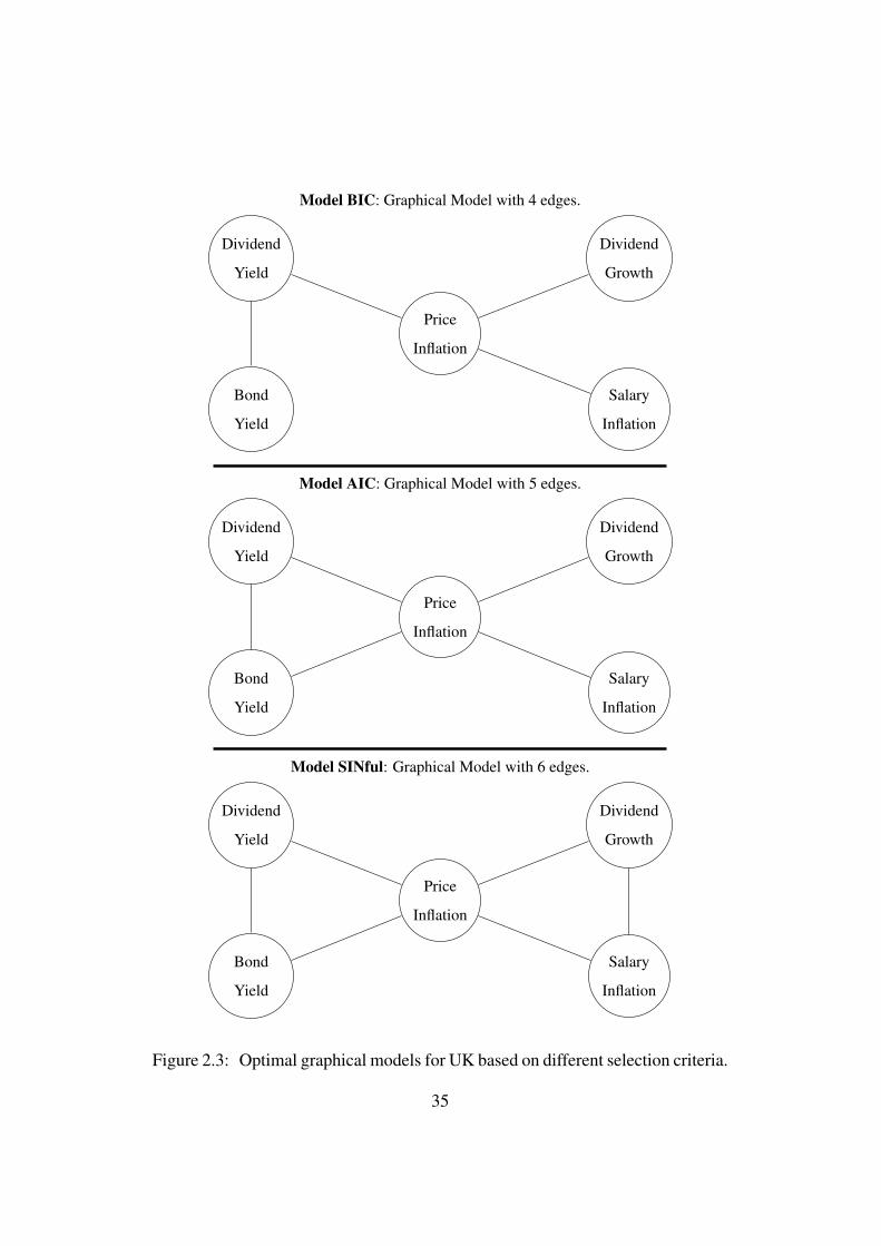
2.3 Optimal graphical models for UK based on different selection cri-
teria. . . . . . . . . . . . . . . . . . . . . . . . . . . . . . . . . . 35
2.4 Optimal graphical models for UK, US and Canada based on si-
multaneous p-values. Significant edges are shown in bold. . . . . 36
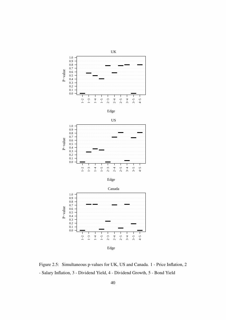
2.5 Simultaneous p-values for UK, US and Canada. 1 - Price Infla-
tion, 2 - Salary Inflation, 3 - Dividend Yield, 4 - Dividend Growth,
5 - Bond Yield . . . . . . . . . . . . . . . . . . . . . . . . . . . . 40
2.6 Fanplots of simulations of UK price inflation, salary inflation and
dividend yield from the Graphical Model and the Wilkie Model. . 44
2.7 Fanplots of simulations UK dividend growth and Bond yield from
the Graphical Model and the Wilkie Model. . . . . . . . . . . . . 45
2.8 Correlations of variables for simulations from the UK Graphical
Model and the Wilkie Model. . . . . . . . . . . . . . . . . . . . . 49
2.9 Plots of simulated share and bond total returns from the UK Graph-
ical Model and the Wilkie Model, where the black dots represent
historical observations. . . . . . . . . . . . . . . . . . . . . . . . 50
xi

2.10 Plots of simulated price and salary inflation from the UK Graph-
ical Model and the Wilkie Model, where the black dots represent
historical observations. . . . . . . . . . . . . . . . . . . . . . . . 51
2.11 Plots of simulated share and bond total returns from the UK Graph-
ical Model. . . . . . . . . . . . . . . . . . . . . . . . . . . . . . 52
2.12 Plots of simulated share and bond total returns from the Wilkie
Model. . . . . . . . . . . . . . . . . . . . . . . . . . . . . . . . . 53
2.13 Fanplots of simulations for price inflation, salary inflation and div-
idend yield for UK, US and Canada from the Graphical Model. . . 55
2.14 Fanplots of simulations for dividend growth and long bond yield
for UK, US and Canda from the Graphical Model. . . . . . . . . . 56
2.15 Plots of simulated share and long bond total returns for UK, US
and Canada. . . . . . . . . . . . . . . . . . . . . . . . . . . . . . 58
2.16 Plots of simulated price and salary inflation for UK, US and Canada. 59
3.1 Log of crude death rates for UK, US and Canada for ages 65,75
and 85 . . . . . . . . . . . . . . . . . . . . . . . . . . . . . . . . 64
3.2 Parameter estimates of model M3 for UK, US and Canada fitted
using males mortality data ages 60-89 and years 1968-2011 . . . . 68
3.3 Simulated mortality rates under Model M7 for UK, US and Canada
for males and females for ages 65, 75 and 85 along with the 90%
confidence interval. . . . . . . . . . . . . . . . . . . . . . . . . . 71
3.4 Projected mortality rates for UK males for ages 65, 75 and 85. . . 74
3.5 Fanplot for M7 and M7 adjusted for UK males for ages 65, 75 and
85 . . . . . . . . . . . . . . . . . . . . . . . . . . . . . . . . . . 75
5.1 Base case distributions of standardised PV FP (as a percentage
of A0 = £41.6bn) for both Graphical Model and Wilkie Model. . 100
xii

5.2 Distributions of standardised PV FP (as a percentage of A0 =
£41.6bn) for the base case and for the asset allocation strategy of
30% equities and 70% bonds at different probability levels using
the Graphical Model. . . . . . . . . . . . . . . . . . . . . . . . . 101
5.3 Distributions of standardised PV FP (as a percentage of A0 =
£41.6bn) for decreased contribution rate of 20% and increased
contribution rate of 25% (base case assumption is 22.5% of salary)
using Graphical Model. The grey coloured density in the back-
ground shows the base case. . . . . . . . . . . . . . . . . . . . . 102
6.1 Distributions of standardised PV FP for Starting Case with no
amortisation and for Base Case distributions (as a percentage of
A0 = $26.1bn). . . . . . . . . . . . . . . . . . . . . . . . . . . . 116
6.2 Distributions of standardised PV FP (as a percentage of A0 =
$26.1bn) for different asset allocation strategies. Base case distri-
bution is superimposed in grey for comparison. . . . . . . . . . . 117
6.3 Distributions of standardised PV FP (as a percentage of A0 =
$26.1bn) for different contribution rates. Base case distribution is
superimposed in grey for comparison. . . . . . . . . . . . . . . . 118
6.4 Distribution of standardised PV FP (as a percentage of A0 =
$26.1bn) using RP-2006 mortality table and AA projection scale.
Base case distribution is superimposed in grey for comparison. . . 119
7.1 Distribution of the standardised PV FP (as a percentage of A0 =
$227.5bn) for the Base Case. . . . . . . . . . . . . . . . . . . . . 133
7.2 Distributions of standardised PV FP (as a percentage of A0 =
$227.5bn) for asset allocation strategy. Base case distribution is
superimposed in grey for comparison. . . . . . . . . . . . . . . . 134
xiii

7.3 Distributions of standardised PV FP (as a percentage of A0 =
$227.5bn) for different contribution rates. Base case distribution
is superimposed in grey for comparison. . . . . . . . . . . . . . . 135
B.1 Plots of partial autocorrelation functions (PACF) of the residuals
for UK. . . . . . . . . . . . . . . . . . . . . . . . . . . . . . . . 177
B.2 Plots of partial autocorrelation functions (PACF) of the residuals
for US. . . . . . . . . . . . . . . . . . . . . . . . . . . . . . . . . 178
B.3 Plots of partial autocorrelation functions (PACF) of the residuals
for Canada. . . . . . . . . . . . . . . . . . . . . . . . . . . . . . 179
C.1 Base case distributions of standardised PV FP (as a percentage
of A0) for the US stylised scheme and UK’s USS. . . . . . . . . . 187
C.2 Distributions of standardised PV FP (as a percentage of A0) for
the base case and for the asset allocation strategy of 30% equities
and 70% bonds at different probability levels using the Graphical
model. . . . . . . . . . . . . . . . . . . . . . . . . . . . . . . . . 188
C.3 Distributions of standardised PV FP (as a percentage of A0) for
decreased contribution rate of 13% and increased contribution rate
of 18% (base case assumption is 15.5% of salary) using Graphical
model. The grey coloured density in the background shows the
base case. . . . . . . . . . . . . . . . . . . . . . . . . . . . . . . 189
xiv

Acknowledgements
I would like to express my deepest gratitude to my supervisor, Dr Pradip Tapadar
who has provided me with persistent help throughout this research. Thank you for
being so patient, for keeping me motivated and for being such a great role model.
Without his guidance, it would not have been possible for me to complete this
research.
I also thank my second supervisor, Dr Jaideep Oberoi for his guidance and
contribution in this research project. It was a pleasure working together.
I also had the chance to collaborate with many brilliafnt academics during
my research. In particular, I thank Dr Douglas Andrews, Dr Stephen Bonnar,
Prof Lori J Curtis, Prof Miguel Leon-Ledesma, Prof Kathleen Rybczynski and
Dr Mark Zhou for their valuable contribution and continuous support during this
research.
I would also like to express my gratitude to the Institute and Faculty of Actu-
aries for funding this research. Without their funding to support this doctorate, I
would not have been able to work on such an exciting project. I would also like to
thank the other project funders that made this project possible: the Canadian Insti-
tute of Actuaries, the National Pension Hub (part of the Global Risk Institute), the
Social Sciences and Humanities Research Council, the Society of Actuaries, the
University of Kent and the University of Waterloo; as well as the volunteers who
served on the Project Oversight Group and the Review Group who attended many
1

meetings, provided helpful comments and asked insightful questions. I am also
very grateful to the International Congress of Actuaries and the Pensions, Benefits
and Social Security Section of the International Actuarial Association for their fi-
nancial support. Thanks to their financial support, I had the opportunity to present
our research findings at various international conferences.
Moreover, I would like to thank Claire Carter and Derek Baldwin for all the
effort they put to make the lives of PhD students so much easier. I also thank all
the wonderful people who I have met during this research. In particular, I thank
Alan, Alex, Jose, Laurentiu, Michele and Tong. My time at the University of Kent
would not have been the same without you.
Furthermore, a special thanks goes to my friends from London; Avinash, Clare
and Mark for making my time in England so much more special.
A tremendous thanks to Mariza for being so kind and supportive especially
towards the end of my research.
Last but certainly not the least, I thank my parents and my sister for their
support both financially and emotionally and for their encouragement throughout.
2
Abstract
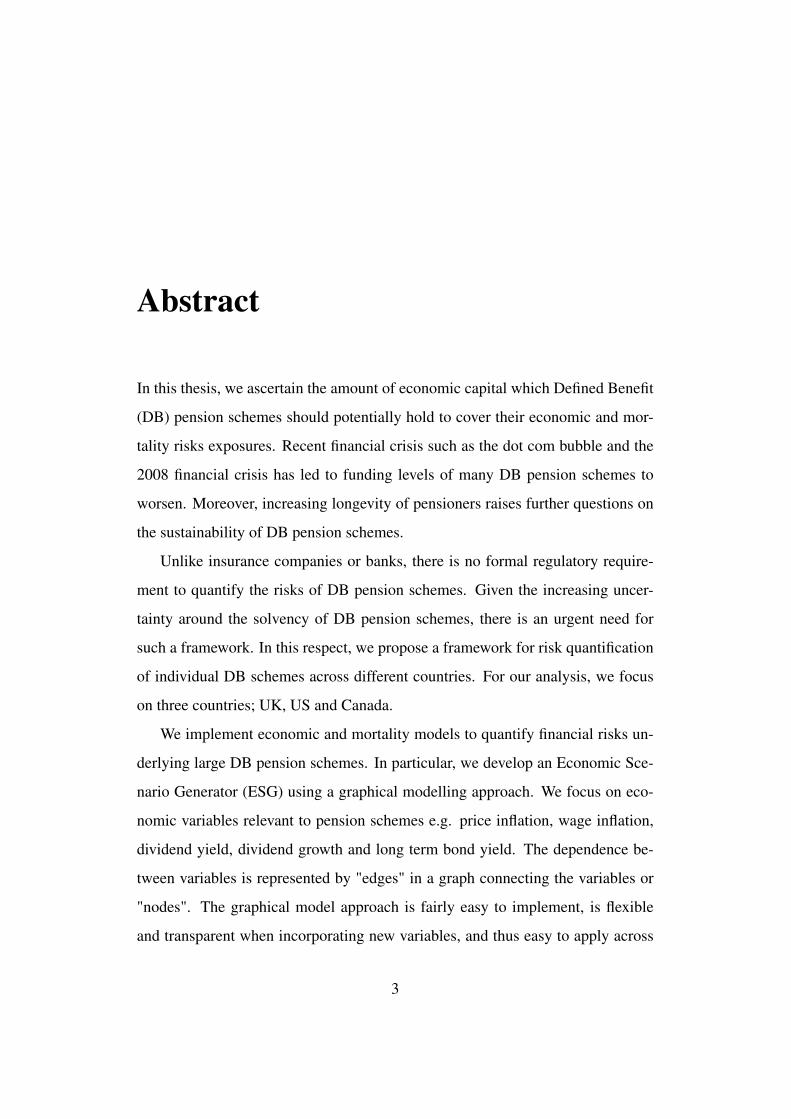
In this thesis, we ascertain the amount of economic capital which Defined Benefit
(DB) pension schemes should potentially hold to cover their economic and mor-
tality risks exposures. Recent financial crisis such as the dot com bubble and the
2008 financial crisis has led to funding levels of many DB pension schemes to
worsen. Moreover, increasing longevity of pensioners raises further questions on
the sustainability of DB pension schemes.
Unlike insurance companies or banks, there is no formal regulatory require-
ment to quantify the risks of DB pension schemes. Given the increasing uncer-
tainty around the solvency of DB pension schemes, there is an urgent need for
such a framework. In this respect, we propose a framework for risk quantification
of individual DB schemes across different countries. For our analysis, we focus
on three countries; UK, US and Canada.
We implement economic and mortality models to quantify financial risks un-
derlying large DB pension schemes. In particular, we develop an Economic Sce-
nario Generator (ESG) using a graphical modelling approach. We focus on eco-
nomic variables relevant to pension schemes e.g. price inflation, wage inflation,
dividend yield, dividend growth and long term bond yield. The dependence be-
tween variables is represented by "edges" in a graph connecting the variables or
"nodes". The graphical model approach is fairly easy to implement, is flexible
and transparent when incorporating new variables, and thus easy to apply across
3

different datasets (e.g. countries). We also show that the results are consistent
with well-established ESGs such as the Wilkie Model in the UK context.
We also compare quantitatively seven stochastic models explaining improve-
ments in mortality rates. In particular, we use the Bayes Information Criteria to
choose a model which provides a good fit to mortality data from UK, US and
Canada.
We use the graphical model alongside the mortality model to examine the risks
of UK, US and Canadian pension schemes. Although the modelling methodology
remains the same, we fit the economic and demographic models to data from all
three countries.
We then implement our framework to calculate the economic capital for exist-
ing and “stylised" pension schemes.For the UK, we carry out risk assessment of
the Universities Superannuation Scheme (USS). For the US, we use a US stylised
scheme for our analysis. The US stylised scheme is based on the membership
profile and benefits of the USS but adapted to be representative of a US pension
scheme. For Canada, we carry out risk assessment of the Ontario Teachers’ Pen-
sion Plan (OTPP). Both the USS and the OTPP are very large pension schemes
with over 300,000 members.
We further carry out sensitivity analysis by varying the mortality assumptions
and the asset allocations of the pension schemes. The overall aim of the exercise
is to determine and compare the long-term sustainability of pension schemes in
different countries.
The interaction between population structure, investments and asset returns
will be of interest to pension funds, actuaries and policy-makers, all of whom are
interested in the overall health of both public and private pension schemes.
4

Chapter 1
Introduction
1.1 Background and Motivation
A pension scheme can be thought as a long-term savings arrangement to transfer
wealth from youth to old age. There are two main types of pension arrangement:
pay-as-you-go (PAYG) and funded schemes. Most state pension schemes are on
a PAYG system. In a PAYG system, the pensions of the retired generation are
paid from the contributions of the current working population. For this system to
be viable on a long run, it requires sufficient people in work, making sufficient
contributions to pay for those who have retired.
A funded pension scheme in contrast is composed of a pension fund plus and
pension annuity. While different types of funded pension schemes exist, what
differentiates one type of funded pension scheme to another is the set of rules
which govern the calculations of the benefits when an individual retires. The
simplest type of funded scheme is a Defined Contribution (DC) scheme which
uses the full fund value at the time of retirement to determine the pension payment.
The investment risk lies entirely with the individual with a DC scheme.
A Defined Benefit (DB) scheme is another type of funded pension scheme in
5

which an employer/sponsor promises a pension payment to an employee based
on the employee’s earnings, number of years of service and age. Unlike a DC
scheme, the pension payment does not depend directly on the total fund value at
the time of retirement. The investment risk lies entirely with the sponsor with a
DB scheme.
In addition to DB and DC schemes, a wide range of other funded pension
schemes exist. While DB and DC represent the two extremes of a “spectrum",
other funded pension schemes typically have features which lie somewhere in
between DB and DC schemes and are commonly referred as hybrid schemes. We
discuss hybrid schemes in Appendix A.2 and A.3. This thesis however focuses
primarily on DB schemes.
Years of high inflation, good investment returns and surplus generated dur-
ing the 1970s and 1980s created the illusion that DB pension schemes are easily
affordable. Due to the creation of large surpluses during those years, pension
risks have generally been excluded from a sponsor’s general risk management
processes. For example, in the 1990s, UK pension schemes were enjoying high
level of funding and actuaries were advsing some schemes to take contribution
holidays. In the US, several multiemployer schemes were fully funded in the mid
1980s and 1990s.
The funding of DB schemes fell drastically in the year 2000 when the price of
technology stocks went down. Moreover, the 2008 global recession led to fund-
ing levels of many schemes to plummet. DB systems in UK, Australia, Ireland
and US saw large increases in deficits following the crisis. Moreover the cri-
sis triggered a large increase in employer and employees’ contributions in many
countries including Canada and the Netherlands.
The problem of DB pension schemes has been further accentuated with popu-
lation ageing taking place as a result of birth rates going down and longevity going
6
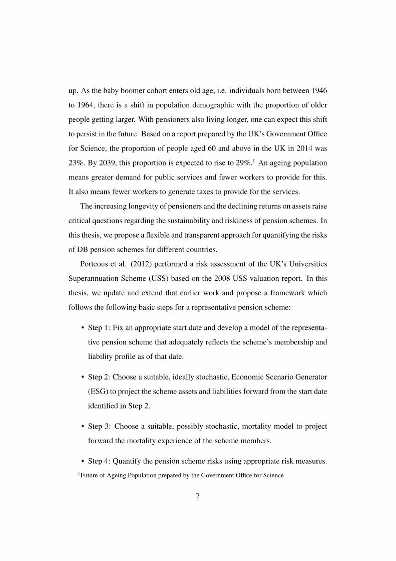
up. As the baby boomer cohort enters old age, i.e. individuals born between 1946
to 1964, there is a shift in population demographic with the proportion of older
people getting larger. With pensioners also living longer, one can expect this shift
to persist in the future. Based on a report prepared by the UK’s Government Office
for Science, the proportion of people aged 60 and above in the UK in 2014 was
23%. By 2039, this proportion is expected to rise to 29%.1 An ageing population
means greater demand for public services and fewer workers to provide for this.
It also means fewer workers to generate taxes to provide for the services.
The increasing longevity of pensioners and the declining returns on assets raise
critical questions regarding the sustainability and riskiness of pension schemes. In
this thesis, we propose a flexible and transparent approach for quantifying the risks
of DB pension schemes for different countries.
Porteous et al. (2012) performed a risk assessment of the UK’s Universities
Superannuation Scheme (USS) based on the 2008 USS valuation report. In this
thesis, we update and extend that earlier work and propose a framework which
follows the following basic steps for a representative pension scheme:
• Step 1: Fix an appropriate start date and develop a model of the representa-
tive pension scheme that adequately reflects the scheme’s membership and
liability profile as of that date.
• Step 2: Choose a suitable, ideally stochastic, Economic Scenario Generator
(ESG) to project the scheme assets and liabilities forward from the start date
identified in Step 2.
• Step 3: Choose a suitable, possibly stochastic, mortality model to project
forward the mortality experience of the scheme members.
• Step 4: Quantify the pension scheme risks using appropriate risk measures.1Future of Ageing Population prepared by the Government Office for Science
7

For our analysis, we quantify and compare the risks of pension schemes from
three countries: UK, US and Canada. For the UK, we have decided to base our
analysis on a representative model of UK’s USS as of March 31, 2014, and project
its assets and liabilities forward from that date onward. The start date chosen is
based on the latest available valuation report at the time we started this research.
For the US, we analyse a US stylised scheme based on the UK’s USS. The
scheme is based on the same model points as the USS but with a number of
changes to the benefit structure and contribution rates to account for the differ-
ences in typical US schemes.
Finally for Canada, our analysis is based on a representative model of the
Ontario Teachers’ Pension Plan (OTPP) using January 1, 2018 as the start date.
Again, our choice for the start date is based on the latest valuation report available.
The publicly available data from the actuarial valuation reports and other docu-
ments typically provide summarised data on membership profile, accrued benefits,
average salary/pension, past service, age and gender distribution, and actuarial li-
ability. As we do not have access to the full underlying membership data, we need
to build a representative model for the pension schemes under consideration, with
appropriate model points for active members, deferred members and pensioners,
to broadly match the published summarised data as of the chosen start date.
Recent regulatory developments within the banking, insurance and pensions
sectors have been key drivers towards a formal economic capital approach towards
financial risk management. Moreover, the financial crisis of 2008 and the after-
math felt worldwide have added to the additional scrutiny of the risk assessment
practices of the financial sector. So any study of the financial risk assessment of
pension schemes needs to be set within this wider framework.
The banking sector started the initiative towards economic capital based fi-
nancial risk management through Basel 1, in 1988, followed by a revised accord,
8

Basel 2, which came into force on 1 January 2007. Following the financial cri-
sis of 2008, a lot of banks had gone bankrupt and others were barely surviving.
The Basel Committee on Banking Supervision issued its first version of Basel 3,
in late 2009, in response to the global financial crisis. In order to aid an effec-
tive and timely adoption, the Basel committee has recommended a timeline of
phase wise implementations to give banks the time to build quality capital and
appropriate standards. The final Basel 3 minimum requirements are expected to
be implemented by 1st January 2022 and will be fully phased in by 1st January
2027. Basel 3 has a “three pillar" structure and is built on upon Basel 1 and Basel
2 framework. The three pillars focus on quantitative and qualitative requirements
to promote greater resilience of the banking sector.
Solvency 2 is an EU insurance regulation which focuses primarily on eco-
nomic capital requirement of insurance and reinsurance companies. Similar to
Basel 3, Solvency 2 is based on a “three pillar" structure summarised below:
• Pillar 1: Quantitative requirement to calculate technical provisions and sol-
vency capital requirement covering all risks.
• Pillar 2: Qualitative requirements covering rules of governance and super-
visory review process.
• Pillar 3: Transparency and disclosure requirements.
The Solvency 2 directive became fully applicable on 1 January 2016. Similar
to Basel 3, Solvency 2 aims to set solvency standards to match risk and encourage
proper risk controls. Other salient features of Solvency 2 are as follows:
• harmonise standards across the EU to avoid the need for Member states to
set higher standards;
• bring valuation of assets and liabilities on a “fair" value basis;
9

• bring greater level protection to policyholders and beneficiaries compared
to previous solvency directives;
• not be too onerous for smaller companies.
In order to be consistent with banking and insurance sectors, we propose to use
economic capital to quantify pension scheme risk. Unlike the banking and insur-
ance sectors however, no established definition of economic capital exists for risk
assessment of pension schemes. We therefore propose the following definition of
economic capital for our purpose:
The economic capital of a pension scheme is the proportion by which
its existing assets would need to be augmented in order to meet net
benefit obligations with a prescribed degree of confidence. A scheme’s
net benefit obligations are all obligations in respect of current scheme
members, including future service, net of future contributions to the
scheme.
We show our results at a number of different confidence levels, including
99.5% degree of confidence which is consistent with both the analysis of Porteous
et al. (2012) and Solvency 2. Policymakers can choose the level of confidence as
is deemed appropriate.
Before we begin our analysis, we provide a literature review on similar work
which deals with measuring and managing pension risks.
1.2 Literature Review
Porteous et al. (2012) perform a risk assessment of the USS based on the valuation
report 2008. They model stochastic economic variables using a graphical model
10
and model stochastic mortality rates following Sweeting (2008). The solvency
capital requirement of the USS is determined in a Solvency 2 framework. As at
2008, the economic capital was estimated at 61% of the best estimate of liabilities.
The work by Porteous et al. (2012) was extended by Yang and Tapadar (2014).
They apply economic capital techniques to the UK’s Pension Protection Fund
(PPF) which takes over eligible schemes with deficit in the event of sponsor in-
solvency. The authors then compare the relative size of the economic capital for
the PPF and individual schemes. They show that for individual schemes, solvency
capital varies between 66% and 134% of its liabilities and for the PPF, economic
capital is estimated at 10% of the liabilities. This reduction is explained by the
PPF benefiting from pooling of risks of a large number of schemes.
Devolder and Piscopo (2014) model a DB scheme based on final salary using
a single model point and model the cashflows for a life aged 35 who retires at 65.
Assets are modelled using a Geometric Brownian motion. The paper observes the
probability of insolvency of the DB scheme over a 30-year horizon. The proba-
bility of default follows an exponential decay and varies between 0% - 40%. The
authors further show the solvency capital requirement over time which varies be-
tween 0 - 30% of liabilities. The solvency capital requirement is calibrated at a
99.5% Value-at-Risk (VaR).
Ai et al. (2015) also use the Solvency 2 framework and measure the solvency
capital requirement of a pension scheme using two approaches. The first approach
treats the pension scheme as a group annuity product offered by an insurer and
applies established insurer factors to the pension scheme. The risks considered
are default and market risk, pricing risk, interest rate risk and operational risk.
These risks are then quantified using the Standard and Poor’s Capital Model fac-
tors 2010. The second approach directly simulates the risk drivers of the pension
scheme and develops a framework for calculating the pension risk given a desired
11

confidence level. Results are comparable under the two approaches. For example,
the equity investment capital charge is 38% using the Standard and Poor’s factor
approach and 35.52% using the simulation approach.
Although the Solvency 2 framework and the VaR approach are popular ways
of quantifying the risks of a pension scheme, there are other ways of quantifying
these risks. Boonen (2015) examines the consequences of using Expected Short-
fall instead of VaR to calculate the solvency capital requirement. The argument
for using Expected Shortfall is that it considers the size of worst case events while
VaR uses only the quantile. The paper assumes a portfolio of 100,000 deferred
life annuities and focusses on three risk classes: equity risk, interest rate risk and
longevity risk. In their analysis, the 98.78% Expected Shortfall corresponds to the
99.5% VaR. This is consistent with certain types of distribution such as the normal
distribution.
Devolder and Lebegue (2016) use ruin theory to estimate the solvency cap-
ital requirement for long term life insurance and pension products, arguing that
the Solvency 2 framework may not be appropriate for products with long term
horizons given that the framework takes a one-year view on risk. They allow for
different terms of contract with a single payment at maturity. For the base case
scenario, only equity risk is taken into account. Under the Solvency 2 framework,
solvency capital is understated at shorter durations (less than 60 years) and over-
stated at longer durations (greater than 60 years). For example, for a product with
a 30-year horizon, solvency capital is 43% higher if using the ruin theory frame-
work. For a product with a 90-year horizon however, solvency capital is 29%
lower using the ruin theory approach. This is due to the benefits of equity invest-
ments over long horizons, which are not properly allowed for under the Solvency
2 framework.
Devolder and Lebegue (2017) further expose the issues of using the Solvency
12

2 framework for measuring pension risks. The authors compare the Solvency 2
framework to a dynamic risk measure where dynamic risk measures are defined
according to the amount of information disclosed through time. They assume the
pension fund consists of maturity guaranteed benefits and members make a single
contribution at the start. The paper shows that solvency capital is independent of
the term of the contract under the Solvency 2 framework. This is not the case
with a dynamic risk measure. Moreover, solvency capital can be much higher
with a dynamic measure. For example, applying a life cycle investment strategy
to a 30-year contract, the solvency capital is 40% of the initial contribution under
the Solvency 2 framework. In contrast, the solvency capital is 100% of the initial
contribution using the dynamic risk measure.
In this section, we have only reviewed literature which has direct relevance to
our research. However risk assessment of pension schemes can be addressed using
a wide variety of approaches and literatures is extensive in this area of research.
So a more detailed literature review is provided in Appendix A to cover these
broad areas of research. There we consider literature considers at the relative
significance of factors driving pension risks such as equity risk, interest rate risk
and longevity risk. Papers that have addressed these issues include Butt (2012),
Liu (2013), Karabey et al. (2014) and Sweeting (2017). Other literature has
compared the impact of different economic scenario generators on pension risks
(such as Devolder and Tassa (2016) and Abourashchi et al. (2016)) and the impact
of different mortality models on pension risks (such as Lemoine (2015) and Arik
et al. (2018)).
We also look at literature on managing risks from the sponsor’s point of view.
Some papers have used financial instruments to hedge or transfer the risk. Exam-
ples of the instruments used include natural hedging (Li and Haberman (2015));
longevity hedges (Lin et al. (2014, 2015)); and pension buyouts (Cox et al.
13

(2018)). Some papers have also focused on risk management based on the scheme’s
structure, as in Kleinow (2011), Aro (2014) and Platanakis and Sutcliffe (2016).
Moreover, some researchers have used optimisation techniques to see the extent
to which the sponsor’s risk can be reduced. Some of the techniques they have
discussed include dynamic asset allocation (Liang and Ma (2015)) and automatic
balancing mechanisms (Godinez-Olivares et al. (2016)).
Finally, we have also looked at pension risks from the point of view of scheme
members. Among these, a number of papers have focused on solving optimi-
sation problems to maximise the expected utility of scheme members. For ex-
ample, Devolder and Melis (2014) examined the benefits to scheme members of
having both funded and unfunded public pensions. Alternatively, Chen and De-
long (2015) studied the asset allocation problem to maximise scheme members’
utility in a defined contribution scheme. Other papers have proposed innovative
pension structures to reduce scheme members’ risks. Structures analysed and
examined included hybrid structures (Khorasanee (2012)) and TimePension (Lin-
nemann et al. (2014)). Intergenerational risk sharing and the benefits to scheme
members/pensioners have also been areas of ongoing research interest (as in Chen
et al. (2014) and Wang et al. (2018)).
1.3 Structure of Thesis
The structure of this thesis is as follows: In Chapter 2, we develop the ESG which
we use to project the assets and liabilities of DB pension schemes. In Chapter
3, we discuss the mortality models we use to project the longevity for members
in the schemes. In Chapter 4, we outline the methodology we propose to use to
quantify the pension scheme risks. In Chapters 5, 6 and 7, we present the risk
assessment of the UK’s USS, the US stylised scheme and the OTPP respectively.
14

Finally, in Chapter 8, we draw our conclusions and propose future work.
15

Chapter 2
Economic Scenario Generators
2.1 Introduction
Projecting pension plan assets and liabilities requires simulation of future eco-
nomic scenarios. Typically actuaries rely on ESGs to produce reasonable simula-
tions of the joint distribution of economic variables relevant for asset and liability
valuations.
A wide range of ESGs are currently used in the industry. These models have
varying levels of complexity and are often proprietary. Among the few published
models for actuarial use, the most well-known is the Wilkie Model first published
in Wilkie (1986). This reduced-form vector auto-regression model for UK eco-
nomic variables, relies on a cascading structure, where the forecast of one or more
variables is used to generate values for other variables, and so on. This model has
been periodically validated and recalibrated in Wilkie (1995) and Wilkie et al.
(2011).
In this research, we want to carry an analysis of UK, US and Canadian pension
schemes. The Wilkie models (Wilkie (1986), Wilkie (1995) and Wilkie (2011))
however are only calibrated to UK data. Although there are research papers which
16

calibrate the Wilkie Model to other countries (e.g. Zhang et al. (2018) have
parameterised the Wilkie Model to US data), we do not make use of these models
in this research. This is because we want to develop a modelling framework which
can be easily calibrated for any country as long as relevant data is available. In
this respect, we develop an ESG using a graphical approach calibrated to UK, US
and Canadian data.
Graphical models rely on capturing the underlying correlation structure be-
tween the model variables in a parsimonious manner, making them useful for
simulating data in high dimensions. In these models, dependence between vari-
ables is represented by edges in a graph connecting the variables or nodes. This
approach allows us to assume conditional independence between variables and to
set their partial correlations to zero. Two variables could then be connected via
one or more intermediate variables, so that they could still be weakly correlated.
Graphical models have also been used in Porteous (1995); Porteous and Tapadar
(2005, 2008a,b); Porteous et al. (2012); Yang and Tapadar (2015).
In section 2.2, we provide a brief overview of the Wilkie Model. We then dis-
cuss in Section 2.3 the ESG we have developed for this research using a graphical
approach.
2.2 The Wilkie Model
2.2.1 Background and Motivation
In 1984, David Wilkie first presented his work on a stochastic investment model
for actuarial use in the UK. The work was formally published in Wilkie (1986).
Periodically, David Wilkie has updated and recalibrated his model in Wilkie (1995)
and Wilkie et al. (2011). He has also co-authored other recent papers Wilkie and
Sahin e.g. 2016, 2017a, 2017b, 2017c, 2017d, which focus on certain specific as-
17

pects of the Wilkie Model e.g. the relationship between price inflation and salary
inflation or small extensions of Wilkie et al. (2011). We will only focus on Wilkie
(1986), Wilkie (1995) and Wilkie et al. (2011) however.
The original purpose of the Wilkie Model was to develop a sufficient economic
and investment model which actuaries could use for long term simulations of fu-
ture economic scenarios without being too concerned with very short-term fluctu-
ations. Model variables were specifically chosen keeping in mind the long-term
nature of a life insurance company or a pension scheme’s assets and liabilities.
The actual constituents of the model and the model parameters have been updated
periodically (Wilkie (1995), Wilkie et al. (2011)) but the overall approach and
structure have broadly remained the same.
2.2.2 Model Structure
Since the the Wilkie Model was first proposed in 1984, the notations have under-
gone some changes over time. We will present the notations used in Wilkie et al.
(2011) to avoid confusion.
In the first paper, Wilkie (1986) presented a model for the following four vari-
ables:
I(t): annual rate of price inflation;
Y (t): dividend yield on an index of ordinary shares;
K(t): annual rate of dividend increase;
C(t): bond yields on government bonds.
The variables were related to each other in a cascade structure, as depicted in
Figure 2.1, where price inflation impacted all the other variables in that model.
18
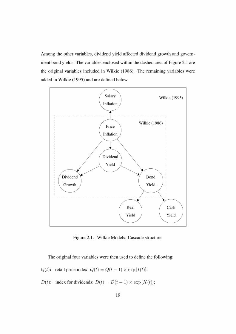
Among the other variables, dividend yield affected dividend growth and govern-
ment bond yields. The variables enclosed within the dashed area of Figure 2.1 are
the original variables included in Wilkie (1986). The remaining variables were
added in Wilkie (1995) and are defined below.
Salary
Inflation
Price
Inflation
Dividend
Yield
Dividend
Growth
Bond
Yield
Real
Yield
Cash
Yield
Wilkie (1986)
Wilkie (1995)
Figure 2.1: Wilkie Models: Cascade structure.
The original four variables were then used to define the following:
Q(t): retail price index: Q(t) = Q(t− 1)× exp [I(t)];
D(t): index for dividends: D(t) = D(t− 1)× exp [K(t)];
19

P (t): price index of ordinary shares: P (t) = D(t)/Y (t).
Wilkie (1995) introduced a few more economic variables:
J(t): annual rate of wage inflation;
B(t): short-term yields on government bonds: logB(t) = logC(t)−BD(t).
BD(t): “log-spread” between bond yield and cash yield;
R(t): real yields on index-linked stocks.
These new variables led to:
W (t): index of wages: W (t) = W (t− 1)× exp [J(t)].
Wilkie (1995) also proposed a model for property indices, but this was later dis-
continued as being unsatisfactory, so we do not consider this here. The detailed
model and the parameterisation is provided in Appendix B.
2.3 Graphical Models
2.3.1 Background
For the purpose of risk calculation over long periods, we propose an alternative
approach of modelling the underlying correlations between the innovations to the
variables e.g. the residuals or the error terms in an autoregression.
Graphical models achieve this in a parsimonious manner, making them use-
ful for simulating data in larger dimensions. In graphical models, dependence
between two variables is represented by an “edge” in a graph connecting the vari-
ables or "nodes". This approach allows us to assume conditional independence
between two variables (that are not directly connected by an edge) and to set their
20

partial correlations to zero. The two variables could then be connected via one or
more intermediate variables, so that they could still be weakly correlated.
As a result, we compare different algorithms to select a graphical model, based
on the Akaike Information Criterion (AIC), the Bayesian Information Criterion
(BIC), p-values and deviance.
2.3.2 Graphical Model Framework
A graph, G = (V , E), is a structure consisting of a finite set V of variables (or
vertices or nodes) and a finite set of edges E between these variables. The exis-
tence of an edge between two variables represents a connection or some form of
dependence. The absence of this connection represents conditional independence.
For instance, if we have a set of three variables V = {A,B,C}, where A
is connected to B and not to C, but B is connected to C, A is connected to C
via B. A is then conditionally independent of C, given B. Such a structure can
be graphically represented by drawing circles or solid dots representing variables
and lines between them representing edges. The graphical model described above
with three variables, A, B and C, is shown in Figure 2.2. We can see that there is
a path between A and C, which goes through B. The graphs we consider here are
called undirected graphs because the edges do not have a direction (which would
otherwise be represented by an arrow). Such graphs model association rather than
causation.
21

A
B
C
Figure 2.2: A graphical model with 3 variables and 2 edges.
Another way of looking at graphical models is that they are excellent tools
for modelling complex systems of many variables by building them using smaller
parts. In fact, graphical models may be used to represent a wide variety of statis-
tical models including many of the more sophisticated time series models used in
actuarial science today. Recent standard and accessible texts on graphical models
include Edwards (2012) and Hojsgaard et al. (2012). The latter provides detailed
guidance on the use of packages written in R to estimate graphical models. In this
research, we make use of these standard packages wherever possible. Our aim is
to demonstrate the use of the undirected graph to develop a parsimonious repre-
sentation of the economic variables that can then be easily used for simulation.1
Graphical models are non-parametric by nature, but they may be used to rep-
resent parametric settings, a feature that is desirable for applications such as ours.
Due to the easy translatability between the traditional modelling structure (covari-
ance matrices) and the graphical structure in multivariate normal settings, we will
focus on the parametric approach here and show that it leads to reasonable out-
comes with our modelling strategy. Such models are known as Gaussian Graphical
models.1Although we do not discuss directed graphs here, they are widely applied for causal inference.
For instance, an arrow from A to B and one from B to C in Figure 2.2 would establish an indirect
causal link between A and C (mediated by B), whereas an arrow from A to C would represent a
direct causal link.
22

One of our key goals is to be able to represent the covariance structure with di-
mension reduction, and the graphical model will allow us to achieve that by effec-
tively capturing conditional independence between pairs of variables and shrink-
ing the relevant bivariate links to zero while allowing for weak correlations to
exist in the simulated data. For the multivariate normal distribution, if the con-
centration matrix (or inverse covariance matrix) K = Σ−1 can be expressed as a
block diagonal matrix, i.e.:
K =
K1 0 · · · 0
0 K2 · · · 0...
... . . . ...
0 0 · · · Km
, (2.1)
then the variables u and v are said to be conditionally independent (given the other
variables) if kuv = 0 where K = (kuv). To achieve this block diagonal structure,
variables may need to be reordered.
As the concentration matrix K depends on the scales of the underlying vari-
ables, it is sometimes easier to analyse the partial correlation matrix ρ = (ρuv),
where:
ρuv =kuv√kuu kvv
. (2.2)
Note that ρuv = 0 if and only if kuv = 0.
For our example graphical model in Figure 2.2 the partial correlation matrix
would look like:
ρ =
1 ρAB 0
ρAB 1 ρBC
0 ρBC 1
, (2.3)
where ρAB 6= 0 and ρBC 6= 0. So, variables A and C are independent given
variable B. Note that this could still generate non-zero unconditional correlation
between A and C.
23
Before using this structure, we will first describe the data in the next section.
2.3.3 Data
In order to build a minimal economic model, which can be used by a life insurance
company or a pension fund, we require retail price inflation (I), salary inflation
(J), stock returns and bond returns over various horizons.
For the UK, the data we use has been generously provided by David Wilkie,
who has carried out a range of checks and matching exercises to construct all
the relevant time series. Following his procedure in Wilkie (1986), we model
dividend yield (Y ), dividend growth (K) and Consols yield (C) to construct stock
and bond returns. Consols yield is the yield on perpetual UK government bonds.
Henceforth, we refer to Consols Yield as bond yield. We use the complete dataset
provided by David Wilkie, which consists of annual values from 1926 to 2017 as
at the end of June each year. An excerpt of the data can be found in Wilkie et al.
(2011).
For the US, our data comes from two sources. The first source is from Robert
Shiller who provides online data for the consumer price index, S&P 500 price
index, S&P 500 dividend index, and 10-year government bond yield.2. The second
source of data comes from Emmanuel Saez who provides online data for average
wages in the US. The data we use extend from 1913 to 20153.
For Canada, the data we use range from 1935 to 2015. For price inflation
and salary inflation, the data we use comes from two sources. We use data from
Emmanuel Saez who provides Canadian online data for the retail price index and
average wages up to the year 2000. From 2001 onwards, we use price inflation
2http://www.econ.yale.edu/~shiller/data.htm3https://eml.berkeley.edu/~saez/
24

data and salary inflation data from the Federal Reserve Economic Data4 and Statis-
tics Canada5 respectively. For the Canadian dividend yield, dividend growth and
bond yield, we use data from Statistics Canada which provide data for the Toronto
Stock Exchange (TSE) index, TSE dividend yield and 10-year government bond
yield.
2.3.4 Modelling
We are only interested in simulating the selected variables jointly, so we may
first wish to take a look at the historical pairwise correlations. The UK, US and
Canadian historical correlations are given in Table 2.1. Price inflation appears
to be correlated consistently across all three countries. However, the correlations
between the variables are not all similar across the three countries. A graphical
model promises to provide the flexible framework needed to generate scenarios
consistent with this long-run dependence structure.
4https://fred.stlouisfed.org/series/FPCPITOTLZGCAN5https://www.statcan.gc.ca/eng/start
25

Table 2.1: Historical correlations for UK, US and Canada
UK US Canada
It Jt Yt Kt Ct It Jt Yt Kt Ct It Jt Yt Kt Ct
It 1 1 1
Jt 0.83 1 0.50 1 0.65 1
Yt 0.35 0.28 1 0.11 -0.04 1 0.31 0.50 1
Kt 0.37 0.35 -0.08 1 0.23 0.22 -0.09 1 0.19 0.15 0.03 1
Ct 0.64 0.73 0.17 0.27 1 0.32 0.05 -0.11 0.01 1 0.44 0.02 -0.24 0.10 126

Table 2.2: Time series parameter estimates for univariate AR(1) regressions UK, US and Canada.
UK US Canada
µ β σ µ β σ µ β σ
It 0.0404 0.6102 0.0387 0.0328 0.6211 0.0392 0.0361 0.7105 0.0225
Jt 0.0528 0.7801 0.0282 0.0464 0.4908 0.0643 0.0600 0.5358 0.0415
Yt 0.0468 0.6718 0.0085 0.0413 0.8293 0.0100 0.0367 0.9112 0.0053
Kt 0.0527 0.4263 0.0852 0.0507 0.2746 0.1084 0.0684 0.1044 0.1755
Ct 0.0617 0.9674 0.0083 0.0489 0.9346 0.0091 0.0601 0.9699 0.007527

2.3.5 Correlations in Levels or in Innovations
Our objective here is to provide an adequate model that is as simple as possible.
When simulating, there is a philosophical question as to whether one should pro-
duce scenarios from a tightly structured model of the levels of the variables, or
whether one should focus on the innovations in the time series processes of these
variables. By construction, the innovations should be i.i.d once a well-specified
regression model has been fitted. We take the view that contemporaneous changes
in variables beyond those predicted by their own past values offer a useful handle
on the range of scenarios to be produced.
Over the history of these variables, there have been several events, but one
could still argue that there is long-term mean reversion in most series, albeit at
different rates. This may be a good reason to focus our attention on modelling the
joint innovations in the series. Rather than model the joint dynamics of variables
using a large number of constraints and parameters, we can minimise the num-
ber of constraints required by restricting them to situations that would rule out
inadmissible values.
Given that the aim of our ESG is to emphasise long-run stable relationships
and to generate a distribution of joint scenarios, we take the approach of estimating
the joint distribution of the residuals of individual time series regressions. This
focuses on the dependence between innovations and, we argue, may allow for a
richer set of scenarios generated with relatively simple models. For each variable,
we will first estimate a time series model independently and then we will fit a
graphical model for the time series residuals across variables.
At the annual frequency we consider here, the dynamics of the variables can
arguably be adequately represented by a simple AR(1) process in most cases. For
28
each time series Xt, we use the following AR(1) time-series model formulation:
µx = E[Xt] (2.4)
Zt = Xt − µx (2.5)
Zt = βx Zt−1 + ex,t where ex,t ∼ N(0, σ2x). (2.6)
The parameter estimates from the AR(1) regressions are provided in Table 2.2 for
UK, US and Canada. All AR(1) coefficients are statistically significance at the
1% level.
In addition, the fit appears satisfactory in the sense that there does not appear
to be significant residual dependence in the errors. Partial autocorrelation plots
of the residuals from these regressions are provided in Appendix B.8 for refer-
ence. While an AR(1) fit appears adequate for the purposes of our model, one can
choose an alternative univariate time series model if deemed appropriate, as we
are interested in the innovations from the model.
2.3.6 Fitting a Graphical Model to Residuals
To estimate a Gaussian Graphical Model for the residuals, we assume that:
et = (eIt , eJt , eYt , eKt , eCt) ∼ N (0,Σ).
The correlations between the residuals for the three countries are given in Table
2.3.
29

Table 2.3: Correlations of residuals from individual AR(1) regressions for UK, US and Canada.
UK US Canada
It Jt Yt Kt Ct It Jt Yt Kt Ct It Jt Yt Kt Ct
It 1 1 1
Jt 0.56 1 0.38 1 0.66 1
Yt 0.34 0.25 1 0.10 -0.39 1 0.15 0.22 1
Kt 0.31 0.28 0.08 1 0.25 0.06 0.28 1 0.08 0.09 0.24 1
Ct 0.31 0.13 0.43 0.13 1 0.23 0.08 0.12 0.03 1 0.21 -0.01 0.29 0.42 130
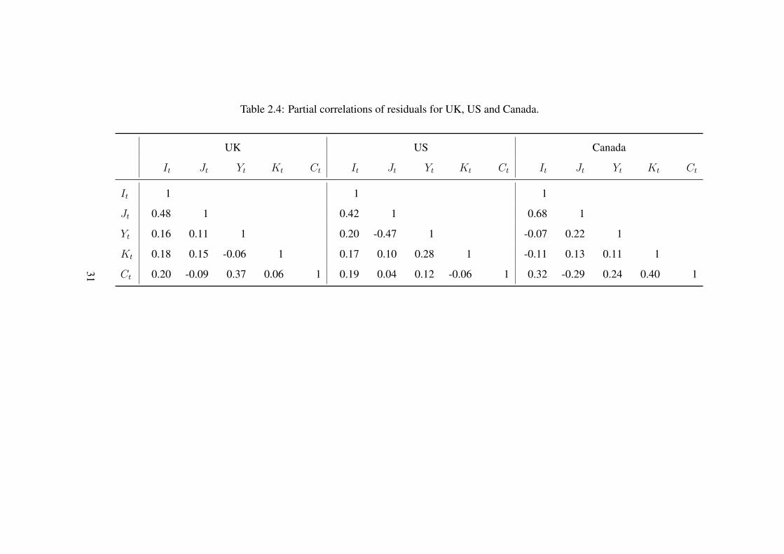
Table 2.4: Partial correlations of residuals for UK, US and Canada.
UK US Canada
It Jt Yt Kt Ct It Jt Yt Kt Ct It Jt Yt Kt Ct
It 1 1 1
Jt 0.48 1 0.42 1 0.68 1
Yt 0.16 0.11 1 0.20 -0.47 1 -0.07 0.22 1
Kt 0.18 0.15 -0.06 1 0.17 0.10 0.28 1 -0.11 0.13 0.11 1
Ct 0.20 -0.09 0.37 0.06 1 0.19 0.04 0.12 -0.06 1 0.32 -0.29 0.24 0.40 131

The resulting partial correlation matrices are given in Table 2.4. Clearly, some
of the partial correlations in the matrices are small. Our goal is to identify the
graphical structures with the minimum number of edges, which describe the un-
derlying data adequately.
For each country, as there are 5 variables in the model, the minimum number
of edges required for a connected graph (i.e. where there exists a path between
any two nodes) is 4. The graph with the maximum possible number of edges is
the saturated model with 5C2 = 10 edges. We will call this Model Sat. The
model with no edges is the independence model, i.e. all variables are independent
of each other, and we will call it Model 0 (as there are no edges).
In total, there are 210 = 1024 distinct models possible. But we will focus only
on those models that are optimal, based on certain desirable features.
2.3.7 Model Choice: Desirable Features and Optimality
Selection of a graphical model can be carried out by traditional statistical crite-
ria. This is usually done in an iterative procedure, where we consider our model
selection criterion of choice before and after adding (or removing) an edge be-
tween two variables. One may begin with Model 0 or Model Sat and proceed in
a pre-defined sequence. In each case, disciplined judgement may be applied, for
instance, by plotting the p-values associated with individual edges and choosing
a desired cut-off point. We consider the following statistical criteria: AIC, BIC,
p-values of individual partial correlation estimates, and deviance.6 Below, we pro-
vide a set of tables summarising the results of the estimation procedures, followed
6It is possible to use the graphical model “language” to estimate other standard models such
as Markov switching or latent Markov models. For direct modelling of multivariate time series,
relevant model selection approaches have been proposed by Runge (2013) and Wolstenholme and
Walden (2015) among others.
32

by a discussion of the criteria used in the procedures.
In Table 2.5, we present summary statistics for UK, US and Canada of the
following models:
Model 0: The independence model with no edges.
Model BIC: The optimal model according to BIC.
Model AIC: The optimal model according to AIC.
Model SINful: The optimal model using simultaneous p-values at confidence
level α = 0.1 and α = 0.6. We choose two confidence levels in order
to distinguish the significant edges from the non-sinificant ones. However,
the overall structure of the graphical model would only depend on α = 0.6.
Model Sat: The saturated model with all possible edges.
The UK graphical structures using model BIC, AIC and SINful are given in
Figure Figure 2.3. In Figure 2.4, we compare Model SINful for UK, US and
Canada. Note that Models BIC, AIC and SINful have the same structure for US
and Canada.
33

Table 2.5: Summary of graphical model fit for UK, US and Canada.
Country Model Edges logL AIC BIC Deviance iDeviance
Model 0 0 1106.48 -2202.96 -2190.25 82.09 0.00
Model BIC 4 1143.82 -2269.64 -2246.75 7.42 74.67
UK Model AIC 5 1145.70 -2271.40 -2245.96 3.66 78.43
Model SINful 6 1146.66 -2271.33 -2243.35 1.73 80.36
Model Sat 10 1147.53 -2265.06 -2226.91 0.00 82.09
Model 0 0 1065.30 -2120.59 -2107.46 63.83 0.00
US Model BIC/AIC/SINful 6 1095.96 -2169.92 -2141.05 2.50 61.33
Model Sat 10 1097.21 -2164.42 -2125.04 0.00 63.83
Model 0 0 955.05 -1900.10 -1888.13 84.70 0.00
Canada Model BIC/AIC/SINful 6 995.66 -1969.32 -1942.98 3.48 81.22
Model Sat 10 997.40 -1964.80 -1928.88 0.00 84.70
34
Model BIC: Graphical Model with 4 edges.
Dividend
Yield
Dividend
Growth
Price
Inflation
Bond
Yield
Salary
Inflation
Model AIC: Graphical Model with 5 edges.
Dividend
Yield
Dividend
Growth
Price
Inflation
Bond
Yield
Salary
Inflation
Model SINful: Graphical Model with 6 edges.
Dividend
Yield
Dividend
Growth
Price
Inflation
Bond
Yield
Salary
Inflation
Figure 2.3: Optimal graphical models for UK based on different selection criteria.
35

UK model SINful
Dividend
Yield
Dividend
Growth
Price
Inflation
Bond
Yield
Salary
Inflation
US model SINful
Dividend
Growth
Dividend
Yield
Price
Inflation
Bond
Yield
Salary
Inflation
Canadian model SINful
Dividend
Growth
Dividend
Yield
Bond
Yield
Price
Inflation
Salary
Inflation
Figure 2.4: Optimal graphical models for UK, US and Canada based on simulta-
neous p-values. Significant edges are shown in bold.
36

Parameter estimation based on the maximum likelihood approach aims to
maximise the likelihood, or log-likelihood logL, of a specified model. Let l̂ be the
maximised value of the log-likelihood. Usually, a model with a higher maximised
log-likelihood is preferred.
In a nested model framework, a model with more parameters will naturally
lead to a higher log-likelihood. This is evident from the logL measures given
in Table 2.5 where the saturated Model Sat has the highest log-likelihood and
the independence Model 0 has the lowest log-likelihood. But, if parsimony is a
desirable feature, a saturated model need not be the optimal model.
In a nested model framework, one can define Deviance of a model, with max-
imised log-likelihood l̂, as:
Deviance = 2((l̂sat − l̂)), (2.7)
where l̂sat is the maximised log-likelihood of the saturated model. So Deviance
represents the log-likelihood ratio relative to the saturated model. On the other
hand, iDeviance of a model, with maximised log-likelihood l̂, measures the log-
likelihood ratio relative to the independence model and is defined as:
iDeviance = 2((l̂ − l̂ind)), (2.8)
From Table 2.5, we can see that in the case of US and Canada, the Graphical
Model is the same for Models BIC, AIC and SINful. We can also see from the
Deviance and iDeviance values in Table 2.5 that Models BIC, AIC and SINful are
much closer to the saturated model than the independence model.
Among these nested models, one can define optimality based on penalised
log-likelihood, where a penalty term is introduced to reflect the number of param-
eters in the model. Typically, this requires minimising the negative of a penalised
likelihood:
− 2 logL+ k × p, (2.9)
37

where p is the number of (independent) parameters and k is an appropriate penalty
factor. Different values of k are used in practice, e.g. k = 2 gives the AIC and
k = log n, where n is the number of observations, gives the BIC.
In Tables 2.5 Model BIC is the optimal model according to BIC and Model
AIC is the optimal model according to AIC.
Model SINful is obtained using a special form of thresholding called the SIN-
ful approach due to Drton and Perlman (2007, 2008). The principle here is based
on a set of hypotheses:
H = {Huv : euev | all other variables },
for which the corresponding nominal p-values are P = {puv}. These are then
converted to a set of simultaneous p-values P̃ = {p̃uv}, which implies that if
Huv is rejected whenever p̃uv < α, the probability of rejecting one or more true
hypotheses Huv is less than α.
In particular Drton and Perlman (2007, 2008) suggest two α thresholds to
divide simultaneous p-values into three groups: a significant set S, an intermediate
set I and a non-significant set N and hence the name SINful.
Figure 2.5 shows the simultaneous p-values for UK, US and Canada. We
define the significant set, S, as the edges present at a significant level of α = 0.1.
For the three countries, S includes the edges between price and salary inflation.
This is expected given that the high correlation between price inflation and salary
inflation for the three countries. For UK, S also includes the edges between the
dividend yield and bond yield while for the US, S includes the edges between
the residuals salary inflation and dividend yield and dividend yield and dividend
growth. Finally for Canada, S includes the edges between the residuals of bond
yield and all other variables except dividend yield.
We define the intermediate set, I, as the edges present between a threshold
of 0.1 and 0.6. For the three countries, the inclusion of I leads to the inclusion
38

of four extra edges. For the UK, these edges connect price inflation to all other
variables and salary inflation to dividend growth. For the US, the inclusion of I
also connects price inflation to all other variables. Finally for Canada, I connects
bond yield to dividend yield and salary inflation to dividend yield.
The remaining 4 edges for each country form the non-significant set N. The
resulting model using the edges in sets S and I produces model SINful in Table
2.5 and Figure 2.4. Here, we have used judgement from a visual overview of
the p-values to determine that there appear to be three distinct groups of edges
for each country. Moreover, choosing 0.6 as threshold leads to the inclusion of 6
edges for each country and thus brings us some consistency when comparing the
simulations for each country later on. One however could potentially choose 0.4
or 0.5 as the threshold in place of 0.6 as long as the process remains transparent,
potentially justifying it using a plot such as Figure 2.5.
39
P−
valu
e
Edge
1−2
1−3
1−4
1−5
2−3
2−4
2−5
3−4
3−5
4−5
0.00.10.20.30.40.50.60.70.80.91.0
UK
P−
valu
e
Edge
1−2
1−3
1−4
1−5
2−3
2−4
2−5
3−4
3−5
4−5
0.00.10.20.30.40.50.60.70.80.91.0
US
P−
valu
e
Edge
1−2
1−3
1−4
1−5
2−3
2−4
2−5
3−4
3−5
4−5
0.00.10.20.30.40.50.60.70.80.91.0
Canada
Figure 2.5: Simultaneous p-values for UK, US and Canada. 1 - Price Inflation, 2
- Salary Inflation, 3 - Dividend Yield, 4 - Dividend Growth, 5 - Bond Yield
.40

2.3.8 Desirable Features in Graphical Model
Our next step will be to use the models above to generate scenarios over long
periods in the future. For this purpose, in addition to dimension reduction, the
modularity feature of the graphical model becomes very important.
A clique is a subset of variables in a graph such that all the variables in this
subset are connected to each other. In other words, the subgraph represented by
the clique is complete or saturated within itself. A maximal clique is one that
is not the subset of another larger clique. When simulating variables using the
multivariate normal distribution, such a clique is the unit from which we simu-
late. As a result, if the maximum size of a clique exceeds 3, then the gains from
dimensionality reduction in estimation are significantly forfeited at the time of
simulation. Graphs with such a preferred structure are referred to as triangulated.
Visual evaluation of the graphical structure to address this is therefore a useful
instance of applying judgement while choosing between models. In Models BIC,
AIC and SINful, the structures are amenable to simulation due to the cliques being
at most of size 3.
Another way to characterise this desirable property is through the graph’s de-
composability, which allows for the derivation of an explicit MLE formula (see
e.g. Edwards (2012) and references therein). Essentially, decomposability implies
the ability to describe the model in a sequential manner, such as in the form of a
set of regressions. When simulating from an estimated model, this allows us to
simulate variables in a sequence, conditional on the realisations of previous vari-
ables. The standard stepwise model selection algorithms usually allow the user to
automatically disregard nondecomposable graphs.
41

2.3.9 Scenario Generation
Using UK as an example, we outline below the steps required for simulating future
economic scenarios. Overall, of the three UK models we have identified, Model
BIC is the minimal. However, the addition of the two links to get to model SINful
is intuitively appealing and consistent with economic theory as well as empirical
evidence. Models BIC, AIC and SINful produce qualitatively similar results, so
we show the results for model SINful as it has an intuitively appealing structure.
In this respect, henceforth in this thesis, the term Graphical Model will be used to
mean Model SINful. The steps for the simulation are as follows:
Step 1: The initial values of the economic variables, i.e. (I0, J0, Y0, K0, C0) are
set at their respective observed values at the desired start date.
Step 2: To simulate (It, Jt, Yt, Kt, Ct) at a future time t, given their values at time
(t−1), we first need to generate the innovations: et = (eIt , eJt , eYt , eKt , eCt).
For UK model SINful, as can be seen from Figure 2.3, (eIt , eJt , eKt) and
(eIt , eYt , eCt) are the two cliques with eIt being the common variable. We
choose one of the cliques, say (eIt , eJt , eKt), and simulate it from the un-
derlying trivariate normal distribution. Then the other clique, (eIt , eYt , eCt),
is simulated using a bivariate conditional normal distribution (eYt , eCt) for
given values of eIt already simulated for the first clique. This shows how
a graphical model approach can help reduce the computationally intensive
task of simulating from a five-dimensional normal distribution to two sim-
pler tasks of simulating from a trivariate and a bivariate normal distributions.
Using the simulated innovations (eIt , eJt , eYt , eKt , eCt),
the values of (It, Jt, Yt, Kt, Ct) can then be calculated using Equations 2.4–
2.6.
42

Step 3: Step 2 is repeated sequentially for the required time horizon to obtain a
single realisation of a simulated future scenario.
Step 4: Steps 1–3 are then repeated for the desired number of simulations.
2.4 Results
We generate simulated values starting from the last data point available, which is
2017 for UK and 2015 for US and Canada. We have produced 10,000 paths for
the joint set of variables.
For the UK, in addition to the scenarios generated through the graphical model,
we also simulate the same number of paths based on the Wilkie Model as a bench-
mark.
2.4.1 Marginal Distributions - UK Graphical Model and Wilkie
Model
The simulation results can be viewed in terms of the marginal distributions of the
variables and also in terms of their joint realisations. As a first sense check, we
look at “fan charts” of the distributions of the five variables over the length of
the simulations. These charts, based on the UK Graphical Model are presented in
Figure 2.6. For each variable, we place the chart from the Wilkie Model alongside
for easy visual comparison.
The different speeds of convergence to the long-term mean are clearly vis-
ible across the different series. However, this is not simply an artefact of the
different AR(1) estimates. While correlations in innovations feed into the cross-
autocovariances of the series, the impact is varied on account of the different levels
of memory in the processes. This is consistent with what we would expect over the
43
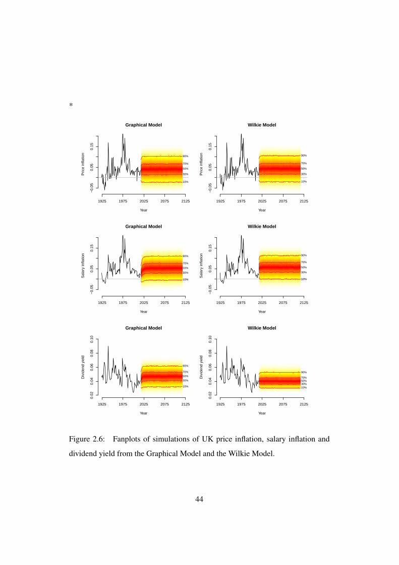
*
Graphical Model
Year
Pric
e in
flatio
n
1925 1975 2025 2075 2125
−0.
050.
050.
15
10%
30%
50%
70%
90%
Wilkie Model
Year
Pric
e in
flatio
n1925 1975 2025 2075 2125
−0.
050.
050.
15
10%
30%
50%
70%
90%
Graphical Model
Year
Sal
ary
infla
tion
1925 1975 2025 2075 2125
−0.
050.
050.
15
10%
30%
50%
70%
90%
Wilkie Model
Year
Sal
ary
infla
tion
1925 1975 2025 2075 2125
−0.
050.
050.
15
10%
30%
50%
70%
90%
Graphical Model
Year
Div
iden
d yi
eld
1925 1975 2025 2075 2125
0.02
0.04
0.06
0.08
0.10
10%
30%
50%
70%
90%
Wilkie Model
Year
Div
iden
d yi
eld
1925 1975 2025 2075 2125
0.02
0.04
0.06
0.08
0.10
10%30%50%70%
90%
Figure 2.6: Fanplots of simulations of UK price inflation, salary inflation and
dividend yield from the Graphical Model and the Wilkie Model.
44

Graphical Model
Year
Div
iden
d G
row
th
1925 1975 2025 2075 2125
−0.
30−
0.15
0.00
0.15
0.30
10%
30%
50%
70%
90%
Wilkie Model
Year
Div
iden
d G
row
th
1925 1975 2025 2075 2125
−0.
30−
0.15
0.00
0.15
0.30
10%
30%
50%
70%
90%
Graphical Model
Year
Con
sols
yie
ld
1925 1975 2025 2075 2125
0.00
0.05
0.10
0.15
10%
30%
50%
70%
90%
Wilkie Model
Year
Con
sols
yie
ld
1925 1975 2025 2075 2125
0.00
0.05
0.10
0.15
10%
30%50%70%
90%
Figure 2.7: Fanplots of simulations UK dividend growth and Bond yield from
the Graphical Model and the Wilkie Model.
45

short-term when starting the simulation from the current values of the series. In
the long run all series have marginal distributions around their long-term means.
It also appears that the overall long-term picture of the marginals from our
model are broadly similar to those from the Wilkie Model. The main differences
(albeit small) appear in the slower rate of mean reversion of the forecasts for salary
inflation. The graphical model also generates a wider distribution of bond yield
and dividend yield than the Wilkie Model.
The fan charts offer a useful sense-check as they can help identify potential
violations of common sense economic constraints that one would like to avoid in
the simulations. For instance, due to the exceptionally low long-term bond yields
in the recent environment, we have imposed a constraint that the long-term yield
does not fall below 0.05%. Should a value below this be predicted, it is simply set
at the minimum value instead. While we have chosen this value to be consistent
with current practice, recent experience suggests that the modeller may choose to
lower the boundary or even do away with this constraint altogether. The model
without the constraint does not preclude negative yields.
These types of constraints may have an impact on the correlations among the
simulated variables, so it may also be useful to check the correlations, which we
do next.
2.4.2 Distribution of Correlations along Simulated Paths - UK
Graphical Model and Wilkie Model
In Figure 2.8, we provide the pairwise correlations among the simulated versions
of the variables based on the Graphical Model and the Wilkie Model. For each
simulation path we calculate one estimate of the correlation. We then plot the dis-
tribution of these correlation estimates across the simulations. While many of the
correlation profiles are very similar between the two approaches, there is a pro-
46
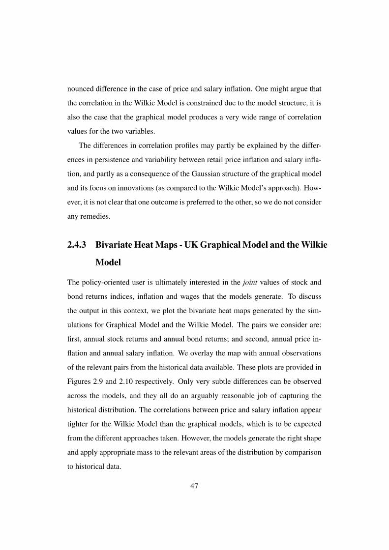
nounced difference in the case of price and salary inflation. One might argue that
the correlation in the Wilkie Model is constrained due to the model structure, it is
also the case that the graphical model produces a very wide range of correlation
values for the two variables.
The differences in correlation profiles may partly be explained by the differ-
ences in persistence and variability between retail price inflation and salary infla-
tion, and partly as a consequence of the Gaussian structure of the graphical model
and its focus on innovations (as compared to the Wilkie Model’s approach). How-
ever, it is not clear that one outcome is preferred to the other, so we do not consider
any remedies.
2.4.3 Bivariate Heat Maps - UK Graphical Model and the Wilkie
Model
The policy-oriented user is ultimately interested in the joint values of stock and
bond returns indices, inflation and wages that the models generate. To discuss
the output in this context, we plot the bivariate heat maps generated by the sim-
ulations for Graphical Model and the Wilkie Model. The pairs we consider are:
first, annual stock returns and annual bond returns; and second, annual price in-
flation and annual salary inflation. We overlay the map with annual observations
of the relevant pairs from the historical data available. These plots are provided in
Figures 2.9 and 2.10 respectively. Only very subtle differences can be observed
across the models, and they all do an arguably reasonable job of capturing the
historical distribution. The correlations between price and salary inflation appear
tighter for the Wilkie Model than the graphical models, which is to be expected
from the different approaches taken. However, the models generate the right shape
and apply appropriate mass to the relevant areas of the distribution by comparison
to historical data.
47

An additional check we can perform is to look at the (annualised) total returns
of stocks and bonds over different horizons. We do this in Figure 2.11 for the
Graphical Model and Figure 2.12 for the Wilkie Model.
As expected, the shape/sign of the bivariate correlation appears to be more
stable for the graphical model than the Wilkie Model. This is because we identi-
fied this type of long-run stable dependence as an objective for our models. An
interesting outcome, however, is the mass placed by the Graphical Model on an
extreme zone during the shorter horizons that does not appear in the Wilkie Model.
Given the recent history of exceptional policy intervention by developed countries
that exceeded the GDP of most countries in the world, this is not a surprising re-
sult. It is mainly driven by exceptionally low yields so that small absolute changes
in yields can lead to very high returns. As the yields bounce away from a lower
bound, they may be pushed back down by developments in other variables such
as price inflation. It also speaks to the ability of the simple model with AR(1)
dynamics and dependent innovations to capture shorter-term risks.
48

−0.5 0.0 0.5 1.0
04
8Price inflation v Salary inflation
Correlation
Den
sity
−0.5 0.0 0.5 1.0
01
23
4
Price inflation v Dividend yield
Correlation
Den
sity
−0.5 0.0 0.5 1.0
01
23
4
Price Inflation v Dividend growth
Correlation
Den
sity
−0.5 0.0 0.5 1.0
01
23
4
Price Inflation v Consols yield
Correlation
Den
sity
−0.5 0.0 0.5 1.0
01
23
4
Salary inflation v Dividend yield
Correlation
Den
sity
−0.5 0.0 0.5 1.0
01
23
4
Salary inflation v Dividend growth
Correlation
Den
sity
−0.5 0.0 0.5 1.0
01
23
4
Salary inflation v Consols yield
Correlation
Den
sity
−0.5 0.0 0.5 1.0
01
23
4
Dividend yield v Dividend growth
Correlation
Den
sity
−0.5 0.0 0.5 1.0
01
23
4
Dividend yield v Consols yield
Correlation
Den
sity
−0.5 0.0 0.5 1.0
01
23
4
Dividend growth v Consols yield
Correlation
Den
sity
Legend
Graphical Model E6Wilkie Model
Figure 2.8: Correlations of variables for simulations from the UK Graphical Model and the Wilkie Model.
49
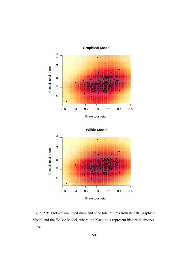
−0.6 −0.4 −0.2 0.0 0.2 0.4 0.6
−0.
20.
00.
20.
40.
6
Graphical Model
Share total return
Con
sols
tota
l ret
urn
−0.6 −0.4 −0.2 0.0 0.2 0.4 0.6
−0.
20.
00.
20.
40.
6
Wilkie Model
Share total return
Con
sols
tota
l ret
urn
Figure 2.9: Plots of simulated share and bond total returns from the UK Graphical
Model and the Wilkie Model, where the black dots represent historical observa-
tions.
50
−0.1 0.0 0.1 0.2 0.3
−0.
10.
00.
10.
20.
3
Graphical Model
Price inflation
Sal
ary
infla
tion
−0.1 0.0 0.1 0.2 0.3
−0.
10.
00.
10.
20.
3
Wilkie Model
Price inflation
Sal
ary
infla
tion
Figure 2.10: Plots of simulated price and salary inflation from the UK Graphical
Model and the Wilkie Model, where the black dots represent historical observa-
tions.
51

−0.2 0.0 0.2 0.4 0.6
−0.
50.
00.
51.
0
Annualised return over 1 year
Share total return
Con
sols
tota
l ret
urn
−0.05 0.00 0.05 0.10 0.15 0.20 0.25
−0.
2−
0.1
0.0
0.1
0.2
Annualised return over 5 years
Share total return
Con
sols
tota
l ret
urn
0.00 0.05 0.10 0.15 0.20
−0.
100.
000.
050.
10
Annualised return over 10 years
Share total return
Con
sols
tota
l ret
urn
0.04 0.06 0.08 0.10 0.12 0.14 0.16
−0.
020.
020.
040.
06Annualised return over 25 years
Share total return
Con
sols
tota
l ret
urn
0.06 0.08 0.10 0.12 0.14
0.00
0.02
0.04
0.06
Annualised return over 50 years
Share total return
Con
sols
tota
l ret
urn
0.06 0.07 0.08 0.09 0.10 0.11 0.12 0.13
0.01
0.03
0.05
0.07
Annualised return over 90 years
Share total return
Con
sols
tota
l ret
urn
Figure 2.11: Plots of simulated share and bond total returns from the UK Graph-
ical Model.
52

−0.2 0.0 0.2 0.4
−0.
3−
0.1
0.0
0.1
0.2
Annualised return over 1 year
Share total return
Con
sols
tota
l ret
urn
−0.05 0.00 0.05 0.10 0.15 0.20
−0.
15−
0.05
0.05
Annualised return over 5 years
Share total return
Con
sols
tota
l ret
urn
0.00 0.05 0.10 0.15
−0.
10−
0.05
0.00
0.05
Annualised return over 10 years
Share total return
Con
sols
tota
l ret
urn
0.04 0.06 0.08 0.10 0.12 0.14
−0.
03−
0.01
0.01
0.02
Annualised return over 25 years
Share total return
Con
sols
tota
l ret
urn
0.06 0.08 0.10 0.12 0.14
0.01
0.02
0.03
0.04
0.05
Annualised return over 50 years
Share total return
Con
sols
tota
l ret
urn
0.06 0.07 0.08 0.09 0.10 0.11 0.12
0.03
0.04
0.05
0.06
Annualised return over 90 years
Share total return
Con
sols
tota
l ret
urn
Figure 2.12: Plots of simulated share and bond total returns from the Wilkie
Model.
53
2.4.4 Marginal Distributions - Results for US and Canada
In Figures 2.13 and 2.14, we compare the marginal distributions for UK, US and
Canada generated by the Graphical Model for each country. Recall that by Graph-
ical Model, we mean the Graphical Model as estimated by the SINful approach.
Also note that the UK graphs are slightly different from their relevant counterparts
in Figures 2.6 and 2.7. This is because the data used in Figures 2.6 and 2.7 are
up to 2017 while the data used in Figures 2.13 and 2.14 are up to 2015 (where
2015 is the latest data available for Canada). We observe a wider fan chart for
US compared to UK and Canada for price inflation, salary inflation and dividend
yield. This is expected given the higher standard deviation, σ for these three US
variables compared to their UK and Canadian counterparts (see Table 2.2). In par-
ticular, we note that US salary inflation was very volatile before the 1950s with
very high and low peaks.
The fan chart for Canadian dividend growth is wider compared to UK and US
dividend growths. This is due to the autoregressive parameter, β, being smaller
for Canada compared to UK and US (0.1044 for Canada compared to 0.4263 for
UK and 0.2746 for US). This also means the Canadian dividend growth moves
back to the average value faster compared to UK and US dividend growths. This
property seems to be reflected in the historical time series.
The fan charts for bond yields are broadly comparable for the three countries.
Bond yield takes a relatively long time to revert back to the mean compared to the
other four variables. This is expected given that the autoregressive parameter, β is
larger than 0.9 for all three countries (see Table 2.2).
54

UK Price Inflation
Year
1924 1964 2004 2044 2084 2124
−0.
100.
000.
100.
20
10%
30%
50%
70%
90%
US Price Inflation
Year
1914 1956 1998 2040 2082 2124
−0.
100.
000.
100.
20
10%
30%
50%
70%
90%
Canada Price Inflation
Year
1934 1972 2010 2048 2086 2124
−0.
100.
000.
100.
20
10%
30%50%70%
90%
UK Salary Inflation
Year
1924 1964 2004 2044 2084 2124
−0.
2−
0.1
0.0
0.1
0.2
0.3
10%30%50%70%90%
US Salary Inflation
Year
1914 1956 1998 2040 2082 2124
−0.
2−
0.1
0.0
0.1
0.2
0.3
10%
30%
50%
70%
90%
Canada Salary Inflation
Year
1934 1972 2010 2048 2086 2124
−0.
2−
0.1
0.0
0.1
0.2
0.3
10%
30%50%70%
90%
UK Dividend Yield
Year
1924 1964 2004 2044 2084 2124
0.00
0.02
0.04
0.06
0.08
10%
30%50%70%
90%
US Dividend Yield
Year
1914 1956 1998 2040 2082 2124
0.00
0.02
0.04
0.06
0.08
10%
30%
50%
70%
90%
Canada Dividend Yield
Year
1934 1972 2010 2048 2086 2124
0.00
0.02
0.04
0.06
0.08
10%
30%
50%
70%
90%
Figure 2.13: Fanplots of simulations for price inflation, salary inflation and divi-
dend yield for UK, US and Canada from the Graphical Model.
55

UK Dividend Growth
Year
1924 1964 2004 2044 2084 2124
−0.
4−
0.2
0.0
0.2
0.4
10%
30%50%70%
90%
US Dividend Growth
Year
1914 1956 1998 2040 2082 2124
−0.
4−
0.2
0.0
0.2
0.4
10%
30%
50%70%
90%
Canada Dividend Growth
Year
1934 1972 2010 2048 2086 2124
−0.
4−
0.2
0.0
0.2
0.4
10%
30%
50%
70%
90%
UK Long Bond Yield (Consols Yield)
Year
1924 1964 2004 2044 2084 2124
0.00
0.05
0.10
0.15
10%
30%
50%
70%
90%
US Long Bond Yield
Year
1914 1956 1998 2040 2082 2124
0.00
0.05
0.10
0.15
10%
30%
50%
70%
90%
Canada Long Bond Yield
Year
1934 1972 2010 2048 2086 2124
0.00
0.05
0.10
0.15
10%
30%
50%
70%
90%
Figure 2.14: Fanplots of simulations for dividend growth and long bond yield for
UK, US and Canda from the Graphical Model.
56

2.4.5 Bivariate Heat Maps - Comparison between UK, US and
Canada
Figure 2.15 compares the bivariate heat maps for UK, US and Canda for simulated
share and bond returns. The black dots on the graphs represent the historical data
and we label the years where returns were unusally high or low. We note that the
Graphical Model does a reasonable job in capturing the historical distributions
for all three countries. Canada seems to have the largest spread of share returns
compared to UK and US. This may be due to the large standard deviation on
the marginal distribution for Canadian dividend growth compared to UK and US.
Canada also has the smallest spread of bond returns. This is expected given that
the paramter σ is smallest for Canadian long bond yield (see Table 2.2). The heat
map shows that UK share and bond returns are more highly correlated compared
to US and Canada.
Figure 2.16 shows the bivariate heat map for simulated price inflation and
salary inflation for UK, US and Canada. Again, the Graphical Model for each
country seems to do a reasonable job in capturing the historical distribution of
price and salary inflation. US has the biggest spread of price and salary inflation
which is expected given the marginal distributions observed from Figure 2.13.
From the heat maps, the correlation between price and salary inflation seems fairly
high for all three countries. This is in line with findings from other authors such
as Kwasi (1988) and Fuhrer and Moore (1995).
57

−0.6 −0.4 −0.2 0.0 0.2 0.4 0.6
−0.
6−
0.4
−0.
20.
00.
20.
40.
6
UK
Share total return
Bon
d to
tal r
etur
n
1939
1973
2015
−0.6 −0.4 −0.2 0.0 0.2 0.4 0.6
−0.
6−
0.4
−0.
20.
00.
20.
40.
6
US
Share total return
Bon
d to
tal r
etur
n
193319371939
1983
2010
−0.6 −0.4 −0.2 0.0 0.2 0.4 0.6
−0.
6−
0.2
0.0
0.2
0.4
0.6
Canada
Share total return
Bon
d to
tal r
etur
n
19801981
19831984
Figure 2.15: Plots of simulated share and long bond total returns for UK, US and Canada.
58

−0.1 0.0 0.1 0.2 0.3
−0.
3−
0.2
−0.
10.
00.
10.
20.
3
UK
Price inflation
Sal
ary
infla
tion
19751980
−0.1 0.0 0.1 0.2 0.3−
0.3
−0.
2−
0.1
0.0
0.1
0.2
0.3
US
Price inflation
Sal
ary
infla
tion
1921
1922
1931
1932
1933
1942
−0.1 0.0 0.1 0.2 0.3
−0.
3−
0.2
−0.
10.
00.
10.
20.
3
Canada
Price inflation
Sal
ary
infla
tion
1941
1942
Figure 2.16: Plots of simulated price and salary inflation for UK, US and Canada.
59
2.5 Summary
We have seen that the simple time series model with AR(1) dynamics combined
with graphically modelled innovations can generate rich and reasonable distribu-
tions for use in long-term risk management.
There are undoubtedly other, more structural, models in the large vector au-
toregression literature that could effectively capture the joint dynamics of vari-
ables. However, such models must by necessity be tightly parameterised and ul-
timately require some dimension reduction approach as the number of relevant
variables increases. In this chapter, we presented a simple application of statisti-
cal graphical models to simulate economic variables over long time horizons. The
fitted model performs comparably to the established benchmark and has the addi-
tional advantage of easy portability to new datasets, transparency, and flexibility.
Although for ease of exposition, we have considered only five economic variables
for each country, the model can easily accommodate extensions to a wider range
of economic variables and also for many different countries. We do recognise
however that computational issues may arise with very large structures.
Despite relying on a simple dynamic and a multivariate normal distribution for
the innovations, the model captures some of the essential features simply through
the design of a suitably reduced form dependence structure. In the next chapters,
we will use these models to quantify the economic risks of DB pension schemes.
60

Chapter 3
Mortality Models
3.1 Introduction
To project the cashflows of a pension scheme, we require a mortality model to
determine the longevity of pensioners and hence estimate the length of time they
receive a pension. There is a wide literature available on mortality models. Early
papers on stochastic mortality models by McNown and Rogers (1989) and Lee and
Carter (1992) have been followed by work of, among others, Booth et al. (2002a,b,
2005), Cairns et al. (2006b) (CBD), Renshaw and Haberman (2006) and Cairns et
al. (2009). The stochastic models vary according to a number of elements such as
inclusion and exclusion of cohort effects, assumptions of smoothness in ages and
the number of sources of randomness driving improvements in future mortality
rates.
A number of papers have sought to draw comparisons between various mod-
els. A notable example is Cairns et al. (2009) who compare eight stochastic mor-
tality models using data from England and Wales and US. We review the work by
Cairns et al. (2009) and update the results based on more recent data in Section
3.2. The analysis by Cairns et al. (2009) was carried out on male lives. For our
61

analysis, we present the results for both male and female lives.
Pension scheme actuaries typically use deterministic mortality tables for pen-
sion scheme valuations. This is the case for the UK’s USS and the OTPP, two
pension schemes for which we carry a risk assessment in later chapters. How-
ever, using these deterministic tables directly is not suitable for our purpose as
we are interested in the full distribution of the scheme assets and liabilities for
which stochastic projection of mortality is favoured. Therefore, in Section 3.4,
we explain how we adjust simulations from a stochastic mortality model such that
the central path from the simulations matches with the mortality rates from a de-
terminsitic table. In this way, we can make our mortality assumptions consistent
with the assumptions used by the valuation actuary of the pension schemes that
we want to model and quantify the risks.
3.2 Cairns et al. (2009)
Cairns et al. (2009) make a quantitative comparison of eight stochastic mortality
models using data from England and Wales and the US. We review seven of those
models and compare them by fitting UK, US and Canadian mortality data. Cairns
et al. (2009) refer to the models as Model M1-M8. All of models M1-M3 and M5-
M8 share the same underlying assumption that the age, period and cohort effects
are qualitatively different in nature. In contrast, model M4 uses B-splines and
P-splines to fit the mortality surface. The model assumes that there is smoothness
in the underlying mortality surface in the period effects as well as in the age and
cohort effects. For our purpose, we do not include model M4 for our comparisons
given that the model is very different from models M1-M3 and M5-M8.
Cairns et al. (2009) use England and Wales data between 1961 and 2004 and
US data between 1968 and 2003 for ages 60 to 89 inclusive. Given that more
62

recent data is now available, we re-fit the seven stochastic models to UK and US
data between 1968-2011. We also fit the models to Canadian data. The data we
use comes from the Human Mortality Database (HMD). Note that more recent
data is available for UK and US but the latest data available for Canada is 2011.
To keep things consistent, we use data up to 2011 for all three countries. Cairns
et al. (2009) only use data for male lives for their analysis but we carry out the
analysis for both genders.
Figure 3.1 shows the log of the crude death rates of UK, US and Canada for
ages 65, 75 and 85. From Figure 3.1, we observe a downward trend in mortality
rates over time. This is expected given that many countries have been experiencing
improving longevity over many years (Costa (2005)). We can also observe the
higher mortality rates of males compared to females for all ages although the
mortality improvement for male lives seem to improve at a higher rate compared
to females over the years. At the age of 85, the difference in the log of the crude
death rates between males and females is smaller.
3.2.1 Age-Period-Cohort Mortality Models
We assume that the force of mortality remains constant over each year of integer
age and over each calendar year. The number of deaths at age x in year t is
assumed to follow one of the following models:
(a) D(t, x) ∼ Binomial [N(t, x), q(t, x)].
(b) D(t, x) ∼ Poisson [E(t, x)× µ(t, x)].
where:
D(t, x): The number of deaths at age x and year t.
N(t, x): The number of individuals alive aged x at the beginning of year t.
63
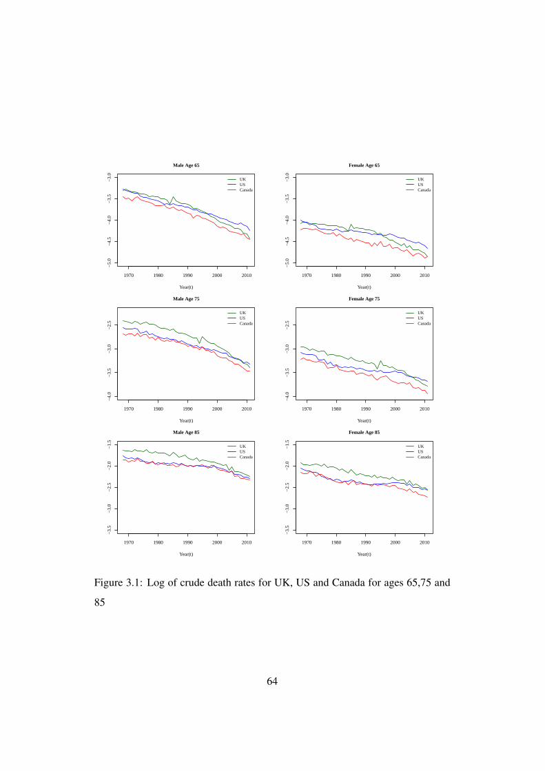
1970 1980 1990 2000 2010
−5.
0−
4.5
−4.
0−
3.5
−3.
0
Male Age 65
Year(t)
UKUSCanada
1970 1980 1990 2000 2010
−5.
0−
4.5
−4.
0−
3.5
−3.
0
Female Age 65
Year(t)
UKUSCanada
1970 1980 1990 2000 2010
−4.
0−
3.5
−3.
0−
2.5
Male Age 75
Year(t)
UKUSCanada
1970 1980 1990 2000 2010
−4.
0−
3.5
−3.
0−
2.5
Female Age 75
Year(t)
UKUSCanada
1970 1980 1990 2000 2010
−3.
5−
3.0
−2.
5−
2.0
−1.
5
Male Age 85
Year(t)
UKUSCanada
1970 1980 1990 2000 2010
−3.
5−
3.0
−2.
5−
2.0
−1.
5
Female Age 85
Year(t)
UKUSCanada
Figure 3.1: Log of crude death rates for UK, US and Canada for ages 65,75 and
85
64

E(t, x): The total exposure of individuals aged x during the calendar year t.
q(t, x): The probability that an individual aged x at time t will die between t and
t+ 1.
µ(t, x): The force of mortality, defined as the instantaneous death rate, at exact
time t for individuals aged exactly x at time t.
The general form of the mortality models we consider here is given by:
log µ(t, x) (or logit q(t, x)) = β(1)x κ
(1)t γ
(1)t−x + β(2)
x κ(2)t γ
(2)t−x + .....+ β(i)
x κ(i)t γ
(i)t−x
(3.1)
where:
• β captures the age effect
• κ captures the period effect
• γ captures the cohort effect
For example, consider the Lee and Carter model:
log µ(t, x) = β(1)x + β(2)
x κ(2)t (3.2)
In this case, i=2, κ(1)t =1, γ(1)t−x=1 and γ(2)t−x=1.
The formula of the seven mortality models are provided in Table 3.1.
3.2.2 Parameter Estimation
Pension schemes are exposed to two types of risks, specific risk and systematic
risk, which arise from the actual mortality experience of the scheme members
being different from the expected.
Given the values of parameters, µ(t, x), variation in the actual mortality ex-
perience is referred to as the specific risk. In other words, if we assume that
65

Table 3.1: Structure of mortality models
Model Formula
M1 - Lee and Carter log µ(t, x) = β(1)x + β
(2)x κ
(2)t
M2 - Renshaw and Haberman log µ(t, x) = β(1)x + β
(2)x κ
(2)t + β(3)
x γ(3)t−x
M3 - Currie log µ(t, x) = β(1)x + κ
(2)t + γ
(3)t−x
M5 logit q(t, x) = κ(1)t + κ
(2)t (x− x)
M6 logit q(t, x) = κ(1)t + κ
(2)t (x− x) + γ
(3)t−x
M7 logit q(t, x) = κ(1)t + κ
(2)t (x− x) + κ
(3)t ((x− x)2 − σ̂2
x) + γ(4)t−x
M8 logit q(t, x) = κ(1)t + κ
(2)t (x− x) + γ
(3)t−x(xc − x)
µ(t, x) is known, then given the relevant exposures to risk, the number of deaths
is a random variable. For example, if for a certain age and time, the exposure
to risk is 10,000 and the probability of death is 0.01, then the number of deaths
can be . . . , 98, 99, 100, 101, 102, . . . with certain probabilities (with a mean of
100). This is known as specific risk. For a large pension schemes like USS with
400,000 scheme members, specific risk does not pose a significant threat, as it is
diversified away through pooling. So we primarily focus on systematic risk in this
thesis
For all models, the log-likelihood is:
l(φ,D,E) =∑t,x
D(t, x) log[E(t, x)µ(t, x;φ)]−E(t, x)µ(t, x;φ)− log[D(t, x)!].
(3.3)where:
φ is the full set of paramters for a given model.
The parameters are then estimated by maximum-likelihood. A number of con-
straints are applicable when estimating the parameters. The constraints are not
discussed here; please refer to Cairns et al. (2009) for more details on the param-
66

eter constraints. We provide the parameter estimates for Model M3 (see Figure
3.2) for male lives for ages 60 to 89 as an example.
As the parameter β(1)x captures the age effect on mortality, as expected the
mortality rate (and hence β(1)x ) increases with age.
The parameter κ(2)t captures the period effect on mortality. For all three coun-
tries, we note that the κ(2)t s become smaller with time which imply an improve-
ment in mortality rates over time. UK had the highest average mortality rate in the
1970s compared to US and Canada. UK mortality improvement since 1970 has
however been more significant compared to US and Canada. Consequently, the
κ(2)t for UK is the largest of the three countries in 1970 but the smallest in 2010.
Finally, γ(3)t captures the cohort effect on mortality. Unlike for the age or
period effect, there isn’t a consistent trend for the cohort effect. Note that the first
five and last five cohorts are excluded in the analysis given lack of data. This
explains the horizonal line at the start and end of the plot for γ(3)t in Figure 3.2.
3.2.3 Model Fit
In order to quantitatively compare the mortality models, Cairns et al. (2009) use
the Bayes Information Criterion (BIC). The BIC provides a mechanism for bal-
ancing the quality of fit and parsimony of the model. It also allows us to compare
models which are not nested. Table 3.2 shows the BIC and rank of the models
for male and female lives using the fitted model for UK, US and Canada for ages
30-105.
For male lives, Model M7 is the highest ranked model for UK while Model
M2 is the highest ranked for US and Canada. As noted in Cairns et al. (2009),
Model M2 however has the problem of being over-parameterised and this may
result in over-fitting. For female lives, Model M8 has the highest rank for UK and
Canada and Model M2 has the highest rank for US. A problem with Model M8
67

60 65 70 75 80 85 90
−4.
0−
3.0
−2.
0
Beta_1(x)
Age(x)
UKUSCanada
1970 1980 1990 2000 2010
−15
−10
−5
05
10
Kappa_2(t)
Year(t)
UKUSCanada
1880 1890 1900 1910 1920 1930 1940 1950
−4
−2
02
4
Gamma_3(t)
Year(t)
UKUSCanada
Figure 3.2: Parameter estimates of model M3 for UK, US and Canada fitted using
males mortality data ages 60-89 and years 1968-2011
68

Table 3.2: Models’ BIC and Rank
Males Females
Model UK US Canada UK US Canada
M1 -10925 (6) -17362 (5) -8299 (7) -12289 (6) -17772 (5) -7444 (3)
M2 -8644 (3) -11132 (1) -7645 (1) -8597 (2) -11391 (1) -7401 (2)
M3 -9767 (5) -15107 (5) -7803 (5) -10076 (5) -15842 (4) -7579 (5)
M5 -11876 (7) -30134 (7) -8216 (6) -13227 (7) -50550 (7) -9970 (7)
M6 -8783 (4) -14474 (4) -7654 (2) -9160 (4) -19988 (6) -7732 (6)
M7 -8501 (1) -12834 (2) -7698 (4) -8687 (3) -12862 (2) -7472 (4)
M8 -8503 (2) -13161 (3) -7672 (3) -8587 (1) -13808 (3) -7363 (1)
however is that it sometimes takes a very long time for the parameters to converge.
For both genders, Model M7 seems to provide a reasonably good fit. The
model also converges fairly quickly and is not over-parameterised. FOr consis-
tency, we use Model M7 for all countries and both genders for the rest of this
thesis to project mortality rates forward. Model M5 seems to have the worst fit to
the data overall.
3.3 Projection of Parameters
Projecting future mortality rates involves projecting the time series κ(t) and γ(t−
x) forward. Systematic risk arises from the uncertainty surrounding the estimate
of the underlying parameters µ(t, x). This is the uncertainty involved in projecting
the time series κ(t) and γ(t − x) forward. For example, if the mortality rates
improve faster than expected then future µ(t, x) will be lower, which in turn will
result in lower deaths. This risk cannot be diversified away and thus poses a bigger
69

threat. So ideally the uncertainty, or randomness, in the projections of µ(t, x)
needs to be recognized and incorporated in a stochastic mortality model.
Cairns et al. (2009) suggest possible approaches to project mortality param-
eters forward based on the historical estimates of these parameters. For our pur-
pose, we project κ(t) linearly over time. Given that we are not interested in future
cohorts (but only on existing ones), therefore we do not project γ(t− x) forward.
Figure 3.3 shows the simulated mortality rates for males and females for ages
65, 75 and 85 from Model M7. For each plot, we show the median and the 90%
confidence intervals.
From Figure 3.3, we make the following observations:
• The mortality rate of younger lives is lower compared to older lives showing
that the age effect is captured in the simulations.
• The mortality rate goes down with time showing that the period effect is
also captured in the simulations.
• The mortality improvement for male lives is steeper compared to female
lives. This trend was also observed in the log of the historical crude death
rates in Figure 3.1.
• The longer the time horizon, the wider the fan charts. This shows the greater
uncertainty when simulating over longer horizons.
3.4 Adjusting Stochastic Mortality Rates
Actuaries typically use determinstic mortality tables to carry pension scheme val-
uations. For example, the USS used the S1NA “light" mortality table for its tri-
ennual valuations in 2014.The S1NA “light" is a mortality table published by the
Institute and Faculty of Actuaries and is based on mortality experience of UK
70

2010 2015 2020 2025 2030 2035
0.00
20.
006
0.01
00.
014
Male q(65) and 90% CI
Year(t)
UKUSCanada
2010 2015 2020 2025 2030 2035
0.00
20.
006
0.01
00.
014
Female q(65) and 90% CI
Year(t)
UKUSCanada
2010 2015 2020 2025 2030 2035
0.01
00.
020
0.03
00.
040
Male q(75) and 90% CI
Year(t)
UKUSCanada
2010 2015 2020 2025 2030 2035
0.01
00.
020
0.03
00.
040
Female q(75) and 90% CI
Year(t)
UKUSCanada
2010 2015 2020 2025 2030 2035
0.02
0.04
0.06
0.08
0.10
0.12
Male q(85) and 90% CI
Year(t)
UKUSCanada
2010 2015 2020 2025 2030 2035
0.02
0.04
0.06
0.08
0.10
0.12
Female q(85) and 90% CI
Year(t)
UKUSCanada
Figure 3.3: Simulated mortality rates under Model M7 for UK, US and Canada for
males and females for ages 65, 75 and 85 along with the 90% confidence interval.
71

self-administered pension schemes between 2000 - 2006. Moreover, the S1NA
“light" table is based on lives whose mortality experience is lower than the gen-
eral population1. The use of the S1NA “light" is justified by the USS by that fact
that academics generally exhibit longer longevity than the general population2.
There is also the issue of adverse selection; individuals who purchase annuities
are generally in better health than individuals who do not purchase annuities. The
choice of the “light" mortality table is justifiable in that regard.
The mortality rates from the S1NA “light" table are projected forward using
projections suggested by the Continuous Mortality Investigation (CMI). The USS
used the CMI-2014 table with a long term rate of 1.5% p.a. Figure 3.4 shows the
S1NA “light" mortality rates for male lives for ages 65, 75 and 85 projected for-
ward using the CMI-2014 table. On the same graphs, we show the corresponding
projections from Model M7 for comparison purposes.
We note that the projected mortality rates using S1NA and CMI-2014 are
lower than the projected mortality rates using Model M7. This is expected given
that Model M7 is calibrated to the UK’s total population while the S1NA “light"
table is a based on lives with lighter mortality experience than overall population.
This mismatch in mortality rates between Model M7 and the CMI projections
means that it may not be appropriate to use Model M7 directly when modelling
a pension scheme like the USS as doing this will entail a large mismatch in the
mortality rates we use and those used by the valuation actuary. To avoid this, we
adjust the central projection from Model M7 to match the projections using tables
S1NA “light" and CMI-2014.
In other words, given a deterministic mortality and projection tables used by
1actuaries.org.uk/system/files/field/document/
cmiworkingpaper35.pdf2https://www.cass.city.ac.uk/__data/assets/pdf_file/0019/
293311/COUGHLAN-Guy-L11.pdf
72

the valuation actuary, the adjustment required is:
adj(x,t) =qval(x,t)
qM7(x,t)
. (3.4)
where qval(x,t) is the projected valuation mortality rate and qM7(x,t) is the central projec-
tion from Model M7.
In this way, by multiplying qM7(x,t) from Model M7 by adj(x,t), the simulated
mortality rates, henceforth denoted by qadj(x,t), will have its central projection corre-
spond to qval(x,t).
Using Model M7 calibrated to UK data and the CMI-2014 as our valuation
projection table, we show in Figure 3.4 the adjustments adj(x,t) for males for ages
65, 75 and 85. We also show the plots for qadj(x,t) for males for ages 65, 75 and 85
in Figure 3.5. As expected, the central projection for qadj(x,t) matches the projection
from the deterministic CMI 2014 projection. We do not observe any anomalies
regarding the uncertainty around the central projection of qadj(x,t) which is reassur-
ing.
We do similar adjustments to the mortality rates for US and Canadian pension
schemes. This will be discussed in more details in Chapter 6 for US and Chapter
7 for Canada.
3.5 Summary
In this chapter, we have compared different stochastic mortality models. In partic-
ular, we have looked at seven mortality models from Cairns et al. (2009). We have
seen that the different stochastic models have varying strengths and weaknesses.
We believe that Model M7 from Cairns et al. (2009) is adequate for our purpose.
The model provides a good fit for both UK, US and Canadian data for both males
and females. Moreover, it does not take a long time for parameters of the model
73

2015 2020 2025 2030 2035
0.00
40.
008
0.01
2
Age 65
Year(t)
M7CMI
2015 2020 2025 2030 2035
0.01
50.
025
0.03
5
Age 75
Year(t)
M7CMI
2015 2020 2025 2030 2035
0.05
0.07
0.09
0.11
Age 85
Year(t)
M7CMI
Figure 3.4: Projected mortality rates for UK males for ages 65, 75 and 85.
74

2015 2020 2025 2030 2035
0.00
40.
008
0.01
2
q(65) Male and 90% CI
Year(t)
M7M7_adj
2015 2020 2025 2030 2035
0.01
00.
020
0.03
0
q(75) Male and 90% CI
Year(t)
M7M7_adj
2015 2020 2025 2030 2035
0.04
0.06
0.08
0.10
0.12
q(85) Male and 90% CI
Year(t)
M7M7_adj
Figure 3.5: Fanplot for M7 and M7 adjusted for UK males for ages 65, 75 and 85
75

to converge and the model is not over-parameterised which are desirable features.
In this respect, we will use Model M7 to project future mortality rates in Chapters
5, 6 and 7 in which we carry out risk assessments of DB pension schemes in UK,
US and Canada respectively.
76

Chapter 4
Risk Quantification of Pension
Schemes
4.1 Introduction
In this chapter we explain the methodology we use to carry risk assessment of DB
pension schemes. As discussed in Section 1.2, there is a wide literature on mea-
suring and managing pension scheme risks. Although the methodology for mea-
suring pension risks varies according to the research objective, most researchers
agree that the two most significant risks for pension schemes are economic risks
and mortality risks. We also focus on these two risks for this research although
we do recognise that pension schemes are exposed to more than these two risks
e.g. operational risk, liquidity risk and expense risk.
For the purpose of valuing its liabilities, the USS assumes that the scheme re-
mains open to existing members but is closed for new entrants. This is generally
referred as a Closed Group with Future Accruals. In this way, current members
continue to contribute and accrue future benefits and their salaries are assumed
to increase in line with wage increases. In order to be consistent with the figures
77
reported in valuation report of the USS, we also assume a Closed Group with Fu-
ture Accruals for our risk assessment. Other types are schemes include Closed
Group without Future Accruals (where the scheme is closed to new members and
where existing members make no further contributions and accrue no further ben-
efits) and Open Group (where the scheme is open to new members and exisiting
members continue to contribute and accure future benefits). The other two types
of schemes are not explored further in this thesis.
4.2 Methodology
We will use the following notation to explain the methodology:
At: Value of pension scheme assets at time t.
Lt: Value of pension scheme liabilities at time t.
Xt: Net cash flow of the scheme at time t (excluding investment returns), i.e.,
benefit payments net of contributions.
I(s,t): Accumulation factor (accumulated value at time t of 1 invested at time s).
These are obtained directly from the simulations of the underlying stochas-
tic economic model.
D(s,t): Discount factor, i.e., I−1(s,t).
Given the long-term nature of pension scheme risks we propose using a run-
off approach, so that the time horizon of our analysis is set until the time when the
last of the current scheme members dies. Assuming that cashflows and valuations
are carried out on an annual basis so that any surplus/deficit is determined at the
end of each year, we define the profit vector, Pt, at time t, as:
Pt = Lt−1 × I(t−1,t) −Xt − Lt, where P0 = A0 −X0 − L0. (4.1)
78

Under this set-up the current present value of future profits, PV FP , is:
V0 =T∑t=0
Pt ×D(0,t) (4.2)
where T is the run-off time horizon. As there will be no residual liabilities after
the last of the current members die, LT = 0.
Using the relationship:
I(0,t−1) × I(t−1,t) = I(0,t) ⇒ I(t−1,t) ×D(0,t) = D(0,t−1), (4.3)
along with the fact that D(0,0) = 1, Equation 4.2 can be rewritten as follows:
V0 =T∑t=0
Pt ×D(0,t), (4.4)
= (A0 −X0 − L0) +T∑t=1
(Lt−1 × I(t−1,t) −Xt − Lt
)×D(0,t), (4.5)
= (A0 −X0 − L0) +T∑t=1
(Lt−1 ×D(0,t−1) −Xt ×D(0,t) − Lt ×D(0,t)
),
(4.6)
=A0 −T∑t=0
Xt ×D(0,t). (4.7)
An intuitive interpretation of Equation 4.7 is that PV FP represents the present
value of the final surplus/deficit, i.e. whether the current level of assets, A0, along
with the future contributions, are adequate to pay all future benefits. Note that
the value of the liabilities do not play a direct role in this measure; rather, the
liabilities are reflected as part of the discounted cashflows, Xt.
Because future cashflows and asset returns are random variables that depend
on the future random realisations of the underlying economic and mortality vari-
ables, the present value of the final surplus/deficit, i.e. V0, is also a random vari-
able. In contrast, a valuation actuary provides a single point estimate of the current
value of future actuarial liabilities, i.e. L0.
79
From this perspective, V0 can be partitioned and expressed as:
V0 = [A0 − L0 ]︸ ︷︷ ︸Current valuation deficit
+
[L0 −
T∑t=0
Xt ×D(0,t)
]︸ ︷︷ ︸Emerging actuarial gains (or losses)
. (4.8)
Note that the point estimate of the value of actuarial liabilities, L0, does not play
a direct role in the calculation of V0. For instance, a prudent valuation basis
would produce a conservative high value forL0 leading to a large current valuation
deficit, but it will then be compensated by a corresponding rise in the emerging
actuarial gains, and vice versa.
Note that Xt represents the benefit payments net of contributions. There are
instances however where other significant cashflows need to be considered when
looking at DB pension schemes. For example, it is a common for sponsors to in-
ject additional funds in pension schemes facing a deficit (i.e. liabilities are higher
than assets). The purpose of the additional funds is to reduce the pension deficit
and we refer to this as an amortisation. The number of years during which the
sponsors inject additional funds into the scheme is referred to as the amortisation
period.
If the amortisation period is 1, i.e. there is an immediate cash injection from
the sponsor to fully cover any deficit, then we can modify Equation 4.7 to:
V0 = A0 −T∑t=0
Xt ×D(0,t) + Y0 (4.9)
where Y0 is the cash injection at time 0, so that Y0 = L0 − A0. We thus have the
following equation:
V0 = A0 −T∑t=0
Xt ×D(0,t) + (L0 − A0) (4.10)
which simplifies to:
80

V0 = L0 −T∑t=0
Xt ×D(0,t). (4.11)
If the amortisation period is over n years, we have:
V0 = A0 −T∑t=0
Xt ×D(0,t) +n−1∑t=0
Yt ×D(0,t) (4.12)
where Yt is the cash injection at time t.
We will look at amortisation in more details in Chapter 6 where we will con-
sider a pension scheme in deficit.
We use V0 as the starting point for quantifying risk in a defined benefit pension
scheme. However, it would be helpful to use some form of standardisation so that
the measure does not depend on the following:
currency: as one of our main goals in this thesis is to compare pension scheme
risks in different countries, namely the UK, US and Canada;
scale: as different benefit structures would imply different magnitudes of scheme
assets and liabilities. Comparing absolute values of the risks for different
types of pension schemes will not be meaningful.
Standardised PV FP , which we will denote by V ∗0 , can be defined in many
ways; two approaches are listed below:
• V ∗0 = V0
A0: Conceptually, this amount can be interpreted as the proportional
increase in assets required to meet all future benefit obligations.
• V ∗0 = V0
L0: Conceptually, this amount can be interpreted as the proportional
loading that needs to be added to the liabilities so that if we had assets
equal to the “loaded" liabilities we would be able to meet all future benefit
obligations.
81

The information contained in V ∗0 is the same for either of the above approaches,
as long as the same standardisation is used consistently throughout. We will use
the standardisation V0/A0 for the rest of this thesis.
4.3 Economic Capital
A risk measure in terms of economic capital can then be defined as:
Definition: The economic capital of a pension scheme is the amount
by which its existing assets would need to be augmented in order to
meet net benefit obligations with a prescribed degree of confidence.
A scheme’s net benefit obligations are all obligations in respect of
current scheme members including future service, net of future con-
tributions to the scheme.
Due to the long-term nature of pension schemes’ benefit obligations, it is im-
portant to use the entire run-off period as the time horizon.
The actual quantification of economic capital, using the distribution of the
random variable V ∗0 , can be carried out in one of the following ways:
Value-at-Risk (V aR): V aR is defined as P [V ∗0 ≤ V aR ] = p, for a given prob-
ability p. V aR represents the amount of additional initial assets required
at time 0 (on top of existing assets) for the pension scheme to meet all its
future obligations with probability, or confidence level, (1− p).
Expected shortfall (ES): ES is defined as the average of all losses which are
greater than or equal to the value of V aR, for a given probability level p,
i.e. E [V ∗0 |V ∗
0 ≤ V aR ]. In other words, ES provides an estimate of the
expected value of losses in the worst p proportion of cases.
82

These definitions of V aR and ES are applicable for continuous random vari-
ables only and are based on McNeil et al. (2015). For our results in later chapters,
we will present representative values of V aR and ES.
4.4 Summary
In this chapter, we propose a methodology to quantify risks of DB pension schemes.
In particular, we propose a run-off approach by projecting cashflows of the scheme
until the last current member of the scheme dies. We define the PVFP as the differ-
ence between the current level of assets of the pension scheme and the projected
discounted cashflows of the scheme. We propose standardising the PVFP so that
the quantified risks does not depend on the currency and the magnitude of pension
scheme assets and liabilities. As PVFP gives a full distribution of results, it might
be useful to present the underlying VaR and ES as the required economic capital
providing a measure of risk.
83

Chapter 5
Risk Assessment of the UK’s
Universities Superannuation Scheme
5.1 Introduction
In this chapter, we perform a risk assessment of the USS. The USS is one of
the largest DB pension scheme in the UK. The USS was established in 1974 to
administer the principal pension scheme for academics and administrative staff in
UK universities and other higher education and research institutions. It is now one
of the largest open DB pension schemes in the UK. It has over 350,000 members
and assets worth over £45 billion.
Porteous et al. (2012) performed a risk assessment of the USS based on the
2008 USS valuation report. That risk assessment was carried out by determining
the economic capital requirements of the scheme using a framework similar to
Solvency 2. Several things have changed for the USS since 2008. In particular, in
2011, the USS was subject to significant changes, the main ones being:
• USS closed its final salary scheme to new members, replacing it with a
career average revalued earnings (CARE) scheme for new members.
84

• Future benefits of existing members was changed from final salary basis to
CARE basis.
• The indexation of deferred pensions and pensions in payment was changed
from the retail price index to the less generous consumer price index, and
uprating of accrued benefits was capped.
The changes were the subject of ‘heated public controversy’ between USS’s
institutional sponsors and the scheme’s members, represented by the University
and College Union, and involved lengthy industrial actions.
Further, in 2014, the USS took a decision to de-risk the scheme’s investments
over the next 20 years by moving equities to alternative and less risky investments.
The strategy has so far proven to be controversial as it has locked the USS in
long-term low rates of return, which could be damaging and potentially further
destabilising.
We update the risk assessment of Porteous et al. (2012) in light of these recent
changes. Our analysis is based on the most recently available valuation report.
We perform the analysis using a stochastic ESG calibrated to the UK economy
(see Chapter 2). The analysis also employs a stochastic mortality model, similarly
calibrated to the UK experience (see Chapter 3).
We show our results at a number of different confidence levels, including
99.5% degree of confidence which is consistent with both the analysis of Porteous
et al. (2012) and Solvency 2.
We start by presenting a brief overview of the membership profile, benefit
structure, contribution rates to reflect the characteristics of a UK pension scheme,
valuation basis and asset allocation of USS. The numbers presented here are based
on the latest valuation carried out for the scheme as at 31 March 2014. As we do
not have the full underlying valuation data, we will create a “model” of USS, using
model points, capturing the broad membership profile.
85
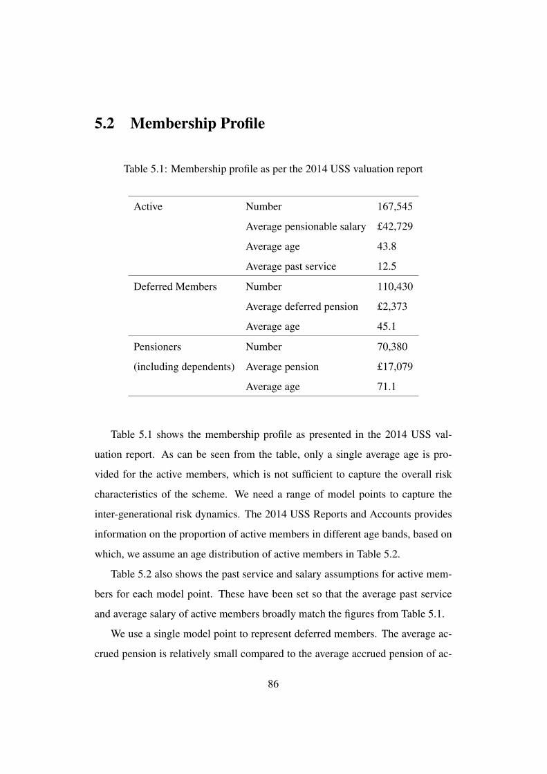
5.2 Membership Profile
Table 5.1: Membership profile as per the 2014 USS valuation report
Active Number 167,545
Average pensionable salary £42,729
Average age 43.8
Average past service 12.5
Deferred Members Number 110,430
Average deferred pension £2,373
Average age 45.1
Pensioners Number 70,380
(including dependents) Average pension £17,079
Average age 71.1
Table 5.1 shows the membership profile as presented in the 2014 USS val-
uation report. As can be seen from the table, only a single average age is pro-
vided for the active members, which is not sufficient to capture the overall risk
characteristics of the scheme. We need a range of model points to capture the
inter-generational risk dynamics. The 2014 USS Reports and Accounts provides
information on the proportion of active members in different age bands, based on
which, we assume an age distribution of active members in Table 5.2.
Table 5.2 also shows the past service and salary assumptions for active mem-
bers for each model point. These have been set so that the average past service
and average salary of active members broadly match the figures from Table 5.1.
We use a single model point to represent deferred members. The average ac-
crued pension is relatively small compared to the average accrued pension of ac-
86

Table 5.2: Model points, past service and salary of active USS members
Age Proportion Number Past service Salary
30 30% 50,264 7 £25,500
40 30% 50,264 11 £42,500
50 20% 33,509 15 £52,500
60 20% 33,509 19 £58,500
Total 100% 167,545
Average 12.2 £42,600
tive members and using more model points to represent deferred members would
not have a significant impact on our results. We also use a single model point to
represent pensioners given the smaller number of pensioners relative to active and
deferred members. We also assume a 50:50 gender split and no salary differential
between genders.
5.3 Benefit Structure – USS Scheme
5.3.1 Pension Benefits
Pension and cash lump sum at retirement are calculated as follows:
Annual pension = Pensionable salary × Pensionable service × Accrual rate.
Lump Sum = 3× Annual pension.
In the valuation report, members’ salaries are assumed to grow in line with a
general pay growth which is assumed to be equal to price inflation plus 1%. In our
model, we assume members’ salaries increase in line with future salary increases
87

as generated by our ESG. In addition to salary inflation, there is an explicit age-
based promotional salary scale, which is based on the LG59/60 promotional salary
scale. LG59/60 promotional salary scale is widely used for actuarial valuation of
eligible schemes, see for example, the 2015 actuarial valuation of the superannua-
tion arrangements of University of London 1. An excerpt of the LG59/60 is shown
in Table 5.3.
Table 5.3: Promotional salary assumptions based on LG59/60 promotional scale.
Age Male(%) Female(%)
35 3.8 3.1
45 2.0 1.8
55 1.1 1.4
Until October 2011, accrual rate was set at 1/80th and pensionable salary was
on final salary (FS) basis and defined as “the highest of either the best inflation
adjusted 12 months’ salary over the last 36 months’ membership; or the average
of your best consecutive inflation adjusted three years’ salary during the last 13
years” for all members. For practical implementation purposes, we will assume
that for FS, the pensionable salary is the member’s salary in the final year of
service.
From 1 October 2011, the FS scheme was closed to new entrants, who joined
a separate scheme based on the CARE basis. For the CARE scheme, the pension-
able salary is an average inflation-adjusted salary over the member’s career. For
instance, consider a member who has worked 3 years in the USS, with inflation at
3% over year one, 4% over year two and 5% over year three. Then the pension-1https://london.ac.uk/sites/default/files/2017-10/
financial-statements-2015-2016.pdf
88
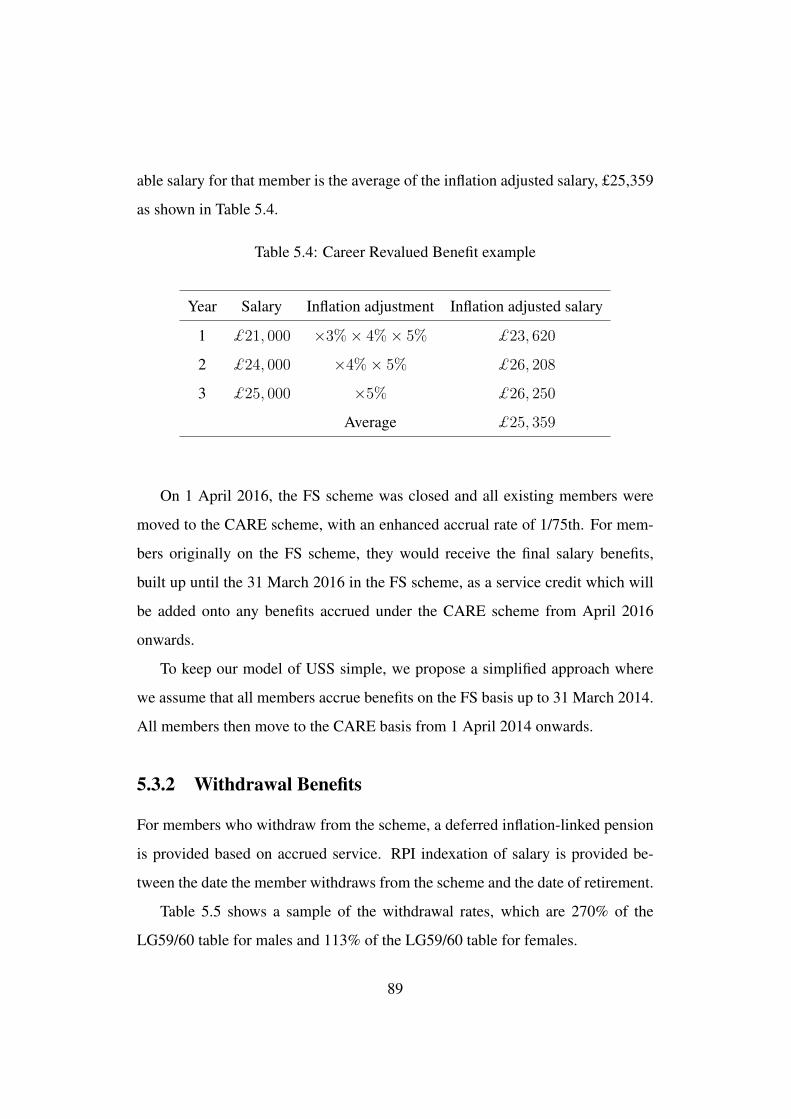
able salary for that member is the average of the inflation adjusted salary, £25,359
as shown in Table 5.4.
Table 5.4: Career Revalued Benefit example
Year Salary Inflation adjustment Inflation adjusted salary
1 £21, 000 ×3%× 4%× 5% £23, 620
2 £24, 000 ×4%× 5% £26, 208
3 £25, 000 ×5% £26, 250
Average £25, 359
On 1 April 2016, the FS scheme was closed and all existing members were
moved to the CARE scheme, with an enhanced accrual rate of 1/75th. For mem-
bers originally on the FS scheme, they would receive the final salary benefits,
built up until the 31 March 2016 in the FS scheme, as a service credit which will
be added onto any benefits accrued under the CARE scheme from April 2016
onwards.
To keep our model of USS simple, we propose a simplified approach where
we assume that all members accrue benefits on the FS basis up to 31 March 2014.
All members then move to the CARE basis from 1 April 2014 onwards.
5.3.2 Withdrawal Benefits
For members who withdraw from the scheme, a deferred inflation-linked pension
is provided based on accrued service. RPI indexation of salary is provided be-
tween the date the member withdraws from the scheme and the date of retirement.
Table 5.5 shows a sample of the withdrawal rates, which are 270% of the
LG59/60 table for males and 113% of the LG59/60 table for females.
89
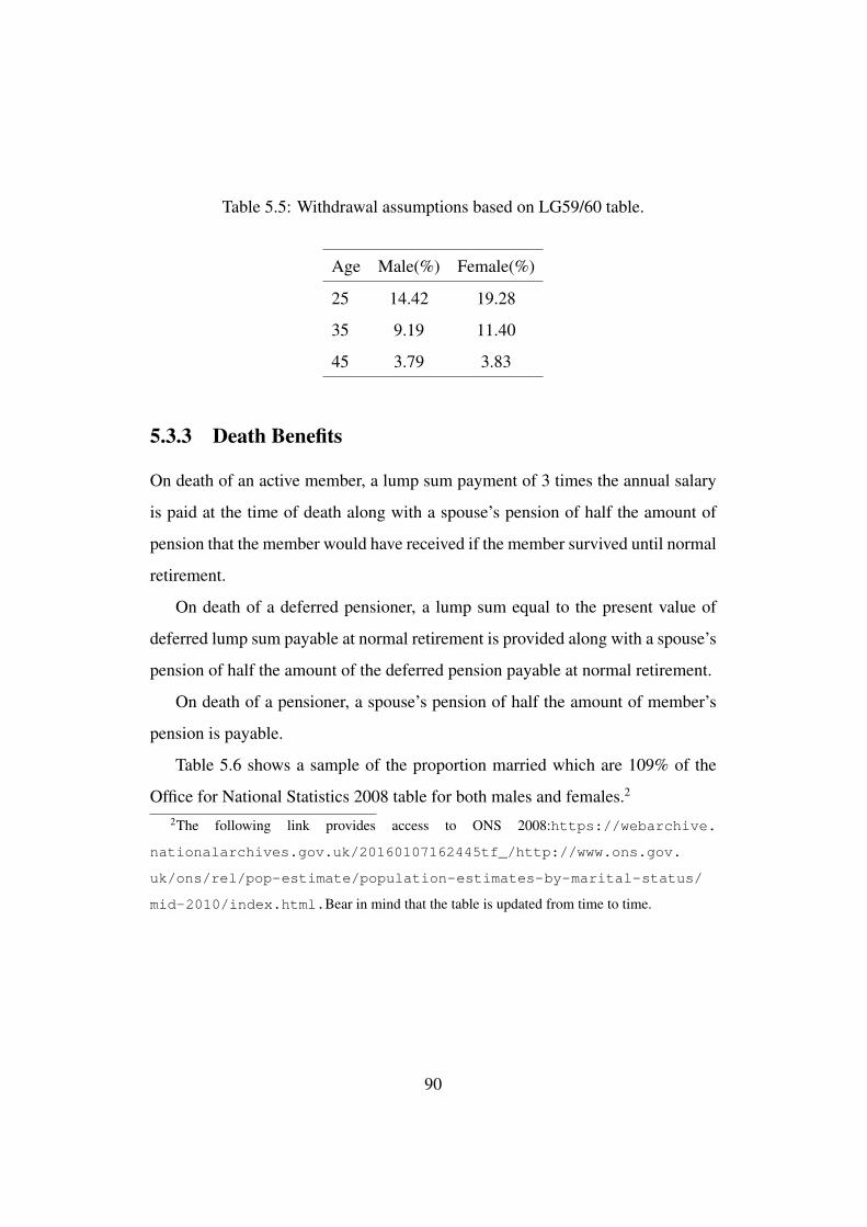
Table 5.5: Withdrawal assumptions based on LG59/60 table.
Age Male(%) Female(%)
25 14.42 19.28
35 9.19 11.40
45 3.79 3.83
5.3.3 Death Benefits
On death of an active member, a lump sum payment of 3 times the annual salary
is paid at the time of death along with a spouse’s pension of half the amount of
pension that the member would have received if the member survived until normal
retirement.
On death of a deferred pensioner, a lump sum equal to the present value of
deferred lump sum payable at normal retirement is provided along with a spouse’s
pension of half the amount of the deferred pension payable at normal retirement.
On death of a pensioner, a spouse’s pension of half the amount of member’s
pension is payable.
Table 5.6 shows a sample of the proportion married which are 109% of the
Office for National Statistics 2008 table for both males and females.2
2The following link provides access to ONS 2008:https://webarchive.
nationalarchives.gov.uk/20160107162445tf_/http://www.ons.gov.
uk/ons/rel/pop-estimate/population-estimates-by-marital-status/
mid-2010/index.html.Bear in mind that the table is updated from time to time.
90

Table 5.6: Proportion married based on ONS 2008 table.
Age Male(%) Female(%)
25 10.90 10.90
35 53.41 53.41
45 69.76 69.76
5.4 Contributions
As at 31 March 2014, employers contribute 16% of salary while employees con-
tribute 6.5% of salary amounting to a total contribution of 22.5% of salary.
5.5 Valuation Method
The USS uses the Projected Unit Method (PUM) to estimate the liabilities of the
scheme. The PUM is a prospective valuation method where liabilities are esti-
mated based on the past service accrued on the valuation date taking into account
future salary inflation. FRS17 requires future cashflows to be discounted at the
yield available on AA-rated corporate bonds, interest rate swaps and other fixed
interest or index-linked bonds.
The PUM formula for the pension element is given by:
Accrued Liability =
[P SAcc
][1 + e
1 + i
]NRA−x
aNRA, where
• P is the number of years of past service at the date of valuation
• S is the pensionable salary at the date of valuation
• Acc is the accrual rate
91
• e is the rate of future salary increase
• i is the discount rate
• x is the current age
• NRA is the normal retirement age
• aNRA is the value of an annuity payable from age NRA.
When projecting liabilities for future years, the FS and CARE schemes are
treated separately. Benefits built up under the FS scheme will increase in line with
increases in official pensions. Official pensions increase are those paid to retired
public sector employees such as teachers, civil servants or National Health Service
(NHS) employees. Benefits built up under the CARE scheme will be based on an
inflation adjusted average salary between 31 March 2014 and the future valuation
dates.
USS 2014 valuation uses a discount rate is 5.2% p.a. decreasing linearly to
4.7% p.a. over 20 years. To check that our liabilities braodly matches the liabilities
of the USS, we use a constant discount rate of 5.0% p.a.
5.6 Valuation Results
USS 2014 valuation reports a liability of £46.9 billion. Using our model of USS,
based on the relevant model points, we obtain a liability value of £48.7 billion,
which is not very far from the figure provided in the actuarial valuation report.
One of the reasons behind the value of liability from the model being slightly
higher is due to our assumption that all members remain under the FS scheme
until 2014 while the valuation report does take into account the fact that new
entrants between 2011 and 2014 have already moved to the CARE scheme.
92

5.7 Assets and Liabilities
The starting values of assets and liabilities as at March 31, 2014 are:
• A0 = £41.6bn;
• L0 = £46.9bn;
giving an initial valuation deficit of £5.3bn. We assume there is no amortisation
of the initial deficit. We note that the USS invests 73% of assets in real assets and
27% of assets in fixed assets. For our model, we assume that 70% of assets are
invested in equities and 30% of assets are invested in bonds. Table 5.7 provides
both actual and benchmark distribution of assets as given in the 2014 Accounts
and Reports.
Table 5.7: USS investment mix.Assets Actual Benchmark
UK equities 15 16
Overseas equities 28 31
Alternative assets 23 19
Property 7 7
Total real 73 73
Fixed interest 28 27
Cash -1 0
Total fixed 27 27
93

5.8 Economic Scenario Generator
To project assets and liabilities forward, we need an ESG. In this chapter, we use
and compare the impact of two ESGs. The first ESG is the Wilkie Model (Wilkie
et al. (2011)). The second ESG is the Graphical Model. Both ESGs are discussed
in detail in Chapter 2.
5.9 Mortality Model
The USS uses the S1NA (light) mortality table adjusted down by 1 year for fe-
males and unadjusted for males. Mortality projections are carried out using the
CMI-2014 projections table. As discussed in Chapter 3, to capture the mortality
risk, we use Model M7 from Cairns et al. (2009) calibrated to UK data. As dis-
cussed in Chapter 3, we need to adjust the projected mortality rates from Model
M7 such that the central projection from Model M7 matches the projection table
used by the valuation actuary (which in this case is the CMI-2014 table).
In other words, for the case of the USS.
qadj(x,t) = qM7(x,t) × adj(x,t) (5.1)
adj(x,t) =qval(x,t)
qM7(x,t)
. (5.2)
where qval(x,t) is the mortality projection using CMI-2014 and qM7(x,t) is the central
projection from Model M7.
94
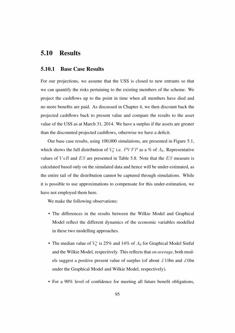
5.10 Results
5.10.1 Base Case Results
For our projections, we assume that the USS is closed to new entrants so that
we can quantify the risks pertaining to the existing members of the scheme. We
project the cashflows up to the point in time when all members have died and
no more benefits are paid. As discussed in Chapter 4, we then discount back the
projected cashflows back to present value and compare the results to the asset
value of the USS as at March 31, 2014. We have a surplus if the assets are greater
than the discounted projected cashflows, otherwise we have a deficit.
Our base case results, using 100,000 simulations, are presented in Figure 5.1,
which shows the full distribution of V ∗0 i.e. PV FP as a % of A0. Representative
values of V aR and ES are presented in Table 5.8. Note that the ES measure is
calculated based only on the simulated data and hence will be under-estimated, as
the entire tail of the distribution cannot be captured through simulations. While
it is possible to use approximations to compensate for this under-estimation, we
have not employed them here.
We make the following observations:
• The differences in the results between the Wilkie Model and Graphical
Model reflect the different dynamics of the economic variables modelled
in these two modelling approaches.
• The median value of V ∗0 is 25% and 14% of A0 for Graphical Model Sinful
and the Wilkie Model, respectively. This reflects that on average, both mod-
els suggest a positive present value of surplus (of about £10bn and £6bn
under the Graphical Model and Wilkie Model, respectively).
• For a 90% level of confidence for meeting all future benefit obligations,
95
the V aR measure requires that 31% (approximately £13bn) and 36% (ap-
proximately £15bn) additional assets (on top of the available £41.6bn) will
be required under the Graphical Model and Wilkie Model, respectively.
Moreover, at that level of confidence, if the loss exceeds V aR, the aver-
age amount of loss, i.e. expected shortfall ES, will be 74% and 55% of A0
under the Graphical Model and Wilkie Model, respectively.
• As expected both Table 5.8 and Figure 5.1 show that for higher confidence
levels (or equivalently lower percentiles), greater amounts of additional as-
sets are required; and the expected shortfall increases substantially.
Table 5.8: Base case economic capital (as a percentage of A0 = £41.6bn) at
different probability levels for both Wilkie Model and Graphical Model.
Graphical Model Wilkie Model
Confidence Level V aR ES V aR ES
50 25 -13 14 -14
90 -36 -74 -31 -55
99.5 -153 -198 -101 -126
5.10.2 Sensitivity to Asset Allocation Strategies
In this section, we change the base case asset allocation strategy from (70% equi-
ties, 30% bonds) to (30% equities, 70% bonds). Using only the Graphical Model,
we present our findings in Table 5.9 and Figure 5.2, which show the base case
results alongside the results for changed asset allocation strategy for ease of com-
parison. All other assumptions are kept the same as that of the base case. We
make the following observations:
96

• For increased bond investment, the distribution of V ∗0 has moved to the left
and has greater dispersion.
• The leftward shift of the distribution indicates a greater probability of larger
deficits. This is reflected in the median (50th percentile) of V ∗0 which shows
a loss of 21% of A0 in terms of V aR (as compared to a surplus of 25% of
A0 for the base case results). In fact Table 5.9 shows that both V aR and ES
has increased at ever increasing rate at all percentile levels.
• The sensitivity patterns can be explained by the fact that the expected returns
from bonds are lower in the long term compared to equities. So a higher
bond investment can lead to potentially larger losses, which is reflected in
the leftward shift and greater dispersion in the distribution.
• Moreover, fixed interest bonds are poor match for real liabilities. Hence
increased fixed interest bond investment has exacerbated the risk.
• The fact that the distribution of V ∗0 has a wider spread for higher bond in-
vestment, it reflects greater underlying uncertainty compared to higher eq-
uity investment. This highlights that the perception of de-risking by moving
to more bonds may be flawed.
5.10.3 Sensitivity to Contribution Rates
In this section, we analyse the impact of changes in the base case contribution
rate of 22.5%. We consider two cases – an increased contribution rate of 25% of
salaries and a decreased contribution rate of 20%. All other assumptions are the
same as the base case, including the asset allocation strategy of 70% equities and
30% bonds.
97

Table 5.9: Economic capital (as a percentage of A0 = £41.6bn) for the base case
and for the asset allocation strategy of 30% equities and 70% bonds at different
probability levels using the Graphical Model.
Equity/Bond 70/30 Equity/Bond 30/70
Percentile V aR ES V aR ES
50 25 -13 -21 -72
90 -36 -74 -103 -149
99.5 -153 -198 -245 -296
We present our findings in Table 5.10 and Figure 5.3. Note that we have also
included the base case results in Table 5.10 for ease of comparison. Similarly
in the two plots of Figure 5.3, we have included the distribution of V ∗0 for the
base case as the grey coloured density in the background. We make the following
observations:
• Compared to the impact of change in asset allocation strategy, changes in
contribution rates have a much reduced effect on the overall risk.
• As an example, at 90% level of confidence (i.e. percentile level of 10%), a
decrease in contribution of 2.5% (i.e. reduced from 22.5% to 20% of salary)
results in an increase of loss from 36% to 41% of A0 in terms of V aR. On
the other hand, increasing the contribution rate to 25%, produces a loss of
30%.
• This leftward and rightward shifts of the distribution of V ∗0 for decreased
and increased contribution rates, respectively, can also be observed in Fig-
ure 5.3. However, note that the magnitude of the shifts are relatively small
compared to the impact of changes in the asset allocation strategy.
98

Table 5.10: Economic capital (as a percentage of A0 = £41.6bn) for three dif-
ferent contribution rates of 20%, 22.5% (base case) and 25% of salary at different
probability levels using Graphical Model.
Contribution rate as a percentage of salary
20% 22.5% 25%
Percentile V aR ES V aR ES V aR ES
50 21 -18 25 -13 29 -8
90 -41 -80 -36 -74 -30 -68
99.5 -160 -208 -153 -198 -146 -191
5.11 Summary
In this chapter, we have carried out a risk assessment of the USS. For the base
case results, using an asset allocation of 70% equity and 30% bonds and Graph-
ical Model for projections, we found a median surplus of 25% of the asset value
and a deficit of 153% at the 99.5th percentile. In comparison, using 30% equity
and 70% bonds, the median deficit is 21% of the asset value and the deficit at the
99.5% percentile is 245%. From these results, it can be argued that the scheme
has a lower risk for a higher proportion of equities. This shows that de-risking is
a far more complex issue than the conventional wisdom of simply moving assets
from risky assets (equity) to less risky assets (bonds). Other considerations such
as asset-liability matching and accounting for the term of the investment also need
to be taken into account when deciding on an investment strategy. We have also
noted that the magnitude of the PV FP shifts with respect to changes in contri-
bution rates are relatively small compared to the impact of changes in the asset
allocation strategy.
99

−300 −250 −200 −150 −100 −50 0 50 100
0.00
00.
010
0.02
0
Base case Graphical Model
PVFP (as a % of A0)
Den
sity
Percentiles
50th90th99.5th
−300 −250 −200 −150 −100 −50 0 50 100
0.00
00.
010
0.02
0
Base case Wilkie Model
PVFP (as a % of A0)
Den
sity
Percentiles
50th90th99.5th
Figure 5.1: Base case distributions of standardised PV FP (as a percentage of
A0 = £41.6bn) for both Graphical Model and Wilkie Model.
100

−300 −250 −200 −150 −100 −50 0 50 100
0.00
00.
010
0.02
0
Base case asset allocation strategy of 70% equities and 30% bonds
PVFP (as a % of A0)
Den
sity
Percentiles
50th90th99.5th
−300 −250 −200 −150 −100 −50 0 50 100
0.00
00.
010
0.02
0
Asset allocation strategy changed to 30% equities and 70% bonds
PVFP (as a % of A0)
Den
sity
Percentiles
50th90th99.5th
Figure 5.2: Distributions of standardised PV FP (as a percentage of A0 =
£41.6bn) for the base case and for the asset allocation strategy of 30% equities
and 70% bonds at different probability levels using the Graphical Model.
101

−300 −250 −200 −150 −100 −50 0 50 100
0.00
00.
010
0.02
0
Contribution rates reduced to 20% of salary
PVFP (as a % of A0)
Den
sity
Percentiles
50th90th99.5th
−300 −250 −200 −150 −100 −50 0 50 100
0.00
00.
010
0.02
0
Contribution rates increased to 25% of salary
PVFP (as a % of A0)
Den
sity
Percentiles
90th90th99.5th
Figure 5.3: Distributions of standardised PV FP (as a percentage of A0 =
£41.6bn) for decreased contribution rate of 20% and increased contribution rate
of 25% (base case assumption is 22.5% of salary) using Graphical Model. The
grey coloured density in the background shows the base case.
102
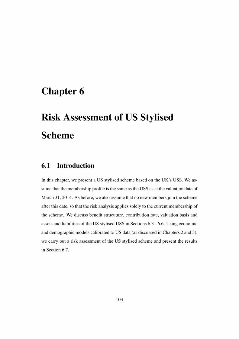
Chapter 6
Risk Assessment of US Stylised
Scheme
6.1 Introduction
In this chapter, we present a US stylised scheme based on the UK’s USS. We as-
sume that the membership profile is the same as the USS as at the valuation date of
March 31, 2014. As before, we also assume that no new members join the scheme
after this date, so that the risk analysis applies solely to the current membership of
the scheme. We discuss benefit strucuture, contribution rate, valuation basis and
assets and liabilities of the US stylised USS in Sections 6.3 - 6.6. Using economic
and demographic models calibrated to US data (as discussed in Chapters 2 and 3),
we carry out a risk assessment of the US stylised scheme and present the results
in Section 6.7.
103

6.2 Membership Profile
We assume the same membership profile as used for the UK’s USS for the US
stylised scheme. The mebership profile of the USS was discussed in Section 5.2.
Tables 6.1 and 6.2 show the membership profile and the model points used for
active members for the US stylised scheme.
Table 6.1: Membership profile
Active Number 167,545
Average pensionable salary $42,729
Average age 43.8
Average past service 12.5
Deferred Members Number 110,430
Average deferred pension $2,373
Average age 45.1
Pensioners Number 70,380
(including dependents) Average pension $17,079
Average age 71.1
6.3 Benefit Structure
To reflect the specific characteristics of US pension schemes, we modify the bene-
fit structure, contribution rates and investment strategies. These modified assump-
tions are outlined in this section.
104

Table 6.2: Model points, past service and salary of active members of the US
stylised scheme
Age Proportion Number Past service Salary
30 30% 50,264 7 $25,500
40 30% 50,264 11 $42,500
50 20% 33,509 15 $52,500
60 20% 33,509 19 $58,500
Total 100% 167,545
Average 12.2 $42,600
6.3.1 Pension Benefits
Pension and cash lump sum at retirement are calculated as follows:
Annual pension = Pensionable salary × Pensionable service × Accrual rate.
Lump Sum = nil.
For the US stylised pension scheme, we assume that pensionable salary is the
member’s salary in the final year of service. Pensionable service will be all years
of service, and the accrual rate is set to 1.5%. We assume no lump sum payment
for the US stylised scheme. Moreover, there is no indexation to the pension during
the payment period.
6.3.2 Withdrawal Benefits
For members who withdraw from the scheme, a deferred pension is provided
based on accrued service. No indexation of salary is provided between the date
the member withdraws from the scheme and the date of retirement. Also, there is
105

no indexation during the payment period.
6.3.3 Death Benefits
On death of an active member, a lump sum payment is paid at the time of death
equal to the present value of the pension that the member would have received if
the member survived until normal retirement.
On death of a deferred pensioner, a lump sum equal to the present value of the
pension that the member would have received if the member survived until normal
retirement.
On death of a pensioner, a spouse’s pension of half the amount of member’s
pension is payable.
6.4 Contributions
To the US stylised scheme, we assume that employees do not contribute, while the
employer contributes an amount equal to the current level of the normal actuarial
cost, expressed as a percentage of salary. Based on our calculations, this amounts
to 10.8% of the final salary.
6.5 Valuation Method
For the US stylised scheme, we use the same valuation method as the USS which
is the PUM. The PUM was described in Section 5.5.
6.6 Assets and Liabilities
The starting values of assets and liabilities as at March 31, 2014 are:
106

• A0 = $26.1bn;
• L0 = $32.6bn.
Assets are assumed to be at 80% of the value of liabilities as at 31 March 2014
(and hence there is a 20% deficit).
To project our assets and liabilties, we use an ESG and a mortality model. For
the ESG, we use the Graphical Model calibrated to US data. This was discussed
in Chapter 2. For the mortality model, we use Model M7 calibrated to US data
from the HMD. This was discussed in Chapter 3.
6.6.1 Investment Strategy
It is assumed that the asset allocation for the US stylised scheme is 50% equities
and 50% bonds.
6.7 Results
6.7.1 Results with no Amortisation
Our first results, using 10,000 simulations, are presented in Figure 6.1, which
shows the full distribution of V ∗0 based on the assumption of no amortisation of
the initial deficit. Representative values of V aR and ES are presented in Table
6.3. We make the following observations.
• The median value of V0 is -25% of A0. This corresponds to a median deficit
of $6.5m which is expected.
• As expected both Table 6.3 and Figure 6.1 show that for higher confidence
levels (or equivalently lower percentiles) greater amounts of additional as-
sets are required; and the expected shortfall increases substantially.
107

6.7.2 Base Case Results
As discussed in Section 6.6, there is a 20% deficit between assets and liabilties.
For our base case, we assume that this deficit will be amortised over a period of
seven years (i.e., n = 7), during which the sponsor injects a total of L0−A0 spread
evenly over those seven years, i.e., Yt = 17(L0 − A0) where t = 0, 1, 2, ...6. Note
that for our case, this represents an additional contribution of approximately 4%
of members’ salaries.
Our base case results are also presented in Figure 6.1, which shows the full
distribution of V ∗0 . Representative values of VaR and ES are presented in Table
6.3. We make the following observations:
• With the amortisation cash flows, the distribution of V ∗0 has moved to the
right and has less dispersion.
• Note that if the amortisation period is 1, there is an immediate cover for the
deficit amount and the average of V ∗0 will be approximately zero because the
base contribution is equal to the expected future benefit accruals. When the
amortisation period is seven years, however, there is a time lag in covering
the deficit, so on average V ∗0 is a small negative value.
6.7.3 Sensitivity to Asset Allocation Strategies
Recall that the base case asset allocation strategy is assumed to be 50% bonds and
50% equity. To test the impact of asset allocation strategies, we now consider two
cases: 75% equity and 25% bonds, and 75% bonds and 25% equity. Table 6.4
and Figure 6.2 show the results for different asset allocation strategies. All other
assumptions are kept the same as those for the base case. We make the following
observations:
108
Table 6.3: Economic capital (as a percentage of A0 = $26.1bn) for the base case
and for the asset allocation strategy at different probability levels.
No Amortisation With Amortisation
Percentile V aR ES V aR ES
50 -25 -88 -1 -60
90 -121 -187 -92 -156
99.5 -339 -444 -305 -415
• For increased equity investment, the distribution of V ∗0 has moved to the
right. Moreover, from Figure 6.2, we note that the distribution has a higher
peak and a steeper tail compared to the base case and is thus less dispersed.
This further highlights that de-risking the investment portfolio does not nec-
essarily serve the purpose of improving the solvency position of a pension
scheme. The fact that, on a long horizon, the expected return on equity
is higher than bonds outweights the impact of increased volatily on equity.
Overall, equity offers a better match to the long term liabilities of the pen-
sion scheme.
• The rightward shift of the distribution is reflected in the median (50th per-
centile) of V ∗0 which shows a surplus of 6% of A0 in terms of VaR (com-
pared to a deficit of 1% of A0 for the base case). The greater dispersion is
reflected by the 99.5th percentile which is much larger than the base case.
• For increased bond investment, the distribution of V ∗0 has significantly moved
to the left. The dispersion is again greater than than the base case but less
dispersed than that with higher equity.
• The median of V ∗0 under the increased bond investment shows a loss of 54%
109

of A0 in terms of VaR. The sensitivity patterns can be explained by the fact
that the expected returns from bonds are lower in the long run compared to
equities. So a higher bond investment can lead to a potentially large losses
which is reflected in the leftward shift.
Table 6.4: Economic capital (as a percentage of A0 = $26.1bn) for the base case
and for the asset allocation strategy at different probability levels.
Equity/Bond 75/25 Equity/Bond 50/50 Equity/Bond 25/75
Percentile V aR ES V aR ES V aR ES
50 6 -58 -1 -60 -54 -119
90 -92 -169 -92 -156 -154 -224
99.5 -343 -478 -305 -415 -387 -505
6.7.4 Sensitivity to Contribution Rates
In this section, we analyse the impact of changes in the base case contribution
rate of 10.8%. We consider two cases; an increased contribution rate of 13.3%
of salaries (an increase of 2.5%) and a decreased contribution rate of 8.3% (a
decrease of 2.5%). All other assumptions are the same as the base case, including
the asset allocation strategy of 50% equities and 50% bonds. We present our
findings in Table 6.5 and Figure 6.3.
• Compared to the impact of changing the asset allocation to 25% equity and
75% bonds, changes in contribution rates have a much reduced effect on the
overall risk.
• For example, at 99.5% confidence level, a decrease in contribution of 2.5%
(i.e. reduced from 10.8% to 8.3% of salary) results in an increase of loss
110

from 305% to 326% of A0 in terms of V aR. On the other hand, increasing
the contribution rate to 13.3%, produces a deficit of 286%.
• This left and right shifts of the distribution of V ∗0 for decreased and in-
creased contribution rates respectively can also be observed in Figure 6.3.
However, the magnitude of the shift at the median is roughly an eighth of
the impact of changes in the asset allocation strategy. The magnitude of the
shift at the 99.5th percentile is roughly half of the impact of changes in the
asset allocation strategy.
Table 6.5: Economic capital (as a percentage of A0 = $26.1bn) for different
contribution rates at different probability levels.
Contribution rate as a percentage of salary
13.3% 10.8% 8.3%
Percentile V aR ES V aR ES V aR ES
50 7 -50 -1 -60 -9 -70
90 -80 -142 -92 -156 -104 -170
99.5 -286 -396 -305 -415 -326 -433
6.7.5 Sensitivity to Mortality Tables
We consider the sensitivity of changing the mortality assumptions to be determin-
istic one. It is quite common for pension schemes actuaries to use deterministic
mortality tables rather than stochastic ones. We use the RP-2006 mortality ta-
ble and the AA projection scale instead of model M7 calibrated to data from the
HMD. Unlike the other sensitivity tests, the mortality rates are deterministic in
this case. All other assumptions, however, remain unchanged from the base case,
111

and the economic assumptions are still stochastic. Note that the results presented
are based on the same set of economic simulations as in the previous sections.
Technically, using different assumptions would mean that L0 and contributions
would be slightly different. For consistency, we do not make any changes to the
contribution rates or the liabilities when changing the mortality table. Note that
RP-2006 has lower mortality rates compared to model M7 calibrated to HMD
data. We present our findings in Table 6.6 and Figure 6.4. As it can be seen, the
differences are minor but nonetheless interesting.
• Compared to the base case, the median of the distribution has moved slightly
to the right.
• Given that RP-2006 has lower mortality rates than M7, it has the following
effects:
– There is more cash inflow at the start, as benefit payments are smaller
given fewer deaths among active members.
– The cash outflow is higher toward the end, as pensions paid are higher
given that pensioners survive longer..
– As higher contributions occur sooner than higher pension payments,
the impact of contributions on V ∗0 is larger. This is reflected in the
median increasing to 6% of A0 in terms of VaR.
• The dispersion has significantly reduced. The deficit at 99.5% percentile
level is 209% of A0 in terms of VaR compared to 305% for the base case.
This is due to:
– mortality rates being deterministic and;
– higher stochastic positive cashflows at the beginning making the dis-
tribution less negatively skewed.
112
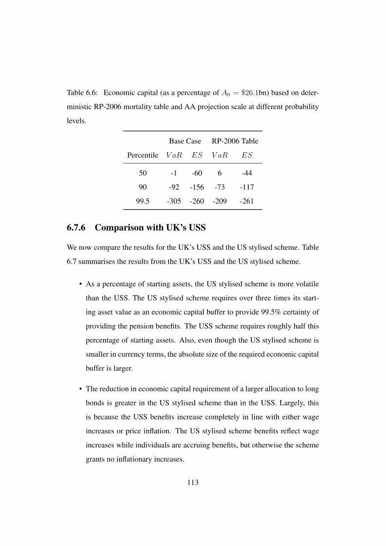
Table 6.6: Economic capital (as a percentage of A0 = $26.1bn) based on deter-
ministic RP-2006 mortality table and AA projection scale at different probability
levels.
Base Case RP-2006 Table
Percentile V aR ES V aR ES
50 -1 -60 6 -44
90 -92 -156 -73 -117
99.5 -305 -260 -209 -261
6.7.6 Comparison with UK’s USS
We now compare the results for the UK’s USS and the US stylised scheme. Table
6.7 summarises the results from the UK’s USS and the US stylised scheme.
• As a percentage of starting assets, the US stylised scheme is more volatile
than the USS. The US stylised scheme requires over three times its start-
ing asset value as an economic capital buffer to provide 99.5% certainty of
providing the pension benefits. The USS scheme requires roughly half this
percentage of starting assets. Also, even though the US stylised scheme is
smaller in currency terms, the absolute size of the required economic capital
buffer is larger.
• The reduction in economic capital requirement of a larger allocation to long
bonds is greater in the US stylised scheme than in the USS. Largely, this
is because the USS benefits increase completely in line with either wage
increases or price inflation. The US stylised scheme benefits reflect wage
increases while individuals are accruing benefits, but otherwise the scheme
grants no inflationary increases.
113

• The effect on economic capital (for either of the schemes) is much larger for
changes in asset allocation than for changes to scheme contributions. The
comparison between the two pension schemes incorporates the differences
in between UK and US demography and economy. One might argue that a
more interesting comparison might be only to change the benefit structure
of the USS but not the economic and demographic assumption. This would
reflect the impact of only changing the benefit structure. In this respect, in
Appendix C, we present the results of the US stylised scheme using UK’s
economic and demographic assumptions.
114

Table 6.7: Economic capital (as a percentage of A0) for UK’s USS and US stylised scheme.
UK’s USS US Stylised Scheme
70% Equity (Base Case) 30% Equity 50% Equity (Base Case) 25% Equity
Percentile V aR ES V aR ES V aR ES V aR ES
50 25 -13 -21 -72 -1 -60 -54 -119
90 -36 -74 -103 -149 -92 -156 -154 -224
99.5 -153 -198 -245 -296 -305 -415 -387 -505
20% Contribution Rate 25% Contribution Rate 8.3% Contribution Rate 13.3% Contribution Rate
Percentile V aR ES V aR ES V aR ES V aR ES
50 25 -13 -21 -72 -9 -70 7 -50
90 -36 -74 -103 -149 -104 -170 -80 -142
99.5 -153 -198 -245 -296 -326 -433 -286 -396
115

−400 −350 −300 −250 −200 −150 −100 −50 0 50 100
0.00
00.
010
0.02
0
Starting Case with no amortisation
PVFP (as a % of A0)
Den
sity
Percentiles
50th90th99.5th
−400 −350 −300 −250 −200 −150 −100 −50 0 50 100
0.00
00.
010
0.02
0
Base Case
PVFP (as a % of A0)
Den
sity
Percentiles
50th90th99.5th
Figure 6.1: Distributions of standardised PV FP for Starting Case with no amor-
tisation and for Base Case distributions (as a percentage of A0 = $26.1bn).
116
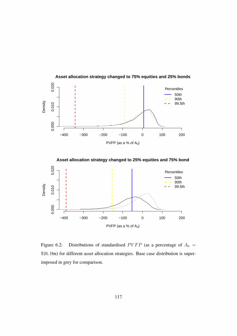
−400 −300 −200 −100 0 100 200
0.00
00.
010
0.02
0
Asset allocation strategy changed to 75% equities and 25% bonds
PVFP (as a % of A0)
Den
sity
Percentiles
50th90th99.5th
−400 −300 −200 −100 0 100 200
0.00
00.
010
0.02
0
Asset allocation strategy changed to 25% equities and 75% bond
PVFP (as a % of A0)
Den
sity
Percentiles
50th90th99.5th
Figure 6.2: Distributions of standardised PV FP (as a percentage of A0 =
$26.1bn) for different asset allocation strategies. Base case distribution is super-
imposed in grey for comparison.
117

−400 −300 −200 −100 0 100 200
0.00
00.
010
0.02
0
Contribution rates increased to 13.3% of salary
PVFP (as a % of A0)
Den
sity
Percentiles
50th90th99.5th
−400 −300 −200 −100 0 100 200
0.00
00.
010
0.02
0
Contribution rates reduced to 8.3% of salary
PVFP (as a % of A0)
Den
sity
Percentiles
50th90th99.5th
Figure 6.3: Distributions of standardised PV FP (as a percentage of A0 =
$26.1bn) for different contribution rates. Base case distribution is superimposed
in grey for comparison.
118
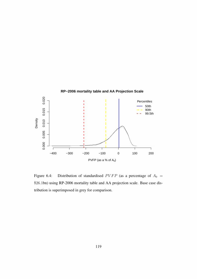
−400 −300 −200 −100 0 100 200
0.00
00.
005
0.01
00.
015
0.02
0
RP−2006 mortality table and AA Projection Scale
PVFP (as a % of A0)
Den
sity
Percentiles
50th90th99.5th
Figure 6.4: Distribution of standardised PV FP (as a percentage of A0 =
$26.1bn) using RP-2006 mortality table and AA projection scale. Base case dis-
tribution is superimposed in grey for comparison.
119

Chapter 7
Risk Assessment of the Ontario
Teachers’ Pension Plan
7.1 Introduction
In this Chapter, we carry out a risk assessment of a Canadian Pension Scheme,
the OTPP. The OTPP is a large open DB scheme operating in Canada with over
300,000 scheme members. The numbers presented here are based on the latest
available valuation carried out for the scheme as at January 1, 2018. The $ sign in
this chapter represents Canadian dollars.
7.2 Membership Profile
Table 7.1 shows the membership profile as presented in the 2018 valuation report.
As can be seen from the table, only a single average age is provided for the active
members, which is not sufficient to capture the overall risk characteristics of the
scheme. We need a range of model points to capture the inter-generational risk
dynamics. The valuation report also provides information on the proportion of
120

Table 7.1: Membership profile
Active Number 144,325
Average pensionable salary $90,468
Average age 44.4
Average past service 14.6
Deferred Members Number 71,205
Average deferred pension $1,965
Average age 45.1
Pensioners Number 129,785
Average lifetime pension $41,154
Average age 71.1
active members in different age bands, based on which, we propose to use an age
distribution of active members given in Table 7.2.
Table 7.2 also shows the past service and salary assumptions for active mem-
bers for each model point. These have been set so that the average past service
and average salary of active members broadly match the figures from Table 7.1.
For deferred members and pensioners, we use single model points to represent
each of these membership categories. We also assume a 50:50 gender split and no
salary differential between genders.
7.3 Benefit Structure – OTPP
7.3.1 Pension Benefits
The annual pension is equal to:
121
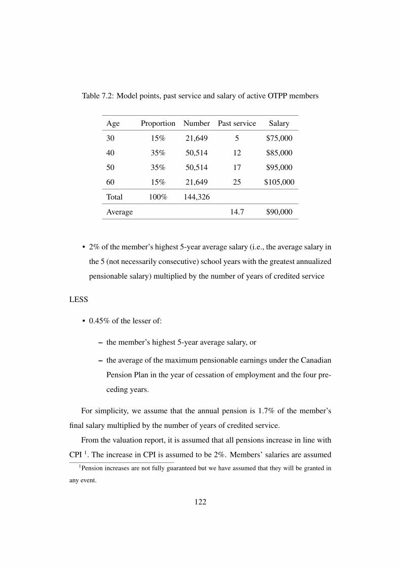
Table 7.2: Model points, past service and salary of active OTPP members
Age Proportion Number Past service Salary
30 15% 21,649 5 $75,000
40 35% 50,514 12 $85,000
50 35% 50,514 17 $95,000
60 15% 21,649 25 $105,000
Total 100% 144,326
Average 14.7 $90,000
• 2% of the member’s highest 5-year average salary (i.e., the average salary in
the 5 (not necessarily consecutive) school years with the greatest annualized
pensionable salary) multiplied by the number of years of credited service
LESS
• 0.45% of the lesser of:
– the member’s highest 5-year average salary, or
– the average of the maximum pensionable earnings under the Canadian
Pension Plan in the year of cessation of employment and the four pre-
ceding years.
For simplicity, we assume that the annual pension is 1.7% of the member’s
final salary multiplied by the number of years of credited service.
From the valuation report, it is assumed that all pensions increase in line with
CPI 1. The increase in CPI is assumed to be 2%. Members’ salaries are assumed1Pension increases are not fully guaranteed but we have assumed that they will be granted in
any event.
122
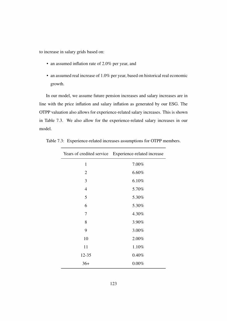
to increase in salary grids based on:
• an assumed inflation rate of 2.0% per year, and
• an assumed real increase of 1.0% per year, based on historical real economic
growth.
In our model, we assume future pension increases and salary increases are in
line with the price inflation and salary inflation as generated by our ESG. The
OTPP valuation also allows for experience-related salary increases. This is shown
in Table 7.3. We also allow for the experience-related salary increases in our
model.
Table 7.3: Experience-related increases assumptions for OTPP members.
Years of credited service Experience-related increase
1 7.00%
2 6.60%
3 6.10%
4 5.70%
5 5.30%
6 5.30%
7 4.30%
8 3.90%
9 3.00%
10 2.00%
11 1.10%
12-35 0.40%
36+ 0.00%
123
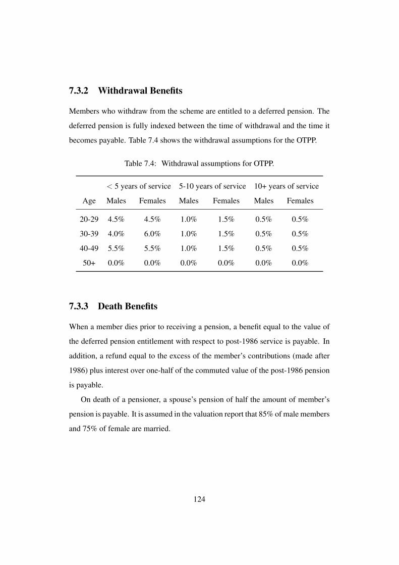
7.3.2 Withdrawal Benefits
Members who withdraw from the scheme are entitled to a deferred pension. The
deferred pension is fully indexed between the time of withdrawal and the time it
becomes payable. Table 7.4 shows the withdrawal assumptions for the OTPP.
Table 7.4: Withdrawal assumptions for OTPP.
< 5 years of service 5-10 years of service 10+ years of service
Age Males Females Males Females Males Females
20-29 4.5% 4.5% 1.0% 1.5% 0.5% 0.5%
30-39 4.0% 6.0% 1.0% 1.5% 0.5% 0.5%
40-49 5.5% 5.5% 1.0% 1.5% 0.5% 0.5%
50+ 0.0% 0.0% 0.0% 0.0% 0.0% 0.0%
7.3.3 Death Benefits
When a member dies prior to receiving a pension, a benefit equal to the value of
the deferred pension entitlement with respect to post-1986 service is payable. In
addition, a refund equal to the excess of the member’s contributions (made after
1986) plus interest over one-half of the commuted value of the post-1986 pension
is payable.
On death of a pensioner, a spouse’s pension of half the amount of member’s
pension is payable. It is assumed in the valuation report that 85% of male members
and 75% of female are married.
124

7.4 Contributions
Both employers and employees contribute to the OTPP. Each party contributes
10.4% of pensionable earnings up to the Year’s Maximum Pensionable Earnings
(YMPE) and 12.0% of pensionable earnings in excess of the YMPE. For 2018,
the YMPE $55,900 for 2018. From the valuation report, the assumed increase in
the YMPE is 3% per year (an assumed inflation rate of 2.0% and an assumed real
increase of 1.0% per year). In our model, we assume the YMPE increases in line
with salary inflation as generated by our ESG.
7.5 Valuation Method
The valuation method of the OTPP was prescribed by the Teachers’ Pension Act
prior to the Regulations being amended to permit other actuarial cost methods.
This method is not considered by the Regulations to be a “benefit allocation
method". The method takes into account the benefits determined as of the time
they are assumed to become payable, based on a teacher’s projected earnings and
service. Based on this valuation method, the liabilities amount to $217bn. The
liability value based on the PUM is also calculated for reporting purposes. The
liabilities using the PUM are $155bn.
7.6 Assets and Liabilities
The starting values of assets and liabilities as at January 1, 2018 are:
• L0 = $155.0bn (based on the valuation report using the PUM and a discount
rate of 4.8% per annum);
• A0 = $227.5bn (based on the valuation report).
125

giving an initial valuation surplus of $72.5bn. The OTPP invests approximately
54% in real assets and 46% in fixed assets. Table 7.5 shows the asset allocation
of the OTPP as given in the 2017 Accounts and Reports. For purposes of our
calculation, we assume an asset allocation of 55% equity and 45% bonds for the
base case.
Table 7.5: OTPP investment mix.
Assets Allocation (%)
Equities 36
Inflation sensitive assets 14
Real estate and infrastructure 25
Money market instruments (21)
Total real 54
Fixed interest 33
Credit and absolute return strategies 13
Total fixed 46
7.7 Economic Scenario Generator
To project assets and liabilities forward, we use the graphical model calibrated to
Canadian data. This has been discussed in Chapter 2.
126

7.8 Mortality Model
For future mortality rates forward, the OTPP uses the 2014 OTPP Generational
Mortality Table and Projection Scale TT (two dimensional tables), which was
developed by the University of Waterloo based on a study of the scheme’s experi-
ence to the end of 2013. These tables are deterministic tables and provide a single
projection path. To capture the mortality risk, we use Model M7 calibrated to
Canadian data from the HMD. We then adjust the projected mortality rates such
that the central projection from M7 matches the projection from the 2014 OTPP
Generational Mortality Table and Projection Scale TT.
7.9 Results
In the following subsections, we discuss the results for the OTPP.
7.9.1 Base Case
Our first results, using 10,000 simulations, are presented in Figure 7.1, which
shows the full distribution of V ∗0 . Representative values of V aR and ES are
presented in Table 7.6. We make the following observations.
• The median value of V ∗0 is 36% ofA0. This corresponds to a median surplus
of $82bn.
• As expected both Table 7.6 and Figure 7.1 show that for higher confidence
levels greater amounts of additional assets are required; and the expected
shortfall increases substantially.
127

Table 7.6: Economic capital for Base Case (as a percentage of A0 = $227.5bn)
at different probability levels.
Percentile V aR ES
50 36 -3
90 -25 -70
99.5 -164 -227
7.9.2 Sensitivity to Asset Allocation Strategies
In this section, we change the base case asset allocation strategy. We consider
two cases: 75% equity and 25% bonds; and 75% bonds and 25% equity. We
present our findings in Table 7.7 and Figure 7.2 in which we show the results for
the changed asset allocation strategy. All other assumptions are kept the same as
that of the base case. We make the following observations:
• For increased equity investment, the distribution of V ∗0 has moved to the
right and has greater dispersion compared to the base case as more exposure
to equities leads to greater expected returns and higher volatility.
• The rightward shift of the distribution is reflected in the median (50th per-
centile) of V ∗0 which shows a surplus of 46% of A0 in terms of VaR (com-
pared to a surplus of 36% of A0 for the base case). The greater dispersion
is reflected by the 90th and 99.5th percentile which are much larger than the
base case.
• For increased bond investment, the distribution of V ∗0 has moved to the left.
The dispersion is again greater than than the base case but less dispersed
than that with higher equity.
128

• The median of V ∗0 under the increased bond investment shows a loss of 10%
of A0 in terms of VaR. The sensitivity patterns can be explained by the fact
that the expected returns from bonds are lower in the long run compared to
equities. So a higher bond investment can lead to potentially large losses
which are reflected in the leftward shift.
• The base case is less dispersed compared to the case of increased equity
investment and to the case of increased bond investment. This may be due
to the fact that the base case benefits from a more appropriate mix of equities
and bonds in a diversified portfolio.
Table 7.7: Economic capital (as a percentage of A0 = $227.5bn) for different the
asset allocation strategies at different probability levels.
Equity/Bond 75/25 Equity/Bond 55/45 Equity/Bond 25/75
Percentile V aR ES V aR ES V aR ES
50 46 0 36 -3 -10 -59
90 23 -80 -25 -70 -86 -135
99.5 -213 -313 -164 -227 -237 -288
7.9.3 Sensitivity to Contribution Rates
In this section, we analyse the impact of changes in the base case contribution
rate of 20.8%. We consider two cases; an increased contribution rate of 23.3%
of salaries (an increase of 2.5%) and a decreased contribution rate of 18.3% (a
decrease of 2.5%). All other assumptions are the same as the base case, including
the asset allocation strategy of 55% equities and 45% bonds. We present our
findings in Table 7.8 and Figure 7.3.
129

• Compared to the impact of change in asset allocation strategy, changes in
contribution rates have a much reduced effect on the overall risk.
• For example, at 99.5% confidence level, a decrease in contribution of 2.5%
(i.e. reduced from 20.8% to 18.3% of salary) results in an increase of loss
from 164% to 169% of A0 in terms of V aR. On the other hand, increasing
the contribution rate to 23.3%, produces a deficit of 160%. As a rough
approximation, eliminating all contributions would not result in as a large
shift in the 99.5% confidence level as the shift with a 75% equity and 25%
bond asset allocation.
• This leftward and rightward shifts of the distribution of V ∗0 for decreased
and increased contribution rates respectively can also be observed in Figure
7.3. However, note that the magnitude of the shifts are relatively small
compared to the impact of changes in the asset allocation strategy.
Table 7.8: Economic capital (as a percentage of A0 = $227.5bn) for different
contribution rates at different probability levels.
Contribution rate as a percentage of salary
23.3% 20.8% 18.3%
Percentile V aR ES V aR ES V aR ES
50 39 -1 36 -3 35 -6
10 -22 -67 -25 -70 -27 -73
0.5 -160 -223 -164 -227 -169 -231
130
7.9.4 Comparison to the UK’s USS and the US Stylised Scheme
We now compare the OTPP’s results to that of the UK’s USS and the US stylised
scheme. Table 7.9 summarises the results for the three schemes.
• Given that the liabilities for the OTPP are real, the results of the OTPP are
more consistent with the UK’s USS than the US stylised scheme.
• As a percentage of starting assets, the OTPP has the largest median surplus
compared to the to the UK’s USS and the US sylised scheme. This is not
surprising given that based on its valuation report, the OTPP has a starting
surplus of $72.5bn. In contrast, the UK’s USS has a deficit of £5.3bn also
based on its valuation report.
• Despite a larger median surplus, the OTPP requires slightly more capital
buffer (as a percentage of asset values) than the UK’s USS to provide 99.5%
certainty of providing pension benefits. This is because UK’s USS has a
higher proportion of real assets compared to the OTPP (55% for the OTPP
compared to 70% for the UK’s USS). This observation further shows that
equities are better matched for real liabilities. It also further highlights the
importance of an asset-liability modelling exercise.
• With a 75% equity allocation, the economic capital at the 99.5th percentile
for the OTPP is still larger than the base case of the UK’s USS where the
equity allocation is comparable. This is consistent with the results from
Chapter 2 where we observed a higher volatility on Canadian equity returns
compared to UK equity returns.
• Given the large volatility on Canadian equity, it might be worthwhile to
explore other real asset allocation for Canada such as index-linked bonds.
131
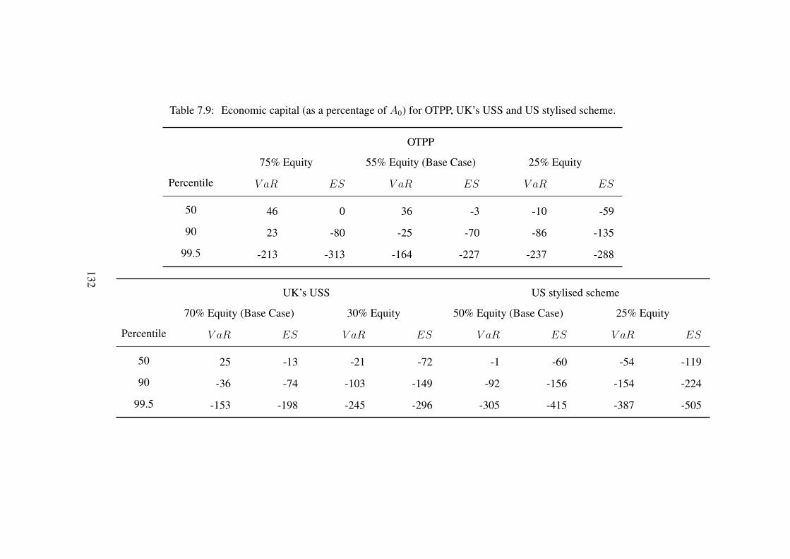
Table 7.9: Economic capital (as a percentage of A0) for OTPP, UK’s USS and US stylised scheme.
OTPP
75% Equity 55% Equity (Base Case) 25% Equity
Percentile V aR ES V aR ES V aR ES
50 46 0 36 -3 -10 -59
90 23 -80 -25 -70 -86 -135
99.5 -213 -313 -164 -227 -237 -288
UK’s USS US stylised scheme
70% Equity (Base Case) 30% Equity 50% Equity (Base Case) 25% Equity
Percentile V aR ES V aR ES V aR ES V aR ES
50 25 -13 -21 -72 -1 -60 -54 -119
90 -36 -74 -103 -149 -92 -156 -154 -224
99.5 -153 -198 -245 -296 -305 -415 -387 -505
132

−400 −300 −200 −100 0 100 200
0.00
00.
005
0.01
00.
015
0.02
0
Base Case
PVFP (as a % of A0)
Den
sity
Percentiles
50th90th99.5th
Figure 7.1: Distribution of the standardised PV FP (as a percentage of A0 =
$227.5bn) for the Base Case.
133
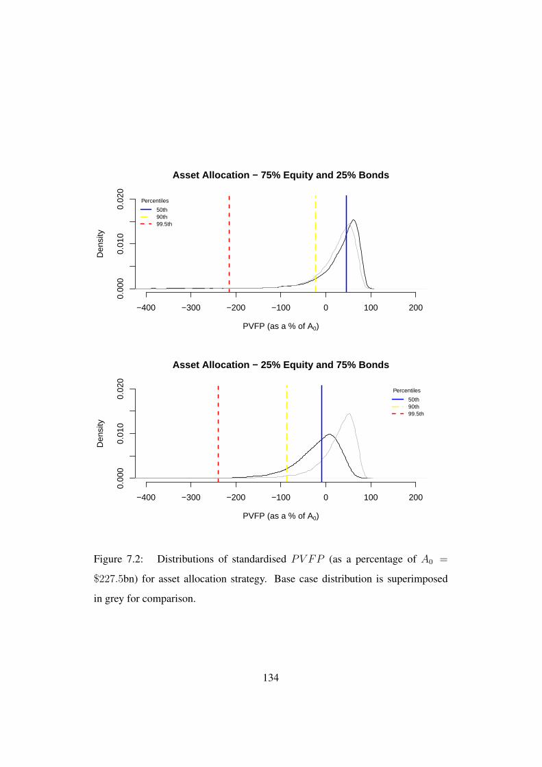
−400 −300 −200 −100 0 100 200
0.00
00.
010
0.02
0
Asset Allocation − 75% Equity and 25% Bonds
PVFP (as a % of A0)
Den
sity
Percentiles
50th90th99.5th
−400 −300 −200 −100 0 100 200
0.00
00.
010
0.02
0
Asset Allocation − 25% Equity and 75% Bonds
PVFP (as a % of A0)
Den
sity
Percentiles
50th90th99.5th
Figure 7.2: Distributions of standardised PV FP (as a percentage of A0 =
$227.5bn) for asset allocation strategy. Base case distribution is superimposed
in grey for comparison.
134
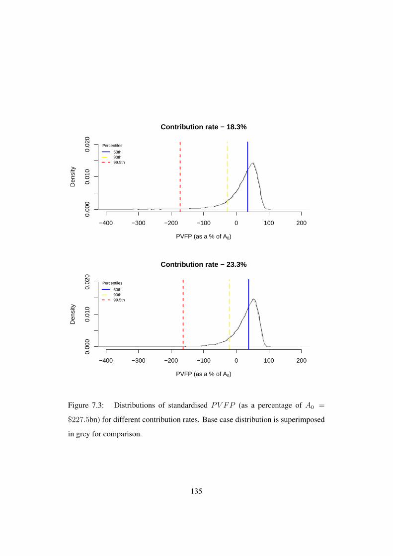
−400 −300 −200 −100 0 100 200
0.00
00.
010
0.02
0
Contribution rate − 18.3%
PVFP (as a % of A0)
Den
sity
Percentiles
50th90th99.5th
−400 −300 −200 −100 0 100 200
0.00
00.
010
0.02
0
Contribution rate − 23.3%
PVFP (as a % of A0)
Den
sity
Percentiles
50th90th99.5th
Figure 7.3: Distributions of standardised PV FP (as a percentage of A0 =
$227.5bn) for different contribution rates. Base case distribution is superimposed
in grey for comparison.
135

Chapter 8
Conclusions
8.1 Summary
In this thesis, we propose a flexible and transparent approach for quantifying the
risks of DB pension schemes for different countries. Our analysis focuses on
pension schemes in UK, US and Canada. Moreover, our analysis focuses on two
risks; economic and mortality risks.
To quantify the economic risks of DB schemes, we develop an ESG using
a graphical modelling approach. The ESG is transparent and flexible and can
be easily adapted for different countries. The graphical ESG was discussed in
Chapter 2.
To quantify the mortality risks, we use Model M7 from Cairns et al. (2009).
The model is adequate for our purpose as it takes into account three main drivers
of mortality namely the age effect, the period effect and the cohort effect. The
model also provides a good fit to data for UK, US and Canada. We discussed
model M7 along with other mortality models in Chapter 3.
In Chapter 4, we discussed the framework we use to quantify DB pension
schemes risks. The approach we use is a run-off approach. We use the graphical
136

ESG along with Model M7 to project forward future cashflows of a chosen DB
scheme and discount them back to obtain a present value. This gives a distribution
of PV FP which is the difference between the current level of assets and the
discounted value of the stochastic projected cashflows of the scheme. We then
use this framework to carry risk assessment of pension schemes in UK, US and
Canada which we discuss in Chapters 5, 6 and 7 respectively.
In Chapter 5, we carry out risk assessment of the UK’s USS. For example,
for the base case, the median of the PV FP distribution shows that the USS has
a surplus of 25% of the current value of assets, A0. In contrast, at the 99.5th
percentile, the USS has a deficit of 153% of A0. We also analyse the impact
of asset allocation on DB pension scheme risks. For example, by increasing the
bond allocation from 30% to 70%, we observe a median deficit of 21% of A0 and
a deficit of 245% of A0 at the 99.5th percentile. One might thus argue that bonds
are a poor match to the real liabilities of the USS. Finally, we analyse the impact
of contribution rates by increasing and decreasing the contribution rates by 2.5%
but the impact on the PV FP distribution proved to be very small.
In Chapter 6, we carry out risk assessment of a US stylised pension scheme.
The US stylised scheme is based on the UK’s USS. The membership profile and
the benefit structure are the same as the USS but adapted to be representative of
a US pension scheme. The two main changes are that the pension benefits are
not indexed to price inflation and there is no lump sum payment at retirement.
It is also assumed that there is a 20% deficit and this deficit is amortised over a
period of seven years. With an asset allocation of 75% equities and 25% bonds,
we observe a median surplus of 6% of A0 and a deficit of 343% at the 99.5th
percentile. In contrast, with an asset allocation of 25% equities and 75% bonds,
we observe a median deficit of 54% and a deficit of 387% at the 99.5th percentile.
Given the median and lower expected returns on bonds, the deficit at the 99.5th
137
percentile is not excessively large with a bond allocation of 75%. This is because
the liabilities are fixed for the case of the US stylised scheme and bonds offer a
good match for fixed liabilities.
Finally, in Chapter 7, we carry out risk assessment of the OTPP. Like the
UK’s USS, the liabilities for the OTPP are also real. The results for the OTPP
are therefore more consistent with the UK’s USS than the US stylised scheme.
With a 75% equity allocation, the OTPP has a larger median and also a larger
economic capital requirement at the 99.5th percentile compared to the base case
of the USS with a comparable equity allocation. The larger median is due to
the funding levels of the OTPP being higher than the USS. The larger economic
capital requirement is due to more volatile returns on Canadian equities compared
to UK equities. This was discussed in Chapter 2.
In summary, we propose a framework which accounts for economic and mor-
tality risks to quantify DB pension scheme risks. We hope that the framework and
the range of results presented in this thesis will help with discussions on measur-
ing and managing DB pension schemes across countries. Moreover, we hope that
the results can also assist on discussions regarding de-risking of pension schemes
and in particular, on discussions with asset allocation and asset-liability matching.
8.2 Future Research
In this section, we discuss possible avenues for extending this research.
• Many academics are currently looking at relationship between asset prices
and demographic factors such as old-age dependency ratio. In this respect,
our graphical model could be extended to include a demographic factor.
This would also allow us to quantify the impact of changing population
demographics on pension schemes.
138

• Our graphical model could also be extended for other asset classes such as
property, infrastructure, index-linked bonds amongst others. In this way,
one could replicate more realistic asset allocations of a DB pension scheme.
• We have only considered risk assessment of DB pension schemes for this
research. This research could be extended for other types of schemes such
as DC schemes or hybrid schemes, Pay-As-You-Go systems, Pension Pro-
tection Funds and social security systems.
• Our analysis is based on the USS’s and the OTPP’s membership profile.
These are large well established schemes. Analysis of smaller DB pension
schemes can produce very different results. The effect of a different mem-
bership distribution could be further investigated.
• We have not considered the impact of a dynamic investment strategy. This
venture could be explored to see how a dynamic investment strategy impacts
DB pension scheme risks.
• Moreover, one may also want to investigate the impact of using more so-
phisticated investment instruments such as longevity swaps and other hedg-
ing tools on DB pension schemes risks.
• Other ESGs and mortality models could be used to quantify DB pension
risks. This could bring more light on the underlying model risk.
• Our research could be extended to accomodate for more risks. In this re-
search, we have only quantified and accounted for the economic and mor-
tality risks. In reality, DB pension schemes are exposed to more risks such
as operational risks, liquidity risks and expense risks. Hence, our model
could be extended to allow for these additional risks.
139

Bibliography
AAS, K., NEEF, L.R., WILLIAMS, L. & RAABE, D. (2018). Interest rate model
comparisons for participating products under Solvency 2. Scandinavian Actu-
arial Journal, 3, 203–224.
ABOURASHCHI, N., CLACHER, I., FREEMAN, M.C., HILLIER, D., KEMP, M.
& ZHANG, Q. (2016). Pension plan solvency and extreme market movements:
a regime switching approach. The European Journal of Finance, 22(13),
1292–1319.
AI, J., BROCKETT, P. & JACOBSON, A. (2015). A new defined benefit pension
risk measurement methodology. Insurance: Mathematics and Economics, 63,
40–51.
ALONSO-GARCIA, J. & DEVOLDER, P. (2017). Liquidity and solvency in pay-
as-you-go defined contribution pension schemes: A continuous OLG sustain-
ability framework. CEPAR Working Paper 2017/12.
ANG, A & MADDALONI, A. (2003). Do demographic changes affect risk premi-
ums? Evidence from international data. Technical report, National Bureau of
Economic Research.
ARIK, A., YOLCU-OKUR, Y., SAHIN, S. & UGAR, O. (2018). Pricing pension
buy-outs under stochastic interest and mortality rates. Scandinavian Actuarial
Journal, 3, 173–190.
140

ARNOTT, R.D. & CHAVES, D.B. (2012). Demographic changes, financial mar-
kets, and the economy. Financial Analysts Journal, 61(1), 23–46.
ARO, H. (2014). Systematic and nonsystematic mortality risk in pension portfo-
lios. North American Journal, 18(1), 59–67.
AVANZI, B. & PURCAL, S. (2014). Annuitisation and cross-subsidies in a two-
tiered retirement saving system. Annals of Actuarial Science, 8(2), 234–252.
BAE, Y. (2010). Stock prices and demographic structure: A cointegration ap-
proach. Economics Letters, 107(3), 341–344.
BILLIG, A. & MENARD, J.C. (2013). Actuarial Balance Sheets as a tool to as-
sess the sustainability of social security pension systems. International Social
Security Association, 2, 31–52.
BLACKBURN, C., HANEWALD, K., OLIVIERA, A. & SHERRIS, M (2016). Longevity
Risk Management and Shareholder Value for a Life Annuity Business. ASTIN
Bulletin, 47(1), 43–77.
BLAKE, D., CAIRNS, A. J. G., DOWD, K & MACMINN, R. (2006). Longevity
Bonds: Financial Engineering, Valuation, and Hedging. Journal of Risk and
Insurance, 73, 647–672.
BOONEN, T.J. (2017). Solvency II capital requirement for life insurance compa-
nies based on expected shortfall. ASTIN Bulletin, 45(3), 703–728.
BOOTH, H., MAINDONALD, J. & SMITH, I. (2002a). Applying Lee-Carter under
conditions of variable mortality decline. Population Studies, 56, 325–336.
BOOTH, H., MAINDONALD, J. & SMITH, I. (2002b). Age-time interactions in
mortality projection: applying Lee-Carter to Australia. Working Papers in
Demography.
141

BOOTH, H., MAINDONALD, J. & SMITH, I. (2005). Evaluation of the variants of
the Lee-Carter method of forecasting mortality: a multi-country comparison.
New Zealand Population Review, 31, 13–34.
BROOKS, R. (2006). Demographic Change and Asset Prices. In Christopher
Kent, Anna Park, and Daniel Rees, editors. Demography and Financial Mar-
kets, RBA Annual Conference Volume. Reserve Bank of Australia, June 2006.
BUTT, A. (2012). Causes of defined benefit pension scheme funding ratio volatil-
ity and average contribution rates. Annals of Actuarial Science, 6(1), 76–102.
CAIRNS, A.J.G., BLAKE, D. & DOWD, K. (2006b). A two-factor model for
stochastic mortality with parameter uncertainty: theory and calibration. Jour-
nal of Risk and Insurance, 73, 687–718.
CAIRNS, A.J.G., BLAKE, D., DOWD, K., COUGHLAN, G.D., EPSTEIN, D. &
KHALAF-ALLAH, M. (2011). Mortality Density Forecasts: An analysis of six
stochastic mortality models. Insurance: Mathematics and Economics, 48(3),
355–367.
CAIRNS, A.J.G., BLAKE, D., DOWD, K., COUGHLAN, G.D., EPSTEIN, D.,
ONG, A. & BALEVICH, I. (2009). A quantitative comparison of stochastic
mortality models using data from England and Wales and the United States.
North American Actuarial Journal, 13, 1–35.
CHEN, A. & DELONG, L. (2015). Optimal investment for a defined-contribution
pension scheme under a regime switching model. ASTIN Bulletin, 45(2), 397–
419.
CHEN, D., BEETSMA, R.M.W.J., PONDS, E.H.M. & ROMP, W.E. (2016). In-
tergenerational risk-sharing through funded pensions and public debt. Journal
of Pension Economics & Finance, 15(2), 127–159.
142

CHEN, Z., PELSSER, A. & PONDS, E. (2014). Evaluating the UK and Dutch
defined-benefit pension policies using the holistic balance sheet framework.
Insurance: Mathematics and Economics, 58, 89–102.
CONTINUOUS MORTALITY INVESTIGATION SAPS MORTALITY COMMITTEE
(2009). Working Paper 35 - The graduations of the CMI self-administered
pension schemes 2000-2006 mortality experience - Final “S1" series of mor-
tality tables.
COSTA, D.L. (2005). Causes of improving health and longevity at older ages: a
review of the explanations. Genus, 1, 21–38.
COUGHLAN, G. (2015). Longevity - It’s Academic.
COX, S.H., LIN, Y., TIAN, RUILIN. & YU JIFENG (2013). Managing Capital
Market and Longevity Risks in a Defined Benefit Pension Plan. The Journal
of Risk and Insurance, 80(3), 585–619.
COX, S.H., LIN, Y. & TIANXIANG, SHI. (2018). Pension risk management
with funding and buyout options. Insurance: Mathematics and Economics,
78, 183–200.
DAVIS, E.P. & LI, C. (2003). Demographics and financial asset prices in the ma-
jor industrial economies. Brunel University, Economics and Finance Working
papers.
DE ROSA, C., LUCIANO, E. & REGIS, L. (2017). Basis risk in static versus
dynamic longevity-risk hedging. Scandinavian Actuarial Journal, 4, 343–
365.
DEVOLDER, P. & LEBEGUE, A. (2016). Risk measures versus ruin theory for
the calculation of solvency capital for long-term life insurances. Dependence
Modelling, 4(1), 306–327.
143

DEVOLDER, P. & LEBEGUE, A. (2017). Iterated VaR or CTE measures: A false
good idea?. Scandinavian Actuarial Journal, 4, 287–318.
DEVOLDER, P., & MELIS, R. (2014). Optimal mix between pay as you go and
funding for pension liabilities in a stochastic framework. ASTIN Bulletin,
45(3), 551–575.
DEVOLDER, P. & PISCOPO, G. (2014). Solvency analysis of defined benefit pen-
sion schemes, Springer. 141–150.
DEVOLDER, P. & TASSA, H. (2016). Solvency measurement for defined benefits
pension schemes. Institut de Statistique, Biostatistique et Sciences Actuar-
ielles - Discussion paper.
DRTON, M. & PERLMAN, M.D. (2007). Multiple testing and error control in
Gaussian graphical model selection. Statistical Science, 22(3), 430–449.
DRTON, M. & PERLMAN, M.D. (2008). A SINful approach to Gaussian graphi-
cal model selection. Journal of Statistical Planning and Inference, 138, 1179–
1200.
DUARTE, T.B., VALLADAO, D.M. & VEIGA, A. (2017). Asset liability man-
agement for open pension schemes using multistagestochastic programming
under Solvency-II-based regulatory constraint. Insurance: Mathematics and
Economics, 77, 177–188.
EDWARDS, D (2012). Introduction to Graphical Modelling. New York: Springer
Science & Business Media.
FAVERO, C.A., GOZLUKLU, A.E. & YANG, H. (2016). Demographics and the
behavior of interest rates. IMF Economic Review, 64(4), 732–776.
144

FERRER-FERNANDEZ, M. & BOADO-PENAS, M.C. (2017). Automatic Balanc-
ing Mechanism in Pay-As-You-Go pension systems: A solution to face de-
mographic risk and restores sustainability?. Anales del Instituto de Actuarios
Espanoles, 4(23), 145–167.
FUHRER, J. & MOORE, G. (1995). Inflation Persistence. The Quarterly Journal
of Economics, 110(1), 127–159.
GODINEZ-OLIVARES, H., BOADO-PENAS, M.C. & HABERMAN, S. (2016).
Optimal strategies for Pay-As-You-Go pension finance: A sustainability frame-
work. Insurance: Mathematics and Economics, 69, 117–126.
GOECKE, O. (2013). Pension Saving schemes with return smoothing mechanism.
Insurance: Mathematics and Economics, 53, 678–689.
GUAN, G. & LIANG, Z. (2014). Optimal management of DC pension plan in a
stochastic interest rate and stochastic volatility framework. Insurance: Math-
ematics and Economics, 57, 58–66.
HAINAUT, D. & DEVOLDER, P. (2006). Life annuitization: why and how much?.
North American Actuarial Journal, 16(4), 449–461.
HE, L. & LIANG, Z. (2015). Optimal assets allocation and benefit outgo policies
of DC pension plan with compulsory conversion claims. Insurance: Mathe-
matics and Economics, 61, 227–234.
HOJSGAARD, S., EDWARDS, D. & LAURITZEN, S. (2012). Graphical Models
with R. New York: Springer Science & Business Media.
HUYNH, W. & MALLIK, G. & HETTIHEWA, S. (2006). The impact of macroe-
conomic variables, demographic structure and compulsory superannuation on
share prices: the case of Australia. Journal of International Business Studies,,
37(5), 687–698.
145
KARABEY, U ., KLEINOW, T. & CAIRNS, A.J.C. (2014). Factor risk quantifica-
tion in annuity models. Insurance: Mathematics and Economics, 58, 34–45.
KWASI, A. (1988). Price Inflation and Wage Inflation: A Cause-Effect Ralation-
ship?. Economics Letters, 27, 35–40.
KEMP, M.H.D. & PATEL, C.C. (2012). Entity-wide risk management for pen-
sion funds. British Actuarial Journal, 17(2), 331–394.
KHORASANEE, Z.M. (2013). Risk-sharing and benefit smoothing in a hybrid
pension plan. ASTIN Bulletin, 41(1), 61–86.
KLEINOW, T. (2011). Pension fund management and conditional indexation.
ASTIN Bulletin, 41(1), 61–86.
KLING, A., RUB, J. & SCHILLING, K. (2014). Risk analysis of annuity con-
version options in a stochastic mortality environment. ASTIN Bulletin, 44(2),
197–236.
KURTBEGU, E. (2018). Replicating intergenerational longevity risk sharing in
collective defined contribution pension plans using financial markets. Insur-
ance: Mathematics and Economics, 78, 286–300.
KUSHNER, H.J. & DUPUIS, P.G. (2001). Numerical methods for stochastic con-
trol problems in continuous time. Springer Verlag. Second edition.
LEE, R.D. & CARTER, L.R. (1992). Modelling and Forecasting U.S. Mortality.
Journal of the American Statistical Association, 87(419), 659–671.
LEMOINE, K. (2015). Mortality regimes and longevity risk in a life annuity port-
folio. Scandinavian Actuarial Journal, 8, 689–724.
LI, H. (2018). Dynamic hedging of longevity risk: The effect of trading fre-
quency. ASTIN Bulletin, 48(1), 197–232.
146

LI, J. & HABERMAN, S. (2015). On the effectiveness of natural hedging for
insurance companies and pension plans. Insurance: Mathematics and Eco-
nomics, 61, 286–297.
LIANG, Z. & MA, M. (2015). Optimal dynamic allocation of pension fund
in mortality and salary risks framework. Insurance: Mathematics and Eco-
nomics, 64, 151–161.
LIN, Y. COX, S.H. (2008). Securitization of Catastrophe Mortality Risks. Insur-
ance: Mathematics and Economics, 42, 628–637.
LIN, Y., MACMINN, R.D. & TIAN, R. (2015). De-risking defined benefit plans.
Insurance: Mathematics and Economics, 63, 52–65.
LIN, Y., MACMINN, R.D., TIAN, R. & YU, J. (2017). Pension risk management
in the enterpriserisk management framework. Insurance: Mathematics and
Economics, 63, 52–65.
LIN, Y., TAN, K.S., TIAN, R. & YU, J. (2014). Downside risk management of
a defined benefit plan considering longevity basis risk. Journal of Risk and
Insurance, 84(S1), 345–366.
LINNEMANN, P., BRUHN, K. & STEFFENSEN, M. (2014). A comparison of
modern investment-linked pension savings products. Annals of Actuarial Sci-
ence, 9(1), 72–84.
LIU, X. (2013). Annuity uncertainty with stochastic mortality and interest rates.
North American Actuarial Journal, 17(2), 136–152.
MANKIW, N.G. & WEIL, D.N. (1989). The baby boom, the baby bust, and the
housing market. Regional science and urban economics, 19(2), 235–258.
MCNEIL, A., FREY, R. & EMBRECHTS, P. (2005). Quantitative Risk Man-
agement: Concepts, Techniques, Tools Revised Edition. Princeton University
Press, Priceton.
147

MCNOWN, R. & ROGERS, A. (1989). Forecasting Mortality: A Parameterized
Time Series Approach. Demography, 26(4), 645–660.
MODIGLIANI, F. & BRUMBERG, R.H. (1954). Utility analysis and the consump-
tion function: An interpretation of cross-section data. New Brunswick.
OBEROI, J., PITTEA, A. & TAPADAR, P. (2018). A graphical modelling ap-
proach to simulating economic variables over long horizons. Annals of Actu-
arial Science. (In press).
GOVERNMENT OFFICE FOR SCIENCE (2016). Future of Ageing Population.
ONTARIO TEACHERS’ PENSION PLAN (2017). 2017 Annual Report.
ONTARIO TEACHERS’ PENSION PLAN (2018). Report on the Actuarial Valuation
for Funding Purposes as at January 1, 2018.
PARK, C. (2010). How does changing age distribution impact stock prices?
A nonparametric approach. Journal of Applied Econometrics, 25(7), 1155–
1178.
PLATANAKIS, E. & SUTCLIFFE, C. (2016). Pension scheme redesign and wealth
redistribution between the members and sponsor: The USS rule change in
October 2011. Insurance: Mathematics and Economics, 69, 14–28.
PORTEOUS, B.T. & TAPADAR, P. (2005). Economic Capital and Financial Risk
Management for Financial Services Firms and Conglomerates. Basingstoke:
Palgrave MacMillan.
PORTEOUS, B.P. & TAPADAR, P. (2008a). Asset allocation to optimise life in-
surance annuity firm economic capital and risk adjusted performance. Journal
of Pension Economics and Finance, 3, 187–214.
PORTEOUS, B.P., TAPADAR, P. & YANG, W. (2012). Economic capital for de-
fined benefit pension schemes: An application to the UK Universities Superan-
nuation Scheme. Journal of Pension Economics and Finance, 11(4), 471–499.
148

RENSHAW, A.E. & HABERMAN, S. (2006). A cohort-based extension to the
Lee-Carter model for mortality reduction factors. Insurance: Mathematics
and Economics, 38, 556–570.
RETROSPECTIVE ON SOLVENCY II WORKING PARTY (2017). A Review of
Solvency II - has it met its objectives.
ROY, A., PUNHANI, S. & SHI, L. (2012). How demographics affect asset prices
global demographics and pensions. Credit Suisse.
SLIPSAGER, S.K. (2018). The real risk in pension forecasting. Scandinavian
Actuarial Journal, 3, 250–273.
SWEETING, P. (2008). Stochastic mortality made easy. London: Staple Inn Actu-
arial Society. The Pension Protection Fund and the Pensions Regulator. The
Purple Book 2008.
SWEETING, P., CHRISTIE, A. & GLADWYN, E. (2015). The missing link: eco-
nomic exposure and pension plan risk. Annals of Actuarial Science, 9(2),
290–303.
SWEETING, P. (2017). The cost and value of defined benefit pension schemes and
the implications for defined contribution pension provision. Pensions Institute.
TROTTIER, D.A., GODIN, F. & HAMEL, E. (2018). Local hedging of variable
annuities in the presence of basis risk. ASTIN Bulletin, 48(2), 611–646.
USS (2014). Report & Accounts for the year ended 31 March 2014.
USS (2015). Scheme Funding Report of the Actuarial Valuation as at 31 March
2014.
WANG, S., LU., YI & SANDERS, B. (2018). Optimal investment strategies
and intergenerational risk sharing for target benefit pension plans. Insurance:
Mathematics and Economics, 80, 1–14.
149

WILKIE A.D. (1986). A stochastic investment model for Actuarial Use. Trans-
actions of the Faculty of Actuaries, 39, 341–403.
WILKIE A.D. (1995). More on a Stochastic Asset Model for Actuarial Use.
British Actuarial Journal, 1(5), 777–964.
WILKIE A.D. & SAHIN, S. (2015). Yet More on a Stochastic Economic Model:
Part 2 - Initial Conditions, Select Periods and Neutralising Parameters. Annals
of Actuarial Science, 10(1), 1–51.
WILKIE A.D. & SAHIN, S. (2016a). Yet More on a Stochastic Economic Model:
Part 3A - Stochastic Interpolation: Brownian and Ornstein-Uhlenbeck (OU)
Bridges. Annals of Actuarial Science, 11(1), 74–99.
WILKIE A.D. & SAHIN, S. (2016b). Yet More on a Stochastic Economic Model:
Part 3B - Stochastic Bridging for Retail Prices and Wages. Annals of Actuarial
Science, 11(1), 100–127.
WILKIE A.D. & SAHIN, S. (2016c). Yet More on a Stochastic Economic Model:
Part 3C - Stochastic Bridging for Share Yields and Dividends and Interest
Rates. Annals of Actuarial Science, 11(1), 128–163.
WILKIE A.D. & SAHIN, S. (2017). Yet More on a Stochastic Economic Model:
Part 4 - A Model for Share Earnings, Dividends, and Prices. Annals of Actu-
arial Science, 12(1), 67–105.
WILKIE A.D., SAHIN, S., CAIRNS, A.J.G. & KLEINOW, T. (2011). Yet More
on a Stochastic Economic Model: Part 1: Updating and Refitting, 1995 to
2009. Annals of Actuarial Science, 5(1), 53–99.
WHITEHOUSE, E., (2009). Pension during the Crisis: Impact on the Retirement-
Income Systems and Policy Responses. The Geneva Papers on Risk and In-
surance - Issues and Practice, 34(4), 536–547.
150

WORLD BANK (1994). Averting the Old Age Crisis: Policies to Protect the Old
and Promote Growth. The World Bank, Washington, D.C..
YANG, W. & TAPADAR, P. (2014). Role of the Pension Protection Fund in fi-
nancial risk management of UK defined benefit pension sector: a multi-period
economic capital study. Annals of Actuarial Science, 9(1), 134–166.
YAO, H., YANG, Z. & CHEN, P. (2013). Markowitz’s mean-variance defined
contribution pension fund management under inflation: A continuous-time
model. Insurance: Mathematics and Economics, 53, 851–863.
VENTURA-MARCO, M. & VIDAL-MELIA, C. (2014). An Actuarial Balance
Sheet Model for Defined-Benefit pay-as-you-go Pension Systems with dis-
ability and retirement contingencies. ASTIN Bulletin, 53, 851–863.
ZHANG, S., HARDY, S. & SAUNDERS, D. (2018). Updating Wilkie’s Economic
Scenario Generator for U.S. Applications. North American Actuarial Journal,
22(4), 600–622.
ZHU, X., HARDY, M. & SAUNDERS, D. (2018). Dynamic hedging strategies for
cash balance pension plans. ASTIN Bulletin, 48(3), 1–31.
151

Appendix A
Literature Review
This Appendix provides a continuation of the literature review provided in Section
1.2 on measuring and managing pension risks. The review is divided in three
sections. In Section A.1, we look at papers which deal with risk assessment of
pension plans. In Section A.2, we look at papers which focus on managing the
sponsor’s risks. In Section A.3, we look at papers which focus on managing the
scheme members’ risks.
A.1 Measuring Pension Risks
Kemp and Patel (2012) explore the application of Enterprise Risk Management
(ERM) style techniques to pension funds. The paper argues that ERM is as ap-
propriate to pension funds as it is to other types of entities such as insurance
companies. According to the authors, the reason for encouraging pension funds
and their sponsors to be more rigorous in their adoption of ERM techniques is the
fact that the entities do not exist in isolation.
Ventura-Marco and Vidal-Melia (2014) present an Actuarial Balance Sheet for
DB pay-as-you-go pension systems with disability and retirement contingencies.
152

The authors develop a theoretical base for applying a Swedish-type Actuarial Bal-
ance Sheet and use the principles of double-entry to show any actuarial imbalance
in the pension system. The authors suggest that the model they propose makes it
possible to assess the degree of solvency from the integrated perspective of both
retirement and disability contingencies.
Butt (2012) uses stochastic economic and demographic variables to simulate
assets and liabilities of a pension scheme over a 30 year horizon. He compares
the relative significance of the factors driving the funding risk of the scheme,
defined as the risk that the funding ratio of the scheme is less than 1. Demographic
factors such as mortality rates and withdrawal rates do not significantly affect
funding risk. Investment factors account for most of the risk. The paper assumes
a pension scheme of deferred annuities. Economic and demographic variables are
parameterised using Australian data. Assets and liabilities are then simulated over
30 years. During the first year, movements in discount rates accounted for 46.4%
of the funding risk while movements in investment returns accounted for 33.3%
of the risk. Movements in mortality rates or withdrawal rates however accounted
for less than 1% of the risk.
Liu (2013) investigates the impact of the two systematic risk factors, the mor-
tality risk and the interest rate risk on the distribution of the annuity rate. The
Lee-Carter and the Cairns-Blake-Dowd models are used to model mortality risk,
and the one and two-factor Cox-Ingersoll-Ross models are used to model interest
risk. Liu (2013) shows that the distribution of the annuity rate is more sensitive
to the long-term mean-reverting rate parameter of the interest rate model than to
other parameters. For example, if the mean-reverting parameter is increased by
40% from the benchmark value, the 95% VaR decreases by 18.42%. In contrast,
if the drift parameter of the Lee-Carter model is decreased by 40%, the 95% VaR
only decreases by 4.7%. The author suggests that it is critical to adopt a suitable
153

interest model in pricing and reserving for annuity-related products.
Karabey et al. (2014) estimate the contribution of different risks to the total
risk in an annuity portfolio. The risks considered are investment risk, mortality
risk and the co-movement risk. They compare the risk contributions for a 25 and
45-year annuity and observe that investment risk is dominant. For example, using
variance decomposition approximations, 89% and 63.5% of the total risk results
from the investment risk for a 25 and 45-year annuity respectively.
Sweeting (2017) explains how investment risk can translate into increased fi-
nancial burden to a sponsor. He compares the cost of employing an individual on
a DB scheme compared to a DC scheme in the UK. Between 1996 to 2016, the
annual average DB total cost has been around 1.0% of earnings higher compared
to DC. As a result, having employees accruing benefits under DB schemes has
resulted in a growing financial burden for firms in this position. This increase in
financial burden is explained by a low growth and low interest environment.
De Rosa et al. (2017) consider the impact of basis risk. They compare static
and dynamic longevity-risk hedging with and without basis risk. Basis risk is
defined as the co-movement between the portfolio and the reference population’s
longevity. They compare a static swap-based hedge for an annuity to a dynamic
Delta-Gamma-Theta based hedge. They calibrate their model on a UK individual
aged 65. When basis risk is ignored, the mean hedging error over a 30 year horizon
is similar under both strategies. With basis risk however, the mean hedging risk is
approximately 88% higher under a static hedging strategy.
Trottier et al. (2018) also highlight the importance of basis risk for pension
schemes. Basis risk here is defined as the imperfect correlation of returns from
the pension fund and returns from futures used to hedge the financial risks. They
compare the riskiness associated with a variable annuity policy with and without
basis risk. A key observation stemming from the paper is that the omission of
154

basis risk leads to severe risk under-estimation. For example, using a minimal
variance investment strategy, the capital requirement is 215% higher if basis risk
is allowed for.
Given that economic risks contribute significantly to pension risks, we look at
some literatures which focus on comparing different economic scenario genera-
tors and their impact on pension risk quantification.
Devolder and Tassa (2016) use ruin theory to quantify the risks of a DB
scheme. They compare the probability of ruin and solvency capital using a simple
Brownian motion and a variance gamma process. To illustrate the differences,
they assume a DB scheme with a single lump sum payment at retirement linked to
the final salary of the member. They note that a variance gamma process requires
more capital than a simple geometric Brownian motion. For example, for a 5-year
horizon, using a simple Brownian motion as the economic scenario generator, the
solvency capital is around 30% of liabilities, but using a variance gamma process,
the solvency capital is around 35% of liabilities. This difference arises because
the variance gamma process takes into account the risks related to sudden crashes
of financial markets.
Abourashchi et al. (2016) quantify the funding risk of a DB scheme defined
as the probability that liabilities are greater than assets. They argue that a simple
lognormal process does not sufficiently capture the fat-tailed properties of asset
returns. Moreover, a lognormal process does not allow for time-varying asset re-
turn variances. The process therefore underestimates extreme market movements
and the true spread of portfolio values. To address this problem, they examine
multivariate Markov regime switching models. The Markov regime switching
processes assume an economy where multiple states exist (e.g. low asset return
state, bull state, low volatility state, crash state) and where transition between the
states is possible. Transition probabilities can be interpreted as the proportion of
155

time the economy spends in each state. The funding risk of a DB scheme for a
single state model is compared to a 4-state Markov regime switching model. Over
a 12-year time horizon, the funding risk increases between 2.5% to 4.5% using
the 4-state model compared to the single state model.
Aas et al. (2018) investigate whether the choice of the interest rate model
has an impact on the valuation of the best estimate of pension liabilities. The
interest rate models compared are the CIR++ model, the G2++ model and the
LIBOR Market model. They observe that for low and medium durations, the
interest rate models produce similar results for the best estimate of liabilities. For
long durations however, the differences in the best estimate can be quite large. The
differences are due to different long-term interest rate distributions generated from
the 3 models. They recommend the use of the G2++-model, which represents a
good trade-off between accuracy and complexity.
Slipsager (2018) analyses the effect of having a stochastic view on inflation
compared to the deterministic view often favoured by regulators. The paper as-
sumes an individual who contributes an amount of $50,000 as a lump sum and
the fund accumulates for 35 years when the individual retires. The author then
estimates the real value of the portfolio at retirement. Deterministic inflation is
prone to producing heavily over-optimistic forecasts and the expected real port-
folio value is thus overstated. Moreover, the deterministic inflation framework
ignores correlation between portfolio returns and consumer price levels and this
may lead to an excessively heavy-tailed distribution. For example, assuming the
fund invests 60% in equity and 40% in bonds, the mean real portfolio value at
retirement is $387,421 using stochastic inflation compared to $427,240 using de-
terministic inflation. The interquartile range is $328,950 using stochastic inflation
and $377,859 using deterministic inflation.
Finally, we look at literatures which compare mortality models and the impact
156

on pension risks. Lemoine (2015) explores the existence of regimes in mortality
evolution and measure their implications for a portfolio of life annuities by cap-
turing the distribution of the mortality time index with a regime-switching model
within a Poisson log-bilinear framework. The author applies regime-switching
models to French mortality data from 1947 to 2007 within a Poisson Lee-Carter
framework. The author finds that French mortality is characterised by two persis-
tent and distinct regimes over the period 1947-2007. The first regime refers to a
strong uncertainty state, which corresponds to the longevity conditions observed
during the two decades following World War II. The second state relates to the
low volatility of longevity improvements observed during the last 30 years. The
author then investigates the implications of mortality regimes for a portfolio of
life annuities and finds that the risks of the life annuity portfolio as well as the
capital requirements are affected by regime switching in the mortality evolution.
The author then discusses the potential costs for a life annuity portfolio by ignor-
ing the changes of trends. For example, if the first regime is active again, a single
state mortality model would under-estimate the probability of ruin by 0.9% for
men and by 1.4% for women.
Arik et al. (2018) examine the pricing of pension buy-outs under dependence
between interest and mortality rate risks with an explicit correlation structure in a
continuous time framework. Stochastic interest rates are modelled using the Va-
sicek and the Cox-Ingersoll-Ross models and stochastic mortality rates are mod-
elled using the Lee-Carter model and Ornstein-Uhlenbeck process. They note that
changing the correlation coefficient between interest rate risk and mortality risk
does not significantly affect the pension buy-out price. However, they highlight
that the choice of the mortality model is essential for pricing of the buy-out deal
and note that the price of the buy-out is 60% higher using the Lee-Carter model
instead of the Ornstein-Uhlenbeck process.
157

A.2 Managing Sponsor’s Risks
In this Section, we look at papers that focus on risks from the sponsor’s point of
view. We start with papers which discuss ways a sponsor can hedge or transfer
pension risks to another party.
Kling et al. (2014) compare two types of financial guarantees; the guaranteed
annuity options and the guaranteed minimum income benefits. For guaranteed
annuity options, the insurer guarantees to convert the funds at a pre-specified rate;
while the guaranteed minimum income benefit guarantees a fixed minimum an-
nuity. Economic scenario generators and stochastic mortality models are used to
compare the risks on the two guarantees and consider a single life aged 50 who
pays a single premium at inception and retires at the age of 65. The 99.5% VaR is
estimated at 1.5% of the premium paid for the guaranteed annuity option and 60%
of the premium paid for the guaranteed minimum income. The risk on guaranteed
minimum income can however be reduced to 14% of the premium by hedging the
financial risks.
Lin et al. (2015) examine 3 hedging strategies: longevity hedge, pension buy-
in and pension buyout and compare them in terms of their hedging costs. They
assume a pension scheme that consists of a retired cohort and which invests in the
SP 500 index, the Merrill Lynch corporate bond index and the 3-month Treasury
bill. Numerical examples from the paper show that if counterparty risk is low, it is
desirable to implement a longevity hedge or a buy-in strategy. When counterparty
risk is high however, a buy-in strategy is more sensitive to counterparty risk than
the longevity hedge as more assets are tied to the buy-in.
Li and Haberman (2015) examine the effectiveness of natural hedging between
annuity and life products. Natural hedging exploits the opposite movements in
the values of annuities and life insurances when mortality changes. The authors
assume a constant investment return of 3% and consider two products; a whole-
158
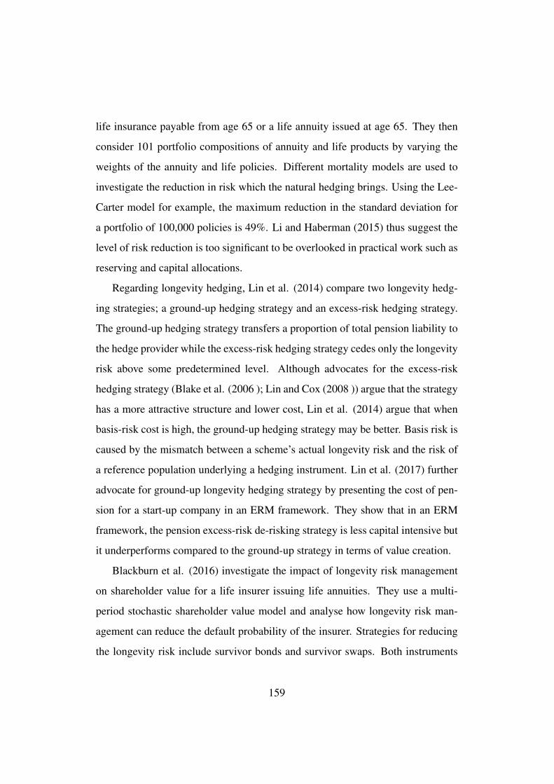
life insurance payable from age 65 or a life annuity issued at age 65. They then
consider 101 portfolio compositions of annuity and life products by varying the
weights of the annuity and life policies. Different mortality models are used to
investigate the reduction in risk which the natural hedging brings. Using the Lee-
Carter model for example, the maximum reduction in the standard deviation for
a portfolio of 100,000 policies is 49%. Li and Haberman (2015) thus suggest the
level of risk reduction is too significant to be overlooked in practical work such as
reserving and capital allocations.
Regarding longevity hedging, Lin et al. (2014) compare two longevity hedg-
ing strategies; a ground-up hedging strategy and an excess-risk hedging strategy.
The ground-up hedging strategy transfers a proportion of total pension liability to
the hedge provider while the excess-risk hedging strategy cedes only the longevity
risk above some predetermined level. Although advocates for the excess-risk
hedging strategy (Blake et al. (2006 ); Lin and Cox (2008 )) argue that the strategy
has a more attractive structure and lower cost, Lin et al. (2014) argue that when
basis-risk cost is high, the ground-up hedging strategy may be better. Basis risk is
caused by the mismatch between a scheme’s actual longevity risk and the risk of
a reference population underlying a hedging instrument. Lin et al. (2017) further
advocate for ground-up longevity hedging strategy by presenting the cost of pen-
sion for a start-up company in an ERM framework. They show that in an ERM
framework, the pension excess-risk de-risking strategy is less capital intensive but
it underperforms compared to the ground-up strategy in terms of value creation.
Blackburn et al. (2016) investigate the impact of longevity risk management
on shareholder value for a life insurer issuing life annuities. They use a multi-
period stochastic shareholder value model and analyse how longevity risk man-
agement can reduce the default probability of the insurer. Strategies for reducing
the longevity risk include survivor bonds and survivor swaps. Both instruments
159
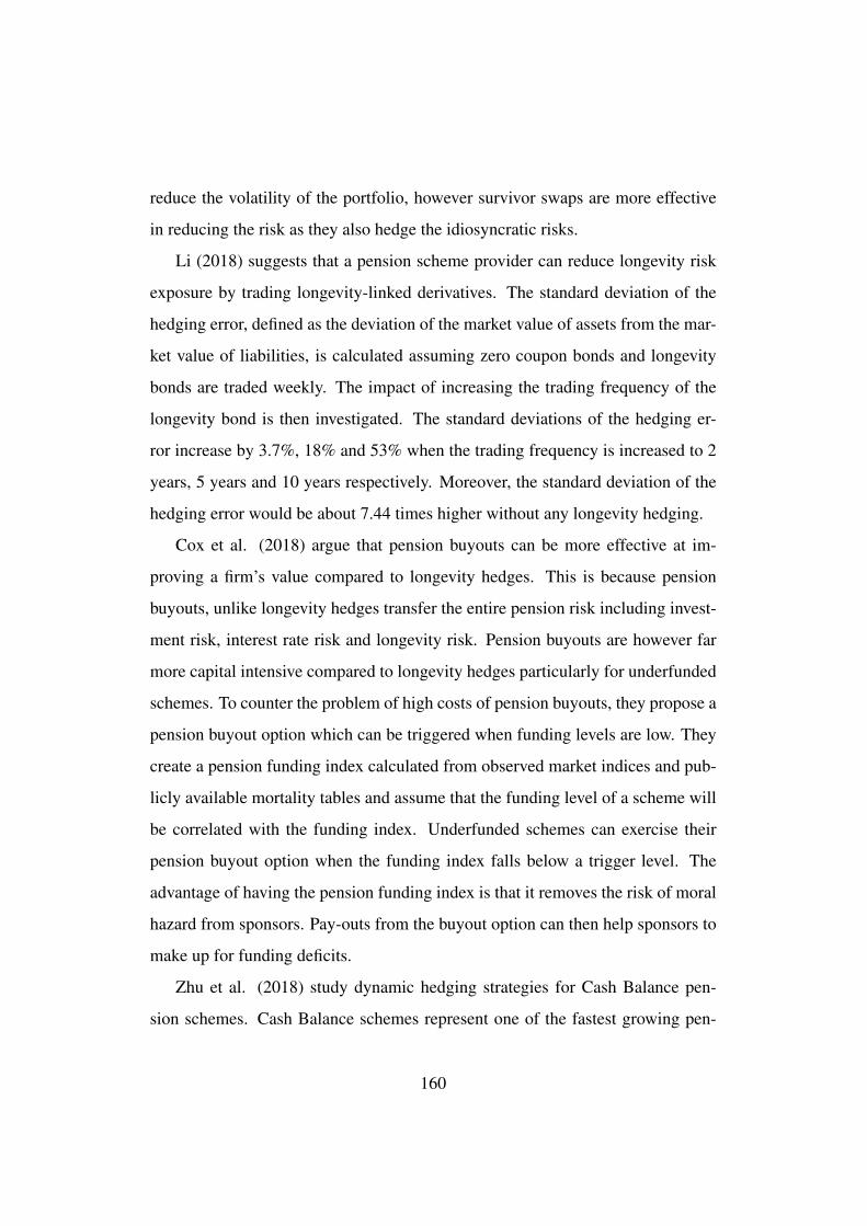
reduce the volatility of the portfolio, however survivor swaps are more effective
in reducing the risk as they also hedge the idiosyncratic risks.
Li (2018) suggests that a pension scheme provider can reduce longevity risk
exposure by trading longevity-linked derivatives. The standard deviation of the
hedging error, defined as the deviation of the market value of assets from the mar-
ket value of liabilities, is calculated assuming zero coupon bonds and longevity
bonds are traded weekly. The impact of increasing the trading frequency of the
longevity bond is then investigated. The standard deviations of the hedging er-
ror increase by 3.7%, 18% and 53% when the trading frequency is increased to 2
years, 5 years and 10 years respectively. Moreover, the standard deviation of the
hedging error would be about 7.44 times higher without any longevity hedging.
Cox et al. (2018) argue that pension buyouts can be more effective at im-
proving a firm’s value compared to longevity hedges. This is because pension
buyouts, unlike longevity hedges transfer the entire pension risk including invest-
ment risk, interest rate risk and longevity risk. Pension buyouts are however far
more capital intensive compared to longevity hedges particularly for underfunded
schemes. To counter the problem of high costs of pension buyouts, they propose a
pension buyout option which can be triggered when funding levels are low. They
create a pension funding index calculated from observed market indices and pub-
licly available mortality tables and assume that the funding level of a scheme will
be correlated with the funding index. Underfunded schemes can exercise their
pension buyout option when the funding index falls below a trigger level. The
advantage of having the pension funding index is that it removes the risk of moral
hazard from sponsors. Pay-outs from the buyout option can then help sponsors to
make up for funding deficits.
Zhu et al. (2018) study dynamic hedging strategies for Cash Balance pen-
sion schemes. Cash Balance schemes represent one of the fastest growing pen-
160

sion scheme designs in the United States and are classified and regulated as DB
schemes. Cash Balance schemes are however hybrid schemes and work as fol-
lows: if the actual investment return earned in a particular year is less than the
minimum guaranteed level, the employer will make further contributions to top
up each member’s fund to the minimum guaranteed level; if the achieved invest-
ment returns are higher than the minimum guaranteed level, the employer may
hold back some, or all, of the excess from individual members’ funds and then
use this amount to top funds up in future years, when the minimum guaranteed
investment return is not achieved. This structure means that it is the employer,
and not the members, who is exposed to the scheme’s investment risk during the
period up to retirement. Zhu and al. (2018) argue that the persistent low interest
environment means that hedging the cash balance liability has become an urgent
question for employers. By comparing a delta hedging strategy to a more tradi-
tional investment strategy, defined as 60% equity and 40% bonds, they show that
over a 10-year horizon, the hedged portfolio targets the terminal liability, while
the unhedged portfolio may end up being vastly over or underfunded.
Other authors have looked at how the sponsor’s risks can be managed based
on how the scheme is structured. Kleinow (2011) discusses Conditional Index-
ing schemes as a way to reduce pension scheme risks in the UK. Conditional
Indexing schemes are similar to DB schemes. The difference between DB and
Conditional Indexing schemes is that the increase in guaranteed pension benefits
is conditional on the availability of sufficient funds. To illustrate the benefits of
Conditional Indexing schemes, the author assumes a scheme where workers make
a single contribution now and are entitled to receive a lump-sum pension payment
at retirement. The available assets are a bank account and a zero-coupon bond
maturing at the time of retirement. From the author’s calculations, a worker earns
an average return on the contribution of 4.71% per annum and the corresponding
161

mean hedging error of the scheme is -1.17%, defined as the percentage differ-
ence between the scheme’s assets and liabilities. Given that the hedging error is
small, the scheme is almost self-financing. He concludes that Conditional Index-
ing schemes represent a possible solution for dealing with funding risks of DB
schemes.
Aro (2014) examines risk pooling in a pension scheme consisting of female
members aged 65. Using a Solvency 2 framework, the author investigates how
the required capital per person changes as the number of members in the scheme
increases. The capital requirement per person decreases exponentially per person
showing that the impact of risk pooling is strong.
Platanakisa and Sutcliffe (2016) discuss the impact of the redesign of the USS
in October 2011. The USS has been subject to several changes in 2011 includ-
ing higher contribution rates and less generous indexation of benefits. The rule
change will result in a transfer of wealth of around £32.5 billion from members
to the sponsor during the period 2011 to 2065. This has effectively resulted in a
substantial pay cut for future pensioners. It is estimated that for future members
of the USS, pension wealth has reduced by 65% while for the sponsor, pension
costs have reduced by 26%.
Some authors use optimisation techniques in order to see the extent to which
the sponsor’s risk can be reduced. Cox et al. (2013) propose a model to identify
the optimal contribution, asset allocation and longevity risk hedging strategies that
minimise total funding risk for a DB scheme throughout the life of a single pension
cohort. Given a target expected total pension cost constraint and a Conditional
VaR constraint on unfunded liability, the scheme’s total funding variation across
all years before and after retirement until the death of the last pension participant
is minimised. As pensioners live longer, the scheme has to make a higher normal
contribution, invest more in the low-risk asset, and pay a much higher expected
162

total pension cost.
Sweeting et al. (2015) provide a methodology for minimising a DB scheme
portfolio’s losses in the event of a fall in value of the sponsor. The paper suggests
that a sponsor’s financial health may be positively linked to the return on assets
backing its pension scheme. They use the example of an oil company for which
the pension scheme’s assets are exposed to energy and industrial risks. They de-
fine the cross conditional VaR 95 as the average return of sponsor’s portfolio in
the worst 5% of years for oil prices and show that through better diversification
of the pension scheme’s assets, the cross conditional VaR 95 can be increased by
changing the underlying portfolio of the DB scheme.
Liang and Ma (2015) compare an optimal dynamic asset allocation of a pen-
sion fund with and without two non-hedgeable risks, the mortality risk and the
salary risk. In the absence of mortality and salary risks, an exact optimal invest-
ment strategy is derived to hedge the investment risk. Liang and Ma (2015) then
derive an approximate investment strategy using a dynamic programming princi-
ple when the two non-hedgeable risks are included. The exact and approximate
solutions are compared using a constant relative risk aversion utility function on
wealth and the results demonstrate that the exact and approximate solutions are
very close to each other.
Godinez-Olivares et al. (2016) propose a solution to restore the long-term sus-
tainability of a pay-as-you-go system using Automatic Balancing Mechanisms,
defined as a set of measures established by law to be applied immediately based
on an indicator reflecting the financial health of the system. Using non-linear op-
timisation techniques, they calculate the optimal path of the contribution rate, age
of retirement and indexation of pensions to maintain sustainability of the system.
If contribution is the only decision variable, it will need to increase from 20% to
31.43%; while if age of retirement is the only variable, it will need to increase
163

from 70 to 78.04 years. Finally, if indexation of pension is the only variable, the
benefits would need to decrease at an annual rate of 5.15% instead of an annual
increase of 5%.
Ferrer-Fernandez and Boado-Penas (2017) use the Automatic Balancing Mech-
anism proposed by Godinez-Olivares et al. (2016) to determine the sustainability
of pay-as-you-go system in the presence of demographic uncertainty. The authors
use projections of population structure of Japan, Germany and India to determine
the optimal path for contribution rate, normal retirement age and pension indexa-
tion for each country. They discuss that the values for the three variables are the
highest for Japan given that Japan has a higher proportion of older people. For ex-
ample, for India, Germany and Japan, the contribution rates need to increase from
15% to 16%, 17.5% and 20% respectively. The normal retirement age should in-
crease from 65 to 65.4, 67 and 68 and the indexation of pension should decrease
from 2% to 1.2%, 0.6% and -2% respectively.
Duarte et al. (2017) use multistage stochastic programming to build a dynamic
asset allocation for open pension schemes under Solvency 2 based regulatory con-
straints. The authors use a tree-structure to represent a dynamic decision process
guaranteeing the temporal sequence: a first stage decision, then the uncertainty re-
alisation of the first period, followed by a second stage decision and continuing in
this manner. The time horizon used is 4 years and decisions are taken half-yearly
for the first 2 years and annually for the 3rd and 4th year. Using the Brazilian mar-
ket as an example and a fictitious database of 1000 participants already receiving
a pension, results show the mean excess surplus for the sponsor is almost double
under the dynamic allocation compared to a fixed allocation.
Alonso-Garcia and Devolder (2017) study how a notional DC scheme, defined
as a DC scheme which is pay-as-you-go financed, can achieve liquidity and sol-
vency with a limited set of assumptions in a continuous overlapping generations’
164

model. The paper provides a dynamic framework so that the indexation and no-
tional rate, i.e. the rate of increase in contributions, chosen will ensure that the
scheme is both solvent and liquid in the short and long-run, as long as the initial
contribution rate is carefully chosen and the scheme is initially solvent.
A.3 Managing Scheme Members’ Pension Risks
In this Section, we review papers which look at pension risks from the point of
view of plan members. First, we look at literature which discusses plan members’
risks in terms of utility functions. These papers usually focus on solving optimi-
sation problems which would maximise the expected utility of plan members.
Hainaut and Devolder (2006) introduce a numerical method for solving the op-
timal level of annuitisation of pensioners. Three asset classes for the policyholder
are considered; a life annuity, a risky asset and a cash account. A Markov chain
approximation developed by Kushner and Dupuis (2001 ) is used to determine the
proportion of wealth that a policyholder should invest in an annuity depending on
his age and whether he has bequest motives. The paper suggests that the optimal
level of annuitisation is proportional to the pensioner’s age and to the volatility of
the risky asset and inversely proportional to the return on risky asset.
Devolder and Melis (2014) examine the benefits to plan members of having
both funded and unfunded public pensions. The risks considered are financial risk
and optimal fraction to be invested in each pension plan in order to maximise the
expected utility of the pension received at retirement. The paper’s results suggest
that plan members are better off with higher allocations to the unfunded plan as
demographic or financial risks increase. Higher allocations to the unfunded plan
would also be favoured as the risk aversion coefficient of plan members increases.
Chen and Delong (2015) study the asset allocation problem in order to max-
165

imise policyholders’ utility in a DC plan. They consider an economy with sev-
eral states or regimes and with different macroeconomic risks. Assets are cate-
gorised as risky and risk-free. The authors then use a backward stochastic differ-
ential equation in order to reach an optimal asset allocation between the two asset
classes. The optimal allocation depends on several factors including demographic
risk and uses a mean-variance approach as optimisation criterion. They determine
the constraints on investment policy, transition intensity from economic recession
to economic boom, the annuity factor, the volatility of the salary process, correla-
tion between assets and the risk aversion coefficients of plan members.
Other authors take a different view on managing policyholders’ risks and pro-
pose innovative pension structures to reduce the policyholders’ risks. Khorasanee
(2013) proposes a new hybrid benefit structure in which the degree of risk sharing
is explicitly defined by parameters controlling the variability of benefits and con-
tributions (referred to as amortisation parameters). The amortisation parameters
can then be chosen such that the sum of the benefit and contribution risk is min-
imised. He assumes a plan which has a single active member at each age from 25
to 64 inclusive. At age 65, each member receives a lump-sum benefit. He then
compares the aggregate risk of the hybrid plan to a DC plan at different switch du-
rations (i.e. the years from retirement when risky assets are switched to risk-free
assets). Based on the paper’s results, the hybrid plan has a lower aggregate risk at
all durations. The main argument for this hybrid pension plan is that it can achieve
a degree of risk sharing between the sponsor and the members which produces an
acceptable level of risks for each party.
Goecke (2013) explores the smoothing of capital market returns and intergen-
erational risk transfer. The author assumes that contributions to the pension fund
are not fully allocated to individual savings accounts. Part of the contributions
goes to a collective fund which is then used to feed the individual savings ac-
166

counts in times of low investment returns. Results indicate that in the long run,
the risk-return-profiles are similar with or without a collective fund. In the short-
run however, having a collective fund leads to a risk reduction of more than 50%.
Similarly, Linnemann et al. (2014) compare TimePension, defined as a formula-
based smoothed investment-linked annuity pension plan, to traditional investment-
linked life-cycle products. TimePension allows risky investment throughout the
accumulation and decumulation period with high expected returns along with
great stability in retirement income payments. TimePension works on the basis
of two accounts. The first account is an individual pension benefit account that is
used for calculating the smoothed income payments. The pension benefit account
balance does not fluctuate with realised investment returns. The second account
serves as an investment buffer to smooth out investment returns. The account
balance fluctuates with realised financial returns and can be negative. Unlike life-
cycle products which require switching from equities to bonds, TimePension can
maintain a high equity allocation throughout the horizon. The smoothing mecha-
nism is mathematically defined such that change in annually adjusted retirement
income is small.
Avanzi and Purcal (2014) develop a generalisation of the World Bank (1994)
model of forced saving for retirement. This broader model consists of two tiers
of second pillar savings - mandated and non-mandated (voluntary). The paper
suggests that the non-mandated savings can be used to subsidise the provision
of annuities on mandated savings on more favourable terms as well as guarantee
the accumulation of the mandated savings at a higher interest. This will reduce
the investment risk and annuity risk that retirees face as well as encourage social
redistribution. It will also foster a liquid private market for annuities. For the
system to work however, a substantial level of non-mandated savings is required.
The paper suggests that non mandated contributions can be encouraged through
167

tax incentives.
Other authors address the problem of plan members’ risks and intergenera-
tional risk sharing. Chen et al. (2014) compare the UK and Dutch systems using
a holistic balance sheet framework. They suggest that the Dutch policy is better
for the sponsor but worse for the participants compared to the UK policy. This
is because the Dutch system requires participants to share the burden in the event
that the plan is underfunded and solvency levels need to be restored. Regulations
allow Dutch pension funds to cut pensions-in-payment in order to restore solvency
levels. Kurtbegu (2018 ) however argues that the fact that the Dutch system makes
no “hard” benefit promise allows for intergenerational risk sharing.
Chen et al. (2016) explore the benefits of intergenerational risk-sharing through
both private funded pensions and via public debt. Shocks are smoothed via public
debt and variations in the indexation of pension entitlements and pension contri-
butions. The intensity of these adjustments increases when the pension funding
ratio or public debt gets closer to their boundaries. They find that best-performing
pension arrangement is a hybrid funded scheme in which both contributions and
entitlement indexation are simultaneously deployed as stabilisation instruments.
They also compare different taxation regimes and conclude that a regime in which
pension benefits are taxed, while contributions are paid before taxes, is preferred
to a regime in which contributions are paid after taxes, but benefits are untaxed.
Wang et al. (2018) also discuss intergenerational risk sharing. The authors
look at a pension plan where pension benefits are not guaranteed but where a tar-
get level of benefit is set (the paper gives the example of Canadian Target Benefit
Plans). The authors then propose an optimisation which aims at achieving the fol-
lowing objectives; (1) benefits which are adequate (at or above the target benefit),
(2) benefits which are stable (benefits not too far from the target on either side) and
(3) benefits which respect intergenerational equity (limit transfers between gener-
168

ations). To achieve this, the authors adopt a combination of linear and quadratic
penalties for deviations from pre-set targets and show that their method provides
justifiable results for a sponsor aiming at providing stable and secure benefits over
time.
Finally, we look at literature where the Hamilton-Jacobi-Bellman (HJB) equa-
tions are used to obtain an optimal asset allocation. Yao et al. (2013) derive the
optimal strategy of a plan member facing stochastic inflation using the Markowitz
mean-variance criterion. Guan and Liang (2014) also consider optimal investment
strategy for DC pension plans in a stochastic interest rate and stochastic volatility
framework. In this case, the optimisation is based on maximising the expected
utility of the terminal value of the pension fund which then serves to purchase an
annuity at retirement. He and Liang (2015) describe an asset allocation of a DC
fund so as to minimise deviations between actual benefit payments and pre-set
targets with more weight given to negative deviations than positive deviations.
169
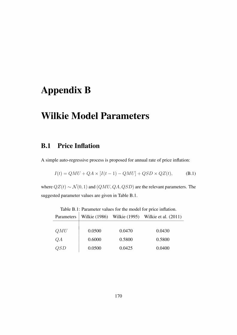
Appendix B
Wilkie Model Parameters
B.1 Price Inflation
A simple auto-regressive process is proposed for annual rate of price inflation:
I(t) = QMU +QA× [I(t− 1)−QMU ] +QSD ×QZ(t), (B.1)
whereQZ(t) ∼ N (0, 1) and (QMU,QA,QSD) are the relevant parameters. The
suggested parameter values are given in Table B.1.
Table B.1: Parameter values for the model for price inflation.
Parameters Wilkie (1986) Wilkie (1995) Wilkie et al. (2011)
QMU 0.0500 0.0470 0.0430
QA 0.6000 0.5800 0.5800
QSD 0.0500 0.0425 0.0400
170

B.2 Wage Inflation
For wages, it was proposed that an AR1 process be combined with the effects of
immediate past and present price inflation as follows:
J(t) = WW1× I(t) +WW2× I(t− 1) +WMU +WN(t),
(B.2)
where: WN(t) = WA×WN(t− 1) +WSD ×WZ(t), (B.3)
where WZ(t) ∼ N (0, 1) and (WW1,WW2,WMU,WA,WSD) are the rele-
vant parameters.
In particular, a value of zero was proposed for WA, suggesting that the auto-
regressive part of the model (WN(t)) could be omitted entirely. However that
would mean that the current rate of wage inflation is fully predictable using current
and immediate past values of price inflation.
The suggested parameter values are given in Table B.2.
Table B.2: Parameter values for the model for wage inflation.
Parameters Wilkie (1986) Wilkie (1995) Wilkie et al. (2011)
WW1 – 0.6000 0.6000
WW2 – 0.2700 0.2700
WMU – 0.0210 0.0200
WSD – 0.0233 0.0219
171

B.3 Dividend Yield
The proposed model for dividend yield:
log Y (t) = YW × I(t) + log YMU + Y N(t), (B.4)
where: Y N(t) = Y A× Y N(t− 1) + Y SD × Y Z(t), (B.5)
where Y Z(t) ∼ N (0, 1) and (YW, YMU, Y A, Y SD) are parameters of the
model. This model says that the natural logarithm of the yield depends directly on
the current rate of price inflation and also a first order auto-regressive model. The
suggested parameter values are given in Table B.3.
Table B.3: Parameter values for the model for dividend yield.
Parameters Wilkie (1986) Wilkie (1995) Wilkie et al. (2011)
YW 1.3500 1.8000 1.5500
YMU 0.0400 0.0375 0.0375
Y A 0.6000 0.5500 0.6300
Y SD 0.1750 0.1550 0.1550
B.4 Dividend Growth
The model for the annual rate of dividend increase, K(t), is made to depend on
price inflation and also on the residuals from the dividend yield process. It also
172

depends on its own lagged residual.
K(t) = DMU +DW ×DM(t) +DX × I(t)︸ ︷︷ ︸Inflation effect
+DY × [Y SD × Y Z(t− 1)]︸ ︷︷ ︸Lagged dividend yield residual
+DB × [DSD ×DZ(t− 1)]︸ ︷︷ ︸Lagged own residual
+DSD ×DZ(t), (B.6)
where DZ(t) ∼ N (0, 1) and
DM(t) = DD × I(t) + (1−DD)×DM(t− 1). (B.7)
The parameter DX is constrained to (1 − DW ) so that there is unit gain from
inflation to dividends. So (DMU,DW,DD,DY,DB,DSD) are the relevant pa-
rameters. The suggested parameter values are given in Table B.4.
Table B.4: Parameter values for the model for dividend growth.
Parameters Wilkie (1986) Wilkie (1995) Wilkie et al. (2011)
DMU 0 0.0160 0.0110
DW 0.0800 0.5800 0.4300
DD 0.2000 0.1300 0.1600
DY -0.0300 -0.1750 -0.2200
DB 0 0.1550 0.4300
DSD 0.1000 0.0700 0.0700
173

B.5 Bond Yield
The model proposed for the bond yield consisted of two parts:
C(t) = CR(t) + CM(t), (B.8)
where CR(t) represented the “real” part and CM(t) was an allowance for ex-
pected future inflation.
The models for CR(t) is as follows:
logCR(t) = logCMU + CN(t), (B.9)
where: CN(t) = CA× CN(t− 1) + CY × Y SD × Y Z(t) + CSD × CZ(t),
(B.10)
where CZ(t) ∼ N (0, 1). Note the dependence of CN(t) on the residual of the
current dividend yield.
Table B.5: Parameter values for the model for long-term bond yield.
Parameters Wilkie (1986) Wilkie (1995) Wilkie (2011)
CD 0.0500 0.0450 0.0450
CMU 0.0350 0.0305 0.0223
CA 0.9100 0.9000 0.9200
CY 0 0.3400 0.3700
CSD 0.1650 0.1850 0.2550
The model for CM(t) is:
CM(t) = max [CD × I(t) + (1− CD)× CM(t− 1), CMIN − CR(t)] .
(B.11)
A floor of CMIN = 0.005 is employed so that C(t) cannot be negative in a
simulation exercise. The relevant parameters are: (CD,CMU,CA,CY,CSD).
The suggested parameter values are given in Table B.5.
174
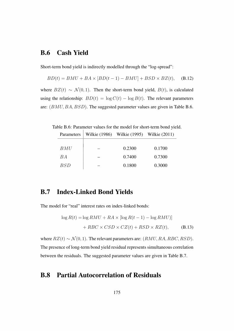
B.6 Cash Yield
Short-term bond yield is indirectly modelled through the “log-spread”:
BD(t) = BMU +BA× [BD(t− 1)−BMU ] +BSD ×BZ(t), (B.12)
where BZ(t) ∼ N (0, 1). Then the short-term bond yield, B(t), is calculated
using the relationship: BD(t) = logC(t) − logB(t). The relevant parameters
are: (BMU,BA,BSD). The suggested parameter values are given in Table B.6.
Table B.6: Parameter values for the model for short-term bond yield.
Parameters Wilkie (1986) Wilkie (1995) Wilkie (2011)
BMU – 0.2300 0.1700
BA – 0.7400 0.7300
BSD – 0.1800 0.3000
B.7 Index-Linked Bond Yields
The model for “real” interest rates on index-linked bonds:
logR(t) = logRMU +RA× [logR(t− 1)− logRMU)]
+RBC × CSD × CZ(t) +RSD ×RZ(t), (B.13)
whereRZ(t) ∼ N (0, 1). The relevant parameters are: (RMU,RA,RBC,RSD).
The presence of long-term bond yield residual represents simultaneous correlation
between the residuals. The suggested parameter values are given in Table B.7.
B.8 Partial Autocorrelation of Residuals
175
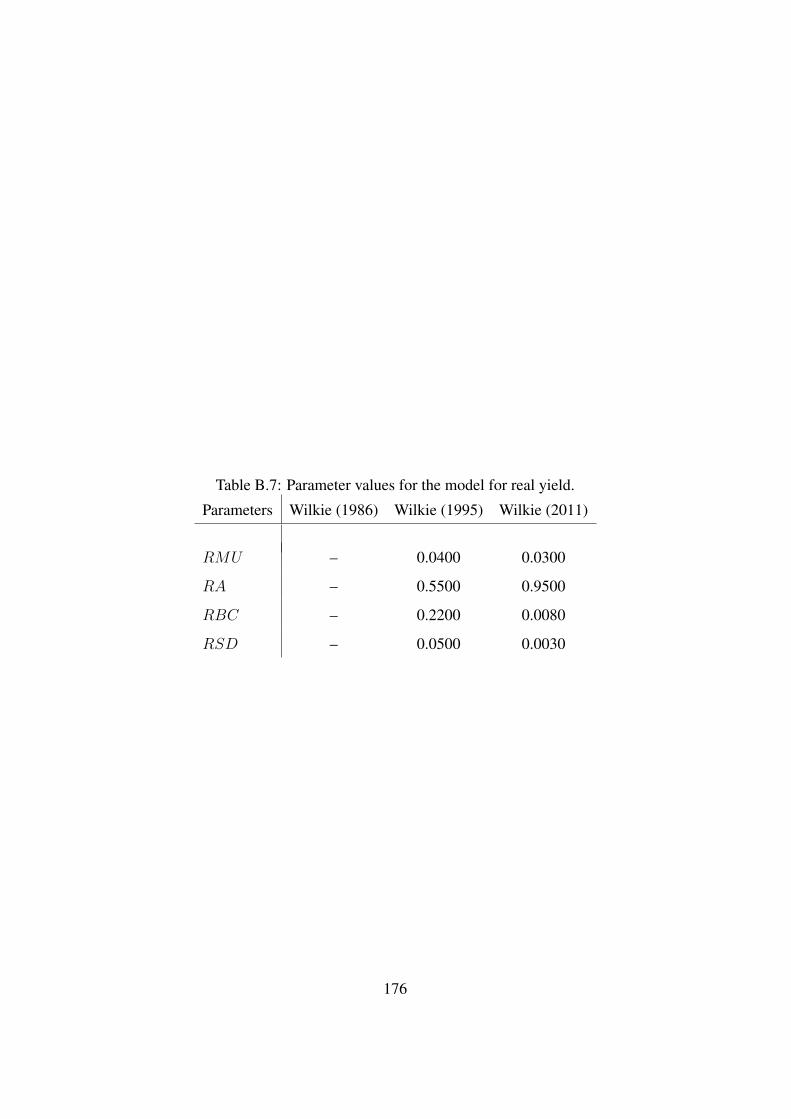
Table B.7: Parameter values for the model for real yield.
Parameters Wilkie (1986) Wilkie (1995) Wilkie (2011)
RMU – 0.0400 0.0300
RA – 0.5500 0.9500
RBC – 0.2200 0.0080
RSD – 0.0500 0.0030
176

−0.
3−
0.1
0.1
0.3
Lag
Par
tial A
CF
UK Price Inflation Residuals
5 10 15
−0.
3−
0.1
0.1
0.3
Lag
Par
tial A
CF
UK Salary Inflation Residuals
5 10 15
−0.
3−
0.1
0.1
0.3
Lag
Par
tial A
CF
UK Dividend Yield Residuals
5 10 15
−0.
3−
0.1
0.1
0.3
Lag
Par
tial A
CF
UK Dividend Growth Residuals
5 10 15
−0.
3−
0.1
0.1
0.3
Lag
Par
tial A
CF
UK Bond Yield Residuals
5 10 15
Figure B.1: Plots of partial autocorrelation functions (PACF) of the residuals for
UK.
177
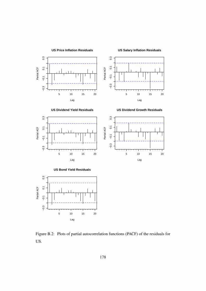
−0.
3−
0.1
0.1
0.3
Lag
Par
tial A
CF
US Price Inflation Residuals
5 10 15 20
−0.
3−
0.1
0.1
0.3
Lag
Par
tial A
CF
US Salary Inflation Residuals
5 10 15 20
−0.
3−
0.1
0.1
0.3
Lag
Par
tial A
CF
US Dividend Yield Residuals
5 10 15 20
−0.
3−
0.1
0.1
0.3
Lag
Par
tial A
CF
US Dividend Growth Residuals
5 10 15 20
−0.
3−
0.1
0.1
0.3
Lag
Par
tial A
CF
US Bond Yield Residuals
5 10 15 20
Figure B.2: Plots of partial autocorrelation functions (PACF) of the residuals for
US.
178

−0.
3−
0.1
0.1
0.3
Lag
Par
tial A
CF
Canada Price Inflation Residuals
5 10 15
−0.
3−
0.1
0.1
0.3
Lag
Par
tial A
CF
Canada Salary Inflation Residuals
5 10 15
−0.
3−
0.1
0.1
0.3
Lag
Par
tial A
CF
Canada Dividend Yield Residuals
5 10 15
−0.
3−
0.1
0.1
0.3
Lag
Par
tial A
CF
Canada Dividend Growth Residuals
5 10 15
−0.
3−
0.1
0.1
0.3
Lag
Par
tial A
CF
Canada Bond Yield Residuals
5 10 15
Figure B.3: Plots of partial autocorrelation functions (PACF) of the residuals for
Canada.
179

Appendix C
Results for US Stylised Scheme
based on USS with UK Economic
and Demographic Assumptions
C.1 Introduction
In this Appendix, we present the results for a US stylised pension scheme based
on the UK’s USS. Unlike in Chapter 7 however, we use UK economic and demo-
graphic assumptions. We make the following assumptions for our modelling:
1. We assume the same membership profile as the USS. We assume the mem-
bership profile of the members are as at the valuation date of March 31,
2014. For more details on the membership profile, please refer to Section
7.2. We also assume that no new members join the scheme after this date,
so that the risk analysis applies solely to the current membership of the
scheme.
2. The benefits are the same as the UK’s USS with the following exceptions:
180

• There is no lump sum when a member retires.
• Pension benefits are not indexed with inflation rates.
3. The starting values of assets and liabilities as at March 31, 2014 are:
• A0 = £28.7bn;
• L0 = £28.7bn;
i.e. there is no surplus or deficit as at March 31, 2014. This is different from
the UK’s USS which has an initial deficit of £5.3bn.
4. The contribution rate, calculated using the projected unit credit normal ac-
tuarial cost, is set at 15.5%. This is different from the UK’s USS where the
contribution rate amounts to 24%.
5. The asset allocation of the scheme is assumed to be 70% real and 30% fixed.
This is the same as the UK’s USS.
6. We use the Graphical Model calibrated to UK data to project stochastic
economic variables forward.
7. Model M7 calibrated to UK data is used for stochastic mortality projections.
C.2 Base Case Results
For our base case, we compare the results of the US stylised scheme to the UK’s
USS. Our base case results, using 10,000 simulations, are presented in Figure C.1,
which shows the full distribution of V ∗0 , Representative values of V aR and ES
are presented in Table C.1. We make the following observations:
181
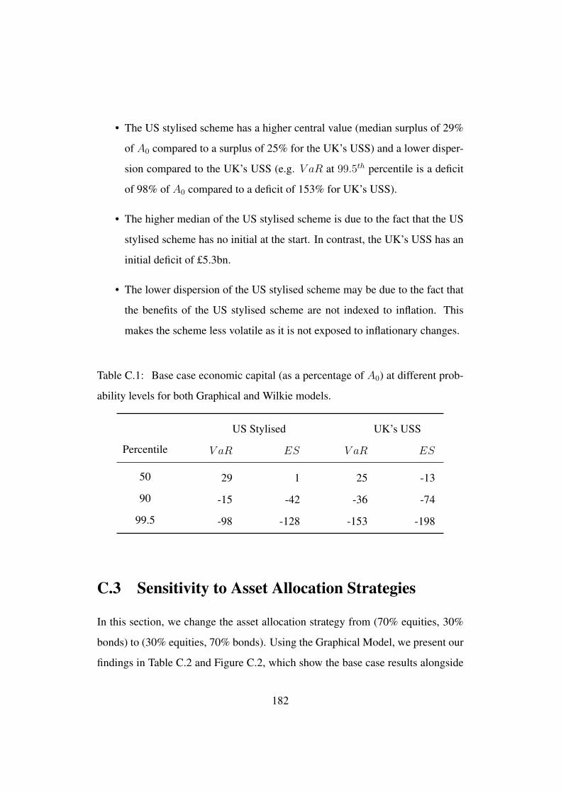
• The US stylised scheme has a higher central value (median surplus of 29%
of A0 compared to a surplus of 25% for the UK’s USS) and a lower disper-
sion compared to the UK’s USS (e.g. V aR at 99.5th percentile is a deficit
of 98% of A0 compared to a deficit of 153% for UK’s USS).
• The higher median of the US stylised scheme is due to the fact that the US
stylised scheme has no initial at the start. In contrast, the UK’s USS has an
initial deficit of £5.3bn.
• The lower dispersion of the US stylised scheme may be due to the fact that
the benefits of the US stylised scheme are not indexed to inflation. This
makes the scheme less volatile as it is not exposed to inflationary changes.
Table C.1: Base case economic capital (as a percentage of A0) at different prob-
ability levels for both Graphical and Wilkie models.
US Stylised UK’s USS
Percentile V aR ES V aR ES
50 29 1 25 -13
90 -15 -42 -36 -74
99.5 -98 -128 -153 -198
C.3 Sensitivity to Asset Allocation Strategies
In this section, we change the asset allocation strategy from (70% equities, 30%
bonds) to (30% equities, 70% bonds). Using the Graphical Model, we present our
findings in Table C.2 and Figure C.2, which show the base case results alongside
182

the results for the changed asset allocation strategy for ease of comparison. All
other assumptions are kept the same as those of the base case. We make the
following observations:
• From Figure C.2, we can see that the changed asset allocation has made the
distribution of V ∗0 more centered and less skewed.
• In particular, the median has shifted to the left, from a surplus of 29% to
a deficit of 5%, as shown in Table C.2. However, the shift to the left is
not as pronounced in the tail of the distribution, e.g. at 99.5th percentile,
the deficit, according to V aR, has increased from 98% to 110%, a much
smaller drop compared to the drop in the median.
• The above pattern can be explained as follows. The expected long-term re-
turn on bonds are much lower than those expected from equities which ex-
plains the fall in the median of the distribution. However, as the US stylised
pension scheme’s retirement benefits are not linked to inflation, the bonds
provide a good match for liabilities and hence the risk reduces, which ex-
plains the fall in skewness.
C.4 Sensitivity to Contribution Rates
In this section, we analyse the impact of changes in the base case contribution
rate of 15.5%. We consider two cases – an increased contribution rate of 18% of
salaries and a decreased contribution rate of 13%. All other assumptions are the
same as the base case, including the asset allocation strategy of 70% equities and
30% bonds.
We present our findings in Table C.3 and Figure C.3. Note that we have also
included the base case results in Table C.3 for ease of comparison. Similarly
183

Table C.2: Economic capital (as a percentage of A0) for the base case and for the
asset allocation strategy of 30% equities and 70% bonds at different probability
levels using the Graphical model.
Equity/Bond 70/30 Equity/Bond 30/70
Percentile V aR ES V aR ES
50 29 1 -5 -30
90 -15 -42 -44 -65
99.5 -98 -128 -110 -131
in the two plots of Figure C.3, we have included the distribution of V ∗0 for the
base case as the grey coloured density in the background. We make the following
observations:
• Compared to the impact of change in asset allocation strategy, changes in
contribution rates have a much reduced effect on the overall risk.
• As an example, at the 90% percentile, a decrease in contribution of 2.5%
(i.e. reduced from 15.5% to 13% of salary) results in an increase of deficit
from -15% to -23% of A0 in terms of V aR. On the other hand, increasing
the contribution rate to 18%, decreases the surplus to -7%.
• This leftward and rightward shifts of the distribution of V ∗0 for decreased
and increased contribution rates respectively can also be observed in Figure
C.3. However, note that the magnitude of the shifts are relatively small
compared to the impact of changes in the asset allocation strategy.
184
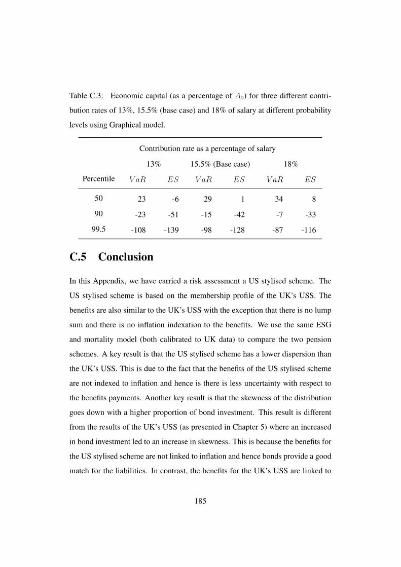
Table C.3: Economic capital (as a percentage of A0) for three different contri-
bution rates of 13%, 15.5% (base case) and 18% of salary at different probability
levels using Graphical model.
Contribution rate as a percentage of salary
13% 15.5% (Base case) 18%
Percentile V aR ES V aR ES V aR ES
50 23 -6 29 1 34 8
90 -23 -51 -15 -42 -7 -33
99.5 -108 -139 -98 -128 -87 -116
C.5 Conclusion
In this Appendix, we have carried a risk assessment a US stylised scheme. The
US stylised scheme is based on the membership profile of the UK’s USS. The
benefits are also similar to the UK’s USS with the exception that there is no lump
sum and there is no inflation indexation to the benefits. We use the same ESG
and mortality model (both calibrated to UK data) to compare the two pension
schemes. A key result is that the US stylised scheme has a lower dispersion than
the UK’s USS. This is due to the fact that the benefits of the US stylised scheme
are not indexed to inflation and hence is there is less uncertainty with respect to
the benefits payments. Another key result is that the skewness of the distribution
goes down with a higher proportion of bond investment. This result is different
from the results of the UK’s USS (as presented in Chapter 5) where an increased
in bond investment led to an increase in skewness. This is because the benefits for
the US stylised scheme are not linked to inflation and hence bonds provide a good
match for the liabilities. In contrast, the benefits for the UK’s USS are linked to
185

inflation and hence bonds do not provide a good match.
186
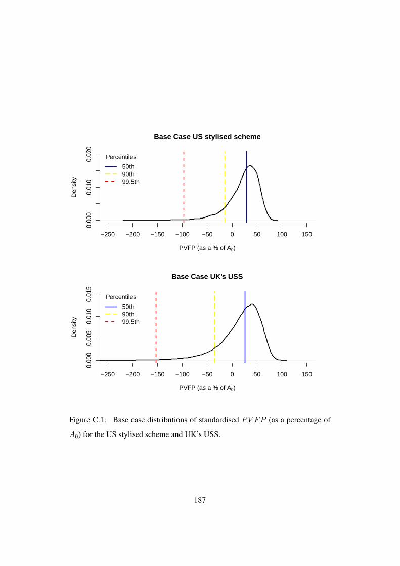
−250 −200 −150 −100 −50 0 50 100 150
0.00
00.
010
0.02
0
Base Case US stylised scheme
PVFP (as a % of A0)
Den
sity
Percentiles
50th90th99.5th
−250 −200 −150 −100 −50 0 50 100 150
0.00
00.
005
0.01
00.
015
Base Case UK's USS
PVFP (as a % of A0)
Den
sity
Percentiles
50th90th99.5th
Figure C.1: Base case distributions of standardised PV FP (as a percentage of
A0) for the US stylised scheme and UK’s USS.
187

−250 −200 −150 −100 −50 0 50 100 150
0.00
00.
010
0.02
0
Base case asset allocation strategy of 70% equities and 30% bonds
PVFP (as a % of A0)
Den
sity
Percentiles
50th90th99.5th
−250 −200 −150 −100 −50 0 50 100 150
0.00
00.
010
0.02
0
Asset allocation strategy changed to 30% equities and 70% bonds
PVFP (as a % of A0)
Den
sity
Percentiles
50th90th99.5th
Figure C.2: Distributions of standardised PV FP (as a percentage of A0) for the
base case and for the asset allocation strategy of 30% equities and 70% bonds at
different probability levels using the Graphical model.
188

−250 −200 −150 −100 −50 0 50 100 150
0.00
00.
010
0.02
0
Contribution rates reduced to 13% of salary
PVFP (as a % of A0)
Den
sity
Percentiles
50th90th99.5th
−250 −200 −150 −100 −50 0 50 100 150
0.00
00.
010
0.02
0
Contribution rates increased to 18% of salary
PVFP (as a % of A0)
Den
sity
Percentiles
50th90th99.5th
Figure C.3: Distributions of standardised PV FP (as a percentage of A0) for
decreased contribution rate of 13% and increased contribution rate of 18% (base
case assumption is 15.5% of salary) using Graphical model. The grey coloured
density in the background shows the base case.
189
Copyright © 2022 FDOKUMEN