1997 Spring Forum - Casualty Actuarial Society

CASUALTY ACTUARIAL SOCIETY FORUM

Spring 1997 Including the Reinsurance Cal1 Papers

CASUALTYACTUARIAL SOCZETY ORGANIZED 1914

0 1997 by the Casualty Actuarial Society. Al1 Rights Reserved.

Printed for the Society by Colortone Press

Landover, Maryland

NOTICE The Casualty Actuarial Society is not responsible for statements or opinions expressed in the papers or reviews in this publication. These papers have not been reviewed by the CAS Committee on Review of Papers.

The Casualty Actuarial Society Forum Spring 1997 Edition

Including the Reinsurance Cal1 Papers To CAS Members:

This is the Spring 1997 Rdition of the Casualty Actuarial Society Forum. It contains 10 Reinsurance Cal1 Papers (see the following note from the CAS Committee on Reinsurance Research).

The Casualty Actuarial Society Forum is a non-refereed joumal printed by the Casuahy Actuarial Society. The viewpoints published herein do not necessarily reflect those of the Casualty Actuarial Society.

The CAS Forum is edited by the CAS Committee for the Casuahy Actuarial Society Forum. Members of the committee invite all interested persons to submit papers on topics of interest to the actuarial community. Articles need not be written by a member of the CAS, but the paper’s content must be relevant to the interests of the CAS membership. Members of the Committee for the Casualty Actuarial Society Forum request that the following procedures be followed when submitting an article for publication in the Forum:

1. Authors should submit a camera-ready original paper, and two copies.

2. Authors should not number their pages.

3. Al1 exhibits, tables, char&, and graphs should be in original format and camera ready.

4. Authors should avoid using gray-shaded graphs, tables, or exhibits. Text and exhibits should be in solid black and white.

TheCASFonunisprintedperiodicallybasedonthenumberofarticlessubmitted. The committee’s goal is to publish two editions during the calendar year.

AH comments or questions may be directed to the Committee for the Casualty Actuarial Forum.

Sincerelv.

AdS Robert G. Blanco, CAS Forum Chairperson

Tl-te Committee for the Casualty Actuarial Society Forum

Robert G. Blanco, C’hairperson

Janet G. Lockwood, Vice Chairperson

Therese A. Klodnicki Keily S. McKeethan Gerald T. Yeung

The 1997 CAS Reinsurance Cal1 Papers Presented at the

1997 CAS Seminar on Reinsurance June l-3,1997

Marriott’s Castle Harbour Resort Tucker’s Town, Bermuda

The Spring 1997 Edition of the CAS Forum is a cooperative effort of the CAS Continuing Education Committee on the CAS Forum and the Research and Development Committee on Reinsurance Research. This edition of the Forum focuses on the 1997 Reinsurance Call Paper Program conducted by the Committee on Reinsurance Research.

The CAS Committee on Reinsurance Research was pleased to present for discussion 10 papers prepared in response to its 1997 Reinsurance Cal1 Paper Program. The topics addressed included: excess reinsurance pricing, property catastrophe risk load, workers compensation reinsurance commutations, the relationship of capital and risk to reinsurance programs, pricing extra-contractual obligations and excess of policy limits exposure, variations of contract terms, reserving issues, and contracts with multi-year limits. Thesepapers were discussed by the authors at the 1997 CAS Seminar on Reinsurance, June 1-3, in Tucker’s Town, Bermuda.

The Committee on the CAS Forum would like to encourage authors to submit papers and articles for further editions.

CAS Committee on Reinsurance Research Robert A. Bear, Chairperson

Paul J. Kneuer, Vice Chairperson

Robert S. Bennett David S. Powell Robert A. Daino Lawrence A. Vitale Malcolm R. Handte Ernest 1. Wilson H. Elizabeth Mitchell

Table of Contents Reinsurance Cal1 Papers

A Simulation Approach in Excess Reinsurance Pricing by Dmitry E. Papush, ACAS . . . . . . . . . . . . . , . . 1

An Apphcation of Game Theory: Property Catastrophe Risk Load by Donaid F. Mango, FCAS . . . . . . . . . . . . . . . . . . 31

Levels of Determinism in Workers Compensation Reinsurance Commutations by Gary Blumsohn, FCAS . . . . . . . . . . . . . . . . . . . 53

Capital and Risk and their Relationship to Reinsurance Programmes by Stewart M. Coutts and Timothy R.H. Thomas . . . . . . 115

Comparing Reinsurance Programs-A Practica1 Actuary ‘s System by Robert A. Daino, FCAS, and Charles A. Thayer . . , , . 141

Pricing Extra-Contractual Obligations ami Excess of Policy Limits Exposures in Clash Reinsurance Treaties by Paul Braithwaite, FCAS, and Bryan C. Ware, FCAS . . . 179

Evaluating Variations in Contract Terms for Casualty Clash Reinsurance Treaties by Emily Canelo and Bryan C. Ware, FCAS . , , . . . . . . 201

Loss Development and Annual Aggregate Deductibles by Vincent P. Connor, ACAS . . . . . . . . . . . . . . . . . 219

An Integrated Pricing and Reserving Process for Reinsurers by Leonard R. Goldberg, FCAS, and Joseph LaBella . . . 237

Reinsurance Contracts with a Multi-Year Aggregate Limit by Regina M. Berens, FCAS . . . . , . . . _ . . . . . . . 289

A Simulation Approach in Excess Xeinsurance Pricing

by Dmitry E. Papush, ACAS

A Simulation Approach in Excess Reinsuranee Pricing

Dmitry Papush

There are numerous papers in the actuaría1 literature dealing with the different aspects and applications of aggregate loss models. The great demand for research in this area stems from the increasing popularity of .insurance and reinsurance arrangements involving aggregate hmit and aggregate deductible provisions. The estimates of aggregate IOSS distributions are also important in the pricing of contracts containing retro adjustments, and profit and contingent commission features.

Some excellent practica1 methods are available to estimate aggregate loss distributions, including Heckman-Meyers [Z] and Panjer [5]. The common assumption used in these methods is that all claims have the same loss size probability distribution. Whiie this assumption is reasonable for many insurance contracts, there are situations where such an assumption becomes impractical.

As an example, one can consider the reinsurance program involving severa1 layers of reinsurance coverage. Each of these layers may have both per occurrence and annual aggregate limits with a possibility to “drop down” if the underlying layers are exhausted, creating a quite diffrcult “two-dimensional”stnmture. This type of reinsurance program is quite common for large medical professional organizations. A specific example is considered later in the paper.

Pricing such programs can be challenging for reinsurance actuaries. From a theoretical standpoint, the major diffrculty involved is that the reinsurer’s loss severity distribution function is changing, depending on the exhaustion of the underlying layer coverage. This makes derived aggregate loss model techniques (Heckman - Meyers, Panjer) diffrcult to apply. One possible soiution is to use stochastic simulation.

The simulation method can aiso be used successfully in place of Heckman - Meyers’ or Panjer’s method to build an aggregate loss distribution from estimated frequency and severity distributions. This paper systematically describes the stochastic simulation approach that involves the following steps: 1) Data preparation 2) Selection of frequency and severity distributions; goodness-of-fit tests 3) Estimarion of the number of simulations required 4) Simulation of the excess losses 5) Pricing recommendations

This paper outlines some theoretical and practica) considerations which may be useful in utilizing this approach. A pricing example will illustrate the application of the method

1. Pricing Example.

1.1. Description of Coverage.

Our main example deals with the coalition of severa1 hospitals (Alpha Hospital Union, AHU) which purchases a multi-layer reinsurance program to protect itself from catastrophic medical malpractice losses. AHU retains the first $3,000,000 per each and every occurrence, and wants to reinsure the excess. Coverage is claims made; the effective date for the coverage is January 1, 1997.

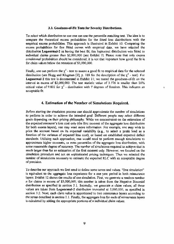
We will consider the pricing of the first two excess reinsurance layers. The first layer covers $3,000,000 in excess of $3,000,000 for each and every occurrence and is subject to an annual aggregate limit of $9,000,000. The second layer covers $3,000,000 for each and every occurrence in excess of the first layer coverage and is subject to annual aggregate limit of $12,000,000. In other words, the second layer covers $3 Mil xs $6 Mil before the tirst layer of excess coverage is exhausted, and $3 Mil xs $3 Mil after that.

Exhibit 1 shows the design of the coverage. After the first excess layer is exhausted, the second layer “ drops down” to replace it. It makes the pricing of the second layer very difficult, because the severity distribution can change in the course of a year. We will demonstrate how to use simulation to estimate expected loss for the first and the second excess layers.

1.2. Data.

We assume that the following information is provided by the client:

l The complete list of all claims for report years 1983 through 1993 that exceed $l,OOO,OOO at 12/3 1/95 evaluation date (see Exhibit 2);

l Incurred and paid loss development triangles by report year (see Exhibits 3-1 and 3-2); l Paid claim count development triangle by report year (see Exhibit 4); l Historical exposure (Basic class Ful1 Time Equivalents) for years 1985 through 1993

and exposure projection for year 1997 (see Exhibit 5).

The loss and exposure data for report years 1994 and 1995 are also available but not used because of their immaturity.

1.3. Pricing Approach.

Our pricing approach is consistent with one described by Patrik [6]. The following main formula (a modification of Formula 6.2.1 from [6]) will be used:

RLCxDF RP= (1.3.1)

(1 -CR-BF)(I -IXL)(I -TER)

4

Here RP = reinsurance premium (gross), RLC = reinsurance loss cost, DF = discount factor, CR = reinsurance ceding commission rate, BF = brokerage fee (if any), IXL = reinsurer’s interna1 expense loading, TER = reinsurer’s target economic return.

We will concentrate on the estimation of RLC; the other elements of the above formula are determined using other sources. Usually IXL is a tünction of the size of the account, and TER ís a fimction of the level of risk (or potential volatility of account loss experience). While our methodology does provide a tool to measure potential account volatility, this topic is outside the scope of this paper.

The simulation method is used to estimate RLC. We model the loss severity and loss frequency distribution functions to simulate a statistically representative sample of loss experience in the reinsurance layers; the mean of this sample should give a good proxy for the expected loss in the layer. The details of the method follow.

1.4. Simulation Method - Step By Step.

When simulating loss experience one should be convinced that the severity and frequency loss distributions used in the simulations reflect reality to the greatest extent possible. To assure that, a good amount of meticulous work should be done.

First, historical individual losses should be trended and developed

Second, loss frequency and loss severity distributions for the projected coverage period should be constructed based on adjusted loss data. Different types of loss severity curves (e.g., lognormal, Pareto, Weibull) fitted to the data should be examined. The Maximum Likelihood or the Least Squares methods may be used for curve fitting.

Next, a rigorous test of the goodness-of-fit needs to be performed. Percentile matching is probably the most importar& but other tests (x2 - test, Kolmogorov - Smimov) can also be performed.

Before starting the actual simulation process one needs to estímate the number of simulations required to achieve a certain precision dependmg on bis goal. We recommend a relatively easy formula based on the application of the Central Limit Theorem.

When one is comfortable with the flequency and severity curves seIected and the estima& number of simulations, one can tun the simulation process.

The following sections explain in detail all the steps mentioned above

2. Data Preparation.

2.1. Trending Individual Losses.

When trending the historical losses to the prospective experience period claim cost leve1 it is important to select a proper severity trend factor. If underlying experience data is credible, it is better to select a trend factor using the account’s own experience. One way of doing so involves the following steps:

l Develop the total incurred losses by year to ultimate; l Develop the number of claims paid by year to ultimate; l Calculate (untrended) average loss size by report year (divide the total ultimate

loss by the ultimate number of claims); l Fit an exponential regression to such averages.

This procedure is documented in Exhibit 6. The corresponding annual severity trend factor is 4.4%. Given the size of the account and regression characteristics we have decided to use this trend factor to bring individual losses to 7/1/97 level.

Altematively, one can look at industrywide trend for Hospital Professional Liability from relevant sources. If necessary, one can adjust it for the difference in medical inflation for the state of the client’s primary operations versus countrywide.

2.2. Developing Individual Losses.

Some individual claims in excess of $I,OOO,OOO from the database illustrated in Exhibit 2 are still open at 12/3 1/95. The ultimate values of these claims might be different from their reserved values which we observed. Generally, it is not easy fo adjust individual claim values for possible development using aggregate development data only. The major complication stems fiom the fact that aggregate loss development is driven by two different forces - the appearance of new claims and the adjustment of values for already outstanding claims. Fortunately, for claims made coverage usualiy there are no new claims which appear after the first year, and al1 the development is attributable to the reserve adjustments for outstanding claims only. This makes it possiblefor &ims mude coverage

to use aggregate loss development data to approximate the development of individual claims. A procedure similar to the one described below can be used to develop individual claims for occurrence coveruge; however, more information would be necessary

The following technique could be used to develop individual losses which are open at 12/3 1/95 at its n’* evaluation (n=l for claims reported in 1995, n=2 for claims reported in 1994, etc.):

l For each report year and fixed n (n=1,2,...) create a development triangle for claims ooen at n’* evaluation onlv. This can be done by subtracting column n of Exhibit 3-2 (paid losses at n’* evaluation) from columns n and subsequent of Exhibit 3-1 (reported losses at n’* evaluation and subsequent);

l Select appropriate loss development factors;

l Apply selected n-to-ultimate development factor to open claims outstanding at n’* evaluation.

For claims that were reported in 1992 (n = 4) this procedure is illustrated in Exhibit 7; the corresponding factor to be applied to report year 1992 claims open at 1213 1/95 is 1.075. Please note that no loss development adjustment is applied to closed claims.

Alternatively, one can fit a series of curves to claim values at l”, 2”d, and subsequent evaluations, and investigate the movement of the parameters. This methodology is consistent with one currently used by ISO (Pareto soup)

3. Selection of Frequency and Severity Distributions.

To calculate the expected losses in both reinsurance layers (see Exhibit 1) we need to project the number of claims in excess of $3,000,000, and the claim severity for such claims. Because AHU retains the first %3,000,000 of each and every claim, we should concentrate on the portion of claims in excess of this amount.

3.1. Selection of Number of Claims Distribution.

For the Excess Claim (in excess of %3,000,000) Frequency distribution we use the Negative Binomial. This discrete distribution has been utilized extensively in actuarial work to represent the number of insurance claims. Since its variance is greater than its mean, the Negative Binomìal distribution is especially useful in situations where the potential claim count can be subject to significant variability. As Exhibit 5 Column (5) illustrates. this is the case in our example. .-

To estimate parameters for the Negative Binomial distribution we start with the estimate of expected number of claims in excess of $3,000,000. Exhibit 5 summarizes our approach.

First, we select the total claim frequency based on the historical exposure information and our estimates of ultimate number of paid claims; this selected number is 0.40 claims per one Ful1 Time Equivaient (FTE) of exposure and is shown at the bottom of column (4). Second, we select the probability that the paid claim exceeds $3 Mil; our selection of 1.50% is shown at the bottom of column (6). Based on these two numbers and the estimation of 840 FTE exposure for year 1997 provided by AHU, we expect 5.00 claims in excess of $3,000,000 for the coming year.

In order to estímate both parameters of the Negative Binomial, we need to estimate the variance of the claim count distribution. One possible approach is to look at the sample of historical claims in excess of $3,000,000 uf a 1997 exposure leve1 and estimate the second moment of that distribution. This approach is documented in Exhibit 8; the estimated variance-to-mean ratio is 4.46.

The result of 4.46 would be appropriate to use had we estimated it fiom an observed statistical sample. However, since we manipulated the data (trending, loss deveiopment, etc.), there was a parameter risk involved. As a res&, the actual variability of the number of excess claims fiom the estimated expectation may have been larger than predicted in Exhibit 8. Meyers [4] addressed this problem. He suggested considering the mean of the Number of Claims distribution to be a random variable. The principal effect of this assumption is to increase the potential variability of the number of claims distribution around its expected value. To attain the same effect, while avoiding unnecessaty complications, one can judgementally increase the indicated variance-to-mean ratio.

Based on our evaluation of possible errors in the estimation procedure used to price medical malpractice accounts. we have judgementally chosen to increase the variance-to- mean ratio to 6.0.

In translating the results of our estimates of mean and variance-to-mean ratio to standard parameters (p,r) of the Negative Binomial distribution (see, for example, [3], p. 52), we havep=O 167;r= 1.

3.2. Selection of Severity Distribution.

To select a ioss severity distribution we apply the maximum likelihood method to fit a curve to individual claim data. Some caution is necessary in deahng with this particular data. The problem is that we do not have the complete set of historical information but only claims whose (untrended and undeveloped) values exceed %1,000,000. This means that for different years we only have information about the incurred claims which exceed some threshold (equal to the trended and developed value of %l,OOO,OOO). For example, for report year 1983, we only have information about claims whose values in 1997 dollars are greater than $l,OOO,OOO x 1.827 x 1.000 = 1,827,OOO (see Exhibit 2). In this case our likelihood hmction can be written in the form:

L = n f(xi,A) / [ 1 - F(ti,A)l (3.2.1)

Here A is the set of parameters describing a member of particular family of distribution hmctions (for example, for the lognormal distribution, 11 consists of the two standard parameters, I-( and o), f(xi,A) - pdf of loss severity distribution given the set of parameters A, x, - the value of (trended and developed) claim i, F(ti,A) - distribution function, ti - corresponding threshold value (1,827,OOO for 1983 claims, etc.). The maximum likelihood estimators are the set of parameters AO that maximizes the function (3.2.1).

It is recommended to try different types of loss distribution to fit the data and select the one that has the best fit. Also, one can fit the curve to the portion of the data in excess of different retention points, such as $2 Mil, $2.5 Mil, etc.; this approach is consistent with one suggested by Finger [ 11. The next section describes our approach in comparing different distributions. Exhibit 9 contains the list of distribution functions fitted to different portions of the data we used in pricing the AHU account.

3.3. Goodness-of-Fit Tests for Severity Distributions.

To select which distribution to use one can use the percentile matching test. The idea is to compare the theoretical excess probabilities for the fitted loss distributions with the empirical excess probabilities. This approach is illustrated in Exhibit 10. Comparing the excess probabilities for five fitted curves with empirical data, we have selected the distribution Lognormal-2 as having the best fit; this lognormal distribution was fitted to individual claims greater than $2,000,000 (see Exhibit 9). Please note that only excess condifional probabilities should be considered; it is not that important how good the fit is for claim values below the retention of $3,000,000.

Finally, one can perform the x2 - test to assure a good flt to empirical data for the selected distribution (see Hogg and Klugman [3], p. 103 for the description of the x2 - test). For Lognormaf-2 this test is documented in Exhibit 11; we tested the goodness-of-fit on the interval in excess of $2,000,000. The test statistic value of 3.776 is smaller than 20% critica1 value of 9.803 for x2 - distribution with 7 degrees of freedom. This indicates an acceptable fit.

4. Estimation of the Number of Simulations Required.

Before starting the simulation process one should approximate the number of simulations to perform in arder to achieve the lntended goal. Different people may select different goals depending on their pricing philosophy. While we concentrated on the estimation of the expected reinsurer’s loss cost only (the first moment of the aggregate loss distribution for both excess layers), one may want more information. For example, one may wish to price the account based on its expected variability {e.g., to select a profit load as a function of the variance of expected loss cost), or based on established expected deficit standards. Utilizing such approaches, one woutd need to perform enough simulations to approximate higher moments, or even percentites of the aggregate loss distribution, with some reasonable degree of accuracy. The number of simulations required to achieve that is much larger than for an estimation of the first moment only. However, we focuied on the simulation procedure and not on sophisticated pricing techniques. Thus we selected the number of simulations necessary to estimate the expected RLC with an acceptable degree of precision.

To describe our approach we first need to define some terms and values. ‘rOne simulation” is equivalent to the aggregate loss experience for a one year period in both reinsurance layers. Exhibit 12 shows the results of one simulation. First, we generate a random number n for claims in excess of $3,000,000; this number is taken from the Negative Binomial distribution as speeified in section 3.1. Secondly, we generate n claim values; all these values are taken from Lognormal-2 distribution tnmcated at 3,000,000, as specified in section 3.2. Next, each claim value is apportioned to two reinsurance layers according to the terms described in section 1.1. Finally, the aggregate loss for each of reinsurance layers is calculated by adding the appropriate portions of n individual claim values.

We repeat N independent simulations resulting in samples of size NMfor the annual aggregate loss in both reinsurance layers, then we use the sample mean X as an estimate of the expected reinsurer’s loss costs. If N is large enough, we can use the Central Limit Theorem to estimate the difference between ? and the true expectation p of the aggregate loss cost. Namely, according to the Central Limit Theorem, even though the aggregate loss distribution is skewed and not normal, for large N the distribution

being derived fìom the sum of N independent aggregate loss distributions, converges to the standard normal distribution ((r is the standard deviation of the aggregate loss distribution). Therefore, at 95% cotidence level,

+~/~1.96*olJN (4.1.1)

Now, if we select T to be an acceptable tolerance for the difference 1 2 - p 1, we can estimate the number N of simulations required to assure that this difference is less than T at the 95% contidence level:

Nz( 1.96*o/T)’ (4.1.2)

For the practica] use of the formula (4.1.2) G and T need to be approximated

When pricing a reinsurance contract, an actuary often knows a proposed price or existing terms for it. This knowledge can help to select T (5% of existing price, for example). Even if the actuary does not know an amount of premium anticipated for an account, he or she can easily approximate such an arnount by nmning a relatively small number of simulations (say, 1000). The mean of the resulting sample could be used to reasonably select T. The same approach could be recommended to approximate the value of o.

For our @IU example after 1000 simulation we have: for the 1-st Excess Layer ? = $4,532,000, o = $3,510,000; for the 2-nd Excess Layer x = $1,788,000, CY = $3,403,000. Selecting T = $50,000 and approximating cs = $3,500,000 we have by formula (4.1.2):

N 2 (1.96 * 3,500,OOO / 50,000 ) * = 18,824

Therefore, at a 95% confidente level, performing 20,000 simulations for an annual aggregate loss should assure that the sample mean differs from the true expected annual aggregate loss by less than $50,000 (for either reinsurance layer).

Alternatively, one can monitor the convergence of the simulation process and stop it when the change in the sample mean (and, possibly, higher moments) in between simulations becomes reasonably small.

10

The third approach ’ is to use an upper bound for o. For example, it can be proven that the standard deviation o of any distribution whose values are concentrated on the tinite segment [O;A] is less than A/2. For the 2-nd Excess layer, using T = $50,000 and A = % 12,OOO.OOO. formula (4.1.2) implies that

Nz (1.96 * 12.000,OOO / 2! 50,000) * = 55,320

The indicated number of simulations for this method is usually signifcantly higher than it is really necessaty to obtain a required tolerance level.

5. Simulation Results for the Excess Loss Distribution.

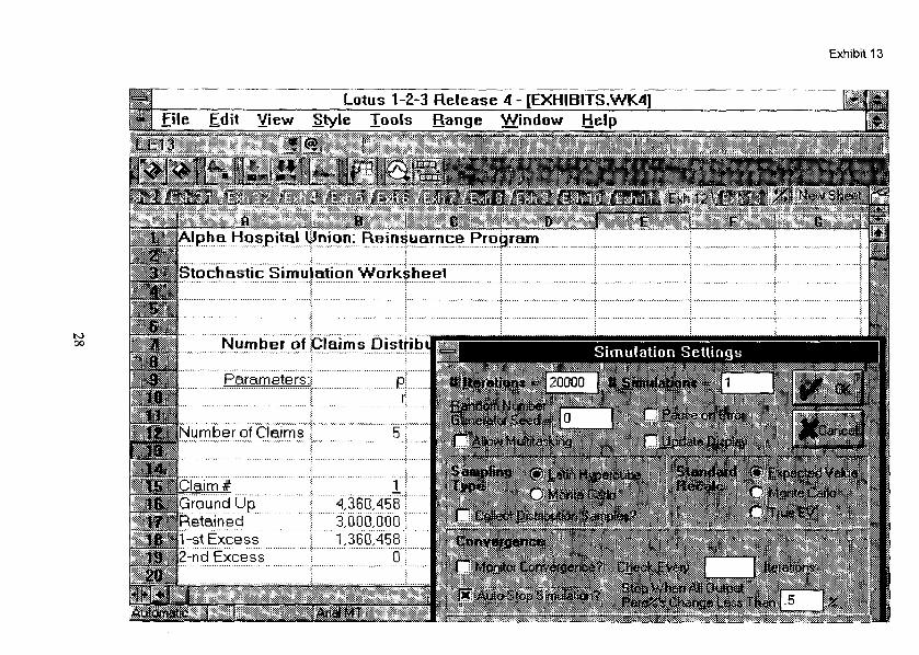
The simulation process has been described in Sectton 4; the results for one simulation are shown in Exhibit 12. Different software packages couid be utilized for simulation. We use a package called (@XX; this one is designed to be used with standard spreadsheets, like Loma i-Z-3 or Excel Exhibit 13 shows the settings for the simulation procedure; the number of simulations to tun (20,000) has been specified in Section 4.

The simulation results are shown separately for the 1 -st and the Z-nd reinsurance layers in Exhibit 14. Please note that the aggregate loss distributions for both reinsurance layers, although shown in detail (the four tirst moments and percentiles), should be used with great caution. The number of simulations we went through has been selected to achieve our goal. which is to obtain a reasonably accurate estimator for the expected aggregate loss. There is no warranty that the percentile statistics shown are accurate estimates of the true percentiles of the aggregate loss distribution; to achieve that, it might-be necessary to tun more simulations.

Using formula (4.1.1) we can refurbish our estimate of / x - u /. Namely, using estimated results for the 1 -st Excess layer, we can conclude that

1 4,481,577 - ~1 1 c: 1.96 * 3,498,020 / d 20,000 = 48,480,

where ut is the expected annual aggregate loss for the I-st Excess iayer. For the 2-nd Excess layer the same approach leads to estimate

1 1,779,283 - u2 ] c; 1.96 * 3,433,117 / 4 20,000 = 47,580,

where uí! is the expected annual aggregate loss for the 2-nd Excess Iayer

r The idea of this method has been suggested to the author by Marc Shamula.

ll

To insure the quality of the results produced by the simulation method one could compare them to the results obtained by using another known technique if it is possible. To do such a comparison we estimated the annual aggregate loss for the 1-st Excess layer using the Panjer method Using the Number of Claims and Severity distributions specitied in Section 4, and the unit length of $25,000 for discretization, we obtained the estimate of $4,482,940. The difference of this resuh from the one produced by simulation method is about 0 03%

6. Pricing Recommendations.

The final step in the process is to convert the estimated ioss cost to a recommended price for reinsurance coverage by using formula (1.3.1). We wili not attempt to give a recipe on how to select corresponding factors. However, we will briefly discuss their relationship with the simulation pricing approach.

CR and BF are externa1 variables suggested by a broker or client and ofien are not under the control of the reinsurer; we will not discuss them.

IXL reflects the reinsurer’s expenses; it tnight be a separate load oc it might be combined with the TER under the concept of ‘Iisk based capital’: If a reinsurance company uses a separate load for IXL in its pricing formula, it is usually expressed as a tünction of the size of account (reinsurance pretnium net of commission and brokerage fees).

TER for the contract should, at least theoretically, reflect the level of risk that the reinsurer is taking by writing a particular contract. Usually the risk of the contract is measured by the potential variability of its loss experience. If a reinsurance company utilizes some unified approach to reflect risk in the pricing formula (e.g., use risk load proportional to the variance of the expected loss cost), the simulation method is an ideal provider of information. Exhibit 14 shows various characteristics of the expected aggregate loss distributions (higher moments, mode, and percentiles) one can use to measure the risk. However, as discussed earlier, one must make sure to tun enough simulations to obtain reliable estimates for these characteristics.

DF is a fimction of the expected payout pattern for the account’s losses and interest rates. While some information can be extracted tiom the historical loss emergence pattem for the account (see Exhibit 3.2) the estimated payout pattern may not be a good predictor for the high attaching reinsurance layers. For example, one can anticipate a significant delay in payments for the 2-nd Excess layer, because the payments in this layer would intensify considerably after the coverage of the I-st Excess layer is exhausted. According to Exhibit 14, the probability that the coverage of the 1-st Excess layer will be depleted is about 25%. An altemative way to deal with this problem is to simulate the payment date of each excess loss in addition to its value. Then calculate the present value of such payments in 1997 dollars while applying the corresponding discount factor to the simulated claim value. Using this approach one can omit the DF multiplier in formula (1.3 1) because the produced RLC is already discounted.

12

Exhibit 15 displays the recommended reinsurance premiums derived by application of formula (1.3.1) for both reinsurance layers of coverage. The loading factors used in this exhibit are for illustrative purposes only, and are not actual factors used for pricing.

7. Final Remarks and Conclusions.

This paper illustrates the application of a simulation method in excess reinsurance pricing. Our considerations were intentionally limited by the data described in Section 1.2; having more detailed information one can achíeve much more accurate results. For example, getting the individual development information for large claims, one can use it to estimate the development factor more accurately. There are countless variations of the types of data which reinsurance actuaries can find available for a pricing analysis. We have not even tried to reflect these variations. Rather, we attempted to show the appiication scheme of the simulation method in reinsurance pricing emphasizing its critica1 points.

We have considered the simulation approach in computing aggregate loss distributions. As we demonstrated, the scope of the applicability of the simulation method is more bread than for other aggregate loss distribution techniques. It combines easy programming with highly accurate results. AJthough it currently requires a substantial amount of computer resources, this will become less of an issue with further advancements of computer technology. With the development of effícient simulation software and increasing speed of modern computers, simulation methods promise to become one of the leading tools in actuarial practice.

8. Acknowledgments.

1 would like to express my deep appreciation to Marc Shamula for his outstanding effort in reviewing the drafts of this paper. He suggested numerous improvements and provided the author with valuable insights.

1 am also very thankful to Gary Patrik for his continuous support and encouragement

13

Bibliography.

1. Finger, R. “Estimating Pure Premium by Layer,” PCAS, LXIII, 1976, p. 34

2. Heckman, P., and Meyers, G. ‘The Calculation of Aggregate Loss Distributions from Claim Severity and Claim Count Distributions,” PCAS, LXXI, 1984, p. 49.

3 Hogg, R., and Klugman, S. Loss Distributions, John Wiley & Sons, 1984.

4. Meyers, G “Arr Introduction to the Competitive Market Equilibrium Risk Load Formula.”

5. Panjer, H. “ Recursive Evaluation of a Family of Compound Distributions,” ASTIN Bullefin, 12, 1981, p. 22.

6. Patrik, G.“Reinsurance,“Foun&zt~ons ofCamaity Actuarial Science (Second Edition), Casualty Actuarial Society, 1992, Chapter 6, p. 277.

14

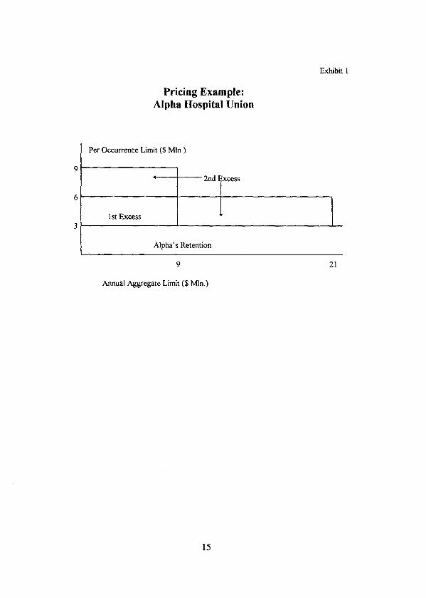
Exhibit 1

Pricing Exampie: Alpha Hospital Union

Per Occurrence Limit ($ Mln.)

9- +--- 2nd Excess

6

1 st Excess 1

3

Alpha’s Retention

9 21

Annual Aggregate Limit ($ Mln.)

15

Exhibit 2

ALPHA HOSPITAL UNION Incurred Cases Over $1,000,000 @ 12/31/95 - Extract

Trendedto 07/01/97

Case-#

Total Incurred

LosS

-pOtt Year 1983 ____ C83-0988 7454,310 C83-0518 5,854,006 C83-0832 4,800,106 C83-0021 3,228,345 C83-0656 3.157,378 C83-0305 2,093,321 C83-0441 2,131,311 C83-0209 2,106.704 C83-0767 1,911,213 C83-0008 1,641.695 C83-0390 1,500,234 C83-0962 1,300,452 C83-0481 1,798,792 C83-0190 1,187,056 C83-0271 1,137,370 C83-0450 1,141,698 C83-0393 1,103,989 C83-0468 1.095,040

Total Report Year 1983

Trend Trended Ea4 Loss

Trended& 1-st Excess 2-nd Excess Developed Layer Layer

LQ!s !&s loss

1.827 13,621,170 1.000 13,621,170 1.827 10,696,954 1 .ooo 10,696,954 1.827 8,771,177 1.000 8,771,177 1.827 5,899,115 1 .ooo 5,899,115 1.827 5,769,438 1 .ooo 59769,438 1.827 3,825,099 1 .ooo 3,825,099 1.827 3,894,519 1.000 3,894,519 1.827 3,849,554 1.000 3,849,554 1.827 3.492,337 1.000 3,492,337 1.827 2,999.849 1.000 2,999,849 1.827 2,741,360 1 .ooo 2,741,360 1.827 2,376,300 1 .ooo 2,376,300 1.827 2,190,538 1.000 2,190,538 1.827 2,169,094 1.000 2,169,094 1.827 2,078,303 1 .ooo 2,078,303 1.827 2,086,210 1 .ooo 2,086,210 1.827 2,017,306 1.000 2,017,306 1.827 2,000,954 1.000 2.000,954

Trend = 4.4%

------ ------------- ------------- ----_--- ------ ------------- ------------- --___-__

Repoti Year 1992 C92-0921 3,720,867 C92-0691 3,032,036 C92-0423 2,877,629 C92-0802 2,376,103 c92-0331 2,309,169 C92-0669 2,240.742 C92-0473 2.281,805 C92-0698 2,217,662 c92-072 1 2.134,174 C92-0205 2.074,380 c92-0075 1,673,136

1.240 4,614,734 1 .ooo 49614,734 1,614,734 1.240 3,760,424 1.075 4,042,456 1,042,456 1.240 3,568,924 1.075 33836,594 836,594 1.240 2,946,916 1.075 3,167,934 167,934 1.240 2,863,902 1 .ooo 2,863,902 1.240 2,779,038 1.075 2,987,465 1.240 2.829,964 1 .ooo 23829,964 1.240 2,750,413 1.075 2,956,694 1.240 2,646,869 1.075 2,845,384 1.240 2.572,710 1.075 2.7651663 1.240 2,075,074 1.075 2,230,705

Total Report Year 1992 3,661,718

3,000,000 3,000,000 3,000,000 3,000,000 3,000,OOO 2,771,177

2,899,115 329,708

0 0 0 0

9,000,000 12,000,000

16

Eixhibi 3-l

ALPHA HOSPITAL UNION

lília 1 1983 1984 1985 1986 43.357 1987 60,455 1988 62,839 1989 80.524 1990 60,507 1991 62,216 1992 57,860 1993 59,360

Link-ratios Irz

$ 1983 1984 1985 1986 1.110 1987 1.094 1988 1.046 1989 1.056 1990 1.104 1991 1.074 1992 1.099 1993 1.102

Last3 1.092 Last5 1.087

Best3 of5 1.092

Selected 1.092

Cumulative 1.272

Percentage Reported 78.6%

73,094 48,147 66,167 65,756 85,021 68,776 66,810 63,610 65,386

66,200 77,151 51,946 70,353 79,543 90.377 71,690 89,397 69,004 70,250

4 88,420 69,814 80,754 54,388 74,966 73,818 93,878 73,010 73,249 71,596

ís 3-4

1.056 1.079 1.063 1.210 1.M3 1.074 1.039 1.085 1.074

1.055 1.047 1.047 1.066 0.928 1.039 1.018 1.056 1.038

4.5 1.033 1.007 1.024 1.016 1.002 1.036 1.051 1.042 1.031

1.066 1.037 1.041 1.067 1.016 1.032 1.070 1.032 1.036

1.070 1.035 1.036

1.165 1.088 1.052

7.2% 6.0% 3.2%

5 91,350 70,282 82,720 55,248 75,122 76,470 98,685 76,054 75,525

E!z!z 1.025 1.034 1.015 1.017 1.012 0.998 1.019 1.015

1.011 1.012 1.015

1.013

1.015

3.4%

6 93,593 72,664 83,984 56,209 76,016 76,333

100,593 77,195

ch2 1.001 0.999 1.004 1.015 1.003 0.989 1.002

0.998 1.003 1.003

1.002

1.002

1.3%

2 93,723 72,591 84,278 57,079 76,213 75,521

100,794

za 0.995 0.997 1.002 1.003 0.998 1.002

1.001 1.000 1.001

1.000

1.000

0.2%

s 93,277 72,397 84,452 57,239 76,032 75,700

9 93,914 71,077 85,566 56,747 76,202

Iu2 93,888 71,213 85,405 56,859

- 1.007 0.982 1.013 0.991 1.002

9a.Q 1.000 1.002 0.998 1.002

iorll. 1.000 1.005 1.001

1.002 1.000 1.002 0.999 NIA NIA 1.000 NIA NIA

1.000 1.000 1.000

1 .ooo 1 .ooo 1.000

0.0% 0.0% 0.0%

11 ut 93,848 93,848 71,575 71,575 85,470 85,470

56,859 76,202 75,700

100,794 77,349 76,660 75,266 76,456

Ik.ulL 1 .ooo 1.000

1.000

1.000

0.0%

Exhibit 3-2


Veru: 1 1983 1984 1985 1986 211 1987 166 1988 390 1989 726 1990 507 1991 381 1992 466 1993 430

Link-ratios 1-2

1983 - 1984 CC 1985

1986 3.801 1987 5.000 1988 5.818 1989 3.372 1990 3.586 1991 3.696 1992 2.601 1993 3.512

Last3 3.269 Last5 3.353

Best3of5 3.490

Selected 3.500

Cumulative 213.098

Percentaae PaidDuriñg PriorPeriod 0.5%

2,234 802 830

2,269 2,448 1,818 1,408 1,212 1,510

10,393 17,436 11,621 13,212 19,637 24,402 24,083 19,560 21,501

4 30,563 17,962 25,322 12.137 19,768 24,774 30,784 27,515 25,554

5 37,828 24,807 42,617 18,960 27,687 34,030 39,690 33,241

6 46,321 30,667 47,263 27,538 36,160 45,975 62,615

z 52,139 34,428 54,168 33.747 41,669 51,405

8 60,068 46,015 57,949 37.267 50,569

9 IQ 68,701 75,438 50,036 56,452 66,211 70,764 41,887 45,711

3-4

7.805 14.490 15.918 8.654 9.969

13.247 13.892 17.740 0.000

1.728 1.452 1.044 1.496 1.262 1.262 1.143 1.306 0.000

43 1.238 1.381 1.683 1.562 1.401 1.374 1.289 1.208 0.000

5-6 1.225 1.236 1.109 1.452 1.306 1.351 1.583 0.000

0 1.126 1.123 1.146 1.225 1.152 1.118 0.000

7-8 8-9 1.152 1.144 1.337 1.087 1.070 1.143 1.104 1.124 1.214 0.000

9L19 1.098 1.128 1.069 1.091

l&lJ Il& 1.081 1.151 1.069 1.186 1.063 1 136

14.960 1.237 1.290 1.413 1.165 1.129 1.118 1.096 1.071 12.701 1.294 1.367 1.360 1.153 1.175 1.124 NIA NIA 12.369 1.277 1.355 1.370 1.140 1.157 1.133 NIA N/A

12.500 1.280 1.350 1.370 1.150 1.160 1.120 1.100 1.070

60.885 4.871 3.805 2.819 2.057 1.789 1.542 1.377 1.252

1.2% 18.9% 5.7% 9.2% 13.1% 7.3% 8.9% 7.8% 7.3%

ll 12 81,548 86,053 60,326 65,303 75,231

1.170

1.170

Afterll

5.6% 14.5%


Report Evaluation Year Year 1 1983 1984 1985 1986 1987 32 1988 28 1989 46 1990 26 1991 20 1992 25 1993 29

Link-ratios 112

G 1983 1984 1985 1986 1987 2.094 1988 2.107 1989 2.196 1990 3.038 1991 3.150 1992 2.240 1993 2.069

Last3 2.486 Last5 2.539

Best3 of 5 2.491

Selected 2.500

Cumulative 12.748

Percentage PaidDuting PriorPeriod 7.8%

2 3

51 67 59 101 79 63 56 60

116 85 105 110 163 125 104 111 102

4 .-

212 176 116 164 162 227 166 142 156

5 354 265 230 145 217 208 269 195 175

6 401 311 375 182 251 249 312 234

7 433 341 313 222 281 269 343

8 466 379 347 260 306 296

9 488 403 385 274 324

10 503 417 390 285

1.1. 511 443 397

2-3 3-4

1.667 1.567 1.863 1.614 1.582 1.651 1.982 1.700

1.517 1.365 1.562 1.473 1.393 1.328 1.365 1.405

475

1.250 1.307 1.250 1.323 1.284 1.185 1.175 1.232

53 1.133 1.174 1.630 1.255 1.157 1.197 1.160 1.200

6-7 1.080 1.096 0.835 1.220 1.120 1.080 1.099

7-8 1.076 1.111 1.109 1.171 1.089 1.100

B-9 1.047 1.063 1.110 1.054 1.059

932 1031 1035 1013 1.040

10-12. 1.016 1.062 1.018

Il.r.U! 1.000 1,060

1.778 1.366 1.197 1.186 1.100 1.120 1.074 1.026 NIA 1.706 1.393 1.240 1.194 1.071 1.116 1.067 NIA N/A 1.655 1.388 1.234 1.186 1.100 1.107 1.059 NIA NIA

1.710 1.410 1.240 1.200 1.100 1.100 1.060 1.030 1.015

5.099 2.982 2.115 1.706 1.421 1.292 1.175 1.108 1.076

1.060

1.060

11.8% 13.9% 13.7% 11.3% 11.7% 7.0% 7.7% 5.1% 2.7% 7.1%

Exhibit 4

.!.& 542 470 421 307 359 348 443 333 298 330 304

Exhibit 5

Report &g 1983 1984 1985 1986 1987 1988 1989 1990 1991 1992 1993

cra ca L41 LS1 02 IZI Ult. Number Trended and

Ultimate of Trended Devel. Loss FTE # of Claims Claim and Developed Probability in 2-nd Excess

Exposure Bitid Frequency Claims 5 %iM {Claim > $sMI Layer -12195 9 1.66% 12.000.000 542

470 762.14 421 798.19 307 773.70 359 834.66 348 861.21 443 836.91 333 859.55 298 834.09 330 813.45 304

0.552 0.384 0.464 0.417 0.515 0.397 0.347 0.396 0.374

7 13 7 5

All Year Average 0.427 1983-93 Avg. 1.24% 1983-89 Avg. 1.65%

Selected 0.40

1997-e& 840.00 333 5.00


Statistical Data

Ciaim Trend = 4.4%

1.49% 0’ 3.09% 4,082,847 2.28% 0 1.39% 0 0.29% 0 1.35% 3,914,229 0.90% 0 0.00% 0 1.21% 0 0.00% 0

1.50%

(2) is Full Time Equivalents for AHU Notes. (3) is from Exhibit 4 (4) = (3) I(2) (5) and (7) are from Exhibit 2 (6) = (5) I(3)

20

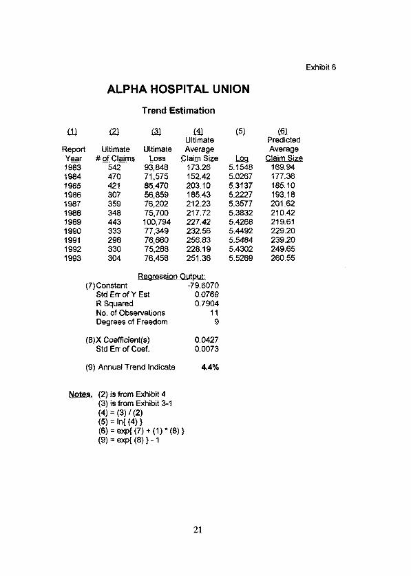
Exhibit 6


111 122

Report Ultimate YS # of Claims 1983 542 1984 470 1985 421 1986 307 1987 359 1988 348 1989 443 1990 333 1991 298 1992 330 1993 304

Trend Estimation

c3-l

Ultimate Loss

93.848 71:575 85,470 56,859 76,202 75,700 100,794 77,349 76,660 75,288 76.458

142 Ultimate Averaae

Claim size 173.26 152.42 203.10 185.43 212.23 217.72 227.42 232.56 256.83 228.19 251.36

s (7)Constant -79.6070

Std Err of Y Est 0.0769 R Squared 0.7904 No. of Observations 11 Degrees of Freedom 9

(8)X Coefficient(s) 0.0427 Std Er-r of Coef. 0.0073

(9) Annual Trend Indicate 4.4%

(2) is from Exhibit 4 Notes. (3) is from Exhibit 3-1

(4) = (3) I(2) (5) = M(4) 1 (6) = eti (7) + (1) l (8) 1 (9) = exp( (8) } - 1

-a 5.1548 5.0267 5.3137 5.2227 5.3577 5.3832 5.4268 5.4492 5.5464 5.4302 5.5269

@ Predicted AVeraQe

Claim size 169.94 177.36 185.10 193.18 201.62 210.42 219.61 229.20 239.20 249.65 260.55

21

Exhibit 7


The Development of Loses ThatWe@Open/V !%u@~~.v&ati~!~($

EvaluationYeg Report Year 1983 1984 1985 1986 1987 1988 1989 1990

1983 1984 1985 1986 1987 1988 1989 1990

Last3 Last5

Best3 of5

Selected

4 5 6 57,857 60,787 63,030 51,852 52,320 54,702 55,432 57,398 58,662 42,251 43,111 44,072 55,198 55,354 56,248 49,044 51,696 51,559 63,094 67,901 69,809 45,495 48,539 49,680

4-5 5-6 1.051 1.037 1.009 1.046 1.035 1.022 1.020 1.022 1.003 1.016 1.054 0.997 1.076 1.028 1.067 1.024

6-î 1.002 0.999 1.005 1.020 1.004 0.984 1.003

1.066 1.044 1.047

1.050

1.016 1.017 1.021

1.020

0.997 1.003 1.004

1.003

1.004 Cumulativer?;O75-1 1.024

z 63,160 54,629 58,956 44,942 56,445 50,747 70,010

7-8 0.993 0.996 1.003 1.004 0.997 1.004

1.001 1.001 1 .OOl

1.001

1.001

8 62,714 54,435 59,130 45,102 56,264 50,926

9 63,351 53,115 60,244 44,610 56,434

Ic? ll 63,325 63,285 53,251 53,613 60,083 60,148 44,722

8-9 1.010 0.976 1.019 0.989 1.003

9-Q 1.000 1.003 0.997 1.003

1QyJ1 -UA

0.999 1.000 1.007 1.000 1.001

1.004 1 .OOl 1.004 0.999 NIA NIA 0.996 N/A NIA

1.000

1.000

1 .ooo

1.000

1 .ooo 1.000

1.000 1 .ooo

ALPHA HOSPITAL UNION Exhibit 8

Number of Claims Distribution Analysis

Report FTE Yez ExDosure 1985 762.14 1986 798.19 1987 773.70 1988 834.66 1989 861.21 1990 836.91 1991 859.55 1992 834.09 1993 813.45

121 fa 141 Ult. Number Number of of Trended Claims > $3M

and Developed @ 1997 Claims > $3M __.~- ~~ !Zg?QS.U~Ce

13 14.328 7 7.367 5 5.428 1 1.006 6 5.852 3 3.011 0 0.000 4 4.028 0 0.000

1997-est. 840.00 6.00

(5) Ali Year Average 4.558

(‘3) All Year Variance 20.327

(7) Variance-to-Mean Ratio 4.460

(2) is Full Time Equivalents for AHU Notes. (3) is form Exhibit 5 (4) = (3) * 840 / (2), where 840 is

estimated FTE exposure for 1997 (5) and (6) are based on column (4)

23

ALPHA HOSPITAL UNION Exhibit 9

Severity Curve Fitting Results

Name of Distribution Loanormal Pareto

Type of Distribution Lognormal Pareto

Data Fitted To AH Claims AH Claims

Parameter Mu = 13.580 B = 4,978,593 Estimators Sigma = 0.861 Q = 6.313

Name of Distribution Loonormal - 2 Pareto - 2

Type of Distribution Lognormal Pareto

Data Fitted To Claims in Excess of $2 Mil Claims in Excess of $2 Mil

Parameter Mu = 14.979 B = 4,625,321 Estimators Sigma = 0.371 Q = 6.524

Name of Distribution Lognormal- 2.5

Type of Distribution Lognormal

Data Fitted To Claims in Excess of $2.5 Mil

Parameter Mu = 15.059 Estimators Sigma = 0.356

24

Exhibit 10

2,oo~ooo 11.86% 2,500,OOO 7.66% 3,000,000 5.09% 3,500,000 3.47% 4,000,000 2.42% 4,500,000 1.72% 5,000,000 1.24% 6,000,OOO 0.68% 7,000,000 0.39%

2,000,000 100.00% 2,500,OOO 79.26% 3,000,000 63.21% 3,500,000 46.29% 4,000,000 27.36% 4,500,000 16.04% 5,000,000 ll .32% 6,000,OOO 4.72% 7,000,000 1.96%

2,500,OOO 100.00% 3,000,000 79.77% 3,500,000 57.15% 4,000,000 34.53% 4,500,000 20.24% 5,000,000 14.28% 6,000,OOO 5.95% 7,000,000 2.48%

Empirical Pareto


Severity Curve Fitting Analysis

100.00% 64.61% 42.94% 29.25% 20.37% 14.47% 10.46% 5.72% 3.30%

100.00% 66.46% 45.28% 31.54% 22.40% 16.19% 8.86% 5.11%

Lognormal Pareto2 Lognorm-2

14.04% 9.59% 89.76% 9.05% 5.97% 74.74% 6.06% 3.83% 56.93% 4.19% 2.53% 40.48% 2.98% 1.72% 27.39% 2.17% 1.19% 17.91% 1.61% 0.84% 11.45% 0.93% 0.44% 4.51% 0.56% 0.24% 1.74%

100.00% 100.00% 100.00% 64.46% 62.21% 83.27% 43.19% 39.97% 63.43% 29.88% 26.41% 45.09% 21.23% 17.89% 30.51% 15.44% 12.38% 19.95% 11.44% 8.74% 12.76% 6.60% 4.59% 5.02% 4.02% 2.55% 1.94%

100.00% 100.00% 100.00% 67.00% 64.25% 76.17% 46.35% 42.45% 54.16% 32.94% 28.75% 36.64% 23.95% 19.92% 23.96% 17.75% 14.06% 15.32% 10.25% 7.38% 6.03% 6.24% 4.10% 2.33%

Lognorm-2.5

93.92% 82.13% 65.83% 48.98% 34.42% 23.21% 15.19% 6.17% 2.42%

100.00% 87.45% 70.10% 52.15% 36.65% 24.71% 16.17% 6.57% 2.57%

100.00% 80.15% 59.64% 41.91% 28.25% 18.49% 7.51% 2.94%

25

Exhibit ll


Goodness-of-Fit Test for Lognormal-2 Distribution

Range Number of Claims x2 From To Empirical Lognorm-2

2,000,000 2,500,OOO 22.00 17.74 1.024 2,500,OOO 3,000,000 17.00 21.03 0.774 3,000,000 3,500,000 19.00 19.43 0.010 3,500,000 4,000,000 19.00 15.46 0.812 4,000,000 4,500,000 12.00 11.19 0.058 4,500,000 5,000,000 5.00 7.63 0.904 5,000,000 6,000,OOO 7.00 8.20 0.176 6,000,OOO Infinity 5.00 5.32 0.020

106 106 ! 3.776 j

Degrees of Freedom 7

~2 (7) 10% Critica1 Value 12.017

~2 (7) 20% Critica1 Value 9.803

26

Alpha Hospital Uníon: Reinsuamce Program

Stochastic Simulation Worksheet

txnw iz

Number of Claims Distribution: N~&e..B&m.~a! Severity Distribution: J&~Ixx&

paametm: P 0.167 Pafam%S: r 1.000 15.059 Mu-l 3,694,545

0.356 Sigma-l 1,358,052 Number of ClaimS 14

Claim# 1 2 3 4 5 6 7 8 9 XI Ground Up 3.220,292 7,365,376 3,324,321 4,977,54? 3,079,357 6,009,490 3,117,650 4,010,786 4,590,674 4,480,066 Retained 3.000,000 3,000,000 3,000,000 3,000,000 3,000,000 3,000,000 3,000,000 3,ooo,OOo 3,000,000 3,000,000 1 -st Excess 220,292 3,000,000 324,321 1,9?7,541 79,357 3,000,000 117,650 280,839 0 0 2-nd Excess 0 1,365,376 0 0 0 9,490 0 729,947 1,590,674 1.480,0%

f: C!amY 11 12 13 14 15 25 17 IB 19 a2 Ground Up 3,674,992 3,346,734 5,064,726 3,929,901 0 0 0 0 0 0 Retained 3,000,000 3,000,000 3,000,000 3,000,000 0 0 0 0 0 0 1 -st Excess 0 0 0 0 0 0 0 0 0 0 2-nd Excess 674,992 346,734 2J64.726 929,901 0 0 0 0 0 0

1 -st Excess

2-nd Excess fTms¿iq

N 03

Exhibit 13

Exhibit 14


Simulation Statistics

Iterations = 20,000

Name 1-st Excess 2-nd Excess Cell L:B28 L:B30 Minimum = 0 0 Maximum = 9,000,000 12,000,000 Mean = 4,481,577 1,779,283 Std Deviation = 3,498,020 3,433,117 Variance = 1.224E+13 l.l79E+13 Skewness = 0.092 2.017 Kurtosis = 1.444 5.803 Mode = 9,000,000 0 5% Perc = 0 0 10% Perc = 0 0 15% Perc = 0 0 20% Perc = 417,546 0 25% Perc = 1,029,013 0 30% Perc = 1,591,121 0 35% Perc = 2,168,108 0 40% Perc = 2,805,473 0 45% Perc = 3,334,980 0 50% Perc = 4,088,441 0 55% Perc = 4,837,891 0 60% Perc = 5,682,205 0 65% Perc = 6,615,973 269,680 70% Perc = 7,713,470 813,716 75% Perc = 9,000,000 1,671,OlO 80% Perc = 9,000,OOO 2,967,957 85% Perc = 9,000,000 4,741,905 90% Perc = 9,000,OOO 7,617,267 95% Perc = 9,000,000 12,000,000 Target #i (Value)= 0 0 Target #1 (Perc%)= 16.67% 62.06% Target #2 (Value)= 9,000,000 12,000,000 Target #2 (Perc%)= 74.91% 94.70%

29

Exhibit 15


Pricing Recommendations

(1) ESTIMATED LOSS COST FOR THE LAYER

(2) COMMISSION

(3) BROKERAGE

(4) IXL AS % OF RISK PREM

(5) TER AS % OF PURE PREM

(6) LOSS DISCOUNT FACTOR

(7) RECOMMENDED REINSURANCE PREMIUM

1 -st Excess Layer

4,481,577

0.00%

5.00%

3.50%

15.00%

0.750

4,313,425

2-nd Exces Layer

1,779,283

0.00%

5.00%

5.00%

25.00%

0.550

1,445,770

30

An Application of Garne Theory: Property Catastrophe Risk Load by Donald F. Mango, FCAS

31

An Application of Game Theory: Property Catastrophe Risk Load’

Donald Mango, F.C.A.S.

Crum & Forster Insurance

Abstract

Two well-known methods for calculating risk load -- Marginal Surplus and Marginal Variance -- are applied to output from caiastrophe modeling software. Risk loads for these “marginal methods” are calculated for sample new and renewal accounts. Differences between new and renewal pricing are examined. For new situations, both current methods allocate the full marginal impact of addition of a new accounl lo that new account. For renewal situalions, a new concept is introduced -- “renewal additivity”. Neither marginal method is renewal additive. A new method is introduced, inspired by game theory, which splits the mutual covariance between any hvo accounts evenly behveen those accounts. The new method is extended and generalized to a proportional sharing of mutual covariance between any two accounts. Both new approaches are tested in new and renewal situations.

(1) Introduction

The calculation of risk load continues to be a topic of interest in the actuarial community -- see Bault [l] for a recent survey of well-known alternatives. One area where the CAS literature is somewhat scarce, and the need is great, is calculation of risk loads for property catastrophe insurance.

The new catastrophe modeling products produce modeled “occurrence size-of-loss distributions” for a series of simulated events. Using the occurrence size-of-loss distribution, one can easily calculate expected losses, loss variance and standard deviation. Two of the more well-known risk load methods from the CAS titerature -- what I call “Marginal Surplus” (MS) from Kreps [3] and “Marginal Variance” (MV) from Meyers [6] -- use the marginal change in portfolio standard deviation (respectively variance) due to addition of a new account as a means to calculate the risk load for that new account. However, as we shall see, problems arise when we use these marginal methods in calculating the risk loads for the renewal of the accounts in a portfolio.

We apply the MV and MS methods to a simplified occurrence size-of-loss distribution, calculate risk loads both in assembling or building up a potiolio of risks, and in subsequently renewing that por?folio. Then we discuss the differences between build-up and renewal results.

1 wuutd Iike to thank Eric Lemieux and Sean Uingsted for their suppoft, editorial soggestions and review of early drafts. / woufd also like fo fhank Paul Kneuer for bis fhoughtfu/ and insighfful review which improved me paper.

33

We then introduce a new concept to the theory of property catastrophe risk loads -- renewal additivity. However, the concept is not new to the field of game theory, where we will draw inspiration for a new approach.

We begin with a brief outline of the mechanics of catastrophe occurrence size-of-loss distributions, and the calculation of risk loads using the two marginal methods.

(2) The Catastroohe Occurrence Size-of-loss Distribution

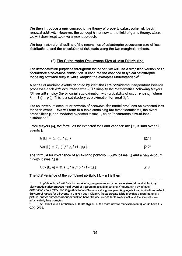
For demonstration purposes throughout the paper, we will use a simplified version of an occurrence size-of-loss distribution. It captures the essence of typical catastrophe modeling software output, while keeping the examples understandable’.

A series of modeled events denoted by identifíer i are considered independent Poisson processes each with occurrence rate h,. To simplify the mathematics, following Meyers [SI, we will employ the binomial approximation with probability of occurrence pi [where h, = -ln(l - p, )]. This is a satisfactoty approximation for small h, 3.

For an individual account or portfolio of accounts, the model produces an expected loss for each event Li. We will refer to a table containing the event identifiers i, the event probabilities pi and modeled expected losses Li as an “occurrence size-of-loss distribution.”

From Meyers [6], the formulas for expected loss and variance are [ Ci = sum over all events ]:

E Ll = Ci { 4 l pi >

Var [L] = Ci { Li2 ’ pi * (1 - pi) }

12.11

The formula for covariance of an existing portfolio L (with losses Li) and a new account n (with losses n,) is :

Cov [L, n] = Ci ( Li * n i * pi l (1 - pi) } 12.31

The total variance of the combined portfolio [ L + n ] is then

2 In particular, we will only be considering single event or occurrence size-of-loss distributions. Many models also produce multi-event or aggregate loss distributions. Occurrence size-of-loss distributions only reflect the largest event which occurs in a given year. Aggregate Ioss distributions reflect the sum of losses for all events in a given year. Clearly, the aggregate table provides a more complete picture, but for purposes of our exposition here, the occurrence table works well and the formulas are substantially less complex. 3 An event with a probability of 0.001 (typical of the more severe modeled events) would have h = 0.0010005.

34

Var [L] + Var [n] + 2 l Cov [L, n] 12.41

(3) The Marainal SurDlus (MS) Method

This is a translation to property catastrophe of the method described in Rodney Kreps’ “Reinsurer Risk Loads from Marginal Surplus Requirements” [3].

Consider:

L, = losses from a portfolio before a new account is added L, = losses from a portfolio after a new account is added S, = Standard deviation of LO S, = Standard deviation of L,

Borrowing from Mr. Kreps, assume needed surplus V is given by

z l Standard Deviation of loss - expected Return L3.11

where z is, to cite Mr. Kreps (p. 197), “a distribution percentage point corresponding to the acceptable probability that the actual result will require even more surplus than allocated.” Then

V,=r*S,-R, V, = z * S, - R, 13.21

The difference in returns R, - RO = r, the risk load charged to the new account. The marginal surplus requirement is then

V,-Vo=Z*fS,-S,]+r l3.31

We determine the risk load based on required return y on that marginal surplus, which is based on management goals, market forces and risk appetite. The MS risk load would be:

r = y*z/(l +y)*[S,-S,] 13.41

(4) The Marainal Variance fM# Method

This is based on Glenn Meyers’ 1995 CAS Discussion Paper program article “Managing the Catastrophe Risk” [SI.

Mr. Kreps sets needed surplus equal to z l standard deviation of return - expected return. If we assume premiums and expenses are invariant, then VaflReturn] = Var[P - E - L] = Va@-].

35

For an existing pottfolio L and a new account n, the MV risk load would be:

r = h * Marginal Variance of adding n to L =h*{Var[n]+2*Cov[L,n]} l4.11

where k is a multiplier similar to y * z / (1 + y ) from the MS method, although dimensioned to apply to variance rather than standard deviatior?.

(5) Buildina UD a Portfolio of 2 Accounts

Now we are prepared to apply the methods to the sample portfolio. Table A shows the occurrence size-of-loss distribution and risk load calculations for building up (assembling) a portfolio of 2 accounts, (X) and (Y). We assume (X) is written ftrst, and is the only risk in the portfolio until (Y) is written.

(5.1) MS Method Here is a summary of pertinent values from Table A for the Marginal Surplus method:

Table 5.1

:ount (X) ) Account (Y) 1 Account (X) 1 Account ] Building Up (X) & (Y): Acc Marginal Surplus + Account (Y) 1 (X + v

(1) Change in Standard 4,429 1 356 4,785 1 4,785 Ueviation

(2) Risk Load Multiplier 0.33 0.33 0.33

(3) Risk Load = (1) l (2) $1.461.71 $117.43 $1,579.14 $1,579.14

* Item (1) is the change in portfolio standard deviation from adding each account, or margina/ standard deviation.

l Item (2) is the Risk Load multiplier of 0.33. Using Mr. Kreps’ formula, a return on marginal surplus y of 20% and a standard normal multiplier z of 2.0 (2 standard deviations, corresponding to a cumulative non-exceedance probability of 97.725%) would produce a risk load multiplier of

y'z/(l +y) = 0.20*211.20 = 0.33 (rounded) l5.11

* Item (3) is the Risk Load, the product of Items (1) and (2).

5 Mr. Meyers develops a variance based risk load multiplier by converting a standard deviation based multiplier using the following formula:

X = (Rate of Return l Std Dev Mult’) / (2 l Avg Capital of Competitors)

36

Since (X) is the first account, the marginal standard deviation from adding (X) equals the standard deviation of (X) (Std Dev [X]) of 4,429. This gives a risk load of $1,461.71,

The marginal standard deviation from writing (Y) equals Std Dev [X + Y] - Std Dev [XI, or $356, implying a risk load of $117.43.

The sum of these two risk loads (X) + (Y) is $1,461.71 + $117.43 = $1,579.14. This equals the risk load which this method would calculate for the combined account (X + YI.

(5.2) MV Method Here is a summary of pertinent values from Table A for the Marginal Varíance method:

Table 5.2

Bui/cBng Up (X) & (v): Account (X) Account (Y) Account (X) Account Marginal Varíance + Account (Y) (X + Y)

(1) Change in Variance 19,619,900 3,279,059 22,898,959 22,898,959

(2) Risk Load Multiplier 0.000069 0.000069 0.000069

(3) Risk Load = (1) l (2) $1,353.02 $226.13 $1,579.14 $1,579.14

l Item (1) is the change in portfolio variance from adding each account, or marginal variance.

l ltem (2) is the Variance Risk Load multíplier h of 0.000069. To simplify comparisons between the two methods (recognizing the difficulty of selecting a MV-based multiplierô), I converted the MS multiplier to a MV basis by dividing by Std Dev [X + yl:

h = 0.33 l 1,579.14 = 0.000069 15.21

This means the total risk load calcuiated for the portfolio by the two methods will be the same, although the individual risk loads for (X) and (Y) will differ between the methods.

l Item (3) is the Risk Load, the product of Items (1) and (2).

Since (X) is the fir.st account, the marginal variance from adding (X) equals the variance of (X) (Var [X]) of 19,619,900. This gives a risk load of $1,353.02.

The marginal variance from writing (Y) equals Var [X + v] - Var [XI, or $3,279,059, implying a risk load of $226.13.

6 Mr. Meyers (61 (p.124) admits that in practice “it might be difficult for an insurer to obtain the (lambdas) of each of its competitors.” He goes on to soggest an approximate method to arrive al a usabte lambda based on required capital being ‘Z standard deviations of the total loss distribution.”

37

The sum of these two risk loads (X) + (Y) is $1,353.02 + $226.13 = $1,579.14. This equals the risk load which this method would calculate for the combined account (X + w.

(6) Renewina the Portfolio of 2 Acccunts

Table B shows the natural extension of the Build-up scenario - renewal of these 2 accounts, in what could be termed a “static” or “steady state” portfolio (one with no new entrants).

As for applying these methods in the renewal scenario, renewing policy (X) is assumed equivalent to adding (X) to a portfolio of (Y); renewing (Y) is assumed equivalent to addìng (Y) to a portfolio of (X).

(6.1) MS Method Here is a summary of pertinent values from Table B for the Marginal Surplus method:

Table 6.1

The marginal standard deviation for adding (Y) to (X) is 356, same as it was during Build-up -- see Section (5.1). The risk load of $117.43 is also the same.

However, adding (X) to (Y) gives a marginal standard deviation of Std Dev [X + v] - Std Dev M , or 4,171. This gives a risk load for (X) of $1.376.27, which is (85.45) less than $1,461.71, the risk load for (X) calculated in Section (5.1).

The sum of these two risk loads is $1,376.27 + $117.43 = $1,493.70. This is also (85.45) less than the total risk load from Section (5.1).

(6.2) MV Method Here is a summary of pertinent values from Table B for the Marginal Variance method:

38

Table 6.2

The marginal variance for adding (Y) to (X) is 3,279,059, same as it was during Build-up -- see Section (5.2). The risk load of $226.13 is also the same.

However, adding (X) to (Y) gives a marginal variance of Var [X + v] - Var M, or 22521,000. The risk load is now $1,553.08, which is $200.06 more than the $1,353.02 calculated in Section (5.2).

The sum of these two risk ioads is $1,553.08 + $226.13 = $1,779.21. This is also $200.06 more than the total risk load from Section (5.2).

(7) ExDiorina the Differences Between New and Renewal

Why are the total Renewal risk loads different f’rom the total Build-up risk loads?

(7.1) MS Method In SeCtiOn (5.1) Build-up, the marginal standard deviation for (X), AStd Dev [X], was :

AStd Dev M = Std Dev [X] = SQRT[L, {X;*p,*(l-p,)} 1,

(Xi = modeleed losses for X for event i] i7.11

while in Section (6.1) Renewal, the marginal standard deviation was

AStd Dev DC] = Std Dev [X + YJ - Std Dev M = SQRT [ Ci { (X,+Y,)’ * pi * (1 - pi) ) ] -

SQRT[ri {Y,‘*p,*(I -pi)}] (7.21

For positive Yi, this value ís less than Std Dev [Xj7. Therefore, we would expect the Renewal risk load to be less than the Buitd-up.

I For example. assume Var [X) = 9. Var M = 4, Cov [X, v] = 1.5; then AStd Dev [x] = Sqrt(Var [X) ) = Sqrf (9) = 3 for X alone AStd Dev [Xj = Sqrt(9 + 4 + 2’1.5) - Sqrt(4) = 4 - 2 = 2 < 3. for X added fo Y

39

Unfortunately, when the MS method is applied in the renewal of all the accounts in a portfolio, the sum of the individual risk loads will be less than the total portfolio standard deviation times the multiplier. This is because the sum of the marginal standard deviations (found by taking the difference in portfolio standard deviation with and without each account in the portfolio) is less than the total portfolio standard deviation*. This is because the square root operator is “sub-additive”: the square root of a sum is less than the sum of the square rootss.

(7.2) MV Method In Section (5.2) Build-up, the marginal variance AVar [X] was

AVar [X] = Var [X] = c, { x; * p, * (1 - pi) 1. 17.31

while in Section (6.2) Renewal the marginal variance was

AVar [X] = Var [X + v] - Var M = {Var[X]+2*Cov[X,Y] +Ver+!j)-q 17.41 = Var [X] + 2 * Cov [X, v] z Var [XI.

Since 2 l Cov [X, u] is greater than zero, we would expect the Renewal risk load to be greater than the Build-up.

However, when the MV method is applied in the renewal of all the accounts in a portfolio, the sum of the individual risk loads will be more than the total portfolio variance times the multiplier. This is because the sum of the marginal variances (found by taking the difference in portfolio variance with and without each account in the portfolio) is greater than the total portfolio variance. The covariance between any two risks in the portfolio is double counted: when each account renews, it is allocated the full amount of its shared covariance with all the other accounts.

The renewal scenarios point out that these two methods are not what I call “renewal additive,” defined as follows:

For a given portfolio of accounts, a risk load method is renewal additive if the sum of the renewal risk toads calculated for each component account equals the risk load calculated when the combined accounts are treated as a single account.

8 The same issue is raised in Mr. Gogol’s discussion 121. 9 For example. Sqrl[S + 16) c Sqtt[S] + Sqrl[lG].

40

Neither the MS nor the MV method is renewal additive: MS because the square root operator is sub-additive; MV because the covariance is double counted. In order for them to be renewal additive, one must assume an entry order for the accounts.

It’s a puuling predicament. We apply the risk load formula for the renewal of account (X). The formula makes sense for the renewal of account (X). It also makes sense for the renewal of account (Y). However, the portfolio total does not make sense. We could say that in the renewal context, these methods were “individually rational” yet the total was not “collectively rational”.

I chose these terms deliberately as a segue to the next section. They come from the field of game theory. These concepts and others (including additivity) have been studied extensively by game theorists, and their results will provide us with inspiration for a new approach.

(9) A New ADDrOaCh from Game Theorv

I focused on ideas in two papers by Jean Lemaire: “An Application of Game Theory: Cost Allocation” [4], and “Cooperative Game Theory and Its Insurance Appiications” 251. In both papers, Mr. Lemaire considers the insurance applications of results from “cooperative games with transferable utílities”‘O.

The material can be daunting. To facilitate the discussion, I will combine and paraphrase the formal game theory definitions from both of Mr. Lemaire’s papers, then follow wíth translations to our problem”.

Basics “A n-person cooperative game with transferable utilities is a pair [N, v(S)] where N = {l, 2, . . . . n} is the set of the players, and v(S), the characteristic function of the game, is a super-additive’* set function that associates a real number v(S) with each coalition S of players” ([4], p. 68).

II) Citing Mr. Lemaire [5] (p.20) : “Cooperative game theory analyzes those situations where participants’ objectives are partiatly cooperative and partially conflicting. It is in the participants’ interest to cooperate, in arder to achieve the greatesl possible total benefits. When it comes to sharing the benefits of cooperation, however, individuals have conflicting goals.... Partticipants are negotiating about sharing a given commodtty (such as money or political power) which is fully transferable between players and evaluated in the sarne way by everyone.... For this reason, the class of games defined here is cailed ‘Cooperative games with transferable utilities.”

In our case, the conflicting goals arise because all but the largest risks must have catastrophe coverage, and must go for this coverage to an insurance company. Insurance companies write many such risks, whlch means they have loss covariance created by the pooling of risks exposed to the same potential catastrophic events. The desire for coverage conftlcts with the desire to be atlocated the teast covariance. II Those wishing a more detailed explanation are strongly encouraged to read Mr. Lemaire’s papers. 12 Super-additivity is defined as follows: for S, T any two disjoint coalitions. and a characteristic function v. super-additivity implies v(S) + v(T) <= v(S union T).

41

Translation: l Player = account. l Coalition S = portfolio. l Characteristic function v(S) = portfolio variance (super-additive because of the covariance component).

Imoutation, Individual rationalitv. additivitv “An imputation is a vector y = (y,, . . . . y,) such that yi >= v(i) for every i, and IX ¡=,, ,,y, = v(N)” ([5] p. 68).

Translation: l Imputation = allocation of the coalition total value V(N) back to the individual members.

l The first condition (y, >= v(i) for evety i) is known as “individual rationality” -- each member’s allocation y, is no smaller than its value would be were it on its own ( = v(i)).

l The second condition (Xi=,, ,o ,yi = v(N)) is known as “additivity” - the sum of the individual allocations must add up to the coalition total value.

In our problem, the imputation is each account’s marginal variance (under the MV method) from adding it to the remainder of the portfolio. This imputation is individually rational, since the allocations are larger than the individual account variances because of the covariance component. However, as we have seen, it is not additive -- the sum of the individual allocations (marginal variances) is greater than the total variance.

Collective rationalitv and the Core “An imputation is collectively rabona1 if there is no sub-coalition S’ under which the players are better off than they were under S.

“The core of the game is the set of all collectively rational imputations.” ([5], p. 25)

Translation: l Collectively rabona1 = the coalition is stable -- there is no incentive for players to split off and form factions.

l The core sets the boundartes for possible, stable allocations.

Shaolev value “The Shapley value is the center of gravity of the core’s extrema1 points.” ([4], p. 72)

Translation: The Shapley value is the only allocation which satisfies the following three axioms ([4], p. 69):

42

1. Symmetty (Order-inclependence) - for all permutations P(S) of accounts in a portfoiio S, c(S) = c(P(S)). Knowing the combination of accounts is sufficient to have an additive allocation.

2. Inessential Plavers (Uncorreiated accounts) - if an account generates no covariance with the existing portfolio, it is simply ailocated its own variance, and nothing more.

3. Additivity - allocations from distinct games should be additive. This particular condition has no parallel in our situation.

Only one allocation method satisfies these three axioms -- the “Shapley value”. It equals the average allocation taken over all possible entrance permutations -- the different orders in which a new member could have been added to the coalition’3 (Le. a new account could have been added to a portfolio).

For example, if we had a portfolio of accounts (A), (B), and (C), and we want to add a new account (D), we could consider the marginal variance for adding (D) in all the following entrance permutations:

Table 9.1 Entry Permutations for Account D

._-... __._ _ ..- -__-~ ..____ __- 13 Mr. Lemaire [5] provides this more complete definition of the Shapley value (p. 29): “The Shapley value can be interpfeted as the mathematical expectatiin of the admission value, when aft orders of formation of the grand coalitin are equiprobable. In computing the value, one can assume. for conveniente, that all players enter the grand coalition one by one, each of them receiving the entire benefits he brings to the coalition formed just before him. All orders of formation of N are considered and intervene with the same weight Un! in the computation. The combinatoria1 coefficient results from the fact that there are (s-l)!(n-s)l ways for a @ayer to be the last to enter coalition S: the (s-l) other players of S and the (n-s) players of N\S (thoseplayets in N which are not in S - DM) can be permuted without affecting jis position.”

43

8 Fourth After (ABC) Var [D] + 2’Cov [D, A] + 2’Cov [D, B] + P*Cov [D, C]

The Shapley value is the straight average of Column (4) Marginal Variance over the eight permutations:

Shapley Value ={Sum[Column(4)]}/8

= { b*Var ID] + 8”Cov [D, A] + 8*Cov [D, B] +

P.11

8*Cov [D, C] } / 8

= Var [D] + Cov [D, A] + Cov [D, B] + Cov [D, C]

Or, to generalize, given

L = losses for existing portfolio n = losses for new account

Shapley Value = Var[n]+Cov[L,n]. WI

Before seeing this result, we might have been concerned about the practicality of this approach - how much computational time míght be required to calculate all the possible entrance permutations for a portfolio of thousands of accounts? This simple reduction formula eliminates those concerns. The Shapley value is as simple to calculate as the marginal variance.

Comparing the Shapley value to the marginal variance formula from Section 4:

Marginal Variance =Var[n]+2’Cov[L,n], WI

we note the Shapley value only takes 1 times the covariance of the new account and the existing portfolio.

We can also calculate the Shapley value under the marginal standard deviation method. However, due to the complex nature of the mathematics -- differences of square roots of sums of products -- no simplifying reduction formula was immediately apparenP.

Therefore, we will focus going forward on the MV method and the variance-based Shapley value. Life will be much easier (mathematically) working with the variances,

~ -~~..- -.~ II Please contact the author if you can successfully reduce formulas involving the average of the difference of square roots of sums of products.

44

and we lose very little by choosing variance. Citing Mr. Bault ([ll, p. 821, from a risk load perspective, “both [variance and standard deviation) are simply special cases of a unifying covariance framework.” In fact, Mr. Bault goes on to suggest “in most cases, tbe ‘oorrect’ answer is a marginal risk approach that incorporates covariance”‘5.

(10) Sharina the Covariance

The risk load question, framed in a’game-theoretical light, has now become:

How do accounts share tbeir mutual covariance for purposes of calculating risk load?

The Shapley method answers, “Accounts split their mutual covariance equally.” At first glance this appears reasonabíe, but consider the following example.

Assume two accounts, (L) and (M). (M) has 100 times the losses of (L) for each event. Their total shared covariance is

2 * Cov(L, M)= 2 * Ci { Li l M, * p, * (1 - pi) } = 2 ‘C, {Li * IOOL, * pi * (1 -pi)} [IO.l]

The Shapley value would equally divide this total covariance between (L) and (M), even though their relative contributions to the total are clearty not equal. There is no question that (L) should be assessed some share of the covariance. The issue is whether there is a more equitable share than simply half.

We can develop a generalized covariance sharing (GCS) method which uses a weight W/(L, X) to determine (L)‘s share of the mutual covartance between itself and account (X) for event i:

CovShareF (L, X) = W,L(L, X) * 2 * Li * xi * pi + (1 - pJ [l 0.23

Then (X)3 share of that mutual covariance would simply be

CovShareix (L, X) = (i - W,L(L, X)] l 2 ’ Li ex, * p, l (1 - pi)

The total covariance share allocation for (L) over all events would be

CovShare,,L = Zz Zi { CovShare:(L, Z) } { C, = sum over every other account in the portfolio } I10.41

16 Mr. Kreps [3] also incorporates covariance in his “Reluctante” R (p. 198), which has the formula R = [yz/(l+y)]/(PSC + o)/(S’ + S), where C is the correlation of the contract with the existing book. The Risk Load is then equal to Ra.

45

The Shapley method is a generalized covariance sharing method with W:(L, X) = 50% for all (L), (X), and i.

Returning to the example with (L) and (M), we can develop an example of a weighting scheme which assigns the shared covariance by event to each in proportion to their loss for that event. W,L(L, M), account (L)‘s share of the mutual covariance between itself and account (M) for event i, equals

W,L(L, M) = [ Li / [ Li + M, ] ] [10.5] = [ Li / [ Li + IOOL, ] ] = (1 1101) = roughly 1% of their mutual covariance for event i

We will call this the “Covariance Share” (CS) method.

(ll) Awlvincr the Shaolev and CS Methods to the Examole

Now we will see how the Shapley and CS methods petform in our 2 Account example for both Build-up and Renewal.

(ll .l) Portfolio Suild-uo Table C shows the Build-up of accounts (X) and (Y) from Section 5, but for the Shapley and CS methods. Here is a summary of the pertinent values from Table C for the Shapley value:

Table Il .1

Building Up (X) & (V): Account (X) Account (Y) Account (X) Account Sbepley Value + Account (Y) (X + Y)

(1) Change in Variance 19,619,900 1,828,509 21,448,409 22,898,959

(2) Risk Load Multiplier 0.000069 0.000069 - 0.000069

(3) Risk Load = (1) l (2) $1,353.02 $126.10 $1,479.11 $1,579.14

and for the Covariance Share:

Table ll .2 Building Up (X) & (v): Account (X) Account (Y) Account (X) Account

Covariance Share + Account (Y) (X + Y) (1) Change in Variance 19,619,900 950,658 20,570,558 22,898,959 (2) Risk Load Multiplier 0.000069 0.000069 0.000069 (3) Risk Load = (1) * (2) $1,353.02 $65.56 $1,418.57 $1,579.14

46

Both Shapley and CS produce the same risk load for (X) as the MV method on build-up - $1,353.02. This is because there is no covariance to share - (X) is the entire portfolio at this point. However, let’s compare the results of the three variance-based methods for account (Y):

Table ll .3

Comparison of Build-up Risk Loads for Account (Y)

Marginal Variance (MV) - $226.13 Section 5.2

Shapley Value $126.10

Difference from MV $100.03

Covariance Share (CSI $65.56

l Difference ffom MV l $~6&57l

Compared to MV, which charges account (Y) for the full increase in variance (Var p/l + 2* Cov pC, YJ), the Shapley method only charges (Y) for Var M + Cov [X, YJ The same can be said for the CS method, although the share of the mutual covariance depends on each account’s relative contribution by event, weighted and summed over all events. Let’s see what happens to that difference from MV upon renewal.

(11.3) Renewal Table D shows the renewal of (X) and (Y) for the Shapley and CS methods. Here is a summary of pertinent values from Table D for the Shapley method:

Table ll .4 Renewing (X) @I r/): Account (X) Account (Y) Account (X) Account

Shapley Value + Account (Y) (X + Y) (1) Change in Variance 21,070,450 1,828,509 22,898,959 22,898,959

(2) Risk Load Multiplier 0.000069 0.000069 0.000069 . (3) Risk Load = (l)‘* (2) $1,453.05 $126.10 $1,579.14 $1,579.14

(4) Build-up Risk Load $1,353.02 $126.10 $1,479.11 $1,579.14

(5) Difference $100.03 $0 $100.03 $0

and for the Covariance Share method:

Table ll .5 Renewing (X) & r/): Account (X) Account (Y) Account (X) Account Covariance Share + Account (Y) (X + v

47

With both the Shapley and CS methods, the sum of the risk loads for Account (X) and Account (Y) equals the risk load for Account (X + Y), namely $1,579.14. This means we have two renewal additive methods, which also means they are legitimate imputations.

To see what happened to difference from MV, compare the risk loads calculated at renewal for (X) with those at build-up:

Table Il .6

Build-up VS Renewal Risk Shapley Cov Share Loads for Account (X)

Renewal $1,453.05 $1,513.59

Build-up $1,353.02 $1,353.02

Additional Renewal Risk Load $100.03 $160.57 over Build-up

Difference from MV $100.03 $160.57

The difference from MV during build-up is simply the portion of (X)‘s risk load attributable to its share of covariance with (Y). It was missed during build-up because it was unknown -- account (Y) had not been written.

(12) Conclusion

These new approaches address the concerns with renewal additivity, and point out the issue of covariance sharing between accounts. Perhaps the ideal solution might involve using a marginal method for the pricing of new accounts, and a renewal additive method for renewals. Any number of variations are possible, as long as one avoids double-counting the covariance.

It is hoped that this paper has also set the stage for further discussion of order dependency. This is a complex issue which was only touched on here, but which moves more to the forefront as advances in computer technology and modeling make ever finer levels of analysis possible.

48

References

fl] Bault, Todd, Discussion of Feldblum: “Risk Loads for Insurers,” PCAS LXXXII, 1995, pp. 78-96.

[Z] Gogoi, Daniel F., Discussion of Kreps: “Reinsurer Risk Loads from Marginal Surplus Requirements,” PCAS LXXIX, 1992, pp. 362-366.

[3] Kreps, Rodney, “Reinsurer Risk Loads from Marginal Surplus Requirements,” PCAS LXXVII, 1990, pp. 196-203.

[4] Lemaire, Jean, “An Application of Game Theory: Cost Allocation,” ASTIN Bulletin, Val. 14, No. 1, 1984, pp. 61-82.

[5] Lemaire, Jean, “Cooperative Game Theory and its Insurance Applications,” ASTIN Bulletin, Vol. 21. No. 1, 1991, pp. 17-40.

[6] Meyers, Glenn, “Managing the Catastrophe Risk,” Incorporatir~g Risk Factors in Dynamic Financial Analysb, Casualty Actuarial Society Discussion Paper Program, 1995, pp. ll l-150.

49

Table (A) Build a Portfolio of 2

Ent i p(i) j 1 Loss for Risk

l-P(i) ( (X) ( MI (X + Y)

: - 2.0% 1 .O% 98.0% 99.0% ~25.000 15,000 200 500 1 25,200 15.500 3.0% 97.0% 10.000 3wJO 13.000 3.0% 97.0% 8,000 1,000 9JwJ 1 .O% 99.0% 5.m 2,000 7,000 2.0% 98.0% 2,500 1.500 4,000

E[L] 1 1.2901 179 1,469 Var[L] j 19.619.900 j 377,959 22.898.959

Std DeviL] 1 4,429 / 615 4,765

covar 1 (X) 1 (X) 1 19.619,900 1

M. 1,450.550.

(Yj I 1,450.550 1 377.959.

00 M (x)+(YJ Change in Std Deviation 4.171 356 4,526

Risk Load (Std Dev) X376.27 117.43 1.493.70 0.33 1 Risk Load (A) 1,461.71 117.43 1.579.14

1 Dirraran~ (85.451, (85.45)

jII / [

“;~w~ “ti;: 22,521,OOo 1.553.08 j /

3,279.059 226.13 25.600.059 1.779.21 0.000069 1 Risk Load (A) 1.353.02 226.13 1.579.14

j Differmxi 200.06) 200.06

Table (B) Renew the Portfolio of 2 Risks

( Event ij PQI I

l-P(i) [ Loss for Risk

(X) [ MI (X + Y)

98.090 25,000 200 25,200 99.0% 15,000 500 15,500 97.0% 10,000 3,000 13,000 97.0% &oao 1,000 9,000 99.0% 5.000 2,000 7,000 98.0% 2,500 1,500 4,000

E[L] 1 1.29or 1791 1,469 VafJL] /

/ 19,6- 22.898.959

Std Dev[L] 4,429 / 615 ] 4.785

Covar ( 3) ( M (X)) 19.619.900 / 1,450.550 (Y) / _t.450.550 l 377.959

.~ (X) 0 (x)+py

Change in Std Deviation 4,171 356 4,526 117.43 1,493.70 117.43 1.579.14

(85.45)

Changa in Variance -22.521.000 3.279.059 25.800.059 Risk Load

r 0.000069 / (Variance) Risk LoadfA)

1.553.08 226.13 1.353.02 226.13 1.779.21 1.579.14

/ Difremncíi 200.06 2So.06

50

Table (C) Build a Portfolio of 2 Risks - Alternatives

covnrlsntsshnfn 1 21.948,301 950.6581 22,698,859 RirkLondEovShere) / 1,613.69 65.56j M79.14

O.LIOOO69 1 Rlsk Load (Ci 1353.02 65.58 1 1 Dlffemm+ 100.57 =D&mdRisk Loadtofn(Cf 1 11

--- _________.~. __

Table (El) Renew the Portfolio of 2 Risks - Alternatives

1 CovadanceShare$ ' 1 Eventi( P(i) / l-P(I)/ WI d

: 2.0% 1.0% 98.0% 99.0% 14,516.129 9920,635 -463.671 79,365

3 3.0% 97.0% 46.153.646 13,646.154 4 3.0% 97.0% 14.222222 1,777,776 5 1.0% 99.0% 14,266,714 5.714.266 6 2.0% 98.0% 4,667.596 1 2.612.500

Total r 2.326.401 1 572.6991 2901,100 L

Shapleyvalue RbkLoad(Shap&y)

0.000069 1

/ 21.070.450 1828.509 1 ' 22.898.959 [ 1.453.05 126.10[ 1.579.14

1.353.02 126.101 100.03 =DefemdRisk Loadfrom[C~ !

/

51

Levels of Determinism in Workers Compensation

Reinsurance Commutations by Gary Blumsohn, KAS

53

Levels of Determinism in Workers’ Compensation Reinsurance Commutations

Gary Blumsohn

Abstract

When commuting workers’ compensation reinsurance claims, the standard

method is to project the future value of the claims using stated assumptions for future medical usage, medical inflation, COLAS, and investment income. The actuary selects a best guess for each variable, and assumes this

deterministic number will be realized in the future. To account for the date of death being stochastic, a mortality table is used to model the future lifetime.

By assuming deterministic values for future medical usage, medical inflation,

COLAS, and investment income, the calculation ignores the possibilities of higher or lower values. It is shown that these do not generally balance out, and that the standard method produces biased results. In low reinsurance

layers, the commutation amount is overstated, and ín high layers it is

understated. By removing deterministic assumptions from the calculation, bias is removed from the results. The paper gives a detailed, realistic, example to illustrate this.

The implications of the paper reach beyond the narrow realm of workers’ compensation reinsurance commutations. The most obvious implications are for workers’ compensation reserving, but the essential message applies to

pricing and reserving of any excess insurance and reinsurance: deterministic assumptions often Iead to biased results.

Biography

Gary Blumsohn, FCAS, is an Associate Actuary with the Liberty Mutual

Group, where he is the actuary responsible for reinsurance. Prior to that he worked at Prudential Reinsurance Company. He has a Bachelor of Economic Science degree from the University of the Witwatersrand (Johannesburg,

South Africa) and a Ph.D. jn economics from New York University. His dissertation was on the impact of changing knowledge on the size of damages

in tort and securities law.

[1 am grateful to the following people for providing comments on earlier drafts of this paper: Eric Brosius, Sholom Feldblum, Joe Gilles, Mike Teng, Bryan Ware, and Wendy Witmer. They helped to improve the paper and

avoid some embarrassing mistakes. Any further mistakes, embarrassing or

otherwise, are my responsibility.]

56

Introduction

Excess reinsurance for workers’ compensation generally pays out over many decades. While workers’ compensation claims are usually reported to the insurer soon after the accident, and the insurer may soon report them to the

reinsurer, the loss payments are slow, being made over the Iifetime of the injured worker or even the lifetime of uninjured dependents. Consequently, even for reinsurance with a relatively modest retention, it can take many

years to breach the retention, and many more years to exhaust a layer. For example, Gary Venter (1995) has estimated that it takes, on average, over 30 years to pay half the ultimate claim amount.

At some point after an excess reinsurance treaty ends, but before the losses have been fully paid, it is common to commute either the reinsurance treaty or the individual reinsured claims. The commutation is a transaction whereby the reinsurer pays the ceding company a flat amount, in exchange

for canceling future liabilities. This saves costs for both parties, since the

expense of submitting claims to the reinsurer and the cost of paying these claims are eliminated. It allows the parties to shut their reinsurance files and spend their time on more profitable activities.

The actuarial techniques for evaluating workers’ compensation commutations differ from the techniques generally used in commutations of other lines of business. With workers’ compensation (and in some other cases, like unlimited medical benefits for no-fault auto) the population of claims is generally known at the time of the commutation - there is very

little lag in claims being reported to the primary company. Also, the amount of the payments is not dependent on some future court verdict. The payments are based on a fixed annual indemnity amount, subject, in some

states, to an annual cost of living adjustment, and on the actual medical

payments to be incurred by the claimant. In the case of peimanent-total disability cases, these payments often continue for the rest of the claimant’s life. Since the losses are so closely tied to the claimant’s life span, it is natural to use the mortality techniques more generally associated with life actuaries than with their property/casualty brethren.

57

While the actuarial techniques in these calculations are by now well accepted, this paper will argue that the results are systematically biased and can be

improved upon. The life-table techniques generally assume that mortality is stochastic, but that various other variables (amount of medical care, inflation

rates, investment yields) are deterministic. These deterministic variables can be stripped away, much as earlier actuaries stripped away the assumption of deterministic mortality. By doing this, we improve the accuracy of our calculations and eliminate some biases.

Though this paper will express the issues in terms of commutations, the issues are similar when doing excess workers’ compensation case reserving using life-table methods. In other words, even though there are layers that

we do not expect to get hit, we should carry reserves for those layers. Over a pool of claimants, some will die before hitting the upper layers, and others will not. The goal should be to get the reserves right on average.

Life-Tabie Techniaues

Method 1: Totally deterministic calculation

The simplest method for performing the calculation is to assume the claimant will live to his life expectancy and then calculate the present value

of the future stream of payments for this time. This method, though simple and appealing, is wrong. As actuaries are well aware, and as will be discussed

in detail later, assuming a deterministic life-span leads to systematically incorrect results.

Method 2: Stochastic date of death

The actuarial literature contains severa1 papers that discuss the calculation of

reserves for long-term workers’ compensation cases, and the calculation of a

commutation value only differs in minor respects from the calculation of a

58

reserve.’ It is generally accepted among actuaríes, and, to a iesser extent, the

wider insurance community, that the right way to reserve these claims is

through the life-table techniques routinely used by life actuaries. The big advance of the life-table method over a method that assumes the insured will live to his exact life expectancy is that it takes into account the probabilities of

the claimant dying either earlier or later than the life expectancy. This is particularly important when dealing with excess reinsurance, because if the

claimant lives beyond his life expeetancy, a higher layer may be breached.

The move from a deterministic number of payments to a stochastic number

of payments, through the use of a life table, is a crucial advance in the accuracy of the calculation. A life-table approach allows for the possibility that a claimant may live to age 95, and hence pierce reinsurance layers that would

not have been pierced if he had died at his Iife expectancy. Thus, in

calculating the value of a commutation for a high reinsurance layer, there may be a positive amount in a layer, even though the layer will not be hit

unless the claimant lives well beyond his life expectancy. In other words, if the claimant lives to his life expectancy of, say, 75, a retention of $5 million

may not be breached. But if he lives another 10 years, to 85, the total payments in the additional 10 years of life may be enough to breach the $5 million retention.

Put another way, there will be a positive commutation amount in layers that we do not expect to get hit. The commutation is (effectively) a purchase of

reinsurance by the reinsurer, covering the possibility of the claimant breaching the retention. There need not be a guarantee that the retention will be breached in order for the expected losses ín the layer to be positive.

1 The classic paper is Ronald Ferguson’s Actuarial Note on Workmen’s Compensution Loss Reserves (1971), which applied life-table methods to excess indemnity reserves. He did not

address the issue of the medical portion of the reserve. Richard Snader (1987) appiied similar

methods to long-term medical ciaíms. A recent valuable addition to the Iiterature is by Lee

Steeneck (199~3, who uses an analysis very cfose to the “Method 2” that will be discussed later

in this paper.

59

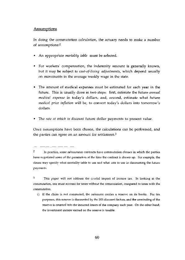
AssumWions

In doing the commutation calculation, the actuary needs to make a number of assumptions:2

l An appropriate mortalify table must be selected.

l For workers’ compensation, the indemnity amount is generally known, but it may be subject to cost-of-living adjustments, which depend usually on movements in the average weekly wage in the state.

l The amount of medical expenses must be estimated for each year in the future. This is usually done in two steps: first, estimate the future annuaf medical expense in today’s dollars, and, second, estimate what future

medical price inflation will be, to convert today’s dollars into tomorrow’s dollars.

l The rafe at which fo discount future dollar payments to present value.

Once assumptions have been chosen, the calculations can be performed, and the parties can agree on an amount for settiement.3

2 In practice, some reinsurance contracts have commutation clauses in which the parties

have negotiated some of the parameters at the time the contract is drawn up. For example, the

clause may specify what mortality table to use and what rate to use in discounting the future

payments.

3 This paper will not address the crucial impact of income tax. In looking at the

commutation, one must account for taxes without the commutation, compared to taxes with the

commutation.

i) If the claim is not commuted, the reinsurer carries a reserve on its books. For tax

purposes, this reserve is discounted by the IRS discount factors, and the unwinding of the

reserve is counted into the incurred losses of the company each year. On the other hand,

the investment income eamed on the reserve is taxable.

60

The problem, though, as this paper will show, is that the life-table method ignores fluctuations in other key variables. Just as it is wrong to assume a claimant’s life-span ís fixed, so it is wrong to assume that medical usage and

inflaiion are fixed. Assuming a deterministic life-span leads to inaccurate calculations. Likewise, assuming deterministic medical care and inflation will lead to inaccurate calculations. A deterministic life span implies that high layers of reinsurance will not be hit, when they do, in fact, have a chance

of getting hit if the claimant lives long enough. Likewise, deterministic

medical care and deterministic inflation understate the costs to the highest

reinsurance iayers.

Just as Ferguson’s paper stripped away one leve1 of determinism from these calculations, so we must strip away further levels of determinism, if we want

to get greater accuracy.

A Comurehensive Examde

The following section gives a realistic example of how one would strip

determinism from the model. The calculations are significantly more

ii) If the claim is commuted, the reinsurer takes down the reserves it holds for the claim

and puts up a paid loss. lf the reserve is greater than the paid loss (as it frequently is,

because statutory accounting demands undiscounted, or perhaps tabularly-discounted,

reserves) the reinsurer’s profit rises by the difference between the reserve and the paid

loss. This profit is taxable.

The ceding company has the reverse entries on its books.

When commuting, the tax benefits or tax hits are as important as any other cash fIows. They

are, however, beyond the scope of this paper. For a detailed discussion of the fax effects, see

Connor and Olsen (1991).

61

complex than the standard life-table method. However, using computers, the problems are not insurmountable, and the results are significantly less biased.

The Data

Suppose we are commuting the following claim:

l Joe Soap has been permanently and totally disabled since 1992. On 1/1/97, the effective date of the commutation, he will turn 35 years old.

l Through 12/31/96, the primary company has paid out $300,000 in medical expenses and $70,000 in indemnity payments.4 This is an unusually large claim, but by no means unheard of. A smaller claim would not affect any

of the conclusions.

l In 1996, Mr. Soap received indemnity payments at the rate of $20,000 per year, but these are subject to a cost-of-living adjustment that is effective on

January 1 of each year, based on the increase in the state-average-weekly-

wage over the previous year.

l The best estimate of his future medical expenses is $70,000 per year, in 1996 dollars. These will increase with medical inflation.

l Joe’s mortality follows that for the overa11 male population, as shown in the 1990 US census. (Exhibit 1) Based on this mortality, his life expectancy

is 39.6 years.5

4 For simplicity, we have ignored ALAE in this example. ALAE is usually covered by

the reinsurance, and should be included if this is the case. However, ALAE is usually a small

portion of workers’ compensation claims, and including it would not change any of the principles

discussed in this paper.

5 One may wonder whether it is reasonable to use mortal+ for the general population,

when Joe is presumably rather badly injured. Depending on the claimant’s condition, one may

wish to use impaired mortality tables. It should be noted, however, that contrary to the usual

62

l Our best guess of future inflation is 4.2% per year.6 We assume, for conveniente, that changes in the state-average-weekly-wage follow the overa11 price inflation in the economy. (We generally expect wages to rise faster than prices over the long run. As productivity increases, real wages generally rise.)

l Our best guess of future medical inflation is 5.36% per year.7 Exhibit 2 shows historical changes in the CPI and medical CH.

intuition on the matter, workers’ compensation lifetime-pension cases do not, overall, appear to

have highet mortality rates than those of the general population. Gillam (1993) shows that

at some ages, the mortality of workers’ compensation claimants is even below that of the

general population. Gillam’s technique weights each claimant equally. However, over a Iarge

book of business, that may not be the optima1 approach, since some claims are bigger than

others. In particular, many of the really big claims are for people who are extremely badly

injured and require, say, 24hour attendant care. One might speculate that a dollar-weighted

average of mortality could be found to be significantly worse than the general population.

By using the 1990 census table, we are ignoring future mortality improvements, that may result

from better medical care in the future. As medical care improves, mortality rates have

historically dropped. By ignoring mortality improvements, we are implicitly assuming Joe

Soap has impaired mortality.

6 The 4.2% used in the text is the average of actual Consumer Price Index changes from

1935 to 1995, using data supplied by the US Bureau of Labor Statistics. Using this average was

a matter of conveniente, rather than a matter of believing that it is a good predictor of future

inflation. The data, though not a predictor of future inflation, give one a reasonable idea of

how inflation could move over the long term.

Steeneck (1996, p. 252), when faced with projecting indemnity inflation into the indefinite

future, selects 4.0% as bis annual rate.

7 As with CPI changes, this average is based on changes in the Medical component of the

CPI from 1935 to 1995. Also, as with the CPI, 1 am using this number for illustrative purposes,

63

l The appropriate risk-adjusted discount rate is assumed to be the same as the expected annual inflation rate, namely 4.2% per year. Again, this

assumption is for conveniente in this illustrative example. In general, discounting should be based on some investment yield, less a risk adjustment to take care of the riskiness in the flows being discounted. (Butsic, 1988) Real interest rates will usually be positive, and 1 am

assuming the appropriate risk adjustment exactly offsets the real interest rate. (This is not the same as assuming that inflation is zero and discounting is done at a zero rate. Assuming zero inflation will ensure that higher reinsurance layers are not touched, when, in fact, there is a

great likelihood that they will be hit.)

l The primary insurer has purchased reinsurance in a number of layers:

I I Laver 1 $130,000 excess of $370,000 I

Layer 2

Laver 3

$500,000 excess of $500,000

$1 million excess of $1 million

I Laver 4 I $3 million excess of $2 million l

Layer 5 $5 million excess of $5 million

Laver 6 $5 million excess of $10 million

I Laver 7 I $5 million excess of $15 million I

I Laver 8 $10 million excess of $20 million I

I Laver 9 $10 million excess of $30 million I

Laver 10 1 $10 million excess of $40 million I

Layer 11 $10 million excess of $50 mitlion

rather than as a prediction of future medical inflation. Steeneck (1996, p. 252), projects annual

medical inflation of 5.5%.

64

I I Laver 12 $10 million excess of $60 million I I Laver 13 I $10 million excess of $70 million I

Laver 14 $10 million excess of $80 million I

l Laver 15 I $10 million excess of $90 million I

I Laver 16 I Unlimited excess of $100 miliion I

The first layer is somewhat artificial: since $370,000 has already been paid by the end of 1996, the layer will pay from the first dollar in 1997. This allows us

to look at the value of al1 Mure payments. Also, the top layer is somewhat unusual. Reínsurers do not usually sell unlimited layers. However, it will be

instructive to see the value of reinsurance on the unlimited top layer.

Method 1: Totully Deterministic Culculafion

Though actuaries would not use a totally deterministic method (i.e., one that

assumes Joe lives exactly to his life expectancy and then dies) it is instructive to see what result this produces. Exhibit 3 shows this calculation, and the

fable beIow summarizes the results.

Higher Layers 0 0

Total, All Layers 11,541 4330

65

Total payments are $11.5 million, exhausting the five layers and part of the sixth. The lack of payments in higher layers implies these layers will not be breached, and no commutation payment is needed. This method ignores the chance of death either earlier or later than one’s life expectancy. We correct

this by using a life-table approach, following Ferguson.

Method 2: Stochastic date of death

JIn Method 2, a mortality table is used to model Joe’s life span, as shown in Exhibit 4. The table beiow compares the commutation amounts from Methods 1 and 2.

5,000 xs 5,000 5,000.0 3,734.8 1,387.7 1,048.5

5,000 xs 10,000 1,910.9 2,647.3 398.7 510.2

5,000 xs 15,000

10,000 xs 20,000

10,000 xs 30,000

10,000 xs 40,000

66

Severa1 points are Worth noting:

l Using Method 2, twelve layers have non-zero commutation amounts, compared to only six layers using Method 1. This is because Method 2

recognizes that people can live beyond their life expectancies. If the person lives to the outer reaches of the mortality table, say to 110, many more layers will be breached. The highest layer reached is $10 million excess of

$60 million, implying that the largest possible claim, for a person living to

the maximum number of years in the Iife table is somewhere between $60 million and $70 million. [Exhibit 4 shows that the maximum possible loss

is $78.4 million, but the tiny probability of this happening means that the

expected losses in the layers above $70 million are below $1,000, and thus

do not show up on the tabIe above.]

l For al1 layers combined (which translates to the value of al1 future amounts payable to the claimant) the nominal total from Method 1 ($11.5

million) is considerably lower than the nominal total from Method 2

($14.4 million). However, the present value from Method 1 ($4.4 million) is onIy sìightly lower than the present value from Method 2 ($4.5 million). How can we explain this?

i) Nominal Total from Method 2 considerably greater thun Method 1 The easiest way of explaining the relation between the nominal totals

is by analogy to a more familiar idea involving annuities. As most

actuaries are aware, the present value of a Iife annuity is Iess than the present value of an annuity certain for the person’s life expectancy.

(Bowers, 1986, pp. 149 - 150 (example 5.13) and p. 158 (exercise 5.45).) In other words, the cost of paying someone $1 per year for life is less than the cost of paying $1 per year for a guaranteed period equal to the person’s life expectancy. The intuition is that if you pay for the

person’s actual lifetime, there’s a chance of Iiving beyond the Iife expectancy, and those payments will be discounted at a higher rate than the earlier payments. By contrast, the annuity certain ignores the

possibility of these higher discounts.

67

How does this relate to the nominal payments from Method 1 being much lower than Method 2? In our situation, we have inflation

affecting the payments in two ways: the indemnity amounts are increased by the annual cost-of-living increase, and the medical

amounts are increased by the annual medical inflation. If the claimant lives to, say, 95 years old, there will be many years of inflation increasing the annual payments, beyond the inflation contemplated in Method 1, which halts at the life expectancy. Thus, without inflation, the nominal amounts from Methods 1 and 2 would be identical; with inflation, the nominal amount from Method 1 will be lower than that

for Method 2.

ii) Presenf value of Mefhod 2 almosf fhe same as Mefhod 1 Without inflation, the payments would be the same each year. Then,

as noted above, the present value of Method 1 (an annuity certain for the life expectancy) would exceed the present value for Method 2 (a life

annuity). When there is inflation, things are more complicated. The issue is whether the effect of the additional inflation beyond the life expectancy outweighs the effect of the additional discounting.

Depending on the rates, the present value of Method 2 could be either higher or lower than the present value of Method 1.

l On the layers that are pierced by Method 1, the commutation value from

Method 2 is lower than the value from Method 1. For example, on the $500,000 excess $500,000 layer, the value under Method 1 is $430,200, while under Method 2 it’s $425,900. This is because Method 1 assumes the

amounts are paid for certain, and discounts only for the time-value of

money. By contrast, Method 2 recognizes that the claimant may die early, and that the amounts may not be paid. Of course, in the layers not pierced in Method 1, the commutation value for Method 2 is always higher.

l We can make no general statement about whether a commutation calculated using Method 1 will produce a total amount, for al1 layers combined, that is greater than or less than the total for Method 2. This

68

will depend on a number of factors. For example, if the primary company

buys reinsurance on only very low layers, Method 1 will tend to be higher. If it buys reinsurance only on high layers, Method 2 will tend to be higher.

Determinism and Risk

Once a claim has been commuted, the cedent takes the risk of future losses. If the claimant lives to a ripe old age, the primary company will suffer a loss -

it would have been better off not to have commuted. That’s not a problem: insurance is about taking risks. The commutation calculation measured the

mortality risk, and included it in the commutation price. Though the primary company may not be happy to have to pay higher than expected losses, the mortality risk has been priced into the commutation amount. But, there are other risks faced by the ceding company that have not been priced

into the commutation amount. Medical inflation is one such example.

The assumed rate of medical inflation is often a contentious issue in

commutation negotiations. The parties may argue over whether we should

use the average for the past decade (currently about 7%), a longer term average (about 6% if we average back to World War 2), or an econometrician’s

projection for medical inflation for the next decade. In many cases we are projecting inflation for 70 years or more, so we cannot expect our numbers to be perfect. But, often, the parties find a number on which they can agree - let us assume it is 5.36%, and let us assume this number is, indeed, the future long-term average medical inflation rate. The parties use Method 2, with 5.36% medical inflation, and agree on the amount. The ceding company, it

would appear, has been compensated for future inflatíon.

The ceding company has not, in fact, been compensated for future inflation. It has been compensated for a fixed 5.36% future inflation. It faces the risk

that 2 or 3 years hence there will be very high medical inflation, say 20% or 25% per year, for 3 or 4 years, after which medical inflation will drop back to its long-term average. This period of abnormally high medical inflation will

quickly erode the retention, which is in nominal dollars, and breach the excess layers much more quickly than the commutation calculation assumes.

69

There is, similarly, a chance that medical inflation for the next few years will

be lower than the long term average, and high medical inflation may not occur for another 60 years. Over the course of the 70 years, one would expect this al1 to even out. So, the skeptic may ask, why should we care? If, on

average, it evens out, and if a company does a large number of commutations over a large number of years, the overa11 result will be about right.

The problem is that it will not be “about right.” Things do not average out in the long run. Just as Method 1 gave biased results, so Method 2, by assuming certain inputs are deterministic, gives biased results. Method 1 may be labeled “completely deterministic.” Method 2 strips away the deterministic life expectancy from Method 1. But there are further layers of determinism that

need to be stripped away if we want to get more accurate answers.

The Effects of Variable Inflatiox\

To see why things do not average out, let’s examine the effects of variable

inflation more closely. Consider an average inflation rate of 5% per year in each of 3 scenarios, and assume the pre-inflation amount payable per year is

$100:

20% inflation in 20% inflation in 5% inflation each

4 121.55 120.00 120.00

Total 552.56 580.00 520.00

70

Inflation early on (scenario 2) Ases the nominal dollar amounts in al1 future

years, causing the total nominal amount to be higher. If there is reinsurance on these payments, the reinsurance retention would be breached earlier, and perhaps a layer will be breached that would not otherwise have been breached. The average inflation over the 3 scenarios is the same, but Scenario

2 results in more dollars of medical expenses, and Scenario 3 results in fewer

dollars of medical expenses.

For a given average inflation rate, the path of inflation over the life of the

claim will affect the future payments: high inflation early on will result in

higher amounts; low inflation early on will result in lower amounts. While

the total amount over al1 layers of reinsurance may roughly average out to be the same when present-valued, the amounts within the various layers will

differ significantly.

If there is high inflation early on, the reinsurance retention will be breached

earlier than expected. There is thus a greater chance that the claimant will

still be alive to receive the payment. This greater possibility of payment

directly affects the commutation calculation.

The standard commutation calculation fails to include certain risks, and thus

neglects to price them. Method 2 assumes mortality is stochastic, but that medical inflation is deterministic. It also assumes wage inflation (and hence cost-of-living adjustments, in states that have them), investment income,

and the annual medical usage of the claimant are deterministic. This will

generally bias the commutation amount upwards for lower layers and

downwards for higher layers. This is analogous to Method 1 overstating the lower layers and understating the higher layers, relative to Method 2. (“Higher” and “lower” is relative to the size of an individual claim.) Making

each of these factors stochastic will remove some of the bias in the calculation.

71

StriDDing Awav Determinism

Method 3: Stochastic economic fuctors and medical costs

Method 3 incorporates severa1 additional random variables into the calculation:

l Inflation is not constant over time. It will fluctuate from year to year, with

the rates not independent from year to year. [A note on terminology: By “inflation,” with no modifier, 1 mean inflation relating to the overa11

economy, most popularly measured by the CPI. When referring

specifically to price rises for medical care, 1 will refer to “medical inflation.“]

l Medical inflation, while roughly tracking the ups and downs of general inflation, will not be the same as inflation.

l Investment yields fluctuate from year to year, but, like inflation, years are not independent.

l The annual medical payment to the claimant will not be a constant real

amount each year. As the claimant’s health changes, this amount will change. The claimant may take a turn for the worse, and require $200,000 of hospitalization one year; or he may have a stable period where his

medical expense is a lot lower than projected.

Each of these variables needs to be modeled. The specific way they have been modeled here is not the only way it could be done. The details of the example are less important than the general point being made, namely, that additional fluctuations need to be taken into account.

1) Inflation

Inflation was modeled using an autoregressive process of the following form:

72

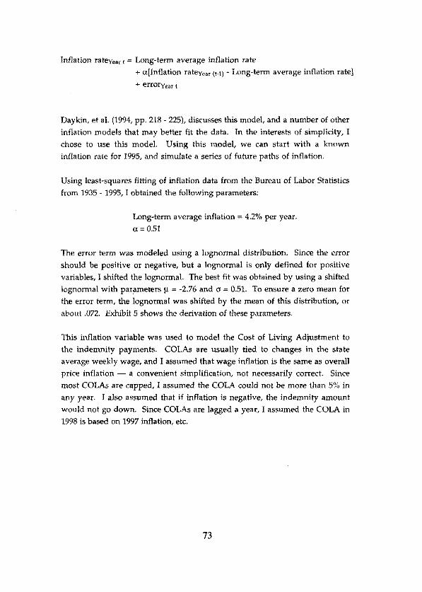
Inflation ratey,,, t = Long-term average inflation rate

+ cc[Inflation ratey,,, u-1) - Long-term average inflation rate]

+ errory,,, t

Daykin, et al. (1994, pp. 218 - 225), discusses this model, and a number of other

inflation models that may better fit the data. In the interests of simplicity, 1

chose to use this model. Using this model, we can start with a known inflation rate for 1995, and simulate a series of future paths of inflation.

Using least-squares fitting of inflation data from the Bureau of Labor Statistics

from 1935 - 1995,I obtained the following parameters:

Long-term average inflation = 4.2% per year. a = 0.51

The error term was modeled using a lognormal distribution. Since the error

should be positive or negative, but a lognormal is only defined for positive variables, 1 shifted the lognormal. The best fit was obtained by using a shifted

lognormal with parameters lt = -2.76 and 0 = 0.51. To ensure a zero mean for the error term, the lognormal was shifted by the mean of this distribution, or

about .072. Exhibit 5 shows the derivation of these parameters.

This inflation variable was used to model the Cost of Living Adjustment to the indemnity payments. COLAS are usually tied to changes in the state average weekly wage, and 1 assumed that wage inflation is the same as overa11 price inffation - a convenient simplification, not necessarily correct. Since

most COLAS are capped, 1 assumed the COLA could not be more than 5% in any year. 1 also assumed that if inflation is negative, the indemnity amount would not go down. Since COLAS are lagged a year, 1 assumed the COLA in 1998 is based on 1997 inflation, etc.

73

2) Medical Inflation

Medical inflation may be higher or lower than inflation, but there is a link between the two: if there were a 20% inflation rate for a sustained period, one would not expect medical inflation to remain at 2%. 1 thus selected a model of medical inflation that is tied to the overa11 inflation rate, but with a degree of error allowed. The model was:

Medical Inflationt = Inflationy,,, t

+ B[Medical inflationy,,, (t-1) - Inflationy,,ct.r)] + [long-term average medical inflation - long-term average inflation]

+ error termy,,, t

The error term is assumed to be normally distributed, with a mean of zero.8

1 used the longest available data series to get these parameters. Tl-te Bureau of

Labor Statistics has medical CH numbers back to 1935. For the period 1935 to 1995, average medical inflation was 1.16 percentage points higher than average inflation. This is what 1 used for the third term of the above

expression. 1 am assuming these long-term trends will continue, although, there is of course no guarantee of this.

The fitted value for 8 was 0.38, and the error term was normally distributed with a mean of 0, and a standard deviation of 0.027. Exhibit 6 shows the

development of this model.

8 The inflation model had a lognormal error term, but the medical inflation model has a

normal error term. The reason was that 1 had a strong feeling that the error for inflation was

skewed, whereas it is less obvious that the difference between overa11 inflation and medical

inflation (which is largely what drives the medical inflation model) is skewed.

74

3) Investment Yields

1 used a very simple model of investment yields. The firm is assumed to invest in one-year bonds that are held to maturity. Consequently, one would never have investment losses. In general, the bond yield would equal the

expected inflation rate plus some small premium. However, one should discount using a risk-adjusted rate, and 1 simply assumed that the risk

adjustment equals the premium over the inflation rate, i.e., the rate used for discounting is the same as the inflation rate. Even íf inflation is negative,

one would not expect interest rates to drop below some threshold (e.g., 2%), so

1 assumed the risk-adjusted discount rate could not go below zero, Le., 1 set the rate for discounting at the greater of zero or the inflation rate.

4) Medical Services Used By Claimant

Medical usage will fluctuate from year to year. In some years, the claimant

will use relatively little, while ín other years he may require surgery, with large medical bilis. The services from year to year may be correlated. For

example, if he has surgery this year, the costs of post-operative treatment may

keep the costs higher than average in the next year. One can model this process using a similar autoregressive model to the way we modeled inflation:

9 This is a rather unrealistic model of investment income, but it will be adequate for our

purposes. Insurers usually buy longer term investments, especially if they are investing reserves

hacking tifetíme workers’ compensation claims. They may also invest in stocks, or other assets,

that do not have fixed yields. ll-tese complications are beyond the scope of the paper.

It is also beyond the scope of the paper to addrass the question of whether discounting should be

based on the fii’s (either the reinsurer or reinsured’s) actual investments, or whether it should

be based on market discount rates.

Medical amounty,,, t = Long-term average medical amount

+ yIMedica1 amounty,,, (r-1) - long-term average medical amount]

+ errory,,, t

The long-term average medical amount for this case is, by assumption,

$70,000. Empirically, there does not appear to be a very strong link between

last year’s medical amount and this year’s, so 1 used y = .05. The error term was modeled by a lognormal with u = 10.80089 and o = 0.75. The mean of this lognormal is 65,000, so 1 shifted the distribution by 65,000 to ensure the error

term has a mean of zero.

Runnin~ the Model

Each of these parameters was then put into a simulation model. By simulating inflation, medical inflation, and the annual medical amount, one can get a set of input parameters for each simulation. These parameters are

then run through the same model as is used for Method 2. The difference is that each time it is run through with different parameters, so that instead of getting a single present value of the future payments, we get a distribution.

(Exhibit 7 shows a single simulation from this distribution.)

The means of these distributions, for each layer, are shown below, compared with the results for Methods 1 and 2:

76

I Expected Nominal Expected Present-Value Payments fin §&Ms)

4380 ) 4,483 1 4,815

It is Worth noting a few things regarding these results:

77

Unlike Methods 1 and 2, Method 3 hits al1 the reinsurance layers. A less deterministic approach ensures that higher layers will be hit. Thus, layers that might otherwise have been thought to have no possibility of a loss, are shown to have some commutation value.

The total nominal value of Method 3 is higher than the nominal value of Method 2 (and Method 2 is higher than Method 1, as discussed earlier).

This is largely explained by the treatment of inflation. The medical and indemnity amounts paid in some future period depend on the products of (1 + inflation) for al1 prior periods. For example, the amount paid in

period 3 depends on what inflation was in periods 1 and 2. The inflation rates are not independent from period to period: they are positively correlated. Thus, the expected value of the product is greater than the product of the expected values, making the overa11 nominal payments for

Method 3 higher than the payments in Method 2.10

The overa11 present value factor for Method 2 is 31% (= 4,483 + 14,377), but

the present value factor for Method 3 is only 27% (= 4,466 + 16,420). In other words, Method 3 has, on average, a steeper discount applied to it.

The relationship between the present values of Methods 2 and 3 is

complex, largely because the assumptions are not consistent between the two methods. Yes, we tried to make them consistent, but the differences

in the assumptions become clear once we examine them more carefully.

Consider the indemnity cost-of-living adjustments. We said that, based on the historical record, inflation averages 4.2% per annum, and this was the number we used for the COLA in Method 2. In Method 3, inflation varies stochastically, with a mean of 4.2%. But our rules for the COLA said that it couldn’t be more than 5%, or less than 0%. In Method 3, the

10 E(XY) = E( + cov(X,Y). Thus, if X and Y are positively correlated, the expected

value of the product exceeds the product of the expected values.

78

average inflation rate is 4.2%, but the average COLA is not 4.2% because it is sometimes capped. In fact, it averages about 2.98%.

Likewise, we said the discount rate was equal to the inflation rate, but that the discount rate could never go negative. On average, then, the discount rate is higher than 4.2% - about 4.39%. This higher effective discount

rate is the main reason for the total present value factor of Method 3 being

less than the total present value for Method 2.

The assumptions between Methods 2 and 3 are not the same: Method 2 assumes higher COLAS than Method 3, and lower discount. Running

Method 2 at the same average COLA as Method 3 (2.98%), and the same average discount (4.39%), changes the Method 2 present value to $4.124 million, which is 8% lower than the $4.483 million we originally

calculated. (See Exhibit 8.)

In general, the relationship between the present values of Methods 2 and 3 will depend on the particular assumptions, and how they interact with the

various caps and correlations.

l In the lowest layers, the nominal value of Method 1 is higher than Method 2, and Method 2 is higher than Method 3.X’ This is because

11 On the oarlier table, the nominal values for Methods 2 and 3 look the same at the low

retentions. In fact, however, the numbers in the table are rounded. If the complete numbers had

been shown, the nominal values in the low iayers would be systematically less (though

admittedly by a small amount) for Method 3 than for Method 2:

Layer

1

2

3

4

Nomina1 Value

(in $Thousands)

Method 2 Method 3

129.74 129.70

494.89 494.55

970.56 969.34

2,729.68 2,715.21

79

Method 1 implies these layers will be hit for certain, whereas Methods 2 and 3 recognize that the claimant could die before the layer is penetrated. In addition, Method 3 recognizes that there could be years of unusually low claim amounts, so that it may take longer than expected to breach the

retention. This reduces the commutation amount in two ways:

i) The longer it is until the retention is breached, the greater the chance of the claimant dying before breaching the retention.

ii) The longer it is until the retention is breached, the steeper the effect of present valuing.

In higher layers, which have a lower probability of being penetrated, this

situation reverses itseff: Method 3 gives higher results than Method 2.

The upper layers are most vulnerable to a period of sustained high inflation or high claim levels. Methods 1 and 2 assume inflation and

claim levels are fixed, so they do not contemplate periods of sustained high inflation or claim levels.

l For the lower layers, where the chances are good that the claimant will live long enough to breach them, Method 2 gives similar results to Method 3. But as the layers get higher, the Method 2 number gets lower and lower as a percentage of Method 3.

Method 2 Result as Percentage of Method 3 Result

Layer Nominal Present Value

1 100% 100%

2 100% 99%

3 100% 97%

4 100% 95%

5 99% 90%

6 94% 83%

80

7 82% 72%

8 56% 48%

9 22% 19%

10 5% 4%

11 1% 1%

Higher Layers 0% 0%

l Note how the present value factor for the losses declines sharply in the

higher layers. For example, for the $5 million excess $5 million layer, the present value is $1.053 million, compared to the nominal value of $3.701 million. This translates to a present value factor of 28%. By contrast, in the $10 million excess $90 million layer, the present value factor is only 4%.

This paper has demonstrated that the commutation calculation is significantly affected by making a variety of variables non-deterministic. Have we now stripped away al1 determinism? Put another way: does this paper describe “the perfect” commutation calculation, or are there further

layers of determinism that can, at least in principie, be stripped away?

There are, indeed, further layers of determinism that can be stripped away from a calculation of this nature, although it will become increasingly more difficult to do so. This paper has shown how we can strip away determinism

in the levels of inflation, medical utilization, etc. But to measure the paths for these variables, we have relied on statistical measures on past data. Clearly, these historical data may no longer be valid predictors of the future.

For example, the paper assumes that the best predictor of medical inflation is

the last 60 years of medical CPI information. One can plausibly argue that what drove medical inflation in the 1930s and 1940s was completely different

from what drove it in the 1970s and 19%Os, and different from what will drive it in future. And it is quite possible that the drivers of inflation will change periodically over the course of the claimant’s lifetime.

This same issue applies to other variables. For example, advances in medical

care could affect the medical utilization for the claimant’s condition - and perhaps render the assumed mortality table redundant.

The next layer of determinism is the models themselves. We have assumed the model stays fixed over the claimant’s lifetime, but we can easily imagine a

situation where the parameters of the model shift, or the model itself changes.

The problem is that this next layer of determinism is not easily subject to measurement, and hence is not amenable to quantification by the usual actuarial methods. But not being able to quantify does not allow us to say that these items do not exist, and to simply ignore them.

The Economics Of Uncertaintv

Economists distinguish between “risk” and “uncertainty.“l* Risk includes those things that can be measured statistically, and uncertainty includes those

things that cannot be measured, but which might occur. For example, if 1 bet on a fair coin coming up heads, 1 am facing a risk. But if 1 bet on the chance of intelligent life being found on an as-yet-undiscovered planet, that is uncertainty - 1 have no way of measuring the associated probabilities.

Most insurance problems consist of a mixture of risk and uncertainty. Insurers are good at dealing with risk. By measuring the probabilities of loss

and pooling the risk, we can largely eliminate the risk and get stable losses in the aggregate. It is far more difficult to deal with rmcertainty.

12 The classic referente on risk and uncertainty is Knight (1921). For a more recent

diicwion of the economics of uncertainty, see O’Driscoll and Rizzo (1985).

82

In this paper, we have been measuring risk: we have only dealt with those

things that can be measured. (Insofar as they cannot be modeled well, there are elements of uncertainty.) The next layer of determinism consists of uncertainty. We have no way of estimating the chances of the inflation

model changing, or what the new model might be.

Without making any attempt to measure the effect of uncertainty, we can

make some qualitative statements about its effects on commutations. Just as

removing earlier layers of determinism increased the commutation amount in the higher layers, so removing yet another layer of determinism will

increase the commutation amount in higher layers, and higher layers that would not otherwise have been pierced, will have some commutation value.

Why? Under the inflation model postulated in the example in this paper, it is conceivable, but extremely unlikely, that there will be years where inflation will run above, say, 100% a year. (Actuaries who have dealt with foreign

insurance and reinsurance may themselves have been burnt by hyperinflation in places like Israel and Argentina.) We can certainly envision unlikely circumstances where the US economy falls apart and there is

hyperinflation. This possibility was not included in the data used for fitting

the models, and is thus not contemplated in the resulting commutation

amount.

Al1 the other variables in the commutation are subject to similar uncertainty:

mortality rates might plummet as cures are found for cancer and heart

disease; or mortality rates might soar, as a new virus kills half the population. The annual medical usage might drop, if a cure is found for the claimant’s ailment, which was previously thought to be permanent. Or the cost of medical care might soar as a new drug is discovered that greatly improves the

claimant’s quality of life, at twice the cost. What if the govemment takes over the entire health-care system, and insurers are no longer responsible for medical care costs?

We can dream up many different situations that will change what insurers owe to claimants. We can put probabilities on none of these, and we also know that there are many possibilities that we may not even think of, until

they actually happen.

83

In commutations, it is common to ignore this uncertainty, and to commute some of the very high layers without payment. This is unwarranted. Commuting reinsurance is really a matter of pricing future possibilities, and reinsurers do not give away free layers, even if they have only a remote chance of being hit. For example, suppose 1 want to buy workers’

compensation reinsurance for a layer of $1 million excess of $800 million. (To

avoid catastrophe issues, let us assume the reinsurance is per claim, not per occurrence.) There has never been a workers’ compensation claim that large, or even remotely close to it. Yet, would a reinsurer be willing to give the

layer away free (assuming they have no costs to service the contract)? Of course they won’t. Reinsurers recognize the remote possibility of having to pay on this contract, and they need to charge for that risk. The risk is remote, but remote is not the same as non-existent. The chance of the layer being hit is not measurable, but not-measurable is not the same as zero.

The pricing issues also apply to commutations. There is no reason why a cedent should be willing to commute a layer for nothing, even when the

actuarial calculations (at some leve1 of determinism) say there is no chance of hitting the layer. Though there is far less uncertainty at the time of a commutation than there was when the contract was written, there is still

enough uncertainty that payment for the cedent re-assuming this risk is warranted.

Other Lines of Business; Pricirw and Reservirw, Too

The issues discussed in this paper apply more broadly than just to workers’ compensation commutations. A commutation for, say, a General Liability

treaty would usually develop the expected losses to ultimate, and commute based on the discounted value of those losses. But this ignores certain risks

that are transferred back to the ceding company in the commutation. For

example, a GL treaty being commuted in 1978 would have relieved the reinsurer for liability for environmental claims that were generated by the Superfund law, which passed a couple of years later. It was unknown, at the time of the commutation, that the cedent was giving up coverage for this risk,

84

but it was not unknown that the cedent was taking the risk of some such change in the future. Just as a company selling GL reinsurance will not give away remote layers free of charge, so the commutation should not be free for

these layers either.

Other lines of business have the same levels of determinism as do workers’ compensation. The difference is that for workers’ compensation we can do the calculations on a claim-by-claim basis, which helps to lay bare many of the

underlying assumptions.

And it is not just commutations that are affected by determinism. It applies

to regular pricing and reserving work as well. The clearest example would be the reserving of workers’ compensation reinsurance, where the methods

used in this paper can be directly applied. But for pricing and reserving of any excess insurance or reinsurance, it is important to keep in mind the problems

of determinism. If we simply assume the future will tum out to be what was

expected, or that the future will follow the pattems of the past, we are bound

to be led astray. The scary part of writing insurance is the uncertainty of what the future will bring. The uncertainty cannot be quantified, but al1 too often

we stick our heads in the sand and assume that if something cannot be quantified, it doesn’t exist.

85

Referentes

Bowers, Newton L., et al, (1986): ActuariaI Mathematics, Society of Actuaries. Butsic, Robert P. (1988): Determining Me Proper Interest Rute for Loss

Reserve Discounting: An Economic Approuch, CAS Discussion Paper Program, pp. 147 - 188.

Connor, Vincent and Olsen, Richard (1991): Commutation Pricing in the Post Tux-Reform Era, KAS, vol. LXXVIII, pp. 81 - 109.

Daykin, CD, Pentikäinen, T., and Pesonen, M. (1994): Practica! Risk Theoy

for Actuuries, Chapman and Hall.

Ferguson, Ronald E. (1971): Acttiuriul Note on Workmen’s Compensution

Loss Reserves, KAS, vol. LVIII, pp. 51 - 57. Gillam, William R, (1993): Injured Worker Mortulity, PCAS, vol. LXXX, pp.

34 - 54. Knight, Frank H. (1921): Risk, Uncertuinty, und Profit, University of Chicago

Press. O’Driscoll, Gerald P. and Rizzo, Mario J. (1985): The Economics of Time and

Ignorance, Basil Blackwell. Snader, Richard H. (1987): Reserving Long Term Medical CIaims, PCAS, vol.

LXXIV, p. 322 - 353. Steeneck, Lee R. (1996): Actuarial Note on Workmen’s Compensution Loss

Reserves - 25 Yeurs Luter, Casualty Actuarial Society Forum, Summer 1996, pp. 245 - 271.

Venter, Gary G. (1995): Workers Compensation Excess Reinsurunce - The Longest Tuil?, NCCI Issues Report, 1995, pp. 18 - 20.

86

Exhibit 1

1990 US Life Table (Males)

4s w

0 100,OW.O 1 98.969.0 2 98,894.0 3 98,840.O 4 98,799.O 5 98.765.0 6 98.735.0 7 98,707.O 8 98.680.0 9 98.657.0 10 98,638.0 11 98.623.0 12 98.608.0 13 98.586.0 14 98.547.0 15 98,485.0 16 98.397.0 17 98,285.0 18 98,154.O 19 98,0 ll .O 20 97,863.0 21 97.7 10.0 22 97,551 .o 23 97.388.0 24 97.221.0 25 97,052.O 26 96,881 .O 27 96.707.0 28 96,530.O 29 96,348.0 30 96,159.O 31 95,962.0 32 95,758.0 33 95,545.0 34 95,322.0 35 95.089.0

Llfe Expectancy

71.8 71.6 70.6 69.7 68.7 67.7 66.8 65.8 64.8 63.8 62.8 61.8 60.8 59.9 58.9 57.9 57.0 56.0 55.1 54.2 53.3 52.3 51.4 50.5 49.6 48.7 47.8 46.9 45.9 45.0 44.1 43.2 42.3 41.4 40.5 39.6

36 94.843.0 38.7 73 56,885.0 10.4 110 0.0

ke I(x)

37 94.585.0 38 94.3 16.0 39 94,038.O 40 93,753.0 41 93.460.0 42 93.157.0 43 92.840.0 44 92.5050 45 92,147.0 46 91.764.0 47 91.352.0 48 90.908.0 49 90,429.O 50 89,912.O 51 89,352.0 52 88,745.0 53 88,084.O 54 87,363.0 55 86,576.0 56 85.719.0 57 84.788.0 58 83,777.0 59 82.678.0 60 81.485.0 61 80.194.0 62 78,803.O 63 77‘314.0 64 75.729.0 65 74,051 .O 66 72.280.0 67 70,414.O 68 68.445.0 69 66,364.0 70 64,164.0 71 61,847.0 72 59,419.0

Life Expeetancy

37.8 36.9 36.0 35.1 34.2 33.3 32.4 31.6 30.7 29.8 28.9 28.1 27.2 26.4 25.5 24.7 23.9 23.1 22.3 21.5 20.7 20.0 19.2 18.5 17.8 17.1 16.4 15.8 15.1 14.5 13.8 13.2 12.6 12.0 11.5 10.9

Life 4ge l(x)

74 54.249.0 75 51,519.0 76 48.704.0 77 45,816.O 78 42.X67.0 79 39.872.0 80 36.848.0 81 33,811.0 82 34782.0 83 27,782.0 84 24.834.0 85 21,962.0 86 19,216.8 87 16.607.4

i9 14.157.7 11,889.0

90 9,819.5 PI 7,962.6 92 6.326.9 93 4,915.0 94 3,723.5 95 2.743.0 96 1.958.3 97 1,349.7 98 894.0 99 566.2 100 340.6 101 193.2 102 102.4 103 50.1 104 22.3 105 8.9 106 3.1 107 0.9 108 0.2 109 0.0

Expectancy

9.9 9.4 8.9 8.4 7.9 7.5 7.1 6.7 6.3 5.9 5.5 5.2 4.9 4.5 4.2 3.9 3.7 3.4 3.2 2.9 2.7 2.5 2.3 2.1 1.9 1.8 1.6 1.5 1.3 1.2 1.1 1.0 0.9 0.8 0.7 0.5

1

Source: Vital Statistics of the United States, 1990 WS De-partment of Health and Humm Services, 19941 Note that the published tables extend only to age 85; beyond 85, the numbers are extrapolations.

87

Exhibit 2

Inflation: Consumer Price Index and Medical Consumer Price Index

Index at December Medical

Year CPI CPI

1935 13.8 10.2 1936 14.0 10.2 1937 14.4 10.3 1938 14.0 10.3 1939 14.0 10.4 1940 14.1 10.4 1941 15.5 10.5 1942 16.9 10.9 1943 17.4 ll.4 1944 17.8 11.7 1945 18.2 12.0 1946 21.5 13.0 1947 23.4 13.9 1948 24.1 14.7 1949 23.6 14.9 1950 25.0 15.4 1951 26.5 16.3 1952 26.7 17.0 1953 26.9 17.6 1954 26.7 18.0 1955 26.8 18.6 1956 27.6 19.2 1957 28.4 20.1 1958 28.9 21.0 1959 29.4 21.8 1960 29.8 22.5 1961 30.0 23.2 1962 30.4 23.7 1963 30.9 24.3 1964 31.2 24.8 1965 31.8 25.5

Annual Inflation Medical

CPl CPI

1.4% 0.0% 2.9% 1 .O% -2.8% 0.0% 0.0% 1 .O% 0.1% 0.0% 9.9% 1 .O% 9.0% 3.8% 3.0% 4.6% 2.3% 2.6% 2.2% 2.6% 18.1% 8.3% 8.8% 6.9% 3.0% 5.8% -2.1% 1.4% 5.9% 3.4% 6.0% 5.8% 0.8% 4.3% 0.7% 3.5% -0.7% 2.3% 0.4% 3.3% 3.0% 3.2% 2.9% 4.7% 1.8% 4.5% 1.7% 3.8% 1.4% 3.2% 0.7% 3.1% 1.3% 2.2% 1.6% 2.5% 1 .O% 2.1% 1.9% 2.8%

Index at December Medical

Year CPI CPI

&mual Inflation Medical

CPI CPI

1966 32.9 27.2 3.5% 6.7% 1967 33.9 28.9 3.0% 6.3% 1968 35.5 30.7 4.7% 6.2% 1969 37.7 32.6 6.2% 6.2% 1970 39.8 35.0 5.6% 7.4% 1971 41.1 36.6 3.3% 4.6% 1972 42.5 37.8 3.4% 3.3% 1973 46.2 39.8 8.7% 5.3% 1974 51.9 44.8 12.3% 12.6% 1975 55.5 49.2 6.9% 9.8% 1976 58.2 54.1 4.9% 10.0% 1977 62.1 58.9 6.7% 8.9% 1978 67.7 64.1 9.0% 8.8% 1979 76.7 70.6 13.3% 10.1% 1980 86.3 77.6 12.5% 9.9% 1981 94.0 87.3 8.9% 12.5% 1982 97.6 96.9 3.8% 11.0% 1983 101.3 103.1 3.8% 6.4% 1984 105.3 109.4 3.9% 6.1% 1985 109.3 116.8 3.8%. 6.8% 1986 110.5 125.8 1.1% 7.7% 1987 115.4 133.1 4.4% 5.8% 1988 120.5 142.3 4.4% 6.9% 1989 126.1 154.4 4.6% 8.5% 1990 133.8 169.2 6.1% 9.6% 1991 137.9 182.6 3.1% 7.9% 1992 141.9 194.7 2.9% 6.6% 1993 145.8 205.2 2.7% 5.4% 1994 149.7 215.3 2.7% 4.9% 1995 153.5 223.8 2.5% 3.9%

Average 4.2% 5.3%

Source: US Department of Labor, Bureau of Labor Statistics

88

Exhibit 3, Page 1

Completely Deterministic commutation cafculation

Parameters: W Evaluation Date: 1m97

(W Age at evaluation date: 35 m Annual indemnity payment 20,000 CD) Annual medical payment: (at mid-1996 price levelsl 70,000

03 lndemnity paid to date 70,000 (F) Medical paid to date 300,000 W Life expectancy: 39.6 (HI Cost-of-Living Adjustment: 4.2% 0) Medical Inflation Rate: 5.36% (0 Annual Discount Rate: 4.2%

1996 and prior 1997 1998 1999 2000 2001 2002 2003 2004 2005 2006 2007 2008 2009 2010 201 I 2012 2013 2014 2015 2016 2017 2018 2019 2020 202 1 2022 2023 2024 2025 2026 2027

(1) Cost of Living

Adjustment

4.2% 4.2% 4.2% 4.2% 4.2% 4.2% 4.2% 4.2% 4.2% 4.2% 4.2% 4.2% 4.2% 4.2% 4.2% 4.2% 4.2% 4.2% 4.2% 4.2% 4.2% 4.2% 4.2% 4.2% 4.2% 4.2% 4.2% 4.2% 4.2% 4.2% 4.2%

(2)

lademaity Payment

70,000 20,840 21,715 22,627 23,57â 24,568 25,600 26,675 27,795 28,963 30,179 31,447 32,161 34,144 35,578 37,072 38,629 40,25 1 41,942 43.704 45,539 47,452 49,445 51,521 53,685 55,940 58,290 60,738 63,289 65,947 68,717 7 1,603

5.36% 5.36% 5.36% 5.36% 5.36% 5.36% 5.36% 5.36% 5.36% 5.36% 5.36% 5.36% 5.36% 5.36% 5.36% S.36% 5.36% 5.36% 5.36% 5.36% 5.36% 5.36% 5.36% 5.36% 5.36% 5.36% 5.36% 5.36% 5.36% 5.36% 5.36%

(4) (5)

MediCPI Payment

TOtaI Pnyment (2) + (4)

300,000 370,000 73,752 94,592 77,705 99,420 81,870 104,497 86,258 109,836 90,882 115,450 95,753 121,353

loo,885 127,560 106,293 134,088 111.990 140,953 117,993 148,172 124,317 155,764 130,981 163,748 138,001 172,145 145,398 180,976 153,191 1 YO.263 161,402 20#,03 1 170,054 210,305 179,169 221,111 188,772 232,476 198,890 244,429 209,551 257,002 220,783 270,227 232,617 284,138 245,085 298,770 258,221 314,161 272,062 330,352 286,644 347,382 302,OOY 365,297 318,196 384,143 335,252 403,968 353921 424,824

(6) CWtltlhtiVe

Total Payment

Cumulative of(5)

370,000 464,592 564,012 668,510 778,346 893,796

1.015,148 1,142,709 1276,797 1,417,750 1,565,922 1,72 1,686 1,885,434 2JJ57.579 2,238,555 2,428,818 2,628,850 2,839,155 3,060,265 3,292,741 3,537,170 3,794,172 4,064,400 4,348,537 4,647,308 4,96 1,469 5,291,820 5,639,203 6,004.500 6,388,643 6,792,611 7,2 17,435

89

Exhibit 3, Page 2

Year

203 I 2032 2033 2034 2035 2036

Total

(1) (2) (3) (4) (5) Cost or Liviag Indemnlty MediCd MediCaI Total

Adjustment Peyment IttrlPtioa Payment Payment (2) + (4)

4.2% 4.2% 4.2% 4.2% 4.2% 4.2% 4.2% 4.2% 4.2%

74,610 77,744 SI,049 84,411

91,651 95,500 99,s ii 6232 14

5.36% 372,154 446,764 5.36% 392,101 469,845 5.36% 413,118 494,127 5.36% 435,261 5 19,672 5.36% 458,591 546,547 5.36% 483,171 574.822 5.36% 509,069 604,569 5.36% 536,356 635,867 5.36% 339,063 40 1,277

2,104,844 9,806,081

C-5) CUltWldiV~

Total Paymeot

Cumulative OfW 7,664,199 8,134,044 8,628,170 9,147,843 9,694,390

10.269,212 10,873,781 11,509,648 11,910,925

Future pnymeab - 11,910,925 - 370,000 = 11,540,925

90

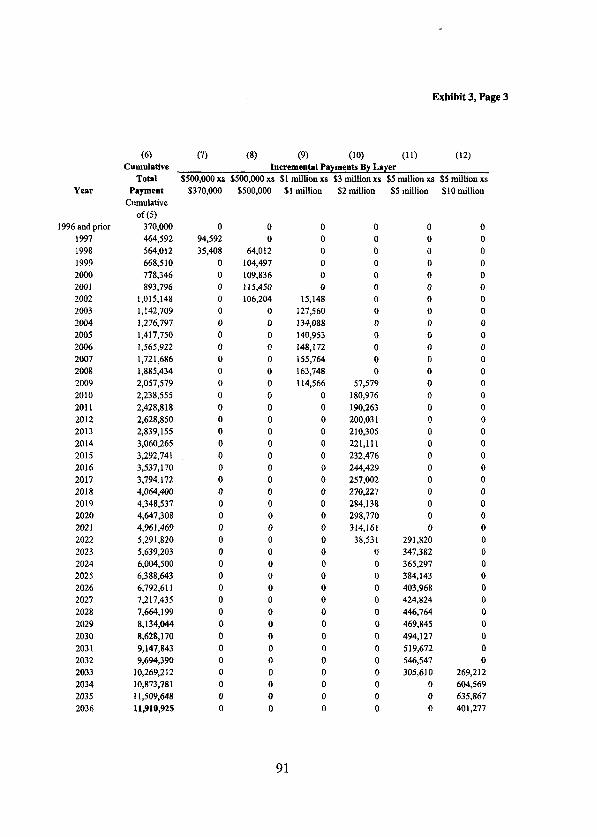
Year

1996 and prior 1991 1998 1999 2000 2001 2002 2003 2004 2005 2006 2007 2008 2ow 2010 2011 2012 2013 2014 2015 2016 2017 2018 2019 2020 2021 2022 2023 2024 2025 2026 2027 2028 2029 2030 2031 2032 2033 2034 203.5 2036

Exhibit 3, Page 3

(6) (7) 61 (9) (10) (11) (12) CUllddiVC Incrementa1 Payments By Lnyer

TotaI $500,ooO xs $500,000 xs $1 million xs $3 miliion xs $5 million xs $5 million xs Paymeat

Cumulative

ofW 370,000 464,592 564,012 668,510 718,346 893,796

1,015,148 1,142,709 1,276,797 1,417,750 1,565,922 1,721,686 1,885,434 2,051,579 2,238,555 2,428,818 2.628.850 2,839,155 3,060,265 3,292,74l 3,537,170 3,794,172 4,064,400 4,348,537 4,647,308 4.96 1.469 5,291,820 5.639.203 6,004,500 6.3x%8,643 6,792,6ll 7,217,435 7,664,199 8,134,044 8.628,170 9,147,843 9.694.390

10,269,212 10,873,781 11,509,648 11,910,925

ã370,Ow %500.000 $1 million $2 million $5 million $10 million

0 0 0 0 0 0 94,592 0 0 0 0 0 35,408 64.012 0 0 0 0

0 104,497 0 0 0 0 0 109,836 0 0 0 0 0 115,450 0 0 0 0 0 106,204 15,148 0 0 0 0 0 127,560 0 0 0 cl 0 134,088 0 0 0 0 0 140,953 0 0 0 0 0 148,172 0 0 0 0 0 155,764 0 0 0 0 0 163,748 0 0 0 0 0 114,566 51,579 0 0 0 0 0 180,976 0 0 0 0 0 190,263 0 0 0 0 0 200,03 1 0 0 0 0 0 210,305 0 0 0 0 0 221,111 0 0 0 0 0 232,476 0 0 0 0 0 244,429 0 0 0 0 0 251,002 0 0 0 0 0 270,227 0 0 0 0 0 284,138 0 0 0 0 0 298,770 0 0 0 0 0 314,161 0 0 0 0 0 38,531 291,820 0 0 0 0 0 347,382 0 0 0 0 0 365,291 0 0 0 0 0 384,143 0 0 0 0 0 403,968 0 0 0 0 0 424,824 0 0 0 0 0 446,764 0 0 0 0 0 469,845 0 0 0 0 0 494,121 0 0 0 0 0 519,672 0 0 0 0 0 546,547 0 0 0 0 0 305,610 269,212 0 0 0 0 0 604,569 0 0 0 0 0 635,867 0 0 0 0 0 401.277

91

Exhibit 3, Page 4

YC3r Factor s370,000 $500,000 SI million $2 million $5 million $10 million Comb;ned

1996 and prior 1997 1998 1999 2000 2001 2002 2003 2004 2005 2006 2007 2008 2009 2010 2011 2012 2013 2014 2015 2016 2017 2018 2019 2020 2021 2022 2023 2024 2025 2026 2027 2028 2029 2030 203 1 2032 2033 2034 2035 2036

0.9796 92,666 0 0 0 0 0 92,666 0.9402 33,289 60,181 0 0 0 0 93,470 0.9023 0 94,284 0 0 0 0 94,284 0.8659 0 95,106 0 0 0 0 95,106 0.8310 0 95,937 0 0 0 0 95,937 0.7975 0 84,697 12,081 0 0 0 96,778 0.7653 0 0 97,628 0 0 0 97,628 0.7345 0 0 98,488 0 0 0 98,488 0.7049 0 0 99,357 0 0 0 99,357 0.6765 0 0 100,236 0 0 0 100,236 0.6492 0 0 101,124 0 0 0 101,124 0.6230 0 0 102,023 0 0 0 102,023 0.5979 0 0 68,503 34,428 0 0 102,93 1 0.5738 0 0 0 103,850 0 0 103,850 0.5507 0 0 0 104,779 0 0 104,779 0.5285 0 0 0 105,718 0 0 105,718 0.5072 0 0 0 106,668 0 0 106,668 0.4868 0 0 0 107,628 0 0 107,628 0.4671 0 0 0 108,599 0 0 108,599 0.4483 0 0 0 109,580 0 0 109,580 0.4302 0 0 0 110,573 0 0 110,573 0.4129 0 0 0 ll 1,577 0 0 111,577 0.3963 0 0 0 112,591 0 0 112,591 0.3803 0 0 0 113,618 0 0 113,618 0.3650 0 0 0 114,655 0 0 114,655 0.3502 0 0 0 13,495 102,209 0 115,704 0.3361 0 0 0 0 I 16,765 0 116,765 0.3226 0 0 0 0 117,838 0 I 17,838 0.3096 0 0 0 0 118,922 0 1 18,922 0.2971 0 0 0 0 120,019 0 120.019 0.2851 0 0 0 0 121,128 0 121,128 0.2736 0 0 0 0 122,249 0 122,249 0.2626 0 0 0 0 123,383 0 123,383 0.2520 0 0 0 0 124,529 0 124,529 0.2419 0 0 0 0 125,688 0 125,688 0.2321 0 0 0 0 126,860 0 126,860 0.2228 0 0 0 0 68,076 59,968 128,045 0.2138 0 0 0 0 0 129,243 129,243 0.2052 0 0 0 0 0 130,454 130,454 0.1969 0 0 0 0 0 79,008 79,008

Total 125.955 430.206 679,440 1,357.7.59 1,387,664 398,673 4,379,697

(13) (14) (15) (16) (17) (18) (19) 120) Present Dlseauoted Value by Layer Value $500,000 xs $500,000 xs .$ I million xs $3 million xs $5 million xs S5 million xs Al1 Layen

92

Exblbit 4, page 1

Method 2: Stochastic Mortal@ (Other inputs deterrninistic)

(B) Cun-ent Ap: 35 (CC) Annual Indemnity Paymnt 2osxKl CD) Annud Medical Paynren: (at mid-1996 ptice levels) 70,wo 03 03 v.3 CH) (0

Indemniiy Paid to De Medical Pald to Dato: Cos-of-tiving Adjuwnenl Medical Intlaücn Raw Annual Diwunt Rafe:

1996 end prior 1997 1998 1999 2cQo 200; 2002 2W3 20x 2005 2006 2007 2W8 x%9 2010 201; 2012 2013 2014 2015 2016 2017 2018 2019 2020 202; 2022 2023 2024 2025 2026 2027 2028 2029 2030 203 1 2032 2033 2034 2035 2036 2037 2038 2039

4.2% 4.2% 4.2% 4.2% 4.2% 4.2% 4.2% 4.2% 4.2% 4.2% 4.2% 4.2% 4.2% 4.2% 4.2% 4.2% 4.2% 4.2% 4.2% 4.2% 4.2% 4.2% 4.2% 4.2% 4.2% 4.2% 4.2% 4.2% 4.2% 4.2% 4.2% 4.2% 4.2% 4.2% 4.2% 4.2% 4.2% 4.2% 4.2% 4.2% 4.2% 4.2% 4.2%

70,oel 20,840 5.36% 21,715 5.36% 22,627 5.36% 23.518 5.36% 24,568 5.36% 25.600 5.36% 26.675 5.36% 27,795 5.36% 28,%3 5.36% 30,179 5.36% 31.447 5.36% 32;767 5.36% 34,144 5.36% 35.578 5.36% 37,072 5.36% 38,429 5.36% 40.25 I 5.36% 41;942 5.36% 43.704 5.36% 45.539 5.36% 47.452 5.36% 49.445 5.36% SI.521 5.36% 53.685 5.36% 55.940 5.36% 58.290 5.36% 6o.738 5.36% 63,289 5.36% 65,941 5.36% 68.717 5.36% 71.603 5.36% 74,610 5.36% 77,744 5.36% 81,009 5.36% a4.411 5.36% 87.956 5.36% 91:651 5.36% 95.500 5.36% 99,51 I 5.36%

103,690 5.36% los,W5 5.36% 112.583 5.36% 117.312 5.36%

(4)

Medial Payment

3oo.ootJ 370,ooo 73,752 94.m 77,705 99.420 81.870 104,497 86258 109,836 90.882 115.450 95,753 121353

100,885 121160 106,293 134,088 111,99O 140.953 117,993 148,172 124.317 155.764 130.981 163.748 13wJ1 172,145 145.398 18OS76 153,191 190263 161.402 200,031 170,054 210.305 179,169 221.111 188.772 232,476 198.890 244,429 209.551 257.w2 220,783 no,22I 232,617 284,138 245.085 298.770 258,221 314,161 272,062 330.352 zsa.a‘f 347,382 302.009 365,297 318.1% 384.143 335.252 403.968 353,221 424,824 372.154 446,764 392,101 469.845 413.118 494,127 435.26; SI 9.672 458.591 546,547 483,171 574,822 509.069 604569 536.356 635,867 565,1C-t 668,795 595.394 703.439 627,307 739.890 660.931 I18.242

70,000 300,ooo

4.2% 5.36%

4.2%

370,Dw 464.592 0.999 564,012 0.9% 66&510 0.993 778346 0.990 893.7% 0.987

1.015.148 0.984 1.142.709 0.981 1276.797 0.978 1;417;750 0.975 1.565,922 0.971 1,721,686 0.967 1.885.434 0.963 2.057579 0.958 2238.555 0.954 2f128.818 0.948 2.628.850 0.943 2.839.155 0.936 3.060.265 0.930 3.292,741 0.923 3.537.170 0.915 3.794.172 0.906 4.c64.4GQ 0.897 4348.537 0.886 4.647.308 0.875 4,%1,469 0.863 5.291.820 0.850 5.639.203 0.836 6,004JW 0.821 6.388643 0.805 6.792.6; 1 0.788 7.217.435 0.769 7.664.199 0.750 8,134044 0.730 8.628.170 0.709 9.147.843 0.686 9.694,390 0.663

10,269.212 0.638 10,873.781 0.612 11,5o9,&18 0.584 12.178443 0.556 12.881.882 0.527 13,621,772 0.497 ;4,403,0;4 0.466

(8) (9) Dilount for mort&y & inveshnmt

(7) x (81

0.97% 0.9784 0.9402 0.93M 0.9023 0.8962 0.8659 0.8576 0.8310 0.8206 0.7975 0.7851 0.7653 0.7510 0.7345 0.7184 0.7049 0.6870 0.6765 0.6568 0.6492 0.6278 0.6230 0.5999 0.5979 0.5730 0.5738 0.5472 0.55oI 0.5222 0.5285 0.4982 0.5072 0.47% 0.4868 0.4526 0.467 1 0.4310 0.4483 0.4loo 0.4302 0.3898 0.4129 0.3702 0.3963 0.3512 0.3803 0.3328 0.3650 0.3150 0.35@2 0.2978 0.3361 0.2810 0.3226 0.2648 0.3096 0.2491 0.297; 0.2340 0.2851 0.2194 0.2736 0.2053 0.2626 0.1917 0.2520 0.1786 0.2419 0.1660 0.2321 0.1538 0.2228 0.1420 0.2138 0.1307 0.2052 0.1199 0.1969 0.1095 0.1890 O.O!X% 0.1813 o.o901 0.1740 0.0812

93

Exhibit 4,page 2

Y&W

2040 2041

2043 2044 2c45 2046 2047 2048 2049 2050 2051 2052 2053 2054 2055 2056 2057 2058 2059 2c60 2061 2062 2063 2064 2065 2066 2067 2068 2069 2070 2071

(1)

cost of LiViflg

AdjUtmellt

42% 4.2% 4.2% 4.2% 4.2% 4.2% 4.2% 4.2% 4.2% 4.2% 4.2% 4.2% 4.2% 4.2% 4.2% 4.2% 4.2% 4.2% 4.2% 4.2% 4.2% 4.2% 4.2% 4.2% 4.2% 4.2% 4.2% 4.2% 4.2% 4.2% 4.2% 42%

(2) (3)

Indemnity Medirnl MediCAI Payment rntlation Paymont

122,239 5.36% 127,373 5.36% 132.723 5.36% 138,297 5.36% 144.lOS 5.36% 150,158 5.36% 156,465 5.36% 163.036 5.36% 169,884 5.36% 177.019 5.36% 184.453 5.36% 192,201 5.36% 200.273 5.36%

6%.356 733,681 773.006 814,440 858,094 904,087 952,546

l,W3,603 1.057.396 1,114,072 lJ73.787 1.236.702 1.302989 1.372.829 w6.413 1.523.940 1.605,624 L691-585 1982,359 1.877.894 1.978,549 2,084,599 2.196.334 2.314,057 2.438.091 2.568372 2.706.459 2.851,525 3w4.366 3.16WQ 3.335.066 3,513,825

208.684 5.36% 217.449 5.36% 226:582 5.36% 236,098 5.36% 246.015 5.36% 2S6,347 5.36% 267,114 5.36% 278,333 5.36% 290.023 5.36% 302303 5.36% 314.896 5.36% 328.122 5.36% 341,903 5.36% 356.263 5.36% 371.226 5.36% 386:817 5.36% 403.044 5.36% 419,992 5.36% 437,632 5.36%

(4) (5) (8) (7) ProbabUity

CumuQtive ofcbcmFmt TO(Pl TOtaI

Payment PSylllCOt (2) + 141 mm. 0, (5)

818.595 15.218.610 861.054 16,079.661 905,729 16.985393 952,737 17,938,129

l.lxl2.199 18,940.328 1.054.24s 19.994574 1,109,011 2l,lO3.585 1.166.639 22.270.22-J 1.227.280 23.497503 1,291.091 24,788.594 1.358.240 26.146.834 1,428,9Q2 27.575.137 1.503.262 29.078998 1.58lJl3 30,660512 1.663.862 323324,374 1,710.522 34074,896 1.841.722 35.916.618 1.937.700 37,854,318 2,038,707 39,893,025 2.145,008 42.038.032 2,2.56.882 44.294.914 2.374.622 46669,535 2.498.537 49.168.073 2.628,953 51.797.026 2.766.212 54.563.238 Z910.675 57.473.913 3.062.721 6G.536.634 3.222.750 63.759.385 3,391,184 67.150.568

0.435 0.403 0.372 0.340 0.308 0.277 0.246 0.217 0.188 0.162 0.137 0.114 0.094 0.075 0.059 0.045 0.034 0.025 0.017 0.012 0.038 0.005 0.003 0.002 0.001

0.0X4 o.ooo2 O.owI 0.00002 O.woOl

O.CWXOl 3.568.464 70,719,032 3.755.058 74,474,091 3.951.457 78.425,548 0.00000M

livingta mid-year

(8)

PlWSeflt VfdW FaCtOr

0.1670 0.1603 0.1538 0.1476 0.1417 0.136a 0.1305 0.1252 0.1202 0.1153 0.1107 0.1062 0.1019 0.0978 0.0939 0.0901 0.0865 0.0830 0.0796 0.0764 0.0733 0.0704 W-576 0.0648 0.0622 0.0597 0.0573 o.osso 0.0528 00507 0.0486 0.0467

(9) Dtscountfor mortality & blvPsment

income (7) x (8) 0.0727 0.0547 0.0572 0.0501 0.0436 0.0376 0.0321 0.0271 0.0226 0.0187 0.0152 0.0121 0.0095 0.0074 O.WSS O.CC41 0.0029 o.co21 0.0014 O.lKC9 O.ooo6 o.ooo3 O.COOZ 0.000I O.OCOO O.OCQO O.OWO 0.0033 O.@XQ O.OOQO O.OlXil O.oooO

94

Ikbibit 4, page 3

w (ll) (12) (13) (14) (15) (16) (17) (18) (19) (20) (21) w

IncrementaI Payments by Layer YCW $13O,OC#l xs SSC0.WO is $1 miIlion xs $3 million xs SS million xs $5 million xs SS million xs $10 million xs SI0 million xs SI0 million xñ $10 millioo x0 $10 millmn xs $10 million xs

S370.030 s561,cao SI millh $2 maion SS million $10 million SI5 milIion $20 million 530 milIion $40 million $50 million WI million S70 miIlion 996 and elior

94,592 35.408

0 0 0 0 0 64,012 0 0 0 0

104,497 0 0 0 0

109,836 0 0 0 0

115,450 0 0 0 0

1c4.204 15,148 0 0 0 0 I27.5M) 0 0 0

0 1%+,088 0 0 0

0 14c,953 0 0 0

0 148.172 0 0 0

0 155.764 0 0 0

0 163.748 0 0 0 0 114566 57,579 0 0

0 0 180,976 0 0

0 0 190,263 0 0

0 0 200.031 0 0

0 0 210305 0 0 0 0 221.111 0 0

0 0 232,476 0 0

0 0 244.429 0 0

0 0 257.w2 0 0

0 0 270.227 0 0

0 0 284.138 0 0

0 0 298,770 0 0

0 0 314,161 0 0

0 0 38.531 291,820 0

0 0 0 347,382 0

0 0 0 365.297 0 0 0 0 384,143 0

0 0 0 403.968 0

0 0 0 424.824 0

0 0 0 446,764 0

0 0 0 469,845 0

0 0 0 494.127 0

0 0 0 519,672 0

0 0 0 546547 0

0 0 0 305.610 269.212

0 0 0 0

0 0 0 0 0 0

0 0

0 0

0 0 0 0 0 0 0 0

0 0

0 0

0 0

0 0 0 0

0 0

0 0

0 0 0 0 0 0

0 0

0 0

0 0

0 0 0 0 0 0

0 0

0 0

0 0

0 0 0 0

0 0

0 0

0 0

0 0

0 0

0

0

0

0

0

0

0

0

0

0

0

0

0

0

0

0

0

0

0

0

0

0

0

0

0

0

0

0

0

0

0

0

0

0

0

0

0

0

0

0

0

0

0

0

0

0

0

0

0

0

0

0

0

0 1997‘ 1998 1999

2ccQ 2COl 2002 2003

0

0 0

0

0

0

0

0

0

0

0

0

0

0

0

0

0

0

2034 2005

0

0

20% 2MJ7 2008 2009 2010 2011 2012

0

0

0

0

0

0

0

0

0

0

0 0

0

0

0

0

0

0

0

0

0

0

0

0

0

0

0

0

0

0

0

0

0

0

2013 0

2014 0

0

0

2015 2016 2017 2018

0 0

0 0 0

2019 0

2020 0

0

0

0

0

0

0

0

0

0

0

0

2ln2 2023 2024 2025 2026 2027 2028 2029 2030 2031

0

0

0 0

2032 0

2033 0

0

0

0

0

2034 2035 2036 2037 2038 2039 2040 2041 2042 2043 2044 2045 2046 2047

0: 2048 2049 2050

2052 2053 2054 2055

2057 2058 2059 2060 2061 2062 2063 2x.4 2055 2056 2067 2068 2069 2070 2071

Exhibit 4, page 4

(10) (Il) (12) (13) (14) (15) (16) (17) (18) (19) (20) (21) (22)

Incrementad Payments by Layer 5130,ooOxs SSM).KQxs SI million xs (63 millionxs $5million xs .$Smillionxs $5 millionrs $lOmillion xs $lOmillionxs $lOmillionxs ElOmilliooxs SIOmillion xs $lOmillionxc

SXMWO SI million $2 milhon SS millioo SI0 million $15 million $20 million $30 tillion $40 million $50 million $60 million $70 million $37O,M.Q 0 0 0 0 0 0 0 0 0 0 0 0 0 0 0 0 0 0 0 0 0 0 0 0 0 0 0 0 0 0 0 0 0 0 0 0 0 0

130,olm

0

0 0 0 0 0 0 0 0 0 0 0 0 0 0 0 0 0 0 0 0 0 0 0 0 0 0

0 0 0 0 0 0 0 0 0

0 0 0 0

0 0 0 0 0 0 0 0 0 0 0 0 0 0 0 0 0 0 0 0 0 0 0 0 0 0 0 0 0 0 0 0 0 0 0 0 0 0

0 0 0 0 0 0 0 0 0 0 0 0 0 0 0 0 0 0 0 0 0 0 0 0 0 0 0 0 0 0

604.569 0 0 635.867 0 0 668,795 0 0 703,439 0 0 739.890 0 0 778,242 0 0 599.986 218,610 0

0 861,054 0 0 905.729 0 0 952,737 0 0 l.002,199 0 0 1.054,245 0 0 5.426 l.l03,585 0 0 lJ66.639 0 0 1.227.280 0 0 1.291,091 0 0 L358.240 0 0 1.428,902 0 0 1.503.262 0 0 921.002 0 0 0 0 0 0 0 0 0 0 0 0 0 0 0 0 0 0 0 0 0 0 0 0 0 0 0 0 0 0 0 0 0 0 0 0 0 0 0 0 0 0 0 0 0 0 0 0 0 0 0 0 0 0

0 0 0 0 0 0 0 0 0 0 0 0 0 0 0 0 0 0 0

660,512 1.663.862 1.750.522 1.841,722 1.937.700 2.038.707

106.975 0 0 0 0 0 0 0 0 0 0 0 0

0 0 0 0 0 0 0 0 0 0 0 0 0 0 0 0 0 0 0 0 0 0 0 0 0

2.038.032 2.256.882 21374,622 2.498.537

831.927 0 0 0 0 0 0 0 0

0 0 0 0 0 0 0 0 0 0 0 0 0 0 0 0 0 0 0 0 0 0 0 0 0 0 0 0 0

1.797.026 1266,212 2.910.675 2526.087

0 0 0 0 0

0 0 0 0 0 0 0 0 0 0 0 0 0 0 0 0 0 0 0 0 0 0 0 0 0 0 0 0 0 0 0 0 0 0 0 0 0 0 0 0 0 0 0 0 0 0 0 0 0 0 0 0 0 0 0 0 0 0 0 0 0 0 0 0

536.634 0 3.222,750 0 3J91.184 0 2.849.432 719.032

0 3.755.058 0 3.951.457

5Gwm I.wo,Mx) 3.OOO.wo 5.ooo,ooo 5.ooo.oM) 5.000.m I0.ooo.wo I0.ooo,OlM 10.ooo.ooo 10.cw.ooo 10.0.ooo 8.425.548

Exhibit 4, psge 5

YW

(23) (24) 05) CN (27) (28) (29) (33 (31) (32) (33) (34) (35) Commuttttion Value by Layer, Discotmted for Botb Mortdity and Invedment Income

Columns am derived by multiplying dic “Mp”ding cohmn fmm Exhibit 4. pages 3 and 4, by Column 9, fmm pages 1 and 2. For examplo. Column 23 = Column 10 x Column 9

wlo.ooo XI S5OO.CCil xs SI dIion xs $3 millii XF $5 mOlion xs SS mlltion xc $5 millim xs SI0 miIlion XI SI0 milIion xs 510 million xs $10 milIion xs SI0 milIion xs $10 miIlion xs so káMm !amuuon $5 millim ~10ndlli0n s15miuion S2Omillion $30 millim $40 million $50 miIlion $60 million $70 million

19?x md prior 1997 1998 1999 2ooo 2001 2002

2011 2012 2013 2014 2015 2016 2017 2018 2019 2020 2Ml 2022 2023

202.5 2026

2028 2029 2030 203 I 2032 2033

92546 33,158

0 0 0 0 0 0 0 0 0 0 0 0 0 0 0 0 0 0 0 0 0 0 0 0 0 0 0 0 0 0 0 0 0 0 0

0 0 0 0 0 59.944 0 0 0 0 93.651 0 0 0 0 P4.194 0 0 0 0 94.733 0 0 0 0 83,377 ll.892 0 0 0

0 95,800 0 0 0 0 96323 0 0 0 0 %,832 0 0 0 0 97323 0 0 0 0 97,792 0 0 0 0 98234 0 0 0 0 65.65 l 32.995 0 0 0 0 99,022 0 0 0 0 99359 0 0 0 0 99,651 0 0 0 0 9R9.892 0 0 0 0 100,073 0 0 0 0 I00.187 0 0 0 0 loo.223 0 0 0 0 100.175 0 0 0 0 100,036 0 0 0 0 99.7% 0 0 0 0 99,445 0 0 0 0 98.971 0 0 0 0 Il.473 86,892 0 0 0 0 97.621 0 0 0 0 %.733 0 0 0 0 95,701 0 0 0 0 94524 0 0 0 0 93201 0 0 0 0 91.726 0 0 0 0 W.088 0 0 0 0 88,273 0 0 0 0 86,265 0 0 0 0 84.057 0 0 0 0 43.408 38,239

0 0 0 0 0 0 0 0 0 0 0 0 0 0 0 0 0 0 0 0 0 0 0 0 0 0 0 0 0 0 0 0 0 0 0 0 0 0 0 0 0 0 0 0 0 0 0 0 0 0 0 0 0 0 0 0 0 0 0 0 0 0 0 0 0 0 0 0 0 0 0 0 0 0

0 0 0 0 0 0 0 0 0 0 0 0 0 0 0 0 0 0 0 0 0 0 0 0 0 0 0 0 0 0 0 0 0 0 0 0 0

0 0 0 0 0 0 0 0 0 0 0 0 0 0 0 0 0 0 0 0 0 0 0 0 0 0 0 0 0 0 0 0 0 0 0 0 0 0 0 0 0 0 0 0 0 0 0 0 0 0 0 0 0 0 0 0 0 0 0 0 0 0 0 0 0 0 0 0 0 0 0 0 0 0 0 0 0 0 0 0 0 0 0 0 0 0 0 0 0 0 0 0 0 0 0 0 0 0 0 0 0 0 0 0 0 0 0 0 0 0 0

0 0 0 0 0 0 0 0 0 0 0 0 0 0 0 0 0 0 0 0 0 0 0 0 0 0 0 0 0 0 0 0 0 0 0 0 0

Exhibit 4, page 6

(23) (24) (25) (26) (2-o (28) (29) (30) (31) (321 (33) (34) (35) Commutation Value by Layer, Discounted for Botb Mortality and Investment lncome

Colums are dcrived by multiplying the corwponding column from Exhibit 4. pagcs 3 and 4. by Column 9. from pageî 1 and 2. For examplc. Column 23 = Column 10 x Column 9

$5l%XO xs $5oO.M0 x.5 $1 million xs $3 million xs $5 million r.s $5 million xs $5 million xs SI0 million XI $10 million xs $10 million xs SI0 million xs $10 million xs $10 million xs YW

2034 2035 2036 2037 2038

50 $5oO,OKl $1 million $2 million $5 millicn $10 million $15 miIlion $20 rnilli0” E30 million $40 million $50 million $60 million no mioion 0 0 0 0 0 0 0 0 0 0 0 0 0 0 0 0 0 0 0 0 0 0 0 0 0 0 0 0 0 0 0 0 0 0

0.W 0.21 0.22 0.03

0.47

0 0 0 0

0 0

0 0 0 0 0 0 0 0 0 0 0 0 0 0 0 0 0 0 0 0 0 0 0 0 0 0 0 0 0 0 0 0 0 0 0 0 0 0 0 0 0 0 0 0 0 0 0 0 0 0 0 0 0 0 0 0 0 0 0 0 0 0 0 0 0 0 0 0 0 0 0 0 0 0 0 0

79.039 0 0 0 0 0 76,233 0 0 0 0 0 73,234 0 0 0 0 0 70.047 0 0 0 0 0 66.684 0 0 0 0 0 63,156 0 0 0 0 0 43,596 15885 0 0 0 0

0 55,676 0 0 0 0 0 51,764 0 0 0 0 0 47,769 0 0 0 0 0 43,723 0 0 0 0 0 39,657 0 0 0 0 0 174 35,433 0 0 0 0 0 31.632 0 0 0 0 0 27,783 0 0 0 0 0 24,088 0 0 0 0 0 20.5W 0 0 0 0 0 17.325 0 0 0 0 0 14,328 0 0 0 0 0 6.770 4,855 0 0 0 0 0 9,234 0 0 0 0 0 7.165 0 0 0 0 0 5.415 0 0 0 0 0 3,975 0 0 0 0 0 2,824 0 0 0 0 0 % 1,838 0 0 0 0 0 1,271 0 0 0 0 0 797 0 0 0 0 0 474 0 0 0 0 0 84 181 0 0 0 0 0 138 0 0 0 0 0 66 0 0 0 0 0 24 0 0 0 0 0 0 0 0 0 0 0 0 0 0 0 0 0 0 0 0 0 0 0 0 0 0 0 0 0 0

L241.298 1.048.489 510.228 254,647 177,949 33,565 4.463 409

0 0 0 0 0 0 0 0 0 0 0 0 0 0 0 0 0 0 0 0 0 0 0 0 0 0 0 0 0 0 0 0 5

II 4 1 0 0

21

0 0 0 0 0 0 0 0 0 0

2039 2o.w 2041 2042

0 0 0 0

2043 0 0 2044 0 0 2045 0 0 2046 0 0 2047 0 0

g 2048 2049 2050

0 0 0 0 0 0

20.51 0 0 2052 0 0 2053 2054 2055

0 0 0 0 0 0

20% 0 0 2057 0 0 2058 0 0 2059 0 0 2060 0 0 2061 2062 2063 2064 20.55

0 0 0 0 0 0 0 0 0 0

2066 0 0 0 0

0 0 0 2068 0 0

2069 0 0 0 2070 0 0 0 2071 0 0

125.704 425,899 Overall Total =

0

659.848 4,482,519

Model: inflation rate = average inflation + a (imt year’s inflarion - average injktion) + error term where error term is represented by a shifted lognomud

a = 0.5087 1 a is chosen to minimize the sum of the squared errors in Col. 4

(1)

Year CPI at

December

1935 13.8 1936 14.0 1937 14.4 1938 14.0 1939 14.0 1940 14.1 1941 15.5 1942 16.9 1943 17.4 1944 17.8 1945 18.2 1946 21.5 1941 23.4 1948 24.1 1949 23.6 1950 25.0 1951 26.5 1952 26.7 1953 26.9 1954 26.7 1955 26.8 1956 27.6 1957 28.4 1958 28.9 1959 29.4 1960 29.8 1961 30.0 1962 30.4 1963 30.9 1964 31.2 1965 31.8 1966 32.9 1967 33.9 1968 35.5 1969 37.7

Exhihit 5, Page 1

Fitting of Auto-regressive model for CPI

(2)

Annuat % Increase in

CPI

1.4% 2.9% -2.8% 0.0% 0.7% 9.9% 9.0% 3.0% 2.3% 2.2% 18.1% 8.8% 3.0% -2.1% 5.9% 6.0% 0.8% 0.7% -0.7% 0.4% 3.0% 2.9% 1.8% 1.7% 1.4% 0.7% 1.3% 1.6% 1 .O% 1.9% 3.5% 3.0% 4.7% 6.2%

(3) (4) (5) Least-

sotlares FIt oiInflation Squared

Model* Error** Errors***

2.8% 3.5% 0.6% 2.0% 2.4% 7.1% 6.6% 3.6% 3.2% 3.2% 11.3% 6.5% 3.6%

::El 5.1% 2.4% 2.4% 1.7% 2.2% 3.6% 3.5% 2.9% 2.9% 2.7% 2.4% 2.7% 2.9% 2.5% 3.0% 3.8% 3.6% 4.4%

O.OOOOO o.Oou74 0.00394 (0.06277) 0.00004 (0.00633) 0.00018 CO.01 332) 0.00565 ti.07520 o.MlO37 0.01935 0.00136 (0.03683) O.í@016 (0.01252) 0.00009 10.00968) 0.02233 0.14943’ 0.00059 (0.02433) 0.00126 (0.03550) 0.003 18 (0.05643) 0.00244 0.04942 0.00009 0.00936 0.00189 (0.04344) O.OGil28 (0.01681) 0.oof01 (0.03171) 0.00017 (0.01293) 0.00006 0.00749 o.oooo4 (0.00666) O.ooMl (0.01760) o.ooo15 (0.01212) 0.00025 (0.015661 o.aoo43 io.02067j o.ooo11 (0.0 1054) 0.00012 co.01 080, 0.00037 (0.01912) 0.00004 (0.00617) o.OcOo2 0.00435 ’ o.ooou6 (Om766) 0.00013 0.01127 0.00031 0.01750

(6)

Error + .07

(7)

log(error t .07)

0.07074 (2.64877) 0.00723 (4.93002) 0.06367 (2.75402) 0.05668 (2.87029) 0.14520 (1.92967) 0.08935 (2.41521) 0.03317 (3.40598) 0.05748 (2.85638) 0.06032 (2.808 15) 0.21943 (1.51674) 0.04567 (3.08639) 0.03450 (3.36693) 0.01357 (4.29960) 0.11942 (2.12514) 0.07936 (2.53376) 0.02656 (3.62827) 0.05319 (2.93387) 0.03829 (3.26246) 0.05707 (2.86352) 0.07749 (2.55767) 0.06334 (2.75926) 0.05240 (2.94887) 0.05788 (2.84931) 0.05434 (2.91243) 0.04933 (3.00923) 0.05946 (2.82247) 0.05920 (2.82677) 0.05088 (2.97827) 0.06383 (2.75151) 0.07435 (2.59901) 0.06234 (2.77520) 0.08 127 (2.50993) 0.08750 (2.43612)

99

Exhihit 5, Page 2

Year CPI at

December

Annual % Increase in

CPI Model*

1970 39.8 5.6% 5.2% 1971 41.1 3.3% 4.9% 1972 42.5 3.4% 3.7% 1973 46.2 8.7% 3.8% 1974 51.9 12.3% 6.5% 1975 55.5 6.9% 8.3% 1976 58.2 4.9% 5.6% 1977 62.1 6.7% 4.5% 1978 67.7 9.0% 5.5% 1979 76.7 13.3% 6.6% 1980 86.3 12.5% 8.8% 1981 94.0 8.9% 8.4% 1982 97.6 3.8% 6.6% 1983 101.3 3.8% 4.0% 1984 105.3 3.9% 4.0% 1985 109.3 3.8% 4.1% 1986 110.5 1.1% 4.0% 1987 115.4 4.4% 2.6% 1988 120.5 4.4% 4.3% 1989 126.1 4.6% 4.3% 1990 133.8 6.1% 4.4% 1991 137.9 3.1% 5.2% 1992 141.9 2.9% 3.6% 1993 145.8 2.7% 3.5% 1994 149.7 2.7% 34% 1995 153.5 2.5% 3.4%

Average Std. Dev.

4.2%

11) (2) (3) (4) klst-

Squsres Fit of Inflation Squared

(5)

Ehor** Errors***

0.00001 0.0037 1 0.00026 (0.01614) o.OOOo1 io.oo3oi j 0.00243 0.04927 0.00344 0.05863 o.OQO19 (0.01386) o.OOoo5 (0.00710~ O.WO48 t3.02180’ 0.00127 0.03563 0.00444 0.06660 0.00137 0.03707 o.Oooo3 0.00509 0.00076 (0.02755) O.OOOOQ (0.00203) 0.00000 fO.00026) O.OQClOl (0.00256j 0.00083 (0.0288 1) o.ooo33 0.01830 O.OOOOO 0.00117 o.ooOO1 0.00353 O.C#029 0.01696 0.00044 (0.02088) o.OOOQ5 (0.00704) O.OOOO6 (0.00773) O.OOCK.l6 (0.00769) 0.00008 (0.00868)

0.00109 0.00032 0.03329

6) (7)

Error + .07 Iog(error + .07)

0.07371 0.05386 0.06699 0.11927 0.12863 0.05614 0.06290 0.09 180 0.10563 0.13660 0.10707 0.07509 0.04245 0.06797 0.06974 0.06744 0.04119 0.08830 0.07117 0.07353 0.08696 0.04912 0.06296 0.06227 0.0623 1 0.06132

(2.60755) (2.92 1291 i2.70328j (2.12637) i2.05085j (2.87997) (2.76621) (2.38814j (2.24785) (1.99068) (2.23427) (2.58910) (3.15954j (2.68875) (2.662981 (2.69655j (3.18948) (2.42704) (2.64263) (2.610071 i2.44231 j (3.01355) (2.76531 j (2.77633) (2.77569) (2.79172)

0.07032 (2.76472) 0.03329 0.51239

* Column 3 is calculated as: [Avg. of Col. 21 + @Value of Col. 3 for previous yr - Avg. of Col. 21 ** Column 4 is calculated as: (Col. 2 - Col. 3)* *** Column 5 is caiculated as (Col. 2 - Col. 3)

Shifted Iognormal to model the error term is calculated by fitting a Iognormal to Col. 6, the error term. plus a shift of .07, which ensures that al1 the error tetms are positive. The Iognormal is Iitted using the method of moments where:

p = -2.7647 o= 0.5124

100

Exhibit 6, Page 1

MOd.21: Medical ir@ation , = inflclion , +fl(Medical inflation ,.I - Injlation ,., ) + (Average

medical ulflaion _ avemg inflntion) + error , / &/3 = 0.382 J

E is chosen to minimize the sum of the squad errors in column 6

0)

Year

Medical Annual % Antmal % oi Medical CPI at Increase In Increase in Inflatlon

December Medical CPI Overall CPI Model*

1935 10.2 1936 10.2 1937 10.3 1938 10.3 1939 10.4 1940 10.4 1941 10.5 1942 10.9 1943 ll.4 1944 11.7 1945 12.0 1946 13.0 1947 13.9 1948 14.7 1949 14.9 1950 15.4 19Sl 16.3 1952 17.0 1953 17.6 1954 18.0 1955 18.6 1956 19.2 1957 20.1 1958 21.0 1959 21.8 1960 22.5 1961 23.2 1962 23.7 1963 24.3 1964 24.8 1965 25.5 1966 27.2 1967 28.9 1968 30.7 1969 32.6 1970 35.0 1971 36.6 1972 37.8 1973 39.8 t 974 44.8 1975 49.2 1976 54.1 1977 58.9

Fittlng of Model for Medica¡ Inflation

(2) 131 14) Least-

Sauares Fit

0.0% 1.4% 1 .O% 2.9% 0.0% -2.8% 1.0% 0.0% 0.0% 0.7% 1.0% 9.9% 3.8% 9.0% 4.6% 3.0% 2.6% 2.3% 2.6% 2.2% 8.3% 18.1% 6.9% 8.8% 5.0% 3.0% 1.4% -2.1% 3.4% 5.9% 5.8% 6.0% 4.3% 0.8% 3.5% 0.7% 2.3% -0.7% 3.3% 0.4% 3.2% 3.0% 4.7% 2.9% 4.5% 1.8% 3.8% 1.7% 3.2% 1.4% 3.1% 0.7% 2.2% 1.3% 2.5% 1.6% 2.1% 1.0% 2.8% 1.9% 6.7% 3.5% 6.3% 3.0% 6.2% 4.7% 6.2% 6.2% 7.4% 5.6% 4.6% 3.3% 3.3% 3.4% 5.3% 8.7% 12.6% 12.3% 9.8% 6.9% 10.0% 4.9% 8.9% 6.7%

3.5% -2.3% 2.2% 2.2% 10.8% 6.8% 2.1% 4.1% 3.5% 19.4% 6.3% 3.4% 0.1% 8.4% 6.2% 1.9% 3.3% 1.5% 2.7% 5.3% 4.2% 3.6% 3.9% 3.3% 2.5% 3.4% 3.1% 2.5% 3.5% 5.0% 5.4% 7.1% 7.9% 6.7% 5.1% 5.1% 9.8% 12.2% 8.2% 7.1% 9.8%

(5)

Error**

-2.48% 2.33% -1.25% -2.25% -9.86% -2.96% 2.46% -1.45% -0.97% -11.08% 0.67% 2.33% 1.22%

-5.05% -0.33% 2.44% 0.26% 0.79% 0.64% -2.05% 0.53% 0.87% -0.12% -0.11% 0.57% -1.27% -0.59% -0.41% -0.68% 1.70% 0.82% -0.88% -1.75% 0.63% -0.54% - 1.79% -4.53% 0.37% 1.64% 2.83% -0.94%

(6)

Squared Error***

o.ocQ62 0.00054 O.OOOl6 0.ooo.51 0.00972 o.oooa7 o.ooo61 o.ooo21 0.00009 0.01228 0.00004 o.ooos4 o.ooo15 0.00255 o.ooGQ1 o.ooo59 o.oooo1 O.OOOO6 0.00004 o.om42 o.oooo3 O.OCCQ8 0.00000 O.OOOOO o.oom3 0.00016 o.ocm3 o.oocQ2 0.00005 o.ocn29 o.omQ7 O.OOGQ8 o.ooo3 1 O.OOOQ4 o.oooo3 0~30032 o.oo205 O.oooOl O.OOO27 0.00080 0.00009

101

Exhibit 6, Page 2

Medical CPI st

December Increase in Increase in

Medical CPI Overall CPI

of Medical Iafhtion Model* Error**

1918 64.1 8.8% 9.0% 11.0% -2.18% 1979 70.6 10.1% 13.3% 14.4% -4.24% 1980 77.6 9.9% 12.5% 12.5% -2.56% 1981 87.3 12.5% 8.9% 9.1% 3.41% 1982 96.9 11.0% 3.8% 6.4% 4.64% 1983 103.1 6.4% 3.8% 7.7% -1.29% 1984 109.4 6.1% 3.9% 6.1% 0.00% 1985 116.8 6.8% 3.8% 5.8% 0.98% 1986 125.8 7.7% 1.1% 3.4% 4.31% 1987 133.1 5.8% 4.4% 8.1% -2.32% 1988 142.3 6.9% 4.4% 6.1% 0.81% 1989 154.4 8.5% 4.6% 6.8% 1.74% 1990 169.2 9.6% 6.1% 8.7% 0.84% 1991 182.6 7.9% 3.1% 5.6% 2.36% 1992 194.7 6.6% 2.9% 5.9% 0.71% 1993 205.2 5.4% 2.7% 5.3% 0.06% 1994 215.3 4.9% 2.7% 4.8% 0.07% 1995 223.8 3.9% 2.5% 4.6% -0.61%

MGill 5.3% 4.2%

(1) (2) (3) (4) Least-

Squares Fit Annual % Annual %

(5) 0-3

Squared Error***

O.OGO48 0.00180 0.00065 0.00116 0.002 1.5 0.00017

Average difference between medical inflation and inflation (i.e., avg. of Col. 2 - avg. of Col. 3) = 1.16% * Column 4 is calculated as Col. 3 for previous year .t @Col. 2 for previous year - Col. 3 for

previous year] + [Avg. of Col. 2 - Avg. of Col. 31 ** Column 5 = Column 2 - Column 4 *** Column 6 = (Column 5)2 D is fitted to minimize the sum of column 6.

102

Exhibit 7, page 1

One Simulation from Method 3 Stochastic Mortality, Inflation, Medical Inflation, and Investment Yields

(4 W CC) CD) 03

Parameters: Evaluation Date: Cumnt Age: Annuallndemnity Payment Annual Medical Pwmenl (atmid-lY96tice Ievelsl Indemnity Paidto &e

111lY7 35

2o.ooo VW&

Medical PaidroDate: CM-of-Livine Adi-t

(1)

Cc&of Lihg

YfW Adjustment

1996andprior 1997 1998 1999 zooo 2001 2oo2 2003 2OQ4 2005 2006 2007 2008 2009 2010 2011 2Ol2 2013 2014 2015 2016 2017 2018 2019 2020 2021 2022 2023 2024 2025 2026 2027 2028 2029 2030 2031 2032 2033 2034 2035 2036 2037 2038

2.7% 0.9% 5.0% 24% 5.0% 5.o% 3.3% 3.1% 1.6% 5.0% 3.4% 5.0% 5.0% 4.8% 2.5% 4.3% 3.9% 5.0% 5.0% 0.8% 0.0% 0.0% 0.0% 0.0% 5.0% 3.8% 5.0% 1.4% 0.1% 3.8% 1.7% 0.0% 1.4% 1.1% 0.0% 0.3% 5.0% 5.0% 5.0% 5.0% 5.0% 33%

(2) (3)

Indemnity MWliil Psyment IIlfbdon

70,ocQ 20,541 2.69% 20.716 9.69% 21.752 7.73% 22.266 11.19% 23.380 10.32% 24:549 5.65% 25,369 5.17% 26.164 1.17% 26,587 6.55% 27,917 6.9?% 28.815 10.27% 30.319 11.64% 31,835 5.11% 33,373 7.04% 34.193 7.38% 35.656 8.53% 37.063 12.24% 38.916 4,444 40;861 -1.51% 41,182 -4.98% 41.182 -1.18% 41,182 4.M)% 41.182 2.30% 41.182 7.33% 43;24I k.19% 44,882 4.18% 47,126 1.48% 41,775 2.19% 47.829 5.16% 49,643 3.11% 50.494 2.92% 50,505 4.66% SI211 4.46% 51.779 2.90% 51,779 3.58% 51,Yw 7.39% 54.558 9.98% 57,286 12.47% 60,151 10.37% 63.158 10.32% 66;316 3.15% 68.476 7.85%

(4) (5) 1-5) (7) Pmbabüity

Cumulati"e ofclaient Medical To<el TO(el

Psyment Fsyment Pqmeet (2) + (4) C"rn. 01 (5)

37ow3 37oMl 3oo,oKl 69,625

(16.357 51.620 43.111 23,845 43,978 95,153

250.254 49640 81,635

101,913 99,335

132,868 110.591 126,342 75,493

241,570 391,743 239,565 117,385 151,238 505.346 321,015 163,486 193,421 118.4JJ7 156,834 603.315 150,581 34935s 149,743 96.200

337,926 307,518 156,003 236.209 236.7% 4o7,slx 533,333 224.wO 567.911 428.832

90.166 460,166 137,073 597,239 73,372 670,610 65.377 735.988 47,225 783.212 68.227 851.739

120,521 972,260 276.419 1.248.680

76,227 1,324,907 lOY, 1.434.459 130.788 1,565,247 129.655 1,694,907 164,703 1.859.605 143.964 2,003.569 160,535 2.164.lo4 III.149 2.275.253 278,632 2.553.886 430,658 2.984544 280,426 3.261.970 158.568 3.423.538 192.421 3.615.959

546;529 4.162,487 362,198 4,524.685 204.669 4.729.354 236.653 4966.016 163.369 5,129.385 203,960 5.333.345 651.090 5,984,435 198,410 6.182.845 398,898 6,581.743 200.237 6.781.980 146.705 6.9283685 389,137 7.317.822 359.297 7,617,119 207.782 7.884.901 288.169 8,173,071 291.354 8.464425 465.oY3 8,929,518 593,483 9,523.ooI 287,158 9,810,16o 634.227 10.444.386 497,308 10,94l,694

(9) Dbcount for mortality & hvestmmt

income 17) x (8)

0.999 I.oooíl 0.9987 0.996 09968 0.9929 0.993 0.9813 0.9747 0.9% 0.9428 0.9337 0.987 O.YolO 0.8897 0.984 0.8623 0.8489 0.981 0.8264 0.8109 0.978 0.8057 0.7880 0.975 0.7822 0.7623 0.971 0.7580 0.7360 0.967 0.7420 0.7176 0.963 0.7343 0.7070 0.958 0.7261 0.6965 0.954 0.7193 0.6858 0.948 0.7029 0.6666 0.943 0.6566 0.6189 0.936 o.M)54 0.5670 0.930 0.5699 0.5299 0.923 0.5364 0.4949 0.915 0.5091 0.4657 0.906 0.4991 0.4522 0.897 0.4969 0.4455 0.886 0.4967 0.4402 0.875 0.4949 0.433, 0.863 0.4931 0.4256 0.850 0.4931 0.4192 0.836 0.4911 0.4106 0.821 0.4454 0.3656 0.805 0.3927 0.3160 0.788 0.3458 0.2723 0.769 02907 0.2237 0.750 0.2520 0.1891 0.730 0.2307 0.1684 0.709 0.2232 0.1582 0.686 0.2208 0.1515 0.663 0.2192 0.1452 0.638 0.2154 0.1373 0.612 0.2116 0.1294 0.584 0.2107 0.1231 0.556 0.2086 O.lIM) 0.527 0.1980 0.1043 0.497 0.1868 0.0928

(8)

103

Exhihit 7, page 2

Year

2039 2040 2041 2042 2043 2044 2045 2046 2047 2048 2049 zoso 2051 2052 2053 2054 2055 2056

2057 2058 2059 2060 2041 2062 2063 2064 2065 2066 2067 2068 2069 2070 2071

(1)

cos<0< Living

40% 00% 0.0% 4.6%

0.3%

2.3% 2.2%

j2.790 2.4% 0.990 1.190 0.0% 00% 0.0% 03% 00% 43% 5 0% 5.0% 33% 00% 5.0% 5 0% 2.5% 45% 0.8% 5.0% 5.0% 50% 5.09c 5.0% 50% 5.0%

(2) 0)

Indemnity Medical Payment Inllslion

71.212 -3.11% 71,212 4.36%

71,212 8.06% 74,508 2.36% 74,714 4.09% 76,449 2.38% 78,156 7.11% 80,276 7.32% 82.185 3.30% 82,966 1.78% 83.851 -0.06% 83.851 1.5490 83.851 2.85% 83.851 3.63%

84.069 2.03% 84.069 11.94% 87.715 6.71% 92.101 14 17% 96,706 6.06%

99.852 -3.28% 99,852 24.39%

104,844 15.98% 110.087 5.35% 112.805 5.22% 117.903 3.14% 118.864 7.99% 124,801 10.89% 131.047 9.24% 137,600 16.37% 144.480 lb.0246

151.704 12.40% 159.289 9.%% 167.253 ll.636

(4)

Medid

586,585 159.131 498.516

436.885 1029.491 _ 523,272

555.505 1.182.773

392.255 274.463

436.779

779,726

239.547

438,803 980,719 451.630

843,iCut 842.189 823.588 400,213

5.305.393 1.891.811 5.825.837 1.102.848

591.854 1.4Ob.116 7.307.112 4.535.733 5.857.809 1.370,853 4,972.397 7.659.607

(5) 16) (7) Probability

Cumulalive d clatmant TOtaI TOtA

PaplWtt PIlyment 12) + (4) Cum. 01 (8)

657.797 11.599.491 230,343 11.829.835 569.728 12.399Jb2

511.393 12.910.956 1.104.205 14.015.160

599.722 14.614.882 633.662 15.248.544

1.263.049 lb.Si1.592 474.440 16.986.033

357,428 17.343,461

520.629 17,8b4.090 863.577 18.727.667 323,398 19.o51.c.5.5 522.654 19.573.720

1.064.789 20.638.509 535.699 21.174,208 930,819 22.105,027 934.290 23.039.317 9201294 23;9i9:bi 1 5oo.c.55 24.459676

5.405.244 29.864.920 I .9%.656 31.861.576 5.935.924 37.797.500 1.215,652 39.013,153

709.757 39.722.910 1.524.980 41.247.889 7.431.919 48.679.808 4.666.780 53.346.589

5.995.408 59.341.997 1.515.332 bO.857,329 5,124.100 65.981.429

0.466 0.435 0.403 0.372 0.340 0.308 0.277 0.246 0.217 0.188 0.162

0.137 0.114 0.094 0.075 0.059 0.045 0.034 0.025 0.017 0.012 0.008 0.005 0.003 0.002 0.001

7.818,896 73.800.325 0.000001

iiving LO mid-year

10.212.211 10,379,Md 84.179.788 0000Q002

(8)

0.1787 0.1720 0.1669 0.1599 0.1517 0.1353 0.1169 0.1061 0.1011 0.0980 0.0945 0.0911 0.0897 0.0888 OO874 0.0843 0.0796

0.0756

0.0702 O.Obdb 0.0599 0.0560 0.0535 0.0501 0.0470 0.0451 0.0440 0.0429 0.0418 0.0404 0.0383 0.0352 0.0320

(9)

mor<ali1y &

i”COlIW (7) x (8) 0.0833 0.0748 0.0673 0.0594 O.OSIS 00417 0.0324 0.0261 0.0219 0.0185 0.0153 0.0125 0.0102 0.0083 0!3Ob6 0.0050 0.0036 0.0026 0.0017 O.OOll o.ooo7 0.0904 O.W3 O.OQO1 O.ooOl O.oooO 0.0000 O.C%il O.OOCO O.CCiUl O.(xKx 0.0000 O.OOLN

104

Yew

(10) (II) (12) (13) (141 (15) (Ib) (17) (18) (19) (20) (211 (22) (23)

IncrementaI Payments by J-ayer S130,000 xs SSoO,wO xs $1 million xs $3 milIion xJ $5 million XI $5 milIion xs $5 million XI 1110 million xs $10 milIion xs $10 million xs SI0 milücm xs $10 million xs $10 miIlion x.s SI0 million xs

u70,ca S5W.CtQ SI million 52million $5 million SlOmillicri SIS milIion 520million S3Omillion $40 miuion $50 milliw Sb0 million no milIion SSO millial 1996MdpnOr

1997 1598 1999 2am WOI 2002 2003 2004 2ca5 2am ím7 2038 2m9 2010 2011 2012 WI3 WI4 WI5 Wlb 2017 2018 2019 2020 2021 2022 2023 2024 2025 2026 2027 2028 2029 2030 203 I 2032

90,165 39.834

0 0 0 0 0 0 0 0 0 0 0 0 0 0 0 0 0 0 0 0 0 0 0 0 0 0 0 0 0 0 0 0 0 0

0 97,239 73372 65377 47,225 b8.527

12os21 27.740

0 0 0 0 0 0 0 0 0 0 0 0 0 0 0 0 0 0 0 0 0 0 0 0 0 0 0 0

0 0 0 0 0 0 0 0 0 0 0 0 0 0 0 0 0 0 0 0 0 0 0 0 0 0 0 0 0 0 0 0 0 0 0 0 0 0 0 0 0 0 0 0 0 0 0 0 0 0 0 0 0 0 0 0 0 0 0 0 0 0 0 0 0 0 0 0 0 0 0 0 0 0 0 0 0 0 0 0 0 0 0 0

248.680 0 0 0 0 0 0 0 0 0 0 0 76227 0 0 0 0 0 0 0 0 0 0 0

109,552 0 0 0 0 0 0 0 0 0 0 0 130.188 0 0 0 0 0 0 0 0 0 0 0 129,655 0 0 0 0 0 0 0 0 0 0 0 160.703 0 0 0 0 0 0 0 0 0 0 0 140395 3.569 0 0 0 0 0 0 0 0 0 0

0 W535 0 0 0 0 0 0 0 0 0 0 0 111,149 0 0 0 0 0 0 0 0 0 0 0 218,632 0 0 0 0 0 0 0 0 0 0 0 430.658 0 0 0 0 0 0 0 0 0 0 0 280,426 0 0 0 0 0 0 0 0 0 0 0 158,568 0 0 0 0 0 0 0 0 0 0 0 192.421 0 0 0 0 0 0 0 0 0 0 0 546,529 0 0 0 0 0 0 0 0 0 0 0 362198 0 0 0 0 0 0 0 0 0 0 0 206.659 0 0 0 0 0 0 0 0 0 0 0 236,663 0 0 0 0 0 0 0 0 0 0 0 33.984 129.385 0 0 0 0 0 0 0 0 0 0 0 203.9a 0 0 0 0 0 0 0 0 0 0 0 651,090 0 0 0 0 0 0 0 0 0 0 0 198,410 0 0 0 0 0 0 0 0 0 0 0 398.898 0 0 0 0 0 0 0 0 0 0 0 200,237 0 0 0 0 0 0 0 0 0 0 0 144705 0 0 0 0 0 0 0 0 0 0 0 389.137 0 0 0 0 0 0 0 0 0 0 0 359.297 0 0 0 0 0 0 0 0 0 0 0 207.782 0 0 0 0 0 0 0 0 0 0 0 288,169 0 0 0 0 0 0 0 0 0

2033 2034 2035 2036 2037 2038 2039 2040 2041 2042 2043 2044 204s 2045 2W7 2048 2049 2050 2051 2052 2053 2054 2055 2056 2057 2058 2059 2Jxd 2061 2062 2063 2061 2065 2055 2067 2068 2069 2070 2071

Exhibit 7, page 4

(10) (II) (12) (13) (14) (15) (161 (17) (18) (19) (20) (21) (22) (23)

Incrementa1 Payments by Laye $130.0X xs S5CQo.wOxs $1 milIion xs 13 millionrs $5 rmllionxs 55millmnrr SSmillionxs SlOmillionxs SlOmillionxs $1Omdlionxs SlOmill~onu SIOmillion xs $lOmillionxs JlOmillionxs

130mi11i0n $40 milli0" $50 milIion $bomaion $70million SSOmillion 1370.OcQ $Soo.Mx) $1 miIlion $2 mill,on ã5 rnillh" $10 nlllli0" $15 milli0" $20 mIlhan 0 0 0 0 0 0 0 0

0 0 0 0

0 0 0 0

0 0 0 0

0 0 0 0

0 0 0 0

0 0 0 0

0 0 0 0

0 0 0 0

0 0 0 0

0 0 0 0

0 0 0 0

0 0 0 0

0 0 0 0 0 0 0 0

0 0 0 0 0 0 0 0

0 0 0 0

0 0 0 0

0 0 0 0

0 0 0 0

0 0 0 0

0 0 0 0

0 0 0 0

0 0 0 0

0 0 0 0

0 0 0 0

0 0 0 0

0 0 0 0 0 0 0 0

0 0 0 0

0 0 0 0

0 0 0 0

0 0 0 0

0 0 0 0

0 0 0 0

0 0 0 0

0 0 0 0

291,354 465,093 593,483 287,158 189.840

0 0 0 0 0 0 0 0 0 0 0 0 0 0 0 0 0 0 0 0 0 0 0 0 0 0 0 0 0 0 0 0 0 0

0 0

0 0

444.386 497,308 657,797 230,343 569,728 511,393

1.104,205 599,722 385.118

0 0 0 0 0 0 0 0 0 0 0 0 0 0 0 0 0 0 0 0 0 0 0 0 0 0

0 0

0 0 0

0 0

0 0 0

0 0

248,544 1.263049

474.440 357.428 520.629 863,577 323,398 522.654 426,ZO

0 0 0 0 0 0 0 0 0 0 0 0 0 0 0 0 0 0

0 0 0

0 0 0 0 0

0 0

0 0 0 0 0 0 0 0 0

0 638,509 535,699 930,819 934,290 920,294 5co.065

5.405,244 135.080

0 0 0 0 0 0 0 0 0 0 0

0

0 0 0 0 0

0 0

0 0 0 0 0 0

0 0

0 0 0

0 0 0 0 0 0 0 0

1,861,576 5.931924 1.215.652

709.757 277.090

0 0 0 0 0 0 0

0 0 0

0 0 0

1247,889 1.431919

1,320,192 0 0 0 0 0

0

0 0 0 0 0

0 0 0 0 0 0 0 0 0

0 0

0 0 0

0 0 0 0 0 0 0 0

0 0 0

0 0

3.346.589 5995.408 0

658.003 857.329 0 5,124,100 0 4,018.571 0 0

0 0 0 0 0

0 0

0 0 0 0 0

0 0 0 0 0 0 0 0 0 0

0 0

0 0 0 0 0

0 0 0

0 0 0

3.800.325 6.199.675

0 0 0

0 0 0 0

0 0 0 0 0 0 0 0 0

0 0

0 0 0 0 0 0 0 0 0

0 0

0 0 0 0 0 0

0 0

0 4.179.788

130,OcQ JW.Mx) 1.OWJ.ooO 3.ooo,MxI 5,ooo.col 5.coO.ooo 5.ooo.ooo 10,oM),w 1o.ooo.Mx) lO,ooO.~ 1O.Wl.ooO lO.Orn3,oM) lO.OOO.ooO 4,179.788

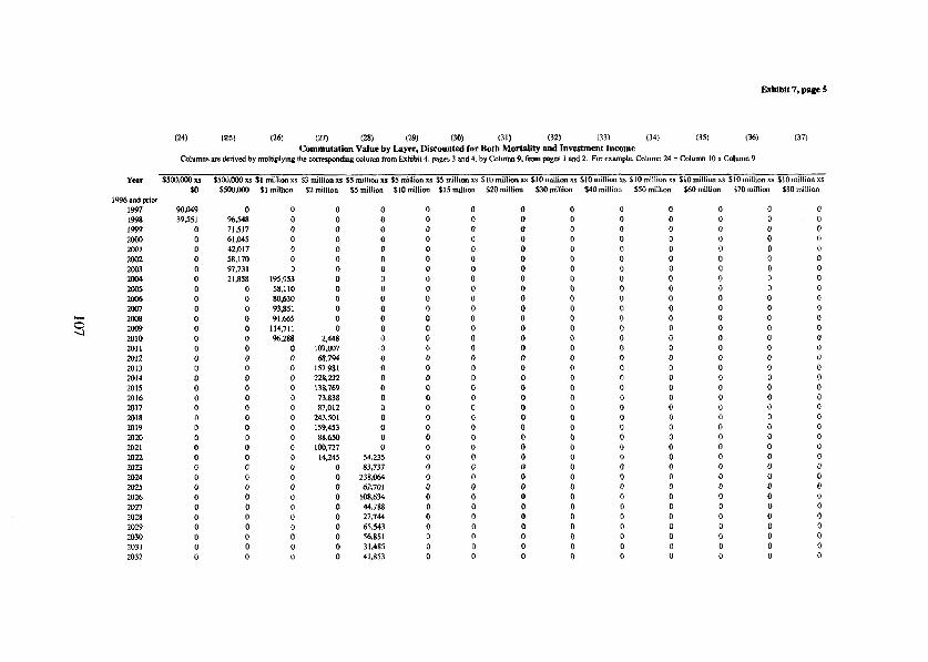
Exbtbit 7, p~ge 9

(24) (25) (26) (2-J) (28) (29) (30) (31) (32) (33) (34) (35) (36) (37) Commutation Value by Iayer, Diseounted for Both Mortality and Iavestment Income

Yclr

Co1umn.s are derived by multiplying !he correspnding colunm fmm Fxhibit 4. pages 3 and 4. by Column 9, fmm pags l and 2. For erample, Column 24 = Column 10 x Column 9

SSW,ooO xs $SW.WO xs SI miIlion xs $3 million XE SS milIion xs S5 million x3 $5 millim xs SI0 mUion as $10 millicm xs SlO million xs $10 million xs $10 million xs 5 10 million rr $10 milhon xs

19% and prior 1941 1998 1999 l!xa 2001 2w. 2003 2w4 2w5 2006 zwl 2w8 lcm9 MIO 2011 2012 2013 2014 2015 2016 2017 2018 2019 ZOU) 2021 2022 %x3 2024 2025 2026 2017 2028 2029 2030 2031 2032

Sn

901149 39,551

0 0 0 0 0 0 0 0 0 0 0 0 0 0 0 0 0 0 0 0 0 0 0 0 0 0 0 0 0 0 0 0 0 0

ssw,wo SI million 52 million s5 miIlion SI0 million $15 maicn

0 0 0 0 0 %.548 0 0 0 0 71.517 0 0 0 0 61.045 0 0 0 0 42,017 0 0 0 0 58,170 0 0 0 0 97,731 0 0 0 0 21.858 195,953 0 0 0

0 58,110 0 0 0 0 80.630 0 0 0 0 93,851 0 0 0 0 9l,655 0 0 0 0 114,711 0 0 0 0 96388 2,448 0 0 0 0 107.W7 0 0 0 0 68.79-t 0 0 0 0 157,981 0 0 0 0 228,122 0 0 0 0 138,769 0 0 0 0 73,838 0 0 0 0 87,011 0 0 0 0 243.501 0 0 0 0 159.453 0 0 0 0 88.650 0 0 0 0 100.727 0 0 0 0 14.245 54.235 0 0 0 0 83.737 0 0 0 0 238,064 0 0 0 0 62.701 0 0 0 0 108,634 0 0 0 0 44.788 0 0 0 0 27.744 0 0 0 0 65,543 0 0 0 0 56.851 0 0 0 0 31,485 0 0 0 0 41.853 0

0 0 0 0 0 0 0 0 0 0 0 0 0 0 0 0 0 0 0 0 0 0 0 0 0 0 0 0 0 0 0 0 0 0 0 0

S20 million S30 millicm 540 million 550 million SM) million $70 millian 580 millmn

0 0 0 0 0 0 0 0 0 0 0 0 0 0 0 0 0 0 0 0 0 0 0 0 0 0 0 0 0 0 0 0 0 0 0 0

0 0 0 0 0 0 0 0 0 0 0 0 0 0 0 0 0 0 0 0 0 0 0 0 0 0 0 0 0 0 0 0 0 0 0 0

0 0 0 0 0 0 0 0 0 0 0 0 0 0 0 0 0 0 0 0 0 0 0 0 0 0 0 0 0 0 0 0 0 0 0 0

0 0 0 0 0 0 0 0 0 0 0 0 0 0 0 0 0 0 0 0 0 0 0 0 0 0 0 0 0 0 0 0 0 0 0 0

0 0 0 0 0 0 0 0 0 0 0 0 0 0 0 0 0 0 0 0 0 0 0 0 0 0 0 0 0 0 0 0 0 0 0 0

0 0 0 0 0 0 0 0 0 0 0 0 0 0 0 0 0 0 0 0 0 0 0 0 0 0 0 0 0 0 0 0 0 0 0 0

0 0 0 0 0 0 0 0 0 0 0 0 0 0 0 0 0 0 0 0 0 0 0 0 0 0 0 0 0 0 0 0 0 0 0 0

Exhibit 7, page 6

YcSr

2033 lo34 2035 2036 2037 2038 2039 2040 2041 2042 2043 2044 2045 2046

8 2047

OO 2048 2049 2050 205, 2052 2053 2054 2055 2056 2057 2058 2059 2060 2061 2062 2063 2064 2065 20% 2067 2Os3 2069 2070 207 I

(24) (25) af4 (27) (28) (29) (30) (31) (32) (33) (34) (35) (36) Commutation Value by Laya, Dkounted for Botb MmWtty nnd Investment Income

Colu”mr are derived by multiplying Ule comsponding colum,, from lW,,bit 4, pages 3 and 4. by Coluw 9. hrm pa.ges 1 and 2. Fa example. Column 24 = Column 10 x Column 9

(37)

s5co.ccQxr 15co.w xs SI milllon XI 13 millio” xs $5 millicn xs $5 mi,lion xs s5 Mllion xs SI0 mdlioo xs SI0 muion xs SI0 millicm xs $10 m,llmn xs $10 maion xs 110 milhon xs SI0 INlliO” X6 so s5oo.Ow Sl miuion 52 miumn 55 mAlion SI0 mdlion $15 miuion $20 miltial $30 Mlllml s-40 million $50 MIllO” S-50 million $70 rmlllon S80 million

0 0 0 0 0 0 0 0 0 0 0 0 0 0 0 0 0 0 0 0 0 0 0 0 0 0 0 0 0 0 0 0 0 0 0 0 0 0 0 0 0 0 0 0 0 0 0 0 0 0 0 0 0 0 0 0 0 0 0 0 0 0 0 0 0 0 0 0 0 0 0 0 0 0 0 0 0 0

0 0 40.012 0 0 60.197 0 0 73.083 0 0 33.316 0 0 19.808 0 0 0 0 0 0 0 0 0 0 0 0 0 0 0 0 0 0 0 0 0 0 0 0 0 0 0 0 0 0 0 0 0 0 0 0 0 0 0 0 0 0 0 0 0 0 0 0 0 0 0 0 0 0 0 0 0 0 0 0 0 0 0 0 0 0 0 0 0 0 0 0 0 0 0 0 0 0 0 0 0 0 0 0 0 0 0 0 0 0 0 0 0 0 0 0 0 0 0 0 0 0

129.600 448.885 731.208 1,470.647 1042,047 overall Tota, = 4,258,655

0 0 0 0 0 0 0 0 0 0 0 0 0 0 0 0

4-5367 0 0 0 46,163 0 0 0 %8Ch5 0 0 0 17.233 0 0 0 38354 0 0 0 30,387 0 0 0 56,878 0 0 0 24.993 0 0 0 12,459 8.041 0 0

0 32.988 0 0 0 10.388 0 0 0 6,598 0 0 0 7.956 0 0 0 10,779 0 0 0 3.310 0 0 0 4,338 0 0 0 2,798 4.192 0 0 0 w-59 0 0 0 3.346 0 0 0 l.401 0 0 0 l.597 0 0 0 562 0 0 0 3.817 0 0 0 58 801 0 0 0 1.514 0 0 0 171 0 0 0 52 0 0 0 10 0 0 0 0 0 0 0 0 0 0 0 0 0 0 0 0 0 0 0 0 0 0 0 0 0 0 0 0

327.641 87.197 18661 2,548

0 0 0 0 0 0 0 0 0 0 0 0 0 0 0 0 0 0 0 0 0 0 0 0 0 0 0 0 0 0 0

45 124

9 0 0 0 0 0

179

0 0 0 0 0 0 0 0 0 0 0 0 0 0 0 0 0 0 0 0 0 0 0 0 0 0 0 0 0 0 0 0 0

24 16

I 0 0 0

40

0 0 0 0 0 0 0 0 0 0 0 0 0 0 0 0 0 0 0 0 0 0 0 0 0 0 0 0 0 0 0 0 0 0 0 I I 0 0

2

0 0 0 0 0 0 0 0 0 0 0 0 0 0 0 0 0 0 0 0 0 0 0 0 0 0 0 0 0 0 0 0 0 0 0

0.00 0.00 0.16 0.04

0.20

0 0 0 0 0 0 0 0 0 0 0 0 0 0 0 0 0 0 0 0 0 0 0 0 0 0 0 0 0 0 0 0 0 0 0 0 0 0

0.02

0.02

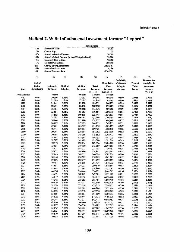
Exhibit 8, page 1

Method 2, With Inflation and Investment Income “Capped”

(A) W fc) CD)

Parametem Evaluation Date: Current A@: Annud Indemnity Payment Annuel Medical Paymnt (U mid-1996 psice teveIs)

1/1/97 35

m.ocm 70,cmO

03) IndeJllnity Paid to Date m Medical hid to Lhte:

70,OOG 3cwoo

2.9785% 5.36%

4.3887%

(4) (5) (6) (7) Prcdmbility

Clmndative dc!aimant MediUl Total TOt81 Ii* ta

Pny=lIt Payment P.W=N IDid-yM (2) + 14 mm. oi (5)

3almo 73,752 77,705 81,870 86.258 m*88?s 95,753

loo,885 106,293 111.990 117,993 124‘317 130.981 138.001 145.398 153.191 161,402

170.054 179.169 188.772 198,890 209.551 220,783 232,617 245,085 258.221 272.Ob2 286644 3@2,w9 318.1% 33S.252 353.22 L 372.154 392.101 413.118 435.261 458.591 483.171 509.069 536.356

565,104 595,394 627.307 660.931

370,oóo 37GOO 94,348 98,914

103.1 Il la&750 114.043 119&34 125.447

464,348 563.262 666,973 nsn3 889,766

1,009170 1.134.817 1.2b6.403 1.404.440 1.549.255 1.701,193 1.860.618

131586 138.037 144.815 151,938 159.425 167,292 175,562 184.253 193.390 202.994 213,089 223.703 234,862 246.594 Z58;929 271,899 285537 299.879 314,960 330.821 347,501 365,043 383,494 402,900 423.313 444,784 467.370

491.129 516.123 542.417 570.079 599.182 629.802 662.019 695,917 731.s8-4

0.999 0.9% 0.993 0.9% 0.987 0.984 0.981 0.978 0.975 0.97 1 0.%7 0.%3

2.027.910 0.958 2,203,472 0.954 2.387.725 0.948 2581.114 0.943

0.936 0.930

2,784.108 2.997.197 3;220;901 3.455.763 3,702.356

3.961285 4.233.185 4,518,722 4.818.601 S.133.561 5.464.382 5.811.882 6,176,926

bS60.419

b-963.320

7,38b,b32

7,831.416

8.298,785 8,789.914 9,306.036 9.848,453

10.418532 11.017.715 11.647.517 12,309;536 13.lm4s3 13.737.036

0.923 0.9fS 0.906 0.85’7 0.886

0.875 0.863 0.850 0.836

0.821 0.80s 0.788 0.769

0.750 0.730 0.709 0.686 0.663 0.638 0.612

0.584

0.556 0.527 0.497 0.466

cmtet LiViIQ

AdJustment

(8)

Present V&e F8CkV In-

(7) x (8)

0.9788 0.9775 0.9376 0.9339 0.8982 0.8922 0.8604 0.8522 0.8243 0.8139 0.78% 0.7773 0.7564 0.7422 0.7246 0.7087 0.6941 0.6765

0.6650 06456

0.6370 0.6160 0.6102 0.5876

0.5846 0.5602 o.sml 0.5340 0.5364 0.5087 0.5139 0.4844 0.4923 0.4610

0.4716 0.4385 0.4518 0.4168 0.4328 0.3958 0.4146 0.3756

0.3971 0.3561

0.3804 0.3372 0.3545 0.3190 0.3491 0.3014 0.3345 0.2843 0.3204 0.2679

0.3069 0.2520 0.2940 0.2366 0.2817 0.2218 0.2698 0.2076

0.2585 0.1939 0.2476 a.1808 0.2372 0.1681 0.2272 O.ISbQ 0.2177 0.1442 0.208s 0.1330 0.1998 0.1222 0.1914 0.1118 0.I833 0.1019 0.1756 0.0925 0.1682 0.0836 0.1611 0.0751

hdemnity Medical PPyment Intlation

70,Ow 20.5% 5.36% 21.209 5.36% 21,841 5.34% 22.49 1 5.36% 23,161 5.36% 23.851 5.36% 24.562 5.36% 2S.293 5.36% 26,046 5.36%

26,822 5.36%

L996 and prior 1997 1992 1999 2ooo 2001 2002 2W3 2004 2005 2006 2007 2008 2w9 2010 2011 2012 2013 2014 2015 2016

2017 2018 2019 2020 2021 2022 2023 2024 2025 2026 2027 2028 m29 2030 203 I 2032 2033 2034 2035 2036

2037 2038 2039

3.0% 3.0% 3.0% 3.0% 3.0% 3.0% 3.0% 3.0% 3.0% 3.0% 3.0% 3.0% 3.0% 3.0% 3.0% 3.0% 3.0% 3.0% 3.0% 3.0% 3.0% 3.0% 3.0% 3.0% 3.0% 3.0% 3.0% 3.0% 3.0% 3.0% 3.0% 3.0% 3.0% 3.0% 3.0% 3.0% 3.09c 3.0% 3.0% 3.0% 3.0% 3.0% 3.0%

27.623 5.36% 28.444 5.36% 29.291 5.36% 30,162 5.36% 31,062 5.36% 31,987 5.36% 32.940 5.36% 33,921 5.36% 34.93 1 5.36% 35,972 5.36% 37.043 5.36% 38;146 5.36% 39,283 5.36% 40.453 5.36% 41,658 5.36% 42,898 5.36% 44.176 5.36% 45,492 5.36% 46,847 5.36% 48,242 5.36% 49,679 5.36%

Sl.lS9 5.36%

52,683 5.36% 54.252 X76% 55.868 5.36%

57,532 5.36% 59,245 5.36% 61.010 5.36% 62.821 5.36% 64.698 5.36% 66.625 5.36%

68,610 5.36% 7O,bS3 5.36%

109

Exbibit 8, page 2

Year

2040 2041 2042 2043 2044 204s

2M7 2048 2049 2050 205 1 2052 2053 2054 205s 2056 2057 2058 2059 2060 2061 2062 2063 2064 206s 2066 2067 2068 2069 2070 2071

(1)

cost of Livine

3.0% 3.0% 3.0% 3.0% 3.0% 3.0% 3.0% 3.0% 3.0% 3.0% 3.0% 3.0% 3.0% 3.0% 3.0% 3.0% 3.0% 3.0% 3.0% 3.0% 3.0% 3.0% 3.0% 3.0% 3.0% 3.0% 3.0% 3.0% 3.0% 3.0% 3.0% 3.0%

(2) (3)

Indemnity Medical Paymeat Intlation

72,758 5.36% 74,925 5.36% 77,lSb 5.36%

79.454 5.36% 81,821 5.36%

84.258 5.36% 86.768 5.34% 89.352 5.36% 92.013 5.36% 94.754 5.36% 97576 5.36%

100,483 5.36%

103.475 5.36% 106,557 S.361 109,731 5.36% 113.ooo 5.36% llb.MS S.36%

119,831 5.36% 123.400 5.36% 127:076 5.36% lM.861 5.36% 134.7s9 5.36%

138.772 5.36% 142,906 5.36%

147,162 5.36%

151.54s 5.36% I Sb;059 5.36%

m.707 S.345% 165.494 5.36% 170,423 5.36% 175.499 5.36%

180,727 5.36%

(4)

696,356 733.681 773.006 814,440 ESE.094 904,087 952,546

l,cQ3,603 1.M7.396

1,114.072 1.173.787 1,236.7@2 1,302,989 1,372,829 lJ46.413 1,523,940 1.605.624 1.691.685 1.782,359 L877.894 1.978.549 2.084.599 2.1%.334 2,314,057 2.438.091 2.568.772

2.706,459 2.851.525 3.004.366 3,1bS,400

3.335.OGS 3.513,825

(5) 6) (7) Probsbtlity

Cumulaüve of chimnnt TOlnl TOtel

PapWlt PayUEllt 12) + (4) Cum. of (5)

769.114 14506.150 808,606 15.314,756 850,163 lb,lb4,919 893,894 17,058,813 939.9 I 5 17.998,728 988,345 18.987.073

1,039,314 rn.026.387 1,092.95S 21JI9.342 1.149.409 22.268.751 1.208.826 23.477578 1,271,363 24.748.941 1,337,x34 2b,oab,l25 Mob464 27.492589 1,479,387 28.971.976 l.SSb,W 3O.S28,120 1.636.940 32.165,ChSO 1.721.989 33,887.049 1,811Jió 35.698566 1.5w5.760 37.604.325 2;c&!no 39,609;295 2.109410 41,718,7OS 2,219,358 43.938.063 2.335,IC-S 46,273,169

2.456963 48.73Jl.132 2S852S3 51,315,385 2,720,318 54.035,703 2,862.518 56.898.220 3.012.232 59.910,452 3.369.8W 63.080.313 3,335,824 66.416,137

0.435 0.403 0.372 0.340 0.308 0.277 0.246 0.217 0.188 0.162 0.137 0.114 0.094 0.075 0.059 0.04s 0.034 0.025 0.017 0.012 0.008 0.005 0.003 0.002 0.001 O.COO4 0.0002 0.0001

0.00002 O.OOXU

3,510,565 69.926,702 0.000001

3.694,552 73.62L254 0.-

livlog to mid-year

Present VIhe Factor

0.1544 0.1479 0.1417 0.1357 0.1300 0.1245 0.1193 0. ,143 O.lOPS 0.1049 O.lcQS 0.0962 0.0922 0.0883 0.0846 0.0811 0.0776 0.0744 0.0713 0.0583 o.Obs4 0.0526 O.MOO 0.0575 0.05s I 0.0528 o.oso5 0.0484 0.0464 0.0444 0.0426 O.MO8

(9)

moi-tality & invstment

inwme (7) x (8) 0.0672 0.0597 0.0526

0.0461

0.0400 0.0345

0.0294

0.0247 0.02c6 0.0170 0.0138 0.0110 o.ooab 0.0366 0.0050 osH37 O.M)26

0.0018 0.0012 O.OCiIS 0.0@35 o.Gm3 o.OcQ2 O.CWJI 0.0053 O.KWJ O.CUOO O.OKUl O.CCQO O.MxK, O.COO!l O.oooO

110

Wbit 8, page 3

(Ic!) (II) (12) (13) (14) (15) (16) 117) (IB) (191 m (21) m

IncrementaI Payments by Layer Y-r $13O,WO xs $503,000 xs $1 dllion xs $3 miIlion xs $5 million XE $5 million xs $5 miilion xs $10 million xs $10 million xs $10 million xs $10 million xs $10 million xs $10 milIion XI

1996 and prior 1997 iwa 1999 Po00 2001 2m

2co4 2005

2013 2014 2015 2016

2018 2019 2020 2021 2022 2023 2024 2025 2026 2027 2028 2029 2030 203 1 2032 2033

$37O,wo 55w,oOO al million $2 million $5 milIion $10 million $15 million S20 million $30 million 540 million $50 miilion 54% miIlion

94.348 0 0 0 0 0 0 0 0 0 0 0 35,652 63,262 0 0 0 0 0 0 0 0 0 0

0 103*711 0 0 0 0 0 0 0 0 0 0 0 108,750 0 0 0 0 0 0 0 0 0 0 0 114,043 0 0 0 0 0 0 0 0 0 0 0 I 10,234 9.370 0 0 0 0 0 0 0 0 0 0 0 l2cl47 0 0 0 0 0 0 0 0 0 0 0 131,586 0 0 0 0 0 0 0 0 0 0 0 138.037 0 0 0 0 0 0 0 0 0 0 0 144,815 0 0 0 0 0 0 0 0 0 0 0 151.938 0 0 0 0 0 0 0 0 0 0 0 159,425 0 0 0 0 0 0 0 0 0 0 0 139,382 27,910 0 0 0 0 0 0 0 0 0 0 0 175.562 0 0 0 0 0 0 0 0 0 0 0 184,253 0 0 0 0 0 0 0 0 0 0 0 193.390 0 0 0 0 0 0 0 0 0 0 0 202,994 0 0 0 0 0 0 0 0 0 0 0 213,089 0 0 0 0 0 0 0 0 0 0 0 223.703 0 0 0 0 0 0 0 0 0 0 0 234,862 0 0 0 0 0 0 0 0 0 0 0 246,594 0 0 0 0 0 0 0 0 0 0 0 258,929 0 0 0 0 0 0 0 0 0 0 0 271,899 0 0 0 0 0 0 0 0 0 0 0 285,537 0 0 0 0 0 0 0 0 0 0 0 299,879 0 0 0 0 0 0 0 0 0 0 0 IS1.399 133,561 0 0 0 0 0 0 0 0 0 0 0 330.821 0 0 0 0 0 0 0 0 0 0 0 347.501 0 0 0 0 0 0 0 0 0 0 0 365.043 0 0 0 0 0 0 0 0 0 0 0 383,494 0 0 0 0 0 0 0 0 0 0 0 402,90l 0 0 0 0 0 0 0 0 0 0 0 423,3 13 0 0 0 0 0 0 0 0 0 0 0 444.784 0 0 0 0 0 0 0 0 0 0 0 467.370 0 0 0 0 0 0 0 0 0 0 0 491.129 0 0 0 0 0 0 0 0 0 0 0 516.123 0 0 0 0 0 0 0 0 0 0 0 542.417 0 0 0 0 0 0 0

670 milIion

0 0 0 0 0 0 0 0 0 0 0 0 0 0 0 0 0 0 0 0 0 0 0 0 0 0 0 0 0 0 0 0 0 0 0 0 0

YUlr

2034 2035 2036 2037 2038 2039 2040 2041 2042 2043 2044 2045 2046

z 2048

Id 2049 2050 2051

2053 2054 2055 2056 2057 2058 2059 2060 2061 2062 2063 2064 2065 2066 2067 2068 2069 2070 2071

Exhibìt 8, page 4

(10) (11) (12) (13) (14) (15) (16) (17) (18) (19) (20) (21) (22)

IncrementaI Payments by Layer $130,000x* fSCWMns SI rmllionxr 63millionxs $5 millionxs á5millionnr á5millionxs $lOmillionxs $lOmillion xs S10millionxs SlOmillionxs SlOmillionxs $lOmillion xs

ã370.WO 05W.MM $1 million $2 milIion $5 million $10 million 5.15 million $20 milhon $30 million f5Omi11ion 560 milIion s70million 0 0 0 0 0 0 0 0 0 0 0 0 0 0 0 0 0 0 0 0 0 0 0 0 0 0 0 0 0 0 0 0 0 0 0 0 0 0

130.0x

0 0 0 0 0 0 0 0 0 0 0 0 0 0

0 0 0 0 0 0 0 0 0 0 0 0 0 0 0 0 0 0 0 0 0 0 0 0 0 0 0 0 0 0 0 0 0 0 0 0 0 0

0 151,547 0 0 0 0 0 0 0 0

418.532 0 599,182 0 629.802 0 662.019 0 695.917 0

0 0 731,584 0 0 0 769.114 0 0 0

0 0

0 0 0 0 0 0 0 0

0

0 0

0 850.163 493,850

0 893.894

314,756

0 939.915 0 988,345 0 1.012.927

0 0 0 0 0 0 0 0 0 0 0 0 0 0 0 0 0 0 0 0 0 0 0

0 0 0 0 0 0 0 0 0 0 0 0 0 0 0 0 0 0 0 0 0 0 0 0 0 0 0 0 0 0

0 -0 0 0 0 0 0 0 0 0 0 0 0 0 0 0 0 0 0 0 0 0 0 0 0 0 0 0 0

0 0

0 0 0 0

0 0 0 0 0 0 0 0 0 0

0 0 0 0 0 0 0 0 0 0 0 0 0 0 0 0 0 0

0 0 0 0 0 0 0 0 0 0 0 0

26.387 1.092,955 1.149.409 1.208.826 L271.363 1.337.184 1.406.464 1,479,387 1.028.024

0 0 0 0 0 0 0 0 0 0 0 0 0 0 0 0 0

0 0 0 0 0 0 0 0 0 0 0 0 0 0 0 0 0 0 0 0

528,120 1.636.940 b721.989 1.811.516 1.9Q5.760 2N4.970

390.705 0 0 0 0 0 0 0 0 0 0 0

$40 niIlion 0 0 0 0 0 0 0 0 0 0 0 0 0 0 0 0 0 0 0 0 0 0 0 0 0 0

1.718.705 2,219.358 2,335,106 2,456.%3 1.269.868

0 0 0 0 0 0 0

0 0 0 0 0 0 0 0 0 0 0 0 0 0 0 0 0 0 0 0 0 0 0 0 0 0 0 0 0 0

1.315.385 2320,318 2.862.518

0 0

3.012.232 89.548

0 0 0 0

0 0 0

0 0 0 0 0 0 0 0 0 0 0 0 0 0 0 0 0 0 0 0 0 0 0 0 0 0 0 0 0 0 0 0 0 0

3.080.313 3.335.824 3.510,565

73,298 0

3.621.254

5w.cinl 1 ,~.wo 3,MM.ooo 5,ooo.ooo 5.m.oco 5.ooo.ooo lO,OOO.ooO 1O.ooO.wO 1o.wo.ooo 10.coo.ooo 10.ooo.ooo 3.621.254

Exhibit 8, pa@ 5

(23) W m CL61 07) (28) (29) (30) (311 m (33) (34 (35) Commutabion Value by Ayer, Diiomted Por Botb Mortality and Investment Income

Columns are daived by multiplying tbe conqonding column from Exhibit 4. pages 3 and 4. by Column 9. from paga 1 and 2. For example, Cobtmn 23 = Column 10 x Column 9

$500,CWxs SSOO,WU xs $1 miUionxs $3 million xs $5 miltion xs $5 miIlion xs $S millionxs GlOmillion xs $10 miIlion xs $10 milliw xs $10 mi&011 xs I1Omillion xs fIOm¡ltion xs $500,000 $1 milllon $2 miuion $5 maion SlOmuion $l5millim $2oMIlton á30millian $40 million $50 núllion $60 mlllfon $70 million

1996 and prior so

1997 9222A 1998 33.2% 1999 2oLw 2001 2Ou2 2C03 x04 Mo.5 2OM 2007 2008

E 2Kw

w 2010 2011

0 0 0 0 0 0 0 0 0 0 0 0 0 0 0 0 0 0 0 0 0 0 0 0 0 0 0 0 0 0 0 0 0 0 0 0 0 0 0 0 0 0 0 0 0

2013 2014

2016 2017 2018 2019 257.0 2021 zoz? 2023 2024 202.5 2026 2027

2029 2030 2031 2032 2033

0 0 0 0 0 0 0 0 0 0 0 0 0 0 0 0 0 0 0 0 0 0 0 0 0 0 0 0 0 0 0 0 0 0 0

0 0 59,081 0 92526 0 92,673 0 92820 0 85,684 7,283

0 93.112 0 93.25 1 0 93,381 0 93,497 0 93595 0 93.67 1 0 78,085 0 0 0 0 0 0 0 0 0 0 0 0 0 0 0 0 0 0 0 0 0 0 0 0 0 0 0 0 0 0 0 0 0 0 0 0 0 0 0 0 0 0 0 0 0 0 0 0

0 0 0 0 0 0 0 0 0 0 0 0

15.636 93,742 93J29 93,678 93.583 93.437 93.233 92.962 92.619 92,196 91.688 91.084 90,375 51578

0 0 0 0 0 0 0 0 0 0 0

0 0 0 0 0 0 0 0 0 0 0 0 0 0 0 0 0 0 0 0 0 0 0 0 0

37,976 88.614 87.554 86,372 85.070 83.645 82.0% 80.413 78583 76.594 74,439 72.121

0 0 0 0 0 0 0 0 0 0 0 0 0 0 0 0 0 0 0 0 0 0 0 0 0 0 0 0 0 0 0 0 0 0 0 0 0

0 0 0 0 0 0 0 0 0 0 0 0 0 0 0 0 0 0 0 0 0 0 0 0 0 0 0 0 0 0 0 0 0 0 0 0 0 0 0 0 0 0 0 0 0 0 0 0 0 0 0 0 0 0 0 0 0 0 0 0 0 0 0 0 0 0 0 0 0 0 0 0 0 0

0 0 0 0 0 0 0 0 0 0 0 0 0 0 0 0 0 0 0 0 0 0 0 0 0 0 0 0 0 0 0 0 0 0 0 0 0

0 0 0 0 0 0 0 0 0 0 0 0 0 0 0 0 0 0 0 0 0 0 0 0 0 0 0 0 0 0 0 0 0 0 0 0 0 0 0 0 0 0 0 0 0 0 0 0 0 0 0 0 0 0 0 0 0 0 0 0 0 0 0 0 0 0

0 0 0 0 0 0 0 0 0 0 0 0 0 0 0 0 0 0 0 0 0 0 0 0 0 0 0 0 0 0 0 0 0 0 0 0 0

2034 2035 0 0 2036 0 0 2037 2038 2039 2cMO 2041 2042 2043 2044 2045 2046 2n47

Y 2048 2049

P 2050 2051 2052 2053 2054 2055 2056 2057 2058 2059 2060 2061 2062 2063 2064 2055 2066 2067 2068 2069 2070 2071

Exhibit 8, page 6

(23) (24) (25) (26) (27) 08) (2% (30) (31) (32) (33) (341 (35) Commutation Value by Layer, Discounted for Both Mortality and Investment Income

Columns are detived by mulriplying tbe correrponding column from Exhihil 4, paga 3 and 4. by Column 9, from paga 1 and 2. For example, Column 23 = Column 10 x Column 9

SSCQ.wO xs áSW.MX) xs $1 million xs $3 million xs $5 million xs SS million xs $5 million xs $10 million xs SI0 mUion xs $10 million xs $10 million lis $10 million xs $10 million xs SO bSW.coa $1 million 12 million $5 million $10 million SI.5 million S20 million $30 million $40 milIion $50 million $60 million $70 million 0 0 0 0

0 0 0 0 0 0 0 0 0 0 0 0 0 0 0 0 0 0 0 0 0 0 0 0 0 0 0 0 0 0 0 0 0 0 0 0 0 0 0 0 0 0 0 0 0 0 0 0 0 0 0 0 0 0 0 0 0 0 0 0 0 0 0 0 0 0 0 0 0 0

0 0 0 0 0 0 0 0 0 0 0 0 0 0 0 0 0 0 0 0 0 0 0 0 0 0 0 0 0 0 0 0 0 0 0 0 0

125,520 422,784 645,876 1 Overnll Tota, = 4,124,102

0 0 0

0 0 0 0 0 0 0 0 0 0 0 0 0 0

J79.539

18513 0 0 0 0 0 0 0 0 0 0 0 0 0 0 0 0 0 0 0 0 0 0 0 0 0 0 0 0 0 0 0 0 0 0 0 0 0

951,989

67.002 64,207 61,265 58.184 54.976 51,655 29,462

0 0 0 0 0 0 0 0 0 0 0 0 0 0 0 0 0 0 0 0 0 0 0 0 0 0 0 0 0 0

0 0 0 0 0 0 0 0 0 0 0 0 0 0 0 0 0 0 0 0 0 0 0 0 0 0 0 0 0 0 0 0 0 0 0

18.778 0 0 0 0 44.748 0 0 0 0 41,203 0 0 0 0 37,629 0 0 0 0 34.054 0 0 0 0 29,736 775 0 0 0

0 27047 0 0 0 0 23.705 0 0 0 0 20.509 0 0 0 0 17,494 0 0 0 0 14,691 0 0 0 0 12,125 0 0 0 0 9,818 0 0 0 0 5,142 2.641 0 0 0 0 6.027 0 0 0 0 4,546 0 0 0 0 3,33 I 0 0 0 0 2,362 0 0 0 0 l.61J 0 0 0 0 1% 863 0 0 0 0 663 0 0 0 0 393 0 0 0 0 220 0 0 0 0 56 58 0 0 0 0 55 0 0 0 0 24 0 0 0 0 9 0 0 0 0 0 0 a 0 0 0 0 0 0 0 0 0 0 0 0 0

437,878 206.147 131305 20.718 2,195 146

0 0 0 0 0 0 0 0 0 0 0 0 0 0 0 0 0 0 0 0 0 0 0 0 0 0 0 0 0 0 0 0 0 0 3 1 0 0

4

0 0 0 0 0 0 0 0 0 0 0 0 0 0 0 0 0 0 0 0 0 0 0 0 0 0 0 0 0 0 0 0 0 0

0.00 0.00 0.00 0.03

0.03

Capital and Risk and their Relationship to Reinsurance Programmes

by Stewart M. Coutts and Timothy R.H. Thomas

115

Capital and risk and their relationship to reinsurance programmes

by Sfewart M Coutts & Timothy R. H Thomas

Abstraet An eariier paper by the same authors developed the Daykin et al. (1994) asseffliability model to examine the effects of different reinsurance progrannnes on the capital of a direct property/casualty insurance company. By modelling the gross premiums and claims separateiy from the impact of reinsurance on them, it is possibie to examine directly the effects of different reinsurance programmes on a company’s expected performance just as easily as changes in asset mix or business volumes.

This paper goes on to discuss how such a modei can be used to quantify capital at risk for management reporting purposes, both for the company as a whole, and within individual profít centres, and how this is affected by different reinsurance strategies. It therefore links closely to the Dynamic Financiai Analysis project being sponsored by the Casualty Actuarial Society.

Biographies Dr Stewart Coutts is a consulting actuary, who has specialised in property/casuaIty insurance for 25 years. He published papers on the rating of motor insurance in the early 1970’s and was a member of the British Solvency Working Party in the mid- 1980’s. The work done by this body was a forerunner of both the Daykin model and the NAIC Risk Based Capital model.

Tim Thomas is a Chartered Accountant, who has worked in various capacities in the insurance industry for over 20 years. He joined the reinsurance division of Wiilis Faber & Dumas as an executive director four years ago, and since then has been involved in various aspects of alternative risk transfer, as well as being involved in the Group’s market security operations. He has a degree in Mathematics from Southampton University.

1. Introduction

1.1 Insurance companies have as their prime business the accepting of unwanted risk on behalf of others. They aceept different types of risk in the expectation of being able to generate an adequate return on capital from the premiums charged. The management of the risk so assumed within the company is therefore of fundamental importance to the success of the operation.

1.2 Intuitively, an insurance company ought to be able to manage exposures of both liabilities and assets in such a way that it allocates its established “risk tolerance” between underwriting activities and investment strategy to maximise its expected overali return on capital. By this, we mean the management’s willingness to live with

117

unstable results in order to boost expected profitability. The “risk tolerance” leve1 of an individual company is clearly a matter for its Board of Directors to establish, subject to regulatory minimum standards.

1.3 By expressing this “Company Standard” leve1 in financia1 terms, it becomes possible to measure the amount of capital at risk in both the company as a whole, and in individual operating units. The company’s performance can then be measured and managed, and different business strategies can be compared - a task ideally suited to stochastic modelling.

1.4 In order to improve retum on capital, either in an individual profit centre or in the company as a whole, we can either increase profits or reduce capital employed. This paper addresses in particular the quantifícation of capital employed, and how this is affected by different reinsurance strategies.

1.5 Reinsurance has traditionaily been bought to stabilise both profits and capital of an insurance company. It therefore has a major impact on the risk capital requirements of both the company as a whole, and each individual unit. If we want to manage risk capital, we have to be able to understand how reinsurance affects it.

1.6 We consider that a better understanding of the overa11 financia1 impact of reinsurance is of increasing importance because of the need to compare the relative merits of different reinsurance structures both with each other, and with the range of new capital market solutions being developed, which offer varying degrees of risk transfer.

2. Capital at risk v REiC

2.1 The risks to which the insurance company are subject can affect a company’s balance sheet in different ways. The RBC model introduced recently in the USA is an attempt to quantify the overa11 effect of these risks, and set approptiate minimum capital standards.

2.2 In this paper, we differentiate between the values given by applying this model, and management’s own interna1 quantifícation of capital at risk. To avoid confusion, we use the term “RBC” as the value determined by the NAIC REK model, and “capital at risk” as the interna1 measure. In no way are we seeking to question the value of the RBC formula itself, both as a regulatory tool, and as a device for educating management as to the value of using quantative techniques to review the effectiveness of their strategies for maximising prudent retums.

2.3 The RBC model is designed to serve as a diagnostic tool for regulators, primarily as an early warning indicator of situations which may need regulatory attention. However, it is likely that companies with high scores will try to capitalise on them by encouraging the creation of “league tables”, which in tum will trigger a flight to perceived quality.

2.4 It is therefore likely that companies, particularly those with lower than average RBC positions, will take action to improve their situations. Some of this action will undoubtedly be of a cosmetic nature, similar to the “financia] reinsurance” abuses

Il8

which FAS 113 has tried to outlaw. Other action will undoubtedly be taken for sound business reasons. In any case, RBC implications will increasingly be taken into account by managements in formulating their strategic plans.

2.5 As managements become increasingly aware of the impact of RBC requirements on business, there will be an increasing realisation of the need to service capital. Thus managements now have a growing need for a tool for allocating capital to, and measurement of performance of, individual operating units.

3. RBC Formulae v Stochastic AsseULiability Modeliing

3.1 The authors see RBC formulae as as a regulatory tool, rather than for use inside a company, either for risk management or capital allocation purposes. From this perspective, there are a number of weaknesses, in particular

l they look back at where the company has come from, rather than attempting to factor in future business plans

l the company’s exposure to catastrophic loss is considered neither gross nor net of reinsurance

l reinsurance factors are based on past average experience and no explicit allowance is made for changing future reinsurance programmes

3.2 Further, a model buih along RBC Enes involves the setting of various parameters for each class of business, which tend to be based on market average data. In theory, it would be possible to adjust these market figures for interna1 management purposes, and to assess the effect of different reinsurance arrangements. However, these adjusted parameters would need to be established and justifled to management at both corporate and proflt centre levels.

3.3 On the other hand, stochastic assetliiability modelling goes back to first principles to generate estimates of each individual cash flow for each Iine of business. By modelling the gross premiums and claims separately from the impact of reinsurance on them, it is possible to examine directly the effects of different reinsurance programmes on a company’s expected performance just as easily as changes in asset mix or business volumes.

4. What is a Stochastic Model?

4.1 Our earlier paper to the Institute of Actuaries in February 1997(Coutts and Thomas (1997)) described the WlSPR stochastic asset/liability model, able to simulate the major types of reinsurance treaty. This model is designed to simulate the development of both assets and liabilities of an insurance company which accepts new business for a period of three years, projecting forward until al1 outstanding claims have been paid. The three year planning horizon was set as a compromise between the desire to establish a medium term view of the company’s development, and the diffrcuity of setting realistic input assumptions.

119

4.2 In this paper, we show how the output f?om this model can be developed as a means of allocating risk capital by profit centre, taking iülly into account the different risk profiles of different classes of business, and how this process is influenced by different reinsurance structures. The model itseif is described more fully in our tirst paper, but for conveniente, the overall design is summarised in Appendix 1.

4.3 Stochastic model Office systems, based on forecasting individual cash flows from each line of business, have been well-established in the Life Insurance industry for several years, and are still in their infancy in PropertyKasuahy insurance. They will grow in importance as their sophistication grows. They need to be driven fiom the top of an organisation as an integral part of the planning process, and require constant amendment and refinement. Their use gives a totally new dimension to management information, not a replacement for previous reports, but extra leverage from there.

4.4 By modelling each cash flow separately, the anticipated results arising from different strategies can be compared, and in particular the inter-relationship between investment risk and insurance risk can be managed. These models allow management to:-

l Establish the risk profíle of the company in financia1 terms . Understand and manage the volatility in eamings . Compare altemative strategies on a leve1 playing field . Allocate risk capital by line of business, and set profit targets l Examine the relative merits of different reinsurance structures

5. Why buy reinsurance?

5.1 Apart from certain non-tinancial considerations, such as the acquisition of technical assistance from reinsurers, the traditional reasons for buying reinsurance are:-

. To protect capital

l To stabilise eamings

l To release capital for altemative uses

5.2 These reasons translate easily into the new language of maximising retum on capital at risk. What has happened is the growth of altemative risk transfer mechanisms, and the extra sophistication of capital markets. The range of options open to management now includes:-

. Traditional bond and equity finance

. “Act of God” bonds

. Reinsurance derivatives

. Financia1 or Finite Risk reinsurance

. Reinsurance captives l Traditional reinsurance

120

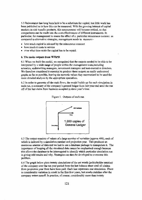
5.3 Reinsurance has long been held to be a substitute for capital, but little work has been published as to how this con be measured. With the growing interest of capital markets in risk transfer products, this measurement will become critica¡, so that comparisons can be made into the cost-effectiveness of different instruments. In particular, for management to assess the effect of a particular reinsurance contract as compared to altemative strategies, management needs to measure:-

l how much capital is released by the reinsurance contract l how much it costs to service l over what time-scale the capital has to be repaid.

6. The main outputs from WISPR

6.1 When we built the model, we recognised that the outputs needed to be able to be interpreted by a wide rmge of people within the management team,including actuaries, underwriting managers, investment managers and non-executive directors. We therefore considered it essential to produce these outputs as easily understood graphs as far as possible, leaving the numeric values they summarised to be used for more detailed analysis by the appropriate specialists.

6.2 in order to generate al1 the cash tlows, the model builds up for each simulation in each nm, a summary of the company’s general ledger from last year-end until the run off of the last claim from business accepted in three year’s time.

Figure 1. Outputs of each run

1,000 copies of General Ledger

6.3 The output consists of values of a large number of variables (approx 400), each of which is indexed by a simulation number and projection year. This produces an enormous amount of data and we had to use a database package to manipulate it. The importance of keeping al1 the simulated data cannot be emphasised enough because this allows the database to be interrogated to identify which particular simulation run is giving odd results and why. Strategies can then be developed to overcome this problem.

6.4 The graph below plots twenty simulations of the net worth (policyholder surplus) of the company over the ten year period ñom the last balance sheet until ali claims from projection year three have been paid. Each line represents one simulation. There is considerable variation in res& in the first four years, but resulta stahilise after the company enters runoff. In practice, of course, considerably more than twenty

121

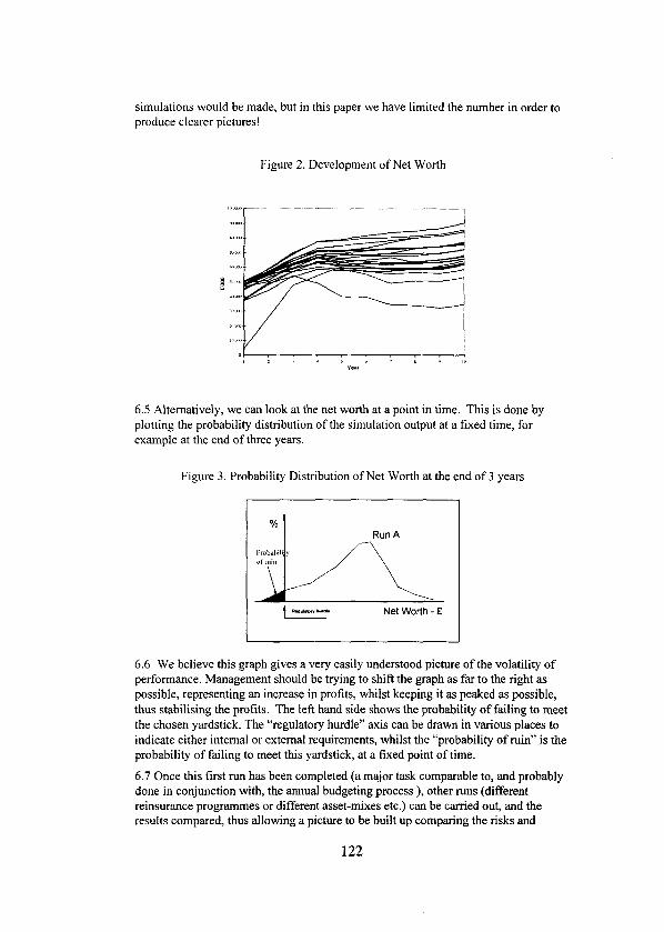
simulations would be made, but in this paper we have limited the number in order to produce clearer pictures!

Figure 2. Development of Net Worth

6.5 Altematively, we can look at the net Worth at a point in time. This is done by plotting the probability distribution of the simulation output at a tixed time, for example at the end of three years.

Figure 3. Probability Distribution of Net Worth at the end of 3 years

t R.o.*4- Net Worth - f

6.6 We believe this graph gives a very easily understood picture of the volatility of performance. Management should be trying to shift the graph as far to the right as possible, representing an increase in profits, whilst keeping it as peaked as possible, thus stabilising the profits. The left hand side shows the probability of failing to meet the chosen yardstick. The “regulatory hurdle” axis can be drawn in various places to indicate either interna1 or externa1 requirements, whilst the “probability of ruin” is the probability of failing to meet this yardstick, at a fixed point of time.

6.7 Once this first tun has been completed (a major task comparable to, and probably done in conjunction with, the annual budgeting process ), other runs (different reinsurance programmes or different asset-mixes etc.) can be carried out, and the results compared, thus allowing a picture to be built up comparing the risks and

122

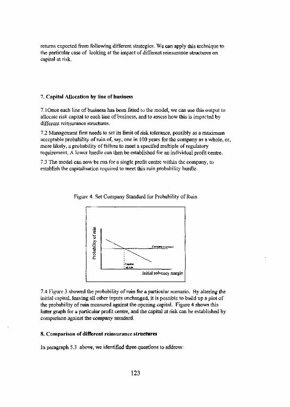
retums expected from foiiowing different strategies. We can apply this technique to the particular case of looking at the impact of different reinsurance stmctures on capital at risk.

7. Capital Aliocation by he of business

7.1 Once each line of business has been fitted to the model, we can use this output to allocate risk capital to each line of business, and to assess how this is impacted by difYerent reinsurance structures.

7.2 Management tirst needs to set its limit of risk tolerance, possibly as a maximum acceptable probability of ruin of, say, one in 100 years for the company as a whole, or, more likely, a probability of failure to meet a specifed multipfe of regulatory requirement. A lower hurdle can then be established for an individual profit centre.

7.3 The model can now be t-un for a single pro& centre within the company, to establish the capitalisation required to meet this ruin probability hurdle.

Figure 4. Set Company Standard for Probability of Ruin

7.4 Figure 3 showed the probability of ruin for a particular scenario. By altering the initial capital, leaving all other inputs unchanged, it is possible to build up a plot of the probability of ruin measured against the opening capital. Figure 4 shows this Iatter graph for a particular profít centre, and the capital at risk can be established by comparison against the company standard.

8, Comparison of different reinsurance structures

In paragraph 5.3 above, we identifred three questions to address:

123

8.1 How much capital does a reinsurance contract release? 8.1.1 We can run the model twice, once with each programme, and plot the probability of ruin against initial solvency margin for both runs. Applying the company minimum standard to these gives the following pictorial results for two different excess of loss reinsurance programmes:-

Figure 5. Measure capital saved

Initial solvency margin

8.1.2 Figure 5 shows the risk capital saved by reducing the excess point at a predetermined probability of ruin. This capital saved can now be used for altemative purposes within the company.

8.2 How much does this cost to service?

8.2.1 The servicing cost of the extra reinsurance is the premium paid away, less the anticipated recoveries, taking into account any lost investment income. This can be examined by comparing the probability distributions.

Figure 6. Expected servicing cost

Net Worth - f

8.2.2 Figure 6 shows the net worth of a company at the end of the period. Run A is the present reinsurance arrangement and Run B is a different one. Tl-re difference

124

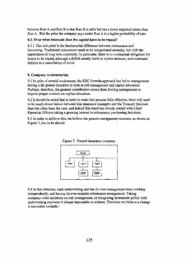
between Run A and Run B ís that Run B is safer but has a lower expected return than Run A. But the price the company pays under Run A is a higher probability of ruin,

8.3. Over what timescale does the capital have to be repaid?

8.3.1 This last point is the fundamental difference between reinsurance and borrowing. Traditional reinsurance tends to be renegotiated annually, but with the expectation of long term continuity. In particular, there is no contractual obligation for losses to be repaid, although a deticit usually leads to a price increase, and continued deticits to a cancellation of cover.

9. Company re-structuring

9.1 In spite of several weaknesses, the RBC formula approach has led to management having a far greater incentive to look at risk management and capital allocation. Perhaps, therefore, the greatest contribution comes from forcing management to impose proper controls on capital allocation.

9.2 It should be noted that in order to make this process fully effective, there will need to be much closer liaison between line insurance managers and the Treasury function than has often been the case, and indeed this trend has already started with Chief Financia1 Offtcers taking a growing interest in reinsurance purchasing decisions.

9.3 In order to achieve this, we believe the present management structure, as shown in Figure 7, has to be altered.

Figure 7. Present insurance company

9.4 In this structure, each underwriting unit has its own management team working independently, and having its own separate reinsurance atrangement. Taking company-wide decisions on risk management, or integrating investment policy with underwriting exposure is almost impossible to achieve. Therefore we believe a change is inevitable towards:-

125

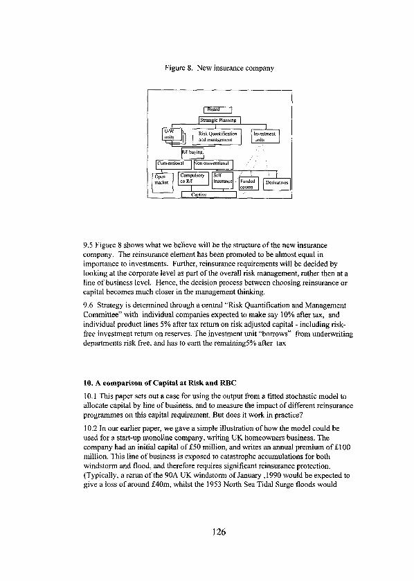
Figure 8. New insurance company

9.5 Figure 8 shows what we believe will be the structure of the new insurance company. The reinsurance element has been promoted to be almost equal in importance to investments. Further, reinsurance requirements will be decided by looking at the corporate leve1 as part of the overa11 risk management, rather then at a line of business level. Hence, the decision process between choosing reinsurance or capital becomes much closer in the management thinking.

9.6 Strategy is determined through a central “Risk Quantification and Management Committee” with individual companies expected to make say 10% afier tax, and individual product lines 5% after tax retum on risk adjusted capital - including risk- free investment retum on reserves. The investment unit “borrows” from underwriting departments risk free, and has to eam the remaining5% after tax

10. A comparison of Capital at Risk and RBC

10.1 This paper sets out a case for using the output from a titted stochastic model to allocate capital by line of business, and to measure the impact of different reinsurance programmes on this capital requirement. But does it work in practice?

10.2 In our earlier paper, we gave a simple illustration of how the model could be used for a start-up monoline company, writing UK homeowners business. The company had an initial capital of £50 million, and writes an annual premium of Ll00 million. This line of business is exposed to catastrophe accumulations for both windstorm and flood, and therefore requires significant reinsurance protection. (Typically, a rerun of the 90A UK windstorm of January ,199O would be expected to give a loss of around £40m, whilst the 1953 North Sea Tidal Surge floods would

126

produce a loss of E90m plus.) The detailed assumptions for this illustration are shown in Appendix 2.

10.3 The first run of the model, with a catastrophe reinsurance programme of £SOmillion excess of El Omillion, 95% placed, produced the individual plots of net Worth previously shown in Figure 2. By taking a cross section through al1 1,000 simulations at the end of Year 3, we produced the following distribution of net Worth (Figure 9):-

Figure 9. Demo insurance Co. Net Worth - Run 1

10.4 It is Worth noting in passing that although al1 the detailed assumptions used are for illustration purposes only, the answers being produced by the model reflect the unstable nature of the results of a mono-line company writing catastrophe-exposed business.

10.5 We now develop the output further to consider whether the initial capital is fully at risk, and indeed whether a lower figure could be justifíed (regulatory issues permitting!). We do this by plotting the probability of ruin, as explained in Section 7 above.

127

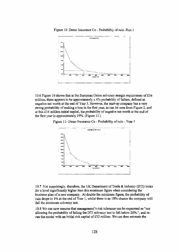
Figure 10 Demo Insurance Co - Probability of ruin -Run 1

10.6 Figure 10 shows that at the European Union solvency margin requirement of £16 million, there appears to be approximately a 4% probability of faiture, defined as negative net worth at the end of Year 3. However, the start-up company has a very strong probability of making a loss in the tirst year, as can be seen from Figure 2, and at this 516 million initial capital, the probability of negative net worth at the end of the tirst year is approximately 19%. (Figure 11.)

Figure ll - Demo Insurance Co - Probability of ruin - Year 1

10.7 Not surprisingly, therefore, the UK Department of Trade & Industry (DTI) looks for a leve1 significantly higher than this minimurn figure when considering the business plan of a new company. At double the minimum figure, the probability of ruin drops to 1% at the end of Year 1, whilst there is an 18% chance the company will fail the minimum solvency test.

10.8 We can now assume that management’s risk tolerance can be expressed as “not allowing the probability of failing the DTI solvency test to fa11 below 20%.“, and re- tun the model with an initial risk capital of £32 million. We can then estimate the

128

RBC requirement for the company at the end of both Years 1 and 3, assuming the same factors are appropriate for both US and UK homeowners business, and that LJK Govermnent securities require no risk factor. At the end of Year 1, this gives an RBC requirement of El 6.4 million, against average total adjusted capital of E2 1.3 million. (see workings in Appendix 3) a ratio of 130%, with a standard deviation of 34%, but with a very skew distribution:-

Figure 12 Probability Distribution of RBC %

Interestingly, whether by design or coincidence, there is also a 20% chance of breaching the Company Action Leve1 of the RRC rules. (By Year 3, that this ratio has improved to 247%, with a standard deviation of 47%.)

10.9 We can demonstrate fiom the detailed outputs that reducing the initial capital from £50 million to £32 million increases the 3-year average post tax return on capital fiom 7.6% to 9%. Not surprisingly, the standard deviation of this return also increases, from 4.6% to 7.8%.

10.10 A risk-averse owner may well be interested in reducing this volatility of eamings by reducing the catastrophe retention to around £6 million. Running the model on this assumption produces a post tax return on capital of 8.46%, with a standard deviation of 6.04%. Altematively, buying this extra layer reduces the capital at risk from E32 million to E30 million whilst the average reduction in ammal post tax profits is £ 0.3 rnillion, equivalent to a 15% post tax servicing cost on the E2million saving.

129

Figure 13 Comparison of Net Assets at the end of Year 3.

10.11 Management can now decide whether they can use this £2 million released capital more effectiviy elsewhere, bearing in mind its servicing cost, and the decrease in volatility in earnings.

11. Conclusion

Il. 1 We believe that Boards of Directors of insurance companies need a better understanding of the financia1 risks being assumed by their companies, and how reinsurance arrangements reduce these to manageable proportions. Although tools like WISPR take considerable effort to install, the benetits are substantial, and the timing is now right. with:-

. Increased attention on capital from rating agencies and regulators

. Lower profit margins l Increase in interest sensitive products l Increase in market volatility . Increase in non-traditional competitors

11.2 Inevitably, such benefits can only be obtained at the cost of fitting far more complicated assumptions than are necessary to tit an RBC model.

11.3 By using stochastic modelling to establish estimates of means and variances, it is possible to take assumptions built up by underwriters, using concepts with which they are familiar, and translate these into the language of investment portfolio management. This reduces the gap in understanding across different disciplines at senior management level, and ailows comparisons of reinsurance with other forms of risk transfer.

Bibliography

130

Daykin, C.D., Pentikäinen, T. and Pesonen, M. (1994). Practica1 risk theory for actuaries (1 st Edition). Chupman and Hall, London.

Coutts, S.M. and Thomas, T.R.H. (1997). Modelhng the impact of reinsurance on financia1 strength. Paper presented to the Institute of Actuaries, London. Feb. 1997.

National Association of Insurance Commissioners - 1996 NAIC Property and Casuahy Risk-Based Capital Report Including Overview and Instructions for Companies.

131

A description of the WISPR stochastic model

Appendix 1

1. Overview

1.1. The model is designed to simulate the development of both assets and liabilities of an insurance company. This company is assumed to accept new business for a period of three years, and then projects until al1 outstanding claims have been paid. The three year planning horizon was set as a compromise between the desire to establish a medium term view of the company’s development, and the difticulty of setting realistíc input assumptions.

1.2. The assets are sub-divided by major categories such as Government stocks, Equities and Property. The models used project forward income cash flows until the claims have runoff or the company is ruined.

1.3. The liabilities work on a class-by-class basis (see section 2), modelling the claim payment cash flows of gross reinsurance results and their associated reinsurance recoveries and reinstatement premiums, afier allowing for the effects of both financia1 and social inflation.

1.4. The reinsurance programme can comprise any combination of four main types, quota share, surplus, risk excess and catastrophe excess. The model can accommodate variable co-reinsurance of each cover, as well as factors such as event caps on proportional treaties. The catastrophe module allows information from GIS (Geographic Information Systems) models to be incorporated for storm, freeze, flood, earthquake and subsidence.

1.5. By combining the cash flows of assets and liabilities the model produces, the potential for profits or losses to emerge from the runoff of outstanding claims.

6. Each tun consists of a user-specified number of Monte Carlo simulations, in each of which the variables are sampled from appropriate probabihty distributions, so that a probability distribution can be built up for the results of the company as a whole. The run can then be repeated with different assumptions, to examine the sensitivity of these results to changing circumstances.

2. Clsss and subclass structure

2.1 The model calculates gross of reinsurance transactions on a sub-class basis, whilst reinsurance transactions are at a class leve1 (Figure Al).

132

Figure Al. Tree structure for group, company, class and subclass

1 XYZ Insurance Companyt

I I I l 1

Household Commeïcial MOtOI Propcrly

Liability MWilX

2.2 Figure Al shows a typical division of class and subclass of an insurance company .The main classes of business being household, motor, etc., with motor being split into subclasses Comprehensive and Third Party. The amount of detail at subclass leve1 is company dependent, for example if a company is writing only two classes of business, homeowners and motor, it might be necessary to have three or four subclasses for each class.

2.3 We believe that in practice, the number of classes should be limited to six, and subclasses to no more than ten, so that the overa11 picture can still be seen without being lost in a mass of detail.

2.4 The class structure will vary from company, and it is essential to determine this before too much time is spent in trying to assemble input data.

3. The main types of reinsurance

3.1 Reinsurance can be broken down into facultative (laying off parts of individual risks) and treaty (Iaying off risks aggregated overa block of business). Treaty reinsurance can be t%rther analysed into proportional (‘principally quota share and surplus) and non-proportional (excess of loss on either a per risk or per event basis, or stop loss). To model reinsurances other than quota share treaties, it is necessary to generate both individual claims and event catastrophes (which is where claims aggregate across severa1 policies to produce a potential recovery). Further, in the case of surplus treaties, commonly used to protect commercial property portfolios, it is

133

necessary to determine the size of cession on each policy subject to a large claim, before a recovery can be calculated.

3.2 There is a bad debt risk involved in ceding business to any reinsurer, however much care is taken in selection, and this can never be entirely removed. Whilst management should not lose sight of this risk, we have ignored it in this paper for simplicity. The model itself can handle the failure of a tixed percentage of security, specified separately for each separate contract, but a more rigorous treatment is worthy of a detailed study.

3.3 We expect a reinsurance programme for the classes of business in Figure A2 to resemble:

Figure A2. Simple reinsurance programme

3.4 Figure A2 shows that the household business is protected by a catastrophe, whilst motor and liability are covered by risk excess of loss. Commercial property is protected by a combination of surplus treaty and risk excess. An umbrella whole account protection covers catastrophe accumulation over household, commercial property and motor.

4. Build up cash ílows by class of business

4.1 The concept of cash flow modelling is now well documented, for example Daykin et al. (1994) (Chapter 1). In a simple diagram, Figure A3 illustrates the standard cash flows which have to be modelled.

134

Figure A3. Cash flow

Cash Flows

;%“ms r, Ezd?sr, Inv. Income and Gains D

Capital D

RECEIPTS

Reins. Premiurns *

Gross Claims 0

Expenses 0

TaW -

Dividends

PAYMENTS

4.2 Altematively Figure A3 can be linked together in the Daykin et al. (1994) transition equatiom-

Assets(end of period) = Assets(beginning) +( Gross Premium - Claims - Expenses - Reinsurance Premiums + Reinsurance Recoveries) + Investment income & gains - Taxation - Dividends + New Capital [+ New borrowings].

4.3 With suitable adjustments for changes in provisions, or receivables, this equation can be interpreted on either a cash basis or on an accounting accruals basis.

SModular Approach gives flexibiiity

5.1 The cash tlow computer programmes have to be designed very carefully, in particular the main problems relate to inter-relationships between transactions and that actuarial art in projecting forward is always improving. With this ín mind, the model was built up in a modular fashion, see Figure A4.

135

Figure A4. Modular structure

5.2 There are five distinctive stages in building up the final output:

Stage 1 : the data base input

Stage 2: modules 1 and 2 which calculate inflation rates and investment returns and individual catastrophe losses

Stage 3: modules 3,4,5,6 which are defined for each sub-class, calculate cashflows and technical reserves gross of reinsurance

Stage 4 : modules 7, 8,9 which are reinsurance recovery calculations

Stage 5: modules 11,12,13,14 which are the basis for the outputs .

5.3 By building up the model in modules as shown above, we have attempted to create a flexible structure which will enable changes ín the computer program to be made with the minimum of effort. Fot example, these changes could take the forro of a more sophisticated asset model, advances in actuarial techniques, the specifícation of a different family of claims curves, etc. This flexible approach has also been adopted in relation to links to other models - for example, we have not attempted to duplicate packages for reserving, or for turning claims data into probability distributions.

136

Assumptions for the demonstration of a simple start-up company Appendix 2

A detailed list of the parameters used in the simulations of the simple start-up company are given below:

l Initial capital £50 m.

l Opening investment portfolio:

Govemment Bonds E45 m Cash £3 m Working Capital £2 m

+ Positive cash flows invested 50% in Govemment Bonds, 50% in equities.

+ Selling Rules

There are two altemative strategies for how a negative cash flow will affect disinvestment. Firstly, to disinvest ín proportion to asset holdings at the start of the year or secondly, the assets are ordered and the asset with the highest priority is sold first. For the start-up company we use the tirst method.

+ The investment assumptions were as follows:-

cadi Equilies BOdS

Mean Real Retum 1% 5% 3% Running Yield 4.5% 3.0% 6.5% Volatility of Capital Growth 20% 10% Volatility of Income Growth 5% 1%

+ The effefective tax rate is 33%, and dividends will be at 50% of after-tax profíts.

+ Financia1 inflation was assumed to be normally distributed with a mean of 3.5% and a standard deviation of 0.5%.

+ The average rate of financial inflation assumed in calculating the value of mean loss ratios was also assumed to be 3.5%.

+ The business plan assumed that in each of the three years of the modellíng period, the gross premium was El00 m, and that losses other than catastrophe ones were normally distributed with a mean loss ratio of 55% and standard deviation of 2%. This information could be estimated from competitors’ published figures, or other sources. Claims reserves are not discounted.

137

+ The uneamed premium canied forward at the end of each year was assumed to be 40%

+ Commissions and oftice expenses were assmned to be 28% of premiums, reducing to 1% of year 3 gross written premium once business is no longer being written.

4 Socia1 inflation can be applied at differential rates for attrition and large losses but was ignored in this case.

+ Claims runoff pattems - the mean proportion and standard deviation of a claim paid in year i of development of the claim. These values are needed for past, future and catastrophe knock-on claims. These are all assumed to follow the same pattem:

Year Rsnoff Pattern Standard Deviation

1 64 5 2 28 3 3 4 3 4 2 2 5 l 2 6 1 2

+ The catastrophe reinsurance programme was structured as follows:-

Layer Indemnity Deductible Rate on line Co-reinsurance

1 10m 10m 20% 5% 2 20m 20m 12% 5% 3 20 m 40 m 8% 5% 4 30 m 60 m 4% 5%

+ The delay (in months) between making gross payments in respect of past and future claims and receiving the recovery payments. For the start-up company these values are taken as 3 months for quota share and 1 month for excess of loss.

+ Because the account is not subject to any wide fluctuations in size of sum insured, no reinsurance of individual risks is necessary, and therefore this run of the model did not need to generate individual large losses other than for catastrophes.

+ Natural per& catastrophe losses - these can be input either as a series of specific large losses or sampled by the model from a probability distribution. Under this, WISPR requires certain assumptions regarding the probability and potential size of each event for each peri1 to be input. These assumptions, obtained either from a GIS type model or from general management views, comprise the estimated maximum loss, the probability of an event of at least one tenth this size happening and a table setting out the relative probabilities of the size of the loss, given that one has happened. This table needs to be completed for each decimal of PML. For the start-up company the tables assumed are as follows:

138

Claim size

tsl!z!m 8000 0.42 PMLE80,OOO 16000 0.20 Probability 20% 24000 0.12

32000 0.07 40000 0.05 48000 0.04 56000 0.03 64000 0.03 72000 0.02 80000 0.02

10000 PMLE100,OOO 20000 Probability 2% 30000

40000 50000 60000 70000 80000 90000

100000

Probabilitv

0.05 0.05 0.05 0.15 0.15 0.15 0.2 0.1 0.05 0.05

139

Estimate of Risk Based Capital requirement - Run 2 Appendix 3

This simplified calculation of the Company Action leve1 REK requirement at the end of Year 1 is based on the requirements as set out in the NAIC instructions for 3 1st December 1996. These are set out in detail for simulation 3 of run 2, and average figures are also shown for each heading. A revenue account for simulation 3 is included for referente.

RO Asset Risk - Subsidiary Insurance Companies

Not applicable

RI Asset Risk - Fixed Income

Only RBC amount is for cash working balance, £3 million at 0.3% = 9,000.

(average 9,000)

R2 Asset Risk - Equity

Not applicable

R3 Asset Risk - Credit

Outstanding reinsurance recoveries E5.7 million at 10% = 570,000

Unpaid reinsurances - ni1

570.000

50% 285,000

(average 103,000)

R4 Underwriting Risk - Reserves

Gross outstanding loss reserves 19,233,OOO at 18.3% = 3,523,OOO

50% of credit REK 285.OOQ

3.808.000

((1,275*0.928) - 1 = 0.1832)

(average 2,553,OOO)

R5 Underwriting Risk - Net Written Premium

93,160,OOO at 17.4% =

((0.917*0.942)+ 0.31 - 1 = 0.1738)

(average 16,176,OOO)

16.192.OOQ

RBC (Company Action Level) = RO+SQRT(RlA2+R2”2+R3”2+R4”2+R5”2)

= SQRT(9000”2+285000”2+3808000”2+16192000”2

=16,636,000

(average 16,4 14,000)

140

Comparing Reinsurance Programs- A Practica1 Actua y’s System

by Robert A. Daino, FCAS, and Charles A. Thayer

141

COMPARING REINSURANCE PROGRAMS

A PRACTICAL ACTUARY’S SYSTEM

By Robert A. Daino and Charles A. Thayer

Biographies:

Mr. Daino has been in the industry since 1971. His experience includes actuarial and senior management positions at bureaus, primary insurers, and a reinsurance brokerage firm. Today, he is President of Cornerstone Consuhants, Inc. in Ramsey, New Jersey and specializes in actuarial, management and related consulting, primarily in the reinsurance and specialty lines arenas. He has designed, prepared and delivered mores of reinsurance program analyses and presentations. He has a B.A in Mathematics from Fordham University, and has been a member of the CAS and AAA for over twenty years. He, his wife and two daughters reside in Upper Saddle River, NJ.

MI. Thayer is a comultant with Cornerstone Consultants, Inc. He holds a Bachelor of Science degree in Mathematics from the University of Vermont. Before joining Cornerstone, he helped establish an actuarial function for a New York City reinsurance broker for six years. He began his insurance career in primaimary insurance, having served with two New England multi-line insurers where he was involved in pricing, product development, data quality and reporting systems. He resides in Mahwah, NJ.

Abstract:

This paper describes the elements of a simulation system used by the authors. A “user manual” approach is used to describe the elements of the system. A practicaJ sample scenario is used to show how the system is used in practice.

It is not the authors’ intent herein to discuss in any depth the technical issues involved in selecting the many parameters involved in a simulation. Rather, we try to show how a system can be used to control the parameters needed, and also help users analyze and communicate the res& to others.

143

COMPARINS REINSURANCE PROORAMS

A PRACYICAL ACTUARY’S SYSTEM

IMRODUCTION

Over the course of several years, the authors have been involved in many situations where reinsurance buyers were faced with making a decision between severa competing recomrnendations for their reinsurance program, often with significantly different structures. We found early on that one of the tools we needed was a simulation system. This paper will describe the elements of our current system, and the steps we take in building a simulation and analyzing the results.

Having developed early versions of this system and presented the res& to buyers, we learned much about what buyers, in general, consider important and what they are interested in seeing when making such a decision. To be sure, there is a wide variation in technical sawy among the many buyers of reinsurance, but most can understand the usefulness of comparing alternatives over many possible loss scenarios, the importance of getting a handle of some sort on the “odds” of favorable and unfavorable things happening, and almost al1 appreciate graphical representations of the results.

With reasonable assumptions about the variability of the number and size of claims by line of business, and with other necessary assumptions needed to mimic the insurance/reinsurance process, a more complete comparison between and evaluation of the severai competing reinsurance programs can be made (versus single scenario comparisons). Most buyers understand this as well.

Furthermore, most buyers understand that, ahhough the final simulation averages and aggregate distributions are only as good as the input assumptions (which are often very sor%), the decision value lies primarily in the comparative analysis that resuhs (ie., the absolute values may be approximate/soft numbers, but the indications about whether Option A is better chan Option B are much stronger).

Our original model was a Lotus 123” spreadsheet, but within the last year, working in conjunction with a group of professional developers and a majar reinsurer, we have brought this over and enhanced it greatly into a VB/Excel” system with a graphical user interface, template Iibraries for maintaining and controlling simulations, histories, etc. In this paper, we will describe rhe elements of this system as well as a practical example of its use.

144

COWPARINO REINSURANCE PROORAMS

A PRACTICAL ACTUARY’S SYSTSM

SYSlEMWERVEW

0 ur simulation system is a 3%bit WindowsrM system designed to build and manage the components of large Excel m - based simulation models. The user is guided through the creation of:

) Simulation Lines of Business - up to 40 lines, based on up to 40 Input Lines of Business (when data is available ín more detail than needed for simulation),

) Reinsurance Programs - up to three competing programs, made up of up to 15 treaties per program. A default gross 3 net - Xo reinsurance” program is automatically included, and

1 Other inputs, as needed, for beginning balance sheet values, investment and tax assumptions.

The system presents Excel Tn-like “patches” to the user in a WindowsTM front-end graphical user interface (GUI) program which also maintains control over every patch within a given client’s scenario. Multiple scenarios can be maintained for each client, and the system can control many clients. Parches can be saved for future use in similar scenarios for this or other clients. The program controls al1 of this in an AccesP database.

Once the user is satisfied that al1 inputs are ready, he instructs the program to compile the ExcelTM simulation workbook. Once the workbook is built, the user can view it, run the simulation or detach the workbook for use outside the control and management of the system (for cases where the standard program is not sufficient to describe the alternatives being compared). The user specifies the outputs he would like to track from the simulation, the number of iterations, etc. The system then performs the simulations and records the requested data in another Access TM database. Standard format exhibits and charts can then be requested from the system, while custom exhibits and charts can easily be built by the user outside the system.

145



The CliedScenario Manager

After an initial welcome screen, the system provides the following initial management window. Clients and their associated scenarios are managed from this window. Al1 sample screens that follow are taken from the “CAS Sample Scenario” developed for the sample “Multi-Line Insurance Company” for the purpose of providing a working example for this paper.

3/21/974:52:2... Yes 3/21/37 4515. Yu

A standard GUI interface for management of chent and scenario properties allows users to build and control multiple scenarios for many clients.

146

COHPARING REINSURANCE PROURAMS


Scenario Manager

This is the place most of the work is done. The major operations available from the scenario window are to Navigate and Change the Scenario Structure, View and Edit a Wizard Sheet, Recahxlate the Scenario, Access the Template Librar-y, Perform a Simulation, Print Reports, and Chart Res&.

The major parts of the Scenario window follow:

t Menu bar

) Tooibar Buttons

) Navigation Tree

The navigation tree is used to view and manipulate the entities of a scenario. With this, a user can add lines of business and reinsurance programs with their respective treaties.

147


A PRACTICAL ACYUARY’S SYSTEM

b Navigation Tree Elastic

The navigation tree area stretches to show more of the entity names or shrinks to show more of the data entry area (see below)

b Wizard Tab

Clicking this Excel m - like tab displays the corresponding wizard sheet.

) Data Entry Area

Gray background regions of this area cannot be modified. Only the white regions can be edited.

) Formula Bar

1 Scratchpad Elastic

The scratchpad elastic allows the user to resize the viewable area of the scratchpad, and in conjunction with the navigation elastic allows the user to customize his view of the workspace

) Scratchpad Area

This is an Excel TY - like spreadsheet on the right-hand side of a wizard sheet. This area is used to perform calculations which can be referenced from the Data Entry Area. A sample screen showing the scratchpad follows.

Navigate and Change the Scenario Structure

The structure of the current scenario can be viewed and altered from the navigation tree on the left-hand side of the Scenario window. This structure can be modified by manipulating its parts, which are also known as entities; the Client/Scenario entity, the Financia1 Assumptions entity, the Lines of Business entity, which in turn contains Line of Business entities, the Reinsurance Programs entity, which in turn contains Program entities, which in turn contain Treaty entities.

When an entity is added to the current scenario, a default set of worksheets is provided. The principal functions here are to Add a New Line of Business (LOB), Add a New Program, Add a New Treaty, and Show an Entity Wizard.

148

COMPARINO REINSURANCP PROORAMS A PRACTICAL ACTUARY’S SYSTEM

Rtsk Function Wizard

To allow the user to model a number of familiar frequency and severity models, we have built into this system the functions in the Excel rM add-in called @Risk n< which provides easy access to many of the functions used by property/casualty actuaries.

Since the spreadsheet-Iike features available in the front-end are not Excel n but rather an Excel-like VB component, the @Risk Ty add-in does not currentiy operate in this front-end. The default value displayed is the mean of the function. For more elaborate functions, the user can detach the workbook and work ouuide the system. (see below)

The Template Library

The application contains a storage area called the Template Library. The Template Library is used to store and retrieve wizard workbooks and wizard sheets. This facility allows the user to reuse wizard workbooks and sheets.

Perform a Simulation

The user can Build and Display the Simulation Workbook, and Run Simulations from the Scenario Window. If the user is satisfied with the workbook buik from his inputs, a simulation can be performed.

Userdefined fields are fields that the user wants to capture but are not available in any of the built-in selections, yet are items of special interest in carrying out the current work. They are availabie only in “detached” workbooks. Workbooks are detached in cases where the system’s standard features are not sufficient to completely describe what the user would like to test (such as very unique treaty terms).

149



Print Reports

Once simulation has been performed, the Prim Reports dialog can be invoked. The user can print summary reports for each line of business, program, and treaty in the current scenario.

g Current ReMsurance d Current Casuaity 1 st Excesî

%f Current cawatty 2nd Exoess

$ CurrentAPR Quota Share

v’ Cwent Property Excwî

Current Pmperty Catestrophe Excess

Recommended Multi-Line Excess

4 Recommended Pmperty Catastrophe

$ Recommended Appregate Excess

For each line of business and reinsurance treaty, there are two summary reports: a Statutory Underwriting Income repon. with the average underwriting results for the simulation, and a page of Highlights that shows averages, maximum and minimum values for several key variables of interest.

In addition, for the Overa11 Gross reporting leve1 and the Net results for each reinsurance program, there are three reports: First, there is the Statutory Income Statement report, including investment and other income. Also, an extensive Highlights page gives averages, maximum and minimum values for key items at the Ceded and Net levels, and a Statutory Average Balance Sheet report that shows average levels of several asset and liability classes for the tun.

150



Chart Results

Severa1 standard charts are available. The system itself generates some default charts that can be modified, printed or deleted by the analyst. The user can also develop new custom charts of each type within the system to compare results of reinsurance programs, treaties or lines of business.

“Green is Good, Red is Bad” Char&:

“Red/Green” charts allow the user to compare the results of two reinsurance options over the whole range of outcomes for a simulation, and especialiy to determine the type of loss scenario in which one alternative does a better job of meeting the insurer’s objectives than another. Each chart focuses on one particular variable, such as ceded or net underwriting profit, after-tax income, year-end surplus or any quantity that has importance in the evaluation process. The idea behind the Red/Green chart is simply to find the difference between the values of that variable for the two programs, determine whether a positive difference is better or worse for the cedant, and to plot green points when the first alternative is better and red ones when it is worse. The more green points that appear, the more often the first program comes out better.

Histograms:

Histograms show the non-cumulative distribution of some variable of interest for the given reinsurance programs, or for selected lines of business or treaties, either as frequencies or counts. In some cases, these will be the roughly bell-shaped curves that are often encountered in insurance statistics. The definition and interpretation of these charts is fairly easy to grasp. Cumulative versions are also avaítable.

151

COMPARINO REINSURANCE PROORAMS


Other Variabllity Charts:

Charts showing the year-to-year change in key percentile values are also available. These charts help the user see the variability of any selected output item in another fashion, which some users find very helpful.

Other Chañs:

Other charts are produced by the system or are in development, which help the user express himself, analyze the output more easily, explain results and communicate to others more conveniently.

152

COMPARINQ REINSURANCE PROORAM8

A PRACTICAL ACTUARY’S SYSTRM

HIGHUGHT’S OF THE INPUT’S

T his section is organizad by input wizard tab much the way the system inputs would be entered. Highlights only are provided in this paper.

CAS Sample Scenario

To illustrate the use of the system, we have~included a scenario called the CAS Sample Scenario for a client called the Multi-Line Insurance Company. See more details about this sample scenario in a separate section below.

The system provides a Test Layer capability to allow the user to test a particular excess of loss reinsurance layer to End out how many claims and loss dollars to that layer are expected from each of the subject lines of business. This helps in checking the aggregate effect on reinsurance layers of size of loss discribution selections for the various lines of business as well as other aspects of the excess layer, all while still in the front-end system, before any simulations have been attempted.

Financia1 Assumptions are entered in two tabs: Balance Sheet Assumptions, and Cash Fíow Assumptions. The system is focused on the underwriting side of the business. It has extensive inputs for product lines and treaties - the driving assumptions for gross, ceded and net results. However, the system builds complete income statements, including investment income, and balance sheets for each reinsurance program. The investment and cash flow assumptions are intentionally simplified, so they will not be a majo, source of questions/issues for clients, and thereby cloud the insurance/reinsurance underwriting result discussions. As a result of client requests for additional functionality, enhancements to the system in the asset and tax areas will be made.

153

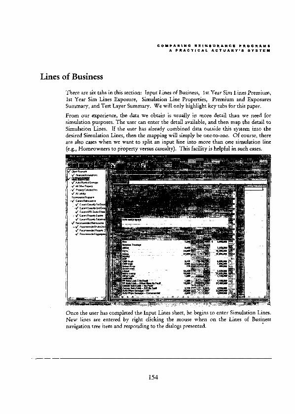
Lines of Business

COMPARIHO REINSURANCE PROORAIS


There are six tabs in this section: Input Lines of Business, 1st Year Sim Lines Premium, 1st Year Sim Lines Exposure, Simulation Line Properties, Premium and Exposures Summary, and Test Layer Summary. We will only highlight key tabs for this paper.

From our experience, the data we obtain is usually in more detail than we need for simulation purposes. The user can enter the detail available, and then map the detail to Simulation Lines. If the user has already combined data outside this system into the desired Simulation Lines, then the mapping will simply be one-to-one. Of course, there are also cases when we want to split an input line into more than one simulation line (eg., Homeowners to property versus casualty). This facility is helpful in such cases.

Once the user has completed the Input Lines sheet, he begins to enter Simulation Lines. New lines are entered by right clicking the mouse when on the Lines of Business navigation tree item and responding to the dialogs presented.

.

154

COMPARINO REINSURANCE PROORAYS


Once al1 Simulation Lines are entered, the user visits the 1st Year Sim Lines Premium Tab and the 1st Year Sim Lines Exposure Tab. These two tabs are identical in structure and have the role of allowing the user to allocate the Input Lines’ premium atad exposure to the selected Simulation Lines, keeping track of the total allocations, and posting the results to the appropriate Simulation Lines.

155

COMPARINO REINSURANCE PROORAYJ


Individual Simulation LOBs

There are nine tabs in this section: Exposure, Rate and Premium, Expenses, Limit Distribution, Payout Pattern, Payout of Existing Loss and LAE Reserves, Size of Loss Distribution, Losses Below Cutoff, Claims Above Cutoff, and Loss Expectations. We will show here only the last four relating to key loss assumptions.

Size of Loss Distribution Tab

Here the user enters the loss sizes and CDF by year for the given LOB. While this example seems to mimic the ISO 5 parameter Pareto model, it is not correct to consider it a continuous model. The size of loss distribution is entered as a discrete distribution, and al1 of the possible loss sizes in the simulation run will come from the list of values in the first column of the table. There is no interpolation in sampling and no attempt to determine an interval mean in computing the key expectations used elsewhere in the model. The averages and variances of the simulation results depend on the loss joints that are selected in the size of loss distribution, so these must be chosen carefully.

156

COMPARINO REINSURANOE PROORAMS

A PRACTICAL ACYUARY’S SYSTEM

Losses Below Cutoff Tab

The cutoff value is the point in the size of loss distribution at which the model will begin to simulate individual claíms for the given LOB. The lower the cutoff, the larger the number of claims the model will individually simulate.

On this tab, we enter the cutoff point, the expected number of claims for each year, and the risk model assumptions we wish to use to simulate the number and average severity of claims below the cutoff. The sample uses a mixed Gamma/Poisson to simulate the number of claims below the cutoff, This procedure is discussed in the Heckman-Meyers paper, “The Calculation of Aggregate Loss Distributions from Claim Severity and Claim Count Distributions” (KAS LXX, 1983, page 22ff). In addition, a censored and truncated Normal random variable with a mean of 1.0 is used to modify the severity below the cutoff that is used to compute the aggregate loss level. The user can easily specify other claims processes using other Excel Tu functions, @Risk TM functions, or even a constant set of claims with fixed amounts.

157

COMPARINO REINSURANCE PROORAWS


Claims Above Cutoff Tab

This rab is analogous to the previous tab, except that it regulates the simulation of claims above the cutoff point. When the simulation workbook is compiled and the simulation is run , the actual size of a simulated claim is chosen from the table in the Size of Loss Distribution tab. The sample uses a mixed GammaA’oisson distribution to simulate the number of claims above the cutoff, but again, the user can specify other processes.

The parameters and claims process chosen here form the heart of the individual large claim simulation done by the model.

158

COMPARINS RBINSURAMCE PROORAHS

A PRACTICA,. ACTUARV’S SYSTEM

Loss Expectations Tab

The Loss Expectations Tab for each LOB brings together the inputs from the previous tabs and allows the user to make a preliminary review of the results that can be expected from the user’s premium, loss frequency and severity assumptions. If care has been taken to preserve the integrity of the means from the severity distribution in the Size of Loss Tab, the results shown here should be a reasonable benchmark for checking the outcomes of the simulation runs. The averages that appear on the final reports from a simulation should come fairly close to the values shown on this tab.

159

COMPARINO REINSURA,dCE PROORAMS

A PRACTIGAL ACTUARY’S SYSTEM

Reinsurance Programs

In this system, a program consists of up to 15 treaties. LJp to three programs can be compared simultaneously. For example, the user might be comparing the Current Program to a Recommended Program and to a Competitor’s Program. The final output would have results of the simulation for each of these three programs plus the default “no reinsurance” or gross - net program.

The system does not accommodate facultative reinsurance. However, to reflect broad assumptions about “fac”, a user could enter facultative covers in bulk as a treaty, with pertinent, broad assumptions.

A treaty is created with a special dialog. In this dialog the user selects the generic treaty type that best matches the treaty. This affects the way that losses and premium are accounted for in the treaty. If the subject premium base is earned premium, the user simply selects that option and moves on. When the subject base is written premium, there is an additional check box the user may select to specify whether there will be a transfer of the subject beginning unearned premium reserve at the start of the first simulation year. The method by which the treaty subject premium is calculated (which treaties inure to this treaty’s benefit, etc.) can be specified by checking the inuring treaties in an extension of the standard dialog. Another dialog is used to specify the LOBs that are subject to each of the treaties.

160

COMPARINO REtNSURANCE PROORAMS A PRACTICAL AOTUARY’S SYSTEY

Treaties

At the treaty leve1 there are five tabs: Treaty Terms, Ceding Commissions, Excess Treaties, Payout Pattern, and Payout of Existing Loss & LAE Reserves. Sample tabs are highlighted below.

Treaty Terms Tab

The Treaty Terms tab gives the user the context in which al1 of the rest of the calculations for the treaty operate. The heading area tells the user the program and treaty names, the type of coverage provided by the treaty, the subject base, and the subject calculation, which teils the user if there are inuring treaties.

161

COMPARINO REINSURANCE PROORAWS

A PRACTICAL ACTUARY’S SYSTRW

162

COMPARINS REINSURANCE PROORAYS

A PRACTICAL AtTUARY’S SYSTEW

CASSAMPLESCENARIO

Input areas covered in the previous sections give the reader a broad overview of the types of inputs and manner in which the many inputs needed to perform a complete simulation are entered. In this section we go into a bit more detail concerning a particular sample.

Note: Rather than populate an appendix with dozens of reported results from our system, we will send a copy of a section showing the individual line of business assumptions, output exhibits, treaty res&, etc., to any reader who calls or writes us for a copy. These give the reader all the basic assumptions needed by line, treaty, etc., as well as key output.

Unes of Business in Sample Scenario

In the CAS Sample Scenario, we show a multi-line insurance carrier that is involved in over a dozen lines of business. We have segregated the overa11 book of business into four simulation lines, to simplify our sample. In a real-world case, we would separate lines based largely on their loss characteristics and reinsurance treatment (lines must map into treaties properly, and significant size of loss differences would be recognized).

The simulation lines in our sample are Automobile Physical Damage, Al1 Other Property, Property Catastrophes and Al1 Liability. Al1 of the individual input lines were included on the Input Limes of Business tab, but the premium and exposures were allocated to the simulation lines (in the 1st Year Sim Lines Premium and 1st Year Sim Lines Exposure tabs). See the section above titled “Lines of Business.”

The Property Catastrophes line serves a unique purpose in this scenario. It’s there to generate losses for the Property Catastrophe treaties in the reinsurance programs. No premium is assigned to this line of business. The Property Catastrophe treaties will pick up losses from this line of business, while their subject premium comes from the other Iines that are specified as subject to the treaties in the Treaty Subject Lines tab for each Program. There can be several such ‘Ges” if needed. In the sample scenario we have assumed that recoveries from the current risk excess would not materially affect the SOL distribution for property cats. If we knew that the distributions differed, we could reflect these differences in the system. Size of loss distributions obtained through a portfolio analysis using one of the severa1 commercially available catastrophe models can be accommodated by the system using one or more Property Catastrophe lines of business.

163

COMPIRINO REINSURANCE PROORAMS A PRACTICAL ACTUARY’S SYSTEM

Reinsurance Programs Used for Sample Scenario

The Multi-Line Insurance Company has a Current Reinsurance Program that consists of five treaties: 1st and 2nd Casualty Excess treaties, a Property Risk Excess treaty, an Automobile Physical Damage Quota Share, and a Property Catastrophe Treaty.

We will assume that there is a proposal for an alternative structure under consideration which we cal1 the Recommended Reinsurance Program, and that other programs may have been considered and rejected, leaving these two alternatives. The Recommended program consists of only three treaties: a Multi-line Excess treaty, a Property Catastrophe treaty and an Aggregate Excess treaty.

The key terms used for the Current Program were:

1” Cas~alty Excess: 100% of $750,000 xs $250,000; ALE included, Swing rated 4%/15% loss load 100/85ths

2nd Cusualry Excess: 100% of $4 mill. xs $1 mill.; ALE included, Fiat rated 6.23% with 35% ceding commission

APD Quota Share: 40% with 30% ceding commission

Property Exceso: 100% of $4,800,000. xs $200,000; ALE included, Flat rated 3.41%

Properry Catastrophe: 95% of $47 mill. xs $3 mill., Flat rated 15.7%. No reinstatements. The property excess inures to the benefit of the cat treaty, but we assume that the benefit to the catastrophe excess of che inuring treaty is negligible.

The key terms used for the Recommended Program were:

MuZti-Line Excess: 100% of $4,650,000 xs $350,000; ALE included, Flat rated 12.3% with 35% ceding commission. Also features a profit commission of 50% after 20% reinsurer expenses, adjusted at the end of 3 years with a deficit carryforward.

Property Carastropbe: 95% of $77 mill. xs $3 mill., Flat rate 18.1% One free reinstatement.

Aggregate Excess of Loss Ratio: 95% of 20% xs 77%, Flat rate 1.20% with a 35% ceding commission and 25% profit commission after 20% reinsurer expenses, adjusted annually.

As you can see, there are significant structural differences between the two programs. The first provides coverage closer to the ground while the second provicfes larger and broader catastrophe and “worst case” coverage.

164

COIPARIHG RCtHSURAHCE PROORAMS

A PRACTICA,. ACTUARY’S SY8TEM

Setting up the Scenario

There are a variety of reasons that buyers seek a change in their reinsurance: saving money (which means different things to different people), adapting coverage to their current mix of business, changes in management, problems with current reinsurer(s) or broker, or changes in strategic direction, goals, or appetite for risk. In today’s reinsurance marketplace, many buyers want to redesign their reinsurance to reduce cessions, simplify administration, broaden protection, and protect earnings.

In our example, Multi-Line Insurance chose to assume more risk down low to pay for more property catastrophe Iimit and an aggregate stop loss. They increased their working cover retentions and canceled the quota share. Under the current program, the company cedes about $33 million, while the new program calls for a cession of $26.5 million.

After al1 of these changes, is the new structure a better way to manage risk than the current program? Is either better than no reinsurance at all? When is it betterl How often? These questions le¿ to the use of simulations to provide better information to evaluate the alternatives.

Which Program is %etterln

Buyers come from many different points of view when deciding between competing programs. Some focus on the amount of ceded premium, some base decisions on historical “what-if’s” (tunning competing proposals through several actual prior years of losses), some rely on estimates of average ceded underwriting profits, others on estimates of total ceded profit (including investment income), and some focus on worst case loss scenarios. Simulation models can provide this information and enhance it by providing insights into the effects of variability, giving estimated odds for profit and loss levels.

The key issues buyers usually focus on initially are ceded premium, expected ceded profits, and the variability and magnitude of worst cases in their net results. We will highlight these items for the comparison at hand.

One straightforward approach is to look at the average, maximum and minimum levels of ceded underwriting profit, total net income and surplus for each of the alternatives: No Reinsurance, the Current Program and the Recommended Program. Al1 of these values are displayed in the Simulation Highlights report produced by the system for each of the programs. Copies of these exhibits follow.

The first year averages are fairly typical of the differences between the programs under review. Average net income and ending surplus were highest for the No Reinsurance option, of course, followed by the Recommended and Current Programs, respectively.

165

COMPARINB REINSURANCE PROQRAMS

A PRACTICAL ACTUANY’S SYSTEY

Under the Recommended program, the ceded profit is $850,000 better and total net income $5OO,OoO better than in the Current program.

Next, we note the minimum and maximum values for each of the alternatives. For surplus and net income, the maximum values are seen in the No Reinsurance alternative, as we would expect The minimum values from the simulation for net income are negative for al1 options, but the Recommended program has much smaller worst case losses due to the stop-loss. In both the No Reinsurance and the Current program, the worst case net losses exhaust the company’s surplus, leaving a negative balance in al1 but Year 6 (2002).

Note: We “allow” negative values in surplus and invested assets (which behave like loans) in standard set-ups, but the system can easily handle defined constraints on behavior. In more elaborace runs we would define the decision rules appropriate to the case.

Before either of these alternatives is selected, the buyer needs to determine the frequency of losses of that magnitude to be sure that the probability of such huge losses is sufficiently remote co assume the risk.

What is the return time for a loss that would cause a given leve1 of reduction in surplus? Equivalently, are the odds of such a loss equal to 1 in 10 , 1 in 20, or more like 1 in 10002 This will help determine the leve1 of risk involved in keeping these losses net. The chart on the next page illustrates the probabilities of losing XX% of surplus in any year in the Simulation Years l-6 for each of the reinsurance alternatives.

As an example of the useful nature of this chart/table combination, consider the probability of having a net loss in surplus: 7.8%, 8.7% and 6.4% (1 in 13, 12 and 16) for the No Reinsurance, Current and Recommended cases, respectively. At a 5% reduction, the odds are 1 in 18, 25 and 909. There are no surplus reductions worse than 10% for the Recommended Program. Coming from another direction, the l-in- loss (1.0% probability) would result in a loss of surplus of 40%, 21%, and 3.5%, respectively. Note that these probabilities are not just single year probabilities. If the reduction in surplus occurs in any one of the years, it is counted in the totals in computing the probabilities. This is a practica1 result, since regulatory concerns would be triggered immediately.

166

c j 1 j I

/

1

/

l i

COMPARINO REINIURANCE PROORAMS

A PRACTICAL ACIUARY’S SYSTLM

Pmbablllty of Loslng X% or More Surplus Any Year In Slmolatlon Yeam l-6

40.0%

3&0%

30.0%

25.0%

20.0%

15.0%

10.0%

5.0%

0.0%

-5.0% -50.0% 40.0% -30.0% -200% -10.0% 0.0% 10.0%

Pereent Chenge In Surplus r--

-No Reins. - - Current - .Reco’d /

From this chart it is clear that the Recommended Program is the best at arresting runaway losses from catastrophes and other sources of high aggregate loss lev&. We did not model other high severity issues such as Clash, ECO/XPL or runaway ALE in this analysis. That would have made matters somewhat worse in the Recommended program, but far worse for the Current program, which has Iittle or no provision for these exposures. Most of the losses would go right to the net. Even without these, there are sigrtificant probabilities of disastrous depletion of surplus under the Current program. If the ful1 spectrum of results from the simulation had been displayed on this chart, the No Reinsurance line would stretch to -140%, and the Current fine would tail out to about the -120% level. Investors and regulators would be dismayed by far smaller losses of capital than these. This is why we stop the chan scale at a -50% reduction, even though greater degrees of impairment may be possible.

While we ‘are considering the odds of observing certain values of interest to the reinsurance buyer, we can look at their distributions using charts available in the system. First, we will consider the non-cumulative distribution of surplus in Simulation Year 6. The non-cumulative “histogram” view gives another dramatic illustration of the reduction in variability achieved. The nearly bell-shaped curves just stop dead at a certain point for the Recommended program, while the other options have rather pronounced tails that stretch well into undesirable values.

167

COWPARINO REINSURANCE PROORAYS A PRACTICAL ACTUARY’S SYSTEM

At the low end of che scale, the text box provides a “zoom in” look at the frequencies.

10%

4%

2%

The fact that the two reinsurance program net results reach their modal and mean values at lower surplus levels accentuates the reinsurance buyer’s dilemma: Buying reinsurance over time causes a reduction in net Worth due to che net costs involved (accumulated ceded profits) in exchange for this “tightening” of the tail(s) of the curve. The same idea is expressed by the differing slopes of the curves in the cumulative distribution graph.

168

COMPARINQ REINSURANCE PROQRAMS A PRACTICA,. ACTUIRY’S SVSTEM

-CtBWd -Recomnended j -___.

Having looked at the best and worst cases, and evaluated some empirical probabilities, we now will want to compare the programs head to head, as if each trial were a horse race. This is the concept behind Red/Green charts, which compare pairs of programs based on the sheer number of trials for which one program has a better re& than the other. “Better” is defined by the user - in this case a program is better when the difference between net after-tax income is positive. AI1 green markers are above the x- axis, al1 red markers are below.

Evaluating a Red/Green chart is easy when it is almost entirely filled with Green markers, especially when they are in the places where they should be Green (Le. - where the need for reinsurance protection is greatest). We refer to the decision between the alternatives in such a case as a “slam dunk,” When the decision between two alternatives is a “slam dunk,” one of the alternatives is better than the other in almost every case. As long as the Red dots appear in relatively low-impact areas, the decision between the two programs is fairly easy. We have seen such comparisons in practice. It makes the decision between the two alternatives simpler. The decision in this sample is by no means a “slam dunk,” but it is helpful to evaluate it using Red/Green charts nonetheless.

169

COMPARINO RIINSURANCE PROORAYS

A PRACTICAI. ACTUARY’S SYSTEM

Comparison of Year 1 Net After Tax Income After 4000 Iterations No Reinrurance VI. Cunmt Relnsurance

Note that this char-t is filled with Red dots, yet the company saw fit to buy this program for years, primarily because the Green markers are “in the right places.” That is, when the total gross loss ratio was greater than 66%, and especially as the loss ratio breaks into the 90% range and above. In the worst years of gross loss experience, the Current program can have a net income benefit of $2~$25 million. At the lower end, the premium is weighing down the program, so that total income is as much as $10412 million worse than it would have been had there been no reinsurance at all.

170

COMPARINO REINSURANCB PROORAYll

A PRACTICAL ACTVARY’S SYSTEYI

Now let’s see how the Recommended program compares with No Reinsurance.

Comparison of Year 1 Net After Tax Income After 4000 Iterations No Reinsutance VS. Recommended Relnsurance

The Recommended program fares better, but it still comes out worse in 3,427 trials out of 4,000. Note, however, that the size of the potential benefit to total income in the worst years has a far wider range than in the Current program, up to $110 million in the most extreme case. Any reinsurance program may look unattractive in the good years, in which there is a large amount of ceded profit. But, this program is a good example of what happens with high risk cessions - when reinsurance is needed, it delivers.

171

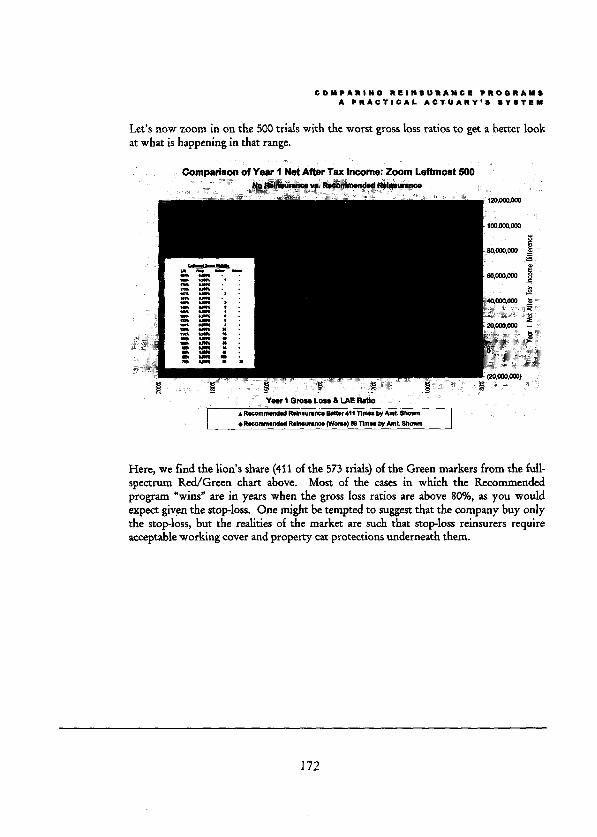
COIIPARINO REIN8URANCL PROQRAY8

1, PRACTICAL ACTUARY’ SYSTEY

Let’s now zoom in on the 500 trials with the worst gross loss ratios to get a better look at what is happening in that range.

Comparison of Year 1 Net After Tax Income: Zoom Lefbnost 500

Here, we find the lion’s share (411 of the 573 trials) of the Green markers from the íüll- spectrum Red/Green chart above. Most of the cases in which the Recommended program “wim? are in years when the gross loss ratios are above SO%, as you would expect given the stop-loss. One might be tempted to suggest that the company buy only the stop-loss, but the realities of the market are such that stop-loss reinsurers require acceptable working cover and property cat protections underneath them.

172

COMPARINO REINSURANCE PROORAMS

A PRACTICAL ACTUARY’S SYSTEY

Nexc, we compare the Current and Recommended programs (Green means Recommended is berter).

Comparison of Year 1 Net After Tax Income After 4000 Iterations Currsnt Rsinsursnce VL Rscommended Reinsuance

.-- --__.. * RsmmmendsdR*nauacaBl,7~Thmaby~S~ . Rd R*int”mw.l (wma) 2.236 nIb% by AmI Stxw”

i-~~d”~lGmsib%&!&R* ._ ~-- __ 7 __~_____

It appears that the Current program wins a majority of the times in head-to-head comparisons with the Recommended structure, but when the gross loss ratio breaks the 95% level, the Recommended program begins to shine. In the most extreme cases, there are clumps of cases where the benefit is %20-$40 million, from the extra property cat coverage mostly, and a handful of very large differences of between $40690 million when the extra cat cover plus reinstatement cover plus the aggregate al1 come to bear.

While this situation does not res& in a simple “slam dunk” superiority between any of the alternatives, we believe the buyer will continue to buy reinsurance as a re& of this analysis. The direct underwriting assumptions here are fairly optimistic, but we still have enough loss potential from property catastrophe shock losses and/or high loss frequency ín the various lines of business to create very unfavorable experience, as we have seen.

Another means of looking at the variability of total income (say) from the reinsurance alternatives at various gross loss ratio levels is a chart we cal1 the “wiggle chart.” This is not yet another probability chart per se, but a graphical display of the range of values of after tax income for each ahernative at every observed value of the gross loss ratio. The picture really highhghts the benefits of the Recommended program, and speaks for itself.

173

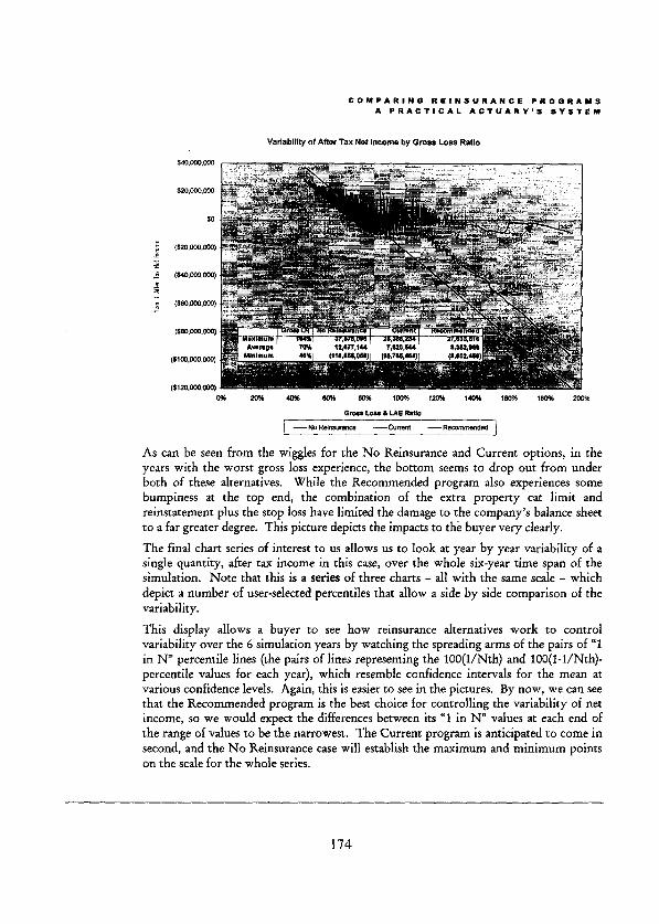
COMPARING REINSURANCE PROORAMS


Varlability of After Tax Net Income by Gross Loss Ratio

-No R~“YmM --c”marl --aa

As can be seen from the wiggles for the No Reinsurance and Current options, in the years with the worst gross loss experience, the bottom seems to drop out from under both of these alternatives. While the Recommended program also experiences some bumpiness at the top end, the combination of the extra propeny cat limit and reinstatement plus the stop loss have limited the damage to the company’s balance sheet to a far greater degree. This picture depicts the impacts to the buyer very clearly.

The final chart series of interest to us allows us to look at year by year variability of a single quantity, after tax income in this case, over the whole six-year time span of the simulation. Note that this is a series of three charts - al1 with the same scale - which depict a number of user-selected percentiles that allow a side by side comparison of the variability.

This display allows a buyer to see how reinsurance alternatives work to control variability over the 6 simulation years by watching the spreading arms of the pairs of “1 in N” percentile Enes (the paírs of lines representing the lOO(l/Nth) and lOO(l-l/Nth)- percentile values for each year), which resemble confidente intervals for the mean at various confidente levels. Again, this is easier to see in the pictures. By now, we can see chat the Recommended program is the best choice for controlling the variability of net income, so we would expect the differences between its “1 in N” values at each end of the range of values to be the narrowest. The Current program is anticipated to come in second, and the No Reinsurance case will establish the maximum and minimum points on the scale for the whole series.

174

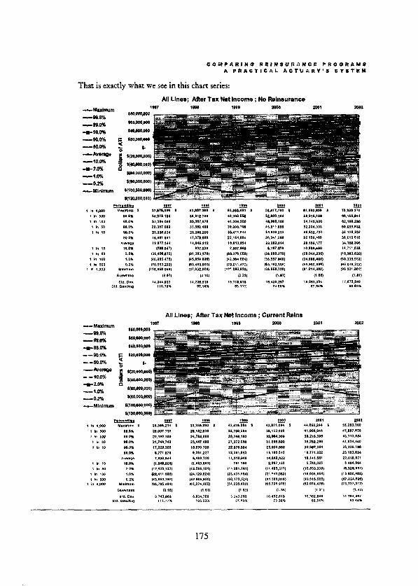
COIWPARINO REtNSURANCE PROORAMS

A PRACTICAI. ACTUARY’S SYSTEWI

That is exactly what we see in this chart series:

- . ..-.. ._. -89.0% -00.0% tmw --m.o?G --so.o% -Avsrspo --- 1o.e% -20% -cm% -0.2% - bllnlrmm

All Unes; After Tax Net lncomr ; Current Reins

175

COMPARINO REINSURANGE PROORAMS


-Mtinum

-.-39.0%

-.-Sm%

tm.o%

-00.0%

--sao%

-*mga

-10.0%

-N-am

-1.0%

--OX/0

-MInImm

All Lines; After Tax Net Income ; Recommended Reins ,997 ,* ,999 m MM

Other Analyses

Since there is a database of results for every trial from each line, each treaty and each program, there are literally dozens of useful analyses one can perform, “drilling down” into issues that arise between the parties involved.

Since the system uses Excel” as its calculator, any function or relationship that can be defined in ExceP can be used in a simulation. Of course, the more one puts “in motion” the “blacker” the box gets. Sometimes that is necessary and sometimes it is not. To keep the focus on underwriting risk, we leave certain issues out of most of our analyses, like interest rate and asset risk, but since they can be described fairly easily in ExceP the system can handle them.

Another frequent analysis involves taking the net present value of future cash flows, which the system handles easily. We usually do this as a cusfom calculation since there are different definitions of what is and is not included in NPV analysis from company to company.

176

COYPARINO RPINSURANCL PROORAWS A PRACTICAL ACTUARY’S 8YSTIM

As an example of how to use the database of results, we answer the questions: “How often do we trigger the aggregate? Total the aggregate?” In just a few minutes a user can extract the ceded losses and limits by year for the stop loss and produce an analysis such as the following:

Conclusion

Perhaps one of the most important conclusions to note is that this is a system - where users can build models quicker, under better control - and where there is a “memory,” letting the user re-use prior elements that “worked” for their needed purposes. This is a very practical res&, too, since simulation has been around for some time in the hard-to- control spreadsheet world. The more comfort and control, the more often and more consistently analyses can be done.

We have seen how users / buyers react to this kind of information, and know that it has been a critical factor in their decisions. We all benefit when actuaries communicate well, and when the best information we have is brought together in meaningful and instructive analyses. We think simulation and the tabular and graphic representation of its results is an excellent vehicle for such communication in the reinsurance arena.

This paper has not been a technical actuarial article, but rather an exposition of our systematic approach to building and using simulations to analyze reinsurance altematives. Our hope is that it might spur discussion of the strengths and weaknesses of this approach.

177

Pricing Extra-Contractual Obligations and Excess of Pulicy Limits Exposures in

Clash Reinsurance Treaties by Paul Braithwaite, FCAS, and

Bryan C. Ware, FCAS

179

About the Authors: Paul Braithwaite is a FCAS and MtL4A. He is Senior Vice President of Zurich Reinsurance Centre, Inc. Bryan Ware is a FCAS and MMA. He is Vice President of Zurich Reinsurance Centre, Inc.

Abstract: The authors examine the loss exposures due to extra-contractual obligations and excess of policy limit tbird party actions. They discuss how these components of clash cover reinsurance can be priced.

180

PRICING EXTRA-CONTRACTUAL OBLIGATIONS AND EXCESS OF POLICY LIMITS EXPOSURES IN CLASE REJMURANCE TREATIES

By Paul Braithwaite and Bryan Ware

“Bad Faith Award Shocks Insurer. “l As headfines such as this become more common

in the trade press, reinsurers need to pay more attention to the prices charged for Extra-

Contractual Obligations (ECO) and Excess of Poficy Limits (XPL) coverage provided in clash

treaties.

Reinsurance casualty clash treaties provide coverage for exposures including multiple

policy occurrences, multiple claimant workers’ compensation (WC) occurrences, runaway

allocated loss adjustment expenses (ALAE), ECOIXPL judgments, and a few other less visible

exposures. In years past, multiclaimant WC losses and runaway ALAE have been the most

frequent kinds of Iosses we have seen reported to clash covers. Multi-policy occurrences are

more common in some lines of business, such as professional liability Enes, or in treaties

structured to cover on a per-coverage-part basis (for instance, an auto accident involving auto

liability and workers’ compensation). But ECO/XPL coverage ís becoming much more important

for reinsurers to consider due to fears of enormous jury awards, particularly punitive damages

against corporate defendants.

Traditionally ín clash pricing, a judgmental rate-on-line approach has been the non.

However, there is a significant amount of data available on which to base pricing models for some

of the events mentioned. By using such an approach, it is possible, at first, to simply add

181

consistency to judgment. Over time, more data can be gathered, increasing the accuracy of the

model projections.

The purpose of this paper is to take an in-depth look at the ECO/XPL component of clash

reinsurance coverage, fust at the defmitions and some background of the coverages, then at the

underwriting considerations which come into play, and finally at the framework of a pricing model

which can be used to incorporate the specific characteristics of the cedant’s book of business into

a price for this component of the clash treaty.

DEFINITIONS and BACKGROLJND

XPL

The Excess of Policy Limits (XPL) component covers judgments in excess of the

original policy limits against the inmred for claims brought by a third party. Consider an insured

who buys a policy with limits of $1 million. The insured loses a lawsuit brought by a third party

for a verdict of $10 million. The $9 million above the policy limit may be an XPL judgment. An

XPL judgment normally involves alleged questionable claims handling or defense of a lawsuit by

the insurer. This ofien takes the form of the cedant failing to settle a claim within the policy limits

when the opportunity was presented It is due to the handling of the claim that the insurer is

considered hable for the excess verdict. The claim for which the damages were awarded must

othenvise be covered by the primary policy.

An XPL judgment may include compensatory and punitive damages, but these are not

always covered by the primary policy. Compensatory damages can include infliction of emotional

distress or loss of business opportunity or business reputation. Punitive damages are usually

182

reserved for situations invoiving conduct that was exceptionally malicious, egregious, or

outrageous.

One example of an XPL clahn, aflirmed on appeal, can be found in the case of Form~m v.

Hemco, 211 Cal. App. 3d 241 (App. Div., California 1989). This case involves a three-year-oid

piaintiff who was injured in 1981 when she fe11 out of a jeep her mother was driving and was run

over by a following vehicle. The plaintiff sued Hemco, who manufactured the mold used to form

the fiberglass top and doors on the jeep. The doors on the jeep were designed to be rear-hinged

and had exposed interior handles. The plaintiff hooked a sleeve on the door handle, opening the

latch. The wind caught the door and threw it open, pulling the plaintiff out of the jeep.

Hemco’s insurance company had the opportunity to settle the case for $1 million in 1984.

They chose to go to court, primarily because Hemco neither designed the jeep top nor

manufactured the actual top on the Fortman jeep. In 1986 a jury awarded MS. Fortman $17.7

million ín economic damages for the personal injury claim and $6 million for pain and suffering.

The court concluded that Hemco provided expertise and could have corrected the design.

Hemco’s insurer was required to pay the entire loss, including the amounts in excess of the policy

iimit. Under the clash reinsurance program that the insurer purchases today, this would have been

a sizeable reported loss to the clash layer.

ECO

The Extra-Contractual Obligations @CO> component of a casuahy clash

reinsurance treaty covers judgments against the reinsured which are “extra” or outside the policy.

The plaintiff in the lawsuit is normally the original insured. The major cost in the judgment is

183

ofien punitive damages. By nature, these are liabilities not covered under any provision of the

policy. ECO claims normally involve wrongful or negligent claims handling by the reinsured. If,

in addition, it is found that the cedant dealt with the claim in “bad faith,” punitive damages may be

awarded. These clauses first began to appear in reinsurance treaties in the late 1970s; XPL

clauses have been around since the 1960s.

A fairly recent example of an ECO loss is the case of Hedrick v. Senby In.wrance Co.,

96-128100-90 (Dist. Ct., Tarrant Co., Texas). This case began with an auto accident on an

interstate in May 1986. A truck rear-ended a northbound car and knocked it and a second car

over the median into the southbound lanes. One of the cars struck head-on another vehicle

containing Virgie Poston and her two adult daughters. Al1 three were killed.

MS. Poston’s grandchildren filed suit against the drivers of both cars and the truck for

damages in the deaths of their mothers and grandmother. The insurance companies for the three

drivers settled, and the money was split among the grandchildren, the husband of one of the

daughters, the driver of the car that struck MS. Poston’s, and MS. Poston’s husband.

Mr. Poston felt that he had been%adequately compensated for the death of his wife. In

1989, he filed suit against bis own insurer, State Farm. According to Mr. Poston’s attomey, the

insurer failed to investigate, lost the claim file, and denied the $20,000 settlement Mr. Poston

sought.

Mr. Poston and his son sued State Farm for bad faith arising out of their handling of the

claim. On December 10, 1993 the jury awarded them $2.17 million in compensatory damages and

184

$100 million in punitive damages. In March of 1994 while the appeaf was pending, this case was

settled out of court for an undisclosed amount.

There are a few items of note in this example. The frrst is the obvious one. It wouId have

been easy for the insurer to settle the claim for a small amount of money early on in the case, and

thereby avoid the shock verdict. The settled amount was probably substantially less than the

verdict. On the other hand, with the negotiating leverage provided by the shock verdict, the

settlement was probably very large. From the reinsurer’s perspective, this claim is also likely to

have been a substantial loss for any clash reinsurance program the insurer chose to purchase.

The second point is the elapsed time involved here. The accident was in May 1986 and

the jury award was iate 1993. It is entirely possible that a clash reinsurer would see no reported

losses to the layer from a claim such as this for seven years. If appealed, the final value of the

claim may not be known for severa1 years afler that. This can be a fairly long-tailed coverage.

UNDERWRITING CONSIDERATIONS

We have identified five general areas of underwriting considerations which we take into

account when determining an expected loss for the ECOKPL component of a clash program: 1)

the states in which the reinsured writes business, 2) other reinsurance coverages the company

purchases, 3) the siie of the ceding company, 4) the quaiity of and approach to claims

management by the reinsured, and 5) the policy limits which the reinsured sells. We will look at

each of these in more detail.

Before we dive into these considerations it is wotthwhile to briefly discuss our goal in this

exercise. The steps we wiil go through in any cfash pricing exercise are to first determine what

185

types of events (ECOBCPL, WC multiclaimant, etc.) represent significant exposure to loss, then to

determine an expected severity and frequency of loss for each type of event. This may take the

form of, for example, an expectation of a $5 million loss every 25 years. Thus our task is

separated into determining both what size of loss is reasonable to expect in the layer (the severlty)

and how often we expect to incur that loss (the frequency).

States

The states in which the company writes business can be particularly important for several

reasons. Different states have different rules about how to handle damages. For instance, in

Texas punitive damages are limited to four times the actual damages, except in cases of gross

negligente or malice, in which case this limit does not apply. However, in a few other states,

punitive damages cannot be covered by insurance at all. The states in which a cedant writes can

have an effect on both the frequency and the severity of losses.

The leve1 of litigation in the states is of utmost importance when determining an

expected frequency of claims. Research has shown that California and Texas tend to have the

highest incidence of punitive damage claims. *J New York, Florida, and Illinois are also higher

than the norm.

This raises some interesting coverage issues. First, are punitive damages insurable?

Punitive damages can be assessed either directly or vicariously against the insured. An example of

a case where punitive damages might be assessed directly is a case where a doctor inadvertently

leaves an instrument inside a patient after surgery. The damages are assessed against the doctor,

However, punitive damages assessed against the hospital ín the same case are vicarious.

186

Currently, 46 states allow recovery, at least in part, of punitive damages,

depending on whether the damages are vicarious or direct. Michigan, New Hampshire, Nebraska,

and Washington do not permit recovery of punitive damages. However, even these states allow

recovev of non-economic damages (usually pain and suffering). Coverage of vicariously

assessed punitive damages is more common than of directly assessed damages.

The next coverage issue is whether the punitive damages are recoverable under

reinsurance in the states in question. In the case of punitives assessed against the insured (XPL),

the indemnity payment is made by the reinsurer on a contractual basis where the original policy

sold by the insurer provided coverage for punitive damages. This assumes that the original

damages were insurable to begin with.

On the other hand, some insurance departments view ECO coverage of punitive damages

similarly to direct errors & omissions insurance. This may then revert to the state laws on

insurability; however, the situation is unclear. Even if state laws mandate that punitive damages

are uninsurable (and thus not reinsurable in this sense), a COUR may rule that in a given situation it

is in the public’s best interest to require a reinsurer to cover the punitive damages. Por example,

New York and California (among other states) prohibit insurance coverage of directly assessed

punitive damages (vicaríously assessed punitives are insurable). Regulators in these two states

have voiced concems with respect to reinsurance recoverables for these uninsurable damages, due

to public policy concems. However, this has not been thoroughly tested in the courts.

187

Other Coverage

The main question to answer here is whether the cedant purchases any insurance or

reinsurance which inures to the benefit of the clash program, specifically errors & omissions

coverage. An E&O policy may cover alleged fauhy claims handling, but not always. If the

company’s reinsurance program is structured such that this is inuring coverage, then the clash

reinsurer is fbrther removed from loss. An E&O policy may provide some protection against

ECO claims, but will probably be of little value on XPL claims. If the answers to these questions

are not contained in the pricing submission material, it is Worth asking.

For instance, say a company buys clash protection for a layer of $15 million excess $10

million, and sells only policy limits of $5 million. A judgment of $20 million, including $15 million

ECO, will be a $10 miilion loss to the clash layer. However, if the reinsured buys an E&O policy

with limits of $10 miilion that inures to the clash protection, then there is no loss to the clash layer

($5 million inside the policy limit, $10 million to the E&O, and $5 million company retention).

The second coverage point to note is the coinsurance percentages allowed. The current

standard is 90%/90%, meaning the company retains a 10% coinsurance share of each ECO and

XPL judgment. The most common variations on these shares are 80%/80%, 80%/100%, and

lOO%/lOO%. (It obten simplifies matters to have the ceding company retain an equal percentage

for ECO and XPL. This usuahy circumvents having to differentiate between the two, which is

sometimes difficult.) Another variation is that the indemnity loss may be required to attach the

layer before ECO or XPL will be covered. From a reinsurer’s standpoint, it is wise to have the

cedant retaining a non-zero percentage. Since the cedant’s actions normally determine the

188

incidence of ECO claims and usually of XPL claims, they should have a direct stake in the

outcome.

In applying coinsurance, the cedant’s share is typically subtracted from the ground-up loss.

For instance, use the same % 15 million xs % 10 million clash layer mentioned above and assume a

$12 million ground-up ECO loss with a 90% reinsurance coverage share. (For simplicity, we are

assuming that the entire loss is ECO. Normally a portion wlll be a covered loss within the policy,

and thus not subject to the coinsurance percentage.) Using this application, the coinsurance share

is 10% of $12 million, or $1.2 million. The remaining loss is $10.8 million, resulting in an

$800,000 loss to the clash layer.

Other variations of this calculation are used in other reinsurance covers. For instance, in

quota share reinsurance, the ECO or XPL loss may be subject to an additional limit or recovered

pro rata in addition to the limit of the contract. Although these methods of calculation are not

meaningful in the clash context, they are mentioned as another source of inuring protection. It is

also wotthwhile to find out if the cedant’s excess of loss reinsurance (if any) provides additional

coverage for ECOBCPL.

Size of the Cedittg Companies

All else equal, a larger insurer wiil have a higher ECO judgment from a given incident than

a smaller company. One reason for this is the actions ofjuries and judges in determining

damages. Punitive damages are by definition intended to be painful. Consider two companies,

one with $10 million in premium, the other with $1 biliion. A $1 million verdict against the first

company will likely have a defmite effect on the way they do business. They will feel the loss,

189

whereas the second company would not. Proportionally, it would take a verdict of $100 million

against the larger company to have the same effect. This sometimes has the effect of making

larger companies targets ofthese lawsuits.

This relationship is not as clear for XPL, where the verdict is offtcially against the

insured. A proportionately larger punitive damage award is probably more likely against a large

insured than a small insured, regardless of the size of the insurer. However, since the claims

handling of the insurer is also responsible for the judgment, its size may become a factor as well.

The deep-pocket effect also comes into play. People are more likely to sue a larger

company because there is a potential for much bigger rewards. Thus, the frequency of losses will

also be higher.

Overall, one would expect less total loss on ECO/XPL covers on 100 insurance companies

of $50 million each in premium than on one company of $5 billion.

Claims Management Fractices

Probably the single most important piece of qualitative information we seek when

determining a price for the ECO/XPL portion of a clash cover is an honest, unbiased evaluation of

the quality of the cedant’s claims management practices. There are severa1 topics which are

important for us to cover when evaluating the cedant’s claims staff.

Whut is the average workload and experience Ievel of the stafJ? The lower the workload,

in general, the less likely a claim is to fall through the cracks.

190

Wha: are the cedant’s views on settling claims? An early settlement in the Hedrick v.

Sentv case mentioned above could have saved potentially $100 million. A company which

chooses to settle potential ECOKPL claims early on may develop a í?equency problem on their

own books, but this probably won’t translate into a problem for high clash layers since the severity

is kept low.

Some companies will choose to go to court on a declaratory judgment action instead of

outright refbsing coverage and taking the chance of suffering an ECOIXPL loss. In a DJ case, the

facts of the case are not disputed by either side. They choose to go to court for a ruling only on

the applicable laws or coverage issues. This approach may avoid the danger of a large punitive

damage award for disputing coverage or failing to provide a defense.

How stable is the claims staffl Do they have trouble hiring and keeping good people? A

stable claims stafTtends to better manage its claims inventory.

Another important indicator of at least the company’s past claims practices is the

leve1 of reported ECOKPL claims over the past ten to twenty years. Large claims will normally

be included in a pricing submission, although they may not be identified as ECO/XPL. Claims

descriptions will ogen identify them.

Policy Limits

The policy limits sold by the cedant are also important. It is important to look at the size

of the policies as well as the relationship between the policy limits and the attachment point of the

clash layer. Limits profiles are normally available from the cedant. Clearly, the lower the policy

191

limit, the more likely a judgment is to be in excess of the limit. An insured buying too little

coverage can be a problem. On the other hand, it is desirable to have a buffer zone between the

most frequent policy limits sold and the attachment of the clash layer.

A PRICING MODEL

The pricing model described in detail below is an exposure rating model. It is

based on the characteristics of the specific cedant being priced. It does not, however, depend on

the actual loss history of the cedant. Before using the model, one should examine the historie

ECO/XPL losses of the cedant. Ideally, there will be none of any consequence. A lack of historie

ECOKPL claims can be significar& depending on the expected number of losses and the number

of years of data available. In practice, there oRen are one or more. If there are, a quick

experience rating is normally done. A look at the experience can at least serve as a reasonability

test of the exposure rate.

Experience Rating

To perform an experience rating, any historie ECO/XPL losses are trended to the

average accident date of the clash treaty being priced. They are also developed to ultimate. The

development is an unusually tricky process, due to the nature of the claims. Closed claims are not

usually liable to change. Open claims often change, but the amount of change depends on the

status of the lawsuit. If a claim has received a jury-awarded shock verdict and appeals are

pending, then the value may very well be expected to drop atter appeal. On the other hand, if the

suit has not gone to trial at all, it may not even be reported in the submission material and may

skyrocket upon verdict. A provision is also included for unreported claims which will arise out of

192

the historie exposures. Our approach when evaluating a cedant who has historie ECO/XPL

claims is to estimate the füture reportings (IBNR) for open and unreported claims. If the cedant

has experienced rapid growth or other changes in the relative leve1 of exposure, an adjustment is

made to reflect this, as well.

Aster trending and developing, these claims are slotted into the layer (adjusting for

coinsurance) and are used to determine an expected frequency of claims and average severity.

These resuits are compared to the exposure rate, determined below. If a cedant has a high

historie frequency of ECOKF’L losses ín the layer, the reinsurer should, of course, re-evaluate

whether this risk is acceptable before continuing.

Exposure Rating Modef

The exposure rating model described here is essentially a market share approach. The

main input is the premium of the company being rated. Severa1 other factors modify the results of

the main calculation. The basic formula is:

E[L] = Premíum * Constant * ms+rc,m Wdx.

The res& of the equation, E&], is the expected losses for the ECOKPL portion of the

clash cover. Each of the three components of this formula, which are multiplied together to get

this res&, can be split into frequency and severity components. This allows E[L] to be stated as a

layer severity and a return period. For example, say the formula shows E[L] to be $100,000.

Splitting the formula into component pieces may show that this corresponds to a $1 míllion loss

every 10 years (or a $10 million loss every 100 years).

193

Premium

The first pottion of the formula is the Premium. To be specific, this is the premium

which gives rise to ECO/XPL exposure. A few aspects must be considered.

1) The first is what lines ofbusiness are exposed. Most clash covers are limited to casualty

business and don? include property in the subject premium base. Property business does

not tend to have XPL claims, and ECO claims arising from property are extremely rare. Any

ECO claim resulting entirely from the handling of a property loss is likely to be of little

consequence.

2) Workers’ Compensution business presents a lower hazard from ECORPL than other

casualty lines. Because of the nature of WC business, it just doesn’t give rise to anywhere near

the number of losses as general liability and auto. However, there is a risk. ECO losses From

compensation claims do happen and should not be ignored. Our solution is to include a small

portion of the WC premium.

3) The final aspect of the premium component is in the uftachmentpoinfs that the company

writes. Clearly a company which writes $50 million of GL and AL business excess of an

average SIR of $500,000 presents a very different risk than one that writes $50 million in

ground-up GL and AL policies. Increasing the premium for the former company can capture

some of this added risk.

194

The second component of the formula is the Constant. OriginaUy, the base

constant is set such that the formula produces the desired frequency of losses for the market.

Once calibrated, this constant is modified multiplicatively on a case-by-case basis in order to

model the fiequency of losses for the individual company being examined. We have identified

four separate factors for which the constant may be adjusted.

1) The frequency is adjusted based on the sraies in which the company writes business. For

example, we have identified California and to a iesser extent Texas as having a particularly high

frequency of ECO/XPL claims. Several other states have also been singled out as deserving an

increase in the fiequency constant.

2) The relative hura& leve1 of the cedant’s book can also affect the frequency. A hazard

adjustment shouid consider the line of business mix as well as the types of risks insured. A more

hazardous book is inherently more likely to produce injuries which could result in ECO/xpL

claims.

3) The ceda& claims munagemenl practices and philosophies are important determinants of the

expected Frequency of losses. Subjective opinions such as “better than average” or”terrible” must

be quantitied. For instance, an “average” company gets a claims handiing multiplier of 1; an

“above average” company may get .75; a “below average” company may get 1 S.

4) The final adjustment to the fiequency is to increase the tiequency constant for ‘%geP

ínsurance companies. The larger the company, the more likely they are to be the recipient of

19.5

lawsuits. This effect is more than simply proportional. The constant needs to be lncreased to

compensate for the deep-pocket effect. One way to measure this is by the overall premium size of

the company. The premium component mentioned earlier is for exposed lines only.

It can also be argued that this target company effect will apply to larger underlying insureds, as

well. If larger insureds are more likely to be sued for larger amounts, this can be factored in here.

Expected Average Seven@

The final component of the formula is the severity. Similarly to the frequency

component, we start with a basic severity curve, then modifjr it to reflect the specífic

characteristics of the cedant. We wíll examine the basic curve and the three categories of

modifiers we have identified.

The data we started with was a collection of punitive damage claims. These were

gathered primarily fiom two sources. The first is underwriting submissions. Any identified

ECO/XPL claims are pulled and collected into a single source. The second group consists of

published studies of large verdicts and settlements, such as are contained in The NationalLuw

Journal.

To this data, we fit a Pareto curve. This is one of severa1 standard curves used in actuarial

work to represent severity distributions. An algebraic formula can then be used to calculate the

expected severity given any attachment and limit combination. We have selected the two

parameter Pareto curve. The first is a shape parameter, which is entirely determined by the fit to

196

the data. The second is the scale parameter, which can be adjusted to reflect differing

characteristics of the cedant.

1) The first severity modifier ís for the srates in which the company writes. Care must be

taken to ensure that this modifier does not overlap with the frequency adjustment for the states.

The adjustment discussed before was done to reflect solely the relative number of lawsuits filed.

This severity adjustment is intended to capture state differences in the amount of the judgments,

given that the suit is filed. Clearly, there is a cause-and-effect relationship here. The iarger the

verdicts in a state, the more people are going to decide to file suit. At the same time, once a

precedent is set for large judgments in a state, future large jury awards are more likely. (This

effect is somewhat similar to the lottery. More people buy tickets when the jackpot gets high,

even though no single person has any greater chance of winning. The increased sales cause the

jackpot to go even higher.) This modifier can be applied as an adjustment to the scale parameter.

2) The second severity modifier is for the coinsurance factor, discussed above. This can be

accomplished by modifying the scale parameter or by adjusting the limit and attachment

upwards (i.e., with a 90% coinsurance factor, it takes a loss greater than $10 million to attach a

layer excess of $9 million). If the latter method is used, the layer severity must be adjusted, as

well.

3) The third severity modifier is for inwingprofeclion, such as Errors & Omissions coverage

purchased by the cedant. This does not change the number of suits filed against the

company, but does lower the chance of penetration of the reinsurance layer. The reinsurer

is coveríng a higher layer for the cases where inuríng protection has an effect.

197

Clearly, the second and third severity modifiers also have an effect on the frequency of

claims in the excess layer being priced. They do not, however, have any effect on the pure

number of cases being pursued. The frequency component is intended to capture only the number

of cases. The severity component then ?djusts for the likelihood of the loss reaching the clash

layer.

SUMMARY

As clash reinsurance becomes a larger portion of many reinsurers’ books of business, it is

important to have logical methods of evaluating the associated exposures. The pricing of this

business has typically been done using judgmental methods. The underwriting considerations

shown above detail what we have identified as the most significant characteristics affecting the

ECOIXPL portion of these exposures. The exposure rating model described presents a method of

translating this information into expected losses for the clash treaty. By using a model such as

this, the reinsurer can add logic and consistency lo the pricing approach as well as compare clash

programs.

Joanne Wojcik, “Bad Faith Award Shocks Insurers,” Business Insurunce, December 13, 1993.

* Margaret Cronin Fisk, “The Year’s Largest Verdicts,” The National Lmv Journal, January 17, 1994.

3 Margaret Cronin Fisk, “Verdicts. The Big Numbers of 1994,” The NafionaZLmv Jourd, February 6, 1995.

198

Acknowledaments

The authors are very grateful to Brenda Sand, Susan Daubard, Sheila Sterling, Charles Kasmer,

Emily Canelo, and Jess McCavitt who assisted with the research for this paper.

This article ìs reprinted courtesy of the Joumal of Reinsurance, Spring 1995 edition.

199

Evaluating Variations in Contract Terms for Casualty Clash Reinsurance Treaties

by Emily Canelo and Bryan C. Ware, FCAS

201

Aburtr Ikedr&ors: Emily Canelo is an Attomey and Senior Vice President at Zurich Reinsurance Center, Inc. Bryan Ware is a FCAS and MAAA. He is Vice President of Zurich Reinsurance Centre, Inc.

Abshact: The authors examine variations in event definitions and commutation clauses which are eommonly eneountered in casualty catastrophe reinsurance contracts in the market today. Changes in these aspects of the contract may a%ct the exposures the reinsurer is asked to cover. In this article, the variations are contrasted with special emphasis given to the effects this may have on the pricing/underwriting process.

202

Evaluating Variations In Contract Terms For Casualty Clash Reinsurance Treaties

1. Introduction

Look across our industry and you will find among the most critica1 issues one factor that is that huge casualty catastrophe losses do happen. They occur in many forms ranging from a large extra-contractual obiigations (ECO) award under a single policy to workers’ compensation multiclaimant lossss to multipolicy losses (true clash) or runaway allocated loss adjustment expense (ALAE). In Iight of this, casualty catastrophe reinsurance remains an integral part of most companies’ reinsurance programs.

Over the years, the clash product has become more sophisticated and more tailored to the specific cedent’s needs. Therefore, any reinsurer selling clash protection must carefully evaluate the various contract terms that have also evolved for their effect on the exposures for which protection is being sought. Reinsurcrs also must be able to model and compare the different coverage that different contract terms will produce.

Our purpose here is to analyze event definitions and commutation clauses and to examine how changing contract clause provisions can affect both the exposures and the modeling needs. We also wili look at the modeling process itself. We will briefly discuss the different ways in which these covers attach and then examine commutation clauses.

For each variation in the clauses under discussion, we will consider related potential changes in the reinsurer’s exposure to loss. We will provide examples of the types of loss covered under one definition which are excluded from others. We will then look at the types of information needed for the reinsurer to price these added exposures.

II. The Modeling Process

Before jumping into the various examples, it will be helpful to lay out the structure of our modeling/pricing procesa The three general steps are: (i) detcrmining the expected losses; (ii) building a discrete aggregate distribution; and (iii) ealculating the return on equity (ROE) for each point of the aggregate distribution.

To determine the expected losses one must first identify the type of event that can cause a loss. Such an event can include ECO and excess of policy limits (XPL) judgments. lt may also include such things as workers’ compensation multictaimant losses, multipolicy losses, the stacking of uninsured motorist limits or runaway allocated loss adjustment expenses. Once the causes of loss have been identified, we determine a frequency and average layer severity for each cause.

Models can be constructed to estimate the frequencies and severities for each cause based on exposure.‘.* Certainly, experience can be used, where available. If neither of these are available, the frequencies and severities can be selected judgmentally.

203

These selections, of course, will vary with each cedent and each reinsurance program. As an example, consider the runaway ALAE exposure on a clash layer attaching at $5 million for two hypothetical cedents. Cedent A writes policies with ALAE payable in addition to the policy limit of $1 million. Clearly, the ALAE exposure will come about from paying very large ALAE amounts on comparatively small insured indemnity losses.

Cedent B uses the same policy form, but writes maximum policy limits of $5 million. Al1 else being equal, Cedent B has about the same exposure to large ALAE losses that Cedent A has. In addition, Cedent B has exposure to relatively small ALAE losses from insured indemnity losses which are at, or near, the $5 million policy limit. Not only does Cedent B have the runaway exposure exhibited by Cedent A, but it also has a “trickle” exposure. The runaway exposure will be characterized by comparatively high severity and low frequency losses. In comparison, the trickle exposure will be characterized by higher frequency, but lower severity, and could result in higher expected losses than the runaway exposure. Both of these exposures should be considered when determining the expected losses.

The next step is to develop an aggregate distribution for the various causes of loss. This can be accomplished by methods such as described by Panjer’ or other methods4 For example, a clash aggregate distribution may indicate the following: 90% chance of no loss; 4% chance of expected losses equaling half the layer; 3% chance of expected losses equaling the ful1 layer; 2% chance of two ful1 layers of losses; and 1% chance of three ful1 layers of losses.

The tina1 step is to calculate retum on equity using the aggregate distribution as input. This means modeling cash flows for each point of the aggregate distribution, calculating a return on equity (net present value return, in dollars, divided by the surplus allocated to the specific layer) for each point, and weighting these ROES together using the probabilities of achieving each expected loss outcome.

This process provides a structure for assessing the implications of the pertinent contract terms. If a change in a contract term can affect expected losses, the reinsurer needs to modify the inputs used in determining the aggregate distribution, produce a new aggregate distribution and recalculate the ROE. If a change affects cash flow only, this can be modeled in the ROE calculation, without change to the aggregate distribution.

III. Event Def’initions

The event definition is the linchpin in underwriting and pricing clash covers. It should reflect both parties’ expectations as to the scope of coverage provided. Although the event definition has become somewhat standardized, increasing litigiousness, unpredictable jury awards, emerging toxic torts and new theories of liability also are defining the type of catastrophic events casualty insurers can expect to face. In light of the uncertainty that these emerging trends impose on clash pricing, it is critica1 that all parties to the reinsurance contract agree on the intent and construction of an event definition.

204

For example, if a cedent is expecting clash coverage for losses that are of a continuous or latent nature, rather than the result of a spontaneous occurrence, the event definition should inciude Ianguage that refers to repeated exposures. If the cedent expects the cover to respond to economíc losses arising out of E&O and IBO policies it has issued to tinancial institutions, the event definition should specifically include wrongful acts and errors and omissions in addition to the standard language appearing in element 4 below. In simple terms, the crafting of an event defmition should encompass a careful review of the underlying business and the scope and extent of catastrophe coverage desired. Failure to do so could result in unnecessary contract disputes.

An event detinition typically includes the following elements:

1. Damage, injury or loss arising out of one or more than one policy; that is the

2. direct consequence of one particular accident, disaster or casualty; that

3. takes place in its entirety at a specitic time and place; and

4. is traceable to the same single accident, disaster or casualty.

A. “Damage, injury or loss arising out of ene or more than one policy.” The terms “darnage, injury or loss” typically relate to the terms used in the insuring agreernent of the underlying policies being covered, i.e., the CGL, umbrella policies etc. If both clash and contingency protection are being purchased to protect against loss arising under a single policy involving, for exarnple, runaway ALAE and a clash of two policies, this intent is captured in element 1 above. However, if the catastrophe protection purchased is strictly clash, then this element should be tailored to read “arising out of more than one policy.”

Another variation on this theme occurs with definitions using “more than one insured,” rather than “more than one policy.” For instance, if an insurer writes commercial auto and workers’ compensation using separate policies, an auto accident involving one insured car driven by a worker where the worker’s employer is also the car owner, could be a clash loss under the “more than one policy” scenario, but not the “more than one insured” wording.

This part of the event definition comes into play when the pricing actuary or underwriter is selecting the types of occurrences which are intended to be covered by the clash layer. Runaway ALAE and ECOIXPL are not nearly as great if the coverage is limited to events arising out of two or more policies. On the other hand, if two or more policies must be involved, one might expect the selected severity to be higher and the payout somewhat quicker than would otherwise be the case. Ideally, the cedent should be able to provide historie losses accumulated using the appropriate event definition.

B. “Direct eonsequence of ene particular eccident, disaster or casualty.” This element sets forth the requirement that recoverable Iosses be caused directly by a single event and that there be an appreciable degree of causation between the single event and the loss. An example of the c \WINDOWS!MIPcLAStn shMolIllb97

205

difticulty with the common factor requirement is illustrated by the following example. Loss attributable to an explosion in a factory gives rise to claims under an insured’s liability and workers’ compensation policies and would be treated as caused by one event. However, if the cedent’s loss was due to two separate explosions occurring at different times during the year could the cedent lump the two incidents together and consider them one event if both incidents resulted from defective made boilers from the same manufacturer? In other words, if the cause of each explosion proved to be the defective made boilers, would that common factor satisfy the criterion that the losses were the result of one particular manufacturing accident? These are, admittedly, difftcult questions without clear cut answers as indicated by court decisions in the US and England’.

Another example illuminating the difticulty in causation analysis is the determination of proximate cause. Proximate cause in a chain of severa1 events refers to the nearest cause preceding the final event. Thus, in’ a causal sequence of events resulting in damage to a California condominium complex, would a subsidence problem be a direct or intervening cause of damage where the builder already had a judgment against it for construction defects?

Pricing for these exposures depends on how well both parties identify and address the problem areas during the underwriting process. Given the uncertainty in judicial outcomes, it is reasonable to assume that half the decisions will favor the cedent and half the reinsurer. Thus, setting up an additional occurrence type in the expected losses for this exposure may be appropriate in the reinsurance analysis.

C. “Taking place in its entirety at a specific time and place.” This element requires that the event must commence and end within a specific time period and occur in its entirety at an identifiable site. Explosions such as occurred in Bhopal, India, or fires like the Puerto Rican Dupont Plaza Hotel are concrete examples of how this element is traditionally interpreted. However, workers’ compensation catastrophe covers often are intended to provide protection against occupational disease or cumulative injury, which, by definition, are gradually occurring injuries. Hence, specific wording should be added to the event definition to encompass this different criterion. Consider, for example: “As respects occupational disease or cumulative injury under workers’ compensation policies suffered by an employee for which an insured is liable, such occupational disease or cumulative injury shali also be deemed to be an “event” within the meaning of this contract.”

Loss aggregation in a clash cover is another problem, particularly with respect to products liability losses and occupational diseases or cumulative injuries. For example, reinsurers should be clear on whether al1 carpa1 tunnel claims incurred by the cedent for workers doing essentially the same functions can be accumulated across insureds. This can be the case if the clash cover is worded to provide aggregate extraction coverage. Aggregate extraction allows a cedent to extract an original insured’s policy loss that is related to a specific clash event and combine it with the losses from other insureds involved in that same event.

206

Again, from a pricing standpoint, the first step is to make sure the desired coverage is understood. It is always worthwhile to discuss intent with the cedent and/or broker to ensure al1 parties share a common understanding of the coverage sought. Model parameters can then be selected and matched accordingly.

D. “1s traceable to the same single accident, disaster or casualty.” This element requires that losses under a catastrophe cover be connected to each other in the sense that they arose out of the same single event. This is the essence of a catastrophe cover. It is not intended to give protection for losses which do not arise out of the same event and so are unrelated. An example of ambiguous wording sometimes used in this context is the term “causativc agency.” The ambiguity arises because that term could be used as a basis on which to allow losses from unrelated lead claims to be aggregated. For example, a cedent could accumulate al1 its lead paint claims based on a “causative agency” theory that lead is the causative agent of all lead paínt claims. Unless this “batch” type of exposure is explicitly understood, priced for (a very diffrcult exercise due to not knowing with certainty what types of events can lead to a batch loss) and expressed contractually, catastrophe covers would not be expected to respond to losses that while alike in nature are not connected to each other. Simply put, clash covers provide protection for a clash of policies or insureds, but not a clash of events.

Disputes over whether an event loss is directly traceable to a single cause or is really the result of multiple unrelated occurrenccs are becoming more common in casualty insurance and reinsurance. This is particularly true for pollution, toxic torts and more recently property construction defect claims. Consider a case similar to our earlier case where a cedent writes a large book of California contractors business, and a major earthquake hits. Insurers writing homeowners business in the state look for subrogation possibilities and tie losses from many of the individual homes back to specific construction defect claims brought against the cedents’ insureds. A cedent might argue that the single or proximate cause is the earthquake, allowing all its construction defect claims to be aggregated into one clash loss to meet the contract’s retention. In contrast, a reinsurer might contend that each construction project claim is a separate event, that the earthquake was merely an intervening cause, and therefore the losses cannot be aggregated. Further difficulties arise when trying to assign these losses to policies and underwriting or accident years.

IV. “Business Disaster” Event Detinitions

Over the years, buyers have been exploring other definitional options for obtaining broader clash coverage. The coverage provided by the event deflnition we discussed above has left uncovered an entire complement of losses often referred to generically as “business disasters.” An example of a “business disaster” cause of loss would be the Savings and Loan crisis, which resulted in multi-policy losses for insurers under both D&O and E&O policies. Where such coverage is contemplated, it is necessary that the event definition clearly reflect that coverage is being provided for al1 wrongful acts, offenses, omissions or errors committed by professionals acting in their professional capacity in comtection with iosses sustained by a financia1 or commercial institution. An example of a business disaster event definition appears at the end of this article in Exhibit A. c IWlh~~nTEMPfL*6HI.s~,~,,~,

207

One of the mosr difficult aspects of the “business disaster” event definition is clarifying what business risk is being covered. The cedent will ofien have specific exposures in mind, but the wording is nonspecific. The reinsurer usually wants the coverage defined as narrowly as possible. Both parties to the contract negotiations should strive for the same understanding of what is and is not covered.

V. Attachment Basis

Generaily, casualty catastrophe covers respond to losses provided that the event occurred during the term of the reinsurance contract. This is the typical “losses occurring during ” (LOD) basis. The exposure to loss can be measured by iooking at the projected makeup of the book for the coming year. Compared to claims-made catastrophe covers, the LOD catastrophe structure has drawbacks for the reinsurer that are similar to those occurrence policies compared to claims-made policies have for insurers. Casualty losses covered by an occurrence structure arise from later calendar periods (are projected further into the future), adding greater uncertainty in expected losses by virtue of the longer tail.

Moving along the attachment spectrum towards claims-made, some clash covers are written on a “losses discovered” basis. In this case, coverage depends on whether the cedent has established a reserve of a specified dollar amount for an event that occurs after the inception of the catastrophe contract. The difticulty in pricing for this exposure depends, to a certain extent, on the adequacy of the reserves for potentially covered claims immediately before the inception of the reinsurance. A claims audit prior to binding the reinsurance can be helpful.

Finally, there is the pure claims-made clash cover where severa1 requirements must be met to qualify for coverage: (i) the event must occur during the term of the reinsurance contract; (ii) notice from the original insured to the insurer has to be given during the tenn of the reinsurance contract; and (iii) the cedent must provide notice of all claims arising from the same event within a specific period of time (e.g., 24 months) from the date of the first notice.

For the losses discovered and pure claims-made structures, the exposure can be estimated by looking at reporting patterns for the various types of possible losses. Usually premium brought to current level is used as a proxy for comparing historie exposure to current exposure. When doing this, an additionai area of concern is changes in the claims adjusting practices of the cedent. The occurrence of ECO/XPL claims tends to be related to the claims management practices of the cedent. Historie problems in this area for a cedent can indicate increased exposure to ECOIXPL claims in a claims-made clash structure.

VI. Commutation Clauses

Most typically, commutation clauses allow the parties to extinguish the reinsurer’s known and unknown -- but predictable -- liabilities under the reinsurance contract by the reinsurer’s payment c \U’lhUO\I,~~:TEIIPCLAS)(I MhwJiloiOl

208

to the cedent of a sum of money that is discounted to reflect the time value of money. In exchange, the cedent gives the reinsurer a ful1 and final release of al1 its past, present and future obligations under the contract.

The items that determine the settlement amount of a proposed commutation include: (i) the value of paid losses and ALAE recoverable; (ii) the estimated value of unpaid losses and ALAE, which includes reserves for outstanding losses, ALAE and IBNR, (iii) the value of disputed items; (iv) the value of present balances due; (v) the value of return premiums and fuhue premiums due; and (vi) the value of credits, such as cash, letters of credit, funds withheld, etc. Calculations done to determine the present value as respects items (ii) through (vi) above should include assumptions for payout patterns, current interest rates, reinvestment and tax considerations. The pricing pmcedures should also include trend analysis, benefrt escalation analysis, reserving analysis, in-depth pricindreserving by treaty or by claim including an analysis of the vaiue and adequacy of the commuting party’s IBNR.

The determination of the commutation values include a stochastic analysis of the claims. This includes, at the ieast, an analysis of the ultimate claim value, and, if possible can also include escalation rates, discount rates, mortality and any other necessary variables.6 Above all, the commutation clause may limit the reinsurer’s options on how the calculations are performed to determine commutation values. Appropriate attention to these issues should be addressed in the contract negotiation process and the origina1 pricing of the reinsurance deal.

Commutation clauses in casualty catastrophe covers, particularly workers’ compensation clash covers, are usually desirable to reinsurers for two key reasons. First, reinsurers can reduce the volatitity in financia1 results that occurs when a reinsurer experiences an unanticipated escalation in frequency or severity of covered losses or ALAE by capping adverse loss experience. Second, a commutation can enable a reinsurer to minimize or eliminate the ultimate liabilities on its books at an early date by making a cash payment that reflects the net present value of the losses in return for a ful1 and final release. Wbere claims involve long-term periodic payouts which can be affected by the escalation of inderrmity benefits, inflation of medical costs and increased life expectancies These goals are accomplihed, however, by sbifting the potential volatility back to the cedent, who must be comfortable with the reassumption of this exposure. If the cedent is uncomfortable with this, a clash product without the price benefit of the commutation clause may be more appropriate.

In a commutation, the cedent receives a cash payment from the reinsurer and reassumes the ceded reserves for outstanding losses, allocated loss adjustment expense and any premium reserves. The balance sheet effect of the commutation for the cedent depends on the answers to a mnnber of questions: (i) does the reinsurer carry its reserves on an undiscounted (most typical) or discounted basis?; (ii) will the commutation payment be discounted (typical) or not?; and (iii) has the ‘cedent w&ten off the reinsurance as uncollectible?

Generally, U.S. reinsurers carry loss reserves on their books on an undiscounted or minimally discounted basis. Where the commutation is effected on a discounted basis, a reinsurer will

209

usually increase its underwriting income and its surplus. If the reinsurer carries its reserves on a discounted basis, surplus will either increase or decrease depending on the assumptions used in determining the discount rate applied in the financia1 statement and the discount rate that applies to the commutation. Normally, if the discount applied to commuted losses is greater than the financia1 statement discount, the reinsurer will sustain a statutory increase in surplus. The cedent will reduce its surplus if it reflects the undiscounted value of the reserves being reassumed but records the cash payment on a discounted basis. For workers’ compensation reserves, if any applicable statutory benefit escalation is not reflected in the reserves, the reserves are effectively discounted.

The tax implications of a commutation are also important to by both parties. Some factors for reinsurers to consider are: (i) U.S. reinsurers carry their loss reserves on their financia1 books on an undiscounted basis, while for tax reporting purposes reserves are discounted. Where the reinsurer may carry its reserves at slightly less than their full future value, a commutation may not increase underwriting income, and so, for tax purposes, there may be a decrease in taxable income; (ii) the impact on IBNR reserves following a commutation may have significant tax consequences for the reinsurer. Factors to consider from the cedent’s perspective include: (i) the effect of reassuming loss reserves that are greater than the cash payment received. This could result in a statutory reduction in surplus and thus have tax implications; and (ii) the deductibility of any decrease or increase in IBNR.

A. Contra& Options

There are a range of contract variations that the parties to a commutation can negotiate.

1. Mandatory v. Optional. From the reinsurer’s point of view a forced or mandatory commutation is often the more desirable. This depends in large part on the line or class of business covered by the reinsurance contract. Many workers’ compensation clash covers include mandatoty commutation wording. A mandatory commutation clause provides that after a specified period of time, usually from the inception date of the contract, both parties must come to an agreement on the commutation payment and terms to discharge the reinsurer of its liabilities under the contract. A mandatory commutation can require that the parties appoint one or more actuaries (or other qualified parties) to determine the net present value (“capitalized value”) of the claims in an arbitration-like proceeding or specify other methods upon which the parties can, by a formula, reach an agreed value.

Where the commutation clause sets forth the specific basis for calculating the final value of the claim or claims being commuted, this type of mandatory commutation is commonly referred to as an “Agreed Value Commutation.” In such a clause, various escalation and discount percentages are agreed to (or can be simulated) for index-iinked benefits, un-indexed or fixed benefits and future medical costs. Tables are also identified for use ín calculating impaired life expectancies, survivors’ life expectancies and remarriage probabilities. At the end of a predetermined period, the final agreed value is calculated based on the above factors. An additional alternative sometimes included in an Agreed Value clause is that: (i) the parties may mutually agree to use another method; (ii) an annuity may be purchased or a quote obtained C,WINLmWS\TMPCLASHI sAMc4I!oIp?

210

which will determine the agreed value; or (iii) reinsurance may be purchased ora quote obtained which will determine the agreed value. For a smaller cedent, purchasing an annuity or reinsurance provides a way to avoid having the reassumed reserves show up on its books and can thus stabilize its hnancial results.

In a mandatory commutation, the issues arising from the Financia1 Accountìng Standards Board (FASB) Statement No. 113, should be reviewed to ensure that the catastrophe cover qualities for risk transfer accounting treatmcnt. In this regard, the cash flow analysis should include the contemplated commutation settlement amount. A mandatory commutation should be carefully evaluated by the reinsurer to determine its effect on the price, depending on the exact structure and application of the commutation, as discussed below.

Optional commutation wording entitles either party to request commutation a certain period of time after the effective date of the contract. If the parties do not agree to commute or fail to agree to the commutation settlement, there is no legal requirement to proceed. A variation on this theme is where either party after a specific period of time may ask to commute, and if agreed to by the other party, the commutation then becomes enforceable. Optional commutations normally have little orno value from a pricing standpoint. Theoretically, any reinsurance contract can be commuted at any time, so long as both parties agree. Al1 the optional commutation clause can do is predetermine some of the parameters to be used in case of commutation, which can, ín fact, be more limiting than helpful.

2. Known and Unknown Liabilities. It is usually desirable from a reinsurer’s perspective that when agreement is reached on the value for a claim or group of claims subject to commutation, the final value should inciude IBNR. Commutation wording such as this the identification of the liabilities being commuted should speci&aIly identify IBNR in addition to paid losses and alfocated loss adjustment expense recoverable and reserves for losses and ALAE. In the event the commutation is for known liabilities only, the wording should referente that the adverse development on the known claims is included in the commutation amount.

The value of the nominal fosses to be commuted can be estimated by a variety of processes. All known losscs in the layer and open potential losses below the layer should be examined. These can be evaluated using the parameters set out in the commutation clause. By examining as many potential losses (losses which may develop into the layer) as possible, the uncertainty surrounding the unknown liabilities should be minimized. As mentioned earlier, a stochastic process of evaluating the claims and parameters can be helpful. Claim reporting patterns for each of the types of occurrences which can cause losses can also be helpful in estimating the remaining liability from unknown losses.

3. Discount Rates and Escalation Rates. To rcffect the net present value of the ultimate losses being commuted, the discount and escalation rates may be selected at thc time of commutation. based on agreed objective measures. Often in commutation clauses applicable to workers’ compensation clash covers, separate escalation rates for indemnity and medical beneflts are considered where applicable. (Escalation rates are typically unnecessary for other lines of business or types of loss.) C,W,NDOt<‘SITI41YC~s~,SAblW,a’~~

211

When selecting escalation and discount rates, it is important to remember that these are normally variables, As discussed ín Levels of Determinism in Workers’ Compensation Reinsurance Commutations, by Gary Blumsohn’, these can be simulated as a measure of the variability in the rates. The importance of selecting proper escalation rates can be magnified when combined with certain commutation mechanics, such as commuting between the layers, discussed below. When applying escalation rates, it is also important to determine whether the losses are reserved by the cedent on a nonescalated basis, to prevent escalating the losses twice.

The bottom line is that the pricing actuary should be aware of the values to be used for the escalation and discount rates, and form an opinion on the adequacy of these rates. Any perceived differences should be considered in the cash flow modeling.

4. Commuting Ground-Up v. Commuting by Layer. The more standard commutation clauses in the market today work by first determining the discounted value of the covered loss. At that point, the retention and reinsurance layers are applied which generally have the effect of collapsing the losses into the retention and the lower layers of a reinsurance structure. On the other hand, commuting by layer means that the ultimate covered loss would first be apportioned to the layers before any discounting occurred. If this is contemplated, the pricing assumptions for al1 layers should reflect this.

The interplay between this mechanism and the discountinglescalation form the heart of the commutation provision. The simplest case is where the loss does not escalate and discounts from the ground up before layering. Say the nominal loss is $11 million ground up and the reinsurance layer is $10 million excess $5 million. Further assume the discounted value of the $11 million loss is $7 million. Then under the ground up commutation, the reinsurer will pay $2 million, but that isn’t the whole story. Looking at the original $11 million as the sum of the $5 million retention and the $6 million excess loss, suppose the retention discounts to $4 million and the excess to $3 million. In this case, the reinsurer saves $1 million ($3m - $2m) off of the discounted value of the reinsurer’s payments had the loss not been commuted. This $1 million has discounted out of the layer, and will revert to the cedent. From a modeling point of view, this approach affects the expected losses as weil as the cash flow and investment income.

On the other hand, using the same example, assume the clash contract has a commutation provision where losses are commuted between the layers. Then, the original $11 million is divided into the $5 million retention and $6 million excess loss before discounting. Using the above figures, the reinsurer will pay the discounted value of the $6 million, or $3 million. In this case, the savings to the reinsurer (and thus on the price the cedent pays), result mainly from a reduction in loss adjustment expenses which would have been paid had the claim not been commuted. The present value of the expected losses at treaty inception is unchanged; only the cash flow and realization of investment income are really affected. (There is no real economic savings on the loss.)

212

For a third example, assume the same reinsurance layer of $10 million xs $5 million, but a nominal loss of $30 million. Further assume the $5 million retention still discounts to $4 million, and the $25 million excess loss discounts to $12 million. Thus, the discounted ground up loss is $16 million, and using the method discussed above of discounting ground up and then layering, the reinsurer suffers a ful1 loss to the $10 million xs $5 million layer. The loss has actually collapsed into the reinsurer’s layer at commutation. The reinsurer pays the ful] $10 million, as it would have without commuting, but pays it much ti than the payments would have come without the commutation. Note that using the method of commuting between the layers, the reinsurer would only have paid the discounted value of the $10 million nominal loss in the layer.

Thus it is possible for the ground up method of discounting to be worse for the reinsurer than the layer discounting method, but it isn’t likely. Given the shape of most loss distributions and the size of losses affecting most clash programs, smaller losses are usually more frequent. Thus, losses tend to discount out of clash layers more than collapse down into them, particularly for higher layers. An exception to this might be a low excess layer on an exposure suffering from very high severity casualty losses.

An additional difficulty may arise in the case of commuting workers’ compensation losses which have escalating benefíts. When valuing a commutation clause which discounts between the layers, losses will be escala@ layered and then discounted. If the escalation rate is consistently overestimated, losses can be overinflated into the reinsurer’s layer, then trapped there by the commutation calculation. Regardless of the discount rate used, the losses aren’t allowed to discount out of the Iayer. (Conversely, a consistent underestimation of the escalation rate, such as using O%, wíll reduce the reinsurer’s liability at commutation using this method.)

5. Mechanisms for handling disputes concerning valuation. To facilitate agreement on the value of the claim or claims ío be commuted, the parties can agree to submit any disputes to a panel of arbitrators who are actuaries, either members of the Ameritan Academy of Actuaries or Fellows of the Casualty Actuarial Society or both.

6. Ful1 and Final Release. The reinsurer will want to be assured that its payment of the commutation amount where it covers both known and unknown liabilities will completely and finally release it fiom al1 past, existing, and future obligations with respect to the liabilities commuted, including any contingent liabilities. This acts to commute the entire contract as the release of the reinsurer of liability for future loss development acts as a sunset provision. If only known liabilities are covered, the ful1 and final release applies to the known liabilities &d the adverse development on the known liabilities. in essence, the parties are essentially commuting losses within the contra& After the commutation of the original losses occurs, subsequent losses are also subject to commutation.

B. Additionaf contractual terms.

1. Offset. The decision to commute may be affected by the existence in the contract of offset provisions that allow the parties to offset debts and credits under the contract in the ordinary c IWINmWS1TEMPcL*Sm s*Mw,0/97

213

course of business and in the event of a party’s insolvency. Of course in the latter situation offsetting may be subject to legal challenge by regulators or the debtor party on the basis that policyholders, claimants and all other general creditors have priority over reinsurers claims under reinsurance contracts. In the absence of an offset clause, commutation may be the only reasonable alternative for a cedent to secure large recoverables.

2. Loss Caps andlor Sunset provisions. Contractual terms that place limits on the amount of money a reinsurer can lose may mitigate the need for the parties to enter into a commutation. For example, a loss ratio cap will limit reinsurance coverage when paid losses exceed some multiple of reinsurance premiums earned over the course of the treaty term. A sunset provision will likewise end the reinsurer’s payment obligations after a specitied number of years from the inception date of the contract. Claims that are not notitied to the reinsurer before the sunset date are not recoverable.

C. Other Considerations.

Beyond the above, there is an additional exposure presented by commutation clauses of which the reinsurer should be aware.

Consider the situation where a cedent has significar% workers’ compensation exposure. One approach for reinsuring large workers’ compensation exposures used frequently in today’s market is to buy “carve-out” coverage, typically from Accident and Health (A&H) markets. These products will usually be sold with commutation and sunset clauses. Complementary coverage can then be purchased from property and casualty markets to reinsure other exposures excluded from the carve-out cover. These will typically include EXOB(PL, Employers Liability (EL), possibly multiclaimant losses (depending on the carve-out product) and non-workers’ compensation losses.

As an example, assume a cedent buys carve-out protection for workers’ compensation single claimant losses with a layer of $10 million excess of $5 million. Then, the cedent buys traditional P&C protection for $10 million excess $5 million, as well. Further assume that the carve-out cover has a commutation clause but the P&C cover does not.

The P&C cover can be worded any number of ways in order to have it apply only after the carve-out cover, and so avoid double coverage or coverage gaps. At times, more than one method to achieve this will be used in a single contract. One method is to have the P&C cover contain a “maximum any one life” (MAOL) warranty or representation which, for our example, would of $5 miilion or less. This will cause the loss amount from any single claimant to be limited to the MAOL and so under this cover there would be no recovery for a single claimant. A second method is to exclude workers’ compensation in the “Business Covered” clause of the contract. Since this method could also exclude losses otherwise covered resulting from workers’ compensation occurrences, such as ECO or EL, care should be taken to clarify the scope of contractual coverage. A third method is to specifically list in the Business Covered article only the types of loss which will be covered, such as occupational disease, cumulative injuries,

214

employers’ liability and ECO. This type of P&C cover is often called a Difference in Conditions (DIC) cover.

A fourth method is to state that the carve-out cover inures to thc benefit of the P&C cover (assuming il is not used in combination with any of the foregoing). There are two exposures worthy of mention with respect to this approach. The first is fairly obvious. In our example, if the cedent has a workers compensation loss which is greater than % 15 million (ground-up), then the excess amount above $15 million can attach the P&C cover. For example, say the cedent has a $16 million loss. The carve-out will pay $10 million, leaving a net ioss to the cedent of $6 million. The P&C cover attaches at $5 million of ultimate net loss to the cedent after inuring reinsurance, so it provides an additional $1 million in protection. Excluding complications caused by the carvc-out’s commutation or sunsct clause, this exposure is fairly easy to price.

The second potential exposure caused by the inuring reinsurance wording relates directly to the commutation clause on the carve-out cover. Considcr the following example. Say the carvc-out has a commutation clause which is mandatory afier five years from expiration with the losses discounted and then layered. The P&C cover has no commutation clause. Assume the cedent has u ground-up loss of $14 million, and at the time of commutation this discounts to $7 miliion. Thus. the carve-out cover pays $2 million at commutation, and the cedent has its $5 million retention. However, these are discounted amounts. Say the $2 million carve-out portion represents $6 miliion undiscounted. Thus, the $5 million cedent retention represents $8 million undiscounted ultimate net loss. Herein lies the problem.

Consider the retention, first. By the time this pays out, the inuring carve-out has long becn commuted. The P&C cover attaches bascd on the cedent’s ultimate net loss. The cedent has very good arguments for claiming a $3 miflion recovery from the P&C cover.

Taken a step further, the ultimate gross loss is our original $14 million. The recovery from inuring reinsurance is $2 million. Unless the P&C cover has a provision which takes credit for the implied future investment income determined in the carve-out commutation calculation or for investment income from annuities purchased with the proceeds of the commutation, the cedent has an argument that its ultimate net loss to the P&C cover is $12 million ($14 million gross - $2 miilion ceded). This would mean the P&C cover potentially responds for $7 million.

This coverage is not what the P&C reinsurer is normally intcnding to do. It also isn’t necessarily the coverage the cedent is trying to purchase to begin with, but could be Worth pursuing in the event of a large loss. The reinsurer should therefore be aware of the ambiguity presented here and structure the contract such that this exposure is either excludcd or paid for.

One way the reinsurer may avoid this problem is if the contract is worded such that it is warranted or deemed that the cedent will “maintain” the inuring coverage. This causes the P&C cover to apply as if the carve-out were never commuted. (The alternative to this is that the contract may be worded such that the cedent “is allowed to purchase” or “agrees to purchase” inuring covcrage, w-hich doesn’t necessarily require its existence throughout the term of the P&C cover.) c \vf,NWWS,,F.MPcLAS,,, sAuw1w37

215

An additional consideration is that a judge or arbiter could tind that this interpretation goes against the custom and practice in the insurance and reinsurance industry. Yet bear in mind that this type of reinsurance structure--a workers compensation carve-out cover followed by a P&C wrap-around cover--has not been in general use long enough to have acquired a customary interpretation.

From the reinsurer’s point of view, the desirable outcome may be to exclude this exposure, because accurately measuring it is virtually impossibte. The exposure to the reinsurers on the P&C cover depends on intricate negotiations in which only the carve-out market and cedent participate, thus precluding any meaningful input from the P&C reinsurers in the determination ofthe ultimate value or discounting of the claim being commuted, which values determine, in part, the P&C markets Losses.

VI. Conelusion

In this paper, we have considered some of the more pivotal sections in a clash reinsurance contract, and some of the variations in these clauses, to show how they can affect the reinsurer’s exposures and the modeling process. Overall, the key is to understand what exposures the cedent has and what exposure it is seeking protection for. lf the pricing actuary and underwriter know what coverage is desired and why, the modeling process becomes more enlightened.

216

Exhibit A

Business Disaster Event Definition

1. “Event” shall mean all damage, injury or loss covered by one OT more poiicies of insurance issued by the company, whìch is a direct consequence of one particular accident, disaster or casualty which takes place in its entirety at a specific time and place and is traceable to the same single act, omission, mistake, error OT series or acts, omissions, mistakes or errors.

As respects coverage provided under policies classified by the company as Professional Liability, Directors and Oficers Liability, Public Officials Liability, Educators Legal Liability or other liability coverages written by the company on a claims made, losses reported or losses discovered basis, the term Event shall also mean, all damage, injury or loss covered by one or more such policies which arises out of a claim(s) against more than one original insured of the company by:

al the same allegedly injured third-party or parties and/or

b) other original insureds of the company that have had a claim(s) against them as in paragraph (a) above and, the alleged act, omission, mistake, error or series of acts, omissions, misfakes or errors are traceable to the same Central Loss.

“Central Loss” shall mean the failure (including but not Iimited to Iiquídation) or impairment (including but not limited to severe financia1 loss and/or tbe need to seek or receive protection under State or Federal statute or regulatory authority) of one or more nonprofit institutions, public entities, or commercial enterprises, without whose failure or impairment there would have been no claim(s) against the original insured(s).

217

Footnotes:

1. Pricing Extra-Contractual Obligations and Excess of Policy Limits Exposures in Clash Reinsurance Treaties, Paul Braithwaite and Bryan Ware, Joumal of Reinsurance, Spring 1995.

2. On Pricing Multiple-Claimant Occurrences for Worker’s Compensation Per-Occurrence Excess of Loss Reinsurance Contracts, Gregory Graves, Casualty Actuarial Society Discussion Paper Program, 1990.

3. Recursive Evaluation of a Family of Compound Distributions, H.H. Panjer, ASTIN Bulletin. 12, Part 1.

4. The methodology for accomplishing this is beyond the scope of this paper.

5. The “Event” Debate ín Asbestos Related Excess of Loss Reinsurance Disputes. Tort and Insurance Law JoumaI, VoI. 3 1, Number 3, Spring 1996.

6. The CAS Iiterature includes a number of good articles on this topic: See, Conner, Vincent and Olsen, Richard (1991): Commutation Pricing in the Post Tax-Reform Era, PCAS, val. LMVIII; Ferguson, Ronald (1971): Actuarial Note on Workmen’s Compensation Loss Reserves, PCAS, vol. LVIII; Steeneck, Lee (1996): Actuarial Note on Workmen’s Compensation Loss Reserves - 25 Years Later, Casualty Actuarial Society Forum, Summer 1996.

7. Blumsobn, Gary (1997): Levels of Determinism in Worker’s Compensation Reinsurance Commutations.

Additional Reading:

1. The Decision Making Process For A Commutation. Terrence M. O’Brien, Coopers & Lybrand. April2,1989.

2. Commutation is A Useful Alternative To Solving An Insurance Dispute. Peter Matthews. Post Magazine. November, 1987.

3. As The Reinsurance Industry gradually Becomes More Aware Of the Benefits To Be Gained From the Commutation Of Losses. Ken Louw. Reuter Textline. September 23, 1987.

4. Commute or Not To Comrnute. Phillip Wolf. Best’s Review. April, 1987.

218

Loss Developmenf and Annuat Aggregute Deductibles by Vincent P. Connor, ACAS

219

Loss Development and Annual Aggregate Deductibles

Vincent P. Connor

Abstract

‘Ihe use of an Am-mal Aggregate deductible by a reinsurer can cause inconsistencies in loss development and incorrect IBNR reserves. This paper describes how AAD business can be added to non AAD business with the combined used to select loss deveiopment factors and estimate IBNR reserves when using a chain ladder or Bornhuetter/Ferguson method. The inclusion of similar AAD and non AAD business in loss development triangles increases the credibility of the Ioss development factors.

Vincent Connor, ACAS, MA& works in the Corporate Actuarial Department of General Reinsurance. Prior to joining General Reinsurance he was in the United States Army for six years. He is a graduate of St. John’s University in New York City.

221

LOSS DEVELOPMENT AND ANNUAL. AGGREGATE DEDUCTIBLES

The reinsurer that uses Animal Aggregate Deductibles (AADs) needs to make some

adjustments for reserving if it is using a Loss or Chainladder method (repotted loss x

(to ultimate factor minus one)) or an Expected Loss or Bornhuetter/Fergusonl (B/F)

method (premium x loss ratio x percent of loss unreported) to develop IBNR

reserves.

This paper will describe how, using certain moditications, AAD business can be

added to non AAD business with the combined used to select loss development

factors and estimate IBNR reserves. The topic will be covered in four parts:

1. AAlXReinsurance background.

2. AAD and Chainladder IBNR.

3. AAD and B/F IBNR.

4. AAD and Indicated Loss Ratios

AAD/REINSURANCE BACKGROUND

Quota share reinsurance provides the benefits of reinsurance on al1 risks. Since

there is a cost to reinsurance, and most ceding companies would like to minimize

costs, some insurance companies look for other types of reinsurance that will meet

their needs but lower their costs.

1. Bomhuetter, Ronald L, and Ferguson, Ronald E. “The Ac~uary and IBNR”. PCAS Val. LIX 1972, p. 181

222

One approach is to use surplus share reinsurance. For policies under a certain

retention or litre the company keeps 100%. For policies over the retention the

company cedes on a share basis the amount over the retention or the surplus

amount. For example, if the retention is $100,000 and the policy limit is $300,000

the company cedes 66 213% (($300,000 - $100,000)/$300,000) of this policy and

recovers 66 2/3% of every loss. Small policies with limits of $100,000 or less cede

0% (($100,000 - lOO,OOO)/lOO,OOO). The result is that the company has share

reinsurance but just on the larger policies.

Another approach is to use excess reinsurance, which applies only to the larger

claims. A $150,000 retention means the insurer pays for claims under $150,000 and

also the first $150,000 of larger claims. Generally one pays less for excess

reinsurance than for surplus share or share reinsurance.

The reinsurance premium can be fiuther lowered if the ceding company has an

ammal aggregate deductible with its excess reinsurance. The ceding company might

be willing to keep the first million dollars of excess losses per accident (or fiscal)

year. This will then be a one million dollar annual aggregate deductible and the

premium will be lower with an AAD because fewer losses are paid by the reinsurer.

Including an AAD will normally result in increased volatility as the more predictable

losses are being excluded.

There is a difference between an AAD and the usual deductible that is applied to an

individual claim. A deductible, for example a $250 Auto Physical Damage

deductible, applies to each claim. An AAD applies to al1 claims above the retention

223

until the aggregate deductible is reached. Table 1 shows the effect of an AAD on a

series of five cases in chronological order.

Table 1

Cover%900,000Xs$100,000

AAD of%1,000,000

Ceding Ceding Company Eroded

Loss # LosS

1 $500,000

2 50,000

3 200,000

4 900,000

5 400,000

Company

Retains Contribution

$100,000 $ 400,000

50,000 0

100,000 100,000

100,000 500,000

100.000 0

Total $2,050,000 $450,000 $1 ,OOO,OOO

to Date Reinsurance

$ 400,000 0

400,000 0

500,000 0

1 ,ooo,ooo 300,000

1 .ooo.ooo 300.000

$1,000,000 $ 600,000

224

AAD AND CHAINLADDER lEQ4-R

The AAD can cause an inconsistency in the loss development tiangle for the

reinsurer because no case losses are incurred until the AAD is eroded. The AAD

business may contribute no losses in, say, the first two years, followed by a sudden

increase in activity in the third year. How can this inconsistency be addressed?

One approach would be to group together in a triangle similar AAD business. This

will work if there is enough similar business to be credible and if enough years are

available to select loss development factors. Given that AADs are written on a

fiscal or policy year as opposed to accident year basis, the varying sizes of AADs,

the number of lines that might be covered, etc., this is not usually a very practica1

solution. If this approach is taken, data must be grouped so that the AAD is

effective the first day of the year e.g. you should not look at an AAD that covers

fiscal year on a calendar year basis.

Another approach is to inciude the business subject to the AAD with the non AAD

business. We would handle the loss as if it were just excess, that is, include the

ground up or eroded AAD Ioss in the triangle with non AAD business and make

adjustments as appropriate. If losses gross of or before the AAD are consistent (as

to loss development) with those without an annual aggregate deductible, then loss

development factors can be selected in the usual manner tiom the combined data.

This approach assumes that the computer system capture losses gross or before the

AAD.

225

How the company structures its reserve segments can influente how AADs are

handled. If al1 of a contract is in one segment it is easier to handle the AAD than if

lines are in different segments and the AAD covers multiple lines.

Let’s assume that we are using a Chainladder method to develop IBNR. That is, we

are taking the reported losses by accident year and multiplying by the to ultimate

development factor less one to determine IBNR. Let’s also assume that the reported

losses gross of the AAD for a particular accident year are $4 million, the ultimate

gross of AAD losses are $8 million (the to ultimate development factor is then 2.0),

and the AAD is $2 million. This is displayed on Figure 1.

If we follow the Chainladder method formula, we will develop an IBNR (assuming

no AAD) of $4 million. That would be the reported losses of $4 million multiplied

by the to ultimate factor minus one of 1 .O (2.0 - 1 .O = 1 .O). If there is an AAD of $2

million and we use the net of AAD reported losses the IBNR calculated would be

$2 million x (2.0-l .O) or $2 million. This is wrong because we are applying factors

developed from losses gross of the AAD to losses that are net of the AAD. Since

we normally would not have factors net of the AAD, the approach is to make the

calculation gross of the AAD and then adjust, if necessary, for the AAD. In this

case no adjustment is necessary for the AAD. The IBNR is $4 million.

Figure 2. shows a chart of the same accident year, only evaluated earlier, i.e. there

are fewer reported losses. Gross of the AAD, there are $1 million of reported

losses, the to ultimate factor is 8.0 and the Chainladder method IBNR is $7 million

(gross of AAD). We can see that if we have ultimate losses gross of the AAD of $8

million, the most the reinsurer is going to pay is the $8 million of ultimate loss less

226

the $2 million of AAD or $6 million. In this case the correct IBNR net of the AAD,

would be $6 million not the formula reserve of $7 million.

Figure 1

Ultimate

$4 Million

$2 hlillion

0

Ultimate Loss $8,000,000 Reported Loss $4,000,000 (Before AAD)

$2,000,000 To Ultimate Factor 2.0 ($8,000,000 + $4,000,000)

227

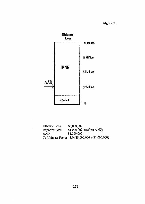
Figure 2.

Ultimate Loss

IBNR

Repotted

Sil Million

SS Million

S2 Million

0

Ultimate Loss $8,000,000 Reported Loss $1 ,OOO,OOO (Before AAD)

$2,000,000 To Ultimate Factor 8.0 ($8,000,000 + $1 ,OOO,OOO)

228

This example assumes that the ultimate losses are known and larger than the AAD.

There actually might be a distribution of possible ultimate loss results. In theory, we

should be subtracting the expected value of the AAD Com the expected value of the

ultimate loss. The expected value of the AAD will be less than the ful1 AAD if mere

is the possibihty that the AAD would not be fulfy used. This paper deals with a

fíxed ultimate Ioss rather than an expected value.

If the AAD only applies to one line of business in a contract that covers multiple

lines of business just the AAD hne can be handled separately. A multi-year contract

that has an AAD that spans a number of years can be included for loss development

purposes, but handled separateiy to develop the IBNR.

The possible relative sizes of AAD, reported loss gross of the AAD and Ultimate

loss before AAD are depicted on the iine graphs on Figure 3. There are six ways to

arder three variables by size assuming none of the three are equal to another.

The first two situations discussed assumed the ultimate Ioss is larger than both the

A4D and reported loss. It is possible for the AAD to be larger than the reported

and ultimate loss. This is shown in situations 3 & 4 on the line graphs on Figure 3.

In this case the IBNR would be zero as the AAD ehminated all losses.

It is also possible for the reported loss to be larger than the ultimate loss and AAD

(situations 5 & 6 on Figure 3). This means that there will be negative development.

In situation 5, the company has reported losses of R which have been partially offset

by the AAD of A. The net of AAD reported losses are R minus A. Since ultimately

there will be no losses as the AAD is larger than the ultimate loss, the TBNR should

bring the booked loss to zero and this negative IBNR amount would be A - R.

229

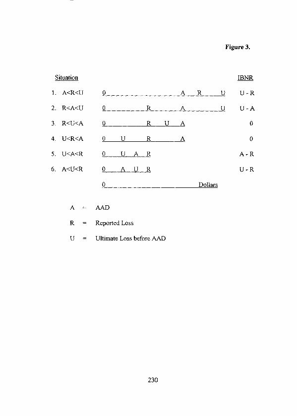
Figure 3.

Situation m

1. A<R<U 0 A R U U-R

2. R<A<U 0 R A U U-A

3. R<U<A 0 R U A 0

4. U<R<A 0 u R A 0

5. U<A<R 0 U A R A-R

6. A<U<R 0 A U R U-R

0 Dollars

A = AAD

R = Repotted Loss

U = Ultimate Loss before AAD

230

In situation 6 when the AAD is less than the ultimate loss, and the ultimate loss is

less than the reported loss, the net of AAD reported loss is the amount between A

and R or R - A. Since the ultimate loss is less than reported loss the IBNR is the

amount between U and R or U - R.

As the situation with the ultimate loss less than the reported loss (negative

development) is unusual, 1 will not consider it further (situations 4, 5 and 6).

In general assuming positive development, one approach to develop net of AAD

IBNR is lo make two calculations, and use the smaller IBNR of the two but not less

than zero. One calculation is to develop the formula IBNR gross of the AAD. This

gives the correct (and smaller) IBNR in situation 1 (the formula IBNR is equivalent

to U-R).

The second calculation is to develop the ultimate loss gross of the AAD and subtract

the AAD fminimum IBNR of zero). This gives the correct (and smaller) IBNR m

situation 2. There is a minimum IBNR value of zero because in situation 3 the

ultimate loss minus the AAD is negative, but the true IBNR is zero. The two

calculations can be expressed as:

min (U-R, (max (0, U-A)).

When the AAD equals the case reported, both calculations produce the same IBNR.

231

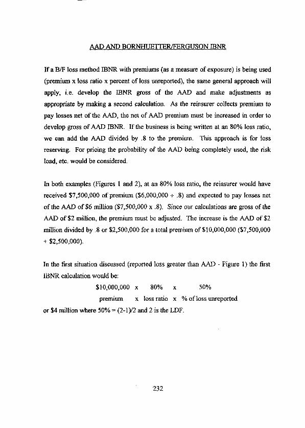
AAD AND BORNHUISTTEWFERGUSON IBNR

If a B/F loss method IBNR witb premiums (as a measure of exposure) is being used

(premium x loss ratio x percent of loss unreported), the same general approach will

apply, i.e. develop the IBNR gross of the AAD and make adjustments as

appropriate by making a second calculation. As the reinsurer collects premium to

pay losses net of the AAD, the net of AAD premium must be increased in arder to

develop gross of AAD IBNR. If the business is being written at an 80% loss ratio,

we can add the AAD divided by .8 to the premium. This approach is for loss

reserving. For pricing the probability of the AAD being completely used, the risk

load, etc. would be considered.

In both examples (Figures 1 and 2), at an 80% loss ratio, the reinsurer would have

received %7,500,000 of premium ($6,000,000 + .8) and expected to pay losses net

of the AAD of $6 million ($7,500,000 x .S). Since our calculations are gross of the

AAD of $2 million, the premium must be adjusted. The increase is the AAD of $2

million divided by .8 or %2,500,000 for a total premium of $10,000,000 ($7,500,000

+ %2,500,000).

In the íirst situation discussed (reported loss greater than AAD - Figure 1) the first

IBNR calculation would be:

$1 o,ooo,ooo x 80% x 50%

premium x loss ratio x % of loss unreported

or $4 million where 50% = (2-1)/2 and 2 is the LDF.

232

The second calculation is ultimate loss of $8 million minus the AAD of $2 million

which equals $6 million. The IBNR is the lower value of $4 million or

min (U-R, (max(0, U-A))) =

min (8-4, (max(O, S-2))) =

min (4,6) = $4 million

Under the second situation discussed (reported loss less than AAD - Figure 2) the

first IRNR calculation is

%10,000,000 x 80% x 718

or $7 million where 7/8 = (S-1)/8 and 8 is the LDF.

The second calcuiation is ultimate loss of $8 million minus the AAD of $2 million,

or $6 million. The IBM therefore is the lower figure of $6 million or

min QJ-R, (max (O,U-A))) =

min (S-I, (max (0,8-2))) =

min (7,6) = $6 million

We can express the two calculation AAD adjustment rule a different way. We can

just use the formula IBNR, however, when the reported loss is less than the AAD

we will subtract the unused AAD from the formula IENR. This can be seen by

looking at the Figure 3 line graphs. In our exatnple (Figure 2) %10,000,000 x .8 x

(7/8)=$7,000,000 minus (AAD of $2,000,000 minus reported loss of $1 ,OOO,OOO) =

$6,000,000. Due to situation 3 the minimum IESNR shouid be zero. The formula is

max (0, U-R-max(0, A-R))

233

In the first situation discussed (reported loss greater than the AAD - Figure 1) no

adjustment is necessary as reported losses are greater than the AAD.

AAD AND INDICATED LOSS RATIOS

When using a B/F loss method, one might initially use a loss ratio based on

conversations with the Pricing Actuary or the Underwriter or based on previous

accident year indications. As data becomes available, it is appropriate to develop an

indicated ultimate or burned loss ratio that incorporates loss development factors to

assist in selecting the loss ratio for the B/F method.

In the second situation discussed (reported loss less than AAD - Figure 2) we can

develop an indicated ultimate loss ratio of 80% (%l,OOO,OOO of reported loss x 8.0

the to ultimate factor + $10,000,000 of AAD adjusted premium). The indicated loss

ratio for the first situation (reported loss more than AAD - Figure 1) is the same

80% or $4,000,000 of reported losses x 2.0 (the to ultimate factor) + $lO,OOO,OOO

AAD adjusted premium.

Just as we are able to add the AAD business in the triangle to the non AAD

expetience, we can also develop indicated loss ratios by iricluding the AAD

business. One problem with mixing AAD with non AAD business in the indicated

loss ratio is that there can be an inconsistency between the loss ratios for the AAD

contract and the non AAD business. If the two do not have the same loss ratios,

doing the IBNR combined and separately for AAD and non AAD can produce

different results. Because of this doing a separate loss ratio calculation for the AAD

contracts is preferred.

234

In general, if losses gross of the AAD are captured, the appropriate IBNR reserves

can be developed net of the AAD by the use of two calculations and by following

certain simple rules. The combination of similar AAD and non AAD business in

loss development triangles increases the credibility of the loss development and

IBNR indications.

235

An In tegrated Pricing and Reserving Process for Reinsurers

by Leonard R. Goldberg, KAS, and Joseph LaBella

237

AN INTEGRATED PRICING AND RESERVING PROCESS

FOR REINSURERS

ABSTRACT

In today’s market of increased competition, more complex reinsurance contracts and

tightening (or should we say frightening) profit margins, actuaries are increasingly

being called upon to improve their pricing and resetving practices concerning

individual accounts as well as aggregate books of business. Increased

understanding of that business is criticai to continued success for both reinsurers

and their clients. The purpose of this paper is to describe a framework for an

integrated pricing and reserving piocess on an individual risk basis. Utilizing this

framework, increasing lev& of sophistication and knowledge can be brought to

bear, risk by risk, on understanding a reinsurer’s book of business.

239

AN INTEGRATED PRICING AND RESERVING PROCESS

FOR REINSURERS

1. SUMMARY

The process described herein is dependent upon having significant actuarial and

undetwriting resources available to analyze the risk on every individual contract that

is eventually written and put on the books. As well, this process relies heavily on a

collaborative environment where underwriting, actuarial, claims, contracts, legal and

accounting all have a significant role to play in understanding and evaluating risk.

The concept of this paper is to explain a structure which a reinsurer (or a large

accounting department of a primary company) can use to gain a thorough

understandíng of their book. ’ The focus is on the process, not techniques.’

Each contract is individually priced by a team that is centered around an underwriter

and an actuary. The result of this analysis is an expected loss ratio, an expected

loss development or lag pattern (note: a lag for a contract is the expected

percentage of losses that have emerged. For example, a lag of 20% means that it is

A second concept behind this paper, proposed by so-called friends of the authors, is to ensure a trip to Bermuda to present this paper. The authors eschew this as a basic concept of the paper. We will leave techniques to more capable actuaries. The reader may find, however, that these sophisticated techniques can be layered into the framework described herein.

240

expected that one fifth of the losses have emerged to date. The lag is also equal to

the inverse of the cumulative loss development factor for the contract.), an expected

payout pattern, an estimate of an aggregate distribution of result, a vector of

committed capital over the lifetime of the deal and an estimated return on equity

(ROE) for the deal. The pricing information that is developed is then used as the

starting point of the reserving and risk analysis processes.

The reserving process begins by using the expected loss ratio, incurred lag and

payout patterns developed from the pricing process. Every quarter, each contract is

reserved either to its expected loss ratio, the Bornhuetter-Ferguson method, or

other appropriate methods. After the data is assembled, staff from various

professional departments meet and agree on expected ultimate loss ratios for each

majar contract. Over time, enough individual contract information is generated to

provide feedback to the underwriters and pricing actuaries as pan of their renewal

process. Similarly, aggregate data is developed to help analyze future contra&.

The aggregate distribution that is used to price each contract is utilized in the

reserving of each account. In particular, accounts with significant loss sensitive

features are heavily dependent on the shape and variability of the aggregate

distribution. individual risk reserving also can provide consistent answers for

accruals on contingent commissions and profit commissions.

241

The detailed information that is gathered from each contract also altows the

company to assign capital to each contract for the current year, and for all years into

the future where there is still risk as to the ultimate result. Using both actual data

and simulation techniques, capital allocation formulas are continuously refined.

Each quarter, a profitability study is produced showing profitability by contract, client

company, line of business, and strategic business unit (SBU). In addition to

“traditional” accounting data, the study aggregates vital statistics such as mean time

to payment of losses, capital utilized, ROE, interest rate assumptions used, and

performance VS. initial benchmarks (actual VS expected losses, ROE, etc).

As levels of sophistication continue to increase, more interesting analyses can be

accomplished. These would include items such as estimating correlations between

risks, estimating correlations between liability and asset accounts, defining drivers of

economic results that affect the whole book (Le.. interest rates), and determining an

optima1 debt to equity mix for the corporation.3

The most interesting fact is that the drivers of this type of analysis are not

sophisticated mathematical techniques, but basic actuarial blockíng and tackling.

This includes good data from client companies, high levels of data quality for what is

input into the reinsurer’s systems, actuarial pricing software that allows for

~-~----.-. ___~-~-- -- In this case, there is almost perfect correlation between the importance of this work (very) and the impossibility of this work (very).

242

experience rating and exposure ratíng, and a generally agreed upon ROE

methodology that is understandable by all parties involved in the process. Also

necessary to the process are ways of linking pricing data to reserving and

profitability data to provide continuous improvement ìn analysis and assumptions. 4

II. CORPORATE PHILOSOPHY AND THE ANALYSIS OF RISK

Not too many years ago, reinsurers operated largely by spreading risk. Shares of

individual contra& tended to be relatively small, and actuarial involvement in the

pricing of contracts was infrequent. As reinsurers and their clients have become

more sophisticated, profit margins have been squeezed, and reinsurers have to

work much harder to find structures that both satisfy client needs and provide an

opportunity for adequate returns to capital. The concepts and techniques contained

in this paper are contingent upon analyzing every risk in great detail. Therefore,

these methodologies can only be well utilized by a company where the corporate

philosophy matches up reasonably close to the following:

A. Be a lead reinsufer - While it is not necessary to always be a lead reinsurer,

generally being the iead provídes greater insight into a contract. There is more

opportunity to talk to client company management about underwriting philosophy,

There are unlimitad ways to do this, and there are always improvements needed. This plus the work on correlations (see Footnote Three) should keep the authors employed for thousands of years.

243

claims management philosophy, strategic direction and the like. Individual contract

reserving and pricing doesn’t do a lot of good if you cari’‘’ really understand what the

client is all about. Also, being the lead allows the reinsurer to work closely with the

broker and client to create a structure that will maximize outcomes for both parties.

6. Underwrite Large Lines - The cost of understanding the risks in great detail

are significar& These costs can only be justified if the reinsurer and the client are

both willing to allow for large lines. This can be difficult, as often reinsurers are

reluctant to take large lines as a major loss could seriously impact results. Similarly,

clients are often unwilling to give a reinsurer a large line as sometimes they feel

this means they may lose some control over the account. The best way to handle

all of these issues is to develop a strong and trusting relationship between the

reinsurer and the client.

c. Collaborative Envlronment - Individual contract analysis cannot be left to

just the actuaries. There has to be a significant amount of input from all professional

units of the company. Underwriting audits, claim audits and accounting audits need

to be íntegrated into the pricing and reserving process. Contract language needs to

be analyzed. Emerging issues of liability need to be explored. Each contract also

has to be thought of as paf-t of a relationship with the client, perhaps spanning many

underwriting units and areas of expertìse. There needs to be significant and varied

client contact that is communicated to all members of the team. All the knowledge

244

gained in the collaboration of the various professional disciplines add to the value of

both the pricing and the reserving of each individual contract. ’

III. PRICING INFORMATION

For every contract that is bound, a signìficant amount of information is collected

through the pricing process. Even when contracts aren? bound, significant

components of the following data are stìll available and can be added to the data

warehouse. Basic information that is passed through into the corporate database on

all contracts includes the following:

A. Expected Loss Ratio (EU?) - ELR’s are developed using both experience

and exposure rating. Data is obtained from the ciient company, and can be

augmented with data from ZRC’s proprietary database, or ISO, RAA, or the NCCI.

For risks with property exposure, the ELR must have a catastrophe and

non-catastrophe component.

B. Aggregate LOSS Dísttfbution - For each contract, an aggregate loss

distribution needs to be established. The aggregate loss distribution describes the

The amount of knowledge that is required todo this well is humbling. The authors are comforted in knowing that many others are responsible for adding to this body of knowledge. In addition, the authors acknowledge the huge value that is added by the others in the process.

245

probable loss scenarios that underlie the selected ELR. The aggregate distribution

performs two functions. The first is to help estimate the riskiness of the contract and

hence, the amount of capital required. The second is to help in the evaluation of

different contract features such as loss corridors, contingent commissìons or

retrospective rating. These two issues are highly interactive. Starting with an

aggregate loss distribution that describes the underlying loss process of a contract,

the team can overlay different contract structures to analyze how the riskiness

(required capital) and profitability changes. Aggregate distributions can be

developed using a number of pre-packaged products. They also can be developed

directly from the company’s historie data, or selected by the team analyzing the

contract.

C. Loss Development Factors (Lags) - Incurred lags (expected percentage of

losses emerged over time) should also be developed as much as possible from

client company data. Lags have multiple uses in this process. They are a critica1

element of the experìence rating approach used to derive an expected loss ratio.

They are also needed as part of the Bornhuetter-Ferguson process which will later

be used as part of the reserving methodologies for the contract. Lags or loss

development factors are often incorporated in a contract that has loss sensitive

elements. They can also be an important determinant of the cash flow for the

various features of a contract, such as when a contingent commission will be paid or

when a retrospectively rated contract will generate additional premium (to the extent

these items are measured from incurred losses).

246

D. Payout Pattern - Estimating a payout pattern is critica1 to understanding the

risk of a reinsurance contract for many reasons. It provides the basis of the timing

for loss cash flows which allow analysis of the present value of any contract. In

aggregate, payout patterns are used to develop the duration of the book of liabilities

and help set asset management poticy. Payout patterns can also provide

information on the sensitivity of a contract to inflation. Note that the payout pattern

and the incurred lags need ta be internally consistent for each contract. It is also

important to think about the relationship of the payout pattern to the aggregate loss

distribution for an individual risk. For some types of contracts, the “bad” end of the

aggregate loss distribution may be more likely to arise due to a spate of early shock

losses. Other contracts may be more influenced by long-emerging losses. All other

things being equal, the former has a wider distribution of net present values than the

later; they both have the same nominal aggregate loss distribution and expected

payout, but the first contract has more downside on an economic or net present

value basis.

E. Analysis of ROE - Of course, there needs ta be some sort of metríc that each

company uses to determine whether they are generating appropriate returns from

each contract. Rather than just using this metric as an underwriting decision tool, it

is possible to capture information from this analysis in the corporate database. An

example of this is our company’s ROE (return on equity) methodology. The

estimated expected return is the weighted average of the present values of all the

estimated after tax cash flows from the contract over all of the points of the

247

aggregate distribution. Equity is then allocated to each contract based upon the

downside risk of each contract (estimated from the aggregate loss distribution), the

mean time to loss payment, the line of business underwritten as well as other

factors. The estimated required capital for any contract is the present value of all

future estimated capital commitments until the risk is extinguished on the contract.

A few more moments on ROE are necessary. The contracts that most reinsurers

write have a varying degree of risk. And the causes of risk vary from contract to

contract. Also, individual contracts can be correlated with other contracts such that

potential for adverse results can increase dramatically. We believe that it is critica1

that any methodology for analyzing profitability contain a consistent way of

measuring risk. We relate risk to capital need, wherein riskier deals require more

capital and therefore a higher dollar return to preserve the ROE. There are other

metrics that can be used effectively.

From the ROE process, we capture information on the present value of the cash

flows under each scenario, the weighted average present value of the cash flows,

the average interest rate used in the analysis, and a vector of required capital

needed annually until the risk of the deal is extinguished. Creating this information

and storing it in the corporate database allows for analysis of capital usage and

expected VS. actual investment returns. It also allows for continua1 updating of

capital allocation process assumptions.

248

We again stress that there are many metrics that can be used to help set pricing

and profit targets, and there is nothing magical about how we define ROE. Two

points are critical. First is that the methodology is widely understood by underwriters

and actuaries. If there is no buy-in to the metric, it becomes another hurdle

to be crossed rather than a value-added exercise. This argues for some simplicity

of approach. The second point is that once the critica1 drivers of the metric are

established, they should be captured and integrated into the databases that are

used to manage the business. This information is at least as ìmportant as the

accounting information that is collected and should be held (at least) to the same

data quality standards.

IV. I-HE RESERVfNG PROCESS USING INDIVIDUAL

CONTRACTDATA

With all of this data availabie, the reserving process by individual contract is

relatively straightforward. Keep in mind that this reserving process is only one

methodology and multiple methodologies can and should be used when arriving at

a range of reasonable results. The individual contract method, with its intense

focus on the “trees” sometimes can cause us to lose touch with the forest. Analysis

of aggregate data is still the only way to view some over-arching trends such as a

change in case reserve adequacy ora speed-upklow down in claim payments.

249

A. Initial Assumptions - Generally, the reserving process starts by capturing

the ELR on an ex-catastrophe basis and the appropriate incurred lag and payment

patterns for each contract. All contracts are grouped into reserve “cells” for

analysis. For larger contracts, a separate reserve cell is established to individually

reserve the contract. For smaller contracts, multiple contracts with similar

characteristics are combined into a reserve cell. Typically, such characteristics

may be class of business (casualty VS. property, for example), line of business

(auto liability, general liability, etc), quota share VS. excess of loss, high VS. low

layer, etc.

We refer to these multiple contract groupings as aggregate cells. The initial ELR of

an aggregate reserve cell will be the weighted average ELR of all contracts in the

cell. The initial incurred lag and payment patterns for an aggregate cell will be

selected from some subset of the contracts that enter into that cell, or sometimes

by using other information (ISO, NCCI, RAA, ZRC’s proprietary database).

As contracts are renewed in subsequent years, the corporate actuarial unit should

review the ELR’s and the lags for consistency with old years. Any major

differences between contract years should result in further discussions among the

reserving actuary, the pricing actuaty and the underwriter to understand these

differences.

250

Sometimes the contract terms change materially, resulting ir-r a significant change in

the ELR, the lags, or both. This could be dueto a difference in price, layer or terms

between years. In these cases, material differences between years can happen.

Other times, new or updated information comes to light which materially changes

the analysis, resulting in revised expectations for the current period. A common

example is when more information (claim count triangles, pricing history, etc) is

available in the renewal package than was available when the contract was initially

priced. This additional infonation can greatty change expectations of a contract’s

profitabilii for both the current and prior years. When this is the case, the ELR’s

for old years are often updated to also refiect the new information.

As an example, let’s say that we bound a new commercial multi-peri1 contract. The

ceding company was not yet set up to supply data triangles, so the pricing analysis

relied upon an exposure rating analysis and an ISO lag pattern. The overall pricing

analysis carne up with a 65W ELR. When the renewal package was received one

year later, paid and incurred loss triangles were included. The analysis of the

renewal contract resulted in an 85% ELR for the current year. After reviewing

these results, and the company specific data that drove them, it was concluded that

it was the historical data, not necessarily the latest twelve months activity, that

drove the new loss ratio pick. If we would have had this data available when we

priced the original contract one year ago, the ELR would have been a 75% after

giving weight to both experience and exposure rating methodologies. In this case,

we would change the prior year’s ELR to reflect this new historical information.

251

In another example, suppose that a similar contract, originally priced at a 65% ELR,

had run adversely over the first twelve months. Assume that lots of good

information has been available on the contract since inception. Even though the

estimated ultimate loss ratio, via the Bornhuetter-Ferguson method, was now 75%,

we would not necessarily change the original 65% ELR that feeds that

methodology. We have no reason to believe that the contract will not run a 65%

loss ratio on a going forward basis.

As the information comes through the underwriting process, the corporate actuary

also has responsibility to look for data quality and consistency. Is the payout

pattern faster than the incurred lag pattern? Are the patterns ver-y dissimilar to

other treaties in the same Une of business? Has the expected loss rabo dropped as

industry pricing has weakened? In the pricinglreserving feedback process, the

pricing actuaries each search very deeply into a smaller number of contracts, and

the corporate actuaries spread their time over a larger number of contracts. The

reserving actuary is usually in the best position to provide such reasonability

checks.

B. Quarterly Updethg Process - Each quarter, earned premium and case

incurred losses are updated for each contra& Generally for our purposes, one of

three methodologies (loss ratio, incurred Bornhuetter-Ferguson, paid

Bornhuetter-Ferguson) are selected. For ver-y green and for very long-tailed

252

contracts, it is often advisable to stick with the initial ELR as the estimated ultimate

loss ratio for a period of time (12-24 months), rather than reacting too early to good

or bad loss development news. For contracts that are more mature and for

shorter tailed contracts, the incurred or paid Bornhuetter-Ferguson process using

the initial ELR and pricing patterns are generally utilized. lnformation based on

either of these methodologies, along with more detailed claims information, are

provided to the SBU managers, underwriters, pricing actuaries, claims professionals,

and accountants each quarter. As a group, these individuals along with the

corporate actuarial staff will try to come to a more complete understanding of

how each majar contract and each aggregate reserve cell is performing. A large

amount of time and effort is expended each quarter in this process. ’

c. Multiple Resewing Methodologies - Individual contract reserving also

allows us to experiment with different methodologies. These different

methodologies can help in formulating a range of reasonable estimates. In addition

to the standard methodologies (loss ratio, íncurred Bornhuetter-Ferguson, paid

Bornhuetter-Ferguson, incurred loss development, paid loss development) there is a

bit more that can be done when reserving by individual contra@. For example, we

have calculated expected ultimate losses using a loss ratio methodology for lags

less than 10% and an incurred Bomhuetter-Ferguson methodology for the rest. We

- -_I -__ Much of this time is expended creating user friendly reserving exhibits (an oxymoron?) that are comprehensible by those outside of the Actuarial profession. In addition, written summaries of the quarter’s indications, trends, and oddities are very necessary icebreakers to the review process.

253

have used loss development capped and cuffed by plus or minus 25% of the

Bornhuetter-Ferguson estimate.

One can also experiment with varying the parameters that feed the methodology of

choice. We tried developing a range around the expected loss ratio, using the

aggregate loss distribution. Another possibility is developing slow and fast lag

patterns around the selected pattern, to develop a range of indications. The

flexibility to try something new is a nice benefit of this process. You may find that

different methodologies are necessary (produce more accurate results) for certain

contracts or lines of business. You may also find that developing an indicated range

of reserves helps valídate (or call into question) your methodology of choice.

D. feedback Loop for Renewals - The result of the quarterly process is to have

a concensus-built estimate of how each major contract and many of the smaller

contracts are performing. A major benefit of this type of process is that the IBNR

should be appropriate for each contract (with some exceptions), and is not an

allocation. In addition, the entire company has a buy-in to every IBNR number as

each number was arrived at through a group process rather than by a corporate

actuary sitting in his or her Office. As experience matures across all contracts, it

then also becomes possible to aggregate data to create pricing parameters such as

loss development factors, trend factors and excess factors for your company’s

specific book of business.

254

E. Mapping of Underiylng Exposure - It is extremely important to be able to

map the exposure spread of every contract. This wili affect how earned premium is

allocated to accident year and how lag factors are interpolated (see next section). A

simple drawing of a square or a parallelogram, is often suffÍcient to describe the loss

occurring or risk attaching base case.’ You then need to consider other pertinent

facts in mapping the contract’s exposure. Is there an unearned premium portfolio on

the front end of this contract? At expiration, does the contract cut-off or run-off? Are

the underiying policies written evenly throughout the life of the contract, or ís there

some seasonality to the ceding company writings? Also, are all underlying policies

one year in length, of variable length, etc? Does the underlying exposure itself

contain some type of seasonality? For example, the winter months may contain

more than their proportional share of Homeowners’ exposure. See Appendix A for

practica1 examples of this process.

One should not ignore the premium earnings pattern that is implied by how the

accounting department actually books the earned premium (which is mostly based

upon how the ceding company reports written and unearned premium to the

reinsurer). These bookings will map out the actual earnings and exposure patterns

for the contract. We need to begin to tap this source of valuable information in our

shop.

- .~ __ Losses Occurring: A contract which covers all accidents that occur (or are reponed, in the claims made case) during the contract period. The exposure looks like an accident year box. Risks Attaching: A contract which covers all accidents that result from underlying policies that incept during the contract period. The exposure looks like a policy year parallelogram.

255

F. Interpoiation of Lag Factors - Another special topic that needs to be

addressed is interpolation of lag factors. Most of the data that is received through

the pricing-reserving loop is accident year in nature. For a January 1 losses

occurring contract, usually no adjustment is needed. However, for contracts that are

written on a risks attaching basis, or if there is a portfolio in, or if the effective

date lands on other than a quarterly point, interpolations of existing lag factors will

be required. Appendix B details a lag interpolation method and shows some of the

situations and calculations in greater detail. Although interpolating the lags can be

complex, this process adds significantly to the understanding of each contra&

results.

There is a further special case for quota share business. In order to completely

match reported loss and IBNR on an individual contract, the interpolation has to be

to the date of the last bordereau report, not the date of the reserve study. Quota

share contracts are generally reported 30, 60 or 90 days in arrears. So using the

date of the reserve study would understate ultimate loss. Also, some loss reports

are not received by the end of the quarter, and a further adjustment is needed. For

aggregate quota share cells, we assume all contracts are 90 days in arrears (we

have tested this assumption on occasion, and it pretty much holds true). For excess

accounts which report individual losses, we assume reporting is current and

therefore consistent with the reserve study date.

256

v. RESERVING FOR CONTRACT FEATURES

One of the majar benefits of analyzing each contract individually and creating an

aggregate distribution for each contract individually is in valuing special contract

features. We differentiate between the value of a feature at expected loss, versus

the expected value of the feature. We believe the latter method is more accurate.

An example may help. Suppose a contract contains a profit commission feature

such that we pay one-half point of commission for every point under a 65 loss rabo.

Further, suppose our expectations of the contra& loss rabo is currently a 67. In

this case, the profit commission at the expected loss rabo is zero. However, based

on the distribution of potential ultimate Iosses around the 67, the expected profit

commission may be 2 or 3 points (because within the aggregate distribution of

results, there are possibilities that the loss rabo may fall below a 65, and some

weight must be given to those possìbilities). This distinction is important, especially ,

when estimating profitability for individual contracts. We price the features based on

their expectations and we should reserve for them on a similar basis. We currently

do not follow this in our shop, as we book the contractual commission based upon

the expected losses. The change is being discussed, though. The following are

more detailed examples of contract features:

A. Retrospectively Rated Contrects - For atmost all retrospectively rated

reinsurance contracts, the aggregate loss dístribution has a wider swing than the

257

minimum and the maximum loss ìn the premium calculation. As a simple example,

suppose there is a contract with a contractual loss ratio of 60 (that is, premium is

calculated as losses multiplied by 100180), a minimum premium of 0, and a

maximum premium of $Im. If expected losses are $400,000, based on that point

estimate, one would expect earned premium of $500,000. However, suppose the

$400,000 is the weighted average of an aggregate loss distribution with a high end

of $2m. If we were to take the weighted average of the retrospective premium under

all of these scenarios, the resulting premium would be somewhat less than

$500,000, and the resulting loss ratio would be somewhat greater than 80 (weight is

being given to the possibility that losses may exceed $800,000, with no resulting

increase in premium after that point).’ See Appendix C for more details.

B. Loss Corridors - In many situations, a reinsured will agree to pay for losses

occurring in a certain layer either defined by loss ratìo or dollars of loss. Sometimes

this loss corridor appears below the expected loss amount and sometimes well

above the expected loss amount. By creating an aggregate loss distribution, each

loss corridor can be priced and reserved for. This can be a very complex exercise

on an individual contract basis. Suppose a contract had an initial expected gross

loss ratio of 70 with a loss corridor from 65 to 75. Perhaps based on the aggregate

loss distribution, the corridor was Worth 3 points, bringing the net loss ratio to 67.

The hardest paf-l of this process is convincing the accounting staff that there is a need to book a loss ratio in excess of the contractual loss ratio. The authors leave this as an exercise for the reader.

258

Now it’s two years later and the estimate of the ultimate gross loss rabo has

increased to 85. Clearly the value of the loss corridor is now more than 3 points, but

its value is still somewhat unclear. In these situations, we would either have to rely

on a subsequent study or be able to develop a re-estimated picture of the complete

aggregate loss distribution after two years of emerged experience. Appendix D

shows more details. *

c. L oss Caps - Often, contracts are capped either as to absolute dollar amount

or to number of reinstatements. Given that the cap is Iower than the high end of the

expected aggregate loss distribution, the weighted average expected loss ratio net

of the cap should be lower than the initlal (uncapped) expected loss rabo.

VI. PROFITABILITY AND CAPITAL USAGE

With all of this great data assembled and ready to use in one place, there are

certainly many other types of analyses that can be done other than straight

reserving. The following lists a few of the analyses that can now be accomplished

using the compiled data:

A. Profitability Studies - The huge amount of work that individual contract

pricing and reserving requires really bears fruit when looking at individual contract

The authors would prefer to say that they have developed a theoretically defensible process that re-estimates the aggregate loss distribution over time to facilitate the re-evaluation of loss sensitive features, but they’d be lying. However, this doesn’t keep.us from trying. All ideas and good wishes are appreciated.

259

profitability. Since all of the numbers are built bottom-up and built on a consensus

basis, each contract’s profitabìlity can truly be considered a best estimate. One can

then aggregate contracts by underwriting year, undetwriter, pricing actuary, client

company, client group, line of business, attachment point, etc, etc. The profitability

of any slice or aggregation of the business is then also a consensus based estimate.

Management should have more confidente in this approach as compared to a top

down allocation.

EL Basic Capital Analyses - It is also now relatively easy to compare the

amount of capital that has been allocated for all contracts undetwritten to the total

capital available in the corporation. If the capital allocation methodology is well

accepted by management, then aggregating the capital numbers can give

management an idea of whether capital is being under-utilized, fully utilized or

over-utilized. Conversely, the comparison between allocated and actual capital can

be used to help make refinements to the capital allocation procedures.

C. Advanced Capital Analyses - With aggregate loss and NPV distributions for

each contract, there are many things that can be done to determine the aggregate

capital need of a reinsurer. We have recently been playing around with different

types of these analyses. Our basic technique is to run simulations by selecting

from each aggregate loss distribution. When doing this type of analysis, there are at

least two interesting questions that need to be answered, and probably a lot more

than that. The first question is one of correlation. How much or how little correlation

260

is there between two accounts in the same line of business? How about two

accounts for the same company? How about the same questions with different lines

of business and different companies? It is also possible that correlation could vary

across the distribution. For example, contracts might be highly correlated at the low

end due to low inffation or some other factor, but act more independent at the high

end of the aggregate loss distribution. The second question that needs to be

answered is one of how the shape of the aggregate loss distribution changes as the

contract matures. Generally, the risk of each contract should shrink over time, so

one would expect the aggregate loss distrìbution to grow more narrow with time.

But, does it narrow as losses are incurred, paid, or based on some combination of

the two? Are there some contracts, such as workers compensation, where the risk

is greatly reduced early on as the cases emerge while other types of business, such

as excess umbrella, might remain a question mark for many years to come’?

We certainly have more questions than answers, but we have attempted some

interesting things with the data we have collected. One example is our work on

Umbrella. We started with the aggregate loss distribution for each contract that we

wrote in a given year. From our ROE model, we extracted the net present value

profit from each loss scenario (we “discretize” our aggregate distributions into

scenarios). We knew that each contract was somewhat independent, but also

correlated due to things like inflation and tort law. We even figured that some losses

would be fully correlated as there are sometimes more than one client writing

261

different layers of the same risk. So here’s what we did -- we randomly selected

pairs of contracts and fully correlated them (Le. if Contract A was at the 80

percentile of the distribution, then so was Contract B). Then we randomly selected

from the fully correlated pairs. We then re-selected the correlated pairs and went

through the process again. We ran one million scenarios in this fashion and

compared the “bad” end of the distribution with the capital allocated to the contracts.

Then we did the same thing with groups of three contracts, four contracts and five

contracts to see how much the shape of the aggregate distribution would change.

While we are not sure if we accomplished anything important, or theoretically

defensible, we did get comfortable with our capital allocation and we had fun. If we

can scrape more time together, having all of this information available should yield

more interesting things in the future.

262

VII. Conclusion

At the core of this paper is the belief that there is real value in an integrated

pricing and reserving process on an individual contract basis. Over time, this type of

process can lead to a greater in-depth knowledge of clients, the marketplace and

profitability. This knowledge should create value for both the client and the reinsurer

in jointly understanding the risks of their businesses and in establishing an

appropriate price per unit of risk. The process requires everyone’s commitment and

much hard work.

Call us in ten years, and we’ll let you know how (and i9 it worked

263

3) Shape is Risks Altachlng (see definition in footnote 7 of the paper) \

7) No “portfolio in” of 7) No “portfolio in” of unearned premium -__) unearned premium -__) from prior from prior reinsurance contract reinsurance contract

4) Underlying policies 4) Underlying policies

6) Cancelled on a 6) Cancelled on a run-off Lmsis run-off Lmsis

period period r”ns r”ns off an off an

1) Inceplion Date 1) Inceplion Date 2) Expiralion Date 2) Expiralion Date 01101196 01101196 12131196 12131196

:1 5; 5) ‘5) 7) 8)

5) Here we are assuming that underlying policies are written evenly throughout the contract period.

6) Here we are also assuming that exposure on underlying policies is not seasonai (Le. not concentrated in winter orsummer, etc.)

Inception Date Expiration Date Claims Ba& (risks attaching or losses occurring) Length of underlying policies Seasonality in writings of underlying policies Seasonality in exposure Unearned Premium portfolio at the beginning of the contract Cancelled on a cut-off or run-off basis

SPFClFICS

01101196 12/31/96

R.A. 12 months

no no no

runoff

264

Accident Year 1996 Accident Year 1997

1) Once the exposure has been sketched, block-off the area within the exposure period.

2) Enter relative weights within the various blocks of exposure (here each full block has a weight of two, and therefore half a block has a weight of one).

3) Count the weights within each quarterly period to determine the exposure within that quarter (for this example, quartets one through four for AY 1996 would be 1, 3, 5, 7).

4) Also take a cumulative count of the weights, quarter to quarter, to determine the percent exposed over time (for this example, quarters one through four for AY 1996 would be 1, 4, 9, 16 or 6%, 25%, 56%, 100%)).

5) All of the exposure information necessary to perform the lag interpolation process ìs now present (see Appendix 6 for that process).

265

1) 2) 3) 4) 5) 6) 7) 8)


Inception Date Expiration Date Claims Basis (risks attaching or losses occurring) Length of underlying policies Seasonality in writings of underlying policies Seasonality in exposure Unearned Premium portfolio at the beginning of the contract Cancelled on a cut-off or run-off basis

01101196 lU31l96

L.O. 12 months

no no

yes cut-off

266

1) 4 3) 4)

:; 7) 8)

Accídent Year 1996 Accident Year 1997

2 1 j 6 2 2 I II //

2 1

6 2 2

r 2 1: 6 2 2

!

2 16 2 2

Inception Date Expiration Date Claims Basís (risks attaching or losses occurting) Length of underlying policies Seasonality in writings of underlying policies Seasonality in exposure Unearned Premium portfolio at the beginning of the contract Cancelled on a cut-off or run-off basís

lOfO~l96 09/30/97

L.O. 12 months

no yes * ws

cut-off

l Note that half of thís contract’s exposure fab during the winter months (first quarter of 1997).

267

1) 2) 31 4) 5) 6) 7) 8)

APPENDIXA


Inception Date Expiration Date Claims Basis (risks attaching or losses occurring) Length of underlying policies Seasonality in writings of underlying policies Seasonality in exposure Unearned Premium portfolio at the beginning of the contract Cancelled on a cut-off or run-off basis

SPFCIFICS

07/01196 12131196

R.A. 12 months

no no no

run-off

268

APPENDIX B

Lag Factor Interpolation

To set the correct mood fqr this process, let’s start with a little joke. How many

actuaries does it take to interpolate a lag factor? And the answer is -- However

many you want. Not a very funny joke, but a very pointed statement. Evety actuary

seems to have their own interpolation method. None of them are correct, but they’re

all pretty good estimates. What’s being presented here is one of those methods.”

We’ll begin with an incurred accident year lag pattern at twelve month evaluations

(twelve months, twenty-four months, etc.). Next, we’ll need to create factors at each

quarter point. For evaluations after twelve months, linearly interpolate between

twelve month points. Granted this is not exactly correct, since any given loss

development pattern is not linear between annuai points. But, for this particular

method, it’s close enough.

For interpolated factors at the first three quarters, we’il be a bit more careful. The

loss development curve between zero and one year definitely has a ramping up

which we cannot ignore. Think of it as accidents just beginning to happen and loss

The general ideas behind the interpolation methods described herein were taught to one of the authors by Malcolm Handte, FCAS, MAAA. Interpretations of this interpolation method have changed some over time. Resulting lags are usually close to other actuaries’ interpolated lags in our shop.

269

reporting beginning to get into the swing of things. Table 1 contains a graph of five

curves that represent more to less severe ramp-ups between zero and one. The

most severe is roughly (1/4)2, (2/4) 2, (3/4)*, (4/4)*, more parabolic in nature. The

least severe is very close to linear. The factors in Table 2 correspond to the points

in the fíve graphs, and represent factors to apply to the twelve month lag point, to

create lags at the first three quarters. We tend to choose pattern one for long tailed

casualty patterns (where twelve month lag points are, say, 15% or less).

Conversely, pattern five goes well with quicker property patterns (with twelve month

lags of 65% or greater). Anything between those two can use patterns two, three or

four, based upon one’s particular judgment.

TABLE 1

1 Lag Interpolation Curve 1

270

TABLE 2

We now have an accident year lag pattem at quarterly evaluations. Graph it if you

like and, if you feel so inclined, smooth some points more to your liking. Now, if all

reinsurance contracts were January 1 incepting losses occurring contracts, the task

at hand would be complete. Unfortunately, a more general method is necessary to

estimate accident year lags for things like a September 20 incepting risks attaching

contract.

In order to accurately interpolate lag factors of any given point in time, we must be

able to sketch the exposure of the given contract. Refer to Appendix A for this

process. Recall, gathered information must inctude the inception and expiration

dates of the contract, the length of the underlying primary poiicies, any seasonality

imbedded in the exposure, whether the contract is losses occurring or risks

attaching, whether or not there is a portfolio of uneamed premium at the beginning

of the contract, and whether the contract is canceled runoff or cutoff,

271

Once the exposure has been sketched, more necessary information must be

gathered in order to complete the interpolation calculation. Table 3 contains the

interpolation formula as well as a list of the necessary pieces of information within

that equation. For example, if the Evaluation Date (ED) is 9/30/96 and earned

premium has been booked (received or accrued) by the reinsurer through this date,

then the Premium Information Date (PID) will be 9130196. But, if a quota share

contract has a one quarter repotiing delay (at 9130196, the reinsurer has just

received the primary company premium statement through 6/30/96), and the

reinsurer does not accrue for the missing premium, then the PID will be 6/30/96. If

you are dealing with an excess of loss contract, and no loss reporting delay is

apparent, then the Loss Information Date (LID) will be 9/30/96. In the case of a

quota share contract, the LID will equal the last date through which primary

company loss statements have been received.

TABLE 3

Equation: LAG (PID) = LAG [LID - MED + AF] x MF

Parameter Description

PID

LID

MED

AF

MF

Premium Information Date (usually equal to the Evaluation Date - ED)

Loss Information Date

Mean Exposure Date

Additive Factor

Multiplicative Factor

272

The Mean Exposure Date (MED) is the average accident date for the premium

earned so far. lt cen usually be determined by viewing the exposure parallelogram

and drawing a line through the apparent mean of exposure. For more complicated

risks attaching shapes, once the exposure diagram has been properly drawn and

weighted, as in Appendix A, we can add up the weights (area under the curve) and

divide by two to get the mean. Then we can determine (usually by eye) where this

mean falls on the exposure parallelogram.

Let’s look at Exhibit 2 in Appendix A and calculate the MED. The contract is ‘ll1196

incepting and is risks attaching. If the ED (and PID) is 12/31/96, we need to find the

mean area under the tnangle between III/96 and 12/31/96. Note that the weights

(area under the curve) are equal to sixteen. Half of this is eight. Sy counting back

from the 12/31/96 point, we can see that the MED falls slightly to the left of 10/1/96.

Here we can estimate and call the MED 9/15/96 (10/1/96 would also be a fairly

good, and easier to handle, estímate).

We can now calculate the relative “age” of the given exposure, as the loss,

information date minus the mean exposure date. Note that this is the key

expression in our search for the appropriate lag factor. Whether we are dealing with

a risks attachíng or losses occurring contract, and regardless of any other

parameters, this relative age of exposure will determine how much time has passed

since the mean date of exposure (or the average accident date), and thus how

“developed” thís exposure is.

273

A twelve month accident year lag factor assumes a 7/1 average date of loss, or six

months of average loss emergence, not twelve months. The loss information date

minus the mean exposure date must be increased to reflect this accident year

assumption, or else the lag would be understated, yielding expected losses to date

that are too low. Therefore, the Additive Factor (AF) is determined based on

symmetry -- six months of emerged loss needs a six month AF, three months of

emerged loss needs a three month AF, etc. The examples in Exhibit 1 display this.

Table 4 contains the AF values at the first four quarterly evaluations. The quarter

four factor is also the factor for all quarters greater than four, and for quarters where

the year of your evaluation date is greater than the accident year you are choosing a

factor for (hence the exposure in that AY has ended).

Addìtíve Factor (AF)

TABLE 4

MultiDlicative Factor (MF1

Quarter Factor (months) Quarter

1 1.5 1

2 3 2

3 4.5 3

4+ 6 4+

Factor

411 = 4.00

412 = 2.00

413 = 1.33

414 = 1.00

274

The Multiplicative Factor (MF) is necessary to gross up the full exposure AY lag for

the portion of exposure “earned” to date. The MF values are listed in Table 4. In

the second example on Exhibit 1, the six month factor pulled from the AY lag pattern

must be multiplied by 412 = 2 since only half of the full AY’s exposure (and premium)

has been eamed as of 6130196. Note that the six month lag of 24% (in the footnote

on Exhibit 1) means that six months after the inception date of this contract, 14% of

the total estimated ultimate losses are estimated to have been reported. In our

example, since half of the full exposure has been earned as of 6130196, (.14 x 2) =

28% of the six month exposure period’s ultimate losses are estimated to have been

reponed as of 6/30/96.

Exhibit 2 deals with a 1011196 incepting losses occurring contra& Note that from

year-end to the following frrst quarter (examples one and two), the AF and MF

values jump from the first quarter values in Table 4 to the fourth quarter values. The

resulting lags appear to be smooth and quite reasonable to the authors.

Risks attaching cases are explored in Exhibits 3 and 4. Note that we use the same

AF and MF factors for the risks attaching cases as we do with the losses occurring

cases. This has been challenged by other actuaries ìn our shop. The MF is easy to

question since it is meant to gross up the full exposure AY lag for the portion of

exposure “earned” to date. If the losses occurring MF at 6/30/96 is 4/2 = 2 since

half of the AY exposure has been earned, then why isn’t the risks attaching MF at

275

6/30/96 equal to 1614 = 4 (since only 25% of a risks attaching contract’s AY

exposure has been earned as of 6/30)? We believe that if the MF for the risks

attaching cases were increased in this fashion, then the AF would necessarily have

to be decreased or else your answers would be too large. We experimented with a

few different sets of factors and really could not get any to work as reasonably well

as the current set.

It is a premise of this methodology that the (LID - MED) expression creates an AY

type measure of exposure. Whether the contract being considered is losses

occurring or risks attaching in nature, the relative “age” of exposure we have

calculated is now a general measure of development that can then be used in the

overall interpolation formula (which uses AF and MF values that are losses occurring

or AY in nature).

The basic “che& of this process is whether or not the resulting interpolated lags

appear reasonable, especially when compared to the interpolated lags in the

quarters surrounding your evaluation quarter. The risks attaching and losses

occurring lags of the same “age” should also appear reasonable (and relatively

close together) when compared to each other. It also helps to compare results to

those from other actuaries’ interpolation methods. This interpolation method should

produce smooth and reasonable results.

276

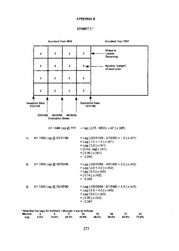
EXHIBIT 1 l


2 2 2 2 2 2

2 2 2 2 2 2

2 2 2 2 2 2

Shape is Shape is 2 2 - - LOS565 LOS565

Occurring Occurring

24 24 Relative Relative “weight” “weight” af each area af each area

2 2

Expiration Date Expiration Date

03131196 06130196 09130196 Evaluation Dates

AY 19## Lag @ Pt0 = Lag [ (LID - MEO) + AF ] x (MF)

1) AY 1996 Lag @ 03/31/96 = Lag [ (03/31/96 - 2/15/96) + 1.5 J x (4/1) =Lag[1.5+1.5]~(4/1) = Lag [ 3.01 x (4/1) = [3 mo. lag] x (4/1) = [ 0.06 ] x (4/1) = 0.240

2) AY 1996 Lag @ 06/30/96 = Lag [ (06/30/96 - 4/01/96) + 3.0 ] x (4/2) = Lag [ 3.0 + 3.0 ] x (4/2) = Lag ( 6.0 ] x (412) = [ 0.14 ] x (4/2) = 0.280

3) AY 1996 Lag @ 09/30/96 = Lag [ (09/30/96 - 5/15/96) + 4.5 ] x (4/3) = Lag [ 4.5 + 4.51 x (413) = Lag [ 9.0 ] x (413) = [ 0.26 ] x (4/3) = 0.347

l Note that the lags for Exhibits 1 through 4 are as follows: Months 3 6 9 12 15

Lag 6.0% 14.0% 26.0% 40.0% 48.0% 18 21 24

56.0% 64.0% 72.0%

277

Accident Year 1996

Shape is Losses -+ 2 Occurring

Accident Year 1997

2 2 2

2 2 2 2

Relative “weight” )2 2 2 2 of each area

Inception ,.‘,g.2 Date 1 2 2 t 1 Ei2YF

12131196 0x31/97 06/30/97 Evaluation Dates

AY19#b#Lag@ PID = Lag((LID- MED)+AF]x(MF)

1) AY1996 Lag@12/31/96 = Lag [(12/31/96 - 11/15/96) * 1.5 1x(4/1) =Lag[1.5+1.5]~(4/1) = Lag[3.0]~(4/1) = [3 mo. lag] x (4/1) = [0.061x (411)

2) AYl996Lag@ 03/31/97

3) AY1996Lag@06/30/97

= 0.240 Linearly interpolating

= Lag [(03/31/97 - 11/15/96) +6.01x (4/4)

J

behveen g and = Lag [4.5 +6.01x (4/4) 12 month points = Lag [10.51x (4/4) = [(9 mo. lag) f (12 mo. - 9 mo. lags) x (l/Z)]x (4/4) = [ 0.26 + (0.40 -0.26)x (1/2)1x (4/4) = [0.26 + (0.14) x(1/2)1x (4/4) = [ 0.26 + 0.071 x (414) = (0.33]x(4/4) = 0.330

= Lag [(06/30/97 - 11/15/96)+6.0)x(4/4) = Lag 17.5 +6.01x(4/4) = Lag [13.51x (4/4) = [ 0.40 + (0.48 -0.40)x (1/2)1x (4/4) = 0.440

278

Accident Year 1996 Accident Yaar 1997

1) AY 1996 Lag @ 09130196

Relaüve “weight” of each area

09130196 12131196 03131197 Evaluation Dates

AY 19## Lag @ PID = Lag [ (LID - MED) + AF ] x (MF)

= Lag [ (09130196 - 7/15/96) + 4.5 ] x (4/3)

= tag [ 2.5 + 4.5 ] x (413)

= Lag [ 7.0 ] x (4/3)

= [(S mo. lag) + (9 mo. - 6 mo. lags) x (113) ] x (4/3)4--- ~inearly interpolating = [ 0.14 + (0.26 - 0.14) x (113) ] x (413) between 6 and 9

= [ 0.14 + (0.12) x (1/3)] x (4/3) month points

= [ 0.14 + 0.041 x (4/3)

= [ 0.181 x (413)

= 0.240

2) AY 1996 Lag @ 12131196 = Lag [ (12/31/96 _ 9/15/96) + 6.0 ] x (414)

= Lag [ 3.5 + 6.0 ] x (4/4)

= Lag [ 9.5 ] x (414)

= [ 0.26 + (0.40 - 0.26) x (116) ] x (4/4)

= 0.283

3) AY 1996 Lag @ 03/31/97 = Lag [ (03/31/97 - 9/15/96) + 6.0 ] x (4/4)

= Lag [ 6.5 + 6.0 ] x (4/4)

= Lag [ 12.5 ] x (414)

= [ 0.40 + (0.48 - 0.40) x (116) ] x (4/4)

= 0.413

279

Accident Year 1996 Accident Year 1997 Accident Year 1998

T T hlception Date Expintion Date

07101166 06/30/97

9 12!31/96 03131197 06130197

Evaluation Dates

AY 19# Lag @ PID = Lag [(LID - MED) + AF] x (MF)

1) AY 1996 Lag @ 12131196 = Lag [ (12/31/96 - 11/01/96) + 3.01 x (4/2) = Lag [ 2.0 + 3.0 ] x (4/2) = Lag [ 5.0 ] x (412) = [(3 mo. lag) + (6 mo. - 3 mo. lags) x (2/3) ] x (412) C~inearly intetpoiating = lo.06 + (0.14 _ 0.06) x (2/3) 1 x (4/2) behveen 3 and 6 = i 0.06 + iO.06) x (2/3) ] i (4;i) month points = [ 0.06 + 0.053 ] x (4/2) = [ 0.1131 x (4/2) = 0.226

2) AY 1996 Lag @ 03/31/97 = Lag [ (03/31/97 11/01/96) + 6.01 x (4/4) = Lag [ 5.0 + 6.0 ] x (4/4) =Lag[ll,O]x(4/4) = [ 0.26 + (0.40 - 0.26) x (2/3) ] x (4/4) = 0.353

31 AY 1996 Lag @ 06130197 = Lag [ (06/30/97 - ll/01 196) + 6.0 ] x (414) q Lag [ 6.0 + 6.0 ] x (414) = Lag [ 14.0 ] x (4/4) = [ 0.40 + (0.46 - 0.40) x (2/3) ] x (4/4) = 0.453

280

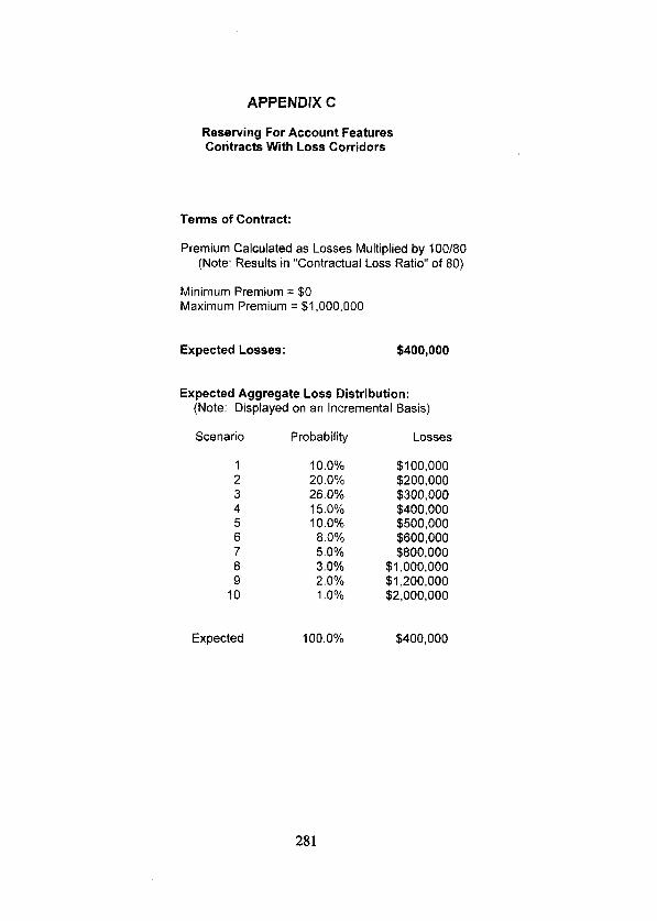
APPENDIX C

Reserving For Account Features Contra& With Loss Corridors

Terms of Contract:

Premium Calculated as Losses Multiplied by 1 OO/80 (Note: Results in “Contractual Loss Ratio” of 80)

Minimum Premium = $0 Maximum Premium = $1 ,OOO,OOO

Expected Losses: $400,000

Expected Aggregate Loss Distribution: (Note: Displayed on an Incrementa1 Basis)

Scenario Probability Losses

2 3 4 5 6 7 8 9

10

10.0% $100,000 20.0% $200,000 26.0% $300,000 15.0% $400,000 10.0% $500,000

8.0% $600,000 5.0% $800,000 3.0% $1 ,ooo,ooo 2.0% $1,200,000 1 .O% $2,000,000

Expected 100.0% $400,000

281

APPENDIX C


Calculation of Retro Premium and Expected Loss Ratio

Probability Losses Premium

10.0% 20.0% 26.0% 15.0% 10.0%

8.0% 5.0% 3.0% 2.0% 1 .O%

$100,000 $200,000 $300,000 $400,000 $500,000 $600,000 $800,000

$1 ,ooo,ooo $1,200,000 $2,000,000

$125,000 $250,000 $375,000 $500,000 $625,000 $750,000

$1 ,ooo,ooo $1 ,ooo,ooo $1 ,ooo,ooo $1 ,ooo,ooo

Expected Amounts $400,000 $467,500

Expected Loss Ratio 85.6%

282

APPENDIX C

Reserving For Account Features Contracts With Loss Corridors

Accounting For Premium and Losses Over Time

Starl with the Expected Loss and Premium

Expected Loss = $400,000

Expected Premium = $467,500

Expected Loss Ratio = 85.6%

Theory: As time elapses. the aggregate distribution of loss collapses areound a single point. If loss emerge as expected ($400,000), premium wili eventually reach $500,000. We need a process that recognizes this but is simple to implement. Our solution was to create an “lnsurance Charge” (IC) equal to Contractual Premium ($500,000) less Expected Premium ($467,500). The IC is multiplied by (1 - Lag). or the percent of loss expected to be unemerged at each point in time. As ali losses are reported, the ultimate premium converges to the contractual premium. This stuff is not rocket science.....

(1) (2) (3) (4) (5) (6)

Estimated Estimated Estimated End of Ultimate Lag Insurance IC x Ultimate

Year Loss Factor Charge (1 - Lag) Premium

0 $400,000 0.00 $32,500 $32,500 467,500 1 $400,000 0.25 $32,500 $24,375 475,625 2 $400,000 0.50 $32,500 $16,250 483,750 3 $400,000 0.70 $32,500 $9,750 490,250 4 $400,000 0.85 $32,500 $4,875 495,125 5 $400,000 0.95 $32,500 $1,625 498,375 6 $400,000 1 .oo $32.500 $0 500,000

Note: There are simpler ways of creating this process. but the above seems to be a good way of generically describing the retrospective premium process. Note that the IC could be calculated for contracts with additive loads, ora combination of additive and multiplicative loads.

283

APPENDIX D


Terms of Contract:

Quota Share contract with a loss corridor between a 65% and 75% loss ratio.

Expected Premium: $1 ,ooo,ooo

Expected Losses: (Ground up - excluding corridor)

$700,000

Expected Aggregate Loss Distribution: (Note: Displayed on an Incrementa1 Basis)

Scenario Probability Losses

8 9

10

6.0% $200,000 12.0% $400,000 20.0% $500,000 25.0% $600,000 14.0% $700,000

9.0% $800,000 6.0% $1 ,ooo,ooo 4.0% $1,500,000 2.0% $2,000,000 2.0% $3,000,000

Expected 100.0% $700,000

284

APPENDIX D

Reserving For Account Features Contracts With Loss Corridors

Calculation of Value of Loss Corridor and Expected Loss Ratio

Probability Ground Up Loss

Losses Corridor Net

Losses

6.0% 12.0% 20.0% 25.0% 14.0%

9.0% 6.0% 4.0% 2.0% 2.0%

$200,000 $400,000 $500,000 $600,000 $700,000 $800.000

$1 ,ooo,ooo $1,500,000 $2,000,000 $3,000,000

90 $0 $0

$50,000 $100,000 $100,000 $100,000 $100,000 $100,000

$200,000 $400,000 $500,000 $600,000 $650,000 $700,000 $900,000

$1,400,000 $1,900,000 $2,900,000

Expected $700,000 $30,000 $670,000

Expected Premium:

Expected Loss Ratio:

Expected Value of Corridor:

$1 ,ooo,ooo

67.0%

3.0%

Thus the initial reserves will be set to equal a 67% loss ratio

285

APPENDIX D


Aggregate Loss Distribution of the Same Account at 24 Months

Note: After time goes by, the aggregate loss distrbution begins to collapse upon the point estimate. For purposes of illustration, we will assume that the aggregate distribution has collapsed by half (perhaps the account has a lag of .50 after 24 months). In the real world, the collapse of the aggregate distribution is often referred to as “non-trivial” which means pretty hard to do.

We will state the distribution as a percent of expected so we can apply to different evaluations of ultimate loss and see what the answers are.

Scenario Probability

1 6.0% 2 12.0% 3 20.0% 4 25.0% 5 14.0% 6 9.0% 7 6.0% 8 4.0% 9 2.0%

10 2.0%

Expected

Initial Ground Up Losses

$200,000 $400,000 $500,000 $600,000 $700,000 $800,000

$1 ,ooo,ooo $1,500,000 $2,000,000 $3,000,000

$700,000

As % Of Expected

28.6% 57.1% 71.4% 85.7%

100.0% 114.3% 142.9% 214.3% 285.7% 428.6%

100.0%

Collapse Agg Distrib Factor @24 Months

0.5 64.3% 0.5 78.6% 0.5 85.7% 0.5 92.9% 0.5 100.0% 0.5 107.1% 0.5 121.4% 0.5 157.1% 0.5 192.9% 0.5 264.3%

100.0%

The aggregate distribution as of 24 months is calculated by taking .5 of the difference between the Mal iosses as a percent of expected and unity and addinglsubtracting this number to the initial losses as a percent of expected.

286

APPENDIX D

Resewing For Account Features Contra& With Loss Corridors

Calculadon of Value of Loss Corridor and Expected Loss Ratio At 24 Months Using Collapsed Aggregate Distribution

Examples Using Better and Worse Than Expected Results

Current Evaluation of Ultimate Los?.: Expected Premium:

Agg Distrib Scenario Probability @24 Months

2 3 4 5 6 7 6 9

10

Expected $500,000

6.0% 64.3% 12.0% 76.6% 20.0% 85.7% 25.0% 92.9% 14.0% 100.0%

9.0% 107.1% 6.0% 121.4% 4.0% 157.1% 2.0% 192.9% 2.0% 264.3%

Expected Loss Ratio: 49.2% Expected Value of Corridor: 0.8%

Current Evaluation of Ultimate Loss: Expected Premium:

Agg Distrib Scenado Probability @24 Months

1 6.0% 64.3% 2 12.0% 78.6% 3 20.0% 85.7% 4 25.0% 92.9% 5 14.0% 100.0% 6 9.0% 107.1% 7 6.0% 121.4% 8 4.0% 157.1% 9 2.0% 192.9%

10 2.0% 264.3%

Expected

Expected Loss Ratio: Expected Value of Corridor:

$500,000 $1,000,000

Ground Up Losses

$321,429 $392,857 $428.571 $464,286 $500,000 $535.714 $607,143 $785,714 $964,286

$1,321,429

$850,000 $1,000,000

Ground Up Losses

$546,429 $667,857 $728,571 $789,286 $850,000 $910,714

$1.032.143 $1,335.714 $1,639,286 $2,246,429

$850,000

287

LOSS Corridor

$0

fi

::

$0 $0

$100,000 $100,000 $100,000

$8,000

LOSS Corridor

W7.85: $78,571

$100,000 $100,000 $100,000 $100,000 $100,000 $100,000 $100,000

$79,857

77.0% 8.0%

Net Losses

$321,429 $392,857 $428,571 $464,286 $500,000 $535,714 $607,143 $685,714 $864,286

$1,221,429

$492,000

Net Losses

$546,429 $650,000 $650,000 $689,286 $750,000 $810.714 $932,143

$1,235,714 $1.539.286 $2,146,429

$770,143

APPENDIX D

Reserving For Account Features Contracts With Loss Corridon

Calculation of Value of Loss Corridor and Expected Loss Ratio At 24 Months Using Collapsed Aggregate Distribution

Flrst let us assume that the esbmate of ultlmate losses has been unchanged at the 24 month evaluation

Current Evaluation of Ultlmate Loss: Expected Premium:

Scenario

2 3 4

5 6 7

8 9

10

Agg Distrib Probability@Z4 Month

6.0% 64.3% 12.0% 76.6% 20.0% 85.7% 25.0% 92.9% 14.0% 100.0%

90% 107.1% 6 0% 121.4%

4 0% 157 1% 2.0% 192 9% 2 0% 264.3%

Expected

Expected Loss Ratio: Expscted Value of Corridor:

$700,000 $1 ,ooo,ooo

Ground Up

Losses

$450,000 $550,000 $600.000

$650.000 $700,000

$750,000 $850.000

$1,100.000 $1.350.000 S1,850,000

$700,000

Loss Corridor

$0 $0 $0 $0

$50,000 $100,000 $100,000

$100,000 $100,000 $100,000

$30,000

67.0% 3.0%

Net Losses

$450,000 $550,000 $600,000

$650,000 $650,000 $650,000 $750,000

$1 ,ooo.ooo $1.250,000 $1.750.000

$670,000

Note that the value of the corridor has not changed in this example. If the loss corridor is about the erpected value of the distribution this is often the case. lf the corndor had been well above the expected loss amount, the 24 month value of the corridor would have been reduced substatially. For example, if the loss corridor was 10 points excess of 140 LR ($1,400,000) the value at 24 months would have been $100.000 X .02 = $2,000, compared to an initial value of $100,000 X (.04 + .02 + .02) = $8.000. (Note on Appendix D Page 3 that initial scenarios 8, 9. and 10 are all greater than $1.400.000 with probabilibes of .04, 02 and .02 respectively)

288

Xeinsurance Contracts with a Multi-Year Agguegate Limit

by Regina M. Berens, FCAS

289

REINSURANCE CONTRACTS WITH A MULTI-YEAR AGGREGATE LIMIT

Regina 1. Berens

ABSTRACT

Exc8ss of Loss reinsuranca contracts commonfy include an aggregate limit which specifies the maximum amount the reinsurer will pay under the contra& This paper discusses pricing implications of an aggregate limit which applies over multiple years. Monte Carlo simulations are usad to test the sensitivity of the pricing to relationships between the average ground-up loss, the per-claim limit and the aggregate limit under the contract. A pricing example using historie data is also included. Risk charges and applications to clash covers are explored. Underwriting and resewing considerations of a contract with a multi- year aggregate are discussed.

THE AUTHOR

Regina Y. Berens is a Consulting Actuary with Muetterties, Bennett and Associates in Mountain Lakes, New Jersey. She is a Fellow of the Casualty Actuarial Society as well as a Member of the CAS Board of Directors, a Member of the Ameritan Academy of Actuaries and a Fellow of the Canadian Institute of Actuaries. MS. Berens is also a Past President of Casualty Actuaries of Greater New York. She chairs the CAS Audit Committee and has served on the Committee on Continuing Education, and the 1987 and 1992 Membership Survey Task Forces. She received a B.A. in Mathematics from the University of Cincinnati in 1975. Her prior experience includes work at Great Ameritan, AFIA and Prudential Reinsurance.

The author wiahaa to thank Chartes F. Cook, Robert A. Daino and Leigh J. Halliwall for raviawing preliminary drafts of this papar and making auggaationa for impmvemanta. Any flawa in the implementation of those suggestions, of course, ara the author’s.

291

INTRODUCTION

A typical exceso of loss contra& protects the purchaser (the ceding insuranm wmpany) for a fixfxl amount oer claim in excass of a nar-clalm mtention. uo to an aaareaate limit. As an example. a cèding wmpany may pur&asa rainsuranca ~or~$500,006~n éxcess of the first $1 miliion per claim, with the reinsurer’s total liabiliiy under the wntract Iimlted to $10 million.

This has the advantage (to the reinsurer) of capping the liabilii under the contract. The ceding wmpany, of course, wants to purchase reinsurance tiich will provide the maximum stability In its year-to-year loss experience. If the losses to the wntract are less than the aggmgate, the cading wmpany may raap part of the savings through losssensitive provisions in the wntract or more favorable prtcing et renewal, but any other savings geas to the rainsurer. If, in the sewnd year if the wntract, the lossas ara in excass of the aggregate, the ralnsurah liability is still cappad at the agreed-upan limit and the ceding wmpany must pay any additional losses.

One way to stabllke the results of the cading company using an Excess of Loss wntract is to provide a multl-year aggregate. This wntract would, for example, wver the layer dascdbed above but Mude an &ggregate limtl of $30 milllon over thtw years. The putpose of this paper is to explore the prictng. undenwiting and raserving Implicattons of this concept. Although it applies to a wntrad bahveen a primary insurance wmpany and a tuinsurer. it wuld apply wtth approptiate adjustments to excess wverage pumhased by a self-insured entity. A threa-year period was selectad to simplify assumptions with regard to changes in exposuras, inflation and other factors which change with each wntract pariod; the model could obviously be generalizad bayond thrae years.

SIMPLIMNG ASSUMPTIONS

1. The ceding wmpany’s exposura is relatively staMe fmm year to year. 2. The treatment of Allocated Loss Adjustment Expensas (ALAE) will not be wnsidemd. This

is aquivalent to including ALAE in the loss portion when calwlating the reinsurer’s liabllity. 3. Inflation is minimal. Under the doubledigit inflation wnditions prevalent in the late 197Os,

some indexing of the attachment polnts. layer and aggregate might ba needed from year to year.

4. Losses have been adjustad to ultimate sattlement value, including IBNR.

THE MODEL

A model was developad which woufd generate ground-up ctaims using a spacified dkbibution. Using a Monte Carto simulation, thraa years’ worth of excess claims were generated, and the rainsumd lossas wmpared using a single-year aggragate and a three-year aggregate equal to thrae times the annual aggragate. A 6% annual rate of inflation was applied to claims in the sawnd and third years.

The model was run for a variety of sample wntracts in order to test the impad of a multi-year aggregete for various wmbinations of the following:

1. Per-claim ratention as a function of the average daim size. 2. The reinsurad layer in ralation to the mtention and as a function of average daim size. 3. The aggmgate as a fundion of expsded Iosses in the exc%ss layer.

A PRIORI EXPECTATIONS

Direction of the pticing impact of a multt-year aggragate.

The impad of thi wntrad pmvision cannot be 8 decraasa in the pure pr8mium. The reinsurat’s liability in any given year is either what t would have baan with a single-year aggragate limit (ii

292

losses under the wntrad are greater than or equal to ene-third of the thme-year mate) or grealer (if the ceding wmpany can cany over ‘cred¡¡’ from a prior year in wtikh losses were less than one-third of the three-year aggregate).

Retentton as a functton of avenga claim size.

If the oeding wmpany retalns a mlnlmal pottion of each daim, the frequertcy and sevetity on the excess wver are likely to be dose to the ground-up frequency and sevetity. Conversely, if the excess wver ls written with 8 high-level attachment point, daims will reach the excess layer less often. The advantage to the cedlng wmpany (and. thus. the percentage surcharge for a multiiyear aggregate) will be greater if its mtenüon is a substantial portion of the average claim size and thus losses to tha excess layer are more volatlle.

The reinsured layer as a functton of the mtentton and tha avengo claim size.

Given a particular retention, the larger the layer, the lamer the average 8xms.s dalm size. This means that the aggregate can be ‘used up’ by fawer daims. If the coverage is vM8n at a relatively high attachment point, the excess tiver bswmes Imfrequency and hiih severtty. The lack of predidabillty In this layer would again make 8 multl-year aggragate more desirable fmm the ceding wmpany’s point of view but also pmportionately more expensive.

The aggmgate as a functlon of expected losses in the layer.

If the aggregate is so large that it would wver all dahns In th8 excess layer except under the most extreme chwmstances, a multi-year aggregate has liile effed. This wouM imply that a wding company woukf be wtlling to accept a wntrad with a lower aggregate limit. if it applied to a series of years so that experience of favorable years might be rewuped In the Mure.

FIRST MODEL: POISSON! LOONORMAL

Th8 fifst simulation was a VanlIla casual& book w+th a relatively simple loss distrtbution. A poflfollo with a Poision frequency with 30 expeded clahns was wnstruded, uslng a Lognofmal severity tih an avemge daim value of $ltQOOO and a Standard Deviation of $37,500. The diW.ribuUon of the seveftty was thus A(i 1.92, .25).

The top sedion of Exhibit I shows the results of the fIrSt rm3el. Surcharges are shovm by layer as well as by ratio of the annual aggregate to the expeded losses. The results of four lterations are shown (each with 1 OO trials) to provlde a gauge of varlabiltty.

As would be expeded, the impad of a three-year aggmgate on the $15O,OOtl XS $15O,tXMl layer is minlmal lf the annual aggregate is set at twlce the expeded losses in the layer. This is because the tossas are mlatively predidable, partlculaiiy wtth the seteded Poissonllognormal fundlons. The most that wuld be sald about provkllng a 3-year aggmgate for a low-level excass wntrad on this type of busll#rss b that lt could be offered to make a pmspedive deal more attradive at liile orno extra cost. The surcharge for the $150,000 XS $300,000 layer is substantial because so few daims penetrate the layer that there is a large percentage lncmase to the expedad lossas when a thrw-year aggragate applles.

The s8cor~I section of Exhibit I shows the results of the model when the distribution ia changad to Poisson with 15 expeded dakns per year and the severity ls Lognormal with an average claim slze of 3300,000. Agaln, the surchafge for a thfee-year aggregate lncreases as the underiying business becomes lower-frequency and higher-severity.

Exhltdt ll showa the msutts of thls first model In gmphic form. The indlcated pemenfage surcharge horms8s as:

(a) me attachment point incmases.

293

(b) Th8 ratii of the annual aggmgate to th8 exp8cted losses decmases. (c) The parameters change fmm 15 exp8cted daims, $300.000 average severity to 30 expeded

daims, $150,000 average severity.

The last r8sult appeamd wunter-intuitive, since the high-frequency. low-sevedty e ple was expected to be less volatile. An examination of the raw data, however, revealed the T ason. For the layen in question (exwss of $300,000), results in the exwss layar are actually mora volatile for the lowseverity exampte since so few claims penetrate the layer.

It should be pointed out, however, that the Poisson-Lognormal mcdel is probably not.meaningful for some types of business. so the procass was repeated with another frequencykeverity distribution.

SECOND MODEL- NEGATNE BINOMIAU SINGLE-PARAMETER PARETO

Negative Binomial claim frequency and Single-Parameter Par8to severity distribl;ns have been used by various authors to model claim distributions for casualty business. The model was m-tun with two distrtbutions:

Negativa Binomial frequency distribution wtth 30 expected claims, p =.lO and a Single Parameter Pareto Severtty with q = 1.5 and average daim value of $150,000.

Negative Binomial frequency distribution with 15 expeded daims. p =.05 and a Single- Parameter Pareto Severity with q = 1.5 and average daim value of $300,000.

The results are shown on Exhibi III in a format similar to Exhibit 1. They are shown graphically in Exhibi IV. At th8 lower layers, the indicated parcentage sumharge is hiih8r for the new distrtbution than for th8 Poissonllognonal model. In the higher layen, hoW8V8r. the percentage surcharge is higher for the Negative BinomiaUPareto model. The mason bewmes apparent from Exhìbit V. which Is a graph of percentiles of daim size from Monte Carlo runs of 3000 daims from a Lognormal atid Pareto distribution, each with an expected daim value of $150,000. At a $150,000 attachment point, far mora dairns fall under the retention with the Pareto model. As the attachment point increases, more daims exweding the attachment point am expected in the Pareto model. but many daims are so large that the expeded payment in the layer is $150.000 (the maximum). This actually mduws volatility in the layer.

MEASURING VARIABILITY; RISK CHARGES

It bewmes appamnt fmm examining the detailed results of 100 iteraüons (which ar8 not reproduced with this pap8r in order to wnsekve trees and teddium) that mosl of the time the three year aggmgate provides no benefit. Some examples ar8 shown in graphic form on Exhibits VI and VII. The graphs were created as follows:

1. The losws wvered by the reinsurance wntrad over the three year period, wtth single-year aggregates ami wtth a three-year aggregate, were sorted based on the value of losses with single-year aggregates.

‘S.W.f’M&k&‘APRdlcaOuidstothe~Pusmaa psrsto’, PCAS IXUI. p. 44.

294

2. Two Unes were graphed: the soded (ascending) losses for each iteration wtth single-year aggiegates and the wrrespondlng value of losses with a three-year aggregate. A ‘spike” thus represen& an instance where the reinsurer wver8d more losses because of the existence of a multi-year aggmgate.

ExhiM VI shows the results of the 100 iterations which make up the 7% surcharge shown on Exhibi III. the sewnd iteration in the sixth line of data. This wrfesponds to $150,000 Excess of $300.000 wverage. with an annual aggregate equal to 2.5 times the expected losses in the layer. The expeded (Negative binomial) number of ground-up losses is 30; average severtty (Pareto) is $150,000.

For the iterations wttere incurred Josses in the layer were low, the three-year aggregate had no benetlt. Where the simulated losses were high. however. the number of cases where the three- year aggregate provided a beneffi increased. There are 19 %pikess in the graph. Le. instances where the reinsurer would have paid more with a thr8e-year aggregate. The average surcharge is $43,253, which is 6.50% of expeded losses in the layer ($365,321). The latgest adual benefe in the simulations was $758,752. The standard deviation of the differences between lossas under annual and three-year aggregates was $123,175.

Exhibit VII shows the msults of the 100 iterations which make up the 22% surcharge shown on Exhibit III, the sewnd iteration in the seventh line of the second sedion of data. This wrresponds to $150,000 Excess of $450,000 wverage, with an annual aggregate equal to 2.5 times the expeded losses in the layer. The expected (Negative binomial) number of ground-up losses is 15; average saverity (Patio) is $300,000.

As would be expeded, the losses in this example showed wnsiderably more vatiation; so did the impad of the threayear aggregate. There are 32 Yipikes’ in the graph, where the reinsurer would have paid more wtth a three-year aggregate. The average surcharge is $106,117, which is 22.16% of expected losses in the layer ($487,968). Th8 lafgest adual beneR in th8 simulations was SI .357,126. The standard deviation of the differences between losses under annual and three-year aggregates was $244,294.

Wìth apologies to FeldMum3, who has pointed out that a risk charge should be a fundion not only of the pafiticular portfolio but of the insurer’s entire book of business, a simplified risk charge will be calculated as a fundion of variance for the two graphed examples. If the risk charge is set et 0.5% of the standard deviation of the additional losses under the three-year aggregate, for the first example the risk-adjusted surcharge is 6.6% rather than the original 6.5%; for the second it is 22.4% rather than the otiginal22.16%.

CLASH COVERS

A clash wver example was wnstnided with the same set of random numbers used in the last sedion to oroduce the 22.16% [non-iisk ad¡ustedI surchame. First. the individual daim severities &e capped at $300~000, to similate á case &ere the &ding wmpany issues polides with limits no hiher tban $300,000 (or, altematively, other reinsurance is available exwss of that limtt). A value of 5% was selected as the probability that anoth8r inaured was involved in the same occurrence. (The possibility of occurrences wtth more than two daimants was ignored). Five percent of the daims, at random. wera then increased by the amount of a sewnd randomly-chosen claim value two simulate a two-daimant occurrence.

The indicated surcharge for SI 50,000 excess $450.000 was then calculated. The sutiarge was $29.221. tiich was 160.9% of the $18,159 losses expeded with annual aggregates. For 36 out of 1 OO iterations, the reinsurer would have paid more with a three-year aggregate. The largest

3 S. F&Mum. ‘R! Lmda fa Irmuran’. PCAS LXXWI, pap 160.

295

difference was $244,000. The standard deviation of the difference between losses incurmd under an annual aggregate and a thre-ebyear aggregate was $52,712. In thi case, an adjustment for risk calculated as desc&ed in the earlier section would have a more substantial impact: the risk-adjusted surcharge would be [($29.221 + .05*52,712)/18,159], or 175.4%. Decntasing the probability of clash to 2.5% increases the surcharge to 317.8% (355% tisk-adjusted) on expeded losses Of $5,419.

A REAL DATA EXAMPLE

Finally, a pricing example was developed using suitably disguised grouncl-up casualty claim statistics from an insured entity. in an attempt to see what happens when this coverage proviston is priced using actual expetience. The losses were mostly Workers’ Comp, with a few Auto and GL claims. The following fadors needed to be taken into account:

Loss Development

Loss development, so easily ignored in the Monte Carlo model. needs to be addressed when working with adual data. In the reinsumd layer (or the layer excess of a Self-lnsumd Retention), there are three sources of development: (1) losses whlch have been reported to the ceding company but appear to be below the retention (and thus may not have been reported to the reinsurer), (2) reported losses above the attachment point but less than the layer, and (3) losses which have been incurred but not yet reported to the ceding wmpany (also known as ‘pure IBNR’). An evaluation of the amount of aggregate left at the end of a centrad petiod should include an estimate for this development.

In this example. losses with 9 or more years of development are In orrler to minlmize distottion from undeveloped data.

Bringing Prior Year Claims to Present Level

In thii example, an annual rate of 8% was used to bting all daims to current level.

Low Credibility of Experienco

The number of reported claims per year for thls entity ranged from 102 to 147. The results from this example should not be expeded to be as smooth as the model would Imply. A ceding company or self-insured operating under these conditions. however. is probably the perfect candidate for purchasing a multi-year aggregate because it has less tolerance for fluduations in year-to-year results than a larger entity.

Changes in Exposure

This may or may not be a significant factor, but it should be Invesligated. A self-insured which varies the extent to which it uses ‘leased’ employees on pmjects from year to year, for example, is not a good candiiate for a multl-year aggregate. (This is because the number of employees adually on the self-insured’s payroll. as opposed to the leasing company’s payroll, wlll fluduate.) Similatiy, a ceding company increasing or decreasing its madcet presente in a given Me of business wlll be more Ilkely to prefer an annual aggregate which is adjusted based upon the fads in 8 given year..

Exhibi VIII shows the results of a three-year VS. annual aggregate for the self-insured entity.

Losses in the $8,000,000 XS $2,000,000 are shown for hvo subsequent threayear petiods. Thls layer was selected because the entity generally had a few catastrophic cJaims of $3 to $8 million (ground-up) in each year, and it is realistic to exped that it would be interested in proteding its bottom line from losses of this magnitude. me annual aggregate In each case was set equal to

296

1.25 times the average incun-ed losses In the layer for the three-year period; the three-year aggregate was set equal to triple that value.

This example illustrates some of the perils of applying the model to real life. We must first assume that a reasonable estimate of prospedive losses in the layer can be made, using either some averaging prowss on past results, ora selected theoretical distribution. In this example. using the results for Years 1 through 3 to set an aggregate limit for Years 4 thmugh 8 would have produced an aggregate higher than the wmpany needed in the later years. If an appropriate distribution wem found to appfoximate res& and seled the aggregate shown in the Exhibtt, 8 13% surcharge woukl result. In Years 1 thmugh 3, the entity would rewver about $3 million more from its insurer under a thme-year aggmgate; in Yean 4 through 8 it woukl have collected nothing extra, despite having pali the 13% surcharge.

An interesting wmplication is shown in the results of Years 7 and 8. The organization increased its emphasis on loss control and loss-reduction programs beginning in Year 6. Although results are shown for Years 7 and 8, it is clear that the underiying loss distribution has changed- both frequency and severity. Renewal decisions made after the implementation of this program would have to take these changes Into account on a prospedive basis.

ADDITIONAL CONSIDERATIONS

Indexation

The leveraged impad of inflation on excess claims has been well-documented in the aduarial literatura and will not be reviewed here. ’ For an ex-f-loss wntrad with a multi-year aggregate, daim inflatlon will emde the amwnt of reinsurance wverage available. One solution, of wurse, is to index the attachment point, the Iayer wvered and the aggregate evety year by an agreed-upon inflation rate? In the absence of indexation, the two parties should be aware of the impad of inflation on the wverage provided.

RenewaURunoff Adjusbnents and Decidons

Since the model is based on a wnb-ad which is renewed annually (as opposed lo 8 wntrad wt~ich MS fmm l/lBY to 12/3l/YY+2), it is possibte that eitber the cedlng wmpany or the reinsurer may decide not to renew. Two examptes, using the wntrad descdbed in the

1. The ceding wmpany, having incurred $20 million of losses within the reinsurance layer in the first year. deddes not to renew.

2. Losses to the wntrad in the fl& year ara $8 millii but the reinsurer decides to tighten pdcing at renewal. me wding wmpany is faced with the decision of accepting renewal terms it finds unoalatable. or walklng awav from $2 million of wverage which wukt be canied forwanf io the nei awklentiear ione-third of the $30 miilioñaggregate. minus $8 million incurred) forwhich it has pakl a surchafge. lt is unlikely, of wurse. that renewal terms would be tightened with such favorable results, but it is probabty not imposible.

’ J. T. Lsnge, “The ~~~I~cK~M~U~B~,PCASLVI.~~~O.

’ R. E. Fagwon. ‘NmPropcdhd Rdmwmca mdttmk4exCl~u8u..PCASLXI,Pa~e141.

297

These wntíngencies are best handled at the inception of the wntrad. One simple solution would be a stipulation that, in the event of non-renewal, a pro-rated portion of the aggregate applies. These renewal or rate change rigMs are valuable options which can be pticed as such. They may or may not offset each other.

In the event of losses tiich are more in line with expedations, some decistons can stlll be made on an annual basis.

First, the expetience should be analyzed to determine tiether the exposures are at a level anticipated under the wntrad. Thls should include an estimate of IBNR In arder to detenine whether the assumptions about expeded losses under the centrad am still valti. If the experience is different from that assumed at the inception of the wntrad, the rate, annual aggregate and/or multiiyear aggregate should be adjusted. This wuld take the form of a re- pricing of the entire three-year period based on new information, with the adjustments applied to the future wntrad period. This, again is a possibility which must be agreed upon In advance between the ceding wmpany and the reinsurer. If it ls not, the likellhood exists that changes In the wntrad provisions for expedence woIse than expeded wukl cause the c8ding wmpany to ‘walk away’ from the wntrad at renewal.

Considering Item 1 in the above sedion, what if the ceding wmpany wishes to purchase additional limits so that $20 million (not $10 million) is available to wver losses in the layer over the next two years? The models used in this paper would pmbably imply a smallar reinstatement premium than is needed, if the worse-than-average experienca in the fhst year is due to fadors not recognized when the aggregate was determlned. While the technique ls still applicable. it is important to determine the reason for the adverse development. Was the exposure greater than expeded? Has the limits profile changed? Do the initial assumptions about ground-up claim frequency and daim sevetity still hold true? Any changes should be taken into acwunt in pricing the reinstatement, i.e. the extension of the thrwe-year aggregate from $30 million to $40 million.

Changes in Exposures

It is generally not prudent to assume that anything in the reinsurance market will remain static. Prtcing of a multiiyear aggregate wuld bs enhanced by including an estimate of the potential growth of the ceding wmpany’s book over the next three yean, lncluding changes in limits profiles if any are anticipated.

The author has done some preliminary analysis using the Negative BinomiaUPareto model with an assumption of a 6% growth in exposure (wrresponding to a 6% increase in ctaim wunt from the first to the sewnd year and from the sewnd to the third year). If the calculation of expeded losses and aggregate limits was based on an assumption of stable exposures, the ceding wmpany has obviously purchased too little protedion and will find itself responsible for more losses over the aggregate limit than it would had the propsr aggregate limit been negotiated. The percentage surcharge for the 3-year aggregate on the portfolio with the expected severity of $300.000 would also be about half of wbat it should have been if exposure growth had been anticipated in the pricing.

Aggregates Coverfng More than Three Years

While an aggregate wveting a lengthier period is possible, it has not been explored in the model. The pmpetiy-casualty industry has occasionally pruvided wverage on a 3-year basis (an unfortunate example being threayear reinsurance wnb-acts which wuld be found In the London market In the 197Os), and ín the current market examples of longer-term wntracts do exist. As a practical matter, however, many fadors can change over the long run tiich would wmplicate pticing a longer-term aggregate.

298

The pos?ibility of the unused (or over-used) portion of an annual aggregate being rolled fotward into the next year at renewal would be wnducive to long-tenn relatlonships between a ceding wmpany and its rainsurer. and such ‘rolle¡+ contrads exist in the curfent market. This is easiest to vlsualize In a zero-inflation, stable-exposurs situation, with appropriate adjustments then made to refled real¡¡. The cumutative aggregate for year n woukl bs n times the expeded losses in the layer. The wverage avallable to the ceding wmpany for losses in the excess layer in year R would be the cumulative aggregate. minus losses incurred on all precedlng years.

Wiih the votatile examples studied eariier In thls paper, multi-year aggregates which accumulate each year would be a very attradive wntrad featun?. Since. as observed earlier, the actual number of yeats tiere a multi-year aggregate provides additional wverage are infrequent. the extension of the multiiyear aggregate beyond three years gives the ceding wmpany a better chance of baing able to take advantage of the addiiional wverage at some point. me author ran some extremely simplified simulations of wntracts in which tba aggmgate was extended each year and found that the c8ding wmpany wuld neady ahvays be assurad of wlleding all losses in the layer each year, unless losses were particulerly disastmus in the fírst year.

Varying exposures and claim inflation could be handled by incteasing the aggregate each year by the agreed-upon multiple of expeded losses in the layer, calculated using approptiate exposures and inflation assumptions. (The aggregate wuld even be adjusted after the fad based on adual exposures.)

It shouki be noted that, as the numb%r of years wvered by the aggregate lncreases at each renewal, the adequaq of reserve estimates can be exlremely important. This is because the aggregate for the current year can be emded by adverse development on old years.

Contracts with Annual Aggregata Daductibles

The wncapts in this paper wuld be extended to wntracts in tiich the ceding wmpany or self- insured absorbs losses in the layer up to 8 certain level bafore the reinsurance wverage applies. As an example, a large self-insured might purchase wverage for $500,000 excess $500,000 par occurrence, with the agreement that the self-insumd pays the first $1.5 million in claims in the layer. The insurer agrees to pay up to $5 million in losses in the layer affer the W-t $1.5 million. The insured layer now exhE& more volatiliiy because of the aggregate deductible, making ít an ideal candidate for a mutiiyear aggrsgate limit approach.

Resarving Implications

As mentioned earlier, an IBNR provision is necessary to evaluate the amount of wver remaining at each evaluation point. Let us retum again to the lnitial example. lf. after the first year. the ultimate sattlement value (including IBNR) of daims in the layer is $8 million, the reinsuret’s liabilii under the wntract for the sawnd year wuld be anywhers fmm zem to $22 million. If, in fad, the losses exceedad 12 millíon, bn’nging total losses above 2/3 of the $30 million aggragate. the excess would ba a ‘creditg againsl potential losses durtng the third year. Any method ussd to evaluate IBNR on wntracts with single-year aggmgate limits wuld be used for this typs of wntrad. with the addiiional wmplicstion that the wmpany’s liabilii for the current year is a fundion of prior yearr’ losses (including an appropdate IBNR provision) on the wntrad.

IBNR (both case development and pure IBNR) evaluation is paiticulady Important in multiiyear aggregate wntracts becausa it is a critical pafi of the year-end decision-making. An understated eslimate of ultimate losses gives the ceding wmpany false assuranca of how much of the three- year aggregate remains for subsequent years. R can also leave the ceding wmpany blissfully unaware of the need to putiase reinstatement wverage, meaning that It will have less protedion than expectsd for later years.

299

Could a Multi-Year Aggregate be provided et some level wtth no surcharge?

It was noted eariier that at low attachment points, the indicated surcharge is minimal. For higher attachment points, there should stlll be some multlple of the annual aggmgate whkh wukl be provided as a three-year aggregate without increasing the expected losses. The answer, interestingly enough, is pmbably unmarketable. For the Negative BinomiaUPareto model, this level was determined fmm one of the simulaüons for both $150,000 excess of $150,000 tiere the average daim is $150,000 and for $150,000 excess $300,000 where the average daim is $300,000. The annual aggregate limit was set at 2.5 times the annual expeded losses. The multi-year aggregate WhicJ~ wuld be supplled with no In-ase to the expeded losses was about 65% of the annual aggregate In the RI-& case and 55% in the sewndl This woukt be 1.625 and 1.375, respedively, times expeded annual losses in the layer.

The reason for this result is that there are adualty very few cases wherw the multl-year aggregate limit pmvided greater protedion (about 5 out of 100 simulations in the $300,000 average claim case) but the impad when it di¡ was substantial; generally 30% more losses were paid by the reinsurer. Thus, the multi-year aggregate had to be cut signiflcantly In arder to affed these cases.

CONCLUSIONS

The objedive of this paper was to explore the implications of applying a muttiiyear aggmgate limit to Excess of Loss reinsurance contra& rather than a single year limit. lt is meant to generate additional thought and dialogue on how best to provide insurance and reinsurance products which fti the needs of the customer and are approptiately priced and resewed. Some wndusions can be drawn from the points wvered in thii paper are the following:

1. A multi-year aggregate can be a useful tool to provide wverage when and where the ceding wmpany (or self-insured) needs it. while still limiting the liability of the reinsurer. It should. however, cany an appmpriate price.

2. Pricing is highly dependent upon the loss disbibution tiich is seleded.

4. In general, the greater the volatility of the business. the higher the percentage surcharge and the indicated risk charge.

5. Prospedive changes in exposures should be quantified in the pricing process.

6. The wnsequences of non-renewal dudng the 3-year period should be specified in the wntrad.

7. The validity of assumptions made at the inception of the wntrad should be checked at each renewal and adjustments made, if necessary.

8. The wntrad wording issues involved in offering a multi-year aggregate can be more wmplicated than the pricing issues.

300

Percentage Surcharge for Thme-Year Aggmgate Exhibi I

Poisson Frequency; Lognonnal Sevetity Annual Aggl Expected Expected No. of lteration Number: Losses Claims Ave Clahn 1 2 3 4 Average In Layer

30 $15OK 30 $15OK 30 S15OK 30 Sl5OK 30 S15OK 30 S15OK 30 S15OK 30 s15OK 30 $15OK 30 SlxlK 30 S15OK 30 s15oK

15 S3OOK 15 S3OOK 15 S3OOK 15 S3OOK 15 t3OOK 15 S3OOK 15 S3OOK 15 s3OOK 15 S3OOK 15 s3OOK 15 S3OOK 15 S3OOK

150x 150 0% 0% 0% 0% 0% 2 150x300 182% 252% 194% 296% 208% 2 150x450 800% NIA NIA NIA 800% 2 150X600 tWA N/A NIA NIA NIA 2 150x150 0% 0% 0% 0% 0% 2.5 150x300 146% 208% 151% 181% 168% 2.5 150x450 800% N/A NIA IVA 800% 2.5 150X800 N/A N/A IUA N/A 2.5 150x150 0% 0% 0% 0% 0% 3 150x300 123% 172% 122% NIA 139% 3 150x450 739% NIA NIA N/A 739% 3 150X600 N/A NIA NIA NIA NIA 3

150x150 0% 150x300 0% 150x450 10% 150X800 203% 150x 150 0% 150x300 0% 150x450 4% 150X600 167% 150x150 0% 150x300 0% 150x450 2% 150X600 144%

0% 0%

10%

0% 0% 4%

130% 0% 0% 2%

98%

0% 0%

12% 258%

0% 0% 6%

209% 0% 0% 3%

173%

0% 0%

11% 224%

0% 0% 5%

171% 0% 0% 2%

171%

0% 2 0% 2

11% 2 218% 2

0% 2.5 0% 2.5 5% 2.5

169% 2.5 0% 3 0% 3 2% 3

147% 3

Percentage surcl~ge is expressed as a function of expected losses wfthin the layer.

301

Exhibit ll

lwo.w%

7oo.c?3%

600.00%

soo.oo%

B 400.00%

UI

300.00%

230.00%

100.00%

0.00% c

Percentage Surcharge for 3-Year Aggrsgete PolssonfLognonnal

A-.9rmty; -hw ---1w20

. . . . . .,wK;.s

-lJM<; 3.0

7 - - - . w2.0 __.._. 3ooK;2,$

-3ooK3.0

Percentage Surcharge for Three-Year Aggmgate

Negative Bfnomial Frsquency; Pareto Severity

Expected No. of Claims Ave Clalm

30 SIJOK 30 $15OK 30 S150K 30 S150K 30 Sl50K 30 S150K 30 S150K 30 S150K 30 $15OK 30 S150K 30 $150K 30 SfSOK

lteration Numbsr:

150x150 150x300 150x450 150X600 150x150 15ox3Ocl 150 x450 150X600 150x150 150x300 150x450 150X600

1 ‘5%

15% 23% 27%

2% 7%

12% 18%

1% 4% 7%

11%

2 5%

13% 21% 32%

2% 7%

12% 20%

1% 4% 6%

11%

3 7%

14% 26% 38% 3% 7%

14% 24%

1% 4% 8%

14%

15 S300K 150x150 15 S3OOK 150x300 15 S3OOK 150x450 15 S3OOK 150X600 15 S300K 150X150 15 S300K 150x300 15 S300K 150x450 15 S300K 150X600 15 S3OOK 150x150 15 S300K 150x300 15 S300K 150x450 15 %300K 150X600

23% 32% 38% 52% 13% 21% 26% 35%

8% 13% 18% 25%

21% 28% 34% 43% 12% 18% 22% 29%

7% 10% 15%

24% 27% 32% 43% 16% 18% 21% 30% 12% 13% 14% 21%

Exhibit III

Annual Agg.! Expacted LO&8

4 Average inLayer 7% 6%

13% 13% 17% 22% 29% 32%

3% 3% 7% 7%

10% 12% 16% 20%

1% 1% 4% 4% 6% 7% 8% 11%

19% 22% 2 26% 27% 2 39% 35% 2 45% 44% 2 11% 13% 2.5 16% 17% 2.5 25% 23% 2.5 30% 30% 2.5

7% 9% 3 10% 11% 3 18% 18% 3 21% 21% 3

2 2 2 2

2.5 2.5 2.5 2.5

3 3 3 3

Percentage surcharge is expressed as a functíon of expected loores within the layer.

303

Exhibit IV

Percentage Surcharge for 3-Year Aggregate Neg. Bínomiall Pareto

4.5.00% T

E

3mo% -.

Q 25.00% --

2

s u) m.w% --

C-

-_-- __-*

_.----

_,-- _/HH _.-.

_.---

5.00% -- *-*-- _---

*d-” -.----

----* _-_-.--- *_----

-_.----

__.--- _----

-.--

0.0096 _I 1

Aw. ammw *nn-ñLyr

-----~15oK;z.o

--- 15oK;zs

----lso(<;%O

n

-x-w 2.0

,-b-XmK; 2.5

-a-3ooK:3.0

1sox150 150x300 150X450 l%JXmo

Lyar

Cumu~ Clahn Severlty PmbablNec Pamto vs. Lognomal; Mean * $16WOO

- Pamto El -LN

Negative BinomiaWareto Simulated Losses, $lSOK X 5300K;

Annwl = 2.6 X Expected; Ave Sev. r)lLOK

Exhibit VI

I-AnnualAa. -----.%Yr.Ana.I

Negativa Binomialff arsto Simulated Losses, $1 SOK X UaOK;

Annual = 2.6 X Expected; Ave Sev. =$JOOK

i : :: :: ::

;: ;: .’

Exhiblt VII

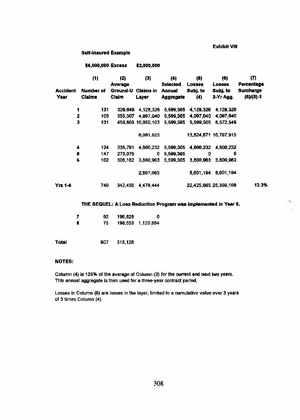
Self-lnsured Exampls Exhibit VIII

$S,QQQ,QQQ Excess $2,000,000

(1) (2) (3) (4) (5) (6) (7) Average Selected Losses Losses Percentage

Accident Number of Ground-U Claims in Annual Subj. to Subj. to surcharge Year Claims Claim Layer Agtmg~ (4) 3-Yr Agg. WWl

1 131 329.849 4.128.320 5,599.305 4,120,326 4,128,X26 2 105 355,307 4.097.040 5,599.305 4,OQ7,040 4,OQ7,04Q 3 131 455.805 10.050.103 5.599.305 5,5QQ,305 8.572549

6.091.823 13.824.871 X,797.915

4 124 335,791 4,800,232 5.599.305 4,800,232 4,800,232 6 147 273,075 0 5,599,305 0 0 6 102 308.162 3.8OO.Q63 5.599.305 3,8OO,Q83 3,800,963

2.867.085 8,6Ol,W4 8,8Ol,lQ4

Yrs l-8 740 342,458 4.479.444 22.425.865 25.399.109 13.3%

. THE SEQUEL: A Loss Reduction Progmm was lmplemented in Year 6.

7 92 196.828 0 8 75 198,553 1,120,884

Tota1 907 315.128

NOTES:

Column (4) is 125% of the average of Column (3) for the cumtnt and next two yean. This annual aggregate is then used for a three-year contract period.

Losses ín Column (6) are losses in the layer, limited to a cumulative value over 3 yean of 3 times Column (4).

308

1997 Spring Forum - Casualty Actuarial Society

Documents

Transcript of 1997 Spring Forum - Casualty Actuarial Society