
1992 Proceedings of the Casualty Actuarial Society, Volume ...
505
VOLUME LXXIX NUMBERS 150 AND 151 PROCEEDINGS OF THE Casualty Actuarial Society ORGANIZED 1914 1992 VOLUME LXXIX Number 150-May 1992 Number 15 1 -November 1992
-
Upload
khangminh22 -
Category
Documents
-
view
0 -
download
0
Transcript of 1992 Proceedings of the Casualty Actuarial Society, Volume ...

VOLUME LXXIX NUMBERS 150 AND 151
PROCEEDINGS
OF THE
Casualty Actuarial Society ORGANIZED 1914
1992
VOLUME LXXIX
Number 150-May 1992
Number 15 1 -November 1992
(‘OPYRIGH’I 1993
(‘ASIiAl~‘l’Y A(‘I’~IARI~ZI. SO(‘ltiI“I
AI.1. RIGH’I S RtSERVFI)
FOREWORD
The Casualty Actuarial Society was organized in 1914 as the Casualty Actuarial and Statistical Society of America, with 97 charter members of the grade of Fellow; the Soci- ety adopted its present name on May 14, 192 I.
Actuarial science originated in England in 1792, in the early days of life insurance. Due to the technical nature of the business, the first actuaries were mathematicians; even- tually their numerical growth resulted in the formation of the Institute of Actuaries in En- gland in 1848. The Faculty of Actuaries was founded in Scotland in 18.56, followed in the United States by the Actuarial Society of America in 1889 and the American Institute of Actuaries in 1909. In 1949 the two American organizations were merged into the Society of Actuaries.
In the beginning of the 20th century in the United States, problems requiring actuarial treatment were emerging in sickness, disability, and casualty insurance-particularly in workers’ compensation, which was introduced in I91 I. The differences between the new problems and those of traditional life insurance led to the organization of the Society. Dr. 1. M. Rubinow. who was responsible for the Society’s formation. became its first presi- dent. The object of the Society was, and is, the promotion of actuarial and statistical sci- ence as applied to insurance other than life insurance. Such promotion is accomplished by communication with those affected by insurance, presentation and discussion of papers. attendance at seminars and workshops, collection of a library, research, and other means.
Since the problems of workers’ compensation were the most urgent, many of the Society’s original members played a leading part in developing the scientific basis for that line of insurance. From the beginning, however, the Society has grown constantly, not only in membership, but also in range of interest and in scientific and related contributions to all lines of insurance other than life, including automobile, liability other than automo- bile, fire. homeowners, commercial multiple peril. and others. These contributions are found principally in original papers prepared by members of the Society and published in the annual Ptvc~eedin~s ofthe Cusrtalty Actuarial Society. The presidential addresses, also published in the Procwditys. have called attention to the most pressing actuarial prob- lems. some of them still unsolved, that have faced the industry over the years.
The membership of the Society includes actuaries employed by insurance companies, industry advisory organizations, national brokers, accounting firms, educational institu- tions, state insurance departments, and the federal government; it also includes indepen- dent consultants. The Society has two classes of members, Fellows and Associates. Both classes are achieved by successful completion of examinations, which are held in Febru- ary, May, and November in various cities of the United States, Canada, Bermuda, and se- lected overseas sites.
The publications of the Society and their respective prices are listed in the Yearhook which is published annually. The Syllohus of‘E.raminatims outlines the course of study recommended for the examinations. Both the Yearhook. at a charge of $40, and the Sylla- bus ofE.~anrinutions. without charge, may be obtained upon request to the Casualty Actu- arial Society, Suite 600, I 100 North Glebe Road, Arlington, Virginia 22201.

JANUARY 1,1992 *EXECUTIVE COUNCIL
MICHAELL.TOOTHMAN.. .......................... President DAVID F? FLYNN ............................. President-Elect JOHNM.PURPLE .................. Vice President-Administration STEVENG.LEHMANN ................ Vice President-Admissions IRENEKBASS ............. Vice President-Continuing Education ALBERTJ.BEER .... Vice President-Programs and Communications ALLAN M. KAUFMAN .... Vice President-Researc.h und Llevelopment
THE BOARD OF DIRECTORS
MICHAELL.TOOTHMAN . . . . . . . . . . . . . DAVIDP FLYNN . . . . . . . . . . . . . . . . .
. . . . . . . . . . . . . . President
. , , . . . . President-Elect
t Immediute Past President
CHARLESA.BRYAN . .._._...................._._...... 1993
t Elected Directors
RONALDL.BORNHUETTER. JANET L. FAGAN . . . . . . . . . WAYNEH.FISHER . . . . . . . . STEPHEN W. PHILBRICK . . . ROBERTA.ANKER . . . . . . . LINDA L. BELL . . . . . . . . . . W. JAMES MACGINNITIE . . . JAMES N. STANARD . . . . . . . RONALDE.FERGUSON . . . . HEIDI E. HUTTER . . . . . . . . . GARY S. PATRIK . . . . . . . . . SHELDON ROSENBERG . . . .
. . . .
. . . .
. . . .
. . .
. . . .
. . . .
. . . .
. . . . . . .
. . . .
. . . .
. . . ,
. _ . . .
. , . . .
. . . .
. . . .
. . . . .
. . . .
. , . .
. . . . . .
. . . . .
. . . .
. . . .
. . .
. . .
. . . . . .
. . .
. . . .
. . . .
. . . . .
. . . . .
. . . . .
1992 1992 1992 1992 1993 1993 1993 1993 1994 1994 I994 1994
* Term expires at the 1993 Annual Meeting. All members of the Executive Council are Officers. The Vice President-Administration also serves as Secretary and Treasurer.
f Term expires at Annual Meeting of year given.
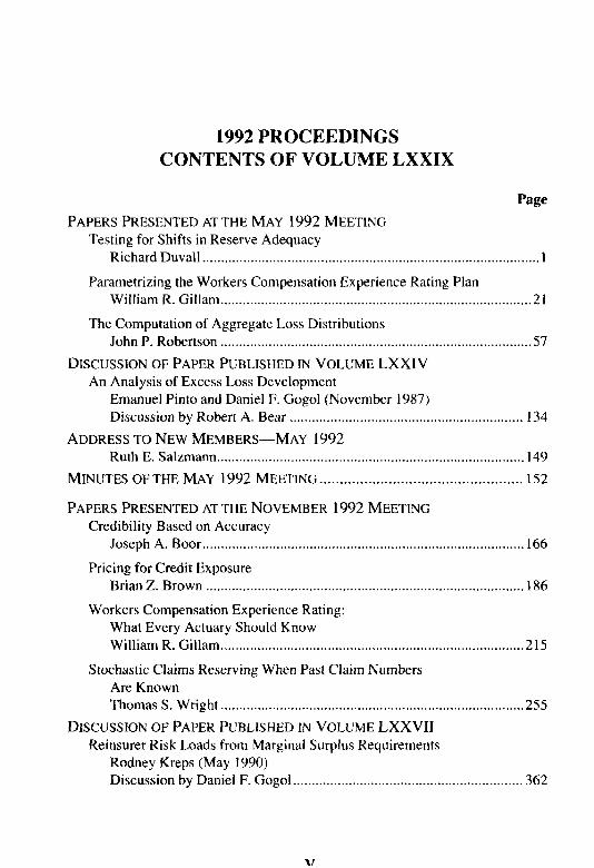
1992 PROCEEDINGS CONTENTS OF VOLUME LXXIX
Page PAPERS PRESENTED AT THE MAY 1992 MEETING
Testing for Shifts in Reserve Adequacy Richard Duvall . . . . . . . . . . . . . . . . . . . . . . . . . . . . . . . . . . . . . . . . . . . . . . . . . . . . . . . . . . . . . . . . . . . . . . . . . . . . . . . . . . . . . . . . . . . I
Parametrizing the Workers Compensation Experience Rating Plan William R. Gillam . . . . . . . . . . . . . . . . . . . . . . . . . . . . . . . . . . . . . . . . . . . . . . . . . . . . . . . . . . . . . . . . . . . . . . . . . . . . . . . . . . . . 2 1
The Computation of Aggregate Loss Distributions John P. Robertson . . . . . . . . . . . . . . . . . . . . . . . . . . . . . . . . . . . . . . . . . . . . . . . . . . . . . . . . . . . . . . . . . . . . . . . . . . . . . . . . . . . . 57
DISCUSSION OF PAPER PUBLISHED IN VOLUME LXXIV An Analysis of Excess Loss Development
Emanuel Pinto and Daniel F. Gogol (November 1987) Discussion by Robert A. Bear . . . . . . . . . . . . . . . . . . . . . . . . . . . . . . . . . . . . . . . . . . . . . . . . . . . . . . . . . . . . . . . 134
ADDRESS TO NEW MEMBERS-MAY 1992 Ruth E. Salzmann . . . . . . . . . . . . . . .._.................................................................. 149
MINUTES OF THE MAY 1992 MEETING . . . . . . . . . . . . . . . . . . . . . . . . . . . . . . . . . . . . . . . . . . . . . . . . . . 152
PAPERS PRESENTED AT THE NOVEMBER 1992 MEETING Credibility Based on Accuracy
Joseph A. Boor . . . . . . . . . . . . . . . . . . . . . . . . . . . . . . . . . . . . . . . . . . . . . . . . . . . . . . . . . . . . . . . . . . . . . . . . . . . . . . . . . . . . . . . 166
Pricing for Credit Exposure Brian Z. Brown .,..,.._....,....,.,.,.........,...,....,.........,......,...,..............,,...,.,., 186
Workers Compensation Experience Rating: What Every Actuary Should Know William R. Gillam . . . . . . . . . . . . . . . . . . . . . . . . . . . . . . . . . . . . . . . . . . . . . . . . . . . . . . . . . . . . . . . . . . . . . . . . . . . . . . . . . . 2 15
Stochastic Claims Reserving When Past Claim Numbers Are Known Thomas S. Wright . . . . . . . . . . . . . . . . . . . . . . . . . . . . . . . . . . . . . . . . . . . . . . . . . . . . . . . . . . . . . . . . . . . . . . . . . . . . . . . . . . 255
DISCUSSION OF PAPER PUBLISHED IN VOLUME LXXVII Reinsurer Risk Loads from Marginal Surplus Requirements
Rodney Kreps (May 1990) Discussion by Daniel F. Gogol . . . . . . . . . . . . . . . . . . . . . . . . . . . . . . . . . . . . . . . . . . . . . . . . . . . . . . . . . . . . . . 362

1992 PROCEEDINGS CONTENTS OF VOLUME LXXIX-CONTINUED
Page DISCUSSION OF PAPER PUBLISHED IN VOLUME LXXVIII
The Competitive Market Equilibrium Risk Load Formula for Increased Limits Ratemaking Glenn G. Meyers (November 1991) Discussion by Dr. Ira Robbin . . . . . . . . . . . . . . . . . . . . . . . . . . . . . . . . . . . . . . . . . . . . . . . . . . . . . . . . . . . . . . . . 367
DISCUSSION OF PAPER PUBLISHED IN VOL~IME LXX111 The Cost of Mixing Reinsurance
Ronald F. Wiser (November 1986) Discussion by Michael Wacek . . . . . . . . . . . . . .._............................................... 385
ADDRESS TO NEW MEMBERS-NOVEMBER I992 Paul S. Liscord . . . . . . . . . . . . . . . . . . . . . . . . . . . . . . . . . . . . . . . . . . . . . . . . . . . . . . . . . . . . . . . . . . . . . . . . . . . . . . . . . . . . . . . 41 1
PRESIDENTIAL ADDRESS-NOVEMBER I992 An Investment in Our Future
Michael L. Toothman . . . . . . . . . . . . . . . . . . . . . . . . . . . . . . . . . . . . . . . . . . . . . . . . . . . . . . . . . . . . . . . . . . . . . . . . . . . . 414 MINUTES OF THE NOVEMBER 1992 MEETING ,........,....._. . . . . f..............,... 423
REPORT OFTHE VICE PRESIDENT-ADMINISTRATION . . . . . . . . . . . . . . . . . . . . . . . . . . . . 43
FINANCIAL REPORT.. ............................................................................ ..44 6
1992 EXAMINATIONS-SUCCESSFUL CANDIDATES .............................. 447
OBITUARIES A. Edward Archibald ............................................................................. 485
George Y. Cherhn.. ................................................................................ 486
John W. Clarke ....................................................................................... 487
Miles R. Drobish.. ................................................................................. .488
James F. Gill ......................................................................................... .48Y
William H. Mayer, Jr. ............................................................................ 490
Joseph M. Muir.. ................................................................................... ,490
Stefan Peters.. ........................................................................................ .49 I
Albert Z. Skelding.. ............................................................................... .492
INDEXTOVOLUMELXXIX . . . . . . . . . . . . . . . . . . . . . . . . . . . . . . . . . . . . . . . . . . . . . . . . . . . . . . . . . . . . . . . . ...494
NOTICE
Papers submitted to the Prr~c~lin,qs of //w Cosutr//y Acrrrcrrirrl SorGry are subject to review by the members of the Committee on Review of Papers and. where appropriate. additional individuals with expertise in the relevant topics. In order to qualify for publication. a paper must be relevant to cx,ualty actuarial science. include original research ideas and/or techniques, or have special educa- tional value. and must not have been previously published or be concurrently considered for publication elsewhere. Specific instructions for preparation and sub- mission of paper, are included in the Yeorhuok of the Casualty Actuarial Society.
The Society is not responsible for statements of opinion expressed in the articles. criticisms, and discussions published in these P~~r~et/i~~,q.s.
Volume LXXIX, Part 1 No. 150
PROCEEDINGS May 10, 11, 12, 13, 1992
TESTING FOR SHIFTS IN RESERVE ADEQUACY
RICHARD M. DUVALL
Abstract
This paper develops regression models that can be used to test for the effects qf changes in reserving practices. The mod- els include terms for exposure, trend, and loss development. A loss triangle of reported losses at annual valuation dates is used to cstimute the parameters of the regression models. Dummy rjariahles are introduced into the loss development factor terms of the models to test for shifts and trends in the loss development factor parameters. The expanded models are estimated, and the parameters associated with the shift and trend variables are tested for signzficance. If shifts in reserve adequacy are indicated, the models can be used to restate re- ported incurred losses for the early valuation dates on a basis that is consistent with recent valuation dates. Similar models can be used to test for changes in settlement rates that create changes in the paid loss development pattern. If a change is revealed, the models can be used to estimate the effects of the change.
1

I. INTKODl~(‘7‘ION
This paper develops regression models that can be used to test for the effects of changes in reserving practices. If shifts in reserve adequacy are indicated, the models can be used to restate reported incurred losses for the early valuation dates in the data sample on a basis that is consistent with recent valuation dates. This topic has been explored by Berquist and Sherman [l ] and more recently by Fleming and Mayer 121. The proce- dures advocated in both of those approaches rely on subjective estimates for some of the parameters. While actuarial methods rely on the judgment of professionals, the credibility of results is improved when it is possible to obtain objective confirmation of the sub.jective assessments.
The Berquist and Sherman procedure for testing for shifts in reserve adequacy is to compare, at each valuation, the rate of growth of the per claim reserve for open claims with the rate of growth of the per claim cost for closed claims. They calculate the rate of growth for both averages over the years in the experience period. If reserving practices are consis- tent. they contend that the rate of growth in average claim reserves should be equal, approximately, to the rate of growth in average closed claims. Unequal rates indicate a change in reserve adequacy over the experience period.
Given a shift in reserving practices, the Berquist-Sherman adjustment for the shift begins by obtaining the rate of inflation in average closed claims. Next. the average reserve at the most recent valuation date is calculated for each year. These average reserves arc trended back to ear- lier valuation dates at the estimated trend rate to obtain the average re- serve at each age for each year in the experience period. The computed average reserves are then multiplied by the number of open claims at each age to get the estimated cost of open claims. Cumulative claim payments are then added to get an estimate of incurred losses on a basis that is consistent with current reserving practice.
Fleming and Mayer observed that if there is an increase in the claim closing rate and if claims close at a cost that exceeds the amount reserved, there will be a change in the incurred loss development pattern. They
TESTING FOR SHIFTS IN RESERVE ADEQUACY 3
present an addition to the Berquist-Sherman method that adjusts the data for this speed-up in claim settlement rates.
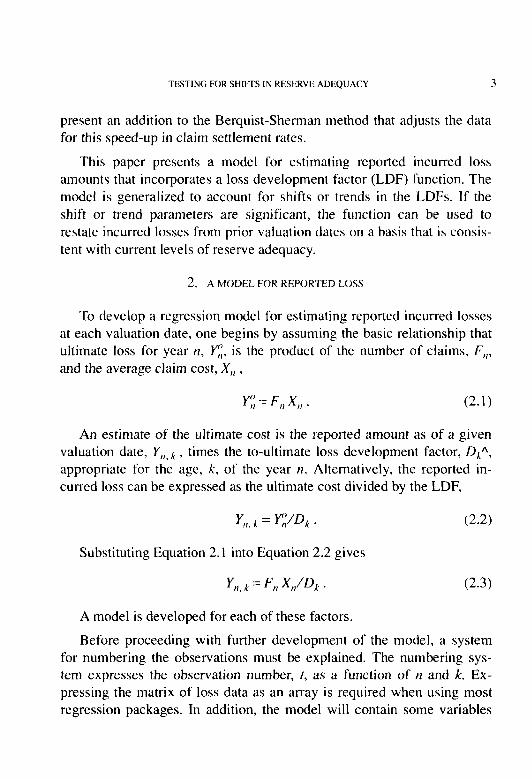
This paper presents a model for estimating reported incurred loss amounts that incorporates a loss development factor (LDF) function. The model is generalized to account for shifts or trends in the LDFs. If the shift or trend parameters are significant, the function can be used to restate incurred losses from prior valuation dates on a basis that is consis- tent with current levels of reserve adequacy.
2. A MODEL FOR REPORTED LOSS
To develop a regression model for estimating reported incurred losses at each valuation date, one begins by assuming the basic relationship that ultimate loss for year n, c, is the product of the number of claims, F,,, and the average claim cost, X,, ,
Y; = F,, X,, . (2.1)
An estimate of the ultimate cost is the reported amount as of a given valuation date, Y,l,x , times the to-ultimate loss development factor, DkA, appropriate for the age, li, of the year n. Alternatively, the reported in- curred loss can be expressed as the ultimate cost divided by the LDF,
Y,,, /,. = Y/;/Dm . (2.2)
Substituting Equation 2.1 into Equation 2.2 gives
Y,,> k = F/l w4 . (2.3)
A model is developed for each of these factors.
Before proceeding with further development of the model, a system for numbering the observations must be explained. The numbering sys- tem expresses the observation number, t, as a function of n and k. Ex- pressing the matrix of loss data as an array is required when using most regression packages. In addition, the model will contain some variables
4 TESTING FOR SHIFI-S IN RESERVE ADEQLIAC’Y
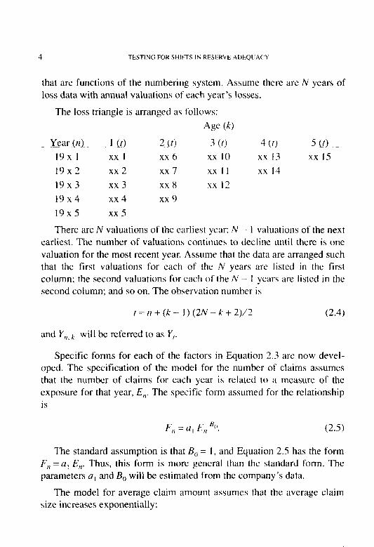
that are functions of the numbering system. Assume there are N years of loss data with annual valuations of each year’s losses.
The loss triangle is arranged as follows:
Age 64)
yeiu frill L!21-- 2f!2 3 co 4 (f> 5 Ill 19x 1 xx 1 xx 6 xx 10 xx 13 xx IS 19x2 xx 2 xx 7 xx I 1 xx 14 19x3 xx 3 xx 8 xx 12 19x4 xx 4 xx 9 19x5 xx 5
There are N valuations of the earliest year; N - 1 valuations of the next earliest. The number of valuations continues to decline until there is one valuation for the most recent year. Assume that the data are arranged such that the first valuations for each of the N years are listed in the first column: the second valuations for each of the N - I years are listed in the second column: and so on. The observation number is
I = II + (k - I ) (2N - k + 2)/2 (2.4)
and Y,,, k will be referred to as Y,.
Specific forms for each of the factors in Equation 2.3 arc now devel- oped. The specification of the model for the number of claims assumes that the number of claims for each year is related to a measure of the exposure for that year, E,,. The specific form assumed for the relationship is
F,, = u , E,, “0, (2.5)
The standard assumption is that B,, = 1. and Equation 2.5 has the form F, = a, E,,. Thus, this form is more general than the standard form. The parameters a, and B,, will be estimated from the company’s data.
The model for average claim amount assumes that the average claim size increases exponentially:
TESTING FOR SHIFK? IN RESERVE ADEQUACY 5
xn=a2enB1. (2.6)
This is the standard form assumed for the trend component of loss costs. Substituting Equations 2.5 and 2.6 into Equation 2.3 gives
Y, = a, E, BO a2 en Bl/D, . (2.7)
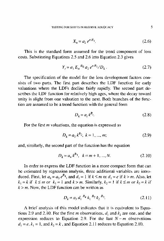
The specification of the model for the loss development factors con- sists of two parts. The first part describes the LDF function for early valuations where the LDFs decline fairly rapidly. The second part de- scribes the LDF function for relatively high ages, where the decay toward unity is slight from one valuation to the next. Both branches of the func- tion are assumed to be a trend function with the general form
D, = ai PJ. (2.8)
For the first m valuations, the equation is expressed as
Dk=a3@2, k=l,...,m; (2.9)
and, similarly, the second part of the function has the equation
Dk=a4p3, k=m+ l,..., N. (2.10)
In order to express the LDF function in a more compact form that can be estimated by regression analysis, three additional variables are intro- duced. First, let a, = a3 eB4, and d, = 1 if k I: m or d, = e if k > m. Also, let k, = k if k I m or k, = 1 and k > m. Similarly, k, = 1 if k I m or k, = k if k > m. Now, the LDF function can be written as
Dk = a3 d, B4 k, B2 k2 B3. (2.11)
A brief analysis of this model indicates that it is equivalent to Equa- tions 2.9 and 2.10. For the first m observations, d, and k, are one, and the expression reduces to Equation 2.9. For the last N-m observations d, = e, k, = 1, and k, = k , and Equation 2.11 reduces to Equation 2.10.

6 TESTIM; FOR SHIf:I’S IN KESliRVI: hDEQi’.\(‘\I
When estimating this function, a decision has to be made concerning the size of 1)1, i.e., at which age the function should be branched. This depends on the exposure that is heing studied, but branching the function at an age of three to four years usually gives a good fit for casualty exposures.
The LDF function is central to the objective of this paper. Changes in reserving practices must be manifest in changes in the parameters of this function if they are to be detected. Therefore, it is important that the function be capable of providing an excellent fit to the observed develop- ment patterns. On the other hand, it is not important that the function be capable of extrapolation outside of the range of the data since its purpose is to identify and measure shifts within the data sample. The particular form used for the LDF function is flexible enough to fit regular loss development patterns, but it is not appropriate for extrapolation to ages outside the data range. For example, the LDF should approach one as the age of the loss data increases. but the LDF from the function specified above approaches zero if B, < 0. The assumed form of the LDF function has two positive features: its flexibility and it% linearity when expressed in logarithmic form.
Substituting Equation 2.11 into Equation 2.7 and combining the Ui gives the expression
Y, = N,, E,, ‘,I c” ‘1
‘f B., k, ‘4 k, B,* (2.12)
where tic) = (I, uZ/tij. This model will be fit to the Berquist-Sherman data and used to test for a shift in reserve adequacy.
3. ESTIMATION OFTHE MODEL
The model developed above is now applied to the Berquist-Sherman Medical Malpractice data. After estimating the model, it is reestimated in several forms that test for a shift in reserve adequacy. Each of the forms tests for a shift in one of the parameters. If the model indicates that a shift has occurred, the data is adjusted for the indicated shift.

TESTING FOR SHIFI-S IN RESERVE ADEQUACY I
The top section of Table 1 reproduces Exhibit A of Berquist-Sherman. The to-ultimate LDFs derived by Berquist and Sherman are labelled least squares estimates (L.S. Est.). Equation 2.1 I is fit to this data with the branching occurring after the fourth valuation (48 months) for each year (m = 4). Logarithms of both sides of the equation are taken:
ln(Dx) = ln(a,) + B, ln(d,) + B, ln(k,) + B, ln(k?). (3.1)
The bottom section of Table 1 gives the results of the least squares estimation of Equation 3.1. All of the coefficients have the anticipated signs and are significant at the 1% level. The coefficient of determination, R2, is .998, which indicates an excellent fit. The residuals were tested for departures from randomness using the Durbin-Watson test and the von Neumann ratio test. The results of both tests did not indicate a rejection of the null hypothesis of randomness at the 5% level of significance. Auto- correlation in the residuals would be anticipated if the observations were ordered in time (time series data), or if one or more explanatory variables were not included in the model, or if the model being fit to the data had the wrong functional form. The loss development factors are not time dependent observations. Because the error terms exhibit random behavior, the form used to estimate the LDF function has an appropriate shape and includes appropriate explanatory variables.
The actual and estimated loss development factors are compared in Figure 1. The chart demonstrates that the form chosen for the LDF func- tion can give a good fit to the empirical function. An accurate fit is essential if the function is to be used to test for reserve adequacy shifts in the incurred loss data.
The complete model is estimated using the natural logarithms of the reported incurred losses in Table I. Unfortunately, the Berquist-Sherman paper does not give any exposure data nor the total number of reported claims. To complete the model, the number of claims is estimated from the data and is used as the exposure base for each loss year. Berquist and Sherman report the number of open claims as of each valuation date, and the number of closed claims has been estimated from two of their exhib- its. Their Exhibit C gives the average cost of claims closed in the intervals between valuation dates. Their Exhibit E gives the cumulative paid losses

Accident Year 12 24 36 48 60 1969 2,897 1970 4.828 1971 5,455 1972 X.732 1973 11,228 1974 X,706 1975 12.928 1976 15.791
12-24 24-36
1969 1.7812 1970 2.2177 1971 2.1890 1972 2.1339 1973 I .7783 1974 3.8432 1975 3.7828
Average Cum.
L.S. Est.
’ 53’3 I.. _-. 11.148X 1 I .3864
5,160 10.707 11,941 18.633 19,967 33,459 48,904
2.0764 1.5791 1.7363 1.725 1 2.5113 I .8972
I .9x9 4.4027 4.1 X92
X Coefficient(s) Standard Error of Coefficient
TABLE I MEDICAL MALPRACTTCE
INCURRED LOSSES (000s OMITTED)
Months of Development
10,714 15,228 16,661 16,907 22,840 26,2 I 1 20,733 30,928 42,395 32,143 57,196 61,163 50.143 73,733 63.477
Age-to-Age Development Factors 36-48 4X-60 60-72
I.4213 1.0941 I.2544 I .3509 1.1476 1.2197 I.4917 1.3708 I.1411 I .7794 1.0694 1.4705
72
20.899 31,970 4X.377
72-84
I .0954 1.0108
.4verage Incurred Loss Development Factors I .502X 1.1705 1.205 1 1.0531 2.2920 1.5252 1.3031 1.0813 2.3340 1.5412 1.2578 1.1369
Regression Output: In (03) B2 B3 B4
2.432 -1.443 -0.554 -1.31 I 0.044 0.130 0.247
X4
22,892 32,316
96
23.506
84-96 96-Ult
1.026X I .oooo
1.0268 I .oooo I .0268 1 .oooo 1.0438 I .oooo
2
0.9;8
Projected Ultimate
23,506 33,183 52,312 79,700
112,457 145,490 215,308 176.05 1

TESTlNGFORSHIFI'SINRESERVEAllEQUACY 9
as of each valuation date. By subtraction, the amount paid between valua- tion dates is determined. Dividing the average claim payment into the total amount paid is used to approximate the number of claims closed during the period. These closed claim counts are accumulated from period to period. The open claims at each valuation are added to the total number closed to date to give the reported claim counts. The reported claim counts are developed to an estimated ultimate number of claims for each year. The estimated claim counts and their development are presented in Table 2.
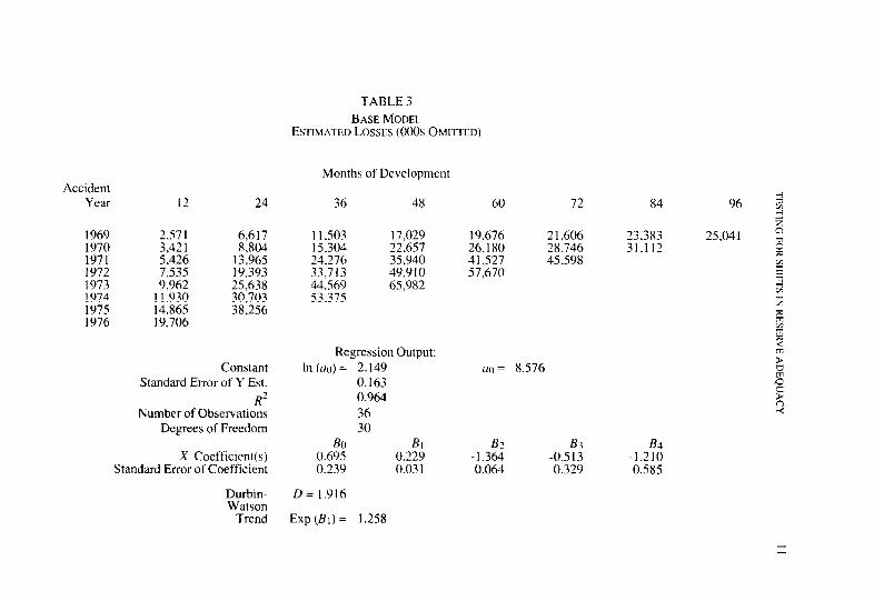
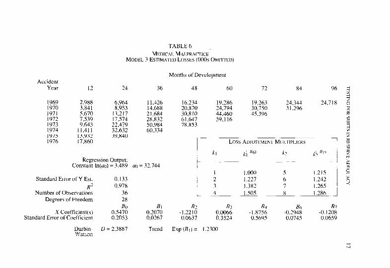
Given the estimated claim count for each year, numbering the years from one to eight, and assigning d,, k,, and k, their values as defined above, Equation 2.12 is estimated by taking the natural logarithms of both sides and using least squares regression. The results of the estimation are reported on Table 3. The error terms are tested for autocorrelation using
FIGURE 1
Loss DEVELOPMENT FACTORS-ACTUAL VERSUS ESTIMATED
12.00 /
11.00 t
10.00
9.00
8.W
7.00
I\ 6.00 r
-7
5.00
4.w
3.00
2.W
l.W LL I’*:! -------I-- - -- 1 2 3 4 5 6 7 8
Age (Years)
- Estimated + Actual

Accident Year
1969 1970 1971 1972 1973 I974 1975 1976
I2 24
I .060 I .672 I ,O5 I 1,877 1.296 2.5 I I I .354 2.72s 1,382 2,828 1,365 2.765 I.544 7.785 I .s94
1969 1970 1971 1972 1973 1974 1975
12-24 24-36
I.578 I .305 1.786 1.247 I.938 I .2so 3.013 I.290 2.046 1.298 2.026 I .3 LO 1 .x04
Average 1 .X84 I .2x3 cum. 3.061 I.621
TABLE 2 MEDKAL MALPRACTICE
NLYBER OF REPORTED CLAIMS
Months of Development
36 48 60
3.1x2 2.566 2.55s 2.340 2.719 2.777 3.138 3.743 3,859 3,515 3.210 4.45’3 3.671 4.665 3.623
Age-to-A2e Development Factors 36-4X ‘u-60 60-72
1.176 0.996 1 ,009 1. I62 1.021 1.010 1.193 I 43 I I.013
72
2.579 3.804 3.909
72-W
1.01 I I.009
1.1’38 1.05’) I.27 I
Average Claim Count Development Factor\ 1.700 I .027 I .o I 1 1.010 1.266 I.055 I.027 1.016
84
2.608 2.828
X4-96
I .007
1.007 1 ,007
96
2.625
96.lilf
I .ooo
1.000 I.000
Projected Ultimate
Accident Year 12 24 36 48
1969 2,571 6,617 1970 3,421 8,804 1971 5,426 13,965 1972 7,535 19,393 1973 9,962 25,638 1974 11,930 30,703 1975 14.865 38,256 1976 19,706
Constant Standard Error of Y Est.
R2 Number of Observations
Degrees of Freedom
Regression Output: In (U(I) = 2.149
0.163 0.964 36 30
Bn BI X Coefficient(s) 0.695 0.229
Standard Error of Coefficient 0.239 0.03 I
Durbin- Watson
Trend
D = I.916
Exp (BI) = 1.258
TABLE 3 BASE MODEL
ESTIMATED LOSSES (000s OMITTED)
Months of Development
I I.503 17,029 15,304 22.657 24.276 35,940 33,713 49,910 44.569 65.982 531375
60 72
19.676 2 1,606 26,180 28,746 41,527 45,598 57.670
84
23,383 31,112
a~ = 8.576
B2 B3 B4 -1.364 -0.513 -1.210 0.064 0.329 0.585
12 TESI’IUG FOR StIII’l’S IN RI:SI:RVI: AIWCJI \(‘k
the Durbin-Watson statistic, D = 1.9 16. This is very close to the expected value. and the hypothesis of independent error terms is acccptcd. The data are not a time series in the normal sense. The data arc ordered such that the 12-month valuations for all years are grouped, then the 24-month valuations, etc. The presence of’ independent error terms indicates that the estimates at each age are neither too large nor too small.
The bottom section indicates that the fit is excellent with a coefficient of determination. R’, of .964. All of the individual coefficients arc signifi- cant at the 5% level, with the exception of R,, which is about 1 .S6 stan- dard errors above zero. Berquixt and Sherman estimated a trend in average claim costs of about 30%. whereas this analysis indicates a trend of 25.8%~ in the average claim COSI. The estimated development of in- curred losses using the model is reported in the top portion of Table 3. These may be compared to the actual values which are reported in Table 1. Since the year-to-year development is variable, there are some substan- tial differences between the individual estimates and the observed values, but, on the whole, the fit is good. Thus, a model that gives good estimates of reported loss amounts has been developed. In the next section, the model will be modified to test changes in loss development patterns. If the revised models give superior results, rcscrving practices will have changed during the sample period.
4. TESTS FOR KFSER\‘IN~i (‘HANGES
If a shift has occurred in reserving patterns, it would be reflected in a change in the parameters of the LDF function, Equation 2.11. There are several parameters that might change with a shift in reserving. The coeffi- cients + and uJ could be affected and/or the exponents R, and B, might change. These possibilities are explored beginning with testing for changes in the coefficients L+ and cr,.
One procedure for testing for a shift in the parameters is to introduce a variable that has a value of unity for valuations that occurred prior to a certain date, and a value of c for valuations after that date. All of the reported losses on the last diagonal of the loss development triangle have the same valuation date. The diagonal elements of the loss development

TESTING FOR SHIFTS IN RESERVE ADEQUACY 13
triangle have values of I = k (2N - k + 1)/2. Assume that the 17 most re- cent valuations reflect the change in reserving practices, then define dz= I if rIk(2N-k+ 1)/2-p, and d,=e if r>k(2N-k+ 1)/2-p. Introducing d2 into Equation 2.12 gives
(4.1)
This equation has been estimated, and the results are given in Table 4.
The coefficient of determination increases slightly from .964 to .972 with the addition of the new variable. The Durbin-Watson statistic is 2.194, indicating a small, insignificant amount of negative autocorrelation in the error terms. The coefficient B, is substantially less significant than in Model 1; however, the coefficient for the shift variable, B,, is highly significant, and indicates that the more recent reported incurred losses are 27.4% larger, on average, than the estimates at the earlier valuations. Also, the estimated trend has decreased from 25.8% to 18.5%. The trends estimated by Berquist and Sherman dropped from 30% to 15%.
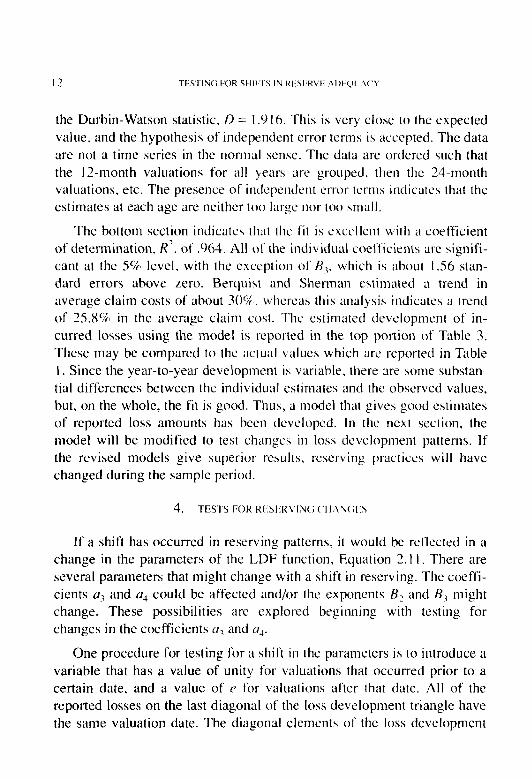
The estimates obtained from this model can be used to restate the reported incurred losses for the earlier valuations on a basis consistent with the reported incurred losses for more recent valuations. The early valuations can be increased by 27.4%, to adjust for the indicated shift in the estimates that has occurred during the past two years. This adjustment has been made for the malpractice data, and the results are displayed in Table 5. The last two diagonals of Table 5 are the same as the correspond- ing numbers in Table 1. All of the numbers above the last two diagonals have been increased by the indicated 27.4%. The restatement results in lower loss development factors and substantially lower estimates of ulti- mate incurred losses for the more recent years.
To test for a shift in the exponents B, and B,, two variables are added to Equation 2.12. The first variable, d3, is assigned a value of unity for valuations before the cutoff date, and a value of k, after the cutoff date, i.e., for the p most recent valuations for each year. Thus, 4 = 1 if rlk(2N-k+ 1)/2-p, and cl,=k, if t>k(2N-k+ 1)/2-p. The sec- ond variable, c&, is also assigned a value of unity for valuations before the

TABLE 4 MEDICALMALPRACTKE
MODEL 2 ESIIMATED LOSSES (000s OMITTED)
Accident Year 12 24
Months of Development
36 48 60 72 84 96
1969 2.874 7.005 1970 3.632 X.854 1971 5.612 13.678 1972 7,449 18,156 1973 9,346 22,781 1974 IO.475 32,526 197s 15.649 38.143 1976 19.698
11.796 17.073 18,631 1 X,936 24.456 24,748 E
14,909 ?I..%0 23.549 30,490 30.91 I 5 2
23.034 33.340 46.347 47,105 c: 30.574 56,373 61.517 2
48.869 70.734 i5 ;n
54.773 = 1:
Constant Standard Error of Y Est.
Number of’ Ohserv~tio~~ Degree5 of Fre’edorn
F Kegresjion Outpul:
$ In(cro) = 1.543 tm = 4.677 z c:
0.147 z >
0.972 5 7 36 F
29 > 5
Bo BI Bz 6.3 BJ BS X Coefficient(s) 0.794 0. I70 -1.185 -0.089 -I ,726 -0.242
Standard Error of Coefficient 0.218 0.035 0.064 0.332 0.559 0.086
Durbin- D = 2.194 Watson
Trend Exp (BI) = 1.185 Shift Exp (Bs) = I ,273
Accident Year
1969 1970 1971 1972 1973 1974 1975 1976
1969 1970 1971 1972 1973 1974 1975
Average 2.4143 Cum. 7.4222
12 24 36 48 60 72
3,690 6,150 6,949
11,123 14,303 11,090 12,928 15,791
12-24 24-36
1.7812 2.0764 2.2177 2.1890 2.1339 1.7783 3.0169 3.7828
6,573 13,639 15.211 23:736 25.435 33,459 48.904
1.5791 1.7363 1.7251 1.9714 1 X972
1.8309 3.0743
TABLE 5 MEDICAL MALPRACTICE
Bs ADJUSTED INCURRED LOSSES (000s OMITTED)
Months of Development
13,648 19,399 21,224 26,623 21,537 29,095 33,390 31,970 26,411 39,398 42,395 48,377 40,946 57,196 61,163 50.143 73.733 63,477
Age-to-Age Development Factors 36-48 48-60 60-72 72-84
1.4213 1.0941 1.2544 0.8599 1.3509 1.1476 0.9575 1.0108 1.4917 1.0761 1.1411 1.3969 1.0694 1.4705
Average Incurred Loss Development Factors 1.4263 1.0968 1.1177 0.9353 1.6791 1.1773 1.0734 0.9604
Projected 84 96 Ultimate
;;i Y 2 D
22,892 23,506 23,506 -n 32.316 33,183 B
46,463 2
65,654 86,807 2 106,587 2 150,347 z 117,204 k
7 m
84-96 96-Ult
1.0268 1 .oooo
1.0268 1 .OOoo 1.0268 l.OoOO

cutoff date and a value of k, for valuations after the cutoff date. With these two variables included, the new equation becomes
(4.2)
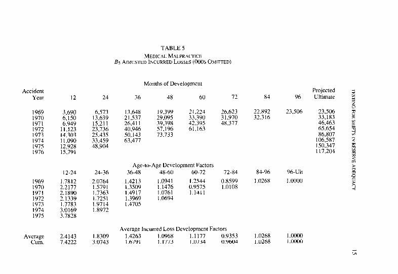
Equation 4.2 has been fit to the Berquist-Sherman data. and the results are summarized in Table 6. The coefficient of determination is marginally higher than for Equation 4.1, and the Durbin-Watson statistic is 2.3887, indicating an insignificant (a = .05) amount of negative autocorrelation in the error terms. As before, all of the coefficients are significant with the exception of B,, and in this case. B, entered with the wrong sign. This model gives a higher estimate of the trend factor than the previous model by about 4.5 percentage points.
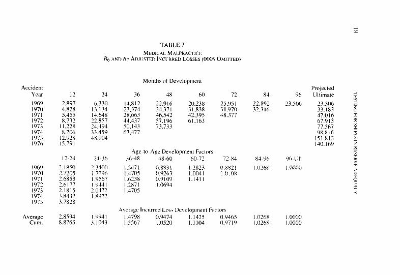
A small table has been inserted to indicate the average ratio of losses valued after the critical date to losses valued before the critical date. The ratios for this model vary with the age of the data at the valuation date. The ratios range from no adjustments for 1, T-month valuations to a 50.5% adjustment for 4%month valuations. These adjustments have been applied to the loss data, and the results are displayed in Table 7. As for the previous model, the adjusted estimates of ultimate incurred loss are con- siderably lower than for the unadjusted data.
A combined form of Equations 4. I and 4.2 that included (I?, cl,, and dd was estimated. The variables d, and (1, cntercd as significant. but tl, was not significant. This indicates that Equation 4.2 is the appropriate model to describe the shift in the reserving practices for these data.
5. SUMMAKI
A procedure that tests for changes in loss development patterns in an objective manner has been demonstrated. If a change is observed, the models developed can be used to restate the early valuations on a basis that is consistent with the current valuations. These models cannot replace the judgment of the actuary, but they do provide an additional tool with which to analyze this problem.
Accident Year 12 24
TABLE 6 MEDICAL MALPRACTICE
MODEL 3 ESTIMATED LOSSES (000s OMITTED)
1969 2.988 6,964 1970 3,841 8.953 1971 5.670 13.217 1972 7.539 17,574 1973 9,643 22,479 1974 11,411 32.632 1975 13.932 39.840 1976 17,860
Regression Output: Constant ln(ao) = 3.4X9
Standard Error of Y Est. 0.133
Number of Observatio:: 0.978
36 Degrees of Freedom 28
BO X Coefficient(s) 0.5470
Standard Error of Coefficient 0.2053
Durbin- D = 1.3887 Watson
Months of Development
36 48 60 72 X4 96 3 m
I 1,426 14,688 2 1,684 2X.X32 50,984 60,334
a0 = 32.744
Bi 0.2070 0.0267
16,234 19,286 19,263 24,344 24,718 5 c
20.870 24.794 30,750 3 1,296 a 30.810 44.460 45,396 % 61.647 SO.1 16 G 78.853
2 %
Loss ADJUSTMENT MCLTIPI.IERS ~1 73
5
h &.‘36’ X’
.I
I 1.000 5 I.215 % 2 1.227 6 1.242 g 3 1.382 7 1.265 ’ -c
L. 4 1.505 8 I .2X6 I
82 & B4 B6 B7 -1.2210 0.0066 -1.8756 -0.2948 -0.1208 0.0637 0.3524 0.5695 0.0745 0.0659
Trend Exp (BI) = 1.2300
3
Accident Year I2
1969 2.897 1970 4,828 1971 5.455 1972 8.732 1973 I I.228 1974 X.706 197s 12.928 1976 IS.791
24
6,330 13,134 14.648 22.x57 24.494 33.459 38.904
12-21
lY6Y 2.1850 1970 3.7205 1971 2.6853 1972 2.6177 1973 2.1815 1974 3.8432 1975 3.7838
24-36
2.3400 I .77Y6 I .Y567 I ,044 I 2.0472 I .XY72
Average 2.8594 I .YY4 I Cum. 8.8765 3.1043
TABLE 7 MEDICAL MALPRACTICE
& AND B7 ADJUSTED INC~IRRED LOSSES (000s OSII-ITED)
Months of Development
36 48 60 72
14,812 ‘2.916 20,238 25.95 I 23,374 34.371 31,838 31.970 28,663 46.542 42.39s 48.377 44.437 57.196 61.163 50,143 73.733 63.477
Age-to-Age Development Factors X-48 48-60 60-72 72-83
1.5471 0.X83 I 12x23 (1.882 1 I .4105 O.Y263 I.0041 I .010x I .6?38 0.9 IO9 I.141 I 1.2871 I .Oh94 I.4705
Average lncurrcd Loss Development Factors I .479x 0.9474 1.1425 KY465 I .5567 I .0520 1.1104 O.Y719
x4
‘2.892 32.316
I .026X I .0268
96
23,506
Yh-L’lt
I .oooo
I .oooo 1 .oooo
Projected Uliimate + g
23,506 i 33,183 z 47,016 2 67,913 Fe 77.567 g 9X.816 I
lSl.813 5 140. I69 2
z 2

TESTING FOR SHIFTS IN RESERVE ADEQUACY 19
The models that have been illustrated test for a change in reserving practices as of a specified date. Models that will detect a trend in the loss development factors, rather than an abrupt change in the factors as of the specified date, can also be employed. As above, one can test for a trend in the coefficients, a3 and ad, or in the exponents, B, and 8,. All data on the same diagonal of the loss development triangle have the same valuation date and are given the same time index of 8 = n + k - 1. This index num- bers the diagonals beginning with one in the northwest comer of the matrix and increases by one for each diagonal added to the triangle. The LDF model that estimates and tests for a trend in the exponents is
(5.1)
Finally, a model for the LDF function that includes a trend factor for the coefficients is
D, = a3 as R k, B2 k2 Bj d, BJ. (5.2)
Both Equation 5.1 and Equation 5.2 have been fit to the Berquist- Sherman data, but the results were not as significant as the models that incorporated a jump in the parameters. The results of the estimation are not reported.
Similar models can be employed to test for changes in claim settle- ment rates that are reflected in changes in paid loss development factors. If paid losses are substituted for reported losses as the dependent variable and the loss development function is interpreted as the paid loss develop- ment function, the models can be used to test for parameter changes in the same manner.
This paper has shown how regression models can be used to estimate the effects of changes in reserving practices. Once the effects have been estimated, the appropriate adjustments can be made to past valuations to restate them on a basis consistent with current reserving practices. The models allow one to test for abrupt changes in reserving practices versus changes that emerge progressively. This procedure is flexible and objec- tive.

20 TESI Il*;(i f:OR SfIII;l S IN RI;SER\‘k. .\I)l:CJI .Ac‘l
[I ] Berquist, James R., and Sherman, Richard E.. “Loss Reserve Ade- quacy Testing: A Comprehensive, Systematic Approach,” PCAS LXIV, 1977, p. 12.3.
121 Fleming. Kirk G., and Mayer, Jeffrey H.. “Adjusting Incurred Losses for Simultaneous Shifts in Payment Patterns and Case Reserve Ade- quacy Levels,” E~~aI~mti~~g IIIS~~IUIIW Conrprru~ Liabilities, Casualty Actuarial Society Discussion Paper Program. 19XX. p. 189.

21
PARAMETRIZING THE WORKERS COMPENSATION EXPERIENCE RATING PLAN
WILLIAM R. GILLAM
Ahsrtwct
This puper describes the de\vlopment of’ the rer~iscd Work- cr.s Compcwsation E,xper-ience Rating Plan. The plarl is hu.sed on s01md stutisticul theory, ccrtuiii niodelirif: uss~rniptioiis, und thornlr~h empirical testing. It is heurtening thut the empiricully derirwl I,aiwl71etl.il’utiOli is con.sistcnt Mlith most of the u.s.sunip- tiotis weded to simplfy the ~II~~Chi.ui~~,foi~i~~lutioii.
The puper- hcgirw with an heuristic deritution of u ~CJ~ICIUI mod(ficution fo~mulu bused on 1os.se.s split into primury und e.we.s.s portions. It delineates the ussumptior~s uhout the com- ponents of ~o.s.s rutio vuriuncv leuding to the uigebruic j~wm of the,fiwmulue tested.
lteruti\~e testing is used to purumetrke those fosnurluc. A simple preliminur-y test procedure is described to c?ur$~ the basic concept.s. The oper-uti\re test procedure is then spec$ed, and results of iterzrtilve testing usiqq thut procedure we dix- played j;)fi,r- the .scIcc~ted~~~~nirrlae.
The pal-ametrizc>d formula finally upprotvd by the Nutionul Council cm Compen.sution Itwrarlce (NCCI) MUS nrhjert to cer’tuirr udjtrstments to muintuin continuity during the trunsi- tkw fkm the old to Ned’ pluns. Credibi1itie.s hu\Te beeu .sculed to ucwunt ,ji,r d#erence.s in stute benefit levels and the eflect of influtiorl.

22 PAKAhll3KI%IN(i I-XI’I:KlFU(‘F KtIfIN(i
1 . THEORETICAL. Jl~SI‘IFI<‘/Z’I’ION
Compensation experience rating is a large-scale. ongoing application of credibility theory. The large volume of data supporting that application provides the raw material for the tests of that theory described below.
Researchers at the NCCI have used testing to crcatc an improved experience rating plan. The power of modern electronic data processing has enabled them to reopen older experience rating files and recalculate experience modifications (mods) as if a hypothetical plan had been in place. The plans tested and the measurement of their performance are described in this paper.
The general strategy was to start with a formula based on sound the- ory, then use iterative testing to parametrize that formula. Least squares or Bayesian credibility was used to develop an algebraic form for the modi- fication formula. Certain assumptions about lash ratio variance simplified the algebra. The parameters that worked best were consistent with a priori judgments about the components of loss variance.
B. Hewistic, Deri\ution of Mod Fomllrlu
This section outlines the theoretical development of the split plan modification formula. Here, a split ~ILIII is one in which individual losses are split by formula into two components, primary and excess, and sepa- rate credibilities are assigned to the totals of the respective loss compo- nents.
The formula is based on a Bayesian view of the process of individual risk rating. The reader may refer to papers by Hewitt [ I], Meyers [2], Mahler [3], and Venter [4] for more general theoretical background.
The split plan modification formula can be derived with one major simplifying assumption: that unconditional expected primary and excess losses are uncorrelated. This simplification is defensible more on the basis of its usefulness than its veracity. The standard used to select the final plan is how well it works, not how well it satisfies the assumptions. In the course of evaluating plan parameters, NCCI researchers found that
PARAMETRIZING EXPERIENCE RATING 23
a change in the primary/excess split formula improved the performance of the plan. They believe this change places the data used for rating in a form that better fits the assumptions.
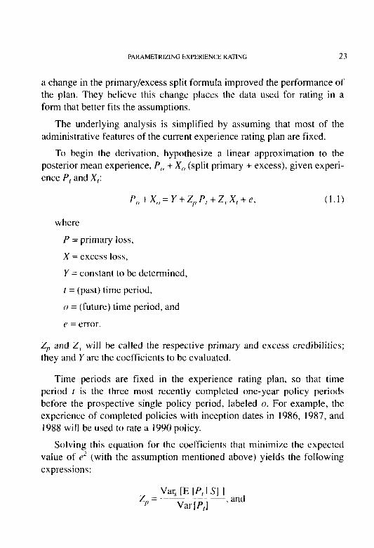
The underlying analysis is simplified by assuming that most of the administrative features of the current experience rating plan are fixed.
To begin the derivation, hypothesize a linear approximation to the posterior mean experience, P,, + X,, (split primary + excess), given experi- ence P, and X,:
P,, + x,, = Y + z/, P, + z,, x, + f, (1.1)
where
P = primary loss,
X = excess loss,
Y = constant to be determined,
I = (past) time period,
o = (future) time period, and
c = error.
Z,, and Z, will be called the respective primary and excess credibilities; they and Y are the coefficients to be evaluated.
Time periods are fixed in the experience rating plan, so that time period t is the three most recently completed one-year policy periods before the prospective single policy period, labeled o. For example, the experience of completed policies with inception dates in 1986, 1987, and 1988 will be used to rate a 1990 policy.
Solving this equation for the coefficients that minimize the expected value of c2 (with the assumption mentioned above) yields the following expressions:

z, = Var, [E IX, I S] ]
Var[X,] . (1.2)
And
Y=(I-Z,,)E[P,]+(I-Z,)EIX,I. (1.3)
where the condition S denotes a particular element of the parameter space (a particular risk) and the subscript .v denotes the prior structure (the dis- tribution of risk parameters).
Equation 1.2 has also been written
z,, = I
I+ E, ]Var[P, I SJ ] ’ Var, [E (f, I S] ]
Using these equations, the linear credibility estimate of the posterior mean becomes
f,, + X,, = UP,1 + UX,l + Z,i V’, - Elf,] I+ Z, (X, - E]X,] ). (I .4)
In practice, the loss functions are ratios to the prior expected total loss, so E[f,] + E]X,J = 1. In this paper, f and X are referred to as lo.s.s ufios, but the denominator is expected loss, not premium.
The rate modification factor is
M= I +Z,,(f,-E]f,])+Z,(X,-E(X,] ). (1.5)

PARAMETRIZING EXPERIENCE RATING 25
C. Var-iunce Assumptions
More assumptions are needed to derive the form of the components of variance in the formulae for Z,, and Z,, .
In Equation 1.4, loss ratio functions f and X were introduced. Those ratios have a variance that decreases as the size of risk increases. The sample ratios f, and X, are the emerged primary and excess actual losses of the individual risk divided by the unconditional expected total losses. The denominator is the e.vposrrr*e. The simplest assumption is that the large risk is essentially a combination of a large number of independent homogeneous units. That assumption leads to a within-variance of the risk loss ratio inversely proportional to exposure. The increase in expo- sure from additional time periods can be thought of as adding more inde- pendent units of exposure. The process variance decreases proportionately. Also, it is usually assumed that the variance of the condi- tional means is independent of exposure (i.e., size of risk). With those assumptions,
and
IS]]=dE,
IS]]=h ,
where E with no subscript represents the total expected losses, or expo- sure, of the individual risk: E = E[f D + X, I S].
Here h, the variance of ratios less than one, is small relative to a, which is measured in dollars of expected loss.
Using equation 1.2,
z,, = /$/E
I = 1 +a/hE

26 PARAMEI‘RI%IN(; liXPCRIl:N(‘I: RA’l’lK(i
E =I E + o/A
This is the familiar expression
z,, = E E+K,,’ (1.6)
where K,, is constant. Similarly,
z,= E- E + K., ’
where K-, is the excess credibility constant. This c.oml.‘ound~j.ucrior7 form, with E alone in the numerator and K a ratio of components of variance, helps to simplify the mod formula.
Second-Le\vel l4uriunc.e Assutnptions
Several investigators have refuted this simple variance assumption. Meyers [2] and Mahler [3] show that within-variance does not decrease in inverse proportion to exposure. Assuming there is a small, non-diversifi- able component of risk loss ratio variance, averaging (’ > 0,
E,<( Var If, I S’] J = c + d/E.
llsing h again as the between-variance,
z,,= h h + (‘ + d/E
= I + ~./h + d/Be
E = CE + d
, so E+m
h

PARAMETRIZING EXPERIENCE RATING 27
Kp’ = “Ecd . (1.7)
Now K,’ is a linear function of the exposure. Here, h and c are small relative to d. The limiting value of primary credibility for the largest risks is less than unity, or b/(h + c.).
This form for K,,’ and a similar one for K,’ are among possible formu- lae tested as described elsewhere in the paper. Because K, (* either p or X) is a linear function of the exposure rather than a constant, it performs better than the constant coefficient K, and considerably better than the formula B value of the old plan. However, it is not as good as the third- level formulae described below. The data show that K should not be constant, nor even a linear function of E, but rather should be a curve, increasing rapidly at first but then decreasing in slope to a more linear form for large values of E.
The variance assumptions resulting in the formula for K at this level were suggested by Mahler [3]. Mahler, in turn, credits Hewitt [5] with observation of the underlying phenomenon.
For this level, it is assumed that the between-variance is not constant across all risk sizes but has a component inversely proportional to expo- sure. This would follow if each larger risk was, at least in part, a random combination of non-homogeneous components. The effect is to flatten the variance of the conditional means as risk size increases. In this case,
Var, [E [P, I S] ] = e + f/E .
Retaining the second assumption about individual risk variance,
zp = e +f/E e+f/E+c+d/E
1 = l+c+d/E .
e +f/E

In compound fraction form, this is
where
,,,‘I = E .
(1.8)
A similar form follows for K.,“. Notice that d and .f‘ are quite large compared to (’ and e. Since c is a small component of within loss ratio variance and e is a large component of between loss ratio variance, it is also plausible that (’ < e.
Dividing through by c, we define c’= C./V. I> = d/c>, and F =f;/e, SO that
This form is selected for parametrization, so the superscripts have been dropped.
In all the sample parameters that worked well (as described below). C was consistently between 0 and 1, which is reasonable if (’ is in fact smaller than e. D and F are large positive numbers, as expected.
In a sense, the final parametrization selected is more general than the underlying variance assumptions. This is because performance testing
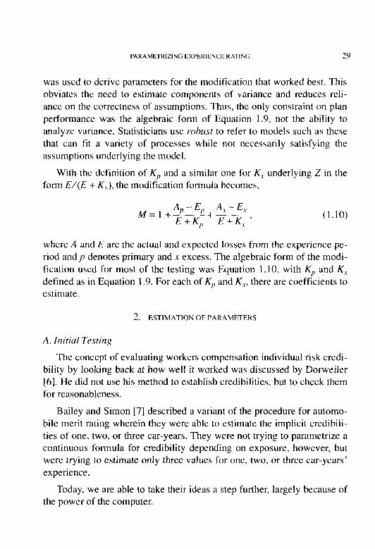
PARAMETRIZING EXPERIENCE RATING 29
was used to derive parameters for the modification that worked best. This obviates the need to estimate components of variance and reduces reli- ance on the correctness of assumptions. Thus, the only constraint on plan performance was the algebraic form of Equation 1.9, not the ability to analyze variance. Statisticians use whrrst to refer to models such as these that can fit a variety of processes while not necessarily satisfying the assumptions underlying the model.
With the definition of K,, and a similar one for K., underlying Z in the form E/(E + K,;), the modification formula becomes,
A, - E,, A \ - E, M= 1 +E+K-+‘+K ) I’ \
(1.10)
where A and E are the actual and expected losses from the experience pe- riod and p denotes primary and x excess. The algebraic form of the modi- fication used for most of the testing was Equation 1.10, with K,, and K.,. defined as in Equation 1.9. For each of K,, and K.,, there are coefficients to estimate.
2. ESTIMATION OF PARAMETERS
A. /nitia/ Testing
The concept of evaluating workers compensation individual risk credi- bility by looking back at how well it worked was discussed by Dorweiler [6]. He did not use his method to establish credibilities, but to check them for reasonableness.
Bailey and Simon [7] described a variant of the procedure for automo- bile merit rating wherein they were able to estimate the implicit credibili- ties of one, two, or three car-years. They were not trying to parametrize a continuous formula for credibility depending on exposure, however, but were trying to estimate only three values for one, two, or three car-years’ experience.
Today, we are able to take their ideas a step further, largely because of the power of the computer.

30 PARAhZETKI/IN(i EXYEKIEN(‘E R.4TiNG
In this study of experience rating, the criterion 01’ “working best” is first measured by the ability of a plan to satisfy Dorweiler’s necessary criterion for correct credibilities: that credit risks and debit risks would be made equally desirable insureds in the prospective period. In workers compensation, credibility is a function of risk size, so this property should exist across all size categories. WC use this criterion as a rrtri~~ trsf, which belies its great value to our early investigations. It also serves to simplify the demonstration of the basic idea behind the testing.
An example of this test is included in Exhibit 1. Nole that the plan proposed earlier is still a long way from the plan that was eventually selected. The test begins with experience rated risks for policies effective in 198 I. Their modifications are computed according to the fi)rmuia to be tested. The 198 1 loss experience that actually emerged may be found in the 1983 rating year files, i.e., the data underlying mods el‘fcctive 1983. The risks in each size group are stratified by their I98 I modifications, so that risks with mods in the lower 50th percentile would be in one stratum and risks with mods in the upper SOth percentile would be in the other. (It should be noted that for the smaller siLc groups, the majority of risks have credit mods, so the upper pcrccntile includes a proportion 01‘ risks with small credits.)
A canonical comparison would be of the subsequent loss ratios of the two strata: actual losses to manual premium on one side, and actual losses to modified premium on the other. The first ratios, actual to manual, should follow the predicted quality of the stratum. Risks with credit mods should prove to have favorable loss ratios on average. and those with debits should average poor ratios. showing that the plan was indeed able to “separate the wheat from the chaff.” In order to see if the differences in predicted quality were correctly offset by the mod. the ratio of losses to modified premiums for the two groups should equal each other. It would be too much to expect that premium rates be correct in aggregate and that the two subsequent loss-to-modified-premium ratios be equal to the per- missible loss ratio.
Effective manual premiums for the three policy periods used for the modification are retained in the experience rating files. Unfortunately, since they are not used for either ratemaking or experience rating, the
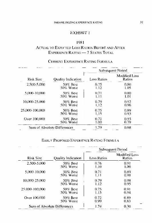
PARAMETRIZING EXPERIENCE RATING
EXHIBIT 1
1981
ACTUAL TO EXPEC’TELI Loss RATUS BEFORE AND AFTER
EXPERIENCE RATING - 7 STATES TOTAL
CURREM EXPERIENCE RATING FORMULA
Subsequent Period
Risk Size Quality Indication Loss Ratios
2.500-5,000 SO%8 Best I 0.75 50% Worst 1.12
0.x0 I .os
s,ooo- 10,000
10,000-25,000
2s,ooo- 100,000
50% Best XN Worst
50% Best 50% Worst
50% Best 50% worst
0.7 I 0.80 I.1 I I.01
0.7Y 0.Y2 I.12 0.96
0.75 O.XY I.15 0.93
Over 100,000 50% Best 50% Worst
Sum of Absolute Differences
EARLY PROPOSED EXPERIENCE RATING FORMULA
Subsequent Period
Modified Loss Risk Size Quality Indication
2,sOO-5,000 50% Best 0.76 0.9 I 50% Worst I.10 I .oo
s,ooo- 10.000 SOo-/cs Best 0.7 I 0.89 50% Worst I.1 I 0.98
10,00&25,000 SO?h Best 0.79 0.98 50% Worst I.12 0.95
25,000- I00,000 50% Best :::: 0.91 50% Worst 0.94
Over 100,000 50% Best 0.72 0.89 50% Worst 0.99 0.x.3
Sum of Absolute Differences -1:: I.?- ~~ Go ~~

32 PARAMITKILIN(i I:SPliKIt:N(‘I: K VI IN<,
numbers are seldom checked and are considered unreliable. The expected loss rates, or ELRs, by class in these files, however. arc sub.ject to review by insure& and insurers. These are not the true loss costs underlying the rates, but estimates of emerged loss for three policy years as of a certain evaluation date. The ELRs used to estimate rating year 1981 expected losses are used to compute the expected ratable losses for modifications effective during the 1983 policy year. The ELRs are meant to be correct on average for the losses on three policy years, including, in this case, 1979, 1980, and I98 I. The three policy years arc at respective third. second, and first reports. ELRs arc probably not correct for any single policy year, but should bear some reasonable relation to the rates effective in the latest year. A key assumption is that the ELRs will be uniformly redundant or inadequate over all insureds with the same rate.
The comparison is then between the ratios of actual to manual ex- pected loss for each stratum and ratios of actual to expected losses MI- jlrstc4 hy the nwclifjccrfion, or modified expected loss. Specifically, I98 I actual loss to 19X I expected loss. taken from the I983 rating year files, should reflect the predicted quality difference. Application of the 1981 modification to I98 I expected losses should make the ratios converge.
Just as it was observed in the case of premiums, it is reasonable to hope that the subsequent ratios to modified expected loss would be close to each other, but it is unreasonable in this case to require values near unity.
The need for credibility in a format not unlike the one finally selected is evidenced by application of the naive test. The xmallcst ratable risks have non-zero excess as well as primary crcdibilities. Starting with the stnallest risks, credibility increases rapidly with risk size, but then in- creases at a slower rate, and never reaches full credibility for even the largest risks.
B. The Quintiles Test
As the testing of the plans progresses and more sophisticated actuarial theory is applied to the algebraic form of the credibility constants, it becomes apparent that a more sophisticated test is needed to measure the

PARAMETRIZING EXPERIENCE RATING 33
quality of alternative formulae. Dorweiler’s sufficient criterion for cor- rectness of the modification is that any subdivision of risks based on prior experience should produce uniform subsequent loss ratios (to modified premium).
Instead of good versus bad as in the naive test, the risks are grouped into five equal-sized strata according to the value of their modifications. The lowest 20% of the values belong to risks in the first quintile; the next 20% to the second; and so on. This is the prior subdivision. The subse- quent aggregate unmodified loss ratios of the strata should reflect the quality difference recognized by the mod. Application of the modifica- tions should cause the ratios to flatten across the strata.
This leads to the ratio of two sums of squared differences: the five squared deviations from the mean of the modified loss ratios, divided by the sum of the squared deviations of the ratios before modification. Lower values indicate greater reduction of loss ratio variances. The statis- tic would pertain to the experience of each group, so for a particular parametrized mod formula, several values are available for comparison. In most of the NCCI testing, coincidentally, five groups were considered.
The quintiles test was developed without reference to risk theory, but it can be characterized as the ratio of posterior structure variance to prior structure variance. The sum of five squared deviations does not capture the entire structure variance, either prior or posterior; but the ratio is valid. Experience rating should reduce this component of variance. Mey- ers 121 uses the more theoretically grounded “efficiency” standard: the proportion by which the total variance is reduced. Either statistic is use- ful; the quintiles test is computationally simpler and has an indisputable best value of zero.
Section 3 outlines the variants of the basic plan for which minimal values of the statistics were sought and it discusses some of the rationale for each. The exhibits shown are the final product of a large number of trial-and-error evaluations.
One sidebar test deserves mention. In this test, primary and excess credibilities were evaluated separately. The mod as a function of either primary or excess losses alone had far less predictive accuracy. Credibili-

34 PAR.4hlfi’I’RI%IN(i fiXPl:Klt:\f‘F KAl’f\(i
ties were lower when losses were used separately as the sole basis for the mod than when they were used together.
This conclusion should be contrasted with that ol’ Meyers [21--that a best modification formula could be based on primary losses only. His conclusion may be correct in the special case of ;I uniform. well-behaved severity distribution for all risks, which was the model he tested. The NCCI tests of real-world data support the split I’ormula with a two-part credibility.
The workers compensation severity distribution is composed of many types of losses. An essential component of workers compensation ratemaking and individual risk ratin g is that the distribution of‘ losses by type varies from class to class and risk to risk.
Potential revised experience rating plans were tested in comparison to the then-current experience rating formula, herein rcfcrred to as the “for- mer” plan.
The former formula was derived through practical simplifications that made sense at the time of its development. II was partly these simplifica- tions, however, that moved the plan away from whatever underlying cred- ibility theory it may have had. The former formula is written:
A,,+WA,+(l -W’)E‘,+H /g=
E-kB (3.1)
It is one fraction, with weighting value W and credibility ballast B --both linear functions of total expected losses. A denotes actual and E represents expected loss for the experience period. Subscripts /> and .V denote primary and excess portions of loss, rcspcctively; and E with no subscript denotes total expected losses.

PARAMETRIZING EXPERIENCE RATING 35
0 for E < 25,000
-E-2s’ooo- for 25 000 5 E I SRP SRP-25,000 ’
1 for E > SRP
B = 20,000 ( 1 - w)
Here the SRP is the state Self-Ruring Point, 25 times the state average serious cost per case. This approach provides a nominal indexing to plan credibilities and ratable loss limits that should vary by state and by year.
In the former multi-split formula, the primary portion of a loss L was
I L if L I 2,000 $1 = ‘P!oL if L > 2,000 (3.2)
8,000 + L
To calculate the excess portion, losses are limited on a per-claim basis to 10% of the SRP, and on a per-accident basis to 20% of the SRP. Denoting the loss so limited by L,. , the excess portion of a loss greater than $2,000 would be
L, = L,.- L,, (3.3)
where L,, is calculated as noted above.
Many of the elements of the former plan are retained, including ELRs and D-ratios by class, the primary-excess split formula, and state ratable loss limitations. Payroll (in hundreds) by class is extended by the respec- tive class ELRs to produce the total expected loss. D-ratios, which also vary by class, measure the primary portion of expected loss.
Putting B = K,, and W = (E + K,,)/(E + K,) into Equation 3.1 results in algebraic equivalence of the new modification formula, Equation 1.10, and the former formula, Equation 3.1. Throughout the testing used to evaluate parameters, the NCCI researchers used Equation 1 .lO for the mod, and concentrated on finding best values of K,, and K,r. The values of

36 l’AK,\hll:l KI%IU(; I:XI’I:KII~.N~‘E K.\I I/x( i
K,, and K., that worked best in all the testing lead to values of M/. and B quite unlike the former plan’s values.
It is highly desirable that differences in bcncfit levels by state be reflected in the credibility constants K,, and K,. The former formula used the SRP to effect a nominal difference in the bV and B tables by state. but only really affected the risks whose expected losses wcrc near the SRP. We want to use an adjustment that results in a true scaling by state, which would be valid across all risk sizes. That objective is accomplished by inserting a value G, measuring relative benefit levels by state, into the formulae for K,, and K,. Equation I .9 is modified to make the following expression for K,, by state:
(3.4)
A similar change was made to the l’ormula for K,.
The G-value not only accounts for differences in benefit levels, but also indexes credibility constants for inflation in average claim costs. This property is seen in the following analysis. Ass~mc inflation of 1 + i between times t and s. For example, let primal-), credibility at time t be given by
Z(t) = E lAK I’
With inflation but no real growth, both E and G increase by the factor I + i. This factor cancels everywhere in the formula fbr Z(x) so rhat
Z(s) = Z(f).
The formula for G is one of the parameters that can be varied to optimize the test statistic. In most of the initial NCCI resting. G was taken as a linear function of the existing SRP.

PARAMETRIZING EXPERIENCE RATING 31
The SRP is retained, but only for use in limitation of ratable losses. There can be no self-rating under any analytic plan, so the SRP is re- named the State Rqfcrence Point.
C. Tested Plans
One assumption underlying Equation 1.9 for the credibility ballast values K,, and K, is that both primary and excess credibilities depend on total expected losses, E. The same assumption underlies the former for- mula, which is Perryman’s First Formula. We call the first alternate for- mula Per.r,J’ntun I because it borrows much from the original.
Ultimately, the NCCI researchers tested four alternative plans in addi- tion to the former plan, herein called Current Multi-Split. For each alter- native plan, optimal values of the credibility parameters were chosen based on results of the testing. The selection of a final plan from among the four optimized alternatives took into consideration not only the asso- ciated values of the test statistic, but also the ease of understanding and implementation.
The tested plans include :
1. Current Multi-Split;
2. Perryman I Multi-Split;
3. Perryman II Multi-Split;
4. Perryman I Single-Split; and
5. Perryman II Single-Split.
Their specifications follow.
I. Current Multi-Split
The basic specifications for this plan have been given. They include the formulae for B, W, the SRP, the primary/excess split of actual losses, and the modification formula itself. They also include calculation of the ELRs and D-ratios by class. The rating values of each insured are in- cluded in the experience rating files for each year. In particular, rating years 198 1 through 1984 were used in the testing.

3x F’ARAME’I‘RIZING liSYtiRII:NCE RAI’ING
2. Peyw~ur~ I Multi-Split
As described in the introduction, this is the first alternative to the former plan. It is Equation 1.10, with Equation 3.2 used to split actual losses into primary and excess components. Values such as ELRs and D-ratios can be carried over directly from the experience rating files, while Kp and K, can be calculated easily from the elements of the files: namely, total expected losses of the risk, state identification of the risk (which would be used to fetch indexed SRP and G values), and three coefficients for each formula, selected by trial and error.
3. PevynwtI II Multi-Split
This formula results from a different assumption about loss variance than the one used in Perryman I. It is only nominally related to Perryman’s Second Formula, as noted below.
In the version tested, it is hypothesized that conditional primary loss variance is a function of expected primary losses and that excess loss variance is a similar function of expected excess losses.
The formula for credibilities takes the following form:
(3.5)
where K,,= CE + GH/(l + GF/E), and E,, is expected primary losses. Notice that i!, ought to be expressed in terms of E,,, not E. This, however, further complicates the formula. The selection of c’. F, and H, as deter- mine_d by performance, could incorporate average D-ratios, if appropriate, and K, could be a function of total expected losses. The resulting credibil- ity parameters could be put in tabular form by state according to expected primary or excess losses.
Denoting the average D-ratio by risk as 6 results in the following formulae:

PARAMETRIZING EXPERIENCE RATING
6E =--- 6E + it,,
E
E + ji;,/i? ’
Similarly,
which yields
E z,, = _______ E+it,/(l -6) ’
(3.6)
(3.7)
Testing of this plan was accomplished using values available from the ex- perience rating files.
For the sake of historical accuracy, the true Perryman’s Second For- mula actually resulted from the unusual expressions for credibilities
Perryman does not derive these expressions and attempts (somewhat less than successfully) to rationalize their contradiction of credibility princi- ples [8].

40 PARAMETRI%IN(; liXIJ1:RIFiUCE RAI.IN(;
One of the key assumptions of the tested formulae is the non-correla- tion of primary and excess loss components. As long as the primary losses had a severity component, the NCCI researchers were not fully satisfied with a credibility-based plan that uses the former primary-excess split.
It is classically assumed that frequency and severity are independent, hence uncorrelated. This is probably not a valid assumption, but it is reasonable. It is less reasonable to assume that primary and excess losses defined by the multi-split formula are uncorrelated. Thus, the NCCI re- searchers considered using a modification formula based strictly on fre- quency and severity. One problem with this idea would be the difficulty of obtaining a valid claim count. (For example, are small medical-only claims recorded on a consistent basis by all carriers for all risks‘?) Be- cause this change would require the cooperation of so many different interests, it was not pursued.
A compromise is to use a single split (into primary and excess catego- ries) of losses. The portion of a loss below the single threshold value would be primary; and the portion of a loss in excess of that value. if any, would be excess. Using $2,000 as the single-split point is a relatively easy choice: it is the smallest size for which individual claims data is reported, so it is the closest to a frequency/severity dichotomy we can obtain using available data.
To test a single-split plan against actual risk experience, expected losses can be taken directly from experience rating files. New D-ratios corresponding to the new split formula are needed, They arc developed by adjusting the multi-split D-ratios in the files to maintain the aggregate adequacy of the D-ratios. For example, if the aggregate emerged actual- primary to ratable-total losses under the former fi,rmula had been 0.40, and under the new split it is 0.38, the D-ratios would all be adjusted (downward) by the factor (0.38)/(0.40). With D-ratios so adjusted, the formula is tested with K,, and K,. in the established Equation I. IO, until optimal values for the six coefficients are obtained.
PARAMETRIZING EXPERIEYKE RATING 41
The last plan to test was the one that utilizes two major variations from Plan 2. Perryman I Multi-Split. Plan 5 uses a single primary-excess split of losses, with the credibility formulae from Plan 3. This is the “fully equipped” model as compared to the other “economy” versions. The question is whether there is enough improvement in performance to jus- tify the additional cost and more difficult handling.
D. SJrmnJay
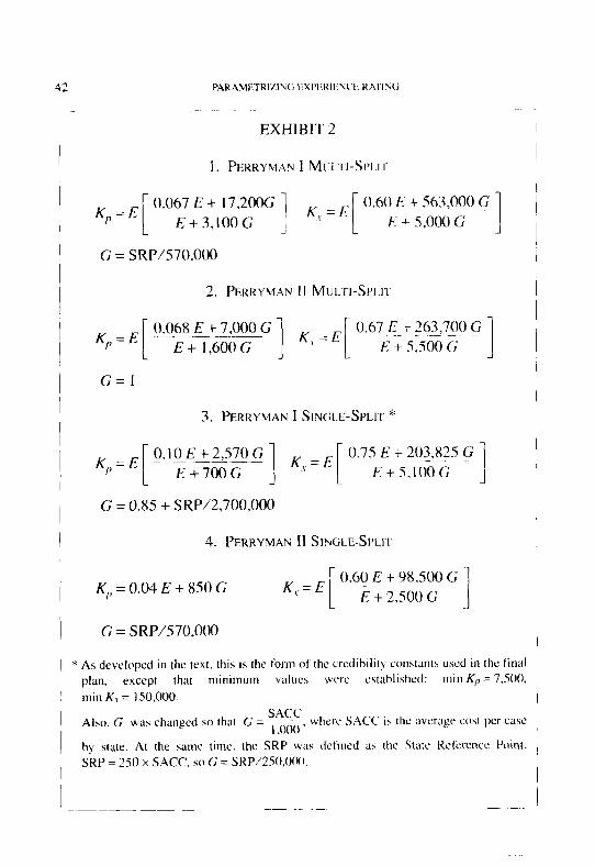
The NCCI researchers tested experience ratings effective on 1980 and 1981 policies. Best parametrizations for each of the plans tested may be seen in Exhibit 2. Of course, “best” is subjective in that no single set of coefficients in any plan produced a lowest value for all 10 evaluations (five size groups and two years). Still, the pattern that emerged for all evaluations was that the smaller sizes deserved more credibility and the larger sizes deserved much less credibility than under the current plan.
Exhibit 3 shows summary statistics and a sample calculation of the test statistic for Size Group Two in 1980.
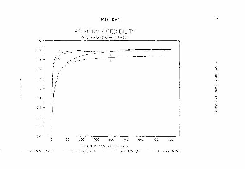
Several credibilities are displayed in Figures 1, 2, and 3. The consis- tent pattern for the four optimized plans can be seen. The plans also bear a fairly logical relation to each other. In particular, credibilities seem to increase substantially in the passage from a multi-split to a single-split formula. This may be due to better satisfaction of the assumption that primary and excess losses are uncorrelated.
By contrast, the use of the Perryman II equation in place of Perryman I does not seem to increase average credibilities much. There is, of course, a slight improvement in the distribution of the credibility assigned to the individual risk, as reflected in the test statistic. As described in Section 4, the evaluation of all the plans included weighing the benefit of increased accuracy against the cost of increased complexity in applica- tion.
PARAMETRI%IN(i tiXt’t:Rll:“;C‘ti RATlhG
EXHIBIT 2
1. PEKK’I’MAV I M~II:~I-SPI.I~
K 0.067 ET 17,200G 1 K, = E i
0.60 E + 563,000 G P E+3,lOOG j E + 5,000 G I
G = SRP/S70.000
K 0.068 E +7.000 G ~~~ .-__ 1 i K = E 0.67&+ 265,700 G‘ P E+ 1,600G ’ E + s,soo G 1
G=l
3. PEKKYMAN 1 SINGLE-SPLIT *
C).lOE+2,57OG 0.75 E f 203.825 G ~__ E+7OOG E + 5,100 G I
G = 0.85 + SRP/2,700,000
4. PERRYMAIU! II SINGLE-SPLIT
K,, = 0.04 E + X50 G
G = SRP/S70,000
K,=E i
0.60 E + 98,500 G E + 2,500 G I
* As developed in the text. this is the form of the credibility constants used in the final plan. except that minimum values WCIT c~tablishetl: min K,, = 7.X)0,
min K, = 150.000. SAC-C
I
L
Also, G was changed so that G = l~ijtb + where SACC’ ilr the average cost per case
by state. At the same time. the SRP was dctined a\ rhc State Rcl’crcncc Point, SRP = 250 x SACC, so (; = SRP/25O,OofJ.
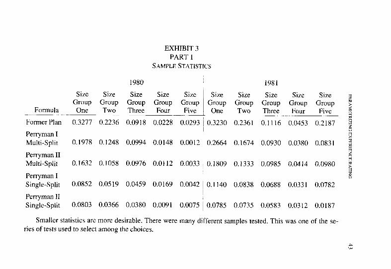
EXHIBIT 3 PART 1
SAMPLE STATISTICS
1981
Size Size Size Size Size Group Group Group Group Group One Two Three Four Five
0.3230 0.2361 0.1116 0.0453 0.2187
0.2664 0.1674 0.0930 0.0380 0.0831
1980
Size Size Size Size Size Group Group Group Group Group
Formula One Two Three Four Five
Former Plan 0.3277 0.2236 0.0918 0.0228 0.0293
Perryman I Multi-Split 0.1978 0.1248 0.0994 0.0148 0.0012
Perryman II Multi-Split 0.1632 0.1058 0.0976 0.0112 0.0033
Perryman I Single-Split 0.0852 0.0519 0.0459 0.0169 0.0042
Perryman II Single-Split 0.0803 0.0366 0.0380 0.0091 0.0075
Smaller statistics are more desirable. There were many different samples tested. This was one of the se- ries of tests used to select among the choices.
0.1809 0.1333 0.0985 0.0414 0.0980
0.1140 0.0838 0.0688 0.0331 0.0782
0.0785 0.0735 0.0583 0.0312 0.0187

P4K/\MH‘KI/IN(; l-l~l’l~KlliN~‘I: K\I IN0
EXHIBIT 3 P.4KI‘ 2
15 ST-\ I’ES TOI..Q Risk Size: $5,000-$ IO,000
PEKKYMAN 1 SIN(;I.I:-SIV.I-I
Quintile Before I 0.63 2 0.76
3 0.86 4 I .05
5 I .32 Mean Total: 0.93
SCpilWl Deviation
From Mean 072 IYS
x-4 14X
I.532 3.005
Quintile Before I 0.68 2 0.70 3 0.87 4 I .06 5 I.30
Mean Total: 0.93
Test Statistic IS6
3.00s := 0.05 IO
CURREKT MLILTI-SPLIT
Squared Deviation
From Mean 613 532
37 I73
I.373 2.737
Squared Deviation
After Front Mean
0.83 I06 O.YS 3
0.05 4
I .oo 42
O.Y? 2
0.03 IS6
AbeI
0.79 0.78 O.Y3 I .04 I .03 O.Y3
Squared Deviation
From Mean
19’ 214
0
I I:! Y4
611
Test Statistic
76;;7 := 0.2236 b. -

10
0.3
08
0.7
0.6
0.5
04
0.3
02
FIGURE 1
0.8
FIGURE 2
PRIMARY CREDIBILITY Perrymon l,il/S,ngle-.Multi-Split
0
__ A: Perry. l,‘S;ngle
I 1 / lCcl 2co 3CC 4x 5oc 6CC ?3c‘ 8OC
EXPECTED LOSSES (Thousands)
- B Perry. l/MuN - C. Perry It/Single ~ D, Perry. II/Multi

10
0.9
0.8
0.7
g 0.6
J m 0 0.5 w rr 1 u
0.4 c
FIGURE 3
EXCESS CREDIBILITY Current vs. Perryman l/Single-Split
0.3
: 0.2
0. I
0.0 :
500 600 700 800 900 1000
EXPECTED LOSSES (Thousands)
- A: current Plan - B. Perry. I/Single

48 PAKAME’l’KI%ING EXPEKIENC‘I: KM‘lNV(i
Selection of an experience rating formula was made primarily on the basis of performance, of course, but also on the basis of practical consid- erations. Ease of acceptance and implementation wcrc among the consid- erations. Fortunately, this did not lead to any great compromise of actuarial principles.
The Individual Risk Rating Plans (IRRP) Subcommittee of the NCCI Actuarial Committee approved the Perryman I Single-Split plan as pa- rametrized in Exhibit 2. Its performance was nearly as good as the Perry- man II Single-Split plan, but the slight improvement offered by the latter did not appear to outweigh the effort necessary to make the more com- plex changes. The improvement offered by a single-split over a multi- split plan was significant and the transition would not be difficult.
Consider Exhibit 4. It shows the average change in modification, plan to plan, for small risks grouped by value of the former modification. These risks constituted the smallest size group used in testing the original formula, as well as in testing this particular plan. Small risks whose I985 mod exceeded 1.20 could expect an average increase, or “swing.” of 62 points in their mods! Even if this selected plan reflected correctly cati- brated credibility, several of the subcommittee representatives thought it would be unacceptable in the market. Some even doubted that it was correct at all, despite the evidence that credibilitics were optimal for this size group. Of course, the tests worked on averages and these were ex- treme cases. Thus, it was possible to believe the tests, yet stilt believe there was a problem to be fixed.
To address this problem, two changes were made to the plan: the SRP was decreased, as it affected limitations on ratable losses: and minimum values for credibility constants K,, and K, were established.
It was decided to make the SRP a multiple of average cost per case by state (SACC), rather than a multiple of the average cost per serious case.

PARAMETRIZING EXPERIENCE RATING
EXHIBIT 4
1985
PEKKYMAN I SIN~;LE-SPLIT
CHANGES IN AVERAGE MODIFICATIONS
FOR RISKS GROUPED BY VALUE OF CURRENT MOD
$2,500-$5,000 EXPECTED LOSSES DURING EXPERIENCE PERIOD
Range of Number of Current Mods Risks
0.80-0.84 I
0.85-0.89 32
0.90-0.94 9,062
0.95-0.99 9,600 1 .oo 484
1.01-1.05 1,637
1.06-1.10 1,238 1.11-1.15 944 1.16-1.20 742
Over 1.20 2,578
Totals 26,318
0.83
0.89 0.93
0.96 1.00
1.03
1.08 1.13 1.18
I .35
1.01
Average Pro osed
d od
0.66 0.70
0.79
0.87 1.02
1.13 1.31 1.42 I .48
I .97
1.03
Change -0.17
-0.19
-0.14
-0.09 0.02
0.10
0.23 0.29 0.30
0.62
0.02
4Y

50 PARAMEI‘RI%IN(~ EXPI:RIENCl< H/WING
Since the average cost per case was between $750 and $3,500 for most states in 1981. a multiple of 250 x SACC generally led to smaller SRPs than the typical $1 million SRPs effective at the time.
In order to test this plan, it was necessary to adjust the ELRs to compensate for the new limits on ratable losses. This was accomplished just like the adjustment of the D-ratios as described in Section j(C.4).
Several minimum values of K,, and K, were tested also, but the analy- sis quickly led to min K, = 150,000 and min K,, = 7,500, which worked well in conjunction with the new loss limitations in the range above.
Exhibit 5 shows comparisons of the swing in mods for groups of risks by size with a 1986 mod greater than 1.2. (Computed for SRP = 250 or 300 x SACC, and with min K,, = 7.500 and min K, = 150.000.) In all cases, the swing was less than 25 points.
Changing the SRP formula also led to a re-examination of the calcula- tion of the state scale factor G. The older G formula may be seen in Exhibit 2 as G = 0.85 + SRP/2.700,000, where the SRP was the value from the former plan. The new formula, resulting from some trial and error, was G = SACC/l,OOO, which worked well with the modified plan.
Independent tests of the new plan still showed the potential for large swings in the values of the mod for risks in the smaller size categories. After considerable discussion, the IRRP subcommittee recommended one more change to the rating plan. Rather than tamper with credibility con- stants, loss limitations, or split points, the subcommittee decided to put absolute caps on the mods of smaller size risks. In this way a debit under the current formula could increase only a limited amount with the change to the new formula.
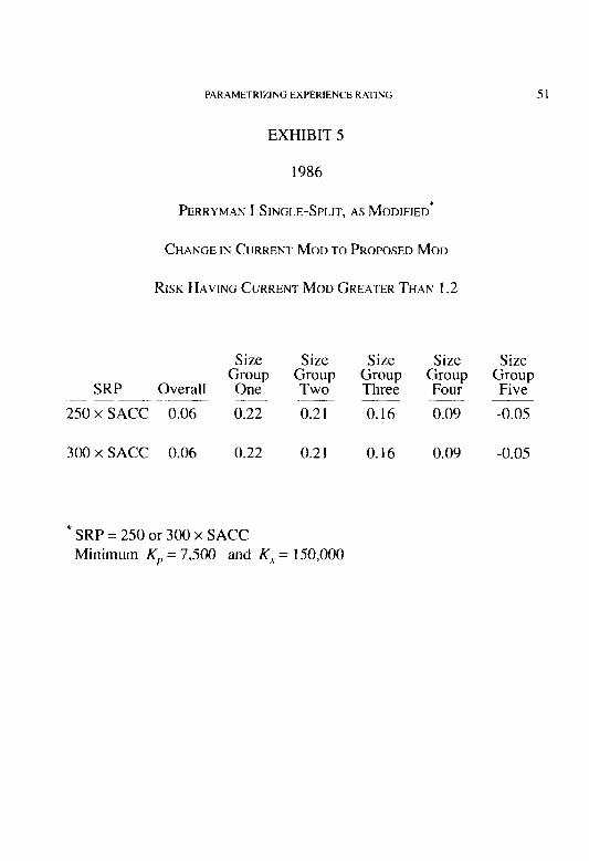
PARAMETRIZING EXPERIENCE RATING 51
EXHIBIT 5
1986
PERRYMAN I SINGLE-SPLIT, AS MODIFIED*
CHANGE IN CURRENT MOD TO PROPOSED MOD
RISK HAVING CURRENT MOD GREATER THAN 1.2
Size Size Size Size Size
SRP Overall Gcnzp G+:“,P Group
Three z--r Group Five -~~ _~~- ~____
250 x SACC 0.06 0.22 0.21 0.16 0.09 -0.05
300 x SACC 0.06 0.22 0.21 0.16 0.09 -0.05
* SRP = 250 or 300 x SACC Minimum K,=7,500 and K-, = 150,000

Range of Number of Current Mod Risks
0.80-0.84 18
0.x5-0.x9 620
0.90-0.94 IO,95 I
0.95-0.99 13,522
1.00 682
I .o I- 1 .os 2,307
1.06-1.10 1.675
1.11-1.15 1,278
1.16-1.20 1,066
Over 1.20 3,576
Totals 35.69;
With minimum K,, = 7,500 and mi
SRP = 250 x SACC
G = SACC + 1,000
Mods Limited
Average Current
Mod
0.83
0.88
0.93
0.96
.oo
.03
.0x
.I3
.1x
.35
.o I
Average Pro osed
d Od
0.79
0.84
0.88
0.93
1.03
1.08
1.30
I .‘h
1.31
1.49
1.03
Change
-0.04
-0.04
-0.05
-0.03
0.02
0 .os
0. 12
0.13
0. I3
0.14
0.0 1
nimum K, = 150,000

PARAMETRIZING EXPF.RlEiWE RATING 53
The following table lists the limits by size.
Expected Loss Size Maximum Modification
0 < E < 5,000 1.6
5,000 I E < 10,000 1.8 10.000 I E < IS,000 2.0
Exhibit 6 is similar to Exhibit 4 and shows that the swing problem is greatly reduced by this action.
No transition program was designed to phase the maximums out, ex- cept the impact of inflation. As experience rating eligibility increased, fewer risks would enjoy a potential I .60 cap.
Although this action was largely pragmatic, it was not without some actuarial justification. Mods higher than the stated limits are probably not deserved, statistical arguments notwithstanding. The test results only showed that mods were correct for the worst 20% of risks O/I adage. Other testing (not shown), using higher percentiles than the XOlh, showed the new formula could result in unreasonably high mods, at least for the smallest risks. In addition, risks just below eligibility have a maximum modification of unity. There should be some continuity at the point of eligibility.
Exhibit 7 shows the quintiles test statistics for the finalized plan. These statistics compare reasonably well with the statistics shown in Ex- hibit j--Part I.
In the matter of a split point, the subcommittee also recommended that appropriate trending be applied to the single-split point used in the testing so that it would have the same relativity to the loss size distribution when actually applied. Trending was based on several years of change in the average cost per case, which led to the single-split point of $S,OOO used in the filing. This is a reasonable value, given that it will be well after 1990 before the revised plan is widely accepted, and a few more years after that before any study can be done to revise the point.
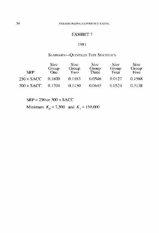
PARAMF.TRI7ING 1:SI’FRIENCl’ K/U’INCi
EXHIBIT 7
SUMMARY-Q~UNTILES TEST SI~ATISTICS
Size Size Size Size Size
SRP c;;;o,“,p
?bY %lz E-rp Group Five
250 x SACC 0.1800 0.1183 0.0546 0.0127 0.1588
300 x SACC 0.1704 0. I 1 so 0.0645 0.0524 0.3138
SRP = 250 or 300 x SACC
Minimum K,, = 7,500 and K, = 150,000

PARAMETRIZING EXPERIENCE RATING 55
Still, several researchers thought $5,000 might be too high. After all, the single-split worked well because of its resemblance to a frequency/se- verity model, and $5,000 may be too high to resemble just claim fre- quency.
The rationale for such a high selected value was twofold. First, there would be no automatic adjustment, and the $5,000 would be retained until a study could be made to determine the optimal value. Second, the resul- tant D-ratios for the single-split point would not have to decrease dramati- cally from the ones in the former plan. Loss size trend would make primary losses increasingly resemble claim count.
It should be noted that a conscious decision was made not to index the split point. As a consequence, it can be expected that average D-ratios will decrease over time. Primary credibilities should be monitored. An initiative to study indexing the split point can be expected in the future.

56 PARAMIiTRl%lh(; I!SI’lIKIt:N~I: R.Yl’liY~;
[ 1 J Hewitt, Charles C.. Jr.. ‘Credibility for Severity,,” PC’AS LVII, 1970, p. 138.
12) Meyers. Glenn G., “An Analysis of Experience Rating.” PCAS LXXII, 1985, p. 278.
[ 3 1 Mahler, Howard C., Discussion of “An Analysis of Experience Rat- ing.” PCAS LXXIV, 1987, p. I 19.
[4] Venter, Gary G., “Credibility.” F‘olltldutiou~~ of‘ C’iisirrIlty A(Tru~t-irrl
.‘ZWW, Casualty Actuarial Society. IWO. Chapter 7.
[Sj Hewitt, Charles C., Jr.. “Loss Ratio Distributions-A Model.” PCAS LIV, 1967. p. 70.
[6] Dorweiler, Paul, “A Survey of Kisk Credibility in Experience Rating,” PCAS XXI, 1934, p. I.
[7] Simon, LeRoy J., and Bailey, Robert A., “An Actuarial Note on the Credibility of Experience of A Single Private I’asw~ger Car.” PCAS XLVI, 1959, p. 159.
181 Perryman, Francis S., “Expericncc Rating Plan Crctlibilities,” PCAS XXIV, 1937, p. 60.
57
THE COMPUTATION OF AGGREGATE LOSS DISTRIBUTIONS
JOHN P. ROBERTSON
Paul R. Halmos recently hailed the fast Fourier transform as one of the 22 most sigmjicant developments in mathematics in the last 7.5 year-s. This paper provides an application of this tool to the computation of aggregate loss distributions jiiom arbitrary frequency and severity distributions. All necessary mathematics is delveloped in the paper, complete algorithms arc given, and examples are provided. Slrfficient details are given to ullo~~ implementation in any computer’ language, and sample APL computer language routines are gillen. The final section includes a discussion of excess loss distributions where computation is not limited to the fast Fourier transform based algorithm.
I thank Walter R. Stromquist, Joseph L. (“Joth”) Tupper, Gary G. Venter, and the Committee on Review of Papers for their help with and suggestions regarding this paper.
1. INTRODUCTION
According to Halmos [ 11, the fast Fourier transform is one of this century’s most significant mathematical developments. This paper pre- sents an algorithm for computing aggregate loss distributions using this device. The algorithm assumes that one knows the claim count distribu- tion, T (the probability distribution of the number of claims that will occur), and the severity distribution of a single claim, S = S, = S2 = . . . (the distribution of the amount of a single claim). The algorithm computes the aggregate loss distribution,
AGG = S, + S, + . . . + S,

(the distribution of the total amount of claims). The algorithm applies to arbitrary frequency and severity distributions.
As an example, claim counts might be expected to follow a Poisson distribution with mean 10, and severity might be expected to follow some distribution with mean $10,000. This implies that the mean of the aggre- gate distribution is $100,000 (10 times $10,000). In any given year, the total amount of claims might vary from $100,000 because the actual number of claims might differ from 10. and because individual claims will vary from the $10,000 mean. The aggregate distribution expresses the probabilities of the possible total amounts of claims in the same way the severity distribution expresses the probabilities of the amounts of a single claim.
The algorithm given here is less of a “black box” than some other algorithms presented in these Procwrlin~~,s in the following way. The algorithm, as a matter of course, computes the distribution for the sum of n claims, where II is any number of claims with nonzero probability in the claim count distribution. While the computer routines presented herein do not Save these distributions, only trivial programming changes are needed to capture and save these distributions for later USC. Capturing these dis- tributions can be useful when the resulting aggregate distribution has unexpected properties and one wants to check that it is being correctly computed, or for other reasons.
The method presented here should be considered to be approximate. Technically, it is an exact method, but it is generally necessary to use an approximation of the severity distribution as input, and this makes the output approximate. The running time for the algorithm is roughly pro- portional to the number of claims expected. For small numbers of claims, this method seems to be faster than other methods (e.g., Heckman and Meyers [Z]), but this advantage disappears as the number of claims grows. The algorithm presented here explicitly computes the entire aggre- gate distribution up to a specified limit, making it easy to derive any statistics of the aggregate distribution.
A quick overview of the algorithm is as follows. Everything in this summary will be described fully below, as it is not possible to give brief
AGGREGATE LOSS DISTRIBUTIONS 59
rigorous definitions of all the concepts used. The severity distribution will be given a discrete representation; that is, the severity distribution will be represented by a vector. The n-fold (discrete) cmvolutions of this vector with itself are computed. The result of these convolutions is very nearly the vector representation of the jr-fold sum of the severity distribution with itself. The precise representation of an n-fold sum will be obtained by computing the convolution of this result with another vector (de- scribed later) to “spread out” the result a bit more. This representation of the density function for the n-fold sum of claims is multiplied by the probability of there being exactly n claims, and these products are added to get the vector representation of the aggregate distribution.
The discwte Fourier- transform is used to compute the convolutions, and the fbsf Foul-ier rnmsform is used for rapid computation of the dis- crete Fourier transform. Convolutions, discrete Fourier transforms, and fast Fourier transforms are defined and discussed in Section 2. The pur- pose of this discussion is to introduce these items and to give examples so the main structure of the algorithm will be clear, The technical details are in the appendices. Additionally, Section 2 discusses the vector used to “spread out” the n-fold convolutions of the vector representing the sever- ity distribution. Two tactics used to speed the overall computations are also covered.
Section 3 of the paper walks through the full algorithm. Section 4 gives examples and discusses use of the algorithm. Sufficient details are given throughout the paper that it should be possible to implement the algorithm in any computer language. As an example, various appendices show routines implementing the algorithm in the APL computer language.
2. CONVOLUTIONS AND THE FAST FOURIER TRANSFORM
Conwlutions
The distribution of the sum of two random variables is given by the ~~nr~~lur~~n of their respective distributions. Heckman and Meyers [2, p. 321 discuss convolutions for the case of continuous random variables. In this case, if X, and X, are independent continuous random variables with

density functions fand g, then the density of the sum of these two vari- ables, i.e., the density of the random variable X, +X,, is given by the convolution off’and ,q, f*g, defined as:
fp,q) (I) = j f(f) g(.\- - 1) t/f 0
For the algorithm presented here, the probability distributions for the severity of a single claim and for the sum of II claims will be given certain discrete representations; that is, they will be represented by certain vec- tors. It will be necessary to compute the convolutions of these vectors. The definition of the convolution of vectors is similar to the above defini- tion of the convolution of continuous functions. Let U = (q,, II,. . . ., II,, _ ,) and V = (IS,,, I’,,. . ., I’,~ _ , ) be two vectors of the same length, 17. Their dis- crete convolution, W = U*V, is a vector of length II defined by:
I, I
M’i = c 11, I’; -/ ?
, -0
where 0 <: i 5 12 - 1 and the indices of the terms I’; _ i arc taken module II. For example, if U = (1, 2, 3) and V = (4, 5, 6) , then
U*V=(lx4+2x6+3x5, 1x5+2x4+3x6. 1x6+2x5+3x4)
= (31, 31,28).
This definition of convolution is not exactly what is needed here. The rro-lz~~~ cxvndrrfion of U with V is defined to have the following compo- nents:
M’i = i ui I’; _ ; .
, =o
That is:
I’() = 14() I’(],
M’, = If0 I’, + Ii, 1’() ,

AGGREGATE LOSS DISTRIBUTIONS 61
M’l = U() 1’2 + 14, l’, + II? I’,, )
M’ ,I- I = f4,) l’,, _ , + 11, I’,, _ ? + . . . + u,, _ ] 1’(, .
The no-wrap convolution of (1,2,3) with (4,5,6) is (1x4, 1x5+2x4. lx6+2x5+3x4)or(4, 13,28).
The no-wrap convolution can be visualized, as below, by taking one vector, reversing it, and placing it so that its first element is directly below the first element of the other vector, Then successively shift the vectors together, multiply elements in the same column, and add the products. Repeat this until the vectors are completely aligned.
No-wrap Convolution
I 2 3
6 s 4
lx4
In contrast, for regular around as shown below:
1 2 3 1 2 3 6 5 4 6 5 4
1x5+2x4 1x6+2x5+3x4
convolutions, the bottom vector is wrapped
Regular Convolution
I 2 3 1 2 3 1 2 3
4 6 5 5 4 6 6 S 4
1x4+2x6+3x5 1x5+2x4+3x6 1x6+2x5+3x4
The analogy of the definition of no-wrap convolution for discrete vectors to the definition of convolution in the continuous case should be clear.
One can obtain the no-wrap convolution of two vectors from a routine that computes (regular) convolutions by padding each of the two vectors to the right with enough zeroes to double the length of each vector, performing the regular convolution with these longer vectors, and then
62 A(;GKIG\TII i.OSS l~lSTK1lil”I IO\\
taking just the left half of the result. For example. the first three compo- nents of the convolution ot u = (/I,,. II,. If,, 0. 0. 0) with V = (I-,,, r, ~ I’?, 0, 0, 0) are:
M’(, = II,, \‘() + II, x 0 + 112 x 0 t- 0 x 0 + 0 x \‘, + 0 x I‘,
W’, = 11() l’, + II, I’,, + II? x 0 + 0 x 0 + 0 x 0 + 0 x 1’2
= II,, 1’, + II, \‘(, :
M’? = II,) \‘? + II, \‘, + I& I’,, + 0 x 0 + 0 x 0 + 0 x 0
The first definition ol‘ convolution will always hc ~~scd (unless other- wise noted). but generally Lcroes will be added lo the vectors being convolved so as to achieve a no-wrap convolution.
Observe that the definition of convolulion i\ \,alid when the vector elements are complex numbers.
A note on notation is needed. The vector U has components u,,, u,, +, etc., sometimes denoted U[O], UI 1 I. U13 J. etc. In parricular. the indices of vector elements start at zero.
Complex numbers and complex roots of‘ unity are used extensively in what follows. The prin?iti\~c II r/1 _ I oot.v of’wzit~ arc
cos(3m/r7) + i sin(kr/77).
where (I and t7 are relatively prime and i is \‘-I The properties ot’ corn- plex numbers needed here are reviewed in Appendix A. and arc also given in Baase [3, p. 2791 and Aho. Hopcrati. and IJllman 14, p. 252).
Given a complex (or real) vector Il. the discrete Fourier transform of lJ is a complex vector of the same length. As in Baase 13. p. 2691, for II 2 1, let 0 be a primitive lath root of unity, and let F be the II x 17 matrix with entriesf) . . , = w’.’ where 0 i i,,j < 17 - 1, The discrctc Fourier transform

AGGREGATE LOSS DISTRIBUTIONS 63
(DFT) of the n-vector U = (u,,, II,, . . . . u,,- ,) is the product FU (with U treated as a column vector). This is a vector of length n with components:
0 0 110 + II 0 If ] + . . . + 0 0 u,, - 1 + II 0 u,, - , , 0 w I 44,) + 0 14, + . . . + 0 I, - ?lI ,I - 2 + 0” - ‘u,, - , *
0 w u,, + 0’11, + . . . + w ‘(” - %,, _ 2 + d” - ’ )I,,, _ , ,
w 0
MO + 0 r,-11~,+...+O(~1-l)(n-2)U,,_~+O(~1~I)(,I-I)U ,,-, .
(Note that the DFT of U depends on the o chosen.)
Let FU be the DFT of U. Given FL’, U is recovered (i.e., the inverse DFT is applied to FU) as easily as FU is computed from U. To obtain U from FU, compute the DFT of FU, divide each resulting term by II, and reverse the order of the last II - I elements of this result.
The DFT helps compute convolutions because
DIT(U*V) = DFT(U) x DFT(V) , or
U:kV = INVDFT(DFT(U) x DFT(V)),
where INVDFT is the inverse DFT.
Thus, to compute the convolution of two vectors, one can compute the DFT of each vector, multiply the DFTs together pointwise, and compute the inverse DFT. This is known as the convolution theorem, proofs of which are given in Baase [3, p. 2781 and Aho, Hopcraft, and Ullman [4, p. 2SS].
For example, let U be (I, 2, 3), let V be (4, 5, 6), and let 0 = -0.5 -t 0.866i, a primitive third root of unity. Then FU is (6, -1.5 - 0.8661’. -1 .S + 0.8661’), FV is (15, -I .S - 0.866i. -1.5 + 0.866i), and the pointwise product, FU x FV, is (90, 1.5 + 2.5981, I.5 - 2.598i).

64 AGGKEGATI: LOSS IXSTKIHL’TIONS
To compute the inverse DFT of this last vector. first apply the (forward) DFT to obtain (93, 84. 93). Then divide each element by 3 and reverse the order of the last two elements, giving (3 1. 3 I, IX). This matches the pre- vious computation.
A more thorough example showin, u the convolution of two vectors representing severity distributions is given in Appendix B. This appendix also discusses the inverse DFT.
The jksr Fourirr trun.yfhnr (FFT) is a particularly fast method for computing the DFl- (and the inverse DFT) for long vectors. Appendix C gives Baase’s 13. p. 27.31 version of the complete fast Fourier transform and inverse FFT. Appendix D gives an APL implementation of these algorithms.
Why use such a complicated method to compute convolutions (i.e., using the convolution theorem and FFTs)? This method is used because, for long vectors, it’s much faster than more straightforward methods (such as computing directly from the definition of convolution). Knuth 15, Vol. 2, p. 65 1 ] discusses the number of calculations needed to compute the fast Fourier transform. Using the FFT to convolve vectors of length I .024 (2”‘) gives a gain in speed by a factor of about 60 compared to the “naive method” of convolution. The time needed by the naive method for computing convolutions of vectors of length II is proportional to II’. More precisely,’ it is O(n’). The time needed by the method using the convolu- tion theorem and the fast Fourier transform is proportional to nln(n)(O(,lln(n))), where )I is the length of the vectors convolved. For large II. trln(rz) increases more slowly than H’,
In the literature there are several different definitions of the DFT and FFT that accomplish the same goals but differ in certain details. Be care- ful before trying to use the algorithms presented hcrc in conjunction with algorithms that appear in other sources or are available in libraries ot
’ That the number ol’computations is OCf(u)) means that there 15 ;I constant c such that the number of computations is less than C’ x,f(ll) fix- all II greater than sonic’ II,.. See Knuth 15. Vol. 1. p. 104).

AGGRECiATE LOSS DIS‘I’KIBl!TIONS 65
computer routines. For example, using the forward FFT from another source with the inverse FFT given here could produce erroneous results. Other routines for the DFT and FFT can certainly be used, as long as all the routines used are consistent among themselves.
In addition to Baase [3, p. 2681, the fast Fourier transform is discussed from several different viewpoints in Knuth [5, Vol. 21, Press, Flannery, Teukolsky, and Vetterling [6, p. 3901, Preparata (7, p. 2071, and Aho, Hopcraft, and Ullman [4, p. 2571. Each of these discusses the theory behind the FFT, thereby explaining what the FFT is doing and showing why the FFT is so efficient. Chiu [8] gives an introduction to the fast Fourier transform motivated by the problem of exact multiplication of large integers. A detailed implementation of the fast Fourier transform suitable for Fortran and similar languages is given in Monro 19, p. 1531. Convolution is discussed in Hogg and Klugman [IO, p. 421, Feller [ 11, p. 61, and many other statistics books.
Other methods that use the fast Fourier transform to compute aggre- gate loss distributions are given by I. J. Good in Borch [ 12, p. 2981 and by Bertram [ 13, p. 1751. The method presented in the latter is summarized in Biihlmann [14, p. 1161.
3. THEALGORITHM
The collecti\~e risk model will be used to model the claims process. That is, the aggregate loss distribution is the distribution:
AGG=S, +Sz+ . ..+S.,
where T is a random variable for the number of claims and each Si is a random variable for severity. It is assumed that the Sj are identically dis- tributed and are pairwise independent and that the S, are independent of T. This definition of aggregate loss distribution is the same as that given by Algorithm 3.2 in Heckman and Meyers 12. p. 301. This model is discussed in Biihlmann [ 15, p. 541, Beard, Pentikiinen, and Pesonen [ 16, p. 501,

Patrik and John [ 17, p. 4 121. and Maycrson. Jones, and Bowers [ 18, p. 177).
There are three inputs to the algorithm. The first. denoted M, is the smallest number of claims that has nonzero prohabilit!, in the claim count distribution. The second, P, is a \‘ector giving the probability density function of the claim count distribution. P(i) is the probability that there are exactly i + M claims for i 2 0.
The third input, S, is a vector representing the severity distribution as a piecewisc uniform distribution. Due to technical considerations involving the fast Fourier transform. the length. II. of S will be an integral power of two; i.e., II = 2” for some positive integer X. Let 1. be the maximum size of claim considered. Then each element J, of S represents the probability
that a given claim is at least ‘L but Icss thn (i+ 1)
I1 /I L. The probability
distribution is unifonn across each $uch interval. In other words, the probability density function.,f(.v). of the claim size distribution is:
I 0. for .V < 0 or .Y L L.
As an example, if L is $16,0(W) and S is (0.50, 0.30. 0.15, 0.05). then there is a 50% probability that any given claim is between $0 and $4,000, a 30% probability that the claim is between $4.000 and $8,0(K). etc. The density function is uniform over the intcrvai $0 to $4,000 at .000125 (= 0.50 + 4,000). Similarly, the density function is uniformly .00007S: i.e., (0.30 + 4,000) over the interval $4.000 to $X,OW, and so on. This is graphed in Figure I. Note that this specification of the severity distribution is the same as that in Heckman and Meyers 131 but rchtricted to uniform intervals.
Define S’ inductively as follow%. Let S’ be the vector of length 2n obtained by catenating II zeroes onto S. That is.
‘St! = 5,. if 0 I i </I - I: 0, ifn I i I 2rr - I.
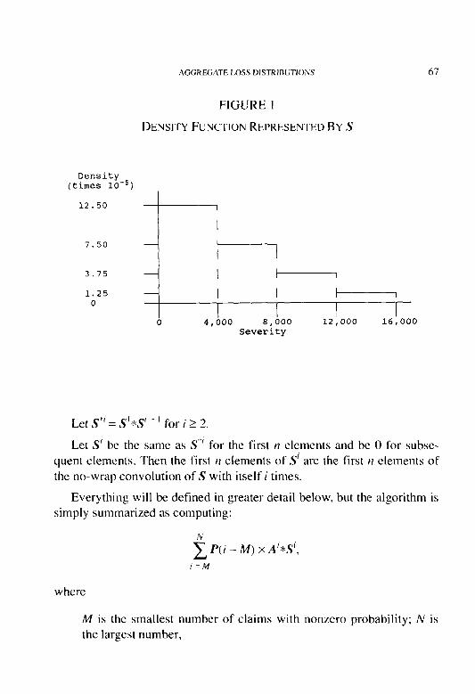
AGGREGATE LOSS DISTRIRlITIONS 67
FIGURE I
DENSITY FUNCTION REPRESENTED BY S
Density (times lo-')
12.50 I
I
7.50 r-----l
3.75 I 1
1.25 1 0
0 4,000 8,000 12,000 16,000 Severity
Let S*’ = S’*S’ - ’ for i 2 2.
Let S’ be the same as S*’ for the first II elements and be 0 for subse- quent elements. Then the first II elements of S’ are the first II elements of the no-wrap convolution of S with itself i times.
Everything will be defined in greater detail below, but the algorithm is simply summarized as computing:
N
c P(i-M)xA'*S',
I = M
where
M is the smallest number of claims with nonzero probability; N is the largest number,

6X AGGREGSI’I; LOSS INS I’KIHI TlOhiS
P(i - M) is the probability of exactly i claims.
A’ is a vector of “spreads” to be defined later. but. for example, A-’ = ( 1%. 7~. ‘hi. 0, 0, 0, . . . . 0).
* is the discrete convolution operator. and
S’ is the vector that is the no-wrap convolution of the severity distri- bution. S. with itself i times.
Very roughly speaking, S’ is the dcnxity function of the sum of the original severity distribution, S, with itself i times. However, it needs to be “spread out” (in a way that will be made prccisc below). Certain vectors of coefficients, A’. to be defined shortly. will hc used to “spread out” the S’. The distribution of exactly i claims is given by A’ -:: S’. More precisely, A’ :j: S’[j] for 0 5,; I II - I is
where F’(.Y) is the distribution function for the sum of the severity distri- bution with itself i times. For II 5,; :I 2r? - I the values of A’ 2: S’[,j] are not meaningful.
To see why the A’ are needed, let S be a uniform distribution on the interval 0 to 1. Let 11 and L be 4. Then S = ( I. 0. 0.0). Doing the convolu- tions gives S’ = S’ = ( I, 0, 0, 0, 0, 0. 0, 0) for all i. But the distribution function of the sum of the uniform distribution on (0. I 1 with itself should have nonzero probability not only between 0 and 1. but also between I and 2. In fact, this distribution should be ( ‘A. ‘A. 0, 0. 0, 0, 0, 0). Simi- larly. the sum of this distribution with itself three times should be (l/b, Z/J, l/h, 0. 0. 0. 0. 0), which has three nonzero terms. A’ ~1: S’ will be (!h, I/“. 0, 0, 0, 0. 0, 0). and A’ ;/: S’ will be ( l/i,, 77. G,. 0. 0. 0. 0. 0).
If S were a discrete distribution. instead of the picccwise uniform distribution used here, the A’ would not bc necess~y. (That S = (.s,), .Y,. . . . )
is discrete means that if .Y is i L. for some i from 0 to 11 - I. then the f?
AGGREGATE LOSS DISTRIBUTIONS 69
probability that a claim equals s is si; for others, the probability is 0. An example is given in Appendix B.)
Use of a piecewise uniform severity distribution roughly doubles the running time of the algorithm compared to the time required for a similar algorithm using a discrete severity distribution. The use of a piecewise uniform distribution is suggested because the author believes that fre- quently a piecewise uniform approximation with II vector elements gives a better approximation to the severity distribution than does a discrete approximation with 2n vector elements. If the severity distribution is more accurately approximated, then the resulting aggregate loss distribu- tion is more accurately approximated. Also, due to memory limitations in many computers, it is often possible to compute the aggregate distribution using the piecewise uniform approximation with II vector elements, but it is not possible (easily) to compute the aggregate distribution using a discrete approximation with 212 vector elements.
In the next subsection the coefficients A’ are defined so they will provide the needed spread. Then, the following two subsections cover two special tactics that substantially speed the running of the algorithm. Then, the full algorithm is discussed.
The Coe$%ients A’
Define a,; by:
u;, = I/i! for i2 I,
a; = 0 forj2 I,
I a;= -; t I’ I (i-j)~jI~+o’+l)~;-’ 1 fori22,jZ 1.
Table 1 gives the first few values of ui. For example,
A’ is the vector of length 211 whose first II elements are given by the a;, and whose last 12 elements are zero. For example, A’ = (I/,4 I’/24 ‘Vi4 ‘h 0, 0, . . . , 0). -. . .i,
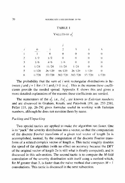
70
TABLE 1
VALUES OF U;
The probability that the sum of i unit rectangular distributions is be- tween ,j and ,j + 1 for i 2 1 andj 2 0 is U: This is the reason these coeffi- cients provide the needed spread. Appendix E shows this and gives a more detailed explanation of the reasons these coefficients are needed.
The numerators of the (I;, i.e., i!uj , are known as Euleriun mnhw and are discussed in Graham, Knuth, and Patashnik [ 19, pp. 253-2581. Feller [ 11, pp. 26-291 gives formulae useful in working with Eulerian numbers, although he does not mention them by name.
Two special tactics are applied to make the algorithm run faster. One is to “pack” the severity distribution into a vector, so that the computation of the discrete Fourier transform of a given real vector of length 2n is accomplished, instead, by the computation of the discrete Fourier trans- form of a related complex vector of length 12. This tactic roughly doubles the speed of the algorithm (with no effect on accuracy because the DFT of the original vector of length 2n is still what is finally computed), and is discussed in this sub-section. The second tactic is to compute the M-fold convolution of the severity distribution with itself using a method which, for M greater than 3, is faster than the naive method that computes M - 1 convolutions. This tactic is discussed in the next subsection.
AGGREGATE LOSS DlSTRlBUTlONS 71
The fast Fourier transform operates on vectors of complex numbers, but here it is used only to transform vectors of real numbers. As such, half of the place values are not really being used, because the imaginary parts of the elements of the input vector are all zero. Clever use of certain symmetry properties of discrete Fourier transforms of purely real vectors and purely imaginary vectors, as discussed in Press, et al. 16, p. 3981, allows the following.
To transform the length 2n vector V = (vo, v,, . . . . I’~,~- ]), where each V; is a real number, rewrite V as PV = (11~~ + iv,, v2 + A,,, . . . , Q,~ _ 2 + iq,, _ ,), where i is 6. This is now a complex vector of length II. PV is referred to as the ~‘crc$~d urztr-urz.sfo,med vector (it is packed because it is written in a more compact form; it is untransformed because the discrete Fourier transformation has not yet been applied). Compute the discrete Fourier transform of PV, and call it FPV. FPV is the packed trunsforn~ed vector. Some simple computations on FPV, called ~c~pucking, yield FV, the (un- packed) discrete Fourier transform of V. While FV is a vector of length 212, if the first n + 1 elements of FV are known, then the remaining n - 1 elements can be deduced using a formula from Appendix F. Similarly, one can pack the transformed vector in such a way that when the inverse discrete Fourier transform is applied, the untransformed vector appears in the form of PV. Note, in particular, that to apply the convolution theorem to real vectors of length 2n, one can instead work with complex vectors whose lengths never exceed II + I.
Packing and unpacking the untransformed vectors is trivial. Depend- ing on how one represents real and complex vectors this might be a simple rearrangement, or just a redefinition of the meaning of each ele- ment of an array. Usually no calculations are needed. Packing and un- packing the transformed vectors does involve some calculation, but not a great amount. Details of the algorithms to pack and unpack are given in Appendix F, and an APL implementation is given in the functions PACK and UNPACK in Appendix G.
Table 2 shows the steps involved in computing the convolution of two real vectors when one packs the vectors.
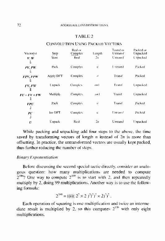
72 AGGRlJ~iAl’I: I.OSS I~IS’I‘RIHI IIONS
TABLE 2
CONVOLUTION USING PACKED VE(‘TOKS Real or ‘I‘rall\~ ,)I
S(q) Complc\ I .crlglll Cilllrarlsl stxt Real 7/i lintrarl~l
Vector(s) v. w
II PC’, PW’
u
FPV, FPW u
FV. FW 8
FU=FVxFW u
FPU u
PC: ii
L’
While packing and unpacking add four steps to the above, the time saved by transforming vectors of length II instead of 2n is more than offsetting. In practice, the untransformed vectors are usually kept packed, thus further reducing the number of steps.
Before discussing the second special tactic directly, consider an analo- gous question: how many multiplications are needed to compute 2’““‘? One way to compute 2”“’ is to start with 2, and then repeatedly multiply by 2, doing 99 multiplications. Another way is to USC the foilow- ing formula:
3°K’ II ((((( 2’ x 2 )‘)y x 2)‘)J . i
Each operation of squaring is one multiplication and twice an interme- diate result is multiplied by 2, so this computes 3”K’ with only eight multiplications.

AGGREGATE LOSS DISTRIBUTIONS 73
In general, to compute u” for II 2 1, one can apply the following algo- rithm. Express II as a binary number, h, and drop the left-most digit (which is always 1). Set r equal to m. Loop: if there are no digits left in h, then stop; f is u”. If there is at least one digit remaining in h, square 3. If the current left-most digit of h is 1, then multiply z by (I. Drop the left- most digit from h. Go back to the step labeled “Loop.”
The binary representation of 100 is 1100100. Dropping the first digit gives 100100. Following the steps above, set z to 2, then square, multiply by 2, square, square, square, multiply by 2, square, and square.
This is called a left-to-right binary nwtlml for c~,~l~oncrzriation and is discussed in Knuth [5, Vol. 2, p. 4411 (along with even faster methods).
This is used as follows. For some applications of the overall algo- rithm, the smallest number of claims with nonzero probability, M, will be greater than one. In these cases, this method is used to compute s” =s * s 3: ... 1: S (with M factors of S, here the :/: is the no-wrap convo- lution). That is, M is written as a binary number, and the left-to-right binary method is applied, with no-wrap convolution at each step instead of multiplication. Since convolution is associative, SM is well defined, and this is a correct way to compute S”.
Now the full algorithm can be described. Figure 2 outlines the algo- rithm using a flowchart. The notation used is described in the presentation of the complete algorithm, below. A summary of the meaning of each variable is given in Table 3.
The complete algorithm is as follows.
Al~cywithnz ji)r. Aggregate Loss Distribution: Let M be the smallest number of claims with nonzero probability, let N be the largest number of such claims (N 2 1 and N 2 M), let P be the vector of probabilities of M, A4 + 1) M + 2, . . . . N claims, and let S be the vector representing the density function of the claim severity distribution. The length of S is II = 2’ for some positive integer k. All vectors are indexed starting at 0, so
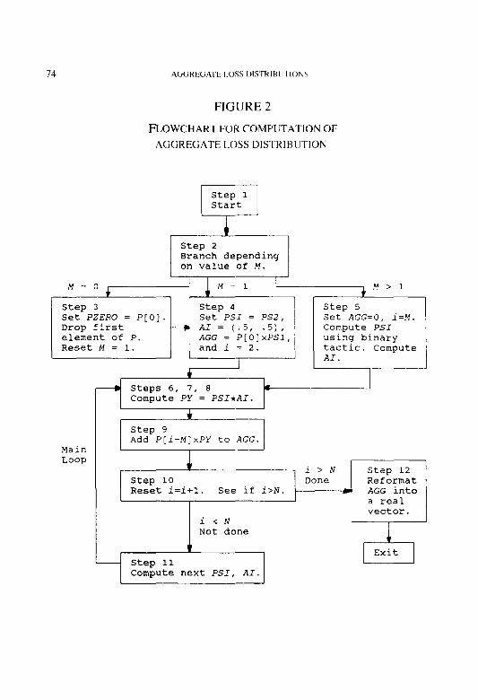
ACiGKEGATE I.OSS [NSTKIBIl~l’IONS
FIGURE 2
FLOWCHARTFORCOMPUTATIONOF AGGREGATELOSS DISTRIBUTION
step 1 Start
i Step 2 Branch depending on value of M.
M>l
Step 3 Step 5 Set PZERO = P[O]. Set PSI = PSZ, Set AGG=O, i=M. Drop first AI = (.5, .5), Compute PSI element of P. AGG = P[O]xPSI, using binary Reset M = 1. and i = 2. tactic. Compute
Stew 6. 7. 8
Main LOOP
Compute'PY'= PSI*AI.
4 --I
Step 9 Add P[i-M]xPY to AGG.
1 i>N Step 12 Step 10 Done Reformat Reset i=i+l. See if i>N. 4 AGG into
a real vector.
isN Not done
I v
I I Exit Step 11 Compute next PSI, AI.
I I

AGGREGATE LOSS DISTRIBUTIONS 7.5
TABLE 3
VARIABLES USED IN THE MAIN ALGORITHM
INPUT VARIABLES: II Length of vectors which will be subjects of the Fm or inverse FFT.
)j = 2” for some positive integer r(.
M Smallest number of claims with nonzero probability.
N Largest number of claims with nonzero probability.
P Probabilities of M through N claims @II = probability of M claims. pt = probability ofM + I claims, . ..).
S Severity distribution. S is a real vector of length II. s = (so, Sl, . . . . s,,- I)
MAJOR VARIABLES: i Index giving the current number of claims.
PSI Packed severilydistribution, (so + is 1, sz + iq, . . . .s,~ - 2 + ;,s,~ - I, 0. 0, . . . . 0). (Here i is 6.)
FSI Transformed (unpacked) severity distribution.
PSI Packed severity distribution convolved with self i times.
SI Severity distribution convolved with self i times. (Unpacked PSI.) FSI Transformed severity distribution convolved with self i times.
AI Vector of spread coefficients, (u[). a{, . ..) = A’ AGG Aggregate distribution.
MINOR VARIABLES: PZERO Probability of zero claims.
B/N Initialized to the binary representation of M, and used in the binary exponentiation tactic.
F.VFLAC Flag to determine whether FSI has been computed for the current i.
X Unpacked PSI. .i Index used in Step 7.
Y Becomes AI*X. PY Packed Y.
FAI Transformed Al. FY Transformed Y = FSI x FAI.

76 A(;(;KfiCi<Yl I. f OSS f)l\ I KIf(I I ION5
the indices for S run from 0 to II - I. The result will be AGG. ;t vector representing the aggregate distribution.
I.
3 i.
3.
4.
5.
[Some initializations. J Set AGG IO be ;I complex vector 01’ length 17 all of whose elements are zero. Pack S into the complex vector PSI of length II so:
PSI = i
so + is,, .S? + is,. . . . . .\‘,) > + is,, ). 0, 0. . . . . 0 )
.
Here i is ~5. Set PZERO, the probability of exactly 0 claims. to 0.
[Branch depending on the value of M.] If M is 0, go to Step 1. ifM is I, go to Step 4. If M is greater than I. go to Step S.
(Initialize if M = 0. ] Let PZFRO hc P( 0 I. Drop the first clement from P. Let M be I.
(Initialize if A4 = 0 or I.] Let AGG bc P(O] times PSI. IfN i\ I, go to Step 10. Let FSI be the unpacked DFT of PSI. Let PSI bc the in- verse DFT of the packed pointwise product ofFSI with itself. Set the last /l/2 elements of PSI to 0. Let AZ bc the two-elcmcnt vector (0.5,O.S). Let I’ be 3. Go to Step 6.
[Begin procedure if M > 1.1 Let H/N be the binary representation of M. Drop the first (left-most) digit from BIN. Let FSf and FSI be the unpacked DFT of PSI.
5.1. [Convolve PSI with itself or PSI with itself. ] Let FSZ be FSI times itself. Let PSI be the inverse DFT of the packed FSI. Set the last rr/2 elements of PSI to 0. If the first digit of BIN i\ 0. go to Step 5.3.
5.2. [Convolve PSI with PSI. ] Let FSZ be the unpiicked DFT of PSI. Let FSI be FSZ times FSZ. Let PSI be the inverse DFT of the packed FSZ. Set the last t1/2 elements of PSI to 0.
5.3. ICheck whether finished.] Drop the first digit from HIN. If there are no digits left, go to Step 5.4 Othcrwi>e. let FSZ bc the unpacked DFT of PSI. Go to Step 5.1.
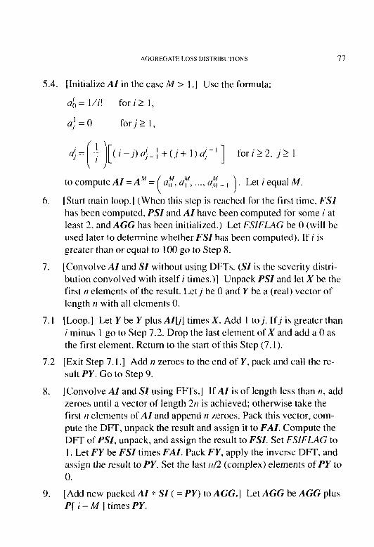
AGGREG.ATF I.OSS DfSTRfR~ITIONS 77
5.4. [Initialize AZ in the case M > I.] Use the formula:
cl;, = l/i! fori 1,
a; =o forj2 I.
ll; = t I[
1 (i-j)ujIi +(,j+ I),:-‘] forik2, ,j> 1 I to compute AZ = A”’ = ut, a?, . . . . dt-, . Let i equal M.
6. [Start main loop.] (When this step is reached for the first time, FSZ has been computed, PSI and AZ have been computed for some i at least 2, and AGG has been initialized.) Let FSlFLAG be 0 (will be used later to determine whether FSZ has been computed). If i is greater than or equal to 100 go to Step 8.
7. [Convolve AZ and SZ without using DFTs. (SZ is the severity distri- bution convolved with itself i times.)] Unpack PSI and let X be the first 17 elements of the result. Letj be 0 and Y be a (real) vector of length II with all elements 0.
7. I [Loop.] Let Y be Y plus AZ[j] times X. Add 1 to,;. Ifj is greater than i minus I go to Step 7.2. Drop the last element of X and add a 0 as the first element. Return to the start of this Step (7.1).
7.2 [Exit Step 7.1.1 Add 17 zeroes to the end of Y, pack and call the re- sult PY. Go to Step 9.
8. ]Convolve AZ and SX using FFTs.] If AZ is of length less than II, add zeroes until a vector of length 2n is achieved; otherwise take the first II elements of AZ and append II zeroes. Pack this vector, com- pute the DFT, unpack the result and assign it to FAZ. Compute the DFT of PSI, unpack, and assign the result to FSZ. Set FSIFLAG to 1. Let FY be FSZ times FAZ. Pack FY, apply the inverse DFT, and assign the result to PY. Set the last /r/2 (complex) elements of PY to 0.
9. [Add new packed AZ * SZ ( = PY) to AGG.] Let AGG be AGG plus P[ i - M J times PY.
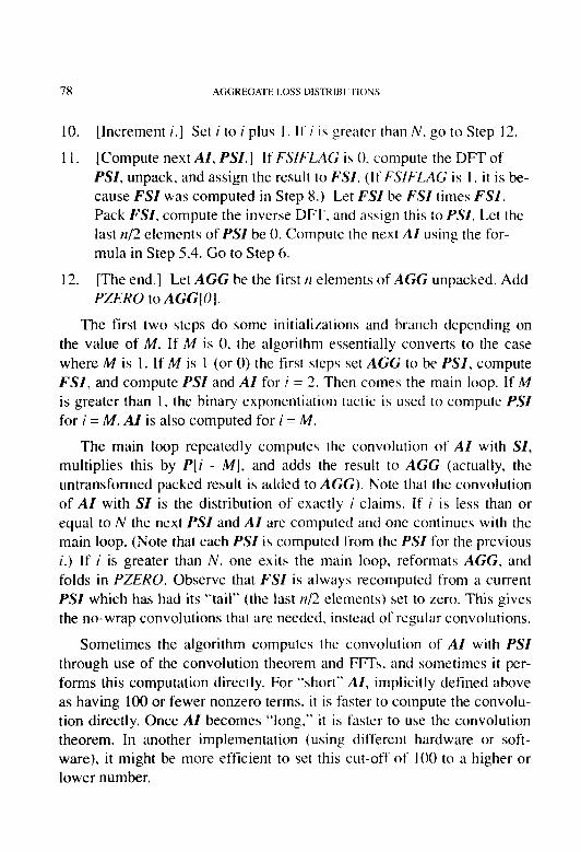
78
10.
Il.
12.
AGGREGATE LOSS DISTRIBLITIONS
[Increment i.] Set i to i plus 1. If i is greater than N, go to Step 12.
[Compute next AZ, PSI.] If FSfFLAG is 0. compute the DFT of PSI, unpack, and assign the result to FSZ. (If FSIFLAG is 1, it is be- cause FSZ was computed in Step 8.) Let FSZ be FSZ times FSZ. Pack FSZ, compute the inverse DFT, and assign this to PSI. Let the last n/2 elements of PSI be 0. Compute the next AZ using the for- mula in Step 5.4. Go to Step 6.
[The end.] Let AGG be the first II elements of AGG unpacked. Add PZERO to AGGIOJ.
The first two steps do some initializations and branch depending on the value of M. If M is 0, the algorithm essentially converts to the case where M is 1. If M is 1 (or 0) the first steps set AGG to be PSI, compute FSI, and compute PSI and AZ for i = 2. Then comes the main loop. If M is greater than 1, the binary exponentiation tactic is used to compute PSI for i = M. AZ is also computed for i = M.
The main loop repeatedly computes the convolution of AZ with SZ, multiplies this by P[i - M], and adds the result to AGG (actually, the untransformed packed result is added to AGG). Note that the convolution of AZ with SZ is the distribution of exactly i claims. If i is less than or equal to N the next PSI and AZ are computed and one continues with the main loop. (Note that each PSI is computed from the PSI for the previous i.) If i is greater than N, one exits the main loop, reformats AGG. and folds in PZERO. Observe that FSZ is always recomputed from a current PSI which has had its “tail” (the last /r/2 elements) set to zero. This gives the no-wrap convolutions that are needed, instead of regular convolutions,
Sometimes the algorithm computes the convolution of AZ with PSI through use of the convolution theorem and FFfs, and sometimes it per- forms this computation directly. For “short” AZ, implicitly defined above as having 100 or fewer nonzero terms. it is faster to compute the convolu- tion directly. Once AZ becomes “long,” it is faster to use the convolution theorem. In another implementation (using different hardware or soft- ware), it might be more efficient to set this cut-off of 100 to a higher or lower number.

AGGREGATELOSSDISTRIHUTIONS 79
Note that if there are fewer than II nonzero terms in AZ only the nonzero terms are kept, and one pads to the right with zeroes when a vector of length n is needed. This differs slightly from definitions of AZ given earlier.
APL functions implementing the complete algorithm are given in Ap- pendix H.
4. EXAMPLESANDADDITIONALDISCUSSION
This section will give some examples of the use of the algorithm, show how parameter uncertainty can be reflected in the aggregate distri- bution, and discuss the computation of aggregate excess distributions. Comments in the first two areas are specific to this fast Fourier transform algorithm, but comments on the third topic apply generally.
Escrmples
Three examples of use of this algorithm will be given. The first is simple and is intended to be easy to reproduce in order to test an actual implementation. It is not meant to be realistic. The second example is more typical of actual distributions that arise in practice. The third exam- ple is reasonably realistic, but is really meant to illustrate the flexibility of the algorithm .
The first example will compute the distribution of esactfy five claims, with each claim following a uniform severity distribution. Let k = 5, so n = 32. (That k = 5 has nothing to do with the fact that the distribution of five claims is being computed; this is a coincidence.) The claim count distribution is defined by setting M = 5, and making P be a vector with one element, (1). The severity distribution, S, is a vector of length 32 (= n), and L is set to 6.4, so each element of S covers a range of 0.2 (= 6.4/32). Letting S be the uniform distribution on [O,l], gives:
s= (0.2,0.2,0.2,0.2,0.2, o,o, . ..) 0).
The output is a vector of length 32, AGG, a complete listing of which is given in Table 4. Since the sum of five claims, each no greater than 1, cannot exceed 5, only the first 25 elements of the output are nonzero. It is

,4(;C;REC;ATE LOSS l)lS I KIHt I’I0Y.S
TABLE 4
AGGREGATE DISTRIBUTION FOR EXAMPLE I
‘umtllalixe Lh~tl-ibution
0.000003
o.ooooxs
(1 OOOfr4X
1~.1)017: I
0.00x333
0 070713
0.044.3Y1
o.ox1Ill
0.143x I I
O.~2SO(10
0 33Xlfl
0.4-lfI.~ I2
Cl.SSY6XX
(l6-~4lx-1
0 7:(too
o.xsflIxo
().Y I xiw
11.‘~5Sf,OX
(l.o-o’;i
0.w lOh7
0 Y’l7’f,Y
(l,‘NO3S’
O.YWY IS
O.YY‘iYY7
I .(H~0000
I .fI00000
I .0lKI000
I .oooooo
I .IHtoooo
I .fMKMMMl
I .0000O0
I .ooofn,o
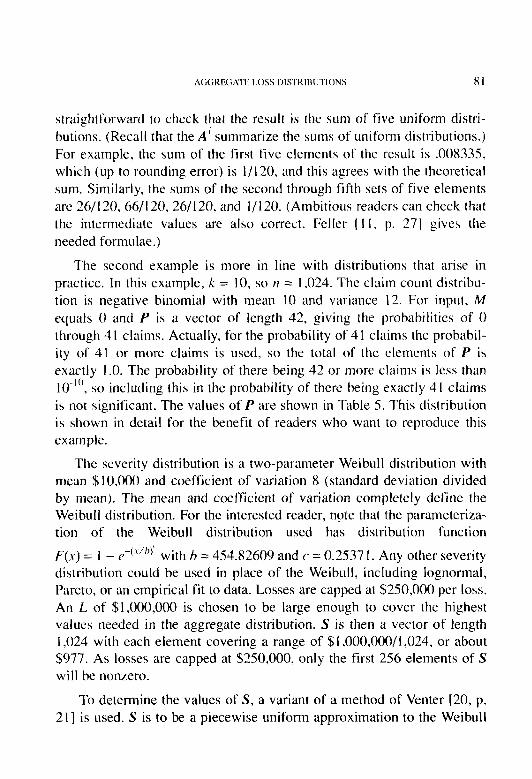
straightforward to check that the result is the sum of five uniform distri- butions. (Recall that the A’ summarize the sums of unifoml distributions.) For example, the sum of the first five elements of the result is .008335, which (up to rounding error) is l/120, and this agrees with the theoretical sum. Similarly, the sums of the second through fifth sets of five elements are 26/120, 66/120, 26/120, and l/120. (Ambitious readers can check that the intermediate values are also correct. Feller ( I I, p. 271 gives the needed formulae.)
The second example is more in line with distributions that arise in practice. In this example, k = 10, so II = 1,024. The claim count distribu- tion is negative binomial with mean 10 and variance 12. For input, M equals 0 and P is a vector of length 42, giving the probabilities of 0 through 41 claims. Actually, for the probability of 4 1 claims the probabil- ity of 41 or more claims is used, so the total of the elements of P is exactly 1.0. The probability of there being 42 or more claims is less than IO-“‘, so including this in the probability of there being exactly 41 claims is not significant. The values of P are shown in Table 5. This distribution is shown in detail for the benefit of readers who want to reproduce this example.
The severity distribution is a two-parameter Weibull distribution with mean $10,000 and coefficient of variation 8 (standard deviation divided by mean). The mean and coefficient of variation completely define the Weibull distribution. For the interested reader, note that the parameteriza- tion of the Weibull distribution used has distribution function Q) = , _ ,-WJ’ with h = 454.82609 and c = 0.2537 I. Any other severity distribution could be used in place of the Weibull, including lognormal, Pareto, or an empirical fit to data. Losses are capped at $250,000 per loss. An L of $ I ,000,OOO is chosen to be large enough to cover the highest values needed in the aggregate distribution. S is then a vector of length 1,024 with each element covering a range of $1,000,000/1,024, or about $977. As losses are capped at $250,000, only the first 256 elements of S will be nonzero.
To determine the values of S, a variant of a method of Venter [20, p. 21) is used. S is to be a piecewise uniform approximation to the Weibull

AG(iRE(iAll~ I OSS I)ISIRIWII'I IONS
TABLE 5
CLAIM COUNT DISTRIBCII'ION FOK ExAhwx2
6
Proh;rhilttb ol(i~~cn Nunher of Cluirw
I .(lOt(XSE.-4
Y l57(17t-4
O.(HJWJ 17s
11.01 I7J28J
0.f Jl4X17Y.5
0.1 J4W~O.i I
0.1J~~X276Xh
o.o’~lo3Sxl
0. I~JK10’1K~
0.i I61 12x1
0. I I4 I7760
0. IO37Y7X I o.cIx7’1!‘JsI
O.(KYYIXJXX
lJ.(,S74366
o.oi73xo47
0.(13511 I YX
0.01 h?.33(lS
(1.01(11 i2i.l
0.00h0-&3Y7
0.003475~x
0.0IJ1Y~071
o.(#Jlo3x1Y
S.4IXZIE-3
?.74673E--I
I .?55OSE-4
b.S I-WE-5
3,lJSh1?7E-5
I.J007YE-5 h.?7Y4OlA
2 75SYhE-6
I. I XS.W-6
5.00074E-7
2.07101t:-7
X.42h I7E-x
?.370371~-x
I .32hsIE-S 5 I iX I E-‘J
I .YhlKa-U
7.37.x-10
1.735li. IO
I .S6OE- ItI
(‘umulative lktrihulion
I .OYXGL-I
I .03WF-3
0.004’) 17%
0.l~lhlhfJI’~
0.040Yxx14
O.OXSh7X1S
0.15305531
0.744YY I I?
(1.7S309615
0.16Y2089h
O.SXiXhSh
0.6X71X437
0.775 174 IX
O.X-tSO2SO6
O.XY7JSO71
O.Y347? 1 I Y O.OSYY71 I7
0.0763062!
O.OXhkw7h
O.YY24X27.1
o.YYsYsxo I
O.YY7XXX7.3
iLYW927”
(I.YYY469O-l
1).91)97437 I
o.YYYx7Yzz
0.9909443h
O.YYY97JYl
O.YYYYXXY.3 o.YYoYYs2 I
0.9YYYY7Y7
ll.YWY9V IS
O.YYY9YY65
0.9YYYYYXh
0.999YYYYJ
O.YYY99YYX
ll.OYYY9YYY
I .OO~J(HJOO~1
I .cmMKXKl
I 00mGi’00
I 1HJ0ooMJ0
I .000(H)rN)o

AGGREGATE LOSS DISTRIBUTIONS x3
distribution. To achieve this, pairs of consecutive elements (szi, s,; + ,) of S are chosen subject to two constraints:
l over each interval 2i . ,b [
, (2i + 2). f 1 the integral of S and the inte-
gral of the Weibull density are the same, and
l over the same intervals the integral of the first moment distribution of S and the first moment distribution of the Weibull are the same.
If RR and SS are the integral of the density function and the integral of the first moment distribution of the Weibull (or whatever distribution is being approximated) over the above interval then
S?i f 1 = RR - S2i
No properties of the Weibull are used in the formulae above; they apply to any distribution, including empirical distributions.
When this method is applied in this particular case, the second element of S becomes negative. Thus, some additional fiddling is done on the first 12 elements of S so that the two constraints are satisfied for these 12 elements taken together, but not pair-wise. Selected values for S (includ- ing the first 12 elements) are shown in Table 6. Note in particular that the value of .007072 is the probability of the severity being in the interval $249,023 to $250,000 plus the probability of the severity being over $250,000. This latter probability has been spread over the interval.
Selected values of the resulting aggregate distribution are shown in Table 7. Column (3) is selected elements of the vector AGG output by the algorithm. Each element, ti, of AGG is the (exact) integral of the density function for the aggregate distribution over the interval
[ i. k, (i + 1) . t 1 . For the purpose of interpolating values between inte-
gral multiples of L + n it is assumed that the density at each point in an L
interval is ti + - i 1
. Column (4) is the distribution function, n

x-l ,\(;(;Kl.GAl’t: l.OSS HIS IKIIII I’IOhS
TABLE 6
Index High End of Range’” 0 .FY77 I I ,YS3 7 2,Y30 3 3.YO6 4 4.xX3 5 S,XSY 6 6.X36 7 7.813 x X,7XY Y Y.766
IO 10,712 II 11.7lY I2 11,695 I3 13,672 14 14.648 IS IS.625 74 73,343 75 73,219 76 75.195 77 76. I72 78 77.148
101 YY.609 IO2 lOO.SX6 IO3 IO I .S63 123 I2 I ,OY4 124 I-73 070 --, 11s 13-3.047 135 230.36’) ‘36 33 I.445 237 132,423 253 238,047 254 24Y.023 355 250.000 256 250,977
I.073 I .ooo,ooo
Probahilit, Di\trihution of’:! Single Claim Sjil Distribution
0.7 I6463 0.7 I6463 0.1 142x1 0.x3074.5 0.0 I5000 0.x45745 0.0 IS000 0.X6074.5 0.0 I0000 0.x7073.5 0.005000 0.x7574.5 0.005000 0.880745 0.005000 o.xxs74s 0.003000 o.xxx74s 0.003000 O.XY 173.5 0.003000 O.XY474S 0.003000 O.XY7745 0.004750 O.YO14Y4 0.004 I40 O.YO6634 0.003xx3 0.Y 1 OS 1 x 0.00344 I 0.‘) I.1955) 0.00033 I O.Y734X5 0.00032 I O.Y73XOh 0.0003 I6 0.974 I22 0.000307 O.Y7442Y 0.000.30? O.Y74737 0.000 IO3 O.YXO24Y 0.000 I Y2 O.YXO440 0.000 1 x7 0.08062X 0.000 I.17 O.YX3X I Y 0.000 I36 O.YX3YSS 0.000 133 O.YX4OXX 0.000( I-1 I O.YY22 I3 0.00004 I O.YY7154 0.000040 O.YY13Y4 0.000035 O.YY2XY3 0.000035 O.YY2Y2X 0.007072 I .oooooo 0.000000 I .oooooo 0.000000 1 000000
*Each range has width of about 977.

Index (1)
0 I 2 3 4 s 6 7
I7
I3
I4
I.5
74
7.5 76
77
7x
123
124
12s
1 so
I.51
I.52
I.53
IS4
235
236
237
253
‘S3
1.55
256
2x3
%‘I
2x5
4 I Y
420
I .O?:!
I.023
AGGREGATE LOSS I~ISTKIBLU’IONS
TABLE 7
DISTRIBUTION OF AGGREGATE Loss AND FIRST MOMENT DISTRIBUTION FOR EXAMPLE 2
First Moment Distribution
High End of Range*
(2) $Y77
I .Ys3
2,030
3.YO6
4.w
S,XSY
6,X36
7.x I3
12.6’)s
Ii.672
I4.643
IS.625
73.242
74.2 10
7S.lYS
76.172
77,14x
I z I .OY3
1’7.070
123.047
147,461
14x.43x
14Y.414
I so.30 I
IS I.367
230.469
23 I .us
‘32,422
24X.047
24Y.0’3
?x~,000
2SO.Y77
177.344
278,320
279,2Y7
410.156
411,133 YYY.013
I ,000,00(1
ACG]il (3)
O.OO?X I?
0.010576
0.02 I673
0.03 I2 I4
0.036 I?4
0.0363SX
0.033s IO
0.02Y3 I?
0.0135 I7
0.0121.53
0.0 I I327
O.OlOY36
0.003 I34
0.0030x2
0.00303 I
0.0029x I
0.002Y31
0.00 IS53
0.00 IS34
0.00 IS IS
0.00 I 13x
0.00 I 17s
0.00 I 1 Ii
0.001 IO1
0.00 IO00
0.000520
0.000s I6
0.0005 I2
0.000453
O.OOO44Y
0.000.507
0.000x.30
0.000836
0.000x I3
0.0007Y2
0.0000Y7
0.000096
0.000000
o.ooooao
Distribution
14) 0.002x I?
O.Oli3X7
0.03506 I
0.06617.5
0. IO23YY
O.I3X7SX
0. I727hX
0.20 I sxo
02046.50
0.306802
0.3lXI2Y
0.37YOhS
0.69 I222
O.hYJ304
0.6Y7315
0.7003 16
0.70374x
0.7YX766
0.X00300
0.X01X16
0.x34470
O.X3SSYS
O.X367OY
0.x37x IO
0.x3x’)00
O.XYYXXY
0.900405
0.900’) 16
0.90x.5x’)
O.YOYO3X
O.YOYS46
0.9 10376
O.YJY7 I6
0.0.50s30
0,‘)s I317
O.YXYYX.3
o.YYooxo
0,YYYYYfl
0.Y90006
X5
L)en~itYF:‘:
(5) I.373
15.3Y2
51.913
I Oh.hXY
151(.7.50
lYS.1X4
311.71’
214.6X7
I6.5.00.5
IhO.
I60.3XX
165.53’)
22x.013
2?7.2lY
236.4 I x
225.61 I
x4.797
I X7.3OY
IXh.SlY
185.732
167.1X0
166.3Y4
165.X02
165.114
164.429
I I Y .60X
IlY.16X
I IX.731
I 12.035
1 I I .63S
126.x54
707.Y73
23 I .42 I
‘35 0x0 --.
720.846
3’) ,907
3Y .S46
0.052
0.05x
Distribution**
(6) I.372
16.X65
6Y.77X
176.467
33.5217
.S3O.SOl
743.213
YS7.YOO
I ,xX4.273
2.044.4x’)
‘33.X77
2.370.4 16
lh.lS4.Y7X
16.3X2.197 16.60X.6 IS
Ih.X.34.226
17.OSY.O7-3
xl.306.213
26.492.741
26.67X.473
3 I .076. I I3
3 I .24?.606
3 I .40x.40x
3 I .s73322
31.737.YSl
43.0X6.466
43.205.634
43.374364
45.166396
4.5.27x.03 I
45.404.5’)5
45.6 I2.569
ss.xY3.oxI
56, I IO.061
56.33Y.YOX
6X.X2X.765
6X,X6X.3 I2
73.x04.42 I
73.x04.479

86 AGGREGATE LOSS L)ISTRIRIITIONS
f,, + t, + . . . + t,, i.e., the cumulative sum of Column (3). Column(4) readily gives the dollar amounts (frequently called c~c@~errce /e,~ls in the con- text of aggregate loss distributions) associated with given probability lev- els, and vice versa. For instance, the probability that aggregate losses will be less than or equal to $250,000 is 9 1 .O%~. By simple interpolation, it is seen that $75,000 corresponds to the 69.7% confidence level. Again through interpolation, the 80% confidence level is $ I2 1,879.
The expected dollars of loss above and below given aggregate limits can be quickly determined. Suppose. lbr example. an insurer has pur- chased reinsurance that covers all loss amounts beyond a total of $250,000. That is, the insurer pays the first $250,000 of losses (which could be one claim or a number of claims), and the reinsurer pays any losses after the first $250,000. The insurer’s cxpccted loss is:
where.f’(.\-) is the density function of the aggregate distribution. As Col- umns (5) and (6) in Table 7 will help calculate this integral, these col- umns are described next.
Each entry in Column (5) is I .~,f’(.\-) tl\- over its interval. For instance, under the above assumption that the density function is a constant 0.036358 + 976.5625 across the fifth interval, I .v,~‘(.v) r1.v over the fifth interval is
(5,859.375)’ - (4,882.X 125)’ x 0.036358 2 976..5625
or 195.282. (This is slightly different from 195.284 shown in Column (5) because the Column (3) entry of 0.036358 is used in the above calcula- tion, while more significant digits were used in the calculation of Table 7.) Column (6) is the cumulative sum of Column (5). Thus, Column (6) gives

AGGREGATE LOSS DlSTRlBtiTl0N.S 87
where i is the index of the interval.
Returning to the original question, if losses are capped at an aggregate of $250,000, Columns (6) and (4) show that expected losses are 45,405 + 250,000 x [I - 0.9095461, or $68,019.
The reinsurer is taking both occurrence and aggregate excess of $250,000, and total expected losses are $100,000 (10 expected claims times $10,000 expected loss per claim), so the reinsurer’s expected losses are $3 I ,98 1 ( 100,000 - 68,019).
Generally, to compute expected losses for an insurer that retains a given amount per occurrence and retains a given aggregate, use a severity distribution capped at the per occurrence limit, compute the aggregate distribution, and compute the expected retained losses up to the aggregate limit as was just done above.
The third example is a variation on the second example. The main purpose is to show how easy it is to use an arbitrary frequency distribu- tion in the algorithm. For this example, the above frequency distribution is modified to assume that there is a 90% probability that claims will follow the distribution in example 2, and an additional 10% probability there will be exactly 20 claims. The same S as above is used. The modi- fied P is shown in Table 8, and some of the output is given in Table 9.
Note that the severity distribution, S, used in examples 2 and 3 is only an approximation to the Weibull distribution. Essentially, having to find a piecewise uniform function to approximate the true severity distribution, with each interval being the same size, L + n, means that S is not going to be precisely the same as the original continuous function. Since S is an approximation to the true severity distribution, the output is an approxi- mation to the true aggregate distribution. Comparisons of aggregate loss distributions computed using this algorithm to aggregate loss distributions
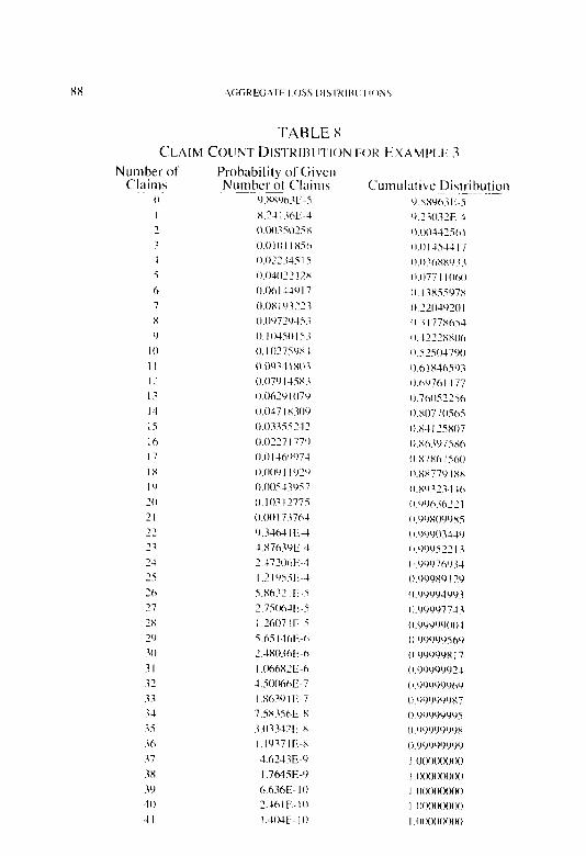
xx
TABLE X CLAIM CO~JNT DISTKIIW’IWN FOR EXAMPLE 3
Number oi Claims
0 I 2 3 1 5 6 7 x Y
IO II 12 Ii I-l IS I6 17
IX
I Y
20
LI
12
23
24
2.5
‘6
27
28
79
30
31
32
i 3
3-l
3s
36
37
3x
2’)
40
-!I
Probability of Given Number ot Claim\
Y.XXYOZE-s X.‘JlW>E-4
0.003503x
0.0101 IXSh
O.O72%S I .i
0.040’? 17x
O.Ohl 11’J I7
O.OXlY3~2.~
O.OY77Y45.3
0.104.50 I?.?
0. IO175Ot(4
O.OYil I x03
0.1)7’Jl1SXi
O.Oh’7YlO7Y
0.017 IX.30’~
0.1)33SS,42
0.0?7 I77Y
0.0 I Jh‘V)71
0.00’l I IO3
0.00.543Y57
0.l03l 2775
0.00I 7.37hJ
Y.34cAlI-4
4,X763YE-4
7,4710riE-4
1.2lYS5li-1
S.Xhi2 I E-i
?.7SOh-IE-s
I .X07 i F-5
S.65 I JOE-(1
2.4xo~oIl-(,
I .06hX2E-0
13XKhE-7
I .X630 I E-7
7.5X35hE-8
3.0334211-8
l.lY37lEh
.l.hX.?E-Y
I .764SE-Y
h.hihE- IO
2.-lhlF-IO
I .JodF.- IO
C‘umulativc Distribution ‘LXXYhili-5 Y.13033-4 I~.ow125hl
1~.Ol4SJ417
O.OlhXXY33
!).077 I IOf,O
0. IiX55’J7X
l~.‘x~1Y~ol
0 .I 177X654
~l.J222XXOh
I).5,5047’JO
l).bl %Km3
r)hYlhI 177
0.7hO.S12.Sh
o.xo77l15hS
0.x4 I1SXO7
o.xmY7sxh
O.X7Xh7Xdl
o.xx77Y)-Ixx
~I.X~l323-M lr.o~Kvl2~ I
(I.YOX0YYX.i
(l.‘J’JUOWW
f ~.YYYS21 Ii
f l.‘J~JO7h’J34 O.OYYXY I 2’)
‘l.~JY~JYl’J~J3
t l.‘FJOY7743
(l.YYYY)4004
O.‘J’)“)YWhY
O.YOYYYX I7
o.YoYYYY2~
~~.‘)‘)‘)0Y)‘wl4
O.‘J’J’J’J’JOX?
0 Y’JYYYYYS
0 00’J’J’)‘FJx 0 ‘J’JYYO~J~J~J
I 0000001H~
I 000otHM~
I .00O00000
I .0fI~HH)0~I0
I .0I)0000ot~
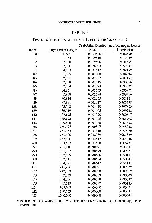
AGGREGATE LOSS DLSl-RlBUTlONS
TABLE 9
DISTRIBUTION OF AGGREGATE LOSSES FOR EXAMPLE 3
89
Probabilitv Distribution of Aggregate Losses Index High End of Ra& Distribution
0 $971 0.002530 1 1,953 0.012049 2 2,930 0.031555 3 3,906 0.059647 4 4,883 0.092 I59
82 8 1,055 0.684594 X3 X2,03 1 0.68745 I 84 83,008 0.690266 85 X3.984 0.693039 X6 84,961 0.695772 87 85,938 0.698466 xx 86,914 0.701121 x9 87,X9 I 0.703738
138 135,742 0.797823 I39 136,719 0.799228 140 137,695 0.8006 I 7 141 138,672 0.801992 142 139,648 0.803352 256 250,971 0.898052 257 25 1,953 0.899470 25X 252,930 0.901529 259 253,906 0.904046 260 254,883 0.906734 297 29 I ,O I6 0.948843 298 29 I.992 0.94952 I 299 292,969 0.9SOl87 300 293,945 0.95084 I 301 294,92 I 0.95 1482 451 441,406 0.989829 452 442,383 0.9899 I9 453 443,359 0.990009 454 444,336 0.990097 455 445,313 0.990 I85
1,021 998,047 0.99999 I I.022 999,023 0.99999 1 1,023 I ,ooo,ooo 0.99999 I
* Each range has a width of about 977. This table gives selected values of the aggregate distribution.
AdG[i] 0.002530 0.0095 I8 0.019506 0.028093 0.0325 I2 0.002900 0.002857 0.0028 I5 0.002773 0.002733 0.002694 0.002655 0.0026 I 7 0.00 I420 0.00 1405 0.001390 0.001375 0.001360 0.000847 0.001418 0.002059 0.002517 0.002688 0.00069 I 0.000679 0.000666 0.000654 0.000642 0.00009 I 0.000090 0.000089 0.000088 0.000087 0.000000 0.000000 0.000000

90 AGGREGATE LOSS DISTRIHI~TIONS
computed using other methods indicate that the algorithm presented here gives very accurate answers.
Apart from the need to use a severity distribution that is an approxima- tion to the true distribution, the algorithm here is precise in the following sense. Each element of the aggregate loss vector is the exact difference of the distribution function for the exact aggregate loss distribution over the interval that corresponds to the element. In particular. this algorithm is not subject to the convergence difficulties sometimes encountered in certain characteristic function methods when the probability of a maximum loss is high. Of course, there is some potential for rounding error, but most computer languages have a provision for doing calculations to at least 17 decimal place accuracy, and as each element of the result (for n = 1,024; 20 expected claims) is affected by about 100,000 calculations. the result should be accurate to at least 12 places.
Note also, once Column (3) of Table 7 has been calculated, how simple and fast it is to calculate Columns (4). (S), and (6). Once AGG has been computed, there is very little computation time needed to determine confidence levels, expected losses subject to an aggregate, or expected losses excess of an aggregate. Also. since the entire aggregate loss distri- bution (up to some limit) is computed, the computation of any quantity that is related to the aggregate distribution (e.g.. expected sliding scale commission for a reinsurance contract) is straightforward and fast.
Comprrtutional Considerutinns
The computational time for this algorithm seems to be roughly propor- tional to the number of elements in the vector P that gives the probabili- ties of the claim counts. The minimum number of claims for which there is a nonzero probability also has some effect on the computing time. But, due to the binary exponentiation tactic, the added computing time in- creases only as the logarithm to the base 2 of the minimum claim count.
Using APL 9 on a 386SX computer with 2 megabytes of RAM, this algorithm will run with k as high as 10. This makes the maximum length of certain vectors 2”) or 2,048. Using APL 9, adding memory will not allow higher values of k because all arrays active at any given moment

AGGREGATE LOSS DISTRIBUTIONS 91
must fit in the workspace available in the first 640K of memory (and this is about 400K because the APL system occupies about 200K).
It is likely that, compared to the computer programs presented in the appendices, the computations can be made more efficient in terms of the amount of memory used. References discuss computing the fast Fourier transform “in-place,” which would use less memory than the programs given in the appendices. APL II, or other languages, might allow higher values of k due to better use of memory above the first 640K.
Increasing k by 1 roughly doubles the amount of memory needed, because the longest vectors double in length. Computational time is domi- nated by the time to compute the fast Fourier transforms, and this time increases by a factor of a bit more than 2 when k is increased by 1. See any of the references given above on the fast Fourier transform for a more precise discussion of the relationship between k and the time of computa- tion
To capture the distribution of the sum of i claims for any i with nonzero probability in the claim count distribution, just capture the PY for that i from Step 9 of the main algorithm, given above. When using the same severity distribution but differing claim count distributions to com- pute several aggregate distributions, the following method might save some time. Capture all the distributions of the sum of exactly i claims that will IX needed (the PYs above), and then just apply the probabilities given by the several claim count distributions and add. This can be much faster than recomputing each aggregate distribution from scratch.
Parameter Uncertainty
Patrik and John [ 171 distinguish process risk from parameter risk in estimating the distribution of final actual results relative to the estimated results. Essentially, if the frequency and severity distributions used are the best estimates of these distributions, then the calculated aggregate distri- bution reflects the inherent process risk or process uncertainty.
The extent to which the correct frequency and severity distributions are not known is termed parameter risk or parameter uncertainty. Some au- thors add specification error to the list of sources of potential difference

92 ACiGRKiATt: 1 OSS LlIS’I’RIHI~‘I IOhS
between actual and expected results. Spec~ijkution ctww refers to the fact that the model being used might not be appropriate. For instance, if it is known that the claim count distribution is Poisson, but the parameter of the Poisson distribution is not known exactly, then estimates of the aggre- gate distribution are subject to parameter uncertainty. If it is not known whether the claim count distribution is Poisson or some other distribution, then estimates are subject to specification error. Heckman and Meyers [2] discuss incorporation of parameter uncertainty into estimates of aggregate loss distributions.
Parameter Uncertainty for the Cluim Count Distribution
To reflect parameter uncertainty in the claim count distribution, one could proceed as follows. First, identify all claim count distributions that might apply, and assign to each claim count distribution the probability that it is the correct distribution. Then, for each claim count distribution (and using some severity distribution), compute the aggregate distribu- tion. Finally. take the weighted average of all these aggregate distribu- tions, according to the probabilities of the claim count distributions. The resulting aggregate distribution reflects the various claim count distribu- tions and the probabilities of those distributions.
For example, one might estimate there is a 20% probability that the claim count distribution is Poisson with mean IO; there is a 50% probabil- ity that the claim count distribution is Poisson with mean 20; and there is a 30% probability that the claim count distribution is negative binomial with mean 15 and variance 30. (This is not necessarily a realistic exam- ple.) Then, for instance, the probability of total losses being less than $X in the combined aggregate distribution would be 20% of the probability of losses being less than $X in the aggregate distribution generated by the Poisson claim count distribution with mean 10, plus 50% of the corre- sponding probability resulting from the Poisson distribution with mean 20, plus 30% of the corresponding probability from the negative binomial distribution with mean 15 and variance 30.
Fortunately, there is a shortcut that makes it possible to compute the aggregate distribution that reflects the uncertainty regarding the claim count distribution without computing a great number of aggregate distri-
AGGREGATE LOSS DISTRIBUTIONS 93
butions. Simply compute the weighted average of the claim count distri- butions, and then use this distribution in the computation of the aggregate loss distribution. For instance, using the above example, in the claim count distribution used as input to the main algorithm, the probability of i claims would be 0.2xf(i) + 0.5~ g(i) + 0.3x h(i), wheref, 8, and II are the probability density functions for the Poisson distribution with mean 10, the Poisson distribution with mean 20, and the negative binomial distribu- tion with mean 15 and variance 30. This combined distribution would be used as the claim count distribution in the algorithm to compute the aggregate loss distribution.
Generally, one will select a family of claim count distributions, and associated probabilities, so that the mean of the combined claim count distribution will be the expected number of claims. The variance of the combined claim count distribution usually will be greater than the vari- ance of the best estimate claim count distribution. The effect of the com- bined claim count distribution on the variance of the new aggregate distribution can be computed by using the formula for the variance of the aggregate distribution:
Here p,v and 0; are the mean and variance of the claim count distribu- tion and p,s and G: are the mean and variance of the severity distribution (Mayerson, Jones, and Bowers [ 18, p. 1791).
A particularly simple situation results if it assumed that the possible claim count distributions are Poisson and that the parameters of these Poisson distributions are distributed according to a gamma distribution with mean h and variance (3’. In this case, the resulting overall claim count distribution will be negative binomial with mean h and variance h + c?. This is discussed in Beard, Pentiktiinen, and Pesonen [ 16. p. 401 and in Heckman and Meyers [2].
As a practical matter, one frequently has a binomial, Poisson, or nega- tive binomial distribution as the best estimate of the claim count distribu- tion. To reflect parameter uncertainty in the claim count distribution used as input to the aggregate loss distribution algorithm, one might, where appropriate, simply use a claim count distribution with the same mean

and a larger variance than the best estimate distribution. For instance, if one’s best estimate of the claim count distribution is Poisson with param- eter h then, to reflect parameter uncertainty. one might use a negative binomial distribution with mean h and variance Iargcr than h.
The three families of claim count distributions mentioned above are related. For the Poisson distribution, the vuriancc and the mean are the same. The negative binomial has variance grcatcr than the mean. The binomial has variance less than the mean. The Poisson is a limiting case of the negative binomial in that, as the variance of the negative binomial approaches the mean, the negative binomial approaches the Poisson. The Poisson is also a limiting case of the binomial.
In conclusion, parameter uncertainty for the claim count distribution can often be reflected in the computed a ggregatc loss distribution by choosing an appropriate claim count distribution with the same mean and larger variance than the best estimate distribution. This allows one to reflect parameter uncertainty while computin, (3 onlv one aggregate loss _ distribution.
To retlect parameter uncertainty for the severity distribution. one can
proceed in the manner first discussed for the claim count distribution. That is. delineate all the severity distributions that might apply: assign to each a probability; compute the aggregate distribution using each severity distribution; and combine all of these aggregate distributions according to the probabilities of the severity distributions.
IJnfortunately, when estimating the effect on aggregate distributions of parameter uncertainty in the severity distribution there is no shortcut quite as efficient as the one for claim count distributions. That is. to reflect pa- rameter uncertainty for the severity distribution, it is not sufficient to use a severity distribution that is the combination of the various severity dis- tributions in the same way that it is possible to use a claim count distribu- tion that is the combination of the several claim count distributions. Later, it will be shown why this last statement is true, but methods of reflecting parameter uncertainty for the severity distribution will be covered first.
AGGRECXI-E LOSS IX‘iTRIBUI‘IONS 9s
Some simplification in the reflection of parameter uncertainty for the severity distribution results if all the possible severity distributions are (or are assumed to be) multiples of some base distribution. More precisely. this assumption is that if F,] is the distribution function of the base sever- ity distribution, B, and if F, is the distribution function of any other severity distribution in the family, Y, then there is a constant, C, such that F, (c-t-) = F, (s). Normally, this is written B = cY; it follows that E(Y) = (I/C) E(B), and Var (Y) = (l/c’) Var (B). Let the constants c be distributed according to a probability distribution with distribution func- tion H and density function h.
Let F,., be the distribution function of the aggregate distribution com- puted using the base severity distribution B (corresponding to F,,). Then the aggregate distribution reflecting parameter uncertainty. T. is given by
T(x) = j FJc:\-) h(c) dc.
If h has a form such that It(r) and r/z(r) are easily integrated over arbitrary intervals, and if F,, is piecewise linear, then T, above, is easily computed. For t in the interval [I,, ui] let F,,(f) = (1; + hir. Then
ca II, /I
;
II, i\ = c I Ui I?((‘) d(’ + hi-r c’h(c’) ~(’ I .
i = 0 I, /.I 1, /I 1 As a practical matter, the sums above are not taken to infinity, but
rather to a high enough value that sufficient accuracy is achieved. If h has been chosen so that the integrals are easy to compute, T is also easy to compute.
Next is the demonstration, promised above, that to reflect the effect of parameter uncertainty in the severity distribution, it is not sufficient to simply use a severity distribution with a larger variance. To see this,
96 ,AGGRECiN’F I.OSS I~IS’I’RIHI~‘I‘IO1\S
consider one way a simulation model could be used to estimate the aggre- gate distribution. Choose a claim count, II. at random from the claim count distribution, N. Then II times draw a random claim severity, Si, from the severity distribution, S. Compute s, + .x2 + . . . + x,~. This sum gives one “draw” from the aggregate distribution; that is. it gives one observation selected at random from the aggregate distribution. Repeat this process, i.e., make draws from the aggregate distribution, until the statistics of interest for the aggregate distribution are known with sufficient accuracy.
There are two methods one might use to reflect parameter uncertainty for the severity distribution when performing the above simulation. The first method is to choose a severity distribution at random each time a severity is needed. Within a given draw. .Y, + , would potentially be drawn from a different distribution than the preceding J,. A second method is to fix a severity distribution each time an II is chosen from N. This one severity distribution is used for all .Y, in the sum s, + .P? + . . . + s,, corre- sponding to one draw. Then another 11 is selected from N, and another severity distribution, possibly different from the severity distribution used in the previous draw, is used, and the process continues.
It is the second method that best reflects parameter uncertainty for the severity distribution. Under this method, only one severity distribution is used for each draw from the aggregate distribution. In contrast. under the first method, in many of the draws from the aggregate distribution, some claim amounts wili come from severity distributions with larger-than-av- erage means and some claim amounts will come from severity distribu- tions with smaller-than-average means. The effects of severity distributions with larger-than-average means and severity distributions with smaller-than-average means will tend to cancel each other to some degree. Thus, the first method will tend lo produce an aggregate distribu- tion with a smaller variance than is correct. Under the second method, each draw is influenced by only one severity distribution.
The first simulation method corresponds to using a severity distribu- tion that is the composite of the family of severity distributions being used to reflect parameter uncertainty. It is the second simulation method, where each draw is influenced by only one severity distribution, that

AGGREGATE LOSS DISTRIBUTIONS 91
corresponds to the methods discussed above for reflecting parameter un- certainty for the severity distribution,
The first and second methods differ fundamentally in the indepen- dence assumptions among samples from the severity distribution. A more mathematical discussion of the differences between the two methods, including a more precise discussion of the difference in independence assumptions, is given in Appendix I.
If a capped severity distribution is being used, e.g., losses are capped at $250,000 per claim, and if parameter uncertainty for the severity distri- bution is reflected using the method that assumes that all distributions are multiples of each other, then the loss cap becomes variable. In some cases, e.g., where the aggregate distribution of a self-insurance program with a given retention is being computed, it may not be appropriate to allow the loss cap to vary. There does not seem to be a simple way to reflect parameter uncertainty for the severity distribution in such a case.
One approach is to increase the degree of parameter uncertainty re- flected in the claim count distribution to a level above that which would otherwise be used, and to not reflect parameter uncertainty in the severity distribution. This approach is not theoretically correct, but, as a practical matter, might be sufficiently accurate. Another approach is to let the cap be essentially variable, and perform tests to determine whether this signif- icantly distorts the results. Finally, and with the greatest accuracy, one can compute a number of aggregate distributions, each using a different se- verity distribution with the correct cap, and take the weighted average.
The results of this subsection apply to all methods used to calculate aggregate loss distributions, not to just the algorithm presented herein. The main results of this subsection appear to be well known, but have not previously appeared directly in actuarial literature. Schumi (21, 221 has presented material similar to this result. Bear and Nemlick (231 present the result in terms of the negative binomial distribution.

OX AGGREGATE LOSS I)ISTRIBIITIONS
Suppose a claim count distribution, a severity distribution, and the corresponding aggregate distribution are specified, In regard to the sever- ity distribution. suppose further that the probability of any given claim being excess of a given attachment point 11 is (x. Suppose it is desired to compute the aggregate distribution l’or claims excess of ,4 (this A has nothing to do with the vector of spreads A used previously). For example, the aggregate distribution might be based on a Poisson claim count distri- bution with parameter 1.000 (i.e., the number of expected claims is 1,000) and a Weibull severity distribution with mean ri; 10.000 and coefficient of variation 8. If A is $100,000 then o! is 0.0 197.
One way to compute the excess aggregate distribution (the aggregate distribution for the amount of claims excess of A per claim) is to keep the same claim count distribution (e.g., Poisson with parameter 1,000 in the example) and adjust the severity distribution so that claims less than A become 0 and claims. X, greater than or equal to A become .\- - it. This gives a severity distribution that generally assighs 21 Iargc probability, namely I - CI, to claims being exactly 0.
Another way is to work directly with the excess claim count and severity distributions. The excess claim count distribution is the distribu- tion of the number of excess claims (the distribution of the number of claims exceeding A). The excess severity distribution is the claim severity distribution for the amount of individual claims excess of A. given that a claim is excess.
The main purpose of this subsection is to note that, for certain claim count distributions. the excess claim count distribution is easily deter- mined. Assume the claim count distribution is binomial, Poisson. or nega- tive binomial. respectively, with mean h and variance CT’. Suppose the probability of a given claim being excess of the attachment point A is cx. Then the excess claim count distribution is binomial, Poisson. or negative binomial, respectively, with mean cxh and variance aL t- a’(o’ - h).
The excess severity distribution is easy to determine if the total distri- bution and the attachment point are known. Suppose the severity distribu- tion has distribution function F. and the attachment point for excess

AGGRWATE LOSS DISTRIBUTIONS 99
claims is A. Then the excess severity distribution has distribution func- tion, H, defined by:
H(sr) = &I- + A) - F(A) __-~ , f0r.r 2 0. I - F(A)
That is, the portion of the severity distribution function below A is elimi- nated, and the remaining distribution is resealed so that H(0) is 0 and H(X) has limit 1 as .Y tends to infinity.
In the example, the excess claim count distribution is Poisson with parameter 19.7 (= 0.0197 x 1,000). The excess severity distribution is the above Weibull distribution restricted to claims exceeding $100,000. In particular, the probability of a claim being 0 is 0 (not 0.9803).
It should be clear that the excess severity distribution is as claimed above. Appendix J has a proof that the excess claim count distribution is as claimed. An interesting open problem is to find other claim count distributions for which the excess claim count distribution is of the same form as the original claim count distribution, or the excess claim count distribution is otherwise easy to compute.
For readers familiar with the notation in Heckman and Meyers, recall that they parameterize claim count distributions with 3c and C. In their method, the parameters for the excess claim count distribution are ah and C.
The above formulae for the mean and variance of the excess claim count distribution hold only if the parameters of the severity distribution are known with certainty. Venter provided the following formulas for the mean and variance of the excess claim count distribution N when o! is uncertainly known:
E(N) = hE(cx) ,
Var (N) = hE(cx) + (0’ - ~)E(cL)~ + ((T’ + h’ - h)Var (a)
Proofs are as follows:
E(N I cx) = ah, so E(N) = E(E(N I a)) = hE(a).
IO0 AGGREGAI’E LOSS I)IS I’Kll3l~‘l’lOhS
Var(NIcx) = ah + c?(cc - A) . so
Var (N) = E(Var (N I CX)) + Vitr (E(N I a))
= hE(a) + (CT’ -- h)E(&) + h’Var ((x)
= hE(a) + (& - h)]Var (a) + E(a)‘] + h%ar (a)
= hE(a) + (CT’ - h)E(c~)~ t (a-‘ + A’ - k)Var (a) .
These formulae are useful either if (y. varies from WC claim to the next (for example. if the excess distribution is for a set of reinsurance contracts with attachment points that vary by contract). or if it is desired to retlect parameter uncertainty with regard to CI.
[ I ] Halmos, Paul R., “Has Mathematical Progress Slowed Down?” Amv.- ir,tul Mutlwmticul Monthly. August-September 199O.Vol. 97, No. 7, pp. 56 l-588.
131 Heckman, Philip E., and Meyers, Glenn G., “The Calculation of Ag- gregate Loss Distributions from Claim Severity and Claim Count Distributions,” PCAS LXX, 19X1. pp. 72-6 I.
(31 Baase, Sara. Cr)n~plrfc>r. A/go!-ithms (Second Edition). Addison-Wes- ley, 1988.
[4] Aho, Alfred V.. Hopcraft. John E., and Ullman. Jeffrey D.. The Dc- S~~II tr~~tl A,ral~.sis c~f’Comprtc~r- P r.og,.trnf.\, Addison-Wesley, 1974.
[S ] Knuth. Donald E.. T/IQ Art cfCotuprtcr~ PI.o~~.~~~~)~~?zIIIS, Addison-Wes- ley; Vol. 1, Fur~riwucwtcrl Algoriths, Second Edition. 1973: Vol. 2. Scn?ilrlrn?cll.ic,cr/ A/gor-iths. Second Edition. I98 I
[6] Press, William H.. Flannery. Brian P., Teukolsky. Saul A., and Vetterling, William T., Nwnc~-iu~l Krt’ipc~\. Cambridge University Press, 19%.

AGGREGATE LOSS DISTRIBUTIONS 101
[7] Preparata, Franc0 P., “Computational Complexity,” Stltclies in Com- plrre~. SU&XY, Pollack, S. V. (ed.), MAA Studies in Mathematics, The Mathematical Association of America, 1982, Vol. 22.
[S] Chiu, Patrick, “Transforms, Finite Fields, and Fast Multiplication,” Matlumatic~s Magazine, December 1990, Vol. 63, No. 5, pp. 330-336.
[9] Monro, Donald M., “Complex Discrete Fast Fourier Transform,” Ap- plied Stutistics, Journal of the Royal Statistical Society (Series C), 1975, Vol. 24, No. 1,pp. 153-160.
[ lO]Hogg, Robert V., and Klugman, Stuart A., Loss Distrihlrtions, John Wiley & Sons, Inc., 1984.
[ 1 I IFeller, William, An Introduction to Probability Theor-y and Its Appli- cations (Second Edition), John Wiley & Sons, Inc., 197 1, Vol. II.
[ 12]Borch, Karl, The Mathemutical Theory cf tnsrrr-awe, Lexington Books, 1974.
[ 13]Bertram, Ji.irgen, “Numerische Berechnung von Gesamtschadenver- teilungen,” Bliittel der deutschen Gesellschqft Ver- sicherungsmathematik, October 198 1, Band 15.2, pp. 175- 194.
[ 14]Biihlmann, Hans, “Numerical Evaluation of the Compound Poisson Distribution: Recursion or Fast Fourier Transform?” Scundinuvian Actuarial Journal, 1984, No. 2, pp. 116- 126.
[ 1 S]Biihlmann, Hans, Mathemutical Methods in Risk Theory, Springer- Verlag, 1970.
[16]Beard, R.E., Pentikainen, T., and Pesonen, E., Risk Theory (Third Edition), Chapman and Hall, 1984.
[17]Patrik, Gary, and John, Russell, “Pricing Excess-of-Loss Casualty Working Cover Reinsurance Treaties,” Psicing Property and Casu- alty Inswnnce Products, Casualty Actuarial Society Discussion Paper Program, 1980, pp. 399-474.
[18]Mayerson, Allen L., Jones, Donald A., and Bowers, Newton L., Jr., “On the Credibility of the Pure Premium,” PCAS LV, 1968, pp. 17% 185.

[ 19]Graham, Ronald L., Knuth, Donald E., and Patashnik, Oren, Con- crete Mutlwnutir~s, Addison-Wesley. 19X9.
[ZO]Venter, Gary G., “Easier Algorithms for Aggregate Excess,” Cuw- ulty Actuuriul Society Forw?~, Fall 1989, pp. 19-37.
[2 I]Schumi. Joseph R., “A Method to Calculate Aggregate Excess Loss Distributions.” Cumalt~ Actluhd Soc,icty Fmrm, Spring 1989, pp. 193-203.
]22]Schumi, Joseph R., “Excess Loss Distributions Over an Underlying Annual Aggregate,” Cumulty Actuariul Soc,iety Forvrv, Fall 1989, pp. 159- 172.
[23]Bear, Robert A., and Nemlick, Kenneth J., “Pricing the Impact of Adjustable Features and Loss Sharing Provisions of Reinsurance Treaties,” PCAS LXXVII, 1990, pp. 60- 123.
[24]Hastings, N.A.J., and Peacock, J.B., Stutisticul f)i.strihrtions, John Wiley & Sons, Inc., 1975.

AGGREGATE LOSS DlSTRlBUTlONS 103
APPENDIX A
COMPLEXNUMBERS
This is a brief summary of the properties of complex numbers used earlier. More extensive treatments are in Baase [3, p.2791, and Aho, Hop- craft, and Ullman [4, p. 252J.
In this Appendix, i is 6. Given two complex numbers, n + hi and c + di, their sum, difference, product, and quotient are given as:
(a + hi) + (c + di) = (a + c) + (b + d)i
(a + hi) - (c + di) = (a - c) + (b - d)i
(a + hi) x (c + di) = (UC - hd) + (ad + bc)i
(a + hi) + (c + di) = [(ac + bd) - (ad -bc)i ]
The complex conjugate of a + hi is a - hi, sometimes denoted (a + hi)*.
A number o is a primitive nrlr root of uniry if w” = 1 and 0’ # 1 for any positivej less than 11. If w is a primitive nth root of unity, then:
mj*=l+wi
0 for j not a multiple of 12 n for j a multiple of n
Let F be the n x n matrix with entries Fjk = oik. This matrix F plays a key role in the discrete Fourier transform (DFT). F’ is:
r n 0 0 . . . 0 0 000 On 000 n 0
OOn 00 -OnO...OO

I 04 AGCREGA’II: I.OSS UISTRIBIII‘IONS
Appendix B shows why this makes the inverse of the DFT so simple.

AGGREGKI‘E LOSS DISTRIBLITIONS 105
APPENDIX B
CONVOLUTION EXAMPLE
This Appendix provides an example of the use of the convolution theorem to compute the sum of two severity distributions. Two vectors are used to represent severity distributions, and the convolution of these vectors represents the sum of the two severity distributions.
The first severity distribution. V, has probability ‘?/Is of a claim amount of $0, probability ‘/IO of a claim amount of $100, probability r/2() of a claim amount of $200, and probability V?o of a claim amount of $300. The second severity distribution, V, has probability %‘s of a claim amount of $0, probability ‘/Is of a claim amount of $100, probability ~/IO of a claim amount of $200, and probability ~/IO of a claim amount of $300. These are represented as vectors as follows:
v = [%, 1/10, h, %o, 0, 0, 0, 01,
v = [-!A, ‘45, ‘/lo, l/II), 0, 0, 0, 01 .
These representations have been padded with zeroes to the right so that no-wrap convolutions can be computed. (They are not what is used in the body of the paper for the main algorithm. These representations are being used only to give an example of the use of the convolution theo- rem.)
As V and V are vectors of length 8, o must be a primitive eighth root of unity. Let o be cos(n/4) + i sin (z/4). This o can also be written “‘+G. 2 2
I or, approximately, 0.70710678 10 + 0.70710678 IOi. (Here i is
fi.) The matrix F, with entries ojn- forj, k from 0 to 7, is:
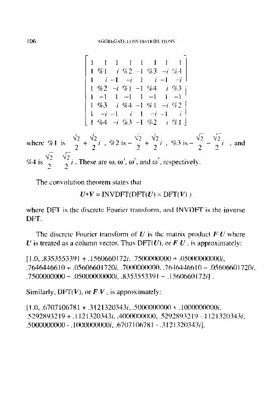
I 06 AGGREGA’I’I: LOSS IIISTRIRl‘TIONS
r 1 I 1 1 1 1 1 1 1 o/cl i o/n2 -1 %3 -i %4 1 i-1 -i 1 i-l -i 1 %2 -i %l -1 o/c4 i %3 1 -1 1 -1 1 -1 1 -1 1 %3 i%4-I %#I -iCG2 1 -i-l i 1 -i-l i 1 %4 -i %13 -I %2 i % 1
where c/r I is v2 +‘\12. v2 v2,
%2 is - V2
6 fi.2 2’ ’ 2
+ 2’ * ‘//3is- - 2
v2 i 2
, and
%4 is 2-2
I . These are o, CJ?, w’. and o’, respectively.
The convolution theorem states that
V*V = INVDFT(DFf(V) x DFf( V) 1
where DFT is the discrete Fourier transform. and INVDFT is the inverse DFT.
The discrete Fourier transform of V is the matrix product F,V where V is treated as a column vector. Thus DFT(V), or F.V . is approximately:
[ 1 .O, .835355339 1 + ,1560660 172i. .75OOOOUOOO + .OSOOOO~X~OOOi, .7646446610 + .0560660 172Oi, .7000000000. .76464466 10 - .0560660 172Oi, .7500000000 - .05000000000i, .835355339 1 - .1560660172iJ
Similarly, DFT( V), or F.V , is approximately:
[ 1 .O, .6707 10678 1 f .3 I2 1320343i. .SOOOOOOOOO + . 1 OOOOOOOOOi, ~52928932 19 + . 1 12 13203431, .4000000000, .5292X932 19 -. 1 12 I320343i, .5000000000- .1OOOOOOOOOi, .6707106781 - .3121320343il.

AGGREGATE LOSS DISTRIBUTIONS 107
DFT( V) x DFT( V) is
[ 1 .O, .5 115685425 + .3654 163056i, .3700000000 + . I OOOOOOOOOi, .3984314575 + .1154163056i, .2800000000, .3984314575 -.1154163056i, .3700000000 - .1OOOOOOOOOi, .5 115685425 - .3654163056i].
For example, the second element of the vector just above is .5 115685425 + .3654 163056i, which is
(A35355339 1 + .1560660172i) x (.6707 10678 1 + .3 12 1320343i).
To compute the inverse DFT of DFf(V) x DFT(V), one first computes the DFT of DFT(V) x DFT(V); divides each term of the result by 8; and inverts the order of the last seven terms. The DFT of DFT(V) x DFT(V), or F. (DFT(V) x DFT(V) ) , is
[3.840000000,0.0, .0400000000, .0800000000, .2000000000, 1.040000000, 1.040000000, 1.760000000].
Dividing by 8 gives
[0.480,0.0,0.005,0.010,0.025,0.130,0.130,0.220].
Reversing the order of the last 7 terms gives
[0.480,0.220,0.130,0.130,0.025,0.010,0.005,0.0].
Thus, for the sum of the distributions V and V there is a probability of 0.480 of a total claim amount of $0, a probability of 0.220 of a total claim amount of $100, a probability of 0.130 of a total claim amount of $200, etc. This can be readily verified by direct computation of these probabili- ties.
This subsection will justify the method used above to compute the inverse DFT. Suppose we have computed DFT(W), which is F.W, for some vector W. Then DFI’(DFT(W)) is F. (F.W). Matrix multiplication is

associative, so this is the same as (F. F) W or F’ W. But F’ (for the example above) is
8 0 0 0 0 0 0 0 0 0 0 0 0 0 0 x 0 0 0 0 0 0 8 0 0 0 0 0 0 8 0 0 0 0 0 0 x 0 0 0 0 0 0 x 0 0 0 0 0 0 8 0 0 0 0 0
-0 8 0 0 0 0 0 0
This is just 8 times the matrix R:
1 0 0 0 0 0 0 0 0 0 0 0 0 0 0 I 0 0 0 0 0 0 I 0 0 0 0 0 0 I 0 0 0 0 0 0 I 0 0 0 0 0 0 I 0 0 0 0 0 0 1 0 0 0 0 0
-0 1 0 0 0 0 0 0
This matrix reverses the order 01‘ the last seven clcmen~x ol‘ any vector to which it is applied.
Thus F’ W is just 8 times W with the last \cven terms reversed. Dividing by 8 and reversing the last seven terms rcstorca W.
Alternatively. F -’ is just (l/x) x R x F, where R is the matrix of’ 1 s and OS above.
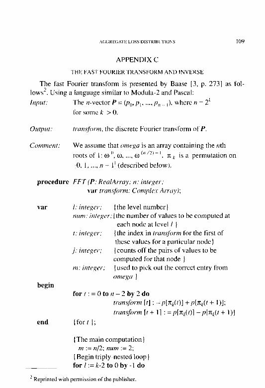
AGGREGATE LOSS DISTRIRI~TIONS 109
APPENDIX C
THE FAST FOURIER TRANSFORM AND INVERSE
The fast Fourier transform is presented by Baase [3, p. 2731 as fol- lows’. Using a language similar to Modula-2 and Pascal: Input: The It-vector P = bo, p,, . . . . I?,, _ ,). where II = 2’
for some k > 0.
Output: transfiwm, the discrete Fourier transform of P.
We assume that omegu is an array containing the rlth roots of 1: w “, 03, . . . . Lo (” “)- ‘. z x is a permutation on ,!(I, 1, . . . . II - 1’ (described below).
procedure FFT (P: RealAwa)!; II: integer; var trunsfiwm: Complex Array);
var
begin
1: integer; (the level number} ~ZNI?I: inte,qcr;{ the number of values to be computed at
each node at level 1 ) t: integer; (the index in trunsform for the first of
these values for a particular node) ,j: illteger; {counts off the pairs of values to be
computed for that node ) m: integer; (used to pick out the correct entry from
omcgga 1
end
for t : = 0 to n - 2 by 2 do transform [I] : = p[q(t)] + p[7Lk(t + l)]; transform [t + I] : = p[n,(t)] - p[7ck(t + l)]
(fort );
( The main computation ) m := n/2; num := 2;
( Begin triply-nested loop ) for/:=k-2toOby-1 do
2 Reprinted with permission of the publisher.
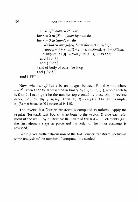
110 AGGREGATF LOSS I>ISl~RIUllTlONS
m := m/2; nuns := 2*num: for t := 0 to (2’ - I)/wH by mnl do for ,j := 0 to (nunz/2)- I do
.vPOdd := ornega[ rt?j]“t,.ccn.~~fi,,-Fni[ t+nun?/2+j]: tran.sform[t + nrrd2 +,j]:= trui7.~fiwn7(t +,j] - .vPOdd; tr.arujhn[ t + j] := trtrnsfiwn~[ t + ,j] + .\-POdd;
end ( for j ) end ( for t )
(end of body of outer for loop } end ( for 1 ]
end ( FFT }
Now, what is xx? Let t be an integer between 0 and II - I, where II = 2&. Then t can be represented in binary by [h,, h,...h, _ ,I, where each hj is 0 or I. Let I‘~v~ (t) be the number represented by these bits in reverse order, i.e., by [h, - ,... h, h,,,. Then 7~: I (t) = t.e\sx (c). (As an example, IQ (3) = 6 because 01 I reversed is I IO.)
The inverse fast Fourier transform is computed as follows. Apply the regular (forward) fast Fourier transform to the vector. Divide each ele- ment of the result by II. Reverse the order of the last II - 1 elements (i.e., the first element stays in place and the order of the other elements is reversed).
Baase gives further discussion of the fast Fourier transform, including some analysis of the number of computations needed.
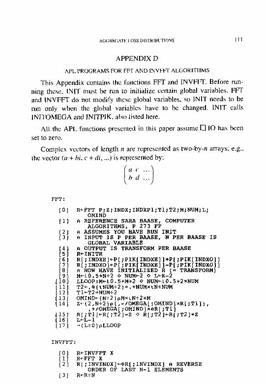
AGGREGATE LOSS DISTRIBUTIONS III
APPENDIX D
APL PROGRAMS FOR FFI- AND INVFFT ALGORITHMS
This Appendix contains the functions FFI and INVFFT’. Before run- ning these, INIT must be run to initialize certain global variables. FFI and INVFFI do not modify these global variables, so INIT needs to be run only when the global variables have to be changed. INIT calls INITOMEGA and INITPIK, also listed here.
All the APL functions presented in this paper assume 17 IO has been set to zero.
Complex vectors of length IZ are represented as two-by-n arrays; e.g., the vector ((I + hi, c + di, . ..) is represented by:
FFT:
101 R+FFT P;Z;INDX;INDXPl;Tl;T2;M;NUM;L; OMIND
111 R REFERENCE SARA BAA%, COMPUTER ALGORITHMS, P 273 FF
I21 c1 ASSUMES YOU HAVE RUN INIT [3] A INPUT IS P PER BAASE, N PER BAASE IS
GLOBAL VARIABLE [4] FI OUTPUT IS TRANSFORM PER BAASE [5] R+INITR [6] R[;INDXE]+P[;PIK[INDXE]]+P[;PIK[INDXO]I [7] R[;INDXO]*P[;PIK[INDXE]]-P[;PIK[INDXO]] 181 A NOW HAVE INITIALIZED R (= TRANSFORM) [9] M+LO.S+N+2 0 NUM+2 0 L+-K-2
[lo] LLOOP:Mc10.5+M+2 0 NUM‘-10.5+2xNUM [ll] T~+,B(LNUM+~)~.+NUMXLN+NUM [12] Tl‘-T2+NUM+2 [13] OMIND+(N+Z)pMxtN+ZxM (141 2+(2,N+2)p( ,-fOMEGA[;OMIND]xR[;Tl]),
,+fOMEGA[;OMIND]xeR[;Tl] [15] R[;Tl]+R[;T2]-2 0 R[;T2]+R[;T2]+2
+(LzO)pLLOOP
INVFFT:
[0] RtINVFFT X [l] RtFFT X [2] R[;INVINDX]+@R[;INVINDX] A REVERSE
ORDER OF LAST N-l ELEMENTS [3] R+R+N

I12
INIT:
LOI ;:; [31 [41
# [71 [81 tg1
(101
INIT KK K+KK N+LO.!i+i?*K 010+-o INITOMEGA K INITPIK K INITRt(2,N)pO INDXE*2xLN+2 INDXO+-INDXE+l INVINDX+l+LN-1 TAIL+(N+2)+tN+2
INITOMEGA:
01 INITOMEGA K
:; N+L0.5+2*K OMEGA+-(2,N+2)pO(LN+2)X2+N
31 OMEGA[O;]+2OOMEGA[o;] 41 OMEGA[l;]+lOOMEGA[l;]
:; OMEGA2+(2,N+l)p~(tN+l)~2+2~N OMEGA2[0;]'2OOMEGA2[0;]
71 OMEGA2[l;]'lOOMEGA2[1;]
INITPIK:
[0] INITPIK K;N [l] N+lO.!i+2*K [21 PIK+2le((Kp2)~tN)

AGGREGATE LOSS DISI‘RIRlJWNS 113
APPENDIX E
PROOF THAT A’ * S’ IS THE DISTRIBUTION OF i CLAIMS
This Appendix gives a proof sketch that A’ * S’ is the probability dis- tribution of the sum of exactly i claims. More precisely, it shows that if A’, S’, II. and L are defined as in the main body of this paper, and X is the probability distribution of exactly i claims, then the probability that X is
between ,jn[:)and (j+ l)x[i]is(A’*S’)[j].
Consider first the case where L = II and S = (1, 0, 0, . . . . 0). This makes S a uniform distribution on the unit interval [0, Il. In this case the first H terms of A’ * S’ are:
af,,al,, a;, . . . cr:,-, .
Let F’ be the distribution function for the sum of i mutually indepen- dent random variables uniformly distributed over [0, I]. Let hj = F’ (j + 1) - F’ 0). It needs to shown that a.1 = hi .
Combining equation 9.1 and Theorem 1 of Section I.9 of Feller [ 11, p. 271,
where 2+ is ? ifs 2 0 and .Y+ is zero ifs < 0. This yields:
.i
/7; = f, c (-1)” i + I
( 1
(; + 1 - ,‘)’ . 1’ = 0 \’
because if ,j < i + 1 then (j + 1 - v)+ is zero for terms with \I >.j , and if
,j > i + 1 then is zero for 1’ > i + 1.

113 AGGREGATE LOSS I)ISl‘KII~lJ-IONS
It is easy to see that ~1, = hi, = I/i! for i > I, and ‘1: = h: = 0 forj 2 1. To complete the proof that 0; = L$ it suffices to show that the h) satisfy the recursion relation used to define the l/i.
To this end, for i > 1 andj > 0 consider:
It needs to be shown that 3 equals /$ This is done by plugging into the above formula the expression for hi as a sum, and rearranging terms:
i!z=(i-j)(i-l)!k$It+(j+l)(i-l)!hj-’
.i- 1 =(i-j)C(-1)’ 0 i (,j-z)‘-‘+(j+ t)i(-l)\’ 0 r, ( ,j + 1 - \v)‘- ’
T = 0 1’ = 0
=c;-j)~(~I,‘~-’ ( i ,‘i , 0’ + I - 1’)’ - ’ t
,’ = 0
(j+ 1) i(- i 0
(j+ I - I’)‘-- \’ ,‘=o
=(j+ l)(l)(l)(j+ l)‘-‘+
i[(-l)(i-j)( ;,;,)+(,;+,)(~,)I(-l)~~(;+,-,,);-~ I’= I
=(-l)(J i:, 1 fj+ 1 -of+ L 1
CL ’ ~l)t~+(i_+ l)(i+ 1-v) (i+ 1) ! i+ 1 i+l I( 1’ ! (i + 1 - 1%) ! I
(-1)“ o‘+ 1 - )?>‘- ’
\‘=I

AGGREGATE LOSS DISTRlBUTlONS 11.5
=(-‘)” ii l ( 1 (j+l-O)‘+~(j+h.) i+l
( ! (-l)“(j+ 1 - v)j-’ 1’ \‘= I
=$-I)~( y ’ )(i+ 1 -1’)j.
Thus , z = /$ . This establishes the main result for this case.
For the general case, consider the positive “quadrant” of [w’, i.e, the points (X0, St, . . . . Si _ ,) such that each ,~~j is greater than or equal to zero. Divide this space into cubes with edge length L + n in the obvious way. Assign a density to each cube as follows. If the cube’s
vertex closest to the origin is .(
L L L v(),~ l’[J2> ...7 \‘j- 1,2
-1 * assign a density of
( S,,(, s,, S,‘, . . . s,., _ , ) f L ’ - t 1 n
where the s,,* are elements of the vector rep-
resenting the severity distribution if \lk I II - 1, and s,.~ = 0 if \jk 2 n , As i
the volume of every cube is !C (1
, the integral of this density over the n
cube is s,.~~ s,., s,~ . . . s,,, ,. Now consider the integral of these densities
between the parallel (i - I)-planes:
x0+x, + . . . +I,_,=~~, and
x0 + x, + , . . + sj-I=(k+ l)f;.
This integral is the probability that the sum of i claims will have a
value between k” and (k + 1) 4.
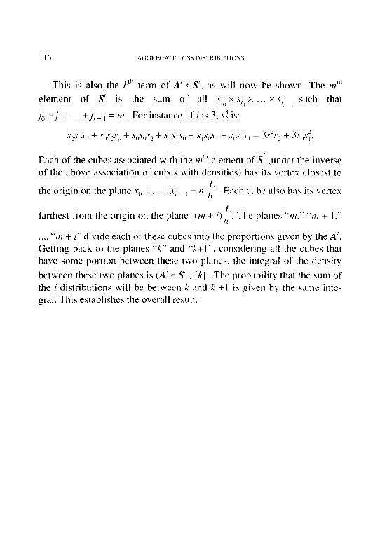
This is also the ,41h tern1 of A’ * S’, as will now be shown. The nr”’ element of S’ is the sum of all .Y/,, x .v,, x . . x s,, , such that
,jo +,j, + .._ +,j, , = HI . For instance. if i is 3, .si is:
.s2”crso + .Y,rs~“o + <So.S,).S~ + s, s,.s,, + .s,.so\ / + .A(,.\ ,.\ ’ = is;.s, + 3s,,s;.
Each of the cubes associated with the I~,“’ element of S’ (under the inverse of the above association of cubes with densities) has its vertex closest to
the origin on the plane .I-~, + . . . + .\; , = 171 ,f . Each cube also has its vertex
farthest from the origin on the plant (nr + i)t. The planes *‘/II.” “I?? + I ,”
. . . . “W + i" divide each of these cubes into the proportions given by the A’. Getting back to the planes “h-” and “X+1”, considering all the cubes that have some portion between these two plants, the integral of the density between these two planes is (A’ 4: S’ ) [ICI The probability that the sum of the i distributions will be between X and X +I is given by the same inte- gral. This establishes the overall result.
AGGREGATTE LOSS LXSTRIBl~TIONS 117
APPENDIX F
PACKING AND UNPACKING
This Appendix provides the formulae for packing and unpacking transformed vectors. This treatment essentially follows that of Press, Flannery, Teukolsky, and Vetterling [6, p. 3981. APL programs to imple- ment these routines are in Appendix G.
Unpacking a transformed vector is discussed first. Assume that one starts with a real (untransformed) vector, U, of length 211 and packs it into a complex vector. PU, of length n, as discussed in the main body of the paper. Then the FFf is applied to PU to obtain a vector PH that is the packed transformation of PU. The next step is to unpack PH to obtain the FFT of ZJ.
The result of unpacking PH will be a complex vector of length II + 1. One might think the result would be a complex vector of length 2n since the goal is to obtain the FFT of U which is of length 217. If R is the (length 217 for the moment) FFT of U, then:
where * denotes complex conjugation. Thus, from the first II + 1 terms (0 to 77) it is easy to derive the remaining terms of R.
Append to the end of PH the first element of PH, making PH a complex vector of length II + I. Let PH2 be the complex conjugate of the “reverse” of PH; i.e., PH2ljj = PH[rl - j]* for 0 <j I II . Define PH3 by:
PH3[j] = -i(PHlj] - PH2[j]) x co.‘,
where i is fiand w is a 2nrh root of unity (such that o? is the ,rth root of unity used in the FFT’). Finally, R is half the sum of PH, PH2, and PH3.

II8 AtiGREGA1 F I.OSS I)ISI‘HIHI7 IOXS
The steps for packing a transformed vector R (of length n+l ). to ready it for application of the inverse F’FT, arc almost the same steps as for unpacking. Let R2 be the complex conjugate of the “reverse” of R. De- fine R3 by:
R3Ljl = i(Rl.il - R2[jl) x 01 '.
where i and o are as immediately above. The final result is the first n terms of half the sum of R, R2, and R3.

AGGREGATE LOSS DlSTRlBlJTlONS
APPENDIX G
APLROUTINESFORPACKINGANDUNPACKING
UNPACK:
RtUNPACK H;H2;H3 R UNPACKS TRANSFORMED DATA. ASSUMES X
IS THE RESULT OF FI APPLYING THE FFT TO A LENGTH 2N REAL
VECTOR WHICH HAD BEEN R PACKED INTO A 2xN COMPLEX ARRAY. R RESULT IS A 2 X N+l ARRAY
H2[1;]+-H2[1;] H3+H-H2 I$L;5N+1)p(,-fH3xOMEGA2),,+fH3xeOMEGA2
H3;1.]+-H3[1.] R+O.;xH+H2+H:
R+PACK X;X2;X3 R PACKS TRANSFORMED VARIABLE x2ex X2[1;]+-X2[1; X3+X-X2 ;;+~;~""'"L
+ X3[0;]+-X3[0; ;+Oi5xX+X2+X3
e -1 1R
1 +fX3xOMEGA2),,-
1
fOMEGA2xeX3
119
OMEGA2 (the 2nth roots of unity) is generated by INIT and INITOMEGA in Appendix D.

120
APPENDIX H
APL FUNCTIONS FOR THE ('OMI'I.t3‘k< Al.GORITHM
This Appendix gives an APL function, AGGDISTR, that implements the full algorithm. AGGDISTR calls a number of subroutines. The sub- routines FFT and INVFFT are listed in Appendis D. and the subroutines PACK and UNPACK arc listed in Appendix G. The only other subroutine needed is MULT, listed below. Before running AGGDISTR it is necessary to run INIT, which sets certain global variables. INIT calls INITOMEGA and INITPIK; these three programs are given in Appendix D.
AGGDISTR:
[0] AGGDISTR;M;M2;P;S;PSl;PSI;PZERO;FSl; FSI;AI;I;BIN;FSIFLAG;X;J;Y;PY;FAI;FY
t:; OIO+O R ----
131 'Input the smallest number of claims with non-zero probability,'
t2 IMr'
E M+" la1 :(;M~O)A(M=~O.~+M))~SKIP~ R M must be a
non-negative integer. 191 ‘M, ‘,(*Ml,’
integer. is not a non-negative Stopped.'
K +O SKIPl:' ' 1121 'Input densities of claim fre uency
distribution. These shoul s iI31 'be the probabilities of M, M+l, M+2,
1141 ' (**- claims.'
0 :;;(pP)#l)v(P[O]+O))pSKIP2 0 FI IF ONLY
ONE NUMBER IS INPUT AND IT IS ZERO, THEN EXIT.
1171 'Only one number was input, and it is ' ,(mP),'. Stopped.'
SKIP2:' ' 'Input vector for severity distribu-
tion. Must be of length ',(mN),'.'

AGGREGATE LOSS DISTRIBUTIONS 121
(231
r241
251 261 271 281 291 301 311
t::; [361 [371
+((pS)=N)pSKIP3 0 R IF S IS NOT OF LENGTH N, THEN EXIT.
'Length of S is ',(apS),'. Should be ' ,(mN),'. Stopped.'
-10 SKIP3:' ' F\ ---- AGGc(2,N)pO PSl+Q(N,2)pS,(NpO) 0 F1 'PACK' S. St0 0 R FREE UP SPACE PZEROc0 0 R INITIALIZE - WILL BE RESET
IF M=O. n ---- FI T;I3;>;ASES ARE CONSIDERED, M=O, M=l,
-+(M=O)pME&l +(M=l)pMEQl +(M>l)pMGTl MEQO:PZEROtP[O] 0 P+,llP 0 Mel
R CONVERT TO CASE M=l MEQl:M2+pP AGG+P[O]xPSI +(M2=1)pENDIT FSltUNPACK FFT PSl PSI+INVFFT PACK FSl MULT FSl PSI[;TAIL]+O AI+ 0.5 0.5 0 I+2 0 PSl+0 -MAINLOOP Q ---- R ---- MGTl: A START BINARY POWER TRICK.
BIN*,ll((l+L2@M)p2)TM A EXPRESS M AS BINARY VECTOR. DROP FIRST TERM
FSIcFSlWNPACK F!?T PSl BINLOOP:FSI+FSI MULT FSI 0 PSIcINVFFT
PACK FSI 0 PSI[;TAIL]+O 'BINLOOP ',(caBIN),' ',sOTS +((ltBIN)=O)pSKIP FSI+UNPACK FFT PSI 0 FSI+FSI MULT FSl 0
PSI+INVFFT PACK FSI 0 PSI[;TAIL]+O SKIP:BINc,llBIN 0 +(O=pBIN)pEXIT FSIcUNPACK FFT PSI +BINLOOP EXIT: R THIS IS THE EXIT FROM THE
BINARY POWER TRICK. &q D-v- AI+,1 0 1~1 A SET AI, INDEX ALO;;:;+I+l 0 AI~(l+I)x(@AI)+AI+(l+~I)x
+(I<MjpALOOP M2+- l+M+(pP) 0 PSl+O A --mm fq ---- MAINLOOP:'MAINLOOP ',(*I),' ',TUTS FSIFLAG+O
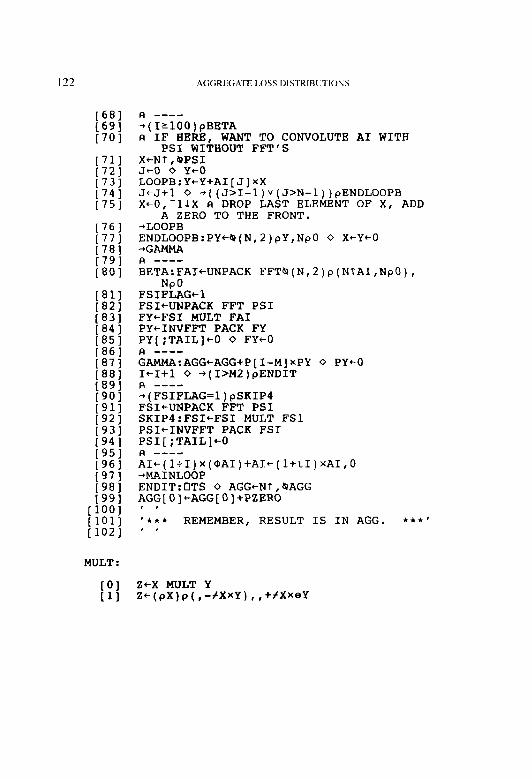
AGGREG,ZTE I.OSS DISTRIHI’TIONS
+(I'lOO)pBETA R IF HERE, WANT TO CONVOLUTE AI WITH
PSI WITHOUT FFT'S X+Nf,BPSI J+O 0 Y+O LOOPB:Y+Y+AI[J]xX JtJ+l 0 +((J>I-l)v(J>N-1))pENDLOOPB X+0, -11X A DROP LAST ELEMENT OF X, ADD
A ZERO TO THE FRONT. +LOOPB ENDLOOPB:PY+B(N,Z)pY,NpO 0 X+Y+O *GAMMA R s--v BETA:FAI+UNPACK FFTQ(N,2)p(NfAI,NpO),
NPO FSIFLAG+l FSI+UNPACK FFT PSI FYcFSI MULT FAI PYtINVFFT PACK FY PY(;TAIL]+O 0 FY*0 R --we GAMMA:AGG+AGG+P[I-M]xPY 0 PY+O I+I+l 0 +(I>M2)pENDIT A -v-e +(FSIFLAG=l)pSKIP4 FSItUNPACK FFT PSI SKIP4:FSIcFSI MULT FSl PSI+INVFFT PACK FSI PSI[;TAIL]+O R ---- AI+(~~I)x(@AI)+AI+(~+LI)~AI,O +MAINLOOP ENDIT:UTS 0 AGG+Nf,@AGG AGG[O]+AGG[O]+PZERO r , I*** REMEMBER, RESULT IS IN AGG. ***' , I
[0] Z+X MULT Y (11 z+(pX)g(,-SXxY),,+fXxeY

AGGREGATE LOSS DlSTRlBUTlONS 123
APPENDIX I
PARAMETER UNCERTAINTY FOR THE SEVERITY DISTRIBUTION
We will show mathematically that it is fundamentally impossible to reflect parameter uncertainty for the severity distribution by computing the aggregate distribution using a severity distribution with a larger vari- ance than the best-estimate severity distribution. This discussion is based on suggestions by Venter.
Parameter uncertainty for the severity distribution is reflected by choosing a distribution u with mean 1 and variance greater than 0, and computing the aggregate distribution:
AGG = US, + US, + . . . + a&.
Here AGG, S;, and T are the aggregate distribution, the severity distri- bution, and the claim count distribution, defined earlier. The above equa- tion is written to indicate that one sample from T is associated with one sample from u and multiple samples from S. The above equation could also be written
AGG = a(Sl + S2 + . . . + S,) .
A general fact about variance (for arbitrary/independent distributions X and Y) that will be used is:
Var(XY) = Var(X) Var(Y) + (E(X))2 Var(Y) + (E(Y))* Var(X). (1.1)
Also, recall that
Var (S, + S, + . . . + ST) = l+Gs* + lts2& (1.2)
Here pr and ps are the means of the claim count and severity distribu- tions, and 0: and 0: are the variances of the respective distributions.
Set
X=U, Y=S,+S,+...+S,, and XY=AGG
and substitute in equation I. 1 above. This gives

124 AGGREGATE I.OSS DISTRIBI~TIONS
Var (AGG) = Var (a) Var (S, + S, + . . . + S,-) + (E(a))’ Var(S, + S, + . . . S,) + (E(S, + Sz + . . . + S,))-) Var(u).
Denote Var(u) by 0: , note that E(S, + S1 + . . . + S,) is p7+t5 , recall that E(U) is I, and substitute using equation I.2 to obtain
Dividing by ( p7. p,, )’ gives a formula for the square of the coefficient of variation for the aggregate distribution:
Var (AGG)
( t-b Its 1’ = ( , + o; ) (1.3)
Now consider what happens as the mean of the claim count distribu- tion, i.e., the expected number of claims. increases towards infinity. For the moment, assume there is no parameter uncertainty for the claim count
2 distribution. The term L0$ tends to zero as p7. increases. If the claim
I \ count distribution is Poisson, or is negative binomial with a fixed “proba-
bility of success” parameter, then the term 0;.
l-2 also tends to zero. (If the
negative binomial is parameterized so the density function is
f(.r) = i 1
?’ + ::‘- 1 p’ (1 -p>“ with J > 0 and 0 < p < I, then p is the proba-
bility of success parameter.)
Thus, for any fixed severity distribution, the limit of the square of the coefficient of variation of the aggregate distribution, as p, goes to infinity, is equal to 0:. In a practical sense, this means that. as the expected number of claims becomes large, the effect of the claim count distribution and the severity distribution on the coefficient of variation of the aggre- gate distribution becomes minimal. The coefficient of variation of the aggregate distribution is determined by the parameter uncertainty for the severity distribution.

AGGREGATE LOSS DISTRIBUTIONS 125
In particular, this shows that there is a fundamental difference between the effect on the aggregate distribution of parameter uncertainty in the severity distribution and the effect of using a severity distribution with a greater variance. If a severity distribution, S’, with a larger variance is substituted for the best-estimate severity distribution, S, and AGG = S’, + S’, + . . . + S’,- is computed (this is the same as setting a to a constant I), then as p7. goes to infinity, the coefficient of variation of the aggregate distribution tends to zero, and not to some positive value as above.
The two approaches differ in the independence assumptions regarding the samples from the severity distribution. If the severity distribution is diffused, then each draw from the severity distribution is a combination of an independent draw from the best-estimate severity distribution and an independent draw from the distribution used to reflect parameter uncer- tainty for the severity distribution. Under the correct method of reflecting parameter uncertainty, each draw is still an independent draw from the severity distribution, but there is only one draw from the distribution reflecting parameter uncertainty for each draw from the claim count dis- tribution.
Equation I.3 shows that diffusing the severity distribution is not an adequate method for the recognition of parameter uncertainty for the severity distribution. Equation I.3 can also show the effect of parameter uncertainty for the claim count distribution, and the remainder of this appendix gives a brief discussion of that effect.
Apart from one quick comment at the end, only one method of repre- senting parameter uncertainty for the claim count distribution will be considered here. It will be assumed that the best-estimate claim count distribution is Poisson with parameter h. That is, the best-estimate claim count distribution, N. has probability density function
p (/y = ,y ) A) = 3L’ e-A .r ! .
Parameter uncertainty is incorporated by assuming that h follows a gamma distribution, denoted A, with probability function

126 AGGREGATti LOSS I~ISTRIBl~TlOhS
Above, I- is the gamma function and h and (’ arc parameters. The distribu- tion A has mean hc and variance /?c. The parameter h is the scale param- eter because changing h by some factor has the eff‘cct of’ multiplying the distribution uniformly by that same factor. The parameter (’ is the shape parameter.
Straightforward computations show that the claim count distribution, T, that results from compounding the Poisson distribution with the gamma distribution is a negative binomial distribution with probability function:
Here h and c are the parameters from the gamma distribution. This nega- tive binomial distribution has mean /x, and variance (hc)(h+I ). Thus
One way to reflect a constant degree of parameter uncertainty in the claim count distribution while increasing the mean is to allow h to in- crease but to hold c constant. This maintains a constant percentage of uncertainty regarding the mean of the claim count distribution. In the
0,; Equation 1.3, the term piu;, tends to zero as u, increases (as it did above).
But now the term Of cl
tends to a positive limit. namely I/C,. Thus, Equation
I.3 shows that the coefficient of variation of the aggregate distribution has a component due to the parameter uncertainty in the claim count distribu- tion that does not drop below a certain minimum no matter how large the mean of the claim count distribution becomes.

AGGREGATE LOSS DISTRIBUTIONS 127
A little more generally, as p7. goes to infinity, the limit of the square of the coefficient of variation of the aggregate distribution is
The severity distribution and the best-estimate claim count distribution have no effect on this limit. This limit depends only on the amount of pa- rameter uncertainty reflected in each of these distributions.

12X AGGREGATE LOSS I)IS’I‘RIl3I”I IO\S
APPENDIX J
PROOFS OF FORMULAE FOR EXCESS ~‘LAIM COUNT DISTRIBLITIONS
This appendix proves that if ;I claim count dislrihution is binomial, Poisson, or negative binomial, with mean h and vsriancc 0’. and the probability of a claim being excess of some attachment point is (x, then the excess claim count distribution is binomial, Poisson. or negative bino- mial, respectively, with mean ah and variance c13L + tx’(o’ - h). For each of the three types of claim count distributions. it is shown that the selec- tion of claim counts from the given distribution with mean h and variance &, followed by selection of excess claims with probability a (under a binomial process) gives a distribution of the same type with mean ah and variance ct3L + c1’((3’ - A).
The Poisson case is considered first. Here h = CT’ . so & will not appear. The total distribution will he T and the exct’ss distribution will be X. For the total distribution:
P(T= I) = ; c,-‘.
Given I claims in the total distribution, the distribution of excess claims is:
P(X=xIT=r)=
P(X = .Y) is the sum over all I of P(T = f) x P(X = .\- I T = f) ; i.e.,
P(X =.\-) = 2 ;’ 8’ .; l I
cr’(l -(x1’-‘. ,=\ .
Letting i = t - .I- so f = s + i this becomes:
p(x = -\.) = 2 h’+,’ e-?’ .t-: i ;=(, 0 + I)! i 1
a’ ( I - of.

AGGREGATE LOSS DISTRIBUTIONS 129
This is a “ground up” computation of the claim count distribution for aggregate claims. The starting point was the distribution of total claims, T, and then excess claims were selected according to a binomial process to get the distribution of excess claims.
It is necessary to show that this sum is m~,y! WY ,-a% .
But:
e -ah ,-h +h -ah = ,-A ,h( I- a) = ,-h. h’ ( I - a)’ c---- i! i = 0
j a-rht -ah m kv ki
.r! e
= c
,-A (.s+i)! _y!Ta-
r
;=,)(.\.+iY . (1 -a)'
as was to be shown.
Now much the same is done for the negative binomial. According to Hastings and Peacock [24, p. 921, the negative binomial has density func- tion:
p( y = \‘) = .Y + J - I
4 1
fq” )’
where x and p are parameters and q = 1 -p. This distribution has mean .q/p and variance q/p*. If parameters .Y and p result in a mean of h and a variance of CT’, then parameters of s and p/O, + a - q) result in mean ah and variance ah + CI”(& - IL). Let T be the total claim count distribution, and let Y be the excess claim count distribution. Then:
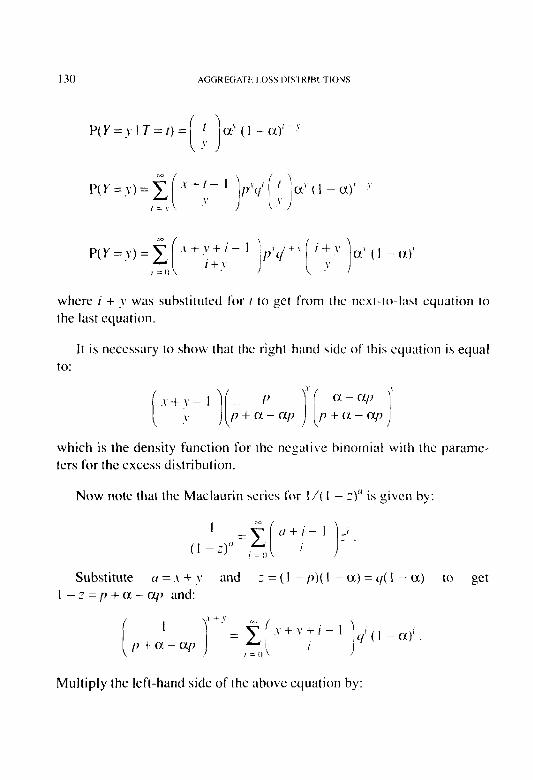
130 AGGREGAl’I’ I OSS I)IS’I’RIHI~TIOVS
P(Y=yIT=t)=
where i + J was substituted for I to get from the next-to-last equation to the last equation.
It is necessary to show that the right-hand side of this ccluation is equal to:
which is the density function for the negative binomial with the parame- ters for the excess distribution.
Now note that the Maclaurin series for I/( I - 1)” is given by:
Substitute (I = .y + .v and 3 = ( 1 - p)( I - a) = q( I - a) to get 1 -z=p+a-ap and:
Multiply the left-hand side of the above equation by:

AGGREGATE LOSS DISTRIBUTIONS 131
K= pW$(s+?‘- I)! (I - l)! yi
(i + y)! and multiply the right-hand side by K ---
(I +y)! ’ rearrange, and obtain:
(,y+;-l)[p&L+ )‘(,-:;yl& ]
as was to be shown.
Finally, consider the binomial. According to Hastings and Peacock [24, p. 361, the binomial has density function:
P(X = x) = ( 1
: p-r y” - .‘,
where n and p are parameters and q = 1 - p. This distribution has mean ?rp and variance qq. If parameters iz and p result in a mean of h and a vari- ance of o’, then parameters of II and crl, result in mean ah and variance ah + a’(& - h). As above, let T be the total claim count distribution, and let X be the excess claim count distribution. Then:
P(X=.\-IT=r)= f a’(1 -@-’ . 0 .\’

132 AGGRIWATF I OSS I~ISI‘RII~I~TIOU6
Let t = .v + i, so:
It is necessary to show that the right-hand side of the above equation is equal to:
” ( 1 (txp).’ (1 - Cx/?)“- ’ . .x
Begin with an equality due to the binomial thcorcm:
( 1 - ap,“I:’ = ” -.I p’ ( 1 - a)’ ( , - ,T)” -.’ (17 -x)! c
I=,, i! (17 -.v- i)! (I -p)' '
Multiply the left side by K = “! f!‘“’ and the right side by K. (.v + i)!
rearrange to get: (.t- + i)! and
I, - .\ j=(, (.\-+i)! (::!-.r-i)! /“/“(I -I’)“- ‘--I ‘:.~ir” c cl’ ( 1 - a)’
or:

AGGREGATE LOSS DISTRIBUTIONS 133
which completes the proof.
134
DISCUSSION OF PAPER PUBLISHED IN VOLUME LXXIV
AN ANALYSIS OF EXCESS LOSS DEVELOPMENT
EMANUEL PINTO AND DANIEL F. GOGOL
DISCUSSION BY ROBERT A. BEAR
Me.s.st~.s. Pinto und Gogol IKIIYJ mudc u ~wl~rahlt~ cwntt-ihution to uctlrurial 1iter.utur.e through their unu1~se.s of’ industry e-l-- cc.s.s loss development puttc~r-ns. Bused upon upplication of u thcoreticul model to industt.? dutu, the ul4thor.s hcov cwl\,it~r,- ins!\’ demonstruted that puid urld ir7crrrrcd loss umi ALAE de- velopment putterns incr-euse sigm~i:cuntlv us the retentiotl inc3wase.s. This is due to the phenomenon thut tlrr selwitv dis- tribution becomes thicker-tailed us claims mutwe. This relqitw* psesents a gener-ulixtiori of the Pinto-Gngol f~wmuiu thut shorz’s hoM1 the authors methodolo~qy cun hc uppliea’ to csti- mate ac’c.ount-spec’ifil. de~v~lopmerlt puttern.s,fiw reIuti\‘cIy high e..yi~ess lqers.
This reviewer would like to thank Kurt A. Reichle for encouraging him to write this discussion. and Daniel F. GopI for his helpful \uggcstions.
1. INTRODUCTION
Messrs. Pinto and Gogol [ I] have made a valuable contribution to actuarial literature through their analyses of industry excess incurred loss development patterns. They have convincingly demonstrated that in- curred loss and allocated loss adjustment expense (ALAE) development increases significantly as the retention increases. The same is likely to be

EXCESS LOSS DEVELOPMENT 13s
true of paid loss and ALAE development, as the following argument shows.
The authors note that estimates of paid excess loss development fac- tors can be computed by multiplying each incurred excess loss develop- ment factor by the quotient of the paid-to-reported ratios for the later and earlier valuations. The paid-to-reported ratios are simply ratios of excess paid losses and ALAE to excess incurred losses and ALAE. These ratios are computed at all valuations for a representative retention, since the authors found that they do not vary substantially as a function of the retention. Thus, paid excess loss development factors may be expressed as the product of incurred excess loss development factors (which in- crease with the retention) and a quantity which does not vary substantially with the retention. This implies that paid loss and ALAE development factors can be expected to increase significantly as the retention increases. Thus, the retention should be appropriately reflected in the estimation of discounted excess losses using paid development factors.
2. COMMENTSONTHEUNDERLYINGMODEL
The function 4’ = a~’ was used by the authors to fit excess develop- ment factors as a function of the retention, based on Insurance Services Office (ISO) data. Basic properties of the underlying Single Parameter Pareto (SPP) severity distribution [2] are summarized in Appendix A. As the retention, x, was normalized through division by $10,000, the parame- ter a represents the factor for development excess of $10,000. The incre- mental factors, a - 1, are then fitted to the inverse power function y = CX” as recommended by Sherman [3]. The inverse power function is used for interpolation and to yield tail factors for development beyond 99 months. The use of this same functional form to extrapolate h-parameters beyond 99 months appears to have been based on goodness-of-fit tests rather than on theoretical considerations, because the parameter h represents the de- cline in the SPP q-parameter between the valuations underlying the age- to-age factor.
Philbrick [2] and Reichle and Yonkunas [4] noted that the tails of fitted SPP severity distributions are thicker than the tails of empirical

136 EXCESS LOSS IIl:VI:I.OPMEN I’
casualty loss distributions at very large loss sizes. This implies that empir- ical average claim sizes in excess of high retentions will be less than those implied by the SPP distribution. Fits to more recent IS0 data led Bear and Nemlick [5] to conclude that the SPP q-parameter varies with the truncation point used in the fitting procedure. This increase in the estimated y-parameter as a function of the truncation point supports the earlier findings of Philbrick and Reichle-Yonkunas. Pinto and Gogol note that the impact of this error will be reduced by using a ratio to estimate a development factor if the error is of comparable magnitude in the numer- ator and denominator.
Bear and Nemlick found that if the truncation point used in the fitting procedure is less than SO% of the attachment point for a particular analy- sis, the errors due to the redundant estimates of excess severities from the SPP distribution become unacceptably large. They used development tri- angles of SPP parameter estimates to derive the shape parameter q at various stages of development and to project ultimate estimates of this parameter by class of business and truncation point. For the casualty classes of business analyzed, their fits of more recent IS0 data confirmed the result noted by Philbrick and Reichle-Yonkunas; i.e., the q-parameter tends to decline as a function of the stage of development. This implies that the severity distribution becomes thicker-tailed as claims mature. (See Appendix A.) This is also confirmed by the t‘~\ct that the h-parame- ters estimated by Pinto and Gogol were positive.
3. ESTIMATING ACCOIINT-SPECIFIC DEVELOPMENT
The authors concentrated on the estimation of industry loss develop- ment patterns for unbounded layers (with losses capped by policy limits), and suggested a reasonable approach for estimating industry incurred loss development patterns for reinsurance layers. This same approach can be applied to industry paid loss development patterns for unbounded layers to estimate paid loss development patterns for reinsurance layers.
This reviewer observes that the basic Pinto-Gogol formula for compu- tation of industry loss development factors for unbounded layers as a function of the retention can be applied in large account primary pricing

EXCESS LOSS DEVEI.OPMENT 137
and in account-specific reinsurance pricing. This formula can also be applied to estimate account-specific development patterns for reinsurance layers and for large account primary excess layers.
A generalization of the Pinto-Gogol formula is presented below and proven in Appendix B. This generalization permits one to estimate the account-specific development pattern for a relatively high layer as a func- tion of the development pattern for a lower layer, assuming the ratios of the gross limit to the retention for both layers are equal.
Let d represent the incurred loss development factor from valuation i to valuation j for losses in the layer from k, to k,. Assume the SPP distribution is an appropriate severity model for claims in excess of k,. Let yi and yi represent the estimated values of the SPP parameter based on claims at valuations i and j, respectively, and let c = y; - yj. Then the incurred loss development factor from valuation i to valuationj for losses in the layer from IC, to x2 is given by
dc” ,
where c = I!’ 2 1 4
and -2 _ k, - =b. xl - k,
This result also holds for unbounded layers (i.e., k2 and x2 are infinite) if the SPP parameters exceed one. If qj represents the projected value of 4, the SPP parameter for fully developed claims, this result may be used to estimate age-to-ultimate development factors.
The SPP parameters can be estimated from account-specific data in large account primary pricing and in reinsurance pricing. The parameters estimated from account-specific data can be credibility weighted with parameters estimated from industry data ([4],[6]).
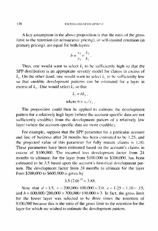
A key assumption in the above proposition is that the ratio of the gross limit to the retention (in reinsurance pricing). or self-insured retention (in primary pricing), arc equal for both layers:
h= -=x1 .\-, .\-, x;
Thus, one would want to select Ic, to be sufficiently high so that the SPP distribution is an appropriate severity model for claims in excess of k,. On the other hand. one would want to select k, to bc sufficiently low so that credible development patterns can be estimated for a layer in excess of k, . One would select X, so that
where b = .\-,/.I-, .
The proposition could then be applied to estimate the development pattern for a relatively high layer (where the account-specific data are not sufficiently credible) from the development pattern of a relatively low layer (where the account-specific data arc more credible).
For example, suppose that the SPP parameter for a particular account and line of business after 24 months has been estimated to be 1.25, and the projected value of this parameter for fully mature claims is 1.10. These parameters have been estimated based on the account’s claims in excess of $100,000. The incurred loss development factor from 24 months to ultimate, for the layer from $100,000 to $300,000, has been estimated to be 3.5 based upon the account’s historical development pat- tern. The development factor from 24 months to ultimate for the layer from $200,000 to $600,000 is given by
3.5 (2.0).15 = 3.88.
Note that d= 3.5, c = 200,000/100,000 = 2.0, c = I.25 - 1. IO = .lS, and h = 600,000/200,000 = 300,000/ 100,000 = 3. In fact, the gross limit for the lower layer was selected to be three times the retention of $100,000 because this is the ratio of the gross limit to the retention for the layer for which we wished to estimate the development pattern.

EXCESS LOSS DEVELOPMENT 139
Development patterns for layers with retentions in excess of $200,000 (more than twice the $lOO,OOO truncation point used in estimating the SPP parameters) could be estimated with reasonable confidence using this procedure, if one had reason to believe the SPP parameters remained relatively stable as higher truncation points were used in the fitting proce- dure. (Recall that errors arising from this source may be reduced by using a ratio to estimate a development factor.)
Finally, it should be noted that paid loss development factors for bounded layers may be estimated by applying the Pinto-Gogol approach of multiplying each incurred loss development factor by the quotient of the paid-to-reported ratios for the later and earlier valuations. This re- viewer suggests that the paid-to-reported ratios be estimated for the par- ticular layer of interest (or at least for a similar layer), but possibly from a broader data source than was used to estimate the incurred loss develop- ment factors.
4. SUMMARY
Based upon application of a theoretical model to industry data, the authors have convincingly demonstrated that paid and incurred loss and ALAE development patterns increase significantly as the retention in- creases. This is due to the phenomenon (confirmed by recent IS0 casu- alty data) that the severity distribution becomes thicker-tailed as claims mature. The proposition presented above shows how the Pinto-Gogol methodology can be applied to estimate account-specific development patterns for relatively high excess layers.

140 EXCESS I OSS I~k\‘lil.Ol’MFUT
REFERENCES
[I] Pinto, Emanuel. and Gogol, Daniel F., “An Analysis of Excess Loss Development.” PCAS LXXIV, 1987, p.227.
[2) Philbrick. Stephen W., “A Practical Guide to the Single Parameter Pareto Distribution,” PCAS LXXII. 19X5. p.44.
]3] Sherman, Richard E., “Extrapolating, Smoothing, and Interpolating Development Factors,” PCAS LXXI, 19x4, p. 122.
[4] Reichle, Kurt A., and Yonkunas. John P., Discussion of Philbrick: “A Practical Guide to the Single Parameter Pareto Distribution.” PCAS LXXII, 19x5. p.85.
[S] Bear, Robert A., and Nemlick, Kenneth J.. “Pricing the Impact of Ad- justable Features and Loss Sharing Provisions of Rcinsurance Trea- ties,” PCAS LXXVII. 1990. p. 60.
(61 Rytgaard, Mette “Estimation in the Parcto Distribution.” ASTIN Col- loqlrilrnr XXI, 19X9, p.389.
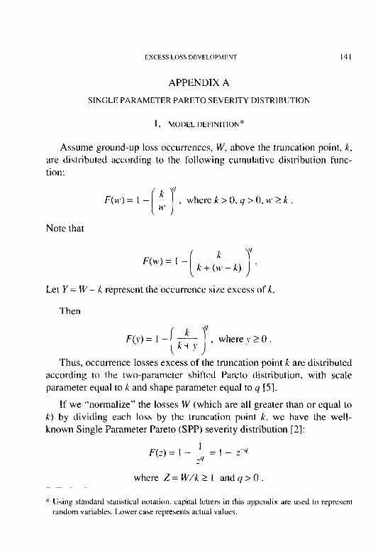
EXCESS LOSS DEVELOPMENT 141
APPENDIX A
SINGLE PARAMETER PARETO SEVERITY DISTRIBUTION
1. MODEL DEFINITION*
Assume ground-up loss occurrences, W, above the truncation point, k, are distributed according to the following cumulative distribution func- tion:
where k > 0, (I> 0, M’ 2 k .
Note that
Let Y = W - k represent the occurrence size excess of k.
Then
, wherey20.
Thus, occurrence losses excess of the truncation point k are distributed according to the two-parameter shifted Pareto distribution, with scale parameter equal to k and shape parameter equal to y [5].
If we “normalize” the losses W (which are all greater than or equal to k) by dividing each loss by the truncation point k, we have the well- known Single Parameter Pareto (SPP) severity distribution [2]:
F(:) zz ] - !; = ] - :-‘I
where Z= W/k2 I andq>O.
* Using standard statistical notation, capital letters in this appendix are used IO represent random variables. Lower case represents actual values.
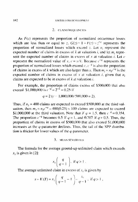
142 EXCESS LOSS fW\‘l~I~Of’Mf;N I
As F(L) represents the proportion of normalized occurrence losses which are less than or equal to :, G(Z) = I - F(Z) = 15’ represents the proportion of normalized losses which exceed :. Let II, represent the expected number of claims in excess of k at valuation i, and let W, repre- sent the expected number of claims in excess of .I- at valuation i. Let c represent the normalized value of .v, C’ = .\-1X. Because CC’ represents the proportion of normalized losses which exceed c’. (.-‘I is also the proportion of claims in excess of k which are also larger than .Y. Then I??; = H,c.-” is the expected number of claims in excess of .V at valuation i, given that II, claims are expected to be in excess of k at valuation i.
For example, the proportion of claims excess of $SOO.OOO that also exceed $l,OOO,OOO is c-” = 2-’ = 0.25 if
y = 2 (c = 1,000.(100/500,000 = 2).
Thus, if 12~ = 400 claims are expected to exceed $SOO,OOO at the third val- uation, then rn3 = or+-” = 400(0.25) = 100 claims are expected to exceed $l,OOO,OOO at the third valuation. Note that if y = 1 .S, then C.-Y= 0.354. The proportion c -y becomes 0.5 if .q = 1, and 0.707 if y = 0.5. Thus, the proportion of claims in excess of $X)0,000 that also exceed $l,OOO,OOO increases as the y-parameter declines. Thus, the tail of the SPP distribu- tion is thicker for lower values of the y-parameter.
3. MEAN SEVERITIES
The formula for the average ground-up unlimited claim which exceeds x, is given in [2]:
ify> 1.
The average unlimited claim in excess of .I-, is given by

EXCEiSS LOSS DEVELOPMENT 143
where s represents the expected value of Y = W - x, and W 2 s, .
The formula for the average ground-up claim which exceeds X, but is limited to s2 is given in [2]:
and s,(l+ln(h)), if q=I,
where h=.~~/,r, and In(h) represents the natural logarithm of h. The for- mula for the average claim in the layer from I, to .I-~ (total losses in the layer divided by the number of claims in excess of .y,) is given by
ifq#I, and
s = s, ((I + In(h) ) - I) =x, In(h), if q = 1, where h =.Y~/.Y, .
Note that s represents the expected value of Y = W - x,, where Y is capped by the layer limit s, -x, and Y 2 0 .
For example, the average claim in the layer from $500,000 to $1 ,OOO,OOO is calculated as follows, assuming q = 2:
since h = 1,000,000/500,000 = 2.
If q = I .5, then s is similarly calculated to be $292,893.
If q = I, then s = (500,000)(ln(2)) = $346,574.
If q = 0.5, then
s = (500,000) 21 -0.5 _ 1
L 1 I -.5 = $414,214.
This example illustrates the property of the SPP distribution that lower values of the q-parameter are associated with higher mean severi-
144 EXCESS I OSS l~lI\‘I;I.Ol~hlliV I
ties. This is because the distribution becomes thicker-tailed (more proba- bility in excess of any large value) as the q-parameter declines.
For casualty classes of business. the r/-parameter tends to decline as a function of the stage of development (121. [4I. IS]). This implies that casualty severity distributions tend to becomc thicker-tailed as claims mature, and so the average claim in any layer (where the SPP distribution is an appropriate model) will increase as claims mature.
EXCESS LOSS DEVEI.OPMEN’I 145
APPENDIX B
PROOF OF PROPOSITION
The proof of the proposition is based upon estimating the incurred losses in a layer as the product of the expected number of claims above the retention and the average claim in the layer. The incurred loss devel- opment factors for both the relatively low and high layers are computed as ratios of layer incurred losses at the appropriate valuations. Simple algebra leads to the formula in the proposition when one assumes that the ratios of the gross limit to the retention for both layers are equal.
Recall that the SPP distribution is assumed to be an appropriate sever- ity model for claims in excess of k,. If 11; represents the expected number of claims in excess of k, at valuation i, then ~1; = II;c.-~~ represents the expected number of claims in excess of s, at valuation i, where c =.r,/k,. The average claim in the layer from .v] to s? (total losses in the layer divided by the number of claims in excess of s, ) at valuation i is given by
where h = X/X,.
The formulas for m; and s; follow from the properties of the SPP distribution and are proven in Appendix A.
Incurred losses in the layer from X, to-r, at valuation i are given by mj si . Similarly, incurred losses in the layer from the retention X, to the gross limit .r2 at va1uation.j are given by “l~~j , where nZj = /I.~c,-Y~ and
h’ - ‘/, - 1 sj = .YI t-~-- 1 l-4, ’ ifqjf 1.
(Note that 1Z.j represents the expected number of claims in excess of k, at valuationj, and nrj represents the expected number of claims in excess of .v, at valuationj.)

146 EXCESS I.OSS IxYEI.ol’S1I:I\I
The incurred loss development factor from valuation i to valuation j for losses in the layer from .v, to .v? is given by
t?j (I - C/i) (h’ - “’ - 1 ) f$= jF(, -q-)(hl-‘,,- 1)
:
f.c’t-c’,.
,‘I I .I I Recall that x~/.v, =kJk, = h and ~=.~,/li,. If (‘= I then .\-, =k, and .t; = k, = hk,. The formula forf’then yields the incurred loss development factor from valuation i to valuation j for losses in the layer from k, to k2, which is denoted d:
J’Z(jX “5 ( 1 - q,) (h’ ~- “j - 1 )
n; (1 - yj) (h’ -(‘I - 1 ) .
Hence, the formula for the incurred loss development factor from valua- tion i to valuationj for losses in the layer from .Y, to I: simplifies to
f’= dc $4, Cl/: - - dc”.
ifq,#l and y,+l.
If j represents the valuation at which claims are fully developed, then ‘Ij = q and f‘ represents the development factor from valuation i to ulti- mate.
In the case of unbounded layers (i.e., P2 and .t-? are infinite), nz, and nrj do not change but Si and “j are as given below (see Appendix A):
Xl s, =
y;-1’ if q, > I.
.t-, and Sj = --~~ , if y, > 1.
Y,- ’
ThenJ’is given by

EXCESS LOSS DEVELOPMENT 147
Ifc=l,thens,=k,andso
f=d= njc?;- ‘1 fl; c4j- ‘1 .
This implies that the incurred loss development factor from valuation i to valuation j for losses in the unbounded layer above s, is given by
f= &Yi - 4, = &.‘,
where d is the incurred loss development factor from valuation i to valua- tion j for losses in the unbounded layer above k,, c = s,/k,, and the SPP parameters are assumed to exceed one.
For bounded layers with qi = qj = 1, the averages of the claims in the layer from X, tos, at valuations i and j (si and Sj) are as follows (see Appendix A):
.si = Sj = St In(h), where h = x2/s,.
The expected numbers of claims in excess of s, at valuations i and ,j are given respectively by
m; = n;(.-’ and mj = nj<*-‘.
This implies that
mj ‘i _ 9 f=--- tili Si tli *
However, the averages of the claims in the layer from k, to k, at valua- tions i and j (t; and rj) are given by
t; = tj = k, In(h), where h = k/k,.
13X f;S(‘FSS I OS5 Ix:VI~I.oPhlf<r\l’l
This implies that the development factor tl for the layer from k, to k, is given by
II- t tf= I’=
II,
‘1, t, Iti
Hence, f= d, which is in agreement with the I’ormula in the proposi- tion due to the unchanging q-parameter.
If qi f 1 and qj = I, then the averages of the claims in the layer from the retention .t-, to the gross limit .\-? L *it valuations i and ,j are proven in Appendix A to be
11’ “I - 1 ,y = \’ I I
! :I 1 - q, *
and s, = .\-, In(h)
The incurred loss development factor from valuation i to valuation ,i for losses in the layer from .v, to ,vl is given by
.f’= m, s, 11, In(h) II
I I-“,- I)/(1 -q,) 1
(.(I, ‘I, VI, s; l’i (17
If (’ = I. then .v, = k, and so .\-? = k, = hk,. The formula forf’then reduces to the formula for tl,
tl = Eli
i
In(h)
“1 (h’ - (‘1 - I )/( 1 - y;) 1.
Substituting into the formula forf;
An analogous proof would hold if y, = I and qj f 1. Q.E.D.
ADDRESS TO NEW MEMBERS-MAY 11, I992
THOUGHTS ON MY CAREER
RUTH E. SALZRIANN
I am happy to be here today to add my congratulations to the new Associates and Fellows. It was 45 years ago that I received my Fellow- ship, and I remember I was very happy, very proud, and gwutly wlic\wl!
Back then, exams were given only once a year, and therefore diplomas were awarded only once a year. This recognition occurred at the Annual Meeting in November, which was always held at the Biltmore Hotel in New York City (and it took me 33 hours by train to get there from Stevens Point, Wisconsin).
At that meeting 45 years ago, there were a total of 21 new Associates and Fellows-and that made 1947 a record year! In the year before, as well as in the year after, there were only 7 new designations.
The entire attendance at the meeting was certainly low by today’s standards. There were only 84 members present, but the 84 represented 30 percent of the total membership. That would be comparable to an attendance of approximately 550 members today.
Our Society has really grown over those 45 years, and I know that salaries have risen just as dramatically. My annual salary in 1947 was $4,520.45. However you look at it, “We’ve come a long way, Baby!”
I really wondered about what I could say today that might have some “take-home” value. It then occurred to me that with the benefit of consid- erable hindsight, I could pass along some thoughts about what made my career all the more worthwhile.
There were, of course, the normal pursuits of job satisfaction and promotions, but there was much more. I particularly enjoyed being in- volved in solving industry problems, and I encourage each of you to become involved in those areas that interest you most. My interests were primarily in the financial and Annual Statement areas.

IS0 .ADDRESS 1’0 NEW MEMBERS
Your participation broadens your outlook, but your contributions give you the most satisfaction. When an idea of yours is accepted by your peers, it is a great feeling. And even when your idea is not that successful, you feel good just because you entered the fray. As the saying goes, “It’s not whether you win, but how you played the game!” The enjoyment comes in knowing that your work was worthy of your best efforts.
The frequency of acceptance and non-acceptance is low. Most often, the work is a team effort. If I grade my recommendations over the years, I get a count of four winners and four losers. And, believe it or not, 1 haven’t given up on those four losers yet. I keep thinking that maybe someday. . .
The second and last thought I would like to address has to do with “how ye are known,” or your professional reputation. You do not start out with a professional reputation, but you surely end up with one. By pass- ing the exams, you have demonstrated your actuarial knowledge and skills. From here on in, it is how you employ this expertise that affects your professional reputation.
With this in mind, you will find that accountability takes on a new significance.
With this in mind, you will find that it is prudent to acknowledge the limitations of your expertise.
With this in mind, you will find that it is prudent to let the data dictate the methodology rather than to superimpose one method or program on all data.
With this in mind, you will find that better interprofessional relation- ships are achieved with the use of language that is clear, simple, and as non-technical as possible.
With this in mind, you will find that the ethical imperative is to use your mathematical capabilities to promote objectivity-the nemesis of bias, rationalization, and wishful thinking.
And I could go on, but you get the idea.

ADDRESS TO NEW MEMBERS 151
Be mindful that a professional reputation is the end-product of any professional career. Let yours be one to be proud of.
In closing, I wish you good luck and fortune. In this era when Con- gresspersons can’t even balance their checkbooks, there has to be a great demand for your expertise.
152
MINUTES OF THE I992 SPRING MEETING
May 10-13. 1992
THE PALMER HOIlSE HILTON. CHlCA(;O
The Board of Directors held their regular quartcrl), meeting from I:00 p.m. to 5:00 p.m.
Registration was held from 4:(X) p.m. until 6:00 p.m.
From 5:X) p.m. until 6:X) p.m., there was a special presentation to new Associates and their guests. The session included an introduction to the standards of professional conduct and the CAS cornmittec structure.
A welcome reception for all members and guests was held from 6:30 p.m. until 7:30 p.m.
Molltiu?‘. Mu?’ I / , I992
Registration continued from 730 a.m. until X:30 a.m.
CAS President Michael Toothman introduced James W. Schacht, Chief Deputy Director, Illinois Department of Insurance, who gave the welcoming address from 8:30 am. until 9:(H) a.m.
At 9:00 a.m.. Mr. Toothman opened the business session which in- cluded the ceremony for new members. There were XX new Associates and I7 new Fellows. The names of these individuals follow:
FELLOWS
Karin H. Beaulieu Catherine E. Eska Julia L. Perrine Allan R. Becker William G. Fitzpatrick Jennifer A. Polson Robert G. Blanc0 Nancy G. Flannery Stephen D. Stayton Patrick J. Bums Brian A. Hughes William Vasek Kenneth E. Carlton III Bruce E. Ollodart Elizabeth A. Daniel J. Czabaj Brian G. Pelly Wellington

MINUTESOFTHE 1992SPRlNGMEETlNG IS3
Kristen M. Albright Todd R. Bault Herbert S. Bibbero Wayne E. Blackbum Annie Blais Daniel D. Blau Betsy L. Blue John P. Booher Christopher K.
Bozman J. Eric Brosius David S. Cash Dennis K. Chan Bryan C. Christman Wei Chuang Kasing L. Chung Gary T. Ciardiello Peter J. Collins Thomas P. Conway Gregory L. Cote Brian K. Cox Timothy J. Cremin Gregory A. Cuzzi Michael K. Daly Manon Debigare Michael L. DeMattei Herbert G. Desson Stephen R. DiCenso Michel Dionne Jeffrey E. Doffing
ASSOCIATES
Michael C. Dubin Francois Dumas Denise A. Feder Charles C. Fung Kim B. Garland Jeffrey C. Gendron Odile Goyer Steven J. Groeschen Farrokh Guiabi Terry D. Gusler Leigh J. Halliwell David L. Homer Paul R. Hussian Hou-Wen Jeng Susan E. Kent Deborah E. Kenyon Kevin A. Kesby Gerald S. Kirschner Timothy F. Koester Gilbert M. Korthals Benoit Laganiere Alan E. Lange Christopher Lattin Marc-Andre Lefebvre Paul R. Livingstone Richard Maguire Katherine A. Mann Leslie R. Marlo Suzanne Martin Keith A. Mathre
Maria Mattioli Thomas S. McIntyre John H. Mize Russell E. Moore Francois Morin Francois L. Morissette David A. Murray Victor A. Njakou Kathleen C. Nomicos Stephen R. Noonan Robert C. Phifer Mark W. Phillips Karin L. Reinhardt Lisa M. Ross Daniel G. Roth Michael R. Rozema David 0. Schlenke Peter Senak Robert D. Share David B. Sommer Barbara H. Thurston Thomas C. Tote Michael Toledano Therese M. Vaughan Jennifer A. Violette Bryan C. Ware John P. Welch Robert J. White Windrie Wong

154 MINUTES OF THE 1992 SPKING Mfil<I‘IU(i
Mr. Toothman introduced Ruth E. Salzmann, a past President of the Society, who addressed the new members from 9:30 a.m. until 9:45 a.m.
Mr. Toothman then recognized special guests in the audience, includ- ing Terry Clarke, Vice President of the British Institute of Actuaries and Chairman of the General Insurance Study Group. as well as W. Paul McCrossan, current President of the Canadian Institute of Actuaries, Jim Murphy, Executive Director of the American Academy of Actuaries, and Tim Tinsley, CAS Executive Director.
Highlights of the program were presented by Albert J. Beer, Vice President-Programs and Communications.
Gary R. Josephson, a member of the Continuing Education Commit- tee, presented a summary of the Discussion Paper Program and the 23 discussion papers to be presented at the meeting.
A summary of the four new Prcmcdit~gs papers was given by Irene K. Bass, Vice President-Continuing Education.
Vice President-Admissions Steven G. Lehmann provided an overview of the Course on Professionalism.
John M. Purple, Vice President-Administration, announced the recipi- ent of the Harold W. Schloss Memorial Scholarship, Jennifer Bunker.
The business session was adjourned at 1030 am.
After a refreshment break, Mr. Toothman introduced Leo McManus, President of L.F. McManus Co., Inc.. who delivered an address on per- sonality types and the need to manage your own personality in order to succeed in management. Mr. McManus spoke from I I :00 a.m. until noon.
A luncheon followed from noon until 1:30 p.m.
The afternoon was devoted to concurrent sessions from 1:30 p.m. until 5:00 p.m., with a break from 3:00 p.m until 3:30 p.m.
The concurrent sessions included presentations of the discussion pa- pers, the PI-weedings papers, the CAS-funded research paper, and a lim- ited-attendance workshop.

MINUTES OF THE I’)92 SPRING MEETING 155
The new Proceedings papers were: I. “The Computation of Aggregate Loss Distributions”
Author: John P. Robertson CIGNA Property & Casualty Co.
2. “Testing for Shifts in Reserve Adequacy”
Author: Richard M. Duvall Sedgwick James, Inc.
3. “Parameterizing the Workers’ Compensation Experience Rating PI an”
Author: William R. Gillam National Council on Compensation Insurance
The CAS-funded research paper was:
“The Profit Provision in the Ratemaking Formula”
Author: Stephen D’Arcy Department of Finance, University of Illinois
The Discussion Papers presented were:
1. “An Evaluation of Surplus Allocation Methods Underlying Risk- Based Capital Applications”
Authors: Michael J. Miller TillinghasVTowers Perrin
Jerry W. Rapp Tillinghastmowers Perrin
2. “Surplus Allocation: An Oxymoron”
Authors: Irene K. Bass William M. Mercer, Inc.
C.K. Khury William M. Mercer, Inc.

156 MINUTES WTHE IY?)? SPKIN(i MI’I:l’lKi(;
3 _ . “Surplus-Concepts, Measures of Return. and Its Determination”
Author: Russell Bingham ITT/Hartford Insurance Group
4. “Analysis of Surplus and Rate of Return Without Using Lever- aged Ratios”
Author: Richard J. Roth, Jr. State of California Department of Insurance
5. “The Implications of Market Return Pricing Strategies Upon Profit and Required Surplus”
Author: Brian E. MacMahon Industrial Indemnity
6. “Simplified Confidence Boundaries Associated With Calendar Year Projections”
Author: James P. McNichols Ernst & Young
7. “Practical Loss Reserving Method With Stochastic Development Factors”
Author: Mary V. Kelly The Co-operators General Insurance Co.
8. “Modelling Asset Variability in Assessing Insurer Solvency”
Author: Louise A. Francis Tillinghastflowers Perrin
9. “Surplus in Investment Strategy Due to Mismatch With Liabili- ties”
Author: John C. Burville ACE Limited
10. “The Value of Junk”
Author: Louise A. Francis Tillinghast/Towers Perrin

MINUTES OF THE 1492 SPRING MEETING 157
1 I. “European Approaches to Insurance Solvency”
Author: Sholom Feldblum Liberty Mutual Insurance Co.
12. “An Application of Risk Theory to Control Solvency and Finan- cial Strength”
Author: Heikki Bonsdorff Ministry of Social Affairs and Health of Finland
13. “Solvency Regulation in Canada”
Authors: Canadian Institute of Actuaries P&C Solvency Sub-Committee
Richard Gauthier, Chairperson Barbara Addie Jean Cote Alain Lessard Christopher J. Townsend
14. “Capitalization of Property/Casualty Insurance Companies”
Author: Paula R. Federman Standard & Poor’s Rating Group
15. “A New Look at Evaluating the Financial Condition of Property and Casualty Insurance and Reinsurance Companies”
Authors: Thomas M. Redman John Hancock Management Co.
Christopher E. Scudellari Ernst & Young
A limited-attendance workshop was also held:
Personality Profile Assessment Presenter: Leo F. McManus
L.F. McManus Co.. Inc.

There was an officers’ reception for new Fellows and their guests from 5:30 p.m. until 6:30 p.m.
The general reception for all members and their guests was held from 620 p.m. until 7:30 p.m.
Tuesday, May 12. 1992
Concurrent sessions. which included both the presentations of papers and panel sessions, were held from 8:X) am. until noon. with a refresh- ment break from IO:(X) a.m. until 1 I’):30 a.m.
One Ploc~wt1ing.s paper was presented: A Discussion of “An Analysis of Excess Loss Development”
Author: Robert A. Bear North Star Reinsurance Corp.
The panel presentations covered the following topics: I. Actuaries in Regulation
Moderator:
Panelists:
Anne Kelly Chief Casualty Actuary New York State Insurance Department
Richard J. Roth, Jr. Assistant Commissioner California Department of Insurance
Robert W. GossroN, Casualty Actuary Illinois Department of Insurance
Kevin J. Conley Actuarial Administrator Iowa Insurance Division.

MINUTES OF TllE 1992 SPRING MEETING 159
2. Questions and Answers with the CAS Board of Directors
Moderator: David P. Flynn (President-Elect) Senior Vice President and Chief Actuary Crum and Forster Corp.
Panelists: Charles A. Bryan (Chairman and Immediate Past President) Partner Ernst & Young
Linda L. Bell (Elected 1990) Senior Vice President and Chief Actuary Transamerica Insurance Group
W. James MacGinnitie (Elected 1990) Consulting Actuary Tillinghast/Towers Perrin
Heidi E. Hutter (Elected I99 I ) Executive Vice President Atrium Corp.
The Discussion Papers presented included: 1. “NAIC Risk-Based Capital Efforts in 1990- 199 1”
Authors: Allan M. Kaufman Milliman & Robertson, Inc.
Elise C. Liebers New York State Insurance Department
2. “Solvency Measurement for Property-Liability Risk-Based Capital Applications”
Author: Robert P. Butsic Fireman’s Fund Insurance Companies
3. “A Method for Risk Quantification for Surplus Requirements”
Author: Anthony Iafrate General Reinsurance Corp.

162 hllNLI’l’I:S 01. ‘Ilit: I’)‘)? SPRING MEETING;
Mike Blivess Steven Book Ron Bomhuetter Chuck Boucek Roger Bovard Paul Braithwaite James Brdnnigan Bob Brian Dale Brooks Brian Brown Randall Brubaker Chuck Bryan James Buck Patrick Bums George Busche Jeanne Camp John Captain Kenneth Carlton Sandy Cathcart .Joel Chansky Jim Christie Mark Cis David Clark Kevin Conley Chap Cook Alan Crowe Patrik Crowe Alan Curry Janice Cutler Daniel J. Czabaj Stephen D’Arcy Ronald Dahlquist E3ob Daino Jerome Degemess Tony Didonato
Robert Downer Paul Dyck Kenneth E%slon Richard Easton Douglas Eland Catherine Eska John Ewert Janet Fagnn Steven Fallon Bill Fanning Sholom Feldblum Ron Ferguson Russell Fisher Walt Fitzgibbon Bill Fitzpatrick Kirk Fleming David Flynn Louise E:rancis Kenneth Frohlich Mike Fusco Alice Cannon Chris Garand Bob Gardner Richard Gauthier Judy Gillam W. Robin Gillam Jim Gillespie Steve Goldberg James Golz Karen Gorvctt Tim Graham Nancy Graves Ronald Greco Ann Griffith Christy Gunn
Sam Gutterman Larry Haefner David Hafling Malcolm Handte Don Hanson Jeff Hanson Dave Hartman Gayle Haskell Paul Henzler Barbara Higgins Anthony Hill Randy Holmberg Mark Homan Carl Honebein Brian Hughes Heidi Huttet Ron Jean Dick Johe Russ John Andy Johnson Jeff Jordan Gary Josephson Bob Kaplan Allan Kaufman Anne Kelly Stan Khury Joel Klcinman Leon Koch Mikhael Koshi Gary Koupf Eric Johnson Rodney Kreps Jeff Kucera Ken Krissinger Mike LaMonica
MINUTES OF THE IYYZ SPRING MEETING 163
Gary LaRose Bob Daino Gus Krause Mike Larsen Fran Lattanzio Robert Lee Steve Lehmann Joseph Levin Peter Licht Aileen Lyle James MacGinnitie Jan Lommele Brian MacMahon Howard Mahler Isaac Mashitz Stuart Mathewson Bob Matthews Debra McClenahan William McGovern Mike McMurray Michael McSally Bob Miccohs Mike Miller Neil Miner F. James Mohl Karl Moller Phil Moore Bob Mucci Donna Munt John Murad Tom Murrin Chris Nelson Ray N&wander Terry O’Brien Bruce Ollodart
FELLOWS
Bruce Paterson Gary Patrik Marc Pearl Steve Peck Kai Pei Brian Pelly Julia Perrine Steve Philbrick John Pierce Jen Polson Debbie Price John Purple Christine Radau Andrew Rapoport Jerry Rapp David Renze Jim Richardson John Robertson Robert Roesch Deborah Rosenberg Gail Ross Richard J. Roth, Jr. John Rowell Ruth Salzmann Jerry Scheibl Tim Schilling Karen Schmitt Roger Schultz Joseph Schumi Jerry Siewert LeRoy Simon David Skurnick Lee Smith Dick Snader David Spiegler
Dan Splitt Stephen Stayton Grant Steer
Stuart Suchoff Ron Swanstrom Vernon Switzer Suan Boon Tan Catherine Taylor Frank Taylor Pat Teufel Mike Toothman Chris Townsend Frank Tresco Ben Tucker Anne-Marie Vanier Bill Vasek Richard Vaughan Andre Veilleux Steven Visner Joe Volponi Bill VonSeggem Mike Walsh Nina Webb Patsy Webster Al Weller Betsy Wellington Chuck White Peter Wildman Ron Wilson Mike Wiseman David Withers Richard Woll Patrick Woods John Zicarelh

164 YINl’TES OE ‘1111: IYYZ SPRING MEETING
Marc Adee Kristen Albright Jean-Luc Allard Bruce Anderson Tony Balchunas Todd Bault Herbert Bibbero Wayne Blackburn Annie Blais Daniel Blau Betsy Blue John P. Booher Jack Brahmer Chris Bozman Eric Brosius Dennis Chan Bryan Christman Wei Chuang K. Leonard Chung Gary Ciardiello Michael Coca Peter Collins Tom Conway Greg Cote Burt Covitz Brian Cox Tim Cremin Dan Crifo Guy Danielson Manon Debigare Lyle Degarmo Jeffrey Deigl Michael DeMattei Herb Desson Stephen DiCenso
ASSOCIATES
Michel Dionne Jeff Doffing Michael Dubin Francois Dumas Stan Durose Charles Emma Phil Evensen Denise Fedcr Carole Ferrer0 Loy Fitz Ross Fonticella Charles Fung Jeff Gendron Terry Goldberg Richard Goldfarb Robert J. Gossrow Odile Goyer Steve Groeschcn Farrokh Guiahi Ewa Gutman Aaron Halpert Philip Heckman Wayne Holdredge Tony Iafrate Paul Hussian Laura Johnson Dan Johnston Marty Kelly Susan Kent Deborah Kenyon Joe Kim GerryKirschner Timothy Koester Gilbert Korthals John Kulik
Benoit Laganiere Alan Lange Chris Lattin Andre Lefebvrc Bill Leincr Eric Lemieux Roland Letoumeau Sam Licitra Elise Liebers Paul Livingstone Rich Maguire Katie Mann Eduardo P. Marchena Leslie Marlo Suzanne Martin Keith Mathre Maria Mattioli Eugene McGovern Jim McNichols Stan Miyao John Mize Kelly Moore Russell Moore Francois Morin Francois Morissette David Murray Robin Murray John Napiersk Kwok Ng Victor Njakou Kathleen Nomicos Stephen Noonan Kathy Pechan Clifford Pence Bob Phifer

MINUTES OF THE 1992 SPRING MEETING 165
Mark Phillips Karin Reinhardt Mayer Riff Kevin Rosenstein Lisa Ross Dan Roth Mike Rozema Michael Sanservero Sandra Santomenno Dave Schlenke Joanne Schlissel Pete Senak
ASSOCIATES
Robert Share Donald Skrodenis David Sommer Keith Spalding Chet Szczepanski Craig Taylor Barbara Thurston Thomas Tote Mike Toledano Janet Trafecanty Scott Vandemyde Terri Vaughan
Jennifer Violette Rebecca Wagner Brian Ware John Welch Russell Wenitsky Robert White Kevin Wick Windrie Wong Scott Yen Chas Yesker Nancy Yost

Volume LXXIX, Part 2 No. 151
PROCEEDINGS November 15, 16, 17, 18, 1992
CREDIBILITY BASED ON ACCURACY
JOSEPH A. BOOK
Ahstruct
This pupor- .shou~.s that the optimal credibility split hctti~een two estimutora is related to hon’ n)ell euc.h estimutor predicts the underlying esperience. First, un eqwtion is dwnw n+ic~h espsesses the credibility assigned to rcrc,h cstimutor in terms oj’ the u\wug:c prediction error of the othclr cstimutor und the UI*- eruge squured diference betMwn the tww cstimutors. That eqlrntion is \>erified wing the cIu.s.sic Buyjsian credibility n/(n + k) ,forrnrrla and a fcwmulu ,fiw nvighting prior oh.ser\~a- lions of time series that MUX de\vzloped by the uuthor. An en- hancement to the classics Buyesiun method for c~luss credibilitic~.s is shown. Finally. the uuthor shoncs thut optimal credibility is proportionul to thug ucc~rruc~q of cur~h estimator, less the extent to which both estimutors muke the same errors.
166

CREDIBILITY BASED ON ACCURACY 167
1. INTRODUCTION
Much of historical credibility emanates from one of three philoso- phies:
1. The square root rule and its cousins.
2. The Bayesian n/(n+k) formula. 3. Alternative Bayesian philosophies that assume that losses are
distributed according to some member of a family of distribu- tions, and assign some judgmental probabilities to the distribu- tions within the family.
Each of these approaches has its own set of problems.
Approach 1, the square root rule, apparently is little more than an ad hoc formula to graduate credibility from 0 to 1 in a fashion that:
a) tends to assign relatively high credibilities to small samples; and
b) achieves full credibility at some point.
Approach 2, the n/(n + k) formula, is based upon a presumption that the sample mean is from a distribution chosen from a set of distributions. The complement of the credibility is to be assigned to the grand mean of all possible distributions. However, many credibility situations are not characterized by the process of first choosing a distribution randomly and then sampling from that distribution. For example, consider the case where a rate change indicated by a state’s data is credibility-weighted against straight trend. While some might argue that the choice between the state’s data and straight trend is just such a “distribution of distribu- tions,” clearly straight trend applied to the last rate indication is not the grand mean of that family of distributions. Further, when those assump- tions do apply, such as in the class ratemaking problem, the grand mean must also be estimated.
Approach 3, the alternative Bayesian approach, relies on a presump- tion that the distribution of potential losses is a member of some family of distributions. The major problem with this approach is that the typical real-world loss distribution is not a precise mathematical curve. Further,
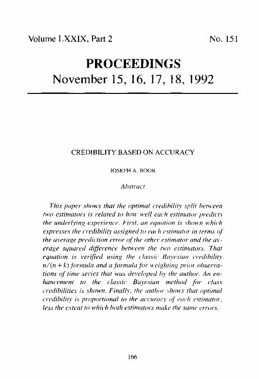
this approach usually imposes some second probability distribution upon the choice of a distribution. An ideal method should be distribution-free.
To avoid these difficulties, it is worthwhiic to list some of the attri- butes of a good approach to credibility.
1. Since the purpose of credibility is to hone an estimate of losses, it should do so in the best fashion possible. Specifically, it should produce optimum estimators of the unknown mean ex- pected loss.
2. It should work in a wide variety of situations; e.g., when the complement of the credibility is assigned to trend, econometric projections, alternative methods of estimating the sample mean, or a sample of a larger but related distribution.
3. It should be distribution-free. it should not work solely when losses approximate some specific mathematical probability dis- tribution.
4. Intuitively, it seems that the credibility should, in some sense, be related to how effectively the observed sample losses approxi- mate the underlying propensity for loss. Further, whatever statis- tic receives the complement of credibility should receive greater weight as its effectiveness in estimating the underlying propen- sity for loss increases.
One method that meets ail these criteria involves minimizing the ex- pected squared error in estimating the propensity for loss. Specifically, if we seek to credibility-weight two statistics .v, and .\-? to approximate Y, and if:
zf = E[ (s, - Y)’ ] ; i.e., tf is the expected error of.\-, as an estimator;
zz = E[ (,I-~ - Y)’ ] ; i.e., T: is the expected error ~f’.t-~ as an estimator;
ii;‘? = E[ (x, - .v$ ] ; i.e., Sf2 is their expected squared difference;
then

CREDIBILITY BASED ON ACCURACY 169
produces the estimate
z.r, + (I - z) .Yz ,
which minimizes the error in estimating Y; i.e.,
E[ (Z.r, + (I - Z).u, - Y)’ ] = min.
The proof is provided in Appendix A.
A quick review of the above criteria will show that this approach does indeed fulfill ail four: it is optimal by design, works with a wide variety of estimators, is distribution-free, and assigns credibility in accordance with predictive accuracy.
3 1. USING OBSERVED ACCURACY
Before going further, it might be worthwhile to note that this method produces the same value of 2 when we attempt to predict an observed value Y’ rather than the actual propensity for losses Y.
In particular, if Y is the propensity for loss, then let Y’= Y + A be the observed losses. In this case, A would be independent of Y, x,, and +x2, and have a mean of 0 and a variance of S’.
Then, since the x and A are independent,
71 12 = TT + s?
T/ = z; + s*,
and

170 CRf~fXBII.ITY RASEDON *\(‘(‘I~RA(‘b
Hence, computing Z for actual observed losses produces the same Z as that appropriate for predicting the underlying propensity for loss. Further. since 2,‘2, z2”, and hi2 may then be estimated from historical observed losses, Z may be estimated from actual observed losses.
One aspect of using historic predictive accuracy must bc noted-it is impractical with the highly-skewed distributions typically associated with individual risks and small pools of losses.
The classic example is the credibility of a medium-size commercial insured’s own experience relative to industry experience. Even when the insured has average exposure (i.e., the unmodified manual rate is right for the insured), the insured will typically experience loss ratios in the 40% to 50% range year after year. However, every five to IO years it will experi- ence a loss ratio in excess of iOO%,. That is because the loss size distribu- tion, and hence the insured’s aggregate loss distribution. is highly skewed. Simply stated, the insured is exposed to very large, but relatively infre- quent, losses. Because those losses are so large, they represent a dis- proportionately large part of the insured’s exposure to loss. Because they are so infrequent, they do not show up in the insured’s loss experience every year.
The naive observer might conclude after viewing several years of low loss ratios that the insured’s own low loss experience is a much better predictor of that insured’s loss experience than the manual rate. The previous section of this paper would seem to support that statement.

CREDIBILITY BASED ON ACCURACY 171
Actual observed accuracy is misleading, however, because of the partial observation of prediction error. Over the last four years or so, only a portion of the distribution of prediction errors (specifically the low side) has been observed. When a large loss occurs, the full range of prediction error can be glimpsed. Depending on how long it takes for that large loss to occur, the manual rate may then appear to be either too high or too low.
Many of the standard actuarial treatments for skewed distributions correct this problem. For instance, one could compare an insured’s histor- ical loss experience with the following year’s basic limits losses and an industry provision for excess losses. One could also replace the industry excess loss provision with, say, 30 years of the insured’s own trended excess losses. Alternatively, one could compare the estimating accuracy of a large body of similar insureds. Although each member insured’s observed losses may not be fully representative of the full error distribu- tion, a large enough body of insureds should approximate all probable prediction errors.
Before proceeding further with an analysis of how this method may be applied in practice, it is worthwhile to investigate whether it reproduces some of the credibility formulae that are already known.
E.wnple I. Clussir Bayesiat? Credibility
Let s be the result of a two-stage process. First, a mean 8 E o is selected randomly from a set of means o with (grand) mean M. Then x,, -u,, . . . . x,, are selected from a distribution with mean 8 and variance S*. Their mean .U is, of course, dependent on 8, but each si - 9 is indepen- dent, not only of the other Sj - 8, but also of 8. Further, let the 8 E o have variance 02. Then, classic credibility [I] says
Z (.u, M, 0) = n/[n + (S2/02) 1.
To prove this, note that independence of the si and 8 implies:
r,; = (SVn) ,
z&= 02, and

177 CKEDIBIl.I’l’Y Ib\SlilI ON A(‘(‘I k\C‘L
Then, the formula states:
In other words, the classic Bayesian credibility is reproduced.
Let s(t) begin at some .v(O) and then bc changed infinitesimally often by infinitesimally small, but variable, perturbations. In other words, the change in .1-(t) from time to time is a result of a very Iargc number of very slight random occurrences, just like those affecting most econometric time series. The random nature of the perturbations assures us that .v(t) will be distributed normally about .v(O) + tp (where lo is the average rate of change), and the variance of .r(t) is to’ (where CT’ ir, the unit variance).’ In fact,
and
To simplify matters, let us consider the case where p = 0. Further, as in most practical problems, when x(I). x(3), . . . . .\-(,I) are estimated by .$(I). -G(2), . . . . .?(,I), there should bc some estimation errors A,. So, .?(i) =x(i) + Ai, and the Ai are independent and identically distributed with mean 0 and variance S’. Then, when weighting .?( I ), .?(2). .?(3), etc. to es- timate .Y(.(II), the weights
’ The limited reading of this author on Poisson proccsscs suggcs15 that ~nc of the con- clusions on the mean and variance may be com1no11 know ledge of statisticians.

CREDIBILITY BASEDON ACCCRACY 173
w; = s’ (‘I - ‘$7; ,
where the F, are defined recursively by
F,= I;
F2 = S’ + 0’ ; and
F;+,=(2S’+o’)Fi-S’F;- I
produce the optimal estimate. To test this, only the two-point estimate will be verified. Unfortunately, similar credibility estimators for three or more estimators are very unwieldy. The two-point estimate involves an estimate for ,?(3) given $2) and G( 1).
According to our formula, the result should be
A(3) = s’,S ( 1)-t CT2 + S’) .gK) . cJ* + 2s’ ’
i.e., it should be true that
Note that, since .~i - -pi is orthogonal to -~j - .\:i and .ri - ,yi:
zf= E] (d?(2) - $3) )’ ]
= E[ (u;(2) -s(2) )” ] + E[ (s(2) -s(3) )’ ] + E] (x(3) - $3) )2 ]
= s2 + (-y + s* = 29 + (3* .
T; = E[ (a?( I ) - d?(3) )’ ]
= E[ &I) - .I-( 1) )’ ] + E[ (s( 1) -s(3) )2 ] + E[ (s(3) -<c(3) )2 ]
= s* + 20’ + s* = 29 + 20’ .

174 CREDIRII.ITY 13.4SI:I) OV .\(‘(‘I’RA(‘l
6f2 = E[ (w;( I ) - .?( 2) )’ 1
= E[ (.:(I) --A( 1) )’ ] + E[ (.Y( I) -x(3) )’ 1 + El (x(2) - .;(2) )’ ]
= s* + (-J* + s2 = 29 + (3’ .
Thus,
z (;(2), $( 1) ;(3) ) = 2sz + ~0’ - (2,P + 0’) + 2s2 + 0’ = s’ + d 9 2 (29 + 02) 2s’ + CT’
So, in at least two cases, this approach does reproduce credibilities al- ready known from other analyses.
To be truly useful, an approach should yield new methods. The true classification ratemaking problem will now be addressed.
3. CLASS CREDIBILITIES
The objective is to produce a rate for a subgroup cx of a large group I-. The means of a and I- are unknown, but have been estimated using:
ti = ( l/n)C U; ; Cli E a for pn and
R=(l/(m+n)) (~~~i+~ll,); h,E p=r-a. i i
Further, Var (Cli) = 0; and Var (hi) = pi have been estimated from actual data.
-- Before proceeding, note that weighting Cr with F using Z (u, 8, pa) ef-
fectively assigns a portion of the complement of the credibility back to .5 since 2 = (na + mTi)/(n + m). So, it may be more worthwhile to evaluate
and then use

CREDIBILITY BASED ON ACCURACY 17s
-- z (ii, 75, &J (n + m) - n z (@ R, pa> = ~ -~ ~~..~m--. _ .
Note that
Var (a) = (~i)/n ; Var (5) = (o$/m ; and
z;=E[ (Z-Q2]=o;/n.
Since the hi are independent, and the 6; - & have mean 0,
C: = E[ (5 - /J,$ ] = c$/m + (J+ - pa)’ ;
and
S:, = E[ (a - fi)‘] = E[ (2 - Q2] + E[ (& - pP)‘] + E[ (h - &#]
= (o~/n) + (p, - pp)* + (c$/m) .
Hence
= (#j/m) + (p, - pp)’ - (0:/n) + (0:/n) + (p, - VP)* f (02,/m)
2 ( (&W + (cl, - clp)* + (+W >
n = n + [oi/( (c$/m) + (p, - pp)’ ) ] ’
Or, if m is much larger than n
Of course, ai and (cl, - P,-)~ are unknown, but they may be estimated using the sample variance of ui E a and the difference between the exist- ing rate for a and the overall average rate.

176 CREDIBIl.IT1’ H?\SEDOi\ ~\(‘(‘I’K~\(‘~
This formula illustrates several key points:
1. Highly heterogeneous classes (high o:~.) should receive lower credibilities.
3 I. Extremely high or low rates [high (pa - pr)?] should be based more heavily on their own expericncc than on the overall aver- age rate.
3. For classes that form a statistically large proportion of the group, the complement of the credibility should be assigned to the mean of the remainder of the group. not the group mean.
4. A NlfMEKICAI. ESAMPLLI
Suppose that one is attempting to find the underlying mean, p,, of a distribution given last year’s observation X,, , _ , of the distribution. and last year’s observation of X,, , _ ,, a related statistic. Further. assume X, ; is thought to be cyclic and biased as a predictor of X,. ,, and its year-to-year variations are thought to be independent of those of X,. Whether X, is cyclic or stationary is not known. The observations are shown in Table 1. Of course, the values X,. , + , and X,. I + , arc unknown at time i, but the goal is to find the Zj such that Z, X,. , + ( I - Zj) X,, , is an optimum estima- tor of p, at time i + 1.
In this case, since X, and X2 arc independent predictors of p., , E[ (X, - X3)’ 1 reduces to tz. , + r;, 1 , so Z becomes Z = rz, /(ri. , + K:. J. X, ‘s error, z:. ,, may be estimated by S’f, ,, the sample variance of the X,,; seen to date. *Since Xz,i *is biased, rf.? will be estimated by s:-. 2 + (X2. ; + , - Y,)’ , where Y; is the last estimate of p,. Th@ method recognizes both the cyclic nature of X1 (by using X,, , + , - Y, ) and a potential cyclic pattern in X, because it considers just the last observed values, not the history of X, and X,. Arbitrarily, the first credibility was chosen at 50%‘. Results are shown in Table 2.

CREDIBILITY BASED ON ACCURACY 177
TABLE I
Year
I
2
3
4
5
6
7
8
9
IO
Xl 72.44
79.06
72.98
79.74
66.69
86.38
68.97
78.61
88.97
74.97
Year xl,i x2. I
1 72.44 104.15 2 79.06 114.66 3 72.98 1 12.75 4 79.74 99.01 5 66.69 103.04 6 86.38 102.80 7 68.97 106.23 8 78.61 97.79 9 88.97 101.63 10 74.97 102.83
TABLE 2
OBSERVED HISTORY
x2 7; = s;. , . , 6 2 (X2 - PJ2
104.15 - - -
I 14.66 43.82 1 IO.46 694.85
112.75 13.51 3 I .34 1018.25
99.0 I 15.04 54.02 656.90
103.04 28.82 44.75 527.70
102.80 47.86 38.36 1175.98
106.23 47.38 3 I .97 368.38
97.79 42.08 36.02 61 1.08
101.63 56.66 32.82 478.30
102.83 50.8 1 29.5 I 158.61
~- - 50%
805.31 95
1049.59 99
710.92 98
572.45 95
1214.34 96
400.35 89
647.10 94
511.12 90
188.12 79
88.30
80.84
73.38
X0.07
68.5 I
87.04
73.07
79.76
90.24
80.82
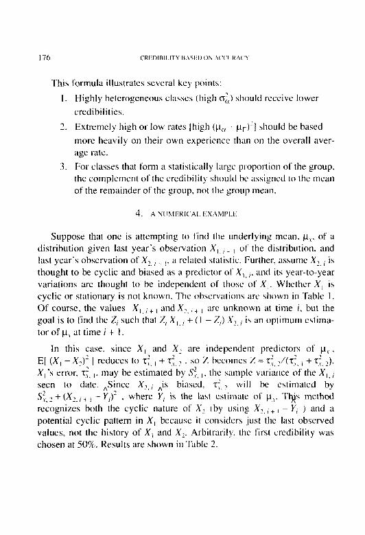
178 (‘REDIBII.ITY BASED ON ACCIIRAC’I
In this case p, looks like a poor predictor of cl., at I’ + I
However, when the true p., is considered, P is a very good estimator of l-h. The Xl., were generated using a normal distribution with mean p, = 80 and variance 0.: = 100 . The X,, ; were generated using a normal distribution with mean 100 and variance 100 for X,, ,. and successively generating each new X,~ ;+, using a normal distribution with mean 100 + .X (X2. i - 100) and variance 36. One can show that the resulting X,,, all have a marginal distribution that has mean 100 and variance 100 since 36 = 100 (1 - (.8)‘) . Therefore, a priori, the credibility of X, should be ( IO0 + 400)/( 100 + 400 + 100) = .83333. However, that credibility should vary with where X, happens to be in its cycle.
It just happened that the X,, , tended to fall on the low side of the distribution, and that the X2,; began on the high side of the distribution and tended to stay there.
In any event, the average squared prediction error of 9 is 44.86, roughly a 20% reduction in the prediction error of X, alone (55.46 as a predictor of the value p., = 80). In fact. the error of 9 is even below 45.6, which results from what retrospectively turns out to be the best possible fixed credibility (96%). That is because this method gives greater weight to X, when it is close to P . m t h e cycle, and less weight when it is further away. So, in this example, the theory works.
5. CREDIBILITY DEMYSTIFIED
One of the side benefits of this approach is that it offers an explanation of credibility that can be understood by laymen. The credibility of each estimator is proportional to its accuracy as an estimator, less the extent to which the two estimators say the same thing. Clearly this explanation is much more desirable than “we’ve always done it this way,” and more understandable to lay people than “we look at the process variance and the variance of the hypothetical means.” But it has yet to be shown that the above explanation is true.

CREDIBILITY BASED ON ACCURACY 179
Note that
Further
= E[ ( (x, - Y) - (s2 - y) I2 ]
= E[ (s, - y>’ ] + E[ (s2 - y> >* ] - 2E[ (x, - y> (-x.2 - Y) ] .
Further, assuming that -xl and s2 are unbiased estimators, p, = ~1~ = Y, so
s;* = z; + z; - 2Cov(.u,, x2)
And when that is included in the formula for Z,
z (x,, x2, Y) = 7; - T: + 7: + T$ - 2Cov(s,, x2)
22; + 22; - 4Cov(x,, x*) ;
22; - 2Cov(x,, x*)
= 22; + 22; - 4COV(X,) X-J ’
72’ - Cov(x,, l-2) =
z; + 2: - 2Cov(x,, x*) *
Dividing top and bottom by 2:~: yields
( 1 A:) - (z?:,/T, z,) z (x,, x2, Y) = -~____~~ *
(l/z?) + (l/T:> - 2 (f?:*/Z,Q ’
where Rf2 is the correlation of X, and x2. Clearly, if 2: is the error of .yl, then l/z: must be s,‘s accuracy. Further, RF2 is the extent to which s, and x2 vary together, and the division by T~Z: normalizes it relative to the in- verse squared errors. Hence, the credibility of each estimator is propor- tional to its accuracy, less the extent to which the estimators say the same thing.

6. PRACTICAL APPf.l~‘AT1ONS AND f~ORMI:f.~\I:
One criticism of this approach is that, like optimum credibility, the appropriate credibility formula depends on the circumstances. For in- stance, if the two estimators are not heavily skewed, their historic accu- racy 12/c (x, ,., - Y’)’ and n/c (.v2,., - Y’)’ may bc used to derive the optimum credibility as shown in Section 2. Per Exalnple 2. the formula (1 + (o’/S’) )/(2 + (o’/S’) ) may be used with o’/S’ estimated using the historic year-to-year changes in .?. As shown in Section 3, the credibility of a class’s own experience should be 4(n + ($,/(K,, - I.,-)‘) ), where II is the number of exposure units, ,S,i is estimated by comparing each year’s class experience to a long-term average. and I’,, - I’[. is the difference between the current rate for class a and the current aver~gc rate. Altema- tively, Sk could be presumed to be constant across all classes and one could then find the SzX that minimized the average squared error (weighted by exposures) when such a formula uses last year’s experience to predict this year’s data.
The most important results are: 1. The credibility of a piece of data and the formula used to derive
it vary with the specific situation. 2. Using the formulae in this paper, one may derive credibility for-
mulae that, up to determining a constant or two, represent the best credibility formulae. The constants can then be determined using historic data to find the constants that minimize the aver- age squared error.
3. The fundamental truth of this paper, that credibility should be based on accuracy, makes intuitive sense and can be understood by laymen.
7. SUMMARY AND~‘ONCl.I~SIONS
In summary, this approach seems to hold promise and appears to offer opportunities to improve the accuracy of loss estimates. However, it will only truly be useful when the estimation errors zf and T; are evaluated. Whether one believes in this approach or not, this author believes that the

CREDIBILITY BASED ON ACCClR.ACY 1x1
large ratemaking organizations should collect statistics on the effective- ness of the various loss estimators they use. Even if other credibility procedures are used, it only makes sense that their effectiveness be moni- tored. Futher, this author believes that greater understanding of how cred- ibility should work can only improve the actuarial work product.
REFERENCES
[ 1 ] Venter, Gary G., et al, Foundurions oj’ Cusuulry Actuuriul Scicwcc, New York, Casualty Actuarial Society, 1990, pp. 375-483.
[2] Efron, Bradley, “Controversies in the Foundations of Statistics,” Anwrican Mathematical Monthly. Vol. 85, No. 4, April 1978, pp. 23 l-246; reprinted in the Casualty Ac‘tuariul Society Formv, Fall 199 1, pp. 259-275.

APPENDIX A
If zf = E[ (x, - Y)’ ] . z; = El (.I-~ - Y)’ 1. and S;., = E[ (I, - .,->)’ J ,
the goal is to set
Q(Z) = E( (Z-l-, + (I - Z) .I’ - Y)’ I = min ,
But algebra gives
E[ (Zx, + ( 1 - z) .\‘? - Y)’ I
= E( (Z (xl - Y) + (1 -Z) (x2 - Y) )’ ]
= Z’ E[ (x, - Y)’ ] + (1 -Z)’ E[ (x2 - Y)’ ]
+2Z(l -Z)E[ (.v,-Y)(x-Y) ]
=Z’z;+(l -.3%;+2Z(l -Z)E[ (.v,-Y)(.\v~-Y) 1.
Using2(A-C)(B-C)=(A-C)‘+(B-Cl’-(A-B)’.
2 E[ (s, - Y) (x2 - Y) 1
= E[ (.I-, - I’)’ ] + E[ (.I-? - Y)’ 1 - E[ ( -\‘, -x1)’ I
= Tf + T; - sfz .
Substituting that back in the overall squared error (Q>) equation,
a, (Z) = E[ (Zx, + (1 -Z) x2 - Y)’ 1
= Z’rf + ( 1 - zyt; + Z( 1 - Z) [r;’ + r; - S;l,]
=Zzf+(l -z)z;+(z2-z)6;,.
This is minimized when
or
or
CREDIBILITY BASED ON ACCURACY 183
Now, this is only a minimum when
However Sf2 is always non-negative.
Note that Z may be negative; i.e., when
But, fortunately, that occurs only where (x2 - Y) and (x, - x2) tend to have the same sign overall; i.e., x2 is generally between xl and Y. Thus, there may be cases where zero credibility is warranted; i.e., xl is not a useful predictor. Alternatively, where
full credibility should be assigned to xl.

184 CRt:DIB11.17’\1’ BASED ON >\(‘(‘t KA(‘\
APPENDIX B
JUST HOW DISTRIBUTION-FKEE IS I~IS7‘KIR1ITION-FREE’!
As noted in the Section 1 of this paper. the credibility. Z. produced by this method produces the lowest expected squared error attainable using the Z\--, + ( I -Z) sJ (additive weighting) formula. That credibility does not depend on the particular characteristics of each estimator’s distribution, but only on how well each estimator predicts the unknown quantity Y, and on the average squared difference between the two estimators. However, it does assume that the best estimator of the unknown Y is the one that minimizes the expected squared estimating error, and that it uses a ZV-, + ( I -Z) .\-? formula. One should consider whether each of these im- plicit assumptions really produces the best estimator of the unknown Y.
Aside from the fact that the expected squared error function is ubiqui- tous in mathematics and related disciplines. there is a practical reason for using it as a penalty function whose minimum defines the best estimator. Conceptually, one might begin by viewing the expected absolute error E [ I estimator - Y I ] as the best penalty function, since it measures the actual error of the estimator. That approach, however, has one consider- able drawback. An extremely large error receives the same weight as a small error, even though extremely large errors may have catastrophic consequences. For example, if a rate would produce precisely the re- quired profit 19 years out of 20 but threaten the company’s solvency one year out of 20, prudence would dictate that the one year out of 20 receives a disproportionate share of attention. One logical approach is to weight each absolute error with the size of that absolute error-in effect to use E[l estimator - Y I 1 estimator - Y I] or Ej(estimator - Y)’ 1 .
The use of an additive weighting is less supportable. This author knows of no reason why an estimator of the form, say .I?. .I$’ - ” would not be a better estimator. It is clear that if .\-, is biased. some Z\-, + (1 -Z) (.\-? - C) formula is better. Superficially, it appears that a rigorous analysis, perhaps using calculus of variations, could produce different formulae for different families of distributions.

CREDIBILITY BASED ON ACCURACY 185
On a more positive note, there are two reasons for using an additive weighting formula. When the two estimators .Y, and x2 are known to be normally distributed about unknown means, but T;, z& and S:, can be estimated, the additive weighting formula is best.’ Also, additive weight- ing has a long history in ratemaking.
’ The author doubts he truly discovered this. Witness the argument in [2].

186 PRICING FOR CREDIT EXPOSURE
BRIAN Z. BROWN
A hstI.uct
This puppet imvpnr~utes jinunc~iu/ theory M’ith inslrr-unce priCiFl,q, A geJleJ7il pJ’Oc’~tll!J’? to lN’iCC fi)J- CJTdit cJ.yJo.slu~t~ PUS
heeJI deWlOped UJId CXtt’JIded t0 .W\Y~JUl iJl.WlYIJlt~t~ pJWdl”‘tS.
For retrospcctiwly ruted inwuds M‘ith a helo~-irn~estment- ,yJ~Jde rUtiJ# jiW171 u CWdit JXJtiJlg U~qcJlcy. the credit e.\pOSliW is .signI~icuJIt to the iJIsuJ-cr. lf‘tl1i.s c.vp0.sirJ.e is igJIoJ.ed, operut-
ing results niuy be JIegutiwl~ cJ$kted, us it is likely that some
udditionul prernirrm unmrnts M’ill not be collected. The princi- pies of credit evposlrrc pric,irlLq CYIH be ertended to the pricing of suretv bonds us outlined irl Section 6. Itz addition, the con- cepts ol;tlhed in this pupcr JJIU~ by Itsed to: 1. e.stublisfI u bud
debt wserw for GAAP ~sttrtct~mts; 2. provide insrrr-unc~cJ wgw lutcws M’ith UJI udditionul nlcthod to deteJwIine colluter-ul r-e-
quirements; 3. estimate .suJ?ty bond loss ratios; uJId 4. prmlide
bunks wjith utI udditiotIul JJIctlIodology to piice letterx of’ credit
ti+Iic,h colluter-ulize unpuid chinI liubilities.
I. IKTKODWTION
The term “credit exposure” is defined as the possibility that one entity will suffer a financial loss due to the inability of a second entity to satisfy its contractual obligations (as a result of the poor financial health of the second entity). Credit exposure, as it relates to underwriting activities of property-casualty insurance companies, refers to the possibility that the insurance company may not be able to collect premiums, deductibles, and other charges when due. This paper will focus on the credit risk associ- ated with issuing retrospectively rated policies and will outline a proce- dure to price this credit exposure. In addition, the credit exposure pricing

PRICING FOR CREDIT EXPOSURE 187
model will be extended to other areas of credit risk exposure, such as surety bond pricing.
For retrospectively rated policies, the insurance company collects pre- mium from the insured based on paid or incurred losses until all claims are closed, or until the insured and insurance company agree on a price to end the retrospective accountings. Thus, if the insured files for bank- ruptcy, the insurance company may not be able to collect all the addi- tional retrospective premiums due. These additional premiums represent a credit exposure to the insurance company. The insurance company may be obligated to pay claims associated with the expired policy even though additional premiums are not forthcoming.
The discussion below is divided into six sections. Sections 2 through 5 deal with the credit exposure associated with retrospectively rated poli- cies. Section 6 describes a pricing model for surety bonds. Section 7 discusses additional applications of the credit exposure pricing model,
2. MAGNITUDE AND QUALITY OF THE CREDIT EXPOSURE
The magnitude of the credit exposure refers to the absolute amount of the expected additional premium due the insurance company on expired policies. Credit exposure results from the nature of retrospectively rated plans. For incurred loss plans, an insured typically receives a return pre- mium at the first retrospective accounting, and thereafter the insured pays additional premium to the insurance company as losses develop. This procedure is similar to the insurance company “lending” the insured the difference between ultimate premium and the collected retrospective pre- mium. This difference between the ultimate premium and the collected premium defines the magnitude of the credit exposure.
For an incurred loss retrospectively rated plan, the insurance company collects standard premium during the first 12 months of the policy period. At 18 months and annually thereafter, a retrospective accounting is per- formed via the following formula:
R,=(B+(CxE)+(CxL,))xT. (2-l)

R, is the retrospective premium at time period f and is subject to a maximum and minimum premium. The maximum and minimum premi- ums are factors of the standard premium.
B is the “basic charge” and covers expenses, profit, and the insurance charge. The basic charge is determined by a factor multiplied by standard premium. The factor C is the loss conversion factor and covers a load for loss adjustment expenses. E is the charge for limiting losses for individual claims that enter the retrospective rating formula. T is the tax multiplier and covers premium tax and some premium-based assessments. The tax multiplier and basic charge may also include a provision for residual market assessments.
L, is the aggregate case incurred loss amount at time t. limited by the per claim amount. Thus, there is no provision for incurred but not re- ported (IBNR) losses in the standard incurred loss retrospective rating formula.’ The magnitude of the credit exposure is proportional to the IBNR.
Figure 1 displays the projected transfer of funds for a standard in- curred loss retrospectively rated plan. In this example, it is assumed that the insured is written for a one-year term and does not renew. The retro- spective rating parameters and incurred loss development pattern are shown on Exhibit 1. For simplicity, the tax multiplier and loss conversion factor are both set equal to one. These assumptions do not affect the conclusions of the paper.
Exhibit 2 displays the amounts underlying the graph on Figure 1, The insurance company collects $2.0 million in standard premium during the first year. The first retrospective accounting is performed with incurred losses evaluated as of 18 months and $674.000 is returned to the insured.’ Over the next seven years, the insurance company will collect the differ- ence between the ultimate retrospective premium ($2.1 million) and the first retrospective accounting premium ($1.326 million), or $774,000. The
’ IBNR is defined IO include both incurred but HOI reported IOSSL’S as well as devclopmcnt on existing case reserves.
’ The example in this paper usumcs that the billing and collection process takes six months. Therefore. the insurance company will return funds to the insured BS of 24 months.

$2500
$2000
$1500
$1000
$500
$0
FIGURE 1 STANDARD INCURRED Loss RETRO PLAN
INSURED WRI~EN FOR ONE YEAR
Premium Dollars (Thousands)
0 1 2 3 4 5 6 7 6 9 Years from Policy Inception
Standard + Ultimate - Collected

190 f’KK‘fN(; f.OK (‘Kf~.flfl I:XI’OSIIKI.
$774,000 is the credit exposure as ot 23 months and. in essence, repre- sents a loan by the insurance company to the insured. If the insured filed for bankruptcy 25 months after the inception of’ the retrospectively rated policy (one month after the insurance company returned funds to the insured), the insurance company could suffer a future earnings toss equal to $774,000.
The credit exposure decreases as losses dcvclop (assuming the insured pays the premium when due). The exposure cquats zero when the insured pays the ultimate premium.
The magnitude of the credit exposure for it specific insured at a spe- cific point in time depends upon how much premium is yet to be col- lected. In general, the quicker the premium is cot&ted. the smatter the credit exposure. Thus, plans with tow loss limits wilt have a smaller credit exposure.
Figure 2 displays the situation where the insurance company insures the above-mentioned risk for three years at a standard premium of $2.0 million a year, and then the insured non-renews. Exhibit 3 displays the numerical backup for Figure 2. The collected premium at Year Two, $3.326 million, equals the first retrospective accounting premium of $1.326 million for the first year of the three-year period plus the $2.0 million in standard premium for the second year of the three-year period. The credit exposure is largest at Year Four. after all politics have had a retrospective accounting. The credit exposure at Year Four (four years after the inception of the first policy) is $133 million or 76.5% of the annual standard premium.
The National Association of Insurance Commissioners (NAIC) has recognized the significance of credit exposure and has altered the statu- tory Annual Statement twice in the last four years in order to provide rnore information on credit exposure. The 198X Statement was altered to display the amount of additional premium that an insurance company anticipates collecting on retrospectively rated plans. Line 9.3 on page 2 of the Statement or tine 33 on page X displays the additional premium amount (Accrued Retrospective Premium). Beginning in loX8. the State- ment also required companies to display the amount of letters of credit,
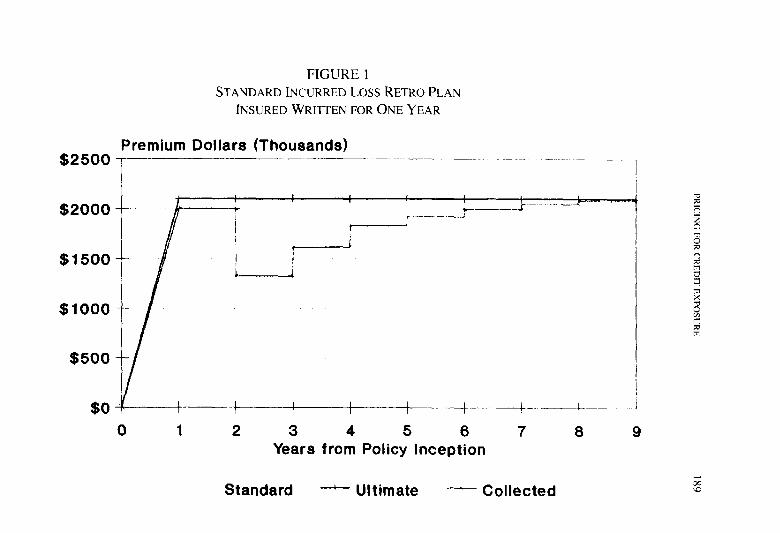
$7
$6
$5
$4
$3
$2
$1
$0
FIGURE2 STANDARD INCURRED LOSS RETRO PLAN
INSURED WRITTEN FOR THREE YEARS
Premium Dollars Ovlillions)
%
I 1 I
T J
I
0 1 2 3 4 5 6 7 8 9 Years from Policy Inception
-- Standard + Ultimate -- Collected

192 PRICING FOR C‘Kf.f)Il I;SI’O\IIKI
collateral, and other funds that secure the accrued retrospective premiums (General Interrogatory # 3 I ). In I99 I, the Statement required that 10% of the amount of unsecured accrued retrospective premium be recorded as a non-admitted asset. These changes show that the NAIC recognizes the possibility that the additional premium due may not be collectible. The collectibility of the additional premium is a f‘unction of the quality of the credit exposure.
Francis Hope stated that “negative rcservcs; i.e., the anticipation of additional premium due the company, [should] be included in the Annual Statement, provided that one is fully confident that the money is truly forthcoming.” [I] Hope probably intended this statement to refer to the accuracy of the retrospective premium reserve: however, it is equally important that the monies due the insurance company be collectible. Amounts due the insurance company may be uncollectible due to the insured’s financial condition.
The quality (collectibility) of the credit exposure is largely determined by the insured’s financial condition. If the insured files for bankruptcy, the insurance company may not be able to collect additional premium. Clearly, an insured in a strong financial position at policy inception is less likely to file for future bankruptcy than an insured in a poor financial position at policy inception. Section 3 outlines several rnethods to deter- mine the financial condition of an insured.
Nationally, credit exposure has increased as the financial strength of American companies has decreased. The rniddtc 1980s saw a large in- crease in the number of leveraged-buyouts (LBOs). The LB0 activity resulted in companies replacing equity with debt. and, therefore. the fi- nancial strength of these companies has decreased. Bonds rated Caa by Moody’+-the bonds closest to default-increased from $7.2 billion at December 1987 to $23.7 billion by March 1990. (31 For non-financial corporations, net interest expense as a percentage of earnings before inter- est and taxes rose from 18.2% in 1979 to 32.9% by year-end 1989. These statistics display the decrease in the credit quality of American corpora- tions. Thus, insurance companies may not be able to collect as much retrospective premium on policies of the 1980s because relatively more insureds may file for bankruptcy.

PRICING FOR CREDIT EXPOSURE 193
3. ANALYZING THE QUALITY OF THE CREDIT EXPOSURE
This section outlines two approaches that can be used to determine the financial strength of a commercial insured:
I. ratio analysis; and
2. independent rating agencies’ ratings.
Rutio Andyis
Ratio analysis depicts relationships between accounts on a firm’s fi- nancial statement. The ratios can be used to measure a firm’s financial health. Ratios can be classified as liquidity ratios, equity ratios, and prof- itability ratios.’
Liquidity ratios measure a firm’s short-term debt paying ability. One commonly used liquidity ratio is the current rutio. The current ratio is a firm’s current assets divided by its current liabilities. Short-term creditors use the current ratio to financially underwrite accounts. All other things being equal, the higher the current ratio, the more likely a firm will be able to pay its short-term debts. Even though credit exposure is similar to long-term debt, an insurance company will be interested in the liquidity ratios because if a firm cannot pay short-term debts it may not be able to pay long-term debts.
A commonly used equity ratio is the debt-to-equity ratio which mea- sures the amount of relative debt of a firm. The higher the debt-to-equity ratio, the more financially leveraged the company. Since the company must eventually repay the debt, a company with a relatively high debt-to- equity ratio may not be able to pay additional insurance premium if the company falls on hard times.
A commonly used profitability ratio is the li~?~~~-iF~t~l~~.~t-~U~~FZ~d ratio. The ratio is:
Times Interest Earned = Income Before Interest and Taxes
~ ~ ~~ ~~ ~~~ - ~~ Interest Expense .
’ Another classification of ratios is market ratios: however, these ratios are more relevant for investment decisions than for credit quality analyGs.

I94 PRIClWi IXOR (‘RlilN I’ l:Sl’OSI KI.
A firm that cannot pay its interest payments when due will eventually have financial problems. The higher the times-interest-earned ratio. the more money a firm will have available for general corporate purposes. Therefore, a firm with a high times-interest-earned ratio is not likely to default on premium payments in the near t‘u1urc.
A financial analyst can use these ratios as tools lo evaluate the credit exposure of a prospective or current insured. These ratios have “rule-of- thumb” levels at which the firm is considrrcrl to he potentially deficient. As a technical note, the rule-of-thumb levels vary considerably by indus- try, and financially underwriting accounts is a complex procedure which often cannot be based solely on financial ratios. Therefore, for accounts that possess a significant credit expoaurc. the analyst should review all of the firm’s published financial information (annual reports, IO-KS, etc.) and meet with a financial officer of the firm. A firm’s ratios may be acceptable: however, the firm may have 3 significant receivable from another firm in poor financial condition. Only the notes to the financial statements will highlight such a problem.
Several independent rating agencies ralc the credit quality of compa- nies. Insurance companies can use the agencies’ ratings to supplement ratio analysis in order to determine the quality of the credit exposure. If the retrospective rating plan for a particular insured has a small credit exposure, it may be more cost effective for the insurance company to rely solely on the agency ratings. Three possible agency ratings are those ot Moody’s, Dun & Bradstreet, and Stand4 & Poor’s,
Moody’s publishes corporate bond ratings indicating the degree of default risk associated with a bond. The default risk on bonds may be similar to the default risk for retrospective premium payments because both are long-term obligations. Moody.5 bond ratings vary from Aaa (where interest payments are protected by a large and stable margin and the bond principal is secure) to C (the lowed class of bonds where the prospect of the bonds ever attaining any real investment standing is ex- tremely poor).

PRICING FOR CREDIT EXPOSURE 195
Dun & Bradstreet provides credit ratings on three million domestic and foreign firms. Dun & Bradstreet’s Busimss /njimnafion Rqxwf con- tains a summary section on each firm. The summary section includes a review of the company’s financial condition and its sales and earnings trend along with the firm’s payment record, as reported by suppliers. The report also includes other financial and operating information. Dun & Bradstreet supplies a composite credit approval rating from 1 to 4, with I being the highest rating.
Standard & Poor’s publishes bond credit quality ratings. Standard & Poor’s bond ratings vary between AAA and D. AAA is the highest rating and signifies that the capacity to pay interest and principal is extremely strong. A rating of D indicates that the firm has defaulted on interest or principal payments.
4. CURRENT INDUSTRY PRACTICES FOR MINIMIZING CREDIT EXPOSURE
The insured’s financial condition will determine the quality of the credit exposure. For firms in excellent financial condition, the insurance company may believe it is not necessary to recognize the credit exposure. I will show later that the risk of default for firms in excellent financial health is minimal, so that it may be reasonable to ignore credit exposure for these accounts. However, for firms in average or below-average finan- cial condition, the insurance company may want to take steps to reduce its credit exposure.
The insurance company can reduce credit exposure by:
I. not offering retrospectively rated plans;
3 -. requiring collateral for anticipated additional retrospective premiums: and
3. altering the cash flow parameters of retrospectively rated poli- cies.
For very large accounts, the first option of not offering retrospectively rated plans and still writing the account is not feasible. Most large in- sureds believe that their loss experience should determine their premium payments. Even though the experience rating plan reflects loss experi-
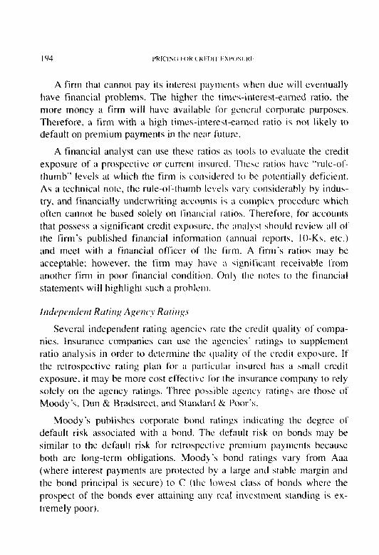
ence, the insureds recognize that retrospectively rated plans will reflect favorable loss experience earlier and more directly.
The second option to reduce the credit exposure is for the insurance company to require collateral from the insured. A letter of credit (LOC) or surety bond may be obtained to secure additional premium amounts. This, in essence, transfers some or all of the credit exposure to the bank or surety.
For example, the insurance company may request collateral equal to the ultimate premium less premium paid to date. Thus. if the insured defaulted at any time, the insurance company’s credit exposure would be fully collateralized. The insurance company could exercise the collateral and collect all expected future amounts due. However, if losses developed higher than anticipated, the insurance company may suffer an earnings loss.
For firms in below-average financial condition. the insurance com- pany may require collateral equal to the maximum premium less premium payments to date. The additional collateral could bc required due to the greater variability of ultimate losses for firms in poor financial condition. For example, firms in poor financial condition may be more likely to lay off workers and overlook loss control in order to cut costs. These mea- sures may increase the variability of ultimate losses.
Finally. insurance companies may alter the cash How of the retrospec- tively rated plan in order to minimize the credit exposure. Two ways to alter the plan are:
1. modify the funding of the retrospectively rated plan: and 3 -. use loss development factors to project losacs used in the retro-
spective rating formula.
The funding for incurred loss retrospective rating plans could be mod- ified in order to minimize the credit exposure. For example, a plan could be designed such that the insured pays full standard premium the first year. with no funds changing hands until 42 months. even though retro- spective accountings are performed at 18 and 30 months. Using the fig- ures on Exhibit 2, this plan would reduce the credit exposure from
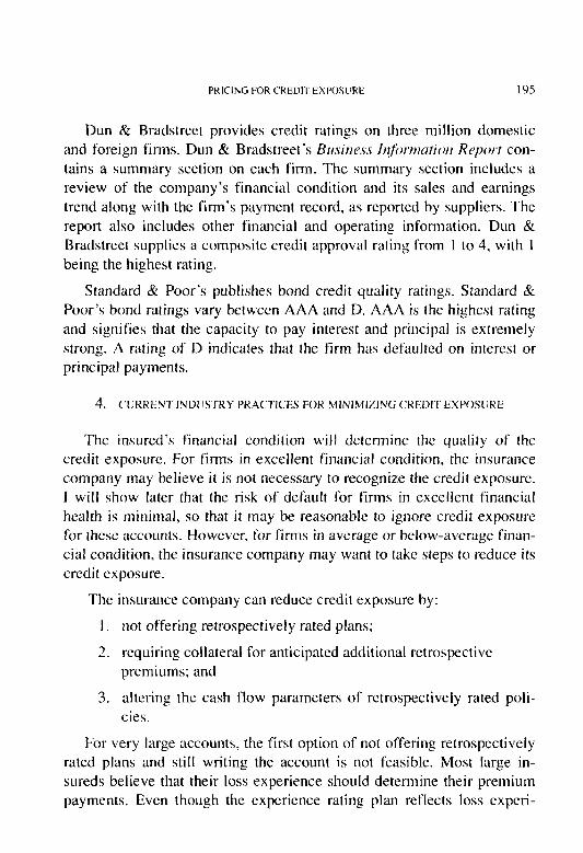
PRlClNti FOR CREDIT EXPOSURE 197
$774,000 at Year Two to $100,000, as collected premium would equal $2 million until Year Four. At Year Four and subsequent, the credit exposure under the revised program would be identical to the credit exposure in Exhibit 2. While this approach does not eliminate the credit exposure, it substantially reduces the exposure for the first three years after policy inception. In return for holding onto the insured’s cash for a longer period of time, the insurance company could increase the dividend amount. The dividend payment could be increased by the amount of additional invest- ment income earned on the incremental funds from 18 to 42 months. The incremental funds are the standard premium less the normally calculated retrospective premiums from 18 to 42 months.
The retrospective rating plan could incorporate incurred loss develop- ment factors to minimize the credit exposure. The development factors would be applied to the incurred losses at 18, 30, and 42 months. These factors would be used to develop the losses that enter the retrospective rating calculation to an estimated ultimate level. Therefore, the expected credit exposure would be zero at 18, 30, and 42 months because collected premium will equal ultimate premium. This analysis ignores any variation in development factors by account. As in the preceding option, the divi- dend amount could be increased for the additional investment income earned by the insurance company.
5. PRICING THE CREDIT EXPOSURE
This section outlines a new method to price the credit exposure on retrospectively rated policies utilizing a financial risk charge (herein re- ferred to as Charge). The Charge is intended to provide sufficient funds to the insurance company to offset the expected loss of funds (on a present value basis) due to premium defaults. This section assumes that the Charge will be an addition to the basic premium. Alternatively, the Charge could be incorporated through a dividend reduction. The dividend reduction Charge calculation is similar to the additional premium calcula- tion. However, the present value analysis would be different because policyholder dividends typically are first paid I8 months after policy inception, as opposed to the basic premium which is usually collected at policy inception.
19x PRICING FOR (‘Rf:DIT EXPOSIIRC
The Charge is largely a function of two factors:
1. the insured’s financial condition; and
2. the nature of the retrospectively rated plan.
Insureds in poor financial condition at policy inception are more likely to default on future premium payments. In addition, the slower the loss development pattern, the more premium there is outstanding at any point in time. Hence, the relative magnitude of the credit exposure is larger in either case. In addition, there is a relationship between the development pattern and financial condition of the insured. The longer it takes to collect the ultimate premium, the more time there is for a good financial risk to turn bad. This is similar to the phenomenon in life insurance, where “select” risks deteriorate over time to average risks (in the aggre- gate). Thus, plans with low loss limits or plans that contain lines of insurance which develop quickly, will have a lower Charge. A paid loss retrospectively rated plan will have a relatively large Charge.
A formula for the Charge is developed below based on the insured’s financial condition at policy inception for a three-line incurred loss retro- spectively rated policy. The illustrative plan includes workers compensa- tion, general liability, and automobile liability coverages. The parameters of the plan are displayed on Exhibit 1.
Moody’s bond default probabilities were used to determine the proba- bility of the insured defaulting on additional retrospective premium pay- ments. The probabilities are published in “Corporate Bond Default and Default Rates.” [2] As both bonds and additional retrospective premium payments are long-term obligations, bond default rates are used as a proxy for premium payment defaults. Moody’s studied bonds by initial rating over a 20-year period in order to determine default probabilities by year and initial rating. A portion of Moody’s table is reproduced in Table 1.
PRICING FOR CREDIT EXPOSURE 199
TABLE I AVERAGE CUMULATIVE DEFAULT RATES
(YEARS) Bond Rating I 2 3 4 5 6
BiGi 0.2% 0.5% 0.9% 1.3% 1.7% 2.2% BLi 1.7% 3.7% 5.5% 7.2% 8.9% 10.4% B 7.0% 11.8% 15.9% 18.9% 21.1% 23.0%
The interpretation of the six-year value for B-rated bonds is that 23.0% of the bonds rated B at time period t will default by time period t + 6. Moody’s has defined default as any missed or delayed interest or principal payment. Thus Moody’s default rates are a conservative esti- mate of retrospective premium defaults.
Moody’s default probabilities are used for illustrative purposes. The Charge could be based on default probabilities from other rating agencies or other studies. All of the tools referenced in Section 3 can be used to determine the insured’s financial condition and default probability.
The Charge can be calculated from Table 1 and an estimate of the incremental retrospective premium at each time period. On Exhibit 2, we can see an estimate of the incremental retrospective premium at specific points in time. For example, as of the second retrospective accounting, the insured will be billed $288,000 (this is the estimated retrospective pre- mium of $1,614,000 at 30 months less the collected premium of $ I ,326,OOO at 18 months).
The financial risk Charge can be calculated as follows:
Financial Risk Charge = 2 P, x RJ( 1 + i)‘, t=3
where P, = cumulative default probability through period t,
R, = incremental retrospective premium at time t, and
i = an appropriate discount rate.
(5.1)

200 PRICING E‘OR C‘Rf:I)l I f:XPOSIIRE
This calculation assumes that the basic premium will bc increased by the amount of the Charge. Therefore, the calculation incorporates present value concepts (discounting) because the Charge is collected at policy inception, whereas the estimated premium defaults will occur over an extended period of time.
The time index begins three years after policy inception, as the finan- cial exposure prior to the third year for standard incurred loss retrospec- tively rated plans is usually small. If the insurance company financially underwrites accounts, it is unlikely that the insured would file for bank- ruptcy in the first year-and-a-half after policy inception. In addition, at the first retrospective accounting, the insurance company typically returns funds to the insured because the first retrospective accounting premium is less than the standard premium.
The Charge calculation for an account with a Baa bond rating by Moody’s and a premium payment vector as on Exhibit 2 is outlined on Exhibit 4. Column 1 on Exhibit 4 is the collected premium from Exhibit 2. Column 2 is the incremental collected premium, the additional pre- mium the insurance company anticipates collecting at each accounting. Column 3 is the cumulative default probability based on Moody’s default rates. Column 4 is the expected default amount which is Column 2 multi- plied by Column 3. Column 5 is the present value of the expected default amount. For illustrative purposes, a 6% discount rate is used.
As displayed on Exhibit 4, the Charge for an insured with a senior unsecured bond rating of Baa and an anticipated premium collection vec- tor as on Exhibit 2 is only 0.43% of standard premium (the sum of Column 5 divided by standard premium). Thus, the current industry prac- tice, of not collateralizing the additional retrospective premium of in- sureds in good financial condition, may not be unreasonable. Insureds rated above Baa will have a lower Charge.
However, for an account with a premium vector as contained in Ex- hibit 2 and a bond rating of B (which is below Baa). the Charge is 5.7% of standard premium (Exhibit 5). Moody’s report did not calculate default rates for firms with ratings below B; however, these companies would probably have a Charge significantly above 5.7%. Exhibit 6 displays the
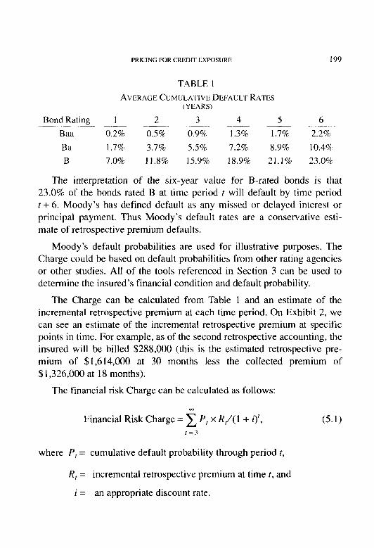
PRICING FOR CREDIT EXPOSURF. 20 1
Charge calculation for a puid loss retrospectively rated plan for a firm whose bonds are rated B. Thus, the only difference between Exhibits 5 and 6 is the type of plan. As discussed previously, the Charge for a paid loss plan will be greater than the Charge for an incurred loss plan due to the slower premium collection pattern for the paid loss plan. For the paid loss plan displayed on Exhibit 6, the Charge is 10.2% of standard pre- mium. The magnitude of this change indicates that ignoring the credit exposure on certain accounts may result in loss of earnings. This analysis assumes that the insurance company does not require any collateral (e.g., LOC) for the paid loss plan. If the insurance company receives collateral, the credit exposure would be reduced and, therefore. the Charge would be lower.
6. PRICING SURETY BONDS
A surety bond is an agreement by one party (the surety) to be responsi- ble to another party (the obligee) for the conduct of a third party (the principal). If the principal fails to fulfill its obligation under the bond, the bond indemnifies the obligee for loss sustained as a result of such default, up to the amount of the bond.
Several states require employers who self-insure their workers com- pensation exposure to provide the state with a surety bond. If the self-in- sured employer files for bankruptcy, the surety is required to make loss payments in place of the self-insured employer. The surety’s payments are limited by the face value of the bond. Some bonds are written such that the obligee can require the surety to make payment for the full face of the bond.
For self-insured workers compensation bonds, the bond price is a function of both the financial health of the self-insured employer and the payment pattern for losses. The concepts used to price credit exposure are directly applicable to pricing surety bonds. This section outlines a proce- dure to price surety bonds based on Moody’s bond default probabilities and the workers compensation payment pattern displayed on Exhibit 7.
Exhibit 8 displays the pricing of a workers compensation self-insured bond, for a one-year period, for a company with a Moody’s senior unse-

202 PRICING FOR (‘RFINI‘ I’SIY)SI;RI~
cured bond rating of B. The first column of Exhibit 8 displays the number of years from the time the bond was written. Column 2 displays the liability, or expected total needed reserves, by year. The total needed reserves equal case reserves plus IBNR reserves. Column 3 is the incrp- nmtd default probability based on Moody’s bond default rates. The in- cremental probabilities are utilized because it is assumed that the bond would be utilized to the full extent of the liability. Column 4 is the expected default in the year (Column 2 multiplied by Column 3). Column 5 is the present value (at a VS discount rate) of the expected default stream. The sum of Column 5 is the discounted loss cost for this bond.
Based on this analysis, the loss cost for an insured with a Moody’s bond rating of B purchasing a $1.8 million bond is $267.600 or IS%* of the face of the bond. Insurance companies typically require collateral on surety bonds (e.g., an LOC) and the collateral will reduce the credit exposure and, therefore. the price of the bond. The bond price should include a provision for company expenses, loss adjustment expenses, and profit. Therefore, without collateral, the bond price would exceed 1.5% of the face value of the bond. This analysis ignores any recovery from the principal in a bankruptcy proceedin,. 0’ therefore, the loss cost is conserva- tive.
7. OTHER /ZPPI.IC‘4TIONS
The financial methodology outlined in this paper has several addi- tional applications including:
1. Providing insurance companies a method to establish a bad pre- mium debt reserve for GAAP statements:
2. Providing insurance regulators a method to determine collateral requirements for self-insured employers:
3. Providing insurance companies a method of estimating surety bond loss ratios; and
4. Providing banks an additional method to price letters of credit.

PRICING FOR CREDIT EXPOSURE 203
Estimution of Premium Bad Debt Reserve
The procedures outlined in Section 6 can be utilized to establish a bad debt reserve for expected premium defaults on retrospectively rated poli- cies for GAAP statements. Referring to Exhibit 5, the expected default amount for this insured at policy inception is $149,200 (the sum of Col- umn 4). The bad debt reserve for this account would then be the “earned” (based on pro rata earnings) portion of the $149,200. The expected de- fault amount for the insured three years after policy inception is $59,140 (the calculation is displayed on Exhibit 9). The expected default amount should be calculated based on the insured’s current bond rating and esti- mated premium collection pattern. The bad debt calculation should be performed by account and policy year and the results summed in order to estimate the bad debt reserve.
The methodology outlined in this paper may help insurance regulators in determining collateral requirements for self-insured employers. As dis- played in Exhibits 4 and 5, the Charge for an insured with a Baa bond rating (investment grade) is 0.43%, while the charge for an insured with a B rating (non-investment grade) is 5.7%, of standard premium. Insurance departments may want to institute a procedure whereby the face value of the surety bond as a percentage of total liabilities varies with the self-in- sured employer’s bond rating. The Iowa workers compensation self-insur- ance statute [3] incorporates a somewhat related concept. In Iowa, an estimate of the self-insured employer’s unpaid claim liability is multiplied by a ratio which varies from 0.00 to 1.00 in order to determine the indicated amount of collateral for the self-insured employer. The ratio is computed based on three financial ratios. A ratio of 0.00 indicates that the firm is in strong financial condition. The ratio gradually increases to 1.00 as the indicated financial condition of the firm deteriorates. As a technical note, Iowa does not rely solely on this procedure to establish collateral requirements. For example, there is a minimum bond requirement of $200,000.
State insurance departments will need to estimate default probabilities for employers not rated by Moody’s or use a procedure which is similar to

204 PRlC’l\G I’OK (‘Kt:Ol I’ I’Sl’OS1’KF
the methodology used in Iowa. In addition, state insurance departments may want to require an actuarial opinion for an employer’s self-insured liabilities. Insurance departments cannot determine an appropriate surety bond amount without an accurate estimate of the amount at risk, which frequently requires an actuarial opinion.
The procedures outlined in Section 6 can be utilized to determine a priori expected loss ratios for surety bonds. Referring to Exhibit 8, this insured has an expected loss of $286.000. Dividing by the premium charged gives the toss ratio. A similar calculation could be performed for alt bonds written during the year and the results aggregated. A Bomhuet- ter-Ferguson projection method could then be used as one method to establish unpaid claim liabilities.
The procedures utilized in Section 6 to price surety bonds can he used by banks to price LOCs collerateralizing insurance products. Typically, the insurance company will only draw down on the LOC in a bankruptcy situation and will draw the full amount of the LOC. Referring lo Exhibit 8, the discounted loss cost of a $ t .X million LOC (supporting, for exam- ple, a deductible program) for an insured with a bond rating of B would be $267,600, or 15% of the LOC amount. This analysis assumes that the bank does not request collateral backing the LOC, and this analysis ig- nores expenses, profit. and any funds received in a bankruptcy proceed- ing.
8. C‘ON(‘l,L~SlOh
As the number of financially related insurance products increases. it is important that financial theory be blended with actuarial pricing concepts. If the credit exposure associated with financialty oriented insurance prod- ucts is ignored, insurance company operating results will be negatively affected as insureds may default on some financial obligations (e.g., retro- spective premium payments).
PRICING FOR CREDIT EXPOSURE 205
REFERENCES
[I] Hope, Francis J., Discussion of Fitzgibbon, “Reserving for Retrospec- tive Returns,” PCAS LIII, 1966, p. 185.
[2] Moody’s Special Report: “Corporate Bond Default and Default Rates,” April 1990.
[3] Workers Compensation Self-Insurance for Individual Employers, Iowa Administrative Code, Title 19 I, Chapter 57, pp. l-6.

206 PRICING FOR (‘REIXI’ IXPOSURE
EXHIBIT 1
STANDARD INCURRED Loss RETKOSPWIIVE PLAK
RETORTING PAIWR~
Assumptions:
Expected Losses = $1,800,000 Standard Premium = $2,000,000 Loss Conversion Factor (C) = 1 .O Tax Multiplier (7’) = I .O Basic Charge (R) = 0. I5 Lines of Insurance =Workers Compensation
No Loss Limit
General Liability Automobile Liability
REPORTING PATTERN
-Quarter 4 6
10 14 18 22 26 30 34 38 42
Incurred Losses as Percentage of
Ultimate Losses 38% 57 73 85 90 94 97 99
100 100 loo
PRICING FOR CREDIT EXPOSURE 207
EXHIBIT 2
STANDARD INCURRED Loss RETROSPECTIVE RATING PLAN
INSURED WRITTEN FOR A ONE-YEAR TERM*
Number of Years from ~ Inception of
Policy 1 2 3 4 5 6 7 8 9
.~~~~~ (Amounts in Thousands> Collected**~ - - Ultimate
Premium Jremium Credit&osure $2,100 $2,000 $100 2,100 1,326 774 2,100 1,614 486 2,100 1,830 270 2,100 1,920 180 2,100 1,992 108 2,100 2,046 54 2,100 2,082 18 2,100 2,100 0
* Assuming insured non-renews after the one-year period. **Assumes a two-quarter lag in collecting/returning funds. Standard Premium equals
$2,000; Basic Charge equals 15%; Expected Losses equals $ I.800; Loss Conversion Factor and Tax Multiplier equal I .OO.
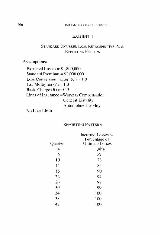
20x PRI(‘IN(i I-OR (‘REDIT EXl’OSIJRli
EXHIBIT 3
STAKDARD INCURRED Loss RFTROSPEUIVF. RATING PIAN INSURED WRITI‘E~ IRK j\ T~W-SYEAK TE.KM’
(AMOIINIX I*\’ THOLK~NDS)
Number of Years from Inception of
Policy I
Ultimate Collected.” Premium Premium
$2,100 $2,000 4,200 3,326 6.300 4,940 6,300 4,770 6,300 5,364 6,300 5,742 6,300 5.95x 6,300 6.120 6,300 6,228
Credit Exposure $ 100
x74 I.360 1,530
936 55x 342 180 72
* Assumes insured is written for three consecutive annual policy periods and then non-renews.
** Assumes a two-quarter lag in collecting/retumin:: funds. Standard Premium equals $2,000: Basic Charge equals IS%‘: Expected Losses cquai~ 3 I .X00: Loss Conversion Factor and Tax Multiplier equal I .oO.

PRICING FOR CREDIT EXPOSIIRE 209
EXHIBIT 4
FINANCIAL RISK CHARGE
FIRM’S BOND RATING Baa (AMOUNTS IN THOUSANDS)
Number of Years (2) (3) (4)
from (1) Incremental Cumulative Expected Inception Collected Collected Default Default of Polix Premium Premium- Probabm Amount
I $2,000 - - 2 1,326 $(674) z 3 1,614 288 .009 $2.59 4 1,830 216 .013 2.81 5 1,920 90 .017 1 s3 6 1,992 72 .022 1.58 7 2,046 54 .026 1.40 8 2,082 36 .03 1 1.12 9 2,100 18 .035 .63
Total $11.66
Financial risk charge as a percentage of standard premium =
,“g = 0.43% 3
(51 Economic* Cost of the
Default -
$217 2.23 1.14 1.11 .93 .70 .37
$8.65
* At a 6%’ discount rate. For example, 2.17 = 2..59/( 1.06)’

2 IO PRICING bOR (‘REDII I<Xl’OSI RF
EXHIBIT 5
Number of Years
from Inception of Policy
1 2 3 4 5 6 7 8 9
Total
(1) Collected Premium $2,000 1,326 1,614 1,830 1,920 1,992 2,046 2,082 2,100
FINANCIAL RISK CFIAKGk FIRMS BOND RATED B
(AMOUNTS IN THO~:SANDS~
(2) (3) Incremental Cumulative Collected Default Premium Probability
-
St6741 - 28X .159 216 .I89 90 .211 72 230 54 244 36 .25s
(41 (5) Expected Economic* Default Cost of the Amount Default
-
-
$45.79 40.82 1 x.99 16.56 13.18 9.18
18 .260 4.68 $149.20
-
$38.45 32.33 14.19 I 1.67 8.77 5.76 2.77
$113.94
Financial Risk Charge as a percentage of Standard Premium =
* At a 6% discount rate. For example. 3X.4.5 = 45.79/(3.(X1)’
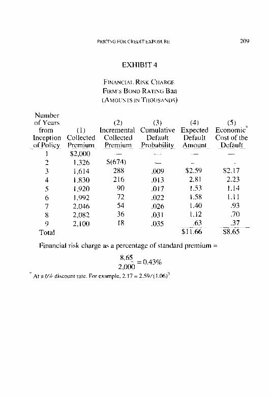
PRICING FOR CREDIT EXPOSURE 211
EXHIBIT 6
FINANCIAL RISK CHARGE
PAID Loss RETROSPECTIVELY RATED PLAN*
FIRM‘S BONDS RATED B (AMOUNTS IN THOUSANDS)
Number (2) of Years Incre- (3) (4) (5)
from (1) mental Cumulative** Expected Economic*** Inception Collected Collected Default Default Cost of the
Premium Premium Amount Default of Policy ~~___ 1
2
3
4
5
6
7
8
9
Total
$606 $606
1,056 450
1,398 342
1,632 234
1,758 126
1,992 234
2,046 54
2,082 36
2,100 18
Probability _~ ~- ~-~~ -
.118
.159
.189
.211
.230
.244
.255
.260
-
$53.10
54.38
44.23
26.59
53.82
13.18
9.18
4.68
$259.16
-
$47.26
45.66
35.03
19.87
37.94
8.77
5.76
2.77
$203.06
Financial Risk Charge as a percentage of Standard Premium =
203.06 ___ = 10.2% 2.000
* Assumes that the plan converts to an incurred loss plan at 66 months and that all premium is collected at the end of the fiscal year.
** Assumes that due to financial underwriting the insured will not default in the first year. As a related point, if the insured defaulted during the first year, the insurance company may not be responsible for the full year’s claim liability.
***At a 6% discount rate.
Note: Exhibit 7 displays the payment pattern.
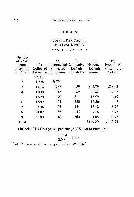
EXHIBIT 7
Number of Years from Inception of
Exposure I 2 3 4 5 6 7 8 9 10 11
Ultimate Payout Losses Pattern $1,800 17%
1 .#OO 42
1,800 61
1,800 74
1,800 Xl
1,800 85
1,800 88
I,800 91
1,800 94
1.800 ‘$7
1.800 l(X)
Percentage Amount Outstanding Outstanding
83% $1,494 .5x 1.044 39 702 36 468 19 342 15 270 I2 216 9 I62 6 IO8 3 54 0 0
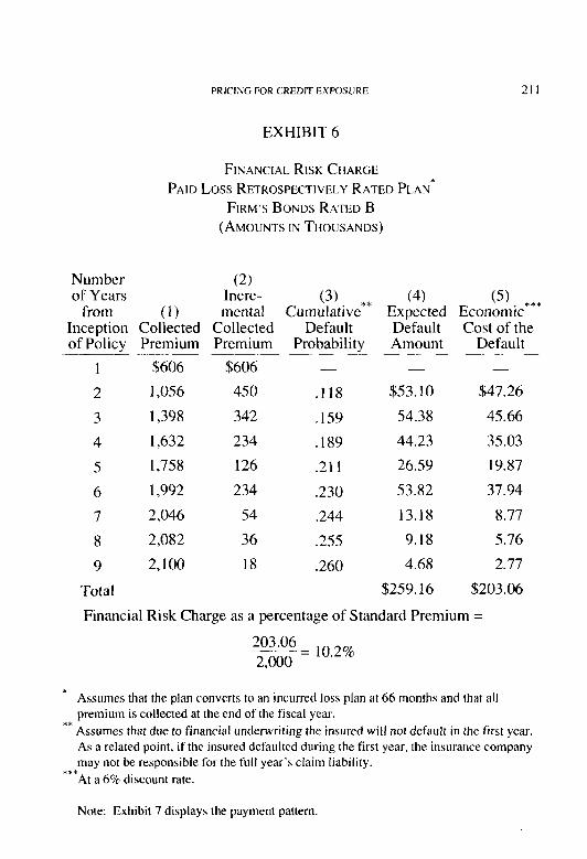
PRICING FOR CREDIT EXPOSURE 213
EXHIBIT 8
(1) Number of Years from Inception of
Exposure 0 I 2 3 4 5 6 7 8 9 IO II
Total
PRICING A SURETY BOND
FIRM’S BONDS RATED B (AMOUNTS IN THOUSANDS)
(2) Liability*
$1,800 1,494 1,044
702 468 342 270 216 162 108 54 0
(3) Incremental
Default Probabilities
.070
.04X
.041
.030
.022
.Ol9
.014
.Ol I
.oos
.004
.004
.004
(4) Expected Default Amount
$126.0 71.7 42.8 21.1 10.3 6.5 3.8 2.4 0.8 0.4 0.2 0.0
$286.0
(5) Economic** Cost of the
Default $126.0
67.6 38.1 17.7 8.2 4.9 2.7 I.6 0.5 0.2 0.1 0.0
$267.6
* Assuming a one-year exposure period. The liability is equal to the total needed reserve. Total needed reserve equals c3se reserves plus IBNR, or ultimate losses less paid losses. The total needed reserves cnn be derived from Exhibit 7. This pricing is conservative ;ts it assumes the insured goes bankrupt when the exposure is the largest.
** At a 6%’ discount rate. For example, 3X. I = 42.X/( I .Oh)’

3-14 PRICIN(i bOK (‘Kl~l~l’l I~.Nl’OSIiKI
EXHIBIT 9
BAD DEBT RESERVE THREE YEARS AITER POLICY INCEPTION
FIRM’S BONDS RATELI B (AMOLKTS IK Twr W,NDS)
Number of Years from Inception of
Policy
3
4
5
6
7
8
9
Total
(2) (3) (1) Incremental Cumulative
Collected Collected Default Premiums Premium Probability
$1,614
1,830 $716 0.070’~
1,920 90 0.1 IX
1,992 72 0. IS9
2,046 54 0. I x9
2.082 36 0.2 I I
2,100 IX 0.230
’ This is Ihe probability that the insured will dcl’x~lt in the nexl li\cal ywr
(4) Expected Default Amount
$15.12
10.62
I I .45
IO.21
7.60
4.14
$59.14
Note: Assumes that the insured has not defaulted through Year Thrw. As a technical note. the firm’s current bond rating. not the firm’s bond rating ;II policy inception. is used in the calculation.

WORKERS COMPENSATION EXPERIENCE RATING: 215
WHAT EVERY ACTUARY SHOULD KNOW
WILLIAM R. GILLAM
Abstract
Workers Compensation experience ruting affects the distri- bution of billions of dollars of insuranct~ premium. It is u lurge-scale upplication of actuariul science, one which bus elvl\,ed since the very first days of the Casualty Actuarial So- ciety. A fuir amount of material exists on the theory underiyinC: the plun, und some of that material is required reading,for uc- tuurial students. This paper tries to bridge the gap henzleen theory and practice. Most of the insureds eligible j&. e.\peri- ence rcrting do not think in terms of over-u/l perfcvmance of the plan. They may agree individual risk equity is fine--us 1onS as it does not affect them advessely. Actuaries cun help relate the theoretical underpinnings of the plan to the bottom-lint effect on the indil,idnal insured.
The exposition begins with u discussion of performunce test- ing. It then puts experience rating into the xwte.vt of the pre- mium transaction ,fw u policy, then turns to a disc~ussion of overull finunciul impuct. The latter part of the puper dctuils the activity necessary to administer esperience ruting, includ- ing the culculution of plan parameters, the assembly of e.xperi- ence datu, und the promulgation of rating forms.
The paper is intended to be expository, describing concepts, wcabulury, and details of the plan from an actrrurial perspec- tive. Itulics are used for emphasis, which may include intro- duction of a new Mwrd. Phrases that demonstrate usage. us wlell as honest-to-goodness quotutions, are shotiw in quotes.

216 M'ORKkRS (‘Op11l'l~\~~\l'lO'. I:XI'I:RII-UC'I- R \II\(m
The primary goal of experience rating is individual risk equity. This equity is not just between individual risks. but equity that pervades the relationship of insureds to their insurers and to society at large. Experi- ence rating engenders an incentive for safety and enhances market com- petition. Even if not the primary goal of experience rating. these desirable results should be touted.
Equity is an actuarial concept: each insured should pay a rate correct for its inherent potential for loss. It is important to stress the word poten- tiul, for the experience rating modification (the ~rod) provides the means IO adjust manual premium prospcctivcly so that next ycar’x rate will be tailored to fit the particular employer. This point is developed later.
The following passage from Dorwcilcr’s prescient presidential address in 1934 explains in practical terms why consideration of risk experience can accomplish this goal:
“The object of experience rating is to dctcrmine a more equita- ble rate for the individual risk based [to] ;I degree on the evi- dence presented by its own experience. It is rccognilcd that individual risks within a classification arc not alike and that there exist inherent differences due, for example in compcnsa- tion, to variations in plants and premises. in operating pro- cesses, in the materials involved, in the management. in the morale of employees, in claim consciousness, and in the rcln- tion to the community. These differences arc of such a nature that it is difficult to label them definitely and they cannot be associated with conditions measurable in advance. It is known. however, that variations in experience do exist in ;I way that definitely precludes ascribing all of them to chance. Experi- ence rating is considered by many as the most practical method yet devised, or even suggested, of giving recognition to variations produced by such factors.“[ I ]
In the parlance of risk theory. Dorwcilcr is talking about the \nrirrt?c,c> of the hvpnthctiml JHC~K~ or the hchzwrr rvrt-itrnr,c of risks within a class.

WORKERS COMPENSATION EXPERIENCE RATING 217
The greater the between variance, the greater the credibility of individual risk experience.
The original idea of applying experience rating to workers compensa- tion was a good one. Quoting Dorweiler:
“Compensation insurance, particularly, is subject to experience rating, for to a considerable degree the losses may be con- trolled and individuality of management reflected in the expe- rience through the employer’s ability to correct defective conditions and to enforce safe practices among employees by his potential power to dismiss or to withhold promotions. There are a few other lines, like employers’ liability, workmen’s collective, and automobile fleet collision, where the assured has similar power to affect losses.” [ 1, p, 41
2. MEASURING HOW WELL EXPERIENCE RATING WORKS
This question has been the subject of much study in the last 10 years, and the science has advanced far beyond what it was in the early years of the CAS.
The first principle is that experience rating be an accurate predictor of an individual insured’s future experience. This is the basis of the “credi- bility conditions” and the empirical performance tests which are de- scribed below. It has some market implications, too, and these are now noted.
The mod is a prospective measure only. There is no intention to re- coup past losses or rebate savings. The debit mod, for instance, gives an indication that more than manual premium will be needed to cover the expected losses of the particular employer next year.
The debit mod should not be thought of as a stigma. To decide be- tween contractors bidding on a project, some owners erroneously elimi- nate those with mods higher than some threshold. The bid itself is far more relevant. Rating bureaus and regulators, who ought to know better, sometimes unfairly attach penalty programs to only those insureds with debits. These insureds have already paid their debt to society, so to speak.

218 WORKERS COhlPliNSKI‘ION IXPERIENCE RAl’lU(i
The rationale for these programs is that a debit mod is an indicator of an unsafe operation. Although a debit mod may reflect poor safety habits, it just as often may be applicable to an employer wirh a good safety program who is a poor fit into the manual classifications. Contractors are especially difficult to classify. Each has a unique set of skills and an equally unique set of projects. Further. even though statistics show that poor prior experience is an indication of poor future experience, any single accident is probably a matter of pure chance.
Many aspects of a rating plan may affect its performance, but in the early days, the quality of the plan was thought to depend largely on “proper” credibility. Dorweiler proposed two conditions for correct credi- bility: necessary and sufficient. These are his words:
“A necessary condition for proper credibility is that the credit risks and debit risks equally reproduce the permissible loss ratio. Also, if the proper credibility has been attained, each [random] subgroup of the credit and debit risks, provided it has adequate volume, should give the permissible loss ratio. While these conditions are necessary for a proper credibility of the experience rating plan, it does not follow that they are also suf- ficient. For a sufficient condition it would be required to estab- lish that the risks within a group cannot be subdivided on any experience basis so as to give different loss ratios for the sub- divisions, assuming the latter have adequate volume.” 11, p. 111
By “reproduce,” Dorweiler was referring to the risk experience that would emerge in the prospective period; i.e., the losses during the time when the mod is applicable to risk premium. Given that rates today are rarely adequate, it is too much to ask that the two subgroups of risks equally reproduce the permissible loss ratio. So the necessary condition is that the two groups show equal loss ratios to standard premium in the prospective period. Since credibility is a function of risk size, the question must be posed for each size group: does the plan satisfy the necessary condition‘? The result of a plan satisfying this necessary condition is that insurers would find credit risks and debit risks equally desirable as in- sureds.
WORKERS COMPENSATION EXPERIENCE RATING 219
Even though Dorweiler calls the condition necessary, it may be too much to require of a plan. Early in the study leading to the 1990s revi- sions of the Workers Compensation Experience Rating Plan, it was seen that the existing plan did not perform well in simple tests (described below) based on the necessary condition, at least among the smallest and largest risks. This testing suggested the need for the changes that have recently been put into effect.
The sufficient condition is that there be no way to select subgroups of risks based on their experience that will produce significantly different loss ratios in the prospective period. It should be clear that it would be difficult, if not impossible, to test all possible a priori subdivisions of risks.
Dorweiler characterizes the sufficient condition as a goal, not a re- quirement. It can be used as a relative measure for judging how well a plan is working. He documented a simple method for testing credibility under this condition using the experience of 1931 experience-rated risks in New York [l, p. 121.
He first grouped risks by size. Within each size group, risks were stratified by the value of their modification. This is a “subdivision on an experience basis.” Following the risks in each subdivision, or stratum, to the effective period of the modifications, he calculated the loss ratio of each stratum, first to modified (actual) premiums, then to manual premi- ums. The ideal result was that the loss ratios to manual premiums would track with the value predicted by the mod, but those to actual premiums would be nearly flat. A trend upward or downward in the loss ratios to actual premium across risks grouped by increasing value of the mod would show too little or too much credibility, respectively.
This author documents a refinement to this test used in developing the revised Workers Compensation Experience Rating Plan [2]. This is the quintiles test in which risks within an expected loss size range are grouped into five equal strata (quintiles) by the value of their modifica- tion. The first stratum contains the 20% of risks with the lowest mods, and so on. The subsequent ratios of actual to expected loss and actual to modified expected loss, are evaluated for each stratum. The test statistic

220 WORKERS (‘OMPENS~HON liXPERlliN(‘li KATING
for each size group is the variance of the modified ratios divided by the variance of the unmodified ratios. A low test statistic indicates a plan that has eliminated much of the between variance (in risk theoretic terms) or made risks of differing experience more equally desirable.
The use of this test in the development of the revised plan demon- strated that experience rating is very effective. Test statistics for the old plan were far lower than unity, showing that, even without proper calibra- tion, experience rating is valuable. The test statistics for the smallest and the largest insureds indicated greater credibilities for the former and smaller for the latter.
Division into quintiles represents only one “subdivision on an experi- ence basis,” so the test does not check all possible subdivisions. Another test of experience rating, which is grounded in modem risk theory (thus avoiding conflict with Dorweiler), is the ~#~c~ic~nc~~ test as documented by Meyers [3]. In this test, the sample variance in loss ratios across all risks in a size group is compared for modified versus unmodified loss ratios. The statistic is the ratio of the former to the latter sample variances: lower statistics indicate better reduction in risk loss ratio variance.
All of these tests have been used to good effect in their historical contexts. Although they have been presented in a progression, each must be considered superior to pure judgment as a means of testing plan per- formance. Judgment is still essential, however, in the choice of data and interpretation of results.
3. PAYING FOR WORKERS ~‘OMI’ENSATION INSLfRANC‘lz
Experience rating is an essential part of the workers compensation pricing system. All insureds over a certain premium size are eligible for experience rating or are rutuhle. “Eligible” is an euphemism, as there is no choice: the insured must accept its mod, be it a credit or debit (i.e., premium reduction or increase). The manual premium, based on the clas- sification of the employer, is tailored by the mod so that it will better reflect the hazard inherent in the insured’s operation.

WORKERS COMPENSATION EXPERIENCE RATING 221
Figure 1 shows a simplified flow chart of the premium determination and bureau reporting process for a rated insured with a policy effective in July 1990. Loosely speaking, in the left columns are statistical plan data items generated by the transaction; in the center is the financial informa- tion pertaining to the insurance contract; on the right is an approximate time line.
During the effective period of a compensation policy, the insured gen- erates loss and payroll experience. This is coded by the insurer and sub- mitted to the rating bureau according to its statistical plan. At the time of quotation for a policy beginning July 1990, experience from the policies incepting July 1986, July 1987, and July 1988 has been coded on unit report cards of the Workers Compensation Statistical Plan, commonly called the Unit Plun. A sample unit card for a 1988 policy is attached as Figure 2. More detail on the unit cards is found below.
The employer provides his/her prospective 1990 exposure data to the agent/broker to obtain insurance. The agent can compute the insured’s nzunlrcrl premiun~ as the extension of manual rates on estimated payroll (in hundreds of dollars). The agent can obtain a 1990 rating form, such as the one in Figure 3, apply the insured’s modification to manual premium, and add certain other elements to compute the standurd pwmium. Note that the form shows the expected loss rates (ELRs) and discount ratios (D-ra- tios), defined below, for the 1990 mods. Their derivation and use is ex- plained in Sections 5 and 6.
The standard premium is a benchmark. It gives the best indication of the true underlying expected loss of the insured. It is the basis of any premium calculation plan. From it, the agent can compute the purunteed cost premium. if the insured elects the simplest plan of paying for cover- age up front. The insured may also elect retrospective rating, if an agree- ment can be reached with an insurer on a specific plan. There may be plans other than retrospective rating wherein the risk premium is affected by the emerged losses during the policy period. For example, losses of the particular insured or of some larger group of insureds can often be the basis of dividend plans on participating policies.
222 WORKERS (‘OMPENSAI’ION t:Xf’LiRfkN(‘t R.&I IN<;
FIGURE 1
POLICY TRANSACTION FLOWCHARI
pOL YR 1984
IFQLYR 1985 1 - F’OL YR 1986 ’
POL YR 1987
FOL YR 1988
I
-I -.I >
pEF---j
AUDITED PAYROLL
1990 UNIT REPORTS
4189
1190
3/90
4/90
6190
12191

WORKERS COMPENSATTION EXPERIENCE RATlNCi 223
FIGURE 2
SAMPLEUNIT CARD
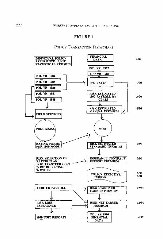
224 WORKERS C’~)MPENS!Y’I’IOI fXPliRII:U(‘I’ R-ITIM;
FIGURE 3
SAMPLE RATlh(i FORM
WORKERS COMPENSATION EXPERIENCE RATING
Risk ID #: 12345 Effective Date: 711190 Name: Hypothetical, Inc. State: N
-__
07/o I /86 06/30/89
SW
r-i&y Pi IEl
99,505 166,327_ 76,651) logy476 1
- SIB “*uz Eacese TOTALS EXP MOD El i’-*,o,.,B, r ,*,,w IPI /
CALCULATION ACTUAL 76,651 65,246 37.222 199.321 / ic, ~w*lo,fisl ,*m ,*,
EXPECTED 63.666 65.246 33.632 162.766
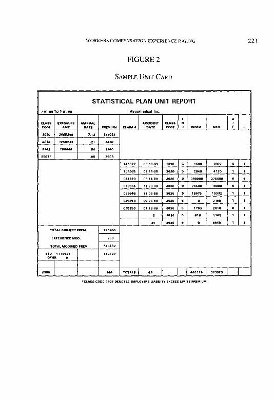
WORKERS COMPENSATION EXPERIENCE RATING 225
In this case, the actual 1990 premium cannot be computed until after the policy period has elapsed. The first adjustment usually occurs 18 months after inception, or six months after the expiration of the policy. Payroll is audited so that authorized rates can be extended on payroll (in hundreds of dollars) by class. After the mod is applied, premium dis- counts are applied or the retrospective premium is calculated for the first (but not the last) time. The expense constant and other non-ratable ele- ments are added. The end result is referred to as the net earned premium. At this point, the insured pays (or receives) the difference between this total and what has already been paid on deposit.
4. PREMIUM IMPACT OF EXPERIENCE RATING
A phenomenon of the 1980s has been the repetitive need for substan- tial workers compensation premium level increases. It is unusual that the need never seems to be satisfied. A state may grant a large rate increase as indicated in one year, only to face a filing for as large an increase the following year. The socioeconomic forces underlying this trend are the subject of much discussion and lie outside the scope of this paper.
In workers compensation, the phrase pronium le~l should be under- stood as something apart from rute level. The rate level in workers com- pensation is a function solely of the manual rates before application of experience rating, schedule rating, premium discounts, retrospective rat- ing, or dividend plans. A change in the premium discount plan, for in- stance, could engender a premium level change with no rate level change, or alternatively, could be accompanied by an offsetting rate level change to assure no premium level change.
Of particular relevance to this article is the nexus of manual premium and standard premium in ratemaking. Overall premium level needs are determined by the adequacy of total standard premium in a state. Inherent in standard premium is the experience rating c@-halunc~, a term used to mean standard premium divided by manual premium or, put another way, manual premium weighted average modification.’ In spite of the fact that
’ California uses the term “off-balance” to denote a factor applied to rates (usually) to cor- rect for the change in the average modification associated with a rate change.
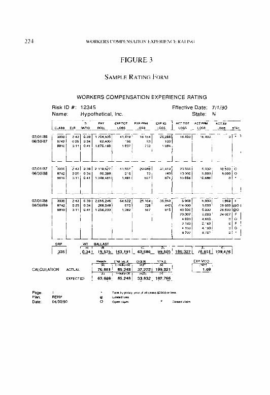
the term “off-balance” sounds like it describes a di.st,/.~~l”~~‘?‘:\’ between manual premium and standard premium, it refers to the relation. Even when there is no discrepancy, we say there is “a unity off-balance.”
The average modification is a function of the adequacy of rating val- ues: ELRs and D-ratios. These values are calculated at the same time as new rates, but pertain to the experience period used in the associated ratings. Technical details on the computation of rating values may be found in Sections 5 and 6. In any case, the accuracy of these values should be judged on the aggregate totals by class (or at least by state) of emerged versus predicted loss. When the ratemakers are on target and rating values are accurate, the off-balance is usually near unity or a slight credit. The slight credit frequently results because insured risks large enough to be rated tend to have better cxpcricnce than smaller risks.
Interestingly enough, even if the rating values are geared to be correct for the subpopulation of rated insurcds, the off-balance is still frequently a credit. Testing at the National Council on Compensation Insurance (NCCI) has shown this to bc the cast. Researchers have been able to derive pairs of adjustment factors applicahlc to ELKS and D-ratios, in several rating years in several states. so that expected losses (total and primary) match. in aggregate, the actual emerged loss experience of rated risks. Recomputing all modifications with these adjustments, the (weighted) averages for rated risks are near unity, but definitely a credit. This suggests that the largest rated risks, those with the most credibility, have relatively better experience than smaller rated risks. at least at the first, second, and third reports. Dorweiler observed the same phenomenon in the larger risks of 193 1:
“These have more favorable experience and by virtue of their size under the experience rating plan rcceivc larger credibility and therefore obtain credits which cannot be expected to be offset by an equal volume of less favorable experience on the smaller experience rated risks whose credibility is less.” [ 1. p. 71
WORKERS COMPENSATION EXPERIENCE RATING 221
In the NCCI committees, there is always some discussion about the effect of experience rating on premium, but no clear indication of what to do about it, if anything.
Contrary to suspicions, there is no ongoing scheme to use experience rating to assure premium adequacy. The calculation of needed premium level change at NCCI uses a loss-to-standard-premium ratio. This pro- duces an indication that contemplates no change in off-balance between the experience period and the prospective period.
Our investigations show that, in most states, over the years the off-bal- ance does not stray more than one or two points from unity. The all-too- common exceptions occur in states that allow rate adequacy to deteriorate for several successive years in times of increasing costs. The increasing off-balance reduces premium inadequacy. Since needed rate level changes are based on standard premium, indicated increases will be lower when the off-balance moves above unity. If adequate rates are approved, and the off-balance moves back toward unity, premium income may remain inadequate.
The production of rates and rating values is carefully monitored in the hope that changes in the off-balance will be minimal. Unfortunately, esti- mations of needed rates and rating values have proven to be difficult even if rate regulation is not a factor. The tendency is for too high a rate level (admittedly a rare occurrence) to result in a credit off-balance and too low a rate level (somewhat more common) to produce a debit off-balance. This is because ELRs are proportional to rates, and rates are presumed accurate. Without specific intent, then, experience rating can partially correct errors in class relativities or a rate level that is too low or too high. In the long run, there can be no net gain or loss but more stability results from experience rating.
5. CALCULATION OF EXPERIENCE RATING VALUES AND
PLAN PARAMETERS
This section describes some of the actuarial tasks necessary to keep the plan functioning properly. The description is technical in nature, aimed primarily at the actuarial student.

22x WORKERS COAlPFNSX11O2 IXl’iiKll~hC‘E KATINC;
Besides experience rating, another essential part of pricing workers compensation is ratemaking. There is ample material available document- ing this part of the process that should be reviewed before entering the special realm described here. See Kallop ]S] or Harwaync 161 for more detail.
We begin with a description of the data elements that underlie the pricing process.
This section provides a brief background on the NCCI ratemaking procedures, especially those relevant to calculation of experience rating values.
The most basic element of the process is the Worko~s C’o,?rl?r’lz.sutiolI Stutistid Plun (called Unit Plan here) of NCCI. The term “unit” refers to the fact that there is a separate report for experience on every policy and every state. evaluated annually to the fifth report. It is on this basis that the members of the NCCI report the data for experience rating and class ratemaking. NCCI summarizes the Unit Plan payroll and losses by risk for experience rating, and by classification within state for class ratemak- ing. Claims less than $2.000 may be (and usually are) summarized, but claims of a greater amount must be listed individually and categorized by injury type. Table I displays the codes fhr the types of injuries reported under the Unit Plan. For each injury type. medical and indemnity portions of a claim are reported separately. (Some states have modified this list.)
There are two compressions of this data made by the NCCI for ratemaking purposes. First, contract medical amounts arc added to medi- cal-only losses for use in most calculations. The second adjustment is a bit more complex. The permanent partial (PP) category. injury type 9, includes claims covering a wide range of values. For cxamplc. some claims coded as PP turn into life annuities not unlike permanent total (PT) cases. Other PP claims may be of short duration. Consequently, PP claims are separated into two categories: ntqjor: which becomes injury type 3, and minor.. which becomes injury type 4.
WORKERS COMPENSATION EXPERIENCE RATING 229
TABLE I UNIT PLAN INJURY TYPE CODES
In&q Type Code Injury Type Desgr@ion I (F) Fatal-Medical
2 Fatal-Indemnity
(PT) Permanent Total-Medical
9 Permanent Total-Indemnity
(PP) Permanent Partial-Medical Permanent Partial-Indemnity
(TT) Temporary Total-Medical Temporary Total-Indemnity
(M) Medical Only Contract Medical
The split is made by reference to a dollar amount called the critical
~luc, which varies by state and over time. PP claims whose indemnity amount exceeds this value are considered major. The critical value is normally calculated as a part of the annual ratemaking process.
After these adjustments are made, the loss data is summarized for ratemaking purposes into three categories: I) the indemnity portions of fatal, PT, and major are summed (0 one serious indemnity loss total; 2) the indemnity portions of minor and temporary total (TT) claims are summed to a mm-serious indemnity loss total; and 3) the medical portions of all claims are summed to one medical loss total. Table 2 displays the groupings.
This categorization is central to the calculation of both rates and rating values. Actuaries perform the many loss manipulations associated with ratemaking (loss development, trend, law changes, multi-dimensional credibility) and compare the results with payroll by class to calculate loss costs by type for the serious, non-serious, and medical categories. These ratios are the projected partial pure premiums by category which underlie rates filed for the prospective period. Each class rate, then, has serious, non-serious, and medical components.

230 WORKERSCOMPENSATION EXPERIEN('ERATlNG
TABLE 2 CATEGORIZATIONOF INJIJRY DATA FOR
CLASSIFICATION RATEMAKING
Fatal Indemnity ( 1) Permanent Total Indemnity (2)
Major Permanent Partial Indemnity (3)
Minor Permanent Partial Indemnity (4) Temporary Total Indemnity (5)
All Associated Medical (1,2,3,4,5) Medical Only (6)
Contract Medical (7)
R. Elements of E.1.petience Ruting
Several sets of values used in the NCCI Experience Rating Plan are revised as part of the regular rate filing process. Plun parun~eters, which vary by state and by size of the insured, are the stute rrfrr-ewe point (SRP), w~eighting (W), and hullust (B) values used in the rating formula. Rating values, applicable to individual insureds, vary by state and by classification. These are the expected loss rates (ELRs), and the discount ratios (D-ratios). Figure 3 shows a replica rating form. These values fit into the modification formula as follows:
where:
M = the risk modification (mod);
A = actual losses of the insured being rated ( p = primary, .Y = excess):
E = expected losses of the insured being rated ( p = primary, .V = excess);

WORKERS COMPENSATION EXPERIENCE RATING 231
W = weighting value; and
B = ballast value.
E is calculated as the sum of expected losses by class:
E= c 4 all classes i
= c ( Payrolli + 100) x (ELR;) all classes i
where ELRj is the expected loss rate for class i .
Then
Ep= C Di X Ei all classes i
E-, = E - E,,
where Di is the discount ratio (D-ratio) for class i. The D-ratio is the esti- mated portion of ratable losses that will be primary.
The actual ratable losses, A, is the sum of the individual losses, in- dexed by II, each limited as described in the next section.
A =CA,, . II
Each loss (occurrence) has a primary component:
A
1
A,, if A,, IL = ,I,, L if A,, > L
where L is the primary loss limit. (L is $5,000 today.)
The actual primary and excess losses of the insured being rated are as follows:

232 WORKF:RS (‘OMPENSATION E:XPERIEM’E RAl‘lN(i
A,, = C A,!,, . I,
A, =A -A,,
Current practice is to calculate the experience rating values at the same time and using the same data as used in the filed rates. It is import- ant to point out that ELRs are usually quite different from the pure loss costs underlying prospective rates. This is discussed further in Subsection E. Some of the similarities are discussed in the rest of this section.
The filed loss costs (rates) provide a best estimate of the amounts necessary by class to cover losses (and expenses) for the future period when the loss costs (rates) will actually be used. Experience rating values pertain to losses that occur a year or more before the time when loss costs (rates) and ratings will be effective. Of interest here are the relative time frames of: 1) the underlying experience used in the rate filing; 3) the prospective effective period of the rates: and 3) the associated experience period to be used in the experience ratings applicable to the prospective period. These three time frames are not the same; reference to Figure 1 will help in visualizing the differences.
A key aspect of ratemaking is the practice of limiting individual losses to minimize volatility in rates and rating values. In ratemaking, the over- all change in premium is estimated in one step (overall rate level) and, in a second step, is distributed among the various classes (class ratemaking). Capped losses are used in this second step to avoid distortions in class relativities due to the effect of unusually large losses. Loss dollars ex- cluded by these caps must be spread back to all classes. respective of industry group, because rates are designed to be adequate for unlimited losses. As of this writing, NCCI uses a multiple of the average serious loss for limitations to single losses in class ratemaking.
In experience rating, losses that arc similarly limited (ratable losses) enter the calculation of the experience modification. The limit applied to a single claim is 10% of the state reference point (SRP) which is defined below. This limiting value is called the state accident limit (SAL). There
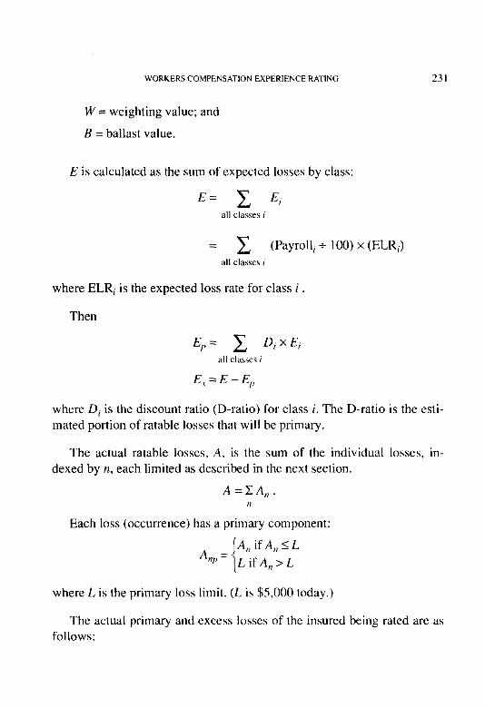
WORKERS COMPENSATION EXPERIENCE RATING 233
is a secondary cap on multiple claim occurrences of twice the SAL, or 20% of the SRP. There are special caps for losses incurred under the U.S. Longshoremen’s and Harbor Workers Act and losses that are strictly employer’s liability. The total disease losses for a policy are also capped at three times the SAL, plus 120% of the risk’s total expected losses for the experience period. (There are specific rules in the Experience Ruting Platl Manml [4] defining these experience periods.)
Another procedure lending stability to ratemaking, as well as to the calculation of experience rating values, is the imposition of swing or change limits. The rate (or rating value) for each class can change only by a specified percentage from one rate filing to the next. The average effect of the loss limits and change limits is spread to all classes in such a way that the selected rate level change is achieved.
D. Calculation of Plan Parameters
I. State Rqfer-ewe Point
The SRP is an index of state benefits. It is used to calculate a value G that is a scale factor for credibilities varying by state and is updated annually as part of the annual rate revision, The SRP is also used to calculate the SAL, as mentioned above.
The SRP is based on the state alrerage cost per claim (SACC) for all types of claims. There is no per-claim limit on losses in this calculation, except that on employer’s liability claims, which currently is $100,000. The SACC is calculated from the latest three years of undeveloped Unit Plan data. This data set is at the same maturity level as the experience period which will be used in the ratings. However, it is necessary to trend the average value from those data, since ratings will be using slightly more recent data. (In hypothetical State N, the length of the trending period is two years. Usually it would be between one year and 18 months. However, statutes in State N require that new rates be filed well in ad- vance of the proposed effective date.) The trend rate is taken from the most recent countrywide Retrospective Rating Expected Loss Size Ranges update filing.
SRP = 250 x SACC, rounded to the nearest $5,000.

234 WORKERS COMl’LINSAfION I:Xi’I,HlliN(‘I~ KhTiU(i
G = SRP/250,000.
G is rounded to the nearest 0.05.
Because of the potential for volatility in the data, and the normal effect of intlation, it is further stipulated that G and SRP not be allowed to decrease from one year to the next, unless there is a significant benefit reduction. There also is a reasonability limit on the upward change, so that any changes over +20% will be investigated.
Exhibit I shows the calculation of the I990 SRP for State N.
2. Caldution oj’the W and B C’rrllrcs hi the NCCI
The f3 and W values arc functions of G and the expected losses, E, of a particular insured. First,
R = E [ (0.1 E + 2,.57OG)/(E + 7OOG) 1,
subject to a minimum $7,500.
Also, we define the intermediate value
C = E [ (0.75E + 203,82SG)/(E + 5, I OOG) I.
subject to a minimum of $ ISO,OOO.
B and C are the respective credibility constants K,, and K,. documented by Mahler 171.
Then
E+B w= -.
E+C
W is rounded to the nearest 0.01. with the requirement that it never increase for decreasing E. (This turns out to be a non-trivial programming challenge, although the effect on W is at most a point or two for small risk sizes and certain G values.)

WORKERS COMPENSATION EXPERIENCE RATING 235
EXHIBIT 1
CALCULATION OF STATE REFERENCE POINT-STATE N
Report
I st
2nd
3rd
Total
(1) (2)
Total Incurred Policy Period Total Cases Losses
l/X6 - 12/X6 165,250 $195,722,X02
11x5 - 12/X5 1 X9,629 206,X05,7 13
I/84 - 12184 188,074 196,806,05 I
542,953 599,334,566
(4) Indicated State Reference Point = ( Total (3) x 250) 276,000
(5) Average Annual Trend = (exp ((0.09833) x (I .OOO))) 1.103
(6) Length of Trending Period in Years 2.000
(7) Trend Factor = (exp ((0.098333) x (6))) 1.217
(8) Trended State Reference Point = (4) x (7) 335,892
(9) Proposed State Reference Point 335,000 (Rounded to the nearest 5,000)
(IO) G = (9)/250,000 (Rounded to the nearest 0.05) I .35
(3) Average Cost
Per Case o.Y( 1) ..~~ __ 1,184
I ,09 1
1,046
I.104
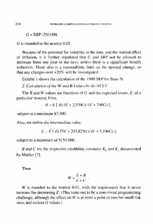
236 WORKEKS (‘OMPESS-\TIOU I:Xf’f,KlfiN(‘F KA’f’fl(i
The above formulae are valid for all rated risks, with appropriate rounding for tabular presentation. 5 is rounded IO the nearest 500 x G in the tables that apply to values of E < 477,500 x G. For higher values of E, 5 is rounded to the nearest dollar.
In particular, it should be noted that in all cases, 0 < W < 1 and 5 > 0. Hence, no insured’s rate is completely determined by its own experience.
The derivation of these formulae is explained elsewhere in the litera- ture 121.
ELRs are used to calculate the insured’s total expected loss, E. in the experience rating plan. The exposure base for the ELRs is $100 of pay- roll, just as for rates. As is the case with manual rates. ELRs are calcu- lated by the bureau for each class at the time a rate filing is made.
The class ELR should be proportional to the loss cost underlying the manual rate, but should be adjusted to the same level as the actual experi- ence to be used in the calculation of the modification. Three major adjust- ments that must be made to rates to obtain ELRs stem from: 1) the loadings (if any) for expense, profit, tax and loss assessment; 2) differ- ences in time frames; and 3) the fact that claims covered by the policy have no limit on size, but claims used in experience rating do.
The first adjustment is simple. Rates can be stripped of taxes, ex- penses. and profit by a single factor, the ~~nti.ssi/~/c lo.ss WOO (PLR) in the filing. Even in states where loss costs arc filed, there is a PLR, although it is close to unity.
The third adjustment is non-trivial. Its explanation is left to the detail described in the second step of the ELR calculation. below.
To better understand the second adjustment, hypothesize rating an individual policy effective 7/t/90, using rates and rating values effective l/1/90. At the time the insured’s prospective premium is being quoted, its experience for the policy effective 7/l/89 is not yet available. That policy is still in effect. Thus the policy effective 7/t/88 is the most recent one
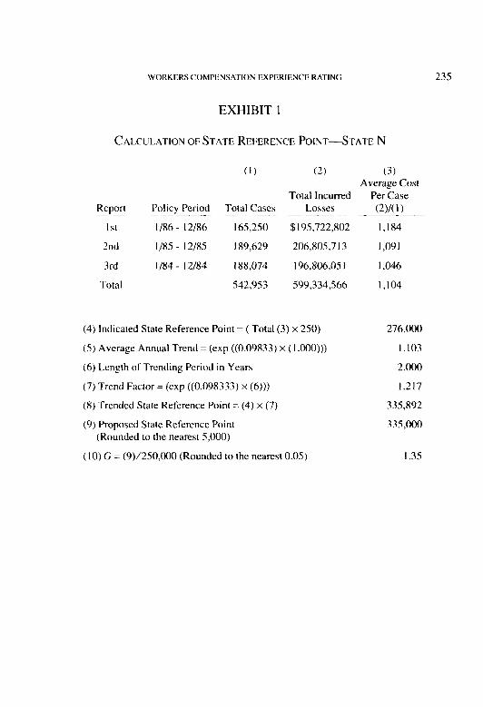
WORKERS COMPENSATION EXPERIENCE RATING 237
completed. In order to increase the credibility of the individual insured’s experience, three years of data are used in the rating calculation, from the policies effective 7/l/86, 7/l/87, and 7/l/88. The manual rates used for the insured’s 7/l/90 policy are intended to reflect ultimate costs in the 1990 policy year. In order to calculate ELRs which can be compared to the actual losses from the experience period, the prospective rates must be adjusted to loss levels prevailing during the three expired policy years (1986, 1987, and 1988). The rate filing contains well-documented analy- ses of trend, loss development, and benefit changes. This information is used to derive factors to adjust the rates.
In the example, suppose that from l/1/86 through 12/31/89 the manual rate for our hypothetical insured’s class was $4, and at l/1/90 it went up to $5 due to a benefit change. Oversimplifying, suppose that losses do not develop after first report and there has been no trend in loss experience. Assume 70% of the premium is allocated for the payment of claims, the remainder being for expenses (27.5%) and profit (2.5%). Thus, $2.80 in claims are expected for every $100 of payroll for the policy periods used in the calculation of the experience modification; i.e., 7/I/86 through 6/30/89.
It is erroneous to compare the $2.80 ELR with the $5 rate and infer that only 56% of the premium is allocated to payment of claims. Actually $3.50, or 70% of the $5 rate, is necessary to pay for claims occurring under the 7/l/90 policy, because the claims under this policy will be paid at the new higher benefit level. But, since the insured’s actual claims experience used in the calculation of its experience modification is at the old benefit level, the class expected loss rate used in the calculation must also be at the old level, namely $2.80, so that a fair comparison can be made.
While the foregoing illustration is a benefit change, the concept ap- plies to anything that would make the past class average experience, reflected in the ELR, different from the future projected average experi- ence underlying the manual rate. Loss development and trend can both be quite significant.
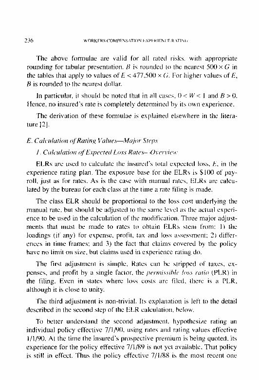
'3X WORKERS COMPENSATION fiSl’l:Kllih(‘f~ R/Yl-IN<;
All of the above elements can make the manual rate considerably higher than the ELK. An ELR of Xc/r of the manual rate, for instance, is not unusual.
The three major steps of the actual ELK calculation are as follows. First, calculate a factor to reduce manual rates IO pure premiums (at second report) on the same benefit level as the experience period used in ratings. This is called the ELR level factor.
Second, calculate the Hazard Group ELR factors and the ELRs by class. Humd Groups are classes grouped according to relative severity. For each Hazard Group, calculate the average cost per case (indemnity and medical combined) for the three serious injury types: fatal, PT, and major. These average costs are used to remove the expected loss above the SAL from the ELR, so that the expected losses correspond to the limited or r-amble losses used as the actual experience in the rating.
Using the ratios of the SAL to the average cost per case by serious injury type and Hazard Group, find the respective (‘.WJSS rutios (ratios of expected excess losses to total losses) from the fomrer ELPF calculation. (See Harwayne [S] for details of this calculation.) There are three excess ratios for each Hazard Group. Using injury weights for the three serious types, also varying by Hazard Group, find a single weighted excess ratio for each Hazard Group. Multiply the ELR level factor from Step 1 by the Hazard Group adjustment factors, which are the complements of the weighted excess ratios.
The resulting four Hazard Group ELR factors are applied to rates respective of Hazard Group to produce the ELRs by class.
The third, and last, step is to check the ELKS for reasonableness. The technicians use checksheets to look for unreasonable changes. These checksheets are described in Section 6.
D-ratios currently are calculated using the most recent single policy year of statistical plan data available. (Subsequent to this writing, a change to use of three years’ data has been made. There are some associ- ated changes, noted parenthetically below.) A policy year is labeled by the

WORKERS COMPENSATION EXPERIENCE RATING 239
year in which the policies were written but extends over two calendar years, and the reporting, verification, and processing of unit data takes some months to complete. Consequently, a rate filing effective l/1/90 would generally contain D-ratios based on statistical plan data from the 1987 policy year. Occasionally, 1986 data would be used.
D-rutio Factors (sometimes called partial D-ratios) are calculated for serious, non-serious, and medical losses. These factors are then weighted by the corresponding pure premium components of the class rates to produce D-ratios by class. The results are then checked for unusual changes in the average D-ratio.
6. CALCULATION OF RATING VALUES-DETAIL
STEP l--Culdution of the ELR Le\lel Factor,
Exhibit 2 shows the worksheets for calculation of the ELR Level Factor. The explanation of the columns on Exhibit 2 follows:
Column 1: The three policy years of the experience rating period. The experience period ends one year before the prospective period of the new rates. This time period is usually later than the periods of statistical data actually available at the time rates are made.
Column 2: A factor to correct for the natural off-balance produced by experience rating. This factor compensates for the fact that, on average, insureds large enough to be eligible for experience rating have better loss experience than the average of the total population, including non-rated risks. This factor is the result of a broad-based analysis of data, but may well be subject to a more state specific procedure in the future.
Column 3: The factors necessary to take the third, second, and first reports that will be available for ratings to the benefit level of the proposed manual rates.
Column 4: Loss development factors to take third, second, and first reports to their ultimate level. These factors are calculated using sta- tistical plan data to fifth report and financial data from fifth report to

EXHIBIT 2 CALCULATION OF ELR LEVEL FACTOR-STATE N
STEP 1 FACTORS DERIVED FROM LATEST RATE REVISION s
c 2
-7 i (2) (3) ~~ (4) (5) (6) (7) (8) E
(1) Off-Balance Benefit ELR Loss Composite Expense Product Reciprocal 2 Policy Year 1 ~~Acijustment Changes Development Factor Factqr~---~- (7) x .__ x (6) _ J-(7) _ 2 01/X6-12/86 i 1.01 I.067 1.072 _~~~ 1.14s I .s73 1.082 0.480 5 01/X7-12/87 1.01 , -1,047 ~_ I.122 ~~~~~ ’ 1‘5 -~~~_ 1.574 2.138 0.468 2 ~__ _~~~~- 01/88-12/8X I .01 1.012 I.216 -r.l45 1.574 7 740 ().446~~- 71
z + ~~ ~__~ ~~~- -~.-z __ %
ELF Level
~~ l-_--~ !L_ ~~~ -~ ~~___ ~ ~~ = z 2
Factor 1 0.465 ZJ z

WORKERS COMPENSATION EXPERIEf-iCE RATING 241
ultimate. In using the financial data, it is assumed that all develop- ment beyond the fifth report is due to serious claims only.
Column 5: The composite factor for miscellaneous changes in the rates. Particularly important is the ratio of the proposed financial data loss ratio to that of the Unit Plan. This ratio includes the impact of trend between the dates of the statistical plan data and the effec- tive period of the proposed rates.
Column 6: The reciprocal of the PLR.
Column 7: The product of Columns 2 through 6.
Note that Column 7 has three factors necessary to take the third, second, and first report loss costs to the same level as the proposed manual rates. Since we wish to perform the reverse operation, we take the reciprocals of the three values and record them in Column 8. The arithme- tic average of the three reciprocals is at the foot of Column 8. This average is the ELR Level Factor which is carried into subsequent steps of the calculation.
Columns 3,4, 5, and 6 are based on analysis of the actual data periods used in ratemaking. Exhibit 3 is the worksheet for these factors and shows how law amendment and loss development factors by injury type are weighted by policy period losses. The data used for weighting generally are not of the same policy period as the ones used for ratings. They are, however, put at the same stage of development. The development factors used in this exhibit were derived as part of the regular ratemaking proce- dure.
It should be noted that the filing schedule of State N has led to a minor inconsistency. The use of latest second, first, and first reports as weights usually matches the policy year of the experience rating period for two of the three years. In State N, however, 1985, 1986, and 1986 are used to weight experience period years 1986, 1987, and 1988. Usually the weights would be based on 1986, 1987, and 1987.

1, (a) Financial Data Loss Ratio
(b) Unit. Stat. Plan Loss Ratio
Cc) = (a)/(b)
2. Other Adjustments+ 0.995 x 0.9997
3. ELR Composite Factor(lc)x(2)
4. (a) Target Coat Ratio
(h) Loss Adjustment Expense
(c) Permissible Loss Ratio 4a/4h
(d) Reciprocal
EXHIBIT 3 CALCI’LATION OF ELK LEVEL FACTOR-STATE N EFFECTIVE 01/01/90
l/85-I?/85 Loss Weight5 A.F.’ 0.8250 Death 6.3-81.433 x 1.056
0.7170Ejor
3.794.9Y7 x I.041 54.973.297 x 1 a45
Minor l.lSlTT
23.816.20s x I.@48 23.155.932 x I.057
Ser. Med. o.OOs N. Ser. Med.
34.533.326 x 1.08X bo.250.523 x I .088
I. 14s Total 206.XOS.7 I 3
.7 I IS Benefit Charge = 1.067
I /X6- I386 Loss Weights --T.
A.F. l.l’Death 7.187.X71 x I .02X
PT 2.Y2O.XY2 x I .02h 0.6353 Major 38.424.036 x 1.0x
I ,574 Minor 2h.S6l.X11 x 1.027 TT 2S.JX2.907 x 1.030 Ser. Med. 27.2x.941 x 1 .oh7 V. Ser. Med. 67.‘) 17.J32 x I .067
Total 19s.722.x02
Benefit Chqe = I.&47
i/X5-12/X5 Lo.\,\ Weight> A.F.* Death 7.1X7.X73 x 1.012 PT 2.Y2O.XY2 x 1 .Ol? Major 3X.424.936 x I ,012
’ Includes change m trend. mini- FO’ 26.561.81 I x I.012
mum premium multiplier 25.4x2.907 x I ,012 change. C&R decision. etc. Ser. .&led. 27.22h.Y4l x 1.013
’ To latest Inu level efl’ective N. Ser. Med. 67.9 17.442 x I .()I 3
l/l/90 Total 197 7” . --. X02
For: Policy Year 0 l/86- 12/X6 2nd/3rd 3rd to Ult.
Dev. Fat. Drv. Fat. 68.030.8X0 x I.131 76.Y42.925 I.130 X6.YJS.SO5
49.43533 x I .OOs 19.6X2.379 O.YYY 19.6.33.697 37.572.259 x 1.036 1X.924,860 I I 80 45.93 I.335 65.552.569 x I .036 67.912.461 0.9YU 67.776.636
220.590.9 I I ‘33.462.625 2SO.286.173
Loss Development = 1.072 ~I_______ ~___.I_ For: Policy YearOl/X7-12/X7
1 st/?nd 2nd to Ult. De\,. Fat. D~v. Fat.
40.8OY.YS2 x I.247 f2.l l.i.OlU I .27x 7Y.3XO.427
53326.371 x 0.066 5 I .706.477 I .004 s I .‘) Ii,30? 29.OSl.I46 x I.065 30.939.470 I.732 i7.XOR.032 72.167.9 I I i I.065 77.178375 I .ou 7Y.XO3.388
204.8SS.3X3 27 I .Y?7.2X7 24X.YO4. I SO
Loss Devzlopmenr = 1.172
l-or: Polk! Year 0 l/XX- 12/8X I St to Ult. Dev. Fat.
19.1 16.105 > I.594
S3.MY.25.5 y O.Y70 77.580.8’~ I x I.301 68.X00.369 x I.101
19x. 166.620
Benefit Charge = I.012 Low Development = I .2 I6
WORKERS COMPENSATlOh! EXPERIENCE RATING 243
STEP 2-Cukulution cf Hazard Group Adjmtnwnt Factors
Exhibit 4 is the start of the calculations underlying Step 2. The most recent first, second, and third reports from statistical plan data are used. The average cost per case is calculated for fatal, PT, and major claims. These three serious injury types are the likely source for claims exceeding the SAL. Medical and indemnity losses of three policy periods are added for each of the three injury types. The number of cases for the policy periods is also added by type. The average cost per case is thus calculated for three years of claims (medical and indemnity) at their respective ma- turities. An adjustment for trend similar to that used for the SRP is made to the losses.
Exhibit 5 shows the final calculations of the Hazard Group ELR Fac- tors. These final calculations adjust for the limitation of losses in the experience ratings.
Line 1: The SAL, which is 10% of the SRP as calculated in the pro- posed rate filing.
Lines 2, 5, and 8: The average cost per case for fatal, PT, and major claims by Hazard Group. These are from Exhibit 4 and are calcu- lated as part of the rate review.
Lines 3, 6, and 9: The ratio of the SAL from Line 1 by type to the average cost per case by type from Lines 2,5, and 8.
Lines 4, 7, and 10: The excess ratios. These are the fractions of the pure premium for the portion(s) of individual loss(es) above the entry ratios on Lines 3, 6, and 9. The excess ratio tables are those used in the former ELPF calculation as described in Harwayne [8].
Line 11: The weights for fatal, PT, and major claims by Hazard Group.
Line 12: The fraction of the total pure premium expected to be above the SAL. It uses Line I 1 to calculate a weighted average of Lines 4,7, and 10.
Line 13: The Hazard Group adjustment factors.
Line 14: The ELR Level Factor from Step 1.

244 WOKKEKS (‘OMPI:NS~Vl~fON I~SI’FKIf~.N(‘I~ K.‘if’IN(;
r-- ~~- ~- ~- EXHIBIT 4 I
ELR FACTOR WoRI<sHE~,I-S7‘,4.1.f: N
AVERAGE Cos I PER Cns~
Injury Type Statewide
Fatal ‘5 89.073
PT 245.992
Major 45.537
Based on total losses and total claims, each by type. undeveloped, from the three-year experience period used for rates.
HMAKD GKOIT
I II 111 IV Fatal $ 83,036 $ 98,104 $ I 17.073 $132,575 PT 249,377 292.786 302,965 38 1,999
Major so,2 10 5 1.983 58, I YO 63,233
Uses countrywide Hazard Group Severity Relativities, adjusted to balance to state total, and appropriate severity trend from the ratemaking experience period to the experience rating experience period.

I.
2.
3.
4.
s.
6.
7.
x.
0.
IO.
II.
I?.
13.
13.
WORKERS COMPENSATION EXPERIENCE RA’I’ING
EXHIBIT 5
ELR FACTOR WORKSHEET-STATEN
IO% of Proposed State Reference Point
Average Fatal Cost
Ratio to Average for Fatal ( I ) / (2)
Excess R;ltio for F;ttal
Average PT Cost
Ratio to Aveqe for PT ( I ) / (5)
Excess Ratio for PT
Average Major PP Cost
Ratio to Average for Major PP (I ) / (X)
Excess Ratlo for Major PP
(A) Fatal Weight Factor
(B) PT Weight Factor
(C) Mit,jor PP Weight Factor
Weighted Average Excess Ratio
Adjuwnent Factor = I .O - ( 12)
ELR Level Factor
33.500
X3.036
0.40
0.693
24Y.377
0.13
0.94 I
so.2 IO
0.67
0.3’)‘)
0.014
0.022
0.328
0.161
O.X3Y
0.465
II
33,500
YX. IO3
0.34
0.7.52
292,7X6
0.1 I
O.YM
51.983
0.64
0.417
0.022
0.030
0.344
0. I XY
O.XI I
0.46.5
IS. Halard Group ELR Facton 0.390 0.377
III
33.soo
I 17.074
0.29
0.x01
302,965
0.1 I
0.954
5x. 190
0.5x
0.4.57
0.03x
0.030
0.432
0.274
0.726
0.465
033x
245
IV
33,5(K)
132.575
0.25
0.830
38 I .999
0.09
0.966
63.233
0.53
0,404
0.096
0.058
0.433
0.35 I
0.649
0.465
0.302
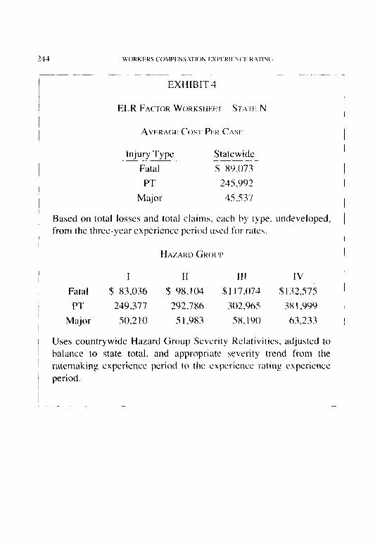
246 WORKERS CUMPENSATlO\ I~SI’IIRII:YCl! RATIi’X;
Line IS: The Hazard Group ELR Factors. This line is the product of (3) x (14). One of the factors is applied to the rate of each class, de- pending on the Hazard Group assignment of the class, to produce the final class ELR.
In addition to the standard calculation of the ELR as described above, the NCCI also has checksheets to identify cases where the ELR Factor (averaged over the Hazard Groups) changes significantly from the previ- ous year. A more detailed investigation is conducted if the change is more than 10%. These checksheets are included in Exhibit 6.
Exhibit 6, Part 1 examines ELRs as a function of macroscopic changes in rates. Exhibit 6, Part 2 considers the microscopic changes by compo- nent to provide insight into the cause of ELR changes.
The checksheet in this exhibit shows a significant decrease in ELR factors over the previous year, which would normally result in an investi- gation of changes in State N. In this case, it was dctemrined that the shift was due to a change to the experience rating plan formula, so that the change in ELR factors was justified. This can plainly be seen on Part 2, where the change in the excess ratio factor is 0.814, explaining most of the decrease.
STEP 4-Cdcd&m of D-rutio Factors
The worksheet for this calculation can be found in Exhibit 7.
Line I : Total Indemnity Losses (unlimited on a per-claim basis).
Line 2: Total Medical Losses (unlimited on a per-claim basis). Even though ratable losses are limited as described above, use of unlim- ited losses in the calculation of D-ratio factors provides a measure of conservatism. This is offset to some degree by the use of losses at first report, when severities are likely to be less skewed and D-ratios too high. (At the same time as the NCCI changes to a three-year ex- perience period, it will begin using limited losses in this part of the calculation.)
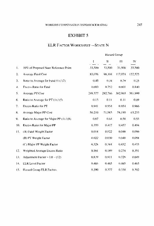
WORKERSCOMPENSATION EXPERIENCERATING 247
EXHIBIT 6 PART I
EXPECTEDLOSS RA~E~HECKSHEET-STATEN
EFFECTIVE DATE: l/l /90
If amount on Line 8 is greater than 1.100 or less than 0.900, the underlying cause of the large change should be determined and brought to the attention of Rates Department Supervisor.
I. Effective Date of Last Change in ELRs 01/01/X8
2. Rate Change Approved Effective on (1) 1.159
3. Rate Change Proposed Effective on (I) I.168
4. Average ELR Factor Underlying Rate Proposal on 0.447 Line 3 (Proposed ELR HGII + Proposed ELR HGIII) / 2
5. Interim Rate Changes Approved Eff. a.
Eff. b.
Eff. C.
Eff. d.
6. CurrentAverage ELR Factor ((4) x ((3)/(2)))/((5a) x (5b) x (SC) x (5d))
7. Proposed Average ELR Factor (Proposed ELR HGII + Proposed ELR HGIII) / 2
8. Change in ELR Factors (7) / (6) 9. Proposed Rate Change
IO. Indicated Change in Expected Losses (8) x (9)
0.45 I
0.358
0.794 1.164
0.924

3. 4. 5. 6. 7. 8.
9.
10.
I I. 12.
Benefit Changes a. 3rd Report b. 2nd Report c. 1st Report d. Average
Loss Development a. 3rd Report b. 2nd Report c. I st Report d. Average
Off-Balance Composite Factor All Reports Financial Data Loss Ratio USP Loss Ratio Loss Ratio Factor (7) / (8) Profit and Exp. Factor All Reports Reciprocal of the Combined Effect of these Factors** a. 3rd Report b. 2nd Report c. 1st Report Comparable ELR Level Factors Average (9) Excess Ratio Factor Overall Change in ELR Factors (1Qx(ll)
(1) Last
Approved Filing
(7) (3)
Proposed Change Filing (2) I ( 1)
I.084 I.067 I .(I61 I .047 I .03 I I .012 I ,060 I ,043
I .os2 1 .0X0 I.175 I. 102
I .()I 1.134 0.81 1s 0.720 I. I27 I.570
0.3X3 0.4x0 0.455 0.173
0.945 xx
I .(I72 I.122 I.216 I.137
I .Ol 1.115 0.x25 0.7 I7 I.151 I.574
0.4x0 0.36X 0.446 0.565
0.769 XX
‘~11/1((1~x(2)x(3~x(4)x(8)1
# From Exhibit 5, Line 13. (HGII + HGIII) / 2
xx xx xx XX
xx xx xx XX
xx xx xx xx xx xx
xx xx xx
O.YX3
0.814 0.800
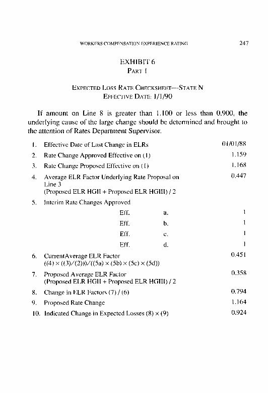
WORKERS COMPENSATION EXPERIENCE RATING 249
EXHIBIT7
CALCULATION OF DISCOUNT RATIO FACTORS-STATE N
(A) Serious
(B) Non-Serious
I.
2.
3.
4.
5.
6.
7.
R.
9.
IO.
II.
12.
13.
Total Indemnity Losses
Total Medical Losw
Total Losses (1) +(2)
Total Primary Losses
Estimated lndemnit ’ Primary (4) X ((1)/A))
Estimated Medical Primary (4) (5)
Primary for D-ratios A & B = (S), C = (6D)
Total Losses for D-ratios A&B=(l),C=(2D)
First Report Partial D-ratios (7) l(8)
First Report Loss Distribution (X) /Sum of (8)
WCSP Experience Adjusted, On Level
Adjusted Experience Distribution (Il)/Sum(ll)
Final D-rat10 Factors (9 x (lW(12)
49.35 1.958 52.329,922
27,437,361 4.5.660.200
76,7X9.3 I9 Y7.YYO. I22
7,124.224 5.5,450.538
4,5X0,876 29.610.587
2,543,34X 25,X39,951
4,580,X76 29,610,5X7
49,s I ,YSX 52,32’),922
0.093 0.566
0.250 0.26.5
290,9X 1,723 17X,348,670
0.33x 0.208
0.069 0.721
(C) Medical
xxx
22.64X.393
22.648.3Y3
22.02X,546
xxx
22,02X,546
so.3 I 1,845
95.74.5.954
OS27
0.485
390.464,1 S2
0.454
OS63
CD) Total
xxx
YS,74S,954
197.427334
xxx
xxx
SO.4 1 I .x4.5
xxx
197.427.834
xxx
I .ooo
xs9,794,54s
1 .OOO
xxx

2 so WORKERS CUMPENSUION I:XPI:RIENC‘1: RAl‘l’4G
Line 3: Total serious and non-serious losses. These include associ- ated medical amounts.
Line 4: Primary Losses. These are the first $5,000 of each claim. (When other changes described above arc made. the split point used in this calculation will be deflated over the appropriate year or two by an appropriate severity trend.)
Lines 5, 6, 7, 8: The denominators of the D-ratio factors for serious and non-serious losses will be indemnity losses only. Medical will be all medical, as can be seen in Line 8. This is appropriate because the pure premium weights are serious indemnity, non-serious in- demnity, and total medical. Lines 5 through 7 adjust the primary losses in Line 4, which are on a combined basis, to a more proper basis.
Line 9: The first report D-ratio factors. The ratios are, from left to right, primary to serious indemnity, primary to non-serious indem- nity, and primary to total medical.
Lines 10, 1 I. 12: An adjustment is necessary because the pure pre- miums used to weight the partial D-ratios contemplate a future dis- tribution of losses into serious. non-serious, and medical. Rather than compute component pure premiums by class for the earlier time period, it works well to put the distribution change adjustment in the partial D-ratios.
Line 13: The final D-ratio t‘actors. These are the partial D-ratios from Line 9. adjusted by the distribution change Line IO / Line 12.
The D-ratio for class XXXX in State N is:
Serious Pure Premium (class XXXX) Total Pure Premiutn (class XXXX)
x Serious D-ratio Factor
+ NonISer. Pure Premium (class XXXX) Total Pure Premium (class XXXX)
x Non-Serious D-ratio Factor

WORKERS COMPENSATION EXPERIENCE RATING 251
Medical Pure Premium (class XXXX) + -- ~~ ---__
Total Pure Premium (class XXXX)
x Medical D-ratio Factor
STEP S-D-rutio Checksheet
Exhibit 8 shows the D-ratio checksheet. The average D-ratio for all classes should not decrease from the past one by more than 10 points, or increase at all. The normal change expected from inflation is a decrease. Greater changes would be investigated. The maximum D-ratio is 0.90 and the minimum is 0.25 for the revised experience rating plan.
Once calculated, these D-ratios are included with the rate filing and go into effect if and when the new rates are approved.
7. ADMINISTRATION OF EXPERIENCE RATING
The accumulation and processing of the experience data for every individual insured is a remarkable undertaking and, when it goes smoothly, it is an often-forgotten function of the NCCI and other bureaus. Promulgation of a mandatory rate modification for every insured of quali- fying size is also a monumental task, though it is seldom forgotten. The players in this piece-insurers, insureds, workers, bureaus, and regula- tors-all have self-interested points of view about the process. Actuaries should have a belief in the objective intent of this measurement of indi- vidual risk quality and its promotion of a correctly functioning market.
In order to calculate the modification factor for an individual em- ployer, data from three annual policies is usually required. Data may come from more than one state, more than one insurer, and more than one medium. The move to electronic media has been slow, and many reports are still collected on unit cards. For each insured there is one card per state, per insurer, per year, and per evaluation. All these cards must be organized so that the data for each insured are in one place to do the rating.
A sample unit card for the first evaluation of a policy is shown in Figure 2. The card shows payroll, rates, premium, and loss for a single

EXHIBIT 8 DISCOUNT RATIO (D-RATIO) CHECKSHEET-STATE N
If the value of line (9) is 2 1 .OOO or 6 0.900, the underlying cause should be determined and brought to the attention of the supervisor.
A. Current Values Effective 01/01/X8 B. Proposed Values Effective Ol/O1/90 Serious Non-Serious -_ - Medical _--
1. D-ratio Factors 0.27 1 1.175 0.253 ,;;I
2. Total Adjusted Losses
2’ / Lkrio~ Now;y,ious IMc;’
For All Industry Groups 204.002.232 133.319.X39 345267.373 xx 2X2.506.527 173.154.04’) 401.29923 1 xx 3. Payroll/$100 xx xx xx 6X2.220.187 xx xx xx x I I .960.370 4. Average Pure Premium
(a/(3)* 0299027 0. I YS42 I 0.506094 xx 0.31793 I 0.2 13154 0.494335 xx 5. Effect by Parts Ubed in Filing
a. Law I.025 1.030 I .Ow xx ’ 1.014 I .OlJ I .ooo xx b. Trend I .07 I I .07 1 0.960 xx I.016 I.016 O.Y73 \x c. Assrszment I .OOO I .oOo I .OOo \T I .oOO I .OOO I .ooo xx d. Total I .098 1.103 0.960 \x I .030 1.030 O.Y73 xx
6. Adjusted Pure Premium (4) y (%I) 0.32X332 0.715549 0.4X58.5 I .07973 I 0.3sX3hv (I.?. I%52 O.-lXO8Y I I.osx9l’
7. Average D-ratio E Sum ((I ) x (6))/Total of (6) 0.086309 0.145958 0.119371 0.45 173x 0.013352 0. I JYSSX O.‘iSh7Y 0.4’8S89 5
X. D-ratios for: 2
a Code 2041 (HGII ,\ TX \\ 0.42 xx \\ xx 0.53 5 b. Code 73X0 (HGIII) YX xx ,r; 0.43 xx \x Yk 0.3X 2
c. Code 7405 (HGIVJ 0.54 0.43 c
xx Y 14 xx 1,. \\ _
d. Code X741 (HGIIIJ \x xx \x 0.43 xx Y\ \\ 0.40 e. Code XXI0 (HGII) x\ \\ \x 0.42 xx \x \x 0.44
4 Expected Average Change m D-ratioh: (78) /(7A) = 0.948756
*Thrw pure premiums retlcct the average only if each class code m a state is 100% credible, but they can be used for comparanvr purposes.
WORKERS COMPENSATK)N EXPERIENCE RATING 253
state. The modification shown is the one applicable to the premium of the policy reported. The experience of that policy will be used to calculate a modification applicable to subsequent policies.
A somewhat simplified form is used for subsequent evaluations, so that only those items that change, such as loss reserves, need to be up- dated. This form makes things easier for the insurer, but requires careful processing by the administrative personnel to assure that the updated totals are correct. In addition to annual update cards, the staff handles numerous off-anniversary corrections and replacements for cards already submitted.
In any case, there could easily be enough activity on the account of a large intrastate insured so that six unit cards would be required to do a rating. A 1990 rating would need one card for the first report (1988 as of 18 months); two cards for the next most recent policy year at second report (I 987 as of 18 months, updated at 30 months); and three cards for the most mature policy year. In practice, there are seldom so many cards used to do an intrastate rating, so that the average number of cards is less than four. As a rule, these insureds tend to be smaller and enjoy a large number of loss-free years, which do not need to be updated. In addition, many newly formed businesses grow so fast that their first rating is based on only two completed policy years.
When rating an interstate insured, the potential number of cards is multiplied by the number of states with subject payroll. There also may be a variety of subsidiary operations, each with its own compensation insurer. The average number of cards for these insureds is more than 15, with some insureds requiring many more than average. Collecting these cards and determining if all states and all years are in hand is a non-trivial activity, occasionally causing delay in the release of modifications. This delay may be due in part to the size of the clerical undertaking. It is also caused by the slowness of some insurers, which in some cases may stem from the low incentive to submit unit cards for non-renewing insureds.
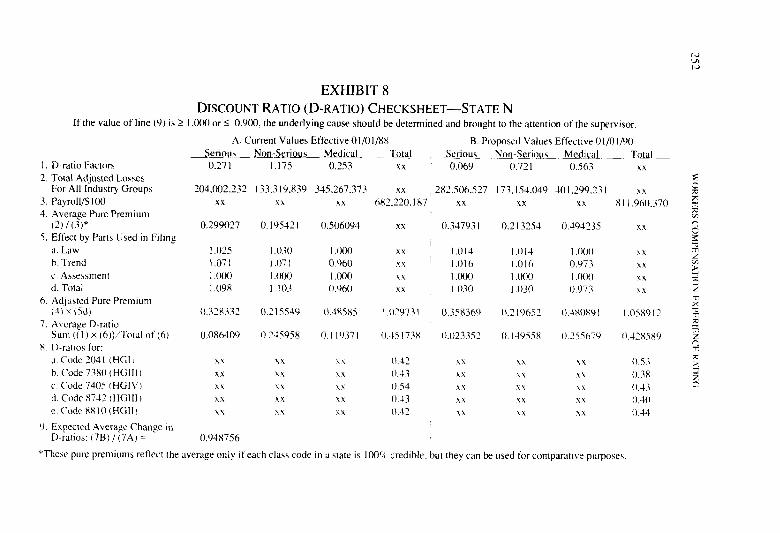
254 WORKERS (‘0MPf:NSSf IOX f:Sf’f<RIf:h(‘li K.t’l’lh(;
REFERENCES
[ I ] Dorweiler. Paul, “A Survey of Risk Credibility in Experience Rating,” PCAS XXI, 1934, p. 1.
[2] Gillam, William R.. “Parametrizing the Workers Compensation Expe- rience Rating Plan,” PCAS LXXIX. 1992, p. 2 I.
[3] Meyers, Glenn G., “An Analysis of Experience Rating,” PCAS LXXII, 1985, p. 278.
(41 NCCI, Experience Rating P lurt MUUIIUI. 1984, New York. New York.
[5] Kallop, Roy, “A Current Look At Workers’ Compensation Ratemak- ing,” PCAS LXIJ, 1975, p.62.
[6] Harwayne, Frank. “Use of National Experience Indications in Work- ers Compensation Insurance Classification Ratemaking,” PCAS LXIV, 1977, p.74.
[7] Mahler, Howard C., “An Actuarial Analysis of the Simplified Experi- ence Rating Adjustment (SERA),” Cuswlty Armccriul Soc,icty Folvm, Spring 1988, p. 279.
[8] Harwayne, Frank, “Accident Limitations for Retrospective Rating,” PCAS LXIII, 1976, p. 1.

STOCHASTIC CLAIMS RESERVING WHEN 255
PAST CLAIM NUMBERS ARE KNOWN
THOMAS S. WRIGHT
This pupc~r addresses the problem of estimuring futrrrc claim payments when two r-un-o&f triangles ure uvuilahle: one of the number of claims, the other of total amolmts. Euch single claim can hn\le partial payments included in the total for se\?- era1 development periods. The method does not require addi- tional information, such as measures of esposure and claims injlutiou. The approach udopted is to model the mean claim amount us u fhction of operutional time, using genetalixd Iineur models. Techniques are described for- jitting und com- puring a number- of models of this type, and fbr predicting the total cjf fhu-e claims from the best fitting model. Formal sta- tistirul tesrs are used for compuring models. It is shown how the root-mean-squur-e (RMS) error- of prediction can be calcu- lated, muking due ullowance for modelling error and random variution in both the number and amounts of future payments. Models are for-m&ted to muke explicit allowance ,for- claims inflation and purtiul payments. Assumptions are minimal, and diagnostic techniques are descr-ibed,for checking their validity in euch application. Numerical examples are given.
ACKNOWLEDGEMENTS
This research was sponsored by Bacon & Woodrow and Milliman & Robert- son, Inc.. I am grateful for the encouragement of Andrew English, Harold Clarke, Mike Brockman, and Spencer Gluck. I would like to thank the Insti- tute of Actuaries for permission to use the data for the example in Section 7, which first appeared in the Journul of the Imtitutc~ of Actuaria.s. 1983. Vol. I IO.

1 _ IN’l’KOIlI’(“llON
This paper complements a previous work bq the author 1 101. That paper, like many others on stochatic claims reserving in property/casu- alty insurance. deals with methods applicable when the past run-off of the number of claims is not known (a common situation for actuaries in the U.K.). This paper addresses the problem of’ claims reserving when at least two run-off triangles are available: WC 01‘ the number 01‘ claims, the other of claim amounts. These primary triangles may be:
(a) the number of claims closed, and the total of all payments on all claims closed (partial payments assigned to the development pe- riod of settlement):
(h) the total number of payments, including partial payments, and the usual paid claims triangle (with each partial payment as- signed to the development period in which it was made); or
(c) the number of claims closed. and the usual paid claims triangle (with each partial payment aa4gncd to the development period in which it was made).
Of these possibilities, (a) and (b) are the simplest to model. and are considered first. They are equivalent to each other as far as the modelling and prediction methods proposed in this paper are concerned. Later, it is shown how basically the same methods can be applied in situation (c), which is more common in practice.
If M’ is used to label origin (i.e., accident, report. or policy) years, and d to label development periods. the two run-off triangles can be denoted Y,,,, and N,,,‘, , respectively, where M’ runs from 1 to W, and d runs from 0 to T - 1. This notation is used for the incremental. rather than the cumula- tive, run-off. For example, in case (a), N,tC, is the number of claims closed in development period d of origin year H‘. and Y,,, is the total of payments on these claims made in development period tl and previous development periods. In case (c), N,,,, is the number of claims closed as in (a), but Y,,, is the total amount of all partial payments made in development period tl of origin year ~$1. including partial payments on claims not yet closed. In both

STOCHASTIC CLAIMS RESERVING 257
cases (a) and (c), N,,,(, should exclude claims settled with no payment if possible. Such claims do not contribute to Y,,,(, , so their inclusion in N,,, introduces an undesirable element of additional random variation.
As in [IO], the methods described here do not involve an assumption that the run-off pattern has been the same for all origin years; indeed, the shape of the run-off may be different for each origin year. Similarly, there is no assumption that the claim size distribution is the same for all devel- opment periods. It is common for larger claims to take longer to settle so that the mean claim size increases with n. Higher moments of the distri- bution may also depend on d. The methods allow projection as far into the future as is necessary, not limited by the extent of the data. The data triangles may have missing values. This does not cause any problems provided the total number of data points is sufficient to fit an adequate model. The occasional negative values which occur in real data can also be handled without special treatment.
The approach used in [IO] is to derive a model for the known data Y,,,(, from more basic models for the unknown quantities N,,,, and the individ- ual claim amounts X,$?, (also unknown). The assumptions of the models for N,,,, and X,,(, are then checked indirectly by applying diagnostic tests to the resulting model for Y,,,(, , If satisfactory, the model that is fitted to the Y,,.(, is used to project into the future. The logical progression of this approach to situations where N,,,, is known would be to formulate models for N,,.,, and Xur, separately (as before), but then to test each of these models directly from the data. This should allow good models to be found for each of these components. These models could then be used to project N,,,(, and X,,,(, separately, and the projections combined into projections for the total payments Y,,,, . However, the calculation of standard errors for predictions of Y,,(, obtained in this way is complex. Hayne 131 deals with the case when, for each origin year, the distribution of future claim amounts X,,,, does not depend on the development period d. The intention in this paper is to remove this restriction (as, for example, when larger claims tend to take longer to settle than smaller claims). In this case, the calculation of standard errors for the predictions would be extremely complex using real-development time, because the precise time of settle- ment of each future claim (hence, the appropriate claim size distribution)

is uncertain. The problem is simplified in this paper by making use of the concept of opwtiond finzc. This concept seems to have been used first in claims reserving by Reid [7] and later taken up by Taylor [S, 91, but a fresh approach. including a number of innovations. is proposed in this paper.
Operational time, 2, is defined as the proportion of all claims closed to date. Thus, for each origin year, operational time starts at 0, and increases ultimately to I. If the individual claim amounts X can be modelled as a function of operational time z rather than development time d. then there is no need for a separate model of the number of claims. This is because the dependence of the number of claims on operational time is known exactly: it follows trivially from the definition of operational time. Projec- tions of future payments Y can therefore be obtained from the mode1 of claim size X,,, alone, and the problem is an order of magnitude simpler than when X,,,(, and N),.,, are both projected.
The data IV,,,, is used at three points in the operational time approach:
l to estimate the ultimate number M,, of claims for each origin year MS (obviously. numbers of claims reported arc also useful for this estimation, if available);
l to calculate a triangle of operational times (for use as the explana- tory variable in the claim size mode1 ): and
l to calculate the observed mean claim sizes Y,,,,/N,,,, (for use as the dependent variable in the claim size model).
There are often substantive reasons for expecting the size of individual claims to depend more on operational time than on development time. The main reason is that changes in claim handling procedures may affect the actual delay to settlement but should not affect the size of claims. The plausibility of such arguments need not be left entirely to judgment. It is possible to use the figures themselves to verify this basic hypothesis of operational time methods. This is shown in Appendix B.

STOCHASTIC CLAIMS RESERVING 259
Summwy cf Later- Sections
Sections 2 through 6 deal with circumstances (a) or (b); that is, when the claim counts triangle gives the number of individual components of each element of the claim amounts triangle. Section 7 describes special procedures and enhancements to the method of earlier sections which may be necessary for case (c). All sections conclude with a numerical example. The data for the examples have been taken from Berquist and Sherman 111, and are reproduced in Appendix A. The data are actually of type (c), so the methods of Sections 2 through 6 are not wholly appropri- ate. They are applied purely for illustrative purposes. Section 7 also con- tains an analysis of the data used by Taylor 191. They are also of type (c), and are given in Appendix A.
Section 2 gives a complete account of the method applicable in cases (a) or (b), under several simplifying assumptions. The assumptions are unrealistic but are made initially in order to simplify the presentation. Sections 3 through 5 show how the assumptions can be relaxed. The assumptions used in Section 2 are that:
I. The expected claim size at each operational time z is the same for all origin years, after allowing for claims inflation. In other words, the mean claim amount in real terms is a function of T but not W. It can therefore be denoted m, . (In the presence of infla- tion, the mean claim amount will depend on w also. See Section 4.)
2. The coefficient of variation of individual claim amounts is the same for all operational times z, that is:
Var(X,)=cp’.m:, (1.1)
where X, is the size of an individual claim at operational time T, and cp is the coefficient of variation.
3. The data Y,,(, have been adjusted for inflation so the triangle is in constant money terms.
4. The ultimate number of claims M,. is fully known (that is, there is no uncertainty) for each origin year W.

Assumption I is the only condition that must hold in order to predict future claim payments using methods proposed in this paper. Even As- sumption I needs not be an assumption in the sense that its validity can be checked using the data themselves. (This is the subject of Appendix B.) Section 3 describes how Assumption 3 can be tested and relaxed if neces- sary. Assumption 3 cannot often be valid in practice because the rate of claims inflation is usually unknown. Section 4 4110~s how the rate of inflation can bc estimated and removed fmm the data at the same time as fitting the claim size model, rendering preadjustment unnecessary. As- sumption 4 only holds in practice if the origin years are report years. Often with accident or policy years. thcrc will bc considerable uncertainty in the estimates of ultimate numbers M,, Section 5 describes how this uncertainty can be taken into account.
The main point of Sections 2 through 4 is to discover how the mean and the variance of an individual claim X, depend on the operational time z. When this has been achieved. since WC know the operational time r ot every future claim (from the definition of operational time I. we can find the expected value and the variance of every future claim. This, in turn. can be used to find the expected value mnd the variance of the total of all future claims.
A broad outline of how predictions can bc mndc from a fitted opcra- tional time model was provided in the previous paragraph. (Here the term “model” refers to the mathematical representation of the relationship be- tween operational time and the mean and variance of X, .) The details of prediction are given in Appendices D. E, and F. These are more complex than would be expected from the comments above: first. because of pa- rameter uncertainty (that is, the fitted model will not be exactly right); second. because uncertainty in the ultimate numbers M,, implies uncer- tainty in the operational time of each future claim; and, third. because of uncertainty about future claims inflation. Section 6 shows how uncertain future claims inflation can be included in the predictions obtained from an operational time model. This is necessary to comply with standard reserv- ing practices.
All the models proposed in this paper are ,, ~v~~wruli~d liwiu. rnr~dt~l~s. Such models can be fitted using an algorithm hnown as Fisher’s scoring

STOCHASTIC CLAIMS RESERVING 261
method. This is the algorithm used in the well-known statistical package GLIM, which was used for all the numerical examples in this paper. Fisher’s scoring method maximizes the so-called qltusi-likelihood, or equivalently, minimizes the del*iance. The deviance can be regarded as a generalization of the weighted sum of squared differences between ob- served and fitted values. The weights are determined from the assumed variances of the observations. The generalization is that the variance of each observation may be a function of its mean, which, of course, is not known. The purpose of fitting the model is to estimate the mean. Fisher’s scoring method sometimes gives conventional maximum likelihood esti- mates. In other cases, it gives estimates which have all the desirable properties of maximum likelihood estimates (asymptotically unbiased, efficient, and Normal) although they may not actually be maximum likeli- hood estimates. An approximate variance/covariance matrix for the pa- rameter estimates is also produced by the algorithm. Further details are not given here as they are well documented elsewhere: the theory in McCullagh and Nelder [5], briefly in Hogg and Klugman [4], and practi- cal aspects in the GLIM manual [6]. The application of GLIM in actuarial work has previously been advocated by Brown [2].
2. SIMPLIFIED SCENARIO
Assumptions
Throughout Section 2, the four assumptions listed in Section 1 are made. These assumptions are not thought to be realistic, but are made at this stage to simplify the presentation. Assumptions 2, 3, and 4 are re- laxed in later sections.
Transformation of the Data
In order to model the dependence of claim size on operational time, the original data triangles I’,,(, and Nnd must first be transformed into a triangle z,,(/ of operational times, and a triangle Sbrtl of observed mean claim amounts. In the subsequent modelling, T will be the explanatory variable, and S will be the dependent variable.

267 STO(‘HAS’~IC‘Cl./\IMS RESERVlNti
Operational time, t, which has previously been defined as the propor- tion of claims closed, is an alternative to development time, cl. This defi- nition gives the value of operational time hct\i’ec>u claim settlements. In this paper, the value of operational time uf each claim settlement is de- fined to be the mean of the values immediately before and after settle- ment. So, for example, if there are M claims for a certain origin year, the operational time of settlement of the Nrh claim is given by z = (N - 'h/M. The values of operational time for each claim settlement are ('/5)/M, (%)/M...., (M - '/5)/M. These values are shown as crosses in Figure 1, which illustrates a typical relationship between operational time and true development time. The mean operational time of the N,,,, claims in development period cl of origin year M’ can be calculated as:
LI = W,,: I + Nw. 2 + . . . + N, (,- , + 'h N,,,, J/M,, . (2.1)
Note that only half of N,,,,, is included in the numerator in order to give the nwm operational time for these claims.
The sample mean size S,,, of the N,,.,! claims from origin year w observed at mean operational time z can bc calculated as S,,, = Y,,.,,/N,,.,, . As S,,, is a sample mean, its expected value is equal to the mean of the underlying population:
E(S,,.,) = 1~1, . (2.2)
The variance of Slt4 is the population variance divided by the sample size. Using the population variance of Assumption 2 (Equation I. I ) gives:
Equations 2.2 and 2.3 are actually approximations in general because the N,.,, claims do not have exactly the same mean and variance. Equation 2.2 is exact if IPI, is linear in T, and equation 2.3 is exact if 1~: is linear in t. Both are good approximations if nrT does not vary greatly within each de- velopment period.

1
FIGURE 1
TYPICAL RELATIONSHIP BETWEEN OPERATIONAL TIME AND REAL DEVELOPMENT TIME
Development Year d Real Development Time ( t )
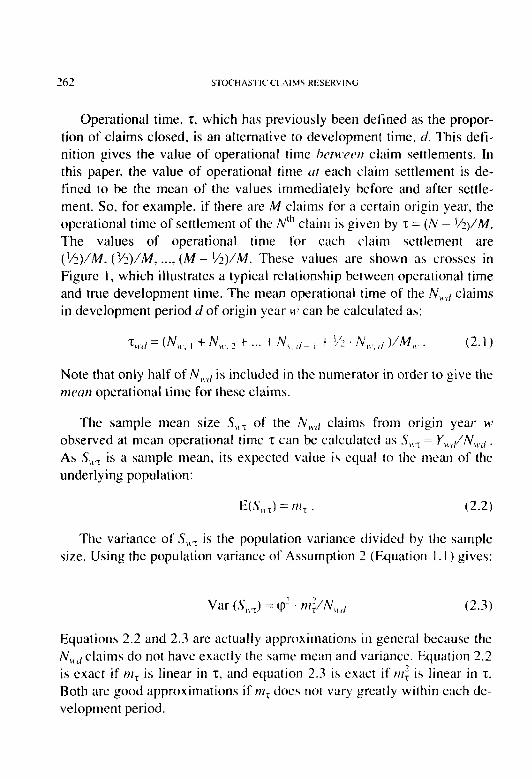
The form of Equation 2.3 for the variance of S,,., can be:
l tested (as described below) and if‘ not true. modified (as described in Section 3), and
l used to test and compare alternatives for the systematic component of the model: that is, the dependence of mr on t (also described below).
It is not necessary to have any further knowledge about the distribution of the data S in order to fit models of “generalized linear” type for the M, ; the variance alone is sufficient.
Equation 2.1 defines a relationship between r. M’, and tl for the ob- served data. Given any two, the third can be found. By virtue of this known relationship, N,,.,, can alternatively be expressed as N,., , and this is done for the remainder of the paper.
Models jiw the Mealt Cluint Six>
An expression is needed to describe how expected severity varies as a function of the length of time a claim is open. A number of possible relationships between m, and z are considered:
1. m, = exp (p,, + /3, . z + p, In(r))
7 -. m, = exp (b,, + p, r + & r’)
3. l?IT = (8,) + p, ty
4. rn, = l/(& + p,/z)
All these models are of generalized linear form; that is, the mean nt, of the data S,,, is some function of a known linear form of the unknown parameters j3:
h(n2,) = x, p.
where

STOCHASTIC CLAIMS RESERVING 265
h(m,) is a known function,
X, is a known vector, and
P = CP,,? PI? I%>.
Table 1 gives h(m,) and x, for each of the models.
TABLE 1
Appendix C shows how models for the mean claim size as a function of operational time can be interpreted in terms of real development time. Such models often correspond to simple relationships between the mean claim size and the distribution function of the delay. A graph of m, for each of the models is given in Figure 2. Although Figure 2 shows typical shapes, each model embodies a family of curves, and different shapes can be obtained within each family by varying the P-parameters. Of course, many other generalized linear models for m, could be formulated. All such models can be fitted, tested, and projected using the methods de- scribed below. The four models considered here have been chosen arbi- trarily, for illustrative purposes.
Testing the Val-iawe Assun~ption
As all the proposed models for mt are of generalized linear form, they can be fitted efficiently, given a second moment assumption, using Fisher’s scoring method. First, it is necessary to test the proposed second moment assumption (Equation 2.3). This can be done by fitting a model (referred to as “Model 0”) which makes minimal assumptions about the form of nz, .
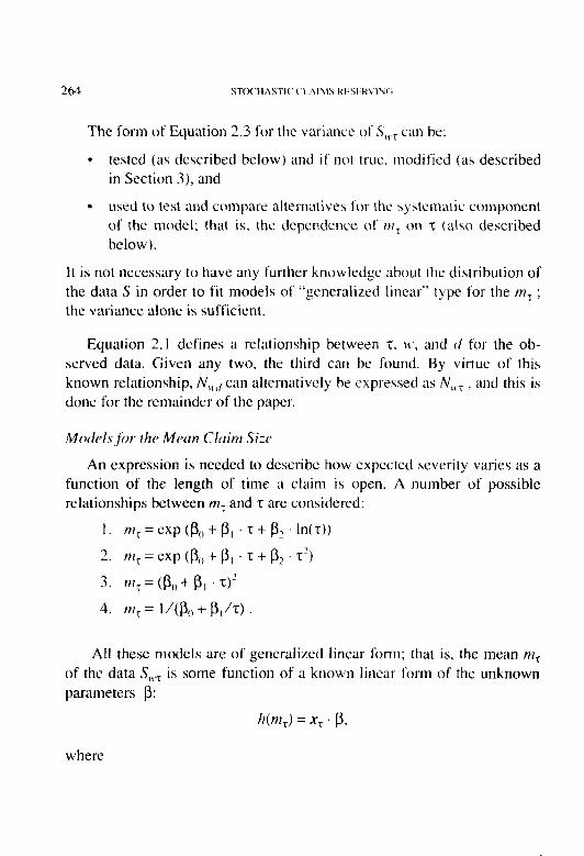
FIGURE 2
TYPICAL SHAPES OF VARIOUS MODELS RELATING MEAN SEVERITY TO OPERATIONAL TIME
. * - ‘T--@ 1000 . + e
. + . + - G
. + 0
800 . + 7 0
c .
-/ A 0
600 . t 0
. *
0 Oiv
Operational Time
267
A suitably minimal assumption is that the expected claim size m, is a piecewise exponential function of z; that is, ln(m,) is a piecewise linear function of z. The important point is that this form of model is very flexible. Any reasonable function m, can be well approximated in this way if the intervals are sufficiently small. It is probably sufficient to take a number of sub-intervals of equal width, the number being equal to the observed number, T, of development periods. A subscript, j, is used to label these sub-intervals of the observed operational time range.
Model 0 can be expressed as:
m, = exp CP,, + C Pj zj) , (2.4)
where each Tj is the amount of z lying in each of the sub-intervals of the
operational time scale such that z = c . Zj . This gives a continuous
piecewise linear function in the expone:t of Equation 2.4. The & are the slopes of the line segments. See Figure 3. An example of this piecewise exponential form for m, is shown in Figure 4. No assumption is made about the relationship between the pj values asj varies from zero to T.
In terms of h(m) and x,, Model 0 is:
h(m) = In(m)
x, = (1, 71, 72, f,, .-*, ‘tT).
If all the sub-intervals of operational time have the same width U, then X, is of the form:
where (k - 1)~ < T < k . u and zk is the fractional part in this sub-interval. Of course, k and ~~ may differ for each data point S,,, , but since T is known for each data point, x, can be determined and the model fitted to estimate the parameters pi for j = I to T.

W,) :
FIGURE 3
TYPICAL MODEL ZERO (ON LOG SCALE )
P4
0 Ll 2u 3u
~I_. -_ .~-- ._I __I -.-i.-
4u Operational Time (7)
N E
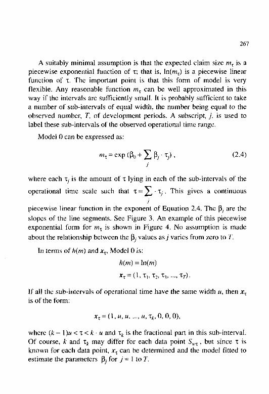
FIGURE 4
FITTED MEAN SEVERITIES FOR BERQUIST AND SHERMAN DATA
-. -- 0.60 0.80 1.00
Operational Time
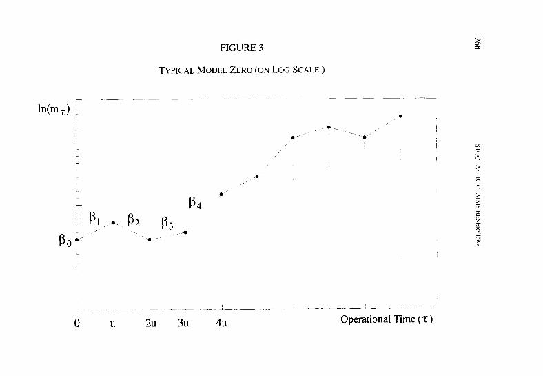
210 STOCHASTI(‘CI.AIMS RESERVIW
Consider the quantities:
(2.5)
If the variance of S is indeed as specified by Equation 2.3 then these quantities have E(R,,) = 0 and Var (R,,) = (p’. After fitting Model 0 (by Fisher’s scoring method), the R,,, can be estimated by using the fitted val- ues for the m, (these estimated R,,= arc the standurdizecl wsiduuls).
The variance assumption can be tested by plotting the R,, against 2. The variance should be constant: that is, it should not depend on z. In such a case, (p2 can be estimated as follows:
q$ = ( c R;,,/(n - T - I)), (2.6) \%“I
where
n is the total number of points in the triangle, and
T + 1 is the number of P-parameters.
If the residual plot shows heteroscedasticity (that is, the variance ap- pears to depend on z), then the variance assumption (Assumption 2 of Section 1) should be modified. (See Section 3.)
Testing Models for the Mean Claim Six
Model 0 is so flexible that we can be fairly confident it will provide a good fit. The quality of fit of other models can therefore be assessed by comparison with the fit of Model 0. When the variance assumption has been validated, any other model for m, of generalized linear form can be formally tested as follows. After fitting by Fisher’s scoring method, the standardized residuals can be calculated from:
R,,, = (S,,, - m,) . K7-/rn, (as for Model 0).
From these, another estimate of (p2 is given by:
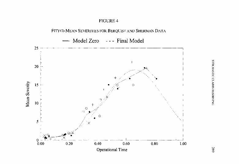
STOCHASTIC CLAIMS RESERVING
cp: = ( c ey(n - p), H7
271
(2.7)
where
n is the total number of points in the triangle, and
p is the number of parameters in the model (the ps), either two or three for each model listed in this section.
The following statistic can then be calculated:
F=[(p:+-p)/(T+ 1 -+&((n-T- l)/(T+ 1 -p)]/& Gw
where cpi is the estimate of (p2 obtained from Model 0.
This should be compared against the theoretical F-distribution with (T + 1 -p) and (n - T - 1) degrees of freedom. If the F-statistic is too large, then the current model for m, cannot be accepted. In such a case, the lack of fit may well be apparent from the plot of residuals against 2. For some values of z, the mean may appear to be significantly different from zero. If the F-statistic could reasonably have come from the theoret- ical F-distribution, then the fitted means m, obtained using Model 0 do not vary significantly from the form assumed in the current model. There- fore, the current model can be accepted. Several of the models proposed in this section may give reasonably small F-statistics. If so, tables will indicate which F-statistic corresponds to the largest tail probability, but it may be safer to use a more general model, of which all acceptable models are special cases.
Estimates of (p2 (hence F-tests) alternatively may be based on the minimized deviance rather than the sum of squares of the standardized residuals. This is more satisfactory in view of the likely skewness of the data. The deviance is less sensitive to the incidence of large claims than the residual sum of squares, so it will be more stable. The deviance is:
272
from which:
hence an F-statistic from Equation 2.8.
The choice between using the residual sum of squares or the deviance to construct F-statistics arises because in neither case is the distribution truly the F-distribution. With an infinite number of data points, and mod- els which were restricted cases of Model 0, both alternatives would have the true F-distribution. Neither of these conditions is satisfied, but the F-statistic based on the minimized deviance provides an effective, prag- matic technique for testing and comparing models. It is of no practical consequence that precise probability levels cannot be assigned to the F-statistics. Further details on the relevant theory are given by McCullagh and Nelder [ 51.
If a simple model is found with an acceptably small F-statistic (not much greater than one), then it can be used for predicting future pay- ments. The expected value of each future claim is obtained by evaluating the fitted mean nrT at the operational time r as defined earlier. Similarly, the variance of each future claim is obtained by evaluating Equation 1.1, using the fitted mean mT, and the estimate of cp’ given by the minimized deviance as described in the preceding paragraphs. Assuming the amounts of future claims are stochastically independent. the mean and variance of the total can be obtained as the sum of the figures for the individual claims. The resulting variance must then be augmented to allow for esti- mation error in the fitted means m, . Details are given in Appendix D.
273
Numerical E.rample
The data used in the examples are the medical malpractice data pub- lished in Berquist and Sherman [l]. They are given in Appendix A. To satisfy Assumption 3 of Section 1, the YYl,d values of Appendix A were brought up to 1976 terms using an assumed inflation rate of 15% (the rate used by Berquist and Sherman) before calculating the sample means S,,, = Y,.,/N,.,, . The triangle of operational times was calculated using Equation 2.1 and is given in Table A.4. A plot of the sample means S,, against operational time 7 is given in Figure 5.
Model 0, which has nine parameters (one intercept parameter, and a slope parameter for each of eight subintervals of the observed range [O.O, OX?] of operational time) gave a minimum deviance of 1,803. The plot of standardized residuals against z is shown in Figure 6. This shows clear evidence of heteroscedasticity. The spread of the points decreases as z increases. This indicates that the variance assumption (Assumption 2, Equations 1.1 and 2.3) is false. Consequently, all results obtained using this variance assumption are invalid. The minimized deviance, the num- ber of residual degrees of freedom, and the F-statistic for each mean claim size model are given in Table 2. The number of degrees of freedom, dfi is the number of data points less the number of model parameters. It appears in the denominator of Equation 2.7.
TABLE 2
Model Deviance
1 3,417
2 2,685
3 3,52 I
4 4,52 1
3 F
33 4.0
33 2.2
34 3.7
34 5.8
It is stressed that the clear falseness of the variance assumption rend- ers the above figures meaningless. They are presented here merely to illustrate orders of magnitude, and to show how the F-statistic relates to the deviance. The example is continued in Section 3.
25
20 :
FIGURE 5
OBSERVEDMEANSEVERITYAGAINSTMEANOPERATIONALTIME (DATAFROMBERQUISTANDSHERMAN)
15 . +
10 -
x
+
b-t
.
I * 1969
+ 1970
0 1971
-z 1972
x 1973
4 1974
i 1975 +I976
~~ _ ~_~ ~ .__ _~ -~ lA ~- ! 0.40 0.60 0.80 1.00
Operational Time
FIGURE 6
RESIDUAL PLOT FOR MODEL ZERO WITH a = 2
-3-.-----"- 0.00 0.20
X
X 7
i? X X
X
X x x
X
- 1
0.40 0.60 Operational Time
X x x' X
X X
, , ~ , N 0.80 1.00 2

3. RELAXING TtIE \‘ARf/\S(‘II ~ASSl~MPTION
If the initial variance assumption (Assumption 2. Equations I. 1 and 2.3) is found to be incorrect when tested as described in Section 2, then an alternative must be tried. The coefficient of variation of individual claims may depend on the mean claim size or,. Since this is usually an increasing function of z, the nature of the dependence should be apparent from the plot of standardized residuals against z for Model 0. For example. if this plot suggests that the variance is decreasing as t increases. then the coef- ficient of variation decreases as the mean r?ry increases. Such a case can probably be modelled adequately by replacing Assumption 2 from Sec- tion I with:
Var (X,) = rp’ n$ . for some a < 2. (3.1)
In terms of the sample mean S,, , this is:
Var (S,,.,) = ‘p’ HrE(/N,,., . (3.2)
Model 0 can be refitted on this basis (details are given below) and the standardized residuals examined to determine whether a needs to be fur- ther adjusted. The standardized residuals are given by:
Similarly, if after fitting Model 0 using the initial assumption the stan- dardized residuals fan out, then the model should be refitted with a > 2.
When the variance has been satisfactorily modelled in this way for Model 0, the other models can be fitted using the variance function de- fined by Equation 3.1, with a taking the value found using Model 0.
The deviance to be minimized when a is not equal to one or two is given by:

STOCHASTICCI.AIMS RESERVING 217
Q = 2 . c A’,,, . [S,,., $S;, a - ITI; - *)/‘( I - a) - (St, Q - rn; - a)/(2 - CX) 1. wl
(3.4)
This is the quantity which is used to calculate F-statistics for testing and comparing the different models for the mean claim size 171, . (See Section 2.1
The example of Section 2 has been rerun using an index a = I .S in the variance function, instead of a = 2. The minimized deviance for Model 0 (which has nine parameters) is now 2,404. The plot of standardized resid- uals against operational time z is given in Figure 7. It shows no evidence of heteroscedasticity, so the variance assumption (Equations 3.1 and 3.2 with cx = 1.5) is acceptable, and the results of modelling under this as- sumption are valid. The minimized deviance and the F-statistic for each of the models of Section 2 are listed in Table 3.
TABLE 3
Model Deviance
1 5,829
2 3,567
3 5,053
4 6,568
df ~~.~ __ 33
33
34
34
F
6.41
2.18
4.25
6.68
Table 3 shows that none of these models fit the data very well. For a model to be acceptable, the F-statistic must be much closer to one.
An F-value of 1.22 is achieved by the following four-parameter model, which is a generalization of Models 1 and 2:
11(m) = In(m)
x, = (1, z, r2, In(~))
The estimated parameters (with their standard errors) are:

FIGURE7
RESIDUAL PLOT FOR MODEL ZERO WITH a = 1.5
2 -x
x
X x
-I y
-2
0.00
x
2:
x Y\
x
x
-
x X
x x
X
x x
x
0.20 0.40 0.60
Operational Time
0.80 1.00

STOCHASTIC CLAIMS RESERVING 279
PI, -3.90 ( 1.08)
PI 18.3 (2.87)
P2 -12.8 (2.29) (coefficient of T’>
P3 -0.87 (0.33) (coefficient of In(z)) .
This model has five fewer parameters than model zero, so the F-statis- tic has five and 27 degrees of freedom. Statistical tables indicate a greater than one-in-three chance of an F-value as large as 1.22, if the model is true. In other words, the variation of the fitted values m, , obtained using Model 0, around the curve obtained under the present model could well be purely random. So, the present model gives a good representation of the underlying pattern in the data. This is confirmed by Figure 4, which shows the fitted values of m, under both models. The difference between the two curves is insignificant compared to the random variation in the data.
Figure 4 also shows that the fitted curve for m, decreases for z greater than about 0.66. This decrease exists in the data (Figure 5), but there are no data for operational times greater than 0.82. It is reasonable to question whether a decreasing curve for m, should be projected beyond this value. It is shown in Section 7 that the decrease in the observed mean claim amounts is caused largely by the presence of partial payments. In the terms of the primary triangles in Section 1, the data is actually type (c), not (a) or (b). It is analyzed here as if it were type (a) or (b) purely to illustrate the method. In practice, one should be very wary of projecting a decreasing curve for m, beyond the observed range of operational times, in either case (a) or (b).
The fitted model also has a minimum at z = 0.05 and m, tending to infinity as z tends to zero. Although unrealistic, this is not important because projections are required only for operational times greater than 0.064 (the present operational time for the latest year of origin, 1976).
Table 4 gives the following quantities for each origin year: estimates of expected total of future payments, approximate standard errors of these estimates, estimates of standard deviations of total future payments, and approximate root-mean-square (RMS) errors of prediction.

2x0 s1'oc‘I1/\s1l(‘(‘l.,\lhlc KEStKVINci
Columns I and 3 have been calculated by totalling the estimated mean and variance for all future claims, as described in Section 2. Column 2 is the standard error of Column 1 arising from uncertainty in the estimated P-parameters of the mean ~7~. It has been calculated using the formulae derived in Appendix D. Column 4 is the combination of Columns 3 and 4, calculated as the square root of the sum of their squares. This is appropri- ate because the uncertainty represented by the standard errors in Column 2 is independent of the uncertainty rcprcsented by Column 3. Column 2 arises from random variation in past claims, whereas Column 3 arises from random variation in future claims (as described in Appendix D).
TABLE 4
Year
I969
1970
1971
1972
1973
(1) Expected
Total Future Payments
3,350
6,260
14,835
25,177
35,842
(3) (4) (2) Standard Root-Mean-
Standard Error Deviation Square Error
1,209 959 1,543
1,875 1,382 2.329
3,422 2,239 4,089
4,497 2.999 5,405
5,120 3,607 6,263
1974 40,098 4,642 3,779 5.985
1975 47,265 4.92 1 4,032 6,362
1976 59.00 1 5.989 4,46 1 7,467
All 23 1,828 3 I.270 X.960 32,528
The final row (labelled “All”) is for all origin years combined. The predicted total of future payments for all origin years combined is $232 million. This is simply the sum of the figures in Column I. The uncer- tainty represented by Column 2 is highly correlated between origin years, because the same set of parameter estimates (p,. given earlier in this section) is used for all origin years. Therefore, the standard error repre-
STOCHASTIC-CLAIMS RESERVING 281
senting this source of uncertainty for all years combined (3 1,270) is only slightly less than the sum of the standard errors for each origin year (the sum of Column 2 is 3 1,675). Full details of this calculation are given in Appendix D. In contrast, the uncertainty represented by Column 3 is stochastically independent between origin years, because the future claims for each origin year are mutually disjoint sets. Therefore, the stan- dard deviation for all years combined (8,960), is simply the square-root of the sum of the squares of the figures in Column 3. The RMS error of prediction for all origin years combined can be calculated in the same
way as for a single origin year; i.e., 32,528 = 3 1,270’ + 8,960’, because the first component represents uncertainty arising from random variation in past claims, and the second component represents uncertainty arising from random variation in future claims. A reasonably safe reserve (for all origin years combined) can be calculated by adding one RMS error ($32.5 million) to the best estimate ($23 1.8 million) to give $264 million. However, since the data were adjusted to remove claims inflation, this is in 1976 terms. Section 6 shows how future claims inflation can be in- cluded in the predictions. Also, the assumed past inflation rate of 15% may not be correct, and no allowance has been made for the uncertainty in the estimates of ultimate claim numbers, M,. , used in the calculations. These two matters are dealt with in Sections 4 and 5, respectively.
4. SIMULTANEOUS ESTIMATION OF INFLATION
Basic Assumptions
This section describes techniques that can be applied to data Y,,d that has not been adjusted for inflation. For some of the models specified in Section 2, the force of claims inflation can be estimated from the data at the same time as estimating the other parameters.
The sample mean payment amounts S,, are now calculated as S,,, = Y,,,~,/N,,, using the unadjusted Y,., . The expected value of S,,, will now depend on the origin year w (as well as z ) because of inflation, so is denoted PI,, . However, by assumption 1 of Section I, the mean in real terms is the same for all origin years. Thus, rnHT is of the form:

2x2 STOClt.4S’t’tC’(‘t ~AtW RI:SfiR\‘tN(;
n1ti-T = exp ~ (M’ + t//P) i ) nr5 (4.1)
for some M, which are the same for all origin years. Here, i represents the annual force of claims inflation: P represents the number of development periods per year; and M’ + LI/P is, therefore, the calendar time (in years) of each data point.
The initial variance assumption is that the coefficient of variation of individual claims is constant, which implies:
Var (S,,.,) = ‘p’ 1l7t.JN,,.~ .
As before. this can be generalized, if necessary. to:
(4.2)
Given a model for nzr, Equation 4.1 yields a model for the mean m,,, of the data S,,, . If i is to be treated as a parameter to be estimated, then the model for nz, must have hum,) lincar in the unknown parameters in order for ~7,,.~ to be of generalized linear form:
/7(~7,,.~) = x,.~ b, for some known vector x,., .
Thus, of the models for ~7~ proposed in Section 2. only Models 0, 1. and 2 can be fitted directly using Fisher’s scoring mcthod. Thcsc all have /7(m) = In(m).
Ifp=(i, p,,, p,, . ..) w h ere the Bj are the same as in Section 2, then the vector x, is given by:
Model 0: x, = (IZ’ + d/P, II, . . . II. ‘I,, 0, . . . 0)
Model 1: x,,,~ = (M’ + d/P, I, t. In(x) )
Model 2: x,,,~ = (W + <f/P. 1. z. z’)
X, is known for each data point as M’, tl, and r arc known.
STOCHASTIC CLAIMS RESERVING 283
Model fitting and testing can proceed with these models exactly as described in Sections 2 and 3, except that the number of parameters in each mode1 has increased by one. If T is the number of operational time intervals used in Model 0, the number of parameters of the model is now T + 2. The number of residual degrees of freedom is therefore II - T - 2. This should replace n - T - 1 in Equations 2.6 and 2.8. Similarly, the number of parameters p of Models 1 and 2 is now one greater than previously.
The question remains of how to fit models such as Models 3 and 4 which do not have h(m) = In@), when the rate of claims inflation is not known. The following procedure can be employed. First, fit Models 0, 1, and 2 as described above (generalizing the variance assumption if neces- sary). If none of these models gives an acceptable fit when compared to Model 0 (using F-tests as in Sections 2 and 3), then use the force of inflation estimated using Model 0 to adjust the data Ywrl into constant money terms. All models can then be fitted to the inflation adjusted data as described in Sections 2 and 3, and the best model determined. If the best model is one such as Models 1 or 2, then the version fitted to the unadjusted data should be used.
Although x,,,~ can be determined from the data for each cell of the triangle, it is not fully known for cells corresponding to the future. The relationship between z, d, and MI for the future depends on the rate at which claims will be settled, which is uncertain. Having fitted a model, the formulae of Appendix D apply only to the factor m, of Equation 4.1 so the predictions are in constant prices. A further stage of estimation is necessary before claims inflation can be incorporated in projections. This approach is illustrated in Section 6.
Note that the methods described here assume that past claims intlation has been at a constant rate. In cases where this is considered to be a poor approximation, the data Y,,.,/ should be preadjusted to remove any non- constant elements of claims inflation believed to be present.

2x4 S-WCHAS’I’I( (‘l./\lhlS RMERVIUG
The methods of Section 4 are illustrated by repeating the example of Sections 2 and 3, this time with the sample means S,,., calculated from the unadjusted data Y,,.,, and N,,.,, from Appendix A. As in Section 2, the residual plot from Model 0 with a = 2 shows that this value is incorrect, and as in Section 3, the value a = I .S is found to be acceptable.
Table 5 gives the minimized deviance and the F-statistic for compar- ing each of Models 1 and 2 to Model 0. These F-statistics each have six and 26 degrees of freedom. The table also gives the estimated force of claims inflation (and its standard error) obtained from each of the models.
TABLE 5
Model Deviance 4f 0 1,961 26
I 4,896 32
2 2,865 32
E Inflation
- 0.132 (0.035)
6.49 0.141 (0.047)
2.00 0.138 (0.036)
From statistical tables, there is only about a one-in-10 chance that an F-variate with six and 26 degrees of freedom is as large as 2. Therefore, neither Model I nor 2 adequately represents the data. This implies that all results obtained from these models are invalid, including the estimates of the force of claims inflation given above.
However, the model used in Section 3 still gives a good fit when applied to the unadjusted data with an additional parameter for inflation. The minimized deviance is 2,402, which gives an F-value of I. I7 on five and 26 degrees of freedom. The estimated parameters (with their standard errors) are:
p:l
0. I35 -3.7 I
PI 17.8
p2 -12.5
P7 -0.80
(0.034) ( 1.06)
(2.80)
(2.20) (coefficient of Z’)
(0.33) (coefficient of In(z)) .
STOCHASTIC CLAIMS RESERVING 285
The figure 0.135 for the force of claims inflation corresponds to a 14.5% annual rate.
The final results in 1976 terms are:
TABLE 6
Year
1969
1970
1971
I972
1973
1974
1975
1976
(1) Expected
Total Future Payments
3,450
6,397
15,034
25,360
35,962
40,132
47,279
59,015
(2) (3) Standard Standard
Error Deviation
1,169 898
1,800 I.287
3,261 2,07 I
4,27 I 2,76 1
4.873 3,3 12
4,464 3,464
4,796 3,696
5.876 4,089
(4) Root-Mean- Square Error
1,475
2,213
3,863
5,086
5,892
5,65 1
6,055
7,158
All 232,630 29,988 8,229 3 I ,096
Adding one standard error to the best estimate gives a reserve for all origin years combined of $264 million, in 1976 terms. Although these results hardly differ from those obtained in Section 3, more confidence can be placed in them now, because the inflation rate has been estimated from the data themselves, and not based on any prior assumptions. How- ever, no allowance has yet been made for the uncertainty in the ultimate numbers of claims M,,.
5. ALLOWING FOR UNCERTAINTY IN 1ILTIMATE NUMBER OF CLAIMS
In previous sections, it has been assumed that the ultimate number of claims, M,, , is accurately known for each origin year w (Assumption 4,

286 S’KKHASTIC CIAIMS RliSERVIN(i
Section 1). This assumption is realized in practice only if the origin years are report years. For any other definition ot’ origin year, there will be an unknown number (possibly zero) of IBNR claims. This number has to be estimated in order to arrive at an estimate of M,,. It is shown in this section how the uncertainty in the M,,. estimates can be taken into account in calculating standard errors of the final results. First, the source of the M,,. estimates is briefly considered.
For reserving purposes, the origin years must usually be either acci- dent years or policy years. In such cases, in addition to the triangle of the number of settled claims, N,,.,, , it may also be possible to obtain a triangle of the number of reported claims. Such a triangle will often give more information about the ultimate number of claims M,,. than does N,,, , because claims are reported before being settled. However. the reported claims triangle will include those claims eventually settled with no pay- ment, whereas N,.,, and M,, should not. These matters should bc consid- ered carefully when estimating the ultimate number M,. of non-zero claims. Whether reported claims, settled claims, or both. are available for estimating M,,. , the stochastic method previously dcvcloped by the author [IO] can be used. As well as estimates of M,, , this method gives standard errors of the estimates, L’,,. . The following paragraphs describe how these standard errors can be used.
The quantities M,,. are used at two points in the methods described in previous sections: in calculating the triangle of operational times 7 (Equa- tion 2.1) and in calculating predictions from the fitted model (Appendix D>.
In the following paragraphs, the effect of variability in M,, is consid- ered for each of these in turn.
If M,. is overestimated for a particular origin year LI’, then the opera- tional times for that origin year will all be underestimated by a certain factor. (M,. appears in the denominator of Equation 2.1.) The observed average claim amounts S,, for that origin year, therefore. will be for later operational times than those calculated and will tend to overestimate the true mean claim amount for the calculated operational times. Conversely, if M,. is underestimated, then the mean claim sizes will also bc underesti-
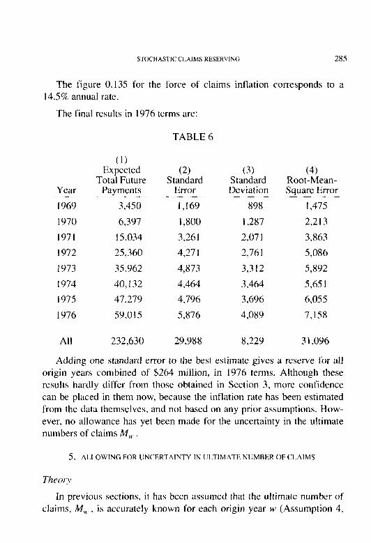
2x7
mated. However, estimation of the mean claim size nr5 is done by fitting a mode1 to the data for all origin years simultaneously. Provided the esti- mates M,. are unbiased and not highly correlated, the effects will tend to cancel out across origin years. There will be more variability in the data S,, across origin years M* than there would otherwise be, but this variabil- ity is already taken into account through the estimate of the scale parame- ter (p2. The additional effect on the variability of the final results is therefore minimal and can reasonably be ignored.
Experience with a number of data sets has confirmed these comments. Ultimate counts M,. may be estimated by a variety of methods, but the parameter estimates of the fitted model for nr, are invariably very similar whichever set of estimates MW is used to calculate the operational times. Usually, it is only the last few origin years that have much uncertainty in the ultimate number M,, . and these origin years contribute only a few data points (2, S) for the modelling. Therefore, the results of the model- ling are relatively insensitive to the choice of estimates M,,, .
Having estimated the parameters pJ of a model relating mean claim size m, to operational time, the method described in Appendix D has been used in previous sections to project the fitted mod:] and to calculate the mean-square-error of the projections. An estimate p of the expected total of future payments for a single origin year is calculated by summing the fitted mean mT over the operational times z of each expected future claim. The values of z for this summation are given in Equation D. I.
In Appendix E it is shown that, whatever the fitted model/for nz, , each increment of one in the estimate h ‘11 WI cause the estimate p to increase by approximately [T,, . 17~~) + $/&, where ‘t, is the operational time reached for the origin year, and m, is the fitted mean valte corresponding to T(~. This implies that the additional uncertainty in f.r caused by the uncertainty in M is represented by a standard error II given by:
u = [To . m, -k pi& . 1’ ) (5.1)
where v is the standard error of the estimate A.
.‘iTOC’HASTIC‘CL.AI\1S KI<SFKVIN(;
Continuing with the example of Section 4. Table 7 gives the quantities in Equation 5.1 for each origin year.
TABLE 7
Year G 1969 3.450
I970 6,397
1971 15.034
1972 25,360
I973 35,962
1974 40, I32
1975 47,279
1976 59.0 IS
To “41 lb 0.85 12.67 2,664 0.79 15.94 2,896
0.70 IX.65 4.065
0.62 18.41 4.77 1
0.53 IS.27 5,280
0.4 I 8.87 4,837
0.25 3.03 5,169
0.06 0.66 6.257
70
102
148
21s
314
461
690
I .097
II
845
1,505
2,484
3,580
4.67 1
5,4X I
6,843
10.393 A
G is the best estimate of future payments as given in Section 4. A4 and 1% come directly from Appendix A. r. is the row total N,, of the number-of- claims-settled triangle divided by M. HIP) is calculated from t,, using the fitted model, which is:
with
m, = exp (p,, + PI z + p, r’ + p; In(r)) ,
p,,= -3.71, PI = 17.8, p2 = -12.5. pj = -0.80.
14 is given from the other quantities using Equation 5. I.
Table 8 gives the final results. Columns I. 2. and 3 are as in Table 6 and Column 4 holds the new component of uncertainty.
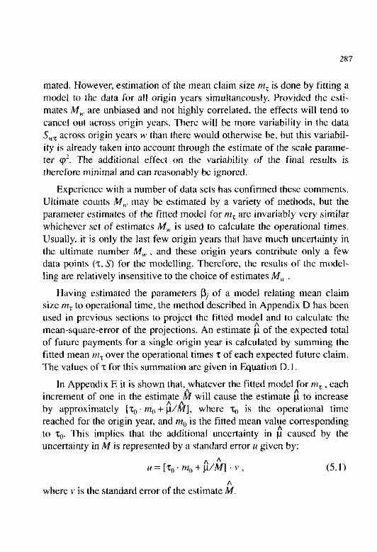
STOCHASTIC CLAIMS RESERVING 289
TABLE 8
Year
1969
1970
1971
1972
1973
1974
197s
1976
(1) Total
Expected Future
Payments
3,450
6,397
15,034
25,360
35,962
40, I 32
47,279
S9,O 1s
(4) Additional
(2) (3) Uncertainty Standard Standard (Number
Error Deviation of Claims) ~~ __ 1,169 898 845
1,800 1,287 1,505
3,261 2,07 I 2,484
4,27 1 2,761 3,580
4,873 3,312 4,67 I
4,464 3,464 S,48 1
4,796 3,696 6,843
5,876 4,089 10,393
(5) Root- Mean- Square Error
1,700
2,676
4,593
6,220
7,5 I9
7.872
9, I37
12,620
All 232,630 29,988 8,229 15,122 34,578
The uncertainty in Column 4 for all years combined has been calcu- lated on the assumption that the estimates M,, are mutually independent. It is the square root of the sum of the squares of the separate origin year figures. If non-zero covariances for the M,. were known, they could easily be brought into the calculation.
The three components of error (Columns 2, 3, and 4) are always mutually independent (to a good approximation), so the overall RMS error (Column 5) is simply the square root of the sum of the squares of these three columns.
Allowing for uncertainty in the number of claims outstanding has resulted in an increase in the overall standard error from $3 I. I million to $34.6 million. The reserve based on best estimate plus one standard error has changed from $264 to $267 million, an increase of I .Ol %.
To demonstrate the validity of Equation 5.1, the variation of l? with h has been investigated empirically. In Table 9, the first column gives the
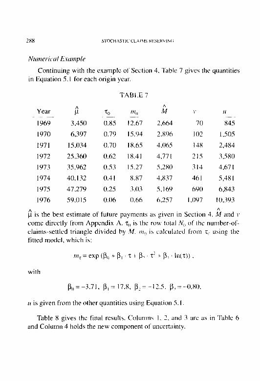
290 ~I’OCHA~I‘I(‘(‘I.AlMS RESliKVIPI(,
theoretical rate of change of fi with h for each origin year; that is, the quantity in square brackets in Equation 5.1. The remaining columns show the actual changes in 1 per unit change in M, when M is changed by the amount shown at the head of each column. A dash indicates that a result could not be calculated because the changed value for M was less than the number of claims paid to date, N,, .
For example, in Table 9, the figure 16.56 in the fifth column for 1972 was obtained as follows: The best estimate 3.77 I of the ultimate number of claims M was increased by 100 to 4,871. Since the number N,, of claims to date is 2,938, this implies 1,933 claims remaining. The fitted mode1 m, of Section 5 was summed over the 1,933 different values z = 2,93&S/4.87 I to z = 4,870.5/4.87 I. This gave the result 27,016. This is 1,656 greater than the best cstimatc of 25.360: and, since M was in- creased by IOO, the mean rate of change is 16.56.
TABLE 9
Change in M
(1) Theoretical (2) (3) (4) (5) (6) (7) (8) (9)
Year Value -10 IO -100 I 00 -500 so0 -1.000 1,000
1969 12.08 12.00 12.15 Il.29 12.79 ~ 14.82 - IS.85 1970 14.75 14.70 14.80 14.22 IS.10 Il.36 16.26 - 16.48 1971 16.78 16.78 16.79 6.67 16.86 IS.80 16.91 13.64 16.59
1972 16.65 16.66 16.64 6.73 16.56 16.89 16.15 16.55 15.56
1973 14.88 14.89 14.86 5.00 14.75 15.51 14.27 16.06 13.74
1974 II.89 I I.90 I I.88 1.98 II.81 12.38 I I.51 13.02 II.22
1975 9.92 9.92 9.92 9.93 9.90 IO.0 I 9.85 IO.14 9.80 1976 9.47 9.47 9.47 9.47 0.47 9.47 9.47 9.48 9.47
These results show that, for all origin years. the rate of change is almost constant within the range A4 + I’, and is close to the theoretical value, so Equation 5. I is a good approximation.
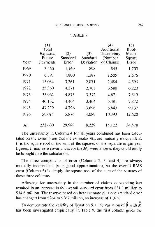
STOCHASTIC CLAIMS RESERVING 291
6. FUTURE INFLATION
Theory
Previous sections have been concerned with finding a model m, of the mean claim amount in constant money terms, and using the fitted model to calculate predictions in constant money terms. This section is con- cerned with the inclusion of future claims inflation in predictions, with due allowance for the inevitable uncertainty. This is necessary if the pre- dictions are to be used as a basis for setting reserves, because reserves are conventionally in current money terms (not discounted).
Uncertainty in future claims inflation arises from two sources:
1. uncertainty in the future rate of claims inflation, and
7 uncertainty in the timing of the run-off of future payments. I.
Appendix F shows how both these elements of uncertainty can be taken into account simultaneously. Obviously, if the run-off of future claim payments is expected to take many years, moderate uncertainty in the future rate of claims inflation may lead to substantial uncertainty in current price predictions, because of the exponential effect of inflation.
Numerical Example
To illustrate the method of Appendix F, future inflation is introduced into the predictions obtained in Section 5. An exponential run-off of the remaining claim settlements over development time is used for all origin years. The time scale of the run-off can be estimated by examining the triangle of operational times (Table A.4).
Since the origin years are accident years, the mean delay to settlement is approximately d years for claims closed in development year d (except d = 0, for which the mean delay is about 0.33 years). The triangle of operational times indicates a “half life” of just over three years. The 95% confidence range for the half life is judged to be 2.8 to 3.6 years. This corresponds to a best estimate of 3.2, and a coefficient of variation of about 0.06. In the notation of Appendix F: U, = 0.06’ = 0.0036.

From Equation F. 13, the best estimate of the parameter p of the expo- nential distribution is:
p = 3.2/ln(2) = 4.6 years.
Using Equation F.14, the remaining real delay I corresponding to fu- ture operational time t is estimated (in years) to be:
r=H(r)=-4.6.Inl (1 -r)/(I -t,,) 1.
For this example. it is assumed that the estimate of the average force of future claims inflation (from mid- 1976 onwards) is 0. I with a standard error of 0.02. Thus, it is expected that inflation will be less in the future than in the past, but the 95% confidence range of 0.06 to 0. I4 contains the best estimate 0.135 of the average past force of inflation (Section 4). In the notation of Appendix F. i = 0.1 and I!, = 0.02’. Equation F.7 gives 0.02 1’ for the variance I/, due to both uncertainty in the future force of intlation and uncertainty in the future time scale. This is only slightly greater than ti, . indicating that the second element of uncertainty is rela- tively minor.
The current price predictions for each origin year are given in Table IO.
TABLE IO
Year I969 1970 1971 1972 1973 I973 197s 1976
(1) Expected
Total Future
Payments 5.531 Y,934
22.7Y4
3x.233 54.79X 63.436 79.899
109,297
(2) Standard
Error 2.056
3,202 6,027
X,374
10.254 10,329 12.21 I 16,480
(5) (3) Additional
Additional (4) Uncertainty Uncertainty Standard (Number of (Inflation) Deviation Claims)
735 I.306 YOO 1.230 l.XOI 1,629 2,657 2.x19 2,767 4,345 3.735 4.160
6,YO 4.530 5.791 7.752 4,Yl7 7.702
IO,903 5,5x0 I I.197 17.05-l 6.658 19.209
(6) Root- Mean- Square Error
2,699 3.203 7,6X0
10.966
34,103 IS.821 20,603 3 I.236
All 383,Y23 68.658 SO.Y76 12. I24 34.X I2 X9.86 I

STOC’HASTIC CLAIMS RESERVING 293
Columns I, 2, 3, 4, and 5 are as in Table 8, except that each expected claim amount nz, has been inflated using the factor exp (i . H(z)) before finding the total for each origin year. The new Column 3 gives the addi- tional element of uncertainty calculated from Equation F. 11. The figure for all years combined (50,976) is simply the sum of the figures for the separate origin years (this comes from repeating the argument given in Appendix D using the variance-covariance matrix of Appendix F). Intu- itively, it is clear that this new component of uncertainty will be highly correlated between origin years, because the projections for all origin years are based on the same estimate of future inflation. If we overesti- mate future inflation, then we overestimate the reserve for all origin years simultaneously. The apparent perfect correlation (additivity of Column 3) is an approximation resulting from the use of first order Taylor series for these standard errors (Appendices D and F). The use of Taylor series approximations does not induce apparent perfect correlation in Column 2 (68,658 is less than the column total of 68,933) because these standard errors represent uncertainty in more than one parameter estimate (the 0s) and the estimation errors are not perfectly mutually correlated.
Column 6 gives the overall mean-square-error calculated as the square root of the sum of the squares of Columns 2,3,4, and 5.
It is interesting to look at the delays and inflation factors of the last claims as given by the estimated function H(z). The expected ultimate number of claims is 6,257 for origin year 1976. The operational times of the last three claims for this origin year are therefore 0.99960, 0.99976, and 0.99992. The expected delays from accident to settlement of these claims (calculated from t = -4.6 In( I - 2)) are 36.0, 38.3, and 43.4 years, respectively. Using the estimated force of inflation i = 0. I, the estimated inflation factors are 36.6,46. I, and 76.7. These factors are obviously very sensitive to the estimate i, which is why the extra element of uncertainty can be substantial.
In practice, the function H(T) would be estimated more carefully than in this example, making use of any additional information on likely de- lays. The estimated time scale parameter (4.6 in the example) need not be the same for all origin years. The method detailed in [lo] can be applied to the number of claims triangle to obtain an estimate and a standard error

294 STOCHASTIC CLAIMS KESEKVIWi
(hence a value for I/,) for each origin year. A Gamma, rather than an exponential run-off can be used to construct H(r) if necessary, but this is unlikely to make much difference to the results except for the last one or two origin years. The use of a Gamma run-off is illustrated in the example of Section 7.
7. PARTIAL l’:ZYMt~‘JTS
Paid claims run-off triangles are usually of type (c) (see Section I) in practice. That is, the counts triangle N,,.,, is the number of claims closed in each development year cl of each origin year H’. but the paid amounts triangle Y,,.,, is the total of all payments made in development period d of origin year MS. Each Y,,.,, includes partial payments on claims settled at some later development period, as well as the settlement payments counted in N,,,(, . The following paragraphs describe special procedures that may be necessary when the partial-paymcnr component of Y,,.,, is substantial.
Dropping the subscripts H’ and tl temporarily. each Y has two compo- nents:
Y = Y, + Y? .
where
Y, is the total of payments made on claims closed, and
Y1 is the total of payments made on claims not closed.
N, will denote the number of settlement payments: thal is. the number of individual payments making up Y,. Similarly, N, will denote the num- ber of prepayments on claims not yet closed: the number of individual payments in Y2 These quantities are not all known: the data consists only of Y and N,, for each ~7. tl combination. The mean claim amount which can be calculated from the data is:
s = (Y, + Y>)/N, (7.1)

STOCHASTIC CLAIMS RESERVING 295
Since the expected values of Y, and Y, may follow two different pat- terns as operational time 7 varies from 0 to 1, the form of the expected value of S (as a function of z) is likely to be more complex than when the component Yz is not included (situation (a) from Section 1). Furthermore, random variation of S around its expected value will be negatively corre- lated with random variation in N,. This is explained further in the follow- ing sections.
Both N, and N2 are subject to random variation. Initially it is assumed that they are stochastically independent. This will be discussed further below. If N, is higher than expected (it just happens that a large number of claims reach the settlement stage at about the same time), Y, will be correspondingly high, as it is the total of the N, settlement payments. But, N2 (hence YJ will not be affected, so S will tend to be lower than ex- pected. Conversely, a low value for N, will tend to give a high value for S, because Y, will be proportionately low, but Yz will not.
There is an argument which suggests that N, and N2 may be positively correlated. This would limit the negative association between N, and S described above, and would eliminate it completely if the expected value of Nz, given N,, were proportional to N,. The argument is that both N, and N, may be affected in the same direction by a common cause: namely, increased activity by the insurance company on claim payment proce- dures, regardless of whether the payments are settlements or prepay- ments. This is discussed further in Appendix G. There are also arguments which suggest that N, and N2 may be negatively correlated. This would substantially increase the negative association between N, and S de- scribed above. First, if the number of claims closed in a certain develop- ment period is unusually large, the number of claims left outstanding at the end of the period will be correspondingly small, so the number of partial payments on such claims will also tend to be small. Second, if many claims are ready for settlement at about the same time, the demand on resources made by these settlements may reduce the resources avail- able to deal with prepayments on outstanding claims.
Previous sections have been concerned with modelling the expected value nzT of the sample means calculated from S = Y,/N,. (In the terms of Section 1, this is situation (a).) It is shown in Appendix G that, under

296 STOCHASTIC CI.AIMS RESERVING;
certain assumptions, the effect of including partial payments Y, in the numerator of S is approximately the same as increasing the mean rrrT by a factor of exp (C R),,J, where c is a constant, and R,,,<, is the ratio of the number of claims outstanding in development period rl to the number settled during development period d. That is. if LM.(, is the number of claims outstanding, then R,.,! = L,,.,,/N ,,,‘, . The coefficient C’ represents the expected partial payment per outstandin, ~7 claim (including those with no partial payments), as a proportion of the mean size of settlement pay- ments. For example, if the average number of partial payments in any development period is one for every five outstanding claims. and the mean size of these partial payments is half the mean size of settlement payments, then c = 0.2 x 0.5.
If the model for nr5 has a linear form for In(nz,), then the factor exp (C R,,.,,) simply introduces a further term to the linear exponent. If Rw,d is known, C’ can be estimated in the same way as the other parameters of the model. For example, in the models of Section 4. the parameter vector becomes:
and the vector X, of known explanatory variables becomes:
Model 0: x,,, = (RI,.,), MI + d/P. II ._. 11, 2,. 0 . 0)
Model 1: x, = (R,,[, w + d/P. I, r, In(t))
Model 2: x,,,~ = (R,,.,,, M’ + d/P, 1, z, 6).
Other models (such as Models 3 and 4) can be fitted by first dividing each observation S by exp (C . R,,,J, using the value of (’ estimated from Model 0. This procedure is similar to the preadjustment for intlation described in Section 4.
Appendix G also shows that if m, represents the mean with the factor exp (C . R,J included, then Equation 2.3 for the variance of S becomes approximately:
Var (S,,) = (p2 &(exp (C R,,,(,) N,,.,,) (7.2)

STOCHASTIC CLAIMS RESERVING 297
Therefore, to fit the models above, the factor N,,., must be replaced by exp (C . R,,,J NH,{, in the deviance (Equation 2.9). An initial estimate of c is required for this purpose. If the estimate of c obtained by fitting Model 0 differs significantly from the initial estimate, then other results should be disregarded and the model fitting should be repeated using the new estimate of c in the deviance.
A number of assumptions are made in Appendix G, leading to the results quoted above. There is no need to consider too carefully how realistic these assumptions are in each application. The purpose of the mathematics in Appendix G is to find a broad model of which can be tested against the data. Standard statistical techniques, such as residual plots and F-tests can be used to determine whether or not the models adequately represent any particular data set. In a similar vein, although the mathematics of Appendix G deal only with the case a = 2 in the variance function, other values of a can be used in fitting the models of this section exactly as described in Section 3, if the data indicate that this is necessary.
If the coefficient c is found to be significant, then forecasting is not as simple as in the pure operational time models of Sections 2 and 3. In order to include the partial payment effect in the forecasts, values of R = L/N must be projected for future operational times so that x,,~ is known. In some cases, R can be modelled as a function of operational time. Projections can then be obtained as described in earlier sections, with just one change. The expression at Equation D.2 for the variance of an origin year total (standard deviation columns in the results tables) is replaced by:
CT’ = (p2 . c (mF/exp (C R,)). (7.3)
This follows from Equation 7.2. The quantity ‘p’ . $/exp (1. RJ is the variance of the total of payments made over a single increment l/M in operational time. m, is the expected value. More generally, separate projections of R can be made for each origin year. The situation is much the same as for claims inflation.

79x Sl‘OC‘tiASTI(‘ ( I.lhl\ KbSEK\ I\( I
If the reported number of claims triangle is not known, then L, the number of claims outstanding. is not known. In such a case. L can be defined as the number of claims not yet settled (whether reported or not). If the proportion not yet reported is approximately constant over develop- ment time, then L is increased by some constant factor under this alterna- tive definition, so the parameter C’ will bc decreased by the same factor. If the run-off of claims closed is approximately exponential from some point onwards, then R = L/N is approximately constant. This can simplify projections. If the run-off is exponential Irom operational time 0 onwards, then the parameter c will probably be insignificant because c R will be subsumed into the parameter p,, of I))~. In such a case, the models of Sections 2, 3, and 4 can be used even if partial payments are substantial.
To illustrate, the methods described above are applied to the data from Berquist and Sherman [ I] used in previous cxamplcs. These methods are more appropriate for this data set than the methods of earlier sections because the claim amounts triangle includes partial payments. In the ter- minology of Section I, the data set is type (c).
The variable R,,.,, was calculated using the numbers L,,.(, of claims outstanding given in Table A.5 Table I I gives the minimized deviance and F-statistics for the models described in this section. The F-statistic for Model 0 compares Model 0 to the less restrictive model of Appendix B. It has eight and 17 degrees of freedom. The F-statistics for Models 1 and 2 compare each of these models to Model 0. They have six and 25 degrees of freedom. The models were fitted using the variance function given in Equation 7.2, with a prior estimate of 0.1 for (’ and an index a = 1.5, instead of 2. This gave satisfactory residual plots. Figure 8 shows the standardized residuals from Model 0 plotted against operational time. The same residuals are plotted against R,,,, in Figure 9 (for the reasons given in Appendix G).

FIGURE 8
RESIDUAL PLOT FOR MODEL ZERO
X
1.00 -x x
x X x
% X
0.00 ~-~ ~- ~ - - ~ x x
X - x
;X X
-1.00 - x x
X X
X
X
x
x
x
x x X
X
X
X
-2.0; oo - - -02d- ~-~ ~-
0.40 0.60 0.80 1.00
Operational Time

FIGURE 9
2.00 -
1 .oo
0.00 -
-1.00
-2.000.00
RESIDUAL PLOT FOR MODEL ZERO ~ .~
X
X
X
x
X X
X
5
>:
X
- ~_~
2.00
>:
x
x >:
x
4.00
Partial Payment Ratio (R)
6.00 8.00
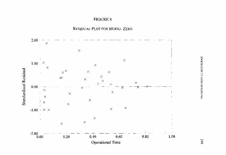
STOCHASTIC CLAIMS RESERVING 301
TABLE 1 I
Model Deviance
0 2,143
1 3,909
2 2,773
~~ .dJ” ~ F
25 0.29
31 3.43
31 1.23
Model 2 appears to fit reasonably well. A direct comparison of the deviance with that obtained in Table 5 is not valid, because the prior weights have been changed but, compared to Model 0, the fit is consider- ably better than in Table 5. The parameter estimates (and standard errors) for Model 2 are:
(’ 0.127 (0.044)
P:
0.176 (0.036)
-1.04 (0.2 1)
PI 9.56 (1.16)
P2 -6.24 (I 26) (coefficient of ?) .
The magnitude of c is consistent with its theoretical interpretation and is not significantly different from the prior estimate of 0.1 used in the weights.
In the examples of previous sections, the fitted models m, have always been decreasing for large values of 7 (see Exhibit 4, for example). In Section 3, this decrease was attributed to the presence of partial payments in the data. In the present example, the partial payments have explicitly been taken into account by including the factor exp (c . R) in the model. Figure 10 shows that R tends to decrease from about z = 0.5 onwards, so the partial payment factor exp (C . R) also decreases. However, the other factor of the fitted model, exp (p,, + p, z + p2 . T’), also decreases for large values of T. This is shown in Figure 11. The next paragraph de- scribes how to test whether this remaining decrease is genuine or is due to estimation error.
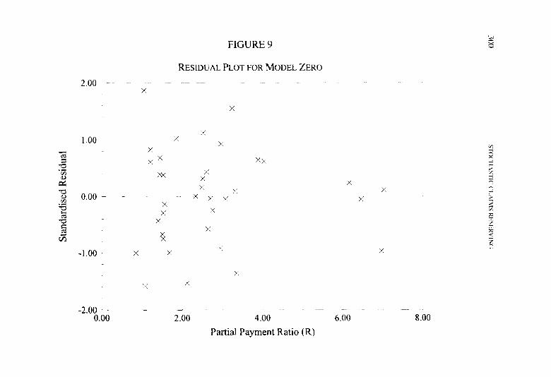
FIGURE 10
FKTEDMODELFORPARTIALPAYMENT RATIO
X x
X
4
0 -~ ~~~ 0.00 0.20 - 0.40 ~~ 0.60 0.80
Operational Time
I .oo

FIGURE 11
FITTED MODELS FOR MEAN SEVERITY
15 i +
& + : * i
-- l 4 Fitted model wthout part-payment factor
-“j :-CL f‘-- +Fitted model with piece-wise exponential part-payment factor
o &~diF~ ZFitted model with constant part-payment factor
-..~~_~___~-.__ ---L--
0.00 0.20 0.40 0.60 0.80 1 .oo
Operational Time (z )
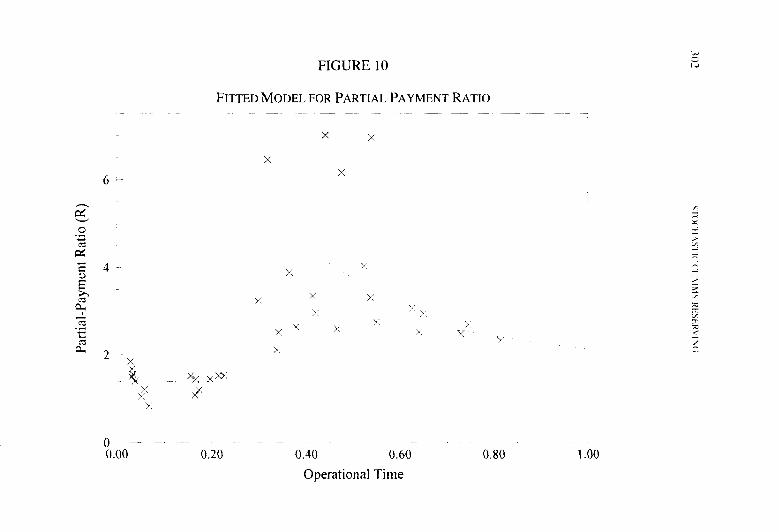
304 STOCtiASTI(‘ (‘I .\IWi KESEKL’IN(~
The slope of the exponent p,, + p, T + & T.’ is b, + 2 & z, so the function does not decrease for z in the range (0, I ) if, and only if, p, is not negative and & is not less than -p,/3. If pi is defined by p3 = p, + p,/2, the exponent can be expressed as p,, + b, (r - t’/2) + p.: ?. and the condition for the function to be non-decreasing is that p, and pi should both be non-negative. This condition can be tcstcd by refitting the model using the new explanatory variable (7: - I’/?) instead of T. This is essen- tially the same model as before so the pnramctc~~ eslimatcs arc unchanged. p3 is estimated lo be - 1.46, which follows from the estimates of p, and & given above. However, fitting the model in this new form gives a standard error for p3 which cannot be calculated from the previous parameter estimates and standard errors. The valise is 0.7?--less than half the abso- lute value of the estimate itself, indicating that p3 is significantly negative. This is confirmed by refitting with p3 set to zero. The minimized deviance becomes 3.154, an increase of 38 1. givin, L o ‘tn I‘-statistic of 4.3 on one and 3 1 degrees of freedom.
The analysis described in the earlier paragraph shows that. for this data set, the decrease in the mean claim amount for large values of z is not fully explained by the partial payment faclor exp (c. R). However, this does not imply that the mean settlement payment decreases with z. A more plausible explanation is that the factor exp (C R) only partly ac- counts for the effects of partial payments. Full details of how this might occur are given Appendix G. Briefly. the explanation is that the rate at which partial payments are made on an open claim tends to decrease the longer the claim remains open.
As the coefficient c is significant. it is necessary to estimate a value of R for each future operational time in order to project the fitted model. Experience with other data sets suggests that R shows little variation as z approaches one. With this in mind, a continuous piecewise linear approxi- mation for R has been estimated by eye from the observed values:
RT = 1.40 for t < 0.2 I
= -0.96 + 1 I .2s x ‘I: for 0.2 1 < t < 0.45
= 7.25 - 7.00 x r for 0.45 < z < 0.65
= 3.80- 1.70 x T for 0.65 < t .

STOCHASTI(‘CI.AIhlS RESERVING 30s
Figure 10 shows both the observed values of R and the piecewise linear approximation R,.
In 1976 money terms, the formula for R, gives the results in Table 12. Column 3 has been calculated using Equation 7.3.
TABLE 12
Year
1969
1970
1971
1972
1973 1974
I975
1976
(1) Expected
Total Future
Payments
6,187
10,119
20,757
3 1,795 42,81 I 46,865
54,903
68,59 1
(21 (3) (4) Standard Standard Additional
Error Deviation Uncertainty
I,71 I 1,323 I.224 2,434 1,710 1,869
4, I38 2,467 2,705
5,287 3,049 3,741 6,029 3,506 5,074 5,554 3,598 6,277 5,913 3,828 7,930
7,197 4,240 12,079
(5) Root- Mean- Square Error
2,485
3,514
5,525
7,159
8,625 9,121
10,607
14,686
All 282,027 37,839 8,828 17,327 42,544
As no allowance has been made for uncertainty in the projected values of R, it is interesting to examine the sensitivity of the results to these projections. The piecewise linear function defined earlier implies an aver- age value of R over the entire range (0, I) of z of 2.47. Table I3 was obtained using this constant value for R.

.X)6
TABLE L3
Year
(1) (5) EXpCCtCd Root-
Total (2) (3, C-1) Mean- Future Standard Standard Additional Square
Payments Error Deviation Uncertaint] Error
1969 6.372
I970 IO,345 lY71 21.017
1 Y72 3 I .X67
1973 42, I x0
1 Y7J 45,069
1Y75 52.742
I Y76 66.357
All 375.X50
I .77X
3.5 12
4.234
5,373
6.0X0
5.541
5.X7.3
7.154
3x. 15’)
I .337
1.723
7,477
3.05 I 3.4x0
3.555
3.7x I 3.lYO
X.767
I.344
I .X7X 7.67Y
3.61 1
1.710
5.X64
7.6X7
1 I .677
16,653
2,544,
3.578 S.SXY
7,156
X.446
X,X16
1().3X6
14.32 I
42.547
Between the two sets of results given in Tables 13 and I3 the estimate for the entire triangle differs by -just over $7 million. which is quite small compared to the RMS error of ahout $43 million. Thus, the uncertainty in future valises of R appears to be relatively unimportant. Experience with other data sets suggests this is true quite generally,. Figure I I shows the fitted model for ))I~ obtained using both the piecewise linear model for R (Curve 2) and the constant model (Curve 3). The difference between these two curves is slight, which explains the similarity in the two sets of results. Curve 3 is simply a scaled up version ol‘curve I which shows the fitted model with the partial payment factor exp ((, R) excluded.
Table 14 gives results based on the piecewisc linear model for R in current money terms. Future inflation has been included using the meth- ods described in Section 6. The run-off of settlements over real develop- ment time was taken to be exponential with the same parameters as in Section 6, and the YSC/r confidence interval lhr the future force of infla- tion was taken as 0. IO to 0. I X.
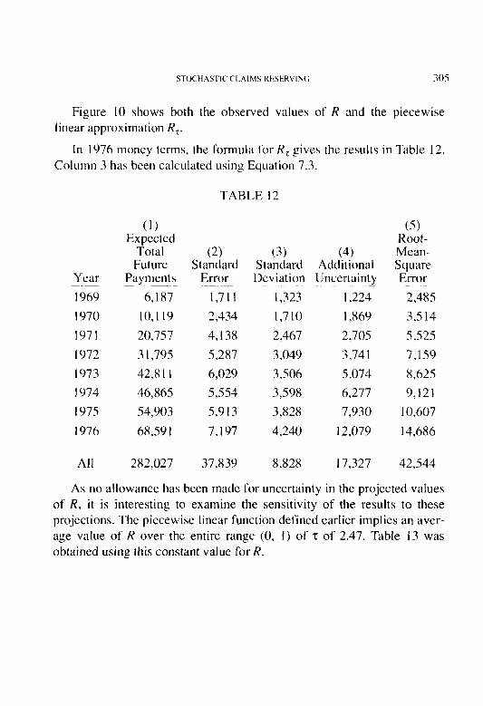
STOCHASTIC CI.AlhlS RESERVING 307
Year 1969 1970
1971
I972
1973
1974
1975
1976
(1) Expected
Total Future
Payments
15,193
24,570
50.29x
77,679
106,385
121.292
155,2’)2
220.25 I
(2) Standard
Error 4,746
7.202
13,404
1 X.976
24,112
25.5 IO
3 I.440
44,179
TABLE 14
(3) Additional Uncertainty (jnflation)
3.317
5,370
I I.132
17,3Y2
24.200
28,3YO
38,697
SY.6 I I
(4) Standard Deviation
3.176
4.OY7
5,994
7.550
X.932
9,628
11,172
13.823
(5) (6) Additional Root- Uncertainty Mean- (Number of Square
Claims) Error I ,46 I 6.799
2,378 IO.156
3,780 1X.X 10
S,XOY 27,447
X,X55 36.404
13.371 41.572
21,330 55.369
38,668 84.X03
All 770,9SY i6Y,So4 188.109 24.66 I 47.574 258.82 I
Berquist and Sherman produced several sets of projections, with to- tals ranging from $430 million to $750 million. The best estimate shown in Table 14 is comparatively high, but the RMS error is large. It would be interesting to see how these estimates compare to the actual experience.
As a final example, the data set from Taylor [9] is analyzed using the methods developed in the present paper. This relates to a compulsory third party motor portfolio for the 12 accident years 1969 to 1980, broken down by development year. There were no claims closed in 1980 for origin year 1969, so the number of data points is 77. The triangles Y\,,(, and N,,.,, are given in Tables A.6 and A.7. The estimates of ultimate numbers M given by Taylor have been used. For the purposes of this example, the standard errors of these estimates have been taken as 5% of the number of claims estimated to be remaining (not yet settled). These figures are given in Table A.8. As the reported counts triangle is not given in 191, values for R = L/N have been calculated using the alternative definition of L given earlier in Section 7. This triangle is given in Table A. 10.

30x sTo(‘fl.\s7’Ic(‘I ~I\‘I\ Kf.Sf-f<\ Ik(i
Figures 12 ; end 13 show the data S and K plotted against operational time r. Figure 14 shows the quantity S/exp (c, K) plotted against T using the prior estimate 0.1 for c’. This quantity is the mean payment per claim closed adjusted to remove the partial payment effect (see Appendix G). One data point has been excluded from Figures I2 and 14 for the sake of clarity: the value of (z, S) for r/= 1 1 of origin year 1970 is (0.995. 108.2). This value for S is more than double the largest value shown in Figure 12. However, it is based on only two settlements. and standardized residual plots show that it is not an outlicr. therefore, it has not been excluded from the analysis.
Table IS gives the results of fitting models with both a partial pay- ment parameter and an inflation parameter to the unadjusted data shown in Figures I, 3 and 13. The variance index was taken to be CI = 2, and the prior estimate of the partial payment parameter for use in the weights was taken as c = 0.1. The plot of standardized residuals from Model 0 against operational time is shown in Figure IS. Thcrc is no evidence of heteroscedasticity. so the F-statistics are valid. The standardizcd residual for the point excluded from Figurca l_ ? and 13 is included in Figure 15.
TABLE IS
Model Deviance (?f F 0 618.6 63 -
I 860.4 72 3.74 2 848.2 72 2.60
The F-statistics indicate that ncithcr Model I nor Model 2 fit the data very well. However, the more general model with both ? and In(z) in the linear predictor (as in the numerical examples of Sections 3 and 4) fits well. The minimized deviance is 704.X. giving an F-statistic of I. IO on eight and 63 degrees of freedom.

FIGURE 12
OBSERVED MEAN SEVERITY vs. OPERATIONAL TIME
(DATA FROM TAYLOR [9])
X
x x
3 x>x XXX O.-Lb- 0.00 0.20
X
x x z* x*
XX x X
X X
x3 x 2:
xx y; x
xx x XX xx xX x
X yx x
- x
0.40 0.60
Operational Time
X -- -~
0.80 1 .oo

FIGURE 13
PARTIAL PAYMENT RATIO (R) vs. OPERATIONAL TOME
(DATA FROM TAYLOR [9],
Operational Time

10
i X
0 bik .x 0.00
FIGURE 14
ADJUSTED MEAN SEVERITY vs. OPERATIONAL TIME
X
X
X
X X
x
1 X X X
%
X x x
X X X X
X X X X
5 xx
x xx
X xx x
XXX xx xx xx X
3i xX xx
T
~_.. - .___~~ .--3
0.20 0.40 0.60 0.80 1.00
Operational Time
X

FIGURE IS
RESIDUAL PLOT FOR MODEL ZERO WITH a = 2
-2
0.00 0.20 0.40 0.60
Operational Time 0.80 1.00
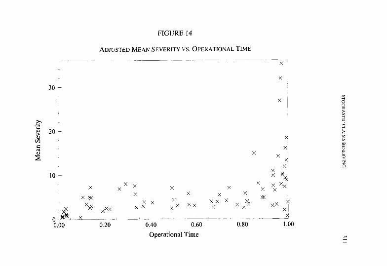
STOCHASTIC CLAIMS RESERVING 313
The parameter estimates are:
c 0.111 (0.024)
i 0.131 (0.013)
PO 5.17 (0.8 1)
Pi -7.1 1 (1.88)
P2 4.54 (I. 18) (coefficient of z’)
P3 1.25 (0.34) (coefficient of In(z)) .
Note that the estimate of c is not significantly different from the value of 0.1 used in the weights. Also, the average force of inflation estimated from the data does not differ significantly from Taylor’s prior estimate of 0.117 (derived from the Australian Capital Territory Average Weekly Earnings Index).
The function exp (8, + p, 2 + PI. 22 + p3 In(z)) represents the pay- ment per claim closed in constant 1980 terms, with the partial payment factor excluded. This is shown in Figure 16. This should be compared to the adjusted data shown in Figure 14. The slight decrease from 7.0 to 6.6 over the range z = 0.27 to r = 0.52 is attributed to a declining partial payment rate on open claims, as explained in Appendix G.
Figure 13 shows the observed values of R used in fitting the model. The form R = o. + a,/~ fits reasonably well to these data. Least squares estimation gives: a,, = 1.32 and a, = 0.463. The fitted curve is shown in Figure 17. Figure 18 shows the fitted mean payment per claim closed with the factor exp (c R) included, using the estimates c’ = 0.111 and R = I .32 + 0.463,‘~. This should be compared to Figure 12. The fitted curve tends to infinity as z tends to zero, but this is unimportant because projection is unnecessary for z less than 0.043. Table 16 gives the fore- casts obtained from this model, in constant terms: the units are thousands of 1980 Australian dollars.

FIGURE 16
FITTED MODEL WITH PARTIAL PAYMENT FACTOR EXCLUDED
4
2
Oh _I- .A.-- _-L 1-1~~~ _1 _ -~ i-~-. -~_ 0.00 0.20 0.40 0.60 0.80 1 .oo
Operational Time

FIGURE 17
FITTED MODEL FOR PARTIAL PAYMENT RATIO
5
1 0.40 0.60 Operational Time
0.80 coo

FIGURE 18
FINALFITTEDMODELFORDATA FROMTAYLOR[~]
20
15 -
5
0 - 1-- _ ~ -~- _~~_~~ ~~ _~ ~ .~
0.00 0.20 0.40 0.60 0.80 1 .oo
Operational Time

STOCHASTIC CLAIMS RESERVING 317
TABLE 16
Year
1969
1970
1971
1972
1973
1974
1975
1976
(1) Expected
Total Future
Payments
0
33
33
97
315
444
774
1,278
(2) (3) Standard Standard
Error Deviation
0 0
5 66
5 66
16 114
49 203
66 238
102 301
147 372
(5) (4) Root-Mean-
Additional Square Uncertainty Error
0 0
0 67
0 67
0 115
15 209
14 247
37 320
54 404
1977 2,550 227 491 113 553
1978 4,650 338 627 223 747
1979 5,041 349 645 249 775
1980 8,494 571 814 426 1,082
All 23,708 1,741 1,436 558 2.325
The RMS error (Column 5) for all years combined indicates that about 10% must be added to the best estimate (Column 1) for a reasonably safe reserve. This gives $26 million in 1980 terms.
To introduce future claims inflation, the method given in [IO] has been applied to the triangle of the number of settlements. This indicates that the run-off pattern does not differ significantly across origin years, the rate of settlement being proportional to exp ( 1.422 x In(t) - 0.897 x r), where t is real development time. Operational times have been converted to ex- pected real development times by numerically inverting the correspond- ing Gamma distribution function, and future claims inflation introduced using the method outlined in Appendix F. The best estimate of the force
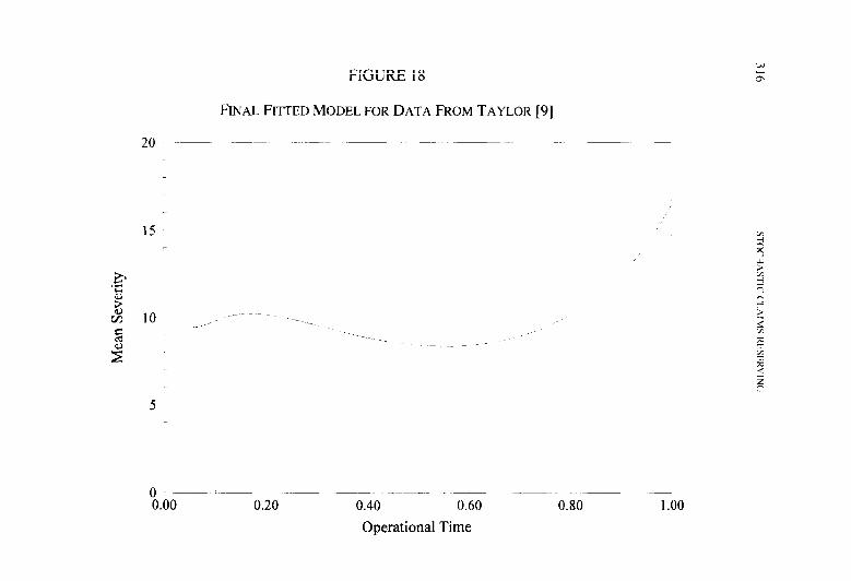
318 STOCHASTIC CLAIMS RESERVING
of inflation in the future was taken as 0.12, and the combined uncertainty of this estimate and the real time scale was taken to be 0.02’. The results are given in Table 17:
Year
1969
1970
1971
I972
1973
1974
1975
1976
1977
1978
1979
1980
All
0
38
38
11s
380
540
959
1,612
3.329
6,275
6,884
12,113
TABLE 17
(1) (5) Expected (3) Additional
Total (2) Additional (4) Uncertainty Future Standard Uncertainty Standard (Number of
Payments Error (Inflation) Deviation Claims)
0 0 0 0
6 8 77 0
6 8 77 0
18 23 137 0
59 65 250 IS
81 8S 296 1s
129 129 38X 3x
193 195 494 5X
317 343 692 12x
486 542 934 27s
SOS 552 976 318
851 X66 I JO5 600
32,283 2,539 2.8 17 2.141 74x
(6) Root- Mean- Square Error
0
78
78
140
265
319
430
568
844
1.216
1.27 1
1 .X8 1
4,419
The additional uncertainty of future inflation means that the best esti- mate of 32,283 must be augmented by 13.7% fhr a reasonably safe re- serve. This gives $36.7 million.

STCJCHASTIC CLAIMS RESERVING 319
8. CONCLUDING REMARKS
Origin Year Effects
All the methods described in this paper are based on the hypothesis that, in real terms, the mean claim amount as a function of operational time is the same for all origin years. The plausibility of this hypothesis should be considered for each data set before proceeding to apply the methods. If there is a trend change in the mean claim amount over the origin years, for fixed operational time, the test of Appendix B should give a warning. However, the basic hypothesis could be violated in other ways. A change in the mix of claim types over origin years might cause a significant violation. For example, in property insurance, the proportion of land subsidence claims may be increased for a certain origin year because of hot dry weather. Since subsidence claims tend to be large, the mean claim amount in real terms would be higher for such an origin year. The approach of Appendix B can be modified to test for the presence of such phenomena. For example, Model 0 could be generalized by having a separate level parameter (PO in Appendix B) for certain origin years. Plots of residuals against origin year should help in deciding which origin years are affected.
If the basic hypothesis is violated because of a changing mix of claim types across origin years, there are two possible remedies:
1. if there are sufficient data points in each group of similar origin years, a separate “level parameter” for each group can be re- tained throughout the analysis, or
2. if the data are available, each claim type can be analyzed sepa- rately.
Frequently in practice, the only data available is of type (c) (Section l), so the methods of Section 7 are appropriate. These methods are partic- ularly valuable when the triangle does not contain data over the full range of operational times, so that projection is necessary. For the Berquist and Sherman data, the highest observed operational time is about 0.85. Figure
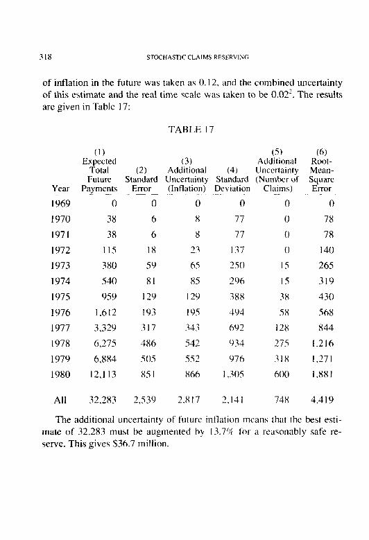
320 STOCHAS’[‘I(‘(‘l.~\lhlS RF?S-:KVlh(~
4 shows the curve for the mean payment per claim closed fitted with no allowance for the presence of partial payments. This should be compared to Curve 2 of Figure 11 which was obtained by the methods of Section 7. The two fitted curves are in close agreement over the mnge of the data, because both fit the data well. However, their projections into the range (0.85, I) of operational time are very different, causing a substantial ef- fect on the forecasts (compare the results in Table 12 to those in Table 8). The improvement in projections possible by considering the effect of partial payments does not, of course. negate the need for caution when projecting a fitted curve beyond the range of the data. An informal Bayes- ian approach is appropriate. The indications of the particular data set under analysis (via F-tests, etc.) should be tempered by experience of more fully developed triangles for similar lines of business.
Even when the full range of operational time is covered by the data, so that no projection of m, is necessary, the methods of Section 7 are recom- mended for data of type (c). The models of Section 7 usually explain more of the variation in such data than the models of earlier sections. This is indicated by a significant estimate of the partial payment parameter c. Consequently, the other parameters of l?rT will bc more reliably estimated if allowance is made for the partial payment effect. As the observed values for R = L/N differ between origin years, the models of Section 7 effectively allow a different function nr, to be fitted for each origin year.
The similarity between projecting the partial payment ratio R and projecting the run-off of settlements over real development time for the purpose of introducing future inflation, was mentioned in Section 7. For future intlation, the distribution function F, of settlement delays must be projected. The relationship between t and f can then be approximated using 7 = F, . The partial payment ratio R = L/N could similarly be ap- proximated using R = (1 - F,)/” where ,f; is the probability density func- tion of the delays (fj=dFJdt). This is the reciprocal of the hazard function of the delay distribution. Thus, projection of R could be based on the same model for the run-off of settlements over real development time as used to introduce future inflation. This possibility has not been fully

STOCHASTIC CLAIMS RESERVING 321
explored but would probably require unusually accurate estimation of F, for reasonably reliable estimates of R.
For triangles which are not well developed (such as the Berquist and Sherman triangle used in the examples) experience with more fully devel- oped triangles for similar lines of business would be very valuable in estimating the real time scale of the remaining run-off. The technique used in the example in Section 6 of estimating the “half life” by examin- ing the triangle of operational times is not recommended for general use. Although not illustrated in the examples, the projected total of payments remaining for each origin year could, of course, be broken down by development year, given a projection for the remaining run-off of settle- ments.
Integrtrtion into a Conprehensi\~e Approach
The question of how the methods proposed in this paper can be com- bined with results obtained by other methods and additional items of information can obviously not be answered definitively because every reserving problem is different. A few suggestions are given below.
If reliable case estimates are available for some of the outstanding claims, the estimate M can be reduced by the number of claims concerned so that the fitted model nr, is summed over those claims for which reliable case estimates are not available. This involves an assumption that the operational times of those claims with reliable case estimates are uni- formly distributed over the remaining interval of operational time, and that the presence of a claim in this class does not depend on its size.
Because large claims are often assessed individually, and as accurately as possible, the entire method could be restricted to smaller claims only.

322 STOCHASTICCLAIMS KESEKVING
REFERENCES
[l] Berquist, J.R., and Sherman, R.E.. “Loss Reserve Adequacy Testing: A Comprehensive Systematic Approach,” PCAS LXIV, 1977, pp. 123- 184.
[2] Brown, R.L., “Minimum Bias With Generalized Linear Models,” PCAS LXXV, 1988, pp. 187-2 17.
[3] Hayne. R.. “Application of Collective Risk Theory to Estimate Vari- ability in Loss Reserves,” PCAS LXXVI, 1989. p. 77.
[4] Hogg, R.V., and Klugman, S.A.. Lo.sx Distributions. John Wiley & Sons, Inc., New York, 1984.
[5] McCullagh, P., and Nelder, J.A., Ge/~c~~li:(~d Lirlc~. Modrls (Second Edition), Chapman and Hall, London, England, 1984.
[6] Payne, CD. (ed.), Murzualfo~~ GLIM RCIPLIW .?.77, Numerical Algo- rithms Group. Oxford, England, 1985.
[7] Reid, D.H., “Claim Reserves in General Insurance,” ./orrrncrl 04’ rht lmtitutc c$Actuuries, 1978, Vol. I OS. p. 2 i I.
[8] Taylor, G.C., “Speed of Finalization of Claims and Claims Run-off Analysis,” ASTIN Bulletin, Vol. 12. 19X I , pp. 8 I- 100.
[9] Taylor, G.C., “An Invariance Principle for the Analysis of Non-Life Insurance Claims.” Jourm~l of the lmtitrltc (?/‘,l(,trr~lt.icl.\. 19X.3. Vol. 1 10, pp. 205-242.
[lo] Wright. T.S., “A Stochastic Method for Claims Rcscrving in General Insurance,” Jo111m1l cf the Imtitlrtr of‘Ar~tirc~rii~.s. 1990. Vol. I 17, pp. 677-73 1.
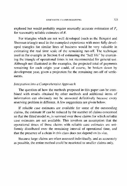
APPENDIX A
DATA USED FOR THE EXAMPLES
The first data set consists of medical malpractice triangles taken from Berquist and Sherman [ 11. The tri- angle below is Y,,,/ , the total amount of all payments made in development year d for each origin year W. This has been calculated from Exhibit E of Berquist and Sherman. The units are thousands of dollars, not ad- justed for inflation.
Year 0
1969 125 1970 43 1971 295 1972 SO 1973 213 1974 172 1975 210 1976 209
1
TABLE A. 1
d
2 3 4 5 6 7
281 1,037 1,543 1,481 3,712 4,459 3,177 486 1,487 1,625 3,882 6,772 4,688 852 1,332 2,592 6,328 6,308 736 3,024 5,961 8,747 620 2,766 7,693
1,415 4,680 1,355
The triangle below is NlcId , the number of claims closed in development year d for each origin year MI. 2
This has been derived from Exhibits C and E of Berquist and Sherman [I]. The final column is No, the total of the N,,.d for each origin year.
TABLE A.2 d
Year 0 1 2 3 4 5 6 7 No
5 1969 311 521 349 179 161 293 261 191 2.266
i x
1970 391 52Y 271 178 303 367 240 2.279 5 ‘Z 2 1971 418 764 236 526 487 422 2.853 ‘: r
1972 311 854 523 629 621 ‘,Y38 g 7 1973 294 1.146 691 657 2.788 Q
1974 332 1.015 613 1.960 z z 197s 406 907 1.313 <
1976 398 398 g
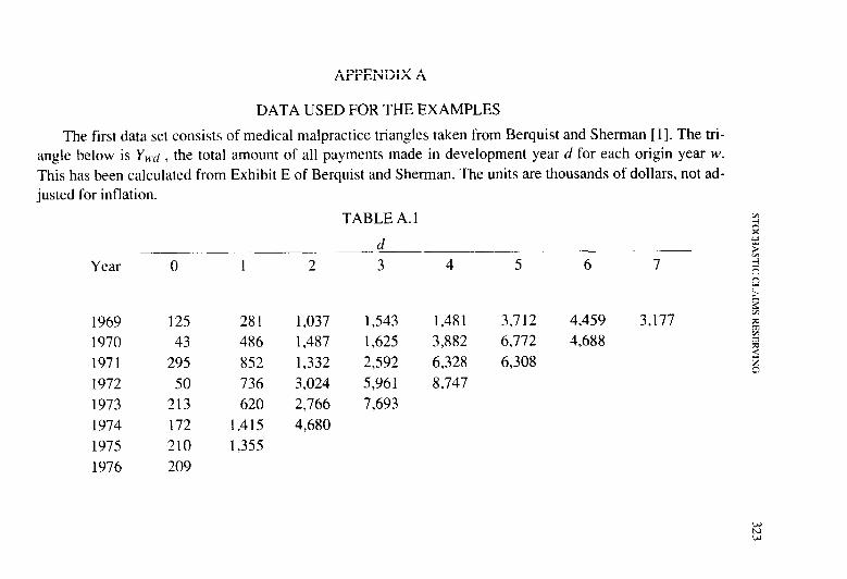
Table A.3 is the number of non-zero claims reported in each development year, from Exhibits C, D, and E of Berquist and Sherman [I]. The final two columns are the best estimate of the ultimate number of claims, and its standard error. These were obtained by applying the stochastic method detailed in [lo] to the reported numbers triangle.
TABLE A.3 d -
Year 0 1 2 3 4 5 6 7 M 1 Y 8
; 1969 1,060 612 511 383 -11 24 29 17 2,664 70 z 1970 1,051 826 463 379 48 27 24 2,896 102 F! 1971 1,296 1,215 627 605 116 50 4,065 148
2 I
1972 1,354 1,372 790 w
695 249 4,771 215 a 1973 1,382 1,446 843 994 5,280 314 K
? 1974 1,365 1,400 8.58 4,837 461 z 1975 1,544 1,241 5,169 690 1976 1,594 6,257 1,097
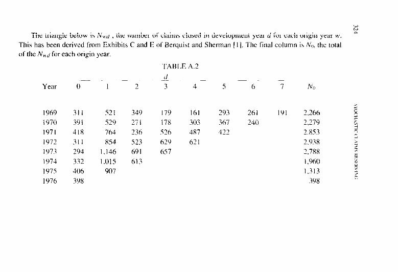
The triangle below gives the mean operational times ~,,.ti calculated from the triangle I&d given in Table ;
A.2 and the estimates M given in Table A.3 using Equation 2.1.
TABLE A.4
1969 1970 1971 1972 1973 1974 1975 1976
0.058 0.215 0.378 0.477 0.54 1 0.626 0.730 0.815 0.068 0.226 0.364 0.442 0.525 0.641 0.746 0.05 1 0.197 0.320 0.414 0.538 0.650 >
r; 0.033 0.155 0.299 0.420 0.55 1 6 0.027 0.164 0.338 0.466
2 B
0.034 0.174 0.342 g 0.039 0.166 E
0.032
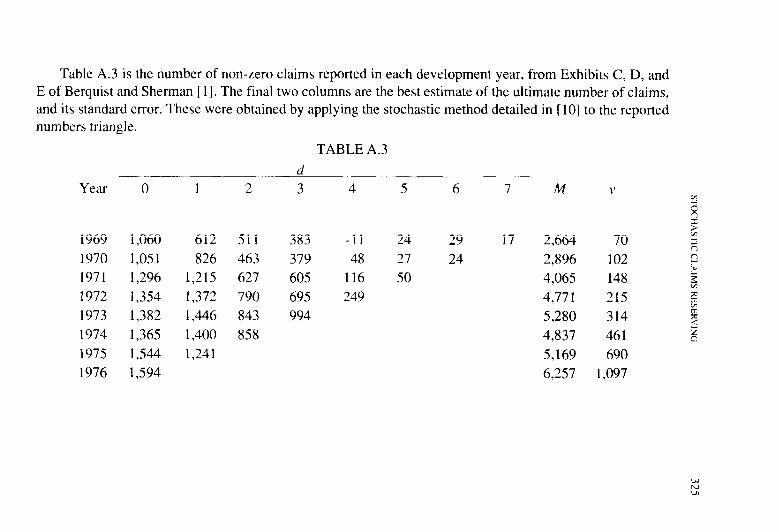
Below is the triangle of average numbers of claims outstanding calculated from the triangles given in Tables A.2 and A.3. These figures are the L,+‘d of Section 7.
TABLE A.5 d
Year 0 1 2 3 4 5 6 7
1969 375 795 921 1,104 1,120 1970 330 809 1,053 1,250 1,223 1971 439 1,104 1,525 1,760 1,614 1972 522 1,302 1,695 1,861 1,708 1973 544 1,238 1,464 1,709 1974 517 1,226 1,541 1975 569 1,305 1976 598
900 649 446 3 925 647 2
is 1,242 0 =!
!2
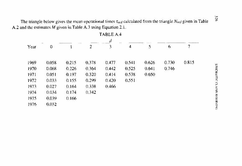
Table A.8 gives the estimated ultimate number of claims, M, for each origin year, and the standard error, :g
v, of this estimate. M has been taken directly from Taylor [9], and v has been calculated (for the purposes of the second example in Section 7) as 5% of the number not yet settled (M - No).
TABLE A.8 Year M 1’
1969 523 0 1970 643 0 1971 676 0 1972 672 0 1973 807 1 1974 670 1 1975 516 3 1976 544 5 1977 622 12 1978 715 23 1979 660 25 1980 894 43

The triangle below gives the mean operational times TMad calculated using Equation 2.1 from the data in Table A.8.
TABLE A.9 d ___. .~ ____.
Year 0 I 2 3 4 5 6 7 8 9 10 I1
1969 0.095 1970 0.036 1971 0.033 1972 0.033 1973 0.032 1974 0.019 1975 0.016 1976 0.015 1977 0.030 1978 0.016 1979 0.023 1980 0.021
0.337 0.222 0.206 0.190 0.136 0.142 0.121 0.134 0.141 0.106 0.138
0.591 0.517 0.490 0.372 0.366 0.407 0.333 0.330 0.291 0.264
0.778 0.732 0.69 1 0.568 0.673 0.665 0.565 0.502 0.494
0.894 0.949 0.976 0.988 0.994 0.997 0.999 1.000 2 0.827 0.887 0.942 0.970 0.984 0.992 0.995 5 0.822 0.931 0.975 0.984 0.989 0.994 5 r;
0.807 0.935 0.965 0.973 0.984 ? ”
0.870 0.935 0.957 0.969 5 0.813 0.889
z 0.934 E m
0.743 0.853 2 52 0.700 0
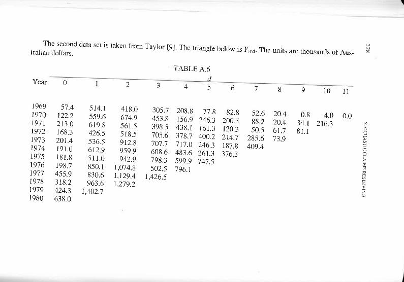
The triangle in Table A. 10 gives the mean number of claims not yet settled, calculated as the difference is
between M (from Table A.8) and the cumulative values of N,,,d (from Table A.7). These figures were used for LMsd in the second example of Section 7.
---.___ .~.._. Year 0 1 2 3
1969 473.5 1970 620.0 1971 654.0 1972 649.5 1973 781.0 1974 657.5 1975 508.0 I976 536.0 1977 603.5 1978 703.5 1979 645.0 1980 875.0
347.0 500.5 536.5 544.0 697.5 575.0 453.5 47 1 .o 534.0 639.5 569.0
214.0 310.5 344.5 422.0 512.0 397.0 344.0 364.5 441.0 526.5
116.0 172.5 209.0 290.5 264.0 224.5 224.5 27 1 .O 315.0
TABLE A. 10 d ~- 4 5
55.5 26.5 111.0 72.5 120.5 46.5 130.0 44.0 105.0 52.5 125.0 74.5 132.5 76.0 163.0
6 7 8 9 10
12.5 37.5 17.0 23.5 34.5 44.0
6.5 3.0 1.5 0.5 Y 8
19.5 10.5 5.0 3.0 $, IO.5 7.5 4.0 5 ri 18.0 10.5 ?
25.0
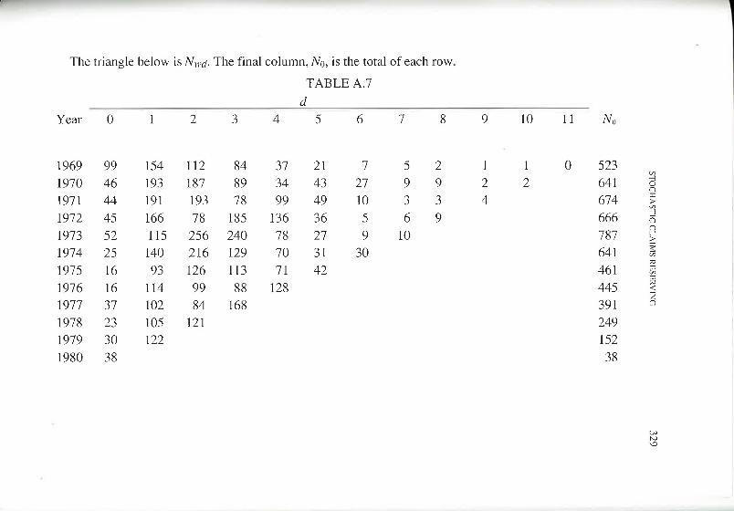
STOCHASTIC CLAIMS RESERVING 333
APPENDIX B
TESTINGMODELZERO
This appendix is concerned with testing the hypothesis that the mean claim amount in real terms is a function of operational time only. This hypothesis underlies all the methods proposed in this paper, and should be checked for each data set before applying these methods. Intuitively, the most likely violation is that there may be a trend across the origin years in the mean claim amount at a certain operational time. Such a trend would give a different mean claim size for the earlier origin years than for the later origin years, for a certain operational time. This can be tested as follows.
The run-off triangle is bisected into Regions A and B as shown in Figure 19. If P is the number of development periods per annum (for example, P = 4 for quarterly development) then calendar time r ’ is given by:
r’=d+P.(w- 1). (B-1)
If d runs from 0 to T - 1, then t ’ also varies from 0 to T - 1, so data for the last calendar period (represented by the hypotenuse of the run-off tri- angle) is given by T - 1 = d + P . (w - l), which is equivalent to:
u’= 1 +(T- 1 -d)/P. 03.2)
Note that data exists for the latest calendar period only for those d-values that give an integer value for W.
The boundary between regions A and B is therefore given by:
w=OSx( 1 +(T- 14)/P},
so region B is defined as those data points satisfying:
w>OSx{ I +(T- 14)/P}.

FIGURE 19
Development Period d
P

STOCHASTIC CLAIMS RESERVING 335
Model 0 of Section 2 is generalized to allow the mean claim amount as a function of operational time to differ between the Regions A and B. This less restrictive model can be expressed as:
(B-3)
03.4)
where the explanatory variables Zj are the same simple functions of z used in Model 0. Model 0 is the special case p;’ = # for all j, and can be tested against the more general model using an F-test in the usual way. How- ever, Model 0 could appear to be unacceptable when tested in this way if an incorrect inflation rate has been used to preadjust the data. For this rea- son it is better to use unadjusted data and include an inflation parameter. Model 0 of Section 4 is generalized to:
m$ = exp (i . (M* + d/P) + pf + C Pp . Zj) . (B.6)
In the example of Section 4, Model 0 has 10 parameters (including i) and gives a minimized deviance of 1,961 using an index a = 1.5 in the variance function, The less restrictive model specified in Equations B.3 and B.4 has 19 parameters, but only 18 can be estimated due to an absence of data in Region A for the last operational time band. The minimized deviance (using the variance function with a = 1.5) is 1,676. Residual plots confirm the assumption a = 1.5. As there are 36 data points, the model has 18 degrees of freedom, giving an estimate of 93.1 for the scale parameter. The mean increase in the deviance per degree of freedom under Model 0 is (1,961-1,676)/8 = 35.6, so the F-statistic is 35.6/93.1 = 0.38 on eight and 18 degrees of freedom. The lack of signifi- cance indicates that Model 0 fits the data as well as the 18-parameter

336 STOCHASTIC C’t.AIhlS KliSliHVIU(i
model, so the hypothesis that the mean m, does not vary across origin years for any z is verified.
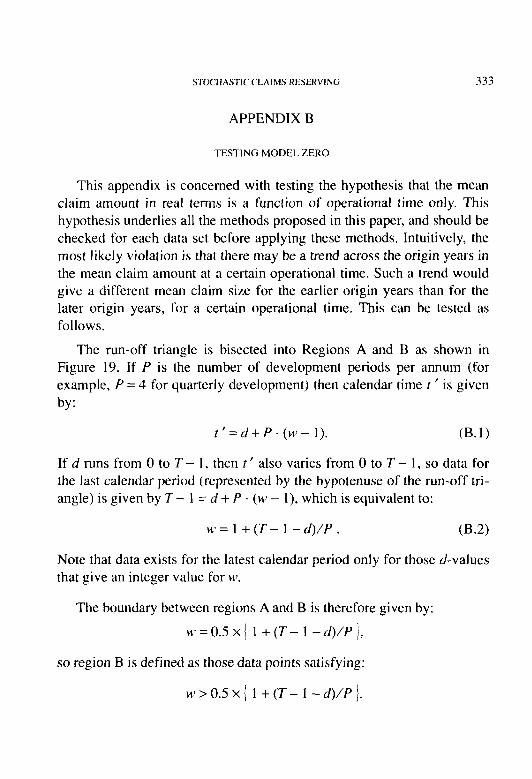
STOCHASTIC CLAIMS RESERVING 337
APPENDIX C
INTERPRETATION OF OPERATIONAL TlME MODELS FOR
MEAN CLAIM AMOUNT
When formulating models for the mean claim amount as a function of operational time, it is helpful to discover what such models imply about the mean claim amount as a function of real development time. This Appendix describes how this can be done, and illustrates the techniques by giving the real-time interpretation of certain special cases and general- izations of the models proposed in Section 2. The following notation is used:
m, = mean claim amount as function of operational time z,
ltt = mean claim amount as function of real development time t,
M = ultimate number of claims closed,
F, = distribution function (over individual settlements) of delay t,
N, = cumulative number of claims closed by real development time t,
C, = expected cumulative amount paid by real development time t.
By definition of z , T and t are related by:
T=NJM. Cl)
Each of the M claims has probability F, of being closed by time t (by definition of F,), so N! is binomially distributed with parameters M and FI . Therefore we have:
E(N,)=M.F, and Var(N,)=M.F,.(l-F,). (C.2)
Hence, using Equation C. 1:
E(2lt)=F, and Var(zIr)=F,.(l -F,)/M. (C.3)
So, if M is reasonably large, to a good approximation we have:

338 STOCHASTICCLAlWi RESER\‘IN(i
z=F,. (C.4)
That is, operational time is simply the distribution function of the real delay.
By definition of m and p, we have:
p, = nz,
Using Equation C.4, this gives:
P, = MF,) . (C.5)
Given a functional form for m,, equation C.5 immediately gives a relationship between p, and F,. For example, Model I of Section 2 in the case p, = 0 is:
nf, = exp $4, + Pz In(G)
= k ,y
Using Equation C.5, this is equivalent to:
That is. in real time, the mean claim size is a power function of the delay distribution function.
By definition,
t
C, = M s p, (IF,
If M is sufficiently large, then from Equation C.4 we have, to a good ap- proximation,
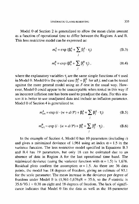
STOCHASTIC CLAIMS RESERVING 339
CC.61 0
For certain functional forms IZI~, the integral on the right of Equation C.6 is analytically tractable and can be expressed simply in terms of m,. In such cases the equation can be rearranged to express the mean claim amount in terms of C,.
For example, consider Model 1 or 2 of Section 2 in the case p2 = 0:
t
nz, = exp (PO + p, T) =$ I m, dcs = (m, - nz,,)/p, ,
0
and, using Equation C.6, we have:
C, = M (m, - m&P, .
Rearranging gives:
IA = PO + PI . C, /M. (C.7)
As a second example, consider the generalization of Model 3 of Sec- tion 2:
m, = Cl% + PI . z>” .
It is straightforward to show that this implies:
t I m, do = [n$+ ‘I” - mf + “‘“I/[$ . (6 + 1) I. 0
Hence, using Equation C.6 and rearranging:
p, = [pf+ ‘) + (6 + 1) . p, . C/M]“““+ ‘).

340 STOCtiASTl~‘~‘I.~\I\1S RI:SER\‘ING
Model 3 is the case 6 = 3 &, so is equivalent to the real-time relationship:
p,= [ p:, + 3. p, C/M 1:'.

STOCHASTIC CLAIMS RESERVING 341
APPENDIX D
PREDICTION WHEN ULTIMATE NUMBERS ARE KNOWN
We have E(X,) = m, and Var (X,) = ‘p’ . my where:
X, is the size of the individual claim payment (in constant money terms) made at operational time z, and
nzT is a function of several parameters which can be expressed as a vector p.
Sections 2 through 4 of the paper describe how the data triangles can be used to decide on the functional form of m,, and to estimate the parameters p, a, and cp. The estimation algorithm (Fisher’s scoring method) also gives the variance-covariance matrix V for the estimates of p. This Appendix describes how the fitted model can be used to predict totals of future claims, under the assumption that the ultimate number of claims M is fully known for each origin year.
Consider a single origin year. If M is the ultimate number of claims, and N,, is the number to date, then there are M - N,, claims in the future. The operational times of these future claims are:
z = (NC,+ 0.5)/M,(N, + 1.5)/M,..., (M-0.5)/M. (D.1)
If R represents the total of future claims, and ~1 and o2 denote the mean and variance of R, respectively, then since separate claim amounts are mutually independent we have:
p=xm, and 02=‘pz.~rn~,
r r (D.2)
the summation being over the values of z given at Equation D. 1.
Hence, an estimate j? can be obtained using the fitted model:
(D.3)
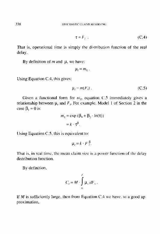
342 STOCHASTIC CLAIMS RESERVING
where A, means m, evaluated using the estimated values of p.
This is the “best estimate” of R given in Columns 1 of the example result tables in Sections 3 through 7.
Now consider the mean-square-error of the estimate for a single origin year given by Equation D.3:
E(R - $)’ = E[(R - kt) + (kt - 6) I’
= E(R - kt)’ + E(;i - cc)’ - 2 E(R - j.t) (fi - /L) . 03.4)
The last term of Equation D.4 is zero because R and b are stochastically independentAThe randomness in R comes from future claims, and the ran- domness in p comes from past claims.
The first term of Equation D.4 is simply (3’ and can be estimated by using the estimated parameters in the expression at Equation D.2. This gives the quantity in the standard deviation columns of the examples.
For the middle term of equation D.4, note that p is a known function of the parameters p. See Equation D.2. Using a first order Taylor series, we have:
where 6 is the vector of first derivatives of p with respect to the j3s.
Hence :
Taking expected values,
E(;i - p)’ zz #. V .&
where V is the variance-covariance matrix of the estimates i.
(D.5)
The vector of derivatives 6 can be calculated from Equation D.2:

STOCHASTIC CLAIMS RESERVING
6; = dp/dp; = C dm,/dpi .
343
03.6)
Each term dm,/df& can be evaluated using the estimated p-values.
The standard error for a single origin year is given by the square root of the estimated right-hand side of Equation D.4:
(b2+:T. V4) .
This is the quantity given in the RMS columns of Tables 4 and 6. The standard error columns of these tables are from:
Now consider the prediction of total future payments for all origin years combined. The best estimate is obtained simply by summing the estimates given by Equation D.3 for each origin year. The mean-square- error of this estimate cannot be obtained so simply. The estimate of CF’ (given by using the estimated parameters in Equation D.2) can be summed over all origin years, because all future claims are mutually independent. However, the “estimation error” component (given by Equa- tion D.5 for a single origin year) cannot be summed over all origin years, because the same estimates B are used in equation D.3 for each origin year, so the estimates are not mutually independent.
Corresponding to the middle term of Equation D.4, we need to evalu- ate E[ (Cl) - (Cp) I’, where the summation is over all origin years.
An analysis similar to that in Equation D.5 shows that:
E[ ($)-(Z~)]‘=-DTWD, (D.7)
where V is the variance-covariance matrix of the estimates p, and ZI is the vector of first derivatives of Zp with respect to the 0s. That is,

344 STOCHASTIC CI.AlMS RESt!RL’IN(;
where, again. summation is over all origin years.
The figure for the total over all origin years, in the second columns of the examples, is the square root of the right-hand side of Equation D.7.
If the number of outstanding claims A4 -N,, is large for some origin years, the amount of computation involved in evaluating Equations D.2, D.3, and D.6 may be substantial. However, when A4 is large the variation in the summands from one point in operational time to the next is usually so small that the sums can be well approximated by integrals. That is, Equation D.2 can be replaced by:
(D.8)
If the form of m, is such that either or both of these definite integrals are analytically tractable, the burden of computation can be substantially reduced. If the first of these is tractable, the 6; can easily be obtained from the first part of Equation D.6:
6, = clCl/tl pi,
after finding p as a function of j3 by analytic integration.
Otherwise, the integration corresponding to the second part of Equa- tion D.6 may be tractable for some i :
Note that for models m, with a log link function, the partial derivatives required for calculating the 6, have a particularly simple form:
m, = exp (x, . b) => dm,/d pi = .\-Ti m, .

STOCHASTIC CLAIMS RESERVING 345
APPENDIX E
PREDICTION WHEN ULTIMATE NUMBERS ARE UNCERTAIN
Appendix D deals with the distributions of future claim totals condi- tional on the ultimate number of claims M. These conditional distribu- tions are relevant for forecasting when M is known. In practice, M is rarely fully known. This appendix shows how uncertainty in M can be allowed for in forecasting. Briefly, the problem is that uncertainty in M for a particular origin year implies uncertainty in the operational times of future claims, given at Equation D.1. The uncertainty affects both the number of future values of z and the values themselves.
Replacing the summation in Equation D.2 by integration (as suggested in Appendix D), and making the conditioning on M explicit, we have:
(E.1) T/O
and
Var (R IM)= (p2 .M. n$ dz, (E.2)
to
where the integration is from the present operational time T,, (= N,JM) to 1.
It is shown below that both these functions are sufficiently near linear in M (compared to the magnitude of the uncertainty in M) to ensure that good approximations of their expected values are given by replacing M by its expected value. That is,
E(E(R I M)) = E(R I M = E(M)), (E.3)
and
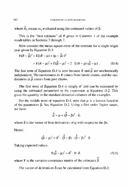
34h sTo(‘tiASt I(.(‘1 \I\lS KI:SEKL tu;
E(Var (R I M)) = Var(R I M = E(M)).
In this appendix. p and c? arc used to dcnotc the unconditional mean and variance of the total R of‘ future claims for an origin year. Thus.
p = E(R) = E(E(R I M)) = E( R I M = E(M)) (E.4)
using Equation E.3, and
(T’ = Var(R) = E(Var(R I M)) + Var(E(R I M))
=Var(RIM=E(M) )+Var(E(RIM)). (E.5)
Equation E.4 implies that the best cstimatc of R is given by evaluating the right-hand side of Equation E. 1 using the estimate fi = E(M) in place of M. Similarly, the first term 011 the right of Equation E.5 is simply the right-hand side of Equation E.2 cvaluatctl using the estimate h = E(M). Thus, the estimates of the unconditional p and (5’ arc exactly the same as the estimates of the conditional p and 0’ given in Appendix D, except for the addition of the second term on the right of Equation E.5. Equation D.4 remains valid, and as the estimate $ is unchanged, the middle term of Equation D.4 (the estimation error) can be evaluated exactlj as described in Appendix D. Therefore, the only change newwary to the mean-square- error given in Appendix D is the addition ot’ the xecond term on the right of Equation E.S.
Using the usual approximation derived from a first order Taylor series:
Var(E(R I M)) = jdE(R I Mb’rIM)’ V:\r(iZ/I).
From Equation E. 1
dE(R
But.

STO(‘HASTIC‘CI.AIMS RESERVING 347
I
d/dM s m, clz = -m,, dz,,/dM = m,, q/M ,
?I
where
m. = m, evaluated at z = r(,, ,
and
m, dz = E(R I M)/M.
3)
Hence,
d E(R I M) E(R I M) dM - M + m. to .
Using the estimate b = E(M) to evaluate the first term gives:
d E(R I M) dM
= (i/b + m,, . 2,) . (E.6)
The accuracy of this approximation is demonstrated in the example of Section 5.
The approximations quoted at Equation E.3 are derived in this section. For any analytic function h(M), a second order Taylor series about E(M) gives:
E(h(M)) = h(E(M)) + t/2 h N (E(M)) Var (M),
so
EMW) = W(M)) (E.7)
if t/z. I h ” (E(M) ) I . Var (E(M)) <:< h(E(M)).

348 STO~‘lI~\STl~‘Cl.,~lMS RESERL’IVi
In the remainder of this section, E(M) is shortened to h. because the best estimate of M is its prior expected value.
It is straight-forward to show that if:
h(M)= M g(z) A. (E.8)
where ,q is any analytic function, then:
h "M = -(N'/M') ,q '(N/M).
Also, if ,e is increasing,
h(M)>(M-N)>g(N/'M), (E.9)
so for functions h(M) of the form in Equation E.8 with *q increasing. a suf- ficient condition for Equation E.7 is:
‘/I (N’/h3) s’ (N/i) .Var(M) << (L-N) ,s(N/b).
Writingf(z) for In(,q(z)) so thatf“ (t) = ,v’ (z)/,r(z), and assuming s(r) > 0, this becomes:
f’(N/i) << 2 2 A (M-N)/(N'. Var (M)).
Writing t for N/M and R for the coefficient of variation of M (Q’ = Var(M)/&) this becomes:
f’(r) << 2 (I - r)/(Q r)? (E.lO)
The functions in Equations E.1 and E.2 arc of the form given in Equation E.8 with <y(r) positive and increasing. In terms off(r) = In(,q(z)), the mean (Equation E.l) is the case: .f(r) = In(nl,), and the variance (Equa- tion E.2) is the case: ,f(t) = 2 In(cp) + a In(nr,).
Therefore, using Equation E.10. a sufficient condition for Equation E.3 is:

STOCHASTIC CLAIMS RESERVING 349
a dln(m,)/dT << 2 . (1 - z)/(Q . T)’ . (E. I I)
This is invariably satisfied by fitted models m, . This appendix demonstrates this for the example of Section 5.
Although the fitted model nl, of Section 5 is not strictly increasing (because of partial payments), it is mostly increasing and the inequality in Equation E.9 remains true for most z. The fitted model has a = 1.5, and
In(m,) = -3.7 1 + 17.8 . z - 12.5 . z2 - 0.80 . In(s) .
Therefore,
dln(m,)/dT = 17.8 - 25 . z - 0.8/T .
Table E. 1 gives both sides of Equation E. I 1 evaluated for each origin year using figures z = TV, and R = 1IVar(M)/M from Table 7.
TABLE E. 1
Year ?,
1969 0.85
1970 0.79
1971 0.70
1972 0.62
1973 0.53
1974 0.41
1975 0.25
1976 0.06
R
0.026
0.035
0.036
0.045
0.060
0.095
0.134
0.175
LHS RHS
-6.6 614
-4.4 549
-1.3 945
1.5 976
4.6 930
8.4 778
12.5 1,337
4.5 17,052
These figures indicate that, for this example, the exclusion of non-lin- ear terms at Equations E.4 and ES leads to an error of no more than about I% in the mean and variance of total future payments for each origin year. The near-linearity of E(R I M) is demonstrated more directly in Sec- tion 5.

.3so STOCHhSI I(‘(‘l.:\Ih15 RI.SI;R\‘IU(I
APPENDIX F
From Appendix D. the cxpcctcd constant-price total of future claims for a single origin year is given by:
fi = c ,:I,. (F.1)
where A, is the fitted mean claim amount in constant terms. and summa- tion is over the operational times t of all cxpcctcd future claims (given in Equation D. I ).
If r represents the real calendar time corr-caponding to operational time 5 (with the convention t = 0 when r = z,,), and if the force of future claims inflation is i. the current price total is obviously given by:
$ = c cxp (i I) -;:I, (F.2)
To evaluate the current price prediction fi’ from equation F.2. the relationship between t and r is needed. This can bc approximated using a continuous curve. A typical shape is shown in Figure 20. The shape can usually be well approximated using an exponential distribution function, although a Gamma distribution function is sometimes necessary for later origin years. There is usually uncertainty about the real time scale.
Thus, we have z = F(cp’ t) for some known function F. The uncer- tainty in the real time scale is represented by the random variable cp’.
Rearranging:
!=q.H(r). (F.3)
where H is the inverse of F, and cp = l/q’. A following section will de- scribe how the function H can be found in cases where the run-off of set- tlements is approximately exponential.

FIGURE 20
TYPICALTAILRELATIONSHIPBETWEENOPERATIONALTIMEANDREALDEVELOPMENTTIME
0 --- Real Development Time (2)

352 STOCtIASTtC C.AlhlS RESt:RVtNG
Substituting from Equation F.3 into Equation F.2. and writing 8 for i. cp gives:
fi ’ = c exp (0 H(t) ) I?!, . (F-4)
In general, there is uncertainty in bolh the rate of future claims intla- tion and the real time scale. so both i and cp are random variables. The expected values are denoted ?and $, and the variances (representing the uncertainty) are denoted Uj and U, . respcctivcly. Since 8 is the product of these two random variables. its mean is given by 6= ?. 6 and its variance by:
U, = U, U, + f2 ii, + G2 U, . (F.5)
It is always possible to have $ = 1 by scaling the function H (Equation F.3). When this is done, we have 8 = ? Equations F.4 and ES become:
fi ’ = C exp (P. II(T)) ;I,. (F.6)
and
Ue = U, . U, + f’ (J, + U, .
Writing A, for the inflation factor exp (f. H(z)). we have:
$=-&r:,;.
(F.7)
(F.8)
Current price predictions can be calculated using the methods de- scribed in Appendices D and E with the following changes:
I. The estimate of the total of future payments is given by Equation F.8 instead of Equation D.3.
2. The “future process variance” (given in the standard deviation columns in the examples) is not given by Equation D.2, but by:

STOCHASTIC CLAIMS RESERVING 353
if the model was fitted using inflation adjusted data (as in Sec- tions 2 and 3), or:
if the model was fitted using unadjusted data (as in Section 4).
3. In calculating the estimation error as described in Appendix D, the variance-covariance matrix V of the estimated P-parameters is extended to:
u, 0 . . . 0 0 . v
0
and the vector 6 is extended to have a first component S,, given by:
S,, = dp ‘/cl; = c H(z) A, . m,. (F. 10)
The effect of this is simply to augment the mean-square-error by an amount:
(dp ‘/d$ . u(j . (F.11)
Note that E(R ’ I i) and Var (R ’ I i) are not nearly linear in i, (where R’ is the total of future claims for an origin year in current prices). There- fore, using the best estimate i in these functions, as done in Equations F.8 and F.9, will not give such good approximations to the unconditional mean and variance as in the case of M (Equations E.4 and ES). Also, it may be noted that the additional element of variance was regarded as part

of the “future process variance” & in Equation E.5. whereas it is regarded here as an element of the “estimation error.” Tttih is unimportant, but it seems more natural to regard Var (E(R’ I i)) as chtimation error because in cases where We has a log link-function (such as Models I and 9 of Scc- tions 3 and 3). i is exactly like one of the P-parameters of‘ the model !N~ .
The exponential model for the run-oft‘ ot’ the remaining ( I - q,) M claim settlements over real development tirnc is:
F(t) - 1 - (I - To) exp (-f/(J) . (F.12)
where
p In(Z) = expected time for half the remaining claims to bc closed. (F. 13)
Inverting this gives:
t = -0 In[ ( 1 - t)i( I - z,,) ]
Comparing with Equation F.3. in order to have 6 = 1. M’C must have:
H(T) =-(I In[I - T)/( 1 - T,,) I. (F. 14)
where the esti!ite fi
IS the best estimate given by Equation F.13. The uncertainty in obtained from Equation F. 13 can bc used to give a value
for the variance U, of cp. A numerical example ih given in Section 6.

STOCHASTIC CLAIMS RESERVING
APPENDIX G
MODELS FOR PARTIAL PAYMENTS
35s
Each figure from the claim amounts triangle has two components:
Yd = Y‘/ I + Yd 1 ’
where
Y,, , = total of settlement payments, and
Y,, 2 = total of partial payments on claims not yet closed.
In this appendix, the second subscript is used to distinguish between these two components. The origin year subscript M’ is dropped to simplify the presentation. Thus:
N,, , = number of claims closed, and
N,, 2 = number of partial payments, in development period cl.
This appendix is concerned with the distribution of Y,, , and Y,,, condi- tional on N,, , . This is relevant for the modelling of Y,, when N,, , is known.
nr, = expected size of settlement payment at operational time z, and
cp = coefficient of variation of settlement payments (assumed the same for all z),
then:
Wd 1) = NC/ I .m, and Var(Y,,,)=N,,, .q’.rr~f, (G.1)
where z is the “mean” operational time of development period d.
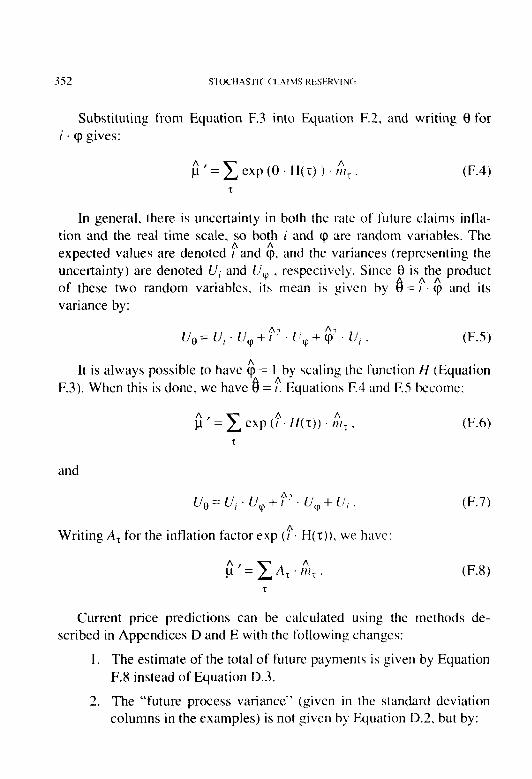
356 STOC’HAS t l(‘(‘I.AI11S RFSFRVIN(i
It is assumed that:
l the expected size of a non-zero partial payment = r 111, (for some constant I-, the same for all ~1. and
l the coefficient of variation of non-zero partial payments = cp (the same as for settlement payments).
It is assumed that each open claim gcncrates partial payments accord- ing to a Poisson process with parameter 1) (/-I is the expected number of partial payments per year of delay until the claim is closed). Therefore, if L,, represents the mean number of claims outstanding at the end of devel- opment period tl. the number of prepayments NdJ is Poisson distributed with parameters L,, ‘1’. Initially it is assumed that l-7 is constant for all M’ and ~1. that is, the partial payment Poisson process is homogeneous over real development time and the rate is the same for all claims. Alternatives are considered shortly.
Under the above assumptions, Y,,, has a compound Poisson distribu- tion. Using standard results from risk theory.
E( Y,, 2) = p I- L,, tt~, .
and
Var(Y,,,)=(l +cp’)./‘,r’.L,,.$. cc.21
Cotditionul Distt-ihutim c~f‘Puytwttt PO. C’luittr C’lost~cl
Conditional on N,, , and L,,, Y,, , and Y t/Z are mutually independent, so the variance (as well as the mean) is additive. Adding Equations (3.1 and G.2 gives:
Et Yc/) = N,, , [ 1 + C’ K,,] tn, .
an d
Var (Y,,) = N, , [q? + (1 + @) I- (’ K,,I tnz ,

STOCHASTIC CLAIMS RESERVING 357
where:
The payment per claim closed, S,, = Y/N,, , therefore has:
E(S,)=[l+(‘.R,].nz,,
and
(G.3)
Var(.S,,)=$.[l +(I +l/(p2).r.~..Rd].m:/Nd,,
If c . R,, < 1 (as is usually the case) then we have:
E(S,) = exp (C . R,,) . m, . (G.4a)
If (I + I/q?) ’ I- = 1 (this seems plausible; e.g., cp = 1, I- = 0.5), then we have:
Var (S,,) = (p2 exp (c R,,) . &Nd,
= (P2 . E(&)‘/[exp (C . RJ .Nd I]. (G.4b)
Equations G.4 can be used to estimate the parameter c by Fisher’s scoring method in the case of a log-link model for m,.
Equation G.4b for the variance of S is more approximate than the expression for the mean. This is acceptable because the variance is only of secondary importance. Its role is to determine the weights in fitting the model for the mean. The expression for the variance can be checked empirically via residual plots. The approximation (1 + I/$) . I- = 1 can be monitored by plotting standardized residuals against R,. Fanning out indicates that ( 1 + l/(p2). r z 1.
If c is known, the data S can be preadjusted to remove the partial payment effect:
S& = S,,/exp (C . R,) .
We then have:
an d
E(S,,‘) = ttjT = mean siLe ol‘~ttlcment payments.
Var (S,,‘) = ‘P’ n$[cxp (c’ K,,) N,, ,]. ((3.5)
If C’ = 0 (i.e.. 1, = 0 or r = 0; no non-zero partial paymcntx). Equations G.3 and G.4 reduce to Equations 2.2 and 2.3.
In previous paragraphs it was assumed that until a claim is closed, it yields partial payments at a constant rate 17 per development year. This implies that the total number of partial payments (and hence the total claim amount) depends on the real time scale. An obvious generalization is to allow the partial payment rate to be a function of d. say I)(,. Intu- itively, one might expect the rate to decrease with d: for example, />11 = k/d (’ or p,, = L- exp(-a d). The l’ornl of‘ Equation G.4 is unchanged ifp,, is not constant. For example, I>,, = k/cl (’ gives the same equations but with c = k . r and R,, = L,J(d * N,, ,). However. for any function /I(, , the expected total number of partial payments. and hence the expected amount of each claim, will depend on the real time scale.
Earlier portions of this appendix have all been concerned with the partial payment rate over real development time. An alternative is to consider the partial payment rate over operational time (defined in terms of the number of claims closed). The simplest model of this type (analo- gous to the constant p,, model presented earlier) is that the partial payment rate over operational time is constant. That is, each claim outstanding at operational time t has a fixed probability of yielding a partial payment in the next increment of operational time, the probability not depending on 5. In terms of the partial payment rate over real devclopmcnt time this can be expressed as I>,, = k I N, ,/M. for some constant X (because N,, ,/M is the increase in operational time). This implies that the expected number of partial payments on a claim is proportional to the operational time of settlement of the claim, and does not depend on the real time scale. (This is invariance in Taylor’s sense; see 191).

STOCHASTIC CLAIMS RESERVIK 359
Using this expression for I),, in the development leads to equations of the same form as Equation G.4 but with (’ = k I- and R,, = L/M instead of R,, = L/N,, , .
If the ratio of the number of claims outstanding (i.e., reported but not closed) to the total number not yet closed is approximately constant, then we have L,,/M = rt (1 - t), where n is a constant. In such a case we have
E(S,,) = exp (c x (1 - z)) m, , (G.6a)
an d
Var (S,) = ‘p’ E(S,,)‘/[exp (c n: . (1 - 2)) . N,, , ] , (G.6b)
where (’ = k . r. Note that the factor exp (r. . 7~ (1 - z)) decreases mono- tonically as z increases from zero to one. Thus, although the mean settle- ment payment ~II, will usually increase, the mean payment per claim closed may decrease for some values of 2. As operational time pro- gresses, the number of claims which may contribute partial payments to the payment per claim closed decreases, so E(S,) may decrease.
Throughout this appendix, E(S,,) denotes the expected value of S,, conditional on N,, , . The absence of any dependence on N,, , in Equation G.6a implies that the Cov(S,,, N,, ,) = 0, so the negative association be- tween S and N, described in Section 7 does not exist under the assump- tions presented earlier. However, this is not usually plausible for the reasons given in Section 7. Empirical studies have confirmed the exis- tence of a negative association between S and N, (for example, Taylor [8], Section 6).
In previous paragraphs, the notation p(/ has been used for the rate (in real time) at which partial payments are made on each claim outstanding in development period d. Similarly, 17~ will be used to denote the rate (in operational time) at which partial payments are made on each claim out- standing in the development period corresponding to operational time z.

360 STOCHASTl~‘~‘l.~\IMS RI:StiRVIN(i
Thus.
p/M = expected number of partial payments per l/M increase in operational time (per outstanding claim).
Therefore:
P,I = N,, I MM.
Previous sections have considered the cases:
p,) = constant (above, in this appendix),
1~~ = constant, that is, p,/ = X N,, ,/‘A4
In the real world, the truth probably lies somewhere between these two extremes. The arguments of Section 7 suggest that /I~, increases with the number of settlements N,, I but not proportionately. In other words, p,, increases but />r decreases as N,, , increases.
This can be modelled using I)(~ = p,, + k N,, ,/M, for some constants p. and A. This implies that /J,~ decreases from some value of tl onwards, as suggested earlier. By varying the ratio of I?,, to k, any situation between the extremes of p(, constant and />r constant can be attained. Repeating the development and using this expression for p,, leads to:
E(S,,) = exp (c,, L/N,, l + (‘, L/M) m, ,
and
Var (S,,) = $ E(S,,)‘/[exp (l.,, .L,,/N,, , + c, L,JM) N,, I ] , (G.7)
where c,, = [j. I and c, = k . I.
If the ratio of the number of claims outstanding IO the total number not yet closed is approximately constant at rt. then we have L,,/M = x (I - r). If ln(m,) includes a constant term and a term linear in z (for example Models 1 and 2 of Section 2). the factor exp (c, L/M) can therefore be subsumed into ni, and we have:
STOCHASTIC CLAIMS RESERVING 361
E(SJ = exp ((a,, . L/N,, , ) m, , G.8)
which is the form obtained in Equations G.4a and G.4b under the assump- tion, p,/, constant. The only difference is that in Equation G.4a, m, is the mean settlement payment, so would normally be a monotonic increasing function of z, whereas, here, with pd not necessarily constant, nt, includes the factor exp (c, . n . (1 - z)) of the partial payment effect, and is not necessarily monotonic increasing.
Since I’, is not estimated (it is confounded with other parameters of m,), the factor exp (c, LJM) cannot easily be included in the denomina- tor of Var (S,). Since C, is probably small, it seems reasonable to omit this factor from the prior weights in fitting the model. Residual plots will indicate if this is unreasonable.
362
DISCUSSION OF PAPER PUBLISHED IN VOLUME LXXVII
REINSURER RISK LOADS FROM MARGINAL SURPLUS REQUIREMENTS
RODNEY KREPS
DISCUSSION BY DANIEL F. GOGOL
I would like to thank Jim Higgins and Tony I;d’rote t’or their suggestions on this discussion.
1. INTRODL~~‘TION
Rodney Kreps’s paper contains some useful formulae, and the central idea is an important one. That idea is to determine risk loads by estimat- ing the additional surplus that is required to write an additional contract, and then requiring premium such that the return on additional surplus equals some rate selected by management. The amount of additional sur- plus is such that writing the contract does not change the probability that the losses from the book of business will cause surplus to fall below zero within the year. The required additional surplus is estimated using the formula
Var(L, + L,) = Var(L,) + Var(L,) + 2Cov(L,. LZ) , (1.1)
where L, is a random variable equal to the ultimate losses from the con- tract, and L, is a random variable equal to the ultimate losses from the rest of the book of business for the next accident year.
I believe this approach could be useful. but it would require some modifications.
2. MARGINAl. SLIRPLUS
If risk loads are estimated based on a required yield on marginal
REINSURER RISK LOADS FROM MARGINAL SURPLUS 363
expected value lower than the required yield. An example may be the best way to point this out.
Suppose that a reinsurance company with surplus S has 1,000 con- tracts on its books, each with standard deviation of losses (3. If the losses from each contract are independent, then the standard deviation of the total losses is GO. Suppose a new contract, independent of the others and with standard deviation (3, is added to the books. The standard devia- tion of total losses becomes Go. Therefore, if I’ (in Kreps’s terminol- ogy) and the desired yield on marginal surplus are small, the marginal surplus is approximately ((G- G)/G)S, i.e., about ( I /2,000)X
So, if Kreps’s method is applied to each of the other 1,000 contracts as they are renewed, the sum of the marginal surplus amounts for each will equal approximately half the total surplus and the required yield on mar- ginal surplus will be approximately twice the yield on total surplus.
The “marginal surplus required” as defined in Kreps’s paper is related to the increase in the standard deviation of the book of business caused by the additional contract. However, if all the contracts in the book of busi-
ness were ordered from first to n ‘h,then~(a,,n-(s,,I-,)=o,,,~, where k= I
CJ~,; is the standard deviation of the set of the first i contracts. Kreps’s method, however, estimates the effect on the standard deviation of each contract as if it were added at the end of the list, when the marginal effect is less.
If Ck is the kth contract in the above type of ordering and A,o is the increase in the total standard deviation caused by the addition of the kth contract, then (3L 2 Ako 2 0; where crk is the standard deviation of the kth contract and 0: is the effect of the kth contract if it is added at the end of the list, as in Kreps’s method. Therefore, there is some W such that, if n is the total number of contracts,
,1 c (Wok + (1 - W’)a~ ) = total standard deviation of the book. (2.1) k= I
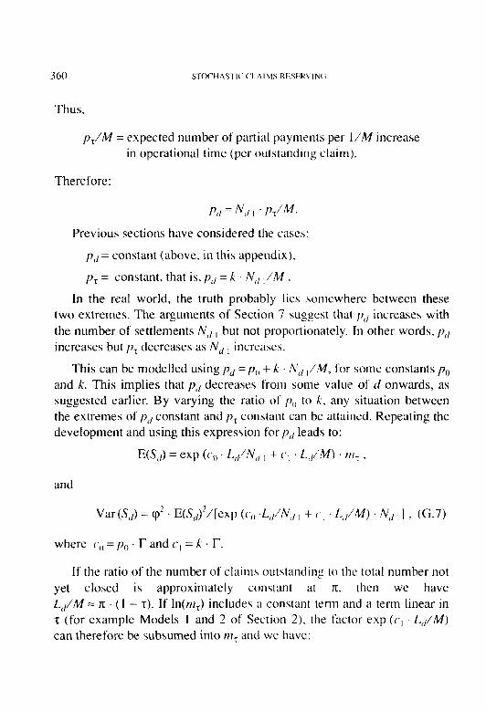
364 KEINSIiRER RISK LOhDS t:K021 VhK(;INAI. StIKPl,L S
If the contribution of the k”’ contract to the total standard deviation of the book is estimated as Wo, + (1 - W)O: , then the sum of the individual estimates equals the total standard deviation. as it should, and each esti- mate uses the same weighting.
.7. VARIANCE OF l.OSS RESERVE
A portion of surplus is needed to support the variance of the loss reserve, and, therefore, some amount may be required for many years to support a new contract. This affects the yield rate. but the paper’s discus- sion of the yield rate on surplus does not address this complication. The method of allocating surplus to contracts based on their effect on total standard deviation could be used for allocating surplus to the various subdivisions of the loss reserves, as well as to contracts. The effect of the standard deviation of the run-off of reserves one year later on the total standard deviation of surplus could be used together with a method for contracts which will be suggested below.
4. DISCOlJNTlh’G OF LOSSI’S
For simplicity, the expected return is defined in the paper as premium less losses and expenses; but in practice, some decision has to be made on discounting losses to correctly reflect economic values in the risk loads. The yield rate on surplus in the paper is based on undiscounted losses without reflecting the time value of money.
5. SlIMiESTED METHOD FOR SELEC’T‘lN~i RISK LOADS
The two problems mentioned above, i.e., the need for discounted losses and the need for surplus to support loss reserves. can be dealt with simultaneously.
Butsic [l] explains the need to discount loss reserves at a rate lower than the risk-free rate. In this way. when the value of the liabilities is invested at the risk-free rate, there is an expected profit and thus a reward for risk. Myers and Cohn [2] use the Capital Asset Pricing Model (CAPM) to compute this discount rate.

REINSURER RISK LOADS FROM MARGINALSURPLUS 365
The term “the value of the loss reserve” means that the value is dis- counted at the above rate. For contract i, let the random variable X, be the present value at the risk-free rate, on the effective date of the contract, of the losses to be paid in the next year plus the value of the loss reserve at the end of the year. Let (J; be the standard deviation of Xi . Surplus could be allocated to each contract i by using Kreps’s method with the above formula WO, + (1 - W’)o,! used in place of of .
The risk load which must be added to E(XJ to provide the required yield on surplus may then be determined. After the end of the year, the required yield on the portion of surplus allocated to the loss reserves of the contract is provided for by the rate at which loss reserves are dis- counted, as mentioned above. Also, a portion of surplus should be allo- cated to assets as well as loss reserves in order to reflect the fact that they are not risk-free. In addition, when surplus is allocated to contracts, loss reserves, and assets, the effect of each on the total risk of the company is considered. Therefore, the covariance between a contract’s risk and the entire remainder of the insurer’s risk must be considered in formula ( I. 1).
Kreps’s approach is only a way of relating the required return on a new contract to its effect on total standard deviation. There is no consider- ation of systematic versus unsystematic risk (in the terminology of mod- ern financial theory). The author states that market pricing is consistent with his approach, but financial theorists generally believe that the covari- ante of stock market returns and the rate of return on surplus must be considered in explaining market pricing. (See Myers and Cohn [2] and Cummins [3].)
The necessary risk load for a high layer may be much different for a small company than for a larger company, using Kreps’s method. The larger company is able to diversify away much of the risk. If a company insures a high layer that it is going to reinsure, it would be reasonable for it to charge for that layer based on the actual cost of reinsurance rather than to apply Kreps’s method to the gross losses.

366 REINSURER RISK LOADS FROM LIAR(IINAl. SURPl.I:S
REFERENCES
[I] Butsic, Robert P., “Determining the Proper Interest Rate for Loss Re- serve Discounting: An Economic Approach,” E\duating Insur-unce Cornpan!: Liahiliries, Casualty Actuarial Society Discussion Paper Program, 1988, p. 147.
[2] Myers. Stewart C. and Cohn. Richard A., “A Discounted Cash Flow Approach to Property-Liability Insurance Rate Regulation,” Fair Rate of Return in Property-Liuhility Irrswunc~~. 1987, p. 55.
[3] Cummins, J. David, “Asset Pricing Models and Insurance Ratemak- ing,” ASTIN Bulletin, Vol. 20, No. 2, 1990, p. 125.

DISCUSSION OF PAPER PUBLISHED IN VOLUME LXXVIII 367
THE COMPETITIVE MARKET EQUILIBRIUM RISK LOAD FORMULA FOR INCREASED LIMITS RATEMAKING
GLENN G. MEYERS
DISCUSSION BY IRA ROBBIN
1. INTRODUCTION
Glenn Meyers has made a valuable contribution to actuarial literature with his well-written paper on how to load increased limits factors (ILFs) for risk. Given the complexity of the topic, he deserves special commen- dation for his coherent presentation. Meyers clearly states his fundamen- tal assumptions and provides sufficient background for the reader to understand his results in context. His skill in composing mathematical derivations is also noteworthy. As to substance, Meyers uses the intu- itively appealing market paradigm as the foundation for his risk load theory. This represents a conceptual step forward. Unfortunately, Meyers does not carry the theory far enough, and, in my opinion, ends up with an incorrect answer.
2. WHAT IS RISK LOAD?
Before explaining why his answer is wrong, it is necessary to set the stage by first defining risk load. What is risk load? I would define it as an extra component of indicated premium arising from the potential for pos- sible deviations between expected and actual loss results. The indicated premium for a coverage is the sum of the expected loss cost, expense provisions, and usual profit load, plus the risk load.
Why is risk load needed? The most general answer is that the price for insurance coverage ought to somehow depend on the volatility of the actual losses covered by the insurance. In the pricing of assets, such as bonds, it is well accepted that the interest rate demanded by the market rises with the riskiness of the asset. With respect to increased limits, risk

368 INCREASIXI LIMITS RATEMAKII\‘G
load is important because increasing the limit of coverage changes the relative volatility of actual results versus initial expectations.
3. OVERALL LEVEL VERSLIS RELATIVITY BY LIMIT OR LINE
When considering risk loads for increased limits. it is useful to split the question into two parts by asking first, “What is the proper overall level of risk load?” and, second, “How should the risk load vary by limit and by line of coverage?” While I have some question about whether Meyers developed a logically consistent theory for setting an appropriate overall level of risk load, my major criticism is that his model produces risk loads that can rise too steeply by limit.
4. PROCESS AND PARAMETER RISti
Before detailing this criticism, I should note my agreement with much of what Meyers has done. In particular, I concur with Meyers that risk loads should reflect not only the stochastic variability of actual results versus expectation (process risk), but also the uncertainty about the loss expectation itself (parameter risk). This is generally accepted in principle by most actuaries knowledgeable in the subject. I also accept the collec- tive risk model Meyers employed to incorporate parameter risk (see Sec- tion 4 of his paper). While I might want to quibble with the specific techniques Meyers used for quantifying parameter risk, I will not do so in this discussion.
5. MARKET EQUlLlBRlUM THEORY AS A FOl NDATION FOK RISK LOAD
I agree with Meyers that market-based theory can provide a sensible foundation for risk load calculations. The basic idea in using a market- based theory is to apply the “supply-versus-demand” concept of general economics to the pricing of risk. A key advantage of this approach is that it explains the need for risk loads in ILFs using fundamental economic principles. I also believe it provides a basis for conceptually defining what risk loads should be included in ILFs filed by a rating bureau. Under my view, risk loads filed by a rating bureau should be those that would be

INCREASED LIMITS RATEMAKING 369
theoretically charged by a rational market in equilibrium. Actual risk loads charged in the real market could, of course, be different since the market may be irrational or in disequilibrium. However, by relying on a theoretical market, one should obtain bureau risk loads that are sound benchmarks unaffected by market cycles or imperfections. Individual companies can then deviate up or down as they deem appropriate.
The theoretical market approach is not universally accepted as the logical foundation for a theory of risk load. Some, for instance, have insisted on determining what the risk load should really be and not what some hypothetical market says it should be. While this “just give me the real risk load” attitude sounds direct and practical, it leads nowhere. The problem is that there is no inherent notion of how to properly price for risk, either before or after the fact. In contrast, the right price for losses is an amount sufficient, on average, to cover the actual losses. After the fact, we know the actual loss costs and what we should have charged for losses. However, we have no actual “risk” costs to tell us what the charge for risk should have been. If there is a difference between expected and actual losses, we have evidence of volatility and thus proof that some risk load should have been charged. Nonetheless, this evidence alone does not tell us how to measure volatility, nor how to translate volatility, however measured, into a charge for risk.
6. UTILITY THEORY
Utility theory has been used as a conceptual framework for pricing risk. Under utility theory, the minimum premium an insurer is willing to accept is the lowest one for which the insurer’s expected utility will not suffer if it provides the coverage. This means that the utility of initial wealth is the same as the expectation of utility of final wealth, where final wealth equals initial wealth plus premium less expenses and actual losses. A key point is that the resulting risk load is, to first approximation, pro- portional to the variance of losses.
I agree with Meyers that a “single insurer, single insured” implementa- tion of utility theory is too simplistic. It produces risk loads an insurer might want to charge if there were no other insurers competing for the
business and if there were no reinsurance market. With only one insurer in the model, there is no market and therefore no room for the forces of supply and demand to operate.
7. THE MEYERS RISK LOAD TtlEORY
In the Meyers model, there are many insurers and many insureds. So far, so good. Each insurer sets a constraint on the variance of losses it will tolerate on its individual book of business, and seeks to achieve the maxi- mum profit subject to that constraint. The insureds are assumed to have an inelastic demand for insurance coverage by limit. For example, half the market may demand coverage at a $1 million limit and will pay the going rate to obtain it. The insurers then “bid” on the risks. Under the given assumption, and a further hypothesis about the total needed risk load over all lines and limits, the market in each subline and limit will be cleared at an optimal price. With some elegant mathematics. Meyers shows that the market clearing price can be viewed as the price that would have been charged by an average insurer acting alone. This result is shown in his Equation 5.6. Thus. Meyers effectively ends up with a variance-based risk load, and his theory co~11d be regarded as another argument for variance. The central question. then. is whether his argu- ment undercuts the serious criticisms made against variance-based risk loads.
8. THE “I’NITS DON’T 21.41(‘11” ORJk(‘l IOU ‘I‘0
VARIANCE-BASED KISK I.OAI)S
Before presenting what I regard a\ valid criticisms of variance-based risk loads, I would like to switch sides for a nnomcnt and refute one set of common arguments made against variance. This set of arguments deals with the units of risk load and with currency translation. Consider that variance is in units of “dollars squared.” while the desired cost is in units of “dollars.” As any engineering or physic\ student knows, if the units don’t match, there is a mistake somewhcrc in the derivation. Related to this is the criticism that variance-based risk load formulae lead to nonsen- sical results if one tries to switch from one currency to another.
INCREASED LIMITS RATEMAKING 371
Both these criticisms are an attack on the formula: RL = h . Var (L) , where RL is risk load, L is loss, and h is a constant. If L is in dollars, then Var (L) is in units of dollars squared. It is true that if h were a unitless constant, then there would be a mismatch of units. However, h should carry units of inverse dollars, so that the resulting risk load is, as it should be, in units of dollars.
This also refutes the currency translation paradox. Write $L for loss in dollars and &L for loss in pounds and let EL = K. $L, where K is the exchange rate constant. It follows that:
Var (CL) = Kz . Var ($L).
Ostensibly confounding results arise if h is viewed as a unitless con- stant and not adjusted for exchange rate. However, if &RL = hi . Var (&L), where X5 = hs/lc , then .CRL = K. $RL. Thus, the problem disappears if h carries units of inverse currency and is properly adjusted to reflect ex- change rates.
9. VARIANCE-BASED RISK LOADS MAY LEAD TO INCONSISTENT
INCREASED LIMITS FACTORS
Having shown I do not find merit in every argument against variance- based risk loads, I will now turn to one I do regard as valid. In my view, the major flaw with variance-based risk loads is that they can lead to prices that may rise too rapidly by limit. For example, it might cost more to raise the limit from $2 million to $3 million than it does to raise the limit from $1 million to $2 million. With a variance-based risk load, it would not be impossible to have the following ILF table:
TABLE 1
Limit ($000) ILF
1,000 2.50
2,000 3.00
3,000 3.75
371 INCfWASfif) l.I\II’I’S KATf:hlAKIN(i
To see what is wrong here, consider matters from the point of view of a prospective insured whose basic limits premium is $10,000. This in- sured will be asked to pay $25,000 for $ I million of coverage, an extra $5,000 to increase coverage from $1 million to $2 million, and an extra $7.500 to increase coverage from $2 million to $3 million. Breaking this down by layer and using an “M” suffix to denote million(s). the insured would see the following:
TABLE 2
Layer cost
0 -$lM $25.000
$lM excess of$lM $S,OOO
$1 M excess of $2M $7.500
What is exceedingly strange about this is that the loss in the lower excess layer ($1 M excess of $ IM) must be $1 million before there is even a penny of loss in the upper excess layer ($lM excess of $2M). Further. loss in the upper layer can never exceed the loss in the lower layer. How can it make sense to charge more for the upper layer when it never has more loss?
This problem of inverted layer costs is referred to as “inconsistency by layer.” increased limits factors are consistent if they exhibit a pattern of declining marginal increases as the limit of coverage is raised. If the ILF formula is viewed as a function with respect to the coverage limit, and this function has a second derivative. then the ILFs are consistent if, and only if. the second derivative is negative. Consistency implies that excess layer costs decline as the attachment point is raised. assuming all layers carry the same limit of excess coverage. and assuming that excess layer costs are computed by taking differences in appropriate ILFs.
Meyers is well aware of the inconsistency problem. He tries to get around it by defining a new notion of consistency. Under the Meyers definition (see Meyers’s Appendix E), one considers any two excess lay- ers with identical limits, but different attachment points. Consistency, according to Meyers, exists if the layer with the higher attachment point

INCREASED LIMITS RATEMAKING 373
always has a lower indicated price. Meyers calculates the indicated price for a layer as the sum of its expected loss plus risk load. His risk load is proportional to the variance of losses in the Iaye): In his paper, Meyers gave a proof that this calculation results in consistency under his defini- tion. Subsequently, Meyers has told this reviewer that the proof may not be valid.
However, even if it were valid, it would prove much less than it may seem. Since Meyers does not calculate layer prices by taking the differ- ence between ILFs, his notion of consistency does not apply to the ILFs, but rather to his premium calculation principle. In fact, taking differences of ILFs gives a larger indicated (variance-based) risk load for a layer than would calculating layer risk load based on the variance of layer losses. This happens because the variance in layer losses is always less than the difference in the variance of losses capped at the upper limit minus the variance of losses capped at the lower limit (see Appendix A). This is the essence of “risk reduction through layering.” (See Miccolis [2].)
Therefore, Meyers is, at least implicitly, asserting that ILFs are not appropriate for pricing layers. Also inherent in his theory is the idea that the price for coverage up to a limit depends on how the coverage is layered. For example, under Meyers, coverage for the layer from zero to $2 million should have a price different than the sum of prices for cover- age on the underlying $1 million plus coverage on the $l-million-excess- of-$I-million layer. Not only does this fail to produce a unique benchmark price for coverage, because it allows that different layerings of coverage could result in different prices, it also leaves open the ques- tion of what layering, if any, should be assumed when filing ILFs. Meyers believes that the bureau should file ILFs under the hypothesis that layer- ing is not allowed, and yet also promulgate advisory factors for various possible layerings. I feel the publication of different costs for different layerings of the same coverage is no solution, and only adds to the confu- sion. Try as he might, Meyers is unsuccessful at defining away the consis- tency problem. ILFs produced with the variance-based risk load can be inconsistent.
374 INCREASEU I.IMITS K~l’l<hlhKINCi
10. VARIANCE REDUCTION THROIIGH PRO RATA SHARING
It is also somewhat troubling that variance-based risk loads lead not only to “risk reduction through layering,” but also to “risk reduction through sharing.” To illustrate this. suppose two insurers decide to be- come “50-50” partners in writing a risk. Each will take half the premium and pay half the loss. If cr* is the variance of the total loss, then 0’/4 is the variance of the loss covered by each insurer. If each uses a variance- proportional risk load with a common risk loading scalar. h, then the total risk load demanded by their syndicate will be h. r 0’/2 . If either insurer had written the risk on its own, then the risk load would have been h cr’. Due to syndication, the risk load has been cut in half. The syndicate operates, in effect, with a reduced risk load constant. More generally, if risk load is in proportion to variance and if expense considerations are neglected, then syndicates ought to be able to take advantage of “risk reduction through sharing” in order to reduce their risk loading constants.
It appears that quota share syndicates would not be allowed in the Meyers’s Competitive Market Equilibrium (CME) model. I deduce this from Equation 5.3 in which Meyers derives the theoretical market risk loading constant as the (harmonic) atwuge of the hs for the individual insurance companies. If the companies were allowed to form a syndicate and quota share the business, the theoretical market h would be much lower than the average h .
1 1. RESTRICTIONS ON THE “(‘OMf’FTITIVE MAKKET“
In the market posited by Meyers, risk load is proportional to variance and there is no excess layer or quota-share reinsurancc. Yet, the variance principle implies that such reinsurance is decidedly advantageous. Im- plicitly, Meyers has prohibited insurers from entering into transactions that his theory says are beneficial.
Meyers must also have some hidden restrictions on the insureds to prevent them from taking advantage of analogous ways to reduce their variance-based risk loads. For example, instead of buying $2 million of coverage, an insured could opt to save money by buying a primary policy
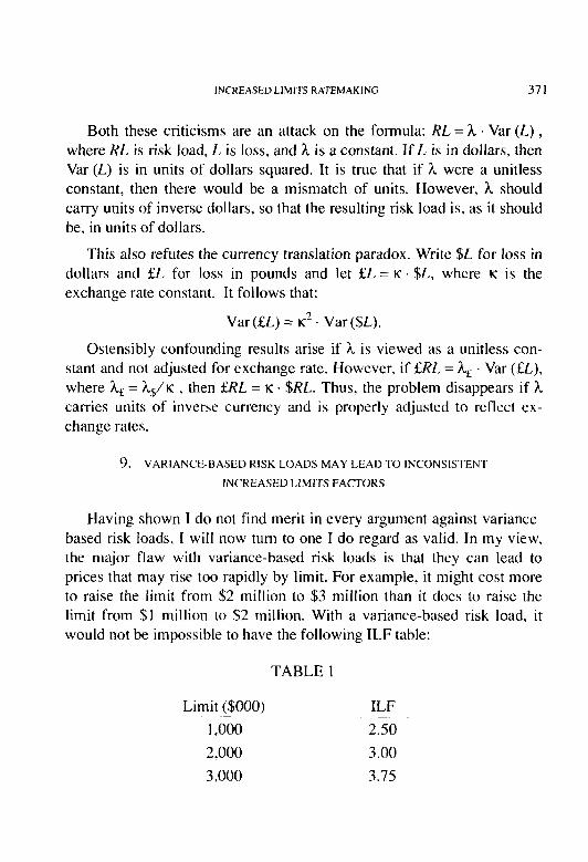
INCREASED LIMfTS RATEMAKING 375
with a limit of $1 million and an excess policy covering $1 million excess of $1 million. As well, the insured could save money by getting two policies with each covering half of the insured’s losses.
If Meyers had a free market model, then the insurers would be allowed to reinsure and the insureds would be permitted to package coverage. In either event, the market would soon cease to operate under the original variance-based risk load. As Venter [3] has noted, variance-based risk loads create arbitrage possibilities. Yet one aspect of competitive market theory is that “arbitrage profit possibilities are quickly extinguished by market competition”[3]. Meyers started off to build a “Competitive Mar- ket Equilibrium” theory, but ended up with ILFs that could never exist in a free market.
12. PUTTING REINSURANCE INTO THE MODEL
In my opinion, the theory ought to be extended to arrive at the theoret- ical premium that would prevail in a competitive market that allowed reinsurance. Additional expenses associated with reinsurance must also be considered. Since reinsurance companies do exist, such an extended the- ory would be a better model of reality than the highly-restricted model proposed by Meyers.
By theoretically allowing coverage to be reinsured, one is not forcing any individual insurer to abandon use of a utility function to price the risk on its net coverage. Each insurer could still use a utility function and end up demanding a risk load proportional to the variance of loss it covers. However, as previously noted, variance reduction through layering or sharing can lead to a market risk load that is not proportional to the variance of the total (unlayered and undivided) loss.
The reduction of variance through layering will lead to a hypothetical market price for coverage by limit in which risk load rises less rapidly than the variance of limited losses. Indeed, if one neglects to consider expenses associated with layering, the continual subdivision into finer layers will drive the process risk component of theoretical market risk loads to zero. This is proven in Appendix A.

376 INCRE4SEI) I 1x41 I‘S liXl’f:bli\KlN(i
However, layering has its costs. At the very least. it leads to additional processing and billing as each reinsurer needs to receive its share of the premium and pay losses in its layer. While such costs may be small, they rise as the number of subdivisions is increased. Intuitively. it is clear that there will come a point when risk load reduction through further layering will be canceled out by the additional costs. At that point. one arrives at the best possible price the theoretical market could offer.
I do not have a general formula for this lowest theoretical price under arbitrary layerings that also retlects the cxpcnses associated with layering. However, I can present to the reader a comparable formula derived by Fred Klinker for the risk-sharing case. As shown in Appendix B, if one allows a syndicate of insurers to take pcrccntage shares of coverage, with each charging a risk load proportional to the I’arI’um.c of its share of loss, and add in expenses which rise with the number of syndicate members, then the total risk load is proportional to the stu~ldurul cle\~iutio~? of the total loss. Since layering is more efficient than sharing in reducing pro- cess variance, it is likely that the lowest theoretical market price for coverage will increase less rapidly by limit than the standard deviation of limited loss. In summary, if Meyers wcrc to complete his theoretical foundation and allow layering and reflect associated expenses, his theory would produce risk loads whose process risk load components would not increase in proportion to process vJariancc, but to something that rises even less steeply by limit than does the process standard deviation.
Venter [3] has advocated calculation of the risk-loaded premium using the expected value of a risk-adjusted distribution. This distribution is obtained by transforming the original loss distribution. In his paper, Ven- ter deduces some general principles from the requirement that the market be free of arbitrage possibilities. The transformation methodology satis- fies these principles. Further, according to Vcntcr, the only premium cal- culation principles with the desired properties are those that can be generated from transformed distributions. However, it is not clear if any transformation would be equivalent to an extended Competitive Market Equilibrium model which incorporated reinsurancc and associated ex- penses. Once such a model is developed. its equivalcncc IO some transfor- mation of distributions should be investigated.
INCREASED LlMlTS RATEMAKING 377
13. SUPPLY AND DEMAND
The supply assumption in the Meyers CME theory is that each com- pany sets a constraint on the loss variance it will tolerate. While this reviewer knows of no company that actually does this in practice, it is likely that most insurers implicitly operate under such a constraint. Thus, the assumption seems reasonable, especially in the context of modelling a theoretical market.
However, the assumption about demand could be much improved. Recall that the Meyers CME theory effectively ignores the demand side of the “supply and demand” equation under the dubious assumption that demand is inelastic. I would assert on general grounds that demand by limit might well be influenced by the pattern of increase in a set of ILFs. While it is beyond the scope of this discussion to propose a theory incor- porating an explicit demand function, future research in this direction would seem worthwhile. Such a theory would require an explicit demand function by limit. Estimation of the demand function might be rather difficult. One problem is that the only data currently available is on the limits of primary policies purchased by insureds. To obtain a true picture of the demand by limit, one would need data on the total coverage af- forded by the combination of primary and excess policies purchased by insureds.
The “demand side” perspective also leads to the consideration of the impact of risk retention groups. Under one approach to risk retention financing where the goal is to minimize the probability of ruin, a risk retention group must assess the total risk load proportional to the standard deviation of losses for all members of the group. Within this framework, principles of game theory were used by Lemaire [1] to calculate a fair cost allocation for each member of the group. The resulting risk load assessment for a group member is not proportional to the variance of the member’s losses. This strongly suggests that variance-based risk loads would not be theoretically tolerated in a market that allowed the forma- tion of risk retention groups. Note also that proper consideration of risk retention groups would entail consideration of expenses. One might end up with a result not too dissimilar from what one would achieve by

378 INCREASED LIMITS RzOEMAKING
incorporating reinsurance layering and associated expenses in the CME theory.
14. CONCI.USION
Meyers has made a valuable contribution to the field of actuarial liter- ature with a well-written and thought-provoking paper. He has laid down some of the foundation for a solid theory of risk load and has artfully applied mathematical techniques to get a result. Meyers was courageous enough to go beyond the “single insurer, single insured” paradigm to develop a competitive market approach. Unfortunately, he posited an arti- ficially restricted market and ended up with variance-based risk load. This is the same answer produced by the “single insurer, single insured” utility theory model. The Meyers theory does nothing to dispel valid criticisms made against variance-based risk load. Most important, his variance- based risk load formula could lead to inconsistent ILFs, where “inconsis- tent” retains its original and appropriate meaning as given by Miccolis 121. In conclusion, I believe Meyers did not succeed in obtaining a risk load formula appropriate to use in bureau increased limits ratemaking.
REFERENCES
[ I] Lemaire, Jean, “Cooperative Game Theory and Its Insurance Applica- tions,” ASTIN Bulletin,, Vol. 2 1. No. 1, 199 I, p. 17.
[2] Miccolis, Robert S., “On the Theory of Increased Limits and Excess of Loss Pricing,” PCAS LXIV, 1977, p. 27.
[3] Venter, Gary G., “Premium Calculation Implications of Reinsurance Without Arbitrage,” ASTIN Bdletirl, Vol. 2 1, No. 2, 199 I, p. 223.
INCREASED LIMITS RATEMAKING 379
APPENDIX A
IMPACT OF LAYERING ON PROCESS VARIANCE
Suppose coverage up to limit K is achieved by stacking n layers, and assume the indicated risk-loaded pure premium for the coverage is the sum of the indicated risk-loaded pure premiums for the layers. Suppose the indicated risk-loaded pure premium for each layer is calculated as the sum of expected loss in the layer plus risk load, and assume risk load is proportional to variance. Consider the “process” variance component of the risk load. I will first show that this layering reduces the risk load compared to the risk load of the unlayered coverage. I will then show that the sum of process variance risk loads becomes smaller as the layer subdivisions grow ever finer. In other words, if expenses are not included in the analysis, infinite layering will drive process variance risk load to zero.
Let 0 = k. < k, < . . . < k, = K be the layer end points.
LetAkj=ki-ki-, fori= 1,2 ,..., n.
Given loss severity random variable, X, define Xi = min(X, kJ and let pi = E(X;) and O* ; = Var (Xi).
Let Yi denote the loss in the i lh layer SO that Yi = Xi - Xi _ , .
Thus, E( Yi) = Acli = cli - pi _ I .
Now, set zf = Var (YJ .
Proposition
Var(X,,)=~rj+2.~~(k;-~i).A~i+, i=l i= I
Proof: Since X, = cYi , it follows that:
(A.1)
Var (min(X, K)) = i 7; + 2 . CCOV(Yiy Yj) . i=l icj
Now consider that, for i < ,j.
Cov(Y,t Yj) = (Ak;) (API) - CAP,) (Api) = ( (Ak,) - (APO 1 C&j) .
The desired result then follows since:
Ak, + AX-2 + . . . + Mi = X; and ApI + Ap? + . . . + A~i = cli .
Since the latter sum in equation A. 1 has only non-negative terms, one can immediately conclude that layering reduces total risk load it’ risk load is proportional to variance.
Var(min(X, K)) 2 i rf i=I
(A.2)
The inequality is strict if there is some non-rero probability of a non- zero loss strictly less than the upper limit. K.
If the subdivision process continues indefinitely. the process risk load will shrink to nothing.
Proof: Consider that 7,’ < AX-F so that c tf < c A/if
Further observe that c A/$ < max Ak, , 2 AL, = max i AX, i K .
The result follows since the latter expression approaches zero by assump- tion and by the fact that K is unchanged by the layering.

INCREASED LIMITS RATEMAKING 3X1
APPENDIX B
RISK LOADS CHARGED BY A PRO RATA SHARING SYNDICATE
(Simplified from the unpublished work of Fred Klinker)
If there is a competitive insurance market with risk sharing among the insurers via pro rata reinsurance, and if the expenses associated with risk sharing are considered, then variance-based risk loads at the level of the individual firm become standard deviation-based at the level of the mar- ket. This seemingly paradoxical result stems from a trade-off between the increased expense and decreased “risk” associated with sharing.
Assume each insurance firm charges a risk load proportional to the variance of loss for the coverage it provides. Now suppose there is a syndicate of I? insurers in which each takes a fixed share, pi , of the total loss, where the pi are non-negative and sum to one.
The loss experienced by the syndicate as a whole, L, is a random variable with expectation E(L) and variance Var (L). The loss experienced by the ith insurer is piL with expectation p;E(L) and variance p: Var (L). Neglecting regular underwriting expenses and the usual profit load, the components of the net premium charged by this insurer are:
Expected loss: P;E CL)
Fixed expense (transaction costs): E
Risk load: h, pf Var (L)
The resulting net premium charged by this insurer is
Pi = pi E(L) + E + h, p: Var (L). @.I)
The resulting premium charged by the syndicate of n insurers is, recalling that the pi are weights summing to unity,

3x2 INCREASED 1~IMITS RATEMAKING
I,
P(n, p,) = E(L) + HE + Var(L) c h, pi’ . (B.2)
Now minimize the premium given in equation B.2. holding u fixed. Equation B.2 will be minimized by minimizing
The minimization is constrained since constrained minimization can be solved bq pliers.
I, II
the p, must sum to unity. The the method of Lagrange multi-
a a P,
Ch,pf=A a c aP’jT,
p, for all i /=I
21, p, = A for all i _
In other words. the optimal pi are proportional to the reciprocals of the hi for all i .
Imposing the constraint that the p, sum to one leads to
I Pi=
h c: I ( > ,~:I ’
It follows that
II
c h, p; = ,= I
= I,
c 1
i-l 4
II
I 1
( > ;,
(B.3)
(B.4)
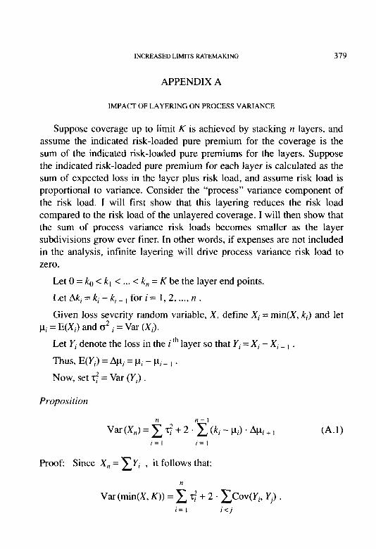
INCREASED LIMITS RATEMAKING 383
where the angled brackets denote the average value. The minimum pre- mium, for fixed n, from equation B.2 and the above, is
Var (L) P(n)=E(L) +n&+ 1 .
n ii ( > (B.5)
Note the behavior of equation B.5 with respect to n, the number of insurers in the syndicate. There is a term due to fixed transaction costs per insurer which increases linearly with the number of insurers. Another term declines as the reciprocal of the number of insurers, which captures the declining aggregate of the variance-based risk loads of the individual insurers. The decline is due to the increasing spread of risk among more insurers.
Because of the above behavior, there is an optimal II for which the premium, P(n), is minimized. This occurs where the derivative of P(n) with respect to II vanishes.
Var (L) 0 = $ P(n) = & - p-i--- .
n2 h ( >
Hence,
Var(L]
n = d- ~ I
E h (W 03.6)
and the minimum value of P(n) is
P=E(L)+2 ( 47) (B.7)
Equation B.6 provides the optimal number of insurers and equation B.7 provides the minimum premium over all possible numbers of insurers and all possible pro rata distributions of risk among insurers. The last
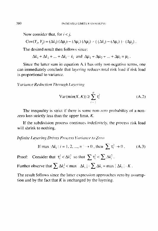
3x4 INCREASF.1) I.IMIT.5 RX1 li’.lhtilNG
term of equation B.7 can be identified as the market risk load. In the immediate context of increased limits factors. with increasing limit- hence increasing Var (L&the optimal number of insurers on the contract will increase according to equation B.6. Also, the market risk load of equation B.7 will increase only as the square root of Var (L); i.e., as the standard deviation of L, where L is the aggregate loss across the syndi- cate, despite the fact that individual insurer risk loads arc variance-based rather than standard deviation-based.

385
DISCUSSION OF PAPER PUBLISHED IN VOLUME LXX111
THE COST OF MIXING REINSURANCE
RONALD F. WISER
DISCUSSION BY MICHAEL WACEK
A hstr-uct
In his I986 puper, “The Cost of Mixiq Reinswunce,” Ron Wiser analyzed the consequences of mixing pro rata and ex- cess of loss winsurance. He cvnc~ludcd thut such mi.l-ed rein- surance situations MY~E alntays unfavorable to the ceding company, both in terms of ,financial cost und loss ratio stahil- ity. This paper rqfutes that conclusion and shows that Wiser prol-cd his argument only ,for the special case of a pasticular. ineflicient reinsurance structure. Some of his reported “cost oj’ nii.Gng” M*US uctuully a result of purchasing redundant rein- surance. The degree of inefficiency in a mixed reinsur-awe strwtuw can he quantiji’ed as the “cost of overlap” betcr,een the types of reinsurunce coverage. This should be measured separutely from the cost of mixing per se. A case of negative cost of mixing is presented, and a r-elutivefy simple test of wlhether the mixing cost M’ill be positive or negative is dcri\*ed and demonstrated.
1. INTRODUCTION
Ron Wiser’s “The Cost of Mixing Reinsurance” [I] is an excellent presentation of many of the major issues involved in the analysis of the effect of mixing proportional and excess of loss reinsurance. It is a well- written paper that introduces the reader to several important concepts. Because I see that paper as so important, I believe it is necessary to comment on some aspects the author has omitted. My primary concern is
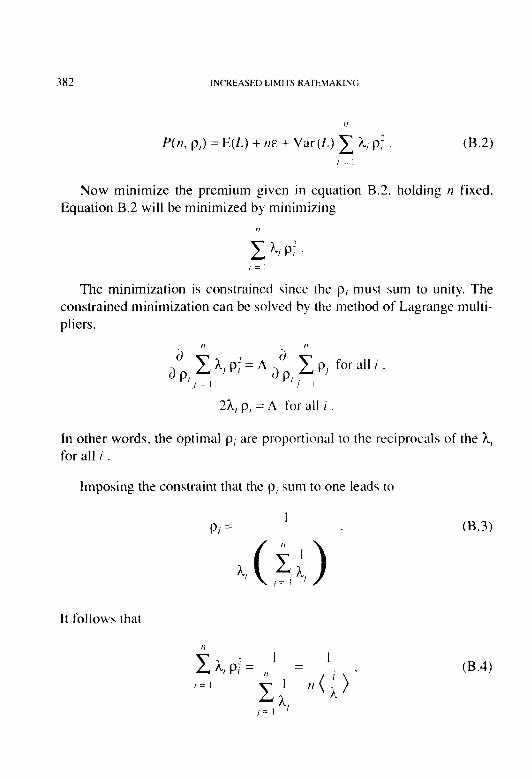
386 COSTOF MIXING REINSI‘RAW‘I.
that the Wiser paper may leave the casual reader with the impression that mixing excess of loss and proportional reinsurance UII~YI~.S has adverse cost and stability consequences for the ceding company. That is not true, as I will show.
This discussion is best read with a copy of Wiser’s paper close at hand. since it frequently refers in detail to the examples presented in that paper. An effort has been made to use the terminology and notation of the original paper, in order to make it easier to read the two together.
The key point of this discussion is to make it clear that Wiser proved his Mixing Loss Ratio Rule O~I/Y for the special case in which the ceding company buys excess of loss coverage all the way up to the top of the policy limits it has issued. In such circumstances, the purchase of propor- tional reinsurance is redundant and is thus inherently inefficient. That it has a cost should come as no surprise. This is understood by most insur- ers, and they do not usually structure their reinsurancc in this way. As a result, Wiser’s conclusion that mixed reinsurance situations are always costly to the ceding company is relevant only to reinsurance arrangements that are not often found in practice.
An insurer normally will determine the net retention it desires for a particular risk and use a mix of proportional and excess of loss reinsur- ante to absorb the exposure between the retention and the policy limit. In property insurance the proportional reinsurancc is typically provided under “surplus share” treaties. which essentially provide the insurer with the capacity to write policy limits larger than it could with its excess of loss rcinsurance alone. These treaties act like a sponge, soaking up the surplus exposure above its excess reinsurancc coverage. Normally, if there is no “surplus” policy limit exposure. the insurer does not cede any exposure to the surplus share treaties. If it does. it is generally according to a line guide agreed to in advance with the surplus and excess reinsur- ers, and the price and terms of the reinsurance contracts will reflect the expected cessions implied by the line guide. Insurers also USC a mixture of excess and proportional reinsurancc to extend their capacity for casualty

COSTOF MIXING REINSURANCE 387
policy limits, though here, the use of surplus share treaties is less com- mon than in property insurance.
Figure 1 is a graphical illustration of this common type of property reinsurance program. It shows: A) a net retention of $500,000; B) a $500,000 excess of $500,000 treaty; and C) a five-line surplus share treaty. This gives the insurer total gross line capacity of $6,000,000. Poli- cies larger than $6,000,000 would require facultative reinsurance (either proportional or excess of loss).
If P denotes the policy limit and F denotes the facultative coverage limit, an insurer with the treaty reinsurance program shown in Figure 1 generally would keep a share, equal to $1 ,OOO,OOO/(P - F). of any “net and treaty” policy limit, P -F, greater than $l,OOO,OOO. The excess rein- surer remains exposed for its entire $500,000 limit, though the composi- tion of that exposure is different after proportional reinsurance is introduced.
Figure 2 illustrates the allocation of loss exposure arising from a $5 million policy issued by an insurer that has the reinsurance program sum- marized in Figure I.
3. ORDER OF REINSURANCE RECOVERIES
In mixed reinsurance situations, i.e., where a policy is protected by a number of reinsurance contracts, working out the correct loss recoveries can be fairly involved. In theory the interplay between the applicable coverages is negotiable but, in practice. the following principles are nor- mally applied as standard unless otherwise agreed:
1 . Mow specific rw~erage responds hefbe less .spec(fic un~~ruge. For example, facultative always responds before treaty. Per risk covers always respond before catastrophe (i.e., per occurrence) covers.
2. Pmporrionul co\*erugu r~esponds hqfim e.wess o$ loss cwveruge, s1rhjer.t. hmlever, to Principlr~ 1. For example, a property surplus treaty responds before a per risk excess cover but after a faculta- tive excess cover.

3xX (‘OSTOF MIXING REINSUR.AN(‘E
This discussion assumes the application of these recovery principles. The conclusions will not be applicable to those relatively rare instances where a proportional treaty has been negotiated to respond qfter an excess of loss treaty.
FIGURE I
5 Line
SCXPlUS
Treaty
XL Treat)
Net Retent.ion
$6,000,000
$l,ooo,ooo
$500,000

FIGURE 2 ALLOCATION OF Loss EXPOSURE
COMMON PROPERTY REINSURANCE STRUCTURE / $5 MILLION Po~rcy
Excess Only $5,000,000
$1,000,000
$500,000
390 COSTOF MIXING REINSURANCE
4. EXCESS LIMIT EXPOSURE
At least a portion of the “cost of mixing” demonstrated by Wiser is a result of the inefficient reinsurance structure he assumed, for both his examples and his general case. Consider his examples.
In the casualty case presented in Wiser’s paper [ 1, pp. 175- 1871, the excess coverage is $2 million excess of $250,000. For some reason, the insurer buys 50% pro rata facultative coverage on a $1 million excess of $100,000 policy. Without the facultative placement, the excess reinsurer is exposed for $750,000 excess of $250,000. But with it, the excess expo- sure is only $250,000 excess of $250,000. We should not find it surprising that the excess reinsurer has a lower expected pure premium and the insurer a higher expected cost of reinsurance! The allocation of loss expo- sure is shown graphically in Figure 3, where it is evident that the propor- tional coverage has crowded out the excess of loss protection. The bar on the left shows the allocation of exposure in the pure excess case. The bar on the right illustrates the mixed case. The much smaller area correspond- ing to excess treaty exposure in the mixed case is indicative of the re- duced exposure compared to the pure excess case.
The same is true of Wiser’s property example [ 1, pp. 19 I-201 1, though the inefficiency of the reinsurance is less extreme than in the first case. The excess coverage is $2 million excess of $250,000. The insurer issues a $20 million policy and cedes 90% of the risk ($18 million) on a pro rata basis. The pro rata placement reduces the excess reinsurer’s maximum exposure from $2 million excess of $250.000 to $1.75 million excess of $250,000. Again, it should be obvious that the excess reinsurer will bene- fit and the insurer’s expected net cost of reinsurance will be increased. The allocation of exposure in the pure excess and mixed scenarios is shown graphically in Figure 4.
In both of these examples the insurer has bought overlupping reinsur- ante coverage. While there might be valid reasons for doing this under certain circumstances (e.g., “protecting the excess treaty”), it will always be more expensive than not doing so. In the casualty case, it is not clear why the insurer bought any proportional cover at all, since it had adequate coverage under its excess of loss treaty alone. In the property case, the
FIGURE 3 ALLOCATION OF Loss EXPOSURE
FIRST CASUALTY EXAMPLE $1 MILLION EXCESS OF $100,000 POLICY
Excess Treaty IlOO%
Excess Retention
Underlying Retention
;1,100,000
;350,000
;100,000
Mixture of Pi?
Pro Rata
Reinsurance (50%)
3 Rata/Excess
Excess
Treaty (50%)
EXCeSS
Retention
Underlying Retention
$1,100,000
$600,000
$100,000

FIGURE 4 ALLOCATION OF Loss EXPOSURE
PROPERTY EXAMPLE / $20 MILLION POLICY
Excess Only
Excess Retontlon*
$20,000,000 Mixture of Pro Rata/Exe
l Area not to scale

COST OF MIXING REINSURANCE 393
correct pro rata purchase to avoid overlap would have been $17.75 mil- lion, or 88.75%, instead of $18 million (90%).
The point is that the “costs of mixing” shown on Wiser’s Exhibits 2 and 3 and implied by his Mixing Loss Ratio Rule include not only the effect of mixing but also the cost of buying down the excess reinsurer’s limits exposure. Indeed, we cannot be certain that the effect of mixing per se is unfavorable without further analysis.
5. COST OF OVERLAP AND COST OF MIXING PER SE
In the casualty example presented by Wiser, the reinsurer’s total policy limit exposure in the pure excess case is $750,000 excess of $250,000, which implies expected losses of $85,144, or 35.48% of the policy losses subject to the excess coverage. See Wiser’s Exhibit 1 .l [ 1, p. 1781. This layer can be subdivided into two layers of $250,000 excess of $250,000 and $500,000 excess of $500,000. The expected losses in these two layers are 19.7 1% and 15.77% of subject losses, respectively. These ratios are easily computed using values from the limited mean function of the size of loss distribution. (See Exhibit 6, or Wiser’s Exhibit 1.2, for a partial tabulation of this function.)
In the mixed reinsurance case, the excess reinsurer’s total policy limit exposure is only $250,000 excess of $250,000 with respect to subject loss exposure of $500,000. (This is equivalent to 50% of $500,000 excess of $500,000 with respect to original policy exposure of $1 million.) The $500,000 excess of $500,000 layer now has no policy.limit exposure at all. The expected excess losses in these two layers are 15.77% and 0% of subject losses, respectively.
The difference in $250,000 excess of $250,000 layq expected losses between the pure excess and mixed reinsurance cases is approximately 3.93% (19.71% - 15.77%) of subject losses, or about $4,720. This is the true cost of mising excess and proportional reinsurance in this example.
See Exhibit 1 of this discussion for a summary of the key limits, limited means, and relative exposure for the first layer. This exhibit mea- sures the cost of mising per se.
394 COST OF MIXING RHNSIIRANCE
Since the ceding company has the same net retention of $250,000 after buying the pro rata coverage as in the pure excess case, all it has achieved is to buy down the excess reinsurer’s limit exposure. This is manifested by the exposure in the $500,000 excess of $500,000 layer going to zero in the mixed case. The cost of the limit buy-down is about $18,927, which is 15.77% of subject losses. This is the measure of the inefficiency of this particular mixed reinsurance structure, the “cost of o~erlup~k~~ reinsur- ance.” See Exhibit 2, which is analogous to Exhibit 1, but summarizes the cost of ol~erfup calculations.
Wiser reports the cost of mixing in this example to be $23,653. In fact, the cost of mixing per se is only $4,720, or 20%1, of this total. The remaining 80% is due to buying unnecessary reinsurance.
In the property example, the excess coverage can be layered as $1.75 million excess of $250,000 and $250,000 excess of $2 million. In the pure excess case the expected losses in these two layers are 32.88% and 1.41% of subject policy losses, respectively. (This can be verified using values from Exhibit 7.)
Matching up these layers with their counterparts in the mixed case, the reinsurer’s exposure in the first layer is 13.88% of subject losses and the second layer is not exposed at all. The cost of mixing is given by the difference in first layer expected losses, which is approximately 19% of $30,000, or $5,699. The cost of overlap is the difference in second layer expected losses. This is equal to 1.4 I c/c of $30,000, or $422. Thus, in this example, 93% of the cost of mixing reported by Wiser is due to mixing itself and 7% is due to the purchase of redundant coverage. The cost of overlap is much lower than in the casualty example because. here, the degree of overlap between excess and proportional reinsurance is much less.
Exhibits 3 and 4 summarize the cost of mixing and cost of overlap calculations, respectively, for this example.

COST OF MIXING REINSURANCE 395
6. NEGATIVE COST OF MIXING
To see that mixing pro rata and excess coverage is sometimes actually favorable to an insurer, suppose an insured having the same loss severity characteristics as in Wiser’s casualty example buys total insurance cover- age of $10 million.
Assume the $5 million excess of $5 million layer is written by an insurer that has excess of loss reinsurance of $1.75 million excess of $250,000. With no proportional reinsurance, the insurer has a total net retention of $3.25 million ($250,000 at the bottom and $3 million at the top). The left portion of Figure 5 illustrates this graphically.
Exhibit 5 shows the calculation for the cost of mixing per se for this example. With excess reinsurance only, the expected excess reinsurance recovery is 49.77% of subject losses. If expected subject losses are $50,000, the expected recovery amount is $24,884.
With proportional reinsurance of 60%, the insurer’s net retention is reduced to $250,000. This eliminates all net exposure above the excess of loss protection, but leaves the excess reinsurer’s maximum loss exposure unchanged at $1.75 million. This is illustrated by the right portion of Figure 5. The expected excess recovery is 40% of $37,695 (the expected losses in the layer $4.375 million excess of $5.625 million) or 75.35% of subject losses (40% of $50,000).
The cost of mixing is (49.77% - 75.35%) of $20,000, or -$5,116. The cost consequences of mixing are adverse to the reinsurer. The insurer sees a cost benefit. It should be clear on the face of it that the insurer also benefits in terms of stabilization: without mixing, it has a much higher net retention, most of it in the form of the unreinsured layer $3 million excess of $2 million.
7. DETERMINING COST OR BENEFIT OF MIXING REINSURANCE
Apart from a minor refinement or two, the following analysis uses Wiser’s notation.

FIGURE 5 ALLOCATIONOFLOSSEXPOSURE
SECONDCASUALTYEXAMPLE/$~ MILLIONEXCESSOF$~ MILL~ONPOLICY
Excess Onlv $10,000,000 Mixture of Pro Rata/Excess $10,000,000
Surplus
Exposure
Zxcess 'Treaty liOO%l
$7,000,000
Pro Rata
Reinsurance 160%)
EXCeSS
Treaty (40%)

COST OF MIXING REINSURANCE 397
Let RateXS(a, M, L) denote the excess pure premium rate for excess treaty retention, M, excess treaty limit, L, and pro rata treaty retention percentage, u. Wiser states that the most general characterization of the excess pure premium rate where there is no proportional reinsurance is:
M+L
M+L RclteX’(, , M, L) = !!---~ -~~~~ ~_____ __.-
Subject Premium ’
wheref(,v) is the p.d.f. describing the distribution of policy losses by size.’ (Note that the variable name on the left side of the equation has been modified slightly from Wiser’s notation to record the reinsurance limit.)
The numerator of formula 7.1 can be expressed in terms of a differ- ence of limited means offlx):
EM + L t-v) - EM t-v) RateXS( 1, M, L) = ~__ ~~~-~ ~
Subject Premium ’ (7.2)
The discerning reader will have noticed that, as the definition of the pure premium rate, formula 7.2 is incorrect-it reflects only claim sever- ity. The subject claim count, E(N), has been left out of the numerator. Correcting for this omission, formula 7.2 becomes:
E(N) . RateXS( 1, M, L) = ---
[ EM + L C-4 - EM (4 1 Subject Premium ’ (7.3)
Subsequent reference to the formulae in the Wiser paper will assume this correction.
In his analysis Wiser assumed that the insurer buys sufficient excess reinsurance to cover the largest policies issued. In such a case, policy limits always truncate excess exposure at or before the point where the
’ The formula appearing in the paper shows the factor before the integral in the second term as (L + M). but it clearly should be L as shown here.

398 COSTOF MIXING REINSURANCE
reinsurance limit does. That makes the second term of formula 7.1 unnec- essary, and Wiser proceeds with the following simplification, which does not depend on L:
E(N) J (x - M) . f(X)dY M
RateXS(l,M)=~ L ~~ J Subject Premium (7.4)
E(N) [E(x) - &&)I = Subject Premium ’
However, because insurers normally do not structure their reinsurance in the way he assumes, the second term cannot be dropped for the analy- sis of a more realistic scenario, much less for the general case. Therefore, the following discussion rests on formula 7.3, which applies in the gen- eral case.
Let us investigate the relationship between expected excess losses in mixed and pure excess cases. In the mixed reinsurance case, the Mixed Pricing Rule tells us to divide the excess retention and limit by the pro rata retention ratio, a, to determine the effective excess layer in terms of the policy loss function,&). The limited mean claim size for a net limit, k, reflecting a pro rata retention, u, is given by the following:
u . E&V, a) = a . beds + (k/u) = a Ek,&) . (7.5)
The excess pure premium rate in the mixed case is given by:
a. E(N). [ EM + L (A-, a) - E, (A a) RuteXS(u, M, L) = ~ ---~--
1 a (Subject Premium)
E(N) [ _ E&, + L (x, a) - E, (s, u) -1 - Subject Premium ’ (7.6)
COST OF MIXING REINSURANCE 399
If R is a relativity describing the relationship between RuteXS(a, M, L) and RuteXS( 1, M, L), then:
R = RafeXS(a, M, L) = EM+L (A u) - EEn (x, u) RuteXS( 1, M, L) E,+,(x)-E,(x) ’
(7.7)
If R < 1, the ceding insurer’s expected loss recoveries from the excess reinsurer will be lower in the mixed reinsurance case than in the pure excess case-the cost of mixing is positive. On the other hand, if R > 1, the insurer will recover more in the mixed case and the cost of mixing is negative.
Let m and m, denote the slope of the limited mean function between 1) E,,,, (x) and E,,,, + L (x), and 2) E, (x, a) and E,,,, + L (x, a), respectively. Then formula 7.7 can be restated as:
R= m, . L/u m,
=- m.L a.m.
(7.8)
From formula 7.8, we can see that whether the cost of mixing is positive (R < 1) or negative (R > 1) depends on the shape of the limited mean function between the points that define the excess reinsurance cov- erage. If the slope on the portion of the curve that defines mixed coverage is less than 100 . a% of the slope in the pure excess case, then R < 1 and the cost of mixing is positive. But if the mixed coverage slope exceeds 100 . a% of the pure excess slope, then R > 1 and mixing has a negative cost.
A result proved by Miccolis [2] can be used to define a simple test of whether mixing has a positive or negative cost to the ceding insurer. Though he used a different notation invented for his discussion of in- creased limits factors. Miccolis showed that
d [ Ek (x)/C ]/dk = [ 1 -@(k)]/C , (7.9)
where C is a constant and J#(k) is the c.d.f. of policy losses by size (Wiser’s notation). Since 1 -pf(k) = Prob (x > k), this tells us that the

400 COSTOF MIXlN(i KEINSI;R,AUCE
slope of the limited mean function at k is the same as the probability, given a claim, that the claim exceeds X.
So for the infinitesimal layer A\- excess of k, the following specifies a precise test for the cost to the ceding insurer of mixing per se:
Prob (X > k/u) < Prob (s > k) (1 <= => Positive Cost Prob (.Y > k/u) = Prob (.I- > X) (I <= => No Cost (7.10) Prob (X > k/cc) > Prob (.\- > k) (I <= => Negative Cost
For excess layers of practical importance, Formula 7.10 is not a pre- cise test, but it suggests a way of screening. There are numerous such screens of varying complexity that could be employed, but here is a simple one that is easy to apply: test the layer endpoints, denoted by k, and k,.
Prob (s > X-,/U) < Prob (a > k,) t (I and <= => Positive Cost
Prob (.v > k/u) < Prob (s > k,) N
Prob (.I- > k,/u) > Prob (.v > k,) I LI (7.1 I) and <= => Negative Cost
Prob (.Y > k/u) > Prob (.I- > k,) . (I
Other Combinations <= => Test Inconclusive
Refinements to this test would be possible, but at the cost of introduc- ing additional complexity.
8. APPLYING THE TEST
To confirm that formula 7.11 correctly identifies the mixing cost char- acteristics of the examples discussed earlier, let us apply the test to those cases.
The first example involved a $1 million casualty policy that attached in excess of a $100,000 self-insured retention (SIR). Recall that despite

COST OF MIXING REINSURANCE 401
$750,000 of loss exposure to the excess reinsurer before proportional reinsurance, after the 50% pro rata cession, the excess limit exposure is only $250,000. The cost of mixing calculation was done in respect of this $250,000 that is present in both the pure excess and mixed cases. Exhibit 1 shows that the excess reinsurer’s exposure is higher in the pure excess case, demonstrating a positive cost of mixing.
Exhibit 6 tabulates various information about the loss distribution “from the ground up” (FGU), i.e., including the SIR, so in the pure excess case, the reinsurance retention of $250,000 equates to $350,000 on the FGU loss table. From Exhibit 6, Prob (x > $350,000) = 1.18%. Fifty per- cent of that (reflecting the pro rata retention a = 50%) is 0.59%. This compares to a mixed case retention in FGU terms of $600,000 ($100,000 + $250,000/.50). Since Prob (s > $600,000) = 0.52% < 0.59%, this is an indication that the cost of mixing may be positive.
Now test the upper end of common excess coverage. In the pure case, this is $600,000 FGU ($100,000 + $250,000 + $250,000). Prob (x > $600,000) = 0.52%. Fifty percent of this is 0.26%. For the mixed case, the upper end of coverage on an FGU basis is $1 ,lOO,OOO ($100,000 + $250,000/.50 + $250,000/.50). Prob (s > $ 1 ,I 00,000) = 0.188% < 0.26%, which confirms the indication of a positive cost of mix- ing.
The second example involved a $20 million property policy with no SIR. Available excess reinsurance coverage is $2 million excess of $250,000, but after a 90% pro rata cession, only $1.75 million is used. The cost of mixing calculation done on Exhibit 3 in respect of this $1.75 million shows a positive cost of mixing.
Exhibit 7 tabulates information about the loss distribution for this example. There is no SIR in this case, so it will not be necessary to make any special adjustments. The excess retention is $250,000 in the pure excess case; according to Exhibit 7, Prob (s > $250,000) = 4.613%. Ten percent of this (reflecting the pro rata retention, u = 10%) is 0.461%. The effective mixed case retention in FGU terms is $2500,000 ($250,000/.10). Prob (s > $2500,000) = 0.293%, which is less than 0.46 I %. This indicates a possible positive cost of mixing.
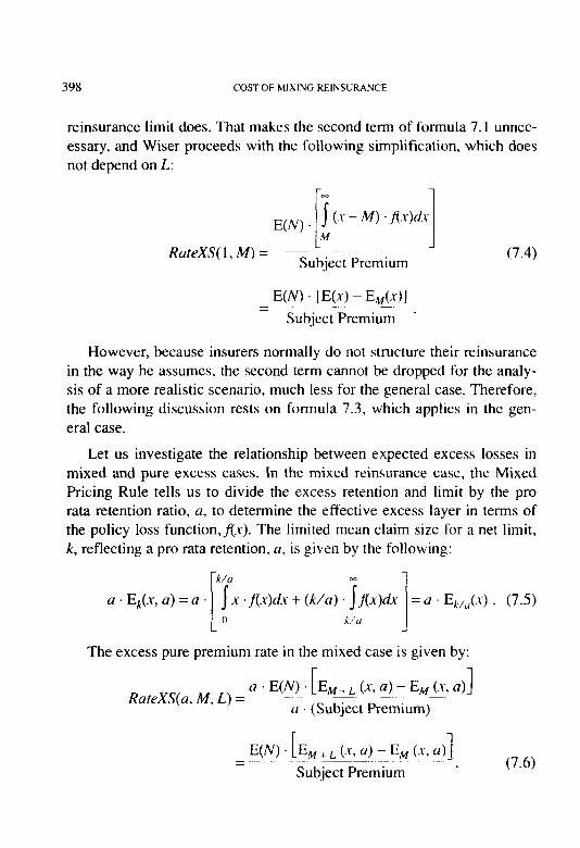
402 COSTOF MIXING KEINSURANCE
Testing the upper end of common excess coverage, which in the pure excess case is $2 million ($250,000 + $1.75 million), yields Prob (s > $2 million) = 0.401%. Ten percent of this is 0.04%. The effec- tive upper bound of coverage in the mixed case is $20 million FGU. Prob (X > $20 million) = 0.01% < 0.04%. which confirms a positive cost of mixing.
The third example involved a $5 million excess casualty policy attach- ing excess of $5 million. There was excess coverage of $1.75 million excess of $250,000 and a proportional cession of 60%. The cost of mix- ing calculation for this example is summarized on Exhibit 5. It shows a negative cost of mixing.
Exhibit 6 is the source of loss information. Since the attachment point of the policy is $5 million, in the pure excess case the reinsurance reten- tion of $250,000 equates to $5.25 million on the FGU loss table. From Exhibit 6, Prob (X > $5.25 million) = 0.008%. Reflecting the pro rata re- tention, 40% of this is 0.003%. This compares to a mixed case retention in FGU terms of $5.625 million ($5 million + $250,000/0.40). Since Prob (s > $5.625 million) = 0.007% > 0.0030/o, this is an indication that the cost of mixing may be negative.
Now examine the upper end of excess coverage. In the pure excess case this is $7 million FGU ($5 million + $250,000 + $1.75 million). Prob (x > $7 million) = 0.004%. Forty percent of this is 0.0016%. This compares to an upper end of $10 million FGU in the mixed case ($5 million + $250,000/0.40 + $1.75 million/0.40). Confirming that the cost of mixing is negative, Prob (x > $10 million) = 0.002% > 0.0016%.
9. CONCLUSION
I hope this discussion will be seen as building on the foundation of Wiser’s original paper. Its purpose has been to aid the reader in under- standing more clearly the effect of mixing proportional and excess of loss reinsurance, and the importance of distinguishing between the cost of overlap and the cost of mixing per se.

COST OF MIXING REINSURANCE 403
REFERENCES
[l] Wiser, Ronald F., “The Cost of Mixing Reinsurance,” PCAS LXXIII, 1986, p. 168.
[2] Miccolis, Robert S., “On the Theory of Increased Limits and Excess of Loss Pricing,” PCAS LXIV, 1977, p. 27.
EXHIBIT 1 ANALYSIS OF REINSURED Loss EXPOSURE vs. INSURED Loss EXPOSURE*
CASUALTY EXAMPLE REINSURED LAYER: $250,000 EXCESS OF $250,000**
CALCULATION OF THE COST OF MIXING PER SE
I
Critical Lnnits of Insured and Reinsured Los Layer\ I and the Corresponding Limited Means
Policies arc> Reiqurcd Layer ~T------J Relattvr Exposure
A B c D E F CI-- H 1 J- K I
i Reinsured Adjusted Effectlke Effective ~ Exposure Rein-
Under- Polk! + Subject Rein- Reten- as % of wred
Remsurance lying POllC) Underlymp Share Effective wrance tion + SUhJWt Suh,jrct Rein\urrd 13) er
structure Retention Limit Retentmn u Retention I .mit Limit LO\\ LO\\ Lavrr Ia\\ Lo\\ #
Pure XS Llmlt\ IOO.004 I .IKX1.000 I . IOO.000 I oO.oO!/r ?SO.oNl 25(I.00() 600.000
I ~~~ Pure - Mixed 4 Y3Y .~... ~~ 3.720 * Loss model I\ lognormal: p = X.6799043: (J = I .8050198. Calculations ust’ Imuted mean\ to precision dlsplayrd. See Exhibn 6 for corresponding
loss dtstribution table. ** Both pure cxccs~ and mixed reinsurancr structures fully expose the ewess reinrurcr in thlc layer. # Bawd on wl+xt prtxuurn~ from rmxcd case.
B=C-A F=G-E H=F/B J=I*H

EXHIBIT 2 ANALYSIS OF REINSURED Loss EXPOSURE vs. INSURED Loss EXPOSURE*
CASUALTY EXAMPLE REINSURED LAYER: $1,750,000 EXCESS OF $500,000**
CALCULATION OF THE COST OF OVERLAP
-I I-
I Critical Limits of Insured and Reinsured Loss Layers
and the Correspondinp Limited Means I T- ( 0 Subject Policies Reinsured Layer ,~ _.“. Relative Exposure
A B c II E F G H I J K ! 52
Reinsured Adjusted ;1
Effective Exposure Rein- g
I Under- Policy + Subject Rein- Effective j as ‘i of sured 2
Reinsurance lying Policy Underlying Share Effective surance Retention Subject Subject Reinsured ~ Layer 0
Structure ~ Retention Limit Retention a Retention
~ Limits l,lOO,OOO lOG.& 600.000 500.000 ~~oO.t& ~ 1 1
Limit +Limit ~ Los\ Loss Layer Loss Loss #
Pure XS
! Lim Means 18.034 9.916 27,950 26.386 1.564 27.950 15.77% 240.000 37,854 18.927’ 2
Mixed Limits Ioo.ooa 1,ooo,000 1.100.000 50.00% 1.100.000 0 1.100.ooo
__ Lim Means’ 18.034 9,916 27.950 27,950 0 27,950 ~ 0.00% 120,000 Oi .~ 0
Pure - Mixed 15.77% 18,927 * Loss model is lognormal: p = 8.6799043: cr = 1.8050198. Calculations use limited means to precision displayed. See Exhibit 6 for corresponding
-..-”
loss distribution table. ** Only pure excess structure exposes the excess reinsurer in this layer. # Baaed on subject premiums from mixed case.
B=C-A F=G-E 6 H=F/B n
J=I*H

EXHIBIT 3 ANALYSIS OF REINSURED Loss EXPOSURE vs. INSURED Loss EXPOSURE*
PROPERTY EXAMPLE REINSURED LAYER: $1,750,000 EXCESS OF $250,000**
CALCULATION OF THE COST OF MIXING PER SE
Reinsurance Structure
-’ , Crltical Limits of Insured and Reinsured Loss Layers
and the CorresppondineLimited Means _.. _. Subject Policies _--” Reinsured Layer Relative Exposure
A B C D E F G H I J
Reinsured Under- Effective Exposure lying Policy + Subject
I
K 2 1 Adjusted i;
Rein 8 Rein- Effective ac 9 of
Reten- Polk\ Underlying Share Effective surance Retention Subject Subject Reinsured ~ sured 1 3
Layer Layer x
lion Llmlt Retention o Retention Limit + Limit Loss Loss Loss Loss # 2 - -___ II
Purr XS Llmlt\ 0 x.000.00 20.ooo.000 Io().owz 250.000 I ,750.000 1.ooo.ocKl 0
Lml Mean\ 0 65.571 65,577 33.205 21.559 54.764 32.88% 300,ooo 98.618 9.863 i
i Mixed Llrnlth 0 20.ooo.00 ?0.om.000 10.00% ‘300.otK~ 17.500.00 20.om.00 I
0 0
Lull Mean\1 0 65.577 65.577 56.475 4,102 65.577 13.8X% 30 .om 1.164~. .--1. Pure Mixed 19.00% 5.699 - -
* Lo\\ model is lo~normal: p = X.X 123226: CT = 2.1482X7 I. Calculation< uw limited mean\ to precirion displayed. See Exhibit 7 for corresponding lo\s diatributlon table.
** Both pure excess and mixed reinsurance structure\ fully expose the excess reinsurer in this layer. # Based on whject premium< from mixed case.
B=C-A F=G-E H=F/B J=I*H

/I
EXHIBIT 4 ANALYSISOFREINSUREDLOSSEXPOSUREVS.INSUREDLOSSEXPOSURE*
PROPERTYEXAMPLE REINSUREDLAYER: $250,000 ExcEssoF$~,OOO,OOO**
CALCULATIONOFTHECOSTOFOVERLAP
I Critical Limits of Insured and Reinsured Loss Layers and the Corresponding L
Subject Policies
A B C D
Under- lying Policy + Subject
<einsurance itructure
I Reten- Policy Underlying Share tion Limit Retention a
__. + tire xs Limits’ 0 2o,m,ow 2O,ooo,OOO 100.00%
LimMeans 0 65,577 65,571
vlixed Limits 0 2O.OOCwOO 2o,ooo,ooo 10.00%
( Lim Means 0 65,571 65,577
Effective Retention
2,OOo.OoO
t *
I
Pure - Mixed 1.41% 422 1
Loss model is lognormal: p = 8.8123226: (J = 2.1482831. Calculations use limited means to precision displayed. See Exhibit 7 for corresponding loss distribution table.
nited Means ___I Reinsured Layer
E
Relative Exposure r
Effective
B=C-A F=G-E H=F/B J=I*H

EXHIBIT5 ANALYSIS OF REINSURED Loss EXPOSURE vs. INSURED Loss EXPOSURE*
REVISED CASUALTY EXAMPLE REINSURED LAYER: $1,750,000 EXCESS OF $250,000**
CALCULATION OF THE COST OF MIXING PER SE
Critical Limns of insured and Reinsured Loss Layers
I
Rein- surance Structure
Pure XS
A
1 Reinwrcd Adjusted LJnder- Effecti\ e Expow-c Rem- lymg Poliq + Subject Rem- Effectl\e a\ [ir of Remcured wred
Keten- POIIC) Llnderl~inf Share Eftectwe ~urance Retention Subyxt Subject Layer Layer tmn Innit Relentton 0 (Retention Limit + Limit LO\\ LO\\ 1.0\5 Loss #
~-i- LInllts 5.000.000 5.ooo.txjo 10.000.000 100.00’~; .5.‘50.00() I .75O.otNj 7.wo.000
Lim Means 29.665 71.5 ‘Y.XXO 29.687 107 ?Y.lY1 1Y.77’; 50.000 24.xx-l 9.953
Mixed Lnnn\ 5.000.000 5.000.000 1lj.000.000 -10.00’; s.62s.otXj 4.375.000 I0.0w.000
I Lim Means ZY.6h.i 215 2Y.XXO ~‘Y.718 lb? Y.XXO 7S..+5Y 20.000 IS .070 15.070 ______ ~~~ ‘,
1- Put-c Mixed -‘.i.58% (5.1 lh)i * Loss model is lognormal: p = 8.67YYO43: ct = I XO5OlYX. Calcula~tons UC limited means to precision displayed. See Exhibit 6 for corresponding loss distribution table. ** Both pure excess and mixed reinsurunce structures fully expose the excess remsurer in this layer. # Baaed on subject premiums from mixed case.
B=C-A F=G-E HTFIR I=l*H
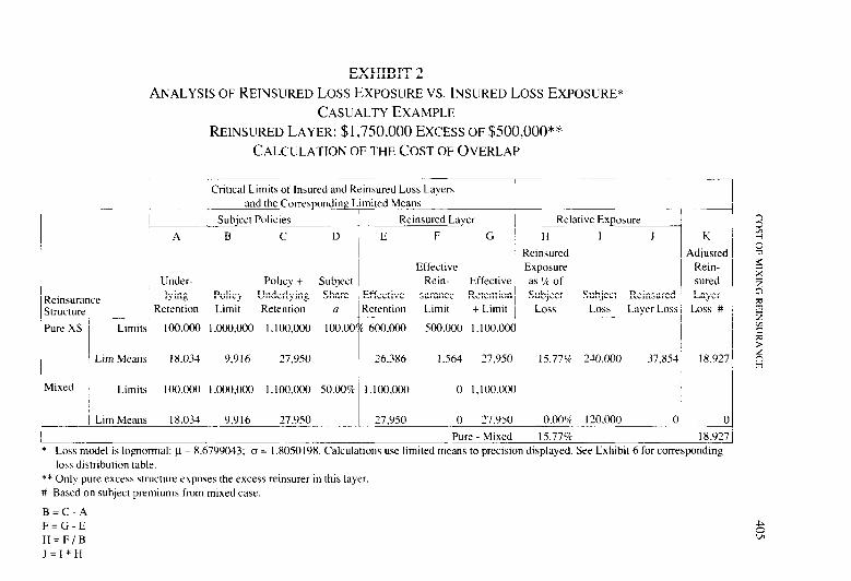
COSTOF MIXING REINSLIRANCE 409
EXHIBIT 6
Limit r(
I00.000
3.50.000 6(H),000
1 ,000,000 1,100,000 I .250,000
Loss DISTRIBUTION TABLE-CASUALTY EXAMPLE
LOG NORMAL MODEL*
t
* c1 = X.6799043 0 = I .XOSOlY8

410 COSTOF MIXING REINSLIRANCE
EXHIBIT 7
Loss DISTRIBUTION TABLE-PROPERTY EXAMPLE
LOG NORMALMODEL*
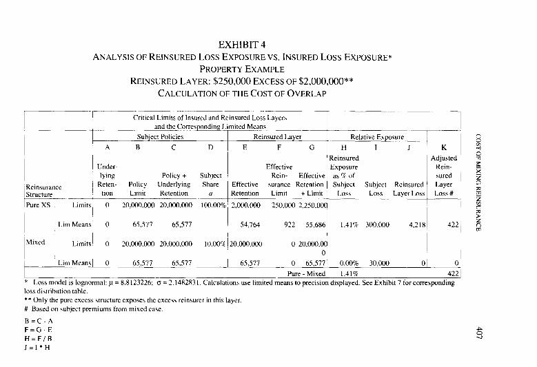
411
ADDRESS TO NEW MEMBERS-NOVEMBER 161992
PAUL S. LISCORD
The theme of this brief address comes from one of your “confreres” who will be writing his last exam this coming Spring. When I asked what he would like to hear upon receiving his Fellowship diploma, he spoke with some apprehension of the ever-increasing expectations of the actuar- ial profession in the form of discipline committees, standards boards, etc., and, perhaps more importantly, the apparent increased probability of mal- practice litigation against actuaries by the publics we serve.
In order to discuss this subject, I think it useful to briefly review how we got where we are as the Casualty Actuarial Society. Then, hopefully, we’ll try to draw some observations from my experiences as an expert witness in a number of litigations involving actuaries.
I’m sure you won’t be surprised that the CAS did not even have a code of professional conduct during its first 50 years of existence. Life was a lot simpler when you only had the Workers Compensation and Automo- bile lines to worry about, and the number of lawyers per capita was at a more reasonable level. It was my generation of actuaries who began composing and subsequently enacting guidelines. We established a code of professional conduct in the 1960s and a series of Statements of Princi- ples for our more important actuarial functions in the 1970s and 1980s. Now, our successor generation is taking the next step by writing profes- sional standards for a whole variety of actuarial functions, and by creating with our sister organizations the Actuarial Board for Counseling and Dis- cipline (ABCD). In some ways, I don’t blame any new member for won- dering what he or she has gotten into.
As for my observations from serving as an expert witness, first and foremost is that allegations of actuarial malpractice usually stem from the plaintiff’s disappointment that actuarial forecasts were not positively ful- filled. While the nature of our profession cannot always guarantee suc- cess, all too often, plaintiffs were simply not adequately apprised of what actuaries do, or better still, what they cannot do. Often, they were over-
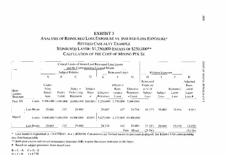
sold on actuarial science. For actuaries in our competitive world, that’s an easy trap to fall into.
Second, a lot of actuarial problems associated with malpractice cases involve what I call the accounting approach to actuarial science. This usually means that a particular methodology is either misapplied or is applied without adequate judgment. Often, the actuary merely applies a formula and accepts the answer because the formula is contained in some actuarial text, or even worse, because it’s been programmed into the black box known as a computer. Further, one of the most important tenets contained in the various CAS Principles is that the actuary must pcr.wr~-
~11~ investigate any changes in the insurance operation being studied so as to modify the data judgmentally as required. It’s these subjective steps that are most often overlooked and the lack of which usually causes most poor forecasts.
Third, in my opinion, such personal investigation also requires a hands-on knowledge of the business most of us serve, the insurance busi- ness. The kind of knowledge I’m talking about is not usually found in actuarial textbooks. For example, most underwriters arc optimists; they have to be or else they could not accept risk. However, this attribute is often exacerbated by management’s insistence on growth. which inevita- bly reduces underwriting selection to the point of lunacy. Actuaries then find themselves in a catch-up posture as to both rates and reserves. De- pending upon the availability of recent data to uncover changing trends, such circumstances can hamper their ability to “prove” their rccommen- dations either to management, or to underwriting, or to both.
Another example of this kind of knowledge would be in the claims operation. Here, the interplay between the adjusters and management is crucial to the understanding of claims data, particularly claim develop- ment. Often management attempts to intervene. usually by strengthening case reserves, which unfortunately distorts, if not completely destroys, historical claim development patterns. At the same time. this strcngthen- ing usually results in the company settling for higher claim amounts. Incidentally, have you ever noticed how adjusters inevitably raise their case estimates just prior to settlement to show management that they have settled for a lower amount than estimated?

ADDRESS TO NEW MEMBERS 413
One last observation: actuarial haste makes for expensive waste in terms of malpractice settlements. Inevitably, most of the actuarial mis- takes I have observed could have been avoided by the actuary’s taking the time to step back to observe the reasonableness of his or her forecast before signing off. The old adage still rings true.
Congratulations on achieving the actuarial successes being recognized today. I’m confident that as you expand your actuarial horizons you will more fully appreciate the guidelines that have been, and are being, estab- lished for the benefit of all actuaries as well as their employers. You certainly have nothing to fear from these constraints. In fact, by observing them to the fullest you will be very well protected against any allegations of wrongdoing that might be directed against you.

414
PRESIDENTIAL ADDRESS-NOVEMBER 16,1992
AN INVESTMENT IN OUR FUTURE
MICHAELL.TOOTHMAN
One of the highlights of my year as President, on a personal basis, was getting Ruth Salzmann back to a CAS meeting, this last May in Chicago, and beyond that having Ruth back at the CAS podium again to provide the address to new members. In her 1979 Presidential Address, Ruth referred to the presidential address as the “last rite” in the term of office of the president.
Then last year, in his address to new members, Dan McNamara indi- cated that CAS past presidents essentially serve the same function as the deceased at an Irish wake-where all the relatives and friends are con- vinced that their beloved has gone on to a better life and are in a mood to celebrate the event. They need a body to legitimize the party, but nobody expects the body to say very much. Such morbid thoughts arise on the occasion when our presidents attempt to provide some last pearls of wis- dom as they slip off into actuarial obscurity.
Fortunately, we at the CAS no longer allow our past presidents to become total “has beens.” We now recycle them in several different ways. One way is the tradition of having a past president address the new Associates and Fellows during the business meeting, but we also now utilize our past presidents on committees. task forces, and on the Board of Directors. This past year, we have been fortunate to have two past presi- dents serve on the Board of Directors, Ron Bornhuetter and Jim MacGinnitie, and their counsel, wisdom. and experience has been of great benefit to the Board. Another past president. Phil Ben-Zvi, has just been elected to a three-year Board term.
Over a year ago, I began to get inquiries from several of our past presidents as to whether I had begun my Presidential Address. Jerry Scheibl was particularly persistent in reminding me of this duty. and I had to continue to reply that I had not yet begun it. Actually. 1 did have an outline of my Presidential Address done well over a year ago, but I have

PRESIDENTIAL ADDRESS 415
now decided not to use it. The title was “Winning the Rat Race,” an appropriate description of what goes on during a president’s term. The outline consisted of five points:
1) Worship God in whatever way you know Him-or Her.
2) Nurture and enjoy the personal relationships.
3) Know and understand yourself as a professional and the profession that you are a part of, and commit some time to improving it.
4) Understand the dynamics of the business you are in.
5) Dream BIG dreams.
As I said, I have decided not to use that address. Perhaps I will use it some time in the future. On the other hand, if any of you like the ideas in that outline, feel free to use it yourself. Still, I would like to spend just a minute on the second point: the personal relationships that one establishes within the CAS over the years.
It is easy for any one of us to get wrapped up in our own individual rat races and not really appreciate all of the opportunities for personal rela- tionships and friendships that present themselves as part of our day-to- day activities. The CAS is filled with wonderful people. What remains, years after the Committee work is completed, are the personal relation- ships that were developed in the performance of that work. Even after business relationships are terminated, the bonds that we share as friends and as members of the actuarial profession remain. So I hope each of you will take advantage of the opportunities you have to serve the CAS and, more importantly, take advantage of the opportunities you have to de- velop those friendships and bonds that will prove to be of lasting value. But, as I said, that is another speech.
Today, I would like to talk about an investment in our future: an investment in the future of the CAS and in the futures of all of us collec- tively as casualty actuaries.
Investments are not always made knowing just where they will lead. By far, the majority of incoming college freshmen either have not yet decided upon their major field of study or will change that selection on at
416 PKESIIEN’I‘IAI. 4lX)KliSS
least one occasion before graduation. I was in the minority on that score. I entered a five-year dual degree program in Applied Mathematics and completed that program, yet my career direction changed drastically over the course of those five years. Many individuals, once they have com- pleted their degree programs, do not work in the field covered by their degree. yet that education is not wasted. Those years of study represent an investment in one’s future, the acquisition of specific knowledge and the development of an ability to think and analyze critically. Those invest- ments almost always prove to be worthwhile, even though we do not know precisely where they will lead at the time that WC‘ make them.
The actuarial exams, though much more specific. can be described in much the same way. Our education as actuaries is not completed at the time that we complete our actuarial exams. Indeed. it has just begun. Much of the knowledge that I USC: in my professional career thehe days was not even known at the time that I was taking actuarial exams. Envi- ronmental liabilities were not an issue back in the early 1970s. Captive insurance companies existed, but were such a small factor in the market- place that they were hardly mentioned anywhere in the S~dl~h~r~s. Finan- cial reinsurance is a whole new area since then, and I do not believe that the term commutation was used anywhcrc in the readings on the S~//rh~r.s that I had. The list can go on and on.
Similarly with on-the-job training. Successful carters usually are the accumulation of one successful task after another or the successful com- pletion of one set of responsibilities after another. It is the rare individual that can lay out his future career progression while still in his Z&-per- haps in very broad strokes-but the point is that it is much more common to really not know what the future may hold. But if you do your current job well and learn as much about your business as possible. good oppor- tunities will become available to you.
So it is with the CAS as an organization and with our profession as a whole.
Today, I would like to focus on investments that wc can make to expand our vision in three areas.

PRESIDEN7lAL AVVRESS 417
First, I have the vision of the CAS in the future becoming a resource for developing casualty actuaries throughout the world.
Second, I have the vision of us as casualty actuaries moving from the realm of assessing risks associated with the insurance transaction to the broader area of risk financing. That is, quantifying the financial impact of future contingent events wherever they occur, not just within the insur- ance transaction. The most obvious area is the whole field of self-insur- ance, which, in its myriad forms, annually makes up a larger and larger percentage of the commercial insurance market.
Third, we must move from being experts in particular liabilities to being experts on the total balance sheet.
I believe it is time for us to make investments as an organization and as professionals that will move us in these directions, yet I cannot tell you what all the implications of those investments will be. I do firmly believe, however, that these investments will prove to be beneficial to the CAS and to the actuarial profession.
In his 1976 Presidential Address, Ron Bornhuetter said that the CAS had been concentrating all its efforts in the continental United States and to this degree had been selfish. He said that there was an acute need, a search for knowledge in the property and casualty business worldwide, and that we were the owners of the biggest bank. Ron’s address, entitled “Challenges,” included the challenge of expanding our horizons beyond the United States. We have accomplished much since 1976, but our hori- zon as an organization has still been limited largely to North America. It is time for us to become active participants in the worldwide actuarial community.
It made me feel very good when I was described once as a “world class” actuary. Whether that description was accurate or not, it is my belief that the CAS has many world class actuaries, but we need a global vision. Over the last few years, I believe we have begun to develop that vision, and we have made some of the initial investments that we need to make, but the first step is one of perspective and attitude. Individually and collectively, we must begin to see ourselves as part of the worldwide actuarial community, and we must begin to view insurance as only one

318 PRESIVEU’I‘IAl. AVVRESS
form of risk financing. At the same time, we must take a more holistic view of our role as financial experts, particularly with regard to insurance companies, as we expand our role from being experts on loss and loss adjustment expense liabilities to bein g experts on the total financial con- dition of insurance companies.
What. then, are some of these investments?
I. The Academic Base
First. we need a broader academic base. In this regard. it could be argued that the profession in Europe is further advanced than it is here in North America. We refer to our field as actuarial science, yet we spend relatively little energy in pushing the frontiers of that science outwards. and we can hardly claim that the science is fully developed.
I am not one to believe that the best actuaries necessarily come from actuarial science programs. Indeed, I believe that there is much more to being a good actuary than being technically competent, but we must, as a profession, maintain and improve upon our technical competence. Other skills need to be developed in addition to that but not at the expense of it. I am convinced that an investment in develop- ing a stronger academic base will strengthen our profession.
2. The Knowledge Base
The idea of improving and expanding upon our collective knowl- edge base goes hand in hand with strengthening the academic base. Our relatively new philosophy of managed research within the CAS is now beginning to pay dividends. but even thih improved flow of productive research does not begin to fulfill the future potential for our profession. A strong academic base will improve the amount of productive research by orders of magnitude. I don’t believe we will ever want to limit our research efforts to academia. But, to believe that we can fulfill the research needs 01‘ our profession without a strong contribution from academia is naive and faulty reasoning in my view. The global vision is important here. in many ways. We have implemented a literature exchange with many foreign actuarial socie- ties, and I hope our membership will start to take advantage of the

PRESIDENTIAL ADDRESS 419
easier access to this literature. Other fields are making advances that are either directly or indirectly applicable to risk financing, and we need to expand our collective knowledge base to encompass those developments. No one can foretell where this investment will lead us, but I am convinced that investments in expanding our collective knowledge base can’t help but benefit our profession.
3. Basic Education
I believe it is now time for us to begin the process of making a major investment in the design of our basic education system and in its implementation. The implementation issue involves accelerating the long-term gradual trend in our exams from an emphasis on spe- cific, detailed knowledge to an understanding of principles and devel- opment of the individual’s ability to apply those principles. The structural investment we must make is to restructure our Syllabus so
as to separate the actuarial principles that apply to casualty insurance anywhere in the world from the knowledge that is important for someone if they are to practice in the United States or in Canada. Once such a syllabus is achieved, conceptually it would be possible for us to qualify actuaries who wish to practice in the United States and who are fully qualified abroad by having them pass simply the exams that focus on the nation-specific material. I believe it is appro- priate for the CAS to make such an investment. Once we have done so, we will be in a better position to participate in the development of casualty actuaries throughout the world.
In all of this, it is not my suggestion that the CAS try to impose itself upon existing actuarial organizations abroad. Rather, I believe that the CAS can serve as an important resource that will add value to a partnership involving the CAS and other existing actuarial organiza- tions around the world. Our members will benefit from such an ex- pansion of our vision, and I believe we bring enough value to the table that the members of the actuarial profession abroad will benefit as well. But, in all our endeavors, we must act as true and equal partners and treat all of our potential partners as we would wish to be treated.

4. Continuing Education
Our continuing education program has been successful by almost any standard. yet we must make a significant short-term investment here as we move to prepare our mcmbcrs to function as appointed actuaries opining on an insurer’s current and future solvency pros- pects. In the longer term, as we adopt a more global perspective. OUI
continuing education program will have to expand to provide many tttorc opportunities than are currently being provided, in order to allow each individual to find those continuing education opportunities that will best assist that individual in the development of his or her career. This investment will rcquirc an expansion of our vision and will require us to leverage our rcsourccs much more than we do today. It will require us to use resources from outside the actuarial community, where appropriate, but it is an investment that will bcne- fit our profession.
5. Standards of Practice and Discipline Procedures
The final investment is one that we have already started to make- an investment in the development of standards of practice and in the establishment of a well-functioning, self-policing procedure. I will combine these two areas because they are so closely related and be- cause we have made the initial investments in both areas. both in the United States and in Canada. These issues arc also very high priority issues for the actuarial profession around the world. Indeed. virtually every actuarial organization is either actively involved or is highly concerned with how to become more involved in these two areas. The initial investments in North America have been made with the estab- lishment of the Actuarial Standards Board and the development of Standards of Practice within Canada. and with the establishment of the ABCD and development of stronger disciplinary procedures within the CIA. Yet these investments are just the beginning. Ongoing investments will be required as further standards of practice arc de- veloped and as we, as a profession. now face up to the questions of whether we are really prepared to police ourselves. As in all of the other investments, WC do not know just where these investments will

PRESIDENTIAL AVDRESS 421
lead, but I am convinced that investments in these areas are necessary to the further development of our profession.
What will these investments mean to us organizationally? I do not know. I believe that in public interface issues it is important for the actuarial profession within each country to be able to speak with one voice. It was for this reason that we established the American Academy of Actuaries within the United States. That organization is important to our collective future. However, the Casualty Actuarial Society and the Society of Actuaries are basically research and educational organizations. The research and educational functions are, for the most part, not nation-spe- cific, and I strongly believe that it is therefore beneficial for the research and educational functions to be organizationally separate from the public interface function.
Some leaders of our profession decry the separation of the casualty branch and have suggested that actuaries ought to be qualified to practice in all practice areas. I believe that that philosophy is misguided. I am persuaded that the casualty branch of the profession is stronger in the United States than it is anywhere else in the world. As Ron Bornhuetter said, we have the biggest bank of property/casualty actuarial knowledge. I believe that it is highly unlikely that our bank would be anywhere near the size that it is if it were not for the founding of the Casualty Actuarial and Statistical Society of America, now the Casualty Actuarial Society, in November I9 14.
I believe it is appropriate for all actuaries to have some basic under- standing of the underlying concepts and principles in the other branches of the actuarial profession-what I would call “conversational compe- tence”-but I believe that it is far more important for us to maintain the depth of knowledge that we provide to members of the Casualty Actuarial Society than it is to dilute that effort over several branches of the actuarial profession. For this reason, we will continue to resist any attempts to undermine a separate casualty organization. Rather our focus needs to be on cooperation, not consolidation, with the other North American actuar- ial organizations wherever that makes sense. Our focus must also be on creating new partnerships with actuarial organizations abroad, as we ex-

422 PRESIDENTIAL ADDRESS
pand our view as casualty actuaries and assist in the development of the actuarial profession on a global basis.
Investments in our future-Big dreams!
This is a wonderful profession. 1 hope that each of you will involve yourselves in it deeply. Debate the vision and the investments. Work to shape them, and then make them happen.
In closing, I would like to share a poem entitled, “Take Time.” It clearly is written with the intention that it be applied to your individual lives, but I would ask that you listen to it and think of how you might apply it in the context of the CAS-
TAKE TIME
Take time to WORK: it is the Price of Success. Take time to THINK: it is the Source of Power. Take time to PLAY: it is the Secret of Perpetual Youth. Take time to READ: it is the Fountain of Wisdom. Take time to WORSHIP: it is the Highway to Reverence. Take time to be FRIENDLY: it is the Road to Happiness. Take time to LAUGH: it is the Music of the Soul. Take time to DREAM: it is Hitching Your Wagon to a Star. TAKE TIME TO LIVE.
In two days, it will be time for me to take some time. Thank you for the honor of serving as your President.

423
MINUTES OF THE 1992 ANNUAL MEETING
November 15-18. 1992
THE BOCA RATON RESORT & CLUB BOCA RATON, FLORIDA
Sunday, November 15, I992
The Board of Directors held their regular quarterly meeting from noon until 5:00 p.m.
Registration was held from 4:00 p.m. until 630 p.m.
From 5:30 p.m. until 6:30 p.m., there was a special presentation to new Associates and their guests. The session included an introduction to the standards of professional conduct and the CAS committee structure.
A welcome reception for all members and guests was held from 6:30 p.m. until 7:30 p.m.
Monday, November 16.1992
Registration continued from 7:00 a.m. until 8:00 a.m.
CAS President Michael Toothman opened the meeting at 8:00 a.m. with the results from the recent election of officers. The members of the 1993 Executive Council will be Vice President-Administration, John M. Purple; Vice President-Admissions, Steven G. Lehmann; Vice President- Continuing Education, David N. Hafling; Vice President-Programs and Communications, Alice H. Gannon; Vice President-Research and Devel- opment, Allan M. Kaufman. President-Elect will be Irene K. Bass. New Board members will be Albert J. Beer, Phillip N. Ben-Zvi, Michael J. Miller, and Susan T. Szkoda.
Toothman thanked the outgoing Board members and welcomed es- teemed guests in the audience, including: Tim Tinsely, executive director of the CAS; Takehisa Kikuchi, vice president, Institute of Actuaries, Japan; James Murphy, executive vice president, American Academy of Actuaries; Donald Sondergeld, past president of the Society of Actuaries; Pablo Noriega, president of the Instituto National de Estadistica (Mex-

424 ~IINl~~l-IiS OI~Tlit’ I992 \NNI’,\I w:r.nN(;
ice): and Oliva Sanchez. director ol’the Escuela dc Actuaria, Universidad Anahuac (Mexico).
John Purple read the Secretaryflreasurer’s Report.
Steven Lehmann and Allan Kaufman introduced the 52 new Associ- ates and David Flynn introduced the 62 new Fellows ai the meeting. The names of these individuals follow.
Rebecca C. Amoroso Anthony J. Balchunas Douglass L. Beck Nathalie Begin Martin Cauchon Denis Cloutier Jeffrey R. Cole Charles Cossette Robert J. Curry Francois Dagneau Patrick K. Devlin John W. Ellingrod James Ely David A. Foley France Fortin John F. Gibson Susan M. Gozzo Eric L. Greenhill Diane K. Hausscrman Todd J. Hess James S. Higgins
FELLOWS
Keith D. Holler George A. Hroziencik Kathleen M. Ireland Peter H. James Brian J. Kincaid Richard 0. Kirste Ronald T. Ko/.lowski David J. Kretsch John A. Lamb Jean-Marc L&eillP Blaine C. Marles Burton F. Marlowe Steven E. Math Liam M. McFarlane William T. Mech Charles B. Mitzel Richard B. Moncher Todd B. Munson Margaret M. O’Brien Jacqueline E. Paslq Susan J. Patschak
Robert Potvin Richard W. Prescott Kenneth P. Quintilian Kay K. Rahardjo Srinivasa Ramanujam Scott E. Reddig Sharon K. Robinson Diane R. Rohn Edmund S. Scanlon Margaret E. Seiter Marie Sellitti Vincent M. Senia Christy L. Simon Christopher M.
Smerald Douglas N. Strommen Michael A. Visintainer Sebastian Vu Christopher P. Walker Marjorie C. Weinstein Gregory S. Wilson

MINUTES OF THE 1992 ANNUAL MEETING 425
Daniel N. Abellera Nancy L. Arico George P. Bradley Donna D. Brasley Ward M. Brooks Linda J. Burrill Anthony E. Cappelletti Mary L. Corbett Jeffrey L. Dollinger Jeffrey D. Donaldson Paul E. Ericksen Lynne W. Faucher Judith M. Feldmeier Russell Frank Laurence B. Goldstein Sandra K. Halpin Bradley A. Hanson Renee Helou
ASSOCIATES
Jeffrey R. Hughes Daniel R. Keddie Ann L. Kiefer Stephen E. Lehecka Stephanie J. Lippl James M. Maher Galina Margulis Heather L. McIntosh Van A. McNeal Raymond D. Muller Mary Beth O’Keefe Douglas W. Oliver Richard A. Olsen William Oostendorp Todd F. Orrett Joseph M. Palmer Jennifer J. Palo Daniel A. Powell
Jean Roy Maureen S. Ruth Melodee J. Saunders Jeffery J. Scott Gregory R. Scruton James J. Smaga Scott J. Swanay Charles F. Toney, II Michael J. Toth James F. Tygh David B.
Van Koevering Phillip C. Vigliaturo William E. Vogan Stephen D. Warfel Joyce A. Weisbecker Ralph T. Zimmer
Paul S. Liscord was introduced and gave the Address to New Mem- bers.
Mr. Toothman presented the 1992 Matthew Rodermund Service Award to Norman J. Bennett. As part of the presentation ceremony, Toothman read a letter from Matt Rodermund.
A moment of silence was held to mark the passing of six members of the CAS during the past year.
Mr. Beer gave the highlights of the program, and Chairman of the Committee on Review of Papers Richard Biondi summarized the six Proceedings papers being presented. The Woodward-Fondiller Prize was awarded to William R. Gillam and the Dorweiler Prize was awarded to John P. Robertson. Mr. Toothman made a call for reviews of previously presented Proceedings papers and received no responses.
A General Session panel discussion was held from IO:00 a.m. until IO:45 a.m. on “The Role of the American Academy of Actuaries.” The

session was led by David G. Hartman. with Ronald L. Bomhuetter and Michael A. Walters as panelists.
The Featured Speakers. Fred Barnes and Morton Kondracke, senior editors of T/w NCM’ Rqmhlic~ and frequent panelists on “The McLaughlin Group.” spoke from 10:4S a.m. until noon.
Their presentation was followed by a luncheon with the Presidential Address by Michael Toothman. Lunch wa\ from noon until I:30 p.m.
The afternoon was dcvotcd to concurrent sessions which consisted ot various panels and papers.
The panel presentations cover4 the following topics:
1. Finite Risk Rcinsurancc-Three Perspectives
Moderator: Heidi E. Hutter Executive Vice President Atrium Corporation
Panelists: Gregory E. Leonard President and Chief’ Exccutivc Officer Pegasus Advisors, Inc.
Richard J. Roth, Jr. Assistant Commissioncl Calit’ornia Department of Insurance
David Holman Partner Ernst & Young
2. The Alphabet Soup of Professionalism: AAA, ABCD, ASB, and CIA
Moderator: Jerome A. Scheibl (Chairman CAS Discipline Committee and Member Actuarial Board for Counseling and Discipline) Vice President-Industry Affitirs Wausau Insurance Companies

MINUTES OF THE 1 ‘)c)2 ANNUAL. MEETING 421
Panelists: W. James MacGinnitic (Chairman American Academy of Actuaries Committee on Professional Responsibility) Consulting Actuary Tillinghastflowers Perrin
Michael J. Miller (Chairman Actuarial Standards Board Casualty Committee) Consulting Actuary Tillinghast/Towers Perrin
3 _ . Loss Distributions and the Collective Risk Model
Speaker: Stuart A. Klugman, F.S.A., Ph.D. Principal Financial Group Professor of Actuarial Science College of Business and Public Administration Drake University
4. What an Investment Department Needs to Know from an Actuary
Moderator: Sheldon Rosenberg Vice President and Chief Actuary Continental Insurance
Panelists: Walter Blasberg President Continental Asset Management
Sar Kun Moy Vice President Continental Asset Management
5. New IS0 Risk Load in ILFs-What Does it Mean‘?
Moderator: Gary S. Patrik Senior Vice President and Actuary North American Reinsurance Corporation

428 MIPXTES OFTl1E I’)‘)2 ANNUAL MEETING
Panelists: Glenn G. Meyers Assistant Vice President and Actuary Insurance Services Office. Inc.
Ira Robhin, Ph.D. Assistant Vice President Director of Actuarial Research CIGNA Property & Casualty Companies
Edward W. Weissnet Vice President, Actuarial Prudential Reinsurance Company
6. The Oakland Fires-What Have We Learned?
Moderator: Karen F. Terry Actuary State Farm Fire and Casualty Company
Panelists: Joseph Meyer Senior Vice President United Services Automobile Association Western Region
Tom Morrison Property Lines Director-Claims Allstate Insurance Companies
7. Risk Classification Principles
Panelists: Cecily A. Gallagher (Chairperson-Committee on Risk Classification) Consulting Actuary TillinghasQTowers Perrin
Frederick F. Cripe Assistant Vice President Allstate Insurance Company
Kevin J. Conley Actuarial Administrator Iowa Insurance Division

MINUTES OFTHE 1992 ANNUAL MEETING 429
8. Questions and Answers with the CAS Board of Directors Moderator: David P. Flynn (President-Elect)
Senior Vice President and Chief Actuary Crum & Forster Corporation
Current Board Members: Janet L. Fagan (Elected 1989)
Director of Casualty Actuarial Services Coopers & Lybrand
Gary S. Patrik (Elected 1991) Senior Vice President and Actuary North American Reinsurance Corporation
The new Proceedings papers presented were:
1. “Workers’ Compensation Experience Rating: What Every Actuary Should Know”
Author: William R. Gillam National Council on Compensation Insurance
2. “Stochastic Claims Reserving When Past Claim Numbers Are Known”
Author: Thomas Wright Consultant
3. “Pricing for Credit Exposure”
Author: Brian Z. Brown Milliman & Robertson, Inc.
The officers held a reception for new Fellows and their guests from 5:00 p.m. until 6:00 p.m. There was a general reception for all members from 6:00 p.m. until 7:OO p.m. The musical comedy, “The Sting,” was presented from 7:00 p.m. until 8:30 p.m.
Tuesday, November 17, I992
A General Session on a “Mock Trial on Actuarial Professional Stan- dards” was held from 8:30 a.m. to IO:00 a.m. David S. Powell, Consult- ing Actuary with Tillinghast/Towers Pert-in, and Ralph B. Levy, Esq., of King & Spalding, were the presenters.
430 MtNLlTES OFTHE ic)c)? ANNIIAI. MI:t:t‘tXi
From IO:00 a.m. until noon, several concurrent sessions were held. The panel presentations, in addition to some of the subjects covered on Monday, covered the topics of:
I. Malpractice Avoidance for Actuaries Moderator: David S. Powell
Consulting Actuary Tillinghast/Towers Perrin
Panelists: Ralph B. Levy King & Spalding
Jack M. Turnquist (Chairman, Actuarial Standards Board) Totidem Verbis
Lauren M. Bloom General Counsel American Academy of Actuaries
2. CAS-Sponsored Research
Moderator: Allan M. Kaufman (Vice President-Research and Development) Principal Milliman & Robertson, Inc.
Panelists: LeRoy A. Boison, Jr. (Liaison to SOA Research Policy Committee) Vice President insurance Services Office. Inc.
Gregory L. Hayward (Chairperson, Ratemaking Commitlee) Actuary State Farm Mutual Automobile Insurance Co.
James W. Yow (Chairperson Valuation & Financial Analysis Committee) Vice President and Corporate Actuary Aetna Life & Casualty

MINUTES OFTHE 1992 ANNUALMEETING 431
3. Catastrophe Insurance Futures
Moderator: Joseph A. Herbers Consulting Actuary Tillinghast/Towers Perrin
Panelists: Gregory Samorajski Group Manager-Financial Instruments Economic Analysis and Planning Chicago Board of Trade
Stephen P. D’Arcy Department of Finance, University of Illinois
Jonathan Lewis Manager, Fixed Income Portfolio Skandia Investment Managers
4. Considerations Regarding Catastrophic Medical Claims and Automobile Insurance
Panelists: William J. VonSeggern Chief Actuary AAA Michigan
Roger M. Hayne Consulting Actuary Milliman & Robertson, Inc.
5. Experience Rating Overview
Moderator: Mark W. Mulvaney Consulting Actuary Milliman & Robertson, Inc.
Panelists: William R. Gillam Assistant Vice President and Actuary National Council on Compensation Insurance
David M. Bellusci Senior Vice President and Actuary Workers’ Compensation Insurance Rating Bureau of California

One new Proceedings paper presented was: 1. A Review of “The Competitive Market Equilibrium Risk Load
Formula for Increased Limits Ratemaking” (Glenn Meyers, PCAS LXXVIII)
Author: It-a Robbin, Ph.D. Assistant Vice President Director of Actuarial Research CIGNA Property & Casualty Companies
The afternoon was reserved for committee meetings.
A clambake was held from 6:30 p.m. until IO:30 pm.
Wednesday. Nownhv- 18, 1992
From 8:OO a.m. to 9:30 a.m. several concurrent sessions were held and two i’roc~eedin~~s papers were presented. They were:
1. Credibility Based on Accuracy”
Author: Joseph A. Boor Director-Actuarial Motors Insurance Corporation
2. A Review of “The Cost of Mixing Reinsurance” (Ronald F. Wiser, PCAS LXXIII)
Author: Michael Wacek General Manager St. Paul Fire & Marine Insurance Company
Following a refreshment break, a General Session was held on the topic of “The NAIC’s Examination of the NCCI.”
Moderator: E. Frederick Fossa Consulting Actuary Milliman & Robertson, Inc.
Panelists: Margaret C. Spencer Arthur Andersen & Co.
Patrick J. Grannan Consulting Actuary Milliman & Robertson, Inc.

MINUTES OF THE 1992 ANNUAL. MEETING 433
Ronald C. Retterath Senior Vice President and Actuary National Council on Compensation Insurance
James D. Watford Actuary Florida Insurance Department
After the transfer of the presidency, Michael Toothman gave the clos- ing remarks. The meeting adjourned at 11:45 a.m.
Nowmher I992 Attenders
In attendance, as indicated by the registration records, were 363 Fel- lows, 193 Associates, and 64 guests, subscribers, and candidates. The list of members’ names follows.
Abell, Ralph Alfuth, Terry Amoroso, Rebecca Anker, Robert Apfel, Kenneth Aquino, John Artes, Lawrence Asch, Nolan Atkinson, Richard Balchunas, Anthony Barnes, W. Brian Bass, Irene Bassman, Bruce Beck, Douglas Beer, Albert Begin, Nathalie Bell, Linda Bellusci, David Bennett, Norman Ben-Zvi, Phillip Berens, Regina
FELLOWS
Biegaj, William Bill, Richard Biller, James Biondi, Richard Blair, Gavin Blakinger, Jean Blanco, Robert Blodget, Hugh Boison, LeRoy Boor, Joseph Bomhuetter, Ronald Boyd, Wallis Bradley, Scott Braithwaite, Paul Brannigan, James Brehm, Paul Brown, Brian Bryan, Charles Buck, James Captain, John Cardoso, Ruy
Carlson, Christopher Carpenter, William Carroll, Lynn Cascio, Michael Cauchon, Martin Caulfield, Michael Charest, Danielle Chernick, David Chiang, Jeanne Christie, James Chuck, Allan Cieslak, Walter Ciezadlo, Gregory Cis, Mark Clark, Brooks Cloutier, Denis Cole, Jeffrey Cook, Charles Corr, Francis Cossette, Charles Gripe, Frederick

Crowe, Alan Cundy, Richard M. Cut-ran, Kathleen Currie, Diana Currie. Ross Curry, Alan Curry, Robert Dagneau, Francois Daino, Robert D’Arcy. Stephen Dean, Curtis G. Dekle. James DeLiberato. Robert Dembiec. Linda Dempster, HowardDevlin. Patrick Dodd, George Dolan, Michael Dornfeld, James Drennan, John Duffy, Timothy Dukatz, Judy Dye. Myron Ezarwaker, Bruce Edlefson, Dale Effinger. Jr., Bob Ellefson, Thomas Ellingrod, John Ely, James Englander, Jeffrey Engles. David E?icson, Janet Faga, Doreen Fagan, Janet Fein, Richard
Finger, Robert Fitzgerald, Beth Fitzpatrick. William Flynn, David Foley, David Forker, David Fortin, France Fossa, E. Frederick Frohlich, Kenneth R. Furst, Patricia Fusco. Michael Gallagher, Cecily Gallagher, Thomas Gannon, Alice Garand. Christopher Gardner, Robert Gebhard, James Gelinne, David Gibson, Richard Gibson, John A. Gibson, John F. Gill, Bonnie Gillam, Judy Gillam. William R. Gilles, Joseph Gillespie. Bryan C. Girard. Gregory Gluck, Spencer Goddard, Daniel Goldfarb, Irwin Gottlieb, Leon Gozzo, Susan Grady, David Grannan, Patrick Grant. Gary
Graves, Gregory Greco, Ronald Grecnhill. Eric Griffith, Ann Groh, Linda Hafling, David Hale, Kyleen Hall, James Harrison, David Hartman, David Hausserman. Diane Hayne. Roger Hayward, Gregory Hennessy. Mary Hccr. E. LeRoy Henry, Dennis Hermes, Thomas Hess, Todd Hcyman, David Higgins, James Hines, Alan Holler, Keith Hough. Paul Howald, Ruth Hroziencik, George Hutter. Heidi Ingco, Aguedo lrcland, Kathleen It-van, Robert James, Peter Jameson. Stephen John. Russell Johnson. Marvin Johnson, Warren Jones, Bruce

MINUTES OF THE 1992 ANNIIAI, MEETING 435
Kane, Adrienne Karlinski, Frank Kaufman, Allan Keen, Eric Keller. Wayne Kincaid, Bryan Kirste, Richard Kist, Fredrick Koupf, Gary Kozlowski, Ronald Krakowski, Israel Kreps, Rodney Lalonde, David Lamb, Dean Lamb, John LaMonica, Michael Lebens, Joseph Lehmann, Steven Leonard. Gregory Leong, Winsome Leveille, Jean-Marc Levin, Joseph Lew, Allen Lipton, Barry Liscord, Paul Lo, Richard Loisel, Andre Lotkowski. Edward Lowe, Stephen Ludwig, Stephen MacGinnitie, James Marks, Steven Marles, Blaine Marlowe, Burton Mashitz, Isaac
FELLOWS
Math, Steven Mathewson, Stuart McAllister, Kevin McClure, John McCoy, Mary McDonald, Gary McFarlane, Liam McManus, Michael Mealy, Dennis Mech, William Menning, David Meyers, Glenn Miccolis, Robert Miller, David Miller, David Miller, Mary Frances Miller, Michael Miller, Philip Miller, Susan Miller, William Mitchell, H. Elizabeth Mitzel, Charles Moncher, Richard Morrow, Jay Mucci, Robert Mueller, Nancy Mulder, Toni Muleski, Robert Mulvaney, Mark Munro, Richard Munson, Todd Murphy, Daniel Murrin, Thomas Muza, James Myers, Thomas
Nelson, Chris Nelson, Janet Nemlick, Kenneth Nester, Karen Newell, Richard Nichols, Richard Nickerson, Gary Norton, Jonathan O’Brien, Margaret O’Connell, Paul Oien, R. Gus Onufer, Layne Overgaard, Wade Pagnozzi, Richard Palm, Robert Parker, Curtis Pasley, Jacqueline Patri k, Gary Patschak, Susan Perreault, Stephen Peterson, Steven Petit, Charles Philbrick, Stephen Pinto, Emanuel Post, Jeffrey Potvin, Robert Pratt, Joseph Prescott, Richard Prevosto, Virginia Pridgeon, Ronald Purple, John Quintano, Richard Quintilian, Kenneth Quirin, Albert Racine. Andre

436 MINL:Tt:S OFTtiE 1992 A'i\'NL.41. MW'l li\(i
Rahardjo, Kay Ramanujam, Srinivasa Reale, Pamela Sealand Reddig, Scott Retterath, Ronald Richardson, James Robinson, Richard Robinson, Sharon Rominske, Steven Rosenberg, Sheldon Ross, Gail Roth, Jr., Richard Salton, Jeffrey Salton. Melissa Sandman, Donald Scanlon, Edmund Scheibl, Jerome Scheuing, Jeffrey Schmidt, Jeffrey Schmidt, Neal Schultheiss, Peter Schultz, Roger Schwartzman, Joy Seiter, Margaret Sellitti, Marie Shepherd, Linda Sherman, Harvey Shoop, Edward Shrum, Roy
FELLOWS
Silver, Melvin Simon, Christy Simon, LeRoy Skurnick, David Smerald, Christopher Sobel, Mark Spidell, Bruce Stanard, James Steeneck, Lee Steinen, Phillip Steiner& Lawrence Stergiou, James Stewart. C. Walter Strommen, Douglas Suchoff, Stuart Sutter, Russel Svendsgaard, Christian Szkoda, Susan Taylor, Angela Taylor, Frank Taylor, Jane Terrill, Kathleen Terry, Karen Thompson, Kevin Tistan, Ernie Toothman, Michael Treitel. Nancy Trudeau, Michcl Venter, Gary
Verges, Ricardo Visintainer, Michael Visintine. Gerald Visner, Steven VonSeggern, William Votta, James Vu. Sebastian Wacek. Michael Walker. Christopher Walker, Glenn Walters, Michael Walters, Mavis Walton, Patrick Wargo, Kelly Weber, Dominic Weinstein, Marjorie Weissner, Edward White, David White, Jonathan Whitlock, Robert Whitman, Mark Wildman, Peter Willsey. Robert Wilson, Gregory Winslow. Martha Wulterkens, Paul Yocius, Richard Yow, James W. Zatorski. Richard
MINUTES OF THE 1992 ANNUAL MEETING 431
Abellera, Daniel Allard, Jean-Luc Allison, Kerry Anderson, Bruce Andler, James Applequist, Virgil Arico, Nancy Ashman, Martha Bauer, Bruno Boardman, Thomas Bradley, George Brasley, Donna Brauner, Yaakov Brooks, Ward Bums, William Burt-ill, Linda Cappelletti, Anthony Casale, Kathleen Cellars, Ralph Chabarek, Paul Charbonneau, Scott Chen, Chyen Chorpita, Fred Closter, Donald Coca, Michael Connor, Vincent Conway, Thomas Corbett, Mary Covitz, Burton Creighton, Kenneth Curry, Michael Daly, Michael Davenport, Edgar Davis, Brian Davis, James
ASSOCIATES
DeConti, Michael Der, William Diss, Gordon Dollinger, Jeffrey Donaldson, Jeffrey dos Santos, Victor Douglas, Frank Dubin, Michael Ebert, Maribeth Elia, Dominick Emmons, William Ericksen, Paul Faucher, Lynne Feldmeier, Judith Fields, David Fonticella, Ross Frank, Russell Gaillard, Mary Gerard, Felix Gerlach, Scott Gidos, Peter Godbold, Nathan Terry Goldberg, Steven B. Goldberg, Terry Goldstein, Laurence Granoff, Gary Griffith, Roger Grose, Carleton Gusler, Terry Gutman, Ewa Haidu, James Halliwell, Leigh Hanson, Bradley Harbus, Jonathan Hav. Randoloh
Head, Thomas Helou, Renee Henry, Thomas Herbers, Joseph Hinds, Kathleen Hobart, Gary Horovitz, Deborah Hofmann, Richard Hughes, Jeffrey Ikeda, Joanne Ill, Jeffrey Jeng, Hou-Wen Johnston, Daniel Jonske, James W. Kaufman, David Kavacky, Trina Keddie, Daniel Kiefer, Ann Kreuser, Adam Kuo, Chung-Kuo Lannutti, Nicholas Larkin, James Larson, Michael Lehecka, Stephen Leo, Carl Lippl, Stephanie Llewellyn, Barry Macesic, David Maguire, Brian Maher, James Main, William Malik, Sudershan Mango, Donald Manis, Donald Manktelow. Blair

43x MINI’TI:S Ol~‘l tll. 16))92 \\\I ,\I.hlWl IN(;
Margulis, Galina Marks-Samuelson,
Rosemary McCreesh, James McCutcheon, John McGee, Stephen McIntosh, Heather Mckay, Donald McNeal. Van A. McPadden. Sean Miller. Brett Mittal, Madan Muller, Raymond Musante, Donald Neghaiwi. Antoine Newman, Henry Nystrom, Keith O’Kccfe, Mary Beth Oliver. Douglas Olsen, Richard Olszewski, Laura Oostendorp, William Orrett. Todd Ostcrgrcn, Gregory Paddock, Timothy Paffenback, Teresa Palmer, Joseph Peacock, Willard Perr, Timothy Poole, Brian
Powell, Daniel Pulis, R. Stephen Rabenold, Eric Raws. Alfred Rech. James Reed, Donna Rhoads, Karin Rosenbach, Allen Rosenstcin, Kevin Roth, Scott Rowe, Bradley Roy. Jean Ruth, Maureen Ryan. John Samson, Sandra Sandler, Robcr~ Saunders. Melodec Schadler, Thomas Schlenker. Sara Schmidt, I,isu Schoenbcrger, Susan Scott, Jeffrey Scruggs. Michael Scruton, Gregory Shannon. Derrick Shepherd, David Silverman. Janet Smaga, James Smith. David Snow, David
Strauss. Frederick Swanay, Scott Taylor. R. Glenn Thompson. Eugene Thompson. Robert Toledano, Michael Torgrimson, Darvin Treskolasky. Susan ‘I‘ygh. James Vulentinc, Peter Van De Water, John Vigliaturo, Philip Vegan. William Wachter, Christopher Walker. Patricia Warfel, Stephen D. Washburn. Monty Watford, James D. Weinstein. Scott Weisbechcr. Joyce Wenitsky. Russell Wcrland, Debra Wills. Mary Walter. Kathy Yczzi, Vincent Yu. Shcng Y unque, Mark Zalcski, Ronald Zimmer. Ralph

REPORT OF THE VICE PRESIDENT-ADMINISTRATION
As 1 complete my first full year as Vice President-Administration, I am amazed, maybe even overwhelmed, by the scope, breadth, and sheer volume of activities in which the CAS is involved. Fulfilling the objective of this report, which is to provide the membership with a brief summary of CAS activities since the last annual meeting, is a real challenge! My apologies, in advance, for any sins of omission.
I will summarize the activities of the last 12 months into three catego- ries: major initiatives, ongoing significant activities. and an update on the “state of the CAS.”
MAJOR INITIATIVES
The CAS Board of Directors approved the Code of Professional Con- duct which became effective on January 1, 1992. This Code replaced the Guides to Professional Conduct and Opinions in their entirety and pro- vides for a greater degree of uniformity with the Codes of other actuarial organizations. The Code obligates CAS members to abide by applicable qualification and practice standards.
In January, the membership voted to approve revisions to the CAS Constitution and Bylaws that recognize the new Code of Conduct and establish the Actuarial Board for Counseling and Discipline (ABCD) as the counseling and investigatory arm of the profession. The ABCD offic- ially became operational on July I, 1992, and has developed rules of procedure which have been circulated to members for comments. At the same time, the CAS Discipline Committee is revising its operating rules and administrative guidelines in order to handle ABCD referrals. These are expected to be reviewed by the CAS Board in March 1993.
The Course on Professionalism was given six times in five different locations during 1992, with 285 students attending. A mock actuarial trial has been introduced in the course and other enhancements are under consideration. A limited attendance workshop was held at the May Meet- ing in Chicago to expose Fellows to case studies from the course, and, in

340 REI’ORfOF7‘HL: VIC‘E I’RfiSll)tN~T-,\L)hllNlS’l’l~.~l’lO~
addition, a mock trial is being presented at the November 1992 Annual Meeting.
The Long Range Planning Committee has identified the issue of “ac- tuarial integrity” as one of its highest priority issues for 1993. Further initiatives to increase the membership’s awareness of professionalism will be developed. A workshop on this topic at the November Meeting will focus on current activities and concerns about development and compli- ance.
The Task Force on International Policy was established by CAS Presi- dent Toothman to develop views and alternatives on the potential future role for the CAS outside of North America. A draft report of the Task Force was presented for discussion at the September Board meeting. The general direction from the Board focused on the following areas:
We should continue to move forward in establishing diplomatic rela- tions. We have already contacted 3 1 international actuarial organiza- tions and have established publication exchange agreements with 18. We will continue to invite the leaders of other actuarial organizations to CAS meetings and seminars.
Both the Syllabus and Continuing Education Committees should ex- plore opportunities for including international content in their readings and seminars.
We should continue high-level counterpart discussions. The Council of Presidents is working to establish four new seats on the Interna- tional Actuarial Association for the Presidents and Presidents-Elect of the CAS and SOA. Mike Toothman recently represented the CAS at the Groupe Consultatif meetings in Dublin. Ireland, as reported in the November Actmn’al RevicM>. Many such contacts are planned for 1993.
The CAS should take a more proactive posture in the international arena. The charge of the International Relations Committee under the

REPORT OF THE VICE PRESIDENT-ADMINISTRATION 441
Vice President-Programs and Communications will be revised in 1993 in accordance with this direction.
The September CAS Board of Directors meeting included a lengthy discussion of what the actuary’s involvement should be regarding the asset side of the balance sheet. The discussion included reference to the AAA‘s Solvency Position Statement recently released by its Board of Directors and the implications for the CAS of this expanded role.
At its September meeting, the CAS Board directed the Executive Council to formulate a plan to educate current and future members about the implications of interlinking the asset and liability sides of the balance sheet. A Task Force on the Appointed Actuary has been created by Presi- dent Toothman. This Task Force, chaired by Robert A. Miller III, is charged with developing a plan to cover those activities the CAS needs to undertake in order to prepare its members to function in the role of appointed actuary in North America opining on an insurer’s current and future solvency.
ONGOINGSlGNIFICANTACTlVITIES
The CAS Office completed its first full year of operation in its Arling- ton, Virginia, location. I’m pleased to report that Tim Tinsley and the entire office staff are focused on delivering quality service to our mem- bers and candidates. Numerous administrative functions have been ab- sorbed by the office, freeing up CAS committees to focus on substantive issues. A staff editor, Brenda Huber, was hired in December. Brenda’s addition has led to savings in printing costs, more timely release of publi- cations, and other enhancements to our various publications.
On a personal note, it has been a pleasure for me to work closely this past year with all the office staff. 1 encourage you to avail yourselves of this valuable resource. I can assure you that you’ll be pleased with the results.
During the year, we entered into a contract with Morant Data Com- pany to install and activate a database system that will provide on-line

442 REPORT OF THE VICE PRESIDEN1’..~DMINISrRATtON
capabilities for all of our office information needs. Much of the work is already done and the system should be operational by year-end 1992. When completed, we will have a robust, integrated membership and can- didate database at the CAS office.
A complete legal audit of the CAS was completed on October 2. The Washington law firm of Jenner & Block undertook a comprehensive re- view of appropriate CAS documents, files, and practices. The final audit is currently under review by the Executive Council with a goal of present- ing the necessary legal and antitrust compliance policy recommendations to the Board in early 1993.
The concept of managed research, where funded programs target spe- cific areas. has borne fruit during the year. Projects underway or com- pleted include:
l A Financial Analysis survey of solvency literature presented at the Valuation Seminar in April 1992.
l Fourteen completed papers on ratemaking to be published in the Feb- ruary 1993 Forum. The material will support four concurrent sessions at the March 1993 Ratemaking Seminar.
l A Theory of Risk prize paper program is on schedule for papers to be completed by January 1993.
l Work continues on the request for proposal for practical methods to implement risk margins. In addition, proposals are being reviewed for the survey of valuation literature RFP.
l Additional research efforts are being considered for next year as well. In that regard. a concurrent session on CAS-sponsored research is being held at the November Meeting. The panel will brief members on current research and solicit input from members for future efforts.
Continuing education opportunities, with additional focus due to the AAA requirement, were numerous and well-attended during 1992. Meet- ings and seminars for the year have included:
l The Spring Meeting in Chicago. attended by 379 members and 132 non-members.
REPORT OFTHE VICE PRESIDENT-ADMINISTRATION 443
The Annual Meeting in Boca Raton, with advance registration of 569 members and 63 non-members.
The Ratemaking Seminar in Dallas attended by 524.
A special interest seminar on valuation issues in April; meeting atten- dance was 156.
A special interest seminar on reinsurance held in June with 122 mem- bers and 75 non-members in attendance. This was a joint effort with the CAS special interest section, Casualty Actuaries in Reinsurance (CARe).
The Casualty Loss Reserve Seminar, jointly sponsored with the AAA and Conference of Consulting Actuaries, held in September with 731 in attendance.
A special interest seminar on rate of return topics was held October I5- I6 in Seattle. Attendance was 90 members and 34 non-members.
The P&C Insurance Liabilities Seminar, which was combined with the Canadian Institute of Actuaries’ Appointed Actuary Seminar, was held October 1-2 in Toronto. A total of 3 I5 attended.
A number of our regional affiliates also sponsored continuing educa- tion sessions as part of their regular meetings.
Efforts were also continued to increase public awareness of the actuar- ial profession. A student newsletter, scheduled for publication in January 1993, was jointly developed by the CAS and SOA. An external informa- tional brochure has been developed, and a video presentation on the actu- arial career is under development.
STATE OF THE CAS
We continue to grow! A total of 5,627 candidates registered for exams in May and November. This represents a 19% increase over 199 1. During the year, 141 new Associates joined the CAS. With the addition of 76 new Fellows, our membership now stands at I,12 1 Fellows and 8 16 Associ- ates.

444 REPORTOF THE Vl(‘li l’RI:SII)PN’I-Al~hlNI~I‘Ri~~flON
The Board of Directors met four times during 1992. New members elected to the Board for next year include Al Beer, Phil Ben-Zvi, Mike Miller, and Susan Szkoda. The membership elected Irene Bass to the position of President-Elect, while Dave Flynn assumed the Presidency.
The Executive Council, with primary responsibility for day-to-day operations, met either by teleconfcrcncc or in person at least once a month during the year. The Board of Directors elected the following Vice Presidents for the coming year:
Vice President-Administration John Purple Vice President-Admissions Steven Lehmann Vice President-Continuing Education Dave Hafling Vice President-Programs and Communications Alice Cannon Vice President-Research and Development Allan Kaufman
In closing, here are some comments on our financial status. The Audit Committee examined the CAS books for fiscal year 1992 and found the accounts to be properly stated. The fiscal year ended with an increase in surplus of $48.899.76 which compares favorably to a budgeted increase of approximately $26,0(X). Members’ equity now stands at $648,794.07, subdivided as follows:
Michelbacher Fund
Dorweiler Fund CAS Trust Scholarship Fund
Rodermund Fund
CLRS Fund
CAS Surplus TOTAL MEMBERS’ EQUITY
I $X3.%3.16 1
7.402.26 3,l 14.76 1’ 7.976.27 ‘!
I 15,551.14 1 :)
s,ooo.oo
525.X54.48 fi;648,794.07 ‘,
For 1992-93. the Board of Directors has approved a budget of approx- imately $2.0 million. This is not directly comparable to last year’s ex- penses, due to an accounting change to no longer rellect meetings and seminars on a net basis.

REPORT OFTHE VICE PRESIDENT-ADMINISTRATION 44s
Member’s dues for next year will be $230, an increase of $15, while fees for the invitational program will increase by $45 to $275. Examina- tion fees for Parts 4-10 will remain the same.
Respectfully submitted,
JOHN M. PURPLE Vice Pl.csidcnt-Administrcrtion November 16, 1992

446 REPORTOFTHE VICE PRESIDENI-AI)MINISTRATlON
TREASURER’S REPORT Fiscal Year Ended 9/30/92
OPERATING RESULTS BY FUNCTION:
FUNCTION -ixams Member Services (b) Programs
INCOME $653,069.35
413,440.05 268.068.68
EXPENSE $533.253.37(a)
681 ,178.49 118,267.45(c)
DIFFERENCE ~______ $119.815.98 (267.738.44) 149.801.23
Other(d) 47,020.9g cl.00 47,020.99 TOTAL $1.381.599.07 $1.332.699.31 $48.899.76(e)
Notes: (a) Does not include exam-related expenses incurred by the Research & Development Function. (b) Areas under the supervision of VP-Administration & VP-Research and Development. (c) Does not mclude rogram-related expenses incurred by the Research & Development Functron. d) Investment mcome ess foreign exchange and miscellaneous bank debits. (e) Change in CAS Surp us. P I
ASSETS Checking Account U.S. Treasury Bills Accrued Interest Prepaid Meeting Exp. Prepaid Room Rentals Prepaid Semrnar Exp. CLRS Receivable CLRS Fund MIS TOTAL ASSE TS
L/AWL/T/ES -Exam Fees Deterred Printing Expense Research Grant Office Expense Nov. Mtg. Fees Deferred Seminar Fees Deferred Mtg. & Sem. Expenses ABCD Payable Legal Audit Payable Inv. Program Deferred Academic Corr. Deferred Act. Review Deferred TOTAL L/AB/L/TES
MEMBERS’EQUIT~ Michelbacher Fund
BALANCE SHEET
g/30/91 9130192 $278,635.93 $255,199.23
767.724.58 972.768.01 15,157.44 12.348.41 10.212.23 9.912.01
0.00 2.400.00 490.00 306.24
40,000.00 50.000.00 5.000.00 5.000.00
0.00 $1.117,220.18
36133.37 $1.344.256.27
244,353.20 278507.00 34,153.80 185.700.00 208.000.00 22.300.00
50,000.00 58,664 70 8.664.70 21.629.00 0.00 (21,629.OO)
5,591 .oo 84,331 50 78.740.50 12,600.OO 40.434 00 27.834.00
1.402.55 0.00 (1.402.55) 0.00 11,600.OO 11.600.00 0.00 10.000.00 10.000.00 0.00 3.530.00 3,530.oo 0.00 225.00 225 00 0.00 170.00 17&&O
$521.275.75 $695.462.20 $174.186 45
$80.171 51 $83,895 16 $3.723 65
IIFFERENCE ($23,436.70) 205.043.43
(2.809.03) (300.22)
2.400.00 (183.76)
1 o,ooo.oo 0.00
36,322~.37 $227.036.09
Dorweiler Fund 6.983.26 7,402 26 419.00 CAS Trust 2.938.45 3.114 76 176.31 Scholarship Fund 7.996.49 7.976 27 (20.22) Rodermund Fund 15.900.00 15.551.14 (348.86) CLRS Fund 5.000.00 5.000.00 0 00 CAS Surplus 476,954.72 525854.48 48,899.76 TOTAL EQUITY $595.944.43 $648.794 07 $52.849.64
John M. Purple, Vice Presrdent-Admincstrahon This is to cert/fy fbat the assets and accounts shown m fbe above hnanoal sfafement have been audifed
and found to be correct. Audit Commrttee. Lee M. Smrth. Chairman, Anthony J Gnppa.
Albert J. &win. William J Rowland, Charles Walter Stewart Russet L. Sutter

447
1992 EXAMINATIONS-SUCCESSFUL CANDIDATES
Examinations for Parts 3B, 4A, 4B, 6, 8, 8C, and 10 of the Casualty Actuarial Society were held on May 4, 5, 6, 7, and 8. Examinations for Parts 3B, 5,5A, 5B, 7, and 9 were held on November 4,5, and 6.
Examinations for Parts 1, 2 and 3 (SOA courses 100, 110, 120, 130 and 135) are jointly sponsored by the Casualty Actuarial Society and the Society of Actuaries. Parts 1 and 2 were given in February, May, and November of 1992 and Part 3 was given in May and November of 1992. Candidates who were successful on these examinations were listed in the joint releases of the two societies.
The Casualty Actuarial Society and the Society of Actuaries jointly awarded prizes to the undergraduates ranking the highest on the Part 1 examination.
For the February 1992 examination, the $200 first prize was awarded to Mark Krosky. The $100 prize winners were Louis Charbonneau, Vin- cent Ha, Gary C. Mei, and Ronnie Y. Tan.
For the May 1992 examination, the $200 first prize was awarded to Hans K. VanDelden. The $100 prize winners were Igor Ioppe, Eve Rain- ville, Shing-Wei Shih, and Christopher James Wiggenhold.
For the November 1992 examination, the $200 first prize was awarded to Chen Hui Su. The $100 prize winners were Levi M. Askovitz, Henry J. Elliott, Yue Wu, and Bo Yao.
The following candidates were admitted as Fellows and Associates at the May 1992 meeting as a result of their successful completion of the Society requirements in the November 1991 examinations.
FELLOWS
Karin H. Beaulieu Catherine E. Eska Julia L. Perrine Allan R. Becker William G. Fitzpatrick Jennifer A. Polson Roberto G. Blanc0 Nancy G. Flannery Stephen D. Stayton Patrick J. Burns Brian A. Hughes William Vasek Kenneth E. Carlton III Bruce E. Ollodart Elizabeth A. Daniel J. Czabaj Brian G. Pelly Wellington

Kristen M. Albright Todd R. Bault Herbert S. Bibbero Wayne E. Blackburn Annie Blais Daniel D. Blau Betsy L. Blue John P. Booher Christopher K.
Bozman J. Eric Brosius David S. Cash Dennis K. Chan Bryan C. Christman Wei Chuang Kasing L. Chung Gary T. Ciardiello Peter J. Collins Thomas P. Conway Gregory L. Cote Timothy J. Cremin Gregory A. Cuzzi Michael K. Daly Manon Debigare Michael L. DeMattei Herbert G. Desson Stephen R. DiCenso Michel Dionne Jeffrey E. Doffing Michael C. Dubin
ASSOCIATES
Francois Dumas Denise A. Fedet Charles C. Fung Kim B. Garland Jeffrey C. Gendron Odile Goyer Steven J. Groeschcn Farrokh Guiahi Terry D. Gusler Leigh J. Halliwell David L. Homer Paul R. Hussian Hou-Wen Jeng Susan E. Kent Deborah E. Kenyon Kevin A. Kesby Gerald S. Kirschner Timothy F. Kocster Gilbert M. Korthals Benoit Laganiere Alan E. Lange Christopher Lattin Marc-Andre Lefebvrc Paul R. Livingstone Richard Maguire Katherine A. Mann Leslie R. Marlo Suzanne Martin Keith A. Mathre
Maria Mattioli Thomas S. McIntyre John H. Mize Russell E. Moore Francois Morin Francois L.
Morissette David A. Murray Victor A. Njakou Kathleen C. Nomicos Stephen R. Noonan Robert C. Phifer Mark W. Phillips Karin L. Reinhardt Lisa M. Ross Daniel G. Roth Michael R. Rozema David 0. Schlenke Peter Senak Robert D. Share David B. Sommer Barbara H. Thurston Thomas C. Tote Michael Toledano Therese M. Vt\ughan Jennifer A. Violette Bryan C. Ware John P. Welch Robert J. White Windric Wong

1992 EXAMINATIONS-SUCCESSFUL CANDIDATES 449
The following is a list of successful candidates in examinations held in May 1992.
Purf 3 B
Tamela Alamo Mark K. Altschuler Kristine M. Anderson Michael J. Anstead Martin S. Arnold Kathleen J. Atkinson Larina D. Baird Patricia A. Baiyor Jaclyn W. Ballin Kelly A. Barratt Rose D. Barrett Claudia M. Barry Philip A. Baum Mary P Bayer Martin Beaulieu Michael J. Bednarick Bruce J. Bergeron Steven L. Berman Abbe Binkowitz Darrin W. Birtciel Mariano R. Blanc0 Karen A. Blaszczak Raju Bohra Carl M. Bolstad Hobart F. Bond Brian K. Bouvier Richard A.
Brassington Jeffrey M. Brobjorg Bruce D. Browning Michael L. Bruess Hayden Burrus Ellen E. Evans
Sandra L. Cagley Donna L. Callison James E. Calton Jacqueline M.
Campbell Francine Cardi Mary Ellen Carino Sondra A. Cavanaugh Elina L. Chachkes Bina S. Cherian Gary C. Cheung Wanchin W. Chou Jennifer A. Cincola Frank S. Conde Greg E. Conklin Christopher G.
Cunniff David F. Dahl Kenneth S. Dailey David B. Dalton Jill A. Davis Robert E. Davis Willie L. Davis Raymond V. DeJaco Emily Y. Deng Kenneth R. Dipierro Gayle L. Dittrich William A. Dowell, Jr. Annette M. Eckhardt Dana L. Eisenberg Ken B. Eliezer
James G. Evans
Mary K. Hays
Michael A. Falcone Sharon R. Farmer Renee L. Feathers Alan E. Feldman Brian M. Femandes Daniel B. Finn Annette L. Fischer William J. Fogarty Lloyd A. Foster Brian A. Franklin Mauricio Freyre Beverly J. Frickel Amy A. Gadsden Micah R. Gentile Barry A. Gertschen Eric J. Gesick David E. Gill Nicholas P. Giuntini Lindsey C. Gleadall Stewart H. Gleason Michael J. Goetsch Matthew L. Gossell Jennifer Graunas John E. Green Paul E. Green Steven A. Green David T. Groff David J. Gronski David W. Haaf Daniel J. Hayes
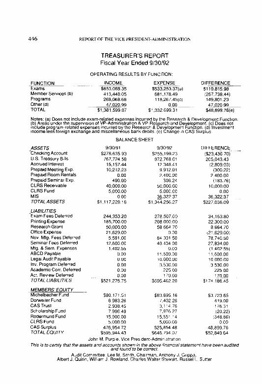
450 1992 EXAMINATIONS-~SlJ(‘(‘~SSF~ll~ C.tNDIDATES
Part 3B (cont’d)
Martin G. Heagen Sara L. Helgeson Glenn S. Hochler Jason N. Hoffman Margaret M. Hook Bernard R. Horovitz Marguerite M. Hunt Chaudhry M. Ishaq Vincent H. Jackson Jean-Claude J. Jacob Deborah M. Jasper Jill C. Johnson Aline Kafafian Kristie L. Kantowski Deborah M. King Diane L. Kinner Wendy A. Knopf Anne Kochendorfer Kevin C. Kolakowski Kimberly A. Kracht Susan M. Krawiec Brian S. Krick Joseph J. LaBella Christine L. Lacke Steven M. Lacke William C. Lawson Betty F. Lee Joan K. Lee Frederic A.
Leederman Claude Lefebvre Daniel Leff Sidney Leffler Paul B. LeStourgeon
Katherine E. Lewis Cheng-Te Liang hlli Liu Lee C. Lloyd John Lum Kyra D. Lynn Sally A. MacFadden Rita M. Maclntyre Jeffrey S. Magrane Leodivini Q. Magtoto Vahan A. Mahdasian John T. Maher Elaine J. Malupa Richard W. Malus Eileen M. McGaheran Patricia McGeeney Peter B. McOrmond Lawrence J.
McTaggart I II Hernan L. Medina Constance M. Mika David J. Miller Scott M. Miller Michael J. Miraglia Kimberly A. Moran Michael W. Mono Janice C. Moskowitz Matthew S. Mrozek Timothy 0. Muzzey Jarow G. Myers Jennifer A. Nelson Kari S. Nelson Robert P. Nelson
Thomas E. Newgarden
Nomran Niami Eric C. Nordman Lauren E. Norton Marc F. Oberholtzer Matthew J. Odendahl Richard D. Olsen Denise R. Olson Milary N. Olson Stanley T. Olszewski James A. Partridge Anna M. Paul David M. Pfahler David R. Picking Karen J. Poklikuha Deborah J. Pomerantz Kathy A. Poppe Elisabeth N. Power Stephen H. Press Julie Privman Rhonda A. Puda Lovely G.
Puthenveetil Jacqueline M.
Rambergcr Eula A. Rath Frank S. Rau Jaak M. Raudsepp Joanne E. Reitz Michael T. Reitz Jennifer L. Reller David c’. Riek Brad M. Ritter

I!?%? EXAMINATIONS-SUCCESSFUL CANDIDATES 451
Part 3B (cm&d)
Christopher R. Ritter Linda L. Roberts Pamela L. Rose William I? Rudolph Douglas A. Rupp Anthony N. Sammur Rachel Samoil James C. Sandor Teresa M. Scham Catherine I.
Schedlbauer Michael K. Schepak Steven M. Schienvar Matt J. Schmitt Lisa M. Schultz Joyce E. Segall-Lopez Anastasios Serafim Alan J. Sexter Lisa A. Sgaramella Paul E. Shangold Scott A. Sheldon Theodore J. Shively
Part 4A
Shawna S. Ackerman Jonathan D. Adkisson Vicki L. Agerton Michael W. Allard Fred S. Allsbrook John P. Alltop K. Athula P. Alwis Timothy P Aman Donald W. Anson Marc D. Archambault
Faith E. Signorile Daniel D. Smalley Cindy W. Smith Gene W. Smith Robert K. Smith Halina H. Smosna Scott G. Sobel Jay M. South Tracey A.
Stark-Beldere Christopher M.
Steinbach Lori E. Stoeberl Judy L. Stolle Heather L. Strinmoen Christopher S. Strohl Mark R. Strona Elizabeth A. Strong Brian J. Sullivan Siu Cheung S. Szeto Rachel R. Tallarini Hung K. Tang
Steven D. Armstrong Martin S. Arnold Kevin J. Bakken Daniel M. Bankson Kendra D. Barnes Dana Barre Robert S. Beatman Corey J. Bilot Gina S. Binder Abbe Binkowitz
Michael J. Tempesta Diane R. Thurston Myles J. Tilley Tammy M. Titus Jennifer M. Tornquist Joseph S. Tripodi Nicole G. Trotman Turgay F. Turnacioglu Nicholas Turville Randall H. Tweedt Steven D. Umansky Jeffrey A. VanKley Amy R. Waldhauer Robert J. Walling III Jon S. Walters David W. Warren Karen E. Watson Erica L. Weida Robert F. Wolf Gretchen L. Wolfer Cheng-Sheng P. Wu George H. Zanjani
Lisa A. Bjorkman Daniel E. Block David Bock01 Donna M. Bono Lesley R. Bosniack Michael D. Brannon Donna D. Brasley Kevin J. Brazee Laura G. Brill Jeffrey H. Brooks

Port 4A (umt’tli
Ward M. Brooks Tracy L.
Brooks-Szegda Conni J. Brown Robert L. Brown David A. Bulin Mark E. Burgess Hayden Burrus Sharon L. Cage Linda E. Callas Julia C. Causbie Maureen A. Cavanaugh
Kevin J. Cawley Joseph G. Cerreta Randall A. Chaffinch Jean-Francois
Chalifoux Andrea L. Chan Edward L. Chan Whye-Loon Chan Debra S. Charlop Soo H. Choo Rene Chouinard Normand R. Chretien Gregory C.
Christensen Alan R. Clark Derek A. Clark Jo Ellen Cockley Maryellen J. Coggins Christopher C.
Coleman David G. Cook
Sheila C. Coolcy William F. Costa Kirsten J. Costello Jose R. Couret Paul T. Cucchiara Kendra S. Cupp Marie-Claude Cyt Charles A.
Dal Corobbo Francis L. Decker Kris D. DeFrain Romulo Deo-Campo Vuong
Sean R. Devlin Behram M. Dinshaw Patricia J. Donnelly Kevin G. Donovan John P. Doucette Robert G. Downs Martin W. Draper Kimberly J. Drennan Barry P. Drobes Raymond S. Duguc Anthony D. Edwards Jeffrey S. Ellis Dawn E. Elzinga Martin A. Epstein Dianne L. Estrada Michael A. Falcone Brian M. Fernandes Jeffrey M. Forden Sally M. Forsythe David I. Frank Kirsten A. Frantom
Bethany L. Fredericks Mauricio Freyre Shina N. Fritz Brad P. Gardner Charles E. Gegax Micah R. Gentile Thomas P. Gibbons Julie T. Gilbert Mary K. Gise Nicholas P. Giuntini Stewart H. Gleason John T. Gleba Ronald E. Glenn Laurcncc B. Goldstein Jic Gong Annette J. Goodreau Karl Goring John W. Gradwell Michael D. Green Joseph P. Greenwood Russell H. Greig Christine M. Grcy Francis X. Gribbon Gary J. Griesmeycr Monica A. Grillo Richard J. Haines Barbara Hallock Sandra K. Halpin Elizabeth E. Hansen William D. Hansen Scott W. Hanson Christopher L. Harris Adam D. Hartman Michelle L. Hartrich

1992 EXAMINATIONS-SUCCESSI:C;L. CANDIDATES 453
Part 4A (um’dj
Michael B. Hawley Ronald J. Herrig Betty-Jo Hill Laura K. Hobart Wayne Hommes David B. Hostetter Melissa K. Houck Alex Y. Hsiao Marie-Josee Huard Gloria A. Huberman Sandra L. Hunt Caleb E. Huntington Randall A. Jacobson Brian J. Janitschke Fong-Yee J. Jao Brian E. Johnson Jill C. Johnson Steven J. Jordan Mark J. Kaufman Kimberly S. Kaune Lowell J. Keith Scott A. Kelly Rebecca A. Kennedy William J. Keros Michael B. Kessler He-Jung Kim John H. Kim Ung M. Kim Jill E. Kirby Russell G. Kirsch Omar A. Kitchlew Michael F. Klein Jonelle A. Kohne Gary R. Kratzer
Kenneth A. Kurtzman Edward M. Kuss Blair W. Laddusaw Jean-Sebastien
Lagarde Jin-Mei J. Lai Ydohsien Lai Mai B. Lam John B. Landkamer John P. Lebens Helen P. LeClair Robin R. Lee Claude Lefebvre Stephen E. Lehecka Glen A. Leibowitz Terry Lem Charles R. Lenz David R. Lesieur Kuen-Shan Ling Timothy D. Logie Nora J. Lovall Michelle Luneau Allen S. Lynch, Jr. John B. Mahon Barbara S. Mahoney Gary P Maile Donna M. Marazzo Lawrence F. Marcus Joseph Marracello Leslie A. Martin Peter R. Martin Michael B. Masters Robert F. Maton Lynda L. Mattes
Marci A. Maxwell Deann M. Mays Camley A. Mazloom Angela T. Mazzaferro Timothy C. McAuliffe Charles L. McGuire Kelly S. McKeethan Michael B. McKnight David W. McLaughry Mary Jo Meeks Timothy J. Melvin Mitchel Merberg Daniel J. Merk Constance M. Mika Michael J. Miller Camille D. Minogue Kenneth B. Morgan Turhan E. Murguz Kevin T. Murphy Amirul Z. Musanif Giovanni A.
Muzzarelli Jennifer A. Naehr Melissa J. Neidlinger Ronald T. Nelson Khanh K. Nguyen Anne H. Nimick Dianna C. Norman Lauren E. Norton Steven B. Oakley Kathleen C. Odomirok Denise R. Olson Joseph M. Palmer Genevieve Pare

454 I!992 EXAMINATIONS WC-CESSFUL CANDIDAlES
Part 4A (cont’d)
Nicholas H. Pastor Abha B. Pate1 Rick S. Pawelski Wende A. Pemrick Luba Pesis Mark A. Piske Anthony K. Postert Thomas M. Potter Tracey S. Powers Arlie J. Proctor Regina M. Puglisi John K. Punzak Gene Z. Qian Karen L. Queen Kathleen M. Quinn Darin L. Rasmussen Peter S. Rauner Brenda L. Reddick Nathalie J. Rekittke Donald A. Riggins Christopher R. Ritter Mart-r Rivelle Jeremy Roberts Ronald J. Robinson Dave H. Rodriguez John W. Rollins Joseph F. Rosta Jean Roy Jean-Denis Roy David A. Russell Sean W. Russell
John C. Ruth Mark T. Rutherford Cheryl Y. Sabiston Rajesh V. Sahasrabuddhe
Michael J. Scholl Sharon M. Schorge Michael F. Schrah Michdel R. Schummer Craig J. Scukas William H. Scully III Patrick J. Seaman Huidong Shang Thomas J. Sheppard Andrea W. Sherry Laura E. Siegel Michael N. Singer Helen A. Sirois Charles L. Sizer Larry K. Smith Theodore S. Spitalnick Beth A. Stahelin Christina L.
Staudhammer Nathan R. Stein Susan D. Stieg Richard A. Stock Lori E. Stoeberl Kevin D. Strous Hung K. Tang Robert D. Taylor
David J. Tenembaum Josephine T. Teruel Santy S. Thalappillil Patricia Therrien Sadhana Tiwari Nathalie L. Tremblay Joseph D. Tritz Scatty M. Tucker Arthur J. Turner Robert C. Turner James F. Tygh Eric Vaith Mark D. VanZanden Robert J. Vogel Lynne K. Wehmueller Shu-Mei Wei Mark S. Wenger Elizabeth A. Wentzien Geoffrey T. Werner James C. Whisenant Wyndi S. White David L. Whitley Michael J. Williams David S. Wolfe Barbara A. Wolinski Denise Y. Wright Cheng-Sheng P. Wu Xuening Wu Edward J. Yorty Timothy W. Young Guangjian Zhu

1992 EXAMINATIONS-SUCCESSFUL CANDIDATES 455
Part 4B
Jonathan D. Adkisson Elise M. Aheam John S. Alexander Anthony L. Alfieri Michael W. Allard Kay L. Allen Fred S. Allsbrook John P. Alltop K. Athula P. Alwis Jennifer J. Andrzejewski
Martin S. Arnold Mark E. Austin Kevin J. Bakken Phillip W. Banet Daniel M. Bankson Michael W. Barlow Claudia M. Barry James C. Berger Claire Bilodeau Corey J. Bilot Lisa A. Bjorkman Jean-Francois Blais Barry E. Blodgett Rejean Boivin Elizabeth S. Borchert Lesley R. Bosniack Scott A. Bowser Lori M. Bradley Betsy A. Branagan Donna D. Brasley Kevin J. Brazee Odile S. Brock Ward M. Brooks
Tracy L. Brooks-Szegda
Conni J. Brown Robert L. Brown David A. Bulin Anthony R. Bustillo Steven M. Byam Sharon L. Cage Douglas A. Carlone Julia C. Causbie Maureen A. Cavanaugh
Kevin J. Cawley Francis D. Cerasoli Joseph G. Cerreta Randall A. Chaffinch Jean-Francois
Chalifoux Andrea L. Chan Debra S. Charlop Sigen Chen Shu-Fang Cheng Ching-Ping Chi Hsiao-Yuan Ching Rene Chouinard William Chow Normand R. Chretien Liping Chu Jo Ellen Cockley Christopher C.
Coleman Craig A. Cooper David C. Coplan William F. Costa
Kirsten J. Costello Jose R. Couret Sandra Creaney Kendra S. Cupp Andrew S. Dahl Charles A.
Dal Corobbo Rachel Dass Smitesh Dave Robin M. Davis Shaila De Leede Francis L. Decker Karen D. Derstine Kevin G. Donovan John P. Doucette Michael J. Doviak Robert G. Downs Martin W. Draper Lucy Drozd David L. Drury Nathalie Dufresne Raymond S. Dugue Jeffrey S. Ellis Sarkis M. El-Zein Martin A. Epstein Dianne L. Estrada James G. Evans Linda S. Eveland Michael A. Falcone William P. Fisanick Stephanie Fontaine David 1. Frank Kirsten A. Frantom Mark J. Franzen

4% 1 YY? l:X;\hllN~Yl‘lOhS SI l(‘(‘l:SSFI~I. (‘A\l)ll)4’l’tS
Part 48 (cotlt’d)
Ramon D. Galanes Isabelle Gaumond Hannah Gee Charles E. Gegax Justin G. Gensler Julie T. Gilbert Serge Girard Stewart H. Gleason John T. Gleba Ronald E. Glenn Lynn E. Galas Jennifer L. Goldberg Laurence B. Goldstein Judith M. Gottesman John W. Gradwell Russell H. Greig Christine M. Grey Francis X. Gribbon Monica A. Grill0 Barbara Hallock Sandra K. Halpin Elizabeth E. Hansen William D. Hansen Joel D. Hanson Claude Hamois Christopher L. Harris ,4dam D. Hartman Michelle L. Hartrich Shohreh Heshmati Anne M. Hoban Brett D. Hodgson D. Kent Holbrook Robert J. Hopper Melissa K. Houck
Pi-Chun Hsu Gloria A. Huberman Sandra L. Hunt Tina T. Huynh Sadagopan S. Iyengai Brian J. Janitschke John F. Janssen Vibha N. Jayasinghe Donald T. Jemison Christopher P. Johnson
Daniel J. Judd Robert B. Katzman Mark J. Kaufman Jack S. Keck Lowell J. Keith Mark R. Kelbaugh Thomas P. Kenia Cynthia A. Keyes Tricia M. Keyes Elizabeth A. Kinney Joseph P. Kirley Michael F. Klein Louis K. Korth Suzanne D. Kuntz Edward M. Kuss Kirk L. Kutch Bertrand J. LaChance Blair W. Laddusaw Jean-Sebastien Lagace Sao-Kun “Connie”
Lam John M. Lamendola Matthew G. Lange
Douglas W. Latimer Khanh M. Le Manuel Alberta T. Lcal
Claude Lefebvre Stephen E. Lehecka David R. Lesieur lsabelle Letourneau Aaron S. Levine Guey-Ru Lieu Chinlong Lin Frank K. 1,ing Pascal Longpre Laura J. Lothschutz Robb W. Luck Kyra D. Lynn Emma B. Macasicb Kenneth W. Macko Barbara S. Mahoney David K. Manski Yishi Mao Donna M. Marazzo Lawrence F. Marcus Albert Maroun Michael B. Masters Robert F. Maton I .ynda L. Mattes Tracey L. Matthew Bonnie C. Maxie l,aura A. Maxwell Dcann M. Mays Camlcy A. Mazloom Deborah L. McCrdry Charles L. McGuire

1992 EXAMINATKWS-SUCCESSFUL CANDIDATES 457
Part 4B (cont’d)
Kelly S. McKeethan Phillip E. McKneely David W. McLaughry William E. McWithey Frederic N. Michaud Stephen J. Mildenhall Michael J. Miller Catherine E. Moody Kenneth B. Morgan Kimberly J. Mullins Peter J. Murdza, Jr. Joseph L. Murdzek Kevin T. Murphy Giovanni A.
Muzzarelli Karen E. Myers Kathleen V. Najim Dianna C. Norman Andres F.
Ochoa-Gomez Kathleen C. Odomirok Helen S. Oliveto Kevin J. Olsen Kory J. Olsen Lowell D. Olson Stanley T. Olszewski Krzysztof M.
Ostaszewski Michael G. Owen Gerard J. Palisi Joseph M. Palmer Charles Pare Genevieve Pare Thomas Passante
Christos G. Patsalides Lisa M. Pawlowski Jeremy P. Pecora Wende A. Pemrick Claude Penland IV Miriam E. Perkins Peter P. Perrotti Anne M. Petrides Aleksey Popelyukhin Anthony K. Postert Thomas M. Potter Trdcey S. Powers Michael D. Price Armand Principato Doug L. Pryor Regina M. Puglisi Patricia A. Pyle Gene Z. Qian Mark S. Quigley Kathleen M. Quinn Kelly L. Raasch Robin A. Rabideau Patrice Raby Kiran Rasaretnam Darin L. Rasmussen Peter S. Rauner Brenda L. Reddick Jennifer L. Reller Ellen J. Respler Donald A. Riggins Dennis L. Rivenburgh, Jr.
Dominique Robert John W. Rollins
Joseph F. Rosta Jean Roy Jean-Denis Roy David A. Russell Sean W. Russell Laura A. Ryan Charles J. Ryherd Samuel E. Sackey Cindy R. Schauer Lori A. Scheirer Michael J. Scholl Annmarie Schuster William H. Scully III Kelvin B. Sederburg Joyce E. Segall-Lopez Vinaya K. Sharma Thomas J. Sheppard Craig T. Shigeno Jeffrey P. Shirazi Charles L. Sizer Raleigh R. Skaggs, Jr. Klayton N.
Southwood Calvin C. Spence, Jr. Theodore S. Spitalnick Michael P. Spurbeck Christina L.
Staudhammer Scott T. Stelljes Richard A. Stock Brian K. Sullivan Steven W. Sun Siu Cheung S. Szeto Due M. Ta

45x 1YY2 EXASlIKATlONS- SI (‘(‘I:SSl~l II (‘.\~I)IIhYII:S
Part 4B (c~ont’cl)
Ken Seng Tan Robert D. Taylor Judith D. Teglas Josephine T. Teruel Daniel A. Tess Patricia Therrien John L. Timmerberg Amy B. Treciokas Joseph S. Tripodi Chuan-Shin D. Tu Robert C. Turner James F. Tygh Pamela J. VdnLeirsburg
Mark D. VanZanden Trent R. Vdughn Wittie 0. Wacker
Part 6
Daniel N. Abellera Mark A. Addiego Craig A. Allen Ann L. Alnes Michael J. Andring Nancy L. Arico I3arry L. Bablin Timothy J. Banick Jack Bamett John A. Beckman Cynthia Bentley Lyne Bergeron Eric D. Besman Michael G. Blake Gina L. Blakeney Gary Blumsohn
Heather A. Waldron Lisa M. Walsh Yu-Hwa Wang Kimberley A. Ward Linda F. Ward Jamil Wardak Jennifer M. Webb Petra L. Wegerich Christopher B. Wei Deyue Wei Geoffrey T. Werner James C. Whisenant Wyndi S. White David L. Whitley Tammy L. Wimcr David S. Wolfe
George P. Bradley James L. Bresnahan Louis M. Brown Michelle M. Bull Linda J. Burrill John F. Butcher II Robert N. Campbell Anthony E. Cappellitti Michael E. Carpenter Daniel G. Carr Michael W. Cash Hsiu-Mei Chang Sigen Chen Peggy Cheng Kuei-Hsia R. Chu Christopher J. Claus
Terry C. Wolfe Milton K. Wong Stephen K. Woodard Mark L. Woods Cheng-Sheng P. Wu Fenghua H. Wu Hsuli Wu Xuening Wu Jacinthe Yelle Robert S. Yenke Edward J. Yorty Kong Hung Yu Jeffery M. Zacek George H. Zanjani Guangjian Zhu Eric E. Zlochevsky
Mary L. Corbett Deanna L. Crist Michael T. Curtis Mujtaba H. Datoo Anne M. DelMastro Lisa A. Doedtman Andrew J. Doll Jeffrey L. Dollinger Jeffrey D. Donaldson Peter F. Drogan Pierro Drolet David M. Elkins Paul E. Ericksen Lynnc W. Faucher Matthew G. Fay Judith M. Feldmeier
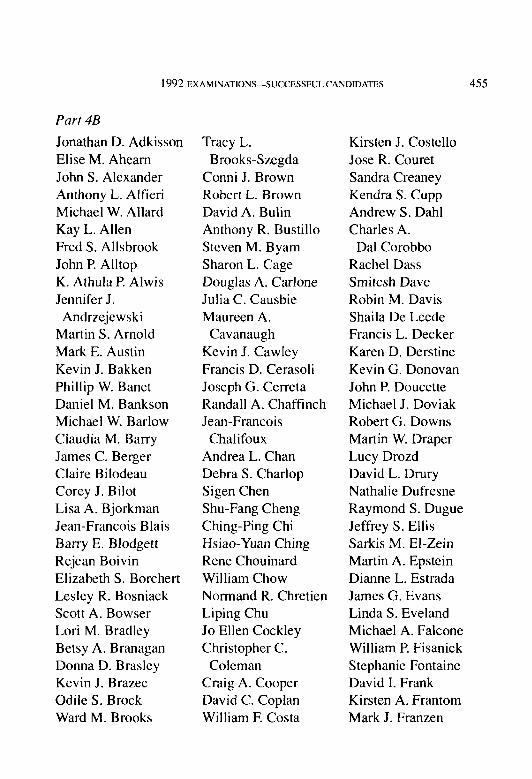
i 992 EXAMINATIOKS- SlICCESSFL:L CANDIDATES 459
Part 6 (wnt ‘d)
Kelly F. Fogarty Russell Frank Douglas E. Franklin Cynthia J. Friess Nathalie Gamache Christopher H. Geering
Donna L. Glenn Marc C. Grandisson William A. Guffey Timothy J. Hansen Bradley A. Hanson Lise A. Hasegawa Matthew T. Hayden Barton W. Hedges Noel M. Hehr Renee J. Helou Mary B. Hemerick Thomas E. Hinds Thomas A. Huberty John F. Huddleston Jeffrey R. Hughes Jason Israel Patrick C. Jensen Anita J. Johnson Daniel K. Johnson Kurt J. Johnson Mark R. Johnson Marvin F. Johnson Jean M. Kamick Charles N. Kasmer Anthony N. Katz Daniel R. Keddie Steven A. Kelner
Timothy P Kenefick George A. Kish Terry A. Knull Elizabeth Kolber Debra K. Kratz Terri C. Kremenski Mary C. Kroggel Cheung S. Kwan Elaine Lajeunesse Rita Ann B. Lamb Marc LaPalme David L. Larson Doris Lee Scott J. Lefkowitz Louise L. Legros Elizabeth A. Lemaster Julie Lemieux-Roy Deanne C. Lenhardt Richard S. Light Edward A. Lindsay Stephanie J. Lippl Ronald P. Lowe, Jr. Christopher J. Luker James M. Maher Daniel J. Mainka Betsy F. Maniloff Anthony L. Manzitto Gabriel 0.
Maravankin Galina Margulis Anthony G.
Martella, Jr. Kelly J. Mathson Robert D. McCarthy
Richard T. McDonald Heather L. McInstosh Kathleen A. McMonigle
Van A. McNeal Lynne S. McWithey Brian J. Melas Timothy Messier Paul A. Mestelle Paul W. Mills Raymond D. Muller David Y. Na Donna M. Nadeau Douglas W. Oliver Richard A. Olsen Melinda H. Oosten Todd F. Orrett Paul S. Osbom Nathalie Ouellet Mary Beth O’Keefe Maureen D. O’Keefe Jennifer J. Palo Charles C. Pearl, Jr. Edward E Peck Daniel B. Perry William Peter Beverly L. Phillips Daniel C. Pickens Glen-Roberts
Pitruzzello Joseph W. Pitts Daniel A. Powell Charlene M. Pratt Mark Priven

360 1997 EXAMIN,~Z’fIO~S-SI;C‘(‘FSS~I I, CA\l~II),TIES
Part 6 (cont’d)
Richard B. Puchalski Eduard J. Pulkstenis Robert E. Quane III John F. Radwanski Frank J. Rau, Jr. Yves Raymond Al J. Rhodes Andrew T. Rippert Douglas S.
Rivenburgh Sallie S. Robinson Paul J. Rogness James J. Romanowski James B. Rowland Jean Roy David L. Ruhm Kenneth W.
Rupert, Jr. James V. Russell Maureen S. Ruth
Melodee J. Saunders Letitia M. Saylor Marilyn E. Schafer Michael B. Schenk Peter R. Schwanke Jeffery J. Scott Gregory R. Scruton Jonathan N. Shampo James J. Smaga Douglas W. Stang Katie Suljak Colleen M. Sullivan Collin J. Suttie Scott J. Swanay Jeanne E. Swanson Todd D. Tabor Joy Takahashi Charles F. Toney Michael J. Toth Son T. Tu
Patrick N. Tures Charles E.
Van Kampen David B. Van Kocvering
Phillip C. Vigliaturo William E. Vogan Joseph W. Wallen Stephen D. Warfel Joyce A. Weisbecker Carol B. Werner William R. Wilkins Marcia C. Williams William M. Wilt John S. Wright Gerald T. Yeung Claude D. Yoder Benny S. Yuen Barry Zurbuchen Ralph T. Zimmer

1992 EXAMINATIONS-SUCCESSFUL CANDIDATES 461
Part 8
Kristen M. Albright Rebecca C. Amoroso Richard R. Anderson Katherine Barnes Alicia E. Bowen Mark L. Brannon J. Eric Brosius Anthony J. Burke Scott K. Charbonneau John S. Chittenden Peter J. Collins Raymond V. Debs Victor G. dos Santos William F. Dove Michael C. Dubin Maribeth Ebert Charles C. Emma Philip A. Evensen Kerry L. Fitzpatrick Scott F. Galiardo Andrea Gardner Bruce R. Gifford Richard S. Goldfarb Charles T. Goldie Edward M. Grab Steven J. Groeschen Carleton R. Grose George M. Hansen Steven T. Harr
Thomas G. Hess Todd J. Hess Keith D. Holler Beth M. Hostager Laura A. Johnson Gerald S. Kirschner Gilbert M. Korthals Nancy E. Kot David J. Kretsch James W. Larkin Eric F. Lemieux Giuseppe F. LePera William G. Main Donald E. Manis Suzanne Martin Steven E. Math Jeffrey F. McCarty Robert L. Miller John H. Mize Kelly L. Moore Michelle M. Morrow David A. Murray Antoine A. Neghaiwi Kwok C. Ng Keith R. Nystrom Margaret M. O’Brien Laura A. Olszewski Chandrakant C. Pate1 Susan J. Patschak
Sarah L. Petersen Mark W. Phillips Lisa M. Ross John M. Ruane, Jr. Stephen P Sauthoff Margaret E. Seiter Derrick D. Shannon Rial R. Simons Steven A. Skov David A. Smith Elizabeth L. Sogge Lisa
Steenken-Dennison Leslie D. Svoboda Eileen M. Sweeney Barbara H. Thurston Susan M. Treskolasky Peter S. Valentine Jennifer A. Violette Christopher P Walker Monty J. Washburn Scott P. Weinstein Leigh F. Wickenden Teresa J. Williams John M. Woosley Chung-Ye S. Yen Sheng H. Yu

Purt NC
Annie Blais Benoit Carrier Jean Cloutier Marie-Julie Demers Shawn F. Doherty
Guy A. Avagliano Anthony J. Balchunas Douglas L. Beck Nathatie Begin Xavier Benarosch Lloyd J. Bouchard Christopher K.
Bozman Paul A. Bukowski Martin Cauchon Denis Ctoutier Michael A. Coca Jeffrey R. Cole Charles Cassette Martin L. Couture Robert J. Curry Francois Dagneau Patrick K. Devlin Stephen R. DiCenso Kevin G. Dickson Michet Dionnc Francois Dumas Bradley C. East wood John W. Ettingrod James Ety George Fescos
Odite Goyel Bradley A. Grangel Math& Lam) France LeBlanc Heidi J. McBride
David A. Foley France Fortin Louis Gariepy John F. Gibson Susan M. Gozzo Eric L. Greenhitt Farrokh Guiahi Diane K. Hausserman James S. Higgins Keith D. Hottel George A. Hrozicncik Anthony Iafrate Joanne K. Ikeda Kathleen M. Ireland Peter James Changseob J. Kim Bryan J. Kincaid Richard 0. Kirste Ronald T. Koztowski John A. Lamb Jean-Marc LCveitl6 Paul R. Livingstone Mark J. Mahon Btaine C. Martes Burton F. Marlowe Liam M. McFarlane
Andre Perez Denis Poirier Robert Potvin
Cassandra M. McGill William T. Mech Charles B. Mitzet Richard B. Moncher Todd B. Munson Kathleen C. Nomicos Charles P. Ortowicz Donald D. Palmer Jacqueline E. Pastey Karen L. Pehrson Timothy B. Perr Richard W. Prescott Kenneth P. Quintitian Kay K. Rahardjo Srinivasa Ramanu.jam Scott E. Rcddig Sharon K. Robinson Diane R. Rohn Allen D. Rosenbach Stuart G. Sadwin Yvcs Saint-Loup Leigh Saunders Oates Edmund S. Scanton Gordon L. Scott Marie Scttitti Vincent M. Senia

1992 EXAMINATIONS-SWCESSFULCANDIDATES 463
Pul.t IO (cwiddj
Christy L. Simon Christopher M.
Smeratd Tom A. Smolen David B. Sommer
Douglas N. Strommen Marjorie C. Weinstein Marianne Teetset John P. Welch Michael A. Visintainer Kevin Wick Sebastian Vu Gnana K. Wignarajah Bryan C. Ware Gregory S. Wi tson

464 1992 EXA~l~.~rlONS-S~‘C(‘ESFI’I. (‘A\I>II~A’lES
The following candidates were admitted as Fellows and Associates at the November 1992 meeting as a result of their successful completion of the Society requirements in the May 1992 examinations.
Rebecca C. Amoroso Anthony Joseph
Batchunas Douglass L. Beck Nathatie Begin Martin Cauchon Denis Ctoutier Jeffrey Roger Cole Charles Cassette Robert John Curry Francois Dagneau Patrick K. Devlin John William Etlingrod James Ety David Alan Foley France Fortin John Foster Gibson Susan Marie Gozzo Eric L. Greenhi I I Diane Kae
Hausserman Todd J. Hess James S. Higgins Keith Douglas Hotter George Alan
Hroziencik
FELLOWS
Kathleen Marie Ireland Peter H. James Brian Joseph Kincaid Richard Owen Kirste Ronald Thaddeus Kozlowski
David Jon Kretsch John A. Lamb Jean-Marc Levei I te Btaine C. Martes Burton F. Marlowe Steven E. Math Liam Michael
McFartane William Theodore
Mech Charles Bradley Mitzet Richard B. Moncher Todd Burton Munson Margaret M. O’Brien Jacqueline Edith
Pastey Susan Jean Patschak Robert Potvin Richard Warren Prescott
Kenneth Paul Quintilian
Kay Ke I I ogg Rahardjo Srinivasa Ramanujam Scott Edward Reddig Sharon K. Robinson Diane Renee Rohn Edmund Sean Scanton Margaret Elizabeth Seiter
Marie Setlitti Vincent M. Senia Christy L. Simon Christopher Michael
Smerdtd Douglas Nelson Strommen
Michael A. Visintainer Sebastian Vu Christopher Patrick
Walker Marjorie Cindy Weinstein
Gregory S. Wilson

1992 EXAMINATIOYS-SUCCESSFUL CANDIDATES 465
Daniel Navarro Abeltera
Ann Louise Atnes Nancy Lee Arico George Peter Bradley Donna Dionne Brastey Ward M. Brooks Linda Jean Burrit I Anthony E. Cappelletti Mary Laurene Corbett Jeffrey Lawrence
Dotlinger Jeffrey David
Donaldson Paul Edmund Ericksen Lynne Woody Faucher Judith Michalojko
Feldmeier Russell Frank Laurence B. Goldstein Sandra Kathleen
Halpin
ASSOCIATES
Bradley A. Hanson Renee He tou Jeffrey Robert Hughes Daniel Robert Keddie Stephen E. Lehecka Stephanie Jean Lippt James Michael Maher Gatina Margutis Heather Lynn
McIntosh Van At ten McNeal Raymond D. Mutter Mary Beth O’Keefe Douglas W. Oliver Richard Alan Olsen Wit tiam Oostendorp Todd Franklin Orrett Joseph Martin Palmer Jennifer Joan Palo Daniel Anthony Powell
Jean Roy Maureen Schatter Ruth Metodee Jane
Saunders Jeffery Jay Scott Gregory R. Scruton James J. Smaga Scott Jay Swanay Charles French Toney II
Michael J. Toth James F. Tygh David Brad Van Koevering
Phittip C. Vigtiaturo William E. Vogan Stephen Douglas Warfe I
Joyce Ann Weisbecker Ralph T. Zimmer
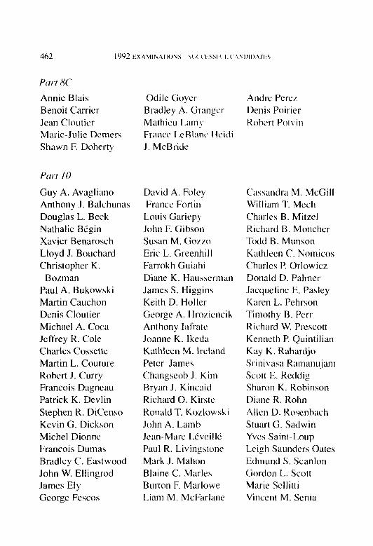
366 Ic)c)? ES,\\ll1\‘r\TlONS SI’(‘(‘I~SSI~Ul C’ANDII)AI k-3
The following is the list of successful candidates in examinations held in November 1902.
Purr 38
Bruce J. Adams Elise M. Ahearn Michael J. Alexander Denise M. Ambrogio Bijoy Anand Julie A. Anderson Mark B. Anderson Adetine T. Anggelico Steven D. Armstrong Aeran A. Atlas Evan C. Ayata Karen L. Babitt Melissa M. Bados Phittip W. Banet Amy L. Baranek Michael W. Barlow Karen L. Barrett Karen E. Bashe Linda S. Baum Andrew S. Becker David J. Betany Joseph M. Bernardi Robert C.
Birmingham Nicole P. Bitros Linda J. Bjork Carol A. Blomstrom Douglas J. Bradac David J. Brazil Charles Brindamour Audrey W. Broderick
Martha E. Bronson Robert F. Brown Stephen J. Bruce Kirsten R. Brumtcy Joanne E. Burk Elise S. Burns Sharon L. Cage Sandra J. Cattanan Michael V. Campbell Janet P. Cappers Douglas A. Cartone Francis D. Cerasoti Joseph G. Cerreta Whye-Loon Ghan Daniel G. Charbonneau
Lisa C. Chen Stephen D. Ctapp Scott R. Clark Lisa V. Clarke Susan M. Cleaver Jeffrey A. Clements Robert A. Ctybornc Brian R. Coleman Pamela M. Corey Dino F. Costabite Brenda K. Cos Gregory E. Daggctt Ted W. Daniel Smitesh Dave Timothy M. DiLet lio
B&ram M. Dinshaw Metodee S. Dixon Patricia L. Drajin Martin W. Draper Sara P. Drexter Stephanie S. Dubose Patrick W. Duncan Denis Durand Jeffrey S. Ellis Lisa D. El) Keith A. Engetbrecht Juan Espadas Todd E. Fansler Daniel J. Flick Richard Y. Fong Donovan M. Fraser Bethany L. Fredericks Kevin J. Fried Michelle R. Garnock Kathy H. Garrigan Carina F. Glasgow Mary T. G laude1 I Mark A. Gorham Allen J. Gould Jeffrey S. Go) Kristin J. Grimshaw Denise H. Guluk John A. Hagglund Francis G. Hall. Jr. Faisat 0. Hamid

1992 EXAMINATIONS-SI;CCESSFUI. CANDIDATES 467
Part 3B (cmt’d)
Alessandrea C. Handley
William D. Hansen Harry K. Hariharan David S. Harris Scott E. Haskell Michael B. Hawley Matthew T. Hayden Daniel J. Henderson Tina M. Henninger Christopher T.
Hochhausler David E. Hodges Amy L. Hoffman Tracy L. Hoffman PO-Wo Hsieh Joseph M. Izzo Randall A. Jacobson David R. James Suzanne M. James Kelly A. Jensen Jean M. Kamick Claudine H.
Kazanecki Dennis J. Keegan Lowell J. Keith Thomas P. Kenia Lisa M. Kerns Michael B. Kessler Robert W. Kirklin James J. Konstanty Dawna L. Koterman Robert E. Krulish Leonard L. Kruse
Cheung S. Kwan Bertrand J. LaChance Douglas H. Lacoss Stephanie J. Ladiana Salvatore T. LaDuca Julia M. Lavolpe Lawrence K. Law Thomas V. Le Thomas C. Lee Neal M. Leibowitz James I? Leise Isabelle Lemay Adam M. Lesser Teresa L. Lett Michael Leybov Michael Lipkin Linda R. Lisi Timothy D. Logie Nora J. Lovall Cara M. Low Susan I. Lynch Kelly A. Lysaght James M. MacPhee Barbara D. Majcherek Robert G. Mallison, Jr. Betsy F. Maniloff Kelly J. Mathson Claudia A. McCarthy Deborah L. McCrary Smith W. McKee Kelly S. McKeethan Leslie A. McMahon Lisa R. McNeal James C. McPherson
Stephanie J. Michalik Stephen J. Mildenhall Michael J. Miller Beth K. Millington Scott P. Monard Robert J. Moser Kevin T. Murphy Jennifer L. Nelson Heather L. Nemeth Denis P. Neumann Khanh K. Nguyen Steven A. Nichols Douglas K. Nishimura Chris M. Norman Sandra F. Norowitz Steven B. Oakley Marie A. Olon Stacey L. Otterson Jill E. O’Dell Marianne E. Papay Thomas Passante Javanika Pate1 Tracie L. Pencak Jennifer L. Pepin David J. Persik Mark A. Piske Joseph W. Pitts Matthew H. Price Cindy Q. Qiu Brentley J. Radeloff William D. Rader, Jr. Kimberly E. Ragland Alicia M. Ransom
468 1 ‘)‘)2 EXAMINATIONS SllCC‘ESSbI I.~‘4\I)II)ATI:S
Par-t 3B (cont’d)
Charles J. Reichardt, Jr.
Meredith G. Richardson
Janelle P. Ridder Brad E. Rigotty Gail S. Rohrbach Luis Romero Jay A. Rosen Jean-Denis Roy David L. Ruhm Sean W. Russell Shama S. Sabade Asif M. Sardar Barbara A. Satsky Rebecca A. Schafer Christine E. Schindler Annmarie Schuster Terri L. Schwomeyer John P. Scott
Terry M. Seckel Michael Shane George L. Shields Nathan I. Shpritz Michael N. Singer Laura M. Smith Michele L. Spale Jonathan C. Stavros D. Gregory Stitts Shelley A. Stone Lauren M. Stump Elizabeth A. Sullivan Patricia A. Sullivan Roxann P. Swenson Ming Tang Judith D. Teglas Steve D. Tews Amy B. Treciokas Beth S. Tropp Mary H. Vale
Tim A. Varso Leslie A. Vernon Edward H. Wagner Robert A. Walsh Edith A. Wendell Jeffrey D. White Steven B. White Wyndi S. White Ellen G. Wiener Bruce P. Williams Jennifer N. Williams William M. Wilt Curtis W. Withers Kah-Leng Wong John S. Wright Nancy E. Yamall Virginia R. Young Philip A. Zakas Michael R. Zarember Darci L. Zelenak

1992 EXAMINATIONS-SUCCESSFUL CANDIDATES 469
Part 4A
Elise M. Ahearn Joseph J. Allard Kay L. Allen Jennifer A. Andrzejewski
John A. Annino Robert C.
Birmingham Barry E. Blodgett Carol A. Blomstrom Jodi L. Bohac Josee Bolduc Edmund L. Bouchie Lori M. Bradley Tobias E. Bradley Betsy A. Branagan Glen R. Bratty Robert F. Brown Michelle L. Busch Tara E. Bush Douglas A. Carlone Francis D. Cerasoli Elina L. Chachkes Joyce Chen Gary C. Cheung Sally M. Cohen Kevin A. Cormier Brian C. Comelison Sandra Creaney Michael T. Curtis Smitesh Dave Jeffrey W. Davis Catherine L. DePolo Sharon D. Devanna
David L. Drury Stephanie S. Dubose Nathalie Dufresne Stephen C. Dugan Sarkis M. El-Zein Bruce D. Fell John R. Ferrara Stephen C. Fiete Daniel B. Finn William P. Fisanick Daniel J. Flick Sy Foguel Heather A. Ford Lilane L. Fox Keith E. Friedman Gary J. Ganci Christian Gaouette Robert J. Garbus Perriann R. Garcia Justin G. Gensler Eric J. Gesick Barbara B. Glasbrenner
Lynn E. Galas Chris D. Goodwin Patricia A. Gorski John E. Green Steven A. Green Daniel E. Greer Scott J. Hartzler Curtis D. Harvey Douglas J. Hatlestad Lisa K. Hiatt Anne M. Hoban
Jason N. Hoffman Dave R. Holmes Eric A. Hoppe Robert J. Hopper Chaudhry M. Ishaq Paul A. Johnson ha M. Kaplan Brian D. Kemp Martin T. King Craig W. Kliethermes Louis K. Korth Kimberly A. Kracht Karen M. Kulchyski Cheung S. Kwan Patrick P. Lacasse Bertrand J. LaChance Matthew G. Lange Steven W. Larson Khanh M. Le Betty F. Lee Paul B. LeStourgeon Philip Lew Yuan Long Liu Lee C. Lloyd William R. Maag Barbara D. Majcherek David K. Manski Christopher M.
Mariani Albert Maroun Meredith J. Martin Tracey L. Matthew Archibald G. Mattis Bonnie C. Maxie

Purt -!A (cont’d)
Phillip E. McKneely Jeffrey A. Mehalic Scott M. Miller Stephen A. Moffett Lisa J. Moorey Jonathan M. Moss Robert J. Moss Karen E. Myers Milary N. Olson Thomas Passante Lisa M. Pawlowski Chantal Pelletier Jeremy P Pecora Claude Penland IV Anne M. Petrides Michael W. Phillips Michael L. Pisula Thomas L. Poklen, Jr. Ni Qin Feng Mark S. Quigley Thomas 0. Rau Ellen J. Respler Dennis L. Rivenburgh, Jr.
Part 4B
Vicki L. Agerton Timothy K. Allen Jason C. Alleyne Timothy P. Aman Steven D. Armstrong John J. Ascencio Bruce E. Bach Kendra D. Barnes
Sallie S. Robinson Rita L. Rogers David M. Savage Daniel V. Scala Cindy R. Schaue! Suzanne E. Schoo Annmarie Schuster Steven G. Searle Jerelyn K. Seeger Jill C. Sidney M. Kate Smith Gregory T. Snider Sandra L. Spiroff Scott D. Spurgat Kenneth W. Stam Trdcey A.
Stark-Beldere Scott T. Stelljes Michael J. Steward II Stephen J. Streff Brian K. Sullivan Frank Tancredi Judith Tcglas
Rajesh K. Barnwal David M. Baxter Martin Bilodeau Gina S. Binder Latisha L. Boothe Edmund L. Bouchie Lee M. Bowron Tobias E. Bradley
Jennifer M. Tornquist Turgay F. Turnacioglu Michael 0. VanDusen Elayne M. Vargo Moxon
Trent R. Vdughn Jennifer A.
VonSchaven Wittic 0. Wacker Galen L. Wadzinski Michael A. Wallace Lisa Marie Walsh Caroline Ward Erica L. Weida Kirby W. Wisian Stephen K. Woodard Jeffrey F. Woodcock Linda Yang Mindy Yu Jeffcry M. Zacek Fcngming Zhang Steven B. Zielke Robin Zinger
David J. Braza Laura G. Brill Linda M. Brockmeier James A. Bull Michelle L. Busch Tard E. Bush Linda E. Callas Victoria J. Carter

I992 EXAMINATIONS-SUCCESSFUL. CANDIDATES 471
Part 4B
Thomas E. Cerulli Peter T. Chang Wei Fun W. Chang Sharon L. Chapman Joyce Chen Gary C. Cheung Ling-Jyh Chiou Soo H. Choo Gregory C.
Christensen Kathy A. Christensen Juite Chuang Clark R. Chumley Frank S. Conde David G. Cook Sharon A. Crosson Malcolm H. Curry Michael T. Curtis Kenneth S. Dailey Jeffrey W. Davis Raymond V. DeJaco Catherine L. DePolo Dina M. Deschino Sean R. Devlin Behram M. Dinshaw Ronald R. Dionne Patricia J. Donnelly Kimberly J. Drennan Barry P. Drobes Mary F. Drueke Denis Dubois Louis Durocher Anthony D. Edwards Ellen E. Evans
Bruce D. Fell John R. Ferrara Daniel B. Finn Ginda K. Fisher Daniel J. Flick Jeffrey M. Forden Walter H. Fransen Keith E. Friedman Richard A. Fuller Scott F. Fuller Wang-Tat D. Fung Serge Gagne Gary J. Ganci Carol Ann Gamey Micah R. Gentile Thomas P. Gibbons Bernard H. Gilden Mary K. Gise Barbara B. Glasbrenner
Yethun Goh Annette J. Goodreau Patricia A. Gorski George J.
Gourdourakos Michael D. Green Steven A. Green John E. Green Joseph P. Greenwood Michael K. Griffin Robert W. Guth Steven K. Haine Richard J. Haines Scott W. Hanson
David S. Harris Michael A. Harris Scott J. Hartzler Curtis D. Harvey Gary M. Harvey Michael B. Hawley Peter A. Heinrichs Daniel E Henke Betty-Jo Hill John D. Hill Jason N. Hoffman Todd H. Hoivik Keith D. Holler Dave R. Holmes Wayne Hommes Yu-Hui A. Huang Marie-Josee Huard Corine Huey Brian L. Ingle Randall A. Jacobson Fong-Yee J. Jao Scott L. Johnson Gregory K. Jones Steven J. Jordan Ira M. Kaplan Joseph P. Karlovich Michael B. Kessler Hyung-Shim Kim Deborah M. King Martin T. King Omar A. Kitchlew Craig W. Kliethermes Robert J. Knadler Rachna Kohli

Purt 4B (cont’di
Jonelle A. Kohne Paul W. Kollner Andrew M. Koren Eleni Kourou Gary R. Kratzer Dean F. Kruger Ignace Y. Kuchazik Patrick P. Lacasse Jin-Mei J. Lai Kunjung Lai Siu-Wai Lai John B. Landkamer Frank A. Laterza Robin R. Lee Paul B. LeStourgeon John N. Levy Pak-Chuen Li Karen A. Liholt Yachin Lin Kim D. Litwack William M. Londeree Richard B. Lord Sak-Man Luk Xinhong Luo Allen S. Lynch, Jr. James P. MacDougall Gary P Maile Keith M. Marcus Laura S. Marin Joseph Marracello Leslie A. Martin Peter R. Martin Michele A. Mathieu Angela T. Mazzaferro
Wendy M. Mazzarella Robert D. McCarthy Cassandra M. McGill Sean L. McIntosh Christopher P.
McMann Arthur J. Mees, Jr. James R. Merz Marci A. Meyer Scott M. Miller Susan A. Minnich Quynh-Nhu T. Morse Matthew S. Mrozek Turhan E. Murguz Iris A. Nance Melissa J. Neidlingcr Gary R. Nidds Lauren E. Norton Steven B. Oakley Denise R. Olson Milary N. Olson Ajay Pahwa Dmitry Papush Nicholas H. Pastor Rick S. Pawelski Mark Paykin Priyantha L. Perera John M. Pergrossi Luba Pesis Kevin W. Piconc Donna M. Pinctti Mark A. Piske Alan D. Potter Matthew H. Price
Arlie J. Proctor John K. Punzak Ni Qin Feng Mary S. Rapp Thomas 0. Rau Patrick J. Reilly Mary B. Rios-Gandara Christopher R. Ritter Jeremy Roberts Michelle N. Rodriguez
Constance D. Rogers Hal D. Rubin John C. Ruth Rajesh V.
Sahasrabuddhe Rome] G. Salam Sujata S. Sanghvi Matt J. Schmitt Suzanne E. Schoo Michael F. Schrah Michael R. Schummer Gordon L. Scott Patrick J. Seaman Jerelyn K. Seegcr Michael Shane Jennifer M. Shantz Stacy L. Shimizu-Hall Laura E. Siegel Cindy W. Smith Jeffery J. Smith Katherine R. Smith L. Kevin Smith Halina H. Smosna

1992 EXAMINATIONS-SUCCESSFULCANDIDATES 473
Part 4B (cont’d)
David E. Sowers Scott D. Spurgat Beth A. Stahelin Robert P Stahnke Glenda M. Stalkfleet PJ. Eric Stallard Michael J. Steward II Curt A. Stewart Lori E. Stoeberl William J. Stone Stephen J. Streff Steven J. Symon Jinhua Tao Sandra L. Theile
Part 5
John S. Alexander John P. Alltop Larry D. Anderson Martin S. Arnold Claudia M. Barry Gina S. Binder Lisa A. Bjorkman Christina M. Bond Conni J. Brown Mark E. Burgess Sandra L. Cagley Pamela J. Cagney Mark W. Callahan Maureen A.
Cavanaugh Jean-Francois
Chalifoux Hong Chen
Sadhana Tiwari Jennifer M. Tornquist Kai L. Tse Scatty M. Tucker Jeffrey R. Turcotte Arthur J. Turner Michael 0. VanDusen Charles J. Veres Michel F. Viau Benjamin A. Walden Isabelle T. Wang Shaun Wang Lynne K. Wehmueller Erica L. Weida
Suhui Chen Bina S. Cherian Christopher J. Claus William B. Cody Frank S. Conde Kirsten J. Costello Christopher G.
Cunniff Raymond V. DeJaco Joseph A. DiBiase Patricia J. Donnelly Kevin G. Donovan Robert G. Downs Sara P. Drexler David L. Drury Martin A. Epstein Dianne L. Estrada James G. Evans
Elizabeth A. Wentzien Scott Werfel L. Alicia Williams Ronald J. Williams Kirby W. Wisian Trevar K. Withers Brandon L. Wolf Jeffrey F. Woodcock Rick A. Workman John Yannis Yatracos Xiang Zhang Robin Zinger Edward J. Zonenberg
Joseph G. Evleth Michael A. Falcone Richard B. Federman John D. Ferraro Daniel B. Finn Jeffrey M. Forden Mark R. Frank J’ne E. Furrow Paul Gauthier Justin G. Gensler Margaret W. Germani Nicholas P. Giuntini Michael F. Glatz Stewart H. Gleason Karl Goring John W. Gradwell Michael K. Griffin Lynne M. Halliwell

474 1 Y’)2 EXAMINATIONS Sl~(‘(‘liSWIII C‘ANDIDATt:S
Purr 5
Brian D. Haney Elizabeth E. Hansen Anne M. Hoban Brook A. Hoffman Eric J. Hornick Linda M. Howell Jill C. Johnson Gregory K. Jones Steven J. Jordan Barbara L. Kanigowski
John P. Kannon Anthony N. Katz Mark J. Kaufman Brandelyn C. Klenner Brian R. Knox Louis K. Korth Debra K. Kratz Thomas F. Krause Brian S. Krick Kenneth A. Kurtzman Edward M. Kuss Kirk L. Kutch Steven M. Lacke Blair W. Laddusaw John M. Lamendola Robert J. Larson Thomas V. Le John P. Lebens Helen P. LeClair Chi Hei Lee Daniel Leff Glen A. Leibowitz Charles R. Lenz IJaul Liu
Nora J. Lovall Barbara S. Mahoney Michael B. Masters Robert F. Maton Tracey L. Matthew Camley A. Mazloom William R.
McClintock David W. McLaughry Stephen J. Mildenhall Mark J. Moitoso Kimberly A. Moran Benoit Morissette Michael J. Moss Turhan E. Murguz Jarow G. Myers Karen E. Myers Kathleen V. Najim Marc F. Oberholtr.cl Leo M. Orth, Jr. Mark A. O’Brien James D. O’Malleq James A. Partridge Wende A. Pemrick Claude Penland IV Michael C. Petersen Glen-Roberts
Pitruzzello Dale S. Porfilio Kiran Rasaretnam Natalie J. Rekittke Cynthia L. Rice Donald A. Riggins Brad M. Ritter Christopher R. Ritter
John W. Rollins Thomas A. Ryan Christina L. Scanell Lawrence M. Schober Michael J. Scholl Jay M. Schwartz Craig J. Scukas Kevin H. Shang Jcffrcy P. Shirazi Jeffery J. Smith Caroline B. Spain Christina L.
Staudhammer Nathan R. Stein Christopher M.
Steinbach Scott T. Stelljes Kevin D. Strous Josephine T. Teruel Daniel A. Tess Marie-Claire Turcotte Laura M. Turner Robert C. Turner Eric Vaith Mark D. van Zanden Martin Vc/ina Lisa Marie Walsh Petra L. Wegerich David L. Whitley Michael J. Williams Tammy L. Winier Mark L. Woods Guang.jian Zhu

1992 EXAMINATIONS-SUCCESSFULCANDIDATES 47s
Part 5A
Michael J. Anstead Mohammed Q. Ashab Nathalie J. Auger Andre Beaulieu Bruce J. Bergeron Lisa A. Brown Bruce D. Browning Peter V. Burchett Randall A. Chaffinch Henry H. Chen Richard M. Chiarini Thomas J. Chisholm Michael J. Christian Theresa A. Christian Darrel W. Chvoy Danielle G. Comtois Sheila C. Cooley Beverly E. Cordner Robert E. Davis Ronald M. Dennis Sean R. Devlin Annette M. Eckhardt Charles V. Faerber Alexander Fernandez, Jr.
Jean-Pierre Gagnon Nathalie Gamache Michael J. Goetsch M. Harlan Grove Julie K. Halper
Part 5B
Cheng-Te Liang
Shohreh Heshmati Anna M. Hnateyko David E. Hodges Wayne Hommes Alex Y. Hsiao PO-Wo Hsieh Thomas A. Huberty Vincent H. Jackson Paul J. Johnson Kathryn A. Karoski William J. Keros W. Keith Landry Matthew G. Lange Manuel Albert0 T. Lea1
Betty F. Lee Thomas L. Lee Marc E. Levine Hsin-Hui G. Lin Steven C. Lin Kevin E. Litton John Lum Victoria S. Lusk Tai-Kuan Ly Lennette U. Maala Joseph A. Malsky Jay E. McClain Camille D. Minogue Thomas M. Mount Hiep T. Nguyen
Russell R. Oeser Pierre Parenteau Leslie C. Pelecovich Armand Principato Jennifer L. Reisig Jeremy Roberts Paul J. Rogness Joseph F. Rosta Caroline Roy Peter A. Royek Anthony V. Rizzuto Asif M. Sardar Matt J. Schmitt Lisa A. Sgaramella Gena A. Shangold Linda M. Sowter Calvin C. Spence, Jr. Scott D. Spurgat Anthony T. Stanford Brian J. Sullivan Siu Cheung S. Szeto Ngoc H. Tran Steven D. Umansky Mary E. Waak Robert J. Walling III Joel D. Whitcraft Thomas J. White David S. Wolfe Doug A. Zearfoss

476 1992 EXAMINATIONS-SLVZCESSFI~I. (‘ANDIDATES
Part 7
Shawna S. Ackerman Jonathan D. Adkisson Rhonda K. Aikens Christopher R. Allan Craig A. Allen Scott C. Anderson Michael E. Angelina William P. Ayres Barry L. Bablin Robert S. Ballmer Timothy J. Banick Philip A. Baum John A. Beckman Douglas S. Benedict Gary Blumsohn Ann M. Bok Elizabeth S. Borchert Maurice P Bouffard Kevin M. Brady Richard A.
Brassington Tracy L.
Brooks-Szegda Pamela A. Burt Richard F. Burt, Jr. John F. Butcher II Mark W. Callahan Michael E. Carpenter Kristi I. Carpine-Taber Benoit Carrier Michael W. Cash Tania J. Cassell Kevin J. Cawley Debra S. Charlop
Jo Ellen Cockley Thomas V. Daley Joyce A. Dallessio David J. Darby Karen L. Davies Marie-Julie Demers Shawn F. Doherty Dean P. Dorman Ronald R. Earls Gregg Evans Matthew G. Fay George Fescos David I. Frank Douglas E. Franklin Kai Y. Fung James E. Cant Donna L. Glenn Ronald E. Glenn Marc C. Grandisson Bradley A. Granger Russell H. Greig William A. Guffey Marc S. Hall Paul J. Hancock Timothy J. Hansen Robert L.
Harnatkiewicz Christopher L. Harris Lise A. Hasegawa Lisa A. Hays Barton W. Hedges Noel M. Heht Mary B. Hcmerick Paul D. Henning
Thomas H. Highet Robert J. Hopper Bernard R. Horovitz Sandra L. Hunt John F. Janssen Patrick C. Jensen Kurt J. Johnson Mark R. Johnson Charles N. Kasmer Janet S. Katz Steven A. Kelner Timothy P. Kenefick Joseph P. Kilroy Bradley J. Kiscaden Michael F. Klein Terry A. Knull Elizabeth Kolber Howard A. Kunst David L. Larson Michel Laurin Lewis Y. Lee Thomas L. Lee Scott J. Lefkowitz Elizabeth A. Lemaster Deannc C. Lenhardt David R. Lesieur Aaron S. Levine Richard S. Light Shu C. Lin Daniel J. Mainka Stephen N. Maratea Richard J. Marcks Lawrence F. Marcus Sharon L. Markowski

477
Part 7 (cont’d)
Kelly J. Mathson Deann M. Mays Robert D. McCarthy Kathleen A. McMonigle
Conrad 0. Membrino Stephen V. Merkey Paul A. Mestelle Anne C. Meysenburg Douglas H. Min Michelle M. Morrow Matthew C. Mosher Giovanni A.
Muzzarelli Timothy 0. Muzzey David Y. Na Mark Naigles James F. Neary Peter M. Nonken Douglas J. Onnen Melinda H. Oosten Paul S. Osbom Nathalie Ouellet Charles C. Pearl, Jr. Edward F. Peck John R. Pedrick Karen L. Pehrson
Miriam E. Perkins Daniel C. Pickens Janice L. Polofsky Mark Priven Cathy A. Puleo Eduard J. Pulkstenis Steven J. Regnier Ellen J. Respler Victor U. Revilla Al J. Rhodes Andrew T. Rippert James J. Romanowski David A. Rosenzweig James B. Rowland Kenneth W. Rupert, Jr. David A. Russell James V. Russell Stephen I? Sauthoff Letitia M. Saylor Michael B. Schenk Peter R. Schwanke Nathan I. Shpritz Jeffrey S. Sirkin Carl J. Somson Victoria G.
Stachowski Douglas W. Stang
Michael J. Steward II Richard A. Stock Brian M. Stall Katie Suljak Todd D. Tabor Christopher Tait Yuan-Yuan Tang Dom M. Tobey Glenn A. Tobleman Thomas A. Trocchia Patrick N. Tures Robert W. VanEpps Charles E.
VanKampen Robert J. Vogel David M. Vogt Joseph W. Wallen Marcia C. Williams Calvin Wolcott Tad E. Womack Cheng-Sheng P. Wu Gerald T. Yeung Claude D. Yoder Edward J. Yorty Jeffery M. Zacek George H. Zanjani

478 1992 EXAMINATIONS Sll(‘(‘liSSIWI. (‘.ANl>lDATES
Part 9
Kristen M. Albright Karen L. Ayres Bruno P. Bauer Todd R. Bault Lisa M. Besman Betsy L. Blue Lloyd J. Bouchard Alicia E. Bowen Christopher K.
Bozman Mark L. Brannon Mark D. Brissman J. Eric Brosius David S. Cash Janet L. Chaffee Kasing L. Chung Jean Cloutier Peter J. Collins Martin L. Couture David B. Cox Michael K. Daly Guy R. Danielson Manon Debigare Kevin G. Dickson Michel Dionne Norman E. Donelson Michael C. Dubin Francois Dumas Bradley C. Eastwood Maribeth Ebert Charles C. Emma Madelyn C. Faggella James E. Fletcher Ross C. Fonticella
Russell Frank Louis Gariepy Kim B. Garland Bruce R. Gifford Bradley J. Gleason Richard S. Goldfarb Linda M. Goss Odile Goyer Edward M. Grab James W. Haidu Leigh J. Halliwell Renee Helou Kathleen A. Hinds Joanne K. Ikeda Laura A. Johnson Deborah E. Kenyon Kevin A. Kesby Gerald S. Kirschner Timothy F. Koester David R. Kunze Frank 0. Kwon Benoit Laganiere Alan E. Lange Christopher Lattin Marc-Andre Lefebvre Stephanie J. Lippl Katherine A. Mann Galina Margulis Leslie R. Marlo James P. McNichols Linda K. Miller John H. Mize Russell E. Moore Francois Morin
Antoine A. Neghaiwi William L. Oostendorp
Ann E. Overturf Timothy A. Paddock Chandrakant C. Pate1 Sarah L. Petersen Denis Poirier Stuart Powers Donna J. Reed Daniel G. Roth Jean Roy Leigh Saunders Oates Thomas E. Schadler Gregory R. Scruton Peter Senak David M. Shepherd David A. Smith Elizabeth L. Sogge David B. Sommer Lisa N. Steenken-Dennison
John P Stefanek Edward D. Thomas Richard D. Thomas Michael Toledano Charles F. Toney II Susan M. Treskolasky Stacy L. Trowbridge Peter S. Valentine Jennifer A. Violette Bryan C. Ware Scott P. Weinstein Peter A. Weisenberger
1992 EXAMINATIONS-SUCCESSFUL CANDIDATES 479
Part 9 (Cc&d)
John P. Welch L. Nicholas
Weltmann, Jr.
Russell B. Wenitsky Kevin Wick Vincent F. Yezzi, Jr.
Sheng H. Yu Ralph T. Zimmer

NEW FELLOWS 5
(Admitted in May 1992)
a f

NEW ASSOCIATES
(Admitted in May 1992) Group 1
-i

NEW ASSOCIATES
(Admitted in May 1992) Group 2
--. I

NEW FELLOWS
(Admitted in November 1992)
-II,- -1

NEW ASSOCIATES E
(Admitted in November 1992)
I

485
OBITUARIES
A. EDWARD ARCHIBALD
GEORGE Y. CHERLIN
JOHN W. CLARKE
MILES R. DROBISH
JAMES F. GILL
WILLIAM H. MAYER, JR.
JOSEPH M. MUIR
STEFAN PETERS
ALBERT Z. SKELDING
A. EDWARD ARCHIBALD 1903-1992
A. Edward Archibald, an Associate of the Casualty Actuarial Society since 1930, a Fellow of the Society of Actuaries since 193 1, and a mem- ber of the American Academy of Actuaries since 1965, died on May 8, 1992, at the age of 89.
When he received his Associateship designation, Mr. Archibald was working for Woodward, Fondiller & Ryan in New York City as an Asso- ciate Actuary. In 1933, he became an Actuary with the Volunteer State Life Insurance Company in Chattanooga, Tennessee, where he was pro- moted to Vice President and Actuary in 1944. He joined Investors Diver- sified Services, Inc. (IDS) of Minneapolis as Director of Management Controls, and was promoted to Vice President of the firm in 1958. In 1966, he was named President of Investors Syndicated Life Insurance and Annuity Corp. in Minneapolis. Beginning in 1967, he served as a director for several years. In 1969, Mr. Archibald returned to Lookout Mountain, Tennessee, and retired in 1972.
A native of Huron, Ontario, Canada, Mr. Archibald was a graduate of the University of Toronto. He was a member of the Lookout Mountain Presbyterian Church, the Downtown Kiwanis Club, Lookout Mountain Golf Club, and Fairyland Club.

486 0BI’I’LlAKIES
Survivors include his wife, Dorothy Burns Archibald, of Lookout Mountain; a daughter, Ellen R. Archibald, of Charleston, West Virginia; and a brother. F.R. Archibald, of Naples. Florida.
DR. GEORGE Y. CHERLIN 1924--- 1992
George Yale Cherlin, an Associate of the Casualty Actuarial Society since 1961, a Fellow of the Society of Actuaries since 1955, and a Mem- ber of the American Academy of Actuaries since 1965, died on August 5, 1992, at the age of 68.
Dr. Cherlin was also a Fellow of the Conference of Consulting Actuar- ies since 1982, and an Enrolled Actuary since 1976. In addition to his memberships in actuarial organizations, Dr. Cherhn also was a member of the American Mathematical Society and the Association for Computing Machinery Special Interest Group.
A former instructor in Mathematics at Rutgers University and the first individual to be awarded a Ph.D. in mathematics from the university (195 1). Dr. Cherlin also received his bachelor and master of science degrees from Rutgers. He was active as a fund raiser for the university, served as president of the Class of 1946, and was a member of Phi Beta Kappa, Sigma Chi, and Beta Iota Lambda. During World War II he served in the United States Navy.
Dr. Cherlin joined Mutual Benefit Life in I95 1 as an actuarial student. He served the company during the years 195 I to 1962, attaining the position of Assistant Mathematician. In 1962, Dr. Cherlin joined the Na- tional Health and Welfare Retirement Association, in New York City, as an actuary. He was promoted to Vice President and Actuary in 1964. He returned to Mutual Benefit Life in 1972 where he assumed the position of Associate Mathematician until 1976 when he was named Second Vice President and Actuary. In 1978, Dr. Cherhn became President of APL Business Consultants, Inc., in Newark. New Jersey. He continued his

OBITUARIES 487
consulting career with STSC, Inc., in New York City, where he worked as a consulting actuary from 1982 until 1983.
Dr. Cherlin returned Mutual Benefit Life in 1983 as an Applications Systems Consultant. He was promoted to Actuary in 1986, a position he held until 1987. He then relocated to the Chicago area and joined the United Insurance Company of America. In 1988, he moved to Milwau- kee, Wisconsin, and joined General Life Insurance as Vice President and Actuary. In 1992, he retired and moved to Mount Shasta, California.
A resident of Newark, New Jersey, for 24 years, Dr. Cherlin was born in New Haven, Connecticut, in 1924. Active in Newark civic affairs, Dr. Cherlin was a former chairman of the Professional Division of the United Appeals and a former president of the Newark Jaycees. He served in numerous volunteer capacities with the Robert Treat Council of the Boy Scouts. He was also associated with the New Jersey Symphony Chorus.
Dr. Cherlin is survived by his wife, Mary Elizabeth Monroe Cherlin, of Mt. Shasta; two sons, Gary Cherlin of Weed, California, and Gregory Cherlin of Princeton, New Jersey; four grandchildren; three sisters, Lil- lian Heimberg of Edison, New Jersey, Judith Sagotsky of Freehold, New Jersey, and Harriet Hunt of San Antonio, Texas.
JOHN W. CLARKE 1916-1992
John W. Clarke, a Fellow of the Casualty Actuarial Society since 1949, died on April 10, 1992, in Missouri City, Texas. He was 76. He was born on February 24, 1916 in Kingston, New York.
Mr. Clarke earned an A.B. degree from Cornell University, a graduate degree from the Massachusetts Institute of Technology, and an LL.D. with high honors from the University of Connecticut. In addition, Mr. Clarke spent five years with the Army Air Corps.
Mr. Clarke began his career with the Travelers Insurance Company in 1937 and held the position of Associate Actuary when he left the firm in 1954. That year he moved to the Pan American Life Insurance Company

488 OBITL‘ARIES
where he rose to the position of Vice President, Actuary, and Controller. From 1956 until 1961, he worked for the Gulf Life Insurance Company and was named Senior Vice President. Mr. Clarke joined the General Reinsurance Life Corp. in 1962 and held the post of President. In 1966, he joined Hartford Life as Executive Vice President and was named Presi- dent of the firm in 1967. He retired in 1972.
Mr. Clarke was a member of several professional and social organiza- tions including the Casualty Actuarial Society, the Connecticut Bar Asso- ciation, the Conference of Actuaries in Public Practice (now the Conference of Consulting Actuaries), and the American Academy of Ac- tuaries. He was also a director of the Hartford Fire Insurance Company and its major subsidiaries.
MILES R. DROBISH 1918-1991
Miles R. Drobish, a Fellow of the Casualty Actuarial Society since 1957 and a member of the American Academy of Actuaries since 1965, died on January 8, 1991, at the age of 73.
A native of San Francisco, California, Mr. Drobish attended the Uni- versity of California, Los Angeles, and the University of California, Berkeley, where he received his bachelor’s degree. He served in the United States Army for three years during World War II.
At the time he received his Fellowship designation, Mr. Drobish was working as a Statistician with the California Inspection Rating Bureau (now known as the Workers’ Compensation Insurance Rating Bureau of California) in San Francisco. He was promoted to Superintendent in 1960, and Assistant Actuary in 1961, a position he held until his retire- ment in 1980.
Mr. Drobish was active in the Casualty Actuarial Society, serving on the Society’s Public Relations Committee from 1976 through 1979, and on its Editorial Committee, Special Publications in 1980.
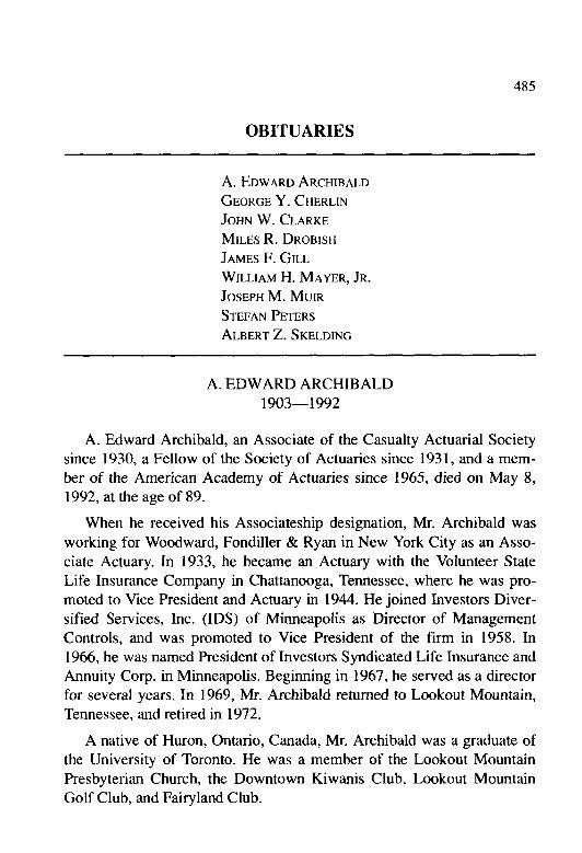
OBITUARIES 489
He is survived by a son, Denman Drobish, of San Francisco, and two grandchildren.
JAMES F. GILL l909- 1992
James F. Gill, an Associate of the Casualty Actuarial Society since 1963, an Associate of the Conference of Consulting Actuaries since 1959, and a Member of the American Academy of Actuaries since 1966, died at home on September 27, 1992. He was 82 years old.
A graduate of the University of Pittsburgh, Mr. Gill worked for the National Association of Independent Insurers in Chicago, Illinois, for 25 years, beginning in 1948. He rose to the position of Vice President and Actuary, a position he held from 1967 until 1973.
In 1973, Mr. Gill joined the Westfield Companies in Westfield Center, Ohio, as Actuary. He retired from the firm in 1980. He then moved to Portland, Oregon, and worked as a consultant before retiring from actuar- ial practice in 1982.
Mr. Gill served on two committees in the Society, the Financial Re- view Committee in 1966, and the Committee on Annual Statement from 1967-l 97 1. He authored two papers published in the Proceedings. His first paper, “An Approximation for the Testing of Private Passenger Lia- bility Territorial Rate Levels Using Statewide Distribution of Classifica- tion Data,” appeared in the 1964 Placeedings and his review of “Ratemaking Procedures for Automobile Liability Insurance” was pub- lished in the 1966 edition. Mr. Gill also moderated a panel discussion on “Loss Reserve Problems-Financial and Ratemaking” at the 1969 CAS Spring Meeting.
Mr. Gill is survived by his wife, Margaret, of Portland; a daughter, Mary Donevan; and a sister, Kathleen Gill.
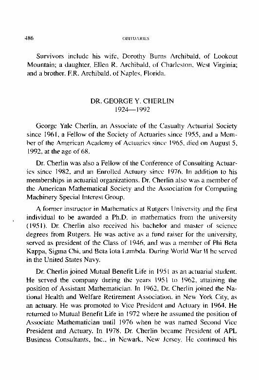
490
WILLIAM H. MAYER. JR. 1910-1990
William H. Mayer, Jr., an Associate of the Casualty Actuarial Society since 1936, died on December 27, 1990, of the complications from Parkinson’s disease. He was 80.
Mr. Mayer worked his entire career at the Metropolitan Life Insurance Company, in New York City. When he became an Associate in 1936 he was working in the actuarial department. He was promoted in 1949 to group contract referee. He became the associate manager of Met Life’s Group Contract Bureau in I95 I, and was appointed manager in 1958.
In 1979, Mr. Mayer retired and resided in Dix Hills, New York, until his death. He is survived by his wife, Marilyn Mayer, of Dix Hills: and four sons: William, Peter, Richard, and Thomas; and an aunt.
JOSEPH M. MUIR 1906 I 989
Joseph M. Muir, an Associate of the Casualty Actuarial Society since 1957, died on September 13, 1989. He was 85.
In 1927, Mr. Muir joined the Mutual Insurance Rating Bureau and the Insurance Advisory Association in New York City where he worked for 42 years until his retirement in 1969. For more than 20 years he held the position of general manager for both organizations.
He earned his Bachelor of Science degree from Cooper Union in New York City, going to night school for seven and a half years.
In 1973, Mr. Muir moved from Haworth, New Jersey, to Boca Raton, Florida, where he lived until his death.
Mr. Muir is survived by his wife, Mabel J. Muir. of St. Augustine, Florida; a daughter, Grace E. Emden, also of St. Augustine; and a grand- daughter, Debra J. Emden, of Metairie, Louisiana.

OBITUARIES 491
DR. STEFAN PETERS 1909-1990
Dr. Stefan Peters, a Fellow of the Casualty Actuarial Society since 1941 and a Fellow of the Society of Actuaries since 195 I, died on August 16, 1990. He was 81.
Dr. Peters was born in Erlangen, Bavaria, Germany, and received his degree in mathematics from the University of Berlin. After graduation, he worked in Berlin until the political climate provoked his emigration. He moved to Trieste, Italy, and spent some time with the Assicurazione Generali as a life actuary. It was in Italy that he met his wife, Renata. In a few years, he was again forced to move, this time to the United States.
Dr. Peters became an Associate in the Society in 1940 while he was working for the Compensation Insurance Rating Board in New York City as an assistant actuary. From this position, he was inducted into the Army of the United States and served his adopted country in enlisted status both at home and overseas in the Mediterranean Theater. This service qualified him for citizenship.
In 1945, Dr. Peters moved to Berkeley, California, and in 1948, he assumed the position of Lecturer with the Department of Statistics, then headed by Jerzy Neyman, at the University of California. In 1949, after the sudden death of Professor Albert Mowbray, FCAS, Dr. Peters took over the insurance classes in the School of Business Administration and was appointed Associate Professor. During this period, he also served as consulting actuary to West Coast Life Insurance Company.
His experience under fascist governments led Dr. Peters to resist im- position of the loyalty oath required of its faculty by the University of California in the early 1950s. After losing a courageous legal battle that went to the California Supreme Court, he moved back to the East Coast in 1952, and took a position with Morse and Seal in New York City as Actuary. He moved to Boston in 1953 and joined the firm of Connell, Price and Company. In 1959, he started several years’ service with Arthur D. Little Consultants in Cambridge, Massachusetts. In 1974, Dr. Peters became the Chief Actuary for the Department of Insurance for the Com-

monwealth of Massachusetts, a position he held until his retirement in 1986.
Dr. Peters published three papers in the Pl.oc,cc~tlirlRs, all on workers compensation insurance. In 194 I, his paper, “A Method of Testing Classi- fication Relativities,” introduced to the Procrtdings what R.A. Fisher called the “analysis of variances.” The paper covered a specific applica- tion of the then relatively new formal testing of hypotheses and making of decisions under uncertainty.
Stefan Peters was admired by his many friends for successfully and gracefully overcoming severe problems in his long life. He was a quiet person whose warmth and friendliness were sometimes apparent only to the close observer, but were always clear to the many students and friends to whom he was ever pleased to give help. We who knew him warmly remember a good friend.
Dr. Peters is survived by his wife; a son, Matthew Peters, of Cam- bridge; and a daughter, Clara Simon, of Albany, New York.
ALBERT 2. SKELDING 1897-1992
Albert Z. Skelding. a Fellow of the Casualty Actuarial Society since 1929 and a member of the American Academy of Actuaries since 1965, died on March 3 1, 1992, at the age of 95.
In 1925, Mr. Skelding became an Associate of the Society. He spent his entire career working for the National Council on Compensation In- surance (NCCI) in New York City. He started as an Associate Actuary and in 1934 he was promoted to Actuary. In I950 he was named Assistant Manager, and in 1957 he was promoted to Associate Genera1 Manager of NCCI, a position he held until his retirement in 196 I
At NCCI, Mr. Skelding worked to gain approval of workers’ compen- sation rate filings throughout the country. AI his retirement party, he delighted well-wishers with his reminiscences of those attempts. Since the methods used to win approval from the state insurance departments
OBITUARIES 493
were not always limited to logical and statistical presentations, his ac- count was both historically interesting and hilarious,
Mr. Skelding held several volunteer positions within the Casualty Ac- tuarial Society. He was elected to the Council of the CAS for a three-year term ending in 1942. He was elected Vice President of the Society from 1942 until 1944 and served as Secretary-Treasurer for 20 years, from 1953 until 1973. He was also active on the committee level, serving on the Examinations Committee, the Program Committee, and the Commit- tee on Publications.
Mr. Skelding also contributed many important book reviews to the Proceedings. He reviewed the following publications: Reversions and Life Interests; An Introduction to the Mathematics of Life Insurance; Compowld Interest Tables; Tuhles .for Calculating by Machine; Loga- rithms to 13 Pluces of Decimals; and the Cost of Compensation for- the Year Ended June 30, 1928 (a Special Bulletin of the New York Depart- ment of Labor).
A lifelong resident of New York, Mr. Skelding was born in Brooklyn, and graduated from City College of New York in 1917. He was named valedictorian of his class, but was unable to attend the ceremonies be- cause of his enlistment in the United States Navy three weeks before he graduated. It is rumored that Mr. Skelding was the youngest ensign to serve in World War 1.
In 1990, he moved from Massapequa, New York, to Lynchburg, Vir- ginia. Until a week before his death, Mr. Skelding was doing calculus problems, playing contract bridge, and handling his own stock portfolio.
He is survived by a son, Robert Skelding, of Lynchburg; two daugh- ters, Kathleen Wennerstrom and Lois MacFarland; and ten grandchildren.
494
INDEX TO VOLUME LXXIX
Page ADDRESS TO NEW MEMBERS
Ruth E. Salzmann-May 1992 . . . . . . . . . . . . . . . . . . . . . . . . . . . . . . . . . . . . . . . . . . . . . . . . . . . . . . I49 Paul S. Liscord-November I992 . . . . . . . . . .._............................_....... 4 I I
ADMINISTRATION, REPORT OF THE VICE PRESII)ENT........................... 439
ANALYSISOFEXCESSLOSSDEVELOPMENT,AN Emanuel Pinto and Daniel F. Gogol (November 1987) Discussion by Robert A. Bear . . . . . . . . . . . . . . . . . . . . . . . . . . . . . . . . . . . . . . . . . . . . . . . .._..... 134
ARCHIBALD,A.EDWARD Obituary . . . . . . . . . . . . . . . . . . . . . . . . . . . . . . . . . . . . . . . . . . . . . . . . . . . . . . . . . . . . . . . . . . . . . . . . . . . . . . . . . . . . . . . . 485
BEAR,ROBERTA. Discussion: An Analysis of Excess Loss Dcvelopmcnt . .._........... I34
BOOR, JOSEPH A. Paper: Credibility Based on Accuracy . . . . . . . . . . . . . . . . . . . . . . . . . . . . . . . . . . . . . . . . . . 166
BROWN,BRIANZ. Paper: Pricing for Credit Exposure . . . . . . . . . . . . . . .._......................._...... 186
CHERLIN,GEORGEY. Obituary . . . . .._.. . . . . . . . . . . . . . . . . . . . . . . . . . . . . . . . . . . . . . . . . . . . . . . . . . . . . . . . . . . . . . . . . . . . . . . . . . 486
CLARKE,JOHN W. Obituary . . . . . . . . . . . . . . . . . . . . . . . . . . . . . . . . . . . . . . . . . . . . . . . . . . . . . . . . . . . . . . . . . . . . . . . . . . . . . . . . . . . . . . . . . 487
COMPETITIVE MARKET EQUILIBRIUM RISK LO/U) FORMULA FOR INCREASEDLIMITS RATEMAKING,THE
Glenn G. Meyers (November I99 I ) Discussion by Dr. Ira Robbin . . . . . . . . . . . . . . . . . . . . . . . . . . . . . . . . . . . . . . . . . . . . . . . . . . . . . . . . 367
COMPUTATIONOFAGGREGATE Loss DISTRIBIJTIONS,THE John P. Robertson . . . . . . . . . . . . . . . . . . . . . . . . . . . . . . . . . . . . . . . . . . . . . . . . . . . . . . . .._....._............ 57
COSTOFMIXING REINSURANCE,THE Ronald F. Wiser (November 1986) Discussion by Michael Wacck . . . . .._............................................... 385
CREDIBILITY BASEDONACCURA~\~ Joseph A. Boor ._............................................................................ 166
DROBISH,MILES R. Obituary . . . . . . . . . . . . . . . . . . . . . . . . . . . . . . . . . . . . . . . . . . . . . . . . . . . . . . . . . . . . . . . . . . . . . . . . . . . . . . . . . . . . . . . . 488
495
INDEX-CONTINUED
Page DLJVALL, RICHARD
Paper: Testing for Shifts in Reserve Adequacy ................................ 1 EXAMINATIONS. 1992-SUCCESSFUL CANDIDATES ............................. 447
FINANCIAL REPORT.. ............................................................................ 446
GILL, JAMES F. Obituary ........................................................................................ 489
GILLAM,~ILLIAM R. Paper: Parametrizing the Workers Compensation
Experience Rating Plan ................................................................ 2 1 Paper: Workers Compensation Experience Rating:
What Every Actuary Should Know.. .......................................... 2 15 GOGOL,DANIEL F.
Discussion: Reinsurer Risk Loads from Marginal Surplus Requirements.. .............................................................................. 362
LISCORD,PAULS. Address to New Members-November 1992.. ............................. 4 1 1
MAYER,~ILLIAM H.,JR. Obituary ........................................................................................ .490
MINUTES May 1992 Meeting.. ....................................................................... 152 November 1992 Meeting.. ............................................................. 423
MUIR,JOSEPH M. Obituary ........................................................................................ 490
OBITUARIES A. Edward Archibald.. .................................................................. 485 George Y. Cherlin.. ....................................................................... 486 John W. Clarke ............................................................................. 487 Miles R. Drobish.. ......................................................................... 488 James F. Gill ................................................................................. 489 William H. Mayer, Jr.. .................................................................. 490 Joseph M. Muir.. ........................................................................... 490

4%
INDEX-CONTINUED
OBITUARIES (cont’d) Page
Stefan Peters . . . . . . . . . . . . . . . . . . . . . . . . .._.........._....._..................................... 49 1 Albert Z. Skelding . . . . . . . . . . . . . . . . . . . . . . . . . . . . . . . . . . . . . . . . . . . . . . . . . . . . . . . . . . . . . . . . . . . . . . . . 492
PARAMETRIZING THE WORKERS COMPENSX~ION EXPERIENCE RATING PLAN
William R. Gillam . . . . . . . . . . . . . . . . . . . . . . . . . . . . . . . . . . . . . . . . . . . . . . . . . . . . . . . . .._....._.......... 2 1 PETERS, STEFAN
Obituary . . . . . . . . . . . . . . . . . . . . . . . . . . . . . . . . . . . . . . . . . . . . . . . . . . . . . . . . . . . . . . . .._...................... 49 1 PRESIDENTIAL ADDRESS-NOVEMBER 1992
“An Investment in Our Future” Michael L. Toothman . . . . .._..........._....._..................................__....... 414
PRICING FOR CREDIT EXPOSURE Brian Z. Brown . . . . . . . . . . . . . . . . . . . . . . . . . . . . . . . . . . . . . . . . . . . . . . . . . . . . . . . . . . . . . . . .._............ 186
REINSURER RISK LOADS FROM MARGINAL SURPUIS REQUIREMENTS
Rodney Kreps (May 1990) Discussion by Daniel F. Gogol......,............................................... 362
REPORT OF THE VICE PRESIDENT-ADMINISTRATION . . . . .._.................... 439 ROBBIN, DR. IRA
Discussion: The Competitive Market Equilibrium Risk Load Formula for Increased Limits Ratemaking _...................... 367
ROBERTSON, JOHN P. Paper: The Computation of Aggregate Loss Distributions............. 57
SALZMANN, RUTH E. Address to New Members-May 1992 . . . . . . . . . . . . . . . . . . . . . . . . . . . . . . . . . . . . . . . . . 149
SKELDING, ALBERT Z. Obituary . . . . . . . . . . . . . . . . . . . . . . . . . . . . . . . . . . . . . . . . . . . . . . . . . . . . . . . . . . . . . . . . . . . . . . . . . . . . . . . . . . . . . . . . 492
STOCHASTIC CLAIMS RESERVING WHEN PAST CLAIM NUMBERS ARE KNOWN
Thomas S. Wright . . . . . . . . . . . . . . . . . . . . . . . . . . . . . . . . . . . . . . . . . . . . . . . . .._....._................. 255 TESTING FOR SHIFTS 1~ RESERVE ADEQUACY
Richard Duvall . . . . . . . . . . . . . . . . . . . . . . . . . . . . . . . . . . . . . . . . . . . . . . . . . . . . . . . . . . . . . . . . . . . . . . . . . . . . . . . . . . . 1
497
INDEX-CONTINUED
Page TOOTHMAN, MICHAEL L.
“An Investment in Our Future” Presidential Address-November 1992 . . . . . . . . . . . . . . . . . . . . . . . . . . . . . . . . . . ..a... 414
WACEK,MICHAEL Discussion: The Cost of Mixing Reinsurance . . . . . . . . . . . . . . . . . . . . . . . . . . . . . . . 385
WORKERSCOMPENSATIONEXPERIENCERATING:WHAT EVERYACTUARYSHOULDKNOW
William R. Gillam . . . . . . . . . . . . . . . . . . . . . . . . . . . . . . . . . . . . . . . . . . . . . . . . . . . . . . . . . . . . . . . . . . . . . . . . 215 WRIGHT,THOMAS S.
Paper: Stochastic Claims Reserving When Past Claim Numbers Are Known . . . . . . . . . . . . . . . . . . . . . . . . . . . . . . . . . . . . . . . . . . . . . . . . . . . . . . 255

49x
EDITORIAL COMMITTEE, PROCEEDINGS Editors
Eugene C. Connell, Editor
Daniel A. Crifo Diane S. Duda Claudia S. Forde James F. Golz Richard W. Gorvett Ronald E. Greco Brenda G. Huber (CAS 0fJi’c~J
John J. Kollar (CJ.Y ojfi2ioi George M. Levine Neil L. Millman Rebecca A. Moody Ann E. Overturf Debbie Schwab Kathleen W. Terrill