DFA Insurance Company Case Study, PartII: Capital Adequacy and Capital Allocation

Stephen W. Philbrick, FCAS, MAAA and Robert A. Painter

99

Dynamic Financial Analysis DFA Insurance Company Case Study Part Ih Capital Adequacy and Capital Allocation

By Stephen W. Philbrick, FCAS, MAAA and Robed A. Painter

Swiss Re Investors 111 S. Calved Street, Suite 1800

Baltimore, MD 21202 Phone: (410) 369-2800

Fax: (410) 369-2900

Abstract

This paper has been submitted in response to the Committee on Dynamic Financial Analysis 2001 Call for Papers. The authors have applied dynamic financial analysis to DFA Insurance Company (DFAIC) to address capital adequacy and capital allocation issues. The DFA model used for this analysis was the Swiss Re Investors Financial

TM Integrated Risk Management ( F I R M ) System. This paper is Part 2 of a two-part submission. Part 1 deals with using DFA to explore reinsurance efficiency and asset allocation issues.

This paper explores different general risk measures used in the past to judge capital adequacy. This overview of various risk measures will incorporate the concept of coherent risk measures. It introduces a practical method for using Tail Conditional Expectation (TCE) as a measure of capital adequacy. We will look at the adequacy of DFAIC's capital position using the TCE risk measure along with other more widely accepted regulatory and rating agency capital adequacy measures for different reinsurance/asset allocation strategies.

Additionally, we will discuss different risk measures associated with capital allocation, including TCE, along with different allocation procedures. This section will also explore the idea of allocating capital to assets. Different allocation methods will be discussed and the Shapley Value method, found in game theory, will be applied to two different risk measures to allocate DFAIC's current capital to line of business and to assets.

100

Dynamic Financial Analysis DFA Insurance Company Case Study Part I1: Capital Adequacy and Capital Allocation

By Stephen W. Philbrick, FCAS, MAAA, and Robert A. Painter

P r e f a c e

Dynamic Financial Analysis (DFA) is still fairly new to a property-casualty insurance industry whose roots can be traced back to the 17 ~ Century and earlier. As such it is not surprising that the industry is cautious about a technology that purports to look at their business in a whole new way. The Casualty Actuarial Society, being active in the formulation and development of DFA, has classified it as:

"a systematic approach to financial modeling in which financial results are projected under a variety of possible scenarios, showing how outcomes might be affected by changing internal and~or extemal conditions'."

As a result of published papers, shared research end call paper programs such as this one, the technical specifications behind DFA have been well developed. This has led to a high level of convergence among many of the different concepts, models and processes behind DFA. Unfortunately, while the details of DFA are better understood, the industry is still scratching its collective head on what to do with this new technology.

Part of the problem has to do with the fact that DFA is mainly considered to be a modeling tool, one that can be used to supplement existing tools. While a modeling tool is essential for implementing dynamic financial analysis, it is just one element of a much grander picture. More than a model, dynamic financial analysis is a way of thinking that weaves through the entire operations of an insurance company. Effective dynamic financial analysis calls for dedicated and knowledgeable professionals who are trained in the intricacies of DFA and enabled to identify and take advantage of current industry and company inefficiencies. DFA promotes moving from existing structures designed to evaluate and reward, the individual pieces of the business to a structure that encourages and rewards the evaluation of strategic decisions in a holistic, total company framework.

1 Casualty Actuarial Society Dynamic Financial Analysis Website, DFA Research Handbook, http://www.casact.org/R ES EARCH/DFA

I01

For these reasons we were excited to embrace this call paper program exercise. While the original concept may have been designed to evaluate different DFA modeling techniques and the resulting analyses as they relate to a common problem and common data, we decided it was a perfect opportunity to show how DFA might work in the insurance company of tomorrow. The ultimate benefit to the company is not just the final answer, but rather the increased understanding and the common grounds of communication that comes from going through the DFA process.

The proposed situation involves DFA Insurance Company (DFAIC), a multi-line property- casualty insurance company that is unknowingly the target of a potential acquisition. The analysis was conducted from the point of view of the acquiring company. We will define the acquiring company, Falcon, as a newly capitalized holding company that is organized and structured to run its business in a holistic manner. Falcon has a financial risk management unit led by its Chief Risk Officer (CRO) w h o repod's direct ly to the CEO. The CEO has asked that the following questions about DFAIC be addressed:

t. Is the Company adequately capitalized? Is there excess capital? How much capital should the Company hold as a stand-alone insurer?

2. How should the capital be allocated to line of business?

3. What is the return distribution for each line of business and is it consistent with the risk for the line?

4. Should the Company buy more or less reinsurance? What type? How efficient is its current reinsurance program?

5. How efficient is the asset allocation?

In a traditional insurance company these questions would be farmed out to different business units within the organization. These units would include but not be limited to the actuarial department, the reinsurance department and the investment department. Each unit would perform their stand-alone analysis and report back to the CEO using terminology and metrics appropriate to their assigned task. The CEO would be left to assimilate all the individual analyses and use professional judgment and insights to build a complete picture of the attractiveness of the potential acquisition.

Falcon, however, is organized in such a way that the complete analysis can be performed within the financial risk management unit with input from professionals in each of the departments mentioned above. The results of the analysis can thus be presented to the CEO using a single set of terminology and metrics that consider both the individual and joint dynamics of the issues in question.

102

Due to the scope and breadth of the required analysis, we will present the DFA study in two papers. This paper will deal with the capital adequacy and capital allocation issues and a sister paper will concentrate on reinsurance and asset allocation strategy issues. Note that despite breaking the analysis up into two papers, the overall analysis is the result of a common DFA model and process.

13FA, being holistic, allows a company to deal with all of its major strategic decisions simultaneously within a single framework. As such it is not unusual to have an analysis that continuously revisits these strategic levers in what we call the DFA spiral. This is in contrast to the traditional approach in which these strategic decisions are evaluated each in their individual silos. Figure 1 gives a graphical picture of these two different approaches.

Figure 1

Traditional Analysis Dynamic Financial Analysis

0

Asset Capital I Reinsuranc~

Allocation I Adequacy I

i I

Unfortunately, a paper does not easily land itself to a spiral analysis, so for the sake of convenience we will first complete a single loop around the DFA spiral, holding the strategic decisions that relate to other sections constant. This will allow us to show how DFA can be used to deal with individual strategic initiatives but still within a holistic framework..We will then begin a second loop taking into consideration the strategic initiatives suggested as a result of the initial loop. This will allow us to identify and discuss the additional opportunities that result from simultaneous changes to two or more strategic initiatives.

103

This paper concentrates on capital adequacy and capital allocation issues. While information concerning revisions to the reinsurance program and asset allocation will be stated, the interested reader should refer to the sister paper "Dynamic Financial Analysis, DFA Insurance Company Case Study, Part I: Reinsurance and Asset Allocation" [11] for a detailed description of the methodology used in the development of these numbers.

Rosdmap

This paper will:

• Set forth the seven steps of The DFA Process--an approach to think about DFA.

• Discuss several risk measures, then use a TCE measure, which satisfies the axioms for a coherent risk measure.

• Apply a DFA approach to a specific case study--the DFAIC hypothetical company supplied by the CAS.

First, the DFA Process will be described. The steps of this process will be used throughout the rest of the paper to organize the discussion.

The next section will begin with a general discussion of capital adequacy. This will be followed by a brief discussion of prior work on this issue and the direction taken in recent research. Next, we will discuss three measures of capital adequacy, and then discuss the general concepts underlying any risk measure.

Next, we will discuss three capital adequacy measures used by regulators and rating agencies. We will then explain why Tail Conditional Expectation (TCE) is selected as the measure of risk over the other three choices. Because the concept of TCE may be new to many readers, and it is the selected method in this paper, we will go into that measure in somewhat more detail than the other two methods. Then we will summarize the results of each of the capital adequacy measures tor DFAIC.

Finally, we will discuss the concept of capital allocation, and show how a TCE measure can be used to allocate capital to segments of DFAIC.

The DFA Process

The DFA Process refers to a high-level overview of how a DFA model can be brought to bear on a specific problem [13]. We have outlined, in Figure 2, the DFA process that we used for our analysis of DFAIC.

104

Figure 2

The Dynamic Financial Analysis P, rocess

7.

3 I 2. Collect Data I

! 1, Set Goals and j I Objectives

Present Findings

It is critical to understand that DFA is more than just a model. The development of a computer model c a n be viewed as "step zero" of the process. It is a necessary step, but it represents the development of a tool, rather than the DFA process itself. The DFA process starts with a thorough discussion and understanding of the goals, objectives, constraints and risk tolerance of a company. This step determines the metrics that w;ll be most important in evaluating alternative strategic initiatives. It also tends to be a valuable exercise as it helps management think through, focus on, and communicate exactly those items that are most important to them as a company. These items are stated in terms of financial statement results and, once determined, provide a common set of metrics that can be applied to all of the company's financial strategic decisions.

Steps 2 through 4 of the DFA process depend on the specifics of the DFA modeling system that is being used for the analysis. Whereas a common DFA process allows for effective and efficient sharing of concepts and ideas, it could be argued that different modeling methodologies and assumptions are healthy in order to address the potential problem of model bias (model risk) and assumption bias (parameter risk).

In order to become comfortable with a particular modeling system for implementing DFA, one must understand both the methodology that underlies the system and how that particular methodology will impact the results of the analysis. By DFA model methodology we refer to the specific technical implementation of the DFA process.

10.5

Whereas the general DFA process has become fairly standardized, there are still a number of different methodologies that are used in the technical implementation of a DFA model. Since the technical implementation of a model can have a significant impact on the results of an analysis, it is imperative that the users of a model sign off on the technical implementations and understand how the specific model methodology will impact the analysis. The risk that model results are specific to a particular DFA methodology is referred to as "model risk." This is a difficult risk to evaluate; due to the time, effort and expense of performing DFA, it is often impractical to duplicate the analysis using different DFA modeling systems. As such, users should look for systems that provide a significant amount of flexibility and whose underlying fixed methodologies are consistent with their views of the insurance and financial markets.

At Swiss Re Investors, we developed our Financial Integrated Risk Management (FIRM TM) System as the modeling tool backing our DFA process. The FIRM System, like most DFA systems, uses simulation techniques to model both the assets and liabilities of an insurance company. The projected cash flows are transformed into future balance sheets and income statements that reflect GAAP, statutory, tax and economic viewpoints. The simulations are generated by a series of stochastic differential equations that are designed to allow the model user to reflect a full range of distributions, dynamics and relationships with respect to the underlying stochastic variables. The tool is designed to allow a high level of flexibility in describing how the underlying stochastic variables behave in an attempt to minimize model risk. This increase in flexibility, however, has the result of moving a significant burden from the model, to the model builder and the model assumptions. Interested readers can find additional information on the mechanics of the Swiss Re Investors FIRM System by referring to our previous CAS DFA call papers.

Assumptions and model parameterization are closely tied to methodology in that they also deal with the technical details of DFA. DFA model assumptions refer to how the asset and liability variables are assumed to behave over the forecast horizon. The major difference between methodology and assumptions is that assumptions can be changed whereas methodology, within a particular system, is generally fixed. Assumptions used in DFA modeling can have a substantial impact on the recommended strategies. In the modeling world this risk is referred to as "parameter risk." The impact of parameter risk can be substantially reduced through the use of sensitivity testing and by having the analysis performed by experienced DFA professionals.

Steps 5 and 6 of the DFA process relate to analysis and sensitivity testing. While there is still some connection to the modeling system used for the analysis, the effectiveness of these steps are more a function of the DFA professional. Even given a good DFA modeling system, the analysis performed can be poor. A good DFA analysis will tie the conclusions to the assumptions in a clear and concise manner. The impact of alternative strategic initiatives will be explained in such a way that someone who is unfamiliar with the details of DFA will still be able to follow, understand and ultimately accept the stated conclusions. Sensitivity testing is required to ascertain that the conclusions are not the product of a particular set of assumptions or the result of a particular set of random scenarios.

106

Finally, the presentation of the DFA study (step 7) should do more than show the numbers and present the conclusions. Rather, the presentation should tell a story. The story should review the highlights of each step of the DFA process and lay out the logic that went into the analysis in such a way that the conclusions become evident before they are revealed. It is important to keep in mind that the value of DFA is not just in the answer but also in the increased understanding of the issues that lead to the answer and ultimate decision.

The remainder of this paper will explore the assumptions and model details that we used in performing our DFA on DFAIC. Several of the steps are identical to the steps in our sister paper on reinsurance and asset allocation. Rather than repeat those steps, we refer the reader to the discussion in that paper. In this paper, we will discuss the aspects that are unique to the adequacy and allocation analysis. For easy reference, the discussion of the parameterization of DFAIC will be included as Appendix A and B.

107

Capital Adequacy

Adequacy of capital is critical to a consumer of insurance products. In many companies, the product is delivere, d at the time of purchase. While a consumer, for example, may have some legitimate interest in the ongoing solvency of a manufacturing company to provide access to spare parts, an insurance product is, at its core, a promise to deliver in the future. The ability to make good on its promises is critical to the insurance company.

The actuarial literature contains many papers on the subject of capital adequacy. The CAS commissioned an annotated bibliography of relevant research papers on the subject. The bibliography is contained in a report by Brender, Brown and Panjer [10]. This report was completed in July 1992. This year was a good year for capital adequacy research for another reason~the CAS issued a call for papers on Insurer Financial Solvency. Those papers are contained in the 1992 Discussion Papers on Insurer Financial Solvency [1]. The early work on capital adequacy focused on the underwriting side of the balance sheet. Over time, various papers have incorporated more sophisticated treatment of assets. [2], [13], [22], [29], [33] This has proceeded through:

Recognition of investment income (acknowledging the existence of assets, but treating assets as largely fixed)

Recognition of asset variability, but treatment of asset variability as independent of underwriting variability

Recognition of asset volatility as well as the economic interdependencies between assets and liabilities

While analytic and simulation techniques have both been used in a variety of papers, the complex nature of the interactions of assets over time and of the relationship between assets and liabilities virtually requires a simulation approach, typically embodied in a Dynamic Financial Analysis (DFA) model. A recent paper by Mango and Mulvey [27] describes a DFA approach to the capital adequacy and allocation problems.

The evolution of capital adequacy has proceeded in another dimension as well. In addition to more sophisticated handling of assets, the analysis of the risk measure has become more refined. Early papers concentrated on the probability of ruin, that is, the probability that the firm would become insolvent. While this is clearly an important issue, it emphasizes the owners of the firm over other interested parties. More recent research has extended this concept in two ways:

1. Recognition that the amount of insolvency, not just the probability, matters to policyholders, or at least to the insolvency funds that must pay in the event of insolvency. As a consequence, regulators are interested in the cost of insolvency, not just the likelihood. [12]

108

2. Formal recognition that firms care about surplus reduction even when it doesn't result in insolvency. While this isn't a new idea, more sophisticated DFA models can be used to analyze reductions in surplus of less than 100%. These options are useful for examining the likeli.hood of ratings downgrades.

Discussion of Risk Measures

The risk measures we will discuss in this section by no means define the universe of possible risk measures. These are some the prominent measures that have emerged in the literature. There is no single measure that is recognized as the best, but some have appealing properties that make them more relevant to the discussion of capital adequacy.

Probability of Ruin, or Ruin Theory, is probably the most intuitive risk measure when discussing capital adequacy: how likely is it that I will be able to stay in business over a given time period? This paper defines Probability of Ruin in its most general sense: the probability that a given variable or event is below some defined limit over a defined period of time. This measure is dependent on the target company selecting a fixed minimum capital limit where they would define themselves as "ruined". This is a binary process where either the company is ruined or not ruined--there is no contemplation of degree of ruin in this risk measure. It is necessary to emphasize that that selection of risk variable and risk limit and tolerance levels should be based on the individual circumstances and goals of the company. Mango[27]

Probability of Ruin is closely associated with Value at Risk (V'aR), a concept that originates from the banking industry. For banks, VaR would be the maximum amount the bank could potentially lose over a time period in which they could not react to market conditions. This might be the amount they could lose from financial positions left open overnight while the bank is closed. In an insurance context, the concept of the company not being able to react to market conditions has been ignored due to the much longer time frames being evaluated in solvency analysis.

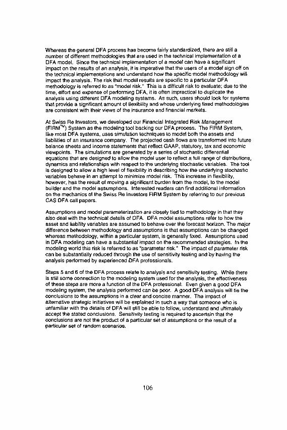
Figure 3 shows the inverted cumulative distribution of results for a given financial variable. The Y-axis measures the magnitude of the financial variable. The X-axis is the percentile of the corresponding financial result. Given a risk tolerance criterion of o~, c~ is defined as 1-q. Following the arrows up from q to the intersection with the distribution and over to A, the VaR is the dollar equivalent for a given risk tolerance c~.

109

Figure 3

" ~ XE f WE L

A

q

A = F" (q)

i [F " ~ ( x ) - A ] d x = Y E F(A)

; A = V a R

; A = Point where YE = EPD Tolerance

A second approach commonly used to measure capital adequacy is Expected Policyholder Deficit (EPD). Whereas Ruin Theory only takes into account the probability of insolvency, EPD considers the magnitude of ruin. EPD incorporates the fact that not all insolvencies are the same. Regulators, policyholders, and debtholders care about the amount by which the company will not be able to fully meet its obligations. As a result, the criterion for this risk measure is defined by a tolerable amount of obligations that will not be met. This EDP criterion can be stated as either a dollar amount or as a percentage of total obligations, and is represented in Figure 3 as the shaded area YE. EDP and the distribution can be expressed in terms of many different financial variables. In Figure 3, total obligations are equal to WE + XE + YE. Point A, as defined by the tolerance area YE, is the level of obligation that the company can handle without being in a "deficit position".

I I 0

The two prior measures are intuitively appealing, but were developed ad hoc. The likelihood that a company might become insolvent seems like a logical risk measure. Similarly, the extension to the cost, rather than simply the probability of insolvency seems like an obvious improvement. Nevertheless, neither approach was developed using the axiomatic approach of mathematics--to first identify desirable properties of a measure, then mathematically search for measures that meet the criteria. In recent years, researchers have taken this approach. A thorough discussion of the selection of the axioms, and the resulting measures, called coherent risk measures is beyond the scope of this paper. However, because we use a coherent risk measure as a critical part of our analysis, and the concept is still relatively new to many people, Appendix C contains a brief introduction to the concept of coherent risk measures, including the underlying axioms.

The third approach used to measure capital adequacy is a coherent risk measure, Tail Conditional Expectation (TCE). [3], [4], [5], [30]. Tail Conditional Expectation combines the ideas behind VaR and EPD into a single measure. In order to calculate the TCE result, a TCE risk tolerance criterion must first be selected. The VaR tolerance is a function of a selected percentile along the x-axis, whereas EPD tolerance is a function of a selected area. The TCE tolerance is conceptually similar to the VaR tolerance in that it is based on selecting an appropriate point along the x-axis. In Figure 4 the TCE tolerance 2 is equal to 1 - q = c~. Referring to Figure 4, again the sum of all potential events is equal to WT + XT+ YT. All results to the right of the vertical line, defined by the TCE tolerance oc, are considered "tail events". The sum of these tail events is equal to XT + YT. The average tail event is equal to the Tail Conditional Expectation. Graphically, the TCE is equal to the height of the XT + ZT such that the area of (XT + Z-r) equals the area of (XT + YT).

2 For a VaR tolerance of c~ and a TCE tolerance of c~, if c~---~ and Fl(x) is a continuously increasing function, then TCE Required Capital z VaR Required Capital

I I1

Figure 4

A

XT

0 q

F-'(x) dx A = " " ; A =TOE

] - q

While these three approaches differ in important ways, there is a common theme. In each case, the analysis of cal~ital adequacy proceeds in these four steps:

1. Select a Financial Variable

2. Select a Time Frame

3. Select a Measure

4. Select a Criterion

Financial Variable

The main decision for the financial variable is how much of the balance sheet to incorporate~whether the emphasis will be on liabilities or both assets and liabilities. In the former case, aggregate losses may be the financial variable; in the latter case, surplus. Secondary considerations:

• Should all liabilities be modeled or just loss and LAE?

• Should the accounting basis be statutory valuation, GAAP valuation, or some other basis?

112

Time Frame

The time frame represents the period of time over which the analysis is performed. In principle, this can be unlimited. Some work in ruin theory looks at unlimited time horizons, but this requires assumptions about future business that are unrealistic if interpreted as true projections about infinite time horizons.

For time periods other than unlimited, it may be necessary to clarify what is meant by the time frame. For example, does a one-year time frame mean that balance sheets and income statements are simply projected forward one year? Or does it mean that one additional year of new business is written, and then all outstanding liabilities are run off? A third alternative (common in valuation exercises) is to project one year's worth of business, including both new and renewal business, and then to include renewal business only, along with the liability runoff, for a specified number of renewal periods, or until the renewal business becomes de minimis. Any projection should clarify which basis is being used.

Typical time frames for insurance companies are one, three, and five years. Projecting beyond five years becomes speculative.

Measure

The simplest measure is the Financial Variable itself (along with its associated distribution). Other measures, such as EPD and TCE, can be formed as a function of the distribution of the variable of interest.

Criterion

Finally, one must specify a critical value of the measure. Generally, this value will be used as a binary separator to distinguish between acceptable and unacceptable levels of capital.

113

A p p l i c a t i o n

The generic approach described above applies to each of the three common approaches to capital adequacy:

Ruin Theory - The financial variable is surplus. However, early historical approaches treated assets as if they were a constant, and treated liabilities as the only random variable. More recently, both assets and surplus are handled as random variables. The time frame can be unlimited in some circumstances, but it is typically a relatively short period of time (before runoff) in DFA studies. The measure is the surplus itself, considered as a random variable. The criterion is some suitably small value such as 0.01 or 0.005, representing the probability that the financial variable can be less than zero in the selected time frame.

Expected Policyholder Deficit - The financial variable is usually the aggregate liability distribution. The time frame typically ranges from one to five years. The measure is the EPD, which can be expressed as a function of the aggregate loss distribution. In words, it is the average loss amount in excess of the assets of the company, averaged over those situations in which the liabilities exceed the assets (that is, the company is technically insolvent). This amount can be expressed in dollars, or it can be expressed as a ratio to the expected liabilities to put it on a comparable basis across companies.

Tail Conditional Expectation - The financial variable is typically aggregate liabilities, although surplus can be used. The time frame typically ranges from one to five years. The measure is TCE, which can be expressed as a function of the aggregate loss distribution. In words, it is the average aggregate loss amount (from ground up, rather than excess of some amount as in the case of EPD) for loss scenarios satisfying a criterion. As is the case with EPD, it can be expressed as a dollar amount, or it can be expressed as a ratio to total liabilities or total assets.

Introduction to DFAIC

DFAIC is the hypothetical company provided by the CAS for this exercise. This company is a privately held property-casualty company operating in all fifty states, writing personal lines and "main street" commercial coverages through independent agents. Key financial values:

• Current Assets 5.381 billion

,, Total Fixed Income (Average Maturity) 4.193 billion (7.4yrs)

• Total Equity 0.564 billion

• Current Liabilities 3.777 billion

• Current Booked Loss+LAE Reserves 2.330 billion

114

• Current Statutory Surplus 1.604 billion

• Previous Year Net Earned Premium Volume 2.409 Billion

• Projected Combined Ratio (Year 1) 107%

DFAIC currently holds per risk and per occurrence covers on all lines of business, along with a property CAT treaty. In total, the company cedes approximately 8% of premium.

Step 1:Goals and Objectives

The goal for the capital adequacy section of the analysis is to answer the first question in the Preface:

Is the Company adequately capitalized? Is there excess capita/?

Our assignment is to determine how much capital the company should carry, as a theoretical exercise, and compare it to the capital requirements according to regulatory and rating agencies. The company will carry the largest of the alternative amounts. If the required capital exceeds the current amount of capital on its balance sheet, the company will consider various ways to increase the actual capital or decrease the need for capital. If the actual capital exceeds the necessary capital, the acquiring company can release the excess capital to the owners, or consider whether additional risk can be taken on. This could be in the form of increased writings, more aggressive asset risks, or reduced reinsurance.

Steps 2-4:Data Collection, Parameterlzation and Model Runs

• The data collection phase is discussed in Step 2 of our sister paper.

• The parameterization is discussed in Appendix A and Appendix B, although certain aspects of the parameterization are discussed in the allocation section of this paper.

• The generation of the model runs is discussed in Step 4 of our sister paper

Steps 5-7:Analyze Output, Sensitivity Test, Present Findings

We will look at the following three different commonly accepted capital adequacy measures to help us analyze DFAIC's capital adequacy: the NAIC's Risk Based Capital(RBC) [34], A.M. Best's Absolute Capital Adequacy Ratio(BCAR) [9], and Standard & Poor's Capital Adequacy Ratio(CAR) [40]. Additionally, we will develop a fourth capital adequacy measure based on Tail Conditional Expectation (TCE). The formulas behind the NAIC, Best, and S&P measures can be found below in Figure 5.

11.5

Risk Based Capital

The Risk Based Capital is one of the means the NAIC uses to monitor capital adequacy. Set forth in the early 1990's, the NAIC RBC Model Act specifies responsibilities for both the regulator and insurer [15]. These responsibilities are triggered when the RBC Ratio (RBC Adjusted Statutory Surplus/Risk Based Capital) falls below 100%. The degree and severity of action increases as this ratio decreases. [34!

Best's Net Required Capital

The Best's capital adequacy model is somewhat similar in structure to the RBC model. Some of the key differences between the two models are the following:

• Best's model is interactive (manual adjustments can be made to the outcome),

• it takes into account the quality of loss reserves,

• it explicitly considers quality of reinsurer, and

• it explicitly considers CAT risk. [8],[9]

Best's does make adjustments to the numerator of the Absolute Capital Adequacy Ratio for many different factors; for this discussion we will assume that these adjustments net out to zero. As a result, we will limit our discussion to the denominator of the ratio, the Net Required Capital (NCR). Best's model self-admittedly produces a significantly higher NCR number than RBC's minimum solvency requirement. In the late 1990's, Best recalibrated its loss reserve and premium risk factors to recognize the concept of Expected Policyholder Deficit (EPD). Generally, a company is considered "Vulnerable" if its Absolute Capital Adequacy Ratio is below 100%.

S&PCAR

The CAR calculation is one element that goes into the S&P Rating. The S&P process considers many of the same variables as both RBC and the Best capital adequacy model. As a general rule, a CAR of greater that 125% is considered "Strong". [40]

116

Figure 5: Capital Adequacy Formulas

RBC = R o + (R, 2 + R2 2 + (.5 x R3) 2 + [(.5 x R 3) + R~I ~ + R~) ''~

R 0 = Noncontrol led Assets and Growth Risk R; = Fixed Income Investment Risk R 2 = Equity Investment Risk R 3 = Receivables Risk R, = Net Loss&LAE Reserve Risk R~ = Net Written Premium Reserve Risk

Bests Absolute Capital Adequacy Ratio = Adjusted Surplus / Net Required Capital

Net Required Capital = (BI 2 + B2 2 + B3~'(.5xB4) = + [(.SxB4) + B5) 2 + B6 ~ + B7~) ;rz

BI = Fixed Income Securities B2 = EquitySecuritles B3 = Interest Rate B4 = Credit B5 = Loss&LAE Reserves B6 = Net Written Premium B7 = Off Balance Sheet

S&P CAR = Total Adjusted Caol ta l - Asset Related Risk Charoes - Credit Reloted Risk Charoes

Underwriting Risk + Reserve Risk + Other Bus~ness Risk

Total Adjusted Capital = Statutory Surplus +/- Loss Reserve Def ic iency + Time Value of Money

TOE Required Capital Method

A graphical representat ion of and the method for calculat ing T C E Requi red Capital are presented in Figure 6 and Figure 7, respect ively. Briefly, the T C E risk measure is appl ied to a distr ibution of s imulated est imates of Required Assets to Cover Liabil i t ies 3 at the end of Year 1 (A1). A~ is synonymous to s imulated Statutory Surplus at the end of year 1 ( individual s imulated results) minus the Average Assets at the end of year 1.

3 This also takes into account of the volati l i ty of assets.

117

The calculation of Statutory Surplus for this adequacy measure is on a basis where the company reserves to the exact ultimate at the end of year 1. This perfect knowledge adjusts both existing reserves and one year of new business to their ultimate undiscounted levels.

We have selected a one-year time frame for this measure because most regulatory measures tend to be over a one-year time horizon. Unlike many other measures that only take into account underwriting results, statutory surplus takes into account the volatility of both assets and liabilities, along with the interactions between the two.

Once a distribution of Required Assets to Cover Liabilities at the end of year 1 (A1) is generated, the TCE risk measure is applied. First, a TCE Tolerance is selected. This selected tolerance (1% in this discussion') represents the largest 1% of all potential outcomes for the financial variable ,~. For ease of discussion, these large tail events will. be called "Large Losses'. Looking to Figure 6, the events defined by the tolerance are equal to X-r + YT. The Average "Large Loss" is equal to the TCE Required Assets (A,('rcE)). From Figure 6, this is equal to the height of ZT + XT, where the area of (ZT + XT) equals the area of (YT + XT), which equals the sum of all "Large Losses". Finally, TCE Required Capital is the difference between TCE Required Assets (Al('rcEi) and the Expected Liabilities at the end of year 1 (E[L~]).

4 This 1% tolerance is the level we selected for DFAIC. More work needs to be done to explore appropriate tolerance levels for different company risk profiles. A company should select its own tolerance based on an understanding the individual risks it faces.

5 "Large Loss" is a misnomer to the extent that asset volatility and other influences contribute to the tail event.

118

Flgure 6

I

i

q=0.99 1

Figure 6 Identities:

1) Total Loss = W, + X, + YT

2) Total "Large Loss" = X~ + Y,

3) Tolerance = 1 - q = 1 - 0.99 = 0.01

4) Z~ = Y,

TCE Required Assets = A~ 0cE) - .~ F " ( x )dx

1 - q

The TCE Required Capital Method emphasizes the tail of the distribution which differs it from standard deviation or variance of financial variables. It specifically concentrates on the scenarios that might be specifically detrimental to solvency. These types of threat scenarios are the reason companies carry capital.

However, the TCE Required Capital amount produced from our DFA model does not take into account all events that could in real life initiate a tail event. For example, our model does not specifically simulate reinsurance credit default, and we have not adjusted results for such contingencies. The three common capital adequacy measures discussed above do atterntSt to take into account reinsurance credit issues. Our TCE Required Capital estimate should be adjusted upwards for such a potential event. There are many other occurrences, such as embezzlement and fraud, which should also be considered when determining an appropriate level of capitalization. Our DFA model, along with these four capital adequacy measures, does not adjust for such occurrences.

[19

Figure 7: TOE Required Capital Method

Step 1: AI = E[A,]- $1

Step 2: Select a TCE to le rance

Step 3: Given a TCE Tolerance, Ca lcu la te a TCE Required Assets = A, ocE) Where F(x) is a funct ion of ,~,,

Step 4: TCE Required Capi ta l = A, c.cE~- E(L,)

Where: = Statutory Surplus at the End of Year 1 Individual Simulation (where it is

assumed that the c o m p a n y correct ly projects and books u l t imate loss with per fec t know ledge of future e c o n o m i c influences on payments )

E(A,] = Expec ted Va lue of Total Assets a t the End of Year 1

A~0cE ~ = TCE Required Assets

E[L,] = Expec ted Va lue of Total Liabilities a t the End of Year 1

The DFA model runs produced the estimates of required capital found in Table 1 for the described capital adequacy measures. Before analyzing this model output, it is especially important to note that these outputs are the result of thousands of stochastic simulations. Adequate modeling of the tail is especially important for the TCE Required Capital measures. Additionally, the modeler should run enough stochastic simulations to produce robust output. The number of simulations should be selected such that the level of sampling error is within an acceptable range. The level of samp!ing error is determined through sensitivity testing. (Step 6 of the "DFA Process")

Table 1

Estimates of Required Capital (Amounts in $MIIIIons)

Best's Net Risk-Based 2 x Risk-Based TCE Required Required Capi ta l Cap i ta l Capi ta l Cap i ta l

End of Year 1 1,223 494 988 805

120

DFAIC currently holds 1.6 billion in statutory surplus. The Best's calculations suggest a required capital of slightly over 1.2 billion. (It should be emphasized that not all aspects of the Best's formulas are public; this calculation represents an estimate based upon what is known about the formula.) The RBC value is much lower, but the RBC value is not intended to produce an acceptable capital requirement. A company carrying the RBC amount would not be immediately shut down, but it would find itself under intense regulatory scrutiny. This company decides to carry at least twice the RBC value to keep the regulators happy. In this instance, double the RBC amount is still less than the number indicated by the Best's calculations.

The company also looks at the S&P formula. The mean S&P Capital Adequacy Ratio at the end of the year will be 265, using their present capital, projected to year-end. This is well above the S&P limit of 125.

If there were no rating agencies or regulatory authorities, the company would be comfortable with the TCE Required Capital indication of 0.8 billion. That this value is lower than the regulatory and rating agency values either indicates that those formulas are slightly more conservative than the assumptions selected for the TCE calculation, or that the riskiness of DFAIC is lower than companies of comparable size and underwriting mix. The regulatory and ratings agency formulas attempt to reflect some of the specific aspects of each company, but also reflect industry averages to some extent. Additionally, the TCE Required Capital estimate did not adjust for quality of reinsurance issues; making an adjustment for this should increase the TCE Required Capital. Also, the TCE Required Capital has been calculated in a DFA/ALM framework which considers the interactions and co-movements of the assets and liabilities. These interactions and co-movements can have diversifying effects which will soften the blows of tail events driven by inflation, especially when the company is maintaining a buy and hold fixed income strategy. These interactions can only be captured in an integrated DFA/ALM modeling process. The regulatory and agency measures do not, and reaJistically can not, incorporate the diversification benefits between assets and liabilities. This effect is more apparent when looking over a longer time horizon. However, even over this very short one-year time horizon there is a slight effect.

After considering all of the risk measures, the company concludes that it will be able to reduce the carried capital by a significant amount without impairing the adequacy of the capital, either as measured by the external (regulatory and rating agency) entities, or by the internal calculation.

As a result, DFAIC looks into alternative reinsurance and asset allocation strategies. All of these alternative strategies are discussed in our sister paper. Ultimately the company decides to explore replacing its current per occurrence reinsurance program with a more efficient aggregate cover. Additionally, in conjunction with this change in reinsurance program, DFAIC decides to increase its asset exposure by increasing its equity allocation from 11% to 20%.

121

Under this revised reinsurance/asset strategy the different estimates of required capital are the following:

Table 2

Estimates of Required Capital (Amounts in SMUlions End of Year I)

Current Strategy

Revised Strategy

Percent Change

Best's Net Risk-Based I 2 x Risk-Based Required Capi ta l ' Cap i ta l Capi ta l

1,223

1,238

+1.2%

494

532

+7.7%

988

1,064

+7.7%

TCE Required Capi ta l

805

839

+4.2

The change in regulatory and agency adequacy measures increased almost solely due to the increase in allocation to equities. The liability components of these formulas remained almost constant; these measures were unable to react to a new, more efficient reinsurance cover. As stated earlier the TCE Required Capital measure is driven by tail scenarios. Comparing the tail "Large Loss" simulations for DFAIC shows that the TCE Required Capital reacts to the change in reinsurance and asset allocation differently than the regulatory and agency measures. The analysis of scenarios showed that the TCE Required Capital reacted in a way consistent with what really occurred. The TCE Required Capital increase was driven by the more aggressive asset strategy, but this increase was dampened by the revised, more efficient, reinsurance structure.

122

Capital Allocation

Roadmap

The capital allocation section will start out with an introduction, discussing some of the controversy surrounding the concept of allocation, and resolving the issue by noting that capital allocation is better thought of as an approach to allocate the cost of shared capital. We will then discuss some of the prior research in this area, highlighting the work on marginal surplus, which led to variance-covariance measures. Next, we will discuss the axiomatic development leading to a Shapley value calculation, and show how this equates to the variance-covariance measure, under an assumption of an overall risk measure based upon standard deviation. As we did in the prior section, we will adopt a coherent risk measure, TCE. This measure will be implemented in a DFA model, and applied to the hypothetical company DFAIC. We will outline the goals of the approach, summarize the required parameterization of the DFA model, discuss certain aspects of the model runs, and then analyze the output of the DFA model, concluding with some observation of how the TCE allocation compares with other classical approaches.

Introduction

In one respect, the issue of capital allocation is as controversial a subject as there is within the actuarial profession. For many subjects, there may be disagreement among professionals as to the best approach, or formula or distribution to use in certain circumstances. However, in the case of capital allocation, there are professionals arguing, not about the best formula, but whether it should be done at all. [6] The opponents to capital allocation have an excellent point--all of the capital of a legal entity is available to pay the claims of any line of business or policy. It is arguably misleading to allocate surplus to a line, as that amount does not serve as a limit on the company's obligation to pay claims.

The proponents of capital allocation usually aren't interested in the assignment of an amount of capital to a line as an end product, but rather as an intermediate result, as part of an exercise to determine required rates of return.for a line, policy or block of business.

The resolution may be to realize that the goal of the exercise isn't allocation of capital, but allocation of the cost of capital, as Stefan Bernegger ~ called it.

e This comment was made at an internal company actuarial meeting

123

When an insurance company writes a policy, a premium is received. A portion of this policy can be viewed as the loss component. When a particular policy incurs a loss, the company can look to three places to pay the loss. The first place is the loss component (together with the investment income earned) of the policy itself. In many cases, this will not be sufficient to pay the loss. The second source is unused loss components of other policies. In most cases, these two sources will be sufficient to pay the losses. In some years, it will not, and the company will have to look to a third source, the surplus, to pay the losses.

The entire surplus is available to every policy to pay losses in excess of the aggregate loss component. Some policies are more likely to create this need than others are, even if the expected loss portions are equal. Roughly speaking, for policies with similar expected losses, we would expect the policies with a large variability of possible results to require more contributions frpm surplus to pay the losses. We can envision an insurance company instituting a charge for the access to the surplus. This charge should depend, not just on the likelihood that surplus might be needed, but on the amount of such a surplus call. We can think of a capital allocation method as determining a charge to each line of business that is dependant on the need to access the surplus account. Conceptually, we might want to allocate a specific cost to each line for the right to access the surplus account. In practice though, we tend to express it by allocating a portion of surplus to the line, and then requiring that the line earn (on average) an adequate return on surplus. Lines with more of a need for surplus will have a larger portion allocated to them, and hence will have to charge more to the customers to earn an adequate rate of return on the surplus. Effectively, this will create a charge to each line for its fair share of the overall cost of capital.

Step 1:Goals and Objectives

The CEO's question related to allocation was,

How should the capital be allocated to line of business?

We now realize that this is the intermediate goa l -our ultimate goal is the determination of a charge to a line (or policy) for the access to capital. The opening sentence of the abstract in Kreps [23] embodies this concept--that the determination of allocated capital is intermediate to determining the charge for capital (risk load):

The return on the marginal surplus committed to support the variability of a proposed reinsurance contract is used to derive an appropriate risk load for reinsurers.

Kreps selected a ruin theory based risk measure:

For example, if the distribution is Normal, then a z of 3.1 is a 1/1000 probability, and an amount of surplus given as above will cover the actual losses 999 years out of lO00 years, on average.

124

While the risk measure is formally a ruin theory measure, he assumed a particular distributional form, so that the risk measure is also a standard deviation measure'. Gogol [18] and Mango [26] note a problem with this measure. As Mango says:

However, problems arise when these marginal methods are used to calculate risk loads for the renewal of accounts in a portfolio. These problems can be traced to the order dependency of the marginal risk load methods.

Both arrived at the same solution, in terms of a formula: the risk load should be proportional to the variance of the additional contract plus the covariance of the contract with the rest of the portfolio. This contrasts with the Kreps approach, which effectively produces a risk load proportional to the variance plus twice the covariance. While the results were the same, the approaches were different. Gogol proved his result as a theorem using return on surplus assumptions [19]. Mango applied a game theoretic approach as outlined in papers by Lemaire [24], [25]. In brief, Mango and Lemaire applied an approach called the Shapley value.

The marginal approach to surplus requirements can be thought of as follows:

Given a company writing a block of business, consider the addition of a new contract. Calculate the surplus requirements for the portfolio without the new contract, and then with the new contract. The increase in required surplus represents the marginal surplus required by the addition of the contract. The risk load, or capital charges, can be made proportional to the marginal surplus. We can think of this process as a "last-in" process. That is, how much capital is needed if this contract is the last one added to the portfolio. The Shapley value can be thought of as a logical extension to this concept. Rather than treating every contract as if it were the last one in, calculate the marginal surplus requirement over all orders of entry. That is, how much surplus would be required if it were the first one in (sometimes called the stand-alone approach), how much would be required if it were the second contract written, the third, etc.? Then the surplus requirement is calculated as the average over all possible orders of entry.

It is important to note that, while this is a convenient way of explaining how the calculation can be done, it isn't a description of how the formula was derived. Similar to the way the TCE approach was developed, Shapley selected a few desirable axioms, and derived the result from the axioms. Thus, the resulting value is not arbitrary, but the result of a theoretically sound basis. The calculation of the Shapley value can get cumbersome, particularly for a large number of contracts or lines of business. Mango's insight was to show that the formula based upon the variance and covariance is equivalent to the Shapley value [26]. Thus, this formula produces a theoretically sound approach to capital allocation, if one accepts the overall standard deviation risk measure for the entire portfolio.

7 There is potential confusion in the terminology of the risk measure. Kreps' risk measure is proportional to standard deviation at the portfolio level, but is a function of the variance and the covariance at the contract level. Thus, describing the risk measure as a standard deviation, variance, or covariance-based measure could be accurate, depending on whether the measure is viewed at the level of the total company portfolio, or the individual portfolios, represented by either contracts or lines of business.

12.5

However, as we have discussed eadier, the standard deviation measure does not conform to the coherence axioms for risk measures. The TCE measure does satisfy those axioms. Consequently, when we chose to allocate the capital to each line of business, we chose the TCE measure as the risk measure. We aren't aware of a simplification to the calculation parallel to the one shown by Mango, so we applied the Shapley method to the TCE measure. We used the formula in Lemaire [24].

Steps 2-3:Data Collection and Parameterlzation

In setting up our model, we condensed DFAIC's business into five distinct lines: Workers Compensation, Auto Liability (both personal and commercial), Property (homeowners and CMP property coverage), General Liability (other liability, product liability, special liability, and CMP liability coverage), and All Other Miscellaneous Lines (predominantly auto physical damage). For ease of discussion, we will refer to the combined miscellaneous lines as Auto Physical Damage (APD). Segregation of business into these five lines allows for the effective modeling of reinsurance programs without burying results within a mass of detail. Each of these five lines is assigned a set of descriptive parameters to appropriately model its constituent line of business. Needed parameterizations relate to such items as premiums, losses (including loss adjustment expenses), other expenses, and payment patterns, as well as their stochastic properties. A preliminary step in our analysis involved restating historical results to be consistent with our five modeled lines of business B. Table 3 summarizes some the attributes that define these five modeled lines of business.

6 E.g. CMP results were segregated into property or casualty and allocated to our Property or General Liability lines of business, respectively.

126

Table 3: Key Liability Values

Une of Business Previous A v e r a g e Current M o d e l e d Year Net Acc iden t Booked M e a n Year Earned Year Loss+LAE 1

Premium Durat ion Reserves C o m b i n e d (Millions) (Years) (Millions) Ratio

Workers C o m p 209 3.9 555 113

Auto Uab 764 2.4 924 120

Home/CMP(Prop) 525 1.3 316 106

Auto Phys Dam 671 0.9 83 94

GL/CMP(Liab) 239 3.8 452 96

All Lines Total 2,409 2.1 2,330 107

See Appendix A for a more detailed explanation of the Liability parameterization.

Model parameterization refers to how the asset and liability variables are assumed to behave over the forecast horizon. Economic and capital market assumptions are an important part of any quantitative assessment of the potential rewards and risks associated with alternative strategic business decisions. The model that we used to generate our DFA economic and capital market simulations (FIRM TM Asset Model) differs from traditional mean/variance models in that economic variables, including interest rates and inflation, are explicitly modeled using accepted and rigorously tested stochastic processes. Details of the economic and capital market model parameterization can be found in Appendix B along with Step 3: Parameterization in our sister paper. DFAIC currently holds approximately 11% of its invested assets in equities. The majority of the remainder is invested in high quality fixed income instruments with an average maturity of approximately 7 years.

DFAIC's current reinsurance program includes excess of loss coverage for property, liability, and workers compensation risks, as well as coverage for catastrophes. In order to model the effects of these and alternative treaties, we generated individual large losses and occurrences on a gross of reinsurance basis. This necessitates the development of both frequency and severity probability distributions within the context of a collective risk model. Both company-specific and industry experience were gathered and analyzed for this purpose. Once the collective risk model was parameterized, individual large losses and catastrophes were generated stochastically and reinsurance covers were applied to obtain simulated losses, by line of business, net of reinsurance.

127

Step 4:Model Runs

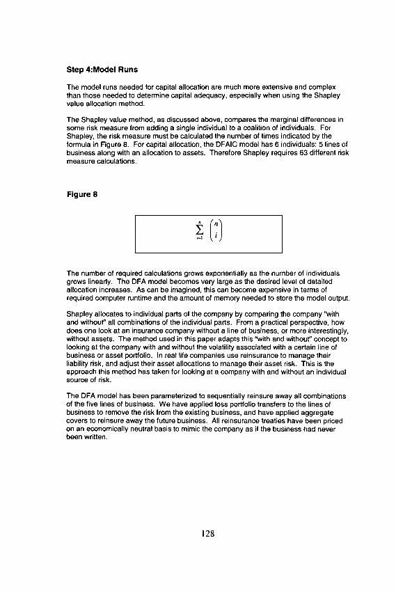
The model runs needed for capital allocation are much more extensive and complex than those needed to determine capital adequacy, especially when using the Shapiey value allocation method.

The Shapley value method, as discussed above, compares the marginal differences in some risk measure from adding a single individual to a coalition of individuals. For Shapley, the risk measure must be calculated the number of times indicated by the formula in Figure 8. For capital allocation, the DFAIC model has 6 individuals: 5 lines of business along with an allocation to assets. Therefore Shapley requires 63 different risk measure calculations.

Figure 8

The number of required calculations grows exponentially as the number of individuals grows linearly. The DFA model becomes very large as the desired level of detailed allocation increases. As can be imagined, this can become expensive in terms of required computer runtime and the amount of memory needed to store the model output.

Shapley allocates to individual parts of the company by comparing the company "with and without" all combinations of the individual parts. From a practical perspective, how does one look at an insurance company without a line of business, or more interestingly, without assets. The method used in this paper adapts this "with and without" concept to looking at the company with and without the volatility associated with a certain line of business or asset portfolio. In real life companies use reinsurance to manage their liability risk, and adjust their asset allocations to manage their asset risk. This is the approach this method has taken for looking at a company with and without an individual source of risk.

The DFA model has been parameterized to sequentially reinsure away all combinations of the five lines of business. We have applied loss portfolio transfers to the lines of business to remove the risk from the existing business, and have applied aggregate covers to reinsure away the future business. All reinsurance treaties have been priced on an economically neutral basis to mimic the company as if the business had never been written.

128

The first instinct of many might be to define minimum asset risk as investing all assets at the risk free rate. However, this is not true in an ALM/DFA framework, where risk is defined by the combined impacts of both assets and liabilities and their interactions. This method defines the minimum asset risk portfolio as the least risky portfolio on the economic efficient frontier. (See our sister paper for a full discussion of the efficient frontier) The minimum economic risk asset portfolio has been calculated for each of the 31 line of business combinations. (See Figure 8 where n=5)

In the past, the volatility of assets has often not been recognized when discussing both capital adequacy and capital allocation. Many of the previous allocation methods concentrate on the risk associated with their respective line of business losses. In a DFA framework, where the entire balance sheet is holistically modeled, the contribution of asset volatility to surplus volatility can recognized. Historically, P&C insurance has thought of assets very differently than it has thought of liabilities. In fact, the differences when considering balance sheet risk are almost non-existent. Assets, like workers comp or auto liability, are just another element of the overall riskiness of the company. The allocation of capital to assets is a realization that the investment department is required to produce a higher return for a more risky investment strategy.

This is best described through a heuristic example. Table 4 displays the capital required for two different asset strategies where the underwriting is held fixed.

Table 4

Asset Strategy Required Capital

Less Risky Investment Strategy $100

More Risky Investment Strategy $200

The company currently is operating under the less risky investment strategy. If the company does not allocate capital to its investment department then the $100 would be split up between the lines of business. The investment managers then decide to move to a more risky investment strategy that doubles the total capital required by the company. The line of business managers are not going to accept this increase in capital allocated to their lines along with the increased return to premium they will be forced to produce to hit their target return on surplus. The investment department should be allocated a portion of this capital on which they should be forced to meet a target return.

129

Steps 5-7:Anslyze Output, Sensitivity Test, Present Findings

The Shapley Value allocation method has been selected to allocate D#AIC's capital for their current net of reinsurance position. Table 5 shows the results of this allocation for two different risk measures: Standard Deviation of Statutory Surplus at the end of Year 5, and TCE Required Capital discussed in the capital adequacy section of this paper. For comparative purposes, Table 5 also includes results using the Marginal "Last-In" allocation method.

The Standard Deviation of Statutory Surplus measure considers the volatility of surplus 5 years in the future assuming DFAIC maintains its historical reserving practices and has a normal responsiveness to unexpected inflation. The TCE Required Capital measure, as discussed in previous sections, looks at the required capital at the end of 1 year assuming the company immediately reserves to ultimate loss with perfect knowledge of the impact of future economic variables on loss payments. The TCE Required Capital has again been calculated using a 1% tolerance for each of the 63 Shapley combinations.

Table 5: Capital Allocation Results

Allocation Method Shapley Value Marginal Last-In Shapley Value

Standard Allocation Risk TCE Required TCE Required Deviation of Measure Capital Method Capital Method Statutory Surplus

End of Year 5

Capital Allocation Center

Workers Comp 38% 43% 14%

Auto Liab 24% 28% 34%

Home/CMP(Prop) 9% 5% ] 5%

Auto Phys Dam 1% -5% 15%

GWCMP(Liab) 18% 20% 1 ] %

Assets 10% 9% 11%

The allocation of capital to assets is comparable between all measures. The percentage allocation to assets would increase if the company were to more aggressively invest its required and excess capital.

130

The Marginal "Last-In" allocation method only evaluates the marginal risk addition to the business as a whole. The Shapley value allocation method builds on the Marginal "Last- In" concept by considering all possible combinations of entry. One of the most striking results presented in Table 5 is the negative allocation to Auto Physical Damage (APD) for the marginal allocation of TCE Required Capital. The APD line of business is very profitable, not very volatile, and makes up approximately one quarter of DFAIC's book of business. The magnitude of the "Large Losses", in the TCE calculation, is dampened when the large and fairly certain expected profit from the APD line is added to the tail scenarios generated by the more volatile and less profitable lines of business. This results in an overall decrease in the TCE Required Capital when this line is added.

But, is it appropriate to analyze the marginal impact of a line of business being added to the business as a whole? The axioms supporting the Shapley value method would say no. As a stand alone, the APD line of business would require capital to operate. These two scenarios, the marginal impact of a line to the business as a whole and the stand alone, produce the extremes of the potential results. Shapley takes both of these extremes into account, along with all other potential combinations.

Table 6 displays the normalized percentage allocation to the individual lines of business for the portion of capital assigned to liabilities for both of the risk measures using the Shapley value allocation method. Additionally, some key loss metrics are shown. The selection of risk measure is dependant on what a company considers risk. The company should hold a total amount of capital, and allocate its capital, in a manner consistent with its definition of risk.

The percentage of capital allocated via the Standard Deviation measure aligns closely with the percentage of loss exposure from the 5 years of new business (Expected Accident Year Loss & LAE) and the existing reserves (Current Booked Loss & LAE Reserves). In fact, for all lines, the allocation percentage falls within the range of the new business and existing reserve percentages, tn addition to the magnitude of loss potential, the measure is to a lesser extent driven by the volatility of the individual lines. For example, the Auto Physical Damage (APD) line accounts for 24% of the new business loss exposure but is assigned a slightly lower percentage of capital. DFAIC's APD line has been modeled with the least loss ratio volatility of any of the lines. This is the factor that dampens the allocation of capital to 17%.

The Standard Deviation method looks at risk as uncertainty of all potential losses, whether good or bad. In contrast, the TCE Required Capital Method concentrates on those extreme tail events that can cause insolvency. Referring to the results in Table 6, the TCE Required Capital Method allocation is very different from the Standard Deviation of Statutory Surplus allocation. The capital is being allocated to the longer tailed lines. In fact, the allocation seems to be driven by the duration of the individual line of business, but dampened by the overall magnitude of the line of business. For example, workers compensation, the longest tailed line is allocated a portion of the capital much greater than its corresponding portion of expected loss exposure. The longer tailed lines, workers compensation and general liability, have increased their allocations over the standard deviation method, while the shorter tailed lines have decreased their allocations.

131

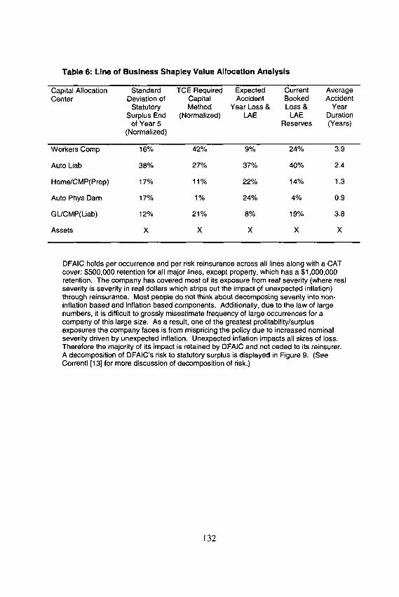
Table 6: Line of Business Shapley Value Allocation Analysis

Capital Allocation Standard TCE Required Expected Current Average Center Deviation of Capital Accident Booked Accident

Statutory Method Year Loss & Loss & Year Surplus End (Normalized) LAE LAE Duration

of Year 5 Reserves (Years) (Normalized)

Workers Comp 16% 42% 9% 24% 3.9

Auto Liab 38% 27% 37% 40% 2.4

Home/CMP(Prop) 17% 11% 22% 14% 1.3

Auto Phys Dam 17% 1% 24% 4% 0.9

GL/CMP(Liab) 12% 21% 8% 19% 3.8

Assets X X X X X

DFAIC holds per occurrence and per risk reinsurance across all lines along with a CAT cover: $500,000 retention for all major lines, except property, which has a $1,000,000 retention. The company has covered most of its exposure from real severity (where real severity is sevedty in real dollars which strips out the impact of unexpected inflation) through reinsurance. Most people do not think about decomposing severity into non- inflation based and inflation based components. Additionally, due to the law of large numbers, it is difficult to grossly misestimate frequency of large occur rences for a company of this large size. As a result, one of the greatest profitability/surplus exposures the company faces is from mispricing the policy due to increased nominal severity driven by unexpected inflation. Unexpected inflation impacts all sizes of loss. Therefore the majority of its impact is retained by DFAIC and not ceded to its reinsurer. A decomposition of DFAIC's risk to statutory surplus is displayed in Figure 9. (See Correnti [13] for more discussion of decomposition of risk.)

132

Figure 9: Decomposition of Statutory Risk

200,000 180,000

I¢ 160,000 O '~'~ 140,000

> 120,000

O 100,000

"~ 80.000 "0 60,000 e -

40.ooo 20,000

Decomposition of Statutory Risk 58°/^

- - ~ 6 % 33% ' ~ ....... Ii I, E] Real Underwriting

- - ~ "":" :;~' [] Inflation I - - - :~.% ;i.' 9*/. I l l Asse t s

1-Year 5-Year

The power of unexpected inflation does not discriminate based on the size of the company. Unexpected inflation does not diversify away. In fact, it cumulates over time. As seen in Figure 9, the contribution of inflation to the overall balance sheet volatility is significant even when looking at the company over a one-year time horizon. As the time horizon extends, the risk from real underwriting (real severity + frequency) diversifies and the contribution of unexpected inflation begins to dominate the risk landscape. Though inflation is currently at relatively low levels, we can not be lulled into believing that the inflation levels of the early 1980's will never return.

At first glance, a 42% allocation to workers compensation seems outrageous, in analyzing the tail events (worst 1% of all simulated combined lines results) this allocation begins to look less outrageous. Again, the company has defined "risk" as tail events that can yield insolvency. For analyzing these tail events, this tail risk seems to be largely driven by unexpected inflation. The average annualized compound inflation rate over a five year period for all modeled simulations is 2.4%, which is in line with the current CPI. The same statistic for the worst 1% of all simulations is 9%. Those lines with the longest duration, workers compensation and general liability, have the greatest exposure to unexpected inflation. As a result, the longer tailed lines are receiving a proportionally large amount of the capital allocated to them.

This capital allocation exercise is all about how a company defines risk. They must select a risk measure that is consistent with how they define risk.

133

Conclusion

In this paper we have:

• Chosen a measure of risk (TCE) that is consistent with reasonable standard, as expressed by the axioms for coherent risk measures

• Chosen an allocation method, using the TCE risk measure, and an allocation approach (Shapley) consistent with reasonable axioms for allocations.

• Chosen a risk variable (statutory surplus) that incorporates the effects of both asset and liability variability.

After we made these choices, we analyzed a hypothetic.a. I company DFAIC in a DFA framework.

We chose a DFA framework because:

• Interactions between line of business results are generally too complex to be modeled analytically

• Modeling the simultaneous impact of economic variables on multiple categories of assets as well as on liability payments is too complex to handle analytically

• Calculation of a risk measure such as TCE requires a simulation approach if the underlying components are modeled using simulation

• We wish to allocate the cost of risk to the assets as well as to each line of business.

We concluded:

That DFAIC is currently adequately capitalized. Moreover, we have a measure of the amount of excess capital that can be released to the owners, and a framework to analyze changes to required capital levels as a result of changes to the reinsurance program, asset mix, or underwriting plans.

That the allocation of capital to line, and hence the required cost of capital to be built into the rating structure differs from the values under other approaches. If our competitors continue to use traditional methods, we will be able to be more competitive in lines where our risk exposure is less.

134

Bibliography

[1] 1992 Discussion Papers on Insurer Financial Solvency, CAS htto:/Iwww,cgsact.orq/pubs/da~/do1392/index.htm

[2] Manuel Almagro, "Capital Allocation and Profitability" CAS 2000 Ratemaking Handouts httlD;/Iwww.casact,ora/coneduc/rotesem/rate20001handoutslfln26,DIDt

[3] Artzner, P., Delbaen, F., Eber, J-M. and Heath, D., =Thinking Coherently", Risk 10, November 1997.

[4] Philippe Artzner, Freddy Delbaen, Jean-Marc Eber and David Heath: =Coherent Measures of Risk", Math. Finance 9 (1999), no. 3, 203-228 http:/ /www.math.ethz.¢h/-delbc~en/ffp/prepdnt~/CoherentMF ,p~f

[5] Artzner, P., "Application of Coherent Risk Measures to Capital Requirements in Insurance", North American Actuarial Journal, vol. 3, 1999. httD:/Iwww.soa.orallibrarv/naal/1997-O9/naai9904 1.odf

[6] I.K. Bass and C.K. Khury, "Surplus Allocation: An Oxymoron" CAS 1992 Discussion Papers on Insurer Financial Solvency http://www.cosoct.org/PUSSIdD~ld~)D92/92d~)r3553.~df

[7] Todd R. Bault, "Risk Loads for Insurers"[Discussion], Proceedings of the Casualty Actuarial Society 1995 Volume LXXXll http;/ /www.casact,org/pubs/prQc~ed/DroceetqJ95/InqJex,htm

[8] A.M. Best Company, Inc., "Best Week Special Supplement: RBC: The Use of Capital Adequacy Models in Best's Rating Process": The A.M. Best Company, October 24, 1994

[9] A.M. Best Company, Inc., "Best Week Property/Casualty Supplement: A.M. Best Enhances its Capital Model as P/C Industry Improves it Capital Management Tools": The A.M. Best Company, June 18, 1998

[10] Allan Brender, Robert Brown and Harry Panjer, "A Synopsis and Analysis of Research on Surplus Requirements for Property and Casualty Insurance Companies" CAS Forum Summer 1993 http://www.¢asact.org/l~Ubs/forun'I/93sforum/95~,fO01 .c~df

[11] John C. Burkett, Thomas S. Mclntyre, and Stephen M. Sonlin, "DFA Insurance Company Case Study, Part h Reinsurance and Asset Allocation," Casualty Actuarial Society Forum, Summer 2001.

[12] Robert P. Butsic, "Solvency Measurement for Property-Liability Risk-Based Capital Applications" 1992 Discussion Papers on Insurer Financial Solvency, CAS http://www.casact,gr.q/llbrary/valuotion/92dD311 ,odf

135

[13] Correnti, Salvatore, Stephen M. Sonlin and Daniel B. Isaac, "Applying a DFA Model to Improve Strategic Business Decisions," Casualty Actuarial Society Forum, Summer 1998, 15-51. Arlington, VA: Casualty Actuarial Society.

[14] Michael Denault, "Coherent Allocation of Risk Capital", Risklab web site. http://www.risklab.¢hlffPlDapers/CoherentAIIQcation.pdf

[15] Kathleen H. Ettlinger, Karen L. Hamilton, Gregory Krohm, "State Insurance Regulation" First Edition: Insurance Institute of America, 1995.

[16] Sholom Feldblum, "NAIC Property/Casualty Insurance Company Risk-Based Capital Requirements" Proceedings of the Casualty Actuarial Society 1996 Volume LXXXIII http:[ /www.qgsact.ora/Dubs/Droceed/Droceed96/9[~297 pdf

[17] Sholorn Feldblum, "Risk Loads for Insurers" Proceedings ot the Casualty Actuarial Society 1990 Volume LXXVII, httD:l lwww.casoct.or.qlpub~lProceedlprocee~90/index.htm

[18] Daniel F. Gogol, Reinsurer Risk Loads from Marginal Surplus Requirements [Discussion] Proceedings of the Casualty Actuarial Society 1992 Volume LXXlX http:/Iwww.¢gsact.ora/DUl~s/proceeqJ/proceed92/index.htm

[19] Daniel F. Gegol, "Pricing to Optimize an Insurer's Risk-Return Relation'" Proceedings of the Casualty Actuarial Society 1996 Volume LXXXlII httlD:/ /www.casact.ora/Dubs/fDroceed/Drocee~96/96041 .pdf

[20] Daniel F. Gogol, "Surplus Allocation for the Internal Rate of Return Model: Resolving the Unresolved Issue", 2001 Winter Forum, Ratemaking Discussion Papers and Data Management/Data Quality/Data Technology Call Papers hffp://www.cosaot.or.q[pubs/forum[O] wforum/0] wf] ] 5.Pdf

[21] Leigh J. Halliwell, "ROE, Utility and the Pricing of Risk" CAS Forum 1999 Spring, Reinsurance Call Papers, hffp:/ /www.cosoct.orq/PUBS/fc)rum/99spforum/99spf071 .#df

[22] Isaac, Daniel and Nathan Babcock, (Proceedings of the XXXII r~ International ASTIN Colloquium, 2001 ),"Beyond the Frontier: Using a DFA Model to Derive the Cost of Capital".

[23] Rodney Kreps, "Reinsurer Risk Loads from Maginal Surplus Requirements', Proceedings of the Casualty Actuarial Society 1990 Volume LXXVII http : / /www.casact.orq/Dvbs/proc~ed/proceed90/index.hfm

[24] Jean Lemaire, "An Application of Game Theory: Cost Allocation," ASTIN Bulletin, Vol. 14, No. 1, 1984, pp. 61-82. hffP:/Iwww.casa¢t,orqllibrgry/a~tinlvoll 4no1/61 .lOdf

[25] Jean Lemaire, "Cooperative Game Theory and its Insurance Applications,"' ASTIN Bulletin, Vol. 21. No. 1, 1991, pp. 17-40. hffp://www.gasact.orq/library/g~tin/vol2 ] no]/17.pdf

136

[26] Donald F. Mango, "An Application of Game Theory: Property Catastrophe Risk Load" Proceedings of the Casualty Actuarial Society 1998 Volume LXXXV hltD;//www.casact,oralrDubs/oroceed/Droceed981980157.pdf

[27] Donald F. Mango, and John M. Mulvey, "Capital Adequacy and Allocation Using Dynamic Financial Analysis" Summer 2000, Dynamic Financial Analysis Call Papers, CAS http://www casact.ora/Dubslforum/OOsforum/OOsfO,~ Ddf

[28] Donald F. Mango, "Risk Load and the Default Rate of Surplus" CAS, 1999 Discussion Papers on Securitization of Risk, h ttlD : / /www.casact.org /IDubs/ dDD / dDD99 /99dDD17 5.Ddf

[29] Glenn Meyers, "An Analysis of the Capital Structure of an Insurance Company" Proceedings of the Casualty Actuarial Society 1989 Volume LXXVl http://www, c¢]~act, org/pubs/proc eed/proce~¢189/89147, pdf

[30] Glenn Meyers, "Coherent Measures of Risk An Exposition for the Lay Actuary" httD:/ /www.casaot.org/pubs/forvm/OO~fq~rurn/meyers/Cob~rent%20Measur~#~%2 Oof%2ORisk.pdf

[31] Glenn Meyers, The Competitive Market Equilibrium Risk Load Formula for Increased Limits Ratemaking, Proceedings of the Casualty Actuarial Society 1991 Volume LXXVIII hffp;//wvcw¢osactoralDubs/oroceed/Droceed9]/index htm

[32] Glenn Meyers, "Underwriting Risk", 1999 Spring Forum, Casualty Actuarial Society, hffD:/ /www.~asact.or.q_ /pu~/forum/99spforum/99spftoc.htm

[33] John M. Mulvey, Michael J. Belfatti, and Chris K. Madsen, "Integrated Financial Risk Management: Capital Allocation Issues" CAS Forum 1999 Spring, Reinsurance Call Papers, http:/ /www.ca~gct.or.q/PUBS/forkJm/99spforum/99spf221 .pdf

[34] National Association of Insurance Commissioners, "Risk-Based Capital Overview and Instructions - Property and Casualty": National Association of Insurance Commissioners Publication Department, 1998

[35] Kevin J. Olsen, "Surplus Allocation: A DFA application", 2001 Winter Forum, Ratemaking Discussion Papers and Data Management/Data Quality/Data Technology Call Papers httD:l/wwwcasoct.org/Dubs/forumlO] wforvm/0] wf659 pdf

[36] Gary S. Patrik, Stefan Bernegger, and Marcel Beat R~egg, "The Use of Risk Adjusted Capital to Support Business Decision-Making" CAS Forum, 1999 Spring, Reinsurance Call Papers, hffcx//www.casact.ora/Dubs/forum/99sDforum/99sDf243.Ddf

[37} Stephen W Philbrick, "Capital Allocation" The Actuarial Review, Volume 26, No. 1 / February 1999 hIlD://www.casact,Qr.a_lDubslactrev/feb991bstorms.htm

137

[38] Stephen W. Philbrick, "Surplus Allocation Redux", The Actuarial Review Volume 27, No. 1 / February 2000 hl-t~3:l/www.co~oct.or.q/pubs/Qotrev/febOO/broin~torms.htrn

[39] Richard J. Roth Jr., "Analysis of Surplus and Rate of Return Without Using Leverage Ratios', Casualty Actuarial Society Discussion Paper Program 1992 May, Vol 1 hfff3:llwww.casact.orQIoubsldDDIdfor3921index.htm

[40] Standard & Poor's Rating Services, "Property/Casualty Insurance Ratings Criteria": McGraw Hill Companies, 1999

138

Appendix A: Liability Parameterlzatlon

Our study of DFAIC's current reinsurance program and how it compares to alternative programs does not include loss portfolio transfers or other retrospective coverage. Hence existing business, with its attendant loss and unearned premium reserves, is modeled on a net of reinsurance basis. New business, however, is modeled on a gross basis. This allows us to vary prospective reinsurance strategies and compare the consequences of differing strategies. Since a principle focus of our paper is the current reinsurance program and its possible alternatives, we begin with a brief discussion of DFAIC's current reinsurance program and its implications for parameterizing our DFA model.

DFAIC's current reinsurance program includes excess of loss coverage for property, liability, and workers compensation risks, as well as coverage for catastrophes. In order to model the effects of these and alternative treaties, we generated individual large losses and occurrences on a gross of reinsurance basis. This necessitates the development of both frequency and severity probability distributions within the context of a collective risk model. Both company-specific and industry experience were gathered and analyzed for this purpose. Once the collective risk model was ready, individual large losses and catastrophes were generated stochastically and reinsurance covers were applied to obtain simulated losses net of reinsurance. Normally, company management would be consulted before finalizing company specific assumptions such as reinsurance arrangements or the frequency and severity of large losses and catastrophes.

In setting up our model, we condensed DFAIC's business into five distinct lines: Workers Compensation, Auto Liability (both personal and commercial), Property (homeowners and CMP property coverage), General Liability (other liability, product liability, special liability, and CMP liability coverage), and All Other Miscellaneous Lines(predominantly auto physical damage). For ease of discussion, we will refer to the other miscellaneous lines as Auto Physical Damage (APD). Segregation of business into these five lines allows for the effective modeling of reinsurance programs without burying results within a mass of detail. Each of these five lines is assigned a set of descriptive parameters to appropriately model its constituent line of business. Needed parameterizations relate to such items as premiums, losses (including loss adjustment expenses), other expenses, and payment patterns, as well as their stochastic properties. A preliminary step in our analysis involved restating historical results to be consistent with our five modeled lines of business ~.

9 E.g. CMP results were segregated into property or casualty and allocated to our Property or General Liability lines of business, respectively.

139

Projections of expected future premiums and loss ratios are in part based upon our assumed future business plans for DFAIC. An analysis of DFAIC's Schedule P reveals a recent deterioration in underwriting results and earned premium levels. Such a situation might indicate past DFAIC rate reductions made in an attempt to maintain market share within a competitive environment. Falcon's business plan is to raise rates thereby restoring loss ratios to DFAIC historical levels in three to five years. Anticipated effects of this business plan are reflected in our parameterization of future written premium levels.

Table 1A: Projected Growth Rates for Written Premium

Workers Comp Auto Liability Property General Liability APD

2000 -2.5% -2.5% -2.5% -2.5% -2.5%

2001 -2.5% -2.5% -2.5% -2.5% -2.5%

2002 -2.5% -2.5% -2.5% -2.5% -2.5%

2003 0% 0% 0% 0% 0%

2004 2.5% 2.5% 2.5% 2.5% 2.5%

DFAIC's simulated losses have been modeled in two pieces, core and large. Briefly, losses are categorized as large or core depending on magnitude. Large losses are simulated through a collective risk model, while core losses, specifically core loss ratios, are generated through a mean-reverting, momentum-driven random walk.

The model user determines the appropriate mean reversion factor, momentum factor and long term average core loss ratio. Considerations in selecting such parameter values might include an anticipated underwriting cycle or other market change. The actual simulated core loss ratio is generated from a user-selected distribution having a mean and a variance defined by the user. A blind algorithmic approach to selecting these parameters is not appropriate. As is true throughout the parameterization process, simulated results must be constantly checked to verify the reasonableness of results. For example, the variance of simulated, total loss ratios was checked against estimates of loss ratio volatility obtained from historical company results.

140

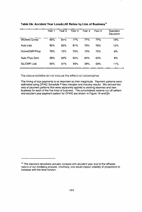
Table 2A: Accident Year Loss&LAE Ratios by Line of Business '°

Year 1 Year 2 Year 3 Year 4 Year 5 Standard Deviation

Workers Comp 85% 81% 77% 77% 77% 18%

Auto Liab 92% 85% 81% 79% 79% 12%

Home/CMP-Prop 78% 75% 75% 75% 75% 8%

Auto Phys Dam 68% 65% 64% 64% 64% 8%

GL/CMP-Liab 66% 61% 59% 58% 59% 11%

The a b o v e statistics do not include the effects of catastrophes

The timing of loss payments is as important as their magnitude. Payment patterns were estimated using DFAIC Schedule P loss triangles and industry results. We derived two sets of payment patterns that were separately applied to existing reserves and new business for each of the five lines of business. The consolidated reserve run-off pattern and accident year payment pattern for DFAIC are shown in Figure 1A and 2A.

lo The standard deviations actually increase with accident year due to the diffused nature of our modeling process. Intuitively, one would expect volatility of projections to increase with the time horizon.

141

Figure 1A: DFAIC's Consolidated Reserve Run-off Pattern

40% - ~

35% J

• o 25% J," ~. l s s ' p 20%-v H

1°~1l l l II = 5%

Duration: 2.7 years

0%- I 2 3 4 5 6 7 8 9 10 11 12 13 14 15

Year

142

Figure 2A: DFAIC's Consolidated Accident Year Payment Pattern

D.

o P a.

50%-

45%-

40%-

35%.

30%-

25%-

20%

15%-

10%-

5%

0%

m

m

m

B B

Duration: 2.1 years

2 3 4 5 O 7 8 9 Ig 11 12 13 14 ~5

Year

Expenses, other than the loss adjustment expenses already incorporated into the loss ratios, were modeled as both fixed and variable. Actual values were again obtained through a combination of company specific and industry wid~ statistics.

We have already discussed some of the randomness modeled into the projected core loss ratios. Further randomness is introduced to the model through the sensitivity of losses, expenses, and premiums to unexpected changes in the level of inflation. For DFAIC, we modeled losses and fixed expenses as immediately and fully responsive to unexpected changes in the level of inflation while premiums were partially responsive after a one-year time lag. Inflation sensitivity introduces a stochastic element affecting loss ratios, expenses, premiums, and payment patterns.

143

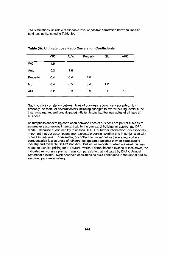
The simulations include a reasonable level of positive correlation between lines of business as indicated in Table 3A.

Table 3A: Ultimate Loss Ratio Correlation Coefficients

WC Auto Property GL APD

WC 1.0

Auto 0.3 1.0

Property 0.4 0.4

GL 0.4 0.5

APD 0.2 0.3

1.0

0.6 1.0

0.3 0.3 1.0

Such positive correlation between lines of business is commonly accepted. It is probably the result of several factors including changes to overall pricing levels in the insurance market and unanticipated inflation impacting the loss ratios of all lines of business.

Assumptions concerning correlation between lines of business are part of a series of parameter assumptions important within the context of building an appropriate DFA model. Because of our inability to access DFAIC for further information, it is especially important that our assumptions are reasonable both in isolation and in conjunction with other assumptions. For example, our collective risk model for generating workers compensation losses gross of reinsurance appears reasonable when compared to industry and available DFAIC statistics. But just as important, when we used this loss model to develop pricing for the current workers compensation excess of loss cover, the indicated reinsurance premium was comparable to that indicated by DFAIC Annual Statement exhibits. Such observed consistencies build confidence in the model and its assumed parameter values.

144

Appendix B: Economic and Capital Market Parameterization

The model that we used to generate our DFA economic and capital market simulations (FIRM TM Asset Model) differs from traditional mean/variance models in that economic variables, including interest rates and inflation, are explicitly modeled using accepted and rigorously tested stochastic processes. Capital market returns are then generated on a consistent basis with the underlying economic environment. This type of model has the following advantages over traditional mean/variance models:

• the explicit modeling of both economic and capital market variables;

• the ability to incorporate mean reversion in yields, providing for control over the serial correlation of capital market returns over time;

• multi-period simulation capabilities; and

• additional flexibility in modeling asset categories such as mortgage-backed securities and other securities with embedded options.

The economic and capital market parameterization process involved identifying and selecting asset classes that best represented the homogeneous groups of invested assets available to DFAIC. The twelve asset classes we defined and modeled were:

• Cash Equivalents

• Government Bonds (1-5 years)

• Government Bonds (5-10 years)

• Government Bonds (10-30 years)

• Corporate Bonds (1-5 years)

• Corporate Bonds (5-10 years)

• Corporate Bonds (10-30 years)

• Municipal Bonds (1-5 years)

• Municipal Bonds (5-10 years)

• Municipal Bonds (10-30 years)

• Common Stock

• Preferred Stock

145

The economic and capital market simulation model required assumptions concerning the initial levels of interest rates, inflation rates, real GDP growth, equity earnings growth, equity PIE levels, and the dividend payout ratio together with a set of long-term levels to which the initial levels will.revert over time. In setting the long-term levels, the goal was to produce risk premiums between asset classes that are consistent with historical data".

For our DFAIC study, we have set long-term levels equal to the initial market conditions as of our model start date (1/1/2000). This avoids bias with respect to expected price appreciation or depreciation due to interest movements or changing PIE ratios over the time horizon. Initial market conditions together with the assumed mean levels for are shown in Table lB.

11 For example, the spread between cash and inflation is historically about 2% and the risk premium for long government bonds over cash is about 2%.

146

Table 1B: Initial and Mean Interest Rate and Share Assumptions

Initial Conditions Mean Variable 1/1/2000 '2 Levels

Government Yields: 3-Month Interest Rate 5.53% 5.53% 1 -Year Interest Rate 6.19% 3-Year Interest Rate 6.34% 5-Year Interest Rate 6.39% 10-Year Interest Rate 6.36% 30-Year Interest Rate 6.56% 6.56%

Corporate Yields: 3-Month Interest Rate 6.16% 6.16% 1-Year Interest Rate 6.70% 3-Year Interest Rate 6.99% 5-Year Interest Rate 7.11% 10-Year Interest Rate 7.28% 30-Year Interest Rate 7.65% 7.65%

Municipal Yields: 3-Month Interest Rate 3.91% 1-Year Interest Rate 4.09% 3-Year Interest Rate 4.54% 5-Year Interest Rate 4.79% 10-Year Interest Rate 5.22% 30-Year Interest Rate 5.99%

Expected Price Inflation 2.5%

Expected Real GDP 2.5%

.£,.&,P ,r'~('l P/l: Pntin 39

S&P 500 Earnings Growth

S&P 500 Dividend Payout Ratio 40%

3.91%

5.99%

2.5%

2.5%

3"2

9.0%

40%

The returns for cash equivalents, bonds and common stock are directly controlled by the initial and mean assumptions shown in Table lB.

,2 Source: Bloomberg

147

Cash Equivalent returns are the accumulation of 1 -month government interest rates over time. Government Bond returns are a function of the applicable interest rate level, the change in the rate and the bond maturity. Corporate and Municipal Bond returns are modeled as a proxy to the US Single A corporate and the insured general obligation municipal bond markets respectively. They are calculated similarly to government bond returns. Corporate yields are modeled at a stochastic spread to government yields and municipal yields are modeled as a stochastic ratio to the government yields. Reported market yields on corporate bonds are adjusted to reflect historical defaults ;s. Common Stock returns are modeled as a proxy to the S&P 500 index. The'returns are composed of capital gains/losses plus dividends".

Table 2B shows the e x p e c t e d annual (arithmetic) and annual ized c o m p o u n d (geometr ic) returns for each of the twelve mode led asset classes.

13 This is based on the 10-year cumulative default study for Single A bonds provided by Moodys. A 50% recovery rate on defaults is assumed.

~4 Because we are assuming that long-term mean P/E ratios are equal to initial P/E ratios, valuation changes are not reflected in the risk premium between stocks and bonds. Thus the modeled equity risk premium is less than the historical average (6-7%), but is in-line with the historical average when adjusted for valuation changes.

148

Table 2B: Simulated Five-Year Return Statistics '5

Expected Annualized Annualized Annual Annual Compound Compound

Asset Class Return Std Dev Return Std Dev

Cash Equivalents 5.9% 1.9% 5.9% 1.4%

US Gov't Bonds (1-5) 6.5% 3.5% 6.5% 0.8% US Gov't Bonds (5-10) 6.9% 6.7% 6.7% 1.8% US Gov't Bonds (10-30) 7.4% 10.7% 6.9% 3.3%

US Corporate Bonds (1-5) 7.2% 3.6% 7.2% 0.9% US Corporate Bonds (5-10) 7.6% 6.8% 7.4% 1.9% US Corporate Bonds (10-30) 8.0% 10.8% 7.5% 3.3%

US Municipal Bonds (1-5) 4.9% 3.2% 4.8% 0.7% US Municipal Bonds (5-10) 6.1% 7.8% 5.8% 2.0% US Municipal Bonds (10-30) 7.0% 11.8% 6.4% 3.2%

US Stock 10.8% 20.0% 9.3% 7,6% Preferred Stock 8.3% 12.6% 7.7% 4.2%

15 Expected annual return statistics are arithmetic averages and are indicative of risk and return expectations over a one-year holding period. Annualized compound return statistics are geometric averages and reflect the impact of time diversification over the five-year holding period.

149

Appendix C: Coherent Risk Measures

This paper assumes that, when choosing a risk measure, the risk measure should be coherent. That is, it should satisfy the axioms of coherence. While this concept is not new, it is relatively new, and has not been discussed in detail in the Casualty Actuarial Society literature. Consequently, while we will refer readers to the original papers for the complete explication of the concepts, we would like to summarize some of the key points here, with specific application to the concept of risk measures used for the determination of surplus levels.

Actuaries have developed a number of risk measures over time and debated the merits of the alternatives. The discussion of standard deviation versus variance versus covariance has been discussed in a number of places [19],[20],[29],[37],[38]. However, until recently, the measures were generally developed ad hoc. Very recently, several researchers [3],[4],[5] have approached the problem by defining a set of axioms, and then examining the set of risk measures that satisfy the axioms.

Let:

,, X~ represent portfolios of risks. (Think of it as the liabilities of a particular insurance company).

• c(be some constant

• p(o) be a function that assigns a value of risk to a portfolio

Axiom T--Translat ion invariance

p(X + ~ r) = p(X) + ~.

That is, if a constant loss is added to a portfolio of risks, the required surplus for the combined portfolio is increased by the amount of the constant loss ~6.

18 The careful read will note that this formula differs from the formula in the papers by Artzner et al. In those papers the right side contains a negative o[, rather than positive. This is because their paper is written in terms of assets. Adding a risk free asset to a portfolio of risky assets reduces the surplus requirement. In actuarial convention, we express losses using positive numbers. If we expressed them in terms of negative values, then the Artzner formulation would apply, and we would interpret the constant as adding a positive amount, an asset, to a set of liabilities. In that case, the addition of a positive amount to a set of losses (expressed as negatives) would reduce the surplus requirement.

150

Axiom S---Subadditivity

p(Xl+X2) < p(Xl) + p(X2)

That is, if we have two separate portfolios of risks, the surplus requirement for the combined portfolio is no larger than the sum of the surplus requirements for each portfolio.

Axiom PH--Positive Homogeneity

p(e.X)= ~ p(X)

If we have a surplus requirement for a portfolio of risks, increasing each risk by a scalar increases the aggregate surplus requirement by the same scalar. As an alternative example, we could say that, if two researchers analyze a portfolio, and one expresses the amounts in dollars, and the other in thousands of dollars, the resulting surplus measures should differ by the same factor, a factor of 1,000.

Axiom M~Monotonicity

For Xl<X2, p(X1)<p(X2)

If a particular portfolio is completely dominated by another portfolio, that is, if for every quantile, the loss amount in the second distribution exceeds the value of the first, the risk measure will be greater for the second lz.

These axioms do not appear to be overly restrictive. However, as various papers have shown [3],[4],[5],[30] traditional risk measures such as VaR (probability of ruin), EPD, standard deviation measures, and variance measures fail one or more of these axioms. The rationale for the TCE measure is that it does satisfy these four axioms.

17 As noted in the previous footnote, this formula differs from that in Artzner et al. The inequality sign is reversed. The reasoning is the same. In actuarial convention, we tend to express losses in positive amounts, as well as surplus requirements. Given two portfolios of risks, one of which dominates the other, the inequality sign will be reversed, depending on whether the losses are expressed as positive or negative values. As long as the researcher is careful with the sign convention, the values of the surplus requirements should work out correctly.

151

152