Sensitivity of Precipitation Forecast Skill Scores to Bilinear Interpolation and a Simple...

918 VOLUME 18W E A T H E R A N D F O R E C A S T I N G

q 2003 American Meteorological Society

Sensitivity of Precipitation Forecast Skill Scores to Bilinear Interpolation and a SimpleNearest-Neighbor Average Method on High-Resolution Verification Grids

CHRISTOPHE ACCADIA, STEFANO MARIANI, MARCO CASAIOLI, AND ALFREDO LAVAGNINI

Istituto di Scienze dell’ Atmosfera e del Clima–Consiglio Nazionale delle Ricerche, Rome, Italy

ANTONIO SPERANZA

Dipartimento di Matematica e Informatica, Universita di Camerino, Camerino, Italy

(Manuscript received 18 April 2002, in final form 24 February 2003)

ABSTRACT

Grid transformations are common postprocessing procedures used in numerical weather prediction to transfer aforecast field from one grid to another. This paper investigates the statistical effects of two different interpolationtechniques on widely used precipitation skill scores like the equitable threat score and the Hanssen–Kuipers score.The QUADRICS Bologna Limited Area Model (QBOLAM), which is a parallel version of the Bologna LimitedArea Model (BOLAM) described by Buzzi et al., is used, and it is verified on grids of about 10 km (grid-boxsize). The precipitation analysis is obtained by means of a Barnes objective analysis scheme. The rain gauge dataare from the Piedmont and Liguria regions, in northwestern Italy. The data cover 243 days, from 1 October 2000to 31 May 2001. The interpolation methods considered are bilinear interpolation and a simple nearest-neighboraveraging method, also known as remapping or budget interpolation, which maintains total precipitation to a desireddegree of accuracy. A computer-based bootstrap technique is applied to perform hypothesis testing on nonparametricskill scores, in order to assess statistical significance of score differences. Small changes of the precipitation fieldinduced by the two interpolation methods do affect skill scores in a statistically significant way. Bilinear interpolationaffects skill scores more heavily, smoothing the maxima, and smearing and increasing the minima of the precipitationfield over the grid. The remapping procedure seems to be more appropriate for performing high-resolution gridtransformations, although the present work shows that a precipitation edge-smearing effect at lower precipitationthresholds exists. Equitable threat score is more affected than Hanssen–Kuipers score by the interpolation process,since this last score weights all kind of successes (hits and correct no-rain forecasts). Correct no-rain forecasts athigher thresholds often outnumber hits, misses, and false alarms, reducing the sensitivity to false alarm changesintroduced by the interpolation process.

1. Introduction

When performing model intercomparison of precip-itation nonprobabilistic skill scores, an accurate exper-imental design is needed. In particular, if comparedmodels have significantly different grid-box sizes, it isimperative to verify precipitation forecasts on a commongrid. On the other hand, if rain gauge data are simplybox averaged, the smoothness of the analysis will de-pend on the average number of rain gauges per grid box(Mesinger 1996). Moreover, a general postprocessingprocedure (grid transformation) applied to the forecastprecipitation fields might change the skill scores in somestatistically significant way. In fact, McBride and Ebert(2000) suggest that spatial averaging or bilinear inter-polation may affect the comparative skills of the models.

Corresponding author address: Mr. Christophe Accadia, Istitutodi Scienze dell’Atmosfera e del Clima–CNR, Area di Ricerca di RomaTor Vergata, Via del Fosso del Cavaliere 100, 00133 Rome, Italy.E-mail: [email protected]

In view of the above problem, this paper investigatesthe effect on skill scores of two simple postprocessingprocedures applied to precipitation field forecast by alimited area model (LAM).

For this purpose, LAM forecasts will be verified ontheir native grids, whereas postprocessed forecasts willbe verified on a different grid, as will be seen in moredetail later. The two verification grids considered havea grid-box size of about 10 km; hence, to produce anadequate (i.e., less sensitive to grid-box size) observedrainfall analysis, a Barnes objective analysis scheme isused (Barnes 1964, 1973; Koch et al. 1983).

The QUADRICS Bologna Limited Area Model(QBOLAM), running operationally at the Dipartimentodei Servizi Tecnici Nazionali of Presidenza del Consigliodei Ministri (Department of National Technical Servicesof the Italian Cabinet Presidency, DSTN-PMC) is usedto study the effect of the different interpolation proce-dures on skill scores. QBOLAM is derived from the Bo-logna Limited Area Model (BOLAM; Buzzi et al. 1994),which has shown excellent forecast capabilities in the

OCTOBER 2003 919A C C A D I A E T A L .

Comparison of Mesoscale Prediction and Research Ex-periments (COMPARE; Georgelin et al. 2000; Nagata etal. 2001). The considered procedures are bilinear inter-polation and a simple nearest-neighbor average method(Baldwin 2000; Mesinger 1996; Mesinger et al. 1990),also known as remapping or budget interpolation. Forbrevity, this last procedure will be called remapping inthe remainder of the paper.

As will be seen in more detail later, these methodsdiffer in many substantial ways, since, for example, bi-linear interpolation treats gridpoint precipitation valuesas defined at points, while remapping considers grid-point values as grid-box values.

The skill scores used are the equitable threat score(ETS; Schaefer 1990) and the Hanssen–Kuipers score(HK; Hanssen and Kuipers 1965; McBride and Ebert2000). This last score is also known as the true skillstatistic (TSS; Flueck 1987) or the Peirce skill score(PSS; Peirce 1884; Stephenson 2000). Another usefulscore is the bias score, or BIA. It is used to comparethe relative frequency of precipitation forecasts and ob-servations (for a review see, e.g., Wilks 1995).

In order to determine from a statistical point of viewwhether the results on different grids are equivalent ornot, a hypothesis test is needed. Common hypothesistests need an a priori definition of a parametric proba-bility density function (PDF) and the assumption of sta-tistical independence for the quantities under exami-nation.

The hypothesis testing method used in this study wasoriginally proposed by Hamill (1999). It is based on aresampling technique called the bootstrap method [Dia-conis and Efron (1983); for a general discussion onmeteorological applications see Wilks (1995) and ref-erences therein]. This is a computer-based method thatbuilds a PDF consistent with the selected null hypoth-esis. Random sampling is performed from the availabledata, followed by a significance assessment of the testbased on a comparison of the observed statistic with thenumerically built statistics. The general method doesnot need any assumptions concerning the probabilitydensity function.

According to Hamill (1999) skill score comparisonbetween two competing models may not be completelyinformative on the actual forecasting skills, because onemodel might have inflated scores due to its tendency tooverforecast a precipitation occurrence. He proposes theBIA adjustment method when performing a skill scorecomparison, in order to take into account the precipi-tation forecast frequency difference that two differentmodels may have. The hypothesis testing method willbe applied in this paper with and without BIA adjust-ment.

The application of this procedure should help to de-termine whether the obtained scores are the result of anactual forecast capability or are simply due to BIA dif-ferences.

The paper is organized as follows. Section 2a de-

scribes the precipitation test data used. Section 2b de-scribes the QBOLAM LAM and the two different gridsused in this study are described, while 2c briefly de-scribes the Barnes objective analysis scheme. A de-scription of the bilinear interpolation and remappingprocedures is provided in section 3. Section 4a gives ashort review of the nonprobabilistic skill scores used.Section 4b illustrates the BIA adjustment procedure.Section 4c describes the bootstrap resampling technique.Results are presented in section 5 and discussed in sec-tion 6. Conclusions and final remarks are in section 7.The appendix contains a detailed analysis of the effectof the BIA adjustment procedure on ETS and HK.

2. Verification and forecast data

a. Rain gauge verification data

The rain gauge data used in the European ProjectINTERREG II C (Gestione del territorio e prevenzionedalle inondazioni, land management and floods preven-tion) have been used to study the effects of bilinearinterpolation on precipitation forecast statistics and toapply the above described hypothesis test. Such raingauge data cover the Italian regions of Liguria and Pied-mont (northwestern Italy), starting from 1 October 2000through 31 May 2001 (243 days). The verification areacorresponds approximately to the shaded area in Fig. 1.This part of Italy is characterized by the presence ofhigh mountains, the northwestern Alps (Fig. 2).

The Liguria rain gauge data were provided by theEnvironmental Monitoring Research Center of the Uni-versity of Genova (Centro di Ricerca Interuniversitarioin Monitoraggio Ambientale, CIMA). The RegionalMonitoring Network provided the Piedmont region data.The Piedmont rain gauge network has 294 rain gaugeswhile the Liguria network has 96 rain gauges. Not allrain gauges were active during the time interval con-sidered, going from a maximum of about 190 rain gaug-es over the two regions in October to a minimum of 70gauges. The average number is about 90 rain gauges.

Time resolution is variable from 5 to 30 min. Rainfallrecords were accumulated for 24 h. Observation thresh-olds used for calculation of the nonparametric scoresare 0.5, 5.0, 10.0, 20.0, 30.0 and 40.0 mm (24 h)21.

b. Description of model QBOLAM and related grids

QBOLAM is a finite-difference, primitive equation,hydrostatic limited area model running operationally ona 128-processor parallel computer (QUADRICS) atDSTN-PCM as an element of the Poseidon sea waveand tide forecasting system. It is a parallel version ofthe BOLAM model described by Buzzi et al. (1994),which has been developed at the Istituto di Scienzedell’Atmosfera e del Clima–Consiglio Nazionale delleRicerche (ISAC–CNR, former FISBAT). Analysis andboundary conditions are provided by the European Cen-


FIG. 1. Map of the area covered by the QBOLAM model: the shaded area shows the verificationregion, and the native grid domain (N grid) and the postprocessing domain (P grid) are shownwith solid and dashed lines, respectively.

FIG. 2. Schematic orography of the northwestern Alps. Some peaks reach heights over 4000m. Mountains are shown only above the 1000-m level, with a 1000-m contour interval. The fourareas shown are used in the course of the paper to discuss the average differences betweenprecipitation on the N and P grids (see section 6).

tre for Medium-Range Weather Forecasts (ECMWF). A60-h forecast starts daily at 1200 UTC. The first 12-hforecasts are neglected (spinup time), and only the fol-lowing 48-h forecasts are considered. Outputs are avail-able routinely every 3 h and are considered here onlyup to 24 h. The horizontal domain [19.98 3 38.58 ofrotated (defined below) latitude 3 longitude] covers the

entire Mediterranean Sea, with 40 levels in the vertical(sigma coordinates). Horizontal grid-box spacing is 0.18for both latitude and longitude on the original compu-tational grid, equivalent to 386 3 210 grid points. Forcomputational and parallelization reasons, simplifiedparameterization of convection (Kuo 1974) and radia-tion (Page 1986) are used.


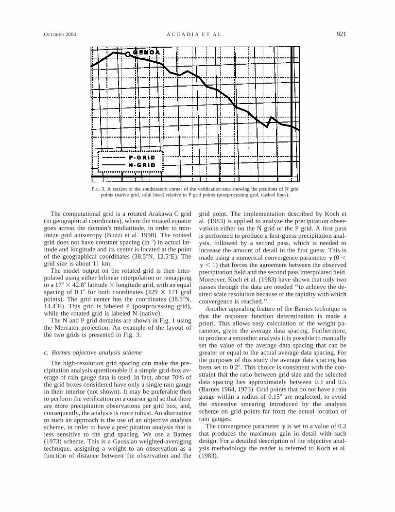
FIG. 3. A section of the southeastern corner of the verification area showing the positions of N gridpoints (native grid, solid lines) relative to P grid points (postprocessing grid, dashed lines).

The computational grid is a rotated Arakawa C grid(in geographical coordinates), where the rotated equatorgoes across the domain’s midlatitude, in order to min-imize grid anisotropy (Buzzi et al. 1998). The rotatedgrid does not have constant spacing (in 8) in actual lat-itude and longitude and its center is located at the pointof the geographical coordinates (38.58N, 12.58E). Thegrid size is about 11 km.

The model output on the rotated grid is then inter-polated using either bilinear interpolation or remappingto a 178 3 42.88 latitude 3 longitude grid, with an equalspacing of 0.18 for both coordinates (429 3 171 gridpoints). The grid center has the coordinates (38.58N,14.48E). This grid is labeled P (postprocessing grid),while the rotated grid is labeled N (native).

The N and P grid domains are shown in Fig. 1 usingthe Mercator projection. An example of the layout ofthe two grids is presented in Fig. 3.

c. Barnes objective analysis scheme

The high-resolution grid spacing can make the pre-cipitation analysis questionable if a simple grid-box av-erage of rain gauge data is used. In fact, about 70% ofthe grid boxes considered have only a single rain gaugein their interior (not shown). It may be preferable thento perform the verification on a coarser grid so that thereare more precipitation observations per grid box, and,consequently, the analysis is more robust. An alternativeto such an approach is the use of an objective analysisscheme, in order to have a precipitation analysis that isless sensitive to the grid spacing. We use a Barnes(1973) scheme. This is a Gaussian weighted-averagingtechnique, assigning a weight to an observation as afunction of distance between the observation and the

grid point. The implementation described by Koch etal. (1983) is applied to analyze the precipitation obser-vations either on the N grid or the P grid. A first passis performed to produce a first-guess precipitation anal-ysis, followed by a second pass, which is needed toincrease the amount of detail in the first guess. This ismade using a numerical convergence parameter g (0 ,g , 1) that forces the agreement between the observedprecipitation field and the second pass interpolated field.Moreover, Koch et al. (1983) have shown that only twopasses through the data are needed ‘‘to achieve the de-sired scale resolution because of the rapidity with whichconvergence is reached.’’

Another appealing feature of the Barnes technique isthat the response function determination is made apriori. This allows easy calculation of the weight pa-rameter, given the average data spacing. Furthermore,to produce a smoother analysis it is possible to manuallyset the value of the average data spacing that can begreater or equal to the actual average data spacing. Forthe purposes of this study the average data spacing hasbeen set to 0.28. This choice is consistent with the con-straint that the ratio between grid size and the selecteddata spacing lies approximately between 0.3 and 0.5(Barnes 1964, 1973). Grid points that do not have a raingauge within a radius of 0.158 are neglected, to avoidthe excessive smearing introduced by the analysisscheme on grid points far from the actual location ofrain gauges.

The convergence parameter g is set to a value of 0.2that produces the maximum gain in detail with suchdesign. For a detailed description of the objective anal-ysis methodology the reader is referred to Koch et al.(1983).


FIG. 4. Schematic example of the remapping procedure. Native grid boxes (N grid) are indicatedby solid lines with center points as numbered black triangles. Dashed lines indicate the examinedpostprocessing grid box (P grid) with center point as black circle. The 5 3 5 subgrid boxes forthe P grid are indicated by dotted lines with center points as small white circles.

3. Bilinear interpolation and remappingprocedures

a. Bilinear interpolation

Grid transformations may be performed using bilinearinterpolation, which is operationally used (see, e.g.,ECMWF 2001). However this method may not be de-sirable for precipitation, because it results in smoothingof the precipitation field, increasing the minima andreducing the maxima. In addition, the bilinear inter-polation method does not conserve the total precipita-tion forecast by the model.

b. Remapping

The other method considered is remapping, which isused to integrate forecast precipitation from the nativegrid to the postprocessed one (Baldwin 2000; Mesinger1996; Mesinger et al. 1990).

The remapping procedure, used operationally at theNational Centers for Environmental Prediction/Envi-ronmental Modeling Center (NCEP/NMC), is applied.It conserves, to a desired degree of accuracy, the totalforecast precipitation of the native grid. This integrationtechnique is a discretized version of a remapping pro-cedure that uses an area-weighted average.

The remapping was performed by subdividing theboxes centered on each postprocessing grid point in 53 5 subgrid boxes, and assigning to each subgrid pointthe value of the nearest native grid point. The average

of these subgrid point values produces the remappedvalue of the postprocessing grid point. An example ofhow remapping works is shown in Fig. 4. The subgridboxes included in the shaded area are assigned the valueof the N grid point labeled 2, whereas the subgrid boxesincluded in the unshaded area are assigned the value ofthe N grid point labeled 5.

4. Statistical methodology used for the sensitivitystudy

a. Nonprobabilistic scores

Nonprobabilistic verification measures are widelyused to evaluate categorical forecast quality. A cate-gorical dichotomous statement is simply a yes–no state-ment, in this particular context it means that forecast orobserved precipitation is below or above a definedthreshold u. The combination of different possibilitiesbetween observations and the forecast defines a contin-gency table. For each precipitation threshold four cat-egories of hits, false alarms, misses, and correct nonrainforecasts (a, b, c, and d as shown in Table 1) are defined.The scores used in this study are the above-mentionedETS and HK scores (see Schaefer 1990; Hanssen andKuipers 1965) and the BIA.

The BIA is the ratio between the number of yes fore-casts and the number of yeses observed. It is defined by

a 1 bBIA 5 . (1)

a 1 c


TABLE 1. Contingency table of possible events for a selectedthreshold.

Rain observed

Yes No

Rain forecast YesNo

ac

bd

A BIA equal to one means that the forecast frequencyis the same as the observation frequency, and the modelis then referred to as unbiased. A BIA greater than 1 isthen indicative of a model that forecast more eventsabove the threshold than observed (overforecasting),while a BIA less than 1 shows that the model forecastless events than observed (underforecasting).

The ETS is defined by

a 2 arETS 5 , (2)a 1 b 1 c 2 ar

where ar is the number of model hits expected from arandom forecast:

(a 1 b)(a 1 c)a 5 . (3)r a 1 b 1 c 1 d

A perfect forecast will have an ETS equal to 1, whilean ETS that is close to 0 or negative will indicate aquestionable ability of the model to produce successfulforecast statistics.

The HK score gives a measure of the accuracy bothfor events and nonevents (McBride and Ebert 2000):

(ad 2 bc)HK 5 . (4)

(a 1 c)(b 1 d)

The HK ranges from 21 to 1. This score is indepen-dent of the event and nonevent distributions. An HKscore equal to 1 is associated with a perfect forecastboth for events and nonevents, while a score of 21means that hits and correct zero-precipitation forecastsare zero. The HK score is equal to 0 for a constantforecast.

Given the probability of detection (POD; Wilks 1995)and the false alarm rate1 (F; Stephenson 2000), it ispossible to define the HK score as a linear combinationof these indexes (Stephenson 2000); that is,

a bHK 5 POD 2 F 5 2 . (5)

a 1 c b 1 d

This expression of HK will be used to interpret theeffects of the BIA adjustment procedure.

1 The conditional false alarm rate (F) must not be confused withthe false alarm ratio (FAR; Mason 1989). The first score is the fre-quency of yes forecasts when the events do not occur, while thesecond one is the ratio between the number of false alarms and thetotal number of yes forecasts.

b. The BIA adjustment procedure

Mesinger (1996) and Hamill (1999) pointed out thatalthough ETS is in the form expressed in Eq. (2), cor-rected for hits in a random forecast using Eq. (3), it isstill influenced by model BIA. The skill of a randomforecast is small for intense precipitation; hence, at high-er thresholds, a model with a greater BIA should nor-mally exhibit a greater ETS (Mesinger 1996). Never-theless, an overforecasting model (BIA . 1) could havetoo many false alarms so that the skill scores could benegatively affected compared with a model with a lowerBIA.

Mason (1989) has shown that a skill score very sim-ilar to ETS, the critical success index (CSI; Donaldsonet al. 1975), is highly dependent on threshold proba-bility, that is, the cutoff probability above which theevent is forecast to occur and below which is forecastto not occur, or not forecast. Moreover, he indicates thatthe HK score also is sensitive to the probability of thethreshold selected.

The threshold probability is a function of the actualprecipitation threshold used to compute the contingencytables (Mason 1989).

Usually the contingency tables are filled using thesame precipitation threshold for both observations andforecasts. To determine the effects on skill scores ofBIA differences between two models (‘‘competitor’’ and‘‘reference’’ in the following), the BIA adjustment pro-cedure is introduced. In this study, the two comparedmodels are the forecasts on the native grid and the post-processed forecasts using either bilinear interpolation orremapping. In the BIA adjustment procedure the con-tingency tables of the competitor forecast are recalcu-lated, adjusting the forecast precipitation threshold,while keeping the observation threshold unchanged, inorder to have the competitor BIA similar to the referenceBIA. This procedure is repeated independently for eachverification threshold (T. M. Hamill 2000, personal com-munication).

The reference forecast should have the BIA closer tounity for almost all the verification thresholds, that is,showing the least tendency to underforecast or over-forecast.

The variation of the forecast threshold can be inter-preted as a variation of the threshold probability in orderto get similar BIA scores.

The BIA adjustment helps to assess whether the skillscore differences between the competitor and referencemodels are the result of an actual different forecast ca-pability, or are simply explained by the differing BIAscores.

The appendix [Eqs. (A6) and (A8)] shows that ETSand HK vary due to the change in the number of hitsand false alarms. This is expected because of the BIAadjustment procedure, which changes the marginal dis-tributions of the forecasts, by changing the forecast


thresholds, and thus leaves the marginal distributions ofthe observations unaltered.

c. The resampling method

For the purpose of model comparison, a confidenceinterval is necessary to assess whether score differencesbetween two competing models are statistically signif-icant. This is computed using as a hypothesis test theaforementioned Hamill resampling technique (Hamill1999). A short description of the resampling methodfollows; for an exhaustive discussion of the details ofthe method the reader is referred to Hamill (1999).

This test (like other hypothesis test methods) requiresthat the time series considered have negligible auto-correlations. Accadia et al. (2003) have shown that mod-el forecast errors are negligibly autocorrelated in timefor the dataset used in this paper if observations andforecasts are accumulated to 24 h. Moreover, in orderto take into account any possible spatial correlation offorecast error when applying the resampling method,the nonparametric scores used in this study are calcu-lated on the whole set of grid points available each day(Hamill 1999).

The null hypotheses used in this study are that thedifferences in skill score (either ETS or HK) and BIAare zero between the two competing model forecastsM1 and M2:

H : ETS 2 ETS 5 0.0,0 M1 M2

BIA 2 BIA 5 0.0. (6)M1 M2

The alternative hypotheses are

H : ETS 2 ETS ± 0.0,A M1 M2

BIA 2 BIA ± 0.0. (7)M1 M2

The test is also applied to HK, which is used in placeof ETS. For the purpose of this study, the competingmodel forecasts M1 and M2 will be two different out-puts from the same model; one on the native grid, theother on the postprocessing grid, either using bilinearinterpolation or remapping, as previously described insection 3.

The scores are computed from a sum of n daily con-tingency tables (n 5 243 days) calculated from dataaccumulated to 24 h. Each table is defined as a vectorof four elements:

x 5 (a, b, c, d,) with i 5 1, 2 and j 5 1, . . . , n,i,j ij (8)

where the index i represents here the QBOLAM outputeither on the N grid or interpolated on the P grid; j isthe day index. The contingency table elements aresummed over the entire time period for both model fore-casts M1 and M2:

n

(a, b, c, d) 5 x , (9)OM1 1,kk51

n

(a, b, c, d) 5 x . (10)OM2 2,kk51

The test statistic is calculated using the contingencytables computed in Eqs. (9) and (10):

(ETS 2 ETS ) or (HK 2 HK ) orM1 M2 M1 M2

(BIA 2 BIA ).M1 M2

The bootstrap method is then applied to resample thetest statistic consistently with the assumed null hypothesisfrom Eq. (6). This is done as follows. Let {Ik}k51, . . . , n

be a random indicator family over the entire set of ndays, where each element can be randomly set equal to1 or 2. It is equivalent to randomly choosing a particulardaily contingency table associated either with model M1or M2, respectively. Using these random indexes, theresampling method is applied by summing the shuffledcontingency table vectors from Eq. (8) over the n days:

n

(a, b, c, d)* 5 x , (11)OM1 I ,kkk51

n

(a, b, c, d)* 5 x . (12)OM2 (32I ),kkk51

The sum in Eq. (12) is calculated over the contingencytable vectors from Eq. (8) not used in Eq. (11), selectedby the index (3 2 Ik). In other words, if Ik 5 2, thenthe two daily contingency tables for day k are swapped,while if Ik 5 1, the swapping is not performed. In thisway, it is possible to build different NB sample sums[Eqs. (11) and (12)] by generating NB new random in-dicator families. As already mentioned, the summationreduces the sensitivity of the scores to small changes inthe contingency table population. The resampled statis-tic

* * * *(ETS 2 ETS ) or (HK 2 HK ) orM1 M2 M1 M2

* *(BIA 2 BIA )M1 M2

is calculated here NB 5 10 000 times to build the nulldistribution. Note that no hypothesis is needed on theresampled PDF.

A significance level of a 5 0.05 is assumed for alltests performed in this study. The null hypothesis H0 istested by a two-tailed test using the percentile method(Wilks 1995).

The (1 2 a)% confidence interval is determined bychecking the position of the score differences, for ex-ample ( M1 2 M2), in the resampled distributionHK HKof ( 2 ), that is, defining the largest and the* *HK HKM1 M2

smallest NBa/2 of the NB bootstrap sample differences.In this way, the numbers tL and tU, which satisfy thefollowing relations, are computed as


FIG. 5. Scores calculated on a set of 243 twenty-four-hour accumulation intervals for native forecasts (N grid) and the postprocessedforecasts (P grid), using bilinear interpolation. (a) BIA, (b) ETS, and (c) HK are calculated without BIA adjustment; the same scores areshown in (d), (e), and (f ), respectively, after BIA adjustment. The confidence intervals are referenced to the P-grid scores, indicating the2.5th and the 97.5th percentiles of the resampled distributions.

a* *Pr*[(HK 2 HK ) , t ] 5M1 M2 L 2

a* *Pr*[(HK 2 HK ) , t ] 5 1 2 , (13)M1 M2 U 2

where Pr*[ ] is representative of the probabilities com-puted from the null distribution. The null hypothesis inEq. (6) is then verified if in the example ( M1 2HK

M2) . tL and ( M1 2 M2) , tU.HK HK HKScore differences outside the interval (tL, tU) are sta-

tistically significant (for the chosen a); that is, the hy-pothesis H0 is rejected.

5. Results

The bootstrap hypothesis test has been applied to theP- and the N-grid outputs to check whether a grid trans-formation via either the bilinear interpolation or the re-mapping produce statistically significant differences onthe nonparametric scores.

The results for 24-h accumulation time are shownwith and without the BIA adjustment, respectively.

a. Effect of bilinear interpolation

Figure 5a shows clearly that bilinear interpolation sig-nificantly reduces the BIA score for precipitation thresh-


TABLE 2. The N-grid category differences after BIA adjustment to P-grid BIA. Results are shown for the bilinear interpolation andremapping methods, respectively. P METH 5 P-grid forecast interpolation method; Threshold 5 precipitation threshold [mm (24 h)21]; Da5 N-grid hit difference after BIA adjustment; Db 5 N-grid false alarm difference after BIA adjustment; Dc 5 N-grid miss difference afterBIA adjustment; Dd 5 N-grid correct no-rain forecast after BIA adjustment; and Dar 5 N-grid random forecast hit difference after BIAadjustment.

P METH Threshold Da Db Dc Dd Dar

Bilinear interpolation 0.55.0

10.020.030.040.0

34025

224236238218

43827

2140217421412130

23405

24363818

24387

140174141130

308.3922.21

218.67212.5727.0623.98

Remapping 0.55.0

10.020.030.040.0

230218224228227214

285244

2140214121132100

22301824282714

228544

140141113100

204.14211.41218.67210.1225.5223.07

TABLE 3. The N-grid category relative differences after BIA adjustment to P-grid BIA. Results are shown for the bilinear interpolationand remapping methods, respectively. P METH 5 P-grid forecast interpolation method; Threshold 5 precipitation threshold [mm (24 h)21];Da/a 5 relative hit difference (%); Db/b 5 relative false alarm difference (%); Dc/c 5 relative miss difference (%); Dd/d 5 relative correctno-rain forecast (%); and Dar/ar 5 relative random forecast hit difference (%).

P METH Threshold Da/a Db/b Dc/c Dd/d Dar/ar

Bilinear interpolation 0.55.0

10.020.030.040.0

6.2620.2121.6624.9528.2425.63

20.0120.3127.31

214.07216.26221.10

211.050.332.406.459.846.98

24.070.050.820.920.710.64

10.2120.2624.88

210.69213.48215.81

Remapping 0.55.0

10.020.030.040.0

4.2320.7421.6623.8525.8624.38

13.0221.9527.31

211.40213.03216.23

27.471.192.405.026.995.43

22.650.290.820.740.570.49

6.7621.3224.8828.60

210.54212.18

olds greater than 5 mm (24 h)21, while it is slightly (butstill significantly) increased for the lowest threshold.The ETS (Fig. 5b) and HK (Fig. 5c) skill scores alsoshow significant differences.

It must be pointed out that the forecast’s skill remainsunaltered; in fact, the observed change in the verificationstatistics is a computational artifice introduced by bi-linear interpolation on a different grid.

The smoothing effect of bilinear interpolation on theprecipitation field produces a decrease in the originalmaxima (decreasing significantly the BIA), while theminima are increased. The smoothing also produces asmearing of the field, decreasing the gradients acrossthe rain–no-rain boundaries. This effect inflates signif-icantly the ETS and HK scores. Actual rainfall obser-vations on the edges of the forecast rain–no-rain bound-aries, verified on the P grid, can be associated with anincreased value of forecast precipitation, rewarding theinterpolated forecast with a hit instead of a miss. Onthe other hand, if precipitation above a certain thresholdis not observed, this edge-smearing effect introducedby the interpolation may decrease the forecast precip-

itation in such a way that a false alarm becomes a correctno-rain forecast.

Figures 5d–f show the results of the hypothesis testsafter performing the BIA adjustment. The skill scoredifferences remain significant; hence, it is possible toinfer that these differences are actually due to an arti-ficially improved capability in forecasting precipitationwhen the original forecast is bilinearly interpolated onthe P-grid. The response of ETS and HK might be sur-prising at first sight, since the N-grid ETS shows somesmall improvements after the adjustment, while HK ev-idently decreases. This different behavior can be inter-preted using Eq. (A6) for ETS and (A8) for HK, in theappendix. The actual changes induced by the BIA ad-justment on the N-grid contingency table elements foreach threshold are reported in Table 2. Table 3 showsthe relative differences. Equation (A6) shows that ETSis sensitive to the change of hits, random hits, and falsealarms. As can be seen from Table 2, in the part con-cerning bilinear interpolation, the decrease of hits forthresholds greater than 0.5 mm (24 h)21 is always small-er compared to the decrease of false alarms. This pro-


FIG. 6. Scores calculated on a set of 243 twenty-four-hour accumulation intervals for native forecasts (N grid) and the postprocessedforecasts (P grid), using remapping. (a) BIA, (b) ETS, and (c) HK are calculated without BIA adjustment; the same scores are shown in(d), (e), and (f ), respectively, after BIA adjustment. The confidence intervals are referenced to the P-grid scores, indicating the 2.5th andthe 97.5th percentiles of resampled distributions.

duces the observed increase of ETS after BIA adjust-ment. Equation (A8) shows that the BIA-adjusted HKcan be expressed as a function of the relative changesof hits and false alarms. The false alarm relative dif-ferences are always greater than the hits relative dif-ferences. On the other hand the false alarm relative dif-ference is multiplied by F, while the hits relative dif-ference is multiplied by POD [Eqs. (5) and (A8)]. PODhas a value that ranges from about 0.7 down to 0.55,while F goes from about 0.2 to 0.05 (not shown). Hence,despite the inbalance between relative changes of hitsand false alarms, the HK variation is dominated by therelative change of hits.

b. Effect of remapping

Remapping on the P grid produces a statistically sig-nificant variation of the considered scores (Figs. 6a–c).The BIA score shows the same qualitative behavior pre-viously discussed for bilinear interpolation, while thedecrease of BIA for thresholds greater than 5 mm (24h)21 is less pronounced (Fig. 6a). The remapping ETS(Fig. 6b) has lower values for all thresholds, comparedwith the bilinear interpolation ETS (see Fig. 5b), butscore differences remain significant (although small)when compared with the N-grid ETS. The HK scoreshows a significant improvement only for the two lowest


TABLE 4. QBOLAM-forecast BIA scores on the native grid and onthe postprocessing grid, using either bilinear interpolation or remap-ping.

Threshold[mm (24 h)21] N grid

Bilinearinterpolation Remapping

0.55.0

10.020.030.040.0

0.8951.1861.3761.5281.5681.619

0.9881.1841.3101.3651.3581.363

0.9551.1701.3101.3951.4031.422

TABLE 5. As in Table 4 but for ETS.



0.55.0

10.020.030.040.0

0.3140.2940.2670.2530.2460.252

0.3310.3230.2940.2980.2870.297

0.3310.3080.2810.2760.2690.277

TABLE 6. As in Table 4 but for HK.



0.55.0

10.020.030.040.0

0.4690.4870.4910.5040.5020.524

0.4970.5230.5160.5380.5220.539

0.4930.5020.4990.5120.5060.523

thresholds (Fig. 6c). The remapping, by design, pro-duces a reduced edge smearing on precipitation fore-casts, while the precipitation maxima are not changedvery much by the simple average. This is consistentwith the property described by Mesinger (1996) thatremapping conserves the total precipitation amount. Thesame considerations previously done about the bilinearinterpolation impact on contingency table elements re-main valid here, but skill scores are less affected dueto the reduced smoothing introduced by remapping.

All these results also show that the remapping arti-ficially changes verification statistics, although in a lessstriking way.

Application of the BIA adjustment procedure (Figs.6d–f) shows that the remapped forecast has an unam-biguously better ETS only for the lowest two thresholds(Fig. 6e). The other ETS differences are explained sim-ply by the tendency of the forecast on the N grid tooverforecast precipitation, thus producing a number offalse alarms that actually decreases the ETS score, de-spite the high BIA. The same considerations about theBIA influence are obviously valid for the previous com-parison between the N-grid forecasts and the bilinearlyinterpolated forecasts. The point is that skill score dif-ferences cannot be explained only by the BIA differ-ence, but are actually due to the effect of bilinear in-terpolation on the precipitation field.

The hypothesis test on HK produces the same qual-itative outcomes as the test without the BIA adjustment.As mentioned before, remapping produces a relativelysmall edge smearing of the precipitation field, whichcan equally contribute to increase the number of suc-cesses (hits and correct no-rain forecasts), especially atthe lowest thresholds. Finally, HK and ETS associatedwith the N-grid show the same qualitative behavior (HKdecreases and ETS slightly increases) after BIA ad-justment previously discussed for bilinear interpolationusing Eqs. (A6) and (A8) and Tables 2 and 3 (see partsabout remapping).

The ETS skill score is generally more affected by thegrid transformation process. Relatively small changeson hits, misses, and false alarms affect ETS more thanHK, especially at higher threshold values, where thenumber of correct no-rain forecasts is much higher thanthe other elements of the contingency table. This reduces

the sensitivity of HK to false alarms (Stephenson 2000)introduced by the grid transformation.

c. Verification scores summary

A summary of BIA, ETS, and HK scores for bothgrid transformation methods is presented in Tables 4,5, and 6 respectively. The two methods change signif-icantly (although artificially) the verification scores,with bilinear interpolation having a greater impact. Bi-linear interpolation does not conserve total precipita-tion; therefore, this result is not particularly striking. Itis more surprising that remapping produces statisticallysignificant score changes. Remapped skill scores, how-ever, are generally closer to those computed on the na-tive grid.

6. Discussion

The application of the hypothesis tests shows that theabove-mentioned changes of the scores due to bilinearinterpolation and remapping on a high-resolution gridare statistically significant. In the situation considered,with a model that has a BIA . 1 for all thresholdsabove 5 mm (24 h)21, bilinear interpolation has an in-flating effect on the ETS and HK scores. This may seemto be a desirable feature, but the application of bilinearinterpolation on a model with an underforecasting ten-dency could result in a general worsening of the skillscores. Moreover, bilinear interpolation does not con-serve the total precipitation, unlike remapping.

The negative impact of bilinear interpolation on thetotal precipitation has been verified considering themean daily differences between the P- and N-grid pre-cipitation totals relative to four different areas, as in-dicated in Fig. 2. Another useful quantity that is cal-culated is the relative mean difference, usually ex-


TABLE 7. Mean total precipitation differences [mm (24 h)21] and relative mean differences for the four areas shown in Fig. 2, calculatedover 243 days. The differences are computed for each area subtracting the N-grid daily total precipitation from the P-grid daily totalprecipitation, interpolated either with bilinear interpolation or remapping. The relative mean difference is the mean difference normalizedby the mean of the daily simple averages of the N-grid and P-grid precipitation totals (%).

Area

Mean difference [mm (24 h)21]


Relative mean difference (%)


1234

277.2226.8210.9223.1

228.54.1

26.817.9

27.624.522.821.2

22.70.7

21.70.9

FIG. 7. Mean difference [in mm (24 h)21] between remapped and bilinearly interpolatedforecasts, computed on the P grid, over 243 days.

pressed as a percentage, which is the ratio between themean total precipitation difference and the mean of thedaily simple average of the N- and P-grid precipitationtotals for the area under consideration. The two averagesare computed over 243 days, for both methods. Theresults, presented in Table 7, show that the mean dif-ference and the relative mean difference are alwayssmaller for the remapping method; the relative meandifferences do not exceed 3% on average. Mean dif-ferences are always negative for bilinear interpolation,

since it smoothes the forecast peaks of precipitation,reducing the total precipitation, despite the effect ofincreasing the minima. Remapping introduces a smallpositive precipitation bias for areas 2 and 4, that is, theareas that cover much part of the Alps. This small pos-itive mean difference can be explained by a smallspreading of precipitation introduced by remapping,slightly increasing the minima, and leaving the maximaalmost unaltered.

It is interesting to see how the mean differences be-


FIG. 8. As in Fig. 7 but for mean relative difference (%).

tween the bilinearly interpolated precipitation field andthe field interpolated via remapping are distributed overthe verification domain. Figure 7 shows the mean dif-ference between remapping and bilinear interpolationcalculated over 243 days. There is a clear anisotropyinduced by the Alps, as shown also by the relative dif-ferences in Fig. 8, that is, the differences weighted bythe average precipitation of the simple mean of bothconfigurations. It is also evident that the greater smooth-ing effect introduced by bilinear interpolation is no-ticeable from some ‘‘tripolar’’ difference patterns, withnegative values outside and positive values inside.These patterns are due to the aforementioned decreaseof maxima (remapping produces on average greater val-ues) and to an increase of minima (bilinearly interpo-lated values are on average greater than remapped val-ues). The greater forecast differences are observed overthe northwestern part of the Alps, on the French andSwiss sides.

This is due to the fact that this part of Italy is mainlyaffected by Atlantic disturbances. Low-level conver-gence of moist air induced by the cyclonic systems andreinforced by the orography produces higher precipi-

tation over the Alps. It is then likely that QBOLAMBIA scores greater than one are due to an overfore-casting tendency over this mountain range. The previousdiscussion indicates that remapping does not drasticallychange the qualitative behavior of the model forecast,although it has a significant impact on skill scores, es-pecially at lower threshold values.

A skill score comparison with another mesoscalemodel on a common verification grid would be fairerusing a remapping procedure. Moreover the grid trans-formation would affect the total precipitation field less.

7. Conclusions

This paper discusses the effect on BIA, equitablethreat score, and Hanssen–Kuipers score of two widelyused grid transformation methods (bilinear interpolationand remapping) when interpolating precipitation fore-casts from one high-resolution grid to another.

It has been shown that for the experimental settingused (grid-box size of about 10 km), the two methodsintroduce small variations on the forecast precipitationfield that change in a significant way the considered


skill scores and the BIA score. Bilinear interpolationdoes not conserve total precipitation in a satisfactoryway (i.e., systematically decreased), and it may affectskill scores more than remapping. This is not a desirablefeature, although it introduces here an artificial improve-ment (QBOLAM has a BIA greater than 1); it couldalso produce a significant decrease in skill scores whenconsidering an underforecasting model, due to an ov-ersmoothing of the precipitation field.

The ETS skill score is more sensitive to both gridtransformation methods than HK. The HK score weightsall successes (hits and correct no-rain forecasts) whileETS responds mainly to hits, misses, and false alarms;it is weakly dependent on correct no-rain forecasts. Thecorrect no-rain forecasts often outnumber the other el-ements of the contingency table, reducing the sensitivityof HK to false alarms (Stephenson 2000) introduced bythe interpolation process. This is particularly true athigher thresholds for both methods.

Only a particular aspect of the grid transformationissue has been considered here, that is, high-resolutiongrid transformations. Precipitation forecasts show great-er spatial variability and strong gradients at higher res-olution. Verification (and intercomparison) of mesoscalemodels on a coarser grid should be less sensitive to smallforecast displacements errors. The impact on skill scoresand precipitation budgets of different interpolationmethods, when the final grid has a grid-box size dif-ferent from the original one, will be the object of futurestudies.

Acknowledgments. We would like to thank the En-vironmental Monitoring Research Center of the Uni-versity of Genova, Italy, that provided the Liguria rain-fall dataset, and Dr. G. Boni for his help. The RegionalMonitoring Network of Piedmont Region, Turin, Italy,provided the Piedmont rainfall dataset; our thanks goalso to Mr. S. Bovo and Mr. R. Cremonini. We thankalso Mr. Antonio De Venere (DSTN-PCM, Rome, Italy)for his continuous help and encouragement, and Mr. C.Transerici (Instituto di Scienze dell’Atmosfera e del Cli-ma–CNR, Rome, Italy) for his help in writing and test-ing the remapping code. Comments and suggestions re-ceived from Dr. M. E. Baldwin and Dr. T. M. Hamillwere very useful. Finally, two anonymous reviewershave made several helpful suggestions to improve thequality of the paper.

APPENDIX

Effect of BIA Adjustment on ETS and HK Scores

In order to assess the effects of the BIA adjustmentprocedure on ETS and HK, it is necessary to investigatehow the imposed variation of contingency table elementschanges the score values. Let (a, b, c, d) and (a9, b9, c9,d9), respectively, be the vector of the contingency table

elements before and after the application of the BIA ad-justment procedure. It is possible to rewrite them as

a9 5 a 1 Da, b9 5 b 1 Db,

c9 5 c 1 Dc, and d9 5 d 1 Dd, (A1)

where Da, Db, Dc, and Dd represent the element var-iations. These quantities are linked together as follows.Introducing a forecast threshold uf different from theobserved threshold u, only the number of forecast yes–no changes according to the difference between thesetwo thresholds. If uf is greater than u, then the numberof yes forecasts increases and the number of no forecastsdecreases by the same quantity; on the other hand, if u f

is less than u, then the number of yes forecasts decreasesand the number of no forecasts increases by the samequantity. Then it is easy to verify that

Da 5 2Dc and Db 5 2Dd (A2)

and

sgn(Da) 5 sgn(Db) and sgn(Dc) 5 sgn(Dd). (A3)

The transformation (A1) and relation (A2) are usedto compute the random forecast hits from the newa9rcontingency table elements using (3):

(a9 1 b9)(a9 1 c9)a9 5r a9 1 b9 1 c9 1 d9

(a 1 Da 1 b 1 Db)(a 1 c)5 5 a 1 Da , (A4)r ra 1 b 1 c 1 d

where

(a 1 c)Da 5 (Da 1 Db) (A5)r a 1 b 1 c 1 d

is the variation of the random forecast hits. The firstfactor is the marginal probability of the observed yesand it ranges from 0 to 1. The transformation (A5) isused to compute ETS9.

The ETS9 and the HK9 scores after BIA adjustmentare calculated from (2)–(4) using (A1)–(A2):

a9 2 a9rETS9 5a9 1 b9 1 c9 2 a9r

a 2 a 1 (Da 2 Da )r r5 , (A6)a 1 b 1 c 2 a 1 (Db 2 Da )r r

(a9d9 2 b9c9)HK9 5

(a9 1 c9)(b9 1 d9)

(ad 2 bc) Da(b 1 d) 2 Db(a 1 c)5 1 .

(a 1 c)(b 1 d) (a 1 c)(b 1 d)(A7)

After some algebra and using (5) the adjusted HK9 canbe rewritten as


Da DbHK9 5 HK 1 2

a 1 c b 1 d

a b5 (1 1 R ) 2 (1 1 R ); (A8)a ba 1 c b 1 d

in this way the HK9 score is expressed as function ofthe unchanged POD and F weighted by 1 plus, respec-tively, Ra 5 Da/a and Rb 5 Db/b, that is, the relativedifferences of the hits and false alarms.

REFERENCES

Accadia, C., and Coauthors, 2003: Application of a statistical meth-odology for limited area model intercomparison using a boot-strap technique. Il Nuovo Cimento, 26C, 61–77.

Baldwin, M. E., cited 2000: QPF verification system documentation.[Available online at http://sgi62.wwb.noaa.gov:8080/testmb/verfsp.doc.html.]

Barnes, S. L., 1964: A technique for maximizing details in numericalweather map analysis. J. Appl. Meteor., 3, 396–409.

——, 1973: Mesoscale objective analysis using weighted time-seriesobservations. NOAA Tech. Memo. ERL NSSL-62, National Se-vere Storm Laboratory, Norman, OK, 60 pp. [NTIS COM-73-10781.]

Buzzi, A., M. Fantini, P. Malguzzi, and F. Nerozzi, 1994: Validationof a limited area model in cases of Mediterranean cyclogenesis:Surface fields and precipitation scores. Meteor. Atmos. Phys.,53, 53–67.

——, N. Tartaglione, and P. Malguzzi, 1998: Numerical simulationof the 1994 Piedmont flood: Role of orography and moist pro-cesses. Mon. Wea. Rev., 126, 2369–2383.

Diaconis, P., and B. Efron, 1983: Computer-intensive methods instatistics. Sci. Amer., 248, 116–130.

Donaldson, B. J., R. Dyer, and R. Kraus, 1975: An objective evaluatorof techniques for predicting severe weather events. Preprints,Ninth Conf. on Severe Local Storms, Norman, OK, Amer. Meteor.Soc., 321–326.

ECMWF, cited 2001: Grid point to grid point interpolation. [Availableonline at http://www.ecmwf.int/publications/manuals/libraries/interpolation/gridToGridFIS.html.]

Flueck, J. A., 1987: A study of some measures of forecast verification.

Preprints, 10th Conf. on Probability and Statistics in Atmo-spheric Sciences, Edmonton, AB, Canada, Amer. Meteor. Soc.,69–73.

Georgelin, M., and Coauthors, 2000: The second COMPARE exer-cise: A model intercomparison using a case of a typical meso-scale orographic flow, the PYREX IOP3. Quart. J. Roy. Meteor.Soc., 126, 991–1030.

Hamill, T. M., 1999: Hypothesis tests for evaluating numerical pre-cipitation forecasts. Wea. Forecasting, 14, 155–167.

Hanssen, A. W., and W. J. A. Kuipers, 1965: On the relationshipbetween the frequency of rain and various meteorological pa-rameters. Meded. Verh., 81, 2–15.

Koch, S. E., M. desJardins, and P. J. Kocin, 1983: An interactiveBarnes objective map analysis scheme for use with satellite andconventional data. J. Climate Appl. Meteor., 22, 1487–1503.

Kuo, H. L., 1974: Further studies of the parameterization of the in-fluence of cumulus convection on large scale flow. J. Atmos.Sci., 31, 1232–1240.

Mason, I., 1989: Dependence of the critical success index on sampleclimate and threshold probability. Aust. Meteor. Mag., 37, 75–81.

McBride, J. L., and E. E. Ebert, 2000: Verification of quantitativeprecipitation forecasts from operational numerical weather pre-diction models over Australia. Wea. Forecasting, 15, 103–121.

Mesinger, F., 1996: Improvements in quantitative precipitation fore-casting with the Eta regional model at the National Centers forEnvironmental Prediction: The 48-km upgrade. Bull. Amer. Me-teor. Soc., 77, 2637–2649.

——, T. L. Black, D. W. Plummer, and J. H. Ward, 1990: Eta modelprecipitation forecasts for a period including Tropical Storm Al-lison. Wea. Forecasting, 5, 483–493.

Nagata, M., and Coauthors, 2001: Third COMPARE workshop: Amodel intercomparison experiment of tropical cyclone intensityand track prediction. Bull. Amer. Meteor. Soc., 82, 2007–2020.

Page, J. K., 1986: Prediction of Solar Radiation on Inclined Surfaces.Solar Energy R&D in the European Community: Series F, Vol.3, Dordrecht Reidel, 459 pp.

Peirce, C. S., 1884: The numerical measure of the success of pre-dictions. Science, 5, 453–454.

Schaefer, J. T., 1990: The critical success index as an indicator ofwarning skill. Wea. Forecasting, 5, 570–575.

Stephenson, D. B., 2000: Use of the ‘‘odds ratio’’ for diagnosingforecast skill. Wea. Forecasting, 15, 221–232.

Wilks, D. S., 1995: Statistical Methods in the Atmospheric Sciences.Academic Press, 467 pp.

Sensitivity of Precipitation Forecast Skill Scores to Bilinear Interpolation and a Simple...

Documents

Transcript of Sensitivity of Precipitation Forecast Skill Scores to Bilinear Interpolation and a Simple...