A bilinear approach to the restriction and Kakeya conjectures

JOURNAL OF THEAMERICAN MATHEMATICAL SOCIETYVolume 11, Number 4, October 1998, Pages 967–1000S 0894-0347(98)00278-1

A BILINEAR APPROACH TO THE RESTRICTIONAND KAKEYA CONJECTURES

TERENCE TAO, ANA VARGAS, AND LUIS VEGA

Contents

1. Introduction 9672. Bilinear restriction estimates 9683. Bilinear Kakeya estimates 9774. Applications 9895. Further remarks 9956. Appendix: Some elementary harmonic analysis 997References 999

1. Introduction

The purpose of this paper is to investigate bilinear variants of the restrictionand Kakeya conjectures, to relate them to the standard formulations of these con-jectures, and to give applications of this bilinear approach to existing conjectures.The methods used are based on several observations and results of Bourgain (see[2]-[6]), together with some refinements by Moyua, Vargas, and Vega [17, 18].

This paper is organized as follows. In the first section we discuss bilinear restric-tion estimates, and show how one can pass back and forth between these estimatesand the standard restriction estimates. We also generalize the 12/7 bilinear restric-tion estimate of [18] to higher dimensions.

In the second section we give analogues of the above results for the Kakeyaoperator. In particular we give a bilinear improvement to Wolff’s Kakeya theoremin arbitrary dimension.

In the third section we give applications of these bilinear estimates in threedimensions. For example, we are able to improve the 42/11 exponent in Wolff’srestriction theorem to 34/9. We are also able to prove a sharp (Lp, Lq) restrictiontheorem which improves on the classical (L2, L4) Tomas-Stein theorem, and alsogive some concrete progress on a bilinear restriction conjecture of Klainerman andMachedon. We also give a non-bilinear approach to these estimates, which givesweaker results but is more direct and probably has a wider range of application.

Received by the editors February 20, 1998.1991 Mathematics Subject Classification. Primary 42B10, 42B25.Key words and phrases. Restriction conjecture, bilinear estimates, Kakeya conjecture.The second author was partially supported by the Spanish DGICYT (grant number PB94-149)

and the European Commission via the TMR network (Harmonic Analysis).

c©1998 American Mathematical Society

967

License or copyright restrictions may apply to redistribution; see http://www.ams.org/journal-terms-of-use

968 TERENCE TAO, ANA VARGAS, AND LUIS VEGA

Finally, we collect some standard harmonic analysis estimates in an Appendixfor easy reference.

This work was conducted at MSRI (NSF grant 9701955). The authors wish tothank Tony Carbery, Adela Moyua, and Wilhelm Schlag for many helpful discus-sions.

2. Bilinear restriction estimates

Fix1 n ≥ 2 and A > 0, and let Q be the cube [−1, 1]n−1 in Rn−1. Let Φ : Q→ Rbe a phase function satisfying the following conditions:

• ‖∂αΦ‖∞ ≤ A for all 0 ≤ |α| ≤ N , where N is a large constant.• Φ(0) = ∇Φ(0) = 0.• For all x ∈ Q, the eigenvalues of the Hessian Φxixj (x) all lie in [1− ε0, 1+ ε0],

where ε0 > 0 is a small constant.We will call such a phase elliptic. The model example of an elliptic phase function isof course the quadratic phase Φ(x) = 1

2 |x|2, but any smooth compact convex surfacewith non-vanishing curvature can be decomposed into finitely many graphs whosegraphing function (after an affine transformation) obeys the above properties. Inparticular, the unit sphere can be decomposed in this manner.

We will consider linear and bilinear bounds for the operator <∗ : L1(Q) →L∞(Rn) defined by

<∗f(x, xn) =∫

Q

e−2πi(x·y+xnΦ(y))f(y) dy.

This operator can be thought of as an adjoint restriction operator associated to thesurface (y,Φ(y)) : y ∈ Q. For 0 < p, q ≤ ∞, we use R∗(p → q) to denote theestimate

‖<∗f‖q . ‖f‖p

for all test functions f , with the constant depending only on n and A. Similarly,we use R∗(p1 × p2 → q) to denote the estimate

‖<∗f<∗g‖q . ‖f‖p2‖g‖p1

for all test functions f , g supported on Q1, Q2 respectively, where Q1, Q2 are anysubcubes of Q whose size and separation are comparable to 1. (We will call suchcubes O(1)-separated in the sequel.)

Estimates of the form R∗(p → q) are adjoint restriction estimates and haveattracted wide interest. The (sharp) restriction conjecture states that

Conjecture 2.1. R∗(p→ q) holds whenever q > 2nn−1 and p′ ≤ n−1

n+1q.

These conditions are well known to be best possible (see e.g. [26]). This conjec-ture has been verified for n = 2 [7], but remains open in higher dimensions. Themain difficulty lies in making the q exponent as low as possible; the estimate istrivial for q = ∞, Holder’s inequality can be used to raise p, and in certain casesfactorization theory can be used to lower p. When (p, q) lie on the sharp line

p′ =n− 1n+ 1

q(1)

we abbreviate the estimate R∗(p→ q) to R∗s(q).

1All constants in this section are assumed to depend only on n and A.


BILINEAR RESTRICTION AND KAKEYA CONJECTURES 969

Table 1. Known restriction theorems for n = 3. ε denotes anarbitrary positive number

1. R∗(1 →∞) = R∗s(∞) Riemann-Lebesgue

2. R∗(2 → 6) Stein, 1967 [10]3. R∗(2 → 4 + ε) Tomas, 1975 [26]4. R∗(2 → 4) = R∗

s(4) Stein, 1975 (For n = 3: Sjolin, 1972)5. R∗(4− 2

15 + ε→ 4− 215 + ε) Bourgain, 1991 [2]

6. R∗(4− 211 + ε→ 4− 2

11 + ε) Wolff, 1995 [27]7. R∗(7

3 + ε→ 4− 211 + ε) Moyua, Vargas, Vega, 1995 [17, 18]

8. R∗(17077 + ε→ 4− 2

9 + ε) Theorem 4.19. R∗

s(4− 527 + ε) Theorem 4.1

?. R∗s(3 + ε)? (critical value)

We summarize2 the known results in n = 3 in Table 1. The classical theoremof Tomas and Stein states that R∗(2 → 2(n+1)

n−1 ) = R∗s(

2(n+1)n−1 ) for any n ≥ 2.

Later improvements have been made on this result ([2], [6], [27]); in particular,Moyua, Vargas, and Vega [17, 18] have recently observed that one has the estimateR∗(7

3 +ε→ 4211 +ε) in three dimensions. However, none of these improvements to the

Tomas-Stein theorem lies on the sharp line p′ = n−1n+1q. As one of the applications

of this paper we will prove a new restriction theorem on this sharp line.Our improvements will be based on the earlier defined bilinear restriction esti-

mates R∗(p × p → q), which we will now discuss. These estimates have appearedimplicitly in many works (e.g. [5], [18]), and are closely related to null form esti-mates for the wave equation (see [14]-[16]; related ideas also appear in [1]), but donot appear to have been explicitly studied until very recently.

When (p, 2q) lie in the range predicted by Conjecture 2.1, then R∗(p, 2q) andR∗(p× p→ q) are almost equivalent. Indeed, in Section 2.5 we will prove

Theorem 2.2. Let n ≥ 2 and 1 < p, q <∞ be such that 2q > 2nn−1 and p′ ≤ n−1

n+12q.Then R∗(p, 2q) implies R∗(p× p→ q). Furthermore, if R∗(p× p→ q) holds for

all ( 1p ,

1q ) in a neighbourhood of ( 1

p ,1q ), then R∗(p, 2q) holds.

However, the bilinear estimate R∗(p× p→ q) can hold for exponents which arenot covered by the above theorem. For instance, when n = 2 an easy computationusing Plancherel’s theorem and a change of variables shows that R∗(2 × 2 → 2)holds, even though the Knapp example shows that R∗(2, 4) fails completely. Thusone expects the range of exponents for the bilinear restriction estimate to be largerthan that of Conjecture 2.1. For n = 3 the first results in this direction were byBourgain [5] (although the theorem R∗(16

9 × 169 → 2) implicitly appeared in [3]);

more recently, Moyua, Vargas, and Vega [18] showed that

R∗(127× 12

7→ 2)(2)

for n = 3. We modestly generalize this result to higher dimensions as

Theorem 2.3. Suppose that n ≥ 2. Then

R∗(p× p→ 2)

holds if and only if p ≥ 4n3n−2 .

2Some of the earlier results were not stated for arbitrary elliptic phase functions.



1/q

1/p

11/3 1/2

2/3

1/2

1

2

6 7a

b

c

3,4

d

0

7/12

3/5

511/21

Figure 1. Prior status of R∗(p× p→ q) and R∗(p→ 2q) for n = 3.

Recently3 Klainerman and Machedon conjectured that

R∗(2 × 2 → n+ 2n

)(3)

for all n ≥ 2. By interpolating (3) with what is implied by Conjecture 2.1, one isled to the following

Conjecture 2.4. If n ≥ 2, then R∗(p× p→ q) holds whenever

q ≥ n

n− 1,(4)

n+ 22q

+n

p≤ n,(5)

n+ 22q

+n− 2p

≤ n− 1.(6)

By Theorem 2.3 and interpolation the conjecture is verified for q ≥ 2 (and thusfor n = 2). The exponents in the above conjecture are best possible; we will sketchthe proof of this statement in Section 2.7. From Theorem 2.2 we see that Conjecture2.4 implies Conjecture 2.1.

We depict the conjectured ranges for the estimates R∗(p→ 2q) and R∗(p×p→ q)in Figure 1. The restriction conjecture states that R∗(p→ 2q) holds for all (p, q) inthe trapezoidal region bounded by 1, c, d, and 0, except for the upper line betweenc and d inclusive; by the above Theorem, this is almost equivalent to R∗(p×p→ q)holding in this region. Klainerman’s conjecture asserts that R∗(p × p → q) holdsat the endpoint b. The combined Conjecture 2.4 states that R∗(p × p → q) holdsin the pentagonal region bounded by 1, b, c, d, and 0, including the upper linementioned previously; this region is best possible.

3Workshop in Harmonic Analysis and PDE, MSRI, July 1997.



By Theorem 2.2 the standard restriction estimate R∗(p → 2q) and the bilinearestimate R∗(p × p → q) are essentially equivalent in the line between c and 1.The points 1–7 correspond to the standard restriction results, while the point acorresponds to the bilinear restriction theorem (2).

From Theorem 2.2 and bilinear interpolation it is possible to obtain new linearand bilinear restriction theorems; for instance, by interpolating between the bilinearform4 of the result in [17] and (2) and using Theorem 2.2, one may obtain the sharprestriction theorem R∗

s(q) for all q > 4 − 217 . We will improve on these results in

Section 4.

2.5. Proof of Theorem 2.2. The first implication is a trivial consequence ofHolder’s inequality, so we concentrate on the latter. In view of the known resultsfor n = 2 we may take n ≥ 3. From the Tomas-Stein theorem (see e.g. [23]) andthe necessity of (4) it suffices to consider the case 2n

n−1 < 2q < 2(n+1)n−1 . In particular

we may assume that 1 < q < 2.The bilinear hypothesis R∗(p × p → q) allows us to control <∗f<∗g if f and g

have O(1)-separated supports. By a parabolic rescaling argument this will implya similar estimate when f and g have O(2−j)-separated supports for any j >0. Piecing these estimates together one may obtain an estimate on <∗f<∗g forarbitrary f , g, from which the conclusion R∗(p→ q) will follow.

We now turn to the details. Assume that the hypotheses of Theorem 2.2 hold.We have to show that

‖<∗f‖2q . ‖f‖p.

By Marcinkeiwicz interpolation it suffices to show the restricted estimate

‖<∗χΩ‖2q . |Ω|1/p

for a slightly better value of (p, 2q), where Ω is some arbitrary subset of Q.Let j0 be the positive integer such that |Ω| ∼ 2−j0(n−1). Then by squaring the

above estimate, we reduce to

22(n−1)

p j0‖<∗χΩ<∗χΩ‖q . 1.(7)

The next step is a Whitney decomposition. For each j > 0, we dyadically decomposeQ into ∼ 2(n−1)j dyadic subcubes τ j

k of sidelength 2−j in the usual manner. Ifτ jk , τ j

k′ are two cubes with the same sidelength which are not adjacent but haveadjacent parents, we say that these cubes are close and write τ j

k ∼ τ jk′ . For almost

every x, y ∈ Q there exists a unique pair of close cubes τ jk , τ j

k′ containing x and yrespectively. Thus we have

<∗χΩ<∗χΩ =∑

j

∑k,k′ :τ j

k∼τ j

k′

<∗χΩ∩τ jk<∗χΩ∩τ j

k′.

Thus to prove (7) it suffices to show that

22(n−1)

p j0‖∑

k,k′:τ jk∼τ j

k′


k′‖q . 2−ε|j−j0|(8)

for all j > 0 and some ε > 0, since (7) follows from the triangle inequality. Infor-mally, the above estimate asserts that the most significant separation scale is of theorder of 2−j0 = |Ω|1/(n−1); this is already evident from the Knapp example.

4I.e. R∗( 73× 7

3, 2111

).



Our next reduction will be to exploit some quasi-orthogonality between the func-tions <∗χΩ∩τ j

k<∗χΩ∩τ j

k′. From the definition of <∗ we see that the Fourier transform

<∗χΩ∩τ jk

is supported on the infinite tube τ jk ×R. Thus, the Fourier transform of


k′is supported in the tube

Tj,k = τ jk ×R,

where τ jk is a cube of sidelength C2−j whose center is twice that of τ j

k . From Lemma6.1 in the Appendix and the assumption q < 2, we thus have

‖<∗χΩ∩τ jk<∗χΩ∩τ j

k′‖q . (

∑k


k′‖q

q)1/q.

Thus (8) will be proven if we can show that

22(n−1)q

p j0∑

k

‖∑

k′:τ jk∼τ j

k′


k′‖q

q . 2−εq|j−j0|.(9)

This will follow from the following estimate.

Proposition 2.6. For all p in a neighbourhood of p, we have


k′‖q . 2−

2(n−1)p′ j2

n+1q j |Ω ∩ τ j

k |1/p|Ω ∩ τ jk′ |1/p.(10)

Proof. This will be accomplished by a parabolic rescaling argument. By translatingΦ and subtracting a harmless affine factor5 we may assume that τ j

k is centered atthe origin. We now observe that since Φ is an elliptic phase, the function

Φ(x) = 22jΦ(2−jx)

is also elliptic. Since R∗(p × p → q) holds for all p in a neighbourhood of p byassumption, we have

‖<∗f <∗g‖q . ‖f‖p‖g‖p

whenever f and g are supported on disjoint O(1)-separated cubes, where <∗ isthe adjoint restriction operator corresponding to Φ. Applying a parabolic scaling(x, xn) → (2jx, 22jxn) to this estimate one obtains

‖<∗f<∗g‖q . 2−2(n−1)

p′ j2n+1

q j‖f‖p‖g‖p

whenever f and g are supported on τ jk and τ j

krespectively, and (10) follows.

It remains to obtain (9) from the proposition. Let p < p be such that (10) holds.If we apply (10) and the triangle inequality, we see that (9) reduces to

22(n−1)q

p j0∑

k

(∑

k′:τ jk∼τ j

k′

2−2(n−1)

p′ j2n+1

q j |Ω ∩ τ jk |1/p|Ω ∩ τ j

k′ |1/p)q . 2−εq|j−j0|.

By polarization and the fact that for each k there are only finitely many cubes τ jk′

close to τ jk , this in turn reduces to

22(n−1)q

p j02−2(n−1)q

p′ j2(n+1)j∑

k

|Ω ∩ τ jk |

2qp . 2−εq|j−j0|.(11)

5Strictly speaking, one may need to increase A by a constant factor to do this; we will glossover this technicality.



We divide into two cases: p ≤ 2q and p > 2q. If p ≤ 2q, then we use (66) fromLemma 6.2 in the Appendix with α = 1 to obtain∑

k

|Ω ∩ τ jk |

2qp . 2−(n−1)j02−(n−1)max(j,j0)(

2qp −1).

Thus (11) reduces to

2(n− 1)qp

j0 − 2(n− 1)qp′

j + (n+ 1)j − (n− 1)j0

− (n− 1)max(j, j0)(2qp− 1) ≤ −εq|j − j0|.

(12)

By convexity it suffices to verify this inequality for the values j = 0, j = j0, andj0 = 0. When j = 0 (12) becomes

2(n− 1)qj0(1p− 1p) ≤ −εqj0,(13)

which is true for some ε > 0 since p < p. When j = j0 (12) becomes

2(n− 1)q(1p− 1 +

n+ 12(n− 1)q

) ≤ 0,

which holds since p′ ≤ n−1n+12q. Finally, when j0 = 0 (12) becomes

(2n− 2(n− 1)q)j ≤ −εqj,(14)

which holds for some ε > 0 since 2q > 2nn−1 .

It remains to treat the case p > 2q. By repeating the above procedure but with(66) replaced by (67), we see that (11) reduces to

2(n− 1)qp

j0 − 2(n− 1)qp′

j + (n+ 1)j − (n− 1)2qpj0

+ (n− 1)j(1− 2qp

) ≤ −εq|j − j0|.(15)

Since the left-hand side is completely linear it suffices to verify this when j = 0 andwhen j0 = 0. But in these two cases (15) reduces (13), (14) as before, and so theargument proceeds as in the previous case.

The fact that Theorem 2.2 requires knowledge of R∗(p × p → q) for all ellipticphase functions is a defect of the argument. When restricted to the quadratic phaseΦ(x) = 1

2 |x|2 however, no other phase functions are required in the proof, due tothe algebraic properties of Φ. The quadratic phase is the simplest of all the ellipticphases; indeed, a parabolic scaling and limiting argument shows that any sharprestriction theorem for an elliptic phase implies the corresponding estimate for thequadratic phase (see [24]).

2.7. Necessity of (4)-(6). In this section we sketch the proof of the assertionthat the conditions in Conjecture 2.4 are necessary. For simplicity we take Φ tobe a graphing function for a small portion of a sphere; one can easily modify thearguments below for more general phases. The estimate R∗(p × p → q) can thenbe rewritten as

‖fdσgdσ‖q . ‖f‖p‖g‖p,(16)



where dσ is surface measure on the unit sphere Sn−1, and f and g are functions onfixed disjoint caps C1, C2 in Sn−1 whose size and separation are comparable to asmall quantity ε = εn.

To prove (4), we take f(w) = 1 on C1, and g(w) = e−2πix0·w on C2, where x0 ∈Rn is a point to be determined later. From standard stationary phase estimates,we see that for any R 1 one can find a cube Q of sidelength R such that|fdσ(x)| ∼ R−n−1

2 on Q. By choosing x0 appropriately, one can also arrangematters so that |gdσ(x)| ∼ R−n−1

2 on the same cube Q. By inserting these estimatesinto (16) one obtains

R−n−12 R−n−1

2 |Q|1/q . 1.If one now uses the fact that |Q| ∼ Rn and takes R → ∞, then condition (4)follows.

The proof of the necessity of (5) and (6) is based on modifications of the standardKnapp example. We note in passing that without modification the Knapp exampleonly gives the weaker condition

n

2q+n− 1p

≤ n− 1.

To prove (5), we will take f and g to be “squashed caps”.6 We factor Rn asR2×Rn−2, and use S1 to denote the great circle S1 = Sn−1∩ (R2×0). We mayassume that S1 intersects C1 and C2. Fix 0 < δ 1. We take f and g to be thecharacteristic functions of the sets

Ci ∩ (B2(wi, δ2)×Bn−2(0, δ)), i = 1, 2,

respectively, where Bk(x,R) denotes the ball in Rk of radius R centered at x, andwi are arbitrary elements of S1 ∩ Ci for i = 1, 2. Then the Fourier transforms offdσ, gdσ exhibit essentially no cancellation on the box

B2(0,1Cδ2

)×Bn−2(0,1Cδ

).(17)

Indeed, we have |fdσ(x)| ∼ |gdσ(x)| ∼ δn on this set. Inserting this estimate into(16) one obtains

δnδn(δ−n−2)1/q . δnp δ

np ,

and by taking δ → 0 one obtains (5).The estimate (6) is proven by taking f and g to be “stretched caps”. With the

notation as before we take f and g to be the characteristic functions of

Ci ∩ (R2 ×Bn−2(0, δ)), i = 1, 2,

respectively, to begin with, although we will later need to multiply f and g by aphase as in the proof of (4).

When restricted to the slab R2 × Bn−2(0, 1Cδ ), the functions fdσ, gdσ behave

essentially like Fourier transforms of measures on S1. Indeed, a stationary phasecomputation shows that

|fdσ(x)| ∼ δn−2|x|− 12

on a large portion of this slab, and similarly for gdσ. Thus, multiplying by a phaseto translate fdσ and gdσ as necessary, one can arrange matters so that

|fdσ(x)| ∼ |gdσ(x)| ∼ δn−2(δ−2)−12 = δn−1

6This example was discovered independently by the authors and Sergiu Klainerman.



on the box (17). Inserting this into (16) one obtains

δn−1δn−1(δ−n−2)1/q . δn−2

p δn−2

p ,

and (6) follows by taking δ → 0.

Unlike the situation with the disc multiplier problem [11], it appears that theBesicovitch set construction does not give any further restrictions on p, q. Indeed,for n = 2 the conditions (4)-(6) are sufficient as well as necessary.

2.8. Proof of Theorem 2.3. Our argument will be a routine modification of theone in [18].

The necessity of the condition on p follows from Section 2.7, so we will only showthe sufficiency of this condition. By Holder’s inequality it suffices to show that

R∗(4n

3n− 2× 4n

3n− 2→ 2).

By symmetry and interpolation this will follow from

R∗(2× n

n− 1→ 2).

It suffices to show that

∫<∗f1(x)<∗g1(x)<∗f2(x)<∗g2(x) dx . ‖f1‖1‖g1‖ n

n−1‖f2‖∞‖g2‖ n

n−1

(18)

for all f1, f2, g1, g2, supported on Q1, Q1, Q2, Q2 respectively, where Q1 and Q2

are O(1)-separated cubes. Indeed, by applying the symmetry f1 ↔ f2, g1 ↔ g2 to(18) and applying multi-linear interpolation one obtains∫

<∗f1(x)<∗g1(x)<∗f2(x)<∗g2(x) dx . ‖f1‖2‖g1‖ nn−1

‖f2‖2‖g2‖ nn−1

,

and the desired estimate follows from substituting f1 = f2 = f , g1 = g2 = g.It remains to prove (18). By Plancherel’s theorem the left-hand side can be

written as∫f1(x)g1(y)f2(z)g2(w)δ(Φ(x) + Φ(y)− Φ(z)− Φ(w))δ(x + y − z − w) dxdydzdw,

where δ is the Dirac distribution. From the positivity of the kernel in the aboveexpression we may reduce (18) to∫

f1(x)g1(y)f2(z)g2(w)χ1(x)χ2(y)χ1(z)χ2(w)

δ(Φ(x) + Φ(y)− Φ(z)− Φ(w))δ(x + y − z − w) dxdydzdw

. ‖f1‖1‖g1‖ nn−1

‖f2‖∞‖g2‖ nn−1

for arbitrary functions f1, f2, g1, g2 on Rn−1, where χ1 and χ2 are smooth cutofffunctions adapted to (a slight thickening of) Q1 and Q2 respectively. Since f1 andf2 are controlled in L1 and L∞ respectively, we may assume that f1(x) = δ(x−x0)and f2 ≡ 1 for some x0; we may take x0 = 0 by translating Φ and subtracting off a



harmless affine factor. In particular, we may assume that 0 is in (a slight thickeningof) Q1. The estimate (18) thus reduces to∫

g1(y)g2(w)χ2(y)χ1(y − w)χ2(w)δ(Φ(y)− Φ(y − w) − Φ(w)) dydw

. ‖g1‖ nn−1

‖g2‖ nn−1

,

which by duality becomes

‖Tg‖n . ‖g‖ nn−1

,(19)

where T is the averaging operator

Tg(y) =∫g(w)χ2(y)χ1(y − w)χ2(w)δ(Φ(y) − Φ(y − w) − Φ(w)) dw.

It is well known (see below) that the estimate (19) will hold if the defining functionφ(y, w) = Φ(y)− Φ(y − w)− Φ(w) satisfies the rotational curvature condition∣∣∣∣det

(φ φy

φw φyw

)∣∣∣∣ > 0 when φ = 0(20)

uniformly on the support of χ2(y)χ1(y − w)χ2(w).However, since Φ is elliptic, we have the estimates

Φyiyj = δij +O(ε0), Φyi(y) = yi +O(ε0|y|), Φ(y) =12|y|2 +O(ε0|y|2),

where δij is the Kronecker delta. Inserting these estimates into the definition of φ,one can estimate the above determinant as∣∣∣∣det

(φ φy

φw φyw

)∣∣∣∣ = |w|2 +O(ε0(|y|2 + |w|2)) when φ = 0.

However, from the support of χ2(y)χ2(w) and the assumption that 0 is in a thick-ening of Q1 we see that |w|, |y| ∼ 1. Thus (20) follows, if ε0 is sufficiently small.This finishes the proof.

The above proof shows that there exist asymmetrical bilinear restriction theo-rems in addition to the symmetrical ones. In particular, one may conjecture that

R∗(n+ 2n

× n+ 22

→ n+ 2n

),

which is a strengthening of (3). Non-symmetrical versions of the counterexamplesin the previous section show that this conjecture is best possible.

For n ≤ 3 Theorem 2.3 is an improvement on the classical Tomas-Stein theorem.However for n > 3 the two estimates are not directly comparable. Because of this,we have no significant improvements to Wolff’s restriction theorem [27] in four andhigher dimensions.

For completeness we sketch a proof of the following standard fact which was usedin the above proof.

Lemma 2.9. If φ satisfies the rotational curvature condition (20) on the supportof a cutoff function ψ(y, w), then the operator

Tf(y) =∫Rn−1

f(w)ψ(y, w)δ(φ(y, w)) dw

obeys (19).



Proof. We imbed this operator in the analytic family Tζ defined by

Tζ(y) =∫f(w)ψ(y, w)aζ (φ(y, w)) dw,

where aζ is defined for Re(ζ) > 0 by

aζ(t) = eζ2 tζ−1+

Γ(ζ)ϕ(t)

and ϕ is a cutoff function adapted to [−ε, ε] for some small ε > 0; for Re(ζ) ≤ 0aζ (and thus Tζ) is defined by analytic continuation. Since T = T0, (19) will followfrom complex interpolation between the estimates

‖T1+itf‖∞ . ‖f‖1,‖T−n−2

2 +itf‖2 . ‖f‖2for all real t and some fixed N > 0. The former estimate follows immediately fromthe observation that the kernel of T1+it is uniformly bounded in t (indeed, the eζ2

term makes it rapidly decreasing in t). To prove the latter estimate, it suffices toshow that T−n−2

2 +it is a Fourier integral operator of order 0 uniformly in t (see e.g.[12]). Accordingly, we write T−n−2

2 +it as

T−n−22 +itf(y) =

∫e2πiφ(y,z)·ξf(w)ψ(y, w)a− n−2

2 +it(ξ) dwdξ,

where ξ ranges over R. From the rotational curvature hypothesis (20) we see thatthe phase is non-degenerate in the sense of [12]. Since the amplitude is a symbolof order −n−2

2 , y, w range over an (n − 1)-dimensional space, and ξ ranges over a1-dimensional space, the reduction-of-variables theorem (see e.g. [12]) states thatT−n−2

2 +it will be a Fourier integral operator of order 0, as desired; the uniformityin t follows from the rapid decrease of a−n−2

2 +it with respect to t, caused by the

eζ2factor.

3. Bilinear Kakeya estimates

We now begin the second part of this paper, in which we give analogues of theprevious results for the Kakeya operator.

Throughout this section 0 < δ 1 will be a small parameter, and we will useA . B to denote the estimate A ≤ Cεδ

−εB for all ε > 0, otherwise we write A B.We say that a quantity A has logarithmic size if 1 . |A| . 1, while we say it haspolynomial size if δC . |A| . δ−C for some constant C. Finally, all functions andquantities in this section are assumed to be non-negative.

Let E be a δ-net of the unit cube Q in Rn−1. We give two measures on E ;the counting measure di and the normalized counting measure dω = δn−1di. Forω, i ∈ E , define the δ × 1 tube T i

ω by

T iω = (y, yn) ∈ Rn : |yn| ≤ 1, |y − ynω − i| ≤ δ;

we will call ω and i the direction and base of T iω respectively. Note that for fixed ω

the tubes T iω essentially form a partition of the unit ball B(0, 1). This discretization

is not essential to the statements and estimates, but it allows for some technicalsimplification to the argument.



For any function f on Rn, define the discretized x-ray transform Xf = Xδf onE × E by

Xf(ω, i) = δ1−n

∫T i

ω

f(x) dx.

For 1 ≤ p, q ≤ ∞, let K(p→ q) denote the estimate

‖Xf‖LqωL∞i

. δ−np +1‖f‖p,

where E ×E is understood to be endowed with the measure dωdi. By taking f to bethe characteristic function of a δ-ball we see that the factor δ−

np +1 is best possible.

The Kakeya conjecture asserts that K(p→ q) holds if and only if 1 ≤ p ≤ n andq ≤ (n − 1)p′. In particular, it is conjectured that K(n → n) holds. It is easy tosee that these conditions on p, q are necessary. The conjecture is trivial for p = 1;the difficulty is in making p (and to a lesser extent q) as large as possible. So farthe best result on this conjecture is due to Wolff [27], who showed that

K(n+ 2

2→ (n− 1)(n+ 2)

n).

In particular, for n = 3 we have K(52 → 10

3 ). This estimate is sharp in the sensethat the 10

3 exponent cannot be raised without decreasing the 52 exponent.

The adjoint estimate

‖X∗g‖p′ . δ−np +1‖g‖

Lq′ω L1

i

to K(p→ q) will be denoted K∗(q′ → p′); note that

X∗g(x) = δ1−n

∫ ∫g(ω, i)χT i

ω(x) dωdi =

∑ω

∑i

g(ω, i)χT iω(x).(21)

Following the philosophy of the previous sections, we define the bilinear version7

K∗(q′ × q′ → p′

2 ) of the above estimate by

‖X∗fX∗g‖p′/2 . δ−2np +2‖f‖

Lq′ω L1

i

‖g‖Lq′

ω L1i

for all f , g supported on E1×E , E2×E , where E1 and E2 are O(1)-separated subsetsof E .

We have the following analogue of Theorem 2.2, which we will prove in Section3.9. For technical reasons we will restrict ourselves to the case p ≤ q, which is thecase of most interest. It is likely that one can use factorization theory and affineinvariance to extend these results to the case p > q.

Theorem 3.1. Suppose that 1 ≤ p ≤ q ≤ (n−1)p′. Then the hypotheses K(p→ q)and K∗(q′ × q′ → p′

2 ) are equivalent.

As with the restriction conjecture, it is possible to have bilinear Kakeya estimateswhich are outside the range of the usual Kakeya conjecture. For instance, one hasthe easy estimate

Proposition 3.2. For any n ≥ 2 we have K∗(1 × 1 → 1).

7Note that the last exponent will usually be less than 1.



We defer the simple proof of this proposition to Section 3.5.Interpolating this estimate with the estimate

K∗(n

n− 1× n

n− 1→ n

2(n− 1)),

which by Theorem 3.1 is the bilinear form of the Kakeya conjecture, we see thatthe Kakeya conjecture is equivalent to

Conjecture 3.3. If n ≥ 2 and 1 ≤ p, q ≤ ∞, then K∗(q′ × q′ → p′

2 ) holds if andonly if

p ≤ n,(22)n− 2q

+2p≥ 1.(23)

We will show the necessity of (22) and (23) in Section 3.11. These two condi-tions correspond to (4) and (6) respectively; the analogue of (5) is the degeneratecondition q ≤ ∞.

Wolff’s theorem [27] is equivalent to

K∗((n− 1)(n+ 2)

n2 − 2× (n− 1)(n+ 2)

n2 − 2→ n+ 2

2n);

in particular, we have K∗(107 × 10

7 → 56 ) for n = 3. In Section 3.7 we improve the

above estimate to

Theorem 3.4. For all n ≥ 2 we have

K∗(n+ 2n+ 1

× n+ 2n+ 1

→ n+ 22n

).

In particular, we have

K∗(54× 5

4→ 5

6)(24)

in three dimensions. The result can be thought of as a bilinear version of the (false)estimate K(n+2

2 → n + 2), and is sharp in the sense that (23) is obeyed withequality.

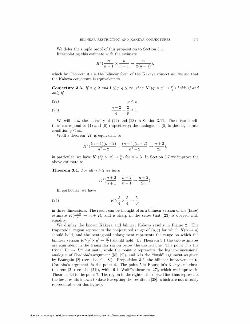
We display the known Kakeya and bilinear Kakeya results in Figure 2. Thetrapezoidal region represents the conjectured range of (p, q) for which K(p → q)should hold, and the pentagonal enlargement represents the range on which thebilinear version K∗(q′ × q′ → p′

2 ) should hold. By Theorem 3.1 the two estimatesare equivalent in the triangular region below the dashed line. The point 1 is thetrivial L1 → L∞ estimate, while the point 2 represents the higher-dimensionalanalogue of Cordoba’s argument ([8], [2]), and 3 is the “bush” argument as givenby Bourgain [2] (see also [9], [8]). Proposition 3.2, the bilinear improvement toCordoba’s argument, is the point 4. The point 5 is Bourgain’s Kakeya maximaltheorem [2] (see also [21]), while 6 is Wolff’s theorem [27], which we improve inTheorem 3.4 to the point 7. The region to the right of the dotted line thus representsthe best results known to date (excepting the results in [28], which are not directlyrepresentable on this figure).



1/p

1/q

1

0

0 1/21/3 2/5

3/101/3

1/4

1/5

1

1

2

3

4

5

6

7

Figure 2. Status of K(p→ q) and K∗(q′ × q′ → p′

2 ) for n = 3.

3.5. Proof of Proposition 3.2. We will need the following geometric observationof Cordoba:

Lemma 3.6. For any ω1, ω2, i1, i2 ∈ E, one has

〈χT

i1ω1, χ

Ti2ω2〉 = |T i1

ω1∩ T i2

ω2| . δn

|ω1 − ω2|+ δ.

In particular, if ω1 and ω2 have unit separation, then the intersection betweenthe two tubes has measure at most δn. We leave the easy proof of this lemma tothe reader.

From this observation we easily see that

‖X∗fX∗g‖1 = 〈X∗δ f,X

∗δ g〉

=∫ ∫ ∫ ∫

δ1−nδ1−n〈χT

i1ω1, χ

Ti2ω2〉f(ω1, i1)g(ω2, i2) dω1di1dω2di2

.∫ ∫ ∫ ∫

δ1−nδ1−nδnf(ω1, i1)g(ω2, i2) dω1di1dω2di2

= δ2−n‖f‖L1ωL1

i‖g‖L1

ωL1i,

which is K∗(1× 1 → 1), as desired.



3.7. Proof of Theorem 3.4. Apart from several technical changes, this theo-rem will be proven using the geometric and combinatorial arguments of Wolff [27],namely Cordoba’s observation (Lemma 3.6) and the “brush” argument. The bi-linear setting allows for some simplification since the average angular separation σbetween two tubes, as defined in [27], may be (heuristically at least) taken to be1. In fact, this result informally follows by setting σ = 1 in Lemma 2.1 of [28], andremoving the “two ends” condition as in that paper. We will also take advantageof some simplifications noted by later authors (notably [19, 20, 21, 22, 28]). Ofcourse, due to the fact that we are in a bilinearized adjoint setting, there are sometechnical difficulties, most notably defining the analogue of the quantity λ in [27].Also, since the target space L(n+2)/2n is not a Banach space, certain reductions andtechniques (e.g. duality, elimination of the i1, i2 variables) become unavailable. Inparticular, the Lebesgue space approach of [13] becomes technically very difficult,and we will use restricted weak-type methods instead. In other words, we will usethe pigeon-hole principle to reduce as many functions as possible to characteristicfunctions.

We first make the trivial observation that since X is discretized, the operatorboundedness of X on Lebesgue spaces is automatic with some large power of δ−1;the issue is to control the dependence on δ efficiently.

Let us normalize f and g so that

‖f‖L

n+2n+1ω L1

i

= ‖g‖L

n+2n+1ω L1

i

= 1.

We have to show that‖X∗fX∗g‖n+2

2n. δ−2 n−2

n+2 .

It will suffice to show the weak-type bound

|X∗fX∗g & α| . α−n+22n δ−

n−2n(25)

for all α > 0, since the strong-type estimate can be recovered (with only a loga-rithmic loss) by integrating this over all α of polynomial size; the contribution ofα δ−C or α δC can be easily controlled using trivial estimates.

We now make the assumption that there exist sets Ωj ⊂ Ej of cardinality Mj > 0for j = 1, 2 such that

‖f(ω, ·)‖L1i

= (M1δn−1)−

n+1n+2χΩ1(ω), ‖g(ω, ·)‖L1

i= (M2δ

n−1)−n+1n+2χΩ2(ω).

(26)

This assumption is justified as any L(n+2)/(n+1)-normalized f , g can be majorizedby a sum of at most logarithmically many functions of this type. We may assumethat the Mj have polynomial size.

From the pigeon-hole principle (25) will follow from the estimate

|E| . (α1α2)−n+22n δ−

n−2n ,(27)

where E is any set such that

X∗f ≥ α1, X∗g ≥ α2 on E,(28)

and α1, α2 > 0 are arbitrary. We may assume that |E|, α1, α2 have polynomialsize, since this estimate is easily obtainable (with a large gain) otherwise.



The αj , j = 1, 2, represent a normalized multiplicity of the tubes in the supportsof f and g; roughly speaking, they are related to the quantity N defined in [27] bythe informal relationship

αj ≈ (Mjδn−1)−

n+1n+2Nj .

Define the quantity A by

|E| = A(α1α2)−n+22n δ−

n−2n .(29)

We have to show that A . 1. We may assume without loss of generality that A isessentially minimal in the sense that

|E| . A(α1α2)−n+22n δ−

n−2n(30)

for all α1, α2, E, f , g which obey (26), (28).To copy Wolff’s argument in [27] we will need some control on the quantity

|E ∩ T iω| if T i

ω is a “typical” tube in a direction in E1. (In [27] such control isautomatic as one is not working in the adjoint setting.) From (28) and (21) wehave the pointwise estimate

δ1−n

∫ ∫f(ω, i)χT i

ω(x) dωdi ≥ α1χE(x).

Integrating this on E we obtain∫ ∫f(ω, i)|T i

ω ∩ E| dωdi ≥ λ1δn−1(M1δ

n−1)1

n+2 ,(31)

where λj is defined for j = 1, 2 by

λj =αj |E|

(Mjδn−1)1

n+2.(32)

From our assumptions we see that the λj are of polynomial size.The λj are the analogues of the quantity λ in [27]. Indeed, from (26) and (31)

we expect |T iω ∩ E| ∼ λ1δ

n−1 on the average. In fact, because we are consideringonly an extremal configuration, a more precise statement is possible. We say that atube T i

ω is good if |T iω ∩E| ≥ 1

4λ1δn−1. Let G be the set of all (ω, i) in the support

of f associated to good tubes. The following improvement of (31) states that mosttubes are good.

Proposition 3.8. We have∫ ∫G

f(ω, i) dωdi ∼ (M1δn−1)

1n+2 .

In particular, we have that G is non-empty, so that λ1 . 1.

Proof. The upper bound follows immediately from (31), so it suffices to show thelower bound. Let c > 0 be a small number of logarithmic size to be chosen later.If the lower bound failed, then we would have∫ ∫

G

f(ω, i) dωdi ≤ c(M1δn−1)

1n+2 .

The idea is to then replace f by f = fχG, and contradict the extremality of A in(30).



Of course, we must modify f further, as well as E, α1 and M1, in order to retain(26) and (28). We replace E by

E = x ∈ E : X∗(f − f) <12α1;

note that f obeys (28) if E is replaced by E and α1 is replaced by 12α1.

The next step is to show that E is comparable to E in size. From the definitionof E we see that ∫

E

X∗(f − f) ≥ 12α1|E\E|.

However, we have from (21) and the definition of f that∫E

X∗(f − f) = δ1−n

∫ ∫Gc

f(ω, i)|T iω ∩ E| dωdi.

Combining the two estimates and using the definition of G we obtain12α1|E\E| ≤ δ1−n

∫ ∫f(ω, i)

14λ1δ

n−1 dωdi.

Using (26) and (32) this simplifies to

|E\E| ≤ 12|E|,

so that |E| ∼ |E| as desired.We now have to modify f , α1, E, and M1 further so that (26) is restored. From

hypothesis we have∫‖f(ω, ·)‖L1

idω =

∫ ∫f(ω, i) dωdi < c(M1δ

n−1)1

n+2 .

However, from (26) we have

‖f(ω, ·)‖L1i≤ (M1δ

n−1)−n+1n+2 .

Thus by Holder’s inequality this implies that

‖f‖L

n+2n+1ω L1

i

≤ cn+1n+2 .

Thus, as before, we can find a logarithmic number of functions fk which each obey(26) for some Mk

1 , and such that

f . cn+1n+2

∑k

fk.

This implies that ∑k

X∗fk & c−n+1n+2α1

on E. Thus, by reducing E by a logarithmic factor one can find a k such that

X∗fk & c−n+1n+2α1

on the reduced set (which we will still call E).Thus (28) is satisfied with f replaced by fk, E replaced by E, and α1 replaced

by α1 ∼ c−n+1n+2α1. But from the definition of A this implies that

|E| . A(α1α2)−n+22n δ−

n−2n .



Comparing this with (30) and our estimates for E and α we thus obtain a contra-diction, if c is sufficiently small.

From the above proposition, the definition of G and the identity∫E

X∗(fχG) = δ1−n

∫ ∫G

f(ω, i)|T iω ∩ E| dωdi

we obtain ∫E

X∗(fχG) & (M1δn−1)

1n+2λ1.

From (32) this becomes ∫E

X∗(fχG) & α1|E|.From (26) we thus have ∫

X∗(fχG)X∗g & α1α2|E|.

Expanding out X∗g using (21) this becomes

δ1−n

∫ ∫g(ω, i)(

∫T i

ω

X∗(fχG)) dωdi & α1α2|E|.

On the other hand, from (26) we have∫ ∫g(ω, i) dωdi = (M2δ

n−1)1

n+2 .

Thus there must exist (ω0, i0) in the support of g such that∫T

i0ω0

X∗(fχG) & α1α2δn−1|E|

(M2δn−1)1

n+2= α1λ2δ

n−1.(33)

The tube T i0ω0

plays the role of the central tube of a “brush”. Unlike Wolff’s argu-ment in [27] (which considered more general angular separations σ than the unitseparation), we will be able to obtain our estimate using only a single brush. Onthe other hand, by utilizing the extremality hypothesis as in Proposition 3.8, onecould certainly obtain a large number of brushes if desired.

By affine invariance we may take ω0 = i0 = 0, so that the central tube is thevertical tube through the origin. In particular, 0 is in E1, so every ω in E2 hasroughly unit separation from the origin.

Let G0 ⊂ G be the collection of all good (ω, i) in the support of f such thatT i

ω intersects the central tube T 00 . Then expanding out X∗(fχG) in (33), we thus

obtain ∫ ∫G0

f(ω, i)δ1−n|T 00 ∩ T i

ω| dωdi & α1λ2δn−1.

From Lemma 3.6 we have |T 00 ∩ T i

ω| . δn, so that∫ ∫G0

f(ω, i) dωdi & α1λ2δn−2.

Let Ω0 ⊂ Ω1 be the collection of all ω such that (ω, i) is in G0 for at least one i.From (26) we see that∫ ∫

G0

f(ω, i) dωdi . #Ω0δn−1(M1δ

n−1)−n+1n+2 ,



so that

#Ω0 & α1λ2δ−1

(M1δn−1)−n+1n+2

.(34)

For each ω ∈ Ω0 we choose a tube Tω from G0 which is in the direction of ω. Thesetubes form the “bristles” of the brush. From construction, |ω| ∼ 1, Tω intersectsT 0

0 , and|Tω ∩ E| & λ1δ

n−1.

As in Wolff [27], we will use (36) to obtain a lower bound on the size of E. Moreprecisely, we will show that

|E| & #Ω0λn1 δ

n−1.(35)

Combining this with (34) yields

|E| & α1λn1λ2δ

n−2

(M1δn−1)−n+1n+2

.

By a completely symmetrical argument one also has

|E| & α2λn2λ1δ

n−2

(M2δn−1)−n+1n+2

.

Multiplying these estimates together one obtains

|E|2 & α1α2(λ1λ2)n+1δ2n−4

(M1δn−1M2δn−1)−n+1n+2

.

Applying (32) this reduces to

|E|2 & (α1α2)n+2|E|2n+2δ2n−4,

which simplifies to (27), as desired.It remains to prove (35). We use the argument in [27]; we adopt the observation

in [22] (see also [13]) that one does not need to utilize the “two ends” reduction in[27] to achieve (35).

We need some notation. For all dyadic numbers λ1 . β . 1 let Γβ be thecylindrical region

Γβ = (y, yn) : |y| ∼ β.From the properties of Tω we see that∑

λ1.β.1

|Tω ∩ E ∩ Γβ| & λ1δn−1

for all ω ∈ Ω0. By the pigeonhole principle, one can refine Ω0 by a logarithmicfactor so that

|Tω ∩ E ∩ Γβ | & λ1δn−1(36)

for all ω in the refined Ω0, and some λ1 . β . 1 independent of the choice of ω;henceforth this β is considered fixed.

The directions in Ω0 are δ-separated. It will be more convenient to work with asparser set of directions, so we take Ω0 to be any δ/β-net of Ω0. From the estimates#Ω0 & βn−1#Ω0 and β & λ1 we see that (35) will follow from

|E| & #Ω0λ2

1

βδn−1.(37)



Let Θ be a δ/β-net of the unit sphere Sn−2 in Rn−1. For each ω ∈ Ω0, we associatean (essentially unique) element θ = θω of Θ by requiring that

|θ − ω

|ω| | . δ/β;

recall that |ω| ∼ 1 for all ω ∈ Ω0. Furthermore, from elementary geometry and thefact that Tω intersects T 0

0 we see that Tω ∩ Γβ is contained in the slab Πθ given by

Πθ = (y, yn) : |y| ∼ β, | y|y| − θ| . δ/β.

As the Πθ are essentially disjoint, (37) will follow from the estimate

|E ∩ Πθ| & #Ω0,θλ2

1

βδn−1(38)

for all θ ∈ Θ, whereΩ0,θ = ω ∈ Ω0 : θω = θ.

For the remainder of the argument ω (and later ω) are always assumed to rangeover Ω0,θ.

We now estimate the quantity

Q =∫

E∩Πθ

∑ω

χTω

in two different ways. Firstly, from the above geometrical considerations and (36)we have

|Tω ∩ E ∩Πθ| & λ1δn−1

for all ω in Ω0,θ. Summing the above estimate we obtain

Q & #Ω0,θλ1δn−1.(39)

We now obtain a different estimate for Q. From the Cauchy-Schwarz inequality wehave

Q . |E ∩Πθ|1/2(∫|E∩Πθ|

(∑ω

χTω)2)1/2.

Squaring both sides and expanding out the integrand into the diagonal and off-diagonal term, this reduces to

Q2

|E ∩Πθ| . (∫|E∩Πθ|

∑ω

χTω) +∑∑

ω 6=ω

|Tω ∩ Tω ∩ E ∩Πθ|.(40)

The first term on the right-hand side is just Q. The second term we may estimateby Lemma 3.6. Thus (40) becomes

Q2

|E ∩Πθ| . Q+∑∑

ω 6=ω

δn

|ω − ω| .

However, ω, ω range over a δ/β-separated set whose elements are within δ/β of theray R+θ. Thus for each ω, the number of ω such that |ω − ω| ∼ 2−j is at most1/(2jδ/β) for any j. Thus the above estimate reduces to

Q2

|E ∩Πθ| . Q+∑

δ/β.2j.1

#Ω0,θ1

2jδ/β

δn

2−j.



Since the number of such j is only logarithmic, we may simplify the above to

1|E ∩Πθ| . 1

Q+

#Ω0,θβδn−1

Q2.

Combining this with (39) and using the hypothesis β & λ1 we obtain1

|E ∩ Πθ| . β

#Ω0,θλ21δ

n−1,

which is (38). This finishes the proof.

3.9. Proof of Theorem 3.1. The proof will be a reprise of the argument in The-orem 2.2. The main difference is that the quasi-orthogonality estimate is replacedby a quasi-triangle inequality, namely Lemma 6.3 in the Appendix. Also the ar-gument is technically simpler as we allow a logarithmic loss in the estimates. Thecase p = 1 is trivial, so we will assume p > 1.

The implication of K∗(q′ × q′ → p′

2 ) from K(p → q) is immediate from dualityand Holder’s inequality. Now suppose that K∗(q′ × q′ → p′

2 ) holds for some p, qobeying 1 ≤ p ≤ n, 1 ≤ q ≤ (n − 1)p′. We have to show that K∗(q′ → p′) holds.Since the Kakeya conjecture is known to hold for p ≤ 2 (see e.g. [2], [27]) we mayassume that p > 2.

Let f be an arbitrary function on E × E . We have to show that

‖X∗fX∗f‖ p′2

. δ−2np +2‖f‖2

Lq′ω L1

i

.(41)

For each integer j > 0 such that δ . 2−j, we divide E into ∼ 2(n−1)j dyadic“subcubes” E ∩ τ j

k of sidelength 2−j, and define the notion of closeness τ jk ∼ τ j

k′ asin Section 2.5. We partition X∗fX∗f as

X∗fX∗f =∑

j

∑k,k′:τ j

k∼τ j

k′

∑m,m′

X∗(fχτ jk⊗ χτ j

m)X∗(fχτ j

k′⊗ χτ j

m′).

We now observe the geometric fact that the summand in the above expression is onlynon-zero when τ j

m and τ jm′ are within O(2−j) of each other; we will implicitly assume

this in our summation. By inserting the above identity into (41) and applyingLemma 6.3 from the Appendix we reduce to

∑j

∑k,k′ :τ j

k∼τ j

k′

∑m,m′

‖X∗(fχτ jk⊗ χτ j

m)X∗(fχτ j

k′⊗ χτ j

m′)‖

p′2p′2

. δp′2 (− 2n

p +2)‖f‖p′

Lq′ω L1

i

.

(42)

This will follow from the following analogue of Proposition 2.6.

Proposition 3.10. We have

‖X∗(fχτ jk⊗ χτ j

m)X∗(fχτ j

k′⊗ χτ j

m′)‖

p′2p′2

.2(1− (n−1)p′q )jδ

p′2 (− 2n

p +2)

‖fχτ jk⊗ χτ j

m‖

p′2

Lq′ω L1

i

‖fχτ j

k′⊗ χτ j

m′‖

p′2

Lq′ω L1

i

.

Proof. By an affine transformation we may take τ jk , τ j

m to be centered at the origin.Applying the hypothesis K∗(q′ × q′ → p′

2 ) to tubes of eccentricity 2jδ we seethat

‖X∗2jδfX

∗2jδg‖p′/2 . (2jδ)−

2np +2‖f‖

Lq′ω L1

i

‖g‖Lq′

ω L1i



for all f , g whose ω-supports are on disjoint cubes. Applying the rescaling (x, xn) →(2−jx, xn), (ω, i) → (2−jω, 2−ji) to this estimate we obtain

‖X∗δ fX

∗δ g‖p′/2 . 2j(n−1)2j(n−1)2−

n−1p′/2 j(2jδ)−

2np +22−

n−1q j‖f‖

Lq′ω L1

i

2−n−1

q j‖g‖Lq′

ω L1i

whenever f and g are supported on τ jk × τ j

m and τ j

k× τ j

m′ respectively, and theproposition follows from substitution and some algebra.

From this proposition (42) reduces to∑j

∑k,k′:τ j

k∼τ j

k′

∑m,m′

2(1− (n−1)p′q )j‖fχτ j

k⊗ χτ j

m‖

p′2

Lq′ω L1

i

‖fχτ j

k′⊗ χτ j

m′‖

p′2

Lq′ω L1

i

. ‖f‖p′

Lq′ω L1

i

.

Since there are only logarithmically many j’s it suffices to show this for a fixed j.By polarization it suffices to show that∑

k

∑m

2(1− (n−1)p′q )j‖fχτ j

k⊗ χτ j

m‖p′

Lq′ω L1

i

. ‖f‖p′

Lq′ω L1

i

,

which we rewrite as

2( 1p′−n−1

q )j

(∑k

∑m

‖fk,m‖p′

Lq′ω L1

i

)1/p′

. ‖f‖Lq′

ω L1i

,(43)

where fk,m = fχτ jk⊗ χτ j

m. It suffices to verify this for the case p = 1 and for the

endpoint (p, q) = (n, n), since the general case 1 ≤ p ≤ q ≤ (n − 1)p′ follows byinterpolation. In these two cases (43) becomes

2−n−1

q j supk,m

‖fk,m‖LqωL1

ω. ‖f‖Lq

ωL1ω,(44) (∑

k

∑m

‖fk,m‖n′Ln′

ω L1i

)1/n′

. ‖f‖Ln′ω L1

i,(45)

respectively. The estimate (44) is trivial, while (45) follows from a further interpo-lation between the trivial estimates

supk,m

‖fk,m‖L∞ω L1i

. ‖f‖L∞ω L1i,∑

k

∑m

‖fk,m‖L1ωL1

i. ‖f‖L1

ωL1i.

We note that if one inserts the result of Theorem 3.4 into the above line ofreasoning, then one not only recovers Wolff’s Kakeya estimate, but also the entropyestimate improvement proven in Lemma 2.1 of [28].

3.11. Necessity of (22)-(23). We now show that the assumptions (22) and (23)in Conjecture 3.3 are necessary.

To show the necessity of (22), we take

f(ω, i) = χE1(ω)δi,0, g(ω, i) = χE2(ω)δi,i0 ,

where δi,j denotes the Kronecker delta function and i0 is a suitable point. A routinecalculation using (21) shows that (if i0 is chosen properly) X∗f,X∗g ∼ 1 on a ball



of radius ∼ 1. Inserting this into K∗(q′ × q′ → p′

2 ) yields

1 . δ−2np +2,

and by taking δ → 0 one obtains (22).To show the necessity of (23), we adapt the “stretched caps” example used to

show (6). We consider a tube T = R×Bn−2(0, δ) in Rn−1, and take

f(ω, i) = χE1∩T (ω)δi,i1 , g(ω, i) = χE2∩T (ω)δi,i2 .

If i1, i2 are chosen appropriately, then X∗f,X∗g are both comparable to 1 on a slabwhich looks roughly like B2(0, 1)×Bn−2(0, δ). Inserting this into K∗(q′× q′ → p′

2 )yields

δn−2p′/2 . δ−

2np +2δ

n−2q′ δ

n−2q′ ,

and by taking δ → 0 one obtains (23).

4. Applications

In this section we use the bilinear estimates above to prove the following restric-tion theorems.

Theorem 4.1. If n = 3, then R∗(p → q) holds whenever p > 17077 and q > 34

9 .Furthermore, R∗

s(q) holds for all q > 4− 527 .

The proof of this theorem will be based on bilinear versions of certain argumentsof Bourgain ([2], [6]; see also [17]). The first step will be to obtain localized linearand bilinear restriction theorems.

Definition 4.2. If 1 ≤ p, q ≤ ∞ and α ≥ 0, then we use R∗(p → q, α) to denotethe estimate

‖<∗f‖Lq(BR) . Rα‖f‖p,

and R∗(p× p→ q, α) to denote the estimate

‖<∗f<∗g‖Lq(BR) . Rα‖f‖p‖g‖p,

where f, g,<∗ are as in Section 2 and BR is a ball of radius R in Rn (the center ofBR is irrelevant by translation symmetry).

It will be convenient to recast these estimates as a restricted bilinear estimateon the Fourier transform.

Proposition 4.3. R∗(p× p→ q, α) is true if and only if one has

‖f g‖Lp(B(x,R)) . RαR−1/p′‖f‖pR−1/p′‖g‖p(46)

for all R 1, x ∈ Rn and all functions f , g supported on AR1 , AR

2 , where

ARi = (x,Φ(x) + t) : x ∈ Qi, |t| . R−1.

Proof. If R∗(p × p → q, α) holds, then (46) follows by translating Φ by O(1/R)and averaging using Holder’s inequality. Now suppose that (46) holds. To showR∗(p× p→ q, α) it suffices to show that

‖(φR<∗f)(φR<∗g)‖q . Rα‖f‖p‖g‖p,



where φR is a real radial L1-normalized bump function adapted to B(0, C/R), suchthat φR is non-negative on B(x,R). But this follows from (46), Young’s inequality,and the identity

φR<∗f = fdσ ∗ φR,

where f(x,Φ(x)) = f(x) is the lift of f to the surface (x,Φ(x)) : x ∈ Q.From this proposition and the trivial estimate

‖f g‖1 ≤ ‖f‖2‖g‖2 = ‖f‖2‖g‖2we obtain the bilinear trace lemma

R∗(2 × 2 → 1, 1).(47)

Thus by interpolating this with other estimates (such as (2)) we may obtain esti-mates of the form R∗(p× p → q, α) with a large value of α. To lower the value ofα we will use a bilinear form of an argument of Bourgain [2, 6] (see also [17]):

Lemma 4.4. If 2 < p, q < ∞ and α > 0 are such that K∗(p2 × p

2 → q2 ) and

R∗(2 × 2 → q, α) hold, then R∗(p× p→ q, α2 + ε) holds for all ε > 0.

Proof. From Proposition 4.3 it suffices to show that

‖f g‖Lq(B(0,R2)) . Rα+εR−2/p′‖f‖pR−2/p′‖g‖p(48)

for all f , g supported on AR2

1 , AR2

2 respectively, and all ε > 0. (The implicitconstants will depend on ε.)

Let φR be as in Proposition 4.3, and define φxR(ξ) = e−2πix·ξφR(ξ) for all x ∈ Rn.

Then from the hypothesis R∗(2× 2 → q, α) and Proposition 4.3 we have

‖φxRf φ

xRg‖Lq(B(x,R)) . RαR−1/2‖f ∗ φx

R‖2R−1/2‖g ∗ φxR‖2

for all x. Averaging this over all x ∈ B(0, R2) we obtain

‖f g‖Lq(B(0,R2)) . Rα(R−n

∫B(0,R2)

(R−1/2‖f ∗ φxR‖2R−1/2‖g ∗ φx

R‖2)q dx)1/q .

Thus to show (48) it suffices to show that

R−n

∫B(0,R2)

(R−1/2‖f ∗ φxR‖2R−1/2‖g ∗ φx

R‖2)q dx . Rε(R−2/p′‖f‖pR−2/p′‖g‖p)q.

(49)

This will be accomplished by repeated use of the uncertainty principle and Plan-cherel’s theorem, together with the Kakeya hypothesis.

Let E , E1, E2 be as in Section 3 with δ = 1R . We partition the annuli AR2

i intocaps Cω for ω ∈ Ei, defined by

Cω = (x, xn) ∈ AR2

i : −∇Φ(x) = ω +O(1R

).From the ellipticity of Φ and some elementary geometry we see that the Cω areessentially disks of diameter 1/R and thickness 1/R2 oriented in the direction (ω, 1),which form a finitely overlapping cover of AR2

i . We decompose

f =∑ω∈E1

fω, g =∑ω∈E2

gω,

where fω, gω are adapted restrictions of f , g respectively to (a suitable dilate of)Cω.



From the support conditions on fω, gω and φxR we see that (49) reduces to

R−n

∫B(0,R2)

(R−1/2(∑ω∈E1

‖fω ∗ φxR‖22)1/2R−1/2(

∑ω∈E2

‖gω ∗ φxR‖22)1/2)q dx

. Rε(R−2/p′‖f‖pR−2/p′‖g‖p)q.

(50)

The function φxR is rapidly decreasing outside of the ball B(x,R). Thus by Plan-

cherel’s theorem the left-hand side of (50) is majorized by

R−n

∫B(0,R2)

(R−1/2(∑ω∈E1

‖fω‖2L2(B(x,R)))1/2R−1/2(

∑ω∈E2

‖gω‖2L2(B(x,R)))1/2)q dx,

(51)

since the portions of φxR on translates of B(x,R) can be handled by translation

symmetry.Let ψω be a Schwarz function which is comparable to 1 on Cω and rapidly

decreasing away from this cap, and whose Fourier transform satisfies the pointwiseestimate

|ψω(x)| . R−n−1χR2T ω0

(x),

where T ω0 is a thickening of Tω

0 and R2T ω0 = R2x : x ∈ T ω

0 .If we define fω = fω/ψω, we have the estimate

|fω(x)| = |fω ∗ ψω(x)| . R−n−1

∫x+R2Tω0

|fω(y)| dy.

From Holder’s inequality and (21) we thus obtain

|fω(x)|2 . R−n−1

∫x+R2Tω0

|fω(y)|2 dy

. X∗Fω(x

R2),

where

Fω(ω′, i) = δω,ω′Rn−1

∫T ω

i

|fω(R2x)|2 dx

and δω,ω′ is the Kronecker delta.Since X∗Fω is essentially constant on balls of radius 1/R we essentially have

‖fω‖2L2(B(x,R)) . RnX∗Fω(x

R2).

From this (and similar considerations for g) we see that (51) is majorized by

R−n

∫B(0,R2)

(R−1/2(∑ω∈E1

RnX∗Fω(x

R2))1/2R−1/2(

∑ω∈E2

RnX∗Gω(x

R2))1/2)q dx,

where Gω is defined in analogy to Fω . We simplify this as

Rn+nq−q

∫B(0,1)

(X∗F (x)X∗G(x))q/2 dx,(52)

where

F (ω, i) = Rn−1

∫T ω

i

|fω(R2x)|2 dx, G(ω, i) = Rn−1

∫T ω

i

|gω(R2x)|2 dx.



On the other hand, from the definition of the hypothesis K∗(p2 × p

2 → q2 ) we have

‖X∗1/RFX

∗1/RG‖q/2 . R

2nq′ −2+ε‖F‖

Lp/2ω L1

i

‖G‖L

p/2ω L1

i

.

Comparing this with (50) and (52), we see that we will be done once we show that

R2q (n+nq−q)R

2nq′ −2‖F‖

Lp/2ω L1

i

‖G‖L

p/2ω L1

i

. (R−2/p′‖f‖pR−2/p′‖g‖p)2.

After some algebraic manipulation we see that it suffices to show that

R2n− 4p +2‖F‖

Lp/2ω L1

i

. ‖f‖2p,together with the completely analogous estimate for g, G. From the definition offω and the measure dω we have

‖f‖2p ∼ Rn−1p/2 ‖(‖fω‖p)2‖L

p/2ω,

and so it suffices to show that

R2n− 4p +2‖F (ω, ·)‖L1

i. R

2(n−1)p ‖fω‖2p

uniformly in ω. From Holder’s inequality,8 the hypothesis p ≥ 2 and the supportconditions on fω we have

‖fω‖2 . R−(n+1)( 12− 1

p )‖fω‖p,

and so after some algebra we reduce to

‖F (ω, ·)‖L1i

. R−n−1‖fω‖22.However, the left-hand side is majorized by

Rn−1

∫B(0,C)

|fω(R2x)|2 dx . R−n−1‖fω‖22,

and the claim follows from Plancherel’s theorem and the pointwise comparabilityof fω and fω.

Applying Lemma 4.4 with p = 52 and q = 5

3 and using (24), we see that

R∗(2× 2 → 53, α) =⇒ R∗(

52× 5

2→ 5

3,α

2+ ε)

for all α, ε > 0. On the other hand, from interpolating (47) with (2) we obtain

R∗(3017× 30

17→ 5

3,15),

so by another interpolation we obtain the implication

R∗(52× 5

2→ 5

3, β) =⇒ R∗(2× 2 → 5

3,25β +

325

)

for all β > 0. Combining these two implications we see that

R∗(2 × 2 → 53, α) =⇒ R∗(2× 2 → 5

3,15α+

325

+ ε).

The map α→ 15α+ 3

25 is a contraction with fixed point α = 320 . Since the estimate

R∗(2 × 2 → 53 , α) holds for at least one value of α, we thus see that

R∗(2× 2 → 53,

320

+ ε)(53)

8This use of Holder’s inequality indicates some room for improvement in this Lemma. Indeed,one can replace the Lp norms on f , g by the Bp norms as used in [17], Lemma 2.2.



for all ε > 0. Applying Lemma 4.4 one more time, we obtain

R∗(52× 5

2→ 5

3,

340

+ ε).(54)

An inspection of the proof of Theorem 2.2 shows that the statement of thetheorem still holds when R∗(p×p→ q) and R∗(p→ 2q) are replaced by their localanalogues R∗(p× p→ q, α) and R∗(p→ 2q, α/2). Applying this to (54) we obtain

R∗(52→ 10

3,

380

+ ε).(55)

We now remove the α completely, borrowing the following argument of Bourgain[2, 6] (for the concrete case n = 3, p > 20/7, q > 10/3, α > 1/20, p > 7/3,q > 42/11, see [17]):

Lemma 4.5 ([2, 6, 17]). If p, q, α are such that n+12 > αq, then R∗(p → q, α)

implies R∗(p→ q) whenever

q > 2 +q

n+12 − αq

,q

p< 1 +

q

p

1n+1

2 − αq.

Applying this to (55) we obtain the first conclusion of Theorem 4.1. UsingTheorem 2.2 to return to the bilinear setting, we thus obtain

R∗(p× p→ q) for p >17077

, q >179.

Interpolating this with (2) and using Theorem 2.2, one obtains the second conclu-sion of Theorem 4.1.

We summarize the various estimates used in Figure 3 (on the next page), which isan expanded version of Figure 1. For comparison, the previously known results arealso displayed. The dotted line thus represents the best global restriction theorems(both linear and bilinear) known to date. (It is possible to improve on these resultsslightly; see [25].)

By interpolating between the main result and (2) we also obtain some progresson Klainerman’s conjecture for the sphere in R3:

Corollary 4.6. If n = 3, then R∗(2 × 2 → p) whenever p > 2− 569 .

These techniques are certainly not best possible. For instance, one can use thetechniques in [5] to obtain better versions of Corollary 4.6. See [25].

The sharp restriction theorem R∗s(q) is scale-invariant under parabolic scaling.

Thus, the compact support condition on Φ can be removed. In particular, one hasa sharp restriction theorem for the entire paraboloid (x, 1

2 |x|2) : x ∈ Rn−1 forq > 4− 5

27 .One can extend the above results to Bochner-Riesz multipliers, so that the

Bochner-Riesz conjecture holds for n = 3 and max(p, p′) ≥ 349 . We sketch the

argument very briefly as follows. By the usual techniques of Carleson-Sjolin reduc-tion and factorization theory (see [6]) it suffices to show that

‖Tf‖Lp(Rn) . λ−n/p‖f‖L∞(Q)

for all p > 34/9, λ 1 and f ∈ L∞(Q), where

Tf(x) =∫

Q

e2πiλ|x−y|a(x, y)f(y) dy,



7/121/2

1/4

1/3

1/q

1/

b

0

9/34

3/10

=1/5

3,4

5

6 7

8

9

ααα =3/40 =3/20

a

2/517/30

Figure 3. Estimates of the form R∗(p × p → q, α) andR∗(p→ 2q, α/2) for n = 3.

Q is thought of as imbedded in Rn, and a is a bump function on Rn × Q whichis supported away from the diagonal x = y. By the analogue of Lemma 4.5 forBochner-Riesz multipliers (see [6]) it suffices to show that

‖Tf‖10/3 . λ3/80+ελ−9/10‖f‖∞for all ε > 0. By a modification of Theorem 2.2 it suffices to show that

‖TfTg‖5/3 . λ3/40+ελ−9/10‖f‖∞λ−9/10‖g‖∞for all f , g with O(1) separated supports, together with variants of this estimate inwhich the phase function |x−y| is replaced by a parabolically scaled (but essentiallyequivalent) version. However, from the analogue of Lemma 4.4 for Bochner-Rieszoperators (which is proven by a bilinear modification of the arguments in [6]) thiswill follow from the restriction estimate (53) and the analogue of Theorem 3.4 forthe Nikodym maximal operator (see e.g. [27]), which is proven similarly. Therequired Nikodym estimate also follows formally from the original formulation ofTheorem 3.4; see the argument in [24].

In higher dimensions n > 3 Theorem 2.3 becomes too weak to be of much use,and we can only achieve a minor improvement on known results. By interpolatingbetween (47) and the bilinear form R∗(2× 2 → n+1

n−1 ) of the Tomas-Stein theorem,



we obtain

R∗(2× 2 → n+ 2n

,1

n+ 2).

Applying this and Theorem 3.4 to Lemma 4.4 we obtain

R∗(2(n+ 2)n+ 1

× 2(n+ 2)n+ 1

→ n+ 2n

,1

2(n+ 1)+ ε).

Applying Theorem 2.2 this becomes

R∗(2(n+ 2)n+ 1

→ 2(n+ 2)n

,1

4(n+ 1)+ ε).

Applying Lemma 4.5 this becomes

R∗(p→ q) for p >2n2 + 6n+ 6n2 + 3n+ 1

, q >2n2 + 6n+ 6n2 + n− 1

.

This is only a slight improvement on the result in Wolff [27], which showedR∗(q → q) for the same range of q. For n > 3 the results obtained by interpo-lating these estimates with Theorem 2.3 are inferior to the Tomas-Stein theorem.

5. Further remarks

In the previous sections we obtained a non-trivial sharp restriction theoremR∗

s(4−ε) from an ordinary restriction theorem R∗(p→ q) (in this case p > 17077 , q >

349 ) and the bilinear estimate (2).

The original formulation of (2) in [17, 18] was stated in terms ofXr spaces. In thissection we show how one can use these estimates instead of the bilinear estimate toobtain non-trivial sharp restriction theorems. Despite the fact that these estimatescan be extended (for characteristic functions) from r > 12

7 to r ≥ 4(√

2 − 1),the methods we will use do not appear to be as efficient as the bilinear techniques.However, they seem to be more robust and applicable to a wider range of situations.

Proposition 5.1. Let n = 3. Suppose that R∗(p → q) holds for some 2 < q < 4,and suppose that the quantity r = 4p′

q satisfies r > 4(√

2− 1). Then we have R∗s(w)

for all w > 4+q2 .

Note that the points ( 1p ,

1q ), (1− 2

w ,1w ), (1

r ,14 ) are collinear when w = 4+q

2 .

Proof. It suffices to show the restricted weak-type estimate

||<∗χΩ| & λ| . 2−2(w−2)j0

λw(56)

for all λ > 0 and Ω ⊆ Q, where j0 is the integer such that |Ω| ∼ 2−2j0 . We mayassume that 2−Cj0 . λ . 1 for some constant C, since (56) is trivial (by e.g. theTomas-Stein restriction theorem) otherwise.

The idea of the proof will be to decompose Ω into a sparse set and a collection ofsets concentrated on caps. On the sparse set the Tomas-Stein estimate R∗

s(4) canbe improved using the Xr estimates of [17, 18]. The sets on caps can be rescaledparabolically to become sets of measure comparable to 1, in which case the estimateR∗(p → q) is equivalent to the scale-invariant estimate R∗

s(q). Combining the twoestimates one expects to obtain R∗

s(4 − ε) for some ε > 0.



We now turn to the details. For each j let 0 < αj ≤ 1 be a quantity to be chosenlater. By the usual Calderon-Zygmund stopping time arguments, we may partitionΩ as

Ω = Ωg ∪⋃

(j,k)∈T

(Ω ∩ τ jk ),

where the “good” set Ωg satisfies

|Ωg ∩ τ jk | ≤ αj |τ j

k |(57)

for all j, k, and τj,k : (j, k) ∈ T is a collection of disjoint dyadic cubes such that

αj |τ jk | < |Ω ∩ τ j

k | ≤ 4αj−1|τ jk |(58)

for all (j, k) ∈ T .We decompose <∗χΩ as

<∗χΩ = <∗χΩg +∑

j

∑k:(j,k)∈T

<∗χΩ∩τ jk.

To control the contribution of <∗χΩg we use the results of [17, 18] and thehypothesis r > 4(

√2− 1) to obtain

‖<∗χΩg ‖4 . ‖χΩg‖Xr =(∑

j

∑k

2−4j( |Ωg ∩ τ j

k ||τ j

k |)4/r)1/4

.(59)

In order for R∗(p → q) to hold we must have p′ ≤ 12q, so that 4/r ≥ 2 > 1.

Applying (66) of Lemma 6.2 with p = 4/r and α = αj we obtain (after somealgebra)∑

k

2−4j( |Ωg ∩ τ j

k ||τ j

k |)4/r . min(2( 8

r−4)(j−j0)2−4j0 , α4r−1j 22(j0−j)2−4j0)

for each j; informally, this shows that the most significant scales occur when j isnear j0. Inserting these estimates into (59) we obtain

‖<∗χΩg ‖44 .∑

j

min(2( 8r−4)(j−j0), α

4r−1j 22(j0−j))2−4j0 .(60)

Let m be a positive integer to be chosen later. We now choose αj so that

α4r−122(j0−j) = 2−m(61)

when − m8r−4

< j − j0 < m2 , and αj = 1 otherwise. The estimate (60) then becomes

‖<∗χΩg ‖44 . m2−m2−4j0 .

From Tchebyshev’s inequality we thus obtain

|<∗χΩg & λ| . m2−m2−4j0λ−4.(62)

It remains to estimate the quantity∑k:(j,k)∈T

<∗χΩ∩τ jk

(63)

for each j. Note that this quantity vanishes when αj = 1 by (58), so we may assumethat − m

8r−4

< j − j0 <m2 .



We will estimate (63) in Lq norm. From Lemma 6.3 in the Appendix we have

‖∑

k:(j,k)∈T

<∗χΩ∩τ jk‖q . (

∑k:(j,k)∈T

‖<∗χΩ∩τ jk‖q′

q )1/q′ .(64)

On the other hand, by parabolically rescaling the hypothesis R∗(p → q) as inProposition 2.6 we obtain

‖<∗χΩ∩τ jk‖Lq . |τ j

k |1−2q− 1

p |Ω ∩ τ jk |1/p.

Combining this with (64) and (58) we obtain

‖∑

k:(j,k)∈T

<∗χΩ∩τ jk‖q .

( ∑k:(j,k)∈T

(|τ jk |1−

2q (4αj−1)1/p)q′)1/q′

.

On the other hand, from (58) we have

#k : (j, k) ∈ T ≤ 22(j−j0)α−1j .

Using this and the fact that 4αj−1 ∼ αj we obtain

‖∑

k:(j,k)∈T

<∗χΩ∩τ jk‖q . |τ j

k |1−2q 2

2q′ (j−j0)

α1p− 1

q′j .(65)

Combining this with (61) and the definition of r one eventually obtains

‖∑

k:(j,k)∈T

<∗χΩ∩τ jk‖q . 2−2(1− 2

q )j02mq

so by the triangle inequality and Tchebyshev’s inequality we have

|∑

j

∑k:(j,k)∈T

<∗χΩ∩τ jk| & λ . 2−2(q−2)j0mq2mλ−q.

Combining this with (62) we obtain

|<∗χΩ| & λ . m2−m2−4j0λ−4 + 2−2(q−2)j0mq2mλ−q.

The claim (56) then follows by choosing 2m = (22j0λ)−4−q2 .

In practice Proposition 5.1 is inferior to the implications obtained by Theorem2.2 and interpolation with (2). For instance, if we insert the first conclusion ofTheorem 4.1 into Proposition 5.1 one obtains R∗

s(w) for w > 4− 19 , which is inferior

to the second conclusion of Theorem 4.1.

6. Appendix: Some elementary harmonic analysis

In this section we state some elementary results which were used repeatedly inthe paper.

We begin with a well-known quasi-orthogonality property of functions with dis-joint frequency support. Define a rectangle to be the product of n (possibly half-infinite or infinite) intervals in Rn.

Lemma 6.1. Let Rk be a collection of rectangles in frequency space such that thedilates 2Rk are almost disjoint, and suppose that fk are a collection of functionswhose Fourier transforms are supported on Rk. Then for all 1 ≤ p ≤ ∞ we have

‖∑

k

fk‖p . (∑

k

‖fk‖p∗p )1/p∗ ,

where p∗ = min(p, p′).



Proof. Let Pk be a smooth Fourier multiplier adapted to 2Rk which equals 1 onRk. We claim that

‖∑

k

PkFk‖p . (∑

k

‖Fk‖p∗p )1/p∗

for arbitrary functions Fk; the lemma then follows by setting Fk = PkFk = fk.By interpolation it suffices to prove this estimate for p = 1, p = 2, and p = ∞.

When p = 2 the estimate is immediate from Plancherel’s theorem. When p = 1 orp = ∞ the lemma follows from the triangle inequality and the estimates

‖PkFk‖1 . ‖Fk‖1, ‖PkFk‖∞ . ‖Fk‖∞,which follow from Young’s inequality and standard estimates on the kernel of Pk.

The next lemma allows us to crudely estimate various Xr-type quantities.

Lemma 6.2. Let Ω ⊆ Q be a set such that |Ω| . 2−(n−1)j0 for some j0 ≥ 0, andlet τ j

k be defined as in Section 2.5. Let 0 ≤ α ≤ 1 be such that |Ω ∩ τ jk | ≤ α|τ j

k | forall k. If p ≥ 1, then we have the estimate∑

k

|Ω ∩ τ jk |p . 2−(n−1)j0 min(α2−(n−1)j , 2−(n−1)j0)p−1.(66)

If p ≤ 1, then we have the estimate∑k

|Ω ∩ τ jk |p . 2−(n−1)pj02(n−1)(1−p)j .(67)

Proof. By the log-convexity of Lp norms, 0 ≤ p ≤ ∞, it suffices to prove the threebounds

supk|Ω ∩ τ j

k | . min(α2−(n−1)j , 2−(n−1)j0),(68) ∑k

|Ω ∩ τ jk | . 2−(n−1)j0 ,(69) ∑

k

1 . 2(n−1)j .(70)

But these bounds follow trivially from the estimates

|Ω ∩ τ jk | ≤ min(|Ω|, α|τ j

k |) . min(2−(n−1)j0 , α2−(n−1)j),∑k

|Ω ∩ τ jk | = |Ω| . 2−(n−1)j0 ,

and the cardinality of the τ jk .

We remark that without further information on Ω these bounds are best possible.In most cases we will set α = 1.

Finally, we present a very easy inequality.

Lemma 6.3. If 1 ≤ p ≤ ∞, then

(∑

k

|ak|p)1/p ≤∑

k

|ak|



for all sequences of numbers ak. Also, if 0 < q ≤ 1, then

‖∑

k

fk‖q ≤ (∑

k

‖fk‖qq)

1/q.

Proof. The first estimate is trivial for p = 1 and p = ∞, and the general case followsby convexity. The second estimate follows by applying the first with ak = |fk(x)|q,p = 1/q and integrating.

References

[1] M. Beals, Self-Spreading and strength of Singularities for solutions to semilinear wave equa-tions, Annals of Math. 118 (1983), 187-214. MR 85c:35057

[2] J. Bourgain, Besicovitch-type maximal operators and applications to Fourier analysis, Geom.and Funct. Anal. 22 (1991), 147–187. MR 92g:42010

[3] J. Bourgain, On the restriction and multiplier problem in R3, Lecture notes in Mathematics,no. 1469. Springer Verlag, 1991. MR 92m:42017

[4] J. Bourgain, A remark on Schrodinger operators, Israel J. Math. 77 (1992), 1–16. MR93k:35071

[5] J. Bourgain, Estimates for cone multipliers, Operator Theory: Advances and Applications,77 (1995), 41–60. MR 96m:42022

[6] J. Bourgain, Some new estimates on oscillatory integrals, Essays in Fourier Analysis in honorof E. M. Stein, Princeton University Press (1995), 83–112. MR 96c:42028

[7] L. Carleson and P. Sjolin, Oscillatory integrals and a multiplier problem for the disc, StudiaMath. 44 (1972), 287–299. MR 50:14052

[8] A. Cordoba, The Kakeya maximal function and the spherical summation multipliers, Amer.J. Math. 99 (1977), 1–22. MR 56:6259

[9] S. Drury, Lp estimates for the x-ray transform, Ill. J. Math. 27 (1983), 125–129. MR85b:44004

[10] C. Fefferman, Inequalities for strongly singular convolution operators, Acta Math. 124 (1970),9–36. MR 41:2468

[11] C. Fefferman, The multiplier problem for the ball, Ann. of Math. 94 (1971), 330–336. MR45:5661

[12] L. Hormander, Fourier Integral Operators, Acta Math. 127 (1971), 79–183. MR 52:9299[13] N. Katz, preprint.[14] S. Klainerman, M. Machedon, Space-time estimates for null forms and the local existence

theorem, Comm. Pure Appl. Math. 46 (1993), no. 9, 1221–1268. MR 94h:35137[15] S. Klainerman, M. Machedon, Remark on Strichartz-type inequalities. With appendices by

Jean Bourgain and Daniel Tataru. Internat. Math. Res. Notices 5 (1996), 201–220. MR97g:46037

[16] S. Klainerman, M. Machedon, On the regularity properties of a model problem related towave maps, Duke Math. J. 87 (1997), 553–589. MR 98e:35118

[17] A. Moyua, A. Vargas, L. Vega, Schrodinger Maximal Function and Restriction Properties ofthe Fourier transform, International Math. Research Notices 16 (1996). MR 97k:42042

[18] A. Moyua, A. Vargas, L. Vega, Restriction theorems and Maximal operators related to oscil-latory integrals in R3, to appear, Duke Math. J.

[19] W. Schlag, A generalization of Bourgain’s circular maximal theorem, J. Amer. Math. Soc.10 (1997), 103-122. MR 97c:42035

[20] W. Schlag, A geometric proof of the circular maximal theorem, to appear, Duke Math. J.[21] W. Schlag, A geometric inequality with applications to the Kakeya problem in three dimen-

sions, to appear, Geometric and Functional Analysis.[22] C. D. Sogge, Concerning Nikodym-type sets in 3-dimensional curved space, preprint.[23] E. M. Stein, Harmonic Analysis, Princeton University Press, 1993. MR 95c:42002[24] T. Tao, The Bochner-Riesz conjecture implies the Restriction conjecture, to appear, Duke

Math J.

[25] T. Tao, A. Vargas, A bilinear approach to cone multipliers and related operators, in prepa-ration.

[26] P. Tomas, A restriction theorem for the Fourier transform, Bull. Amer. Math. Soc. 81 (1975),477–478. MR 50:10681



[27] T. H. Wolff, An improved bound for Kakeya type maximal functions, Revista Mat. Iberoamer-icana. 11 (1995), 651–674. MR 96m:42034

[28] T. H. Wolff, A mixed norm estimate for the x-ray transform, to appear in Revista Mat.Iberoamericana.

Department of Mathematics, University of California–Los Angeles, Los Angeles,

California 90024

E-mail address: [email protected]

Departamento de Matematicas, Universidad Autonoma de Madrid, 28049 Madrid,

Spain


Departamento de Matematicas, Universidad del Pais Vasco, Apartado 644, 48080,

Bilbao, Spain



A bilinear approach to the restriction and Kakeya conjectures

Documents

Transcript of A bilinear approach to the restriction and Kakeya conjectures