1

An Implicit Surface Triangulator based on Exact Surface Curvature

Ioannis Pantazopoulos and Spyros Tzafestas

Intelligent Robotics and Automation Laboratory

Signals, Control and Robotics Division

Electrical and Computer Engineering Department

National Technical University of Athens,

Zographou, Athens, Greece

e-mail: {jpanta,tzafesta}@softlab.ece.ntua.gr

Fax: +30-1-7722490

Abstract

A technique for generating a triangular net from an implicit surface description is presented. This technique can be applied to 2nd-order differentiable functions - describing the surface - and is based on finding the principal curvatures at each generated point. It is therefore well adapted to the shape of the surface, taking more samples in the areas with high curvature. The triangular net is competed

in a second phase where extra edges are added that connect the vertices already extracted.

1. Introduction In the recent years, a great effort was made towards automated animation of deformable objects, solid modeling of industrial objects, and scientific visualization with the aid of implicit function descriptions [Beier 1993]. This kind of information usually achieves smoothness in the visualized data while being compact in the description. Although, in the final rendering, these objects are ray traced, a problem well understood and solved, in the mid-stages of animation, fast rendering of the object is always preferred. While the former solves a possible difficult root finding problem, the latter uses the z-buffer to quickly render the polygons (using local illumination models). Several methods have been proposed for surface triangulation. Most of them are based on evaluations of the implicit surface function at the vertices of a uniform grid in some predefined area [Bloothmental 1988, 1994, Velho 1996, Wyvill et al. 1986]. There, whenever the function has different sign on the vertices, its intersections with the edges of the cell are found and triangles are appropriately extracted. Sometimes, the intersections may not be found accurately, thus giving a quick approximation of the surface [Lorensen et al. 1987]. Usually, the cells are not cubical but rather tetrahedral [Payne et al 1986, Allgower et al. 1987]. In some methods, there is only the need for a starting point (a cell where an intersection with the surface exists). Depending on where the intersections lie, neighbor cells are added so that the rest of the surface is found as well [Wyvill et al. 1986]. These are known as continuation methods. These methods demand a starting point (i.e. a point that zeroes the implicit function) and so it is difficult to find surfaces with more than one components (non connected surface). The grid may not be fixed but it is sometimes recursively subdivided to gain more accuracy [Adaptive Marching Cubes]. Others make an approximation of the curvature and, if needed, a subdivision of the extracted triangles is performed in a second refinement stage [Velho 1996]. Witkin et al. [1994], solve an optimization problem to acquire samples on the surface. Fingueiredo et al. [1992] propose a physically based approach to polygonizing the surface. Overveld et al. [1993], presented a technique that bounds the surface in the first place and shrinks to the actual surface afterwards, providing the surface is of genus 0. We present a simple implicit surface triangulator which is based on the exact curvature of the surface. This gives the polygonizer the ability to refine only when needed by taking small steps on the surface when the curvature is high and taking large steps when the curvature is low. Our method starts from a given point on

2

the surface and seeks for neighbor points on the surface, i.e. it is a continuation method. Care should be taken in the structuring (i.e. the connections between extracted points on the surface), in order the surface reconstruction to yield an orientable, with out any holes, connected manifold. The paper is organized as follows. In section 2, we give some basic definitions of differential geometry while in section 3 we provide the theoretic scheme of our algorithm. In section 4, we describe the structuring phase which is used to complete the triangulation and post-process the triangular net. In section 5, we give a method of blending two or more surfaces. Finally, in section 6, we discuss our implementation results and in section 7 we provide some concluding remarks.

2. Differential Geometry Definitions Before proceeding to the actual algorithm we give some basic definitions from differential geometry [Carmo 1976] that will be useful. Definition 1. A regular surface is a subset S⊂ R3 where for each point there exists a neighborhood V and a parameterization p:U⊂ R2→V∩S such as: a. p is an infinitely differentiable parameterization of the form: ( ) ( ) ( ) ( )[ ]Tvuzvuyvuxvu ,,,, =p b. the continuous inverse parameterization p-1 also exists, and c. the differential dp is one to one. The latter condition is known as the regularity condition. For a regular surface, the unitary normal vector is defined for every point q of the surface by the following relation:

vu

vu

pppp

N××

=

The above mapping is known as Gauss map. In this way, a tangential plane is defined for all points of the surface. Every movement on the tangential plane Tq of point q of the surface results in a change of direction of the unitary normal vector that lies also on the same plane Tq. This change is described by the mapping dNq which is actually a linear mapping, as given by the following lemma stated without proof. Lemma 1. The mapping qqq TTd →:N is a self-adjoint linear mapping. Using the mapping dNq, a quadratic form may be introduced, known as the second fundamental form

RTII qq →: ,: ( ) ( ) qqq TwwwdwII ∈⋅−= ,N

Actually, this corresponds to the normal curvature of the surface at point q, when taking a step along unitary direction w of the tangential plane. The normal curvature is defined as the curvature of a curve, parameterized by arc length, that passes from point q with w as tangential vector, projected onto the normal of the surface (see figure 1).

3

Ν

a(q)

a'(q)

a''(q)kn(q)

φ

p(u,v)

q

Figure 1. The normal curvature for the arc length parameterized curve a(s), lying on the surface p(u,v), can be found by the projection of its second derivative, at point q, onto the normal vector of the surface at

the same point q. Thus, when applied on unitary directions, the quadratic form achieves minimum (kmin) and maximum (kmax) curvatures. These values are the eigenvalues of the 2×2 matrix of mapping dNq and called principal curvatures. They are achieved in directions given by the corresponding eigenvectors that are called principal directions (respectively emin and emax). Thus the point q can be classified to the following categories according to the sign of the minimum and maximum curvatures (see figure 2A-2D): a. Elliptic, if the eigenvalues have the same sign. b. Hyperbolic, if the eigenvalues have opposite sign. c. Parabolic, if exactly one of the eigenvalues is zero. d. Planar, if both eigenvalues are zero.

Figure 2A-2D). The four different points depending on the possible curvatures. From left to right, top-down, we have an elliptic (any point on an ellipsoid), hyperbolic, parabolic (the lowest points on the

paraboloid) and planar point (zero point of the monkey saddle : z(x,y)=x3-3xy2).

4

We will now going to find the mapping dNq (i.e. the corresponding matrix) in terms of the parameterization p of the surface. Without any proof, we give now the equations of Wiengarten that express the change in the direction of normal vector in a frame defined by the axis pu, pv. Note that the matrix need not be symmetric because the parameterization may not be orthogonal.

( ) ( ) ( )qqqe uupN ⋅= ( ) ( ) ( )qqqf uvpN ⋅= ( ) ( ) ( )qqqg vvpN ⋅= ( ) ( ) ( )qqqE uu pp ⋅= ( ) ( ) ( )qqqF vu pp ⋅=

( ) ( )qqqG vv pp ⋅=)(

( ) ( ) ( ) ( )( ) ( ) ( ) ( )( )211 qFqGqEqGqeqFqfa −−=

( ) ( ) ( ) ( )( ) ( ) ( ) ( )( )212 qFqGqEqGqfqFqga −−=

( ) ( ) ( ) ( )( ) ( ) ( ) ( )( )221 qFqGqEqEqfqFqea −−=

( ) ( ) ( ) ( )( ) ( ) ( ) ( )( )222 qFqGqEqEqgqFqfa −−=

( ) waaaa

wd q ⋅

=

2221

1211N

Having defined the matrix (aij) we are able to compute the principal curvatures and directions.

3. The Exact Curvature Triangulator Suppose we are given a starting point qin on the surface. We would like to expand a triangular net from this point covering the whole surface (by whole surface we mean here the component of the surface where the point lies). Additionally, we would like to do this in an adaptive way, so as in areas with high curvature, where the surface is well approximated by large polygons, take large steps and in areas with low curvature take smaller steps. In overall, we would like to have some fixed error for all triangles in the approximation of the surface. This will provide the best visual quality for the given error. Given a differentiable function RRf →3: , a surface can be generated by the points (x,y,z) that zero the function f. This is the implicit surface description. If there is no point on this surface where f achieves a critical value (i.e. zero gradient) then the output surface is guaranteed to be a regular one. From now on, we will assume that the surface described by the function f is a regular one. For this regular surface, it is easy to find a normal vector for each point. Assuming a parameterization of the surface and a point q lying on the surface (i.e. ( ) ( ) ( )( ) 0,,,,, =qqqqqq vuzvuyvuxf ), then by differentiating partially with respect to u, v one gets:

0=⋅+⋅+⋅ uzuyux zfyfxf 0=⋅+⋅+⋅ vzvyvx zfyfxf

The above relations can be written in an inner product form: 0=⋅∇ uf p 0=⋅∇ vf p

Thus, the gradient of the function is orthogonal to the derivatives of the parameterization and thus parallel to the normal vector of the surface. We can retrieve two different formulations for the unitary normal vector, that differ only at the sign:

ff

∇∇±=N

Obviously, one needs to keep only one value of the normal vector. We can choose either of the sign and consider it the same all the way, as long as function f has continuous partial derivatives and the reconstructed surface is an orientable manifold. These conditions guarantee that the gradient of the function

5

will not abruptly change its sign and the surface described has an inner and outer volume clearly defined. Further, we will assume that f has continuous second partial derivatives. h (ih=N)

s t

x y

z

O

q

P

Figure 3. Change of parameters results in a local frame with its origin at point q and its z-axis parallel to the surface’s normal vector at the same point q.

Consider now a frame with q as its origin and is, it, ih as its axes, where the ih-axis has the same direction as the unitary normal vector N (see figure 3). We can find the homogeneous transformation P, transforming from the new frame to the global frame. This will be given by the following equation:

[ ]

⋅=

⋅

=

111000134333231

24232221

14131211

hts

qhts

rrrrrrrrrrrr

zyx

ts Nii

Additionally, the above transformation gives us the ability to express changes in the global frame to changes in the local tangential frame. The partial derivatives of x, y, z in respect to s, t, h will be:

[ ]Tssss zyx=i

[ ]Ttttt zyx=i

[ ]Thhh zyx=N

We are now ready to admit a parameterization of the surface in the local frame, as follows. Lemma 2. There exists some open neighborhood of point q where we can admit the parameterization

( ) ( )[ ]Ttshtsts ,, == pp in the local frame. Proof. Because of the regularity of the surface, there should exist an open neighborhood of point q and a parameterization ( ) ( ) ( )[ ]Tvuzvuyvuxvu ,,,),( == rr of variables u, v in the global frame, so that:

( )( ) ( ) ( ) ( )( ) 0.,,,,, == vuzvuyvuxfvurf Applying the one to one homogeneous transformation P, the function can be written with respect to s, t, h variables:

( ) ( ) 0,,,, 333231222221111211 =+++++++++= qhNtrsrqhNtrsrqhNtrsrfhtsg We can use now the chain rule to compute the partial derivative gh, as follows:

ffNfNfNfzfyfxfg zyxhzhyhxh ∇=⋅∇=++=++= N321 Having considered regular surfaces, the gradient of f is never zero and thus, using the implicit function theorem there is a neighborhood of q, where we can solve with respect to h:

( ) ( ) ( )( ) ( ) ( ) ( )( )( ) ( )tshvuzvuyvuxtvuzvuyvuxshh ,,,,,,,,,,,, ==

6

Now, using Wiengarten’s equations we will find the normal curvatures of the surface at point q. First of all, we need to compute the first and second derivatives of p with respect to s, t. These are easily computed:

[ ]Tss h01=p

[ ]Ttt h01=p

[ ]Tssss h00=p

[ ]Tstst h00=p

[ ]Ttttt h00=p

Considering the function f that has continuous first and second partial derivatives, we are now able to compute the partial derivatives of h as well. Using the chain rule, we first differentiate with respect to s and t:

( ) ( ) ( ) 0=+⋅++⋅++⋅ shszshsyshsx hzzfhyyfhxxf ( ) ( ) ( ) 0=+⋅++⋅++⋅ thtzthtythtx hzzfhyyfhxxf

So the partial derivatives can be computed: ( ) ( ) ( ) ( )Ni ⋅∇⋅∇−=++++−= ffzfyfxfzfyfxfh shzhyhxszsysxs ( ) ( ) ( ) ( )Ni ⋅∇⋅∇−=++++−= ffzfyfxfzfyfxfh thzhyhxtztytxt

For s=t=0, we will have ∇ f//N and thus 0=⋅∇=⋅∇ ts ff ii . So: ( ) ( ) 00,00,0 == ts hh

Now, we further differentiate the previous relations in order to obtain second derivatives of h. Thus, differentiating the first relation with respect to s, we obtain:

( ) ( ) ( ) 0=⋅+++⋅+++++ sshzhyhxshzshyshxsszssyssxs hzfyfxfhzfyfxfzfyfxf where:

( ) ( ) shxzhxyhxxsxzsxysxxxs hzfyfxfzfyfxff ⋅+++++= ( ) ( ) shyzhyyhyxsyzsyysyxys hzfyfxfzfyfxff ⋅+++++= ( ) ( ) shzzhzyhzxszzszyszxzs hzfyfxfzfyfxff ⋅+++++=

For s=t=0, we have hs=0 and so by rearranging terms, the second derivative hss is found to be: ( ) [ ] ( ) [ ] ( )qfzyxqzyxh T

sssfsssss ∇⋅⋅−= H0,0 where Hf is the Hessian matrix of f:

=

zzzyzx

yzyyyx

xzxyxx

f

fffffffff

H

Analogously, one finds: ( ) [ ] ( ) [ ] ( )qfzyxqzyxh T

tttfsssst ∇⋅⋅−= H0,0

( ) [ ] ( ) [ ] ( )qfzyxqzyxh Ttttfttttt ∇⋅⋅−= H0,0

Now, we can compute the factors e, f, g, E, F, G of Wiengarten’s equations at point q (note that the vector N should be expressed in the local frame, i.e. [ ]T100=N ):

( ) ( )0,0ssss hqe =⋅= pN ( ) ( )0,0stst hqf =⋅= pN ( ) ( )0,0tttt hqg =⋅= pN

( ) 1=⋅= ssqE pp ( ) 0=⋅= tsqF pp

1)( =⋅= ttqG pp ( )0,011 ssha −= ( )0,012 stha −=

7

( )0,021 stha −= ( )0,022 ttha −=

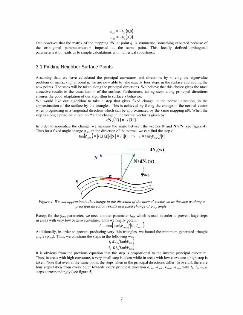
One observes that the matrix of the mapping dN, at point q, is symmetric, something expected because of the orthogonal parameterization imposed at the same point. This locally defined orthogonal parameterization leads us to simple calculations with numerical robustness.

3.1 Finding Neighbor Surface Points Assuming that, we have calculated the principal curvatures and directions by solving the eigenvalue problem of matrix (aij) at point q, we are now able to take exactly four steps in the surface and adding the new points. The steps will be taken along the principal directions. We believe that this choice gives the most attractive results in the visualization of the surface. Furthermore, taking steps along principal directions ensures the good adaptation of our algorithm to surface’s behavior. We would like our algorithm to take a step that gives fixed change in the normal direction, in the approximation of the surface by the triangles. This is achieved by fixing the change in the normal vector when progressing in a tangential direction which can be approximated by the same mapping dN. When the step is along a principal direction l*e, the change in the normal vector is given by:

( ) eeN ⋅⋅−=⋅ klld q In order to normalize the change, we measure the angle between the vectors N and N+dN (see figure 4). Thus for a fixed angle change φstep in the direction of the normal we can find the step l:

( ) ( ) klklkl stepstep ϕϕ tantan =⇒⋅=⋅⋅= Ne

N

wS

N+dNq(w)

dNq(w)

φstep

Figure 4. We can approximate the change in the direction of the normal vector, so as the step w along a principal direction results in a fixed change of φstep angle.

Except for the φstep parameter, we need another parameter lmax which is used in order to prevent huge steps in areas with very low or zero curvature. Thus we finally obtain:

( ){ }max,tanmin lkl stepϕ= Additionally, in order to prevent producing very thin triangles, we bound the minimum generated triangle angle (φmin). Thus, we constrain the steps in the following way:

( )min21 tan ϕll ≤ ( )min12 tan ϕll ≤

It is obvious from the previous equation that the step is proportional to the inverse principal curvature. Thus, in areas with high curvature, a very small step is taken while in areas with low curvature a high step is taken. Note that even at the same point, the steps taken in the principal directions differ. In overall, there are four steps taken from every point towards every principal direction emin, -emin, emax, -emax with l1, l1, l2, l2 steps correspondingly (see figure 5).

8

N

s

t

l1⋅⋅⋅⋅emin

-l1⋅⋅⋅⋅emin

l2⋅⋅⋅⋅emax -l2⋅⋅⋅⋅emax q

p(u,v)

Figure 5. The steps taken lie on the s-t plane of the local frame and are parallel to the principal directions emin, emax. The length of the steps are calculated so as the change in the direction of the normal vector is

fixed .

3.2 Finding Next Point after making a Step After taking a step w in the tangential plane, we need to find an actual point lying on the surface in the corresponding area. We can find a very good initial approximation of the surface point when moving in the tangential direction (w1,w2). The approximation in the global frame is given by:

( )( )22 2221

2121 wwwwwwa ttstssts pppppP +⋅+++⋅=

Note, that this approximation is of 2nd order, thus it should lie very closely to the surface. We can continue with an approximation scheme to quickly find a close point lying on the surface:

( ) ( ) ( ) ( )2qOqqfqfqqf ∆+∆⋅∇+=∆+ Ignoring 2nd order terms and assuming that a movement along the gradient ∇ f(q) gives zero for the new position q+∆q, the correction will be:

( )( )

( )ii

iii qf

qfqfqq ∇

∇−=+ 21

This iteration process is repeated until the implicit function’s error is small enough ( ( ) epsqf i < ). The convergence is very fast and only a few function evaluations are needed.

4. Structuring In the previous sections, we have described how to take steps on the surface from a given point. This procedure can be repeated again and again for all produced points. Obviously, we should have some criteria to terminate the procedure, i.e. not taking any more steps from a given point. Additionally, we should find some criteria to connect neighboring points on the surface so as to produce a valid triangular net. We enlist here the constraints that a triangular net should follow. The procedure of adding points and connections on the surface should not violate these constraints. Constraint 1. At most two triangles may be incident to an edge. This is obvious as we expect orientable manifolds to be triangulated. Constraint 2. Vertices that lie “very close” to a triangle’s plane, are not inside the triangle when projected on its plane. Here, the term “very close” requires some care in its treatment. For example, in areas with very small tubular neighborhood, there may be some false close vertices (see figure 6). For this reason, a vertex is considered close to another one if both their distance and normals’ angle are less than a predefined threshold.

9

S

p

q

N(p)

N(q)

S

q N(q)

p

N(p)

Figure 6. Due to small tubular neighborhood of this part of surface S, vertices p, q lie very near with each other (left figure). This may lead to false connection between p, q which can be avoided by comparing

normal vectors. We assume that cases like the one in the right figure, where p, q are very near and have approximately the same normal vector, do not take place. If such case exists then our algorithm will not be

able to resolve the ambiguities. We divide the extraction of the triangular net in two phases. The output of the first phase is a proper sampling of the surface along with some connections, that we will call the skeleton of the surface. The skeleton of the surface is well sampled (no other points can be added without violating the restrictions), but it misses several connections to become a triangular net. This will be the target of the second phase.

4.1 Constructing the Skeleton In the first phase, we add points and connections if these do not violate already existing connections, i.e. if they do not intersect with other connections. Additionally, if a new point lies very close to an existing one, then the point is not added and instead the connection is established with the existing one. The pseudo-algorithm is shown below: AddConnection(Vertex A,Point p){

kmin=infinite;for every vertex B with ||A-B||<edistance and normal(A)*normal(B)>cos(eangle)

for every connected, to B, vertex Cproject A, p, C on plane of B, giving A’, p’, C’kmin=min{kmin,intersection(A’+k(p’-A),B+(C’-B)*m)}

endend

if kmin>a1find closest vertex D to pif ||D-p||/||A-p||<eratio connect(A,D);else { D=addVertex(p); connect(A,D); }

else if kmin>a2addConnection(A,projectOnSurface(A+(p-A)*kmin /2));

end}

Typical values for the parameters of the algorithm are: edistance=3*max{distance(A,neighbors(A))}, eangle=2*φstep, a1=2, a2=1.4, eratio=0.1. This procedure is executed when a new point has been generated. We see that the point is finally added as a vertex, only when there is no intersection of the new edge with another one and there is no vertex very close. The vertex is added also in a FIFO queue so as it will be processed later (i.e. expand to give new vertices in its principal directions). After all neighbors of vertex A have been checked and possibly added, the vertex is removed from the queue. When, the queue becomes empty the first phase is completed.

4.2 Adding Connections to Skeleton

10

The second phase must, in a way, “cover” the holes of the first phase. Remember that we assume that the surface is without boundary i.e. no holes are present. These holes are actually non-planar polygons that have to be triangulated in some way. The best way to do that, when dealing with planar polygons, is to apply a constrained Delaunay triangulation to the polygon. Here we should proceed with carefully, because by dealing with non planar polygons, there are certain restrictions in connecting vertices of the polygons (for example, vertices with large deviation in the normal vector should not be connected). Instead, we employ a heuristic technique to perform the triangulation. First of all, we add the edges that lie very close to a principal direction of the vertices they connect. Second, we apply an iterative relaxation scheme, where we add the edges in an ordered way, beginning with those that form the greatest possible angle and continue until (almost) all edges are inserted. After the last procedure, a triangular net will be constructed. A third step can also be performed where the triangulation of each quadrilateral may be changed along its second diagonal if this results in greater minimum angle of the inner triangles (swap-edge operations). TriangulateSkeleton(){// first step: add edges close to principal directions.

for every vertex Afor every vertex B

if close(A,B) and edge(A,B) does not intersect other edge andinsertion of edge(A,B) does not generate any angle below 75o

{connect(A,B)

}

// second step: iteratively add edges.for φ-angle equal to 85o down to 5o with 10o step

for every vertex Afor every vertex B

if close(A,B) and edge(A,B) does not intersect other edgeand

insertion of edge(A,B) does not generate any angle belowφ

{connect(A,B)

}

// third step: swap edges for a few steps.for (each quadrilateral of the net)

if (splitting quadrilateral along 2nd diagonal gives greater minimum angle){

remove 1st diagonal.add 2nd diagonal.

}}

As can be seen, when adding one edge we have again to verify that there is no intersection with an existing edge as this will result in violation of constraint 2. Finally, adding the edge is performed only if the vertices are close enough (i.e. both their Euclidean distance and normals’ angle are below a given threshold).

4.3 Finding Initial Points on the Surface As we have said, a disadvantage of the algorithm is that it requires some initial points on the surface, to be given. Several schemes can be used to find some points on the surface, as for example, solving the equation described by the function with respect to one parameter and giving some values to the others, perform a random search in 3d space or an optimization scheme that seeks a minimum of [f(x)]2. One could apply also, a binary search between points with opposite signs of the function f as most of cell-like polygonizers do. Of course, if the surface is not connected, i.e. it has more than one parts disconnected with each other, then we have to find at least one point at each part. Note though, that there is no problem in applying our algorithm when having two or more points on the same part of the surface. The triangular nets obtained from the points will be fused together. Note also that, typically, in cases of infinite surface reconstruction one has to specify a maximum volume that the algorithm can generate points.

11

5. Blending More Than One Surfaces Typically, the union of two or more surfaces is described by a “min” function of their respective implicit functions [Ricci 1973]. This gives the impression of the exact union of the surfaces but it suffers from the abrupt changes in the normal vector on their intersections. Additionally, this can not be the case for our triangulator as it requires a 2nd order differentiable surface. Blending two or more surfaces is a way of producing smooth surfaces from two or more parts described by their own implicit functions [Blinn 1982]. Following Zorner et al. [2000], we can achieve a 2nd order differentiable surface using the following implicit function:

( ) ( ) ( )

+−= ∑∑

==

21

2

1

2

1

1 εn

ii

n

ii ff

ng xxx

where n is the number of the components, fi is the corresponding implicit function and ε a small real number to guarantee the smooth gluing of the surfaces. The first and second derivatives with respect to a variable xj are given by the following relations, where it is obvious that they are continues provided that fi have continuous partial derivatives too:

( ) ( ) ( ) ( ) ( )

∂∂

⋅

+−

∂∂

=∂∂

∑∑∑=

−

==

n

i j

ii

n

ii

n

i j

i

j xfff

xf

nxg

1

21

2

1

2

1

1 xxxxx ε

( ) ( ) ( ) ( ) ( ) ( ) ( )

( ) ( ) ( ) ( ) ( )

∂∂∂

+∂∂

∂∂

⋅

+−

−

∂∂

⋅∂∂

⋅

++

∂∂∂

=∂∂

∂

∑∑

∑∑∑∑

=

−

=

==

−

==

n

i kj

ii

k

i

j

in

ii

n

i k

ii

n

i j

ii

n

ii

n

i kj

i

kj

xxfxf

xf

xff

xff

xfff

xxf

nxxg

1

221

2

1

2

11

23

2

1

2

1

22 1

xxxx

xxxxxxx

ε

ε

6. Implementation and Results We have written a program in C++ that implements the algorithm proposed above1. We can see in figure 7, the progress in constructing the triangular net of several quadrics (skeleton, wireframe and goureau rendering). We can also see in figure 8, additional surfaces that are the result of blending two or more quadrics. The whole procedure of triangulating a surface, given a starting point, take about 5-10 seconds in a Pentium III, 550 Mhz, 256 Mb, running Windows NT. Of course, it depends on the detail that one wants to achieve. This algorithm can be quite accelerated with optimizations that we didn’t pursue for ease of development. We can observe the regular way of the triangles in the surfaces, along with its adaptation to surface curvature. We believe that this regular way and the quality of the triangles (small angles are not favored in our algorithm) gives the best visual quality. Additionally, the algorithm can produce very easily continuous levels of detail of the surface by altering the maximum steps taken along each principal direction, though these steps should not become too large for correct results. Of course, there are some drawbacks regarding our algorithm. Specifically, it requires the surface to be a 2nd order differentiable manifold, while the gradient and Hessian of the corresponding function are assumed given. For each point, evaluations of the gradient and Hessian take place along with the evaluation of the function. From a computational point of view, this is not very bad as most evaluations (of function and gradient) take place at finding points on surface after taking a step which is relatively fast. A second

1 One can download a demo from www.softlab.ntua.gr/~jpanta/ImplicitSurfaces

12

drawback regards the overall time taken by our algorithm which, we believe, can be accelerated in several ways.

Figure 7. Several quadrics drawn from the output of the polygonization algorithm. The left column corresponds to the “skeleton” of the surface, the second column corresponds to the fully triangulated

surface and the right column to the rendered one (φstep=5o, lmax=0.5, φmin=atan(1/3)).

Figure 8. Quadric blend. From left to right: a double ellipsoid, a donut-like object (4 spheres) and a blend of three random quadrics. In the first row, we see the triangulated surface while in the second row the

rendered one. (φstep=7o, lmax=1, φmin=15o, ε2=0.25 except for the last: φstep=5o)

13

7. Conclusions and Future Plans An algorithm that extracts a triangular net of a 2nd-order differentiable manifold has been presented in this paper. This algorithm needs the computation of the gradient and Hessian of the function that describes implicitly the surface. The computations involve the calculation of the principal curvatures and directions which are then used to spread samples all over the surface. The triangular net is completed by a post-processing phase where all the holes of the net are filled with triangles. Our future plan is to optimize the whole procedure and especially the phase of triangulating the skeleton of the surface. We believe that certain optimizations, some of which are not taken into account in the sake of a clearer development, will results in an interactive surface reconstruction by our algorithm. Acknowledgment This paper has been supported by the Greek Secretariat of Research and Technology and the European Union (Project PENED HYGEIOROBOT).

References Allgower E. L. and Gnutzmann S., “An Algorithm for Piecewise Linear Approximation of Implicitly Defined Two-Dimensional Surfaces”, SIAM Journal of Numerical Analysis, Vol. 24, No. 2, pp. 2452-2469, April, 1987. Beier T., “Practical Uses for Implicit Surfaces in Animation”, Modelling, Visualizing, and Animating Implicit Surfaces, (SIGGRAPH ’93 Course Notes), pp. 20.1-20.10, 1993. Blinn J. F., “A Generalization of Algebraic Surface Drawing”, ACM Transactions on Graphics, Vol. 1, No. 3, pp. 235-256, 1982. Bloothmental J., “Polygonization of Implicit Surfaces”, Computer Aided Geometric Design, Vol. 5, No. 4, pp. 341-355, 1988. Bloothmental J., “An Implicit Surface Polygonizer”, Graphic Gems IV, Academic Press, Vol. 4, pp. 324-349, 1994. Carmo M. P., “Differential Geometry of Curves and Surfaces”, Prentice Hall, 1976. Fingueiredo L. H, Gomes J., Terzopoulos D. and Velho L., “Physically-based Methods for Polygonization of Implicit Surfaces”, Graphics Interface ’92, pp. 250-257, May, 1992. Lorensen W. E. and Cline H. E., “Marching Cubes: A High Resolution 3D Surface Construction Algorithm”, Computer Graphics, Vol. 21, No. 4, pp. 163-169, 1987. Overveld C. W. A. M. and Wyvill B., “Shrinkwrap: An Efficient Adaptive Algorithm for Triangulating an Iso-Surface”, Technical Report 93/514/19, University of Calgary, March 1993. Payne B. and Toga A., “Surface Mapping Brain Function on 3D Models”, IEEE Computer Graphics and Applications, Vol. 10, September 1990. Ricci A., “A Constructive Geometry for Computer Graphics”, Computer Journal, Vol. 16, No. 2, pp. 157-160, May 1973. Witkin A. P. and Heckbert P. S., “Using Particles to Sample and Control Implicit Surfaces”, Computer Graphics, (Proc. SIGGRAPH ’94), pp. 269-278, 1994. Wyvill G., McPheeters C. and Wyvill B., “Data Structure for Soft Objects”, The Visual Computer, Vol. 2, No. 4, pp. 227-234, August 1986. Velho L., “Simple and Efficient Polygonization of Implicit Surfaces”, Journal of Graphics Tools, Vol. 1, No. 2, pp. 5-24, 1996. Zorner T., Koopman P., Eekelen M. and Plasmeijer R., “Polygonizing Implicit Surfaces in a Purely Functional Way”, Proc. of the 12th Int. workshop on the Implementation of Functional Languages, selected papers, IFL '00, Aachen, Germany, September 4-7, 2000, Selected Papers. Springer-Verlag, LNCS 2011, pp. 158-175, 2000.