May 2013

Working Reports contain information on work in progress

or pending completion.

The conclusions and viewpoints presented in the report

are those of author(s) and do not necessarily

coincide with those of Posiva.

F. Eichinger, J. Hämmerl i

H.N. Waber, L.W. Diamond

University of Bern, Inst i tute of Geological Sciences

J.A.T. Smel l ie

Conterra AB

Working Report 2011-63

Chemistry and Dissolved Gases of Matrix PoreWater and Fluid Inclusions in Olkiluoto

Bedrock From Drillhole ONK-PH9

ABSTRACT Matrix pore water and gas dissolved in matrix pore water in drillcore samples from drillhole ONK-PH9 have been successfully characterised for their chemical and isotopic composition. Based on the comparison of natural tracers in matrix pore water and adjacent fracture groundwater, conclusions about the palaeohydrogeological history of the encountered system are drawn. The investigations are based on naturally saturated core samples from the subhorizontal drillhole ONK-PH9 which was drilled from the ONKALO access tunnel at a vertical depth of 306 m into the bedrock intersecting the water-conducting hydrogeological zone HZ20B. Pore water samples were taken from this highly transmissive water-conducting zone and the adjacent low transmissive bedrock along a continuous eleven metre long profile. Additional samples have been collected at intervals between five and ten metres until 100 m drillhole length (DHL). Comparison of chloride and bromide concentrations and stable isotope signatures of matrix pore water and fracture groundwater indicate for samples from the high transmissive zone of HZ20B a transient state between the two reservoirs. This suggests that the presently higher mineralised fracture groundwater has been circulating for a too short time period in the fracture zone in order to equilibrate with the low mineralised pore water in the rock matrix several decimetres away. Stable water isotopes and Br/Cl mass ratios of pore water infer the influence of the SO4-rich, mostly Littorina seawater-derived present-day fracture groundwater and indicate the ongoing exchange without having yet attained equilibrium. In the undisturbed bedrock from HZ20B the Cl and Br concentrations as well as stable water isotopes of matrix pore water describe almost uniform trends, becoming diluted in Cl and Br and depleted in heavy isotopes along the profile. These trends indicate a long-term influence of dilute, cold climate meteoric water, over a considerably longer time than the circulation of the present day brackish fracture groundwater. Pore water Br/Cl mass ratios provide evidence of the preservation of a predominately non-marine Cl-component, which is also in contrast to the present day fracture groundwater. Along the profile, pore water concentrations follow a regular pattern with respect to the distance to the nearest water-conducting fracture, the measured transmissivity and the transport properties of the rocks, i.e. the pore diffusion coefficient. The last collected pore water sample at greatest distance to the the nearest water-conducting fracture, has the lowest Cl and Br concentrations as well as stable water isotope signatures and a Br/Cl mass ratio in the range of seawater. This might indicate the presence of a cold climatic fresh water component and a marine Cl component originating from a pre-Holocene marine stage. Helium concentrations of matrix pore water from samples in the low-transmissive bedrock zone from HZ20B increase along the profile and are constantly higher than that of fracture groundwater sampled from the drillhole. The transient state between matrix pore water and fracture groundwater with respect to He indicates a considerably longer residence time of matrix pore water compared to that of fracture groundwater in the HZ20B zone. Comparison of the helium concentrations in matrix pore water and the maximal accumulation of in situ produced He shows that the majority of the He

produced since the last hydrothermal event has been lost from the rock to the pore water and from there to the fracture groundwater and finally to the atmosphere. Dissolved hydrocarbon concentrations in matrix pore water and fracture groundwater indicate also transient conditions between the two reservoirs. Methane, ethane, propane and butane concentrations in matrix pore water are generally higher than those in fracture groundwater, but show different trends along the profile. This is reflected in the pore water hydrocarbon C1/(C2+C3) ratios, which vary along the profile, indicating the preservation of hydrocarbons formed under various conditions in the system. The hydrocarbon signature of pore water of the last taken sample located at greatest distance to the nearest water-conducting fracture displays a hydrocarbon ratio in the pore water in the same range as that of fluids entrapped in fluid inclusions. This might indicate the preservation of hydrocarbons of a similar origin in the two reservoirs. For the hydrocarbons enclosed in fluid inclusions a thermogenic origin is indicated by their chemical and isotopic composition. The hydrocarbon signatures represent a mixture of five fluid inclusion generations present in quartz in all lithologies. The salinity of these two to three phase inclusion generations varies between 0.7 and 17.3 wt.% NaCleq and the gas phases are composed of nitrogen, hydrogen, carbon dioxide and methane in variable proportions. The shape of the natural tracer profiles developed in the pore water from within the high transmissive zone into the very low transmissive intact rock matrix suggests consistently for all tracer a diffusion-dominated exchange between matrix pore water and fracture groundwater. Quantification of this exchange could be attemped by modelling and under knowledge of the fracture groundwater composition in few the low-transmissive (<10-9 m2/s) fractures observed along the profile. Keywords: Matrix pore water, connected porosity, pore diffusion coefficient, fluid inclusions, hydrocarbon gases, methane, noble gases, helium, helium in situ production, palaeohydrogeology.

Kalliomatriksin huokosvesien ja fluidisulkeumien kemia ja liuenneet kaasut Olkiluodon kairanreiässä ONK-PH9 TIIVISTELMÄ Raportissa tarkastellaan kalliomatriksin huokosveden ja siihen liuenneiden kaasujen kemiallista ja isotooppikoostumusta kairanreiän ONK-PH9:n näytteestä. Reikä kairattiin pitkin ONKALO:n ajotunnelia 306 m:n syvyydestä eteenpäin. Se leikkasi vettäjohtavan hydrogeologisen vyöhykkeen HZ20B. Näytteet otettiin vyöhykkeen alueelta ja siihen rajautuvasta matalan transmissiviteetin kalliosta muodostaen 11 m pitkän jatkuvan näytesarjan. Lisäksi otettiin tästä näyteprofiilista eteenpäin 5 ja 10 m:n välein yksittäisiä näytteittä aina 100 m:n reikäpituuteen saakka. Pohjavedellä kyllästyneiden kairansydän-näytteiden karakterisointi perustuu uuttotekniikan. Näiden tulosten perusteella, ja vertaamalla vastaaviin tuloksiin läheisissä rakopohjavesissä, voidaan tulkita tutkimus-kohteen paleohydrogeologista kehitystä. Kloridi- ja bromidipitoisuuksien sekä veden stabiilien isotooppien suhteen perusteella HZ20B-vyöhykkeessä matriksi huokosvesi ja rakopohjavesi ovat transientissa tilassa. Tämä tulkitaan siten, että nykyisen kaltainen pohjavesi on kiertänyt rakoverkotossa liian vähän aikaa, jotta se olisi tasapainottunut muutamien desimetrien päässä kalliossa olevan huokosveden kanssa. Kuitenkin huokosveden stabiilien isotooppien ja Br/Cl-suhteet viittaavat vuorovaikutukseen nykyisin vyöhykkeestä tavatun SO4-pitoisen, Litorinameriperäisen rakopohjaveden kanssa saavuttamatta kuitenkaan tasapainoa. Hydrogeologisen vyöhykkeen HZ20B ulkopuolella, tiiviimmässä kalliossa matriksi-huokosvesistä määritetyt Cl- ja Br-pitoisuudet sekä veden stabiilien isotooppien suhteet muodostavat keskenään hyvin samansuuntaiset jakaumat. Konsentraatiot laskevat ja isotooppisuhteet ovat kevyemmät kuin HZ20B-vyöhykkeessä. Nämä trendit viittaavat pitkäaikaiseen vuorovaikutukseen laimean meteorisen veden kanssa, joka edustaa kylmempää ilmastoa kuin rakovyöhykkeessä. Huokosveden Br/Cl-suhteet poikkeavat myös selvästi merellisestä alkuperästä halogenidien suhteen. Etäisimmässä huokosvesinäytteessä, joka sijaitsi myös kauimpana tunnetuista vettä-johtavista raoista, on alimmat Cl- ja Br-pitoisuudet, veden stabiilien isotooppien suhde sekä Br/Cl-suhde, joka vastaa meriveden suhdetta. Nämä tulokset saattavat indikoida sitä, että näytteen huokosvedessä on säilynyt kylmän ilmaston ja meriveden komponentit, jotka olisivat Holoseenia edeltävältä ajalta. Heliumkaasupitoisuudet huokosvedessä ovat vyöhykkeessä HZ20B samanlaisia kuin rakopohjavedessä, mutta pitoisuus kasvaa selvästi vyöhykkeestä poispäin mentäessä. Korkeat pitoisuudet hydrogeologisen vyöhykkeen ulkopuolella viittaavat huokosveden merkittävästi pidempään viipymäaikaan kuin vyöhykkeen rakopohjavedessä. Huokos-veden heliumpitoisuudet ovat kuitenkin selvästi matalampia kuin olisi paikan päällä muodostuneen heliumin maksimitaso arvioidun viimeisen hydrotermisen tapahtuman jälkeen. Tämä tarkoittaa sitä, että suurin osa kivessä muodostuneesta heliumista on vapautunut huokosveteen ja edelleen rakopohjaveteen sekä sitä kautta lopulta vapau-tunut ilmakehään.

Hiilivetypitoisuudet huokosvesien ja rakopohjaveden (HZ20B) välillä viittaavat transienttiin tilaan näiden pohjavesivarastojen välillä. Metaani-, etaani-, propaani- ja butaanipitoisuudet ovat korkeampia kuin vyöhykkeen rakovedessä, mutta näiden keski-näiset suhteet vaihtelevat pitkin profiilia. Metaanin suhde lyhytketjuisiin hiilivetyihin (C1/(C2+C3)) nähden vaihtelee profiilissa, mikä viittaa siihen, että huokosvedessä on säilynyt erilaisissa olosuhteissa muodustuneita hiilivetyjä. Etäisimmän näytteen hiilivetysuhde on pieni ja se on samaa luokkaa kuin on mitattu fluidisulkeumien kaasufaasista, mikä viittaisi samasta lähteestä peräisin oleviin hiilivetyihin. Fluidisul-keumien hiilivetyjen kemiallinen ja isotooppikoostumus, jotka on mitattu kvartsirakeista eri kivilajeista, viittaavat termogeeniseen alkuperään. Fluidisulkeumien, jotka ovat kahden tai kolmen faasin (neste, kaasu, kide) muodostamia, suolaisuus vaihtelee 0,7 – 17,3 paino-% (NaClekv) välillä ja niiden kaasufaasi koostuu typen, vedyn, hiilidioksidin sekä metaanin muodostamista seoksista keskinäisten suhteiden vaihdellessa. Huokosvesien luonnon merkkiaineprofiiilit hydrogeologisesta vyöhykkeestä (HZ20B) matalan transmissiviteetin kallioon viittaavat yhdenmukaisesti diffuusion kontrolloi-maan vuorovaikutukseen huokosveden ja rakoveden välillä. Vuorovaikutuksen mallin-taminen edellyttäisi kuitenkin yksityiskohtaista koostumusaineistoa pitkin profiilia tava-tuista matalan trnsmissiviteetin (< 10-9 m2/s) rakojen pohjavesistä. Avainsanat: Kalliomatriksin huokosvesi, yhdistävä huokoisuus, huokosdiffuusioker-roin, fluidisulkeumat, hiilivetykaasut, metaani, jalokaasut, helium, heliumin muodos-tuminen in situ, paleohydrogeologia.

1

TABLE OF CONTENTS ABSTRACT TIIVISTELMÄ 1  INTRODUCTION .................................................................................................... 3 

1.1  Background and motivation .............................................................................. 3 

1.2  Hydrogeological setting .................................................................................... 5 

1.2.1  Hydraulic situation in drillhole ONK-PH9 ................................................... 5 

1.2.2  Hydrochemistry of fracture groundwater from drillhole ONK-PH9 ............ 7 

2  MATERIALS AND METHODS .............................................................................. 11 

2.1  Sampling ........................................................................................................ 11 

2.1.1  Samples for matrix pore water investigations ......................................... 11 

2.1.2  Samples for reactive dissolved gas and noble gas investigations .......... 13 

2.2  Experimental set-ups and analytical methods ................................................ 14 

2.2.1  Petrological and mineralogical investigations ......................................... 15 

2.2.2  Fluid inclusion investigations ................................................................... 15 

2.2.3  Water content and water-loss (connected) porosity ................................ 16 

2.2.4  Matrix pore water extraction methods ..................................................... 17 

2.2.5  Reactive dissolved gases in matrix pore water ....................................... 22 

2.2.6  Noble gases in matrix pore water ............................................................ 24 

3  PETROGRAPHY AND MINERALOGY ................................................................. 27 

3.1  Pegmatitic Granite .......................................................................................... 29 

3.2  Diatexitic Gneiss ............................................................................................. 34 

3.3  Veined Gneiss ................................................................................................ 36 

4  WATER CONTENT AND WATER-LOSS POROSITY .......................................... 39 

4.1  Water contents ............................................................................................... 41 

4.1.1  Pegmatitic granite ................................................................................... 41 

4.1.2  Diatexitic Gneiss ..................................................................................... 41 

4.1.3  Minor lithologies ...................................................................................... 42 

4.2  Bulk density .................................................................................................... 46 

4.3  Water-loss (connected) porosity ..................................................................... 46 

5  PORE DIFFUSION COEFFICIENT OF CHLORIDE ............................................. 49 

6  FLUID INCLUSIONS............................................................................................. 53 

6.1  Generations of fluid inclusions in quartz ......................................................... 56 

6.2  Fluid inclusions in fracture calcite ................................................................... 63 

6.3  Gases in fluid inclusions ................................................................................. 66 

6.3.1  Characterisation and quantification of gases in fluid inclusions in quartz 66 

2

6.3.2  Stable isotopes of gases in fluid inclusions ............................................. 67 

6.4  Discussion ...................................................................................................... 70 

7  CHEMICAL COMPOSITION OF EXTRACTED PORE WATER ........................... 73 

7.1  Chemical composition of the experiment solutions ........................................ 73 

7.2  Chloride concentration in matrix pore water ................................................... 77 

7.3  Bromide concentration of matrix pore water ................................................... 83 

7.4  Bromide/Chloride ratio of matrix pore water ................................................... 87 

7.5  Chlorine isotope composition of matrix pore water ........................................ 90 

8  18O AND 2H OF MATRIX PORE WATER .......................................................... 97 

9  CHARACTERISATION OF DISSOLVED GASES IN MATRIX PORE WATER .. 103 

9.1  Reactive gases ............................................................................................. 106 

9.1.1  Concentrations of reactive gases .......................................................... 106 

9.1.2  Origin of hydrocarbons .......................................................................... 115 

9.1.3  Stable isotope signatures of gaseous CO2 ............................................ 121 

9.2  Noble gases ................................................................................................. 123 

9.2.1  Noble gases in matrix pore water .......................................................... 125 

9.2.2  In-situ production and accumulation rates of 4He.................................. 128 

10  SUMMARY AND CONCLUSIONS ...................................................................... 133 

REFERENCES ........................................................................................................... 141 

ACKNOWLEDGEMENTS ........................................................................................... 147 

APPENDIX I: Fluid inclusion raw data ........................................................................ 149 

APPENDIX II: Chemical Composition of Test Solutions from Out-Diffuison Experiments ............................................................................................................................ 155 

APPENDIX III: Gas concentrations in air .................................................................... 165 

APPENDIX IV: Results of gas chromatograph analyses: Raw data ........................... 167 

APPENDIX V: Noble gas volumes (raw data) ............................................................ 171 

APPENDIX VI:Possible Influence of Drilling Fluid – Scoping calculations ................. 175 

APPENDIX VII: Error calculations by Gaussian Error Propagation ............................ 177 

3

1 INTRODUCTION 1.1 Background and motivation In low-permeable crystalline bedrocks, such as those occurring at Olkiluoto, matrix pore water resides in the connected inter- and intragranular pore space. In the low permeability matrix of the bedrock solute transport may be dominated by diffusion. Matrix pore water and flowing fracture groundwater, which resides in regional and local fracture networks, are connected systems and interact mainly by diffusion. Depending on the residence time of fracture groundwater in the water-conducting zones, interaction between the pore water and the fracture groundwater influences the chemical and isotopic composition of the groundwater and vice versa. Such interaction can be quantified as a function of time and space by comparing the signatures of chemically conservative elements and their isotopes (e.g. chloride, bromide, 2H, 18O and 37Cl) of the two reservoirs. The characterisation of matrix pore water and its transport processes is of importance for the long-term safety assessments of radioactive waste disposal. Because repository construction will be restricted to bedrock of low permeability, pore water will interact over time with the construction materials, in particular the technical barriers (e.g. cement, bentonite, Cu-canister) potentially leading to deterioration in their physical properties. Therefore, it is important to know the composition of the pore water and its evolution over recent geological time, certainly during the last thousands to hundreds of thousands of years in accordance with the expected lifespan of a geological repository for nuclear waste. Furthermore, matrix diffusion is considered as a possible retardation factor for radionuclides in repository safety assessments. Due to the diffusive exchange between fracture groundwater and matrix pore water, released radionuclides can be retarded during matrix diffusion, for example, by subsequent sorption on mineral surfaces. Matrix diffusion thus enhances the accessible surface area for radionuclides susceptible to sorption by orders of magnitude compared to the accessible surface areas in the fracture alone. Matrix diffusion has therefore the potential to increase the transport time to the biosphere within time scales that are comparable to the half-life of the radionuclide under consideration. Matrix pore water also acts as an archive of past changes in fracture groundwater compositions and thus of the palaeohydrological history of a site. The preservation of a chemical and isotopic signature in pore water depends on the solute transport properties of the rock (i.e. solute-specific diffusion coefficient, connected porosity), the time period of circulation of fracture groundwater with a constant composition, and the distance in three dimensions between the matrix pore water sample to the nearest water-conducting fracture. In Olkiluoto, the bedrock matrix pore water has been characterised based on core samples from two sub-vertical deep drillings (OL-KR39, OL-KR47; Eichinger et al. 2006; Eichinger, 2009; Eichinger et al. 2009), which were taken in intervals of >20 m along drillhole. In these two studies the chemistry and isotope signatures of matrix pore waters from different bedrock zones were compared with those of present-day fracture groundwaters. Thereby valuable information about the palaeohydrogeological history of

4

the Olkiluoto investigation site could be gained. In these early studies the large distances between the individual samples and water-conducting fractures, the latter being only detected in one-dimension by the drillhole, put some limitations on the data interpretation. In the present study, matrix pore water from core samples from a horizontal drillhole (ONK-PH9) drilled from the Onkalo access tunnel to intersect the water-conducting hydrogeological zone HZ20B was characterised based on conservative dissolved constituents (Cl, Br) and stable isotope ratios (18O, 2H, 37Cl). Samples were taken along a continuous profile from the water-conducting zone into the intact rock matrix. It was aimed to derive a detailed description of the pore water/fracture groundwater interaction and to interpret the palaeohydrogeological history of the system. This was based on the short distances between the individual pore water samples, their exact location with respect to the nearest water-conducting fracture and the detailed characterisation of the encountered hydraulic system. In addition to the chemical and isotopic tracers, gases and noble gases dissolved in matrix pore water and their isotope signatures can provide valuable information about the palaeohydrogeological evolution of the investigation site. In the context of safety assessment of a nuclear waste repository the investigation of hydrocarbons is of importance. For example, the occurrence of minor amounts of hydrocarbons in the fracture groundwater might be beneficial to safety assessment owing to their ability to buffer dissolved O2 that infiltrates from the surface. In contrast, the large amounts of hydrocarbon (mainly CH4) observed in some Olkiluoto fracture groundwaters in the presence of dissolved sulphate affect safety assessment adversely, owing to the possibility of bacterially mediated sulphate reduction. The resulting formation of HS- potentially results in increased corrosion of the copper canisters and other repository materials. In case of similar large amounts of dissolved hydrocarbons in the pore water of the low-permeability, non-fractured bedrock zones where the repository will be sited, such processes might even become enhanced. Thus, heating of the host rock by the nuclear waste would lower the gas solubility in the pore water and result in degassing. This might contribute to further undesired chemical and physical reactions in and around the repository system (e.g. increased sulphate reduction, creation of new flow-paths due to small-scaled hydraulic fracturing, etc). Matrix pore water and fluid inclusions are potential reservoirs for dissolved hydrocarbons and might constitute important end-members in the overall groundwater evolution of the Olkiluoto site. Therefore, a detailed characterisation of dissolved gases in matrix pore water, fracture groundwater and fluid inclusions is important. Information about the origin of the various gases and the discrimination between proximal and distal sources was approached by the isotopic characterisation of dissolved gases. The characterisation of inert noble gases provides information about the gas migration in the bedrock system. Combined with the in situ production of noble gases in the bedrock some information about the noble gas residence time in the pore waters might also be obtained.

5

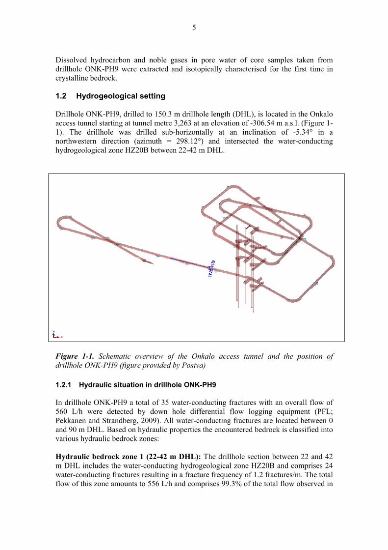
Dissolved hydrocarbon and noble gases in pore water of core samples taken from drillhole ONK-PH9 were extracted and isotopically characterised for the first time in crystalline bedrock. 1.2 Hydrogeological setting Drillhole ONK-PH9, drilled to 150.3 m drillhole length (DHL), is located in the Onkalo access tunnel starting at tunnel metre 3,263 at an elevation of -306.54 m a.s.l. (Figure 1-1). The drillhole was drilled sub-horizontally at an inclination of -5.34° in a northwestern direction (azimuth = 298.12°) and intersected the water-conducting hydrogeological zone HZ20B between 22-42 m DHL.

Figure 1-1. Schematic overview of the Onkalo access tunnel and the position of drillhole ONK-PH9 (figure provided by Posiva) 1.2.1 Hydraulic situation in drillhole ONK-PH9 In drillhole ONK-PH9 a total of 35 water-conducting fractures with an overall flow of 560 L/h were detected by down hole differential flow logging equipment (PFL; Pekkanen and Strandberg, 2009). All water-conducting fractures are located between 0 and 90 m DHL. Based on hydraulic properties the encountered bedrock is classified into various hydraulic bedrock zones: Hydraulic bedrock zone 1 (22-42 m DHL): The drillhole section between 22 and 42 m DHL includes the water-conducting hydrogeological zone HZ20B and comprises 24 water-conducting fractures resulting in a fracture frequency of 1.2 fractures/m. The total flow of this zone amounts to 556 L/h and comprises 99.3% of the total flow observed in

6

drillhole ONK-PH9. The zone can be subdivided in a core zone (28-40 m DHL) asymmetrically surrounded by rim zones (22-28 m and 40-42 m DHL). Water-conducting fractures in the core zone (n=17) have low to high transmissivity (7.1*10-10 - 1.8*10-7 m2/s) with largely variable flow rates between 0.8 and 208 L/h (Figure 1-2). Water-conducting fractures in the surrounding rim zones (n=4 for tunnel facing side, n=3 for tunnel averted side) have low transmissivity (7.7*10-11 - 1.5*10-10 m2/s) with low flow rates between 0.09 and 0.24 L/h (Figure 1-2). Hydraulic bedrock zone 2 (0-22 m DHL, 42-90 m DHL): In the present report the hydraulic bedrock zone 2 has been subdivided into a Zone 2a covering the interval between 0-22 m DHL and Zone 2b between 42-90 m DHL to facilitate comparison of the hydraulic and groundwater data with pore water data. Both zones have similar hydraulic properties and fracture intensity. They are characterised by an intermediate to low frequency of water-conducting fractures with only 2 fractures between 0-22 m DHL (0.09 fractures/m) and 9 fractures between 42-90 m DHL (0.19 fractures/m). The transmissivity of these fractures is low to intermediate (9.7*10-12 – 2.3*10-9) and individual flow rates vary between 0.01 and 2.6 L/h (Figure 1-2). Hydraulic bedrock zone 3 (90-150 m DHL): This zone represents the intact matrix bedrock where flow rates and transmissivities were below the detection limit (i.e. for the transmissivity <10-11 m2/s) and no water conducting fractures could be detected in drillhole ONK-PH9.

7

Figure 1-2. Transmissivity (left) and water flow (right) of water-conducting fractures encountered by drillhole ONK-PH9 as a function of distance from the tunnel wall (PFL-data from Pekkanen and Strandberg, 2009). The subdivision into individual hydraulic zones is based on the dominant hydraulic properties of the drillhole. On the right side the fracture groundwater sampling intervals are shown. 1.2.2 Hydrochemistry of fracture groundwater from drillhole ONK-PH9 Fracture groundwater was sampled and analysed by Posiva from two open intervals during the drilling of drillhole ONK-PH9. The chemical and isotope compositions of the sampled groundwaters are given in Table 1-1. Interval 1 covers the conducting fractures within the drillhole at distances between 0 and 35 m DHL, and Interval 2 those between 37.75 and 150 m DHL (Figure 1-2). Groundwater sampled from Interval 1 comprises 18 water-conducting fractures from the hydraulic zones 1 and 2 with a total flow of 323 L/h. Groundwater sampling from Interval 2 comprises in total 14 water-conducting fractures from the hydraulic zones 1 and 2 with a total flow of 234 L/h.

8

Fracture groundwater from both intervals is of a general Na-Ca-Cl chemical type with SO4-concetrations around 300 mg/L and can thus be classified as brackish SO4 type groundwater according to the Posiva groundwater classification system (Posiva, 2009). Oxygen and stable isotope water ratios are between -10.15 and -10.07‰ V-SMOW for 18O and -76.3‰ V-SMOW for 2H. The Br/Cl mass ratios of fracture groundwater are 3.9 and 4.0, respectively. The slightly elevated Br/Cl mass ratios of the sampled groundwaters compared to marine waters suggest an influence of brackish Cl-type water in these groundwaters. The chemical and isotopic compositions of the sampled fracture groundwaters are typical for Olkiluoto groundwater sampled between 70 and 300 m b.s. (Posiva, 2009). Both groundwaters contain rather high 14C activities and measurable 3H. Whereas the latter suggests the presence of a young (<50 a) component, which might be attributed to drilling fluid contamination, the 14C activities suggest a residence time in the order of a few thousands of years at maximum. Gases dissolved in fracture groundwater of Interval 2 were determined and found to consist mainly of nitrogen, carbon dioxide, methane, helium and argon (Table 1-2). Minor amounts of saturated and unsaturated higher hydrocarbons ( i.e. ethane, ethene and propane) could also be detected (Table 1-2). Table 1-1. Drillhole ONK-PH9: Chemical and isotope composition of fracture groundwater sampled in two intervals (data from Posiva, pers.com. 15.07.2009).

Sample Units PH9-Int 1 PH9-Int 2 Interval m DHL 0-35 37.75-150 pH -log(H+) 7.3 7.3 EC mS/cm 10.48 9.8 CATIONS Sodium (Na+) mg/L 1490.0 1360.0 Potassium (K+) mg/L 7.1 6.6 Magnesium (Mg2+) mg/L 100.0 92.0 Calcium (Ca2+) mg/L 580.0 530.0 Strontium (Sr2+) mg/L 5.9 5.6 Aluminium (Al3+) mg/L n.a. n.a. Silica (Si4+) mg/L 5.6 6.1 ANIONS Fluoride (F-) mg/L 0.7 0.7 Chloride (Cl-) mg/L 3350.0 3060.0 Bromide (Br-) mg/L 13.0 12.2 Sulphate (SO4

2-) mg/L 332.0 290.0 Nitrate (NO3-) mg/L <0.02 <0.02 Alkalinity as HCO3

- mg/L 66.6 106.8 TDS mg/L 5950.9 5470.0 Br*1000/Cl mg/mg 3.9 4.0 ISOTOPES IN GROUNDWATER 13C ‰ PDB -14.03 -10.52 2H ‰ V-SMOW -74.7 -76.3 18O ‰ V-SMOW -10.07 -10.15 37Cl ‰ SMOC n.a. -0.27 3H TU 0.65 1.00 14C pmc 48.9 62.5

9

Table 1-2. Drillhole ONK-PH9: Contents of dissolved gases in fracture groundwater (data provided by Posiva, pers. com. 15.07.2009)

Sample PH9-Int 2 Interval m DHL 37.75-150 Nitrogen (N2) mL/L 47.5 Oxygen (O2) mL/L 0* Carbon dioxide (CO2) mL/L 3.9 Hydrogen (H2) µL/L <2.5 Argon (Ar) mL/L 0.6 Helium (He) mL/L 0.6 Methane (CH4) mL/L 0.7 Ethane (C2H6) µL/L 1.9 Ethene (C2H4) µL/L 0.1 Ethine (C2H2) µL/L <0.05 Propane (C3H8) µL/L 0.1 Propene (C3H6) µL/L <0.08 C1/(C2+C3) 368.4

*measured oxygen induced by air contamination and used as a correction factor

10

11

2 MATERIALS AND METHODS 2.1 Sampling 2.1.1 Samples for matrix pore water investigations A total of 35 drillcore samples were collected from drillhole ONK-PH9 for matrix pore water investigations between the 18th and 20th of November 2008. Eleven samples originated from hydraulic bedrock zone 1 (30 – 42 m DHL), one sample from the drillhole section between the tunnel and the water-conducting hydrogeological zone HZ20B (hydraulic zone 2a), 18 samples along a continuous profile following hydraulic zone 1 (hydraulic zone 2b, 42.6 - 52.6 m DHL), and 5 samples at larger intervals of between 5 and 10 m taken at greater distances along the drillhole (hydraulic zone 2b and 3, 57 – 97 m DHL). Immediately after recovery of the drillcore from the drillhole, the cores were photographed, wiped clean with a damp cloth and packed into a PVC bag, flushed with nitrogen and subsequently evacuated and sealed. The same procedure was repeated for a second PVC bag and finally with a bag of plastic coated Al-foil. This triple sealing approach was designed to minimise the evaporation of pore water, which would result in a reduction of the water content and thus a deviation of the calculated pore-water concentrations from those present under in situ conditions. Before the samples were prepared for the different experiments, they were stored in a refrigerator at 4 °C. All samples prepared for pore water investigations, including their depth along drillhole and sample length, are listed in Table 2-1.

12

Table 2-1. Drillhole ONK-PH9: List of samples used for pore water investigations.

Sample No Hydraulic bedrock section Drillhole length

Average Drillhole length

Core Sample length

m m m

PH9-1 Hydraulic bedrock zone 2a

18.97 - 19.47 19.22 0.50

PH9-2

Hyd

raul

ic b

edro

ck z

one

1

30.50 - 30.74 30.62 0.24

PH9-3 32.51 - 32.86 32.69 0.35

PH9-4 33.08 - 33.48 33.28 0.40

PH9-5 33.65 - 34.05 33.85 0.40

PH9-6 34.29 - 34.55 34.42 0.26

PH9-7 35.12 - 35.49 35.31 0.37

PH9-8 35.96 - 36.26 36.11 0.30

PH9-9 36.74 - 37.00 36.87 0.26

PH9-10 37.75 - 38.00 37.88 0.25

PH9-11 40.88 - 41.13 41.01 0.25

PH9-12 41.85 - 42.17 42.01 0.32

PH9-13

Hyd

raul

ic b

edro

ck z

one

2b

42.43 - 42.75 42.59 0.32

PH9-14 42.75 - 43.15 42.95 0.40

PH9-15 43.15 - 43.55 43.35 0.40

PH9-16 43.62 - 43.82 43.72 0.20

PH9-17 44.32 - 44.63 44.48 0.31

PH9-18 45.09 - 45.40 45.25 0.31

PH9-19 45.50 - 45.96 45.73 0.46

PH9-20 45.96 - 46.26 46.11 0.30

PH9-21 46.26 - 46.58 46.42 0.32

PH9-22 46.58 - 47.01 46.80 0.43

PH9-23 47.30 - 47.68 47.49 0.38

PH9-24 47.68 - 48.17 47.93 0.49

PH9-25 48.17 - 48.58 48.38 0.41

PH9-26 49.11 - 49.63 49.37 0.52

PH9-27 50.05 - 50.35 50.20 0.30

PH9-28 50.99 - 51.45 51.22 0.46

PH9-29 51.79 - 52.27 52.03 0.48

PH9-30 52.42 - 52.68 52.55 0.26

PH9-31 56.92 - 57.37 57.15 0.45

PH9-32 69.42 - 69.94 69.68 0.52

PH9-33 77.84 - 78.37 78.11 0.53

PH9-34 87.18 - 87.48 87.33 0.30

PH9-35 Hydraulic bedrock zone 3

97.03 - 97.49 97.26 0.46

13

2.1.2 Samples for reactive dissolved gas and noble gas investigations From drillhole ONK-PH9 drillcore samples were also taken for investigations of the dissolved reactive gases (12 samples) and noble gases (15 samples) in the pore water (Table 2-2). For these samples core sections of adequate length were broken by hand immediately after drillcore recovery and wiped clean with a CuSO4 impregnated towel, to avoid induced bacterial activity during the outgassing experiment. Subsequently, the cores were weighed and placed into stainless steel cylinders. The cylinders were then sealed and repeatedly flushed either with high purity He gas for dissolved gas extraction or high purity N2 gas for noble gas extraction. Finally, the cylinders were placed under vacuum and stored at constant room temperature. Records were taken of the time of exposure of the core sample, the flushing and final sealing of the cylinder, and the final pressure of the sample cylinder (Table 2-2).

14

Table 2-2. Drillhole ONK-PH9: List of samples used for dissolved reactive gas and noble gas investigations including sampling data.

Sample No Drillhole length

Average Drillhole length

Core Sample length

Exposure time

Flushing time* Final pressure

m m m min min mbar

Reactive gas samples

PH9-HC1 18.20 - 18.30 18.25 0.10 8 1:20/0:40/1:10 0.8

PH9-HC2 34.05 - 34.15 34.10 0.10 12 2:00/1:00/1:30 1.6

PH9-HC3 37.00 - 37.10 37.05 0.10 15 2:30/2:00/2:00 1.9

PH9-HC4 42.35 - 42.43 42.39 0.08 20 2:00/2:00/1:20 0.6

PH9-HC5 47.18 - 47.27 47.23 0.09 20 2:00/2:00/1:00 0.7

PH9-HC6 48.60 - 48.68 48.64 0.08 12 2:00/1:30/2:00 0.4

PH9-HC7 51.45 - 51.51 51.48 0.06 13 2:00/2:00/1:45 0.5

PH9-HC8 56.83 - 56.92 56.88 0.09 16 2:00/2:00/2:00 0.4

PH9-HC9 69.94 - 70.03 69.99 0.09 13 2:00/2:00/2:00 0.2

PH9-HC10 78.66 - 78.75 78.71 0.09 10 2:00/2:10/2:00 0.3

PH9-HC11 87.48 - 87.58 87.53 0.10 11 1:50/1:30/1:30 0.4

PH9-HC12 97.59 - 97.67 97.63 0.08 20 1:30/1:30/1:30 0.3

Noble gas samples

PH9-NG1 18.62 - 18.72 18.67 0.10 8 1:10/0:30/0:30 1.0

PH9-NG2 33.00 - 33.08 33.04 0.08 3 2:00/1:00/0:30 1.2

PH9-NG3 35.49 - 35.58 35.54 0.09 5 2:00/0:45/0:30 1.4

PH9-NG4 37.22 - 37.31 37.27 0.09 10 1:20/0:45/0:30 1.4

PH9-NG5 42.28 - 42.35 42.32 0.07 3 2:00/1:00/0:30 1.1

PH9-NG6 43.55 - 43.62 43.59 0.07 4 1:30/1:00/0:30 1.0

PH9-NG7 45.00 - 45.09 45.05 0.09 5 1:00/1:00/0:30 0.3

PH9-NG8 47.12 - 47.18 47.15 0.06 10 1:00/1:00/0:30 1.1

PH9-NG9 48.68 - 48.76 48.72 0.08 3 1:30/1:00/0:30 1.2

PH9-NG10 51.51 - 51.59 51.55 0.08 3 1:30/1:00/0:30 1.1

PH9-NG11 56.74 - 56.83 56.79 0.09 5 1:30/1:00/0:30 0.9

PH9-NG12 70.13 - 70.22 70.18 0.09 6 1:30/0:30/0:30 0.4

PH9-NG13 78.75 - 78.85 78.80 0.10 5 1:30/1:00/0:30 0.7

PH9-NG14 87.05 - 87.15 87.10 0.10 7 1:30/1:00/0:30 0.7

PH9-NG15 97.77 - 97.87 97.82 0.10 5 1:30/1:00/0:45 1.4

* every sample was flushed and evacuated twice before final evacuation 2.2 Experimental set-ups and analytical methods Unless otherwise specified, the analytical work has been conducted at the RWI laboratories, Institute of Geological Sciences, University of Bern, Switzerland.

15

2.2.1 Petrological and mineralogical investigations Mineralogical investigations were performed on rock material of four samples representing the dominant lithologies in drillhole OL-KR47, and included transmitted and reflected light microscopy of thin sections. Mineralogical modal compositions were determined by point counting (1,000 points, grid spacing x and y = 0.8 mm). 2.2.2 Fluid inclusion investigations Microthermometry and Raman microspectroscopy Fluid inclusion petrography and microthermometry investigations were conducted using a Linkham THMSG-600 heating-cooling stage with a Linkham TMS 91 temperature control on an Olympus BX51 microscope equipped with a 100/0.80 LM PlanFI objective lens. Laser Raman microspectroscopy was performed using a Jobin Yvon LabRam HR 800 confocal-laser Raman microprobe with a frequency-doubled Nd-YAG laser. The Raman microprobe is equipped with an Olympus BX41 microscope with an Olympus 100/0.95 UM PlanFI objective lens, and a Linkham MDS-600 heating-cooling stage with a Linkham TMS 94 temperature. Measurement conditions consisted of a laser beam at 532.12 nm, an aperture of 400m, a slit of 100m, and variable accumulation times. Quartz separation and characterisation of gases in fluid inclusions To liberate the fluid inclusion gas it was necessary to first disaggregate the drillcore samples into their component minerals. The preferred mineral to be crushed for gas analyses is quartz, which contains the highest amount of fluid inclusions. Disaggregation of the rock further ensures that no matrix pore water components influence the analyses. To disaggregate the samples a selective fragmentation device (selFragTM) was applied. This method is based on very short pulsed high voltage discharges applied to solids emerged in water. The pulses produce high pressure waves which propagate along grain boundaries and disaggregate the rock sample. To check that the selFragTM method does not have any influence on fluid inclusion properties, Raman and microthermometric analyses were conducted before and after the selFragTM treatment. These tests revealed no differences. Once the samples were disaggregated the quartz grains were hand picked under a binocular microscope. An advantage of the selFragTM method is that single mineral grains are liberated intact and much fewer unwanted fines are produced than with common grinding methods. To liberate the fluid inclusion gas, the hand picked quartz samples were crushed in an evacuated piston-cylinder device. An induction coil is used to drive the piston against the upper end of the cylinder, compressing a strong spring. Subsequent expansion of the spring hurls the piston downwards, where its conical nose crushes the sample. Numerous impacts are required to achieve complete crushing to a fine powder. A maximum of 5 g of quartz was placed in the piston device and during the crushing the sample was held at 150 °C with two cartridge heaters to avoid sorption of gas on the freshly broken quartz surfaces. For qualitative and quantitative gas analyses the crusher was directly connected to a Shimadzu GC 17A device, equipped with 2 capillary columns (Column 1: Chrompack

16

Plot Molecular Sieve 5 A; Column 2: Chrompack CP-PoraBond Q) and two micro-volume thermal conductivity detectors (VICI Instruments Inc.) and one flame-ionisation detector. The gas chromatograph was calibrated with control standards before each block of measurements was conducted. For the analyses of the stable isotopes of the liberated gases by direct mass spectrometry the crushing device was attached directly to the gas separation line where the hydrocarbons were oxidised to CO2 on which 13C is measured. Carbon dioxide liberated from the fluid inclusions was trapped together with H2O vapour in a liquid N2 trap. The concentrated CO2 was then measured on its 13C signal. The gas samples were analysed using an isotope-ratio mass spectrometer (MAT-251, Fa. MAT, Bremen) equipped with a direct-inlet technique (dual inlet). For GC-IRMS measurements following crushing, the crusher was filled with He carrier gas until a pressure of > 1 atm was reached. The line consisted of a purge and trap PTA-3000 device (Fa. IMT Germany), a gas chromatography GC 3400 device (Varian, Bremen), a separation column type PoraPlot U (Altmann Analysentechnik GmbH, Holzkirchen) with helium as the carrier phase (2.4 mL/min), and an isotope ratio mass spectrometer (IRMS) delta S (Finnigan MAT). The ChromStar software (BRUKER-FRANZEN Analytik GmbH, Bremen) was used to evaluate the signals. The instrumental error of 13C in CH4 and CO2 is 0.3‰. Owing to the low amounts of gas it is not yet clear how large the total uncertainty of the measurements is. It is assumed that it is between 2–3‰. To determine the 2H ratio of hydrocarbons, H2O produced during the hydrocarbon oxidation was trapped in a liquid N2 trap. Several crushing runs were necessary to yield sufficient H2O. The concentrated water was subsequently allowed to react to H2 using Mn (H2O + Mn H2 + MnO). Following this, the produced hydrogen was analysed by GC-IRMS (Delta E, Finnigan MAT). The analytical uncertainty was determined by multiple measurements of the international gas standard NBS 22 and is ~ 5‰. All the gas chromatography and mass spectrometry investigations were conducted at Hydroisotop GmbH, Germany.

2.2.3 Water content and water-loss (connected) porosity The water content was determined on core material used for the diffusive isotope exchange technique, the large sized cores used in out-diffusion experiments and the core pieces used for the gas equlibration experiments. The sample material used in these experiments remained saturated throughout the experiments (see section 4). The degree of sample saturation upon arrival of the samples in the laboratory was estimated by comparing the weights of the large sized samples (600 to 1,000 g) used in the out-diffusion experiments before and after the experiment. The drillcore pieces were placed in a crystallisation dish, weighed and subsequently dried at 105°C until stable weight conditions were achieved. Before taking the initial wet weight of the core pieces, the surface was allowed to dry until stable weight was

17

achieved for ~10 sec to minimise the influence of surface water on the water content (Eichinger, 2009). Subsequently, weighing was carried out weekly until the sample weight remained constant (±0.002 g) for at least 14 days. Drying times of the large size samples were between 108 and 254 days. The calculation of the water-loss (i.e. connected) porosity from the gravimetric water content requires a measure of the grain density. In rocks of low porosity the bulk wet density can be used as a proxi for the grain density. A measure for the bulk wet density of the rocks investigated was obtained from volume and saturated mass of the core samples used for out-diffusion experiments. The volume was calculated from measurements of height and diameter of the core samples using a vernier calliper with an error of ± 0.01 mm. Variations in the core diameter over the lengths of the samples was found to be less than 0.05 mm for most samples and a constant diameter was used in the calculation of the volume. For the derived bulk wet density this results in an error of less than 5% for fully intact cores. The water-loss (connected) porosity, WL, is then calculated according to

(2-1)

where, WCwet is the water content based on the wet weight of the rock sample and bulk,,

wet the bulk wet density of the rock. The density of water, water, is assumed to be 1 g/cm3 because the highest Cl concentrations in the pore water are only about two thirds of that of ocean seawater (cf. chapter 7).

2.2.4 Matrix pore water extraction methods In the laboratory, the samples were unpacked and immediately wrapped in parafilm to prevent evaporation of pore water during subsequent dry sawing into full-diameter cylinders of variable length. After sawing, the surfaces of the obtained pieces were cleaned with paper towels and again wrapped in parafilm. The entire sample preparation was conducted as rapidly as possible (within 20 minutes) after opening the sealed bags in order to minimise evaporation. The different experimental set-ups and the analytical programme performed on the individual rock samples and experiment solutions are given in Table 2-3.

Diffusive isotope exchange technique

The diffusive isotope exchange technique applied to determine the water isotope composition, 18O and 2H, of the pore water and the mass of pore water was originally developed by Rogge (1997) and Rübel et al. (2002) for sedimentary rocks and later adapted for crystalline rocks by Waber and Smellie (2005, 2006) and Eichinger et al. (2006). In this method pieces of the core samples are placed into two vapour-tight containers together with different test waters of known isotope composition. The test water (2 mL) was placed in a Petri dish in the centre of a glass vessel and surrounded by hand crushed core pieces of about 4-6 cm3 in size. The pore water and test water are

WL WCwet *bulk,wet

water

18

then allowed to isotopically equilibrate via the vapour phase without any direct contact between the core material and the test water for 60 days. After complete equilibration the two test waters were removed and analysed by conventional ion-ratio mass spectrometry at Hydroisotop GmbH, Germany. The results are reported relative to the V-SMOW standard with a precision of 0.15 for 18O and 1.5‰ for 2H. The test water as well as the core material was weighed before and after the experiment to test for possible loss of test water on the container walls and/or rock material due to unwanted evaporation and/or condensation. To minimise condensation, about 0.3 mol of NaCl are dissolved in the test water to lower its water vapour pressure. For every sample two experiments were performed, one using a test water with an isotope composition close to that expected in the pore water ("LAB"-sample), and one using a test water with an isotope composition far from that expected for the pore water ("SSI"-sample). The test water used for the LAB-sample was normal laboratory tap water (18O = -11.44‰ V-SMOW; 2H = -81.4‰ VSMOW), while that for the SSI sample was water from an ice core drilled in Greenland (18O = -24.60‰ V-SMOW; 2H = -187.1‰ V-SMOW). The equilibration time in the three reservoirs, i.e.rock pore water, test water and the air inside the container as a diaphragm, depends on the volume of the container, the size of the rock pieces and the distance of the rock pieces to the test water (see Rogge 1997). If successful, the diffusive isotope exchange technique delivers the 18O and 2H ratios and the mass of the pore water present in the connected pore space of the rock sample. These parameters are calculated from the analytical results obtained for the two test water solutions using mass-balance relationships according to

mpw * c pw t 0mtw * ctw t 0 (mpw mtw ) * ctw t (2-4)

where m = mass, c = isotope concentration, pw = pore water, tw = test water; t = 0 means the isotope concentrations at the beginning, and t = at the end of the experiment. The water content of the applied samples is calculated by transformation of equation 2-4 to

mPW mTW (Std 2) (CTW(Std 2) CTW (Std 2)) mTW (Std1) (CTW (Std1) CTW(Std1))

(CTW(Std1) CTW(Std 2)) (2-5)

where Std 1 = test solution 1 and Std 2 = test solution 2. Equation 2-5 can be set up for the 18O and 2H concentration of the test water, resulting in two independent values for the mass of pore water. The stable isotope ratios are calculated by transformation of equation 2-4 to

19

CPW CTW(Std1) mTW (Std 2) (CTW(Std 2) CTW (Std 2))CTW(Std 2) mTW (Std1) (CTW (Std1) CTW(Std1))

mTW (Std 2) (CTW(Std 2) CTW (Std 2)) mTW (Std1) (CTW (Std1) CTW(Std1))

(2-6). The errors of the calculated 18O, 2H and mass of the pore water are computed for each sample using Gauss’ law of error propagation (see Appendix VII for details). Out-diffusion experiments

Out-diffusion experiments were performed on intact core samples of about 12 or 19 cm in length and about 5 cm in diameter by immersing them in ultrapure water. The volume of test water varied between 77 and 119 mL. During the experiments the two water reservoirs, i.e. pore water and test water, tend to equilibrate until steady state is achieved. After placing the core sample in the PE-vessel, the vessel was sealed and put in a shaking water bath (40 rpm) at a constant temperature of 45°C to accelerate the diffusion processes. The PE vessels were covered by a vapour-tight lid which is equipped with two swagelockTM valves and PEEKTM sampling lines. To avoid undesired bacterial activity during the experiments 0.1 mL of chloroform was added to the test water. The core, the experiment container, and the test water were weighed before and after the experiment to ensure that no loss of test water occurred during the entire experiment. At specific time intervals of initially a few days and later a few weeks, 0.5 mL of solution were sampled using a PVC-syringe to determine the chloride concentration as a function of time. Based on the experience from previous drillings, the two reservoirs were allowed to equilibrate for 195 days. After equilibrium with respect to chloride was achieved, the vessels were removed from the water bath and cooled to room temperature. Subsequently, the core was weighed and the supernatant solution was analysed immediately for pH and total alkalinity and later also for major cation and anion concentrations. The chloride contents of the 0.5 mL time-series samples from the out-diffusion experiments, and the major cations (Na, K, Ca, Mg, Sr) and anions (F, NO3, SO4) of the final test solutions were analysed by ion chromatography using a Metrohm IC 861 Advanced Compact IC system with a 10L injection loop. The analytical error of these analyses is ±5% based on multiple measurements of the standard solutions. The alkalinity titration and pH measurements were performed using a Metrohm Titrino DMP 785 instrument. Bromide concentrations of the out-diffusion test solutions were determined by ICP-MS using an Agilent 7500 ICP-MS operated in normal gas mode at the British Geological Survey. The analytical error of these analyses is 15 % based on multiple measurements of standard solutions. Silicon was determined by colorimetric methods and aluminium by atomic absorption spectroscopy using a Varian Spectra 300 AAS; both methods have an analytical uncertainty of 5%. Because no ultracentrifugation was applied to the solutions before measurement, some interference with colloidal Si and Al cannot be excluded and the overall error is probably larger than the analytical uncertainty. The 37Cl/35Cl isotopic ratio, expressed as 37Cl relative to SMOC, was measured at the University of Waterloo Environmental Isotope Laboratory (EIL) in Canada using a VG

20

SIRA 9 mass spectrometer. Analytical errors were determined by multiple measurements of the samples. Chloride and bromide concentrations of the experiment solution can be converted to pore water concentrations by applying mass balance calculations. A prerequisite therefore is that steady-state conditions between test water and pore water are achieved. With the knowledge of the mass of pore water in the rock sample, the chloride concentration of the pore water can be calculated according to:

Cpw

(mpw mTWi ms)*CTW (mTWi *CTWi) ms *Cs

n

n

mpw

(2-7)

where Cpw = pore water concentration; mpw = mass of pore water,; mTWi = initial mass of test water ; CTWi = initial Cl-concentration of test water; CTW∞ = equilibrium concentration at the end of the experiment, ms = mass of sub sample used for time series; Cs = Cl concentration of sub sample used for time series.

The last term ms * Cs

n

in equation 2-7 describes the amount of Cl removed from the

initial experiment solution for Cl time-series samples. A correction for chloride in the initial experiment solution (mTWi*CTWi) is necessary if this solution is not entirely free of chloride. The unit for the pore water concentration is given as mg/kgH2O (and not mg/L) because it is derived on a mass basis rather than a volumetric basis. This is because the density of the pore water is not known beforehand. For the present samples, however, the difference between mg/kgH2O and mg/L is negligible at the expected ionic strength and total mineralisation of the pore water. The errors of the calculated p���water chloride and bromide concentrations are computed for each sample using Gauss’ law of error propagation (see Appendix VII for details).

21

Tab

le 2

-3. D

rill

hole

ON

K-P

H9:

Por

e w

ater

exp

erim

ents

and

ana

lyse

s pe

rfor

med

on

dril

lcor

e sa

mpl

es a

nd e

xper

imen

t sol

utio

ns.

Sam

ple

P

etro

ph

ysic

al

and

p

etro

logi

cal

inve

stig

atio

ns

Dif

fusi

ve I

soto

pe

Exc

han

ge

tech

niq

ue

Ou

t-d

iffu

sion

Exp

erim

ents

G

ravi

met

ric

wat

er c

onte

nt/

P

oros

ity

Min

eral

ogy,

F

luid

In

clu

sion

s

Exp

erim

enta

l se

t-u

p

18O

, 2 H

E

xper

imen

tal

set-

up

p

H

and

A

lkal

init

y A

nio

ns

and

C

atio

ns

37C

lB

r/C

l ra

tio

Ch

lori

de

tim

e se

ries

P

H9-

1 X

X

X

X

X

X

X

X

P

H9-

2 X

X

X

X

X

X

P

H9-

3 X

X

X

X

X

X

X

X

P

H9-

4 X

X

X

X

X

X

P

H9-

5 X

X

X

X

P

H9-

6 X

X

X

X

X

X

P

H9-

7 X

X

X

X

X

X

P

H9-

8 X

X

X

X

X

X

P

H9-

9 X

X

X

X

P

H9-

10

X

X

X

X

X

X

PH

9-11

X

X

X

X

X

X

X

X

X

X

P

H9-

12

X

X

X

X

X

X

X

X

X

P

H9-

13

X

X

X

X

X

X

X

X

X

P

H9-

14

X

X

X

X

X

X

X

X

PH

9-15

X

X

X

X

X

X

X

X

X

PH

9-16

X

X

X

X

X

X

P

H9-

17

X

X

X

X

X

X

X

X

PH

9-18

X

X

X

X

X

X

X

PH

9-19

X

X

X

X

X

X

X

X

X

PH

9-20

X

X

X

X

X

X

X

PH

9-21

X

X

X

X

X

X

P

H9-

22

X

X

X

X

X

X

X

X

X

P

H9-

23

X

X

X

X

X

X

PH

9-24

X

X

X

X

X

X

P

H9-

25

X

X

X

X

X

X

PH

9-26

X

X

X

X

X

X

XX

X

X

X

X

X

PH

9-27

X

X

X

X

X

X

X

X

P

H9-

28

X

X

X

X

X

X

X

X

PH

9-29

X

X

X

X

X

X

X

X

P

H9-

30

X

X

X

X

X

X

X

X

X

P

H9-

31

X

X

X

X

X

X

X

X

PH

9-32

X

X

X

X

X

X

X

X

P

H9-

33

X

X

X

X

X

X

X

X

PH

9-34

X

X

X

X

X

X

X

X

P

H9-

35

X

X

X

X

X

X

X

X

X

X

21

22

2.2.5 Reactive dissolved gases in matrix pore water Gases dissolved in the matrix pore water were allowed to outgas into the vacuum that was applied to the gas tight cylinder during sampling over a time period of 250 days at room temperature. Reactive gases include gases such as oxygen, nitrogen and carbon dioxide and saturated and unsaturated hydrocarbons. These were analysed at Hydroisotop GmbH, Germany. The experimental set-up and the analytical gas programme performed on the core samples is given in Table 2-4. Qualification and quantification of extracted gases Prior to the gas analysis, the cylinders were cooled to 0°C to minimise the water vapour pressure in the cylinder. Afterwards, the cylinder was plugged directly on the gas chromatograph, the attached clamped Cu-tube was opened and the total gas pressure in the cylinder was measured by a connected pressure gauge with a determination range between 0.1 and 1,100 mbar. The total gas pressures in the cylinders varied between 26 and 594 mbar. The gas composition was then analysed by a Shimadzu GC 17A gas chromatograph, equipped with a GC-WLD detector for the detection of gaseous O2, N2, and CO2 and a GC-FID detector for the detection of saturated and unsaturated hydrocarbon gases (C1-C4). The gas chromatograph was calibrated with control standards before each group of measurements was conducted. The detection limits of these methods vary for the different gas species and are listed in Appendix IV. The errors of the gas analyses are given by the standard deviation of multiple (10 times) analyses of a test gas of known composition. To calculate the exact volume of the liberated gas mixture and a single gas phase, the void volume in the gas cylinder had to be determined, i.e. the sum of the cylinder volume and the Cu-tube volume minus the volume of the rock sample. All cylinders have a constant volume of 360 mL and the Cu-tubes a constant radius of 0.4 cm and a length between 6 and 15 cm. Because of the uneven shapes of the used drillcore fragments, the volume of the cores could not be determined as described in chapter 2.2.2. Therefore, the volumes were determined after Hübschmann and Links (1987) and calculated according to:

Vrock mrockair

mrockwater

water

(2-8)

where Vrock is the volume of the core sample, mrock,air the mass of the core sample under atmospheric conditions, mrock,water the mass of the core sample emerged in deionised water, and water the density of the water at a certain temperature (0.998 g/cm3 at 21°C; Vogel, 1974). Based on the measured oxygen concentrations of the gases, the determined N2, CO2 and CH4 concentrations of the extracted gases were subsequently corrected for a possible contamination by air. Concentrations of higher hydrocarbons in air are very low and even greater air contamination would not alter the concentrations measured for a pore water sample. A correction for the higher hydrocarbon gases was thus not required. The gas composition of atmospheric air, used for the corrections, is given in Appendix III.

23

The original gas concentration (corrected for air contamination) is calculated according to

CX ,Sample,corrected CX ,Sample,measured CO2 ,Sample,measured * CX ,air

CO2 ,air

(2-9),

where CX is the concentration of a gas species X in vpm and CO2 is the concentration of oxygen in vpm. The proportion of the single gas species of the total extracted gas volume is calculated according to:

VX CX

Vgas,tot

with Vgas,tot Pgas *VVoid (2-10),

where Vx is the volume of a certain gas species X in mL, Cx the concentration of the gas species X in % of the total amount of gas, Vgas,tot the total volume of the extracted gas in mL, Pgas the final gas pressure in the cylinder in mbar and Vvoid the void volume in the cylinder in ml. The final gas pressure measured in the cylinder after equilibration is a mixture of the gases liberated from the pore water and the water vapour pressure at a certain temperature. Therefore the measured final pressures were corrected according to PWV 5.268721 0.663623 * T 0.002364 * T 2 0.000716 * T 3 (2-11) where PWV is the water vapour pressure at a certain temperature T in mbar (Lide, 1994). Finally, the gas contents of the single gas species dissolved in matrix pore water is calculated according to:

CX ,PW VX

VPW

*1000 (2-12),

where Cx,PW is the gas concentration of a gas species X dissolved in pore water in mlgas/LPW, VX the volume of a certain gas species X in mlgas and VPW the volume of pore water in the used drillcore segment in mlH2O. The amount of pore water was determined gravimetrically by drying as described in section 2.2.2. All given gas concentrations are related to standard temperature and pressure conditions (STP = 0°C, 1.013 bar). Stable isotope analyses on reactive gases Carbon stable isotope ratios of CH4 and CO2 could be determined on seven samples and stable isotope ratios of N2 on three gas samples. Due to the low pore water content of the rocks and consequently low amounts of gas available, it was not possible to quantify carbon stable isotope ratios of higher hydrocarbons and hydrogen isotope ratios on methane and higher hydrocarbons.

24

For the gas isotope analyses the gas cylinders were filled with He as a carrier gas to a pressure of 1.5 to 2 bars. Before an aliquot of the gas was transferred to gas tight GC-IRMS glass vials, the gas mixture was allowed to equilibrate for about an hour under increased temperature. Afterwards, the carbon isotope ratios of CH4 and CO2 were determined by a Varian MAT-250 GC-IRMS which is equipped with a direct dual inlet system, and the results are reported relative to the PDB standard. The instrumental error of 13C in CH4 and CO2 is 0.3‰. Owing to the low gas amounts, analytical errors of 5‰ for 13C-CH4 and 2‰ for 13C-CO2 were estimated. An aliquot of six samples were sent to the institute of biogeochemistry and marine chemistry (University of Hamburg) for the determination of hydrogen isotopes on CH4. Due to the low methane concentrations in the extracted gases hydrogen isotope ratios of methane could not be analysed. Nitrogen isotope ratios of extracted gases are analysed by a Varian MAT-250 GC-IRMS. Prior to the analyses other gases are eliminated by oxidative combustion at 950 °C. The results are reported as 15N relative to atmospheric nitrogen and the error of these measurements is given by the standard deviations of 10-fold measurements of a standard gas. 2.2.6 Noble gases in matrix pore water Noble gases dissolved in matrix pore water of the drillcore samples were allowed to outgas into the vacuum that was applied to the gas tight cylinder during sampling over a time period of 340 days at room temperature. The analytical programme performed on the individual rock samples is given in Table 2-4. All noble gas analyses were conducted at the Institute of Environmental Physics, University of Heidelberg, Germany. The concentrations of the noble gas isotopes 3He, 4He, 20Ne, 22Ne, 36Ar and 40Ar in the gas mixture were measured by a GV 5400He Noble Gas Mass Spectrometer. The analytical errors of the single noble gases were determined by multiple measurements of atmospheric air. The volume of an individual noble gas species in mL/L was calculated according to equations 2-8, 2-10 and 2-12. The degree of air contamination of the extracted gas was monitored by the measured neon content (=20Ne+22Ne). As outlined in chapter 9 there is negligible in situ production of 20Ne and 22Ne even over a geological time span of more than 1 Ga. Consequently, the Ne isotope concentrations in matrix pore water cannot exceed that of the air saturated water, i.e. the concentrations brought into the system by surface-derived water. The time of such infiltration is unknown and could have taken place under different climatic conditions. To account for the temperature dependent solubility of Ne, the Ne content in air saturated water was taken as a range ([Ne]asw = (1.9 ± 0.2)*10-7 cc STP Ne/gH2O, Weiss, 1971) corresponding to an infiltration temperature between 5 and 25°C. An air contamination is present in the gas samples once the measured total Ne (20Ne+22Ne +22Ne) content in the gas sample exceeds that range. The excess of the single noble gas species (C(X)ex), introduced to the gas samples by air contamination is calculated using the measured Ne isotope contents, the Ne/C(X) ratio in air and the range of Ne ([Ne]asw) during infiltration according to

25

C(X)ex CNetot

1.9*107 CNeair

C(X)air

(2-13)

where C(X)ex is the excess of the single noble gas species, CNeair in cc/ccgas the concentration of Ne in air in cc/ccair and C(X)air the concentration of the single noble gas species in air in cc/ccgas. Helium and argon were extracted from the rock samples by fusion in Mo crucibles at a temperature of 1,600 °C in a double vacuum furnace (cf. Tolstikhin et al. 1996). The extracted gases were allowed to enter an all-metal line where they were purified using Ti-Zr getters. The abundances of He and Ar isotopes were measured using a static mass spectrometer (MI 1201) with a resolving power of ~1,000 that allows complete separation of 3He+ from H3

+ and HD+ (Kamensky et al. 1984). The sensitivity for He was 510-5 A torr-1 which allowed measuring 4He/3He ratios up to ~108. The sensitivity for Ar was 310-4 A torr-1. A mixture of pure 3He, helium from a high-pressure tank with a 4He/3He of 5107, and air Ne, Ar, Kr and Xe in atmospheric proportion was used as a standard for the calibration of the mass spectrometer. In this mixture the ratios of 4He/3He = 6.29105 and 4He/20Ne = 47 were measured and verified at CRPG (Nancy) using air as the primary standard. The concentrations were determined by the peak-height method with an uncertainty of 5% (1). The uncertainties in the 4He/3He ratios in the order of 106 and 108 were 2% and 20%, respectively, and the uncertainties in the 40Ar/36Ar ratios of 300 and 50,000 were 0.3% and 25%, respectively. The analytical blanks were within 110-9 and 110-10 ccSTP for 4He and 36Ar, respectively. The concentrations of U and Th on whole rock and mineral separates were measured by X-radiographic techniques in Neva Expedition, St. Petersburg, Russia. The lowest measurable concentration is about 0.5 ppm. Potassium and Li were determined by spectrophotometric techniques after acid digestion and dissolution in distilled water in the Geological Institute, Apatity. The reproducibility of the analyses of these four elements was within 10%.

26

Tab

le 2

-4. D

rill

hole

ON

K-P

H9:

Dis

solv

ed g

as e

xper

imen

ts a

nd a

naly

ses

perf

orm

ed o

n dr

illc

ore

sam

ples

and

ext

ract

ed g

ases

.

Q

uant

ific

atio

n of

gas

es

Isot

opes

of

diss

olve

d ga

ses

Isot

opes

of

nobl

e ga

ses

Sam

ple

Gra

vim

etri

c w

ater

co

nten

t

Vol

ume

of

core

sa

mpl

es

O2,

N2,

C

O2

H

ydro

-ca

rbon

s N

oble

ga

ses

13C

-CH

4 13

C-C

2H6

13C

-CO

2 15

N-N

2 2 H

-CH

4 3 H

e, 4 H

e 40

Ar,

36A

r 20

Ne,

22N

e

PH

9-H

C1

X

X

X

X

P

H9-

HC

2 X

X

X

X

PH

9-H

C3

X

X

P

H9-

HC

4 X

X

X

X

PH

9-H

C5

X

X

P

H9-

HC

6 X

X

PH

9-H

C7

X

X

X

X

X

X

X

PH

9-H

C8

X

X

P

H9-

HC

9 X

X

X

X

X

X

X

P

H9-

HC

10

X

X

X

X

P

H9-

HC

11

X

X

X

X

P

H9-

HC

12

X

X

X

X

P

H9-

NG

1 X

X

PH

9-N

G2

X

X

X

X

X

X

X

X

P

H9-

NG

3 X

X

PH

9-N

G4

X

X

X

X

X

X

P

H9-

NG

5 X

X

X

X

X

X

X

X

X

X

PH

9-N

G6

X

X

P

H9-

NG

7 X

X

X

X

X

X

X

X

X

P

H9-

NG

8 X

X

PH

9-N

G9

X

X

X

X

X

X

X

X

X

X

X

PH

9-N

G10

X

X

PH

9-N

G11

X

X

PH

9-N

G12

X

X

PH

9-N

G13

X

X

PH

9-N

G14

X

X

X

X

X

X

X

X

X

X

X

X

PH

9-N

G15

X

X

26

27

3 PETROGRAPHY AND MINERALOGY The interpretation of pore water derived by indirect methods using rock material requires knowledge about the rock composition and the physical properties of the rock. For a specific lithology such information about the mineralogical and the fluid inclusion composition can be transferred from one sample to another without losing accuracy in the interpretation of pore water data. The drillcore of drillhole ONK-PH9 consists mainly of diatexitic gneiss (about 39%), veined gneiss (~30%) and pegmatitic granite (~21%). Other lithologies (~10%) include K-feldspar porphyry, tonalite-granodiorite-granite (TGG-gneiss), mica gneiss and quartz gneiss. The majority of the 35 samples collected for the pore water investigations consist of pegmatitic granite (n=20), diatexitic gneiss (n=8) and veined gneiss (n=2) and five samples cover the minor lithologies such as mica gneiss (n=4) and K-feldspar porphyry (n=1; Table 3-1). The core samples show variable degrees of alteration along the profile. Macroscopically, a high degree of alteration could be observed on core samples taken between 32.7 and 42.6 m DHL and between 48.4 and 52.6 m DHL (Table 3-1). These rocks are characterised by pinkish to red coloured K-feldspars and the occurrence of illite clusters. Several core samples are cut by open fractures (Table 3-1). Along these open fractures a greenish colouring of feldspars could be observed, indicating a fracture controlled saussuritisation of the feldspars.

28

Table 3-1. Drillhole ONK-PH9: Lithology and degree of fracturing and hydrothermal alteration of core samples used for matrix pore water investigations (samples PH9-xx), and for dissolved radioactive gas (samples PH-9HCxx) and noble gas investigations (PH9-NGxx).

Sample Average distance m DHL

Lithology Open fractures

Macroscopic alteration

PH9-1 19.2 Diatexitic Gneiss PH9-2 30.6 Veined Gneiss PH9-3 32.7 Pegmatitic Granite X PH9-4 33.3 Pegmatitic Granite X PH9-5 33.9 Pegmatitic Granite X PH9-6 34.4 Pegmatitic Granite X PH9-7 35.3 Pegmatitic Granite X PH9-8 36.1 Diatexitic Gneiss X X PH9-9 36.9 Diatexitic Gneiss X PH9-10 37.9 Pegmatitic Granite X X PH9-11 41.0 Pegmatitic Granite X X PH9-12 42.0 Pegmatitic Granite X PH9-13 42.6 Pegmatitic Granite X PH9-14 43.0 Pegmatitic Granite PH9-15 43.4 Pegmatitic Granite PH9-16 43.7 Pegmatitic Granite PH9-17 44.5 Mica Gneiss PH9-18 45.2 Mica Gneiss PH9-19 45.7 Mica Gneiss PH9-20 46.1 Mica Gneiss/Pegmatitic Granite PH9-21 46.4 Pegmatitic Granite PH9-22 46.8 Pegmatitic Granite PH9-23 47.5 Pegmatitic Granite PH9-24 47.9 Pegmatitic Granite

PH9-25 48.4 Veined Gneiss/Pegmatitic Granite X

PH9-26 49.4 Pegmatitic Granite PH9-27 50.2 Pegmatitic Granite PH9-28 51.2 Diatexitic Gneiss X PH9-29 52.0 Diatexitic Gneiss X PH9-30 52.6 Diatexitic Gneiss X PH9-31 57.1 Diatexitic Gneiss X PH9-32 69.7 K-Feldspar Porphyry PH9-33 78.1 Mica Gneiss PH9-34 87.3 Diatexitic Gneiss PH9-35 97.3 Veined Gneiss

29

Table 3-1. continued.

Sample Average distance m DHL

Lithology Open fractures Macroscopic alteration

PH9-HC1 18.3 TGG Gneiss PH9-HC2 34.1 Pegmatitic Granite X PH9-HC3 37.1 Pegmatitic Granite X X PH9-HC4 42.4 Pegmatitic Granite X PH9-HC5 47.2 Pegmatitic Granite X X PH9-HC6 48.6 Pegmatitic Granite PH9-HC7 51.5 Diatexitic Gneiss PH9-HC8 56.9 Diatexitic Gneiss PH9-HC9 70.0 K-feldspar Porphyry PH9-HC10 78.7 Diatexitic Gneiss PH9-HC11 87.5 Diatexitic Gneiss PH9-HC12 97.6 Veined Gneiss PH9-NG1 18.7 TGG-Gneiss PH9-NG2 33.0 Pegmatitic Granite X PH9-NG3 35.5 Diatexitic Gneiss X PH9-NG4 37.3 Pegmatitic Granite X PH9-NG5 42.3 Pegmatitic Granite X PH9-NG6 43.6 Pegmatitic Granite PH9-NG7 45.1 Mica Gneiss PH9-NG8 47.2 Pegmatitic Granite PH9-NG9 48.7 Pegmatitic Granite PH9-NG10 51.6 Diatexitic Gneiss PH9-NG11 56.8 Diatexitic Gneiss PH9-NG12 70.2 K-feldspar Porphyry PH9-NG13 78.8 Diatexitic Gneiss PH9-NG14 87.1 Diatexitic Gneiss PH9-NG15 97.8 Veined Gneiss

Detailed petrographical and mineralogical investigations were restricted to four rock samples representing altered (PH9-11) and macroscopically unaltered pegmatitic granite (PH9-20), diatexitic gneiss (PH9-28) and veined gneiss (PH9-35). The modal composition of the mineralogy of these samples is given in Table 3-2. 3.1 Pegmatitic Granite The majority of samples taken from drillhole ONK-PH9 consist of pegmatitic granite. It is a white to pinkish, medium to coarse-grained rock with an isotropic texture. It is mainly composed of quartz, K-feldspar and plagioclase with minor amounts of biotite and muscovite (Table 3-2). Apatite, pyrite, chalcopyrite, maghemite, graphite, zircon and monazite are present as accessories in this lithology. Intercalated palaeosomatic parts, which mainly consist of biotite, can be present. Along the drillhole the pegmatitic granite samples show a variably high degree of hydrothermal alteration. The pegmatitic granite sample PH9-11 (41.0 m DHL) represents a medium to coarse-grained macroscopically altered pegmatitic granite. The occurrence of pinkish to red K-feldspars and messy illite clusters (Figure 3-1) is evidence for pervasive hydrothermal

30

alteration processes. Two open fractures (Figure 3-1) with apertures of several mm are present in the investigated sample. Quartz, the most abundant mineral in this pegmatitic granite sample, occurs as medium- (1.0-3.3 mm) to coarse- (3.3–10 mm) grained, xenomorphic - hypidiomorphic minerals. Several microfissures are present and filled with sericitic minerals. In several cases, these filled microfissures penetrate grain boundaries of adjacent minerals. K-feldspar is present as medium- to coarse-grained, hypidiomorphic crystals (Figure 3-1). Microcline twinning is frequently developed. K-feldspars show a high degree of sericitisation along microfissures and along the cleavage. Some K-feldsparscrystals display strong intergrowth with white mica. Cordierite, which occurs as medium-grained (1-3.3 mm) xenomorphic mineral is almost fully pinitised and is mostly intergrown with flaky muscovites. Sericite-filled microfissures in quartz and feldspars, close to fully pinitised cordierites, are associated with the altered cordierites (Figure 3-1). The sericitic infilling of the microfissures seem to be genetically linked with the pinitisation of cordierite. Plagioclase occurs as medium to small (0.3-1 mm) grained xenomorphic – hypidiomorphic crystals. Lamellar twining can be mostly observed. Most of the plagioclase minerals are highly sericitised. White mica is present as small to fine grained flakes. These hypidiomorphic minerals are intergrown with pinitised cordierites. Pyrite occurs as hypidiomorphic – idiomorphic grains with individual grains up to 2 mm in size. It is mostly associated with pinitised cordierites often surrounded by a sericitic outer rim (Figure 3-1). Illite has been observed on the surface of drillcore PH9-11. It occurs as roundish medium- to coarse-grained, brownish clusters (Figure 3-1) and is heterogeneously distributed in the core segment PH9-11.

31

Figure 3-1. Pegmatitic granite (sample PH9-11): (a) Overview of the macrostructure including open fractures and illitised zones; (b) microstructure under transmitted plane-polarised light, and (c) under transmitted cross-polarised light with the main rock forming minerals indicated; (d) pinitised cordierite and sericite filled microfissures in quartz associated with cordierite (transmitted plane-polarised light); (e) pyrite with sericitic rim surrounded by quartz under transmitted cross polarised light (qtz = quartz; kfs = K-feldspar; py = pyrite; crd = cordierite; ser = sericite).

32

Sample PH9-20 (46.11 m DHL) represents a medium- to coarse-grained isotropic white pegmatitic granite, which is intercalated by several palaeosomatic parts which are heterogeneously distributed within the sample (Figure 3-2). The sample was directly taken on the contact between migmatitic gneiss and pegmatitic granite. K-feldspar, which is the most abundant mineral in this sample, occurs as xenomorphic – hypidiomorphic medium- to coarse-grained crystals, mostly displaying microcline twinning. K-feldspars are moderately sericitised. Several coarse-grained K-feldspar crystals contain roundish fine-grained quartz and plagioclase inclusions. Plagioclase is present as xenomorphic–hypidiomorphic medium- to small-grained crystals. Plagioclases are moderately sericitized and show lamellar twinning. They frequently contain microfissures, which are filled with white mica. Several round, fine-grained quartz grains (0.25 mm in diameter) can be present within individual plagioclase minerals, which gives the plagioclases a poikiloblastic appearance. Plagioclase also occurs as fine-grained, zoned inclusions in coarse-grained K-feldspars. Quartz occurs as xenomorphic – hypidiomorphic small- to fine-grained crystals. The larger grains often show microfissures which are clearly infilled with white mica and sericite. Biotite occurs as hypidiomorphic small-grained flakes. Rutile needles and large amounts of zircons (up to 5 vol. % in the biotite host mineral) are often enclosed within the almost unaltered biotites. Cordierite is present as medium-grained, hypidiomorphic minerals. As shown in figure 3-2 d,e cordierite does not show any alteration. It occurs sporadic and randomly distributed in sample PH9-20. Pyrite occurs as hypidiomorphic – idiomorphic fine-grained crystals. Xenomorphic chalcopyrite is less abundant than pyrite and distinctly smaller (<< 1 mm).

33

Figure 3-2. Pegmatitic granite (sample PH9-20): (a) Overview of the macrostructure, (b) of the microstructure at larger magnification in a thin section (transmitted plane polarised light, and (c) under transmitted cross-polarized light including the main rock forming minerals (kfs = K-feldspar; bio = biotite). Fresh, unaltered cordierite surrounded by biotite and quartz is shown, (d) under transmitted plane polarised light, and (d) under transmitted cross polarised light (e).

34

3.2 Diatexitic Gneiss Diatexitic gneiss is the main lithology encountered by drillhole ONK-PH9 and several of the collected samples (n=8) consist of this lithology. It is a fine- to coarse-grained rock with a wide spectrum of generally asymmetrical and disorganised migmatitic structures. A pervasive foliation is not well developed. Diatexitic gneiss is mainly composed of quartz, K-feldspar, biotite and plagioclase with minor amounts of muscovite. Apatite, pyrite, chalcopyrite, maghemite, graphite, zircon and monazite are present as accessory minerals. Along the drillhole the collected diatexitic gneiss samples display a variable degree of alteration. Sample PH9-28 (51.22 m DHL) is a fine- to coarse-grained, slightly foliated, diatexitic gneiss (Figure 3-3). It is mainly composed of quartz, K-feldspar, biotite, plagioclase, cordierite and minor amounts of muscovite (Table 3-2). Apatite, pyrite, chalcopyrite, maghemite, graphite, zircon and monazite are present as accessories. Quartz, the most abundant mineral in this lithology, occurs as xenomorphic – hypidiomorphic small- to medium-grained crystals. Medium-grained quartz frequently contains microfissures with sericite infillings (Figure 3-3d). K-feldspar occurs as xenomorphic – hypidiomorphic medium- to coarse-grained crystals (Figure 3-3) and often display microcline twinning. They are often sericitied but generally to a lower degree than the plagioclases. The larger K-feldspars contain roundish quartz and plagioclase inclusions. The K-feldspars often contain micro-fissures filled with white mica and fine-grained sericite minerals. Biotite mostly occurs as hypidiomorphic small-grained minerals, which are slightly oriented, and compared to other rock types the biotite is more altered. Rutile needles and titanite accumulate along the biotite cleavages and very fine-grained zircons (<< 0.125 mm) can be observed as inclusions. Plagioclase is present as xenomorphic – hypidiomorphic, small- to medium-grained crystals, which are moderately to highly sericitised. Microfissures filled with white mica and sericite penetrate the grain boundaries of the neighbouring minerals. Some plagioclase grains, which are enclosed in K-feldspars, show zonation and contain round shaped quartz grains (Figure 3-3d). Cordierite, which occurs as medium-grained minerals, is completely pinitised. White mica occurs as hypidiomorphic small- to fine-grained flakes. They are often intergrown with K-felsdpars and are frequently present close to altered cordierites.

35

Figure 3-3. Diatexitic gneiss (sample PH9-28): (a) Overview of the macrostructures, (b), of the microstructures at larger magnification in a thin section under transmitted plane-polarised light, and (c), under transmitted crossed-polarised light including the main rock forming minerals (c & d; kfs = K-feldspar; bio = biotite; ser = sericite; cal = calcite; plg = plagioclase). A sericite/calcite filled microcrack which penetrates the fabric is shown in (d). Typical round shaped quartz grains are enclosed in a zoned plagioclase (transmitted cross-polarised light).

36

3.3 Veined Gneiss Veined gneiss is the second most abundant rock type encountered by drillhole ONK-PH9. Two of the collected core samples belong to this lithology. It has a well developed foliated migmatitic structure comprising palaeosome bands with intercalated elongated, folded or stretched leucosomatic lenses (Figure 3-4). The diameters of these lenses vary between several millimetres and up to ten centimetres and make up 20-40 % of the total rock. Veined gneiss is mainly composed of K-feldspar, quartz, biotite, cordierite and plagioclase with minor amounts of muscovite (Table 3-2). Apatite, pyrite, chalcopyrite, maghemite, graphite, zircon and monazite are present as accessory minerals. Macroscopic variances of degrees of alteration of veined gneisses along the profile are not observable. The veined gneiss sample PH9-35 (97.26 m DHL) represents a small- to coarse grained, foliated veined gneiss. K-feldspar occurs as medium- to coarse-grained xenomorphic – hypidiomorphic crystals. They often display microcline twinning and are only slightly sericitised. They frequently contain microfissures, which are filled with white mica and sericite. Coarse-grained K-feldspars contain roundish fine-grained quartz and plagioclase inclusions. Quartz occurs as xenomorphic – hypidiomorphic, medium- to small-grainedminerals. Various sericite-filled microfissures are observable. These microfissures seem to be more abundant in this sample than in the previous ones and extend in some cases from one grain into the adjacent one (Fig. 3-4). Biotite is present as hypidiomorphic, medium- to small-grained flaky crystals. The minerals do not show any alteration except of those which are in contact with pinitised cordierite which show a moderate chloritisation. The biotite is slightly oriented and frequently contains small grains (0.125 mm in diameter) of zircons. Cordierite occurs as small- to medium-grained crystals. Most grains show an almost unaltered core with highly pinitised rims (Figure 3-4). The outer zones of the cordierites are often intergrown with moderately chloritised biotite, but almost totally unaltered cordierite grains could also be found. Plagioclase is present as xenomorphic – hypidiomorphic small-grained crystals. Some minerals are strongly sericitised and individual grains may show an unaltered rim. Roundish fine-grained quartz inclusions are present in several plagioclase grains. Graphite occurs as hypidiomorphic, small- to fine-grained flakes. They are randomly distributed in the sample and often adhere to biotite. Pyrite occurs as xenomorphic – idiomorphic small- to fine grained minerals. Chalcopyrite occurs in very low amounts and is distinctly smaller than pyrite.

37

Figure 3-4. Veined gneiss (sample PH9-35): (a) Overview of the macrostructure, (b) of the microstructure at larger magnification in a thin section under transmitted plane-polarised light, and (c) under transmitted crossed-polarised light including the main rock forming minerals (kfs = K-feldspar; qtz = quartz; crd = cordierite; ser = sericite); (d) Sericite-filled microcrack which penetrates through grain boundaries of quartz grains; (e) pinitized cordierite with a fresh inner core and a microfracture filled with calcite and clay minerals under transmitted plane- polarised light, and (f) under transmitted cross-polari sed light.

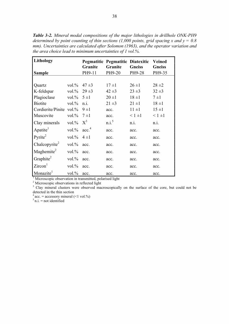
38

Table 3-2. Mineral modal compositions of the major lithologies in drillhole ONK-PH9 determined by point counting of thin sections (1,000 points, grid spacing x and y = 0.8 mm). Uncertainties are calculated after Solomon (1963), and the operator variation and the area choice lead to minimum uncertainties of 1 vol.%.

Lithology Pegmatitic Granite

Pegmatitic Granite

Diatexitic Gneiss

Veined Gneiss

Sample PH9-11 PH9-20 PH9-28 PH9-35 Quartz vol.% 47 ±3 17 ±1 26 ±1 28 ±2 K-feldspar vol.% 29 ±3 42 ±3 23 ±3 32 ±3 Plagioclase vol.% 5 ±1 20 ±1 18 ±1 7 ±1 Biotite vol.% n.i. 21 ±3 21 ±1 18 ±1 Cordierite/Pinite vol.% 9 ±1 acc. 11 ±1 15 ±1 Muscovite vol.% 7 ±1 acc. < 1 ±1 < 1 ±1

Clay minerals vol.% X3 n.i.5 n.i. n.i.

Apatite1 vol.% acc.4 acc. acc. acc.

Pyrite2 vol.% 4 ±1 acc. acc. acc.

Chalcopyrite2 vol.% acc. acc. acc. acc.

Maghemite2 vol.% acc. acc. acc. acc.

Graphite2 vol.% acc. acc. acc. acc.

Zircon1 vol.% acc. acc. acc. acc.

Monazite1 vol.% acc. acc. acc. acc. 1 Microscopic observation in transmitted, polarised light 2 Microscopic observations in reflected light 3 Clay mineral clusters were observed macroscopically on the surface of the core, but could not be detected in the thin section 4 acc. = accessory mineral (<1 vol.%) 5 n.i. = not identified

39

4 WATER CONTENT AND WATER-LOSS POROSITY Water content, bulk density and water-loss porosity were determined on 36 originally saturated drillcore samples from drillhole ONK-PH9. The water content was determined by two independent methods, i.e. gravimetrically by drying at 105 °C to stable weight conditions and by the diffusive isotope exchange technique. A detailed description of both methods is given in chapter 2. The gravimetric water content (WCWL) was determined on the same core pieces used earlier for the out-diffusion experiments (WCWL,core), which had a weight between 590 and 1,040 g, and on core pieces used for the diffusive isotope exchange technique (WCWL,IsoEx) with weights between 196 and 426 g for each experiment. During both experiments the applied core samples remained saturated. This was controlled by taking the exact weights of the cores before and after the experiments. If not specifically mentioned, the gravimetric water content values discussed below are the average of the individual core pieces of the single samples. The water content values derived by isotope mass balance from the isotope measurements of the isotope diffusive exchange experiments (cf. chapter 2) are referred as WCIsoEx in the subsequent text. Due to the low mass of pore water in the crystalline rocks from Olkiluoto, the determination of the water is very sensitive to any processes that might cause a change in the mass of pore water. Such processes are, for example, stress release during and after drilling, the generation of a disturbed zone (DDZ) during the drilling process and desaturation during sample packing and preparation in the laboratory. By applying adequate sampling and packing procedures (cf. chapter 2.1.1), desaturation can be minimised. The influence of drilling fluid due to stress release and a disturbed zone is limited to the time the core is in contact with the drilling fluid. As discussed in detail in Eichinger et al. (2009) and Eichinger (2009) it can be assumed for the Olkiluoto bedrock that the effect of drilling fluid contamination induced by stress release and a disturbed zone is less than 10% and hence in the uncertainty range of the measurements. The influence of possible stress release effects during the experiments and evaporation effects prior to the experiments can be directly evaluated by taking the weights of the large sized out-diffusion cores before and after immersing the cores in water for about 200 days. For all cores used in the out-diffusion experiment, the weight of the core before and after the experiment agreed within ≤ 0.01% of the total weight (Figure 4-1), what corresponds to a variation in the mass of pore water ≤ 10%. The fact that the weights did not increase during the experiments reveals that the cores were saturated at the time of their arrival in the laboratory and that no measurable ingress of water has occurred into potentially newly created pore spaces.

40

Figure 4-1. Weights of samples from drillhole ONK-PH9 used for out-diffusion experiments measured before and after the out-diffusion experiment (i.e. immersion in water over approx. 200 days); The errors of the water content measurements are ± 0.002g and are within the symbol size in the diagram (PGR = pegmatitic granite, DGN = diatexitic gneiss, MGN = mica gneiss, VGN = veined gneiss, KFP = K-feldspar porphyry); the corresponding masses are listed in Appendix II. In a few diffusive isotope exchange experiments (n=8) an increased sorption of test water from the crystallisation dish on the rock surfaces was observed. The water content of those samples was corrected for the amount of surface sorbed water, which amounted to a maximum of 40 % of the total water content. It should be noted that such sorption has no effect on the isotope composition given that complete equilibration is attained. In nine diffusive isotope exchange experiments (Table 4-1) test water has been lost from leaky glass containers by evaporation during the equilibration period. For these samples neither the gravimetric WCWL,IsoEx nor the isotopically derived WCIsoEx were further considered. Along drillhole ONK-PH9 the degree of alteration varied. In the previous pore water campaigns (OL-KR39 and OL-KR47, Eichinger et al. 2006, 2009) care was taken to select only macroscopically unaltered and unfractured rocks. In drillhole ONK-PH9 the sampling of a continuous profile was prioritised and hence significantly macroscopically altered samples (for more details cf. section 3) were taken also. Macroscopically visible alteration could be observed on pegmatitic granite and diatexitic gneiss samples between 32.7 and 42.6 m DHL (area of hydraulic zone HZ20B, hydraulic bedrock zone 1) and between 48.4 and 52.6 m DHL. Open fissures with an aperture of < ~ 2 mm were observed in the altered diatexitic gneiss sample PH9-

41

8 (36.1 m DHL) and in the altered pegmatitic granite samples PH9-10 and PH9-11 (37.9 and 41.0 m DHL, Table 4-1). 4.1 Water contents

4.1.1 Pegmatitic granite Gravimetric water content Average values of the gravimetric water content (WCWL,ave), of macroscopically unaltered pegmatitic granite from drillhole ONK-PH9 vary between 0.18 and 0.38 wt.% (n=12; Table 4-1, Figure 4-2). The large spread of water contents determined gravimetrically along the profile and also in subsamples (PH9-23 and PH9-26; Table 4-1, Figure 4-2) are due to textural and mineralogical heterogeneities within the same drillcore section. The gravimetric water content determined on unaltered pegmatitic granite samples is in good agreement with the average gravimetric water contents of samples from drillholes OL-KR39 and OL-KR47, which range from 0.24 to 0.34 wt.% (Eichinger et al. 2006, 2009). Average values of the gravimetric water content of macroscopically altered pegmatitic granite sampled from drillhole ONK-PH9 varies between 0.35 and 0.76 wt.% (n = 10; Table 4-1, Figure 4-2). The wide spread in the determined gravimetric water contents along the profile and in the subsamples of all investigated samples can be attributed to mineralogical and textural heterogeneities. The higher water content of altered pegmatitic granite samples, compared to unaltered samples, is due to a considerably high intragranular connected porosity of altered main rock forming minerals like feldspar, cordierite and biotite (see also Eichinger 2009). Water content determined by diffusive isotope exchange The water contents of macroscopically altered and unaltered pegmatitic granite determined by diffusive isotope exchange (WCIsoEx) vary between 0.18 and 0.35 wt.% for unaltered, and between 0.27 and 0.50 wt.% for macroscopically altered pegmatitic granite. The comparison of the water content values determined by the two different methods on the same core pieces shows for two macroscopically unaltered (PH9-23, PH9-26) and three altered pegmatitic granite samples (PH9-11, PH9-12, PH9-13) that WCWL,IsoEx is higher than WCIsoEx (Table 4-1, Figure 4-3). This trend contrasts with the observations made for samples from drillholes OL-KR39 and OL-KR47, where an opposite trend was detected for several samples (Eichinger et al. 2006, 2009). This phenomenon is currently not understood. 4.1.2 Diatexitic Gneiss Gravimetric water content Average values of the gravimetric water content (WCWL, aver) of macroscopically unaltered diatexitic gneiss are between 0.16 and 0.21 wt.% (n=2; Table 4-1, Figure 4-2).

42

These values are slightly higher than the water content determined for a single diatexitic gneiss sample from drillhole OL-KR 47 (0.150.04 wt.%, Eichinger et al. 2009). The deviation is caused by textural and mineralogical heterogeneities. The gravimetric water content of macroscopically altered diatexitic gneiss samples is higher than determined on unaltered ones and ranges between 0.38 and 0.95 wt.% (n=6, Table 4-1, Figure 4-2). The wide spread of values, which is observed along the profile, as well as on individual subsamples, can again be explained by textural and mineralogical heterogeneities. Water content determined by diffusive isotope exchange WCIsoEx of unaltered and altered diatexitic gneiss are 0.12 (n=2) and 0.40 wt.% (n=1), respectively (Table 4-1). Two samples (PH9-1, PH9-28) show higher WCWL,IsoEx than WCIsoEx values (Figure 4-3) 4.1.3 Minor lithologies Gravimetric water content The average gravimetric water contents of mica gneiss vary between 0.08 and 0.14 wt.% (n=5; Table 4-1, Figure 4-2). The differences of water content values of mica gneiss samples along the profile can be attributed to textural heterogeneities. However, alteration effects could not be determined macroscopically on the selected mica gneiss samples. The obtained values are in good agreement with the water content of a mica gneiss sample taken from drillhole OL-KR39 (0.120.03 wt.%, Eichinger et al. 2006). WCWL determined on two veined gneiss samples diverge widely between 0.390.07 (PH9-35) and 1.270.13 wt.% (PH9-2; Table 4-1, Figure 4-2). The relatively high water content of the veined gneiss sample PH9-2 is related to the considerably high proportion of pinitised cordierite in the sample (~10-20 Vol.%). As shown by Eichinger (2009), pinitised cordierite can have a high intragranular porosity which is filled with pore water and connected to the surrounding intergranular pore space. WCWL of the veined gneiss sample PH9-35 is in the same range as water contents of veined gneiss samples from drillholes OL-KR39 and OL-KR47 which vary between 0.10 and 0.50 wt.%. Water content determined by diffusive isotope exchange The water content of mica gneiss determined by diffusive isotope exchange is between 0.09 and 0.12 wt.% (n=2). Comparison of WCIsoEx with WCWL,IsoEx shows that the values are in good agreement (Table 4-1, Figure 4-3). The water content of veined gneiss determined by diffusive isotope exchange (n=1) is 0.43 wt.% and agrees well with the gravimetric determined water content (WCWL,IsoEx Table 4-1, Figures 4-3). For the K-feldspar porphyry a gravimetric water content of 0.11 wt.% was determined (n=1, Table 4-1, Figure 4-2). The WCIsoEx of this sample is also 0.11 wt.%, in good agreement with the WCWL,IsoEx (Figure 4-3).

43

Figure 4-2. Drillhole ONK-PH9: Water content of core samples from the encountered lithologies determined gravimetrically (WCWL) on originally saturated samples versus distance along the drillhole. WCWL reflects the average of WCWL,core and WCWL,IsoEx. The given errors are the standard deviations of the average value. The different colours mark the various hydraulic bedrock zones.

44

Figure 4-3. Water content determined by the diffusive isotope exchange technique versus the gravimetric water content (and also as a function of the sample lithology) determined on drillcore samples used in the earlier out-diffusion experiments.. PGR: pegmatitic granite, DGN: diatexitic gneiss, MGN: mica gneiss, VGN: veined gneiss, KFP: K-feldspar porphyry, alt.: altered.

45

Sample Distance DHL Gravimetric WC (WCWL) WC by isotopic exchange (WCIsoEx)

WCWL, Core WCWL,IsoEx WC,IsoEx WCWL,ave WCWL,ave WCIsoEx errorWC,IsoEx m wt.% wt.% wt.% wt.% wt.% wt.% Pegmatitic Granite, macroscopically unaltered PH9-14 43.0 0.30 0.35 0.02 0.33 (3)1 0.04 0.35 0.03 PH9-15 43.4 0.28 * 0.28 (1) 0.01 * PH9-16 43.7 0.27 - 0.27 (1) - - PH9-20 46.1 0.18 ** 0.18 (1) - PH9-21 46.4 0.20 * 0.20 (1) 0.01 * PH9-22 46.8 0.30 0.30 0.02 0.30 (3) 0.02 0.31 0.03 PH9-23 47.5 0.33 0.22 0.01 0.28 (3) 0.08 0.18 0.04 PH9-24 47.9 0.34 * 0.34 (1) 0.01 * PH9-26a 49.4 0.36 0.25 0.01 0.31 (3) 0.08 0.18 0.05 PH9-26b 49.4 0.30 - 0.30 (1) - - PH9-27 50.2 0.36 * 0.36 (1) - * Pegmatitic Granite, macroscopically altered PH9-3 32.7 0.49 0.33 0.01 0.41 (3) 0.11 0.27 0.06 PH9-4 33.3 0.48 * 0.48 (1) * PH9-5 33.9 0.70 - 0.70 (1) - PH9-6 34.4 0.56 - 0.56 (1) - PH9-7 35.3 0.80 0.45 0.02 0.63 (3) 0.25 0.43 0.08 PH9-102 37.9 0.76 - 0.76 (1) - PH9-112 41.0 0.80 0.56 0.03 0.68 (2) 0.17 0.503 0.04 PH9-12 42.0 0.68 0.49 0.01 0.59 (3) 0.13 0.40 0.04 PH9-13 42.6 0.41 0.30 0.03 0.35 (3) 0.07 0.27 0.06 PH9-25 48.4 0.41 * 0.41 (1) * Diatexitic Gneiss, macroscopically unaltered PH9-1 19.2 0.22 0.20 0.01 0.21 (3) 0.01 0.12 0.08 PH9-34 87.3 0.18 0.15 0.03 0.16 (3) 0.03 0.12 0.03 Diatexitic Gneiss, macroscopically altered PH9-82 36.1 0.85 - 0.85 (1) - PH9-9 36.9 0.95 - 0.95 (1) - PH9-28 51.2 0.49 0.48 0.04 0.49 (3) 0.01 0.40 0.04 PH9-29 52.0 0.42 * 0.42 (1) 0.06 * PH9-30 52.6 0.45 * 0.45 (1) 0.04 * PH9-31 57.1 0.47 * 0.47 (1) 0.04 * Mica Gneiss PH9-17 44.5 0.15 * 0.15 (1) * PH9-18 45.2 0.14 - 0.14 (1) - PH9-19 45.7 0.08 0.11 0.01 0.10 (3) 0.02 0.12 0.03 PH9-33 78.1 0.09 0.11 0.01 0.10 (3) 0.01 0.09 0.03 Veined Gneiss PH9-2 30.6 1.27 - 1.27 (1) - PH9-35 97.3 0.34 0.43 0.07 0.39 (3) 0.06 0.43 0.03 K-Feldspar Porphyry PH9-32 69.7 0.11 0.11 0.01 0.11 (3) 0.01 0.10 0.02

- Diffusive isotope exchange experiments were not conducted. * Experiment performed but perturbed by evaporation; values are not reliable. ** Individual subsamples consist of different lithologies. 1 number in parenthesis marks the number of individual subsamples used to calculate the average WCWL 2 samples not suitable for pore water investigations due to open fractures 3 WCIsoEx based only on mass balance calculations using 2H

Table 4-1. Water content determined gravimetrically and by the diffusive isotope exchange technique of the different lithologies in drillhole ONK-PH9. The error of the gravimetric water content determined on the core pieces used for the diffusive isotope exchange technique (WCWL,IsoEx) is the standard deviation of the measured subsamples (n=2), the error of the average gravimetric water content (WCWL,ave), and the standard deviation of the three measured sub-samples (n=3); the error of the WCIsoEx is determined by Gaussian error propagation.

46

4.2 Bulk density Bulk density measurements were derived from wet mass and volume of the large size drillcore samples used for the out-diffusion experiments. Previous studies (Eichinger et al. 2009) showed that bulk density values of the main lithologies determined volumetrically are in good agreement with those determined by Hg-displacement. For macroscopically unaltered and altered pegmatitic granite the bulk wet density ranges from 2.57 to 2.73 g/cm3 (Table 4-2) with averages of 2.64±0.05 g/cm3 (n=12) for unaltered and 2.62±0.05 g/cm3 for altered pegmatitic granite (n=9). The differences in the determined bulk wet density values can be attributed to textural heterogeneities (varying proportions of palaeosomatic parts and/or open structures) and varying degrees of alteration of main rock forming minerals. The bulk wet density of pegmatitic granite from drillhole ONK-PH9 is in good agreement with that determined for pegmatitic granite from drillholes OL-KR39 and OL-KR47 (2.59-2.62 g/cm3, Eichinger et al. 2006, 2009). The bulk wet density of the two macroscopically unaltered diatexitic gneiss samples is uniform at 2.64±0.01 g/cm3 (n=2) whereas it varies between 2.62 and 2.69 g/cm3 (n=6, Table 4-2) for the altered diatexitic gneiss with an average of 2.66±0.03 g/cm3. The variations in bulk wet density data are due to textural and mineralogical heterogeneities of the used samples. The determined bulk wet density of unaltered diatexitic gneiss from drillhole ONK-PH9 are in good agreement with the bulk wet density of a diatexitic gneiss sample from drillhole OL-KR47 (2.63 g/cm3, Eichinger et al. 2009). The bulk wet density of mica gneiss is between 2.72 and 2.80 g/cm3 (n=4) and is in the same range as that determined on samples from drillhole OL-KR39 (2.73-2.77 g/cm3, Eichinger et al. 2006). For veined gneiss the bulk wet density varies between 2.69 and 2.74 g/cm3 (n=2, Table 4-2). The values determined for veined gneiss samples from this drillhole are also in good agreement with those from drillholes OL-KR39 and OL-KR47, which vary between 2.65 and 2.76 g/cm3. The K-feldspar porphyry sample has a bulk wet density of 2.70 g/cm3 (Table 4-2). 4.3 Water-loss (connected) porosity The water-loss (connected) porosity was calculated according to equation (2-1) using the water content and,as a first approximation, the bulk wet density of the samples. As shown in a previous study (Eichinger et al. 2009), the porosity values calculated by equation (2-1) for the major lithologies of the Olkiluoto bedrock are within the given uncertainty range and are in good agreement with those calculated from the water content and the grain density.

47

The water-loss porosity of macroscopically unaltered pegmatitic granite varies between 0.54 and 1.05 Vol.% (n=12, Table 4-2, Figure 4-4) and that of macroscopically altered pegmatitic granite between 0.87 and 2.13 Vol.% (n=9). For macroscopically unaltered diatexitic gneiss the water-loss porosity ranges from 0.46 to 0.58 Vol.% (n=2, Table 4-2, Figure 4-4) and that of macroscopically unaltered diatexitic gneiss is between 0.88 and 2.53 Vol.% (n=6). Water-loss porosities of mica gneiss and veined gneiss range between 0.22 and 0.40 Vol.% (n=4) and between 0.94 and 3.41 Vol.%, respectively (Table 4-2, Figure 4-4). For the K-feldspar porphyry sample a water-loss porosity of 0.30 Vol.% was calculated (Table 4-2, Figure 4-4).

Figure 4-4. Drillhole ONK-PH9: Water-loss porosity determined on out-diffusion cores as a function of distance along drillhole. The different coloured areas mark the various hydraulic zones.

48

Table 4-2. Drillhole ONK-PH9: Bulk wet density, water-loss and water content porosity values of samples from various lithologies.

Sample Dist bulk,wet Water loss porosity (WL) Water content porosity (WC,IsoEx)

meas. WL,core WL,IsoEx WL,IsoEx WL,ave WL,ave IsoEx error,IsoEx m DHL g/cm3 Vol.% Vol.% Vol.% Vol.% Vol.% Vol.% Vol.% Pegmatitic Granite, macroscopically unaltered PH9-14 43.0 2.71 0.81 0.95 0.05 0.88 (3)1 0.10 0.95 0.08 PH9-15 43.4 2.62 0.73 * 0.73 (1) * PH9-16 43.7 2.57 0.69 - 0.69 (1) - PH9-20 46.1 2.64 0.48 ** 0.48 (1) PH9-21 46.4 2.69 0.54 * 0.54 (1) * PH9-22 46.8 2.62 0.78 0.78 0.05 0.78 (3) 0.05 0.81 0.08 PH9-23 47.5 2.65 0.88 0.58 0.03 0.73 (3) 0.21 0.48 0.11 PH9-24 47.9 2.60 0.88 * 0.87 (1) * PH9-26a 49.4 2.60 0.94 0.65 0.03 0.79 (3) 0.20 0.47 0.13 PH9-26b 49.4 2.62 0.79 - 0.79 (1) - PH9-27 50.2 2.62 0.94 1.05 0.03 0.99 (3) 0.07 * Pegmatitic Granite, macroscopically altered PH9-3 32.7 2.61 1.28 0.86 0.03 1.07 (3) 0.29 0.70 0.16 PH9-4 33.3 2.63 1.26 * 1.26 (1) * PH9-5 33.9 2.61 1.83 - 1.83 (1) PH9-6 34.4 2.61 1.46 - 1.46 (1) PH9-7 35.3 2.67 2.14 1.20 0.05 1.67 (3) 0.66 1.15 0.21 PH9-102 37.9 2.59 1.97 - 1.97 (1) - PH9-112 41.0 2.60 2.08 1.46 0.08 1.77 (2) 0.44 1.303 0.10 PH9-12 42.0 2.57 1.75 1.26 0.03 1.50 (3) 0.34 1.03 0.10 PH9-13 42.6 2.73 1.12 0.90 0.08 1.01 (3) 0.15 0.74 0.16 PH9-25 48.4 2.73 1.12 * 1.12 (1) * Diatexitic Gneiss, macroscopically unaltered PH9-1 19.2 2.64 0.58 0.53 0.03 0.56 (3) 0.04 0.32 0.21 PH9-34 87.3 2.63 0.47 0.45 0.08 0.46 (3) 0.02 0.32 0.08 Diatexitic Gneiss, macroscopically altered PH9-82 36.1 2.65 2.25 - 2.25 (1) - PH9-9 36.9 2.68 2.54 - 2.54 (1) - PH9-28 51.2 2.68 1.31 1.29 0.11 1.30 (3) 0.02 1.07 0.11 PH9-29 52.0 2.62 1.10 * 1.10 (1) * PH9-30 52.6 2.69 1.21 * 1.21 (1) * PH9-31 57.1 2.65 1.24 * 1.24 (1) *

Mica Gneiss PH9-17 44.5 2.72 0.41 * 0.41 (1) * PH9-18 45.2 2.76 0.39 - 0.39 (1) - PH9-19 45.7 2.75 0.22 0.30 0.03 0.26 (3) 0.06 0.33 0.08 PH9-33 78.1 2.80 0.25 0.31 0.03 0.28 (3) 0.04 0.25 0.08

Veined Gneiss PH9-2 30.6 2.69 3.41 - 3.41 (1) - PH9-35 97.3 2.74 0.93 1.18 0.19 1.05 (3) 0.17 1.18 0.08

K-Feldspar Porphyry PH9-32 69.7 2.70 0.30 0.30 0.03 0.30 (3) 0.03 0.27 0.05 - Diffusive isotope exchange experiments were not conducted. * Experiment performed but perturbed by evaporation; values are not reliable. ** Individual subsamples consist of different lithologies. 1 number in parenthesis marks the number of individual subsamples used to calculate the average WCWL 2 samples not suitable for pore water investigations due to open fractures 3 IsoEx based on WCIsoEx only determined by using 2H

49

5 PORE DIFFUSION COEFFICIENT OF CHLORIDE Chloride pore diffusion coefficients were derived by modelling the chloride breakthrough curves obtained from the out-diffusion experiments of 10 samples from drillhole ONK-PH9. The chloride breakthrough curves are given by the Cl-contents in the small size subsamples that have been collected periodically from the out-diffusion experiments (cf. section 2.2.3). The pore diffusion coefficient is obtained by fitting the observed data with an analytical solution for radial diffusion out of the cylinder into a well mixed solution reservoir (Crank 1975). The applied model (T. Gimmi, RWI, University of Bern) is restricted to homogeneous hydraulic properties (porosity, diffusion coefficient) across the core cylinder, and cannot take into account heterogeneous properties due to rock anisotropy and possibly induced effects such as a disturbed zone induced by stress release and the drilling process. The pore diffusion coefficient, Dp, for a solute in a geological media mainly depends on the shape and size of water-conducting pores (constrictivity) and on the pathways given by the connected pore network (tortuosity, cf. e.g. Ohlsson and Neretnieks 1995). It can be defined as:

DP DW

D

2 (5-1)

where DP = pore-diffusion coefficient in m2/s; DW = diffusion coefficient in pure water

in m2/s; D = constrictivity; = tortuosity; the term D

2 is called the geometry factor.

In a first assumption the pore diffusion coefficient of a given species, DP, can be converted to the effective diffusion coefficient of this species, De, according to: De DP *WC (5-2)

where De is the effective diffusion coefficient in m2/s and WC the species accessible porosity. In clay-poor crystalline rocks and because of the lack of better knowledge, the species-accessible porosity for chemically conservative components such as Cl- and Br- is considered to be equal to the water-content (connected) porosity. In such a case, De describes the mobility of a dissolved substance in the water-filled pores, taking in account the porosity, tortuosity and constrictivity. Artefacts induced by sampling (e.g. the creation of a DDZ, stress release), sample preparation (e.g. microcracks due to sawing), sample packing and the experiment (e.g. evaporation effects) will affect the pore diffusion coefficient determined experimentally in the laboratory. To minimise such artefacts, large sized (600 – 1,000 g) and naturally saturated drillcore samples were used for the out-diffusion experiments. Large sized drillcore samples have the advantage of a large ratio of internal core volume to surface area which helps to minimise induced artefacts. An extended discussion about the influence of possible artefacts on such derived pore diffusion coefficients, and a

50

comparison with pore diffusion coefficients derived for Olkiluoto bedrock by other methods, is given in Eichinger (2009) and Eichinger et al. (2009). The shape of the Cl-breakthrough curves obtained for most rock samples from drillhole ONK-PH9 suggests a heterogeneous hydraulic system from the rim to the centre of the core (Figure 5-1). The curves show an initial steep slope in the transient state during the first five to ten days. The slope then proceeds to change until the concentrations reach a plateau, which is indicative for attained equilibrium between Cl- in the solution surrounding the core and Cl- in the pore space of the core. The shapes of the curves therefore suggest an initial fast out-diffusion from a small rim zone followed by a slower diffusion from the central part of the core. It appears that this rim zone represents the zone influenced by the drilling process. To overcome the limitations given by the applied model (homogeneous hydraulic system) several runs have been performed for each sample to derive a best-fit pore diffusion coefficient, DP, and its uncertainty band. In these runs all parameters remained equal except for DP, which was varied by weighing the fit to the data points produced in the first few days of out-diffusion (steep slope), and to those produced 10-15 days after the beginning of out-diffusion until the end of the experiment (moderate slope). For pegmatitic granite, diatexitic gneiss and veined gneiss samples encountered by drillhole ONK-PH9, the influence of the disturbed zone results in a pore diffusion coefficient that is approximately a factor 1.4 higher compared to the undisturbed inner zone of the core cylinders (Figure 5-1). For the fine to very fine-grained mica gneiss samples a factor of 2 is suggested (Figure 5-1). In accordance with previous studies of pore diffusion coefficients for Olkiluoto bedrocks (Eichinger et al. 2006, 2009, Eichinger, 2009), the error of the pore diffusion coefficient for chloride in pegmatitic granite, veined gneiss and diatexitic gneiss is conservatively assumed to be a factor 2 around the modelled best fit to the measured data (Figure 5-1). For the mica gneiss, more a factor of 4 would emerge. However, the shapes of the Cl-breakthrough curves of this rock type indicate a very large heterogeneity/anisotropy of these core samples and a non-equilibrium state at the end of the experiment. This inhibits the derivation of a reliable range of a chloride pore diffusion coefficient by the applied model.

51

Figure 5-1. Chloride breakthrough curves of samples taken from drillhole ONK-PH9 and the pore diffusion coefficient modelled at 45°C. The best fit is marked by the solid red line, and the dashed red and black curves indicate the uncertainty range of a factor of 2 and 4, respectively,around the best fit. The chloride pore diffusion coefficients of macroscopically unaltered pegmatitic granite vary between 2.0 and 4.9*10-11 m2/s (10°C) (n=3; Table 5-1). The variation is assigned to the textural heterogeneity of these samples The pore diffusion coefficient determined for the homogeneous pegmatitic granite samples are in good agreement with values obtained for pegmatitic granite samples from drillhole OL-KR39 and KR47, which range between 3.0 and 8.9*10-11 m2/s (Eichinger et al. 2006, 2009). The pore diffusion coefficient for chloride determined for the macroscopically altered pegmatitic granite sample PH9-12 is 2.6*10-11 m2/s at 10 °C (Table 5-1). This pore diffusion coefficient of the altered pegmatitic granite sample PH9-12 is lower than those

52

obtained for unaltered homogeneous pegmatitic granite samples from previous studies. This would be consistent with the higher amount of more fine-grained mineral aggregates resulting in a higher geometric factor (cf. equation 5-1) for the altered pegmatitic granite compared to the unaltered pegmatitic granite. Chloride pore diffusion coefficients of altered diatexitic gneiss samples are identical within the uncertainty band and vary between 1.8 and 2.0*10-11 m2/s at 10°C (n=2; Table 5-1). No Cl time series of out-diffusion experiments of altered diatexitic gneiss samples were taken and there exist also no Dp values for diatexitic gneiss from the previous investigation campaigns. Chloride pore diffusion coefficients for mica gneiss samples can only be estimated with a large uncertainty due to the distinct anisotropy of the samples. Best estimate of DP would be about 1.2*10-11 (10 °C) m2/s (n=2, Table 5-1). No DP values for mica gneiss exist from previous investigation campaigns. For the veined gneiss sample PH9-35 a chloride pore diffusion coefficient of 1.4*10-11 m2/s (10 °C) is determined (Table 5-1). This value is in good agreement with pore diffusion coefficients determined on veined gneisses with leucosomatic proportions <40 Vol.% from drillholes OL-KR39 and OL-KR47, which vary between 1.0 and 2.0*10-11 m2/s at 10 °C (Eichinger et al. 2009). Table 5-1. Drillhole ONK-PH9: Modelled pore diffusion coefficients, DP, of chloride at 45 oC and 10 °C and the effective diffusion coefficient of chloride, De, calculated according to equation 5-2, using the water-loss porosity, WL.

Sample Distance WL DP*10-11 DP*10-11 DP,min*10-11 DP,max*10-11 De*10-13

DHL 45°C 10°C 10°C 10°C 10°C

m Vol.% m2/s m2/s m2/s m2/s m2/s

Pegmatitic Granite

PH9-15 43.4 0.74 5.0 2.0 1.4 2.9 1.5

PH9-22 46.8 0.78 12.0 4.9 3.4 6.9 3.8

PH9-26 49.4 0.93 7.0 2.8 2.0 4.0 2.7

Pegmatitic Granite, altered

PH9-12 42.0 1.76 6.5 2.6 1.9 3.7 4.6

Diatexitic Gneiss, altered

PH9-28 51.2 1.30 5.0 2.0 1.4 2.9 2.7

PH9-30 52.6 1.22 4.5 1.8 1.3 2.6 2.2

Mica Gneiss

PH9-18 45.2 0.38 3.0 1.2 0.6 2.4 0.2

PH9-19 45.7 0.22 3.0 1.2 0.6 2.4 0.1

Veined Gneiss

PH9-35 97.3 0.94 3.5 1.4 1.0 2.0 1.3

53

6 FLUID INCLUSIONS Petrographic, laser Raman microspectrometric and microthermometric methods have been applied to investigate the composition of fluid inclusions in quartz crystals of 5 samples from the subhorizontal drillhole ONK-PH9 (306 m b.s.), consisting of the main lithologies, i.e. pegmatitic granite (PH9-11/PH9-20), diatexitic gneiss (PH9-28), veined gneiss (PH9-35) and mica gneiss (PH9-18/PH9-20). After these non-destructive methods, core samples were disaggregated and single quartz crystals were separated. Subsequently, these quartz grains were crushed to liberate the fluid inclusions and analyse them by gas chromatography and mass spectrometry. The petrographic identification of fluid inclusion generations is based on studies of "assemblages", i.e. groups of coeval inclusions which can be clearly related to individual healed fractures or crystal growth zones. Details of the methods used are described in Chapter 2 and in Hämmerli (2009). The salinity of individual fluid inclusions was calculated from ice melting temperatures (Tm(ice)) according to the calibration of Bodnar (1993) or from gas-hydrate clathrate melting temperatures according to the method of Diamond (1994). In assemblages where the inclusions were trapped from heterogeneous fluids, Tm(ice), the total homogenisation temperatures (Th) were measured in the inclusions that display the smallest volume fractions of vapour (vapour). The vapour bubble was always present when the last crystal of ice melted upon heating. No information is available on the mixture of solutes that account for the salinity, and so salinity values are reported as if all the salt were NaCl (i.e. as mass% NaCl equivalent). Volume fractions of the individual phases in the fluid inclusions were determined by the spindle-stage method of Bakker and Diamond (2006). In the following text the solids within the fluid inclusions are distinguished as accidentally captured crystals or as daughter crystals. Daughter crystals are minerals that have precipitated within the inclusions upon cooling and pressure decrease, whereas accidentally captured crystals are minerals that were trapped at the same time as the fluid. All fluid inclusions found in the investigated samples hosted by quartz crystals are secondary. This means that they were formed after the host metamorphic quartz had finished growing and had acquired its metamorphic texture. The inclusions formed when fluid infiltrated small scale brittle fractures and the fractures subsequently healed by dissolution-precipitation processes. The healed fractures are now represented by planar arrays of fluid inclusions (termed fluid inclusion assemblages) that cross cut mineral grain boundaries in the host rock (Figure 6-1). Thus, the fluids were trapped at temperatures within the brittle field of quartz (below about 400 °C), after the peak of the last metamorphic event in the Olkiluoto bedrocks. Apart from this maximum constraint, the age of the fracturing and inclusion formation events is not known. The clear mutual cross-cutting relationships between the healed fractures allowed the relative ages of 7 generations of inclusions to be recognised (Figure 6-2). The generations are numbered 1, 2a, 2b, 3, 4, 5a and 5b, where 1 represents the earliest and 5 the latest generation. All the fluid inclusion generations were found in each sample,

54

regardless of its lithology. Evidence from the new samples allowed the timing of two fluid generations to be established, which formerly (Eichinger et al. 2010) could not be distinguished. The generation which was formerly termed 3b is now termed 3 and former generation 3a is now numbered 4. Owing to a lack of unequivocal petrographic evidence so far, the relative ages of generations 2a/2b and 5a/5b could not be established. Once the generations and their relative timing were identified, the gas compositions, the aqueous salinity and the phase volume fractions of the inclusions were determined. From these the bulk chemical composition and densities (molar volumes) of the palaeofluids were calculated using thermodynamic data and the mass- and volume-balance equations in Diamond (2003a) (Table 6-1). The main characteristics of the 7 generations are summarised in Figure 6-3 and are explained in detail below. A compilation of the raw data can be found in the Appendix. Figure 6-1. Picture of a thin section in transmitted, cross-polarised light, showing a planar assemblage of fluid inclusions cross-cutting the grain boundary of two individual quartz grains (quartz 1 and quartz 2).

Quartz 1 Quartz 2

Grain boundary

Fluid inclusion plane

55

Figure 6-2. Example of cross-cutting between two fluid inclusion generations. Photos (transmitted, plane-polarised light) are taken at different depths within the same thin section. The "aqueous liquid + vapour" fluid inclusion assemblage cuts the "all vapour" fluid inclusion assemblage, which proves that the latter is younger in relative age.

All vapour

Aq. liquid + vapour

shallow deep

20 m

56

Figure 6-4. Heterogeneous fluid inclusion assemblage

Crystal without fluid

Crystal within fluid inclusion

10 m

albite

vapour

aq. liquid 10 m

Figure 6-5. Accidentally captured albite crystal

Figure 6-3. Paragenetic diagram of fluid inclusion generations based on cross-cutting observations; the relative age between generation 2a/2b and 5a/5b is not yet unravelled (*daughter mineral, *(*)interpreted as a daughter mineral, **accidentally entrapped mineral).

6.1 Generations of fluid inclusions in quartz Generation 1: This generation is the most frequent in all samples. The shapes of the inclusions vary from equant to irregular forms. Mostly, the inclusions are < 25 m in diameter. At room temperature the inclusions contain at most three phases: an aqueous liquid wetting the inclusion walls, a central vapour bubble and frequently a solid. Within individual assemblages the volume fraction of the vapour is highly variable (vapour= 5–100%). The volume fraction of the solids is also variable (solid= 0–50%). Some assemblages show crystals without a liquid or vapour phase (Figure 6-4). The vapour phases consist of variable mixtures of CO2, CH4, N2 and H2, whereby H2 and CO2 are mutually exclusive (Figure 6-6). Within a single assemblage the inclusions often contain the same composition but some assemblages show large internal differences.

57

Solid phases are sometimes present inside the inclusions, regardless of the value of vapour. Crystals of nahcolite (NaHCO3) have been found as daughter minerals (precipitated within the fluid inclusion during post-entrapment cooling) and as accidentally captured minerals. Calcite has been rarely observed as accidentally captured crystals in multiphase inclusions. Raman analyses showed that an accidentally trapped albite crystal is present in at least one inclusion (Figure 6-5), but this occurs alone rather than part of an assemblage, and so it cannot be assigned unequivocally to one of the numbered fluid generations. This inclusion possibly represents a primary inclusion which was trapped during high grade metamorphism. The calculated salinity of generation 1 inclusions is 3.4–6.2 mass% NaCleq. Homogenisation of the vapour-poor end members of the inclusion assemblages occurred via a bubble-point transition (LV L) in the temperature range Th = 308–324 °C. The internal pressure at room temperature is around 70 bar.

Figure 6-6. Gas composition in generation 1 fluid inclusions. Each symbol represents the mean composition of an individual assemblage. The variable volume fractions of vapour (vapour) within individual assemblages indicate that the inclusions were entrapped from a heterogeneous fluid: a gas poor, aqueous “liquid” that coexisted with an H2O-poor, gas rich “vapour”. Accordingly, the lowest Th values of the vapour poor inclusions (308–324 ˚C) represent the entrapment temperatures of all the inclusions. The accidentally entrapped nahcolite, calcite and albite crystals indicate that these minerals were already present in the palaeofluid prior to inclusion trapping.

58

CO2 (g)

CO2 (l)

10 m

Figure 6-7. All-vapour assem-blage with liquid and gaseous CO2

Generation 2a: The shapes of the inclusions are predominately equant. Often they appear dark under transmitted, polarised light, owing to their low density and hence low refractive indices. Generally the inclusions are < 20 m in diameter and at room temperature they contain at most three phases: a dominant dense liquid carbonic phase (Figure 6-7), a minor vapour phase (vapour = 5–50 %, whereby in vapour-rich or liquid carbonic inclusions it is well known that up to ~10 vol.% aqueous liquid may be invisible using standard microscopy), and frequently a solid (nahcolite = 5–10 % or 0 %). The vapour phase of generation 2a fluid inclusions is dominated by CO2. Most assemblages contain more than 95 mol.% CO2 and minor amounts of CH4 and N2

(Figure 6-9). The carbonic phase (CO2) homogenisation temperatures (Th(car)) were in most cases between 25–26 °C (LV V) whereas only a few inclusions showed distinctly lower values of 18–19 °C. The solids were identified as nahcolite (NaHCO3). Within individual assemblages, either all or none of the fluid inclusions contain nahcolite crystals. Therefore, the nahcolite crystals seem to have precipitated as a daughter phase after the inclusions had sealed off and cooled. Ice or clathrate melting temperatures could not be measured and therefore it was not possible to calculate the aqueous salinity. In a few cases, where the aqueous liquid that wets the inclusion walls was visible, total homogenisation temperatures (Th) could be measured (Th = 301–333 °C). Mostly, the internal pressures at room temperature are in the range between 67 and 70 bar. The uniform vapour values within individual assemblages indicate that the inclusions were trapped from a homogeneous, H2O-poor, CO2-rich, high density fluid. The minimum entrapment temperature of this fluid was 301 °C. Generation 2b: This generation is rarely present in the investigated samples. The shapes of the inclusions vary between equant and irregular. Generally, the equant inclusions are smaller (20 m in diameter) than the irregular ones (≤ 40 m in diameter). At room temperature the inclusions contain at most two phases: a dominant vapour phase (vapour = 70 to ~100 %; note that at such high vapour contents up to ~10 vol.% aqueous liquid may go unnoticed using standard microscopy), and a minor aqueous liquid phase.

Figure 6-8. H2-rich fluid inclusion

10 m

59

The major gas species is H2, although the amount of N2 can be as high as 48 mol.% (Figure 6-9). Carbon dioxide and CH4 have not been observed. Within individual assemblages vapour is uniform. The calculated salinity of generation 2b inclusions is 1.2–3.2 mass% NaCleq. Total homogenisation (Th) occurs via = dew-point transitions (LVV) and varies between 329 and 341 °C. The internal pressure at room temperature is around 40 bar. The uniform vapour values within individual assemblages indicate that the inclusions were trapped from a homogeneous, H2O-poor, gas-rich fluid with vapour-like density. The minimum entrapment temperature of this fluid was 329 °C.

Figure 6-9. Gas composition in generation 2 fluid inclusions. Blue circles denote generation 2a inclusions and red circles denote generation 2b inclusions.

60

Figure 6-10. Generation 3 fluid inclusion

10 m

Generation 3: The shapes of the inclusions vary from highly idiomorphic quartz forms to irregular forms. Generally the inclusions are <50 m in diameter, although those with irregular shapes can reach 100 m. Most of the inclusions are biphase (Figure 6-10) at room temperature, consisting of an aqueous liquid and a central vapour bubble (vapour = 12–13 %). Within individual assemblages vapour is uniform. The gas is composed of H2 and/or N2 with minor amounts of CH4 (Figure 6-11). In some assemblages the inclusions contain crystals of nahcolite (nahcolite = 5 % or 0 %). Microcrystalline graphite is also present as a coating on the inner walls of the inclusions. This graphite is mostly invisible optically, but it has been frequently detected by Raman analysis. Raman microspectroscopic determination of the graphite crystallinity (Beyssac et al. 2002) showed that the graphite in the fluid inclusions experienced lower peak temperatures (398–440 °C) than the graphite in the host-rock (≥650 °C). Although it is still debatable whether precipitated graphite is suitable for quantitative geothermometry (Luque et al. 1998), the spectra are sufficiently different to be sure that the host rock graphite is not genetically directly related to the graphite in the fluid inclusions. Owing to its occurrence as a thin film, the graphite in the fluid inclusions is interpreted to be a daughter phase. The calculated salinity of generation 3 inclusions is 0.7–3.9 mass% NaCleq. Homogenisation (Th) occurred via a bubble point transition (LV L) in the temperature range Th = 151–313 °C. The internal gas pressure at room temperature is around 35 bar.

Figure 6-11. Gas composition in generation 3 fluid inclusions. Triangles represent individual inclusions.

61

10 m

Figure 6-12. Homogeneously-entrapped assemblage of generation 3a fluid inclusions

The uniform vapour values within individual assemblages indicate that the inclusions were entrapped from a homogeneous, gas-poor, low salinity aqueous “liquid”. The minimum entrapment temperature of this fluid varies between 151 and 313 °C.

Generation 4: The shapes of the inclusions vary from equant forms to elongated forms and generally they are <25 m in diameter. At room temperature the inclusions contain at most three phases: an aqueous liquid, commonly a central vapour bubble (vapour15–19 %) and a solid phase (nahcolite = 5% or 0%). Within individual assemblages vapour is uniform (Figure 6-12). The gas is composed predominately of CH4 and/or N2 with minor amounts of H2 (Figure 6-13). The visible solids were identified as nahcolite (NaHCO3). Within individual assemblages, either most of the fluid inclusions contain nahcolite crystals or none of them do. Therefore, the nahcolite crystals, where present, seem to have precipitated as daughter phases after the inclusions had formed and cooled. Their absence in some of the assemblages may be due to metastability (supersaturation) or differences in chemical compositions. Microcrystalline graphite coating the inner walls of the inclusions has been frequently detected by Raman analysis (it is mostly invisible optically). Owing to its occurrence as a thin film, the graphite in these fluid inclusions is interpreted to be a daughter phase. The calculated salinity of generation 4 inclusions is 6.0–8.0 mass% NaCleq. Homogenisation (Th) occurred via a bubble-point transition (LV L) at Th = 280–358 °C. The internal pressure of the inclusions at room temperature is around 40 bar.

Figure 6-13: Gas composition in generation 4 fluid inclusions. Diamonds denote mean values of individual assemblages.

62

10 m

Figure 6-14. Flat, irregular shaped, generation 5 inclusion

The uniform vapour values within individual assemblages indicate that the inclusions were trapped from a homogeneous, gas-poor, aqueous “liquid”, with a minimum entrapment temperature of 280 °C. Generation 5: Generally, the shapes of the inclusions are highly irregular and flat (Figure 6-14) and can reach sizes up to 100 m in length, frequently with typical necking-down features. At room temperature the inclusions contain at most three phases: a dominant aqueous liquid, a vapour bubble (vapour = 0–10 %) and a solid phase (nahcolite = <5 % or 0 %). Often these inclusions do not contain a free vapour bubble. Such monophase inclusions are due to phase metastability, which is a well known phenomenon in inclusions that have been trapped at temperatures below 100 °C. The vapour-nucleation reaction is insufficiently overstepped by cooling to room temperature and so the inclusions remain indefinitely in a metastable “stretched liquid” state (e.g. Diamond, 2003). Analyses were carried out only on "stable" inclusions which contain a vapour bubble. The dominant gas species is N2 followed by H2 or CH4 (Figure 6-15) carbon dioxide was detected. The calculated salinity of generation 5 inclusions is 9.2–17.3 mass% NaCleq. Total homogenisation (Th) occurs via a bubble-point transition (LV L) in the temperature range 133–339 °C. The internal pressure of the inclusions at room temperature is around 40 bar. From the spread in salinities it is likely that the inclusions identified as fluid generation 5 in fact represent two different generations (5a and 5b), as shown in Figure 6-3. However, owing to the predominance of metastable liquid and hence to the low number of salinity measurements, the various cross-cutting assemblages could not be easily distinguished and so their relative ages were not determined.

63

Figure 6-15. Gas composition of generation 5 fluid inclusions. Red crosses denote mean values of individual inclusion assemblages. 6.2 Fluid inclusions in fracture calcite An open calcite vein ("fracture calcite") was found in one investigated sample (PH9-5). Microscopic investigations have shown that this calcite can be divided into two generations: early dusty, microcrystalline calcite containing opaque minerals such as pyrite, overgrown by later idiomorphic crystals of transparent calcite. The dusty, brownish colour is attributed to very fine-grained clay minerals. The later overgrowth of transparent calcite is thinner (~0.3 mm) than the early dusty calcite layers (~0.8 mm), and the two are separated by a sharp boundary. The dusty, microcrystalline calcite contains abundant fluid inclusions, most of which are metastable, monophase stretched aqueous liquid (e.g. Diamond, 2003). Vapour-rich inclusions have also been observed among the liquid inclusions. The shapes of the inclusions vary between equant, idiomorphic calcite forms and irregular shapes, the latter being more common. As shown in Figure 6-16, the fluid inclusion assemblages have variable vapour values, which means that the paleofluid from which the inclusions were trapped consisted of an aqueous liquid coexisting with a free vapour phase. Fluid inclusions in the dusty, microcrystalline calcite show salinities of 12.4–15.9 mass% NaCleq; only one assemblage was found with a distinctly higher salinity (21.7 mass% NaCl equivalent). Since the fluid inclusion assemblages were trapped in a heterogeneous state, only the inclusions with the lowest vapour values yield information on the entrapment temperature. Thus, the total homogenisation temperatures (Th) of these assemblages indicate that the dusty, microcrystalline calcite formed at 108–128 °C.

Figure 6-16. Heterogeneous fluid inclusion assemblage in dusty, micro-crystalline calcite (transmitted, plane-polarised light).

64

The transparent calcite overgrowths contain much fewer inclusions than the dusty microcrystalline calcite. Indeed, only a few isolated inclusions (rather than obvious assemblages) have been found (Figure 6-17). Their shapes are less irregular than those in the dusty calcite, and they are larger in size. The total homogenisation temperature is 173 °C (LV L). The final ice melting temperatures (Tm(ice)) are between -7.5 °C and -20 °C, which corresponds to a broad range of salinities of 11.1–22.4 mass% NaCleq. Owing to the low number of observed inclusions it is not yet clear whether they were entrapped from a heterogeneous or a homogeneous fluid.

Figure 6-17. Fluid inclusion in clear, white calcite (transmitted, plane-polarised light).

65

Tab

le 6

-1. C

alcu

late

d bu

lk p

rope

rtie

s of

the

pala

eofl

uid

gene

rati

on.

Generation Incl

usio

n nu

mbe

r1)

Phase state2)

Vm

[cm

3 /mol

]

[g/c

m3 ]

XH

2

[mol

%]

XN

2

[mol

%]

XC

H4

[mol

%]

XC

O2

[mol

%]

XH

2O

[mol

%]

XN

aCl

[mol

%]

CN

aCle

q.3)

[g/k

g]

CC

l4)

[g/k

g]

1 P

H9-

35/2

/1/1

L

het

21.3

6 ±

0.16

0.

882

± 0.

010

n.i.

0.

164

± 0.

008

0.04

4 ±

0.00

2 n.

i.

97.8

13

± 0.

010

1.97

9±

0.01

65

.64

39.8

2

1 P

H9-

35/2

/1/2

V

het

37.0

9 ±

1.63

0.

506

± 0.

010

n.i.

0.

041

± 0.

004

0.03

7 ±

0.00

3 n.

i.

98.0

91

± 0.

007

1.83

1±

0.01

60

.56

36.7

4

1 P

H9-

18/3

/3/2

L

het*

57.1

7 n.

a.

0.75

8 ±

0.01

0 n.

i.

3.00

0

1.00

0

96

n.

i.

n.i.

0.

00

0.00

2a

PH

9-35

/1/1

/1

Lho

m*

48.3

9 ±

0.00

0.

903

± 0.

010

n.i.

n.

i.

1.50

0

98.5

n.i.

n.

i.

0.00

0.

00

2b

PH

9-11

/2/6

/1

Vho

m

51.4

8 ±

4.12

0.

352

± 0.

010

0.71

6 ±

0.08

8 0.

661

± 0.

082

n.i.

0

98

.249

±

0.16

9 0.

374

± 0.

01

12.3

5 7.

49

3 P

H9-

11/2

/4/1

L

hom

20.6

9 ±

0.12

0.

878

± 0.

010

0.05

9 ±

0.00

3 0.

081

± 0.

004

0.00

3 ±

0.00

1 0

99

.479

±

0.00

7 0.

379

± 0.

01

12.3

5 7.

49

3 P

H9-

11/2

/5/1

L

hom

20.4

5 ±

0.11

0.

889

± 0.

010

0.01

1 ±

0.00

1 0.

085

± 0.

004

0.00

4 ±

0.00

1 0

99

.521

±

0.00

5 0.

379

± 0.

01

12.3

5 7.

49

4 P

H9-

28/1

/3/1

L

hom

21.2

5 ±

0.15

0.

888

± 0.

010

0.00

0 ±

0.00

0 0.

000

± 0.

000

0.35

4 ±

0.01

7 0

97

.525

±

0.01

6 2.

121

± 0.

01

70.5

5 42

.80

4 P

H9-

18/1

/1/2

L

hom

22.1

5 ±

0.20

0.

849

± 0.

010

0.00

8 ±

0.00

1 0.

176

± 0.

009

0.02

0 ±

0.00

1 0

97

.866

±

0.01

0 1.

929

± 0.

01

63.9

4 38

.79

5a

PH

9-11

/1/1

/3

Lho

m

20.1

2 ±

0.09

0.

997

± 0.

010

0.00

1 ±

0.00

1 0.

004

± 0.

001

0.00

3 ±

0.00

1 0

94

.959

±

0.00

1 5.

032

± 0.

01

171.

92

104.

29

5b

PH

9-28

/1/9

/1

Lho

m

20.1

3 ±

0.09

0.

970

± 0.

010

0.00

4 ±

0.00

1 0.

005

± 0.

001

n.i.

0

96

.242

±

0.00

1 3.

749

± 0.

01

126.

38

76.6

7 1)

The

incl

usio

n nu

mbe

r is

com

pose

d of

: dri

llho

le n

umbe

r (P

H9)

, sam

ple

num

ber

(e.g

. 5),

chi

p nu

mbe

r (e

.g. 1

), th

e fl

uid

incl

. ass

embl

age

num

ber

(e.g

. 3),

and

the

flui

d in

cl. n

umbe

r (e

.g. 4

) P

H9-

5/1/

3/4.

2)

Pha

se s

tate

dur

ing

incl

usio

n en

trap

men

t: L

het:

Liq

uid-

like

pha

se o

f he

tero

gene

ous

liqu

id-v

apou

r m

ixtu

re,

Vhe

t: V

apou

r-li

ke p

hase

of

hete

roge

neou

s li

quid

-vap

our

mix

ture

, L

hom:

Hom

ogen

eous

liq

uid,

L

hom*:

H

omog

eneo

us h

igh-

dens

ity

carb

onic

liqu

id, V

hom: H

omog

eneo

us g

as-r

ich

vapo

ur,

Lhe

t*:

Het

erog

eneo

us h

igh-

dens

ity

carb

onic

liqu

id.

3) In

the

abse

nce

of m

ore

info

rmat

ion,

all

dis

solv

ed s

olid

s ar

e as

sum

ed e

quiv

alen

t to

NaC

l. C

once

ntra

tion

s gi

ven

in g

/kg

solu

tion.

4)

Chl

orid

e co

ncen

trat

ion

calc

ulat

ed f

rom

con

cent

rati

on o

f N

aCl eq

uiv.. C

once

ntra

tion

s gi

ven

in g

/kg

solu

tion

.

n.i.

= n

ot id

enti

fied

65

66

6.3 Gases in fluid inclusions 6.3.1 Characterisation and quantification of gases in fluid inclusions in quartz The gases in quartz-hosted fluid inclusions in core samples from drillhole ONK-PH 9 were liberated by an evacuated piston-cylinder device and analysed by gas chromatography (cf. Chapter 2). Total gas volumes between 42.7 and 149.9 µl/gqtz STP were liberated from individual rock samples (Table 6-2). In all samples N2, CO2 and H2 are the dominant gas species: N2 varies between 38.1 to 55.9 vol.%, CO2 makes up between 14.5 and 43.2 vol%, and H2 makes up between 13.4 and 30.3 vol.% of the total gas (Table 6-2 and 6-3). Raman microspectroscopic analyses of individual fluid inclusions have shown that N2 occurs in all fluid inclusion generations, whereas carbon dioxide is found only in the two oldest generations (1 and 2a). All the CO2 found in the bulk gas analyses can therefore be attributed to these two generations. The large amount of CO2 in the GC analyses is consistent with the fact that CO2 in the inclusions is in the dense liquid state. Upon crushing, the liquid CO2 evaporates and increases its volume dramatically. Despite the fact that H2 was detected by Raman microspectroscopy, its amount is surprisingly high. An explanation could be a high abundance of generation 3 inclusions, in which the major gas species is H2. The amount of methane extracted from fluid inclusions varies between 1.8 and 2.6 % of the total gas, depending on the sample (Table 6-2, 6-3). Methane can be attributed to generation 1 and 3 fluid inclusions since they show the highest CH4 fractions. Higher hydrocarbons, i.e. ethane, propane and butane, are also present in the fluid inclusions and make up between 0.1 and 0.3 % of the total gas (Table 6-2, Table 6-3). Additionally, small amounts of unsaturated hydrocarbons, i.e. ethene, propene and 1-butene were found, which make up between 0.01 and 0.03 % of the total gas extracted (Table 6-2, Table 6-3). The liberated gases are characterised by hydrocarbon ratios (C1/C2+) between 6.9 and 25.2 (Table 6-2) and give a first idea about the dominant provenance of hydrocarbons. Bacterial processes produce C1/C2+ ratios of around 1,000, whereas thermogenic breakdown and abiogenic processes typically yield ratios of <100 (Pitkänen and Partamies 2007). Accordingly, it can be inferred that the hydrocarbons trapped in fluid inclusions originate predominately from thermogenic or abiogenic processes.

67

Table 6-2. Volumes of gas species released from quartz upon crushing at STP (0 °C, 0.1013 MPa) determined by gas chromatography. Sample PH9-11 PH9-20 PH9-28 PH9-35 Lithology PGR MGN/PGR DGN VGN Methane l/gqtz 3.536 1.044 2.029 2.679 Ethene l/gqtz 0.005 0.004 0.006 0.013 Ethane l/gqtz 0.097 0.077 0.176 0.180 Propene l/gqtz 0.002 0.002 0.002 0.006 Propane l/gqtz 0.021 0.016 0.047 0.048 i-Butane l/gqtz 0.005 0.011 0.016 0.013 1-Butene l/gqtz 0.003 0.002 0.013 0.023 n-Butane l/gqtz 0.007 0.020 0.034 0.017 H2 l/gqtz 17.988 11.442 25.475 27.492 CO2 l/gqtz 57.997 6.175 24.156 54.313 N2 l/gqtz 54.707 23.901 32.028 65.143 Total gas V l/gqtz 134.368 42.694 83.982 149.927 Gas ratios C1/C2+ l/l 25.20 7.98 6.89 8.90 H2/CH4 l/l 5.09 10.96 12.55 10.26

Analytical uncertainties: CH4=2.3%, C2H4=2.1%, C2H6=1.9%, C3H8=3.5%, i-C4H10=6.9%, n-C4H10=2.1%, N2=1.5% CO2=2.6%, H2=1.9% Table 6-3. Composition of gases expressed as volume fractions of the total liberated per sample. Sample PH9-11 PH9-20 PH9-28 PH9-35 Methane Vol.% 2.631 2.444 2.416 1.787 Ethene Vol.% 0.004 0.008 0.007 0.009 Ethane Vol.% 0.072 0.180 0.210 0.120 Propene Vol.% 0.001 0.004 0.002 0.004 Propane Vol.% 0.016 0.038 0.056 0.032 i-Butane Vol.% 0.004 0.025 0.019 0.009 1-Butene Vol.% 0.002 0.004 0.015 0.016 n-Butane Vol.% 0.005 0.046 0.040 0.011 H2 Vol.% 13.387 26.802 30.333 18.337 CO2 Vol.% 43.163 14.463 28.763 36.226 N2 Vol.% 40.714 55.984 38.137 43.450

6.3.2 Stable isotopes of gases in fluid inclusions Stable carbon isotope signatures of methane and hydrocarbons could be analysed by GC-IRMS in all four samples. A detailed description of the applied methods can be found in Chapter 2.

68

The 13C values of methane and ethane are almost constant between -42.5 and -43.7 ‰ vs. PDB for CH4, and between -41.8 and -45.0 ‰ vs. PDB for C2H6 (Table 6-4). Stable carbon isotope signatures of propane, i- and n-butane are less negative than those of methane and ethane and vary between -31.9 and -37.6 ‰ vs. PDB for C3H8, between -28.2 and -33.5 ‰ vs. PDB for i-C4H10 and between -22.9 and -27.0 ‰ vs. PDB for n-C4H10. Indications of the origin of the hydrocarbons can be obtained by plotting the carbon isotope signatures of the liberated gases versus their carbon numbers. Hydrocarbons extracted from fluid inclusions in samples from drillhole ONK-PH9 show an enrichment of 13C with increasing carbon number. According to the literature (James, 1983; Schoell et al. 1988; Sherwood Lollar et al. 1994), this trend resembles those diagnostic of thermogenic hydrocarbons. However, the 13C values of methane in samples PH9-28 and PH9-35 are slightly less negative than the 13C values of ethane (Table 6-5 and Figure 6-20). An explanation could be that the methane originally produced by thermogenic breakdown reactions was later oxidised (Kiyosu, 1996), prior to entrapment in the fluid inclusions. However, no direct evidence for this has been found so far. Another possibility is the carbon isotope exchange in the system CO2-CH4. The 3C values obtained for CO2 are less negative (i.e. enriched in 13C) than those for methane. An isotopic exchange between stable carbon isotopes of CO2 and CH4 would also lead to a shift of the 13C values in CH4. However, these assumptions have to be confirmed by further isotope fractionation calculations. The ratios of the stable carbon isotopes of CO2 in fluid inclusions in samples from drillhole ONK-PH9 lie between -13.2 and -16.7 ‰ vs. PDB (Table 6-4) Table 6-4. 13C of hydrocarbons and CO2 liberated from fluid inclusions; the cumulative error is ± 5 ‰.

Sample PH9-11 PH9-20 PH9-28 PH9-35 Methane ‰ PDB -42.5 -43.7 -43.6 -42.7 Ethene ‰ PDB b.d. * -21.6 b.d. b.d. Ethane ‰ PDB -43.3 -41.8 -45.0 -42.9 Propane ‰ PDB -42.6 -31.9 -36.4 -37.6 i-Butane ‰ PDB n.a. -28.2 -33.5 -33.4 n-Butane ‰ PDB -27.0 -24.3 -22.9 -24.6 Carbon dioxide -16.2 -17.6 -13.2 -14.0

*below detection limit

69

Figure 6-18. 13C values of saturated hydrocarbons vs. carbon number; the cumulative errors are ± 5 ‰ vs. PDB. The stable hydrogen isotopes of the liberated gases were also analysed by GC-IRMS (cf. Chapter 2). The ratios vary between -211.6 and -254.7‰ V-SMOW (Table 6-5). Owing to the small amounts of hydrocarbons and the unexpectedly high amounts of hydrogen in the liberated gas (Table 6-2), only the bulk 2H ratios could be analysed. Based on the knowledge of the H2/HC ratios of the liberated gases, which are almost linearly proportional to the 2H ratios of the gas compounds (Figure 6-19), the 2H signatures of the hydrocarbons can be determined. Since methane is the main hydrocarbon species (87–96% of the total hydrocarbon volume), it is assumed that the calculated 2H ratios represent those of CH4 in the fluid inclusions. This assumption is confirmed by more recent analyses of 2H on purified methane extracted from the core samples (Eichinger et al. in prep.) The regression line in the 2H – H2/CH4 plot (Figure 6-19) suggests that the 2H values of this methane lies between -180 and -152‰ vs. V-SMOW, with a best fit at -166‰ vs. V-SMOW. Table 6-5. Bulk 2H values of liberated H2 plus hydrocarbons in ‰ vs. V-SMOW.

Sample PH9-11 PH9-20 PH9-28 PH9-35 HC+H2 -211.6 -254.3 -254.7 -241.2

70

Figure 6-19. Bulk 2H ratios of hydrogen and hydrocarbons from fluid inclusions versus their H2/CH4 ratios. Empty squares denote samples from drillhole OL-KR47 (not taken into account in this study), black squares represent samples from drillhole ONK-PH9; dotted line displays the best-fit regression line. The two grey solid lines represent linear functions (y=mx+b) that define the upper and lower limits of uncertainty. The intercepts on the ‘y’ axis can be taken as bracketing the minimum (-152) and maximum (-180) 2H (CH4) possible values. 6.4 Discussion Consistent cross-cutting relationships in all investigated lithologies suggest that at least 7 different generations of fluid inclusions are present. Each of these in turn represents a distinct generation of palaeofluids that circulated in the bedrock. The time of fluid circulation is not known exactly. According to Hudson and Cosgrove (2006), no evidence for hydrothermal activity younger than the diabase dyke intrusions (1.2 Ga) has been found at Olkiluoto. However, burial by Palaeozoic sediments may have elevated the rock temperatures above the ~100 °C needed to explain trapping of the final generation fluid inclusions (e.g. in fracture calcite). Since the saline generation 5 inclusions resemble those in fracture calcite, it is conceivable that they are genetically linked. Based on isotopic measurements, Blyth el al. (2000) suggest that at least some of the fracture calcites can be attributed to diabase intrusions. But so far no direct evidence has been found. The difference in gas compositions between the fluid inclusion generations may be due to variable fluid–rock interaction at small scales. For instance, reaction with the irregularly distributed host-rock graphite (via e.g. 2H2O + 2C CO2 + CH4) may

71

produce variable gas ratios. However, so far it does not seem possible to explain the notably high H2 contents of the palaeofluids by reactions within the investigated rocks. The isotopic values of 13C and 2H suggest that the gases enclosed in fluid inclusions originate via thermal breakdown of organic matter. The comparison between isotopic signatures of fracture groundwater and fluid inclusions indicate that the inclusions do not represent an end member of the suggested abiogenic-/bacterial methane mixing path as shown in Figure 6-19. In considering the origin of the methane and HHC at Olkiluoto it is important to recall that all the analysed fluid inclusions in quartz were trapped well after the peak metamorphism of the host rocks. This makes it unlikely that the HHC could be of local prograde thermogenic origin, as they would not have survived the subsequent peak of high-grade metamorphism. If the hydrocarbons are of thermogenic origin, then they would have to have been transported into the Olkiluoto bedrocks from a distant source that experienced a thermal event later in the geological history of the region, such as Rapakivi granite intrusions (1.5 Ga) or olivine diabase emplacements (1.2 Ga).

Figure 6-19. Isotopic signatures of CH4 in fluid inclusions compared to local fracture groundwater and possible end member compositions (mod. after Pitkänen and Partamies, 2007); the different coloured fields indicate different methane origins. Based on preliminary analyses the fluid inclusions plot in the red square. The light red ellipse denotes the uncertainties of the analyses.

72

73

7 CHEMICAL COMPOSITION OF EXTRACTED PORE WATER Out-diffusion experiments for the derivation of the pore water chloride and bromide concentrations were performed on 36 core samples from drillhole ONK-PH9. The diameter of the rock samples varied between 49.6 and 50.1 mm with a cylinder length between 113.1 and 195.0 mm. The corresponding volume varied between 220.30 and 382.88 cm3 with a saturated mass between 589.44 and 1,039.97 g. The mass ratio of experiment solution to rock sample was between 0.110 and 0.148 (Appendix II). 7.1 Chemical composition of the experiment solutions During the out-diffusion experiment a continuous exchange between pore water and test water takes place until steady state conditions are achieved. This exchange seems to occur mainly by diffusion (Chapter 5). For chemically conservative elements, for which the pore water is the only source, the pore water concentration can be calculated based on the knowledge of the pore water mass in the rock sample. For reactive elements the contribution of mineral dissolution reactions during the experiment has to be taken into account. Such reactions are mainly induced at the surface of the drillcore, which is in contact with the ultrapure water in the experiment container. Major reactions that influence the experiment solution chemistry are the dissolution of biotite, cordierite (K, Mg, Fe, F, Al, Si), plagioclase (Ca, Na, Al, Si), K-feldspar (K, Na, Al, Si), calcite (Ca, HCO3) and pyrite (Fe, SO4). Chemically conservative elements such as Cl and Br are not influenced by mineral dissolution because the investigated rocks do not contain minerals with Cl and Br as major or trace elements. Chloride (and possibly also bromide) occurs, however, also in mineral fluid inclusions, which partly contain highly saline fluids (cf. chapter 6). As shown previously, fluids entrapped in fluid inclusions of the crystalline rocks from Olkiluoto are not released during out-diffusion experiments (cf. Eichinger et al. 2006). Hence, the Cl-concentration of the test solutions is not influenced by fluid inclusion leakage during the experiment. The concentrations of Cl and Br in the out-diffusion experiment solutions can thus be converted to in situ pore water concentrations using mass balance calculations (cf. chapter 2). For rocks with similar mineralogy the contribution from mineral dissolution to the experiment solution is expected to be similar. Thus, for a specific rock type, changes in the chemical type of the experiment solution and its total mineralisation from one sample to another might also reflect differences in the in situ pore water. Modelling the water-rock interaction during the out-diffusion experiments performed with granitic and monzodioritic rocks from the Forsmark and Laxemar-Simpevarp area, Sweden (Waber et al. 2009 a, b) showed that the contributions to measured major ion concentrations are in the range of several µmoles/L. This is in contrast with the concentrations in the experiment solutions which are in the range of several mmoles/L. It thus appears that the contribution of water-rock interaction during the experiment is limited and the chemical type of the test solution essentially reflects the chemical type of matrix pore water, except for dissolved carbon and sulphate.

74

The complete chemical compositions of the experiment solutions from the out-diffusion experiments are given in Appendix II. In the experiment, the carbon system of the test water – pore water system was influenced by in- and/or out-gassing of atmospheric CO2 depending on the sample. For all samples, the CO2 partial pressures calculated for the solutions after the experiments (log pCO2 = -2.43 to -2.03) are greater than that of the atmosphere (log pCO2 ~ -3.5). At the beginning of the experiment the test water was in equilibrium with atmospheric CO2 and contained only a small amount of dissolved carbon (0.32 mmol/L). The reactivity of the carbonate system and the dependent pH do not allow a specification and quantification of the DIC because the experiments were not conducted under closed system conditions. In most experiments, degassing of CO2 was observed in the initial stages and in some experiments in-gassing of CO2 occurred towards the final stages. The pH of the experiment solutions varies between 7.3 and 7.9 at a total mineralisation between 272 and 1,146 mg/L. It should be noted that the total mineralisation obtained for the experiment solutions is dependent on the water content of the sample and the water/rock ratio used in the experiment (Appendix II), and does not directly reflect differences in pore water salinity. The chemical type of the analysed experiment solutions and hence some indications about the general pore water type vary with the distance along the drillhole and are independent of the rock type the pore water was extracted from. Experiment solutions of samples of the highly transmissive hydraulic bedrock zone 1 (22-42 m DHL) are of a Na-HCO3-Cl type with variable amounts of SO4

2-, Ca2+ and Mg2+ (Table 7-1, Figure 7-1a), whereby the concentration of SO4

2- is variably perturbed by sulphide mineral oxidation during the experiment. Test solutions obtained from the samples PH9-10 and PH9-11 (37.9 and 41.0 m DHL) deviate from this trend and are of a Na-Cl-HCO3 (PH9-10) and Na-Cl-SO4-HCO3 type (PH9-11). These two core samples have pronounced open fractures with apertures of about 1-2 mm. The higher proportions of Cl- in these two samples compared to the other samples from this zone might be caused by the presence of fracture groundwater in the open features. The high proportion of SO4

2- in the test solution of sample PH9-11 seems to be caused by the oxidation of pyrite during the experiment. According to the mineralogical investigations (chapter 3), this sample contains approximately 4 % pyrite, whereas all other samples seem to have only accessory contents of pyrite (Table 3-2). Fracture groundwater sampled in hydraulic bedrock zone 1 is of a Na-Ca-Cl type with minor amounts of SO4

2- and Mg2+ (Figure 7-1). In this zone, distances between pore water samples and the nearest water-conducting fracture are ≤ 0.8 m.. Test solutions of samples from the low transmissive bedrock zones 2 (0-22, 42-90 m DHL) and 3 (90-150 m DHL) are predominately of a Na-HCO3 type with variable amounts of Cl-, SO4

2-, Ca2+ and Mg2+. Experiment solutions of core samples taken at 19.1 m DHL (PH9-1), between 43.7 and 46.4 m DHL (PH9-16 to PH9-21) and at 69.7 m DHL (PH9-32) are of a Ca-Na-HCO3 type with variable amounts of Cl-, SO4

2- and Mg2+ (Table 7-1, Figure 7-1 b, c and d). The occurrence of the different water types is independent of the rock type. This gives further evidence that the contribution of major anions and cations from mineral dissolution during the out-diffusion experiments is low

75

to negligible, except for HCO3- and in rocks rich in pyrite and cordierite possibly also

SO42- and Mg2+. There is also no obvious correlation between the water type and the

distance to the nearest water-conducting fractures in one dimension, which varies between 0.3 and 7.9 m.

Figure 7-1. Schoeller diagrams of experiment solutions from out-diffusion experiments conducted with core samples from the different bedrock zones of drillhole ONK-PH9, a) from the high transmissive hydraulic bedrock zone 1 (22-42 m DHL), and b) to d) from the low transmissive hydraulic bedrock zones 2a and 2b (0-22, 42-90 m DHL) and 3 (90-150 m DHL); A.E. = alkaline earth elements, Alkal. = Alkalinity.

76

Table 7-1. General classification of experiment solution chemistry from out-diffusion experiments of samples from drillhole ONK-PH9 (typology after Jäckli, 1970); HCO3

- and SO4

2- contents of test solutions might be modified by water-rock interactions during the experiment.

Sample Distance (m DHL)

Dist to nearest WC frac (m DHL)

Hydraulic bedrock section

Lithology Solution type

PH9-1 19.2 3.6 Hydraulic bedrock zone 2a

DGN Ca-Na-HCO3-(Cl)-(SO4)

PH9-2 30.6 ≤ 0.8

Hyd

raul

ic b

edro

ck z

one

1**

VGN Na-HCO3-Cl-SO4 PH9-3 32.7 ≤ 0.8 PGR Na-(Ca)-HCO3-Cl PH9-4 33.3 ≤ 0.8 PGR Na-(Ca)-HCO3-Cl-(SO4) PH9-5 33.9 ≤ 0.8 PGR Na-(Ca)-HCO3-Cl-(SO4) PH9-6 34.4 ≤ 0.8 PGR Na-(Ca)-HCO3-Cl-(SO4) PH9-7 35.3 ≤ 0.8 PGR Na-HCO3-Cl-(SO4) PH9-8* 36.1 ≤ 0.8 DGN Na-HCO3-Cl-SO4 PH9-9 36.9 ≤ 0.8 DGN Na-HCO3-Cl PH9-10* 37.9 ≤ 0.8 PGR Na-Cl-HCO3-(SO4) PH9-11* 41.0 ≤ 0.8 PGR Na-(Ca)-Cl-SO4-HCO3 PH9-12 42.0 ≤ 0.8 PGR Na-(Ca)-HCO3-Cl-(SO4) PH9-13 42.6 1.1

Hyd

raul

ic b

edro

ck z

one

2b

PGR Na-Ca-HCO3-Cl-(SO4) PH9-14 43.0 1.4 PGR Na-Ca-HCO3-Cl PH9-15 43.4 1.8 PGR Na-Ca-HCO3-Cl-(SO4) PH9-16 43.7 2.2 PGR Ca-Na-HCO3-(Cl) PH9-17 44.5 2.6 MGN Ca-Na-HCO3-(SO4)-(Cl) PH9-18 45.2 1.8 MGN Na-Ca-HCO3-(SO4)-(Cl) PH9-19 45.7 1.3 MGN Ca-Na-HCO3-(SO4) PH9-20 46.1 1.0 MGN/PGR Ca-Na-HCO3-(Cl) PH9-21 46.4 0.6 PGR Ca-Na-HCO3-(Cl) PH9-22 46.8 0.3 PGR Na-Ca-HCO3-Cl PH9-23 47.5 0.4 PGR Na-Ca-HCO3-Cl PH9-24 47.9 0.9 PGR Na-Ca-HCO3-Cl-(SO4) PH9-25 48.4 1.3 VGN/PGR Na-(Ca)-HCO3-SO4-(Cl) PH9-26a 49.3 1.4 PGR Na-Ca-HCO3-Cl PH9-26b 49.6 1.1 PGR Na-Ca-HCO3-(Cl) PH9-27 50.2 0.4 PGR Na-Ca-HCO3-(Cl) PH9-28 51.2 0.6 DGN Na-(Ca)-HCO3-SO4-(Cl) PH9-29 52.0 1.4 DGN Na-(Ca)-HCO3-(Cl)-(SO4) PH9-30 52.6 1.9 DGN Na-Ca-HCO3-SO4-(Cl) PH9-31 57.1 6.5 DGN Na-HCO3-Cl-SO4 PH9-32 69.7 1.2 KFP Ca-Na-HCO3-Cl-(SO4) PH9-33 78.1 1.1 MGN Na-Ca-HCO3 PH9-34 87.3 5.1 DGN Na-Ca-HCO3-(Cl)

PH9-35 97.3 7.9 Hydraulic bedrock zone 3

VGN Na-HCO3-(Cl)-(SO4)

*Samples intercalated by open fractures ** The distances to the nearest wc frac. in HBZ 1 are given as a range, because of the strong tectonisation and heterogeneity of this zone

77

7.2 Chloride concentration in matrix pore water The conservative behaviour of chloride, the absence of Cl-bearing minerals in the rock and the non-destructive character of the out-diffusion method make the pore water the only source for dissolved Cl in the experiment solution. This allows the calculation of the Cl concentration in the pore water using mass balance calculations according to equation 2-5 given that a steady state in the out-diffusion experiment is achieved. This latter condition is fulfilled for most samples as shown by their chloride breakthrough curves (cf. chapter 5). In hydraulic bedrock zone 1 (22-42 m DHL), which is characterised by a high frequency of water-conducting fractures with greatly varyable transmissivities between 7.7*10-11 to 1.8*10-7 m2/s, the chloride content of matrix pore water is between 2.11 and 2.91 g/kgH2O (Table 7-2, Figure 7-2). The distance between a pore water sample and the nearest water-conducting fracture in this zone is ≤ 0.8 m. Because of the strong tectonization and structural heterogeneities in this zone, the exact distances are difficult to determine. During drilling, fracture groundwater was collected from two intervals in drillhole ONK-PH9: A first sample was collected from the open drillhole drilled to 35 m DHL over the entire Interval 1 (i.e. 0-35 m DHL). A second sample was collected from Interval 2 covering a packed-off section between 37.8 m DHL and the end of the drillhole at 150 m DHL. Groundwater from Interval 1 has a Cl content of 3.35 g/L and groundwater from Interval 2 has a Cl content of 3.06 g/L (Figure 7-2, written comm. by Posiva, 15.07.2009). The groundwater samples comprise the water flowing in all fractures of the individual packed intervals and reflect predominately the composition of the water flowing in the high transmissive fractures in these intervals. Matrix pore water in this zone appears to be generally diluted compared to fracture groundwater with respect to chloride (Figure 7-2). Most pore water samples suggest lower Cl concentrations compared to that in the fracture groundwater. This apparent discrepancy can be explained by the different geologic suitability of a drillcore sample for pore water characterisation, Firstly, some fractured samples are not suited for such investigations and are considerably contaminated by drilling fluid (see Appendix VI). Secondly, for samples suited for pore water investigations, the apparent discrepancy has to be explained by the palaeohydrogeological evolution in the time period defined by the distance of a pore water sample to nearest water-conductive fracture and the determined Cl pore diffusion coefficient. The drilling fluid used to drill drillhole ONK-PH9 represented a dilute surface water from the Korvensuo reservoir with a Cl content of 0.01 g/L. The samples PH9-8, PH9-10 and PH9-11 contain macroscopically visible open hair- fissures and fractures with apertures up to 2 mm. Obviously, pressurised drilling fluid will replace the fluid residing in such fissures/fractures under in-situ conditions. As a consequence, the Cl determined in the out-diffusion experiment solution will be diluted and a too low apparent Cl concentration will be calculated for the pore water. Within this context it should be noted that the water content measurements indicated saturation of the samples, i.e. the

78

difference in Cl concentration is entirely induced by the exchange between fracture water in the sample and drilling fluid, and not because of an artefact induced on the water content measurement by desaturation. Thus, the in situ Cl concentration in these unsuitable pore water samples is modified by a simple mixing process what allows an estimate of the contamination based on mass balance calculations, and the assumption of established equilibrium between Cl in the entire pore space (i.e. including fissures/fractures) and the fracture groundwater prior to drilling. Such calculations suggest that in the hydraulic bedrock zone 1 the proportion of drilling fluid might be between 13 and 25 % of the water in the total pore space of these fractured samples. Samples PH9-2 to PH9-7, PH9-9 and PH9-12 from hydraulic bedrock zone 1 show no visible open fractures and therefore seem to indicate suitable pore water samples. These samples also have Cl concentrations that are lower than the fracture groundwater. Although macroscopic inspection of these samples from a highly tectonised zone might lack the required accuracy for exclusion of any drilling fluid contamination, the samples suggest a pore water concentration that is lower than the fracture groundwater. This would suggest a transient state between the pore water and the fracture groundwater, suggesting that there has been inadequate time for the higher mineralised fracture groundwater circulating in the fracture zone to equilibrate with the older, still residing low mineralised pore water. Support for a low mineralised pore water being present in the rock matrix before the circulation of the presently flowing fracture groundwater comes from samples located at greater distances in front of and behind the highly transmissive hydraulic bedrock zone 1. Thus, matrix pore water of the unfractured core sample PH9-1 (19.2 m DHL) taken in front of hydraulic bedrock zone 1, and located 3.6 m away from the nearest water-conducting fracture, has a Cl-concentration of 1.60 g/kgH2O. This is only about half of the Cl concentration in the today's fracture groundwater and clearly indicates a transient state between the two reservoirs. The comparison of the Cl-concentrations of pore waters from hydraulic bedrock zone 1 and from hydraulic bedrock zone 2 (i.e. in front of and behind HBZ 1) shows that pore water from HBZ 1 has higher Cl-concentrations than that of HBZ 2, the latter being only a few meters distant to HBZ 1. This can be attributed to the shorter distances between pore water samples and the next water-conducting fracture in HBZ 1 compared to HBZ 2, indicating the ongoing, but up to present not complete equilibration between present-day fracture groundwater and matrix pore water. This observation is in agreement with the other tracers, shown in the further course of the text. Similarly, chloride contents of matrix pore water of suitable core samples from hydraulic bedrock zone 2 taken further away along the drillhole are all lower than those in hydraulic bedrock zone 1, except for one sample (see below). Chloride concentrations first decrease from 2.56 to 1.19 g/kgH2O from 42.0 m to 43.7 m DHL (Figure 7-2 bottom, samples PH9-12 to -16 in Table 7-2) before they describe a smoothly curved profile between about 44.5 m and 52 m DHL with maximum concentrations of 1.76 g/kgH2O at 47.5 m DHL and minimum concentrations of 1.32 g/kgH2O at 51.2 m DHL (Figure 7-2 bottom, samples PH9-17 to -28 in Table 7-1). This is followed again by an increase up to 2 g/kgH2O of Cl in the nearest metre along drillhole (Figure 7-2 bottom, samples PH9-29, PH9-30 in Table 7-2). The only

79

exception from these general trends is given by sample PH9-15 at 43.4 m DHL, which interrupts the decreasing trend just behind hydraulic bedrock zone 1 with an elevated Cl concentration (2.2 g/kgH2O) compared to its neighbouring samples. Pore water chloride concentration in this section of hydraulic bedrock zone 2 between 42-53 m DHL follow a regular pattern with respect of the distance to the nearest water-conducting fracture, the measured hydraulic transmissivity of such fractures and the transport properties of the rocks, i.e. the diffusion coefficients. Thus, the decrease in Cl concentrations between 42 m to 43.7 m DHL must be attributed to the increasing distance to the last water-conducting fracture of the high transmissive hydraulic bedrock zone 1. In the smoothly curved section between 44.5 m and 52 m DHL there occur only two water-conducting fractures with distinctly low hydraulic transmissivities of 9.7*10-12 m2/s (47.1 m DHL) and 2.2*10-10 m2/s (50.7 m DHL). The first one coincides with the maximum pore water Cl concentration in this section (Figure 7-2 bottom), whereas Cl concentrations are lower again around the second, more transmissive one. This indicates that a change in infiltration (e.g. from fresh water to seawater) will arrive at considerably later time in the lower fractures with their lower transmissivities. The transposition of a fracture water signal into the rock matrix then depends on the diffusion coefficient of the rock. In the section between 42-53 m DHL the different diffusion coefficients seem to compensate to some degree the difference in fracture transmissivity. This is because the section consists of pegmatitic granite in the first 2 m (42-43.9 m, samples PH9-12 to -16), mica gneiss in the nearest 2.2 metres (43.9-46.1 m, samples PH9-17 to -20), pegmatitic granite in central following 3.6 metres (46.1-49.8 m, samples PH9-20 to -26) and diatextitic gneiss intercalated by pegmatitic granite in the last 3 metres (49.8-53 m, samples PH9-27 to -30). Pegmatitic granite and diatexitic gneiss have diffusion coefficients that are higher by at least a factor of about 2 compared to mica gneiss (cf. chapter 5). Thus, an older fracture water signature left in the matrix pore water would be preferentially expected in a sample of mica gneiss located at the same distance from a fracture as a pegmatitic granite or diatexitic gneiss sample. Across the entire hydraulic bedrock zone 2, pore water chloride concentrations are lower than those in fracture groundwater and a transient state is established between the two reservoirs. The lowest Cl concentrations in pore water of this zone occur in the section between 42-53 m DHL. The above described decrease in Cl pore water concentrations in the mica gneiss in the first 1.5 m of this section thus indicates that dilute pore water with certainly less than 1.5 g/kgH2O of Cl must have been present before the concentration increased again to those observed today in the sample located nearest to the water-conducting fracture at about 41.5 m (Figure 7-2, bottom). In the adjacent pegmatitic granite these ancient low Cl concentrations are still preserved in spite of its higher diffusivity and, for some samples, shorter distance to the nearest water-conducting fracture because of the three orders of magnitude lower transmissivity compared to the water-conducting fracture (Figure 7-2, bottom). Further support in this direction comes from the Br/Cl ratios in the pore water as shown in the following section. Further along drillhole ONK-PH9 from 53-90 m DHL pore water samples were taken in regular intervals of 5 to 10 metres. Chloride concentrations in the pore water of this

80

section vary between 1.36 and 2.90 g/kgH2O (samples PH9-31 to-34 in Table 7-2, Figure 7-2). This section is characterised by a low frequency of water-conducting fractures of low transmissivity (3.4*10-11 to 1.4*10-10 m2/s, Figure 7-2). The distances between pore water samples and the nearest water-conducting fracture vary between 0.3 and 6.5 m. Pore water Cl concentrations in this section are in the same range as those of samples collected along the continuous profile between 42-53 m DHL, except for sample PH9-32 at 69.7 m DHL. This sample composed of K-feldspar porphyry is located 1.2 m from the nearest water-conducting fracture with a transmissivity of 1.1*10-10 m2/s and has a higher Cl concentration (2.90 g/kgH2O) compared to surrounding pore waters similar to that of present-day fracture groundwater sampled from this drillhole section. Unfortunately, neither the groundwater composition of this fracture nor the transport properties of this rock type are not known to allow further statements about the attainment of a steady state between pore water and fracture groundwater at this location. Pore water of the last core sample collected from drillhole ONK-PH9 (PH9-35, 97.3 m DHL) has the overall lowest Cl-concentration (0.87 g/kgH2O, Table 7-2, Figure 7-2). This sample is taken in hydraulic bedrock zone 3, where no water-conducting fractures were detected and the distance to the nearest water-conducting fracture in the drillhole exceeds 7.9 m. The low pore water Cl in hydraulic bedrock zone 3 being significantly lower than that of present-day fracture groundwater thus supports the transient state between the two reservoirs as also pointed out above for hydraulic bedrock zone 2. The systematic relationship between pore water Cl concentration, distance to the nearest water-conducting fracture, fracture transmissivity and rock diffusivity argue against a significant perturbation by the drilling process of the indirectly derived pore water Cl concentrations. This becomes especially evident by looking at the variable Cl concentrations obtained for the different hydraulic bedrock zones in samples collected continuously from the drillcore. It would be difficult to explain such variable degrees of drilling fluid contamination that would be required to produce the observed variable pore water concentrations in adjacent samples. Nevertheless the quantitative proof of the insignificance of drilling fluid contamination is pending. Another uncertainty in pore water investigations in fractured rocks, however, could be better defined by drillhole ONK-PH9. This involves the uncertainty of steeply dipping fractures not encountered by a vertical or slightly inclined drillhole. In contrast to previous drillholes used for pore water characterisation at Olkiluoto, drillhole ONK-PH9 was drilled almost horizontally. Thus, this drillhole would have encountered all fractures with exception of the horizontal ones. As a consequence, the low pore water Cl contents cannot be explained by "unseen" fractures of higher transmissivity and low Cl fracture groundwater. This is a supporting argument for the low pore water Cl concentration of 0.57 and 2.15 g/kgH2O observed in pore water at similar depth (293-323 m below surface) in the inclined drillhole KR-39 and KR-47 (Eichinger et al. 2006, 2009) being real. In these drillholes the distances between pore water samples and nearest water-conducting fracture in one dimension are between 4.1 and 28.5 m, and with respect to Cl a transient state between pore water and fracture groundwater is indicated.

81

Table 7-2. Drillhole ONK-PH9: Chloride concentration of pore water from out-diffusion solutions and the water content of the core samples; the errors of chloride concentrations are determined by Gaussian error propagation (Appendix VII); applied water contents are determined directly on the drillcore section used for the out-diffusion experiments.

Sample Drillhole Length

Hydraulic bedrock zone

Dist. to nearest wc frac.

T of nearest wc frac.

WC ClPW Error ClPW

[m DHL]

[m] [m2/s] [wt.%] [g/kgH2O] [g/kgH2O]

PH9-1 19.2 Hydraulic bedrock zone 2a

3.6 4.0*10-10 0.22 1.60 0.14

PH9-2 30.6

Hyd

raul

ic b

edro

ck z

one

1**

≤ 0.8 1.2*10-9 1.27 2.11 0.15 PH9-3 32.7 ≤ 0.8 2.5*10-9 0.49 2.22 0.16 PH9-4 33.3 ≤ 0.8 7.9*10-8 0.48 2.40 0.17 PH9-5 33.9 ≤ 0.8 2.7*10-8 0.70 2.73 0.19 PH9-6 34.4 ≤ 0.8 1.9*10-9 0.56 2.75 0.19 PH9-7 35.3 ≤ 0.8 1.3*10-9 0.8 2.13 0.15 PH9-8* 36.1 ≤ 0.8 1.3*10-9 0.85 2.53 0.18 PH9-9 36.9 ≤ 0.8 7.1*10-10 0.95 2.60 0.18 PH9-10* 37.9 ≤ 0.8 2.1*10-8 0.76 2.73 0.20 PH9-11* 41.0 ≤ 0.8 1.6*10-10 0.80 2.91 0.20 PH9-12 42.0 ≤ 0.8 7.7*10-11 0.68 2.56 0.17 PH9-13 42.6

Hyd

raul

ic b

edro

ck z

one

2b

1.1 7.7*10-11 0.41 2.06 0.15 PH9-14 43.0 1.4 7.7*10-11 0.30 1.85 0.15 PH9-15 43.4 1.8 7.7*10-11 0.28 2.23 0.17 PH9-16 43.7 2.2 7.7*10-11 0.27 1.19 0.10 PH9-17 44.5 2.6 9.7*10-12 0.15 1.32 0.14 PH9-18 45.2 1.8 9.7*10-12 0.14 1.45 0.14 PH9-19 45.7 1.3 9.7*10-12 0.08 1.53 0.12 PH9-20 46.1 1.0 9.7*10-12 0.18 1.60 0.16 PH9-21 46.4 0.6 9.7*10-12 0.20 1.67 0.16 PH9-22 46.8 0.3 9.7*10-12 0.30 1.49 0.11 PH9-23 47.5 0.4 9.7*10-12 0.33 1.76 0.12 PH9-24 47.9 0.9 9.7*10-12 0.34 1.64 0.11 PH9-25 48.4 1.3 9.7*10-12 0.41 1.71 0.12 PH9-26a 49.3 1.4 2.2*10-10 0.36 1.38 0.09 PH9-26b 49.6 1.1 2.2*10-10 0.30 1.45 0.11 PH9-27 50.2 0.4 2.2*10-10 0.36 1.44 0.11 PH9-28 51.2 0.6 2.2*10-10 0.49 1.32 0.09 PH9-29 52.0 1.4 2.2*10-10 0.42 1.51 0.11 PH9-30 52.6 1.9 2.2*10-10 0.45 2.03 0.15 PH9-31 57.1 6.5 4.3*10-11 0.47 1.57 0.11 PH9-32 69.7 1.2 1.1*10-10 0.11 2.90 0.24 PH9-33 78.1 1.1 3.5*10-11 0.09 1.36 0.15 PH9-34 87.3 5.1 1.0*10-10 0.18 1.64 0.13

PH9-35 97.3 Hydraulic bedrock zone 3

7.9 1.0*10-10 0.34 0.87 0.06

* Samples are intercalated by open fissures and may contain a significant portion of drilling fluid and/or fracture groundwater. Strictly speaking these samples are not suited for pore water characterisation. ** The distances to the nearest wc frac. in HBZ 1 are given as a range, because of the strong tectonisation and heterogeneity of this zone

82

Figure 7-2. Drillhole ONK-PH9: Chloride concentrations in pore water, fracture groundwater (GW) and used drilling fluid (DF) as a function of the distance along the drillhole (left) compared to the measured hydraulic transmissivity of water-conducting fractures (right, PFL data from Pekkanen and Strandberg, 2009). The error was calculated by Gaussian error propagation varies between ±7 and 12 %. The figure at the bottom is a close-up of the continuous pore water profile from the end of hydraulic bedrock zone 1 (pink) into the undisturbed bedrock of hydraulic bedrock zone 2 (blue). The light grey bars indicate the analytical uncertainty (±5%) of the groundwater analyses.

83

7.3 Bromide concentration of matrix pore water Bromide occurs in aqueous systems predominately as Br- and behaves in absence of high DOC similarly conservative as Cl. According to the chloride breakthrough curves, equilibrium between matrix pore water and test water is achieved for all samples with respect to Cl. Due to the similar ionic diffusion coefficients of Cl and Br in water (DCl = 2.032*10-9; DBr = 2.080*10-9 m2/s; Lide, 1994), it is inferred that in the out-diffusion experiments equilibrium is also attained with respect to Br. Bromide concentrations of matrix pore water from drillhole ONK-PH9 vary between 3.2 and 17.4 mg/kg H2O and show the same trends as pore water chloride over the sampled profile (Table 7-2, Figure 7-2). In the high transmissive hydraulic bedrock zone 1 (22-42 m DHL) Br-concentrations of matrix pore water are between 7.2 and 10.2 mg/kg H2O (Table 7-3, Figure 7-3). Pore water appears to be diluted compared to fracture groundwater with respect to Br. This confirms the transient state between the two reservoirs as already observed for chloride. Samples PH9-8, PH9-10 and PH9-11, which contain macroscopically visible open hair-fissures and fractures with apertures up to 2 mm show Br-concentrations almost in equilibrium with fracture groundwater. Following the same line of arguments as for Cl (cf. section 7.2), for these samples, which are considered to be unsuitable for the quantification of the pore water composition, one can estimate the possible proportion of admixed drilling fluid. The drilling fluid has a Br content of 0.3 mg/L, the fracture groundwater from Interval 1 (0-35 m DHL) has 13.0 mg/L, and fracture groundwater from Interval 2 has 12.2 mg/L (Figure 7-3, written comm. by Posiva, 15.07. 2009). For Br, a drilling fluid portion of 20% – 30% of the total water is calculated for these fractured samples based on mass balance considerations. This is similar to the portion of drilling fluid calculated for chloride (cf. section 7.2). As already observed for Cl, the suitable, i.e. non-fractured pore water samples from hydraulic bedrock zone 1, have even lower Br concentrations than the fractured samples and more comparable to those of the fracture groundwater. This suggests also for Br a transient state between pore water and fracture groundwater, always keeping in mind that macroscopic inspection of these samples from a highly tectonised zone might lack the required accuracy for exclusion of any drilling fluid contamination. As for Cl, there has been inadequate time for the higher mineralised fracture groundwater circulating in the fracture zone to reach equilibrium with the older and more dilute pore water. Support for a low mineralised pore water being present in the rock matrix before the circulation of the presently flowing fracture groundwater comes from samples located at a greater distance in front of and behind the highly transmssive hydraulic zone 1. Matrix pore water of core samples PH9-1 (19.2 m DHL, HBZ 2a) in front of hydraulic bedrock zone 1 and PH9-13 (42.2 m DHL, HBZ 2b) just behind zone 1 has Br concentrations of 9.1 mg/kg H2O and 6.7 mg/kg H2O, respectively. These lower Br contents compared to fracture groundwater from drillhole ONK-PH9 clearly indicate transient conditions (Table 7-3, Figure 7-3).

84

Bromide concentrations of matrix pore water from hydraulic bedrock zone 2b taken in the subsequent section of the drillhole (42 – 53 m DHL) are lower or in the same range as those of hydraulic bedrock zone 1. Bromide concentrations decrease from 9.5 mg/kg H2O at the interface of zone 1 to zone 2b to 4.7 mg/kg H2O at 43.7 m DHL (Figure 7-3 bottom, samples PH9-12 to PH9-16 in Table 7-3), before they show a smoothly curved profile to a distance of about 52 m DHL with maximum concentrations of 7.7 mg/kg H2O at 46.8 m DHL and minimum concentrations of 6.6 mg/kg H2O at 49.3 m DHL (Figure 7-3 bottom, samples PH9-17 to PH9-29 in Table 7-3). This is followed by an increase of the pore water Br concentration up to 10.2 mg/kg H2O in the next half metre of the drillhole (Figure 7-3 bottom, sample PH9-30 in Table 7-3). The only exception from these trends is given by sample PH9-15 at 43.4 m DHL, which interrupts the decreasing trend just behind hydraulic bedrock zone 1 with a higher Br content (9.1 mg/kg H2O) compared to its neighbouring samples. The trends displayed by the Br contents of matrix pore water from 42 to 53 m DHL are parallel to those obtained for pore water chloride. This confirms the results obtained from the Cl profile with respect to the distances to the nearest water-conducting fractures and the variable rock properties present in this zone. Further along drillhole ONK-PH9, from 53 – 90 m DHL in hydraulic bedrock zone 2b, Br concentrations of pore water of samples taken at regular intervals of 5 to 10 metres are between 3.2 and 17.4 mg/kg H2O (Figure 7-3, Sample PH9-31 to PH9-35 in Table 7-3). Pore water Br concentrations in this section are in the same range as those of samples collected along the continuous profile between 42 and 53 m DHL, except for sample PH9-32 at 69.7 m DHL. As mentioned in section 7.2, this sample is comprised of K-feldspar porphyry and is located 1.2 m from the nearest water-conducting fracture with a transmissivity of 1.1*10-10 m2/s. The pore water Br content of 17.4 mg/kg H2O is higher compared to the average fracture groundwater collected from interval 2 (12.2 mg/L). No further statements about the equilibration state between pore water and fracture groundwater can be made for this location, because neither the groundwater composition of this specific, low transmissive fracture nor the transport properties of this rock type are known. Pore water of the last core sample collected from drillhole ONK-PH9 (PH9-35, 97.3 m DHL, hydraulic bedrock zone 3) has the overall lowest Br content of 3.2 mg/kg H2O (Table 7-3, Figure 7-3). This low pore water Br in hydraulic zone 3 being significantly lower than that of present-day fracture groundwater thus supports the transient state between the two reservoirs as also pointed out above for hydraulic zone 2. Matrix pore water Br concentrations of samples collected from 296 and 323 m b.s. in drillhole OL-KR47 are 8.0 and 8.9 mg/kg H2O, respectively (Eichinger et al. 2009). They are in the same range as pore water Br concentrations of pore water samples from drillhole ONK-PH9 (306 m b.s.), and lower than the average fracture groundwater from Intervals 1 and 2 in this drillhole.

85

Table 7-3. Drillhole ONK-PH9: Bromide concentrations and Br/Cl mass ratios of matrix pore water; bromide concentrations are calculated according to equation 2-7; the error of the pore water Br concentration was determined by Gaussian error propagation (Appendix VII); The cumulated error of the Br/Cl ratio is ±15 %.

Sample Drillhole Length

Hydraulic bedrock zone

Dist. to nearest wc frac.

ClPW BrPW Error BrPW

Br*1000/Cl

[m DHL]

[m] [g/kg H2O]

[mg/kg H2O]

[mg/kg H2O]

[mg/mg]

PH9-1 19.2 Hydraulic bedrock zone 2a

3.6 1.60 9.1 1.6 5.7

PH9-2 30.6

Hyd

raul

ic

bedr

ock

zone

1**

*

≤ 0.8 2.11 7.2 1.2 3.4

PH9-3 32.7 ≤ 0.8 2.22 7.3 1.2 3.3

PH9-6 34.4 ≤ 0.8 2.75 9.6 1.6 3.5

PH9-8** 36.1 ≤ 0.8 2.53 8.9 1.5 3.5

PH9-10** 37.9 ≤ 0.8 2.73 9.9 1.7 3.6

PH9-11** 41.0 ≤ 0.8 2.91 10.2 1.7 3.5

PH9-12 42.0 ≤ 0.8 2.56 9.5 1.5 3.7

PH9-13 42.6

Hyd

raul

ic b

edro

ck z

one

2b

1.1 2.06 6.7 1.1 3.2

PH9-14 43.0 1.4 1.85 6.4 1.1 3.4

PH9-15 43.4 1.8 2.23 9.1 1.5 4.1

PH9-16 43.7 2.2 1.19 4.7 0.8 4.0

PH9-17 44.5 2.6 1.32 * 1.3 -

PH9-18 45.2 1.8 1.45 * 1.3 -

PH9-19 45.7 1.3 1.53 * 1.1 -

PH9-22 46.8 0.3 1.49 7.7 1.3 5.2

PH9-26a 49.3 1.4 1.38 6.6 1.3 4.8

PH9-27 50.2 0.4 1.44 7.3 1.7 5.1

PH9-29 52.0 1.4 1.51 7.5 1.5 4.9

PH9-30 52.6 1.9 2.03 10.2 3.0 5.0

PH9-31 57.1 6.5 1.57 8.8 0.3 5.6

PH9-32 69.7 1.2 2.90 17.4 1.6 6.0

PH9-33 78.1 1.1 1.36 * 0.5

PH9-34 87.3 5.1 1.64 9.1 1.6 5.5

PH9-35 97.3 Hydraulic bedrock zone 3

7.9 0.87 3.2 1.2 3.7

*Br of test solution below detection limit (<0.09 mg/L) ** Samples are intercalated by open fissures and may contain a significant portion of drilling fluid and/or fracture groundwater. Strictly speaking these samples are not suited for pore water characterisation. *** The distances to the nearest wc frac. in HBZ 1 are given as a range, because of the strong tectonisation and heterogeneity of this zone

86

Figure 7-3. Drillhole ONK-PH9: Bromide concentrations in pore water and fracture groundwater (GW), and used drilling fluid (DF), as a function of the distance along the drillhole (left) compared to the measured hydraulic transmissivity of water-conducting fractures (right, PFL data from Pekkanen and Strandberg, 2009). The error was calculated by Gaussian error propagation and varies between ± 17 and 20 %. The figure at the bottom is a close-up of the continuous pore water profile from the end of hydraulic bedrock zone 1 (pink) into the undisturbed bedrock of hydraulic bedrock zone 2 (blue). The light grey bars indicate the analytical uncertainty (±5 %) of the groundwater analyses.

87

7.4 Bromide/Chloride ratio of matrix pore water The Br/Cl element ratio can serve as a valuable tracer to provide information about the origin of chloride in pore water and fracture groundwater. In the high transmissive hydraulic bedrock zone 1 the Br/Cl mass ratio of matrix pore water is between 3.4 and 3.7 (Table 7-3, Figure 7-4). These values are in the same range as the Br/Cl mass ratios of Baltic seawater sampled around Olkiluoto (2.8 – 3.5), Littorina seawater (3.5), and presently flowing fracture groundwater (3.9 – 4.0), which is derived from Littorina seawater (Posiva, 2009 and written comm. by Posiva, 15.07.2009). Pore water from the hydraulic bedrock zone 1 plot on the seawater dilution line on the Br-Cl diagram (Figure 7-5). This indicates that most of the chloride of the matrix pore water is derived from a marine water component. In contrast, fracture groundwater sampled in drillhole ONK-PH9 plots above the seawater dilution line suggesting the presence of different Cl-bearing water components in the two reservoirs. As described in the previous sections, the Br and Cl concentrations of the drilling fluid are orders of magnitude lower compared to fracture groundwater and matrix pore water. Whereas these low concentrations in the drilling fluid might possibly dilute the absolute concentrations of Br and Cl in the pore water by contamination, they will not alter the Br/Cl ratio in the pore water. Therefore, also the Br/Cl mass ratios of the pore waters from the fractured core samples not suited for the quantification of ion concentrations in pore water (PH9-8, PH9-10 and PH9-11) will represent in situ pore water values as do those of the unfractured core samples. The Br/Cl mass ratios of pore water from hydraulic bedrock zone 1 overlap within the uncertainty range with those of present-day fracture groundwater. This suggests that the predominant source of Cl and Br in the pore water of this zone appears to be the present-day fracture groundwater. Bromide-chloride mass ratios of matrix pore water from hydraulic bedrock zone 2b taken between 42 and 53 m DHL increase from 3.7 to 5.2 from 42.0 m to 46.8 m DHL (Figure 7-4, samples PH9-12 to PH9-22 in Table 7-3) before levelling out between 4.8 and 5.2 to 52.6 m DHL (Figure 7-4, samples PH9-22 to PH9-31 in Table 7-3). The Br/Cl mass ratios of matrix pore water between 42.0 and 43.0 m DHL (PH9-13, PH9-14 in Table 7-3) plot on the seawater dilution line in the Br-Cl diagram (Figure 7-5), indicating the presence of a large marine water component. Matrix pore water from the nearest section between 43.4 and 53 m DHL (samples PH9-15 to PH9-30 in Table 7-3) plots to the left of the seawater dilution line with increasing distance along drillhole. This suggests the presence of an increasingly larger non-marine chloride component in these pore waters (Figure 7-5). The Br/Cl mass ratio of pore water of sample PH9-1 (19.2 m DHL), which was taken in hydraulic bedrock zone 2a in front of hydraulic bedrock zone 1, mirrors the conditions determined in hydraulic bedrock zone 2b. A Br/Cl mass ratio of 5.7 (Table 7-3, Figure 7-4), which plots above the seawater dilution line on the Br-Cl diagram (Figure 7-5), gives evidence for the presence of a non-marine Cl component preserved in matrix pore water. Further into the hydraulic bedrock zone 2b (53-90 m DHL), the Br/Cl mass ratios of samples taken at regular intervals of 5 to 10 metres vary between 5.5 and 6.0 (samples

88

PH9-31 to PH9-34 in Table 7-3). Pore water Br/Cl mass ratios in this section are higher than the ratios of present-day fracture groundwater. They are also higher than that of Baltic and Littorina seawater (Figure 7-4) and plot significantly above the seawater dilution line on the Br-Cl diagram (Figure 7-5). Again this is strong evidence for the presence of a significant non-marine Cl component in matrix pore water. The comparison of the Cl and Br concentrations and the Br/Cl mass ratios of matrix pore waters from hydraulic bedrock zones 2a and 2b with those of fracture groundwaters from the drillhole and Baltic and Littorina seawater, supports the assumption that an old dilute water type is present in the matrix pore water that with time has become overprinted by water containing a marine signature. Pore water of the last core sample taken in the non-transmissive hydraulic bedrock zone 3 from drillhole ONK-PH9 (PH9-35, 97.3 m DHL) has a Br/Cl mass ratio of 3.7 (Table 7-3, Figure 7-4), which is in the range of mass ratios of pore water from hydraulic zone 1, but significantly lower than the Br/Cl ratios determined for the previous samples. In the Cl-Br diagram this sample plots on the seawater dilution line (Figure 7-5) suggesting an influence by a marine Cl-component. In drillhole OL-KR47 pore water Br/Cl mass ratios of 4.3 and 4.2 have been determined at depths of 296 and 323 m b.s. (Eichinger et al. 2009). These values are in the same range as those determined for matrix pore water samples from drillhole ONK-PH9 between 43.4 and 43.7 m DHL in the hydraulic bedrock zone 2b.

89

Figure 7-4. Drillhole ONK-PH9: Br/Cl mass ratios in pore water, fracture groundwater (GW) and Baltic seawater as a function of distance along the drillhole (left) compared to the measured hydraulic transmissivity of water-conducting fractures (right, PFL data from Pekkanen and Strandberg, 2009). The cumulated error is ±15 %. The figure at the bottom is a close-up of the continuous pore water profile from the end of hydraulic bedrock zone 1 (red) into the undisturbed bedrock of hydraulic bedrock zone 2 (blue); Br-concentrations of Baltic seawater are plotted as a range according to Posiva (2009); The light grey bars indicate the analytical uncertainty (±5 %) of the groundwater analyses.

90

Figure 7-5. Drillhole ONK-PH9: Bromide versus chloride concentrations of matrix pore water, fracture groundwater, drilling fluid and end member compositions of present-day and palaeo surface waters (data from Posiva, 2009); Note the difference between pore water from hydraulic bedrock zone 1 and hydraulic bedrock zones 2 and 3; the black line marks the dilution line of ocean water; the Br and Cl contents of Baltic seawater given in this plot reflect seawater surrounding Olkiluoto. 7.5 Chlorine isotope composition of matrix pore water In rocks where there are no mineral sources for Cl, the stable isotope composition of dissolved Cl potentially reveals information about the origin of chloride. Generic calculations of two-sided diffusion during out-diffusion experiments show that the 37Cl values in the initial reservoir (here the rock pore water) and the bounding reservoir (the experiment solution) will become equal when steady state with total chloride is attained between the two reservoirs (Gimmi and Waber 2004). The same applies for the radial geometry of drillcore samples used in the out-diffusion experiments. Chloride isotope ratios, expressed as 37Cl relative to standard mean ocean chloride (SMOC), were analysed on experiment solutions from 25 drillcore samples (Table 7-4). All samples were equilibrated after 200 days and steady state between test water and matrix pore water was achieved with respect to total Cl and the chlorine isotopes. From

91

this point of view, it can be expected that the chlorine isotope ratios of the experiment solution represent those of the in situ pore water. Statements about the in situ equilibration state between matrix pore water and fracture groundwater with respect to stable chlorine isotopes can only be made by considering the total chloride concentration in the two reservoirs. For example, equal 37Cl ratios can only be expected, if Cl is in steady-state. Matrix pore water of the highly transmissive hydraulic bedrock zone 1 (22 – 42 m DHL) has 37Cl values between -1.09 and -0.30‰ SMOC (Figure 7-6, samples PH9-2 to PH9-12 in Table 7-4). Fracture groundwater collected from Interval 2 (37.8 – 150 m DHL) has a 37Cl signature of -0.27‰ SMOC (written comm. by Posiva, 25.02.2010). Interval 1 fracture groundwater was not analysed for stable chlorine isotopes. Comparison between fracture groundwater and matrix pore water with respect to 37Cl signatures cannot be done for the section between 22 and 37 m DHL in hydraulic bedrock zone 1, because a 37Cl value for Interval 1 groundwater is missing. Further into the hydraulic bedrock zone 1 (37.9 to 42.0 m DHL) the 37Cl ratio of matrix pore water is in the same range as that of the fracture groundwater at 37.9 m DHL (PH9-10) and then becomes continuously depleted in 37Cl with increasing distance along drillhole towards the end of zone 1 (Figure 7-6, samples PH9-11 and PH9-12 in Table 7-4). Due to the low Cl concentrations in the drilling fluid compared to those in the matrix pore water, the 37Cl isotope ratios of the matrix pore water cannot be influenced by drilling fluid contamination. This means that the 37Cl isotope ratios of the pore water samples from rock cores, which are intercalated by open fractures (PH9-8, PH9-10 and PH9-11), might either represent in situ pore water values or a mixture of in situ pore water and fracture groundwater. The pore water of these three samples have the highest 37Cl ratios in this zone, all of which are in within the range of that of the fracture groundwater (PH9-10), or slightly depleted in 37Cl compared to the fracture groundwater (PH9-8 and PH9-11, Figure 7-6, Figure 7-7). Pore water of the samples PH9-10 and PH9-11 has also the highest Cl-concentrations detected in this zone (Figure 7-2, Figure 7-7), and which are similar to the Cl concentration in the fracture groundwater. As for Cl, the similarity in 37Cl in the two pore water samples and the fracture groundwater may be attributed to the presence of fracture groundwater in the open fissures of the pore water samples. The larger water volume in the fissures will overrule the signals of the pore water in the out-diffusion experiment solution and the true pore water signal can no longer be resolved. Based on the exchange between pore water and fracture groundwater it can be expected, however, that in these three samples the pore water Cl concentration and the 37Cl is not greatly different from that of the fracture groundwater. In the first metre of hydraulic bedrock zone 2 a clear trend in pore water 37Cl ratios cannot be observed. Pore waters which are characterised in this section show strongly diverging 37Cl ratios, which are -0.13‰ SMOC at 42.6 m and -1.87‰ SMOC at 43.0 m DHL (Figure 7-6, samples PH9-13 and PH9-14 in Table 7-4). Subsequently, the 37Cl signatures of matrix pore water show a smoothly curved profile between 43.0 and 52.0 m DHL with a maximum 37Cl ratio of -0.85‰ SMOC at 46.8 m DHL and a

92

minimum ratio of -1.87 ‰ SMOC at 43.0 m DHL (Figure 7-6, samples PH9-14 to PH9-29 in Table 7-4). This is followed by an increase in 37Cl to a value of -0.38 ‰ SMOC in the next metre along drillhole (Figure 7-6, sample PH9-30 in Table 7-4). An exception to these general trends is given by sample PH9-15 at 43.4 m DHL, which interrupts the smooth increasing trend with a higher 37Cl isotope ratio compared to the adjacent samples. An interruption of the general trends by this sample is also observed within the pore water chloride and bromide profiles. In the drillhole section between 43.0 and 52.0 m the pore water 37Cl isotope ratios are lower than those in the fracture groundwaters. This is consistent with pore water Cl-concentrations, which are also lower. The pore water 37Cl ratio trends describe in the bedrock zone between 43 and 53 m DHL are almost similar to those described by the pore water Cl-concentrations (Figure 7-2). The highest pore water 37Cl signatures are associated with the highest pore water Cl-concentrations determined in this zone (Figure 7-7). As described for the pore water chloride, the enrichment of 37Cl in pore water from samples PH9-22 (46.8 m DHL) and PH9-27 (50.1 m DHL) can be correlated to the distance to the nearest water-conducting fracture. Both samples are taken only 30 to 40 cm from the nearest water-conducting fracture with a transmissivity of 9.7*10-12 and 2.2*10-10 m2/s, respectively. Pore water 37Cl ratios in the section between 53 and 58 m DHL (PH9-31) are in the same range as fracture groundwater at distances between 1.9 and 6.5 m from the next water conducting fracture (Figure 7-6, Table 7-4). Stable chlorine isotope ratios of matrix pore water of samples taken at 69.7 m and 97.3 m DHL are significantly depleted in 37Cl compared to fracture groundwater and the matrix pore water from hydraulic bedrock zone 1 and 2 (Figure 7-6, samples PH9-32 and PH9-35 in Table 7-4). The first sample (PH9-32, 69.7 m DHL) is composed of K-feldspar porphyry and is located 1.2 m from the nearest water conducting fracture with a transmissivity of 1.1*10-10 m2/s, and also has a higher Cl concentration compared to surrounding pore waters, similar to that of present-day fracture groundwater sampled from this drillhole section (Figure 7-7). Unfortunately, neither the groundwater composition of this fracture nor the transport properties of this rock type are known. This allows no further statements about the behaviour of 37Cl. The last sample (PH9-35, 97.3 m DHL) has the lowest Cl-concentration determined in the entire profile and, significantly, is taken furthest away from the nearest water-conducting fracture (8m). In the bedrock encountered by drillhole ONK-PH9, there is a near absence of equilibrium between matrix pore water and the fracture groundwaters with respect to total chloride and stable chlorine isotopes (Figure 7-7). The differences in Cl concentrations and 37Cl signatures observed in pore water and fracture groundwater, which vary along the drillhole, cannot be explained by a single process, and therefore several processes have to be taken into account. These are: (a) influence of waters containing Cl with different provenances, (b) varying residence times of such waters in

93

the fracture system, and (c) isotope fractionation during diffusion in and/or out of the rock matrix. Nevertheless it can be stated that to reach steady state between fracture groundwater and matrix pore water with respect to stable chlorine isotopes, a system of long lasting stable conditions is required. According to the data, this seems not to be the case for the encountered bedrock system in drillhole ONK-PH9. Stable chlorine isotope values characteristic of hydraulic bedrock zone 2 were also detected in the pore water of core samples from drillhole OL-KR47 at similar depth (Eichinger et al. 2009). The chloride isotope ratio of matrix pore water from sample OL-KR47 (296 m b.s.) is -1.97 ‰ SMOC. This sample is 28.4 m away from the nearest water-conducting fracture detected along the drillhole, and diluted in Cl compared to the fracture groundwater.

94

Table 7-4. Drillhole ONK-PH9: Chlorine isotope compositions in experiment solutions (TW) from the out-diffusion experiments; the error of the 37Cl ratios is determined by multiple measurements of the samples.

Sample Distance Dist. nearest wc-frac.

Hydraulic bedrock zone

WC ClTW ClPW 37Cl (37Cl)

m DHL m wt.% mg/L g/kg H2O ‰ SMOC ‰ SMOC

PH9-1 19.2 3.6 Hydraulic bedrock zone 2a

0.22 29.2 1.60 -1.65 0.13

PH9-2 30.6 ≤ 0.8

Hyd

raul

ic b

edro

ck

zone

1**

*

1.27 186.6 2.11 -0.87 0.07

PH9-3 32.7 ≤ 0.8 0.49 72.9 2.22 -0.93 0.15

PH9-6 34.4 ≤ 0.8 0.56 129.6 2.75 -1.09 0.10

PH9-8** 36.1 ≤ 0.8 0.85 172.2 2.53 -0.56 0.17

PH9-10** 37.9 ≤ 0.8 0.76 169.1 2.73 -0.30 0.09

PH9-11** 41.0 ≤ 0.8 0.8 150.8 2.91 -0.66 0.19

PH9-12 42.0 ≤ 0.8 0.68 119.3 2.56 -0.86 0.13

PH9-13 42.6 1.1

Hyd

raul

ic b

edro

ck z

one

2b

0.41 55.5 2.06 -0.18 0.14

PH9-14 43.0 1.4 0.3 37.5 1.85 -1.87 0.12

PH9-15 43.4 1.8 0.28 51.0 2.23 -1.03 0.18

PH9-16 43.7 2.2 0.27 24.1 1.19 -1.59 0.20

PH9-17 44.5 2.6 0.15 16.6 1.32 -1.28 0.12

PH9-18 45.2 1.8 0.14 16.8 1.45 -*

PH9-19 45.7 1.3 0.08 10.2 1.53 -*

PH9-22 46.8 0.3 0.3 35.1 1.49 -0.85 0.16

PH9-26a 49.3 1.4 0.36 40.4 1.38 -*

PH9-27 50.2 0.4 0.36 35.4 1.44 -0.94 0.13

PH9-29 52.0 1.4 0.42 50.4 1.51 -1.16 0.21

PH9-30 52.6 1.9 0.45 64.2 2.03 -0.38 0.19

PH9-31 57.1 6.5 0.47 60.0 1.57 -0.35 0.17

PH9-32 69.7 1.2 0.11 30.2 2.90 -3.95 0.23

PH9-33 78.1 1.1 0.09 10.0 1.36 -*

PH9-34 87.3 5.1 0.18 22.4 1.64 -*

PH9-35 97.3 7.9 Hydraulic bedrock zone 3

0.34 25.5 0.87 -3.31 0.13

* Analyses not reliable due to analytical difficulties ** Samples are intercalated by open fissures and may contain a significant portion of drilling fluid and/or fracture groundwater. Strictly speaking these samples are not suited for pore water characterisation. *** The distances to the nearest wc frac. in HBZ 1 are given as a range, because of the strong tectonisation and heterogeneity of this zone

95

Figure 7-6: Drillhole ONK-PH9: 37Cl of matrix pore water and fracture groundwater versus distance along drillhole (left) compared to the measured hydraulic transmissivity of water-conducting fractures (right, PFL data from Pekkanen and Strandberg, 2009). The errors are the standard deviations of multiple measurements. The figures at the bottom visualise the continuous pore water profile originating from the end of hydraulic bedrock zone 1 (red) into the undisturbed bedrock of hydraulic bedrock zone 2 (blue); The light grey bars indicate the analytical uncertainty (±0.1 ‰) of the groundwater analyses.

96

Figure 7-7. Drillhole ONK-PH9: 37Cl versus the inverse Cl-concentrations of matrix pore water and fracture groundwater taken from drillhole ONK-PH9 (data provided by Posiva).

97

8 18O AND 2H OF MATRIX PORE WATER Isotope diffusive exchange experiments have been carried out on 27 core samples (54 individual experiments) from drillhole ONK-PH9. The 18O and 2H values of pore water are calculated according to equation 2-6 (cf. chapter 2), expressed relative to the standard V-SMOW, and are listed in Table 8-1 and graphically shown in Figures 8-1 and 8-2. Several experiments experienced evaporation during the time of equilibration (Table 8-1). The isotope composition measured on these test waters cannot be converted to pore water oxygen and hydrogen isotope signatures and therefore are not taken into account for further characterisation and interpretation. The matrix pore water of the core sample taken in front of hydraulic bedrock zone 1 (PH9-1, 19.2 m DHL) is depleted in 18O and 2H compared to pore water further along the drillhole in the same zone (Table 8-1, Figure 8-1). In the 18O-2H diagram the isotope composition of this sample plots close to the GMWL, just above the present-day fracture groundwater but between the end-member compositions of Baltic seawater and Littorina seawater. The pore water stable isotope ratios are in the same range as those of the fracture groundwater sampled from the first interval in drillhole ONK-PH9 (18O = -10.07‰, 2H = -74.7‰, written comm. by Posiva, 15.07.2009; Figure 8-1). Whereas this might suggest a steady-state situation between the two reservoirs, it has to be recognised that an identical isotope composition can be produced by end members of different origin and/or different climatic conditions. The concentrations of Cl and Br of this sample indicate a transient state between pore water and fracture groundwater (cf. chapter 7) suggesting that the similar isotope composition is more a coincidence of isotope signal produced during different time periods, rather than a steady-state situation between pore water and present-day fracture groundwater. Water isotope signatures of pore water samples from the highly transmissive hydraulic bedrock zone 1 (22-42 m DHL) vary between -7.26 and -6.95‰ for 18O and between -56.7 and -53.3‰ for 2H, respectively (Figure 8-1, samples PH9-3, PH9-7 and PH9-12 in Table 8-1). The pore water isotope composition is similar to that of the drilling fluid used for drillhole ONK-PH9 (Figure 8-1) and the possibility of drilling fluid contamination of the pore water samples needs to be examined first (see also Appendix IV). The similarity of the pore water and drilling fluid isotope compositions would require an almost complete replacement of the pore water by drilling fluid of about 81-93% (18ODF = -7.45‰, 2HDF = -61.7‰, written comm. Posiva, 15.07.2009) Such a large proportion of drilling fluid is inconsistent with the determined Cl concentrations (2.22 and 2.13 g/kgH2O) in pore water of the two samples, which would become less than 0.65 and 0.24 g/kgH2O, respectively, at such a level of contamination with drilling fluid (Cl = 0.01 g/kgH2O). The discrepancy would become even larger if Cl in pore water and fracture groundwater would be equal, i.e. at steady state (cf. chapter 7). Therefore, drilling fluid contamination cannot account for the isotope composition of the pore water samples in hydraulic zone 1 (PH9-3, PH9-7 and PH9-12). Because significant contamination can be excluded, the isotope signature of pore water from hydraulic bedrock zone 1 appears to be enriched in 18O and 2H compared to the

98

today's fracture groundwater collected from the first groundwater sampling interval (Figure 8-1). Similarly as for Cl and Br, a transient state is thus also indicated for the stable water isotopes between pore water and fracture groundwater. Interestingly, the pore water stable isotope signatures from hydraulic bedrock zone 1 plot in the 18O-2H diagram between that of Baltic and Littorina seawater close to the Global Meteoric Water Line (GMWL; Figure 8-2). This suggests a seawater component in these pore waters as already indicated by the Br/Cl ratio (c.f. chapter 7). In the continuous profile sampled away from hydraulic bedrock zone 1 into the low transmissive hydraulic bedrock zone 2 (42 – 53 m a.b.), stable water isotope signatures are initially similar to those in hydraulic zone 1 and then become increasingly depleted in 18O and 2H until the minimum values of -10.73 for 18O and -88.8 for 2H at 46.8 m DHL, finally levelling out at values of around -8.5‰ and -70‰ to -85‰ for 18O and 2H, respectively (Figure 8-1, samples PH9-13 to PH9-28 in Table 8-1). It should be noted that for the latter samples the more negative 2H values of around -85‰ are associated with a large uncertainty (higher analytical uncertainty in the 2H determinations, cf. chapter 2). They are less reliable than the 18O and are more likely in the range of -70‰. Stable isotope signatures of matrix pore water sampled along this section in hydraulic bedrock zone 2 plot to the right of the GMWL, mainly between those of Baltic seawater and subglacial and glacial end member components. The profile described by the 18O values and less so by the 2H values between 42-53 m DHL in hydraulic zone 2 shows some similarities to that described by Cl and Br. However, the isotope data frequency is only about a third of that for Cl and Br due to insufficient amounts of core material and experimental failures. Therefore, the resolution given by the isotope data is much lower than that given by the chemical pore water data. This is especially the case between 43.0-45.7 m where the inflection of lowest Cl concentrations in the pore water occurs, but no isotope data are available. Similarly, isotope data are missing in the near vicinity of the two water-conducting fractures at around 47 m DHL (transmissivity of 9.7*10-12 m2/s) and 50.5 m (transmissivity of 2.3*10-9 m2/s). In spite of these restrictions it becomes obvious that in combination with the Cl pore water data a significant contamination of the samples by drilling fluid can be excluded and a transient state between pore water and fracture groundwater is established also between 42-53 m in hydraulic bedrock zone 2. Further along drillhole ONK-PH9 from 69.7 m to 97.3 m DHL the stable isotope signatures of matrix pore water become increasingly depleted to values of -12.36‰ for 18O and -97.2‰ for 2H with increasing distance to the nearest water-conducting fracture (Figure 8-1 samples PH9-32 to PH9-35 in Table 8-1), except for sample PH9-32 (see below). This bedrock zone representing the end of hydraulic bedrock zone 2 and hydraulic bedrock zone 3, is characterised by a low frequency of water-conducting fractures with low transmissivities (3.4*10-11 to 1.4*10-10 m2/s). The distances between pore water samples and the nearest water-conducting fracture vary between 1.1 and 7.9 m. At low Cl and Br concentrations (cf. chapter 7), the stable isotope compositions of pore water from 78-97 m DHL plot along or close to the GMWL in the 18O-2H diagram (Figure 8-2). In ranges from present-day fracture groundwater compositions (PH9-34)

99

to a composition between sub-glacial and glacial water in sample PH9-35 which is characterised by the lowest Cl content and the greatest distance from the nearest water-conducting zone (Figure 8-2). This supports the hypothesis made in chapter 7 that dilute pore water of cold-climate origin was present in the bedrock up to at least 8 m from the nearest water-conducting fractures before the more recent Littorina and Baltic seawater-dominated fracture groundwaters started to overprint these signatures. As mentioned above, sample PH9-32 (69.7 m DHL) appears to be an exception to this general trend. However, this sample with its isotope signature enriched in 18O and 2H has to be treated with care due to its large experimental and analytical uncertainty (Table 8-1) and also the elevated Cl and Br pore water concentrations (Table 7-2). Whereas on first sight this could indicate a similar seawater influence as observed in pore water of hydraulic bedrock zone 1, the sample is located at about 1.2 m from a fracture with a transmissivity that is 2-3 orders of magnitude lower than that of hydraulic bedrock zone 1 fractures. These hydraulic differences clearly argue against a similar pore water evolution in sample PH9-32 and the samples of hydraulic bedrock zone 1. Sample PH9-32 consists of the only K-feldspar porphyry rock sample ever investigated for its pore water (Eichinger et al. 2006, Eichinger et al. 2009) and has a very low porosity (Table 4-2). Therefore, without the possibility for comparison, the enriched isotope values and chemical concentrations could be due to sample de-saturation. In turn, the hydraulic measurements of this dike-type rock and its location might also underestimate the hydraulic transmissivity if averaged over too large an interval. Therefore, no conclusive statements about the pore water of this sample can be made. Stable isotope ratios of matrix pore water from the subvertical drillholes OL-KR39 and OL-KR47 are between -9.86 and -7.36 ‰ V-SMOW for 18O and between -86.4 and -61.9 ‰ for 2H at similar depths (296 – 323 m b.s. Eichinger et al. 2006, 2009) and cover the same range as those of most pore waters obtained from drillhole ONK-PH9. At this depth interval in the two deep drillholes matrix pore water is also enriched in the heavy isotopes compared to fracture groundwater at equal depth, indicating a transient state between the two reservoirs. However, at similarly low Cl concentrations the distances between pore water samples and the nearest water-conducting fracture vary between 4.1 and 28.5 m in the deep drillholes. On first sight this might indicate a different imprint of fracture groundwater of older, warm-climate based origin. However, the limitation of the deep drillholes not encountering all water-conducting fractures needs to be kept in mind for such an hypothesis made earlier (Eichinger et al. 2006, 2009). In this respect, the results of drillhole ONK-PH9 might give new insight of the longer-term evolution of the pore water down to a depth of about 300 m below the surface.

100

Table 8-1. 18O and 2H ratios of matrix pore water from drillhole ONK-PH9 core samples; the errors are calculated applying Gaussian error propagation (Appendix VII).

Sample Distance Dist. to nearest wc frac.

Hydraulic bedrock zone

18O pore water

error(18O) 2H pore water

error(2H)

[m DHL] [m] [‰ V-SMOW]

PH9-1 19.2 3.6 Hydraulic bedrock zone 2a

-9.38 1.07 -67.1 15.0

PH9-3 32.7 ≤ 0.8

Hyd

raul

ic

bedr

ock

zone

1**

**

-7.26 0.98 -56.7 18.4 PH9-4* 33.3 ≤ 0.8 - - PH9-7 35.3 ≤ 0.8 -6.95 0.71 -53.3 5.2 PH9-11*** 41.0 ≤ 0.8 - - PH9-12 42.0 ≤ 0.8 -7.13 0.82 -56.1 7.9 PH9-13 42.6 1.1

Hyd

raul

ic b

edro

ck z

one

2b

-7.22 1.35 -68.4 18.7 PH9-14 43.0 1.4 -8.27 0.65 -68.6 6.1 PH9-15* 43.4 1.8 - - PH9-17* 44.5 2.6 - - PH9-19 45.7 1.3 -9.59 0.72 -72.1 18.0 PH9-20* 46.1 1.0 - - PH9-21* 46.4 0.6 - - PH9-22 46.8 0.3 -10.73 0.85 -88.8 5.4 PH9-23 47.5 0.4 -8.61 1.48 -84.1 18.1 PH9-24* 47.9 0.9 - - PH9-25* 48.4 1.3 - - PH9-26 49.4 1.4 -8.10 1.17 -85.6 19.4 PH9-27* 50.2 0.4 - - PH9-28 51.2 0.6 -8.51 0.79 -70.3 4.1 PH9-29* 52.0 1.4 - - PH9-30* 52.6 1.9 - - PH9-31* 57.1 6.5 - - PH9-32 69.7 1.2 -5.89 2.23 -49.5 19.1 PH9-33 78.1 1.1 -9.63 1.40 -85.9 18.0 PH9-34 87.3 5.1 -10.47 1.61 -75.2 13.7

PH9-35 97.3 7.9 Hydraulic bedrock zone 3

-12.36 0.40 -97.2 2.4 * Experiment performed, but perturbed by evaporation; values are not reliable. ** Analyses could not be conducted due to low amount of test solution. *** Sample intercalated by open fissures, not suitable for pore water investigations. **** The distances to the nearest wc frac. in HBZ 1 are given as a range, because of the strong tectonisation and heterogeneity of this zone

101

Figure 8-1. Drillhole ONK-PH9: 18O (left) and 2H (centre) isotope signatures of pore water, fracture groundwater (GW) and drilling fluid (DF) as a function of vertical sample depth along the entire profile (top) and along the continuous profile taken from the end of hydraulic bedrock zone 1 into the undisturbed bedrock of hydraulic bedrock zone 2 (bottom). The positions of water-conducting fractures and their transmissivities are shown to the right; The different colours mark the various hydraulic bedrock zones.

102

Figure 8-2. Drillhole ONK-PH9: 18O and 2H compositions of pore water compared to GMWL and several reference waters (values are taken from Posiva, 2009). Error bars indicate cumulated error calculated by Gauss’law of error propagation.

103

9 CHARACTERISATION OF DISSOLVED GASES IN MATRIX PORE WATER

For the first time ever an attempt was undertaken in drillhole ONK-PH9 to extract and characterise the various gas types dissolved in the pore water of crystalline rocks. The dissolved hydrocarbon gas concentrations in pore water were determined on gas extracted from 14 core samples and dissolved noble gas concentrations on gas extracted from five core samples. In all extracted gas samples the concentrations of the reactive gases oxygen, nitrogen (if not used as flushing gas, cf. chapter 2.2.5) and carbon dioxide were also monitored and used for the detection and correction of possible air contamination. The experiments were conducted using intact core pieces of 7-10 cm length and with masses between 326.8 and 466.0 g. A detailed description of the sampling and analytical procedures and the derivation of the pore water gas concentrations from those measured in the extracted gas phase is given in sections 2.2.5 and 2.2.6. The raw data of the gas chromatographic and mass-spectrometric measurements are given in Appendices IV and V. In the experimental set-up, gases dissolved in pore water migrate from the rock to the void volume. The closed system is set under vacuum, allowing an almost complete degassing of the pore water. Based on scoping calculations using diffusion as the transport mechanism, dissolved hydrocarbon gases and noble gases were allowed to equilibrate with the surrounding low-pressure atmosphere in the cylinders for 250 (PH9-HC) and 340 days (PH9-NG), respectively (Figure 9-1). The model calculations were performed using a code by T. Gimmi (RWI, University of Bern) with an analytical solution for radial diffusion out of the cylinder into a defined reservoir (Crank, 1975). These approaches take only diffusive transport driven by the concentration gradient between pore water and void volume into account and, therefore, describe a maximal equilibration time. A faster degassing due to possible suction effects is not taken into account in these scoping calculations.

104

Figure 9-1. Diffusive equilibration of gases dissolved in matrix pore water. The model calculations show that the equilibration time in days (d) is sufficient enough to achieve equilibrium with respect to the analysed gases. The diffusive exchange in the experiments of the gases and noble gases with the lowest (Butane, Xenon) and the highest diffusion coefficients in free water (Methane, Helium) were modelled (D(He) = 7.2*10-9 m2/s, D(Xe) = 1.5*10-9 m2/s, D(CH4) = 1.9*10-9 m2/s, D(C4H10) = 9.6*10-10 m2/s at 20°C, Jähne et al. 1987). The conversion of these diffusion coefficients in free water to pore diffusion coefficients of the single gases in the rock samples were calculated according to equation 5-1 using an average geometry factor of 0.016 as estimated for chloride (cf. chapter 5). After the complete diffusive equilibration, the gas present in the void space of the cylinder is in equilibrium with the gas dissolved in matrix pore water. The efficiency of the diffusive release of gases from matrix pore water is given by the ratio of the connected pore volume, to the void space in the cylinder, which varies between 0.0058 and 0.0143 for the set-up experiments (Appendix IV). The proportion of the water volume to the sum of pore volume and void volume is < 2 %. The remaining volume of gas in the pore water is thus also <<2 % of the total gas volume. Hence, the release of gases from the rock pore space to the void volume of the sampling cell water can be considered as quantitative.

105

As for dissolved chemical compounds, the concentration of a dissolved gas in the pore water might be subjected to contamination during drilling and sampling. Such possible artefacts need to be explored before the interpretation of the elaborated gas data.

In situ gas concentrations of matrix pore water can be changed by the penetration of drilling fluid in the core triggered by stress release and by the drilling process (drilling disturbed zone). The evaluation of the influence of these disturbing processes on the pore water done for the water contents (chapter 4) and the chemical and isotopic signatures of pore water (chapters 7 and 8), indicate only a minor influence of drilling fluid on these pore water parameters.

For gases dissolved in pore water exchange with the surrounding drilling fluid, and/or atmospheric air, might occur in the time period between the release of the core samples from the bedrock and the set-up of the experiments (closing of the gas tight cylinders). The time periods between drilling and recovery of the cores and experimental set-up were below two hours. Modelling of the diffusive loss of He and CH4 from the cores during the sampling shows that within two hours only gas dissolved in matrix pore water that occurs in the rim (~2.5 mm) of the cores is affected (Figure 9-2). It thus appears that the diffusive loss of gases during sampling is within the error of the gas analyses and can be neglected. Helium and methane were used for this estimation of the gas loss during sampling, because they have the highest diffusion coefficients of all analysed gases and noble gases and thus provide an upper limit for the loss of individual gas species induced by diffusive exchange.

Figure 9-2. Calculation of the diffusive gas loss during sampling. The model, which is based on an analytical solution for radial diffusion out of the cylinder into an infinite reservoir (Crank, 1975) shows that only gases dissolved in pore water of the rim zone of the core samples are affected; R = radius of the core, r = specific position within the core, C(r,t) = gas concentration in pore water at a specific position in the core at the time 2h, Ci = initial gas concentration dissolved in pore water (= 1), DP = pore diffusion coefficient at 10 °C determined according to equation 5-1 using diffusion coefficients in free water of D(He) = 5.7*10-9 m2/s, D(CH4) = 0.9*10-9 m2/s (Jähne et al, 1987) and a geometry factor of 0.016.

106

Not included in this model exercise is the possibility of the formation of a free gas phase after the core is recovered from the drillhole and hence from the in situ hydrostatic pressure. Such a free gas phase might be formed in the pore space, because of the lower solubility of gases at low pressure. Such formation of a free gas phase would obviously require that the pore water is gas oversaturated at atmospheric pressure. Up to now, it is not well known how free gas phases potentially created during decompression of the rock behave in the in situ saturated pore space of crystalline rocks. For sedimentary rocks it is assumed that the loss of gases due to a degassing of a possible free gas phase from the pore space can be neglected due to the high suction power potentials in the rock matrix and the short time of exposure to the atmosphere between core recovery and the conditioning in the stainless steel cylinders (Osenbrück, 1996). So far it is assumed that the latter was also the case for the present samples. The exposure time of the cores to the atmosphere was only between 3 and 20 minutes and it can be assumed that the loss of gas by out-gassing of a possible free gas phase is low. This potential disturbing effect will be evaluated in detail by future laboratory experiments. 9.1 Reactive gases Reactive gases were extracted, analysed and evaluated from 14 samples, among 8 samples foreseen for reactive pore water gas characterisation (samples labelled with “HC” in Table 9-1) and 6 samples foreseen for the extraction of noble gases from pore water (samples labelled with “NG” in Table 9-1). Gas aliquots of the latter were used for reactive gas characterisation because 4 of the “HC” cylinders with reactive gas samples leaked and had atmospheric pressure after the equilibration time. The detected gases consist mainly of the saturated hydrocarbons, methane, ethane, propane and butane in addition to carbon dioxide, nitrogen and oxygen. Minor amounts of unsaturated hydrocarbons, i.e. ethene, propene and butene could also be detected. Saturated hydrocarbons, also called alkanes, consist of carbon and hydrogen. In alkanes the individual carbon atoms are connected by single bonds. In contrast, in unsaturated hydrocarbons, which are called alkenes or olefins and also consist of carbon and hydrogen, the individual carbon atoms are connected by C=C double bonds.

9.1.1 Concentrations of reactive gases The raw data of the reactive gas analyses are given in Appendix IV and the pore water gas concentrations corrected for air contamination are given in Table 9-1. Oxygen was used as a tracer for air contamination in the cylinders and the analytical set-up, based on the assumption that in situ pore water is oxygen free. This assumption is justified by the long residence time of the pore water in rocks that contain sulphide minerals and by the observation from fracture groundwaters indicating notable amounts of reducing gas species (Pitkänen and Partamies, 2006). The proportion of air contamination was calculated according to equation 2-9 (cf. chapter 2.2.4). Oxygen concentrations vary between 1 and 20 Vol.% (cf. Appendix IV) and the proportions of air in the gas compounds calculated on this basis are between 5.1 and 96.5 % of the total gas volume. Due to the variable air contamination during the experiments, gas species, like nitrogen, carbon dioxide and argon are difficult to correct (i.e. only with a large uncertainty), because they are main components of air. In contrast, concentrations of hydrocarbons

107

and noble gases (cf. section 9.1.2) in air are low and air contamination has even at high levels a limited (i.e. hardly measurable) effect on such concentrationswill eseentially lead to a dilution of the measured signal compared to the in-situ signal and might be better corrected. For direct comparison with the groundwater data from the Olkiluoto site, the extracted and corrected volumes of the individual gas species are converted to millilitres gas per litre pore water STP (standard temperature and pressure = 0 °C and 1013 hPa) using the amount of pore water according to equation 2-11 (chapter 2.2.4). Hydrocarbon gas contents Hydrocarbon gases are commonly formed by biological processes either directly by microbial processes at low temperatures (biogenic HC) or by thermal breakdown of more complex organic precursors (thermogenic HC, Schoell, 1988, Whiticar, 1990, 1999). Additional production of hydrocarbons can also occur in the crust or in the mantle (mainly methane) via abiogenic mechanisms (abiogenic HC) (e.g. Sherwood-Lollar, 1993b, 2002). In contrast to the non-reactive tracers chloride, bromide, chlorine isotopes (chapter 7), stable water isotopes (chapter 8) and helium (see below) used so far for the characterisation of matrix pore water, hydrocarbons are not conservative. Concentration changes can thus be caused by transport mechanisms and by geochemical reactions in the bedrock system induced, for example by microbial processes. Such biogenic processes are known to occur in the water-bearing fractures, but yet not known to occur in the low-permeable rock matrix. Thus, it can be assumed that the hydrocarbon signals present in a fracture groundwater might be transmitted into the matrix pore water presumably by diffusion and that they are most probably not further changed by any microbiological processes there. Methane (CH4) Matrix pore water of core samples from drillhole ONK-PH9 has CH4 concentrations between 0.2 and 15.1 ml/L (Table 9-1). The CH4 concentration of Interval 2 fracture groundwater (38-150 m DHL) is 0.7 ml/L (written comm. by Posiva). Gases dissolved in groundwater from Interval 1 were not analysed. At the Olkiluoto site, CH4 concentrations vary between 0.1 and 920 ml/L in fracture groundwater collected from 0 – 1,000 m b.s. and generally tend to increase with depth (Pitkänen and Partamies 2007). In the bedrock zone between 260 and 340 m b.s., CH4 concentrations of fracture groundwaters from various drillholes vary considerably between 0.6 and 120.5 ml/L. According to Pitkänen and Partamies (2007), this large variation in CH4 reflects the variation in groundwater types and redox conditions and corresponds well with the changing bacterial activities in this reactive zone. Matrix pore water of a core sample taken in hydraulic bedrock zone 2a (18.3 m DHL) has a CH4 concentration of 13.8 ml/L (Figure 9-3, sample PH9-HC1 in Table 9-1), which is within the range of pore water of core samples taken between 51 and 98 m DHL in hydraulic bedrock zones 2b and 3, but significantly higher than in the transmissive bedrock zone 1 (see below).

108

Matrix pore water of core samples from the high-transmissive hydraulic bedrock zone 1 (22-42 m DHL) has CH4 concentrations similar to that of fracture groundwater (Figure 9-3, samples PH9-NG2 to PH9-NG4 in Table 9-1). This is in contrast to the observations made for the conservative tracers Br and Cl as well as for the stable water isotopes, which all indicate transient conditions between matrix pore water and fracture groundwater in this bedrock zone. The distances between water-conducting fractures and the nearest gas sample are ≤ 0.6 m and thus in the same range as those between pore water samples and water-conducting fractures. In the first 40 cm of hydraulic bedrock zone 2b (42-90 m DHL) the methane concentrations of matrix pore water are similar to those of pore water from hydraulic zone 1 and fracture groundwater (Figure 9-3, samples PH9-NG5 and PH9-HC4 in Table 9-1). The distances between pore water samples and the last fracture of hydraulic bedrock zone 1 are 0.8 and 0.9 m. The trend described by the CH4 pore water concentrations in this zone contrasts the observations made for the other tracers, which yield increasing differences between matrix pore water and fracture groundwater with increasing distance from hydraulic bedrock zone 1. In the next section of drillhole ONK-PH9 (45-98 m DHL) in hydraulic bedrock zones 2b and 3, CH4 concentrations of pore water increase sharply to 15.1 ml/L at 51.5 m DHL before they decrease smoothly to 5.6 ml/L at 97.6 m DHL (Figure 9-3, samples PH9-NG7 to PH9-HC12 in Table 9-1). Interestingly, pore water CH4 concentrations are distinctly higher in these rather low transmissive sections compared to hydraulic bedrock zone 1 and the fracture groundwater. Pore water CH4 concentration in this section of hydraulic bedrock zones 2b and 3 follow a regular pattern with respect of the distance to the nearest water-conducting fracture and the measured hydraulic transmissivity of such fractures. The pore water of the core sample PH9-HC7 (51.5 m DHL), which is located closest to a water-conducting fracture (0.8 m), has the highest CH4 concentration. This particular fracture has a transmissivity of 2.2*10-10 m2/s. The distances between the other matrix pore water gas samples and the nearest water-conducting fracture are between 1.5 and 8.3 m. The transmissivities of those fractures are between 3.5*10-11 and 1.0*10-10 m2/s. This indicates that either a change in fracture water composition (i.e. from a high CH4 to a low CH4 concentration water) will arrive at a considerably later time in the lower fractures with its lower transmissivity or that a different evolution of bacteria occurred in these two low transmissive fractures. Across the drillhole section between 51 and 98 m DHL pore water CH4 concentrations are higher than those of fracture groundwater and a transient state is established between the two reservoirs. The occurrence of transient conditions between matrix pore water and fracture groundwater is consistent with the results obtained from Br, Cl and stable isotopes (chapter 7 and 8).

109

Figure 9-3. Drillhole ONK-PH9: Methane dissolved in matrix pore water versus distance along drillhole (left) compared to the measured hydraulic transmissivity of water-conducting fractures. The cumulated errors are ±24 %, the filling colours mark the different hydraulic zones along the profile. Higher saturated hydrocarbons (C2-C4) Higher saturated hydrocarbons, i.e. ethane, propane, i-butane and n-butane (C2-C4), were detected in matrix pore water from drillhole ONK-PH9. Their concentrations in matrix pore water along the profile vary between <0.001 and 0.47 ml/LPW (Table 9-1, Figure 9-4). In fracture groundwater from interval 2 (37.8-150 m DHL), the concentrations of higher hydrocarbons vary between <0.0001 and 0.002 ml/L (Table 9-1). Fracture groundwaters taken between 0 and 1,000 m b.s. from various drillholes from the Olkiluoto site have ethane and propane concentrations of <0.0001 up to 20 ml/L and generally increase with increasing depth, similar as observed for CH4 (Pitkänen and Partamies, 2007). In the bedrock zone between 260 and 340 m b.s., ethane and propane concentrations of fracture groundwaters from various drillholes cover a range of several orders of magnitude (<0.0001 - 0.8 ml/L). The groundwater C2 and C3 concentrations thus show a similar large variability as observed for methane what is also attributed to the chemical heterogeneity due to bacterial activity in this zone.

110

Pore water from the core sample taken in hydraulic bedrock zone 2a in front of zone 1 (PH9-HC1, 18.3 m DHL) has high C2-C4 concentrations compared to matrix pore water from hydraulic bedrock zone 1, in the same range or slightly higher than those detected in pore water from hydraulic bedrock zone 2 and 3 (Table 9-1, Figure 9-4). This trend agrees well with methane dissolved in pore water of this sample. Matrix pore water along the highly transmissive bedrock zone 1 (22-42 m DHL) has constant ethane concentrations (sample PH9-NG2 to PH9-NG4 in Table 9-1, Figure 9-4). The concentrations of propane, i-butane and n-butane decrease with increasing drillhole length in this zone. In general, the concentrations of higher hydrocarbons dissolved in matrix pore water are significantly higher than those detected in fracture groundwater. This is in contrast to the methane, which shows more similar concentrations. At present this different behaviour is not well understood especially when considering the fact that they also occur in pore water samples located close to the nearest water-conducting fracture (≤ 0.6 m). In hydraulic bedrock zone 2b and 3 (42-98 m DHL) individual gas species follow different trends along the profile and the trends do not agree with that observed for methane. Pore water ethane concentrations increase sharply in the first 40 cm of hydraulic bedrock zone 2b (samples PH9-NG5 and PH9-HC4 in Table 9-1), before they drop to concentrations even lower than those detected in hydraulic bedrock zone 1 at 45.0 m DHL (sample PH9-NG7). Subsequently they smoothly increase to 70.0 m DHL and stay almost constant to 98 m DHL (Figure 9-4, samples PH9-HC10 to PH9-HC12 in Table 9-1). The pore water ethane concentrations determined in hydraulic bedrock zone 2b are all significantly higher than that in fracture groundwater. A dependency of pore water ethane concentrations to the distance to the nearest water-conducting fracture could not be detected. Propane, i-butane and n-butane concentrations of matrix pore water of the first 3 m of hydraulic bedrock zone 2b (samples PH9-NG5 to PH9-NG 7 in Table 9-1) are in the same range than those detected in pore water of hydraulic zone 1. Subsequently they decrease and stay almost constant to 87 m DHL, before they increase sharply to 98 m DHL (sample PH9-HC7 to PH9-HC12 in Table 9-1, Figure 9-4) at constant ethane concentrations. The concentrations of propane, i-butane and n-butane in matrix pore water of core samples from hydraulic bedrock zone 2b are all significantly higher than those in fracture groundwater. A dependency of the pore water gas concentration to the distance to the nearest water-conducting fracture can be observed for the last taken sample at 98 m DHL. This sample, which is most distant from the nearest water-conducting fracture (8.3 m), has the highest propane, i-butane and n-butane concentrations detected along the profile.

111

F

igu

re 9

-4.

Dri

llho

le O

NK

-PH

9: S

atur

ated

hyd

roca

rbon

con

cent

rati

ons

(C2-

C4)

of

mat

rix

pore

wat

er a

nd f

ract

ure

grou

ndw

ater

as

func

tion

of t

he d

ista

nce

alon

g dr

illh

ole;

the

cum

ulat

ed e

rror

s va

ry b

etw

een

23 %

(et

hane

) an

d 28

% (

i-bu

tane

); th

e fi

llin

g co

lour

s m

ark

the

diff

eren

t hyd

raul

ic z

ones

alo

ng th

e pr

ofil

e

111

112

Unsaturated Hydrocarbons Low amounts of the unsaturated hydrocarbons ethene (C2H4), propene (C3H6) and 1-butene (C4H8) were detected in pore water of core samples from drillhole ONK-PH9 (Table 9-1). Their pore water concentrations vary between <0.001 ml/L and 0.055 ml/L along the profile. The origin of those gases in natural bedrock systems is not well understood so far. The unsaturated hydrocarbons ethene, propene and 1-butene could be also detected in fluid inclusions, in which the gases seem to originate from thermogenic breakdown reactions (cf chapter 6). On the other hand, Faber et al. (1987) explain the occurrence of unsaturated hydrocarbons in groundwater by artefacts induced by the drilling process. Carbon dioxide (CO2) In the pore water – gas system as set-up in the used experiments, CO2 is reactive until pCO2 in the void volume is equal to the pCO2 in the remaining pore water. During the time of equilibration, the dissolved inorganic carbon of pore water follows the reaction: CO2 H2O H2CO3 HCO3

H CO32 2H .

When CO2 is removed from the pore water by degassing, the system tends to reach equilibrium and dissolved HCO3

- will react to CO2 according to the above relationships. The reactivity of the DIC in this system does not allow calculating the initial pore water CO2 concentration and CO2 also cannot be used as a pore water tracer. Nevertheless, the general trends described by the CO2 concentrations along the profile are consistent with true pore water tracers such as helium and methane. The lowest CO2 concentrations could be detected in the high transmissive hydraulic bedrock zone 1, whereas samples from hydraulic bedrock zones 2a, 2b and 3 tend to have higher CO2

concentrations (Figure 9-5).

113

Figure 9-5. Drillhole ONK-PH9: Carbon dioxide degassed from matrix pore water samples versus distance along drillhole (left) compared to the measured hydraulic transmissivity of water-conducting fractures. The cumulated errors are ±25 %, the filling colours mark the different hydraulic zones along the profile. Nitrogen (N2) The equilibrated gas compounds were also analysed for nitrogen. Because of the high abundance of N2 in air, and the high contamination with air of some samples, N2-concentrations corrected for air contamination are not reliable and do not represent in situ conditions. The N2 concentrations are therefore not discussed any further.

114

Tab

le 9

-1.

Dri

llho

le O

NK

-PH

9: H

ydro

carb

on c

once

ntra

tion

s of

mat

rix

pore

wat

er a

nd f

ract

ure

grou

ndw

ater

; va

lues

are

cor

rect

ed f

or

cont

amin

atio

n w

ith

air;

Gro

undw

ater

gas

con

cent

rati

ons

are

prov

ided

by

Pos

iva.

Ana

lyti

cal

erro

rs o

f th

e in

divi

dual

gas

es a

re g

iven

in

App

endi

x IV

. The

cum

ulat

ed e

rror

of t

he d

isso

lved

gas

es p

er li

ter

pore

wat

er is

bet

wee

n ±

23 %

(et

hane

) an

d ±

28 %

(bu

tane

).

Sam

ple

PH

9-H

C1

PH

9-N

G2

PH

9-H

C2

PH

9-N

G4

PH

9-N

G5

PH

9-H

C4

PH

9-N

G7

PH

9-N

G9

PH

9-H

C7

PH

9-H

C9

PH

9-H

C10

P

H9-

NG

14

PH

9-H

C11

P

H9-

HC

12

frac

. G

W

Int

2

Dis

t. a.

b.

m D

HL

18

.3

33.0

34

.1

37.3

42

.3

42.4

45

.0

48.7

51

.5

70.0

78

.7

87.1

87

.5

97.6

38

-150

Hyd

raul

ic

bedr

ock

zone

HB

Z

2a

HB

Z 1

***

HB

Z 2

B

HB

Z

3

Dis

t nea

rest

wc-

frac

. m

4.

6 ≤

0.6

≤ 0.

6 ≤

0.6

0.8

0.9

2.0

1.7

0.8

1.5

1.7

2.3

1.8

8.3

Wat

er C

onte

nt*

wt.%

0.

24

0.54

0.

83

1.09

0.

57

0.68

0.

35

0.49

0.

78

0.34

0.

43

0.27

0.

59

0.40

Mas

s of

PW

* g

1.14

1.

94

3.39

3.

56

2.42

2.

77

1.33

2.

03

2.97

1.

30

1.84

1.

40

2.36

1.

57

Sat

urat

ed H

ydro

carb

ons

Met

hane

(C

H4)

m

l/L

PW

13

.75

0.38

0.

44

0.25

0.

21

0.27

2.

74

3.87

15

.13

13.1

5 12

.44

10.6

6 9.

53

5.58

0.

70

Eth

ane

(C2H

6)

ml/

LP

W

0.47

0.

03

0.03

0.

03

0.21

0.

20

0.01

0.

07

0.08

0.

14

0.15

0.

12

0.16

0.

12

0.00

2

Pro

pane

(C

3H8)

m

l/L

PW

0.

13

0.03

0.

02

0.01

0.

007

0.01

1 0.

009

0.00

3 0.

006

0.00

3 0.

005

0.00

3 0.

023

0.15

8 0.

0001

i- B

utan

e (C

4H10

) m

l/L

PW

0.

055

0.02

3 0.

011

0.00

7 0.

002

0.01

7 0.

009

<0.

001

0.00

4 0.

007

0.00

7 0.

001

0.05

6 0.

213

<0.

0001

n- B

utan

e (C

4H10

) m

l/L

PW

0.

125

0.05

5 0.

017

0.01

5 0.

006

0.01

3 0.

019

0.00

1 0.

003

0.00

3 0.

003

0.00

2 0.

034

0.46

8 <

0.00

01

Uns

atur

ated

hyd

roca

rbon

s

Eth

ene

(C2H

4)

ml/

LP

W

0.01

5 <

0.00

1 0.

010

0.00

7 0.

007

0.01

5 <

0.00

1 <

0.00

1 0.

003

0.01

0 0.

010

<0.

001

0.00

6 0.

003

0.00

01

Pro

pene

(C

3H6)

m

l/L

PW

0.

055

<0.

001

0.00

8 0.

006

0.00

3 0.

009

<0.

001

<0.

001

0.00

4 0.

007

0.00

8 0.

001

0.00

6 0.

005

<0.

0001

1-B

uten

e (C

4H8)

m

l/L

PW

0.

040

<0.

001

0.00

8 0.

005

0.00

5 0.

007

<0.

001

<0.

001

<0.

001

0.00

7 0.

008

0.00

1 0.

014

0.00

5 <

0.00

01

C1/

(C2+

C3)

23.0

6.

9 9.

4 5.

8 1.

0 1.

3 12

9.1

55.0

17

1.8

93.6

79

.6

102.

4 53

.7

20.1

36

8

Deg

asse

d ca

rbon

di

oxid

e (C

O2)

**

ml/

LP

W

297.

7 42

.7

6.0

29.6

63

.9

24.2

19

.6

17.4

24

.3

112.

7 12

.7

20.4

64

.9

64.3

3.

9

* M

ass

of p

ore

wat

er d

eter

min

ed o

n ga

s sa

mpl

es f

rom

wei

ght m

easu

rem

ents

bef

ore

and

afte

r ou

t-ga

ssin

g.

** D

ue to

the

reac

tivity

of

CO

2, th

e lis

ted

valu

e do

es n

ot r

efle

ct th

e in

situ

por

e w

ater

CO

2 co

ncen

trat

ion.

**

* T

he d

ista

nces

bet

wee

n po

re w

ater

gas

sam

ples

and

the

near

est w

ater

-con

duct

ing

frac

ture

is d

iffi

cult

to d

eter

min

e in

the

high

tran

smis

sive

hyd

aulic

bed

rock

zon

e 1

due

to th

e st

rong

tect

oniz

atio

n an

d th

e he

tero

gene

ities

of

this

zon

e

114

115

9.1.2 Origin of hydrocarbons Different processes can lead to the generation of hydrocarbons (HC) in natural hydrogeological systems. Valuable tools to distinguish between different hydrocarbon generating processes are the molecular ratio between methane (CH4 = C1) and the sum of ethane (C2H6 = C2) and butane (C3H8 = C3), expressed as C1/(C2+C3), and the stable isotope signatures of carbon and hydrogen of the individual hydrocarbon species. Biogenic hydrocarbons have C1/(C2+C3) ratios of generally ≥ 1000 (Whiticar, 1999) due to the limited formation of higher HCs in low temperature bacterial processes. In contrast, thermogenic hydrocarbons have molecular C1/(C2+C3) ratios of generally ≤ 10, depending on the precursor material. During the abiogenic hydrocarbon formation, higher hydrocarbons are produced by polymerisation of methane (Schoell 1988). The molecular ratio of such abiogenic HCs are considered to be in the same range as those of the thermogenic HCs. Later in the evolution, the molecular C1/(C2+C3) ratio of once formed hydrocarbons can be modified, for example by bacterial oxidation of CH4. Obviously, this process will decrease the molecular ratio again. The stable isotope signatures of hydrocarbons give indications about the provenance of hydrocarbon gases and possible reactions, which might modify the hydrocarbon concentrations in natural water systems.. Discrimination of the different CH4 forming processes and a classification scheme for CH4 has been developed based on its relationship between the 2H and 13C ratios (Schoell 1988, Whiticar 1990, 1999, Sherwood Lollar et al. 2002) as shown in Figure 9-9. The hydrocarbon ratio and stable isotope composition of hydrocarbons in matrix pore water can be influenced by physical transport processes from the groundwater, but most probably no longer by biogenic processes in the pore space. Thus a hydrocarbon signal and its isotope signature in the pore water reflect the changes of this signal in fracture groundwater. There, such a signal can be changed by changes in the infiltration water or by locally occurring biogenic processes under more or less stagnant conditions (lack of hydraulic gradient) as observed for the fracture groundwater at greater depth. Hydrocarbons formed under different conditions and in different environments (i.e. lakes, soil, wetlands, sea, bedrock) have distinct hydrocarbon ratios and isotope signatures. These distinct signatures will eventually be transmitted to the pore water. Yet, it has to be kept in mind that at this time an influence of bacterial processes during the experiments, possibly modifiying the in situ present hydrocarbon concentrations, ratios and isotope signatures, cannot be completely excluded. Hydrocarbon ratios The C1/(C2+C3) ratios determined in matrix pore water of core samples from drillhole ONK-PH9 vary widely between 1.0 and 171.8 (Table 9-1). The hydrocarbon ratio of Interval 2 fracture groundwater is 368 and hence significantly higher than those observed in matrix pore water along the profile of drillhole ONK-PH9. Fracture groundwaters sampled between 0 and 1,000 m b.s. at the Olkiluoto investigation site have hydrocarbon ratios between 10 and 1,470 (Pitkänen and Partamies 2007). In the bedrock zone between 260 and 340 m b.s., the hydrocarbon ratios in fracture

116

groundwaters vary considerably between 10 and 295, expressing the chemical and bacterial heterogeneity in this zone besides also possible artefacts from sampling and analyses. The C1/(C2+C3) ratio in matrix pore water from the sample taken in front of hydraulic bedrock zone 1 (PH9-HC1, 18.3 m DHL) is 23.0 and is lower than the hydrocarbon ratios determined for pore water in hydraulic bedrock zone 2b between 45 and 87 m DHL, but similar to that of core sample taken at 97.6 m DHL (cf. below). The lower C1/(C2+C3) ratio in pore water of samples PH9-HC1 and PH9-HC12 compared to pore water from hydraulic bedrock zone 2b can be correlated to the distance to the nearest water-conducting fracture. These two samples are taken furthest away from the nearest water-conducting fracture The matrix pore water hydrocarbon ratios determined in samples from the highly transmissive hydraulic bedrock zone 1 are <10 (Figure 9-6, samples PH9-NG2 to PH9-NG4 in Table 9-1) and hence significantly lower than the hydrocarbon ratio in fracture groundwater. The differences are caused by the considerably higher ethane and propane concentrations in pore water compared to those in fracture groundwater. In the first 40 cm of hydraulic bedrock zone 2b, pore water C1/(C2+C3) ratios are in the same range than those determined in hydraulic bedrock zone 1 (Figure 9-6, samples PH9-NG5 and PH9-HC4 in Table 9-1), indicating a similar hydrocarbon origin. This finding agrees with the trend observed for methane (Figure 9-3). Further into the hydraulic bedrock zone 2b and 3 (42.4 – 97.6 m DHL) the hydrocarbon ratio of matrix pore water increases to 172 at 51.5 m DHL (samples PH9-NG7 to PH9-HC7 in Table 9-1) before it decreases almost continuously to 20 at 97.6 m DHL (Figure 9-6, samples PH9-HC9 to PH9-HC12 in Table 9-1). Samples PH9-NG9 (48.7 m DHL) and PH9-NG 14 (87.1 m DHL) deviate from these general trends. In general, the pore water C1/(C2+C3) ratios in this zone are lower than that of fracture groundwater. The continuous decrease in C1/(C2+C3) ratios of pore water in the zone between 51.5 and 97.6 m DHL is parallel to the trend described by pore water CH4 (Figure 9-3). As observed for methane (chapter 9.1.1) and the dissolved natural tracers chloride and bromide (chapter 7), there is also a correlation between the hydrocarbon ratios and the distance to the nearest water-conducting fracture in hydraulic bedrock zone 2b and 3. The highest pore water C1/(C2+C3) ratio is determined on sample PH9-HC7 (51.5 m DHL), which is 0.8 m away from the nearest water-conducting fracture. The distances between the other matrix pore water gas samples and the nearest water-conducting fracture are between 1.5 and 8.3 m. Matrix pore water of the last taken sample (PH9-HC12, 97.6 m DHL), located at the greatest distance to the nearest water-conducting fracture (8.3 m), has the lowest C1/(C2+C3) ratio detected in bedrock zone 2b and 3 and can be taken as the background value of the pore water that is not significantly influenced by present-day fracture groundwater or contamination. It is known from fluid inclusion investigations conducted on samples from drillhole ONK-PH9 (chapter 5) that a hydrocarbon bearing fluid with similar C1/(C2+C3) ratios than that of pore water at 97.6 m DHL was present

117

in the pore space. This indicates that in pore water at 97.6 m DHL a similar hydrocarbon signature might still be preserved as it is present in the fluids entrapped in fluid inclusions.

Figure 9-6. Drillhole ONK-PH9: Ratio of C1/(C2+C3) in matrix pore water versus the distance along drillhole. The cumulated error of the ratio is ±25 %; The C1/(C2+C3) ratio of fracture groundwater from interval 2 is 368 and is not shown in the diagram; the filling colours mark the different hydraulic zones along the profile. Stable isotope signatures of dissolved reactive gases Stable carbon isotope signatures, 13C, could be determined on methane (13C-CH4) from seven pore water gas samples and on ethane (13C-C2H6) from two samples from drillhole ONK-PH9 (Table 9-2). The amount of extracted gases from the core samples was, however, too small for the analysis of hydrogen isotopes on all hydrocarbons and carbon isotopes on the higher hydrocarbons (C2-C4). This is unfortunate because without hydrogen isotope analyses on methane no detailed discrimination of the methane formation processes can be made. Future improvement of sampling equipment and analytical techniques will make the production of such data possible. Furthermore, so far a perturbation of the stable carbon ratios of methane caused by bacterial activities during the experiments cannot be fully excluded. However, further investigations are required to completely exclude such processes. Hence, the statements

118

in the following section about possible methane provenances based on stable carbon isotopes have to be regarded as preliminary. Methane dissolved in pore water from sample PH9-NG4 (37.3 m DHL) taken in the high transmissive bedrock zone 1 (22-42 m DHL), has a 13C isotope ratio of -43 ‰ PDB (Table 9-2, Figure 9-7). An identical 13CCH4 value is also obtained for sample PH9-NG5 in zone 2b (42.3 m DHL), which has an equally low CH4 concentration and which is located about 30 cm from the end of hydraulic bedrock zone 1 (Figures 9-3, 9-7, 9-8). The lack of hydrocarbon isotope data from the fracture groundwater sampled in drillhole ONK-PH9 inhibits a comparison with the 13C ratios obtained for methane and ethane in pore water. Methane 13C values from fracture groundwaters sampled at similar depth (277-347 m b.s.) in previous drillings show a large scatter between -22.4‰ and -56.5‰ PDB (Posiva, 2009). This also inhibits a reasonable extrapolation of a groundwater 13CCH4 value to the fracture groundwater sampled from drillhole ONK-PH9. Further into hydraulic bedrock zone 2b, 13CCH4 first becomes enriched in 13C to -25‰ PDB at 45.0 m DHL, before it becomes continuously depleted in 13C with increasing distance from hydraulic zone 1 to -52‰ PDB at 87.1 m DHL (Figure 9-7, samples PH9-NG7 to PH9-NG14 in Table 9-2). An exception of this trend is sample PH9-NG9 (48.7 m DHL) which is located close to a water-conducting fracture with a transmissivity of 2.2*10-10 m2/s, and has a 13CCH4 of -54‰ PDB. As shown above, the sample also shows a deviation in its C1/(C2+C3) signature, i.e. a significantly lower hydrocarbon ratio than the adjacent pore water samples. In hydraulic bedrock zone 2b, the 13C isotope ratios of methane dissolved in pore water are consistent with its concentrations. Methane in pore water of samples PH9-HC7 and HC9, which have the highest CH4 concentrations, is enriched in 13C compared to the other two samples from this zone, which have lower CH4 concentrations (Figure 9-8). Carbon isotope signatures of methane between -25 and -30‰ PDB for core samples from 45.0 m (PH9-NG7), 51.5 m (PH9-HC7) and 70.0 m a.b. (PH9-HC9), would be consistent for an abiogenic or a thermogenic source if possible later modification of the isotope signature by various reaction processes can be excluded (Figure 9-9). In contrast, 13C values of methane dissolved in pore water of core samples taken at 48.7 (PH9-NG9) and 87.1 m a.b. (PH9-NG14) ranges between -54 and -52‰ PDB. This might indicate a bacterial production or a thermogenic origin to methane dissolved in the matrix pore water (Figure 9-9). 13C isotope signatures of ethane dissolved in pore water of core samples from the hydraulic zone 2b vary between -43 and -38‰ PDP (Table 9-2, Figure 9-7).

119

Table 9-2. Drillhole ONK-PH9: Stable carbon isotope ratios of methane and ethane dissolved in matrix pore water; the analytical error is ± 5 ‰.

Sample

PH9-NG4

PH9-NG5

PH9-NG7

PH9-NG9

PH9-HC7

PH9-HC9

PH9-NG14

Distance m DHL 37.3 42.3 45.0 48.7 51.5 70.0 87.1

Hydraulic bedrock zone HBZ 1 HBZ 2b

Dist nearest wc-frac. m ≤ 0.6 0.8 2.0 1.7 0.8 1.5 2.3

CH4 ml/LPW 0.25 0.21 2.74 3.87 15.13 13.15 10.66

C2H6 ml/LPW 0.07 0.12 13C-CH4 ‰ PDB -43 -42 -25 -54 -30 -30 -52 13C-C2H6 ‰ PDB -43 -38 2H-CH4 ‰ PDB * * * * * * *

* 2H-CH4: attempted to analyse, but CH4 concentration of extracted gases is too low.

Figure 9-7. Drillhole ONK-PH9: Stable carbon isotope ratios (13C) of methane and ethane dissolved in matrix pore water as a function of the distance along drillhole; the analytical error is ± 5 ‰.

120

Figure 9-8. Drillhole ONK-PH9: Stable carbon isotope ratio of methane versus methane concentration in matrix pore water.

121

Figure 9-9. Isotopic classification of methane dissolved in matrix pore water from core samples from drillhole ONK-PH9. Due to the lack of 2H values, the isotopic ranges of methane dissolved in pore water are marked as a bar. Pore water methane is compared to methane dissolved in Olkiluoto fracture groundwater (Pitkänen & Partamies 2007) and to end-member signatures according to Whiticar (1999) and Sherwood-Lollar et al. (2002). In summary, a coherent pattern of pore water methane and higher hydrocarbon concentrations, hydrocarbon ratios and stable carbon isotopes is obtained, even though some uncertainties regarding the ethane concentrations (sample PH9-NG5 and HC4) and 13C isotope signatures (PH9-NG9) cannot be explained at the moment. The overall picture shown along the profile of drillhole ONK-PH9 becomes additionally complicated by the variable transmissivity of the present water-conducting fractures. Chemical and isotopic signatures from the groundwater arrive later in the low transmissive fractures compared to fractures with higher transmissivities. 9.1.3 Stable isotope signatures of gaseous CO2

Stable carbon isotope signatures of CO2 (13C-CO2) have been determined on six samples. 13C isotope ratios of degassed CO2 vary between -14.1 and -18.9 ‰ PDB and show a slight increase from hydraulic bedrock zone 1 into hydraulic bedrock zone 2b. In the latter, the slight increasing trend continues (Table 9-3, Figure 9-11). The stable isotope signatures of degassed CO2 along the profile are in the same range to those of SO4-type fracture groundwater sampled from previous drillings between 260 and 340 m below surface, which vary between -12.6 and -18.0 ‰ PDB (Posiva 2009).

122

This indicates that the degassed CO2 from pore water may have the same origin as that of fracture groundwater. At this juncture, it cannot be completely excluded that the measured CO2 concentrations and stable carbon isotope ratios were modified by reactions during the experiments. Such reactions are not spontaneous at room temperature (20°C), but can be mediated by sulphate reducing and/or metanotrophic bacteria, following the reactions: CH4 SO4

2 HCO3 HS H2O and/or CH 4 2O2 CO2 2H 2O .

Such bacteria could, for instance, be introduced into the experiments by the drilling process (e.g. grease), core handling, or drilling fluid and groundwater in contact with the drill cores. In addition, the degassing of CO2 from the pore water into the void space of the sample cylinder during the equilibration by out-gassing might affect to some degree the concentration of CO2 and its isotope signature because the loss of CO2 from pore water remaining in the rock sample might get buffered by calcite dissolution, thus resulting in an increasing contribution of CO2 and 13C from mineral carbonate. Table 9-3. 13C isotope ratios of degassed carbon dioxide compared to 13C of pore water methane; the analytical error of 13C-CO2 is ±2 ‰.

Sample Distance CO2 CH4 13C-CO2 13C-CH4 m DHL ml/L ml/LPW ‰ PDB ‰ PDB PH9-NG-4 37.3 29.6 0.3 -14.1 -43.3 PH9-NG-5 42.3 63.9 0.2 -15.5 -41.5 PH9-NG9 48.7 17.4 3.9 -17.1 -58.8 PH9-HC-7 51.5 24.3 15.1 -16.1 -29.6 PH9-HC-9 70.0 112.7 13.2 -16.3 -29.6 PH9-NG14 87.1 20.4 10.7 -18.9 -55.7

123

Figure 9-11. Drillhole ONK-PH9: 13C isotope ratios of degassed carbon dioxide of pore water versus distance along drillhole; the analytical errors are ±2 ‰; the dark bar marks the 13C isotope ratios of CO2 of fracture groundwater sampled between 230 and 310 m b.s. from previous drillholes (data taken from Pitkänen and Partamies 2007). 9.2 Noble gases Noble gases like helium and argon are continuously produced in rocks by radioactive decay of different elements in rock forming minerals (e.g. Porcelli et al. 2002). Noble gases are distinguished in radiogenic and nucleogenic ones. Noble gas isotopes, which are directly produced by radioactive decay, such as 4He and 40Ar, are described as radiogenic. Those, produced by nuclear reactions of particles or by thermogenic neutrons, such as 3He and 36Ar, are described as nucleogenic noble gas isotopes. Helium produced in minerals is readily released to the surrounding pore water due to the strong activation energy during the production process (Lehmann et al. 2003; Tolstikhin et al. 2005). In contrast, in situ produced argon tends to remain in the minerals (K-Ar dating, e.g.Ballentine and Burnard 2002; Kelley 2002,). Once released to the pore water, noble gases are transported by diffusion from the rock matrix into adjacent fracture groundwater. The chemical inert character of noble gases as trace dissolved gases, and their continuous in situ production, make them a valuable tracer to investigate solute transport processes. Transport processes can be evaluated by comparing the calculated noble gas production rates, the measured noble gas concentrations in the rock, pore

124

water and groundwater, and the possible external input of noble gases into the system (Ballentine et al. 2002; Ozima & Podosek 2005). Radiogenic and nucleogenic noble gases dissolved in matrix pore water and fracture groundwater in subsurface bedrock systems can either have a local source, i.e. in situ production in the rock matrix, or can be influenced by the ingress of noble gases produced in external sources, i.e. the mantle or the atmosphere (Porcelli & Ballentine, 2002). The different provenances of noble gases dissolved in pore water and fracture groundwater can be distinguished by comparing noble gas isotope ratios such as 3He/4He and 40Ar/36Ar ratios. In fracture groundwater at the Olkiluoto investigation site helium shows an increasing trend as a function of depth and salinity (Pitkänen and Partamies 2007). In the first 200 m b.s., He concentrations are below 1 mL/L and tend to increase continuously reaching 22 mL/L below 800 m b.s. According to Pitkänen and Partamies (2007), the increasing trend with depth and salinity may represent an increase in groundwater residence times. Fracture groundwater sampled in the bedrock zone between 260 and 340 m b.s. has Heconcentrations between 0.9 and 8.6 mL/L (Figure 9-12). A more detailed classification shows that He concentrations in brackish Cl-type groundwater are generally higher than He concentrations in SO4-type groundwater, caused by the longer residence times of brackish Cl-type water. Fracture groundwater sampled from drillhole ONK-PH9, which is located 306 m b.s., has a He concentration of 0.6 mL/L, whereas fracture groundwater taken at exactly the same depth from drillhole KR2 (sample KR2_329_1, 306.2 m b.s., Pitkänen and Partamies 2007) has a He concentration of 4.3 mL/L. This indicates that the fracture groundwater sampled in drillhole ONK-PH9 is younger than that sampled in drillhole KR2. The helium concentrations in fracture groundwater at the Olkiluoto site are in the same range as those found in fracture groundwaters from other crystalline shield environments. In groundwaters from Stripa (Sweden), the Canadian Shield and the Indian Craton, mean He concentrations of 1.7 mL/L, 15.6 mL/L and 23.7 mL/L were determined (Andrews et al. 1989a, Bottomley et al. 1994; Minisalle et al. 2000). As outlined in the following, the He concentrations of matrix pore water cover the range of fracture groundwater sampled between 260 and 340 m b.s.. At greater depth considerably higher He concentrations are known to occur in the fracture groundwater, which bears consequences for the interpretation of He in the pore water - fracture groundwater system (cf. below).

125

Figure 9-12. He concentrations of fracture groundwater sampled in the depth interval between 260 and 340 m b.s. in previous drillholes at the Olkiluoto investigation site compared to He in matrix pore from core samples from drillhole ONK-PH9 (306 m b.s.). Groundwater data are taken from Pitkänen & Partamies (2007). 9.2.1 Noble gases in matrix pore water Noble gas concentrations of matrix pore water were determined on five core samples from drillhole ONK-PH9 following the procedure described in chapter 2. The conversion of the analytical results into the noble gas concentrations dissolved in matrix pore water (mlnoble gas/LPW) was carried out according to equations 2-8, 2-10 and 2-12. The individual noble gas analyses were corrected for air contamination. This was done in parallel two ways, (a) by the measurements of the 20,22Ne-concentrations by mass spectrometry, and (b) by the analyses of O2 concentrations by gas chromatography. The calculations were carried out according to equation 2-13 for Ne and according to equation 2-9 for O2. A correction for the 20,22Ne concentration is feasible, because the geogenic production rate of 20,22Ne is very low for 20Ne (1.5*10-21 ccSTP/(grock*a), and 5.2*10-21 ccSTP/(grock*a) for 22Ne in the crust; Leya and Wieler, 1999). Given the average porosity of Olkiluoto rocks as 0.5 Vol.% (Eichinger, 2009), this would convert to an accumulation rate of 8*10-21 ccSTP/(gH2O*a) for 20Ne, and of 3*10-20 ccSTP/(gH2O*a) for 22Ne in the pore water. Assuming a closed system behaviour since the last significant hydrothermal overprint of the rock 413 Ma ago (Larson et al. 1999), the totally in situ produced 20,22Ne is 3.3*10-12 ccSTP/gH2O and 1.2*10-11 ccSTP/gH2O, and thus far below the concentrations measured in the matrix pore water today (3.8*10-7 to 3.6*10-5 ccSTP/gH2O). Therefore, more than 99.9 % of the 20,22Ne in a pore water sample would originate from the atmosphere and consequently the neon isotopes can be used to track air contamination. As discussed above, it can be inferred that the pore

126

water of the used core samples is oxygen free and that the measured amounts of O2 are similarly caused by air contamination. For all samples, the amount of air contamination determined by the O2 content does not correlate with that determined by the 20,22Ne concentration. The reasons for those divergences are probably analytical problems during the mass spectrometric analyses of Ne. On the basis of the experiences gained during this project, such weaknesses can be improved for future pore water noble gas samples. The differences in the calculated amounts of air contamination have no influence on the pore water 4He concentrations. These values are thus considered as reliable. The concentrations of the other analysed noble gases, i.e. 3He, 36Ar, 40Ar, 84Kr and 132Xe vary significantly depending on the kind of correction. Due to this uncertainty regarding the correction and analytical problems, these values are not considered as reliable and are not further discussed in the text. The concentrations of 4He dissolved in water represents a number for the total amount of He because the amount of dissolved 3He is at least a factor 106 lower than 4He. This allows a comparison of the 4He concentrations determined for matrix pore water with the total helium concentrations determined for fracture groundwater. 4He concentrations of matrix pore water 4He concentrations in matrix pore water of core samples from drillhole ONK-PH9 vary between 0.4 and 5.7 mL/L (Table 9-4, Figure 9-13). The He concentration of Interval 2 fracture groundwater (37.8 – 150 m DHL) is 0.6 mL/L. Helium in Interval 1 fracture groundwater was not analysed. The 4He concentration of pore water in a core sample from the highly transmissive hydraulic bedrock zone 1 is 0.4 mL/L STP (sample PH9-NG2 in Table 9-3). Assuming a similar 4He concentration in interval 1 groundwater than in interval 2 groundwater, the 4He concentrations dissolved in matrix pore water and fracture groundwater are in the same range. This is in agreement with methane dissolved in pore water and fracture groundwater and indicates equilibrium between both reservoirs with respect to 4He in hydraulic bedrock zone 1. In hydraulic bedrock zone 2b (42-90 m DHL) 4He pore water concentrations increase sharply from 0.9 mL/L to 3.6 mL/L in the first 7 m along drillhole (Figure 9-13, samples PH9-NG5 to PH9-NG9 in Table 9-4), before they increase smoothly, reaching 5.7 mL/L at 87.1 m DHL (sample PH9-NG14 in Table 9-4). Compared to fracture groundwater, pore water of core samples from the hydraulic bedrock zone 2b has generally higher 4He concentrations, indicating transient conditions between both reservoirs. This finding agrees well with the results obtained by the comparison of pore water and fracture groundwater conservative tracer concentrations, i.e. Cl, Br and stable water isotope signatures (chapter 7 and 8), which all indicate transient conditions between the two reservoirs in hydraulic bedrock zone 2. The same can be stated for the reactive methane, which indicates also transient conditions in hydraulic bedrock zone 2, except of the first 40 cm, where CH4 appears to be influenced by fracture groundwater.

127

The transient state between fracture groundwater and matrix pore water with respect to 4He suggests that the time present-day low He fracture groundwater is flowing in the encountered fracture systems is not sufficient to reach steady-state between the two reservoirs. The almost ten times higher 4He concentration in matrix pore water at 87 m DHL, compared to that in fracture groundwater from interval 2, indicates a considerably longer residence time of matrix pore water compared to that of fracture groundwater in the encountered system. Assuming closed system behaviour, i.e. no gain or loss of He, the helium concentration measured in the last pore water sample would indicate an apparent residence time for the pore water in the rock of 13 Ma, based on in situ production of 4He alone. Because at present the He concentration in fracture groundwater is lower than in the pore water, a He loss from the pore water system towards the fracture groundwater seems likely, indicating that this apparent residence time is more of a minimum value. However, as indicated above, deeper fracture groundwaters have higher helium concentrations than observed at the 306 m level in the matrix pore water, suggesting that a He flux from depth also has to be taken into account in the comprehensive interpretation of the helium data. Table 9-4. Noble gas concentrations of matrix pore water of core samples from drillhole ONK-PH9.

Sample PH9-NG2 PH9-NG5 PH9-NG7 PH9-NG9 PH9-NG14

Distance a.b. m a.b. 33.0 42.3 45.1 48.7 87.1 Dist. nearest wc-frac. m ≤ 0.6 0.8 2.0 1.7 2.3

Lithology PGR alt. PGR alt. MGN PGR DGN

Water content wt.% 0.54 0.57 0.35 0.49 0.27 4He ml/LPW 0.4 0.9 1.6 3.6 5.7 3He ml/LPW -* -* -* -* -* 36Ar ml/LPW -* -* -* -* -* 40Ar ml/LPW -* -* -* -* -*

-* data are not reliable due to considerable air contamination and/or analytical difficulties and possibly incomplete equilibration (Ar)

128

Figure 9-13. 4He concentrations of matrix pore water in core samples from drillhole ONK-PH9 and fracture groundwater versus distance along drillhole. The cumulated errors are -22 %,and +32 % and are estimated based on the analytical and cumulated errors of the water content, the volume and the pressure measurements. A potential He loss during sampling is taken into account, leading to a higher positive error; the filling colours mark the different hydraulic zones along the profile.

9.2.2 In-situ production and accumulation rates of 4He Radiogenic 4He is produced in bedrock systems by radioactive decay processes of uranium and thorium hosted in rock forming minerals. To evaluate the in situ production of 4He in Olkiluoto bedrock, five core samples representative of the main lithologies at Olkiluoto were analysed for their U and Th concentration and the 4He concentrations in the whole rock. A detailed description of the analytical methods is given in chapter 2. Representative core samples from drillhole OL-KR47 and ONK-PH9 consist of veined gneiss (PH9-35), unaltered pegmatitic granite (KR47-30), altered pegmatitic granite (PH9-3), diatexitic gneiss (KR47-23) and TGG-gneiss (KR47-19). Uranium and thorium can occur in appreciable amounts in zircon and monazite, which are present as accessories in all main lithologies of the Olkiluoto bedrock (chapter 3, Eichinger et al. 2009). Ore minerals such as pyrite, chalcopyrite, pyrrhotite and bornite, which occur as rock forming (pyrite) and accessory minerals in all lithologies, can contain uranium in traces.

129

Veined gneiss and TGG- (tonalite-granodiorite-granite) gneiss, which are assumed to comprise 43 % and 8 % of the Olkiluoto bedrock (Kärki & Paulamäki 2006), have the highest determined uranium and thorium concentrations (Table 9-5) of the investigated lithologies. In contrast, pegmatitic granite and diatexitic gneiss, which comprise 20 % and 21 % of the Olkiluoto bedrock (Kärki and Paulamäki 2006), have significantly lower U- and Th-concentrations (Table 9-5). Uranium concentrations of the altered pegmatitic granite are slightly higher and Th-concentrations are slightly lower than in the unaltered pegmatitic granite (Table 9-5). Mica gneiss, which comprises 7 % of the Olkiluoto bedrock was not investigated, but its mineralogical properties are similar to those of veined gneiss. 4He is produced in rocks by the -decay of 238,235U and 232Th. The in situ production rate of 4He, P4He, can be calculated according to Andrews et al. (1989b) as: P4 He 1.21* U 0.287 Th *1013 (9-1)

where P4,He is the production rate in ccSTP/(grock*a), a the time in years, and [U] and [Th] the average radionuclide concentrations in the rock in ppm. The 4He in situ production rates in the individual lithologies vary between 7.1*10-13 and 2.6*10-12 ccSTP/(grock*a) (Table 9-5). This corresponds to an average 4He production rate of approximately 1.8*10-12 ccSTP/(grock*a) in Olkiluoto bedrock. The 4He concentration in the solid crystal phases of the bedrock depends on the in situ production and the diffusive release from the minerals in the surrounding pore water. The rate of diffusion of 4He from the minerals depends on the temperature the bedrock is exposed to. At elevated temperatures (>100-150 °C) 4He is lost from the minerals more rapidly than it can be accumulated. The temperature at which the rate of production of 4He is equal to the rate of loss and the minerals are hence in equilibrium with respect to 4He production and loss, is called the closing temperature. The closing temperature for 4He producing minerals is between 100 and 150 °C (Ballentine and Burnard 2002; Farley 2002). This puts a geological time constraint over which the Olkiluoto bedrock can be assumed to have behaved as a closed system for He, and thus allows the calculation of a maximum concentration for He produced in the rock. Fission track studies on apatites of the Olkiluoto bedrock indicate that the last known hydrothermal event, when fluid with temperatures > 100 °C circulated in the bedrock, occurred 413 Ma before present and can be related to the Caledonian orogeny (Larson et al. 1999). Thus, a closed system with respect to 4He can be assumed over the last 413 Ma according to these investigations. The maximum production of 4He in this period in the individual lithologies of Olkiluoto bedrock varies between 2.9*10-4 and 1.0*10-3 ccSTP/grock and averages at a maximum 4He production of 7.5*10-4 ccSTP/grock over the last 413 Ma (Table 9-5).

130

The release of 4He from the minerals in the pore water can be estimated by taking the quotient of the 4He concentration measured in the rock and the maximum produced 4He concentrations within the last 413 Ma according to:

1 X rock

X prod.max

(9-2)

where is the release coefficient in %, [X]rock the noble gas concentration in the rock in ccSTP/grock, and [X]prod,max the maximum produced noble gas concentration in ccSTP/grock. The measured 4He concentrations (analytical procedure is described in chapter 2) in the individual representative rock samples vary between 9.9*10-6 and 2.8*10-4 ccSTP/grock (Table 9-5). The calculations according to equation 9-2 show that the release of 4He from the rocks into the surrounding pore water varies between 6 and 98 % of the total produced 4He (Table 9-5). It is significant that less 4He is released from the rather isotropic medium- to coarse-grained diatexitic gneiss (6 %) and the pegmatitic granite (45 %), than from the foliated fine-grained veined gneiss (86 %) and TGG-gneiss (75 %). The retention and release of 4He in and from the mineral phases depends inter alia on the grain size and the morphology of the minerals (Ballentine and Burnard 2002). 4He is released faster from the minerals in the surrounding pore water in fine-grained planar mineral aggregates such as in veined gneiss and TGG-gneiss, compared to medium- to coarse grained isotropic aggregates such as in pegmatitic granite and diatexitic gneiss. There are also significant differences in 4He release between unaltered and altered pegmatitic granite. In unaltered variety only approximately the half of the maximal produced 4He is released from the mineral phases, whereas in altered pegmatitic granite almost all (98 %) of the maximal produced 4He is released into the pore space. The higher release rate of 4He in altered pegmatitic granite compared to unaltered might be related to the higher intragranular porosity (cf. chapter 4) and hence a smaller effective grain size in the altered sample. Taking into account the calculated production rates and release coefficients of 4He in the individual lithologies, and the petrophysical properties of the single rock types, the accumulation rate of the individual noble gases in pore water can be calculated according to:

A P *rock

water

*1WC

WC

* (9-3)

where A is the accumulation rate in ccSTP/(gPW*a), P the production rate of 4He in ccSTP/(grock*a), the release rate, rock the rock grain density in g/cm3, water the density of water (=1g/cm3) and WL the water-loss porosity.

131

The accumulation rates of 4He in pore water are between 2.1*10-11 and 8.2*10-10 ccSTP/(gPW*a) with an estimated average of 4.2*10-10 ccSTP/(gPW*a) for the Olkiluoto bedrock (Table 9-5). Taking the time period into account, in which closed system conditions are assumed (413 Ma), the maximum 4He accumulation in pore water of the individual core samples is between 9 and 339 mLHe/LPW STP (Table 9-5) averaging at 174 mLHe/LPW STP. As shown above, matrix pore water of samples from drillhole ONK-PH9 contains only a fraction (0.9-5.7 mL/LPW) of the in situ produced 4He. This means that the majority of the in situ produced 4He is transported (most probably) by diffusion into fracture groundwater and hence advectively released from the fractures to the atmosphere.

132

Tab

le 9

-4.

Sum

mar

y of

in

situ

pro

duct

ion

and

accu

mul

atio

n of

hel

ium

iso

tope

s in

mai

n li

thol

ogie

s fr

om O

lkil

uoto

bed

rock

; th

e as

sum

ed

tim

e pe

riod

sin

ce n

o hi

gh te

mpe

ratu

res

occu

rred

in O

lkil

uoto

bed

rock

(41

3 M

a) is

est

imat

ed a

ccor

ding

to il

lite

K-A

r da

ting

s (L

arso

n et

al.

1999

).

Sam

ple

Dep

th

b.s.

/ D

ist a

.b.

Dis

t to

near

est w

c-fr

ac.

Lit

h.

Pro

port

ion

of w

hole

ro

ck v

ol. 1

Gra

in

dens

ity

WC

-po

rosi

ty

U

Th

4 He

in r

ock

4 He

in-s

itu

prod

ucti

on r

ates

M

ax.

prod

ucti

on

of 4 H

e (4

13 M

a)

Rel

eas

e in

P

W

4 He

accu

mul

atio

n ra

tes

in p

w

Max

. 4 He

accu

mul

atio

n in

pw

(41

3 M

a)

[m

] [m

]

%

[g/c

m3 ]

[Vol

. %]

[ppm

] [c

cST

P/g

rock

] [c

cST

P/(

g roc

k*a)

] [c

cST

P/g

rock

] %

[c

cST

P/(

g PW

*a)]

[m

l/L

PW

] S

TP

PH

9-3

306

/ 32.

6 ≤

0.5

PG

R

alt.

2.

61

1.28

8.

6 5.

8 9.

9E-0

6 1.

2E-1

2 5.

0E-0

4 98

2.

4E-1

0 98

PH

9-35

30

6 / 9

7.3

7.9

VG

N

50 2

2.73

0.

93

15.3

24

.8

1.5E

-04

2.6E

-12

1.1E

-03

86

6.4E

-10

264

KR

47-1

9 56

1 7.

6 T

GG

8

2.62

0.

58

12.7

31

.7

2.6E

-04

2.5E

-12

1.0E

-03

75

8.2E

-10

339

KR

47-2

3 64

0 64

D

GN

21

2.

62

0.49

4.

9 3.

9 2.

8E-0

4 7.

1E-1

3 2.

9E-0

4 6

2.1E

-11

9

KR

47-3

0 79

2 21

5 P

GR

20

2.

59

0.68

5.

7 9.

3 2.

2E-0

4 9.

6E-1

3 4.

0E-0

4 45

1.

6E-1

0 67

Who

le r

ock

99

1.8E

-12

7.5E

-04

4.

2E-1

0 17

4

1 The

pro

port

ions

of

the

indi

vidu

al l

itho

logi

es o

f O

lkil

uoto

bed

rock

are

tak

en f

rom

Kär

ki a

nd P

aula

mäk

i, 20

06. T

hese

are

det

erm

ined

bas

ed o

n th

e pr

opor

tion

s of

the

lit

holo

gies

on

the

tota

l len

gth

of d

rill

cor

es ta

ken

so f

ar.

2 The

pro

port

ion

of v

eine

d gn

eiss

is 4

3%, a

nd th

at o

f m

ica

gnei

ss is

7%

. Due

to th

e co

mpa

rabl

e m

iner

alog

ical

com

posi

tion

and

the

fact

that

no

deta

iled

data

exi

st f

or th

e m

ica

gnei

ss, t

he

two

lith

olog

ies

wer

e co

mbi

ned.

132

133

10 SUMMARY AND CONCLUSIONS In crystalline bedrock systems, matrix pore water residing in the intragranular and intergranular connected pore space of low permeable crystalline rocks interacts with groundwater flowing in fractures via the connected pore space in the rock matrix. Based on previous pore water investigations at Olkiluoto, it could be shown on a decimetre scale that such exchange occurs by diffusion and it was proposed that diffusion is also the dominant transport process in the intact rock matrix on a metre to decametre scale between two (or more) water-conducting fractures (Eichinger et al. 2006, 2010). Thus, the exchange between the reservoirs pore water and fracture groundwater is driven by once established chemical and isotopic gradients. Such exchange will end as soon as the gradients disappear, i.e. as soon as chemical and isotopic equilibrium is reached between matrix pore water and fracture groundwater. The attainment of equilibrium at a certain distance from a water-conducting fracture depends on the time period of interaction under constant chemical and isotopic composition in the fracture groundwater. Thus, the pore water may act as an archive of past fracture groundwater compositions and the palaeohydrogeological history of a site. The present study aimed to support the previously made hypothesis that the interaction between pore water in the intact rock matrix and flowing groundwater in water-conducting fractures occurs by diffusion also on a metre to decametre scale. For this purpose drillhole ONK-PH9 provided an excellent opportunity because it was known beforehand that this drillhole would penetrate through the water-conducting hydrogeological zone HZ20B. Drillhole ONK-PH9 was drilled subhorizontally in the ONKALO access tunnel at a vertical depth of 306 m. It first penetrates into intact bedrock before it intersects the highly tectonised and water-conducting hydrogeological zone HZ20B between about 22 m and 42 m drillhole length (DHL). From there the drillhole encountered more or less intact bedrock with only a few very low transmissive fractures until the end of the drillhole at about 150 m DHL. Pore water samples were collected at regular intervals in the highly transmissive water-conducting hydrogeological zone HZ20B and along a continuous, eleven metres long profile extending from the end of HZ20B into the low transmissive bedrock. From there onwards samples have been collected at intervals between five and ten metres until 100 m DHL. Matrix pore water was extracted from drillcore samples by indirect laboratory methods applied to originally saturated core samples. The composition of matrix pore water was characterised utilising the natural tracers Cl, Br, 18O, 2H and 37Cl. In addition, gases dissolved in matrix pore water of low-permeable crystalline rocks were characterised for the first time. This included the determination of concentrations and isotope compositions of reactive gases (methane, ethane, propane and butane) and noble gases. For the latter reliable data could only be gained so far for 4He. The comparison of the various tracer concentrations in the pore water with those in the fracture groundwater of the encountered fracture systems (mainly HZ20B) and its interpretation as a function of time and distance allows to draw conclusions about the palaeohydrogeological evolution of the hydrogeologic system at Olkiluoto.

134

The time-space constraint in the evaluation of the pore water – fracture groundwater exchange requires knowledge about the structural and hydraulic situation of the bedrock. Such information was obtained in one dimension from drillhole logging data (Karttunen et al. 2010) and – on a larger scale and in three dimensions – from the structural and hydraulic model of the site (e.g. Posiva, 2009). Independent of the dominant exchange mechanism (i.e. by diffusion and/or by advection), equal concentrations in pore water and fracture groundwater are first attained close to the interface between rock matrix and fracture and then propagate further into the intact rock matrix as a function of time. A specific signal to be transposed from a fracture groundwater to the pore water also depends on the transmissivity of the water-conducting fracture. This is because an infiltration signature of a fracture groundwater will arrive at a certain depth earlier in a highly transmissive fracture than in a low-transmissive fracture. For instance, this can be seen by the occurrence of brackish Cl and brackish SO4 type groundwaters in high transmissive fractures at a specific depth, whereas these groundwater types are not yet present in the low transmissive fractures at the same depth (Posiva, 2009). The bedrock encountered by drillhole ONK-PH9 is divided into three main hydraulic zones according to the drillhole logging: Hydraulic bedrock zone 1 (HBZ 1: 22-42 m DHL) includes the large-scale hydrogeological zone HZ20B, which is characterised by a high frequency of water-conducting fractures of intermediate to high transmissivities up to 1.8*10-7 m2/s. The total inflow into this zone amounted to 556 L/h and comprised 99.3% of the total inflow observed in drillhole ONK-PH9. The distances between pore water samples and nearest water-conducting fractures are commonly ≤ 0.8 m. Hydraulic bedrock zone 2 comprises the bedrock in front of and behind the deformation zone HZ20B in drillhole ONK-PH9. It is further subdivided into the zone 2a (HBZ 2a), which extends from 0 m to 22 m DHL in front of HZ20B and contains two water-conductive fractures with a transmissivity up to 2.3*10-9 m2/s. Hydraulic bedrock zone 2b (HBZ 2b) comprises the bedrock behind HZ20B, extends from 42 m to 90 m DHL and contains nine water-conducting fractures all of them of lower transmissivity between 2.2*10-10 – 9.7*10-12. In both these subzones the distance between pore water sample and the nearest water-conducting fracture varies between about 0.3 and 6.5 m. Hydraulic bedrock zone 3 (HBZ 3) finally comprises the intact bedrock towards the end of drillhole ONK-PH9 from 90 m to 150 m DHL where no water-conducting fractures were observed. From this zone only one pore water sample could be collected in a distance of 7.9 m to the nearest low transmissive fracture located in HBZ 3. Fracture groundwater was sampled from two intervals between 0 m and 36 m in hydraulic bedrock zones 2a and 1 (GW Interval 1) and between 38 m and 150 m in hydraulic bedrock zones 1, 2b and 3 (GW Interval 2). Because of the above-mentioned inflow proportions of the different hydraulic zones the analysed water compositions represent essentially the fracture groundwater of HBZ 1, i.e. of the hydrogeological zone HZ20B (Karttunen et al. 2010). The fracture groundwater is of a general Na-Ca-Cl chemical type with SO4-concentrations of around 300 mg/L. It is classified as brackish SO4 type groundwater according to the Posiva groundwater classification system. According to the chemical and isotopic properties, the sampled groundwater contains proportions of Littorina seawater and cold climatic fresh water and minor amounts of brackish Cl type groundwater.

135

The transport properties in the low permeable rock matrix as deduced from the large-sized pore water samples (cylindrical core samples of a diameter of ca. 50 mm and a length of ca. 120-200 mm) indicate that on this scale solute transport in the intact rock matrix is dominated by diffusion in all major lithologies. Pore diffusion coefficients derived from modelling measured concentration time-series of out-diffusion experiments yield values for chloride between 2.0 and 4.9*10-11 m2/s (10 °C) for the pegmatitic granite and between 1.8 and 2.0*10-11 m2/s (10 °C) for the diatexitic gneiss. These values compare well with pore diffusion coefficients of chloride obtained for these rocks in pervious boreholes (Eichinger et al. 2006 and 2010). The back calculation of chemical experiment data derived by indirect methods to pore water concentrations requires the accurate knowledge of the connected porosity accessible for the dissolved component. Connected porosity values were determined on originally saturated core samples by two independent methods, i.e. by the gravimetric determination of the water loss and by the diffusive isotope exchange. The values obtained agree well within the uncertainty range of the two methods. The connected porosity varies between 0.54 and 1.05 Vol.% for the pegmatitic granite and between 0.46 and 0.58 Vol.% for diatexitic gneiss, the two main lithologies encountered by drillhole ONK-PH9. The connected porosity of macroscopically altered samples is generally higher and varies between 0.87 and 2.13 Vol.% for altered pegmatitic granite and between 0.88 and 2.53 Vol.% for altered diatexitic gneiss. Variations in connected porosity within the same lithology along the profile can be related to textural heterogeneities within the investigated core sample and to the degree of alteration of the major rock-forming minerals. Natural tracer concentrations in matrix pore water of samples taken along drillhole ONK-PH9 shows the following trends: In HBZ 1 (22-42 m DHL) matrix pore water has lower Cl and Br concentrations and is enriched in 18O and 2H compared to the fracture groundwater. This indicates a transient state between the two reservoirs. Therefore, the circulation of the higher mineralised fracture groundwater in the deformation zone HZ20B has been too short to completely equilibrate with the still lower mineralised pore water located ≤ 0.8 m away in the rock matrix. Pore water stable isotope signatures from hydraulic bedrock zone 1 plot in the 18O-2H diagram between that of Baltic and Littorina seawater close to the Global Meteoric Water Line (GMWL). This suggests a Littorina seawater component in these pore waters as it seems also to be present in the fracture groundwater, but at different proportions. The Br/Cl mass ratios of matrix pore water point into the same direction as they are in the same range as those of fracture groundwater suggesting the present-day fracture groundwater as the predominant source for Cl and Br. 37Cl ratios of pore water from HBZ 1 are in the same range or depleted in 37Cl compared to that of fracture groundwater. Thus, chemical and isotopic tracer concentrations consistently confirm the ongoing, but not yet complete equilibration between fracture groundwater and matrix pore water in HBZ 1. Pore water from the low transmissive hydraulic bedrock zone 2a, taken 3.6 m from the next water conducting fracture, is diluted with respect to Cl and Br and slightly enriched in the heavy isotopes compared to fracture groundwater. This suggests transient state between both reservoirs. The provenance of pore water Cl and Br in this zone appears to

136

be predominately non-marine. At similar distance to the HZ20B, the chemical and isotopic properties of pore water in HBZ 2a are mirrored by those observed in HBZ 2b. In the undisturbed HBZ 2b (42-53 m DHL) pore water chloride and bromide concentrations decrease sharply in the first 2 metres away from HBZ 1, before they describe a smoothly curved profile as a function of increasing distance from hydraulic bedrock zone 1 and deformation zone HZ20B, respectively. Pore water stable isotope signatures describe a similar profile, first becoming depleted and subsequently again enriched in the heavy isotopes. Pore water chloride and bromide concentrations are lower than those in fracture groundwater and a transient state is established between the two reservoirs. The concentration differences indicate a long-term influence of dilute fracture groundwater. Such circulation must have had occurred in the highly transmissive fractures over a considerably longer time period than the circulation of present-day brackish fracture groundwater. In the 18O-2H diagram matrix pore water stable isotope signatures from the interval between 42 and 53 m DHL plot to the right of the GMWL between those of the end member components of Baltic seawater, subglacial and glacial water. This suggests that the fresh water component preserved in the pore water was formed under cold climate conditions. Along the same interval the Br/Cl mass ratios of matrix pore water first continuously increase from ratios similar to those of present-day fracture groundwater to ratios significantly higher ratios. In combination with the low Cl and Br concentrations this indicates an increasing component of a non-marine Cl-component with increasing distance from the HZ20B, and the preservation of a predominately non-marine Cl-component about 5 m away from this highly transmissive zone. Stable chlorine isotope signatures of matrix pore water become first depleted in 37Cl and subsequently remain almost constant to 53 m DHL. Across the entire interval the 37Cl ratio of matrix pore water are generally lower than those of the fracture groundwater. Combined with the total Cl contents, the different 37Cl ratios of the matrix pore water also corroborate a transient state between fracture groundwater and matrix pore water. Further into the low transmissive HBZ 2b from 53 m to 90 m DHL pore water samples were collected at regular intervals of 5 to 10 metres. The chloride and bromide concentrations of matrix pore water of such samples are in the same range as those between 42 m and 53 m DHL and so are the Br/Cl mass ratios, except for one sample with a higher Cl and Br concentration near-by a water conducting fracture at about 70 m DHL. All other samples have lower Br and Cl concentrations than the fracture groundwater in HBZ 1 and the there observed transient state between pore water and fracture groundwater is further continued into the intact rock matrix. Stable isotope values for pore water from 53 m to 90 m DHL in HBZ 2b are only available for three samples: Two of these samples have isotope composition slightly depleted in 18O and 2H compared to the samples from the interval between 42 m and 53 m DHL in HBZ 2b and plot in the 18O-2H diagram along the GMWL between present-day fracture groundwater, and subglacial and glacial water, respectively. The third sample with the higher Cl and Br pore water concentrations is also enriched in 18O and 2H and falls off the general pattern given by the other samples in HZB 2b. The different pore water composition of this sample could either be due to location close to a water-conducting fracture with a lower transmissivity than those in the HZB 1 zone and thus potentially a

137

different (older) fracture groundwater composition, due to fact that this is the only pore water sample made of K-feldspar porphyry, or a combination of these two factors. In spite of the rather limited data set for some tracers the pore water data of this interval are in general support of the preservation of a non-marine Cl component of cold climate origin and thus the circulation of such dilute water component in the transmissive fracture of HBZ 1 over a considerably longer time period than that of the present-day fracture groundwater. The last taken sample from the very low transmissive hydraulic bedrock zone HBZ 3 at 97 m DHL shows the lowest pore water Cl and Br concentrations and the most depleted stable water isotope signatures determined in pore water along the profile. This sample is at greatest distance from any water-conducting fracture. The dilute Cl and Br concentrations combined with the depletion in 18O, 2H and 37Cl compared to fracture groundwater and matrix pore water from the previous zones is fully consistent with the preservation of a large proportion of a cold climate water component as deduced for the samples from HBZ 2. Yet, the pore water Br/Cl mass ratio in this sample is lower than those observed in pore water of all samples from HBZ 2 and similar to that of seawater. This might indicate the presence of a marine-derived Cl component, which would have to be certainly of pre-Holocene in origin based on the long distance to the nearest water-conducting fracture in one dimension. Only on 5 out of 15 samples collected for noble gas concentrations in pore water meaningful data could be obtained while the remaining samples suffered too large contamination by air during sampling, storage and/or the required gas purification steps. On these five samples reliable concentrations could be obtained for 4He whereas the concentrations of the heavy noble gases were very low and seem to be affected by incomplete equilibration (due to large differences in the diffusion coefficient in free water between He and heavier noble gases) and partly also by air contamination. The small data set limits the interpretation of the He transfer from pore water to fracture groundwater. Nevertheless, the observations made are in agreement with and in support of the results obtained for the chemical natural tracer of the pore water. Air-contamination corrected 4He concentrations of pore water in HBZ 2b (42-90 m DHL) increase sharply in the first 7 m, before they increase smoothly until 87 m DHL. Compared to the fracture groundwater from HBZ 1 the 4He concentrations in matrix pore water become increasingly higher with increasing distance from the highly transmissive zone. Such transient state between these two reservoirs is in agreement with the results of the other natural tracers in the pore water. Similar as for the latter, the time of the circulation of the present-day groundwater has not yet been long enough to attain a steady state situation with respect to 4He between the two systems. In contrast to the other tracers, however, the attainment of a steady state with respect to 4He does not only depend on the chemical gradient and the diffusion distance, but also on the in situ production of He in the rock itself. It is reasonable to assume the transfer of 4He from the minerals to the pore water in the rocks has occurred similar as today since the rocks have metamorphicaly overprinted and cooled to temperatures below about 100 °C. For the rocks at Olkiluoto such temperature conditions were reached before about 413 Ma years (Larson et al. 1999). The in situ production of 4He can then be calculated for this time period based on the uranium and thorium contents of the different rock types.

138

Furthermore and assuming similar transport conditions for 4He from the pore water to the fracture water and from there out of the system, an estimation of the release of the in situ produced 4He from the rock into the pore water over the above time period can be made. On first place such estimates indicate that since the final cooling of the rocks to less than 100 °C more than 80% of the 4He has been lost from the minerals to the pore water and from there to the fracture groundwater, which forms the final pathway to the atmosphere. The estimates further suggest that more 4He has been released to the pore water from the fine-grained, foliated rock types compared to the medium- to coarse-grained isotropic rock types. This suggests that the diffusion of 4He from the minerals into the surrounding pore water depends on the grain size, morphology and type of the minerals what is consistent with observations made on other crystalline rocks (e.g. Tolstikhin et al. 1996, 2010). Knowledge about the in situ production further allows estimating the time required to produce the highest 4He concentration observed in the sample at greatest distance to the HBZ 1 zone: about 13 Ma would be required to produce the 5.7 ml/LH2O of 4He in the pore water of the sample located some 45 m from HBZ 1. This time period gives only an order of magnitude estimate for the He-system because this system is in an obvious transient state and the calculation does not take any subsurface fluxes (gain of 4He from depth and loss of 4He towards water conducting-fractures) into account. Similar as for the noble gases 12 samples were collected for reactive gas concentrations in pore water. The gas of 8 out of these samples could be analysed, whereas the remaining samples suffered too large contamination by air during sampling, storage and/or the various analytical steps. The dataset could, however, be expanded by gas aliquots obtained from the suitable noble gas samples so that the total data set of reactive gases amounts to 14 samples. This number gives a solid base for the investigation of the pore water – fracture water exchange of dissolved reactive gases along the continuous profile sampled in drillhole ONK-PH9. Unfortunately, however, the amount of extractable gas from the pore water allowed only for about half of these samples the analyses of all gas isotopes and thus a thorough evaluation of possible induced perturbations of the measured gas compositions by potential microbial activity during the equilibration process. Nevertheless, the regular concentrations patterns obtained (especially for CH4) suggest that such effects were minor if not absent. Methane concentrations in pore water and fracture groundwater from HBZ 1 are almost identical indicating a steady state situation for methane between these two reservoirs. In contrast, the concentrations of higher hydrocarbons (C2-C4) in pore water are significantly higher than those in the fracture groundwater. The reason for these different trends for methane and higher hydrocarbon concentrations is not yet understood. The concentrations of higher hydrocarbons are very low and difficulties related to degassing processes during groundwater sampling and/or contamination of the pore water samples might both play a role. The differences in C2-C4 concentrations in matrix pore water and fracture groundwater result in significantly different C1/(C2+C3) ratios in the two reservoirs in HBZ 1. In HBZ 2b and 3 from 42-100 m DHL, the concentrations of CH4 and C2-C4 are generally higher than those analysed on the fracture groundwater of HBZ 1. Methane concentrations increase sharply in the first 10 m, before they decrease smoothly. The

139

same trend is observed for the carbon isotope composition of CH4, first becoming enriched in 13C in the first metres of HZB 2b and then depleted again towards HBZ 3, except for one sample. The regularity in the distribution patterns of concentrations and isotope composition of CH4 suggest that the observed CH4 distribution in the pore water is real. In contrast, the concentrations of ethane, propane and butane dissolved in matrix pore water follow individual trends along the drillhole different from that of CH4. The carbon isotope composition of C2H6 is identical within the analytical uncertainty for the two samples analysed although the total concentration differ by almost a factor of two. Currently these observations are not well understood from an evolutionary point of view. The C1/(C2+C3) ratios in the pore water of HBZ 2b and HBZ 3 are distinctly lower than the same ratio in the fracture groundwater of HZB 1 with the lowest ratio recorded for the sample in HBZ 3 most distant to any water-conducting fracture. They describe a similar spatial distribution from the highly transmissive zone HBZ 1 away into the intact bedrock as CH4, except for one sample. Interestingly, the lowest C1/(C2+C3) ratio of 20.1 and recorded for the sample in HBZ 3 further overlaps with the range of ratios obtained from fluids entrapped in fluid inclusions. To what degree an evolutionary relationship exists between the hydrocarbon gases in the pore water far away from water-conducting fractures and the fluids entrapped in mineral fluid inclusion cannot be resolved with the present data. However, the coherent picture obtained for the different hydrocarbon gases and – at least partly – their isotopic composition in the pore water samples might indeed suggest that these compounds are also subjected to a similar exchange between pore water and fracture groundwater as the chemically inert tracers. Additional data would be required to further evaluate the origin and transport mechanisms of hydrocarbon gase in pore water and their exchange with flowing fracture groundwater. Fluid inclusions represent another, although isolated fluid reservoir in the rock matrix. Five fluid inclusion generations could be identified in quartz of the lithologies encountered by drillhole ONK-PH9, all of them being of secondary origin. All fluid inclusion generations consist of a liquid phase with salinities between 0.7 and 17.3 mass% NaCleq and a gas phase of variable composition. Nitrogen is present in all five inclusion generations, hydrogen and methane in four and CO2 is only present in the two oldest generations. The first four fluid inclusion generations all contain a solid phase (graphite, nahcolite and calcite) besides the liquid and gas. These latter gases entrapped in the quartz fluid inclusions were liberated and investigated for their chemical and isotopic composition. In total 43 to 150 µLgas/gQtz STP could be extracted from the individual quartz separates. The extracted gas consisted mainly of N2 (38-56 Vol.%), CO2 (14-43 Vol.%) and H2 (13-30 Vol.%) with minor amounts of CH4 (1.8 to 2.6 Vol.%) and higher hydrocarbons (0.01-0.21 Vol.%). The C1/(C2+C3) ratios of the liberated gases vary between 9 and 30 and suggest in combination with the isotopic composition of CH4 and of the higher hydrocarbons a thermogenic origin for these hydrocarbons. In conclusion, the pore water investigations on samples collected along a profile away from the highly transmissive and water-conducting deformation zone HZ20B indicate that exchange of solutes in the pore water and in the fracture groundwater occurs. The shape of the concentration profiles of chemically inert tracers combined with the transport properties derived on a centimetre to decimetre scale suggest that this

140

exchange occurs mainly by diffusion also over a metre to decametre scale. Deviation from the general concentration patterns in the pore water can be correlated to low transmissive fractures where a specific groundwater signal arrived with a time lag. Pore water in the rock matrix of the highly transmissive HZ20B zone is of different chemical and isotopic composition than fracture groundwater collected from this zone. This transient state indicates that the circulation of the present-day fracture groundwater has occurred over a too short time period for a complete equilibration of pore water and fracture groundwater by diffusion. Chemical and isotope compositions of the pore water indicate that the pore water contains only within the highly transmissive HZ20B zone a significant proportion of a marine-derived component induced by present-day fracture groundwater besides a non-marine cold-climate derived fresh water component. With increasing distance from the HZ20B zone the proportion of this fresh water component increases. At greatest distance from HZ20B it appears that the small amount of salinity preserved in the pore water is of an old, certainly pre-Holocene marine origin that was diluted by (various?) mainly cold-climate derived fresh water component(s). The results obtained for the chemical tracers are supported by the data of dissolved noble and reactive gases in the pore water although further investigations are needed to allow a detailed interpretation of the transport and evolution of these gases. Finally, modelling the chemical and isotopic data in the heterogeneous system would help to quantify the various water types preserved in the pore water and their timed occurrences in the water-conducting fractures could be approached by. In this context fracture groundwater data from the low-transmissive fractures encountered by borehole ONK-PH9 would greatly decrease the uncertainty of such modelling exercises.

141

REFERENCES Andrews, J.N., Hussain, N., Youngman, M.J., 1989a. atmospheric and radiogenic gases in groundwaters from the Stripa granite. Geochimica et Cosmochimica Acta, 53, 1831-1841. Andrews, J.N., Davis, S.N., Fabryka-Martin, J., Fontes, J.-C., Lehmann, B.E., Loosli, H.H., Michelot, J.L., Moser, H., Smith, B., Wolf, M., 1989b. The in situ production of radioisotopes in rock matrices with particular reference to the Stripa granite. Geochimica et Cosmochimica Acta, 53, 1803-1815. Baker, A.K., Brennikmeijer, C.A.M., Oram, D., O’Sullivan, D., Slemr, F., Schuck, T.J., van Velthoven, P., 2010. Composition and trends of NMHC in the UT/LS region observed by the CARIBIC aircraft. Contribution at the Glbal Atmosphere Watch Conference. http://www.wmo.int/pages/prog/arep/gaw/documents/Baker_GAW_VOC_2010.pdf Bakker, R.J., Diamond, L.W., 2006. Estimation of volume fractions of liquid and vapor phases in fluid inclusions, and definition of inclusion shapes. American Mineralogist, 91, 635-657. Ballentine, C.J., Burnard, P.G., 2002. Production, Release and Transport of Noble Gases in the Continental Crust. Reviews in Mineralogy & Geochemistry, 47, 481-529. Ballentine, C.J., Burgess, R., Marty, B., 2002. Tracing Fluid Origin, Transport and Interaction in the crust. Reviews in Mineralogy & Geochemistry, 47, 539-608. Beyssac, O., Goffe, B., Chopin, C., and Rouzaud, J. N., 2002. Raman spectra of carbona-ceous material in metasediments: a new geothermometer. Journal of Metamorphic Geology 20, 859-871. Bigler, T., Ihly, B., Lehmann, B.E., Waber, H.N., 2005. Helium Production and Transport in the Low-Permeability Callovo-Oxfordian Shale at the Site Meuse/Haute Marne, France. NAGRA NAB Report 05-07, NAGRA, Wettingen, Switzerland. Blyth, A., Frape, S., Blomqvist, R., and Nissinen, P., 2000. Assessing the past thermal and chemical history of fluids in crystalline rock by combining fluid inclusion and isotopic investigations of fracture calcite. Applied Geochemistry, 15, 1417-1437. Bodnar, R. J., 1993. Revised equation and table for determining the freezing-point depression of H2O-NaCl solutions. Geochimica et Cosmochimica Acta, 57, 683-684. Bottomley, D.J., Ross, J.D., Clarke, W.B., 1984. Helium and neon isotope geochemistry of some groundwaters from the Canadian Precambrian Shield. Geochimica et Cosmochimica Acta, 48, 1973-1985.

142

Chapoy, A., Mohammadi, A.H., Richon, D., Tohidi, B., 2004. Gas solubility measurement and modeling for methane-water and methane-ethane- n butane-water systems at low temperature conditions. Fluid Phase Equilibria, 230, 113-121. Crank, J., 1975. The Mathematics of Diffusion; Oxford Science Publications; Oxford. Diamond, L.W., 1994. Salinity of Multivolatile Fluid Inclusions Determined from Clathrate Hydrate Stability. Geochimica et Cosmochimica Acta, 58 (1), 19-41. Diamond, L. W., 2003a. Introduction to gas–bearing aqueous fluid inclusions. In Fluid Inclusions: Analysis and Interpretation (ed. I. M. Samson, A. J. Anderson, and D. D. Marshall), pp. 101-158. Mineralogical Association of Canada. Diamond, L. W., 2003b. Systematics of H2O inclusions. In Fluid Inclusions: Analysis and Interpretation (ed. I. M. Samson, A. J. Anderson, and D. D. Marshall), pp. 55-79. Mineralogical Association of Canada. Eggenkamp, H.G.M., 1994. 37Cl: The geochemistry of chlorine isotopes. PhD-thesis, University of Utrecht, Utrecht, Netherlands. Eggenkamp, H.G.M., Middelburg, J.J. and Kreulen, R., 1994. Preferential diffusion of Cl- 35 relative to Cl-37 in sediments of Kau Bay, Halmahera, Indonesia. Chem.Geol., 116, 317-325. Eichinger, F., 2009. Matrix pore water – fracture groundwater interaction in crystalline bedrock based on natural tracers: An archive of long-term hydrogeological evolution. PhD-thesis, University of Bern, Bern, Switzerland. Eichinger, F.L., Waber, H.N., Smellie, J.A.T., 2006. Characterisation of Matrix Pore Water at the Olkiluoto Investigation Site, Finland. Posiva Working Report 2006-103, Posiva OY, Olkiluoto Finland. Eichinger, F., Hämmerli, J., Waber, H.N., Diamond, L.W., Smellie, J.A.T., 2010. Characterisation of Matrix Pore Water and Fluid Inclusions in Olkliuoto Bedrock from Drilling OL-KR47. Posiva Working Report 2009-58, Posiva Oy, Olkiluoto, Finland. England, P., Thompson, A., 1984. Pressure-temperature-time paths of regional metamorphism; I Heat transfer during the evolution of regions of thickened continental crust. Journal of Petrology, 25, 894-928. Faber, E., Gerling, P., Dumke, I., 1987. Gaseous hydrocarbons of unknown origin found while drilling. Advances in Organic Geochemistry, 13, 875-879. Farley, K.A., 2002. (U-Th)/He Dating: Techniques, Calibrations, and Applications. Reviews in Mineralogy & Geochemistry, 47, 819-844.

143

Gimmi, T. and Waber, H.N., 2004. Modelling of Tracer Profiles in Pore Water of Argillaceous Rocks in the Benken Borehole: Stable Water Isotopes, Chloride, and Chlorine Isotopes; Nagra Tech. Rep. 2004-05, Nagra, Wettingen, Switzerland. Hämmerli J.,2009. Evolution of paleo-fluids in the granite–gneiss host rocks of a planned nuclear waste repository at Olkiluoto, Finland: Evidence from fluid inclusions. Unpublished MSc thesis, University of Bern, Bern, Switzerland. Hübschmann, U., Links, E., 1987. Einführung in das Chemische Rechnen. Handwerk und Technik Verlag, Würzburg, Germany. Hudson, J.A & Cosgrove, J., 2006. Geological history and its impact on the rockmechanics properties of the Olkiluoto site. Posiva Working Report 2006-14, Posiva Oy, Eurajoki, Finland. Jäckli, H., 1970. Kriterien zur Klassifikation von Grundwasservorkommen. Eclogae geol. Helv., 63 (2), 389-434. Jähne, B., Heinz, G., Dietrich, W., 1987. Measurement of the Diffusion Coefficients of Sparingly Soluble Gases in Water. Journal of Geophysical Research, 92, C10, 10,767-10,776. James, A. T., 1983. Correlation of natural-gas by use of carbon isotopic distribution between hydrocarbon components. Aapg Bulletin-American Association of Petroleum Geologists 67, 1176-1191. Karttunen, P., Kosunen, P., Lamminmäki, T., Pekkanen, J., Pöllänen, J., Tarvainen, A.M., Toropainen, V., 2010. Drilling and Associated Drillhole Measurements of the Pilot Hole ONK-PH9. Posiva Working Report 2010-09, Posiva OY, Olkiluoto, Finland. Kärki. A., Paulamäki, S., 2006. Petrology of Olkiluoto. Posiva Report 2006-02, Posiva OY, Olkiluoto, Finland. Kelley, S., 2002. K-Ar and Ar-Ar Dating. Reviews in Mineralogy & Geochemistry, 47, 785-810. Kiyosu, Y. and Imaizumi, S., 1996. Carbon and hydrogen isotope fractionation during oxidation of methane by metal oxides at temperatures from 400 degrees to 530 degrees C. Chemical Geology, 133, 279-287.

Larson S. Å., Tullborg, E.-L., Cederbom, C. & Stiberg, J.-P., 1999. Sveconorwegian and Caledonian foreland basins in the Baltic Shield revealed by fission-track thermochronology. Blackwell Science Ltd, Terra Nova, 11, 5, 210–215.

Lehamnn, B.E., Loosli, H.H., 1991. Isotopes formed by Underground Production. In: Pearson, F.J. et al. (eds.). Applied Isotope Hydrogeology – A Case Study in Northern Switzerland. Studies in Envrionmental Science 43, Elsevier Amsterdam, 239-296.

144

Lehmann, B.E., Waber, H.N., Tolstikhin, I., Kamensky, I., Gannibal, M., Kalashnikov,E., Pevzner, B., 2003. Helium in solubility equilibrium with quartz and porefluids in rocks: A new approach in hydrology. Geophysical Research Letters, 30, 3, 28-1 – 28-4. Leya, I., Wieler, R., 1999. Nucleogenic production of Ne isotopes in Earth’s crust and upper mantle induced by alpha particles from the decay of U and Th. Journal of Geophysical Research, 104, 15439-15450. Lide, D.R., 1994. CRC Handbook of chemistry and physics. 75th ed., CRC Press, Boca Raton, USA. Minissale, A., Vaselli. O., Chandrasekharam, D., Magro, G., Tassi, F., Casiglia, A., 2000. Origin and evolution of “intracratonic” thermal fluids from central-western peninsular India. Earth Planetary Science Letters, 181, 377-394. Ohlsson, Y. and Neretnieks, I., 1995. Literature survey of matrix diffusion theory and of experiments and data including natural analogues; SKB Tech. Rep. 95-12, Svensk Kärnbränslehantering AB, Stockholm, Sweden. Osenbrück, K., 1996. Alter und Dynamik tiefer Grundwässer: Eine neue Methode zur Analyse der Edelgase im Porenwasser in Gesteinen. Dissertation Ruprecht-Karls-Universität Heidelberg, Heidelberg, Germany. Ozima, M., Podosek, F.A., 2005. Noble gas geochemistry. Cambridge University Press, Cambridge, UK. Pekkanen, J., Strandberg, J., 2009. Flow measurements in drillhole ONK-PH9, ONKALO. Unpublished working report, PRG-Tec Oy, Olkiluoto, Finland. Pitkänen, P. and Partamies, S., 2007. Origin and Implications of Dissolved Gases inGroundwater at Olkiluoto. Posiva Report 2007-04, Posiva Oy, Olkiluoto, Finland. Porcelli, D., Ballentine, C.J., Wieler, R., 2002. An Overview of Noble Gas Geochemistry and Cosmochemistry. Reviews in Mineralogy & Geochemistry, 47, 1-18. Porcelli, D., Ballentine, C.J., 2002. Models for the Distribution of Terrestrial Noble Gases and Evolution of the Atmosphere. Reviews in Mineralogy & Geochemistry, 47, 411-469. Posiva, 2009. Olkiluoto Site Description 2008. Posiva Report 2009-01, Posiva Oy, Olkiluoto, Finland. Prinzhofer, A., Girard, J.P., Buschaert, S., Huiban, Y., Noirez, S., 2009. Chemical and isotopic characterization of hydrocarbon gas traces in porewater of very low permeability rocks: The example of the Callovo-Oxfordian argillites of the eastern part of the Paris Basin. Chemical Geology, 260, 269-277. Rogge, T., 1997. Eine molekular-diffusive Methode zur Bestimmung des

145

Porenwassergehaltes und der Zusammensetzung von stabilen Isotopen im Porenwasser von Gestein; unveröffentlichte Diplomarbeit; Heidelberg. Rübel, A.P., Sonntag, Ch., Lippmann, J., Pearson, F.J. and Gautschi, A., 2002. Solute transport in formations of very low permeability: Profiles of stable isotope and dissolved noble gas contents of pore water in the Opalinus Clay. Mont Terri, Switzerland; Geochimica et Cosmochimica Acta, 66, 1311-1321. Schoell, M., 1988. Multiple Origins of Methane in the Earth. Chemical Geology, 71, 1-10. Sherwood-Lollar, B. S., Weise, S. M., Frape, S. K., Barker, J. F., 1994. Isotopic constraints on the migration of hydrocarbon and helium gases southwestern Ontario. Bull. Can. Petrol. Geol. 42, 283-295. Sherwood Lollar, B., Westgate, T.D., Ward, J.A., Slater, G.F., Lacrampe-Couloume, G., 2002. Abiogenic formation of alkanes in the Earth’s crust as a minor source for global hydrocarbon reservoirs. Nature, 416, 522-524. Tolstikhin, I., Lehmann, B.E., Loosli, H.H., Gautschi, A., 1996. Helium and argon isotopes in rocks, minerals, and related groundwaters: A case study in northern Switzerland. Geochimica et Cosmochimica Acta, 60, 9, 1497-1514. Tolstikhin, I.N., Lehmann, B.E., Loosli, H.H., Kamensky, I.L., Nivin, V.A., Orlov, S.P., Ploschansky, L.M., Tokarev, I.V., Gannibal, M.A., 1999. Radiogenic helium isotope fractionation: The role of tritium as 3He precursor in geochemical applications. Geochimica et Cosmochimica Acta, 63, 10, 1605-1611. Tolstikhin, I.N., Gannibal, M., Tarakanov, S., Pevzner, B., Lehmann, B., Ihly, B., Waber, H.N., 2005. Helium transfer from water into quartz crystals: A new approach for porewater dating. Earth and Planetary Science Letters, 238, 31-41. Tolstikhin, I.N., Kamensky, I., Tarakanov, S., Kramers, J., Pekala, M., Skiba, V., Gannibal, M., Novikov, D., 2010. Noble gas isotope sites and mobility in mafic rocks and olivine. Geochimica et Cosmochimica Acta, 74(4), 1436-1447. von Vogel, H.U., 1974. Chemiker-Kalender. Springer Verlag, Berlin, Germany. Waber, H.N. and Smellie, J.A.T., 2005. SKB Site Investigations Forsmark – Borehole KFM06: Characterisation of pore water. Part I: Diffusion experiments; SKB P-Report P-05-196, Svensk Kärnbränslehantering AB , Stockholm, Sweden. Waber, H.N. and Smellie ,J.A.T., 2006. Oskarshamn site investigations. Borehole KLX03: Characterisation of pore water. Part 2: Rock properties and diffusion experiments; SKB P-Report P-06-77. Svensk Kärnbränslehantering AB, Stockholm, Sweden.

146

Waber, H.N. and Smellie, J.A.T., 2008. Characterisation of Pore Water in Crystalline Rocks. Applied Geochemistry, 23(7), 1834-1861.

Waber, H.N., Gimmi, T., Smellie, J.A.T., 2009a. Porewater in the rock matrix. Site descriptive modeling. SDM-site Forsmark. SKB R-Report R08-105, SKB, Stockholm, Sweden. Waber, H.N., Gimmi, T., Smellie, J.A.T., deHaller, A., 2009b. Porewater in the rock matrix. Site descriptive modeling. SDM-site Laxemar. SKB R-Report R08-112, SKB, Stockholm, Sweden. Weiss, R.F., 1971. Solubility of helium and neon in water and seawater. Journal of Chemical engineering Data, 16, 235-241. Whiticar, M.J., 1999. Carbon and hydrogen isotope systematics of bacterial formation and oxidation of methane. Chemical Geology, 161, 291-314. Witherspoon, P.A., Saraf, D.N., 1965. Diffusion of Methane, Ethane, Propane, and n-Butane in Water from 25 to 43°C. The Journal of Physical Chemistry, 69 (11), 3752-3755. Yanamoto, S., Alcauskas, J.B., Crozier, T.E., 1976. Solubility of Methane in Distilled Water and Seawater. Journal of Chemical and Engineering Data, 21, 1, 76-78.

147

ACKNOWLEDGEMENTS Much appreciation is given to the Posiva Onkalo tunnel crew for the on-site support during the drilling/sampling campaign. The support of Ismo Aaltonen, Petteri Pitkänen and Mia Ylä-Mellä throughout the study is higly appreciated. Many thanks go to Werner Aeschbach-Hertig and Martin Wieser (IfU, University of Heidelberg) for the effort during the noble gas analyses. Much appreciation is given to Peter Maier, Siegmund Ertl and Andrej Voropaev (Hydroisotop) for their support and suggestions with respect to the gas and isotope analyses. We are grateful for the analytical support by Ruth Maeder (aqueous extraction chemistry) at the institute of Geological Sciences, University of Bern.

148

149

APPENDIX I: FLUID INCLUSION RAW DATA

Figure AI-1. Gas chromatogram of the detected hydrocarbons in fluid inclusion gas (intensity vs. retention time).

Figure AI-2. Gas chromatogram of H2, N2 and O2. Oxygen represents the degree of air contamination is used to correct the other gases.

150

Tab

le A

I-1.

Raw

dat

a of

flui

d in

clus

ions

det

erm

ined

by

Ram

an a

nd m

icro

ther

mom

etri

c m

etho

ds.

Sample 

Gen

. Co

nten

t Mol %  

Tempe

rature (°C) 

Salinitiy 

vapou

rGraph

ite °C

 N2 

H2 

CH4 

CO2  Tnice 

Tmice 

Thcar 

Thliq. 

Thvap. 

NaC

l equiv. 

PH9‐20

/1/bs/4/1 

1 H2O

, N2, CH4, H2 

39.8 

54.5 

5.6 

0.0 

  

  

  

  

PH9‐20

/1/bs/4/2 

1 H2O

, N2, CH4, H2 

41.5 

53.9 

4.5 

0.0 

 ‐2 

  

 3.39

  

 

PH9‐20

/1/bs/4/3 

1 H2O

, N2, CH4, H2 

24.2 

69.8 

5.9 

0.0 

 ‐2.1 

 32

4  

3.55

  

 

PH9‐20

/1/1/1 

1 H2O

, CH4 

0.0 

0.0 

100.0 

0.0 

  

  

  

  

PH9‐18

/3/3/1 

1 H2O

, N2, CH4, CO2 

3.4 

0.0 

4.4 

92.1 

 metastable 

  

  

 

PH9‐18

/3/3/2 

1 N2, CH4, CO2 

3.1 

0.0 

0.8 

96.1 

  

  

  

  

PH9‐20

/1/bs/2/1 

1 H2O

, N2, H2 

18.3 

81.7 

0.0 

0.0 

 ‐2.5 

  

 4.18

  

 

PH9‐20

/1/bs/2/2 

1 H2O

, N2, H2 

15.8 

84.2 

0.0 

0.0 

 ‐3.5 

  

 5.71

  

 

PH9‐35

/2/1/1 

1 H2O

, N2, CH4 

78.9 

0.0 

21.1 

0.0 

 ‐3.8 

 30

8  

6.16

 0.15

68 

 

PH9‐35

/2/1/2 

1 H2O

, N2, CH4, Calcite 

52.7 

0.0 

47.3 

0.0 

 ‐3.5 

  

 5.71

 0.51

36 

 

PH9‐18

/1/2/3 

2b 

H2O

,H2, N2 

32.7 

67.3 

0.0 

0.0 

 ‐1.9 

  

341 

3.23

  

 

PH9‐35

/1/1/1 

2a 

CO2, CH4 

0.0 

0.0 

1.5 

98.5 

  

25.8 

  

  

 

PH9‐35

/1/1/2 

2a 

CO2, CH4 

0.0 

0.0 

1.5 

98.5 

  

25.8 

  

  

 

PH9‐35

/1/bs/6/1 

2a 

H2O

, N2, CH4, CO2 

2.3 

0.0 

2.7 

95.0 

  

  

301 

  

 

PH9‐35

/1/bs/6/2 

2a 

H2O

, N2, CH4, CO2 

4.2 

0.0 

4.7 

91.1 

  

  

  

  

PH9‐11

/1/2/1 

2a 

H2O

, N2, CH4, CO2 

3.1 

0.0 

0.4 

96.5 

  

  

  

  

PH9‐11

/1/2/2 

2a 

H2O

, N2, CH4, CO2 

1.8 

0.0 

0.4 

97.9 

  

25.3 

  

  

 

PH9‐11

/1/2/3 

2a 

H2O

, N2, CH4, CO2 

1.5 

0.0 

0.3 

98.2 

  

25.5 

  

  

 

PH9‐11

/1/3/1 

2a 

H2O

, N2, CH4, CO2 

22.3 

0.0 

5.5 

72.2 

  

  

  

  

PH9‐11

/1/3/2 

2a 

H2O

, N2, CH4, CO2 

19.5 

0.0 

4.6 

76.0 

  

  

  

  

PH9‐11

/2/6/1 

2b 

H2O

, N2, H2 

48.6 

51.4 

0.0 

0.0 

 ‐0.7 

  

329 

1.22

 0.65

44 

 

PH9‐11

/2/3/1 

2a 

CO2, N2, CH4 

2.9 

0.0 

0.9 

96.2 

  

  

333 

  

 

PH9‐11

/2/3/2 

2a 

CO2, N2, CH4 

3.1 

0.0 

1.0 

95.9 

  

  

  

  

PH9‐11

/2/2/1 

2a 

CO2, N2, CH4 

1.6 

0.0 

1.4 

97.0 

  

  

  

  

PH9‐11

/2/2/2 

2a 

CO2, N2, CH4 

1.9 

0.0 

0.3 

97.8 

  

  

  

  

PH9‐20

/4/3/1 

2a 

CO2, CH4 

0.0 

0.0 

0.7 

99.3 

  

  

  

  

PH9‐20

/4/3/2 

2a 

CO2, CH4 

0.0 

0.0 

0.2 

99.8 

  

19 

  

  

 

PH9‐18

/3/1/1 

2a 

CH4, CO2, N2 

1.4 

0.0 

0.4 

98.2 

  

18 

  

  

 

PH9‐18

/3/1/2 

2a 

CH4, CO2, N2 

1.8 

0.0 

0.5 

97.7 

  

  

  

  

150

151

Sample 

Gen

. Co

nten

t Mol %  

Tempe

rature (°C) 

Salinitiy 

vapou

rGraph

ite °C

 N2 

H2 

CH4 

CO2  Tnice 

Tmice 

Thcar 

Thliq. 

Thvap. 

NaC

l equiv. 

PH9‐35

/1/4/1 

3 H2O

, N2, CH4, nahcolite 

79.9 

0.0 

20.1 

0.0 

 ‐2.3 

 17

3.3 

 3.87

  

 

PH9‐35

/1/4/2 

3 H2O

, N2, CH4, nahcolite 

  

  

 ‐2.3 

  

 3.87

  

 

PH9‐11

/2/4/1 

3 H2O

, N2, CH4, H2, graph

ite 

57.3 

41.2 

1.5 

0.0 

 ‐0.7 

 15

4  

1.22

  

398 

PH9‐11

/2/4/2 

3  

  

  

 ‐0.7 

 15

1  

1.22

  

 

PH9‐28

/2/2/1 

3 H2O

, H2 

0.0 

100.0 

0.0 

0.0 

 ‐0.6 

  

 1.05

  

 

PH9‐28

/2/2/2 

3 H2O

, H2 

0.0 

100.0 

0.0 

0.0 

 ‐0.7 

  

 1.22

  

PH9‐28

/1/4/1 

3 H2O

, CH4, N2, H2 

48.3 

48.7 

3.0 

0.0 

 ‐0.8 

  

 1.40

  

 

PH9‐35

/1/2/1 

3 H2O

, N2, H2 

77.6 

22.4 

0.0 

0.0 

 ‐1.8 

  

 3.06

  

 

PH9‐35

/1/2/2 

3  

  

  

 ‐1.6 

 23

4  

2.74

  

 

PH9‐35

/1/2/3 

3  

  

  

  

 19

7  

  

 

PH9‐35

/1/5/3 

3 H2O

, N2, CH4, H2, nahcolite 

68.6 

25.0 

6.4 

0.0 

 ‐1.9 

  

 3.23

  

 

PH9‐28

/1/5/1 

3 H2O

, H2, N2, nahcolite 

20.9 

79.1 

0.0 

0.0 

 ‐0.5 

 30

9  

0.88

  

 

PH9‐28

/1/5/2 

3 H2O

, H2, N2, nahcolite 

19.2 

80.8 

0.0 

0.0 

 ‐0.5 

 31

3  

0.88

  

 

PH9‐35

/1/bs/9/1 

3 H2O

, N2, H2 

56.8 

43.2 

0.0 

0.0 

 ‐1.4 

 18

6  

2.41

  

 

PH9‐35

/1/bs/9/2 

3 H2O

, N2, H2, nahcolite 

70.8 

29.2 

0.0 

0.0 

 ‐1.5 

  

 2.57

  

 

PH9‐35

/1/bs/5/2 

3 H2O

, N2, H2, CH4 

58.8 

24.1 

17.0 

0.0 

 ‐2.1 

  

 3.55

  

 

PH9‐35

/1/bs/8/1 

3 H2O

, N2, CH4, H2, graph

ite 

81.3 

8.0 

10.8 

0.0 

  

  

  

0.11

88 

419 

PH9‐35

/1/bs/8/2 

3 H2O

, N2, CH4, H2 

72.7 

12.3 

15.0 

0.0 

 ‐1.7 

 15

1  

2.90

  

 

PH9‐11

/1/4/1 

3 H2O

, N2, CH4, H2,nahcolite

 71.1 

13.7 

15.1 

0.0 

 ‐0.6 

 18

1  

1.05

  

 

PH9‐11

/2/4/3 

3 H2O

, N2, H2 

41.1 

58.9 

0.0 

0.0 

  

  

  

  

PH9‐11

/2/4/4 

3 H2O

, N2, H2 

40.3 

59.7 

0.0 

0.0 

  

  

  

  

PH9‐11

/2/5/1 

3 H2O

, N2, CH4, H2 

84.6 

11.3 

4.1 

0.0 

 ‐0.7 

 16

8  

1.22

  

 

PH9‐11

/2/5/2 

3 H2O

, N2, CH4, H2, graph

ite 

83.6 

8.8 

7.6 

0.0 

 ‐0.7 

  

 1.22

  

433 

PH9‐20

/4/1/1 

3 H2O

, N2,  H

2 43.9 

56.1 

0.0 

0.0 

 ‐0.4 

  

 0.70

  

 

PH9‐20

/4/1/2 

3 H2O

, N2,  H

2 41.2 

58.8 

0.0 

0.0 

 ‐0.4 

  

 0.70

  

 

PH9‐20

/4/1/3 

3 H2O

, N2,  H

2 44.5 

55.5 

0.0 

0.0 

 ‐0.4 

  

 0.70

  

 

PH9‐20

/4/2/1 

3 H2O

, N2,  H

2, CH4 

87.5 

9.9 

2.7 

0.0 

 metastable 

  

  

  

PH9‐20

/4/2/2 

3 H2O

, N2,  H

2 60.9 

36.2 

2.9 

0.0 

 ‐0.4 

  

 0.70

  

 

PH9‐35

/1/4/1 

3 H2O

, N2, CH4, nahcolite 

79.9 

0.0 

20.1 

0.0 

 ‐2.3 

 17

3.3 

 3.87

  

 

151

152

Sample 

Gen

. Co

nten

t Mol %  

Tempe

rature (°C) 

Salinitiy 

vapou

rGraph

ite °C

 N2 

H2 

CH4 

CO2  Tnice 

Tmice 

Thcar 

Thliq. 

Thvap. 

NaC

l equiv. 

PH9‐35

/1/3/1 

3 H2O

, N2,  H

2 72.0 

28.0 

0.0 

0.0 

 ‐2.1 

 18

7  

3.55

  

 

PH9‐35

/1/3/2 

3  

  

  

 ‐2.2 

  

 3.71

  

 

PH9‐35

/1/bs/7/1 

3 H2O

, N2, CH4 

88.9 

0.0 

11.1 

0.0 

 ‐0.8 

 16

8  

1.40

  

 

PH9‐35

/1/bs/7/2 

3 H2O

, N2, CH4, graph

ite 

86.2 

0.0 

13.8 

0.0 

 ‐0.8 

  

 1.40

  

 

PH9‐28

/1/8/1 

3 H2O

, N2, H2 

83.7 

16.3 

0.0 

0.0 

 metastable 

  

  

 

PH9‐28

/1/8/2 

3 H2O

, N2, H2, graph

ite 

95.8 

4.2 

0.0 

0.0 

 metastable 

  

  

418 

 

PH9‐20

/2/1/1 

3  

  

  

 ‐1.8 

  

 3.06

  

 

PH9‐20

/2/1/2 

3  

  

  

 ‐2.2 

  

 3.71

  

 

PH9‐11

/2/5/3 

3 H2O

, N2, CH4, H2 

52.6 

37.4 

10.0 

0.0 

  

  

  

  

PH9‐28

/1/6/1 

3 H2O

, H2, N2, CH4 

34.7 

5.0 

60.3 

0.0 

 ‐1.2 

  

 2.07

  

 

PH9‐28

/1/3/1 

4 H2O

, CH4 

0.0 

0.0 

100.0 

0.0 

 ‐4.1 

  

 6.59

  

 

PH9‐28

/1/3/2 

4 H2O

, CH4 

0.0 

0.0 

100.0 

0.0 

 ‐4.5 

  

 7.17

  

 

PH9‐18

/1/1/3 

4 H2O

, N2, H2, graph

ite 

73.2 

26.8 

0.0 

0.0 

 ‐3.7 

 28

0  

6.01

  

440 

PH9‐18

/1/1/2 

4 H2O

, N2, CH4, H2, graph

ite 

86.1 

3.8 

10.1 

0.0 

 ‐3.7 

 35

0  

6.01

  

420 

PH9‐18

/1/1/4 

4  

  

  

  

 30

9  

 0.12

96 

 

PH9‐11

/1/6/2 

4 H2O

, N2, CH4, graph

ite 

61.3 

0.0 

38.7 

0.0 

 ‐4.4 

 26

5  

7.02

  

 

PH9‐11

/1/6/3 

4 H2O

, N2, CH4, H2 

59.9 

11.2 

28.9 

0.0 

 ‐5.1 

 36

8  

8.00

  

 

PH9‐11

/1/1/2 

5 H2O

, N2, CH4, H2 

49.4 

14.7 

35.9 

0.0 

 ‐10.6 

 20

4  

14.57 

  

PH9‐11

/1/1/3 

5 H2O

, N2, CH4, H2 

48.6 

15.1 

36.3 

0.0 

 ‐10.7 

 20

9  

14.67 

0.09

87 

 

PH9‐11

/1/1/4 

5 H2O

, N2, CH4, H2 

  

  

 ‐10.1 

 18

8  

14.04 

  

PH9‐11

/1/1/5 

5 H2O

, N2, CH4, H2 

  

  

 ‐9.9 

 14

8  

13.83 

  

PH9‐28

/1/9/1 

5 H2O

, N2, H2 

55.6 

44.4 

0.0 

0.0 

 ‐7.6 

 30

7  

11.22 

0.10

123 

 

PH9‐28

/1/9/2 

5 H2O

, N2, H2 

69.3 

30.7 

0.0 

0.0 

 ‐7.5 

 33

5  

11.10 

  

PH9‐28

/1/9/3 

5  

  

  

 ‐8.4 

  

 12.16 

  

PH9‐28

/1/10/1 

5 H2O

, H2, N2 

75.6 

24.4 

0.0 

0.0 

 ‐6 

 16

8  

9.21

  

 

152

153

Sample 

Gen

. Co

nten

t Mol %  

Tempe

rature (°C) 

Salinitiy 

vapou

rGraph

ite °C

 N2 

H2 

CH4 

CO2  Tnice 

Tmice 

Thcar 

Thliq. 

Thvap. 

NaC

l equiv. 

PH9‐11

/6/1/B 

5 H2O

, ? 

  

  

 ‐8.6 

 16

9.7 

 12.39 

  

PH9‐11

/7/1/1 

5 H2O

, ? 

  

  

 ‐7.1 

 13

3  

10.61 

  

PH9‐11

/5/2/1 

5 H2O

, ? 

  

  

 ‐8 

 20

2  

11.70 

  

PH9‐11

/5/1/1 

5 H2O

, ? 

  

  

 ‐13.5 

 33

8.7 

 17.34 

0.15

39 

 

PH9‐11

/5/1/2 

5 H2O

, ? 

  

  

 ‐11 

 31

5  

14.97 

0.15

3 

PH9‐18

/3/2/1 

? H2O

, CH

4, 

N2, 

CO2, 

H2, 

nahcolite

 12.0 

5.4 

13.2 

69.5 

 ‐9.1 

  

 12.96 

0.18

7277

4  

PH9‐18

/3/2/2 

? H2O

, CH4, N2, CO2 

2.6 

0.0 

1.5 

95.9 

 ‐7.1 

  

 10.61 

0.18

7277

4  

PH9‐18

/3/2/3 

? H2O

, CH4, N2, fluo

recence 

  

  

 ‐7.4 

  

 10.98 

0.18

7277

4  

PH9‐5/1/3/1 

clear  cc 

  

  

 ‐55 

‐7.5 

 17

2.5 

 11.10 

  

PH9‐5/2/4/1 

clear  cc 

  

  

  

‐20 

  

 22.38 

  

PH9‐5/1/1/1 

dusty cc 

  

  

 ‐61 

‐9 

  

 12.85 

  

PH9‐5/1/1/2 

dusty cc 

 (Smallest bub

ble) 

  

  

‐59 

‐11.8 

 10

8.3 

 15.76 

  

PH9‐5/1/1/4 

dusty cc 

  

  

  

‐11.9 

  

 15.86 

  

PH9‐5/1/2/1 

dusty cc 

  

  

 ‐60 

‐11 

 20

1.2 

 14.97 

  

PH9‐5/2/1/1 

dusty cc 

 (Smallest bub

ble) 

  

  

‐57 

‐11.1 

 12

7.5 

 15.07 

  

PH9‐5/2/1/2 

dusty cc 

  

  

 ‐59 

‐8.6 

 >>12

8  

12.39 

  

PH9‐5/2/2/1 

dusty cc 

 (Smallest bub

ble) 

  

  

‐56 

‐8.8 

 12

8  

12.62 

  

PH9‐5/2/3/1 

dusty cc 

  

  

  

‐19 

 10

2  

21.68 

  

153

154

155

APPENDIX II: CHEMICAL COMPOSITION OF TEST SOLUTIONS FROM OUT-DIFFUISON EXPERIMENTS Table AII-1: Drillhole ONK-PH9: Chemical composition of experimental solutions from out-diffusion experiments at steady state conditions.

Sample PH9-1 PH9-2 PH9-3 PH9-4

Distance along drillhole m 19.09 30.61 32.61 33.36

Rock Type PGR VGN PGR PGR

Time days 198 198 198 198

Experiment Temperature ºC 45 45 45 45

Ratio Exp.Water : Rock 0.119 0.131 0.144 0.118

m (core) before exp. g 989.537 908.433 629.286 964.540

m (core) after exp. g 989.450 908.380 629.260 964.610

weight differences % 0.009 0.006 0.004 -0.007

Grav. water content wt.% 0.22 1.27 0.49 0.48

pH (lab), UniBe -log(H+) 7.5 7.8 7.9 7.6

Sample Temperature ºC 20 20 20 20

Experiment solution type Ca-Na-HCO3-(Cl)-

(SO4) Na-HCO3-Cl-SO4 Na-(Ca)-HCO3-Cl

Na-(Ca)-HCO3-Cl-(SO4)

CATIONS mg/l

Sodium (Na+) mg/l 45.5 338.5 158.2 160.0

Potassium (K+) mg/l 2.7 3.2 2.8 3.2

Magnesium (Mg2+) mg/l 1.4 4.6 2.7 3.8

Calcium (Ca2+) mg/l 47.3 22.4 17.0 22.9

Strontium (Sr2+) mg/l <0.5 <0.5 <0.5 <0.5

Aluminium (Al3+) g/l 22 83 58 31

Silicium (Si4+) mg/l 7.7 8.5 9.4 10.7

ANIONS

Fluoride (F-) mg/l 1.6 3.2 2.7 2.0

Chloride (Cl-) mg/l 29.2 186.6 72.9 93.0

Bromide (Br-) g/l 166 638 240 n.a.

Sulfate (SO42-) mg/l 22.8 162.3 33.3 41.1

Nitrate (NO3-) mg/l <0.5 1.2 0.4 <0.5

Total Alkalinity as HCO3 mg/l 189.2 430.2 297.2 291.1

TDS mg/l 536 1146 584 613

Charge Balance % 0.4 1.4 1.7 0.9

Br*1000/Cl molal mol/mol 2.5 1.5 1.5 -

Na/Cl molal mol/mol 2.4 2.8 3.3 2.7

K/Na molal mol/mol 0.035 0.006 0.010 0.012

SO4/Cl molal mol/mol 0.289 0.321 0.169 0.163

Na/(Cl+SO4) mol/mol 1.9 2.1 2.9 2.3

37Cl ‰ SMOC -1.65 -0.87 -0.93 n.a.

156

Table AII-1. continued Sample PH9-5 PH9-6 PH9-7 PH9-8

Distance along drillhole m 33.90 34.42 35.41 36.08

Rock Type VGN VGN PGR/VGN VGN

Time days 198 198 198 198

Experiment Temperature ºC 45 45 45 45

Ratio Exp.Water : Rock 0.125 0.114 0.128 0.116

m (core) before exp. g 957.300 971.010 606.762 968.314

m (core) after exp. g 957.370 971.020 606.790 968.400

weight differences % -0.007 -0.001 -0.005 -0.009

Grav. water content wt.% 0.70 0.56 0.80 0.85

pH (lab), UniBe -log(H+) 7.7 7.6 7.8 7.7

Sample Temperature ºC 20 20 20 20

Experiment solution type Na-(Ca)-HCO3-Cl-

(SO4) Na-(Ca)-HCO3-Cl-

(SO4) Na-HCO3-Cl-(SO4) Na-HCO3-Cl-SO4

CATIONS mg/l

Sodium (Na+) mg/l 222.5 174.4 237.2 255.4

Potassium (K+) mg/l 3.6 3.2 2.8 2.1

Magnesium (Mg2+) mg/l 4.8 4.6 3.1 3.3

Calcium (Ca2+) mg/l 26.8 30.8 20.7 23.5

Strontium (Sr2+) mg/l <0.5 <0.5 <0.5 <0.5

Aluminium (Al3+) g/l 16 28 19 20

Silicium (Si4+) mg/l 11.1 12.1 9.4 10.3

ANIONS

Fluoride (F-) mg/l 2.2 2.1 3.3 2.4

Chloride (Cl-) mg/l 145.2 129.6 125.5 172.2

Bromide (Br-) g/l n.a. 450 n.a. 608

Sulfate (SO42-) mg/l 92.1 65.4 98.2 142.4

Nitrate (NO3-) mg/l 2.1 <0.5 2.7 <0.5

Total Alkalinity as HCO3 mg/l 313.0 269.1 352.7 311.2

TDS mg/l 805 675 840 909

Charge Balance % 1.1 0.3 0.6 -1.7

Br*1000/Cl molal mol/mol - 1.5 - 1.6

Na/Cl molal mol/mol 2.4 2.1 2.9 2.3

K/Na molal mol/mol 0.010 0.011 0.007 0.005

SO4/Cl molal mol/mol 0.234 0.186 0.289 0.305

Na/(Cl+SO4) mol/mol 1.9 1.7 2.3 1.8

37Cl ‰ SMOC n.a. -1.09 n.a. -0.56

157

Table AII-1. continued Sample PH9-9 PH9-10 PH9-11 PH9-12

Distance along drillhole m 36.92 37.87 40.96 41.94

Rock Type VGN PGR PGR VGN

Time days 198 198 198 198

Experiment Temperature ºC 45 45 45 45

Ratio Exp.Water : Rock 0.127 0.115 0.140 0.132

m (core) before exp. g 612.396 991.348 597.840 593.004

m (core) after exp. g 612.375 991.450 597.820 592.973

weight differences % 0.003 -0.010 0.003 0.005

Grav. water content wt.% 0.95 0.76 0.80 0.68

pH (lab), UniBe -log(H+) 7.7 7.4 7.4 7.7

Sample Temperature ºC 20 20 20 20

Experiment solution type Na-HCO3-Cl Na-Cl-HCO3-(SO4) Na-(Ca)-Cl-SO4-

HCO3 Na-(Ca)-HCO3-Cl-

(SO4)

CATIONS mg/l

Sodium (Na+) mg/l 235.7 179.5 158.8 151.3

Potassium (K+) mg/l 2.4 2.4 3.7 3.0

Magnesium (Mg2+) mg/l 3.1 2.2 4.6 3.0

Calcium (Ca2+) mg/l 21.2 16.1 32.0 24.5

Strontium (Sr2+) mg/l <0.5 <0.5 <0.5 <0.5

Aluminium (Al3+) g/l 19 32 34 12

Silicium (Si4+) mg/l 10.2 13.3 13.6 10.5

ANIONS

Fluoride (F-) mg/l 2.9 1.9 1.2 2.5

Chloride (Cl-) mg/l 181.2 169.1 150.8 119.3

Bromide (Br-) g/l n.a. 613 529 441

Sulfate (SO42-) mg/l 57.0 61.0 165.9 52.9

Nitrate (NO3-) mg/l <0.5 0.7 <0.5 <0.5

Total Alkalinity as HCO3 mg/l 341.7 166.6 140.9 296.5

TDS mg/l 842 596 653 650

Charge Balance % -1.8 -0.1 -4.8 -5.8

Br*1000/Cl molal mol/mol - 1.6 1.6 1.6

Na/Cl molal mol/mol 2.0 1.6 1.6 2.0

K/Na molal mol/mol 0.006 0.008 0.014 0.012

SO4/Cl molal mol/mol 0.116 0.133 0.406 0.164

Na/(Cl+SO4) mol/mol 1.8 1.4 1.2 1.7

37Cl ‰ SMOC n.a. -0.30 -0.66 -0.86

158

Table AII-1. continued Sample PH9-13 PH9-14 PH9-15 PH9-16

Distance along drillhole m 42.51 43.06 43.43 43.72

Rock Type PGR VGN VGN/PGR PGR

Time days 198 198 198 198

Experiment Temperature ºC 45 45 45 45

Ratio Exp.Water : Rock 0.139 0.148 0.117 0.134

m (core) before exp. g 601.063 640.455 972.553 626.362

m (core) after exp. g 601.003 640.388 972.480 626.315

weight differences % 0.010 0.010 0.008 0.008

Grav. water content wt.% 0.41 0.30 0.28 0.27

pH (lab), UniBe -log(H+) 7.6 7.4 7.4 7.5

Sample Temperature ºC 20 20 20 20

Experiment solution type Na-Ca-HCO3-Cl-

(SO4) Na-Ca-HCO3-Cl

Na-Ca-HCO3-Cl-(SO4)

Ca-Na-HCO3-(Cl)

CATIONS mg/l

Sodium (Na+) mg/l 109.7 56.0 66.4 32.4

Potassium (K+) mg/l 2.7 2.9 3.5 3.1

Magnesium (Mg2+) mg/l 2.6 2.3 3.9 1.7

Calcium (Ca2+) mg/l 28.0 39.7 56.0 48.8

Strontium (Sr2+) mg/l <0.5 <0.5 <0.5 <0.5

Aluminium (Al3+) g/l 25 19 17 42

Silicium (Si4+) mg/l 10.2 8.8 9.2 10.3

ANIONS

Fluoride (F-) mg/l 1.8 2.0 1.5 0.7

Chloride (Cl-) mg/l 55.5 37.5 51.0 24.1

Bromide (Br-) g/l 180 129 207 96

Sulfate (SO42-) mg/l 37.6 11.9 52.1 9.8

Nitrate (NO3-) mg/l <0.5 <0.5 <0.5 0.5

Total Alkalinity as HCO3 mg/l 248.9 198.3 202.0 186.1

TDS mg/l 484 348 432 305

Charge Balance % -0.5 0.2 1.5 1.2

Br*1000/Cl molal mol/mol 1.4 1.5 1.8 1.8

Na/Cl molal mol/mol 3.0 2.3 2.0 2.1

K/Na molal mol/mol 0.014 0.031 0.031 0.057

SO4/Cl molal mol/mol 0.250 0.117 0.377 0.151

Na/(Cl+SO4) mol/mol 2.4 2.1 1.5 1.8

37Cl ‰ SMOC -0.18 -1.87 -1.03 -1.59

159

Table AII-1. continued Sample PH9-17 PH9-18 PH9-19 PH9-20

Distance along drillhole m 44.52 45.25 45.83 46.05

Rock Type MGN MGN VGN VGN

Time days 198 198 198 198

Experiment Temperature ºC 45 45 45 45

Ratio Exp.Water : Rock 0.117 0.115 0.113 0.132

m (core) before exp. g 1002.991 967.590 991.975 619.102

m (core) after exp. g 1002.890 967.513 991.958 619.044

weight differences % 0.010 0.008 0.002 0.009

Grav. water content wt.% 0.15 0.14 0.08 0.18

pH (lab), UniBe -log(H+) 7.4 7.3 7.4 7.5

Sample Temperature ºC 20 20 20 20

Experiment solution type Ca-Na-HCO3-

(SO4)-(Cl) Na-Ca-HCO3-

(SO4)-(Cl) Ca-Na-HCO3-(SO4) Ca-Na-HCO3-(Cl)

CATIONS mg/l

Sodium (Na+) mg/l 46.2 65.8 35.6 40.6

Potassium (K+) mg/l 3.4 2.1 3.3 3.6

Magnesium (Mg2+) mg/l 2.0 0.8 1.0 1.6

Calcium (Ca2+) mg/l 48.1 18.3 38.1 47.1

Strontium (Sr2+) mg/l <0.5 <0.5 <0.5 <0.5

Aluminium (Al3+) g/l 19 15 20 34

Silicium (Si4+) mg/l 8.6 3.7 3.5 9.6

ANIONS

Fluoride (F-) mg/l 1.2 0.8 0.7 1.4

Chloride (Cl-) mg/l 16.6 16.8 10.2 21.2

Bromide (Br-) g/l <90 <90 <90 n.a.

Sulfate (SO42-) mg/l 25.3 26.8 24.7 12.3

Nitrate (NO3-) mg/l <0.5 <0.5 0.6 1.2

Total Alkalinity as HCO3 mg/l 205.6 155.6 159.3 192.8

TDS mg/l 346 286 272 319

Charge Balance % 2.7 3.5 2.5 3

Br*1000/Cl molal mol/mol - - - -

Na/Cl molal mol/mol 4.3 6.1 5.4 2.9

K/Na molal mol/mol 0.043 0.019 0.055 0.052

SO4/Cl molal mol/mol 0.562 0.590 0.892 0.214

Na/(Cl+SO4) mol/mol 2.7 3.8 2.8 2.4

37Cl ‰ SMOC -1.28 b.d. -0.40 n.a.

160

Table AII-1. continued Sample PH9-21 PH9-22 PH9-23 PH9-24

Distance along drillhole m 46.34 46.76 47.42 47.83

Rock Type VGN PGR PGR PGR/VGN

Time days 198 198 198 198

Experiment Temperature ºC 45 45 45 45

Ratio Exp.Water : Rock 0.129 0.120 0.117 0.119

m (core) before exp. g 640.760 969.881 962.119 942.695

m (core) after exp. g 640.695 969.820 962.140 942.710

weight differences % 0.010 0.006 -0.002 -0.002

Grav. water content wt.% 0.20 0.30 0.33 0.34

pH (lab), UniBe -log(H+) 7.5 7.4 7.5 7.4

Sample Temperature ºC 20 20 20 20

Experiment solution type Ca-Na-HCO3-(Cl) Na-Ca-HCO3-Cl Na-Ca-HCO3-Cl Na-Ca-HCO3-Cl-

(SO4)

CATIONS mg/l

Sodium (Na+) mg/l 48.5 60.5 80.7 61.5

Potassium (K+) mg/l 3.4 3.1 3.1 2.1

Magnesium (Mg2+) mg/l 1.9 1.3 1.3 0.7

Calcium (Ca2+) mg/l 51.1 40.6 35.4 35.7

Strontium (Sr2+) mg/l <0.5 <0.5 <0.5 <0.5

Aluminium (Al3+) g/l 25 28 29 24

Silicium (Si4+) mg/l 9 9.6 9.8 3.7

ANIONS

Fluoride (F-) mg/l 2.1 1.1 1.2 0.6

Chloride (Cl-) mg/l 26.0 35.1 48.5 43.8

Bromide (Br-) g/l n.a. 182 n.a. n.a.

Sulfate (SO42-) mg/l 21.8 20.7 15.9 24.9

Nitrate (NO3-) mg/l <0.5 <0.5 <0.5 <0.5

Total Alkalinity as HCO3 mg/l 212.9 200.7 225.8 171.5

TDS mg/l 366 362 411 340

Charge Balance % 1.2 0.8 0.1 -0.3

Br*1000/Cl molal mol/mol - 2.3 - -

Na/Cl molal mol/mol 2.9 2.7 2.6 2.2

K/Na molal mol/mol 0.041 0.030 0.023 0.021

SO4/Cl molal mol/mol 0.309 0.218 0.121 0.210

Na/(Cl+SO4) mol/mol 2.2 2.2 2.3 1.8

37Cl ‰ SMOC n.a. -0.85 n.a. n.a.

161

Table AII-1. continued Sample PH9-25 PH9-26a PH9-26b PH9-27

Distance along drillhole m 48.35 49.25 49.56 50.14

Rock Type VGN PGR PGR TGG

Time days 198 198 198 198

Experiment Temperature ºC 45 45 45 45

Ratio Exp.Water : Rock 0.114 0.121 0.140 0.141

m (core) before exp. g 999.847 963.091 598.925 589.442

m (core) after exp. g 999.815 963.080 598.888 589.402

weight differences % 0.003 0.001 0.006 0.007

Grav. water content wt.% 0.41 0.36 0.30 0.36

pH (lab), UniBe -log(H+) 7.6 7.6 7.5 7.6

Sample Temperature ºC 20 20 20 20

Experiment solution type Na-(Ca)-HCO3-

SO4-(Cl) Na-Ca-HCO3-Cl Na-Ca-HCO3-(Cl) Na-Ca-HCO3-(Cl)

CATIONS mg/l

Sodium (Na+) mg/l 165.1 79.5 75.2 73.9

Potassium (K+) mg/l 3.0 2.9 2.1 2.5

Magnesium (Mg2+) mg/l 1.4 0.9 0.9 1.1

Calcium (Ca2+) mg/l 33.2 32.2 27.9 30.1

Strontium (Sr2+) mg/l <0.5 <0.5 <0.5 <0.5

Aluminium (Al3+) g/l 21 30 25 26

Silicium (Si4+) mg/l 7 10.5 8.8 9.7

ANIONS

Fluoride (F-) mg/l 3.3 1.7 2.6 1.6

Chloride (Cl-) mg/l 59.5 40.4 30.5 35.4

Bromide (Br-) g/l n.a. 193 n.a. 181

Sulfate (SO42-) mg/l 98.3 21.1 6.1 12.4

Nitrate (NO3-) mg/l 2.2 <0.5 2.0 <0.5

Total Alkalinity as HCO3 mg/l 312.4 223.9 231.3 226.4

TDS mg/l 675 402 376 382

Charge Balance % 0.1 -1.2 -1.3 -1.8

Br*1000/Cl molal mol/mol - 2.1 - 2.3

Na/Cl molal mol/mol 4.3 3.0 3.8 3.2

K/Na molal mol/mol 0.011 0.021 0.017 0.020

SO4/Cl molal mol/mol 0.610 0.193 0.074 0.129

Na/(Cl+SO4) mol/mol 2.7 2.5 3.5 2.9

37Cl ‰ SMOC n.a. -4.45 n.a. -0.94

162

Table AII-1. continued Sample PH9-28 PH9-29 PH9-30 PH9-31

Distance along drillhole m 51.14 51.92 52.50 57.20

Rock Type VGN PGR PGR VGN

Time days 198 198 198 198

Experiment Temperature ºC 45 45

Ratio Exp.Water : Rock 0.121 0.122 0.132 0.118

m (core) before exp. g 979.632 953.337 610.284 975.895

m (core) after exp. g 979.585 953.283 610.228 975.942

weight differences % 0.005 0.006 0.009 -0.005

Grav. water content wt.% 0.49 0.42 0.45 0.47

pH (lab), UniBe -log(H+) 7.7 7.6 7.7 7.3

Sample Temperature ºC 20 20 20 20

Experiment solution type Na-(Ca)-HCO3-

SO4-(Cl) Na-(Ca)-HCO3-(Cl)-

(SO4) Na-Ca-HCO3-SO4-

(Cl) Na-HCO3-Cl-SO4

CATIONS mg/l

Sodium (Na+) mg/l 189.4 137.3 166.2 120.5

Potassium (K+) mg/l 2.5 2.4 3.0 1.4

Magnesium (Mg2+) mg/l 0.9 1.1 1.7 0.6

Calcium (Ca2+) mg/l 24.6 24.6 41.5 7.8

Strontium (Sr2+) mg/l <0.5 <0.5 <0.5 <0.5

Aluminium (Al3+) g/l 26 29 18 252

Silicium (Si4+) mg/l 7.2 6.6 5.9 6.9

ANIONS

Fluoride (F-) mg/l 2.2 2.2 2.8 2.0

Chloride (Cl-) mg/l 49.6 50.4 64.2 60.0

Bromide (Br-) g/l n.a. 250 322 338

Sulfate (SO42-) mg/l 101.2 64.2 104.7 65.7

Nitrate (NO3-) mg/l <0.5 <0.5 <0.5 <0.5

Total Alkalinity as HCO3 mg/l 375.9 279.5 338.0 156.8

TDS mg/l 745 561 720 414

Charge Balance % -0.9 -0.7 -0.8 -0.2

Br*1000/Cl molal mol/mol - 2.2 2.2 2.5

Na/Cl molal mol/mol 5.9 4.2 4.0 3.1

K/Na molal mol/mol 0.008 0.010 0.011 0.007

SO4/Cl molal mol/mol 0.754 0.469 0.602 0.404

Na/(Cl+SO4) mol/mol 3.4 2.9 2.5 2.2

37Cl ‰ SMOC n.a. -1.16 -0.38 -0.35

163

Table AII-1. continued Sample PH9-32 PH9-33 PH9-34 PH9-35

Distance along drillhole m 69.68 78.11 87.33 97.26

Rock Type VGN MGN VGN/PGR VGN

Time days 198 198 198 198

Experiment Temperature ºC

Ratio Exp.Water : Rock 0.110 0.116 0.134 0.111

m (core) before exp. g 990.727 1039.965 609.777 1008.445

m (core) after exp. g 990.696 1039.900 609.755 1008.395

weight differences % 0.003 0.006 0.004 0.005

Grav. water content wt.% 0.11 0.09 0.18 0.34

pH (lab), UniBe -log(H+) 7.4 7.6 7.6 7.8

Sample Temperature ºC 20 20 20 20

Experiment solution type Ca-Na-HCO3-Cl-

(SO4) Na-Ca-HCO3 Na-Ca-HCO3-(Cl)

Na-HCO3-(Cl)-(SO4)

CATIONS mg/l

Sodium (Na+) mg/l 38.5 52.4 56.4 137.8

Potassium (K+) mg/l 3.3 2.7 2.8 1.9

Magnesium (Mg2+) mg/l 1.0 1.1 1.1 0.8

Calcium (Ca2+) mg/l 37.1 26.7 37.0 9.8

Strontium (Sr2+) mg/l <0.5 <0.5 3.7 <0.5

Aluminium (Al3+) g/l 14 46 20 59

Silicium (Si4+) mg/l 4.2 10.2 8.9 3.7

ANIONS

Fluoride (F-) mg/l 2.7 1.6 1.6 1.6

Chloride (Cl-) mg/l 30.2 10.0 22.4 25.5

Bromide (Br-) g/l 181 <90 124 94

Sulfate (SO42-) mg/l 21.6 6.6 8.9 33.3

Nitrate (NO3-) mg/l <0.5 <0.5 <0.5 <0.5

Total Alkalinity as HCO3 mg/l 145.2 207.5 217.8 314.2

TDS mg/l 279 307 351 524

Charge Balance % -1.8 -1.6 0.8 -0.4

Br*1000/Cl molal mol/mol 2.7 - 2.5 1.6

Na/Cl molal mol/mol 2.0 8.1 3.9 8.3

K/Na molal mol/mol 0.050 0.031 0.030 0.008

SO4/Cl molal mol/mol 0.264 0.246 0.146 0.483

Na/(Cl+SO4) mol/mol 1.6 6.5 3.4 5.6

37Cl ‰ SMOC -3.95 b.d. b.d. -3.31

164

165

APPENDIX III: GAS CONCENTRATIONS IN AIR Table AIII-1. Elemental composition of air (Ozima & Podosek 2002)

Gas species Volume Fraction

% of tot air

Nitrogen N2 78.08

Oxygen O2 20.94

Carbondioxide CO2 0.038

Methane CH4 1.76*10-4

Ethane* C2H6 0.6*10-7

Propane* C3H8 0.07*10-7

i-Butane* i-C4H10 0.009*10-7

n-Butane* n-C4H10 0.014*10-7

Argon Ar 0.934

Helium He 5.24*10-4

Neon Ne 1.82*10-3

GAS RATIOS

O2/Ar 22.4

He/Ne 0.29

Ar/Ne 513 * Baker et al. (2010) Table AIII-2. Isotopic composition of noble gases in air (Ozima & Podosek 2002)

NG isotopes Proportion of total NG in air

NG isotope contents in air

% of tot NG % of tot air 36Ar 0.3364 3.14*10-3 40Ar 99.6 9.30*10-1 3He 0.000138 7.23*10-10 4He 99.999862 5.24*10-4 20Ne 90.5 1.65*10-3 22Ne 9.23 1.68*10-4

NOBLE GAS RATIOS 40Ar/36Ar 296 3He/4He 1.38E-06 20Ne/22Ne 9.80

166

167

AP

PE

ND

IX IV

: R

ES

UL

TS

OF

GA

S C

HR

OM

AT

OG

RA

PH

AN

AL

YS

ES

: R

AW

DA

TA

T

able

AIV

-1 G

as c

once

ntra

tion

s of

out

-gas

sed

gas

com

poun

ds a

fter

equ

ilib

rati

on (

unco

rrec

ted)

Sam

ple

U

nit

s P

H9-

HC

1 P

H9-

HC

2 P

H9-

HC

3 P

H9-

HC

4 P

H9-

HC

-7

PH

9-H

C-9

P

H9-

HC

-10

PH

9-H

C-1

1 D

ista

nce

alon

g dr

illho

le

m

18.2

5 34

.10

37.0

5 42

.39

51.4

8 69

.99

78.7

1 87

.53

Fin

al p

ress

ure

(ST

P)

mba

r 28

8.7

435.

7 22

.7

139.

7 19

.7

61.3

13

9.7

586.

7 E

quili

brat

ion

time

d 25

0 25

0 25

0 25

0 25

0 25

0 25

0 25

0 M

ass

of c

ore

sam

ple

g 46

6.00

41

1.61

41

9.20

40

8.79

38

6.20

38

9.95

42

5.18

40

4.35

V

olum

e of

cor

e sa

mpl

e cm

3 17

6.9

153.

8 15

6.9

155.

9 14

2.2

143.

2 15

3.8

148.

7 W

ater

con

tent

wt.%

0.

24

0.83

1.

13

0.68

0.

78

0.34

0.

43

0.59

V

oid

volu

me

in c

ylin

der

cm3

196.

1 21

9.2

216.

1 21

7.2

229.

9 23

0.4

218.

7 22

6.4

Rat

io V

PW

: V

void

0.

0058

0.

0154

0.

0217

0.

0128

0.

0129

0.

0057

0.

0084

0.

0104

HY

DR

OC

AR

BO

NS

M

etha

ne

CH

4 vp

m

277.

4 15

.5

8.2

24.4

10

48.0

40

2.6

747.

8 16

9.3

Eth

ane

C

2H6

vpm

9.

5 1.

1 0.

4 18

.5

5.7

4.2

9.1

2.8

Pro

pane

C

3H8

vpm

2.

5 0.

6 0.

2 1.

0 0.

4 0.

1 0.

3 0.

4 i-

But

ane

i-C

4H10

vp

m

1.1

0.4

0.3

1.6

0.3

0.2

0.4

1.0

n- B

utan

e n-

C4H

10

vpm

2.

5 0.

6 0.

2 1.

2 0.

2 0.

1 0.

2 0.

6 E

then

e C

2H4

vpm

0.

3 0.

4 0.

5 1.

4 0.

2 0.

3 0.

6 0.

1 P

rope

ne

C3H

6 vp

m

1.1

0.3

0.4

0.8

0.3

0.2

0.5

0.1

1-B

uten

e C

4H8

vpm

0.

8 0.

3 0.

2 0.

6 <

0.1

0.2

0.5

0.3

N

OR

MA

L G

AS

ES

N

itrog

en

N2

vpm

79

9800

79

0800

55

9900

79

8400

93

200

3813

00

8005

00

7889

00

Oxy

gen

O2

vpm

17

9600

17

4500

13

6100

16

0100

10

600

8190

0 18

4100

19

1600

C

arbo

ndio

xide

C

O2

vpm

63

00

100

600

2500

17

00

3600

11

00

1500

A

rgon

A

r vp

m

1210

0 10

200

5900

83

00

1200

38

00

8700

79

00

O

2/A

r ra

tio

14.8

17

.1

23.1

19

.3

8.8

21.6

21

.2

24.3

Air

con

tam

inat

ion

%

85.8

83

.3

65.0

76

.5

5.1

39.1

87

.9

91.5

15

N-N

2 ‰

-air

2.0

1.1

1.1

1.0

167

168

Tab

le A

IV-1

. con

tinu

ed

Sam

ple

Un

its

PH

9-H

C12

P

H9-

NG

2 P

H9-

NG

4 P

H9-

NG

5 P

H9-

NG

7 P

H9-

NG

9 P

H9-

NG

14

Dis

tanc

e al

ong

drill

hole

m

97

.63

33.0

4 37

.27

42.3

2 45

.05

48.7

2 87

.10

Fin

al p

ress

ure

mba

r 34

6.7

91.8

21

.7

68.7

8.

3 2.

7 14

.7

Equ

ilibr

atio

n tim

e d

250

345

345

345

345

345

345

Mas

s of

cor

e sa

mpl

e g

390.

59

355.

64

326.

84

425.

68

381.

57

415.

90

475.

96

Vol

ume

of c

ore

sam

ple

cm3

142.

8 13

5.4

122.

9 16

2.7

136.

5 15

6.9

175.

0 W

ater

con

tent

wt.%

0.

40

0.54

1.

09

0.57

0.

35

0.49

0.

27

Voi

d vo

lum

e in

cyl

inde

r cm

3 22

7.3

243.

7 24

9.6

216.

0 24

1.7

218.

3 19

9.6

Rat

io V

PW

: V

void

0.00

69

0.00

79

0.01

43

0.01

12

0.00

55

0.00

93

0.00

70

H

YD

RO

CA

RB

ON

S

M

etha

ne

CH

4 vp

m

111.

5 34

.0

163.

8 35

.5

1950

.0

1427

6.7

5460

.0

Eth

ane

C2H

6 vp

m

2.4

2.3

20.1

34

.2

9.1

250.

1 51

.7

Pro

pane

C

3H8

vpm

3.

2 2.

4 8.

0 1.

1 6.

0 9.

4 1.

6 i-

But

ane

i-C

4H10

vp

m

4.3

2.0

4.9

0.4

6.7

1.6

0.4

n- B

utan

e n-

C4H

10

vpm

9.

4 4.

8 9.

6 0.

9 13

.6

3.3

1.0

Eth

ene

C2H

4 vp

m

0.1

<0.

1 4.

9 1.

1 <

0.1

0.8

<0.

1 P

rope

ne

C3H

6 vp

m

0.1

<0.

1 3.

9 0.

5 <

0.1

0.7

0.7

1-B

uten

e C

4H8

vpm

0.

1 <

0.1

3.5

0.8

<0.

1 1.

2 0.

4

NO

RM

AL

GA

SE

S

N

itrog

en

N2

vpm

78

7800

82

8000

93

8700

83

3800

96

8000

76

2200

81

6400

O

xyge

n O

2 vp

m

2021

00

1690

00

2210

0 14

4600

15

000

1360

00

1495

00

Car

bond

ioxi

de

CO

2 vp

m

1650

40

00

1950

0 10

700

1400

0 64

300

1070

0 A

rgon

A

r vp

m

8150

10

000

6300

11

600

1500

0 61

00

6200

O

2/A

r ra

tio

24.8

16

.9

3.5

12.5

1.

0 22

.3

24.1

A

ir c

onta

min

atio

n %

96

.5

80.7

10

.6

69.0

7.

2 64

.9

71.4

168

169

Table AIV-2. Analytical detection limits and analytical errors of gases determined by GC-FID and GC-WLD

Detection limit

Analytical error

HYDROCARBONS vpm % CH4 0.84 2.1 C2H6 0.47 1.8 C3H8 0.33 3.4 i-C4H10 0.25 6.7 n-C4H10 0.26 3.9 C2H4 0.50 2.0 C3H6 0.37 4.3 C4H8 0.39 5.0 NORMAL GASES Vol.% % N2 0.01 1.5 O2 0.01 1.4 CO2 0.01 2.6 Ar 0.01 1.2

170

171

APPENDIX V: NOBLE GAS VOLUMES (RAW DATA) Table AV-1. Noble gas volumes (uncorrected) determined by mass spectrometry.

Sample PH9-NG2 PH9-NG5 PH9-NG7 PH9-NG9 PH9-NG14

Distance along drillhole m 33.04 42.32 45.05 48.72 87.1

Final pressure (20°C) mbar 87.10 77.50 37.50 26.30 30.30

Time d 345 345 345 345 345

mass of core sample g 355.64 425.68 381.57 415.90 475.96

Volume of core sample cm3 135.4 162.7 136.5 156.9 175

water content wt.% 0.54 0.57 0.35 0.49 0.27

Void volume in cylinder cm3 246.3 216 241.7 218.3 199.6

Ratio VPW : Vvoid 0.0079 0.0112 0.0055 0.0093 0.0070

Noble gas volumes 36Ar mL 6.51E-05 6.38E-05 1.66E-05 6.38E-07 6.20E-06 40Ar mL 1.87E-02 1.85E-02 4.68E-03 2.02E-04 1.77E-03

Ar total mL 1.88E-02 1.86E-02 4.70E-03 2.02E-04 1.77E-03

3He mL 2.17E-11 4.34E-12 1.05E-11 4.20E-12 1.16E-12 4He mL 9.82E-05 3.01E-04 2.67E-04 9.58E-04 1.04E-03

He total mL 9.82E-05 3.01E-04 2.67E-04 9.58E-04 1.04E-03

20Ne ml 3.67E-05 3.30E-05 9.72E-06 3.46E-07 3.93E-06 22Ne ml 3.68E-06 3.34E-06 9.62E-07 3.42E-08 3.87E-07

Ne total ml 4.04E-05 3.63E-05 1.07E-05 3.80E-07 4.32E-06

84Kr ml 8.04E-06 8.11E-06 1.96E-06 1.15E-07 5.77E-07 132Xe ml 2.40E-07 2.98E-07 5.80E-08 1.50E-08 1.95E-08

Noble gas ratios 36Ar/40Ar 3.48E-03 3.45E-03 3.55E-03 3.16E-03 3.51E-03 40Ar/36Ar 287.36 289.86 281.69 316.43 284.64

3He/4He 2.21E-07 1.44E-08 3.93E-08 4.39E-09 1.11E-09

20Ne/22Ne 9.960 9.880 10.100 10.114 10.147 22Ne/20Ne 0.1004 0.1012 0.0990 0.0989 0.0985

Air contamination by Ne % 86 87 53 3 26

Air contamination by O2 % 75 70 9 66 57

172

Table AV-2. Noble gas volumes corrected using the 20,22Ne concentration of gas compounds.

Sample PH9-NG2 PH9-NG5 PH9-NG7 PH9-NG9 PH9-NG14 Distance along drillhole m 33.04 42.32 45.05 48.72 87.1

Final pressure (20°C) mbar 87.10 77.50 37.50 26.30 30.30

Time d 345 345 345 345 345

mass of core sample g 355.64 425.68 381.57 415.90 475.96

Volume of core sample cm3 135.4 162.7 136.5 156.9 175

water content wt.% 0.54 0.57 0.35 0.49 0.27 Void volume in cylinder cm3 246.3 216 241.7 218.3 199.6

Ratio VPW : Vvoid 0.0079 0.0112 0.0055 0.0093 0.0070

Noble gas volumes corrected 36Ar mL -4.10E-05 7.88E-06 -1.49E-05 -1.33E-07 -8.38E-06 40Ar mL -1.71E-02 -5.41E-04 -6.38E-03 5.60E-05 -2.96E-03

Ar total mL -1.72E-02 -5.33E-04 -6.39E-03 5.59E-05 -2.97E-03

3He mL 4.99E-11 -7.31E-11 5.12E-11 2.98E-11 -3.74E-12 4He mL 7.64E-04 2.10E-03 2.16E-03 7.03E-03 7.00E-03

He total mL 7.64E-04 2.10E-03 2.16E-03 7.03E-03 7.00E-03

84Kr mL -4.68E-06 -1.29E-06 -1.16E-06 1.51E-08 -4.58E-07 132Xe mL -2.18E-07 -4.06E-08 -5.43E-08 1.14E-08 -1.77E-08

Noble gas ratios 36Ar/40Ar 2.39E-03 -1.46E-02 2.34E-03 -2.38E-03 2.83E-03 40Ar/36Ar 418.30 -68.56 426.85 -420.96 352.92

3He/4He 6.53E-08 -3.48E-08 2.37E-08 4.23E-09 -5.35E-10

Air contamination % 86 87 53 3 26

173

Table AV-3. Noble gas volumes corrected using the O2 concentration of gas compounds. Sample PH9-NG2 PH9-NG5 PH9-NG7 PH9-NG9 PH9-NG14

Distance along drillhole m 33.04 42.32 45.05 48.72 87.1

Final pressure (20°C) mbar 87.10 77.50 37.50 26.30 30.30

Time d 345 345 345 345 345

mass of core sample g 355.64 425.68 381.57 415.90 475.96

Volume of core sample cm3 135.4 162.7 136.5 156.9 175

water content wt.% 0.54 0.57 0.35 0.49 0.27

Void volume in cylinder cm3 246.3 216 241.7 218.3 199.6

Ratio VPW : Vvoid 0.0079 0.0112 0.0055 0.0093 0.0070

Noble gas volumes corrected 36Ar mL 3.26E-05 9.47E-05 1.11E-04 -1.14E-04 -6.65E-05 40Ar mL 4.64E-03 2.52E-02 3.10E-02 -3.36E-02 -2.02E-02

Ar total mL 4.68E-03 2.53E-02 3.11E-02 -3.37E-02 -2.02E-02

3He mL 6.68E-11 -5.31E-11 8.02E-11 3.59E-12 -1.71E-11 4He mL 7.76E-04 2.12E-03 2.18E-03 7.01E-03 6.99E-03

He total mL 7.76E-04 2.12E-03 2.18E-03 7.01E-03 6.99E-03

20Ne mL 3.99E-05 4.63E-05 6.67E-05 -5.96E-05 -3.03E-05 22Ne mL 3.56E-06 4.54E-06 6.56E-06 -6.08E-06 -3.18E-06

Ne total mL 4.35E-05 5.09E-05 7.32E-05 -6.57E-05 -3.35E-05

84Kr mL -3.16E-06 5.11E-07 1.46E-06 -2.34E-06 -1.66E-06 132Xe mL -1.63E-07 2.40E-08 3.98E-08 -7.33E-08 -6.10E-08

Noble gas ratios 36Ar/40Ar 7.02E-03 3.76E-03 3.59E-03 3.39E-03 3.30E-03 40Ar/36Ar 142 266 279 295 303

3He/4He 8.61E-08 -2.51E-08 3.68E-08 5.12E-10 -2.45E-09

20Ne/22Ne 11.22 10.20 10.16 9.79 9.53 22Ne/20Ne 0.08911 0.09799 0.09844 0.10212 0.10499

Air contamination % 75 70 9 66 57

174

175

APPENDIX VI: POSSIBLE INFLUENCE OF DRILLING FLUID – SCOPING CALCULATIONS An ingress of drilling fluid into the pore space can be caused by stress release and/or the creation of a drilling disturbed zone during the drilling process. During the time the drilled core is in contact with drilling fluid, pore water and drilling fluid can mix. The maximum time, the drilled cores are in contact with drilling fluid, i.e. the time, the core section is drilled until it is released from the drillhole, was 1-2 h in drillhole ONK-PH9. The possible ingress of drilling fluid leading to a deterioration of the chemical and isotope signature of the pore water would result in equal proportions of contamination calculated for all conservative natural traces. Therfore, a potential contamination can be evaluated by comparing the calculated maximum proportions of drilling fluid possible in the pore water based on mixing calculations. Potential proportions of drilling fluid in pore water are calculated according to mass balance considerations. These scoping calculations are based on the assumption that pore water is in equilibrium with fracture groundwater with respect to chloride and 18O. It is assumed that the dilution in Cl and change in 18O is only caused by mixing with drilling fluid. The Cl-concentrations and stable oxygen isotope signatures of fracture groundwater and drilling fluid used to drill drillhole ONK-PH9 are given in table AVI-1. The results of the mass balance calculations based on the two tracers are shown in Table AVI-2 and in Figure AVI-1. The results of the calculations of the potential amounts of drilling fluids by the 18O ratios and Cl-concentrations of the individual components show largely different potential proportions, except for a few samples where hair fissures were identified. Such differences are inconsistent with a contamination of the pore water by drilling fluid inside the overall uncertainty range given as the propagated experimental and analytical error. Table AVI-1. Cl-concentrations and 18O ratios of the endmembers, i.e. fracture ground-water and used drilling fluid.

Fracture groundwater Drilling fluid Cl mg/l 3300 10 18O ‰ V-SMOW - 10.1 -7.45

176

Table AVI-2. Calculated proportions of potential drilling fluid by 18O and Cl-concentrations.

PW sample Dist Hydraulic bedrock zone 18OPW ClPW

Prop of DF calculated by 18O

Prop of DF calculated by Cl

m DHL ‰ V-SMOW (mg/kgH2O) % %

PH9-1 19.22

HB

Z 1

-9.38 1604 27 52

PH9-3 32.685 -7.26 2219 100 33

PH9-7 35.305 -6.95 2131 100 36

PH9-12 42.01 H

BZ

2

-7.13 2556 100 23

PH9-13 42.59 -7.22 2060 100 38

PH9-14 42.95 -8.27 1851 69 44

PH9-19 45.73 -9.59 1528 19 54

PH9-22 46.795 -10.73 1490 0 55

PH9-23 47.49 -8.61 1755 56 47

PH9-26a 49.37 -8.1 1380 75 58

PH9-28 51.22 -8.51 1323 60 60

PH9-32 69.68 -5.89 2903 100 12

PH9-33 78.105 -9.63 1362 18 59

PH9-34 87.33 -10.47 1643 0 50

PH9-35 97.26 -12.36 869 0 74

Figure AVI-1. Comparisonof portential drilling fluid proportions in pore water calculated by the 18O and Cl-concentrations of pore water and the portential endmembers.

177

APPENDIX VII: ERROR CALCULATIONS BY GAUSSIAN ERROR PROPAGATION AVII-1: Diffusive isotope exchange technique, calculation of isotope signatures of matrix pore water Calculation

CPW CTW(Std1) mTW (Std 2) (CTW(Std 2) CTW (Std 2)) CTW(Std 2) mTW (Std1) (CTW (Std1) CTW(Std1))

mTW (Std 2) (CTW(Std 2) CTW (Std 2)) mTW (Std1) (CTW (Std1) CTW(Std1)) mPW = mass of pore water (g) mTW = mass of test water (g) CTW = isotopic signature of test water at the beginning of the experiment (‰) CTW = isotopic signature of test water after equilibration (‰) Std 1 = Experiment 1 applying standard 1 Std 2 = Experiment 2 applying standard 2 Error calculation after Gaussian error propagation

(CPW )

dCPW dmTW (Std1) (mTW (Std1)) 2 dCPW dmTW (Std 2) (mTW (Std 2)) 2 dCPW dCTW (Std1) (CTW (Std1)) 2 dCPW dCTW (Std 2) (CTW (Std 2)) 2 dCPW dCTW(Std1) (CTW(Std1)) 2 dCPW dCTW(Std 2) (CTW(Std 2)) 2

Analytical errors (error of measurement) (mTW(Std1)) = 0.002 g (mTW(Std2)) = 0.002 g (CTW(Std1)) = 0.1 ‰ for 18O and 1.0‰ for 2H (CTW(Std2)) = 0.1 ‰ for 18O and 1.0‰ for 2H (CTW(Std1)) = 0.1 ‰ for 18O and 1.0‰ for 2H (CTW(Std2)) = 0.1 ‰ for 18O and 1.0‰ for 2H Derivations

dCPW dmTW (Std1) CTW (Std1) CTW(Std1) CTW(Std 2)

mTW (Std1) CTW (Std1) CTW(Std1) CTW (Std 2) CTW(Std 2) mTW (Std 2)

CTW (Std1) CTW(Std1) CTW(Std 2) mTW (Std1) CTW (Std 2) CTW(Std 2) CTW(Std1) mTW (Std 2) CTW (Std1) CTW(Std1)

mTW (Std1) CTW (Std1) CTW(Std1) CTW (Std 2) CTW(Std 2) mTW (Std 2) 2

178

dCPW dmTW (Std 2) CTW (Std 2) CTW(Std 2) CTW(Std1)

mTW (Std1) CTW (Std1) CTW(Std1) CTW (Std 2) CTW(Std 2) mTW (Std 2)

CTW (Std1) CTW(Std1) CTW(Std 2) mTW (Std1) CTW (Std 2) CTW(Std 2) CTW(Std1) mTW (Std 2) CTW (Std 2) CTW(Std 2)

mTW (Std1) CTW (Std1) CTW(Std1) CTW (Std 2) CTW(Std 2) mTW (Std 2) 2

dCPW dCTW (Std1) CTW(Std 2) mTW (Std1)

mTW (Std1) CTW (Std1) CTW(Std1) CTW (Std 2) CTW(Std 2) mTW (Std 2)

CTW (Std1) CTW(Std1) CTW(Std 2) mTW (Std1) CTW (Std 2) CTW(Std 2) CTW(Std1) mTW (Std 2) mTW (Std1)

mTW (Std1) CTW (Std1) CTW(Std1) CTW (Std 2) CTW(Std 2) mTW (Std 2) 2

dCPW dCTW (Std 2) CTW(Std1) mTW (Std 2)

mTW (Std1) CTW (Std1) CTW(Std1) CTW (Std 2) CTW(Std 2) mTW (Std 2)

CTW (Std1) CTW(Std1) CTW(Std 2) mTW (Std1) CTW (Std 2) CTW(Std 2) CTW(Std1) mTW (Std 2) mTW (Std 2)

mTW (Std1) CTW (Std1) CTW(Std1) CTW (Std 2) CTW(Std 2) mTW (Std 2) 2

dCPW dCTW(Std1) CTW(Std 2) mTW (Std1) CTW (Std 2) CTW(Std 2) mTW (Std 2)

mTW (Std1) CTW (Std1) CTW(Std1) CTW (Std 2) CTW(Std 2) mTW (Std 2)

CTW (Std1) CTW(Std1) CTW(Std 2) mTW (Std1) CTW (Std 2) CTW(Std 2) CTW(Std1) mTW (Std 2) mTW (Std1)

mTW (Std1) CTW (Std1) CTW(Std1) CTW (Std 2) CTW(Std 2) mTW (Std 2) 2

dCPW dCTW(Std1) CTW(Std 2) mTW (Std1) CTW (Std 2) CTW(Std 2) mTW (Std 2)

mTW (Std1) CTW (Std1) CTW(Std1) CTW (Std 2) CTW(Std 2) mTW (Std 2)

CTW (Std1) CTW(Std1) CTW(Std 2) mTW (Std1) CTW (Std 2) CTW(Std 2) CTW(Std1) mTW (Std 2) mTW (Std1)

mTW (Std1) CTW (Std1) CTW(Std1) CTW (Std 2) CTW(Std 2) mTW (Std 2) 2

dCPW dCTW(Std 2) mTW (Std1) CTW (Std1) CTW(Std1) CTW(Std1) mTW (Std 2)

mTW (Std1) CTW (Std1) CTW(Std1) CTW (Std 2) CTW(Std 2) mTW (Std 2)

CTW (Std1) CTW(Std1) CTW(Std 2) mTW (Std1) CTW (Std 2) CTW(Std 2) CTW(Std1) mTW (Std 2) mTW (Std 2)

mTW (Std1) CTW (Std1) CTW(Std1) CTW (Std 2) CTW(Std 2) mTW (Std 2) 2

179

AVII-2: Calculation of chloride and bromide concentrations based on out-diffusion experiments Calculation

Cpw

(mpw mTWi ms)*CTW (mTWi *CTWi) ms *Cs

n

n

mpw

Simplified equation without the correction for mass and concentration removed by the sub-sampling

Calculation CPW CTW *(mPW mTWi) CTWi * mTWi

mPW

mPW = mass of pore water (g) mTWi = initial mass of test water (g) CPW = pore water concentration (mg/kgH2O) CTWi = initial Cl-concentration of test water (mg/l) CTW = final equilibrium concentration of test water (mg/l) Error calculation after Gaussian error propagation

(CPW ) dCPW dmPW (mPW ) 2 dCPW dmTWi (mTWi) 2

dCPW dCTW (CTW) 2 dCPW dCTWi (CTWi) 2

Analytical errors (error of measurement) (mPW) = Uncertainty of wet mass of core (= Difference between mass before and after the

experiment) + approximate uncertainty of dry mass of cores (= 0.01 g) (mTWi) = 0.1 g (CTWi) = 5% (Cl), 15% (Br) of the analysed concentration (CTW) = 5% (Cl), 15% (Br) of the analysed concentration

180

Derivations

dCPW dmPW CTW * mPW CTW * (mPW mTWi) CTW * mTWi

mPW2

dCPW dmTWi CTW CTWi * mPW

mPW2

dCPW dCTW mPW mTWi * mPW

mPW2

dCPW dCTWi mTWi * mPW

mPW2