International Journal of Control, Automation, and Systems (2011) 9(2):237-248 DOI 10.1007/s12555-011-0205-4

http://www.springer.com/12555

A Recursive State Estimator in the Presence of State Inequality Constraints

Mohamed Fahim Hassan, Mohamed Zribi*, and Hamed M. K. Alazemi

Abstract: This paper proposes an optimal recursive estimator to estimate the states of a stochastic dis-

crete time linear dynamic system when the states of the system are constrained with inequality con-

straints. The case when the constraints are strictly satisfied is treated independently from the case when

some of the constraints are violated. For the first case, the well known Kalman filter estimator is used.

In the second case, an algorithm which uses a series of successive orthogonalizations on the measure-

ment subspaces is employed to obtain the optimal estimate. It is shown that the proposed estimator has

several attractive properties such that it is an unbiased estimator. More importantly, compared to other

estimator found in the literature, the proposed estimator needs less computational efforts, is numerical-

ly more stable and it leads to a smaller variance. To show the effectiveness of the proposed estimator,

several simulation results are presented and discussed.

Keywords: Inequality constraints, Kalman filter, recursive estimation.

1. INTRODUCTION

The Kalman Filter has been extensively used to

estimate the states of physical systems. The applications

of Kalman filters are wide and diverse; they cover areas

such as computer vision, navigation, missile tracking, etc.

However, the state variables of physical systems are

generally constrained by equality and inequality

constraints. Examples of systems whose states are

constrained include robotic systems, biomedical systems,

chemical processes, navigation, etc.

Several researchers have worked on the design of state

estimations when the states of the system are constrained

either by equality constraints or inequality constraints or

both [1-6,8-16,19,21-31]. For example, Wen and

Durrant-Whyte [30] reduced the model of the system by

substituting the equality constraints into the model of the

system. Therefore, the constrained problem is reduced to

an unconstrained one. However, the proposed scheme

cannot handle the case of inequality constraints; also the

physical meaning of some of the states will be lost. Some

researchers such as [29] dealt with equality constraints as

measurements which are not corrupted with noise. They

used the same state equation while they augmented the

measurement equation. Again, this method can not

handle the inequality constraints case. Simon and Chia

[24] incorporated state equality constraints in the Kalman

filter; they projected the unconstrained solution onto the

state constraint surface. Another approach of handling

the equality constraint is through putting restrictions on

the gain of the Kalman filter so that the updated state

estimate satisfies the constraints [5].

The paper proposes a recursive estimator to estimate

the states of linear dynamic systems in the presence of

state inequality constraints. The usual Kalman filter is

used when the constraints are strictly satisfied. However,

when some of the constraints are violated, the proposed

algorithm uses a series of successive orthogonalizations

on the measurement subspaces to obtain the optimal

estimate. Simulation results are presented to show the

effectiveness of the proposed algorithm.

The paper is organized as follows. Section 2 gives the

motivation of our research as well as examples of some

engineering and non-engineering problems in which

constraints are imposed either due to physical reasons or

design objectives. For completeness of the presentation,

Section 3 gives some background material needed for the

paper. Section 4 describes the statement of the estimation

problem. Section 5 presents the development of the

optimal recursive estimator; the algorithm which can be

used to implement the proposed estimator is also

provided. The simulation results of two illustrative

examples are presented and discussed in Section 6.

Finally, some concluding remarks are given in Section 7.

2. MOTIVATION OF THE PROBLEM

Many practical engineering and non-engineering

problems are subject to constraints on the states and/or

the control. These constraints are due to physical

limitations and/or imposed constraints by the designer in

order to keep safe, acceptable and economically viable

operations. In this section, we describe some engineering

and non-engineering systems which are subject to

constraints.

The first example is related to biological pollution in

© ICROS, KIEE and Springer 2011

__________

Manuscript received March 7, 2009; April 21, 2010; acceptedSeptember 24, 2010. Recommended by Editorial Board memberSungshin Kim under the direction of Editor Young Il lee. Mohamed Fahim Hassan and Mohamed Zribi are with theElectrical Engineering Department, Kuwait University, P.O. Box5969, Safat 13060 Kuwait (e-mails: {m.fahim, mohamed.zribi}@ku.edu.kw). Hamed M. K. Alazemi is with the Computer Engineering De-partment, Kuwait University, P.O. Box 5969 Safat 13060, Kuwait(e-mail: bomohamed@gmail.com).

* Corresponding author.

Mohamed Fahim Hassan, Mohamed Zribi, and Hamed M. K. Alazemi

238

streams. This pollution is mainly the result of the

damping of sewage, fertilizers, industrial wastes in water

streams [9]. These nutrients over-stimulate the growth of

bacteria (BOD) which use up dissolved oxygen (DO) as

they decompose. This contributes in harmfully affecting

the respiration ability of fish and other invertebrates

which reside in the water body. Three options are

available in controlling wastewater in order to satisfy the

constraints imposed by water authorities standards (BOD

concentration must be less or equal to a certain upper

limit; while DO concentration must be greater than or

equal a certain lower bound). In the first one, wastewater

is treated at a fixed level, stored in tanks and discharged

in a controlled manner into the water body. This option

imposes other physical constraints on the system. More

specifically, the volume of the treated wastewater in the

tanks must not be less than zero and it must not exceed

the capacity of the tanks to avoid overflow. In the second

option, wastes are discharged in the stream with a

constant rate and pollution control is carried out through

variable waste treatment. However, increasing the

treatment levels beyond certain limits will dramatically

increase the cost. Such an economical aspect imposes an

upper limit on the level of treatment (control). In the

third option, the above two techniques are combined

together which will lead to a nonlinear dynamic model

[10].

Another example of systems which are subject to

constraints on the states and/or the control is the problem

dealing with the analysis and design of controllers for

active queue management (AQM) routers supporting

transmission control protocol (TCP). A two state

dynamic fluid-flow model of TCP is used [13]. The first

state variable of the model is the average TCP window

size W (packets); and the second state variable is the

average queue length (packets). However, in this model

the size of the window must be within the upper and

lower bounds imposed physically on the window size

(0≤W ≤Wm) [13].

A third example of systems which are subject to

constraints on the states and/or the control is related to

interconnected power systems. For these systems, it is

unlikely that the outputs of the generation at any instant

of time will exactly be equal to the load of the system.

As a result, the frequency is not constant and it changes

continuously. If the frequency falls by more than 1 Hz,

the reduced speed of the power station pumps, fans, etc

may reduce the station output and a serious situation will

arise. To avoid this problem, a lower bound has to be

imposed on the frequency of the system [11].

In addition to the systems mentioned above, other

systems which are subject to constraints on the states

and/or the control can be found in the literature.

Examples of such systems include: the two state

continuous stirred tank reactor (CSTR) [17], the batch

reactor [17], the tracking of a land based vehicle [24] and

the tracking of a vehicle along circular roads [31].

Most of these systems are stochastic by nature, and not

all the state variables are available for direct

measurements. Therefore, it is necessary, to reconstruct

these states through an observer. However, in order to

keep track of the actual states of the system, it is neces-

sary to take into consideration the imposed constraints on

the system while designing such an observer. For this

reason, the problem of state estimation with constraints

has attracted many researchers and it is also the

motivation of the work to be developed in this paper.

3. BACKGROUND

It is well known that one of the most important

properties of the Kalman filter is its recursive nature.

This property arises from the fact that the existing

estimator is updated according to the received new set of

measurements. More precisely, the updating process is

based on the component of the new data which is

orthogonal to the old data set.

The actual orthogonalization procedure used in the

Kalman filter is based on the following theorems [18],

[7].

Theorem 1: Let β be a member of the space H of

random variables which is a closed subspace of L2, and

let 1

β̂ denote its orthogonal projection on a closed

subspace Y1 of H (thus 1

β̂ is the best estimate of β in

Y1). Let y2 be an m-vector of random variables

generating a subspace Y2 of H and let ŷ2 denote the m-

dimensional vector of the projections of the components

of y2 onto Y1 (thus ŷ2 is the vector of best estimates of y2

onto Y1). Also, let ỹ2=y - ŷ2. Then the projection of β on

to the subspace 1 2Y Y⊕ denoted by ˆ,β is given by:

β̂ =1

1 2 2 2 2

ˆ ,T Ty y y yβ β

−

+ E E� � � �

where E is the expected value.

The proof of Theorem 1 is given in [18].

The above equation can be interpreted as β̂ is 1

β̂

plus the best estimate of β in the subspace 2Y�

generated by ỹ2.

Accordingly, if we have a discrete time system which

is represented by the following state equation:

( 1) ( 1 ) ( ) ( 1 ) ( )x k k k x k k k w k+ = Φ + , + Γ + , (1)

with the output of the system given by:

( 1) ( 1) ( 1) ( 1),y k H k x k v k+ = + + + + (2)

where ( 1) n

x k + ∈ℜ is the state vector, ( 1 )k kΦ + , ∈

,

n n×

ℜ ( 1 ) n m

k k×

Γ + , ∈ℜ are the system matrices;

( ) m

w k ∈ℜ and ( ) pv k ∈ℜ are uncorrelated zero-mean

gaussian white noise sequences with positive semi-

definite covariance matrices Q and R respectively. Also,

( ) py k ∈ℜ is the output vector, and ( 1) p nH k

×

+ ∈ℜ is

the measurement matrix.

Consider the Hilbert space Y formed by the

measurement vectors y(k) (k=1,2,…). At the instant k+1,

A Recursive State Estimator in the Presence of State Inequality Constraints

239

this space is denoted by Y(k+1). The optimal minimum

variance estimator ˆ( 1 1)x k k+ | + is given by:

ˆ( 1 1) [ ( 1) ( 1)]

[ ( 1) ( )]

[ ( 1) ( 1 )],

x k k x k Y k

x k Y k

x k y k k

+ | + = + | +

= + |

+ + | + |

E

E

E �

(3)

where

( 1 ) ( 1) [ ( 1) ( )].y k k y k y k Y k+ | = + − + |E� (4)

Equation (3) is the algebraic form of the geometric

result of Theorem 1.

Now, let’s assume that the vector y(k+1) is

decomposed into N sub-vectors, i.e.,

1 2( 1) [ ( 1) ( 1) ( 1)].T T T T

Ny k y k y k y k+ = + + +� (5)

Then the optimal estimate ˆ( 1 1)x k k+ | + is obtained

after a succession of orthogonal projections of x(k+1) in

the Hilbert space generated by: [2,3]

1

1 2

2 1

3

{ ( ) ( 1 ) ( 1 1)

( 1 1) ( 1 1)},N

N

Y k k k k kY Y

Y k k Y k k−

⊕ + | ⊕ + | +

⊕ + | + ⊕ ⊕ + | +

� �

� ��

where 1( 1 1)i

ik kY

− + | +� is the subspace generated by the

subspace of measurements of Yi(k+1) and the projection

of it on the subspace generated by:

1 2 1{ ( ) ( 1) ( 1) ( 1)}.

iY k Y k Y k Y k

−

⊕ + ⊕ + ⊕ ⊕ +�

This leads to the following Theorem.

Theorem 2: The optimal estimate ˆ( 1 1)x k k+ | + is

given by the projection of x(k+1) on the space generated

by all the measurements up to the instant k, {Y(k)}, and

the projection of x(k+1) on the subspace generated by: 1 1

1 2{ ( 1 ) ( 1 1) ( 1 1)}.N

Nk k k k k kY Y Y

−

+ | ⊕ + | + ⊕ ⊕ + | +� � ��

The proof of Theorem 2 is given in [7].

4. STATEMENT OF THE ESTIMATION

PROBLEM

Consider the system described by the discrete time

model given by (1)-(2). The objective of the paper is to

obtain the best state estimator which minimizes the

expected value of the admissible cost function given by:

]

1

0

min min ( 1 1)

( 1 1) ( 1) ,

fk

T

k

J k kx

x k k Y k

−

=

= + | +

× + | + | +

∑ E �

�

(6)

such that,

( 1) ( 1 ) ( ) ( 1 ) ( ),x k k k x k k k w k+ = Φ + , + Γ + , (7)

( 1) ( 1) ( 1) ( 1),y k H k x k v k+ = + + + + (8)

( 1) ,x x k x≤ + ≤ (9)

where

( 1) ( 1) ( ) ( 1) ( 1 )

( 1 ) and ( 1) are as defined earlier.

x k y k w k v k k k

k k H k

+ , + , , + , Φ + , ,

Γ + , +

The error ( 1 1)x k k+ | +� is such that ( 1 1)x k k+ | + =�

ˆ( 1) ( 1 1)x k x k k+ − + | + where ˆ( 1 1)x k k+ | + is the

estimate of x(k +1). The vectors n

x x, ∈ℜ are the

minimum and maximum values of ˆ( 1 1)x k k+ | +

element by element.

The random processes w(k) and v( j ) appearing in the

model (7)-(8) are white gaussian with the following

properties:

[ ( )] 0 0 1 ,w k k= ∀ = , ,E � (10)

[ ( ) ( )] 0 1 ,Tjkw j w k Q j kδ= ∀ , = , ,E � (11)

where δjk is the Kronecker-delta function defined such

that δjk =1 if j=k and δjk =0 if j ≠ k.

[ ( )] 0 1 2 ,v k k= ∀ = , ,E � (12)

[ ( ) ( )] 1 2 .Tjkv j v k R j kδ= ∀ , = , ,E � (13)

The two random processes w(k) and v(k) are

independent, i.e.,

[ ( ) ( )] 0 1 2 0 1 .Tv j w k j k= ∀ = , , ; = , ,E � � (14)

Also, it is assumed that:

[ (0)] 0,x =E (15)

[ (0) (0)] (0),Tx x P=E (16)

where P(0) is a positive definite matrix, and x(0) is

independent of {w(k), k=0,1, …} and of {v(k+1), k=0, 1,

…} such that,

[ (0) ( )] 0 0 1 ,Tx w k k= ∀ = , ,E � (17)

[ (0) ( 1)] 0 0 1 .Tx v k k+ = ∀ = , ,E � (18)

Moreover, the model described by (7)-(8) has the

following properties.

P1: The stochastic processes {x(k), k=0,1, …} and

{y(j), j=0,1, …} are gaussian with zero means.

P2:

[ ( ) ( )] 0 0 1 .Tx j w k k j j k= ∀ ≥ ; , = , ,E � (19)

P3:

[ ( ) ( )] 0 1 2 0 1 .Ty j w k k j j k= ∀ ≥ ; = , , ; = , ,E � � (20)

P4:

[ ( ) ( )] 0 0 1 1 2 .Tx j v k k j j k= ∀ , ; = , , ; = , ,E � � (21)

P5:

[ ( ) ( )] 0 1 2 .Ty j v k k j j k= ∀ > ; , = , ,E � (22)

5. DEVELOPMENT OF THE OPTIMAL

RECURSIVE ESTIMATOR

To incorporate the inequality constraints into the

Kalman filter, we have to distinguish between two

different cases. In the first case, the constraints are

strictly satisfied, whilst in the second case some of the

constraints are violated.

Mohamed Fahim Hassan, Mohamed Zribi, and Hamed M. K. Alazemi

240

5.1. Optimal state estimator for strictly satisfied

constraints

Let us assume that we are at the (k +1) discrete instant of

time and that ˆ( )x k k| and ( )xxP k k|� �

are given.

The well known Kalman filter estimator when the

constraints are strictly satisfied is given by:

1

ˆ( 1 1)

ˆ ˆ( 1 ) K ( 1)[ ( 1) ( 1 )],

x k k

x k k k y k y k k

+ | +

= + | + + + − + | (23)

where

ˆ( 1 1) [ ( 1) ( 1)],x k k x k Y k+ | + = + | +E (24)

and

ˆ( 1 ) [ ( 1) ( )]

ˆ( 1 ) ( ),

x k k x k Y k

k k x k k

+ | = + |

= Φ + , |

E (25)

ˆ( 1 ) [ ( 1) ( )]

ˆ( 1) ( 1 )

y k k y k Y k

H k x k k

+ | = + |

= + + | .

E (26)

Define ( 1 )x k k+ |� and ( 1 )y k k+ |� such that:

ˆ( 1 ) ( 1) ( 1 ),x k k x k x k k+ | = + − + |� (27)

ˆ( 1 ) ( 1) ( 1 )y k k y k y k k+ | = + − + | .� (28)

The gain K1(k+1) in (23) is such that:

1

1

K ( 1) [ ( 1) ( 1 )]

( [ ( 1 ) ( 1 )])

T

T

k x k k ky

y k k k ky−

+ = + + |

× + | + |

E

E

�

� �

or

1

1

1

K ( 1) [ ( 1 ) ( 1 )]

( [ ( 1 ) ( 1 )])

( 1 ) ( 1) ( 1 ),

T

T

Txx yy

k x k k k ky

y k k k ky

P k k H k P k k

−

−

+ = + | + |

× + | + |

= + | + + |

E

E

� � � �

� �

� � (29)

where

( 1 ) ( 1 ) ( ) ( 1 )

( 1 ) ( 1 ),

T

xx xx

T

P k k k k P k k k k

k k Q k k

+ | = Φ + , | Φ + ,

+ Γ + , Γ + ,

� � � � (30)

( 1 ) ( 1) ( 1 ) ( 1)Tyy xxP k k H k P k k H k R+ | = + + | + + .� � � �

(31)

Hence, the covariance matrix of the filtered estimate

ˆ( 1 1)x k k+ | + is given by:

1

( 1 1)

[ ( 1 1) ( 1 1)]

[ K ( 1) ( 1)] ( 1 ),

xx

T

xx

P k k

x k k k kx

I k H k P k k

+ | +

= + | + + | +

= − + + + |

E

� �

� �

� � (32)

where

ˆ( 1 1) ( 1) ( 1 1)x k k x k x k k+ | + = + − + | + .� (33)

The recursive estimator will then proceed to the next

discrete instant of time.

5.2. Optimal state estimator for saturated constraints

If a subset of the state vector violates the constraints

imposed on the system, a set of equality constraints have

to be included into the model. Accordingly, the problem

(6)-(9) reduces to the following:

]

1

0

min min ( 1 1)

( 1 1) ( 1) ,

fk

T

k

J k kx

x k k Y k

−

=

= + | +

× + | + | +

∑ E �

�

(34)

such that,

( 1) ( 1 ) ( ) ( 1 ) ( ),x k k k x k k k w k+ = Φ + , + Γ + , (35)

( 1) ( 1) ( 1) ( 1),y k H k x k v k+ = + + + + (36)

( 1) ( 1) ( 1),d k D k x k+ = + + (37)

where ( 1)( 1) q kd k

++ ∈ℜ ; ( 1)q k n+ ≤ is the number of

violated constraints at the instant (k+1). Note that d(k+1)

includes the elements of x and of x which have to be

imposed on the subset of states which violated these

constraints. Also, ( 1)( 1) q k nD k

+ ×+ ∈ℜ is a matrix which

contains ones and zeros, where the ones are located at the

position of the state variable which has to be saturated at

the value corresponding to the associated element in the

d(k +1) vector.

In order to handle this situation, the measurement

vector given by (36) will be augmented by (37) as

measurements with zero variance. As a result, the new

augmented measurement equation will take the form:

( 1) ( 1) ( 1) ( 1),a a ay k H k x k v k+ = + + + + (38)

where

( 1) ( 1)( 1) , ( 1) ,

( 1) ( 1)

( 1) 0( 1) and ( 1)

0 0 0

a a

a a

y k H ky k H k

d k D k

v k Rv k R k

+ + + = + = + +

+ + = + = .

Accordingly, the state estimator which satisfies the

improved system constraints and its corresponding

covariance matrix are given by the following lemma.

Lemma 1: The optimal state estimator which

minimizes the cost function (34) subject to the system

model described by (35) and (38) is given by:

1 2ˆ( 1 1) ( 1 1) K ( 1)[ ( 1)ˆ

ˆ( 1 1)],

x k k k k k d kx

d k k

+ | + = + | + + + +

− + | + (39)

1 12

( 1 1)

[ K ( 1) ( 1)] ( 1 1),

xx

x x

P k k

I k D k P k k

+ | +

= − + + + | +

� �

� �

(40)

where 1( 1 1)ˆ k kx + | + is obtained from (23) when

replacing ˆ( 1 1)x k k+ | + by 1( 1 1);ˆ k kx + | + the covari-

ance 1 1x x

P� �

is obtained from (32) when replacing x� by

1,x� and,

1ˆ ˆ( 1 1) ( 1) ( 1 1),d k k D k x k k+ | + = + + | + (41)

ˆ( 1 1) ( 1) ( 1 1),d k k d k d k k+ | + = + − + | +� (42)

A Recursive State Estimator in the Presence of State Inequality Constraints

241

1 1( 1 1) ( 1 1) ( 1),T

x xxdP k k P k k D k+ | + = + | + +� � �

(43)

1 1( 1 1) ( 1) ( 1 1) ( 1),T

x xddP k k D k P k k D k+ | + = + + | + +� � � �

(44) 1

2K ( 1) ( 1 1) ( 1 1)

xd ddk P k k P k k

−+ = + | + + | + .� � � (45)

The proof of this lemma is given in Appendix A.

5.3. Properties of the constrained estimator

The proposed recursive estimator has several attractive

properties.

Property 1: Using equation (40), it can be shown that

1 1( 1 1) ( 1 1).

xx x xP k k P k k+ | + ≤ + | +� � � �

Property 1 means that the constrained estimator has a

smaller covariance than the corresponding unconstrained

estimator.

Property 2: The proposed estimator is an unbiased

estimator.

To show this property, we use equations (39), (37),

(41) and (42) to obtain:

1 2

1 2

1 2

( 1 1)

ˆ( 1) ( 1 1)

( 1) ( 1 1) K ( 1) ( 1 1)ˆ

( 1 1) K ( 1) ( 1 1)

( 1 1) K ( 1) ( 1 1).

x k k

x k x k k

x k k k k d k kx

x k k k d k k

x k k k d k k

+ | +

= + − + | +

= + − + | + − + + | +

= + | + − + + | +

= + | + − + + | +

�

�

��

��

(46)

Taking the expected value of the above equation, we get:

1 12 1

[ ( 1 1)]

[ ( 1 1)]1

K ( 1) ( 1) [ ( )].k k

x k k

k kx

k D k x + | +

+ | +

= + | +

− + +

E

E

E

�

�

�

(47)

Since the unconstrained Kalman filter estimator is an

unbiased one, then,

1[ ( 1 1)] 0k kx + | + = .E � (48)

Therefore, equation (47) implies that:

[ ( 1 1)] 0x k k+ | + = .E � (49)

Property 3: Using the proposed estimator, the value

of the cost function is less than the cost obtained if the

covariance matrix of the unconstrained estimator is

always used to estimate the constrained one.

This property is clear from the fact that at the next

discrete time instant, ( 1 1)xxP k k+ | +� �

resulting from

(40) is used to calculate the new gain and hence the new

covariance matrix ( 2 2).xxP k k+ | +� �

Please note that

this property has also been verified through simulations.

Property 4: The proposed algorithm is based on the

multiple projection approach. It has been shown in [7]

and [20] that such an approach improves the numerical

stability of the estimator. Moreover, in most of the

techniques found in the literature, if a subset of the

constraints is violated, the correction procedure is carried

out only on the states corresponding to the violated

constraints while neglecting their effects on the other

states. In the developed procedure, the impact of this

action on the other states is also taken into consideration.

As a result, such a procedure increases the numerical

stability of the algorithm. This feature is more apparent

when dealing with nonlinear systems.

5.4. The Estimation algorithm

The algorithm which can be used to implement the

proposed recursive estimator is detailed below.

Step 1: Initialization: assign values to P(0), Q and R.

We assume that at the (k+1) discrete instant of time

ˆ( )x k k| and ( )xxP k k|� �

are given.

Step 2: Calculate the predictor estimator ˆ( 1 )x k k+ |

and ˆ( 1 )y k k+ | using (25) and (26) respectively. Then,

calculate the covariance matrices ( 1 )xxP k k+ |� �

and

( 1 )yy

P k k+ |� �

using (30) and (31). Finally, compute

1K ( 1)k + using (29).

Step 3: Calculate the unconstrained filter estimator

ˆ( 1 1)x k k+ | + using (23) and then compute the

corresponding covariance matrix ( 1 1)xxP k k+ | +� �

using

(32).

Step 4: If ˆ( 1 1)x k k+ | + is strictly satisfied, i.e.,

ˆ( 1 1) ,x x k k x≤ + | + ≤ then if k equals kf stop, Else let

k=k +1 and go back to Step 2.

Else Let 1̂( 1 1)x k k+ | + = ˆ( 1 1),x k k+ | + then calcu-

late ˆ( 1 1)d k k+ | + and ( 1 1)d k k+ | +� using (41), (42).

Compute the matrices ( 1 1),xdP k k+ | +� ( 1 1),

ddP k k+ | +� �

2ˆ( 1), ( 1 1)K k x k k+ + | + and ( 1 1)

xxP k k+ | +� �

using (43),

(44), (45), (39) and (40) respectively. If k equals kf stop,

Else let k=k+1 and go back to Step 2.

6. ILLUSTRATIVE EXAMPLES

This section presents the simulation results of two

examples using the developed constrained recursive

estimator. The first example is a numerical one; the

second example is a practical example involving the

control of pollution levels.

6.1. A numerical example

Consider the following estimation problem:

1

0

min min [ ( 1 1)

( 1 1) ( 1)],

fk

T

k

J k kx

x k k Y k

−

=

= + | +

× + | + | +

∑ E �

�

(50)

such that,

0 7326 0 0861( 1) ( )

0 1722 0 9909

0 0609 1 0( ) ( ),

0 0064 0 1

x k x k

u k w k

. − . + = . .

. + + .

(51)

( 1) ( 1) ( 1),y k Hx k v k+ = + + + (52)

( 1) ,x x k x≤ + ≤ (53)

Mohamed Fahim Hassan, Mohamed Zribi, and Hamed M. K. Alazemi

242

( ) ,u u k u≤ ≤ (54)

where E[x(0)xT(0)]=P(0)=I, with I being the 2 by 2

identity matrix, E[w(k)wT(j)]=0.01Iδjk; E[v(k)vT(j)]=0.01

Iδjk; y(k+1) is a scalar. The matrix 1 2H

×

∈ℜ will be

specified later on. The vectors x, ,x and the scalars u,

u are the lower and upper bounds of x(k +1), u(k)

respectively element by element. These values will be

specified later on.

The above problem is simulated for four different set

of parameters. To have a realistic situation, the control

strategy which minimizes the quadratic cost function

given by:

2 2 2

1 2

0

min min ( ) ( ) 0 01 ( ),k

J x k x k u k

∞

=

= + + .∑ (55)

while satisfying the model of the system (51) as well as

the system constraints given by (53) and (54) is firstly

designed for the deterministic system using the approach

developed by Hassan et Ali [6]. The obtained trajectories

as well as the output measurements are corrupted by the

noise signals w(k) and v(k +1) for estimation purposes.

In order to compare the recursive algorithm developed

in this paper with the one presented in the paper by

Simon and Chia [24], the following situations will be

handled in each of our simulation cases.

Situation 1: To get the trajectories of x(k +1) and

y(k +1) and hence calculate the unconstrained Kalman

filter estimator, it will be assumed that the system

constraints are not applicable in this phase while they

will be applicable in the estimation phase. It is important

to note that this situation is not a physically realizable

one in real life applications since constraints are usually

applied on the system while it is running and hence the

measurement vector y(k +1) includes the already

constrained states. However, this scenario has to be

carried out to be able to compare our results to those in

[24]. Our technique as well as that developed in [24] will

be applied and comparisons will be made through the

estimation of the cost function.

Situation 2: In this situation, it will be assumed that

the constraints are applied within our system simulations

to get the measurement vector y(k +1). This is the

physically realizable case. Then, the constrained Kalman

filter estimator will be calculated using our technique

and that proposed by [24] in which we consider the

unconstrained estimator is the one resulting from the

Kalman filter before applying the proposed modification

to get the constrained one. Again, the two techniques will

be compared through the estimation of the cost function.

Case 1: Simulations using the first set of parameters In this case, we let x(0)=[1 1]T H=[0 1]T, x1 is

unconstrained, x2= −0.5, no upper bound on the second

state, u = −2, u = 2 and kf = 81.

At first the simulations are carried out for situation 1,

the cost is found to be 4.0666 using the proposed

recursive technique; the cost is found to be 4.1086 when

using the technique proposed by [24].

Then, the simulations are carried out for situation 2.

The actual and estimated states for x1 and x2 are shown in

Figs. 1 and 2 respectively. In this case, the cost is found

to be 4.1085 using the proposed recursive technique, the

cost is found to be 4.2407 when using the technique

proposed by [24].

Case 2: Simulations using the second set of param-

eters

In this case, we let x(0)=[1 1]T, H=[1 0]T, x1 is

unconstrained, x2= −0.5, no upper bound on the second

state, u= −2, u = 2 and kf = 81.

At first the simulations are carried out for situation 1,

the cost is found to be 14.517 using the proposed

recursive technique; the cost is found to be 14.549 when

using the technique proposed by [24].

Then, the simulations are carried out for situation 2.

The actual and estimated states for x1 and x2 are shown in

Figs. 3 and 4 respectively. In this case, the cost is found

to be 14.7646 using the proposed recursive technique,

the cost is found to be14.7721 when using the technique

proposed by [24].

Case 3: Simulations using the third set of param-

eters In this case, we let x(0)= [46.0825 -7.0175]T, H=[0 1],

0 10 20 30 40 50 60 70 80−0.6

−0.4

−0.2

0

0.2

0.4

0.6

0.8

1

Time instant

The

sta

te x

1

x1x1^

Fig. 1. The plot of x1 and 1̂x versus time (Example 1,

Case 1).

0 10 20 30 40 50 60 70 800

0.2

0.4

0.6

0.8

1

1.2

1.4

Time instant

The

sta

te x

2

x2x2̂

Fig. 2. The plot of x2 and 2x̂ versus time (Example 1,

Case 1).

A Recursive State Estimator in the Presence of State Inequality Constraints

243

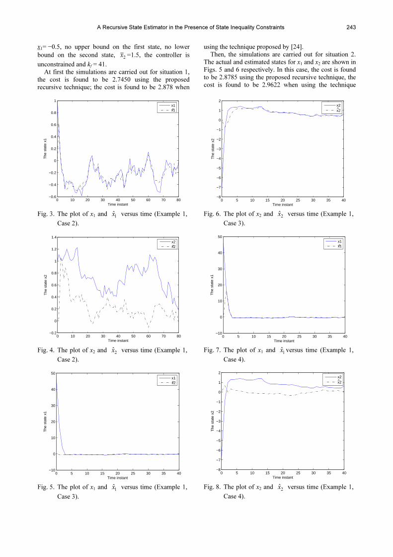
x1= −0.5, no upper bound on the first state, no lower

bound on the second state, 2x =1.5, the controller is

unconstrained and kf = 41.

At first the simulations are carried out for situation 1,

the cost is found to be 2.7450 using the proposed

recursive technique; the cost is found to be 2.878 when

using the technique proposed by [24].

Then, the simulations are carried out for situation 2.

The actual and estimated states for x1 and x2 are shown in

Figs. 5 and 6 respectively. In this case, the cost is found

to be 2.8785 using the proposed recursive technique, the

cost is found to be 2.9622 when using the technique

0 10 20 30 40 50 60 70 80−0.6

−0.4

−0.2

0

0.2

0.4

0.6

0.8

1

Time instant

The

sta

te x

1

x1x1̂

Fig. 3. The plot of x1 and 1̂x versus time (Example 1,

Case 2).

0 10 20 30 40 50 60 70 80−0.2

0

0.2

0.4

0.6

0.8

1

1.2

1.4

Time instant

The

sta

te x

2

x2x2̂

Fig. 4. The plot of x2 and 2x̂ versus time (Example 1,

Case 2).

0 5 10 15 20 25 30 35 40−10

0

10

20

30

40

50

Time instant

The

sta

te x

1

x1x2^

Fig. 5. The plot of x1 and 1̂x versus time (Example 1,

Case 3).

0 5 10 15 20 25 30 35 40−8

−7

−6

−5

−4

−3

−2

−1

0

1

2

Time instant

The

sta

te x

2

x2x2̂

Fig. 6. The plot of x2 and 2x̂ versus time (Example 1,

Case 3).

0 5 10 15 20 25 30 35 40−10

0

10

20

30

40

50

Time instant

The

sta

te x

1

x1x1̂

Fig. 7. The plot of x1 and 1̂x versus time (Example 1,

Case 4).

0 5 10 15 20 25 30 35 40−8

−7

−6

−5

−4

−3

−2

−1

0

1

2

Time instant

The

sta

te x

2

x2x2^

Fig. 8. The plot of x2 and 2x̂ versus time (Example 1,

Case 4).

Mohamed Fahim Hassan, Mohamed Zribi, and Hamed M. K. Alazemi

244

proposed by [24].

Case 4: Simulations using the fourth set of param-

eters In this case, we let x(0)= [46.0825 -7.0175]T, H=[1 0],

x1= −0.5, no upper bound on the first state, no lower

bound on the second state, 2x =1.5, the controller is

unconstrained and kf = 41.

At first the simulations are carried out for situation 1,

the cost is found to be 6.6464 using the proposed

recursive technique; the cost is found to be 8.911 when

using the technique proposed by [24].

Then, the simulations are carried out for situation 2.

The actual and estimated states for x1 and x2 are shown in

Figs. 7 and 8 respectively. In this case, the cost is found

to be 6.712 using the proposed recursive technique, the

cost is found to be 9.2528 when using the technique

proposed by [24].

6.2. A practical example

In this example, we consider a practical system in

which it is desired to control the pollution levels in the

two reach river system given in [9] and [20]:

102 2

0min min ( ) ( )d Q RJ x t x u t dt

= || − || + || ||∫ (56)

subject to:

1 32 0 0 0

0 32 1 2 0 0( ) ( )

0 9 0 1 32 0

0 0 5 0 32 1 2

0 1 0 5 35

0 0 10 9( ) ( ),

0 0 1 4 19

0 0 1 9

x t x t

u t w t

− . − . − . = . − .

. − . − .

. . . + + + . .

.

�

(57)

0 1 0 0( ) ( ) ( ),

0 0 0 1y t x t v t

= +

(58)

where the state variables x1(t) and x3(t) represent the

concentrations of the BOD in mg/l; the states x2(t) and

x4(t) are the concentrations of the DO in mg/l and the

vector containing the desired values of the state variables

is xd = [4.068 5.946]T. Also, u=[u1 u2]T is the deviation of

the waste water treatment from the nominal values.

The weighting matrices of the cost functions are

chosen such that Q=I4 and R=I4 where I4 is the 4 by 4

identity matrix; E[x(0)xT(0)]=P(0)=I4.The vectors w(t)

and v(t) are zero mean uncorrelated white Gaussian noise

vectors at the input and the output of the system with

covariances E[w(t) wT(t)]=5I4 and E[v(t) vT(t)]=I2.

To maintain the ecological balance of the system

while maintaining the cost of waste water treatment

within reasonable limits, the following constraints are

imposed on the system given by equations (56)-(58):

3( ) 6 5 mg l,x t ≤ . / (59)

( ) 25.u t ≥ − (60)

In order to implement the technique developed in this

paper, the problem given by equations (56)-(58) is

discretized using a first order approximation (Euler’s

method) with a sampling period ∆T=0.1 day. Figs. 9 to

12 depict the actual and estimated states of the system. It

is clear from Fig. 11 that the estimated trajectory 3x̂

satisfies the constraints imposed on the system.

Fig. 9. The plot of x1 and 1̂x vs time (Example 2).

Fig. 10. The plot of x2 and 2x̂ vs time (Example 2).

Fig. 11. The plot of x3 and 3x̂ vs time (Example 2).

A Recursive State Estimator in the Presence of State Inequality Constraints

245

Fig. 12. The plot of x4 and 4x̂ vs time (Example 2).

6.3. Comments on the simulation results

1) It is noticed that in most of our simulation results,

the difference between the two estimation costs is not

very large. This is simply due to the fact that the

constrained estimators did not hit the constraints except

in only few points. However, when the estimators reach

the constraints in a reasonable number of points (as in

case 4 of the first example when the the set of parameters

4 is used), the difference in the cost between the two

techniques is significant. It is natural to expect that the

two techniques will lead to the same value of the cost

function if the estimators did not hit the constraints

during the estimation period.

2) The results obtained from the recursive estimator is

optimal since Kalman filtering gains are based on the

actual covariance matrices resulting from the constrained

Kalman filter rather than the unconstrained Kalman filter

as proposed by [24].

7. CONCLUSION

The paper deals with the design of a recursive

estimator to estimate the states of linear dynamic system

in the presence of state inequality constraints. The

developed algorithm distinguishes between the case

when the constraints are strictly satisfied and the case

when some of the constraints are violated. The usual

Kalman filter is used when the constraints are strictly

satisfied. However, when some of the constraints are

violated, the proposed algorithm uses a series of

successive orthogonalizations on the measurement

subspaces to obtain the optimal estimate.

It is found that the proposed estimator has several

attractive properties. The constrained estimator has a

smaller covariance than the corresponding unconstrained

estimator. Also, the proposed estimator is an unbiased

estimator. In addition, when using the proposed estimator,

the value of the cost function is less than that obtained if

the covariance matrix of the unconstrained estimator is

always used to estimate the constrained one.

The proposed estimator is illustrated through

simulation results of a numerical example and a practical

example. The simulation results indicate that the

proposed estimator works well.

Future work will address the application of the

proposed recursive estimator to some real life problems

such that data transmission over networks.

APPENDIX A: PROOF OF LEMMA 1

The general filtered state estimator when a subset of

the state vector violates the constraints imposed on the

system is given by:

ˆ( 1 1) [ ( 1) ( 1)],a

x k k x k Y k+ | + = + | +E (61)

where

( )

( 1) ( 1)

( 1)

a

Y k

Y k y k

d k

+ = + . +

(62)

Equation (61) can be written in the form:

( 1) ( ) ( 1)ˆ( 1 1) .

( 1)

x k Y k y kx k k

d k

+ | , + , + | + = +

E (63)

Using Theorem 2, we can write,

( 1) ( ) ( 1)ˆ( 1 1) ,

( 1 1)

x k Y k y kx k k

d k k

+ | , + , + | + =

+ | + E

� (64)

where

( 1) ( )( 1 1) ( 1)

( 1)

d k Y kd k k d k

y k

+ | , + | + = + − . +

E� (65)

Now, since ( 1 1)d k k+ | +� is orthogonal to the

subspace generated by the measurement vector Y(k +1),

where YT(k +1)=[YT(k) yT(k +1)], then, it is possible to

write (64) in the form:

ˆ( 1 1) [ ( 1) ( ) ( 1)]

[ ( 1) ( 1 1)].

x k k x k Y k y k

x k d k k

+ | + = + | , +

+ + | + | +

E

E � (66)

Moreover, let

( 1 ) ( 1) [ ( 1) ( )].y k k y k y k Y k+ | = + − + |E� (67)

Again, since ỹ (k+1 | k) is orthogonal to the subspace

generated by the measurement vector Y(k), equation (66)

can take the following form:

ˆ( 1 1) [ ( 1) ( )]

[ ( 1) ( 1 )]

[ ( 1) ( 1 1)].

x k k x k Y k

x k y k k

x k d k k

+ | + = + |

+ + | + |

+ + | + | +

E

E

E

�

�

(68)

The first two terms in the right half of (68) correspond

to the optimal filtered estimate of the unconstrained state

variables. Denoting this estimate by 1( 1 1),ˆ k kx + | +

then using (68) we can write,

1ˆ ˆ( 1 1) ( 1 1)

[ ( 1) ( 1 1)],E

x k k x k k

x k d k k

+ | + = + | +

+ + | + | +� (69)

Mohamed Fahim Hassan, Mohamed Zribi, and Hamed M. K. Alazemi

246

where 1̂( 1 1)x k k+ | + and its associated predicted esti-

mator 1̂( 1 ),x k k+ | covariance matrices

1 1( 1 ),

x xP k k+ |� �

1 1( 1 1)

x xP k k+ | +� �

and K1(k +1) are as given by equations

(23)-(33) while replacing x by x1.

Now, we consider the impact of the second term in

(69) which reflects the effects of the saturated constraints

on the optimal filter estimator. Let ( 1 1)d k k+ | +� be

such:

ˆ( 1 1) ( 1) ( 1 1),d k k d k d k k+ | + = + − + | +� (70)

where

ˆ( 1 1) [ ( 1) ( ) ( 1)]

[ ( 1) ( ) ( 1 )]

d k k d k Y k y k

d k Y k y k k

+ | + = + | , +

= + | , + |

E

E �

(71)

1

[ ( 1) ( 1) ( ) ( 1 )]

( 1) ( 1 1)ˆ

D k x k Y k y k k

D k k kx

= + + | , + |

= + + | + .

E �

Let 1 1̂( 1 1) ( 1) ( 1 1).x k k x k x k k+ | + = + − + | +� Using

(70), the fact that ( 1) ( 1) ( 1)d k D k x k+ = + + and (71),

we obtain,

1

1

( 1 1) ( 1) ( 1)

ˆ( 1) ( 1 1)

( 1) ( 1 1)

d k k D k x k

D k x k k

D k x k k

+ | + = + +

− + + | +

= + + | + .

�

�

(72)

Now,

1

[ ( 1) ( 1 1)]

( 1 1) ( 1 1) ( 1 1),xd dd

x k d k k

P k k P k k d k k−

+ | + | +

= + | + + | + + | +

E

� � �

�

� (73)

where

1 1

11

1

( 1 1) [ ( 1) ( 1 1)]

ˆ[( ( 1 1) ( 1))

( ( 1 1) ( 1))]

( 1 1) ( 1)

T

xd

T T

T

x x

P k k x k k kd

x k k kx

x k k D k

P k k D k

+ | + = + + | +

= + | + + +

+ | + +

= + | + + .

E

E

�

� �

�

�

�

(74)

Similarly,

1 1

( 1 1) [ ( 1 1) ( 1 1)]

( 1) ( 1 1) ( 1).

T

dd

T

x x

P k k d k k k kd

D k P k k D k

+ | + = + | + + | +

= + + | + +

E� �

� �

� �

(75)

Using equations (72)-(75), equation (69) leads to,

1

2

ˆ ˆ( 1 1) ( 1 1)

K ( 1) ( 1 1)

x k k x k k

k d k k

+ | + = + | +

+ + + | +� (76)

where

1

2K ( 1) ( 1 1) ( 1 1)

xd ddk P k k P k k

−+ = + | + + | + .� � � (77)

Recall that:

ˆ( 1 1) ( 1) ( 1 1)x k k x k x k k+ | + = + − + | + .� (78)

Therefore, by using equation (76) we can write,

1 2

1 2

( 1 1)

ˆ( 1) ( 1 1)

( 1) ( 1 1) K ( 1) ( 1 1)ˆ

( 1 1) K ( 1) ( 1 1)

x k k

x k x k k

x k k k k d k kx

x k k k d k k

+ | +

= + − + | +

= + − + | + − + + | +

= + | + − + + | + .

�

�

��

(79)

Also,

1 2

1 2

( 1 1)

[ ( 1 1) ( 1 1)]

( ( 1 1) K ( 1) ( 1 1))

.( ( 1 1) K ( 1) ( 1 1))

xx

T

T

P k k

x k k k kx

k k k d k kx

x k k k d k k

+ | +

= + | + + | +

= + | + − + + | +

× + | + − + + | +

E

E

� �

� �

��

��

(80)

After simple mathematical manipulation, this leads to:

1 1

2( 1 1) [ K ( 1) ( 1)]

( 1 1)

xx

x x

P k k I k D k

P k k

+ | + = − + +

× + | + .

� �

� �

(81)

Then, the estimator will proceed to the next discrete

instant of time.

REFERENCES

[1] L. Chia, D. Simon, and H. J. Chizeck, “Kalman

filtering with statistical state constraints,” Control

and Intelligent Systems, vol. 34, no. 1, pp. 73-79,

2006.

[2] T. Chia, P. Chow, and H. Chizek, “Recursive para-

meter identification of constrained systems: an ap-

plication to electrically stimulated muscle,” IEEE

Trans. on Biomedical Engineering, vol. 38, no. 5,

pp. 429-441, 1991.

[3] H. E. Doran, “Constraining Kalman filter and

smoothing estimates to satisfy time-varying restric-

tions,” Rev. Econom. Statist., vol. 74, no. 3, pp.

568-572, 1992.

[4] J. D. Geeter, H. V. Brussel, and J. De Schutter, “A

smoothly constrained Kalman filter,” IEEE Trans.

Pattern Anal. Machine Intell., vol. 19, no. 10, pp.

1171-1177, 1997.

[5] N. Gupta and R. Hauser, “Kalman filtering with

equality and inequality state constraints,” http://

arxiv.org/abs/0709.2791, 2007.

[6] M. F. Hassan and A. K. Ali, “A coordinating ap-

proach for the solution of discrete linear servo-

mechanism problem with constraints,” Asian Jour-

nal of Control, vol. 10, no. 4, pp. 478-494, 2008.

[7] M. F. Hassan, G. Salut, M. G. Singh, and A. Titli,

“A new decentralized filter for large scale intercon-

nected dynamical system,” IEEE Trans. on Auto-

matic Control, vol. 23, no. 2, pp. 262-268, 1978.

[8] N. Haverbeke, B. Pluymers, and B. De Moor,

“Constrained state estimation: a critical evalua-

tion,” Proc. of 25th Benelux Meeting on Systems

and Control, The Netherlands, March 13-15, 2006.

[9] M. F. Hassan, “Water quality simulation and con-

trol in streams,” Encyclopedia of Environmental

A Recursive State Estimator in the Presence of State Inequality Constraints

247

Control Chronology, vol. 13, Waste Water Treat-

ment Technology, Gulf Publicity Company, pp. 77-

138, 1989.

[10] M. F. Hassan and H. T. Attia, “Stream quality con-

trol via a constrained nonlinear time-delay model,”

Journal of Mathematical Control Science and Ap-

plications, vol. 12, no. 1, pp. 23-34, 2008.

[11] M. F. Hassan, A. A, Abouelsoud, and H. M. Soli-

man, “Constrained load-frequency control,” Elec-

tric Power Components and Systems, vol. 36, pp.

266-275, 2008.

[12] S. Hayward, “Constrained Kalman filter for least-

squares estimation of time-varying beam forming

weights,” Mathematics in Signal Processing IV,

Oxford University Press, pp. 113- 125, 1998.

[13] C. V. Hollot, V. Misra, D. Towsley, and W. Gong,

“Analysis and design of controllers for AQM rou-

ters supporting TCP flows,” IEEE Trans. on Auto-

matic Control, vol. 47, no. 6, pp. 545-559, 2002.

[14] S. Julier and J. LaViola, “On Kalman filtering with

nonlinear equality constraints,” IEEE Trans. on

Signal Processing, vol. 55, no. 6, pp. 2774-2784,

2007.

[15] S. Julier and J. Uhlmann, “Unscented filtering and

nonlinear estimation,” Proc. of the IEEE, vol. 92,

no. 3, pp. 401-422, 2004.

[16] S. Ko and R. Bitmead, “State estimation for linear

systems with state equality constraints,” Automati-

ca, vol. 43, no. 8, pp. 1363-1368, 2007.

[17] S. Kolas, B. A. Foss, and T. S. Schei, “Constrained

nonlinear state estimation based on the UKF ap-

proach,” Computers and Chemical Engineering,

vol. 33, pp. 1386-1401, 2009.

[18] D. Luenberger, Optimization by Vector Space Me-

thods, Wiley, New York, 1969.

[19] K. Mahata and T. Soderstrom, “Improved estima-

tion performance using known linear constraints,”

Automatica, vol. 40, no. 8, pp. 1307-1318, 2004.

[20] M. S. Mahmoud, M. F. Hassan, and M. G. Darwish,

Large Scale Control Systems: Theories and Tech-

niques, Marcel Dekker Inc, New York and Basel,

1985.

[21] D. Massicotte, R. Morawski, and A. Barwicz, “In-

corporation of positivity constraint into a Kalman-

filter-based algorithm for correction of spectrome-

tric data,” IEEE Trans. on Instrumentation and

Measurement, vol. 46, no. 1, pp. 2-7, 1995.

[22] J. Porrill, “Optimal combination and constraints for

geometrical sensor data,” International Journal of

Robotics Research, vol. 7, no. 6, pp. 66-77, 1988.

[23] C. Rao, J. Rawlings, and D. Mayne, “Constrained

state estimation for nonlinear discrete time systems:

Stability and moving horizon approximations,”

IEEE Trans. on Automatic Control, vol. 48, no. 2,

pp. 246-258, 2003.

[24] D. Simon and T. Chia, “Kalman filtering with state

equality constraints,” IEEE Trans. on Aerospace

and Electronic Systems, vol. 38, no. 1, pp. 128-136,

2002.

[25] D. Simon and D. L. Simon, “Kalman filtering with

inequality constraints for turbofan engine health es-

timation,” IEE Proceedings - Control Theory and

Applications, vol. 153, no. 3, pp. 371-378, 2006.

[26] B. Teixeira, J. Chandrasekar, H. Palanthandalam-

Madapusi L. Aguirre, L. Torres, L. Aguirre, and D.

Bernstein, “Gain-constrained Kalman filtering for

linear and nonlinear systems,” IEEE Trans. on Sig-

nal Processing, vol. 56, no. 9, pp. 4113-4123, 2008.

[27] P. Vachhani, R. Rengaswamy, V. Gangwal, and S.

Narasimhan, “Recursive estimation in constrained

nonlinear dynamical systems,” AIChE Journal, vol.

51, no. 3, pp. 946-959, 2005.

[28] P. Vachhani, S. Narasimhan, and R. Rengaswamy,

“Robust and reliable estimation via unscented re-

cursive nonlinear dynamic data reconciliation,”

Journal of Process Control, vol. 16, no. 10, pp.

1075-1086, 2006.

[29] L. Wang, Y. Chiang, and F. Chang, “Filtering me-

thod for nonlinear systems with constraints,” IEE

Proceedings - Control Theory and Applications, vol.

149, no. 6, pp. 525-531, 2002.

[30] W. Wen and H. Durrant-Whyte, “Model-based mul-

ti-sensor data fusion,” Proc. of IEEE International

Conference on Robotics and Automation, Nice,

France, pp. 1720-1726, 1992.

[31] C. Yang and E. Blasch, “Kalman filtering with non-

linear state constraints,” Proc. of the 9th Interna-

tional Conference on Information Fusion, Seattle,

WA, pp. 1-8, 2006.

Mohamed Fahim Hassan was born in

Cairo, Egypt on June 21, 1947. He

received his B.Sc. and M.Sc. degrees in

Electrical Engineering from Cairo

University, Faculty of Engineering, Cairo,

Egypt in 1970 and 1973 respectively, and

his D.Sc. (Doctor d’Etat) in Systems

Science and Automatic Control from

Paul Sabatier University, Toulouse,

France in 1978. He has been a faculty member in Electronics

and Communication Department, Faculty of Engineering, Cairo

University since 1978 till now where he held the positions of

Assistant Professor from 1978 to 1983, Associate Professor

from 1983 to 1988 and Professor from 1988 till now. Currently

he is on leave from Cairo University and joined Kuwait

University where he is a Professor of Control Engineering in

College of Engineering and Petroleum. Prof. Hassan was also

the Coordinator and Assistant Director of the Computer

Education Program, Department of Public Service, The

American University in Cairo from 1985 to 1994. He was the

recipient of many outstanding research prizes and medals from

Egypt and USA. His research activities are in the areas of large

scale systems, optimization theory, stochastic control theory,

estimation theory and adaptive control. In addition to that, he

supervised many projects sponsored by Egyptian government

and US- Aid. Prof Hassan is a co-author of one book, author of

many book chapters and encyclopedia chapters. Moreover, he

is an author and co-author of more than 150 technical papers in

most of the international journals and conferences. Prof.

Hassan is a reviewer of many international journals and

conferences.

Mohamed Fahim Hassan, Mohamed Zribi, and Hamed M. K. Alazemi

248

Mohamed Zribi obtained his B.S. de-

gree in Electrical Engineering (Magna

Cum Laude Honors) in 1985 from the

University of Houston, Houston, Texas.

He received his M.S.E.E and Ph.D. de-

grees in Electrical Engineering in 1987

and 1992 from Purdue University, West

Lafayette, Indiana. He held a faculty

position in the School of Electrical Engi-

neering, Nanyang Technological University, Singapore from

1992 till 1998. He is currently a professor in the Electrical En-

gineering Department, College of Engineering & Petroleum,

Kuwait University. His research interests are in nonlinear con-

trol, adaptive control, control applications and robotics.

Hamed M. K. Alazemi received his

B.Sc. and M.S. degrees in Electrical

Engineering from Washington University

(Saint Louis) in 1992 and 1994

respectively, and his Ph.D. degree from

the University of Washington (Seattle) in

2000. He is currently an associate

professor at the Computer Engineering

Department at Kuwait University where

his research interests include analysis/design of Computer

communication network. His recent research emphasis includes

control and communication design, routing in WDM networks

and stochastic performance evaluation and combinatorial

optimization.