MLESAC: A new robust estimator with applicationto estimating image geometry

P. H. S. Torry and A. Zissermanzy Microsoft Research Ltd,St George House, 1 Guildhall St,

Cambridge CB2 3NH, UKphiltorr@microsoft.com

andz Robotics Research Group, Department of Engineering ScienceOxford University, OX1 3PJ., UK

az@robots.ox.ac.uk

Received March 31, 1995; accepted July 15, 1996

A new method is presented for robustly estimating multiple view relations from

point correspondences. The method comprises two parts, thefirst is a new robust

estimatorMLESAC which is a generalization of theRANSAC estimator. It

adopts the same sampling strategy asRANSAC to generate putative solutions, but

chooses the solution to maximize the likelihood rather thanjust the number of in-

liers. The second part to the algorithm is a general purpose method for automatically

parametrizing these relations, using the output ofMLESAC. A difficulty with multi

view image relations is that there are often non-linear constraints between the param-

eters, making optimization a difficult task. The parametrization method overcomes

the difficulty of non-linear constraints and conducts a constrained optimization. The

method is general and its use is illustrated for the estimation of fundamental matri-

ces, image-image homographies and quadratic transformations. Results are given

for both synthetic and real images. It is demonstrated that the method gives results

equal or superior to previous approaches.

1. INTRODUCTION

This paper describes a new robust estimatorMLESAC which can be used in a widevariety of estimation tasks. In particularMLESAC is well suited to estimating complexsurfaces or more general manifolds from point data. It is applied here to the estimation ofseveral of the multiple view relations that exist between images related by rigid motions.These are relations between corresponding image points in two or more views and includefor example, epipolar geometry, projectivities etc. Theseimage relations are used forseveral purposes: (a) matching, (b) recovery of structure [1, 8, 11, 27, 40] (if this ispossible), (c) motion segmentation [31, 36], (d) motion model selection [14, 37, 35].

The paper is organized as follows: In Section 2 the matrix representation of the two viewrelations are given, including the constraints that the matrix elements must satisfy. Forexample, there is a cubic polynomial constraint on the matrix elements for the fundamental

1

matrix. It will be seen that any parametrization must enforce this constraint to accuratelycapture the two view geometry.

Due to the frequent occurrence of mismatches, a RANSAC [4] like robust estimatoris used to estimate the two view relation. The RANSAC algorithm is a hypothesis andverify algorithm. It proceeds by repeatedly generating solutions estimated from minimalset of correspondences gathered from the data, and then tests each solution for supportfrom the complete set of putative correspondences.RANSAC is described in Section 4.In RANSAC the support is thenumberof correspondences with error below a giventhreshold. We propose a new estimator that takes as support the log likelihood of thesolution (taking into account the distribution of outliers) and uses random sampling tomaximize this. This log likelihood for each relation is derived in Section 3. The new robustrandom sampling method (dubbed MLESAC—Maximum LikelihoodEstimation SAmpleConsensus) is adumbrated in Section 5.

Having obtained a robust estimate using MLESAC, the minimumpoint set basis canbe used to parametrize the constraint as described in Section 6. The MLE error is thenminimized using this parametrization and a suitable non-linear minimizer. The optimizationis constrained because the matrix elements of many of the twoview relations must satisfycertain constraints. Note that relations computed from this minimal set always satisfy theseconstraints. Thus the new contribution is three fold: (a) toimprove RANSAC by use of abetter cost function; (b) to develop this cost function in terms of the likelihood of inliersand outliers (thus making it robust); and (c) to obtain a consistent parametrization in termsof a minimal point basis.

Results are presented on synthetic and real images in Section 7. RANSAC is compared toMLESAC, and the new point based parametrization is comparedto other parametrizationsthat have been proposed which also enforce the constraints on the matrix elements.

Notation. The image of a 3D scene pointX is x in the first view andx0in the second,

wherex andx0are homogeneous three vectors,x = (x; y; 1)>. The correspondencex $ x0 will also be denoted asx1 $ x2. Throughout, underlining a symbolx indicates

the perfect or noise-free quantity, distinguishing it fromx = x+�x, which is the measuredvalue corrupted by noise.

2. THE TWO VIEW RELATIONS

Within this section the possible relations on the motion of points between two views aresummarized, three examples are considered in detail: (a) the Fundamental matrix [3, 10],(b) the planar projective transformation (projectivity),(c) the quadratic transformation. Allthese two view relations are estimable from image correspondences alone.

The epipolar constraint is represented by the Fundamental matrix [3, 10]. This relationapplies for general motion and structure with uncalibratedcameras. Consider the movementof a set of point image projections from an object which undergoes a rotation and non-zero translation between views. After the motion, the set ofhomogeneous image pointsfxig; i = 1; : : : n; as viewed in the first image is transformed to the setfxi0g in the secondimage, with the positions related byx0>i Fxi = 0 (1)

wherex = (x; y; 1)> is a homogeneous image coordinate andF is the Fundamental Matrix.

Should all the observed points lie on a plane, or the camera rotate about its optic axisand not translate, then all the correspondences lie on a projectivity:x0 = Hx : (2)

Should all the points be consistent with two (or more)F thenx0>F1x = 0 and x0>F2x = 0 (3)

thus x0 = F1x�F2x (4)

hence they conform to a quadratic transformation. The quadratic transformation is ageneralization of the homography. It is caused by a combination of a camera motionand scene structure, as all the scene points and the camera optic centres lie on acriticalsurface[19], which is a ruled quadric surface. Although the existence of the criticalsurface is well known, little research has been put into effectively estimating quadratictransformations.

2.1. Degrees of Freedom within Two View ParametrizationsThe fundamental matrix has 9 elements, but only 7 degrees of freedom. Thus if the

fundamental matrix is parametrized by the elements of the3 � 3 matrix F it is overparametrized. This is because the matrix elements are not independent, being related bya cubic polynomial in the matrix elements, such thatdet[F] = 0. If this constraint is notimposed then the epipolar lines do not all intersect in a single epipole [16]. Hence it isessential that this constraint is imposed.

The projectivity has 9 elements and 8 degrees of freedom as these elements are onlydefined up to a scale. The quadratic transformation has 18 elements and 14 degreesof freedom [18]. Here if the constraints between the parameters are not enforced theestimation process becomes very unstable, and good resultscannot be obtained [18],whereas our method has been able to accurately estimate the constraint.

2.2. Concatenated or Joint Image Space

Each pair of corresponding pointsx, x0defines a single point in a measurement spaceR4, formed by considering the coordinates in each image. This space is the ‘joint image

space’ [38] or the ‘concatenated image space’ [24]. It mightbe considered somewhateldritch to join the coordinates of the two images into the same space, but this makes senseif we assume that the data are perturbed by the same noise model (discussed in the nextsubsection) in each image, implying that the same distance measure for minimization maybe used in each image. The image correspondencesfxig $ fx0ig; i = 1; : : : n; induced bya rigid motion have an associated algebraic varietyV in R4. Fundamental matrices definea three dimensional variety inR4, whereas projectivities and quadratic transformations areonly two dimensional.

Given a set of correspondences the (unbiased) minimum variance solution forF is thatwhich minimizes the sum of squares of distances orthogonal to the variety from each point(x; y; x0 ; y0) inR4 [12, 14, 15, 21, 23, 26, 35]. This is directly equivalent to the reprojectionerror of the back projected 3D projective point.

x

x x’

x’H-1

H

zz’

z’ = H z

H x’ H x-1

FIGURE 1

In previous work such as [17] the transfer error has often been used as the error functione.g. for fittingH this is d2 �x;H�1x0�+ d2 �x0 ;Hx� (5)

whered() is the Euclidean image distance between the points. The transfer distance isdifferent from the orthogonal distance as shown in Figure 1.This is discussed further inrelation to the maximum likelihood solution derived in Section 3.

3. MAXIMUM LIKELIHOOD ESTIMATION IN THE PRESENCE OFOUTLIERS

Within this section the maximum likelihood formulation is given for computing any ofthe multiple view relations. In the following we make the assumption, without loss ofgenerality, that the noise in the two images is Gaussian on each image coordinate with zeromean and uniform standard deviation�. Thus given a true correspondence the probabilitydensity function of the noise perturbed data isPr(DjM) = Yi=1:::n� 1p2���n e��Pj=1;2(xji�xji )2+(yji�yji )2�=(2�2) ; (6)

wheren is the number of correspondences andM is the appropriate 2 view relation, e.g. thefundamental matrix or projectivity, andD is the set of matches. The negative log likelihoodof all the correspondencesx1;2i , i = 1::n :� Xi=1:::n log(Pr(x1;2i jM; �)) = Xi=1:::n Xj=1;2 �(xji � xji )2 + (yji � yji )2� ; (7)

discounting the constant term. Observing the data, we inferthat the true relationMminimizes this log likelihood. This inference is called “Maximum Likelihood Estimation”.

Given two views with associated relation for each correspondencex1;2 the task becomesthat of finding the maximum likelihood estimate,x1;2 of the true positionx1;2, such thatx1;2 satisfies the relation and minimizes

Pj=1;2 �xji � xji�2 + �yji � yji�2. The MLE

errorei for theith point is thene2i = Xj=1;2 �xji � xji�2 + �yji � yji�2 (8)

ThusPi=1:::n e2i provides the error function for the point data, andM for which

Pi e2iis a minimum is the maximum likelihood estimate of the relation (fundamental matrix, orprojectivity). Hartley and Sturm [12] show howe, x andx0

may be found as the solutionof a degree 6 polynomial. A computationally efficient first order approximation to these isgiven in Torret al. [32, 34, 35].

The above derivation assumes that the errors are Gaussian, often however features aremismatched and the error onm is not Gaussian. Thus the error is modeled as a mixturemodel of Gaussian and uniform distribution:-Pr(e) = � 1p2��2 exp(� e22�2 ) + (1� )1v� (9)

where is the mixing parameterandv is just a constant (the diameter of the search window),� is the standard deviation of the error on each coordinate. Tocorrectly determine andv entails some knowledge of the outlier distribution; here itis assumed that the outlierdistribution is uniform, with� v2 :: + v2 being the pixel range within which outliers areexpected to fall (for feature matching this is dictated by the size of the search window formatches). Therefore the error minimized is the negative loglikelihood:�L = �Xi log � 1p2���n exp � Xj=1;2(xji � xji )2 + (yji � yji )2! =(2�2) + (1� ) 1v!! :

(10)

Given a suitable initial estimate there are several ways to estimate the parameters of themixture model, most prominent being theEM algorithm [2, 20], but gradient descentmethods could also be used. Because of the presence of outliers in the data the standardmethod of least squares estimation is often not suitable as an initial estimate, and it is betterto use a robust estimate such asRANSAC which is described in the next section.

4. RANSACThe aim is to be able to compute all these relations from imagecorrespondences over

two views. This computation requires initial matching of points (corners) over the imagepairs. Corners are detected to sub-pixel accuracy using theHarris corner detector [9].Given a corner at position(x; y) in the first image, the search for a match considers allcorners within a region centred on(x; y) in the second image with a threshold on maximumdisparity. The strength of candidate matches is measured bysum of squared differences inintensity. The threshold for match acceptance is deliberately conservative at this stage tominimise incorrect matches. Because the matching process is only based on proximity andsimilarity, mismatches will often occur. These are sufficient to render standard least squaresestimators useless. Consequently robust methods must be adopted, which can provide agood estimate of the solution even if some of the data are mismatches (outliers).

Potentially there are a significant number of mismatches amongst the initial matches.Correct matches will obey the epipolar geometry. The aim then is to obtain a set of “inliers”

consistent with the epipolar geometry using a robust technique. In this case “outliers” areputative ‘matches’ inconsistent with the epipolar geometry. Robust estimation by randomsampling (such asRANSAC) has proven the most successful [4, 30, 39].

First we describe the application of RANSAC to the estimation of the fundamentalmatrix. Putative fundamental matrices (up to three real solutions) are computed fromrandom sets of seven corner correspondences (the minimum number required to computea fundamental matrix). The fundamental matrices may be estimated from seven points byforming the data matrix:Z = 264 x01x1 x01y1 x01 y01x1 y01y1 y01 x1 y1 1

......

......

......

......x07x7 x07y7 x07 y07x7 y07y7 y07 x7 y7 1 375 : (11)

The solution forF can be obtained from the two dimensional nullspace ofZ. Let f1 andf2 be obtained from the two right hand singular vectors ofZ with singular values of zero,thus they form an orthogonal basis for the null space. LetU1 andU2 be the3� 3 matricescorresponding tof 1 andf2. Then the three fundamental matricesFl, l = 1; 2; 3 consistentwithZ can be obtained fromFl = �U1+(1��)U2, subject to a scaling and the constraintdet[F] = 0 (which gives a cubic in� from which 1 or 3 real solutions are obtained). Thesupport for this fundamental matrix is determined by the number of correspondences inthe initial match set with errore (given in (8)) below a thresholdT . The error used is thenegative log likelihood which is derived in the last section. If there are three solutions, theneach is tested for support. This is repeated for many random sets, and the fundamentalmatrix with the largest support is accepted. The output is a set of corner correspondencesconsistent with the fundamental matrix, and a set of mismatches (outliers).

For projectivities each correspondence provides two constraints on the parameters:v>1 h = 0 and v>2 h = 0 (12)

where v1 = � x y 1 0 0 0 �xx0 �yx0 �x0 �v2 = � 0 0 0 x y 1 �xy0 �yy0 �y0 �andh is the corresponding vector of the elements ofH. Thus four points may be used

to find an exact solution.RANSAC proceeds in much the same manner, with minimalsets of four correspondences being randomly selected, and each set generating a putativeprojectivity. The support for each set is measured by calculating the negative log likelihoodfor all the points in the initial match set, and counting the number of correspondenceswith error below a certain threshold determined by consideration of the inlier and outlierdistributions.

To estimate a quadratic transformation from seven correspondences the method used forgenerating fundamental matrices is modified. A critical surface is a ruled quadric passingthrough both camera centres. Seven correspondences define aquadric through the cameracentres. If it is ruled then there will be three real fundamental matricesF1, F2 andF3formed from the design matrixZ given in (11) of the seven points. These matrices can beused to generate the critical surface. In this case, any two of the fundamental matrices may

be combined to give the quadratic transformation by using Equation (4) (it does not matterwhich two as any pair gives the same result as any other pair).If only one solution is realthen another sample can be taken.

How many samples should be used?.Ideally every possible subsample of the data wouldbe considered, but this is usually computationally infeasible, so an important question ishow many subsamples of the data set are required for statistical significance. Fischler andBolles [4] and Rousseeuw and Leroy [22] proposed slightly different means of calculation,but each proposition gives broadly similar numbers. Here wefollow the latter’s approach.The numberm of samples is chosen sufficiently high to give a probability� in excess of95% that a good subsample is selected. The expression for this probability� is� = 1� (1� (1� �)p)m; (13)

where� is the fraction of contaminated data, andp the number of features in each sample.Generally it is better to take more samples than are needed assome samples might bedegenerate. It can be seen from this that, far from being computationally prohibitive, therobust algorithm may require fewer repetitions than there are outliers, as it is not directlylinked to the number but only the proportion of outliers. It can also be seen that the smallerthe data set needed to instantiate a model, the fewer samplesare required for a given level ofconfidence. If the fraction of data that is contaminated is unknown, as is usual, an educatedworst case estimate of the level of contamination must be made in order to determine thenumber of samples to be taken, this can be updated as larger consistent sets are foundallowing the algorithm to “jump out” ofRANSAC e.g. if the worst guess is50% and aset with80% inliers is discovered, then� could be reduced from50% to 20%. Generally,assuming no more than50% outliers then 500 random samples is more than sufficient.

5. THE ROBUST ESTIMATOR: MLESACTheRANSAC algorithm has proven very successful for robust estimation, but having

defined the robust negative log likelihood function�L as the quantity to be minimized itbecomes apparent thatRANSAC can be improved on.

One of the problems withRANSAC is that if the thresholdT for considering inliers isset too high then the robust estimate can be very poor. Consideration ofRANSAC showsthat in effect it finds the minimum of a cost function defined asC =Xi � �e2i � (14)

where�() is �(e2) = � 0 e2 < T 2constant e2 � T 2 : (15)

In other words inliers score nothing and each outlier scoresa constant penalty. Thus thehigherT 2 is the more solutions with equal values ofC tending to poor estimation e.g. ifTwere sufficiently large then all solutions would have the same cost as all the matches wouldbe inliers. In Torr and Zisserman [34] it was shown that at no extra cost this undesirablesituation can be remedied. Rather than minimizingC a new cost function can be minimizedC2 =Xi �2 �e2i � (16)

where the robust error term�2 is�2(e2) = � e2 e2 < T 2T 2 e2 � T 2 : (17)

This is a simple, redescending M-estimator [13]. It can be seen that outliers are stillgiven a fixed penalty but now inliers are scored on how well they fit the data. We setT = 1:96� so that Gaussian inliers are only incorrectly rejected five percent of the time.The implementation of this new method (dubbedMSAC m-estimator sample consensus)yields a modest to hefty benefit to all robust estimations with absolutely no additionalcomputational burden.Once this is understood there is no reason to useRANSAC inpreference to this method.Similar schemes for robust estimation using random samplingand M-estimators were also proposed in [29] and [25].

The definition of the maximum likelihood error allows us to suggest a further improve-ment overMSAC. As the aim is to minimise the negative log likelihood of the mixture�Lthen it makes sense to use this as the score for each of the random samples. The problemis that the mixing parameter is not directly observed. But given any putative solution forthe parameters of the model it is possible to recover that provides the minimum�L, asthis is a one dimensional search it provides little computational overhead

To estimate , using Expectation Maximization (EM), a set of indicator variables needsto be introduced:�i, i = 1 : : : n, where�i = 1 if the ith correspondence is an inlier, and�i = 0 if the ith correspondence is an outlier. TheEM algorithm proceeds as followstreating the�i as missing data [5]: (1) generate a guess for , (2) estimate the expectationof the �i from the current estimate of , (3) make a new estimate of from the currentestimate of�i and go to step (2). This procedure is repeated until convergence and typicallyrequires only two or three iterations.

In more detail for stage (1) the initial estimate of is 12 . For stage (2) denote the expectedvalue of�i by zi then it follows thatPr(�i = 1j ) = zi. Given an estimate of this can beestimated as: Pr(�i = 1j ) = pipi + po (18)

andPr(�i = 0j ) = 1� zi. Herepi is the likelihood of a datum given that it is an inlier:pi = � 1p2���k exp0@�0@Xj=1;2(xji � xji )2 + (yji � yji )21A =(2�2)1A (19)

andpo is the likelihood of a datum given that it is an outlier:po = (1� )1v : (20)

For stage (3) = 1nXi zi : (21)

This method is dubbedMLESAC (maximum likelihood consensus). For real systems itis sometimes helpful to put a prior on , the expected proportion of inliers, this depends

1. Detect corner features using the Harris corner detector [9].

2. Putative matching of corners over the two images using proximity and cross correlation.

3. Repeat until 500 samples have been taken or “jump out” occursas described in Section 4.

(i) Select a random sample of the minimum number of correspondencesSm = fx1;2i g.

(ii) Estimate the image relationM consistent with this minimal set using the methods described in Section 4.

(iii) Calculate the errorei for each datum.

(iv) ForMSAC calculateC2, or for,MLESAC calculate and hence�L for the relation, as describedin Section 5.

4. Select the best solution over all the samples i.e. that with lowest�L orC2. Store the set of correspondencesSm that gave this solution.

5. Minimize robust cost function over all correspondences, using the point basis provided by the last step as theparametrization, as described in Section 6.

]A brief summary of all the stages of estimation

TABLE 1

[

on the application and is not pursued further here. The two algorithms are summarized inTable 1. The output of MLESAC (as with RANSAC) is an initial estimate of the relation,together with a likelihood that each correspondences is consistent with the relation. Thenext step is to improve the estimate of the relation using a gradient descent method.

6. NON-LINEAR MINIMIZATION

The maximization of the likelihood is a constrained optimisation because a solution forF,Q orH is sought that enforces the relations between the elements of the constraint. Ifa parametrization enforces these constraints it will be termedconsistent. In the followingwe introduce a consistent parametrization and describe variations which result in aminimalparametrization. A minimal parametrization has the same number of parameters as thenumber of independent elements (degrees of freedom) of the constraint. The advantagesand disadvantages of such minimal parametrizations will bediscussed.

The key idea is to use the point basis provided by the robust estimator as the parametriza-tion. For the simplest case, the projectivity, a four point basis is provided. By fixingx; y andvaryingx0; y0 for each correspondence, elements of the projectivity may be parametrized interms of the 4 correspondences and a standard gradient descent algorithm [7] can be con-ducted withx0; y0 as parameters. Note this parametrization has exactly 8 DOF (2 variablesfor each of the 4 correspondences). Another approach is to alter all the 16 coordinates,the non-linear minimization conducted in this higher dimensional parameter space willdiscard extraneous parameters automatically. This approach has the disadvantage that itrequires an increased number of function evaluations as there are more parameters thandegrees of freedom. Similarly, 7 points may be used to encodethe fundamental matrix andthe parameters so encoded are guaranteed to be consistent, i.e. their elements satisfy thenecessary constraints (Sometimes the 7 points may provide three solutions, in which casethe one with lowest error is used). This method of parametrization in term of pointswasfirst proposed in Torr and Zisserman [33].

A number of variations on the free/fixed partition will now bediscussed, as well as con-straints on the direction of movement during the minimisation. In all cases the parametriza-

tion is consistent, but may not be minimal. Although a non-minimal parametrization overparametrizes the image constraint, the main detrimental effects is likely to be the cost ofthe numerical solution and poor convergence properties. The former is one of the measuresused to compare the parametrizations in Section 7.

First the parametrizations forF are described. Given the minimal number of correspon-dences that can encode one of the image relations three coordinates can be fixed and onevaried e.g. we could encodeF by seven correspondences(xi; yi) $ (x0i; y0i) i = 1 : : : 7,by fixing thex; y; x0

coordinates of these correspondences the space ofF is parametrizedby the seveny0

coordinates. This is referred to as parametrizationP1. The parametrizationP1 forH andQ fixesx; y for the minimal basis set and variesx0

, y0. This parametrization

is both minimal and consistent, but the disadvantage forF of this is that should the epipolarlines in image 2 be parallel to they axis then the movementof these points will not changeF.In order to overcome this disadvantage methodP2 moves coordinates inR4 in a directionorthogonal to the constraint surface (variety) defined by the image relation. The directionof motion is illustrated in Figure 2 for a two dimensional case. Here and forF there isone orthogonal direction to the manifold. In the cases ofH andQ, methodP2moves eachcoordinate inx; y; x0 ; y0

in two directions orthogonal to the manifold. Perturbing eachpoint in this space then has two degrees of freedom, so the parametrization has 8 dof intotal (forH), i.e. it is minimal. In fact, bothP1andP2 are minimal and consistent having7 DOF forF, 8 DOF forH and 14 DOF forQ. A third methodP3 is now defined that usesall the coordinates of the correspondences encoding the constraint as parameters. Givinga 28 DOF parametrization forF andQ, and 16 forH. Note thatP3 is over parametrizedhaving more parameters than degrees of freedom.

By way of comparison methodP4 is the linear method for each constraint and is usedas a benchmark. Furthermore each constraint is estimated using standard parametrizationsas follows. The projectivity and quadratic transformations are estimated by fixing one ofthe elements (the largest) of the matrix. For the projectivity this is minimal whereas it isnot for the quadratic transform. The non-linear parametrization fixing the largest elementis dubbedP5. P6 is Luong’s parametrization for the fundamental matrix. This is a 7 DOFparametrization in terms of the epipoles and epipolar homography designed by Luongetal [16], this is both minimal and consistent.

After applying MLESAC, the non-linear minimization is conducted using the methoddescribed in Gill and Murray [6], which is a modification of the Gauss-Newton method.All the points are included in the minimization, but the effect of outliers are removed asthe robust function places a ceiling on the value of their errors, (thus they do not affectthe Jacobian of the parameters), unless the parameters moveduring the iterated searchto a value where that correspondence might be reclassified asan inlier. This schemeallows outliers to be re-classed as inliers during the minimization itself without incurringadditional computational complexity. This has the advantage of reducing the number offalse classifications, which might arise by classifying thecorrespondences at too early astage.

An advantage of the method of Gill and Murray is that is does not require the calculationof any second orderderivatives or Hessians. Furthermore ifthe data is over parametrized thealgorithm has an effective strategy for discarding redundant combinations of the variables,and choosing efficient subsets of direction to search in parameter space. This makes it idealfor comparing minimizations conducted with different amounts of over parametrization.

Control Points

(a) (b)Direction of Perturbation Direction of Perturbation

(c) (d)

FIGURE 2

As a match may be incorrect, it is desirable that, if in the course of the estimation processwe discover that the corner is mismatched, we are able to alter this match. In order toachieve this we store for each feature not only its match, butall its candidate matchesthat have a similarity score over a user defined threshold. After each estimation of therelation, in the iterative processes described above, features that are flagged as outliers arere-matched to their most likely candidate that minimizes the negative log likelihood.

Convergence problems might arise if either the chosen basisset isexactlydegenerate,or the data as a whole are degenerate. In the first case the image relationM cannot beuniquely estimated from the basis set. To avoid this problemthe rank of the design matrixZ matrix given by (11) can be examined. If the null space is greater than 2 (1 forH),which it surely will be given degenerate data, then that particular basis can be discarded.Provided the basis points do not becomeexactlydegenerate then any basis set is suitablefor parametrizingM.

In the second case, should the data as a whole be degenerate then the algorithm will failto converge to a suitable result, the discussion of degeneracy is beyond the scope of thispaper and is considered further in Torret al. [35].

7. RESULTS

We have rigorously tested the various parametrizations on real and synthetic data. Twomeasures are compared: The first assesses the accuracyof thesolution. The second measureis the number of cost function evaluations made i.e. the number of timesD is evaluated. Inthe case of synthetic data the first measure is�p = 0@Xij d2 �xji ;xji�n 1A 12

(22)

for the set of inliers, wherexji is the point closest to the noise free datumxji which satisfiesthe image relation,xji is theith point in thej image, andd() is the Euclidean image distance

between the points. This provides a measure of how far the estimated relation is from thetrue data i.e. we test the fit of our computed relation from thenoisy data against theknownground truth. In the case of real data the accuracy is assessed from the standard deviationof the inliers �r = Xi e2in ! 12 : (23)

First experiments were made on synthetic data randomly generated in three space; 100 setsof 100 3D points were generated. The points were generated inthe field of view 10-20focal lengths from the camera. The image data was perturbed by Gaussian noise, standarddeviation1:0, and then quantized to the nearest 0.1 pixel. We then introduced mismatchedfeatures to make a given percentage of the total, between10 and50 percent. With syntheticdata the estimate can be compared with the ground truth as follows: The standard deviationof the error of theactualnoise free projections of the synthetic correspondences tothe fittedrelation is measured. This gives a good measure of the validity of each method in terms ofthe ground truth.

A comparison was made between the robust estimators lookingat the standard deviationof the ground truth error before applying the gradient descent stage, for various percentagesof outliers. The results were found to be dramatically improved: a reduction of variancefrom 1.43 to 0.64 when estimating a projectivity, suggesting that MLESAC should beadopted instead of RANSAC. After the non-linear stage the standard deviation of theground truth error�p drops to 0.22. Figure 3 shows that estimated error on syntheticdata (conforming to random fundamental matrices) for four random sampling style robustestimators: RANSAC [4], LMS [22, 39], MSAC and MLESAC. It canbe seen that MSACand MLESAC outperform the other two estimators, providing a5 � 10% improvement.This is because the first two have a more accurate assessment of fit, whereas LMS usesonly the median, and RANSAC counts only the number of inliers. For this example theperformance of MSAC and MLESAC are very close, MLESAC gives slightly better resultsbut at the expense of more computation (the estimation of themixing parameter for eachputative solution). Thus the choice of MLESAC or MSAC for a particular applicationsdepends on whether speed or accuracy is more important.

The initial estimate of the seven (for a fundamental matrix or critical surface) or four (foran image-image homography/projectivity) point basis provided by stage 2 is quite close tothe true solution and consequently stage 3 typically avoidslocal minima. In general thenon-linear minimisation requires far more function evaluations than the random samplingstage. However, the number required varies with parametrization, and is an additionalmeasure (over variance) on which to assess the parametrization.

Fundamental matrix-synthetic data.. The five parametrizations forF were comparedalong with the linear method for fitting the Fundamental matrix. The results are summarisedin Table 2. Luong’s methodP6 produced a standard deviation of 0.32 with an average of238 function evaluations in the non-linear stage. The 28 DOFparametrizationP3 in termsof points did significantly worse in the trials with an estimated standard deviation of 0.53and an average of 2787 function evaluations, whereas the 7 DOF P2 parametrization didsignificantly better with an estimated standard deviation of 0.22 at an average of 119function evaluations. It remains yet to discover why the “orthogonal” parametrizationprovided the best results, but in general it seems that movement perpendicular to the

10 20 30 40 50 60 700

0.5

1

1.5

2

2.5

3

3.5

4Comparison of Robust Estimators

Outlier Percentage

Err

or

Sta

nd

ard

De

via

tio

n

FIGURE 3

TABLE 2The DOF, average number of evaluations of the total cost function in the gradient

descent algorithm, and the standard deviation�p (22) for the perfect syntheticpoint data for the fundamental matrix.

Method DOF Evaluations �pP1 Vary y0

7 120 0.34P2 Orthogonal Perturbation 7 119 0.22P3 Vary x, y, x0

, y028 2787 0.53

P4 Linear - - 0.85P5 Fix largest element ofF 7 260 0.54P6 Luong 7 238 0.32

constraint of the point produces speedy convergence to a good solution, perhaps because itmoves the parameters in the direction that will change the constraint the most.

Fundamental matrix-Chapel Sequence. Figures 4 (a)-(b) show two views of an outdoorchapel, the camera moves around the chapel rotating to keep it in view. The matches fromthe initial cross correlation are shown in (c) and it can be seen that they contain a fairnumber of outliers. The basis provided by MLESAC is given in (d). As the minimizationprogresses the basis points move only a few hundredths of a pixel each, but the solution wasmuch improved, final inliers and outliers are shown in (e) and(f); the standard deviation ofthe inlying data�r have decreased from 0.67 to 0.23.

Projectivity-synthetic data.. When fitting the projectivity the several different parametriza-tions P1-P3, P5were used. In this case, the results of all parametrizationswere almostidentical, with standard deviations of the error within0:04 pixels of each other. The num-ber of function evaluations required in the non-linear minimization was on average 124 forthe 8 DOF orthogonal parametrization, compared with 457 forthe 16 DOF. Hence the 8

(a) (b) (c)

(d) (e) (f)

FIGURE 4

TABLE 3The DOF, average number of evaluations of the total cost function in the gradient

descent algorithm, and the standard deviation�p (22) for the perfect syntheticpoint data for the homography matrix.

Method DOF Evaluations �pP1 Vary x0

andy08 132 0.34

P2 Orthogonal Perturbation 8 124 0.30P3 Vary x, y, x0

, y016 457 0.31

P4 Linear - - 0.42P5 Fix largest element ofH 8 260 0.32

DOF has the slight advantage of being somewhat faster. The lack of difference betweenthe parametrizations might be explained by the lack of complex constraints between theelements of the homography matrix, which is defined up to a scaling by 9 elements.

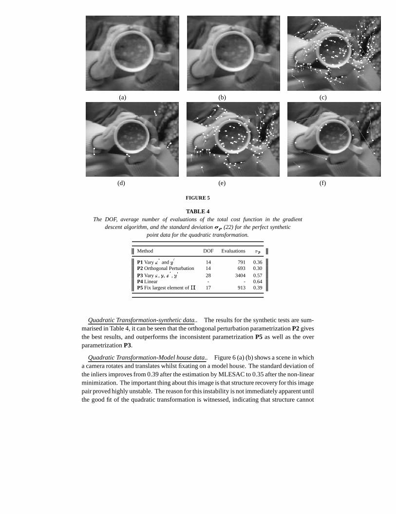
Projectivity-Cup Data.. Figure 5 (a) shows the first and (b) the second image of acup viewed from a camera undergoing cyclotorsion about its optic axis combined withan image zoom. The matches are given in (c), basis (d), inliers (e) outliers (f) for thisscene when fitting a projectivity. It can be seen that outliers to the cyclotorsion are clearlyidentified. The non linear step does not produce any new inliers as the MLESAC step hassuccessfully eliminated all mismatches, the error on the inliers is reduced by1% when theimage coordinates in one image are fixed and those in the othervaried.

(a) (b) (c)

(d) (e) (f)

FIGURE 5

TABLE 4The DOF, average number of evaluations of the total cost function in the gradient

descent algorithm, and the standard deviation�p (22) for the perfect syntheticpoint data for the quadratic transformation.

Method DOF Evaluations �pP1 Vary x0

andy014 791 0.36

P2 Orthogonal Perturbation 14 693 0.30P3 Vary x, y, x0

, y028 3404 0.57

P4 Linear - - 0.64P5 Fix largest element ofH 17 913 0.39

Quadratic Transformation-synthetic data.. The results for the synthetic tests are sum-marised in Table 4, it can be seen that the orthogonal perturbation parametrizationP2givesthe best results, and outperforms the inconsistent parametrizationP5 as well as the overparametrizationP3.

Quadratic Transformation-Model house data.. Figure 6 (a) (b) shows a scene in whicha camera rotates and translates whilst fixating on a model house. The standard deviation ofthe inliers improves from 0.39 after the estimation by MLESAC to 0.35 after the non-linearminimization. The important thing about this image is that structure recovery for this imagepair proved highly unstable. The reason for this instability is not immediately apparent untilthe good fit of the quadratic transformation is witnessed, indicating that structure cannot

be well recovered from this scene. In fact the detected corners approximately lie near aquadric surface which also passes through the camera centres. This is shown in Figure 7.

(a) (b) (c)

(d) (e) (f)

FIGURE 6

8. CONCLUSION

Within this paper an improvement overRANSAC:MLESAC has been shown to givebetter estimates on our test data. A general method for constrained parameter estimationhas been demonstrated, and it has been shown to provide equalor superior results to existingmethods. In fact few such general purpose methods exist to estimate and parametrize com-plex quantities such as critical surfaces. The general method (of minimal parametrization interms of basis points found fromMLESAC) could be used for other estimation problemsin vision, for instance estimating the Quadrifocal tensor between four images, complexpolynomial curves etc. The general methodology could be used outside of vision in anyproblem where minimal parametrizations are not immediately obvious, and the relationsmay be determined from some minimal number of points.

Why does the point parametrization work so well? One reason is that the minimal pointset initially selected byMLESAC is known to provide a good estimate of the imagerelation (because there is a lot of support for this solution). Hence the initial estimate ofthe point basis provided byMLESAC is quite close to the true solution and consequentlythe non-linear minimisation typically avoids local minima. Secondly the parametrizationis consistent which means that during the gradient descent phase only image relations thatmight actually arise are searched for.

FIGURE 7

It has been observed that theMLESACmethod of robust fitting is good for initializingthe parameter estimation when the data are corrupted by outliers. In this case there are justtwo class to which a datum might belong, inliers or outliers.TheMLESACmethod maybe generalized to the case when the data has arisen from a moregeneral mixture modelinvolving several classes, such as in clustering problems.Preliminary work to illustratethis has been conducted [28].

There are two extensions that are trivial toMLESAC that allow the introduction ofprior information1, although prior information is not used in this paper. The first is to allowa priorPr(M) on the parameters of the relation, which is just added to the score function�L. The second is to allow a prior on the number of outliers and the mixing parameter .

AcknowledgementsThank you to the reviewers for helpful suggestions, and Richard Hartley for helpful

discussions.

REFERENCES

1. P. Beardsley, P. H. S. Torr, and A. Zisserman. 3D model aquisition from extended image sequences. In B. Bux-ton and Cipolla R., editors,Proc. 4th European Conference on Computer Vision, LNCS 1065, Cambridge,pages 683–695. Springer–Verlag, 1996.

2. A. P. Dempster, N. M. Laird, and D. B. Rubin. Maximum likelihood from incomplete data via the emalgorithm. J. R. Statist. Soc., 39 B:1–38, 1977.

3. O.D. Faugeras. What can be seen in three dimensions with anuncalibrated stereo rig? In G. Sandini, editor,Proc. 2nd European Conference on Computer Vision, LNCS 588,Santa Margherita Ligure, pages 563–578.Springer–Verlag, 1992.1In this case the nameMLESAC is still appropriate as the aim is still to maximize the likelihood, now it is

the posterior likelihood

4. M. Fischler and R. Bolles. Random sample consensus: a paradigm for model fitting with application to imageanalysis and automated cartography.Commun. Assoc. Comp. Mach., vol. 24:381–95, 1981.

5. A. Gelman, J. Carlin, H. Stern, and D. Rubin.Bayesian Data Analysis. Chapman and Hall, 1995.

6. P. E. Gill and W. Murray. Algorithms for the solution of thenonlinear least-squares problem.SIAM J NumAnal, 15(5):977–992, 1978.

7. Numerical Algorithms Group.NAG Fortran Library vol 7. NAG, 1988.

8. C. Harris. The DROID 3D vision system. Technical Report 72/88/N488U, Plessey Research, Roke Manor,1988.

9. C. Harris and M. Stephens. A combined corner and edge detector. In Proc. Alvey Conf., pages 189–192, 1987.

10. R. I. Hartley. Estimation of relative camera positions for uncalibrated cameras. InProc. 2nd EuropeanConference on Computer Vision, LNCS 588, Santa Margherita Ligure, pages 579–587. Springer-Verlag,1992.

11. R. I. Hartley. Euclidean reconstruction from uncalibrated views. InProc. 2nd European-US Workshop onInvariance, Azores, pages 187–202, 1993.

12. R. I. Hartley and P. Sturm. Triangulation. InDARPA Image Understanding Workshop, Monterey, CA, pages957–966, 1994.

13. P. J. Huber. Projection pursuit.Annals of Statistics, 13:433–475, 1985.

14. K. Kanatani.Statistical Optimization for Geometric Computation: Theory and Practice. Elsevier Science,Amsterdam, 1996.

15. M. Kendall and A. Stuart.The Advanced Theory of Statistics. Charles Griffin and Company, London, 1983.

16. Q. T. Luong, R. Deriche, O. D. Faugeras, and T. Papadopoulo. On determining the fundamental matrix:analysis of different methods and experimental results. Technical Report 1894, INRIA (Sophia Antipolis),1993.

17. Q. T. Luong and O. D. Faugeras. Determining the fundamental matrix with planes: Instability and newalgorithms.CVPR, 4:489–494, 1993.

18. Q. T. Luong and O. D. Faugeras. A stability analysis for the fundamental matrix. In J. O. Eklundh, editor,Proc.3rd European Conference on Computer Vision, LNCS 800/801, Stockholm, pages 577–586. Springer–Verlag,1994.

19. S.J. Maybank. Properties of essential matrices.Int. J. of Imaging Systems and Technology, 2:380–384, 1990.

20. G.I. McLachlan and K. Basford.Mixture models: inference and applications to clustering. Marcel Dekker.New York, 1988.

21. V. Pratt. Direct least squares fitting of algebraic surfaces.Computer Graphics, 21(4):145–152, 1987.

22. P. J. Rousseeuw.Robust Regression and Outlier Detection. Wiley, New York, 1987.

23. P.D. Sampson. Fitting conic sections to ‘very scattered’ data: An iterative refinement of the Booksteinalgorithm. Computer Vision, Graphics, and Image Processing, 18:97–108, 1982.

24. L. S. Shapiro.Affine Analysis of Image Sequences. PhD thesis, Oxford University, 1993.

25. C. V. Stewart. Bias in robust estimation caused by discontinuities and multiple structures.IEEE Trans. onPattern Analysis and Machine Intelligence, vol.PAMI-19,no.8:818–833, 1997.

26. G. Taubin. Estimation of planar curves, surfaces, and nonplanar space curves defined by implicit equationswith applications to edge and range image segmentation.IEEE Trans. on Pattern Analysis and MachineIntelligence, vol.PAMI-13,no.11:1115–1138, 1991.

27. C. Tomasi and T. Kanade. Shape and motion from image streams under orthography: A factorisation approach.International Journal of Computer Vision, 9(2):137–154, 1992.

28. P. Torr, R. Szeliski, and P. Anandan. An integrated bayesian approach to layer extraction from image sequences.In Seventh International Conference on Computer Vision, volume 2, pages 983–991, 1999.

29. P. H. S. Torr, P. A. Beardsley, and D. W. Murray. Robust vision. In J. Illingworth, editor,Proc. 5th BritishMachine Vision Conference, York, pages 145–155. BMVA Press, 1994.

30. P. H. S. Torr and D. W. Murray. Outlier detection and motion segmentation. In P. S. Schenker, editor,SensorFusion VI, pages 432–443. SPIE volume 2059, 1993. Boston.

31. P. H. S. Torr and D. W. Murray. Stochastic motion clustering. In J.-O. Eklundh, editor,Proc. 3rd EuropeanConference on Computer Vision, LNCS 800/801, Stockholm, pages 328–338. Springer–Verlag, 1994.

32. P. H. S. Torr and D. W. Murray. The development and comparison of robust methods for estimating thefundamental matrix.Int Journal of Computer Vision, 24(3):271–300, 1997.

33. P. H. S. Torr and A Zisserman. Robust parameterization and computation of the trifocal tensor.Image andVision Computing, 15:591–607, 1997.

34. P. H. S. Torr and A. Zisserman. Robust computation and parametrization of multiple view relations. InU Desai, editor,ICCV6, pages 727–732. Narosa Publishing House, 1998.

35. P. H. S. Torr, A Zisserman, and S. Maybank. Robust detection of degenerate configurations for the fundamentalmatrix. CVIU, 71(3):312–333, 1998.

36. P. H. S. Torr, A. Zisserman, and D. W. Murray. Motion clustering using the trilinear constraint over threeviews. In R. Mohr and C. Wu, editors,Europe-China Workshop on Geometrical Modelling and Invariants forComputer Vision, pages 118–125. Springer–Verlag, 1995.

37. P.H.S. Torr. An assessment of information criteria for motion model selection. InCVPR97, pages 47–53,1997.

38. W. Triggs. The geometry of projective reconstruction i:Matching constraints and the joint image. InProc.5th Int’l Conf. on Computer Vision, Boston, pages 338–343, 1995.

39. Z. Zhang, R. Deriche, O. Faugeras, and Q. T. Luong. A robust technique for matching two uncalibratedimages through the recovery of the unknown epipolar geometry. AI Journal, vol.78:87–119, 1994.

40. Z. Zhang and O. Faugeras.3D Dynamic Scene Analysis. Springer-Verlag, 1992.