GENERALIZED ESTIMATOR FOR ESTIMATING POPULATION MEAN UNDER TWO STAGE SAMPLING

© 2014 Pakistan Journal of Statistics 465

Pak. J. Statist.

2014 Vol. 30(4), 465-486

GENERALIZED ESTIMATOR FOR ESTIMATING POPULATION

MEAN UNDER TWO STAGE SAMPLING

Riffat Jabeen1§

, Aamir Sanaullah2 and Muhammad Hanif

3

National College of Business Administration and Economics, Lahore, Pakistan

Email: [email protected]

[email protected]

[email protected]

§ Corresponding author

ABSTRACT

Koyuncu and Kadilar (2009) proposed a family of ratio-type estimators for population

mean using auxiliary information in simple random sampling. Srivastava and Garg

(2009) proposed a general class of ratio estimator for estimating population mean using

auxiliary variablein two-stage sampling. In this paper, motivated by Srivastava and Garg

(2009) and Koyuncu and Kadilar (2009) we have proposed a general class of estimators

for population mean for three different cases in two-stage sampling design. The mean

square error (MSE) and bias expressions have been obtained in a general form up to the

first order of approximation for the three cases. It has also been shown that for each of the

three cases in two-stage sampling, minimum MSE of this class is asymptotical equal to

the MSE of regression estimator. An empirical study has also been carried out, in order to

demonstrate the performance of proposed general class of estimators for three cases in

two-stage sampling design.

KEYWORDS

Auxiliary variable; mean square error; two stage sampling; first stage sampling unit;

second stage sampling unit.

1. INTRODUCTION

When nature of a population is to visualize in some clusters, a multi-stage sampling

design is be more suitable. In sampling survey, it is often valuable if the units are

sampled in more than one-stage [Cochran 1977, Kalton 1983, and Sarndal et al. 1992].

Morris (1955), and Leroux and Reimer (1959) discussed some applications of two-stage

sampling design. Seelbinder (1951) discussed method to determine the first stage

sampling units and the method for the selecting two-stage sampling units under without

replacement taking probability of inclusion proportional to size, has been illustrated by

Durbin (1967). Brewer and Hanif (1970) extended the work of Durbin (1967) to a general

case. For rare and clustered populations Seber (1982) used two-stage sampling design in

various situations. The idea was devised by Jensen (1994) independently. Whittemore

(1997) provided the use of multi-stage sampling design and inference using maximum

likelihood estimator (MLE) and Horvitz-Thompson (1952).

mailto:[email protected]

mailto:[email protected]

Generalized estimator for estimating population mean… 466

Srivastava and Garg (2009) proposed a general class of estimator for estimating

population mean using multi-auxiliary variables under two-stage sampling. Saini and

Bahl (2012) envisaged difference and ratio estimators in two-stage sampling using double

sampling and multi-auxiliary information. Nafiu (2012) made a comparison among three

designs, one-stage, two-stage and three-stage sampling design. Sahoo and Pandey (1999)

proposed general family of estimators using information of two auxiliary variables in two

stage sampling design. Sahoo et al. (2011) proposed a general class of estimators in two-

satge sampling using two auxiliary. Mishra (2012) proposed a number of ratio estimators

and compared their efficiencies in two-stage sampling design. Singh et al. (2007) derived

a family of estimators by using correlation coefficients in two phase sampling. Sahoo

et al. (2009) produced a class of predictive estimators under two-stage sampling. Singh

et al. (2011) made some improvements in estimating population mean using two auxiliary

variables in two phase sampling. Sanaullah (2014) advised exponential estimators in

stratified sampling using auxiliary information. Khoshnevisan et al. (2007) advised a

general family of estimators for population mean using simple random sampling by

utilizing the information of single auxiliary variable. Singh et al. (2013) advised ratio,

regression and product estimators when the population mean is not known in advance.

Multi-stage sampling is often more precise than a simple random sampling for a same

cost and it is therefore in this study we are considering Koyuncu and Kadilar (2009)

general family of estimator under two-stage sampling design.

In two-stage sampling, a population is divided into clusters (equal or unequal sizes) as

first stage units (fsu’s) and then each cluster is further divided into sub-units as second

stage units (ssu’s). At first stage, a sample of clusters is selected by simple random

sampling with or without replacement as fsu’s and at second stage another sample of sub-

units from each cluster (fsu) is selected as ssu’s. Information on the study and auxiliary

variables are collected from ssu’s. In multi-stage sampling, this process is repeated over

more than two-stages to select ultimate sampling units [Thompson (1992) and Goldstein

(1995)].

Let a population consists of N first stage units (fsu’s) and each fsu consists of

iM second stage units (ssu’s). Let a sample of n fsu’s is selected and a sample of im

ssu’s from each of n fsu’s is selected by assigning weights ii

M

M to the fsu’s. Let M

be the average number of ssu’s belonging to each fsu. Further we assume that the

selection of units at each stage has been done using simple random sampling. Let ijy be

the value of j-th second-stage unit in the i-th fsu ( 1,2,..., ; 1,2,..., )ij M i N and

.1

1 iM

i ijji

Y yM

and iy ,1

1 im

ijji

ym

are the means belonging to the thi fsu respectively in

the population and sample.

Let

2yS

2

1 10

1

1

iMN

iji j

Y YM

(Population variance of Y )

Jabeen, Sanaullah and Hanif 467

2

2

1

1

1

iM

yi ij iji

S Y YM

(Population variance of iY belonging to thi fsu)

2yiC

2

2

yi

i

S

Y (Coefficient of variation of Y for thi fsu)

i = Correlation coefficient between iY and iX belonging to thi fsu in the

population.

Similarly the notations for the auxiliary variable X can also be defined in the same

fashion.

2. SOME AVAILABLE ESTIMATORS

Koyuncu and kadilar (2009) introduced a general family of estimator as:

*1

(1 )

g

aX bt y

ax b aX b

, (2.1)

where and g are assumed to be the unknown constants whose values are to be

estimated. ( 0),a and b are assumed to be known as either real numbers or (Linear or

Non-linear) functions of some known parameters of auxiliary variable x such as

standard deviation x , coefficient of variation xC , skewness 1( )x , kurtosis

2 ( )x and correlation coefficient from the population, and is a suitable constant

to be determined later.

The mean square error of *1t is,

* 2 2 2 2 2 2 2 2 2

1MSE 2y x

N nt Y C g g g g C

nN

222 2 1x yg C C

. (2.2)

where aX

aX b

.

Khoshnevisan et al. (2007) proposed a generalized estimator for estimating

population mean under single phase sampling using simple random sampling design

as,

*2

(1 )

g

aX bt y

ax b aX b

, (2.3)



estimated. ( 0),a and b are assumed to be known as either real numbers or (Linear or


standard deviation x , coefficient of variation xC , skewness 1( )x , kurtosis

2 ( )x and correlation coefficient from the population.

The MSE of *1t is,

* 2 2 2 2 2 2

2MSE 2y x x y

N nt Y C g C g C C

nN

, (2.4)

where aX

aX b

.

A usual unbiased weighted estimator of population mean for unequal first stage units

in two-stage sampling design is,

*3

1

1 n

i ii

t yn

,

(2.5)

The variance of the 2t is

22 2 2

31 1 1

1 1( )

1 i

N N N

i i i i m i i yii i i

fVar t Y Y f Y C

N N nN

(2.6)

Srivastava and Garg (2009) proposed an estimator for the estimation of population

mean under two-stage sampling design as,

* 14

1

1 n

i ii

t tn

, (2.7)

where 1 ii i

i

yt X

x is a classical ratio estimator for thi fsu’s.

The MSE *3t for two-stage sampling design is,

2* 2

41 1

1

1

N N

i i i i i ii i

fMSE t z E z v

N nN

, (2.8)

where 21i i i ii i m y i x yz Y f C C C

and 2 2 2 2

i i i ii i m y x i x yv Y f C C C C .

where

1 1andi i i iz E t MSE t (2.9)


Srivastava and Garg (2009) proposed a regression estimator for the estimation of

population mean under two-stage sampling design as,

* 25

1

1 n

i ii

t tn

, (2.10)

where 2i i i it y b X x is a classical regression estimator for thi fsu’s.

The MSE *5t for two-stage sampling design is,

2* 2

51 1

1

1

N N

i i i i i ii i

fMSE t z E z v

N nN

, (2.11)

where

i iz Y and 2 2 2 2i i i i ii m y i x i i x yv f S b S b S S . (2.12)

where 1 1andi i i iz E t MSE t .

3. PROPOSED GENERALIZED ESTIMATORS

IN TWO-STAGE SAMPLING

In this particular study, some ratio and product type estimators have been generalized

under two-stage sampling design. The proposed class of estimators is useful for the

estimation of population mean using single auxiliary information in two-stage sampling.

The proposed estimator has been discussed for the following three different cases in

two-stage sampling,

Case-I: when first stage units are of unequal sizes and weighted mean is used.

Case-II: when first stage units are of unequal sizes and un-weighted mean is used.

Case-III: when first stage units are of equal size.

Proposed Estimator for Case-I:

We propose a weighted generalized estimator for unequal fsu’s in two-stage sampling

design as,

1

1 nG GTS i i

i

k tn

, (3.1)

where GTSk is proposed weighted generalized estimator in two-stage sampling design, i

is weighting known constant and Git is proposed ratio type estimator for population mean

for ssu’s belonging to the thi fsu’s as,

1,2,..., .(1 )

g

i i iGi i

i i i i i i

a X bt y i n

a x b a X b

, (3.2)



estimated. ( 0),ia and ib are assumed to be known as either real numbers or (Linear or


standard deviation xi , coefficient of variation xiC , skewness 1 ( )i x , kurtosis

2 ( )i x and correlation coefficient i for ssu’s belonging to thi fsu’s from the

population. For different values of the constants in (3.2), we may get different ratio and

product type estimators as shown in Table 1.

Table 1

Some Members of Estimator ( Git )

Ratio Estimator

1g

Product Estimator

1g ia ib

0i it y 0

i it y 0 0 0

1 ii i

i

Xt y

x

2 i

i ii

xt y

X

1 0 1

3 i

i

i x

i ii x

X Ct y

x C

4 i

i

i x

i ii x

x Ct y

X C

1 ixC 1

25

2

( )

( )

i

i

i x

i ii ii x

x X Ct y

x x C

26

2

( )

( )

i

i

i i x

i ii i x

x x Ct y

x X C

2 (x )i ixC 1

27

2

( )

( )

i

i

x i i

i ix i i

C X xt y

C x x

28

2

( )

( )

i

i

x i i

i ix i i

C x xt y

C X x

ixC

2 (x )i 1

29

2

( )

( )

i

i

i x

i ii i x

x Xt y

x x

210

2

( )

( )

i

i

i i x

i ii i x

x xt y

x X

2 (x )i ix 1

11 i ii i

i i

Xt y

x

12 i i

i ii i

xt y

X

1 i 1

13 2

2

( )

( )

i ii i

i i

X xt y

x x

14 2

2

( )

( )

i ii i

i i

x xt y

X x

1 2 (x )i 1

151

1

i

i

x i

i ix i

Xt y

x

16

1

1

i

i

x i

i ix i

xt y

X

ix 1 1

117

1

(x )

(x )

i

i

x i i

i ix i i

Xt y

x

118

1

(x )

(x )

i

i

x i i

i ix i i

xt y

X

ix

1(x) 1


Ratio Estimator

1g

Product Estimator

1g ia ib

219

2

(x )

(x )

i

i

x i i

i ix i i

Xt y

x

220

2

(x )

(x )

i

i

x i i

i ix i i

xt y

X

ix

2 (x )i 1

21 1 2

1 2

( ) (x )

( ) (x )

i i ii i

i i i

x xt y

x X

22 1 2

1 2

( ) (x )

( ) (x )

i i ii i

i i i

x xt y

x X

1(x) 2 (x )i 1

23 2 1

2 1

( ) ( )

( ) ( )

i i ii i

i i i

x X xt y

x x x

24 2 1

2 1

( ) ( )

( ) ( )

i i ii i

i i i

x x xt y

x X x

2 (x )i 1( )ix 1

25 1

1

i ii i

i i

Xt y

x

26 1

1

i ii i

i i

xt y

X

i 1 1

27 i i

i i

x i x

i ix i x

X Ct y

x C

28 i i

i i

x i x

i ix i x

x Ct y

X C

i ixC 1

3.1 The Bias and Mean Square Error of GTSk in Two-Stage Sampling Design

In order to obtain the bias expression, let us define the expectation of GTSk

in two-

stage sampling design as,

1 2

G GTS TSE k E E k , (3.3)

1 21

1 nG

i ii

E E tn

, (3.4)

21

1where

NG

i i i ii

z z E tN

(3.5)

(terms retain upto order two in (3.15)).

Now the bias of GTSk may be written as,

Bias G GTS TSk E k Y

1

1.

N

i i ii

z YN

(3.6)

In order to find expression for the MSE of GTSk in two-stage sampling, let us define

1 2 1 2

G G GTS TS TSMSE k MSE E k E MSE k

(3.7)

where


*1 2 1

1

1( )

nGTS i i

i

MSE E k MSE zn

(3.8)

2* *

1

*

1

*2

1

where

1

where (terms retain uptoorder onein (3.15) ).

N

i i i ii

N

i i i ii

Gi i

fz E z

N

E z zN

z E

(3.9)

and

21 1 22 1

2

1

where

nGTS i i

i

Gi i

E MSE k E vn

v MSE t

(3.10)

In order to derive the bias and MSE of the proposed class of estimator, we need to

find iz , *iz and iv from the units of second stage. It is therefore we define,

1 ,

ii i yy Y e 1 ,ii i xx X e 1,2, , i n , (3.11)

where yie and are the sampling error. Further we assume that 0i iy xE e E e ,

and some expectations under two-stage sampling design are obtained in order to obtain

the bias and mean square error as,

2 2 2 2, ,

1 1 1 1where ,

i i i i i i i i i i i

i

y m y x m x y x m i y x

mi i

E e f C E e f C E e e f C C

f fn N m M

(3.12)

we rewrite (3.2) in the form of e’s as

1 1i i

g

G i ii i y x

i i i

a Xt Y e e

a X b

, (3.13)

or

1 1

i i

gGi i y i xt Y e e

where,

i i

i

i i i

a X

a X b

, (3.14)

Consider i xiie <1 so that we can expand the series of 1

g

i iie

in (3.13). On

ignoring the terms in yie and xie of order higher than two as,

ixe


2 2 2( 1)1

2i i i i i

Gi i y i x i x i x y

g gt Y e g e e g e e

, (3.15)

We take expectation of (3.15) for ssu’s belonging to every thi fsu as,

2 2

2( 1)1

2 i i i

G ii i x i i x y i

g gE t Y C g C C z

, (3.16)

Now from (3.16) and (3.6), we will have the bias of GTSk as,

2 2

2

1

( 1)1Bias k

2 i i i

NG iTS i i x i i x y

i

g gY C g C C

N

(3.17)

We can rewrite (3.15) as

2 2 2( 1)

2i i i i i

Gi i i y i x i x i x y

g gt Y Y e g e e g e e

, (3.18)

We retain the terms upto the order one and then take expectation of (3.18). we get,

*Gi i iE t Y z

(3.19)

In order to obtain the MSE, we take square of (3.18), retain terms in e’s upto the order

one and take expectation,

2

2 2 2 2 2 2 2i i i i

Gi i i m y i i x i i i x y iE t Y Y f C g C g C C v (3.20)

By substituting (3.19) and (3.20) respectively in (3.9) and (3.10), we have

2

1 211

NGTS i i i i

i

fMSE E k Y E Y

N

where 1

1 N

i i i ii

E z YN

(3.21)

and

2 2 2 2 2 2 2

1 21

12

i i i i

nGTS i i m y i x i i x y

i

E MSE k Y f C g C g C CnN

(3.22)

The MSE of GTSk is finally obtained in two-stage sampling as,

2

1

1

( )1

N

i iNG iTS i i

i

Yf

MSE k YN N

2 2 2 2 2 2 2

1

12

i i i i

n

m i i y i x i i x yi

f Y C g C g C CnN

(3.23)


The values of mean square errors of the ratio-type and product-type estimators

mentioned in Table 1 may also be obtained directly by substituting different values of

g , ia , ib and i

to the expression (3.23).

3.2 Optimum Choices of i

The MSE of GTSk in (3.23) is minimum if 2 2 2 2 2 2 2

i i i im i y i i x i ii i x yf Y C g C g C Cv

is minimum. It is therefore the minimization of iv with respect to yields its optimum

value as,

i

i

i yopt

i x

C

gC

. (3.24)

The minimum MSE for thi fsu on substituting the optimum value in (3.20), may be

written as,

min 2 2 21

i ii i m y iv Y f C , (3.25)

Remark 1:

For g 1 , some ratio-type estimators are expressed in Table 1. We may express the

MSE iGit v given in (3.18) for these ratio-type estimators for thi fsu as,

2

1 1

2 2

2 2 2 2

2 2 2 2

2 ( ) 1

2 ( ) 3,5,..., 27

i i i i i

j j

i i i i i

i m y i x i i y x

j ji i

i m y i i x i i i y x

Y f C C C C j G

MSE t vY f C C C C j G

,

(3.26)

The j ji iMSE t v in (3.26) is minimum for

1

2

i

j

i

i y

i

i x

C

C

.

Remark 2:

For g 1 , some product-type estimators are expressed in Table 1. We may express

MSE iGit v given in (3.18) for these product-type estimators for

thi fsu may be

expressed as,

2

2 2

2 2 2 2

2 2 2 2

2 ( ) 2

2 ( ) 4,6,..., 28

i i i i i

k k

i i i i i

i m y i x i i y x

k ki i

i m y i i x i i i y x

Y f C C C C k G

MSE t v

Y f C C C C k G

,

(3.27)


The k ki iMSE t v in (3.25) is minimum for

2

i

k

i

i y

i

i x

C

C

.

where

1

i

ii

i x

X

X C

,

22

2 i

i ii

i i x

x X

x X C

,

3

2

i

i

x i

ix i i

C X

C X x

,

24

2

i ii

i i x

x X

x X

, 5 i

ii xy

X

X

,

6

2

ii

i i

X

X x

, 7

1

x ii

x i

X

X

,

8

1

ii

x i i

X

X x

,

9

2

x ii

x i i

X

X x

,

110

1 2

i ii

i i i

x X

x X x

,

211

2 1

i ii

i i i

x X

x X x

, 12

1

xy i

ixy i

X

X

, 13

i

x ii

x i x

X

X C

.

Now the minimum MSE of optTSk

in two-stage sampling is obtained on substituting

(3.25) in (3.23) as,

2

2 2 2 21

1 1

1min. 1

1 i i

N

i iN Nopt i

i i m i i y iTSi i

Yf

MSE k Y f Y CN N nN

. (3.28)

which is asymptotical equal to the MSE of regression estimator in two-stage sampling

design (see, Srivastava and Garg, 2009).

On using the optimal value opt , we get an asymptotically optimal estimator (AOE)

in two-stage sampling as,

1

1 nAOE opt

TS i ii

k tn

where

1

g

i i iopti i opt opt

i i i i i i

a X bt y

a x b a X b

(3.29)

The values of opt can be searched out from the previous surveys or may be guessed

from the knowledge drawn in due course of time, for case in point, see Horvitz and

Thompson (1952), Murthy (1967), Singh & Vishwakarma (2008), Singh and Kumar

(2008), Singh and Karpe (2010), Upadhyaya et al. (2011), Yadav and Kadilar (2013) and

Sanaullah et al. (2014).

In many real life situations, it is not possible for the researcher to presume the valueopt by employ all the resources, so it is better to replace opt in (3.29) by their

consistent estimates as,


ˆˆˆ

ˆi

i

i yopt

i x

C

gC

(3.30)

So an estimator in (3.29) may be written as

1

1 nAOE opt

TS i ii

k tn

where

ˆ ˆ1

g

i i iopti i opt opt

i i i i i i

a X bt y

a x b a X b

(3.31)

Similarly an unbiased estimator for the MSE of optTSk is given as,

2

21

1 1

1min. ( )

1

n

i iN Nopt opti

i i i iTSi i

Yf

MSE k Y vn n nN

(3.32)

Remark 3:

If we assume 1ii

M

M , and

1

imij

ij i

yy

m

(see Sukhatme et al., 1984) then an

estimator in (3.1) may be turned for case-II as,

1

1 nG GTS i

i

k tn

where

(1 )

g

i i iGi i

i i i i i i

a X bt y

a x b a X b

(3.33)

Similarly the expression for the bias and MSE of GTSk may obtained respectively by

putting 1i into (3.17) and (3.23) as,

2 2

2

1

( 1)1Bias k

2 i i i

NG iTS i x i i x y

i

g gY C g C C

N

(3.34)

and

2 2 2 2 2 21

1 1

1( ) 2

1 i i i i

N

iN nG iTS i m i y i x i i x y

i i

Yf

MSE k Y f Y C g C g C CN N nN

(3.35)

Remark 4:

In some situations of practical importance we have first stage units of equal size then it

is possible to have 1ii

M

M , im m , iM M , mi m

M m

mMf f

and 1

mij

ij

yy

m

Sukhatme et al. (1984). An estimator in (3.1) may be turned for case-III as,


1

1 nG GTS i

i

k tn

where

(1 )

g

i i iGi i

i i i i i i

a X bt y

a x b a X b

(3.36)

Similarly the expression for the bias and MSE of GTSk in case-III may also be obtained

respectively by putting 1ii

M

M , im m , and iM M , mi m

M m

mMf f

into

(3.17) and (3.23) as,

2 2

2

1

( 1)1Bias k

2 i i i

NG iTS i x i i x y

i

g gY C g C C

N

(3.37)

and

2 2 2 2 2 21

1 1

12

1 i i i

N

iN nG iTS i m i y i x i i x y

i i

Yf

MSE k Y f Y C g C g C CN N nN

(3.38)

4. EFFICIENCY COMPARISONS

In this section, the proposed class of estimators has been compared in theory with

usual unbiased weighted estimator *3

1

1 n

i ii

t yn

, Srivastva and Garg (2009) ratio-

type estimator *4t and, Srivastva and Garg (2009) regression-type estimator *

5t for

population mean. The comparisons have been made for three different cases in two-stage sampling design. Let us consider following

Notations for case-I,

2 2 2 21

1

N

i i mi i xi

Y f C L

, 2 2 2

21

N

i i mi xi

Y f C L

, 2 2 2

31

N

i i mi yii

Y f C L

,

2 2 2 2 24

1

N

i i mi i i xi

Y f b R C L

, 2 2

11

N

i i mi i i xi yii

Y f C C M

, 2 2

21

N

i i mi i xi yii

Y f C C M

,

2 23

1

N

i i mi i i i xi yii

Y f b R C C M

, 2 2 2

41

N

i mi i yii

Y f C M

Notations for case-II,

2 2 25

1

N

i mi i xi

Y f C L

, 2 2

61

N

i mi xi

Y f C L

, 2 2

71

N

i mi yii

Y f C L

,2 2 2 2

81

N

i mi i i xi

Y f b R C L

,

25

1

N

i mi i i xi yii

Y f C C M

, 2

61

N

i mi i xi yii

Y f C C M

,2

71

N

i mi i i i xi yii

Y f b R C C M

.

2 2 28

1

N

i mi i yii

Y f C M

.


Notations for case-III, 2 2 2

9m xY f C L , 2 210m xY f C L ,

2 211m yY f C L , 2 2 2 2

12m xY f b R C L ,

29m x yY f C C M ,

210m x yY f C C M ,

211m x yY f bR C C M ,

2 2 212

1

N

i mi i yii

Y f C M

.

Comparisons for Case-I:

i) We first compare our proposed generalized estimator with usual two-stage estimator

*3 0G

TSMSE k MSE t if

1 1

1 1

2 2min 0, max 0,

M M

gL gL

(4.1)

When condition (4.1) is satisfied, we may infer that proposed generalized estimator is

more efficient than usual two-stage estimator.

ii) We compare proposed generalized estimator with Srivastva and Garg (2009) ratio

estimator

*4 0G

TSMSE k MSE t

if

2 21 1 1 2 2 1 1 1 2 2

1 1

2 2min max

M M L M L M M L M L

gL gL

(4.2)


more efficient than Srivastva and Garg (2009) ratio estimator.

iii) We compare proposed generalized estimator with Srivastva and Garg (2009)

regression estimator

*5 0G

TSMSE k MSE t

if

2 21 1 4 3 1 1 1 4 3 1

1 1

2 2min , max ,

M M L M L M M L M L

gL gL

(4.3)


more efficient than Srivastva and Garg (2009) regression estimator.

iv) We compare proposed generalized estimator with optimal conditions to generalized

proposed estimator

min 0G GTS TSMSE k MSE k

if


2 21 1 4 1 1 1 4 1

1 1

min maxM L M M M L M M

gL gL

(4.4)

When condition (4.4) is satisfied, we may infer that proposed generalized estimator

under optimal conditions is more efficient than proposed generalized estimator.

Comparisons for Case-II:


*3 0G

TSMSE k MSE t if

5 5

5 5

2 2min 0, max 0,

M M

gL gL

(4.5)




estimator

*

4 0GTSMSE k MSE t if

2 25 5 4 6 5 5 5 4 6 5

4 4

2 2min max

M M L M L M M L M L

gL gL

(4.6)


more efficient than Srivastva and Garg (2009) ratio estimator.



*5 0G

TSMSE k MSE t

if

(4.7)


more efficient than Srivastva and Garg (2009) regression estimator.

iv) We compare proposed generalized estimator with optimal conditions to generalized

proposed estimator

2 25 5 4 6 5 5 5 4 6 5

5 5

2 2min , max ,

M M L M L M M L M L

gL gL


min 0G GTS TSMSE k MSE k if

2 25 5 8 5 5 5 8 5

5 5


gL gL

(4.8)


under optimal conditions is more efficient than proposed generalized estimator.

Comparisons for Case-III:


*3 0G

TSMSE k MSE t if

9 9

9 9

2 2min 0, max 0,

M M

gL gL

(4.9)




estimator

*4 0G

TSMSE k MSE t if

2 29 9 9 10 10 9 9 9 10 10

9 9

2 2min max

M M L M L M M L M L

gL gL

(4.10)


is more efficient than Srivastva and Garg (2009) ratio estimator.



*5 0G

TSMSE k MSE t

if

2 29 9 10 10 9 9 9 10 10 9

9 9

2 2min , max ,

M M M L L M M M L L

gL gL

(4.11)


is more efficient than Srivastva and Garg (2009) regression estimator.


iv) We compare proposed generalized estimator with optimal conditions to generalized proposed estimator

min 0G GTS TSMSE k MSE k if

2 29 9 12 9 9 9 12 9

9 9


gL gL

(4.12)

When condition (4.12) is satisfied, we may infer that proposed generalized estimator under optimal conditions is more efficient than proposed generalized estimator.

For (g, i ) = (1, i ), the comparisons in (4.1) – (4.10) can be obtained for ratio-type

estimators. Similarly for (g, i ) = (-1, i ), the comparisons in (4.1) – (4.9) can be made

for product-type estimators.

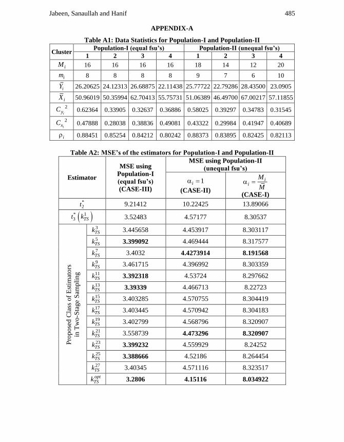
5. EMPIRICAL COMPARISON

In order to demonstrate the performance of proposed estimators, we take two real populations from Srivastva and Garg (2009) page # 116-118. The comparisons of proposed estimator with some existing estimators have been made numerically for three different aforementioned cases in two-stage sampling (see Section 3). The MSE and percent relative efficiency (PRE) values of the estimators are given in Table A2

and Table A3 respectively. The PRE is calculated as

*2

100j

TS jTS

MSE tPRE k

MSE k .

Population-I has four clusters with equal fsu’s in each cluster. Let a first-stage sample

of size two 2n is selected from fsu’s and then a second-stage sample of eight 8m

is selected from each cluster.

In population-II there are four clusters with unequal fsu’s. Let a sample of two fsu’s is

selected and then ssu’s im may be selected in some proportion to iM as,

1

32i N

ii

Mim

M

(Srivastava and Garg, 2009).

For these populations, correlations within the clusters are positive (see Table 1A). It is therefore these populations are applicable only for ratio/ratio-type estimators. Further description about the two populations has been given in Table 1A.

Some numerical comparisons may be discussed separately in three different cases as following:

a) Case-I (Unequal FSU’s with weight i = iM

M)

Table A2 shows that MSEs for the proposed class of ratio-type estimators are less

than the MSEs of *2t

and Srivastava and Garg (2009) *3t for case-I in two-stage


sampling design. Further it is observed that the proposed generalized estimator optTSk

has minimum MSE and it has MSE equal with the MSE of regression estimator.

Furthermore it is observed that 7TSk and 13

TSk have almost equal and minimum MSE

values among the proposed class of estimators. From the Table A3, it is very clear

that the PRE value for optTSk is maximum (=173%) which shows it is the most efficient

estimator among the proposed estimators. Furthermore it is noticed that both 7TSk and

13TSk have almost equal PRE values of 169% which is higher among other class of

proposed estimators which shows 7TSk and 13

TSk are also more efficient estimators

among proposed class of estimators.

b) Case-II (Unequal FSU’s with weight 1i )

Table A2 shows that the MSEs for proposed class of ratio-type estimators are less

than the MSEs of *2t

and Srivastava and Garg (2009) *3t for case-II in two-stage

sampling design. From the Table A3 one can reach at the same conclusion that optTSk

is the most efficient estimator with a PRE value of 246%. It is also noted that 9TSk

have almost equal PRE values of 232% which is no doubt higher among the other

class of proposed estimators so this is also observed as more efficient. If we compare

the proposed class of estimators for their efficiency in case-II with the efficiency in

case-I, it can be observed that the proposed class is more efficient for case-II in two-

stage sampling.

c) Case-III (Equal FSU’s)

From Table A2 it is observed that the MSEs for some of the proposed class of ratio-

type estimators are less than the MSEs of *2t

and Srivastava and Garg (2009) *3t for

case-III in two-stage sampling design. From the Table A3 it can be concluded that the

PRE value of optTSk is almost 281% which is maximum among the class of proposed

estimators. Furthermore it is noted that the PRE values of 5TSk , 11

TSk , 13TSk , 23

TSk , and

27TSk are higher among the class of proposed estimators, it is therefore one can

conclude that these are also more efficient estimators in two stage sampling design. If

the estimators of proposed class in case-III are compared for their efficiency with the

proposed estimators in case-II and case-I, it is observed that the proposed class is

more efficient for case-III in two-stage sampling.

6. CONCLUDING REMARKS

Finally from the above empirical results, it is concluded the performance of the

proposed class of estimators is higher as compare to *2t and Srivastava and Garg (2009) *

3t

for all of the three cases in two-stage sampling. It is therefore the proposed class of

estimators is justified for their application in two-stage sampling design.


ACKNOWLEDGEMENT

The authors are grateful to anonymous referees and the chief Editor for their constructive comments and suggestions, which led to considerable improvement in presentation of this manuscript.

REFERENCES

1. Brewer, K.R. and Hanif, M. (1970). Durbin’s new multistage variance estimator. J. Roy. Statist. Soc., Series B. 32(2), 302-311.

2. Cochran, W.G. (1977). Sampling Techniques. New-York, John Wiley and Sons. 3. Durbin, J. (1967). Design of multi-stage surveys for the estimation of sampling errors.

J. Roy. Statist. Soc., Series C. 16, 152-164. 4. Goldstein, H. (1995). Multilevel Statistical Models. Halstead Press, New York. 5. Horvitz, D.G. and Thompson, D.J. (1952). A generalization of sampling without

replacement from a finite universe. J. Amer. Statist. Assoc., 47, 663-685. 6. Jensen, A.L. (1994). Subsampling with mark and recapture for estimation abundance

of mobile populations. Environ Metrics, 5, 191-196. 7. Kalton, G. (1983). Introduction to Survey Sampling. Sage, Newbury Park. 8. Khoshnevisan, M., Singh, R., Chauhan, P., Sawan, N. and Smarandache, F. (2007).

A general family of estimators for estimating population mean using known value of some population parameter(s). Far East Journal of Theoretical Statistics. 22, 181-191.

9. Koyuncu, N. and Kadilar, C. (2009). Efficient estimators for the population mean, Hacettepe Journal of Math. and Statistics, 38, 2, 217-225.

10. Leroux, E.J. and Reimer, C. (1959). Variation between samples of immature stages, and of mortalities from some factors, of the eye-spotted bud moth, Spilonolaocellana D. & S.) (Lepidoptera: Olethreutidae), and the pistol casebearer, Coleophoraserratella (L.) (Lepidoptera: Coleophoridae), on apple in Quebec. Can. Ent., 91, 428-449.

11. Ma, X., Spe, M., Al-Harbi, S.P. and Efendiev, Y. (2006). A multistage sampling method for rapid quantification of uncertainty in history matching geological models. Annual Technical Conference and Exhibition. Austin. TX. 24-27.

12. Mishra, S.S. (2012). A note on ratio estimators in two-stage sampling. Intl. J. Scientific and Res. Pub., 2(12), 1-6.

13. Morris, R.F. (1955). The development of sampling techniques for forest insect defoliators, with particular reference to the spruce budworm. Can. J. Zool. 33, 225-294.

14. Murthy, M.N. (1967). Sampling Theory and Methods, Statistical Publishing Society, Calcutta.

15. Nafiu, L.A. (2012). Comparison of one-stage, two-stage, and three-stage estimators using finite population. The Pacific Journal of Science and Technology, 13(2), 166-171.

16. Sahoo, L.N., Das, B.C. and Sahoo, J. (2009). A class of predictive estimators in two stage sampling. J. Ind. Soc. of Agri. Statist., 63(2), 175-180.

17. Sahoo, L.N., Sahoo, R.K., Senapati, S.C. and Mangaraj, A.K. (2011). A general class of estimators in two-stage sampling with two auxiliary variables. Hacettepe Journal of Mathematics and Statistics, 40(5), 757-765.

18. Sahoo, L. and Pandey, P. (1999). A class of estimators using auxiliary information in two-stage sampling design using information from two auxiliary variables. Aust. & N.Z.J. Statist. 41(4), 405-410.


19. Saini, M. and Bahl. S. (2012). Estimation of population mean in two stage design using double sampling for stratification and multi-auxiliary information. Intl. J. Comp. Applica., 47(9), 17-21.

20. Sanaullah, A., Ali, H.A., Noor-ul-Amin, M. and Hanif, M. (2014). Generalized exponential chain ratio estimators under stratified two-phase random sampling. App. Math. and Compu., 226, 541-547.

21. Sarndal, C.E., Swensson, B. and Wretman, J.H. (1992). Model Assisted Survey Sampling. New York, Springer-Verlag.

22. Seber, G.A.F. (1982). The Estimation of Animal Abundance and Related Parameters, 2nd edition. Edward Arnold, London.

23. Seelbinder, B.M. (1953). On Stein’s two-stage sampling scheme. Ann. Math., 24(4), 640-649.

24. Singh, H.P. and Vishwakarma, G.K. (2008). A family of estimators of population mean using auxiliary information in stratified sampling. Communications in Statistics-Theory and Methods, 37(7), 1038-1050.

25. Singh, H.P. and Karpe, N. (2010). Estimation of mean, ratio and product using auxiliary information in the presence of measurement errors in sample surveys. J. Statist. Theo. and Prac., 4(1), 111-136.

26. Singh, H.P. and Kumar, S. (2008).A general family of estimators of finite population ratio, product and mean using two phase sampling scheme in the presence of non-response. Statist. Theo. and Prac., 2(4), 677-692.

27. Singh, H.P. and Vishwakarma, K. (2007). Modified exponential ratio and product estimators for finite population mean in Double sampling. Aust. J. Statist., 36, 217-225.

28. Singh, R., Chauhan, P. and Sawan, N. (2007). A family of estimators for estimating population means using known correlation coefficients in two-phase sampling. Statistics in Transition, 8(1), 89-96.

29. Singh, R., Chauhan, P. and Sawan, N. and Smarandache, F. (2011). Improvements in estimating population mean using two auxiliary variables in two phase sampling. Italian Jour. of Pure and Appld. Math., 28, 135-142.

30. Singh, R., Vishwakarma, G.K., Gupta, P.C. and Pareek, S. (2013). An alternative approach to estimation of population mean in two-stage sampling. Mathematical Theory and Modeling, 3(13), 48-53.

31. Srivastava, M. and Garg, N. (2009). A general class of estimators of a finite population mean using multi-auxiliary information under two stage sampling scheme. JRSS, 2(1), 103-118.

32. Sukhatme, P.V. and Sukhatme, B.V. (1970). Sampling Theory for Surveys with Applications. Asia Publishing House, New Delhi.

33. Thompson, S.K. (1992). Sampling. John Wiley and Sons: New York, NY. 34. Upadhyaya, L.N., Singh, H.P., Chatterjee, S. and Yadav, R. (2011). Improved ratio

and product exponential type estimators. J. Statist. Theo. and Prac., 5(2), 285-302. 35. Whittemore, A.S. and Halpern, J. (1997). Multi-stage sampling in genetic

epidemiology. Stat. Med., 16, 153-67. 36. Yadav, S.K. and Kadilar, C. (2013). Improved Exponential Type Ratio Estimator of

Population Variance. Revista Colombiana de Estadística, 36(1), 145-152.


APPENDIX-A

Table A1: Data Statistics for Population-I and Population-II

Cluster Population-I (equal fsu’s) Population-II (unequal fsu’s)

1 2 3 4 1 2 3 4

iM 16 16 16 16 18 14 12 20

im 8 8 8 8 9 7 6 10

iY 26.20625 24.12313 26.68875 22.11438 25.77722 22.79286 28.43500 23.0905

iX 50.96019 50.35994 62.70413 55.75731 51.06389 46.49700 67.00217 57.11855

2

iyC 0.62364 0.33905 0.32637 0.36886 0.58025 0.39297 0.34783 0.31545

2

ixC 0.47888 0.28038 0.38836 0.49081 0.43322 0.29984 0.41947 0.40689

i 0.88451 0.85254 0.84212 0.80242 0.88373 0.83895 0.82425 0.82113

Table A2: MSE’s of the estimators for Population-I and Population-II

Estimator

MSE using

Population-I

(equal fsu’s)

(CASE-III)

MSE using Population-II

(unequal fsu’s)

1i

(CASE-II)

ii

M

M

(CASE-I)

*2t 9.21412 10.22425 13.89066

*3t 1

TSk 3.52483 4.57177 8.30537

Pro

po

sed

Cla

ss o

f E

stim

ato

rs

in T

wo

-Sta

ge

Sam

pli

ng

3TSk 3.445658 4.453917 8.303117

5TSk

3.399092 4.469444 8.317577

7TSk

3.4032 4.4273914 8.191568

9TSk

3.461715 4.396992 8.303359

11TSk 3.392318 4.53724 8.297662

13TSk 3.39339 4.466713 8.22723

15TSk 3.403285 4.570755 8.304419

17TSk 3.403445 4.570942 8.304183

19TSk

3.402799 4.568796 8.320907

21TSk

3.558739 4.473296 8.320907

23TSk

3.399232 4.559929 8.24252

25TSk 3.388666 4.52186 8.264454

27TSk

3.40345 4.571116 8.323517

optTSk 3.2806 4.15116 8.034922


Table A3: PRE’s of the Estimator w.r.t. *2t

for Population-I and Population-II

Estimator

PRE using

Population-I

(equal fsu’s)

(CASE-III)

MSE using Population-II

(unequal fsu’s)

1i

(CASE-II)

ii

M

M

(CASE-I)

*2t 100 100 100

*3t 1

TSk 261.4061 223.6388 167.2491

Pro

po

sed

Cla

ss o

f E

stim

ato

rs

in T

wo

-Sta

ge

Sam

pli

ng

3TSk 267.4125 229.5564 167.2945

5TSk

271.0759 228.7589 167.0037

7TSk

270.7487 230.9317 169.5727

9TSk

266.1721 232.5283 167.2896

11TSk 271.6172 225.3407 167.4045

13TSk 271.5314 228.8987 168.8376

15TSk 270.7419 223.6884 167.2683

17TSk 270.7292 223.6793 167.273

19TSk

270.7806 223.7843 166.9368

21TSk

258.9153 228.5619 166.9368

23TSk

271.0648 224.2195 168.5244

25TSk 271.9099 226.1072 168.0772

27TSk

270.7288 223.6708 166.8845

optTSk 280.8669 246.2986 172.8786

GENERALIZED ESTIMATOR FOR ESTIMATING POPULATION MEAN UNDER TWO STAGE SAMPLING

Documents

Transcript of GENERALIZED ESTIMATOR FOR ESTIMATING POPULATION MEAN UNDER TWO STAGE SAMPLING